Distributed Computing on Core-PeripheryNetworks: Axiom-based Design

Chen Avin1,?,??, Michael Borokhovich1,??, Zvi Lotker1,??, and David Peleg2,??

1 Ben-Gurion University of the Negev, Israel.avin,borokhom,zvilo@cse.bgu.ac.il

2 The Weizmann Institute, Israel. david.peleg@weizmann.ac.il

Abstract. Inspired by social networks and complex systems, we pro-pose a core-periphery network architecture that supports fast computa-tion for many distributed algorithms and is robust and efficient in num-ber of links. Rather than providing a concrete network model, we takean axiom-based design approach. We provide three intuitive (and inde-pendent) algorithmic axioms and prove that any network that satisfiesall axioms enjoys an efficient algorithm for a range of tasks (e.g., MST,sparse matrix multiplication, etc.). We also show the minimality of ouraxiom set: for networks that satisfy any subset of the axioms, the sameefficiency cannot be guaranteed for any deterministic algorithm.

1 Introduction

A fundamental goal in distributed computing concerns finding a network archi-tecture that allows fast running times for various distributed algorithms, but atthe same time is cost-efficient in terms of minimizing the number of commu-nication links between the machines and the amount of memory used by eachprocessor.

For illustration, let’s consider three basic networks topologies: a star, a cliqueand a constant degree expander. The star graph has only a linear number of linksand can compute every computable function after only one round of communica-tion. But clearly, such an architecture has two major disadvantages: the memoryrequirements of the central node do not scale, and the network is not robust.The complete graph, on the other hand, is very robust and can support extremelyfast performance for tasks such as information dissemination, distributed sortingand minimum spanning tree, to name a few [1,2,3]. Also, in a complete graphthe amount of memory used by a single processor is minimal. But obviously, themain drawback of that architecture is the high number of links it uses. Con-stant degree expanders are a family of graphs that support efficient computationfor many tasks. They also have linear number of links and can effectively bal-ance the workload between many machines. But the diameter of these graphs

? Part of this work was done while the author was a visitor at ICERM, Brown uni-versity.

?? Supported in part by the Israel Science Foundation (grant 1549/13).

arX

iv:1

404.

6561

v1 [

cs.D

C]

25

Apr

201

4

is lower bounded by Ω(log n) which implies similar lower bound for most of theinteresting tasks one can consider.

A natural question is therefore whether there are other candidate topologieswith guaranteed good performance. We are interested in the best compromisesolution: a network on which distributed algorithms have small running times,memory requirements at each node are limited, the architecture is robust to linkand node failures, and the total number of links is minimized (preferably linear).

To try to answer this question we adopt in this paper an axiomatic approachto the design of efficient networks. In contrast to the direct approach to networkdesign, which is based on providing a concrete type of networks (by determinis-tic or random construction) and showing its efficiency, the axiomatic approachattempts to abstract away the algorithmic requirements that are imposed on theconcrete model. This allows one to isolate and identify the basic requirementsthat a network needs for a certain type of tasks. Moreover, while usually the per-formance of distributed algorithms is dictated by specific structural propertiesof a network (e.g., diameter, conductance, degree, etc.), the axioms proposedin this work are expressed in terms of desired algorithmic properties that thenetwork should have.

The axioms3 proposed in the current work are motivated and inspired by thecore-periphery structure exhibited by many social networks and complex sys-tems. A core-periphery network is a network structured of two distinct groupsof nodes, namely, a large, sparse, and weakly connected group identified as theperiphery, which is loosely organized around a small, cohesive and densely con-nected group identified as the core. Such a dichotomic structure appears in manyareas of our life, and has been observed in many social organizations includingmodern social networks [4]. It can also be found in urban and even global sys-tems (e.g., in global economy, the wealthiest countries constitute the core whichis highly connected by trade and transportation routes) [5,6,7]. There are alsopeer-to-peer networks that use a similar hierarchical structure, e.g., FastTrack[8] and Skype [9], in which the supernodes can be viewed as the core and theregular users as the periphery.

The main technical contribution of this paper is proposing a minimal set ofsimple core-periphery-oriented axioms and demonstrating that networks satisfy-ing these axioms achieve efficient running time for various distributed computingtasks while being able to maintain linear number of edges and limited memoryuse. We identify three basic, abstract and conceptually simple (parameterized)properties, that turn out to be highly relevant to the effective interplay betweencore and periphery. For each of these three properties, we propose a correspond-ing axiom, which in our belief captures some intuitive aspect of the desiredbehavior expected of a network based on a core-periphery structure. Let usbriefly describe our three properties, along with their “real life” interpretation,technical formulation, and associated axioms.

3 One may ask whether the properties we define qualify as “axioms”. Our answeris that the axiomatic lens helps us focus attention on the fundamental issues ofminimality, independence and necessity of our properties.

Task Running time Lower boundson CP networks All Axioms Any 2 Axioms

MST * O(log2 n) Ω(1) Ω( 4√n)

Matrix transposition O(k) Ω(k) Ω(n)

Vector by matrix multiplication O(k) Ω(k/ logn) Ω(n/ logn)

Matrix multiplication O(k2) Ω(k2) Ω(n/ logn)

Find my rank O(1) Ω(1) Ω(n)

Find median O(1) Ω(1) Ω(logn)

Find mode O(1) Ω(1) Ω(n/ logn)

Find number of distinct values O(1) Ω(1) Ω(n/ logn)

Top r ranked by areas O(r) Ω(r) Ω(r√n)

k - maximum number of nonzero entries in a row or column. * - randomized algorithm

Table 1: Summary of algorithms for core-periphery networks.

The three axioms are: (i) clique-like structure of the core, (ii) fast converge-cast from periphery to the core and (iii) balanced boundary between the coreand periphery. The first property deals with the flow of information within thecore. It is guided by the key observation that to be influential, the core must beable to accomplish fast information dissemination internally among its members.The corresponding Axiom AE postulates that the core must be a Θ(1)-cliqueemulator (to be defined formally later). Note that this requirement is strongerthan just requiring the core to possess a dense interconnection subgraph, sincethe latter permits the existence of “bottlenecks”, whereas the requirement of theaxiom disallows such bottlenecks.

The second property focuses on the flow of information from the periphery tothe core and measures its efficiency. The core-periphery structure of the networkis said to be a γ-convergecaster if this data collection operation can be performedin time γ. The corresponding Axiom AC postulates that information can flowfrom the periphery nodes to the core efficiently (i.e., in constant time). Notethat one implication of this requirement is that the presence of periphery nodesthat are far away from the core, or bottleneck edges that bridge between manyperiphery nodes and the core, is forbidden.

The third and last property concerns the “boundary” between the core andthe periphery and claim that core nodes are “effective ambassadors”. Ambas-sadors serve as bidirectional channels through which information flows into thecore and influence flows from the core to the periphery. However, to be effectiveas an ambassador, the core node must maintain a balance between its inter-actions with the “external” periphery and its interactions with the other coremembers, serving as its natural “support”; a core node which is significantlymore connected to the periphery than to the core becomes ineffective as a chan-nel of influence. In distributed computing terms, a core node that has manyconnections to the periphery has to be able to distribute all the information itcollected from them to other core nodes. The corresponding Axiom AB statesthat the core must have a Θ(1)-balanced boundary (to be defined formally later).

To support and justify our selection of axioms, we examine their usefulnessfor effective distributed computations on core-periphery networks. We consider a

collection of different types of tasks, and show that they can be efficiently solvedon core-periphery networks, by providing a distributed algorithm for each taskand bounding its running time. Moreover, for each task we argue the necessity ofall three axioms, by showing that if at least one of the axioms is not satisfied bythe network under consideration, then the same efficiency can not be guaranteedby any algorithm for the given task.

Table 1 provides an overview of the main tasks we studied along with theupper and lower bounds on the running time when the network satisfies our ax-ioms and a worst case lower bound on the time required when at least one of theaxioms is not satisfied. For each task we provide an algorithm and prove formallyits running time and the necessity of the axioms. As it turns out, some of thenecessity proofs make use of an interesting connection to known communicationcomplexity results.

The most technically challenging part of the paper is the distributed construc-tion of a minimum-weight spanning tree (MST), a significant task in both thedistributed systems world (cf.[10,11,12]) and the social networks world [13,14,15].Thus, the main algorithmic result of the current paper is proving that MST canbe computed efficiently (in O(log2 n) rounds) on core-periphery networks. Toposition this result in context we recall that for the complete graph G = Kn,an MST can be constructed distributedly in O(log log n) time [1]. For the widerclass of graphs of diameter at most 2, this task can still be performed in timeO(log n). In contrast, taking the next step, and considering graphs of diameter3, drastically changes the picture, as there are examples of such graphs for whichany distributed MST construction requires Ω ( 4

√n) time [16].

The rest of the paper is organized as follows. Section 2 formally describes core-periphery networks, the axioms and their basic structural implications. Section3 provides an overview on the MST algorithm and Section 4 an overview on therest of the task we study. Due to lack of space we defer many of the technicaldetails and proofs to the Appendix.

2 Axiomatic design for core-periphery networks

Preliminaries Let G(V,E) denote our (simple, undirected) network, where Vis the set of nodes, |V | = n, and E is the set of edges, |E| = m. The network canbe thought of as representing a distributed system. We assume the synchronousCONGEST model (cf. [12]), where communication proceeds in rounds and ineach round each node can send a message of at most O(log n) bits to each of itsneighbors. Initially each node has a unique ID of O(log n) bits.

For a node v, let N(v) denote its set of neighbors and d(v) = |N(v)| itsdegree. For a set S ⊂ V and a node v ∈ S, let Nin(v, S) = N(v) ∩ S denote itsset of neighbors within S and denote the number of neighbors of v in the setS by din(v, S) = |Nin(v, S)|. Analogously, let Nout(v, S) = N(v) ∩ V \ S denotev’s set of neighbors outside the set S and let dout(v) = |Nout(v, S)|. For twosubsets S, T ⊆ V , let ∂(S, T ) be the edge boundary (or cut) of S and T , namely

the set of edges with exactly one endpoint in S and one in T and |∂(S, T )| =∑v∈S |Nout(v, S) ∩ T |. Let ∂(S) denote the special case where T = V \ S.

Core-periphery networks Given a network G(V,E), a 〈C,P〉-partition is apartition of the nodes of V into two sets, the core C and the periphery P. Denotethe sizes of the core and the periphery by nC and nP respectively. To representthe partition along with the network itself, we denote the partitioned networkby G(V,E, C,P).

Intuitively, the core C consists of a relatively small group of strong and highlyconnected machines designed to act as central servers, whereas the periphery Pconsists of the remaining nodes, typically acting as clients. The periphery ma-chines are expected to be weaker and less well connected than the core machines,and they may perform much of their communication via the dense interconnec-tion network of the core. In particular, a central component in many of ouralgorithms for various coordination and computational tasks is based on assign-ing each node v a representative core node r(v), essentially a neighbor acting as a“channel” between v and the core. The representative chosen for each peripherynode is fixed.

For a partitioned network to be effective, the 〈C,P〉 partition must possesscertain desirable properties. In particular, a partitioned network G(V,E, C,P) iscalled a core-periphery network, or CP-network for short, if the 〈C,P〉-partitionsatisfies three properties, defined formally later on in the form of three axioms.

Core-periphery properties and axioms We first define certain key parame-terized properties of node groups in networks that are of particular relevance tothe relationships between core and periphery in our partitioned network archi-tectures. We then state our axioms, which capture the expected behavior of thoseproperties in core-periphery networks, and demonstrate their independence andnecessity. Our three basic properties are:

α-Balanced Boundary. A subset of nodes S is said to have an α-balanced

boundary iff dout(v,S)din(v,S)+1 = O(α) for every node v ∈ S.

β-Clique Emulation. The task of clique emulation on an n-node graph Ginvolves delivering a distinct message Mv,w from v to w for every pair of nodesv, w in V (G). An n-node graph G is a β-clique-emulator if it is possible toperform clique emulation on G within β rounds (in the CONGEST model).

γ-convergecast. For S, T ⊆ V , the task of 〈S, T 〉-convergecast on a graph Ginvolves delivering |S| distinct messages Mv, originated at the nodes v ∈ S, tosome nodes in T (i.e., each message must reach at least one node in T ). The setsS, T ⊂ V form a γ-convergecaster if it is possible to perform 〈S, T 〉-convergecaston G in γ rounds (in the CONGEST model).

Consider a partitioned network G(V,E, C,P). We propose the following setof axioms concerning the core C and periphery P.

AB . Core Boundary. The core C has a Θ(1)-balanced boundary.

AE . Clique Emulation. The core C is a Θ(1)-clique emulator.

AC . Periphery-Core Convergecast. The periphery P and the core C forma Θ(1)-convergecaster.

Let us briefly explain the axioms. Axiom AB talks about the boundary be-tween the core and periphery. Think of core nodes with a high out-degree (i.e.,with many links to the periphery) as “ambassadors” of the core to the periphery.Axiom AB states that while not all nodes in the core must serve as ambassadors,if a node is indeed an ambassador, then it must also have many links within thecore. Axiom AE talks about the flow of information within the core, and postu-lates that the core must be dense, and in a sense behave almost like a completegraph: “everyone must know everyone else”. The clique-emulation requirementis actually stronger than just being a dense subgraph, since the latter permitsthe existence of bottlenecks nodes, which a clique-emulator must avoid. AxiomAC also concerns the boundary between the core and periphery, but in additionit refers also to the structure of the periphery. It postulates that informationcan flow efficiently from the periphery to the core. For example, it forbids thepresence of periphery nodes that are far away from the core, or bottleneck edgesthat bridge between many periphery nodes and the core. Fig. 1 (I) provides anexample for CP-network satisfying the three axioms.

We next show that the axioms are independent. Later, we prove the necessityof the axioms for the efficient performance of a variety of computational tasks.

Theorem 1. Axioms AB, AE, AC are independent, namely, assuming any twoof them does not imply the third.

We prove this theorem by considering three examples of partitioned networks,described next, each of which satisfies two of the axiomes but not the third (hencethey are not CP-networks), implying independence.

The lollipop partitioned network Ln: (Fig. 1 (II)(a) The lollipop graph consistsof a√n-node clique and an n−

√n-node line attached to some node of the clique.

Set the core C to be the clique and the periphery P to be the line. Observe thatAxioms AE and AB hold but AC is not satisfied since the long line will requirelinear time for periphery to core convergcast.

The sun partitioned network Sn: (Fig. 1 (II)(b)) The sun graph consists of ann/2-node cycle with an additional leaf node attached to each cycle node. Set thecore C to be the cycle and the periphery P to contain the n/2 leaves. Axioms ACand AB hold but Axiom AE does not, since the distance between diametricallyopposing nodes in the cycle is n/4, preventing fast clique emulation.

The dumbbell partitioned network Dn: (Fig. 1 (II)(c)) The dumbbell graph iscomposed of two stars, each consisting of a center node connected to n/2 − 1leaves, whose centers are connected by an edge. Set the core C to be the twocenters, and the periphery P to contain all the leaves. Then Axioms AE and AChold while Axiom AB does not.

(a)

(b) (c)

...

(I) (II)

Fig. 1: (I) An example for a 36-node CP-network that satisfies all three axioms.The 6 core nodes (in gray) are connected in clique. In this example every corenode is also an ambassadors with equal number of edges to the core and outsidefrom the core. The core and periphery form a convergecaster since the peripherycan send all its information to the core in one round. (II) Networks used in proofs:(a) The lollipop partitioned network L25. (b) The sun partitioned network S16.(c) The dumbbell partitioned network D16 .

Structural implications of the axioms The axioms imply a number of simpleproperties of the network structure.

Theorem 2. If G(V,E, C,P) is a core-periphery network (i.e., it satisfies Ax-ioms AB, AE and AC), then the following properties hold:

1. The size of the core satisfies Ω(√n) ≤ nC ≤ O(

√m).

2. Every node v in the core satisfies dout(v, C) = O(nC) and din(v, C) = Ω(nC).3. The number of outgoing edges from the core is |∂(C)| = Θ(n2C).4. The core is dense, i.e., the number of edges in it is

∑v∈C din(v, C) = Θ(n2C).

Proof. Axiom AE necessitates that the inner degree of each node v is din(v, C) =Ω(nC) (or else it would not be possible to complete clique emulation in constanttime), implying the second part of claim 2. It follows that the number of edgesin the core is

∑v∈C din(v, C) = Θ(n2C), hence it is dense; claim 4 follows. Since

also∑v∈C din(v, C) ≤ 2m, we must have the upper bound of claim 1, that is,

nC = O(√m). Axiom AB yields that for every v, dout(v, C) = O(nC), so the first

part of claim 2 follows. Note that |∂(C)| =∑v∈C dout(v, C) = O(n2C), so the upper

bound of claim 3 follows. To give a lower bound on nC, note that by Axiom ACwe have |∂(C)| = Ω(n − nC) (otherwise the information from the n − nC nodesof P could not flow in O(1) time to C), so nC = Ω(

√n) and the lower bounds of

claims 1 and 3 follow.

An interesting case for efficient networks is where the number of edges islinear in the number of nodes. In this case we have the following corollary.

Corollary 1. In a core-periphery network where m = O(n), the following prop-erties hold:

1. The size of the core satisfies nC = Θ(√n)

2. The number of outgoing edges from the core is |∂(C)| = Θ(n).3. The number of edges in the core is

∑v∈C din(v, C) = Θ(n).

Now we show a key property relating our axioms to the network diameter.

Claim 1. If the partitioned network G(V,E, C,P) satisfies Axioms AE and ACthen its diameter is Θ(1).

The following claim shows that the above conditions are necessary.

Claim 2. For X ∈ E,C, there exists a family of n-node partitioned networksGX(V,E, C,P) of diameter Ω(n) that satisfy all axioms except AX .

3 MST on a Core-Periphery Network

In this section we present a time-efficient randomized distributed algorithm forcomputing a minimum-weight spanning tree (MST) on a core-periphery net-work. In particular, we consider an n-node core periphery network G(V,E, C,P),namely, a partitioned network satisfying all three axioms, and show that an MSTcan be distributedly computed on such a network in O(log2 n) rounds with highprobability. Upon termination, each node knows which of its edges belong to theMST. Formally, we state the following theorem.

Theorem 3. On a CP-network G(V,E, C,P), Algorithm CP-MST constructsan MST in O(log2 n) rounds with high probability.

We also show that Axioms AB , AE , and AC are indeed necessary for ourdistributed MST algorithm to be efficient.

Theorem 4. For each X ∈ B,E,C there exists a family FX = GX(V,E, C,P)(n)of n-node partitioned networks that do not satisfy Axiom AX but satisfy the othertwo axioms, and the time complexity of any distributed MST algorithm on FXis Ω(nαX ) for some constant αX > 0.

The formal proof of Theorem 4 can be found in Appendix B, but the idea ofthe proof is as following. For each case of Theorem 4 we show a graph in which,for a certain weight assignment, there exist two nodes s and r such that in orderto decide which of the edges incident to r belong to the MST, it is required toknow the weights of all the edges incident to s. Thus, at least deg(s) (i.e., degreeof s) messages have to be delivered from s to r in order to complete the MSTtask, which implies a lower bound on any distributed MST algorithm.

Now let us give a high level description of the algorithm. Our CP-MST algo-rithm is based on Boruvka’s MST algorithm [17], and runs in O(log n) phases,each consisting of several steps. The algorithm proceeds by maintaining a forestof tree fragments (initially singletons), and merging fragments until the forestconverges to a single tree. Throughout the execution, each node has two officials,

namely, core nodes that represent it. In particular, recall that each node v is as-signed a representative core neighbor r(v) passing information between v andthe core. In addition, v is also managed by the leader l(i) of its current fragmenti. An important distinction between these two roles is that the representative ofeach node is fixed, while its fragment leader may change in each phase (as itsfragment grows). At the beginning of each phase, every node knows the IDs ofits fragment and its leader. Then, every node finds its minimum weight outgoingedge, i.e., the edge with the second endpoint belonging to the other fragmentand having the minimum weight. This information is delivered to the core by themeans of the representative nodes, which receive the information, aggregate it(as much as possible) and forward it to the leaders of the appropriate fragments.The leaders decide on the fragment merging and inform all the nodes about newfragments IDs.

The correctness of the algorithm follows from emulating Boruvka’s algorithmand the correctness of the fragments merging procedure, described in AppendixB. The main challenges in obtaining the proof were in bounding the runningtime, which required careful analysis and observations. There are two majorsources of problems that can cause delays in the algorithm. The first involvessending information between officials (representatives to leaders and vice versa).Note that there are only O(

√m) officials, but they may need to send information

about m edges, which can lead to congestion. For example, if more than α ·√m

messages need to be sent to an officials of degree√m, then this will take at least

α rounds. We use randomization of leaders and the property of clique emulationto avoid this situation and make sure that officials do not have to send or receivemore than O(

√m logm) messages in a phase. The second source for delays is

the fragments merging procedure. This further splits into two types of problems.The first is that a chain of fragments that need to be merged could be long,and in the basic distributed Boruvka’s algorithm will take long time (up to n) toresolve. This problem is overcome by using a modified pointer jumping techniquesimilar to [16]. The second problem is that the number of fragments that need tobe merged could be large, resulting in a large number of merging messages thatcontain, for example, the new fragment ID. This problem is overcome by usingrandomization and by reducing the number of messages needed for resolving amerge. Full description of the algorithm along with the proofs of correctness andrunning time can be found in Appendix B.

4 Additional Algorithms in Core-Periphery Networks

In addition to MST, we have considered a number of other distributed problemsof different types, and developed algorithms for these problems that can be ef-ficiently executed on core-periphery networks. In particular, we dealt with thefollowing set of tasks related to matrix operations. (M1) Sparse matrix transpo-sition. (M2) Multiplication of a sparse matrix by a vector. (M3) Multiplicationof two sparse matrices.

We then considered problems related to calculating aggregate functions ofinitial values initially stored one at each node in V . In particular, we developedefficient algorithms for the following problems. (A1) Finding the rank of eachvalue, assuming the values are ordered. (As output, each node should know therank of the element it stores.) (A2) Finding the median of the values. (A3)Finding the (statistical) mode, namely, the most frequent value. (A4) Findingthe number of distinct values stored in the network. Each of these problemsrequires Ω(Diam) rounds on general networks, whereas on a CP-network it canbe performed in O(1) rounds.

An additional interesting task is defined in a setting where the initial valuesare split into disjoint groups, and requires finding the r largest values of eachgroup. This task can be used, for example, for finding the most popular headlinesin each area of news. Here, there is an O(r) round solution on a CP-network,whereas in general networks the diameter is still a lower bound.

In all of these problems, we also establish the necessity of all 3 axioms, byshowing that there are network families satisfying 2 of the 3 axioms for whichthe general lower bound holds. Due to space limitation, we discuss in this sectiononly one of these problems, namely, multiplication of a vector by a sparse matrix.Our results for the other problems can be found in Appendix D.

A few definitions are in place. Let A be a matrix in which each entry A(i, j)can be represented by O(log n) bits (i.e., it fits in a single message in the CON-GEST model). Denote by Ai,∗ (respectively, A∗,i) the ith row (resp., column) ofA. Denote the ith entry of a vector s by s(i). We assume that the nodes in Chave IDs [1, . . . , nC] and this is known to all of them. A square n× n matrix Awith O(k) nonzero entries in each row and each column is hereafter referred toas an O(k)-sparse matrix.

Let s be a vector of size n and A be a square n × n O(k)-sparse matrix.Initially, each node in V holds one entry of s (along with the index of the entry)and one row of A (along with the index of the row). The task is to distributivelycalculate vector s′ = sA and store its entries at the corresponding nodes in V ,such that the node that initially stored s(i) will store s′(i). We start with a claimon the lower bound (the proof can be found in Appendix C).

Claim 3. The lower bound for any algorithm for multiplication of a vector bya sparse matrix on any network is Ω(D), and on a CP-network is Ω(k/ log n).

Algorithm 1. The following algorithm solves the task in O(k) rounds on aCP-network G(V,E, C,P).

1. Each u ∈ V sends the entry of s it has (along with the index of the entry)to its representative r(u) ∈ C (recall that if u ∈ C then r(u) = u).

2. C nodes redistribute the s entries among them so that the node with ID istores indices [1 + (n/nC)(i− 1), . . . , (n/nC)i] (assume n/nC is integer).

3. Each u ∈ V sends the index of the row of A it has to r(u) ∈ C.4. Each representative requests the s(i) entries corresponding to rows Ai,∗ that

it represents from the C node storing it.

5. Each representative gets the required elements of s and sends them to thenodes in P it represents.

6. Each u ∈ V sends the products A(i, j)s(i)nj=1 to its representative.7. Each representative sends each nonzero value A(i, j)s(i) it has (up to O(knC)

values) to the representative responsible for s(j), so it can calculate s′(j).8. Now, each node u ∈ V that initially stored s(i), requests s′(i) from its

representative. The representative gets the entry from the correspondingnode in C and sends it back to u.

We state the following results regarding the running time of Algorithm 1.

Theorem 5. On a CP-network G(V,E, C,P), the multiplication of a O(k)-sparse matrix by a vector can be completed in O(k) rounds w.h.p.

Before we start with the proof, we present the following theorem from [2].

Theorem 6 ([2]). Consider a fully connected system of nC nodes. Each nodeis given up to Ms messages to send, and each node is the destination of atmost Mr messages. There exists algorithm that delivers all the messages to their

destinations in O(Ms+Mr

nC

)rounds w.h.p.

This theorem will be extensively used by our algorithms since it gives runningtime bound on messages delivery in a core that satisfies Axiom AE . The result ofthe theorem holds with high probability which implies that it exploits a random-ized algorithm. Nevertheless, our algorithms can be considered deterministic inthe sense that all the decisions they make are deterministic. The randomness ofthe information delivery algorithm of Theorem 6 does not affect our algorithmssince the decisions when and what message will be sent along with the messagesource and destination, are deterministically controlled by our algorithms.

Proof of Theorem 5. Consider Algorithm 1 and the CP-network G(V,E, C,P).At Step 1, due to AB and AC , each representative will obtain O(nC) entries of sin O(1) rounds. For Step 2, we use Theorem 6 with the parameters: Ms = O(nC)and Mr = O(n/nC), and thus such a redistribution will take O((nC+n/nC)/nC) =O(1) rounds. At Step 3, due to AB and AC each representative will obtain O(nC)row indices of A in O(1) rounds.

For Step 4, we again use Theorem 6 with the parameters: Ms = O(nC)(indices of rows each representative has), Mr = O(n/nC) (number of entries ofs stored in each node in C), and obtain the running time for this step: O((nC +n/nC)/nC) = O(1) rounds. At Step 5, each representative gets the requiredelements of s which takes running time is O(1) due to Theorem 6, and thensends them to the nodes in P it represents which also takes O(1) due to AC .Step 6 takes O(k) rounds since A has up to k nonzero entries in each row. Step 7again uses Theorem 6 with parameters Ms = O(knC), Mr = O(n/nC), and thusthe running time is O(kn/n2

C) = O(k).At Step 8, a single message is sent by each node to its representative (takes

O(1) due to AC), then the requests are delivered to the appropriate nodes in

C and the replies with the appropriate entries of s′ are received back by therepresentatives. All this takes O(1) rounds due to the Axiom AE and Theorem6. Then the entries of s′ are delivered to the nodes that have requested them.Due to AC this will also take O(1) rounds.

The following theorem shows the necessity of the axioms for achieving O(k)running time. The proof of the theorem can be found in Appendix C.

Theorem 7. For each X ∈ B,E,C there exists a family FX = GX(V,E, C,P)(n)of n-node partitioned networks that do not satisfy Axiom AX but satisfy the othertwo axioms, and input matrices of size n × n and vectors of size n, for everyn, such that the time complexity of any algorithm for multiplying a vector by amatrix on the networks of FX with the corresponding-size inputs is Ω(n/ log n).

References

1. Lotker, Z., Patt-Shamir, B., Pavlov, E., Peleg, D.: Minimum-weight spanning treeconstruction in o(log log n) communication rounds. SIAM J. Computing 35(1)(2005) 120–131

2. Lenzen, C., Wattenhofer, R.: Tight bounds for parallel randomized load balancing.In: STOC. (2011) 11–20

3. Lenzen, C.: Optimal deterministic routing and sorting on the congested clique. In:PODC. (2013) 42–50

4. Avin, C., Lotker, Z., Pignolet, Y.A., Turkel, I.: From caesar to twitter: An ax-iomatic approach to elites of social networks. CoRR abs/1111.3374 (2012)

5. Fujita, M., Krugman, P.R., Venables, A.J.: The spatial economy: Cities, regions,and international trade. MIT press (2001)

6. Krugman, P.: Increasing Returns and Economic Geography. The Journal of Polit-ical Economy 99(3) (1991) 483–499

7. Holme, P.: Core-periphery organization of complex networks. Physical Review E72 (Oct 2005) 046111

8. Liang, J., Kumar, R., Ross, K.W.: The fasttrack overlay: A measurement study.Computer Networks 50 (2006) 842 – 858

9. Baset, S., Schulzrinne, H.: An analysis of the skype peer-to-peer internet telephonyprotocol. In: INFOCOM. (2006) 1–11

10. Attiya, H., Welch, J.: Distributed Computing: Fundamentals, Simulations andAdvanced Topics. McGraw-Hill (1998)

11. Lynch, N.: Distributed Algorithms. Morgan Kaufmann (1995)12. Peleg, D.: Distributed Computing: A Locality-Sensitive Approach. SIAM (2000)13. Adamic, L.: The small world web. Research and Advanced Technology for Digital

Libraries (1999) 852–85214. Bonanno, G., Caldarelli, G., Lillo, F., Mantegna, R.: Topology of correlation-based

minimal spanning trees in real and model markets. Phys. Rev. E 68 (2003)15. Chen, C., Morris, S.: Visualizing evolving networks: Minimum spanning trees

versus pathfinder networks. In: INFOVIS. (2003) 67–7416. Lotker, Z., Patt-Shamir, B., Peleg, D.: Distributed MST for constant diameter

graphs. Distributed Computing 18(6) (2006) 453–460

17. Nesetril, J., Milkova, E., Nesetrilova, H.: Otakar boruvka on minimum spanningtree problem translation of both the 1926 papers, comments, history. DiscreteMathematics 233(1 - 3) (2001) 3 – 36

18. Wyllie, J.: The complexity of parallel computations. Technical report. Dept. ofComputer Science, Cornell University (1979)

19. Mitzenmacher, M., Upfal, E.: Probability and Computing: Randomized Algorithmsand Probabilistic Analysis. Cambridge Univ. Press (2005)

20. Soltys, K.: The hardness of median in the synchronized bit communication model.In: Proc. TAMC. (2011) 409–415

APPENDIX

A Proofs for Section 2

Claim 1 (restated). If the partitioned network G(V,E, C,P) satisfies AxiomsAE and AC then its diameter is Θ(1).

Proof. Suppose the partitioned network G(V,E, C,P) satisfies Axioms AE andAC . Let u, v be two nodes in V . There are 3 cases to consider. (1) Both u, v ∈C: Then Axiom AE ensures O(1) time message delivery and thus O(1) dis-tance. (2) u ∈ P and v ∈ C: Axiom AC implies that there must be a nodein w ∈ C such that d(u,w) = O(1). By Axiom AE , d(w, v) = O(1), thusd(u, v) ≤ d(u,w) + d(w, v) = O(1). (3) Both u, v ∈ P : Then there must bew, x ∈ C such that d(u,w) = O(1) and d(x, v) = O(1). Since d(w, x) = O(1) byAxiom AE , it follows that d(u, v) ≤ d(u,w) + d(w, x) + d(x, v) = O(1). Henced(u, v) = O(1) for any u, v ∈ V , so the diameter of G(V,E) is constant.

Claim 2 (restated). For X ∈ E,C, there exists a family of n-node partitionednetworks GX(V,E, C,P) of diameter Ω(n) that satisfy all axioms except AX .

Proof. For X = C, let GC(V,E, C,P) be the lollipop partitioned network Ln.As mentioned before, for this network Axiom AC is violated while the other arenot. Also note that the diameter of GX is Ω(n).

For X = E, let GE(V,E, C,P) be the sun partitioned network Sn. As men-tioned before, for this network Axiom AE is violated while the other are not.Also note that the diameter of GE is Ω(n).

B Algorithm for MST

B.1 Description of the CP-MST algorithm

Let us now describe the phases of our algorithm.

Phase 0 – Initialization

1. Obtaining a Representative. Each node u ∈ V obtains a representativer(u) ∈ C in the core.

2. Renaming. Each node u ∈ V receives a unique ID, id(u) ∈ [1, . . . , n].3. Fragment ID Initialization. Each node u ∈ V forms a singleton fragment

with its unique id(u).4. Obtaining a Leader. Each fragment i obtains a (random) leader l(i) ∈ C

in the core.5. Fragment State Initialization. Each leader keeps a state (active/frozen/root/waiting)

for each of its fragments. The initial state of all fragments is active.

Before describing the subsequent phases of the algorithm a few definitionsare in place. Throughout, let f(u) denote the fragment that u belongs to.Dually, let V i denote the set of nodes in fragment i and let V i(w) denotethe subset of V i consisting of the nodes that are represented by w. For arepresentative w ∈ C, let Frep(w) be the set of fragments that w represents,namely, Frep(w) = i | V i(w) 6= ∅, and let Flead(w) be the set of fragmentsthat w leads, namely, Flead(w) = i | l(i) = w. For a set of nodes Si be-longing to the same fragment i, an outgoing edge is one whose second end-point belongs to a different fragment. Let mwoe(Si) be the minimum weightoutgoing edge of Si. For a node u, a fragment i and a representative w, wemay occasionally refer to the fragment’s mwoe as either mwoe(u), mwoe(V i) ormwoe(V i(w)). The merge-partner of fragment i, denoted mp(i), is the fragmentof the second endpoint of the edge mwoe(V i). Define F jlead(w) ⊆ Flead(w) tobe the set of fragments led by w that attempt to merge with the fragmentj, i.e., F jlead(w) = i | i ∈ Flead(w) ∧ mp(i) = j. Define a speaker fragment

spkj(w) = minF jlead(w), that is responsible for sending merge-requests on be-

half of all the fragments in F jlead(w) and updating them upon the reception ofmerge-replies. We now proceed with the description of the algorithm.

Phase b ∈ [1 . . . B] (similar to Boruvka’s phases):

1. Finding mwoe. Each u ∈ V finds an edge (u, v) = mwoe(u) and obtainsf(v) and l(f(v)).

2. Periphery to Representatives. Each node u ∈ V sends to its representa-tive r(u) ∈ C its (u, v) = mwoe(u), f(u), l(f(u)), f(v) and l(f(v)).

3. Representatives to Leaders. Each representative w ∈ C, for each frag-ment i ∈ Frep(w), sends (u, v) = mwoe(V i(w)), i, f(v), and l(f(v)) to theleader l(i) of i.

4. Leaders Merge Fragments. Each leader w ∈ C, for each fragment i ∈Flead(w), finds (u, v) = mwoe(V i) and mp(i) = f(v), and then executesMergeFrags(i).

5. Leaders to Representatives. Each leader w ∈ C, for each active frag-ment i ∈ Flead(w), sends an update message with the new fragment namenewID(i), the new leader node l(newID(i)) and the edge to add to the MSTto all the representatives of the nodes in V i. If w 6= l(newID(i)), then thefragment i is removed from Flead(w).

6. Representatives to Periphery. Each representative w ∈ C, for each i ∈Frep(w) for which the update message with newID(i) and l(newID(i)) wasreceived, forwards it to all the nodes V i(w).

B.2 MergeFrags procedure

The MergeFrags procedure is the essential part of our algorithm, executed ateach phase b. The procedure is executed by each leader w ∈ C for each fragmenti ∈ Flead(w). For a fragment i, its leader maintains a state parameter state(i) ∈active, frozen, root, waiting. Each fragment i attempts to merge with some

other fragment mp(i). Towards that, the leader of i initiates a merge-requestto a leader of the fragment mp(i) (the fragment at the other end of mwoe(i)).Since these requests do not have to be reciprocal, merge requests usually forma merge-tree whose nodes are fragments and whose directed edges representmerge-requests (see Figure 2 for illustration). In order to minimize the numberof merge-request messages sent by fragment leaders we propose to designate,for each set of fragments sharing the same leader that attempt to merge withthe same target fragment, a speaker fragment that will act on behalf of all thefragments in the set, and update all of them upon reception of merge-replies.

6 216 9 1

3 520

12 430 8

10 7

25 13

18 11

21 15

)(8 vFlead

mp(9)=5

mp(3)=8

mp(8)=10

spk5(u)=1

spk8(u)=3

spk8(v)=7

)(10 wFlead

)(12 vFlead

)(18 vFlead

)(3 wFlead

)(5 uFlead

)(8 uFlead

)(7 wFlead

Fig. 2: Illustration of a fragments merge-tree. An arrow i → j means that frag-ment i attempts to merge with fragment j, i.e., j = mp(i). The root of themerge-tree is fragment 8, since it has a reciprocal arrow with fragment 10 and8 < 10.

The root of that tree is a fragment that received a reciprocal merge-request(actually there are two such fragments, so the one with the smaller ID is selectedas a root). However, since merge-requests are not sent by every fragment butonly by speakers, the root node is detected by the speaker and not the rootfragment itself (except for the case when the root is the speaker). For example,in Figure 2, fragment 4 sends a merge request to fragment 10 and gets a merge-reply with the next pointer of 10, which is 8 (the next pointer of fragment i isalways set initially to mp(i)). Fragment 4 then realizes that 8 belongs to F 10

lead(w)and thus identifies the reciprocity between 8 and 10. Fragment 4 (the speaker)then notifies 8 that it should be the root (7 does not notify 10 since 8 < 10).For a detailed description of the root finding procedure see Algorithm 3 in the

Appendix. So, when a fragment i that is led by w is in the active state andattempts to merge with another fragment (mp(i)), it first tries to find the rootusing the procedure FindRoot. By the end of the FindRoot procedure, i maynot find a root, in which case its state will become frozen; i may find that the

root is another fragment k in Fmp(i)lead (w), and then i will notify k, but i’s state

will become frozen; i may find that it is a root by itself, in which case its state

will become root; and finally, i may be notified by a speaker of Fmp(i)lead (w) and i’s

state will become root.

Once a fragment enters the root state, it starts waiting for all the tree frag-ments to send it merge-requests. These merge-requests are sent by each fragmentusing the pointer-jumping procedure PJ (see Algorithm 2 in the Appendix),while it is in the frozen state. Once the requests of all the tree fragments reachthe root (using pointer-jumping), it chooses a new random ID (newID) for thefragment among all the fragments in the tree and a random Core node to bethe new leader (newLead) for this fragment, and sends this information back toall of them. At this point, the merge-tree is considered to be resolved and allits fragments (including the root) change their state to active. The simple statediagram of Algorithm MergeFrags can be found in Figure 3, and a detailedpseudocode in Algorithm 1 in the Appendix.

active

frozen waitingroot

FIN received from root

new phase start

try to find root fragment (FINDROOT)

I’m root

new phase start && pointer-jumping not finished

perform 2 iterations of pointer-jumping

I’m not root

notify root if found

perform 2 iterations

of pointer-jumping

pointer-jumping finished

new phase start && no merge-request received

newID = rand fragment ID from all the

fragments IDs in the merge-tree

newLead = rand node among all the nodes in

the Core

send FIN with newID and newLead to all the

current leaders of fragments in the merge-tree

notified by other fragment

Fig. 3: State diagram of Algorithm MergeFrags. The algorithm is executed byevery leader for every fragment it leads. Each title indicates an event and thetext below it is the action performed upon that event.

Now we briefly describe the pointer-jumping approach used to resolve frag-ment trees, or simply merge-trees. Pointer-jumping is a technique (developed

Algorithm 1 MergeFrags(i)

Executed every phase by every leader w ∈ C for each fragment i ∈ Flead(w).

1: if state(i) = active then2: next← mp(i)3: state(i)← frozen4: [isFound, rootFrag]← FindRoot(i)5: if isFound = true then6: state(rootFrag)← root

7: if state(i) = frozen then8: [isF inished, next]← PJ(i, next, 2)

9: next(Fmp(i)lead (w))← next

10: if isF inished = true then11: state(F

mp(i)lead (w))← waiting

12: if state(i) = waiting then13: receive merge-requests14: send merge-replies with next (which now points to the root)15: wait for FIN msg from root with newID and newLead16: if FIN msg received then17: newID(F

mp(i)lead (w))← newID

18: state(Fmp(i)lead (w))← active

19: if state(i) = root then20: wait for incoming merge-requests21: store the sources of the requests22: reply on all requests with null23: if num of requests = 0 and size of merge-tree ≤ 22+phase then24: newID ← random ID among all fragments in the merge-tree25: newLead← random node in C26: send FIN msg with newID and newLead to all the stored sources27: state(i)← active

in [18] and often used in parallel algorithms) for contracting a given linked listof length n, causing all its elements to point to the last element, in O(log n)steps. We use the pointer-jumping approach for resolving fragments trees, view-ing the fragments as the nodes in a linked list with each fragment i initiallypointing at mp(i). Each fragment chain can be of length at most O(n), and thuscan be contracted in log n rounds, resulting in a log n time overhead per phase.In order to overcome this, we use a technique first introduced in [16], called“amortized pointer-jumping”, in which the contraction of long chains is deferredto later phases, while in each phase only a small constant number of pointer-jumps is performed. The argument for the correctness of this approach is that ifthe chain (or tree) is large, then the resulting fragment, once resolved, is large

Algorithm 2 PJ(i, next, iter) (pointer jumping)

Executed by each fragment i in the frozen stateInput: next – first fragment to try, iter – how many pointer-jumps to performOutput 1: indication whether the root was reachedOutput 2: pointer to the root or to the next fragment in the chain

1: while iter > 0 do2: if i = spkmp(i)(w) then3: send merge-request to next

4: receive merge-requests5: send merge-replies with next

6: if i = spkmp(i)(w) then7: receive merge-reply with next′

8: if next′ = null then9: return [true, next]

10: next← next′

11: iter ← iter − 1

12: return [false, next]

Algorithm 3 FindRoot(i)

1: if i = spkmp(i)(w) then2: send merge-request to mp(i)

3: receive merge-requests4: send merge-replies with mp(i)

5: if i = spkmp(i)(w) then6: receive merge-reply with next′

7: if next′ ∈ F mp(i)lead (w) then

8: if next′ ≤ mp(i) then9: return [true, next′]

10: return [false,NULL]

enough to satisfy the fragment growth rate needed to complete the algorithm inB = O(log n) phases (see Claim 7).

B.3 Correctness of the CP-MST Algorithm

We now show that our CP-MST algorithm is correct, i.e., it results in an MST.The following claim shows that the MergeFrags algorithm indeed resolves amerge-tree.

Claim 4. Once a fragment tree becomes active, all the (old) fragments in thetree have the same (new) fragment ID.

Proof. This follows directly from the description above, and the observation thatin the pointer-jumping procedure, at every step at least one more node points tothe root. Thus, if at some phase the root of the fragment tree does not receiveany merge-request, then every other fragment in the tree is in waiting state, i.e.,points to the root. Consequently, the root knows all the fragments in the treeand can inform their leaders about the new fragment ID, newID, and the newleader node l(newID).

Claim 5. The CP-MST algorithm emulates Boruvka’s MST algorithm and thusconstructs an MST for the network.

Proof. In Boruvka’s algorithm, fragment merges can be performed in any order.What’s important is that a merge between any two fragments will occur if andonly if they share an edge that is an mwoe for at least one of the fragments. Sinceour algorithm satisfies this property, it results in an MST.

B.4 Running time analysis of the CP-MST algorithm

We now analyze the run-time of Algorithm CP-MST in a Core-Periphery net-work.

Theorem 3 (restated). On a CP-network G(V,E, C,P), Algorithm CP-MSTterminates in O(log2 n) rounds with high probability.

In order to prove this theorem, we analyze each part of the algorithm sep-arately. The Theorem will follow directly by proving the following Claims 6, 7and 8. We start with the initialization phase.

Claim 6. The initialization phase (Phase 0) takes O(1) rounds.

Proof. In the first step of the initialization phase, each node u ∈ V has to obtaina representative r(u) ∈ C. If u ∈ C, it represents itself, i.e., r(u) = u. Eachperiphery node u ∈ P sends a “representative-request” message towards thecore C with its ID. This is done in parallel using a γ-covergcast protocol on Pand C, which ensures that each such message is received by some node in C. Oncea node w ∈ C receives such a message, it replies to u on the same route and usets r(u) = w. Due to Axiom AC , this covergcast process requires O(1) rounds.

Next consider the renaming step. This step can be performed in the followingsimple way: each node sends to its representative its ID, and each representativesends its own ID and the number of nodes it represents to all core members.Note that this can be done in O(1) rounds due to Axiom AE . Now, every coremember can sort the core IDs and reserve a sufficiently large range of IDs foreach representative. Each node in the core can now set its own new ID and send

unique new IDs in the range [1 . . . n] to the nodes it represents. We assume nodesin the core C take IDs [1 . . . nC].

All nodes use their IDs to set their initial fragment number. Each initial frag-ment i = f(u) (which is a singleton at this phase) obtains a leader by asking therepresentative r(u) of node u to select a random core member w uniformly atrandom and declare it as a leader of i, l(i) = w. This is done in a balanced wayby picking a random permutation and assigning leaders according to it. Thisoperation requires O(1) steps and every node in C becomes the leader of O(nc)fragments.

Now we show that the number of Boruvka phases needed to accomplish CP-MST is B = O(log n).

Claim 7. Our MST algorithm takes O(log n) phases, i.e., B = O(log n).

Proof. The proof is by induction. Assume that every active fragment f at phasex ≤ i has size (in nodes) |f | > min(2x, n). We show that in the phase j > i atwhich f becomes active again, its size will be at least min(2j , n). In phase i, fjoins a fragments tree that was created at some phase k ≤ i, and according toinduction assumption, every fragment in this tree has size at least min(2k, n).That tree will be resolved in phase j, i.e., after j − k phases. Let D be thediameter of the tree in phase j. Since the algorithm uses pointer jumping with 2

iterations at each phase, it follows that j − k ≤ dlogDe2 . The size of the resolvedtree is at least min(2k, D) since it comprises of at least D fragments each of sizeof at least min(2k, n). Clearly,

2kD = 2k+logD ≥ 2k+dlog De

2 ≥ 2j , (1)

and thus |f | ≥ min(2j , n). So each active fragment at phase j is of size at leastmin(2j , n). If in phase log n there are no active fragments, then the algorithmwaits for at most log n time, which is sufficient to resolve any fragments tree,and then, the size of the fragment is min(22 logn, n) = n, which means that thealgorithm has terminated.

Finally, we analyze the steps performed in phases b ∈ [1, . . . , B].

Claim 8. For every phase b ∈ [1, . . . , B], the run-times of the 6 main steps arebounded as follows:

(1). Finding own mwoe – O(1).(2). Periphery to Representatives – O(1).(3). Representatives to Leaders – O(log n).(4). Leaders Merge Fragments – O(log n).(5). Leaders to Representatives – O(log n).(6). Representatives to Periphery – O(1).Thus, every phase b takes O(log n) rounds.

Proof. Before embarking on the proof, we give the following auxiliary lemma.The result of this lemma is well known and its proof is analogous to the proofof Lemma 5.1 in [19].

Lemma 1. When up to O(n log n) balls are thrown independently and uniformlyat random into Ω(n) bins, the maximum loaded bin has O(log n) balls with prob-ability at least 1− 1

n8 .

Proof. Let X1 be the random variable representing the number of balls in bin1, and k1, k2, k3, k4, and α are constants. Then, assuming that number of ballsis k1n log n and number of bins is k3n:

Pr(Xi ≥M) ≤(k1n log n

M

)·(

1

k3n

)M(2)

≤ (k1n log n)M

M !· 1

(k3n)M(3)

= (k4 log n)M · 1

M !, where k4 = k1/k3 (4)

≤ (k4 log n)M ·( e

M

)M. (5)

By taking M = α log n we obtain:

Pr(Xi ≥ α log n) ≤(k4e

α

)α logn

. (6)

If α = k2e(k4e+ 1):

Pr(Xi ≥ k2e(k4e+ 1) log n) ≤(

1

e

)k2e logn=

1

nk2e. (7)

By taking union bound over all the n bins we obtain that the probability thatany bin has at most k2e(k4e + 1) log n = O(log n) balls with probability of atmost n · 1

nk2e ≤ 1n8 for k2 ≥ 4.

Now we are ready to proceed with the proof.

1. Finding own mwoe. In this step every node sends a single message to allits neighbors, so the running time is O(1).

2. Informing Representatives. Each node u ∈ V sends mwoe(u) to r(u) ∈ Cusing γ-covergcast. By Axiom AC , the running time is O(γ) = O(1).

3. Informing Leaders. Since the network satisfies AxiomAE , one may assumethat C is a clique. To derive the running time of this step we have to calculatehow many messages are sent between a representative u and a leader v in C.It suffices to look only at Core edges, since this step involves communicationonly between nodes in C (representatives and leaders). Using Theorem 2, we

have that dout(u) = O(nC), and since P and C form a Θ(1)-convergecaster,it follows that on each edge towards P, u ∈ C receives a constant number of“representative-requests” at the initialization phase. The last claim impliesthat u represents O(nC) nodes and thus at most O(nC) fragments. Henceevery representative node has to send O(nC) messages, each destined to aleader of a specific fragment. Since the “leadership” on a fragment is as-signed independently at random to the nodes in C, sending messages fromrepresentative to leaders is analogous to throwing O(nC) balls into nC bins.Hence using Lemma 1, it follows that the most loaded edge (bin) from arepresentative u to some leader v handles O(log nC) messages (balls), withprobability at least 1− 1

n8C

. Applying the union bound over all O(nC) repre-

sentative nodes and all O(log n) = O(log nC) phases of the algorithm, we getthat the most loaded edge in step 3 (Informing Leaders) is at most O(log n)with probability at least 1− 1

n . Thus, this step takes O(log n) time.4. Leaders Merge Fragments. Every execution of Procedure MergeFrags

requires sending/receiving merge-request/reply messages from every leaderu ∈ C, for each fragment i ∈ Flead(u). For each merge-request there is exactlyone merge-reply, thus it suffices to count only merge-requests. Moreover, ifthere are multiple fragments that reside at the same leader node and needto send a merge-request to the same other fragment, only one message willactually be sent by the speaker fragment. The last observation implies thatevery request message sent by a leader is destined to a different fragment(i.e., to its leader). As in the analysis of the previous step, since “leadership”is assigned independently at random to the nodes in C, sending messagesfrom leaders to leaders is analogous to throwing A balls into nC bins, whereA is the number of fragments that the node u leads. Using the similar “ballsand bins” argument, A can be bounded w.h.p. by O(

√n) – up to n fragments

(balls) are assigned to nC = Ω(√n) Core nodes (bins).

We now apply Lemma 1 with O(√n) balls (fragments led by a node) and

nC = Ω(√n) bins (edges towards other Core nodes), and conclude that the

most loaded edge from a leader u to some other leader v carries O(log n)messages, with probability at least

1− 1

(√n)8

= 1− 1

n4.

Applying the union bound over all the O(√m) leaders and all O(log n) phases

of the algorithm, we get that the most loaded edge in the process of sendingmerge-requests carries at most O(log n) messages with probability at least1− 1

n .The last part of step 4 (Leaders Merge Fragments) is when the root fragmentsends the FIN (“finish”) message to all the merge-tree members. the size ofeach active fragment at the beginning of phase j is at least 2j (see Claim 7)and at most 2j+1 (as the root does not release a tree at phase j − 1 if it istoo large). Thus, the number of merge-trees resolved at phase i is at mostn

2i+1 (every resolved tree becomes an active fragment at the next phase). In

case 2i+1 ≤√n, it follows from the “balls and bins” argument that a leader

node u ∈ C has at most O(√n logn2i+1 ) roots. For each root, a leader has to

send a message for each fragment in its tree. The number of fragments inthe tree is bounded by the number of nodes in the tree, which is 2i+2 (thisis because the tree becomes an active fragment at the beginning of the nextphase j = i + 1 and its size is limited by 2j+1). Thus, a leader has to send

O(√n logn2i+1 ) · 2i+2 = O(

√n log n) messages. Each message is destined to a

leader of some fragment which is located at the randomly chosen node in C.So the same “balls and bins” arguments yields that the most loaded edgecarries O(log n) messages with high probability.

In case 2i+1 >√n, the “balls and bins” argument yields that a leader u ∈ C

has at most O(log n) roots. Now, since a root has to send at most one messageto each leader (even if the node is a leader of multiple fragments of the tree),the total number of messages needed to be sent by a leader is O(nC log n).Since every message is destined to a random leader, we obtain a bound ofO(log n) on the maximum edge load, with high probability.

Thus, step 4 (Leaders Merge Fragments) takes O(log n) time.

5. Informing Representatives. Obviously, this step takes the same time(O(log n)) as step Informing Leaders, since it involves the transfer of thesame amount of information (except in the opposite direction).

6. Informing Periphery. This step takes the same time (O(1)) as the In-forming Representatives step, since again it involves transferring thesame amount of information (in the opposite direction).

B.5 Axiom necessity for the CP-MST algorithm

Theorem 4 (restated). For each i ∈ 1, 2, 3 there exist a family Fi = Gi(V,E, C,P)(n)of partitioned networks that do not satisfy Axiom Ai but satisfy the other twoaxioms, and the time complexity of any distributed MST algorithm on Fi isΩ(nαi) for some constant αi > 0.

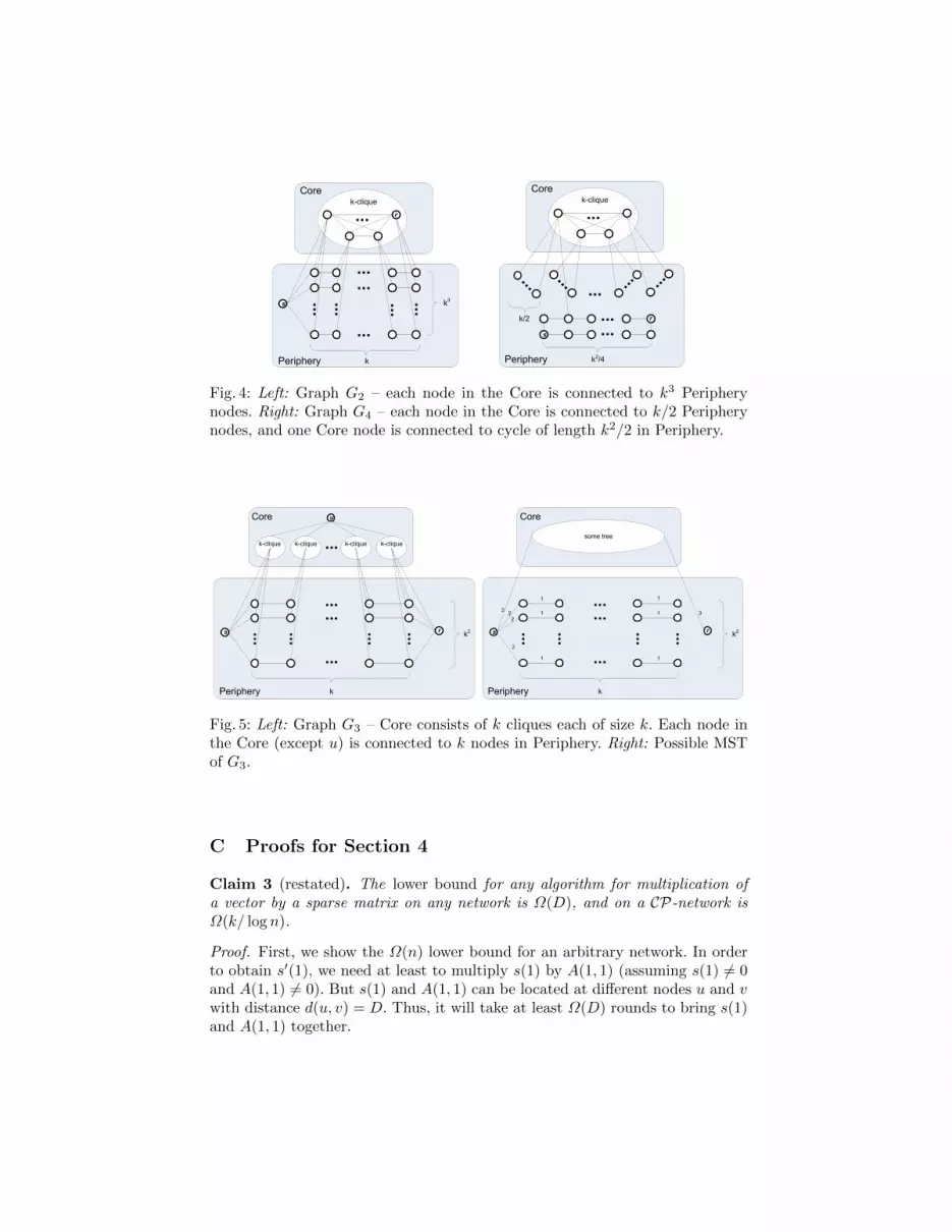
Proof. 1. Consider a graph G2 on Figure 4 (Left) in which Core is a clique ofsize k and each node in the Core is connected to k3 Periphery nodes (onenode in Core is also connected to s, so it has k3 + 1 Periphery neighbors).The number of nodes in G2 is thus: n = k + k · k3 + 1 = Θ(k4).

In [16], it was shown that any distributed algorithm will take at leastΩ(

4√n√

logn

)time on G1. In the graph G1, Core is a clique, thus G1 satisfies Axiom AE .Since every node in Periphery has a direct edge to the Core, we can say thatG1 satisfies Axiom AC , i.e., it is possible to perform a convergcast in O(1).

But notice that din = 4√n while dout =

4√n3 and thus G1 does not satisfy

Axiom AB .

2. Consider a graph G3 on Figure 5 (Left) in which Core is a collection of kcliques, each of size k, where a single node in each clique is connected to aspecial Core node u, and there are no edges between cliques. Each node in theCore (except of u) is connected to k Periphery nodes, such that all nodes inspecific clique are connected to the Periphery nodes that reside in a specificcolumn. One Core node (from the leftmost clique) is additionally connectedto s and another Core node (from the rightmost clique) is connected to r.The number of nodes in G3 is thus: n = k · k + k · k2 + 2 = Θ(k3).Let’s take a look at the nodes s and r and assume the following weightsassignment. All the edges between Core and Periphery have weights 10,except of the two edges that come from s and r. Weights of all the edgesincident to s are 2 and weights of all the edges incident to r are 3. Assumealso that all the rest weights in Periphery are 1. Easy to see that such weightswill yield MST illustrated in Figure 5 (Right). Notice that if the weight ofsome edge incident to s will be increased (let’s say to 5) this will cause thisedge to be removed from the MST and the appropriate edge incident to rto be included. Thus, in order to allow r to know which of its edges belongto the MST, it needs to receive information regarding all the edges incidentto s, i.e., at least k2 messages should be delivered from s to r. Next we willshow that delivering k2 messages from s to r will require at least k/2 time.First, note that any path s→ r that is not passing via the node u has lengthof at least k, thus we can assume that all the messages will take paths viau. Second, we can see that the edge cut of the node u (i.e., its degree) is kand thus, after k/2 time it will forward at most k2/2 messages, which is notsufficient for completing the MST task. Thus, any MST algorithm on thegraph G will take at least Ω(k) = Ω( 3

√n) time.

It is left to show that G3 satisfies Axioms AB and AC , but not AE . For everynode in the Core, din = k and dout = k except the node u for which dout = 0.So, for each node in the core dout

din+1 = O(1) which means that AB is satisfied.Since every node in Periphery has a direct edge to the Core, we can saythat G3 satisfies Axiom AC , i.e., it is possible to perform a convergcast inO(1). It is also easy to see that in the Core there is no O(1)-clique emulation(AE), since in order to send k messages out of any clique in Core to anyother clique in Core we need k time since there is only one edge from anyclique towards the node u that interconnects cliques.

3. Consider a graph G4 on Figure 4 (Right) in which Core is a clique of sizek and each node in the Core is connected to k/2 Periphery nodes. OneCore node is additionally connected to a cycle of size k2/2 that resides inPeriphery. The number of nodes in G4 is thus: n = k+k ·k/2+k2/2 = Θ(k2).It is easy to see that Axioms AB and AE are satisfied, but Axiom AC isnot. For some weights assignment, the decision regarding which edge of r toinclude in the MST depends on the weights of the edges incident to s. Thelast implies that at least one message has to be delivered from s to r whichwill take Ω(k2) = Ω(n) time.

s

...

...

...

...

...

...

r

...

Core

Periphery

...

k-clique

k3

k

......

r

Core

Periphery

...

k-clique

k2/4

k/2

... ...

...

...

s ...

Fig. 4: Left: Graph G2 – each node in the Core is connected to k3 Peripherynodes. Right: Graph G4 – each node in the Core is connected to k/2 Peripherynodes, and one Core node is connected to cycle of length k2/2 in Periphery.

k-clique

s

Core

Periphery

k2

k...

k-clique

...

k-clique

...

k-clique...

r

...

...

...

u

...some tree

s

Core

Periphery

k2

k

...

...

...

...

r

...

...

...

22

2

2

3

1

1

1

1

1

1

Fig. 5: Left: Graph G3 – Core consists of k cliques each of size k. Each node inthe Core (except u) is connected to k nodes in Periphery. Right: Possible MSTof G3.

C Proofs for Section 4

Claim 3 (restated). The lower bound for any algorithm for multiplication ofa vector by a sparse matrix on any network is Ω(D), and on a CP-network isΩ(k/ log n).

Proof. First, we show the Ω(n) lower bound for an arbitrary network. In orderto obtain s′(1), we need at least to multiply s(1) by A(1, 1) (assuming s(1) 6= 0and A(1, 1) 6= 0). But s(1) and A(1, 1) can be located at different nodes u and vwith distance d(u, v) = D. Thus, it will take at least Ω(D) rounds to bring s(1)and A(1, 1) together.

Now we are going to show that for any CP-network, the lower bound isΩ(k/ log n) rounds. Consider a CP-network as in Figure 1 (I). Let u be a nodein P add its degree is 1. Let v be any other node in V . Assume that u initiallystores the row A1,∗ and the entry s(1), while v stores row A2,∗ and the entrys(2).

Next, we show a reduction from the well-known equality problem (EQ),in which two parties are required to determine whether their input vectorsx, y ∈ 0, 1k are equal. Assuming we are given a procedure P for our vec-tor by matrix multiplication problem, we use it to solve the EQ problem. Giveninput vectors x, y for the EQ problem (at u and v respectively), we create aninput for the vector by matrix multiplication problem in the following way. Nodeu assigns A(1, i) = x(i) for every i ∈ [1, . . . , k] and s(1) = 1, while node v assignsA(2, i) = y(i) for every i ∈ [1, . . . , k] and s(2) = 1. All the other entries of A ands are initialized to 0. It follows that s′(i) =

∑nj=1 s(j)A(j, i) = A(1, i)+A(2, i) =

x(i)+y(i) for every i ∈ [1, . . . , k]. Given the value of s′(i), one can decide whetherx(i) = y(i) for every i ∈ [1, . . . , k], since clearly x(i) = y(i) if’f s′(i) ∈ 0, 2(and otherwise s′(i) = 1). Notice that the vector s′ is stored distributedly in thenetwork – one entry in each node. But the indication to v and u whether all theentries are in 0, 2 can be delivered in O(1) rounds in the following way. Eachnode in P sends its entry of s′ to its representative who checks all the receivedentries and sends an indication bit to all the other nodes in C. So, every node inC knows now whether all the entries in s′ are in 0, 2 (actually, we are interestedonly in the first k entries). Representatives can now inform the nodes in P theyrepresent in O(1) rounds. It follows that using procedure P one can solve the EQproblem, which is known to require at least k bits of communication. Therefore,assuming that each message is O(log n) bits, our problem requires Ω(k/ log n)communication rounds.

Theorem 7 (restated). For each X ∈ B,E,C there exist a family FX =GX(V,E, C,P)(n) of partitioned networks that do not satisfy Axiom AX butsatisfy the other two axioms, and input matrices of size n×n and vectors of sizen, for every n, such that the time complexity of any algorithm for multiplyinga vector by a matrix on the networks of FX with the corresponding inputs isΩ(n/ log n).

Proof. Now we show the necessity of the Axioms AB , AE and AC for achievingO(k) running time. Consider the following cases where in each case one of theaxioms is not satisfied while the other two satisfied.Necessity of AB : Consider the family of dumbbell partitioned networks Dn. Asdiscussed earlier, Axiom AB is violated while the other hold. Let us denote thecore’s nodes as u and v. In O(k) rounds u (resp. v) can collect all the rows of Aand entries of s stored at the nodes of P connected to u (resp. v). So, assumingn/2 is integer, after O(k) rounds, u and v have each n/2 rows of A and n/2entries of s. Assume also an input for which u has rows A1,∗, A2,∗, . . . , An/2,∗and entries s(n/2 + 1), s(n/2 + 2), . . . , s(n), and v has all the remaining rows ofA and entries of s.

We now show a reduction from the well-known equality problem (EQ), inwhich two parties are required to determine whether their input vectors x, y ∈0, 1n are equal. Assuming we are given a procedure P for our vector by matrixmultiplication problem, we use it to solve the EQ problem. Given input vectorsx, y for the EQ problem (at u and v respectively), we create an input for thevector by matrix multiplication problem in the following way. Node u assignsA(i, i) = x(i)+1 for every i ∈ [1, . . . , n/2] and s(i) = x(i)+1 for every i ∈ [n/2+1, . . . , n], while node v assigns A(i, i) = y(i)+1 for every i ∈ [n/2+1, . . . , n] ands(i) = y(i) + 1 for every i ∈ [1, . . . , n/2]. All the other entries of A are initializedto 0, thus A is a diagonal matrix. It follows that s′(i) =

∑nj=1 s(j)A(j, i) =

s(i)A(i, i) = (x(i) + 1)(y(i) + 1) for every i. Given the value of s′(i), one candecide whether x(i) = y(i), since clearly x(i) = y(i) if’f s′(i) ∈ 1, 4 (andotherwise s′(i) = 2). It follows that using procedure P one can solve the EQproblem, which is known to require at least n bits of communication. Therefore,assuming that each message is O(log n) bits, our problem requires Ω(n/ log n)communication rounds.Necessity of AE : Consider the family of sun partitioned networks Sn. As dis-cussed earlier, Axiom AE is violated while the other hold. The diameter of Sn isΩ(n), hence any algorithm for this task will require Ω(n) communication rounds(due to the lower bound discussed earlier).Necessity of AC : Consider the family of lollipop partitioned networks Ln. As dis-cussed earlier, Axiom AC is violated while the other hold. Again, the diameterof Ln is Ω(n), hence any distributed matrix transpose algorithm requires Ω(n)rounds.

D Algorithms for additional problems

D.1 Matrix transposition

Initially, each node in V holds one row of an O(k)-sparse matrix A (along withits index). The task is to distributively calculate the matrix AT and store itsrows in such a way that the node that stores row Ai,∗ will eventually store rowATi,∗. We start with a claim on the lower bound.

Claim 9. The lower bound for any algorithm for transposing an O(k)-sparsematrix on any network is Ω(D), and on a CP-network is Ω(k).

Proof. Consider a nonzero entry A(i, j) where j 6= i. Consider the nodes uand v that initially store Ai,∗ and Aj,∗ respectively. Clearly, in any algorithm,A(i, j) should be delivered to the node v (which is required to eventually obtainA∗,j = ATj,∗). Since the distance d(u, v) may be as large as the diameter, thelower bound is Ω(D) rounds.

For a CP-network, the lower bound is Ω(k) since there are inputs for whichrow ATi,∗ has k nonzero values which must be delivered to the node that initiallyhas row Ai,∗. There are CP-networks in which minimum degree is 1 (see Figure

1 (I) for an illustration) and hence, delivering Ω(k) messages will require Ω(k)communication rounds.

Algorithm 2. The following algorithm generates AT in O(k) rounds on a CP-network G(V,E, C,P).

1. Each u ∈ V sends its row (all the nonzero values with their indices in A)to its representative r(u) ∈ C. Now each representative has O(nC) rows of A(or O(knC) entries of A).

2. Each representative, for each entry A(i, j) it has, sends it to the node inC that is responsible for the row ATj,∗. By agreement, every node in C is

responsible for the rows of AT with indices 1 + (n/nC)(i − 1), . . . , (n/nC)i(assuming n/nC is integer).

3. Now, each node in C stores O(n/nC) rows of AT . So, each node u ∈ V thatinitially stored the row i of A, requests ATi,∗ from its representative. Therepresentative gets the row from the corresponding node in C and sends itback to u.

Theorem 8. On a CP-network G(V,E, C,P), the transpose of a O(k)-sparsematrix can be completed in O(k) rounds w.h.p.

Proof. Consider Algorithm 2 and the CP-network G(V,E, C,P). Step 1 of thealgorithm will take O(k) rounds since each row has up to k nonzero entries andsending one entry takes O(1) due to Axiom AC . Now each representative hasO(knC) values since it represents up to O(nC) nodes in P (due to Axiom AB).

In the beginning of Step 2, each representative knows the destination for eachof the A(i, j) entries it has (since, by agreement, each node in C is responsiblefor collecting entries for specific rows of AT ). So, it will send O(knC) messages,each one to a specific single destination. Since each node in C is responsible forO(n/nC) rows of AT , it will receive O(kn/nC) messages. Thus, using Axiom AEand Theorem 6 we get O(k) running time.

At Step 3, a single row (with O(k) nonzero entries) is sent by each node toits representative (takes O(k) due to the Axiom AC), then the requests are de-livered to the appropriate nodes in C and the replies with the appropriate rowsof AT are received back by the representatives. All this takes O(k) rounds dueto the Axiom AE and Theorem 6. Then the rows of AT are delivered to thenodes that have requested them. Due to the Axiom AC this will also take O(k)rounds.

We now show the necessity of the Axioms AB , AE and AC for achievingO(k) running time.

Theorem 9. For each X ∈ B,E,C there exist a family FX = GX(V,E, C,P)(n)of partitioned networks that do not satisfy Axiom AX but satisfy the other two

axioms, and input matrices of size n × n for every n, such that the time com-plexity of any matrix transposition algorithm on the networks of Fi with thecorresponding inputs is Ω(n).

Proof. Consider the following cases where in each case one of the axioms is notsatisfied while the other two satisfied.Necessity of AB : Consider the family of dumbbell partitioned networks Dn.As discussed earlier, Axiom AB is violated while the other hold. Let A be amatrix where at least the following n/2 entries are nonzero (assume n/2 is even):A(n/2+1, 1), A(n/2+2, 2), . . . , A(n, n/2). Then we input the rows A1,∗−An/2,∗to the nodes in the first star of of Dn, and rows An/2+1,∗ −An,∗ to the nodes inthe second star of Dn. Clearly, the entries we specified before are initially locatedin the second star but they all must be delivered to the first star (by problemdefinition, an entry A(i, j) should be eventually stored in a node that initiallyhas row Aj,∗). Since there is only one edge connecting the stars, any algorithmfor the specified task will take Ω(n) rounds.Necessity of AE : Consider the family of sun partitioned networks Sn. As dis-cussed earlier, Axiom AE is violated while the other hold. The diameter of Sn isΩ(n), hence any algorithm for this task will require Ω(n) communication rounds(due to the lower bound discussed earlier).Necessity of AC : Consider the family of lollipop partitioned networks Ln. As dis-cussed earlier, Axiom AC is violated while the other hold. Again, the diameterof Ln is Ω(n), hence any distributed matrix transpose algorithm requires Ω(n)rounds.

D.2 Matrix multiplication

Let A and B be square n × n matrices with O(k) nonzero entries in each rowand each column. Initially, each node in V holds one row of A (along with theindex of the row) and one row of B (along with the index of the row). The taskis to distributively calculate C = AB and store its rows at the correspondingnodes in V , such that the node that initially stored row i of B will store row iof C. We start with a claim on the lower bound.

Claim 10. The lower bound for any algorithm for O(k)-sparse matrix multi-plication on any network is Ω(D), and on a CP-network is Ω(k2).

Proof. Let us start with a lower bound for any network. In order to obtainC(1, 1), we need at least to multiply A(1, 1) by B(1, 1) (assuming input in whichA(1, 1) 6= 0 and B(1, 1) 6= 0). But A(1, 1) and B(1, 1) can be located at differentnodes u and v with distance d(u, v) = D. Thus, it will take at least Ω(D) roundsto bring A(1, 1) and B(1, 1) together.

For a CP-network, consider a network illustrated on Figure 1 (I), where de-gree of a node u ∈ P is 1. Assume that initially u has row A1,∗ and B1,∗ andthus, by problem definition, it has to eventually receive the row C1,∗. We show

now that there are Ω(k2) messages are required to allow u to obtain C1,∗. As-

sume that bji for i, j ∈ [1, . . . , k] are k2 distinct values. Consider an input inwhich A(1, i) = 1 for every i ∈ [2, . . . , k+ 1], B(2, i) = b1i for every i ∈ [1, . . . , k],B(3, i) = b2i for every i ∈ [k+1, . . . , 2k], and so on until B(k+1, i) = bki for everyi ∈ [k(k − 1) + 1, . . . , k2]. All other entries of A and B are set to 0. Easy to seethat C(1, i) = b1i for every i ∈ [1, . . . , k], C(1, i) = b2i for every i ∈ [k+1, . . . , 2k],and so on until C(1, i) = bki for every i ∈ [k(k − 1) + 1, . . . , k2]. So, in order to

obtain the row C1,∗, u must receive all the k2 values bji which will take Ω(k2)communication rounds.

Algorithm 3. The following algorithm solves the O(k)-sparse matrix multipli-cation task in O(k) rounds on a CP-network G(V,E, C,P).

1. Each node in V send its row of B to its representative. Now, each node in Chas O(knC) entries of B.

2. Now, nodes in C redistribute the rows of B among themselves in a way thatthe node with ID i will store rows 1 + (n/nC)(i − 1), . . . (n/nC)i (assumingn/nC is integer). Now, each u ∈ C has O(n/nC) rows of B

3. Each node in V sends its row of A to its representative. Notice that the rowi of B needed to be multiplied only by values of the column i of A.

4. Each u ∈ C sends the values of A it has to the nodes in C that hold thecorresponding rows of B. I.e., the value A(i, j) will be sent to the node inC which holds the row Bj,∗. Now we have all the summands prepared anddistributed across all the nodes in C. It is now left to combine correspondingsummands.

5. Each u ∈ C sends each of its values to the corresponding node in C that isresponsible for gathering the summands for the values of specific O(n/nC)rows of the resulting matrix C.

6. Now each node u ∈ V that initially stored row i of B, requests row i of C fromits representative. The representative gets the row from the correspondingnode in C and sends it back to u. Easy to see that this step takes O(k2)rounds.

Theorem 10. On a CP-network G(V,E, C,P), the multiplication of two O(k)-sparse matrices can be completed in O(k) rounds w.h.p.

Proof. Consider Algorithm 3 and the network G(E, V ) with partition 〈C,P〉 thatsatisfies Axioms AB ,AE ,AC .

Step 1 will take O(k) due to the Axiom AC and the fact that the number ofnonzero entries in each row is bounded by k. Each node in C will have O(knC)entries of B since it represents O(nC) nodes in P due to the Axiom AB . UsingTheorem 6 with the parameters: Ms = O(knC) and Mr = O(kn/nC), we showthat the redistribution performed at Step 2 takes O((knC + kn/nC)/nC) = O(k)rounds.

For Step 4, we again use Theorem 6 with the parameters: Ms = O(k)O(nC)(O(k) values per row), Mr = O(n/nC)O(k) (O(k) values per column of A), and

obtain that the running time is O(k). Note that, each node in C has O(n/nC)rows (of B) with O(k) elements in each. Each row was multiplied by O(k) valuesreceived in the previous step (O(k) since each column of A has O(k) nonzerovalues). Thus, each u ∈ C has O(k2n/nC) values that needed to be sent to theappropriate nodes in the next step.

At Step 5, each u ∈ C sends each of its values to the corresponding node in Cthat is responsible for gathering the summands for the values of specific O(n/nC)rows of the resulting matrix C. Clearly, Ms = O(k2n/nC) since each row of Bhas O(k) different entries, and was multiplied by O(k) different entries of A. Nowlet’s find Mr. Each u ∈ C is responsible for O(n/nC) rows of C. Thus, e.g., for arow C1,∗ it needs to receive the following summands: C(1, 1) =

∑A(1, i)B(i, 1),

C(1, 2) =∑A(1, i)B(i, 2), ..., C(1, n) =

∑A(1, i)B(i, n). Since the number of

nonzero entries in each row of A and B is O(k), the number of nonzero entriesin each row of C is bounded by O(k2). Thus, for each row of C, a node in C willreceive O(k2) messages. So, Mr = O(k2n/nC) and thus the running time of thisstep is O(k2).

At the last step, each node u ∈ V sends a single message (request for arow) to its representative. This tales O(1) due to the convergecast. Then, therepresentative gets the row from the corresponding node in C and sends it backto u. Using Axiom AE and Theorem 6 with Ms = O(nC) and Mr = O(n/nC)we get O(1) running time for delivering the request inside the core. In a similarway, sending the rows inside the core will take O(k2) rounds. The same amountof time will be required to deliver those rows to the nodes in P that requestedthem (O(1) per row entry due to convergecast, and O(k2) nonzero entries perrow).

Theorem 11. For each X ∈ B,E,C there exist a family FX = GX(V,E, C,P)(n)of partitioned networks that do not satisfy Axiom AX but satisfy the other twoaxioms, and input matrices of size n × n, for every n, such that the time com-plexity of any algorithm for the multiplication of two O(k)-sparse matrices onthe networks of FX with the corresponding inputs is Ω(n/ log n).

Proof. Necessity of AB : Consider the family of dumbbell partitioned networksDn. As discussed earlier, Axiom AB is violated while the other hold. As we didin the proof of Theorem 7, we can show a reduction of from the well equalityproblem (EQ) to our problem of multiplication of two sparse matrices. Here weinitialize A and B to be diagonal matrices and the first core node, u, will havefirst half of A’s rows and second half of B’s rows. Due to the initialization, eachentry of the resulting matrix C will be a multiplication of the correspondingentries of x and y. Thus, obtaining C will allow us to determine whether x and yare equal. Thus, the lower bound for our problem is Ω(n/ log n) communicationrounds.The proof of the necessity of AE and AC is the same as in the proof of Theorem9, and is based on the diameter argument.

Now we show another set of algorithms that deal with aggregate functions.In some of the following algorithms , we use the following result on distributedsorting in clique, presented in [3].

Theorem 12 ([3]). Consider a clique network G(V,E) where nodes in V haveIDs [1, . . . , n]. Each node is given n values. For simplicity, assume that all the n2

values are distinct4. The following tasks can be solved deterministically in Θ(1)rounds.

1. Node i needs to learn the values with indices i(n−1) + 1, . . . in according thetotal order of all values.

2. Node i needs to determine the indices of its input (initial) values in the totalorder of all values.

Observation 1. Theorem 12 can be naturally extended to the case where eachnode initially holds O(n) keys (instead of exactly n).

D.3 Find my rank

Let each node v ∈ V hold some initial value. Each node needs to know theposition of its value in the ordered list of all the values, i.e., the rank of its value.We start with a claim on the lower bound.

Claim 11. The lower bound for any algorithm for finding the rank of each valueon any network is Ω(D), and on a CP-network is Ω(1).

Proof. Consider the two nodes u, v ∈ V . In order to decide whose value is larger,at least one bit of information must travel between them. Thus, the lower boundfor this task on any graph is Ω(D).

Algorithm 4. The following algorithm finds the rank of each value in O(1)rounds on a CP-network G(V,E, C,P).

1. Each node in V sends its initial value to its representative in C.2. Nodes in C perform sorting of all the values they have, and obtain the ranks

of those values. So, each node u ∈ C will know the ranks of the values it hadreceived from the nodes it represents.

3. The ranks are delivered to the appropriate nodes in P.

Theorem 13. On a CP-network G(V,E, C,P), the the task of obtaining a rankcan be completed in O(1) rounds w.h.p.

4 This limitation can be eliminated by chaining each value with the node ID and itsorder at the node. Thus, each input value becomes unique.

Proof. Consider Algorithm 4 and the CP-network G(V,E, C,P). The first steptakes O(1) due to Axiom AC . Now, each representative u ∈ C has O(nC) valuesdue to the Axiom AB . Step 2, is performed in O(1) rounds due the Theorem 12and Axiom AE . The last step will take O(1) rounds due to AC .

Theorem 14. For each X ∈ B,E,C there exist a family FX = GX(V,E, C,P)(n)of partitioned networks that do not satisfy Axiom AX but satisfy the other twoaxioms, and input matrices of size n×n and vectors of size n, for every n, suchthat the time complexity of any algorithm for finding the rank of each value onthe networks of FX with the corresponding inputs is Ω(n).

Proof. Necessity of AB : Consider the family of dumbbell partitioned networksDn. As discussed earlier, Axiom AB is violated while the other hold. Consider asorted list of n values (ai ≤ ai+1): a1, a2, a3, ..., an. Clearly, every two adjacentvalues must be compared in any sorting procedure. For example, if we assumethat some sorting procedure does not compare a2 and a3, and also a4 = a3 + 2then we can replace a2 with a3 + 1 and get the same output a1, a2, a3, ..., anwhich is now incorrect since a2 > a3.

Let us denote the two core’s nodes as u and v. Node u and all the nodesin P that are connected to it, will be assigned values (one value to one node)with odd indices in the ordered list (i.e., a1, a3, . . .). The other n/2 values willbe assigned to the remaining n/2 nodes (one value to one node).

Now, in order to obtain a sorted list, at least the following comparisons musttake place: a1 with a2, a3 with a4, and so on. We can see that about n/2 pairs ofvalues have to be brought together while initially they are located at the differentsides of the link (u, v). Thus, Ω(n) messages must be sent over the link (u, v) inorder to perform the sorting task. The last takes Ω(n) communication rounds.The proof of the necessity of AE and AC is the same as in the proof of Theorem9, and is based on the diameter argument.

D.4 Find median

Let each node v ∈ V hold some initial value. Each node needs to know the valuewhich is the median in the ordered list of all the values in the network. We startwith a claim on the lower bound.

Claim 12. The lower bound for any algorithm for finding median on any net-work is Ω(D), and on a CP-network is Ω(1).

Proof. Consider two nodes u, v ∈ V . It is obvious that if u wants to obtain themedian of the initial values, at least one bit of information must travel betweenu and v (otherwise u will never know that v exists while v may even be themedian). Since the distance d(u, v) can be as large as the diameter, the lowerbound for this task is Ω(D) communication rounds.

Algorithm 5. The following algorithm finds the median in O(1) rounds on aCP-network G(V,E, C,P).

1. Each node in V sends its initial value to its representative in C.2. Nodes in C perform sorting of all the values they have, and obtain the ranks

of those values. So, each node i ∈ C now knows values with indices i(nC −1) + 1, . . . inC according to the total order of all values.

3. The node in C which has the value with index n2/2 (which is the medianvalue) sends it to all the nodes in C.

4. The median value is delivered to the nodes in P.

Theorem 15. On a CP-network G(V,E, C,P), the finding median of all theinitial values can be completed in O(1) rounds w.h.p.

Proof. Consider Algorithm 5 and the CP-network G(V,E, C,P). The first steptakes O(1) due to Axiom AC . Now, each representative u ∈ C has O(nC) valuesdue to Axiom AB . Step 2, is performed in O(1) rounds due to Theorem 12 andAxiom AE . The last step will take O(1) rounds due to AC .

Theorem 16. For each X ∈ B,E,C there exist a family FX = GX(V,E, C,P)(n)of partitioned networks that do not satisfy Axiom AX but satisfy the other twoaxioms, and input matrices of size n×n and vectors of size n, for every n, suchthat the time complexity of any algorithm for finding median of all the initialvalues on the networks of FX with the corresponding inputs is Ω(log n).

Proof. Necessity of AB : Consider the family of dumbbell partitioned networksDn. As discussed earlier, Axiom AB is violated while the other hold. In constanttime, each of the two centers A and B can learn the inputs of its star. Now theproblem becomes for A and B to learn the median of the union of their sets. Thisoperation is known to require at least Ω(log n) communication rounds. More for-mally, it is shown in [20] that the Median function does not admit a deterministicprotocol using O(log1−ε n) rounds and a logarithmic amount of communicationat each round, for any ε > 0 (even though the total communication complexityof the problem is known to be only O(log n) bits). This allows us to concludethe same lower bound in our case too.The proof of the necessity of AE and AC is the same as in the proof of Theorem9, and is based on the diameter argument.

D.5 Find mode

Let each node v ∈ V hold some initial value. Each node needs to know the value(values) that appears most frequently. We start with a claim on the lower bound.

Claim 13. The lower bound for any algorithm for finding mode on any networkis Ω(D), and on a CP-network is Ω(1).

Proof. Consider two nodes u, v, w ∈ V . Assume an input for which the most fre-quent value appears with frequency 2 and is initially located at v and w, whileall the other nodes have other distinct values. Obviously, if u needs to learn themode, at least one bit of information must travel from v to u, since otherwise uwill not be aware of the v’s existence. Since the distance d(u, v) can be as largeas diameter, the lower bound for this task is Ω(D) communication rounds.

Algorithm 6. The following algorithm finds the mode in O(1) rounds on aCP-network G(V,E, C,P).

1. Each node in V sends its initial value to its representative in C.2. Nodes in C perform sorting of all the values they have, and obtain the ranks

of those values. So, each node i ∈ C now knows values with indices i(nC −1) + 1, . . . inC according to the total order of all values.

3. Each node in C sends to each other node in C:(a) its most frequent value (values) and its frequency,(b) its minimum value and its frequency,(c) its maximum value and its frequency.The minimum and maximum are needed in order capture the most frequentvalues that appear at the boundaries of the ranges.

4. Now each node in C can find the most frequent value (values) and deliversit to the nodes in P it represents.

Theorem 17. On a CP-network G(V,E, C,P), the task of finding mode (themost frequent value) can be completed in O(k) rounds w.h.p.

Proof. Consider Algorithm 6 and the CP-network G(V,E, C,P). The first steptakes O(1) due to Axiom AC . Now, each representative u ∈ C has O(nC) valuesdue to Axiom AB . Step 2, is performed in O(1) rounds due the Theorem 12 andAxiom AE . Step 3 takes O(1) due to Axiom AE since each node in C needs tosend O(1) values to all the other nodes in C. The last step will take O(1) roundsdue to AC (and assuming there are O(1) most frequent values).

Theorem 18. For each X ∈ B,E,C there exist a family FX = GX(V,E, C,P)(n)of partitioned networks that do not satisfy Axiom AX but satisfy the other twoaxioms, and input matrices of size n×n and vectors of size n, for every n, suchthat the time complexity of any algorithm for the finding mode on the networksof FX with the corresponding inputs is Ω(n/ log n).

Proof. Necessity of AB : Consider the family of dumbbell partitioned networksDn. As discussed earlier, Axiom AB is violated while the other hold. Assumesuch an input that every element appears exactly once or twice on each side(for simplicity assume there are n/4 types of elements altogether, and somenodes do not have any element). Hence the most frequent element will appear2, 3 or 4 times in the graph. The case where the answer is 2 occurs only when

every element appears exactly once on every side. This case is easy to check in aconstant amount of communication between the two centers, so we assume we dothis check first, and it remains to consider the case where this does not happen.It thus remains to decide whether the answer is 3 or 4. To do that, A (the centerof the first star) defines a set SA of all the elements that appear twice in its star,and B defines a set SB similarly for its side. Now the answer is 4 if’f the sets SAand SB intersect. Set disjointness has communication complexity n, so A andB must exchange at least n bits, or, at least Ω(n/ log n) messages. Since thesemessages all cross the single edge connecting the two centers, they require thismuch time.The proof of the necessity of AE and AC is the same as in the proof of Theorem9, and is based on the diameter argument.

D.6 Find the number of distinct values

Let each node v ∈ V hold some initial value. Each node needs to know thenumber of distinct values present in the network. We start with a claim on thelower bound.

Claim 14. The lower bound for any algorithm for finding the number of distinctvalues on any network is Ω(D), and on a CP-network is Ω(1).

Proof. Consider two nodes u, v ∈ V . Assume an input for which all the valuesin the network are distinct. Obviously, that if u needs to learn the number ofdistinct values, at least one bit of information must travel from v to u, sinceotherwise u will not be aware of the v’s existence. Since the distance d(u, v) canbe as large as diameter, the lower bound for this task is Ω(D) communicationrounds.

Algorithm 7. The following algorithm finds the number of distinct values inO(1) rounds on a CP-network G(V,E, C,P).

1. Each node in V sends its initial value to its representative in C.2. Nodes in C perform sorting of all the values they have, and obtain the ranks

of those values. So, each node i ∈ C now knows values with indices i(nC −1) + 1, . . . inC according to the total order of all values.

3. Each node in C sends to every other node in C the number of distinct valuesand the two border values (min,max). Then, every node in C will be able tofind the number of distinct values (for each repeated border value, decrease1 from the total count).

4. Each representative delivers the number of distinct nodes to the nodes in Pit represents.

Theorem 19. On a CP-network G(V,E, C,P), the task of finding the numberof distinct values can be completed in O(1) rounds w.h.p.

Proof. Consider Algorithm 7 and the CP-network G(V,E, C,P). The first steptakes O(1) due to Axiom AC . Now, each representative u ∈ C has O(nC) valuesdue to the Axiom AB . Step 2, is performed in O(1) rounds due the Theorem12 and Axiom AE . Step 3 takes O(1) due to Axiom AE since each node in Cneeds to send O(1) values to all the other nodes in C. The last step will takeO(1) rounds due to AC .

Theorem 20. For each X ∈ B,E,C there exist a family FX = GX(V,E, C,P)(n)of partitioned networks that do not satisfy Axiom AX but satisfy the other twoaxioms, and input matrices of size n×n and vectors of size n, for every n, suchthat the time complexity of any algorithm for finding the number of distinctvalues on the networks of FX with the corresponding inputs is Ω(n/ log n).

Proof. Necessity of AB : Consider the family of dumbbell partitioned networksDn. As discussed earlier, Axiom AB is violated while the other hold. Assumethat the inputs are taken out of a range of m distinct possible values. In constanttime, the two star centers A and B can collect m-bit vectors x and y respectively,representing the values that exist in their respective stars. The goal is for A andB to decide the number of distinct values in the graph, i.e., the number of 1’sin the vector x ∨ y. We show a reduction from set disjointness to this problem,hence the lower bound for set disjointness holds for it. Assume we are given aprocedure P for our problem. We use it to solve set disjointness as follows. (1)A computes |x| and informs B. (2) B computes |y| and informs A. (3) A and Binvoke procedure P and compute |x ∨ y|. (4) The answer is “yes” (the sets aredisjoint) iff |x ∨ y| = |x| + |y|. It is easy to verify that the reduction is correct,hence we get the desired lower bound of Ω(m/ log n) on the number of roundrequired for finding the number of distinct values.The proof of the necessity of AE and AC is the same as in the proof of Theorem9, and is based on the diameter argument.

D.7 Get the top k ranked by areas

Let each node v ∈ V hold some initial value. Assume that each value is assignedto a specific area of a total

√n areas. E.g., values may represent news and areas

topics, so that each news belongs to a specific topic. Assume also that each nodein V is interested in one specific area. The task is to deliver to each node in Vthe largest k values from the area it is interested in. We start with a claim onthe lower bound.

Claim 15. The lower bound for any algorithm for finding the k top rankedvalues from a specific area on any network is Ω(D), and on a CP-network isΩ(k).

Proof. First, let us show the lower bound for any network. Consider two nodesu, v ∈ V and assume input in which u is interested in the value initially stored

at v. Obviously, delivering the value from v to u will take at least d(u, v). Sincethe distance d(u, v) may be as large as diameter, the lower bound on the runningtime is Ω(D).

For a CP-network, the lower bound is Ω(k) since obviously, there are inputsfor which k values must be delivered to a node in P. There are CP-networksin which minimum degree is 1 (see Figure 1 (I) for an illustration) and hence,delivering Ω(k) messages will require Ω(k) communication rounds.

Algorithm 8. The following algorithm finds the k top ranked values from aspecific area in O(k) rounds on a CP-network G(V,E, C,P).

Without loss of generality, assume that all the values are from the range[1, . . . , n], and each area has its own range for its values (e.g., politics [1, . . . , 100],sports [101, . . . , 200], etc.).

1. Each node in V sends its initial value to its representative in C.2. Perform sorting using Theorem 12 and Axiom AE . It takes O(1). Each nodei ∈ C now knows values with indices i(nC − 1) + 1, . . . inC according to thetotal order of all values.

3. Now, each node in C will send the largest k values from each area to theappropriate node in C, so that each node in C will be responsible for at mostone area (recall that we have

√n areas and nC = Ω(

√n)).

4. Each representative sends requests for areas (up to O(nC) areas) requestedby nodes it represents. Each request is destined to a specific node in C that isresponsible for the requested area. Upon request, each node in C returns thek largest value for the area it is responsible for to the nodes that requestedthem.

5. Each representative u ∈ C delivers the values to the nodes in P it represents.

Theorem 21. On a CP-network G(V,E, C,P), the task of finding the k topranked values from a specific area can be completed in O(k) rounds w.h.p.

Proof. Consider Algorithm 8 and the CP-network G(V,E, C,P). From Theorem2, we know that nC = Ω(

√n), thus we can say that the number of areas is O(nC).

The first step takes O(1) due to Axiom AC . Now, each representative u ∈ C hasO(nC) values due to the Axiom AB . At Step 2, each node has O(nC) values (eachdestined to a specific single node), so Ms = nC. Each node has to receive Mr = kvalues (more precisely: Mr = 2k, since it is possible that after the initial sorting,an area is split across two nodes, and each of these two nodes will send up to kvalues from that area and the receiving node will have to select the correct k).Thus, this step will take (according to Theorem 6) O((nC + k)/nC) = O(k/nC).Step 3 takes O(k) since sending requests will take O(1) (due to the Axiom AEand Theorem 6 with Ms = nC, Mr = nC), and receiving the desired values willtake O(k) (since Ms = knC and Mr = knC). The last step will take O(k) sinceeach node in P needs k values, and delivering a single value from r(u) ∈ C tou ∈ P takes O(1) due to the Axiom AC .

Theorem 22. For each X ∈ B,E,C there exist a family FX = GX(V,E, C,P)(n)of partitioned networks that do not satisfy Axiom AX but satisfy the other twoaxioms, and input matrices of size n × n and vectors of size n, for every n,such that the time complexity of any algorithm for finding the k top ranked val-ues from a specific area on the networks of FX with the corresponding inputs isΩ(knC).

Proof. Necessity of AB : Consider the family of dumbbell partitioned networksDn. As discussed earlier, Axiom AB is violated while the other hold. Consider√n/2 areas and assume that all the k

√n/2 values belonging to these areas are

initially located at the nodes of the first star of Dn. Consider a subset of nodesof the second star. Let the subset size be

√n/2 and each node in this subset

is interested in different area of the areas stored in the first star we mentioned.We can see that in order to complete the task, all the k

√n/2 values have to be

sent from the first to the second star, which are interconnected by a single edge.Thus, the running time will be Ω(k

√n) rounds.

The proof of the necessity of AE and AC is the same as in the proof of Theorem9, and is based on the diameter argument.