Embed Size (px)
Citation preview
1 / 32
Agglomeration Shadow:
A Non-Linear Core–Periphery Model of Urban Growth in China (1990-2006)
Zhao Chen, Ming Lu and Zheng Xu
Abstract: The core–periphery (CP) model of urban systems lacks evidence from real data for the
nonlinear relationship between distance to core and market potential. China remains in the
process of industrialization and globalization, thereby making it suitable for practical application
of the CP model of urban systems. Using Chinese city-level data from 1990 to 2006, this paper
estimates the impact of spatial interactions in China’s urban system on urban economic growth,
and fills the gap between CP model of urban systems and reality. Our results show that a
proximity to major ports and international markets is essential for urban growth. Moreover, the
geography–growth relationship follows the ∽-shaped nonlinear pattern implied by the CP model
in a monocentric urban system, presenting the existence of agglomeration shadow.
Key Words: agglomeration shadow, core–periphery model, urban systems, trade policy, China,
Zhao Chen: China Center for Economic Studies, Fudan University, Shanghai, 200433, China, Email:
[email protected]; Ming Lu: School of Economics, Fudan University and Zhejiang University, Email:
[email protected]; Zheng Xu: Corresponding author, University of Connecticut, Storrs, CT 06269, U.S. E-mail:
[email protected], phone: 1-(860) 336-8768, fax: 1-(860) 486-4463. Financial support from MOE project
(10YJA790126), the Key Project of National Natural Science Foundation (71133004), the Shanghai Leading
Academic Discipline Project (B101) and Fudan Laboratory for China Development Studies are greatly appreciated.
We thank Jacques-François Thisse, Stephen L. Ross, Thierry Mayer, Dao-Zhi Zeng, Wing-Thye Woo, Robert
Feenstra, Deborah Swenson, Chun Chung Au and seminar/conference participants at UC Davis, Bank of Finland,
Fudan University, Peking University, Chinese University of Hongkong, and Hongkong University of Science and
Technology for their useful comments. The content of this article is the sole responsibility of the authors.
2 / 32
I. Introduction
From its position as the backbone of new economic geography (NEG) theory (Krugman,
1991), the core–periphery (CP) model suggests the existence of a nonlinear distribution of
economic activities in spatial economy caused by the interplay of scale economies and transport
costs. These nonlinearities, as proved by Fujita and Krugman (1995), Fujita, Krugman and Mori
(1999), indicate a ∽-shaped correlation between the distance to the core and local market
potential. However, current empirical studies using US and European data barely test the
presence of such nonlinearities (Black and Henderson, 1999; Dobkins and Ioannides, 2004;
Brülhart and Koenig, 2006). As Krugman (1991) points out, the share of manufacturing in
national income matters in the presence of the CP pattern. As a consequence, the decreasing
share of manufacturing in both the US and Europe may give some indication as to why previous
studies have been unable to provide convincing evidence in this regard.
Using Chinese city-level data from 1990 to 2006, this paper proves the existence of the CP
pattern and agglomeration shadow in Chinese urban systems by estimating the nonlinear impact
of the distance to major ports on urban economic growth. Industrialization and globalization
have been two important forces underpinning rapid economic growth in China since the 1980s.
Being a rapidly industrializing country with a vast geographic territory, China provides an
appropriate context to examine how geography influences the spatial distribution of economic
activities.
More particularly, when joined with globalization and developments in export-led
manufacturing, coastal ports and nearby cities have greater access to international markets, thus
providing key advantages for economic growth (Hanson, 1998). Therefore, in this paper, we
assume that there are two national-level hierarchical monocentric urban systems in China, the
cores of which are the major ports and megacities of Shanghai and Hong Kong. Further, as
predicted by the CP model, we hypothesize that the spatial interaction within each urban system
follows a ∽-shaped nonlinear relationship between the distance to the port and urban growth,
and test this using empirical methods. Our key finding is that a ∽-shaped nonlinear correlation
indeed exists in relation to the geographic distance of cities to major ports and economic growth
in China’s urban systems. Consequently, the economic forces entailed by the CP pattern are
currently reshaping Chinese economic geography.
The remainder of the paper is structured as follows. Section II briefly reviews the theoretical
and empirical work on spatial interaction between cities. Section III introduces details of China’s
urban system and explains why it represents a feasible application of the CP theory. Section IV
discusses the data and our chosen econometric approach. Sections V and VI respectively present
the results and some checks of robustness. Section VII provides some concluding remarks.
II. Literature Review
The NEG theory emphasizes the interplay of centripetal and centrifugal forces in
determining spatial economies (Krugman and Elizondo, 1996). Centripetal forces here include
3 / 32
both pure external economies and a variety of market scale effects, such as forward and
backward linkages, while centrifugal forces comprise pure external diseconomies, such as
transport costs and land rents (Krugman, 1991). For the most part, the CP model formalizes the
role of agglomeration and dispersion in the dynamic formation of a monocentric urban system, of
which a prominent feature is the emergence of a hierarchy of cities based on market potential,
featuring especially a symbiotic relationship among cities (Fujita, Krugman, and Mori, 1999).
Fujita and Krugman (1995), Fujita and Mori (1997), and Fujita, Krugman, and Mori (1999)
assume that manufacturing concentrates in the core of these systems because of the presence of
scale economies, while the periphery is the agricultural hinterland. Near the core, the market
potential curve decreases by distance as the ever-closer proximity to demand and supply brings
about scale economies and lowers transportation costs (Venables, 1996). However, as
transportation costs increase by distance, firms producing goods that are close substitutes may
find that they will earn more if moving away from the core city and instead serve customers in
fringe areas (Fujita and Krugman, 1995).
In this case, the potential curve will increase at distances further away from the core.
However, as distance increases, the potential curve will eventually fall again for similar reasons
as it did nearer the core. Using numerical simulation, the CP pattern is then a ∽-shaped
relationship between the distance to the core and market potential in the periphery in a
monocentric urban system. This curve shows that as the distance to the core increases, the
market potential in the hinterland first declines, when the agglomeration effects are stronger and
later rises as dispersion forces dominate. Later, the curve will again decline for more remote
areas (Fujita and Krugman, 1995; Fujita and Mori, 1997; Fujita, Krugman, and Mori, 1999).
As Fujita and Krugman (2004) conclude, “…buttressing the approach with empirical work” is
one of the most important directions for future research in NEG. Based on the implications of CP
theory, Dobkins and Ioannides (2001) suggest that nonlinearities should appear in the spatial
interactions in urban systems. Consequently, directly examining the spatial interactions among
cities in relation to the geographic distance between them, their urban economy, or their place in
the urban hierarchy, has generally become one of the streams of empirical research, not only
concerning agglomeration (Hanson, 2001), but also the spatial distribution of cities (Partridge et
al., 2010). However, “…due to the highly nonlinear nature of geographical phenomena”, it’s not
easy “…to make the models consistent with the data” (Fujita and Krugman, 2004).
For the most part, the empirical work on spatial interaction has partly verified the CP model
and the role of agglomeration forces in urban systems, more or less finding that closer is better.
Nonetheless, the nonlinearity of the CP model remains unverified. For instance, Combes and
Overman (2004) use a geographic information system map to depict gross domestic product
(GDP) per capita at the country level in Europe in 1996, thereby suggesting the spatial
distribution of economic activity in the European Union follows the CP pattern. However, there is
no evidence of nonlinearity. More to the point, although maps of wages and employment can
display similar patterns, they also suggest that this pattern may not as marked in terms of total
4 / 32
GDP. Using regional data over 1996–2000, Brülhart and Koenig (2006) analyze the internal
spatial wage structures of the Czech Republic, Hungary, Poland, Slovakia, and Slovenia, and find
that real wages fall with distance to the national capital and Brussels. However, none of the
estimates is statistically significant.
The empirical evidence drawn from the US urban system is even more complex and
puzzling. For example, Black and Henderson (1999) examine the correlation between population
growth in US metropolitan areas and initial conditions over the period 1950–1990. They
conclude that population growth is faster in cities closer to the coast and to cities with larger
initial populations; though this effect weakens as neighboring population masses become larger.
Similarly, Dobkins and Ioannides (2001) and Ioannides and Overman (2004) employ US
metropolitan data over the period 1900–1990 and conclude that distance from the nearest
higher-tier city is not always a significant determinant of urban size and growth. Moreover, there
is no evidence of the nonlinear effects of either size or distance on urban growth over such a long
sample period. Finally, Partridge et al. (2010) explore whether the proximity to higher-tiered
urban centers affected US county population growth over the period 1990–2000. Their results
suggest that larger urban centers indeed promote growth in more proximate places, but only
those with fewer than 250,000 persons. As a result, Partridge et al. (2010) conclude that NEG
theory (and the CP model) only partly explains modern US urban growth, thereby suggesting the
need for a broader framework.
Encouraged by the above studies, we believe the time is right to clarify whether the CP
model is relevant in explaining contemporary urban systems. We also believe that an empirical
study of the Chinese urban system is most suitable for testing nonlinearities in the CP model,
especially as unlike the US and Europe, China is still experiencing urbanization and
industrialization. During this critical process, transport costs and scale economies are essential
determinants of the spatial distribution of urban economies. Besides, the globalization process is
also helping to reshape China’s economic geography and urban system, making coastal areas
advantageous in attracting foreign direct investment (FDI) and developing export-led
manufacturing (Wan, Lu, and Chen, 2007). Whether the evolution of the urban system in China
approximates the purported nonlinear CP pattern is then an interesting topic and a useful
empirical exercise.
III. China’s Urban System Evolution and an International Comparison
Krugman (1991) questions, “…how far will the tendency toward geographical concentration
proceed?” Taking early nineteenth-century America as an example, with a small share of
manufacturing employees, a combination of weak economies of scale, and high transportation
costs, Krugman (1991) believes that pre-industrial society was satisfied by small towns serving
local market areas. Consequently, the answer to the question posed earlier depends on the
underlying parameters of the economy, such as the share of manufacturing, the presence of
economies of scale, and transportation costs. However, Fujita and Krugman (1995) find that a
5 / 32
reduction in transportation costs is most likely to cause a population migration from the city to
the hinterland. Therefore, with the dramatic development of transportation technology and
declining manufacturing shares, postindustrial societies, like the US and Europe, have since the
late 1970s begun to exhibit a trend in “anti-urbanization” (Frey and Speare, 1992).
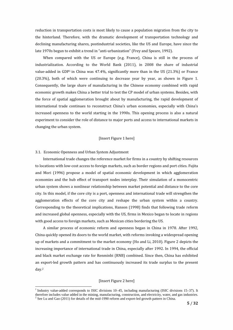
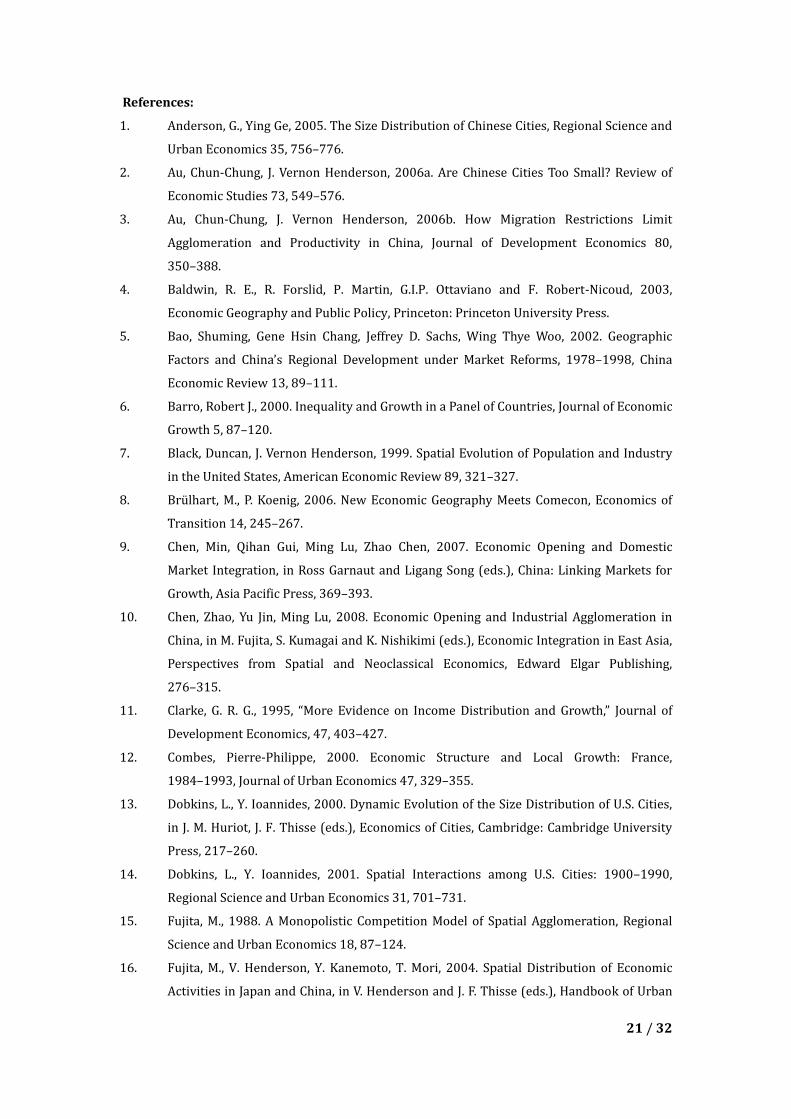
When compared with the US or Europe (e.g. France), China is still in the process of
industrialization. According to the World Bank (2011), in 2008 the share of industrial
value-added in GDP1 in China was 47.4%, significantly more than in the US (21.3%) or France
(20.3%), both of which were continuing to decrease year by year, as shown in Figure 1.
Consequently, the large share of manufacturing in the Chinese economy combined with rapid
economic growth makes China a better trial to test the CP model of urban systems. Besides, with
the force of spatial agglomeration brought about by manufacturing, the rapid development of
international trade continues to reconstruct China’s urban economies, especially with China’s
increased openness to the world starting in the 1990s. This opening process is also a natural
experiment to consider the role of distance to major ports and access to international markets in
changing the urban system.
[Insert Figure 1 here]
3.1. Economic Openness and Urban System Adjustment
International trade changes the reference market for firms in a country by shifting resources
to locations with low-cost access to foreign markets, such as border regions and port cities. Fujita
and Mori (1996) propose a model of spatial economic development in which agglomeration
economies and the hub effect of transport nodes interplay. Their simulation of a monocentric
urban system shows a nonlinear relationship between market potential and distance to the core
city. In this model, if the core city is a port, openness and international trade will strengthen the
agglomeration effects of the core city and reshape the urban system within a country.
Corresponding to the theoretical implications, Hanson (1998) finds that following trade reform
and increased global openness, especially with the US, firms in Mexico began to locate in regions
with good access to foreign markets, such as Mexican cities bordering the US.
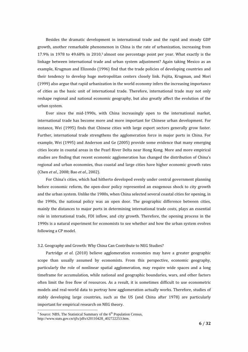
A similar process of economic reform and openness began in China in 1978. After 1992,
China quickly opened its doors to the world market, with reforms invoking a widespread opening
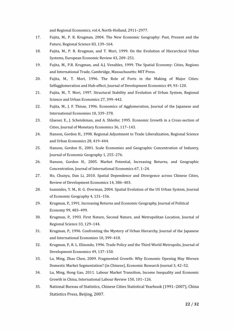
up of markets and a commitment to the market economy (Ho and Li, 2010). Figure 2 depicts the
increasing importance of international trade in China, especially after 1992. In 1994, the official
and black market exchange rate for Renminbi (RNB) combined. Since then, China has exhibited
an export-led growth pattern and has continuously increased its trade surplus to the present
day.2
[Insert Figure 2 here]
1 Industry value-added corresponds to ISIC divisions 10–45, including manufacturing (ISIC divisions 15–37). It
therefore includes value added in the mining, manufacturing, construction, and electricity, water, and gas industries. 2 See Lu and Gao (2011) for details of the mid-1990 reform and export-led growth pattern in China.
6 / 32
Besides the dramatic development in international trade and the rapid and steady GDP
growth, another remarkable phenomenon in China is the rate of urbanization, increasing from
17.9% in 1978 to 49.68% in 2010,3 almost one percentage point per year. What exactly is the
linkage between international trade and urban system adjustment? Again taking Mexico as an
example, Krugman and Elizondo (1996) find that the trade policies of developing countries and
their tendency to develop huge metropolitan centers closely link. Fujita, Krugman, and Mori
(1999) also argue that rapid urbanization in the world economy infers the increasing importance
of cities as the basic unit of international trade. Therefore, international trade may not only
reshape regional and national economic geography, but also greatly affect the evolution of the
urban system.
Ever since the mid-1990s, with China increasingly open to the international market,
international trade has become more and more important for Chinese urban development. For
instance, Wei (1995) finds that Chinese cities with large export sectors generally grow faster.
Further, international trade strengthens the agglomeration force in major ports in China. For
example, Wei (1995) and Anderson and Ge (2005) provide some evidence that many emerging
cities locate in coastal areas in the Pearl River Delta near Hong Kong. More and more empirical
studies are finding that recent economic agglomeration has changed the distribution of China’s
regional and urban economies, thus coastal and large cities have higher economic growth rates
(Chen et al., 2008; Bao et al., 2002).
For China’s cities, which had hitherto developed evenly under central government planning
before economic reform, the open-door policy represented an exogenous shock to city growth
and the urban system. Unlike the 1980s, when China selected several coastal cities for opening, in
the 1990s, the national policy was an open door. The geographic difference between cities,
mainly the distances to major ports in determining international trade costs, plays an essential
role in international trade, FDI inflow, and city growth. Therefore, the opening process in the
1990s is a natural experiment for economists to see whether and how the urban system evolves
following a CP model.
3.2. Geography and Growth: Why China Can Contribute to NEG Studies?
Partridge et al. (2010) believe agglomeration economies may have a greater geographic
scope than usually assumed by economists. From this perspective, economic geography,
particularly the role of nonlinear spatial agglomeration, may require wide spaces and a long
timeframe for accumulation, while national and geographic boundaries, wars, and other factors
often limit the free flow of resources. As a result, it is sometimes difficult to use econometric
models and real-world data to portray how agglomeration actually works. Therefore, studies of
stably developing large countries, such as the US (and China after 1978) are particularly
important for empirical research on NEG theory.
3 Source: NBS, The Statistical Summary of the 6th Population Census,
http://www.stats.gov.cn/tjfx/jdfx/t20110428_402722253.htm.
7 / 32
Research using Chinese data may helpfully contribute to the empirical study of NEG for the
following reasons: First, China has a vast territory, as well as a large population. The vast
territory not only provides the space required by agglomeration, but also plenty of samples for
empirical study. Meanwhile, a large population provides sufficient market potential. Second,
compared with the US, China has a larger interregional geographical diversity and a more
obvious geographical heterogeneity because of the concentration of ports along the eastern coast.
Interregional geographic differences are significantly less in the US, which has large ports on both
its western and eastern coasts. Finally, China has witnessed rapid economic development in the
past thirty years, especially after 1992, with corresponding changes in the spatial distribution of
economic activities. This allows us to better observe the impact of spatial agglomeration on the
urban system.
3.3. China’s Urban System
In China, a “city” is a local administrative and jurisdictional entity. There are three different
administrative levels of cities in the Chinese urban system: municipalities, prefecture-level cities,
and county-level cities. This does not include smaller settlements with townships or lower
administrative levels. The major administrative criteria announced in 1963 defined a city as an
urban agglomeration with a total urban population of greater than 100,000 inhabitants. The
economic and political importance of urban agglomeration is also one of the government’s
considerations in defining cities. However, the definition of cities has generally been consistent
since at least 1949 when the People’s Republic of China was established (Anderson and Ge,
2005).
China’s National Bureau of Statistics (NBS) reports information about both prefecture- and
county-level cities, but we use only data on prefecture-level and above cities in our research. As
for county-level cities, their boundaries and number have fluctuated greatly in recent history (see
Table 1). The number of prefecture-level cities has also increased greatly since 1990, so the
boundaries of the prefecture-level cities may also have changed. However, for cities at the
prefecture level and above, NBS reports information on both Diqu (urban area plus rural counties
within the same administration) and Shiqu (urban area only). In general, Shiqu is a good
definition of the metropolitan area by international standards (Fujita et al., 2004), and the
entities implied by new cities usually arise outside the Shiqu, so this information is comparable
across time and is thus used in our study.
[Insert Table 1 here]
The definition of China’s urban hierarchy is another problem. As mentioned above, three
administrative levels of cities are included in China’s urban system: municipalities (or
province-level cities), and prefecture- and county-level cities; provincial capitals also comprise a
special administrative level in prefecture-level cities. Cities of different levels have different
population sizes. However, corresponding to the CP model, our study focuses on the spatial
8 / 32
agglomeration in urban system, for which urban size (e.g. population) and market potential are
much more important than administrative level. Accordingly, we distinguish between cities using
different definitions and sizes, as shown in Table 2. In the model specification, we use dummies
to control for administrative level, special economic zones (SEZ), and city size, etc.
[Insert Table 2 here]
IV. Model Specification and Data
4.1. Model Specification
Our model is used to estimate how geographical location, mainly distance to a major port,
affects urban growth. The reduced-form estimation, where geography is the focus, is widely used
in earlier empirical studies of the spatial interaction between cities (Brülhart and Koenig, 2006;
Dobkins and Ioannides, 2000). We also use cross-sectional ordinary least squares (OLS)
regression for our basic reduced-form CP model of the urban system, as based on the economic
growth model in Barro (2000). As the urban system is constantly evolving during the opening
process, the different growth rates of cities in different locations will reflect the shifts in the
urban system. In addition, given all the explanatory variables are exogenous geographic factors
or the initial values of the control variables, the potential endogeneity problem in OLS estimation
is not a major concern. The model specification is as follows:
𝐷𝑔𝑑𝑝𝑖𝑡 = 𝑓(𝑙𝑛𝑔𝑑𝑝𝑖0, 𝑖𝑛𝑣𝑒𝑖0, 𝑙𝑎𝑏𝑖0, 𝑒𝑑𝑢𝑖0,𝑔𝑜𝑣𝑖0, 𝑓𝑑𝑖𝑖0; 𝑐𝑜𝑛𝑖0; 𝑔𝑒𝑜𝑖0,… )
Per capita GDP growth is the dependent variable. The extant literature also uses urban per capita
GDP growth as a measure of the urban economic activities (Glaeser et al., 1995; Dobkins and
Ioannides, 2000). We do not employ real wages, income, population, and per capita GDP in our
analysis for the following reasons. First, wage and income data are not available at the city level in
China. Second, in the early years of our sample, the urban population in China did not include
migrants without local household registration identity (hukou) (Au and Henderson, 2006b), so it
does not well represent the urban economy or size. Third, as we wish to illustrate the dynamics of
urban economies following China’s openness to the world, per capita GDP growth (not the level of
GDP), should be a better measurement to observe the evolution of the urban system.
Nevertheless, we also estimated models specifying per capita GDP instead of GDP growth as the
dependent variable. However, our main results concerning the Chinese urban system were
unchanged.4
In our study, we highlight the roles of openness and international trade in determining the
distribution of China’s urban economic activities, so the key variable of geography is the city’s
distance to the nearest major port. We construct our dataset over the period 1990–2006 to
capture best the drastic openness in place since the early 1990s. Problematically, most of the
information about China’s cities in 1992 and 1993 is missing from the Chinese Cities Statistical
Yearbook (National Bureau of Statistics, 1991–2007). Consequently, we use the data for
4 For brevity, we do not discuss these results, but they are available from the authors upon request.
9 / 32
1994–2004 to check the robustness of our results after 1994 (coinciding with the period of
far-reaching openness and depreciation of the RMB).
Hanson (2001) suggested that three issues might cause trouble in identifying agglomeration
effects in empirical studies: (i) unobserved regional characteristics, (ii) simultaneity in regional
data, and (iii) multiple sources of externalities, of which the former two are particularly crucial
when it comes to the spatial interaction of cities. As for “unobserved regional characteristics,” we
attempt to control for as many variables as the data will allow according to both the literature on
economic growth and past empirical studies of China. “Simultaneity in regional data,” however,
may be a minor issue in our study, as the core explanatory variables in our model are geographic
and will not change. As for the other explanatory variables, we use their initial values in 1990 to
counter simultaneity bias in the model. As such, the estimated results represent the long-term
impact of these explanatory variables on urban economic growth. Besides, it is quite uncommon
to control for so many initial state variables in the empirical studies employing NEG theory.
Therefore, we also estimate several models including only geographic variables. However, the
basic model follows the economic growth literature to control for other factors influencing
growth and this helps control for heterogeneity across cities.
4.2. Data
In this paper, we use China’s urban area (Shiqu) data (1990–2006) complied from the
Chinese Cities Statistical Yearbook (National Bureau of Statistics, 1991–2007), including 286 cities
at the prefecture- and above level5 from 30 provinces across mainland China. Hong Kong, Macao,
Taiwan and Tibet are not included. Local statistical bureaus in China have for some years
collected data on all enterprises in their local area, and report GDP figures at the level of the
appropriately defined metropolitan area (Fujita et al., 2004; Au and Henderson, 2006a). Though
we may express some doubt as to the quality of statistical data in China, these GDP figures are of
a high quality, as discussed by Au and Henderson (2006a), especially when econometric models
find highly significant results that are consistent with established economic theory. The
remaining data sources and the construction of the variables are as follows.
4.2.1. Urban Economic Growth
The dependent variable 𝐷𝑔𝑑𝑝𝑖𝑡 is the compound average annual growth rate of real per
capita GDP from 1990–2006 deflated by the urban consumer price index (CPI) in each province
for city i over t years. The theoretical assumptions of NEG emphasize the agglomeration of
manufacturing and services (Krugman, 1991), so we correspondingly removed agricultural
output and population from the GDP and population indicators, respectively.
4.2.2. Spatial Interactions among Cities
Hanson (1998, 2005) approximates the access of each region to its principal markets using
5 We have data on 286 cities in 2006 and 211 cities in 1990.
10 / 32
geographic distance. Therefore, geographic distance, as well as driving or road/railway distance,
is used to approximate the spatial interaction among cities (Dobkins and Ioannides, 2000;
Brülhart and Koenig, 2006; Partridge et al., 2010). In particular, we use straight geographic
distances to major ports as our measure of spatial interaction. The main reason is that exogeneity
is its second nature, which avoids the potential endogeneity bias brought about by measures of
traffic distance, such as driving hours.
We assume that there are two hierarchical monocentric urban systems in China. The first is
the national urban system, the cores of which are the major ports, like Shanghai and Hong Kong.
The distances to these ports measure the remoteness of cities to the global market. The second is
the regional urban system(s), the cores of which are large cities like Guangzhou, Chongqing, and
Wuhan, etc. The spatial interaction within each urban system exhibits the CP structure, which we
testify to using our empirical results. Here, we use the distance to the nearest “big” city (distbig)
to measure the interaction within regional urban systems, and the distance to the nearer major
port (disport) to measure the interaction within national urban systems.
To exploit how the agglomeration of major ports affects urban economic activities in China’s
spatial system, we need to identify “major ports.” According to the China Statistical Abstract 2009,
in 2008, Hong Kong accounted for 10.8% of overall Chinese cargo throughput, Shanghai 10.6%,
and Tianjin 7.4%.6 As to ports in different regions, the Bohai Sea ports (Tianjin, Qingdao,
Qinhuangdao, Dalian) in total accounted for 24% of overall cargo throughput, with the Pearl
River Delta ports (Hong Kong, Guangzhou, Shenzhen) representing 22.4%, and the Yangtze River
Delta ports (Shanghai, Ningbo-Zhoushan) another 21.4%. The above data clearly show that cargo
throughput in China mainly concentrates in these three areas. However, the distribution of the
Bohai Sea ports is widely dispersed. Therefore, agglomeration in Tianjin may not be as strong as
in Shanghai and Hong Kong. Therefore, we initially define Shanghai and Hong Kong as “major
ports” in our study but include Tianjin when testing for robustness. In fact, Shanghai and Tianjin
are provincial-level cities and respectively major ports in the Yangtze River Delta and Bohai Belt
city cluster. Likewise, Hong Kong is the major port of the Pearl River Delta and an international
financial center. Hong Kong is also adjacent to Shenzhen, another economic center and major
port in the Pearl River Delta. Thus, the distance to Hong Kong actually represents the distance to
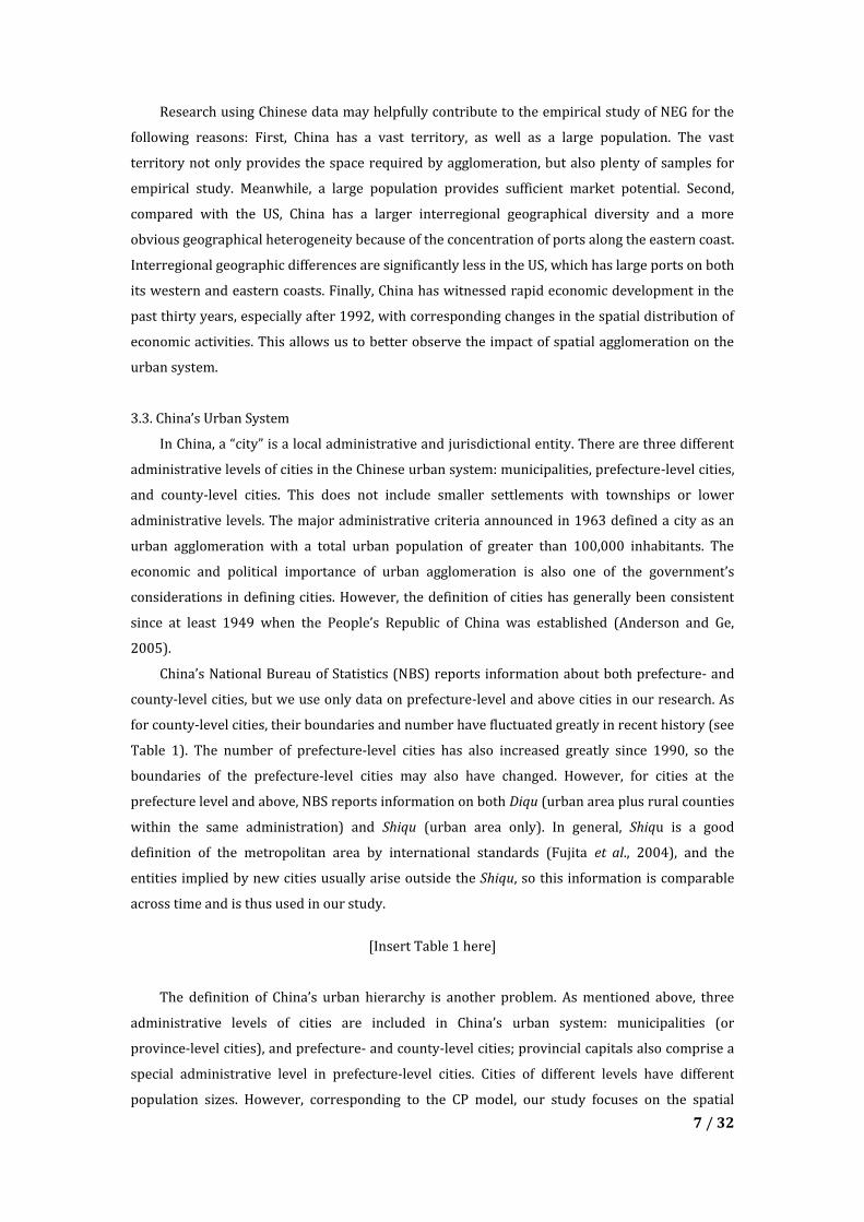
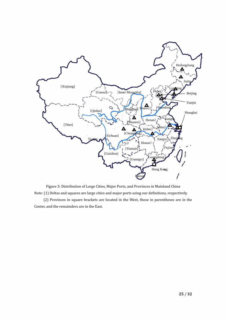
Hong Kong and Shenzhen.7 See Figure 3 for the location of the major ports.
[Insert Figure 3 here]
In Table 2, we attempt to reveal a proper definition for higher-level cities in the regional
urban system using their nonagricultural population. To construct time-consistent data, we only
6 Because of the different measurements of cargo throughput used, Shanghai sometimes ranks higher than Hong
Kong. Fortunately, this is not a major issue in our study as both are classified as major ports. 7 We compile our information about port cargo throughput from the China Statistical Abstract 2009 (National Bureau
of Statistics, 2009). Though this publication also contains information on ports in mainland China and Hong Kong in
1990, measurement differs and they are therefore difficult to compare. Therefore, we were obliged to use the most
recent year (e.g. 2008) of data for cargo throughput using the same measurement (tons).
11 / 32
use the information on cities in 1990 to identify large cities, with the information after 1990
merely used to illustrate how quickly urban sizes in China have evolved. We identify a
nonagricultural population of 1.5 million as the lower boundary of large cities in China’s regional
urban hierarchy. The reasons for this criterion are as follows. First, in 1990, there were nine
cities with a nonagricultural population greater than two million, eight of which located in coastal
areas. Accordingly, this would not well represent the urban hierarchy in inland areas. Second, in
1990, there were 31 cities with a nonagricultural population of more than one million, most of
which were municipalities and provincial capitals. Therefore, high-level cities defined according
to this criterion may correlate highly with municipalities and provincial capitals in China.
Moreover, if we set a nonagricultural population of one million as the lower boundary, there are
simply too many large cities defined.
Considering these, we define large cities in China’s urban hierarchy as those with a
nonagricultural population of more than 1.5 million in 1990. Our assumption is that via
agglomeration, these 14 large cities either already had or would generally become the regional
centers of the domestic and regional market and thus play a central role in China’s urban system
for each region within the CP structure. Figure 3 depicts the distribution of large cities in China.8
As shown, almost all are provincial capitals, with the exception of Dalian. To test whether the
results are sensitive to our definition of large cities, we substitute the distance to the nearest
large city for the distance to the nearest municipality or provincial capital to check the
robustness of our empirical results (as discussed in Section VI). We measure geographic distance
using China Map 2008, issued by Beijing Turing Software Technology Co., Ltd., China Transport
Electronic & Audio-Video Publishing House. As the CP model displays nonlinear characteristics,
we also include the squared and cubed values of distance in some of our regressions to capture
any nonlinearity.
For the 14 large cities defined, their distances to the nearest large city are all zero. Their
economic growth may benefit from their city size, so we use a dummy bigcity to control for this
effect. However, this should not be a problem for our major ports as Hong Kong is not included in
our sample and the bigcity dummy already controls for Shanghai. In addition, the GDP level of the
nearest large city in the initial year is also controlled for by gdpofbig, which is ln(GDP) in 1990,
exclusive of agricultural output.
4.2.3. Market Segmentation and Border Effect
Policy is an important factor affecting spatial agglomeration in NEG theory. When it comes to
studies on the Chinese urban system, an important policy factor that affects regional economic
development is interregional market segmentation. For example, several studies have suggested
that there is a serious market segmentation problem among Chinese provinces (Young, 2000;
Ponect, 2005; Chen, et al., 2007). Interprovincial division is likely to increase the actual distance
between cities in different provinces, and limit the spatial interaction among cities. Our study
8 These are Shanghai, Beijing, Tianjin, Shenyang, Wuhan, Guangzhou, Ha’erbin, Chongqing, Xi’an, Nanjing, Dalian,
Chengdu, Changchun, and Taiyuan.
12 / 32
attempts to reveal whether the administrative boundary limits spatial interaction within the
urban system. Denoted as samepro, the dummy variable represents whether a city is in the same
province as its nearest large city. If the “border effect” of China’s provinces does not affect spatial
interaction between cities (and thus urban economic growth) this variable should be
insignificant.
4.2.4. Other Geography Variables
In fact, spatial interaction is only the second nature of cities. For studies of China’s urban
economy, there are some other geographic factors of first nature that we should control for that
may, according to Krugman (1993), also indicate potential initial advantages.
Mainland China is usually divided into three regions: East, Center, and West. The Eastern
region has eight provinces and three municipalities, Central China has seven provinces, and the
West has eleven provinces and one municipality. In terms of the concentration of ports, there are
significant interregional differences in climate, access to water, topography, and other features of
the environment (Ho and Li, 2010), along with economic development. National-level policies are
also designed for achieving interregional economic balance between the East, Center, and West.
Therefore, we use dummy variables for “west” and “center” to capture any interregional
differences in geography and policies.9 However, the regional division of mainland China does not
strictly follow geographic location. For example, Guangxi Province is geographically located in the
south coastal area, but grouped by the Strategy of Western Region Development launched by
Chinese government in 1999 with the West given its poor economic performance. Figure 3
illustrates the distribution of China’s provinces.
Cities with ports in coastal area or with river ports along large rivers may also benefit from
access to international or domestic markets, so we also specify seaport and riverport as dummies
to control for this initial geographic advantage. The list of cities with seaports or river ports is
from “The First China Port City Mayors (International) Summit 2006” held by the Development
and Research Center, the Ministry of Communications, the Municipal Government of Tianjin, and
the China Communications and Transportation Association.10
4.2.5. Initial State of Economic Growth Factors
Following the traditional economic growth literature (for example, Barro, 2000) and studies
on China’s economic growth, we will also measure some other factors that may contribute to
9 West includes cities from 12 provinces and one municipality, namely, Chongqing, Sichuan, Yunnan, Tibet, Shaanxi,
Gansu, Qinghai, Ningxia, Xinjiang, Inner Mongolia, Guangxi, and Guizhou. Center includes cities from seven
provinces, namely, Hebei, Anhui, Jiangxi, Henan, Hubei, Hunan, and Shanxi. The cities of the remaining 12
provinces and municipalities are in the East. These are Heilongjiang, Jilin, Liaoning, Tianjin, Beijing, Shandong,
Jiangsu, Shanghai, Zhejiang, Fujian, Guangdong, and Hainan. 10 There are 32 cities with seaports: Qingdao, Yantai, Weihai, Rizhao, Haikou, Sanya, Tianjin, Tangshan,
Qinhuangdao, Cangzhou, Dalian, Jinzhou, Yinkou, Lianyungang, Fuzhou, Xiamen, Quanzhou, Zhangzhou,
Guangzhou, Shenzhen, Zhuhai, Shantou, Zhanjiang, Zhongshan, Shanghai, Ningbo, Wenzhou, Zhoushan, Taizhou,
Beihai, Fangchenggang, and Qinzhou. There are another 22 cities with river ports: Ha’erbin, Jiamusi, Wuhu,
Ma’anshan, Tonglin, Anqinq, Yueyang, Nanjing, Wuxi, Suzhou, Nantong, Yangzhou, Zhenjiang, Foshan,
Dongguan, Luzhou, Wuhan, Yichang, Nanchang, Jiujiang, Nanning, Wuzhou, and Chongqing.
13 / 32
China’s urban economic growth, such as initial economic performance, investment, labor,
education, etc.
𝑙𝑛𝑔𝑑𝑝𝑖0 is the logarithm of the per capita output of manufacturing and service in 1990,
which is controlled for to observe whether the Chinese economy experiences conditional
convergence at the city level.
𝑖𝑛𝑣𝑒𝑖0 is the ratio of investment to GDP, where GDP is the total output of manufacturing and
services in 1990.
We specify the ratio of employees to total population (𝑙𝑎𝑏𝑖0 ) in 1990 to proxy for labor.
China’s urban labor market reforms radically pushed ahead in the mid-1990s, so in 1990 the
number of urban employees contained a substantial amount of disguised unemployment in state-
and collective-owned enterprises. Therefore, a high labor ratio may not be significantly positive
for urban economic growth. We use the ratio of teachers to students in primary and junior
schools (𝑒𝑑𝑢𝑖0) in 1990 to control for the effect of education; this may not be a good
measurement, but is the best we could identify.
The government expenditure-to-GDP ratio and FDI-to-GDP ratio in 1990, as usually
controlled for in the economic growth literature, are respectively 𝑔𝑜𝑣𝑖0 and 𝑓𝑑𝑖𝑖0 , where GDP is
the total output of three sectors, as we cannot distinguish between the final flows of government
expenditure and foreign direct investment across sectors. The effects of government expenditure
and foreign direct investment on economic growth are conventionally difficult to predict
beforehand (Barro, 2000; Clarke, 1995; Partridge, 1997).
𝑐𝑜𝑛𝑖0 represents several other control variables related to Chinese urban economic growth,
including the ratio of the nonagricultural population to the total population (urb) (to account for
the level of urbanization) and population density (density) and its square (den_2) (to reflect
internal population agglomeration in urban areas). We also use the ratio of service GDP to
manufacturing to proxy for the industrial structure of the urban sector (SM).
4.2.6. Policy
We can never ignore policy in empirical studies of agglomeration and urban economies.
Other than the administrative boundaries mentioned, there may be some other policy advantages
affecting China’s urban economic growth that are controlled for in the literature (Bao et al., 2002;
Ho and Li, 2010).
As discussed earlier, in our prefecture-level database, different administrative levels of cities
remain, namely, municipalities, provincial capitals, and other cities. Because municipalities and
provincial capitals potentially enjoy special policies from the central and provincial governments,
we use a dummy variable (capital) to capture any benefits. For example, in 1997 Chongqing rose
from an ordinary prefecture-level city to become a municipality. After considering its special
history,11 we define Chongqing as a provincial capital in 1990.
Likewise, in the process of Chinese reform and openness, starting in 1980 four special
11 Chongqing was the capital of the Republic of China during World War II and is an important city in western China.
14 / 32
economic zones (SEZs) were created in China’s coastal areas, and 14 cities later chosen as open
coastal cities (OCCs) in 1994.12 The intention of these SEZs and OCCs was to attract FDI, obtain
access to international markets, and gain special policy advantages. We use the dummies SEZ and
open to measure the effects of this preferential policy. However, as we expect these variables to
correlate highly with FDI, seaport dummy and some others, we do not expect significant
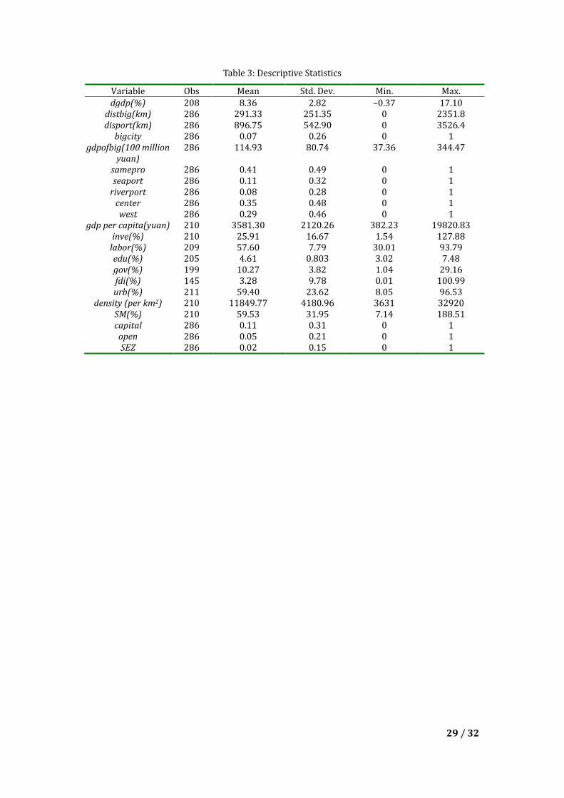
estimated coefficients. Table 3 provides descriptive statistics for all the variables.
[Insert Table 3 here]
V. Estimation Results
Table 4 includes the estimated results of the model. In addition to the more conventional
economic growth factors, we include the geographic variables in equations (1)–(3). In equation
(1), we only add the linear item of distance to the nearest large city and major port, while we add
the squares and cubes of distances in equation (2) and drop the insignificant cube of distance to a
large city in equation (3).
[Insert Table 4 here]
5.1. Nonlinearity of the CP Structure in China’s Urban System
In equation (1), both of the distances are insignificantly negative, which means urban
economic growth decreases away from large cities and major ports, but the effect is statistically
insignificant. As discussed, the nonlinearity of the CP model may exist in China’s urban system. If
so, and as Fujita and Mori (1997) and Fujita, Krugman, and Mori (1999) have showed, the
∽-shaped correlation between distance and economic activity may be present in our estimated
results. Consequently, we add the squares and cubes of distance in equation (2).
The results of equation (2) show that the distance to a major port and its square and cube
are all significant, which proves nonlinearity in China’s urban system. However, none of the three
terms for distance to a large city is significant. We surmise a ∽-shaped curve could only occur
when the distance to a large city is sufficiently long, otherwise, we would only observe a U-shape
when using real data. Therefore, we drop the cube of the distance to a large city from equation
(3). Obviously, in equation (3) all distance variables are significant: the distance to the large city
is negative, its squared term is positive. In contrast, the distance to a major port is negative, while
the squared term is positive and the cubed term is negative.
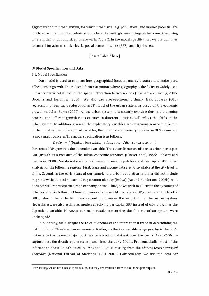
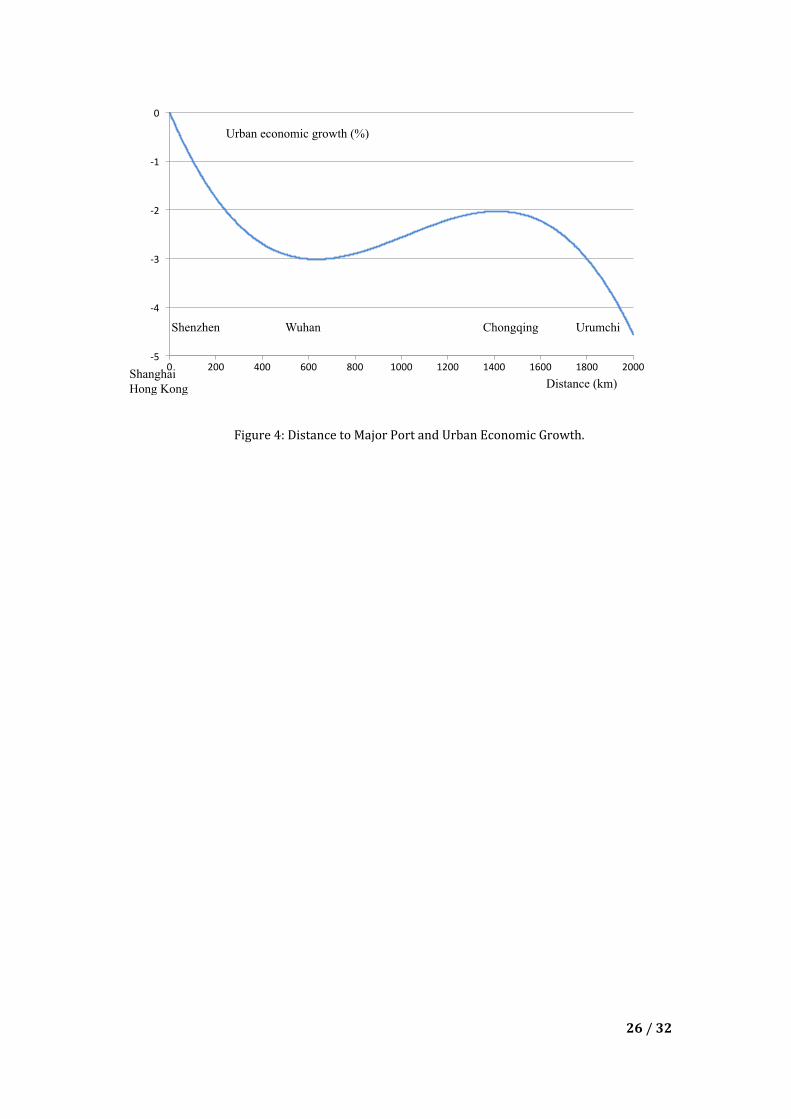
Based on estimated results, we respectively simulate the correlation between the distances
to the major ports or large cities and the urban economic growth rate in Figures 4 and 6. The
horizontal axis represents the distance (kilometers) away from major ports, and the vertical axis
is the urban economic growth rate (%). We discover a CP pattern of urban system evolution
consistent with theory.
12 The four SEZ established in 1980 are Shenzhen, Zhuhai, Xiamen, and Shantou. The 14 OCC in 1994 are Tianjin,
Shanghai, Dalian, Qinhuangdao, Yantai, Qingdao, Lianyungang, Nantong, Ningbo, Wenzhou, Fuzhou, Guangzhou,
Zhanjiang, and Beihai.
15 / 32
[Insert Figure 4 here]
Figure 4 suggests that the impact of distance to major port on urban economic growth has
basically the same shape as the market potential curve of the CP model in the urban system
(Fujita and Mori, 1997; Fujita, Krugman, and Mori, 1999). While a city is located within about 600
km away from a major port, the closer it is to the major port and international markets, the larger
market potential and the higher economic growth rate it has. When the distance is farther away,
international market access is no longer that important. Therefore, a location far away from a
port may promote the accumulation of regional and domestic market potential, as well as the
development of local economies. When distance is sufficiently long (farther than 1,500 km from a
port), cities remote from both the domestic and international markets suffer from low market
potential and a lower economic growth rate. In addition, when we follow economic geography
studies (Dobkins and Ioannides, 2001; Partridge et al., 2009) and only control for the geographic
variables in model (4), the results do not change much and all the coefficients are statistically
more significant. Interestingly, the model including only two distance variables explains 6.9% of
the variance in city growth, compared with 42.8% when all the variables are included in model
(3).
Our result provides convincing evidence of the CP model of the urban system in the case of
China. Moreover, even though we assume the national urban geography is monocentric and
therefore the result matches the CP model in a monocentric urban system, Figure 4 also shows
that China’s national urban system has the potential to evolve into a multicentric system.
According to Fujita, Krugman, and Mori (1999), the reason is that with the growth of total
population, the market potential for cities at the second turning point will increase. Thus, another
core of China’s urban national system may emerge in western China. Of course, whether this
comes about depends on many other variables, for example, the development of infrastructure
and institutional changes that promote the mobility of production factors.
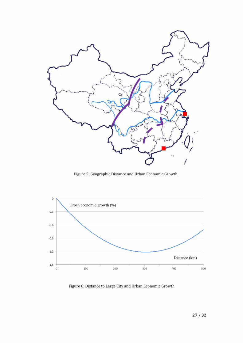
To make the effects of the distances to major ports clearer, we mark the two turning points
of economic growth curve on the map of mainland China in Figure 5. Here, 600 km from Hong
Kong and Shanghai, denoted with a dashed curve, is the location with the lowest average growth,
all other things being equal, while 1,500 km away, marked by a solid curve, is the place with
second-highest growth rate.
[Insert Figure 5 here]
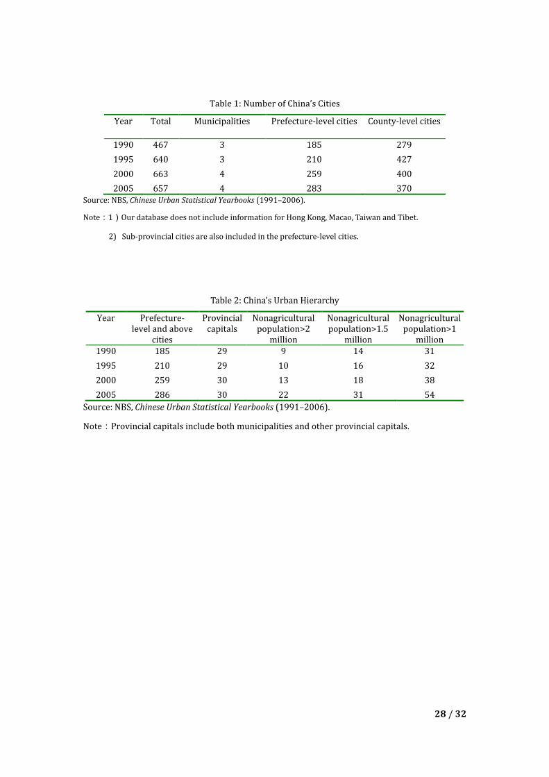
In Figure 6, we simulate the correlation between the distance to the nearest large city and
urban economic growth using the results of our regressions. When a city is close to a large city,
spatial agglomeration effects promote large cities to absorb economic resources from their
surroundings, which is a significant centripetal force. Meanwhile, being closer to a large city, also
means greater market access for a regional economic center. Therefore, the closer to the central
16 / 32
cities, the faster a city grows. However, when further away from big cities, instead of the
centripetal force, the centrifugal force plays the dominant role. Therefore, the further the
distance, the faster a city grows. Our estimated result shows the turning point is about 300 km,
which means that within about 300 kilometers, the interplay between cities displays a strong
centripetal force, which is similar to the findings in Hanson (2005). The difference is that we also
find that when the distance is greater than 300 km, because of transportation costs and other
external diseconomies, centrifugal force dominates the spatial interaction between cities
performance.
[Insert Figure 6 here]
However, in the regional urban systems, there is no sign of the possibility of multicentric
systems. This may be because of the limited population or scope surrounding the cores. In Figure
4, the complete ∽-shaped curve requires at least 1,400 km distance, while the real distance to the
nearest large city in regional systems is not sufficiently long. In fact, China’s urban system today
is the result of a long-term evolution, thus new large cities may have emerged where there was a
greater market potential because of the spatial agglomeration of established large cities, as
shown by the numerical simulation in Fujita, Krugman, and Mori (1999). Therefore, in Figure 4,
what we can see may be only the left half of the ∽-shaped curve, not the whole. Moreover, the
impact of major ports is stronger than large cities on urban economies because within a certain
distance economic growth decreases much faster as distance from major ports increases than it
does away from a large city.
Based on the above, we can safely conclude that the national urban system in China has
presented a complete CP structure because of the adjustment of urban economies to
international markets. The importance of large cities in regional urban systems is less significant
but also verified. We also find evidence for the agglomeration shadow modeled by Krugman
(1993) in the Chinese urban system. This suggests that being closer to an agglomeration center is
not always good news for the local economy. This finding adds new evidence in helping solve the
paradox that Partridge et al. (2009) found between the positive closeness–growth relationship
when using real data and the theoretical hypothesis of an “agglomeration shadow.”
5.2. Border Effect
The same-province dummy (samepro) is always significantly negative, which means cities
have a lower growth rate if they are in the same province as their nearest large city. This is
because the absorptive effects of large cities will be larger in this circumstance. This means that
the border effect, similar to the findings in Parsley and Wei (2001) and Poncet (2005) exists
between Chinese provinces, which is likely to increase the actual distances between cities in
different provinces. Based on our estimates, China’s interprovincial border effect is equivalent to
17 / 32
as much as 260 km13 for two neighboring cities. Poncet (2005) finds that the interprovincial
border in China is like an international border in Europe, so our estimate of the interprovincial
border effect is acceptable.
The border effect in this paper presents as the distortion of the spatial concentration. We
believe this is consistent with China’s history of province-level market segmentation (Young,
2000; Ponect, 2005) and migration restrictions (Au and Henderson, 2006a, 2006b). Moreover,
Chen et al. (2007) argue that provincial governments have an incentive to restrict the
agglomeration effects from large cities in other provinces using administrative force to protect
their own economic development. Further, Lu and Chen (2009) find that most observations of
market segmentation increase provincial economic growth. These conclusions are also consistent
with the findings in this paper. Although in cities of the same province segmentation can prevent
them from the absorptive effects of large cities in other provinces, market segmentation always
brings losses in resource allocative efficiency. In turn, this lowers the growth rate for the whole
economy, resulting in an underdeveloped city scale (Au and Henderson, 2006a), and a smaller
scale inequality among Chinese cities (Fujita et al., 2004).
5.3. Geography and Policy
We also note that in equations (1)–(3), the center, west, and capital dummies are not
significant. This differs from the findings in previous research, including Bao et al. (2002) and Ho
and Li (2010). This is because with the spatial interaction among cities controlled for in our
paper, no other growth disadvantages significantly exist in the western or central regions, and
there are no other obvious advantages in provincial capitals or municipalities. In other words,
spatial agglomeration in China’s urban system contributes most to interregional economic
disparity in China.
Though correlated with the dummy variables for open and SEZ, the dummy seaport is
significantly positive, whereas open and SEZ are insignificant. This implies the possibility that
geography is more important than policy for China’s long-run urban growth. Nevertheless, this
needs further study. Furthermore, the riverport dummy is insignificantly positive.
5.4. Other Economic Growth Factors
In our regressions, we also control for other urban economic growth factors, the impacts of
which do not vary significantly across equations (1)–(3). Most of the factors are insignificant,
except for education as measured by the teacher–student ratio. Education (edu) is significantly
positive. This is because education investment in the initial stage promotes human capital
accumulation and economic growth in the long run.
Our regression results also imply that the impact of investment (inve) is insignificantly
negative which may be because Chinese cities with high investment have no obvious economic
advantage in the long term because, as a whole, the Chinese economy suffers from low efficiency
13 We simply estimate this border effect by dividing the coefficient of the same-province dummy by the linear term of
the distance to the nearest large city in equation (3).
18 / 32
spawned by overinvestment (Zhang, 2003).
Some other factors, like labor (lab), government expenditure (gov), FDI (fdi), urbanization
(urb), population density (density, den_2), and industrial structure (SM) all have insignificant
impacts on urban economic growth in the long run based on our regression results. Finally, the
initial level of per capita GDP has an insignificant negative impact on China’s urban economic
growth, showing no significant trend in conditional convergence at city level. The insignificant
variables do not become significant even if we drop the variables for distance to major ports and
large cities. We also exercised estimation by substituting right-hand-side variables with their
average values across the time span of our data, and the results do not change significantly.14
There are three possible explanations. First, the most obvious is that these factors have no
long-term impact on urban economic growth. Second, measurement error in the variables may
have reduced their levels of significance. Third, the sample size in our study is limited. In fact, the
t-statistics for the significance test of the coefficients of labor and population density are greater
than one, thereby indicating marginal significance.
VI. Robustness Checks
We estimate several models based on equation (3) test the robustness of our key findings in
Table 5. In equations (5) and (6), we change the definition of a large city to retest the hypothesis
about regional urban systems. In particular, we redefine large cities as provincial capitals and
municipalities. Thus, distance to the nearest large city is replaced by distance to the provincial
capital (distcap). Therefore, municipalities do not have any spatial interactions when using this
definition. We again measure the geographic distance using China Map 2008 (Beijing Turing
Software Technology Co., Ltd., China Transport Electronic & Audio-Video Publishing House,
2008). We only include the linear term of distance to the provincial capital in equation (5) and
add the squared term to equation (6). For consistency with the variable for which we control, we
drop the dummies samepro and bigcity, and replace the variable gdpofbig by gdpofcap (the
economic scale of the provincial capitals, that is, ln(GDP) in 1990 excluding agricultural output).
In equation (7), we add Tianjin into our definition of major ports and replace distance to the
nearer major port between Shanghai and Hong Kong (disport) by distance to the nearest major
port among Shanghai, Hong Kong and Tianjin (disport*).
Time span is also an important issue for our study as we highlight the role of China’s
openness and international trade in the changing urban system. However, a large amount of
information in 1992 and 1993 are missing from the Chinese Urban Statistical Yearbooks (National
Bureau of Statistics, 1993–94). Therefore, we use the urban data from 1994 and replace the
dependent variable with the average annual growth rate of real per capita GDP from 1994 to
2006 (dgdp*) deflated by provincial urban CPI, where agricultural output and population are also
excluded. Another benefit of this robustness check is the greater number of observations,
increasing from 133 in equation (3) to 193 in equation (8). Table 4 includes the results of the
14 Results available from authors upon request.
19 / 32
robustness checks, with only the variables relevant to spatial interaction reported to save space.
[Insert Table 5 here]
As shown in Table 5, in equation (5), instead of distance to nearest large city and its square,
we only include distance to the provincial capital, which is significantly negative, suggesting the
provincial capitals have strong absorptive effects on the surrounding cities. In equation (6), we
include both the distance to the provincial capital and its square, both of which are not
significant. Consequently, provincial capitals have only significant centripetal forces, which is not
conducive to the economic growth of remote cities. One explanation is that the number of
provincial capitals is about twice that of large cities, so that for most observations the distance to
the provincial capital is much shorter than to the nearest large city. In this context, only a
negative distance–growth relationship would appear, which we can see as the first part of the
U-shape we find for the relationship between the distance to the nearest large city and urban
growth. Moreover, the larger initial economic scale of the provincial capital, the slower its urban
economic growth, as gdpofcap is significantly negative. This result shows a stronger absorptive
effect for larger central cities. The variables for the distance to major ports are usually significant.
In equation (7) where Tianjin is included as a major port in China’s urban system, the
variables for distance to major ports are still significant, but the significance levels decrease,
which proves that the economic agglomeration of Tianjin is not as strong as Shanghai and Hong
Kong. We also estimated three separate regressions using the data within each city group. The
∽-shaped relationship between distance-to-port and urban growth is robust in city groups
centered on Shanghai and Hong Kong. However, for the cities centered on Tianjin, the
relationship is insignificant. This is understandable as Tianjin is not comparable with Shanghai
and Hong Kong in terms of economic scale and cargo throughput. What is more, the difference
between Tianjin and other leading ports in the Bohai Belt is not huge in terms of cargo
throughput. If we construct a variable of distance to the four major ports in the Bohai Belt
weighted by their cargo throughputs, then the distance–growth relationship becomes
significant.15 This indicates again that Tianjin is not strong enough to act as a core of a national
level urban system. In addition, the variables for distance to nearest large city are insignificant
with the same sign as in equation (3). This suggests that the robustness of the importance of
large cities and regional urban systems is less than major ports and the national urban system.
In equation (8) with the dependent variable now specified as economic growth during
1994–2006, the significance of the distance-to-port variables are almost the same as in equation
(3), while the significance of the distance to large cities decreases substantially. It is then possible
that ever since China’s rapid openness to the international market in 1994, the agglomeration
patterns of China’s urban system change to meet the needs of developing international trade, so
that the distance to major ports is becoming more and more important, at least when compared
15 These results are not reported to conserve space, but available upon request.
20 / 32
with that to large cities. However, this is beyond the scope of this paper and further study is
required.
In existing NEG literature, per capita GDP, rather than its growth, usually serves as the
dependent variable. In our study, we also attempt to substitute the growth rate of per capita GDP
with its level, and conduct panel data regression and year-by-year estimation. To ensure that our
results are robust, even if we only consider the manufacturing sector, we regress GDP per worker
for secondary and tertiary industries on the geographic and other explanatory variables. These
additional regression exercises do not alter our major findings significantly.16
VII. Conclusions
This paper represents an early attempt to verify the spatial pattern of China’s urban system
following the CP model. China’s open policy since the 1990s as a natural experiment makes China
a feasible application and suitable experimental field for testing the NEG theory of urban systems.
The most important finding of this paper is to verify the ∽-shaped nonlinear correlation
between the geographical distance to major ports and urban economic growth, which is
consistent with the CP model of urban systems in NEG theory. We find that China’s urban
economies adjust to increasingly important international trade according to their access to global
market, especially after China’s drastic opening up since the mid-1990s. Compared with distance
to port, the distance to the nearest large city has a U-shaped relationship with urban growth.
The agglomeration shadow first modeled by Krugman (1993) is also evident in China’s
urban system, which means that being closer to agglomeration centers is not always good news
for the local economy. This finding adds new evidence in helping solve the paradox that Partridge
et al. (2009) found between the positive closeness–growth relationship found when using in real
data and the theoretical hypothesis of an agglomeration shadow.
The border effect arising Chinese interprovincial segmentation is equivalent to increasing
the actual distance between cities, as well as limiting the spatial interaction between China’s
cities. Such administrative boundaries protect the economic growth of small cities from the
absorption effects of larger cities in other provinces. Nevertheless, it also leads to efficiency
losses in interregional agglomeration and scale economies.
Our paper emphasizes the role of shifts in trade patterns in shaping the urban system in
China, and our robustness check suggests some evidence of agglomeration pattern changes after
1994. However, in the modern era, agglomeration patterns can also change with lower
transportation costs, improved communication technology, shifts in trade patterns, and industry
structural change (Partridge et al., 2009). Consequently, we need further study to consider how
China’s openness and involvement in globalization has continued to reshape its urban system.
16 We do not report these results to save space, but they are available upon request.
21 / 32
References:
1. Anderson, G., Ying Ge, 2005. The Size Distribution of Chinese Cities, Regional Science and
Urban Economics 35, 756–776.
2. Au, Chun-Chung, J. Vernon Henderson, 2006a. Are Chinese Cities Too Small? Review of
Economic Studies 73, 549–576.
3. Au, Chun-Chung, J. Vernon Henderson, 2006b. How Migration Restrictions Limit
Agglomeration and Productivity in China, Journal of Development Economics 80,
350–388.
4. Baldwin, R. E., R. Forslid, P. Martin, G.I.P. Ottaviano and F. Robert-Nicoud, 2003,
Economic Geography and Public Policy, Princeton: Princeton University Press.
5. Bao, Shuming, Gene Hsin Chang, Jeffrey D. Sachs, Wing Thye Woo, 2002. Geographic
Factors and China’s Regional Development under Market Reforms, 1978–1998, China
Economic Review 13, 89–111.
6. Barro, Robert J., 2000. Inequality and Growth in a Panel of Countries, Journal of Economic
Growth 5, 87–120.
7. Black, Duncan, J. Vernon Henderson, 1999. Spatial Evolution of Population and Industry
in the United States, American Economic Review 89, 321–327.
8. Brülhart, M., P. Koenig, 2006. New Economic Geography Meets Comecon, Economics of
Transition 14, 245–267.
9. Chen, Min, Qihan Gui, Ming Lu, Zhao Chen, 2007. Economic Opening and Domestic
Market Integration, in Ross Garnaut and Ligang Song (eds.), China: Linking Markets for
Growth, Asia Pacific Press, 369–393.
10. Chen, Zhao, Yu Jin, Ming Lu, 2008. Economic Opening and Industrial Agglomeration in
China, in M. Fujita, S. Kumagai and K. Nishikimi (eds.), Economic Integration in East Asia,
Perspectives from Spatial and Neoclassical Economics, Edward Elgar Publishing,
276–315.
11. Clarke, G. R. G., 1995, “More Evidence on Income Distribution and Growth,” Journal of
Development Economics, 47, 403–427.
12. Combes, Pierre-Philippe, 2000. Economic Structure and Local Growth: France,
1984–1993, Journal of Urban Economics 47, 329–355.
13. Dobkins, L., Y. Ioannides, 2000. Dynamic Evolution of the Size Distribution of U.S. Cities,
in J. M. Huriot, J. F. Thisse (eds.), Economics of Cities, Cambridge: Cambridge University
Press, 217–260.
14. Dobkins, L., Y. Ioannides, 2001. Spatial Interactions among U.S. Cities: 1900–1990,
Regional Science and Urban Economics 31, 701–731.
15. Fujita, M., 1988. A Monopolistic Competition Model of Spatial Agglomeration, Regional
Science and Urban Economics 18, 87–124.
16. Fujita, M., V. Henderson, Y. Kanemoto, T. Mori, 2004. Spatial Distribution of Economic
Activities in Japan and China, in V. Henderson and J. F. Thisse (eds.), Handbook of Urban
22 / 32
and Regional Economics, vol.4, North-Holland, 2911–2977.
17. Fujita, M., P. R. Krugman, 2004. The New Economic Geography: Past, Present and the
Future, Regional Science 83, 139–164.
18. Fujita, M., P. R. Krugman, and T. Mori, 1999. On the Evolution of Hierarchical Urban
Systems, European Economic Review 43, 209–251.
19. Fujita, M., P.R. Krugman, and A.J. Venables, 1999. The Spatial Economy: Cities, Regions
and International Trade, Cambridge, Massachusetts: MIT Press.
20. Fujita, M., T. Mori, 1996. The Role of Ports in the Making of Major Cities:
Selfagglomeration and Hub-effect, Journal of Development Economics 49, 93–120.
21. Fujita, M., T. Mori, 1997. Structural Stability and Evolution of Urban System, Regional
Science and Urban Economics 27, 399–442.
22. Fujita, M., J. F. Thisse, 1996. Economics of Agglomeration, Journal of the Japanese and
International Economies 10, 339–378.
23. Glaeser, E., J. Scheinkman, and A. Shleifer, 1995. Economic Growth in a Cross-section of
Cities, Journal of Monetary Economics 36, 117–143.
24. Hanson, Gordon H., 1998. Regional Adjustment to Trade Liberalization, Regional Science
and Urban Economics 28, 419–444.
25. Hanson, Gordon H., 2001. Scale Economies and Geographic Concentration of Industry,
Journal of Economic Geography 1, 255–276.
26. Hanson, Gordon H., 2005. Market Potential, Increasing Returns, and Geographic
Concentration, Journal of International Economics 67, 1–24.
27. Ho, Chunyu, Dan Li, 2010. Spatial Dependence and Divergence across Chinese Cities,
Review of Development Economics 14, 386–403.
28. Ioannides, Y. M., H. G. Overman, 2004. Spatial Evolution of the US Urban System, Journal
of Economic Geography 4, 131–156.
29. Krugman, P., 1991. Increasing Returns and Economic Geography, Journal of Political
Economy 99, 483–499.
30. Krugman, P., 1993. First Nature, Second Nature, and Metropolitan Location, Journal of
Regional Science 33, 129–144.
31. Krugman, P., 1996. Confronting the Mystery of Urban Hierarchy, Journal of the Japanese
and International Economies 10, 399–418.
32. Krugman, P., R. L. Elizondo, 1996. Trade Policy and the Third World Metropolis, Journal of
Development Economics 49, 137–150.
33. Lu, Ming, Zhao Chen, 2009. Fragmented Growth: Why Economic Opening May Worsen
Domestic Market Segmentation? (in Chinese), Economic Research Journal 3, 42–52.
34. Lu, Ming, Hong Gao, 2011. Labour Market Transition, Income Inequality and Economic
Growth in China, International Labour Review 150, 101–126.
35. National Bureau of Statistics, Chinese Cities Statistical Yearbook (1991–2007), China
Statistics Press, Beijing, 2007.
23 / 32
36. Overman, Henry G., Y. M. Ioannides, 2001. Cross-Sectional Evolution of the U.S. City Size
Distribution, Journal of Urban Economics 49, 543–566.
37. Parsley, D., S. Wei, 2001. Explaining the Border Effect: The Role of Exchange Rate
Variability, Shipping Cost, and Geography, Journal of International Economics 55, 87–105.
38. Partridge, M. D., D. S. Rickman, K. Ali and M. R. Olfert, 2009. Do New Economic Geography
Agglomeration Shadows Underlie Current Population Dynamics across the Urban
Hierarchy? Papers in Regional Science 88, 445–466.
39. Poncet, S., 2005. A Fragmented China: Measure and Determinants of Chinese Domestic
Market Disintegration, Review of International Economics 13, 409–430.
40. Venables, A. J., 1996. Equilibrium Locations of Vertically Linked Industries, International
Economic Review, 37, 341–359.
41. Wan, Guanghua, Ming Lu, Zhao Chen, 2007. Globalization and Regional Income Inequality:
Empirical Evidence from within China, Review of Income and Wealth 53, 35–59.
42. Wei, S., 1995. The Open Door Policy and China’s Rapid Growth: Evidence from City-level
Data, in Takatoshi Ito, Anne O. Krueger (eds.), Growth Theories in Light of the East Asian
Experience, NBER-East Asian Seminar on Economics, Vol. 4, University of Chicago Press.
43. Young, A., 2000. The Razor’s Edge: Distortions and Incremental Reform in the People’s
Republic of China, Quarterly Journal of Economics 115, 1091–1135.
44. Zhang, Jun, 2003. Investment, Investment Efficiency, and Economic Growth in China,
Journal of Asian Economics 14, 713–734
24 / 32
Figure 1: Share of Industry Value-Added in GDP (%) in China, US and France (1980–2008)
Sources: World Bank National Accounts data and OECD National Accounts data files.
Figure 2: International Trade, Urbanization, and GDP Growth in China (1978–2008)
Source: NBS, China Statistical Abstract 2009.
25 / 32
Figure 3: Distribution of Large Cities, Major Ports, and Provinces in Mainland China
Note: (1) Deltas and squares are large cities and major ports using our definitions, respectively.
(2) Provinces in square brackets are located in the West, those in parentheses are in the
Center, and the remainders are in the East.
HeilongJiang
Liaoning
Jinlin
Beijing [Inner Mongolia]
Tianjin
Shandong
Jiangsu
Shanghai
Zhejiang
Fujian
g Guangdong [Guangxi]
[Tibet]
[Xinjiang]
[Ningxia]
[Sichuan]
[Qinhai]
[Gansu]
[Guizhou]
[Yunnan]
[Chongqing]
[Shaanxi]
Hainan
( Hebei)
( Henan)
( Shanxi)
( Anhui)
( Jiangxi) ( Hunan)
( Hubei)
Tianjin
Hong Kong
26 / 32
Figure 4: Distance to Major Port and Urban Economic Growth.
27 / 32
Figure 5: Geographic Distance and Urban Economic Growth
Figure 6: Distance to Large City and Urban Economic Growth
28 / 32
Table 1: Number of China’s Cities
Year Total Municipalities Prefecture-level cities County-level cities
1990 467 3 185 279
1995 640 3 210 427
2000 663 4 259 400
2005 657 4 283 370 Source: NBS, Chinese Urban Statistical Yearbooks (1991–2006).
Note:1)Our database does not include information for Hong Kong, Macao, Taiwan and Tibet.
2) Sub-provincial cities are also included in the prefecture-level cities.
Table 2: China’s Urban Hierarchy
Year Prefecture- level and above
cities
Provincial capitals
Nonagricultural population>2
million
Nonagricultural population>1.5
million
Nonagricultural population>1
million 1990 185 29 9 14 31
1995 210 29 10 16 32
2000 259 30 13 18 38
2005 286 30 22 31 54
Source: NBS, Chinese Urban Statistical Yearbooks (1991–2006).
Note:Provincial capitals include both municipalities and other provincial capitals.
29 / 32
Table 3: Descriptive Statistics
Variable Obs Mean Std. Dev. Min. Max. dgdp(%) 208 8.36 2.82 –0.37 17.10
distbig(km) 286 291.33 251.35 0 2351.8 disport(km) 286 896.75 542.90 0 3526.4
bigcity 286 0.07 0.26 0 1 gdpofbig(100 million
yuan) 286 114.93 80.74 37.36 344.47
samepro 286 0.41 0.49 0 1 seaport 286 0.11 0.32 0 1
riverport 286 0.08 0.28 0 1 center 286 0.35 0.48 0 1 west 286 0.29 0.46 0 1
gdp per capita(yuan) 210 3581.30 2120.26 382.23 19820.83 inve(%) 210 25.91 16.67 1.54 127.88
labor(%) 209 57.60 7.79 30.01 93.79 edu(%) 205 4.61 0.803 3.02 7.48 gov(%) 199 10.27 3.82 1.04 29.16 fdi(%) 145 3.28 9.78 0.01 100.99 urb(%) 211 59.40 23.62 8.05 96.53
density (per km2) 210 11849.77 4180.96 3631 32920 SM(%) 210 59.53 31.95 7.14 188.51 capital 286 0.11 0.31 0 1 open 286 0.05 0.21 0 1 SEZ 286 0.02 0.15 0 1
30 / 32
Table 4: Geography and Urban Economic Growth
(Dependent variable is the compound average growth rate between 1990 and 2006.)
(1) (2) (3) (4) dgdp dgdp dgdp dgdp Disport/103 –0.215 –12.9** –11.2** –7.37*** (0.716) (5.55) (4.29) (2.79) disport_2/106 15.0** 12.8*** 8.81*** (6.79) (4.82) (3.03) disport_3/109 –4.98** –4.17** –3.14*** (2.36) (1.60) (0.995) distbig/103 –1.69 –4.99 –8.02** –5.58** (1.49) (7.35) (3.52) (2.21) distbig_2/106 6.76 13.2** 12.1*** (14.8) (5.40) (3.54) distbig_3/109 3.57 (7.59) bigcity 0.754 0.883 0.724 (0.918) (0.988) (0.925) gdpofbig0 –0.549 –0.742 –0.763 (0.625) (0.637) (0.633) samepro –1.947*** –2.165*** –2.211*** (0.666) (0.707) (0.697) seaport 1.978** 2.022** 1.962** (0.838) (0.843) (0.831) riverport 0.752 0.730 0.614 (0.649) (0.693) (0.645) center –1.391* –0.989 –1.025 (0.797) (0.812) (0.806) west –0.980 –1.349 –1.330 (0.878) (0.878) (0.874) lngdp –0.845 –1.249* –1.201 (0.726) (0.745) (0.735) Inve/102 –3.45* –2.78 –2.74 (2.01) (2.01) (2.00) Labor/102 4.27 4.16 4.11 (3.36) (3.44) (3.43) edu 0.552*** 0.590*** 0.584*** (0.172) (0.171) (0.170) Gov/102 4.39 2.69 3.07 (7.43) (7.53) (7.46) Fdi/102 3.05 1.46 1.32 (2.56) (2.62) (2.59) Urb/103 7.01 3.51 4.60 (13.5) (13.6) (13.3) Density/104 2.15 2.70 2.80 (2.07) (2.08) (2.06) den_2/109 –5.07 –7.77 –7.99 (6.00) (6.05) (6.01) SM/103 –8.87 –5.16 –4.75 (10.6) (10.7) (10.6) capital 1.051 0.598 0.548 (0.775) (0.792) (0.782) open –0.348 –0.287 –0.282 (1.043) (1.031) (1.027) SEZ –1.798 –1.976 –2.005 (1.436) (1.416) (1.410) Constant 13.06* 19.72** 19.39** 10.39*** (7.626) (8.290) (8.230) (0.847)
31 / 32
Observations 132 132 132 202 R2 0.387 0.430 0.428 0.069
Notes: (1) Standard errors in parentheses;
(2) * p < 0.10, ** p < 0.05, *** p < 0.01.
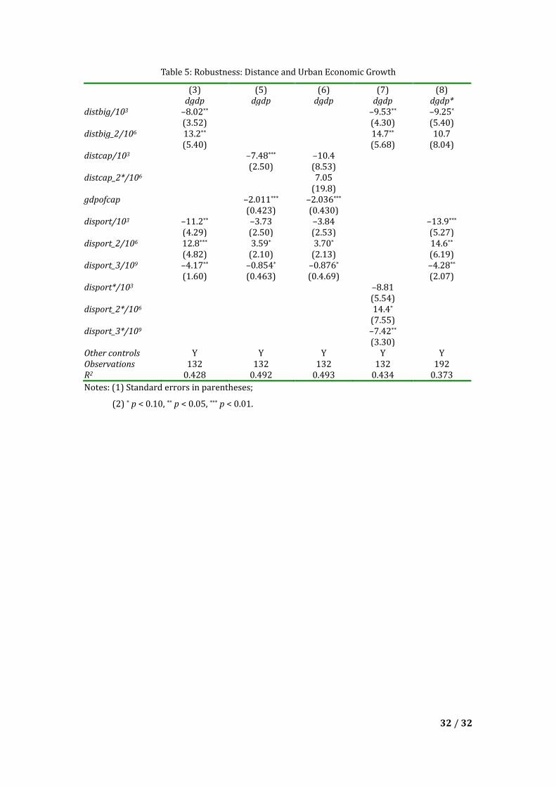
32 / 32
Table 5: Robustness: Distance and Urban Economic Growth
(3) (5) (6) (7) (8) dgdp dgdp dgdp dgdp dgdp* distbig/103 –8.02** –9.53** –9.25* (3.52) (4.30) (5.40) distbig_2/106 13.2** 14.7** 10.7 (5.40) (5.68) (8.04) distcap/103 –7.48*** –10.4 (2.50) (8.53) distcap_2*/106 7.05 (19.8) gdpofcap –2.011*** –2.036*** (0.423) (0.430) disport/103 –11.2** –3.73 –3.84 –13.9*** (4.29) (2.50) (2.53) (5.27) disport_2/106 12.8*** 3.59* 3.70* 14.6** (4.82) (2.10) (2.13) (6.19) disport_3/109 –4.17** –0.854* –0.876* –4.28** (1.60) (0.463) (0.4.69) (2.07) disport*/103 –8.81 (5.54) disport_2*/106 14.4* (7.55) disport_3*/109 –7.42** (3.30) Other controls Y Y Y Y Y Observations 132 132 132 132 192 R2 0.428 0.492 0.493 0.434 0.373
Notes: (1) Standard errors in parentheses;
(2) * p < 0.10, ** p < 0.05, *** p < 0.01.


