arX

iv:0

909.

0166

v1 [

mat

h-ph

] 1

Sep

200

9

Dispersive behavior in Galactic Dynamics

Simone Calogero, Juan Calvo,

Oscar Sanchez & Juan Soler

Departamento de Matematica Aplicada,

Facultad de Ciencias, Universidad de Granada,

18071 Granada, Spain∗

Abstract

The purpose of this paper is to study the relations between different

concepts of dispersive solution for the Vlasov-Poisson system in the grav-

itational case. Moreover we give necessary conditions for the existence

of partially and totally dispersive solutions and a sufficient condition for

the occurence of statistical dispersion. These conditions take the form of

inequalities involving the energy, the mass and the momentum of the solu-

tion. Examples of dispersive and non-dispersive solutions—steady states,

periodic solutions and virialized solutions—are also considered.

AMS classification (2000). Primary: 35B05, 35B40, 82B40, 82C40

1 Introduction

Gravitational systems composed by a large number of classical particles in whichcollisions and external forces are negligible, e.g. the stars of a galaxy, can bedescribed by the Vlasov-Poisson system. The regularity of solutions to thissystem has been extensively studied in the mathematical literature and thisproblem is by now well-understood, cf. [20, 22, 31]. On the contrary, very littleis known on the time asymptotics of the Vlasov-Poisson system.

The large time behavior of solutions to the Vlasov-Poisson system is rela-tively simple in the case of electrostatic interaction among the particles, which isobtained from the gravitational case by reversing the sign in the right hand sideof the field (Poisson) equation. In the electrostastic case all solutions exhibita (strong or Lq-norm) dispersive character [15, 21]. In the gravitational casethe dynamics is more intricate: There exist (stable or unstable) steady states,periodic solutions (breathers) and (fully or partially) dispersive solutions. Forthe applications in Astrophysics it would be desirable to have a classification

∗E-mail: calogero@ugr.es, juancalvo@ugr.es, ossanche@ugr.es, jsoler@ugr.es

1

of the possible asymptotic behavior of solutions in terms of relations betweenquantities preserved by the evolution (such us the energy and the mass). Thisis clearly a very difficult—may be impossible—task, but in this paper we showthat partial answers in this direction can be given for the Vlasov-Poisson system.We shall focus in particular on solutions that for large times exhibit some sortof dispersive behavior. The examples considered in the following sections showthat solutions of the Vlasov-Poisson system may disperse in several differentways. Another goal of the present paper is to study the relations between thesevarious concepts of dispersion.

Let us recall some fundamental facts about the Vlasov-Poisson system in thegravitational (galactic dynamics) case (more details can be found in [24]). Thedynamics of the stars of the galaxy is described by the distribution function inphase space f = f(t, x, p), which gives the probability density to find a particle(star) at time t ∈ R in the position x ∈ R

3 with momentum p ∈ R3. The mass

density ρ = ρ(t, x) of the galaxy is given by

ρ =

∫

R3

f dp . (1.1)

For notational simplicity we assume that the stars have all the same mass mand fixed units such that m = 4πG = 1, where G is Newton’s gravitationalconstant. The gravitational potential U = U(t, x) generated by the galaxysolves the Poisson equation

∆xU = ρ , lim|x|→∞

U = 0 , ∀ t ∈ R , (1.2)

where the boundary condition at infinity means that the galaxy is isolated. Theassumption that the stars interact only by gravity leads to the Vlasov equation:

∂tf + p · ∇xf −∇xU · ∇pf = 0 . (1.3)

The system (1.1)–(1.3) is the Vlasov-Poisson system. The solution of (1.2) isgiven by the formula

U = −1

4π

∫

R3

ρ(t, y)

|x − y|dy , (1.4)

whence the Vlasov-Poisson system is equivalent to the non-linear Vlasov equa-tion obtained by replacing the formula for U in (1.3). The energy E and themass M of a solution are given by

E =1

2

∫

R6

|p|2f dp dx −1

2

∫

R3

|∇xU |2dx , M =

∫

R6

f dp dx (1.5)

and are conserved quantities. Likewise, the total linear momentum Q and an-gular momentum L,

Q =

∫

R6

p f dp dx , L =

∫

R6

x ∧ p f dp dx , (1.6)

2

are conserved quantities. Moreover, since the characteristic flow of the Vlasovequation preserves the Lebesgue measure, then all Lq norms of f are preserved:

‖f(t)‖Lq = const. , for all 1 ≤ q ≤ ∞ . (1.7)

Hereafter we denote by Lq either Lq(R6) or Lq(R3), depending on the functionunder consideration, e.g. f(t) ≡ f(t, ·, ·) or ρ(t) ≡ ρ(t, ·). The invariance ofVlasov-Poisson by (time dependent) Galilean transformations is the propertythat, given u ∈ R

3 and the transformation of coordinates

Gu : t′ = t , x′ = x − ut , p′ = p − u , (1.8)

then fu(t, x, p) = f(t′, x′, p′) and Uu(t, x) = U(t′, x′) solve the system (1.1)–(1.3) if and only if (f, U) does. Note that Q can be made to vanish with asuitable Galilean transformation; the resulting reference frame is at rest withrespect to the center of mass of the distribution, which is defined as

cρ(t) = M−1

∫

R3

xρ dx . (1.9)

Throughout the paper we assume that f is a non-trivial global classical solutionof the Vlasov-Poisson system such that, at any fixed time t, f has compactsupport in the variables (x, p) (however this assumption can be substituted bysuitable decay conditions on the variables (x, p) or by requiring only that f hasbounded moments in these variables up to a sufficientely high order). We shallrefer to these solutions as regular solutions. It is well known that for any initialdatum 0 ≤ f0 = f|t=0 ∈ C1

c (R6), there exists a unique global regular solutionof the Vlasov-Poisson system, see [20, 22, 31].

An important role in our discussion is played by spherically symmetric solu-tions of the Vlasov-Poisson system. A solution of Vlasov-Poisson is sphericallysymmetric if f(t, Ax, Ap) = f(t, x, p) for all rotations A ∈ SO(3). The potentialinduced by a spherically symmetric solution is a function of the radial variabler = |x| only and indeed we have the representation formula

∂rU =1

r2

∫ r

0

λ2ρ(t, λ) dλ . (1.10)

Clearly, the center of mass of spherically symmetric solutions is at r = 0.This paper is organized as follows. In Section 2 we introduce several concepts

of dispersion for a mass distribution—not necessarily originated by the Vlasov-Poisson system and give some examples. In Section 3 we specialize to the caseof the Vlasov-Poisson system. We give necessary or sufficient conditions forthe existence of various types of dispersive solution. For completeness we alsobriefly discuss in Section 4 two examples of non-dispersive solutions, namelyperiodic solutions and steady states.

To conclude this Introduction we remark that the Vlasov-Poisson systemceases to be valid as a physical model when the stars move with large velocities(of the order of the speed of light) or in the presence of very massive galax-ies, since then relativistic effects become important. Typical relativistic effects

3

are the redshift of the luminous signals emitted by the galaxy and the forma-tion of black holes. The model which is currentely believed to represent thephysically correct relativistic generalization of the Vlasov-Poisson system is theEinstein-Vlasov system [1], where Poisson’s equation is substituted by Einstein’sequations of General Relativity. As compared to the Vlasov-Poisson system, theEinstein-Vlasov system is far more complicated and less understood. Anotherrelativistic generalization of Vlasov-Poisson is the Nordstrom-Vlasov system [7],which, although not physically correct, is mathematically interesting since it al-ready captures some of the technical and conceptual new difficulties that areencountered when studying a relativistic (i.e., Lorentz invariant) system. Thelarge time behavior of the relativistic models will be discussed elsewhere [9].

2 Dispersive behavior

In this section we introduce several concepts of dispersion for regular massdistributions. By a regular mass distribution of total mass M we mean a non-negative C1 function ρ(t, x) such that ρ(t, ·) has compact support and ‖ρ(t)‖1 =M (independent of time t). This terminology is consistent with the one used forsolutions of the Vlasov-Poisson system: The mass distribution ρ defined by (1.1)is regular whenever f is regular.

2.1 Strong dispersion

Definition 1. A regular mass distribution ρ is said to be strongly dispersive ifthere exists q > 1 such that the limit

limt→∞

‖ρ(t)‖Lq exists and is zero . (2.11)

Obviously, strong dispersion is a Galilean invariant concept. For the Vlasov-Poisson system in the plasma physics case, which is obtained from (1.1)–(1.3)by reversing the sign in the right hand side of (1.2), it was proved in [15, 21] (seealso [11]) that all solutions are strongly dispersive, with (2.11) being verified forq ∈ (1, 5/3]. In the gravitational case, examples of strongly dispersive solutionsare those constructed in [3] for small initial data, see also [14]. For these solutionsthere holds the estimate

ρ(t, x) ≤ C(1 + |t| + |x|)−3 ,

for a positive constant C, which clearly implies strong dispersion.

2.2 Total and partial dispersion

The next types of dispersive solution that we are going to discuss use the notionof ‘concentration function of a measure’ introduced by Levy [17] and applied byP.-L. Lions in the proof of the concentration-compactness Lemma [19].

4

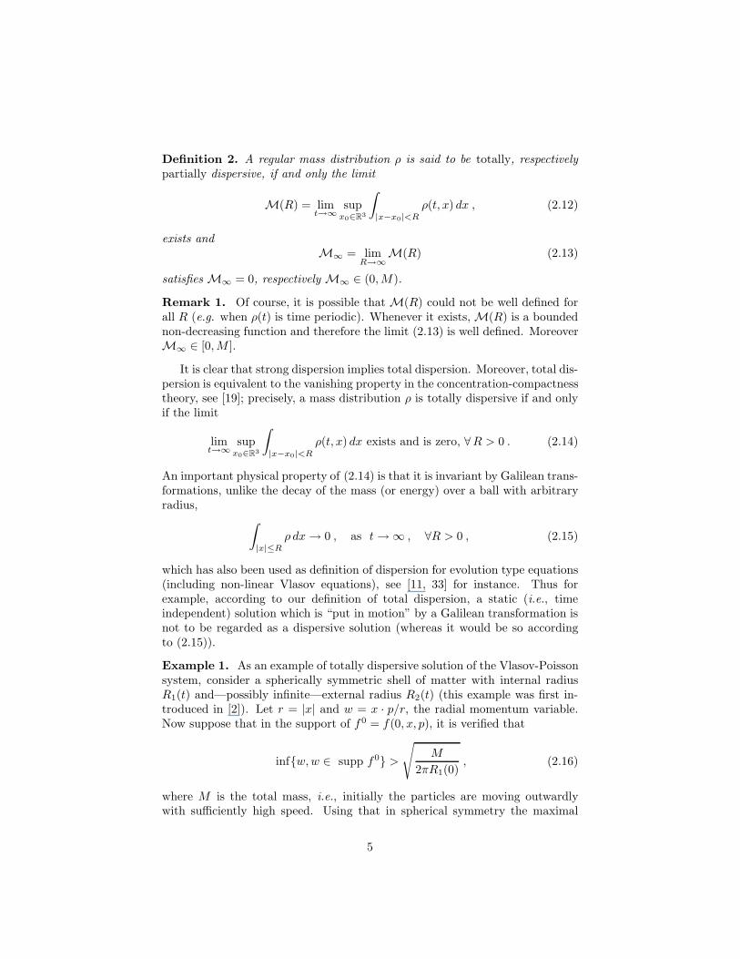
Definition 2. A regular mass distribution ρ is said to be totally, respectivelypartially dispersive, if and only the limit

M(R) = limt→∞

supx0∈R3

∫

|x−x0|<R

ρ(t, x) dx , (2.12)

exists andM∞ = lim

R→∞M(R) (2.13)

satisfies M∞ = 0, respectively M∞ ∈ (0, M).

Remark 1. Of course, it is possible that M(R) could not be well defined forall R (e.g. when ρ(t) is time periodic). Whenever it exists, M(R) is a boundednon-decreasing function and therefore the limit (2.13) is well defined. MoreoverM∞ ∈ [0, M ].

It is clear that strong dispersion implies total dispersion. Moreover, total dis-persion is equivalent to the vanishing property in the concentration-compactnesstheory, see [19]; precisely, a mass distribution ρ is totally dispersive if and onlyif the limit

limt→∞

supx0∈R3

∫

|x−x0|<R

ρ(t, x) dx exists and is zero, ∀R > 0 . (2.14)

An important physical property of (2.14) is that it is invariant by Galilean trans-formations, unlike the decay of the mass (or energy) over a ball with arbitraryradius,

∫

|x|≤R

ρ dx → 0 , as t → ∞ , ∀R > 0 , (2.15)

which has also been used as definition of dispersion for evolution type equations(including non-linear Vlasov equations), see [11, 33] for instance. Thus forexample, according to our definition of total dispersion, a static (i.e., timeindependent) solution which is “put in motion” by a Galilean transformation isnot to be regarded as a dispersive solution (whereas it would be so accordingto (2.15)).

Example 1. As an example of totally dispersive solution of the Vlasov-Poissonsystem, consider a spherically symmetric shell of matter with internal radiusR1(t) and—possibly infinite—external radius R2(t) (this example was first in-troduced in [2]). Let r = |x| and w = x · p/r, the radial momentum variable.Now suppose that in the support of f0 = f(0, x, p), it is verified that

inf{w, w ∈ supp f0} >

√

M

2πR1(0), (2.16)

where M is the total mass, i.e., initially the particles are moving outwardlywith sufficiently high speed. Using that in spherical symmetry the maximal

5

force experienced by a particle is bounded by M/4πr2, see (1.10), we find that,along the characteristics of the Vlasov equation,

d

dt

(

1

2w2 −

M

4πr

)

= w w +M

4πr2r = w

(

w +M

4πr2

)

,

which is positive in the time interval [0, T ) in which w > 0, i.e., as long as theshell keeps moving outwardly. It follows that

w(t)2 > w(0)2 −M

2πr(0)> inf

supp f0w2 −

M

2πR1(0):= W > 0 ,

where for the last inequality we use (2.16). This implies that T = ∞, that is,the shell moves outwardly for all future times. Moreover, W > 0 is a uniformlower bound on the radial momentum, which entails

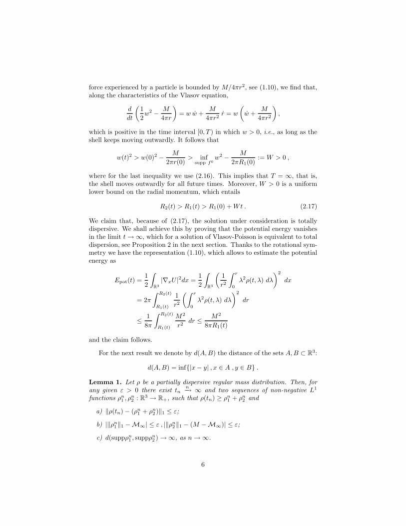
R2(t) > R1(t) > R1(0) + Wt . (2.17)

We claim that, because of (2.17), the solution under consideration is totallydispersive. We shall achieve this by proving that the potential energy vanishesin the limit t → ∞, which for a solution of Vlasov-Poisson is equivalent to totaldispersion, see Proposition 2 in the next section. Thanks to the rotational sym-metry we have the representation (1.10), which allows to estimate the potentialenergy as

Epot(t) =1

2

∫

R3

|∇xU |2dx =1

2

∫

R3

(

1

r2

∫ r

0

λ2ρ(t, λ) dλ

)2

dx

= 2π

∫ R2(t)

R1(t)

1

r2

(∫ r

0

λ2ρ(t, λ) dλ

)2

dr

≤1

8π

∫ R2(t)

R1(t)

M2

r2dr ≤

M2

8πR1(t)

and the claim follows.

For the next result we denote by d(A, B) the distance of the sets A, B ⊂ R3:

d(A, B) = inf{|x − y| , x ∈ A , y ∈ B} .

Lemma 1. Let ρ be a partially dispersive regular mass distribution. Then, forany given ε > 0 there exist tn

n−→ ∞ and two sequences of non-negative L1

functions ρn1 , ρn

2 : R3 → R+, such that ρ(tn) ≥ ρn

1 + ρn2 and

a) ‖ρ(tn) − (ρn1 + ρn

2 )‖1 ≤ ε;

b) |‖ρn1‖1 −M∞| ≤ ε , |‖ρn

2‖1 − (M −M∞)| ≤ ε;

c) d(suppρn1 , suppρn

2 ) → ∞, as n → ∞.

6

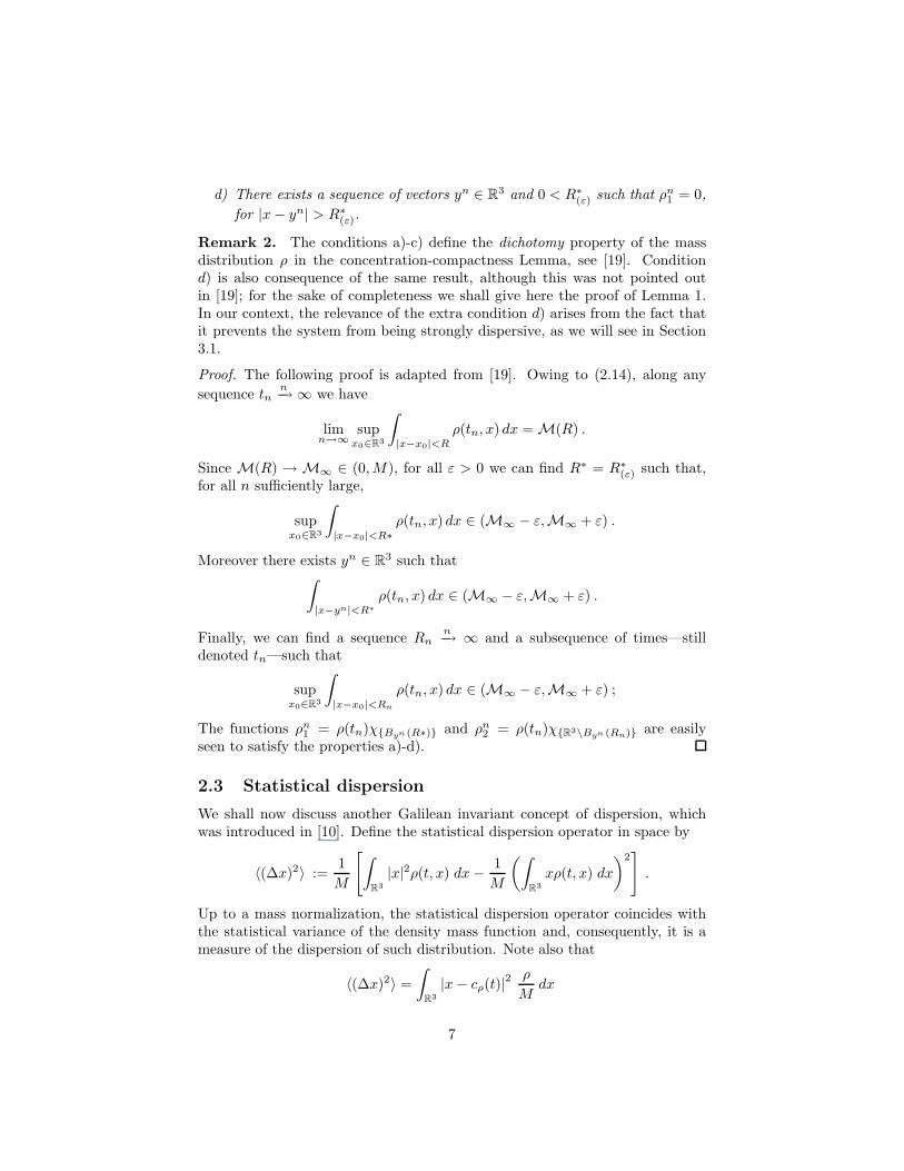
d) There exists a sequence of vectors yn ∈ R3 and 0 < R∗

(ε) such that ρn1 = 0,

for |x − yn| > R∗(ε).

Remark 2. The conditions a)-c) define the dichotomy property of the massdistribution ρ in the concentration-compactness Lemma, see [19]. Conditiond) is also consequence of the same result, although this was not pointed outin [19]; for the sake of completeness we shall give here the proof of Lemma 1.In our context, the relevance of the extra condition d) arises from the fact thatit prevents the system from being strongly dispersive, as we will see in Section3.1.

Proof. The following proof is adapted from [19]. Owing to (2.14), along any

sequence tnn−→ ∞ we have

limn→∞

supx0∈R3

∫

|x−x0|<R

ρ(tn, x) dx = M(R) .

Since M(R) → M∞ ∈ (0, M), for all ε > 0 we can find R∗ = R∗(ε) such that,

for all n sufficiently large,

supx0∈R3

∫

|x−x0|<R∗

ρ(tn, x) dx ∈ (M∞ − ε,M∞ + ε) .

Moreover there exists yn ∈ R3 such that

∫

|x−yn|<R∗

ρ(tn, x) dx ∈ (M∞ − ε,M∞ + ε) .

Finally, we can find a sequence Rnn−→ ∞ and a subsequence of times—still

denoted tn—such that

supx0∈R3

∫

|x−x0|<Rn

ρ(tn, x) dx ∈ (M∞ − ε,M∞ + ε) ;

The functions ρn1 = ρ(tn)χ{Byn (R∗)} and ρn

2 = ρ(tn)χ{R3\Byn (Rn)} are easilyseen to satisfy the properties a)-d).

2.3 Statistical dispersion

We shall now discuss another Galilean invariant concept of dispersion, whichwas introduced in [10]. Define the statistical dispersion operator in space by

〈(∆x)2〉 :=1

M

[

∫

R3

|x|2ρ(t, x) dx −1

M

(∫

R3

xρ(t, x) dx

)2]

.

Up to a mass normalization, the statistical dispersion operator coincides withthe statistical variance of the density mass function and, consequently, it is ameasure of the dispersion of such distribution. Note also that

〈(∆x)2〉 =

∫

R3

|x − cρ(t)|2 ρ

Mdx

7

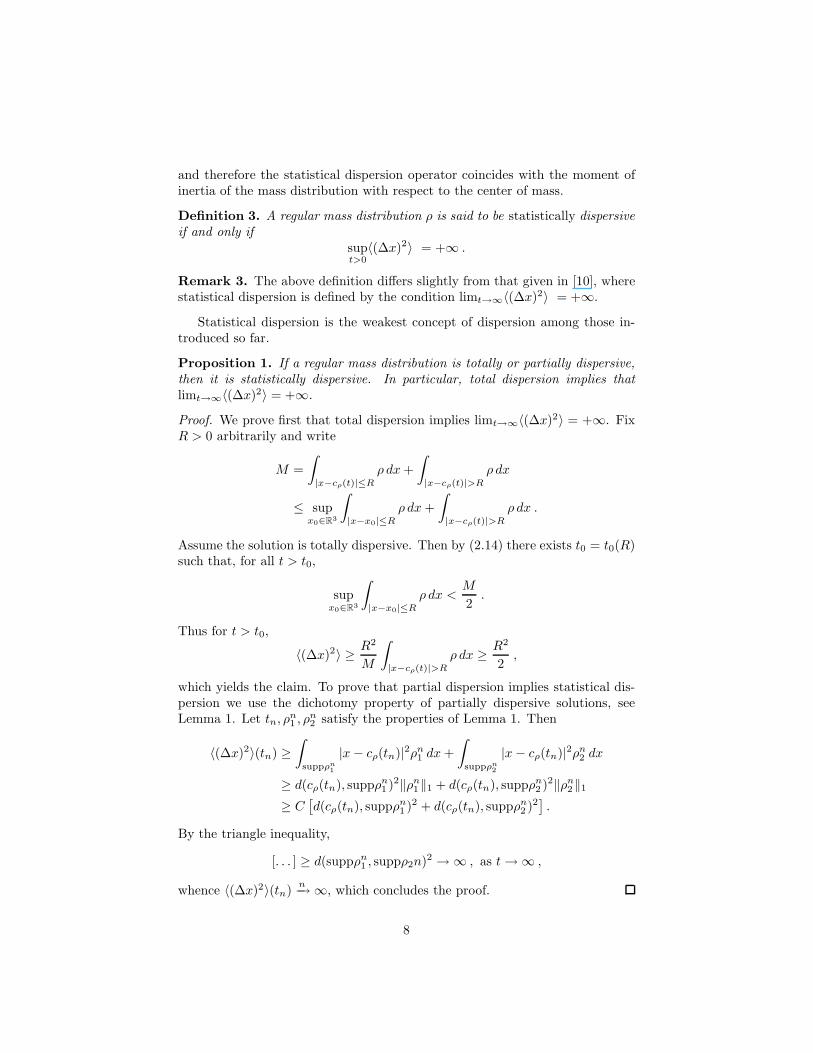
and therefore the statistical dispersion operator coincides with the moment ofinertia of the mass distribution with respect to the center of mass.

Definition 3. A regular mass distribution ρ is said to be statistically dispersiveif and only if

supt>0

〈(∆x)2〉 = +∞ .

Remark 3. The above definition differs slightly from that given in [10], wherestatistical dispersion is defined by the condition limt→∞〈(∆x)2〉 = +∞.

Statistical dispersion is the weakest concept of dispersion among those in-troduced so far.

Proposition 1. If a regular mass distribution is totally or partially dispersive,then it is statistically dispersive. In particular, total dispersion implies thatlimt→∞〈(∆x)2〉 = +∞.

Proof. We prove first that total dispersion implies limt→∞〈(∆x)2〉 = +∞. FixR > 0 arbitrarily and write

M =

∫

|x−cρ(t)|≤R

ρ dx +

∫

|x−cρ(t)|>R

ρ dx

≤ supx0∈R3

∫

|x−x0|≤R

ρ dx +

∫

|x−cρ(t)|>R

ρ dx .

Assume the solution is totally dispersive. Then by (2.14) there exists t0 = t0(R)such that, for all t > t0,

supx0∈R3

∫

|x−x0|≤R

ρ dx <M

2.

Thus for t > t0,

〈(∆x)2〉 ≥R2

M

∫

|x−cρ(t)|>R

ρ dx ≥R2

2,

which yields the claim. To prove that partial dispersion implies statistical dis-persion we use the dichotomy property of partially dispersive solutions, seeLemma 1. Let tn, ρn

1 , ρn2 satisfy the properties of Lemma 1. Then

〈(∆x)2〉(tn) ≥

∫

suppρn1

|x − cρ(tn)|2ρn1 dx +

∫

suppρn2

|x − cρ(tn)|2ρn2 dx

≥ d(cρ(tn), suppρn1 )2‖ρn

1‖1 + d(cρ(tn), suppρn2 )2‖ρn

2‖1

≥ C[

d(cρ(tn), suppρn1 )2 + d(cρ(tn), suppρn

2 )2]

.

By the triangle inequality,

[. . . ] ≥ d(suppρn1 , suppρ2n)2 → ∞ , as t → ∞ ,

whence 〈(∆x)2〉(tn)n−→ ∞, which concludes the proof.

8

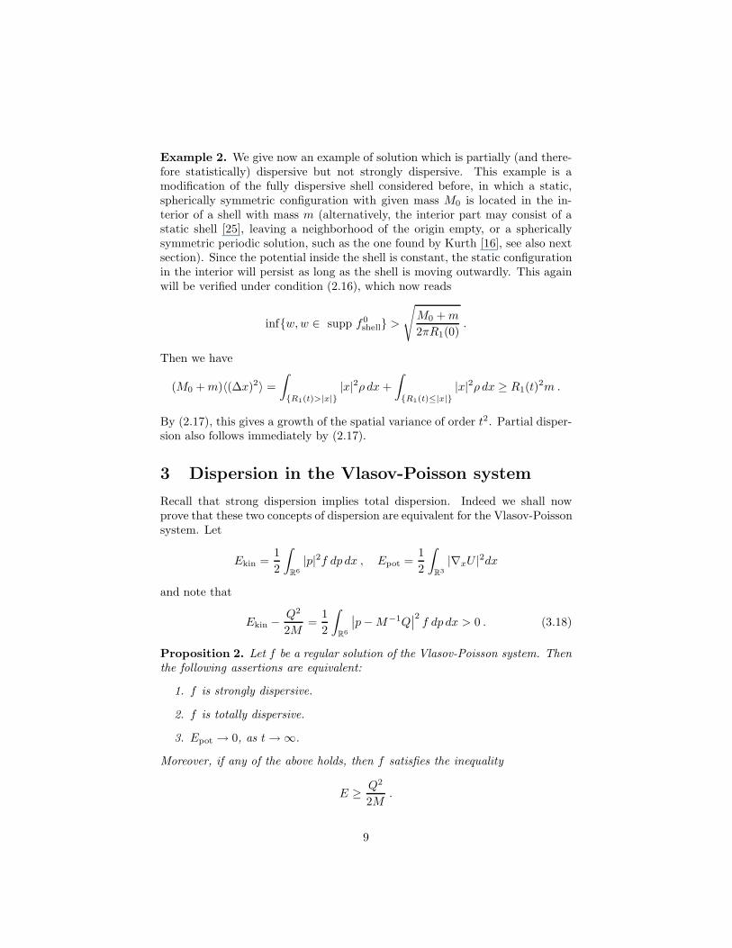
Example 2. We give now an example of solution which is partially (and there-fore statistically) dispersive but not strongly dispersive. This example is amodification of the fully dispersive shell considered before, in which a static,spherically symmetric configuration with given mass M0 is located in the in-terior of a shell with mass m (alternatively, the interior part may consist of astatic shell [25], leaving a neighborhood of the origin empty, or a sphericallysymmetric periodic solution, such as the one found by Kurth [16], see also nextsection). Since the potential inside the shell is constant, the static configurationin the interior will persist as long as the shell is moving outwardly. This againwill be verified under condition (2.16), which now reads

inf{w, w ∈ supp f0shell} >

√

M0 + m

2πR1(0).

Then we have

(M0 + m)〈(∆x)2〉 =

∫

{R1(t)>|x|}

|x|2ρ dx +

∫

{R1(t)≤|x|}

|x|2ρ dx ≥ R1(t)2m .

By (2.17), this gives a growth of the spatial variance of order t2. Partial disper-sion also follows immediately by (2.17).

3 Dispersion in the Vlasov-Poisson system

Recall that strong dispersion implies total dispersion. Indeed we shall nowprove that these two concepts of dispersion are equivalent for the Vlasov-Poissonsystem. Let

Ekin =1

2

∫

R6

|p|2f dp dx , Epot =1

2

∫

R3

|∇xU |2dx

and note that

Ekin −Q2

2M=

1

2

∫

R6

∣

∣p − M−1Q∣

∣

2f dp dx > 0 . (3.18)

Proposition 2. Let f be a regular solution of the Vlasov-Poisson system. Thenthe following assertions are equivalent:

1. f is strongly dispersive.

2. f is totally dispersive.

3. Epot → 0, as t → ∞.

Moreover, if any of the above holds, then f satisfies the inequality

E ≥Q2

2M.

9

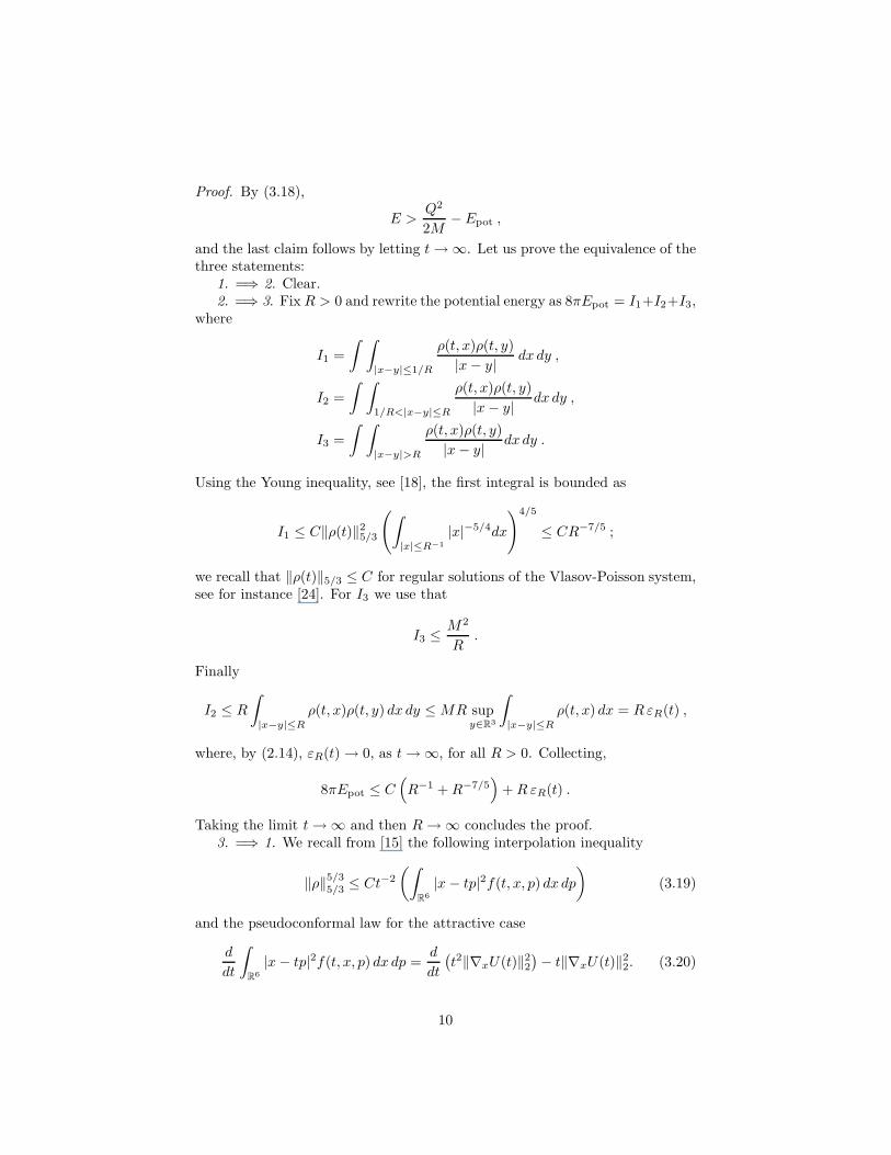
Proof. By (3.18),

E >Q2

2M− Epot ,

and the last claim follows by letting t → ∞. Let us prove the equivalence of thethree statements:

1. =⇒ 2. Clear.2. =⇒ 3. Fix R > 0 and rewrite the potential energy as 8πEpot = I1+I2+I3,

where

I1 =

∫ ∫

|x−y|≤1/R

ρ(t, x)ρ(t, y)

|x − y|dx dy ,

I2 =

∫ ∫

1/R<|x−y|≤R

ρ(t, x)ρ(t, y)

|x − y|dx dy ,

I3 =

∫ ∫

|x−y|>R

ρ(t, x)ρ(t, y)

|x − y|dx dy .

Using the Young inequality, see [18], the first integral is bounded as

I1 ≤ C‖ρ(t)‖25/3

(

∫

|x|≤R−1

|x|−5/4dx

)4/5

≤ CR−7/5 ;

we recall that ‖ρ(t)‖5/3 ≤ C for regular solutions of the Vlasov-Poisson system,see for instance [24]. For I3 we use that

I3 ≤M2

R.

Finally

I2 ≤ R

∫

|x−y|≤R

ρ(t, x)ρ(t, y) dx dy ≤ MR supy∈R3

∫

|x−y|≤R

ρ(t, x) dx = R εR(t) ,

where, by (2.14), εR(t) → 0, as t → ∞, for all R > 0. Collecting,

8πEpot ≤ C(

R−1 + R−7/5)

+ R εR(t) .

Taking the limit t → ∞ and then R → ∞ concludes the proof.3. =⇒ 1. We recall from [15] the following interpolation inequality

‖ρ‖5/35/3 ≤ Ct−2

(∫

R6

|x − tp|2f(t, x, p) dx dp

)

(3.19)

and the pseudoconformal law for the attractive case

d

dt

∫

R6

|x − tp|2f(t, x, p) dx dp =d

dt

(

t2‖∇xU(t)‖22

)

− t‖∇xU(t)‖22. (3.20)

10

Integrating (3.20), we get

∫

R6

|x − tp|2f dx dp −

∫

R6

|x|2f0 dx dp = t2‖∇xU(t)‖22 −

∫ t

0

s‖∇xU(s)‖22 ds,

so that

0 ≤ t−2

∫

R6

|x − tp|2f dx dp ≤ t−2

∫

R6

|x|2f0 dx dp + ‖∇xU(t)‖22 ,

and the r.h.s. converges to zero by hypothesis, which in combination with (3.19)concludes the proof.

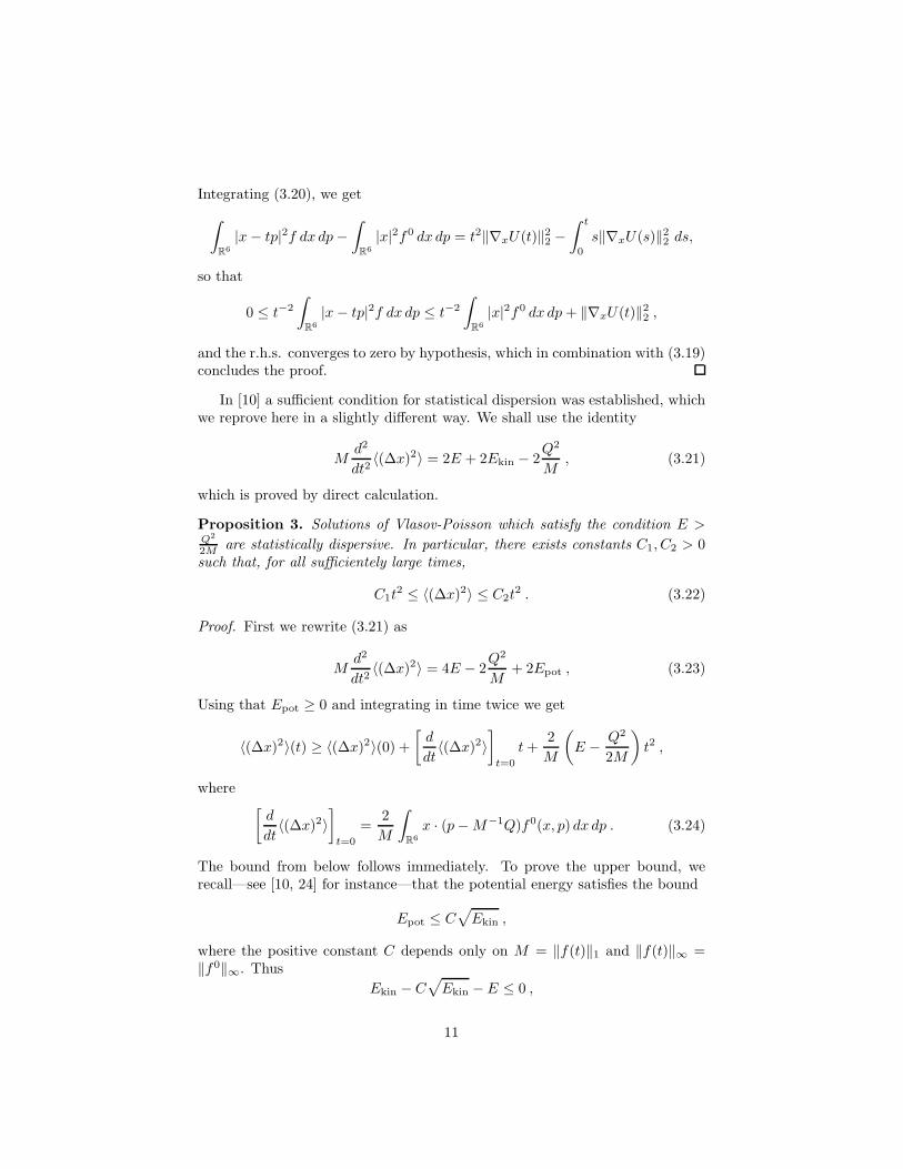
In [10] a sufficient condition for statistical dispersion was established, whichwe reprove here in a slightly different way. We shall use the identity

Md2

dt2〈(∆x)2〉 = 2E + 2Ekin − 2

Q2

M, (3.21)

which is proved by direct calculation.

Proposition 3. Solutions of Vlasov-Poisson which satisfy the condition E >Q2

2M are statistically dispersive. In particular, there exists constants C1, C2 > 0such that, for all sufficientely large times,

C1t2 ≤ 〈(∆x)2〉 ≤ C2t

2 . (3.22)

Proof. First we rewrite (3.21) as

Md2

dt2〈(∆x)2〉 = 4E − 2

Q2

M+ 2Epot , (3.23)

Using that Epot ≥ 0 and integrating in time twice we get

〈(∆x)2〉(t) ≥ 〈(∆x)2〉(0) +

[

d

dt〈(∆x)2〉

]

t=0

t +2

M

(

E −Q2

2M

)

t2 ,

where[

d

dt〈(∆x)2〉

]

t=0

=2

M

∫

R6

x · (p − M−1Q)f0(x, p) dx dp . (3.24)

The bound from below follows immediately. To prove the upper bound, werecall—see [10, 24] for instance—that the potential energy satisfies the bound

Epot ≤ C√

Ekin ,

where the positive constant C depends only on M = ‖f(t)‖1 and ‖f(t)‖∞ =‖f0‖∞. Thus

Ekin − C√

Ekin − E ≤ 0 ,

11

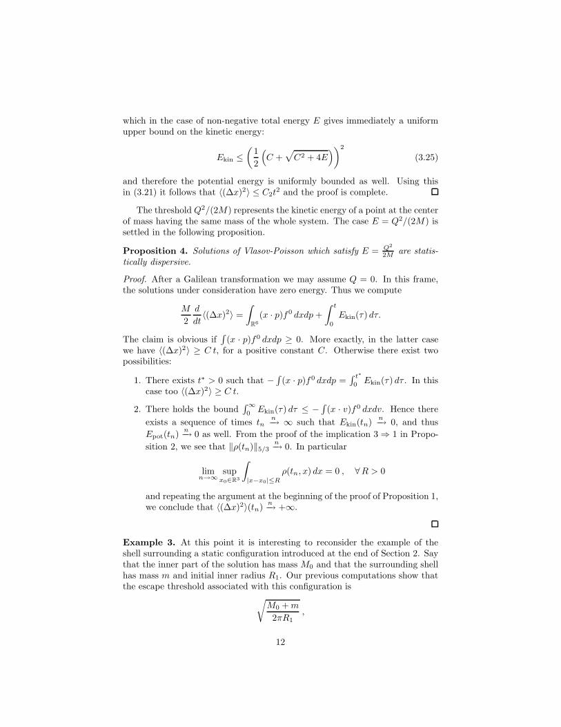
which in the case of non-negative total energy E gives immediately a uniformupper bound on the kinetic energy:

Ekin ≤

(

1

2

(

C +√

C2 + 4E)

)2

(3.25)

and therefore the potential energy is uniformly bounded as well. Using thisin (3.21) it follows that 〈(∆x)2〉 ≤ C2t

2 and the proof is complete.

The threshold Q2/(2M) represents the kinetic energy of a point at the centerof mass having the same mass of the whole system. The case E = Q2/(2M) issettled in the following proposition.

Proposition 4. Solutions of Vlasov-Poisson which satisfy E = Q2

2M are statis-tically dispersive.

Proof. After a Galilean transformation we may assume Q = 0. In this frame,the solutions under consideration have zero energy. Thus we compute

M

2

d

dt〈(∆x)2〉 =

∫

R6

(x · p)f0 dxdp +

∫ t

0

Ekin(τ) dτ.

The claim is obvious if∫

(x · p)f0 dxdp ≥ 0. More exactly, in the latter casewe have 〈(∆x)2〉 ≥ C t, for a positive constant C. Otherwise there exist twopossibilities:

1. There exists t∗ > 0 such that −∫

(x · p)f0 dxdp =∫ t∗

0 Ekin(τ) dτ . In thiscase too 〈(∆x)2〉 ≥ C t.

2. There holds the bound∫∞

0 Ekin(τ) dτ ≤ −∫

(x · v)f0 dxdv. Hence there

exists a sequence of times tnn−→ ∞ such that Ekin(tn)

n−→ 0, and thus

Epot(tn)n−→ 0 as well. From the proof of the implication 3 ⇒ 1 in Propo-

sition 2, we see that ‖ρ(tn)‖5/3n−→ 0. In particular

limn→∞

supx0∈R3

∫

|x−x0|≤R

ρ(tn, x) dx = 0 , ∀R > 0

and repeating the argument at the beginning of the proof of Proposition 1,we conclude that 〈(∆x)2〉(tn)

n−→ +∞.

Example 3. At this point it is interesting to reconsider the example of theshell surrounding a static configuration introduced at the end of Section 2. Saythat the inner part of the solution has mass M0 and that the surrounding shellhas mass m and initial inner radius R1. Our previous computations show thatthe escape threshold associated with this configuration is

√

M0 + m

2πR1,

12

see (2.16), so that any particle with initial radial momentum greater than thisthreshold will escape towards infinity. We shall now prove that it is possible toobtain an escaping shell even when the total energy of the system is negative.Note that the total energy E consists of the energy E0 of the interior partplus the kinetic energy of the shell minus the potential energy of the shell (theinteraction energy has negative sign and as a consequence the term contributingto the potential energy can be not consired). Neglecting the last negative termand estimating above the kinetic energy of the shell we get

E < E0 +1

2m sup

shell|p|2 ,

where the supremum is taken in the support of the shell at time t = 0. Theinterior part has energy E0 < 0, since it is static (cf. Proposition 5); thus inorder to have the whole shell escaping to infinity while the total energy of thesystem remains negative we must choose the initial radial momenta for all theparticles in the shell according to

M0 + m

2πR1< inf

shellw2 < inf

shell|p|2 < sup

shell|p|2 <

−2E0

m.

This can be done if m is strictly contained in the interval between zero and thevalue 1

2 [−M0 +√

M20 − 16πE0R1]. For bigger values of m we have no guarantee

that the total energy can be kept negative.

The previous example shows us that:

• There are solutions that are partially (therefore statistically) dispersivewith E < Q2/2M , so that there is no simple way to extend the results ofPropositions 3 and 4. By Proposition 2, these solutions cannot be totallydispersive.

• We know that spherically symmetric solutions with E > 0 disperse sta-tistically with a dispersion rate of t2 (equivalently their spatial supportspreads with a velocity of order t). We will see in Section 3.1 that forsolutions with E = 0 this needs not to be the case. On the other handthe previous example shows that there are solutions with E ≤ 0 whichalso statistically disperse with a rate t2. So there is no evident relationbetween the admisible rates of dispersion and the sign of the energy.

• There is no lower limit for the fraction of total mass of the system that islost to infinity for a partially dispersive system.

• Using these ideas we can also show that there exist dispersive solutionsas “close” as desired to a stable steady state. More precisely, given apolytropic steady state (see [29] for details and notation) with mass M ,polytropic index µ and L1+1/µ-norm J , which is stable in the sense of[29], we can find solutions as described above that are partially dispersiveand that remain in the stability region of the polytrope. (This is not a

13

contradiction since the quantity of mass that is lost to infinity is almostnegligible.) These solutions correspond to initial data of the followingtype. Starting form the given polytrope we construct—by scaling—a sec-ond polytrope having mass M−m and L1+1/µ-norm J−j, for m, j positiveand small. Then we add an outer shell of mass m and L1+1/µ-norm lessor equal to j. We choose m, j in order that all the computations in Ex-ample 3 remain valid and that the total energy of the solution is as closeas desired to the energy of the original polytrope. Then we can invoke thestability criterium in [29].

3.1 Kurth’s solution

We conclude this section by considering an explicit class of spherically symmetricsolutions to the Vlasov-Poisson system found by Kurth in [16] (see also [13],[24]). The main idea of this model is to find a solution whose associated densityis of the form

ρ(t, x) = (4π/3)−1φ(t)−3χ{|x|<φ(t)} (3.26)

where the function φ is interpreted as the radius of the system. This functionφ solves the following ODE

φ3φ′′ + φ = 1 ,

subject to the initial condition φ(0) = 1. We get solutions to the Vlasov-Poissonsystem exhibiting different types of behavior depending on the prescribed valueof φ′(0):

• If φ′(0) = 0, the solution is static;

• If 0 < |φ′(0)| < 1, the solution is periodic in time;

• If |φ′(0)| ≥ 1, the solution is strongly dispersive.

Let us relate the above classification in terms of φ′(0) with the values of theenergy E. Note first that the associated distribution function f can be chosento be spherically symmetric so that Q = 0. Doing so, the energy of Kurth’ssolutions is given by, see [13],

E =3

5

(

(φ′)2 + φ−2 − 2φ−1)

=3

5(φ′(0)2 − 1) .

Moreover M = 1, which follows integrating (3.26). Thus

• If E = −3/5 (⇔ φ′(0) = 0), the solution is static (this steady state isstudied in [5]).

• If −3/5 < E < 0 (⇔ 0 < |φ′(0)| < 1), the solution is time periodic.

• If E ≥ 0 (⇔ |φ′(0)| ≥ 1), the radius of the system goes to infinity and,by (3.26), ρ → 0 in Lq, for all q > 1, i.e., the solution is strongly (andtherefore also totally) dispersive. When E = 0 (⇔ |φ′(0)| = 1), we have〈(∆x)2〉 ∼ t4/3. When E > 0 (⇔ |φ′(0)| > 1), we get 〈(∆x)2〉 ∼ t2, inagreement with Proposition 3.

14

Let us prove the latter claim. First we show that 〈(∆x)2〉 ∼ O(φ(t)2). Sincethe solution under study is spherically symmetric, we have

〈(∆x)2〉 =

∫

R3

|x|2ρ(x) dx = 4π

(

4π

3

)−1

φ(t)−3

∫ φ(t)

0

r4 dr =3

5φ(t)2.

Thus we reduce the problem to find out the large time behavior of the functionφ. Following Kurth [16], if |φ′(0)| = 1 we have that

φ(t) =1

2(1 + v(t)2) ,

where v(t) solves

v(t) +1

3v(t)3 = 2

(

t +2

3

)

.

For t big the term v(t)3 dominates and then φ(t) ∼ O(t2/3). If |φ′(0)| > 1, wehave that

φ(t) =|φ′(0)|ch (v(t)) − 1

|φ′(0)|2 − 1,

where v(t) solves

v(t) − |φ′(0)|sh (v(t)) = (|φ′(0)| − 1)3/2(t − t0)

(t0 depends on |φ′(0)|). For t big enough |sh (v(t))| dominates |v(t)|, and weinfer that |v(t)| ∼ O(log t), which entails φ(t) ∼ O(t).

Note that the solution with E = 0 (there are two of them actually) is the onlyknown example of statistically dispersive solution for which statistical dispersiontakes place at a slower rate than t2 and for which the support spreads moreslowly than t. Also the rate for strong dispersion is slower than for the otherexamples considered in this paper. Taking a closer look to the trajectoriesreveals that these are strongly oscillatory (like in a forced harmonic oscillator).

This special solution highlights also the role of condition d) in Lemma 1.For we can surround this “slowly dispersing” solution with a strongly dispersiveshell configuration, and the resulting solution verifies a), b) and c) but not d),and happens to be totally but not partially dispersive, see previous Remark 2.

4 Remarks on non-dispersive solutions

In this section we briefly consider non-dispersive solutions of the Vlasov-Poissonsystem. In particular, we consider steady state solutions and time periodic(breather) solutions.

We distinguish between two types of steady states: Static solutions, whichare defined as time-independent solutions of the Vlasov-Poisson systen (1.1)–(1.3), and travelling steady states, which are defined as solutions f(t, x, p) suchthat there exists a Galilean transformation Gu such that f ◦Gu is a time indepen-dent solution of the Vlasov-Poisson system (i.e., a static solution). For static

15

solutions one has Q = 0, wheras Q 6= 0 for travelling steady states. In fact, itis easy to show that the Galilean transformation which transforms a travellingsteady state with linear momentum Q and mass M to a static solution (withlinear momentum Q = 0 and mass M) is the transformation Gu, where

u =Q

M.

The construction of static solutions for the Vlasov-Poisson system can bedone in two ways. Firstly, by choosing a particle density f which depends onlyon quantities that are conserved along the characteristics of the time indepen-dent Vlasov equation; with this choice the Vlasov equation is automaticallysatisfied and the problem is reduced to that of proving an existence theoremfor the non-linear elliptic equation obtained by replacing f in the Poisson equa-tion. So far this ‘direct’ method was used mostly in the spherically symmetriccase (see however [32]), where by the Jeans Theorem [5] all solutions of thetime independent Vlasov equation can be expressed in terms of the particlesenergy and angular momentum. A second method to construct steady statesof the Vlasov-Poisson system is by minimizing the energy (or a related) func-tional subject to suitable constraints (the choice of the functional and/or theconstraints selects the type of steady state to be constructed). The advantageof the variational method on the direct method is that the former automaticallyproves a stability property for the steady state. We refer [12, 26, 27, 29, 24] andreferences therein for several works on the construction and stability of steadystates of the Vlasov-Poisson system.

To make a connection with the results proved in the previous sections fordispersive solutions, let us note the following simple bounds on the energy ofsteady states and time periodic solutions:

Proposition 5. Static solutions of the Vlasov-Poisson system satisfy E < 0,

whereas travelling steady states satisfy E < Q2

2M . Time periodic solutions of the

Vlasov-Poisson system satisfy E < − Q2

2M .

Proof. The key to prove the result is the dilation identity:

d

dt

∫

R6

x · p f dp dx = E + Ekin , (4.27)

which follows by direct computation. If f is a static solution, then the previousidentity implies the virial relation E = −Ekin, which yields the claim for staticsolutions. For travelling steady states, a Galilean transformation with u =(M)−1Q yields the virial identity in the form E − (M)−1Q2 = −Ekin, which,using (3.18), implies the claim of the proposition for travelling steady states. Inthe case of periodic solutions, we integrate the dilation identity over a period Tto get

0 = ET +

∫ T

0

Ekindt .

Using again (3.18) concludes the proof.

16

Remark 4. In the case of static solutions of the Nordstrom-Vlasov system, theinequality E < 0 is replaced by E < M , see [8]. For the (spherically symmetric)Einstein-Vlasov system, one can obtain an inequality for static solutions whichinvolves not only the energy and the mass but also the central redshift [9].

4.1 Virialized solutions

It is a classical result in Astrophysics that bounded systems of self-gravitatingparticles roughly in equilibrium verify that the time average of the kinetic energyof the ensemble equals twice the time average of its potential energy. Thisstatement and some of its variants and particularizations go under the nameof “virial theorems” (cf. [23, 30, 6], for instance), and are common tools inAstrophysics. We shall comment here on the connection between the notion ofvirialized solutions of the Vlasov-Poisson system and our preceding results.

In this section we shall only consider solutions such that Q = 0, i.e., thereference frame is chosen at rest with respect to the center of mass of the system,as we did in the proof of Proposition 4. Following [23] we shall say that a solutionof the Vlasov-Poisson system is virialized if and only if

limt→∞

∫ t

0E + Ekin(τ) dτ

t= 0 . (4.28)

Note that solutions with E > 0 cannot be virialized in this sense. In fact, it isa straightforward consequence of the inequality (3.18) that virialized solutionsof the Vlasov-Poisson system must necessarily satisfy

E ≤ 0 .

Examples of virialized solutions are Kurth’s solutions with energy E ≤ 0.

Remark 5. The notion of virialized system is usually applied in Astrophysicsonly in the case of N -body bounded systems, but, as pointed out in [23], strictboundedness is not necessary (Kurth’s solution with energy E = 0 shows thatalso in the case of Vlasov-Poisson, the support of a virialized solution can spreadout to infinity). This remark led to interpret the virialized systems as apparentlybounded systems, i.e., systems that disperse so slowly that in our time scale theyappear to be bounded and in equilibrium.

The following proposition extends the result in [23], which is valid for N -body systems, to the continuos setting; note that the diameter of the N -bodysystem used in [23], is replaced by the statistical dispersion operator 〈(∆x)2〉.

Lemma 2. Let f(t) be a given solution of the Vlasov-Poisson system withQ = 0. Then the following statements hold true:

1. If f(t) is virialized then limt→∞〈(∆x)2〉

t2 = 0.

2. If limt→∞〈(∆x)2〉

t2 = 0 and limt→∞

R

t

0E+Ekin(τ) dτ

t exits, then f(t) is viri-alized.

17

Dispersive behavior Necessary Sufficient Example

Strong Dispersion E ≥ Q2/2M ? Example 1(VP)↑ ↓

Total Dispersion E ≥ Q2/2M ? Kurth’s E ≥ 0↓

Statistical Dispersion ? E ≥ Q2/2M↑

Partial Dispersion ? ? Example 2

Other solutions

Static Solutions E < 0 – Kurth’s E = − 35

Periodic Solutions E < −Q2/2M – Kurth’s E ∈ (− 35 , 0)

Virialized Solutions E ≤ 0 – Kurth’s E = 0

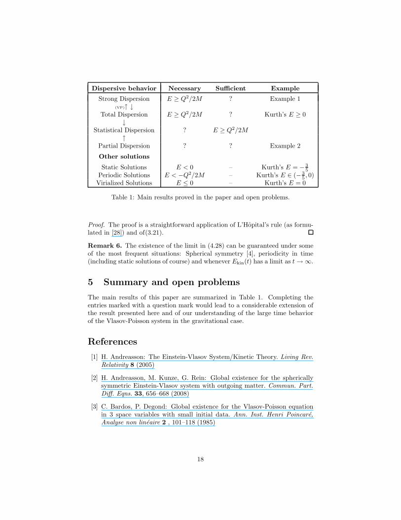
Table 1: Main results proved in the paper and open problems.

Proof. The proof is a straightforward application of L’Hopital’s rule (as formu-lated in [28]) and of(3.21).

Remark 6. The existence of the limit in (4.28) can be guaranteed under someof the most frequent situations: Spherical symmetry [4], periodicity in time(including static solutions of course) and whenever Ekin(t) has a limit as t → ∞.

5 Summary and open problems

The main results of this paper are summarized in Table 1. Completing theentries marked with a question mark would lead to a considerable extension ofthe result presented here and of our understanding of the large time behaviorof the Vlasov-Poisson system in the gravitational case.

References

[1] H. Andreasson: The Einstein-Vlasov System/Kinetic Theory. Living Rev.Relativity 8 (2005)

[2] H. Andreasson, M. Kunze, G. Rein: Global existence for the sphericallysymmetric Einstein-Vlasov system with outgoing matter. Commun. Part.Diff. Eqns. 33, 656–668 (2008)

[3] C. Bardos, P. Degond: Global existence for the Vlasov-Poisson equationin 3 space variables with small initial data. Ann. Inst. Henri Poincare,Analyse non lineaire 2 , 101–118 (1985)

18

[4] J. Batt: Asymptotic properties of spherically symmetric self-gravitatingmass systems for t → ∞. Transport theory and Stat. Phys. 16 (4-6), 763–768 (1987)

[5] J. Batt, W. Faltenbacher, E. Horst: Stationary spherically symmetric mod-els in stellar dynamics. Arch. Rat. Mech. Anal. 93, 159–183 (1986)

[6] J. Binney, S. Tremaine: Galactic dynamics. Princeton University Press,Princeton (1987)

[7] S. Calogero: Spherically symmetric steady states of galactic dynamics inscalar gravity. Class. Quantum. Grav. 20, 1729–1741 (2003)

[8] S. Calogero, O. Sanchez, J. Soler: Asymptotic behavior and orbital sta-bility of galactic dynamics in relativistic scalar gravity. To appear inArch. Rat. Mech. Anal.

[9] S. Calogero, J. Calvo, O. Sanchez, J. Soler: Preprint

[10] J. Dolbeault, O. Sanchez, J. Soler: Asymptotic behavior for the Vlasov-Poisson system in the stellar dynamics case. Arch. Rat. Mech. Anal. 171,301–327 (2004)

[11] R. Glassey, W. Strauss: Remarks on collissionless plasmas. ContemporaryMathematics 28, 269–279 (1984)

[12] Y. Guo, G. Rein: Stable models of elliptical galaxies. Mon. Not. R. Astron.Soc. 344, 1296–1306 (2003).

[13] E Horst, R Hunze: Weak solutions of the initial value problem for theunmodified non-linear Vlasov equation. Math. Meth. Appl. Sci. 6, 262–279(1984)

[14] H. J. Hwang, A. D. Rendall, J. L. Velazquez: Optimal gradient estimatesand asymptotic behavior for the Vlasov-Poisson system with small initialdata. Preprint: math.AP/0606389

[15] R. Illner, G. Rein: Time decay of the solutions of the Vlasov–Poisson sys-tem in the plasma physical case. Math. Meth. Appl. Sci. 19 (1996), 1409–1413.

[16] R Kurth: A global particular solution to the initial value problem of thestellar dynamics. Quart. Appl. Math. 36, 325–329 (1978)

[17] P. Levy: Theorie de l’addition des variables aleatoires. Gauthier-Villars,Paris (1954)

[18] E. H. Lieb, M. Loss: Analysis. Providence: American Math. Soc. (1996)

[19] P. L. Lions: The concentration-compactness principle in the Calculus ofVariations. The locally compact case, part 1. Ann. Inst. Henri Poincare,Analyse non lineaire. 1, 109–145 (1984)

19

[20] P.-L. Lions, B. Perthame: Propagation of moments and regularity for the3-dimensional Vlasov-Poisson system. Invent. Math. 105, 415–430 (1991)

[21] B. Perthame: Time decay, propagation of low moments and dispersiveeffects for kinetic equations. Commun. Part. Diff. Eqns. 21, 659–686 (1996)

[22] K. Pfaffelmoser: Global classical solutions of the Vlasov-Poisson system inthree dimensions for general initial data. J. Diff. Eqns. 95, 281–303 (1992)

[23] H. Pollard: A sharp form of the virial theorem. Bull. Amer. Math. Soc.LXX, 703–705 (1964)

[24] G. Rein: Collisionless Kinetic Equations from Astrophysics—The Vlasov-Poisson System. Handbook of Differential Equations, Evolutionary Equa-tions. Vol. 3. Eds. C.M. Dafermos and E. Feireisl, Elsevier (2007)

[25] G. Rein: Static shells for the Vlasov-Poisson and Vlasov-Einstein systems.Indiana Univ. Math. J. 48, 335–346 (1999)

[26] G. Rein: Stationary and static stellar dynamic models with axial symmetry.Nonlinear Analysis; Theory, Methods and Applications 41, 313–344 (2000).

[27] G. Rein, A. D. Rendall: Compact support of spherically symmetric equilib-ria in non-relativistic and relativistic galactic dynamics. Math. Proc. Cam-bridge Philos. Soc. 128, 363–380 (2000).

[28] W. Rudin: Principles of Mathematical Analysis. McGrawHill, U.S.A.(1976)

[29] O. Sanchez, J. Soler: Orbital stability for polytropic galaxies. Ann. Inst.Henri Poincare, Analyse non lineaire 23, 781–802 (2006)

[30] W. C. Saslaw: Gravitational physics of stellar and galactic systems. Cam-bridge Monographs on Mathematical Physics (19)

[31] J. Schaeffer: Global existence of smooth solutions to the Vlasov-Poissonsystem in three dimensions. Commun. Part. Diff. Eqns. 16, 1313–1335(1991)

[32] A. Schulze: Existence of axially symmetric solutions to the Vlasov-Poissonsystem depending on Jacobi’s integral. Commun. Math. Sci. 6, 711–727(2008)

[33] W. Strauss: Non-linear wave equations. Providence: American Math. Soc.(1992)

20