Embed Size (px)
Citation preview


Lecture Notes in Earth Sciences Editors: S. Bhattacharji, Brooklyn G . M. Friedman, Brooklyn and Troy H. J. Neugebauer, Bonn A. Seilacher, Tuebingen and Yale

Springer Berlin Heidelberg New York Hong Kong London Milan Paris Tokyo

Horst J. Neugebauer Clemens Simmer (Eds.)
Dynamics of Multiscale Earth Systems
With approx. 150 Figures and 50 Tables
Springer

Editors
Professor Horst J. Neugebauer Universitat Bonn Institut fur Geodynamik Nussallee 8 53115 Bonn
Clemens Simmer Meteorologisches Institut der Universitat Bonn Auf dem Huge1 20 53121 Bonn
"For all Lecture Notes in Earth Sciences published till now please see final pages of the book"
ISSN 0930-03 17 ISBN 3-540-41796-6 Springer-Verlag Berlin Heidelberg New York
Cataloging-in-Publication Data applied for
Bibliographic information published by Die Deutsche Bibliothek. Die Deutsche Bibliothek lists this publication in the Deutsche Nationalbibliographie; detailed bibliographic data is available in the Internetat <http://dnb.ddb.de>.
This work is subject to copyright. All rights are reserved, whether the whole or part of the material is concerned, specifically the rights of translation, reprinting, re-use of illustrations, recitation, broadcasting, reproduction on microfilms or in any other way, and storage in data banks. Duplication of this publication or parts thereof is permitted only under the provisions of the German Copyright Law of September 9, 1965, in its current version, and permission for use must always be obtained from Springer-Verlag. Violations are liable for prosecution under the German Copyright Law.
Springer-Verlag Berlin Heidelberg New York a member of Bertelsmannspringer Science+Business Media GmbH
O Springer-Verlag Berlin Heidelberg 2003 Printed in Germany
The use of general descriptive names, registered names, trademarks, etc. in this publication does not imply, even in the absence of a specific statement, that such names are exempt from the relevant protective laws and regulations and therefore free for general use
Typesetting: Camera ready by editors Printed on acid-free paper 3213 141 - 5 4 3 2 1 0

Preface
In many aspects science becomes conducted nowadays through technology andpreferential criteria of economy. Thus investigation and knowledge is evidentlylinked to a specific purpose. Especially Earth science is confronted with twomajor human perspectives concerning our natural environment: sustainability ofresources and assessment of risks. Both aspects are expressing urgent needs ofthe living society, but in the same way those needs are addressing a long lastingfundamental challenge which has so far not been met. Following on the patternsof economy and technology, the key is presumed to be found through a develop-ment of feasible concepts for a management of both our natural environment andin one or the other way the realm of life. Although new techniques for observa-tion and analysis led to an increase of rather specific knowledge about particularphenomena, yet we fail now even more frequently to avoid unforeseen implica-tions and sudden changes of a situation. Obviously the improved technologicaltools and the assigned expectations on a management of nature still exceed ourtraditional scientific experience and accumulated competence. Earth- and Life-Sciences are nowadays exceedingly faced with the puzzling nature of an almostboundless network of relations, i. e., the complexity of phenomena with respectto their variability. The disciplinary notations and their particular approachesare thus no longer accounting sufficiently for the recorded context of phenomena,for their permanent variability and their unpredictable implications. The largeenvironmental changes of glacial climatic cycles, for instance, demonstrate thiscomplexity of such a typical phenomenology. Ice age cycles involve beside thereorganisation of ice sheets as well changes of the ocean-atmosphere system, thephysics and chemistry of the oceans and their sedimentary boundaries. They arelinked to the carbon cycle, and the marine and terrestrial ecosystems and lastnot least the crucial changes in the orbital parameters such as in eccentricity,precession frequency and tilt of the planet during its rotation and movementin space. So far changes of solar radiation through the activity of the sun itselfhave not yet been adequately incorporated. The entire dynamics of the climatesystem has therefore the potential to perform abrupt reorganisation as demon-strated by sedimentary records. It becomes quite obvious, in order to reveal thecomplex nature of phenomena we evidently have to reorganise our own scientificperspectives and our disciplinary bounds as well.
Reflecting assessment of environmental risks from a perspective of complex-ity, we may discover quickly our traditional addiction to representative averagesand the idea of permanence which we equate with normality in contrast to ex-ceptional disasters. A closer look onto those extremes, however, gives ampleevidence that even our normality is based onto ongoing changes which are usu-ally expressed through the variance around the extracted means. Within theconcept of complexity the entire spectrum of change has to be considered, what-ever intensity it may have. In such a broader context, variability is usually notat all representative for the particularity of phenomena. We might be even more

VI Preface
astonished being confronted with an inability of predicting not only the extremedisasters, but equally well the small changes within the range of variance aboutaverages, what we called previously the case of normality.
Encouraged by the potential of new technologies, we might again becometempted to “search for the key where we may have some light, but where wenever have lost it”. That means, the idea of management without improving ourunderstanding of complexity of Earth-systems will just continue creating popu-lar, weak and disappointing approaches of the known type. It is definitely norsufficient and neither successful to search for some popular compact solutions interms of some kind of index-values or thresholds of particular variables for thesake of our convenience. Complexity of phenomena is rather based on ongoingchange of an extended network of conditional relations ; that means, the changeof a system can generally not be related to one specific cause. What we there-fore need for the search of appropriate concepts of sustainability is primarily animproved complex competence. At that state we are facing in the first order veryfundamental scientific problems ahead of the technological ones. We encountera class of difficulties which exceed by far any limited disciplinary competenceas well as any aspect of economical advantage. The difficulties we do encounterwhen investigating complexity are well expressed synonymously by the univer-sal multi-scale character of phenomena. We might thus strive for an enhanceddiscussion of the expanding scale concept for the investigation of geo-complexity.
Scales are geometrical measures and quite suitable to express general prop-erties or qualities of phenomena such as length, size or volume. Even so space-related features, as for instance intensity or momentum might be addressed byscales as well. The close relationship of scales to our perception of space justifiestheir universal character and utility. An entire scale-concept might be establishedand practised through characterising objects and phenomena by their represen-tative scales. In this sense we might even comprehend a complex phenomenologyby analysing it with respect to its inherent hierarchy of related scales. The con-sideration of scales might give us equally well an idea about the conditionalbackground of phenomena and their peculiar variability. Complexity of changeof entire systems such as for instance fracture pattern, slope instabilities, distri-bution of precipitation and others are progressively investigated by means of astatistical analysis of scales through the fit of characteristic scaling laws to largedata sets. At present, it appears to be the most efficient way of revealing the hid-den nature of complexity of phenomena which are depending on a large context.Insight comes thereafter mostly from the conditions, necessary for reproducingstatistical probability distributions through modelling. However, our traditionaladdiction to the common background of linear deterministic relations gives us ahard time establishing quantitative models on complex system behaviour. Rep-resenting complex change quantitatively requires the interaction between differ-ent variables and parameters at least on a local basis. Consequently, there arenumerous attempts to build representative complex models through graduallyadopting non-linearity up to the degree of self-organisation in the critical state.Conceptual as well as methodological problems of both analysing and modelling

Dynamics of Multi-Scale Earth Systems VII
complexity have been assigned to the scale-concept for the convenience of auniversal standard for comparison. Within this context a key question becomesaddressed implicitly throughout the various measurements, techniques of anal-ysis and complex modelling which will be discussed: do our considerations ofnatural phenomena yield sufficient evidence for the existence of representativeaverages.
About ten traditional disciplines, among them applied mathematics, com-puter science, physics, photogrammetry and most of the geo-sciences formed aunited power of competence in addressing the complexity of Earth-systems ondifferent manifestations. Related to a limited area of mountain and basin struc-tures along a section of the Lower Rhine, we studied two major aspects: the his-torical component of past processes from Earth history by means of structuraland sedimentary records as well as temporary perspectives of ongoing processesof change through recent observations. Our common matter of understandingwas the conceptual aim of performing complementary quantitative modelling.Therefore the presented volume gives in the beginning a comprehensive presen-tation on the different aspects of the scale-concept. According to the addressedphenomena the scale related representation of both spatial data sets and physicalprocesses will be discussed in the chapters two and three. Finally some structuraland dynamical modelling aspects of the complexity of change in earth systemswill be presented with reference to the scale-concept.
After a period of ten years of interdisciplinary research, plenty of scientific ex-perience has been developed and accumulated. Naturally, even a long record forwarm acknowledgements arose from a wide spectrum of support which made thisunusual scientific approach possible. Therefore the present book will give somerepresentative sampling of our themes, methods and results at an advanced stateof research work. We will take the opportunity to gratefully acknowledge thesubstantial funding of our scientific interests within the Collaborative ResearchCentre 350: Interaction between and Modelling of Continental Geo-Systems —by the German science foundation — Deutsche Forschungsgemeinschaft — en-closing the large group of critical reviewers. In the same sense we like to thankour head board of the Rheinische Friedrich-Wilhelms-University at Bonn. Largeamounts of data have been kindly provided from various sources: a peat miningcompany, water supply companies and various federal institutes and surveys. Weare very grateful for the numerous occasions of generous help. Finally we liketo thank our colleagues from two European research programs in the Nether-lands and Switzerland. The editors are indebted to Michael Pullmann and SvenHunecke for their valuable help in preparing this book.
Last not least, we like to acknowledge the assistance of the reviewers withthe contributing papers with gratitude.
Horst J. Neugebauer & Clemens Simmer

Table of Contents
I Scale Concepts in Geosciences
Scale Aspects of Geo-Data Sampling . . . . . . . . . . . . . . . . . . . . . . . . . . . . . . . . . 5Hans-Joachim Kumpel
Notions of Scale in Geosciences . . . . . . . . . . . . . . . . . . . . . . . . . . . . . . . . . . . . . . 17Wolfgang Forstner
Complexity of Change and the Scale Concept in Earth System Modelling . 41Horst J. Neugebauer
II Multi-Scale Representation of Data
Wavelet Analysis of Geoscientific Data . . . . . . . . . . . . . . . . . . . . . . . . . . . . . . . . 69Thomas Gerstner, Hans-Peter Helfrich, and Angela Kunoth
Diffusion Methods for Form Generalisation . . . . . . . . . . . . . . . . . . . . . . . . . . . . 89Andre Braunmandl, Thomas Canarius, and Hans-Peter Helfrich
Multi-Scale Aspects in the Management of Geologically Defined Geometries103Martin Breunig, Armin B. Cremers, Serge Shumilov, and Jorg Siebeck
III Scale Problems in Physical Process Models
Wavelet and Multigrid Methods for Convection-Diffusion Equations . . . . . . 123Thomas Gerstner, Frank Kiefer, and Angela Kunoth
Analytical Coupling of Scales — Transport of Water and Solutes in PorousMedia . . . . . . . . . . . . . . . . . . . . . . . . . . . . . . . . . . . . . . . . . . . . . . . . . . . . . . . . . . . . 135
Thomas Canarius, Hans-Peter Helfrich, and G.W. Brummer
Upscaling of Hydrological Models by Means of Parameter AggregationTechnique . . . . . . . . . . . . . . . . . . . . . . . . . . . . . . . . . . . . . . . . . . . . . . . . . . . . . . . . . 145
Bernd Diekkruger
Parameterisation of Turbulent Transport in the Atmosphere . . . . . . . . . . . . . 167Matthias Raschendorfer, Clemens Simmer, and Patrick Gross
Precipitation Dynamics of Convective Clouds . . . . . . . . . . . . . . . . . . . . . . . . . . 186Gunther Heinemann and Christoph Reudenbach
Sediment Transport — from Grains to Partial Differential Equations . . . . . 199Stefan Hergarten, Markus Hinterkausen, and Michael Kupper

X Table of Contents
Water Uptake by Plant Roots — a Multi-Scale Approach . . . . . . . . . . . . . . . 215Markus Mendel, Stefan Hergarten, and Horst J. Neugebauer
IV Scale-Related Approaches to Geo-Processes
Fractals – Pretty Pictures or a Key to Understanding Earth Processes? . . . 237Stefan Hergarten
Fractal Variability of Drilling Profiles in the Upper Crystalline Crust . . . . . 257Sabrina Leonardi
Is the Earth’s Surface Critical? The Role of Fluvial Erosion and Landslides 271Stefan Hergarten
Scale Problems in Geometric-Kinematic Modelling of Geological Objects . . 291Agemar Siehl and Andreas Thomsen
Depositional Systems and Missing Depositional Records . . . . . . . . . . . . . . . . 307Andreas Schafer
Multi-Scale Processes and the Reconstruction of Palaeoclimate . . . . . . . . . . 325Christoph Gebhardt, Norbert Kuhl, Andreas Hense, and Thomas Litt
A Statistical-Dynamic Analysis of Precipitation Data with High TemporalResolution . . . . . . . . . . . . . . . . . . . . . . . . . . . . . . . . . . . . . . . . . . . . . . . . . . . . . . . . 337
Hildegard Steinhorst, Clemens Simmer, and Heinz-Dieter Schilling

List of Authors
Braunmandl, Andre, Bonner Logsweg 107, 53123 Bonn,[email protected]
Breunig, Martin, Prof. Dr., Institut fur Umweltwissenschaften, HochschuleVechta, Oldenburger Straße 97, 49377 Vechta, [email protected]
Brummer, Gerhard W., Prof. Dr., Institut fur Bodenkunde, Rheini-sche Friedrich-Wilhelms-Universitat Bonn, Nußallee 13, 53115 Bonn,[email protected]
Canarius, Thomas, Dr., Hochstraße 71, 55128 Mainz, [email protected]
Cremers, Armin Bernd, Prof. Dr., Institut fur Informatik III, Rheini-sche Friedrich-Wilhelms-Universitat Bonn, Romerstraße 164, 53117 Bonn,[email protected]
Diekkruger, Bernd, Prof. Dr., Geographisches Institut, RheinischeFriedrich-Wilhelms-Universitat Bonn, Meckenheimer Allee 166, 53115 Bonn,[email protected]
Forstner, Wolfgang, Prof. Dr., Institut fur Photogrammetrie, RheinischeFriedrich-Wilhelms-Universitat Bonn, Nußallee 15, 53115 Bonn, [email protected]
Gebhardt, Christoph, Meteorologisches Institut, Rheinische Friedrich-Wilhelms-Universitat Bonn, Auf dem Hugel 20, 53121 Bonn, [email protected]
Gerstner, Thomas, Institut fur Angewandte Mathematik, Rheini-sche Friedrich-Wilhelms-Universitat Bonn, Wegelerstraße 6, 53115 Bonn,[email protected]
Gross, Patrick, Steinmetzweg 34, 64625 Bensheim, [email protected]
Heinemann, Gunther, Prof. Dr., Meteorologisches Institut, RheinischeFriedrich-Wilhelms-Universitat Bonn, Auf dem Hugel 20, 53121 Bonn,[email protected]
Helfrich, Hans-Peter, Prof. Dr., Mathematisches Seminar der Land-wirtschaftlichen Fakultat, Rheinische Friedrich-Wilhelms-Universitat Bonn,Nußallee 15, 53115 Bonn, [email protected]
Hense, Andreas, Meteorologisches Institut, Rheinische Friedrich-Wilhelms-Universitat Bonn, Auf dem Hugel 20, 53121 Bonn, [email protected]
Hergarten, Stefan, Dr., Lehrstuhl fur Geodynamik, Geologisches Institut,Rheinische Friedrich-Wilhelms-Universitat Bonn, Nußallee 8, 53115 Bonn,[email protected]

XII DynamicsofMulti-ScaleEarthSystems
Hinterkausen, Markus, Dr., Birkenweg 16, 71679 Asperg, [email protected]
Kiefer, Frank, Dr., Institut fur Angewandte Mathematik, Rheinische Friedrich-Wilhelms-Universitat Bonn, Wegelerstraße 6, 53115 Bonn, [email protected]
Kunoth, Angela, Prof. Dr., Institut fur Angewandte Mathematik, Rhei-nische Friedrich-Wilhelms-Universitat Bonn, Wegelerstraße 6, 53115 Bonn,[email protected]
Kuhl, Norbert, Dr., Institut fur Palaontologie, Rheinische Friedrich-Wilhelms-Universitat Bonn, Nußallee 8, 53115 Bonn, [email protected]
Kumpel, Hans-Joachim, Prof. Dr., GGA-Institut, Stilleweg 2, 30655 Hannover,[email protected]
Kupper, Michael, Lehrstuhl fur Geodynamik, Geologisches Institut,Rheinische Friedrich-Wilhelms-Universitat Bonn, Nußallee 8, 53115 Bonn,[email protected]
Leonardi, Sabrina, Dr., Geologisches Institut, Rheinische Friedrich-Wilhelms-Universitat Bonn, Nußallee 8, 53115 Bonn, [email protected]
Litt, Thomas, Prof. Dr., Institut fur Palaontologie, Rheinische Friedrich-Wilhelms-Universitat Bonn, Nußallee 8, 53115 Bonn, [email protected]
Mendel, Markus, Dr., Lehrstuhl fur Geodynamik, Geologisches Institut,Rheinische Friedrich-Wilhelms-Universitat Bonn, Nußallee 8, 53115 Bonn,[email protected]
Neugebauer, Horst J., Prof. Dr., Lehrstuhl fur Geodynamik, Geologisches In-stitut, Rheinische Friedrich-Wilhelms-Universitat Bonn, Nußallee 8, 53115 Bonn,[email protected]
Raschendorfer, Matthias, Am Lindenbaum 38, 60433 Frankfurt,[email protected]
Reudenbach, Christoph, Dr., Fachbereich Geographie, Universitat Marburg,Deutschhausstraße 10, 35037 Marburg, [email protected]
Schafer, Andreas, Prof. Dr., Geologisches Institut, Rheinische Friedrich-Wilhelms-Universitat Bonn, Nußallee 8, 53115 Bonn, [email protected]
Schilling, Heinz-Dieter, Prof. Dr., Meteorologisches Institut, RheinischeFriedrich-Wilhelms-Universitat Bonn. Heinz-Dieter Schilling was one of the driv-ing forces of the research program. He died on November 22th, 1997, on a researchexpedition in the table mountains of Venezuela.
Shumilov, Serge, Institut fur Informatik III, Universitat Bonn, Romerstraße164, 53117 Bonn, [email protected]

List of Authors XIII
Siebeck, Jorg, Institut fur Informatik III, Universitat Bonn, Romerstraße 164,53117 Bonn, [email protected]
Siehl, Agemar, Prof. Dr., Geologisches Institut, Rheinische Friedrich-Wilhelms-Universitat Bonn, Nußallee 8, 53115 Bonn, [email protected]
Simmer, Clemens, Prof. Dr., Meteorologisches Institut, Rheinische Friedrich-Wilhelms-Universitat Bonn, Auf dem Hugel 20, 53121 Bonn, [email protected]
Steinhorst, Hildegard, Dr., Abteilung ICG-1 (Stratosphare), Institut furChemie und Dynamik der Geosphare, Forschungszentrum Julich, 52435 Julich,[email protected]
Thomsen, Andreas, Institut fur Informatik III, Rheinische Friedrich-Wilhelms-Universitat Bonn, Romerstraße 164, 53117 Bonn, [email protected]

Scale Aspects of Geo-Data Sampling
Hans-Joachim Kumpel
Section Applied Geophysics, Geological Institute, University of Bonn, Germany
Abstract. Sampling data values in earth sciences is all but trivial. Thereason is the multi-scale variability of observables in nature, both inspace and in time. Sampling geo-data means selecting a finite numberof data points from a continuum of high complexity, or from a systemof virtually infinite degree of freedom. When taking a reading a filteringprocess is automatically involved, whatever tool or instrument is used.The design of adequate sampling strategy as well as proper interpretationof geo-data thus requires a-priori insight into the variability of the targetstructure and/or into the dynamics of a time varying observable. Ignoringthe inherent complexity of earth systems can ultimately lead to grosslyfalse conclusions. Retrieving data from nature and deducing meaningfulresults obviously is an expert’s task.
Earth systems exhibit an inherent, multi-scale nature, hence, its observablestoo. When we want to sample geo-data, e. g. by taking soil samples or readingsfrom a sensor in the field, we have to keep in mind that even the smallest soilsample is an aggregate of a myriad of minerals and fluid molecules; and thatthe sensor of any instrument, due to limited resolution, renders values that areintegrated over some part of the scanned medium. Any set of measurementsextracts only a tiny piece of information from an Earth system.
In this book, an Earth system classifies a complex, natural regime on Earth.It could be a group of clouds in the atmosphere, a network of fissures in a rock, ahill slope, a sedimentary basin, the Earth’s lithosphere; or it could be a specificgeographical region as, for instance, the Rhenish Massif, or a geological provincelike the Westerwald volcanic province, a part of that Massif. Earth systemsare coupled systems, in which various components interact; and they are opensystems, as there is always some interaction with external constituents. WhatEarth systems have in common, besides of their multi-scale structures in spaceand their complex dynamics in the time domain, is a large, virtually infinitenumber of particles or elements, and consequently of degrees of freedom.
The problem of adequate data sampling in an Earth system obviously existson both the spatial and the time scale: Taking a reading may need seconds,hours, months. Can we be sure that the dynamics of the target parameter canbe neglected during such time spans? We wouldn’t have to bother if structuralvariabilities were of comparatively large wavelengths, or if temporal fluctuationsexhibit rather low frequencies. This will, however, generally not be the case. [email protected] [now at: Leibniz Institute for Applied Geosciences
(GGA), Hannover, Germany]
H.J. Neugebauer and C. Simmer (Eds): LNES 97, pp. 5–15, 2003.
c© Springer-Verlag Berlin Heidelberg 2003

6 Hans-Joachim Kumpel
When observables present a multi-scale variability, the resolution of readingswill actually often be less than the nominal resolution of the sensor or of themeasurement technique we apply.
How do we classify sampled data in terms of accuracy, precision, resolution?The values we call ‘readings’, are they average values? What kind of averaging isinvolved? If — on the scale of sampling — a multi-scale variability is significant,should we name the readings ‘effective’ values, since we can but obtain a ratherlimited idea about their full variability? What would be the exact understandingof an effective value?
It may be useful to recall some basic definitions of limitations that alwaysexist in sampling. By ‘resolution’ we mean the smallest difference between tworeadings that differ by a significant amount. ‘Precision’ is a measure of how wella result was determined. It is associated with the scatter in a set of repeatedreadings. ‘Bias’ is the systematic error in a measurement. It can be caused by abadly calibrated or faulty instrument and corrupts the value of a reading thatmay have been taken with high precision. ‘Accuracy’ is a measure of correctness,or of how close a result comes to the true value (Fig. 1). However, the truevalue is usually unknown. Scientists need to estimate in some systematic wayhow much confidence they can have in their measurements. All they have is animagination, or model, of what they believe is the true value. An Earth systemitself is often imagined as a grossly simplified model. ‘Error’ is simply defined asthe difference between an observed (or calculated) value and the true value. And‘dynamic range’ of an instrument or technique denotes the ratio of the largestdifference that can be sensed (i. e. its measuring range) and its resolution.
Readings are typically corrupted by statistical (or random) errors that re-sult from observational fluctuations differing from experiment to experiment.The statistical error can be quantified from the observed spread of the resultsof a set of representative measurements, i. e. by testing how well a reading isreproducible (if repetition is possible). A bias is more difficult to identify and inmany cases is not even considered. It is repeated in every single measurementand leads to systematic differences between the true and the measured value. Abias can be assessed by application of standards, or by comparison with redun-dant observations obtained by using a different technique. An accurate readinghas both a low statistical and a low systematic error. Bias and precision arecompletely independent of each other. A result can be unbiased and precise, orbiased and imprecise, but also unbiased and imprecise, or biased and precise. Inthe two latter cases the results may not be satisfactory. By the way, fuzzy logicis a useful technique to handle imprecise or even indistinct problems — yet atthe expense of resolution.
To be more specific on problems that are particular to geo-data sampling, letus first consider cases for limitations on the spatial scale. In all geoscience innu-merable kinds of sampling methods do exist. A few examples are given below,mainly from geophysics. They can give only a brief glance of the broadness ofconflicts existing with geo-data sampling. Apart from that, in view of the multi-scale nature of observables, we may differ between two aspects: Limited repre-

Scale Aspects of Geo-Data Sampling 7
sentative character of a single observation, e. g. due to the extended geometry ofan instrument or a sampling technique; and limited representative character ofseveral readings, taken of a quantity that presents a certain variability in space,for instance, along a profile.
A frequent problem in geoscience that is common to both aspects is ‘under-sampling’. In an Earth system, we will never have sufficient readings to unam-biguously describe a structure or a process in all its details. Imaging of detailson all scales is impossible due to the limited dynamic range of any scanningtechnique. There is always a ‘bit’ or ‘byte’ (1-D), a ‘pixel’ (2-D), or a ‘voxel’ (3-D), i. e. a smallest element bearing information, and a maximum total numberof elements that can be retrieved and stored. To code the structure of a surfaceof one square metre at micrometre resolution in black and white (or that of asquare kilometre at resolution of a millimetre) would require a dynamic rangeof 4 × 10¹² or four million Megapixels. Common data loggers have a dynamicrange of 2048 bits, broadband loggers offer 8 million. Aliasing occurs if shortwavelength fluctuations are undersampled leading to appearance of these fluc-tuations in the long wavelength part of the archived data set (e. g. Kanasewich,
Fig. 1. Precision, bias and accuracy (inspired by Wagner, 1998).

8 Hans-Joachim Kumpel
1981). Unless short wavelength variability is suppressed through filtering priorto sampling, a certain degree of aliasing is unavoidable in geoscience. However,by the process of filtering, original data is lost. How can we still get along ingeoscience?
As for the aspect of limited representative character of single readings, wemay e. g. think of distance measurements, for instance through an extensometer.This is a geometrically extended instrument, two points of which are coupledto the ground. Instrument readings are changes of the distance between the twopoints divided by the instrument’s overall spread, called the baselength. Whencompared to previously taken readings, data values indicate the bulk shorteningor lengthening of the rock formation between the instrument’s grounded points,yielding one component of the surface deformation tensor (Fig. 2a). In practice,the baselength may range from several centimetres to hundreds of metres. So-phisticated extensometers have a resolution of one part in ten billion (10−10), yeteach single reading represents an integral value over all shortenings or lengthen-ings that may occur anywhere between the grounded points (Figs. 2b, c). Whatcan we learn from a measurement which is both so accurate and so crude?
On a larger scale, a similar problem exists with measurements called VeryLong Baseline Interferometry (VLBI). These yield distance data over baselinesof hundreds or thousands of kilometres, namely between two parabola anten-nae that receive radio signals from a distant quasar (e. g. Campbell, 2000). Asingle reading when processed is the change in the distance between two VLBIstations. It can be resolved with millimetre precision. However, from the mul-titude of point displacements occurring at the Earth’s surface, like local shiftsof ground positions, regional size displacements along faults, or plate tectonicmovements on the global scale, only changes in the bulk distance between theVLBI stations are extracted. Any thinkable configuration of VLBI systems willlargely undersample the full spectrum of ground movements. Do the measure-ments make sense?
A different situation is met with observation of potential fields, as in gravity,magnetics, or geoelectrics. Here, a single reading reflects a certain field strengthat the location of the sensor element. When interpreting the reading one has tobe aware that the observed value represents a superposition of contributions ofmasses, magnetic dipoles, electric charges from the closest vicinity up to — inprinciple — infinite distance. Any reading is actually the integral over a verylarge number of contributors in the sensor’s near and far field. Is there any hopeto reduce such inherent ambiguity?
In the latter case it helps when we know — from the theory of potential fields— that the larger the distance to a contributor, the lower will be its influence;or, a contributor at larger distance needs either to be more extended or to be ofhigher source strength to provoke the same effect as a close by contributor. Forinstance, spheres of identical excess density ∆ρ provoke the same change ∆g ingravity when their distances ri to the gravity sensor scale to their radii Ri with

Scale Aspects of Geo-Data Sampling 9
Fig. 2. Principle of extensometer (a) and impossibility to distinguish between lengthfluctuations of long (b) and short wavelength (c).
R3i /r
2i = const. (because from Newton’s law,
∆g =∆mi
r2i
=∆ρVi
r2i
=43π∆ρ
R3i
r2i
with ∆mi, Vi denoting the excess mass and the volume of a sphere; Fig. 3).Knowing basic physical laws thus allows us to differ between more and lessdominating constituents, and those that are negligible — without being able tospecify the shape of an anomalous body in the subsurface.
Knowledge of basic geoscientific principles, similarly, helps to understand ex-tensometer readings or VLBI data. The concept of plate tectonics has given theclue to understand why extended areas of the Earth’s surface are comparativelyrigid (and therefore called plates) and large movements occur mostly at plateboundaries (e. g. Kearey and Vine, 1996). In fact, significant variations in thelength of VLBI baselines can largely be attributed to plate boundary regionsrather than to processes of deformation within the plates; displacements gener-ally do not occur at arbitrary locations in between VLBI stations. This also holds

10 Hans-Joachim Kumpel
for smaller scales: Extensometer readings are well understood from insight intothe distribution of stiffer and weaker portions of a probed rock formation, andinto the nature and wavelength of stresses that lead to shortening or lengtheningof the baselength (Agnew, 1986). How representative and informative individualreadings are can often be estimated from a-priori knowledge or an expert’s as-sumption of the most influential processes being involved. This applies to manysampling procedures: A-priori knowledge leads to the imagination of models;good models are fundamental for every sampling strategy.
How well is the signature of a geo-signal represented in our data if we havesampled a whole series of values — along a profile, in an area, or in 3-D? As vari-ability exists on all scales, the smaller the sampling intervals, the more detailsare resolved (Fig. 4). Some methods allow sampling of a large number of data
Fig. 3. Principle of gravimeter and identical attraction effect of anomalous masses atcloser and larger distances.

Scale Aspects of Geo-Data Sampling 11
values, others do not; or we may be able to obtain densely sampled data alongone axis in space, but not along another. Rock cores recovered from boreholes ordata from geophysical borehole-logging, for example, provide a wealth of infor-mation along the borehole axis (see Leonardi; this volume), with centimetre, forcore material even sub-millimetre resolution. The limited number of boreholesdrilled in an area, however, may restrict lateral resolution to wavelengths of tensor hundreds of kilometres, which does often not allow to trace alterations andboundaries of geological formations over respective distances. Or, whereas mon-itoring of in-situ deformation using extensometers — due to logistic constraints— can be operated at a few locations only, areal coverage by e. g. a geomagneticfield survey may be rather dense. Still, spatial resolution of the latter techniqueis far of being sufficient if we want to resolve details of e. g. the structure of poresto understand colloid transport on the micro-scale.
When surveying potential field quantities, useful information can be retrievedif we have recorded a series of values over some area and apply the principles ofpotential theory. For example, iterated smoothing of signal amplitudes throughapplication of a technique called ‘upward continuation’ allows to define the max-imum burial depth of a contributor, provided the embedding material has uni-form source strength (e. g. Telford et al., 1976). Analysis of signal gradients andsolution of boundary value problems likewise reduces the ambiguity of a dataset. Yet, as long as we have no direct access to the hypothetic contributor, weare unable to verify its exact shape, position and strength. Again, only whenwe have some a-priori knowledge of the most likely petrological regime and ofa geologically plausible distribution of anomalous sources in the subsurface, wecan make adequate use of such observations and assessments.
In seismics and ground penetrating radar, wave or pulse reflection techniquesare successfully applied to scan the morphology of subsurface structures. Al-though signals reflected from subsurface targets can be tracked with dense arealcoverage, resolution of these techniques is proportional to the shortest wave-length that is preserved in the recorded signal. As only signals of rather longwavelength ‘survive’ when travelling over large distances, gross alterations inthe morphology of structures or the bulk appearance of sedimentary layers is allwhat can be resolved from greater depth. However, even the shortest wavelengthis larger than the finest structure in the target medium. How signal averagingtakes place for bundles of thin layers, i. e. how seismic or radar signals are re-lated to the real structure in the ground is still a matter of research (Ziolkowski,1999). Experience from inspection of outcrops at the Earth’s surface or an ex-pert’s imagination about structures and layering may still allow meaningful in-terpretation beyond the resolution of the measurement technique (Schafer, thisvolume; Siehl and Thomsen, this volume).
Focusing on temporal effects, time series in geosciences often include a broadspectrum of variability. Signals may be very regular or highly irregular. Diurnaland semidiurnal constituents of tidal forces acting on the Earth, for instance,are well known from the ephemeridae (coordinates) of the influential celestialbodies, i. e. the moon and the sun. They can be computed with high accuracy,

12 Hans-Joachim Kumpel
Fig. 4. Multi-scale variability of geo-data signals.
also for the future (Wenzel, 1997). The occurrence of earthquakes, on the otherhand, is very uncertain. Mean recurrence periods of large events can statisticallybe assessed from the seismicity history. Such periods can last tens, hundreds,or thousands of years, and probably longer. Reliable earthquake catalogues re-port historical events for the last several hundred years, at best. Accordingly,stochastic assessment of an earthquake cycle, if existing, is rather uncertain. Inno case, the available data allows to predict the date, magnitude, and locationof the next earthquake (Geller, 1997).
The time scales that matter in geoscience are enormous. For VLBI measure-ments, correlation of fluctuations in the radio signals of quasars are carried outin the 10−11 s range. A pumping test to assess the transmissivity and hydraulicperformance of a well-aquifer-system may last several hours, days, or weeks. Sed-imentation and rock alteration processes take place over millions of years. Andsome of the radioactive isotopes that contribute to the Earth’s heat balance havedecay rates of billions of years (i. e. in the 1017 s), thus compete with the age ofthe Earth.
In geology and paleontology, sampling often means identification of markersand fossils, structural elements or petrological parameters over very differentranges of time. Depending on the presence or absence of markers, continuoussedimentary sequences may allow stratigraphic interpretation with time reso-lution as short as years, yet sometimes only to as much as millions of years.

Scale Aspects of Geo-Data Sampling 13
Growth patterns of certain intertidal bivalves or tidal bundles in laminated sedi-ments reveal features that are linked to the succession of high and low tides, soallow resolution of semidiurnal cycles. Such a pattern may have formed severalhundred million years ago; the absolute age may still be uncertain by severalmillion years (Scrutton, 1978).
When sampling data values of time varying signals, equivalent problems existas in the space domain. A single value may be some type of average of a quicklychanging observable. Meteorologists, for instance, take air temperature readingsfrom devices attached to ascending balloons. During the recording process theoutside temperature is permanently changing. As thermal adjustment needs time— due to the heat capacity of the sensor — only smoothed temperature valuesand persistent signal parts are obtained. Similarly, super-Hertz fluctuations ofthe Earth’s magnetic field, induced by solar-ionospheric effects, are not sensed bymagnetometers that are in common use for geomagnetic surveys. To what extentsuch fluctuations can be tolerated? Geoscientists have experienced that manytime varying signals present some type of power law characteristic, meaningthat high frequency variability occurs with much lower amplitudes than lowfrequency variability. Knowing the power law characteristic of a sequence onemay neglect the existence of high frequency fluctuations for many purposes.Power law characteristics are also common in the space domain, e. g. in themorphology of the Earth’s surface, of rock specimen, of fractures, in boreholedata, etc. (Turcotte, 1992; Hergarten, this volume; Leonardi, this volume).
Sampling of a series of values over time, e. g. by repeatedly taking measure-ments at the same site, may be feasible at high sampling rate for one technique,but not for another. For instance, ground shaking can be recorded up to kilo-hertz resolution using a suitable seismograph; a single pumping test to checkhydraulic transmissivity of an aquifer could last days or weeks. Due to advancedtechnology, instrumental performance allows recording of observables mostly at— what is believed — sufficiently high sampling rates. For geological records,however, undersampling in the time domain is more the rule than the exceptionbecause sedimentary sequences and rock alteration processes are often disrupted,distorted, eroded or overprinted.
All these examples show that averaging, integration, interpolation, and ex-trapolation are extensively used in geoscience. Researchers are obliged to trainthemselves to regularly ask: In how far are we allowed to interpret a single read-ing which has been taken from data exhibiting a certain degree of variability?To what extent does a set of readings represent the full range and variability ofthe observables? Depending on the type of measurement, the technique applied,and the inherent nature of accessible parameters, the consequences are different.In most cases, more readings will allow to assess parameters more reliably; buteven a billion data values may not be enough. Knowing the intrinsic variabilityof Earth systems, overall caution is a must. Sampling of geo-data necessarilymeans filtering; truly original parameter values are an illusion. That is whysampling crucially requires an expert’s insight into the structural and dynamicvariety of the target object, which may be called a conceptual model. Likewise,

14 Hans-Joachim Kumpel
correct interpretation of imperfect data requires a sound understanding of therelevant mechanisms in the Earth system under study. Geoscientists generallydeal with systems that are highly underdetermined by the available data sets.Mathematically spoken, they are ill-posed problems.
Besides of undersampling, a dilemma in geoscience is that most statisticaltools have been designed for either periodic signals, or for data showing sometype of white or Brownian noise, or exhibiting normal (Gaussian) scattering.That is they are actually not applicable to power law data. Parameters like theNyquist frequency or spectral resolution describe in how far periodic signals canbe resolved from discrete series. But for data sets presenting power law charac-teristics, such assessments become vague. Still, as suitable algorithms seem to benot available, and other parameters — like fractal dimension, Hurst coefficient,power law exponent — allow only rather general conclusions, the traditionalstatistical tools are continously applied.
In fact, the true variability of an Earth system’s observable and the involvedaveraging process are often unknown. It may therefore be pragmatic and morecorrect to call observations or instrument readings effective values. The termeffective medium is used by modellers to describe a milieu that can not be rep-resented in all its details. In poroelasticity, for instance, — a theory to describethe rheology of porous, fluid filled formations — the shape of pores and matrixbounds is ignored. By taking a macroscopic view, the behaviour of a sedimentaryrock under stress and the redistribution of internal pore pressure can still be sim-ulated in a realistic manner and is fairly well understood. Darcy’s law, describinghow fluid flow depends on the gradient in hydraulic head and on the conductivityof a permeable medium, is a similar example for the widely accepted use of effec-tive parameters. It has excessively been documented that in geoscience the useof imperfect and undersampled data, together with an expert’s insight into boththe structural variability of the medium and the knowledge of the fundamentalgoverning processes, leads to plausible prognoses and important findings; hence,that effective observables are valuable — and indispensable.
References
Agnew, D.C., 1986: Strainmeters and tiltmeters. Rev. Geophys., 24, 579–624.
Campbell, J., 2000: From quasars to benchmarks: VLBI links between heaven andEarth. In: Vandenberg, N. R., and Beaver, K. D. (eds.), Proc. 2000 General Meetingof the IVS, Kotzting, Germany, 20–34, NASA-Report CP-2000-209893.
Geller, R. J., 1997: Earthquakes: thinking about the unpredictable. EOS, Trans., AGU,78, 63–67.
Hergarten, St., 2002: Fractals — just pretty pictures or a key to understanding geo-processes?, this volume.
Kanasewich, E.R., 1981: Time sequence analysis in geophysics. The University of Al-berta Press, 3rd ed., Edmonton, 480 p.
Kearey, Ph. and Vine, F. J., 1996: Global tectonics. Blackwell Science, 2nd. ed., Oxford,333 p.

Scale Aspects of Geo-Data Sampling 15
Leonardi, S., 2002: Fractal variability in the drilling profiles of the German continentaldeep drilling program — Implications for the signature of crustal heterogeneities,this volume.
Schafer, A., 2002: Depositional systems and missing depositional records, this volume.Scrutton, C.T., 1978: Periodic growth features in fossil organisms and the length of
the day and month. In: P. Brosche and J. Sundermann (eds.), Tidal friction andthe Earth’s rotation, Springer, Berlin, 154–196.
Siehl, A. and Thomsen, A., 2002: Scale problems in geometric-kinematic modelling ofgeological objects, this volume.
Telford, W.M., Geldart, L. P., Sheriff, R. E. and Keys, D. A., 1976: Applied Geophysics.Cambridge Univ. Press, Cambridge, 860 p.
Turcotte, D. L., 1992: Fractals and chaos in geology and geophysics. Cambridge Univ.Press, Cambridge, 221 p.
Wagner, G.A., 1998: Age determination of young rocks and artifacts — physical andchemical clocks in Quarternary geology and archeology. Springer, Berlin, 466 p.
Wenzel, H.-G., 1997: Tide-generating potential of the Earth. In: Wilhelm, H., Zurn,W., and Wenzel, H.-G. (Eds.), Tidal Phenomena, Lecture Notes in Earth Sciences,66, 9–26, Springer, Berlin.
Ziolkowski, A., 1999: Multiwell imaging of reservoir fluids. The Leading Edge, 18/12,1371–1376.

Notions of Scale in Geosciences
Wolfgang Forstner
Institute for Photogrammetry, University of Bonn, Germany
Abstract. The paper discusses the notion scale within geosciences. Thehigh complexity of the developed models and the wide range of partici-pating disciplines goes along with different notions of scale used duringdata acquisition and model building. The paper collects the different no-tions of scale shows the close relations between the different notions: mapscale, resolution, window size, average wavelength, level of aggregation,level of abstraction. Finally the problem of identifying scale in modelsis discussed. A synopsis of the continuous measures for scale links thedifferent notions.
1 Preface
The notion scale regularly is used in geosciences referring to the large variety ofsize in space and time of events, phenomena, patterns or even notions.
This paper is motivated by the diversity of notions of scale and the diversityof problems related to scale which hinder a seamless communication amonggeoscientists. The problem is of scientific value as any formalisation establishingprogress needs to clarify the relation between old and new terms used.
Each notion of scale is model related as it is just another parameter and asnature is silent and does not tell us its internal model. The notion scale thereforeonly seemingly refers to objects, phenomena or patterns in reality. Actually itrefers to models of these objects, phenomena or patterns and to data acquiredto establish or prove models about objects, phenomena or patterns.
Each formalised model needs to adequately reflect the phenomena in con-cern, thus a mathematical model used in geoscience has no value in its own.The diversity of notions of scale therefore is no indication of conflicting modelsbut of different views of reality. Integrating or even fusing models of the samephenomenon but referring to different notions of scale requires a very carefulanalysis of the used notion scale.
As there is no a priory notion of scale, integrating models with differentnotions of scale may result in new models with a new notion of scale, only beingequivalent to the old notions in special cases. This effect is nothing new and wellknown in physics, where e. g. the transition from the deterministic Newtonianmodel of gravity to the probabilistic model of quantum physics lead to newnotions of space and time.
H.J. Neugebauer and C. Simmer (Eds): LNES 97, pp. 17–39, 2003.
c© Springer-Verlag Berlin Heidelberg 2003

18 Wolfgang Forstner
We distinguish two notions of the term model :
1. model of the first type: The notion model may mean a general model, e. g.a mathematical model, a law of nature, thus refer to a class of phenomena,such as the models in physics. This type of model is denoted as model of thefirst type or mathematical or generic model, depending on the context.
2. model of the second type: the notion model may mean a description of aphenomenon being in some way similar to reality, thus refer to a specificphenomenon, such as a digital elevation model. This type of model is denotedas model of the second type or specific model.
Modeling means building a model. It therefore also has two meanings: buildinga model of the first type, thus finding or combining rules, relations or law ofnatures, e. g. when specifying a process model; and building a model of the secondtype, thus developing a description of a situation, e. g. the layered structure ofsediments in a certain area.
Scale may directly appear in general models models, e. g. a wavelength. Itseems not to appear in descriptions, thus models of the second type, e. g. in adigital elevation model consisting of a set of points z(xi, yi). However, it appearsin the structures used for describing a phenomenon or in parameters derivedfrom the descriptions, e. g. the point density of the points of a digital elevationmodel.
As the notion scale is model related we describe the different notions of scaleas they are used in the different steps of modeling in geosciences and try toshow their mutual relations. The paper is meant to collect well known tools andnotions which may help mutual understanding within neighboured disciplines.The paper tries to formalise the used notions as far as possible using a minimumof mathematical tools.
We first want to discuss crisp and well defined notions of scale all referring toobservations. Later we will discuss notions which are semiformal or even withoutan explicit numerical relation to the size of the object in concern, which how-ever, are important in modeling structures. Finally we will discuss the problemsoccurring with the notion scale in process models.
2 Continuous Measures of Scale
There exist a number of well definable continuous numerical measures of scale,which we want to discuss first. They all describe data, thus models of the secondtype. They refer to different notions of scale. But there are close functionalrelationships, which we collect in a synopsis.
2.1 Scale in Maps
Scale in cartography certainly is the oldest notion. Other notions of scale can beseen as generalisations of this basic notion. The reason is the strong tendencyof humans to visualise concepts in space, usually 2D space, e. g. using maps,

Notions of Scale in Geosciences 19
sketches or in other graphical forms for easing understanding and communica-tion.
Maps are specific models of reality and comparable to observations or data.The map scale refers to the ratio of lengths l′ in the map to the corresponding
lengths l in reality:
s =l′
l[1] (1)
It is a dimensionless quantity. A large scale map, e. g. 1 : 1,000 shows much detail,a certain area in the map corresponds to a small detail in reality. Small scalemaps, e. g. 1 : 1,000,000 show few details, a certain area in the map correspondsto a large area in reality.
The scale number
S =1s
[1] (2)
behaves the opposite way.In maps of the earth, e. g. topographic or geological maps, the scale is ap-
proximately constant only in small areas. This is due to the impossibility to mapthe earths surface onto a plane with constant scale.
One therefore has to expect scale to vary from position to position. Thereforescale in general is inhomogeneous over space. The spatial variation of scale maybe described by a scale function:
s = s(x′, y′) =dl′(x′, y′)dl(x, y)
This implicitly assumes the ratio of lengths to be invariant to direction. Thisinvariance w. r. t. direction is called isotropy. Maps with isotropic scale behaviourare called conformal. Conformal maps of a sphere can be realized and are called.The Gauss-Kruger-mapping and the stereographic mapping of the earth areconformal, in contrast to the gnomonic mapping.
In general scale is not only inhomogeneous thus spatially varying but alsovaries with the direction. Then scale is called anisotropic. The ratio of a smalllength in the map to its corresponding length in reality then depends on thedirection α
s = s(x′, y′, α′) =dl′(x′, y′, α′)dl(x, y, α)
e. g. the map of the geographical coordinates (λ, φ) directly into (x, y)-coordinates by
x = λ y = φ
shows strong differences in scale in areas close to the poles as there the y-coordinate overemphasises the distance of points with the same latitude λ (cf.fig. 2 left).
The four possible cases are shown in fig. 1.

20 Wolfgang Forstner
Fig. 1. Homogeneous isotropic scale, homogeneous anisotropic scale, inhomogeneousisotropic scale and inhomogeneous anisotropic scale
We will show how to formalise the concept of anisotropy and inhomogeneitywhen discussing scale as window size during analysis.
Here we only want to mention the so-called indicatrix of Tissot (cf.Tissot 1881, pp. 20 ff and Snyder 1987, pp. 20): It is the image of a differen-tially small circle. In the case of a mapping from one plane to another it can bedetermined from the mapping equations(
x′
y′
)=(x′(x, y)y′(x, y)
)with the Jacobian
J(x, y) =
∂x′
∂x
∂x′
∂y∂y′
∂x
∂y′
∂y
∣∣∣∣∣∣∣(x,y)
thus the differentially local mapping (dx′, dy′)T = J(dx, dy)T Then the differ-entially small circle in the local (dx, dy)-coordinate system dx2 + dy2 = 1 ismapped to the differentially small ellipse, namely Tissot’s indicatrix, in the lo-cal (dx′, dy′)-coordinate system
(dx′ dy′)[J(x′, y′)TJ(x′, y′)]−1
(dx′
dy′
)= 1
In case of map projections from a curved surface to plane or a curved surfacethe equations are slightly different. Examples for this detailed scale analysis fortwo classical map projections are shown in fig. 2.
We will observe inhomogeneity and anisotropy also when analysing othernotions of scale and formalise the concept of anisotropy and inhomogeneity whendiscussing scale as window size during analysis.
2.2 Resolution
Resolution often is used to refer to the scale of gridded data, representingmodels2, either in time or space. It refers to the smallest unit of discourse or theleast distinguishable unit.

Notions of Scale in Geosciences 21
Fig. 2. Map scale for three map projections with Tissot’s indicatrices indicating the localscale distortions. Top: equirectangular projection (anisotropic and inhomogeneous).Middle: Hammers projection (anisotropic and inhomogeneous). Bottom: Lambert conicconformal projection (isotropic and inhomogeneous).

22 Wolfgang Forstner
It therefore also can be generalised to non spatial concepts, as e. g. whenresolving differences of species of plants during their classification.
Resolution of gridded data refers to the grid width in space and time:
∆x [m] or ∆t [s] (3)
The grid size ∆x standing also for ∆y or ∆z in case of two-dimensional or three-idimensional data. Resolution obviously has a dimension. High resolution refersto small grid widths, low resolution to large grid widths.
This notion is also used in case of data given up to a certain digit, e. g. theheight 12.3 m indicates the resolution to be ∆z = 1 dm.
Resolution in case of gridded data often is linked to the envisaged application.It often reflects the accuracy of the model behind the data or for which the dataare used.
This implicit assumption leads to confusion or even to severe errors in casethe meta information of the data, i. e. the purpose and the instrumentation ofthe data acquisition is not known or given. The resolution, in the sense of thelast digit, therefore should reflect the underlying accuracy, 12.4 km obviously notsaying the same as 12.40 km or even 12.400 km.
The sampling theorem inherently limits the reconstruction of the underlyinghigh resolution signal from sampled data. If the underlying signal is band-limited,i. e. is smooth to some degree measured by the wavelength of the smallest detail,the grid width should be adapted to the smallest detail, namely being not largerthan half the minimum wave length λmin/2. Practically one should take the so-called Kell-factor K ≈ 0.7 − 0.8 into account, which states that the grid sizeshould be Kλmin/2 in order to capture the smallest details, This especially isimportant for signals with isolated undulations, which in case of homogeneoussampling dictate the grid width.
Again resolution may be inhomogeneous and anisotropic: Geological mod-els Siehl 1993 usually have a much higher resolution ∆z in z-direction than in(x, y)-direction (∆x,∆y) reflecting the different variability of the phenomena inplanimetry and height. They are highly anisotropic. This can also be seen fromthe usually small slope, i. e. the small height variations of the terrain w. r. t. tothe planar grid size.
On the other hand if the data are not given in a regular grid they may showlarge differences in density e. g. where undulations in the surface are locallyhigher. Binary, Quad- or octrees Samet 1989 or triangular irregular networksusually show a high degree of inhomogeneity.
2.3 Window Size for Smoothing
When characterising phenomena by local features or properties being below theminimum size they either are
1. of no interest or2. aggregated from a higher resolution.

Notions of Scale in Geosciences 23
Therefore the window size used for determining local properties of a signaloften can be a measure for scale.
We want to take the example of smoothing to show one way of formalisinginhomogeneity and anisotropy already discussed before and depicted in fig. 1.
Averaging all data within a neighbourhood with a representative radius rleads to a smoothed signal with an inherent scale r. Several weighting schemes arein use: unit weight for all observations leads to a rectangular type window for one-dimensional signals, or top box or cylindrical type window for two-dimensionalsignals. In case points further away from the centre of the window one mightuse triangular ore bell-shaped weighting functions in 1D or cone-shaped or bell-shaped weighting functions in 2D. We will derive a measure, denoted as
σx [m] or σt [s] (4)
in space or time signals, which is more suitable for describing the scale of awindow, as it refers to the average radius taking the weighting scheme intoaccount.
Fig. 3. Windows for one and two dimensional signals having the same width, thusleading to the same scale during sampling. As smoothing with box-type and bell-shaped windows with the same width leads to the same degree of smoothing, we obtainthe relation between resolution, representing a box-type window, and window-size.Observe, the radius of the window, where the weight is non-zero is not a suitablemeasure, as it theoretical would be infinite for Gaussian windows.
In case the window is given by the weighting function w(x) or the weightsw′(x) with the sum of all weights being 1, the scale can be computed from
σx =
√∫x
x2 w(x) dx or σx =√∑
x
x2 w′(x) (5)
depending on whether the window is continuous or discrete. Obviously the scalecorresponds to the standard deviation of the function when interpreted as aprobability density function.
When using a box filter, thus a filter with constant weight 1/r within awindow (−r/2, r/2) we obtain
σBox =1√12
r (6)

24 Wolfgang Forstner
When using a Gaussian bell shaped weighting function Gσ(x) as filter thescale is identical to the parameter σ of the Gaussian function (cf. fig. 3, left).
In two dimensions the circular symmetric Gaussian is given by Gσ(x, y) =Gσ(x)Gσ(y) It can be represented by a circle with radius s. Usually a homo-geneous weighting is used to derive smoothed versions of a signal, e. g. whensmoothing height or temperature data.
Inhomogeneous windowing can be achieved by spatially varying σ(x, y). Thisallows to preserve finer structures by locally applying weights with smaller win-dows.
As soon as the window needs to be anisotropic, i. e. elliptic there is not onescalar describing the local scale. In case of different scales in x- and y-directionone may use the Gaussian: Gσxσy
(x, y) = Gσx(x) Gσy
(y) which shows just to usedifferent window sizes in x- and y-direction. This type of anisotropic smoothingonly is adequate if the spatial structure is parallel to one of the two coordinatesystems. It can be represented by an ellipse Because the anisotropy usually isnot parallel to the reference coordinate system one in general needs a rotationalterm.
This can be achieved by generalizing the scalar value of the scale to a 2×2matrix Σ representing an ellipse: (x y)Σ−1(x y)T = 1 which in case the scalematrix Σ = Diag(σ2
x, σ2y) contains the squares of the scales in x-and y-direction
reduces to the special case above. Because of symmetry the scale matrix is definedby three values:
1. the larger scale σ1
2. the smaller scale σ2
3. the direction α in which the larger scale is valid
We then have
Σ =(
cosα − sinαsinα cosα
)(σ2
1 00 σ2
2
)(cosα − sinαsinα cosα
)T
(7)
with the rotation matrix indicating the azimuth α of the most dominant scale.We now can explicitely represent anisotropic inhomogeneous scale by a spa-
tially varying scale matrix : Σ = Σ(x, y). This makes the visualisation of thedifferent situations of inhomogeneity and anisotropy in fig. 1 objective.
An example for an anisotropic window is given in fig. 4. Observe the formto be similar to a small hill having different width in the principle directionsand not being oriented parallel to the coordinate system. This enables to linkthe window size and form with the intended scale of the analysis, e. g. whenanalysing landforms.
2.4 Average Wavelength
The notion scale often is used to indicate the average size of objects or phenom-ena in concern, both in space and time. Though the average size usually is not a

Notions of Scale in Geosciences 25
–3–2
–10
12
3x
–3
–2
–1
0
1
2
3
y
00.5
11.5
22.5
3
σ1
σ2x
y
α
Fig. 4. Left: An anisotropic Gaussian window. It may directly related to the local formof a surface indicating its orientation and its two scales in the two principle directions.Right: Parameters for describing the anisotropic scale.
very precise value and depends on the crispness of the context the value as suchcan be defined well and thus related to other concepts of scale.
In case we have one-dimensional signals with a dominant wavelength we mayidentify the scale of that signal with the average wavelength
λ [m] or λ [s] (8)
Fig. 5 and 6 show two simulated signals with dominant wavelength, one withaverage wavelength λ = 40 the other with λ = 160.
–15–10
–50
51015
100 200 300 400 500
0
2468
1012
100 200 300 400 500
Fig. 5. A signal with short wavelength, λ = 40 (above) together with its amplitudespectrum (below). It is a profile generated using an autoregressive process (cf. belowsect. 4.1). The amplitude spectrum shows two peaks, symmetric with respect to theorigin, which is in the middle of the graph. The distance between the peaks is large(compared to the following figure) indicating a large frequency, thus a short wavelength.
As the wavelength λ [m] or λ [s] of a periodic signal z(x) or z(t) is λ = 1/f ,where f [1/m] or f [Hz] is the frequency we could also average the frequency.This should take the amplitudes of the periodic signals into account.

26 Wolfgang Forstner
–60–40–20
0
2040
100 200 300 400 500
0
2468
101214
100 200 300 400 500
Fig. 6. A signal with long wavelength, λ = 160 (above) together with its amplitudespectrum (below). It is a profile generated using an autoregressive process (cf. below).The amplitude spectrum shows two peaks, symmetric with respect to the origin, whichis in the middle of the graph. The distance between the peaks is small (compared tothe previous figure) indicating a small frequency, thus a long wavelength.
In case we take the quadratic mean, weight it with the squared mag-nitude Z(f) of the amplitude spectrum1, thus with the power spectrumPz(f) = |Z(f)|2 Castleman 1996 and normalise, we obtain the effective band-width Ryan et al. 1980 assuming independent and homogeneous noise
b =
√√√√∫ +∞−∞ f2Pz(f) df∫ +∞−∞ Pz(f) df
It can easily be derived from the original signal without performing a spectralanalysis:
b =12π
σz
σz′
where
σz =
√√√√ 1(N − 1)
N∑i=1
(z(xi) − µz)2 and σz′ =
√√√√ 1N
N∑i=1
(z′(xi))2
are the standard deviations of the signal and its derivative, assuming the meanof the slope to be zero.
Thus we may derive an estimate for the signal internal scale, namely theaverage wavelength from
λ = 2πσz
σz′(9)
1 We use the Fourier transform F (u) =∫
exp(−j2πux)f(x)dx according toCastleman 1996.

Notions of Scale in Geosciences 27
This is intuitive, as a signal with given amplitude, thus given σz, has longeraverage wavelength if it is less sloped. Of course this is only meaningful in casethere is a dominant wavelength.
For regularly spaced data we may determine the standard deviation of thesignal and the slope from:
σz =
√√√√ 1N − 1
N∑i=1
(zi − µz)2 σz′ =
√√√√ 1N − 2d
N−d∑i=d+1
(zi+d − zi−d
2d
)2
(10)
showing no systematic error if N is large enough, say N > 40. One may need tosmooth the data before calculating the derivative. The distance d for calculatingthe slope can be used to apply some (crude) smoothing.
For two-dimensional data z = z(x, y) we can also derive the data internalscale, which now may be anisotropic, as we have discussed above. We obtain a2×2-matrix for the average squared wavelength for two-dimensional data
Λ = 4π2 σ2z Σ−1
z′z′ (11)
with the matrix
Σz′z′ =(
σ2zx
σzxzy
σzxzyσ2
zy
)
containing the variances σ2zx
and σ2zy
of the slopes zx = ∂z/∂x and zy = ∂z/∂xand their covariance σzxzy
. The wavelength in general will be anisotropic, thusdepend on the direction. The maximum and the minimum wavelength show intwo perpendicular directions. Their value results from the square-roots of theeigenvalues of Λ. The direction of the largest wavelength can be determined inanalogy to (9) from
α =12atan2(2Λ12,Λ11 − Λ22)
being an inversion of (7).As an example, the data inherent scale matrix has been calculated from the
ripple image fig. 7. The ellipse visualises the scale in the different directions.The diameters indicate the the estimated wavelength in that orientation. Thewavelength of the ripples is approximated by the shorter diameter, which appearsto be a fairly good approximation. The wavelength in the direction along theripples would only be infinity, in case the ripples would be perfectly straight,thus the directional variation of the ripples leads to a finite, but long estimatedwavelength.
2.5 Smoothness
In contrast to the previous notions of scale which are related to the extension ofthe object in space or time we also use the notion scale related to the smoothnessof the object.

Wolfgang Forstner
D
50
l ~ r o w
150
200
Fig. 7. Wavelengths and orientation estimated from an image of a ripple structure. The derivatives are calculated similar to (10) with d = 5. The wavelength of the ripples corresponds to the shorter diameter of the scale-ellipse. It locally is a bit larger, as it has been calculated from the complete image shown.
Objects loose crispness in case they are viewed from further away in space or are further in the past. We use the notion of a coarser scale if we talk about objects, in case we are not interested in the details, even if we do not change map scale or the grid size when presenting the object. Objects then appear generalised.
In case smoothness is achieved by an averaging process we may formalise this by linking it to the used window size Ax or At.
Assume a surface is rough or noisy with a certain standard deviation a,. Smoothing the data with a window size of width a, or at reduces the roughness of the noise by a factor
Thus the smoothing factor k is the larger the larger the smoothing is. The degree of smoothing is directly related to the scale parameter induced by the size of the smoothing window. Obviously this is a relative measure and requires to define a basic unit in which 0, or at is measured. In case of gridded data this is the basic resolution Axo or Ato of the data. Smoothing then would lead to data which have less resolution, thus could be represented with a coarser grid with grid width Ax or At.
This relation easily can be derived from analysing the effect of smoothing gridded data z(x, y) with a box filter. Assuming the data to have random errors and have the same standard deviation a,, then smoothing with a r x r-window leads to a standard deviation of the smoothed data, assuming Axo = 1 for this

Notions of Scale in Geosciences 29
derivation
z(x, y) =1r2
x+r/2∑u=x−r/2
y+r/2∑v=y−r/2
z(x− u, y − v)
which is the average of r2 values which therefore has standard deviation
σz =1rσz =
1√12 σx
σz
where the window-size√
12 σx of the box filter from (6) is used. Thus the noiseis reduced by a factor k ≈ 3.5σx.
The relation only holds for noise in the data. In case the data are alreadysmooth and are further smoothed the relations are more complicated.
2.6 Synopsis of Continuous Scale Measures
We now want to find the relations between these continuous measures.We want to distinguish:
1. Map scale s as dimension-less quantity indicating the zooming factor usuallybeing much smaller than 1, thus indicating a reduction.
2. Map scale number S as dimensionless quantity indicating the reduction fac-tor usually being much larger than 1.
3. Resolution ∆x or ∆t as spacing of gridded data also the smallest distinguish-able unit in the data.
4. Window-size σx or σt as average radius of function for averaging or smooth-ing data. The value is identical to the standard deviation of a Gaussianwindow.
5. Average wavelength λx or λt for signals with a repetitive structure.6. Relative smoothness k of the data referring to smoothness of original data.
Having six measures we need at least five relations in order to be able to deriveone from another. We have the following relations, which only hold in certaincontexts, which are indicated in the equations:
1. Map scale and map scale number (table 1, row 3, col. 3)
S =1s
This relation is generally valid.2. Resolution and window size (table 1, row 4, col. 4)
σxs=
√112
∆x ≈ 0.28∆x
A rectangular window with width ∆x has the same effect in smoothing asa Gaussian window with parameter σx. The notion resolution ∆x refers tothe width of a rectangular window whereas the notion window size refers tothe parameter of a Gaussian window of equivalent smoothing effect.Obviously, the relation between resolution and window size is made via theeffect of smoothing, indicated by the s above the equal sign.

30 Wolfgang Forstner
3. Map scale and resolution can be linked in case we define the basic resolution∆xmap of a map. This may e. g. relate to the printing resolution, e. g. 600 dpi,leading to a resolution of ∆xmap = 25.6 [mm]/600 ≈ 40µm. As this resolu-tion is on the printed map, thus at map scale we have the relation (table 1,row 5, col. 5)
s =∆xmap
∆x
where ∆x now relates to the resolution in object space, e. g. for a map ofscale 1:10,000 printed with 600 dpi we have ∆x ≈ 40 cm.This relation is generally valid.
4. Average wavelength λx and window-size σx can be linked the following way:In case we smooth a pure noise signal the resulting signal will be smooth.Its average wavelength is (table 1, row 6, col. 6)
λxsw= 2
√2π σx ≈ 9 σx
The reason is: The Gaussian window function Gσ(x) has effective bandwidthb = 1/2
√2π σx. The graph in fig. 8 indicates this relation between window
size and average wavelength to be plausible.
0
0.5
1
1.5
2
2.5
3
–4 –2 0 2 4x
Fig. 8. Gauss function 8·G1(x) with σ = 1 in the range [−√2π,
√2π] ≈ [−4.5, 4.5]. It
appears as one wave with length λ = 2√
2π ≈ 9.
Obviously, the relation between wavelength and window size is made via theeffect of smoothing white noise, indicated by the sw above the equal sign.
5. Relative smoothness k and window size σx can be linked if we refer to somebasic resolution ∆x0. It is defined as that resolution, where the data showmost detail, thus show highest roughness or have original uncorrelated mea-surement errors. Then we have an increase k of smoothness or a reduction1/k of noise. Thus we have (table 1, row 7, col. 6)
ksw=
√12
σx
∆x0
The definition of this notion of scale refers to gridded data, but can alsobe used for non gridded data, e. g. when reducing the density of data, thenindicating the ratio of the average point distance after and before the datareduction.Obviously, the relation between relative smoothness and window size is madevia the effect of smoothing white noise.

Notions of Scale in Geosciences 31
Obviously we have three scale measures being proportional, namely resolution,window size and average wavelength, related by
λxsw= 2
√2π σx
s=
√23π∆x or λx
sw≈ 9σxs≈ 2.56∆x ≈ 1.3 (2∆x)
The factor 1.3 indicates, that waves of length λ do not need 2 samples but by afactor 1.3 more (table 1, row 6, col. 5). This corresponds to experience that theactual resolution ∆xa of gridded data is by a factor K less, thus ∆xa = ∆x/Kthan the Nyquist theorem Castleman 1996 in case of band limited signals wouldsay, namely ∆x, the Kell factor K which is between 0.7 and 0.8.
Using these five relations we can derive all possible relations between thenumerical measures for scale. They are collected in the following table. Theguiding relations are shown in bold face letters.
Table 1. Relations between numerical notions of scale. Each row contains the name,the symbol and the dimension of each measure of scale. In the 6 last columns eachmeasure is expressed as a function of the others, the relations either hold generally,refer to smoothing (s), or refer to smoothing white noise or detail of highest roughness(sw). Constants: c1 = 1/
√12 ≈ 0.288, c2 = 2
√2π ≈ 8.89, thus c−1
1 ≈ 3.45, c−12 ≈ 0.112,
c1c2 ≈ 2.56, c−11 c−1
2 ≈ 0.390.
1 2 3 4 5 6 7 8
1 notion dim. s S ∆x σx λx k
map scale (sw) (sw) (sw)2
s 1—
1S
∆xmap∆x
c1∆xmapσx
c1c2∆xmap
λx
∆xmap∆x0
1k
map scale (sw) (sw) (sw)3
number S 1 1s
—∆x
∆xmap
σxc1∆xmap
λxc1c2∆xmap
∆x0∆xmap
k
resolution [m], (s) (sw) (sw)4
∆x [s]∆xmap
s∆xmap S
—c−11 σx c−1
1 c−12 λx ∆x0 k
window [m], (sw) (sw) (s) (sw) (sw)5
size σx [s]c1∆xmap
sc1∆xmap S c1∆x
—c−12 λx c1∆x0 k
average [m], (sw) (sw) (sw) (sw) (sw)6
wavelength λx [s]c1c2∆xmap
sc1c2∆xmap S c1c2∆x c2σx
—c1c2 ∆x0k
relative (sw) (sw) (sw) (sw) (sw)7
smoothness k 1∆xmap
∆x0
1s
∆xmap∆x0
S 1∆x0
∆x σxc1∆x0
λxc1c2∆x0
—

32 Wolfgang Forstner
Comments We want to discuss the relevance of the other relations betweenthe different measures of scale, this will make their dependency on the contestexplicit:
– map scale/window size ssw= 0.28∆xmap/σx (table 1, row 2, col. 6):
In order to visualise the details in the map at the required resolution ∆xmap
and in case one has taken averages of the objects details with a window ofsize σx, then one should take a map scale of approx. s. The map resolutionin this case needs not be the printing resolution, but the minimum size ofdetails in the map to be shown separately.E. g. if the map should show a resolution of ∆xmap = 1 mm and the smooth-ing window size at object scale is σx = 10 m one should choose a map scales ≈ 0.281/10, 000 ≈ 1 : 35, 000).Vise versa, a map showing details at a separation distance of ∆xmap can beassume to have been generated by averaging object details with a windowof size σx
– map scale/average wavelength ssw= 2.56∆xmap/λx (table 1, row 2, col. 7):
This relation is similar to the previous one: If details have wavelength λx andone wants to visualise them in the map at the required resolution ∆xmap,then one should take a map scale of approx. s.
– map scale/smoothing factor ssw= ∆x0/∆xmap k (table 1, row 2, col. 8):
In case one filters a signal with basic resolution ∆x0 with a smoothing factork and wants to show it in a map with a resolution ∆x then one should choosea scale s.Vices versa (table 1, row 6, col. 3), if one wants to show a signal with basicresolution of ∆x0 in a map at scale s with a resolution in that map of ∆xone should apply a smoothing with factor k.
– resolution/smoothing factor ∆xsw= ∆x0 k (table 1, row 4, col. 8):
This important relations states, that a signal with resolution ∆x0 that issmoothed with a smoothing factor k, can be resampled with ∆x. Vice versa(table 1, row 7, col. 5) in case one wants to decrease resolution from ∆x0
to ∆x one needs to smooth with a smoothing factor k, being realizable by asmoothing filter with window size σx = 0.28∆x0k (table 1, row 5, col. 8).
Obviously, the relations hold under specific conditions, thus one needs to takethe individual context of the derivation of the relations into account.
3 Discrete Measures of Scale
Taking the average size of an object as measure for scale already contains un-certainty in its definition. Though the notion of a window size is well definedthe average size of objects usually is not. Moreover there are applications whereeven the average size of a set of phenomena is not adequate to represent thescale on which the phenomena are handled. Generalisation of river networks orthe interpretation of sets of bore holes in no way can be adequately characterisedby the above mentioned measures. Therefore there exist other notions of scaleused in geosciences. Two are collected in the following.

Notions of Scale in Geosciences 33
3.1 Level of Aggregation
One of the main properties of spatial objects is the ability to partition theminto parts or aggregate them into large units. In object oriented modeling theserelations are represented in aggregation or is-part-of hierarchies.
Examples are manifold: The aggregation level of spatial political units asstates, counties, towns or of time domains in geology.
In hydrology e. g. the scale of the modeling might be reflected in the size ofcatchments. Taking an average size of catchments would correspond to the win-dow size mentioned above. However, there is no unique way to average. Takingthe minimum size of the catchments as characteristics reflects the resolution.Again, there is a conceptual difference as the compartment sizes are not multi-ples of the minimum size, unless the basis for the definition are raster data. Alsomaximum sizes or the size range may be used to characterise scale of modeling.
3.2 Level of Abstraction
An even more general way to perceive scale is the property of an object to be aspecial case of another one or to generalise a set of objects. In object orientedmodeling these relations are represented in specialisation or is-a hierarchies.
Examples again are manifold: species on biology are classified in a is-a hierar-chy, phenomena in meteorology or geophysics are also classified in specialisationhierarchies. Obviously referring to a more general class of objects is using acoarser scale in reasoning, while referring to very specific objects is using a finescale in reasoning. This type of scale selection often is used to guide modelingand may lead to specific types of mathematical relations, e. g. different types ofpartial differential equations.
As the different scale types — aggregation and abstraction — interfere anddirectly relate to the used ontology, one could use the term ontological scaleto indicate the scale depending on the different types of hierarchies. Thoughit is a notion of scale with quite some degree of uncertainty in its definition, itcovers all legends of maps including the abstraction hierarchies of different objecttypes and at the same time the spatial extent of the shown objects reflected inthe different signatures, enabling a differentiated description: e. g. large citiesare shown with an approximation of their boundary, small are shown with acircle as symbol, principal cities are given an underlined name, other cities notunderlined.
The relations between the very different notions of scale are by far not un-derstood enough to guarantee clear specifications for data acquisition, to allowformalisation of simulation models or to enable generalisation for generatingmaps on demand.
4 Scale Defining Parameters in Models
The notions discussed so far all refer to description of reality either in observa-tions or data or in models of the second type. Scale also appears in models of the

34 Wolfgang Forstner
first type aiming at explaining observations. Fourier techniques are the classicaltool to represent and analyse scale.
The goal of this subsection is to show the difficulty of predicting scale inmodels.
Mathematical models, thus models of the first type, contain variables, suchas pressure or velocity, which change over space and time, and parameters whichare constant. Moreover, boundary conditions heavily influence the behaviourover space and time. The notion of scale of a phenomenon is depending on theparameters and the boundary conditions. Thus without a specification of theparameters or the boundary conditions a scale of the phenomenon cannot betold. In nonlinear models even small changes of the parameters may change thetype of the generated process. Unfortunately there is no canonical way how ascale of the phenomenon is related to the parameters or the boundary conditions.Moreover, the notion of scale in models shows the same variety as in data.
Two examples want to demonstrate the difficulty of identifying some scalein models: both are recursive processes, where the current state xi depends onlyon one or a few, say K, previous values
xi = f(xi−k, pj), i = 1, . . . , I; j = 1, . . . , J ; k = 1, . . . ,K.
The J parameters pj specify the underlying the process.
4.1 Parameters in Autoregressive Models
In the first example we only deal with a linear relationship, which allows to usethe powerful tools of linear system theory. Autoregressive (AR) models are one ofthe best understood models for one dimensional signals, such as time processesor terrain profiles. The underlying theory is found in Box and Jenkins 1976,Lucker 1980.
We want to demonstrate the ability to generate models for time series with agiven spectral content and the difficulty to interprete the parameters. The mod-els shown here explicitely contain a stochastic component to generalise specificsignals.
The most simple AR-model is given by the recursive generation:
xi = axi−1 + εi
of the sequence xi, i = 0, 1, . . . The parameter a influences the general ap-pearance of the process. The sequence εi of random values defines the actualform of the sequence. The distribution of ε may be characterised by its standarddeviation σε. Fig. 9 shows two samples of such AR-processes, one with a = 0.95one with a = 0.99. Obviously the parameter a controls the appearance, larger alead to longer dependencies, thus subjectively to a larger scale, thus to highersmoothness. However, the roughness of the signals does not allow to talk abouta typical wavelength, i. e. representative value for the scale.

Notions of Scale in Geosciences 35
–3–2–1
0
12
100 200 300 400 500
–4–20
246
100 200 300 400 500
Fig. 9. Top: AR-process with a = 0.95. Bottom: AR-process with a = 0.99. In bothcases σε = 0.25
Signals with a predominant wavelength can be achieved with higher orderAR-process:
xi =K∑
k=1
akxi−k + εi
where K is the order of the AR-process. Again the parameters ak control thebehaviour.
For second order processes we are able to choose parameters a1 and a2 whichlead to signals with one predominant scale, i. e. wavelength. In the top of thethree figures 5, 6, shown above, and 10 we observe three signals with typicalwavelengths 40, 160 and 40 resp.
Obviously the first two profiles differ in their dominance of a specific wave-length, the last profile is more noisy than the first. The bottom of the threeprofiles shows the theoretical Fourier spectrum2. One can easily identify twopeaks. Their distance is inversely proportional to the wavelength.
This shows, that it has been quite reasonable to identify the average wave-length λ = 1
u derived from the average frequency as natural scale of a signal. Inthe examples, shown so far, however, we are able to predict the scale from theparameters of the underlying process.
If we now have a look at the parameters a1 and a2 in the following table theydo not immediately show us the structure of the signals. In this special case ofa linear system, one however is able to tell the properties of the signal, namelyits roughness and average periodicity.3
2 The theoretical Fourier or amplitude spectrum is only depending on the processparameters a and σε and given by σε/|1− a exp(j2πf)| Lucker 1980. The empiricalFourier spectrum is given by the Fourier transform of the signal.
3 By looking at the roots of the polynomial P (z) = 1 − a1z − a2z2.
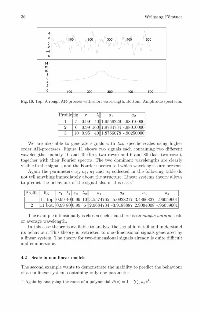
36 Wolfgang Forstner
–6–4–20
24
100 200 300 400 500
0
2468
101214
100 200 300 400 500
Fig. 10. Top: A rough AR-process with short wavelength. Bottom: Amplitude spectrum.
Profile fig. r λ a1 a2
1 5 0.99 40 1.9556229 -.980100002 6 0.99 160 1.9784734 -.980100003 10 0.95 40 1.8766078 -.90250000
We are also able to generate signals with two specific scales using higherorder AR-processes. Figure 11 shows two signals each containing two differentwavelengths, namely 10 and 40 (first two rows) and 6 and 80 (last two rows),together with their Fourier spectra. The two dominant wavelengths are clearlyvisible in the signals, and the Fourier spectra tell which wavelengths are present.
Again the parameters a1, a2, a3 and a4 collected in the following table donot tell anything immediately about the structure. Linear systems theory allowsto predict the behaviour of the signal also in this case.4
Profile fig. r1 λ1 r2 λ2 a1 a2 a3 a4
1 11 top 0.99 40 0.99 10 3.5574765 -5.0928217 3.4866827 -.960596012 11 bot. 0.99 80 0.99 6 2.9684734 -3.9188887 2.9094008 -.96059601
The example intensionally is chosen such that there is no unique natural scaleor average wavelength.
In this case theory is available to analyse the signal in detail and understandits behaviour. This theory is restricted to one-dimensional signals generated bya linear system. The theory for two-dimensional signals already is quite difficultand cumbersome.
4.2 Scale in non-linear models
The second example wants to demonstrate the inability to predict the behaviourof a nonlinear system, containing only one parameter.
4 Again by analysing the roots of a polynomial P (z) = 1 −∑k akzk.

Notions of Scale in Geosciences 37
–60–40–20
0
2040
100 200 300 400 500
0
5
10
15
20
100 200 300 400 500
–20
–100
10
20
100 200 300 400 500
0
2468
101214
100 200 300 400 500
Fig. 11. Two profiles, each with two wavelengths and their theoretical Fourier spectrum
The well known logistic map Kneubuhl 1995
xk = a xk−1(1 − xk−1)
is fully deterministic. It shows all types of behaviour, fixed points, periodic se-quences as well as chaotic i. e. non predictable sequences for a > 3.5699 . . . (cf.figure 12). Though this sequence is well studied it has the flavour of non linearsystems which need to be studied individually and only in special cases allowprediction of their behaviour without simulation studies. This is in contrast toone-dimensional linear systems, which are theoretically fully understood.
The examples of this section give a clear message: In case the system can beadequately modelled as a linear system, one should exploit the power of linearsystems theory. This especially holds, if reality is modelled phenomenologicallyor only simple linear physical laws are involved. Even in case the approximationis crude, it helps making predictions. However, all real systems are likely to benonlinear, which makes the theory based definition of a scale very difficult.

38 Wolfgang Forstner
Fig. 12. Sequences of the logistic map with a = 1, 2.5, 2.8, 3.1, 3.4, 3.5, 3.6 and 3.7
4.3 Omni-scale models
Real data often show no dominant scale, i. e. one dominant wavelength. Theyoften show a continuum of wavelengths, i. e. the height z(x) is composed of sinewaves of all frequencies:
z(x) =∑
k
hk sin(kx + pk)
where the phases pk and especially the amplitudes hk depend on the frequency.Terrain data have been analysed by Mandelbrot 1980. In case of terrain pro-
files Frederiksen et al. 1985 often found a linear dependency
log hk = c− α log k
between the logarithmic amplitude hk and the logarithmic frequency k. Thusoften all frequencies are present in terrain profiles, there is no specific wavelengthor scale in the data.
The slope α is large for smooth terrain, e. g. in the range of α ≈ 2.5, theslope is small for rough terrain, e. g. in the range α ≈ 2 or less.
5 Conclusions and Outlook
The paper discussed the various notions of scale resulting from the diversity ofthe disciplines within the geosciences. They refer to data and to models andappear in several degrees of crispness.
There seem to be basically two different crisp types of notions of scale in use:
1. scale as the ratio between model and reality. The only application of thisnotion is the scale in map scale.

Notions of Scale in Geosciences 39
2. scale as a measure of the extent of an object on space or time. This holdsfor nearly all notions, quantitative and qualitative.
The other notions qualitatively refer to the size of the data set in concern. Thereare quite some close relations between the crisp notions of scale, all referring insome way to linear systems theory. Their use definitely is promising and helpsgetting a first insight into geoprocesses.
In contrast to this coherence, however, there are only few crisp relationsbetween the more qualitative notions, which hinders a smooth communication.Taking the complexity of geoprocesses into account one needs to discuss howfar a crisp notion of scale actually carries research and at which steps withinmodeling more detailed concepts need to support the description of the inherentstructure of natural processes. These concepts definitely refer to the used quali-tative notions of scale in some way, but they certainly will be more adequate.
References
Box, G.E. P.; Jenkins, G.M. (1976): Time Series Analysis. Holden-Day, 1976.Castleman, K.R. (1996): Digital Image Processing. Prentice Hall Inc., 1996.Frederiksen, P.; Jacobi, 0.; Kubik, K. (1985): A Review of Current Trends in Terrain
Modelling. ITC Journal, 1985-2, pp. 101–106.Kneubuhl, F. (1995): Lineare und nichtlineare Schwingungen und Wellen. Teubner
Studienbucher Physik. Teubner, 1995.Lucker, R. (1980): Grundlagen Digitaler Filter. Springer, 1980.Mandelbrot, B. (1982): The Fractal Geometry of Nature. Freeman and C., San Fran-
cisco, 1982.Ryan, T.W.; Gray, R.T.; Hunt, B. R. (1980): Prediction of Correlation Errors in Stere-
opair Images. Optical Engineering, 1980.Samet, H. (1989): The design and Analysis of Spatial Data Structures. Addison-Wesley,
Reading, Mass., 1989.Siehl, A. (1993): Interaktive geometrische Modellierung geologischer Flachen und
Korper. Die Geowissenschaften, 11(10-11):342–346, 1993.Snyder, J. P. (1987): Map Projections – A Working Manual. US Government Printing
Office, Wash., 1987.Tissot, A. (1881): Memoire sur la Representation des Surfaces et les Projections des
Cartes Geographiques. Gauthier-Villars, Paris, 1881.

Complexity of Change and the Scale Concept in EarthSystem Modelling
Horst J. Neugebauer
Section Geodynamics, Geological Institute, University of Bonn, Germany
Abstract. The concept of scales is based on the spatial perception ofphenomena. It is rather appropriate to address and to analyse the com-posite nature of phenomena. Consequently scales will be utilised as wellfor comparing various strategies of conceptual modelling, such as em-pirical analogues, effectual objects and relational states. This discussionbecomes illustrated by means of an adaptable example and the corre-sponding scaling behaviour. Finally the statistical analysis of scales re-veals both the limitations of phenomena and their fundamental potentialfor change. The universal nature of change becomes evident only throughan extended perspective which is comprehending small and large-scaleproperties assigned to the common representative scales.
1 Nature Survey
Modelling is a principal process to access phenomena in nature. This becomesevident as soon as we reflect the various attempts of gaining knowledge aboutnatural phenomena and from the consideration of their equivalence as well astheir limited continuance. Those attempts reflect our concern with nature likean early orientation through semantic classification, the recognition of specificprinciples and their application for practical use, up to the desire for a predictionof risks and future developments of natural systems. It is a common and wellknown experience that in any case of specification or observation we rely on somekind of concept, an idea, view or reminiscence on some practical experience tobegin with. That means however, whatever we sense, address or practise withrespect to nature will implicitly reflect an adjacent and complementary contextas well; it is like a specific image we take from reality; this represents a merelysubtle distinction or a limited experience. Modelling has thus to do with defining,describing and comparing objects with respect to some part of the context.Therefore we are relying on an universal but concealed principle of measuring,our perception of space. The situation becomes quite simply illustrated by thephenomenon of a fault. It is an obvious example, which can be representedmost strictly by the relative spatial displacement of sites. It is a fundamentalconvenience and of great practical use, dealing with distinguished objects insteadof a non-distinguished net of potential relations. Therefore, in practice we usuallydiscern the separated natural context of the addressed phenomena while we [email protected]
H.J. Neugebauer and C. Simmer (Eds): LNES 97, pp. 41–63, 2003.
c© Springer-Verlag Berlin Heidelberg 2003

42 Horst J. Neugebauer
follow ideas, express ourselves in semantic terms, using graphs or performingsome direct action. Although we denote objects by fixed conventional terms, ourpersonal associations are not unique at all among us. In science we thus followconventions for reproducible measurements and the use of comparable standardsof analysis. Further on we developed alternative theories for the representationof phenomena, like for instance, the equivalent concepts of waves and particlesin physics or waves and rays in seismology, which both lead to sound results, yetrepresenting a variety of experience and perspectives with matter and energy.Last but not least, we may meet the detached context of objects again throughmany unexpected re-actions to our mental or implemented concepts. Natureis responding seldom straight and linear, but mostly rather unexpected andoblique. In this sense our technologies touch more and more the unknown contextand become thus less a consequence of science but increasingly a reinforcingpromoter for targets of modern sciences.
Our concern will therefore be at first to trace back the boundaries of con-ventional objects to their phenomenology to some extend. Spatial scales serveas a profound and powerful tool for that purpose. They should help to identifythe “condensed experience” against the complementary context of natural phe-nomena. Scales are simply geometrical sizes or measures, such as length, area,volume or other properties attributable to them. They will be used successfullyto analyse the interdependency among phenomena. For this purpose it shouldbe sufficient to follow our well known attempts in Earth science. Clearly, theconsideration of objects through the perspective of the discrimination from theirdedicated context causes important consequences: For any phenomenon we findboth, an associated inner context and the indicated outer context. While theinner context for instance is leading to the characteristic properties, the qualityof the object; the outer one will be identified by its functioning and consequentlyby its possible physical origin. Under this perspective we become interested fur-ther into the mental and sensual motivation which might lead to the statementof a phenomenon. Usually a systematic comparison drawn from a large pool ofobservations provide the characteristic criteria of similarity in order to specify aphenomenon. This resemblance within some basic particulars serves as a generalprinciple of spatial analogies under the signature of popular terms. The moti-vation for defining objects appears thus being already the most fundamentalconcept of modelling. Whenever phenomena are observed over sequential states,we meet the change of objects either in terms of a declining appearance or evenas a sequence of fluctuations on a lasting sequence of states. We might againeasily recognise, that considering the change of phenomena as denoted parts of aphenomenology appears to be another perspective of the principle of modellingand a model by itself. Models, respectively objects might thus come into exis-tence either in form of semantic terms, cartoons, a sequence of numbers or evena set of mathematical equations as well.
Dealing with natural phenomena through characterising their behaviour andspecific features, we face immediately the established views of scientific disci-plines. What seems therefore to be distinguished from each other appears rather

Complexity of Change and the Scale Concept in Earth System Modelling 43
as mere aspect or part of our perceived phenomenology. Empirical observationsand analogue experiments are as selective as for instance the so called exactrepresentation through a differential equation, or even the performance of a sta-tistical probability analysis. Every modelling approach has the target to attainan outermost knowledge about phenomena, to this extend we have some kind ofequivalence of methods. However, when we need to know information about thepossible predictability of processes in the future, for example the occurrence ofan earthquake or the potential for a landslide, neither the empirical knowledgenor the deterministic quantification can lead to a proper answer independently.Modelling the statistical probability for instance, requires the conceptual and dy-namical experiences as a precondition. For a better understanding of complexityof earth systems, we should therefore examine the different steps where we looseor even overlook information in our scientific approach of natural phenomena.So, discussing the purpose, the way and the implications of modelling, it will beof primary importance to reflect at first about an universal concept or measureto distinguish the complexity of pretended objects and their variability. Such afundamental tool are the spatial scales, the basic constituents of our perceptionof space. On the basis of the scale concept we might be able to compare modelconcepts among themselves and conclude on their final benefit.
2 Abstraction of Experience
The definition of phenomena appears to be the most fundamental procedureof modelling, the formation of semantic terms. Whenever we denote particularphenomena, the introduced names represent symbols of structures, features, setsand states or even changes which have been sensed or alternatively measured.Since science is deliberate to tighten the correspondence between symbols andtheir meaning, we finally reach a growing diversity of the disciplinary terminologywith even more specific symbols, codes and notions. Our first modelling aspectthus concerns the principle of accumulating “evidence” for a certain phenomenonaround a typical dimension or scale. This procedure might concern a repeatedcomparison of observations, based on the correlation of distributed samples fromcorresponding stages of recurrent processes. This deduced basic quality of notionscan easily be recognised from such simple examples as clouds, creeks, faultsand others; each case resembles in some particulars between the correspondingobservations but remain otherwise unlike: The procedure of naming objects isthus based on obvious similarities and a terminology has therefore the quality ofanalogues. The entire definition is sized implicitly through our relative perceptionof space. We might share this experience now by means of an example, forinstance, the phenomenon and its terminus, fault.
The common sense of the concept is expressed by an original citation ofa dictionary of geological terms: A fault is a fracture or fracture zone alongwhich there has been displacement of sides relative to one another parallel tothe fracture. A closer look on the statement reveals instantly the two inherentand complementary characteristics representing a fault: an outer and an inner

44 Horst J. Neugebauer
layer model of large-scalemaster fault
fault on the referencescale of observance
small-scale structure ofclay smear and faultblock fragmentation
100 m
10 m
10 cm
Fig. 1. Fault structure on different levels of spatial resolution. Scale equivalent proper-ties cover an approximate range of five orders of magnitude.
context, which together build a reciprocal spatial relation, like that illustratedin Figure 1. The inner aspect of the notation fault is related to the fractureitself, especially the geometrical manifestation of small-scale fragmentation androughness as shown on the lower right side. Following the dictionary again, wedistinguish a horizontally striking fault line of a certain length and shape aswell as a corresponding vertically dipping fault plane as illustrated through thereference scale sketch in the central part of the cartoon. We recognise a seam-less conjunction to the outer context, which appears already in the scarp andthe aperture of the fracture. This outer context comprehends both material andgenetic aspects of a fault. Thereafter, displacements in the past accumulated amemory indicating a historical record, the large-scale mean offset combined withthe relative sense of movement as indicated on the upper right. These structuralfeatures reveal thus in terms of the relative positions of the sides the possibledisplacement modes like: vertically normal or thrust and horizontally strike-slip.Usually a fault is only an element of an even wider fault complex or a system asfor instance a fault basin. Here, associated sedimentary deposits might exposeanother sequence of marker significant for the tectonic history of the entire fault

Complexity of Change and the Scale Concept in Earth System Modelling 45
population. To this extend the terminus fault is a comprehension of addressedstructural features and physical qualities; in terms of the spatial reference ofthe terminology to associated scales, it is the merge of a selected hierarchicalinner and outer context. With this respect, the term fault denotes already acomplex semantic model or analogue of a considerably variable extent. For ourconsideration however, it seams still more expedient to intensify the aspect ofrepresentative spatial scales of objects into this discussion. We assumed for in-stance, that the mentioned features correspond approximately to about fourorders of magnitude in their geometrical dimension of space. However, our expe-rience shows an additional multitude of phenomena on respectively even smallerand larger scales associated with the definition of a fault and thus in extensionto the introduced inner and outer context. So the fault is an entire concept,which is part of an external mechanical environment and the equivalent tectonicframe up to the dimension of the earth crust on a global scale. Yet, on theother end of smaller scales we have an extension of the fracture system throughparticular fault segments over the roughness of the fracture surface down to asignificant concentration of micro-cracks and crystalline dislocations beneath thesurface of the respective fault blocks. With respect to the associated scales ofthe phenomenology, we deal with an entire hierarchy related with the conceptof a fault. Further on, we find the originally addressed phenomenon fault beingan inherent part of an entire phenomenology, in the sense of a linked networkaround a reference scale of observance without obvious limitations within adja-cent scales. Against this background of relations, i. e. the frame of complexity,any limitation of the phenomenology is selective, has restricted competence andis thus non-unique. However, it will illustrate the basic operation of modellingas a conceptual processing of experience within the spatial frame of percep-tion. Modelling means therefore the condensation of our experience either in thelimited analogue of semantic terms, as mentioned before. Or alternatively estab-lishing a limited relationship between particular phenomena in order to developa conceptual model based on their reciprocal dependence, like for instance amathematical balance. Such conceptual models typically result from empiricalcorrelation of repeated sequences of observations, from theoretical considerationsor, especially in Earth science, from analogue experiments in the laboratory.
A conceptual model, such as our example of a fault in Figure 1, is buildaround a predominant reference scale of the manifestation, which is usually rep-resenting the characteristics of observance. While the corresponding phenomenol-ogy, the inner and outer context of the primary fault approach remains more orless unattended, i. e., it depends mainly on the chance for an acquisition of ad-ditional information or related ideas. So, how are we arranging ourselves withthis peculiar situation, the need of deciding on appropriate bounds for the def-inition of objects? Obviously, this question became rarely addressed explicitly,usually we rather ask: what are the implications and where do they come from?In a common sense we escape instead towards the limitations of the causalityprinciple. The implications are thus linked with parts of the implied inner con-text, while causation partly replaces elements of the outer context. Therefore

46 Horst J. Neugebauer
small-scale phenomena are shrunk down to mere attributes expressed either inqualitative notions or as quantitative averages. The large-scale context however,is usually addressed being equivalent to the ultimate causation of a phenomenon,either through reasoning or in terms of some specific determinant. All together,this is the procedure of “sense-making”, the making of an object, e. g. namedfault. Although there is a mutual consent about the essentials of an object, withthis procedure the scale problematic becomes concealed within the object prop-erties and the presumed causation; it is thus changing its significance. On thisfundamental level of approach, no demand is raised for an explicit integrationof scales, respectively up- or down-scaling of influence. Such a condensation ofthe phenomenology into a causal relationship of a conceptual model will on theother side allow only a weak appraisal of quality. Modelling on a conceptualsemantic level preponderates the purpose of representation and reconstructionrather than prediction. The latter requires even more specific confinements, aswe will discuss later on.
Another obstacle, that impedes progress of modelling experience in this cat-egory comes from the handling of time. Our every day experience of time isadjusted to an universal time in the sense of Newton. Time is associated withstandard cyclic changes as a scale unit as is generally known. Thereafter timeis the basic variable to trace ongoing changes of phenomena typically by corre-sponding time series. With reference to our complex example of a fault, absolutetime is missing, we only find structural evidence for the past changes in theentire context. However, those signatures are only characteristics in the senseof a relative chronological order, and there a multitude of signs appears, indi-cating changes all over the hierarchy of related phenomena and their assignedscales. This leaves us with the general question on the representative relevanceof historical time marker in order to decipher detailed changes during the geo-logical history. Although we might be able to distinguish between displacementsof fault-sections from the integrated record of change by the sediment deposits,any proper displacement time record however remains unidentifiable and anyconceptual approach appears finally to be non unique. Even for a most obviouscase of a fault, we are therefore left with a complex accumulation of interferingchanges on an entire zoo of spatial scales of the fault phenomenology. The pre-dominance of spatial information and the variance of scales leads usually to arather flexible practice of conceptual scientific cartoons
3 Consistency in Space
Let us now consequently look for some general aspects of conceptual modelling,in order to describe objects like our example of a fault quantitatively from variousperspectives. In the first case, we only make use of a perceptible characteristics,i. e., its obvious quality, which appears to be associated with its mere manifes-tation in space. Intuitively we related the term fault to a selected scale of theperceptible phenomenology. This seems to be equivalent with the qualitativechoice of an obvious scale of the system like that in Figure 1. With this speci-

Complexity of Change and the Scale Concept in Earth System Modelling 47
fication we consequently express the phenomenon quantitatively by means of aspatial reference system. Computer science provides suitable strategies for thosequantitative representations of generalised geo-objects. At that level of modellingour objects are completely represented by merely spatial elements, such as thetopological, metrical and geometrical characters of the phenomena. All are basicattributes and sufficient for a quantitative modelling of objects. The topologicalrelations such as the existence of a relative offset of the adjacent fault-blocksalong the fracture correspond to the category of a characteristic quality. Whilethe manifestation of the fault is expressed through a proper spatial measure,indicating the amount of relative displacement of fault blocks. In addition, theposition and the orientation of the particular fault in space, according to a geo-metrical reference system needs to be specified. Figure 2 gives a simple examplerepresenting a fault as a spatial object: the geometrical parameter representa-tion. The geometry of objects is composed by means of primitive solids and theircorresponding operations. The technical design of such representations followsnaturally operational aspects related to their use in optimised information sys-tems. Generally, the required operational aspects and the systematic storage ofthese object representations is supported by the narrow range of the geometricalinformation necessary and of course, the inherent principle of similarity betweenthe considered objects.
αlh
Fig. 2. Geometrical representation of a fault by the offset of fault-blocks in space.
The spatial abstraction of geo-objects serves frequently as a basic frame fornumerous considerations, interpretations and even speculations. Any of thesereasonings is equivalent with the immediate ascent of the context, respectivelythe multitude of scales involved. The idea to deduce a kind of a historical recordof displacements from a spatial fault pattern seems quite attractive. However,even so a limiting state for the beginning of fault displacements might be pro-posed, any reconstruction of some “time-record” in the sense of the historicaldisplacement process requires the knowledge of the entire record of the displace-ment rate. That means, we need to know the information on the change of thepassed displacements or that of the corresponding context throughout the his-tory. As this detailed record will usually not be available, any approach to an“inversion” of a represented spatial situation remains extremely unconstrained

48 Horst J. Neugebauer
and appears thus rather arbitrary. The only control we might be able to performis obviously a mere geometrical check up on the consistency of stages in space.Such a geometrically balanced reconstruction of an assemblage of displaced blocksneeds however additional information on physical and chemical changes and theredistribution of matter. We neither have a fair chance to invert the causes of thedisplacements associated with faulting quantitatively from the observed spatialrepresentation. Although we are usually dealing with a scale-limited pattern ofobservations, we are alternatively missing the entire scaling information of theformer dynamic regime of sequential faulting. This is not a general critique ofthe fundamental concept, but it rather reveals the limitations of the spatial ap-proach from a solid, quantitative viewpoint. We recognise that modelling changefrom the past on the spatial basis has only rather weak constraints on the com-plex relationship of faulting and its scaling behaviour. Thus an entire spectrumof experiences of statistical, experimental and observational nature are usuallyhypothetically attributed and associated to the geometrical approach. Causal re-lationships are therefore not yet comprehended within the spatial representationincluding topology and geometry.
4 Principles of Conservation
The fundamental, but rather restrictive spatial model concept became consider-ably improved through the incorporation of at least major aspects of causality.Only through the control of specific causes and their implications, which are bothparticular components of the previously addressed context, the spatial manifes-tation of a quality advances definitely to what we call an object. Whenever we liketo accomplish how, for example, the displacements along a fault evolve, we haveto exceed the spatial concept in many respects. Geometrically we will introducean outer bound of space in order to make a proper statement of the question.Physically fault blocks need to be characterised by their physical state and me-chanical properties, the shear zone itself by frictional parameters and others.However, it is most important to refer the model approach to a solid principle ofconstraints providing sufficient control on the calculated response of the objectto a specific causation at any state. That means, such unique conditions are forinstance met through an accurate conservation of matter, forces and energy dur-ing the entire process of displacement of the fault model throughout the wholesystem considered. This effort is still not generally acknowledged in Earth sci-ences. However, it marks clearly the transition between spatial description andinterpretation on one side and the opportunity for a quantitative approximationof the caused function of phenomena by means of a reproducible analogue onthe other side. Especially our abilities of approaching the responding functionof an object quantitatively reveal the state of knowledge, whenever prediction isrequired. Returning to our fault example, quantification of rupture formation,propagation and fault-slip are common. Seismology is specially interested in theradiation of elasto-dynamic deformation according to displacement or tractiondiscontinuities across an internal fault surface. Modelling requires thus a repre-

Complexity of Change and the Scale Concept in Earth System Modelling 49
sentative equivalent of a finite fault plane within an external space; the fault isrepresenting some predominant spatial scale of the system, like that indicatedin Figure 3. Deformed and crushed rocks of the fault gauge, shown in Figure 1,
Fig. 3. Body-force-equivalent of a representative source volume for slip-motion.
exhibiting the sub-scales of the fault zone and the possibility of heterogeneousdisplacements, are comprehended by an effective slip within a plane of zero thick-ness. Because the thickness of the apparent displacement discontinuity initiatingwaves is almost always far less than the wavelength of the recorded seismic radi-ation. In the same sense the rock adjoining the fault zone, corresponding to thesuperior scales of the system, is described by isotropic effective elastic constantsand an average density. The theoretical concept allows thus to state a constrainton the accelerations, body forces and traction or alternatively the displacements,acting throughout a representative volume, representing faulting. This approxi-mation determines the displacement at an arbitrary point in space and time interms of the quantities that originated the motion, the equivalent forces. Thislinks the abstract model approach with observable features imposed through thedynamics of faulting. According to the radiated seismic wave pattern, the sourceof fault-slip can even be replaced by body-force equivalents for discontinuitiesin traction and displacement within a reference volume. The requirements nec-essary for the equivalence of forces are quite remarkable and contradicting tocommon practice in tectonics. Representative forces are usually presumed as asingle couple of opposing components in the direction of fault-surface displace-ments, like indicated in the lower left of Figure 3. However, additional forces,single couples or linear combinations of these alternative extremes, directed nor-mally to the fault plane are necessary in order to meet a relevant equivalence to

50 Horst J. Neugebauer
fault-slip. It seems quite obvious now, modelling the response-function to fault-ing becomes a composition between the apparent spatial characteristics of a faultand the specific causation of slip by a dynamic source function. The design ofthe latter requires an incorporation of additional scales through the restrictionto a definite finite fault plane, respectively an equivalent volume and the con-sidered environment of the system. Herewith the object fault attains a morespecific, improved quality from the related physical properties and their symme-try. Finally, the modelled function of faulting becomes more or less determinedby the intensity and the time dependence of the specific source function. Thisis underlined by the expressed measure of fault-slip, which is called the seismicmoment. It is the product of the fault area, the average slip, and the shear mod-ulus. Even so this model concept is capable to quantify in particular dynamicfaulting and seismic wave radiation, there remains still the need to access sizeand frequency of faulting episodes through the course of time. This peculiarity ofthe phenomenology is however missing in a steady-state model of fault function.This comes from the particular bounds we introduced by defining an object. Aswe have seen earlier, it will only be possible on the cost of the context. Lookingfor a representation of faulting as a particular event in space and time, we needa revision of our modelling perspective towards a transient situation of an evenmore complex dynamic system.
5 Return of Context?
Can we find a suitable modification of our modelling concept, which allows tofollow faulting in a self-organising manner? As a sporadic appearance of limitedfault-slip in an even more complex system of continuous change? Seismologyand fracture mechanics indicate fluctuating areas of temporary fault-slip acrosslarger fault zones separated by quiet intervals. Those events of faulting mightthus be understood as specific states of ongoing changes in a complex system.The continuity of change has to be presumed to happen all over the hierarchy ofscales, particularly within the fault zone and its neighbourhood. The temporalvariation of the respective dimension of the active slip area can easiest be con-trolled by means of a model with a local scale approximation. This modellingconcept is appropriately visualised as an aggregate of slider blocks combinedthrough various spring elements, as shown in Figure 4. Herewith each blockwithin the model frame represents a local scale fraction of potential state offaulting. Every local slip in the system is relaxed, that means distributed withrespect to its local neighbourhood. The global driving force established on theupper boundary is opposing the frictional forces at the lower boundary, whichis supporting the individual blocks. Fault failure allowing local slip motion ofblocks is bound to a static or dynamical threshold, where shear stress exceeds acritical value. Principally one is repeating the balance of forces and their relax-ation according to the system properties for each interval of change. This canbe achieved either by means of a set of discrete differential equations or alter-natively using explicit rules for the local change, which are typical for cellular

Complexity of Change and the Scale Concept in Earth System Modelling 51
Fig. 4. Spring-block model for fluctuating fault-slip areas.
automata. The most essential and remarkable change in this modelling strategyis to assume, that the friction of an individual block recovers as soon as it comesto rest. That means, the opposing forces of external driving and internal fric-tional resistance become regenerated after each interval or iteration. The forcesbecome thus interactive. Opposite to the previous concept, the momentary lo-cal state of force balance is no longer predetermined entirely from outside; it israther evolving internally step by step for each block. The idea meets very wellthe observation of random obstacles to faulting like spatial roughness, dynami-cal friction or even long term chemical crystallisation and healing. The mutualinfluence between driving and frictional forces at the blocks in addition to thelocal relaxation rules as represented by springs and leaf springs, become thuscritical for the apparent scales of the temporal slip events. Hence, every localityis now not only conditional upon the forces and their neighbours, but even so acondition for them. These features together are essential for the appearance ofirregular fluctuations of slip motions over the entire model plane. That means,one of the forces is transcending the other temporarily on an respective area offluctuating spatial scales. Turning back to our previous general discussion of thecontext and its implication on the change of objects, we easily recognise now:quality and manifestation of faulting undergoes progressive change, while theinduced function becomes now an integral counterpart of the causation. To thisextent we have overcome our assumption about the permanence of objects; wefind the view of ongoing change of phenomena within their context more ap-propriate for a better understanding of our complex natural environment. Thecapability of this modelling concept appears primarily not of interest for a partic-ular case of faulting. Although we improved the relational context of modelling,practically we will not at all be able to access the required concurrent changesduring a specific tectonic situation sufficiently well. Nevertheless, the more pre-cise rendering of the coupled phenomenology through the local scale approachenables investigations corresponding to the long term organisation of change, forinstance in a complex fault system. We are placed into a position now, wherewe know about the fundamental background to reproduce the scaling behaviourof faulting. In particular we become able to ascertain the character of complex-ity from the statistics of modelled slip events; further on we might analyse therecurrence time of slip motion or study conditions for a spatial-temporal clus-

52 Horst J. Neugebauer
tering. This kind of modelling approach provides a rather new insight into therole of self-organising interaction. A key to access complexity is therefore thescaling behaviour of complex relational processes. The theory of a multiple-scaleapproach provides basic ideas of what complexity might be and how it shouldbe identified. An adequate analysis of proper observations could possibly reveala necessary appraisal of the concept.
6 Encounter Complexity
In order to distinguish between different concepts of modelling and quantifi-cation, we might finally introduce an even more systematic frame of referencefor the representation of phenomena compared to their context, i. e., their om-nipresent scale dependence. The attendance of the scientific community to adoptthe multiplicity of scale dependent constituents in the consideration of our men-tal and material phenomena seems not yet well established. Hence, the perfor-mance of modelling complexity is not necessarily compatible among disciplinesand mostly inadequate because of the different degrees of approximation prac-tised, as we have seen from the previous discussion. From our fault example inFigure 1, we kept in mind, that the entire hierarchy of associated scales is far frombeing merely an addition to an object. Scales are rather a measure equivalentto the complexity of phenomena and thus an integral part of our capacity com-prehending objects. In this sense they indicate substantial modifications in thedefinition or modelling of objects. Therefore a comparison of different modellingconcepts, their predictive abilities and implications becomes necessary. This canbe achieved by the use of only few universal categories for the characterisationof phenomena, with a flexible incorporation of the corresponding context. Whilethe context can still be taken equivalent to the addressed hierarchy of scales asbefore. Following our experience of similarity on different scale levels, we adopt aminimum of four conceptual modes or categories for the entire characterisation.They serve as defining devices for the degree of complexity of objects attachedby accretion such as our previously discussed example of a complex fault sce-nario. The four particular categories as well as their changing correspondencesare introduced and compiled in Figure 5. Hence, we separate describing objectsin three major classes with respect to the expressed degree of complexity of aphenomenon.
In order o distinguish a phenomenon from its natural environment in a mostfundamental manner, requires at least two, at the maximum four basic categories.Of prominent importance is the salient quality of a phenomenon, which meansits addressed characteristics. We might think here either of a single quality oreven a comprehensive set of qualities which remain the same in all its diversemanifestations considered. According to our fault example, the most prominentquality of a fault is the fracture, respectively a characteristic discontinuity of thematerial matrix. Associated with this characteristic is a potential performanceof a specific task or the possible achievement of a concrete goal, that means itspotential function. With respect to spatial and temporal aspects function might

Complexity of Change and the Scale Concept in Earth System Modelling 53
a
b
c
Fig. 5. Categories characterising modelling concepts: empirical analogues above, effec-tual objects in the middle and relational states below.
be a complete and spontaneous process, but equally well somehow distributedin space and successive in time. The function of a fault corresponds clearly toits potential performance of displacements along the fracture plane, which is inaccord with our previous definition. Thereafter we find both, the quality and thepotential function being fundamental for the third category, the manifestation,which is the way a phenomenon becomes evident in our spatial perception. Themanifestation reflects thus the present state of a characterised object, whateverdevelopment it might have passed before. Alternatively we might understand itas the comprehension of an entire record of past stages, including the presentmoment of observation. From the exposition of the fault in Figure 1 we rememberan entire set of spatial features of the fault structure. Together they comprise theachieved dislocation of blocks, representing the indicated manifestation. Finally,the function and the characteristics in association with the manifestation of aphenomenon provides the basis for any reasoning onto its probable causation.For our example, we might be able to derive some principal conditions uponthe probable causes of the dislocation from the relative mode of displacements.For instance, it means the relative spatial position of exemplary fault blocks

54 Horst J. Neugebauer
compared to the direction of gravitational body-forces. Our approach thus doesnot only comprise the formal definition of a fault, such as given above. It ratherextends the conceptual fault representation by a comprehension of the context onthe potential integration of various scales. Thus, the four categories demonstratetheir capacity for an extensive review of the entire correspondence, as we willdiscuss later on.
We have now established a quite elementary schema for our representation ofphenomena compared to their natural context on different levels of complexity.With a quality and its manifestation, we address a phenomenon spatially. Wefix some reference scale in space which is linked to a certain property. Throughthe association of a function and its specific causation, the hitherto spatial phe-nomenon becomes determined as an object, having an origin and implications.The objects becomes thus accomplished by certain bounds from the context,respectively their corresponding scales. So far any modelling procedure, eithersemantic, conceptual, experimental or quantitative, reproduces obviously a com-mon process of a conceptual defining of manifestations. This process not onlymeets the task of delimiting objects out of an extensive spectrum of internaland external conditions. But even so, we become confronted with the momen-tary character of the manifestations, that means with their potential for suddenchange. To account for fluctuating changes of objects, we have to overcome lin-ear determinism. Our perspective has to become reorganised with respect to thedegree of relative correspondence among the four categories. We have to acceptrelationship between causation and function both ways, forward and backward.This of course, will not be achievable without affecting quality and manifestationsimultaneously. Because of the transparency of correlation, the four categoriesare organising themselves. Objects become relational events of change. The in-troduction of the four corresponding categories is thus additionally exposing theneed to compensate the obvious loss of context by denoting objects somehow.Although the problem of complexity emerged from the discussion of the mul-tiplicity of scales assigned to a certain phenomenology, the schema of Figure 5comprehends even so the more general aspect of inner and outer contexts withrespect to the manifestation. From this point of equivalence, we might finallycompare easily a variety of three fundamental families of modelling conceptsqualitatively.
7 Competence of modelling
We will consider now the different traditional degrees of abstraction of phe-nomena: as spatial analogues, determined objects and temporary events. Forthis purpose we will make use of the four previous categories according to ourmental and practical experience. The first modelling family, as indicated in Fig-ure 5a, is rather dominated by the manifestation of a characteristic phenomenon,what we called a quality. While its particular function as well as the possiblecausation remain inherent or cryptic. This valuation of properties is emphasis-ing the empirical nature of the approach, which is based on the fundamental

Complexity of Change and the Scale Concept in Earth System Modelling 55
similarities of numerous examples and cases, we discussed before. The result isa deficient low level of differentiation of objects, because it is lacking definitiveconstraints from the context. Therefore the entire process leaves plenty of spacefor opinions and views, it is supporting a remaining indifference of the qualifiedphenomena. Consequently, we meet another obstacle with the historical develop-ment, accumulated in the manifestation. As discussed previously, time appearsonly as an inherent historical aspect. It can hardly be reconstructed from struc-tural features precisely; only fragmentary relation comes from assigned tracesof available past physical and chemical changes within the phenomenology. It isnot surprising , that under the historical aspect of time, the origination of man-ifestations and thus the appropriate course of the entire function remains ratherhypothetical. So any unwrapping of the historical record will be strongly depen-dent on the examination of additional models, the consistency of the availableinformation and the compatibility of the various sources. Basically this kind ofmodelling is thus solely adopting spatial information, selecting the major scales,as we learned from our example in the beginning. On the other hand, this entirecomplex spatial correspondence is a prevailing procedure for any further degreeof differentiation.
The forthcoming model family becomes determined through the expressedcharacter of the context, respectively the scales or properties addressed in addi-tion to the spatial aspect. A phenomenon becomes thus constituted as a scalelimited object through a specific correspondence between the typical functionin response to a specific causation, as symbolised in Figure 5b. The explicitrole of the causal relationship leads consequently towards a much more distin-guished but passive quality of the manifestation. i. e. the defined object. Theself-contained character of objects becomes effectuated through various sourceslike experiments, measurements and calculations. They are highly differentiatedfrom their environment and therefore obey only very specific and parameterisedinformation about their context. This procedure to configurate objects quantita-tively leads to a completely determined relationship. Hence the time aspect is nolonger a historical one. Time becomes reversed into a forward directed sequen-tial time in response to the causation. Herewith we exceed the transition fromthe former flexible concepts of spatial analogues towards the precepts for thefiguration of objects through a specific dynamical behaviour. We reach thus thepotential for a reproducible quantification of the causal relationship. The idea ofobjectivity claims an unique characteristics as far as possible, i. e. an object issupposed to reproduce the same response to the same prescribed source exactlyand independent of the moment of time. Obviously we have to pay for this de-sirable ideal of an universal characterisation. The consequences are unexpectedchanges of our objects due to the pretended exception from of the interactingconfining context. However, this step allows a linear quantitative representationfor well constraint conditions according to the limited characteristic spectrumof scales. Established laws for the conservation of mass, energy and momen-tum express this self-contained constraints for the consistency of the models.However, with this modelling concept in terms of definitive objects the above

56 Horst J. Neugebauer
obstacle becomes imposed. Although, we might be able to characterise objectsby calculating their response for a representative set of scales, we wont meet theexperienced sudden alterations of objects during time. Hence, on this level ofmodelling we clearly miss, how objects come into existence and why they dis-appear again. If we allow “unexpected changes” of our phenomena, i. e. changesindependent from the assumed causation, they will no longer be reproducedthrough the presented family of modelling. Too many scales with their links tothe system have been eliminated by the derivation of effective parameters andconstant averages.
Whenever we experience randomly fluctuating phenomena, we might easilyrecognise the limitations of the previous conceptual approach of objects. Al-though this approximation finds reasonable short term benefit in technology, itprincipally fails in the analysis of change. For instance, we do not find any apriori scale for rupture length on a fault or for the size of clouds during theirlife cycle, etc. Changing phenomena are presumably supported through an on-going interaction of related phenomena across an entire hierarchy of scales, whatwe called previously their conditional context. Consequently, the relative natureof those relational events require fundamentally different modelling techniques.They should comprehend the interdependency between major system variableson the basis of the constitutive relations among these components. In particularthe full interaction among each of the constituents, as indicated in Figure 5c,becomes necessary to succeed in reproducing changing properties, respectivelyscales. As indicated earlier, the correspondence of the four categories allowschange in the manner of self-organisation. Clearly, the diversity of variables hasto be accommodated quantitatively by suitable methods, which allow appropri-ate resolution of their spatial dimensions and their variability in time. While thisis necessary for every variable itself, the main focus of modelling becomes nowthe linkage between the variables and parameters of the system. Usually a spe-cific reproduced state of such a system, is indicated through a critical thresholdof one variable only. It is worthwhile to notice, that there are various successfultechniques approximating such coupled complex systems. Usually the rules ofinteraction with the respective neighbourhood are based on supporting grids,which are small compared to the scales of the commonly considered events.The entire schema is enclosed within the global frame of the model boundaryconditions, affecting the various states of the system. The most straight wayis the choice of a small resolution for the entire numerical schema. Wheneverwe have information on the scaling rules of certain phenomena, we might solvethe problem separated, using variable splitting or so called nesting-techniques.Not surprisingly, the understanding of time will change again with the degreeof complex coupling. While we leave behind the view of a particular dominatedresponse by a causation, the change of the complex system becomes considerablylimited to the very moment of stepwise interaction. As change occurs locally atevery supporting point, the coupled system has the ability of spontaneous vari-ation on an arbitrary size. In the limit, “time” shrinks just to the length of aninterval of change in the deterministic sense. The basic approach to complexity

Complexity of Change and the Scale Concept in Earth System Modelling 57
leads thus towards a pattern of conditions, which originates phenomena as tran-sient objects on a local and instantaneous supporting basis. This concept of arelative reality is clearly opposing the previous view of the function of stationaryobjects. Now the texture of phenomena appears through and through relational.Consequently, the presented correspondence of the categories holds generally forevery local sampling point and its vicinity, thus the schema, presented in Fig-ure 5c, resembles symbolically the entire global concept equally well. The salientfeatures we accomplished with this concept are obviously the internal degrees offreedom, organising changes of the system through the interaction among the re-spective categories. Especially the scales of the modelled states of the system areno longer predetermined and the prediction of change attains a fundamentallynew quality now.
8 Statistics of Scales
Finally we found that scales are generally relative features which have to dowith our relative perception of space. So far we have identified scales with arepresentative linear measure of the spatial manifestations of a certain qual-ity or even with a temporary state of an entire phenomenology. On the otherside, modelling revealed that change of phenomena requires the peculiarity of acomplex conditional relationship to become generated. From this viewpoint wemay conclude the statistical signature of change being equally well indicative forthe mere quality addressed by scales and the assignable complexity of the phe-nomenology. Therefore a statistical analysis of scales might give more evidenceabout the nature of change. However, as there is not a thing in nature supposedto be without change, our knowledge about change becomes critically dependingon the model concepts we adopted earlier for its exploitation.
Geological structures are, for instance, fully packed with hierarchies of scales.These structures are indicating a historical record of properties from changes inthe past. Yet, we are not able to decipher those scales reliably without a con-sistent model concept, respectively some significant statistical scaling laws. Inthe absence of physically sound concepts a compilation of data is the only wayforward to evaluate their statistical significance. A first step in the direction ofa kind of trustworthy link between observed properties and their alleged originis the interpretation through regular change. It corresponds to the representa-tion of phenomena according to the causal model concept, shown in Figure 5b.Somehow we are used to the concept of steady objects, which are specified spa-tially and through their conceivable function in response to a specific causationas described earlier. This concept leads to characteristic scaling laws. In terms ofstatistics, a rather constraint distribution of scales appear to be representativefor those objects. As the generated phenomena are presumed to be dominateddirectly by specific causes, they will respond within a limited range of proper-ties only. We found earlier the reaction being predetermined through selectivelimitations of the object design. This is most frequently the case for experi-mental testing devices in the laboratory or with our practical applications in

58 Horst J. Neugebauer
technology and their theoretical representations. Quantitatively the spectrumof scales is completely determined by the presumed constant parameters of thecorresponding differential equations. The assigned phenomena are thus indicatedstatistically as scale-dependent. Under the addressed relationship between spe-cific causes and consequences the function of objects appears predictable withinthe limits of the restricted concept, e. g. as long as the variability of the naturalsystem parameters remains negligible compared to the determined one. We callthat the presumable existence of characteristic or representative scales, such aslength, size or volume. Following this perspective, we will expect that any typicalstatistical scaling law of analysed properties is thus reflecting a mean value andpossibly an assigned limiting variance. The normal or lognormal probability dis-tribution of frequencies is a very prominent scale-limited law beside others, forinstance, the exponential distribution. The range of sampled properties shouldat least cover more than one order of magnitude, as evident from Figure 6.Otherwise one would not be able to distinguish noticeably between differentdistribution functions.
Fig. 6. Statistical distribution functions in logarithmic representation. Indication of anextraordinary sample property or scale size by star symbol.
Especially in Earth science our attention becomes progressively extended to-wards the perspective of irregular change as already demonstrated. When changeoccurs more or less unexpected, we search for both the significance of irregulari-ties in the analysis of apparent scales as well as for the concomitant constituentsof a system, allowing instantaneous mutability. Thus we are running straight intoan omnipresent paradigm, called complexity or even more precise for our discus-sion: geo-complexity. Our previous sections on the third model category indicatedalready, that sudden change is most likely embedded within a complex processof permanent change. Therefore we have concluded that continuously changingsystems need to be supported by at least more than a single causal condition.This led finally to the expectation, that irregular fluctuating phenomena are

Complexity of Change and the Scale Concept in Earth System Modelling 59
backed up by a communicating system of interfering conditions, which clearlyin turn set up the reasons for an enhanced spectrum of scales. Like the spatialnature of scales itself, the analysed phenomena are frequently indicated by onlya single variable or property associated with a pretended critical threshold. Thusignoring the latent complexity of conditions may consequently lead to the falseimpression of sudden changes. In this sense, scales are mostly quantities, whichcomprehend varying properties of particular complex systems on a distinct level.For example, scaling fault slip, the statistical property of the slip-area is definedby a fixed threshold criterion compared to many small-scale details of distributedlocal slip across this area. As we are not able to reveal the multiple-scale na-ture from a single event of change, we make use of an equivalence we addressedalready in the beginning. We sample the sequence of fluctuating changes of a spe-cific system instead of the non-accessible complexity of single object. Thereforewe postulate implicitly the equivalence among the conditional relations, i. e., thenetwork of processes required to generate a certain quality temporarily. Alongthis line of equivalence the statistical analysis of representative scale samplesappears to be synonymous for the complexity of the generating system.
Numerous statistical studies at various scales and properties and in differentearth systems have shown that their probability distribution clearly follows thepower law. This forms a straight line for a logarithmic scaling of both axis, asshown in Figure 6. The power law distribution of scales is equally well repro-duced from the statistics of slip-areas through the simulations of the slider-blockmodel, given in Figure 4. Opposite to the scale-related distribution functions,the power law has the important implication, that there is no indication of anycharacteristic or representative scale, state or property, like length, size or areaof displacement. Therefore it is called a scale-invariant or fractal distribution.The main distinctive characterisation comes from its exponent, which is a mea-sure for the slope and corresponds to a fractal dimension. Yet, with respect toour limiting perception of space the power laws have to be limited as well byphysical length scales that form the upper and lower bound to the scale range ofobservation. Therefore, it has been appreciated that resolution effects imposedon the power law properties can be rather misleading and result in a lognormaldistribution. Alternatively, fractures with scales smaller than the distributionmode are probably insufficiently sampled and large-scale samples might not beidentified consistently or within the particular sampling period. Although thefit of those two opposing statistical scaling-laws, shown in Figure 6, to sampleddata sets is sometimes ambiguous, they yet merge the limiting members of typ-ical references of the scaling concepts in Earth sciences: the characterisation ofrepresentative objects contrary to fluctuating random change.
9 How is Change Organised?
Following the two distinguished types of statistical scale distribution, as de-noted in Figure 6, we will finally consider the characteristics of change. For anormal distribution and the spatial aspect of scales, change is organised around a

60 Horst J. Neugebauer
mean size with a drastic deficiency of both smaller and larger sizes. That wouldobviously imply that objects such as the water level of rivers, the amount offalling rain, the length of a fault and a river or the thickness of sediment lay-ers definitely obey an average size statistically. Any deviation from the averageis grouped around that mean size according a limiting variance with a rapidlydecaying probability of smaller and larger dimensions. Focusing our attentiononto the average, we are supposing a phenomenon being more or less on thataverage or just normal. Smaller changes will not question the rule by their as-sumed insignificance and larger changes are denoted exceptional, what we calldisaster, yet they are believed to “prove the rule of averages”. So far statisticsis expressing our normal perspective, equivalent to the existence of representa-tive scales, volumes or objects. Reviewing the statistical normal distribution interms of the phenomenological context, we might become afflicted by doubts.We “made objects”, first through the picking of a quality around a certain scaleand second by adding an explanation in terms of a limited context through arestricted causation and function, as demonstrated in Figure 5. That means weperform this design procedure ourselves, through our restricting perception andour relational comprehension of space. On the other side our daily practical ex-perience with the sustainability of objects raises doubts as well. Usually we failin both the prediction and management of change, especially of the extremeswhich are exceeding our representative scales. Interested in a possible reasonfor this insufficient appreciation of change, we may find the limitations of ourprevious experience to be accountable. Our previous experience is consecutivelylimiting existing and new limitations, respectively objects guided and driventhrough specific motivations. Limitations of experience are thus driving men-tally an ongoing loop of refining and reappearance of phenomena accompaniedby the reluctance against change.
Our understanding of normality of objects might benefit from the resort toan even more advanced normality, that of change expressed by the power law.As extended scale statistics of many observations and models on change, such asearthquakes, river networks, landslides and many others follow the power law,we must accept the non-appearance of any reference scale, size or volume. Fromthe viewpoint of phenomena, the characteristic scales are lost now in favour ofan upper and lower spatial bound of qualities expressible by scales, as indicatedin Figure 6. This range, respectively hierarchy of scales might more or less beingrelated to the limits of a phenomenology. What remains is just change, randomchange within the spatial bounds which are defined through the respective powerindex of the distribution function. However, according to the power law distri-bution function change varies generally both ways up to infinity; between aninfinitely increasing frequency approaching smaller scales and a decreasing fre-quency for scales approaching infinite size without any further preference. Thismeans in a fractal sense, the number of smaller scales necessary to substitutelarger ones and vice versa follows exactly the power law distribution. Becauseof this equivalence of scales among one another, their invariance, scales and inparticular change find no other universally addressable allocation than a random

Complexity of Change and the Scale Concept in Earth System Modelling 61
variability. Generally one may conclude now that we experience just space bymeans of our limited phenomena. From the power law we find space tending tobe infinite for both vanishing probabilities of increasing size as well as for a mostprobable increasing number of decreasing scales. This unconstrained equivalenceprovides the basis for the permanence of change of any composite properties inspace. Phenomena are thus of no real significance, they appear non-specific andrelational, they have neither a permanent existence nor an individual entity.Their design has been performed rather arbitrarily by means of a limiting ex-perience through the mind. This perspective together with the infinite natureof space, allows the range of imaginable experience to become unrestricted orinfinite as well. Change is thus universal. It appears to be assigned to any ofour finite scale selections, it is occurring permanently and randomly. This is af-fecting the idea of an objective reality fundamentally. As discussed earlier, scaledependence corresponds to very accentuated states.
Surveying these qualities now from a more universal viewpoint by comparingpower law and normal distribution function, as visible from Figure 6, the loss ofproperties through defining objects against their context becomes even evidentstatistically. Especially the share of smaller scales is drastically reduced, whilethat of larger ones is shrinking as well. Objects appear thus clearly effectuatedthrough both the detachment from the universe of attributable scales and theadditional accentuation of the mean reference scales. Sampling of a complexsystem with fluctuating change meets in fact the qualities of a power law, butremains still finite compared to infinity of space. The supposed predictability bothbased on established representative scales and of our complex systems remains ineither case an illusion. Objective views fail as soon as the representative rangeof scales becomes lost. Let us, for instance, take a look on a global fracturesystem such as the split-up of lithosphere forming the entire Atlantic ocean. Onthis global scale we will not et all being able to pick the tremendous number ofstatistically equivalent small-scale fractures down to the order of crystal-scalefissures and dislocations. In between we will fall into nearly any trap animatedthrough limited “representative” fracture formations and limited scale-consistentpattern. From a particular statistical analysis of complex phenomena, such asfor example the observed size of fault-slip, water levels or land-slides, we canprincipally even not exclude extreme events trustworthy, as demonstrated inFigure 6. Those catastrophic samples, far right, might meet our distribution on amuch lower probability level which we have never experienced before. As powerlaw distributions are met via both samples and simulations, we might finallyaccept the limitations of our approach and try to adopt the valuable clues frommodelling.
In terms of analysing self-organising systems statistically, the power law dis-tribution function was associated with the favoured state of self-organising crit-icality. This critical condition has been found to be even a preferred state ofearth systems compared with the sub-critical range of scale-dependent objectsand the super-critical field of unrestricted random change, whenever the ap-propriate modelling rules for complexity are met. We might be interested in

62 Horst J. Neugebauer
the specific circumstances for this kind of universal preference of scale-invariantchanges. What makes it so attractive? Most likely, is seams now to be only amatter of diverging viewpoints between objective reality and permanent change.Therefore let us accomplish a little experiment together in our mind. Imagine,we like to move a huge sphere made of wet clay across a landscape, which is span-gled with little crater-shaped pits and terraces of different depth and diameter.Only with the ultimate concentration of our strength we start to move the spheretoward the aimed straight direction. We push the sphere to overcome friction,the variation of its shape and the local roughness of the ground, passing step bystep one obstacle after the other. Up and on, we even do need technical tools inorder to assist our action of going properly straight. So far, the entire process isextremely exhausting and there is nothing attractive with this kind of slavery.Let us now, during a break, take notice of a rather moderately sweeping slope inthe landscape. Forsaking the burden of going straight, we find the small share ofsupport through the slope just sufficient to keep the sphere on the move. Only atiny supporting push is required to surmount the most extreme obstacles. Thusthe sphere starts immediately to find the ultimate solution for the move itself,while the entire network of conditions become integrated. Local and regionalslopes, the ground friction, the internal mass distribution as well as the deform-ing surface of the sphere and finally our repeated slight pushing work smoothlytogether. Actually, the movement becomes self-organising in accomplishing thechanging conditions instantaneously. The scaling distribution is expanding. Theparticular effort moving the sphere becomes remarkably low now, yet the processof motion through the landscape and the changing shape of the sphere appearsno longer conceivable. The record of movements will follow a fractal distribution.It seems quite obvious, changes of the position are most attractive for a systemwhenever they are the identical expression of the entire complex relationshipof conditions. From that point of view on change, the endeavour for a straightand clearly defined path, respectively the compulsive objective position, appearsrather disproportionate. Therefore the object-centred view in conjunction withthe statistics of scales appears again to be rather deliberate and exceptional.
10 A Dilemma of Change?
Obviously, sooner or later our effort in characterising and representing phenom-ena becomes overwhelmed from random change. The progression of change obeysnot any preferred quality or assigned spatial scale-selection. But, how can we getaccustomed to the experience of universal change? Unfortunately our own in-tention with sense based objects is rather conservative. Even the use of a modelconcept for complexity and fluctuating change keeps us depending on the de-nomination of specific phenomena. Denoted once, we experience them again andagain in an unpredictable sequence of size and frequency. Our vital interestsinto prediction are in return motivated through specific concepts, such as dis-ciplinary, scientifically, economical or even political aims. Change, however, isindependent from any experience used for its investigation. It is like any of the

Complexity of Change and the Scale Concept in Earth System Modelling 63
fractal spatial subdivisions of the infinite space appear equivalent to another,there is nothing compulsory but rather equivalence. Statistics reveals that fromboth a simultaneous and a sequential sense of scale analysis. How can we ben-efit from the omnipresence of complexity scientifically? From a viewpoint ofchange the inconvenience with objects is that they are in general changeable,non-reliable and non-predictable. We will thus not escape from change throughraising bounds, how narrow they might ever be drawn. However, we found theconditional relations being critical for change. When phenomena are thus notindependent among each other and neither independent from our conceptualperspectives, we finally might start to question our own concepts. We may find,for example, the investigation of interaction and change more important thanhitherto. Under the view of complex change, we may finally feel more confidentthat any of our intentions become reflected, unforeseen through a network ofconditional relations. Our favour for management and sustainability may raisea complete change of our thinking against the background of random change.Amazing enough, we started out surveying nature and are now demanding ourown responsibility. Complexity is thus primarily a question of perceiving nature.

Wavelet Analysis of Geoscientific Data
Thomas Gerstner1, Hans-Peter Helfrich2, and Angela Kunoth1
1 Institute for Applied Mathematics, University of Bonn, Germany2 Mathematical Seminar of the Agricultural Faculty, University Bonn, Germany
Abstract. Wavelets have shown to be an indispensable tool for a scale–sensitive representation and analysis of spatial or temporal data. In thischapter we illustrate the basic mathematical background for wavelets aswell as fast algorithms for multivariate wavelet constructions on boundeddomains. Finally, we will show an application of wavelets to analysis andcompression of precipitation data.
1 Introduction
Ever since the first application of wavelet transforms in geophysics in Morletet al. (1982) for the analysis of seismic signals, there has been a vast amountof wavelet-related research, both on the theoretical as well as on the practicallevel. An extensive description of different activities in geophysics can be found inKumar and Foufoula-Georgiou (1997). The numerous applications cover not onlythe analysis and compression of all variants of signals and images but also thecomputation of solutions of partial differential equations for process simulation.These very different types of applications already indicate one of the specialfeatures of wavelets: the notion of wavelets does not describe a particular fixedobject but rather stands for variants of a concept which is adapted according tothe application at hand.
The underlying methodology may be sketched as follows. Many physical pro-cesses, signals or images, large amounts of data, or solutions of partial differentialequations are in fact objects (such as functions) living on different scales. Withthese scales one may associate meshes of different diameters or mesh sizes. Todescribe the objects mathematically, one needs appropriate representations ofthe object. In order to obtain such representations, most applications ask for
(A) scalability;(B) spatial locality.
Requirement (A) means that the representation is able to capture features ona coarse mesh as efficiently as on a fine mesh. Thus, the description of theobject should in principle allow for a multi-scale representation of the object.Requirement (B) indicates that local features of an object should only be realizedin a ‘spatial neighbourhood’. (A) and (B) together would allow for an efficient
H.J. Neugebauer and C. Simmer (Eds): LNES 97, pp. 69–88, 2003.
c© Springer-Verlag Berlin Heidelberg 2003

70 Thomas Gerstner, Hans-Peter Helfrich, Angela Kunoth
representation for the object. In addition, it ideally requires also only minimalstorage.
Different mathematical descriptions of an object may satisfy one or the otherof the two requirements. The concept of wavelets is that they provide in principlea methodology satisfying (A) and (B).
In order to specify these remarks, we mention two typical cases.Case 1: Fourier Analysis of DataModern experimental methods and measuring devices deliver a huge amount ofdata. In order to handle the data properly, an abstract data model is required.One purpose of the model is to make the data be retrievable in an efficientmanner.
One idea to do that is to assume a hierarchy and to develop a multi-scalerepresentation of the data. The classical procedure is to make a frequency anal-ysis of the data using the Fourier Theorem. In this way, one can decompose a(2π-periodic) function f of time t with limited energy into an integral (or a sum)of different signals, each of which gives a precisely defined frequency. That is, fis represented by a decomposition
f(t) =1√2π
∞∑j=−∞
cjeijt, (1)
with i =√−1, and where the coefficients cj are simply determined by
cj =1√2π
∫ π
−π
f(t) e−ijt dt. (2)
For example, in the case of temperature data which is sufficiently dense, theFourier model can very precisely exhibit seasonal and daily variations. All wavesωj that generate the signal are obtained by scaling the base wave ω(t) = exp(it),that is, one defines ωj(t) := ω(jt). However, in view of the above requirements,the Fourier model has very strong limitations. In the case of temperature data,the frequency space gives a clear picture of seasonal variations, but it does notshow sudden climatic changes such as those occurring during the passage of acold front. The reason is that the frequency synthesis is not localisable: eachfrequency spreads over all of the time axis. That is, the Fourier model satisfiesrequirement (A) but not (B). Apparently the reason is that the base wave ω isa function having global support, i. e., living on all of the (time) axis.
To overcome these restrictions, there have been various attempts to ‘localise’the Fourier transform, leading to what is known as the windowed Fourier trans-form.Case 2: Finite ElementsIn the numerical simulation of physical processes, one often needs to computean approximate solution of a partial differential equation. To this end, one canprescribe to the underlying domain where the process is to be modelled a meshof a uniform mesh size. Solving the equation then corresponds to approximat-ing the solution in terms of local piecewise polynomials, commonly called Finite

Wavelet Analysis of Geoscientific Data 71
Elements, which live on this mesh. Since these functions are usually locally sup-ported, an expansion of the solution in terms of these functions would satisfyrequirement (B). Of course, the finer the mesh is, the better one expects thesolution to be. If one only works with one grid of the same mesh size, this wouldmean that requirement (A) is not met. Working on a very fine grid, one wouldthen need a lot of time to solve the resulting systems of equations, and also muchstorage. This can be remedied by allowing for meshes of different sizes and FiniteElements living on them to represent the solution, thus, leading to a hierarchicalrepresentation of the solution.
Now the wavelet concept provides a methodology to overcome the prescribedlimitations and offers a systematic way for both a practical as well as a powerfulanalytical tool. In the following description of the main features, we focus firston the general principles, independent of a certain application. We will laterdescribe additional properties one can use for particular applications.
The concept is perhaps most conveniently described in terms of the multi-scale decomposition of a function f : R → R (which can, for instance, be asignal). The general idea is to split f into a sum of functions that are obtainedby scaling and shifting one basis function ψ. That is, in the abbreviation
ψj,k(t) := 2j/2 ψ(2jt− k), j, k ∈ Z, (3)
the index j stands for the level of resolution and k refers to the location ofthe function. In these terms, the function f is represented by a multi-resolutiondecomposition
f(t) =∞∑
j=−∞
∞∑k=−∞
djkψj,k(t) (4)
with wavelet coefficients djk. In this decomposition the first sum is taken over
the scales from the coarse to the finer scales and the second sum is taken overall locations. As in the case of a Fourier series all functions ψj,k used in therepresentation are derived from one function, the mother wavelet ψ. In order toachieve localisation in time, besides the decomposition given by the outer sumin functions with varying oscillation speed, the inner sum gives a decompositionwith different localisations. Thus, one can view j as the scaling parameter orthe stage which replaces the frequency or the frequency band in the Fouriersynthesis and k as the localisation parameter. The waves ωj(t) = exp(ijt) in theFourier expansion (1) are here replaced by ‘generalised’ waves ψj,k which havean additional index k representing the location. It is this analogy which givesthe collection of all ψj,k the terminology wavelets.
The important property of wavelets that is used in different contexts is thatnot only an expansion (4) exists but that in addition a norm involving theexpansion coefficients controls the function norm. In mathematical terms, thismeans that the collection of ψj,k is a Riesz basis, that is, each f ∈ L2(R) (thespace of square Lebesgue integrable functions, or energy space) has a unique

72 Thomas Gerstner, Hans-Peter Helfrich, Angela Kunoth
decomposition (4) and
‖f‖2L2(R) ∼
∞∑j=−∞
∞∑k=−∞
|djk|2 (5)
holds independent of f . Here the relation a ∼ b means that a can be estimatedfrom above and below by a constant multiple of b. Recall that the Fourier ex-pansion of f also satisfies such a stability estimate with the equality sign. Thestability estimate implies that small disturbances of the function f result in smalldeviations in the coefficients and vice versa.
The mother wavelet should have properties that lead to a meaningful inter-pretation of the decomposition. A proper choice makes it possible to split thesignal recursively into a trend and a fluctuation. At each stage of the analysis,one may view the actual trend as the smooth part of the time series and theresidual or fluctuations as the rough part. One obtains a decomposition rangingfrom very smooth to very rough components. The most important cases are theones where the location effect can be most effective. In mathematical terms, thismeans that ψ has compact support, that is, ψ vanishes outside a fixed interval.Then each of the basis functions ψj,k in the decomposition (3) has compactsupport which is centred around 2jk with width proportional to 2−j . That is,for high values of j corresponding to a high scale, the functions ψj,k representhigh-frequency parts of the functions f . The easiest and for many years knownexample of wavelets are based on choosing ψ as the Haar wavelet, consisting ofpiecewise constants,
ψ(t) =
1, t ∈ [0, 1/2),−1, t ∈ [1/2, 1). (6)
However, since the Haar wavelets lack smoothness it does not very well repre-sent smooth functions. The triumphant march of wavelets through all sorts ofapplications then began in fact with the construction of smoother variants withcompact support which are also L2-orthogonal (see (10) below) in Daubechies(1987). In these cases, ψ is no longer a piecewise polynomial and even cannot bewritten explicitly as a function in closed form (which is actually never needed foranalysis or computation purposes). For a compactly supported ψ, the above de-composition (4) provides not only a decomposition into different frequencies butin addition a decomposition into different local contributions of the same oscil-lation speed. This property of the set ψj,k is commonly called time-frequencylocalisation.
The above concept is by no means restricted to time series. Similar consid-erations can be used to analyse spatial data. Consider elevation data that comefrom a measurement device with a very fine resolution. The data are influencedby the roughness of the ground and disturbances caused by the vegetation. Itis not possible to derive form parameters such as slope and curvature withoutsuitable generalisations that depend on the cartographic scale used in the rep-resentation of the data (compare also Chapter 1.3). Since it is not desirable tofix the scale once for all, we have to look for a suitable scaling procedure whereaccording to the actual scale small disturbances are smoothed out.

Wavelet Analysis of Geoscientific Data 73
In this section we will show by several model problems how wavelets can beused to analyse geophysical data. We will explain some simple algorithms thatcan be efficiently used for different classes of problems. But first we have tocollect a number of definitions and theoretical results on wavelets as an analysistool.
2 More on the Theory of Wavelets
Like in the Fourier case, there exists both a discrete and a continuous wavelettransform, depending on the type of application.
In order to describe the continuous wavelet transform first, consider for aparameter a = 0, a ∈ R, the family of functions
ψa : a = 0, a ∈ R
which are generated by dilation of ψ as
ψa(x) :=1√|a| ψ
(xa
).
For |a| > 1, the function is expanded, for |a| < 1 it is squeezed. Thus, a playsthe role of the (inverse) frequency 1/j in (1) and can therefore be viewed as ascale. In addition, one introduces a second parameter b denoting the location bywhich ψa can be translated. Thus, one considers the family of functions
ψa,b : a = 0, a, b ∈ R
where
ψa,b(x) :=1√|a| ψ
(x− b
a
).
The factor |a|−1/2 assures that all functions have the same norm. Now the Con-tinuous Wavelet Transform of a function f is an integral transformation of theform
(Wψf)(a, b) =∫
R
f(x)ψa,b(x) dx, (7)
in terms of the scale a and the location b. It is important to note that forf ∈ L2 and appropriately chosen ψ, the continuous wavelet transform (Wψf)is invertible. We later describe the requirements on ψ. The inverse continuouswavelet transform can be determined to be
f(x) =∫
R
∫R
(Wψf)(a, b)ψa,b(x) a−2 da db. (8)
The terminology continuous comes from the fact that a and b are real numbers.Applying the continuous wavelet transform to a function f , one obtains for eachpair of parameters a and b different information on f ; the information on the

74 Thomas Gerstner, Hans-Peter Helfrich, Angela Kunoth
scale being represented by a and different values of b measuring the signal atdifferent locations at this scale.
By the wavelet transform (7) the function f is analysed, whereas by theinverse wavelet transform (8) the function is synthesised from its wavelet trans-form. Consider the case of the Haar wavelet (6). For fixed a and b, the right handside of (7) gives the mean deviation of the function f from its mean value, thatis the fluctuation of the function, in the interval [b, b + a]. The reconstructionby the inverse wavelet transformation may be done by taking the limit of a sumwith the fluctuations as coefficients.
Of course, different choices of the mother wavelet ψ may well influence theoutcome of an analysis. It is for this flexibility that we spoke at the beginning ofthis section of a methodology rather than a fixed method. In order to guaranteerequirement (B), locality, a good choice of ψ is a function with compact supportor at least sufficiently fast decay. In addition, ψ should have zero mean or, moregenerally, ∫
R
tr ψ(t) dt = 0, r = 0, . . . , d− 1, (9)
where d is a natural number. In this case, one says that ψ has moment condi-tions up to order d. The moment conditions in fact require a certain oscillatorybehaviour of ψ, thus, the term ‘wavelet’ for describing a damped wave. Theamount of moment conditions plays an important role in the analysis. Indeed,the conditions (9) imply that ψ (and also all its scaled and shifted versions ψa,b)are orthogonal to all polynomials of degree d − 1. This implies that for suffi-ciently smooth f which is evaluated in a Taylor series, the continuous wavelettransform only depends on the d-th remainder of the Taylor series. The quantity(Wψf)(a, b) gives a measure of the oscillatory behaviour of the function f in avicinity of b whose size depends on a. Thus, for a → 0, one has (up to a constantfactor) (Wψf)(a, b) → f (d)(b). Moreover, higher moment conditions of ψ implya faster decay rate of (Wψf)(a, b) as |a| → ∞. This explains also why the Haarwavelet which only has moment conditions of order 1, i. e., only the mean valuevanishes, is often not the best choice.
Like in the Fourier case, the continuous integral transform is a useful tool fortheoretical purposes. For practically analysing signals, one resorts to the DiscreteWavelet Transform that corresponds to the transform (7) for discrete values ofa and b. In fact, it can be viewed as choosing for j ∈ Z, k ∈ Z the parameters asa = 2−j , b = ak and computing with the notation from (3) the expansion (4),
f(t) =∞∑
j=−∞
∞∑k=−∞
djkψj,k(t).
For many applications the most interesting case is when the coefficients can bedetermined as
djk =
∫R
f(t)ψj,k(t) dt. (10)

Wavelet Analysis of Geoscientific Data 75
This corresponds to L2-orthogonal or shortly orthogonal wavelets where the col-lection ψj,k satisfies the orthogonality conditions∫
R
ψj′,k′(t)ψj,k(t) dt = δjj′δkk′ , j, j′, k, k′ ∈ Z, (11)
where δ is the Kronecker symbol. Note that the coefficients determined by (10)have a form corresponding to that of the Fourier coefficients (2).
If f is known, one can theoretically determine its wavelet expansion (4) bycomputing all the coefficients dj
k. But even if the ψj,k are known explicitly, thiswould be much too expensive if one explicitly computed all integrals (10). In-stead one uses the Fast Wavelet Transform which is usually introduced througha Multi-resolution Analysis of L2(R). This is indeed also a way to constructwavelets with different properties.
2.1 Multi-resolution Analysis
The concept of Multi-resolution Analysis (Mallat 1989) based on Haar waveletsmay be introduced using a simple example as follows. Consider a function fwhich is piecewise constant on each of the intervals [2−1k, 2−1(k+1)] for integerk, see Figure 1. The function f can be additively decomposed into a functiong which is piecewise constant on the intervals [k, k + 1] for integer k and a‘remainder’ h. Thus, g would capture the ‘coarse’ part of f by averaging overtwo adjacent intervals and h the difference between f and g. Then f = g+h canbe considered as a two-scale decomposition of f , where g consists of piecewiseconstants with respect to the coarse scale j = 0 (that is, on intervals [k, k+1]) andf on a finer scale j = 1 (being piecewise constant on the intervals [2−1k, 2−1(k+1)]). Both functions f and g can be represented in terms of (scaled) translatesof the characteristic function φ(t) which equals 1 on [0, 1) and 0 elsewhere. Thatis, defining
φj,k(t) := 2j/2 φ(2jt− k), j, k ∈ Z, (12)
we can write f(t) =∑
k∈Zfkφ0,k(t) and g(t) =
∑k∈Z
gkφ1,k(t). In order to beable to use only one function φ to represent functions on different scales, it isimportant that φ(t) can be written as a linear combination of translates of scaledversions of φ on the next finer level. This means that there are some coefficientsa := amm∈Z such that one has a relation of the form
φj,k(t) =∑m∈Z
am−2k φj+1,m(t), j, k ∈ Z. (13)
This relation is often denoted as refinement equation for φ. For φ being thecharacteristic function, the coefficients are just a0 = a1 = 1√
2and a = 0 for all
other indices . The coefficient sequence a is called the mask of φ.For each j, translates of φj,k generate a space Vj ,
Vj =
v ∈ L2(R) : v(t) =
∑k∈Z
ckφj,k(t)
. (14)

76 Thomas Gerstner, Hans-Peter Helfrich, Angela Kunoth
0 1 2 3−1
−0.5
0
0.5
1
1.5
2
t
f(t)
0 1 2 3−1
−0.5
0
0.5
1
1.5
2
t
g(t)
0 1 2 3−1
−0.5
0
0.5
1
1.5
2
t
h(t)
Fig. 1. f ∈ V1 (top figure) is split into g ∈ V0 (bottom left) and h ∈ W0 (bottom right).
For φ chosen as the characteristic function, the space Vj consists of all functionswhich are piecewise constant on each interval [2−jk, 2−j(k + 1)], k ∈ Z. Becauseof the refinement relation (13), the spaces Vj are nested, i. e., Vj ⊂ Vj+1. Asthe resolution level j increases, the Vj become larger and in the limit j → ∞approximate L2(R). The set of all spaces Vjj∈Z which therefore satisfy
· · · ⊂ V−2 ⊂ V−1 ⊂ V0 ⊂ V1 ⊂ V2 ⊂ · · · ⊂ L2(R) (15)
is called a Multi-resolution Analysis of L2(R). Since the function φ plays a par-ticular role in this concept, it is called the generator of the multi-resolutionanalysis. Because φ satisfies the refinement relation (13), it is sometimes alsocalled refinement or scaling function.
So far the spaces Vj have been introduced from which f and g in Figure 1come from. Now the question arises how the function h representing the ‘detail’f − g can be represented. In terms of spaces, this can be described as follows.Because of the inclusion Vj ⊂ Vj+1, there exists an orthogonal complement of Vj
in Vj+1 that we denote by Wj . That is, Vj+1 can be decomposed into the directsum
Vj+1 = Vj ⊕Wj , (16)
where Vj contains the ‘low’ frequencies and Wj the ‘details’ or differences fromone resolution level j to the next finer resolution level j + 1. Repeating thisprocess, one ends up with an orthogonal decomposition of L2(R),
L2(R) =⊕j∈Z
Wj . (17)

Wavelet Analysis of Geoscientific Data 77
Finally, every function f ∈ L2(R) can be decomposed according to
f(t) =∑j∈Z
fj(t), fj ∈ Wj , (18)
where the part fj corresponds to the frequency j. As it turns out, the spaces Wj
are spanned by translates of the wavelets ψj,k defined in (3), i. e.,
Wj =
w ∈ L2(R) : w(t) =
∑k∈Z
dkψj,k(t)
. (19)
Since by (16) Wj ⊂ Vj+1, the wavelets ψj,k can also be represented by linearcombinations of the generator on level j + 1, i. e., for some coefficients b :=bmm∈Z one has a relation of the form
ψj,k(t) =∑m∈Z
bm−2k φj+1,m(t), j, k ∈ Z. (20)
The coefficients b are called the mask of the wavelet ψ.If the scaling functions φj,k are orthogonal on each level j, that is,∫
R
φj,k(t)φj,(t) dt = δk,, k, ∈ Z, (21)
one can show that the coefficients bk in (20) are indeed uniquely determined by
b = (−1)−1 a1−, (22)
where a is the sequence in the refinement relation (13). For φ being the char-acteristic function, one can thus see that the Haar wavelet given in (6) is thewavelet corresponding to the characteristic function, see Figure 2. Here b0 = 1√
2,
b1 = − 1√2, and all other mask coefficients vanish. Thus, given a, one can imme-
diately determine b and gets from this via (20) a representation of the waveletsψj,k. Although this is no explicit representation, it is sufficient for computationalpurposes. In fact, the Fast Wavelet Transform which we describe next is onlybuild from the mask coefficients a and b that determine φj,k and ψj,k.
2.2 The Fast Wavelet Transform
Consider a fixed parameter J > 0 which will stand for the highest ‘desired’ levelof resolution and let j = 0 be the coarsest level. Recalling (16), the correspondingspace VJ can be decomposed as
VJ = V0 ⊕J−1⊕j=0
Wj . (23)

78 Thomas Gerstner, Hans-Peter Helfrich, Angela Kunoth
0 0.5 1
−1
−0.8
−0.6
−0.4
−0.2
0
0.2
0.4
0.6
0.8
1
t
phi(t
)
0 0.5 1
−1
−0.8
−0.6
−0.4
−0.2
0
0.2
0.4
0.6
0.8
1
t
psi(t
)
Fig. 2. φ as characteristic function and ψ Haar wavelet.
That means, each function v ∈ VJ can be written either in its single-scale ex-pansion involving only the generator functions on level J ,
v(t) =∑k∈Z
ck φJ,k(t), (24)
or in its multi-scale expansion involving the generators on level 0 and all waveletson all intermediate resolution levels 0, . . . , J − 1,
v(t) =∑k∈Z
c0k φ0,k(t) +J−1∑j=0
∑k∈Z
djk ψj,k(t). (25)
Thus, in either representation the function v is encoded in the expansion coeffi-cients which we abbreviate as vectors c and d = (c0,d0,d1, . . . ,dJ−1)T of thesame length. Both representations convey different information. The coefficientsck indicate a geometric location of v whereas the coefficients dj
k have the charac-ter of differences. Usually all coefficients ck are needed to represent v accurately,while many of the dj
k may in fact be very small. This fact will be used laterfor data compression by thresholding, see Section 2.5. In order to benefit fromboth representations, one needs a mechanism to transform between them. Thatis, one looks for a linear transformation
TJ : d → c (26)
and its inverse T−1J : c → d. This transformation is indeed determined with
the aid of the refinement relations (20) and (13). In order to explain the main

Wavelet Analysis of Geoscientific Data 79
mechanism, it is more convenient to write these relations in a matrix-vector formas follows. (This form will also be used later for describing wavelets on boundedintervals and domains.) Assemble in the (column) vector Φj(t) all functionsφj,k(t) in their natural order,
Φj(t) = (. . . , φj,k−1(t), φj,k(t), φj,k+1(t), . . .)T ,
and correspondingly for Ψj(t). Then the equations (13) and (20) can be writtenin abbreviated form as
Φj(t) = MTj,0 Φj+1(t) (27)
andΨj(t) = MT
j,1 Φj+1(t). (28)
Here the matrices Mj,0 and Mj,1 consist of the mask coefficients a and b, thatis,
(MTj,0)k,m = am−2k, (MT
j,1)k,m = bm−2k. (29)
To derive TJ , one starts from the multi-scale representation (25) which isabbreviated in matrix-vector form as
v = (c0)TΦ0 + (d0)TΨ0 + (d1)TΨ1 + · · · + (dJ−1)TΨJ−1
and inserts the two relations (28) and (27) until the single-scale representation(24) with respect to level J ,
v = cTΦJ ,
is reached. Then one can derive that TJ has the representation
TJ = TJ,J−1 · · ·TJ,j0 , (30)
where each factor has the form
TJ,j :=(
Mj 00 I
). (31)
Here for each j Mj = (Mj,0,Mj,1) is a ‘square’ matrix consisting of the two‘halfs’ from the relations (27) and (28) and I is the identity. Schematically TJ
can be visualised as a pyramid scheme, see e. g. Dahmen (1997), Louis, Maass andRieder (1997), and Meyer (1993). The transformation TJ is called the (discrete)Wavelet Transform. If each of the matrices Mj,0, Mj,1 has only a fixed finitenumber of entries in each row and column independent of j (which is the casewhen the masks a and b only involve a finite number of coefficients, like in theHaar basis case), it can be shown that applying the transform (30) in the aboveproduct form is an O(N) algorithm, where N is the number of unknowns onlevel J , i. e., the length of c or d. Thus, applying the transform TJ needs evenless operations than Fast Fourier Transform, justifying therefore the term FastWavelet Transform.
In the case of orthogonal wavelets, one has that T−1J = TT
J . However, thereare applications where one does not need orthogonality. In these cases, the inverseof TJ will also be derived as a pyramid scheme so that also the application ofT−1
J is a fast O(N) algorithm.

80 Thomas Gerstner, Hans-Peter Helfrich, Angela Kunoth
2.3 Different Types of Wavelets on R and Rn
For many applications the orthogonal wavelets satisfying (11) with compactsupport constructed in Daubechies (1987) are the wavelets of choice. In thesecases, the Riesz basis property (5) is satisfied with equality sign. One can showthat wavelets with such properties cannot be made symmetric. Another reasonto relax these conditions is that one sometimes asks for other properties of thewavelets. In principle, the wavelet methodology provides a mechanism to realizedifferent species. In this subsection, a number of them which live on R (and cantherefore be constructed by Fourier techniques) are listed.
From the application point of view, the property that is usually importantis the requirement for the wavelets to have compact support, entailing that themasks a and b only have finitely many coefficients and that the correspondinglybuilt Fast Wavelet Transform can be applied in O(N) operations, as describedabove.
Particular interest hold these types of wavelets that are constructed fromgenerators which are splines, that is, piecewise polynomials. However, the differ-ent resulting spline-wavelets are then either globally supported or they are nolonger orthogonal in the sense of (11). Relaxing this condition and only requir-ing orthogonality between different levels leads to prewavelets. These and othertypes have been intensively studied in Chui (1992). Another class that proves attimes useful are the interpolatory wavelets which interpolate prescribed functionvalues. In Bertoluzza (1997) these interpolating wavelets are used in an adaptivecollocation method for the numerical solution of elliptic boundary value prob-lems. The nice fact that these wavelets interpolate is paid for by the fact thatthey do not satisfy the Riesz basis property (5).
Another class that seems to be a very good compromise of different fea-tures are the biorthogonal spline-wavelets derived in Carnicer, Dahmen and Pena(1992). In this setting, one works in fact with two multi-resolution analyses Vj,Vj of L2(R) (called the primal and dual multi-resolution analysis, respectively)and has therefore also the flexibility of two generators φ for Vj and φ for Vj.Consequently, one also obtains two mother wavelets ψ and ψ whose dilates andtranslates satisfy the biorthogonality conditions∫
R
ψj′,k′(t) ψj,k(t) dt = δjj′δkk′ , j, j′, k, k′ ∈ Z. (32)
The interesting point is that one can take as φ piecewise polynomials (specificallyB-Splines or Finite Elements). The corresponding wavelets ψj,k are then justlinear combinations of these piecewise polynomials and are often more useful tocompute with, for instance, in the numerical analysis for partial differential equa-tions, see e. g. Dahmen, Kunoth and Urban (1996). The dual multi-resolutionanalysis is in fact only used for analysis purposes, e. g., to determine whetherthe Riesz basis property (5) holds. (This in turn is important for questions likepreconditioning when it comes to the efficient solution of linear systems.)

Wavelet Analysis of Geoscientific Data 81
Another generalisation are many variations of multiwavelets. There one workswith instead of just one generator φ with a finite number of generators φ1, . . . , φm
to generate multi-resolution analyses.There are by now also a number of techniques to transform wavelets with
specific properties into other ones with other properties. A special case of thegeneral principle called stable completion in Carnicer, Wahmen and Pena (1996)is referred to as lifting scheme in Sweldens (1996). This principle is used inSection 3.
So far all these investigations are for univariate functions on all of R. Formore than one dimension, it is more difficult to construct wavelets, see e. g.Louis, Maass and Rieder (1997). For this reason, one often just works withtensor products of the univariate ones to generate multivariate wavelets.
2.4 Wavelets on Bounded Domains and Manifolds
Essentially all the previous constructions of wavelets with different properties arebased on the massive use of Fourier techniques. However, as soon as one needsfor any application (like the numerical solution of partial differential equations)wavelets on a finite interval, a bounded domain or a manifold in R
n, this isno longer possible. On the other hand, there are a number of very favourableproperties of wavelets (among them the Riesz basis expansion into functionswith compact support) that one would like to use for the discretisation of partialdifferential or integral equations that typically live on bounded domains. A firstidea to use periodisation is, of course, only applicable for periodic problems.
When constructing wavelets on bounded subsets Ω of Rn, one cannot simply
restrict the expansion (4) to Ω since one would loose the Riesz basis property(5). All the different constructions of orthogonal and biorthogonal wavelets onthe interval therefore essentially use the same idea. Namely, to leave as many aspossible of the functions living in the interior of the interval or the domain un-touched, and then to build fixed linear combinations of all generators overlappingthe ends of the interval in such a way that the moment conditions (9) are stillsatisfied. For constructing the corresponding wavelets from the generators, onethen uses the stable completion techniques (Carnicer, Dahmen and Pena 1996) orthe lifting scheme (Sweldens 1996), see Dahmen, Kunoth and Urban (1999) for ageneral construction of biorthogonal interval-adapted wavelets. Such generatorsand functions also satisfy refinement relations of the form (27) and (28) whereΦj and Ψj are then vectors of finite length and the matrices MT
j,0 and MTj,1 are
up to the boundary effects of the form (29). Examples of interval-adapted primalwavelets consisting of piecewise linear and piecewise quadratic polynomials aredisplayed in Figure 3. For domains or manifolds in R
n which can be representedas the union of disjoint smooth parametric images of a cube, these constructionscan then be used to generate wavelets on such domains or manifolds. Two tech-niques have been used there, either to compose the functions by glueing themtogether, or by using a sophisticated mathematical tool, the characterisation offunction spaces by Ciesielski and Figiel, see Dahmen (1997) for the main ideas.An example for such a piecewise linear continuous wavelet at the corner of a

82 Thomas Gerstner, Hans-Peter Helfrich, Angela Kunoth
box (taken from a private communication by Dahmen, Harbrecht, Schneider) isdisplayed in Figure 4.
0 0.2 0.4 0.6 0.8 1−2
0
2
4
0 0.25 0.5 0.75 1
-2
-1
0
1
2
Fig. 3. Examples of primal wavelets for d = 2, 3 adapted to the interval [0, 1].
Fig. 4. Piecewise linear continuous wavelet at the corner of a box.
2.5 Methods for Analysing Data by Wavelets
In this section we describe some common techniques for analysing data bywavelets, cf. Ogden (1997). Consider discrete values c = (c1, . . . , cN )T withN = 2J of a function that is transformed by a discrete orthogonal wavelettransform of the form
d =1√N
TTJ c (33)
into the vector of wavelet coefficients d representing the signal, see (26). Forsimplicity, we assume that by a suitable preprocessing of the data the first sumon the right hand side of (25) is not needed in the representation, i. e., c0 ≡ 0.Furthermore, it has been assumed that the matrix TJ is orthogonal. Thus, thereconstruction of the function values is achieved by the transformation
c =√N TJ d.
Now the scaling of the matrix in (33) is chosen such that
dT d =1N
N∑i=1
c2i (34)

Wavelet Analysis of Geoscientific Data 83
holds, i. e., the right hand side of (34) should be of the same order as the L2-normof the function.
There are several methods for analysing the signal c depending on the pur-pose. As pointed out earlier, many of the coefficients dj
k are very small and canbe neglected without altering the original signal too much.
For the purpose of compact storage and fast transmission of data, one cansuppress all coefficients that are smaller than a given threshold λ. The valueof λ controls the amount of compression and the level of detail visible whentransforming back the distorted signal. By this way, we get a filtering of thedata. An application to precipitation data is given in the next section.
One purpose of filtering is the recovery of a function from noisy, sampleddata. Assume that the data comes from discrete values f(ti) of an unknownfunction disturbed by white noise, i. e.,
ci = f(ti) + εi,
where εi ∼ N (0, σ) are statistically independent random variables that are nor-mally distributed with variance σ2. By (33) the wavelet coefficients are alsonormally distributed and independent. We have for d = (dj
k)
djk = θj
k +1√N
zjk,
where the unknown wavelet coefficients θjk come from the function values f(ti)
and zjk = N (0, σ) is white noise. In Donoho and Johnstone (1994) two ways of
thresholding are proposed:
1. Hard thresholding: All coefficients with |djk| ≤ λ are set to zero and the other
coefficients remain unchanged.2. Soft thresholding: Set
θjk =
djk − λ, dj
k > λ,
0, |djk| < λ,
djk + λ, dj
k < −λ,
as an estimate θjk for θj
k.
A common choice of the threshold is
λ =σ√N
,
which ensures that the dropped coefficients are of the same order of magnitudeas the noise of those coefficients.
The advantage of recovery methods of functions by wavelets is that the es-timation procedure can easily be adapted to handle cases where the noise leveldepends on time or space. This is a consequence of the good localisation prop-erties of wavelets. The disadvantage of the method is that the variance σ2 or a

84 Thomas Gerstner, Hans-Peter Helfrich, Angela Kunoth
good estimate is needed in order to carry out a reconstruction of optimal order.But it is possible to carry over cross-validation methods to function estimationby wavelets (Hurvich and Tsai 1998).
Finally, we present an application of the wavelet analysis technique.
3 Application: Wavelet Analysis of Precipitation Data
In order to improve the prediction of the weather forecast for central Europe,inside the global weather forecast model GME the non-hydrostatic local modelLM is nested (Theis and Hense 2000). The current resolution of the local modelLM is 7 km and provides a weather prediction for the next two days. Since theatmosphere is a chaotic and turbulent system, depending on the current weathersituation the size of the prediction uncertainty may vary strongly in space andtime with varying amplitudes in different scales. Therefore it is important toinclude into a prediction also an estimate for its probability. One possibility isto adequately filter the data, see (Theis and Hense 2000) for details. This isdone here in such a way that first the given data (which can be viewed as dataliving on the smallest resolution level) is transformed into multi-scale data, livingon different levels, by means of the Fast Wavelet Transform defined in (26),(30). Recalling that the new data has the character of difference informationfrom one scale to the next, discarding the coefficients that live below a certainthreshold provides then the desired filtering. For the wavelet transform, the
Fig. 5. Wavelet analysis of modelled precipitation data “Kolner Hagelunwetter”.

Wavelet Analysis of Geoscientific Data 85
wavelets constructed in terms of the lifting scheme (Sweldens 1996) are used(Gerstner 1999).
Figures 5 and 6 show two situations where this filtering has been applied.The original data is visualised in the lower right graphic. The other three graph-ics each show the filtered data, filtered at different levels. Level=6 means thatwavelet coefficients belonging to resolution level 7 or higher are discarded. Ac-cordingly, as Level becomes higher, more and more detail of the data is seen.
Uncertainty estimates may be derived from the discarded levels, but thisis a problem not yet solved. One in fact obtains different results when thresh-olding of the wavelet coefficients in different norms is compared. For anotherdata set (courtesy of P. Gross, Meteorological Institute, University of Bonn) wehave compared wavelet representations with respect to the L1-norm (Figure 7)and with respect to the L∞-norm (Figure 8). While structures at higher levelsare similar, at lower levels (top right, bottom right in 3D) quite different pat-terns begin to exhibit which would allow different precipitation forecasts. Thisimportant aspect of wavelet analyses will be addressed in further studies.
Fig. 6. Wavelet analysis of modelled precipitation data “Donauhochwasser”.

86 Thomas Gerstner, Hans-Peter Helfrich, Angela Kunoth
Colour shaded data
Corresponding grids
Colour shaded 3D view
Fig. 7. Wavelet analysis of modelled precipitation data in L1-norm.

Wavelet Analysis of Geoscientific Data 87
Colour shaded data
Corresponding grids
Colour shaded 3D view
Fig. 8. Wavelet analysis of modelled precipitation data in L∞-norm.

88 Thomas Gerstner, Hans-Peter Helfrich, Angela Kunoth
References
S. Bertoluzza, An adaptive collocation method based on interpolating wavelets, in: Mul-tiscale Wavelet Methods for PDEs, W. Dahmen, A. J. Kurdila, P. Oswald (eds.),Academic Press, 1997, 109–136.
J.M. Carnicer, W. Dahmen, J.M. Pena, Local decomposition of refinable spaces, Appl.Comp. Harm. Anal. 3, 1996, 127–153.
C.K. Chui, An Introduction to Wavelets, Academic Press, 1992.A. Cohen, I. Daubechies, J.-C. Feauveau, Biorthogonal bases of compactly supported
wavelets, Comm. Pure Appl. Math. 45, 1992, 485–560.W. Dahmen, Wavelet and Multiscale Methods for Operator Equations, Acta Numerica
1997, 55–228.W. Dahmen, A. Kunoth, K. Urban, A wavelet Galerkin method for the Stokes problem,
Computing 56, 1996, 259–302.W. Dahmen, A. Kunoth, K. Urban, Biorthogonal spline-wavelets on the interval —
Stability and moment conditions, Appl. Comput. Harm. Anal. 6, 1999, 132–196.I. Daubechies, Orthonormal bases of wavelets with compact support, Comm. Pure and
Appl. Math. 41, 1987, 909-996.D. L. Donoho, I. M. Johnstone, Ideal spatial adaption via wavelet shrinkage, Biometrika,
81, 1994, 425–455.T. Gerstner, Adaptive hierarchical methods for landscape representation and analysis, in
Process Modelling and Landform Evolution, S. Hergarten, H. J. Neugebauer (eds.),Lecture Notes in Earth Sciences 78, Springer, 1999, 75–92.
T. Gerstner, Multiresolution visualization and compression of global topographic data, inrevision for GeoInformatica, 2000 (shortened version in Proc. Spatial Data Handling2000, to appear, also as SFB 256 report 29, Universitat Bonn, 1999).
P. Kumar, E. Foufoula-Georgiou, Wavelet analysis for geophysical applications, Reviewsof Geophysics 35, 4, 1997, 385–412.
C.M. Hurvich and C.-L. Tsai, A crossvalidatory AIC for hard wavelet thresholding inspatially adaptive function estimation, Biometrika, 85, 701–710, 1998.
A. Louis, P. Maass, A. Rieder, Wavelets. Theory and Applications, Wiley, 1997.S. Mallat, Multiresolution approximation and wavelet orthonormal bases of L2, Trans.
Amer. Math. Soc. 315, 1989, 69–88.R. T. Ogden, Essential Wavelets for Statistical Applications and Data Analysis,
Birkhauser, Boston, 1997.Y. Meyer, Wavelets: Algorithms & Applications, SIAM, Philadelphia, 1993.J. Morlet, G. Arens, E. Fourgeau, D. Giard, Wave propagation and sampling theory,
Part 1. Complex signal and scattering in multilayered media, Geophysics 47, 2,1982, 203–221; Part 2, Sampling theory and complex waves, Geophysics 47, 2, 1982,222–236.
W. Sweldens, The lifting scheme: A custom-design construction of biorthogonalwavelets, Appl. Comput. Harmon. Anal. 3, 1996, 186–200.
S. Theis, A. Hense, Filterung von LM-Vorhersagefeldern mittels einer Wavelettrans-formation (in German), Manuscript, Meteorologisches Institut, Universitat Bonn,April 2000.

Diffusion Methods for Form Generalisation
Andre Braunmandl1, Thomas Canarius2, and Hans-Peter Helfrich3
1 Institute of Photogrammetry, University of Bonn, Germany2 Institute for Applied Mathematics, University of Bonn, Germany
3 Mathematical Seminar of the Agricultural Faculty, University of Bonn, Germany
Abstract. In this section we focus our interest on techniques originatingin computer vision. There we have the problem of distinguishing finescale structures from coarse scale structures in digital images. A majorstep in solving this problem is related to the concept of a scale space.The classical example is the Gaussian scale space, which gives a linearmethod for the transition from fine to coarse scales. We demonstraterelations of this scale space to smoothing and averaging procedures.We show that the concept of a scale space is also applicable to formgeneralisations of digital elevation models (DEM). Anisotropy and inho-mogeneity of DEM demand an application of nonlinear diffusion methodsthat have to be customised by steering parameters, which have to be in-terpretable in the context of DEM form generalisation. An example isgiven for elevation data from the Broeltal near Bonn.
1 Introduction
The interpretation of objects is based on the scale of perception. Their mereexistence as semantic objects is restricted to a certain range of scales. As anexample take a pencil. If we look at it from some distance we see only the desk itis lying on. Getting closer we will notice it as a small round — maybe coloured— stick. Getting still a little bit closer reveals that this stick is not perfectlyround, but has a hexagonal profile. It has a printing on it and a sharp tip onone end. And with a more thorough investigation of the tip, we will probablynotice that it is not really sharp, because someone has already written with it.In normal cases, our interest in this pencil will cease at this point. We do nothave to look any closer, because for our purpose — writing — we know enoughabout it. But it is quite obvious that there are many more details on this pencil,such as the structure of its wood or the roughness of its surface. It is possibleto find details down to atomic dimension and more, but in this context it wouldbe senseless to speak of a pencil.
The question is, how much detail do we actually need for our purposes? Ifthis is clear before the mensuration process, it is possible to acquire exactlythe data that we need. But there are cases — especially in computer vision —where data is already available and the task is to identify structures belonging tocertain objects. Two kinds of problems can arise in this case. First, there is not [email protected]
H.J. Neugebauer and C. Simmer (Eds): LNES 97, pp. 89–101, 2003.
c© Springer-Verlag Berlin Heidelberg 2003

90 Andre Braunmandl, Thomas Canarius, and Hans-Peter Helfrich
* =Fig. 1. A qualitative example for convolution of a function with a Gaussian.
enough detail in the data to identify an object; that is, relevant information ismissing. This problem can only be solved by using more detailed data. Second,there is too much detail in the data. The overall object structure is hidden byinsignificant details. One solution is smoothing the data. This way small detailsare omitted and larger patterns become visible.
In these cases, where we need to switch between different levels of detail orjust have to evaluate what is the desired level of detail, we can use the scalespace framework. In the following, we will explain how scale space is definedmathematically and show examples of how to apply it in geoscientific context.
As an application, we mention the computation of geomorphological param-eters such as slope and curvature from data of a digital elevation model. Highresolution data is influenced by the roughness of the ground and small distur-bances. In order to get slope and curvature, first and second partial derivatives ofthe height functions are needed. Numerical procedures for computing the deriva-tives are very sensitive to small perturbations in the data. By an appropriatepresmoothing of the data, the numerical differentiation can be stabilised.
2 Gaussian Scale Space
The notion of scale space has been introduced by Witkin (1983). In fact thebasic theory was developed by Iijima (1962) and refined by Otsu (1981), buttheir work did not become popular because it was published in Japanese.
The classical example of a scale space is the Gaussian scale space, which canbe interpreted as an idealised erosion process with a rough surface as an initialcondition. To be more specific, let the surface be given by z = u0(x, y), wherez denotes the height at a point with Cartesian coordinates (x, y). The Gaussianfilter can be obtained by the solution of the heat equation
∂u
∂t= ∆u, (1)
u(0, x, y) = u0(x, y), (2)
where ∆ denotes the Laplacian operator. The parameter t delivers the scale in

Diffusion Methods for Form Generalisation 91
the functions u(t, x, y), which by the initial condition approximate the roughfunction u0(x, y). We get
u(t, x, y) = u0(x, y) ∗ g(t, x, y). (3)
The ∗ is the sign for the convolution operation and
g(t, x, y) =1
4πtexp
(−x2 + y2
4t
)(4)
is the well known Gaussian kernel function. notation to writeIn order to apply equation (3), we need to know each detail of the rough
surface z = u0(x, y). In practice, we have to assume that the observation is givenby a local smoothing of the “real” surface. As we see later under weak hypotheses,the asymptotic state of iterative linear smoothing results in convolution with theGaussian kernel. It may be justified to assume that the observation process isgiven by equation (3) for some fixed t > 0. In order to get u(t + h, x, y) withh > 0, which represents an observation at a coarser scale, by exploiting theassociative property of the convolution with Gaussians, we obtain
u(t + h, x, y) = u(t, x, y) ∗ g(h, x, y). (5)
That is, we have access to all observations with t > t0 just by convoluting ourobservation data with the Gaussian kernel (4), where t is replaced by h. Property(5) is called recursivity , because we can get the scale for parameters of an equallyspaced grid with mesh size h by applying iteratively the convolution with a fixedkernel function.
The observation process model, presented above, obviously describes a ho-mogeneous (translational invariant) and isotropic (rotational invariant) observa-tion. It is not surprising that this model does not fit all requirements of every“real” observation process occurring in practice. As an example, sharp lines couldnot be observed in this model. But the fundamental requirement of causality isfulfilled. This criterion states that no spurious details are introduced by the gen-eralisation process leading from fine to coarse scales, that is, every local extremain coarse scale representations can be traced back to the original observationdata. This has already been shown in the pioneering papers of Witkin (1983)and Koenderink (1984).
Since differentiation commutes with convolution,
∂n
∂xn
∂m
∂ymu(t, x, y) =
∂n
∂xn
∂m
∂ymu0(x, y) ∗ g(t, x, y)
= u0(x, y) ∗ ∂n
∂xn
∂m
∂ymg(t, x, y), (6)
the Gaussian scale space offers a direct way to uniquely determine all spatialderivatives. Obviously the causality criterion also applies to all spatial deriva-tives.

92 Andre Braunmandl, Thomas Canarius, and Hans-Peter Helfrich
An Example: Geometric Relief Classification In context of a Digital ElevationModel (DEM) the direction of gravity plays a central role and — in the scalerange of some meter to some kilometre — curvature is an attribute which triggersmany environmental processes. The local shape of a surface in the vincity of apoint can be described as the deviation from the tangent plane (Taylor’s formula)
z =12(rx2 + 2sxy + ty2),
where the origin (0, 0, 0) of the coordinate system (x, y, z) is shifted to the tan-gent point. Here we use the notations
p =∂u
∂x, q =
∂u
∂y, r =
∂2u
∂x2, s =
∂2u
∂x∂y, t =
∂2u
∂y2.
By an rotation of the coordinate system, we can achieve that the middle termon the right hand side vanishes. Moreover, we can choose the coordinate system(x, y, z) such that x-axis and y-axis are lying in the tangent plane and the z-axisis orthogonal to that plane, and
z =12(κ1x
2 + κ2y2) (7)
holds. In that case, the transformed coefficients κ1 and κ2 are the principlecurvatures, i. e., the maximum and the minimum of curvatures of plane curvesgenerated by intersection of the surface with planes perpendicular to the tangentplane. From a differential geometric point of view, equation (7) describes pre-cisely the local behaviour of the surface up to terms of order two. Unfortunately,the principle curvatures do not depend on the direction of the gravity vector.From this point of view, these quantities are not sufficient for a geomorphometricdescription.
Therefore, it seems to be preferable to introduce new coordinates (X,Y, z)by rotation around the z-axis, such that the axis opposite to the direction ofthe gravity vector remains unchanged. By choosing the rotation angle such thatthe X-axis is directed along the direction of the steepest descent and the Y -axisalong the level curves, where both new axes are again in the horizontal plane,we obtain (Koendering and van Doorn, 1997)
z =12(RX2 + 2SXY + TY 2),
where the transformed quantities R,S, T are given by
R =p2r + 2pqs + q2t
p2 + q2
S =(p2 − q2)s− pq(r − t)
p2 + q2
T =q2r − 2pqs + p2t
p2 + q2.

Diffusion Methods for Form Generalisation 93
These quantities have now a geometrical meaning, which makes more sense in ageomorphometric context. For example, the classification of relief units given inDikau (1988) relies on the signs of R and S. In a two dimensional setting, thecurvature of the level curve is equals to −T cosφ, and S/ tanφ is the curvature ofthe slope line projected to the horizontal plane, where φ denote the slope angledetermined by tanφ =
√p2 + q2. In the three-dimensional setting, −R cos3 φ is
the curvature of the slope line viewed as space curve.It is not reasonable to compute the partial derivatives from rough observa-
tions. For example, if we approximate the first derivative ux by a finite differencequotient
ux ≈ u(x + h, y) − u(x, y)h
,
then for small values of the mesh size h this expression is very sensitive to smalldisturbances of the data, whereas the approximation to the derivative is betterfor small values of h. By applying equation (6), we can calculate derivativesdepending on the scale parameter t in a stable way. Clearly, in order to get thederivatives we have to discretise equation (6), but for a suitable discretisationprocess the result should not get worser for small mesh sizes.
3 Diffusion and Smoothing
Consider elevation data that comes from a measurement device with a very fineresolution. The data is influenced by the roughness of the ground and distur-bances caused by the vegetation. It is not possible to derive form parameterssuch as slope and curvature without suitable generalisations that depend on thecartographical scale used in the representation of the data. In order to achievethis goal, we have to look for a suitable procedure where according to the actualscale small disturbances are smoothed out. In this section, we show that twocommon methods of smoothing lead in the limit to Gaussian filtering.
3.1 Smoothing by Averaging
By the law of large number, one may conclude that a conveniently rescaled it-erated convolution of a linear positive kernel converges to a convolution witha Gaussian kernel. It follows that all iterative linear smoothing methods con-verge to the application of the heat equation to the signal. Starting with afine-structured image with various inhomogeneities and local characteristics itproceeds by coarsening the information typically using local information. Theapplication of the heat equation uniformly and unconditionally to the whole sig-nal or image results in a smoothing of the whole image by a convolution withthe fundamental solution of the heat equation which is the Gaussian kernel.This process is by no means selective nor in any sense structure driven. Themain effect that one observes is a smoothing of coarse grain structure which ison the other hand sensitive to noise. To stress the relation between diffusion and

94 Andre Braunmandl, Thomas Canarius, and Hans-Peter Helfrich
a) scale ≈ 50m b) scale ≈ 200 m
Fig. 2. Relief visualisation and curvature classification of a DEM (mesh size 50 m) basedon the Gaussian scale space. The middle row shows a classification using the horizontalcurvature component and the bottom row shows the same using the vertical curvaturecomponent for both selected scales. Regions of concave, respectively convex curvature,are displayed in black, respectively in white. Regions of curvature below a thresholdare displayed in gray.

Diffusion Methods for Form Generalisation 95
smoothing, we define a discrete evolution operator by taking mean values overa circle with centre (x, y) with radius h:
Mhu(x, y) :=1
πh2
∫Bh(x,y)
u(x′, y′) dx′dy′.
Using Taylor’s formula, u(x, y) can be represented around (0, 0) as
u(x, y) = u(0, 0) + ux(0, 0)x + uy(0, 0)y
+12(uxx(0, 0)x2 + uyy(0, 0)y2 + 2uxy(0, 0)xy
)+ o(x2 + y2)
Taking the mean value over Bh(x, y) we get
Mhu(x, y) − u(x, y)h2/8
= ∆u(x, y) + o(1) .
The same holds for convolution with a Gaussian with t = h2/8 and we get
Mhu(x, y) = u(x, y) ∗ g(t, x, y) + o(t). (8)
If we replace the image (signal, data set) iteratively by the mean value over asmall neighbourhood we get from equation (8) in the limit
limn→∞
(Mh/n
)nu(x, y) = u(x, y) ∗ g(t, x, y).
As a conclusion, we want to state that the heat equation (or the convolutionby a Gaussian kernel at different scales) is the asymptotic state of the class ofiterative linear smoothing filters with radial symmetric, positive weights.
3.2 Smoothing as a Compromise Between Data and Model Fitting
In order to get a reasonable smoothing behaviour for data from a Digital Eleva-tion Model, we have to consider methods that give a compromise between thedegree of approximation to the rough data and the degree of smoothness. Wewill show that a more direct solution of this problem may again lead to Gaussianfiltering.
By introducing norms in suitable function spaces, we can give a formalisationof the smoothing problem :
Find an approximation v(x, y) to the data u0(x, y) such that the twoquantities1. ‖u0 − v‖0
2. ‖v‖1
are small.

96 Andre Braunmandl, Thomas Canarius, and Hans-Peter Helfrich
2566 2567 2568 2569 2570
5608
5609
5610
5611
5612
2566 2567 2568 2569 2570
5608
5609
5610
5611
5612
2566 2567 2568 2569 2570
5608
5609
5610
5611
5612
2566 2567 2568 2569 2570
5608
5609
5610
5611
5612
Fig. 3. Isolines from a digital elevation model and smoothing with three parameters
The first term ‖u0 − v‖0 stands for a measure for the deviation u0 − v of thesmoothed data v from the original data u0. Such a measure is called norm,if some simple properties are fulfilled. The term ‖v‖1 should give a measurefor the smoothness of the data. Of course, the problem to be solved is now tochoose suitable norms. In general, it is not possible to make both terms smallsimultaneously. The behaviour of the two terms should again be controlled by ascaling parameter t.
For the approximation norm ‖ · ‖0, we would like to choose some weak normthat does not depend on the smoothness of the data. A common choice is theL2-norm that gives the root of mean squared deviation between the original andthe smoothed data.
For the control of the smoothness, we can use a Sobolev norm, i. e., the rootof the integral over the sum of squares of all derivatives up to the order m. Inthis case, the appropriate function space is the Sobolev space Hm(Ω), whichconsists of all functions with square integrable derivatives (in the distributionalsense) up to the order m.
The compromise between approximation and smoothness is achieved by min-imising a weighted sum of the two quantities. We have now to solve the varia-tional problem:
Find u(t, ·) ∈ Hm(Ω) such that∫Ω
(u0(x, y) − u(t, x, y))2 + t
∫Ω
m∑k=0
(mk
)(∂mu(t, x, y)∂xm−k∂yk
)2
dxdy (9)
is minimal.
For convenience, we have taken squares of the norms that simplifies the solutionof (9). In the case m = 1, we obtain by a standard variational principle (Eulerequations) a linear elliptic boundary-value-problem
u(t, x, y) + t∆u(t, x, y) = u0(x, y) in Ω, (10)∂u(t, x, y)
∂ν= 0 on ∂Ω. (11)
The condition (11) states that the derivative of the function u in direction ofthe outer normal ν on the boundary ∂Ω of the domain Ω vanishes. In the case

Diffusion Methods for Form Generalisation 97
Ω = R2, the requirement u(t, x, y) ∈ L2(Ω) replaces the boundary condition.
The solution of (10,11) may be formally written as
u(t, x, y) = (Id − t∆)−1u0(x, y), (12)
where Id denotes the identity operator, which maps each function u ∈ L2(Ω)to itself. It may be interesting to note that equation (12) gives for small t anapproximate solution of the initial value problem (1, 2) for the heat equation.By this way, we see that the regularisation process in the case m = 1 leads to anapproximation of the Gaussian scale space. From semi-group theory for ellipticlinear operators, it can be concluded that
u0(x, y) ∗ g(t, x, y) = limn→∞(Id − t
n∆)nu0(x, y)
holds. That means that iterative smoothing by this method leads to the Gaussianscale space.
For m > 1, a partial differential equation of order 2m is obtained. In thiscase the regularisation method has better smoothing properties.
The mentioned smoothing methods have the disadvantage that sharp struc-tures are smoothened out. In contrast to this, the Mumford-Shah procedure(Mumford and Shah, 1989) that minimises
Ef (u,K) =∫
Ω
(u0(x, y) − u(t, x, y))2 dxdy + t
∫Ω\K
|∇u|2 dxdy + |α||K|
with nonnegative parameters α and β preserves edges. Here K denotes the setof discontinuities with one dimensional Hausdorff measure |K|. In the simplecase, where the set K of discontinuities consists of smooth curves, the Hausdorffmeasure |K| denotes the total length of the curves.
This free discontinuity problem is studied in detail in (Morel and Solimini1995). The Mumford Shah functional can be regarded as a continuous versionof the Markov random field method of Geman and Geman (1984), which can befound in some books on stochastic optimisation and uses simulated annealing tofind global minimisers.
4 Nonlinear Diffusion Scale-Space
Gaussian scale space is not the optimal choice for every application. Its smooth-ing properties are very strong and it tends to remove all sharp structures in thedata. Large differences in the data are leveled out very effectively. In recogni-tion of objects, this property is obviously not very useful. Even if coarse scaleobjects are in the centre of interest, if their border is sharp in the original datait should remain sharp in scale space until the specific scale of the object isreached. Only structures belonging to finer scale objects should be eliminated.Obviously knowledge about the objects of interest (domain specific knowledge)is necessary to achieve this goal.

98 Andre Braunmandl, Thomas Canarius, and Hans-Peter Helfrich
4.1 The Perona-Malik Model
In 1987 Perona and Malik presented an approach for edge detection in digitalimages using an adapted scale space method. One problem in edge detectionis noise. Edges are defined by their gray level gradient, but noise also leads togray level gradients. The only way to distinguish both effects is their relevantscale. Noise is an effect that occurs on the scale of pixel width, which is thefinest scale representable by a digital gray level image. Edges occur on nearly allrepresentable scales. As we see, edge detection is a typical scale space problemand Gaussian scale space is recognised to be a major help for this task. But edgeswith a low gray level gradient are very difficult to detect and the use of Gaussiansmoothing reduces the detectability of this low edges in the same degree as thenoise.
Perona and Malik pointed out that it is useful to reduce smoothing on theedges and to have normal Gaussian smoothing in the rest of the image. In theircontext of application, images consist of regions of constant gray level divided byedges with gray level gradient, which we denote here by p = ∇u. Their idea wasto find an indicator function for edges and use this function to stop smoothingwhere edge probability is high. The most obvious choice is based on the graylevel gradient, so they constructed the following indicator function
d(p) =1
1 + p2
λ2
, λ > 0, (13)
which determines the diffusivity, and the corresponding diffusion equation
∂u
∂t= ∇ · (d(|∇u|)∇u) = ∇ ·
(∇u
1 + |∇u|2λ2
). (14)
This nonlinear diffusion method combines domain specific knowledge — theinformation about edges — with properties of the Gaussian scale space approach.This way the two processes of edge detection and smoothing interact, insteadof being applied subsequently and — as experiments have shown — performsbetter than two step methods, where in the first step edges are detected, and inthe second step a modified Gauss filter is applied.
4.2 Geometric Generalisation of Digital Elevation Models
We will now focus our interest on the generalisation of digital elevation models(DEM). Weibel (1989) proposed an automatic method for cartographic gener-alisation with visually very impressive results. This concept does not imply thegeneralisation of slope or curvature information, which would be necessary fora morphometric DEM analysis. At this point, we will utilise methods from theGaussian scale space approach that have the potential to handle slope and cur-vature information.
DEM generalisation is a selective process that describes local surface formstructures depending on their spatial context, where non relevant form structures

Diffusion Methods for Form Generalisation 99
are omitted. Only structures that are relevant with respect to the chosen spatialcontext remain. The larger the spatial context, the more structures are omit-ted, and the simpler the DEM description becomes. That is, two contradictingobjectives steer a generalisation process:
1. Simplicity of description.2. Preservation of (relevant) information, which splits up in two major aspects:
(a) Exactness of height approximation.(b) Preservation of form character.
The degree of generalisation is given by the weighting between both objectives.A maximum generalisation leads to the simplest case of a flat plain where allinformation of the original DEM is lost but the mean height value. No generali-sation is done if all information is preserved, that is, the original DEM remainsunchanged and no simplification has been performed. In between these two ex-trema, a compromise between both objectives takes place.
Gaussian smoothing without modification is able to fulfil the objective of sim-plicity. Spatially small structures are smoothed out while spatially large struc-tures remain nearly unchanged. The problem is that spatially small structuresmay be relevant in a spatially large context and in this case they should remain,e. g., the crest of a ridge should remain sharp until the whole ridge is omitted. Wehave to find quantitative local measures describing the DEM surface form withrespect to a given extend of spatial context, to determine relevance of surfacestructures. Measures of this kind have been extensively investigated by Forstner(1991) in the context of the interpretation of digital images.
One approach is to measure relevance of surface structures by its curvatureproperties. Following the Perona-Malik model and ideas of Weickert (1998) wepropose the diffusion equation
∂u(t)∂t
=(D(H2(u(t)) ∗ g(t))∇u(t)
), (15)
as a tool for generalisation of DEM, where the diffusity is tensorial and dependson the Hessian matrix H(u(t)). The smoothing of the Hessian has been intro-duced to refer the curvature information to the correct scale (see Forstner 1991,Weickert 1998).
In Braunmandl (2002), it is shown how the form of the diffusitivity tensor Dhas to be designed such that the resulting diffusion equation fulfils the objectiveof information preservation better than Gaussian smoothing, while leading to thesame amount of simplicity. As an example of the results of this work, we show inFigure 4 the results of the geometric relief classification given in Section 2 basedon the modified diffusion equation (15).
Acknowledgement The authors are indebted to the LandesvermessungsamtNordrheinwestfalen, Germany, for supplying the 50 m Digital Elevation Model,from which the data for the examples was taken.

100 Andre Braunmandl, Thomas Canarius, and Hans-Peter Helfrich
a) scale ≈ 50m b) scale ≈ 200 m
Fig. 4. Relief visualisation and curvature classification of a DEM (mesh size 50 m) basedon the nonlinear scale space (Braunmandl 2002). The middle row shows a classificationusing the horizontal curvature component and the bottom row shows the same using thevertical curvature component for both selected scales. Regions of concave, respectivelyconvex curvature, are displayed in black, respectively in white. Regions of curvaturebelow a threshold are displayed in gray.These results should be compared with the ones in figure 2. The nonlinear scale spacepreserves the sharpness of large scale structures and removes small scale structures,whereas the smoothing properties correspond to the Gaussian scale space.

Diffusion Methods for Form Generalisation 101
References
Luis Alvarez, Freederic Guichard, Pierre-Louis Lions, and Jean-Michel Morel. Axiomsand Fundamental Equations of Image Processing. Archive Rational Mechanics andAnalysis, 123:199–257, 1993.
Andre Braunmandl. Geometrische Generalisierung von Digitalen Hohenmodellen, Dis-sertation, Bonn, 2002
Wolfgang Forstner. Statistische Verfahren fur die automatische Bildanalyse und ihreBewertung bei der Objekterkennung und -vermessung, volume 370 of C. DeutscheGeodatische Kommission, Munchen, 1991.
R. Dikau Entwurf einer geomorphographisch-analytischen Systematik von Reliefein-heiten. In: Heidelberger Geographische Bausteine, H. 5, Heidelberg, 2002
Stuart Geman and Donald Geman. Stochastic Relaxation, Gibbs Distributions, andthe Bayesian Restoration of Images. IEEE Transactions on Pattern Analysis andMachine Intelligence, 6(6):721–741, 1984.
Taizo Iijima. Basic Theory on Normalization of a Pattern (in Case of Typical One-Dimensional Pattern). Bulletin of Electrical Laboratory, 26:368–388, 1962. (inJapanese).
Jan J. Koenderink. The Structure of Images. Biological Cybernetics, 50:363–370,1984.
Jan J. Koenderink and A. J. van Doorn, Image Structure, In E. Paulus and F.Wahl, editors, Mustererkennung 1997, 3–35, 19. DAGM-Symposium, Braunschweig,Springer Verlag, 1997
Jean-Michel Morel and Sergio Solimini. Variational Methods in Image Segmentation.Birkhauser, 1995.
D. Mumford and J. Shah. Optimal Approximation by Piecewise Smooth Functions andAssociated Variational Problems. Communications on Pure and Applied Mathe-matics, XLII:577–685, 1989.
Nobuyuki Otsu. Mathematical Studies on Feature Extraction in Pattern Recognition.PhD thesis, Researches of the Electrical Laboratory, Ibaraki, Japan, 1981. (inJapanese).
P. Perona and J. Malik. Scale-Space and Edge Detection Using Anisotropic Diffusion.In IEEE Computer Society Workshop on Computer Vision (Proceedings), 16–22,1987.
R. Weibel. Konzepte und Experimente zur Automatisierung der Reliefgeneralisierung,volume 15 of Geo-Processing. Geographisches Institut, Universitat Zurich, 1989.
J. Weickert Anisotropic diffusion image processing. Teubner, 1998.Andrew P. Witkin. Scale-space filtering. In Eighth International Joint Conference on
Artificial Intelligence (IJCAI ’83 Proceedings), volume 2, 1019–1022, 1983.

Multi-Scale Aspects in the Management ofGeologically Defined Geometries
Martin Breunig, Armin B. Cremers, Serge Shumilov, and Jorg Siebeck
Institute of Computer Science, University of Bonn, Germany
Abstract. The interactive geological modelling and the geometric-kineticmodelling of geological objects need an efficient database support. In thischapter we present multi-scale aspects in the management of geologicallydefined geometries. From the computer science side, object-oriented datamodelling provides a framework for the embedding of multi-scale infor-mation by enabling geoscientists to model different “semantic scales” ofthe data. In particular, the concepts of inheritance and aggregation im-plicitly deal with multi-scale aspects. According to these concepts, thedatabase-backed software system GeoStore has been developed. It han-dles geological data in two different scales: the large-scale data of theLower Rhine Basin and the small-scale data of the Bergheim open pitmine. We describe the database models for both scales as well as the stepsundertaken to combine these models into one view. Furthermore, thereare interesting connections between interactive multi-scale modelling andgeo-database query processing techniques. In this context, we have devel-oped the “multi-level R*-tree”, an index structure allowing “perspectiveregion queries.” Multi-scale landform data modelling and managementimposes manifold requirements. We discuss some of them and concludethat they can be met by a hierarchical data type: a directed acyclic graphstructure which, if implemented in an object-oriented database system,is readily extensible. Another important aspect is the interoperabilitybetween modelling and data management tools. We describe the tasksto be carried through for accessing and recycling data in different scalescontained in heterogeneous databases. In particular, we present the eX-tensible Database Adapter (XDA) which performs network-transparentintegration of client-side GIS tools and object-oriented spatial databasesystems.
Introduction
The interactive geological modelling and the geometric-kinetic modelling of geo-logical objects (Siehl 1993, Alms et al. 1998) need an efficient database supportto handle large sets of spatial and spatio-temporal data. Important issues to beconsidered are the development of graphical database query languages, the sup-port of an efficient spatial (3D) and spatio-temporal (4D) database access andthe access to heterogeneous and distributed geological data. The problems to be [email protected]
H.J. Neugebauer and C. Simmer (Eds): LNES 97, pp. 103–117, 2003.
c© Springer-Verlag Berlin Heidelberg 2003

104 Martin Breunig, Armin B. Cremers, Serge Shumilov, and Jorg Siebeck
solved in the field — on the geological as well as on the computer science side— are manifold. However, first success has been achieved in the developmentof geological 3D/4D information systems. An example of such a development isGeoStore (Bode et al. 1994). In a close cooperation between geologists and com-puter scientists, this information system for geologically defined geometries hasbeen developed on top of GeoToolkit (Balovnev et al. 1997), an object-oriented3D/4D database kernel system. GeoStore has been developed to handle geolog-ical data of the Lower Rhine basin in two different scales: the large-scale dataof the basin with focus on the so-called Erft block and the small-scale data ofthe Bergheim open pit mine. Whereas the first mentioned area covers about42 × 42 km, the last spans an area of about two square kilometres, which allowsa detailed study of the geological structures.
Seen from a data handling perspective, the mentioned large-scale geologicalapplication focuses on spatial scales. The small-scale application, however, aimsat the construction of a kinematic model. That is why this application alsoinvolves temporal scales. In this paper we present first approaches for these twoapplications to the modelling and management of multi-scale geological data ofthe Lower Rhine Basin.
1 General data modelling aspects: generalisation andspecialisation used for object-oriented geological datamodelling
Object-oriented data modelling implicitly provides a framework for the embed-ding of multi-scale information. The generalisation of sub-classes and the spe-cialisation of a super-class into several sub-classes, respectively, describe twodifferent directions of the same abstraction modelled for specific and generalobjects inclusively their methods. A typical example from geology are specificstratigraphic surfaces of the Lower Rhine Basin that can be grouped into aclass “Stratigraphic Surfaces” for convenient data processing. Objects with thesame data structure (i. e. their attributes) and the same behaviour (i. e. theiroperations) usually are grouped into a common class. The interface of this classabstracts from implementation details like the internal data structure of a geo-logical fault or the method used to interpolate between two geological sectionsfor the construction of stratigraphic boundary surfaces. This framework allowsthe geoscientist to model different “semantic scales” of the data, i. e. different ab-straction levels of the same objects. Stratigraphic surfaces, for example, have thesame attributes and operations as pure geometric surfaces. However, they addtheir own attributes and operations like their lithologies or their interpolationmethod used in geometric-kinetic modelling of geological objects. Furthermore,“sub-strata” can be modelled to indicate different parts of a single stratum be-tween different geological faults. According to the terminology of object-orientedmodelling the stratigraphic surface “inherits” the structure and behaviour of the(more general) pure geometric surface class. In this way inheritance, expressinggeneralisation and specialisation in the so-called “is-a relationship”, and aggre-

Multi-Scale Aspects in the Management of Geologically Defined Geometries 105
gation, expressing the so-called “part-of relationship” implicitly deal with multi-scale aspects of object-oriented data modelling. Inheritance enables the sharingof attributes and operations between geological classes which are typically basedon hierarchical relationships. The use of inheritance also leads to a less redundantdatabase design. This makes the modelling and the management of geologicalobjects clearer and more comfortable.
1.1 Modelling of multi-resolution geometries in geology
One of the most challenging problems in geological data modelling is the treat-ment of geometries being represented in different scales. This multi-resolutionproblem of geological data modelling is so manifold that we cannot treat all ofits facets in this contribution. In the following we will try to emphasise spe-cific aspects that are closely connected to the construction of a 3D geologicalunderground model of the Lower Rhine Basin. Furthermore, we focus on firstexperiments dedicated to small-scale geometric-kinetic modelling of geologicalobjects in the Bergheim open pit mine (see also Siehl and Thomsen, in thisvolume).
The central point is to ensure the geometric and topological consistencyof the geological underground model in space and time. This means that thesurfaces and bodies have to “fit” against each other in a plausible way so thatthe geologist finds the most likely scenery of geological states and processes in themodel. Beginning with the recent state the balanced backward reconstructionhas to consider a spatially consistent time series of the geological past.
Large-scale model In the first step of the large-scale geological modelling process,sections of the Lower Rhine Basin have been digitised (Klesper 1994). In thisstep, point data has been transferred to line data. In the second step, the linedata on the sections have been interpolated by triangulated stratigraphic andfault surfaces. Figure 1 shows the large-scale object model of GeoStore.
The main classes are sections, strata and faults, which can be geometricallyrepresented as lines (on the sections) and as surfaces (between the sections),respectively. There are also spatial relationships explicitly stored in the modellike “left and right fault” or “hanging stratum”. The surfaces are geometricallyrepresented as triangle networks, i. e. lists of triangles in 3D space. For eachtriangle, its three neighboured triangles are explicitly stored in GeoStore. Withthis spatial representation, the topology of the triangle networks can be efficientlyscanned in geometric algorithms like intersections.
Small-scale model Concerning the small-scale examinations, the detailed struc-tural study of the Bergheim open pit mine aims at the construction of a kinematicmodel of a small faulted domain (Siehl and Thomsen, in this volume). The bal-anced volume-controlled 3D-restoration of the geological blocks is not possiblewithout developing a suitable geometric and topological data structure for thesmall-scale surfaces and bodies. The small-scale 3D-model (Figure 2) has been

106 Martin Breunig, Armin B. Cremers, Serge Shumilov, and Jorg Siebeck
Fig. 1. Large-scale object model of GeoStore
designed as extension of GeoToolKit. Model3D and Region are the main classes.Every region can be represented as a closed box (Figure 3) made from connectedparts of stratigraphic, fault and section surfaces — TFaces. It is a boundary boxrepresentation for volumes. Model3D consists of several regions and stores topol-ogy relations between them. It allows effective search and extraction of neigh-boured regions during spatial queries. For each region, its neighboured regionsare explicitly stored in GeoStore. With this spatial representation, the topologyof the triangle networks can be efficiently scanned in geometric algorithms likeintersections.
In future it will also be interesting to examine different versions of objectsto represent time series of the 4D model. This means that the time units forthe backward restoration could be varied to test different variants of time series.The temporal scale will become an important aspect to investigate for geologicaldata handling.

Multi-Scale Aspects in the Management of Geologically Defined Geometries 107
Fig. 2. Small-scale object model of GeoStore
Combination of large-scale and small-scale model Finally, it is important “toswitch” between the large-scale and the small-scale geometric model in GeoStore.This means that the 3D model has to be considered at two levels of abstraction:to get a general overview, the geologist should use the large-scale model. Fora detailed analysis of small regions, however, it should be possible “to zoom”into the detailed geological structures of the small-scale model. Furthermore,the well data can help to synchronise the time of the small-scale and the large-scale geological model. Geometrically, this data are additional points which canbe extrapolated to line- and surface-data, spatially located between differentsections and faults.
1.2 Management of multi-resolution geometries in a database
Object-oriented databases Object-oriented database management systems(ODBMS) directly support the object-oriented modelling techniques describedabove. They map the user-defined objects directly, i. e. in a 1:1-mapping intothe database objects. We will give examples for the management of geologi-cal objects below. However, until today most databases are relational databasemanagement systems (RDBMS) that store the data as “relations”, i. e. as tables.Unfortunately, they do not allow the direct management of objects. During theexecution of database queries, the “objects” can be constructed out of the valuesof the data sets in different tables. However, such so-called join-operations areexpensive in their run time, because they compare each element of each data

108 Martin Breunig, Armin B. Cremers, Serge Shumilov, and Jorg Siebeck
Fig. 3. Detailed geometries of the Bergheim open pit mine
set against each other. To support data abstractions, RDBMS provide aggregatefunctions like COUNT, AVG, SUM, MIN, MAX and others, which can be usedin the expressions of the query languages. These functions count the number ofdata sets or give the average, sum, minimum or maximum value for the valuesof a certain attribute in a given data set. They allow the abstraction from con-crete data values to aggregated values in a different “semantic scale”. A typicalexample is the database query returning the average value of density in a set ofgiven geological blocks.
Multi-Scale Aspects in the Management of Geologically Defined Geometries 109
Geo-databases Let us investigate the aspect of multi-scale data modelling andmanagement with geo-databases. The “heart” of these software systems is re-sponsible for the processing of spatial database queries. Selecting objects thatcontain or intersect a given 2D- or 3D-box, spatial database queries are wellsuited to support geological analysis and interpretations. The spatial object re-trieval can be divided into the two steps of the coarse filter and the fine filterselection (Nievergelt & Widmayer 1997). During the coarse filter selection thecoordinates of a box are compared with the “minimal bounding boxes”, i. e. theapproximated geometries of the objects stored in the database. The comparisonsare executed at different object approximation hierarchies with the intersect orthe contains predicate, respectively. The coarse filter reduces the search spaceof the objects stored on secondary memory significantly. It is also often used ingeometric algorithms as a pre-step for computations to reduce the average timecomplexity. Against that, the fine filter selection is responsible for the compari-son of the exact geometries with the geometric predicate, i. e. the query box, inmain memory. A typical example is the intersection of geological surfaces witha given box in 3D space.
Examples of spatial access methods that directly use the spatial object re-trieval described above are the R-tree (Guttman 1994) and the R*-tree (Beck-mann et al. 1990). Their balancing operations automatically provide the optimalheight and the balance of the tree. R-trees subdivide space into overlapping rect-angles (2D) or boxes (3D), respectively.
Database support for the interactive geological modelling To support the inter-active geological modelling in an appropriate way, an efficient spatial databaseaccess for multi-resolution geometries in space and time has to be provided. How-ever, even for the ‘more easy case’ of multi-resolution space there are still manyopen problems like up- and downscaling between different geometric resolutionsfor geological modelling data, the efficient spatial access for multi-resolution ob-jects and the consistent spatial data management for objects in different scales.
Our experiments started from two different directions: from the applicationside, i. e. from geology, and from the computer science side by developing specialdata structures.
As we described before for the data modelling, the geological data of theLower Rhine Basin stored in GeoStore (Bode et al. 1994, Balovnev et al. 1997)correspond to two different scales: in the first step digitised large-scale data likesections, stratigraphic boundary surfaces and faults of the Erft block have beeninserted into the database. The user can access this data by analysing the resultsof spatial 2D and 3D database queries. The resulting data sets can be visualisedin the 2D map and in the 3D viewer of GeoStore, respectively.
Then the well data of the examination area have been inserted into Geo-Store. In the map, the wells are represented as point data. In the 3D viewer,however, the wells can be viewed as lines. The lithologies in the well can becompared with the lithologies of near sections. A typical spatial database queryin this context is: “Select all wells that are nearer than 3 km to section 117C”.

110 Martin Breunig, Armin B. Cremers, Serge Shumilov, and Jorg Siebeck
In a separated object-oriented well management tool, which was developed inclose cooperation between the computer scientists and the geologists at BonnUniversity, the measured values of electro logs like natural radioactivity can bevisualised and selected from the well database. In this sense, the fine scale valuesof the electro logs can be compared with the large-scale values of the lithology.The analysis of this data leads to a comparison of geological data with differentscales. The similarity of patterns between different electro log curves also allowsinterpretations for facies analysis (Klett & Schafer 1996).
GeoStore was developed on top of GeoToolKit (Balovnev et al. 1997), anobject-oriented 3D/4D database kernel. GeoToolKit is closely connected withthe object storage system ObjectStore1. The generic spatial access methods ofGeoToolKit allow the efficient storage of geometric 3D objects. The correspond-ing GeoToolKit interface provides a “space” in which objects can be insertedin, deleted and retrieved from. In first tests we also investigated the multi-scalemanagement of data in spatial access methods. However, our experiments wererestricted to fixed scales, i. e. no up- and downscaling was performed. The ob-jective was to support the visualisation of large 3D data sets selected by thedatabase. For this, a “multi-level R*-tree” has been developed (Wagner 1998),which manages geologically defined triangle networks used for geological surfaceswith three different resolutions. Figure 4 shows geologically defined surfaces ofthe Lower Rhine Basin in three resolutions, retrieved by a perspective regionquery of GeoToolKit’s R*-tree. The corresponding space is divided into threedistance zones.
We have carried out some experiments with objects of a fixed number con-cerning the resolution of their triangle meshes. For each zone one view cone isprovided. In comparison to “usual region queries” the perspective region queryin the R*-tree additionally considers a reference point with a given view direc-tion and a view opening angle. The objects being in the respective distance zone,have to be loaded from the database as soon as the position of the observer ischanging. A copy of the visualised data is given to a rendering machine, whichtransforms the world coordinates into the two-dimensional plane of the picture.Hidden surfaces are determined, the light sources and shadows are computedand the colour values are transferred.
This approach is particularly useful to support the zooming of object partsduring the loading of large data sets. It allows “perspective region queries”,which consider different views of the geological observer in a scene. The ap-proach has been tested with our large-scale data. It could also be used for ad-vanced spatio-temporal geological applications. Such applications also requirean efficient approach for temporal data modelling like the one proposed in(Polthier & Rumpf 1995).
1 ObjectStore is registered trademark of eXceleon Corporation

Multi-Scale Aspects in the Management of Geologically Defined Geometries 111
Fig. 4. Result of a spatial query retrieved by the multi-level R*-tree with large datageological data sets of the Erft block in the Lower Rhine Basin
2 Modelling and management of multi-scale landform data
GeoStore can also handle digital elevation models (DEMs) like that of the LowerRhine Basin. The spatial and temporal management of DEMs is another inter-esting point in our investigations, which aim at the support for the analysis oflandform phenomena by spatio-temporal database queries. In this paragraph wegive a brief sketch of some of the aspects that are involved within multi-scalemodelling of landform phenomena in a database system’s context.
Landform phenomena are scale-dependent. A typical classification for ’scale’in this context is the classification from pico- to mega-scale (see table 1). Thelandform objects under investigation may roughly be grouped into these classes.One common approach to multi-scale landform modelling is to decompose com-plex forms into simpler units and thus building a hierarchy of landforms. On eachscale so-called form facets and form elements can be defined (Kugler 1974), whichare composed to landforms and aggregated to landform associations. The geom-etry of form facets and form elements are of type surface. Dikau (Dikau 1988)gives a system for the meso-scale, in which the classification of landform unitsis based on geometric DEM-parameters like slope, exposition and curvature. Inthe following we will focus on aspects of the database support for this approachof multi-scale landform modelling.
Although the object-oriented approach of data-modelling adapts very well toobject hierarchies, much more than e. g. the pure relational model (see above),we claim that the multi-scale aspects of landform modelling should not rest

112 Martin Breunig, Armin B. Cremers, Serge Shumilov, and Jorg Siebeck
Table 1. Typical classification of geomorphological scale (from Dikau 1988, altered).
Main type of size order representative example
(width of unit in m.)
Mega 106 or more continental shields
Macro BA 104–106 mountain area
Meso BA 102–104 valley, hill
Micro BA 100–102 dune, terrace
Nano 10−2–100 erosion rills
Pico 10−2 or less glacial striations
completely on the application’s layer of a geo-information-system. Rather, someof the responsibilities should be pushed towards the database kernel — thusadopting the strategy of GeoStore (Balovnev et al. 1997, see above). Amongthese responsibilities are:
– Offering data types which reflect the spatial hierarchy and that admit toinsert, delete, update and query landform objects (including landform asso-ciations) on different scales.
– Possibility to store a generalised spatial extent along with a landform. If ahigher scale form is missing a spatial extent, then its spatial extent may bethe result of a function of the spatial extents of all its aggregated forms onthe next smaller scale. The most obvious function is the set-based union ofspatial extents.
– Ensuring spatial integrity constraints, e. g. the topological constraint that anaggregated form may not overlap with its aggregation form.
– Built-in efficient data access: low-level clustering of the objects on secondarystorage (such as disks), use of access methods, topological support and queryevaluation techniques.
These responsibilities can be met by a hierarchical data type. Through theobject-oriented modelling technique (see above) the elements of the hierarchymay be internally implemented as a base class containing a minimal set of at-tributes and operations, e. g. ancestors and predecessors of a given element orthe operation of returning a spatial extent. On an application level one addsinherited classes which can then also be part of a hierarchy and are intendedto be representatives for instance of the landforms listed in Table 1. Note thatit is even possible to seamlessly replace operations (as virtual functions), e. g.the one for returning a spatial extent which may be an implementation of anapplication-specific generalisation algorithm.

Multi-Scale Aspects in the Management of Geologically Defined Geometries 113
Hierarchies can very often be represented adequately by directed-tree-likedata-structures2. Note, that this is not necessarily the case in hierarchical land-form modelling. As Kugler (Kugler 1974) points out, a form element may beregarded as belonging to the adjacent valley or the mountain. Thus, two differ-ent landforms may ’share’ a common form element. Consequently, the tree-likestructure should be replaced by a directed acyclic graph (DAG) which givessupport for node sharing. On the other hand there may be application-drivenunique assignments of a form to a higher scale landform: the geoscientist whoinvestigates concavities would ascribe the aforementioned form element to thevalley, but not to the mountain. At a first glance, these are contrary positions.In fact they correspond to so called views on the data. In the example above theDAG would be stored internally, with the form element having two ancestors,but the concavity-investigator only sees one. Put together, the embedded datatype should be able to handle these DAG-structures and should furthermoresupport application-driven views on them.
Another point to note about the hierarchical view concerns the typical usecases which lead to the operations to be performed on sets of hierarchies. Thereseem to be two different overall approaches: (a) Starting from basic landformunits and assembling them to higher scale objects and (b) identifying objectson a higher scale and disassembling them to smaller ones. Obviously, both ap-proaches are needed and must be supported. For short, given two or more hier-archies: Establishing a new root (i. e. object on a higher scale) with the inputhierarchies as descendants is an operation on hierarchies that corresponds toapproach (a). Given a node of a hierarchy: Appending another hierarchy to thelist of descendants of the given node corresponds to approach (b). Those oper-ations belong to an algebra to be defined on these hierarchies. Such an algebraformalises the operations and establishes a clear semantic to them. It can beused within a multi scale query language. The methods which derive or grouplandform units can
– be incorporated within the database kernel itself,– rest outside the system in different tools or applications that deliver their
output through a well-defined interface to the database system, or finally– can be realized as a module linked at runtime to the database system and
that contains routines which are being called-back by the database system.
The first alternative works fastest during runtime, but is obviously not wellextensible, because the addition of another computation method implies recom-piling parts of the database kernel. The second one offers the most flexibilityincluding not only computational methods but also — very important — man-ual work of a geoscientist. Ideally, the tools in use are part of an integratedgeo-informational infrastructure (see below). Yet, the last alternative is best,since it can simulate the second one and is also extensible and fast.
2 The tree must in fact be directed because only those trees admit a unique assignmentof roots and subtrees.

114 Martin Breunig, Armin B. Cremers, Serge Shumilov, and Jorg Siebeck
3 Interoperability between modelling and data managementtools
Interoperability between geological modelling tools and a database guaranteesthe consistent storage and multi-dimensional retrieval of shared geological ob-jects. In the last years it could be shown that object-oriented software architec-tures are well suited to support interoperability between geoscientific softwaretools (Shumilov & Breunig 2000). They also serve as a basis for the integrationof heterogeneous data sources. Furthermore, the object-oriented modelling tech-nique provides a graphical presentation for the design of databases and softwaretools, independent of programming languages.
The access and the recycling of data contained in different projects ordatabases is an important aspect of multi-scale data management. Providinga uniform access to multiple independent data sources, we have to deal withmultiple scales of objects on the following three levels: in a concrete database,in the common integrated data repository and in the client side. Specifically, thetasks required to carry out these functions are comprised of:
– Locating, accessing and retrieving relevant data from multiple heterogeneousresources;
– Abstracting and transforming retrieved data to a common model and levelso that they can be integrated;
– Integrating the transformed data according to matching keys;– Reducing the integrated data by abstraction to increase the information
density in the result to be transmitted.
The problem of access to heterogeneous data sources usually is solved by theintegration of the database system with a middleware platform like the Com-mon Object Request Broker Architecture (CORBA) (OMG 1999). In contrast todatabase systems, middleware provides a flexible transparent distribution modelwith a larger-scale set of services across heterogeneous networks. In this envi-ronment the database objects will be made accessible to remote clients throughcorresponding transient mediators (Balovnev et al. 1999). Mediators act as usualCORBA objects as well as database clients. In other words, they mediate be-tween CORBA client and database converting data parameters and delegatingall function calls in both directions.
The transience of mediators has several advantages, each with their own price.Since the mediators are transient, it is necessary to control their lifetime — thecreation and deletion. Care should be taken to avoid the creation of multiplemediators tied with the same database object. In GeoStore these questions, asgood as other related problems such as distributed garbage collection of unusedmediators are solved by the development of an eXtensible Database AdapterXDA (Shumilov & Cremers 2000).
CORBA clients work with remote server objects through the CORBA In-teroperable Object References (IORs). A reference identifies an object in thedistributed CORBA environment. References can be used inside the database,

Multi-Scale Aspects in the Management of Geologically Defined Geometries 115
but they are especially beneficial when applied to external databases, allowingto build local data configurations from large-scaled distributed data repositories.With the persistence of object references, it makes perfect sense for the clientto store an object reference for later use or exchange it with other clients. Forexample, references to the persistent CORBA objects implemented by a serverX can be stored by a server Y (a client of server X) and vice-versa, therebyenabling the construction of ORB-connected multi-scalable-databases.
Not every object stored in the database should be exposed to the distributedenvironment. Geological applications are characterised by a high granularity.They usually consist of an extremely large number of small-scale objects whichdo not have unique names. The lightweight objects should be hidden from theremote clients view to keep remote method invocation’s overhead to the mini-mum. Traditionally, those issues will be addressed by adopting a convenient wayof database views. The database view defines a subset of all persistent-capableclasses (i. e. all classes, of which instantiations — objects — are stored in thedatabases). And further, for each individual class from that subset, the view candefine a subgroup of all member variables/functions. In GeoStore, the databaseview is implemented by CORBA transient mediator objects.
The CORBA/ODBMS integration allows us to speed up all operations whichneed to process large amounts of data by performing them locally at the serversite. In general, we can conclude that for successful use of a CORBA/ODBMSintegration layer, the amount of data transfer between client and server is critical.The basic questions here are: which amount of data should be transferred to theclient and how this data should be represented for the client. For example, notall of the triangles stored in the database for one geological boundary surface willbe necessary for it’s visualisation in different scales. It is useful to dynamicallyscale the surface representation and to minimise the network traffic between theserver and the client.
Future developments of CORBA/ODBMS integration process will be cer-tainly influenced by the modern rapidly evolving technologies such as XML andJava. In many real-world application domains CORBA/ODBMS integration sim-plifies the database access and improves the database navigation facilities. Thisis especially interesting for web browser access to databases. With the integra-tion of the Java language into the ORB environment, Java applets can interactwith the persistent CORBA objects through domain-specific interfaces, withoutany knowledge of how the objects are actually stored. The other question is howto describe data that will be transported to the client. What meta-informationabout the objects does the client need and how should this meta-information berepresented? Therefore in the future we have to consider the application of XMLfor the development of generic definition of the data types transmitted, as XMLis a standard and will be employed to enable data transfer between differentapplications across heterogeneous platforms.

116 Martin Breunig, Armin B. Cremers, Serge Shumilov, and Jorg Siebeck
References
Alms A., Balovnev O., Breunig M., Cremers A.B., Jentzsch T., Siehl A. (1998):Space-Time Modelling of the Lower Rhine Basin Supported by an Object-OrientedDatabase, in: Physics and Chemistry of the Earth, Vol. 23, No. 3, pp. 251–260.
Balovnev O., Bergmann A., Breunig M., Shumilov S. (1999): Remote Access to ActiveSpatial Data Repositories. In: Proceedings of the First International Workshop onTelegeoprocessing (TeleGeo’99), Lyon-Villeurbanne, France, pp. 125–130.
Balovnev O., Bergmann A., Breunig M., Cremers A.B. & Shumilov S. (1998): ACORBA-based approach to Data and Systems Integration for 3D Geoscientific Ap-plications. In: Proceedings of the 8th Intern. Symposium on Spatial Data Handling(SDH’98), Vancouver, Canada, pp. 396–407.
Balovnev O., Breunig M., Cremers A.B. (1997): From GeoStore to GeoToolKit: Thesecond step. In: Proceedings of the 5th Intern. Symposium on Spatial Databases.LNCS, Vol. 1262, Springer, Berlin, pp. 223–237.
Beckmann N., Kriegel H.-P., Schneider R., Seeger B. (1990): The R*-tree: an efficientand robust access method for points and rectangles. In: Proceedings of ACM SIG-MOD, Atlantic City, N.Y., pp. 322–331.
Bode T., Breunig M., Cremers A.B. (1994): First experiences with GeoStore, an in-formation system for geologically defined geometries. In: Proceedings IGIS ’94,Ascona, LNCS, Vol. 884, Springer, Berlin, pp. 35–44.
Dikau, R. (1987): Entwurf einer geomorphographisch-analytischen Systematik von Re-liefeinheiten. Heidelberger Geographische Bausteine 5.
Guttman A. (1984): R-trees: a dynamic index structure for spatial searching. In: Pro-ceedings of ACM SIGMOD, Boston, MA, pp. 47–57.
Klesper C. (1994): Die rechnergestutzte Modellierung eines 3D-Flachenverbandes derErftscholle (Niederrheinische Bucht). PhD thesis, Geological Institute, Universityof Bonn. In: Berliner Geowissenschaftliche Abhandlungen (B) 22, 117 p.
Klett M., Schafer A. (1996): Interpretation des Tertiars der Niederrheinischen Buchtanhand von Bohrungen. — abstract; 148. Jahrestagung der Deutschen GeologischenGesellschaft, 1.–3. Okt., Bonn.
Kugler, H. (1974): Das Georelief und seine kartographische Modellierung. DissertationB. Martin-Luther-Universitat Halle, Wittenberg.
Polthier K., Rumpf M. (1995): A concept for time-dependent processes. In: Goebel etal. (eds.), Visualization in Scientific Computing, Springer, Vienna, pp. 137–153.
Nievergelt J., Widmayer P. (1997): Spatial data structures: concepts and design choices.In: M. van Krefeld et al. (eds.), Algorithmic Foundations of Geographic InformationSystems, LNCS, Tutorial No. 1340, Springer, Berlin, pp. 153–198.
Object Management Group (1999): CORBA/IIOP 2.3.1 Specification. OMG formaldocument. October 1999.http://www.omg.org/corba/c2indx.htm.
Siehl A. (1993): Interaktive geometrische Modellierung geologischer Flachen undKorper, in: Die Geowissenschaften, Berlin, 11. Jahrg., Heft 10–11, pp. 342–346.
Shumilov S., Breunig M. (2000): Integration of 3D Geoscientific Visualisation Tools.In: Proceedings of the 6th EC-GI & GIS Workshop, Lyon, France.
Shumilov S., Cremers A.B. (2000): “eXtensible Database Adapter — a framework forCORBA/ODBMS integration”, In: Proceedings of the 2nd International Workshopon Computer Science and Information Technologies (CSIT’00), Ufa, Russia.
W3C (1998): World Wide Web Consortium, Extensible Markup Language (XML) 1.0.http://www.w3.org/TR/1998/REC-xml-19980210.

Multi-Scale Aspects in the Management of Geologically Defined Geometries 117
Wagner M. (1998): Effiziente Unterstutzung von 3D-Datenbankanfragen in einemGeoToolKit unter Verwendung von R-Baumen, Diploma Thesis, Institute of Com-puter Science III, University of Bonn, 90 p.

Wavelet and Multigrid Methods forConvection-Diffusion Equations
Thomas Gerstner, Frank Kiefer, and Angela Kunoth
Institute for Applied Mathematics, University of Bonn, Germany
Abstract. Multi-scale methods such as wavelet and multigrid schemesare efficient algorithms for the numerical solution of large classes of par-tial differential equations (PDEs). In this chapter we illustrate the basicideas behind iterative methods for the solution of large linear systemswhich arise from the discretisation of PDEs. Besides describing the con-cepts of wavelet preconditioning, we summarise the main ingredients ofmultigrid methods. Examples from computational geosciences will showthe importance of multi-scale methods for the simulation of large andcomplex systems.
The simulation of physical processes typically requires the numerical solution ofvarious types of partial differential equations that model the processes (see e. g.Griebel, Dornseifer and Neunhoeffer (1998), Hattendorf, Hergarten and Neuge-bauer (1999)). Discretising the equations on realistic domains in three dimen-sions, one finally faces the problem to solve very large but sparsely populatedsystems of linear equations. While the amount of unknowns no longer allows fordirect solution techniques to decompose the system matrices, classical iterativemethods converge only very slowly. This is due to the fact that standard (single–scale) discretisations lead to system matrices with condition numbers dependingon the discretisation in such a way that they grow very fast as the discretisationstep size becomes finer. These large condition numbers in turn are the reasonfor the slow convergence of iterative methods.
In contrast, wavelet and multigrid methods provide the solution of very largeand sparse systems up to prescribed accuracy quickly in a fixed number of it-erations. The key to their success is the fact that the differential equations arediscretised with respect to different discretisation step sizes or grids providinga hierarchical decomposition of the domain in order to capture the multi-scalebehaviour of the solution. The solutions on the different scales are then appro-priately catenated to build the solution of the initial system. This can be viewedas preconditioning the linear system of equations: by applying these multilevelmethods one can achieve what is asymptotically the best possible, namely, thatthe convergence speed of the methods does not depend any more on the numberof unknowns.
The necessary details for describing wavelet techniques are collected in Chap-ter 1.2. We briefly explain here how wavelets are used for preconditioning. The [email protected]
H.J. Neugebauer and C. Simmer (Eds): LNES 97, pp. 123–134, 2003.
c© Springer-Verlag Berlin Heidelberg 2003

124 Thomas Gerstner, Frank Kiefer, and Angela Kunoth
basic mathematical ideas for multigrid methods are described in terms of inter-grid operators called restriction and prolongation operators that map matricesand vectors living on one grid into structures on a grid of another length scale.Below we describe the construction and usage of both classical and wavelet-basedmultigrid methods for process simulation. However, before we do so, we derive astandard discretisation for a (partial) differential equation and discuss classicaliterative methods in order to be able to precisely describe the effects of applyingthe multilevel techniques.
Discretisation of Partial Differential Equations There is indeed a variety ofmultilevel methods that can be viewed rather as a methodology than a singlemethod. However, they all rely on a few basic principles that can be sufficientlydescribed in terms of the simplest example of process modelling, a stationary (nottime-dependent) one-dimensional partial differential equation. Namely, considerthe boundary value problem
−u′′(x) = f(x), 0 < x < 1,
u(0) = u(1) = 0.(1)
In order to solve this problem by a numerical method, one introduces a grid onthe underlying domain Ω := (0, 1) (which is an open interval here) and thencomputes the solution u of (1) approximately with respect to the grid points.Namely, decompose Ω into N + 1 subintervals by defining (equidistant) gridpoints xj := jh where h = (N + 1)−1 is the grid size or resolution. We use thenotation Ωh := xjj=0,...,N+1 to refer to the grid.
In order to derive a discretisation of the differential equation (1) relative tothe grid Ωh, there are different methods available. Modern methods are oftenbased on deriving a weak formulation of the differential equation which then al-lows for using for instance finite elements or wavelets. Since we want to describethe main ideas, here we apply a classical difference method. That is, one ap-proximates the second partial derivative by a (second order) difference quotient,evaluated at the (interior) grid points,
−u′′(xj) ≈ u(xj+1) − 2u(xj) + u(xj−1)h2
, j = 1, . . . , N. (2)
By setting uj := u(xj) and observing that the boundary values in (1) giveu0 = uN+1 = 0, one obtains a linear system of N equations for the N unknownsv := (u1, . . . , uN )T that approximate u at the grid points xj ,
Av = b. (3)
Here the vector b ∈ RN is just the right hand side f(x) of (1) evaluated on Ωh,
and A is a N ×N -matrix with entries determined by the differences in (2), that

Wavelet and Multigrid Methods for Convection-Diffusion Equations 125
is,
A =1h2
2 −1−1 2 −1
−1 2 −1. . . . . . . . .
−1 2
. (4)
Since A is nonsingular, the system (3) has for any given b a unique solution v.Note that A is a tridiagonal matrix because it has nonzero entries only on thediagonal and its side diagonals.
In order to describe different methods for solving the system (3), it is moreinstructive at this point to consider the two-dimensional version of the differentialequation (1) and its discretisations. To this end, consider the Poisson problemon the unit square, involving a second order partial differential equation,
−∆u(x, y) := −(
∂2
∂x2 + ∂2
∂y2
)u(x, y) = f(x, y), (x, y) ∈ Ω := (0, 1)2,
u|∂Ω = 0,(5)
where ∂Ω denotes the boundary of Ω. For discretisation, associate with Ω againa grid Ωh that consists of subdividing the x and the y axis into N + 1 subin-tervals, yielding Ωh := (xi, yk), 0 ≤ i, k ≤ N + 1. The discretisation of (5)is then performed analogously to the one-dimensional case, approximating nowthe second order partial derivatives by second order differences in the x and ydirection each. To set up the corresponding linear system of equations, the gridpoints (xi, yk) are ordered (for instance) lexicographically, yielding the problemto determine n := N ×N unknowns vj ≈ u(xi, yk) that solve
Mv = b (6)
where
M =
A −I
−I A −I
−I A −I. . . . . . . . .
−I A
. (7)
Here A is the matrix from the univariate problem (4), I := h−2I where I isthe identity matrix of size N and b contains the values of the right hand sidef evaluated on Ωh. Like A above, the matrix M is nonsingular, admitting forany given right hand side a unique solution v∗. Note that M has an amountof entries which is proportional to the number of unknowns n = N2. Suchmatrices are called sparse. However, in contrast to A, the matrix M has inaddition to the tridiagonal pattern two side diagonals which are ‘far away’ fromthe main diagonal, its distance being determined by the number of unknownsin the respective spatial direction. These always occur in some form or another(using any ordering of the unknowns) when the spatial dimension is larger than

126 Thomas Gerstner, Frank Kiefer, and Angela Kunoth
one. Of course, if one increases the grid refinement and enlarges N , the size ofthe matrix grows quadratically. Sparse matrices are usually stored in a sparseformat, that is, one stores only the nonzero entries and the necessary informationon their position, therefore requiring O(n) amount of storage. If now the linearsystem Mv = b is solved by any direct method like Gaussian elimination or QR-decomposition, this creates fill-in, that is, all the diagonals consisting of zerosbetween the main diagonals and the diagonal ‘far away’ fill up with non-zeroentries, requiring a much higher amount of storage. In three spatial dimensions,this effect is even more dramatic.
Iterative Methods For that reason, one usually solves sparse systems of the form(6) by iterative methods. These require in principle only asymptotically the sameamount of storage. Also by the discretisation of a boundary value problem (5) onealready introduces a discretisation error. Thus, also the linear system needs tobe solved only up to an accuracy determined by the discretisation error. Usinga direct method instead which would solve Mv = b exactly (up to machineprecision) would be a waste of time.
Next we describe some basic iterative methods for the solution of linear sys-tems Av = b, see e. g. Hackbusch (1994). For simplicity, for the remainder ofthis chapter, we consider the system stemming from the one-dimensional equa-tion (1). The basic iterative methods are derived from writing the (scaled) equa-tions (3) as a fixed point equation v = v + C(b−Av) from which the iteration
v(i+1) = (I − CA)v(i) + Cb, i = 0, 1, 2, . . . (8)
follows. Then, C ∈ Rn×n is some nonsingular matrix determined later and I ∈
Rn×n is the identity. That is, starting from some initial guess v(0), one obtains
by the assignment (8) the next iterate v(1), uses this to determine v(2), and soon, until a prescribed tolerance is met. Any iteration is called convergent if theiterates v(i) converge for an arbitrary initial guess v(0) to the (unique) solutionv∗ of (6). The iteration (8) converges if and only if for the spectral radius ρ,
ρ(I − CA) < 1,
holds, that is, the modulus of all eigenvalues of I − CA is strictly smaller than1. For convergent iterations, the value of ρ(I − CA), the convergence factor,determines the speed of convergence. Roughly speaking, it is the factor by whichthe error e(i) := v(i) − v∗ is reduced in each iteration sweep. From this, one canalso determine the amount of iterations that are required to reduce an initialerror e(0) = v(0) − v∗ by a factor of 10−c for a given constant c as follows. Forsome vector norm ‖ · ‖ let m be the smallest integer such that the error in thei-th iterate satisfies
‖e(i)‖ ≤ 10−c ‖e(0)‖,which is approximately the case if
(ρ(I − CA))m ≤ 10−c.

Wavelet and Multigrid Methods for Convection-Diffusion Equations 127
This is satisfied ifm ≥ − c
log10(ρ(I − CA)).
The quantity log10(ρ(I − CA)) is called the convergence rate. It is the amountof iterations which are required to reduce the error by one decimal digit. Notethat the closer ρ(I −CA) is to 1, the smaller the convergence rate and thus theslower the convergence is.
Up to this point, we have not yet specified the role of the matrix C in (8).If C = A−1, the inverse of A, then I − CA = 0 and the iteration (8) terminatesafter one step. But determining A−1 explicitly is just the problem that is tobe avoided. Nevertheless, it gives an idea how one should choose C, namely, toapproximate A−1 as good as possible at ideally low cost. Different possibilitiesstem from splitting A additively into
A = D + L + U, (9)
where D is the diagonal, L the strict lower triangular and U the strict uppertriangular part of A. Choosing now C = D−1 is the approximation to A−1 whichis easiest to compute, but also has mostly only very limited effects. This method(possibly with an appropriate weighting term) is called Jacobi method. Observingthat triangular matrices can also be easily inverted (by forward or backwardsubstitution), a more sophisticated choice which is still quickly computable is totake C = (D+U)−1. This variant is commonly called Gauss-Seidel method. BothJacobi and Gauss-Seidel methods are nowadays seldom used by themselves sincetheir convergence (provided that they converge) is usually too slow. However,they are used as one of the basic ingredients in multigrid methods where thesebasic iterative methods are usually referred to as smoothing iterations. This isdue to the fact that one can observe e. g. by Fourier mode analysis that smalloscillations in the errors are quickly ‘smoothed’ out by such iterations.
Up to this point, the description of the iterative methods and the remarkson convergence apply to any linear system of equations. For the particular case(6), the matrix stemming from the discretisation of the partial differential equa-tion (1) or (5) has particular properties. Namely, A (and also M defined in (7))is symmetric and positive definite, thus A has only positive real eigenvalues. Forsuch matrices, both the Jacobi and the Gauss-Seidel iterations converge. Theirconvergence speed depends on the (spectral) condition number of A which isgiven in terms of the largest and smallest eigenvalues of A,
κ2(A) :=λmax(A)λmin(A)
.
Essentially the spectral radius ρ for each of these methods satisfies
ρ(I − CA) ≈ κ2(A) − 1κ2(A) + 1
= 1 − 2κ2(A) + 1
which is strictly smaller than one. However, for matrices A stemming from thediscretisation of the partial differential equation (5), the condition number is

128 Thomas Gerstner, Frank Kiefer, and Angela Kunoth
proportional to h−2,κ2(A) = O(h−2) (10)
resulting in a spectral radius which is very close to 1. Thus, if one wants todecrease the grid size h in order to obtain a better approximation to the solutionof the partial differential equation, this results in growing condition numbersand exceedingly slow convergence of such methods. Here one speaks of an ill-conditioned matrix A.
Preconditioning The other extreme is when the matrix C in the iteration (8)can be found in such a way that the spectral radius of I − CA does not de-pend on the grid spacing h at all. There are essentially two strategies whichcan achieve that. They can by summarised as preconditioning techniques sincethey massively improve the condition number of the system matrix. The firststrategy is denoted by additive preconditioning technique. There are basicallytwo techniques that make up this class, namely, the Fast Wavelet Transformand the BPX Preconditioner (Dahmen and Kunoth 1992). The first techniqueconsists of applying an appropriately scaled version of the Fast Wavelet Trans-form described in Chapter 1.2, yielding a transformed matrix A which satisfiesκ2(A) = O(1) independent of h ∼ 2−J .
Table 1. Condition numbers for −u′′ + u = 1 using periodised biorthogonal spline-wavelets.
d = 2, j0 = 0
Level Jno prec. D−1 A−1
ΨJ
3 2.73e+02 5.17e+00 1.62e+004 1.11e+03 5.59e+00 1.95e+005 4.43e+03 6.13e+00 2.27e+006 1.77e+04 6.50e+00 2.51e+007 7.08e+04 6.83e+00 2.72e+008 2.83e+05 7.09e+00 2.88e+009 x 7.32e+00 3.01e+00
Here we present some numerical results from Kunoth, Piquemal and Vor-loeper (2000). In Table 1 we have discretised the one-dimensional problem−u′′ + u = 1 with periodic boundary conditions u(0) = u(1) by means of peri-odised biorthogonal spline-wavelets which are based on the piecewise linear hatfunction (indicated by d = 2) and coarsest level 0. The second column labelledno prec. shows the effect (10) on the condition number with growing finest levelJ . (‘x’ indicates that the condition number has not been computed.) Using thewavelet preconditioner indicated by D−1, one sees in the third column that thecondition number stays uniformly bounded independent of J . A further reduc-tion in the absolute values of the condition numbers is achieved by taking into

Wavelet and Multigrid Methods for Convection-Diffusion Equations 129
Table 2. Condition numbers for −u′′ +u = 1, u(0) = u(1) = 0, using boundary adaptedwavelets.
d = 2, j0 = 3
Level Jno prec. D−1 A−1
ΨJ
4 1.81e+02 4.59e+01 2.34e+015 7.40e+02 5.51e+01 2.48e+016 2.96e+03 6.12e+01 2.58e+017 1.19e+04 6.66e+01 2.61e+018 4.75e+04 7.07e+01 2.64e+019 1.90e+05 7.41e+01 2.67e+01
account a scaling by the inverse of the diagonal of A in terms of the wavelet rep-resentation instead of the diagonal scaling, listed in the last table and denotedby A−1
ΨJ .For many applications, periodic boundary conditions are not realistic. There-
fore we have also tested the effect of using wavelets which are adapted to boundeddomains, which is an interval here, described in Chapter 1.2, (see also Dahmen,Kunoth and Urban 1999). The effect of the boundary adaption on the absolutevalues of the corresponding condition numbers can be seen in Table 2. Asymp-totically, they still remain uniformly bounded. It is known that these numberscan be further reduced by more sophisticated strategies to construct waveletsadapted to intervals, see Barsch (2001) and Dahmen, Kunoth and Urban (1997).Another influence comes here from the fact that the coarsest level is 3 (for tech-nical reasons in the construction due to the fact that then the functions livingat each end of the boundary do not overlap).
The other strategy for preconditioning is the class of multigrid methods thatcan also be viewed as multiplicative preconditioning techniques. Both strategiesare optimal in the sense that they provide the solution in a fixed amount of stepsindependent of the grid spacing h.
Multigrid Methods In the following, we will describe the basic ingredients ofmultigrid methods for the efficient solution of sparse linear systems which arisefrom the discretisation of elliptic partial differential equations (see Briggs, Hen-son and McCormick 2000, for an introduction as well as Braess 2001, and Hack-busch 1985). Multigrid methods consist of two complementary components,
– the smoothing iteration,– and the coarse grid correction.
If one applies classical iterative methods of the form (8) (e. g. a Gauss-Seidel orJacobi method) for the solution of such linear systems, these traditional solversstrongly damp out high frequency (rough) parts of the error between the dis-crete solution and the iterates with only a few iterations. However, low frequency(smooth) error components will be reduced only slowly and the error reduction

130 Thomas Gerstner, Frank Kiefer, and Angela Kunoth
is minimal as soon as the error essentially consists of only smooth components.In this sense traditional iterative methods are called smoothers. Now, low fre-quency error components may be represented on a coarser scale without loss ofaccuracy but with considerably less degrees of freedom. Thus, the central ideais to transport the smoothed error onto a coarser grid to reduce it there withthe help of an appropriate coarse grid problem, implying lower computationalcosts. Since ideally the problem on the coarse grid has the same structure as theoriginal problem on the fine grid, this procedure may be continued recursively,resulting in what is called multigrid methods.
In order to describe the coarse grid correction in somewhat more detail, itwill be sufficient to consider only two different grids. The previously introducedgrid Ωh will play the role of the fine grid. In addition, we assume that there isa second grid ΩH with respect to a coarser discretisation H > h and such thatthe grid points of ΩH are also grid points of Ωh. Here we consider for simplicity
H = 2h.
We denote by Vh = RNh and VH = R
NH the spaces of corresponding gridfunctions, respectively. For transporting vectors and matrices from one grid tothe other, one needs two linear intergrid operators. The one that takes vectorsfrom the fine to the coarse grid is called restriction operator,
Rh→H : Vh → VH ; (11)
its counterpart prolongation operator,
PH→h : VH → Vh. (12)
For instance, one chooses Rh→H and PH→h of the following form
Rh→H =12
12 1 1
2
12 1 1
2
12 1 1
2
. . . . . . . . .
∈ R
Nh×NH , (13)
and
PH→h =
12
112
12
112
12
112
12
. . . . . . . . .
∈ RNH×Nh . (14)

Wavelet and Multigrid Methods for Convection-Diffusion Equations 131
The prolongation and restriction operators are usually chosen such that theysatisfy the consistency conditions PH→h = cRT
h→H with some constant c whichis 2 here.
Now the coarse grid correction can be described as follows. Let vh ∈ Vh besome approximation of the solution of the linear system Ahv = bh discretisedwith respect to the fine grid Ωh. Denote by rh := bh − Ahvh the residual. Theresidual is transported onto the coarse grid ΩH by applying the restriction oper-ator Rh→H to rh, yielding the vector r := Rh→Hrh. Then the equation AHe = ris solved up to some accuracy by a basic iterative method, giving an approxi-mation eH to e. Finally one transports eH back to the fine grid by applying theprolongation operator PH→h and adds this to the previous approximation vh,giving a new approximation
vh := vh + PH→heH . (15)
The terminology ‘coarse grid correction’ stems from the fact that vh can formallyalso be expressed as
vh := vh + PH→hA−1H Rh→H(bh −Ahvh) (16)
where, of course, instead of the explicit computation of A−1H on the coarse grid
the linear system is solved iteratively.From the viewpoint of the wavelet terminology of Chapter 1.2 and subdivision
schemes in Computer Aided Geometric Design, the intergrid operators Rh→H
and PH→h can be interpreted also as mask matrices (Dahlke and Kunoth 1994).If one restricts the smoothing procedure to those degrees of freedom which
are represented by grid points that do not belong to the coarser grid, one ob-tains the Hierarchical basis Two-Grid Method (Bank 1996, Bank, Dupont andYserentant 1988). From the point of view of subspace correction methods (Xu1992), the corresponding smoothing iteration can be considered as a correctionstep which is performed only with respect to a hierarchical complement space.This complement space is spanned by fine grid functions that are located in gridpoints which do not belong to the coarser grid anymore. Note that the Hierar-chical Basis Two-Grid Method may also be interpreted as a block Gauss-Seidelmethod for the two scale hierarchically transformed linear system. In this senseit can be seen as an approximate block LU-factorisation of the hierarchicallytransformed discrete operator.
Working with more than two grids and applying the above procedures re-cursively, one can immediately generate (Hierarchical Basis) Multigrid Methods.There are many different variants when working with several grids. Some ofthe possibilities are starting from the finest and descending through all gridsto the coarsest (‘V-cycle’) or moving up and down between intermediate grids(‘W-cycle’).
If one chooses wavelet-like basis functions to span the complement spaceswithin the hierarchical basis multigrid method, one obtains Multi-scale Methodswhich can be viewed as wavelet-like multigrid or generalised hierarchical basismethods (Griebel and Kiefer 2001, Kiefer 2001, Pflaum 2000, Vassilevski and

132 Thomas Gerstner, Frank Kiefer, and Angela Kunoth
Wang 1998). They can be interpreted as ordinary multigrid methods which usea special kind of multi-scale smoother (Kiefer 2001). Furthermore, one can showan optimal convergence behaviour similar to classical multigrid (Vassilevski andWang 1997) for ‘nicely’ elliptic problems. From a theoretical point of view this isdue to the enhanced stability properties of the corresponding subspace decom-positions (Carnicer, Dahmen and Pena 1996, Oswald 1994). From the multigridinterpretation the reason for this is the stronger effect of the respective smooth-ing iteration compared to the hierarchical one. However, since wavelet-basedmulti-scale smoothers still compute corrections only for parts of the unknowns,it is rather difficult to construct robust multi-scale solvers which do not dependon the mesh size used for discretisation and the coefficients of the partial dif-ferential operator involved. One way to construct robust solvers based on directsplittings of the underlying function spaces is a smart choice of the multiscale de-compositions itself. In Kiefer (2001) a rather general Petrov-Galerkin multiscaleconcept is developed. Here, problem-dependent coarsening strategies known fromrobust multigrid techniques (matrix-dependent prolongations, algebraic multi-grid (AMG)), (see Alcouffe et al. 1981, Briggs, Henson and McCormick 2000,Dendy 1982, Dendy 1983, Griebel 1990, Hemker et al. 1983, Oeltz 2001, Ruge andStuben 1987, Stuben 1999, de Zeeuw 1990, de Zeeuw 1997) are applied togetherwith specific wavelet-like and hierarchical multi-scale decompositions of the trialand test spaces on the finest grid. The main idea is to choose one complementspace hierarchically (to implicitly generate physically meaningful coarse-grid op-erators) and the other one wavelet-like (to stabilise the multi-scale setting withrespect to the mesh size, and to strengthen the smoother). The numerical re-sults in Kiefer (2001) show that by this choice wavelet-type multi-scale solverscan be constructed which result in robust and efficient solvers. There also tablesof multigrid convergence rates can be found for the following example. On the
0 0.1 0.2 0.3 0.4 0.5 0.6 0.7 0.8 0.9 10
0.1
0.2
0.3
0.4
0.5
0.6
0.7
0.8
0.9
1
Fig. 1. Left picture: circular convective vector field; right picture: AMGlet generatedby a wavelet-like stabilisation of the corresponding AMG-based hierarchical basis de-composition of the trial space.

Wavelet and Multigrid Methods for Convection-Diffusion Equations 133
left hand side of Figure 1 a circular convective vector field is shown. It belongsto the singularly perturbed convection-diffusion operatorq
A = −∆− 4 · 106 (x(x− 1)(1 − 2y) ∂x − y(y − 1)(1 − 2x) ∂y)
subject to homogeneous Dirichlet boundary conditions on the unit square. Sincethe wavelet-type basis functions are implicitly generated by the AMG-approach,we call them AMGlets. On the right of Figure 1, one can see that apparently theAMGlet follows the convective flow and takes positive and negative values as awavelet should.
References
R.E. Alcouffe, A. Brandt, J. E. Dendy, J. W. Painter. The multi-grid method for thediffusion equation with strongly discontinuous coefficients, SIAM J. Sci. Comput.2, 1981, 430–454.
R. E. Bank, Hierarchical bases and the finite element method, Acta Numerica 5, 1996,1–43.
R. E. Bank, T. F. Dupont, H. Yserentant, The hierarchical basis multigrid method,Numer. Math. 52, 1988, 427–458.
T. Barsch, Adaptive Multiskalenverfahren fur elliptische partielle Differentialglei-chungen — Realisierung, Umsetzung und numerische Ergebnisse (in German),IGPM, RWTH Aachen, Dissertation, 2001.
W. L. Briggs, V. E. Henson, S. F. McCormick, A Multigrid Tutorial, SIAM, Phiadelphia,2000.
D. Braess, Finite Elements: Theory, Fast Solvers and Applications in Solid Mechanics,2nd. ed., Cambridge University Press, Cambridge, 2001.
J.M. Carnicer, W. Dahmen, J.M. Pena, Local decomposition of refinable spaces, Appl.Comp. Harm. Anal. 3, 1996, 127–153.
S. Dahlke, A. Kunoth, Biorthogonal wavelets and multigrid, in: Adaptive Methods —Algorithms, Theory and Applications, Proceedings of the 9th GAMM Seminar,W. Hackbusch, G. Wittum (eds.), NNFM Series Vol. 46, Vieweg, Braunschweig,1994, 99–119.
W. Dahmen, A. Kunoth, Multilevel preconditioning, Numer. Math. 63, 1992, 315–344.W. Dahmen, A. Kunoth, K. Urban, Biorthogonal spline-wavelets on the interval —
Stability and moment conditions, Appl. Comp. Harm. Anal. 6, 1999, 132–196.W. Dahmen, A. Kunoth, K. Urban, Wavelets in numerical analysis and their quantita-
tive properties, in: Surface Fitting and Multiresolution Methods, A. Le Mehaute, C.Rabut, L. L. Schumaker (eds.), Vanderbilt University Press, Nashville, TN, 1997,93–130.
J. E. Dendy, Black box multigrid, J. Comput. Phys. 48, 1982, 366–386.J. E. Dendy, Black box multigrid for nonsymmetric problems, Appl. Math. Comput. 13,
1983, 261–283.M. Griebel, Zur Losung von Finite-Differenzen- und Finite-Element-Gleichungen mit-
tels der Hierarchischen Transformations-Mehrgitter-Methode, Technical Report342/4/90 A, TU Munchen, 1990.
M. Griebel, T. Dornseifer, T. Neunhoeffer, Numerical Simulation in Fluid Dynamics,a Practical Introduction, SIAM, Philadalphia, 1998.

134 Thomas Gerstner, Frank Kiefer, and Angela Kunoth
M. Griebel, F. Kiefer, Generalized hierarchical basis multigrid methods for convection-diffusion problems, Manuskript, IAM, Universitat Bonn, 2001.
W. Hackbusch, Multigrid Methods and Applications, Springer, New York, 1985.W. Hackbusch, Iterative Solution of Large Sparse Systems of Equations, Springer, New
York, 1994.I. Hattendorf, S. Hergarten, H. J. Neugebauer, Local slope stability analysis, in: Process
Modelling and Landform Evolution, S. Hergarten, H. J. Neugebauer (eds.), LectureNotes in Earth Sciences, Springer No. 78, 1999, 169–185.
P.W. Hemker, R. Kettler, P. Wesseling, P.M. de Zeeuw, Multigrid methods: Develop-ment of fast solvers, Appl. Math. Comput. 13, 1983, 311–326.
F. Kiefer, Multiskalen-Verfahren fur Konvektions-Diffusions Probleme (in German),Dissertation, IAM, Universitat Bonn, 2001.
S. Knapek, Matrix-dependent multigrid homogenization for diffusion problems, SIAMJ. Sci. Comput. 20, 1999, 515–533.
A. Kunoth, A.-S. Piquemal, J. Vorloeper, Multilevel preconditioners for discretizationsof elliptic boundary value problems — Experiences with different software packages,IGPM-Preprint #194, RWTH Aachen, July 2000.
D. Oeltz, Algebraische Mehrgitter-Methoden fur Systeme partieller Differentialgleichun-gen (in German), Diplomarbeit, IAM, Universitat Bonn, 2001.
P. Oswald, Multilevel Finite Element Approximations, Teubner Skripten zur Numerik,Teubner, Stuttgart, 1994.
C. Pflaum, Robust convergence of multilevel algorithms for convection-diffusion equa-tions, SIAM J. Numer. Anal. 37, 2000, 443–469.
J.W. Ruge, K. Stuben, Algebraic multigrid, in: Multigrid Methods, S. McCormick (ed.),SIAM, Philadelphia, 1987.
K. Stuben, Algebraic multigrid (AMG): An introduction with applications, TechnicalReport 53, GMD-Forschungszentrum Informationstechnik GmbH, St. Augustin,1999.
P. S. Vassilevski, J. Wang, Stabilizing the hierachical basis by approximate wavelets. I:Theory, Numer. Lin. Algebra Appl. 4, 1997, 103–126.
P. S. Vassilevski, J. Wang, Stabilizing the hierachical basis by approximate wavelets, II:Implementation and Numerical Results. SIAM J. Sci. Comput. 20, 1998, 490–514.
J. Xu, Iterative methods by space decomposition and subspace correction, SIAM Rev.34, 1992, 581–613.
P.M. de Zeeuw, Matrix-dependent prolongations and restrictions in a black-box multi-grid solver, J. Comput. Appl. Math. 33, 1990, 1–27.
P.M. de Zeeuw, Acceleration of Iterative Methods by Coarse Grid Corrections, PhDthesis, University of Amsterdam, 1997.

Analytical Coupling of Scales — Transport of Waterand Solutes in Porous Media
Thomas Canarius1, Hans-Peter Helfrich2, and G. W. Brummer3
1 Institute for Applied Mathematics, University of Bonn, Germany2 Mathematical Seminar of the Agricultural Faculty, University of Bonn, Germany
3 Department of Soil Science, University of Bonn, Germany
Abstract. In almost all phenomena in the natural sciences many scalesare present. Each of these scales contains specific information about theunderlying physical process. Upscaling techniques allow the transfer ofinformation, i. e., laws which are given on a micro-scale to laws valid on ahigher scale. This means that the laws valid on the micro-scale are gener-alised to a higher scale, but does not mean that the laws are of the sametype. By some typical examples, we describe the results of mathematicalhomogenisation. As an application, we consider the problem of fluid flowin porous media involving strong capillary forces as well as water uptakeby roots.
1 Introduction
There are many applications for the technique of mathematical homogenisation,for example in material sciences, quantum physics and chemistry, continuummechanics, hydrology, and many more.
Homogenisation was first developed for periodic structures because in manyfields of science one has to solve boundary value problems in periodic media.Quite often the size of the period is small compared to the size of the total sys-tem and we look for an asymptotic description when the size of the period tendsto zero. This results in a coarse scale description of processes that take placeon different scales (in space, in time), which is coupled in an intricate way to alower scale description. Furthermore, it can yield effective operators and effectiveparameters. On the micro- and meso-scale, the kind and rate of water and solutetransport processes essentially depend on the aggregate and grain size distribu-tion, on the porosity, and on the chemical and mineralogical composition of theporous media (soils, sediments, rocks). Already on the micro-scale, aggregateor particle sizes and pore sizes comprise more than ten orders of magnitude inporous media and vary from coarse aggregates/particles or macro-pores (diam-eter: cm, mm) to colloids or micro-pores (µm, nm) down to ions and moleculesor nano- and subnano-pores (nm, pm). Combined with the different size rangesof aggregates or particles and pores, different kinds and rates of water and so-lute movement take place. In the range of coarse aggregates or particles and [email protected]
H.J. Neugebauer and C. Simmer (Eds): LNES 97, pp. 135–143, 2003.
c© Springer-Verlag Berlin Heidelberg 2003

136 Thomas Canarius, Hans-Peter Helfrich, and G. W. Brummer
macro-pores, water exists in mobile form, and water flow can be described byDarcy’s Law. Combined with the water flow, a transport of solutes takes place,strongly influenced by the affinity of the solutes to the solid and liquid phasesand exchange processes between both phases of the porous media. In the rangeof colloids, molecules, and ions combined with micro- and nano-pores, water ex-ists in immobile forms (Selim et al. 1995) and serves as a medium for diffusionof ions and molecules. The diffusion processes, which can be described by Fick’sLaws, lead to an exchange of dissolved substances between immobile and mo-bile water phases and between immobile water and surfaces of solid particles,especially of colloid surfaces. In particular, the movement of substances with ahigh affinity to colloid surfaces (e. g., phosphorus, potassium, heavy metals) isinfluenced in this way by ad-, desorption and cation/anion exchange processeson colloid surfaces of humic substances, clay minerals, and iron and manganeseoxides. In many cases, minerals of colloid sizes contain micro- and nano-poresor lattice defects. After the adsorption on external colloid surfaces, therefore, adiffusion into the interior of colloids (solid-state-diffusion) can take place (e. g.,Brummer et al. 1988). These processes on the molecular level, combined withthe binding capacity of the soil colloids and their degree of saturation, deter-mine the kind and rate of transport processes, especially of substances with ahigh matrix affinity. Therefore, deterministic models for the description of waterand solute transport processes in porous media have to consider these processeson the micro-scale, which can be described by partial differential equations.
Mathematical homogenisation allows for the upscaling of models given by(partial) differential equations and provides a homogenised model. This incor-porates interaction between the scales. The number of scales under considera-tion is not limited. There could be a high number of them or even infinitelymany (see Allaire 1992, for further reading and references). In some cases, itis possible in the homogenised description to decouple the different scales byintroducing a memory term τ . In this context, integro-differential equations(Vogt 1982, Peszynska 1995) or (nonlinear) storage terms (Bourgeat et al. 1996,Hornung et al. 1994) occur. For the case of a model for a chromatograph, thehomogenisation limit was rigorously obtained (Vogt 1982) and the validity ofthe model was experimentally tested (Sattel-Schwind 1988).
Transport of solutes in porous media, especially in soil, in connection withdiffusion processes can be modelled on mathematical homogenisation by par-tial differential equations with memory terms (Hornung and Showalter 1990,Hornung et al. 1994). For numerous percolation experiments, such models in-corporating sorption processes were tested and applied to parameter estimationof relevant soil parameters (Niemeyer 2000, Spang 2000).
To describe the fluid flow in porous media, which has been done in the engi-neering literature and which has been justified in particular cases with rigorousmathematical methods, one can deploy double porosity models. Such models willbe obtained by averaging local properties of the system over a representativeelementary volume that contains both pore space and matrix space. A doubleporosity model of a porous media is a coarse grain media in which the fissures

Analytical Coupling of Scales 137
play the role of pores with high conductivity and the blocks of porous mediaplay the role of grains with less conductivity, but which exist in a large number.In Hornung et al. 1994 a problem of diffusion, convection, and nonlinear chem-ical reactions in a periodic array of cells is studied. There it is assumed thatin the cells there are porous bodies which are surrounded by semi-permeablemembranes, i. e., fluxes and concentrations are coupled nonlinearly at the inter-faces between the bodies and the surrounding fluid. Substances are diffusing andreacting in the fluid and in the solid part. On the interface between the fluidand the solid part continuity of the flux and nonlinear transmission conditionsare considered and a homogenisation limit is rigorously derived.
2 Examples for Mathematical Homogenisation
In this section, we will give two examples for mathematical homogenisation. Thecharacteristics of typical problems in this field are:
– The process is described by an initial boundary value problem for a partialdifferential equation.
– The medium to be considered is periodical.
Alternatively, one can consider in particular settings a medium with randomlyplaced heterogeneities, i. e., a porous medium where the permeability and theporosity are statistically homogeneous random fields oscillating at a dimension-less scale ε. Furthermore, the following assumptions are usually made:
– Essential parameters vary in a periodic way.– The period ε is small in relation to the size of the domain.– The scale parameter ε usually corresponds to the relation between the scale
of the heterogeneities and the scale of the reservoir.
To illustrate the main ideas of the above, we will now give two simple, butinstructive, examples. Later on, we will discuss one particular problem in moredetail.
2.1 A Diffusion Problem
As a first example, we consider a stationary diffusion problem, where the diffu-sivity tensor A varies very rapidly. In order to give a mathematical description,we associate with the problem a small parameter ε that gives the period of theoscillation. We assume that the diffusivity tensor is given by A = A(x, x
ε ), whereA(x, y) = (Ai,j)(x, y) is a uniformly elliptic, essentially bounded matrix. Thefirst variable x ∈ R
3 is utilised for the slow variations of the matrix, whereas thesecond variable y gives, after scaling to y = x/ε with a small scale parameter ε,the rapid oscillations. It is assumed that A(x, y) is periodic in each component

138 Thomas Canarius, Hans-Peter Helfrich, and G. W. Brummer
yi, i = 1, 2, 3 with period 1. Having this in mind, we are looking for a solutionuε (e. g., concentration of a solute) of the boundary value problem
−div(A(x,x
ε)∇uε) = f(x) in Ω,
uε = 0 on ∂Ω.
It is well known that the problem has a unique solution uε for each fixed ε. Usingstraightforward homogenisation (Allaire 1992), the homogenised problem
−div(A∗(x)∇u) = f(x) in Ω, (1)u = 0 on ∂Ω (2)
is obtained, with
A∗i,j(x) =
∫Q
A(x, y)(→ei +∇ywi(x, y)) · (→ej +∇ywj(x, y))dy,
where→ei denotes the ith unit vector and Q = [0, 1]3 denotes the unit cube in
R3. The functions wi(x, ·) are the periodic solutions of
−divy(A(x, y)(→ei +∇ywi(x, y))) = 0
with period 1 in the variable y.Thus, we notice that the effective equations (1),(2) have the same type as
the original equation, but the effective operator A∗(x) is not obtained by simpleaveraging. In order to illustrate this, consider the one-dimensional case, wherethe matrix A(x, y) is simply a scalar, positive coefficient a(y) with period 1.Then the homogenised coefficient is given by (Jikov et al. 1994)
a∗ =1∫1
a(y)dy.
From a numerical point of view, it would require much effort to solve the equation(1),(2) for small ε. This is due to the fact that the number of elements for a fixedlevel of accuracy grows like 1/εN .
2.2 Flow in a Porous Medium
The next example concerns the flow of a fluid in an unsaturated porous medium.Because it is only intended to show the occurrence of storage terms, we consideran oversimplified linear model. Here the porous medium is considered to be thesoil or aggregated soils. We assume that the porous medium has a double porositystructure, i. e., it consists of two pore systems with different pore conductivity.The porous medium has a periodic structure as shown in Figure 1, where thebright region is a region of high conductivity, the dark one is of low conductivity.

Analytical Coupling of Scales 139
εΩ
mε
Ω
f
Fig. 1. Sketch of the geometry
A simple linear model for the fluid flow is given by
∂σεf
∂t− div(k(x/ε)∇σε
f ) = 0, x ∈ Ωεf , t > 0,
∂σεm
∂t− ε2div(k(x/ε)∇σε
m) = 0, x ∈ Ωεm, t > 0.
Here σεf , σε
m denote the flow in the region of high conductivity, resp. low con-ductivity. The scale factor ε2 causes the process in Ωε
m proceeding on a differenttime scale than that in Ωε
f , i. e., we have t as time scale in Ωεf and τ = ε2t as
time scale in Ωεm. In order to get a unique solution, we have to specify boundary
and initial conditions. We choose as boundary condition on the boundary ∂Ω ofthe whole domain Ω a zero flux condition
(k(x/ε)∇σεf ) · ν = 0, x ∈ ∂Ω, t > 0,
where ν denotes the outer normal of the domain. Further, we assume that theflow
σεf = σε
m, x ∈ ∂Ωεm, t > 0
is continuous across the common boundary of the pore and matrix space. Theinitial conditions
σεm(0, x) = σinit(x), x ∈ Ω,
σεf (0, x) = σinit(x), x ∈ Ω
state that the flows in both pore systems are given at time zero. Again, un-der appropriate assumptions existence and uniqueness for a unique solution foreach fixed ε is well known. In the homogenisation limit which can be performed(Allaire 1992), a coupled system of differential equations is obtained that splitsin two parts. For the coarse scale we get for the homogenisation limits σm, σf

140 Thomas Canarius, Hans-Peter Helfrich, and G. W. Brummer
of σεf and σε
m
∂σf
∂t− div(kh∇σf ) = − 1
|Ωm1 |∫
Ω1m
kh∇yσm(x, y) dy, x ∈ Ω, t > 0, (3)
(kh∇σf ) · ν = 0, x ∈ ∂Ω, t > 0,σf (0, x) = σinit(x), x ∈ Ω
where Ω1m denotes a unit cell that is associated to each macroscopic point, and
kh is the homogenisation limit of the conductivity k. On the fine scale we have
∂σm(t, x, y)∂t
− divy(kh∇yσm(t, x, y)) = 0, y ∈ Ω1m, t > 0, (4)
σm(t, x, y) = σf (x), x ∈ ∂Ω1m, (5)
σm(0, x, y) = σinit(x), x ∈ Ω1m. (6)
We note that we get a global coarse scale equation, which describes the behaviouron the coarser scale in terms of space, as well as a local equation, which describesthe mesoscopic behaviour and which is coupled to the coarse scale equation inevery point. The local and the global equation belong to the same type; inthe above case they are parabolic equations. In order to get the solution of themacroscopic problem, for each x we have to solve a three-dimensional microscopicproblem. For that reason, a numerical solution of the coarse equations in thisway would be very expensive.
Fortunately, we can make a further reduction of the equations (4), (5),(6)that is associated with a type change. In order to do this, we observe that theboundary condition (5) for the equation on the fine scale does not depend on y.Thus we can solve this equation by introducing the solution r(y) of the micro-scopic problem
∂r
∂t− divy(kh∇yr) = 0, y ∈ Ω1
m, t > 0,
r(y, t) = 1, y ∈ ∂Ω1m, t > 0,
r(y, 0) = 0, y ∈ Ω1m
as a fundamental solution. We do not need this solution for each y, since onlythe mean value of the solution on the fine scale must be known for the solutionof the equation (3) on the coarse scale. By taking the mean value
τ(t) = 1|Ω1
m|∫
Ω1mr(y, t) dy
we can compute the right hand side of (3) and obtain eventually an integro-differential equation
∂σf
∂t− div(kh∇σf ) = −
∫ t
0
∂σf
∂t(t− s)τ(s) ds, x ∈ Ω, t > 0
for the coarse scale. It follows that the contribution of the fine scale equationacts as a storage term or memory term for the high scale equation. Since the

Analytical Coupling of Scales 141
function τ(t) can be precomputed, we can describe the macroscopic flow by asingle integro-differential equation. This means that we have now to solve anequation of a different type.
3 Application
We will now study the problem of fluid flow in porous media involving strongcapillary forces, as well as water uptake by roots. As in the preceeding example,we assume that the porous medium is periodic with double porosity structure.The domain Ω splits into cubic cells with side length ε, where pore space andmatrix space occurs in each cell. By Γ ε
1 we denote the common boundary of thepore space Ωε
f and the matrix space Ωεm. The plant is modelled as having a root
in each cell with boundary Γ ε2 .
We assume that the flow of a fluid through the porous medium obeys Darcy’slaw in pore space as in matrix space. Constitutive relations for the water contentS and the conductivity K are given as functions of the hydraulic pressure P ,which are shown in Figure 2. The different order of magnitude in pore space and
0 0.2 0.4 0.6 0.8 10
0.25
0.5
0.75
1
1.25
1.5
1.75
2
s
k(s)
−8 −7 −6 −5 −4 −3 −2 −1 0 10
0.25
0.5
0.75
1
1.25
p
s(p)
Fig. 2. Hydraulic conductivity and water content
in matrix space of the conductivity is controlled by a scaling parameter αε.From the continuity equation and Darcy’s law we get Richards’ equation as
a mesoscopic description for the hydraulic pressure P εm in the matrix and P ε
f
in the pore space. We assume that the pressure is continuous at the commonboundary Γ ε
1 of the pore and matrix space. At the boundary Γ ε2 of the roots,
we impose a continuity condition for the flow. For convenience, the boundaryof the whole domain Ω is splitted in two parts ΓD and ΓN where the pressureis prescribed on ΓD and a zero flux condition is given on ΓN . By
→en we denote
the unit vector in direction of the gravity. νΩεm
, νΩ are the outer normals of Ωand Ωε
m, resp. Together with the continuity law, we obtain the equations for the

142 Thomas Canarius, Hans-Peter Helfrich, and G. W. Brummer
pressure
∂tS(P εf ) − div(K(S(P ε
f ))(∇P εf +
→en) = 0 in Ωε
f , t > 0,
∂tS(α1/2ε P ε
m) − αεdiv(K(S(α1/2ε P ε
m))(∇P εm+
→en) = 0 in Ωε
m, t > 0,P ε
f = P εm on Γ ε
1 , t > 0,
K(S(P εf ))(∇P ε
f +→en) · νΩε
m= αεK(S(α1/2
ε P εm))(∇P ε
m+→en) · νΩε
mon Γ ε
2 , t > 0,P ε
f = P εD on ΓD, t > 0,
Kεf (∇P ε
f +→en) · νΩ = 0 on ΓN , t > 0.
We now incorporate water uptake by plant roots by assuming specific outflowconditions on a periodic system of inner boundaries, one in each individual cell.We assume that the maximal outflow at any time is controlled and that a thresh-old has to be passed.
We take into account the influence of capillarity by the scaling of the satu-ration. Finally, we have incorporated the outflow of water into roots. We omita detailed description here and do not give the variational equations, whichdescribe the water uptake.
In order to derive the homogenisation limit, we have to use another importantconcept, the concept of Young measures. This has been treated in great detail (cf.Ball 1989). It allows us to derive a limit for certain functions, in the sense that weget a statistical description or local distribution for function values (see above).Once having established the existence of solutions for generic initial values, itis possible, by assuming an appropriate relationship between the ε dependingparameters, to obtain a homogenisation limit which can be written formally as
∂t(|Yf |S(P ) + |Ym|(1 − Sm)) − div(KH(S(P ))(∇P+→en) = χS∗>0k,
where the source/sink term k is determined by an elliptic equation. |Yf | and|Ym| are the volumina of the pore space and the matrix space in a cell of lengthε = 1. Here S∗ is the limit of the external saturation, Sm the limit of thematrix saturation, and KH is the homogenisation limit of the conductivity K(s. Canarius 1999 for a more detailed discussion). χS∗>0 is a characteristicfunction, which takes the value 1 if S∗ > 0 and is equal to 0 otherwise. Wearrive at a coupling of a macroscopic/global equation with a mesoscopic, whichdetermines k and which involves also nonlocal effects.
References
Arbogast, T., J. Douglas and U. Hornung (1990): Derivation of the double porositymodel of single phase flow via homogenisation theory, SIAM J. Math. Anal., 21,823–836.
Allaire, G. (1992): Homogenisation and two-scale convergence, SIAM J. Math. Anal.,23, 1482–1518.

Analytical Coupling of Scales 143
Ball, J. (1989): A version of the fundamental theorem for Young measures, in: PDEsand Continuum models for phase transitions. Lecture Notes in Physics 344, M.Rascle, D. Serre, M. Slemrod (eds.), Springer-Verlag, Berlin-Heidelberg-New York,287–315.
Bourgeat A., S. Kozlov, and A. Mikelic (1995): Effective equations of two phase flow inrandom media. Calculus of Variations and Partial Differential Equations, 3, 385–406.
Bourgeat A., S. Luckhaus, and A. Mikelic (1996): Convergence of the homogenisationprocess for a double porosity model of immiscible two-phase flow. SIAM J. Math.Anal., 27, 1520–1543.
Bourgeat A., A. Mikelic, and S. Wright (1994): Stochastic two-scale convergence in themean and applications. J. Reine Angew. Math., 456, 19–51, 1994.
Brummer, G. W., J. Gerth, and K.G. Tiller (1988): Reaction kinetics of the adsorptionand desorption of nickel, zinc and cadmium by goethite. I. Adsorption and diffusionof metals. J. Soil Sci. 39, 37–52.
Canarius, T. (1999): Ein parabolisches Hindernisproblem mit Anwendungen in dermathematischen Hydrologie. Dissertation, Universitat Bonn.
Hornung U., W. Jager, and A. Mikelic (1994): Reactive transport through an arrayof cells with semi-permeable membranes. Mathematical Modelling and NumericalAnalysis, 28, 59–94.
Hornung, U. and R. E. Showalter, Diffusion models for fractured media. Journal ofMathematical Analysis and Applications, 147, 69–80.
Jikov, V.V., S.M. Kozlov and O. A. Oleinik (1994): Homogenisation of DifferentialOperators and Integral Functionals. Springer Verlag, Berlin, Heidelberg, New York.
Niemeyer, A. (2000): Prozeßanalyse mit Hilfe von mathematischen und statistischenMethoden am Beispiel von Ad- und Desorption im Boden. Dissertation, UniversitatBonn.
Peszynska M. (1995): Memory effects and microscale, in: Modelling and optimizationof distributed parameter systems: application to engineering, K. Malanowski, Z.Nahorski, M. Peszynska (eds.). Chapman Hall, London-Glasgow-Weinheim, 361–367.
Sattel-Schwind, K. (1988): Untersuchung uber Diffusionsvorgange bei Gelpermeations-Chromatographie von Poly-p-Methylstyrol, Dissertation, Fachbereich Chemie, Uni-versitat Heidelberg.
Selim, H.M. and Liwang Ma (1995): Transport of reactive solutes in soils: A modifiedtwo-region approach. Soil Sci. Soc. Am. J. 59, 75–82.
Spang (2000): Messung und Modellierung von Sorptionsprozessen in einem Loßboden— Batch- und Saulenperkolationsexperimente mit Stoffen unterschiedlicher Ma-trixaffinitat, Dissertation, Universitat Bonn.
Vogt, C. (1982): A homogenisation theorem leading to a Volterra integro-differentialequation for permeation chromatography, Preprint 155, SFB 123, Universitat Hei-delberg.

Upscaling of Hydrological Models by Means ofParameter Aggregation Technique
Bernd Diekkruger
Geographical Institute, University of Bonn, Germany
Abstract. The classical approaches to water and solute transport in soilshave been developed under the assumption of homogeneity of the prop-erties and boundary conditions. Often, this assumption is not valid forfield conditions. Because heterogeneity can not be neglected for waterand solute transport, methods for considering scale dependent spatialvariability are needed. Different approaches to handling variability anduncertainty are presented here. The concept of effective parameters isdiscussed using different approaches. As the concept of effective param-eters is not applicable in all cases, a method for considering the internalvariability of the most important parameter is introduced. It is shownthat upscaling can not be performed using a single method. Dependingon data quality and data availability and on the problem that has tobe solved, an appropriate upscaling method has to be chosen from thedifferent available approaches.
1 Introduction
According to the definition of Bloschl (1996), scaling denotes a change in scale,either in time or in space. He differentiates between a more specific definitionin which scaling is interpreted as the change in area or volume, and a broaderdefinition in which scaling refers to all aspects of changing a scale includingextrapolation, interpolation, aggregation and disaggregation. In this context up-scaling means increasing and downscaling decreasing the scale. This is similar tothe definition of scaling given by King (1991) who defines “scaling up” as “thetranslation or extrapolation of ecological information from small local scales tolarger landscapes and regional scales”.
In regional analysis two contradictory phenomena have to be considered:the increase of spatial variability with scale and the decrease of knowledgeabout this variability. On single sites, experiments can be carried out on alimited number of points. However, already for small catchments only soil mapsare available for spatial analysis. These soil maps may have an acceptableresolution for small catchments (in Germany 1:5,000) but for larger areas onlysoil maps at the scale of 1:50,000, 1:200,000, or even 1:1,000,000 are typicallyavailable. The use of upscaling techniques is therefore limited by the availabilityof information. Most of the examples shown below relate to water transport in [email protected]
H.J. Neugebauer and C. Simmer (Eds): LNES 97, pp. 145–165, 2003.
c© Springer-Verlag Berlin Heidelberg 2003

146 Bernd Diekkruger
soils. Therefore, a brief description of the important equations is given.
Notations
q=|q| volumetric water flux density [cm/d]S S(x,y,z,t) = source and sink term [cm3/cm3/d]Ψm soil matric potential [hPa]|Ψm| soil suction [hPa]Ψh hydraulic potential [hPa]Ψp pressure potential [hPa]Ψz gravitational potential [hPa]θ water content [cm3/cm3]Θ (θ-θr)/(θs-θr) = normalised water content [-]θs saturated water content [cm3/cm3]θr residual water content [cm3/cm3]Kr normalised hydraulic conductivity [-]K(θ) = KrKs = hydraulic conductivity [cm/d]Ks saturated hydraulic conductivity [cm/d]
One of the basic equations describing water transport in porous media is themass conservation equation
∂θ
∂t= −∇q + S
which states that the rate of temporal change of the water content per unitvolume equals the net gain of fluid in space per unit volume plus sinks or sourceswithin this unit. This equation is complemented by a functional relationshipbetween the flow vector q and the water content θ. Darcy’s law relates thewater flow to the gradient of a potential, the hydraulic potential Ψh, which inturn depends on the water content θ. The hydraulic potential is the sum of thegravitational potential, the matric potential and the pressure potential.
Ψh = Ψz + Ψm + Ψp
The gravitational potential is simply the vertical distance from a reference ele-vation. The matric potential is due to the adsorptive forces of the soil matrix.It depends on the water content of the soil. The pressure potential is related tothe weight of the water column above the point under consideration. The latterpotential is only important in saturated soils. The water flow is then related tothe water potential by
q = −K(θ)∇Ψh.
It has to be noted that K is a function of the water content θ. This relation-ship is referred to as the conductivity curve. Combination of the equation ofconservation of mass with Darcy’s law yields the Richards equation:
∂θ
∂t= ∇(K(θ)∇Ψh) + S.

Upscaling of Hydrological Models 147
More details can be found in Mendel et al. (2002). In order to solve Richardsequations the basic soil hydrological properties, the retention and conductivitycurves, have to be specified. It is useful, to introduce normalised hydraulic con-ductivities and water contents. The conductivity function is written in the formK = KsKr , where Ks denotes the saturated hydraulic conductivity, and Kr de-scribes the functional relationship. Kr is referred to as the normalised hydraulicconductivity. The normalised water content is defined by
Θ =θ − θr
θs − θr.
Several parameterisations of empirical relationships are in use. One of theseapproaches is the parameterisation of the retention and conductivity curves ac-cording to van Genuchten (1980) which are in wide use:
Θ = 1
(1+(α|Ψ |)n)m for Ψ < 01 for Ψ ≥ 0
where m = 1 − 1/n and a and n are fitting parameters. In van Genuchten(1980), the conductivity curves have been parameterised as a function of thewater content
Kr = Θ1/2(1 − (1 −Θ1/m)m)2
Assuming that Richards equation is valid on all scales of interest, the prob-lem is to determine the parameters of the retention and the conductivity curvesfor each scale. Since the water flux q depends in a nonlinear way on the soil hy-drological properties, the expectation of q(x, t, Φ) cannot be obtained by simplyinserting the expectations of the parameters into the equation for q (Smith andDiekkruger 1996):
E[q(x, t, Φ)] = q(x, t, E[Φ])
in which Φ is the vector of the model parameters Φ = (θs, θr,Ks, α, n). Therefore,other scaling concepts are required.
In this paper different methods for determining effective parameters are de-scribed. Depending on the model concept and the discretisation, one or evenmore soil units have to be considered within a discretisation unit. This requiresdifferent aggregation techniques and will be discussed below. The problem is fur-ther complicated if only the texture class is known but no measurements of thesoil hydrological properties are available. Texture classes relate to classified dataon sand, clay, and silt content of the soil. In this case the uncertainty concerningthe basic information has to be considered. Due to the non-linear behaviour ofthe hydrological processes, effective parameters may not exist in all cases. Anexample is given here of how to deal with this problem.
2 Upscaling using effective parameters
Upscaling is important because the inherent random variability of propertiessuch as soils, relief, and vegetation cannot be neglected if processes such as

148 Bernd Diekkruger
water and solute transport are to be simulated. Small scale variability meansthat differences from point to point may occur which results in differences in thestate variables such as water content and solute concentration. Often, one is notinterested in this small scale variability but in a mean response over a larger area.Furthermore, it may be too time consuming to consider small scale variabilityif one is only interested in the mean behaviour on a larger scale. Therefore,the parameters have to be aggregated into so called effective parameters. Aneffective parameter is defined as a parameter that represents the mean behaviourof a certain model result over a given area and time period. It has to be notedthat the derivation of effective parameters requires the definition of an objectivecriterion. Different objective criteria may result in different effective parameters.
This will be illustrated by computing one-dimensional water and solute trans-port characteristics in porous media. The following concept is based on the no-tion of an ensemble of uncorrelated soil columns each with a different set of soilparameters from which effective parameters are derived. This concept impliesthat lateral flow in the soil can be neglected which is applicable if the correla-tion lengths of the underlying spatial fields are small so that microscale patternsonly weakly influence the flow field. The expectation of a model result at anytime t and any point x can be computed from the statistical distribution f ofthe model parameters (Richter et al. 1996):
E[q(x, t, Φ)] =∫Φ
q(x, t, Φ)f(Φ)dΦ
As shown before, the water flux q depends in a nonlinear way on the soilhydrological properties. Therefore, the expectation of q cannot be obtained bysimply inserting the expectations of the parameters.
For calculating effective parameters, the following steps have to be performed:
1. Define an objective criterion based on water fluxes, soil water content, soluteconcentration, or soil suction.
2. Calculate mean profiles or time series of the results of interest considering theensemble of parameters. This can be performed by simulating all measuredsoil properties or, if the underlying probability density functions of the pa-rameters are known, by either direct integration or by the Latin Hypercube(LH) method (see below and Richter et al. 1996).
3. Construct percentile bands for the profiles and time series at chosen locationsor points in time.
4. Take either any parameter set that results in a profile or time series withina prescribed percentile band as effective parameter set, or search for a pa-rameter set that best describes the mean behavior using inverse modellingtechniques (see below).

Upscaling of Hydrological Models 149
3 Derivation of effective parameter using the Latin Hypercubeapproach
The derivation of effective parameters requires the calculation of the mean be-havior of the model. An intuitive approach is to generate a random sample ofthe parameter vector and to derive estimators from the sampling statistics ofthe model output. This approach is referred to as Monte Carlo method. In manypractical situations, the number of replications is limited by the running timeof the numerical code. Therefore, sampling techniques have been developed thatare more efficient than simple random sampling (McKay et al. 1979). These arestratified random sampling and Latin hypercube sampling. Let S denote thesampling space of the parameter vector Φ. Stratified sampling is performed bypartitioning S into disjoint subsets and obtaining random samples from eachsubset. Latin hypercube sampling is an extension of stratified sampling. Assum-ing that the components of Φ are uncorrelated, the technical procedure is asfollows:
i) The range of each component of the random vector Φ, Φi, is partitionedinto n intervals. The intervals are spaced such that the probability that Φi
falls into any interval is 1/n. The intervals can easily be constructed fromthe distribution function of Φi (cf. Fig. 1). Let k denote the number ofcomponents of Φ. The sample space is thus partitioned into nk cells.
ii) Select n cells such that all intervals are represented for each component.This is achieved by the so called Latin hypercube sampling method. Therationale behind this method is explained by a two dimensional example
CONCENTRATION
DIS
TR
IBU
TIO
NF
UN
CT
ION
0 0.8 1.6 2.4 3.2 40
0.25
0.5
0.75
1
FUNCTION
DENSITY CUMULAT. DISTRIBUTION
Fig. 1. Generation of realizations of random variables by means of their distributionfunction.

150 Bernd Diekkruger
with n=5. The sample space is thus partitioned into 25 cells. Suppose nowthat a sample of size n=5 is to be obtained. A sampling scheme with theabove properties can be constructed in the following way.
Let the rows and columns of a 5 × 5 square represent the partitions of com-ponent Φ1 and Φ2 respectively. Each cell is thus labeled by the interval number(i, j). The restriction that each interval must be represented in the sample isequivalent to the condition that each row and each column is sampled once. Leta, b, c, d, e denote the first column of the square. Then the following columns areconstructed by permutation. Figure 2 shows a possible arrangement. A feasiblerandom sample is then composed of all cells labeled a. Such an arrangement iscalled a Latin square. This method ensures that each component of the randomvector Φ has all partitions of its sample space represented and that the compo-nents are properly matched. Extension to more than two dimensions leads toLatin hypercubes.
Φ1
1 2 3 4 5
a b c d e 1
d e a b c 2
b c d e a 3 Φ2
e a b c d 4
c d e a b 5
Fig. 2. Latin square arrangement for a two-dimensional sampling problem.
In the above example all components could be easily matched (n = 25 repli-cations). In practice, the typical number of parameters is on the order of 5 to 10.Consider the case of 5 parameters with 10 intervals for each parameter. Typicalcomputation times for water transport models in the unsaturated zone includingcrop growth and evaporation over a vegetation period are in the order of 0.5 to1 min per simulation on a PC. If for one replication all 105 partitions of theparameter space are simulated this would amount to about 70 days of computertime. It is obvious that the computer time is prohibitively large and that onlya limited number of partitions can be used. As shown by McKay et al. (1979),the Latin hypercube sampling method has several advantages over random sam-pling and stratified random sampling. Using the Latin Hypercube method it ispossible to consider any distribution function as well as correlated parameters.
The following example is based on a soil survey consisting of 86 sample pointson a field of about 3 ha (Diekkruger et al. 1996, Richter and Diekkruger 1997).

Upscaling of Hydrological Models 151
At each sampling location, soil texture, organic matter content, bulk density aswell as the soil water retention curve and the saturated hydraulic conductivitycurves were measured at two depths. As an example, the saturated hydraulicconductivity is shown in Fig. 3. Due to the geological, pedological, and hydro-logical situation it can be assumed that the water flow at this flat site is mainlyvertical and the lateral flow is neglected. Therefore, for each sampling locationa one-dimensional model can be used. The extrapolation from the local, homo-geneous scale to the large heterogeneous area is performed via the expectationof the model results. As in this example the data base is quite large, the knowndensity function can be used for simulating water and solute transport. In orderto test the suitability of the Latin Hypercube approach, the results obtainedfrom using measurements were compared with the results from using the LHapproach and results from the expectations of the probability density functions.
The vegetation period from March 1 to Oct. 31, 1994 was simulated. Barleywas grown as crop on this field. It was assumed that the pesticide chlorotoluronand bromide as a tracer were applied. The pesticide degradation and sorptionparameters were derived from the study of Pestemer et al. (1996). They varywith bulk density, organic matter content and water content. The simulated total
0 200 400 600 800sat. hydraulic conductivity [cm/d]
0
4
8
12
16
20
freq
uenc
y
Fig. 3. Log-normal distribution of the saturated hydraulic conductivity Ks.

152 Bernd Diekkruger
Fig. 4. Contour map of the total residue of chlorotoluron [mg kg−1], the depth of thebromide peak [m], the cumulative evapotranspiration [cm], and the silt plus clay content[% by weight] (from top to bottom).
chlorotoluron residues and the depth of the bromide peak are given in Fig. 4.They correlate with the cumulative evapotranspiration as also shown in Fig. 4.
As described before, it is important that for deriving effective parameters onehas to define criteria such as total pesticide residue or total evapotranspirtion.

Upscaling of Hydrological Models 153
The results of the different simulations are given in Tab. 1. For the chosen crite-ria ‘total chlorotoluron (CT) residue’, ‘depth of bromide peak’, and ‘cumulativeevapotranspiration’ the averaged values are comparable with the simulation us-ing mean values. Differences may occur when choosing other criteria. Effectiveparameters derived from the simulation results are given in Tab. 2. They weredefined according to step 4 explained in chap. 2 considering all chosen criteria.That set of parameters was defined as effective set of parameters which bestdescribes the mean behaviour µS or µLH . No inverse modelling technique has tobe applied in this case. Although the mean simulation results are comparable,the effective parameters differ significantly.
4 Determination of effective parameters using the inversemodelling technique
Several methods have been developed for the identification of soil hydraulicparameters under laboratory conditions by solving the inverse problem. Thesemethods require measured data such as water fluxes, water content or soil suc-tion. Many authors are using water flux data from soil columns (one-step outflowexperiments), where the boundary conditions are held constant (Hornung 1983,
Table 1. Mean values and standard deviation of the criterion measures ‘total chloro-toluron (CT) residue’, ‘depth of bromide peak’, and ‘cumulative evapotranspiration’.The last column shows the results obtained by a simulation based on the expectationsof the model parameters. Notation: LH = Latin Hypercube, S = simulation of samplepoints, M = mean parameter values, µS = mean result obtained from simulating allsample points, σS = corresponding standard deviation, µLH = mean result obtainedusing the Latin Hypercube method, σLH = corresponding standard deviation, µM =mean result obtained using mean of the parameter values.
criterion measure µS σS µLH σLH µM
total CT residue [kg ha−1] 0.237 0.163 0.260 0.222 0.236
depth of bromide peak [m] 0.855 0.265 0.843 0.224 0.875
cumulative evapotranspiration [mm] 386.3 19.6 385.5 1.760 382.6
Table 2. Effective parameters derived from the modal classes of the histograms of thecriterion measures ‘total chlorotoluron (CT) residue’, ‘depth of bromide peak’, and‘cumulative evapotranspiration’. Notation: LH = Latin Hypercube, S = simulation ofsample points, u = upper soil layer, l = lower soil layer.
θs θr Ks α n ρ Corg
LHu 0.37 0.090 312 0.046 1.50 1.49 0.98
Su 0.33 0.0 120 0.038 1.20 1.58 0.95
LHl 0.38 0.055 308 0.098 1.70 1.61 0.36
Sl 0.28 0.0 132 0.057 1.251 1.73 0.33

154 Bernd Diekkruger
Parker et. al. 1985 a and b, Valiantzas and Kerkides 1990). Others are using wa-ter content and soil suction data measured in time and space (Kool and Parker1988). All methods have shown that the identification of hydraulic parametersof the Richards equation is feasible although the problem is frequently ill condi-tioned. Ill conditioned means that the solution of the mathematical problem isnot unique. Nevertheless, it is rarely shown that this method is also applicableunder field conditions.
Feddes et al. (1993) suggested to use the inverse modelling technique to deter-mine large scale effective soil hydraulic properties. In this study they simulatedthe 1-d water fluxes of 32 different sites using measurements of soil hydrologicalproperties. The outputs of these simulations were averaged to obtain mean soilwater profiles and areal evapotranspiration and infiltration. By using the inversemodelling technique one set of parameters was estimated which resulted in asimulation similar to the mean areal behavior. They were able to simulate wa-ter fluxes and water content to a certain accuracy and concluded that, if arealmeasurements of evapotranspiration and water content are available the inversetechnique is able to determine effective parameters.
A similar study was carried out by Richter et al. (1996) who analyzed theapplicability of the inverse modelling technique to field measurements of soilsuction and water content. Because their field data exhibited small scale spatialvariability their study is comparable to the approach of Feddes et al. (1993).However, the situation is more complicated because different soil layers have tobe considered.
The Estimation ProblemGiven are:1. a dynamical model in terms of a partial differential equation with parameter
vector Φ = (Φ1, . . . , Φp) and with initial and boundary conditions.2. time series of measured state variables e. g. water content and/or soil suction,
or water fluxes in one or several depth layers.3. a performance criterion which measures the deviations between model pre-
dictions and observations.4. an error structure.
The mathematical problem then is to find a parameter vector Φ whichminimizes the performance criterion chosen.
Performance CriteriaThe choice of the performance criterion has a large influence on the convergenceof the optimization procedure. The most widely used criterion is the weightedsum of squared deviations between predicted and observed values.
L(Φ|y11, . . . , ykn) =k∑
i=1
n∑j=1
wij [yij − yij(Φ)]2
with weighting factors wij . The yij denote measurements taken at time tj indepth layer i and the yij denote the solutions of the boundary value problem.

Upscaling of Hydrological Models 155
In water transport models time lags of several days between observed andsimulated time series of the soil suction frequently occur and are acceptable. Inthis case the classical application of the least squares criterion results in largeresidual sum of squares and in a poor performance of the optimisation procedure.Convergence is frequently not achieved at all or the procedure converges to a fakeminimum yielding parameter values that cause the trajectories to run throughthe mean values of the data.
It is therefore necessary to use alternative measures of deviations betweenmodel predictions and measurements. One possibility is to calculate least squaredistances in all variables which is also called orthogonal distance regression. Thedisadvantage is that in cases where large amplitudes at a small temporal scale aremeasured this method may try to minimise the deviation between an increasein measurements and a decrease in simulation results which is obviously notappropriate.
A third criterion is the difference of the areas under the simulated and mea-sured time series where the time series of measured data is approximated by apolygon. This criterion is often called l1-approximation and captures a possiblebias. In the study of Arning (1994) it was shown that this criterion gives thebest results when time lags occur.
The identification problem is thus to find a parameter vector Φ such that
L(Φ|y11, . . . , ykl) = minΦ∈U
[L(Φ|y11, . . . , ykl)]
where U denotes the admissible parameter space and, in this example, Φ =(Ks, θs, θr, α, n). If data sets of water content θ and matrix potential Ψ areused simultaneously for the estimation, the total deviation is calculated as aweighted sum of both performance criteria. In this case, the weighting factors arenecessary to compensate for different orders of magnitude between water contentand soil suction. Parameter estimation was carried out using a combination of adeterministic one-dimensional simulation model which solves Richards’ equationand the statistic software BMDP. The program package BMDP offers an interfacefor a user-written FORTRAN subroutine for derivate free non-linear regressionproblems. The algorithm is based on the Gauss-Newton scheme. BMDP deliversestimates of the variables, their standard deviation as well as the correlationmatrix.
One objective of this investigation was to study the influence of differentmeasurement periods on the estimates. The quality of the estimated sets ofparameters was verified by comparing long-term simulations of about five yearswith field measurements. For all calibration periods it was possible to find a set ofparameters which produce an acceptable agreement with the measurements. Thisis illustrated for one example in Fig. 5. When the estimated set of parametersis applied to a long-term forecast, often reliable simulation results are obtained(Fig. 6) for the upper and lower part of the soil profile. In the root zone a largerange of soil suction and water content was measured while in the lower part ofthe profile wet conditions due to a perched water table occur during the whole

156 Bernd Diekkruger
d)
F M A M J J A1988
c)
F M A M J J A1988
F M A M J J A
b)
1988
F M A M J J A1988
20
0
40a)
Fig. 5. Precipitation data [mm] (a), and simulated and measured soil suction [hPa] (b-d) for the calibration period Feb. to Aug. 1988 for the depths of 40 cm (b), 100 cm (c)and 210 cm (d).
period. As the temporal variability of the state variables is low below the rootzone, the estimates for this layer exhibit high standard deviations.
This demonstrates that it is indispensable to estimate the saturated prop-erties of the soil in a different way. One way is to use so called pedotransferfunctions to estimate the soil hydraulic properties from soil texture. This would

Upscaling of Hydrological Models 157
Fig. 6. Precipitation data [mm] (a) and simulated and measured soil suction [hPa] (b-e)for a five year period for the depths of 40 cm (b), 80 cm (c), 150 cm (d) and 240 cm (e).The parameters were estimated by solving the inverse problem.

158 Bernd Diekkruger
Table 3. Simulated water balances (mm) for the period Jan. 1987 to Dec. 1991 usingparameters measured in the laboratory, derived from a pedotransfer function and bysolving the inverse problem for two different periods.
P2 P5Lab PTF
2/88–9/88 12/90–6/91
groundwater recharge 579 538 605 510
evapotranspiration 2343 2397 2498 2519
evaporation 927 1066 1080 1060
transpiration 1416 1331 1418 1459
help to determine the wet part of the conductivity and retention curve in orderto obtain a unique solution. It should further be noticed that if measured statevariables are to be used, the range of e. g. soil suction is limited to the measure-ment range using a given measurement technique. If one measures soil suctionusing tensiometer cups this is limited to about 800–900 hPa which means thatfor the soils no measured soil suction data are available.
The performance of different sets of parameters can be evaluated by com-paring the water balances. This is shown in Tab. 3 where groundwater rechargeand evapotranspiration are given for the simulation period of five years. Thehydraulic properties were measured in the laboratory, estimated using the pedo-transfer function of Rawls and Brakensiek (1985) and estimated by solving theinverse problem for two different calibration periods. The differences betweenthese simulations are small. It has to be noted that evapotranspiration exertsthe largest influence on the model outcomes. As a good simulation of the statevariables does not necessarily result in good simulated water fluxes, the waterfluxes are uncertain. This is illustrated in Tab. 4 for an artificial one-layer situ-ation using “measured” state variables. As can be seen, the correlation betweensome of the parameters is high. For some parameters, this correlation decreasesand for others it increases if the saturated water content θs is fixed to a mea-sured value. This means that although the simulated results using estimated
Table 4. Correlation matrix for an artificial one-layer situation. Upper values θs esti-mated using the inverse modelling technique, lower values θs fixed the measured value.
θs θr Ks α θr
1.0000θs
1.0000
-0.1756 1.0000θr
– 1.0000
0.9939 -0.1323 1.0000Ks
– 0.2152 1.0000
0.9927 -0.1514 0.9992 1.0000α
– 0.3289 0.8274 1.0000
-0.9496 -0.8803 0.2783 -0.8988 1.0000n
– -0.1562 0.8963 -0.6840 1.0000

Upscaling of Hydrological Models 159
effective parameters are reliable, the uncertainty concerning the parameters isquite high. Continuous measurements of evapotranspiration may help in address-ing this problem. In this study it is assumed that the evapotranspiration modelis calibrated correctly because the most important parameters were determinedin lysimeter studies. However, it is difficult to measure e. g. temporally and spa-tially variable root lengths. This problem is more complicated in areas that arecharacterised by different land uses as can often be found in raster based modelsusing large grid sizes (see below).
Nevertheless, considering the spatial and temporal variability of soil prop-erties and boundary conditions, the results of this study are promising becausethey showed that plausible estimates of hydraulic properties are feasible. Thismeans that the derivation of effective parameters using inverse modelling tech-nique is practical.
5 Upscaling using aggregated parameters
Kabat et al. (1997) differentiate between effective and aggregated parameters.While in their approach effective parameters are related to areas with a singlesoil texture class, aggregated parameters refer to areas consisting of several soiltexture classes. While, in regional simulations, effective parameters are requiredwhen the simulation units are derived from the intersection of soil map, land usemap, relief information, etc. within a GIS, aggregated parameters are requiredfor grid-based simulations in which the grid size is larger than the mappingunits. For deriving effective parameters Kabat et al. (1997) applied the inversemodelling technique (see above).
The problem of deriving aggregated parameters often arises when atmo-spheric models are used which include approaches for simulating soil water dy-namics. As grid size is often large, the inhomogeneities within a grid cell influencethe simulated water fluxes significantly. Using areally dominant parameters mayresult in acceptable results over a number of grids but may also be completelywrong for a single grid. Following the idea of Noilhan and Lacarrere (1995), Ka-bat et al. (1997) derived a mean soil water retention curve and a mean hydraulicconductivity curve from a pedotransfer function using averages of the sand andthe clay fraction. When applying the aggregated soil parameters they found thatthe simulated water fluxes were predicted within an accuracy of about 10 %.
Assuming that a clay, a loam, and a sand soil can be found within one grid cellwith the same probability, one is interested in the mean effective (or aggregated)parameters. Therefore, in the first step one has to derive mean values of θs, θr,Ks, α and n from soil texture using e. g. the pedotransfer function of Rawls andBrakensiek (1985). As pointed out by Kabat et al. (1997), the consideration ofthe dominant soil type is not a feasible solution in this case. Even if 60 % of thesoil within the area is a clay soil the mean behaviour may differ significantlyfrom that of the clay soil. Therefore, the standard approach often chosen in GISapplications is not feasible.

160 Bernd Diekkruger
Different approaches to calculating effective values are possible:
a) Calculate mean parameters of the soil hydrological properties. This canbe done by considering the expected type of probability density function(normal – lognormal)
b) Calculate the ensemble retention θe(Ψ) and conductivity K(θe) curves byaveraging the individual curves. As shown by Smith and Diekkruger (1996)the resulting curve is not necessarily described by the same functional rela-tionship as the original curves.
c) Calculate the mean texture from the given textures and apply the pedo-transfer function to the mean value.
d) Calculate the integral of the most important property used in the simulationand search for a mean characteristic that fits to the integral property. If oneis mainly interested in mean evapotranspiration the integral property for asimulation of a vegetation period would be the plant available water contentθpaw.
An example for calculating aggregated soil properties according to ap-proaches a and c is given in Tab. 5. It can be seen that in this case the meanvalues differ only slightly. For different objective criteria chosen, no significantdifferences between the simulations may be obtained if both parameter sets wereapplied in a simulation model. As shown in the study of Smith and Diekkruger(1996), soil water content profiles may differ significantly if different methods forobtaining effective parameters were compared. As discussed before, differencesin soil water content may not necessarily lead to differences in water fluxes.Nevertheless, because solute transport and solute transformation may be moresensitive to changes in water content this is not a general finding in derivingeffective parameters.
Often, only the texture class is known for a given site. If one has to de-rive model parameters from the texture class one has to relate a distinct sand,silt, and clay content to the area of interest. The uncertainty related to thisdisaggregation may cause significant differences in the simulation results. As isshown in Fig. 7 the ratio of fast (runoff + interflow) and slow (groundwater) flowcomponents is significantly influenced by the methods of disaggregating the soil
Table 5. Soil texture derived soil hydrological properties and mean properties for the ag-gregated soil. 1mean parameters derived from averaging soil texture. 2mean parameterscalculated from averaging soil properties. ∗lognormally distributed
soil type sand content clay content porosity θs θr Ks 1/α n-1 θpaw
clay 5 60 0.55 43.4 12.0 1 80 0.16 17.6
sand 10 10 0.45 40.7 4.2 4.6 53 0.36 28.7
loam 70 5 0.35 29.8 5.0 46.4 16 0.49 12.0
mean1 28.3 25 0.45 35.9 9.1 5.0 39 0.28 18.5
mean2 - - - 38.0 7.1 6.0∗ 41∗ 0.34 19.4

Upscaling of Hydrological Models 161
U [%]
C [%]
50
30
35 45
C/G
Fig. 7. Ratio of fast (runoff+interflow) to slow (groundwater) flow components withinthe texture class clayey loam (German classification). Interpolation was performedusing the Kriging method. C/G = centre of gravity. C = clay content, U = silt content(redrawn from Bormann 2000).
texture class. Therefore, the definition of effective parameters has to consideruncertainties related to the data base. In this case, the centre of gravity (ratioof about 0.3) was not representative of the analysed texture class (mean ratio ofabout 0.6).
All approaches for deriving aggregated parameters are applicable if theboundary conditions and all other parameters such as vegetation and relief arespatially uniform. As land use patterns in general are independent from soil typedistribution, and evapotranspiration is directly influenced by slope and aspect,this concept has to be further modified. Furthermore, as discussed below, runoffcan not be computed correctly using mean or effective parameters.

162 Bernd Diekkruger
6 Upscaling considering explicitly the subgrid variability of theimportant parameters
In some cases the concept of effective parameters fails. This will be illustrated byanalysing the infiltration-runoff process. Numerous studies have pointed out thatthe saturated hydraulic conductivity is the most important parameter controllinginfiltration. Let us assume a soil in which the inhomogeneity of the saturatedhydraulic conductivity Ks can be described by a log-normal probability densityfunction with the expectation of 10 cm d−1 and a standard deviation of 10 cmd−1. Effective Ks-values are defined here as those values that result in the samerunoff volume as the detailed Ks-values. The runoff volume of a storm of a givenintensity and a duration of 2 hours is computed using the Smith and Parlange(1978) infiltration equation. Runoff volume and effective Ks values are given inTab. 6. As can be seen from the results, the effective parameter Ks is a functionof the rainfall intensity which means that the definition of a constant effectiveparameter fails in this case.
As we have seen above the mean soil water behaviour could be describedby effective soil hydrological parameters including Ks. Calculating the waterfluxes and solute transport in the soil is rather time consuming compared to thecalculation of the infiltration rate using an infiltration equation. Therefore, thefollowing concept is proposed and realized in the Soil-Vegetation-Atmosphere-Transfer-model SIMULAT (Diekkruger 1996):
a) Calculate the mean infiltration rate considering the variability of the mostimportant parameter (here Ks) by means of the Latin Hypercube method.
Table 6. Results of the runoff production simulations. Parameters of the probabilitydensity function are µks = 10 cm d−1 and σks = 10 cm d−1. The design storm had auniform rainfall intensity and a duration of 2 hours.
rainfall runoff runoff runoff production runoff coefficient effectiveintensity production coefficient using expected using expected Ks value[cm d−1] [cm d−1] [-] value of Ks value of Ks [-] [cm d−1]
12 0.24 0.0150 0 0 2.80
18 1.32 0.0757 0 0 4.60
24 3.84 0.1614 0.36 0.0135 5.90
30 7.44 0.2491 3.48 0.1163 6.80
36 11.88 0.3290 8.04 0.2248 7.30
42 16.68 0.3972 13.32 0.3164 7.80
48 21.72 0.4533 18.84 0.3918 8.10
54 27.12 0.5027 24.48 0.4525 8.35
60 32.76 0.5457 30.24 0.5046 8.50
72 44.28 0.6144 41.88 0.5821 8.57
84 55.92 0.6661 53.52 0.6369 8.63
96 67.80 0.7058 65.40 0.6819 8.68
108 79.68 0.7377 77.40 0.7172 8.73
120 91.56 0.7635 89.40 0.7455 8.80

Upscaling of Hydrological Models 163
b) Calculate mean soil water fluxes using effective parameters and mean infil-tration rates.
This concept is applicable if the averaging-power of the vegetation is smooth-ing out the variability in soil properties. This is frequently observed in soils wherethe plant available water is the limiting factor for evapotranspiration.
In grid based simulation models, a combination of methods for aggregatedsoils and methods for calculating the subgrid variability of the most importantparameters has to be applied. Actually, this concept is further developed byconsidering the relief effects (slope, aspect, elevation) on the potential evapo-transpiration. The combination of methods for calculating effective parameterswith methods for calculating mean boundary conditions may lead to appropriatesimulation results on the larger scale, while due to non-linear modul behaviourany of the two methods alone will not.
7 Conclusion
As shown in the examples upscaling can not be performed by using a singlemethod. Depending on the problem, the data availability and the data qualitydifferent approaches are feasible. It is quite clear that soil properties can notbe measured on the scale of interest. Therefore, one has to calculate propertiesin a scale dependent way. The rules for deriving effective parameters dependon the problem that has to be solved. In the case of pure water flow, differentobjective criteria are important than in the case of solute transport. Althoughit is often possible to define effective parameters, one has to carefully checkunder which conditions they are applicable as shown by the inverse modellingexample. Because the effective parameter are often not only a property of theporous media but also of the boundary conditions, they may not always be timeinvariant as shown in the example considering the internal variability of runoffproduction.
References
Arning, M. (1994): Losung des Inversproblems von partiellen Differentialgleichungenbeim Wassertransport im Boden, Doctoral dissertation, Institute of Geography andGeoecology, Technical University of Braunschweig, Germany, 137 p.
Bormann, H. (2000): Hochskalieren prozeßorientierter Wassertransportmodelle —Methoden und Grenzen. Doctoral dissertation, Geographical Institute, UniversityBonn. Bonner Geographische Abhandlungen (in press).
Bloschl, G. (1996): Scale and scaling in hydrology. Habilitationsschrift. Wiener Mit-teilungen, Band 132, 346 p.
Diekkruger, B. (1996): SIMULAT — Ein Modellsystem zur Berechnung derWasser- und Stoffdynamik landwirtschaftlich genutzter Standorte. In: Richter,O., Sondgerath, D., and B. Diekkruger (eds.): Sonderforschungsbereich 179“Wasser- und Stoffdynamik in Agrarokosystemen”. Landschaftsokologie undUmweltforschung 24, pp. 30–47.

164 Bernd Diekkruger
Diekkruger, B., Flake, M., Kuhn, M., Nordmeyer, H., Ruhling, I., and D. Sondgerath(1996): Arbeitsgruppe “Raumliche Variabilitat”. In: Richter, O., Sondgerath, D.,and B. Diekkruger (eds.): Sonderforschungsbereich 179 “Wasser- und Stoffdynamikin Agrarokosystemen”. Landschaftsokologie und Umweltforschung 24, pp. 1232–1306.
Feddes, R.A., Menenti, M., Kabat, P., and W.G. M. Bastiaanssen (1993): Is large scaleinverse modelling of unsaturated flow with areal average evaporation and surfacesoil moisture as estimated from remote sensing feasible? J. Hydrol. 143:125–152.
Hornung, U., 1983: Identification of nonlinear soil physical parameters from an input-output experiment In: P. Deuflhard and E. Harrier (eds.), Workshop on NumericalTreatment of Inverse Problems in Differential and Integral Equations, Birkhauser,Boston, Mass., pp. 227–237.
Kabat, P., Hutjes, R.W. A., and R. A. Feddes (1997): The scaling characteristics of soilparameters: From plot scale heterogeneity to subgrid parameterization. J. Hydrol.190:363–396.
King, A.W. (1991): Translating models across scales in the landscape. In: Turner,M. G. and R.H. Gardner: Quantitative methods in landscape ecology. pp. 479–517.Springer Verlag.
Kool, J. B. and Parker, J. C. (1988): Analysis of the inverse problem for transientunsaturated flow, Water Resour. Res., 24 (6), pp. 817–830.
McKay, M. D., Beckman, R. J., and W. J. Conover (1979): A comparison of three meth-ods for selecting values of input variables in the analysis of output from a computercode. Technometrics. 2(21):239–245.
Mendel, M., Hergarten, S., and Neugebauer, H. J. (2002): Water uptake by plant roots— a multi-scale approach. This volume.
Noilhan, J. and. P. Lacarrere (1995): GCM gridscale evaporation from mesoscale mod-elling. J. Climate 2:206–233.
Parker, J. C., Kool, J. B., and van Genuchten, M.Th. (1985a): Determining soil hy-draulic properties from one-step outflow experiments by parameter estimation: I.Theory and numerical studies, Soil Sci. Soc. Am. J., 49, pp. 1348–1354.
Parker, J. C., Kool, J. B. and van Genuchten, M. Th. (1985b): Determining soil hy-draulic properties from one-step outflow experiments by parameter estimation: II.Experimental studies, Soil Sci. Soc. Am. J., 49, pp. 1354–1359.
Pestemer, W., Nordmeyer, H., Bunte, D., Heiermann, M., Krasel, G., and U. Wal-ter (1996): Herbiziddynamik im Boden. In: Richter, O., Sondgerath, D., and B.Diekkruger (eds.): Sonderforschungsbereich 179 “Wasser- und Stoffdynamik inAgrarokosystemen”. Landschaftsokologie und Umweltforschung 24, pp. 537–597.
Richter, O., Diekkruger, B., and P. Nortersheuser (1996): Environmental fate modellingof pesticides: from the laboratory to the field scale. Verlag Chemie. 281 p.
Rawls, W. J. and D. L. Brakensiek (1985): Prediction of soil water properties for hy-drological modeling. In: Proceedings of the symposium watershed management inthe eighties. 293–299, Denver.
Richter, O. and B. Diekkruger (1997): Translating environmental fate models of xeno-biotic across scale. Hydrology and Earth System Sciences 4:895–904.
Smith, R. E. and B. Diekkruger (1996): Effective Soil Water Characteristics and Ensem-ble Soil Water Profiles in Heterogeneous Soils. Water Resour. Res. 32.7:1993–2002.
Smith, R. E. and J.-Y. Parlange (1978): A parameter-efficient hydrologic infiltrationmodel. Water Resour. Res. 14(3):533–538.
Valiantzas, J. D. and P.G. Kerkides (1990): A simple iterative method for the simulta-neous determination of soil hydraulic properties from one-step outflow data, WaterResour. Res., 26, (1), pp. 143–152.

Upscaling of Hydrological Models 165
Van Genuchten, M.Th. (1980): A closed-form equation for predicting the hydraulicconductivity of unsaturated soils, Soil Sci. Soc. Am. J., 44, pp. 892–898.

Parameterisation of Turbulent Transport in theAtmosphere
Matthias Raschendorfer2, Clemens Simmer1, and Patrick Gross1
1 Meteorological Institute, University of Bonn, Germany2 German Weather Service, Offenbach, Germany
Abstract. The thermo-hydrodynamic equations describing the state ofthe atmosphere can only be solved numerically with discrete space andtime intervals. Therefore the equations have to be averaged over theseintervals. Averaging the equations results in covariance products whichrepresent the sub-grid scale (turbulence) contributions to the mean atmo-spheric flow. Since these covariance products add additional unknownsleading to a closure problem, they have to be parameterised by use ofknown quantities. The general concept of parameterisation is describedon the basis of turbulent transport theory. In this context the two tur-bulence parameterisation schemes of the Lokal-Modell (LM), the currentmeso-scale limited area weather forecast model of the German WeatherService (DWD), are discussed in more detail. Differences in the simu-lated atmospheric states resulting from these schemes are shown in acase study.
1 Why do meteorologists need parameterisations?
1.1 Basic set of equations
The atmosphere being mainly constituted of the three components dry air, watervapour and liquid water can be described accurately enough by the equation ofstate for an ideal gas:
p = ρRT (1)
with p, total atmospheric pressure, ρ, the air density, T , the air temperature,and R, the specific gas constant of the air mixture. In addition a couple of budgetequations are applicable to some properties φ of the atmosphere, which all canbe written in the following general form:
∂t(ρφ) + ∇ · (ρφv − aφ∇φ) = Qφ. (2)
Here v := (v1, v2, v3) = (u, v, w) is the wind vector, ∂t the local time deriva-tive and ∇ := (∂1, ∂2, ∂3) the Nabla-operator with ∂i the local derivative ini-direction of a local Cartesian coordinate system, where i = 3 belongs to the [email protected]
H.J. Neugebauer and C. Simmer (Eds): LNES 97, pp. 167–185, 2003.
c© Springer-Verlag Berlin Heidelberg 2003

168 Matthias Raschendorfer, Clemens Simmer, and Patrick Gross
vertical upward direction for a given point in the atmosphere. Qφ is the sourceterm of a property φ and aφ := ρkφ is the dynamic molecular diffusion coefficient,assumed to be a constant, rather than the corresponding kinematic coefficientkφ.
In order to get a closed set of equations for the state of the atmosphere, weneed such equations for the following seven properties:
– φ = vi : velocity component in i-direction (momentum density), with thesource term
Qvi = −∂ip + ρgi − 2ρ[Ω × v]i, (3)
with g = (0,0,-g) the vector of earth gravity, Ω the vector of the angularvelocity of the earth. Further, in (2) for i = 1, 2, 3, µ := avi is the kinematicviscosity.
– φ = T : temperature, with source term
QT =(Qh + dtp)
cp(4)
with Qh the diabatic and isobaric heat source, cp specific heat capacity ofthe air mixture and dt := ∂t + v · ∇ the total time derivative
– φ = qv : mass fraction of water vapour– φ = ql : mass fraction of liquid water– φ = 1 : unity, with source term Q1 = 0 (continuity equation)
We will omit here the explicit presentation of the more complicated sourceterms for the water phases as well as their laminar diffusion coefficients forbrevity. These seven equations are often called the primitive equations in me-teorological jargon. Here, the three budget equations for vi represent the localtemporal change of the three-dimensional wind vector, which is controlled by thetransport of the wind components as well as the pressure gradient, gravity, andCoriolis forces. The underlying physical principle of the equation of motion is theconservation law for momentum. The conservation of inner energy derived fromthe first law of thermodynamics is inherent in the equation of the temperaturetendency. Besides temperature advection, the source term QT is responsible fora temperature change. It contains the pressure work dtp and the diabatic andisobaric heating Qh, which includes radiative heating, the convergence of diffu-sive flux densities, as well as heating due to phase changes of water. The lattersources and sinks also occur in the budget equations for water vapour and liquidwater. These budget equations, as well as the continuity equation, are basedon the fundamental law for mass conservation. Together with the equation ofstate the above eight so-called thermo-hydrodynamical equations form a closedset to determine the state of the atmosphere (described by the eight variablesv1, v2, v3, T, qv, ql, p and ρ), if the source terms are known. These equations, orappropriate approximations form the core of any numerical weather predictionor climate model.
More advanced meteorological models separate the liquid phase into cloudwater and rain water and often include another budget equation for the solid

Parameterisation of turbulent transport in the atmosphere 169
water phase. Even more detailed models exist (so-called spectral cloud models),which further separate the different hydrometeor classes into size classes withindividual budget equations, which can be even further expanded by additionalbudget equations for aerosol classes with complicated physic-chemical sourceterms describing the interaction between the cloud particles.
The prognostic equations — these are the seven equations with temporalchange terms mentioned above — are defined in terms of differential operatorsin space and time. Therefore they are only valid in the limit of infinitesimal tem-poral interval and spatial increments. In terms of practical applications, however,they are valid only when the volume elements contain a sufficient large numberof molecules to apply statistical thermodynamics in order to allow for the defi-nition of a temperature or of pressure. Because most of the basic equations areinhomogeneous partial differential equations of second order, they do not havean analytical solution. Therefore they have to be solved numerically on a gridwith discrete space and time scales.
1.2 Averaging the basic equations and the closure problem
Meteorological phenomena cover a wide range of horizontal scales ranging frommillimetres to thousands of kilometres. The explicit simulation of atmosphericflow with a numerical model including the smallest horizontal scales would thusrequire numerical grid spacing in the order of 1 mm, which, at least with todayscomputer power, is absolutely unrealistic. Thus, it is necessary to average thebasic equations over larger space and time intervals. In the framework of numeri-cal simulations, these intervals can be identified by the grid spacing and the timestep of a numerical model. In contrast to the original differential equations whichdescribe in principle the whole spectrum of atmospheric motions, the discretised(finite difference) equations of a numerical model resolve only those scales whichare larger than at least twice the grid spacing. However, the flow of the smallerscales (sub-grid scale flow) still has to be taken into account, because e. g. a con-siderable amount of temperature, water vapour and momentum is transportedby small scale turbulent motions.
Mathematically a filter operator in space and time has to be applied to theprimitive equations before the numerical discretisation can be done. This filterhas to be designed in such a way that two constraints are fulfilled. On the onehand, the filtered fields have to be as smooth as needed in order to approximatedifferentiation in space and time properly within the numerical grid. On theother hand, the grid scale structure of the variable fields should not be changedby the filter, because this structure can be described by the numerical modelon the discrete grid. A convenient filter taking into account both of those tworequirements is the (moving) averaging operator over the finite time interval∆t and (the air containing part of) the grid volume element G, which for anyvariable ζ is defined as follows:
ζ(x, t) :=1
|∆t| · |G|∫
∆t×G
ζ(x + r, t + τ)d3r · dτ. (5)

170 Matthias Raschendorfer, Clemens Simmer, and Patrick Gross
According to Reynolds (1895) any variable ζ may be decomposed into itsaverage and the deviation:
ζ ′ := ζ − ζ. (6)
ζ describes the resolvable part of the flow and is also called the grid scale valueof ζ. The sub grid scale perturbation ζ ′ represents the non resolvable part of theflow.
We assume that the mean value of a variable varies much more slowly thanthe deviation from the average. Than we can assume ζ ′ = 0, which sometimes iscalled the Reynolds approximation.
Often, people apply an ensemble average instead of that volume average,where the ensemble contains a large number of realisations of the flow. Althoughthat average fulfils the Reynolds approximation exactly, it is only a formal op-erator which can not be realised physically. In particular, it is not related to thegrid spacing and it can not be used to express the influence of the sub grid scalevariations of the earth’s surface. Thus, in the following, we always think abouta volume average. In order to describe formally the effect of the density fluctu-ations, we use here the weighted averaging operator, which is called Hesselbergmean. For a variable ζ the Hesselberg mean and it’s deviation are defined asfollows:
ζ :=ρζ
ρ, ζ ′′ := ζ − ζ. (7)
According to Boussinesq (see Van Mieghem 1973) it is in close approximationρ′
ρ ≈ − θ′v
θv, where θv := θ
[1 +
(Rd
Rv
)· qv − ql
]represents the virtual potential
temperature, with Rd, Rv being the specific gas constants for dry air and watervapour respectively. Thus it is ζ ′′ = −ρ′ζ′′
ρ ≈ θ′vζ′
θvrather than ζ ′′ = 0. Comparing
the magnitude of related terms with the other terms in a equation, shows thatin the most cases density fluctuations can be neglected. Only in connection withbuoyancy they have to be considered.
Before we can write the so-called filtered (or averaged) budget equations, wehave to look, if the filter operator and the differentiation operators do commute.It is easy to be seen that this holds for the time derivative. But in the case ofdifferentiation in space this is not true in general. Both operators can only becommuted if the air containing part of the control volume G does not changeduring it’s shift in space. Though this is no real problem in the free atmosphere,we have to pay attention in the vicinity of the earth surface, where the controlvolume may contain some fixed bodies (roughness elements). In this case com-mutation is not valid (see also section 2.2), rather it is ∂iζ = ∂iζ + ∂iζ ′, where∂iζ ′ represents the effect of rigid intersections on the averaged gradient of anyvariable ζ.
Applying the averaging operator to the basic budget equations leads to:
∂t(ρφ) + ∇ · Fφ + Rφ = Qφ, (8)
where Fφ = ρφv + ρφ′′v′′ − aφ∇φ is the averaged total flux density of φ and Rφ
is the residual term generated by the averaging of the total flux diverge in the

Parameterisation of turbulent transport in the atmosphere 171
Table 1. Demonstrating the closure problem by means of a simplified compilation ofequations and unknowns for various statistical moments of temperature. The full setof equations includes even more unknowns (after Stull, 1988).
prognostic order of the number of number ofequation for moment equations unknowns
φ first 1 3
ρv′′φ′′i second 3 6
ρφ′′v′′i v′′
j third 6 10
case of intersecting obstacles. The three parts of the total flux density are dueto advection, sub grid scale (turbulent) motion and molecular diffusion, wherethe latter can be neglected except very close to rigid surfaces.
1.3 The closure problem
The averaged budget equations now include the additional quantities ρφ′′v′′,which are called covariances, double correlations, second order statistical mo-ments or (because of their physical meaning) turbulent flux densities.
According to Boussinesq the covariances can be approximated like ρφ′′v′′ ≈ρφ′v′, which often is used in the literature. These correlation products followfrom the averaging of the non-linear advection term and represent the scaleinteraction. They describe the mean contribution of transport induced by thesub-grid scale motions to the overall flow and thus link the non-resolvable scalesto the resolvable ones. Thus, the covariance terms represent the inter-scale ex-change processes of the flow. They are often of the same order or even largerthan the terms containing the grid scale variables. Especially in the atmosphericboundary layer, which is characterised by highly fluctuating variables, the sub-grid scale terms play a dominant role in the averaged budget equations. Theboundary layer is a very important part of the atmosphere, because it commu-nicates the exchange between the Earth’s surface and the free atmosphere. Thisexchange is physically accomplished by eddies of different sizes. The developmentof turbulent eddies is driven by surface heating and wind shear.
Because the covariances are a priori unknown, the number of unknowns in thesystem of the averaged equations becomes larger than the number of equations.If we construct budget equations for these covariances from the basic equations,new unknowns in the form of e. g. triple correlations (third moments like ρφ′′ϕ′′v′′arise). This procedure may be repeated, but each time higher order correlationterms will appear, which lead to an inflating growth of unknowns as shown inTable 1. Therefore it is impossible to close the averaged thermo-hydrodynamicequations, because there will be always more unknowns than equations. Thisproblem is referred to as the closure problem. Besides the advection term, also

172 Matthias Raschendorfer, Clemens Simmer, and Patrick Gross
the averaging of the source terms produce additional unknowns, if they are non-linear functions in the model variables.
A solution to overcome the closure problem is to express the unknown sta-tistical moments (as well as the averaged source terms) with the help of someartificially constructed approximations in terms of known grid-scale variables.This procedure is called parameterisation. Thus, a parameterisation is an ap-proximation to nature which will never be perfect, but should be physicallyreasonable. The aim of a parameterisation is to be suitable for the consideredapplication. In the context of solving the averaged thermo-hydrodynamic equa-tions a parameterisation is also a closure assumption.
2 Parameterisation of turbulence
Now we look closer at the parameterisation of turbulent processes hidden in thecovariances discussed above. In the framework of turbulence the potential tem-perature θ := T (p0
p )Rcp , which is the temperature an air parcel would have if it is
moved adiabatically (no exchange of mass or energy with its neighbourhood) toa reference pressure p0 (usually 1,000 hPa), is often used instead of the tempera-ture, because it is a conservative property during adiabatic parcel displacements.Thus we get rid of one mayor source term in the averaged temperature budgetequation, namely the adiabatic heating.
After a general description of turbulence parameterisations we present inmore detail two turbulence schemes implemented in the “Lokal-Modell” (LM)(Doms and Schaettler, 1999), the operational weather prediction model of theGerman Weather Service, DWD. The treatment of cloud microphysical processesin atmospheric models, which constitutes the main contributions to the sourceand sink terms in the scalar budget equations as well as the usual parameter-isation of radiation will not be discussed here. A comprehensive description ofthese parameterisations is given in Pielke (1984).
2.1 General aspects
Many turbulence concepts have been developed in order to close the averagedequations by the construction of closure assumptions (see e. g. Stull 1988). Theseapproximations can be sub-divided into classes, which depend on the highestorder of prognostic equations that are retained (see Tab. 1). A closure assumptiontaking into account the prognostic equations for the mean values (first moments)and approximating the second moments is referred to as a first order closure. Aclosure of second order additionally considers the budgets of the second ordermoments but approximates unknown terms in these new equations.
First order closure In a first order closure one has to find an expression forthe covariance term ρφ′′v′′, which represents turbulent flux densities of momen-tum (components of the Reynolds stress tensor), temperature, water vapour or

Parameterisation of turbulent transport in the atmosphere 173
cloud water. These quantities are of crucial interest, because they dominate theexchange processes between the Earth’s surface and the free atmosphere.
Most of the closure assumptions treat turbulent fluxes like molecular diffu-sion, which can be described according to Fick’s law. This leads to the followingflux gradient parameterisation:
ρφ′′v′′ := −ρKφ∇φ (9)
where Kφ is called turbulent diffusion coefficient or eddy diffusivity. This pa-rameterisation often is called Austausch- or K-theory as well. In this approachthe turbulent fluxes are always directed down the mean gradient of the relatedproperty. Kφ has dimensions of m2
s , thus, from dimension analysis we expectthat it represents the product of an effective size and an effective velocity of co-herent patterns (eddies, turbulence elements) within the turbulent flow. So, Kφ
is a measure of the mixing strength of the turbulent flow. With the first orderclosure the determination of the turbulent fluxes is shifted to the calculation ofKφ, which has to be expressed as a function of the mean atmospheric variablesand usually depends on static stability and vertical wind shear.
The validity of the approach is based on the mixing-length theory proposedby Prandtl in 1925 (see e. g. Stull 1988), who claims, however, that K-theory isonly valid for neutral and stable conditions. The classical approach to investigatethe stability of the atmosphere is the parcel method, in which a small isolatedair parcel is vertically displaced from its original position. If the parcel afterthe displacement is warmer than its environment, the parcel will be acceleratedaway from its initial position by buoyancy. This is the case if ∂zθ < 0 and theatmosphere is referred to as unstable. But if θ increases with height, the parcelwill be accelerated back towards its former position and the atmosphere is stable.A neutral stratification exists, if θ is constant with height. In neutral and stablesituations the turbulent transfer is dominated by small eddies of a length scalesmaller than the scale of the mean gradient. In highly convective conditions,however, large eddies dominate the turbulent transport. In the real atmospherethese eddies can even account for a transport up the gradient (counter gradientflux), which is not reflected by K-theory.
Second order closure Now budget equations of the second order moments haveto be derived. Even a second order closure may result in a flux gradient form.The characterising distinction is, that the parameterisation of Kφ does use sec-ond order equations. If we have two concentration variables φ and ϕ with thecorresponding source terms Qφ and Qϕ, the budget equation of the covarianceρφ′′ϕ′′ has the following form:
∂t
(ρφ′′ϕ′′)+ ∇ · Fφϕ + Rφϕ = −
(ρφ′′v′′ · ∇ϕ + ρϕ′′v′′ · ∇φ
)− (aφ + aϕ
)∇φ′′ · ∇ϕ′′
+ aφϕ′′∇2ϕ + aϕφ′′∇2ϕ
+ φ′′Qϕ + ϕ′′Qφ (10)

174 Matthias Raschendorfer, Clemens Simmer, and Patrick Gross
By comparing this equation with the averaged budget of a first order moment(8), we recognise that it has a similar form. Here, Fφϕ := ρφ′′ϕ′′v + ρφ′′ϕ′′v′′ −(aφϕ′′∇φ′′ + aϕφ′′∇ϕ′′) is the total flux density of the second moment and Rφϕ
is the residual term expressing all effects of intersected bodies except those beinghidden in the last source term. The triple correlation part of the flux is, asmentioned before, one of the crucial expressions which has to be parameterised.Although mean gradients become considerably large in the laminar layer close tothe rigid surfaces, the gradients of the deviations φ′′ will be much smaller. Thus,the two molecular components of the flux are usually neglected, even close tothe rigid surfaces. Strictly speaking, this is not correct in general. For instance,in the case of strong variations of the concentrations at the rigid surface themolecular components of the flux will be responsible for transport of varianceinto the lower atmosphere. Only in the case of momentum this effect is absentdue to the non slip condition at rigid surfaces.
The first source term on the right hand side describes production related tothe mean gradients of the model variables and the second term is the non diffusivepart of the molecular (laminar) processes called dissipation. As dissipation isimportant only in the small scale part of the spectrum, where turbulence isassumed to be isotropic, due to a symmetry argument, this term will vanish inthe case of φ, ϕ being different if (at least) one is a velocity component. Dueto the Boussinesq approximation the third term, being an additional molecularterm, is negligible in general.
The fourth term contains the source terms of the original first order budgetsand has to be parameterised as well. In order to get as far as possible rid ofthose source terms, modellers often choose a modified set of variables, by whichthose source terms can be neglected at least for some of these variables. In thatcase they are called ”conservative” variables. The following two variables areconservative with respect to water condensation or evaporation: qw := qv + ql
total water content and θl := θ− LcθcpT
ql liquid water potential temperature, whereLc is the specific heat of water fusion. Like θ also θl is conserved during adiabaticprocesses. Thus, if we neglect radiative heating and diffusive fluxes of heat in thesecond order equations, we can treat θl and qw as conservative in this framework.But momentum can hardly be substituted by a conservative variable, thus wehave to live with the momentum sources. Thus in the ρφ′′v′′i -equation we gete. g. the following term resulting from the pressure gradient:
−φ′′∂ip = −φ′′∂ip− ∂iφp′ + p′∂iφ + φ∂ip′ (11)
This term is of great importance and needs to be parameterised. For eachterm in this expansion there either exist parameterisation formulae, or theyare neglected. The latter is the case for the second term, the so-called pressurecovariance term. The first term is called buoyancy term and describes in thecase of φ being a velocity component the buoyant production of sub-grid scalemomentum transport. The third term is called return-to-isotropy term, as inthe equation for ρv′′ · v′′ the trace of the resulting tensor vanishes, if we assumeincompressibility. The fourth term is called drag production and it describes the

Parameterisation of turbulent transport in the atmosphere 175
pressure effect of roughness elements. If there are no roughness elements present,this term vanishes due to ∂ip′ = ∂ip′ = 0. Because of ρφ′′ = 0, the term in φ′′Qvi ,resulting from buoyancy, vanishes. Further, in atmospheric applications the termresulting from the Coriolis force can be neglected in general.
It is beyond the scope of this article to deal with the development of theseparameterisations. Thus, it is only mentioned that for all the above terms thereexist parameterisations. In the case of triple correlation, which describe turbulenttransport (diffusion) of second order moments, usually a gradient approach isused like the following form:
ρφ′′ϕ′′v′′i ∝ −Λq ∂iρφ′′ϕ′′ (12)
where Λ is a turbulent length scale and q :=√
2ekt is the turbulent velocityscale, with ekt = 1
2v′′ · v′′ the kinetic energy fluctuation. Since q is needed also
in other parameterisations, the budget equation of the turbulent kinetic energy(TKE) ρekt is of great importance. It has the following general form:
∂tρekt + ∇ · F ekt + Rekt = −∑i,j
ρv′′i v′′j ∂j vi − ε− v′′ · ∇p, (13)
where F ekt := ρektv+ρektv′′ is the total flux density of TKE, Rekt is the residualterm for intersection effects similar to Rφϕ above and ε := µ
∑i ∇v′′i · ∇v′′i ≥ 0
is the dissipation of TKE towards inner energy (heat).The only approximation in this equation is the neglect of all molecular terms
except dissipation. The first term on the right hand side describes TKE pro-duction by wind shear and the third term, −v′′ · ∇p = −v′′ · ∇p − ∇ · vp′ +p′∇ · v′′ + v ·∇p′, TKE production by pressure work. In this expression the thirdterm, which is the return-to isotropy term, vanishes if we assume incompressibil-ity. Thus, in the absence of roughness elements, the pressure term consists onlyof the contribution by buoyant production (first term) and pressure transport(second term), where the latter usually is neglected or assumed to be a part ofthe sub grid scale flux density ρektv′′.
In numerical weather prediction models second order closure usually is donewith a lot of additional simplifications in order to minimise computational effort.These are mainly the following approximations:
– Local equilibrium for all second order budgets except the TKE equationthus neglecting the sum of local time derivation, advection and turbulenttransport
– Boussinesq approximation: ρφ′′ϕ′′ ≈ ρφ′ϕ′ and φ′′ = −ρ′φ′′ρ ≈ θ′
vφ′
θv(see also
1.1 and 1.2)– Rotta hypothesis: parameterisation of the return-to-isotropy term according
to Rotta (see e. g. Mellor and Yamada 1982)– Kolmogorov hypothesis: parameterisation of the TKE dissipation according
to Kolmogorov (see e. g. Mellor and Yamada 1982)– Free atmosphere approximation: neglecting the effects of roughness elements
in the second order equations

176 Matthias Raschendorfer, Clemens Simmer, and Patrick Gross
By the use of these approximations the second order equations in the quasi-conservative properties θl and qw together with the three velocity componentsbuild a set of 15 linear equations in the 15 second order moments which can beformed by five variables. By application of the boundary layer approximation,that is by neglecting all horizontal gradients of mean quantities, the whole set ofsecond order equations can be reduced to only two linear equations in the twounknowns SM and SH , which are the so-called stability functions for momentum(M) and scalar quantities like heat (H). The desired covariances needed in theaveraged model equations then have flux gradient form like in the first orderclosure. The general form reads
φ′w′ = −Kφ∂zφ, Kφ = qΛSφ, Sφ :=
SH for φ ∈ qw, θlSM for φ ∈ u, v (14)
where ∂z is used to describe the local derivative in vertical direction. Accordingto the hierarchy of second order closures according to Mellor and Yamada (1974,1982) such a procedure has the level 2.5. In particular, the so called buoyant heatflux, arising in the buoyancy term of (11) using the Boussinesq approximation,has the following representation: θ′vφ′ = KHΓv, where Γv is the effective verticalgradient of the virtual temperature. This gradient can be represented as a linearcombination of the vertical gradients of θl and qw.
2.2 Turbulence parameterisations of the Lokal-Modell (LM)
Modellers creating a weather prediction or climate model have to weigh whichkind of turbulence parameterisation is the best choice for the scale of the intendedmodel application. They have to take into account both the degree of realismgiven by a higher order closure and the computational costs connected withthem. In the LM two types of turbulence parameterisations are implementedwhich account for the variety of grid spacing (scales) the model is used with.
The old turbulence parameterisation of the Lokal-Modell The old parameterisa-tion was originally designed for meteorological applications in large-scale forecastmodels of the meso-β-scale (≈ 10− 100 km) and larger and is used in the globalmodel (Global-Modell, GME) as well. It was developed also to fit the computerpower of the previous generation used at DWD, thus an additional prognosticequation had to be avoided. Consequently the TKE equation was used in thelocal equilibrium form, which is a diagnostic equation, where buoyant produc-tion, shear production and dissipative destruction are assumed to be in balance.That is a level 2.0 closure according to Mellor and Yamada (1974, 1982). Thisdiagnostic TKE-equation can be introduced in the linear equations for the twostability functions. This results in a form, in which the latter can be expressedas (non linear) functions of the gradient Richardson number
Ri :=g
θv
∂zθl
(∂zu)2 + (∂zv)2. (15)

Parameterisation of turbulent transport in the atmosphere 177
In this parameterisation sub-grid scale condensation is not taken into account,so, instead of θl, here θ is used.
The Ri-dependency of the stability functions gives a limitation for the solu-tion, which is well defined only for Ri ≤ Ric. Ric is about 0.19 for the modelvalues used. Thus, for strong stable thermal stratification, as it is the case inthe nocturnal boundary layer, the solution of the closure procedure depends onassumed minimum diffusion coefficients, which have to be chosen as additionalmodel parameters.
A special type of parameterisation is needed for the calculation of the surfacefluxes at the lower model boundary. The layer between the surface and the lowestmodel level is assumed to be a constant flux layer, thus, the vertical fluxes canbe deduced by integration and have a bulk form like:
φ′w′(z) =: −Cφ · [φ(zA) − φ(0)], z ∈ [0, zA] (16)
Here z = zA is the height of the first model level and z = 0 is the meanheight of the rigid surfaces. Then, the turbulent transfer coefficient Cφ is avertical integral of the inverse diffusion coefficient
Cφ =(∫ zA
0
dz
Kφ(z)
)−1
, (17)
which is calculated based on the Monin-Obuchov similarity theory (see e. g. Stull1988). It depends on the so called roughness length of the surface and on thermalstratification of the constant flux layer and can only be determined with the helpof empirical stability functions. The whole procedure is implemented accordingto Louis (1979).
The new turbulence parameterisation of the Lokal-Modell The new turbulenceclosure scheme is on the level 2.5 according to Mellor and Yamada (1974, 1982)and thus contains a prognostic TKE equation. The most important advantage ofthis scheme is, that those terms of the TKE budget, which had to be neglectedin the diagnostic TKE equation, can now be added. These are in particularadvection and turbulent diffusion of TKE.
As there is a great interest in a realistic simulation of the lower boundarylayer, the new scheme includes an option to have several model layers in thatlowest part of the atmosphere (roughness layer), which may be interspersed witha variety of irregular roughness elements, such as plants of a canopy, buildings ofa city or hills of a sub grid scale orography. The fact that volume averaging andspatial differentiation do not commute, if the averaging volume is intersected byobstacles, provides the effect of those bodies mainly in form of surface integralsalong the inner boundaries of the obstacles (see discussion above). This concepthas been introduced by Raupach and Shaw (1981). But a revised application ofthat method showed that there has to appear an additional term, describing thereduction of the air volume fraction due to the presence of rigid obstacles in thegrid box. These terms arise in the first order budgets and in the second order

178 Matthias Raschendorfer, Clemens Simmer, and Patrick Gross
budgets (such as the TKE equation) as well. Up to now, a parameterisationof them is realised only in the case of the budgets for momentum (form dragforce) and TKE (wake production), which both are due to sub grid scale pressuregradients along the surface of a fixed body in a flow.
A specific problem within plant canopies is the short cut of the turbulencespectrum by the action of very small bodies, such as leaves and branches, whichtransform kinetic energy of large eddies with a big mixing potential into thekinetic energy of very small ones, being on the dissipative scale. Application ofband pass filtered 2-nd order equations, which exclude the dissipative part of thespectrum, result in a similar closure scheme. The only difference to the previousscheme of Mellor and Yamada is the appearance of different canopy dependentvalues of the model constants, representing enhanced dissipation.
Mainly because of the lack of appropriate external parameters describing theintersections statistically, all that described issues connected with rigid intersec-tions are not yet operational in the LM.
Some new development was done by the parameterisation of TKE-productionconnected with sub grid scale thermal circulation structures, which are forcedby sub grid scale patterns of the surface temperature. This effect is hidden inthe pressure term as well and has a considerable effect in very stable nocturnalboundary layers over heterogeneous terrain. This production term forces thescheme to simulate more mixing in stable boundary layers and thus removes tosome extent a well known shortcoming of traditional turbulence schemes. Butsingle column simulations showed that this positive effect is suppressed to a largeextent, if Monin-Obukhov-similarity-theory is used to describe the turbulentsurface fluxes of heat and moisture. That is due to the simulation of a strongdecoupling between soil and atmosphere, if the surface temperature is muchlower than that of the air above. This problem could be solved by applying theTKE-scheme down to the lower boundary of the turbulent Prandtl layer. Thiswas achieved by the evaluation of vertical gradients in that regime with the helpof logarithmic Prandtl layer profiles. The main effect of this unified approach isa consistent formulation of the surface layer scheme and the TKE-scheme usedabove the surface layer.
The additional TKE-production terms all together come from the followingexpansion of the pressure term:
−v′′ · ∇p ≈ PB + PC + PD. (18)
On the right hand side, the LM uses the following parameterisations:
– turbulent buoyancy term: PB = − g
θvρKHΓv (which is state of the art),
– thermal circulation term: PC = ∂z (H · PB),– wake production term: PD = ρ |v|3
ldrg.
Here, H = lpatRd
g Γv is a vertical length scale of coherence, where lpat is the hori-zontal length scale of sub grid scale thermal surface patterns. Further, ldrg is theeffective isotropic drag length scale of obstacles intersecting the correspondinggrid box.

Parameterisation of turbulent transport in the atmosphere 179
Errors due to non local effects, which may occur in the convective bound-ary layer or within a plant canopy (where sometimes counter gradient fluxesare present), are related to simplifications in the second order equations. Thisis, in particular, the neglect of the third order moments, which describe turbu-lent transport of second order moments. Those errors are significant, when thelength scale of vertical turbulent diffusion at a point is larger than the depthof the vertical interval belonging to this point, where the vertical profiles of thefirst order moments can be treated as linear. As it is intended to stay withinthe framework of a level 2.5 scheme, this problem is considered by a modifieddetermination of vertical gradients, using vertical profiles, which are smoothedwith the help of a stratification dependent length scale of vertical diffusion. Butthis method has not yet been tested sufficiently and can only solve for a specialgroup of non local processes.
A further improvement of the new scheme is related to the consideration ofsub grid scale clouds and their interaction with turbulence. In order to includecondensation effects during sub grid scale vertical movements into the turbulencescheme, the second order budgets are formulated in terms of the “conservative”(see also 2.1) thermodynamic variables θl (liquid water potential temperature)and qw (total water content). The turbulent fluxes of those quantities then haveto be transformed in those of the model variables T (temperature), qv (watervapour content) and ql (cloud water content), which is done by the use of a sta-tistical sub grid scale cloud model proposed by Sommeria and Deardorff (1976).Their model calculates the volume fraction and the water content of sub gridscale clouds with the aid of the variance of the saturation deficit distribution ina grid box, which can be expressed in terms of turbulent quantities.
Finally, a laminar surface layer is introduced. This makes it possible to dis-criminate between the values of the model variables at the rigid surfaces (e. g.radiative surface temperature) and values at the lower boundary of the turbulentatmosphere. This innovation results in an increase of the diurnal variation of thesoil surface temperature, which is now in better agreement with measurements.
2.3 First Results
The influence of the thermal circulation term on boundary layer developmentis exemplified in Figs. 1a, 1b, and 2. In order to test this effect without theinfluence of a presumably not very accurate surface scheme and soil model, singlecolumn simulations, forced by observed temperatures and dew points at 2 mheight, were performed. The simulations started with vertical profiles obtainedby radio soundings at midnight (hour = 0). All measurements are taken fromthe Lindenberg observatory of DWD. The simulations belong to a high pressuresituation in July 1997, when the wind speed was low, so that the single columnsimulations are easier to compare with data from measurements.
In Fig. 1 measured (mes) and simulated profiles of potential temperature(Tet) are shown after 18 hours (well mixed layer) and 24 hours (stable stratifiedlayer) of simulation time. (a) shows the simulation without using the circulationterm (lpat = 0 m) and (b) shows the case with lpat =2,000 m. Obviously, in

180 Matthias Raschendorfer, Clemens Simmer, and Patrick Gross
15 16 17 18 19 20 21 22 23 24 25 26
500
1000
1500
2000
2500
3000
Tet _mes, hour = 0.00Tet _mes, hour = 18.00Tet _mes, hour = 24.00Tet _l_pat=0m, hour = 18.00Tet _l_pat=0m, hour = 24.00
date: 100797
height in m
1-d simulations without the circulation term
potential temperature in deg. Celsius15 16 17 18 19 20 21 22 23 24 25 26
500
1000
1500
2000
2500
3000
Tet _mes, hour = 0.00Tet _mes, hour = 18.00Tet _mes, hour = 24.00Tet _l_pat=2000m, hour = 18.00Tet _l_pat=2000m, hour = 24.00
date: 100797
height in m
1-d simulations including the circulation term
potential temperature in deg. Celsius
Fig. 1. Measured and simulated profiles of potential temperature in the boundary layerfor July 10th, 1997 at the Lindenberg observation site of DWD. (a) show the simulationswithout the circulation term, while (b) show the simulations with the circulation termin the turbulence closure scheme
0 10 20 30 40 50 60 70 80 90
17
18
19
20
21
22
Tet _mes, Layer = 18.00Tet _l_pat=0m, Layer = 18.00Tet _l_pat=2000m, Layer = 18.00
date: 100797
potential temperature in deg. Celsius
time series at the 18-th layer in 300m height
forecast time in hours
Fig. 2. Measured and simulated time series of potential temperature in the boundarylayer beginning July 10th, 1997 at the Lindenberg observation site of DWD in 300 mabove ground.

Parameterisation of turbulent transport in the atmosphere 181
the first case the model gives a much too shallow inversion layer, whereas thecirculation term is able to reproduce the measured shape of the inversion fairlywell. As seen in Fig. 2, which shows measured and simulated time series at modellayer 18 at about 300 m height, only in the case including the circulation term(lpat =2,000 m) the diurnal temperature wave is comparable to the measuredamplitude. It is the additional TKE production by this term during nocturnalcooling, that mixes the cold air at the surface more efficiently with higher levels.
Figures 3, 4 and 5 show some results of 12 hour forecast with the LM duringthe low pressure situation over Germany of 22.07.1999, starting at 00 UTC. Ob-viously, both, the old model version (ref) and the new version (new) reproducea jet stream (Fig. 3). Although the new version produces more mixing at stablestratification (Fig. 5), it completely retains the jet stream structure. Fig. 4 showscross sections for horizontal wind speed and potential temperature at the con-stant latitude −5.5 with respect to the rotated coordinate system of LM, whichis at about 52 geographical latitude (see the y-axis of Fig. 3). The wind speedchart shows two jet maxima corresponding to the western and eastern flanks ofthe trough. In Fig. 5 the related TKE fields for both LM versions are plotted.Due to the stable stratification (see right picture of Fig. 4) the old scheme givesjust the background value for TKE over most of the higher troposphere. Only atsome discrete areas, where the Richardson number is less than its critical value,the old scheme is able to calculate a physical solution. But the new scheme is ableto simulate some realistic structure of the TKE field even in the higher tropo-sphere. There are two local TKE maxima belonging to the upper and lower edgeof each of both jet maxima, where strong vertical gradients of horizontal velocityoccur. But at the western jet maximum, especially the upper region of large ver-tical velocity gradients corresponds to the region of strong stable stratification,damping the shear production of TKE. Thus the corresponding TKE maximumhas a rather low magnitude and is shifted somewhat towards regions with weakerthermal stability in the west of the jet. Furthermore, above the mixed boundarylayer, which has a height of about 1,500 m, the new scheme produces a moreintensive entrainment zone. The sharp upper borders of the boundary layer inboth versions are due to the coarse vertical model resolution in comparison withthe strong vertical TKE-gradients at that height. Regions, where the boundarylayer disappears, belong to sea surfaces of the Atlantic ocean and the northernsea.
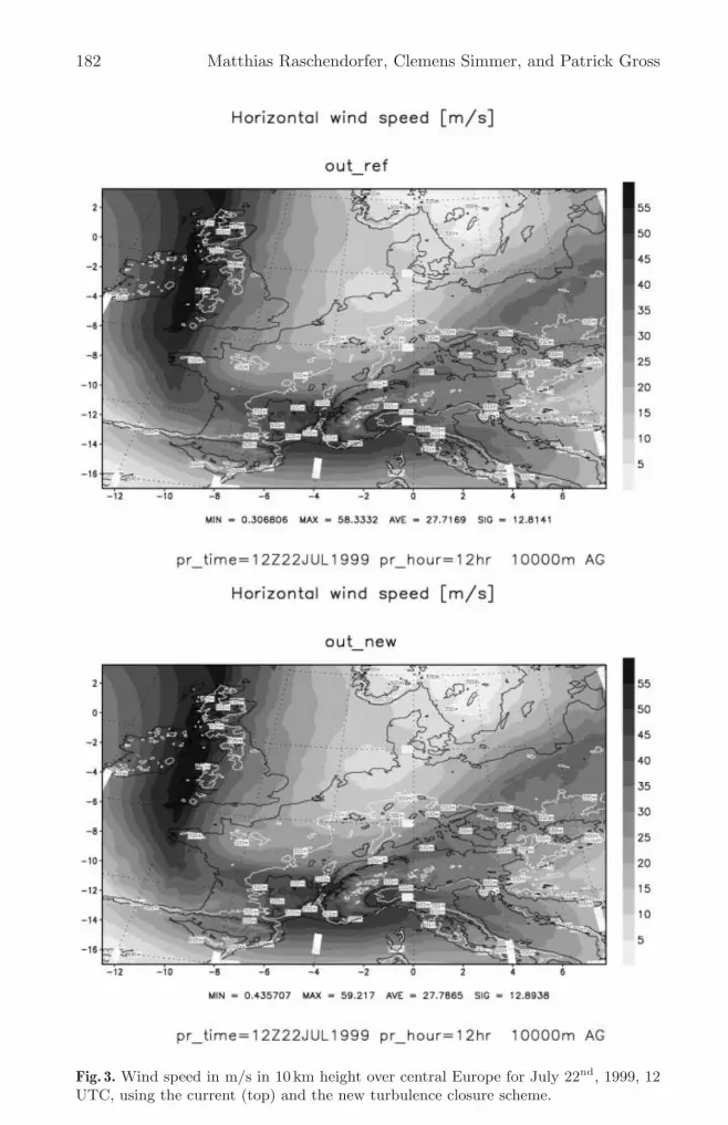
182 Matthias Raschendorfer, Clemens Simmer, and Patrick Gross
Fig. 3. Wind speed in m/s in 10 km height over central Europe for July 22nd, 1999, 12UTC, using the current (top) and the new turbulence closure scheme.

Parameterisation of turbulent transport in the atmosphere 183
Fig. 4. Vertical cross section from West to East at about 52N on July 22nd, 1999, 12UTC. Top: horizontal wind speed (m/s) with old turbulence scheme. Bottom: potentialtemperature (Degree Celsius) with the old scheme. Both are very similar with the newscheme.

184 Matthias Raschendorfer, Clemens Simmer, and Patrick Gross
Fig. 5. Vertical cross section from West to East at about 52N on July 22nd, 1999,12 UTC. Top: turbulent kinetic energy (m2/s2) with new turbulence scheme. Bottom:same with current turbulence scheme.

Parameterisation of turbulent transport in the atmosphere 185
3 Conclusions
In this contributions, we have tried to describe the basic problem of closing theset of thermo-hydrodynamical equations used in dynamic meteorological models.The necessity originates from the importance of sub-grid scale processes for thedescription of atmospheric processes. These sub-grid scale processes, produceadditional terms and unknowns when the basic set of equations is averaged toappropriate scales in time and space. Adequate equations for describing theseadditional terms lead to an exploding number of further unknowns, which mustbe restricted by parameterisations. Basic concepts for these additional equationsand parameterisations have been described using the Lokal Modell (LM) of theGerman Weather Service (DWD) as an example.
References
Doms, G. and Schattler, U. (1999): The nonhydrostatic limited-area model LM (Lokal-Modell) of the DWD. Deutscher Wetterdienst, Offenbach. 180 pp.
Louis, J.-F. (1979): A parametric model of vertical eddy fluxes in the atmosphere.Bound. Layer Metoer., 17, 187–202.
Mellor, G. L. and Yamada, T., (1982): Development of a turbulence closure model forgeophysical flow problems. Rev. Geophys. Space Phys., 20, 831–875.
Mellor, G. L. and Yamada, T., (1974): A hierarchy of turbulence closure models forthe planetary boundary layer. J. Atmos. Sci., 31, 1791–1806. (Corrigenda (1977) J.Atmos. Sci. 34, 1482)
Miegham van, J., (1973): Atmospheric Energetics. Oxford Monographs on Meteorology,Clarendon Press. Oxford.
Raupach M.R. and Shaw R.H., (1981): Averaging procedures for flow within vegetationcanopies. Bound. Layer Meteo., 22, 79–90
Pielke, R.A. (1984): Mesoscale meteorological modeling. Academic Press, Orlando. 612pp.
Sommeria G. and Deardorff J. W., (1977): Sub grid scale condensation in models ofnon precipitating clouds J. Atmos. Sci., 34, 344–355.
Stull R.B., (1988): An Introduction to Boundary Layer Meteorology. Kluwer, Dor-drecht, 666 p.

Precipitation Dynamics of Convective Clouds
Gunther Heinemann1 and Christoph Reudenbach2
1 Meteorological Institute, University of Bonn, Germany2 Geographical Institute, University of Bonn, Germany
Abstract. The dynamics of precipitation processes represent a typicalexample for a multi-scale geo-system. The gaps between the scales ofthe cloud microphysics, resolutions of cloud models and remote sensingmethods have to be closed by upscaling or parameterisation techniques.The section gives an overview over the governing processes for the gen-eration of precipitation and the importance of the cloud physics for themodelling and remote sensing of precipitation processes. An example ofa cloud model simulation is presented, and a possible approach for pa-rameterisations of convective precipitation processes for infrared remotesensing is given.
1 Introduction
The dynamics of regional convective precipitation processes comprises a wide in-terval in space and time. It ranges from scales of the cloud microphysics (0.1µm)to organised convective systems (100 km). The interaction between the micro-physical scales (release of latent heat) and the scales of the cloud dynamics (orderof 1 km, up- and downdrafts, interaction within cloud clusters) is of high impor-tance for the precipitation processes. Fig. 1 gives a schematic overview over thestructure of a thunderstorm cloud (supercell storm), while Fig. 2 shows an imageof a thunderstorm from space. The essential elements with respect to the mod-elling and remote sensing of precipitation processes are a) up- and downdraftareas, where condensation and rain formation as well as evaporation of cloudliquid water (CLW) occur; b) the formation of a cirrus anvil at the tropopause,which is characterised by a deformation of the tropopause (overshooting top) inthe area of strongest updrafts; c) rain at elevated levels that evaporates beforeit reaches the surface (virga). Both, the schematic sketch in Fig. 1 and the realthunderstorm in Fig. 2, show the overshooting top and the anvil, which are keyfeatures for the precipitation retrieval discussed in Section 3.
The latter characteristics of the three-dimensional structure of convectiveprecipitation leads to problems using the term ”precipitation” in the frame ofinterdisciplinary research. While the vertical distribution of ice and rain rates isof main interest for questions of the precipitation processes, the surface precipi-tation is the main need for hydrological applications, since it triggers processesin vegetation and soil. This aspect is also relevant for methods of remote sensing
H.J. Neugebauer and C. Simmer (Eds): LNES 97, pp. 186–198, 2003.
c© Springer-Verlag Berlin Heidelberg 2003

Precipitation Dynamics of Convective Clouds 187
Fig. 1. Schematic structure of a supercell thunderstorm depicting essential elementswith respect to the modelling and remote sensing of precipitation processes (inspiredby Houze, 1993).
Fig. 2. Image of a supercell thunderstorm made from the space shuttle (courtesy ofNASA) with the regions of the anvil and overshooting top marked.
of precipitation, which assume a coupling of structure and height of cloud topswith the surface precipitation (algorithms using infrared satellite data), as wellas for rain retrievals using weather radars, which assume a coupling of the dropsize distribution (DSD) at the cloud base with the surface precipitation.

188 Gunther Heinemann and Christoph Reudenbach
Convective precipitation processes occur on a continuum of scales, but usu-ally a separation into discrete subscales is being made when models are used tosimulate these processes. The transition of scales of the cloud microphysics upto the thunderstorm scale need to be parameterised either in a physical and/orin a statistical way. The treatment of the various spatial/temporal scale interac-tions represents therefore an essential problem for the remote sensing, modellingand measurements of convective precipitation. Some aspects of problems andsolutions of the scale interactions and the parameterisations of convective pre-cipitation processes are discussed in this chapter.
2 Scale interactions and parameterisations in cloud microphysics
The size distribution of precipitation particles is important for the interactionprocesses between the particles and for the precipitation process. The scales ofthe drop size distribution (i. e. the DSD) range from 0.1µm (size of the condensa-tion nuclei) to those of raindrops of up to several mm. Cloud drops and rain areusually classified using the fall speed (Houze, 1993), which is related to the dropradius. Particles exceeding a radius of 100µm (1 m/s fall speed) are attributedto rain (drizzle for 100–250µm). In raining clouds a tendency of a bimodal DSDcan be found, which justifies the separation between cloud droplets and rain
Fig. 3. Simulations of the drop size distribution (expressed as the mass distributionfunction g) of a convective cloud. Six time steps are shown (t1 = 0 s, t6 = 2000 s),the dashed curve indicates a simulation without the breakup process (from Issig, 1997;modified).

Precipitation Dynamics of Convective Clouds 189
(Fig. 3). The following processes are involved in the formation of cloud drops(generation of an initial DSD) and the formation of raindrops with a sufficientlarge fall speed (for more details see e. g. Pruppacher and Klett, 1978):
1. Condensation and evaporation: Because of the increase of the saturation wa-ter vapour pressure with decreasing drop radius, the initial drop formationfor supersaturations occurring in the atmosphere requires condensation nu-clei with a scale of 0.1µm, which are supplied by the atmospheric aerosol.Depending on the size and chemical composition of the aerosol particlesan efficient further growth by condensation can take place up to the scale ofcloud droplets (10µm). These processes can be parameterised by experimen-tally obtained functions, if the aerosol composition and its size distributionis known.
2. Coagulation (growth by collision): Further growth is possible by the processof coagulation, i. e. the collection of smaller drops by (faster falling) largerdrops. This process is governed by the DSD and the effective collection cross-section. The latter depends on the product of the geometric cross-sections ofthe colliding drops and an efficiency factor, which can be larger or smallerthan unity. This collision efficiency can be described by experimentally de-rived functions, but is taken as unity as a first approximation in many cloudmodels.
3. Breakup of drops: Aerodynamical instability leads to the breakup of dropsexceeding a radius of about 2.5 mm. The breakup and the size distribution ofthe new drops is parameterised statistically by suitable probability functions.The effect of this process is demonstrated in Fig. 3.
4. Ice/water phase interactions: If the ice phase is also present, all processesof the liquid phase have to be considered in analogy also for the pure icephase (processes 1–3). In addition, the processes between the ice and waterphase are important, particularly the growth of ice crystals at the cost ofsupercooled droplets as well as the coagulation processes between ice andwater particles (leading to graupel and hail).
Cloud models, which include all processes in detail and simulate the develop-ments of the size spectra by integrating the relevant differential equations, arecalled spectral models. Since the computation of the detailed microphysical pro-cesses is very time consuming, simpler models are used for many applications,which consider the same processes in form of parameterisations of the exchangebetween the reservoirs of water vapour, cloud water, rain water, cloud ice, snowand graupel (bulk models). As an example, the bulk parameterisation of thecoagulation processes reads as (Kessler, 1969; Houze, 1993):
dqr
dt
∣∣∣∣coag
= kc (qc − qc,0) (1)
qc cloud liquid water contentqr rain water contentqc,0 threshold value (1 g/kg)

190 Gunther Heinemann and Christoph Reudenbach
k−1c autoconversion time (∼= 1000 s for qc > qc,0 ; = 0 for qc ≤ qc,0
The main advantage of spectral models is their ability to simulate the DSDand hence all moments of the DSD. This allows the computation of the Rayleighradar reflectivity (Z) and the rainrate (R) as important quantities for the remotesensing of the precipitation using radar measurements:
N =∫ ∞
0
f(D) dD drop number (2)
ql =πρw
6
∫ ∞
0
D3f(D) dD liquid water content (3)
Z =∫ ∞
0
D6f(D) dD Rayleigh radar reflectivity (4)
R =πρw
6
∫ ∞
0
D3V (D)f(D) dD rain rate (5)
D is the drop diameter, f(D) the DSD, ρw the density of water and V(D) the fallspeed.
Fig. 4. Time-height cross-sections simulated by the spectral cloud model of Issig (1997)for the situation of 4th July 1994 near Koln for the vertical velocity (isolines every2 m/s), graupel content (shaded, in g/kg), and snow content (stippled for values ex-ceeding 0.01 g/kg). The time series of the surface rain rate (in mm/h) is shown as athick line, arrows indicate downdraft areas.
An example of a simulation using a 1.5D cloud model (Issig, 1997) is pre-sented in the following. This model treats the liquid phase in a spectral way, the

Precipitation Dynamics of Convective Clouds 191
ice phase is bulk-parameterised. The initial aerosol distribution is taken fromClark (1974). The simulation shown in Fig. 4 uses as initial conditions tempera-ture and humidity profiles of the “Lokal-Modell” of the German weather service(DWD) valid at 14 UTC, 4th July 1994, which is the case of the “Koln hailstorm”(Druen and Heinemann, 1998). The cloud develops within 30 min, the maximumupdraft area lies between 5,000 and 7,000 m. The conversion from cloud dropletsto rain water starts after 30 min at these heights. The growth of the drops contin-ues until their fall speed exceeds the updraft, and after 0.7 h rain starts to reachthe ground. The maximum surface rain rate is 25 mm/h. The main rain eventat the surface lasts about 15 min, and around 1.2 h simulation time a very weaksecondary rain maximum is present, which is associated with graupel meltingbefore it can reach the ground. This rain water from melted graupel particles isalso the reason that moderate values of the Z field are present after the mainsurface rain event (see below). A large fraction of the rain water evaporates inthe atmosphere.
The simulated Z values as a function of the near-surface rain rate (Z/Rrelation) reflect the temporal development of the DSD (Fig. 5). Prior to themaximum rain rate, the rain consists of larger drops at the same rain rate whencompared to the situation after the maximum. For the derivation of rain ratesfrom radar (Z) measurements this implies, that the Z/R relation depends onthe development stage of the convective cloud, which is in turn triggered by theactual atmospheric conditions leading to the thunderstorm development. Twostandard Z/R relations are shown additionally in Fig. 5. The first is the relationused operationally by the DWD (Z=256 R1.42), which is close to the well-knownMarshall and Palmer (1948) distribution (Z=296 R1.47), and the second is arelation for a DSD of thunderstorms (GDSD; Ulbrich, 1983; Fujiwara, 1965).The GDSD is in better agreement with the simulations compared to the standardDWD relation, and both relations show large differences for times prior to thenear-surface rain maximum. The application of these standard Z/R relations forthe development phase of the rain event would result in an overestimation ofrain rates with a factor of 4–8.
The cloud model simulations can also be used to investigate the height depen-dence of the Z/R relation. The Z/R relation valid at 1,875 m above the groundis similar to that at 125 m after the rain maximum (except the secondary rainevent associated with the melting of graupel), but larger differences can be seenprior to the near-surface rain maximum, where higher Z values at the same rainrate indicate that larger rain drops occur more frequently compared to the sur-face level. Breakup processes seem to be responsible for the modification of theDSD between these model levels.
3 Scale transitions and parameterising techniques used insatellite remote sensing
Numerical modelling approaches combined with remote sensing data promisea more physically based linkage between the recorded surface observations and

192 Gunther Heinemann and Christoph Reudenbach
Fig. 5. Temporal development of the Z/R relation for the simulation of Fig. 4 for themodel levels at 125 and 1,875 m. Z/R relations of DWD (solid) and GDSD (dashed)are shown (see text). Z is shown as dBZ= 10 log Z. The upper branches of the curvescorrespond to the first phase of the rain event.
the appropriate processes. On the other hand, they lead to new problems inconnection with the handling of the occurring scale transitions. In spite of thisproblems, the application of temporal high-resolution remote sensing data offersthe only reliable observation basis for the detection of convective process pat-terns. The achievable accuracy of quantification is crucially dependent on thehandling of the appropriate scale transitions.
In this Section, an algorithm for the quantitative estimation of precipitationusing infrared geostationary satellite data is outlined. The algorithm is based onthe technique introduced by Adler and Negri (1988), but was modified substan-tially. In the new algorithm, which is described in detail in Reudenbach et al.(2001), observed Meteosat infrared (IR) cloud surface temperatures are coupledwith the modelled temperatures and precipitation rates of a 1D cloud model withbulk parameterisation of cloud microphysics (Zock et al. 1995). Fig. 6 explainsschematically the basic relations and proposed solutions which are discussed indetail in the following.
As Fig. 6 shows, a conceptual model has to be developed which is able toconnect the cloud microphysics and dynamics in a suitable way with satelliteobservations. Due to the physical constraints of IR-sensors the only possibil-

Precipitation Dynamics of Convective Clouds 193
Fig. 6. Basic scheme of numerical model, remote sensing and ground measurement dataintegration corresponding to the spatial and temporal scale transitions.
ity to link observation and simulation appears to be the top cloud surface. Anumerical cloud model (see sec. 1) will be employed to calculate the necessarymeteorological fields (cloud top temperature, precipitation) in a physically con-sistent way. However coupling the simulation results with satellite observationsis only possible if one takes into account the occurring spatial and temporalscale transitions. The diverging scales of the cloud model and the Meteosat pixelresolution (Fig. 6) have to be linked up with a suitable upscaling procedure.
For the adaptation of the Meteosat spatial resolution to the cloud model,simultaneous NOAA AVHRR data (1.1 km resolution) have been used, to utilisean empirical correction of Meteosat IR brightness temperatures of the convec-tive cores. The retrieval algorithm provides an estimation of the stage of clouddevelopment which is used to fit the temporal scales of cloud model run andMeteosat observation together.
As a result the highly parameterised microscale processes of the cloud-dynamics and microphysics of the cloud model provides a physically based es-timate of the convective response, (i. e. precipitation rate and maximum cloudheight) in a given atmosphere, which can be implemented in a satellite basedretrieval technique.
The geostationary satellites of the Meteosat series are scanning the Earth’sdisk completely at half-hour intervals (resolution of approx. 6×10 km2 for Central

194 Gunther Heinemann and Christoph Reudenbach
Fig. 7. Scheme of convective life cycle stages (after Johnson and Young, 1983).
Europe). By means of a suitable algorithm the convective minima are isolatedfrom the temperature patterns of each picture sequence and assigned to a de-fined stage of the convective life cycle. The cloud system is classified into early,mature and the decay stages. Appropriate precipitation regimes are assignedto the respective stage (Fig. 7): the early stage (young storms) is associatedwith convective precipitation; the mature stage (mature storms) is associatedwith convective and stratiform precipitation and the stage of decaying stormsprovides no precipitation. In this way it is determined whether the detected spa-tial/temporal signal (Meteosat pixel) corresponds to the model conceptions ofconvective precipitation genesis.
The rain algorithm for active convective cores is based on the 1D parcel-typecloud model. The linkage of remote sensing and model data is established byusing the Meteosat infrared temperatures and the simulated cloud top temper-atures. The model is adapted to the regional atmospheric conditions by usingactual atmospheric profiles of humidity and temperature simulated by the LM ofthe DWD (see previous section). In order to derive the regression between cloudtop temperature and rain rate, the cloud model is operated with a variable diam-

Precipitation Dynamics of Convective Clouds 195
Fig. 8. Cloud model-derived rain rate/cloud top temperature relationships for two ac-tual profiles of 4th July 1994 (dashed) and the averaged linear regression (solid line)for about 30 profiles. The parameter varied is the diameter of the convective updraftarea.
Fig. 9. Statistical upscaling of the spatial cloud model resolution to Meteosat viewinggeometry.
eter of the updraft area. Fig. 8 shows two examples of relations between meanrain rate (Rmean) and the modelled cloud top temperature Tct. In order toobtain an averaged statistical relation, Rmean/Tct regressions have to be com-puted for LM profiles in the area of observed convection. The rain rate can thenbe approximated by linear regression analysis:
In a preliminary step it is necessary to find a suitable solution for the ad-justment of the spatial scale of the 1D cloud model according to the viewing

196 Gunther Heinemann and Christoph Reudenbach
geometry of Meteosat. The used cloud model can be applied up to a diameter ofapprox. 4 km. The spatial resolution of the modelled precipitation event deviatesthus clearly from the observation geometry of the Meteosat data. A linear statis-tical upscaling procedure is used to decrease the resulting parameterising errorswhich are caused by cloud surface temperatures that were detected too warm.Simultaneous Meteosat IR temperatures and spatially better resolved NOAAAVHRR temperature data (1 × 1 km2) of identical minima are used (Fig. 9) tocarry out a linear regression analysis.
The derived transformation function serves as statistical scale adjustmentof the Meteosat temperatures in reference to the temperatures calculated bythe cloud model. To validate the precipitation estimation point measurementsof ground stations are used. However, the extreme variability of the observedconvective precipitation events prevents the use of individual point observationsfor validating purposes. In order to derive representative statements about spa-tial precipitation based on ground measurements, rain gauge networks with highspatial and temporal resolution within the area of the City Bonn were used(Fig. 10). Rain rates of 5 minutes enables a spatial mean value of the groundmeasurements according to the spatial resolution of the remote sensing data.The kriging technique was used to interpolate the spatial means. It calculatesa weighted sum of known observations to estimate an unknown value (Pebesmaand Wesseling, 1998).
Fig. 10. Ground measurement network (City Bonn) with corresponding remote sensingviewing geometry areas.

Precipitation Dynamics of Convective Clouds 197
In Fig. 11 all rain gauge data during the “Koln hailstorm” event (4th July1994, 10–14 UTC) of the 15 stations are spatially interpolated and averagedover the size of the Meteosat pixel. Due to the temporal resolution of Meteosatmean rain rates are computed as 30 minutes averages. The interpolated rainrate applies significantly better to the Meteosat derived rain rates. Due to thespatially and temporally aggregated and interpolated ground data according tothe Meteosat viewing geometry it is possible to make quantitatively more validpredictions about the area integral sensor signal as this would be possible fromthe individual point measurements.
Fig. 11. Comparison of rainfall rates (30 minutes averages and the 4 h average) duringthe heavy precipitation event 10–14 UTC, 4th July 1994, at Bonn. ECST is the satellitederived estimate for the Meteosat pixel. Gauge 15 is the arithmetic mean of the 15 raingauge stations shown in Fig. 10; Gauge 9 is the arithmetic mean of the 9 gauges withinthe Meteosat pixel; Gauge interpol. marks the spatially interpolated and averaged dataover the area of the Meteosat pixel.
References
Adler, R. F., Negri, A. J., 1988: A satellite infrared technique to estimate tropical con-vective and stratiform rainfall. Journ. Appl. Meteor. 27, 30–51.
Clark, T. L., 1974: A study in cloud phase parameterization using the Gamma distri-bution. J. Atmos. Sci. 31, 142–155.
Druen, B., Heinemann, G., 1998: Rain Rate Estimation from a Synergetic use of SSM/I,AVHRR and Meso-Scale Numerical Model Data. Meteorol. Atmos. Phys., 66, 65–85.

198 Gunther Heinemann and Christoph Reudenbach
Fujiwara, M., 1965: Raindrop-size distribution from individual storms. J. Atmos. Sci.,22, 585–591.
Issig, C., 1997: Ein spektrales Wolkenmodell mit integriertem Strahlungsuber-tragungsmodell zur Unterstutzung von Niederschlagsalgorithmen aus Fernerkun-dungsdaten. PhD Dissertation, Bonn, 104 p.
Houze, R.A., 1993: Cloud dynamics. Academic Press, San Diego, USA, 570 pp.Johnson, D.H., Young, G. S., 1983: Heat and moisture budgets of tropical mesoscale
anvil clouds. J. Atmos. Sci. 40, 2138–2147.Kessler, E., 1969: On the distribution and continuity of water substance in atmospheric
circulations. Meteor. Monogr. 32, Amer. Meteor. Soc., Boston, USA, 84 pp.Marshall, J. S., and W. M. Palmer, 1948: The distribution of raindrops with size. Jour-
nal of Meteorology, 5, 165–166.Pebesma, E. J. and C.G. Wesseling, 1998. ‘Gstat: a program for geostatistical mod-
elling, prediction and simulation.’ Computers and Geosciences. 24 (1): 17–31.Pruppacher, H.R., Klett, J.D., 1978: Microphysics of clouds and precipitation. Reidel
Publishers, Dordrecht, 714 pp.Reudenbach, C., Heinemann, G., Heuel, E., Bendix, J., Winiger, M., 2001: Investigation
of summertime convective rainfall in Western Europe based on a synergy of remotesensing data and numerical models. Meteor. Atmosph. Phys. 76, 23–41.
Ulbrich, C.W., 1983: Natural variations in the analytical form of the raindrop sizedistribution. J. Clim. Appl. Meteorol., 22, 1764–1775.
Zock, A., Menz, G. and Winger, M. 1995: Regionalisation of rainfall models in EasternAfrica using Meteosat Real-Time-Window data. Proceedings of the InternationalGeoscience and Remote Sensing Symposium (IGARSS’95), 10–14 July 1995 Flo-rence, Italy (New York: I. E. E. E.), 250–252.

Sediment Transport — from Grains toPartial Differential Equations
Stefan Hergarten, Markus Hinterkausen, and Michael Kupper
Section Geodynamics, Geological Institute, University of Bonn, Germany
Abstract. We illustrate that sediment transport phenomena cover a widerange of spatial and temporal scales and point out the need for contin-uum models of sediment transport. We show, however, that continuumapproaches to sediment transport only result in feasible models in somespecial cases such as rolling, saltation, and suspended load and discussthe capabilities and the limitations of these approaches with examplesfrom modelling soil erosion processes and ripple formation.
1 Phenomena, Processes, and Scales
Large parts of the earth’s surface are shaped by sediment transport processes. Forthis reason, modelling landform evolution is mainly modelling sediment transportprocesses.
The structures formed by sediment transport processes cover a wide range ofspatial scales. It starts at the microscopic roughness of the surface and continueswith structures on the centimetre to meter scale, such as gullies and ripples. Thenext larger elements are river banks, landslides, and dunes; they may extend tosome hundred meters. Finally, the largest scale of sediment transport phenomenaconsists of basins formed by fluvial erosion.Sediment fluxes may be driven by
– wind,– water (in oceans, lakes, and rivers, or Hortonian runoff during heavy rainfall
events) or– gravity (landslides, debris flow).
Unconsolidated sediments are granular matter; their grain sizes vary fromless than 1µm for clay particles to about 1 cm for gravel. Even large boulders ofmore than 1 m size may participate in sediment transport. But their probabilityof being moved is considerably lower than for smaller particles. Thus, their directcontribution to landform evolution may be negligible, but their presence canaffect transport of smaller particles strongly by armouring and reinforcing surfacematerials.
In many cases, the sizes of the particles contributing to sediment transportare indeed much smaller than the characteristic scales of the pattern generated [email protected]
H.J. Neugebauer and C. Simmer (Eds): LNES 97, pp. 199–213, 2003.
c© Springer-Verlag Berlin Heidelberg 2003

200 Stefan Hergarten, Markus Hinterkausen, and Michael Kupper
H H+δH
Fig. 1. Definition of an average surface height (left) and illustration of the effect ofadding one grain (right).
by the transport process. If we, for instance, consider a typical sand of 0.3 mmgrain diameter, a volume of (10 cm)3 consists of 4×10⁷ particles. Thus, modellingtransport processes by simulating individual particle motions is only feasible forinvestigating phenomena on the grain scale, but not for modelling effects onlarger scales. Therefore, mostly particle densities (concentrations) are introducedin order to describe the sediment as a continuum.
The first step towards a continuum description is introducing an averagesurface height H(x, t). The vector x = (x1, x2) describes the coordinates on themodel scale that is much larger than the grain scale. Thus, H(x, t) can be seenas an average surface height of a sediment pile that consists of many particles;it can be defined as illustrated in the left hand part of Fig. 1. For simplicity, werestrict our considerations to identical grains for the moment, but most of theideas can easily be extended to sediments of multiple particle sizes.
As shown in the right hand part of Fig. 1, the average surface height increasesby an amount δH if a grain is added. This effect can be quantified by introducinga representative particle volume V in such a way that
δH =V
A(1)
if one grain is added to an area A. As sediments contain a certain amount ofvoid space (pores), V is greater than the volume of a single sediment grain; Vcan be computed by dividing the particle volume by the fraction of pore space(porosity).
As a result of Newton’s principle, the state of a moving particle cannotbe characterised by its position x = (x1, x2, x3) in space alone; the velocityv = (v1, v2, v3) is necessary, too. Thus, a particle concentration c(x,v, t) whichdepends on six independent variables (plus time) has to be defined within thetransporting medium (air or water). In the general case, this procedure will resultin a six-dimensional partial differential equation.
In computational quantum mechanics, such high-dimensional problems arecommon subjects, but they can only be solved if most properties of the solu-tion are a priori known. Thus, such a general continuum approach to sedimenttransport does not have any advantages compared to simulating individual grainmotions. Feasible formulations are only obtained if further assumptions aboutthe transport mechanisms are made.

Sediment Transport — from Grains to Partial Differential Equations 201
The complexity of the resulting equations depends on the interactions of thetransported particles; these interactions may be
– interactions with the driving fluid (air or water),– interactions with the sediment surface or– interactions with other particles being transported.
The latter kind of interactions mostly leads to quite complicated, nonlinear equa-tions. Neglecting them is reasonable as long as the particle concentration is suf-ficiently small. At higher concentrations, the relevance of particle-particle col-lisions increases. This effect is ubiquitous in landslides and debris flows whereparticle-particle interactions are at least as important as interactions with thedriving fluid, if the latter is present at all.
In the following we focus on three established transport mechanisms whichneglect particle-particle interactions and their transfer to continuum models.The more complicated case with high particle densities leads to the theory ofgranular flow; discussing its numerous approaches goes beyond the scope of thisintroduction, so that we recommend the review articles of Iverson (1997) or Janand Shen (1997).
2 Sediment Transport Mechanisms and their ContinuumRepresentation
2.1 Rolling
Heavy particles are unlikely to be lifted up by water or air, so that they tendto move along the sediment surface. In each river, a certain amount of sedimentis transported by rolling. The toppling of sand grains from steep sandpiles or atthe lee side of ripples and dunes is a similar mechanism.
Since particle motion is restricted to the sediment surface, rolling can beconsidered as a two-dimensional process in a planar view. Thus, the particleconcentration describes the number of rolling particles per area instead of vol-ume; x and v are two-dimensional vectors.
In this case, the mass balance equation that describes the evolution of thesurface height can be written in the form
∂
∂tH(x, t) = −divj(x, t) (2)
with the stream density
j(x, t) = V
∫c(x,v, t)v dv1dv2 . (3)
However, this is the trivial part. Quantifying the driving forces leads to a four-dimensional, time-dependent partial differential equation for c(x,v, t). Thus, fur-ther assumptions about the mechanism are necessary.

202 Stefan Hergarten, Markus Hinterkausen, and Michael Kupper
A simple, in some cases sufficient idea is to allow only motion with a fixed ve-locity (that may, for instance, depend on the surface gradient) and keep only thenumber of rolling grains variable. Such a two state approximation was introducedby Bouchaud et al. (1995) for simulating avalanche dynamics on sandpiles.
2.2 Suspended Load
Suspended load is the opposite limiting case to rolling. If the particles are lightand the flow is turbulent, an apparently random pattern of particle motionoccurs. Each particle is exposed to a nearly random acceleration many times; soit performs a large number of small scale movements. This may look as if theparticles were floating; but this is — strictly speaking — not correct. No matterhow small the particles are, their density is higher than that of water, so thatthey sink in the mean. As the settling velocity decreases with decreasing particlesize, the random motion may govern the behaviour, so that the particles maystay in suspension for a long time.
Since the particles are exposed to high accelerations, effects of inertia arenegligible for suspended load. Thus, there is no need to keep track of the particlevelocity, so that considering a concentration c(x, t) where x = (x1, x2, x3) isappropriate. The particle concentration in the fluid is then determined by thebalance equation
∂
∂tc(x, t) = −divj(x, t) (4)
where j(x, t) is the particle stream density. Assuming that the velocity of theparticles is the sum of the fluid velocity v(x, t), the settling velocity vs, and arandom component, the stream density is
j(x, t) = c(x, t) (v(x, t) + vs) −D(x, t) ∇c(x, t) . (5)
The first term at the right hand side describes an advective transport, while thesecond term acts as a diffusive component.
Finding an expression for the diffusivity D(x, t) is the nontrivial part; it quan-tifies the effects of turbulence and eventually of particle collisions. Approachescan be derived from the theory of turbulent flow; but as shown later in the ex-ample of soil erosion, it may be appropriate to use D(x, t) for a calibration withempirically-based formulas for transport capacity, too.
The evolution of the sediment bed is then determined by the sediment fluxat the surface:
∂
∂tH(x1, x2, t) = −V n ·j(x1, x2,H(x1, x2, t), t) (6)
where n is the upper normal vector at the surface.We started at the wide range of the spatial scales of sediment transport phe-
nomena, but the time scales cover a wide range, too. Compared to the timescales of surface evolution, the time needed for moving individual particles isvery short. From the long term point of view, the flow field and the sediment

Sediment Transport — from Grains to Partial Differential Equations 203
concentration adapt immediately to any changes in surface geometry or bound-ary conditions. Thus, there is no memory in these rapid processes, so that theycan be described by steady-state equations. This step is called separation oftime scales; for suspended load, this means that the left hand side of Eq. 4 canbe neglected. However, while the separation of time scales is a great progress inmany multi-scale phenomena, it does not really make things easier for suspendedload.
2.3 Saltation
Saltation is a transport mechanism between rolling and suspended load. Thepower of the flow is sufficient for lifting up particles, but not high enough forkeeping them in the fluid for long times. The acceleration acting on the particlesduring their motion is not so strong that effects of inertia are negligible. Thus,the particle traces are not as random as for suspended load; variations may resultfrom the process of lifting rather than from the later stages of motion.
This phenomenon can be simulated efficiently if the time scales can be sepa-rated and if the number of saltating particles is low, so that they do not interactwith each other. In this case, the traces of a particle starting at any point of thesurface can be computed, provided that the initial velocity and the forces actingduring the saltation step are given. Thus, it is in principle possible to computethe statistical distribution of the saltation lengths, so that the problem can bereduced to a two-dimensional plane view model.
It is convenient to use the two-dimensional master equation for computingthe changes of the surface height:
∂
∂tH(x, t) = V
(∫ν(y, t)w(y, x, t) d2y − ν(x, t)
). (7)
Here, ν(x, t) is the number of saltating particles per area and time starting atthe location x at the surface; w(y, x, t)d2x is the probability that a particle thatstarts at the location y settles in the interval [x, x + δx]. The first term at theright hand side of Eq. 7 describes those particles which start at any location andsettle at x, while the second term describes the particles starting at x.
Eq. 7 can in principle be written in flux density form with a particle streamdensity j(x, t), but it is quite complicated and has not any advantages.
Transforming Eq. 7 into a numerical scheme is straightforward; it is simplya redistribution of particle packets according to the statistical distribution ofthe saltation lengths. However, computing this distribution is costly, so thatfurther simplifications may be necessary. For instance, if the saltation lengthsare smaller than the model resolution, Eq. 7 can be written in the same formas the equation for rolling grains with a very simple particle stream density(Hergarten and Neugebauer 1996). Another important limiting case is that ofa narrow distribution of the saltation lengths; this means that the statisticalvariation can be neglected. Such an approach is used in the model of Nishimoriand Ouchi (1993) and in the ripple model discussed in Section 4.

204 Stefan Hergarten, Markus Hinterkausen, and Michael Kupper
µ
C
i
i
δ
free particlesolid particleµ
iF L
H
x
y
z
Fig. 2. Illustration of particle motions and soil structure on the grain scale.
3 Soil Erosion
3.1 Particle Motion and Soil Structure
A simplified concept for describing soil erosion processes is illustrated in Fig. 2.It illustrates particle motions and soil structure on the grain scale. The soilcontains particles with the same kind of structure but different sizes.
In contrast to sand or gravel sediments as they occur in many fluvial sys-tems, cohesion plays an important part in soil erosion; it prevents the particlesfrom easily being detached by the flow. For simplicity we describe the cohesionby a two-state approximation: Each particle is either connected tightly to itsneighbours or can be detached by the flow.
Turbulent surface runoff of water is the major driving force to particle move-ment. Moreover, stresses on surface caused by the water can disconnect solidparticles, so that they can be lifted up afterwards.
For small particle sizes, suspended load is the dominating sediment transportmechanism. So we introduce particle concentrations Ci(x, t) in the fluid, wherethe index i represents a class of particles that is characterised by a grain size.In order to describe the different particles in the soil we consider concentrationsµLi
(x, t) for the free particles and µFi(x, t) for the solid particles in the soil, too.
While Ci(x, t) refers to a number of particles per volume, µLi(x, t) and µFi
(x, t)are relative volume concentrations. With the condition∑
i
(µLi(x, t) + µFi
(x, t)) = 1 (8)
they describe changes in the mixture between the classes and the two states.

Sediment Transport — from Grains to Partial Differential Equations 205
3.2 Surface Runoff
Our description of surface runoff is based on a generalisation of Manning’s for-mula (Hergarten et al. 2000); beside the surface height H(x, t) it involves thethickness of the water layer δ(x, t) as a second variable:
v = − 1nδ
23 |∇(H + δ)| 12
∇(H + δ)
|∇(H + δ)| . (9)
The Manning formula describes the average fluid velocity of turbulent flow on astructured surface of a slope. The parameter n considers the microscopic rough-ness of the surface.
Taking into account that the temporal evolution of the water level δ dependson the rainfall rate R and the infiltration rate I, the balance equation reads:
∂δ
∂t+ div(δ v) = R− I . (10)
3.3 Erosion and Deposition
Due to suspended load as the dominating transport mode the temporal changesof the particle concentrations Ci(x, t) can be described by Eq. 4, and the particlestream density ji(x, t) is given by Eq. 5 with the fluid velocity from Eq. 9.
In order to develop an expression for the diffusivity D(x, t) we use this for acalibration with the empirically-based formula for the transport capacity fromEngelund and Hansen (1967):
Cstati =
0.05√g d4
i
ρw
ρ− ρw|v|
√δ |∇ (H + δ) | 32 (11)
where
di = particle diameter,ρ = mass density of the particles,
ρw = density of water,g = gravitational acceleration.
This formula describes a stationary particle concentration Cstati in case of steady,
spatially homogeneous runoff. Comparing this empirical relation with the solu-tion of the balance equation (Eq. 4) under the same conditions leads to anequation which defines the diffusivity D(x, t).
Model calibration requires a second empirically-based formula that deter-mines the rate E of disconnecting solid particles; we choose that of Foster (1982):
E = a τ b. (12)

206 Stefan Hergarten, Markus Hinterkausen, and Michael Kupper
τ is the shear stress at the soil surface; a and b are parameters specified by thesoil characteristics. The stress τ is given by the component of gravity force perarea of the water parallel to the slope:
τ = ρwg δ |∇ (H + δ) | . (13)
The evolution of the slope surface H(x, t) and of the mixture ratios is determinedby the sediment flux in direction of the upper normal vector at the surface(see Eq. 6). Finally, the total particle stream density j(x, t) is the sum of theindividual stream densities ji(x, t).
3.4 Some Results
Figs. 3 and 4 provide a rough overview over the capabilities of the model. Themodel domain consists of an artificial slope of 16 m×64 m size with a roll-out atthe foot. In order to introduce some inhomogeneity, a small noise is superposed.The surface runoff is caused by several rainfall events with a rate of 1.67 ×10⁻⁵ m/s (60 mm/hour). There is no inflow at the upper edge, and we assumeperiodic boundary conditions at the sides of the domain. Fig. 3 shows that apattern of erosion rills evolves with increasing number of events, so that flowis concentrated in this rills. The description with partial differential equationsenables us to trace the evolution on this scale in detail.
Another example is illustrated in Fig. 4; it shows the spatial distribution ofthe mixture ratio between two particle classes of different sizes. The diameter ofthe small particles is 0.05 mm, while that of the large particles is 1 mm. In thebeginning, the large particles are confined to a layer of 5 mm thickness in theupper region. Through the erosion process, they are transported downslope andthe layer becomes smaller. While small particles tend to be transported out ofthe system, large particles are partly deposited at the foot of the slope. As aresult of the inhomogeneous flow paths due to rill formation, deposition is quiteinhomogeneous.
However, we should be aware that suspended load is the only transport mech-anism in this simplified model. While this assumption is reasonable for the smallparticles, particles of 1 mm are transported by saltation rather than by sus-pended load in reality, so that a more comprehensive model which includes atleast two different transport mechanisms is required for such simulations.
4 Ripple Formation
Sediment ripples in flumes arise if saltation is the dominating transport mode.In contrast to suspended load the grains are transported in a thin layer over thebed. “The detachment of grains is due to the friction shear stress interactingbetween the flow and the bed surface; their downstream motion is due to thelocal flow velocities” (Yalin 1992).
The flow structure over ripples is illustrated in Fig. 5. The turbulent flow de-taches at a ripple crest and creates a “roller” at the lee side before it reattaches at

Sediment Transport — from Grains to Partial Differential Equations 207
Fig. 3. Spatial distribution of surface runoff during the n-th rain event. The gray scaleindicates the thickness of the water layer.

208 Stefan Hergarten, Markus Hinterkausen, and Michael Kupper
Fig. 4. Mixture ratio at different times. The gray scale corresponds to the average grainsize; dark areas represent large particles.

Sediment Transport — from Grains to Partial Differential Equations 209
the stoss side of the adjacent ripple. One can observe that the sediment transportceases in the separation zone and sediment is predominantly deposited. Threeregions of different velocity profiles can be distinguished: the internal boundarylayer, the wake region, and the outer region (McLean and Nelson 1994).
stream direction
point of reattachment
wake region
separation zone
internal boundary layer
Fig. 5. Schematic plot of the flow structure over a bedform.
Since the transport mode is saltation, Eq. 7 is appropriate for describing theimpact of the flow on the sediment bed. Hence the sediment transport varieswith the number of entrained particles ν(x, t) and with the distribution of salta-tion lengths w(x, y, t). As a first approach we choose the saltation length to beconstant and consider the influence of the fluid flow in the term ν(x, t) which isexclusively depending on the current bed topography.
4.1 Lee/Stoss Effect
The basic idea is to describe the number of moved particles along the sedimentbed by a kind of shadowing: shadowing is relatively strong in the separation zonewhere the sediment transport is reduced in consequence of the upstream ripplecrest, whereas the shadowing effect ceases behind the point of reattachment.
For the sake of simplicity the average transport direction is chosen to beparallel to the x1-axis. We assume that due to the shadowing mechanism thenumber of moving particles over ripples is reduced compared with the number ofmoved particles over a flat bed. We parameterise this behaviour with a “shadowfunction” S(x) which varies between zero and one, so that the number of movedparticles can be determined as follows:
ν(x, t) = ν0 · S(x, t) (14)
where ν0 is the number of moved particles over a flat bed. An at least qualita-tively reasonable approach for the shadow function can be obtained by varia-

210 Stefan Hergarten, Markus Hinterkausen, and Michael Kupper
tional calculus:
S(x) =
[1 − 1
∆minu≥H
u(xmax)=Hmax
(max
ζε[xmax,x]
− u′(ζ)
)]+
(15)
with continuous functions u as shown in Fig. 6. The symbol [ ]+ denotes thepositive part of the term in brackets. ∆ is the steepness of u(x) where theparticles are not moved any longer, so that S is equal to zero then. As a resultof this approach, the sand transport decreases at the lee side of a ripple andincreases at the stoss side of the adjacent ripple.
ζ
H
H(x)
max
H(x,y;t)
u( )
xmax x
Fig. 6. Illustration of the variational calculus to obtain the shadow function S(x).
As mentioned above, we assume that the saltation length of the particles isconstant. Thus, the corresponding probability function w(y, x, t) has the shapeof Dirac’s delta function δ(x − y − l ex), and Eq. 7 turns into:
∂
∂tH(x, t) = V ·
(ν(x − l e1) − ν(x, t)
)= V ν0 ·
(S(x − l e1)︸ ︷︷ ︸Deposition
− S(x)︸︷︷︸Erosion
)(16)
The alteration of the sand bed height is given by the difference between thenumber of incoming and outgoing particles.
4.2 The Diffusional Processes
Eq. 16 describes a process that creates patterns due to the lee/stoss charac-teristics. However, ripples observed in nature reach a quasi-steady state witha limited height of the crest after a transient process (Baas 1999). Hence, be-sides constructive processes, there are also destructive influences that smooththe bed’s surface.
We identify the following behaviour: the steeper the slope the larger is thenumber of particles which move downhill due to rolling; moreover avalanchingoccurs, if the slope exceeds the angle of repose (for sand approximately 32). Bothprocesses can be described by a diffusional approach for the stream density:
jd(x, t) =
−D
(|∇H| − tan ϕ
)∇H
|∇H| if |∇H| > tan ϕ
0 else. (17)

Sediment Transport — from Grains to Partial Differential Equations 211
with ϕ as the smallest angle where rolling occurs; D denotes the diffusivity. Theimpact of the diffusional stream on the total sediment transport is shown inFig. 7.
leestoss
Fig. 7. Influence of diffusion on a constant sediment transport downstream.
Eventually the governing equation of the model reads:
∂H
∂t= −divjd + V ν0 ·
(S(x − l e1) − S(x)
)(18)
4.3 Results
To illustrate the capabilities of the model we perform an exemplary simulationexperiment (see Fig. 8): in the initial state we assume a sediment bed whichis flat except for small, random fluctuations in height. After some time, ripplesbegin to grow and migrate downstream, whereby little ones are captured bybigger ones. The patterns are three-dimensional, and the ripple crests evolvetowards a lunate shape.
We expect that the system should reach a quasi-stationary state where thegrowth of the ripple crests ceases. However, we observe in our simulation thatthe development of the ripples continues until a single ripple occupies the wholemodel region. Finally, an equilibrium between constructive and destructive pro-cesses is achieved, so that the growth process ceases in fact. However, length andheight of the resulting equilibrium shape is controlled by the size of the modeldomain rather than by physical properties in this preliminary model.
Nishimori and Ouchi (1993) have derived a similar model for wind-drivenripples. They also use a diffusional particle stream, but choose a different ap-proach to determine the saltation lengths. Their saltation length l is a functionof the surface height:
l = L0 + bH(x). (19)
In contrast to our model they are able to simulate a quasi-stationary state ofthe ripples. If we compare their results with ours, we find following differences:
– Our bedforms are asymmetric and migrate downstream in accordance toobservation; however the growth is only limited by the model region.
– Nishimori and Ouchi’s model produces ripples which are limited in height,but their shape is symmetric and they migrate in the wrong direction (up-stream).

212 Stefan Hergarten, Markus Hinterkausen, and Michael Kupper
Fig. 8. Ripple development; l = 1 × grid spacing, D = 10, V ν0 = 1, k = 1, ϕ = 0.1,periodic boundary conditions.
4.4 Next Steps
The evolution from little ripples structures to bigger ones appears to be realisticin our model, although we do not reach a natural equilibrium state yet. It willbe necessary to find out how a variable saltation length affects the results, andif this could lead to a final state that is independent of the boundary conditions.Furthermore, it is well-known, that the ripple development is strongly dependenton the sediment size. Yalin (1992) found the empirical relation that the ripplewave length in equilibrium state is about 1000 times the particle size. This

Sediment Transport — from Grains to Partial Differential Equations 213
indicates that the scale of particles is important for the final state and has to beconsidered in a continuum approach.
5 Conclusions
Sediment transport phenomena include a wide range of spatial and temporalscales. Simulations of pattern formation on large scales (larger than a few cen-timetres) can only be performed on a continuum basis. In the general case, thecontinuum formulation leads to high-dimensional partial differential equationsthat cannot be solved efficiently. Feasible models can only be developed for somespecial cases, such as rolling, saltation, and suspended load. Thus, there is nota general theory that can replace the search for an adequate approach for thephenomenon under consideration.
References
Bass, H. J. (1999): Equilibrium morphology of current ripples in fine sand. Sedimen-tology, 46, 123–138.
Bouchaud, J.-P., M.E. Cates, J. Ravi Prakash, and S. F. Edwards (1995): Hysteresisand metastability in a continuum sandpile model. Phys. Rev. Lett., 74, 1982–1985.
Engelund, F., and E. Hansen (1967): A Monograph on Sediment Transport in AlluvialStreams. Tekniks Verlag, Copenhagen.
Foster, G.R. (1982): Modeling the erosion process. In: Hydrologic Modeling of SmallWatersheds, edited by C.T. Haan. ASAE Monograph 5.
Hergarten, S., and H. J. Neugebauer (1996): A physical statistical approach to erosion.Geol. Rundsch., 85(1), 65–70.
Hergarten, S., G. Paul, and H. J. Neugebauer (2000): Modelling surface runoff. In: SoilErosion — Application of Physically Based Models, edited by J. Schmidt. Springer,Environmental Sciences, Heidelberg, 295–306.
Iverson, R.M. (1997): The physics of debris flow. Rev. Geophys., 35(3), 245–296.Jan, C.-D., and H.W. Shen (1997): Review dynamic modelling of debris flows. In: Re-
cent developments on debris flows, edited by A. Armanini and M. Michiue. Springer,LNES 64, 93–116.
Mclean, S.R., J.M. Nelson, and S. R. Wolf (1994): Turbulence structure over two-dimensional bed forms. J. Geophys. Res. 99(C6): 12729–12747.
Nishimori, H., and N. Ouchi (1993): Formation of ripple patterns and dunes in wind-blown sand. Phys. Rev. Lett., 71, 197–200.
Yalin, M. S. (1992): River Mechanics. Pergamon Press Ltd., Oxford, 220 pp.

Water Uptake by Plant Roots — a Multi-ScaleApproach
Markus Mendel, Stefan Hergarten, and Horst J. Neugebauer
Section Geodynamics, Geological Institute, University of Bonn, Germany
Abstract. The soil-root-stem water pathway is a major component of thesubsurface hydrological system. We model water uptake and water trans-port through the soil and through the root system as coupled processes.The model is based on a differential equation approach. The couplednon-linear equation system is solved numerically. On the macroscale,fluid flow through the soil matrix within and outside of the rooted areais modelled using a two-dimensional, axial-symmetric Richards equation.Flow through the root system is described by a Darcy equation. Wateruptake and transport through the root system are considered to be pas-sive processes; osmotic effects are neglected. In order to obtain the sourceand sink distribution of the root system, local soil water potentials (neara single root) are computed in a one-dimensional approximation in a fur-ther step. The model is capable of simulating hydraulic lift, which is thetransport of water from moist into drier soil layers through plant rootsystems. The calculated amount of passively shifted water is consistentwith experimental data. We discuss under which conditions hydrauliclift could be an optimised strategy for the plant and how water uptakepatterns are modified by the multi-scale (local) approach.
1 Multi-Scale Concept
Vegetated areas constitute an important part of the earth’s hydrologic system.Approximately 70 % of the water falling on the soil surface is returned to theatmosphere through evapotranspiration (Molz 1981). Water transpired by plantsis taken up by thin rootlets of the root system so that a water potential gradientat the root soil interface emerges. On a larger scale water flows by diffusion orthrough macropores (Germann 1990) into the rooted soil domain in order tobalance the water deficit induced by the transpiration. Evidently an interactionexists between the water flow through the soil, water uptake by rootlets, waterflow through the root system and the transpiration.
Quantitative studies of water uptake by plant roots date back to studiesby Gardner (1960). Later many comparable models followed; for an overviewsee Molz (1981) and Clothier and Green (1997). In all these approaches, wateruptake is modelled by a Richards equation choosing a special term for the righthand side (sink term), in this context also called the extraction function.
H.J. Neugebauer and C. Simmer (Eds): LNES 97, pp. 215–232, 2003.
c© Springer-Verlag Berlin Heidelberg 2003

216 Markus Mendel, Stefan Hergarten, Horst J. Neugebauer
The first aim of the presented article is to investigate the interaction of waterflow through the soil (described by the Richards equation) and through the rootsystem. Describing the latter process we need a further differential equation. Ex-perimental data show that water flow through single rootlets can be describedin a first approximation by Poiseuille’s law (Zimmermann 1983). Using this ap-proach, Doussan et al. (1998) model water flow through a system of individualroots. Passing over to a continuum level Poiseuille’s law leads to a saturatedDarcy equation that describes water transport through the whole root system.Water flow through the root system shall be driven by the transpiration, i. e. wedo not consider osmotic water transport; the transpiration rate is therefore usedas the upper boundary condition for the Darcy equation (see Fig. 3).
Restricting to these two macro-scale equations local soil water potential gra-dients around individual roots cannot be resolved. Since the fundamental studiesof Gardner (1960) there has been an ongoing debate under plant physiologistsif gradients in the rhizosphere (the soil at the root surface) are sufficiently largeto be of physiological importance to the plant. In the literature, you can findsupport for both opinions. For an overview see Oertli (1996).
As the problem is still under discussion, the second aim of this article isto regard meso-scale water flow towards the individual roots as well. This ismanaged technically by separating the two scales in the following way: For eachcell of a global grid, where the macro-scale equations are solved, an averagedcatchment area of an individual root is calculated. The radius of the cylindri-cal catchment area is a function of the root density; it is approximately 1 cm.Within this cylinder the diffusion of water towards the root is computed in a one-dimensional approximation. A discussion of the applicability of meso-scale soilwater diffusion follows in section 3.1. We will investigate under which conditionswater uptake patterns are modified significantly by the multi-scale approach.
2 Physiology of Water Uptake and Transport through PlantTissue
In the following we shall summarise some basics of plant physiology that areimportant for the understanding of the model assumptions.
Roots take up water from the soil to meet the requirements of the transpiringcrown. A generally accepted theory describing the mechanism of sap ascent isthe cohesion theory. It states that water is pulled through the plant by tensionin xylem vessels created by the evaporation of water from the leaves; that meanswater transport is driven by the difference in water potential of soil and dryair without consumption of any metabolic energy. The cohesion theory was firstproposed 100 years ago (Bohm 1893).
As a corollary, a continuous column of water exists between soil and leaves,since water subjected to a negative pressure is in a metastable state. Homoge-neous cavitation (embolism) in water theoretically occurs at pressures between-80 and -200 MPa (Green et al. 1990). The stability of water in xylem vesselsabove this limit depends on the absence of heterogeneous nucleating sites where

Water Uptake by Plant Roots – a Multi-Scale Approach 217
water contacts xylem walls or inclusions, and on the exclusions of air by capillaryforces in cell-wall pores (Pockman et al. 1995). Despite the fact that the cohesiontheory was occasionally questioned, it represents the generally accepted theoryfor explaining sap ascent (Tyree 1997).
Water uptake by plant roots is determined by the radial conductivity Kr (roothydraulic conductivity) from the root surface to the root xylem and the axialconductance Ka (axial conductivity). Axial conductance and radial conductivitycan be measured (e. g. Doussan et al. 1998, Tyree et al. 1998); axial conductancecan often be calculated approximately using Poiseuille’s law. Ka, calculated withPoiseuille’s law, is usually two to five times larger than the measured value due toirregularities of xylem walls (Zimmermann 1983). Ka of roots has been measuredfor relatively few species; it ranges from 5 to 42×10−17m4 s−1Pa−1 for the mainroots of maize, sorghum and desert succulents. The values for lateral roots areone to two orders of magnitude lower (Moreshet et al. 1996). Kr also varieswith plant species, ranging from 0.1 to 70× 10−14ms−1Pa−1 when measured byapplying a hydraulic pressure gradient to the roots (Huang and Nobel 1994).Furthermore, Kr depends on soil saturation, soil temperature, root order (mainroots, lateral roots, root hairs), root maturation and the position along the rootaxis (Doussan et al. 1998, Steudle and Meshcheryakow 1996, North and Nobel1996).
Alm et al. (1992) showed by using a finite-element model of radial conductiv-ity and axial conductance for individual roots that Ka may substantially limitwater uptake by causing large gradients in xylem water potential Px. Doussan etal. (1998) extended this model by coupling a model of root architecture of maizewith local information on axial conductance and radial conductivity (“HydraulicTree Model”). Neither of both approaches contains an equation describing waterflow through the whole soil matrix on the scale of the root system (macro-scale)and towards the single root (meso-scale).
Since the studies of Caldwell and Richards (1989), it is known that some treesand shrubs perform a process termed hydraulic lift. Hydraulic lift is the transportof water from moist into drier, in general upper, soil layers through plant rootsystems. Plant roots thus do not only take up water but may also lose water if thesoil is dry. Emerman (1996) discusses two theories of hydraulic lift. In the firsttheory, hydraulic lift promotes the uptake of nutrients and thus provides woodyplants with a competitive advantage. The second theory assumes that hydrauliclift is a stress response, which results from the inability of tree roots to performthe osmoregulation that would be necessary to prevent shallow roots from leakingwater. Caldwell et al. (1998) claims that hydraulic lift facilitates water movementthrough the soil-plant-atmosphere system. Hydraulic lift can be measured byanalysing the stable hydrogen isotope composition of water in understory plantsaround trees (soil water and groundwater vary in isotope composition), or bycollecting intact soil cores from the vicinity of a tree at the same distance atwhich thermocouple psychrometers have been placed (Emerman and Dawson1996). Using the second method, Emerman and Dawson estimate the quantity

218 Markus Mendel, Stefan Hergarten, Horst J. Neugebauer
10 m
10 cm
R=1-10 mm
catchment area of a root (mesoscale)
(one-dimensional calculation of local pressure distribution)
fluid flow, soilfluid flow, root system
macroscale
one order of rootshomogeneous root distribution
Fig. 1. Macro-scale and meso-scale: On an axial-symmetric, two-dimensional domain(macro-scale) soil water potential Ps and xylem water potential Px are computed usingEqs. 1 and 2. The “local” soil water potential distribution Ploc is calculated within acylindric domain around a single root that is chosen exemplarily for each “global” gridcell.
of HLW (hydraulically lifted water) of a mature sugar maple tree to 102 ± 54litres per day.
3 Model Assumptions and Equations
In this chapter we explain the differential equations. The coupled nonlineardifferential equation system consists of two Richards equations (Eqs. 1, 3) anda saturated Darcy equation (Eq. 2). The domains Ω1 and Ω2, where Eqs. 1, 2are solved, are illustrated in Fig. 1. The catchment area of the single root (Ω3)is shown in Figs. 3 and 2.
Soil macro-scale (Ω1)
φ∂S(Ps)
∂t− div [Kf(S)∇Ps − ρf g] = −2πRr ar Kr (Prhi − Px)Srhi (1)

Water Uptake by Plant Roots – a Multi-Scale Approach 219
Root system (Ω2)
φxβP∂Px
∂t− div [ ar Ka∇Px − ρf g] = 2πRr ar Kr (Prhi − Px)Srhi (2)
Soil meso-scale (Ω3)
φ∂Sloc(Ploc)
∂t− div [Kf(Sloc)∇Ploc] = div [Kf(S)∇Ps − ρf g] (3)
The variables and parameters are:
S = saturation, (macro-scale)Ps = soil water potential, (macro-scale) [Pa]Px = xylem water potential, (macro-scale) [Pa]ar = root density [m−2]Kf = (unsaturated) hydraulic conductivity [m2 Pa−1 s−1]Kr = radial conductivity [mPa−1 s−1]Ka = axial conductance of one root [m4 Pa−1 s−1]Rx = xylem radius (≈ 10−4 m)Rr = root radius (5 × 10⁻⁴ m)φ = porosity
φx = xylem volume per cell/cell volume (≈ 10−4)βP = compressibility of water (5 × 10⁻¹⁰ Pa−1)g = vector of acceleration (9.81 · ez ms−2)ρf = fluid density (103 kg m−3)∇ = gradient operator
The symbol ar denotes the root density tensor; it regards that the root densitymay depend on the direction for each grid cell. Ploc is the local soil water potentialon the meso-scale (Ω3, see Figs. 1 and 2). Prhi is the local soil water potentialvalue in the rhizosphere. The same applies to Sloc and Srhi. Prhi and Srhi areimportant for computing the water uptake amount (see the sink terms of Eqs. 1and 2).
3.1 Definition of Local Approach and Global Approach
In the following, we speak about the local approach if we mean numerical simula-tions based on the coupled differential equation system (Eqs. 1,2,3). Here, wateruptake is assumed to be proportional to the difference of Px and Prhi. Waterdiffusion on the meso-scale is calculated on a constant grid spacing of 0.5mm(Fig. 2). In contrast to the pore-scale, the meso-scale shall include a “sufficient”

220 Markus Mendel, Stefan Hergarten, Horst J. Neugebauer
number of soil pores. What does sufficient mean in this case? The applicationof a diffusion equation is only physically reasonable if the grid cell width usedis greater than a variable called Lagrangean length scale L (Fischer et al. 1979).L is the length required to arrange all pores participating in the flow processaccording to their size and relative abundance (for an exact definition of L seeFischer et al. 1979). L depends strongly on the soil type and on the saturation.For a saturation S = 0.8, the Lagrangean length scale ranges from 9 cm (sand)over 0.3 cm (loam) and 0.2 cm (sandy clay loam) to 0.02 cm (clay loam and clay)(Germann 1990). S = 0.8 corresponds to a rather wet soil. If the soil is drier,which is more typical near a transpiring tree, L decreases by up to one orderof magnitude (note that larger pores dry first). Thus the computation of waterdiffusion towards plant roots in the meso-scale should be possible at least for afine-pored and homogeneous soil.
Common approaches (see Molz 1981) do not use a differential equation onthe meso-scale, so that pressure gradients near the root surface are neglected. Ifwe want to use this global approach, we have to replace the local variables Prhi
and Srhi on the right hand side (sink term) of Eqs. 1, 2 with the global ones(Ps and S) and remove Eq. 3. We will see later how water uptake patterns aremodified using the multi-scale approach.
3.2 Flow through the Soil on the Macro-Scale
Fluid flow through the soil may temporarily occur in two domains. One domaincomprises the structural pores, referred to as the macropore system. Here wateris primarily driven by gravity and is affected only little by capillary forces. Onthe other hand, we observe flow through the soil matrix (matrix flow) that isusually described using Richards’ equation (Richards 1931).
Matrix Flow The Richards equation (Eqs. 1,3) can be derived from the equationof continuity (mass conservation)
∂ρb
∂t+ divj = q (4)
where ρb = φSρf is the bulk density of the fluid, j = ρbv is the volumetric flux,v the pore velocity, i. e. the velocity of the fluid in the pores, and q is the sinkterm, and Darcy’ s law that may be written as
vDa = −Kf (S) · (∇Ps − ρfg). (5)
The Darcy velocity vDa = φSv is the velocity of the fluid moving in the porousmedium. The Richards equation consists of 3 terms. It states that the saturationof a soil element increases (described by the first term) if fluid enters throughthe wall of the element (second term) or a source exists inside the element (sinkterm). That is why water uptake by plant roots can be modelled by choosing

Water Uptake by Plant Roots – a Multi-Scale Approach 221
a right hand side of Richards’ equation. For the saturation and permeabilityfunctions we use the relations of van Genuchten (1980):
S(P ) =1(
1 +(−10−4 1
hbP)λ+1
) λλ+1
(6)
Kf (S) = Kf,max
√S
(1 −
(1 − S
λ+1λ
) λλ+1)2
(7)
with
λ = pore size index ∈ [0.03, 1.1]hb = bubbling pressure ∈ [0.013Pa, 1.87Pa]
The values of pore size index and bubbling pressure depend strongly on soiltexture. We neglect effects of hysteresis as well as water vapour transport. Thelatter would only play an important role if we considered a large temperaturegradient in the soil (in general in the upper soil layer) or a very small satura-tion. Since the studies of Gardner (1960), many models have been built aroundextraction functions (sink terms) in the Richards equations. In a review, Molz(1981) discusses the applications, relative advantages and limitations of severalof such functions. We have chosen an extraction function most similar to that ofHerkelrath et al. (1977), but we point out two important modifications: In ourapproach Prhi means the soil water potential in the rhizosphere (soil near theroot surface). Correspondingly, Srhi is the saturation in the rhizosphere. Bothvariables are solutions of Eq. 3. In Herkelrath’s approach, the soil water poten-tial and saturation variables of the sink term of Eq. 1 are global, that means,averaged values. The “local computation” is reasonable since roots only “feel”the pressure at the membrane surface. Furthermore, Px is not assumed constant,but is also the solution of a differential equation (Eq. 2).
Thus our model describes the whole physical process of water uptake withoutthe need for fitting parameters (apart from the van Genuchten parameters) or theneed for xylem pressure values that are very difficult to obtain experimentally.
Macropore Flow Macropores are e. g. animal burrows, such as worm and insecttunnels, as channels formed by living or dead roots or desiccation cracks orjoints. The depth limit of these macropores ranges between 0.5 and 3 m inhumid climates and may reach more than 20 m in the tropics (Germann 1990).In many field experiments it has been shown that macropore flow supplies asubstantial, often predominant contribution to the total flow (e. g. Germannand Levy 1986). Flow velocities in macropores are of up to several cm/s (e. g.Beven and Germann 1981). Modelling macropore flow, one usually starts withan empirical relationship between macropore flow density jma and macroporewater content Sma:
jma = αmaSβmama

222 Markus Mendel, Stefan Hergarten, Horst J. Neugebauer
The parameters αma and βma describe the geometry of the macropore system.Including mass conservation, this leads to a differential equation of first order inspace and time (approach of the kinematic wave) that can be solved numerically.Fluid flow from the macropore to the matrix can be described using Richards’equation. Merz (1996) compares measured infiltration rates and saturation frontswith 3 model approaches:
1. only matrix diffusion2. neglect of the exact hydraulic flow process into the macropores.
Macropores will be filled uniformly with w ater after precipitation.3. macropore infiltration and matrix diffusion
Model 3 is in best agreement to the measured values. The pure matrix modelis capable of fitting experimental saturation fronts reasonably well too, if Kf -values are increased by a power of ten. Since it is not the main aim of our modelto give an optimised calculation of infiltration rates, we consider macropore flowonly according to the above mentioned approach 1 with an increased verticalKf -value by a power of ten.
3.3 Flow through the Root System
Modelling water flow through the whole root system, i. e. including all itsrootlets, is not possible for computational reasons. One possibility is to proceedon an artificial root system with a strongly reduced quantity of root segments.The volume of water Q that flows per second through a root segment in x di-rection can be computed as
Q = −Ka∂Px
∂x(8)
Ka is the axial conductance of the root segment. In our model, a root densityconsisting of one order of roots and expressed either in root surface/matrixvolume or in root length/matrix volume, takes the place of several single roots.Including mass conservation, this yields a saturated Darcy equation (Eq. 2).Note that xylem vessels are always saturated (if not cavitated), thus Ka is not afunction of a saturation variable like Kf is in Eq. 5. Obviously the root systemis described strongly simplified compared to a natural root system that consistsof several root orders (main roots, lateral roots and root hairs) with differentphysiological properties (see chapter 2).
Xylem diameter, which is related to axial conductance (Hagen-Poiseuille),horizontal and vertical root density and radial conductivity of roots can be variedwithin the global grid, but are assumed to be uniform in one (global) grid cell.The usage of a saturated Darcy equation requires that the root system is more orless “regular” in structure. Unlike in a porous media, where pores are connectedand flow is commonly described using the Darcy equation, connections betweendifferent root segments do not necessarily exist within one cell of the grid. Thesink term of Eq. 2 is identical with that of Eq. 1, but differs in sign, since sink

Water Uptake by Plant Roots – a Multi-Scale Approach 223
and source are reversed. The Darcy equation we use is linear. Cavitations withinthe root system are assumed to be negligible. The shape of the root system(the direction of the root segments) is expressed by a variable distribution ofaxial conductance and horizontal and vertical root density. Since xylem vesselsare very rigid (Roth et al. 1992) and the compressibility of water is small, thefirst term of Eq. 2 makes little effect. We consider water uptake to be passive.Modelling osmotic water uptake is quite complicated. Osmotic and hydraulicflow into the root use different paths. For a detailed description see Steudleand Peterson (1998). On the other hand, osmotic (active) water uptake often isstated to be slight during the summer season (e. g. Mohr and Schopfer 1992).
3.4 Flow through the Soil on the Meso-Scale
Pressure and saturation distributions near a single root are calculated in a one-dimensional approximation. In chapter 3.1 we have discussed under what as-sumptions the computation of fluid diffusion on the meso-scale is physicallyreasonable. On the meso-scale the grid cell width is set constant = 0.5mm (seeFig. 2). The first grid cell corresponds to the root. The radius of the cylinderranges between 0.2 cm to 5 cm, depending on root density (see Figs. 1 and 3).Fluid flow into the root is determined by the radial conductivity Kr.
In the case of modelling hydraulic lift Kr is set to be independent of thedirection of the pressure gradient. Without hydraulic lift, Kr is approximately0 in the case of Prhi < Px, i. e. fluid flow from roots to the soil is assumed to beinsignificant.
3.5 Coupling Macro-Scale and Meso-Scale
Fig. 2 shows how to couple the diffusion equations of macro- and meso-scale.The radius of the “catchment area” of a root (Figs. 1 and 2) is computed ina first approximation as a simple function of the root density tensor ar(r, z).Xylem pressure Px (solution of Eq. 2) is used as a Dirichlet boundary conditionfor Eq. 3. Prhi, the solution of Eq. 3, is the corresponding boundary condition forEqs. 1 and 2. (Note that Prhi is not identical with Ploc, but Prhi := Ploc[cell 2]).How does the macro-scale soil flow affects the meso-scale? In our approach, theglobal flow (divergence term of Eq. 1) “enters” uniformly into this cylinder (Ω3,Fig. 2). An alternative approach would be to let the global flow enter the meso-scale through the cylinder wall using a Neumann boundary condition. Eq. 3,integrated over the cylinder, leads to Eq. 1, i. e. the mass balance is guaranteed.
4 Numerical Methods
For the numerical realization a finite-difference scheme with consistently stag-gered grids is used. Both global equations are two-dimensional, the local equationis one-dimensional. We use a radial-symmetric discretisation. For boundary andinitial conditions used for the equations see Figs. 1 and 2. Multigrid-methods are

224 Markus Mendel, Stefan Hergarten, Horst J. Neugebauer
∇[Kf (Ps)∇Ps − ρf g]
equations (1,2)
no flow
PxPrhi
Srhi
Kf (1)Kf (2)
Kf (1) = Srhi Rr Kr
Kf (2) . . . after van Genuchten
oo
o
Fig. 2. “Catchment area” of the root: The water potential variables defined for the gridcells in the meso-scale are termed Ploc. The central grid cell corresponds to the root.Here Px is used as a Dirichlet value (Ploc[cell 1] = Px). Grid cell width is set constant= 0.5 mm. The radius of the cylinder ranges between 0.2 cm to 5 cm, depending on rootdensity (see Figs. 1 and 3). Ploc[cell 2] is called Prhi and is needed for the sink termsof Eqs. 1 and 2.
applied to solve the two-dimensional equations, the one-dimensional equation issolved by Gauss elimination. For detailed information about multigrid-methodssee the article of Gerstner and Kunoth in this volume. The K(S)-function is ap-proximated by a polynomial function within S=0.9 and 1 for numerical reasons.The stability of the numerical code has been tested by investigations on differentgrid sizes (spatial resolution) and different time step widths.
5 Simulation Example
Fig. 3 shows the axial-symmetric soil domain (Ω1) with the initial and boundaryconditions of Eqs. 1 and 2 used in the simulation example. Radius and depth ofΩ1 are 10m. Initial condition of soil and xylem water potential is hydrostatic.Ground water level is located in 5.5m depth. Radius and depth of the rooted area(Ω2) amount to 5m. Within this domain, Eq. 2 is solved. Root density decreaseslinearly in radial and vertical direction from the stem. At the upper, centralboundary of the rooted area (radius < 0.31 m) transpiration rate T [m3 s−1] isset as a Neumann condition (T (t) ∼ sin t and T (12 p.m.) = 0). Alternatively, Px
or a combination of Px and T could have been used as a boundary condition. Theloss of water in Ω1, due to transpiration, is compensated by precipitation that is

Water Uptake by Plant Roots – a Multi-Scale Approach 225
precipitation
no flow no flow
no flow
no flow
transpiration
no flow no flow
no flow
S = 1
S > 0.8
S > 0.6
S > 0.4
root density [m ] :-2
> 40000> 20000> 10000> 5000> 2500> 1250< 1250
radius
heightsoil (Ω1)
root density (Ω2)
Fig. 3. Root density ar [m−2], boundary and initial conditions (Eqs. 1 and 2) used in thesimulation example. The initial distribution of water potential in soil and root systemis hydrostatic. Radius and height of domain Ω1 (soil) are 10 m. Radius and height ofdomain Ω2 (root system) is 5 m. The ground water level is located in 5.5 m depth.
assumed to be constant in time, but is reduced by 50 % for r < 5m because of theinterception of the shoot. Using this boundary conditions, we expect the systemto approach a stationary state (apart from diurnal oscillations). Precipitation isassumed to be constant in time, because it is impossible to resolve infiltrationfronts, due to realistic rain events, without an adaptive grid refinement in verticaldirection.
In order to compare simulated HLW and soil water potential oscillationsnear the stem with experimental data of a sugar maple tree, the values for thetranspiration rate (1. value: 400 l/d) and soil parameters (loam to sandy loam ac-cording to the USDA classification system) are chosen comparably to measureddata of Emerman and Dawson (1996). Few information exists about the distri-bution of radial conductivity Kr of plant roots with regard to the macro-scale.Kr values are chosen near the upper limit of the range measured for differentspecies (see chapter 2). In so doing the influence of root hairs and mycorrhiza istaken into account, i. e. the Kr-value used should be interpreted as an effectivevalue. Within a distance of less than 2 meters to the stem Kr decreases linearlydue to suberation, lignification and bundling of roots. Certainly, this can onlybe a very rough approximation of a real spatial Kr-distribution. Actually, Kr

226 Markus Mendel, Stefan Hergarten, Horst J. Neugebauer
Table 1. Model parameters used in the simulation example. Note: in the literature Kf
variables are often expressed in [m s−1]. In this case Kf values are by a factor 104
greater and hb is expressed in [m].
soil (loam to sandy loam) root system
Kf,max,vertical = 5 × 10⁻⁹ m2Pa−1s−1 ρr,φ = 104 m−2
Kf,max,horizontal = 2.5 × 10⁻¹⁰ m2Pa−1s−1 root radius = 5 × 10⁻⁴m
Kf,max,meso−scale = 5 × 10⁻¹⁰ m2Pa−1s−1 Kr,max = 10−12 m Pa−1s−1
λ(pore size index) = 0.3 Ka = 2 × 10⁻¹⁶ m4Pa−1s−1
hb(bubbling pressure) = 0.3 Pa T = 400, 3,000 l/d
φ = 0.5 T (t) ∼ sin(t)
precipitation = 400, 3,000 l d−1Ω−11 T (12 p.m.) = 0
can be varied within the model as a function of space, time, root density, soilwater potential, and transpiration rate. Ka = 2 × 10⁻¹⁶ m4Pa−1s−1 is a meanvalue for main roots, measured for various plant species (see chapter 2). Table1 summarises the parameters used in the simulation example.
Fig. 4 shows the temporal development of soil saturation within the rootedarea in 0.8m and 4.2m depth including hydraulic lift (without hydraulic liftsaturation values decrease slightly faster, the curves are quite similar). For initialand boundary conditions see Figs. 2 and 3.
Assuming a (unrealistically high) transpiration rate of 3,000 l/d, a stationarysolution of the equation system does obviously not exist. This can also be shownby an analytical examination for the one-dimensional case (we dispense withthe calculation here): using the relations of van Genuchten, for all soil types(λ, α > 0) an upper boundary exists for the transpiration rate that yields toa stationary solution for the diffusion problem. Fluid flow through soil behavesobviously completely different than laminar flow does through a pipe, in whichany flow rate can be created assuming an appropriate pressure gradient.
5.1 Water Uptake with and without Hydraulic Lift
In the following we will compare how water is taken up by roots either withor without the concept of hydraulic lift. Fig. 5a,b show diurnal water uptakeoscillations in different soil depths near the stem (radius = 0.47m) in the longterm equilibrium, both computed using the local approach.
Including hydraulic lift, roots near the surface take up water during the dayand release water in the night. Water uptake maxima are shifted towards thenight as a function of depth. The computed “phase velocity” (of the maxima)is about 0.5m/h. The amplitudes of the water uptake curves become smalleras a function of the depth. Obviously the system behaviour is similar to thepropagation of a travelling wave. In deeper soil horizons, roots take up waterduring the whole day with very little diurnal fluctuations. The root zone withthe maximum effective diurnal water uptake (water uptake minus water release)is in approximately 4m depth.

Water Uptake by Plant Roots – a Multi-Scale Approach 227
0
0.1
0.2
0.3
0.4
0.5
0.6
0.7
0 50 100 150 200
days
S 1.09 m, 400 l/d
3.59 m, 3,000 l/d
1.09 m3,000 l/d
3.59 m, 400 l/d
Fig. 4. Development of saturation S in 2 different depths (1.09 m, 3.59 m). With hy-draulic lift. For initial and boundary conditions see Fig. 3, 2. Transpiration in [l/d].Saturation values are averaged (in a weighted manner) in horizontal direction withinthe rooted domain. The system tends towards a long term equilibrium if transpirationis not to strong (i. e. T=3,000 l/d).
Without hydraulic lift, water is taken up almost exclusively in deeper soilhorizons. Since roots are not allowed to release water, soil layers near the surface,dried during the day, cannot be refilled by deeper soil water or ground waterduring the night (apart from matrix diffusion).
Table 2 shows the values of diurnal variations of soil water potential andxylem water potential in the long term equilibrium including and excludinghydraulic lift.
Note the following details:
1. Including hydraulic lift, transpiration can be performed using smaller xylemtensions (greater xylem water potentials). This could mean a competitiveadvantage for the plant and thus a selective value of hydraulic lift becausesmaller xylem tensions reduce the probability of cavitations (embolism) ofxylem vessels within one individual (Hargrave et al. 1994).
2. Soil saturation within the upper rooted area remains higher including hy-draulic lift, because water is pumped through the root system from thewetter, outside soil regions into the drier rooted soil. This is in agreementwith soil water potential measurements at different distances away from asugar maple tree that undergoes hydraulic lift (Dawson 1993).

228 Markus Mendel, Stefan Hergarten, Horst J. Neugebauer
-40
-20
0
20
40
0 12 24
Q [l
m
d ]
time [h]
z = 0.16 m0.47
1.09
1.72
2.97 -3
6 18
-1
-5
0
5
10
15
20
0 6 12 18 24
Q [l
m
d
]
time [h]
-3
z=4.53 m
4.84
4.22
3.91
0.47
-1
a
b
Fig. 5. Water uptake (Q > 0) and water release (Q < 0) of roots. The system is in along term equilibrium. Local approach. T = 400 l/d, radius: 0.47 m, different depths.a: with hydraulic lift. b: without hydraulic lift. To improve clarity, some graphs aresuppressed.
3. The amount of simulated HLW (local approach) is consistent with the valuemeasured by Emerman and Dawson (1996) (102 ± 54 l/d, sugar maple tree).Neglecting local pressure gradients (global approach) simulated HLW is evenabove the measured range. Thus we support the thesis that hydraulic lift isa passive process and does not need an active, osmotic component.
4. The amplitude of diurnal soil water potential variations near the surfaceis higher by two to three orders of magnitude in the case of hydraulic lift.

Water Uptake by Plant Roots – a Multi-Scale Approach 229
Table 2. Daily oscillations of soil water potential Ps [Pa] and xylem water potentialPx [Pa]. Radius: 0.47 m. Depth: 0.47 m. S(aver.): daily-averaged saturation. LA: localapproach. GA: global approach. The system is in a long term equilibrium. T : 400 l/d.HLW is the amount of shifted water by hydraulic lift.
quantity hydraulic lift no hydraulic lift
S(aver.) 0.23 0.19
∆Ps (LA) 1.94 × 10⁵ Pa 530 Pa
Px(min) −21.8 × 10⁵ Pa −23.6 × 10⁵ Pa
HLW (LA) 137 ≈ 0
HLW (GA) 157 ≈ 0
This supports the experimental method of measuring the amount of HLWwith psychrometers or TDR. Emermann and Dawson (1996) have measureddaily soil water potential oscillations near the stem of a sugar maple tree toaround 1 MPa. The simulated value of ∆Ps at nearly the same distance anddepth (r=0.47m, z=0.47m) is smaller: ∆Ps = 0.19 MPa (local approach)and ∆Ps = 0.22 MPa (global approach). One can explain this difference asfollows: In the simulation the root density is assumed to decrease (only)linearly from the stem in vertical and radial direction. As a consequencethe root water potential drops mainly at the upper, central edge of therooted domain. Simulated daily root water potential oscillations decrease bynearly one order of magnitude within one metre distance to the stem. Due tothe maximum principle (i. e. Strauss 1995), soil water potential oscillationsare even smaller than root water potential oscillations. Evidently, the rootdensity distribution chosen in the simulation is not very realistic.
Fig. 6 shows the dependence of root and soil water potential oscillations onthe effective radial conductivity Kr. Assuming a high value for the radial con-ductivity, Prhi and Ps as well as the calculated values of HLW differ significantly.This is a direct consequence of Ohm’s law. If the radial conductivity is smaller orthe soil water potential is higher, e. g. due to a smaller transpiration or a differentsoil type, local gradients can be neglected in a good approximation (Fig. 6b).The calculated value of HLW decreases assuming a lower value for the radialconductivity. For Kr = 10−14 mPa−1 s−1 the calculated HLW is 80 l/d (81 l/dusing the global approach). This is still within the range measured by Emerman& Dawson (1996) for a sugar maple tree.
6 Conclusions
The main aim of this study was to investigate passive water uptake and passivewater transport through the soil and the root system as a coupled process.The calculated amount of passively shifted water in the case of hydraulic lift is

230 Markus Mendel, Stefan Hergarten, Horst J. Neugebauer
-6
-5.5
-5
-4.5
-4
-3.5
-3
0 6 12 18 24
P [1
05 Pa]
time [h]
-7
-6.5
-6
-5.5
-5
-4.5
-4
-3.5
-3
0 6 12 18 24
P [1
05 Pa]
time [h]
Ps
PrhiPrhiPrhiPrhiPrhiPrhiPrhi
Px
Ps
Prhi
Px
Kr = 10−12 m Pa−1 s−1
Kr = 10−13 m Pa−1 s−1
a
b
Fig. 6. Daily oscillations of water potential: Px, Prhi, Px. The system is in a longterm equilibrium. T : 400 l/day. Radius: 0.47 m. Depth: 0.47 m. Local approach: Kr =10−12 m Pa−1s−1 (top), Kr = 10−13 m Pa−1s−1 (bottom). For further parameters seeTable 1.
consistent with experimental data; thus our simulation suggests that hydrauliclift is a passive process without any active component. The process of hydrauliclift seems to be an optimising strategy for the plant because smaller xylemtensions reduce the probability of cavitations of xylem vessels.
The equation describing water flow through the root system is quite simple.There is only one order of roots included. With regard to a more detailed in-

Water Uptake by Plant Roots – a Multi-Scale Approach 231
terpretation of simulated water uptake patterns, the model must be extendedto several root orders. Furthermore in a more detailed discussion of hydrauliclift the influence of understory plants has to be included. Shallow-rooted neigh-bours of trees and shrubs that are undergoing hydraulic lift are claimed to profitfrom the shifted water (e. g. Dawson 1993). If the groundwater level is too deep,hydraulic lift could also be a disadvantage for a tree that is influenced by un-derstory plants with regard to the water balance. More information is neededabout plants performing hydraulic lift. The calculation of local water potentialgradients around the root may be superfluous under certain conditions, e. g. ifthe saturation is high. But since hydraulic lift is a phenomenon underlying greatsoil water potential gradients (during the summer season), the local approachshould be regarded as a fundamental extension of existing approaches modellingwater uptake by plant roots.
References
Alm, D.M., J. C. Cavelier and P. S. Nobel (1992): A finite-element model of radial andaxial conductivities for individual roots: development and Validation for two desertsucculents. Annals of Botany 69, 87–92.
Beven, K. J. and P. Germann (1981): Water flow in soil macropores. Soil Sci. Soc. Am.J. 32, 15–29.
Bohm, J. (1893): Capillaritat und Saftsteigen. Ber Dtsch Bot Ges 11, 203–212.Caldwell, M. M. and J. H. Richards (1989): Hydraulic lift: water efflux from upper roots
improves effectiveness of water uptake by deep roots. Oecologia 79, 1–5.Caldwell, M.M., T. E. Dawson and J. H. Richards (1998): Hydraulic lift: consequences
of water efflux from the roots of plants. Oecologia 113, 151-161.Clothier, B. E. and S.R. Green (1997): Roots: The big movers of water and chemical
in soil. Soil Science 162, 534–543.Dawson, T. E. (1993): Hydraulic lift and water use by plants: implications for water
balance, performance and plant-plant interactions. Oecologia 95, 565–574.Dawson, T. E. (1996): Determining water use by trees and forests from isotopic, energy
balance and transpiration analyses: the roles of tree size and hydraulic lift. TreePhysiology 16, 263–272
Doussan, C., G. Vercambre and L. Pages (1998): Modelling of the hydraulic architectureof root systems: An integrated approach to water absorption — distribution of axialand radial conductances in maize. Annals of Botany 81, 225–232.
Emerman, S.H. (1996): Towards a theory of hydraulic lift in trees and shrubs. In:Morel-Seytoux H. J. (ed.). Sixteenth American Geophysical Union hydrology days.Hydrology Days Publication, Atherton, Calif, 147–157.
Emerman, S.H. and T.E. Dawson (1996): Hydraulic lift and its influence on the wa-ter content of the rhizosphere: an example from sugar maple, Acer saccharum.Oecologia 108, 273–278.
Fischer, H.B., List, E. J., Koh, R. C. Y., Imberrger, J. and N.H. Brooks (1979): Mixingin Inland and Coastal Waters, Academic Press, New York.
Gardner, W. R. (1960): Dynamic aspects of water availability to plants. Soil Sci. 89,63–73.
Germann, P. F. and B. Levy (1986): Rapid response of shallow groundwater tablesupon infiltration. EOS 91, 2–25.

232 Markus Mendel, Stefan Hergarten, Horst J. Neugebauer
Germann, P. F. (1990): Macropores and hydrological hillslope processes. In: Anderson,M. B. and T.P. Burt (Ed.): Process Studies in Hillslope Hydrology. John Wiley &Sons Ltd., 327–363.
Green, J. L., D. J. Durbon, G.H. Wolf and C.A. Angell (1990): Water and solutions atnegative pressures: Raman Spectroscopic Study to -80 megapascals. Science 249,649–652.
Hargrave, K. R., Kolb, K. J., Ewens, F. W. and D. Davis (1994): Conduit diameter anddrought-induced embolism in salvia mellifera Greene (Labiatae). New Phytologist126, 695–705.
Herkelrath, W. N., E. E. Miller and W. R. Garner (1977): Water uptake by plants, 2,The root contact model. Soil Sci. Am. J. 41, 1039–1043.
Huang, B. and P. S. Nobel (1994): Root hydraulic conductivity and its components,with emphasis on desert succulents. Agron. J. 86, 767–774.
Merz, B. (1996) Modellierung des Niederschlag-Abfluß-Vorgangs in kleinen Einzugsge-bieten unter Berucksichtigung der naturlichen Variabilitat, IHW, Heft 56, Institutfur Hydrologie und Wasserwirtschaft Universitat Karlsruhe.
Mohr, H. and P. Schopfer (1992): Pflanzenphysiologie, Springer, Berlin.Molz, F. J.(1981): Models of water transport in the soil-plant system: A review. Water
Resour. Res., 17, 1245–1260.Moreshet, S., Huang, B. and M.G. Huck (1996): Water permeability of roots. In: Plant
roots, the hidden half. Marcel Dekker, Inc.North, G. B. and P. S. Nobel (1996): Radial hydraulic conductivity of individual root
tissues of opuntia ficus-indica L. Miller as soil moisture varies. Annals of Botany77, 133–142.
Oertli, J.J. (1996): Transport of water in the rhizosphere and in roots. In: Waisel, Y.,Eshel, A. and U. Kafkafi: Plant roots — the hidden half. Marcel Dekker, Inc. NewYork.
Pockman, W.T., J. S. Sperry and J. W. O’Leary (1995): Sustained and significant neg-ative water pressure in xylem. Nature 378, 715–716.
Renner, O. (1915): Theoretisches und Experimentelles zur Kohasionstheorie derWasserbewegungen. Jahrbuch fur Wissenschaftliche Botanik 56, 617–667.
Richards, L.A. (1931): Capillary conduction of liquid through porous medium. Physics1, 318–333.
Roth, A., V. Mosbrugger and H. J. Neugebauer (1994): Efficiency and evolution ofwater transport systems in higher plants — a modelling approach, I. The earliestland plants. Phil. Trans., R. Soc. Lond. B., 137–152.
Steudle, E. and A.B. Meshcheryakov (1996): Hydraulic and osmotic properties of oakroots. J. Exp. Bot. 47, 387–401.
Steudle, E. and C.A. Peterson (1998): How does water get through roots? J. Exp. Bot.49, 775–788.
Strauss, W.A. (1995): Partielle Differentialgleichungen. Vieweg & Strauss. Braun-schweig/Wiesbaden.
van Genuchten, M.Th. (1980): A closed-form equation for predicting the hydraulicconductivity of unsaturated soils. Soil Sci. Soc. Am. J. 44, 892–896.
Tyree, M. T. (1997): The cohesion-tension theory of sap ascent: current controversies.Journal of Experimental Botany 48, 1753–1765.
Tyree, M. T., V. Velez and J.W. Dalling (1998): Growth dynamics of root and shoothydraulic conductance in seedlings of five neotropical tree species: scaling to showpossible adaptation to differing light regimes. Oecologia 114, 293–298.
Zimmerman, M. H. (1983): Xylem Structure and the Ascent of Sap. Springer-Verlag,Berlin.

Fractals – Pretty Pictures or a Key to UnderstandingEarth Processes?
Stefan Hergarten
Section Geodynamics, Geological Institute, University of Bonn, Germany
Abstract. We illustrate two basically different definitions of fractals andtheir relevance to nature, especially to earth sciences. After this, two con-cepts that are able to explain the occurrence of fractals are discussed withrespect to the use of fractals for elucidating the underlying processes:scale–invariant processes as a well–understood, hierarchical mechanismleading to static fractals, and self–organised criticality as a not com-pletely understood phenomenon resulting in dynamic fractals.
1 A Little History
A stone, when it is examined, will be found a mountain in miniature.The fineness of Nature’s work is so great, that, into a single block, afoot or two in diameter, she can compress as many changes in form andstructure, on a small scale, as she needs for her mountains on a large one;and, taking moss for forests, and grains of crystal for crags, the surfaceof a stone, in by far the plurality of instances, is more interesting thanthe surface of an ordinary hill; more fantastic in form, and incomparablyricher in colour — the last quality being most noble in stones of goodbirth (that is to say, fallen from the crystalline mountain ranges).
J. Ruskin, Modern Painters, Vol. 5, Chapter 18 (1860)
This citation is to be found in Turcotte’s (1992) book on fractals and chaos ingeology and geophysics. Shall it be considered as the birth of the concept of scaleinvariance? However, it took more than 100 years to embed these impressionsinto a quantitative scientific concept; although the idea has, for instance, beenpresent in geology for many years. Each photograph of a geological feature shouldinclude an object that determines the scale, for instance a coin, a rock hammer ora person. Without this, it might be impossible to recover whether the photographcovers 10 cm or 10 km.
The first quantitative analyses and the introduction of a formal definitionof scale invariance go back to a work of Mandelbrot (1967) who showed howthe measured length of a coast line depends on the length of the ruler used formeasuring. The mathematical Hausdorff dimension can be used for assigning a
H.J. Neugebauer and C. Simmer (Eds): LNES 97, pp. 237–256, 2003.
c© Springer-Verlag Berlin Heidelberg 2003

238 Stefan Hergarten
non-integer dimension to such objects; for a coast line it is between one and two.The fractional dimension leads to the term fractals.
Since the late 1970’s, Mandelbrot’s ideas have attracted many scientists fromvarious disciplines. Although fractals themselves may be somehow beautiful, it ismore their apparent relevance to nature that makes them attractive. Simple al-gorithms led to fractal surfaces that were not just pretty, but looked very similarto the earth’s surface (Voss 1985, Feder 1988, Turcotte 1992). Fig. 1 shows sucha surface generated using a Fourier transform algorithm as illustrated by Tur-cotte (1992). However, the fact that such surfaces look realistic does not implyat all that the land surface is fractal in the sense discussed in the following.
Fig. 1. A computer-generated fractal surface. For a realistic impression, the relief wasfilled with water up to a certain level.
Still more than the pattern itself, the imagination of its formation makes theidea of scale invariance fascinating to scientists. How does nature generate scale-invariant objects? What distinguishes their evolution from that of the majority ofscale-dependent patterns? Do fractals guide us to any fundamental mechanismthat unifies processes which seem to be completely different from our limitedpoint of view?
2 What is a Fractal?
There is not a universal, straightforward definition of fractals; there are severaldefinitions that are not equivalent. All these definitions represent the heuristicdefinition:
A fractal is an object that looks the same on all scales
or better:

Fractals – Pretty Pictures or a Key to Understanding Earth Processes? 239
A fractal is an object that is statistically similar on all scales.
Let us begin with an example. Fig. 2 shows two computer-generated patterns.We can imagine them as a very simple model of a fractured rock. Which one isfractal?
Fig. 2. Two computer-generated multi-scale patterns. Which one is fractal?
Obviously, both cover a wide range of scales, but it is not obvious that onlyone of them is fractal. Our eyes are able to distinguish whether a line is straightor whether two lines are parallel, but we are not practised in looking at differentscales simultaneously. Thus, we must focus on different scales explicitly — as ifwe look trough different magnification glasses — if we want to see scale invarianceor scale dependence.
Let us now switch to a more precise definition that includes a reasonabledefinition of the term statistically similar :
A fractal consists of objects of all sizes, and the number N of objects witha linear size (e. g., length, square root of area or cubic root of volume)greater than r decreases as r−D.
The power law distributionN(r) ∼ r−D (1)
is called fractal distribution. D is the fractal dimension of the distribution.Strictly speaking, N(r) should be replaced by a probability P (r) that an ar-bitrarily chosen object has a linear size greater than r. But still then, the powerlaw distribution (Eq. 1) requires that there is a minimum object size. However,from the view of a physicist or a geo-scientist this limitation is not crucial becausescale invariance of natural patterns should end at least at the atomic scale.

240 Stefan Hergarten
Fig. 3 shows the number of fragments N(r) with linear sizes (length of theedges) greater than or equal to r for the examples from Fig. 2. The data from theleft hand part of Fig. 2 can be fitted with a straight line; the fractal dimensionis D = 1.585. In contrast, the number of small fragments is too low in the righthand image, so that it cannot be fractal according to the definition given above.
100
102
104
106
108
10-5 10-4 10-3 10-2 10-1 100
num
ber
of fr
agm
ents
linear fragment size
leftright
Fig. 3. Number of fragments N(r) with linear sizes greater than or equal to r for theexamples from Fig. 2.
The example shows that even the presence of objects at all scales is notsufficient for scale invariance. There is a large class of patterns between fractalsand those which are governed by a single scale; the relation between objectsat different scales distinguishes fractals from other patterns. In this sense, thenecessity of including an object that determines the scale into a photographof a geological feature might be closer to the idea of scale invariance than theimpressions of J. Ruskin.
There are several examples for power law statistics in earth science. In thiscontext it should be mentioned that any data set obtained from nature consistsof a finite number of objects with a minimum and a maximum object size. Thus,a power law distribution can only be recognised over a limited range of scales;this distinguishes pure mathematical fractals from those found in the real world.Moreover, observed distributions will mostly exhibit power law behaviour onlyapproximately. Both the range of scales and the deviations from the power laware criteria for the quality of a fractal in the real world.
Rock fragments do — in fact — often exhibit fractal statistics. Fig. 4 showsdata from granite broken by a nuclear explosion (Schoutens 1979), broken coal(Bennett 1936), and projectile impact on basalt (Fujiwara al. 1977). The frag-

Fractals – Pretty Pictures or a Key to Understanding Earth Processes? 241
ment sizes obey power law statistics over two to four orders of magnitude; thefractal dimension is close to 2.5. However, this value is not universal for rock frag-ments, (Turcotte 1992), and there are several examples where the distributionis not fractal at all.
100
102
104
106
108
1010
0.01 0.1 1 10 100 1000
num
ber
of fr
agm
ents
fragment radius [mm]
granitecoal
basalt
Fig. 4. Size distribution of rock fragments from granite broken by a nuclear explo-sion (Schoutens 1979), broken coal (Bennett 1936), and projectile impact on basalt(Fujiwara al. 1977). The data were taken from Turcotte (1992).
Earthquakes are the most famous example of scale invariance in geo-science.Gutenberg and Richter (1954) were the first to state the statistical frequency-sizerelation of earthquakes:
log10 N(m) = a− bm , (2)
where m is the magnitude, N(m) is the number of earthquakes (per fixed timeinterval) in a certain region with a magnitude larger than m, and a and b areparameters. While a describes the regional (or global) level of seismic activityand thus varies strongly, b is found to be between 0.8 and 1.2 in general. TheGutenberg-Richter law states that an earthquake of magnitude larger than m+1is by a certain factor (about 10) less probable than an earthquake of magnitudelarger than m, independently of the absolute value of m. The Gutenberg-Richterlaw turned out to be valid over a wide range of magnitudes; as an example, Fig. 5shows the earthquake statistics from Southern California between 1932 and 1972(Main and Burton 1986).
However, the magnitude of an earthquake is related to the energy of theseismic waves released by the earthquake, but does not define a linear objectsize immediately. So we need a little theory from seismology. During an earth-quake, a displacement of material along a fault occurs. The rupture area is

242 Stefan Hergarten
0.01
0.1
1
10
100
4 5 6 7 8
freq
uenc
y [y
r-1]
magnitude
Fig. 5. Frequency of earthquake occurrence in Southern California between 1932 and1972 (Main and Burton 1986). The data were taken from Turcotte (1992).
that part of the fault which is displaced; its size A is roughly proportionalto 10m (Kanamori and Anderson 1975, Turcotte 1992, Lay and Wallace 1995).With this, the Gutenberg-Richter law can be rewritten in the form
N(A) ∼ A−b. (3)
If we assume that the linear extension is proportional to the square root of therupture area, the Gutenberg-Richter law implies a power law distribution of therupture areas with a fractal dimension that is twice the exponent b.
In our examples, defining the objects was straightforward. Our eyes distin-guish the fragments in Fig. 2 immediately, real rock fragments can be weighted,and the rupture areas of earthquakes are related to the measured magnitude.
However, we could have taken the fractures (straight lines) in Fig. 2 instead ofthe fragments (squares), and it is not clear whether both obey similar statistics.As soon as the data set consists of a map, a photograph, a digital elevation modelor something similar, recognising objects and measuring their sizes becomes adifficult task. Mostly, the recognition has to be done manually. Moreover, wehave to keep in mind what objects we refer to. For instance, if we want to usethe statistical definition for investigating fractal properties of the earth surface,we have to define and recognise objects such as mountains, slopes, plains, andrivers. We will end up with the specific result that some of these objects arefractally distributed and some are not, but should not ask whether the earthsurface itself is fractal.
For this reason, the statistical definition of fractals is straightforward at firstsight, but complicated. There are several other definitions of fractals that donot require any definitions of objects. The most common one is based on thebox-counting method and can be applied to any set:

Fractals – Pretty Pictures or a Key to Understanding Earth Processes? 243
The set is covered by a regular grid of squares (in two dimensions) orcubes (in three dimensions) of linear size r. Let N(r) be the number ofboxes needed for covering the set. If N(r) follows the power law relation(Eq. 1)
N(r) ∼ r−D
with a non-integer exponent D, the set is called fractal; D is the fractaldimension.
If a set is fractal in the sense of the box-counting definition, its fractal dimensionD coincides with its Hausdorff dimension. Fig. 6 illustrates how a set is coveredby boxes of different sizes.
If we apply the box-counting method to the patterns from Fig. 2, we firsthave to decide whether the set consists of the fragments or of the fractures. If wetake the fragments, the whole area will be covered with boxes, no matter howsmall they are. Thus, the pattern is not fractal in this sense.
Fig. 7 shows the result of applying the box-counting method to the fracturesfrom Fig. 2. The results are qualitatively the same as we obtained using thestatistical definition: Only the left hand part is fractal. It may be surprising thatthe fractal dimension of D = 1.585 coincides with that obtained from the sizestatistics; but we shall not forget that we once considered fragments and oncefractures. Thus, the coincidence should not be over-interpreted.
Although the power law relations in the box-counting definition and in thestatistical definition are formally the same, the meaning of the quantities isessentially different. Thus, the two definitions are not equivalent in general.
The fundamental difference between both definitions can be seen in differentterms of scales. In the statistical definition, the scale is defined by the sizes ofthe objects, while the scale in the box-counting definition (i. e., the linear boxsize) can be interpreted as a resolution. Because our eyes are used to focus onobjects rather than on a resolution, the statistical definition seems to be morestraightforward than the box-counting definition, although more complicated indetail.
If we compare the results from analysing the non-fractal right hand partof Fig. 2 in Figs. 3 and 7, we see that the deviations from the power law aremore significant if the statistical definition applied than in box counting. Thus,the statistical definition apparently yields a more reliable criterion for elucidat-ing fractal properties than box counting does if the available range of scales islimited.
Fig. 8 shows that box counting may lead to strange results; the data wereobtained from applying the box-counting algorithm to the artificial example fromFig. 6 which is surely non-fractal. A straight line with a slope of of D = 2 fits thedata fairly well for small box sizes up to 8; which means that the set looks likea two-dimensional area at small scales. This is not really surprising because theedges of letters are quite smooth. Between r = 16 and r = 512, a straight linewith D = 1.3 looks reasonable. This illustrates the major problem with applyingthe box-counting method to the real world: Due to limited observing facilities,the available range of scales may be quite small; unfortunately, it often covers

244 Stefan Hergarten
Fig. 6. Illustration of the box-counting algorithm. The box size increases from 16 (top)to 128 (bottom).
only one or two orders of magnitude. Our example shows that a fair power lawbehaviour obtained from box counting over such a small range is a poor criterionand does not comply with the concept of scale invariance in a reasonable way.Unfortunately, many authors looking for fractals in nature seem not to be awareof this problem, so that apparent fractals are often a result of over-interpretation.
Let us conclude this section with some statements:
– Not everything that covers a wide range of scales is fractal.– The term fractal should not be used in an unspecific way; the definition
referred to and — in case of the statistical definition — the considered objectsshould be mentioned.
– The statistical definition requires a definition of objects and their sizes, whilethe box-counting definition can be applied to arbitrary sets. In this sense,the statistical definition represents our intuitive ideas of scales better thanthe box-counting definition, but it is more complicated in detail.
– In the real world, fractals can only cover a limited range of scales; in manycases, limited observation facilities reduce this range further.
– A fair power law obtained from box counting over one or two orders ofmagnitude is a poor criterion for scale invariance.
– The statistical definition only considers object sizes, while box counting com-bines sizes, distances and alignment.

Fractals – Pretty Pictures or a Key to Understanding Earth Processes? 245
100
102
104
106
108
10-5 10-4 10-3 10-2 10-1 100
num
ber
of fi
lled
boxe
s
linear box size
leftright
Fig. 7. Results of applying the box-counting method to the fractures in Fig. 2.
– The box-counting dimension is between zero and the dimension of the spacethe set is embedded, while the fractal dimension of the size distribution mayexceed the Euclidian dimension of the embedding space.
– In contrast to box counting, the statistical definition allows overlapping ob-jects as a result of spatio-temporal processes, such as the rupture areas ofearthquakes.
This short introduction into the basics of scale invariance should be enoughfor a first insight, although it cannot cover this wide field completely. We haveleft out some further definitions of fractals, the difference between (isotropic)self-similar fractals and self-affine fractals (which have anisotropic scaling prop-erties), and multifractals as a more general type of fractals. Self-affine scalingmay occur in the analysis of one-dimensional data series, which is discussed laterin this volume (Leonardi 2002). For further reading on these topics, the booksof Mandelbrot (1982), Feder (1988) and Turcotte (1992) are recommended.
3 Application of Fractals
We should now know what fractals are, but the question what they are good foris still open.
In some cases, direct implications can be drawn from fractal properties. Forinstance, the Gutenberg-Richter law tells us something about the role of smalland large earthquakes for crustal deformation. Obviously, the few large earth-quakes cause much more damage than the large number of small earthquakes.But apart from the damages, a large part of crustal deformation is performedby earthquakes rather than by solid state flow of rocks.

246 Stefan Hergarten
100
101
102
103
104
105
106
1 10 100 1000
num
ber
of fi
lled
boxe
s N
(r)
linear box size r
D = 2
D = 1.3
Fig. 8. Result of the box-counting algorithm applied to the image from Fig. 6.
With little more theory, the fractal size distribution of the rupture areas(Eq. 3) enables us to assess whether the deformation is governed by the ma-jority of small earthquakes or by a few large events. The contribution of anearthquake to crustal deformation does not only depend on the size A of itsrupture area, but on the displacement occurring along the rupture area, too.This result can be quantified using the seismic moment M that is proportionalto the product of A and to the average displacement measured over the rupturearea. Theory states that the displacement increases with the square root of therupture area, so that M ∼ A
32 (Kanamori and Anderson 1975, Turcotte 1992,
Lay and Wallace 1995). Thus, Eq. 3 can be transformed into a distribution ofthe seismic moments:
N(M) ∼ M− 23 b. (4)
When we introduced the power law distribution (Eq. 1), we already stated thatsuch a distribution can only be valid above a minimum object size. On the otherhand, the sizes of the rupture areas must at least be limited by the thickness ofthe earth’s crust, so that there must be an upper limit for M , too. Let us assumethat the Gutenberg-Richter law (and thus Eq. 4) is valid between a minimummoment M1 and a maximum moment M2. The total deformation induced by allearthquakes between M1 and M2 is then proportional to
M2∫M1
M∂N(M)∂M
dM ∼∣∣∣M1− 2
3 b2 −M
1− 23 b
1
∣∣∣ .If we remember that b is between 0.8 and 1.2 in general, we see that the totaldeformation is governed by the small number of large earthquakes because the

Fractals – Pretty Pictures or a Key to Understanding Earth Processes? 247
deformation tends towards infinity in the limit M2 → ∞, while it is bounded inthe limit M1 → ∞. On the other hand, the majority of small earthquakes wouldgovern the total deformation if b was greater than 3
2 .This was a quite simple example for conclusions that can immediately be
drawn from fractal properties. However, there are more sophisticated applica-tions such as the computation of hydraulic parameters for porous media withfractal properties (Pape et al. 1999).
Extrapolation is another obvious, although sometimes misleading applicationof fractals. If we know that a distribution is fractal, we can use this property forextrapolating to object sizes that cannot be observed because they rarely occur.Let us take a look again on the earthquake statistics of California (Fig. 5).Assuming that the Gutenberg-Richter law holds for large magnitudes, we canextrapolate the risk of an earthquake of magnitude 8 or greater to 1 per 100years, and the risk of an earthquake of magnitude 9 or greater to 1 per 800 years.However, the problem of extrapolating a fractal distribution is the same as forany kind of extrapolation because we assume that the relation holds outside therange of the data. Thus, we do in principle need an independent estimate of thevalidity of the Gutenberg-Richter law at large magnitudes. It is known that theGutenberg-Richter law breaks down for large events; the upper limit appears tocorrespond to a limitation in rupture area due to the transition from the brittlecrust to ductile behaviour. This limit seems to be somewhere between magnitude8 and 9, so that we can conclude that the estimate of the risk of a magnitude8 earthquake may be quite realistic, while the risk of a magnitude 9 earthquakeshould be lower than estimated from the fractal distribution if it occurs at all.
There are several other scientific applications of fractals. For instance, frac-tal distributions can be used for generating models of fracture networks inrocks with similar statistical properties as natural fracture networks. Suchdata sets can serve as a basis for modelling flow of water in fractured rocks(Kosakowski et al. 1997).
However, beside such rather direct applications, the question about the originof fractals in nature is the major challenge of research on fractals. In the middleof it, there is the idea that there might be a fundamental type of processes behindthe variety of fractal patterns, and that this type of process may open a viewthat unifies several processes which seem to be different from our limited pointof view yet.
4 Fractals as a Result of Scale-Invariant Processes
Mostly, small things are made with small tools, and large things with large tools.From this experience, we tend to identify the scales of the patterns we see withthe scales of the processes that generated the patterns. This leads us to a firstidea on the origin of fractals: scale-invariant processes. There may be processesthat are able to act on different scales and do not depend on the scale in anyway. However, most physical processes do not fall into this category, but havetheir own characteristic scales.

248 Stefan Hergarten
Let us begin with a simple example — the growth of a fractal tree. It startswith a stem of unit length; we assume that n branches of length λ ∈ (0, 1) growout of the stem. This procedure is continued on the smaller scales, so that eachbranch of length r has n smaller branches of length λr. Fig. 9 shows such a tree,built with n = 4 and λ = 0.417.
Fig. 9. Fractal tree.
It can easily be seen that the lengths of the kth order branches are rk = λk,where k = 0, 1, 2, . . . , and that the number of branches of length rk is nk. Thus,the number of branches of length rk or greater can be computed using a geometricseries:
N(rk) =k∑
i=0
ni =nk+1 − 1n− 1
=nnk − 1n− 1
=nn
log rklog λ − 1n− 1
=n r
log nlog λ
k − 1n− 1
.
Apart from the term −1 in the dominator, the distribution exhibits power lawbehaviour with a fractal dimension
D = − log nlog λ
.
For large values k, i. e., for small object sizes, it approaches a power law distri-bution because the dominator is governed by the first term then. The deviations

Fractals – Pretty Pictures or a Key to Understanding Earth Processes? 249
from the power law at large object sizes are a result of the finite size of the tree;They would vanish if we assumed that there are 1
n−1 objects that are larger thanthe stem.
The algorithm is straightforward and coincides with our imagination of grow-ing trees, although the stem and the branches grow simultaneously in nature.Despite this, we must not claim that trees are fractal in nature because our algo-rithm used the scale-invariance of the growth process, namely the scale-invariantrelation of the numbers and sizes of branches. So this is a nice model that is ableto explain why trees are fractal if they are, but not to explain whether they are.
For the parameter values used in our example — n = 4 and λ = 0.417 — weobtain D = 1.585. This is exactly the same fractal dimension as we obtained forthe left hand example in Fig. 2, although the pictures look completely different.
It is not surprising that two images obeying the same object size statisticsmay look different; it only reminds us on the necessity of keeping in mind whatthe objects are. We may not expect that a picture made of squares (our simplifiedgeometry of fragments in Fig. 2) looks the same as a picture made of lines (thebranches in Fig. 9).
The standard fragmentation algorithm leading to the scale-invariant statisticsof fragments is quite similar to that of the fractal tree. It works as follows: Westart with one block of unit volume V0 = 1 and split it into f pieces of equalvolume V1 = V0
f . We then assume than any of this first order fragments maybe fragmented into f pieces at a given probability p; then we apply the sameprocedure to these second order fragments of volume V2 = V1
f , and so on. Weassume that the parameters of the fragmentation process — f and p — arearbitrary, but the same at all scales. For fragmentation of rocks, f = 2 seemsto be reasonable; however, the examples shown in Fig. 2 were constructed withf = 4.
It can easily be seen that the number of first order fragments is n1 = f(1−p)because 1 − p is the probability that a fragment does not break up again. Thenumber of second order fragments is then n2 = f2p(1−p); this can be generalisedto the order k:
nk = fkpk−1(1 − p) .
The number of fragments of size Vk = V0fk or greater can be computed in analogy
to the fractal tree; it obeys a proper power law for the small fragments:
N(V ) ∼ Vlog(fp)log f .
For computing the fractal dimension D of the distribution, we have to transformthe fragment volumes V into linear sizes r using the relation V ∼ rd, where d isthe spatial dimension. This leads to a fractal dimension
D = dlog(fp)log f
.
As already mentioned, the size distribution of rock fragments often follows apower law with a fractal dimension D ≈ 2.5. In the simple fragmentation model,this can be achieved assuming p = 0.89 if f = 2.

250 Stefan Hergarten
The left hand side of Fig. 2 results from a two-dimensional application of thefragmentation algorithm with f = 4 and p = 0.75, yielding the fractal dimensionD = 1.585.
But what about the right hand size that is not fractal? It was generated usingbasically the same algorithm, but assuming that the fragmentation process isscale-dependent. The probability of being split is p = 0.75 for the first orderfragments and decreases with decreasing fragment size. Here, we have used apower law relation between fragment size and probability: p ∼ re where e = 0.1.Although this dependence is not very strong, it leads to a significant deviationfrom the fractal distribution (Fig. 3) that can easily be recognised with boxcounting, too (Fig. 7).
Does this hypothetic scale-dependence of the fragmentation process have anyrelevance to nature? It should have because it is not obvious why natural frag-mentation processes should be scale-invariant. A scale-invariant fragmentationmay be realistic for explosions or impact of projectiles as shown in Fig. 4, butas soon as a macroscopic stress field becomes important, there should be a scaledependence. Each step of fragmentation should release stress, and thus shouldlead to a reduced probability of further fragmentation processes. Hence patternsresulting from thermal cracking due to cooling, desiccation or faulting due totectonic forces should have a size distribution like that of the right hand pat-tern in Fig. 2 as shown in Fig. 3 rather than a fractal one; the deviation fromthe fractal distribution should reveal valuable information about the underlyingprocesses.
5 Self-Organised Criticality
The explanation of fractals discussed in the previous section was based on theintuitive identification of process and pattern scales. In their two seminal pa-pers (Bak et al. 1987, Bak et al. 1988), Per Bak and his coworkers introduced acompletely different mechanism for generating fractals — self-organised critical-ity (SOC). The concept was developed introducing a simple cellular automatonmodel, often referred to as Per Bak’s sandpile or Bak-Tang-Wiesenfeld (BTW)model.
The lattice is a regular, quadratic grid in two dimensions. We start withpicking one of the sites randomly and put something at this site. In this ratherabstract model it does not matter whether it is a grain of sand, a portion ofenergy, a sheet of paper on the desk of an bureaucrat or something else; let usfor simplicity speak of grains. In the following, further grains are added withoutconsequences until there are four grains at any site. The site with four grainsbecomes unstable, and the four grains are distributed homogeneously among thefour neighbours of the unstable site. After this, one or more of the neighbouringsites may become unstable, too, because their number of grains is four. If so,they relax simultaneously in the same way; then their neighbours are checked,and so on. The procedure is repeated until all sites have become stable again. If

Fractals – Pretty Pictures or a Key to Understanding Earth Processes? 251
a site at the boundary becomes unstable, the grains passing the boundary arelost.
Thus, the BTW automaton is based on two rules. The first rule — addingindividual grains — represents some gentle driving of the model. The secondrule is the threshold relaxation rule that may induce avalanches under certaincircumstances. It can easily be seen that the effect of the threshold relaxationrule strongly depends on the actual state of the system, i. e., on the number ofgrains and on their distribution. If there are very few grains, there will be no largeavalanches; in contrast, if there are three grains at each site, one additional grainwill immediately cause a large avalanche. Fig. 10 shows the course an avalancheof medium size taken from a long simulation on a 128× 128 grid. Only a 10× 10region is plotted. During the avalanche, 28 sites became unstable; and it took11 relaxation cycles until all sites became stable again. 27 sites participated inthe avalanche, which means that one cell became unstable twice. We will referto the number of participating sites, which can be seen as a measure of the areaaffected by the avalanche, as the cluster size. The third stage shown in Fig. 10shows that there may be more than four grains at some sites temporarily. In thiscase, four grains are redistributed, while the rest remains at the site.
Fig. 11 shows the number of grains that are present on the lattice versus thetotal number of grains supplied. During the first phase of the simulation, bothnumbers nearly coincide, which means that very few grains are lost through theboundary. The reason for this behaviour is that the number of grains per siteis small, so that only few relaxations take place. After about 35,000 grains havebeen added, a long term equilibrium between the number of supplied grains andthose lost through the boundaries is achieved. In this state, the average numberof grains per site is about 2.1. The lower part of Fig. 11 shows that this stateis not a steady state; the number of grains is not constant but fluctuates in anirregular way. This indicates the occurrence of avalanches of various sizes: Whileonly single grains are added, a large number of grains (several hundreds) can belost during one avalanche.
A quantitative analysis of this behaviour led to a surprising result: As shownin Fig. 12, the distribution of the cluster sizes A follows a power law — the modelgenerates fractals. It should be mentioned that the plot presents the probabilitydensity p(A) and not the number of avalanches N(A) with a cluster size largerthan A as required for the statistical definition of fractals. However, the lattercan be obtained from integrating the probability density.
The exponent of the power law is close to 1.05:
p(A) ∼ A−1.05.
Integration leads toN(A) ∼ A−0.05,
and thus to a fractal dimension D ≈ 0.1. If the number of avalanches N(A) witha cluster size larger than A is plotted directly, it does not exhibit a clean lawbehaviour. The reason is to be seen in the low fractal dimension in combinationwith the finite size of the lattice: Cutting off the probability density at the model

252 Stefan Hergarten
Fig. 10. Course of an avalanche in the BTW model.

Fractals – Pretty Pictures or a Key to Understanding Earth Processes? 253
Fig. 11. Number of grains that are present on the lattice versus the total number ofgrains supplied on a 128 × 128 grid in the BTW model.

254 Stefan Hergarten
10-5
10-4
10-3
10-2
10-1
100 101 102 103 104
prob
abili
ty d
ensi
ty p
(A)
cluster size A
Fig. 12. Probability density of the cluster size distribution in the BTW model on a128 × 128 grid. The statistics include 106 avalanches. The first 105 avalanches wereskipped in order to avoid effects of the initial state.
size leads to a shift of the cumulative distribution in downward direction. This isthe same effect which restrained the size distribution of the tree’s branches frombeing a clean power law function. The smaller the fractal dimension is, the moreimportant this effect becomes, so that the power law could only be recognisedon very large grids.
But where does the name self-organised criticality come from? The statewhere small and large avalanches occur obeying a fractal statistics is calledcritical state. This term originally comes from thermodynamics where the criticalstate has scale-invariant properties, too.
Classical systems in thermodynamics become critical only under special con-ditions; in general, temperature and pressure must be tuned to the critical point.In contrast, SOC systems approach this state as a result of their own dynamics,without any tuning. No matter what the initial conditions are or how the systemis disturbed, after some time it approaches its critical state. In terms of nonlin-ear dynamics, the critical state is an attractor in phase space. This property isexpressed in the term self-organised.
Strictly speaking, we have left out an aspect of the definition of SOC. Inthe critical state, the temporal signal of the system should be a pink noise, alsocalled 1/f noise or flicker noise. This means that the power spectrum (obtainedby a Fourier transformation) should be a power law with an exponent close toone. However, it is in general not clear what the temporal signal of the systemis; in the BTW model it might be the number of present grains, the numberof relaxations or the number of grains lost at the boundaries (as functions oftime, i. e., of the number of supplied grains). Because the power spectra dependon this choice, this aspect of SOC is less clear than the fractal distribution of

Fractals – Pretty Pictures or a Key to Understanding Earth Processes? 255
the cluster sizes. Moreover, power spectra tend to be noisy, so that it may bedifferent to distinguish whether they show power law behaviour or not.
After discussing the basic ideas of SOC, let us revisit the example of earth-quakes. The straightforward explanation of the fractal distribution of their rup-ture areas is that the distribution of fault sizes is fractal, and that each fault hasits characteristic earthquake. In this model, the fractal distribution of the faultsizes is transferred to the distribution of the rupture areas. Although there isevidence for a fractal distribution of fault sizes (Turcotte 1992), the argument isnot conclusive: The SOC concept shows that each fault could be in principle beable to produce a fractal earthquake statistics, and that the fault size might playa minor part. One could think of transferring the BTW model to the rupturedynamics at a fault, but we should we aware that the fractal dimension is pre-dicted wrongly (D = 0.1 instead of D ≈ 2) then. However, there are extensionsof the BTW model (Olami et al. 1992) which are able to predict the fractal sizedistribution of earthquakes correctly in the framework of SOC.
Since the 1990’s, much research on the SOC concept has been done. Severalmodels for phenomena in physics, biology, economics, and geo-science turned outto exhibit SOC behaviour at least roughly. For an overview, the books of Bak(1996) and Jensen (1998) are recommended. It seems that the common propertyof SOC systems is that they are slowly driven, interaction dominated thresholdsystems (Jensen 1998). However, apart from such classifications, the nature ofSOC is not well understood yet.
The SOC concept provides an explanation for the generation of dynamicfractals, which means that the distribution of the event sizes is scale-invariant.In contrast, the scale-invariant processes discussed in the previous section led tostatic fractals, i. e., to a final, steady state with fractal properties. However, wewill see later in the volume (Hergarten 2002) that there are, too, systems suchas drainage networks which seem to be somewhere between static and dynamicfractals.
6 Conclusions
Fractals are among the most fascinating patterns. Unfortunately, they cannotbe defined in a unique way; there are several definitions which are not equiva-lent. In contradiction to mathematical fractals, fractals in the real world onlycover a limited range of scales. Depending on the definition referred to, an ap-parent scale-invariant behaviour in images or data sets from nature should beinterpreted carefully.
Beside some direct applications, the question for the origin of fractals innature makes them attractive to scientists. There is not a unique mechanismthan can be assumed to be responsible for the occurrence of fractals; there are atleast two basically different ideas: scale-invariant processes as a well-understood,hierarchical mechanism leading to static fractals, and self-organised criticalityas a not completely understood phenomenon resulting in dynamic fractals. Theoccurrence of different types of fractals and the deviations from scale-invariant

256 Stefan Hergarten
behaviour in some cases provides a valuable tool for elucidating the underlyingprocesses.
References
Bak. P., C. Tang, and K. Wiesenfeld (1987): Self-organized criticality. An explanationof 1/f noise. Phys. Rev. Lett., 59, 381–384.
Bak. P., C. Tang, and K. Wiesenfeld (1988): Self-organized criticality. Phys. Rev. A,38, 364–374.
Bak. P. (1996): How Nature Works: the Science of Self-Organized Criticality. Coperni-cus, Springer, New York.
Bennett, J.G. (1988): Broken coal. J. Inst. Fuel, 10, 22–39.Feder, J. (1988): Fractals. Plenum Press, New York.Fujiwara, A., G. Kamimoto, and A. Tsukamoto (1977): Destruction of basaltic bodies
by high-velocity impact. Icarus, 32, 277–288.Gutenberg, B., and C.F. Richter (1954): Seismicity of the Earth and Associated Phe-
nomenon. 2nd edition, Princeton University Press, Princeton.Hergarten, S. (2002): Is the Earth’s surface critical? The role of fluvial erosion and
landslides. In: Dynamics of Multi-Scale Earth Systems, edited by H. J. Neugebauerand Clemens Simmer, this volume.
Jensen, H. J. (1998): Self-Organized Criticality. Emergent Complex Behaviour in Phys-ical and Biological Systems. Cambridge Lecture Notes in Physics, 10, CambridgeUniversity Press, Cambridge.
Kanamori, H., and D. L. Anderson (1975): Theoretical basis of some empirical relationsin seismology. Seis. Soc. Am. Bull., 65, 1072–1096.
Kosakowski, G., H. Kasper, T. Taniguchi, O. Kolditz, and W. Zielke (1997): Analysisof groundwater flow and transport in fractured rock — geometric complexity ofnumerical modelling. Z. Angew. Geol., 43(2): 81–84.
Lay, T., and T.C. Wallace (1995): Modern Global Seismology. International GeophysicsSeries, 58, Academic Press, San Diego.
Leonardi, S. (2002): Fractal variablity in the drilling profiles of the KTB — implica-tions for the signature of crustal heterogeneities. In: Dynamics of Multiscale EarthSystems, edited by H. J. Neugebauer and Clemens Simmer, this volume.
Main, I.G., and P.W. Burton (1986): Long-term earthquake recurrence constrained bytectonic seismic moment release rate. Seis. Soc. Am. Bull., 76, 297–304.
Mandelbrot, B.B. (1967): How long is the coast of Britain? Statistical self-similarityand fractional dimension. Science, 156, 636–638.
Mandelbrot, B.B. (1982): The Fractal Geometry of Nature. Freeman, San Francisco.Olami, Z., H. J. Feder, and K. Christensen (1992): Self-organized criticality in a contin-
uous, nonconservative cellular automaton modeling earthquakes. Phys. Rev. Lett.,68, 1244–1247.
Pape, H., C. Clauser, and J. Iffland (1999): Permeability prediction for reservoir sand-stones based on fractal pore space geometry, Geophysics, 64(5), 1447–1460.
Schoutens, J. E. (1979): Empirical analysis of nuclear and high-explosive cratering andejecta. In: Nuclear Geophysics Sourcebook, vol. 55, part 2, section 4, Rep. DNAOIH–4–2 (Def. Nuclear Agency, Bethesda, MD).
Turcotte, D. L. (1992): Fractals and Chaos in Geology and Geophysics. CambridgeUniv. Press, Cambridge.
Voss, R. F. (1985): Random fractal forgeries. In: Fundamental Algorithms in ComputerGraphics, edited by R.A. Earnshaw. Springer, Berlin, 805–835.

Fractal Variability of Drilling Profiles in the UpperCrystalline Crust
Sabrina Leonardi
Section Applied Geophysics, Geological Institute, University of Bonn, Germany
Abstract. A composite statistical analysis has been carried out on severalpetrophysical log data recorded in the deep and super-deep boreholes ofthe German Continental Deep Drilling Program (KTB). The results showthat all the logs examined present similar statistics suggesting the fractalvariability of magnetic, electric, acoustic and bulk properties of rocksdown to 9 km depth. The inferred scale invariance may help modellingthe complexity of small scale heterogeneities in crystalline crust.
1 Introduction
The history of the geodynamical processes of rock formations has been recordedin the structures of the Earth’s crust, which are distributed over many orders ofscales. On a macroscopic scale (kilometres and tens of kilometres), the crust ischaracterised by volumes of different lithological types, which were fractured bymainly tectonic events. On a microscopic scale (centimetres and even millime-tres), rocks are composed of a framework and a pore space, the latter resultingfrom interstitial voids and micro-fissures.
Direct observations are thus in open contrast with the majority of geophysicalmodels, which presuppose the homogeneity of the Earth’s crust on large scales(Fig. 1a). A homogeneous medium is characterised by the unvarying propaga-tion of physical properties, like e. g. seismic waves or electric pulses. The as-sumed statistical homogeneity of the Earth’s crust with depth should be thuscounterchecked by the uniform scattering of borehole physical parameters, whichcan be, in turn, approximated by white noise (Fig. 1b). White noise sequencesare characterised by completely uncorrelated data values and flat power spectra(e. g. Priestley, 1981). From a statistical point of view, white noise distributionsare described in terms of average values µ and standard deviations σ.
However, several geophysical variables recorded in boreholes at different ge-ological sites (e. g. Hewett, 1986; Pilkington and Todoeschuck, 1990; Pilkingtonet al., 1994; Wu et al., 1994; Gritto et al., 1995; Holliger, 1996; Leonardi andKumpel, 1996; Shiomi et al., 1997; Dolan et al., 1998; Leonardi and Kumpel,1998; 1999), cannot be interpreted with white noise models and exhibit, on thecontrary, a scaling or 1/f-noise behaviour, meaning that their power spectraP (k) are proportional to the wave number k according to a power law of type
P (k) ∝ 1kb
(1)
H.J. Neugebauer and C. Simmer (Eds): LNES 97, pp. 257–269, 2003.
c© Springer-Verlag Berlin Heidelberg 2003

258 Sabrina Leonardi
Fig. 1. Alternative types of rock variability in the crystalline crust: Macroscopicallyhomogeneous model (a) and white noise scattering of physical properties (b); hetero-geneous model (c) and scaling behaviour of physical properties approximated by 1
f−
noise with b = 1 (d).
where the spectral exponent b typically ranges between 0.5 and 1.5 (Fig. 1d).In case of scaling behaviour, µ and σ values alone are insufficient to describethe statistics of petrophysical properties; further parameters, that quantify thedegree of scaling are needed. Crustal inhomogeneities, in turn, occur on a widerange of scales and cannot be levelled out by means of scale reduction (Fig. 1c).The concept of scale invariance is strictly related to fractal geometry (Man-delbrot, 1982), that branch of mathematics dealing with objects and variablespreserving their statistical similarity on different orders of scales. The degree ofscale invariance of a given object can be quantified by means of fractal dimension(Hergarten, this volume).
In this study, a composite statistical analysis is carried out on several log datafrom the German Continental Deep Drilling Program (KTB). The parametersrecorded range from magnetic to electric to acoustic to bulk properties of rocks.Such a wide spectrum of petrophysical quantities reflect the lithological andstructural character of the geological formations encountered. The aim is torelate the dominant statistical features of the KTB log data to the signature ofcrustal heterogeneities.

Fractal Variability of Drilling Profiles 259
Fig. 2. Petrophysical properties recorded in the KTB-HB. Symbols: χ = magnetic sus-ceptibility; ρD = electric resistivity, deep mode; ρS = electric resistivity, shallow mode;V p = seismic velocity, P-waves; V s = seismic velocity, S-waves; γ = natural radioac-tivity; δ = density; φ = porosity; Φ = caliper of the borehole (reprinted from Geophy.J. Int., 135, S. Leonardi and H.-J. Kumpel: Variability of geophysical log data and thesignature of crustal heterogeneities at the KTB, pp. 964–974, copyright 1998, with kindpermission from Blackwell Science).

260 Sabrina Leonardi
Fig. 3. Petrophysical properties recorded in the KTB-VB. Symbols as in Fig. 2(reprinted from Geophy. J. Int., 135, S. Leonardi and H.-J. Kumpel: Variability ofgeophysical log data and the signature of crustal heterogeneities at the KTB, pp. 964–974, copyright 1998, with kind permission from Blackwell Science).

Fractal Variability of Drilling Profiles 261
2 The KTB petrophysical logs
The KTB project has been carried out in the crystalline basement of the westernborder of the Bohemian Massif, geographically located in the Bavarian Oberp-falz, Germany. Two boreholes were drilled: a 4,000 m deep pilot hole (‘Vor-bohrung’, VB hereafter) and a 9101 m super-deep main hole (‘Hauptbohrung’,HB hereafter), 200 m far from each other. Lithologically, this area is characterisedby three main types of rocks: paragneisses — derived from former greywackesediments —, metabasites — mainly consisting of amphibolites and metagab-bros —, and alternations of gneiss-metabasites of probably volcano-sedimentaryorigin (Hirschmann et al., 1997). The protolith age of metabasites and parag-neisses is estimated to be pre- to early Ordovician (about 500 Ma ago); the formerrock successions were metamorphosed during the Variscan orogeny (from 480 to380 Ma; Hirschmann et al., 1997) at temperature estimated to be 650–750C andpressure of 8–14 kbar.
With one exception, the petrophysical properties that are analysed in thiswork were recorded in situ in both boreholes with a sampling interval zε =0.1524 m (Figs. 2–3). The magnetic susceptibility data from the HB was obtainedby laboratory measurements on rock cuttings at zε = 2 m. Details relative tothe recording of log data are summerised by Leonardi and Kumpel (1998). Thegreat depths of the boreholes and the high sampling rate imply a large amount ofdata values (20,000 to 60,000 for each log). Since the vertical resolution of mostrecording tools is estimated to be 0.5 to 1.0 m (Leonardi and Kumpel, 1998),the effective number of independent data values decreases to 3,000 to 18,000 foreach log. Such a high number of independent data points is seldom available fromboreholes, but is of basic importance for the significance of statistical studies.
3 Composite statistical analysis
The fluctuations within the log data recorded in the KTB boreholes (Figs. 2–3)may be mainly explained with lithological and structural variations within thedrilled geological formations (Leonardi and Kumpel, 1998; 1999). Major fluc-tuations are related to main lithological types and faults; in particular somepetrophysical properties — like γ radiation — match with rock composition,while others — like electric resistivity — are more sensitive to tectonic struc-tures (Fig. 4). Note that some fluctuations within the logs are related to thegeometry of the borehole caliper and are thus caused by drilling effects (Figs. 2i,3i). Consistently, small-scale fluctuations (Fig. 5) should be related to petro-mineralogical changes as like small-scale cracks and fissures.
A deterministic analysis of all the small-scale variations would require avirtually infinite amount of information about the petro-physical-chemical andtextural-structural features of the crust at the KTB site down to 9 km; alterna-tively an empirical statistical approach can be used. In this case, it is generalrule to approximate the data to some known statistical distribution. In order toanalyse the small-scale fluctuations of the KTB log data (Figs. 2–3), their de-terministic linear trends were first subtracted. The latter are usually identified

262 Sabrina Leonardi
0
1000
2000
3000
4000
5000
6000
7000
8000
90000 2 4 6Ln ( ), APIγ
Dep
th, m
-3 3 9 15Ln ( ), mΩρ
a b c d
Fig. 4. Distribution of main lithological types (a) and faults (b) in the KTB-HB, com-pared with γ-ray (c) and electric resistivity (d) logs.

Fractal Variability of Drilling Profiles 263
with the steady increasing in the values of some physical parameters — like tem-perature and pressure — with depth (Wu et al., 1994; Holliger, 1996; Leonardiand Kumpel, 1998).
The classical methods of data series analysis assume stationary sequences andGaussian probability distribution of the data values (Priestley, 1981); in otherwords the statistical properties of a given log should not change with depth.This condition is, of course, difficult to be fulfilled by real signals. The logs fromthe KTB boreholes, in particular, presented an evident bimodal probability dis-tribution, caused by the lithological alternation of paragneisses and metabasites(Fig. 4; Leonardi and Kumpel, 1998). However, it has been proved that the sta-tistical properties of the KTB logs do not significantly vary within the differentrock formations (Leonardi, 1997). The lack of Gaussian distribution is thus re-stricted to the few main lithological ‘jumps’ and does not affect the results ofour analysis.
Methods like autocorrelation functions, spectral and rescaled range (or R/S-)analyses are suitable tools to quantify the degree of correlation and of scaleinvariance within the log data.
0 1800 3600 5400 72003.0
5.0
7.0
9.0
1800 2700 3600 45004.0
6.0
8.0
2700 2900 3100 3300Depth, m
5.0
6.0
7.0
Vp,
km
/s
Fig. 5. Seismic velocity (P-wave) recorded in the KTB-HB at different depth scales.

264 Sabrina Leonardi
Autocorrelation functions estimate the standardised covariance between theobserved value y(zi) and that y(zi + ∆z), where ∆z is the depth shift. Whitenoise sequences are completely uncorrelated and their autocovariances as liketheir correlation lengths a are equal to zero, showing that every two adjacentvalues are independent. Correlated data series, on the other side, present positiveautocovariance values and therefore a > 0.
Spectral analysis estimates the distribution of the amplitudes of a given dataseries over an interval of wave numbers k. White noise sequences are charac-terised by the homogeneous distribution of amplitudes over the whole k rangeand their power spectra P (k) are fitted by flat lines with spectral exponentsb = 0. Correlated noise sequences, on the contrary, exhibit power law spectraof type eq. (1); in this case one speaks of scaling noise and it is possible to de-termine a fractal relation over a certain range of wave numbers k. Scaling noisesequences with 0.5 ≤ b ≤ 1.5 preserve indeed their statistical properties under achange of resolution (Mandelbrot, 1982). Given the log y(z) with scaling noisefeatures, if the depth z is rescaled by rz, then y(z) should be replaced by rHy(z),where r is a constant and H depends on the value of b. Such a transformation,that scales the two co-ordinates z and y(z) by different factors is called affineand curves that reproduce themselves under an affine transformation are calledself-affine (Turcotte, 1992). Voss (1988) established a direct mathematical rela-tion between the exponent H and the fractal dimension DF for scaling noise,which in one dimension gives:
DF = DE −H (2)
and DE is the Euclidean dimension. DF is also related to the spectral exponentb through
DF =5 − b∗
2(3)
for one dimensional scaling noise, where b∗ = b + 2 (Voss, 1988).A method to calculate the exponent H is given by the rescaled range (or R/S-
) analysis. This was first introduced by Hurst (1957), therefore H is also namedHurst exponent. The R/S-analysis allows to quantify the persistence of a signal,i. e. how a local trend is continued in the whole sequence. For practical purposes,the data series y(z) is integrated over the depth interval z and then dividedin subintervals of N data values. The range R(N), or the difference betweenmaximum and minimum amplitude value is estimated and H is calculated fromthe relation
H ∝ logR∗
logN(4)
and R∗ corresponds to R/S, i. e. it represents the standardised value of the rangeR. The Hurst exponent assumes values in the range [0,1]. H > 0.5 are typical ofpersistent signals, where the local trend depicts the whole sequence on a smallerscale; whereas for H < 0.5 the local trend is reversed compared to the wholesequence. Values H = 0.5 characterise uncorrelated or white noise, where eachvalue is independent from its neighbours.

Fractal Variability of Drilling Profiles 265
4 Results and discussion
Correlation lengths of the KTB petrophysical logs are illustrated in Fig. 6; spec-tral and Hurst exponents are shown in Fig. 7 and Fig. 8 respectively. The com-posite statistical analysis ascertain and quantify positive correlation and signalpersistence in all the examined logs. Details about the methods of analyses arereported by Leonardi and Kumpel (1998).
Fig. 6. Correlation lengths a in m of the KTB petrophysical properties from HB (blackcircles) and VB (white circles). One standard variation uncertainties are of the orderof 10 %. Symbols as in Fig. 2.
Study of autocorrelation functions shows that the KTB log data behave ascorrelated noise with correlation lengths of the order of hundreds of metres(Fig. 6). Although the resolution of the recording tools may be in part responsiblefor this positive correlation, there is no doubt that, within each log, the recordedvalues are related to the upper and deeper ones. In other words, the variationsof the petrophysical properties within the two boreholes are not sudden, as incase of white noise distributions, but gradual, like for correlated noise.
The spectral exponents for depth spacing from 10zε to 1,000zε, i. e. in therange from metres to hundreds of metres, show values 0.6 ≤ b ≤ 1.9 (Fig. 7).In this scale range the KTB log data can be statistically described as flickeror 1
f -noise (Mandelbrot, 1982; Voss, 1988). The results of this study confirmprevious analyses carried out on log data from different boreholes (Pilkingtonand Todoeschuck, 1990; Leary, 1991; Pilkington et al., 1994; Wu et al., 1994;Kneib, 1995; Holliger, 1996; Leonardi and Kumpel, 1996; Shiomi et al., 1997;Dolan et al., 1998). For smaller scales (less than metres), the influence of therecording tools, i. e. of their vertical resolutions, becomes predominant and the

266 Sabrina Leonardi
Fig. 7. Spectral exponents b of the KTB petrophysical properties from HB (black circles)and VB (white circles). One standard variation uncertainties are of the order of 10%.Symbols as in Fig. 2.
Fig. 8. Hurst exponents H of the KTB petrophysical properties from HB (black circles)and VB (white circles). One standard variation uncertainties are less than 5%. Symbolsas in Fig. 2.

Fractal Variability of Drilling Profiles 267
Fig. 9. Spectral density of the velocity log from the HB. A straight line with b = 1.0 isthe best linear fit for a range of metres to hundreds of metres. At lower scale, larger bvalues are needed.
correlation can be better fitted by Brownian motion models (Fig. 9). This resultalso suggests that different b values should be taken for different scale ranges(Goff and Holliger, 1999; Marsan and Bean, 1999).
The R/S-analysis shows that the Hurst exponents, for depth scaling from10zε to 1,000zε, i. e. in a scale range from metres to kilometres, take values from0.59 to 0.84 (Fig. 8), reflecting persistence within the corresponding signals. Inother words, what we see on a smaller scale can be statistically found on a largerone.
Fractal properties characterise all the logs recorded in the KTB boreholes.Fractal dimensions DF may be calculated by means of Hurst exponents (eq. 2)or recurring to spectral exponents (eq. 3). Following eq. 2, 1.16 < DF < 1.41;whereas according to eq. 3, 0.6 < DF < 1.2. The discrepancy between the tworesults are mainly related to the lack of Gaussian probability distributions andto the multiscaling properties of the KTB logs (Fig. 9; Leonardi and Kumpel,1998; 1999; Goff and Holliger, 1999).
5 Conclusions
Several analysis techniques, like the study of autocorrelation functions, spec-tral methods and rescaling put into evidence that a wide range of petrophysicalparameters from boreholes down to 9 km depth preserve their statistical proper-ties at different scales, possibly from decimetres to kilometres. Scale invariancefeatures can be quantified by means of spectral and Hurst exponents, or alter-natively — following eqs. 2 and 3 — by fractal dimensions.

268 Sabrina Leonardi
Scaling properties of rock parameters seem to be a universal feature of theupper crust, since results similar to those presented here were found not onlyfor crystalline basements but also for logs recorded in volcanic and sedimen-tary formations (Pilkginton and Todoeschuck, 1990; Shiomi et al., 1997). Onedimensional model for vertical log data may be extended to the two horizontaldimensions (Holliger et al., 1994; Wu et al., 1994) to get a 3D picture of theupper crustal petrophysical properties.
Since at least three independent parameters, such as average values µ, stan-dard deviations σ and fractal dimensions DF are required to describe the vari-ability of log data, all of them should be used for modelling the geodynamicalprocesses of the Earth’s upper crust in a more realistic way.
References
Dolan, S. S., Bean, C. J. and Riollet, B., 1998. The broad-band fractal nature of hetero-geneity in the upper crust from petrophysical logs. Geophys. J. Int., 132, 489–507.
Goff, A. J., Holliger, K., 1999. Nature and origin of upper crustal seismic velocity fluc-tuations and associated scaling properties: Combined stochastic analyses of KTBvelocity and lithology logs J. Geophys. Res., 104, 13, 169-13, 182.
Gritto, R., Kaelin, B. and Johnson, L.R., 1995. Small scale crustal structure: conse-quences for elastic wave propagation at the KTB site. In: KTB Report 94-1 (K.Bram and J.K. Draxler eds.), 351–365.
Hergarten S., 2002. Fractals — Pretty pictures or a key to understanding geo-processes?, this volume.
Hewett, T.A., 1986. Fractal distributions of reservoir heterogeneity and their influenceon fluid transport. SPE Paper No. 15386, New Orleans.
Hirschmann, G., Duyster, J., Harms, U., Konntny, A., Lapp, M., de Wall, H., Zulauf,G., 1997. The KTB superdeep borehole: petrography and structure of a 9-km-deepcrustal section. Geol. Rundsch., 86, Suppl., 3–14.
Holliger, K., 1996. Upper-crustal seismic velocity heterogeneity as derived from a vari-ety of P-wave sonic logs. Geophys. J. Int., 125, 813–829.
Holliger, K., Carbonell, R., Levander, A., and Hobbs, R., 1994. Some attributes ofwavefields scattered from Ivrea-type lower crust, Tectonophysics, 232, 267–279.
Hurst, H. E., 1957. A suggested statistical model of some time series which occur innature. Nature, 180, 494.
Kneib, G., 1995. The statistical nature of the upper continental crystalline crust derivedfrom in-situ seismic measurements. Geophys. J. Int., 122, 594–616.
Leary, P., 1991. Deep borehole evidence for fractal distribution of fractures in crystallinerock. Geophys. J. Int., 107, 615–627.
Leonardi, S., 1997. Variability of geophysical log data and the signature of crustalheterogeneities. An example from the German Continental Deep Drilling Program(KTB). Galunder Verlag, Wiehl.
Leonardi, S. and Kumpel, H.-J., 1996. Scaling behaviour of vertical magnetic suscep-tibility and its fractal characterisation: an example from the German ContinentalDeep Drilling Project (KTB). Geol. Rundsch., 85, 50–57.
Leonardi, S. and Kumpel, H.-J., 1998. Variability of geophysical log data and thesignature of crustal heterogeneities at the KTB. Geophys. J. Int., 135, 964–974.

Fractal Variability of Drilling Profiles 269
Leonardi, S. and Kumpel, H.-J., 1999. Fractal variability in superdeep borehole —Implications for the signature of crustal heterogeneities. Tectonophysics, 301, 173–181.
Mandelbrot, B.B. (1982): The Fractal Geometry of Nature. Freeman, San Francisco.Marsan, D. and Bean, C. J., 1999. Multiscaling nature of sonic velocities and lithology
in the upper crystalline crust: Evidence from the KTB main borehole. Geophys.Res. Lett., 26, 275–278.
Pilkington, M. and Todoeschuck, J. P., 1990. Stochastic inversion for scaling geology.Geophys. J. Int., 102, 205–217.
Pilkington, M., Gregotski, M.E., and Todoeschuck, J. P., 1994. Using fractal crustalmagnetization models in magnetic interpretation. Geophys. Prosp., 42, 677–692.
Priestley, M.B., 1981. Spectral Analysis and Time Series. Academic Press, London.Shiomi, K., Sato, H. and Ohtake, M., 1997. Broad-band power-law spectra of well-log
data in Japan. Geophys. J. Int., 130, 57–64.Turcotte, D. L. (1992): Fractals and Chaos in Geology and Geophysics. Cambridge
Univ. Press, Cambridge.Voss, R. F., 1988. Fractals in nature: from characterization to simulation. In: The Sci-
ence of Fractal Image (H.-O. Peitgen and D. Saupe eds.). Springer, Berlin, 21–70.Wu, R. S., Xu, Z. and Li, X.-P., 1994. Heterogeneity spectrum and scale-anisotropy
in the upper crust revealed by the German continental deep-drilling (KTB) holes.Geophys. Res. Lett., 21, 911–914.

Is the Earth’s Surface Critical? The Role of FluvialErosion and Landslides
Stefan Hergarten
Section Geodynamics, Geological Institute, University of Bonn, Germany
Abstract. Fluvial erosion and landsliding are among the most importantlandform evolution processes; both result in fractal structures at theearth’s surface. We discuss these two phenomena with respect to theframework of self–organised criticality (SOC) and point out some basicdifferences between both. While SOC provides an explanation of fractallandslide statistics, the role of SOC in fluvial erosion is still unclear.
1 Fractal Properties of the Earth’s Surface
The enthusiasm about scale invariance in the 1980’s did not stop at the earth’ssurface. Increasing computer power allowed the generation and visualisation ofartificial fractal surfaces that looked very much like the earth’s surface at firstsight (Voss 1985, Feder 1988, Turcotte 1992, Hergarten 2002). Apparently, therichness of details contained in fractal surfaces and the hope of finding a unifyingconcept that is able to explain the shape of the earth’s surface may have madescientists insensitive to the question whether the earth’s surface is really fractal.Fractal analyses of the real surface often covered only a small range of scalesand were focused on determining fractal dimensions rather than on justifyingthe hypothesis of scale invariance.
Fractal models of the earth’s surface mostly compose objects of different sizesexplicitly or are based on spectral methods (Feder 1988, Turcotte 1992). Theyare not able to give reasons why objects of different sizes occur, and the resultingsurfaces cannot be interpreted as a result of a physical evolution process. Thus,they cannot deepen our understanding of Earth surface processes in any way.There have been attempts to generate fractal surfaces with a process-based back-ground, such as a nonlinear Langevin equation suggested by Sornette and Zhang(1993) which was successful in generating at least fractal profiles in a physicallyreasonable way. However, it is well-known that the earth’s relief is shaped bya variety of processes; much research has been done on these processes and ontheir dependence on climate and topography. From this point of view, describingthe earth’s surface with the help of just one simple equation or algorithm seemsto be oversimplified. Thus, all these fractal approaches were never accepted ascomprehensive models of the earth’s surface.
Detailed analyses of fractal properties of the earth’s surface confirmed thesedoubts. Evans and McClean (1995) showed that the earth’s relief is in fact not [email protected]
H.J. Neugebauer and C. Simmer (Eds): LNES 97, pp. 271–290, 2003.
c© Springer-Verlag Berlin Heidelberg 2003

272 Stefan Hergarten
as fractal as it seemed to be, and that the deviations mirror the fact that earthsurface processes depend on climate and topography. There is no doubt thatthere are some fractal elements in the earth’s surface; so recent research focuseson the analysis of these components and on the question whether they tell ussomething about the underlying processes.
As already discussed in in this volume (Hergarten 2002), self-organised criti-cality (SOC) has become the seminal concept in this discussion. However, recog-nising SOC in earth surface processes is still difficult, and there are still manyopen questions. In the following, we try to shed some light on these aspectsin the examples of fluvial erosion and landsliding, which are among the mostimportant processes contributing to pattern formation at the earth’s surface.
2 Fluvial Erosion
2.1 Fractal Properties of Drainage Networks
Scale-invariant properties of drainage networks were discovered long before theframework of fractals was established. In the 1940’s, Horton found relationsbetween the numbers of rivers of different orders that can — afterwards — beinterpreted as some kind of scale invariance. However, this interpretation is notstraightforward; so we focus on other fractal properties of drainage networks.
Hack’s (1957) law is the most established fractal relation for drainage net-works; it relates the sizes of drainage areas with river lengths. As long as braidedrivers are not considered, river networks have a tree structure. This means thatrivers join, but do not branch; from any point there is a unique way to the outletof the drainage basin. For this reason, a unique drainage area can be assignedto each point of the river network; it consists of that part of the basin whichdelivers its discharge to the considered point. Let A be the size of the drainagearea of an arbitrary point, and L be the length of the longest river within thisarea. Hack’s law relates these quantities for different locations in a basin:
L ∼ Ah. (1)
It should be mentioned that this is only a statistical relation; neither naturaldrainage basins nor the artificial networks obtained by the models discussed laterobey Hack’s law exactly. Observational values of the exponent h are between 0.52and 0.6 (Maritan et al. 1996b, Rigon et al. 1996).
Hack’s law does not immediately refer to a fractal in the sense discussedearlier (Hergarten 2002); especially, it does not provide a fractal distribution ofdrainage areas or river lengths, but only states a relation between both. Butwhat makes Hack’s law fractal? It is the deviation of h from 0.5, which is theexpected exponent of non-fractal length-area relations.
Hack’s law allows two basically different interpretations:
1. Rivers are convoluted at all scales, so that their lengths grow faster than thedistances between source and end point.

Is the Earth’s Surface Critical? 273
2. Small and large drainage areas differ in shape, their length grows faster thantheir width. This means that drainage areas are not self-similar, but may beself-affine (Mandelbrot 1982, Feder 1988, Turcotte 1992).
The first explanation is quite straightforward and fits into our imaginationof rivers quite well. However, detailed studies (Rigon et al. 1996, Maritan etal. 1996b) have shown that both effects are present and are comparable in theirimportance.
The power law distribution of drainage areas was discovered later(Rodriguez-Iturbe et al. 1992):
P (A) ∼ A−β (2)
where P (A) is the probability of finding a drainage area larger than A. β isbetween 0.41 and 0.46 for real basins (Maritan et al. 1996b). This means thatthe drainage areas obey a fractal distribution with a fractal dimension D = 2βlower than one.
2.2 Chance-Dominated Network Evolution Algorithms
Leopold and Langbein (1962) were the first to reproduce fractal properties ofdrainage networks with a model. In their approach, a rectangular region is di-vided regularly into quadratic tiles; precipitation acts uniformly on all tiles. Inthe first step, the source of the first river is randomly chosen. This river thenperforms some kind of random walk: The drainage direction from the source israndomly chosen among the connections to the four nearest neighbours; diagonalflow directions are not allowed. Then a random flow direction is chosen for thissite under the restriction that backward flow is not allowed. The process endswhen the river leaves the model area. After this, a second river is generated bythe same procedure; it ends if the river leaves the area or if it joins another river.Rivers are generated until the whole area is drained; some more rules have to beimposed in order to avoid loops.
The model reproduces Hack’s law (Eq. 1) with an exponent h ≈ 0.57, whichis in perfect coincidence with the mean value for real basins. However, the riversare more convoluted than natural rivers (Rinaldo et al. 1998); and in return theelongation of the drainage areas (i. e., their self-affinity) is underestimated; thus,the good value of h is misleading. The model leads to fractal distributions of thedrainage areas (Eq. 2), but the obtained exponent β ≈ 0.52 is significantly toohigh.
Several scientists have followed the random walk idea, e. g., Scheidegger(1967). His model aims at simulating the drainage in alpine valleys, so he in-troduced preferential flow directions. This restriction immediately avoids theproblem of loops, but the quantitative results are further away from naturethan those of Leopold and Langbein; in the limit of infinite model size, h = 2
3and β = 1
3 are obtained (Huber 1991, Maritan et al. 1996a). A review on fur-ther chance-dominated network evolution algorithms is given by Rinaldo et al.(1998).

274 Stefan Hergarten
2.3 Drainage Networks Emerging from Landform Evolution Models
Although chance-dominated algorithms that describe the growth of a networkmay provide qualitatively reasonable results, they cannot really deepen our un-derstanding of network organisation. The major problem is that their statisti-cal rules do not represent any knowledge about the flow of water and aboutsediment transport. Intuitively, we tend to prefer models where the drainagenetwork emerges as a result of landform evolution. Especially in the 1990’s,a large number of landform evolution models was developed. Among themare rather comprehensive models that distinguish between fluvial and hill-slope processes (e. g., Howard 1994, Kooi and Beaumont 1996, Tucker andBras 1998), but also simplified models that focus on fractal properties ofthe drainage pattern (Takayasu and Inaoka 1992, Inaoka and Takayasu 1993,Kramer and Marder 1992).
The question of scales in sediment transport processes, especially on the gapbetween the grain sizes and the — in general much larger — model scale that isdetermined by the macroscopic geometry of the system, was discussed earlier inthis volume (Hergarten et al. 2001). In a numerical model, the surface heightsare mostly defined on a discrete grid which determines the spatial resolution ofthe model. For instance, if we represent a basin of 100×100 km2 by a grid ofone million nodes, we obtain a spatial resolution of 10 m; this only allows anappropriate representation of rivers that are at least several ten meters wide.Hence there is a second gap between scales in this kind of model — the spatialresolution of the model does not even allow to resolve the structures that governthe macroscopic flow field. Thus, such a large scale landform evolution modelmust refer to a description of rivers as linear (one-dimensional) objects whichmay be characterised by additional parameters that describe the cross sectionand the properties of the river bed.
It is convenient to align the rivers to the grid on which the surface heights aredefined. This means that only a discrete set of flow directions is allowed, i. e., flowfrom any nodes to their neighbours. The most common, regular grid topologiesused in this context are quadratic (Kramer and Marder 1992, Rinaldo et al. 1993)and hexagonal (Takayasu and Inaoka 1992, Inaoka and Takayasu 1993). On ahexagonal lattice, each node in the bulk has six neighbours of equal distance, sothat the flow directions are discretised in 60 steps. On a quadratic grid, eachnode in the bulk has four direct neighbours; in order to reduce grid anisotropy,the four diagonal neighbours are included into the neighbourhood in contrastto the random walk approach of Leopold and Langbein (1962) discussed in theprevious section, so that there are eight discrete flow directions. Flow routingbetween nodes is then straightforward; each node delivers its discharge to thatneighbour where the steepest downslope gradient occurs.
In order to generate any discharge, precipitation has to be regarded. Let uscover the model area with tiles of equal size in such a way that every tile containsexactly one node, and let us assume that each node collects the precipitationfrom its tile. Then, the discharge at any node — measured in units of the rainfallper tile — coincides with the drainage area of this node — measured in units of

Is the Earth’s Surface Critical? 275
the tile area. Thus, we do not need to distinguish between discharge and drainageareas in the following.
Erosion and deposition in fluvial systems are governed by the their capabil-ity of detaching particles from the river bed and by their transport capacity.Depending on discharge, slope, and sediment properties, either or both may be-come the limiting factor to erosive action. Let us, for simplicity, focus on thedetachment-limited case; this means that all particles that are once detachedleave the basin through the outlet. In this case, balancing the downstream sedi-ment transport can be replaced by a local erosion rule for the surface height Hi
at the node i:∂Hi
∂t= −E(qi,∆i) , (3)
where qi is the discharge at the node i, ∆i the (steepest) downslope gradient,and E the rate of erosion.
Expressions for the erosion rate E(qi,∆i) can be partly derived fromhydrodynamic principles; a common approximation is (Rinaldo et al. 1998,Sinclair and Ball 1996):
∂Hi
∂t= −E(qi,∆i) ∼ −qµ
i ∆νi . (4)
The parameters µ and ν are positive, and ν ≈ 2µ. Following Takayasu and Inaoka(1992) we choose µ = 1 and ν = 2. In this case, an implicit time discretisationof the slope gradients ∆i in Eq. 4 can be performed if the discharges are oncecomputed. This avoids instabilities that may propagate in upstream direction,so that we do not need to limit the erosion rate at large discharges and slopesas Takayasu and Inaoka did. Introducing non-dimensional variables, the propor-tionality in Eq. 4 can be replaced by an identity. It should be mentioned thatEq. 4 leads to a permanent decrease of surface heights; in order to obtain a morerealistic behaviour, tectonic uplift should be regarded, too. We introduce thisphenomenon by adding a given uplift rate R, so that Eq. 4 is enlarged to
∂Hi
∂t= R− qi ∆
2i . (5)
In addition, the surface heights can be scaled in such a way that R = 1.Eq. 5 requires additional boundary conditions at these nodes where water
leaves the model area. In the following, we only consider domains with a singleoutlet which is located at a corner. However, the number of outlets and theirlocation is not a crucial point of the model. We assume an equilibrium betweenerosion and tectonic uplift at the outlet, so that its height remains constant.
Local depressions of the surface, which mostly result in lakes in reality, requirea special treatment, too. Obviously, the straightforward idea of flow routingin direction of the steepest descent is not applicable here. One could think ofsimply allowing a flow in uphill direction in this case, but this may result inloops in the drainage network. Thus, in a realistic model these lakes must betreated in a more sophisticated manner, e. g. by filling them up with water

276 Stefan Hergarten
Fig. 1. Evolution of a drainage network. Only sites with a drainage area larger than10 tiles are assumed to be channelised, smaller flows are not plotted. For clarity, theline widths are proportional to the fourth root of the discharge, so that the differ-ences between large and small rivers are less pronounced than in nature. The lowerleft network describes the stage where the network first drains the whole area, i. e.,immediately after the last lake has vanished; the lower right one shows the final state(t → ∞).

Is the Earth’s Surface Critical? 277
Fig. 2. Four examples of equilibrated drainage networks with random initial conditions.Only sites with drainage areas larger than 10 tiles are assumed to be channelised,smaller flows are not plotted. For clarity, the line widths are proportional to the fourthroot of the discharge, so that the differences between large and small rivers are lesspronounced than in nature.

278 Stefan Hergarten
(Takayasu and Inaoka 1992, Inaoka and Takayasu 1993). However, simulationsshow that all lakes vanish through time under the given boundary conditions; sowe do not take care of lakes and simply assume that the water vanishes at localminima of the surface without any erosive action.
Fig. 1 shows a network evolution on a quadratic 256×256 grid. The initialsurface was nearly flat with small, uncorrelated random values of Hi. The outletis located at the lower left corner of the domain.
The drainage network grows like a tree, starting at the outlet. This upstreamgrowth corresponds to the well-known fact that disturbances in fluvial systemspreferably proceed in upstream direction. Nevertheless, the lower parts of Fig. 1illustrate that there is still a significant reorganisation after the pure growthprocess ceases, until finally a steady state is achieved.
Because of the small statistics, a single simulation like that shown in Fig. 1is not sufficient for recognising or predicting fractal network properties such asHack’s law (Eq. 1) or the distribution of drainage areas (Eq. 2). Larger modelareas provide better statistics, but the numerical effort increases rapidly withincreasing grid size because the high discharges require short time steps, andit takes a long time until the surface becomes stationary. For this reason, anensemble average over several simulations on a 256×256 grid with random initialconditions is performed. Fig. 2 shows four equilibrated networks resulting fromdifferent initial conditions.
Fig. 3. Length of the longest rivers within a given drainage area versus drainage area,obtained from 100 realisations on a 256×256 grid. The dots represent the individualvalues obtained from all 100×256×256 points, the solid line is an average.
Fig. 3 shows the length of the longest rivers versus the drainage areas, ob-tained from 100 realisations. The simulations reproduce Hack’s law (Eq. 1) quitewell with an exponent of 0.57 over three decades in area. The dots illustrate the

Is the Earth’s Surface Critical? 279
statistical character of Hack’s law; the river lengths scatter by half an order ofmagnitude for a given drainage area.
Fig. 4 shows the cumulative probability distribution of the drainage areas,again obtained from 100 realisations. The plots roughly show power law be-haviour, but deviate at large and at small areas. The deviations at small areasare not surprising because the grid structure with only eight discrete flow direc-tions certainly affects network organisation at small scales. On the other hand,comparing the curves for different model sizes suggests that the deviations atlarge areas result from the finite model size. Thus, one should not simply fit apower law to one of the curves, but extrapolate the straight part (that between101 and 102 for the 256×256 grid) in order to get an estimate of the exponentin the limit of infinite model size. For the model discussed here, this leads to anexponent β = 0.46 in the discharge distribution (Eq. 2), which is at the upperlimit of the range observed in nature.
10-3
10-2
10-1
100
100 101 102 103 104
cum
ulat
ive
prob
abili
ty P
(A)
drainage area A
64x64128x128256x256
Fig. 4. Cumulative size distribution of the drainage areas, obtained from 100 realisationson grids of different sizes.
The results obtained from this landform evolution model are significantlybetter than those from the random walk approaches discussed before. This isnot really surprising because local erosion rules are closer to our intuitive un-derstanding of drainage network evolution than random walk is. However, if wekeep in mind that the model is very simple and considers just one aspect ofcomplex landform evolution, it is surprising that the fractal network propertiesare so close to those observed in nature.

280 Stefan Hergarten
2.4 Optimal Channel Networks
In the previous section we have learned that simple landform evolution modelsmay result in drainage networks with quite realistic fractal properties. However,our understanding of the process would be deepened if the final, stationarynetwork could be characterised without considering the whole evolution process.
A characterisation of steady states is possible in many physical systems; letus, for instance consider a ball being placed at an arbitrary position on a surface.No matter how complicated the motion of the ball is, we know that it will finallyend at a local minimum of the surface, provided that gravity is the driving force.
Unfortunately, the steady state version of Eq. 5 (left hand side vanishes) isnot sufficient for such a characterisation; it allows much more solutions thanthose with realistic fractal properties. Thus, an additional criterion is needed forcharacterising realistic networks.
Rinaldo et al. (1992, 1993) proposed the total energy dissipation of the wa-ter flow through the network as a criterion. They claimed that those networksare preferred where the energy expenditure is minimal and introduced the term“optimal channel networks” (OCNs) for networks obeying this condition. How-ever, networks which are optimal in the sense of minimum energy expenditurecannot be computed analytically; numerical methods are required for optimisingan initial (e. g. random) network successively.
Apparently, OCNs reproduce the fractal properties of drainage networksgradually better than landform evolution starting at a random surface(Rinaldo et al. 1998); introducing random components (Caldarelli et al. 1997)improves the results further. Nevertheless, theoretical basis and relevance of theprinciple of minimum energy expenditure in landform evolution are still unclear.
2.5 Are Drainage Networks Critical?
We have discussed three different model concepts for predicting fractal propertiesof drainage networks; all of them finally result in stationary drainage patterns.In the random walk models and in the optimisation approach, stationarity ispre-defined, while the evolution in the erosion models ceases over long times.
It was immediately recognised that this behaviour does not meet the cri-teria of self-organised criticality (SOC) (Bak et al. 1987, 1988, Bak 1996). Asalready discussed in this volume (Hergarten 2002), SOC requires that the sys-tem tends towards a state which is only steady in the long term average, andwhere fluctuations of all sizes occur. The fractal size distribution of these eventsis the spatial fingerprint of SOC systems, while the fractal properties of thedrainage networks discussed here are static. Takayasu and Inaoka consideredthe tree-like growth observed in their erosion model (Takayasu and Inaoka 1992,Inaoka and Takayasu 1993) as a new type of SOC — “spatial SOC”. However,discussion (Sapozhnikov and Foufoula-Georgiou 1996) has shown that this be-haviour is far away from SOC in the original sense, and that considering it anew type of SOC does not provide any new insights.
From this point of view, drainage networks are not self-organised critical; butthere are still two arguments that suggest that this is not the whole story:

Is the Earth’s Surface Critical? 281
1. The earth’s surface is not in a steady state but undergoes permanent changes.2. As mentioned above, the fractal properties of those networks obtained from
optimising energy expenditure seem to be better than those obtained fromlandform evolution models with random initial conditions. Successive op-timisation means that the actual network is disturbed, and the success ofthe disturbance is assessed with respect to minimum energy expenditure.This could mean that the landform evolution process starting at a randomsurface does not allow enough optimisation. The incision of the rivers dur-ing their growth from the outlet might be too strong to allow a sufficientreorganisation afterwards.
Hence the processes that lead to a permanent alteration of the earth’s surface innature may be a key to understanding network evolution within the frameworkof SOC. These processes may be
– meandering,– variable tectonic uplift rates or– variations in erodibility due to different layers of rock.
However, it is not clear at all whether these processes result in fluctuations thatobey fractal statistics, as required for SOC, and whether these fluctuations haveanything to do with the observed fractal properties of drainage networks.
3 Landslides
3.1 The Fractal Frequency-Magnitude Relation of Landslides
Landslides are another example of fractal properties at the earth’s surface.Especially in the 1990’s, several studies on the frequency-magnitude rela-tion of landslides were carried out (Hovius et al. 1997, Pelletier et al. 1997,Sugai et al. 1994, Yokoi et al. 1995); most of them resulted in scale-invariantdistributions of the affected areas, although the range of scales covered by apower law distribution is narrow. Fig. 5 shows results obtained by Hovius et al.(1997) from mapping about 5,000 landslides in New Zealand. The logarithmicallybinned probability density can be fit by a power law with an exponent b ≈ 1.16.Because of the logarithmic bin widths, this exponent coincides with the exponentb of the cumulative size distribution:
P (A) ∼ A−b, (6)
where P (A) is the probability that the area affected by a landslide is largerthan A. Most studies result in exponents that are slightly larger than one; butPelletier et al. (1997) also report on distributions with exponents up to two.

282 Stefan Hergarten
10-4
10-3
10-2
10-3 10-2 10-1 100
freq
uenc
y [k
m-2
yr-1
]
landslide area [km2]
Fig. 5. Frequency-magnitude relation obtained from landslide mapping for a part of amountain belt in New Zealand (Hovius et al. 1997). The distribution is non-cumulative,but represents a logarithmically binned probability density. The straight line shows apower law with an exponent of 1.16.
3.2 Are Landslides like Sandpile Avalanches?
Obviously, the size distributions of landslide areas resemble dynamic fractalproperties as required for SOC. Thus, explaining the fractal frequency-magnituderelation of landslides as a SOC phenomenon is tempting.
Landsliding is a dissipative phenomenon because material moves downslope,except for the runout of rapid flows. Thus, SOC behaviour can only be expectedif the long term driving forces that steepen the surface are considered, too;otherwise a landslide model must result in a quite flat equilibrium surface in theend. Depending on the scales under consideration, these driving processes maybe tectonic uplift or erosion, for instance the incision of a river at the foot ofa slope. In the following, we focus on the scale of individual slopes and assumefluvial erosion to be the major driving process (Fig. 6).
fluvial erosion
landsliding
Fig. 6. Sketch of fluvial erosion as the long term driving force to landsliding.

Is the Earth’s Surface Critical? 283
straight slope
concave slopelower load
reduced risk
convex slopehigher load
increased risk
Fig. 7. Effect of profile curvature on landslide probability.
Obviously, the probability of landslide occurrence depends strongly on thesurface gradient; but as Fig. 7 illustrates, the curvature may play an importantpart, too, because it affects the load acting on the slip surface. The effect of plancurvature (in direction perpendicular to the slope gradient) may differ signifi-cantly from that of profile curvature (taken in direction of the slope gradient)because plan concavity focuses surface runoff and subsurface flow. A straightfor-ward idea is combining gradient (in main slope direction) and curvature linearlyto an expression for the landslide probability u:
u(x1, x2) = α∂
∂x1H(x1, x2) − β1
∂2
∂x21
H(x1, x2) − β2∂2
∂x22
H(x1, x2) . (7)
H(x1, x2) denotes the surface height; we assume that x1 is the main upslopedirection; α, β1, and β2 are parameters. While α and β1 are positive in general,β2 may be negative according to the effects of drainage discussed above. Let us— for simplicity — skip the difference between β1 and β2 and replace both bya single parameter β.
If we switch to a discrete formulation on a quadratic grid with unit spacing,Eq. 7 turns into:
ui = α(Hi −Hk) + β∑
j∈N(i)
(Hi −Hj) , (8)
where ui and Hi are landslide probability and surface height at the node i, N(i)is the nearest neighbourhood of the node i (consisting of four nodes in the bulk),and k is the downslope neighbour of the node i.
As mentioned above, the long term driving forces such as fluvial erosion,which lead to continuous, slow changes in the surface heights, must be regarded.Deriving Eq. 8 with respect to the time leads to an expression for the slowchanges in landslide probability at the node i through time:
∂
∂tui = ri , (9)

284 Stefan Hergarten
where the rates ri depend on the assumptions on the driving forces. If only fluvialerosion is assumed as illustrated in Fig. 6, ri vanishes everywhere, except at thelower boundary. If we — in contrast — consider a plane that is slowly tilted, ri
is the same at all nodes.Let us assume that the node i becomes unstable as soon as ui ≥ 1. In this
case, material is removed from this node until ui = 0. For simplicity, the unstablematerial is not transferred to the downslope neighbours, but simply removedfrom the system. An interpretation of this rule is that unstable material movesto the foot of the slope rapidly and is immediately carried away by the river.
It should be mentioned that the rule ui → 0 — which is somehow arbitrary— introduces an assumption about the depth of a landslide; inserting this ruleinto Eq. 8 leads to the following rule for Hi:
Hi → Hi − ui
α + 4β. (10)
Thus, the depth of the slide is pre-defined to be ui
α+4β . However, assuming thatui does not decrease to zero, but to another (positive or negative) value, altersthe depth without any further effects on the model.
The relaxation of a node i (ui → 0) does not only affect the node itself,but also alters the landslide probability at its neighbours. Writing Eq. 8 for theneighbours of the node i and inserting Eq. 10 leads to the following relaxationrules:
ui → 0 , uj → uj + aij ui for j ∈ N(i) , (11)
where
aij =
α+βα+4β if j is the upslope neighbour of i
βα+4β else
. (12)
Obviously,∑
j∈N(i) aij = 1 in the bulk; this means that the landslide probabil-ity of the unstable node i is entirely transferred to its neighbourhood. Such arelaxation without any loss in sum is called “conservative relaxation”.
Except for the lower boundary that is defined by a river at the slope foot,posing reasonable long term boundary conditions is difficult. Periodic boundaryconditions provide an easy way out of this problem; Fig. 8 shows two variants.The black lines illustrates which sides are linked with each other through theperiodic boundary conditions; both variants are equivalent.
This cellular automaton is quite similar to the seminal SOC model — theBak-Tang-Wiesenfeld (BTW) model (Bak et al. 1987, 1988). It can be inter-preted as some kind of idealised sandpile (e. g. Jensen 1998); its properties werediscussed earlier in this volume (Hergarten 2002). Apart form the anisotropicrelaxation rule (Eq. 11), the model coincides with the conservative limiting caseof the Olami-Feder-Christensen (OFC) model (Olami et al. 1992) which is usedfor predicting the fractal frequency-magnitude relation of earthquakes.
Thus, it is not surprising that our landslide model exhibits SOC behaviouras the BTW model and the OFC model do; as long as the anisotropy is nottoo strong, it does not affect the results. So this simple model is able to explain

Is the Earth’s Surface Critical? 285
Fig. 8. Boundary conditions for a slope with a river at the slope foot.
the fractal frequency-magnitude relation of landslides qualitatively in analogyto sandpiles.
It is not surprising, too, that the exponent of the fractal frequency-magnituderelation is close to that of the BTW and conservative OFC models. Both yieldprobability densities with an exponent of about one, which means that the ex-ponent of the cumulative size distribution b is close to zero. Compared with theobserved values of about one or greater, the exponent from the model is much toolow, so that the predicting capabilities of this model are poor in a quantitativesense.
One could think about modifying the model in order to obtain higher expo-nents, for instance in the following ways:
– Combining slope and curvature (Eq. 7 respectively. Eq. 8) nonlinearly.– Assuming that ui does not decrease to zero in Eq. 11.– Moving unstable material towards the downslope neighbours instead of re-
moving it immediately.
The second and third ideas do not impose any significant change; the modelremains similar to the conservative OFC model. Apparently, a nonlinear combi-nation of slope and curvature makes the problem still worse.
Although this discrepancy in the exponents might be considered a minorproblem from a qualitative point of view, it should be emphasised that b deter-mines the relation between small and large events (Hovius et al. 1997). Does thesmall number of large events contribute more than the large number of smallevents or vice versa? Let us consider the contribution of the landslides with ar-eas between A1 and A2 to the total area of all landslides. As shown earlier forthe example of earthquakes (Hergarten 2002), this contribution is proportionalto |A1−b
2 − A1−b1 |. Thus, the minority of large events governs the distribution
for b < 1, while the majority of small events is more important if b > 1. Fi-nally, b ≈ 1 is an interesting situation where the contributions of large and smallevents are of comparable importance. Although the exact value of b may be ofminor relevance, the question whether b is larger, smaller or about one is evenqualitatively important.

286 Stefan Hergarten
From this point of view, there is a fundamental difference between the dy-namics of landslides and that of idealised sandpiles, and the fact that there aremodels that yield more realistic exponents (Hergarten and Neugebauer 1998,2000) as discussed in the following section tells us something about the natureof landsliding processes.
3.3 A Two-Variable Approach
In the previous section we have seen that landslide dynamics cannot be explainedquantitatively by some kind of sandpile dynamics based on the geometric prop-erties of the surface. Thus, there must be another component beside the surfacegeometry that contributes to landslide probability considerably.
It is well-known that the mechanical properties of soil and bedrock and thewater pressure are important factors in assessing landslide risk; so integratingthem into the model is a quite straightforward idea. Water pressure varies rapidlyat the time scales of weeks and months; hence we suspect that changes in waterpressure rather act as a trigger than impose a long term increase of landslideprobability. For this reason we focus on time-dependent weakening, for instanceas a result of weathering.
In order to introduce a time-dependent weakening in a lumped way, we intro-duce a second variable vi and assume that the landslide probability now dependson both the geometric component ui (as defined in Eq. 8) and vi. The time de-pendence of weakening is incorporated by a linear increase of vi through time.It seems to be reasonable that the rate of increase is the same at all nodes, sothat the time scale can be chosen in such a way that the rate is one. Thus, thelong term driving rule of the model (Eq. 9) is enlarged to:
∂
∂tui = ri ,
∂
∂tvi = 1 . (13)
We assume that the site i becomes unstable as soon as uivi ≥ 1. For somereasons, this product approach is better than, for instance, adding ui and vi
(Hergarten and Neugebauer 2000).As already mentioned, unstable material is immediately removed from the
system. Thus, vi is reset to zero in case of instability without transferring it tothe neighbourhood, so that the relaxation rule (Eq. 11) is enlarged to:
ui → 0 , vi → 0 , uj → uj + aij ui for j ∈ N(i) . (14)
General properties of this model in the isotropic case (aij = 14 for j ∈ N(i))
with open boundaries were discussed by Hergarten and Neugebauer (2000). Aftersome transient period, the system approaches a quasi-steady state where the sizedistribution of the avalanches shows power law behaviour (Eq. 6), i. e. a criticalstate. Thus, the model exhibits SOC behaviour; the exponent b is found to beclose to one.
Anisotropy and boundary conditions affect the results slightly. Fig. 9 showsthe cumulative size distribution of the events for α = 1 and β = 2 with the

Is the Earth’s Surface Critical? 287
boundary conditions from Fig. 8. Comparing the results of simulations for dif-ferent grid sizes shows a significant finite-size effect that makes fitting a powerlaw distribution difficult. However, plotting the probability density instead ofthe distribution and extrapolating to infinite model sizes shows that the sizedistribution tends towards a power law with an exponent b = 0.85.
10-5
10-4
10-3
10-2
10-1
100
100 101 102 103 104
cum
ulat
ive
prob
abili
ty P
(A)
landslide area A
256x1024128x51264x256
Fig. 9. Cumulative size distribution of the landslide areas, obtained from 2×10⁷ eventseach (after the critical state has been reached) for different model sizes.
Compared to the first approach that only considers surface geometry, thistwo-variable approach leads to a quite realistic size distribution of the landslides.From this we conclude that the fractal frequency-magnitude relation of landslidescan be explained within the framework of SOC by the dynamics of at least twosystem components which may be interpreted in terms of surface geometry andsoil or bedrock properties.
4 Conclusions and Open Questions
After discussing two landform evolution processes — fluvial erosion and land-sliding — with respect to SOC, we should now come back to the question aboutcriticality of the earth’s surface. It should be clear that actually nobody is ableto answer this question: Landform evolution consists of a variety of processes,and we are far away from understanding all the complex interactions betweenthem.
Thus, we can only elucidate the relevance of the SOC concept to individualearth surface processes, perhaps coupled with one more process in order to regardlong term driving forces. Fluvial erosion and landsliding are just two examples,

288 Stefan Hergarten
but were not chosen without reasons: In both, fractal distributions of object sizesare observed in nature, but the results are non-unique: While the concept ofSOC provides an explanation for scale-invariant landslide statistics as dynamicfractals, the fractal nature of drainage patterns seems to be of static origin,although we may hope to recognise SOC in drainage network evolution, too,quite soon.
In order to obtain a more comprehensive view of the role SOC in landformevolution, soil erosion caused by surface runoff of water and by wind must beconsidered, too. Apparently, erosion rills have fractal properties over a limitedrange of scales, but these scales are smaller than that of drainage basins orlandslides.
Finally, the question remains whether the process or only the model is self-organised critical or not. It is easy to say that only the model is critical, andthat the model has nothing to do with the real world. However, one can alsoargue the opposite way: If the model in not critical, but we are convincedthat nature is, we can say that the model is not appropriate. But when is amodel appropriate? There are in fact many landform evolution models thatcapture more processes and describe them in more detail than the two modelsdiscussed here (e. g., Coulthard et al. 1998, Densmore et al. 1998, Howard 1994,Kooi and Beaumont 1996, Tucker and Bras 1998). If we want to predict quan-tities such as erosion rates under given conditions, these models are all betterthan the simple ones discussed here. But are they able to generate the largestatistics required for investigating a phenomenon with respect to SOC? Doestheir accuracy not depend crucially on the availability and accuracy of param-eter values? And do we really understand where a certain effect comes from ifsuch a variety of processes is considered? Thus, the question whether a modelis appropriate cannot simply be answered by checking if all the processes whichseem to be important are regarded, but depends crucially on the purpose.
Regardless of all these open questions, at least on the landscape scale modelsseem to be the only link between observations and rather abstract concepts suchas SOC. SOC cannot be observed directly because most processes cannot beresolved with respect to time with adequate accuracy. Laboratory experiments,e. g., of braided rivers (Sapozhnikov and Foufoula-Georgiou 1997), may becomea step between nature and theoretical models. However, observing system be-haviour may still be difficult in laboratory; and we must not forget that, strictlyspeaking, a laboratory experiment is a model, too.
In summary, there are still many open questions concerning the role of SOCin earth surface processes, but this seminal concept seems to be on its way tooccupy its field in geomorphology.
References
Bak. P., C. Tang, and K. Wiesenfeld (1987): Self-organized criticality. An explanationof 1/f noise. Phys. Rev. Lett., 59, 381–384.
Bak. P., C. Tang, and K. Wiesenfeld (1988): Self-organized criticality. Phys. Rev. A,38, 364–374.

Is the Earth’s Surface Critical? 289
Bak. P. (1996): How Nature Works: the Science of Self-Organized Criticality. Coperni-cus, Springer, New York.
Caldarelli, G., A. Giacometti, A. Maritan, I. Rodriguez-Iturbe and A. Rinaldo (1997):Randomly pinned landform evolution. Phys. Rev. E, 55, R4865–4868”.
Densmore, T. J., M. J. Kirkby, and M. G. Macklin (1998): Non-linearity and spatialresolution in a cellular automaton model of a small upland basin. Hydrology andEarth System Sciences, 2(2–3), 257–264.
Densmore, A. L., M.A. Ellis, and R. S. Anderson (1998): Landsliding and the evolutionof normal-fault-bounded mountains. J. Geophys. Res. 103(B7), 15203–15219.
Evans, I. S., and C. J. McClean (1995): The land surface is not unifractal: variograms,cirque scale and allometry. Z. Geomorph. N. F., Suppl. 101, 127–147.
Feder, J. (1988): Fractals. Plenum Press, New York.Hack, J. T. (1957): Studies of longitudinal profiles in Virginia and Maryland. US Geol.
Survey Prof. Paper 294–B. Washington D. C.Hergarten, S. (2002): Fractals — just pretty pictures or a key to understanding earth
processes? In: Dynamics of Multiscale Earth Systems, edited by Horst J. Neuge-bauer and Clemens Simmer, this volume.
Hergarten, S., and H. J. Neugebauer (1998): Self-organized criticality in a landslidemodel. Geophys. Res. Lett., 25(4), 801–804.
Hergarten, S., and H. J. Neugebauer (2000): Self-organized criticality in two-variablemodels. Phys. Rev. E, 61(3), 2382–2395.
Hergarten, S., M. Hinterkausen, and M. Kupper (2001): Sediment transport — fromgrains to partial differential equations. In: Dynamics of Multiscale Earth Systems,edited by Horst J. Neugebauer and Clemens Simmer, this volume.
Hovius, N., C. P. Stark, and P.A. Allen (1997): Sediment flux from a mountain beltderived by landslide mapping. Geology, 25(3), 231–234.
Howard, A.D. (1994): A detachment-limited model for drainage basin evolution. WaterResour. Res., 30(7), 2261–2285.
Huber, G. (1991): Scheidegger’s rivers, Takayasu’s aggregates, and continued fractions.Physica A, 209, 463–470.
Inaoka, H., and H. Takayasu (1993): Water erosion as a fractal growth process. Phys.Rev. E, 47, 899–910.
Jensen, H. J. (1998): Self-Organized Criticality. Emergent Complex Behaviour in Phys-ical and Biological Systems. Cambridge Lecture Notes in Physics, 10, CambridgeUniversity Press, Cambridge.
Kooi, H., and C. Beaumont (1996): Large-scale geomorphology: Classical conceptsreconciled and integrated with contemporary ideas via a surface process model. J.Geophys. Res., 101(B2), 3361–3386.
Kramer, S., and M. Marder (1992): Evolution of river networks. Phys. Rev. Lett., 68,381–384.
Leopold, L. B., and W. B. Langbein (1962): The concept of entropy in landscape evo-lution. US Geol. Survey Prof. Paper 500–A. Washington D. C.
Mandelbrot, B.B. (1982): The Fractal Geometry of Nature. Freeman, San Francisco.Maritan, A., F. Colaiori, A: Flammini, M. Cieplak, J. R. Banavar (1996a): Universality
classes of optimal channel networks. Science, 272, 984–986.Maritan, A., A. Rinaldo, R. Rigon, A. Giacometti, and I. Rodriguez-Iturbe (1996b):
Scaling laws for river networks. Phys. Rev. E, 53(2), 1510–1515.Olami, Z., H. J. Feder, and K. Christensen (1992): Self-organized criticality in a contin-
uous, nonconservative cellular automaton modeling earthquakes. Phys. Rev. Lett.,68, 1244–1247.

290 Stefan Hergarten
Pelletier, J. D., B.D. Malamud, T. Blodgett, and D. L. Turcotte (1997): Scale-invarianceof soil moisture variability and its implications for the frequency-size distributionof landslides. Engin. Geol., 48, 255–268.
Rigon, R., I. Rodriguez-Iturbe, A. Maritan, A. Giacometti, D.G. Tarboton, and A.Rinaldo (1996): On Hack’s law. Water Resour. Res., 32(11), 3367–3374.
Rinaldo, A., I. Rodriguez-Iturbe, R. L. Bras, E. J. Ijjasz-Vasquez, and A. Marani (1992):Minimum energy and fractal structures of drainage networks. Water Resour. Res.,28(9), 2182–2195.
Rinaldo, A., I. Rodriguez-Iturbe, R. Rigon, and R. L. Bras (1993): Self-organized fractalriver networks. Phys. Rev. Lett., 70, 822–825.
Rinaldo, A., I. Rodriguez-Iturbe, and R. Rigon (1998): Channel networks. Annu. Rev.Earth Planet. Sci., 26, 289–327.
Rodriguez-Iturbe, I., E. J. Ijjasz-Vasquez, and R. L. Bras (1992): Power law distribu-tions of discharge mass and energy in river basins. Water Resour. Res., 28(4),1089–1093.
Sapozhnikov, V.B., and E. Foufoula-Georgiou (1996): Do the current landscape evolu-tion models show self-organized criticality? Water Resour. Res., 32(4), 1109–1112.
Sapozhnikov, V.B., and E. Foufoula-Georgiou (1997): Experimental evidence of dy-namic scaling and indications of self-organized criticality in braided rivers. WaterResour. Res., 33(8), 1983–1991.
Scheidegger, A. E. (1967): A stochastic model for drainage patterns into an intramon-tane trench. Bull. Assoc. Sci. Hydrol., 12, 15–20.
Sinclair, K.C., and R.C. Ball (1996): A mechanism for global optimization of rivernetworks from local erosion rules. Phys. Rev. Lett., 76, 3359–3363.
Sornette, D., and Y.-C. Zhang (1993): Non-linear Langevin model of geomorphic ero-sion processes. Geophys. J. Int., 113, 382–386.
Sugai, T., H. Ohmori, and M. Hirano (1994): Rock control on the magnitude-frequencydistribution of landslides. Trans. Japan. Geomorphol. Union, 15, 233–251.
Takayasu, H., and H. Inaoka (1992): New type of self-organized criticality in a modelof erosion. Phys. Rev. Lett., 68, 966–969.
Tucker, G. E., and R. L. Bras (1998): Hillslope processes, drainage density, and land-scape morphology. Water Resour. Res., 34(10), 2751–2764.
Turcotte, D. L. (1992): Fractals and Chaos in Geology and Geophysics. CambridgeUniv. Press, Cambridge.
Voss, R. F. (1985): Random fractal forgeries. In: Fundamental Algorithms in ComputerGraphics, edited by R.A. Earnshaw. Springer, Berlin, 805–835.
Yokoi, Y., J. R. Carr, and R. J. Watters (1995): Fractal character of landslides. Envir.& Engin. Geoscience, 1, 75–81.

Scale Problems in Geometric-Kinematic Modelling ofGeological Objects
Agemar Siehl and Andreas Thomsen
Geological Institute, University of Bonn, Germany
Abstract. To reveal, to render and to handle complex geological objectsand their history of structural development, appropriate geometric mod-els have to be designed. Geological maps, sections, sketches of strain andstress patterns are such well-known analogous two-dimensional models.Normally, the set of observations and measurements supporting them issmall in relation to the complexity of the real objects they derive from.Therefore, modelling needs guidance by additional expert knowledge tobridge empty spaces which are not supported by data. Generating digitalmodels of geological objects has some substantial advantages comparedto conventional methods, especially if they are supported by an efficientdatabase management system. Consistent 3D models of some complexitycan be created, and experiments with time-dependent geological geome-tries may help to restore coherent sequences of paleogeological states. Inorder to cope with the problems arising from the combined usage of 3D-geometry models of different scale and resolution within an informationsystem on subsurface geology, geometrical objects need to be annotatedwith information on the context, within which the geometry model hasbeen established and within which it is valid, and methods supportingstorage and retrieval as well as manipulation of geometry at differentscales must also take into account and handle such context informationto achieve meaningful results. An example is given of a detailed struc-tural study of an open pit lignite mine in the Lower Rhine Basin.
1 Introduction
Three-dimensional geometric models of specific geological objects are based onconceptual process models of generic classes of geological objects. The observedsupporting data normally are sparse, compared to the complexity of the objectsand their geological history, and the patterns of geological facts can only be inter-preted if the geologist experiments with alternative process-oriented hypothesesin mind how the structures could have developed. It is a typical procedure ofinverse reasoning, yielding normally a set of possible solutions. This is the pri-mary motivation why we make geometric models in geology using computeraided design methods: to ensure spatial consistency of the assembly of geologi-cal surfaces and bodies while finding the most likely assumption how they may
H.J. Neugebauer and C. Simmer (Eds): LNES 97, pp. 291–306, 2003.
c© Springer-Verlag Berlin Heidelberg 2003

292 Agemar Siehl and Andreas Thomsen
have developed establishing the best fit of ideas and data. Such consistent three-dimensional models of geological objects may define the present day boundaryconditions for subsequent backward reconstructions to access paleogeologicalstates, so time is coming in as fourth dimension. The final objective is to deci-pher the interaction of uplift and subsidence, erosion and sedimentation, burialhistory and subsequent structural development, by modelling a time series ofbalanced 3D restorations of paleostructural and paleogeographical stages.
In the course of modelling large geological objects, substantial amounts ofraw and model data of some geometrical and topological complexity are gener-ated, which have to be managed adequately. It is essential to provide efficientinteroperability between modelling tools and a database supporting higher di-mensional spatial access to stored geological objects. Object oriented modellingtechniques appear to be a convenient communication basis for geoscientists andcomputer scientists, because a direct analogy of the conceptual hierarchy of realgeo-objects can be established with the object oriented database representation.It is then possible to interactively select and combine different data sources andto provide a great variety of user-defined views and problem-oriented graphicaloutputs, which makes such numerical models superior to conventional printedmaps, cross-sections and block drawings. But the geological model behind isalways determined by the primary setting of its purpose, the size of the consid-ered area, spatial distribution of accessible data and sampling resolution, whichin turn defines a restricted range of scale to further processing and display. More-over, when supervising the modelling process, the scientist incorporates specificgeological background knowledge not included in the original data, either byapplying certain rules and algorithms or by freeform adjustment of model geo-metry to data and geological plausibility, which again is scale-dependent. Dif-ferent models with their specific domain size and resolution are thus causallyrelated to their origin, and a meaningful integration of different models gener-ated in different scales cannot be performed by a simple numerical procedure ofup- and downscaling, but needs the formulation of integrity constraints to estab-lish compatibility of different model versions of the same group of objects. Thisis a crucial point in the daily routine of geological mapping and 3D modelling,where the switching between different scales of representation is taking placecontinuously during the investigation and analysis of spatial relationships, butwithout the geologist always being fully conscious of the formal consequencesthereof. The present example of a geometric/numerical modelling of parts of theLower Rhine Basin provides us with the occasion to present some of the arisingproblems and to discuss first attempts to their solution.
2 The study area: Lower Rhine Basin
A joint project of geologists and computer scientists at Bonn University dealswith the development of database-supported space-time models of the sedimen-tary and structural evolution of the Lower Rhine Basin. It is an intracratonicgraben system and part of the Mid European earthquake belt, forming an active

Scale Problems in Geometric-Kinematic Modelling of Geological Objects 293
branch of the intraplate rift system which connects the North Sea Rift with theUpper Rhine Graben. The rather shallow earthquakes with hypocenters locatedat depths between 5 and 20 km reach a magnitude up to 6.
Target area for this study (Fig. 1) is the southern part where it is borderedto the East and Southwest by the Variscan Rhenish Massif and to the West bythe Caledonian Brabant Massif. Wide spanned flexural subsidence commencedin Middle Oligocene about 35 Ma ago, and was followed from Lower Mioceneonward (about 20 Ma) by dominantly fault controlled subsidence. In Oligoceneand Miocene times the Southern North Sea repeatedly flooded the Lower RhineEmbayment and transgressed as far South as Bonn.
During the Miocene coastal swamps developed which today form enormouslignite deposits. Uplift of the Rhenish Massif and the regression of the North Sea
Fig. 1. Map of Lower Rhine Basin (LRB) with two work areas: Southern LRB (Rur andErft blocks) and Bergheim lignite mine.

294 Agemar Siehl and Andreas Thomsen
ended lignite formation in late Miocene time. Subsidence drastically acceleratedin the last 3 Ma during the Pliocene and Quaternary. Fluvial and limnic depositsdominate the Pliocene sedimentation, while during the Quaternary the riversRhine and Maas deposited thick sand and gravel terraces.
The deepest parts of the basin have subsided more than 1,500 m below presentsea level. Extensional tectonics with a rotational and a slight dextral wrenchcomponent created a half graben system of tilted blocks with a characteristicpattern of synthetic main normal faults (dipping SW) and antithetic conjugatefaults (dipping NE).
The basin is still subsiding at a mean rate of 2 mm/a, according to GPS mea-surements (Campbell et al. 2000, Campbell et al. 1994). Maximum subsidencetogether with the anthropogenic component amounts up to 22 mm per year.There are indications for lateral dilatational movements up to 6 mm/a.
Although the Lower Rhine Basin has not been covered by seismic surveys,extensive exploration and mining of lignite at deep open pit mines has providedan excellent three-dimensional database for the reconstruction of basin develop-ment in the southern part. The deposits contain 55,000 million tons of lignite,about one third of all European resources, which are being exploited by Rhein-braun AG, Koln at several huge open pit mines. The database consists of drillhole and well log data and in mining areas also of series of closely spaced detailedlithological cross-sections. Selected stratigraphic horizons and faults were digi-tised from these sections and used as input to model the present state subsurfacegeological structure. Additional data from geological maps and survey sketcheswere evaluated and interpreted to support the overall geometry of stratigraphicand tectonic structures.
3 Restoration of meso-scale basin evolution
A study region of 42 km by 42 km covering the main tectonic units (Rur andErft blocks) and the major fault zones (Erft and Rur fault systems, Peel bound-ary fault) was chosen to develop a 3D-model of the main stratigraphic sur-faces (Jentzsch and Siehl 1999) as the starting position for a backward, so-calledpalinspastic restoration of basin evolution in the past 32 million years (Fig. 1).The area stretches from the Netherlands — German border to the Bergheimopen cast mine near Koln (see below).
The data used to build the initial static model were taken from a series of20 lithostratigraphic maps (scale 1 : 25,000) produced by the mining survey andavailable to us by courtesy of Rheinbraun AG. The dataset includes top andbase of the main lithological units (lignite seams, major clay layers) from baseOligocene to the Pliocene Reuver clay.
In order to keep data volumes to a minimum, the maps had to be generalised.Based on a careful inspection of all features, this was done by manual elimina-tion of minor faults, simplification of detailed boundary and fault polygons, andaggregation of complicated fault zones to single faults. The editing resulted in

Scale Problems in Geometric-Kinematic Modelling of Geological Objects 295
Fig. 2. Generalisation of original detailed fault network by manual elimination, simpli-fication and aggregation of features. Adapted from (Jentzsch, in prep.)
a simplified dataset of major structures only, corresponding to a generalisationscale of approx. 1 : 250,000 (Fig. 2).
A backstripping algorithm has been applied to a geometrical 3D-model con-sisting of prismatic volumes, constructed from an initial set of stacked trian-gulated surfaces. The result is a collection of palinspastically restored volumesfor each timestep of basin evolution. The backstripped volumes of each layerare then arranged within a time scene, and the set of time scenes form an hi-erarchical time scene tree (Polthier and Rumpf 1995). By interpolating betweensuccessive key-frames, the subsidence history of the basin can be rendered as aninteractive, continuous animation.
4 Detailed structural study of Bergheim open pit mine
A study of the Bergheim open pit lignite mine at the Ville Horst at the north-eastern margin of the study area aims at the construction of a kinematic modelof a typical small faulted domain with detailed spatial information on strata andfault geometry. The objective is to learn more about the characteristic mechan-ical behaviour of the graben infill which could be upscaled to the structural de-velopment of a larger area within the rift system. For this purpose a new methodfor balanced volume-controlled 3D-restoration of a system of independent fault-delimited volume blocks is developed, that permits relative displacements ofblocks at faults, without affecting internal consistency.
The investigated crustal block comprises an area of 2 km ×2 km up to a depthof 0.5 km. Lateral and vertical extensions are of the same order of magnitude,so no vertical exaggeration has to be applied for modelling and visualisation.Whereas the fault geometry is quite intricate, stratification between faults is

296 Agemar Siehl and Andreas Thomsen
Fig. 3. A digitised cross-section of the Mio-Pliocene strata of the Bergheim open pitmine. The hatched area indicates the filled part of the mine, the lignite seam is markedgrey (adapted from Thomsen et al., 1998).
rather regular, with the upper Miocene main lignite seam of about 100 m thick-ness in the middle part of the sections (Fig. 3). The initial data of this studyconsist of a set of about 20 SW-NE directed geological sections at a scale of1 : 2,000, arranged parallel to each other at distances of about 200 m, designedby the mining survey. The geometry of a set of volume blocks delimited by morethan hundred faults as sliding surfaces is reconstructed, and a kinematic modelof the balanced displacements of such blocks is being developed, controlled onlyby the geometric configuration of the study area.
Techniques of the type “inclined shear” (White et al. 1986) are not appliedto the restoration of this small area, because the listric form of the normal faultsat greater depth cannot be observed on such a small near-surface section.
GOCAD software is used for the interactive modelling of the geometry(Mallet 1992), whereas storage and retrieval are managed by software devel-oped in co-operation with the group of Breunig and Cremers at the ComputerScience Department of Bonn University on the basis of the object-oriented 3D-geometry database software GeoToolKit and the commercial system ObjectStore(Balovnev et al. 1997, Breunig et al. 2002). Restoration of earlier states of devel-opment is done using Rouby’s method of restoration (Rouby et al. 1996)(Fig. 4):The projection into the map plane of a horizon to be restored is divided intoblocks separated by faults and additional artificial borders, if necessary. By a se-quence of horizontal shifts and rotations of the blocks, a configuration is searchedat which the total size of gaps and overlaps attains a minimum. This best fit con-figuration is interpreted as a possible restoration of the initial situation beforeextension. From the comparison of initial and actual configuration, a displace-ment vector field is derived. This automatic iterative optimisation proceduremay lead to several distinct approximative solutions (local minima of the tar-get function). It is controlled by the definition of neighbourhood relationshipsbetween blocks, by the choice of blocks to be kept fixed, and by the order inwhich blocks are chosen for displacement. Separate restoration of parts of thedomain provides another means of guiding the method. The geologist may usethese controls to introduce assumptions based on geological knowledge, e. g. onthe order of deformation increments.

Scale Problems in Geometric-Kinematic Modelling of Geological Objects 297
Fig. 4. Rouby’s method of restoration in the map plane. At each iteration step, oneblock is shifted and rotated in the map plane such as to minimise gaps and overlapsbetween neighbours (adapted from Rouby et al. 1996).
5 Working with different versions of the same geometric model
In some cases, the modelling of position, form and connectivity of geologicalsurfaces can be done with statistical and numerical methods. A good exampleis Mallet’s (1992) algorithm of Discrete Smooth Interpolation (DSI), that startswith a given set of points and constraints and constructs an approximation bya triangle mesh that minimises a combined target function measuring distancefrom the given points and overall curvature of the surface by an iterative nonlin-ear optimisation method. In general, however, there is no automatic method toturn data points into a complete geometric model, and such methods are onlyused as additional tools during the interactive design process. Even in the caseof a numerical algorithm like DSI, the definition of the mesh, of constraints, andthe calibration of parameters such as the weight of smoothness of the surfaceagainst distance from the given data points, the number of iterations etc. leaveample space for the design of several variants of a geometric model. The inter-active design of a geometry model can be regarded as the building of successiveversions of similar model objects, that are distinguished by variations of nodeco-ordinates, of connectivity, precision, and of detail. In general, however, it isassumed that the overall quality, as appreciated by the scientist on the basis ofhis geological knowledge, is increasing during the process of modelling, so thatnormally there is no need to conserve earlier versions. Therefore the last versionis considered as the best, and retained. If, however, the available information

298 Agemar Siehl and Andreas Thomsen
contains questionable data or, otherwise, leaves enough freedom of interpreta-tion that two or more different versions can be accepted as plausible, then theconservation of alternative models may be useful. A practical example would be,to have one of two alternative models including and excluding certain data pointsas outliers, and to submit both variants of the geometry models to a later deci-sion process until additional data are available. Another example is the design ofa time-dependent geometry model by constructing a series of different versionsof essentially the same model structure with varying geometry and topology atdifferent time instances.
6 Different versions of a time-dependent geometry model inkinematic reconstruction
The reconstruction of the movements and deformations of geological bodies in akinematic model is an extensive inverse time-space problem, for which in mostcases insufficient information leaves much freedom for various solutions and in-terpretations. In the present case, however, constraints of volume or mass balanceand of physical plausibility are available to restrict the set of possible solutions.Instead, another question arises: given a sequence of reconstructed geometrymodels of the same region at different time steps by a method like Rouby’s al-gorithm, is it principally possible to integrate the different states of the modelin time into a consistent sequence of plausible movements? In case of insuffi-cient available information from observation, the correct order of deformationincrements can only be assumed, so different interpolation paths of the processtrajectory may exist, which have to be discussed. More generally, it may behelpful to consider alternative reconstructions at given time steps, and judge thequality of the reconstruction by the resulting sequence of movements in total,rather than only by inspecting individual steps (Fig. 5).
Thus the reconstruction of the movements of a set of geological bodies natu-rally leads to the comparison of different versions of the same model, even whenreferring to the same time instance. Once a time-dependent sequence of geom-etry models has been accepted, it can be transformed into a kinematic modelorganised e. g. in a time scene tree (Polthier and Rumpf 1995).
7 Comparison of different, but related geometric models
In the previous examples, variants of the same geometric model of a set of geo-logical bodies have been considered, and variations concerned mostly geometry(co-ordinates), topology (connectivity), scalar properties like density, qualitativeproperties like lithology, and dependent variables. When we wish to compare dif-ferent models referring to the same geological problem, a comparison on the basisof the constituting variables alone is not sufficient and may lead to insignificantresults. A geometric model of geological bodies cannot be separated from itsspecific context, which for the time being we loosely define as everything rele-vant to the use of the model, and not contained within its data structure. This

Scale Problems in Geometric-Kinematic Modelling of Geological Objects 299
t=0t=-20 *10
time
6
t= 0: present situation
based on observation.
possible restored states at earlier
time step
unknown trajectory of the real process
interpolated trajectory of the restored process
restoration of a particular earlier state
Fig. 5. Reconstruction of the development of a faulted domain from map plane restora-tion of individual stratum surfaces implies the problem of arranging possible restoredstates at different times into a coherent sequences of movements.
implies that the context initially is not accessible to the model software, and thequestion arises, what part of it has to be integrated into the numerical model.We therefore need to describe more explicitly what is necessary for two geometrymodels to be comparable in a meaningful way.
Some of the more important features of such a context are: initial purposeof the modelling, geological background knowledge of the domain that is beingmodelled and of the problem under consideration, evaluation of the input dataas well as other data that exist but are excluded from the modelling, mathe-matical properties of the data structure and algorithms used, especially theirlimits, advantages and shortcomings, and last not least 3D-extension, scale andresolution, which is closely related to the level of detail of the model.
Often there exist other models with different properties that are relevantto the problem considered — in literature, in archives or in databases directly

300 Agemar Siehl and Andreas Thomsen
accessible to the computer. In the following, we suppose that the purposes of themodels to be compared are closely related, and that the geometrical domains ofthe models partly overlap. We shall focus on questions concerning the handlingof different scales and resolutions. As a comparison of two geometry models Aand B may involve a great number of geometrical operations, let us assume thatduring this process a common third model C is emerging, even though this maybe temporary, and never be displayed explicitly. The context of this model ofcourse will comprise both initial contexts (Fig. 6).
model A
model B
context of B
context of A
model C
context of C
Fig. 6. Comparison of two geometry models can be considered as a geometrical operationand involves the contexts of both operands
As an example for the scales involved in such a common context, when com-paring the Bergheim and the basin-scale model, we encounter scales rangingfrom 1 : 2,000 to 1 : 250,000, and extensions from e. g. 2 km to 100 km. Let usconcentrate on the scale range of a common model and on the transformationsnecessary for establishing it (Fig. 7).
8 Complex geometry models involving different scales
When assigning a range of scales to a geological geometry model, besides theactual map scale, we must take into account the accuracy and numerical precisionof input data, the resolution of the information contained in the model, definedby the smallest distinguished objects, the possible variation of interpretation, andthe level of aggregation (cf. Kumpel 2002, and Forstner 2002 for a discussion ofdifferent aspects of scale in Geo-Data sampling and Geoscientific Modelling).
Thus any computer based geometry model not only is characterised by therestricted range of scales given by its level of detail and by the numerical precisionof data and algorithms, but also by a larger range of scales covered by such

Scale Problems in Geometric-Kinematic Modelling of Geological Objects 301
Fig. 7. Embedding of part of the geometry model of the southern LRB into the geometrymodel “Tagebau Bergheim”. Both volume blocks and profile cross-sections at scale1 : 2,000 and a scaled down layer boundary surface (modelled at scale 1 : 250,000) aredisplayed. Near the centre the different amounts of detail of faults as well as differencesof positions of layer surfaces are visible.
aspects as the origin of the input data, the geological problem posed, and thegeologist’s interpretation and background knowledge.
Input data for geometrical-geological models normally consist of a hetero-geneous set of digitised maps and sections, additional geological field and lab-oratory sampling, lithological and geophysical borehole data tied together andmore or less influenced by preceding interpretations. Each kind of data will haveits own range of scale, which may substantially differ from that of the actualmodel, as input data originally may have been collected for purposes differentthan those of the actual modelling. Therefore transformations to the scale of theactual model may be necessary, in the course of which any lower scale detailswill be lost, averaged — or else have to be exaggerated, if especially important(Fig. 8).
In 3D-modelling, spatial anisotropy plays an important role. Extensions andscales of the range of geological processes, e. g. sedimentation, in vertical direc-tion may have extensions of some centimetres or meters, whereas in horizontaldirection they may cover several kilometres. For visualisation, normally a verti-

302 Agemar Siehl and Andreas Thomsen
A
B
C
scale
A
B
scale transformation
abstract geometry model
C
Fig. 8. An abstract geometry model may comprise different realisations at differentscales, and include scale transformation methods.
cal scale exaggeration is used, but this causes unrealistic distortions of geometry,concerning the dip (vertical inclination) of strata and faults. Modelling tools likeGOCAD do not handle such anisotropies in a consistent way. The principal rea-son for this shortcoming is that anisotropy cannot simply be linked to a specialco-ordinate axis (z-axis) but must rather be seen as orthogonal to the beddingplanes of the strata, which in a basin model are later deformed by compactionand tectonical movements, so that the present position and orientation haveno direct relation to the primary sedimentation processes. The normal way tohandle this problem is to model curved surfaces — the stratum boundaries —rather than 3D volumes, and to take care that the discretisation of a sequence ofsuch surfaces is compatible, i. e. that artificial fluctuations in stratum thicknesscaused by inappropriate node positions and connectivity in subsequent surfacesare avoided.
Whereas such considerations apply to a 1 : 250,000 scale model of the south-ern Lower Rhine Basin, in the case of the Bergheim model, at a scale of 1 : 2,000,horizontal and vertical extensions are comparable, and therefore no vertical exag-geration is necessary. Rather, details of stratigraphy at a small scale are ignoredto obtain volume bodies that have a length of some 100 m and a thickness ofsome 10 m. The purpose of this model is the balanced reconstruction of thehorizontal and vertical movements, and the operational units of the computermodel are volume cells rather than layer surfaces. A comparison of the Bergheimmodel with the larger scale Lower-Rhine Basin models (Jentzsch (in prep.),Alms et al. 1998, Klesper 1994) therefore does not only involve a change of scaleand of detail, but also a change of the structure of the model.

Scale Problems in Geometric-Kinematic Modelling of Geological Objects 303
The scope of processes the models are built to represent differ as well:large area movements and basin development are modelled with a limited num-ber of normal faults, in one case using the inclined simple shear approach(Alms et al. 1998), in another a vertical subsidence model (Jentzsch (in prep.))with a much greater number of simplified faults (Fig. 2). On the contrary, inthe Bergheim model, a purely geometrical approach that resembles a 3D-puzzleis done to understand the formation of a great number of faults. Nevertheless,the global geological processes of extension, subsidence, sedimentation and com-paction are identical, and the invariant, namely volume/mass balance, too.
9 Some basic principles and requirements
Summing up the above-mentioned examples and considerations, we suggest thefollowing list of requirements and basic principles of a computer-based represen-tation of a multi-scale geometric model of complex geological objects:
1. As the geological processes and the observations cover a range of scales ratherthan a single scale, the context of the model covers a scale interval.
2. The information contained in the model is only a limited extract of a muchricher context, and input data may have different resolution.
3. Related geological data and models may have different scales as well.4. The geological processes and the resulting geometry are highly anisotropic,
but this anisotropy cannot simply be reduced to a difference in scale of thevertical vs. horizontal axes.
5. The geometry model itself has limited resolution, but it may be used ina context where a scale different from the original scale of the model isrequested e. g. in a comparison of two models with different resolutions.
6. A change of scale may imply a different mathematical model of the geologicalprocess and different effects may be taken into account — e. g. inclined shear(White et al. 1986) vs. spatial puzzle solved using restoration in the mapplane (Rouby et al. 1996).
10 Abstract geometry model and realisations at different scales
We conclude that a 3D-model should be considered at two levels of abstraction:On one hand, it is a geometry model of a certain geological problem, using aspecific data structure and algorithms, at a given extension and level of detailor resolution. This is the normal approach when considering one model at atime with the exception that resolution and the assigned scale of such a modelshould be documented explicitly for each of the co-ordinates, when storing it ina data base, and that changes of resolution and scale of e. g. input data duringthe process of modelling must be documented together with the model.
On a higher level of abstraction, the geometry model does not have a specificscale, but is a complex object with different realisations depending on a numericalparameter, namely scale, which does not vary continuously, but in certain steps.

304 Agemar Siehl and Andreas Thomsen
At each step, i. e. at each scale, a different set of details has to be modelled. Thetask arising is to determine rules and methods controlling a change in scale, orrather the generation of scale-dependent versions of the abstract geometry model.The scale-dependent realisations of the model may be considered as differentversions of the abstract model depending on a numerical parameter. There is acertain similarity to the realisation of a time-dependent geometry model withdifferent versions depending on the numerical parameter time. Even though theabstract model covers a range of scales, it is based on data at a certain scale andresolution, which limits the level of detail and precision at which the model canbe realised.
We can arrange the rules and methods controlling such realisation in twogroups:
– coarsening / generalisation with respect to the original data, i. e. suppression,averaging or exaggeration of details
– refining by embedding a more general geometry model in another model thatrequires more detail, which cannot be automatically provided.
An example would be to use part of a geometry build at a scale of 1 : 50,000as starting point for a model at 1 : 10,000, followed if necessary by a refining ofthe mesh, and maybe a smoothing operation. After such a transformation, theresulting geometry may well fit into a model at 1 : 10,000, but still will not carrymore information than at scale 1 : 50,000. To obtain a true 1 : 10,000 geometry,we need to supply additional information on detail visible at 1 : 10,000.
Both changes of realisation may not only imply a transformation of co-ordinates, but also a remeshing, or even a complete change of the modellingdata structure. Normally, methods for generalisation will be more easy to definethan methods to add information to embedded coarser geometrical objects. Aspecial case is a model based on data with different resolution in different partse. g. close to the surface, or near a mining area. In such a case, both generalisa-tion and embedding may be applied at the same time in different regions or, incase of anisotropy, in different space directions.
The main difference from conventional methods is that original scales as wellas rules and methods for changes of scale are to be documented explicitly andbecome part of the abstract data model.
From the point of view of data modelling, an important task is to reduceredundancy within such a multi-resolution geometry model by identifying a basicset of data and transformations from which versions at specific scales can begenerated, rather than managing different versions in parallel, and to allow fora sort of top-down modelling by the incremental addition of detail.
11 Outlook: towards a complex geological multi-resolutiongeometry model
A geological model that is supported by geological interpretation of sparsesubsurface data and has been designed interactively cannot be based only

Scale Problems in Geometric-Kinematic Modelling of Geological Objects 305
on numerical methods, and hence changes of resolution cannot be handledsolely by numerical methods, such as have been presented by Gerstner (1999),Gerstner et al. 2002. Applying techniques of object-oriented modelling (cf.Breunig et al. 2002), it is desirable to define the geometry of geological objectsin an abstract way, independent of a concrete representation by a certain geo-metrical structure (triangulated surfaces, boundary representation, voxels), andwith the possibility of varying detail at different discrete levels of resolution.
A first approach is simply to store different versions of the same object atdifferent resolutions, letting the scale of the representation be a stepwise varyingparameter of the methods applied. With such a representation, however, thefollowing problems arise:
– The construction of such an object with complete multiple versions requiresan important amount of supplementary work.
– To ensure compatibility of different versions of the same object, integrity con-straints must be defined. In fact, the formulation of such constraints wouldformally establish what we mean by saying that different representations atdifferent scales are “compatible”.
– A lot of redundancy will occur, with all the resulting problems caused byupdates of the object.
If, however, we were able to define rules which control the derivation of gener-alisations from detailed models, different versions of the same object might begenerated only when necessary, thus avoiding problems of redundancy.
The well known process of selection of a “window” into a 3D-model andof “zooming in”, may be taken as a paradigm of how to work with a multi-resolution geometry model: in a top-down approach, a model first is constructedat a general level of resolution, leaving aside most of the details. Then, if abetter understanding of the geology is gained, and if also more data are avail-able, certain windows, i. e. parts of the modelled region are selected, where moredetail can be added, e. g. based on information from a borehole database, orfrom seismic sections. The interesting question is to what extend this can bedone incrementally. The resulting 3D-model will possess a different resolution indifferent parts, depending on the density of available information.
References
Alms, R., Balovnev, O., Breunig, M., Cremers, A.B., Jentzsch, T. and Siehl, A. (1998):Space-Time Modelling of the Lower Rhine Basin Supported by an Object-OrientedDatabase, EGS2001. — Physics and Chemistry of the Earth, Vol. 23, 251–260,Amsterdam (Elsevier).
Balovnev, O., Breunig, M. and Cremers, A.B. (1997): From GeoStore to GeoToolKit:The second Step. – In: M. Scholl, A.Voisard (eds.): Advances in Spatial Databases,Proceedings of the 5th Intern. Symposium on Spatial Databases (SSD 97) 223–237,Berlin, July 1997, LNCS 1262, Berlin (Springer).
Breunig, M., Cremers, A.B., Floren, J., Shumilov, S. and Siebeck, J.: Multi-scale As-pects in the Management of Geologically defined Geometries, this volume.

306 Agemar Siehl and Andreas Thomsen
Campbell, J., Kumpel, H. J., Fabian, M., Gorres,B., Keysers, Ch. J., Kotthoff, H. andLehmann, K. (2000, submitted): Recent Movement Pattern of the Lower RhineBasin from GPS Data, 9 p., 6 figs, 2 tables.
Campbell, J., Freund, P. and Gorres, B. (1994): Hohen- und Schwereanderungen inder Rheinischen Bucht — Ein neues Projekt an der Universitat Bonn. — Vermes-sungswesen und Raumordnung, 56/2, 109–120.
Forstner, W.: Notions of Scale in Geosciences, this volume.Gerstner, T. (1999): Multiresolution Visualisation and Compression of Global Topo-
graphic Data, SFB 256 report, Universitat Bonn, 1999, submitted to GeoInformat-ica.
Gerstner, T., Helfrich, H.-P. and Kunoth, A.: Wavelets, this volume.Jentzsch, T. (in prep.)Jentzsch, T. and Siehl, A. (1999): From Palinspastic Reconstruction to Kinematic Basin
Models. — 19th GOCAD meeting, June 1999, Nancy, 6 p. [extended abstract].Klesper, Ch. (1994): Die rechnergestutzte Modellierung eines 3D-Flachenverbandes der
Erftscholle (Niederrheinische Bucht). — Berliner Geowissenschaftliche Abhandlun-gen (B) 22, 117 p. 51 Abb., Berlin (FB Geowiss.).
Kumpel, H.-J.: Scale Aspects of Geo-Data Sampling, this volume.Mallet, J. L. (1992): GOCAD: A Computer aided Design Program for Geological Ap-
plications. — In: A.K. Turner, Three–Dimensional Modeling with GeoscientificInformation Systems, NATO ASI Series C, 123–141, (Kluwer Academic Publish-ers).
Polthier, K., and Rumpf, M. (1995): A Concept for Time-Dependent Processes. — In:Goebel, M., Muller, H., Urban, B. (eds.): Visualization in Scientific Computing,137–153, Wien (Springer).
Rouby, D., Souriot, Th., Brun, J. P. and Cobbold, P. R. (1996): Displacements, Strains,and Rotations within the Afar Depression (Djibouti) from Restoration in MapView. — Tectonics, 15, 5, 952–965.
Thomsen, A., Jentzsch, T. and Siehl, A. (1998): Towards a Balanced Kinematic Modelof a Faulted Domain in the Lower Rhine Basin. GOCAD ENSG Conference on 3DModelling of Natural Objects: A Challenge for the 2000’s, June 1998, Nancy, 12 p.[extended abstract].
White, N., Jackson, J.A. and McKenzie, D. P. (1986): The Relationship between theGeometry of Normal Faults and that of the Sedimentary Layers in their HangingWalls. — J. Struct. Geol., 8., 897–909.

Depositional Systems and Missing DepositionalRecords
Andreas Schafer
Geological Institute, University of Bonn, Germany
Abstract. Depositional systems consist of components showing differentscales. These are the scales of bedforms, environments, and sedimen-tary basins. The deposition of sediments within these scales providesstrata, sedimentary sequences, and stratigraphic units. These altogetherare geological documents. They contain stratigraphical gaps which canbe evident as visible erosion surfaces or can be hidden within the sedi-mentary sequence. The missing thickness of strata and the time gaps aredifficult to specify. Yet, depositional records and gaps both are necessaryto describe depositional models, both a modern geomorphic setting andan ancient rock record.
1 Introduction
Sediments and sedimentary rocks document depositional processes. AmanzGressley (1814–1865) demonstrated, that modern depositional environments onland or in the sea close to each other are able to follow on top of each otherin an ancient stratigraphic record (Cross and Homewood 1997). Conterminousenvironments along an inclined depositional relief become vertically superposedas a consequence of the progradation of the environments — environments lowerin the profile will be placed below environments higher in the profile (Walther1894). As a consequence, paleogeographic settings of past landscapes can bereconstructed from measured sections, from wells, and from seismic lines withdifferent scales and completeness. Ancient depositional systems can be deducedfrom observation and reconstruction, especially with the aid of sediment mod-els under the scope of uniformitarian principles (Reineck and Singh 1980). Theactual geomorphology of the earth’s surface displays individual depositional sys-tems. The ancient rock record superposes depositional systems forming faciestracts. These are of different scales and also contain erosion surfaces or struc-tural discordances, where the geologic record is incomplete with respect to timeand bed thickness. Yet, deposits and gaps both are depositional documents andboth are necessary for the environmental interpretation of rocks.
At a bedform scale, the deposition of either fines, sands, and/or coarse clasticscomposing bedsforms and strata reflect the hydrodynamic variation of a deposi-tional system (Petijohn et al. 1987). In aquatic environments — lakes, rivers, orthe sea — the forces of waves and currents produce bedforms from non-cohesive [email protected]
H.J. Neugebauer and C. Simmer (Eds): LNES 97, pp. 307–324, 2003.
c© Springer-Verlag Berlin Heidelberg 2003

308 Andreas Schafer
sediments, reflecting the parent hydrodynamic conditions. Bedforms of sands atthe sediment/water interface are formed as ripples and dunes. They build whensands are transported in suspension above unconsolidated ground. As a conse-quence, sedimentary structures may be used to infer, that the transport energyonce was able to move and deposit the down-stream moving load (Allen 1982;Blum and Tornqvist 2000).
At an environment scale, outcrop and subsurface sections show successionsof strata containing siliciclastic rocks, carbonates, or chemical precipitates to-gether with the biotic record. Metres to decametres of clastic strata composed oflayered, rippled, contorted strata, or smoothly alternating fines and sands maybe part of and represent fluvial plains, coast-line clinoforms, shelves, or deep-sea fans. Channel lags of rivers, scours of cross-over bars of a braided alluvium,rapidly prograding alluvial systems, deeply eroding estuarine channels, high-energy coastlines reworked by the sea, long-time retrogradation of the bay-line ofa delta — they all represent actual deposystems and may follow on precursor de-positional systems, which lost a considerable part of their topmost stratigraphicrecord due to intense erosion. Therefore, facies interpretation of sedimentaryrocks has to reconstruct depositional models of ancient paleogeographic settingsfrom mostly incomplete strata (Reading 1996).
At a basin scale, depositional sequences of rocks demonstrate the balance be-tween basin subsidence versus retrogradation or progradation of alluvial settingsor coast lines of shelf seas. The depositional sequences will prograde toward thedepocentre of the basin, if (1) the sediment supply to it from a source in theproximal part of the system, (2) the subsidence of the basin, and (3) the eustaticcontrol of the sea-level are adequate to preserve a thick sedimentary fill. In casethe accommodation space of the basin is small with respect to the sediment sup-plied to it, nothing will be deposited in its marginal positions. The sedimentswill pass by to deeper reaches of the basin (Einsele 2000).
The depositional systems, either small or large, are expected to be contin-uous under uniform hydrodynamic, structural and/or stratigraphic conditions.Nevertheless, natural environments at a bedform scale, at an environment scale,and at a basin scale mostly are not uniform. The sedimentary systems of a geo-logic record inhibit both structural discordances and erosional surfaces of varioussizes. They also are time gaps in stratigraphy, as for instance was observed byReineck (1960). And time gaps, missing depositional records are difficult to spec-ify, yet can be deciphered by applying time related Wheeler diagrams (Wheeler1964) to the stratigraphic records of ancient rock successions, where the timecontrol is good.
The aim of this paper is to show that stratigraphic successions generallycontain missing stratigraphic records.
2 Hierarchy of depositional processes
Facies document depositional processes in sedimentary basins. Sedimentary se-quences are the basic units for the sedimentological interpretation of strata

Depositional Systems and Missing Depositional Records 309
(Leeder 1999; Walker and James 1992). Often, the sedimentary sequences areincomplete and contain stratigraphic gaps in their depositional record. Sedimen-tary sequences and their stratigraphic gaps may differ much with respect to timeand space. Nevertheless, both are important for the sedimentological interpreta-tion (Emery and Myers 1996).
2.1 Bedforms
Most processes of transport and deposition of sediments that are relevant togeology are made by turbulent waterflows. They provide vivid, non stable, andnon reproducible vortices and discordances in the water body. With respect tothe Reynolds number, the stream velocity of non-laminar, turbulent waters in aflume (or in rivers) with a hydraulic radius of 5 to 10 m has to be more than 0.2to 0.5 mm/sec (Tanner 1978). Natural water flows usually have a higher velocity— the stream velocity will be about 18 cm/sec when fine sands of 0.2 mm indiameter are suspended in flowing water. Depending on the water depth withrespect to the Froude number, tranquil (subcritical) stream velocities of about 10to 120 cm/sec develop bedforms from non-cohesive sands of a grain-size between30 to about 500 microns. Rapid (supercritical) stream velocities will destroy thesebedforms again.
For the formation of bedforms, the sands have to be washed free from clayminerals and have to form a loose unconsolidated substrate, because the clayminerals tend to react with the salinity of the water body and form floccules(Sundborg 1967). Floccules from aggregates of clay build adhesive muddy sub-strates after their deposition. They are deposited from standing water bodiesduring stand-still phases of high-water and low-water tides in tidal environ-ments, forming coherent mud layers on the tidal flat surface or delicate flasers inindividual ripple troughs (Reineck and Singh 1980). These mud layers hardly canbe reworked again to single mineral particles and therefore prevent a build-upof bedforms.
Tranquil waterflow in a water depth of roughly about 1 dm to 10 m is neces-sary to build geologically relevant bedforms. The sandy substrate forms eddiesbehind the relief of the ground. With accelerating stream velocity and increas-ing bed roughness, the sand is lifted to form suspensions. Transverse bedforms(ripples, dunes) originate, showing a progradation of their slip-faces downstreamand a luvside erosion. The eddies are not continuous vortices, keep close to theleeside of the bedforms, are flattened at their upper side, and provide a backflowregime in the ripple troughs (Fig. 1). Depending on the dimension of the hy-draulic active water way and the suspended sediment freight, bedforms stronglyreflect the hydraulic conditions of the flume and natural water flows. Also wavesof free water bodies and along shore lines show vortex trajectories in direct rela-tionship to the height and length of the oscillating wave, from several millimetresto several metres in diameter (Allen 1979). This results in symmetrical bedforms,in wave ripples.
Bedforms from unidirectional waterflows range from cm-scale ripples to m-scale mega-ripples (dunes) in a two-dimensional and a three-dimensional shape
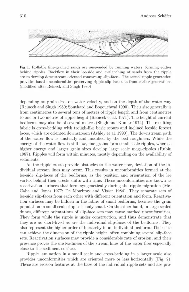
310 Andreas Schafer
Fig. 1. Rollable fine-grained sands are suspended by running waters, forming eddiesbehind ripples. Backflow in their lee-side and avalanching of sands from the ripplecrests develop downstream oriented concave-up slip-faces. The actual ripple generationprovides basal unconformities preserving ripple slip-face sets from earlier generations(modified after Reineck and Singh 1980)
depending on grain size, on water velocity, and on the depth of the water way(Reineck and Singh 1980; Southard and Bogouchwal 1990). Their size generally isfrom centimetres to several tens of metres of ripple length and from centimetresto one or two metres of ripple height (Reineck et al. 1971). The height of currentbedforms may also be of several metres (Singh and Kumar 1974). The resultingfabric is cross-bedding with trough-like basic scours and inclined leeside foresetfaces, which are oriented downstream (Ashley et al. 1990). The downstream pathof the water flow is unsteady and modified by the bed roughness. While theenergy of the water flow is still low, fine grains form small scale ripples, whereashigher energy and larger grain sizes develop large scale mega-ripples (Rubin1987). Ripples will form within minutes, mostly depending on the availability ofsediments.
As the ripple crests provide obstacles to the water flow, deviation of the in-dividual stream lines may occur. This results in unconformities formed at thelee-side slip-faces of the bedforms, as the position and orientation of the leevortex behind their crests shifts with time. These unconformities are known asreactivation surfaces that form syngenetically during the ripple migration (Mc-Cabe and Jones 1977; De Mowbray and Visser 1984). They separate sets oflee-side slip-faces from each other with different orientation and form. Reactiva-tion surfaces may be hidden in the fabric of small bedforms, because the grainpopulation in small scale ripples is only small. On the other hand, in large-scaleddunes, different orientations of slip-face sets may cause marked unconformities.They form while the ripple is under construction, and thus demonstrate thatthey are as short-lived as are the individual slip-faces of the bedforms. Theyalso represent the higher order of hierarchy in an individual bedform. Their sizecan achieve the dimension of the ripple height, often combining several slip-facesets. Reactivation surfaces may provide a considerable rate of erosion, and theirpresence proves the unsteadiness of the stream lines of the water flow especiallyclose to the sediment surface.
Ripple lamination in a small scale and cross-bedding in a larger scale alsoprovides unconformities which are oriented more or less horizontally (Fig. 2).These are erosion features at the base of the individual ripple sets and are pro-

Depositional Systems and Missing Depositional Records 311
eu
eu
eu
eueu
rs
rs rs
rs
rs
bedform migration
eu
Fig. 2. Slip-faces from sandy aquatic bedforms form sets of downstream orientedconcave-up inclined strata. They are subsequently eroded by the next younger gen-eration of bedforms. Result is a sedimentary structure of either small-scale currentripple lamination or large-scale trough cross-bedding, depending on the size and formof the migrating bedforms, each of them separated by sub-horizontal erosion unconfor-mities (eu). Minor deviations in the downstream water-flow and erosions of slip-facesets develop reactivation surfaces (rs), proving synchronous reworking of the migratingbedforms. Reactivation surfaces are the next lower hierarchy relative to the individualslip-face sets, followed by the erosion unconformities.
vided by the downstream migration of the bedforms. They are horizontal if nonet sedimentation takes place, but may rise downstream if there is an increasein sediment volume, resulting in a climbing-ripple lamination (Leeder 1999).Trough-like cross-bed sets and current-ripple lamination will only be preservedto minor parts of the original height of the bedforms. Sediment layers subse-quently following each other will erode the stratum of bedforms prior to theactual one. Thus, rippled resp. cross-bedded carpets of sands in a vertical sec-tion only represent about one third of the original bedform height or even lessthan this (Rubin 1987). The unconformities underneath the actual series of bed-forms are syngenetic and include time breaks of a duration depending on theindividual sub-environment where the formation of the bedforms takes place.The unconformities separate ripple sets or cross-bed sets and clearly are erosionsurfaces. With respect to the slip-faces and their reactivation surfaces, they areof a lower order in the deposition hierarchy. They are near-horizontal beddingplanes of depositional sequences with only minor differences between the indi-vidual grain-size populations. Erosion surfaces may also be syngenetic surfaces,while deposition and erosion is more or less at the same time.
2.2 Vertical Facies Successions
Vertically stacked facies successions form sedimentary sequences through lay-ered sediments or sedimentary rocks. The sequences contain strata with beddingfeatures, which reflect the hydrodynamic conditions during deposition (Walker1984; Reading 1996; Leeder 1999), also forming the substrate for biota. Facies

312 Andreas Schafer
and facies successions of siliciclastic sediments describe processes of depositionby traction transport or suspension transport through the water column. Sedi-mentary sequences consist of individual strata of stacked depositional environ-ments of past landscapes. Sedimentary sequences are uniform, if the conditions— which lead to their deposition — also are uniform. Yet, if for instance a cut-offof a meander loop occurs, the sedimentary sequence of the river plain will bechanged from a channel facies to an oxbow-lake facies (Walker and James 1992).
Sedimentary sequences or facies succession motifs (sensu Cross, pers. comm.)describe depositional environments (e. g. a high-energy coast; Fig. 3). They con-tain the deposits of individual sub-environments verifying smaller reaches withinthem (e. g. shoreface, swash zone of the shore, dunes on the back shore). Eachsub-environment alongshore has its specific grain-size range depending on theenergy of the sea, its specific range of bedding-features, relevant to the paleoe-cology of species of plants and animals. Each sub-environment shows a differentchance of preservation and a different rate of accumulation (Reineck and Singh1980). These individual characteristics result in different vertical lengths of sedi-mentary sequences with different succession motifs of fining-up or coarsening-upfeatures or in an interbedded style. To these sedimentary sequences, character-istic syngenetic unconformities and time gaps due to deposition, erosion, andre-deposition are included, only some of them being clearly visible. River chan-nel scours in a fluvial plain commonly show specific evidence, multiple crevassesplays mostly will be obliterated. Tidal channel outlets at a high-energy beachbeing of equivalent grain-size range as the coast will not show up, whereas muddytidal channels show clear evidence by point bars in mixed tidal flats.
Following this, sedimentary sequences are non-uniform build-ups, althoughthey are used as idealised sections to describe depositional models (Walker 1984).A fining-up sequence of several metres in a cored well shows a grain-size suitefrom coarse to fine and is coupled with a set of sedimentary structures fromtrough cross-bedding to small-scaled current-ripple lamination, including high-energy lamination, wave ripples and the like, desiccation cracks, and plant rootsin the overbank fines. This fining-up sequence may represent a continuous sectionthrough a meandering channel (Fig. 4). Nevertheless, it has to be consideredthat each sub-storey of this section consists of many sets of individual timespans, where deposition and reworking took place. The build-up of a sedimentarysequence in a meandering lowland river can be of a duration of half an hour orcan be a matter of several years depending on climate, tectonic frame, or earthperiod. This can only be shown by means of Wheeler diagrams, if the timecontrol is good (Wheeler 1964). The overall length of sedimentary sequencesalso is very variable, ranging from a metre to several tens of metres, rich insmall- and/or large-scale stratal gaps. Although sedimentary sequences are byno means complete, they are widely used as ideal sections through depositionalmodels. They are divided into units of grain-size trends related to the individualenergy content of the depositional environment (Moslow 1984; Fielding 1987).

Depositional Systems and Missing Depositional Records 313
sandmudfinemedium
tim
e
GAP
thic
kn
ess
salt marsh
coastal dune
back shore
fore shore
shoreface
transition zone
shelf
HTL
LTL
SWB
Fig. 3. This facies succession motif forms by sediment accumulation and reworking ata marine high-energy coast, being the most active coastal clinoform with respect tosediment accumulation and reworking. The paleogeographic range is from the shelf tothe back shore, where peats accumulate in the salt marshes and elevated areas. Theprofile length is different with respect to the individual coast. The shoreface lengthdepends on the exposition to the sea and energy of the wave fetch, causing differentdepths of the wave base. Moreover, the width of the fore shore is defined by the tidalrange and can be rather different, from several tens of metres to several kilometres. Also,the width of the back shore with eolian sands and algal mats upon, vary considerablyin area. The extension of the low-energy back-barrier tidal flats and the salt marshesalong the high-tide line (HTL) of the coast together with lagoons and bays reflectthe amount and quality of sediments provided from riverine input. The ‘time’ columnreveals numerous stratigraphical gaps, yet only few of them show up in the ‘thickness’column.

314 Andreas Schafer
sandmudfinemedium
GAPtim
e
thic
kn
ess
flo
od
pla
inm
ea
nd
erin
gch
an
ne
l
Fig. 4. A fluvial sedimentary sequence through a meandering channel shows a gener-alised section through its various storeys. The lower sandy part is the lateral accretionstorey of the meandering channel where point bars accrete downstream and towardeither sides of a channel in a lowland river. Individual downstream migrating mega-ripples form trough-cross-bed sets. They are embracketted by lateral accretion surfaceswhich can be understood as time surfaces and may be exemplified by major unconformi-ties. Rapidly waning of the flood develop small-scaled sedimentary features, dominantlycurrent-ripple lamination of fine-grained sands. In the vertical accretion storey mudsare deposited on the flood plain. They derive from a low-energy flooding. Numerousparaconformities with soil horizons, rootlets, desiccation cracks, and a wide variety ofconcretion nodules will be preserved. Seldom and only close to the channels, a floodingcauses crevasse splay, resulting both in a low-energy current-ripple lamination and ahigh-energy parallel-bedding of fine-grained sands, often resulting a soft deformationof muddy substrates underneath. The ‘time’ column reveals numerous stratigraphicalgaps, yet only few of them show up in the ’thickness’ column.

Depositional Systems and Missing Depositional Records 315
Sedimentary sequences contain stratal gaps, only some of them being wellresolved in the ancient record. If these gaps are paraconformities in flood plains,the identification of the individual time gap is not possible. If these gaps are atthe base of channels and form marked disconformities, it depends on the fluvialmodel, whether a time gap of several years or tens of years is evident due tothe position of the river in a proximal or a distal part of the alluvial plain and,whether the base level rises or falls. Disconformities may prove the time gapthat can range from tens to thousands of years, and easily reach geologic ages,if angular unconformities are revealed (Boggs 1995). As a result, the missingstratigraphical record in depositional sequences can be little, if they are withinone depositional model. But stratigraphical gaps can be enormous, if the tectonicframe of the basin is responsible for disconformities or angular unconformities,when rivers cut their courses across a newly exposed alluvial plain.
2.3 Sequence Stratigraphy — Systems Tracts, Sequences, and Parasequences
Sequence stratigraphy provides a conceptual framework to coordinate the ar-rangement of sedimentary sequences in sedimentary basins (Vail et al. 1991;Posamentier and James 1993). Due to the rise and fall of the sea level, to thetectonics of the earth crust underneath, and to the input of sediment from anuplifted orogen in the hinterland, sedimentary sequences form in tight relationto the ‘relative sea level’.
For the use of sequence stratigraphy, stratigraphic charts in regional geol-ogy are divided with a cyclicity of about 3 to 0.5 million years. This 3rd-ordercyclicity (Haq et al. 1987; Wilgus et al. 1988) is related to the earth’s stress fieldand to a large-scale climate development due to the earth’s ice shield. The basicunits are ‘systems tracts’. They can be a lowstand, transgressive, and highstandsystems tract, each of which consists of a series of different depositional environ-ments, from the deep sea to the continental alluvium (Weimer and Posamentier1993). The ‘systems tracts’ provide the stratigraphic correlation between conti-nents across the oceans. Stratigraphical standards in sedimentary basins are ofdifferent scales, and they use sediment models to define sedimentary sequences.As stratigraphic approaches meanwhile differ somewhat from the initial concept,various ‘systems tracts’ exist today. Yet, measured sections in sedimentary basinsare rather easily correlated with the 3rd-order cyclicity (Hardenbol et al. 1998).
Sequence stratigraphy also recognizes cyclicities higher than the 3rd order,which are the Milankovitch cycles. They depend on the geometry of the earth’sorbit around the sun, the eccentricity (e) of the earth’ circuit, the obliquity(o) of the earth’ axis, and its precession (p) i. e. its wobble while turning (p)(Emery and Myers 1996). This provides four periods with different time spans:413 ka and 112 ka (e), 41 ka (o), 21 ka (p). These measures of differing cyclici-ties allow subdivision of the ‘systems tracts’ (3rd order) into smaller units (4th,5th, and 6th orders), so that sedimentary sequences of shorter time length canbe used for geological field and subsurface work. Depending on the individualsedimentary basin, its time frame, and the sedimentary model of its basin-fill,in sequence stratigraphy ‘parasequences’ and ‘sequences’ are currently in use

316 Andreas Schafer
(Fig. 5). ‘Parasequences’ are shoaling-up, progradational successions, separatedfrom each other by ‘marine flooding surfaces’ being preferably used in coastalmarine environments, whereas ‘sequences’ are separated from each other by sub-aerial unconformities, i. e. ‘sequence boundaries’. These are preferably used incontinental environments, considering that ‘sequence boundaries’ are surfaceswith subaerial exposure (Fig. 6; Plint and Nummedal 2000).
incised valley
transgressive surface (TS)transgressive
systems tract (TST)
sequencehighstand
systems tract (HST)
open marinefacies
coastal faciessaltmarsh faciesalluvial facies
sequence boundary (SB)
sequence boundary (SB)
3.
FS
FS
2.
1.
mfs
parasequenceparasequence
Fig. 5. A coastal scenery shows the relationship of ‘systems tracts’, ‘sequences’, and‘parasequences’ in a sequence stratigraphical concept. Due to a relative sea-level high-stand, ’parasequences’ of a prograding coastal environment provide coarsening-up litho-facies sections. At the coastal clinoform (i. e. coastal facies), they are separated by‘flooding surfaces FS’ (equivalent to ‘transgressive surface TS’). The same time, in thealluvial reach of the coast, ‘sequences’ develop which are confined by erosive ‘sequenceboundaries SB’. The prograding ‘parasequences’ are combined to form a ‘highstandsystems tract HST’ (modified after Walker 1990).
This sequence stratigraphy concept, since its origin more than 25 years ago,meanwhile has become the dominant stratigraphic paradigm to work in bothsiliciclastic and carbonate environments. Nevertheless, quite often it is difficultto overcome the restricted range of the outcrop size or basin geometry exposed.The stratigraphical lengths and gaps between ‘systems tracts’, ‘sequences’, and‘parasequences’ in sequence stratigraphy may range widely. Therefore, they arenot always ideal to individual facies studies. On the other hand, sequence stratig-raphy has become established to use it in basin analysis, whether by seismicsections, well profiles, or measured sections in outcrop studies (Nummedal et al.2001).
2.4 Base Levels
The concept of base level cyclicity (Barrell 1917; Cross and Lessenger 1997,1998) is an approach with more practical use in field work. Transgressive surfacesand sequence boundaries still keep their stratigraphical meaning. Base levels arefixed to the storm wave base of the coastal clinoform forming an ideal surface

Depositional Systems and Missing Depositional Records 317
Fig. 6. This figure is redrawn from Plint and Nummedal (2000: Fig. 2), with respect tothe original version the time section is omitted and the facies section slightly exagger-ated in vertical height. The model (referring to a field example in Alberta, Canada)shows a ramp setting sequence constructed by shifting equilibrium profiles according tothe relative sea-level curve at the right of the figure. Erosion and deposition happenedalong the axis of an incised valley, well verified during the falling stage of the relativesea-level, during regression. At the base of the section, a transgressive series sits ontop of a maximum flooding surface of an older series, providing a Highstand SystemsTract. During regression, coastal sediments of the Falling Stage Systems Tract progradetoward the sea to the right. As regression continues, the proximal fluvial environmentalso progrades seaward and deeply erodes the coastal deposits. In the Lowstand Sys-tems Tract, at the most basinward position, marine sediments are laid down. Duringsubsequent transgression, the Transgressive Systems Tract follows with coastal plainmuddy sediments of a backbarrier environment located behind shoaling sands and bar-rier islands. The Highstand Systems Tract causes frequent flooding, ravinement, andlastly a maximum flooding, the surfaces of all of them trending landward. On top of theMaximum Flooding Surface, the Highstand Systems Tract shows a variety of coastalenvironments which are fed from a river net widely extending to the hinterland.
of erosion, and can be traced from here in a landward direction (Fig. 7). Thebase level correlates with the height of the relative sea level. This is clear at thecoast, but may be ambiguous in continental basins far off the sea, as the drainagesystem of major rivers also is guided by the structural model of the basin. Crossand Homewood (1997: p. 1624–1625) sum up the modern understanding of thebase level concept, that will be cited partially in the following.
Barrell (1917): “Where base level is above the earth’s surface, sediment willaccumulate if sediment is available. Where base level is below the earth’s surface,sediment is eroded and transported downhill to the next site where base level isabove the earth’s surface. These transits of base level . . . produce a stratigraphicrecord . . . as regular vertical successions of facies separated by surfaces of uncon-formity. . . . time [is] continuous and . . . is fully represented in the stratigraphicrecord by the combination of rocks plus surfaces of stratigraphic discontinuity.”
Wheeler (1964) “considered stratigraphic base level as an abstract (nonphys-ical), nonhorizontal, undulatory, continuous surface that rises and falls with re-spect to the earth’s surface. Stratigraphic base level is a descriptor of the inter-actions between processes that create and remove accommodation space.

318 Andreas Schafer
Fig. 7. The base level is fixed to the storm wave base at the coastal clinoform, separatingthe ‘shoreface’ from the ‘transition zone’. During storms, especially winter storms, thecoast can be reworked, also totally removed during a slow transgression. From here,the base level may be traced to continental environments in the coastal alluvium.Depending on the tendency ’transgression’ or ‘regression’ of the sea, this surface ofpotential erosion shifts toward the land or toward the sea. It results in ‘base level rise’or ‘base level fall’, each precisely depicted by a sequence of depositional features at anyplace of observation between the deep sea and continental alluvium (see text for moredetails).
. . . defined stratigraphic base level as a potentiometric energy surface thatdescribes the energy required to move the Earth’s surface up or down to a posi-tion where gradients, sediment supply, and accommodation are in equilibrium.”
Wheeler’s stratigraphic base level is the conceptual device that links severalconcepts (Cross and Homewood 1997):
– Gressley’s facies and facies tracts,– Wather’s notion of the ‘zig zag’ uphill and downhill movement of facies tracts,– Gressley’s and Walther’s identification that this movement is recorded as
regular vertical facies successions that define stratigraphic cycles,– Barrel’s notion that base level cycles are the clock of stratigraphy (and there-
fore that correlations based upon physical stratigraphy are possible),– Barrell’s concept of sediment volume partitioning.
The base level method has been adopted since a while to sedimentologicalfield research (Cross et al. 1993; Cross and Lessenger 1998). With some sim-plification, base level rise considers a deepening of the environment due to anincrease of the A/S rate (accommodation space to sediment supply), whereasbase level fall describes its shallowing due to a decrease of the A/S rate. Bothhalf cycles are more or less equivalent to coastal onlap and coastal offlap of thesequence stratigraphy concept (Galloway 1989). The base level concept resolvesa stratigraphic sequence in a much smaller scale, even in a 5th- and 6th-ordercyclicity. The cyclic development of the depositional environment — whether itis in the deep sea, on the coastal clinoform, or far off the sea in a continentalbasin — provides a fining-up or a coarsening-up of the depositional sequencetogether with a shift of the individual energy content and the balance betweenthe accommodation space of the sedimentary basin and the sediment supply toit. This observation can easily be made by sedimentological measures in field

Depositional Systems and Missing Depositional Records 319
FUTMU
CUFS
shelf
low-energycoast
lagoonal
delta
delta front
delta foot
prodelta
distributarychannel
tidalchannel
high-energy
coast
shelf
2
3
4
1
2
3
4
5
1
fall
fall
rise
rise
fall
fall
rise
rise
fall
MSCS
floodplain
lagoonaldelta
A/S max
A/S max
A/Smin
A/S min
braidedriver
lagoon
peat
peat
A/Smin
A/Smin
FUTMU
CUFS
MSCS
CK FKMK
ravinement
Fig. 8. Two successions of rocks are shown, each consisting depositional sequences whichare ‘measured’ from ideal fluvial, deltaic, and coastal environments, each with the inter-pretation of the depositional environments and subenvironments alongside. In addition,the base level cyclicity is indicated by triangles pointing upward (‘base level rise’) ordownward (‘base level fall’), also the quotient A/S (accommodation space vs. sedimentsupply), reflecting the variation of the relative sea-level, the structural development ofthe sedimentary basin, and the sediment supply to it.

320 Andreas Schafer
and on cores (Fig. 8). As the observation mostly is done in outcrop-scale, thisconcept is extremely helpful and preferably focuses on small-scale work. Baselevel cyclicity is a logic concept useful at any scale of cyclicity. It explains indi-vidual depositional sequences and the basin-fill geometry of sedimentary basins(Cross and Lessenger 1998).
3 Missing depositional record
As was shown above, depositional sequences are used as entities (cf. Figs. 3 and4). Yet, at a closer look, numerous gaps of erosion or non-deposition in thesesedimentary sequences occur (Dott 1983). Depending on the local environment,the stratigraphical gaps present different time spans. Sedimentological modelsprefer complete sedimentary sequences, ignoring their origin, stratigraphic, andgeographic position. These models are ideal and tend to disregard the gaps whichare provided from the environment, due to shifts of transport directions, tides,emersion, etc.
On the other hand, the concept of sequence stratigraphy and base level cyclic-ity is based on the understanding of stratigraphic gaps. Sequence boundarieswith a clear-cut subaerial exposure, reveal stratigraphic gaps in thickness andtime, during which deposits having been removed. The stratigraphic relevance ofsequence boundaries comes clear in Wheeler diagrams when regressive surfacesprovide stratigraphical gaps in the individual stratigraphic sequence (Wheeler1964). As the sequence stratigraphic concept is based on the 3rd-order cyclicity,the missing depositional record can easily be of a duration of 0.5–3 million years.Clearly, this is a time span only relevant in a basin-scale context.
The attempts to increase the time resolution of depositional cycles and ofstratigraphic gaps in between, normally leads to a high-frequency sequencestratigraphy with a cyclicity in a Milankovitch range of a 4th-order (500 ka–100 ka) or 5th-order (100 ka–20 ka) concept. Although high-order cycles are welldefined, only the cycle lengths of 400 ka and 100 ka will be deciphered in thestratigraphic record with some certainty, not so the 40 ka and the 20 ka signal.The latter two cycle lengths interfere with autocyclic signals from the environ-ment itself, from weather and shifts of drainage patterns.
Miall (1991) proposes a ten-grouped depositional hierarchy for use in clasticsediments that subdivides a range from the 3rd-order cyclicity (group 10) toburst-and-sweep processes in traction currents or grain-fall and -flow in eoliandunes (group 1). This range embraces a time-scale from 3 million years to afew seconds. The high-order groups 10 to 8 are established parallel to the 3rd-,4th-, and 5th-order of the sequence stratigraphic concept, whereas below group7, a 6th-order cyclic behaviour of depositional processes is revealed, both incontinental and marine environments. The physical scale of the depositionalunits are of 14 orders of magnitude. Also, the sedimentation rates are from105 m/ka (group 2) to 10−1 to 10−2 m/ka (groups 9 and 10). Bounding surfaces,surfaces of non-deposition, or erosional discordances are more frequent towardthe higher-order groups. Sedimentation rates in low-order groups depend on

Depositional Systems and Missing Depositional Records 321
SB
SB
10 m
rise
fall
1 m
basinenvironmentsub-environment
0,1m
bed
hours - 102
years
depositional sequence
102
104
yearsto
sequence set
104
106 yearsto
coastal sequence
Fig. 9. Coastal depositional sequences consisting each of a set of beds, forming detailsof a full transgressive-regressive cycle as used in basin analysis (modified after Aigneret al. 1990, following the concept of Cross and Lessenger 1997). The base level cyclicity(verified as hemi-cycles) is indicated by triangles (base level rise and base level fall).Moreover, time ranges for the deposition, erosion, and redeposition of the individualbeds, depositional sequences, and sequence sets are shown.
sedimentation/erosion processes in even one depositional cycle, whereas in high-order groups depositional processes are more due to the accommodation space ofthe environment, and lastly, of the entire sedimentary basin. As a consequence,“the sedimentation rate varies in inverse relation to the length of time over whichthe measurement is made”.
Base level cyclicity enables to show more from the small-scaled variationof the environments (Cross and Lessenger 1997). In a continental environment,channel migration, floodplain emersion, multiple stacking of fluvial fan lobesetc. can be defined as base level rise cycles. These may be of a length of a 5th-or a 6th-order cyclicity. This environment-bound cyclicity defines flooding anderosion unconformities between depositional sequences. On the other hand, itenables to sum up small-scaled stacked channels to define a thick fluvial suc-cession with relevance to the fill of a large-scaled sedimentary basin (Ramonand Cross 1997). Each, the individual environment and the basin-fill can wellbe verified. Missing depositional records provide precise surfaces on top of en-vironments and paleogeographic settings. They form time lines which can beunderstood as interbasinal correlation surfaces. As an example, a set of coastalsequences show the hierarchy of sub-environments and environments for use in

322 Andreas Schafer
basin analysis (Fig. 9). The variability of scales of time used for deposition ofthese beds and their thicknesses may indicate that also gaps exist in which noth-ing was deposited or — more often in a coastal environment — in which bedswere removed by reworking during winter storms or by variations of the relativesea level, in detail and in basin-scale.
Acknowledgements I appreciate the discussion that Tim A. Cross (ColoradoSchool of Mines, Golden, Colorado, USA) offered to an early version of thispaper. Also, the help of Agemar Siehl, Clemens Simmer, and Christian Derer(all from University of Bonn) is kindly acknowledged.
References
Aigner, Th., Bachmann, G. H. and Hagdorn, H. (1990): Zyklische Stratigraphie undAblagerungsbedingungen von Hauptmuschelkalk, Lettenkeuper und Gipskeuper inNordost-Wurttemberg. Jber. Mitt. oberrhein. geol. Ver., N. F. 72, 125–143.
Allen, J. R. L. (1979): Physical Processes of Sedimentation. 248 pp., 5th ed., (Allen andUnwin) London.
Allen, J. R. L. (1982): Sedimentary Structures. Their Character and Physical Basis. —volume I, 594 pp.; volume II, 644 pp., (Elsevier) Amsterdam, New York.
Ashley, G. M. (symposium chairperson) (1990): Classification of large-scale subaqueousbedforms: A new look at an old problem. J. Sedimentary Petrology, 60, 160–172.
Barrell, J. (1917): Rhythms and measurement of geologic time. — Geol. Soc. America,Bull., 28, 745–904.
Blum, M.D. and Tornqvist, T. E. (2000): Fluvial responses to climate and sea-levelchange: a review and look forward. Sedimentology, 47, Suppl. 1, 2–48.
Boggs, S. jr. (1995): Principles of Sedimentology and Stratigraphy. — 774 pp., 2nd ed.,(Prentice-Hall) Englewood Cliffs, NJ.
Cross, T.A. et al. (1993): Application of high-resolution sequence stratigraphy to reser-voir analysis. — in: Eschad, R. and Doligez, B. (eds.): Subsurface reservoir char-acterisation from outcrop observations. Proceedings of the 7th Exploration andProduction Research Conference, Technip, 11–33, Paris.
Cross, T.A. and Homewood, P.W. (1997): Amanz Gressley’s role in founding modernstratigraphy. — Geol. Soc. America, Bull., 109, 1617–1630.
Cross, T.A. and Lessenger, M.A. (1997): Correlation strategies for clastic wedges. — in:Coulson, E.B.; Osmond, J. C. and Williams, F. T. eds.): Innovative Applications ofPetroleum Technology in the Rocky Mountain Area. Rocky Mountain Associationof Geologists, 183–203.
Cross, T.A. and Lessenger, M. A. (1998): Sediment volume partitioning: rationale forstratigraphic model evaluation and high-reolution stratigraphic correlation. — in:Gradstein, F.M., Sandvik, K.O. and Milton, N. J., Sequence Stratigraphy — Con-cepts and Applications, NPF Spec. Publ., 8, 171–195.
De Mowbray, T. and Visser, M. J. (1984): Reactivation surfaces in subtidal channeldeposits, Oosterschelde, Southwest Netherlands. J. Sediment. Petrol., 54, 811–824.
Dott, R. H. jr. (1983): 1982 SEPM Presidential Address: Episodic sedimentation —how normal is average? How rare is rare? Does it matter?, J. Sed. Petrol., 53, 1,5–23.

Depositional Systems and Missing Depositional Records 323
Einsele, G. (2000): Sedimentary Basins. Evolution, Facies, and Sediment Budget. —792 pp., 2nd ed., (Springer) Heidelberg, Berlin, New York.
Emery, D. and Myers, K. J. (ed. 1996): Sequence Stratigraphy. — 297 pp., (Blackwell)Oxford.
Fielding, C.R. (1987): Coal depositional models for deltaic and alluvial plain sequences.Geology, 15, 661–664.
Galloway, W.E. (1989): Genetic stratigraphic sequences in basin analysis I: architectureand genesis of flooding- bounded depositional units. Amer. Assoc. Petrol. Geol.,Bull., 73, 125–142.
Haq, B.U.; Hardenbol, J. and Vail, P.R. (1987): Chronology of fluctuating sea levelssince the Triassic. Science, 235, 1156–1166.
Hardenbol, J.; De Graciansky, C.; Jacquin, T. and Vail, P.R. (eds. 1998): Mesozoicand Cenozoic Sequence Stratigraphy of European Basins. Soc. Econ. Pal. Min.,Spec.Publ., 60, 1–485.
Leeder, M.R. (1999): Sedimentology and Sedimentary Basins. From Turbulence toTectonics. — 592 pp., (Blackwell) Oxford.
McCabe, P. J. and Jones, C.M. (1977): Formation of reactivation surfaces within su-perimposed deltas and bedforms. J. Sediment. Petrology, 47, 707–715.
Miall, A.D. (1991): Hierarchies of architectural units in terrigenous clastic rocks, andtheir relationship to sedimentation rate. — in: Miall, A.D. and Tyler, N. (eds.): Thethree-dimensional facies architecture of terrigenous clastic sediments and its impli-cations for hydrocarbon discovery and recovery.- SEPM Concepts in Sedimentologyand Paleontology, 3, 6–12, Tulsa.
Moslow, T. F. (1984): Depositional models of shelf and shoreline sandstones. Amer.Assoc. Petrol Geol., Contin. Educ. Course Note, Series 27, 102 pp.
Nummedal, D., Cole, R., Young, R., Shanley, K. and Boyles, M. (2001): BookCliffs Sequence Stratigraphy: The Desert and Castlegate Sandstone. — 81 pp.,GJGS/SEPM Fied Trip # 15, June 6–10, 2001 (in conjunction with the 2001 An-nual Convention of the American Association of Petroleum Geologists); Denver,Colorado.
Pettijohn, F. J., Potter, P. E. and Siever, R. (1987): Sand and Sandstone. — 553 pp.,2nd ed., (Springer) Berlin, Heidelberg, New York.
Posamentier, H.W. and James, D. P. (1993): An overview of sequence-stratigraphicconcepts: uses and abuses. Spec. Publs. Int. Ass. Sediment., 18, 3–18.
Ramon, J. C. and Cross, T. A. (1993): Characterization and prediction of reservoir ar-chitecture and petrophysical properties in fluvial channel sandstones, middle Mag-dalena Basin, Colombia. CT and F-Ciencia, Technologıa y Futuro, 1, 3, 19–46.
Reading, H.G. (1986): Sedimentary Environments and Facies. — 615 pp., 2nd ed.,(Blackwell) Oxford.
Reineck, H.-E. (1960): Uber Zeitlucken in rezenten Flachsee-Sedimenten. Geol. Rund-schau, 49, 149–161.
Reineck, H.-E. and Singh, I. B. (1980): Depositional Sedimentary Environments. — 549pp., 2nd ed., (Springer) Heidelberg, Berlin, New York.
Reineck, H.-E.; Singh, I. B. and Wunderlich, F. (1971): Einteilung der Rippeln undanderer mariner Sandkorper. Senckenbergiana maritima, 3, 93–101.
Rubin, D. M. (1987): Cross-bedding, bedforms, and paleocurrents. Concepts in Sedi-mentology and Paleontology, 1, 1–187, Tulsa.
Singh, I. B. and Kumar, S. (1974): Mega and giant ripples in the Ganga, Yamuna, andSon rivers, Uttar Pradesh, India. Sediment. Geol., 12, 53–66.
Southard, J. B. and Bogouchwal, L. A. (1990): Bed configurations in steady unidirec-tional water flows. Part 2: Synthesis of flume data. J. Sediment. Petrol., 60, 658–679.

324 Andreas Schafer
Sundborg, A. (1967): Some aspects on fluvial sediments and fluvial morphology. I.General views and graphic methods. Geograf. Ann., 49, 333–343.
Tanner, W.F. (1978): Reynolds and Froude Numbers. — in: Fairbridge and Bourgeois(eds.): The Encyclopedia of Sedimentology. Encyclopedia of Earth Sciences Series,6, 620–622.
Vail, P.R.; Audemard, F.; Bowman, S. A.; Eisner, P.N. and Perez-Cruz, C. (1991): Thestratigraphic signatures of tectonics, eustasy and sedimentology — an overview. —in: Einsele, G.; Ricken, W. and Seilacher, A. (eds.): Cycles and Events in Stratig-raphy. — 617–659, (Springer) Berlin, Heidelberg, New York.
Walker, R.G. (ed. 1984): Facies Models. Geoscience Canada Reprint Series 1, 317 pp.,2nd ed., (Geol. Assoc. Canada) St. Johns.
Walker, R.G. and James, N. P. (ed. 1992): Facies Models. Response to Sea LevelChange. — 409 pp., (Geol. Assoc. Canada) St. Johns.
Walther, J. (1893/1894): Einleitung in die Geologie als historische Wissenschaft.Beobachtungen uber die Bildung der Gesteine und ihrer organischen Einschlusse.— Dritter Teil: Lithogenesis der Gegenwart. Beobachtungen uber die Bildung derGesteine an der heutigen Erdoberflache. — 535–1055, (Gustav Fischer) Jena.
Wheeler, H. E. (1964): Baselevel, lithosphere surface, and time-stratigraphy. Geol. Soc.Amer., Bull., 75, 599–610.
Weimer, P. and Posamentier, H.W. (eds. 1993): Siliciclastic sequence stratigraphy.Amer. Assoc. Petrol. Geol., Memoir, 58, 1–492.
Wilgus, C.K.; Hastings, B. S.; Kendall, C. G. S. C.; Posamentier, H.W.; Ross, C.A.and Van Wagoner, J. C. (eds. 1988): Sea-level changes: An integrated approach.Soc. Econ. Pal. Min., Spec. Publ., 42, 1–407.

Multi-Scale Processes and the Reconstruction ofPalaeoclimate
Christoph Gebhardt1, Norbert Kuhl2, Andreas Hense1, and Thomas Litt2
1 Meteorological Institute, University of Bonn, Germany2 Institute for Palaeontology, University of Bonn, Germany
Abstract. In this section, we focus on multi-scale problems encounteredwhen reconstructing palaeoclimate on the basis of terrestrial botanicalproxy data (pollen and macro remains). Climate and the taxonomicalcomposition of the vegetation are affected and linked by complex geo-processes acting on various spatial and temporal scales. We describehow the resolution of these data — both in space and time — lim-its the scale of features which can be reconstructed. We then presenta Bayesian statistical transfer function relating vegetation and climatewhich is based on a Boolean approach (“taxon existent”–“taxon non-existent”). This transfer function allows for an effective avoidance of“no modern analogue”-situations and intents to reduce the influence ofsub-scale processes (e. g. local effects) and of non-climatic factors on thereconstruction.We present two types of transfer functions: a reconstruction model suit-able for reconstructions of local palaeoclimate and a backward modelwhich can be used to reconstruct spatially coherent climatological fields.The reconstruction model is given by probability density functions forthe climate conditional on the existence of certain taxa. The backwardmodel is deduced from the reconstruction model in a straightforwardway using the Bayes theorem. For the spatially coherent reconstruction,the backward model is combined with a dynamical constraint in orderto stabilise the reconstruction which is normally based on a relativelysparse network of palaeo-observations. We use a singular value decom-position of the dynamics to restrict the reconstruction to the dominantand resolvable scales.
1 Introduction
The reconstruction of palaeoclimate depends on the use of proxy data, becauseit is not directly measurable. The relation of proxy data to modern climateconditions can be converted into a transfer function which is applied back intime. The description of the underlying processes by the transfer functions canbe based either on a statistical approach or on an explicit modelling.
Various types of data can serve as substitute for direct meteorological mea-surements, e. g. physical or biological (cf. Berglund 1986, Frenzel 1991, Schleser
H.J. Neugebauer and C. Simmer (Eds): LNES 97, pp. 325–336, 2003.
c© Springer-Verlag Berlin Heidelberg 2003

326 Christoph Gebhardt, Norbert Kuhl, Andreas Hense, and Thomas Litt
et al. 1999). In the following, pollen and macro remains serve as an examplefor botanical proxy data. In suitable environments, they are conserved over longperiods. The use of these data implies that a significant relation between theproxy data, i. e. the plants that produced the fossils, and the considered climateparameters exist. However, organisms are influenced by and interact with theenvironment in a very complex way. Moreover, the influence of climate as well asother factors differ on different scales, urging to address the appropriate scale.
Palaeo-conditions can be calculated quantitatively by transfer functions usingtoday’s dependences of the proxy data. For establishing the relationship betweenbiological data and environmental variables multivariate numerical analyses wereused based on multiple linear regression models (Birks and Birks 1980, Birks andGordon 1985). In this respect climate estimates from botanical data and theirapplication for palaeoclimatological reconstructions are important, but the quan-tification of the function relating vegetation and climate is problematic (see theclassical study by Iversen 1944 using climatic indicator species). First numeri-cal methods in pollen analysis were developed by Webb and Bryson (1972) toreconstruct palaeoclimate. This method was later adopted and modified (Guiot1990; Huntley and Prentice 1988, Pons et al. 1992, Field et al. 1994). However,the lack of modern analogues for several fossil pollen spectra is a disadvantageof this method (as measured by the dissimilarity coefficients, see Overpeck et al.1985).
The study of the plant — climate relations depends on the knowledge ofthe plant distributions (chorology) and the climate conditions in the studiedgeographical region. Fig. 2 shows an example of the combination of a griddedclimatology and distribution area. To which extent factors influence plant distri-bution depends, amongst others, on the regarded scale. As can be learned fromthe contributions of the previous chapters, the methods suitable for the descrip-tion of the dynamics of and the interactions between different earth systems(e. g. atmosphere, biosphere, hydrosphere, . . . ) depend on the considered scales.On the comparatively small scales, explicit modelling of the dynamical processesand the coupling between different scales is possible (Mendel et al. 2002). Onlarger scales, the numerical solution of the underlying differential equations isonly feasible using a coarser resolution. The effects of the subgrid-scale processesand their interactions with the resolved scales can be parametrised in dependenceof the large-scale features (Gross et al. 2002; Heinemann and Reudenbach 2002)or their mean behaviour is described using “effective parameters” (Diekkruger2002). Our contribution deals with the large-scale end of the processes presentedin this book. On these large spatial and temporal scales, it is sufficient and moresuitable to apply a statistical model which summarises the effects of the interac-tion between climate and vegetation using a few parameters. The atmosphericdynamics can be satisfactorily described as quasi-stationary processes acting onthe broadest spatial scales. The quantification of the dependences of proxy dataon climate is closely connected to the chosen scale. Therefore it is essential tofind the suitable scales. In the following, we will demonstrate that the large scalesare the important scales in the presented reconstruction problem.

Multi-Scale Processes and the Reconstruction of Palaeoclimate 327
2 Variability of data on different spatial and temporal scales
2.1 The meteorological data
We consider the case that the climatological data set is given as gridded fieldsof climatic near-surface variables. Such data are subject to various types of vari-ability on different temporal and spatial scales. The spatial variability includes
– large-scale effects (O(10,000)–O(1,000)) km) due to solar insolation varia-tions at the top of the atmosphere and land-sea contrasts
– meso-scale orographic and land-sea distribution effects (O(1,000)–O(100) km)
– and small-scale effects (< O(100) km) due to soil type, orography, and veg-etation.
The temporal variability is composed of
– long timescale effects due to astronomic forcing factors (Milankovitch cycles)and changes in the oceanic thermohaline circulation
– decadal and interannual variations due to El Nino or long term changes ofthe North Atlantic Oscillation
– fast variations like the annual or even the daily cycle.
The palaeoclimate reconstruction is restricted to certain spatial and temporalscales which are basically determined by the characteristics specific to the givendata — the recent climatological and botanical data as well as the palaeobotani-cal data —, the assumptions related to the chosen method of reconstruction, andthe characteristics of atmospheric dynamics. First of all, the grid-spacing of theclimatological data (e. g. 0.5 × 0.5 longitude-latitude grid (New et al. 1999))determines a lower limit of the spatial scale that can be resolved by the recon-struction. However, due to the multi-scale variability inherent in the atmosphericdynamics, aliasing effects representing undersampled sub-scale variability mightbe misinterpreted as features on the grid scale.
Furthermore, a reconstruction based on terrestrial botanical proxy data as-sumes identical dependences on climate for both modern botanical observationsand palaeovegetation. Additionally, the reconstruction of a high-dimensional fieldfrom a small set of palaeo-observations is a (seriously) ill-defined regression prob-lem which can only be stabilised by additional information such as a given cli-matic reference field. In consequence of the last two points, the palaeoclimate tobe reconstructed should be similar to an a priori chosen background state, e. g.the present climate. However, it is yet unclear how large the maximum deviationcan be. A safe meteorological estimate would be to avoid deviations larger thanabout ±5 K which is about the internal variability scale of present-day naturalclimate fluctuations in Europe. Due to the characteristics of the atmosphericdynamics, such anomalies or deviations of climatic variables from the modernmean are basically large-scale features: If we assume that e. g. the rate of changeof the temperature dT
dt following the trajectory of an air parcel is controlled by

328 Christoph Gebhardt, Norbert Kuhl, Andreas Hense, and Thomas Litt
a forcing function Q depending on space and time we get an equation which de-scribes the temporal and spatial structure of the temperature field completely.This equation states that the temporal rate of change of the field structure canbe described by the local temperature change and the horizontal advection in agiven flow v. We can write for two realisations i = 1, 2, e. g. the present day andthe climate of the Last Interglaciation (Eemian),
dT
dt=
∂Ti
∂t+ ∇(viTi) = Qi i = 1, 2 (1)
thereby assuming non-divergent flow conditions (∇vi = 0).As we investigate the structure of climate anomalies, we introduce the average
temperature T and its anomaly T ′ as
T = 12 (T1 + T2)
T ′ = T1 − T2.(2)
Taking the difference of the process equations above we obtain an equation forthe anomalies
∂T ′
∂t+ ∇(vT ′) + ∇(v′T ) = Q′ (3)
where the averages and anomalies of the flow velocity and the forcing functionare given as defined above for the temperature (Eq. 2).
Additionally it is assumed that the effects of the anomalous flow v′ upon theanomalous temperature can be parametrised as a diffusion process (K being thediffusion coefficient) leading to an equation for the temperature anomaly T ′:
∂T ′
∂t+ ∇(vT ′) − ∇(K∇T ′) = Q′. (4)
Thus we have derived a linear advection-diffusion equation for the anomalies. Thenon-linearities are transformed into the equation for the average which needs notto be considered in the present context because anomalies from a backgroundclimate are studied. As Eq. (4) is solved on a regular spatial grid with N gridpoints it has to be discretised. Let T be an N -dimensional vector with the gridvalues of T ′ as components. In consequence, the local rate of change and thelinear advection-diffusion operator can be written as an N ×N matrices D andM, respectively. Thus the discretised equation is given by
DT + MT = Q (5)
where Q is defined as the vector of forcing anomalies analogous to T .If we further assume a quasi-stationary anomaly field DT ≈ 0, the solution of
the remaining equation can be discussed best within the framework of dynamicalmodes of the advection-diffusion operator M. The dynamical modes can be foundby performing a singular value decomposition (SVD) of the operator matrix. TheSVD of the matrix M is given by M = UΛVT (Press et al. 1992 ) where thesuperscript T denotes the transpose of a matrix. The matrix U contains the

Multi-Scale Processes and the Reconstruction of Palaeoclimate 329
left singular vectors un in its columns (UT U = 1), Λ is a diagonal matrixwith the singular values λn, n = 1, . . . , N as components (λn ≥ 0). The rightsingular vectors vn are the columns of V and build a complete, orthogonal basisof the N -dimensional space (VTV = VVT = 1). It is convenient to take thesevectors as dynamical modes of the advection-diffusion operator. The temperatureanomalies can be expressed in terms of these modes as T =
∑Nn=1 τnvn with each
coefficient given by τn = vTn · T . Writing the τn into a vector τ and inserting the
SVD in the stationary form of Eq. (5) leads to
MT = UΛVT T = UΛτ = Q. (6)
The solution is thus given by τ = Λ−1UT Q and can be transformed back toT = Vτ . Note that the forcing anomalies Q are unknown but not zero. In casethis forcing has a non zero projection upon the left singular vectors un, thestationary solution for T is strongly affected by those dynamical modes whichhave the smallest singular values λn. Experience shows that these modes possessthe largest spatial scales which means that small-scale features of the consid-ered variable are subjected to a larger “friction” than the large-scale deviations.Thus large-scale deviations have a longer life time than small-scale anomaliesthereby determining the stationary solution. This is exemplified in Fig. 1 whichshows for the study area Mid-Europe the two gravest modes (b,c) for a dis-cretised advection-diffusion operator using as a mean flow v the climatologicalmean for January (a) at about 1,500 m height above sea level (pressure height850 hPa). The modes resemble Fourier modes subjected to modifications by ad-vection, geometry and boundary conditions describing in (b) a positive definitebut non-uniform contribution and in (c) a zonally uniform meridional gradientwith negative contribution in the northern half of this area. This example showsthat the large-scale features emerging from the atmospheric dynamics are thedominant scales of spatial variability. Thus non-representative small-scale vari-ability in the climatological as well as in the botanical data is effectively treatedby constraining the reconstruction to the large scales of the dominant modes ofan atmospheric model such as the advection-diffusion model.
Furthermore, using only a small number of large-scale dynamical modes inthe reconstruction reduces the dimension of the climatic phase space whichhelps to further stabilise the reconstruction based on a small number of palaeo-observations. It will be shown in Section 3 how the dynamical constraints canbe incorporated in the reconstruction.
The time scale of the modern climate is set by the averaging period of thedata set which usually ranges over several decades (e. g. 1961–1990 (New et al.1999)). When considering temporal scales, it has to be kept in mind that transferfunctions derived from vegetation data rely on the assumption of a stationarybiome model where the species distribution is in equilibrium with the forcingparameters. This assumption is not valid for periods with highly dynamical cli-mate that results in dynamic, short-term deviations in vegetation patterns duringtransition periods. It is clear that under rapid transient conditions which wereprobably observed at the end of the last glacial period, equilibrium biome models

330 Christoph Gebhardt, Norbert Kuhl, Andreas Hense, and Thomas Litt
Fig. 1. Example for the structure of dynamical modes of a linear advection-diffusionmodel to describe the temperature field for palaeo-reconstruction over Mid Europe. (a)average flow field v climatological mean at pressure level 850 hPa (∼ 1,500 m above sealevel) for January, (b) and (c) the two gravest dynamical modes of a discrete advectiondiffusion operator Eq. (3)

Multi-Scale Processes and the Reconstruction of Palaeoclimate 331
can not be used directly for reconstruction. Furthermore, if the sampling inter-val of the palaeo-observations from the stratigraphy is larger than the responsetime of the vegetation in case of a transient climate variation aliasing effectscould result in mimicking slow temporal variability through undersampled fastprocesses.
2.2 The botanical data
The distribution of plants changes over time for various reasons, of which climaticchanges are a main driving force on all scales. However, species distributionsdepend on other factors as well. The impact of these factors on the occurrenceand abundance of a taxon varies on different spatial and temporal scales. Thisimpact has to be recognised and eliminated as far as possible when plants areused as proxy data solely for macroclimate. Major factors on a large scale includethe anthropogenic impact, the atmospheric composition (e. g. CO2 content) andcompetition as well as the vegetation history. The relief, soil properties and soildevelopment, ecological factors (e. g. fire and diseases) and hydrology have apronounced influence on plant distribution on a somewhat smaller scale.
Today the anthropogenic impact plays a crucial role for the composition ofthe vegetation. Without anthropogenic help several taxa would not have enoughcompetitive strength to be abundant in plant communities which otherwisewould be dominated by stronger competitors. The modern chorology shouldinclude the present knowledge about anthropogenic changes of the vegetationand provide maps of the natural species distributions, e. g. maps of Meusel et al.(1964), Meusel et al. (1978), Meusel and Jager (1992).
Competition as a natural source of interference has a major influence onplant distribution on small and large spatial as well as temporal scales. Com-petition leads to a difference between the physiological optimum of a plant andits ecological optimum (Ellenberg 1996) which depends on the interaction withother plants and is therefore hard to determine. For example, although climaticconditions would be favourable for gymnosperms such as Pinus (pine) to growall over Europe, its modern natural habitat is limited to poor soils or quite coldclimatic conditions. Only in these areas, the absence of stronger competitors al-lows Pinus to survive. Ancient plant societies may differ from today, resultingin a possible error by assuming present-day plant dependence on climate undertoday’s competitive situation being the same as it was under palaeo-conditions.Since little is known about the complex modifications of distributions, this as-sumption has to be made in fact. However, the problem can be minimised byaddressing the presence and absence of a taxon (Boolean approach) rather thanits abundance. When macro climate conditions are favourable for a plant to growat all, its abundance is also subject to other factors than climate. However, theless favourable the overall climate conditions are, the more likely it is that otherfactors dominate up to the extent that the species does not occur. How this factcan be used for a statistical approach when determining the transfer function isshown in the next chapter.

332 Christoph Gebhardt, Norbert Kuhl, Andreas Hense, and Thomas Litt
Fig. 2. Combination of the distribution area of Ilex aquifolium (coloured areas) withJanuary temperature (in C, as indicated by colours and isolines)
The use of a relatively large resolution has the major advantage of reducingthe influence of factors with impact on a smaller scale. Among these factorsare — besides the ones already described — the geology of the substratum aswell as the impact that animals have on vegetation (grazing, dispersion). Thegeology determines hydrological and soil features, but also the relief which cancause severe differences between micro and macro climate conditions. Comparingplant distribution and climate on a large scale, it is unlikely for climate values inareas with a strong relief to represent the spot where the plant actually occurs.For that reason, those data have to be omitted, as is the case e. g. for the Alpes(compare Fig. 2). In addition to the chosen scale, the use of the informationabout the presence and absence of taxa (Boolean approach) rules out the dangerof a great portion of systematic errors, because species abundance is subject tosmall-scale influences to a much greater extent than just species occurrence.
3 The botanical-climatological transfer functions
In general, two kinds of transfer functions can be established: a reconstructionmodel where climate is described in dependence of the proxy data and a back-ward model which assigns a pattern of proxies to a given climatic state. These

Multi-Scale Processes and the Reconstruction of Palaeoclimate 333
models can be given either by an explicit model of the underlying processes orby a statistical approach which summarises the effects of these processes. Thesuggested form of a statistical reconstruction model is based on a Bayesian ap-proach: The reconstruction model R is defined as the conditional probabilitydensity function (pdf) for the climate given the co-existence of one or severaltaxa R := pdf(climate|vegetation). Such an approach transforms the processescontrolling the interdependence between vegetation and climate to an expressionwhich assigns limiting and optimal climatic states to a given spectrum of plants.The pdf can be estimated from the recent botanical and climatological data byeither a non-parametric (e. g., Kernel) or a parametric (e. g., Gaussian) densityfunction (Fig. 3).
In the first case, the smoothness of the estimated pdf and therefore theapproximation level of the statistically summarised processes can be controlledeasily. With a parametric estimation, an a priori assumption about the relevantprocesses is made and their effect is described by the parameters of the pdf. The
0.00
0.05
0.10
0.15
0.20
-10 -5 0 5 10 150.00
0.05
0.10
0.15
0.20
-10 -5 0 5 10 15˚C
prob
abili
ty d
ensi
ty
Fig. 3. Probability density functions describing the probability of January temperature,given the occurrence of Ilex aquifolium: histogram, Kernel-approximation (—) andGaussian function (—)
pdf(climate|vegetation) is suitable for local reconstructions of the palaeoclimatewhich is gained from the pdf by the most probable climate and its uncertaintyrange given the taxa of the palaeorecord at a specific site. Due to the statisticalnature of the transfer function, the inclusion of all the co-existing taxa using acommon pdf results in a reduction of the uncertainty range. This follows fromthe gain of information which is provided by the existence of each taxon.
For a spatially coherent reconstruction of a climatological field, the usuallysmall number of fossil sites is insufficient. Thus auxiliary conditions such asconstraints C on the reconstructed climate have to be used to overcome theseproblems. As these constraints are normally given as functions of the climaticstate, the backward model is chosen for the reconstruction. A statistical back-ward model describes the probability B = Prob(V |climate) of the existence ofa certain taxon V given a specific climatic state and can be deduced from the

334 Christoph Gebhardt, Norbert Kuhl, Andreas Hense, and Thomas Litt
pdf(climate|V ) with help of the Bayes theorem:
Prob(V |climate) =pdf(climate|V ) · Prob(V )
pdf(climate)
The a priori probability Prob(V ) corresponds to an assumption about the exis-tence of taxon V which has to be based on any knowledge other than climate.If there is no prior knowledge, Prob(V ) = 0.5 can be chosen. The a posterioriprobability Prob(V |climate) represents the effect on the taxon V given a specificclimatic state according to the processes linking climate and vegetation.
The inclusion of information provided by observational data into the deter-mination of a transfer function can lead to more reliable results. The implemen-tation of a reconstruction model is straightforward as it can be applied to thefossil proxy data directly. A reconstruction on the basis of a backward modelis slightly more challenging from a mathematical point of view but it has theadvantage that any constraints on the climate (e. g., dynamical processes andtheir multi-scale variability) can be taken into account easily. Let k be the cli-matic state vector at a given point in space where the dimension of this vectorcorresponds to the number of reconstructed variables. Then B(k) is the proxy-information related to a given climate according to the backward model. Theconstraints on the climate are described by C(k) ≈ 0. A cost function J (k)integrates the deviations of B(ki) from the fossil proxy data Bo(ri) at the fossilsites ri and the violation of the constraints over a geographical area Ω:
J (k) =I∑
i=1
||Bo(ri) −B(ki)||B + γ ·∫
Ω
||C(k)||C dΩ
where γ is a weighting factor used to control the relative importance of the twoterms, I is the number of fossil sites, and || · ||B and || · ||C are any suitable norms.This cost function summarises the processes ‘proxies climate’ and the physicalprocesses which are assumed to be valid for the climate. The climatic state whichminimises the cost function represents the reconstructed palaeoclimate and isfound by variational methods.
The reconstruction method using a cost function is adjusted to this specialstatistical backward model by replacing B(ki) with Prob(V |ki) and Bo(ri) with 1(i. e. Taxon V does occur in the palaeorecord) in the cost function. A reasonablereconstruction of a climatological field can only be done on spatial scales at leastas coarse as the resolution of the input data, because no information about thesmaller scales is available.
4 Summary
The knowledge of plant dependences on climate allows their use for climatereconstructions based on transfer functions. However, the complexity of inter-action between vegetation and its environment on various spatial and temporal

Multi-Scale Processes and the Reconstruction of Palaeoclimate 335
scales complicates the identification and quantification of transfer functions. Thisproblem can be widely overcome by restricting these functions to the informa-tion “taxon existent” instead of the more detailed frequency approach and byapplying it to the most preferable scales. The use of relatively large scales andthe Boolean approach leads to a reduction of local effects and to the minimi-sation (but not exclusion) of other impacts than climate. We discussed waysof generating transfer functions (backward model and reconstruction model) onthe basis of a quantitative description of the underlying processes using Bayesianstatistics. This results in a robust botanical climatological transfer function forthe reconstruction of palaeoclimate which is relatively insensitive to sample er-rors, particularly to those in the modern data. Another major advantage ofthe Boolean approach is the effective avoidance of “no modern analogue situa-tions”. These situations occur in periods with very dissimilar climate comparedto present climate and therefore dissimilar vegetation composition.
The presented approaches can serve as tools for climate reconstructions thatresult in a reconstructed most probable climate on the basis of a given palaeoveg-etation, including a quantification of a reconstruction uncertainty.
References
Atkinson, T.C., Briffa, K.R. and Coope, G. R. (1987): Seasonal temperatures in Britainduring the past 22,000 years, reconstructed using beetle remains. Nature 325:587–582.
Bartlein, P. J., Lipsitz, B. B. and Thompson, R. S. (1986): Climatic response surfacesfrom pollen data for some eastern North American taxa. Journal of Biogeography13:35–37.
Bartlein, P. J., Anderson, K.H., Anderson, P. M., Edwards, M.E., Mock, C. J., Thomp-son, R. S., Webb, R. S., Webb, T., III and Whitlock, C. (1998): Paleoclimate Sim-ulations for North America Over the Past 21,000 Years: Features of the SimulatedClimate and Comparisons with Paleoenvironmental Data. Quaternary Science Re-views 17/6–7:549–585.
Berglund, B. E. (ed.) (1986): Handbook of Holocene Palaeoecology and Palaeohydrol-ogy. Wiley and Sons Ltd. pp. 407–422.
Birks, H. J. B. and Birks, H.H. (1980): Quaternary Palaeoecology. Arnold, London. 289pp.
Birks, H. J. B. and Gordon, A. D. (1985): Numerical Methods in Quaternary PollenAnalysis. Academic Press, London and other. 317 pp.
Diekkruger, B. (2002): Upscaling of hydrological models by means of parameter aggre-gation technique. This volume.
Ellenberg, H. (1996): Vegetation Mitteleuropas mit den Alpen. 5. Aufl., 1095 pp.Field, M.H., Huntley, B. and Muller, H. (1994): Eemian climate fluctuations observed
in a European pollen record. Nature 371:779–783.Frenzel, B. (ed.) (1991): Evaluation of climate proxy data in relation to the European
Holocene. Gustav Fischer Verlag, Stuttgart and other, 309 pp.Gross, P., Simmer, C. and Raschendorfer, M. (2002): Parameterization of turbulent
transport in the atmosphere. This volume.Guiot, J. (1990): Methodology of the last climatic cycle reconstruction in France from
pollen data. Palaeogeography, Palaeoclimatology, Palaeoecology 80:49–69.

336 Christoph Gebhardt, Norbert Kuhl, Andreas Hense, and Thomas Litt
Heinemann, G. and Reudenbach, C. (2002): Precipitation dynamics. This volume.Huntley, B. and Prentice, J.C. (1988): July Temperatures in Europe from Pollen data,
6000 Years Before Present. Science 241:687–690.Iversen, J. (1944): Viscum, Hedera and Ilex as climate indicators. Geol. Foren.
Forhandl. 66:463–483.Mendel, M., Hergarten, S. and Neugebauer, H. J. (2002): Water uptake by plant roots
— a multi-scale approach. This volume.Meusel, H., Jager, E. and Weinert, E. (1964): Vergleichende Chorologie der zentraleu-
ropaischen Flora -Karten-. Band I, 258 pp.Meusel, H., Jager, E., Rauschert, S. and Weinert, E. (1978): Vergleichende Chorologie
der zentraleuropaischen Flora -Karten-. Band II, 421 pp.Meusel, H. and Jager, E. (1992): Vergleichende Chorologie der zentraleuropaischen
Flora-Karten. Band III, 688 pp.New, M.G., Hulme, M. and Jones, P.D. (1999): Representing 20th century space-
time climate variability. In: Development of a 1961–1990 mean monthly terrestrialclimatology. J. Climate 12:829–856.
Overpeck, J. T., Webb III, T. and Prentice, I. C. (1985): Quantitative Interpretation ofFossil Pollen Spectra: Dissimilarity Coefficients and the Method of Modern Analogs.Quaternary Research 23:87–108.
Pons, A., Guiot, J., De Beaulieu, L. and Reille, M. (1992): Recent Contributions to theClimatology of the last Glacial-Interglacial Cycle based on French Pollen Sequences.Quaternary Science Reviews 11:439–448.
Press, W. H., Vetterling, W.T., Teukolsky, S. A. and Flannery, B. P. (1992): NumericalRecipes in C: the art of scientific computing. Second edition. Cambridge UniversityPress, 994 pp.
Schleser, G. H., Helle, G., Lucke, A., Vos, H. (1999): Isotope signals as climate proxies:the role of transfer functions in the study of terrestrial archives. Quaternary ScienceReviews 18(7):927–943.
Thompson, R. S., Anderson, K.H. and Bartlein, P. J. (1999): Atlas of Relations BetweenClimatic Parameters and Distributions of Important Trees and Shrubs in NorthAmerica. U.S. Geological Survey Professional Paper 1650–A+B.
Webb, T., III and Bryson, R.A. (1972): Late- and post-glacial climatic change in thenorthern Midwest, USA: quantitative estimates derived from fossil pollen spectraby multivariate statistical analysis. Quaternary Research 2:70–115.
Webb, T., III (1980): The reconstruction of climatic sequences from botanical data.Journal of Interdisciplinary history 10:749–772.

A Statistical-Dynamic Analysis of Precipitation Datawith High Temporal Resolution
Hildegard Steinhorst, Clemens Simmer, and Heinz-Dieter Schilling
Meteorological Institute, University of Bonn, Germany
Abstract. The analysis of precipitation data time series with high tempo-ral resolution is carried out. A first task is the definition and separationof independent rainfall events in the time series. Based on the empiricalprobability density functions of the precipitation features models are fit-ted to the data. Two classes of models were used, each in the originalversion and then in a modified version optimised for the high resolu-tion measurements. For the first class of models each rainfall event isdescribed by a Poisson process. The second class of models additionallyconsiders the clustering of rainfall events: the individual events again aregenerated by a Poisson process, but each event can give rise to a wholecluster of rain cells. The comparison of the simulated autocorrelationfunctions with the empirical ones shows the advantage of the modifiedmodels for the investigated scale.
1 Introduction
Precipitation is the most important component of the hydrological cycle. In-formation on precipitation is necessary for hydrological investigations like thecalculations of runoff and discharge or the prediction of floods. Measured precip-itation time series contain either the cumulative rain amount or the precipitationintensity for subsequent disjoint time intervals. These time series exhibit alwaysthe intermittent character of precipitation: rainfall of highly variable intensityis always followed by completely rain-free periods. In addition to the measuredprecipitation records also simulated time series, generated with suitable models,can be used for this purposes. Simulated time series are interesting for examplewhen the measured time series are too short or incomplete, or when the reso-lution of the record does not match the actual demands. For precipitation datain the range of hours or days a lot of models do exist, but only few investiga-tions about the structure and the statistics of precipitation data in the range ofminutes are known.
We analyse precipitation records of a dense city precipitation gauge network(Cologne), which has been recording in five minutes intervals. We first checkthe feasibility of existing precipitation models for this high temporal scale. The
H.J. Neugebauer and C. Simmer (Eds): LNES 97, pp. 337–350, 2003.
c© Springer-Verlag Berlin Heidelberg 2003

338 Hildegard Steinhorst, Clemens Simmer, and Heinz-Dieter Schilling
models assume for each precipitation descriptor (for example the duration of therain events or the total precipitation amount) certain statistical distributions.So we first check for all descriptors the applicability of the assumed empiricaldistribution on the five minutes scale. We find that the inclusion of the high-frequency scales requires some modifications of the distributions (Chapter 2 and4).
In the literature the construction of models which can statistically matchall observed scales is an important task (Rodriguez-Iturbe et al., 1987). Thisimplies the validity of the main statistical characteristics and also the modelparameters over a range of levels of aggregation. An advantage of this wouldbe the possibility to calculate the statistical structure of the hourly scale forexample, even if observations are made only in the daily scale.
2 Precipitation models
A precipitation model is a mathematical framework for representing the con-tinuous rainfall process (Rodriguez-Iturbe et al., 1984). The measured, discretevalues, however, are in fact already integrals over this process. The kind of pre-cipitation model, we consider for the representation of rainfall time series consistsof a set of mathematical equations for the first order statistics (mean, variance,covariances with a lag of minutes to hours) of the discrete, cumulative precipi-tation amount during the time interval T . This interval can be hours, days, orweeks. With the model equations a direct comparison of the theoretical moments(simulated with the model equations) and the empirical moments (obtained fromthe measurement record) is possible. This comparison is used here for the de-termination of the optimal model parameters (Chapter 3.c) and for the finalevaluation of the models (Chapter 4). In the models, which are valid so far forhourly or daily records, some assumptions about the descriptors of a precipi-tation event and about their distributions are made. The parameter values ofthese distributions are considered unknown a priori and will be determined in aseparate step with the help of the model equations (Chapter 3.c).
In general the precipitation models under consideration here are based on thetheory of stochastic point processes. In these models the rainfall intensity processξ(t) is used for the mathematical description of the rainfall process. This con-tinuous process ξ(t) contains the basic rainfall characteristics, like the frequencyand occurrence of the events (storms). Also the duration and the intensity of theprecipitation events is determined by the rainfall intensity process.
2.1 Rectangular pulses models
Precipitation models have different dependence structures referring to the be-haviour of events and cells. Mostly used are rectangular pulse models. In thesemodels each event is associated with a period of rainfall of random durationand constant intensity. An example is the rectangular pulse model of Rodriguez-Iturbe et al. (1984) with a Markov dependence structure (RPM). A Poisson pro-cess with a parameter λ determines the chance of occurrence of rainfall pulses.

A Statistical-Dynamic Analysis of Precipitation Data 339
T1 marks the beginning of the first pulse, T2 the beginning of the second and soon (Fig. 1). With each occurrence time Tn is connected the duration tnr and theintensity inr . Both are assumed to be independent random variables. Differentpulses may overlap in this kind of model. Then the total intensity is the sumof all active contributions (Rodriguez-Iturbe et al., 1987). In Fig. 1 the pulsesNo. 2 and No. 3 overlap and form one event. The distributions of duration andintensity are assumed to follow an exponential function with the parameters ηand µ. The size of the interval T in the original model equations may vary fromone hour, to 6 or 12 hours, or even to a day or a month.
Fig. 1. Schematic description of the rectangular pulses model (after Rodriguez-Iturbeet al., 1984)
The equations for the mean, variance and lag-covariances of the cumulativeprecipitation amount Y (T ) in the interval T of the original rectangular pulsemodel (RPM) follow from the form of the distributions and are dependent onthe a priori unknown distribution parameters λ, η and µ:Mean:
E[Y (T )] =Tλ
µη(1)
Covariance (lag k-1):
Cov[Y1(T ), Yk(T )] =2λη3µ2
(1 − e−ηT
)2e−ηT (k−2) k ≥ 2 (2)
Variance (k=1):
Var[Y (T )] =4λη3µ2
(ηT − 1 + e−ηT
)(3)
It seems obvious that a record with a finer resolution of five minutes shouldbe more suitable for the representation of the real rainfall intensity process than

340 Hildegard Steinhorst, Clemens Simmer, and Heinz-Dieter Schilling
e. g. an hourly record. Thus we tested the goodness of fit for the frequency dis-tributions of the high resolution time series. The result was, that for the highresolution data the distribution forms assumed for the larger time intervals didnot give always the best fit. In the modified rectangular pulse model (MRPM)for the five minutes resolution data, the occurrence of the events is better de-scribed by a geometrical distribution with the parameter p. For the intensitydistributions the Pareto distribution
f(x, x0, α) =α
x0
(x0
x
)α+1
with two free parameters α and x0 leads to a better fit than the exponentialdistribution. The lower threshold of the density function is given by x0. For theduration, the exponential distribution with the parameter η is still acceptable.Thus for the equations of the MRPM follows:Mean:
E[Y (T )] =p
(1 − p)αx0
(α− 1)T
η(4)
Covariance (lag k-1):
Cov[Y1(T ), Yk(T )] =p
(1 − p)αx2
0
(α− 2)e−ηT (k−2)
η3
(1 − e−ηT
)2k ≥ 2 (5)
Variance (k=1):
Var[Y (T )] =p
1 − p
αx20
(α− 2)eηT
η3(1 − e−ηT )2 (6)
Fig. 2. Schematic description of the Neyman-Scott rectangular pulses model

A Statistical-Dynamic Analysis of Precipitation Data 341
2.2 Cluster models
More complicated but also more close to the reality are cell cluster models (Kav-vas and Delleur, 1981). The Neyman-Scott cluster model (NSM, see Fig. 2) be-longs to this category (Rodriguez-Iturbe et al., 1987; Entekhabi et al., 1989).The rainfall intensity is now the result of two independent Poisson processes.The first process controls the occurrence of the cluster origins and determinesthe rain events with the parameter λ. In Fig. 2 Ti indicates the beginning of therain event number i. Each rain event may consist of one or more cells. The secondPoisson process, with the parameter µc controls the occurrence of cells belongingto an event. t1,1 and t1,2 indicate the beginning of the two cells belonging to thefirst event. In the same way the numbering of the intensity and duration of thecells is indicated. Overlap of pulses is allowed, even if they belong to differentevents. In the case of overlap the intensities are given by the sum of the individ-ual pulse intensities (for example event No. 2 in Fig. 2). The distance of the cellstart from the beginning of the storm follows an exponential distribution withthe parameter β. The duration and the intensity of the cells is exponentiallydistributed with the parameters η and µ, respectively. After Entekhabi et al.(1989) the equations of the original Neyman-Scott cluster model NSM are:Mean:
E[Y (T )] =Tλµc
µη(7)
Covariance (lag k):
Cov[Yi(T ), Yi+k(T )] =λ
η3(1 − e−ηT )2e−ηT (k−1)
2µc
µ2+
(µ2c + 2µc)µ2
β2
2(β2 − η2)
−λ(1 − e−βT )2e−βT (k−1) (µ2c + 2µc)
2µ2β(β2 − η2)k ≥ 1 (8)
Variance:
Var[Y (T )] =λ
η3
(ηT − 1 + e−ηT
)4µc
µ2+
(µ2c + 2µc)µ2
β2
(β2 − η2)
−λ(βT − 1 + e−βT
) (µ2c + 2µc)
µ2β(β2 − η2)(9)
As in the case of the rectangular pulse model the distributions of the modelcharacteristics were analysed for both the aggregated daily and the five minutesrecords. Again modifications of the model proved to be more suitable for thefine resolution data, resulting in the modified Neyman-Scott rectangular pulsemodel (MNSM).Mean:
E[Y (T )] =p
(1 − p)c
(1 − c)αx0
(α− 1)T
η(10)

342 Hildegard Steinhorst, Clemens Simmer, and Heinz-Dieter Schilling
Covariance (lag k):
Cov[Yi(T ), Yi+k(T )] =p
(1 − p)c
(1 − c)e−ηT (k−1)
η3
(1 − e−ηT
)2
αx20
(α− 2)+[
c
(1 − c)− 1](
αx0
α− 1
)2β2
(β2 − η2)
− p
(1 − p)c
(1 − c)
[c
(1 − c)− 1](
αx0
α− 1
)2
1(β2 − η2)
e−βT (k−1)
β
(1 − e−βT
)2k ≥ 1 (11)
Variance:
Var[Y (T )] =p
(1 − p)c
(1 − c)eηT
η3
(1 − e−ηT
)2
αx20
(α− 2)+[
c
(1 − c)− 1](
αx0
α− 1
)2β2
(β2 − η2)
− p
(1 − p)c
(1 − c)
[c
(1 − c)− 1](
αx0
α− 1
)2
1(β2 − η2)
eβT
β
(1 − e−βT
)2(12)
The occurrence times of both the events and the cells is better representedby geometrical distributions with parameters p and c. The intensity of the cellsis better fitted by a Pareto distribution with parameters α and x0. For thedistance of the cells from the origin of the event and the duration of the cells theexponential distribution is maintained with parameters β and η. For the clustermodels NSM and MNSM it is possible also to aggregate or disaggregate the sizeof the time interval T .
3 Theory for the selection of suitable model parameters
The analysis, so far, was only directed towards finding the most appropriate sta-tistical distributions for the models. The explicit values of the parameters of thedistributions, however, are considered unknown. Even in the case of the modi-fied models, where the empirical and the theoretical distributions were calculatedand compared with a Kolmogorov-Smirnov test, the values of the empirical dis-tribution parameters can not be used as model parameters. The main reason isthe different definition of an event or of a cell in the statistics of the empiricaldata and the definition of the pulses which are the base of the model events andmodel cells: In the models an overlap of pulses is allowed which makes no sensein the real precipitation process. The problems arising with the empirical datato this respect are presented in the following two sub-chapters. For all cases the

A Statistical-Dynamic Analysis of Precipitation Data 343
optimum model parameters will be calculated in an separate step based directlyon the model equations and presented in the third sub-chapter. This procedureensures that the parameter values harmonise both with each other and withthe model. The procedure is then applied to the rain gauge date of the city ofCologne (last sub-chapter).
3.1 Identification of independent rainfall events
A first analysis task is the definition and separation of independent rainfallevents. Such a separation has to take into consideration both the prevailingweather conditions and the investigated scale. In a single synoptic disturbancecan be embedded multiple meso-scale disturbances and each meso-scale distur-bance may produce several cells with precipitation,followed by time periods with-out rainfall (Restrepo-Posada and Eagleson, 1982). In the analysis it is assumedthat rain events are independent from each other in case the rain-free periodsbetween successive rain periods are large compared to the investigated scale. Ifthe break between two rain periods is small, they probably form different cellsof one event. Thus rain events are independent and may contain a single cell orseveral cells. In the five minutes time series rainfall events show in general manycells with rather short duration, interrupted by breaks in the same range of fiveto ten minutes. For larger scales generally a smoothing effect can be observed.
Restrepo-Posada and Eagleson (1982) present a practical criterion to sep-arate independent rain events based on the duration of the rain-free periodsbetween the rain events. It is assumed that a Poisson process describes the ran-dom arrival of precipitation events and that the events are mutually independent.Further, they suppose that in this case the duration of the rain-free periods tbis distributed exponentially and that the duration of the rain events is smallin comparison with the duration of the rain-free periods. For the exponentialdistribution the coefficient of variation CV [tb], which is defined as the ratio ofthe mean and the standard deviation has the value one:
CV [tb] =σ[tb]E[tb]
= 1 (13)
Thus CV can be used as an identification criterion for independent events:First the CV of the rain-free time periods is calculated for a range of different tb.From the results the value tbo which satisfies Eq. 13 is found, which is then chosenas the criterion for the separation of independent events. With this methodologytbo can be calculated for different values of minimum rain-free periods in a singleprocessing of the original data.
We find, that his criterion works well for precipitation records in the rangeof hours or days. For higher temporal resolutions, however, the resulting inde-pendent rain events and the durations of the rain-free periods exceed by far theinvestigated scale. The mean duration of the rain-free period tb between inde-pendent events analysed for the rain gauge network of the city of Cologne (fordetails see below) using the above criterion is 14.7 hours. Obviously, this crite-rion only separates events of the synoptic scale in this data set. If this criterion

344 Hildegard Steinhorst, Clemens Simmer, and Heinz-Dieter Schilling
would be used for the five minutes resolution records, the specific characteristicsof this range would be lost.
To represent and maintain the characteristic Al features of the five minutesrecords another empirical criterion — the PQ-criterion — is tested. The motiva-tion for this criterion comes from the inherent scale independent characteristicof rainfall: if, for example, precipitation originates from a large, synoptical dis-turbance, the duration of precipitation is in general longer (in the range of somehours) and similar characteristics hold for the rain-free periods. If convective con-ditions prevail, the duration of both the precipitation events and the rain-freeperiods are in general smaller. The dependence of statistical properties of precip-itation records on the duration of the event has been proposed by Koutsoyiannisand Foufoula-Georgiou (1993). In hydrological design, for example. the conceptof mass curves (normalised cumulative storm depth versus normalised cumula-tive time since the beginning of the event) is such a relative and extensively usedmeasure.
To follow this concept in a first step rain-free periods were sorted out, whenthey are smaller than a given threshold Pgr. This results in a provisional cluster-ing of cells (see Fig. 3 a and b.). In a second step, the ratio of the duration of therain-free period (following a cell cluster) and the mean duration of this cluster iscalculated. The mean duration means, that the mean value of the duration of thelast and the last but one cell cluster is used. If this ratio is smaller than a giventhreshold Qgr, it is assumed, that it separates only cells of the same event andthat the cell clusters before and the cluster after belong together (Fig. 3c). Em-pirical results show that for the majority of the cell clusters this ratio is smalleror equal to four. To determine the optimum values of the thresholds Pgr andQgr different values are tested. In every case the empirical cumulative frequencydistribution of the number of events per day is determined. This is comparedwith a geometrical distribution under the null hypothesis, namely, that the dis-tributions do not differ significantly (using the Kolmogorov-Smirnov test). If thenull hypothesis is not rejected, it is assumed that the given thresholds separateindependent events. Independent events means in this context only, that theycan be regarded as independent in the scale of five minutes. The minimum val-ues, which satisfy this condition are chosen as the thresholds Pgr and Qgr. Forthe data of Cologne the distribution of the original cells is rejected. After theapplication of the above criterion using the thresholds Pgr = 2 and Qgr = 3 theresulting rain events meet the requirements satisfactorily (Fig. 4).
3.2 Checking model assumptions by the parameter distributions
To check the model assumptions over the range of hours, days, and months thefive minutes records were aggregated to the respective sums and their empiricalfrequency distributions were compared with the expected, theoretical distribu-tion of the models. In these aggregated scales the given assumptions can all beaccepted. For the five minutes resolution data also the distributions of the oc-currence of events per day, the number of cells per event and their temporaldistribution related to the beginning of the event, of the duration of cells and

A Statistical-Dynamic Analysis of Precipitation Data 345
(a)
0 10 20 30 40 50 60 70 80 90 1000,0
0,5
1,0
1,5
2,0
11 12
9 10
5 6 7 8
3 4
Cell 2
Cell 1P
recip
itati
on
[mm
/5-M
in]
Time [5-Min.]
(b)
0 10 20 30 40 50 60 70 80 90 1000,0
0,5
1,0
1,5
2,0
Cellcluster
3
Cell cluster 1
11 129 10
5 6 7 83 4
Cell 2
Cell 1
Pre
cip
itati
on
[mm
/5-M
in]
Time [5-Min.]
Cellcluster
4
Cellcluster
5
(c)
0 50 100 150 200 250 3000,0
0,5
1,0
1,5
2,0
Event 4
Event 3
Event 2
Event 1
Pre
cip
ita
tio
n[m
m/5
-Min
]
Time [5-Min.]
Fig. 3. Schematic application of the PQ-criterion: (a) Original precipitation record, thenumbers specify the cells. (b) The cells are grouped into provisional cell clusters (afterthe application of the first step). The figure shows the same time interval as above. (c)After the second step the cell clusters are grouped into independent events. To showmore than one event, the time domain is greater than above. The full time domain of(a) and (b) represents here event No. 1.

346 Hildegard Steinhorst, Clemens Simmer, and Heinz-Dieter Schilling
0 1 2 3 4 5 6 7 8 9 100
200
400
600
800
1000
1200
1400
_>
Kölnempirical FDgeometrical FD
Fre
qu
en
cy
(da
ys)
Arrival of events per day
Fig. 4. Empirical frequency distribution of the number of arrivals of events per day afterthe application of the PQ-criterion and a geometrical distribution for the precipitationdata of Cologne.
the amount of the precipitation data are checked. We had to reject in some casesthe theoretical distributions used for the hourly or daily scales. Like we foundfor the optimal description of the models above the geometrical distribution re-places here the Poisson distribution. For the precipitation amount the Paretodistribution matches better than the exponential distribution.
3.3 Estimation of model parameters
The model equations contain a set of m unknown parameters, namely the pa-rameters of the distributions of the statistics of the events and cells (arrival, du-ration, rain amount, . . . ). The geometrical, exponential and Poisson distributioneach need only one parameter. For the Pareto distribution two parameters arenecessary. To estimate the optimum parameter values a minimum least squaretechniques is used (Entekhabi et al., 1989; Islam et al., 1990), e. g. the minimumof the following expression is determined.(
F1(X)θ1 − 1
)2
+(F2(X)θ2 − 1
)2
+ · · · +(Fm(X)θm − 1
)2
(14)
Here the set of parameters is determined by the vector X. The empiricalstatistical moments are given by θ1 to θm, and F1(X) to Fm(X) indicate theirtheoretical values (calculated with the model equations). The parameter set forwhich expression (14) reaches a minimum, defines the optimum values for themodel parameters.

A Statistical-Dynamic Analysis of Precipitation Data 347
The parameter set estimation is performed by fitting empirical moments ofthe cumulative rain process at different levels of aggregation (Rodriguez-Iturbeet al., 1987). The choice of the fitted empirical moments is free. Important isonly, that the number of the given empirical parameters is equal to the number mof the unknown model parameters. It is possible to use only moments of a singlelevel of aggregation and to fit then the model to this scale. For some complexmodels, which need the specification of more parameters, it is also possible to fitthe model to moments of a range of scales simultaneously. This indicates, that itmight be impossible to determine for each model a single “true” parameter set.
In the literature the final evaluation of a model is made by testing how goodit fits the empirical autocorrelation function. Interesting is the behaviour of thesimulated autocorrelation function for greater lags. Usually, these values are notdirectly specified in the model. So the correspondence between model and mea-sured time series finally proves the appropriateness of the model assumptions.Also the autocorrelation function for another level of aggregation is interesting.Here the model can show or not show its ability to represent and simulate thestatistical characteristics of different scales with a single parameter set.
3.4 Application to the rain gauge network of Cologne
The city of Cologne maintains a dense network of precipitation gauges with oneminute temporal resolution. The average distance between the gauges is aboutfive km. To obtain representative empirical values we included all stations inde-pendently in the statistics being aware, of course, of some dependence betweenthe time series due to common events. To test the possible influence of theweather situation our analysis is done for three samples. The first sample con-tains the complete five minute record (the one minute data has been summed upaccordingly to reduce some artefacts inherent to the measuring method) of foursummer months, namely June to August 1995 and June 1996. Also two reducedsamples were used, either only the data from days with thunderstorms or itscomplement. For all cases the theoretical autocorrelation is determined with themodel equations and then compared to the empirical autocorrelation function ofthe measurements. For the three samples and two temporal scales (five minutesand one hour) the following precipitation models were fitted:
1. Original rectangular pulses model (RPM): This model has three model pa-rameters and requires therefore the declaration of three empirical moments.For the fitting of each scale the mean value, the variance and the covariance(lag=1) of the respective scale are used in expression (14).
2. Modified rectangular pulse model (MRPM): This model has four model pa-rameters. For the necessary additional parameter we use the autocorrelation(lag=1) of the fitted scale.
3. Original Neyman-Scott model (NSM): This model with five model param-eters requires another additional information, which we provide with theautocorrelation (lag=2) of the fitted scale.

348 Hildegard Steinhorst, Clemens Simmer, and Heinz-Dieter Schilling
4. Modified Neyman-Scott model (MNSM): This model has six model param-eters. Additional to the five parameters mentioned above (mean value, thevariance and the covariance (lag=1), autocorrelation (lag=1), autocorrela-tion (lag=2)) the autocorrelation (lag=1) of the other (aggregated or disag-gregated, respectively) scale will be used.
(a)
0 1 2 3 4 5 6 7 8 9 100,0
0,1
0,2
0,3
0,4
0,5
0,6
0,7
0,8
0,9
1,0 emiricalRPMMRPMNSMMNSM
Auto
corr
ela
tion
Time lag [5 minutes]0 1 2 3 4 5 6 7 8 9 10
-0,1
0,0
0,1
0,2
0,3
0,4
0,5
0,6
0,7
0,8
0,9
1,0
empiricalRPMMRPMNSMMNSM
Auto
corr
ela
tion
Time lag [hours]
(b)
0 1 2 3 4 5 6 7 8 9 100,0
0,1
0,2
0,3
0,4
0,5
0,6
0,7
0,8
0,9
1,0empiricalRPMMRPMNSMMNSM
Auto
corr
ela
tion
Time lag [5 minutes]
0 1 2 3 4 5 6 7 8 9 10-0,1
0,0
0,1
0,2
0,3
0,4
0,5
0,6
0,7
0,8
0,9
1,0empiricalRPMMRPMNSMMNSM
Auto
corr
ela
tion
Time lag [hours]
(c)
0 1 2 3 4 5 6 7 8 9 100,0
0,1
0,2
0,3
0,4
0,5
0,6
0,7
0,8
0,9
1,0
empiricalRPMMRPMNSMMNSM
Auto
corr
ela
tion
Time lag [5 minutes]
0 1 2 3 4 5 6 7 8 9 10-0,1
0,0
0,1
0,2
0,3
0,4
0,5
0,6
0,7
0,8
0,9
1,0
empiricalRPMMRPMNSMMNSM
Auto
corr
ela
tion
Time lag [hours]
Fig. 5. Simulated theoretical and empirical autocorrelation of the precipitation dataof the city of Cologne. The model parameters were fitted to the 5 minutes scale: (a)complete sample, (b) days without thunderstorms, (c) days with thunderstorms.
Fig. 5 represents the results for Cologne with the model parameters fittedto the five minutes scale and Fig. 6 the results for the hourly scale. When themodel parameters are fitted to the statistical moments of the five minutes scale

A Statistical-Dynamic Analysis of Precipitation Data 349
the resulting simulated autocorrelation for this scale is poor for the simple pulsesmodels. The modified pulse model (MRPM) shows some better results as theoriginal RPM. The best results, however, show the cluster models. In generalthe modified version (MNSM) is better than the original one (NSM), regardlesswhich data set is used. The simulated autocorrelation function of the aggregatedhourly scale, however, falls too quickly to zero in all cases.
(a)
0 1 2 3 4 5 6 7 8 9 100,0
0,1
0,2
0,3
0,4
0,5
0,6
0,7
0,8
0,9
1,0
empiricalRPMMRPMNSMMNSM
Auto
corr
ela
tion
Time lag [5 minutes]
0 1 2 3 4 5 6 7 8 9 10-0,1
0,0
0,1
0,2
0,3
0,4
0,5
0,6
0,7
0,8
0,9
1,0
empiricalRPMMRPMNSMMNSM
Auto
corr
ela
tion
Time lag [hours]
(b)
0 1 2 3 4 5 6 7 8 9 100,0
0,2
0,4
0,6
0,8
1,0 empiricalRPMMRPMNSMMNSM
Auto
corr
ela
tion
Time lag [5 minutes]
0 1 2 3 4 5 6 7 8 9 10-0,1
0,0
0,1
0,2
0,3
0,4
0,5
0,6
0,7
0,8
0,9
1,0
empiricalRPMMRPMNSMMNSM
Auto
corr
ela
tion
Time lag [hours]
(c)
0 1 2 3 4 5 6 7 8 9 100,0
0,1
0,2
0,3
0,4
0,5
0,6
0,7
0,8
0,9
1,0 empiricalRPMMRPMNSMMNSM
Auto
corr
ela
tion
Time lag [5 minutes]
0 1 2 3 4 5 6 7 8 9 10-0,1
0,0
0,1
0,2
0,3
0,4
0,5
0,6
0,7
0,8
0,9
1,0
empiricalRPMMRPMNSMMNSM
Auto
corr
ela
tion
Time lag [hours]
Fig. 6. Simulated theoretical and empirical autocorrelation of the precipitation data ofthe city of Cologne. The model parameters were fitted to the hourly scale: (a) completesample, (b) days without thunderstorms, (c) days with thunderstorms
When the model parameters are fitted to the statistical moments of thehourly data for the simulated autocorrelation function of the five minutes data

350 Hildegard Steinhorst, Clemens Simmer, and Heinz-Dieter Schilling
the results are in general poor; the simulated autocorrelation is always too large.For larger time lags both original models show somewhat more similarity thanthe modified versions. The simulation of the autocorrelation of the hourly datawith the modified cluster model (MNSM) shows the best results with all datasets (all days, thunderstorm days, days without thunderstorms).
4 Discussion
As expected the results of the cluster models with more parameters to fit to werebetter than the simple pulses models. This underlines the cluster characteristicsof the precipitation process. If the models should be valid for different scales, theoriginal models lead to more stable results. Thus the modifications undertakenlead to improvements only for the representation of scale specific characteristicsof rainfall. For the original models too, the results are better, if for each scaleand data set a new parameter set is determined. But the improvements were notcomparable to the improvements obtained for the modified models.
References
Entekhabi, D., Rodriguez-Iturbe, I., and Eagleson, P. S., 1989: Probabilistic Represen-tation of the Temporal Rainfall Process by a Modified Neyman-Scott RectangularPulses Model: Parameter Estimation and Validation, Water Resour. Res., Vol. 25,No. 2, 295–302.
Islam, S., Entekhabi, D., Bras, R. L. and Rodriguez-Iturbe, I., 1990: Parameter Estima-tion and Sensitivity Analysis for the Modified Bartlett-Lewis Rectangular PulsesModel of Rainfall. J. Geophys. Res., Vol. 95 (D3), 2093–2100.
Koutsoyiannis, D. and Foufoula-Georgiou, E., 1993: A Scaling Model Of A StormHyetograph. Water Resour. Res., Vol. 29, No. 7, 2345–2361.
Restrepo-Posada, P. and Eagleson, P., 1982: Identification Of Independent Rainstorms,Journal of Hydrology, 55, 1982, 303–319.
Rodriguez-Iturbe, I., Febres De Power, B. and Valdes, J. B., 1987: Rectangular PulsesPoint Process for Rainfall: Analysis of Empirical Data, Journal of GeophysicalResearch, Vol. 92, 9645–9656.
Rodriguez-Iturbe, I., Gupta, V. K. and Waymire, E., 1984: Scale Considerations in theModelling of Temporal Rainfall, Water Resour. Res., Vol. 20, No. 11, 1611–1619.

Index
A/S rate, 318accommodation space, 318accuracy, 6, 7, 11advection term, 171aerosol, 169aggregated parameters, 159aliasing, 7, 8, 327anisotropy– smoothing, 24approximation– boundary layer, 176– Boussinesq, 171, 175– free atmosphere, 175attractor, 254Austausch theory, 173auto regressive models, 34autocorrelation, 347, 349– function, 337, 339average– statistical, 60
balanced volume-controlled 3D-restoration, 105
balancing operations, 109basin evolution, 294Bayes theorem, 334Bayesian statistics, 335bedding plane, 311bedforms, 309bias, 6, 7boundary layer– atmospheric, 171– nocturnal, 177box counting, 242Brownian motion, 267bubbling pressure, 221buoyancy, 173, 174
causability, 53causality, 57, 91cellular automaton, 51, 284change, 42– characteristics, 57, 59– fluctuating, 54, 56– management of, 60– permanent, 58
– random, 59– stationary, 55– sudden, 59channel network– optimal, 280chorology, 326closure– assumption, 172– first order, 172–173– level 2.0, 176– level 2.5, 176– problem, 169–172– second order, 172–176cloud– microphysics, 186– model, 189– processes, 172– water, 173cluster model, 341–342coastline clinoform, 313coefficient– of turbulent diffusion, 173cohesion theory, 216Common Object Request Broker
Architecture, 114complexity, 52, 56, 59condition, 127– convective, 344conditional relations, 57, 59conductivity curve, 147conservation law, 55conservation law– for momentum, 168– for inner energy, 168– for mass, 168consistency, 131constant flux layer, 177constitutive relations, 56convection, 133convective– conditions, 173– systems, 186convergence rate, 126CORBA, 114CORBA/ODBMS integration layer, 115Coriolis force, 168, 175

352 Index
correlation, 171– triple, 171cost function, 334counter gradient flux, 173critical state, 254criticality– self-organised, 250– – in earth surface processes, 272crustal heterogeneities, 258cyclicities, 315
DAG, 113Darcy velocity, 220Darcy’s law, 146data– analysis, 82– management– – consistent spatial, 109– noisy, 83– proxy, 325– storage, 83– transmission, 83database– management systems– – object-oriented (ODBMS), 107– – relational (RDBMS), 107– queries– – spatial, 109– view, 115density– air, 167– of momentum, 168depocentre, 308depositional– model, 308– system, 307diffusion, 133– coefficient, 177– molecular, 173– problem, 137dimension– Euclidean, 264– fractal, 239, 258directed acyclic graph, 113discharge, 337disconformity, 315discretisation, 124distribution– exponential, 339–343, 346– fractal, 59, 239
– geometric, 346– geometrical, 340, 342– of drainage areas, 273– of landslides, 281– Pareto, 340, 342, 346– Poisson, 346– power law, 239disturbance– meso-scale, 343– synoptic, 343, 344double porosity, 136, 138drag production, 174drainage– area, 272– network, 272drop size– distribution, 187dynamic– fractal, 255– range, 6, 7dynamical– constraints, 329– modes, 328
Earth– rotation vector, 168– surface processes, 271– system, 5–7, 13, 14earthquake, 241– magnitude of, 241– rupture area of, 241eddy, 171– diffusivity, 173Eemian, 328effective– equations, 138– operator, 135, 138– parameter, 135, 145– size, 173equation– advection-diffusion, 328– budget, 167– – filtered, 170– – for covariances, 171– – for liquid water, 168– – for water vapour, 168– – scalar, 172– integro-differential, 140– master, 203– of continuity, 168

Dynamics of Multi-Scale Earth Systems 353
– of motion, 168– of state, 168– – ideal gas, 167– of temperature tendency, 168– partial differential, 124– prognostic, 169– thermo-hydrodynamic, 168, 171, 172erosion, 272error, 6extraction function, 221
facies tract, 307fault– displacement, 50– dynamics, 48– model, 43– slip, 49faulting– episodes, 51Fick’s law, 173filter– box filter, 23– Gaussian, 24filtering, 83finite elements, 70, 80floods, 337fluctuations, 51flux– density– – turbulent, 171– gradient parameterisation, 173– turbulent, 173form– element, 111– facet, 111fossil, 326Fourier– analysis, 70– modes, 329fractal, 238– dimension, 59– dynamic, 255– geometry, 258– static, 255fragmentation, 249frequency-magnitude relation– of landslides, 281Froude number, 309function– lognormal, 58
– power law, 58
gas constant– specific, 167– – for dry air, 170– – for water-vapour, 170Gaussian, 333generalisation, 104– of sub-classes, 104geometry model– database support, 296– multi-resolution, 304– time-dependent, 298geophysics, 69GeoStore, 105, 110GeoToolKit, 106, 110Global-Modell, 176GOCAD, 296gradient approach, 175graphical database query languages, 103gravity, 168– of Earth, 168Gutenberg-Richter law, 241
Hack’s law, 272heat– capacity– – specific, 168– source, 168– specific– – of water fusion, 174heating– adiabatic, 172– radiative, 168, 174homogenisation, 135, 136Hurst exponent, 264hydraulic lift, 215
inheritance, 104integration of heterogeneous data sources,
114interoperability, 114Interoperable Object References (IORs),
114iterative methods, 126
Java, 115
K-theory, 173Kell-factor, 22
354 Index
kernel, 333kinetic energy– of turbulence, 175Kolmogorov hypothesis, 175Kolmogorov-Smirnov test, 342, 344KTB, 258
landform, 111– modelling– – multi-scale, 111– objects, 111– phenomena, 111landsliding, 281Last Interglaciation, 328Latin Hypercube, 148least square technique, 346length scale– turbulent, 175liquid water, 168Lokal-Modell, 172, 176–191
macro remains, 326magnitude– of earthquakes, 241manifold, 81map– logistic, 37– plane restoration, 296– scale, 19marine flooding surface, 316Markov process, 338mass– balance equation, 201– curve, 344mediators, 114memory term, 136, 140meta-information, 115Meteosat, 192middleware platform, 114Milankovitch cycles, 315mixing length theory, 173model, 18– backward, 332– categories, 54– climate, 168, 176– cloud, 169– complexity, 50– conceptual, 43– consistence, 48, 55– description, 18
– deterministic, 55– dynamical, 49– generic, 18– geometrical, 47– kinematic, 105, 295– large-scale, 107– mathematical, 18– non-linear, 36– object– – large-scale, 105– omni-scale, 38– pulse, 338–340– small-scale, 107D-, 105– specific, 18– weather prediction, 168, 176modelling– concepts, 52– interactive geological, 109– inverse, 153– large-scale geological, 105– small-scale geometric-kinetic, 105moment– seismic, 246– statistic, 346momentum transport– sub-grid scale, 174Monin-Obukhov similarity, 177Monte Carlo method, 149multi-resolution– analysis, 75– objects, 109multigrid, 129, 130– algebraic, 132
Nabla operator, 167network– of rain gauges, 347noise– 1/f , 254, 257– flicker, 254– pink, 254– scaling, 264– white, 257
object– causation, 53– function, 53– manifestation, 53– quality, 53

Dynamics of Multi-Scale Earth Systems 355
octree, 22optimal channel network, 280
palaeobotany, 327palaeoclimate, 325– reconstruction, 325palinspastic restoration, 294paraconformity, 315parameterisation– sub-grid scale, 167–185parasequence, 316parcel method, 173perception– spatial, 45performance criterion, 154petrophysical– logs, 261– properties, 258phase change– of water, 168pixel, 7plant physiology, 216Poisson process, 337, 338, 341, 343pollen, 326– analysis, 326– spectrum, 326pore size index, 221porous medium, 138power law, 13, 14, 239precipitation, 84, 337–350– cumulative, 338, 339– models, 337–350precision, 6–8preconditioning, 128prediction, 60pressure– atmospheric, 167– covariance, 174– gradient, 168, 174– work, 168primitive equations, 168principal curvature, 92probability– density function, 333, 337– distribution, 58process– adiabatic, 174– turbulent, 172
quadtree, 22
R*-tree, 109R-tree, 109radiation, 172rain gauge networks, 196random walk, 273reactivation surface, 310reality– objective, 61– relative, 57reconstruction model, 332recovery, 83recursivity, 91relative sea level, 315relief classification, 93rescaled range (or R/S-) analyses, 263resolution, 5–8, 11–14, 20retention curve, 147return-to-isotropy, 174Reynolds– approximation, 170– number, 309– stress tensor, 172Richards– equation, 146, 218Richardson number– gradient, 176ripple, 309– formation, 206robustness, 132rolling– of sediment grains, 201Rotta hypothesis, 175Rouby’s method, 296roughness length, 177runoff, 337rupture area– of earthquakes, 241
saltation, 203sampling, 5–8, 10, 12, 13, 59– theorem, 22sandpile, 284satellite retrieval, 193scalability, 69scale, 69– anisotropic, 19– average wavelength, 25, 29– concept, 42– data internal, 27– definition, 42

356 Index
– hierarchy, 60– in AR-models, 34– in maps, 18– in models, 34– independence, 58– inhomogeneous, 19– interaction, 171– invariance, 237, 258– invariant, 59– level of abstraction, 33– level of aggregation, 33– local, 51– map scale, 29– map scale number, 29– meso-β, 176– multiple scales, 36– non-linear models, 36– number, 19– parameter, 137– properties, 57, 61– relations, 32– relative smoothness, 27, 29– representative, 58, 61– resolution, 29– resolved, 326– scale matrix, 24– smoothness, 27– space, 90– – Gaussian, 90, 91– spatial, 104, 326, 327– statistics, 57, 60– subgrid, 326– synoptic, 343– temporal, 104, 106, 326, 327– transitions, 191– window size, 29scaling, 145self-organisation, 56self-organised– criticality, 61, 250– – in earth surface processes, 272separation– of time scales, 203sequence– boundary, 316– sedimentary, 311– stratigraphy, 315singular value decomposition, 328size– effective, 173
slip-face, 309smoothing, 91, 93, 95, 129– anisotropic, 24soil erosion, 204space– limitation, 55spatial– access methods, 109– anisotropy, 301– consistency, 291– locality, 69specialisation, 104– of a super-class, 104spectral exponent, 258splines, 80stability– functions, 176, 177– of atmosphere, 173– static, 173static fractal, 255statistic, 6, 12, 14statistical– moment– – second order, 171– upscaling, 196storm wave base, 318stratal gap, 312stratification– neutral, 173stream– density, 201– velocities– – rapid, 309– – tranquil, 309subgrid variability, 162supercell storm, 186surface– fluxes, 177– heating, 171– runoff, 205suspended load, 202sustainability, 60systems tracts, 315
temperature– air, 167, 168– potential, 172, 174– – virtual, 170terrain, 38– profile, 38

Dynamics of Multi-Scale Earth Systems 357
thermodynamics– first law of, 168– statistical, 169threshold, 83– critical, 56thunderstorm, 187, 347, 350time– historical, 46, 55– model, 56– scales– – separation of, 203– scene– – tree, 295– universal, 46Tissot’s indicatrix, 20transfer– coefficient– – turbulent, 177– function, 332transpiration, 216triangle networks, 105triangular irregular networks, 22turbulence– atmospheric, 167–185turbulent waterflow, 309type change, 140
uncertainty range, 333unconformity, 315undersampling, 7, 8, 13, 14upscaling, 136, 145
van Genuchten parameters, 221variables– conservative, 174variation coefficient, 343variational methods, 334velocity– effective, 173– scale– – turbulent, 175viscosity– kinematic, 168
water vapour, 168, 172wavelet, 69, 71, 80, 131– transform, 73, 77weather– prediction– – numerical, 175
– radar, 187Wheeler diagram, 308wind– shear, 171– – vertical, 173– vector, 167window size, 23
XML, 115
Z/R relation, 191


