Embed Size (px)
Citation preview
Diagnosis of Repeated/Intermittent Failures in DiscreteEvent Systems ∗
Shengbing Jiang†, Ratnesh Kumar‡, and Humberto E. Garcia§
Abstract
We introduce the notion of repeated failure diagnosability for diagnosing theoccurrence of a repeated number of failures in discrete event systems. This generalizesthe earlier notion of diagnosability that was used to diagnose the occurrence of afailure, but from which the information regarding the multiplicity of the occurrence ofthe failure could not be obtained. It is possible that in some systems the same type offailure repeats a multiple number of times. It is desirable to have a diagnoser whichnot only diagnoses that such a failure has occurred but also determines the numberof times the failure has occurred. To aide such analysis we introduce the notions ofK-diagnosability (K failures diagnosability), [1,K]-diagnosability (1 through K failuresdiagnosability), and [1,∞]-diagnosability (1 through ∞ failures diagnosability). Herethe first (resp., last) notion is the weakest (resp., strongest) of all three, and theearlier notion of diagnosability is the same as that of K-diagnosability or that of [1,K]-diagnosability with K = 1. We give polynomial algorithms for checking these variousnotions of repeated failure diagnosability, and also present a procedure of polynomialcomplexity for the on-line diagnosis of repeated failures.
Keywords: Discrete event system, failure diagnosis, repeated failures, diagnosabilitytesting, polynomial algorithm.
1 Introduction
Failure analysis of discrete event systems is an active area of research, see for example [10,14, 15, 13, 3, 5, 2, 12, 11, 4, 9, 17, 6, 7]. Generally speaking, a failure is said to have occurredin a system if the system executes a behavior that violates a specification representing
∗The research was supported in part by the U.S. Department of Energy contract W-31-109-Eng-38,and also in part by the National Science Foundation under the grants NSF-ECS-9709796 and NSF-ECS-0099851, a DoD-EPSCoR grant through the Office of Naval Research under the grant N000140110621, anda KYDEPSCoR grant. A condensed version of this paper first appeared in [8]. The work was performedwhile the first two authors were at the University of Kentucky.
†GM R&D and Planning, Mail Code 480-106-390, 30500 Mound Road, Warren, MI 48090-9055,[email protected]
‡Department of Electrical & Computer Engineering, Iowa State University, 2215 Coover Hall, Ames, IA50011, [email protected]
§Argonne National Laboratory, Idaho Falls, ID 83403-2528, [email protected]
1
system’s nominal behavior. Examples of failures include execution of a faulty event [14],reaching a faulty state [17], or more generally violating a formal specification expressed,say, in a temporal logic [7]. The task of failure analysis is to monitor the system behavior,and determine the occurrence of any failures (called failure detection), and identify its typeor origin (called failure isolation or diagnosis). Note that failure diagnosis is equivalent tofailure detection when there is only one possible type of failure.
In many situations it is not possible to detect/diagnose the occurrence of a failure imme-diately after it occurs, but it is desired that the detection/diagnosis occur within a boundeddelay. Systems, for which failure detection/diagnosis is possible within a bounded delay ofits occurrence, are called detectable/diagnosable.
Discrete event systems are event-driven systems that involve discrete quantities whichevolve in response to the occurrences of discrete changes, called events. Example of event-driven systems include manufacturing systems, communication networks, and transportationnetworks. Breakdown of a sensor or a actuator in a manufacturing system, loss of a messagepacket or breakdown of a link in a communication network, and blockage of link in a trans-portation network are examples of failures in such discrete event systems. The qualitativeor untimed behaviors of such systems is given as a collection of all possible sequences ofstates/events the system can visit/execute, and is modeled as a formal language or a statemachine. Such a description contains information about the order in which state-transitionsand events can occur, and is useful for studying certain (qualitative) properties of systemsthat only depend on such untimed description of the system behavior.
A notion of failure diagnosis of qualitative behaviors of discrete event systems was firstproposed by Sampath et al. [14]. The idea is that if the discrete event system being monitoredexecutes a faulty behavior, then it must be diagnosed within a bounded number of state-transitions/events. A method for constructing a diagnoser was developed, and a necessaryand sufficient condition of diagnosability was obtained in terms of certain properties of theconstructed diagnoser. An algorithm of polynomial complexity for testing diagnosabilitywithout having to construct a diagnoser was obtained in [6, 16]. This later work not onlyprovided a computationally superior test for diagnosability, but also by applying this test,the construction of a diagnoser for systems that are determined to be not diagnosable canbe avoided.
The notion of diagnosability developed in [14] was applied to failure diagnosis in HVAC(heating, ventilating, and air-conditioning) systems in [15], and a distributed implementationof the diagnoser was reported in [3]. The notion of failure diagnosis was extended to a notionof active failure diagnosis, where one could control the behavior of the system to betterdiagnose it, in [13]. A template based approach to failure detection in timed discrete eventsystem was developed in [5, 2, 12]. Common to all these work is that they are “event-based”.“State-based” approaches and their extension to timed systems were considered in [10, 9, 17].
In all prior work, the occurrence of a failure was specified either as the occurrence ofa faulty event (“event-based” approach) or as the visit of a faulty state (“state-based” ap-proach). However, more generally a failure can be defined to be the execution of a state/eventtrace that violates a given formal specification, such as reaching a “deadlock” state, or reach-ing a “live-lock” set of states, or reaching a state from where no “fair execution” is possiblein future. We say a trace to be a failure-trace if its execution implies that the given formalspecification has already been violated, whereas we say a trace to be an indicator-trace if
2
its execution implies that the given formal specification is not necessarily violated by thetrace or any of its finite extensions, but is violated by all its feasible infinite extensions. Afailure-trace, on the other hand, is a trace for which any of its infinite extension (feasibleas well as infeasible) violates the given specification. The formal specification language oflinear-time temporal logic (LTL) was used to express such failure specifications in [7]. Theproblem of failure diagnosis was reduced to that of model-checking [1], and an algorithm ofcomplexity polynomial in the number of system states and exponential in the length of theLTL specification formula was obtained for failure diagnosis. A diagnoser that is a nondeter-ministic state machine, and that has a size that is polynomial in the size of the system statesand exponential in the length of the LTL specification formula, was also obtained. Havingsuch a nondeterministic representation of the diagnoser makes it practical to have it storedand utilized (a deterministic representation is likely to have a size that is exponential in thesize of system states).
All prior work on failure analysis of discrete event systems consider whether or not afailure occurred, and determined its type. The information regarding the multiplicity of theoccurrence of the failure could not be obtained. It is possible that in some systems the sametype of failure repeats a multiple number of times. Similarly, intermittent or non-persistentfailures may occur repeatedly. For example at a bottle filling station, a multiple numberof bottles may be filled improperly. Although the work on template approach to failuredetection considered detection of such repeatedly occurring failures, it did not attempt toformalize a notion that will allow determining the multiplicity of the occurrence of a failure.
It is desirable to have a failure analysis formalism which not only allows determiningthat a failure, has occurred, but also determines each time the failure has occurred. To aidesuch analysis, we introduce the notion of repeated failure diagnosability for diagnosing themultiplicity of the occurrence of repeatedly occurring failures in discrete event systems. Thisgeneralizes the earlier notion of diagnosability developed in [14], where the objective was todiagnose the occurrence of a failure, but not its multiplicity of occurrence. Specifically, weintroduce the notions of K-diagnosability (K failures diagnosability), [1,K]-diagnosability (1through K failures diagnosability), and [1,∞]-diagnosability (1 through ∞ failures diagnos-ability). Here the first (resp., last) notion is the weakest (resp., strongest) of all three, andthe notion of diagnosability developed in [14] is the same as that of K-diagnosability or thatof [1,K]-diagnosability with K = 1.
Recall that a system is said to be diagnosable in the sense of [14] if there exists anextension bound such that for any trace s containing a failure of a certain type, for anyextension t of s of length more than the bound, for all traces u indistinguishable to st, itholds that u contains a failure of the same type. We call this property of a system to be1-diagnosability to indicate that it can be used to diagnose whether a failure has occurred(at least one time).
A natural generalization of this property provides us the notion of K-diagnosability thatcan be used to diagnose whether a certain type of failure has occurred at least K times: Asystem is said to be K-diagnosable if there exists an extension bound such that for any traces containing at least K failures of a certain type, for any extension t of s of length morethan the bound, for all traces u indistinguishable to st, it holds that u contains at least Kfailures of the same type.
It turns out that the property of K-diagnosability as defined above is not monotonic
3
in K, i.e., K-diagnosability does not necessarily imply (K − 1)-diagnosability (for K ≥ 2).In other words, it is possible to have a system for which it is possible to determine with abounded delay that at least K failures of a certain type have occurred, but it is not possibleto determine with a bounded delay that at least (K − 1) failures of a certain type haveoccurred (see Example 1). This motivates a stronger notion of diagnosability, which we call[1, K]-diagnosability, that is monotonic in K. We say a system is [1, K]-diagnosable if itis J-diagnosable for each 1 ≤ J ≤ K. Obviously, [1, K]-diagnosability is monotonic in K,i.e., it holds that if a system is [1, K]-diagnosable, then it is also [1, K − 1]-diagnosable (forall K ≥ 2). Note that it also holds that [1, K]-diagnosable and K-diagnosable are bothequivalent to diagnosable in the sense of [14] under K = 1.
The property of [1, K]-diagnosability can be used to determine with bounded delay ifthe given system has executed at least K or less failures of a certain kind. Thus a repeatedoccurrence of a failure of a certain type can be determined for up to its first K occurrences.Of course it is desirable to be able to determine with bounded delay the repeated occurrenceof a failure of a certain type for any number of its occurrences. This motivates the notionof [1,∞]-diagnosability, which is obtained by setting K to be ∞ in the definition of [1, K]-diagnosability. In other words, a system is [1,∞]-diagnosable only if it is J-diagnosable foreach J ≥ 1.
We give polynomial algorithms for checking these various notions of repeated failurediagnosability, and also present a method to construct a diagnoser for the diagnosis of therepeated failures. The test for the diagnosability is based on the observation that a system isdiagnosable with respect to a given set of failures if and only if it is diagnosable with respectto each of the failures individually. In other words, it suffices to assume that there is onefailure type, thereby reducing the problem of failure diagnosis to that of a failure detection.The diagnoser operates on-line and determines the potential states of the system followingeach observation, tagged with either the total number of failures or the total number ofundetected failures associated with each such state.
The work is further illustrated through a simple traffic monitoring example, where amouse moves around in a maze of rooms, one of which is occupied by a cat. The task offailure analysis is to determine the number of times the mouse has visited the room wherethe cat stays, by monitoring the motion of the mouse through a set of sensors.
The rest of the paper is organized as follows. Section 2 presents the definitions of variousnotions of repeated failure diagnosability. Algorithms for testing these notions is given inSection 3. Section 4 presents an on-line diagnosis procedure for systems which are determinedto be diagnosable. Finally, Section 5 presents an illustrative example and Section 6 concludesthe work presented.
2 Notions of Diagnosability for Repeated Failures
In this section, we give definitions of various notions of diagnosability for repeated failuresdescribed above.
We suppose that the discrete event system P to be diagnosed for repeated failures ismodeled by a four tuple,
P = (X,Σ, R, x0),
4
where
• X is a finite set of states;
• Σ is a finite set of event labels;
• R : X × Σ ∪ {ε} × X is a transition relation that is total on the state set, i.e., ∀x ∈X, ∃σ ∈ Σ ∪ {ε}, ∃x′ ∈ X, (x, σ, x′) ∈ R (this implies P is deadlock-free or non-terminating);
• x0 ∈ X is the initial state.
From the above definition, we know that P is non-deterministic and is assumed to benon-terminating (deadlock free). If P given to be a terminating system, i.e., if it containssome terminating states where no transition is defined, we can add self-loops on ε on everyterminating state of P without altering its diagnosability. So, from now on we assumewithout loss of any generality, that P has appropriately been augmented with self-loops onε, and so it is non-terminating.
Let L(P ) ⊆ Σ∗ denote the language generated by P . A finite state-trace π = (x1 · · · xn) issaid to be contained in P if for all i > 0 there exists a σi ∈ Σ∪{ε} such that (xi, σi, xi+1) ∈ R.Here the length of π is n, which we denote by |π|. A finite state-trace π = (x1 · · · xn) is saidto be generated by P if π is contained in P and it starts from the initial state of P , i.e.,x1 = x0. We use TrP to denote the set of all finite state-traces generated by P . A finitestate-trace π = (x1 · · · xn) is called a cycle if xn = x1.
Let M : Σ ∪ {ε} → ∆ ∪ {ε} be an observation mask with M(ε) = ε, where ∆ is the setof observed symbols and it may be disjoint with Σ. The definition of M can be extended toevent traces inductively as follows: ∀s ∈ Σ∗, σ ∈ Σ, M(sσ) = M(s)M(σ). For any two state-traces π1 = (x1
0x11 · · · x
1k1
) and π2 = (x20x
21 · · · x
2k2
) in P , π1 and π2 are called indistinguishable
with respect to the mask M if they can generate a common event-trace observation, i.e.,Oπ1
∩Oπ26= ∅, where
Oπi= {M(s) ∈ ∆∗ | s = (σi
1 · · · σiki
) ∈ L(P ), (xij−1, σ
ij, x
ij) ∈ R, 1 ≤ j ≤ ki} for i = 1, 2.
Let F = {Fi, i = 1, 2, . . . ,m} be the set of failure types, and ψ : X → 2F be the failureassignment function. For all Fi ∈ F and π ∈ TrP , let NFi
π denote the number of states in πlabeled with a Fi-type failure; in which case π is said to contain NFi
π failures of type Fi.
Remark 1 By defining a failure assignment function over the set of system states, we havetaken a “state-based” approach, where states are associated with one or more failure labels.In an “event-based” approach, one associates failure labels with events or event labels ofstate transitions. It is possible to transform an “event-based” approach to a “state-based”one by replacing each transition (x, σ, x′) ∈ R by a pair of transitions (x, σ, x̂) and (x̂, σ̂, x′),where x̂ and σ̂ are newly added state and event respectively with M(σ̂) := ε, and next byassociating the failure labels of event σ as the failure labels of state x̂.
In the following we define the various notions of diagnosability for repeated failures. Webegin with the definition of K-diagnosability.
5
Definition 1 Given a system P , an observation mask M , and a failure assignment functionψ, P is said to be K-diagnosable (K ≥ 1) with respect to M and ψ if the following holds:
(∀Fi ∈ F)(∃nKi ∈ N )
(∀π0 ∈ TrP , NFi
π0≥ K)
(∀π = π0π1 ∈ TrP , |π1| ≥ nKi )
(∀π′ ∈ TrP , Oπ ∩Oπ′ 6= ∅)
⇒ (NFi
π′ ≥ K),
where N is the set of all natural numbers.
Definition 1 states that a system is K-diagnosable if the execution of any state-tracecontaining at least K failures of a same failure type can be deduced with a finite delay fromthe observed behavior through the mask M . More precisely, for any failure type Fi, thereexists a number nK
i such that for any state-trace π0 containing at least K failures of the typeFi, for any sufficient long (at least nK
i states longer) extension π of π0, and for any finitestate-trace π′ generated by P , if π′ and π are indistinguishable with respect to M , i.e., ifthey can generate a same masked event-trace (Oπ ∩ Oπ′ 6= ∅), then π′ must also contain atleast K failures of the type Fi.
Remark 2 It turns out that the property of K-diagnosability as defined above is not mono-tonic in K, i.e., K-diagnosability does not necessarily imply (K − 1)-diagnosability (forK ≥ 2). In other words, it is possible to have a system for which it is possible to determinewith a bounded delay that at least K failures of a certain type have occurred, but it is notpossible to determine with a bounded delay that at least (K − 1) failures of a certain typehave occurred, as illustrated by the following example.
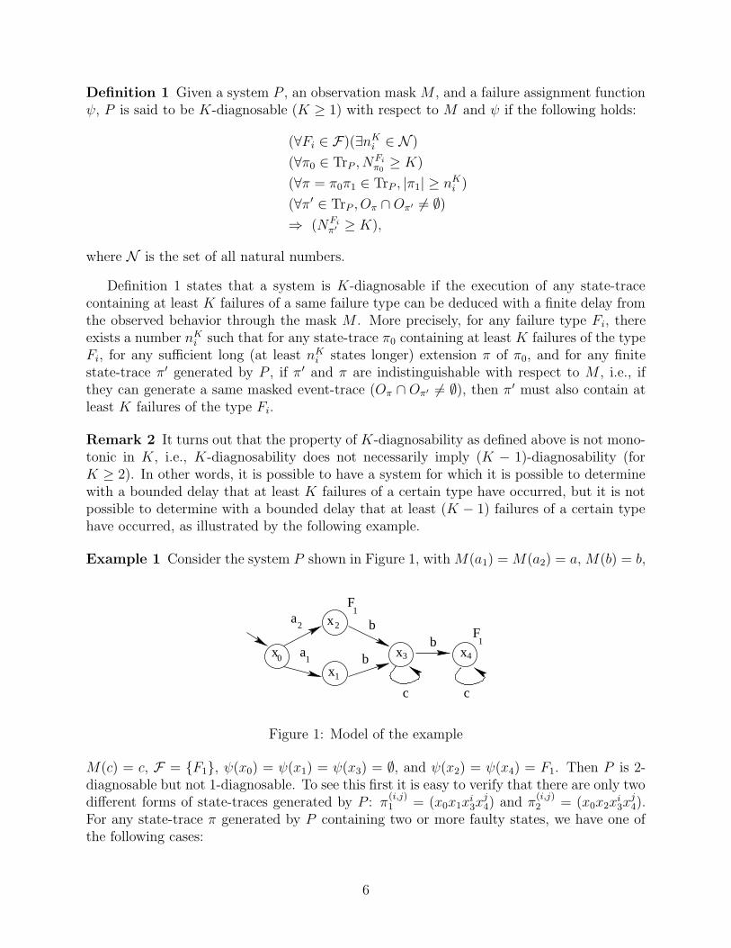
Example 1 Consider the system P shown in Figure 1, with M(a1) = M(a2) = a, M(b) = b,
x3
x1
a2
a1
x2F
1
F1
b
bx0
b
c c
x4
Figure 1: Model of the example
M(c) = c, F = {F1}, ψ(x0) = ψ(x1) = ψ(x3) = ∅, and ψ(x2) = ψ(x4) = F1. Then P is 2-diagnosable but not 1-diagnosable. To see this first it is easy to verify that there are only twodifferent forms of state-traces generated by P : π
(i,j)1 = (x0x1x
i3x
j4) and π
(i,j)2 = (x0x2x
i3x
j4).
For any state-trace π generated by P containing two or more faulty states, we have one ofthe following cases:
6
1. π is of the form of π(i,j)1 with j ≥ 2. Then for any state-trace π′ 6= π sharing a common
event-trace observation with π, π′ must be of the form of π(i,j)2 with j ≥ 2, which
implies that π′ must contain at least three faulty states.
2. π is of the form of π(i,j)2 with j > 1. Then for any state-trace π′ 6= π sharing a common
event-trace observation with π, π′ must be of the form of π(i,j)1 with j > 1, which
implies that π′ must contain at least two faulty states.
3. π is of the form of π(i,j)2 with j = 1. Then we can pick n1 = 1 to satisfy the requirement
of 2-diagnosability. To see this, let ππ0 be any extension of π with |π0| ≥ n1 = 1, thenwe must have that π0 = (x4)
` with ` ≥ 1. Any state-trace π′ 6= ππ0 sharing a common
event-trace observation with ππ0 must be of the form of π(i,j)1 with j > 1, which implies
that π′ must contain at least two faulty states.
From Definition 1, the above discussion implies that P is 2-diagnosable. But P is not 1-diagnosable. This is because for any integer n1, we can choose π0 = (x0x2), π = π0(x3)
n1+1,and π′ = (x0x1x
n1+13 ), then we have that π0 contains 1 faulty state, |π| − |π0| = n1 + 1 > n1,
π′ and π generate a same observed event-trace (abcn1), but π′ does not contain any faultystate. From Definition 1, we know that P is not 1-diagnosable.
The lack of monotonicity of K-diagnosability motivates a stronger notion of diagnos-ability, which we call [1, K]-diagnosability, that is monotonic in K. We say a system is[1, K]-diagnosable if it is J-diagnosable for each 1 ≤ J ≤ K. Formally,
Definition 2 Given a system P , an observation mask M , and a failure assignment functionψ, P is said to be [1, K]-diagnosable (K ≥ 1) with respect to M and ψ if the following holds:
(∀Fi ∈ F)(∃ni ∈ N )
(∀J, 1 ≤ J ≤ K)
(∀π0 ∈ TrP , NFi
π0≥ J)
(∀π = π0π1 ∈ TrP , |π1| ≥ ni)
(∀π′ ∈ TrP , Oπ ∩Oπ′ 6= ∅)
⇒ (NFi
π′ ≥ J).
Remark 3 Obviously, [1, K]-diagnosability is monotonic in K, i.e., it holds that if a systemis [1, K]-diagnosable, then it is also [1, K − 1]-diagnosable (for all K ≥ 2). Note that it alsoholds that [1, K]-diagnosable and K-diagnosable are both equivalent to diagnosable in thesense of [14] under K = 1.
It is obvious that if P is [1, K]-diagnosable then ∀J , 1 ≤ J ≤ K, P is J-diagnosable.Conversely, if for all J with 1 ≤ J ≤ K, P is J-diagnosable, i.e., for each Fi ∈ F there existsa bound nJ
i satisfying the requirement of J-diagnosability, then we can pick ni = maxJ=KJ=1 n
Ji
to satisfy the requirement of [1, K]-diagnosability. Thus P is [1, K]-diagnosable if and onlyif for all J with 1 ≤ J ≤ K, P is J-diagnosable.
7
The property of [1, K]-diagnosability can be used to determine with bounded delay ifthe given system has executed at least K or less failures of a certain kind. Thus a repeatedoccurrence of a failure of a certain type can be determined for up to its first K occurrences.Of course it is desirable to be able to determine with bounded delay the repeated occurrenceof a failure of a certain type for any number of its occurrences. This motivates the notionof [1,∞]-diagnosability, which is obtained by setting K to be ∞ in the definition of [1, K]-diagnosability.
Definition 3 Given a system P , an observation mask M , and a failure assignment functionψ, P is said to be [1,∞]-diagnosable with respect to M and ψ if the following holds:
(∀Fi ∈ F)(∃ni ∈ N )
(∀J ≥ 1)
(∀π0 ∈ TrP , NFi
π0≥ J)
(∀π = π0π1 ∈ TrP , |π1| ≥ ni)
(∀π′ ∈ TrP , Oπ ∩Oπ′ 6= ∅)
⇒ (NFi
π′ ≥ J).
Remark 4 It is obvious that if P is [1,∞]-diagnosable, then for all K ≥ 1, P is K- and[1, K]-diagnosable. But the converse need not hold as illustrated by the following example.
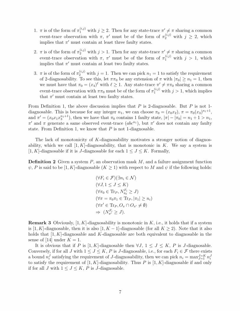
Example 2 Consider the system P shown in Figure 2, where M(a1) = M(a2) = a, M(b) =
x3
F1
x1
a2
a1
x2
F1
b
bx0
c
Figure 2: Model of the example
b, M(c) = c, and F = {F1}, ψ(x0) = ψ(x1) = ∅, ψ(x2) = ψ(x3) = F1. It is easy to verifythat P is K-diagnosable for any finite K > 0. This is because any state-trace generated byP containing more than 3K states, has at least K of them faulty. So we can pick n1 = 3Kto satisfy the requirement of K-diagnosability.
But P is not [1,∞]-diagnosable. This is because in this example, the delay boundassociated with K-diagnosability is an increasing function of K, and no uniform delaybound can be found that works for every K > 0. To see this, suppose such an uniformbound exists and that it is n1. We pick k to be the smallest integer bigger than thereal number n1/3, and set K = 2(k + 1). Then for the state-traces π0 = (x0x2x3)
k+1,π = π0π1 = (x0x2x3)
k+1(x0x2x3)k = (x0x2x3)
2k+1, and π′ = (x0x1x3)2k+1, we have that π0
contains K faulty states, |π1| = 3k > n1, π′ and π generate a same observed event-trace
(abc)2k+1, but π′ contains 2k + 1 faulty states which is less than K, a contradiction to the[1,∞]-diagnosability. From Definition 3, we know that P is not [1,∞]-diagnosable.
8
3 Tests for Repeated Failure Diagnosability
In this section, we present algorithms for testing the various notions of diagnosability forrepeated failures defined above. From the various definitions of diagnosability, it is easy tosee that a system P is K-diagnosable (resp., [1, K]- or [1,∞]-diagnosable) with respect toa given failure type set {Fi, 1 ≤ i ≤ m} if and only if P is K-diagnosable (resp., [1, K]- or[1,∞]-diagnosable) with respect to each singleton failure type set {Fi}, 1 ≤ i ≤ m. Henceit suffices to test for diagnosability with respect to each failure type individually. So in thefollowing we assume, without loss of any generality, that there is only one failure type F1,i.e., F = {F1}.
Let P be a given system, M be the observation mask, and ψ : X → {∅, F1} be thefailure assignment function. From Definitions 1 and 2, we know that P is K-diagnosable(resp., [1, K]-diagnosable) if and only if there does not exist a pair of state-traces (π1, π2)in P such that NF1
π1≥ J and NF1
π2< J (J = K for K-diagnosability, J ∈ [1, K] for [1, K]-
diagnosability), and π1 and π2 share a common event observation, and π1 is infinitely long.The above suggests a test for K- and [1, K]-diagnosability as follows:
1. Construct a transition graph (no event label associated with each transition) from the“masked synchronous composition” of P with itself for capturing all pairs of state-traces (π1, π2) in P that share a common event observation. The “masked synchronouscomposition” of P with itself , denoted by P ′ = (X ′,∆, R′, x′0), is defined as follows:
• X ′ = X ×X is the state set;
• ∆ is the event set;
• R′ ⊆ X ′ × (∆ ∪ {ε}) ×X ′ is the state transition set that is defined as:∀x12 = (x1, x2) ∈ X ′, ∀x′12 = (x′1, x
′2) ∈ X ′, and ∀τ ∈ ∆ ∪ {ε}, (x12, τ, x
′12) ∈ R′ if
and only if one of the following holds
– τ = ε, x1 = x′1 (resp., x2 = x′2), and ∃σ ∈ Σ ∪ {ε} such that M(σ) = ε and(x2, σ, x
′2) ∈ R (resp., (x1, σ, x
′1) ∈ R);
– τ 6= ε, and ∃σ1, σ2 ∈ Σ such that M(σ1) = M(σ2) = τ , (x1, σ1, x′1) ∈ R, and
(x2, σ2, x′2) ∈ R.
• x′0 = (x0, x0) is the initial state.
In deriving the transition graph from the masked synchronous composition of P withitself, we also keep track of the number of failures for each state-trace in each pair bytagging the value-pair (min{NF1
π1, K},min{NF1
π2, K}) at each state-pair (x1, x2) in the
transition graph.
2. Check whether there exists a cycle in the transition graph such that the cycle con-tains a state-pair (x1, x2) tagged with a value-pair (J, i) and i < J (J = K for K-diagnosability, J ∈ [1, K] for [1, K]-diagnosability). If there exists such a cycle, andthe cycle embeds an infinite state-trace with a higher number of faults, then P is notK- and [1, K]-diagnosable respectively. This is because there does not exist a pair ofindistinguishable state-traces (π1, π2) in P such that NF1
π1≥ J , NF1
π2< J , and π1 is
infinitely long, if and only if there does not exist a cycle in the transition graph such
9
that the cycle contains a state-pair (x1, x2) tagged with a value-pair (J, i) with i < Jand x1 is contained in a infinitely long state-trace embedded in the cycle.
Note that because we allow unobservable cycles in the system P , there may exist a cyclein the transition graph that results from one infinite and one finite state-trace pair that areindistinguishable. If such a cycle contains a state-pair (x1, x2) tagged with a value-pair (J, i)and i < J , and the finite state-trace along the cycle has a higher number of faults, then thecycle is not be treated as a “bad” one as stated above. This is because for diagnosability tohold the finite state-trace needs to be extended sufficiently long, but along the above cyclethe finite state-trace is not extended sufficiently long. The above situation is illustrated inExample 3 below. Thus for the test of K- and [1, K]-diagnosability, we shall check only thosecycles that embeds an infinite state-trace with a higher number of faults. In order to tellwhether a cycle embeds an infinite state-trace with a higher number of faults, we introducea binary valued entry k in each state-pair of the transition graph such that k = 1 if and onlyif the state-pair results from an extension of the state-trace with a higher number of faults.Now a cycle is “bad” if it contains a state-pair (x1, x2) tagged with a value-pair (J, i) and abinary valued entry k such that i < J and k = 1.
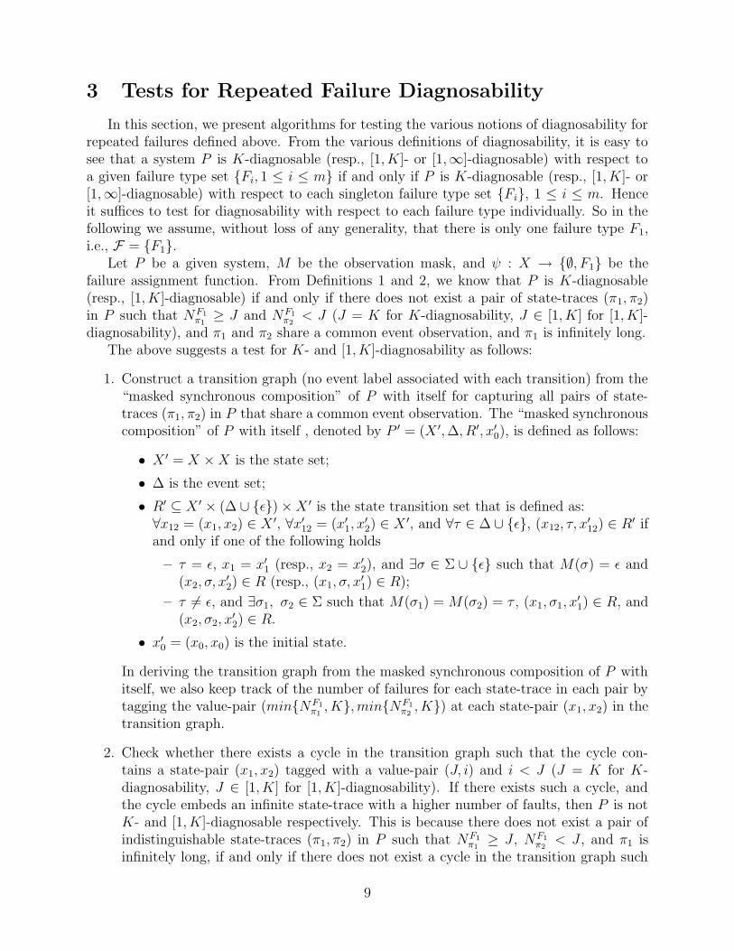
Example 3 Consider the system P shown in Figure 3, where M(a1) = M(a2) = a 6= ε,
x3
x1
a2
a1
x2
F1
x0
b
b
c
Figure 3: Example for 1-diagnosability
M(b) = ε, M(c) = c, and F = {F1}, ψ(x0) = ψ(x1) = ψ(x3) = ∅, ψ(x2) = F1. It is easy toverify that P is 1-diagnosable. This is because π = (x0x2x
ω3 ) is the only faulty state-trace
generated by P , and no other state-trace shares a common event observation with π.If we introduce only the value-pair (min{NF1
π1, K},min{NF1
π2, K}) and not the binary
valued entry k mentioned above, we can get a transition graph from the masked compositionof P with itself as shown in Figure 4. There is a self-loop at the state ((x3, x2), (0, 1)), whichindicates that there are two state-traces in P sharing a common event observation, and thenumber of faults associated with these traces is 0 and 1 respectively. But this self-loop is nota bad-cycle. Since the two state-traces involved are π1 = (x0x1x
ω3 ) and π2 = (x0x2), with
NF1
π1= 0 and NF1
π2= 1. But π2, which is the trace with a higher number of faults, never gets
extended along the self-loop due to the presence of unobservable cycle xω3 in π1.
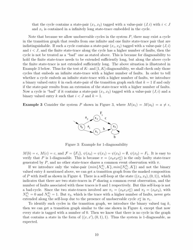
To identify such cycles in the transition graph, we introduce the binary valued tag k,then we can get a transition graph similar to the one shown in Figure 4, except that nowevery state is tagged with a number of 0. Then we know that there is no cycle in the graphthat contains a state in the form of ((x, x′), (0, 1), 1). Thus the system is 1-diagnosable, asexpected.
10
(x ,x ), (0, 1)1 2
(x ,x ), (0, 1)23
(x ,x ), (1, 0)2 1
(x ,x ), (1, 0)2 3
(x ,x ), (0, 0)1 1
(x ,x ), (0, 0)13(x ,x ), (0, 0)1 3
(x ,x ), (0, 0)3 3
(x ,x ), (1, 1)2 2
(x ,x ), (1, 1)3 3
(x ,x ), (0, 0)0 0
Figure 4: Transition graph for 1-diagnosability
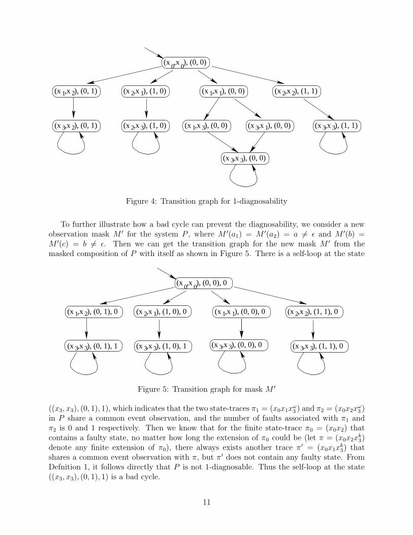
To further illustrate how a bad cycle can prevent the diagnosability, we consider a newobservation mask M ′ for the system P , where M ′(a1) = M ′(a2) = a 6= ε and M ′(b) =M ′(c) = b 6= ε. Then we can get the transition graph for the new mask M ′ from themasked composition of P with itself as shown in Figure 5. There is a self-loop at the state
(x ,x ), (1, 1), 03 3
(x ,x ), (0, 0), 00 0
(x ,x ), (0, 1), 01 2 (x ,x ), (1, 0), 02 1
(x ,x ), (0, 1), 133 (x ,x ), (1, 0), 13 3
(x ,x ), (0, 0), 01 1 (x ,x ), (1, 1), 02 2
(x ,x ), (0, 0), 03 3
Figure 5: Transition graph for mask M ′
((x3, x3), (0, 1), 1), which indicates that the two state-traces π1 = (x0x1xω3 ) and π2 = (x0x2x
ω3 )
in P share a common event observation, and the number of faults associated with π1 andπ2 is 0 and 1 respectively. Then we know that for the finite state-trace π0 = (x0x2) thatcontains a faulty state, no matter how long the extension of π0 could be (let π = (x0x2x
k3)
denote any finite extension of π0), there always exists another trace π′ = (x0x1xk3) that
shares a common event observation with π, but π′ does not contain any faulty state. FromDefnition 1, it follows directly that P is not 1-diagnosable. Thus the self-loop at the state((x3, x3), (0, 1), 1) is a bad cycle.
11
The algorithm for testing K- and [1, K]-diagnosability is given as follows.
Algorithm 1 Algorithm for testing K- and [1, K]-diagnosability:
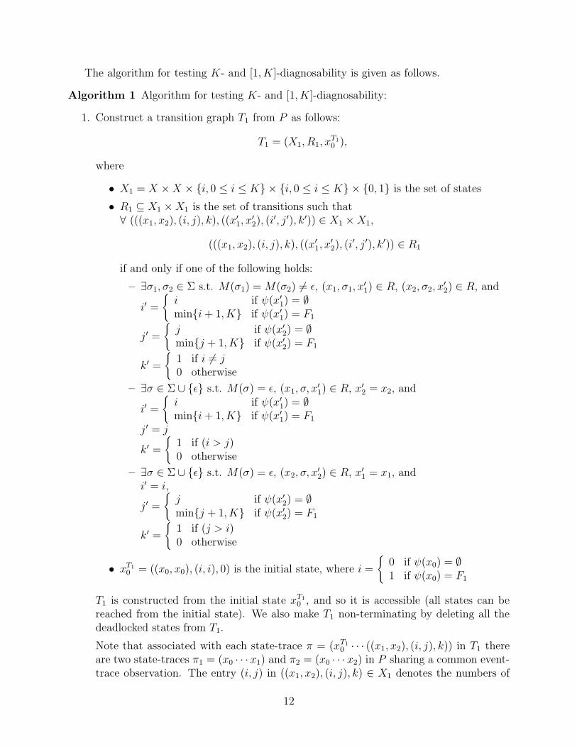
1. Construct a transition graph T1 from P as follows:
T1 = (X1, R1, xT1
0 ),
where
• X1 = X ×X × {i, 0 ≤ i ≤ K} × {i, 0 ≤ i ≤ K} × {0, 1} is the set of states
• R1 ⊆ X1 ×X1 is the set of transitions such that∀ (((x1, x2), (i, j), k), ((x
′1, x
′2), (i
′, j′), k′)) ∈ X1 ×X1,
(((x1, x2), (i, j), k), ((x′1, x
′2), (i
′, j′), k′)) ∈ R1
if and only if one of the following holds:
– ∃σ1, σ2 ∈ Σ s.t. M(σ1) = M(σ2) 6= ε, (x1, σ1, x′1) ∈ R, (x2, σ2, x
′2) ∈ R, and
i′ =
{
i if ψ(x′1) = ∅min{i+ 1, K} if ψ(x′1) = F1
j′ =
{
j if ψ(x′2) = ∅min{j + 1, K} if ψ(x′2) = F1
k′ =
{
1 if i 6= j0 otherwise
– ∃σ ∈ Σ ∪ {ε} s.t. M(σ) = ε, (x1, σ, x′1) ∈ R, x′2 = x2, and
i′ =
{
i if ψ(x′1) = ∅min{i+ 1, K} if ψ(x′1) = F1
j′ = j
k′ =
{
1 if (i > j)0 otherwise
– ∃σ ∈ Σ ∪ {ε} s.t. M(σ) = ε, (x2, σ, x′2) ∈ R, x′1 = x1, and
i′ = i,
j′ =
{
j if ψ(x′2) = ∅min{j + 1, K} if ψ(x′2) = F1
k′ =
{
1 if (j > i)0 otherwise
• xT1
0 = ((x0, x0), (i, i), 0) is the initial state, where i =
{
0 if ψ(x0) = ∅1 if ψ(x0) = F1
T1 is constructed from the initial state xT1
0 , and so it is accessible (all states can bereached from the initial state). We also make T1 non-terminating by deleting all thedeadlocked states from T1.
Note that associated with each state-trace π = (xT1
0 · · · ((x1, x2), (i, j), k)) in T1 thereare two state-traces π1 = (x0 · · · x1) and π2 = (x0 · · · x2) in P sharing a common event-trace observation. The entry (i, j) in ((x1, x2), (i, j), k) ∈ X1 denotes the numbers of
12
faulty states (up to a maximum of K) contained in the two state-traces π1 and π2
respectively, i.e., i = min{NF1
π1, K} and j = min{NF1
π2, K}. The binary valued entry
k in ((x1, x2), (i, j), k) ∈ X1 is used to indicate whether the state ((x1, x2), (i, j), k) isreached from a state ((x′1, x
′2), (i
′, j′), k′) such that if i′ > j′ (resp., j ′ > i′), then thereexists σ ∈ Σ ∪ {ε} such that (x′1, σ, x1) ∈ R (resp., (x′2, σ, x2) ∈ R). In other words,k = 1 indicates that the state-trace with a higher number of faults ending in the statex′1 (resp., x′2) has evolved by one step by executing a transition in P (to end in thestate x1 (resp., x2)). This is needed to deal with the fact that we allow an unboundednumber of unobservable events to occur in P .
2. Delete all those states ((x1, x2), (i, j), k) ∈ X1 and their associated transitions from T1
for which i = j. If it is for the test of K-diagnosability, then also delete those statesand their associated transitions for which i < K and j < K.
3. Check if there is a state ((x1, x2), (i, j), k) with k = 1 that is contained in a cycle inthe remainder graph. If the answer is yes, then output that the system is not [1, K]-or K-diagnosable; otherwise output that the system is [1, K]- or K-diagnosable. Thislast step can be performed using a depth first search.
The following theorem establishes the correctness of Algorithm 1.
Theorem 1 Given a system P , an observation mask M , a failure assignment function ψ :X → {∅, F1}, and the transition graph T1 derived using Algorithm 1, we have the following:
1. P is K-diagnosable if and only if T1 does not contain a cycle cl,
cl = (xT1
1 xT1
2 . . . xT1
n xT1
1 ), n ≥ 1,
with xT1
k = ((xk, x′k), (i, i
′), jk), k = 1, 2, . . . , n, i 6= i′, and either i = K or i′ = K, and∃k ∈ {1, · · · , n} with jk = 1.
2. P is [1, K]-diagnosable if and only if T1 does not contain a cycle cl,
cl = (xT1
1 xT1
2 . . . xT1
n xT1
1 ), n ≥ 1,
with xT1
k = ((xk, x′k), (i, i
′), jk), k = 1, 2, . . . , n, i 6= i′, and ∃k ∈ {1, · · · , n} with jk = 1.
Proof: For the necessity of the first assertion, suppose P is K-diagnosable, but there existsa cycle cl in T1, cl = (xT1
1 xT1
2 · · · xT1
n xT1
1 ), n ≥ 1, such that xT1
k = ((xk, x′k), (i,K), jk), k =
1, 2, · · · , n, i < K, and ∃k ∈ {1, · · · , n} with jk = 1. Since T1 is accessible, there existsa state-trace tr generated by T1 ending with the state xT1
1 , i.e., tr = (xT1
0 · · · xT1
1 ), andalso the state-trace tr` = tr(xT1
2 · · · xT1
n xT1
1 )` for any ` ≥ 0 is generated by T1. From theconstruction of T1, we know that associated with each tr`, ` ≥ 0, there are two state-tracesπ`
1 = (x0 · · · x1) and π`2 = (x0 · · · x
′1) generated by P and sharing a common event-trace
observation, and NF1
π`
1
= i, NF1
π`
2
≥ K. Then for any integer nK1 , we can choose another
integer `0 such that `0 > nK1 . Now for the state-traces π0
2, π = π`02 , and π′ = π`0
1 , we havethat NF1
π02
≥ K, |π| − |π02| ≥ `0 > nK
1 (where the first inequality comes from the fact that
13
jk = 1 for some k ∈ {1, · · · , n}, which implies that the state xT1
k in the cycle cl is resultedfrom a state movement in the state trace π`0
2 that has a bigger number of failures than π`01 ,
i.e., |πj2| − |πj−1
2 | ≥ 1 for any j ≥ 1), and π and π′ share a common event-trace observation(since they are both associated with tr`0). But NF1
π′ = NF1
π01
= i < K. From Definition 1, we
know P is not K-diagnosable, a contradiction. So the necessity of the first assertion holds.For the sufficiency of the first assertion, suppose T1 does not contain a cycle cl =
(xT1
1 xT1
2 · · · xT1
n xT1
1 ), n ≥ 1, with xT1
k = ((xk, x′k), (i, i
′), jk), k = 1, 2, · · · , n, i 6= i′, andeither i = K or i′ = K, and ∃k ∈ {1, · · · , n} with jk = 1. This implies that for all((x, x′), (i, i′), j) ∈ X1, if i 6= i′, j = 1, and either i = K or i′ = K, then xT1 is not containedin a cycle. Because T1 is non-terminating, it further implies that for any state-trace π in T1,if π contains more than m1 = 2|X|2K number of states of the type ((x, x′), (i, i′), 1), witheither i = K or i′ = K, then one of such states must be in the form of ((x, x′), (K,K), 1),since otherwise one state must appear twice (there are at most m1 number of states of thetype ((x, x′), (i, i′), 1) with either i = K or i′ = K, and i 6= i′), i.e., this state must becontained in a cycle, a contradiction.
Now we let nK1 = m1 + 1. Then for any state-trace π0 ∈TrP with NF1
π0≥ K, any of
its extension π = π0π1 ∈ TrP with |π1| ≥ nK1 , and any state-trace π′ = π′
0π′1 ∈ TrP with
Oπ ∩ Oπ′ 6= ∅ and Oπ0∩ Oπ′
06= ∅, we have that for any state-trace tr ∈ TrT1
that π0 andπ′
0 are associated with, tr must end with a state ((x1, x′1), (K, i), j) ∈ X1. if i = K, then
from Definition 1, we know that P is K-diagnosable. Otherwise, let tr1 be any extensionof tr in T1 that π and π′ are associated with, i.e., tr1 = trtr′. If in tr′ there is a state((x, x′), (K,K), j), then from Definition 1, P is K-diagnosable. Now suppose that in tr ′
there is not such a state ((x, x′), (K,K), j), then it is obvious that tr′ must end with a state((x2, x
′2), (K, i
′), j) such that K > i′, i.e., along the trace tr′, π1 always has a bigger numberof failures than π′
1. Because tr′ is composed from π1 and π′1, tr
′ must have |π1| number ofstates that are resulted from the state movement in π1. Also because π1 always has a biggernumber of failures than π′
1, the above |π1| number of states in tr′ must be in the form of((x, x′), (K, j), 1) with j < K. In other words, tr′ must contain |π1| ≥ nK
1 > m1 (more thanm1) number of states of the type ((x, x′), (K, j), 1). As argued above, tr′ must contain astate ((x, x′), (K,K), 1), a contradiction. So the sufficiency of the first assertion also holds.
For the necessity of the second assertion, suppose P is [1, K]-diagnosable, but thereexists a cycle cl in T1, cl = (xT1
1 xT1
2 · · · xT1
n xT1
1 ), n ≥ 1, such that xT1
k = ((xk, x′k), (i, i
′), jk),k = 1, 2, · · · , n, i < i′ ≤ K, and jk = 1 for some k ∈ {1, · · · , n}. Then using a similarargument as above for the necessity of the first assertion and by viewing i′ as K, we can showthat P is not i′-diagnosable. This implies that P is not [1, K]-diagnosable, a contradictionto the hypothesis. So the necessity of the second assertion holds.
For the sufficiency of the second assertion, suppose T1 does not contain a cycle cl =(xT1
1 xT1
2 · · · xT1
n xT1
1 ), n ≥ 1, with xT1
k = ((xk, x′k), (i, i
′), jk), k = 1, 2, · · · , n, i 6= i′, and jk = 1for some k ∈ {1, · · · , n}. This implies that for all ((x, x′), (i, i′), j) ∈ X1, if i 6= i′ andj = 1 then xT1 is not contained in a cycle. Following a similar argument as above for thesufficiency of the first assertion, we have that for any state-trace π in T1, if π contains morethan m2 = |X|2(K + 1)K number of states of the type xT1 = ((x, x′), (i, i′), 1), then π mustcontain a state in the form of ((x, x′), (i, i), 1).
Now we let n1 = m2 + 1. Then for any state-trace π0 ∈ TrP with NF1
π0≥ J , 1 ≤ J ≤ K,
14
any of its extension π = π0π1 ∈TrP with |π1| ≥ n1, and any state-trace π′ = π′0π
′1 ∈TrP
with Oπ ∩ Oπ′ 6= ∅ and Oπ0∩ Oπ′
06= ∅, we have that if tr ∈ TrT1
is any state-trace thatπ0 and π′
0 are associated with, then tr must end with a state ((x1, x′1), (i, i
′), j) ∈ X1 withi ≥ J . If i′ ≥ i, then from Definition 2, P is [1, K]-diagnosable. Otherwise, let tr1 be anyextension of tr in T1 that π and π′ are associated with, i.e., tr1 = trtr′. If tr′ contains a state((x, x′), (`, `′), k) with ` = `′, then from the construction of T1, we know that ` ≥ i, thus` ≥ J , which implies that NF1
π′ ≥ J . It follows from Definition 2 that P is [1, K]-diagnosable.Now suppose tr′ does not contain such a state ((x, x′), (`, `), k), then it is obvious that forevery state ((x, x′), (`, `′), k) in tr′, we must have ` > `′. Following a similar argument asabove for the sufficiency of the first assertion, we have that tr′ must contain more than m2
number of states of the type ((x, x′), (`, `′), 1). As argued above, tr′ must contain a state((x, x′), (`, `), 1), a contradiction. So the sufficiency of the second assertion also holds.
From the definition of [1,∞]-diagnosability, we also know that P is [1,∞]-diagnosable ifand only if there does not exist a pair of state-traces (π1, π2) in P such that NF1
π1≥ J and
NF1
π2< J (J ≥ 1), and π1 and π2 share a common event observation, and π1 is infinitely long.
However we cannot directly use Algorithm 1 for the test of [1,∞]-diagnosability, since J isnow unbounded, i.e., if we keep track of the number of faults with each state-trace in eachstate-trace pair of the transition graph, then we may get a transition graph with an infinitenumber of states. So instead of keeping track of the number of faults with each state-tracein the pair, we keep track of the difference of the number of faults with each state-tracein the pair. Although the fault-difference may still be unbounded, it can be shown that ifthe fault-difference goes beyond the bound |X|2 (|X| is the number of states in the systemP ), then P is not [1,∞]-diagnosable (see Theorem 2 below). Thus even for checking [1,∞]-diagnosability, we are able to work with a finite transition graph. Similar to the test of K-and [1, K]-diagnosability, we need the binary valued tag k. It turns out that the informationof fault-difference and the entry k is not enough for testing [1,∞]-diagnosability, as shownin Example 4 below. We need to introduce into the transition graph another binary valuedentry j to indicate whether a fault is reported, i.e., whether the two state-traces in the pairboth have experienced a fault upon reaching the state. This is because if a fault is detectedalong both the state-traces, the fault-difference counter remains unchanged, but this is notbad, as a fault does not remain undetected forever. Then the system is [1,∞]-diagnosableif and only if there is no cycle that contains a state ((x, x′), i, j, k) with i 6= 0, j = 0, andk = 1 (Theorem 2), where i is the fault-difference, j is the binary valued entry indicatingthe reporting of a fault, and k is the binary valued entry indicating the extension of thestate-trace with a higher number of faults.
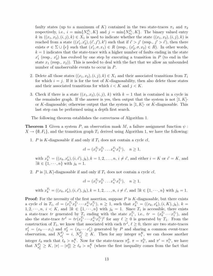
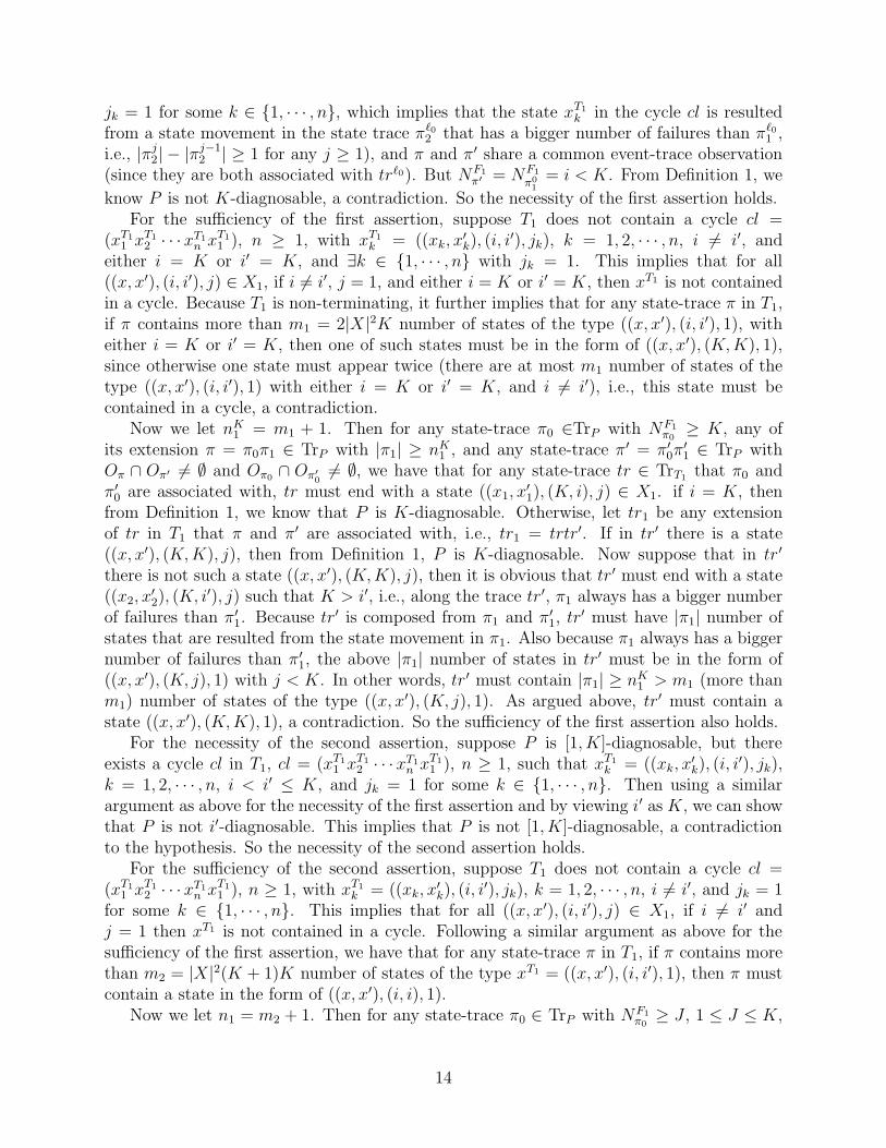
Example 4 Consider the system P shown in Figure 6, where M(a1) = M(a2) = a, M(b) =b, and F = {F1}, ψ(x0) = ψ(x1) = ∅, ψ(x2) = ψ(x3) = F1. It is easy to verify that P is[1,∞]-diagnosable applying Definition 3.
If we do not introduce the binary valued entry j indicating the reporting of a fault, wecan get a transition graph from the composition of two copies of masked P as shown inFigure 7. There is a self-loop at the state ((x3, x3),−1, 1), which indicates that there aretwo infinite state-traces π1 = (x0x1x
ω3 ) and π2 = (x0x2x
ω3 ) in P sharing a common event
observation, and the fault-difference between the two traces is −1. But this self-loop is not a“bad” cycle. Note that a fault is reported each time the pair of the two state-traces visits the
15
x3
x1
a2
a1
x2
F1
F1
b
x0
b
b
Figure 6: Example for [1,∞]-diagnosability
(x ,x ), −1, 01 2 (x ,x ), 1, 02 1 (x ,x ), 0, 01 1 (x ,x ), 0, 02 2
(x ,x ), 0, 00 0
(x ,x ), 0, 03 3(x ,x ), −1, 13 3 (x ,x ), 1, 13 3
Figure 7: Transition graph for [1,∞]-diagnosability
state (x3, x3), and because of this fault report, although the fault-difference counter remainsunchanged, the loop is not a “bad” one, since no fault remains undetected forever along theloop.
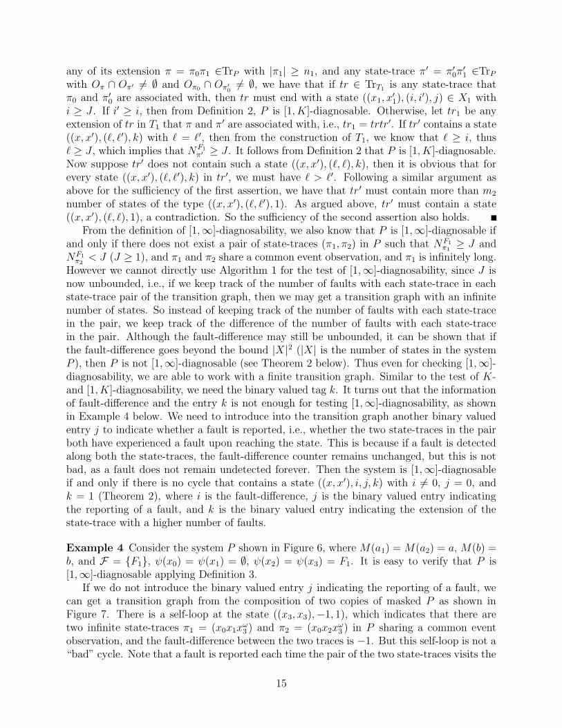
If we also introduce the binary valued entry j into the transition graph for indicatingthe reporting of a fault, then we can get a transition graph as shown in Figure 8. Fromthe graph, we know that there is no cycle in the graph that contains a state of the form((x, x′), i, 0, 1) with i 6= 0. Thus the system is [1,∞]-diagnosable, which is true.
The algorithm for testing [1,∞]-diagnosability is given in the following.
Algorithm 2 Algorithm for testing [1,∞]-diagnosability:
1. Construct a transition graph T2 from P as follows:
T2 = (X2, R2, xT2
0 ),
where
• X2 = X ×X × {i, |i| ≤ |X|2} × {0, 1} × {0, 1} is the set of states
• R2 ⊆ X2 ×X2 is the set of transitions such that∀ (((x1, x2), i, j, k), ((x
′1, x
′2), i
′, j′, k′)) ∈ X2 ×X2,
(((x1, x2), i, j, k), ((x′1, x
′2), i
′, j′, k′)) ∈ R2
if and only if one of the following holds:
16
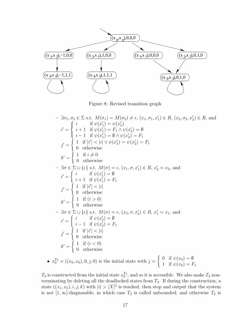
(x ,x ),−1,0,01 2 (x ,x ),1,0,02 1 (x ,x ),0,0,01 1 (x ,x ),0,1,02 2
(x ,x ),0,0,00 0
(x ,x ),0,1,03 3(x ,x ),−1,1,13 3 (x ,x ),1,1,13 3
Figure 8: Revised transition graph
– ∃σ1, σ2 ∈ Σ s.t. M(σ1) = M(σ2) 6= ε, (x1, σ1, x′1) ∈ R, (x2, σ2, x
′2) ∈ R, and
i′ =
i if ψ(x′1) = ψ(x′2)i+ 1 if ψ(x′1) = F1 ∧ ψ(x′2) = ∅i− 1 if ψ(x′1) = ∅ ∧ ψ(x′2) = F1
j′ =
{
1 if |i′| < |i| ∨ ψ(x′1) = ψ(x′2) = F1
0 otherwise
k′ =
{
1 if i 6= 00 otherwise
– ∃σ ∈ Σ ∪ {ε} s.t. M(σ) = ε, (x1, σ, x′1) ∈ R, x′2 = x2, and
i′ =
{
i if ψ(x′1) = ∅i+ 1 if ψ(x′1) = F1
j′ =
{
1 if |i′| < |i|0 otherwise
k′ =
{
1 if (i > 0)0 otherwise
– ∃σ ∈ Σ ∪ {ε} s.t. M(σ) = ε, (x2, σ, x′2) ∈ R, x′1 = x1, and
i′ =
{
i if ψ(x′2) = ∅i− 1 if ψ(x′2) = F1
j′ =
{
1 if |i′| < |i|0 otherwise
k′ =
{
1 if (i < 0)0 otherwise
• xT2
0 = ((x0, x0), 0, j, 0) is the initial state with j =
{
0 if ψ(x0) = ∅1 if ψ(x0) = F1
T2 is constructed from the initial state xT2
0 , and so it is accessible. We also make T2 non-terminating by deleting all the deadlocked states from T2. If during the construction, astate ((x1, x2), i, j, k) with |i| > |X|2 is reached, then stop and output that the systemis not [1,∞]-diagnosable, in which case T2 is called unbounded; and otherwise T2 is
17
called bounded, and we continue to the next step.
Note that associated with each state-trace π = (xT2
0 · · · ((x1, x2), i, j, k)) in T2 thereare two state-traces π1 = (x0 · · · x1) and π2 = (x0 · · · x2) in P sharing a commonevent-trace observation. The entry i in ((x1, x2), i, j, k) ∈ X2 indicates the differenceof the number of faulty states contained in the two state-traces π1 and π2, i.e., i =NF1
π1− NF1
π2. The binary valued entry j in ((x1, x2), i, j, k) ∈ X2 is used to indicate
whether a fault is reported at the state ((x1, x2), i, j, k). This happens when eitherψ(x1) = ψ(x2) 6= ∅, or |i| gets decremented through the transition from a prior stateto the state ((x1, x2), i, j, k). A fault is reported at ((x1, x2), i, j, k) if and only ifj = 1. As is the case with the previous algorithm, the binary valued entry k in((x1, x2), i, j, k) ∈ X2 is used to indicate whether the state ((x1, x2), i, j, k) is reachedfrom a state ((x′1, x
′2), i
′, j′, k′) such that if i′ > 0 (resp., j ′ > 0), then there existsσ ∈ Σ ∪ {ε} such that (x′1, σ, x1) ∈ R (resp., (x′2, σ, x2) ∈ R). In other words, k = 1indicates that the state-trace with a higher number of faults ending in the state x′
1
(resp., x′2) has evolved by one step by executing a transition in P (to end in the statex1 (resp., x2)). This is needed to deal with the fact that we allow an unboundednumber of unobservable events to occur in P .
2. Delete all those states ((x1, x2), i, j, k) and their associated transitions from T2 suchthat either i = 0 or j = 1.
3. Check whether there is a state ((x1, x2), i, j, k) with k = 1 that is contained in a cyclein the remainder graph. If the answer is yes, then output that the system is not [1,∞]-diagnosable; otherwise output that the system is [1,∞]-diagnosable. This last step canbe performed using a depth first search.
The following theorem guarantees the correctness of Algorithm 2.
Theorem 2 Given a system P , an observation mask M , a failure assignment function ψ :X → {∅, F1}, and the transition graph T2 derived using Algorithm 2, P is [1,∞]-diagnosableif and only if T2 is bounded as defined in Algorithm 2, and T2 does not contain a cycle cl,
cl = (xT2
1 xT2
2 . . . xT2
n xT2
1 ), n ≥ 1,
with xT2
k = ((xk, x′k), i, 0, jk), k = 1, 2, . . . , n, i 6= 0, and jk = 1 for some k ∈ {1, 2, · · · , n}.
Proof: For necessity, suppose P is [1,∞]-diagnosable. For contradiction, first we supposethat T2 is not bounded. Then there must exist a state-pair trace π in T2 such that
π = π0π1 = [(x0, x0)(x1, x′1) · · · (x`, x
′`)][(x`+1, x
′`+1) · · · (x`+n−1, x
′`+n−1)(x`, x
′`)]
and when the loop π1 is executed once, the difference between the number of failures ofthe two state-traces associated with π will increase at least by one. In other words, for anyk ≥ 0, we can have a state-pair trace πk = π0(π1)k in T2, and if we let πk
1 and πk2 be the two
state-traces associated with πk (assuming that NF1
π01
≥ NF1
π02
), then we have ∀k ≥ 0,
NF1
πk+1
1
−NF1
πk+1
2
≥ (NF1
πk
1
−NF1
πk
2
) + 1.
18
It further implies that
NF1
πk
1
−NF1
πk
2
≥ NF1
πk−1
1
−NF1
πk−1
2
+ 1
≥ NF1
πk−2
1
−NF1
πk−2
2
+ 2
≥ . . .
≥ NF1
π01
−NF1
π02
+ k
≥ k.
The above also implies that at least one state-pair in π1 is resulted from a state movementin πk
1 (because πk1 has a bigger number of failures than πk
2 , and the difference between thenumber of failures in πk
1 and πk2 is increased along the trace-segment π1), i.e., |πj+1
1 |−|πj1| ≥ 1
for any j ≥ 0.Now for any integer n1, we let k = n1 × |π1| + 1 and J = NF1
πk
1
. Then for the state-traces
πk1 , π
k+n1
1 , and πk+n1
2 , we have that NF1
πk
1
= J , |πk+n1
1 | − |πk1 | ≥ n1 (since |πj+1
1 | − |πj1| ≥ 1
for any j ≥ 0), and πk+n1
1 shares a common event-trace observation with πk+n1
2 . But we alsohave
NF1
πk+n12
≤ NF1
πk
2
+ n1 × |π1|
≤ NF1
πk
1
− k + n1 × |π1|
= J − 1
< J.
From Definition 3, we know P is not [1,∞]-diagnosable. A contradiction to the hypothesis.So T2 must be bounded.
Next we suppose that there exists a cycle cl in T2,
cl = (xT2
1 xT2
2 · · · xT2
n xT2
1 ),
n ≥ 1, such that xT2
k = ((xk, x′k), i, 0, jk), k = 1, 2, · · · , n, i > 0, and jk = 1 for some
k ∈ {1, · · · , n}. Since T2 is accessible, there exists a state-trace tr generated by T2 endingwith the state xT2
1 , i.e., tr = (xT2
0 · · · xT2
1 ), and also the state-trace tr` = tr(xT2
2 · · · xT2
n xT2
1 )`
for any ` ≥ 0 is generated by T2. From the construction of T2, we know that associated witheach tr`, ` ≥ 0, there are two state-traces π`
1 = (x0 · · · x1) and π`2 = (x0 · · · x
′1) generated
by P sharing a common event-trace observation; and NF1
π`
1
−NF1
π`
2
= i. Then for any integer
n1, we can choose another integer `0 such that `0 > n1, and let J = NF1
π01
. Then for the
state-traces π01, π = π`0
1 , and π′ = π`02 , we have that NF1
π01
≥ J , |π| − |π01| ≥ `0 > n1 (where
the first inequality follows from the fact that jk = 1 for some k ∈ {1, · · · , n}, which impliesthat the state xT2
k in the cycle cl is resulted from a state movement in the state trace π`01
that has a bigger number of failures than π`02 , i.e., |πj
1| − |πj−11 | ≥ 1 for any j ≥ 1), and π
and π′ share a common event-trace observation (since they are both associated with tr`0).We also have that NF1
π′ = NF1
π`02
= NF1
π02
= NF1
π01
− i = J − i < J (where the second equality
follows from the fact that along the cycle cl the fault-difference remains unchanged and no
19
fault is reported, which implies that all states invloved in the cycle cl are non-faulty states,in other words, NF1
π`
2
= NF1
π02
and NF1
π`
1
= NF1
π02
for any `). From Definition 3, we know P is not
[1,∞]-diagnosable, a contradiction to the hypothesis. So the necessity holds.For sufficiency, suppose T2 is bounded and T2 does not contain a cycle
cl = (xT2
1 xT2
2 · · · xT2
n xT2
1 ), n ≥ 1,
such that xT2
k = ((xk, x′k), i, 0, jk), k = 1, 2, · · · , n, i 6= 0, and jk = 1 for some k ∈ {1, · · · , n}.
This implies that for all xT2 = ((x, x′), i, j, k) ∈ X2, if i 6= 0, j = 0, and k = 1 then xT2
is not contained in a cycle. Because T2 is non-terminating, it further implies that for anystate-trace π in T2, if π contains more than m = |X|2 × |X|2 × 2 = 2|X|4 number of statesof the type ((x, x′), i, j, 1), then for one of such states we must have either i = 0 or j = 1,since otherwise one state must appear twice (there are at most m number of states of thetype ((x, x′), i, j, 1), i.e., this state must be contained in a cycle, a contradiction.
Now we let n1 = (m + 1)|X|2. Then for any state-traces π0 ∈ TrP with NF1
π0≥ J ≥ 1,
π = π0π1 ∈ TrP with |π1| ≥ n1, and π′ = π′0π
′1 ∈ TrP with Oπ∩Oπ′ 6= ∅ and Oπ0
∩Oπ′
06= ∅, let
tr ∈ TrT2be any state-trace that π0 and π′
0 are associated with, and ((x1, x′1), i, j, k) be the
last state of tr with i = NF1
π0−NF1
π′
0
. Since T2 is bounded, we have |i| ≤ |X|2. If i ≤ 0, then
NF1
π′ ≥ NF1
π′
0
≥ NF1
π0≥ J . This according to Definition 3 implies that P is [1,∞]-diagnosable.
Otherwise, let tr1 be any extension of tr in T2 with which π and π′ are associated with,i.e., tr1 = trtr′. If in tr′ there is a state ((x, x′), i′, j′, k′) with i′ = 0, then it implies thatNF1
π′ ≥ NF1
π0≥ J . This according to Definition 3 implies that P is [1,∞]-diagnosable. If
tr′ does not contain such a state ((x, x′), 0, j ′, k′), then it is obvious that for every state((x, x′), i′, j′, k′) in tr′, we have i′ > 0, i.e., along the trace tr′, π1 always has a bigger numberof failures than π′
1. Because tr′ is composed from π1 and π′1, tr
′ must have at least |π1|number of states that are resulted from the state movement in π1. Also because π1 alwayshas a bigger number of failures than π′
1, the above |π1| number of states in tr′ must be inthe form of ((x, x′), i′, j′, 1). In other words, tr′ must contain |π1| ≥ n1 > m|X|2 numberof states of the type ((x, x′), i′, j′, 1). As argued in the paragraph above and because of theassumption that tr′ does not contain any state in the form of ((x, x′), 0, j ′, k′), there mustbe at least one state in the form of ((x, x′), i′, 1, 1) among every m number of states of thetype ((x, x′), i′, j′, 1) in tr′. Now since tr′ contains more than m|X|2 number of states of thetype of ((x, x′), i′, j′, 1), so tr′ must contain at least |X|2 number of states of the type of((x, x′), i′, 1, 1). It implies that at least |X|2 ≥ i number of failures have been reported alongtr′, i.e., NF1
π′
1
≥ |X|2 ≥ i. Further we have
NF1
π′ = NF1
π′
0
+NF1
π′
1
= NF1
π0− i+NF1
π′
1
≥ NF1
π0
≥ J.
It follows from Definition 3 that P is [1,∞]-diagnosable. So the sufficiency also holds.
Remark 5 From Algorithms 1 and 2, we know that the number of states in T1 is at most2|X|2×(K+1)2, and the number of states in T2 (if it is bounded) is at most 8|X|4+4|X|2. It
20
is easy to verify that each state in T1 and T2 has at most |X|2 transitions. So the complexityof Algorithm 1 is O(|X|4) and that of Algorithm 2 is O(|X|6). For a deterministic system P ,the complexity of Algorithm 1 is O(|X|2 × |Σ|2) and that of Algorithm 2 is O(|X|4 × |Σ|2).
Note that if the failure type set F is not a singleton, then we can invoke Algorithm 1 or 2once for each failure type. Thus we obtain polynomial algorithms in the number of systemstates and the number of failure types for testing K-, [1, K]-, and [1,∞]-diagnosability.
4 On-line Diagnosis of Repeated Failures
In this section, we give a procedure to construct a diagnoser for on-line diagnosis ofrepeated failures. Let P = (X,Σ, R, x0) be a system with failure assignment function ψ,which is to be diagnosed using the observations of event-traces filtered through a maskM . If P passes the diagnosability test (K-, [1, K]-, or [1,∞]-diagnosability), then we usethe following procedure for the purpose of on-line diagnosis of repeated failures. As inthe previous section, we assume that F contains only one failure type, i.e., F = {F1}. IfF contains more than one failure type, then we concurrently apply the on-line diagnosisprocedure for each individual failure type.
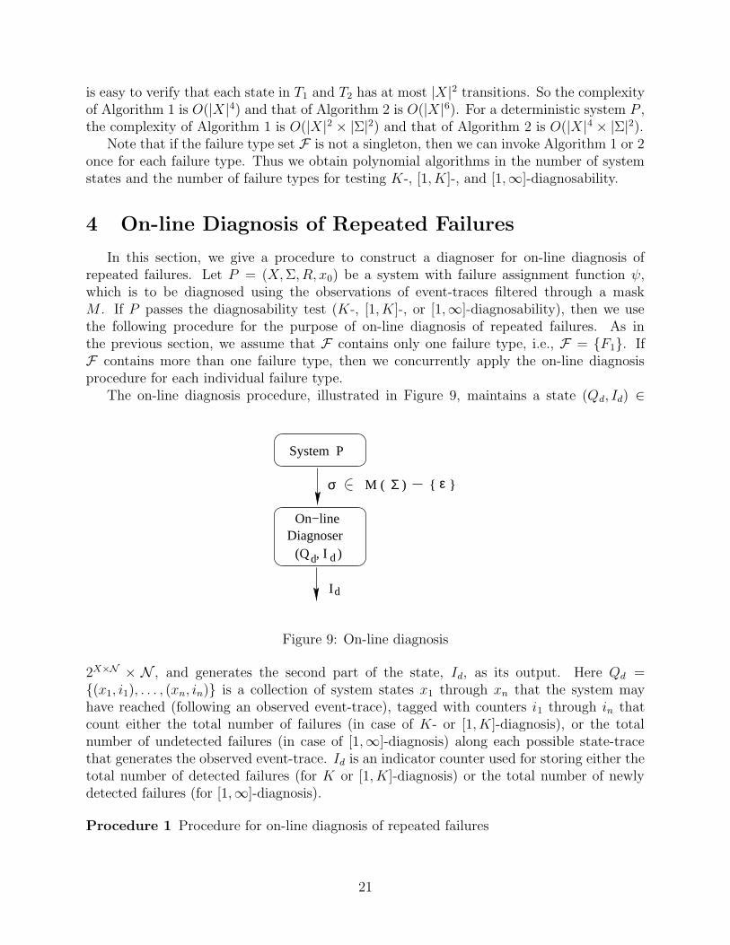
The on-line diagnosis procedure, illustrated in Figure 9, maintains a state (Qd, Id) ∈
Id
ε{ }M ( )Σ
On−lineDiagnoser
(Q , I )d d
σ
System P
Figure 9: On-line diagnosis
2X×N × N , and generates the second part of the state, Id, as its output. Here Qd ={(x1, i1), . . . , (xn, in)} is a collection of system states x1 through xn that the system mayhave reached (following an observed event-trace), tagged with counters i1 through in thatcount either the total number of failures (in case of K- or [1, K]-diagnosis), or the totalnumber of undetected failures (in case of [1,∞]-diagnosis) along each possible state-tracethat generates the observed event-trace. Id is an indicator counter used for storing either thetotal number of detected failures (for K or [1, K]-diagnosis) or the total number of newlydetected failures (for [1,∞]-diagnosis).
Procedure 1 Procedure for on-line diagnosis of repeated failures
21
1. Initialize Qd = {(x0, i0)} and Id = 0, where x0 is the initial state of P , and i0 indicateswhether or not the initial state is faulty, i.e.,
i0 =
{
0 if ψ(x0) = ∅1 if ψ(x0) = F1
2. Recursively add (x′, i′) ∈ X ×N into Qd such that
• exists (x, i) ∈ Qd and σ ∈ Σ ∪ {ε} such that M(σ) = ε and (x, σ, x′) ∈ R, and
• for K- and [1, K]-diagnosis:
i′ =
{
i if ψ(x′) = ∅min{i+ 1, K} if ψ(x′) = F1
for [1,∞]-diagnosis:
i′ =
{
i if ψ(x′) = ∅i+ 1 if ψ(x′) = F1
3. When a new observation δ ∈M(Σ) with δ 6= ε becomes available,
• update Qd as follows:
– for all (x, i) ∈ Qd, delete (x, i) from Qd, and add all (x′, i′) ∈ X ×N into Qd
such that there exists σ ∈M−1(δ) with (x, σ, x′) ∈ R, and
– for K- and [1, K]-diagnosis:
i′ =
{
i if ψ(x′) = ∅min{i+ 1, K} if ψ(x′) = F1
for [1,∞]-diagnosis:
i′ =
{
i− Id if ψ(x′) = ∅(i+ 1) − Id if ψ(x′) = F1
• set Id = min{i | ∃x ∈ X s.t. (x, i) ∈ Qd}, and
– for K-diagnosis:If Id = K, then output that at least Id failures have been detected and stop,else go to Step 2.
– for [1, K]-diagnosis:Output that at least Id failures have been detected and stop if Id = K, elsego to Step 2.
– for [1,∞]-diagnosis:Output that Id new failures have been detected and go to Step 2.
Remark 6 It follows from the sizes of state sets of T1 and T2 that for K- or [1, K]-diagnosis,the size of Qd is bounded by |X|×(K+1), i.e., |Qd| ≤ |X|×(K+1), and for [1,∞]-diagnosis,the size of Qd is bounded by |X| × (|X|2 + 1), i.e., |Qd| ≤ |X| × (|X|2 + 1).
From above, we know that the on-line diagnosis procedure has a polynomial space andtime complexity in the number of system states. If F contains more than one failure type,then as stated above we can apply |F| concurrent on-line diagnosis procedures. Thus weobtain an on-line diagnosis procedure that has a polynomial space and time complexity inthe number of system states and the number of failure types.
22
Remark 7 The above procedure for constructing a diagnoser on-line can be used for con-structing a diagnoser off-line as well. Instead of maintaining only the present state of thediagnoser, this requires maintaining all possible states of the diagnoser, and also transi-tions on all possible observed “events”. For an illustration, we have provided an off-lineconstruction of a diagnoser for the example presented in Section 5.
The following theorem establishes the soundness and the completeness of Procedure 1,where the soundness of the procedure means that it never reports a failure that has notoccurred, i.e., there are no “false alarm”, and the completeness of the procedure means thatit never misses a failure, i.e., there are no “missed detections”.
Theorem 3 Procedure 1 is sound and complete, whenever the system being diagnosed isdiagnosable (K-, [1, K]-, or [1,∞]-diagnosable as the case may be).
Proof: For soundness, let π be a state-trace generated by the system P , and NF1
π bethe number of faulty states contained in π. In order to establish soundness by way of acontradiction, we suppose that NF1
π < K if it is the case of K- or [1, K]-diagnosis, and thatProcedure 1 reports i > NF1
π failures for the state-trace π, where i = K for K-diagnosis,and i ≤ K for [1, K]-diagnosis. From Procedure 1, this implies that any state-trace π ′ ofP , that shares a common event-trace observation of π, contains at least i faulty states. Sofrom Procedure 1, π must also contain at least i > NF1
π faulty states, a contradiction. ThusProcedure 1 is sound.
For completeness, suppose the system P is diagnosable (K-, [1, K]-, or [1,∞]-diagnosableas the case may be). Let π0 be a state-trace generated by P and NF1
π0be the number of faulty
states contained in π0. We assume that NF1
π0≥ K if it is the case of K-diagnosis. Since P is
diagnosable, we know that there exists an integer n1 such that for any extension π = π0π1
of π0 generated by P with |π1| ≥ n1, and any state-trace π′ generated by P , if π and π′
share a common event-trace observation, then π′ must contain at least NF1
π0faulty states.
From the construction of Procedure 1 it follows that after the execution of any extension πthat is at least n1 state longer than π0 (since P is non-terminating, such an extension doesexist), the value of Qd computed by the procedure is such that ∀(x, i) ∈ Qd, the state x isreached by the execution of a state-trace that contains at least NF1
π0faulty states. Further,
if it is the case of K-diagnosis, then the procedure has had reported K failures, and if it isthe case for [1, K]- or [1,∞]-diagnosis, then the procedure has had reported min{N F1
π0, K}
or NF1
π0failures respectively. Thus no failure is missed by the procedure, i.e., Procedure 1 is
complete.
5 Illustrative Example
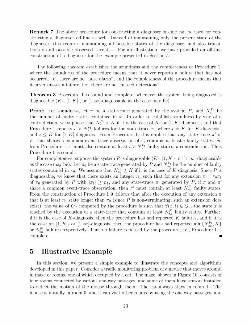
In this section, we present a simple example to illustrate the concepts and algorithmsdeveloped in this paper. Consider a traffic monitoring problem of a mouse that moves aroundin maze of rooms, one of which occupied by a cat. The maze, shown in Figure 10, consists offour rooms connected by various one-way passages, and some of them have sensors installedto detect the motion of the mouse through them. The cat always stays in room 1. Themouse is initially in room 0, and it can visit other rooms by using the one way passages, and
23
: observable
: unobservable
cat 1
2mouse0 3
Figure 10: Mouse in a maze: repeated monitoring
it never stays at one room forever. A failure is said to have occurred if the mouse movesto the room where the cat stays. The task of repeated failure diagnosis is to monitor themotion of the mouse by observing the sensor signals, and to detect the number of times thefailure has occurred.
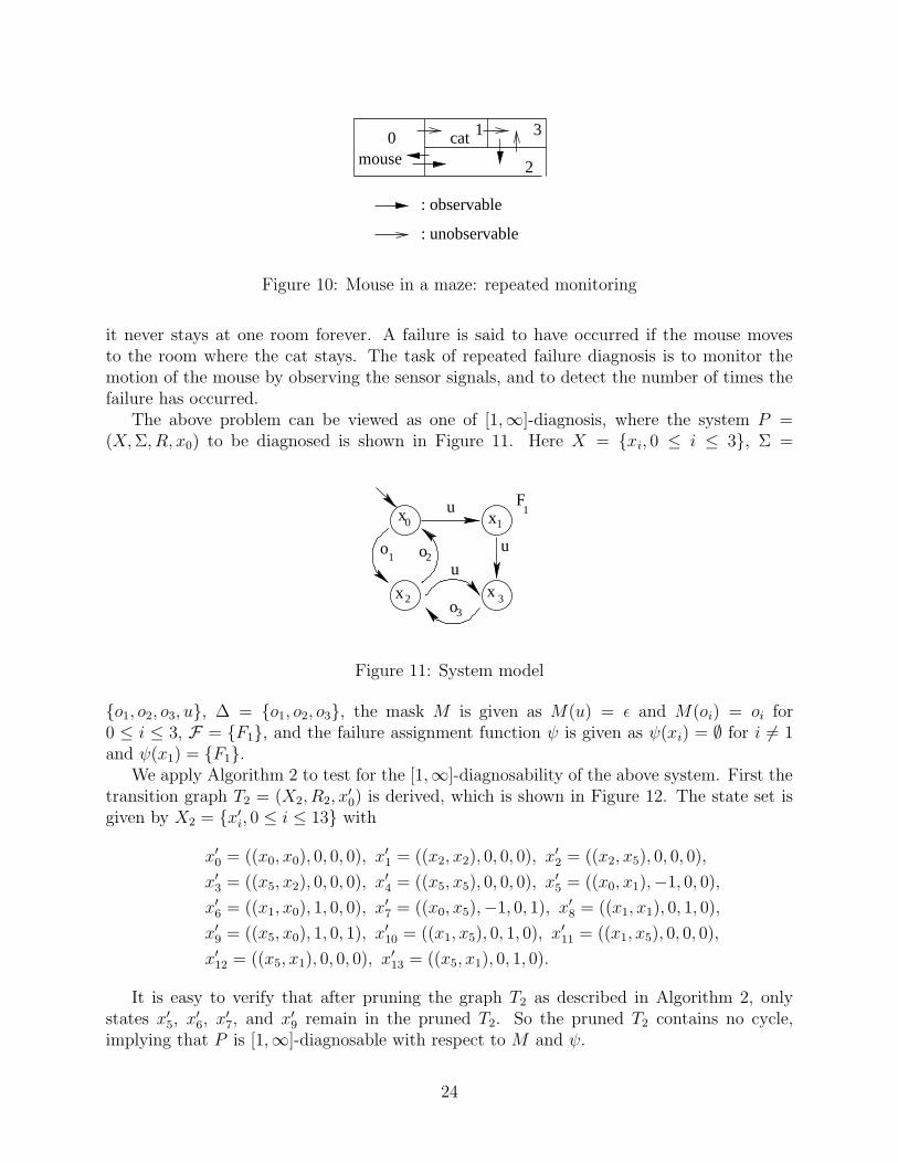
The above problem can be viewed as one of [1,∞]-diagnosis, where the system P =(X,Σ, R, x0) to be diagnosed is shown in Figure 11. Here X = {xi, 0 ≤ i ≤ 3}, Σ =
u
u
u
o3
x2
x0
o2o
1
x1
F1
x 3
Figure 11: System model
{o1, o2, o3, u}, ∆ = {o1, o2, o3}, the mask M is given as M(u) = ε and M(oi) = oi for0 ≤ i ≤ 3, F = {F1}, and the failure assignment function ψ is given as ψ(xi) = ∅ for i 6= 1and ψ(x1) = {F1}.
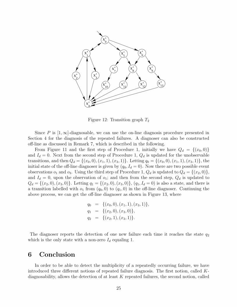
We apply Algorithm 2 to test for the [1,∞]-diagnosability of the above system. First thetransition graph T2 = (X2, R2, x
′0) is derived, which is shown in Figure 12. The state set is
given by X2 = {x′i, 0 ≤ i ≤ 13} with
x′0 = ((x0, x0), 0, 0, 0), x′1 = ((x2, x2), 0, 0, 0), x
′2 = ((x2, x5), 0, 0, 0),
x′3 = ((x5, x2), 0, 0, 0), x′4 = ((x5, x5), 0, 0, 0), x
′5 = ((x0, x1),−1, 0, 0),
x′6 = ((x1, x0), 1, 0, 0), x′7 = ((x0, x5),−1, 0, 1), x′8 = ((x1, x1), 0, 1, 0),
x′9 = ((x5, x0), 1, 0, 1), x′10 = ((x1, x5), 0, 1, 0), x
′11 = ((x1, x5), 0, 0, 0),
x′12 = ((x5, x1), 0, 0, 0), x′13 = ((x5, x1), 0, 1, 0).
It is easy to verify that after pruning the graph T2 as described in Algorithm 2, onlystates x′5, x
′6, x
′7, and x′9 remain in the pruned T2. So the pruned T2 contains no cycle,
implying that P is [1,∞]-diagnosable with respect to M and ψ.
24
x1’ x
6’
x7’ x
8’ x
9’
x5’
x0’
x10’ x
11’ x
13’x
12’
x4’
x2’ x
3’
Figure 12: Transition graph T2
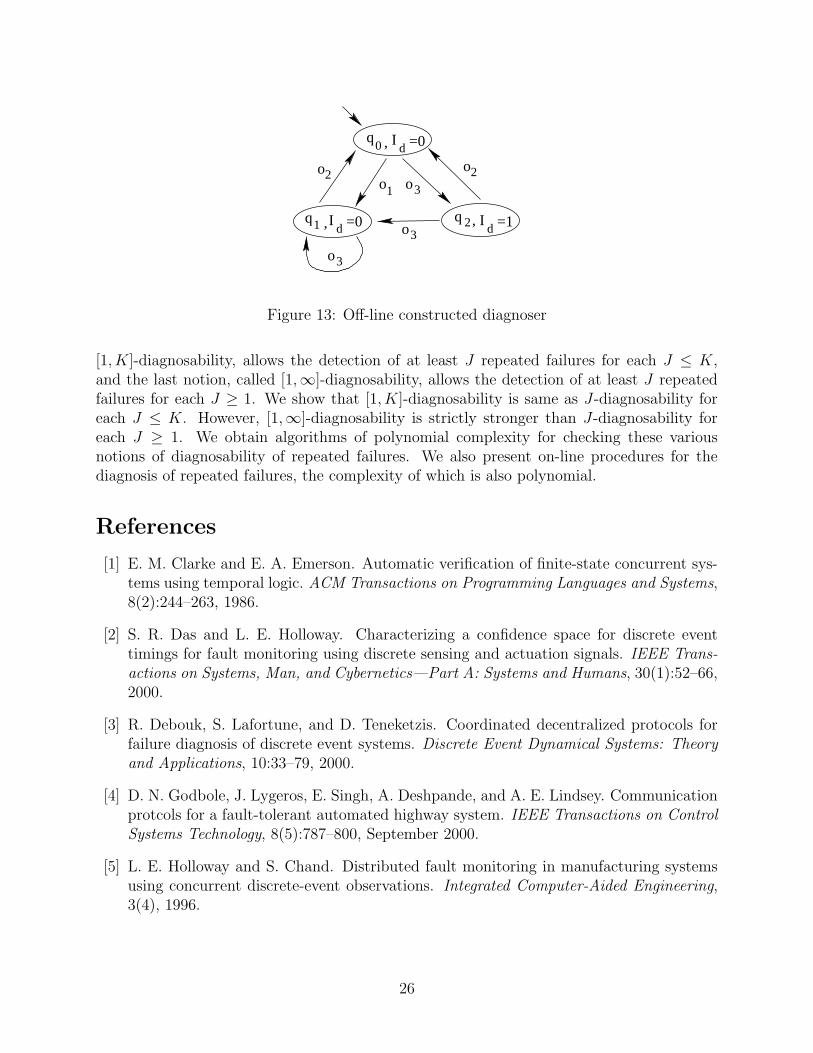
Since P is [1,∞]-diagnosable, we can use the on-line diagnosis procedure presented inSection 4 for the diagnosis of the repeated failures. A diagnoser can also be constructedoff-line as discussed in Remark 7, which is described in the following.
From Figure 11 and the first step of Procedure 1, initially we have Qd = {(x0, 0)}and Id = 0. Next from the second step of Procedure 1, Qd is updated for the unobservabletransitions, and thenQd = {(x0, 0), (x1, 1), (x3, 1)}. Letting q0 = {(x0, 0), (x1, 1), (x3, 1)}, theinitial state of the off-line diagnoser is given by (q0, Id = 0). Now there are two possible eventobservations o1 and o3. Using the third step of Procedure 1, Qd is updated to Qd = {(x2, 0)},and Id = 0, upon the observation of o1; and then from the second step, Qd is updated toQd = {(x2, 0), (x3, 0)}. Letting q1 = {(x2, 0), (x3, 0)}, (q1, Id = 0) is also a state, and there isa transition labelled with o1 from (q0, 0) to (q1, 0) in the off-line diagnoser. Continuing theabove process, we can get the off-line diagnoser as shown in Figure 13, where
q0 = {(x0, 0), (x1, 1), (x3, 1)},
q1 = {(x2, 0), (x3, 0)},
q2 = {(x2, 1), (x3, 1)}.
The diagnoser reports the detection of one new failure each time it reaches the state q2
which is the only state with a non-zero Id equaling 1.
6 Conclusion
In order to be able to detect the multiplicity of a repeatedly occurring failure, we haveintroduced three different notions of repeated failure diagnosis. The first notion, called K-diagnosability, allows the detection of at least K repeated failures, the second notion, called
25
Id =0q
0 ,
q1 Id =0, q 2 I
d =1,
o1 o3
o2o2
o3
o3
Figure 13: Off-line constructed diagnoser
[1, K]-diagnosability, allows the detection of at least J repeated failures for each J ≤ K,and the last notion, called [1,∞]-diagnosability, allows the detection of at least J repeatedfailures for each J ≥ 1. We show that [1, K]-diagnosability is same as J-diagnosability foreach J ≤ K. However, [1,∞]-diagnosability is strictly stronger than J-diagnosability foreach J ≥ 1. We obtain algorithms of polynomial complexity for checking these variousnotions of diagnosability of repeated failures. We also present on-line procedures for thediagnosis of repeated failures, the complexity of which is also polynomial.
References
[1] E. M. Clarke and E. A. Emerson. Automatic verification of finite-state concurrent sys-tems using temporal logic. ACM Transactions on Programming Languages and Systems,8(2):244–263, 1986.
[2] S. R. Das and L. E. Holloway. Characterizing a confidence space for discrete eventtimings for fault monitoring using discrete sensing and actuation signals. IEEE Trans-
actions on Systems, Man, and Cybernetics—Part A: Systems and Humans, 30(1):52–66,2000.
[3] R. Debouk, S. Lafortune, and D. Teneketzis. Coordinated decentralized protocols forfailure diagnosis of discrete event systems. Discrete Event Dynamical Systems: Theory
and Applications, 10:33–79, 2000.
[4] D. N. Godbole, J. Lygeros, E. Singh, A. Deshpande, and A. E. Lindsey. Communicationprotcols for a fault-tolerant automated highway system. IEEE Transactions on Control
Systems Technology, 8(5):787–800, September 2000.
[5] L. E. Holloway and S. Chand. Distributed fault monitoring in manufacturing systemsusing concurrent discrete-event observations. Integrated Computer-Aided Engineering,3(4), 1996.
26
[6] S. Jiang, Z. Huang, V. Chandra, and R. Kumar. A polynomial algorithm for testingdiagnosability of discrete event systems. IEEE Transactions on Automatic Control,46(8):1318–1321, August 2001.
[7] S. Jiang and R. Kumar. Failure diagnosis of discrete event systems with linear-timetemporal logic fault specifications. In Proceedings of 2002 American Control Conference,Anchorage, Alaska, May 2002.
[8] S. Jiang, R. Kumar, and H. E. Garcia. Diagnosis of repeated failures in discrete eventsystems. In Proceedings of 2002 IEEE Conference on Decision and Control, Las Vegas,December 2002.
[9] M. Larsson. Behavioral and structural model based approaches to discrete diagnosis.PhD thesis, Linkoping University, Linkoping, Sweden, 1999.
[10] F. Lin. Diagnosability of discrete event systems and its applications. Discrete Event
Dynamic Systems: Theory and Applications, 4(1):197–212, 1994.
[11] J. Lygeros, D. N. Godbole, and M. Broucke. A fault tolerant control architecturefor automated highway system. IEEE Transactions on Control Systems Technology,8(2):205–219, March 2000.
[12] D. Pandalai and L. Holloway. Template languages for fault monitoring of timed discreteevent processes. IEEE Transactions on Automatic Control, 45(5):868–882, May 2000.
[13] M. Sampath and S. Lafortune. Active diagnosis of discrete event systems. IEEE Trans-
actions on Automatic Control, 43(7):908–929, 1998.
[14] M. Sampath, R. Sengupta, S. Lafortune, K. Sinaamohideen, and D. Teneketzis. Diagons-ability of discrete event systems. IEEE Transactions on Automatic Control, 40(9):1555–1575, September 1995.
[15] M. Sampath, R. Sengupta, S. Lafortune, K. Sinaamohideen, and D. Teneketzis. Failurediagnosis using discrete event models. IEEE Transactions on Control Systems Technol-
ogy, 4(2):105–124, March 1996.
[16] T. Yoo and S. Lafortune. On the computational complexity of some problems arisingin partially-observed discrete event systems. In Proceedings of 2001 American Control
Conference, Arlington, VA, June 2001.
[17] S. H. Zad. Fault diagnosis in discrete-event and hybrid systems. PhD thesis, Universityof Toronto, Toronto, Canda, 1999.
27


