Developing a Practical Projection-BasedParallel Delaunay AlgorithmGuy E. Blelloch Gary L. Miller Dafna TalmorComputer Science DepartmentCarnegie Mellon Universityfblelloch,glmiller,talmorg@cs.cmu.eduAbstractIn this paper we are concerned with developing a practi-cal parallel algorithm for Delaunay triangulation that workswell on general distributions, particularly those that arisein Scienti�c Computation. Although there have been manytheoretical algorithms for the problem, and some implemen-tations based on bucketing that work well for uniform distri-butions, there has been little work on implementations forgeneral distributions.We use the well known reduction of 2D Delaunay trian-gulation to 3D convex hull of points on a sphere or paraboloid.A variant of the Edelsbrunner and Shi 3D convex hull isused, but for the special case when the point set lies on ei-ther a sphere or a paraboloid. Our variant greatly reducesthe constant costs from the 3D convex hull algorithm andseems to be a more promising for a practical implementationthan other parallel approaches. We have run experimentson the algorithm using a variety of distributions that aremotivated by various problems that use Delaunay triangu-lations. Our experiments show that for these distributionswe are within a factor of approximately two in work fromthe best sequential algorithm.1 IntroductionDelaunay triangulation along with its dual, the Voronoi Dia-gram, is an important problem in many domains, includingimaging, computer vision, terrain modeling, and meshingfor solving PDEs. In many of these domains the triangu-lation is a bottleneck in the computation time, making itimportant to develop fast algorithms. There are now manysequential algorithms available for Delaunay triangulationalong with e�cient implementations. Su and Drysdale [23]present an excellent experimental comparison of several suchalgorithms. The development of parallel algorithms is not asadvanced. As a �rst step researchers have developed manytheoretical parallel algorithms [7, 1, 8, 26, 20, 12]. How-ever, there have been very few e�cient implementations,and these few depend on having a uniform distribution ofpoints [16, 24, 22]. Attempts to implement the theoreticallygood algorithms have met with limited success [22]. Thereare several obstacles to constructing good practical parallel

Delaunay triangulation algorithms: (1) the known parallelsolutions are highly irregular and dynamic, (2) they requiresigni�cant inter-processor communication, and (3) they havevery large constants in their asymptotical work analysis evenif we ignore communication costs.Our goal was to develop a practical parallel algorithmthat works on general distributions. Since there are manydi�erent parallel machines with very di�erent characteristicwe tried to design our criteria for success in a machine inde-pendent way. Also, since reducing the total work executedby a parallel algorithm (point 3 above) is a prerequisite togetting a practical parallel algorithm, we decided that aninitial goal should be to construct a parallel algorithm thatdoes little work beyond the best sequential algorithm. Toquantify the constants in the work required by an algorithm,we say algorithm A is � work-e�cient compared to algo-rithm B if A performs at most 1=� times the number ofoperation of B. For example, the standard tree-algorithmfor pre�x sums [15] is 50% work-e�cient relative to the se-quential pre�x sums, since for n values the parallel versionrequires 2n � 2 operations whereas the sequential requiresonly n�1. The goal is to design parallel algorithms that areas close as possible to 100% work-e�cient relative to the bestsequential algorithm. Some natural measures of work thatwe considered included: oating point operations, memoryreferences, comparisons, and data movement. We settled on oating point operations as our primary measure of work be-cause it is machine independent and is reasonably correlatedwith runtime for this class of algorithms.In most Delaunay algorithms although the asymptoticwork for n points is bound by O(n log n) the actual workcan depend signi�cantly on the distribution of the points.Because of this, when considering � work-e�ciency we needto state results relative to particular distributions (this wasnot necessary for the pre�x sums example since the workis only dependent on the data size). For the results to beuseful it is necessary to select a \representative" set of distri-butions. Our selection of point distributions was motivatedby scienti�c domains and includes some highly nonuniformdistributions. The four distributions we use are discussed inSection 3.1 and pictured in Figure 6.We considered a variety of parallel Delaunay algorithmswith the goal of getting high � work-e�ciency on the dataset distributions. The most promising algorithm we consid-ered uses a projection based approach, loosely based on theEdelsbrunner and Shi [11] approach for 3D Convex Hulls.Our algorithm does O(n log n) work and has O(log3 n) depth(parallel time) on a CREW PRAM if we use Overmars and

Van Leeuwen's linear-work subroutine for 2-d convex hullson sorted input [18]. However, by using subroutines thatare not known to be theoretically optimal we signi�cantlyreduce both the experimental work and depth over our dataset. We implemented several variants of our algorithm andran experiments on our distributions to measure operationcounts ( oating-point operations) and parallel depth. Wecompared the operation counts to Dwyer's algorithm [10],which is the best of the sequential Delaunay algorithms stud-ied by Su and Drysdale [23]. Our algorithm is approximately50% work-e�cient relative to Dwyer's if it is run all the wayto the end. Furthermore, if the algorithm is used as a coarsepartitioner to break a problem into components that canthen be solved independently on a set of processors usingDwyer's algorithm, then the algorithm is very close to 100%work e�cient. Finally, the point distribution has little e�ecton the total work, suggesting that our algorithm is reason-ably robust across a variety of nonuniform distributions.1.1 Background and choicesMany of the algorithms for Delaunay triangulation, bothparallel and sequential, are based on the divide-and-conquerparadigm. These algorithms can be characterized by therelative costs of the divide and merge phases. An early se-quential approach developed by Shamos and Hoey [21] (forVoronoi diagrams) and re�ned by Guibas and Stol� [13] (forDelaunay triangulation), is to divide the point set into twosubproblems using a median, then to �nd the Delaunay di-agram of each half, and �nally to merge the two diagrams.The merge phase does most of the work of the algorithm andruns in O(n) time, so the whole algorithm runs in O(n log n)time. Unfortunately, these original versions of the mergewere highly sequential in nature. Aggarwal et al. [1] �rstpresented a parallel version of the merge phase, which leadto an algorithm with O(log2 n) depth. However, this algo-rithm was signi�cantly more complicated than the sequen-tial version, and was not work e�cient|the merge requiredO(n log n) work. Goodrich, Cole and O'Dunlaing improvedthe method making it work e�cient [8], but it remains ham-pered by messy data structures, and as it stands can beruled out as a promising candidate for implementation.1Reif and Sen [20] developed a randomized parallel divide-and-conquer paradigm, called \polling". They solve themore general 3D Convex-hull problem, which can be usedfor �nding the Delaunay triangulation. In their algorithma sample of the points is used to split the problem into aset of smaller independent subproblems. For this algorithm,the work is concentrated in the divide phase, and mergingsimply glues the solutions together. The size of the sampleensures even splitting with high probability. A point can ap-pear in more than one subproblem and so to avoid blow-uptrimming techniques are used. A simpli�ed version of thisalgorithm was considered by Su [22]. His �ndings show thatwhereas the paradigm does indeed evenly divide the prob-lem, the expansion factor is close to 6 on all the distributionshe considered. This will lead to an algorithm that is at best1=6 work-e�cient, and therefore, pending further improve-ments, is not a likely candidate for implementation. Dehneet al derive a similar algorithm based on sampling [9]. Theyshow that the algorithm is communication e�cient whenn > p3+� (only O(n=p) data is sent and received by each1We note, however, that there certainly could be simpli�cationsthat make it easier to implement.

processor). The algorithm is quite complicated, however,and it is unclear what the constants in the work are.Edelsbrunner and Shi [11] present a 3D convex hull al-gorithm based on the 2D algorithm of Kirkpatrick and Sei-del [14]. The algorithm divides the problem by �rst usinglinear programming to �nd a facet of the 3D convex hullabove a splitting point, then using projection onto verticalplanes and 2D convex hulls to �nd two paths of convex-hulledges. These paths are then used to divide the probleminto four subproblems, using planar point location to de-cide for each point which of the subproblems it belongs to.The merge phase again simply glues the solutions. The al-gorithm takes O(n log2 h) time where h is the number offacets in the solution. When applied to Delaunay triangula-tion the algorithm takes O(n log2 n) time since the numberof facets will be �(n). This algorithm can be parallelizedwithout much di�culty since all the sub-steps have knownparallel solutions, giving a depth (parallel time) of O(log3 n)and work of O(n log2 h). Ghouse and Goodrich [12] showedhow the algorithm could be improved to O(log2 n) depthand O(min(n log2 h; n log n)) work using randomization andvarious additional techniques. The improvement in workmakes the algorithm asymptotically work-e�cient for Delau-nay triangulation. However, these work bounds were basedon switching to the Reif and Sen algorithm if the output sizewas large. Therefore, when used for Delaunay triangulation,the Ghouse and Goodrich algorithm simply reduces to theReif and Sen algorithm.1.2 Our algorithm and experimentsThe complicated subroutines in the Edelsbrunner and Shiapproach, and the fact that it requires O(n log2 n) workwhen applied to Delaunay triangulation, initially seems torule it out as a reasonable candidate for a parallel implemen-tation. We note, however, that by restricting ourselves to apoint set on the surface of a sphere or parabola (su�cient forDelaunay triangulation) the algorithm can be greatly sim-pli�ed. Under this assumption, we developed an algorithmthat only needs a 2D convex-hull as a subroutine, removingthe need for linear programming and planar point location.Furthermore our algorithm only makes cuts parallel to thex or y axis allowing us to keep the points sorted and use anO(n) work 2D convex-hull. These improvements reduce thetheoretical work to O(n log n) and also greatly reduce theconstants. This simpli�ed version of the Edelsbrunner andShi approach seemed a promising candidate for experimen-tation: it does not su�er from unnecessary duplication, aspoints are duplicated only when a Delaunay edge is found,and it does not require complicated subroutines, especiallyif one is willing to compromise on non theoretically-optimalcomponents, as discussed below.Through alternating rounds of experimentation and al-gorithmic design, we re�ned this initial algorithm. We im-prove the basic algorithm from a practical point of view byusing the 2D convex-hull algorithm of Chan et al [6]. Thisalgorithm leads to a non optimal theoretical work since itruns in worst case O(n log h) work (instead of linear), but inpractice our experiments showed that it runs in linear work,and has a smaller constant than the provably linear workalgorithm. Our �nal algorithm is not only simple enoughto be easily implemented, but is also highly parallel andperforms work comparable to e�cient sequential algorithmsover a wide range of distributions. The algorithm can alsobe used to partition the problems into processors, and solv-

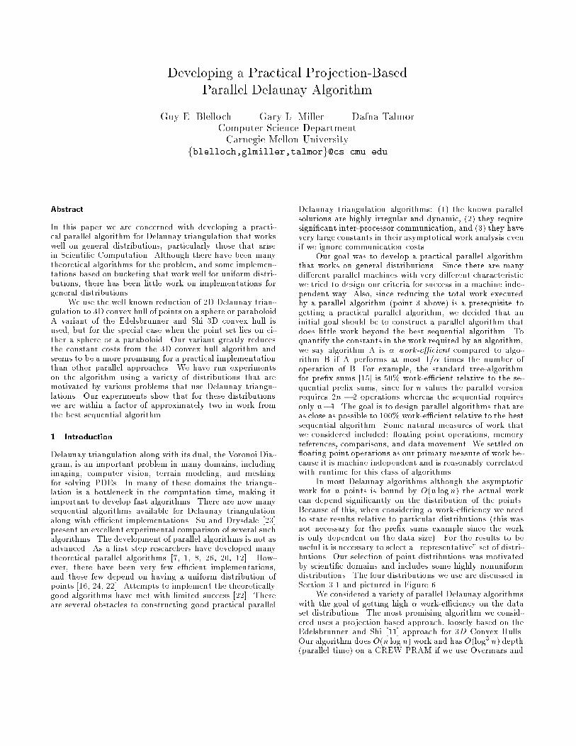
ing each subproblem using the sequential algorithm on eachprocessor, with the work for the coarse partitioning beingnegligible.The algorithm was implemented and evaluated in theNESL parallel programming language [4]. The emphasisof our study is on measuring the algorithms in a manneras implementation-independent as possible. Hence, we seekto quantify the number of operations, recursion levels, etc.,rather than run times.The rest of the paper is organized as follows: in sec-tion 2 we discuss the algorithm, justify our design choicestheoretically, and mention some of the details of the im-plementation, such as the data structures. In section 3 wedescribe the test-bed, and present the experimental results.A preliminary version of this work was presented atthe MSI Workshop on Computational Geometry [3]. Theearlier version only included the basic algorithm. Here wehave optimized the basic algorithm, included an optimizedend-game, and a systematic comparison of our optimizedcode with the best sequential code we know of.2 Projection-based DelaunayThe goal of this section is to present our algorithm, concen-trating on the theoretical motivations for our design choices.Our claim is that these choices lead to a parallel algorithmwhich is not only e�cient, but simple to implement as well,and therefore we also present in some detail the data struc-tures we use.The basic algorithm uses a divide-and-conquer strategy.Each subproblem is determined by a region R which is theunion of a collection of Delaunay triangles. The region R isrepresented by the following information: (1) the polygonalborder B of the region and (2) the set of points P of the re-gion, composed of internal points and points on the border.Note that the region may not be connected. At each call, wedivide the region into two regions using a median line cut ofthe internal points, and a corresponding path of Delaunayedges. The new path separates Delaunay triangles whose cir-cumcenter is to the left of the median line, from those whosecenter is to the right of the median line. We then determinethe new border of Delaunay edges for each subproblem bymerging the old border with the new path. Since we areusing a median cut, our algorithm guarantees that the num-ber of internal points is reduced by a factor of at least twoat each call. This simple separation is at the heart of ouralgorithm being e�cient. Unlike early divide-and-conquerstrategies for Delaunay triangulation which do most of thework when returning from recursive calls [21, 13, 8], thisalgorithm does all the work before making recursive calls.To �nd the separating path (which we call H), we projectthe points onto a paraboloid whose center is on the medianline L, then project the points horizontally onto a verticalplane whose intersection with the x-y plane is L (see Figure2). The 2D lower convex hull of those projected points, is therequired new border path H. In general, the structure of Hmay be more complicated. We discuss this below. Figure 1gives a more detailed description of the algorithm. Oncethe subproblem has no more internal points, we move to theend-game strategy to be described later in this section.Correctness of the median splits: We now show the Delau-nay path H is related to the median line L in the followingsense:

Algorithm: Delaunay(P;B)Input: P , a set of points in R2,B, a set of Delaunay edges of P which is the border of aregion in R2 containing P .Output: The set of Delaunay triangles of P which arecontained within B.Method:1. If all the points in P are on the boundary B, returnEnd Game(B).2. Find the point q that is the median along the x axisof all internal points (points in P and not on theboundary). Let L be the line x = qx.3. Let P 0 = f(py � qy; jjp� qjj2) j (px; py) 2 Pg. Thesepoints are derived from projecting the points P ontoa 3D paraboloid centered at q, and then projectingthem onto the vertical plane through the line L.4. Let H = Lower Convex Hull(P 0). H is a path ofDelaunay edges of the set P . Let PH be the set ofpoints the path H consists of, and �H is the path Htraversed in the opposite direction.5. Create two subproblems:� PL = fp 2 P jp is left of Lg [ PHPR = fp 2 P jp is right of Lg [ PH� BL = Border Merge(B;H)BR = Border Merge(B; �H)6. Return Delaunay(PL; BL) [Delaunay(PR; BR)Figure 1: The projection-based parallel algorithm. Initially B isthe convex hull of P . The algorithm as described cuts along the xaxis, but in general we can switch between x and y cuts, and allour implementations switch on every level. The algorithm uses thethree subroutines End Game, Lower Convex Hull, and Bor-der Merge, which are described in the text.Lemma 1 There is no point in P which is left(right) of theline L, but right(left) of H.This implies that we can determine whether a point not onH is left or right of H by comparing it against the line L, asimpler computational task.Proof outline: Lemma 1 is easily seen to be true in a muchmore general setting. Let Q be a convex body in IR3 withboundary �Q. A point q in �Q is said to be light if it isvisible from the x direction, i.e., the ray fq + �x̂j� > 0gdoes not intersect Q, where x̂ = (1; 0; 0). We say the point qis dark if the ray fq��x̂j� > 0g does not intersect Q. Theboundary between light and dark is called the silhouette. Inthe case when �Q is our paraboloid then the silhouette is justthe image of the line L. In general the silhouette is allthose points that lie on a supporting plane whose normal isalso normal to x̂.If we further assume that the points P are containedin �Q with convex hull �P we can de�ne the light, dark, andsilhouette points of �P . In the case when �Q is our paraboloidthen the silhouette in general will consist of faces and edgesof �P . For ease of exposition, we assume no faces appear onthe silhouette. We also assume that the points are in generalposition, i.e. that all faces are triangular. H is then a simple

(a) Median line L and path H. (b) points projected onto the paraboloid. (c) the paraboloid points projected ontothe vertical plane.Figure 2: This �gure shows the median line, all points projected on a parabola centered at a point on that line, and the horizontal projectiononto the vertical plane through the median line. The result of the lower convex hull in the projected space, H, is shown in highlighted edgeson the plane.path .Clearly no point q 2 �Q\ �P can be light as a point in �Qbut dark as a point in �P because �P in contained in Q. Thisis exactly what Lemma 1 states and thus proves the lemma.2 We now return to the case where the points P lie onthe paraboloid. We give a simple characterization of whena face on �P is light, dark or on the silhouette in term of itscircumscribing circle.De�nition 1 A Delaunay triangle is called a left, right,middle triangle with respect to a line L, if the circumcen-ter of its Delaunay circle lies left of, right of, or on the lineL respectivelyLemma 2 A face F is dark, light, or on the silhouette ifand only if its triangle in the plane is left, right, or middlerespectively.Proof: The face F supporting plane is of the form ax+by�z = c with normal n = (a; b;�1). Now F is dark, light,or on the silhouette if and only if a < 0, a > 0, or a = 0respectively. The vertical projection of the intersection ofthis plane, and the paraboloid, is described by x2+y2 = ax+by+c, or by (x�a=2)2+(y�a=2)2 = c+(a=2)2+(b=2)2. Thisis an equation describing a circle whose center is (a=2; b=2)and contains the three points of the triangle. Hence, this isthe Delaunay triangle's circumcenter and this circumcenteris simply related to the normal of the corresponding face ofthe convex hull. 2Therefore the only time that a triangle will cause a faceto be on the silhouette is when its circumcenter is on L.For ease of exposition, we assume the following degeneracycondition: No vertical or horizontal line contains both apoint and a circumcenter.Analysis: We now consider the total work and depth of thealgorithm. Our bounds are based on an CREW PRAM. Thecosts depend on the three subroutines End Game,Lower Convex Hull, and Border Merge. In this sec-tion we brie y describe subroutines that lead to theoreticallyreasonable bounds, and in the following sections we discussvariations for which we do not know how to prove strongbounds on, but work better on our data sets.Lemma 3 Using a parallel version of Overmars and VanLeeuwen's algorithm for the Lower Convex Hull and

Goodrich, Cole and O'Dunlaing's algorithm [8] for the End Game,our method runs in O(n log n) work and O(log3 n) depth.Proof: We �rst note that since our projections are alwayson a plane perpendicular to the x or y axis, we can keep ourpoints sorted relative to these axes with linear work (we cankeep the rank of each point along both axis and compressthese ranks when partitioning). This allows us to use Over-mars and Van Leeuwen's linear-work subroutine for 2D con-vex hulls on sorted input. Since their algorithm uses divide-and-conquer and each divide stage takes O(log n) sequentialtime, the full algorithm runs with O(log2 n) depth. Theother subroutines in the partitioning are the median, pro-jection and Border Merge These can all be implementedwithin the bounds of the convex hull (Border Merge isdiscussed later in this section). The total cost for partition-ing n points is therefore O(n) work and O(log2 n) depth.As discussed earlier, when partitioning a region (P;B)the number of internal points within each partition is atmost half as many as the number of internal points in (P;B).The total number of levels of recursion before there are nomore internal points is therefore at most log n. Furthermore,the total border size when summed across all instances ona given level of recursion is at most 6n. This is because 3nis a limit on the number of Delaunay edges in the �nal an-swer, and each edge can belong to the border of at most twoinstances (one on each side). Since the work for portion-ing a region is linear, the total work needed to process eachlevel is O(n) and total work across the levels is O(n log n).Similarly, the depth is O(log3 n).This is the cost to bring us down to components whichhave no internal points (just borders). To �nish o� we needto run the End Game. If the border is small (our experi-ments indicate that the average size is less than 10), it canbe solved by any technique, and if the border is large, thenthe Goodrich, Cole and O'Dunlaing algorithm [8] can beused. 2Border merge: We now discuss how the new Delaunay pathis merged with the old border, to form two new borders. Thegeometric properties of these paths, combined with the datastructure we use lead to a simple and elegantO(n) work O(1)time intersection routine.The set of points is represented using a vector. Theborder B is represented as an unordered set of triplets.

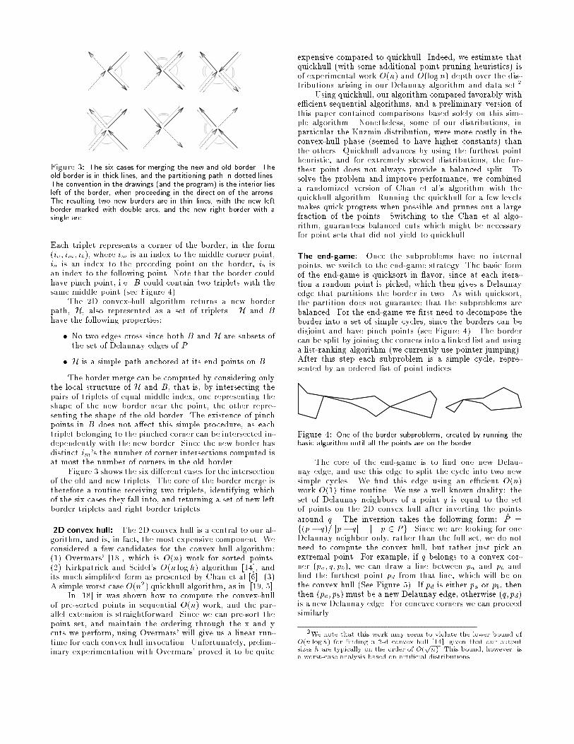
Figure 3: The six cases for merging the new and old border. Theold border is in thick lines, and the partitioning path in dotted lines.The convention in the drawings (and the program) is the interior liesleft of the border, when proceeding in the direction of the arrows.The resulting two new borders are in thin lines, with the new leftborder marked with double arcs, and the new right border with asingle arc.Each triplet represents a corner of the border, in the form(ia; im; ib), where im is an index to the middle corner point,ia is an index to the preceding point on the border, ib isan index to the following point. Note that the border couldhave pinch point, i.e. B could contain two triplets with thesame middle point (see Figure 4).The 2D convex-hull algorithm returns a new borderpath, H, also represented as a set of triplets. H and Bhave the following properties:� No two edges cross since both B and H are subsets ofthe set of Delaunay edges of P .� H is a simple path anchored at its end points on B.The border merge can be computed by considering onlythe local structure of H and B, that is, by intersecting thepairs of triplets of equal middle index, one representing theshape of the new border near the point, the other repre-senting the shape of the old border. The existence of pinchpoints in B does not a�ect this simple procedure, as eachtriplet belonging to the pinched corner can be intersected in-dependently with the new border. Since the new border hasdistinct im's the number of corner intersections computed isat most the number of corners in the old border.Figure 3 shows the six di�erent cases for the intersectionof the old and new triplets. The core of the border merge istherefore a routine receiving two triplets, identifying whichof the six cases they fall into, and returning a set of new leftborder triplets and right border triplets.2D convex hull: The 2D convex hull is a central to our al-gorithm, and is, in fact, the most expensive component. Weconsidered a few candidates for the convex hull algorithm:(1) Overmars' [18], which is O(n) work for sorted points.(2) Kirkpatrick and Seidel's O(n log h) algorithm [14], andits much simpli�ed form as presented by Chan et al [6]. (3)A simple worst case O(n2) quickhull algorithm, as in [19, 5].In [18] it was shown how to compute the convex-hullof pre-sorted points in sequential O(n) work, and the par-allel extension is straightforward. Since we can pre-sort thepoint set, and maintain the ordering through the x and ycuts we perform, using Overmars' will give us a linear run-time for each convex hull invocation. Unfortunately, prelim-inary experimentation with Overmars' proved it to be quite

expensive compared to quickhull. Indeed, we estimate thatquickhull (with some additional point pruning heuristics) isof experimental work O(n) and O(log n) depth over the dis-tributions arising in our Delaunay algorithm and data set.2Using quickhull, our algorithm compared favorably withe�cient sequential algorithms, and a preliminary version ofthis paper contained comparisons based solely on this sim-ple algorithm. Nonetheless, some of our distributions, inparticular the Kuzmin distribution, were more costly in theconvex-hull phase (seemed to have higher constants) thanthe others. Quickhull advances by using the furthest pointheuristic, and for extremely skewed distributions, the fur-thest point does not always provide a balanced split. Tosolve the problem and improve performance, we combineda randomized version of Chan et al's algorithm with thequickhull algorithm. Running the quickhull for a few levelsmakes quick progress when possible and prunes out a largefraction of the points. Switching to the Chan et al algo-rithm, guarantees balanced cuts which might be necessaryfor point sets that did not yield to quickhull.The end-game: Once the subproblems have no internalpoints, we switch to the end-game strategy. The basic formof the end-game is quicksort in avor, since at each itera-tion a random point is picked, which then gives a Delaunayedge that partitions the border in two. As with quicksort,the partition does not guarantee that the subproblems arebalanced. For the end-game we �rst need to decompose theborder into a set of simple cycles, since the borders can bedisjoint and have pinch points (see Figure 4). The bordercan be split by joining the corners into a linked list and usinga list-ranking algorithm (we currently use pointer jumping).After this step each subproblem is a simple cycle, repre-sented by an ordered list of point indices.Figure 4: One of the border subproblems, created by running thebasic algorithm until all the points are on the borderThe core of the end-game is to �nd one new Delau-nay edge, and use this edge to split the cycle into two newsimple cycles. We �nd this edge using an e�cient O(n)work O(1) time routine. We use a well known duality: theset of Delaunay neighbors of a point q is equal to the setof points on the 2D convex hull after inverting the pointsaround q. The inversion takes the following form: _P =f(p � q)=jjp� qjj j p 2 Pg. Since we are looking for oneDelaunay neighbor only, rather than the full set, we do notneed to compute the convex hull, but rather just pick anextremal point. For example, if q belongs to a convex cor-ner (pa; q; pb), we can draw a line between pa and pb and�nd the furthest point pd from that line, which will be onthe convex hull (See Figure 5). If pd is either pa or pb, thenthen (pa; pb) must be a new Delaunay edge, otherwise (q; pd)is a new Delaunay edge. For concave corners we can proceedsimilarly.2We note that this work may seem to violate the lower bound ofO(n log h) for �nding a 2-d convex hull [14], given that our outputsizes h are typically on the order of O(pn). This bound, however, isa worst-case analysis based on arti�cial distributions.

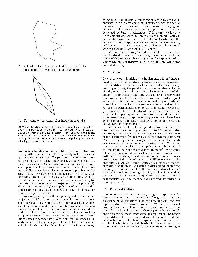
(a) A border piece. The point highlighted, q, is theone singled for expansion in the end-game.(b) The same set of points after inversion around q.Figure 5: Starting in (a) with a border subproblem, we look fora new Delaunay edge of a point q. We do that by using inversionaround q to move to the dual problem of �nding convex-hull edges,as in (b), drawn in thick lines. The new Delaunay edge we pick isto the point farthest from the line between the points preceding andfollowing q, shown in a thin line.Comparison to Edelsbrunner and Shi Here we explain howour algorithm di�ers from the original algorithm presentedby Edelsbrunner and Shi. We partition the points and bor-der by �nding a median, computing a 2D convex hull of asimple projection of the points, and then using some simplelocal operations for merging the borders. Since Edelsbrun-ner and Shi are solving the more general problem of 3Dconvex hull, they have to (1) �nd a 4-partition using 2 in-tersecting lines in the XY plane, (2) use linear programmingto �nd the face of the convex-hull above the intersection, (3)compute two convex hulls of projections of the points (4),Merge the borders, and (5) use point location to determinewhich points belong to which partition. Each of these stepsis more complex than ours.We can get away with the simpler algorithm since in ourprojection in 3D, all points lie on a surface of a parabola.This allows us to easily �nd a face of the convex-hull (we justuse the median point), and to simply partition the pointsusing a median line. Furthermore, our partitions can all bemade parallel to the x or y axis, which allows us to keepour points sorted along the cut for the convex-hull. Withthis we can use a linear work algorithm for the convex hull,as discussed. This is not possible with the Edelsbrunnerand Shi algorithms since in their algorithm it is necessary

to make cuts in arbitrary directions in order to get the 4-partition. On the down side, our partition is not as good asthe 4-partition of Edelsbrunner and Shi since it only guar-antees that the internal points are well partitioned (the bor-der could be badly partitioned). This means we have toswitch algorithms when no internal points remain. Our ex-periments show, however, that for all our distributions theaverage size of components when switching is less than 10,and the maximum size is rarely more than 50 (this assumeswe are alternating between x and y cuts).We note that proving the su�ciency of the median testfor the divide phase was the insight that motivated ourchoice of the projection-based algorithm for implementation.This work was also motivated by the theoretical algorithmspresented in [17].3 ExperimentsTo evaluate our algorithm, we implemented it and instru-mented the implementation to measure several quantities.The quantities we measure include the total work ( oating-point operations), the parallel depth, the number and sizesof subproblems on each level, and the relative work of thedi�erent subroutines. The total work is used to determinehow work-e�cient the algorithm is compared with a goodsequential algorithm, and the ratio of work to parallel-depthis used to estimate the parallelism available in the algorithm.We use the other measures to better understand how the al-gorithm is e�ected by the distributions, and how well ourheuristic for splitting works. We have also used the mea-sures extensively to improve our algorithm and have beenable to improve our convex-hull by a factor of 3 over ourinitial naive implementation.We measured the di�erent quantities over four data setdistributions, for sizes varying from 210 to 217. For each dis-tribution, each data set, and each size we ran �ve instancesof the distribution (seeded with di�erent random numbers)The results are presented using median values and intervalsover these experiments, unless otherwise stated. Our inter-vals are de�ned by the outlying points (the minimum andthe maximum over the relevant measurements). We de�neda oating point operation as a oating point comparison orarithmetic operation, though our instrumentation contains abreak down of the operations into the di�erent classes. Thedata �les are available upon request if a di�erent de�nitionof work is of interest. Although oating-point operationscertainly do not account for all costs in an algorithm theyhave the important advantage of being machine independent(at least for machines that implement the standard IEEE oat instructions) and seem to have a strong correlation torunning time [23].3.1 Data DistributionsThe design of the data set is always of great importance forthe experimentation and evaluation. Our goal is to test ouralgorithm on distributions that are non uniform, and yetrepresentative of real-world problems. We therefore pickeddistributions from di�erent domains, such as the distribu-tion of stars in a at galaxy (Kuzmin) or point sets origi-nating from the mesh generation domain, where Delaunaytriangulation plays an important role. Many of these distri-butions fall under the class of Lipschitz distributions|thatis, the density function's derivative is bounded by a con-stant. This allows for arbitrary re�nements of the triangles

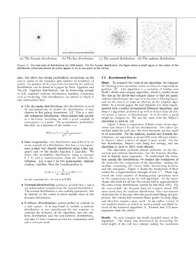
(a) The Kuzmin distribution. (b) The line distribution. (c) The normal distribution. (d) The uniform distribution.Figure 6: Our test-suite of distributions for 1000 points. For the Kuzmin distribution, the �gure shows a small region in the center of thedistribution (otherwise almost all points appear to be at one point at the center).sizes, but allows for certain probabilistic restrictions on theaspect ratios of the triangles and number of neighbors ofpoints. An analysis of the expected extremes for the uniformdistribution can be found in a paper by Bern, Eppstein andYao [2]. Lipschitz distributions can be interesting enoughto defy standard uniform distribution handling techniquessuch as bucketing. Our distributions are shown in Figure 6and summarized here.� The Kuzmin distribution: this distribution is usedby astrophysicists to model the distribution of starclusters in at galaxy formations [25]. This is a radi-ally symmetric distribution, whose density falls quicklyas r increases, providing us with a good example ofconvergence to a point. The accumulative probabilityfunction, as a function of the radius r is:M(r) = 1� 1p1 + r2� Line singularity: this distribution was de�ned by usas an example of a distribution that has a convergencearea (points very densely distributed along a line seg-ment) and yet the density function is Lipschitz. Wede�ne this probability distribution using a constantb � 0, and a transformation from the uniform dis-tribution. Let u and v be two independent, uniformrandom variables, then the transformation is:(x; y) = ( bu� bu + b ; v)in our experiments, we set b = 0:001.� Normal distribution: points (x; y) such that x and yare independent samples from the normal distribution.The normal distribution is also radially symmetric, butits density at the center is much smaller than in theKuzmin distribution.� Uniform distribution: points picked at random ina unit square. It is important to include a uniformdistribution in our experiments for two reasons: tocontrast the behavior of the algorithm over the uni-form distribution and the non-uniform distributions,and also to form common ground for comparison withother relevant work.

3.2 Experimental ResultsWork: To estimate the work of our algorithm, we comparethe oating-point operation counts to Dwyer's sequential al-gorithm [10]. This algorithm is a variation of Guibas andStol�'s divide-and-conquer algorithm, which is careful aboutthe cuts in the divide-and-conquer phase so that for quasi-uniform distributions the expected run time is O(n log log n),and on the rest is at least as e�cient as the original algo-rithm. In a recent paper, Su and Drysdale [23] have experi-mented with a variety of sequential Delaunay algorithm, andDwyer's algorithm performed as well or better than all oth-ers across a variety of distributions. It is therefore a goodtarget to compare to. We use the same code for Dwyer'salgorithm as used in [23].Figure 7 shows a comparison of oat-counts of our algo-rithm and Dwyer's for all our distributions. The values aremedian value for each size, the error intervals are too smallto be noticeable. For the uniform, normal and Kuzmin dis-tributions our algorithm is about 50% work e�cient relativeto Dwyer's (does a factor of about 2 more work). For theline distribution, Dwyer's cuts bring less savings, and ouralgorithm is close to 100% work e�cient.Our algorithm performs almost uniformly on the line,normal and uniform distribution, but the Kuzmin distribu-tion is slightly more expensive. To understand the varia-tion among the distributions we studied the breakdown ofthe work into the components of the algorithm|�nding themedian, computing 2D convex hulls, intersecting borders,and the end-game. Figure 8 shows the breakdown of oatcounts for a representative example of size 217. These rep-resent the total number of oating-point operations usedby the components across the full algorithm. As the �gureshows, the work for all but the convex-hull is approximatelythe same across distributions (varies by less than 10%). Forthe convex-hull, the Kuzmin data set requires about 25%more work than the uniform distribution. Our experimentsshow that this is because after the paraboloid lifting and pro-jection, the convex-hull removes fewer points in early stepsand therefore requires more work. In an earlier version ofour implementation in which we used a simple quickhull in-stead of the balanced algorithm [6], Kuzmin was 75% moreexpensive than the others.Depth: We now consider the depth (parallel time) of thealgorithm. The depth was determined by measuring thetotal depth of the call tree (always taking the maximum

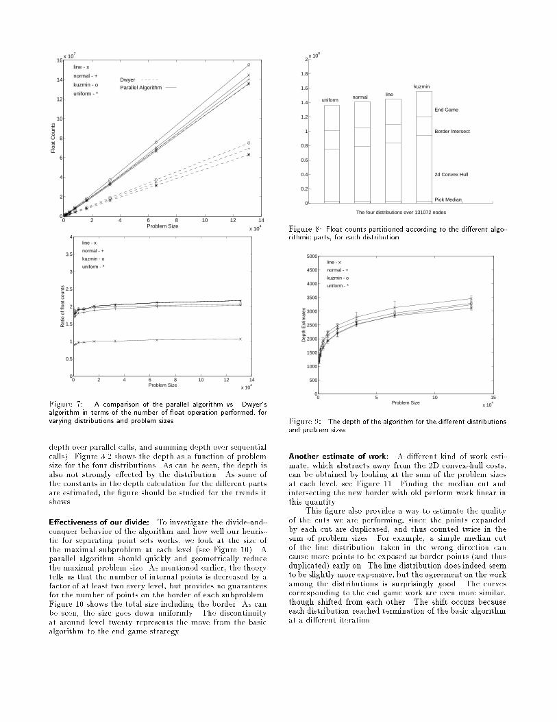
0 2 4 6 8 10 12 14

x 104

0

2

4

6

8

10

12

14

16x 10

7

Problem Size

Flo

at C

ount

s

uniform - *

kuzmin - o

normal - +

line - x

Dwyer

Parallel Algorithm

0 2 4 6 8 10 12 14

x 104

0

0.5

1

1.5

2

2.5

3

3.5

4

Problem Size

Rat

io o

f flo

at c

ount

s

uniform - *

kuzmin - o

normal - +

line - x

Figure 7: A comparison of the parallel algorithm vs. Dwyer'salgorithm in terms of the number of oat operation performed, forvarying distributions and problem sizes.depth over parallel calls, and summing depth over sequentialcalls). Figure 3.2 shows the depth as a function of problemsize for the four distributions. As can be seen, the depth isalso not strongly e�ected by the distribution. As some ofthe constants in the depth calculation for the di�erent partsare estimated, the �gure should be studied for the trends itshows.E�ectiveness of our divide: To investigate the divide-and-conquer behavior of the algorithm and how well our heuris-tic for separating point sets works, we look at the size ofthe maximal subproblem at each level (see Figure 10). Aparallel algorithm should quickly and geometrically reducethe maximal problem size. As mentioned earlier, the theorytells us that the number of internal points is decreased by afactor of at least two every level, but provides no guaranteesfor the number of points on the border of each subproblem.Figure 10 shows the total size including the border. As canbe seen, the size goes down uniformly. The discontinuityat around level twenty represents the move from the basicalgorithm to the end game strategy.

0

0.2

0.4

0.6

0.8

1

1.2

1.4

1.6

1.8

2x 10

8

The four distributions over 131072 nodes

Pick Median

2d Convex Hull

Border Intersect

End Game

uniformnormal line

kuzmin

Figure 8: Float counts partitioned according to the di�erent algo-rithmic parts, for each distribution.0 5 10 15

x 104

0

500

1000

1500

2000

2500

3000

3500

4000

4500

5000

Problem Size

Dep

th E

stim

ates

uniform - *

kuzmin - o

normal - +

line - x

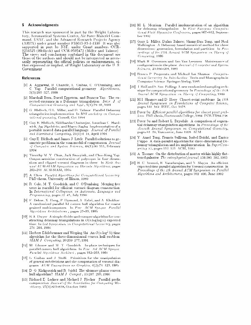
Figure 9: The depth of the algorithm for the di�erent distributionsand problem sizes.Another estimate of work: A di�erent kind of work esti-mate, which abstracts away from the 2D convex-hull costs,can be obtained by looking at the sum of the problem sizesat each level, see Figure 11. Finding the median cut andintersecting the new border with old perform work linear inthis quantity.This �gure also provides a way to estimate the qualityof the cuts we are performing, since the points expandedby each cut are duplicated, and thus counted twice in thesum of problem sizes. For example, a simple median cutof the line distribution taken in the wrong direction cancause more points to be exposed as border points (and thusduplicated) early on. The line distribution does indeed seemto be slightly more expensive, but the agreement on the workamong the distributions is surprisingly good. The curvescorresponding to the end game work are even more similar,though shifted from each other. The shift occurs becauseeach distribution reached termination of the basic algorithmat a di�erent iteration.

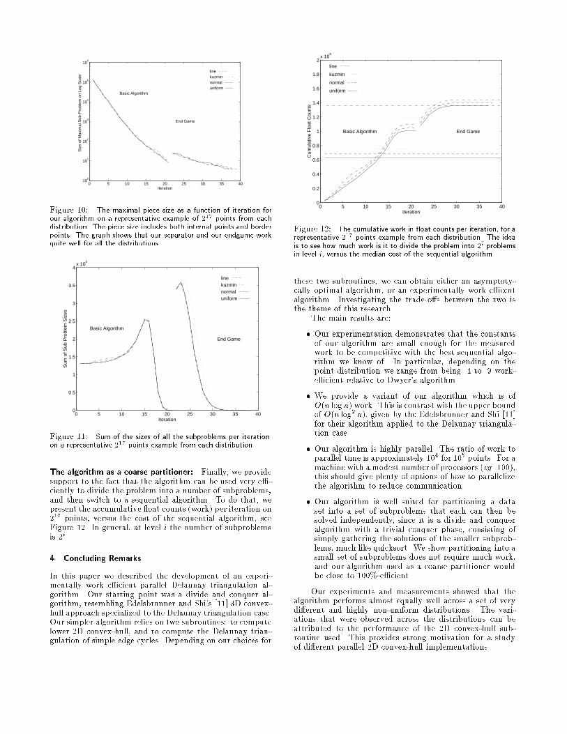
0 5 10 15 20 25 30 35 40

line kuzmin normal uniform

100

101

102

103

104

105

106

Iteration

Siz

e of

Max

imal

Sub

-Pro

blem

on

Log

Sca

le

Basic Algorithm

End GameFigure 10: The maximal piece size as a function of iteration forour algorithm on a representative example of 217 points from eachdistribution. The piece size includes both internal points and borderpoints. The graph shows that our separator and our endgame workquite well for all the distributions.0 5 10 15 20 25 30 35 40

0

0.5

1

1.5

2

2.5

3

3.5

4

line kuzmin normal uniform

x 105

Iteration

Sum

of S

ub P

robl

em S

izes

Basic Algorithm

End GameFigure 11: Sum of the sizes of all the subproblems per iteration,on a representative 217 points example from each distribution.The algorithm as a coarse partitioner: Finally, we providesupport to the fact that the algorithm can be used very e�-ciently to divide the problem into a number of subproblems,and then switch to a sequential algorithm. To do that, wepresent the accumulative oat counts (work) per iteration on217 points, versus the cost of the sequential algorithm, seeFigure 12. In general, at level i the number of subproblemsis 2i.4 Concluding RemarksIn this paper we described the development of an experi-mentally work e�cient parallel Delaunay triangulation al-gorithm. Our starting point was a divide and conquer al-gorithm, resembling Edelsbrunner and Shi's [11] 3D convex-hull approach specialized to the Delaunay triangulation case.Our simpler algorithm relies on two subroutines: to computelower 2D convex-hull, and to compute the Delaunay trian-gulation of simple edge cycles. Depending on our choices for

0 5 10 15 20 25 30 35 400

0.2

0.4

0.6

0.8

1

1.2

1.4

1.6

1.8

2line

kuzmin

normal

uniform

x 108

Iteration

Cum

ulat

ive

Flo

at C

ount

s

End GameBasic AlgorithmFigure 12: The cumulative work in oat counts per iteration, for arepresentative 217 points example from each distribution. The ideais to see how much work is it to divide the problem into 2i problemsin level i, versus the median cost of the sequential algorithm.these two subroutines, we can obtain either an asymptoty-cally optimal algorithm, or an experimentally work e�centalgorithm. Investigating the trade-o�s between the two isthe theme of this research.The main results are:� Our experimentation demonstrates that the constantsof our algorithm are small enough for the measuredwork to be competitive with the best sequential algo-rithm we know of. In particular, depending on thepoint distribution we range from being .4 to .9 work-e�cient relative to Dwyer's algorithm.� We provide a variant of our algorithm which is ofO(n log n) work. This is contrast with the upper boundof O(n log2 n), given by the Edelsbrunner and Shi [11]for their algorithm applied to the Delaunay triangula-tion case.� Our algorithm is highly parallel. The ratio of work toparallel time is approximately 104 for 105 points. For amachine with a modest number of processors (eg. 100),this should give plenty of options of how to parallelizethe algorithm to reduce communication.� Our algorithm is well suited for partitioning a dataset into a set of subproblems that each can then besolved independently, since it is a divide and conqueralgorithm with a trivial conquer phase, consisting ofsimply gathering the solutions of the smaller subprob-lems, much like quicksort. We show partitioning into asmall set of subproblems does not require much work,and our algorithm used as a coarse partitioner wouldbe close to 100%-e�cient.Our experiments and measurements showed that thealgorithm performs almost equally well across a set of verydi�erent and highly non-uniform distributions. The vari-ations that were observed across the distributions can beattributed to the performance of the 2D convex-hull sub-routine used. This provides strong motivation for a studyof di�erent parallel 2D convex-hull implementations.

5 AcknowledgmentsThis research was sponsored in part by the Wright Labora-tory, Aeronautical Systems Center, Air Force Materiel Com-mand, USAF, and the Advanced Research Projects Agency(ARPA) under grant number F33615-93-1-1330. It was alsosupported in part by NSF, under Grant numbers CCR-9258525 (Blelloch) and CCR-9505472 (Miller and Talmor).The views and conclusions contained in this document arethose of the authors and should not be interpreted as neces-sarily representing the o�cial policies or endorsements, ei-ther expressed or implied, of Wright Laboratory or the U. S.Government.References[1] A. Aggarwal, B. Chazelle, L. Guibas, C. O'Dunlaing, andC. Yap. Parallel computational geometry. Algorithmica,3(3):293{327, 1988.[2] Marshall Bern, David Eppstein, and Frances Yao. The ex-pected extremes in a Delaunay triangulation. Inter. J. ofComputational Geometry and Appl., 1(1):79{91, 1991.[3] G. Blelloch, G.L. Miller, and D. Talmor. Parallel Delaunaytriangulation implementation. In MSI workshop on Compu-tational geometry, Cornell, Oct 1994.[4] Guy E. Blelloch, Siddhartha Chatterjee, Jonathan C. Hard-wick, Jay Sipelstein, and Marco Zagha. Implementation of aportable nested data-parallel language. Journal of Paralleland Distributed Computing, 21(1):4{14, April 1994.[5] Guy E. Blelloch and James J. Little. Parallel solutions to ge-ometric problems in the scan model of computation. Journalof Computer and System Sciences, 48(1):90{115, February1994.[6] Timothy M. Y. Chan, Jack Snoeyink, and Chee-Keng Yap.Output-sensitive construction of polytopes in four dimen-sions and clipped voronoi diagrams in three. In Sixth An-nual ACM-SIAM Symposium on Discrete Algorithms, pages282{291. ACM-SIAM, 1995.[7] A. Chow. Parallel Algorithms for Computational Geometry.PhD thesis, University of Illinois, 1980.[8] R. Cole, M. T. Goodrich, and C. O'Dunlaing. Merging freetrees in parallel for e�cient voronoi diagram construction.In International Colloquium on Automata, Languages andProgramming, pages 32{45, July 1990.[9] F. Dehne, X. Deng, P. Dymond, A. Fabri, and A. Khokhar.A randomized parallel 3d convex hull algorithm for coarsegrained multicomputers. In Proc. ACM Sympos. ParallelAlgorithms Architectures., pages 27{33, 1995.[10] R.A. Dwyer. A simple divide-and-conquer algorithm for con-structing delaunay triangulations in O(n log logn) expectedtime. In 2nd Symposium on Computational Geometry, pages276{284, 1986.[11] Herbert Edelsbrunner andWeiping Shi. An O(n log2 h) timealgorithm for the three-dimensionaal convex hull problem.SIAM J. Computing, 20:259{277, 1991.[12] M. Ghouse and M. T. Goodrich. In-place techniques forparallel convex hull algorithms. In Proc. 3rd ACM Sympos.Parallel Algorithms Architect., pages 192{203, 1991.[13] L. Guibas and J. Stol�. Primitives for the manipulationof general subdivisions and the computation of voronoi dia-grams. ACM Transactions on Graphics, 4(2):74{123, 1985.[14] D. G. Kirkpatrick and R. Seidel. The ultimate planar convexhull algorithm? SIAM J. Comput., 15:287{299, 1986.[15] Richard E. Ladner and Michael J. Fischer. Parallel pre�xcomputation. Journal of the Association for Computing Ma-chinery, 27(4):831{838, October 1980.

[16] M. L. Merriam. Parallel implementation of an algorithmfor delaunay triangulation. In First European Computa-tional Fluid Dynamics Conference, pages 907{912, Septem-ber 1992.[17] Gary L. Miller, Dafna Talmor, Shang-Hua Teng, and NoelWalkington. A Delaunay based numerical method for threedimensions: generation, formulation and partition. In Pro-ceedings of the 27th Annual ACM Symposium on Theory ofComputing, 1995.[18] Mark H. Overmars and Jan Van Leeuwen. Maintenance ofcon�gurations in the plane. Journal of Computer and SystemSciences, 23:166{204, 1981.[19] Franco P. Preparata and Michael Ian Shamos. Computa-tional Geometry An Introduction. Texts and Monographs inComputer Science. Springer-Verlag, 1985.[20] J. Reif and S. Sen. Polling: A new randomized sampling tech-nique for computational geometry. In Proceedings of the 21thAnnual ACM Symposium on Theory of Computing, 1989.[21] M.I. Shamos and D. Hoey. Closest-point problems. In 16thAnnual Symposium on Foundations of Computer Science,pages 151{162. IEEE, Oct 1975.[22] Peter Su. E�cient parallel algorithms for closest point prob-lems. PhD thesis, DartmouthCollege, 1994. PCS-TR94-238.[23] Peter Su and Robert L. Drysdale. A comparison of sequen-tial delaunay triangulation algorithms. In Proceedings of theeleventh Annual Symposium on Computational Geometry,pages 61{70, Vancouver, June 1995. ACM.[24] Y. Ansel Teng, Francis Sullivan, Isabel Beichl, and EnricoPuppo. A data-parallel algorithm for three-dimensional De-launay triangulation and its implementation. In SuperCom-puting 93, pages 112{121. ACM, 1993.[25] A. Toomre. On the distribution of matter within highly at-tened galaxies.The astrophysical journal, 138:385{392, 1963.[26] B. C. Vemuri, R. Varadarajan, and N. Mayya. An e�cientexpected time parallel algorithm for Voronoi construction. InProceedings of the 4th Annual ACM Symposium on ParallelAlgorithms and Architectures, pages 392{400, June 1992.