DENSITY-SENSITIVE SEMISUPERVISED INFERENCE

By Martin Azizyan‡, Aarti Singh∗,‡ and Larry Wasserman†,‡

Carnegie Mellon University‡

April 10, 2012

Semisupervised methods are techniques for using labeled data(X1, Y1), . . . , (Xn, Yn) together with unlabeled data Xn+1, . . . , XNto make predictions. These methods invoke some assumption thatlinks the marginal distribution PX of X to the regression functionf(x). For example, it is common to assume that f is very smoothover high density regions of PX . Many of the methods are ad-hocand have been shown to work in specific examples but are lacking atheoretical foundation. We provide a minimax framework for analyz-ing semisupervised methods. In particular, we study methods basedon metrics that are sensitive to the distribution PX . Our model in-cludes a parameter α that controls the strength of the semisupervisedassumption. We then use the data to adapt to α.

∗Supported by Air Force grant FA9550-10-1-0382 and NSF grant IIS-1116458.†Supported by NSF Grant DMS-0806009 and Air Force Grant FA95500910373.AMS 2000 subject classifications: Primary 62G15; secondary 62G07Keywords and phrases: nonparametric inference, semisupervised, kernel density, effi-

ciency

1

arX

iv:1

204.

1685

v1 [

mat

h.ST

] 7

Apr

201

2

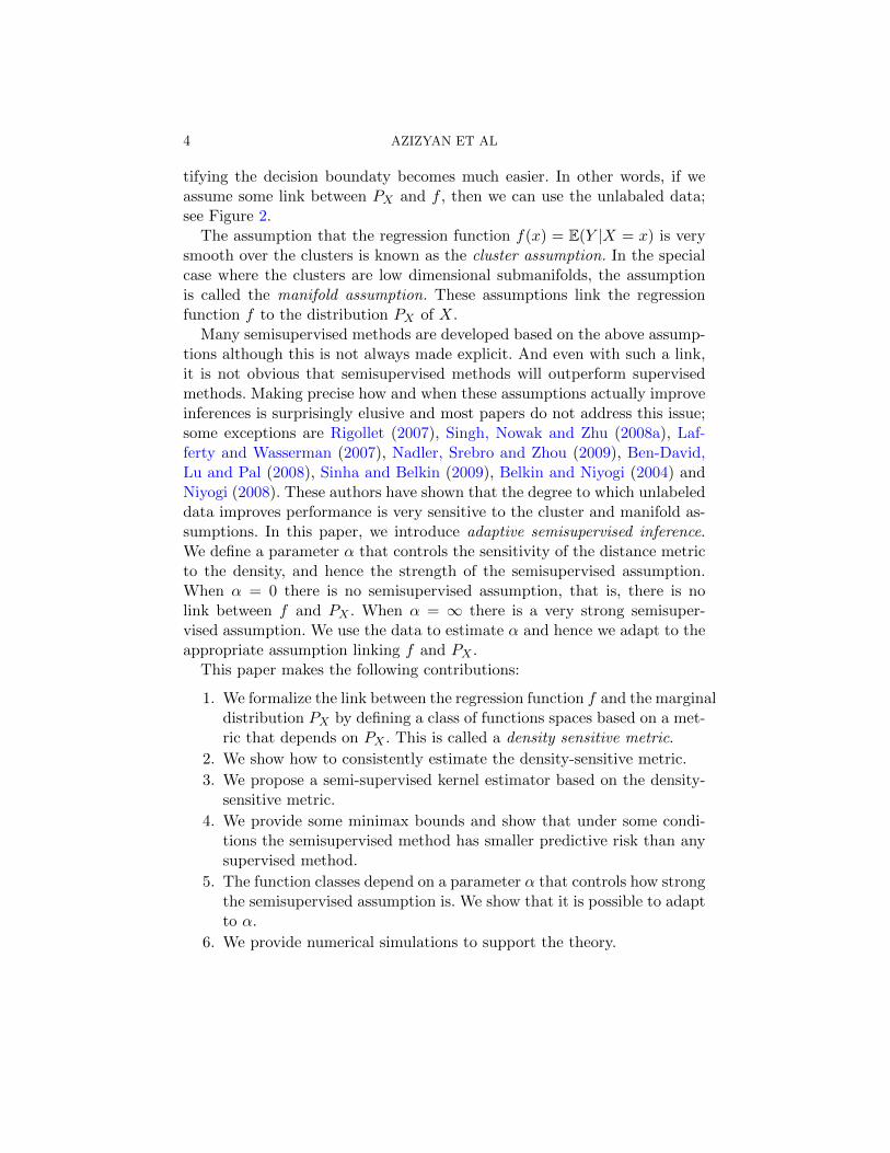
2 AZIZYAN ET AL

CONTENTS

1 Introduction . . . . . . . . . . . . . . . . . . . . . . . . . . . . . . . 32 Definitions . . . . . . . . . . . . . . . . . . . . . . . . . . . . . . . . 63 Density-Sensitive Metrics . . . . . . . . . . . . . . . . . . . . . . . 8

3.1 The Exponential Metric . . . . . . . . . . . . . . . . . . . . . 83.2 The Regression Function . . . . . . . . . . . . . . . . . . . . . 83.3 Properties of the Function Spaces . . . . . . . . . . . . . . . . 9

4 Estimating Density-Sensitive Metrics . . . . . . . . . . . . . . . . . 104.1 Estimating The Density . . . . . . . . . . . . . . . . . . . . . 104.2 Estimating the Exponential Distance . . . . . . . . . . . . . . 114.3 A Computable Estimator . . . . . . . . . . . . . . . . . . . . 11

5 Density-Sensitive Inference . . . . . . . . . . . . . . . . . . . . . . 146 Minimax Bounds . . . . . . . . . . . . . . . . . . . . . . . . . . . . 16

6.1 The Class Pn . . . . . . . . . . . . . . . . . . . . . . . . . . . 166.2 Supervised Lower Bound . . . . . . . . . . . . . . . . . . . . . 176.3 Semisupervised Upper Bound . . . . . . . . . . . . . . . . . . 226.4 Comparison of Lower and Upper Bound . . . . . . . . . . . . 22

7 The Reciprocal Distance . . . . . . . . . . . . . . . . . . . . . . . . 227.1 The Class Pn . . . . . . . . . . . . . . . . . . . . . . . . . . . 237.2 Supervised Lower Bound . . . . . . . . . . . . . . . . . . . . . 247.3 Semisupervised Upper Bound . . . . . . . . . . . . . . . . . . 297.4 Comparison of Lower and Upper Bound . . . . . . . . . . . . 31

8 Adaptive Semisupervised Inference . . . . . . . . . . . . . . . . . . 319 Simulation Results . . . . . . . . . . . . . . . . . . . . . . . . . . . 3410 Discussion . . . . . . . . . . . . . . . . . . . . . . . . . . . . . . . . 3611 Additional Proofs . . . . . . . . . . . . . . . . . . . . . . . . . . . . 36

11.1 Proof of Theorem 4.1 . . . . . . . . . . . . . . . . . . . . . . . 3611.2 Propositions for Section 4.3 . . . . . . . . . . . . . . . . . . . 3911.3 Proofs For Section 7.3 . . . . . . . . . . . . . . . . . . . . . . 41

References . . . . . . . . . . . . . . . . . . . . . . . . . . . . . . . . . . 45Author’s addresses . . . . . . . . . . . . . . . . . . . . . . . . . . . . . 46

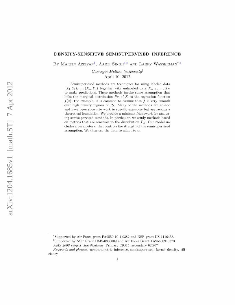
SEMISUPERVISED INFERENCE 3

Fig 1. The covariate X = (X1, X2) is two-dimensional. The response Y is binary and isshown as a square or a circle. Left: The labaleled data. Right: Labeled and unlabeled data.

1. Introduction. Suppose we have data (X1, Y1), . . . , (Xn, Yn) from adistribution P , where Xi ∈ Rd and Yi ∈ R. Further, we have a second setof data Xn+1, . . . , XN from the same distribution but without the Y ′s. Werefer to L = (Xi, Yi) : i = 1, . . . , n as the labeled data and U = Xi :i = n + 1, . . . , N as the unlabeled data. There has been a major effort,mostly in the machine learning literature, to find ways to use the unlabeleddata together with the labeled data to constuct good predictors of Y . Thesemethods are known as semisupervised methods. It is generally assumed thatthe the m = N − n unobserved labels Yn+1, . . . , YN are missing completelyat random and we shall assume this throughout.

To motivate semisupervised inference, consider the following example. Wedownload a large number N of webpages Xi. We select a small subset of sizen and label these with some attribute Yi. The downloading process is cheapwhereas the labeling process is expensive so typically N is huge while n ismuch smaller.

Figure 1 shows a toy example of how unlabeled data can help with pre-diction. In this case, Y is binary, X ∈ R2 and we want to find the decisionboundary x : P (Y = 1|X = x) = 1/2. The left plot shows a few labeleddata points from which it would be challenging to find the boundary. Theright plot shows labeled and unlabeled points. The unlabeled data show thatthere are two clusters. If we make the seemingly reasonable assumption thatf(x) = P (Y = 1|X = x) is very smooth over the two clusters, then iden-

4 AZIZYAN ET AL

tifying the decision boundaty becomes much easier. In other words, if weassume some link between PX and f , then we can use the unlabaled data;see Figure 2.

The assumption that the regression function f(x) = E(Y |X = x) is verysmooth over the clusters is known as the cluster assumption. In the specialcase where the clusters are low dimensional submanifolds, the assumptionis called the manifold assumption. These assumptions link the regressionfunction f to the distribution PX of X.

Many semisupervised methods are developed based on the above assump-tions although this is not always made explicit. And even with such a link,it is not obvious that semisupervised methods will outperform supervisedmethods. Making precise how and when these assumptions actually improveinferences is surprisingly elusive and most papers do not address this issue;some exceptions are Rigollet (2007), Singh, Nowak and Zhu (2008a), Laf-ferty and Wasserman (2007), Nadler, Srebro and Zhou (2009), Ben-David,Lu and Pal (2008), Sinha and Belkin (2009), Belkin and Niyogi (2004) andNiyogi (2008). These authors have shown that the degree to which unlabeleddata improves performance is very sensitive to the cluster and manifold as-sumptions. In this paper, we introduce adaptive semisupervised inference.We define a parameter α that controls the sensitivity of the distance metricto the density, and hence the strength of the semisupervised assumption.When α = 0 there is no semisupervised assumption, that is, there is nolink between f and PX . When α = ∞ there is a very strong semisuper-vised assumption. We use the data to estimate α and hence we adapt to theappropriate assumption linking f and PX .

This paper makes the following contributions:

1. We formalize the link between the regression function f and the marginaldistribution PX by defining a class of functions spaces based on a met-ric that depends on PX . This is called a density sensitive metric.

2. We show how to consistently estimate the density-sensitive metric.

3. We propose a semi-supervised kernel estimator based on the density-sensitive metric.

4. We provide some minimax bounds and show that under some condi-tions the semisupervised method has smaller predictive risk than anysupervised method.

5. The function classes depend on a parameter α that controls how strongthe semisupervised assumption is. We show that it is possible to adaptto α.

6. We provide numerical simulations to support the theory.

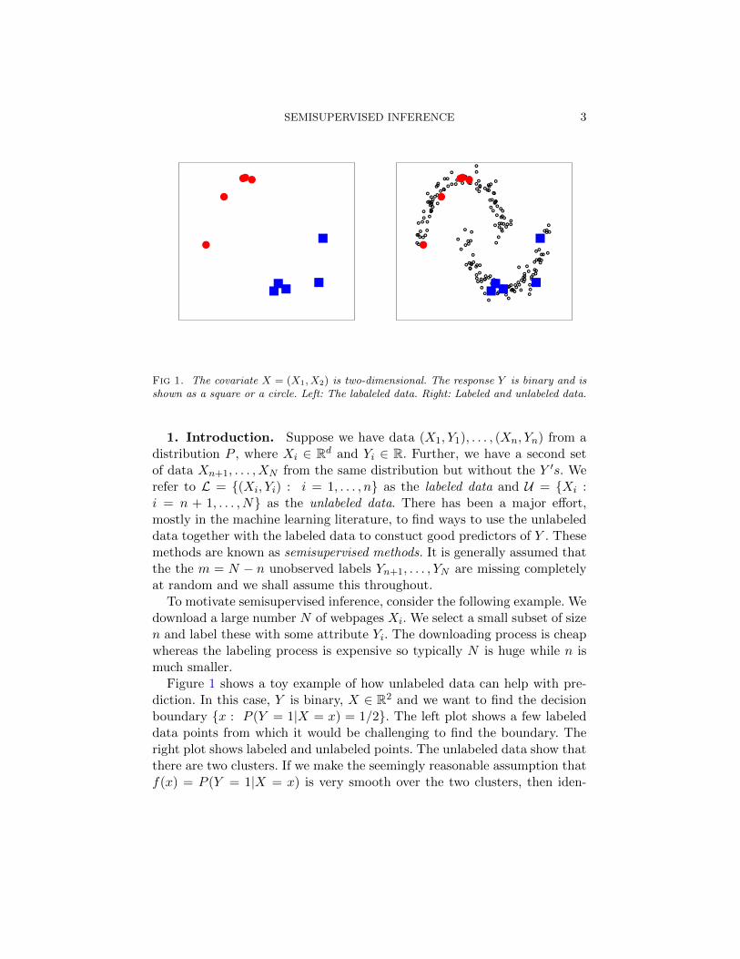
SEMISUPERVISED INFERENCE 5

Ln =⇒ f Ln =⇒ fSS assumption⇐===== PX ⇐= UN

Fig 2. Supervised learning (left) uses only the labeled data Ln. Semisupervised learning(right) uses the unlabaled data UN to estimate the marginal distribution PX which helpsestimate f if there is some link between PX and f . This link is the semisupervised (SS)assumption.

In addition, we should add that we focus on regression while most previousliterature only deals with binary outcomes (classification).

Related Work. There are a number of papers that discuss conditions un-der which semisupervised methods can succeed or that discuss metrics thatare useful for semisupervised methods. These include Bousquet, Chapelleand Hein (2004), Singh, Nowak and Zhu (2008a), Lafferty and Wasserman(2007), Sinha and Belkin (2009), Ben-David, Lu and Pal (2008), Nadler, Sre-bro and Zhou (2009), Sajama and Orlitsky (2005), Bijral, Ratliff and Srebro(2011), Belkin and Niyogi (2004), Niyogi (2008) and references therein. Pa-pers on semisupervised inference in the statistics literature are rare; someexceptions include Culp and Michailidis (2008), Culp (2011a) and Liang,Mukherjee and West (2007). To the best of our knowledge, there are nopapers that explicitly study adaptive methods that allow the data to choosethe strength of the semisupervised assumption.

There is a connection between our work on the semisupervised classifica-tion method in Rigollet (2007). He divides the the covariate space X intoclusters C1, . . . , Ck defined by the upper level sets pX > λ of the densitypX of PX . He assumes that the indicator function I(x) = I(p(y|x) > 1/2) isconstant over each cluster Cj . In our regression framework, we could simi-larly assume that

f(x) =

k∑j=1

fθj (x)I(x ∈ Cj) + g(x)I(x ∈ C0)

where fθ(x) is a parametric regression function, g is a smooth (but nonpara-metric function) and C0 = X −

⋃kj=1Cj . This yields parametric, dimension-

free rates over X − C0. However, this creates a rather unnatural and harshboundary at x : pX(x) = λ. Our approach may be seen as a smootherversion of this idea.

6 AZIZYAN ET AL

Outline. This paper is organized as follows. In Section 2 we give definitionsand assumptions. In Section 3 we define density sensitive metrics and thefunction spaces defined by these metrics. In Section 4 we present results onestimating density sensitive metrics. In Section 5 we define a density sensitivesemisupervised estimator and we bound its risk. In Section 6 we present someminimax results. We discuss adaptation in Section 8. We provide simulationsin 9. Section 10 contains closing discussion. Additional proofs are containedin Section 11.

2. Definitions. Recall that Xi ∈ Rd and Yi ∈ R. Let

(1) Ln = (X1, Y1), . . . , (Xn, Yn)

be an iid sample from P . Let PX denote the X-marginal of P and let

(2) UN = Xn+1, . . . , XN

be an iid sample from PX .Let f(x) ≡ fP (x) = E(Y |X = x). An estimator of f that is a function of

Ln is called a supervised learner and the set of such estimators is denotedby Sn. An estimator that is a function of Ln

⋃UN is called a semisupervised

learner and the set of such estimators is denoted by SSN . Define the risk ofan estimator f by

(3) RP (f) = EP[∫

(f(x)− fP (x))2dP (x)

].

Of course, Sn ⊂ SSN and hence,

infg∈SSN

supP∈P

RP (g) ≤ infg∈Sn

supP∈P

RP (g).

We will show that, under certain conditions, semisupervised methods out-perform supervised methods in the sense that the left hand side of the aboveequation is substantially smaller than the right hand side. More precisely,for certain classes of distributions Pn, we show that

(4)inf g∈SSN supP∈Pn RP (g)

inf g∈Sn supP∈Pn RP (g)→ 0

as n→∞. In this case we say that semisupervised learning is effective.

Remark: In order for the asymptotic analysis to reflect the behavior offinite samples, we need to let Pn to change with n and we need N = N(n)→

SEMISUPERVISED INFERENCE 7

∞ and n/N(n)→ 0 as n→∞. As an analogy, one needs to let the number ofcovariates in a regression problem increase with the sample size, to developrelevant asymptotics for high dimensional regression. Moreover, Pn musthave distributions that get more concentrated as n increases. The reasonis that, if n is very large and PX is smooth, then there is no advantage tosemisupervised inference. This is consistent with the finding in Ben-David,Lu and Pal (2008) who show that if PX is smooth, then “ ... knowledgeof that distribution cannot improve the labeled sample complexity by morethan a constant factor.”’

Other Notation. If A is a set and δ ≥ 0 we define

A⊕ δ =⋃x∈A

B(x, δ)

where B(x, δ) denotes a ball of radius δ centered at x. Given a set A ⊆ Rd,define dA(x1, x2) to be the length of the shortest path in A connecting x1

and x2.We write an = O(bn) if |an/bn| is bounded for all large n. Similarly,

an = Ω(bn) if |an/bn| is bounded away from 0 for all large n. We writean bn if an = O(an) and an = Ω(bn). We also write an bn if there existsC > 0 such that an ≤ Cbn for all large n. Define an bn similarly. Weuse symbols of the form c, c1, c2, . . . , C, C1, C2, . . . to denote generic positiveconstants whose value can change in different expressions.

To prove lower bounds, we will use Assouad’s Lemma (see Lemma 24.3in van der Vaart (1998)). Recall that the Hamming distance between twovectors v and w is ρ(v, w) =

∑j I(vj 6= wj).

Lemma 1 (Assouad’s Lemma) Let Ω = 0, 1q be the collection of bi-nary vectors of length q ≥ 1. Let PΩ = Pω : ω ∈ Ω be a collection of 2q

probability measures indexed by ω ∈ Ω. Also let

‖Pν ∧ Pω‖ = 1− supA|Pν(A)− Pω(A)|

denote the affinity between two distributions, where the supremum is overall measurable sets A. Let fω : ω ∈ Ω be a collection of functions. Forany semi-distance d, and any p > 0,(5)

inff

maxω∈Ω

Eω[dp(fω, f)] ≥ q

2p+1

(min

ω,ν:ρ(ω,ν)6=0

dp(fω, fν)

ρ(ω, ν)

)×(

minω,ν:ρ(ω,ν)=1

‖Pω ∧ Pν‖).

8 AZIZYAN ET AL

3. Density-Sensitive Metrics. We allow the marginal distributionPX for X to be arbitrary. We define a smoothed version of PX as follows.Let K denote a symmetric kernel on Rd with compact support, let σ > 0and define

(6) pσ(x) ≡ pX,σ(x) =

∫1

σdK

(||x− u||

σ

)dPX(x).

Thus, pX,σ is the density of the convolution PX,σ = PX ?Kσ where Kσ is themeasure with density Kσ(·) = σ−dK(·/σ). PX,σ always has a density evenif PX does not. This is important because, in high dimensional problems,it is not uncommon to find that PX can be highly concentrated near a lowdimensional manifold. And these are precisely the cases where semisuper-vised methods are often useful (Ben-David, Lu and Pal (2008)). Indeed, thiswas one of the original motivations for semisupervised inference. We definePX,0 = PX . For notational simplicity, we shall sometimes drop the X andsimply write pσ instead of pX,σ.

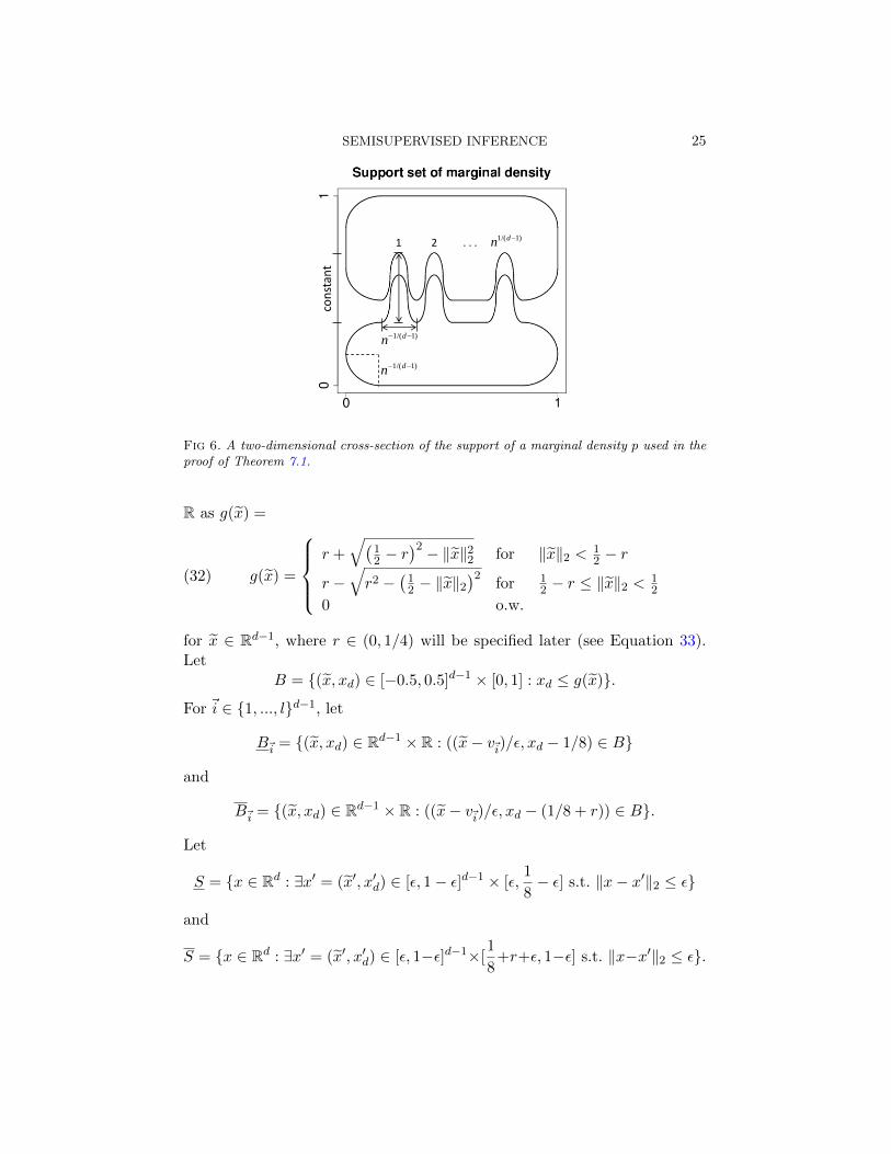
3.1. The Exponential Metric. Following previous work in the area, wewill assume that the regression function is smooth in regions where PX putslots of mass. To make this precise, we define a density sensitive metric asfollows. For any pair x1 and x2 let Γ(x1, x2) denote the set of all continuousfinite curves from x1 to x2 with unit speed everywhere and let L(γ) be thelength of curve γ; hence γ(L(γ)) = x2. For any α ≥ 0 define the exponentialmetric

(7) D(x1, x2) ≡ DP,α,σ(x1, x2) = infγ∈Γ(x1,x2)

L(γ)∫0

exp[−αpX,σ(γ(t))

]dt.

In Section 7 we also consider a second metric, the reciprocal metric. Largeα makes points connected by high density paths closer; see Figure 3. Notethat α = 0 corresponds to Euclidean distance. Similar definitions are used inSajama and Orlitsky (2005), Bijral, Ratliff and Srebro (2011) and Bousquet,Chapelle and Hein (2004).

3.2. The Regression Function. Recall that f(x) ≡ fP (x) = E(Y |X = x)denotes the regression function. We assume that X ∈ [0, 1]d ≡ X and that|Y | ≤ M for some finite constant M .1 We formalize the semisupervisedsmoothness assumption by defining the following scale of function spaces.

1 The results can be extended to unbounded Y with suitable conditions on the tails ofthe distribution of Y .

SEMISUPERVISED INFERENCE 9

X Y Z

Fig 3. With a density density metric, the points X and Z are closer than the points Xand Y because there is a high density path connecting X and Z.

.

Let F ≡ F(P, α, σ, L) denote the set functions f : [0, 1]d → R such that, forall x1, x2 ∈ X ,

(8) |f(x1)− f(x2)| ≤ L DP,α,σ(x1, x2).

Let P(α, σ, L) denote all joint distributions for (X,Y ) such that fP ∈F(P, α, σ, L) and such that PX is supported on X .

3.3. Properties of the Function Spaces. The variance of our estimatorwill depend on

(9)

∫dP (x)

P (BP,α,σ(x, ε))

where BP,α,σ(x, ε) = z : DP,α,σ(x, z) ≤ ε. Let SP denote the support of Pand let NP,α,σ(ε) denote the covering number, the smallest number of ballsof the form BP,α,σ(x, ε) required to cover SP . A simple argument shows that

(10)

∫dP (x)

P (BP,α,σ(x, ε))≤ NP,α,σ(ε/2).

In the Euclidean case α = 0, we have NP,0,σ(ε) ≤ (C/ε)d. But when α > 0and P is concentrated on or near a set of dimension less than d, the NP,α,σ(ε)can be much smaller than (C/ε)d. The next result gives a few examplesshowing that concentrated distributions have small covering numbers. Wesay that a set A is regular if there is a C > 0 such that, for all small ε > 0,

(11) supx,y∈A||x−y||≤ε

dA(x, y)

||x− y||≤ C.

Recall that SP denotes the support of P .

10 AZIZYAN ET AL

Lemma 2 Suppose that SP is regular.

1. For all α, σ and P , NP,α,σ(ε) ε−d.2. Suppose that P =

∑kj=1 δxj where δx is a point mass at x. Then, for

any α ≥ 0 and any ε > 0, NP,α,σ(ε) ≤ k.

3. Suppose that dim(SP ) = r < d. Then, NP,α,σ(ε) ε−r.4. Suppose that SP = W ⊕ γ where dim(W ) = r < d. Then, for ε ≥ Cγ,NP,α,σ(ε)

(1ε

)r.

Proof. (1) The first statement is follows since the covering number of SPis no more than the covering number of [0, 1]d and on [0, 1]d, DP,α,σ(x, y) ≤||x− y||. Now [0, 1]d can be covered O(ε−d) Euclidean balls.(2) The second statement follows since x1, . . . , xk forms an ε-coveringfor any ε.(3) We have that DP,α,σ(x, y) ≤ dSP (x, y). Regularity implies that, for smalldSP (x, y), DP,α,σ(x, y) ≤ c||x − y||. We can thus cover SP by Cε−r balls ofsize ε.(4) As in (3), cover W with N = O(ε−r) balls of D size ε. Denote these ballsby B1, . . . , BN . Define Cj = x ∈ SP : dSP (x,Bj) ≤ γ. The Cj form acovering of size N and each Cj has DP,α,σ diameter maxε, γ.

4. Estimating Density-Sensitive Metrics. In this section we con-sider estimating the density-sensitive metrics.

4.1. Estimating The Density. Let m = N − n denote the number ofunlabeled points and let

(12) pσ(x) =1

m

m∑i=1

1

σdK

(||x−Xi+n||

σ

)be the usual kernel estimator of pσ.

To estimate the distance, we need to bound ||pσ − pσ||∞ uniformly overa range of values of σ. The uniform in bandwidth result by Einmahl andMason (2005) provides almost sure bounds of this type. For example, theirresult implies that, almost surely, there is an m0 such that for all m ≥ m0

and all c > 0, and for all (c logm/m)1/d ≤ σ ≤ 1,

(13) ||pσ − pσ||∞ ≤K(c)

√d log(1/σ) ∨ log logm√

mσd.

However, such a bound is not uniform over a class of distributions. Insteadwe use the following result whose proof is in Section 11.

SEMISUPERVISED INFERENCE 11

Theorem 4.1 Let X1, . . . , Xm ∼ P where P has support on a compact setX ⊂ Rd. Let pσ(x) = 1

σd

∑iK(||x−Xi||/σ). Let pσ(x) = E(pσ(x)). Suppose

that K(x) ≤ K(0) for all x and that

|K(y)−K(x)| ≤ L||x− y||

for all x, y. Let 0 < a ≤ A <∞. If ε ≤ 2/3 then

(14) supP∈P

Pm

(sup

a≤σ≤A||pσ − pσ||∞ > ε

)≤(

C

a2dε

)d+1

exp

(−3mε2ad

28K(0)

)where P is the set of distributions such that PX is supported on X .

Thus, for large m, πm e−cmε2ad . Now let am

(1m

) 1d(1+γ) where γ is

any small, positive number. Then, with probability at least 1− 1/m,

(15) supam≤σ≤A

||pσ − pσ||∞ <

√C logm

admm.

4.2. Estimating the Exponential Distance. Define

(16) Dα,σ(x1, x2) = infγ∈Γ(x1,x2)

∫ L(γ)

0exp [−αpσ(γ(t))] dt.

Lemma 3 Suppose that ||pσ(x)− pσ(x)||∞ ≤ εm. For all x1, x2

(17) e−αεmDP,α,σ(x1, x2) ≤ Dα,σ(x1, x2) ≤ eαεmDP,α,σ(x1, x2).

Proof. Follows easily from the definition of the metric.

4.3. A Computable Estimator. Although the above estimator Dα,σ isconsistent, it is not easily computable because it involves searching over allpossible paths connecting each pair of points. In fact, even if P is known,DP,α,σ is not computable. A computable estimator for the exponential dis-tance was proposed by Sajama and Orlitsky (2005) but this estimator is

12 AZIZYAN ET AL

only consistent for α = 1. Bijral, Ratliff and Srebro (2011) presented a com-putable estimator but it is not consistent. Here we given an algorithm thatapproximates Dα,σ and is consistent, uniformly over a range of values of α.

Remark: In this section we assume that PX is known and we show how toapproximate DP,α,σ. When PX is unknown, simply subsitute pX,σ for pX,σ.The bounds then get multiplied by a factor of eαεm .

In what follows, “path” always means piecewise differentiable, continu-ous, finite length curve with unit speed where differentiable. Define K∗max =supu‖∇K(u)‖ and Kmax = sup

uK(u) = K(0), and suppose that K is sup-

ported on the unit ball. Let σmax ≥ σmin > 0 and αmax ≥ 0. Let X ∗ be theconvex hull of X ⊕ σmax. Let

C = u1, . . . , uJ

be a Euclidean ζ-covering of X ∗. (The cover can, but need not, include theobserved data.)

For any 0 ≤ α ≤ αmax and σmin ≤ σ ≤ σmax, define the graph Gα,σ =(V,E,Wα,σ) where V = v1, ..., vJ, (vi, vj) ∈ E iff ‖ui − uj‖ ≤ ξ, and fori, j s.t. (vi, vj) ∈ E define the edge weight

W i,jα,σ = ‖ui − uj‖ exp

[−αpX,σ

(ui + uj

2

)].

Note that each node vj corresponds to one point uj in the cover. Also define

Gα,σ = (V,E, Wα,σ) where W i,jα,σ = DP,α,σ(ui, uj) for i, j s.t. (vi, vj) ∈ E.

For any 0 ≤ α ≤ αmax and σmin ≤ σ ≤ σmax, for i, j ∈ 1, ..., J,define the estimated distance D∗P,α,σ(ui, uj) and the intermediate distance

DP,α,σ(ui, uj) to be the graph (i.e. shortest-path) distances between vertices

vi and vj on Gα,σ and Gα,σ, resp. Note that the distances are only definedfor points in uiJi=1. Let

Λ = exp

[αKmax

σd

]αK∗max

σd+1≤ exp

[αmaxKmax

σdmin

]αmaxK

∗max

σd+1min

.

Theorem 4.2 If ζ ≤ 7/(32Λ) then, for any 0 ≤ α ≤ αmax and σmin ≤ σ ≤σmax and for any i, j ∈ 1, ..., J,

(18)1

8DP,α,σ(ui, uj) ≤ DP,α,σ(ui, uj) ≤ 8DP,α,σ(ui, uj).

SEMISUPERVISED INFERENCE 13

Note that this bounds D, which is sufficient for our purposes. It is possibleto modify the proof to show that, in fact, D consistently estimates D.

Proof. Let ξ = 4ζ. By Proposition 2 in Section 11 we have that for i, js.t. (vi, vj) ∈ E

(1− Λξ)W i,jα,σ ≤ W i,j

α,σ ≤ (1 + Λξ/2)W i,jα,σ.

So for all i, j ∈ 1, ..., J,

1

1 + Λξ/2Dα,σ,P (ui, uj) ≤ Dα,σ,P (ui, uj) ≤

1

1− ΛξDα,σ,P (ui, uj).

Clearly for all i, j ∈ 1, ..., J, DP,α,σ(ui, uj) ≤ Dα,σ,P (ui, uj). Also for

i, j such that ‖ui − uj‖ ≤ ξ DP,α,σ(ui, uj) = Dα,σ,P (ui, uj). Suppose i, jsuch that ‖ui − uj‖ > ξ. Let γ be the path such that DP,α,σ(ui, uj) =L(γ)∫0

exp [−αpX,σ(γ(t))] dt. Of course, L(γ) > ξ. Divide γ into a sequence of

paths γ0, γ1, ..., γQ such that γ0(0) = ui, γQ(L(γQ)) = uj , L(γ0) ∈ (0, ξ−2ζ],and for k ∈ 1, ..., Q L(γk) = ξ − 2ζ and γk−1(L(γk−1)) = γk(0). ClearlyQ ≥ 1. For k ∈ 1, ..., Q let rk = γk(0), let rQ+1 = uj , and let nk such that‖rk − unk‖ ≤ ζ. By Proposition 1 in Section 11,

Dα,σ,P (ui, uj) ≤ W i,n1α,σ +

Q∑k=1

Wnk,nk+1α,σ

≤ DP,α,σ(ui, r1) +

Q∑k=1

(2DP,α,σ(rk, unk) +DP,α,σ(rk, rk+1))

= DP,α,σ(ui, r1) +

Q∑k=1

DP,α,σ(rk, rk+1)

(1 + 2

DP,α,σ(rk, unk)

DP,α,σ(rk, rk+1)

)

≤ DP,α,σ(ui, r1) +

Q∑k=1

DP,α,σ(rk, rk+1)

[1 + 2ζ

(Λ +

1 + Λζ

ξ − 2ζ

)]≤[1 + 2ζ

(Λ +

1 + Λζ

ξ − 2ζ

)]DP,α,σ(ui, uj)

and the result follows since ξ = 4ζ and ζ ≤ 7/(32Λ).

Remark: For any points x, y not in the cover C, we can define D(x, y) =

14 AZIZYAN ET AL

1. Construct a Euclidean ζ-covering uiJi=1 of the convex hull of X ⊕ σ.

2. Construct a graph with the covering points as nodes, and edges between pairsof points closer than ξ for some ξ > 2ζ.

3. Set the edge weight between connected neighbors i and j to

‖ui − uj‖ exp[−αpX,σ

(ui + uj2

)].

4. Approximate the DP,α,σ-distance between any two points as the graph(i.e. shortest path) distance between the corresponding nearest neighbors inuiJi=1.

Fig 4. Computing Density-Sensitive Metrics

D(ui, uj) where ui is the closest point in C to x and uj is the closest pointin C to y.

A summary of the algorithm is given in Figure 4.

To further speed up the algorithm, we have found the following heuristicto be useful. We approximate the edge weight between all pairs of points iand j by(19)

Wi,j =

‖Xi −Xj‖ exp

[−αpi+pj2

]if Xj is a k-nearest neighbor of Xi,

‖Xi −Xj‖ otherwise

where k is an integer and pi is the k-NN density estimate at the i’th point.

5. Density-Sensitive Inference. We consider the following semisu-pervised learner which uses a kernel that is sensitive to the density. Let Qbe a kernel and let Qh(x) = h−dQ(x/h). Let

(20) fh,α,σ(x) =

∑ni=1 YiQh

(Dα,σ(x,Xi)

)∑n

i=1Qh

(Dα,σ(x,Xi)

) .

In the following we take, for simplicity, Q(x) = I(||x|| ≤ 1). Now we give anupper bound on the risk of fh,α,σ.

SEMISUPERVISED INFERENCE 15

Theorem 5.1 Suppose that |Y | ≤ M . Define the event Gm = ||pσ −pσ||∞ ≤ εm (which depends on the unlabeled data) and suppose that P(Gcm) ≤1/m. Then, for every P ∈ P(α, σ, L),

(21) RP (fh,α,σ) ≤ L2(heαεm)2 +M2

[4 + 1

e N (P, α, σ, e−εmαh/2)]

n+

4M2

m.

Proof. The risk is

RP (f) = En,N[(1− Gm)

∫(fh,α,σ(x)− f(x))2dP (x)

]+En,N

[Gm∫

(fh,α,σ(x)− f(x))2dP (x)

].

Since |Y | ≤M and supx |f(x)| ≤M ,

En,N[(1− Gm)

∫(fh,α,σ(x)− f(x))2dP (x)

]≤ 4M2P(Gcm) ≤ 4M2

m.

Now we bound the second term.Condition on the unlabeled data. Replacing Euclidean distance with Dα,σ

in the proof of Theorem 5.2 in Gyorfi et al. (2002), we have that

En[∫

(fh,α,σ(x)− f(x))2dP (x)

]≤ LR2 +

M2[4 + 1

e

∫ dP (x)

P (Bα,σ(x,h))

]n

where

R = supDP,α,σ(x1, x2) : (x1, x2) such that Dα,σ(x1, x2) ≤ h

and Bα,σ(x, h) = z : Dα,σ(x, z) ≤ h. On the event Gm, we have from

Lemma 3 that e−αεmDα,σ(x1, x2) ≤ Dα,σ(x1, x2) ≤ eαεmDα,σ(x1, x2) for allx1, x2. Hence, R2 ≤ e2αεmh2 and∫

dP (x)

P (Bα,σ(x, h))≤∫

dP (x)

P (BP,α,σ(x, e−αεmh)).

A simple covering argument (see p 76 of Gyorfi et al) shows that, for anyδ > 0, ∫

dP (x)

P (BP,α,σ(x, δ))≤ N (P, α, σ, δ/2).

The result follows.

16 AZIZYAN ET AL

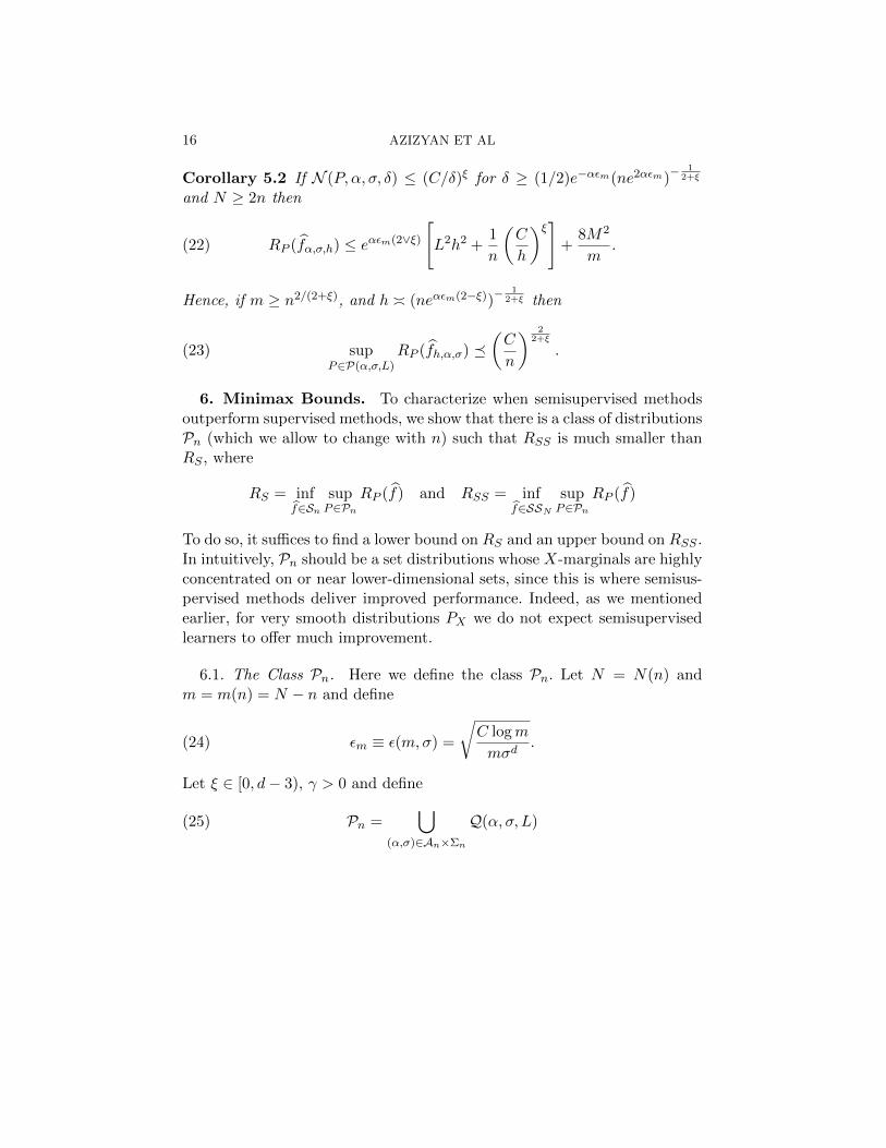
Corollary 5.2 If N (P, α, σ, δ) ≤ (C/δ)ξ for δ ≥ (1/2)e−αεm(ne2αεm)− 1

2+ξ

and N ≥ 2n then

(22) RP (fα,σ,h) ≤ eαεm(2∨ξ)

[L2h2 +

1

n

(C

h

)ξ]+

8M2

m.

Hence, if m ≥ n2/(2+ξ), and h (neαεm(2−ξ))− 1

2+ξ then

(23) supP∈P(α,σ,L)

RP (fh,α,σ) (C

n

) 22+ξ

.

6. Minimax Bounds. To characterize when semisupervised methodsoutperform supervised methods, we show that there is a class of distributionsPn (which we allow to change with n) such that RSS is much smaller thanRS , where

RS = inff∈Sn

supP∈Pn

RP (f) and RSS = inff∈SSN

supP∈Pn

RP (f)

To do so, it suffices to find a lower bound on RS and an upper bound on RSS .In intuitively, Pn should be a set distributions whose X-marginals are highlyconcentrated on or near lower-dimensional sets, since this is where semisus-pervised methods deliver improved performance. Indeed, as we mentionedearlier, for very smooth distributions PX we do not expect semisupervisedlearners to offer much improvement.

6.1. The Class Pn. Here we define the class Pn. Let N = N(n) andm = m(n) = N − n and define

(24) εm ≡ ε(m,σ) =

√C logm

mσd.

Let ξ ∈ [0, d− 3), γ > 0 and define

(25) Pn =⋃

(α,σ)∈An×Σn

Q(α, σ, L)

SEMISUPERVISED INFERENCE 17

where Q(α, σ, L) ⊂ P(α, σ, L) and An × Σn ⊂ [0,∞]2 satisfy the followingconditions:

(C1)α

σd> C

(d− ξ − 1

(d− 1)(2 + ξ)

)log n

(C2) Q(α, σ, L) =

P ∈ P(α, σ, L) : N (P, α, σ, ε) ≤

(C

ε

)ξ∀ ε ≥

(1

n

) 12+ξ

(C3) α ≤ log 2

ε(m,σ).

(C4)

(1

m

) 1d(1+γ)

≤ σ ≤ 1

4C0

(1

n

) 1d−1

where C0 is the diameter of the support of K.Here are some remarks about Pn:

1. (C3) implies that eαεm ≤ 2 and hence that (1/2)DP,α,σ(x1, x2) ≤Dα,σ(x1, x2) ≤ 2DP,α,σ(x1, x2) with high probability.

2. (C4) implies that m ≥ (1/σ)−d(1+γ) for each σ ∈ Σn. Hence, from thediscussion following Theorem 4.1,

supP∈Pn

Pm

(supσ∈Σn

||pσ − pσ||∞ > ε(m,σ)

)<

1

m

and thus, Theorem 5.1 and Corollary 5.2 apply.

3. The constraint in (C2) on N (ε) holds whenever P is concentrated onor near a set of dimension less than d and α/σd is large. The constraintdoes not need to hold for arbitrarily small ε.

4. Some papers on semisupervised learning simply assume that N = ∞since in practice N is usually very large compared to n. In that case,there is no upper bound on α and no lower bound on σ.

The class Pn may seem complicated. This is because showing conditionswhere semisupervised learning provably outperforms supervised learning issubtle. Intuitively, the class Pn is simply the set of high concentrated distri-butions with α/σ large.

6.2. Supervised Lower Bound.

Theorem 6.1 There exists C > 0 such that

(26) RS = inff∈Sn

supP∈Pn

RP (f) ≥(C

n

) 2d−1

.

18 AZIZYAN ET AL

A0

A1

Fig 5. The extended tendrils used in the proof of the lower bound, in the special case whered = 2. Each tendril has length 1− ε and joins up with either the top A1 or bottom A0 butnot both.

Proof. Let A1 and A0 be the top and bottom of the cube X :

A1 = (x1, . . . , xd−1, 1) : 0 ≤ x1, . . . , xd−1 ≤ 1A0 = (x1, . . . , xd−1, 0) : 0 ≤ x1, . . . , xd−1 ≤ 1.

Fix ε = n−1d−1 . Let q = (1/ε)d−1 n. For any integers s = (s1, . . . , sd−1) ∈

Nd−1 with 0 ≤ si ≤ 1/ε, define the tendril

(s1ε, s2ε, . . . , sd−1ε, xd) : ε ≤ xd ≤ 1− ε.

There are q = (1/ε)d−1 ≈ n such tendrils. Let us label the tendrils asT1, . . . , Tq. Note that the tendrils do not quite join up with A0 or A1.

Let

C = A0

⋃A1

⋃ q⋃j=1

Tj

.

Define a measure µ on C as follows:

µ =1

4µ0 +

1

4µ1 +

1

2q(1− 2ε)

∑j

νj

where µ0 is (d − 1)-dimensional Lebesgue measure on A0, µ1 is (d − 1)-dimensional Lebesgue measure on A1 and νj is one-dimensional Lebesguemeasure on Tj . Thus, µ is a probability measure and µ(C) = 1.

Now we define extended tendrils that are joined to the top or bottom ofthe cube (but not both). See Figure 5. If

Tj = (s1ε, s2ε, . . . , sd−1ε, xd) : ε ≤ xd ≤ 1− ε.

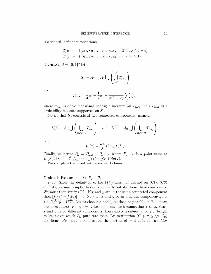
SEMISUPERVISED INFERENCE 19

is a tendril, define its extensions

Tj,0 = (s1ε, s2ε, . . . , sd−1ε, xd) : 0 ≤ xd ≤ 1− εT1,j = (s1ε, s2ε, . . . , sd−1ε, xd) : ε ≤ xd ≤ 1.

Given ω ∈ Ω = 0, 1q let

Sω = A0

⋃A1

⋃ q⋃j=1

Tj,ωj

and

Pω,X =1

4µ0 +

1

4µ1 +

1

2q(1− ε)∑j

νj,ωj

where νj,ωj is one-dimensional Lebesgue measure on Tj,ωj . This Pω,X is aprobability measure supported on Sω.

Notice that Sω consists of two connected components, namely,

U (1)ω = A1

⋃ ⋃j:ωj=1

Tj,ωj

and U (0)ω = A0

⋃ ⋃j:ωj=0

Tj,ωj

.

Let

fω(x) =L ε

8I(x ∈ U (1)

ω ).

Finally, we define Pω = Pω,X × Pω,Y |X where Pω,Y |X is a point mass atfω(X). Define d2(f, g) =

∫(f(x)− g(x))2dµ(x).

We complete the proof with a series of claims.

Claim 1: For each ω ∈ Ω, Pω ∈ Pn.Proof: Since the definition of the Pω does not depend on (C1), (C3)

or (C4), we may simply choose α and σ to satisfy these three constraints.We must then verify (C2). If x and y are in the same connected componentthen |fω(x) − fω(y)| = 0. Now let x and y be in different components, i.e.

x ∈ U (1)ω , y ∈ U (0)

ω . Let us choose x and y as close as possible in Euclideandistance; hence ||x − y|| = ε. Let γ be any path connecting x to y. Sincex and y lie on different components, there exists a subset γ0 of γ of lengthat least ε on which Pω puts zero mass. By assumption (C4), σ ≤ ε/(4C0)and hence PX,σ puts zero mass on the portion of γ0 that is at least C0σ

20 AZIZYAN ET AL

away from the support of Pω. This has length at least ε− 2C0σ ≥ ε/2. SincepX,σ(x) = 0 on a portion of γ0,

DP,α,σ(x, y) ≥ ε

2=||x− y||

2.

Hence, ||x− y|| ≤ 2DP,α,σ(x, y). Then

|fω(x)− fω(y)|DP,α,σ(x, y)

≤ 2|fω(x)− fω(y)|||x− y||

and the latter is maximized by finding two points x and y as close togetherwith nonzero numerator. In this case, ||x−y|| = ε and |fω(x)−fω(y)| = Lε/8.Hence, |fω(x)− fω(y)| ≤ LDP,α,σ(x, y) as required. Now we show that eachP = Pω satisfies

N (P, α, σ, ε) ≤(C

ε

)ξfor all ε ≥ n

− 12+ξ . Cover the top A1 and bottom A0 of the cubes with

Euclidean spheres of radius δ. There are O((1/δ)d−1) such spheres. The

DP,α,σ radius of each sphere is at most δe−αK(0)/σd . Thus, these form an

ε covering as long as δe−αK(0)/σd ≤ ε. Thus the covering number of thetop and bottom is at most 2(1/δ)d−1 ≤ 2(1/(eαK(0)/σdε))d−1. Now coverthe tendris with one-dimensional segments of length δ. The DP,α,σ radius

of each segment is at most δe−α/σd. Thus, these form an ε covering as long

as δe−αK(0)/σd ≤ ε. Thus the covering number of the tendrils is at mostq/δ = n/δ ≤ n/(εeαK(0)/σ2

). Thus we can cover the support with

N(ε) ≤ 2

(1

eα/σdε

)d−1

+n

εeα/σ2

balls of size ε. (C2) then implies that N(ε) ≤ (1/ε)ξ for ε ≥ n− 1

2+ξ asrequired.

Claim 2: For any ω, and any g ≥ 0,∫g(x)dPω(x) ≥ 1

2

∫g(x)dµ(x).

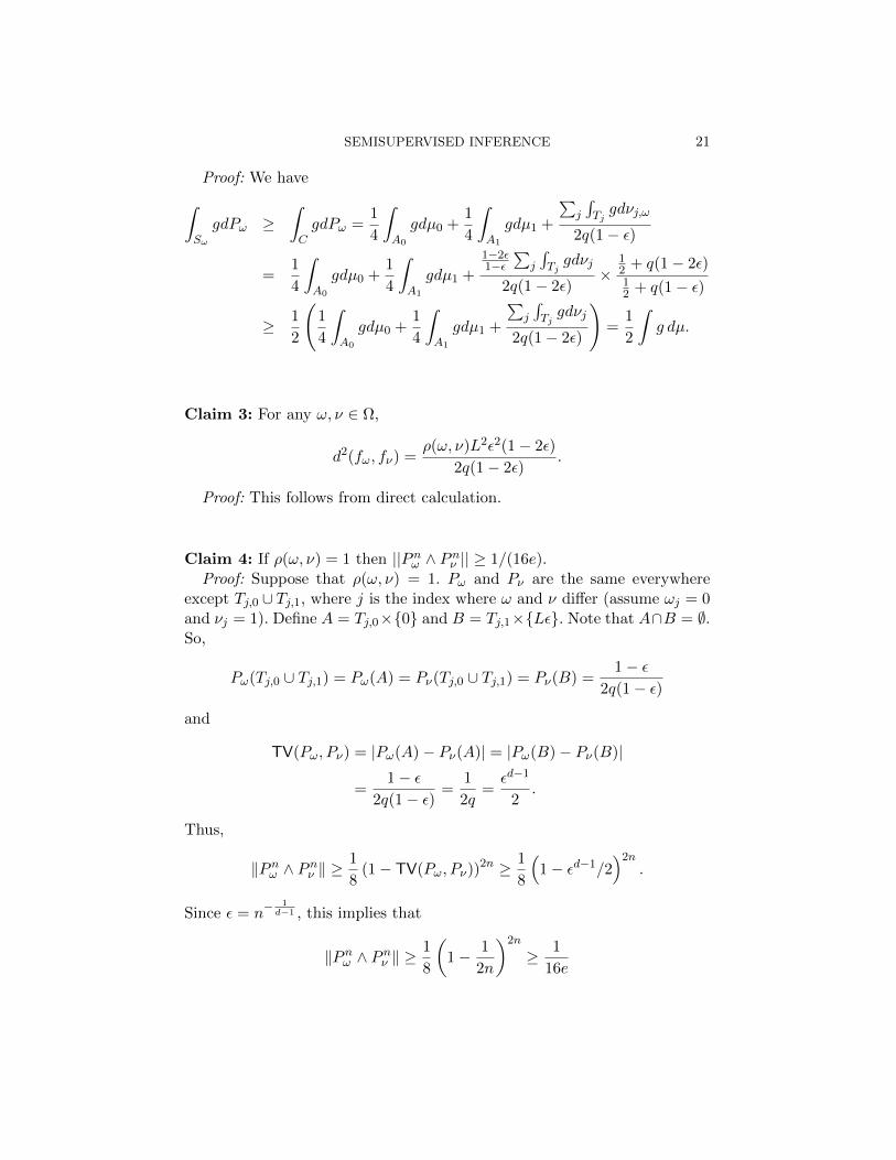
SEMISUPERVISED INFERENCE 21

Proof: We have∫Sω

gdPω ≥∫CgdPω =

1

4

∫A0

gdµ0 +1

4

∫A1

gdµ1 +

∑j

∫Tjgdνj,ω

2q(1− ε)

=1

4

∫A0

gdµ0 +1

4

∫A1

gdµ1 +

1−2ε1−ε

∑j

∫Tjgdνj

2q(1− 2ε)×

12 + q(1− 2ε)12 + q(1− ε)

≥ 1

2

(1

4

∫A0

gdµ0 +1

4

∫A1

gdµ1 +

∑j

∫Tjgdνj

2q(1− 2ε)

)=

1

2

∫g dµ.

Claim 3: For any ω, ν ∈ Ω,

d2(fω, fν) =ρ(ω, ν)L2ε2(1− 2ε)

2q(1− 2ε).

Proof: This follows from direct calculation.

Claim 4: If ρ(ω, ν) = 1 then ||Pnω ∧ Pnν || ≥ 1/(16e).Proof: Suppose that ρ(ω, ν) = 1. Pω and Pν are the same everywhere

except Tj,0 ∪ Tj,1, where j is the index where ω and ν differ (assume ωj = 0and νj = 1). Define A = Tj,0×0 and B = Tj,1×Lε. Note that A∩B = ∅.So,

Pω(Tj,0 ∪ Tj,1) = Pω(A) = Pν(Tj,0 ∪ Tj,1) = Pν(B) =1− ε

2q(1− ε)

and

TV(Pω, Pν) = |Pω(A)− Pν(A)| = |Pω(B)− Pν(B)|

=1− ε

2q(1− ε)=

1

2q=εd−1

2.

Thus,

‖Pnω ∧ Pnν ‖ ≥1

8(1− TV(Pω, Pν))2n ≥ 1

8

(1− εd−1/2

)2n.

Since ε = n−1d−1 , this implies that

‖Pnω ∧ Pnν ‖ ≥1

8

(1− 1

2n

)2n

≥ 1

16e

22 AZIZYAN ET AL

for all large n.

Completion of the proof. Recall that ε = n−1d−1 . Combining Assouad’s

Lemma with the above claims, we have

RS = inff∈Sn

supP∈Pn,ξ

RP (f) ≥ inff∈Sn

supP∈PΩ

RP (f) ≥ 1

2inff

maxω∈Ω

Eω[d2(fω, f)]

≥ q

16× (L/8)2ε2(1− 2ε)

2q(1− 2ε)× 1

16e= C

qε2(1− 2ε)

2q(1− 2ε)

≥ Cε2 = Cn−2d−1

6.3. Semisupervised Upper Bound. Now we state the upper bound forthis class.

Theorem 6.2 Let h = (ne2(2−ξ))− 1

2+ξ . Then

(27) supP∈Pn

R(fh,α,σ) ≤(C

n

) 22+ξ

.

Proof. This follows from (C2), (C3) and Corollary 5.2.

6.4. Comparison of Lower and Upper Bound. Combining the last twotheorems we have:

Corollary 6.3 Under the conditions of the previous theorem, and assumingthat d > ξ + 3,

(28)RSSRS(

1

n

) 2(d−3−ξ)(2+ξ)(d−1)

→ 0

as n→∞.

This establishes the effectiveness of semi-supervised inference in the min-imax sense.

7. The Reciprocal Distance. In this section we consider a seconddensitive-sensitive metric, called the reciprocal distance. This distance ismore difficult to implement but it provides a more dramatic distinctionbetween supervised and semisupervised methods.

SEMISUPERVISED INFERENCE 23

Define the reciprocal distance

(29) D(x1, x2) ≡ DP,α(x1, x2) = infγ∈Γ(x1,x2)

L(γ)∫0

[1

pX(γ(t))

]αdt.

Let N (P, α, ε) denote the covering number of SP under this distance. LetF ≡ F(P, α, L) denote the set functions f : [0, 1]d → R such that, for allx1, x2 ∈ X ,

(30) |f(x1)− f(x2)| ≤ L DP,α(x1, x2).

Let P(α,L) denote all joint distributions for (X,Y ) such that fP ∈ F(P, α, L)and such that PX is supported on X . The rest of the section shows thatthere is a class Pn where semisupervised inference provably outperformssupervised inference under the reciprocal distance.

7.1. The Class Pn. The condition number τ(S) of a set S with boundary∂S is the largest real number τ > 0 such that, if d(x, ∂S) ≤ τ then x has aunique projection onto the boundary of S. Here, d(x, ∂S) = infz∈∂S ||x−z||.When τ is large, S cannot be too thin, the boundaries of S cannot be toocurved and S cannot get too close to being self-intersecting. If S consistsof more than one connected component, then τ large also means that theconnected components cannot be too close to each other.

Let εm = c1(logm)−1/2 and δm = 2c2

√d((log2m)/m

) 1d . Let W(K,λ, τn)

denote all distributions P such that τ(SP ) ≥ τn, the number of connectedcomponents of SP is at most K and

1 < λ ≤ infx∈SP

p(x) ≤ supx∈SP

p(x) ≤ Λ <∞.

As before, let N = N(n) and m = m(n) = N − n. Also, let η > 0. Define

(31) Pn =

[ ⋃α∈An

P(α,L)

]⋂W(K,λ, τn)

24 AZIZYAN ET AL

where An ⊂ [0,∞] satisfies the following conditions:

(C1) τn n−(d−1).

(C2) εm ≤ minλ/2, λ[21/α − 1]

.

(C3)

(λ

2

)α>

2n

τd−1n

.

(C4)δmτn≤ 1

n.

(C5) m nd2.

(C6) p is Holder(η) smooth over its support.

7.2. Supervised Lower Bound.

Theorem 7.1 Assume d ≥ 2. Then, there exists C > 0 such that

inff∈Sn

supP∈Pn

En∫

(f(x)− f(x))2dP (x) ≥ C.

First we provide some intuition regarding the proof strategy. We constructa set of joint distributions over X and Y that depends on n, and apply As-souad’s Lemma. Intuitively, we need to take advantage of the decreasingcondition number τn. This is because if τn were to be kept fixed, as n in-creases the semi-supervised assumption would reduce to familiar Euclideansmoothness.

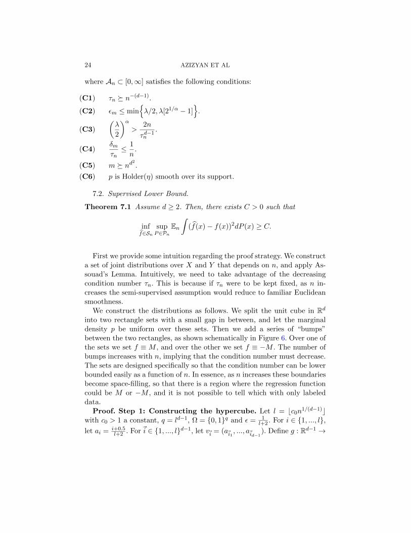
We construct the distributions as follows. We split the unit cube in Rdinto two rectangle sets with a small gap in between, and let the marginaldensity p be uniform over these sets. Then we add a series of “bumps”between the two rectangles, as shown schematically in Figure 6. Over one ofthe sets we set f ≡ M , and over the other we set f ≡ −M . The number ofbumps increases with n, implying that the condition number must decrease.The sets are designed specifically so that the condition number can be lowerbounded easily as a function of n. In essence, as n increases these boundariesbecome space-filling, so that there is a region where the regression functioncould be M or −M , and it is not possible to tell which with only labeleddata.

Proof. Step 1: Constructing the hypercube. Let l = bc0n1/(d−1)c

with c0 > 1 a constant, q = ld−1, Ω = 0, 1q and ε = 1l+2 . For i ∈ 1, ..., l,

let ai = i+0.5l+2 . For~i ∈ 1, ..., ld−1, let v~i = (a~i1 , ..., a~id−1

). Define g : Rd−1 →

SEMISUPERVISED INFERENCE 25

con

stan

t )1/(1 dn

1 2 . . .

)1/(1 dn

)1/(1 dn

Fig 6. A two-dimensional cross-section of the support of a marginal density p used in theproof of Theorem 7.1.

R as g(x) =

(32) g(x) =

r +

√(12 − r

)2 − ‖x‖22 for ‖x‖2 < 12 − r

r −√r2 −

(12 − ‖x‖2

)2for 1

2 − r ≤ ‖x‖2 <12

0 o.w.

for x ∈ Rd−1, where r ∈ (0, 1/4) will be specified later (see Equation 33).Let

B = (x, xd) ∈ [−0.5, 0.5]d−1 × [0, 1] : xd ≤ g(x).

For ~i ∈ 1, ..., ld−1, let

B~i = (x, xd) ∈ Rd−1 × R : ((x− v~i)/ε, xd − 1/8) ∈ B

and

B~i = (x, xd) ∈ Rd−1 × R : ((x− v~i)/ε, xd − (1/8 + r)) ∈ B.

Let

S = x ∈ Rd : ∃x′ = (x′, x′d) ∈ [ε, 1− ε]d−1 × [ε,1

8− ε] s.t. ‖x− x′‖2 ≤ ε

and

S = x ∈ Rd : ∃x′ = (x′, x′d) ∈ [ε, 1−ε]d−1×[1

8+r+ε, 1−ε] s.t. ‖x−x′‖2 ≤ ε.

26 AZIZYAN ET AL

For any Γ ⊆ 1, ..., ld−1, let SΓ = S ∪

(⋃~i∈Γ

B~i

)and SΓ = S\

(⋃~i∈Γ

B~i

).

Let ~Γ be an arbitrary ordering of 1, ..., ld−1. Given ω ∈ Ω, let Γ(ω) = ~Γi :ωi = 1, and let Sω = SΓ(ω), S

ω= SΓ(ω), and Sω = Sω ∪ Sω.

Let pω(x) = ISω (x)Leb(Sω) , fω(x) = MISω(x) −MISω(x), and let PωY |X be a

point mass at fω(x). Finally, let Pω denote the measure on Rd+1 defined bythe X marginal pω(x) and the conditional distributionand PωY |X .

Step 2: Lower Bound. Note that Leb(B~i) = Leb(B~i), and so for any

ω, ω′, Leb(Sω) = Leb(Sω′) = Leb(S)+Leb(S). Let λ = 1/(Leb(S)+Leb(S)),

i.e. λ = 1/Leb(Sω) for any ω. Let ω, ω′ ∈ Ω such that ρ(ω, ω′) = 1 (whereρ denotes the Hamming distance), and without loss of generality assumeωi = 0 and ω′i = 1. Also denote ~i = ~Γi. Then the L1 distance between Pω

and Pω′

is

d1(Pω, Pω′) =

∫Rd

∫R

|pω(x)dPωY |X − pω′(x)dPω

′

Y |X |dx

=

∫Sω∪Sω

′

∫R

λ∣∣∣dPωY |X − dPω′Y |X ∣∣∣dx+

∫B~i\B~i

∫R

λPωY |Xdx+

∫B~i\B~i

∫R

λPω′

Y |Xdx

+

∫B~i∩B~i

∫R

λ∣∣∣dPωY |X − dPω′Y |X ∣∣∣dx

= 0 + λLeb(B~i\B~i) + λLeb(B~i\B~i) + 2λLeb(B~i ∩B~i)= λ(Leb(B~i) + Leb(B~i)) = 2λεd−1 Leb(B)

where in the first step we have used the fact that x /∈ Sω ∪ Sω′ ⇒ pω(x) =pω′(x) = 0, and divided Sω ∪ Sω′ into four non-intersecting components.

Then we can bound the affinity of the product measures Pωn and Pω′

n forρ(ω, ω′) = 1 as

‖Pωn ∧ Pω′

n ‖ ≥1

8(1− d1(Pω, Pω

′)/2)2n =

1

8(1− λεd−1 Leb(B))2n.

SEMISUPERVISED INFERENCE 27

For any ω 6= ω′, we have, for arbitrary ~j ∈ 1, ..., ld−1,

d2(fω, fω′) =

∑ ∫B~i∆B~i

M2dx+

∫B~i∩B~i

4M2dx

= ρ(ω, ω′)(M2 Leb(B~j∆B~j) + 4M2 Leb(B~j ∩B~j))

= 2ρ(ω, ω′)M2(Leb(B~j) + Leb(B~j ∩B~j))

= 2ρ(ω, ω′)M2εd−1(Leb(B) + Leb(Br))

where the sum is only over indices where ω and ω′ differ and Br = x ∈ B :x− (0, ..., 0, r) ∈ B. Then, by Assouad’s lemma,

infω

maxω∈Ω

Eω[d2(fω, f ω)] ≥ M2(lε)d−1

32(Leb(B) + Leb(Br))(1− λεd−1 Leb(B))n.

Also we have

1

λ

∫(fω(x)− fω′(x))2pω(x)dx =

∫Sω

(fω(x)− fω′(x))2dx

=

∫(fω(x)− fω′(x))2dx−

∫Sω′\Sω

(fω(x)− fω′(x))2dx

= d2(fω, fω′)−M2 Leb(Sω

′\Sω) ≥ d2(fω, fω′)−M2qεd−1 Leb(B\Br)

= d2(fω, fω′)−M2

(l

l + 2

)d−1

(Leb(B)− Leb(Br)).

Since λ > 1,

inff

supP∈Pn

En∫

(f(x)− f(x))2dP (x) ≥ infω

maxω∈Ω

Eω∫

(f ω(x)− fω(x))2pω(x)dx

≥ M2(lε)d−1

32(Leb(B) + Leb(Br))(1− λεd−1 Leb(B))n −M2 (lε)d−1 (Leb(B)− Leb(Br)).

As soon as n ≥ 2d, l ≥ 2 and (εl)d−1 ≥ 12d−1 . Clearly Leb(B) ≤ 1

2 . Let

c0 ≥ 3. Then ε ≤ 1/8 and λ ≤ (1− 2ε)−(d−1)(1− 4ε− r)−1 ≤ 2d+1, so

(1− λεd−1 Leb(B))n ≥

(1− 2d

cd−10 n

)2n

→(e−2d/cd−1

0

)2.

So if we let c0 > (2d/ log(5/4))1/(d−1), then e−2d/cd−10 > 4/5 and for suffi-

ciently large n we will have (1− λεd−1 Leb(B))2n ≥ 8/25. Hence,

inff

supP∈Pn

En∫

(f(x)− f(x))2dP (x) ≥ M2

50 · 2d−1(Leb(Br)− 50 Leb(B\Br)) .

28 AZIZYAN ET AL

Since

Leb(Br) =1

2

(1

2− r)d πd/2

Γ(d/2 + 1)and Leb(B\Br) ≤

rπ(d−1)/2

2d−1Γ((d− 1)/2 + 1),

then

Leb(Br)− 50 Leb(B\Br) ≥1

2

(1

2− r)d πd/2

Γ(d/2 + 1)− 50rπ(d−1)/2

2d−1Γ((d− 1)/2 + 1)

≥ πd/2

2dΓ(d+1

2

)(d+ 1)

[(1− 2r)d − 100(d+ 1)r√

π

].

Now let r be such that

(33) (1− 2r)d − 100(d+ 1)r√π

=1

2.

Then

inff

supP∈Pn

En∫

(f(x)− f(x))2dP (x) ≥ M2πd/2

50 · 4dΓ(d+1

2

)(d+ 1)

.

Step 3: Verifying condition number: For any ω,

τ(Sω) = min

τ(Sω), τ(S

ω),

1

2infu∈Sω

infv∈Sω

‖u− v‖2.

Due to the shape of the function g, for arbitrary ~i ∈ 1, ..., ld−1 we have

τ(Sω) ≥ minτ(∂S), τ(∂B~i\∂S)

By definition of S it is easy to see that τ(∂S) = ε. Also

τ(∂B~i\∂S) = τ((x, xd) ∈ [−ε/2, ε/2]d−1 × [0, 1] : xd = g(x/ε))≥ ετ((x, xd) ∈ [−1/2, 1/2]d−1 × [0, 1] : xd = g(x)) = εr.

Since r < 1, we have τ(Sω) ≥ rε, and similarly τ(Sω) ≥ rε. Now,

1

2infu∈Sω

infv∈Sω

‖u− v‖2 ≥ε

2inf

u,v∈[−0.5,0.5]d−1‖(u, g(u))− (v, g(v) + r)‖2

=ε

2

(√1

4+ r2 − 1

2

)

SEMISUPERVISED INFERENCE 29

which is smaller than εr, so for n sufficiently large,

τ(Sω) ≥ ε

2

(√1

4+ r2 − 1

2

)≥ 1

2(c0n1/(d−1) + 2)

(√1

4+ r2 − 1

2

)

≥ n−1d−1

1

2(c0 + 1)

(√1

4+ r2 − 1

2

)

which completes the proof.

Step 4: Each Pω is in Pn. This follows by construction.

7.3. Semisupervised Upper Bound. Define pm to be the kernel densityestimator based on the unlabeled data with bandwidth (logm/m)1/(4+d).Let S = x : pm(x) > 0. Recall that εm = c1(logm)−1/2 and δm =

2c2

√d((log2m)/m

) 1d . Define

Dα(x1, x2) = infγ∈Γ(x1,x2)

L(γ)∫0

1

pm(γ(t))αdt

where

Γ(x1, x2) =γ ∈ Γ(x1, x2) : ∀t ∈ [0, L(γ)], γ(t) ∈ S\R∂S

,

R∂S =

x : inf

z∈∂S‖x− z‖2 < 2δm

.

We define Dα(x1, x2) =∞ if Γ(x1, x2) = ∅. Let

fh,α(x) =

∑ni=1 YiQh(Dα(x,Xi))∑ni=1Qh(Dα(x,Xi))

.

Theorem 7.2 Let h =√

1/n. Then,

supP∈Pn

RP (fh,α) 1

n.

30 AZIZYAN ET AL

Proof. Let S = SP . Let Sm =

x ∈ S : inf

z∈∂S‖x− z‖2 ≥ 3δm

. Then,

∫(fh,α(x)−f(x))2dP (x) =

∫Sm

(fh,α(x)−f(x))2dP (x)+

∫S−Sm

(fh,α(x)−f(x))2dP (x).

Now∫S−Sm

(fα(x)− f(x))2dP (x) ≤ 2M2P (S\Sm) ≤ 2ΛM2 Leb(S\Sm).

Since the radius of curvature of ∂S is at least τn, and τn > 3δm, we have byProposition 6,

Leb(S\Sm) ≤ Vol(∂S)(τn + 3δm)d − τdn

τd−1n

≤ c3

[(1 +

3δmτn

)d− 1

]

≤ c3

d∑i=1

(d

i

)3δmτn≤ 3c32d

δmτn≤(

1

n

)from (C4) where Vol denotes the d− 1-dimensional volume on ∂S.

Arguing as in Theorem 5.1, we have, for each P ∈ Pn, that

E∫Sm

(fh,α(x)− f(x))2dP (x) ≤ L2 (R(h/2))2 +M2

[4 + 1

e N(P, α, h2

)]n

+4M2

m

where R = supDP,α(x1, x2)/Dα(x1, x2) : x1, x2 ∈ Sm and N (P, α, ε)

denotes the covering number of Sm under Dα. In Proposition 5 in Section11.3 we show that DP,α(x1, x2) ≤ [(λ + εm)/λ]αDα(x1, x2) for x1, x2 ∈ Sm.By (C2) this implies that R ≤ 2. We also show in Proposition 5 thatDα(x1, x2) ≤ dSm(x1, x2)/(λ − εm)α for x1, x2 ∈ Sm. Here, dSm(x1, x2) isthe length (in Euclidean distance) of the shortest path in Sm connecting x1

and x2. Thus

N (P, α, h/2) ≤ Nm(h

2(λ− εm)α

)where Nm denotes the covering number under dSm . (C3) implies that h(λ−εm)α > τ−(d−1). By Proposition 7, each connected component of SP may becovered by one set and hence Nm

(h2 (λ− εm)α

)≤ K. We thus have that

E∫Sm

(fh,α(x)− f(x))2dP (x) ≤ L2 (2h)2 +M2

[4 + 1

e K]

n+

4M2

m

and the result follows since h = n−1/2 and m ≥ n.

SEMISUPERVISED INFERENCE 31

7.4. Comparison of Lower and Upper Bound. Finally we have:

Corollary 7.3 Under the conditions of the previous theorem,

(34)RSSRS(

1

n

)→ 0

as n→∞.

8. Adaptive Semisupervised Inference. We have established a boundon the risk of the density-sensitive semisupervised kernel estimator. Thebound is achieved by using an estimate Dα,σ of the density-sensitive dis-tance. However, this requires knowing the density-sensitive parameter α,along with other parameters. It is critical to choose α (and h) appropriately,otherwise we might incur a large error if the semisupervised assumption doesnot hold or holds with a different density sensitivity value α. We considertwo methods for choosing the parameters.

The following result shows that we can adapt to the correct degree ofsemisupervisedness if cross-validation is used to select the appropriate α, σand h. This implies that the estimator gracefully degrades to a supervisedlearner if the semisupervised assumption (sensitivity of regression functionto marginal density) does not hold (α = 0).

For any f , define the risk R(f) = E[(f(X) − Y )2] and the excess riskE(f) = R(f)−R(f∗) = E[(f(X)− f∗(X))2] where f∗ is the true regressionfunction. Let H be a finite set of bandwidths, let A be a finite set of valuesfor α and let Σ be a finite set of values for σ. Let θ = (h, α, σ), Θ = H×A×Σand J = |Θ|.

Divide the data into training data T and validation data V . For nota-tional simplicity, let both sets have size n. Let F = fTθ θ∈Θ denote thesemisupervised kernel estimators trained on data T using θ ∈ Θ. For eachfTθ ∈ F let

RV (fTθ ) =1

n

n∑i=1

(fTθ (Xi)− Yi)2

where the sum is over V . Let Yi = f(Xi) + εi with εii.i.d∼ N (0, σ2). Also, we

assume that |f(x)|, |fTθ (x)| ≤M , where M > 0 is a constant.2

2 Note that the estimator can always be truncated if necessary.

32 AZIZYAN ET AL

Theorem 8.1 Let F = fTθ θ∈Θ denote the semisupervised kernel estima-tors trained on data T using θ ∈ Θ. Use validation data V to pick

θ = arg minθ∈Θ

RV (fTθ )

and define the corresponding estimator f = fθ. Then, for every 0 < δ < 1,

(35) E[E(fθ)] ≤1

1− a

[minθ∈Θ

E[E(fθ)] +log(J)/δ)

nt

]+ 4δM2

where 0 < a < 1 and 0 < t < 15/(38(M2 + σ2)) are constants. E denotesexpectation over everything that is random.

Proof. First, we derive a general concentration of E(f) around E(f) whereE(f) = R(f) − R(f∗) = − 1

n

∑ni=1 Ui, and Ui = −(Yi − f(Xi))

2 + (Yi −f∗(Xi))

2.If the variables Ui satisfy the following moment condition:

E[|Ui − E[Ui]|k] ≤Var(Ui)

2k!rk−2

for some r > 0, then the Craig-Bernstein (CB) inequality (Craig 1933) statesthat with probability > 1− δ,

1

n

n∑i=1

(Ui − E[Ui]) ≤log(1/δ)

nt+t Var(Ui)

2(1− c)

for 0 ≤ tr ≤ c < 1. The moment conditions are satisfied by bounded randomvariables as well as Gaussian random variables (see e.g. Haupt and Nowak(2006)).

To apply this inequality, we first show that Var(Ui) ≤ 4(M2 + σ2)E(f)

since Yi = f(Xi) + εi with εii.i.d∼ N (0, σ2). Also, we assume that |f(x)|,

|f(x)| ≤M , where M > 0 is a constant.

Var(Ui) ≤ E[U2i ] = E[(−(Yi − f(Xi))

2 + (Yi − f∗(Xi))2)2]

= E[(−(f∗(Xi) + εi − f(Xi))2 + (εi)

2)2]

= E[(−(f∗(Xi)− f(Xi))2 − 2εi(f

∗(Xi)− f(Xi)))2]

≤ 4M2E(f) + 4σ2E(f) = 4(M2 + σ2)E(f)

Therefore using CB inequality we get, with probability > 1− δ,

E(f)− E(f) ≤ log(1/δ)

nt+t 2(M2 + σ2)E(f)

(1− c)

SEMISUPERVISED INFERENCE 33

Now set c = tr = 8t(M2 + σ2)/15 and let t < 15/(38(M2 + σ2)). With thischoice, c < 1 and define

a =t2(M2 + σ2)

(1− c)< 1.

Then, using a and rearranging terms, with probability > 1− δ,

(1− a)E(f)− E(f) ≤ log(1/δ)

nt

where t < 15/(38(M2 + σ2)).Then, using the previous concentration result, and taking union bound

over all f ∈ F , we have with probability > 1− δ,

E(f) ≤ 1

1− a

[EV (f) +

log(J/δ)

nt

].

Now,

E(fθ) = R(f

θ)−R(f∗)

≤ 1

1− a

[RV (f

θ)− RV (f∗) +

log(J/δ)

nt

]≤ 1

1− a

[RV (f)− RV (f∗) +

log(J/δ)

nt

]Taking expectation with respect to validation dataset,

EV [E(fθ)] ≤ 1

1− a

[R(f)−R(f∗) +

log(J/δ)

nt

]+ 4δM2.

Now taking expectation with respect to training dataset,

ETV [E(fθ)] ≤ 1

1− a

[ET [R(f)−R(f∗)] +

log(J/δ)

nt

]+ 4δM2.

Since this holds for all f ∈ F , we get:

ETV [E(fθ)] ≤ 1

1− a

[minf∈F

ET [E(f)] +log(J/δ)

nt

]+ 4δM2.

The result follows. In practice, both Θ may be taken to be of size na for some a > 0. Then we

can approximate the optimal h, σ and α with sufficient accuracy to achievethe optimal rate. Setting δ = 1/(4M2n), we then see that the penalty for

34 AZIZYAN ET AL

−3 −2 −1 0 1 2 3 4

−4

−2

0 2

4

−10

−5

0

5

10

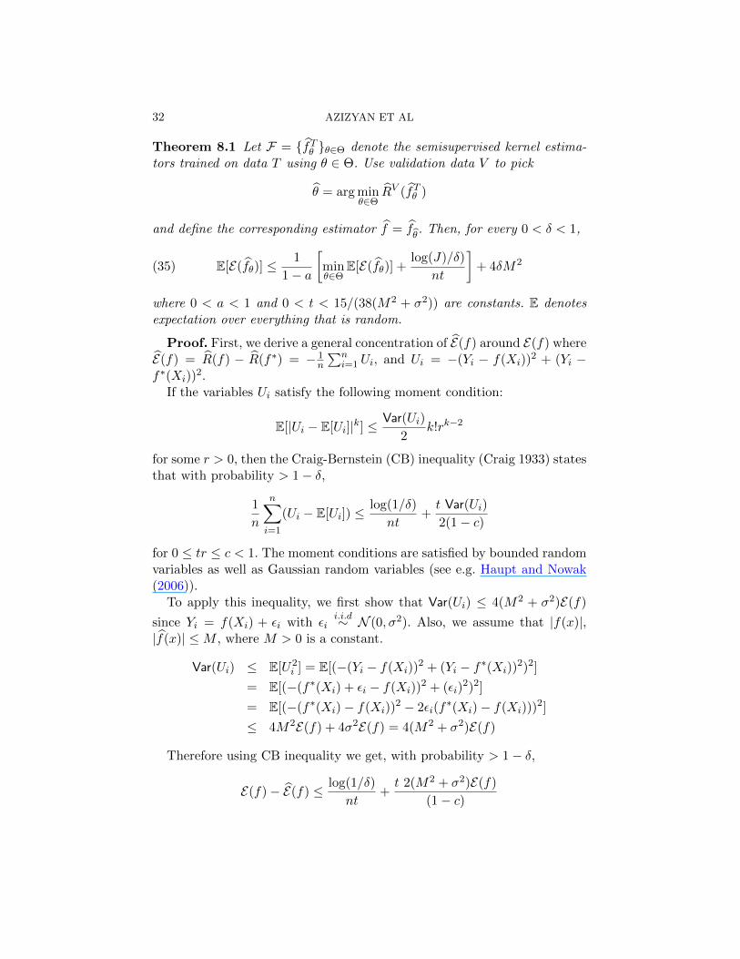
Fig 7. The swiss roll data set. Point size represents regression function.

adaptation is log(J/δ)nt + δM = O(log n/n) and hence introduces only a loga-

rithmic term.

Remark: Cross-validation is not the only way to adapt. For example, theadaptive method in Kpotufe (2011) can also be used here.

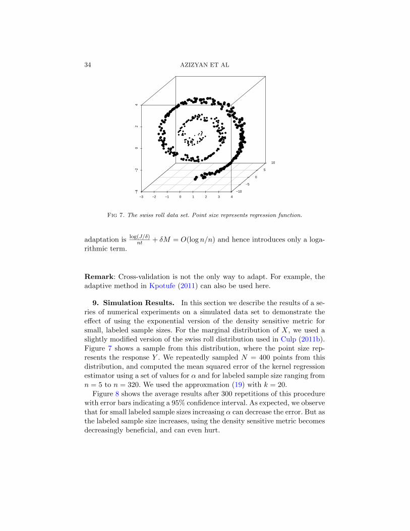
9. Simulation Results. In this section we describe the results of a se-ries of numerical experiments on a simulated data set to demonstrate theeffect of using the exponential version of the density sensitive metric forsmall, labeled sample sizes. For the marginal distribution of X, we used aslightly modified version of the swiss roll distribution used in Culp (2011b).Figure 7 shows a sample from this distribution, where the point size rep-resents the response Y . We repeatedly sampled N = 400 points from thisdistribution, and computed the mean squared error of the kernel regressionestimator using a set of values for α and for labeled sample size ranging fromn = 5 to n = 320. We used the approxmation (19) with k = 20.

Figure 8 shows the average results after 300 repetitions of this procedurewith error bars indicating a 95% confidence interval. As expected, we observethat for small labeled sample sizes increasing α can decrease the error. But asthe labeled sample size increases, using the density sensitive metric becomesdecreasingly beneficial, and can even hurt.

SEMISUPERVISED INFERENCE 35

Swiss roll regression

Labeled sample size

MS

E (

95%

CI)

5 11 26 61 139 320

05

1015

18

alpha = 0alpha = 8alpha = 16alpha = 32alpha = 96alpha = 192

Fig 8. MSE of kernel regression on the swiss roll data set for a range of labeled samplesizes using different values of α.

36 AZIZYAN ET AL

10. Discussion. Semisupervised methods are very powerful but, likeall methods, they only work under certain conditions. We have shown that,under certain conditions, semisupervised methods provably outperform su-pervised methods. In particular, the advantage of semisupervised methodsis mainly when the distribution PX of X is concentrated near a low dimen-sional set rather than when PX is smooth.

We introduced a family of estimators indexed by a parameter α. Thisparameter controls the strength of the semi-supervised assumption. Thebehavior of the semi-supervised method depends critically on α. Finally, weshowed that cross-validation can be used to automatically adapt to α sothat α does not need to be known. Hence, our method takes advantage ofthe unlabeled data when the semi-supervised assumption holds, but doesnot add extra bias when the assumption fails. Our simulations confirm thatour proposed estimator adapts well to alpha and has good risk when thesemi-supervised smoothness holds and when it fails.

The analysis in this paper can be extended in several ways. First, it ispossible to use other density sensitive metrics such as the diffusion distance(Lee and Wasserman, 2008). Second, we defined a method to estimate thedensity sensitive metric that works under broader conditions than the twoexisting methods due to Sajama and Orlitsky (2005) and Bijral, Ratliff andSrebro (2011). We suspect that faster methods can be developed. Finally,other estimators besides kernel estimators can be used. We will report onthese extensions elsewhere.

11. Additional Proofs.

11.1. Proof of Theorem 4.1. To prove Theorem 4.1 We use the approachin Yukich (1985). (See also Gine and Guillou (2002) and Prakasa-Rao (1983).)If ` ≤ u, define the bracket [`, u] = h : ` ≤ h ≤ u. A collection(`1, u1), . . . , (`N , uN ) is a ε bracketing of a class of functions F if F ⊂⋃Nj=1[`j , uj ] and

∫|uj−`j |pdP ≤ εp for j = 1, . . . , N . The bracketing number

N[ ](ε,F , Lp(P )) is the size of the smallest ε bracketing.

Theorem 11.1 Let X1, . . . , Xn ∼ P . Define P (f) =∫f(z)dP (z) and Pn(f) =

1n

∑ni=1 f(Xi). Let A = supf

∫|f |dP and B = supf ||f ||∞. Then

Pn

(supf∈F|Pn(f)− P (f)| > ε

)≤ 2N[ ](ε/8,F , L1(P )) exp

(− 3nε2

4B[6A+ ε]

)+2N[ ](ε/8,F , L1(P )) exp

(− 3nε

64B

).

SEMISUPERVISED INFERENCE 37

Hence, if ε ≤ 2A/3,(36)

Pn

(supf∈F|Pn(f)− P (f)| > ε

)≤ 4N[ ](ε/8,F , L1(P )) exp

(− 3nε2

4B[6A+ ε]

).

Proof. (This proof follows Yukich (1985).) For notational simplicity in theproof, let us write, N(ε) ≡ N[ ](ε,F , L1(P )). Define zn(f) =

∫f(dPn − dP ).

Let [`1, u1], . . . , [`N , uN ] be a minimal ε/8 bracketing. We may assume thatfor each j, ||uj || ≤ B and ||`j || ≤ B. (Otherwise, we simply truncate thebrackets.) For each j, choose some fj ∈ [`j , uj ].

Consider any f ∈ F and let [`j , uj ] denote a bracket containing f . Then

|zn(f)| ≤ |zn(fj)|+ |zn(f − fj)|.

Furthermore,

|zn(f − fj)| = |∫

(f − fj)(dPn − dP )| ≤∫|f − fj | (dPn + dP ) ≤

∫|uj − `j | (dPn + dP )

=

∫|uj − `j | (dPn − dP ) + 2

∫|uj − `j |dP

=

∫|uj − `j | (dPn − dP ) + 2

( ε8

)= zn(|uj − `j |) +

ε

4.

Hence,

|zn(f)| ≤ |zn(fj)|+[[zn(|uj − `j |) +

ε

4

].

Thus,

Pn(supf∈F|zn(f)| > ε) ≤ Pn(max

j|zn(fj)| > ε/2) + Pn(max

j|zn(|uj − `j |)|+ ε/4 > ε/2)

≤ Pn(maxj|zn(fj)| > ε/2) + Pn(max

j|zn(|uj − `j |)| > ε/4).

Now

Var(fj) ≤∫f2j dP =

∫|fj | |fj |dP ≤ ||fj ||∞

∫|fj |dP ≤ AB.

Hence, by Bernstein’s inequality,

Pn(

maxj|zn(fj)| > ε/2

)≤ 2

N∑j=1

exp

(−1

2

n(ε/2)2

AB +Bε/6

)≤ 2N(ε/8) exp

(− 3

4B

nε2

6A+ ε

).

38 AZIZYAN ET AL

Similarly,

Var(|uj − `j |) ≤∫

(uj − `j)2dP ≤∫|uj − `j | |uj − `j |dP

≤ ||uj − `j ||∞∫|uj − `j |dP ≤ 2B

ε

8=Bε

4.

Also, ||uj − `j ||∞ ≤ 2B. Hence, by Bernstein’s inequality,

Pn(

maxjzn(|uj − `j |) > ε/4

)≤ 2

N∑j=1

exp

(−1

2

n(ε/4)2

2B ε4 + 2B(ε/4)/3

)

≤ 2N(ε/8) exp

(− 3nε

64B

).

The following result is from Example 19.7 from van der Vaart (1998).

Lemma 4 Let F = fθ : θ ∈ Θ where Θ is a bounded subset of Rd.Suppose there exists a function m such that, for every θ1, θ2,

|fθ1(x)− fθ2(x)| ≤ m(x) ||θ1 − θ2||.

Then,

N[ ](ε,F , Lq(P )) ≤

(4√d diam(Θ)

∫|m(x)|qdP (x)

ε

)d.

Proof. Letδ =

ε

4√d∫|m(x)|qdP (x)

.

We can cover Θ with (at most) N = (diam(Θ)/δ)d cubes C1, . . . , CN of sizeδ. Let c1, . . . , cN denote the centers of the cubes. Note that Cj ⊂ B(cj ,

√dδ)

where B(x, r) denotes a ball of radius r centered at x. Hence,⋃j B(cj ,

√dδ)

covers Θ. Let θj be the projection of cj onto Θ. Then⋃j B(θj , 2δ

√d) covers

Θ. In summary, for every θ ∈ Θ there is a θj ∈ θ1, . . . , θN such that

||θ − θj || ≤ 2δ√d ≤ ε

2∫|m(x)|qdP (x)

.

Define `j = fθj−εm(x)/2∫m and uj = fθj +εm(x)/2

∫m. We claim that

the brackets [`1, u1], . . . , [`N , uN ] cover F . To see this, choose any fθ ∈ F .Let θj be the closest element θ1, . . . , θN to θ. Then

fθ(x) = fθj (x) + fθ(x)− fθj (x) ≤ fθj (x) + |fθ(x)− fθj (x)|

≤ fθj (x) +m(x)||θ − θj || ≤ fθj (x) +m(x)ε

2∫|m(x)|qdP (x)

= uj(x).

SEMISUPERVISED INFERENCE 39

By a similar argument, fθ(x) ≥ `j(x). Also,∫

(uj − `j)qdP ≤ εq. Finally,note that the number of brackets is

N = (diam(Θ)/δ)d =

(4√d diam(Θ)

∫|m(x)|qdP (x)

ε

)d.

Now we prove Theorem 4.1.

Proof. Let θ = (x, σ), Θ = X × [a,A], fθ(u) = σ−dK(||x − u||/σ) andF = fθ : θ ∈ Θ. We apply Theorem 11.1 with A = 1 and B = K(0)/ad.We need to bound N[ ](ε,F , L1(P ). Let θ = (x, σd) and ν = (y, τd). Somealgebra shows that

|fθ(u)− fν(u)| ≤ C

a2d||θ − ν||.

Apply Lemma 4 to get

N[ ](ε,F , L1(P )) ≤(

C

a2dε

)d+1

.

Hence, Theorem 11.1 yields,

Pn(

supx|pσ(x)− pσ(x)| > ε

)≤ 2

(C

a2dε

)d+1

×[exp

(− 3nε2ad

4K(0)(6 + ε)

)+ exp

(− 3nεad

64K(0)

)].

Note that the proofs of the last two results did not depend on P . Hence,

the results hold uniformly over P .

11.2. Propositions for Section 4.3.

Proposition 1 Given x, y, z ∈ Rd, let γ1 be the path from x to y such that

DP,α,σ(x, y) =L(γ1)∫

0

exp [−αpX,σ(γ1(t))] dt. Then

DP,α,σ(y, z) ≤ DP,α,σ(x, y)‖y − z‖L(γ1)

(1 + exp

[αKmax

σd

]αK∗max

σd+1(L(γ1) + ‖y − z‖)

).

40 AZIZYAN ET AL

Proof. Let γ2 be the straight line from y to z (i.e. L(γ2) = ‖y−z‖). Then

DP,α,σ(y, z) = infγ∈Γ(y,z)

L(γ)∫0

exp [−αpX,σ(γ(t))] dt

≤L(γ2)∫0

exp [−αpX,σ(γ2(t))] dt ≤ L(γ2) supt∈[0,L(γ2)]

exp [−αpX,σ(γ2(t))]

≤ L(γ2)

DP,α,σ(x, y)

L(γ1)+ sup

u0

∥∥∥∇u exp [−αpX,σ(u)]∣∣u=u0

∥∥∥ supt1∈[0,L(γ1)]t2∈[0,L(γ2)]

‖γ1(t1)− γ2(t2)‖

≤ L(γ2)

(DP,α,σ(x, y)

L(γ1)+ α sup

u0

[exp [−αpX,σ(u)] ‖∇upX,σ(u)‖

]u=u0

(L(γ1) + L(γ2))

)≤ L(γ2)

(DP,α,σ(x, y)

L(γ1)+ α sup

u0

[‖∇upX,σ(u)‖

]u=u0

(L(γ1) + L(γ2))

)≤ L(γ2)

(DP,α,σ(x, y)

L(γ1)+

α

σd+1K∗max(L(γ1) + L(γ2))

)≤ DP,α,σ(x, y)

L(γ2)

L(γ1)

(1 + exp

[αKmax

σd

]αK∗max

σd+1(L(γ1) + L(γ2))

)where the second to last inequality is due to the dominated convergencetheorem (exchanging differentiation and expectation with respect to P ),and Jensen’s inequality (the L2 norm is a convex function).

Proposition 2 Given x, y ∈ Rd,

‖x− y‖ exp

[−αpX,σ

(x+ y

2

)](1− exp

[αKmax

σd

]αK∗max‖x− y‖

σd+1

)≤ DP,α,σ(x, y)

and

DP,α,σ(x, y) ≤ ‖x− y‖ exp

[−αpX,σ

(x+ y

2

)](1 + exp

[αKmax

σd

]αK∗max‖x− y‖

2σd+1

)

SEMISUPERVISED INFERENCE 41

Proof. Let γ be the straight line from x to y.

DP,α,σ(x, y) ≤L(γ)∫0

exp [−αpX,σ (γ(t))] dt

≤ L(γ) supt∈[0,L(γ)]

exp [−αpX,σ (γ(t))]

≤ ‖x− y‖(

exp

[−αpX,σ

(x+ y

2

)]+‖x− y‖

2supu0

∥∥∥∇u exp [−αpX,σ(u)]∣∣u=u0

∥∥∥)≤ ‖x− y‖

(exp

[−αpX,σ

(x+ y

2

)]+αK∗max‖x− y‖

2σd+1

)≤ ‖x− y‖ exp

[−αpX,σ

(x+ y

2

)](1 + exp

[αKmax

σd

]αK∗max‖x− y‖

2σd+1

).

Now the ball B(x+y

2 , ‖x− y‖)

contains the balls B1 = B (x, ‖x− y‖/2) andB2 = B (y, ‖x− y‖/2). The integral over any path γ connecting x and y isat least as large as the integral over γ ∩B

(x+y2 , ‖x− y‖

). Hence,

DP,α,σ(x, y) ≥ ‖x− y‖

(inf

u∈B(x+y2,‖x−y‖)

exp [−αpX,σ (u)]

)

≥ ‖x− y‖(

exp

[−αpX,σ

(x+ y

2

)]− αK∗max‖x− y‖

σd+1

)≥ ‖x− y‖ exp

[−αpX,σ

(x+ y

2

)](1− exp

[αKmax

σd

]αK∗max‖x− y‖

σd+1

).

11.3. Proofs For Section 7.3.

Proposition 3 If m ≥ m0, where m0 ≡ m0(λ,Λ) is a constant, then forall marginal densities p of distributions in Pn, we have with probability >1− 1/m,

supx∈S\R∂S

|p(x)− pm(x)| ≤ εm and ∂S ⊂ R∂S

where εm = c1(logm)−1/2 for constant c1 ≡ c1(K,C2, d, η,Λ), S = x :

pm(x) > 0, and R∂S =

x : inf

z∈∂S‖x− z‖2 < δm

where δm = 2c2

√d(

log2mm

) 1d

for some constant c2 > 0.

42 AZIZYAN ET AL

Proof. Follows from Theorem 1 in Singh, Nowak and Zhu (2008b) bynoting that since the density estimate will be 0 a.s. outside the boundaryregion, and we have p ≥ λ on S, for sufficiently large m (i.e. small εm), wemust have S\R∂S ⊆ S ⊆ S ∪R∂S .

Proposition 4 Assume supx∈S\R∂S

|pm(x)− p(x)| ≤ εm and ∂S ⊂ R∂S. Let

Dα(x1, x2) = infγ∈Γ(x1,x2)

L(γ)∫0

1

p(γ(t))αdt

and Ψ = (x1, x2) : x1, x2 ∈ S\R∂S , Γ(x1, x2) 6= ∅. Then for any (x1, x2) ∈Ψ, (

λ

λ+ εm

)αDα(x1, x2) ≤ Dα(x1, x2) ≤

(λ

(λ− εm)+

)αDα(x1, x2).

Proof. Note that by the triangle inequality, R∂S ⊆ R∂S , so S\R∂S ⊆S\R∂S since τn > 2δm for m large enough. We see that if (x1, x2) ∈ Ψ,then x and y must be in the same connected component of S\R∂S , and,furthermore, all points along any path in Γ(x1, x2) must also be in the sameconnected component. For (x1, x2) ∈ Ψ,

Dα(x1, x2) = infγ∈Γ(x1,x2)

L(γ)∫0

1

p(γ(t))αp(γ(t))α

pm(γ(t))αdt

≤ infγ∈Γ(x1,x2)

L(γ)∫0

1

p(γ(t))αdt

[ supt∈[0,L(γ)]

(p(γ(t))

pm(γ(t))

)α]

≤ supz∈S\R∂S

(p(z)

pm(z)

)αDα(x1, x2)

and

supz∈S\R∂S

(p(z)

pm(z)

)α≤ sup

z∈S\R∂S

(p(z)

(p(z)− εm)+

)α≤(

λ

(λ− εm)+

)α.

So

Dα(x1, x2) ≤(

λ

(λ− εm)+

)αDα(x1, x2).

SEMISUPERVISED INFERENCE 43

Similarly,

Dα(x1, x2) ≥ infz∈S\R∂S

(p(z)

p(z) + εm

)αDα(x1, x2) ≥

(λ

λ+ εm

)αDα(x1, x2).

Proposition 5 With the notation of Proposition 4, for all x1, x2,

Dα(x1, x2) ≤ Dα(x1, x2).

Assume supx∈S\R∂S

|pm(x)−p(x)| ≤ εm and ∂S ⊂ R∂S. Then for any (x1, x2) ∈

Ψ, Dα(x1, x2) ≤dS\R∂S

(x1,x2)

λα and(λ

λ+ εm

)αDα(x1, x2) ≤ Dα(x1, x2) ≤ dSm(x1, x2)

(λ− εm)α+

where we recall that Sm =

x ∈ S : inf

z∈∂S‖x− z‖2 ≥ 3δm

. Thus

Dα(x1, x2) ≤(λ+ εmλ

)αDα(x1, x2).

Proof. Since for any x1 and x2, Γ(x1, x2) ⊆ Γ(x1, x2), clearlyDα(x1, x2) ≤Dα(x1, x2). If ∂S ⊂ R∂S ,

Dα(x1, x2) = infγ∈Γ(x1,x2)

L(γ)∫0

1

p(γ(t))αdt ≤

[sup

z∈S\R∂S

1

p(z)α

] infγ∈Γ(x1,x2)

L(γ)∫0

dt

≤ 1

λαdS\R∂S (x1, x2) ≤ 1

λαdSm(x1, x2)

since, by the triangle inequality, Sm ⊆ S\R∂S . Applying Proposition 4, theresult follows.

Proposition 6 Let X be a compact subset of Rd, and T > 0. Then for anyτ ∈ (0, T ), for all sets S ⊆ X with condition number at least τ , Vol(∂S) ≤c3/τ for some c3 independent of τ , where Vol is the d−1-dimensional volume.

Proof. Let ziNi=1 be a minimal Euclidean τ/2-covering of ∂S, and Bi =x : ‖x− zi‖2 ≤ τ/2. Let Ti be the tangent plane to ∂S at zi. Then usingthe argument made in the proof of Lemma 4 in Genovese et al. (2010),

Vol(Bi ∩ ∂S) ≤ C1 Vol(Bi ∩ Ti)1√

1− (τ/2)2/τ2≤ C2τ

d−1

44 AZIZYAN ET AL

for some constants C1 and C2 independent of τ . Since X is compact,

N (∂S, ‖ · ‖2, τ/2) ≤ C(

1

τ

)dfor some constant C depending only on X and T , where N denotes thecovering number (note that even though ∂S is a d − 1 dimensional set, wecan’t claim N (∂S, ‖ · ‖2, τ) = O(τ−(d−1)), since ∂S can become space-fillingas τ → 0). So

Vol(∂S) ≤N∑i=1

Vol(Bi ∩ ∂S) ≤ C2τd−1N (∂S, ‖ · ‖2, τ/2) ≤ C2Cτ

−1

and the result follows with c3 = C2C.

Proposition 7 Let X be a compact subset of Rd, and T > 0. Then for anyτ ∈ (0, T ), for all compact, connected sets S ⊆ X with condition number atleast τ , sup

u,v∈SdS(u, v) ≤ c4τ

1−d for some c4 independent of τ .

Proof. First consider the quantity supu,v∈∂S

dS(u, v). Since ∂S ⊆ S, clearly

supu,v∈∂S

dS(u, v) ≤ supu,v∈∂S

d∂S(u, v).

Since ∂S is closed, there must exist u∗, v∗ ∈ ∂S such that

supu,v∈∂S

d∂S(u, v) = d∂S(u∗, v∗).

Let ziNi=1 be a minimal τ -covering of ∂S in the d∂S metric. Let ziNi=1 ⊆ziNi=1 such that d∂S(u∗, z1) ≤ τ , d∂S(v∗, z

N) ≤ τ , and for any 1 ≤ i ≤ N−1,

d∂S(zi, zi+1) ≤ 2τ . Then

d∂S(u∗, v∗) ≤ d∂S(u∗, z1) + d∂S(v∗, zN

) +N−1∑i=1

d∂S(zi, zi+1) ≤ 2τN .

So, d∂S(u∗, v∗) ≤ 2τN (∂S, d∂S , τ). By Proposition 6.3 in Niyogi, Smale andWeinberger (2008) (or see Lemma 3 in Genovese et al. (2010)), if x, y ∈ ∂Ssuch that ‖x − y‖2 = a ≤ τ/2, then d∂S(x, y) ≤ τ − τ

√1− (2a)/τ . In

particular, if ‖x − y‖2 ≤ τ/2, then d∂S(x, y) ≤ τ . So any Euclidean τ/2-covering of ∂S is also a τ -covering in the d∂S metric. Then we have

supu,v∈∂S

dS(u, v) ≤ d∂S(u∗, v∗) ≤ 2τN (∂S, d∂S , τ) ≤ 2τN (∂S, ‖ · ‖2, τ/2)

≤ Cτ

(1

τ

)d= Cτ1−d

SEMISUPERVISED INFERENCE 45

for some constant C depending only on X and T (note that, as in the proof of6, even though ∂S is a d−1 dimensional set, we can’t claim N (∂S, ‖·‖2, τ) =O(τ−(d−1)), since ∂S can become space-filling as τ → 0).

Now let u†, v† ∈ S such that supu,v∈S

dS(u, v) = dS(u†, v†) which must exist

since S is compact. Let u‡, v‡ ∈ ∂S be the (not necessarily unique) projec-tions of u† and v† onto ∂S. Clearly the line segment connecting u† and u‡

is fully contained in S, and the same applies to v† and v‡. So,

dS(u†, v†) ≤ dS(u†, u‡) + dS(u‡, v‡) + dS(v‡, v†)

≤ ‖u† − u‡‖2 + ‖v† − v‡‖2 + dS(u∗, v∗)

≤ 2 diam(X ) + Cτ1−d

and setting c4 = 2T d−1 diam(X ) + C, the result follows.

References.

Belkin, M. and Niyogi, P. (2004). Semi-supervised learning on Riemannian manifolds.Machine Learning 56(1-3) 209–239.

Ben-David, S., Lu, T. and Pal, D. (2008). Does Unlabeled Data Provably Help? Worst-case Analysis of the Sample Complexity of Semi-Supervised Learning. In 21st AnnualConference on Learning Theory (COLT).

Bijral, A., Ratliff, N. and Srebro, N. (2011). Semi-supervised Learning with DensityBased Distances. In 27th Conference on Uncertainty in Artificial Intelligence.

Bousquet, O., Chapelle, O. and Hein, M. (2004). Measure based regularization. InAdvances in Neural Information Processing Systems.

Culp, M. (2011a). On Propagated Scoring for Semisupervised Additive Models. Journalof the American Statistical Association 106 248-259.

Culp, M. (2011b). spa: Semi-Supervised Semi-Parametric Graph-Based Estimation in R.Journal of Statistical Software 40.

Culp, M. and Michailidis, G. (2008). An Iterative Algorithm for Extending Learnersto a Semi-Supervised Setting. Journal of Computational and Graphical Statistics 17545-571.

Einmahl, U. and Mason, D. M. (2005). Uniform in bandwidth consistency of kernel-typefunction estimators. The Annals of Statistics 33 1380-1403.

Genovese, C., Perone-Pacifico, M., Verdinelli, I. and Wasserman, L. (2010). Min-imax Manifold Estimation. Arxiv preprint arXiv:1007.0549.

Gine, E. and Guillou, A. (2002). Rates of strong uniform consistency for multivariatekernel density estimators. Annales de l’Institute Henri Poincare (B) Probability andStaistics 38 907-921.

Gyorfi, L., Kohler, M., Krzyzak, A. and Walk, H. (2002). A distribution-free theoryof nonparametric regression. Springer Verlag.

Haupt, J. and Nowak, R. (2006). Signal reconstruction from noisy random projections.IEEE Trans. Info. Th. 52 4036–4048.

Kpotufe, S. (2011). k-NN Regression Adapts to Local Intrinsic Dimension. NIPS.

46 AZIZYAN ET AL

Lafferty, J. and Wasserman, L. (2007). Statistical Analysis of Semi-Supervised Re-gression. In Advances in Neural Information Processing Systems 20 801–808.

Lee, A. B. and Wasserman, L. (2008). Spectral Connectivity Analysis. Arxiv preprintarXiv:0811.0121.

Liang, F., Mukherjee, S. and West, M. (2007). The Use of Unlabeled Data in Predic-tive Modeling. Statistical Science 22 189-205.

Nadler, B., Srebro, N. and Zhou, X. (2009). Statistical analysis of semi-supervisedlearning: The limit of infinite unlabelled data. In Advances in Neural Information Pro-cessing Systems 22 1330–1338.

Niyogi, P. (2008). Manifold Regularization and Semi-supervised Learning: Some The-oretical Analyses Technical Report No. TR-2008-01, Computer Science Department,University of Chicago. URL http://people.cs.uchicago.edu/∼niyogi/papersps/ ssmini-max2.pdf.

Niyogi, P., Smale, S. and Weinberger, S. (2008). Finding the Homology of Submani-folds with High Confidence from Random Samples. Discrete & Computational Geometry39 419–441.

Prakasa-Rao, B. L. S. (1983). Nonparametric Functional Estimation. Academic Press.Rigollet, P. (2007). Generalization error bounds in semi-supervised classification under

the cluster assumption. Journal of Machine Learning Research 8 1369–1392.Sajama, and Orlitsky, A. (2005). Estimating and computing density based distance

metrics. In Proceedings of the 22nd international conference on Machine learning. ICML2005 760–767.

Singh, A., Nowak, R. D. and Zhu, X. (2008a). Unlabeled data: Now it helps, now itdoesn’t Technical Report, University of Wisconsin - Madison, ECE Department. URLhttp://www.cae.wisc.edu/∼singh/SSL TR.pdf.

Singh, A., Nowak, R. and Zhu, X. (2008b). Unlabeled data: Now it helps, now it doesn’t.In Neural Information Processing Systems (NIPS).

Sinha, K. and Belkin, M. (2009). Semi-supervised Learning using Sparse EigenfunctionBases. In Advances in Neural Information Processing Systems 22 (Y. Bengio, D. Schu-urmans, J. Lafferty, C. K. I. Williams and A. Culotta, eds.) 1687–1695.

van der Vaart, A. W. (1998). Asymptotic Statistics. Cambridge University Press, Cam-bridge.

Yukich, J. E. (1985). Laws of Large Numbers for Classes of Functions. Journal of Mul-tivariate Analysis 17 245-260.

Department of Statisticsand Machine Learning DepartmentCarnegie Mellon UniversityPittsburgh, Pennsylvania 15213USAE-mail: mazizyan@cs.cmu.edu

aarti@cs.cmu.edularry@stat.cmu.edu