Density fluctuations in liquid4He. Path integrals and maximum entropy

Journal of Low Temperature Physics, Vol. 104, Nos. 5/6, 1996

Density Fluctuations in Liquid 4He. Path Integrals and Maximum Entropy

Massimo Boninsegni* and David M. Ceper|ey

National Center for Supercomput&g Applications, University of Illinois at Urbana-Champaign

(Received April 8, 1996; revised June 4, 1996)

We estimate the dynamic structure factor S(q, co) for liquid 4He in both its normal and superfluid phases. A path integral Monte Carlo simulation is performed to compute the imaginary-time polarization propagator F(q, r), from which S(q, co) is extracted by maximum entropy. Results for normal 4He are in good quantitative agreement with recent neutron scattering experimental data; broad agreement is found for superJluid 4He as well, though sharp features are lost, particularly at low q. We attribute the excessive smoothness of the results to the entropic "prior probability" function used in the maximum entropy reconstruction. The experimentally observed ground state excitation spectrum E(q) is accurately reproduced in the O<~q~2.5 A -1 range.

1. INTRODUCTION

Dynamic functions describing the linear response of a quantum many- body system to a weak external probe are of great theoretical interest for at least two reasons: (a) they are directly accessible to experiment and (b) they are related to its elementary excitations.l For bulk liquid 4He, the dynamic structure factor S(q, co) describes the density fluctuations, and indirectly the elementary excitations (phonons and rotons) which govern the behavior of the system at low temperatures. 2< S(q, ~o) has been investigated experimentally for several generations of neutron scattering measurements of increasing precision. 5 10 Various interpretations have been proposed to account for the main features of the experimentally observed S(q, co), 1l-!4 as well as of the corresponding elementary excitation spectrum E(q) at different temperatures and pressures. 15-17 The general aim is to gain understanding of the interplay between elementary excitations and phenomena

*Present address: Department of Physics and Astronomy, University of Delaware.

339

0022-2291/96/0900-0339$09.50/0 �9 1996 Plenum Publishing Corporation

340 Massimo Boninsegni and David M. Ceperley

such as superfluidity and Bose-Einstein condensation, in liquid 4He as well as in other Bose systems.

Most microscopic calculations of S(q, co) based on realistic inter- atomic potentials have been carried out with the ground state variational method)' 4, 18-20 The variational approach has yielded considerable physical insight, but it leaves some questions unanswered. One can estimate approximately the position of the lowest-energy peak of S(q, co), but physical properties such as the width of the peak, related to the lifetime of the excitation, remain undetermined. Also, the effect of temperature is difficult to study by a ground state technique, particularly at temperatures near or above the lambda transition. Thus, the theoretical understanding would benefit from a robust numerical scheme enabling the computation of S(q, co) at finite temperature directly from the ab initio microscopic Hamiltonian.

A generally applicable numerical procedure to calculate dynamic responses is still lacking. Quantum Monte Carlo (QMC) techniques are a well-established tool to calculate reliably thermodynamic properties of Bose systems, but their impact on the investigation of the dynamics of condensed 4He has so far been limited. The main difficulty lies in the imaginary-time formulation of QMC methods; one can calculate imaginary- time propagators, which, unlike their real-time counterpart, are related to the physical frequency spectra via an inverse Laplace transformation, which is an ill-posed problem. Thus, the inherent statistical uncertainty affecting QMC data usually rules out an unambiguous reconstruction of the spectral functions.

Various approaches to overcome this problem, namely the extraction of dynamic response functions from QMC data, have been proposed; among them, the Maximum Entropy method (ME) 21'22 has been applied with some success to determine single- and two-particle spectral properties for quantum lattice models such as the Anderson, 23 Hubbard, 24-26 as well as spin -1 Antiferromagnetic Heisenberg model27; recently, an application to a problem in the continuum has been reported, namely the absorption spectrum of a solvated electron in fluid helium. 28

The application of ME to this type of problem is still at a preliminary stage; different "recipes" have been adopted in the various applications, and only recently has some progress been achieved toward defining a systematic procedure to determine the real-time response from imaginary- time correlation functions. 29 Nonetheless, ME presently appears as a promising approach for extending the use of QMC to the determination of dynamic properties of quantum many-body systems; thus, it seems worth- while to apply it to liquid 4He, which is well characterized experimentally, theoretically and computationally.

Density Fluctuations in Liquid 4He 341

In this work, we have calculated the imaginary-time polarization propagator (intermediate scattering function) F(q, r) for liquid 4He, with a path integral Monte Carlo (PIMC) simulation of 64 4He atoms interacting via a pair potential; we have then used a ME procedure to obtain the dynamic structure factor S(q, co). We report results for both the normal and the superfluid phases of liquid 4He, at T = 4 K and T = 1.2 K, for wave vectors q up to 2.5 ~-1.

One of the technical aspects in which the ME methods often differ is the determination of the "regularization" parameter e. In this work, rather than seeking an optimal value for 0~, we have histogrammed its probability density, ~(c~), with a separate Monte Carlo simulation. Then, we have obtained S(q, co) by averaging ME results obtained with the different values of ~, using ~(~) as weight function. In the Maximum Entropy method an input model for S(q, co) is specified, and in principle it should incorporate whatever prior knowledge is available; because of the difficulty in choosing functions with the strong peak structure characteristic of a superfluid, we used a featurless, "flat" default model.

In general, our results seem to feature the same qualities and suffer from the same problems as those found in other applications, namely:

(a) the reconstructed images have very smooth features. This is most evident at T= 1.2 K, particularly at low momentum q; the experimentally-observed sharp phonon-roton peak is not adequately reproduced in our calculation. The agreement with experiment improves at higher temperatures, as the spectral functions become smoother; our results for normal 4He at T = 4 K are in agreement with recent neutron scattering measurements.

(b) even for the superfluid phase, broad features of the spectral functions of interest are recovered; all of our calculated S(q, co) dis- play a broad but well-defined peak, whose position is in good agreement with experiment. The elementary excitation spectrum E(q) accurately reproduces the one observed experimentally, at least for q<2.3 A -1.

It appears that ME is acceptable for estimating the dynamical structure factor in the normal phase and the excitation energy in the superfluid. On the other hand, given the quality of our data, high for continuum PIMC simulations, it appears that we are still far from a satisfactory method of calculating dynamic functions for Bose superfluid.

This paper is organized as follows. In the next section we introduce the imaginary-time polarization propagator F(q, r) and outline its calculation using PIMC; in section III we briefly discuss the problem of inferring


S(q, co) from the computed F(q, T), and give a description of our procedure, based on Maximum Entropy, to achieve this goal. In section IV we present our results for the S(q, co), and draw our conclusions in section V.

2. DYNAMIC CORRELATIONS F R O M PATH INTEGRALS

We consider a system of N 4He atoms at temperature T. Le t /~ be the Hamiltonian of the system. The polarization propagator F(q, t) (the intermediate scattering function) is defined as3~

1 F(q, t ) : ~ </3q(t)/0~(0)> (1)

where/Sq =~Y~ie iqri is the Fourier transform of the density. Our notation for a general time-dependent operator zi(t) is A ( t ) = ei~'tAe-i~q'(h = 1) and < A > = Tr[ A~]/Z is the thermal average, with ~ = e -~q being the statistical operator and Z = Tr[p] the canonical partition function. The operator Nq =/~-q creates a density fluctuation of momentum q; the presence of the subscript q should prevent any confusion with the statistical operator /~ defined above.

The dynamic structure factor S(q, co), is the Fourier transform of the intermediate scattering function:

F(q, t) = de) S(q, co) e i~~ (2) - - c o

It can be easily shown 1 that S(q, co)>/0. Now, (2) can be analytically continued, to define a function F(q, z) of the complex variable z = z + it; thus, on the real axis z = z, one has

fo F(q, r) = de) S(q, co) e-~~ = do) S(q, co)(e o)~ + e o~(z-~) (3)

where the "imaginary-time" polarization propagator F(q, r) is defined as in (1) with the replacement it ~ z; the second equation in (3) is based on the detailed balance condition: S(q, - c o ) = exp(-coil) S(q, co). Any imaginary- time propagator is periodic, i.e. F(q, r + fl) = F(q, r); moreover, F(q, fl - r) = F ( - q, z) = F(q, v) for an isotropic system (for a derivation of these properties of S(q, co), see, for instance Ref. 1). Thus, one need only compute F(q, z) for O<~z<~fi/2.

For convenience, we introduce the following functions:

�9 S (q , co)( 1 + e -~~ F(q, z) ~- V(q, z), ~(q, co) -= (4) Sq Sq


where

Sq = F(q, 0) = do) S(q, co)(1 + e -~)~) (5)

is the static structure factor. Thus, (3) can be written in terms of F(q, r) and S(q, co) as follows:

F(q, r ) = fo dco S(q, co) e ~i + e -~ j (6)

Clearly, it is

F(q, 0 ) = dco S(q, co)= 1 (7)

The dynamic structure factor S(q, co) satisfies the well-known f-sum rule 31

f +oo

(co) = do) co S(q, co) = coq (8) o~

with coq = q2/2m; (8) can be written in terms of S(q, co) as

(co)Sq = IodcocoS(q'co) tanh(~ -) = S q coq (9)

We seek a solution to the integral equation (6) for the unknown, non- negative function S(q, co), subject to the normalization condition (7) and the additional integral identity (9). S(q, co) is related to the dynamic structure factor S(q, co) through (4). Note that, in principle, other sum rules can be derived (see, for instance, Ref. 17), and utilized to characterize the solution S(q, co). The f-sum rule is equivalent to specifying the derivative of F at ~ = 0 and higher sum rules are equivalent to specifying higher derivatives. Since the time dependence of F(q, ~) is to some extent already present in the PIMC-determined correlation functions, it is not clear how much is to be gained by also fixing these derivatives; in this work, only (8) was explicitly taken into account.

We calculated F(q, v), as well as S(q), for superfluid 4He at T = 1.2 K and normal liquid 4He at T = 4 K, by means of a PIMC simulation of 64 4He atoms interacting via an accurate and realistic two-body potential. 32 The simulations were carried out at the saturated vapor pressure of bulk liquid 4He (i.e., at a density of 0.02186 A -3 at T = 1.2 K and 0.01873 A-3 at T = 4 K ) . Simulations of this type have been shown to afford a


remarkably accurate quantitative description of the normal-superfluid transition in liquid 4He.15"33 35 The above calculation is a straightforward application of the present PIMC technology; thus, the details of the calculation will not be reviewed here (see Ref. 33).

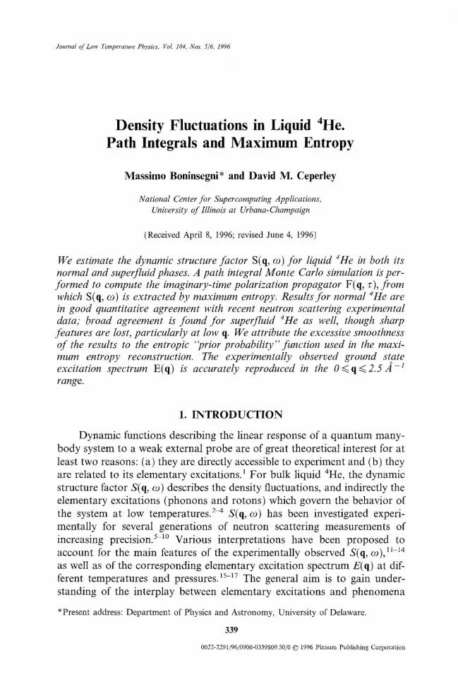
An example of the computed F(q, v) is shown in Fig. 1, at T = 1.2 K for various q-vectors. For each q, we obtained a numerical estimate of Sq, as well as of a set of L values F(q, l 6z), with I = 1,..., L and L c~ = fl/2, & being the time step adopted in the PIMC simulation. Space and time sym- metries were used to improve statistics, thereby reducing the statistical errors to ~ 5 %. The values of Sq which we obtained at both temperatures reproduce previously published PIMC results, that are also in remarkable agreement with the experimentally measured S q. 33

The main task is then the inference of S(q, co) from the calculated F(q, ~) through the inversion of the integral transformation (3).

3. DETERMINING S(Q, co) F R O M F(Q, z)

In order to invert (6) numerically, the integral on the right-hand side is approximated by a sum:

M ~e 0a~a~+e ~2L-z)ja~a~o-~ F(q, 16z-) = Z S(q, jdcn) L 1 ~ - ~ ~ j den l= 1,..., L (10)

j = l

where M 6co = cop,, (z) m being chosen sufficiently large that S(q, ~o) can be set equal to zero for co > co,,,. For a given q, (10) is a system of L equations in the M unknowns S(q, j Oco). Naturally, 6co must be taken sufficiently small, so that going from (3) to (10) entails no significant loss of accuracy. Analysis of experimental data 8" 9 suggests that, for our problem of interest, co,~ should be typically >50 K and c~co ~0.5 K, so that M > 100. In principle, L could be as large as desired, but taking too small a time step is detrimental to the efficiency of the PIMC simulation33; moreover, reducing 6v causes greater statistical correlation between nearby values of of F(q, ~), so that the overall computational efficiency is reduced.

In our work, we chose & with the main aim of keeping the PIMC calculation efficient, while ensuring the convergence of the physical estimates33; the results which we present here were obtained with L = 40 at T = 1.2 K, which corresponds to &=0.025 K -1, and with L = 2 0 at T = 4 K, i.e. &=0.0125 K -1. We will come back to this point when dis- cussing our results.

Because in our study M > L, (10) is underdetermined; this fact alone ensures that, in general, no unique solution exists, irrespective of the ill- posedness of the problem and of statistical errors of F(q, l &).


In the Bayesian method, out of all possible solutions one searches for the one that is most probable, in terms of its consistency with the PIMC data and any available prior information. Consider the example of fitting a function to noisy data. A standard procedure is to minimize the ,g2, using restrictive assumptions on the fitted function. One discards most of the possible solutions, focusing on a limited subset of "acceptable" functions of relatively few parameters. The most probable solution is determined by adjusting these parameters so that a good fit to the data is reobtained. Essentially, the Z2-fitting procedure is adequate in those instances where there is little or no doubt as to what the solution should look like; as the prior information is reduced, the approach becomes increasingly ineffective and uncontrolled. This is particularly the case when the problem is ill- posed and statistical errors affect the data, as the ensemble of possible solutions widens greatly. 36

In general, attempts to utilize Z2-fitting to determine spectral properties from QMC data, assuming little or no prior information, have produced, at best, qualitatively interesting results. 37 One can understand this problem by looking at the curves shown in Fig. 1. Because of their limited structure, within their statistical errors they can be adequately fit by many different linear combinations of exponentials, corresponding to a wide range of possible spectral functions, going from almost featurless, single- peaked ones, to others rich in structure. To put it differently, the Laplace transform is a smoothing operation; thus, inversion amplifies the noise.

1.0

0.8

0.6

0.4

0.2

q=0.62 ,, q=1.08 + q=1.64 q=2.01 •

[ ]

+

[ ]

x

+ o

[ ] x

x

+

+

•

• •

+ x

0.0 ' ' +

0.0 0.1 0.2 0.3 0.4 .c(K -1 )

Fig. 1. F(q, r) computed by PIMC, at T= 1.2 K, for different wave vectors q (in A-t). Statistical errors are smaller than the sizes of the symbols.


In the Bayesian approach one maximizes the product of the likelihood function and another function, the "prior probability", i.e. the probability of a given function in the absence of any data. The various Maximum Entropy methods and their application in quantum physics from QMC data are described in several references, 21' 22, 29 to which we refer readers interested in the full justification of the method.

To simplify the notation we only consider a specific wave vector q and set F = {/~1,..., EL} ~ {x~(q, ~T), J~'(q, 2 &),..., F(q, L &)}, S= {S~, $2, . . . , ~'~M} ~--- {~(q, &o), g(q, 2 &o),..., S(q, M&o)} and

j e -lj & am + e - (2L- l ) j 6z 6~ ) Kzy = [ i + e_--75Z~ a7; &o (11)

Thus, Eq. (10) can be written in matrix form as

!~ = KS

The ffl are obtained as averages in the PIMC calculation, and have statistical uncertainties a l = C,, where C is the covariance matrix. 3s In general, C o ~ C,j 6 o, i.e. values of F(q, v) calculated at different imaginary times are correlated with each other.

In the ME approach, the solution Ss of (12) maximizes ~ ( S , 0c), defined as:

~ - ( S , o~) = 5~ .~(S, ~) (13)

with

6' (1/2) Q(S) Y(S) - (14)

Zo where Q(S) = (F - it), C I(F - F), with F = KS, is the usual X 2 m e a s u r e of the goodness of the fit to the data [r provided by S and

~ ( s , ~) = z ~ ( ~ ) 15)

where

mj, } 16,

is the entropy of S, defined with respect to a default model m; 0~ 1s a regularization parameter, and Z e and Z ~ ( e ) are normalization constants for S and ~.


The likelihood function 5 ~ can be rigorously derived in the limit of good statistics, using the central limit theorem. On the other hand, the use of ~(S, 0~), i.e. the prior probability for S, incorporating any prior knowledge one might have about the physical spectrum S(q, co) has so far not been given, in our view, an equally convincing justification.

Clearly the prior function should be zero for a solution S which is physically impossible, e.g. a negative-valued solution. The probability of obtaining a given value of S(q, co) is characterized by some mean value (the

model m) and width ( x / ~ ) . The prior probability is maximum when S = m; thus, in the absence of data, Ss = m. Increasing the value of the parameter c~ pulls the estimated value of S s closer to the input model. On the other hand, as the statistical errors decrease, 5O(S) becomes sharply peaked and the default model can be overruled. In other words, in the limit ~ o% the data become irrelevant; on the other hand, as 0 ~ 0~(S) is constant, and the problem is again one of X 2 fitting. Different values of lead, in general, to different solutions, and the various procedures treat 0~ differently.

In the "classic" ME approach, a probability density ~(~) is introduced for ~, and, following purely Bayesian arguments, determined self-con- sistently21, 29:

~(~)=p(~) f~Sg(S, ~) (17)

where @ S - d S 1 dS2. . , dSM and p(~) is the prior probability for ~; it is often set to a constant or to the so-called Jeffrey's prior, i.e. p(~) = 1/cq and in practice does not play too important a role. 29

The solution to (12) is then determined as

s~ = f d~ ~(~) ~(~) (18)

where gs(c~) is the function S~. that maximizes (13) for the given value of 0~. The simplest procedure consists of assuming lr(~) to be sharply peaked

around its maximum, say at c~ = ~s; thus, only values of e near % will con- tribute significantly to the integral in (18), and ~(~) may be replaced by c~(~-0~,). One can therefore determine approximately % first, by maximizing ~r(~) with respect to ~, and then obtain an approximate ME solution to (12) by maximizing Y(S, %) with respect to S.

In order to provide a more reliable estimation of (18), one must go beyond the assumption of a sharply peaked ~(0~), for which there is no clear theoretical justification, and which is often found to be invalid. 29' 39

348 Massilno Boninsegni and David M. Ceperley

In this work, we histogram ~(~) by means of a random walk (Metropolis Monte Carlo) in {S, 0~}-space, and perform an explicit numerical evaluation of (18) using the histogrammed rc(0~). This procedure clearly does not require any particular assumption on ~(~). A similar approach was adopted, in a slightly different context, in Ref. 40. In the following sub- section, we describe in some detail the procedure to histogram rc(0~), which is central to our scheme.

3.1. Determination of ~(a) by Random Walk

The probability density ~(0~) is histogrammed by generating an ensemble { Si, 0~i}, with i = 1, 2,..., Ns, in which every element is statistically sampled with a probability oc J ( S , ~) N(S), where ~ ( S , 0r is defined in (13) and

N(S) oc exp{ - [ (co) - coq ] 2/2r]2co~ } (19)

with (co) defined as in (8), ensures that (9) be satisfied, within a relative fluctuation 1/. The value of tl is set equal to the relative uncertainty with which Sq is known from the PIMC simulation. The additional constraints of non-negativity of S(q, co) and (7) are also included, as explained below.

The Markov chain (Metropolis algorithm) in {S, c~}-space, proceeds as follows. Initially, we set S = m and c< to a small number, such as 0.001. From a given {S, ~}, we sample a new {S', ~'} through two different types of elementary moves, namely:

(a) the displacement of a fraction of area c from one of the M intervals, say j, to another one, say j ' randomly picked among the 2l - 1 intervals j - l, j - 1 + 1,..., j - 1, j + 1,..., j + l; this proposed move clearly conserves the total area. The move is attempted with a probability oc Sj, thereby preventing S s from becoming negative, and accepted with probability p ( S - ~ S ' ) = Y ( S ' , ~ ) N(S ' ) /~(S, ~) N(S), where S' = {$1S2... S j - c. . . S/ + c. . . SM}. Here, l is adjusted to obtain an acceptance ratio of about 0.5.

(b) the variation of c~ by a random quantity c~, accepted with probability ~ ( S , 0r c~0r 0~); 80~=re~, where r is a random number between - 1 and 1 and ~ is a parameter adjusted to obtain an acceptance ratio of about 0.5.

Typically, a move of type (b) is attempted every M moves of type (a); we refer to a combination of M moves of type (a) and one of type (b) as a pass. A few hundred passes are normally needed in order for ~r to stabi- lize. Thus, after discarding the first 500, we perform on the order of 5,000 passes to histogram ~(0~).


0.12

0.10

0.08

0.06

0.04

0.02

L - - . -

m

/ 40 45

i

m

I

50 0.00

35 55 60 75 65 70

0.12 - - T - - T - - T 1 T F - F - -

0.10

0.08

0.06

0.04

0.02

0.00 80 90 100 110 120 130 140 150 160

o~

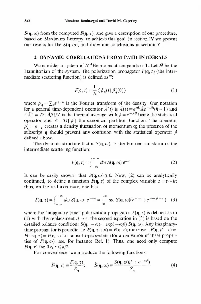
Fig. 2. Histograms of ~(c~) at T = I . 2 K and q=0.45,~ - I (top), and at T = 4 K and q = 2.5/~ -1 (bottom).


Before illustrating some typical results for g(~), we briefly comment on a technical point that has generated some controversy in previous applications of ME. The definition of the likelihood function (14) involves the covariance matrix C, which can be computed in the PIMC simulation. As mentioned in Sec. III, the diagonal approximation for C is incorrect, because of correlations between PIMC data at different imaginary times. It has been suggested, however, that because the off-diagonal elements of C computed by QMC methods are typically affected by relatively large statistical uncertainties, C is often ill-conditioned; thus, a more stable algorithm can be obtained by setting C~ = Cii ~/j.41 A definitive solution to this issue has not been offered yet29; in this work, we used the full C, calculated during the PIMC simulation, as well as its diagonal approximation, and saw no significant differences in the results for ~(0~) and S(q, co) for the two cases.

The normalization constant ZQ does not enter in the Metropolis simulation, whereas Zj,(0~) explicitely appears through its e dependence. We evaluated Zy(c~) as suggested in, 21'29 namely by taking a gaussian approximation to e ~s~(s~ and performing the normalization integration by steepest descent. This is correct if c~> 1, which we find always satisfied (typically o~ ~> 50).

Figure 2 shows typical results for ~(~). We find that ~ is not peaked very sharply around its maximum, particularly at T = 4 K. We determine a window of ~ within which 99 % of all the sampled values of 0~ fall, and divide this window into 20 bins, which are then utilized to calculate S s = S( c5, co) by means of (18). The resulting S(q, co) are presented in the next section.

4. RESULTS

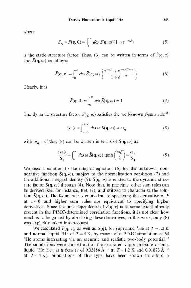
Results for S(q, co) at T = 4 K, inferred from the F(q, v) data computed by PIMC, following the procedure described in Sec. III, are shown in Fig. 3, for the two wave vectors q=0.75 A -1 and q = 1.40 A -1. They are compared with neutron scattering results from Ref. 42. The agreement is excellent.

Above the normal-superfluid transition the experimentally observed S(q, co) is relatively smooth; the broad peak at low energy is only a remnant of a much sharper peak, observed at temperatures below the 2-transition. The broadening of this peak at higher temperature has been conjectured to reflect the disappearance of the condensate. 17

In our calculated spectral functions at T = 1.2 K a clear strengthening of the low-energy peak is observed, with respect to the results at T = 4 K


',e' v

09

0.014 [

0.012

0.010

0.008

0.006

0.004

0.002

0.000 ' *

-30

f

I

-20

i i

This work o Experiment

'~ q=0.75 ~.i

I I I I i

-I0 0 I0 20 30 co (K)

0.016

0.014

0.012

,,,. 0.01

~" 0.008

oo 0.006

0.004

0.002

0

-20

i f i

z ~ j : This work ,, .:~ ~ , Experiment ,,

q=1.4o,

, ,~/Ti ~ ~ ,~

I i I I ~ . - - - ~ ,

-10 0 10 20 30 40 co(K)

Fig. 3. Dynamic structure factor S(q, o~) for liquid 4He at T = 4 K and saturated vapor pressure, for q=0.75 A. 1 (top) and q = 1.40A ~ (bottom), determined by Maximum Entropy with PIMC data (diamonds), compared to experimental results from Ref. 42 (triangles). Dashed lines are guides to the eye.


0.014

0.012

0,010

0.008

O.OO6

0.004

0.002

0 ~ -20

T=1.2 K T=4.0 K []

q=0.45 ~1

% A O ~ o ~ z

&D

c:F'- 133

5~ : D ,5

2

0 -10 10 20 30 40 o,~ (K)

Fig. 4. Dynamic structure factor S(q, co) for liquid 4He computed in this work at T = 1.2 K (triangles) and T = 4.0 K (squares), for the wave vector q = 0.45 ~ - 1.

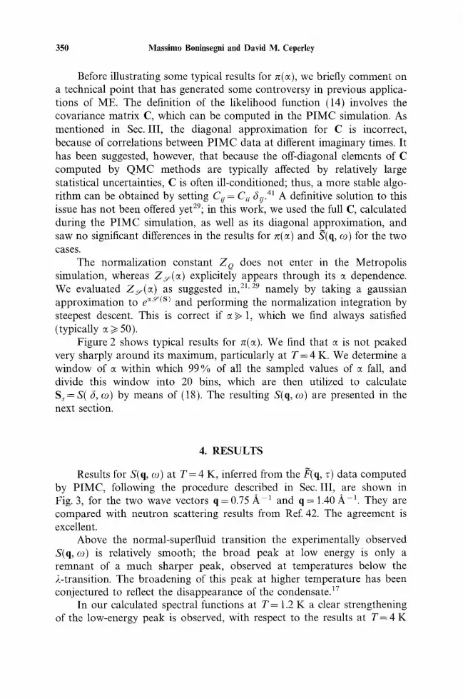
in agreement with experiment; this is shown, for example, in Fig. 4, where our results at the two temperatures considered, for the lowest q studied (0.45/~-x), are compared.

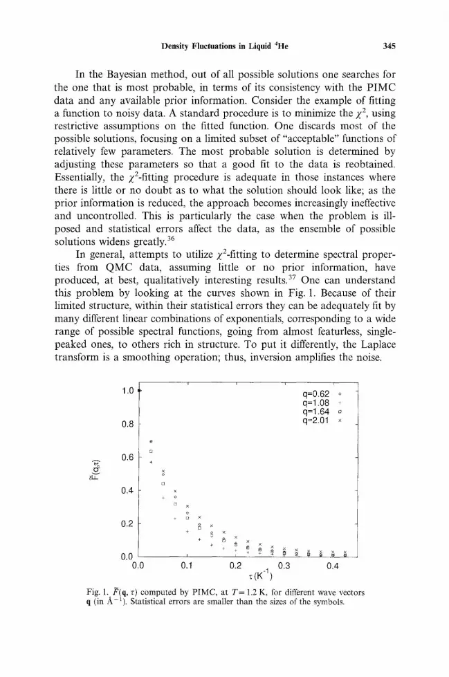
However, as Fig. 5 shows, our calculated S(q, co) remain smooth even at low temperature, and fail to develop the sharp features shown by the experimentally observed S(q, co); in particular, the low-energy peak, despite being accurately positioned, is much broader than in the experiment.

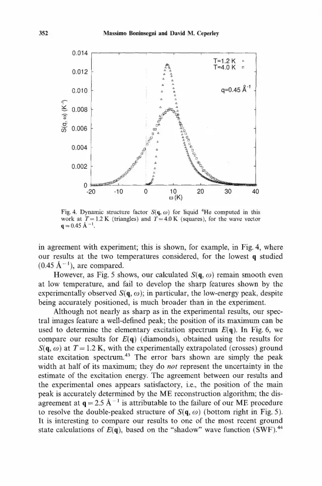
Although not nearly as sharp as in the experimental results, our spectral images feature a well-defined peak; the position of its maximum can be used to determine the elementary excitation spectrum E(q). In Fig. 6, we compare our results for E(q) (diamonds), obtained using the results for S(q, co) at T= 1.2 K, with the experimentally extrapolated (crosses) ground state excitation spectrum. 43 The error bars shown are simply the peak width at half of its maximum; they do no t represent the uncertainty in the estimate of the excitation energy. The agreement between our results and the experimental ones appears satisfactory, i.e., the position of the main peak is accurately determined by the ME reconstruction algorithm; the dis- agreement at q = 2.5 A 1 is attributable to the failure of our ME procedure to resolve the double-peaked structure of S(q, co) (bottom right in Fig. 5). It is interesting to compare our results to one of the most recent ground state calculations of E(q), based on the "shadow" wave function (SWF). 44


0.06

0.07

0.06

0.05

*~ 0.04

co 0.03

0.02

0.01

0.00

.". Thiswork (T=1.2 K) * i.~ Experiment (T=1.3 K) ,

f i q=0.75 X"

10 15 20 25 30 (K)

0.030

0.025

0.020 v

0.015

0.010

0.005

0,OO0

This work (T=1.2 K) o i Experiment (T=1.3 K ) ,

z ~ q=1.30 ,~-I 'O,o

i ~,,

/ ; ~

,i /

10 15 20(K)o~ 25 30 35

0.5

0.4

~, 0.3

r 0.2

0.1

0.0

This work (T=1.2 K) o Experiment (T=1.3 K) -

q=1.80 ~,"

f

6 8 10 12 14 16 18 20 e (K)

0.04

0.03

0.02

0.01

0.00

o/' /

i 10 20

This work (T=1.2 K) Experiment (T=1.3 K)

~D a ~"~ o q=2.50 ~176

", D

~,~ %

i 30 (K) 40 50 60

Fig. 5. Dynamic structure factor S(q, co) for liquid 4He at T = 1.2 K and saturated vapor pressure, for various q vectors ranging from 0 .45 /k - 1 to 2.3 A-1, determined by M a x i m u m Entropy with PIMC data (diamonds), compared to experimental results from Refs. %10 (triangles and squares). Dashed lines are guides to the eye.

In Fig. 6 the results of such a calculation are represented by the squares; the relative accuracy of the two calculations, with respect to the experimental data, is quite comparable. Beyond the "roton" region (i.e., ~ 2 It - 1) they both tend to overestimate the excitation energy, though for different and presumably unrelated reasons.

Besides the relative accuracy in determining the peak position, another interesting feature of our results is that, despite the poor definition of the single peak, the calculated S(q, co) clearly shows a gap at low energy, i.e., a rather fundamental aspect of the physics of the low-lying excitations of superfluid helium is recovered (Fig. 5).


L L I

35

30

25

20

15

10

5

0 0.0

This work ~ Experiment §

SWF []

+~++§247 D + ~ r

D T + % + + ~ u +

[ ]

+ +

+

i i i i i

0.5 1.0 1.5 2.0 2.5 q (~-1)

3.0

Fig. 6. Excitation spectrum E(q) determined using the maximum value of S(q, o0) at T= 1.2 K (diamonds). Error bars correspond to half widths of S(q, co) at half maxima and not to the statistical or systematic error: Crosses are the ground state excitation spectrum determined experimentally (Ref. 43). Also shown for comparison are the T=0 variational results (squares) obtained with the shadow wave function, from Ref. 44.

A possible concern is that the smoothness of our spectral functions might be attributed to the finite size of the simulation system (64 atoms). While finite-size effects are to be expected, particularly at low q, it seems unlikely that they could result in smoother spectral functions. Typically, spectral functions for finite systems are not smoother, but rather feature spurious structure, which disappears in the thermodynamic limit.

We attribute the broadening to an entropic prior which naturally favors the most "conservative" spectral functions, i.e. those providing adequate fits to the F(q, T) data with the smoothest features. At high T, where the dynamic structure factor is indeed smooth, ME does provide satisfactory results. At low q and T, on the other hand, where the extremely sharp phonon-roton peaks dominates, the full reconstruction of the spectrum proves beyond the capability of the ME approach, using the P I M C data.

It might be argued that different results could have been obtained, with the same data set, by choosing a different input model. In order to address this issue, we have at tempted to reconstruct our spectral images by using two other models, namely a Lorentzian with two adjustable parameters (i.e., position and width of the single peak), as well as the output of a previous ME reconstruction, in an iterative fashion, using a flat


input model for the first iteration. Leaving aside their considerable degree of arbitrariness, these two choices have both failed to yield significantly different results than those obtained using a flat input model, displayed in Fig. 5. In particular, if a Lorentzian model is assumed, even with a sharp peak, our ME reconstruction algorithm broadens this peak considerably, even if positioned exactly as observed experimentally. On the other hand, if the output of the ME algorithm is utilized as input model in a second reconstruction, the new output is indistinguishable from the initial one.

Another possibility to enhance the resolution of the ME algorithm might be to include further theoretical information besides the non- negativity and the f-sum rule. As mentioned above, it is possible to derive sum rules involving moments of S(q, co) higher than the first; however, information involving higher moments of S(q, e)) should affect mostly the asymptotic, high-frequency part of the image, which is already rather well represented in our results. The compressibility sum rule, on the other hand, involves the (o)-1) moment, and could therefore be utilized to regularize the low-frequency part of the image; it involves a parameter (the speed of sound) that can be taken from experiment. In this work, we did not attempt to include such sum rule, which is strictly valid in the q ~ 0 limit only.

In principle, our results could also be affected by the values of the time step c~r used in the PIMC calculations. It is conceivable that, upon under- sampling the imaginary-time functions, one may cause distortion in the reconstructed image, much like for ordinary time signals. In order to ascer- tain the sensitivity of our reconstructed S(q, c~) on the value of c~r, we also performed simulations at the above two temperatures with twice as many time slices, i.e. halving the value of ~r; in both cases, our results for S(q, e)) were indistinguishable from those obtained with a larger value of 6r.

5. CONCLUSIONS

We have adopted a combination of path integral Monte Carlo and Maximum Entropy inversion to calculate the dynamic structure factor S(q, co) for normal and superfluid 4He. Path integral Monte Carlo was used to calculate the imaginary time polarization propagator F(q, r), from which the dynamic structure factor was inferred, using the Maximum Entropy method.

The results of our calculation are in qualitative agreement with experiment, but suffer from the problems common to other similar calculations, namely, sharp features are very difficult to recover.

Naturally, one could improve the results by reducing the statistical errors of the PIMC data. The data for _P(q, ~) utilized in this work were


obtained in approximately 1,000 hours of CPU time on a mid-range workstation; the relative errors on P(q, r), which is an exponentially decaying function, are, typically, of the order of 1% for r ~ 0, to about 10 % for r ~ ill2. While it is conceivable that, upon reducing the statistical errors by a factor of, say, four, the results of the reconstruction algorithm could sharpen somewhat, it seems that recovering all of the features of the experimental spectra will easily require orders of magnitude more computational time.

For continuum quantum many-body Bose systems at finite temperature PIMC is the only existing exact numerical method; therefore, it makes sense to attempt to devise techniques aiming at extracting the maximum amount of information from PIMC-generated data. We think that efforts to improve the calculation of the dynamical structure factor using maximum entropy methods should probably make use of other types of correlation functions; alternatively, the prior probability function could be defined in a different space, at least for the superfluid since it does not seem physically reasonable to express the probability of a dynamic structure factor in S(q, og)-space.

ACKNOWLEDGMENTS

This work was supported by the Office of Naval Research under contract N00014-J-92-1320. Calculations were performed on the HP-Convex Exemplar at NCSA. The authors wish to thank K. H. Andersen for providing experimental data and to acknowledge useful discussions with B. F i l l H. R. Glyde, and J. E. Gubernatis.

REFERENCES

1. S. W. Lovesey, Condensed Matter Physics: dynamic correlations, Benjamin-Cummings (1986).

2. L. D. Landau, J. Phys. U.S.S.R. 5, 71 (1941). 3. R. P. Feynman, Phys. Rev. 94, 262 (1954). 4. R. P. Feynman and M. Cohen, Phys. Rev. 102, 1189 (1956). 5. A. D. B. Woods, in Quantum Fluids, edited by D. F. Brewer (North Holland Amsterdam

1965). 6. A. D. B. Woods and E. C. Svensson, Phys. Rev. Lett. 41, 974 (1978) 7. R. Seherm, K. Guckelsberger, B. F~tk, K. Sk61d, A. J. Dianoux, H. Godfrin, and W. G.

Stirling, Phys. Rev. Lett. 59, 217 (1987). 8. E. F. Talbot, H. R. Glyde, W. G. Stirling, and E. C. Svensson, Phys. Rev. B 38, 11229

(1988). 9. B. F~tk and K. H. Andersen, Phys. Lett. A 160, 468 (1991).

10. K. H. Andersen, W. G. Stirling, R. Scherm, A. Stunault, B. F i l l A. Godfrin, and A. J. Dianoux, J. Phys. C 6, 821 (1994)

11. N. Hugenholtz and D. Pines, Phys. Rev. 116, 489 (1959). 12. J. Gavoret and P. Nozi~res, Ann. Phys. 28, 349 (1964).


13. P. C, Hohenberg and P. C. Martin, Phys. Rev. Lett. 12, 69 (1964). 14. H. R. Glyde and A. Griffin, Phys. Rev. Lett. 65, 1454 (1990). 15. A. Griffin, Excitations in Bose-Condensed Liquids, Cambridge University Press (1993). 16. H. R. Glyde, Phys. Rev. B 45, 7321 (1992). 17. H. R. Glyde, Excitations in Liquid and Solid Helium, Oxford University Press, Oxford,

(1994). 18. E. Manousakis and V. R. Pandharipande, Phys. Rev. B 30, 5064 (1984). 19. E. Manousakis and V. R. Pandharipande, Phys. Rev. B 33, 150 (1986). 20. G. L. Masserini, L. Reatto, and S. A. Vitello, Phys. Rev. Lett. 69, 2098 (1992). 21. J. Skilling, in Maximum Entropy in Action, ed. by B. Buck and V. A. Macaulay, Clarendon

Press (1991). 22. See, for instance, D. S. Sivia, Los Alamos Science 19, 180 (1990) and references therein. 23. R. N. Silver, D. S. Sivia, J. E. Gubernatis, and M. Jarrell, Phys. Rev. Lett. 65, 496 (1990). 24. S. R. White, Phys. Rev. B 44, 4670 (1991). 25. N. Bulut, D. J. Scalapino, and S. R. White, Phys. Rev. Lett. 72, 705 (1994). 26. R. Preuss, A. Muramatsu, W. vonder Linden, P. Dieterich, F. F. Assaad, and W. Hanke,

Phys. Rev. Lett. 73, 732 (1994). 27. M. Makivid and M. Jarrell, Phys. Rev. Lett. 68, 1770 (1992) 28. E. Gallicchio and B. Berne, J. Chem. Phys. 101, 9909 (1994). 29. For a comprehensive review of this subject, see J. E. Gubernatis and M. JarrelI, Physics

Reports, in press. 30. See, for instance, A. L. Fetter and J. D. Walecka, Quantum Theory of Many-particle

Systems, McGraw-Hill (1971). 31. G. Placzek, Phys. Rev. 86, 337 (1952). 32. R. A. Aziz, M. J. Slaman, A. Koide, A. R. Allnatt, and W. J. Meath, Mol. Phys. 77, 321

(1992). 33. D. M. Ceperley, Rev. Mod. Phys. 67, 279, (1995) 34. D. M. Ceperley and E. L. Pollock, Phys. Rev. Lett. 56, 351 (1986). 35. E. L. Pollock and D. M. Ceperley, Phys. Rev. B 36, 8343 (1987). 36. See, for instance, G. J. Daniell, in Maximum Entropy in Action, ed. by B. Buck and V. A.

Macaulay, Clarendon Press ( 199l ). 37. E. L. Pollock and D. M. Ceperley, Phys. Rev. B 30, 2555 (1984). 38. See, for instance, S. Brandt, Statistical and Computational Methods in Data Analysis,

North-Holland (1970). 39. R. K. Bryan, Eur. Biophys. J. 18, I65 (1990). 40. M. Caffarel and D. M. Ceperley, or. Chem. Phys. 97, 8415 (1992). 41. A. Muramatsu, private communication. 42. K. H. Andersen, private communication. 43. R. J. Donnelly, J. A. Donnelly, and R. N. Hills, J. Low Temp Phys. 44, 471 (1981). 44. D. Galli, L. Reatto, and S. A. Vitiello, J. Low Temp. Phys. 101, 755 (1995).

Documents

Density fluctuations in liquid4He. Path integrals and maximum entropy