Information Fusion 13 (2012) 31–47

Contents lists available at ScienceDirect

Information Fusion

journal homepage: www.elsevier .com/locate / inf fus

Entropy/cross entropy-based group decision making under intuitionisticfuzzy environment

Meimei Xia, Zeshui Xu ⇑School of Economics and Management, Southeast University, Nanjing 211189, China

a r t i c l e i n f o a b s t r a c t

Article history:Received 18 August 2009Received in revised form 12 November 2010Accepted 7 December 2010Available online 22 December 2010

Keywords:Intuitionistic fuzzy valuesWeight vectorEntropyCross entropyAggregation operatorGroup decision making

1566-2535/$ - see front matter � 2011 Published bydoi:10.1016/j.inffus.2010.12.001

⇑ Corresponding author.E-mail addresses: meimxia@163.com (M. Xia), xu_

We study the group decision making problem under intuitionistic fuzzy environment. Based on entropyand cross entropy, we give two methods to determine the optimal weights of attributes, and develop twopairs of entropy and cross entropy measures for intuitionistic fuzzy values. Then, we discuss the proper-ties of these measures and the relations between them and the existing ones. Furthermore, we introducethree new aggregation operators, which treat the membership and non-membership information fairly,to aggregate intuitionistic fuzzy information. Finally, several practical examples are presented to illus-trate the developed methods.

� 2011 Published by Elsevier B.V.

1. Introduction

Intuitionistic fuzzy set (IFS), as a generalization form of fuzzyset (FS), was introduced by Atanassov [1]. Since it assigns to eachelement a membership degree, a non-membership degree and ahesitancy degree, IFS is more powerful in dealing with vaguenessand uncertainty than FS. Since its appearance, IFS has attractedmore and more attentions from researchers. For example, Gauand Buehrer [2] gave the definition of vague set (VS), which wasshown to be equivalent to IFS by Bustince and Burillo [3]. Atanas-sov and Gargov [4] defined the notion of interval-valued intuition-istic fuzzy set (IVIFS) which is a generalization of IFS. More andmore authors have been giving the applications of IFS theory tomulti-attribute decision making in which there are two hot topics:(1) determine the weights of attributes; (2) aggregate the informa-tion for alternatives. For the first point, Li [5] constructed severallinear programming models to generate optimal weights for attri-butes by maximizing the comprehensive values of alternatives.Based on Li’s models [5], Lin et al. [6] proposed a much simplermodel to determine the weights of attributes. Wang et al. [7]extended Li’s idea [5] and proposed a similar framework to handlemulti-attribute decision making problems under interval-valuedintuitionistic fuzzy environment. Li et al. [8] constructed severalfractional programming models based on the TOPSIS method [9]to determine attribute weights. For the multi-attribute decision

Elsevier B.V.

zeshui@263.net (Z. Xu).

making problems in which the information about attribute weightsis incompletely known and the attribute values take the form ofintuitionistic fuzzy values (IFVs), Wei [10] established an optimiza-tion model based on the basic idea of traditional grey relationalanalysis (GRA). Ye [11] proposed a multi-attribute decision makingmethod with the information about attribute weights completelyunknown based on weighted correlation coefficients using entropyweights. Wei [12] established two optimization models to deter-mine attribute weights based on the maximizing deviation method[13,14] for dealing with situations where the information aboutattribute weights is completely or incompletely known.

For the second point, a lot of research has been done about theaggregation methods in the last decades [15–17], etc. Yager [18]gave the ordered weighted averaging (OWA) operator and thenextended it and proposed a class of generalized OWA (GOWA)operators [19]. Xu [20] developed some aggregation operators forIFVs, such as the intuitionistic fuzzy weighted averaging (IFWA)operator, intuitionistic fuzzy ordered weighted averaging (IFOWA)operator, intuitionistic hybrid aggregation (IFHA) operator andestablished various properties of these operators. Then Xu andYager [21] proposed some geometric aggregation operators forIFVs, such as the intuitionistic fuzzy weighted geometric (IFWG)operator, intuitionistic fuzzy ordered weighted geometric (IFOWG)operator, and intuitionistic hybrid geometric (IFHG) operator. Zhaoet al. [22] combined Yager’s operator and Xu’s operator and devel-oped some generalized aggregation operators, such as the general-ized intuitionistic fuzzy weighted averaging (GIFWA) operator,generalized intuitionistic fuzzy ordered weighted averaging

32 M. Xia, Z. Xu / Information Fusion 13 (2012) 31–47

(GIFOWA) operator, and generalized intuitionistic fuzzy hybridaggregation (GIFHA) operator.

Although many weight-determining methods and aggregationoperators have been developed under intuitionistic fuzzy environ-ment, there are some issues to be pointed out: (1) The entropymeasure used in entropy weight method [11] is invalid in manysituations, and thus should be improved; (2) The TOPSIS method[8] may lose some original decision information due to that itneeds to translate the intuitionistic fuzzy decision matrix into aninterval-valued matrix; (3) To get more reasonable attributeweights, we should combine the existing weight-determiningmethods; (4) All the existing intuitionistic fuzzy aggregation oper-ators use different operational laws on membership and non-membership information, it is necessary to develop some neutraloperational laws about them due to that we are neutral in mostcases and want to be treated fairly. In order to avoid such issues,the rest of the paper is organized as follows. In Section 2, we givesome basic concepts; Section 3 develops a method to determinethe weights of attributes based on entropy and cross entropy; Sec-tion 4 proposes some new entropy and cross entropy measures.Section 5 gives some new intuitionistic fuzzy aggregation opera-tors. In Section 6, two examples are given to illustrate the proposedmethods; Section 7 gives some conclusions.

2. Basic concepts

Definition 2.1 [23]. Let X = {x1,x2, . . . ,xn} be fixed. A fuzzy set (FS)defined on X is given as:

A ¼ fðxi;lAðxiÞÞjxi 2 Xg ð1Þ

where the function lA(xi)(0 6 lA(xi) 6 1) is the membership degreeof xi to A in X.

Definition 2.2 [1]. Let X = {x1,x2, . . . ,xn} be fixed. An inuitionisticfuzzy set (IFS) A on X can be defined as:

A ¼ fðxi;lAðxiÞ; mAðxiÞÞjxi 2 Xg ð2Þ

where the functions lA(xi) and mA(xi) denote the membership degreeand non-membership degree of xi to A in X with the condition that

0 6 lAðxiÞ 6 1; 0 6 mAðxiÞ 6 1; lAðxiÞ þ mAðxiÞ 6 1 ð3Þ

and pA(xi) = 1 � lA(xi) � mA(xi) is called an intuitionitsic index (orhesitation degree) of xi to A.

For convenience, Xu [20] named the pair (la,ma) an intuitionis-tic fuzzy value (IFV) denoted as a with the condition 0 6 la, ma 6 1,la + ma 6 1. Especially, if la + ma = 1, then a reduces to (la,1 � la).Let �a ¼ ðma;laÞ be the complement of a, and V be the set of allIFVs.

Chen and Tan [24] introduced a score function s(a) = la � ma toget the score of a. Later, Hong and Choi [25] defined an accuracyfunction h(a) = la + ma to evaluate the accuracy degree of a. Basedon the score function s and the accuracy function h, Xu and Yager[21] gave an order relation between any two IFVs a and b:

If s(a) < s(b), then a < bIf s(a) = s(b), then

(i) If h(a) = h(b), then a = b(ii) If h(a) < h(b), then a < b

Two other important concepts for IFVs are entropy and crossentropy which have been applied to many areas, such as patternrecognition [26], image segmentation [27] and decision making[11], etc. Since its wide applications, a lot of work has been doneabout the entropy and cross entropy of FSs (or IFSs).

Entropy of a FS, first mentioned by Zadeh [28], is a useful tool tomeasure the fuzziness of information. Szmidt and Kacprzyk [29]extended the axioms of De Luca and Termini [30] and proposedthe following definition for an entropy measure on V.

Definition 2.3. An entropy on V is a real-valued function E:V ? [0,1], satisfying the following axiomatic requirements:

(1) E(a) = 0, if and only if a = (0,1) or a = (1,0);(2) E(a) = 1, if and only if la = ma;(3) E(a) 6 E(b), if la P lb P mb P ma or la 6 lb 6 mb 6 ma;(4) EðaÞ ¼ Eð�aÞ.

Cross entropy is used to measure the discrimination informa-tion, according to Shannon’s inequality [31], Vlachos and Sergiadis[27] gave a definition of intuitionsitic fuzzy cross entropy.

Definition 2.4. For two IFVs a and b, CE(a,b) is called a crossentropy between a and b, if the following conditions are satisfied:

(1) CE(a,b) P 0;(2) CE(a,b) = 0 if and only if a = b.

The above measures describe the entropy and cross entropy forIFVs. For IFSs A and B on X = {x1,x2, . . . ,xn}, the entropy and crossentropy can be given as:

EðAÞ ¼ 1n

Xn

i¼1

EðAiÞ ð4Þ

CEðA;BÞ ¼ 1n

Xn

i¼1

CEðAi;BiÞ ð5Þ

where Ai = (xi,lA(xi),mA(xi)) and Bi = (xi,lB (xi),mB(xi)) are IFVs,xi 2 X, i = 1,2, . . . ,n.

Vlachos and Sergiadis [27] showed that the entropy and crossentropy for IFSs degenerate to their fuzzy counterparts when IFSsbecome FSs. In fact, a FS A defined on X can be represented asA = {(xi,lA(xi),1 � lA(xi))jxi 2 X}. In other words, a FS can be consid-ered as a special case of an IFS, thus the entropy or cross entropyfor IFSs can also be suitable for FSs. Vlachos and Sergiadis [27] fur-ther defined the relationship between entropy and cross entropyfor IFSs which can also be true for IFVs:

Theorem 2.1. Let a be an IFV, then

EðaÞ ¼ �1t

CEða; �aÞ þ 1 ð6Þ

is an intuitionistic fuzzy entropy, and t is the normalization factor.

3. Method for intuitionistic fuzzy group decision making

An intuitionistic fuzzy group decision making problem can bedescribed as:

Let G = {G1,G2, . . . ,Gm} be the set of alternatives, C = {C1,C2, . . . ,Cn} the set of attributes, D = {D1,D2, . . . ,Ds} the set of decision mak-ers, and k = (k1,k2, . . . ,ks)T the weight vector of decision makers,where kk P 0, k = 1,2, . . . ,s, and

Psk¼1kk ¼ 1 (Due to that a decision

maker cannot be expected to have sufficient expertise to commenton all aspects of the problem but on a part of the problem for whichhe/she is competent [32], different decision makers should be as-signed different weights [33], especially in situations involvingpolicy specification. In the last decades, many methods have beendeveloped to determine the weights of decision makers [34–38].Usually, we should determine their weights according to theirknowledge, skills and experiences). Let RðkÞ ¼ ðaðkÞij Þn�m be an

M. Xia, Z. Xu / Information Fusion 13 (2012) 31–47 33

intuitionistic fuzzy decision matrix, given by the decision makerDk, where aðkÞij ¼ ðl

ðkÞij ; m

ðkÞij Þ is an IFV for the alternative Ai with re-

spect to the attribute Cj provided by the decision maker Dk. Assumethat the weight vector of attributes, w = (w1,w2, . . . ,wn)T, is to beknown, with wj P 0, j = 1,2, . . .,n, and

Pnj¼1wj ¼ 1.

Sometimes, the information about attribute weights is com-pletely unknown or incompletely known because of time pressure,lack of knowledge or data, and the expert’s limited expertise aboutthe problem domain. To get the optimal alternatives, we shoulduse methods or optimal models to determine the weight vectorof attributes and use aggregation operators to aggregate all theindividual decision matrices, and then aggregate the attribute val-ues for each alternative to get the final ranking of alternativeswhich can be described as the following steps:

Step 1. Utilize models or methods to determine the weight vectorof attributes, w = (w1,w2, . . .,wn)T.

Step 2. Aggregate all the individual intuitionistic fuzzy decisionmatrices RðkÞ ¼ ðaðkÞij Þm�n (k = 1,2, . . . ,s) into a collectiveintuitionistic fuzzy decision matrix R = (aij)m�n by usingaggregation operators.

Step 3. Utilize aggregation operators to get the aggregated valueszi(i = 1,2, . . . ,m) of the alternatives Gi(i = 1,2, . . . ,m).

Step 4. Utilize the score function and the accuracy function to cal-culate the scores s(zi)(i = 1,2, . . . ,m) (i = 1,2, . . . ,m) andthe accuracy degrees h(zi)(i = 1,2, . . . ,m).

Step 5. Get the priority of alternatives by ranking s(zi) andh(zi)(i = 1,2, . . . ,m).

In Step 1, to determine the weights of attributes, several meth-ods have been developed, such as the TOPSIS method [8], maximiz-ing deviation method [10] and entropy method [11], but some ofthem need to translate the intuitionistic fuzzy decision matrix intoan interval-valued decision matrix [8] which may lose some origi-nal information; some of them only focus on the divergence ofalternatives [10] or only focus on entropy information of attributes[11], and the entropy measure used in the entropy method is notreasonable which will be discussed in Section 3. In the following,we propose a combined method to determine the weights of attri-butes based on the entropy and cross entropy.

For the decision maker Dk and the attribute Cj, the average crossentropy of the alternative Gi to all the other alternatives can begiven as:

1m� 1

Xm

l¼1

CE aðkÞij ;aðkÞlj

� �ð7Þ

and the overall cross entropy for the attribute Cj, which can bedescribed as the measure of divergence among all alternativesunder the attribute Cj, is given as:

Xs

k¼1

Xm

i¼1

kk1

m� 1

Xm

l¼1

CE aðkÞij ;aðkÞlj

� � !ð8Þ

If the performance values of each alternative have little differenceunder an attribute, then it shows that such an attribute plays asmall important role in the priority procedure and should be evalu-ated a small weight; Contrariwise, if an attribute makes the perfor-mance values have obvious difference, then such an attribute playsan important role in choosing the best alternative and should beassigned a bigger weight. Considering the entropy of attributes,the overall entropy of the attribute Cj is given as:

Xs

k¼1

Xm

i¼1

kkE aðkÞij

� �ð9Þ

According to the entropy theory, if the entropy value for an attri-bute is smaller across alternatives, it can provide decision makerswith the useful information. Therefore, the attribute should be as-signed a bigger weight; Otherwise, such an attribute will be judgedunimportant by most decision makers. In other words, such anattribute should be evaluated as a very small weight. Combiningthese two aspects, we have

Xs

k¼1

Xm

i¼1

kk1

m� 1

Xm

l¼1

CEðaðkÞij ;aðkÞlj Þ þ 1� EðaðkÞij Þ

� � !ð10Þ

Then the bigger the value of Eq. (10) is, the bigger weight we shouldassign to the attribute Cj.

If the information about attribute weights is completelyunknown, we can establish the following equations for determin-ing attribute weights:

wj ¼Ps

k¼1

Pmi¼1kk

1m�1

Pml¼1CEðaðkÞij ;a

ðkÞlj Þ þ 1� EðaðkÞij Þ

� �� �Pn

j¼1

Psk¼1

Pmi¼1kk

1m�1

Pml¼1CEðaðkÞij ;a

ðkÞlj Þ þ 1� EðaðkÞij Þ

� �� � ;j ¼ 1;2; . . . ;n ð11Þ

Due to the increasing complexity of practical decision situations,the decision makers may not be confident in providing exact valuesfor attribute weights. Instead, the decision makers may only possesspartial knowledge about attribute weights [39]. In such a case, let Hbe the set of incomplete information about attribute weights, to getthe optimal weight vector, the following model can be constructed:

ðMOD1Þ MaxEw ¼Xs

k¼1

Xn

j¼1

Xm

i¼1

kk1

m� 1

Xm

l¼1

CE aðkÞij ;aðkÞlj

� �

þ 1� E aðkÞij

� �� ��wj

s:t:w 2 H;Xn

j¼1

wj ¼ 1; wj P 0; j ¼ 1;2; . . . ;n

In Section 3, we will give some entropy, cross entropy measures tosupport the proposed weight- determining method.

4. Entropy/cross entropy pairs for intuitionistic fuzzy values

As for the uncertain measure of IFS, Burillo and Bustince [40]defined the distance measure between two IFSs and gave an axiomdefinition of intuitionistic fuzzy entropy and a theorem whichcharacterizes it. Szmidt and Kacprzyk [29] used a differentapproach from Burillo and Bustince [40] to introduce the non-probabilistic entropy measure for IFS based on the geometric inter-pretation of IFS and the distances between them. Hung [41] gavetwo entropy measures induced by distances between two IFSswhich were illustrated to be computed easily and could producereliable results. Hung and Yang [42] constructed J-divergence ofIFSs and introduced some useful distance and similarity measuresbetween two IFSs, and applied them to clustering analysis and pat-tern recognition. Vlachos and Sergiadis [27] introduced the con-cepts of discrimination information and cross entropy for IFSsand revealed the connection between the notions of entropies forFSs and IFSs in terms of fuzziness and intuitionism. Wang and Lei[43] constructed some entropy measures for IFSs. Zhang and Jiang[26] proposed two new entropy and cross entropy measures forVSs which are different from that of [43], and then applied themto pattern recognition and medical diagnosis. However, the exist-ing entropy measures for IFSs maybe invalid which will be dis-cussed in the following section. To avoid such a problem, wepropose some new entropy and cross entropy measures.

Fig. 1. Values of E1:2M ðaÞ.

Fig. 2. Values of E1:8M ðaÞ.

34 M. Xia, Z. Xu / Information Fusion 13 (2012) 31–47

4.1. Entropy/cross entropy pair-1

Hung and Yang [42] gave the J-divergence of IFVs a and b asfollows:

Jpða; bÞ ¼1

p� 1lp

a þ lpb

2�

la þ lb

2

� �p(

þmp

a þ mpb

2� ma þ mb

2

� �p

þpp

a þ ppb

2� pa þ pb

2

� �p); 1 < p 6 2 ð12Þ

By Ref. [42], we know that 0 6 Jpða;bÞ 6 1p�1 1� 1

2p�1

� �. For conve-

nience, we can normalize it and define a cross entropy measure ofIFVs as:

CEpMða;bÞ ¼

1

1� 21�p

lpa þ lp

b

2�

la þ lb

2

� �p

þmp

a þ mpb

2

(

� ma þ mb

2

� �p

þpp

a þ ppb

2� pa þ pb

2

� �p); 1 < p 6 2

ð13Þ

By Ref. [42], it is easy to prove that CEpM a;bð Þ satisfies the conditions

(1), (2) in Definition 2.4, and it also satisfies the followingconditions:

(a) 0 6 CE(a,b) 6 1;(b) CE(a,b) = CE(b,a);(c) CE(a,b) 6 CE(a,c), CE(b,c) 6 CE(a,c), if la 6 lb 6 lc, ma P

mb P mc.

Especially, for an IFV b ¼ �a, by (3), we have

CEpMða; �aÞ ¼

1

1� 21�p

lpa þ mp

a

2� la þ ma

2

� �p

þ mpa þ lp

a

2

�

� ma þ la

2

� �p

þ ppa þ pp

a

2� pa þ pa

2

� �p�

¼ 21� 21�p

lpa þ mp

a

2� la þ ma

2

� �p� �

; 1 < p 6 2 ð14Þ

Based on Theorem 2.1, CEpMða; �aÞ can be used to measure the fuzzi-

ness of a, but it only considers the membership and non-member-ship information. Considering the hesitation information, we canreplace la and ma with la + pa and ma + pa (or 1 � ma and 1 � la) ,respectively, in Eq. (14) and give a new entropy measure:

EpMðaÞ ¼

21� 21�p

1� la þ 1� ma

2

� �p

� ð1� laÞp þ ð1� maÞp

2

� �þ 1; 1 < p 6 2 ð15Þ

Figs. 1 and 2 depict the entropy of EpM að Þ (1 < p 6 2) when p = 1.2

and p = 1.8, the color of each point (la,ma) on the simplex denotesthe entropy value of the IFV a = (la,ma). As the divergence of laand ma becomes bigger, both the values of E1:2

M ðaÞ and E1:8M ðaÞ become

smaller, and it is obvious that the values of E1:2MðaÞ are no smaller

than those of E1:8M ðaÞ.

Theorem 4.1. The mapping defined by Eq. (15) is an intuitionisticfuzzy entropy.

The Proof of Theorem 3.1 is provided in Appendix A.

4.2. Entropy/cross entropy pair-2

For two IFVs a and b, Vlachos and Sergiadis [27] gave the crossentropy measure:

CEvsða;bÞ ¼ 2la ln la þ lb ln lb

2�

la þ lb

2ln

la þ lb

2

�

þ ma ln ma þ mb ln mb

2� ma þ mb

2ln

ma þ mb

2

�ð16Þ

Hung and Yang [42] gave the J-divergence of IFVs:

CEhyða;bÞ ¼la ln la þ lb lnlb

2�

la þ lb

2ln

la þ lb

2

þ ma ln ma þ mb ln mb

2� ma þ mb

2ln

ma þ mb

2

þ pa ln pa þ pb lnpb

2� pa þ pb

2ln

pa þ pb

2ð17Þ

By analyzing CEvs(a,b) and CEhy(a,b), we can find that CEvs does notconsider the hesitation degree, and both the above cross entropymeasures are invalid when one of the values la, ma, pa, lb, mb andpb are zero, moreover, they are not normalized. To avoid such is-sues, based on Ref. [44], we give a revised form:

Fig. 4. Values of E1NðaÞ.

M. Xia, Z. Xu / Information Fusion 13 (2012) 31–47 35

CEqNða;bÞ ¼

1Tð1þ qlaÞ lnð1þ qlaÞ þ ð1þ qlbÞ lnð1þ qlbÞ

2

�

�1þ qla þ 1þ qlb

2ln

1þ qla þ 1þ qlb

2

þ ð1þ qmaÞ lnð1þ qmaÞ þ ð1þ qmbÞ lnð1þ qmbÞ2

� 1þ qma þ 1þ qmb

2ln

1þ qma þ 1þ qmb

2

þ ð1þ qpaÞ lnð1þ qpaÞ þ ð1þ qpbÞ lnð1þ qpbÞ2

� 1þ qpa þ 1þ qpb

2ln

1þ qpa þ 1þ qpb

2

�; q > 0

ð18Þ

where T = (1 + q)ln(1 + q) � (2 + q)(ln(2 + q) � ln2). T is a function ofq, when q > 0. T increases as q(q > 0) increases and obtains its min-imum value 0 at q = 0 (see Fig. 3)

Theorem 4.2. The mapping defined by Eq. (18) is an intuitionisticfuzzy cross entropy, and satisfies the conditions (a)–(c) given inSection 3.1.

The Proof of Theorem 4.2 is provided in Appendix A.Let b ¼ �a, we have

CEqNða; �aÞ ¼

1Tð1þ qlaÞ lnð1þ qlaÞ þ ð1þ qmaÞ lnð1þ qmaÞ

2

�

� 1þ qla þ 1þ qma

2ln

1þ qla þ 1þ qma

2

þ ð1þ qmaÞ lnð1þ qmaÞ þ ð1þ qlaÞ lnð1þ qlaÞ2

� 1þ qma þ 1þ qla

2ln

1þ qma þ 1þ qla

2

þ ð1þ qpaÞ lnð1þ qpaÞ þ ð1þ qpaÞ lnð1þ qpaÞ2

� 1þ qpa þ 1þ qpa

2ln

1þ qpa þ 1þ qpa

2

�

¼ 1Tð1þ qlaÞ lnð1þ qlaÞ þ ð1þ qmaÞ lnð1þ qmaÞ�� 1þ qla þ 1þ qmaÞ ln

1þ qla þ 1þ qma

2

� �; q > 0

ð19Þ

Fig. 3. The function of T = (1 + q)ln(1 + q) � (2 + q)(ln (2 + q) � ln2).

where T = (1 + q)ln(1 + q) � (2 + q)(ln(2 + q) � ln2).Similar to Ep

MðaÞ, we replace la and ma with 1 � ma and 1 � la inEq. (19), and define another entropy measure:

EqNðaÞ ¼ �

1Tðð1þ qð1� laÞÞ lnð1þ qð1� laÞÞ

þ ð1þ qð1� maÞÞ lnð1þ qð1� maÞÞ � ð1þ qð1� laÞþ 1þ qð1� maÞÞðlnð1þ qð1� laÞ þ 1þ qð1� maÞÞ � ln 2ÞÞþ 1; q > 0 ð20Þ

where T = (1 + q)ln(1 + q) � (2 + q)(ln(2 + q) � ln2).Figs. 4 and 5 depict the entropy of Eq

NðaÞ (q > 0) when q = 1 andq = 10, the color of each point (la,ma) on the simplex denotes theentropy value of the IFV a = (la,ma). As the divergence of la andma becomes bigger, the values of E1

NðaÞ and E10N ðaÞ become smaller,

and we can find that the values of E1NðaÞ are no bigger than those of

E10N ðaÞ.

Fig. 5. Values of E10N ðaÞ.

Table 1Comparison of the fuzziness with different entropy measures under A.

A1/2 A A2 A3 A4

Ezl 0.41560 0.4200 0.2380 0.15460 0.1217Eza 0.3210 0.3440 0.1970 0.1330 0.0980Ezb 0.4160 0.4200 0.2380 0.1550 0.1220Ezc 0.3340 0.3200 0.1400 0.0610 0.0280Ezd 0.2780 0.2460 0.1190 0.0560 0.0270Eze 0.3750 0.3700 0.1890 0.1080 0.0750Ebb 0.4090 0.5000 0.4900 0.4670 0.4670Esk 0.3450 0.3740 0.1970 0.1310 0.1090

E2hc

0.3420 0.3440 0.2610 0.1990 0.1610

Es 0.4330 0.4310 0.3270 0.2530 0.2080E 0.5518 0.5217 0.3491 0.2357 0.1417

36 M. Xia, Z. Xu / Information Fusion 13 (2012) 31–47

Theorem 4.3. The mapping defined by Eq. (20) is an intuitionisticfuzzy entropy.

The Proof of Theorem 4.3 is provided in Appendix A.

4.3. Comparative examples

For interval valued fuzzy sets (IVFSs), Zeng and Li [45] gave anentropy measure Ezl, Zhang et al. [46] defined five entropy mea-sures Eza, Ezb, Ezc, Ezd and Eze. We can develop the correspondingentropies on IVFSs by the relationship between IVFSs and IFSs.

For an IFS A on X = {x1,x2, . . . ,xn}, let Ai = (xi,lA(xi),mA(xi)) andBi = (xi,lB(xi),mB(xi)), then

EzlðAÞ ¼ 1� 1n

Xn

i¼1

jlAi� mAi

j ð21Þ

EzaðAÞ ¼ 1�

ffiffiffiffiffiffiffiffiffiffiffiffiffiffiffiffiffiffiffiffiffiffiffiffiffiffiffiffiffiffiffiffiffiffiffiffiffiffiffiffiffiffiffiffiffiffiffiffiffiffiffiffiffiffiffiffiffiffiffiffiffiffiffiffiffiffiffiffiffiffiffiffiffiffiffiffiffi2n

Xn

i¼1

ðjlAi� 0:5j2 þ j1� mAi

� 0:5j2Þ

vuut ð22Þ

EzbðAÞ ¼ 1� 2n

Xn

i¼1

ðjlAi� 0:5j þ j1� mAi

� 0:5jÞ ð23Þ

EzcðAÞ ¼ 1� 2n

Xn

i¼1

maxðjlAi� 0:5j; j1� mAi

� 0:5jÞ ð24Þ

EzdðAÞ ¼ 1�

ffiffiffiffiffiffiffiffiffiffiffiffiffiffiffiffiffiffiffiffiffiffiffiffiffiffiffiffiffiffiffiffiffiffiffiffiffiffiffiffiffiffiffiffiffiffiffiffiffiffiffiffiffiffiffiffiffiffiffiffiffiffiffiffiffiffiffiffiffiffiffiffiffiffiffiffiffiffiffiffiffiffiffiffi4n

Xn

i¼1

maxðjlAi� 0:5j2; j1� mAi

� 0:5j2Þ

vuut ð25Þ

EzeðAÞ ¼ 1� 2n

Xn

i¼1

jlAi� 0:5j þ j1� mAi

� 0:5j4

þmaxðjlAi

� 0:5j þ j1� mAi� 0:5Þ

2

�ð26Þ

Burillo and Bustince [47] defined an intuitionistic fuzzy entropyEbb(A). Szmidt and Kacprzyk [29] suggested an entropy as Esk(A).Hung and Yang [48] proposed two intuitionistic fuzzy entropiesE2

hcðAÞ and Es(A). Vlachos and Sergiadis [27] gave an entropy mea-sure Evs(A). Zhang and Jiang [26] gave an entropy measure Ezj(A)which can be listed below:

EbbðAÞ ¼1n

Xn

i¼1

ð1� lAi� mAi

Þ ð27Þ

EskðAÞ ¼1n

Xn

i¼1

lAi^ mAi

þ pAi

lAi_ mAi

þ pAi

¼ 1n

Xn

i¼1

ðlAiþ pAi

Þ ^ ðmAiþ pAi

ÞðlAiþ pAi

Þ _ ðmAiþ pAi

Þ

¼ 1n

Xn

i¼1

ð1� mAiÞ ^ ð1� lAi

Þð1� mAi

Þ _ ð1� lAiÞ ð28Þ

E2hcðAÞ ¼

1n

Xn

i¼1

1� l2Ai� m2

Ai� p2

Ai

� �ð29Þ

EsðAÞ ¼ �1n

Xn

i¼1

ðlAilnlAi

þ mAiln mAi

þ pAilnpAi

Þ ð30Þ

EvsðAÞ ¼ �1

ln 2

Xn

i¼1

lAiln lAi

þ mAiln mAi

� ðlAiþ mAi

Þ lnðlAi

�þ mAi

Þ � pAiln 2

�ð31Þ

EzjðAÞ ¼1n

Xn

i¼1

lAi^ mAi

lAi_ mAi

ð32Þ

vs

Ezj 0.2851 0.3050 0.1042 0.0383 0.0161

E1:2M

0.5854 0.5809 0.4481 0.3480 0.2843

E1:5M

0.5680 0.5572 0.4128 0.3111 0.2509

E1:8M

0.5556 0.5394 0.3856 0.2824 0.2253

E1N

0.5561 0.5409 0.3887 0.2860 0.2287

E20N

0.5831 0.5793 0.4461 0.3460 0.2816

E100 0.5940 0.5931 0.4658 0.3662 0.3006

Example 4.1 [26]. Let A = {(xi,lA(xi),mA(xi))jxi 2 X} be an IFS inX = {x1,x2, . . . ,xn}. For any positive real number n, De et al. [49]defined the IFS An as follows:

An ¼ fðxi; ½lAðxiÞ�n;1� ½1� mAðxiÞ�nÞjxi 2 Xg ð33Þ

We consider the IFS A in X = {6,7,8,9,10} defined as:

A ¼ fð6;0:1;0:8Þ; ð7;0:3;0:5Þ; ð8;0:5;0:4Þ; ð9;0:9;0:0Þ; ð10;1:0;0:0Þg

By taking into account the characterization of linguistic vari-ables, De et al. [49] regarded A as ‘‘LARGE’’ in X. Using the aboveoperations, we have

A1/2 may be treated as ‘‘More or less LARGE’’,A2 may be treated as ‘‘Very LARGE’’,A3 may be treated as ‘‘Quite very LARGE’’,A4 may be treated as ‘‘Very very LARGE’’.

We use these IFSs to compare the above entropy measures, thecomparison results are presented in Table 1. From the viewpoint ofmathematical operations, the entropies of these IFSs have the fol-lowing requirement [48]:

EðA1=2Þ > EðAÞ > EðA2Þ > EðA3Þ > EðA4Þ ð34Þ

Based on Table 1, we see that the entropy measures Ezc, Ezd, Eze, Es

and Evs satisfy (34), but

EzlðAÞ > EzlðA1=2Þ > EzlðA2Þ > EzlðA3Þ > EzlðA4ÞEzaðAÞ > EzaðA1=2Þ > EzaðA2Þ > EzaðA3Þ > EzaðA4ÞEzbðAÞ > EzbðA1=2Þ > EzbðA2Þ > EzbðA3Þ > EzbðA4ÞEbbðAÞ > EbbðA2Þ > EbbðA3Þ ¼ EbbðA4Þ > EbbðA1=2ÞEskðAÞ > EskðA1=2Þ > EskðA2Þ > EskðA3Þ > EskðA4ÞE2

hcðAÞ > E2hcðA

1=2Þ > E2hcðA

2Þ > E2hcðA

3Þ > E2hcðA

4ÞEzjðAÞ > EzjðA1=2Þ > EzjðA2Þ > EzjðA3Þ > EzjðA4Þ

Our proposed entropy measures indicate that

EpMðA

1=2Þ > EpMðAÞ > Ep

MðA2Þ > Ep

MðA3Þ > Ep

MðA4Þ;

p ¼ 1:2;1:5;1:8; 0 < p 6 2

EqNðA

1=2Þ > EqNðAÞ > Eq

NðA2Þ > Eq

NðA3Þ > Eq

NðA4Þ;

q ¼ 1;20;100; q > 0

Therefore, the performances of Ezc; Ezd; Eze; Es; Evs; EpM

ðp ¼ 1:2;1:5;1:8;0 < p 6 2Þ and EqNðq ¼ 1;20;100; q > 0Þ are good,

but the performances of Ezl; Eza; Ezb; Ebb; Esk; E2hc and Ezj are poor.

For Example 4.1, Figs. 6 and 7 give more details about the entro-py measures Ep

M ð1 < p 6 2Þ and EqN ðq > 0Þ as the parameter

p(1 < p 6 2) and q (q > 0) change. From Figs. 6 and 7, it is noted

N

Fig. 6. Values of EpMð1 < p 6 2Þ in Example 4.1.

Fig. 7. Values of EpNðq > 0Þ in Example 4.1.

M. Xia, Z. Xu / Information Fusion 13 (2012) 31–47 37

that EpM ð1 < p 6 2Þ decreases as the parameter p(1 < p 6 2) in-

creases, while EqN ðq > 0Þ increases as the parameter q (q > 0)

increases.

Example 4.2 [50]. Assume that ai (i = 1,2,3,4) represent fourhouses we consider to buy:

a1 ¼ ð0:7;0:3Þ; a2 ¼ ð0:6;0:2Þ; a3 ¼ ð0:5;0:1Þ; a4 ¼ ð0:4;0Þ

Table 2Comparison of the fuzziness with different entropy measures under a.

a1 a2 a3 a4

Ezl 0.6000 0.6000 0.6000 0.6000Eza 0.6000 0.5528 0.4343 0.2789Ezb 0.6000 0.6000 0.6000 0.4000Ezc 0.6000 0.4000 0.2000 0.0000

Ezd 0.6000 0.4000 0.2000 0.0000

Eze 0.6000 0.4000 0.2000 0.2000

Ebb 0.0000 0.2000 0.4000 0.6000

Esk 0.4300 0.5000 0.5600 0.6000

E2hc

0.4200 0.5600 0.5800 0.4800

On the one extreme, for the house a1,70% of attributes havedesirable values, and 30% of attributes have undesirable values.On the other extreme, for the house a4 we only know that it has40% desirable attributes and 60% of attributes are indeterminate.So we intuitively feel that it is easier to classify the house a1 tothe set of those fulfilling (worth buying) our demands than toclassify the house a4 to the set of houses unfulfilling ourdemands.

Intuitively, the entropy of them should be

Eða1Þ < Eða2Þ < Eða3Þ < Eða4Þ ð35Þ

We use ai (i = 1,2,3,4) to compare the above measure entropies.The results are listed in Table 2, based on which we see that Ebb

and Esk satisfy (33), but

Ezlða1Þ ¼ Ezlða2Þ ¼ Ezlða3Þ ¼ Ezlða4Þ; Ezaða1Þ > Ezaða2Þ > Ezaða3Þ > Ezaða4Þ

Ezbða1Þ > Ezbða2Þ > Ezbða3Þ > Ezbða4Þ; Ezcða1Þ > Ezcða2Þ > Ezcða3Þ > Ezcða4Þ

Ezdða1Þ > Ezdða2Þ > Ezdða3Þ > Ezdða4Þ; Ezeða1Þ > Ezeða2Þ > Ezeða3Þ > Ezeða4Þ

E2hcða3Þ > E2

hcða2Þ > E2hcða4Þ > E2

hcða1Þ; Esða2Þ > Esða3Þ > Esða4Þ > Esða1Þ

Evsða1Þ > Evsða2Þ > Evsða3Þ > Evsða4Þ; Ezjða1Þ > Ezjða2Þ > Ezjða3Þ > Ezjða4Þ

Our entropy measures indicate that

EpMða4Þ > Ep

Mða3Þ > EpMða2Þ > Ep

Mða1Þ; p ¼ 1:2;1:5;1:8; 0 < p 6 2

EqNða4Þ > Eq

Nða3Þ > EqNða2Þ > Eq

Nða1Þ; q ¼ 1;20;100; q > 0

Therefore, the performances of Ebb; Esk; EpM ðp ¼ 1:2;1:5;1:8;0 <

p 6 2Þ and EqNðq ¼ 1;20;100; q > 0Þ are good, but the performances

of Ezl; Eza; Ezb; Ezc; Ezd; Eze; E2hc; Es; Evs and Ezj are poor.

More results about the entropy measures EpM ð1 < p 6 2Þ and

EqN ðq > 0Þ in Example 4.2 can be found in Figs. 8 and 9 , it is noted

that EpM ð1 < p 6 2Þ decreases as the parameter p(1 < p 6 2) in-

creases, while EqN ðq > 0Þ increases as the parameter q (q > 0)

increases.From the above two examples, we can conclude that the perfor-

mances of EpMð1 < p 6 2Þ; Eq

Nðq > 0Þ are better than the existing en-tropy measures.

Example 4.3 [42,51–54]. Assume that there are three patternsdenoted with IFVs in X = {x1,x2,x3}. These three patterns aredenoted as follows:

A1 ¼ fðx1;0:1;0:1Þ; ðx2;0:5;0:1Þ; ðx3;0:1;0:9Þg;A2 ¼ fðx1;0:5;0:5Þ; ðx2;0:7;0:3Þ; ðx3;0:0;0:8Þg;A3 ¼ fðx1;0:7;0:2Þ; ðx2;0:1;0:8Þ; ðx3;0:4;0:4Þg:

Assume that a sample B = {(x1,0.4,0.4), (x2,0.6,0.2), (x3,0.0,0.8)} isgiven. Then by using the developed cross entropy measures pro-posed in Section 4.2, we can obtain

a1 a2 a3 a4

Es 0.6109 0.9503 0.9433 0.6731Evs 0.8813 0.8490 0.7900 0.6002Ezj 0.4286 0.3333 0.2000 0.0000

E1:2M

0.8682 0.8869 0.9004 0.9107

E1:5M

0.8536 0.8668 0.8769 0.8850

E1:8M

0.8440 0.8498 0.8544 0.8583

E1N

0.8426 0.8525 0.8612 0.8689

E20N

0.8669 0.8881 0.9034 0.9150

E100N

0.8762 0.8974 0.9123 0.9233

Fig. 8. Values of EpM ð1 < p 6 2Þ in Example 4.2.

Fig. 9. Values of EqNðq > 0Þ in Example 4.2.

Fig. 10. Values of CEpMð1 < p 6 2Þ in Example 4.3.

Fig. 11. Values of CEqNðq > 0Þ in Example 4.3.

38 M. Xia, Z. Xu / Information Fusion 13 (2012) 31–47

CE1:2M ðA1;BÞ ¼ 0:1437; CE1:2

M ðA2;BÞ ¼ 0:0547; CE1:2M ðA3;BÞ ¼ 0:2000;

CE1:6M ðA1;BÞ ¼ 0:1242; CE1:6

M ðA2;BÞ ¼ 0:0321; CE1:6M ðA3;BÞ ¼ 0:1907;

CE2MðA1;BÞ ¼ 0:1100; CE2

MðA2;BÞ ¼ 0:0200; CE2MðA3;BÞ ¼ 0:1800;

CE2NðA1;BÞ ¼ 0:1234; CE2

NðA2;BÞ ¼ 0:0282; CE2NðA3;BÞ ¼ 0:1926;

CE16N ðA1;BÞ ¼ 0:1407; CE16

N ðA2;BÞ ¼ 0:0476; CE16N ðA3;BÞ ¼ 0:2023;

CE1000N ðA1;BÞ ¼ 0:1556; CE1000

N ðA2;BÞ ¼ 0:0710; CE1000N ðA3;BÞ ¼ 0:2035:

Obviously, the sample B belongs to the pattern A2 by using theminimum degree of cross entropy. These results are in agreementwith the ones obtained in [42,51–54]. For Example 4.3, more re-sults about the proposed cross entropy measures are shown in Figs.10 and 11, it is noted that the value of CEp

M decreases as p(1 < p 6 2)increases, and the value of CEq

N increases as q(q > 0) increases.

5. Aggregation operators for intuitionistic fuzzy information

For a, b 2 V and k P 0, Xu [20], Xu and Yager [21] gave someoperational laws by which we can get other IFVs:

(1) aþ b ¼ ðla þ lb � lalb; mambÞ;

(2) ab ¼ ðlalb; ma þ mb � mambÞ;(3) ka ¼ ð1� ð1� laÞ

k; mk

aÞ;(4) ak ¼ ðlk

a;1� ð1� maÞkÞ.

The laws (1)–(4) can be described in detail by the Figs. 12–15. InFig. 12, let x = la and y = ma, the colour denotes the value ofla + lb � lalb. In Fig. 13, let x = la and y = ma, the colour denotesthe value of lalb. In Fig. 14, let x = la and y = k, the colour denotesthe value of 1 � (1 � la)k. In Fig. 15, let x = la and y = k, the colourdenotes the value of lk

a. Moreover, we find that all the values ofx + y � xy, xy, 1 � (1 � x)y and xy are non-decreasing as x and yincrease.

By comparing Figs. 12 and 13, we can find that the values ofx + y � xy seem to be no smaller than those of xy for the same point(x,y). By comparing Figs. 14 and 15, it’s obvious that the values ofxy are no smaller than those of 1 � (1 � x)y for the same point (x,y).To give more evidence, we give Figs. 16 and 17, where Fig. 16 de-scribes the values of x + y � xy � xy, and Fig. 17 describes the val-ues of xy � (1 � (1 � x)y), it is noted that all the values are non-negative.

For a, b 2 V and k P 0, based on the above analysis, it is evi-dent that

Fig. 13. Values of xy.

Fig. 14. Values of 1 � (1 � x)y.

Fig. 15. Values of xy.

Fig. 16. Values of x + y � xy � xy.

Fig. 12. Values of x + y � xy.

M. Xia, Z. Xu / Information Fusion 13 (2012) 31–47 39

la þ lb � lalb P lalb; ma þ mb � mamb P mamb;

lka P 1� ð1� laÞ

k; mk

a P 1� ð1� maÞk ð36Þ

thus

aþ b ¼ ðla þ lb � lalb; mambÞPab ¼ ðlalb; ma þ mb � mambÞ ð37Þ

and

ka ¼ 1� ð1� laÞk; mk

a

� �6 ak ¼ lk

a;1� ð1� maÞk� �

ð38Þ

In other words, the values of a + b are not always smaller than thoseof ab, and the values of ka are not always bigger than those of ak.

Based on the above operational laws, many aggregation opera-tors have been developed [20–22]. It is noted that all the aboveoperational laws use different operations on membership andnon-membership information. However, in most cases, we are

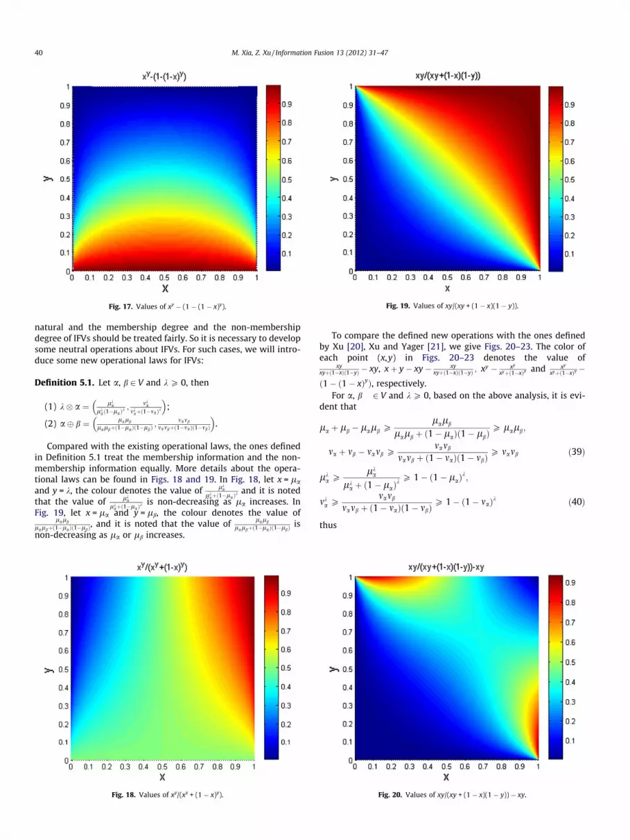
Fig. 17. Values of xy � (1 � (1 � x)y). Fig. 19. Values of xy/(xy + (1 � x)(1 � y)).

40 M. Xia, Z. Xu / Information Fusion 13 (2012) 31–47

natural and the membership degree and the non-membershipdegree of IFVs should be treated fairly. So it is necessary to developsome neutral operations about IFVs. For such cases, we will intro-duce some new operational laws for IFVs:

Definition 5.1. Let a, b 2 V and k P 0, then

(1) k� a ¼ lka

lkað1�laÞ

k ;mka

mkaþð1�maÞk

� �;

(2) a� b ¼ lalb

lalbþð1�laÞð1�lbÞ;

mamb

mambþð1�maÞð1�mbÞ

� �.

Compared with the existing operational laws, the ones definedin Definition 5.1 treat the membership information and the non-membership information equally. More details about the opera-tional laws can be found in Figs. 18 and 19. In Fig. 18, let x = laand y = k, the colour denotes the value of lk

alk

aþð1�laÞk and it is noted

that the value of lka

lkaþð1�laÞ

k is non-decreasing as la increases. InFig. 19, let x = la and y = lb, the colour denotes the value of

lalb

lalbþð1�laÞð1�lbÞ, and it is noted that the value of lalb

lalbþð1�laÞð1�lbÞis

non-decreasing as la or lb increases.

Fig. 18. Values of xy/(xy + (1 � x)y).

To compare the defined new operations with the ones definedby Xu [20], Xu and Yager [21], we give Figs. 20–23. The color ofeach point (x,y) in Figs. 20–23 denotes the value of

xyxyþð1�xÞð1�yÞ � xy, xþ y� xy� xy

xyþð1�xÞð1�yÞ ; xy � xy

xyþð1�xÞy and xy

xyþð1�xÞy�ð1� ð1� xÞyÞ, respectively.

For a, b 2 V and k P 0, based on the above analysis, it is evi-dent that

la þ lb � lalb Plalb

lalb þ ð1� laÞð1� lbÞP lalb;

ma þ mb � mamb Pmamb

mamb þ ð1� maÞð1� mbÞP mamb ð39Þ

lka P

lka

lka þ ð1� laÞ

k P 1� ð1� laÞk;

mka P

mamb

mamb þ ð1� maÞð1� mbÞP 1� ð1� maÞk ð40Þ

thus

Fig. 20. Values of xy/(xy + (1 � x)(1 � y)) � xy.

Fig. 21. Values of x + y � xy � xy/(xy + (1 � x)(1 � y)).

Fig. 22. Values of xy � xy=ðxy þ ð1� xÞyÞ.

Fig. 23. Values of xy/(xy + (1 � x)y) � (1 � (1 � x)y).

M. Xia, Z. Xu / Information Fusion 13 (2012) 31–47 41

la þ lb � lalb � mamb

Plalb

lalb þ ð1� laÞð1� lbÞ� mamb

mamb þ ð1� maÞð1� mbÞP lalb � ðma þ mb � mambÞ ð41Þ

lka � ð1� ð1� maÞkÞ

Plk

a

lka þ ð1� laÞ

k �mamb

mamb þ ð1� maÞð1� mbÞ

P 1� ð1� laÞk � lk

a ð42Þ

and

aþ b P a� b P ab; ak P k� a P ka ð43Þ

which indicate that the defined operations are neutral.

Theorem 5.1. Let a and b be two IFVs, k P 0, then k � a and a � bare also IFVs.

The Proof of Theorem 5.1 is provided in Appendix A.

Based on the operational laws (1) and (2) in Definition 4.1, wedevelop some intuitionistic fuzzy aggregation operators as follows:

Definition 5.2. For a collection of IFVs a = (a1,a2 , . . . ,an),w =(w1,w2, . . . ,wn)T is the weight vector of ai (i = 1,2, . . . ,n) withwi P 0, i = 1,2, . . . ,n, and

Pni¼1wi ¼ 1, if SIFWA: Vn ? V, and

SIFWAwða1;a2; � � � ;anÞ ¼ ðw1 � a1Þ � ðw2 � a2Þ � � � � � ðwn � anÞð44Þ

then we call the function SIFWA a symmetric intuitionistic fuzzyweighted averaging (SIFWA) operator. Especially, if w = (1/n,1/n, . . . ,1/n)T, then the SIFWA operator can be written as:

SIFAða1;a2; � � � ;anÞ ¼1n� a1

� �� 1

n� a2

� �� � � � � 1

n� an

� �ð45Þ

which is called a symmetric intuitionistic fuzzy averaging (SIFA)operator. By the defined operational laws, it is easy to prove that:

SIFWAwða1;a2; . . . ;anÞ

¼

Qni¼1

lwiai

Qni¼1

lwiaiþQni¼1ð1� lai

Þwi

;

Qni¼1

mwiai

Qni¼1

mwiaiþQni¼1ð1� mai

Þwi

0BB@

1CCA ð46Þ

Example 5.1 [55]. Consider that a customer wants to buy a car,which will be chosen from five types. In the process of choosingone of the cars, six factors are considered—G1: the consumptionpetrol, G2: the maximum mileage, G3: the price, G4: the degree ofcomfort, G5: the design of each type of car, and G6: the safety factor.Suppose that the characteristic information of the alternatives A1

(i = 1–3) are represented by the IFVs aij (i = 1,2,3; j = 1,2, . . . ,6)listed in Table 3 (the intuitionistic fuzzy decision matrix). Let w =(0.15,0.25,0.14,0.16,0.20,0.10)T be the weight vector ofGi(i = 1,2, . . . ,6), we use the IFWA [20], GIFWA [22] (here we letk = 2), IFWG [21] and SIFWA (Eq. (46)) operators to collect theoverall values of each type of car, the results are listed in Table 4.

By analyzing Table 4, we can find that the four aggregationoperators can get the same ranking of alternatives, but the mostvalues obtained by the SIFWA operator are smaller than those ob-tained by the IFWA [20] and GIFWA [22] operators, and are biggerthan those obtained by the IFWG [21] operator.

Table 3Intuitionistic fuzzy decision matrix R.

C1 C2 C3 C4 C5 C6

G1 (0.4,0.5) (0.7,0.1) (0.4,0.3) (0.5,0.4) (0.2,0.6) (0.5,0.4)G2 (0.5,0.3) (0.5,0.2) (0.6,0.2) (0.7,0.1) (0.3,0.6) (0.4,0.3)G3 (0.6,0.4) (0.5,0.1) (0.5,0.3) (0.7,0.2) (0.4,0.3) (0.7,0.1)G4 (0.3,0.4) (0.7,0.1) (0.5,0.1) (0.6,0.2) (0.4,0.5) (0.4,0.2)

42 M. Xia, Z. Xu / Information Fusion 13 (2012) 31–47

Definition 5.3. For a collection of IFVs a = (a1,a2 , . . . ,an), andx = (x1,x2 , . . . ,xn)T is the associated weight vector with xi

P 0,i = 1,2, . . . ,n, andPn

i¼1xi ¼ 1. If SIFOWA: Vn ? V, and

SIFOWAxða1;a2; . . . ;anÞ ¼ ðx1 � arð1ÞÞ � ðx2 � arð2ÞÞ � � � �� ðxn � arðnÞÞ ð47Þ

then we call the function SIFOWA a symmetric intuitionistic fuzzyordered weighted averaging (SIFOWA) operator, where ar(i) is theith largest of ak(k = 1,2,. . .,n). Moreover, we have

SIFOWAxða1;a2; . . . ;anÞ

¼

Qni¼1

lwiarðiÞ

Qni¼1

lwiarðiÞ þ

Qni¼1ð1� larðiÞ

Þwi

;

Qni¼1

mwiarðiÞ

Qni¼1

mwiarðiÞ þ

Qni¼1ð1� marðiÞ Þ

wi

0BB@

1CCA ð48Þ

The SIFOWA operator is developed based on the idea of the or-dered weighted averaging (OWA) operator [18]. The fundamentalaspect of the OWA operator is its reordering step. Several methodshave been developed to obtain the OWA weights. Yager [18] sug-gested a way to compute the OWA weights using linguistic quan-tifiers. O’Hagan [56] developed a procedure to generate the OWAweights that have a predefined degree of orness and maximizethe entropy of the OWA weights. Yager [57] introduced some fam-ilies of the OWA weights. Filev and Yager [58] developed two pro-cedures, based on the exponential smoothing, to obtain the OWAweights. Yager and Filev [59] suggested an algorithm to obtainthe OWA weights from a collection of samples with the relevantaggregated data. Xu and Da [60] established a linear objective-pro-

Table 4Comparison of rankings with different aggregation operators.

z1 z2

IFWA (0.4903,0.3047) (0.5135,0Scores (rankings) 0.1857(4) 0.2668(3)

GIFWA2 (0.5104,0.2893) (0.5244,0Scores (rankings) 0.2212(4) 0.2859(3)

IFWG (0.4244,0.3912) (0.4779,0Scores (rankings) 0.0332(4) 0.1643(3)

SIFWA (0.4544,0.3335) (0.4956,0Scores (rankings) 0.1208(4) 0.2311(3)

Table 5Comparison of rankings with different aggregation operators.

z1 z2

IFOWA (0.4627,0.3561) (0.5109, 0Scores (rankings) 0.1066(4) 0.2660(3)

GIFOWA2 (0.4726,0.3471) (0.5178,0Scores (rankings) 0.1255(4) 0.2772(3)

IFOWG (0.4336,0.3964) (0.4891,0Scores (rankings) 0.0372(4) 0.2093(3)

SIFOWA (0.4466,0.3711) (0.5000,0Scores (rankings) 0.0756(4) 0.2462(3)

gramming model to obtain the OWA weights under partial weightinformation. Especially, based on the normal distribution (Gauss-ian distribution), Xu [61] developed a method to obtain the OWAweights, whose prominent characteristic is that it can relieve theinfluence of unfair arguments on the decision result by assigninglow weights to those ‘‘false’’ or ‘‘biased’’ ones.

In Example 5.1, assume that the associated weight vector is

x ¼ ð0:0865;0:1716;0:2419;0:2419;0:1716;0:0865ÞT

If we use the IFOWA [20] , GIFOWA [22] (here we let k = 2) , IFOWG[21] and SIFOWA (Eq. (48)) operators to aggregate the attribute val-ues, then the results are shown in Table 5.

By analyzing Table 5, we can find that the four aggregationoperators can get the same ranking of the alternatives, but themost values obtained by the SIFOWA operator are smaller thanthose obtained by the IFWA [20] and GIFOWA [22] operators,and are bigger than those obtained by the IFOWG [21] operator.

From Definitions 5.1 and 5.2, we know that the SIFWA operatoronly weights the argument itself, but ignores the importance of theordered position of the argument, while the SIFOWA operator onlyweights the ordered position of the argument, but ignores theimportance of the argument. To solve this drawback, we shouldintroduce a symmetric intuitionistic fuzzy hybrid aggregation (SIF-HA) operator, which weights both the given argument and its or-dered position.

Definition 5.4. For a collection of IFVs a = (a1,a2

, . . . ,an),x = (x1,x2, . . . ,xn)T is the associated weight vectorwith xi P 0, i = 1,2, . . . ,n, and

Pni¼1xi ¼ 1. If SIFHA: Vn ? V, and

SIFHAw;xða1;a2; . . . ;anÞ ¼ ðx1 � _arð1ÞÞ � ðx2 � _arð2ÞÞ � � � �� ðxn � _arðnÞÞ ð49Þ

then we call the function SIFHA a symmetric intuitionistic fuzzy hy-brid aggregation (SIFHA) operator, where _arðiÞ is the ith largest ofnwk � ak (k = 1,2, . . . ,n) and w = (w1,w2, . . . ,wn)T is the weight vectorof a = (a1,a2, . . . ,an). Especially, if w = (1/n,1/n, . . . ,1/n)T, then the

z3 z4

.2468) (0.5715,0.2050) (0.5283,0.2034)0.3666(1) 0.3249(2)

.2385) (0.5769,0.2007) (0.5411,0.1964)0.3761(1) 0.3447(2)

.3136) (0.5519,0.2425) (0.4851,0.2697)0.3095(1) 0.2153(2)

.2645) (0.5630, 0.2129) (0.5070,0.2179)0.3500(1) 0.2891(2)

z3 z4

.2449) (0.5609, 0.1998) (0.4968,0.2078)0.3610(1) 0.2890(2)

.2406) (0.5677,0.1958) (0.5060,0.2024)0.3719(1) 0.3036(2)

.2797) (0.5364,0.2370) (0.4694,0.2579)0.2994(1) 0.2114(2)

.2538) (0.5498,0.2076) (0.4826,0.2188)0.3423(1) 0.2638(2)

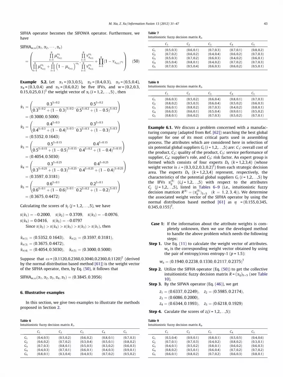
Table 7Intuitionistic fuzzy decision matrix R2.

C1 C2 C3 C4 C5

G1 (0.5,0.3) (0.6,0.1) (0.7,0.3) (0.7,0.1) (0.8,0.2)G2 (0.7,0.2) (0.6,0.2) (0.4,0.4) (0.6,0.2) (0.7,0.3)G3 (0.5,0.3) (0.7,0.2) (0.6,0.3) (0.4,0.2) (0.6,0.1)G4 (0.5,0.4) (0.8,0.1) (0.4,0.2) (0.7,0.2) (0.7,0.3)G5 (0.7,0.3) (0.5,0.4) (0.6,0.3) (0.6,0.2) (0.5,0.1)

M. Xia, Z. Xu / Information Fusion 13 (2012) 31–47 43

SIFHA operator becomes the SIFOWA operator. Furthermore, wehave

SIFHAw;x a1;a2; � � � ;anð Þ

¼

Qni¼1

lxi_arðiÞQn

i¼1lxi

_arðiÞþQni¼1

1� l _arðiÞ

� �xi;

Qni¼1

mxi_arðiÞQn

i¼1mxi

_arðiÞ

þYn

i¼1

ð1� m _arðiÞÞxi

0BB@

1CCA ð50Þ

Table 8Intuitionistic fuzzy decision matrix R3.

C1 C2 C3 C4 C5

G1 (0.6,0.3) (0.5,0.2) (0.6,0.4) (0.8,0.1) (0.7,0.3)G2 (0.8,0.2) (0.5,0.3) (0.6,0.4) (0.5,0.2) (0.6,0.3)G3 (0.6,0.1) (0.8,0.2) (0.7,0.3) (0.4,0.2) (0.8,0.1)G4 (0.6,0.3) (0.6,0.1) (0.5,0.4) (0.9,0.1) (0.5,0.2)G5 (0.8,0.1) (0.6,0.2) (0.7,0.3) (0.5,0.2) (0.7,0.1)

Example 5.2. Let a1 = (0.3,0.5), a2 = (0.4,0.3), a3 = (0.5,0.4),a4 = (0.3,0.4) and a5 = (0.6,0.2) be five IFVs, and w = (0.2,0.3,0.15,0.25,0.1)T the weight vector of ai (i = 1,2, . . . ,5) , then

_a1 ¼0:35�0:2

0:35�0:2 þ ð1� 0:3Þ5�0:2 ;0:55�0:2

0:55�0:2 þ ð1� 0:5Þ5�0:2

!

¼ ð0:3000;0:5000Þ

_a2 ¼0:45�0:3

0:45�0:3 þ ð1� 0:4Þ5�0:3 ;0:35�0:3

0:35�0:3 þ ð1� 0:3Þ5�0:3

!

¼ ð0:5352;0:1643Þ

_a3 ¼0:55�0:15

0:55�0:15 þ ð1� 0:5Þ5�0:15 ;0:45�0:15

0:45�0:2 þ ð1� 0:4Þ5�0:15

!

¼ ð0:4054;0:5030Þ

_a4 ¼0:35�0:25

0:35�0:25 þ ð1� 0:3Þ5�0:25 ;0:45�0:25

0:45�0:25 þ ð1� 0:4Þ5�0:25

!

¼ ð0:3597;0:3181Þ

_a5 ¼0:65�0:1

0:65�0:1 þ ð1� 0:6Þ5�0:1 ;0:25�0:1

0:25�0:2 þ ð1� 0:2Þ5�0:1

!

¼ ð0:3675;0:4472Þ

Calculating the scores of _aj (j = 1,2, . . . ,5), we have

sð _a1Þ ¼ �0:2000; sð _a2Þ ¼ 0:3709; sð _a3Þ ¼ �0:0976;sð _a4Þ ¼ 0:0416; sð _a5Þ ¼ �0:0797

Since sð _a2Þ > sð _a4Þ > sð _a5Þ > sð _a3Þ > sð _a1Þ, then

_arð1Þ ¼ ð0:5352;0:1643Þ; _arð2Þ ¼ ð0:3597; 0:3181Þ;_arð3Þ ¼ ð0:3675;0:4472Þ;_arð4Þ ¼ ð0:4054;0:5030Þ; _arð5Þ ¼ ð0:3000;0:5000Þ

Suppose that x = (0.1120,0.2360,0.3040,0.2360,0.1120)T (derivedby the normal distribution based method [61]) is the weight vectorof the SIFHA operator, then, by Eq. (50), it follows that

SIFHAw;xða1;a2;a3;a4;a5Þ ¼ ð0:3845;0:3956Þ

6. Illustrative examples

In this section, we give two examples to illustrate the methodsproposed in Section 2.

Table 6Intuitionistic fuzzy decision matrix R1.

C1 C2 C3 C4 C5

G1 (0.4,0.5) (0.5,0.2) (0.6,0.2) (0.8,0.1) (0.7,0.3)G2 (0.6,0.2) (0.7,0.2) (0.3,0.4) (0.5,0.1) (0.8,0.2)G3 (0.7,0.3) (0.8,0.1) (0.5,0.5) (0.3,0.2) (0.6,0.3)G4 (0.4,0.3) (0.7,0.1) (0.6,0.1) (0.4,0.3) (0.9,0.1)G5 (0.8,0.1) (0.3,0.4) (0.4,0.5) (0.7,0.2) (0.5,0.2)

Example 6.1. We discuss a problem concerned with a manufac-turing company (adapted from Ref. [62]) searching the best globalsupplier for one of its most critical parts used in assemblingprocess. The attributes which are considered here in selection ofsix potential global suppliers Gi (i = 1,2,. . .,5) are: C1: overall cost ofthe product, C2: quality of the product, C3: service performance ofsupplier, C4: supplier’s role, and C5: risk factor. An expert group isformed which consists of four experts Dk (k = 1,2,3,4) (whoseweight vector is k = (0.3,0.2,0.3,0.2)T) from each strategic decisionarea. The experts Dk (k = 1,2,3,4) represent, respectively, thecharacteristics of the potential global suppliers Gi (i = 1,2,. . .,5) bythe IFVs a kð Þ

ij (i, j = 1,2,. . .,5) with respect to the attributesCj (j = 1,2,. . .,5), listed in Tables 6–9 (i.e., intuitionistic fuzzydecision matrices RðkÞ ¼ ðaðkÞij Þ5�5 ðk ¼ 1;2;3;4ÞÞ. We determinethe associated weight vector of the SIFHA operator by using thenormal distribution based method [61] as g = (0.155,0.345,0.345,0.155)T.

Case 1: If the information about the attribute weights is com-pletely unknown, then we use the developed methodto handle the above problem which needs the followingsteps:

Step 1. Use Eq. (11) to calculate the weight vector of attributes.wa is the corresponding weight vector obtained by usingthe pair of entropy/cross entropy-1 (p = 1.5):

Table 9Intuitio

G1

G2

G3

G4

G5

wa ¼ ð0:1940;0:2238;0:1330;0:2117;0:2375ÞT

Step 2. Utilize the SIFHA operator (Eq. (50)) to get the collectiveintuitionistic fuzzy decision matrix R = (aij)5�5 (see Table10).

Step 3. By the SIFWA operator (Eq. (46)), we get

z1 ¼ ð0:6337;0:2249Þ; z2 ¼ ð0:5985;0:2174Þ;z3 ¼ ð0:6086;0:2000Þ;z4 ¼ ð0:6344;0:1993Þ; z5 ¼ ð0:6218;0:1929Þ

Step 4. Caculate the scores of zi(i = 1,2,. . .,5):

nistic fuzzy decision matrix R4.

C1 C2 C3 C4 C5

(0.3,0.4) (0.9,0.1) (0.8,0.1) (0.5,0.5) (0.4,0.6)(0.7,0.1) (0.7,0.3) (0.4,0.2) (0.8,0.2) (0.3,0.1)(0.4,0.1) (0.5,0.2) (0.8,0.1) (0.6,0.2) (0.6,0.3)(0.8,0.2) (0.5,0.1) (0.6,0.4) (0.7,0.2) (0.7,0.2)(0.6,0.1) (0.8,0.2) (0.7,0.2) (0.6,0.3) (0.8,0.1)

Table 10Group intuitionistic fuzzy decision matrix R.

C1 C2 C3 C4 C5

G1 (0.4418,0.3768) (0.5949,0.1531) (0.6568,0.2395) (0.7438,0.1273) (0.6949,0.3051)G2 (0.6824,0.1666) (0.6232,0.2627) (0.4241,0.3440) (0.5553,0.1386) (0.6352,0.2470)G3 (0.5779,0.1868) (0.7438,0.1770) (0.6535,0.2979) (0.4044,0.2000) (0.6429,0.1868)G4 (0.5454,0.3296) (0.6700,0.1000) (0.5188,0.2732) (0.6902,0.2089) (0.6787,0.1869)G5 (0.7405,0.1161) (0.5454,0.2823) (0.6054,0.3156) (0.5793,0.2109) (0.6319,0.1325)

Table 1Compar

wa

Scorwb

Scorwc

Scor

Table 12Intuitionistic fuzzy decision matrix R.

44 M. Xia, Z. Xu / Information Fusion 13 (2012) 31–47

sðz1Þ ¼ 0:4088; sðz2Þ ¼ 0:3810; sðz3Þ ¼ 0:4086; sðz4Þ¼ 0:4351; sðz5Þ ¼ 0:4289

C1 C2 C3 C4

G1 (0.5,0.4) (0.6,0.3) (0.3,0.6) (0.2,0.7)G2 (0.7,0.3) (0.7,0.2) (0.7,0.2) (0.4,0.5)

Step 5. Rank the alternatives according to the descending order ofs(zi)(i = 1,2, . . . ,5):

G3 (0.6,0.4) (0.5,0.4) (0.5,0.3) (0.6,0.3)G (0.8,0.1) (0.6,0.3) (0.3,0.4) (0.2,0.6)

G4 � G5 � G1 � G3 � G2

4

G5 (0.6,0.2) (0.4,0.3) (0.7,0.1) (0.5,0.3)

In Step 1, we can also use the pair of entropy/cross entropy-2(q = 1) to get the weight vector of attributes, that is:

wb ¼ ð0:1931;0:2219;0:1325;0:2133;0:2392ÞT

By repeating the above steps, the corresponding results are listed inTable 11.

Case 2: If the information about the attribute weights is com-pletely unknown. Suppose that the known weight infor-mation is presented as:

H ¼ fw1 P 0:1; 0:2 6 w2 6 0:3; w3 P 0:15; 0:2 6 w4 6 0:5; 0:3

6 w5 6 0:4g

We can use (MOD-1) to derive the weights for attributes. Based onthe pair of entropy/cross entropy-1 (p = 1.5), we can establish thefollowing model:

Max Ew ¼ 1:2758 w1 þ 1:4724 w2 þ 0:8747 w3 þ 1:3924 w4

þ 1:5626 w5

s:t: w 2 H

Solving the above model, we can get the optimal weight vector:

wc ¼ ð0:1;0:2;0:15;0:2;0:35ÞT

By repeating the above steps, the corresponding results are listed inTable 11. Although the rankings are slightly different under differ-ent weight vectors, the optimal alternative is A4.

If there is only one decision maker, then the proposed methodin Section 2 can be used to solve the problem proposed by Wei[10] and Ye [11]. Next, we give an example adapted from Ref.[10] to compare the proposed method with Wei’s method [10]and Ye’s method [11].

Example 6.2. Let us suppose that there is an investment company,which wants to invest a sum of money in the best option (adaptedfrom Ref. [10]). There is a panel with five possible alternatives to

1ison of rankings under different weight vector.

z1 z2

(0.6337,0.2249) (0.5985,0.2174)es (rankings) 0.4088(3) 0.3810(5)

(0.6342,0.2249) (0.5984,0.2173)es (rankings) 0.4097(3) 0.3811(5)

(0.6575,0.2246) (0.5914,0.2280)es (rankings) 0.4329(2) 0.3634(5)

invest the money: G1: a car company, G2: a food company, G3: acomputer company, G4: an arms company, and G5: a TV company.The investment company must take a decision according to thefollowing four attributes: C1: the risk analysis, C2: the growthanalysis, C3: the social-political impact analysis, and C4: theenvironmental impact analysis. The five possible alternatives Gi

(i = 1,2,. . .,5) are to be evaluated using the intuitionistic fuzzyinformation by the decision maker under the above four attributes,as listed in Table 12.

Then, we utilize the developed approach to get the most desir-able alternative(s).

Case 1: If the information about the attribute weights is com-pletely unknown, we utilize the developed approach toget the most desirable alternative(s).

Step 1. Utilize Eq. (11) to get the weight vector of attributes(Here we use the pair of entropy/cross entropy-1(p = 1.3):

z3

(0.0.4(0.0.3(0.0.4

w ¼ ð0:3003;0:1541;0:3122;0:2334ÞT

Step 2. By the SIFWA operator (Eq. (46)), we obtain the overallvalues of alternatives:

z1 ¼ ð0:3715;0:5180Þ; z2 ¼ ð0:6353;0:2889Þ;z3 ¼ ð0:5539;0:3438Þ;z4 ¼ ð0:4727;0:3053Þ; z5 ¼ ð0:5803;0:1930Þ

Step 3. Calculate the scores of the overall intuitionistic fuzzyvalues:

sðz1Þ ¼ �0:1465; sðz2Þ ¼ 0:3464; sðz3Þ ¼ 0:2121; sðz4Þ¼ 0:1674; sðz5Þ ¼ 0:3872

Step 4. Rank all alternatives in accordance with the scores of theoverall intuitionistic fuzzy values:

z4 z5

6086, 0.2000) (0.6344,0.1993) (0.6218,0.1929)086(4) 0.4351(1) 0.4289(2)6081, 0.2000) (0.6346,0.1994) (0.6218,0.1927)908(4) 0.4081(1) 0.4291(2)6149,0.2018) (0.6441,0.1918) (0.6127,0.1935)231(4) 0.4523(1) 0.4192(3)

M. Xia, Z. Xu / Information Fusion 13 (2012) 31–47 45

G5 � G2 � G3 � G4 � G1

thus the most desirable alternative is G5.

In such case, if we use Ye’s method, we can get the weight vec-tor of attributes:

w ¼ ð0:2659;0:2486;0:2370;0:2486ÞT

and get the same ranking of alternatives:

G5 � G2 � G3 � G4 � G1

Case 2: If the information about the attribute weights is partlyknown and the known weight information is given asfollows:

H ¼ f0:15 6 w1 6 0:2; 0:16 6 w2 6 0:18; 0:3 6 w3

6 0:35; 0:3 6 w4 6 0:45g

Step 1. Utilize the (MOD-1) to establish the following program-ming model:

Max Ew ¼ 0:9903w1 þ 0:5082w2 þ 1:0296w3 þ 0:7697w4

s:t: w 2 H

Solving this model, we get the weight vector of attributes:

w ¼ ð0:19;0:16;0:35; 0:3ÞT

Step 2. By Eq. (46), we obtain the overall values of alternatives:

z1 ¼ ð0:3435;0:5457Þ; z2 ¼ ð0:6157; 0:2957Þ;z3 ¼ ð0:5495;0:3334Þ;z4 ¼ ð0:4051;0:3605Þ; z5 ¼ ð0:5766;0:1943Þ

Step 3. Calculate the scores of the overall intuitionistic fuzzyvalues:

sðz1Þ ¼ �0:2022; sðz2Þ ¼ 0:3201; sðz3Þ ¼ 0:2161; sðz4Þ¼ 0:0446; sðz5Þ ¼ 0:3823

Step 4. Rank all alternatives in accordance with the scores of theoverall intuitionistic fuzzy values:

G5 � G2 � G3 � G4 � G1

and thus the most desirable alternative is G5

Based on the above analysis, although the proposed method,Ye’s method and Wei’s method can get the same ranking of alter-natives, Ye’s method only considers the entropy information ofattribute and Wei’s method only considers the divergences be-tween alternatives, moreover, the entropy used in Ye’s method isnot very good which has been discussed in Section 3. Thus, the pro-posed method is more reasonable.

7. Conclusions

In this paper, we have investigated group decision making prob-lems under intuitionistic fuzzy environment. We have proposedthe entropy/cross entropy based method to determine the weightsof attributes. The attribute, which has small entropy and largecross entropy, should be assigned a large weight. To support theweight-determining methods, two new pairs of intuitionistic fuzzyentropy and cross entropy measures have been constructed whichgeneralize the existing ones. Some examples have been used toillustrate the advantages of the proposed entropy and crossentropy measures. Moreover, we have developed a class of neutral

operators to aggregate intuitionistic fuzzy information treating themembership and non-membership information fairly. An examplehas shown that the proposed aggregation operators can get moreneutral results than the existing ones. Finally, we have given anexample to compare the proposed method with Ye’s methodand Wei’ method. It is worth noting that the results of this papercan be extended to the interval-valued intuitionistic fuzzyenvironment.

Acknowledgments

The work was supported in part by the National Science Fundfor Distinguished Young Scholars of China (No. 70625005), theNational Natural Science Foundation of China (No. 71071161),the Program Sponsored for Scientific Innovation Research of Col-lege Graduate in Jiangsu Province (No. CX10B_059Z), and the Sci-entific Research Foundation of Graduate School of SoutheastUniversity.

Appendix A

A.1. Proof of Theorem 4.1

ð1Þ EpMðaÞ ¼ 0() 2

1� 21�p

1� la þ 1� ma

2

� �p�

� ð1� laÞp þ ð1� maÞp

2

�¼ �1

() 1� 21�p ¼ ðð1� laÞp þ ð1� maÞpÞ � 21�pðð1� laÞ þ ð1� maÞÞp

() ð1� laÞp þ ð1� maÞp ¼ 1 andðð1� laÞ þ ð1� maÞÞp ¼ 1

() a ¼ ð1; 0Þ or a ¼ ð0;1Þ

ð2Þ EpMðaÞ ¼ 1() 1� la þ 1� ma

2

� �p

� ð1� laÞp þ ð1� maÞp

2

¼ 0() la ¼ ma:

(3) Let f ðx; yÞ ¼ xþy2

� �p � xpþyp

2

� �; x > y; t ¼ x� y > 0;1 < p 6 2

then

f ðt; yÞ ¼ t þ 2y2

� �p

� ðt þ yÞp þ yp

2

� �;

f 0t ðt; yÞ ¼12

pt2þ y

� �p�1

� pðt þ yÞp�1

!< 0

and thus f is a decreasing function of t.Similarly, we can prove that when x < y, t = y � x, f is a decreasingfunction of t. Let x = 1 � la, y = 1 � ma, and if la P lb P mb P maand la 6 lb 6 mb 6 ma, then we can obtain E(a) 6 E(b).

(4) It is obvious.

A.2. Proof of Theorem 4.2

It is obvious that CEqNða; bÞ ¼ CEq

Nðb;aÞ. Let q > 0,

Dqða;bÞ ¼ð1þ qlaÞ lnð1þ qlaÞ þ ð1þ qlbÞ lnð1þ qlbÞ

2

�1þ qla þ 1þ qlb

2ln

1þ qla þ 1þ qlb

2

þ ð1þ qmaÞ lnð1þ qmaÞ þ ð1þ qmbÞ lnð1þ qmbÞ2

� 1þ qma þ 1þ qmb

2ln

1þ qma þ 1þ qmb

2

46 M. Xia, Z. Xu / Information Fusion 13 (2012) 31–47

þ ð1þ qpaÞ lnð1þ qpaÞ þ ð1þ qpbÞ lnð1þ qpbÞ2

� 1þ qpa þ 1þ qpb

2ln

1þ qpa þ 1þ qpb

2

and f = (1 + qx)ln(1 + qx) and 0 6 x 6 1, then f0= qln(1 + qx) + q P 0

and f 00 ¼ q2

1þqx > 0, thus f is a concave-up function of x, and Dq(a,b)is convex. Therefore, Dq(a,b) increases as ka � bk1 increases, whereka � bk1 = jla � lbj + jma � mbj + jpa � pbj. Then Dq(a,b) attains itsmaximum at a = (0,1,0),b = (1,0,0) (or a = (1,0,0), b = (0,0,1) ora = (0,0,1), b = (0,1,0)), Dq(a,b) attains its minimum when la = lb

and la = lb, which follows that

0 6 Dqða;bÞ 6 ð1þ qÞ lnð1þ qÞ � ð2þ qÞðlnð2þ qÞ � ln 2Þ

and Dq(a,b) = 0 if and only if la = lb, ma = mb, thus

0 6 CEqNða;bÞ ¼

Dqða;bÞð1þ qÞ lnð1þ qÞ � ð2þ qÞðlnð2þ qÞ � ln 2Þ 6 1

If la 6 lb 6 lc and ma P mb P mc, then

jla � lbj þ jma � mbj þ jpa � pbj 6 jla � lcj þ jma � mcj þ jpa � pcj;jlb � lcj þ jmb � mcj þ jpb � pcj 6 jla � lcj þ jma � mcj þ jpa � pcj

therefore

CEqNða;bÞ 6 CEq

Nða; cÞ; CEqNðb; cÞ 6 CEq

Nða; cÞ

A.3. Proof of Theorem 4.3

It’s easy to prove EqNðaÞ ¼ Eq

Nð�aÞ.Let H ¼ ð1þqð1�laÞÞ lnð1þqð1�laÞÞþð1þqð1�maÞÞ lnð1þqð1�maÞÞ

2 �

1þ qð1� laÞ þ 1þ qð1� maÞ2

ln1þ qð1� laÞ þ 1þ qð1� maÞ

2;

q > 0

Then EqNðaÞ ¼ � 2

ð1þqÞ lnð1þqÞ�ð2þqÞðlnð2þqÞ�ln 2ÞH þ 1; q > 0

Let f = (1 + q(1 � x))ln(1 + q(1 � x)) and 0 6 x 6 1, thenf0= � qln(1 + q(1 � x)) � q 6 0 and f 00 ¼ q2

1þqð1�xÞ P 0, thus f is a con-cave-up function of x, and H is convex. Therefore H increases asjla � maj increases, and Eq

NðaÞ decreases as la � ma increases,

EqNðaÞ attains its minimum value 0 at a = (0,1) (or a = (1,0)) and at-

tains its maximum value 1 at la = ma. If la 6 lb 6 mb 6 ma orla P lb P mb P ma, then jla � majP jlb � mbj, we can getEq

NðaÞ 6 EqNðbÞ which completes the proof.

A.4. Proof of Theorem 5.1

Since 0 6 lka

lkaþð1�laÞ

k ;mka

mkaþð1�maÞk

6 1 and

mka

mka þ ð1� maÞk

¼ 11þ ð1=ma � 1Þk

61

1þ ð1=ð1� laÞ � 1Þk

¼ ð1� laÞk

ð1� laÞk þ lk

a

then we have

lka

lka þ ð1� laÞ

k þmk

a

mka þ ð1� maÞk

6lk

a

lka þ ð1� laÞ

k þð1� laÞ

k

lka þ ð1� laÞ

k

¼ 1

thus, k � a is an IFV. Similarly,

0 6lalb

lalb þ ð1� laÞð1� lbÞ;

mamb

mamb þ ð1� maÞð1� mbÞ

6 1mamb

mamb þ ð1� maÞð1� mbÞ6

11þ ð1=ma � 1Þð1=mb � 1Þ

61

1þ ð1=ð1� laÞ � 1Þð1=ð1� laÞ � 1Þ

¼ð1� laÞð1� lbÞ

lalb þ ð1� laÞð1� lbÞ

Thus

lalb

lalb þ ð1� laÞð1� lbÞþ mamb

mamb þ ð1� maÞð1� mbÞ

6

lalb

lalb þ ð1� laÞð1� lbÞþ

ð1� laÞð1� lbÞlalb þ ð1� laÞð1� lbÞ

¼ 1

which implies that a � b is an IFV.

References

[1] K. Atanassov, Intuitionistic fuzzy sets, Fuzzy Sets and Systems 20 (1986)87–96.

[2] W.L. Gau, D.J. Buehrer, Vague sets, IEEE Transactions on Systems, Man, andCybernetics 23 (1993) 610–614.

[3] H. Bustince, P. Burillo, Vague sets are intuitionistic fuzzy sets, Fuzzy Sets andSystems 79 (1996) 403–405.

[4] K. Atanassov, G. Gargov, Interval valued intuitionistic fuzzy sets, Fuzzy Setsand Systems 31 (1989) 343–349.

[5] D.F. Li, Multiattribute decision making models and methods usingintuitionistic fuzzy sets, Journal of Computer and System Science 70 (2005)73–85.

[6] L. Lin, X.H. Yuan, Z.Q. Xia, Multicriteria fuzzy decision-making methods basedon intuitionistic fuzzy sets, Journal of Computer and System Sciences 73 (2007)84–88.

[7] Z.J. Wang, K.W. Li, W.Z. Wang, An approach to multiattribute decision makingwith interval-valued intuitionistic fuzzy assessments and incomplete weights,Information Sciences 179 (2009) 3026–3040.

[8] D.F. Li, Y.C. Wang, S. Liu, F. Shan, Fractional programming methodology formulti-attribute group decision-making using IFS, Applied Soft Computing 9(2009) 219–225.

[9] C.L. Hwang, K. Yoon, Multiple Attribute Decision Making Methods andApplications, Springer, Berlin, 1981.

[10] G.W. Wei, Maximizing deviation method for multiple attribute decisionmaking in intuitionistic fuzzy setting, Knowledge-Based Systems 21 (2008)833–836.

[11] J. Ye, Fuzzy decision-making method based on the weighted correlationcoefficient under intuitionistic fuzzy environment, European Journal ofOperational Research 205 (2010) 202–204.

[12] G.W. Wei, GRA method for multiple attribute decision making withincomplete weight information in intuitionistic fuzzy setting, Knowledge-Based Systems 23 (2010) 243–247.

[13] Y.M. Wang, Using the method of maximizing deviations to make decision formulti-indices, System Engineering and Electronic 7 (1998) 24–26, 3.

[14] Z.B. Wu, Y.H. Chen, The maximizing deviation method for group multipleattribute decision making under linguistic environment, Fuzzy Sets andSystems 158 (2007) 1608–1617.

[15] T. Calvo, G. Mayor, R. Mesiar, Aggregation Operators: New Trends andApplications, Heidelberg, Kluwer, 2002.

[16] R.R. Yager, J. Kacprzyk, The Ordered Weighted Averaging Operator: Theory andApplication, Kluwer, Norwell, MA, 1997.

[17] Z.S. Xu, Q.L. Da, An overview of operators for aggregating information,International Journal of Intelligent System 18 (2003) 953–969.

[18] R.R. Yager, On ordered weighted averaging aggregation operators in multi-criteria decision making, IEEE Transactions on Systems, Man, and Cybernetics18 (1988) 183–190.

[19] R.R. Yager, Generalized OWA aggregation operators, Fuzzy Optimization andDecision Making 3 (2004) 93–107.

[20] Z.S. Xu, Intuitionistic fuzzy aggregation operators, IEEE Transactions on FuzzySystems 15 (2007) 1179–1187.

[21] Z.S. Xu, R.R. Yager, Some geometric aggregation operators based onintuitionistic fuzzy sets, International Journal of General Systems 35 (2006)417–433.

[22] H. Zhao, Z.S. Xu, M.F. Ni, S.S. Liu, Generalized aggregation operators forintuitionistic fuzzy sets, International Journal of Intelligent Systems 25 (2010)1–30.

[23] L.A. Zadeh, Fuzzy sets and systems, in: Proceeding of the Symposium onSystems Theory, Polytechnic Institute of Brooklyn, New York, 1965, pp. 29–37.

[24] S.M. Chen, J.M. Tan, Handling multicriteria fuzzy decisionmaking problemsbased on vague set theory, Fuzzy Sets and Systems 67 (1994) 163–172.

M. Xia, Z. Xu / Information Fusion 13 (2012) 31–47 47

[25] D.H. Hong, C.H. Choi, Multicriteria fuzzy decision-making problems based onvague set theory, Fuzzy Sets and Systems 114 (2000) 103–113.

[26] Q.S. Zhang, S.Y. Jiang, A note on information entropy measures for vague setsand its applications, Information Sciences 178 (2008) 4184–4191.

[27] I.K. Vlachos, G.D. Sergiadis, Intuitionistic fuzzy information-applications topattern recognition, Pattern Recognition Letters 28 (2007) 197–206.

[28] L.A. Zadeh, Probability measures of fuzzy events, Journal of MathematicalAnalysis and Applications 23 (1968) 421–427.

[29] E. Szmidt, J. Kacprzyk, Entropy for intuitionistic fuzzy sets, Fuzzy Sets andSystems 118 (2001) 467–477.

[30] A. De Luca, S. Termini, A definition of nonprobabilistic entropy in the setting offuzzy sets theory, Information and Control 20 (1972) 301–312.

[31] J. Lin, Divergence measures based on Shannon entropy, IEEE Transactions onInformation Theory 37 (1991) 145–151.

[32] E.N. Weiss, V.R. Rao, AHP design issues for large scale systems, DecisionSciences 18 (1987) 43–61.

[33] R. Ramanathan, L.S. Ganesh, Group preference aggregation methods employedin AHP: an evaluation and an intrinsic process for deriving members’weightages, European Journal of Operational Research 79 (1994) 249–265.

[34] S.E. Bodily, A delegation process for combining individual utility functions,Management Science 25 (1979) 1035–1041.

[35] H.W. Brock, The problem of ‘utility weights’ in group preference aggregation,Operations Research 28 (1980) 176–187.

[36] R.L. Keeney, A group preference axiomatization with cardinal utility,Management Science 23 (1976) 140–145.

[37] R.L. Keeney, C.W. Kirkwood, Group decision making using cardinal socialwelfare functions, Management Science 22 (1975) 430–437.

[38] H. Theil, On the symmetry approach to the committee decision problem,Management Science 9 (1963) 380–393.

[39] S.H. Kim, S.H. Choi, J.K. Kim, An interactive procedure for multiple attributegroup decision making with incomplete information: range based approach,European Journal of Operational Research 118 (1999) 139–152.

[40] P. Burillo, H. Bustince, Entropy on intuitionistic fuzzy sets and on interval-valued fuzzy sets, Fuzzy Sets and Systems 78 (1996) 305–316.

[41] W.L. Hung, A note on entropy of intuitiontistic fuzzy sets, International Journalof Uncertainty, Fuzziness and Knowledge-Based Systems 5 (2003) 627–633.

[42] W.L. Hung, M.S. Yang, On the J-divergence of intuitionistic fuzzy sets with itsapplication to pattern recognition, Information Sciences 178 (2008) 1641–1650.

[43] Y. Wang, Y.J. Lei, A technique for constructing intuitionistic fuzzy entropy,Control and Decision 22 (2007) 1390–1394.

[44] O. Parkash, P.K. Sharma, R. Mahajan, New measures of weighted fuzzy entropyand their applications for the study of maximum weighted fuzzy entropyprinciple, Information Sciences 178 (2008) 2389–2395.

[45] W.Y. Zeng, H.X. Li, Relationship between similarity measure and entropy ofinterval valued fuzzy sets, Fuzzy Sets and Systems 157 (2006) 1477–1484.

[46] H.Y. Zhang, W.X. Zhang, C.L. Mei, Entropy of interval-valued fuzzy sets basedon distance and its relationship with similarity measure, Knowledge-BasedSystems 22 (2009) 449–454.

[47] P. Burillo, H. Bustince, Estructures algebraicas en conjuntos IFS, II CongressoNacional de Logica y Tecnologia Fuzzy, Boadilla del monte, Madrid, Spain,1992, pp. 135–147.

[48] W.L. Hung, M.S. Yang, Fuzzy entropy on intuitionistic fuzzy sets, InternationalJournal of Intelligent Systems 21 (2006) 443–451.

[49] S.K. De, R. Biswas, A.R. Roy, Some operations on intuitionistic fuzzy sets, FuzzySets and Systems 114 (2000) 477–484.

[50] E. Szmidt, J. Kacprzyk, Some problems with entropy measures for theAtanassov intuitionistic fuzzy sets, Lecture Notes in Computer Science 4578(2007) 291–297.

[51] H.B. Mitchell, On the Dengfeng–Chuntian similarity measure and itsapplication to pattern recognition, Pattern Recognition Letters 24 (2003)3101–3104.

[52] Z.Z. Liang, P.F. Shi, Similarity measures on intuitionistic fuzzy sets, PatternRecognition Letters 24 (2003) 2687–2693.

[53] W.L. Hung, M.S. Yang, Similarity measures of intuitionistic fuzzy sets based onHausdorff distance, Pattern Recognition Letters 25 (2004) 1603–1611.

[54] W.L. Hung, M.S. Yang, On similarity measures between intuitionistic fuzzysets, International Journal of Intelligent Systems 23 (2008) 364–383.

[55] F. Herrera, L. Martı́nez, An approach for combining linguistic and numericalinformation based on 2-tuple fuzzy linguistic representation model in decisionmaking, International Journal of Uncertainty, Fuzziness and Knowledge-BasedSystems 8 (2000) 539–562.

[56] M. O’Hagan, Aggregating template rule antecedents in real-time expertsystems with fuzzy set logic, in: Proc. 22nd Ann. IEEE Asilomar Conf. onSignals, Systems and Computers, Pacific Grove, CA, 1988, pp. 681–689.

[57] R.R. Yager, Families of OWA operators, Fuzzy Sets and Systems 59 (1993) 125–148.

[58] D.P. Filev, R.R. Yager, On the issue of obtaining OWA operator weights, FuzzySets and Systems 94 (1998) 157–169.

[59] R.R. Yager, D.P. Filev, Induced ordered weighted averaging operators, IEEETransactions on Systems, Man, and Cybernetics 29 (1999) 141–150.

[60] Z.S. Xu, Q.L. Da, The uncertain OWA operator, International Journal ofIntelligent Systems 17 (2002) 569–575.

[61] Z.S. Xu, An overview of methods for determining OWA weights, InternationalJournal of Intelligent Systems 20 (2005) 843–865.

[62] F.T.S. Chan, N. Kumar, Global supplier development considering risk factorsusing fuzzy extended AHP-based approach, Omega 35 (2007) 417–431.