Geomorphology 308 (2018) 161–174

Contents lists available at ScienceDirect

Geomorphology

j ourna l homepage: www.e lsev ie r .com/ locate /geomorph

Delineation of gravel-bed clusters via factorial kriging

Fu-Chun Wu a,⁎, Chi-Kuei Wang b, Guo-Hao Huang c

a Department of Bioenvironmental Systems Engineering, National Taiwan University, Taipei, Taiwanb Department of Geomatics, National Cheng Kung University, Tainan, Taiwanc Geographic Information System Research Center, Feng Chia University, Taichung, Taiwan

⁎ Corresponding author.E-mail address: fcwu@ntu.edu.tw (F.-C. Wu).

https://doi.org/10.1016/j.geomorph.2018.02.0130169-555X/© 2018 Elsevier B.V. All rights reserved.

a b s t r a c t

a r t i c l e i n f o

Article history:Received 22 November 2017Received in revised form 3 February 2018Accepted 5 February 2018Available online 16 February 2018

Gravel-bed clusters are themost prevalent microforms that affect local flows and sediment transport. A growingconsensus is that the practice of cluster delineation should be based primarily on bed topography rather thangrain sizes. Here we present a novel approach for cluster delineation using patch-scale high-resolution digitalelevation models (DEMs). We use a geostatistical interpolation method, i.e., factorial kriging, to decompose theshort- and long-range (grain- and microform-scale) DEMs. The required parameters are determined directlyfrom the scales of the nested variograms. The short-range DEM exhibits a flat bed topography, yet individualgrains are sharply outlined, making the short-range DEM a useful aid for grain segmentation. The long-rangeDEM exhibits a smoother topography than the original full DEM, yet groupings of particles emerge as small-scale bedforms,making the contour percentile levels of the long-rangeDEMauseful tool for cluster identification.Individual clusters are delineated using the segmented grains and identified clusters via a range of contour per-centile levels. Our results reveal that the density and total area of delineated clusters decrease with increasingcontour percentile level, while the mean grain size of clusters and average size of anchor clast (i.e., the largestparticle in a cluster) increase with the contour percentile level. These results support the interpretation thatlarger particles group as clusters and protrude higher above the bed than other smaller grains. A striking featureof the delineated clusters is that anchor clasts are invariably greater than the D90 of the grain sizes even thougha threshold anchor size was not adopted herein. The average areal fractal dimensions (Hausdorff-Besicovichdimensions of the projected areas) of individual clusters, however, demonstrate that clusters delineatedwith dif-ferent contour percentile levels exhibit similar planform morphologies. Comparisons with a compilation ofexisting field data show consistency with the cluster properties documented in a wide variety of settings. Thisstudy thus points toward a promising, alternative DEM-based approach to characterizing sediment structuresin gravel-bed rivers.

© 2018 Elsevier B.V. All rights reserved.

Keywords:Gravel-bed riversClustersDelineationFactorial krigingDigital elevation model (DEM)

1. Introduction

Gravel-bed rivers exhibit a wide variety of bedforms ranging in scalefrom microforms (e.g., imbrication, cluster), mesoforms (e.g., transverserib, stone cell, step-pool, pool-riffle),macroforms (e.g., bar), tomegaforms(e.g., floodplain, terraces) (Hassan et al., 2008). Among these, clustersare the most prevalent microforms, observed to cover 10–50% of thebed surface (Wittenberg, 2002; Papanicolaou et al., 2012). Clusters havedrawn much attention from river scientists and engineers due to theirimpacts on: (1) local turbulence structures (Buffin-Bélanger and Roy,1998; Lawless and Robert, 2001a; Lacey and Roy, 2007; Strom et al.,2007; Hardy et al., 2009; Curran and Tan, 2014a; Rice et al.,2014), (2) flow resistance (Hassan and Reid, 1990; Clifford et al., 1992;Lawless and Robert, 2001b; Smart et al., 2002), (3) sediment transport(Brayshaw et al., 1983; Brayshaw, 1984, 1985; Billi, 1988; Paola and

Seal, 1995; Hassan and Church, 2000; Strom et al., 2004), and (4) bedstability (Reid et al., 1992; Wittenberg and Newson, 2005; Oldmeadowand Church, 2006; Mao, 2012). Besides, clusters also provide insightsinto the flow and sediment supply conditions of their formation(Papanicolaou et al., 2003; Wittenberg and Newson, 2005; Strom andPapanicolaou, 2009; Mao et al., 2011).

The term “clusters” was traditionally used by many researchersto refer to the so-called “pebble clusters”, which normally comprisethree components: obstacle, stoss, and wake (Brayshaw, 1984). Theobstacle is a large clast providing an anchor for cluster formation;upstream of the obstacle is an accumulation of smaller particles thatconstitute the stoss zone; downstream of the obstacle is a wake zonecharacterized by deposition of fine material. More recently, clustershave been perceived more broadly to refer to “discrete, organizedgroupings of larger particles that protrude above the local mean bedlevel” (Strom and Papanicolaou, 2008; Curran and Tan, 2014a).Using this broad working definition, researchers have identified clustermicroforms with a variety of shapes, such as rhombic clusters, complex

162 F.-C. Wu et al. / Geomorphology 308 (2018) 161–174

clusters, line clusters, comet clusters, ring clusters, heap clusters, trian-gle clusters, and diamond clusters (e.g., de Jong and Ergenzinger,1995; Wittenberg, 2002; Strom and Papanicolaou, 2008; Hendricket al., 2010). Papanicolaou et al. (2012) used the areal fractal(Hausdorff-Besicovich) dimensions of the projected areas to discrimi-nate the planform morphologies of the clusters.

Although the broad definition of clusters has opened up newavenues for recent progress in cluster research, to date identificationof clusters still relies largely on visual inspection (e.g., Entwistleet al. 2008; Strom and Papanicolaou, 2008; Hendrick et al., 2010;L'Amoreaux and Gibson, 2013). A set of predetermined criteria forcluster identification are normally adopted in these studies. A typicalexample is given here: (1) A cluster consists of a minimum numberof (e.g., 3 or 4) abutting or imbricated particles; (2) at least oneof these particles is an anchor clast greater than the specified grainsize (e.g., D50 or D84) of the bed surface; (3) a cluster protrudes abovethe surrounding bed surface (e.g., Oldmeadow and Church, 2006;Hendrick et al., 2010). As can be seen, specifying a minimum numberof constituent particles and a threshold grain size for anchor clast issomewhat arbitrary and based on the rule of thumb. The subjectivityof the “gestalt sampling” could produce operational bias. In particular,researchers have found it extremely difficult to visually recognizebed structures whose dimensions are of the same order of magnitudeas their spacing and the grain sizes of their constituent particles(Entwistle et al. 2008; L'Amoreaux and Gibson, 2013).

In laboratory settings, identification of clusters was recently advancedby a combined analysis of bed-surface images and digital elevationmodels (DEMs) (Curran and Tan, 2014a; Curran and Waters, 2014),with the procedure described as follows. First, clusters are visually identi-fied by the particle arrangements shown in the digital photos. Then, thevisually identified clusters are verified with the DEM, checking whetherclusters are discrete and protruding above the mean bed level by a spec-ified minimum height (e.g., D85 or D95). Last, each verified cluster is con-firmed by checking whether the cluster consists of a recognizable anchorclast ND90, around which at least two particles ND50 were deposited. Incontrast to the previous laboratory approaches that used only images orDEMs to identify clusters (Mao, 2012; Piedra et al., 2012; Heays et al.,2014), the combined use of images and DEMs represents technologicalprogress, providing a more robust approach. This approach, however,continues to rely on visual inspection at the identification stage and spec-ification of some quantitative criteria (e.g., threshold protrusion heightand grain sizes) at the verification and confirmation stages, thus isprone to a certain degree of subjective judgment.

Attempts to apply advanced methods to studies of field clusters havebeenmade by two groups of researchers. The first group (Entwistle et al.2008) used the DEM derived from terrestrial laser scanning (TLS) and anoptimized moving window to compute the local standard deviations(SD) of bed elevation across a study reach. The resultant SD surface wasinterrogated to extract the SD that corresponded to the observed clusters.The statistics derived from the classified SDwere then applied to a valida-tionDEM to produce amap of predicted clusters. The density and spacingmetrics of these predicted clusters were consistent with field observa-tions, while the shapes and constituent grains of individual clusterswere not resolvablewith this statistical approach. By contrast, the secondgroup (L'Amoreaux and Gibson, 2013) used image analysis and nearestneighbor statistics to quantify the relative abundance and spatial scaleof clusters, yet individual clusters were not resolvable with such spatialstatistics. The most debatable aspect of this approach is, perhaps, tocollectively treat large grains (ND84) and medium grains (between D50

and D84) as clusters just because they were found in proximity to similargrains more frequently than the spatially random null hypothesis wouldpredict. The lack of a topographic component in this type of analysis,however, made clusters a 2D statistical feature of plane sampling ratherthan a 3D morphological feature of bed structures.

While the use of DEMs in cluster identification has proved promisingin laboratory settings, extending this approach to field studies would

require: (1) high-resolution DEMs that resolve both the grain- andmicroform-scale topographies, and (2) DEM-based delineation of clus-ters. High-resolution DEMs that capture grain-scale details over thereach-scale extent are now achievable using the hyperscale surveymethods, such as TLS or Structure-from-Motion photogrammetry (seereviews by Milan and Heritage (2012) and Brasington et al. (2012)).However, a standardized DEM-based method for delineating clustersis still lacking. Herewe present a novel, DEM-based approach for clusterdelineation. This approach is facilitated by the feature recognitioncapability of the factorial kriging that decomposes the grain- andmicroform-scale components of DEM. The grain-scale DEM serves asan aid for segmentation of grain boundaries, while the microform-scale DEM is used to identify individual clusters. The delineated clustersare compared with a compilation of existing field data to confirm therobustness of the presented approach.

2. Factorial kriging

TheDEMof a gravel-bed surfacemay be considered as a random fieldof spatial elevation data (e.g., Matheron, 1971; Journel and Huijbregts,1978; Furbish, 1987; Robert, 1988; Goovaerts, 1997; Nikora et al.,1998), where the dependency between the bed elevations at two loca-tions is expressed as a function of the spatial lag, i.e., the separationdistance and direction between the two locations. The organizationof the gravel-bed surface has been investigated by many researchersusing the semivariogram (or simply called variogram) (e.g., Robert,1988, 1991; Nikora et al., 1998; Butler et al., 2001; Marion et al., 2003;Aberle and Nikora, 2006; Cooper and Tait, 2009; Hodge et al., 2009;Mao et al., 2011; Huang and Wang, 2012; Curran and Waters, 2014),which is a second-order structure function summarizing all the informa-tion about the spatial variation in bed elevation over a range of scales.The empirical (also termed sample or experimental) 2D variogramof the DEM, denoted as γðhÞ, may be expressed by a general form ofsemivariance as follows:

γ hð Þ ¼ 12N hð Þ

XN hð Þ

i¼1

z xið Þ−z xi þ hð Þ½ �2 ð1Þ

where h= lag vector separating locations xi and xi + h; z(x)= bedelevation at x; N(h)=number of data pairs separated by h, typically his limited to half of the DEM extent to ensure that sufficient data pairsare used. Use of Eq. (1) also requires that bed elevations are normally dis-tributed and second-order stationary (Butler et al., 2001; Hodge et al.,2009). Hence, the elevation data must be normalized to a zero meananddetrendedwith a trend surface to remove first-order nonstationarity(Oliver andWebster, 1986; Hodge et al., 2009). The detrended (or resid-ual) elevations retain the topographies of sediment grains and micro-forms, with the general bed slope removed.

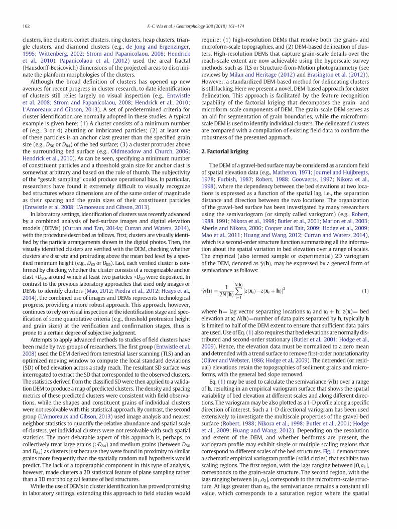
Eq. (1) may be used to calculate the semivariance γðhÞ over a rangeof h, resulting in an empirical variogram surface that shows the spatialvariability of bed elevation at different scales and along different direc-tions. The variogrammay be also plotted as a 1-D profile along a specificdirection of interest. Such a 1-D directional variogram has been usedextensively to investigate the multiscale properties of the gravel-bedsurface (Robert, 1988; Nikora et al., 1998; Butler et al., 2001; Hodgeet al., 2009; Huang and Wang, 2012). Depending on the resolutionand extent of the DEM, and whether bedforms are present, thevariogram profile may exhibit single or multiple scaling regions thatcorrespond to different scales of the bed structures. Fig. 1 demonstratesa schematic empirical variogram profile (solid circles) that exhibits twoscaling regions. The first region, with the lags ranging between [0,a1],corresponds to the grain-scale structure. The second region, with thelags ranging between [a1,a2], corresponds to themicroform-scale struc-ture. At lags greater than a2, the semivariance remains a constant sillvalue, which corresponds to a saturation region where the spatial

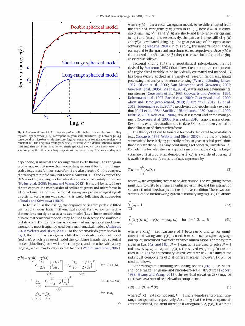
Fig. 1. A schematic empirical variogram profile (solid circles) that exhibits two scalingregions. Lags between [0, a1] correspond to grain-scale structure; lags between [a1,a2]correspond to microform-scale structure; lags Na2 correspond to saturation region withconstant sill. The empirical variogram profile is fitted with a double spherical model(red line) that combines linearly two single spherical models (blue lines), one has ashort range a1, the other has a long range a2, with c1 and c2 being the corresponding sills.

163F.-C. Wu et al. / Geomorphology 308 (2018) 161–174

dependency isminimal andno longer varieswith the lag. The variogramprofile may exhibit more than two scaling regions if bedforms at largerscales (e.g., mesoform or macroform) are also present. On the contrary,the variogram profile may not reach a constant sill if the extent of theDEM is not large enough or bed elevations are not completely stationary(Hodge et al., 2009; Huang and Wang, 2012). It should be noted herethat to capture the mean scales of sediment grains and microforms inall directions, an omni-directional variogram profile integrating alldirectional variograms was used in this study, following the suggestionof Isaaks and Srivastava (1989).

To be useful in the kriging, the empirical variogram profile is fittedwith a continuous, basic mathematical model. For a variogram profilethat exhibits multiple scales, a nested model (i.e., a linear combinationof basic mathematical models) may be used to describe the multiscalebed structure. For example, linear, exponential, and spherical models areamong the most frequently used basic mathematical models (Atkinson,2004; Webster and Oliver, 2007). For the schematic diagram shown inFig. 1, the empirical variogram is fitted with a double spherical model(red line), which is a nested model that combines linearly two sphericalmodels (blue lines), one with a short range a1 and the other with a longrange a2, whichmay be expressed as follows (Webster and Oliver, 2007):

γ hð Þ ¼ γ1 hð Þ þ γ2 hð Þ

¼

c13h2a1

−12

ha1

� �3" #

|fflfflfflfflfflfflfflfflfflfflfflfflfflfflfflfflffl{zfflfflfflfflfflfflfflfflfflfflfflfflfflfflfflfflffl}γ1 hð Þ

þ c23h2a2

−12

ha2

� �3" #

|fflfflfflfflfflfflfflfflfflfflfflfflfflfflfflfflffl{zfflfflfflfflfflfflfflfflfflfflfflfflfflfflfflfflffl}γ2 hð Þ

for 0 b h ≤ a1

c1|{z}γ1 hð Þ

þ c23h2a2

−12

ha2

� �3" #

|fflfflfflfflfflfflfflfflfflfflfflfflfflfflfflfflffl{zfflfflfflfflfflfflfflfflfflfflfflfflfflfflfflfflffl}γ2 hð Þ

for a1b h ≤ a2

c1|{z}γ1 hð Þ

þ c2|{z}γ2 hð Þ

for hNa2

8>>>>>>>>>>>>>><>>>>>>>>>>>>>>:

ð2Þ

where γ(h)= theoretical variogram model, to be differentiated fromthe empirical variogram γðhÞ given in Eq. (1), here h= |h| is omni-directional lag; γ1(h) and γ2(h) are short- and long-range variograms;(a1,c1) and (a2,c2) are, respectively, the pairs of (range, sill) of γ1(h)and γ2(h), evaluated using, e.g., the gstat package of the open sourcesoftware R (Pebesma, 2004). In this study, the range values a1 and a2correspond to the grain and microform scales, respectively. Once γ(h) isdecomposed intoγ1(h) andγ2(h), they can beused in the factorial kriging,described as follows.

Factorial kriging (FK) is a geostatistical interpolation methoddevised by Matheron (1982) that allows the decomposed componentsof a regionalized variable to be individually estimated and mapped. FKhas been widely applied in a variety of research fields, e.g., imageprocessing and analysis for remote sensing (Wen and Sinding-Larsen,1997; Oliver et al., 2000; Van Meirvenne and Goovaerts, 2002;Goovaerts et al., 2005a; Ma et al., 2014), water and soil environmentalmonitoring (Goovaerts et al., 1993; Goovaerts and Webster, 1994;Dobermann et al., 1997; Bocchi et al., 2000; Castrignanò et al., 2000;Alary and Demougeot-Renard, 2010; Allaire et al., 2012; Lv et al.,2013; Bourennane et al., 2017), geophysics and geochemistry explora-tion (Galli et al., 1984; Sandjivy, 1984; Jaquet, 1989; Yao et al., 1999;Dubrule, 2003; Reis et al., 2004), risk assessment and crime manage-ment (Goovaerts et al., 2005b; Kerry et al., 2010), among many others.Despite its extensive application, to date FK has not been applied tothe delineation of cluster microforms.

The theory of FK can be found in textbooks dedicated to geostatistics(e.g., Goovaerts, 1997; Webster and Oliver, 2007), thus it is only brieflysummarized here. Kriging generally refers to geostatistical predictionsthat estimate the value at any point using a set of nearby sample values.Consider the bed elevation as a spatial random variable Z(x), the krigedestimate of Z at a point x0, denoted as Zðx0Þ, is a weighted average ofN available data, z(x1), z(x2), …, z(xN), expressed by

Z x0ð Þ ¼XNi¼1

λiz xið Þ ð3Þ

where λi are weighting factors to be determined. The weighting factorsmust sum to unity to ensure an unbiased estimate, and the estimationvariance is minimized subject to the non-bias condition. These two con-straints lead to the following systemof ordinary kriging (OK) equations:

XNi¼1

λi ¼ 1 ð4aÞ

XNj¼1

λ jγ xi;x j� �þ ψ x0ð Þ ¼ γ xi;x0ð Þ for i ¼ 1;2; …;N ð4bÞ

where γ(xi,xj)= semivariance of Z between xi and xj, for omni-directional variograms γ(h) is used, h = |xi − xj|; ψ(x0)= Lagrangemultiplier, introduced to achieve varianceminimization. For the systemgiven in Eqs. (4a) and (4b), N + 1 equations are used to solve N + 1unknowns λ1, λ2, …, λN and ψ(x0). The solved weighting factors areused in Eq. (3) for an “ordinary kriged” estimate of Z. To estimate theindividual components of Z at different scales, however, FK will beused as follows.

For a variogram exhibiting two scaling regions (Fig. 1), i.e., short-and long-range (or grain- and microform-scale) structures (Robert,1988; Huang and Wang, 2012), the residual elevation Z(x) may beexpressed as a sum of two elevation components:

Z xð Þ ¼ Z1 xð Þ þ Z2 xð Þ ð5Þ

where Zk(x)= k-th component, k= 1 and 2 denotes short- and long-range components, respectively. Assuming that the two componentsare uncorrelated, the omni-directional variogram of Z, γ(h), is a nested

164 F.-C. Wu et al. / Geomorphology 308 (2018) 161–174

combination of short- and long-range omni-directional variograms γ1

(h) and γ2(h), as shown in Eq. (2). Similar to the ordinary kriging inEq. (3), each elevation component Zkmay be estimatedwith aweightedaverage of available data z(xi) by the factorial kriging:

Zkx0ð Þ ¼

XNi¼1

λki z xið Þ for k ¼ 1;2 ð6Þ

where Zk ¼ factorial kriged estimate of Zk, and λik are weighting factors

for the k-th component. The weighting factors are determined by solv-ing the following system of FK equations:

XNi¼1

λki ¼ 0 ð7aÞ

XNj¼1

λkjγ xi; x j� �

−ψk x0ð Þ ¼ γk xi; x0ð Þ for i ¼ 1;2;…;N ð7bÞ

where ψk(x0)= Lagrange multiplier; here γk(xi,x0) for k=1 and 2 are,respectively, replaced by γ1(h) and γ2(h) determined from Eq. (2), and

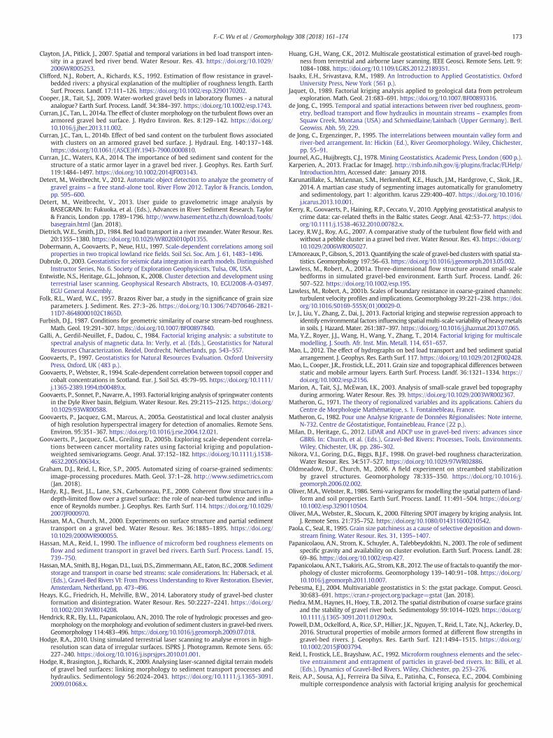
Fig. 2. An example gravel-bed patch collected from Nanshih Creek (northern Taiwan): (A) ordirange component of FK DEM; (D) surface elevation distributions of OK DEM, and short- and lo

γ(xi,xj) is replaced by γ(h). Eq. (7a) states that λik must sum to 0 over i(rather than 1) to ensure an unbiased estimate and accord with Eq. (5),while Eq. (7b) states thatλik are selected to reach aminimumestimationvariance. The system in Eqs. (7a) and (7b) is solved for each scale (each k)to determine the weighting factors λi

k, which are used in Eq. (6) toestimate individual components of spatial elevations, referred to as“factorial kriged (FK) DEM components”.

As an illustration, we present in Fig. 2 a gravel-bed patch collectedfrom Nanshih Creek (Taiwan) to show the ordinary kriged (OK) DEMand the short- and long-range components of the factorial kriged (FK)DEM. It is evident that the full bed topography (Fig. 2A) is the superpo-sition of grain- and microform-scale topographies (Fig. 2B and C). Theshort-range FK DEM exhibits a flat bed, with 90% of the elevations in anarrow range between −0.04 and +0.03 m (Fig. 2D). The long-rangeFK DEM is smoother than the OK DEM, with 90% of the elevations in arange between−0.12 and+0.09 m, slightly smaller than the 90%eleva-tion range of the OK DEM (between −0.14 and +0.1 m). Individualgrains are sharply outlined in the short-range FK DEM, suggesting thatthe grain-scale DEM may well serve as an aid for segmentation ofgrain boundaries. Individual grains are not fully recognizable in thelong-range FK DEM, while groupings of particles emerge as small-

nary kriged (OK) DEM; (B) short-range component of factorial kriged (FK) DEM; (C) long-ng-range FK DEMs.

165F.-C. Wu et al. / Geomorphology 308 (2018) 161–174

scale bedforms such as clusters. This feature recognition capability ofthe microform-scale DEM is used herein to devise a DEM-basedapproach for cluster identification. As a final note, the advantage ofthe FK is that the parameters used in the computations, i.e., γ(h), γ1

(h) andγ2(h), are determined directly from the variogrammodelswith-out a need for trial and error. In addition, the FKDEMs aremore intuitivesince the full (OK) DEM is simply the sum of short- and long-range FKDEMs.

3. Case study

3.1. Study site

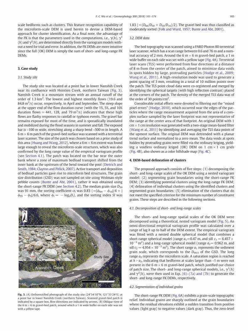
The study site was located at a point bar in lower Nanshih Creeknear its confluence with Hsintien Creek, northern Taiwan (Fig. 3).Nanshih Creek is a mountain stream with an annual runoff of theorder of 1.3 km3. The lowest and highest monthly flows (19.6 and84.8 m3/s) occur, respectively, in April and September. The steep slopeat the upper end of the flow duration curve (with the 1%, 5%, and 10%duration flows = 441, 128, and 79 m3/s) indicates that these highflows are flashy responses to rainfall or typhoon events. The gravel barremains exposed for most of the time, and is sporadically inundatedandmobilized during theflood seasons in summer and fall. The exposedbar is ~100 m wide, stretching along a sharp bend ~500m in length. A6m × 6mpatch of the gravel-bed surfacewas scannedwith a terrestriallaser scanner. The size of the patchwas chosen based on a prior study ofthis area (Huang andWang, 2012), where a 6m × 6m extent was foundlarge enough to reveal the microform-scale structures, which was alsoconfirmed by the long range value of the empirical variogram profile(see Section 4.1). The patch was located on the bar near the outerbank where a zone of maximum bedload transport shifted from theinner bank at the upstream of the bend toward the pool (Dietrich andSmith, 1984; Clayton and Pitlick, 2007). Active transport and depositionof bedload particles gave rise to microform bed structures. The grainsize distribution (GSD) was not sampled on site using Wolman-stylepebble counts (Bunte and Abt, 2001), rather it was obtained usingthe short-range FK DEM (see Section 4.2). The median grain size D50

was 91 mm, the sorting coefficient σI was 0.83 (=|ϕ84 − ϕ16|/4 + |ϕ95 − ϕ5|/6.6, where ϕi = − log2Di), and the sorting index SI was

Fig. 3. (A) Orthorectified photograph of the study site (24°54′10”N, 121°33′24″E) ata point bar in lower Nanshih Creek (northern Taiwan). Scanned gravel-bed patch isindicated by a square box, flow directions are indicated by arrows. (B) Oblique view ofthe 6 m × 6 m gravel-bed patch, around which a 1 m wide buffer on each side was setwith a yellow tape.

1.83 (=(D84/D50 + D50/D16)/2). The gravel bed was thus classified asmoderately sorted (Folk and Ward, 1957; Bunte and Abt, 2001).

3.2. DEM data

The bed topographywas scanned using a FARO Photon 80 terrestriallaser scanner, which has a scan range between 0.6 and 76m and a nom-inal accuracy of 2 mm. Around the 6 m × 6 m gravel-bed patch, a 1 mwide buffer on each sidewas setwith a yellow tape (Fig. 4A). Terrestriallaser scans (TLS) were performed from four directions at a distanceof 8 m from the center of the patch, aimed to minimize data voidsin spots hidden by large, protruding particles (Hodge et al., 2009;Wang et al., 2011). A high-resolution mode was used to generate apoint spacing of 3 mm, resulting in a total of 10 million points overthe patch. The TLS point cloud data were co-registered and merged byidentifying the spherical targets (with high reflection contrast) placedat the corners of the patch. The density of the merged TLS data was ofthe order of 30 points/cm2.

Considerable initial efforts were devoted to filtering out the “mixedpixel errors” (Hodge, 2010), which occurred near the edges of the par-ticles where the range measurement acquired from the area of a com-plex surface sampled by the laser footprint was not representative ofthe range at the center area of that footprint. An original DEM with 1cm× 1 cmresolutionwas generatedwith a two-stagemean-based filter(Wang et al., 2011) by identifying and averaging the TLS data points ofthe upmost surface. The original DEM was detrended with a planartrend surface and normalized to a zero mean. The data voids at spotshidden by protruding grains were filled via the ordinary kriging, yield-ing a voidless ordinary kriged (OK) DEM on 1 cm × 1 cm grids(Fig. 4B), also shown as a color hillshade map (Fig. 4C).

4. DEM-based delineation of clusters

The proposed approach consists of five steps: (1) decomposing theshort- and long-range scales of the OK DEM using a nested variogrammodel; (2) segmenting grain boundaries using the short-range FKDEM; (3) identifying potential clusters using the long-range FK DEM;(4) delineation of individual clusters using the identified clusters andsegmented grain boundaries; (5) elimination of the clusters that donotmeet the specified criterion for theminimumnumber of constituentgrains. These steps are described in the following sections.

4.1. Decomposition of short- and long-range scales

The short- and long-range spatial scales of the OK DEM weredecomposed using a theoretical, nested variogram model (Fig. 5). Anomni-directional empirical variogram profile was calculated over arange of lag h up to half of the DEM extent. The empirical variogramwas fitted with a nested double spherical model that combines ashort-range spherical model (range a1=0.47 m, and sill c1 = 6.457 ×10−3 m2) and a long-range spherical model (range a2= 0.962 m, andsill c2 = 4.954 × 10−3 m2). The short range a1 represents the sedimentgrain scale, which corresponds to the D99.5 of the GSD. The longrange a2 represents the microform scale. A saturation region is reachedat h N a2, indicating that bedforms at scales larger than ~1 m were notpresent in the 6 m × 6 m gravel-bed patch, which justified our choiceof patch size. The short- and long-range spherical models, i.e., γ1(h)and γ2(h), were then used in Eqs. (6)–(7a) and (7b) to generate theshort- and long-range FK DEMs, respectively.

4.2. Segmentation of individual grains

The short-range FK DEM (Fig. 6A) exhibits a grain-scale topographicrelief. Individual grains are sharply outlined at the grain boundarieswhere the residual elevations exhibit a sudden transition from positivevalues (light gray) to negative values (dark gray). Thus, the zero-level

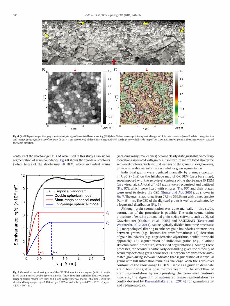
Fig. 4. (A)Oblique-perspective grayscale intensity image of terrestrial laser scanning (TLS) data. Yellow arrowspoint at spherical targets (14.5 cm indiameter) used for data co-registrationand merge; (B) grayscale map of OK DEM (1 cm× 1 cm resolution) of the 6 m× 6m gravel-bed patch; (C) color hillshademap of OK DEM. Red arrows point at the same location towardthe same direction.

166 F.-C. Wu et al. / Geomorphology 308 (2018) 161–174

contours of the short-range FK DEMwere used in this study as an aid forsegmentation of grain boundaries. Fig. 6B shows the zero-level contours(white lines) of the short-range FK DEM, where individual grains

Fig. 5. Omni-directional variograms of the OK DEM: empirical variogram (solid circles) isfitted with a nested double spherical model (gray line) that combines linearly a short-range spherical model (red line) and a long-range spherical model (blue line), with theshort and long ranges: a1=0.470 m, a2=0.962 m, and sills c1 = 6.457 × 10−3 m2, c2 =4.954 × 10−3 m2.

(includingmany smaller ones) become clearly distinguishable. Some frag-mentations associatedwith grain-surface texture are exhibited also by thezero-level contours. Such textural features on the grain surfaces, however,provide no additional information useful for grain segmentation.

Individual grains were digitized manually by a single operatorin ArcGIS (Esri) on the hillshade map of OK DEM (as a base map),superimposed with the zero-level contours of the short-range FK DEM(as a visual aid). A total of 1469 grains were recognized and digitized(Fig. 6C), which were fitted with ellipses (Fig. 6D) and their b-axeswere used to derive the GSD (Bunte and Abt, 2001), as shown inFig. 7. The grain sizes range from 27.6 to 569.6 mm with a median sizeD50= 91 mm. The GSD of the digitized grains is well approximated bya lognormal distribution (Fig. 7).

Although grain segmentation was done manually in this study,automation of the procedure is possible. The grain segmentationprocedure of existing automated grain-sizing software, such as DigitalGravelometer (Graham et al., 2005) and BASEGRAIN (Detert andWeitbrecht, 2012, 2013), can be typically divided into three processes:(1) morphological filtering to enhance grain boundaries or intersticesbetween grains (e.g., bottom-hat transformation); (2) detectionof grain boundaries (e.g., edge detection algorithms, double-thresholdapproach); (3) segmentation of individual grains (e.g., dilation/skeletonization procedure, watershed segmentation). Among theseprocesses, the second is particularly demanding given the difficulty ofaccurately detecting grain boundaries. Our experience with these auto-mated grain-sizing software indicated that segmentation of individualgrains with full automation remains a challenge. With the zero-levelcontours of the short-range FK DEM usable as a guide to delineategrain boundaries, it is possible to streamline the workflow ofgrain segmentation by incorporating the zero-level contoursinto, e.g., the algorithm of automated image segmentation re-cently devised by Karunatillake et al. (2014) for granulometryand sedimentology.

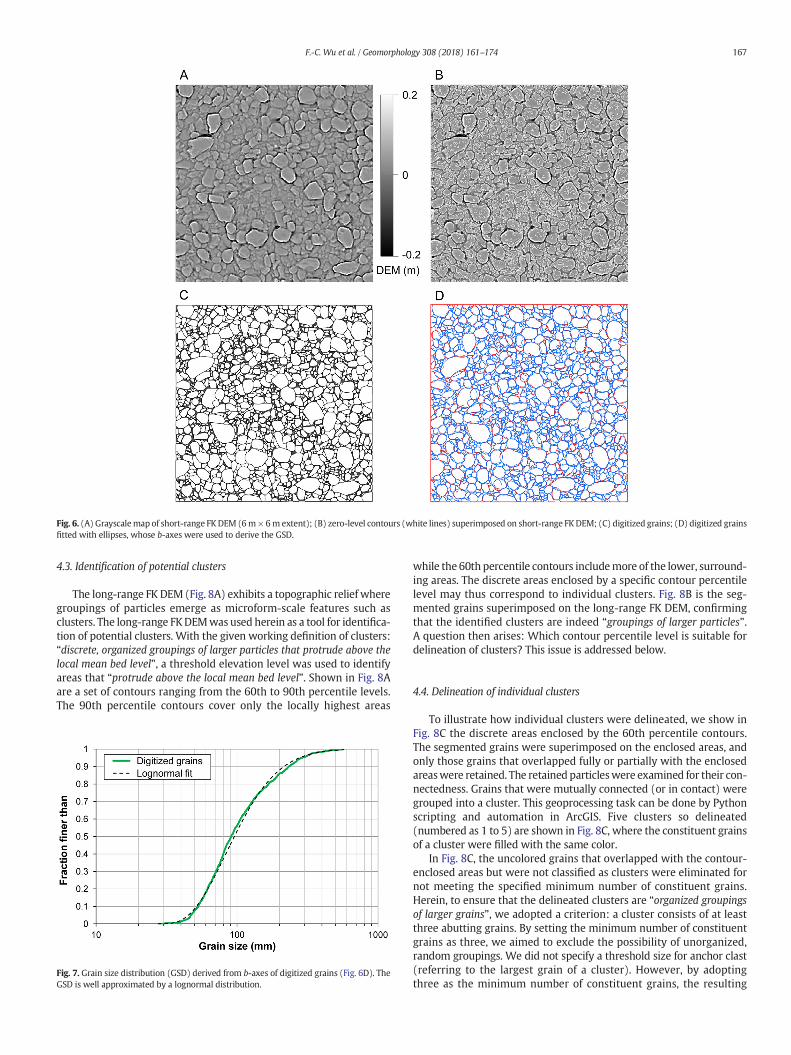
Fig. 6. (A) Grayscalemap of short-range FKDEM (6m × 6m extent); (B) zero-level contours (white lines) superimposed on short-range FKDEM; (C) digitized grains; (D) digitized grainsfitted with ellipses, whose b-axes were used to derive the GSD.

167F.-C. Wu et al. / Geomorphology 308 (2018) 161–174

4.3. Identification of potential clusters

The long-range FK DEM (Fig. 8A) exhibits a topographic relief wheregroupings of particles emerge as microform-scale features such asclusters. The long-range FKDEMwas used herein as a tool for identifica-tion of potential clusters. With the given working definition of clusters:“discrete, organized groupings of larger particles that protrude above thelocal mean bed level”, a threshold elevation level was used to identifyareas that “protrude above the local mean bed level”. Shown in Fig. 8Aare a set of contours ranging from the 60th to 90th percentile levels.The 90th percentile contours cover only the locally highest areas

Fig. 7. Grain size distribution (GSD) derived from b-axes of digitized grains (Fig. 6D). TheGSD is well approximated by a lognormal distribution.

while the 60th percentile contours includemore of the lower, surround-ing areas. The discrete areas enclosed by a specific contour percentilelevel may thus correspond to individual clusters. Fig. 8B is the seg-mented grains superimposed on the long-range FK DEM, confirmingthat the identified clusters are indeed “groupings of larger particles”.A question then arises: Which contour percentile level is suitable fordelineation of clusters? This issue is addressed below.

4.4. Delineation of individual clusters

To illustrate how individual clusters were delineated, we show inFig. 8C the discrete areas enclosed by the 60th percentile contours.The segmented grains were superimposed on the enclosed areas, andonly those grains that overlapped fully or partially with the enclosedareaswere retained. The retained particleswere examined for their con-nectedness. Grains that were mutually connected (or in contact) weregrouped into a cluster. This geoprocessing task can be done by Pythonscripting and automation in ArcGIS. Five clusters so delineated(numbered as 1 to 5) are shown in Fig. 8C, where the constituent grainsof a cluster were filled with the same color.

In Fig. 8C, the uncolored grains that overlapped with the contour-enclosed areas but were not classified as clusters were eliminated fornot meeting the specified minimum number of constituent grains.Herein, to ensure that the delineated clusters are “organized groupingsof larger grains”, we adopted a criterion: a cluster consists of at leastthree abutting grains. By setting the minimum number of constituentgrains as three, we aimed to exclude the possibility of unorganized,random groupings. We did not specify a threshold size for anchor clast(referring to the largest grain of a cluster). However, by adoptingthree as the minimum number of constituent grains, the resulting

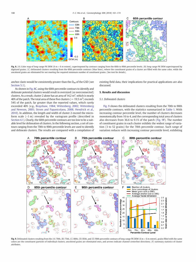
Fig. 8. (A) Color map of long-range FK DEM (6 m × 6 m extent), superimposed by contours ranging from the 60th to 90th percentile levels; (B) long-range FK DEM superimposed bydigitized grains; (C) delineated clusters resulting from the 60th percentile contours (blue lines), where the constituent grains of a cluster are filled with the same color, while theuncolored grains are eliminated for not meeting the required minimum number of constituent grains. (See text for details).

168 F.-C. Wu et al. / Geomorphology 308 (2018) 161–174

anchor clastswould be consistently greater than theD90 of the GSD (seeSection 5.1).

As shown in Fig. 8C, using the 60th percentile contours to identify anddelineate potential clusterswould result in oversized (or overconnected)clusters. As a result, cluster 2 alone has an area of 14.2 m2,which is nearly40% of thepatch. The total area of thesefive clusters (=19.5m2) exceeds54% of the patch, far greater than the reported values, which rarelyexceeded 40% (e.g., Brayshaw, 1984; Wittenberg, 2002; Wittenbergand Newson, 2005; Strom and Papanicolaou, 2008; Hendrick et al.,2010). In addition, the length and width of cluster 2 exceed the micro-form scale (~1 m) revealed by the variogram profile (described inSection 4.1). Clearly, the 60th percentile contours are too low to be a suit-able level for delineation of clusters. In the following section, a set of con-tours ranging from the 70th to 90th percentile levels are used to identifyand delineate clusters. The results are compared with a compilation of

Fig. 9.Delineated clusters resulting from the (A) 70th, (B) 75th, (C) 80th, (D) 85th, and (E) 90thcolors are the constituent particles of individual clusters, uncolored grains are eliminated onattributes.

existing field data, their implications for practical applications are alsodiscussed.

5. Results and discussion

5.1. Delineated clusters

Fig. 9 shows the delineated clusters resulting from the 70th to 90thpercentile contours, with the statistics summarized in Table 1. Withincreasing contour percentile level, the number of clusters decreasesmonotonically from 16 to 4, and the corresponding total area of clustersalso decreases from 36.6 to 9.1% of the patch (Fig. 9F). The numberof constituent grains in each cluster exhibits the widest range of varia-tion (3 to 52 grains) for the 70th percentile contour. Such range ofvariation reduces with increasing contour percentile level, exhibiting

percentile contours of long-range FK DEM (6m × 6m extent), grains filledwith the samees, and arrows indicate channel centerline directions; (F) summary statistics of cluster

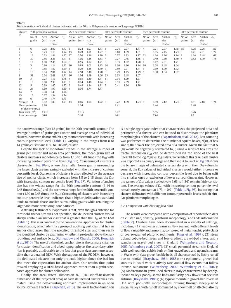
Table 1Attribute statistics of individual clusters delineated with the 70th to 90th percentile contours of long-range FK DEM.

ClusterID

70th percentile contour 75th percentile contour 80th percentile contour 85th percentile contour 90th percentile contour

No. ofgrains

Area(m2)

Anchorsize(×D90)

DAT No. ofgrains

Area(m2)

Anchorsize(×D90)

DAT No. ofgrains

Area(m2)

Anchorsize(×D90)

DAT No. ofgrains

Area(m2)

Anchorsize(×D90)

DAT No. ofgrains

Area(m2)

Anchorsize(×D90)

DAT

1 6 0.28 2.07 1.77 5 0.24 2.07 1.77 5 0.24 2.07 1.77 4 0.21 2.07 1.75 18 1.08 2.26 1.822 5 0.23 1.15 1.74 13 0.49 1.81 1.77 3 0.10 1.39 1.81 3 0.65 2.45 1.73 3 0.41 2.01 1.723 16 0.53 1.81 1.77 37 2.50 2.26 1.70 5 0.77 2.23 1.77 22 1.24 2.26 1.84 9 1.24 2.48 1.634 39 2.56 2.26 1.71 11 1.05 2.45 1.63 4 0.77 2.45 1.65 3 0.40 2.39 1.80 5 0.52 1.99 1.785 13 1.08 2.45 1.64 6 0.55 1.82 1.71 3 0.33 1.82 1.70 4 0.47 2.01 1.716 3 0.10 1.14 1.75 16 0.89 2.01 1.73 24 1.26 2.26 1.84 16 1.58 2.48 1.647 7 0.58 1.82 1.69 3 0.29 1.45 1.79 9 0.80 2.01 1.71 6 0.69 1.99 1.728 18 0.94 2.01 1.72 44 2.58 2.48 1.70 3 0.29 1.45 1.79 5 0.30 1.34 1.679 52 2.74 2.48 1.71 16 1.04 1.99 1.66 25 2.23 2.48 1.6710 3 0.23 1.16 1.78 4 0.55 2.39 1.71 11 0.94 1.99 1.6711 10 0.68 2.39 1.73 3 0.14 1.48 1.74 3 0.53 2.39 1.7112 5 0.39 1.45 1.75 9 0.48 1.34 1.71 7 0.41 1.34 1.7013 24 1.30 1.99 1.69 4 0.36 1.74 1.7714 7 0.38 1.48 1.7615 16 0.67 1.34 1.7416 6 0.49 1.74 1.73Average 14 0.82 1.80 1.73 13 0.86 1.94 1.72 9 0.72 1.99 1.73 8 0.69 2.12 1.73 9 0.81 2.18 1.74Mean grain sizeof cluster (×D90)

1.16 1.24 1.41 1.44 1.48

Total area (m2) 13.18 11.17 8.67 5.55 3.26Area percentage 36.6 31.0 24.1 15.4 9.1

169F.-C. Wu et al. / Geomorphology 308 (2018) 161–174

the narrowest range (3 to 18 grains) for the 90th percentile contour. Theaverage number of grains per cluster and average area of individualclusters, however, do not exhibit any monotonic trends with increasingcontour percentile level (Table 1), varying in the ranges from 8 to14 grains/cluster and 0.69 to 0.86 m2/cluster.

Despite the lack of monotonic trends in the average number ofgrains per cluster and mean area per cluster, the mean grain size ofclusters increases monotonically from 1.16 to 1.48 times the D90 withincreasing contour percentile level (Fig. 9F). Coarsening of clusters isobservable in Fig. 9A–E, where the smaller, lower grains surroundingthe larger clasts are increasingly excluded with the increase of contourpercentile level. Coarsening of clusters is also reflected by the averagesize of anchor clasts, which increases from 1.8 to 2.18 times the D90

with increasing contour percentile level (Fig. 9F). Variation of anchorsize has the widest range for the 70th percentile contour (1.14 to2.48 times theD90) and the narrowest range for the 90th percentile con-tour (1.99 to 2.48 times the D90). Coarsening of clusters with increasingcontour percentile level indicates that a higher delineation standardtends to exclude those smaller, surrounding grains while retaining thelarger and more protruding, core particles.

A striking feature of our approach is that, even though a criterion forthreshold anchor size was not specified, the delineated clusters wouldalways contain an anchor clast that is greater than the D90 of the GSD(Table 1). This is in contrast to the conventional approaches for clusteridentification, which identify a group of abutting particles that has ananchor clast larger than the specified threshold size, and then verifythe identified cluster by examining whether it protrudes above the sur-rounding bed surface (e.g., Oldmeadow and Church, 2006; Hendricket al., 2010). The use of a threshold anchor size as the primary criterionfor cluster identification and a bed topography as the secondary crite-rion is probably attributable to the fact that grain sizes are more acces-sible than a detailed DEM. With the support of the FK DEM, however,the delineated clusters not only protrude higher above the bed butalso meet the expectation for anchor sizes. Our results thus pointtoward employing a DEM-based approach rather than a grain-size-based approach for cluster delineation.

Finally, the areal fractal dimension DAT (Hausdorff-Besicovichdimension of the projected area) of each delineated cluster was esti-mated, using the box-counting approach implemented in an opensource software FracLac (Karperien, 2013). The areal fractal dimension

is a single aggregate index that characterizes the projected area andperimeter of a cluster, and can be used to discriminate the planformmorphologies of the clusters (Papanicolaou et al., 2012). Box countingwas performed to determine the number of square boxes, N(μ), of boxsize μ, that cover the projected area of a cluster. Given the fact that N(μ) would be negatively correlated to μ, using a series of box sizes thefractal dimension DAT can be determined via the slope of the bestlinear fit to the log N(μ) vs. log μ data. To facilitate this task, each clusterwas exported as a binary image and then input to FracLac. Fig. 10 showsthe binary images of delineated clusters along with their DAT values. Ingeneral, the DAT values of individual clusters would either increase ordecrease with increasing contour percentile level due to being splitinto smaller ones or exclusion of lower surrounding grains. However,the ranges of DAT values (collectively 1.63 to 1.84) remain fairly consis-tent. The average values of DAT with increasing contour percentile levelremain nearly constant at 1.73 ± 0.01 (Table 1, Fig. 9F), indicating thatclusters delineated with different contour percentile levels exhibit sim-ilar planform morphologies.

5.2. Comparison with existing field data

The results were compared with a compilation of reported field dataon cluster size, density, planform morphology, and GSD information(Table 2). Clusters have been documented in a variety of settings,including: (1) headwater streams in New Zealand with different levelsof flow variability and armoring, composed of metamorphic platy clastsor coarse-grained plutonic sediments (Biggs et al., 1997); (2) steepupland cobble-bed rivers and low-gradient gravel-bed rivers, and awandering gravel-bed river in England (Wittenberg and Newson,2005; Wittenberg et al., 2007); (3) small, perennial streams in Englandwith well-rounded cobble beds or flint-gravel beds, and upland streamsinWaleswith slate gravel/cobble beds, all characterized byflashy runoffdue to rainfall (Brayshaw, 1984, 1985); (4) ephemeral gravel-bedstreams in Israel with relatively rare, annual flow events that followintense rainstorms (Wittenberg, 2002; Wittenberg et al., 2007);(5) Mediterranean gravel-bed rivers in Italy characterized by deeply-incised valleys, poorly-sorted beds and flashy peak flows that occur inautumn (Brayshaw, 1985); (6) typical mountain gravel-bed rivers inUSA with pool-riffle morphologies, flowing through steeply-sidedglacial valleys, with runoff dominated by snowmelt or affected also by

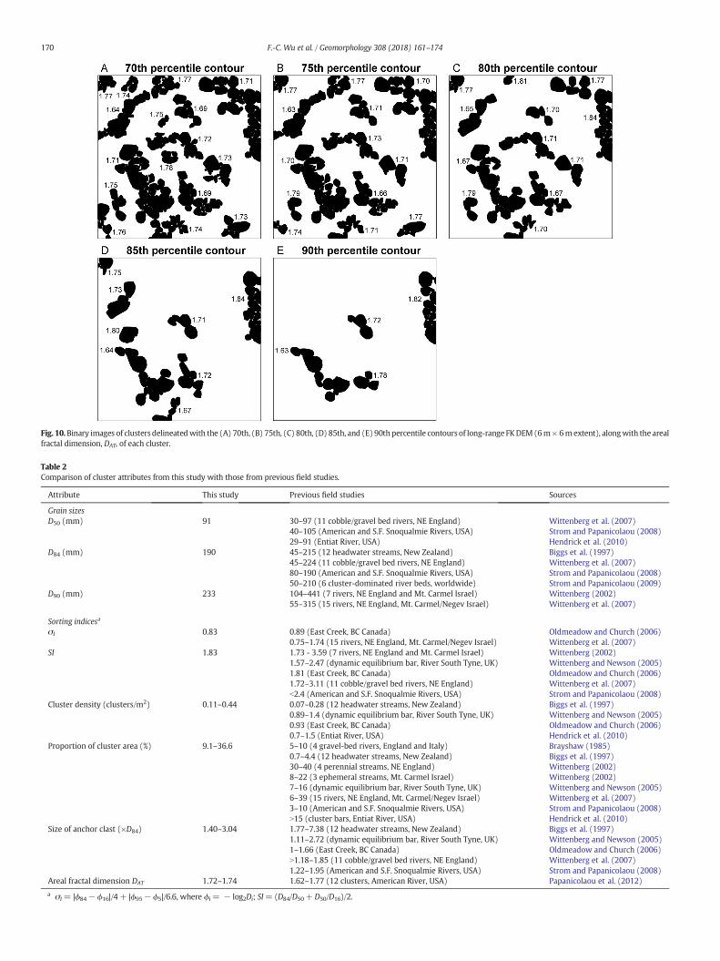
Fig. 10.Binary images of clusters delineatedwith the (A) 70th, (B) 75th, (C) 80th, (D) 85th, and (E) 90th percentile contours of long-range FKDEM (6m× 6mextent), alongwith the arealfractal dimension, DAT, of each cluster.

Table 2Comparison of cluster attributes from this study with those from previous field studies.

Attribute This study Previous field studies Sources

Grain sizesD50 (mm) 91 30–97 (11 cobble/gravel bed rivers, NE England) Wittenberg et al. (2007)

40–105 (American and S.F. Snoqualmie Rivers, USA) Strom and Papanicolaou (2008)29–91 (Entiat River, USA) Hendrick et al. (2010)

D84 (mm) 190 45–215 (12 headwater streams, New Zealand) Biggs et al. (1997)45–224 (11 cobble/gravel bed rivers, NE England) Wittenberg et al. (2007)80–190 (American and S.F. Snoqualmie Rivers, USA) Strom and Papanicolaou (2008)50–210 (6 cluster-dominated river beds, worldwide) Strom and Papanicolaou (2009)

D90 (mm) 233 104–441 (7 rivers, NE England and Mt. Carmel Israel) Wittenberg (2002)55–315 (15 rivers, NE England, Mt. Carmel/Negev Israel) Wittenberg et al. (2007)

Sorting indicesa

σI 0.83 0.89 (East Creek, BC Canada) Oldmeadow and Church (2006)0.75–1.74 (15 rivers, NE England, Mt. Carmel/Negev Israel) Wittenberg et al. (2007)

SI 1.83 1.73 - 3.59 (7 rivers, NE England and Mt. Carmel Israel) Wittenberg (2002)1.57–2.47 (dynamic equilibrium bar, River South Tyne, UK) Wittenberg and Newson (2005)1.81 (East Creek, BC Canada) Oldmeadow and Church (2006)1.72–3.11 (11 cobble/gravel bed rivers, NE England) Wittenberg et al. (2007)b2.4 (American and S.F. Snoqualmie Rivers, USA) Strom and Papanicolaou (2008)

Cluster density (clusters/m2) 0.11–0.44 0.07–0.28 (12 headwater streams, New Zealand) Biggs et al. (1997)0.89–1.4 (dynamic equilibrium bar, River South Tyne, UK) Wittenberg and Newson (2005)0.93 (East Creek, BC Canada) Oldmeadow and Church (2006)0.7–1.5 (Entiat River, USA) Hendrick et al. (2010)

Proportion of cluster area (%) 9.1–36.6 5–10 (4 gravel-bed rivers, England and Italy) Brayshaw (1985)0.7–4.4 (12 headwater streams, New Zealand) Biggs et al. (1997)30–40 (4 perennial streams, NE England) Wittenberg (2002)8–22 (3 ephemeral streams, Mt. Carmel Israel) Wittenberg (2002)7–16 (dynamic equilibrium bar, River South Tyne, UK) Wittenberg and Newson (2005)6–39 (15 rivers, NE England, Mt. Carmel/Negev Israel) Wittenberg et al. (2007)3–10 (American and S.F. Snoqualmie Rivers, USA) Strom and Papanicolaou (2008)N15 (cluster bars, Entiat River, USA) Hendrick et al. (2010)

Size of anchor clast (×D84) 1.40–3.04 1.77–7.38 (12 headwater streams, New Zealand) Biggs et al. (1997)1.11–2.72 (dynamic equilibrium bar, River South Tyne, UK) Wittenberg and Newson (2005)1–1.66 (East Creek, BC Canada) Oldmeadow and Church (2006)N1.18–1.85 (11 cobble/gravel bed rivers, NE England) Wittenberg et al. (2007)1.22–1.95 (American and S.F. Snoqualmie Rivers, USA) Strom and Papanicolaou (2008)

Areal fractal dimension DAT 1.72–1.74 1.62–1.77 (12 clusters, American River, USA) Papanicolaou et al. (2012)

a σI = |ϕ84− ϕ16|/4 + |ϕ95− ϕ5|/6.6, where ϕi= − log2Di; SI= (D84/D50 + D50/D16)/2.

170 F.-C. Wu et al. / Geomorphology 308 (2018) 161–174

171F.-C. Wu et al. / Geomorphology 308 (2018) 161–174

flash floods following rain-on-snow events or intense summer thunder-storms (Strom and Papanicolaou, 2008; Hendrick et al., 2010;Papanicolaou et al., 2012); (7) a mountain stream in a volcanic terrainin the USA, with its plane bed composed of well-sorted cobbles/pebblesand the flow regime dominated by snowmelt (de Jong, 1995); (8) ananthropogenically influenced, small headwater stream in Canada, withstep-pool sequences present at the upstream side of a culvert and anarmored reach developing downstream of the culvert (Oldmeadowand Church, 2006). Our results add data for a different geographicregion. Further background about the settings of these reported sitescan be found in the Supplementary information.

The attributes compared include grain sizes, sorting indices, clusterdensity, area percentage, and size of anchor clast (Table 2). Our charac-teristic sizes (D50, D84, D90= 91, 190, 233 mm) are well within the grainsize ranges reported, amongwhich the sediments of the upland cobble-bed rivers in England are the coarsestwhereas those of the low-gradientgravel-bed rivers in England are the finest. Our sorting indices, σI andSI=0.83 and 1.83, indicating a moderately sorted river reach, resemblethose of the armored East Creek in British Columbia, Canada.

Our cluster densities range from 0.11 to 0.44 clusters/m2, which arewithin the reported lower bound values (headwater streams, NewZealand) and upper bound values (Entiat River, USA). The wide rangeof cluster densities documented in these sites is attributable to differ-ences in flow variability, armoring and grain shape, the criteria adoptedto define clusters, and the clustered bars selected for sampling (Biggset al., 1997; Hendrick et al., 2010). Our proportions of cluster arearange from 9.1 to 36.6%, which are within the lower bound values asso-ciated with the headwater streams (New Zealand) and upper boundvalues associated with the poorly-sorted, perennial streams (England).The sizes of anchor clasts were scaled by theD84 in a number of datasetscompiled, with the lower bound values observed in East Creek (Canada)

Fig. 11. 3Dvisualization of clusters delineatedwith the (A) 70th, (B) 80th, and (C)90th percentileextent). Arrows indicate channel centerline directions.

andupper bound values observed inheadwater streams (NewZealand).Asmentioned earlier, our anchor sizes range from 1.14 to 2.48 times theD90 (equivalent to 1.4 to 3.04 times theD84), which are concordant withthe reported range. In particular, our anchor sizes resemble those docu-mented in the wandering River South Tyne (UK). Such resemblancemay be attributed to their similarities in sorting indices SI and transportmechanisms. Clusters at our study site and South Tyne were both sam-pled from a dynamic equilibrium bar that is exposed during low flowsbut inundated and subjected to active transport during flashy highflow events. Flow direction at the South Tyne study site varies withthe stage. Low flows run along the chute or diagonally across the bar,whereas high flows run directly downstream, normal to the chute.This is similar to the stage-dependent variation of transport directionat our study site on a point bar along a channel bend (Clayton andPitlick, 2007).

The work of Papanicolaou et al. (2012) was the only one that docu-mented fractal dimensions of field clusters, which included four lineclusters, four triangle clusters, and four rhombic clusters recorded in amountain gravel-bed stream (American River, USA). Their averagevalues of DAT for line, triangle, and rhombic clusters are 1.62, 1.77, and1.76, respectively. Our average values of DAT, ranging from 1.72 to1.74, are similar to their results. The DAT values of individual clustersshown in Fig. 10 also coincide with their findings, where the pseudo-line clusters on the upper left side of Fig. 10A–C exhibit the lowestvalues of DAT (=1.64 ± 0.01), while the mega clusters on the upperright side of Fig. 10C–E (with the border cropped) exhibit the highestvalues of DAT (=1.83 ± 0.01).

As our results fall within the ranges of reported field data, we canconclude that the FK DEM provides a novel, promising tool for clusterdelineation. Currently there is nouniversally accepted definition of clus-ters, hence to recommend a standard contour percentile level for

contours of long-range FKDEM, and (D) the sameviewwith noclustersmapped (6m× 6m

172 F.-C. Wu et al. / Geomorphology 308 (2018) 161–174

delineation of clusters may not be practical. Nonetheless, lower levels(e.g., 70th–75th percentile contour) may be used if more of the smaller,surrounding grains are to be included. By contrast, higher levels(e.g., 80th–85th percentile contour) may be used if only those largerand more protruding, core particles are to be retained. In the absenceof benchmark surfaces with correctly delineated clusters togetherwith a unique definition for clusters, delineation of clusters will inevita-bly remain subjective in nature. Given that clusters vary in their constit-uent grains, sizes and shapes across environments, however, theparameters used in the FK, i.e., γ(h), γ1(h) and γ2(h), can be objectivelydetermined from the DEM-based variogram models.

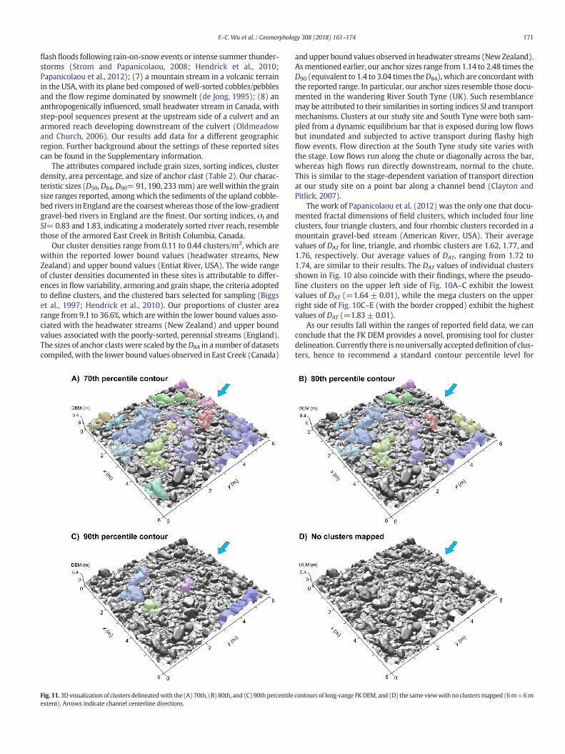
Finally, it is deemed intuitive to examine the delineated clusters by3D visualization, because it would be helpful to have a real sense ofwhat field scientists would see on site. The color patterns of delineatedclusters (Fig. 9A–E) were superimposed on the hillshade map of OKDEM in ArcScene (Esri), and exported as oblique-perspective, stereo-scopic images. Fig. 11 presents the resulting images of clusters delin-eated with the 70th, 80th, and 90th percentile contour levels. Asmentioned earlier, with increasing contour percentile level the lower,smaller grains surrounding the higher, larger clasts are increasinglyexcluded, leaving only the more protruding core particles. Since ourapproach is based on DEMs rather than grain sizes, it may excludesome of the largest but isolated clasts that are not connected or in con-tact with at least two sufficiently high grains to meet the definition ofa cluster. These largest but isolated clasts could otherwise be classifiedas a cluster if the required minimum number of constituent grains islowered as two, or a small separation distance is specified allowing forclosely neighboring particles to be effectively identified as abuttingones.

6. Conclusions

In this study, we used the FK to decompose the short- and long-range (grain- and microform-scale) DEMs. The parameters used in theFK were determined from the nested variogram models derived fromthe OK DEM. The short-range FK DEM was used as an aid for grain seg-mentation. The contour percentile levels of the long-range FKDEMwereused to identify potential clusters. Individual clusters were delineatedon the basis of the segmented grains and identified clusters.

Our results reveal that the density and total area of delineated clus-ters decrease with increasing contour percentile level, while the meangrain size of clusters and average anchor size increase with the contourpercentile level. These results support the observation that larger grainsgroup as clusters and protrude higher above the bed than other smallergrains. The average areal fractal dimension of clusters shows that clus-ters resulting from different contour percentile levels exhibit similarplanform morphologies. A striking feature of the delineated clusters isthat anchor clasts are invariably greater than the D90 even though athreshold anchor size is not adopted herein. Comparisons with existingfield data show consistency with the observed cluster attributes. Ourresults thus point toward a promising DEM-based approach for charac-terizing sediment structures in gravel-bed rivers.

Delineation of clusters is important in river science because clustersaffect the flowfield near the bed, change the bed structure and aresignificant controls on sediment transport and thus bed stability(e.g., Robert et al., 1996; Church et al., 1998; Curran and Tan, 2014b).Essential attributes such as the spatial pattern, density, area coverage,and dimensions may be extracted from the delineated clusters. More-over, isolating roughness scales of gravel-bed topography is increasinglyapplied in studies of surface processes such as armoring (Powell et al.,2016; Bertin et al., 2017). With grain boundaries segmented and clus-ters delineated, isolation of grain and microform DEMs could be per-formed on an individual grain or cluster basis, which could potentiallyprovide further insights into the roughness parameterization.

Automation of our approach would be a direction for future efforts.With the zero-level contours of the short-range FK DEM usable as an

aid to delineate grain boundaries, it is possible to streamline theworkflow by integrating novel algorithms of automated grain segmen-tation for cluster delineation. In addition, as possible areas for improve-ment, omni-directional variogram may be replaced by 2D variogramsurface to devise a novel, directional FK. The minimum number ofconstituent grains required for a cluster may be adjusted, and a smallseparation distance may be specified allowing for closely neighboringgrains, particularly some of those largest but isolated clasts, to be effec-tively identified as abutting ones.

Acknowledgments

This workwas supported by theMinistry of Science and Technology,Taiwan (MOST), granted to FCW (102-2221-E-002-122-MY3, 103-2221-E-002-146-MY3, and 106-2221-E-002-074-MY3). We appreciateJordan Clayton, an anonymous reviewer, and Scott Lecce for thoughtfulfeedback that improved the manuscript.

Appendix A. Supplementary information

Supplementary information to this article can be found online athttps://doi.org/10.1016/j.geomorph.2018.02.013.

References

Aberle, J., Nikora, V., 2006. Statistical properties of armored gravel bed surfaces. WaterResour. Res. 42. https://doi.org/10.1029/2005WR004674.

Alary, C., Demougeot-Renard, H., 2010. Factorial kriging analysis as a tool for explainingthe complex spatial distribution of metals in sediments. Environ. Sci. Technol. 44:593–599. https://doi.org/10.1021/es9022305.

Allaire, S.E., Lange, S.F., Lafond, J.A., Pelletier, B., Cambouris, A.N., Dutilleul, P., 2012.Multiscalespatial variability of CO2 emissions and correlations with physico-chemical soil proper-ties. Geoderma 170:251–260. https://doi.org/10.1016/j.geoderma.2011.11.019.

Atkinson, P.M., 2004. Resolution manipulation and sub-pixel mapping. In: de Jong, S.M.,van der Meer, F.D. (Eds.), Remote Sensing Image Analysis: Including the SpatialDomain. Springer, pp. 51–70.

Bertin, S., Groom, J., Friedrich, H., 2017. Isolating roughness scales of gravel-bed patches.Water Resour. Res. 53:6841–6856. https://doi.org/10.1002/2016WR020205.

Biggs, B.J.F., Duncan, M.J., Francoeur, S.N., Meyer, W.D., 1997. Physical characterisation ofmicroform bed cluster refugia in 12 headwater streams, New Zealand. N. Z. J. Mar.Freshw. Res. 31:413–422. https://doi.org/10.1080/00288330.1997.9516775.

Billi, P., 1988. A note on cluster bedform behaviour in a gravel-bed river. Catena 15:473–481. https://doi.org/10.1016/0341-8162(88)90065-3.

Bocchi, S., Castrignanò, A., Fornaro, F., Maggiore, T., 2000. Application of factorial krigingfor mapping soil variation at field scale. Eur. J. Agron. 13:295–308. https://doi.org/10.1016/S1161-0301(00)00061-7.

Bourennane, H., Hinschberger, F., Chartin, C., Salvador-Blanes, S., 2017. Spatial filtering ofelectrical resistivity and slope intensity: enhancement of spatial estimates of a soil prop-erty. J. Appl. Geophys. 138:210–219. https://doi.org/10.1016/j.jappgeo.2017.01.032.

Brasington, J., Vericat, D., Rychkov, I., 2012. Modeling river bed morphology, roughness,and surface sedimentology using high resolution terrestrial laser scanning. WaterResour. Res. 48. https://doi.org/10.1029/2012WR012223.

Brayshaw, A.C., 1984. Characteristics and origin of cluster bedforms in coarse-grainedalluvial channels. In: Koster, E.H., Steel, R.J. (Eds.), Sedimentology of Gravels andConglomerates, Can. Soc. Petrol. Geol, pp. 77–85.

Brayshaw, A.C., 1985. Bed microtopography and entrainment thresholds in gravel-bed rivers. Geol. Soc. Am. Bull. https://doi.org/10.1130/0016-7606(1985)96b218:BMAETIN2.0.CO.

Brayshaw, A.C., Frostick, L.E., Reid, I., 1983. The hydrodynamics of particle clusters andsediment entrapment in coarse alluvial channels. Sedimentology 30:137–143.https://doi.org/10.1111/j.1365-3091.1983.tb00656.x.

Buffin-Bélanger, T., Roy, A.G., 1998. Effects of a pebble cluster on the turbulent structure of adepth-limited flow in a gravel-bed river. Geomorphology 25:249–267. https://doi.org/10.1016/S0169-555X(98)00062-2.

Bunte, K., Abt, S.R., 2001. Sampling surface and subsurface particle-size distributionsin wadable gravel- and cobble-bed streams for analysis in sediment transport,hydraulics, and streambed monitoring. General Technical Report RMRS-GTR-74.USDA Forest Service, Rocky Mountain Research Station, Fort Collins, CO (428 p.).

Butler, J.B., Lane, S.N., Chandler, J.H., 2001. Characterizationof the structureof river-bedgravelsusing two-dimensional fractal analysis. Math. Geol. 33:301–330. https://doi.org/10.1023/a:1007686206695.

Castrignanò, A., Giugliarini, L., Risaliti, R., Martinelli, N., 2000. Study of spatial relationshipsamong some soil physico-chemical properties of afield in central Italy usingmultivariategeostatistics. Geoderma 97:39–60. https://doi.org/10.1016/S0016-7061(00)00025-2.

Church, M., Hassan, M.A., Wolcott, J.F., 1998. Stabilizing self-organized structures ingravel-bed stream channels: field and experimental observations. Water Resour.Res. 34:3169–3179. https://doi.org/10.1029/98WR00484.

173F.-C. Wu et al. / Geomorphology 308 (2018) 161–174

Clayton, J.A., Pitlick, J., 2007. Spatial and temporal variations in bed load transport inten-sity in a gravel bed river bend. Water Resour. Res. 43. https://doi.org/10.1029/2006WR005253.

Clifford, N.J., Robert, A., Richards, K.S., 1992. Estimation of flow resistance in gravel-bedded rivers: a physical explanation of the multiplier of roughness length. EarthSurf. Process. Landf. 17:111–126. https://doi.org/10.1002/esp.3290170202.

Cooper, J.R., Tait, S.J., 2009. Water-worked gravel beds in laboratory flumes - a naturalanalogue? Earth Surf. Process. Landf. 34:384–397. https://doi.org/10.1002/esp.1743.

Curran, J.C., Tan, L., 2014a. The effect of cluster morphology on the turbulent flows over anarmored gravel bed surface. J. Hydro Environ. Res. 8:129–142. https://doi.org/10.1016/j.jher.2013.11.002.

Curran, J.C., Tan, L., 2014b. Effect of bed sand content on the turbulent flows associatedwith clusters on an armored gravel bed surface. J. Hydraul. Eng. 140:137–148.https://doi.org/10.1061/(ASCE)HY.1943-7900.0000810.

Curran, J.C., Waters, K.A., 2014. The importance of bed sediment sand content for thestructure of a static armor layer in a gravel bed river. J. Geophys. Res. Earth Surf.119:1484–1497. https://doi.org/10.1002/2014JF003143.

Detert, M., Weitbrecht, V., 2012. Automatic object detection to analyze the geometry ofgravel grains – a free stand-alone tool. River Flow 2012. Taylor & Francis, London,pp. 595–600.

Detert, M., Weitbrecht, V., 2013. User guide to gravelometric image analysis byBASEGRAIN. In: Fukuoka, et al. (Eds.), Advances in River Sediment Research. Taylor& Francis, London :pp. 1789–1796. http://www.basement.ethz.ch/download/tools/basegrain.html (Jan. 2018).

Dietrich, W.E., Smith, J.D., 1984. Bed load transport in a river meander. Water Resour. Res.20:1355–1380. https://doi.org/10.1029/WR020i010p01355.

Dobermann, A., Goovaerts, P., Neue, H.U., 1997. Scale-dependent correlations among soilproperties in two tropical lowland rice fields. Soil Sci. Soc. Am. J. 61, 1483–1496.

Dubrule, O., 2003. Geostatistics for seismic data integration in earthmodels. DistinguishedInstructor Series, No. 6. Society of Exploration Geophysicists, Tulsa, OK, USA.

Entwistle, N.S., Heritage, G.L., Johnson, K., 2008. Cluster detection and development usingterrestrial laser scanning. Geophysical Research Abstracts, 10, EGU2008-A-03497.EGU General Assembly.

Folk, R.L., Ward, W.C., 1957. Brazos River bar, a study in the significance of grain sizeparameters. J. Sediment. Res. 27:3–26. https://doi.org/10.1306/74D70646-2B21-11D7-8648000102C1865D.

Furbish, D.J., 1987. Conditions for geometric similarity of coarse stream-bed roughness.Math. Geol. 19:291–307. https://doi.org/10.1007/BF00897840.

Galli, A., Gerdil-Neuillet, F., Dadou, C., 1984. Factorial kriging analysis: a substitute tospectral analysis of magnetic data. In: Verly, et al. (Eds.), Geostatistics for NaturalResources Characterization. Reidel, Dordrecht, Netherlands, pp. 543–557.

Goovaerts, P., 1997. Geostatistics for Natural Resources Evaluation. Oxford UniversityPress, Oxford, UK (483 p.).

Goovaerts, P., Webster, R., 1994. Scale-dependent correlation between topsoil copper andcobalt concentrations in Scotland. Eur. J. Soil Sci. 45:79–95. https://doi.org/10.1111/j.1365-2389.1994.tb00489.x.

Goovaerts, P., Sonnet, P., Navarre, A., 1993. Factorial kriging analysis of springwater contentsin the Dyle River basin, Belgium. Water Resour. Res. 29:2115–2125. https://doi.org/10.1029/93WR00588.

Goovaerts, P., Jacquez, G.M., Marcus, A., 2005a. Geostatistical and local cluster analysisof high resolution hyperspectral imagery for detection of anomalies. Remote Sens.Environ. 95:351–367. https://doi.org/10.1016/j.rse.2004.12.021.

Goovaerts, P., Jacquez, G.M., Greiling, D., 2005b. Exploring scale-dependent correla-tions between cancer mortality rates using factorial kriging and population-weighted semivariograms. Geogr. Anal. 37:152–182. https://doi.org/10.1111/j.1538-4632.2005.00634.x.

Graham, D.J., Reid, I., Rice, S.P., 2005. Automated sizing of coarse-grained sediments:image-processing procedures. Math. Geol. 37:1–28. http://www.sedimetrics.com(Jan. 2018).

Hardy, R.J., Best, J.L., Lane, S.N., Carbonneau, P.E., 2009. Coherent flow structures in adepth-limited flow over a gravel surface: the role of near-bed turbulence and influ-ence of Reynolds number. J. Geophys. Res. Earth Surf. 114. https://doi.org/10.1029/2007JF000970.

Hassan, M.A., Church, M., 2000. Experiments on surface structure and partial sedimenttransport on a gravel bed. Water Resour. Res. 36:1885–1895. https://doi.org/10.1029/2000WR900055.

Hassan, M.A., Reid, I., 1990. The influence of microform bed roughness elements onflow and sediment transport in gravel bed rivers. Earth Surf. Process. Landf. 15,739–750.

Hassan,M.A., Smith, B.J., Hogan, D.L., Luzi, D.S., Zimmermann, A.E., Eaton, B.C., 2008. Sedimentstorage and transport in coarse bed streams: scale considerations. In: Habersack, et al.(Eds.), Gravel-Bed Rivers VI: From Process Understanding to River Restoration. Elsevier,Amsterdam, Netherland, pp. 473–496.

Heays, K.G., Friedrich, H., Melville, B.W., 2014. Laboratory study of gravel-bed clusterformation and disintegration. Water Resour. Res. 50:2227–2241. https://doi.org/10.1002/2013WR014208.

Hendrick, R.R., Ely, L.L., Papanicolaou, A.N., 2010. The role of hydrologic processes and geo-morphology on themorphology and evolution of sediment clusters in gravel-bed rivers.Geomorphology 114:483–496. https://doi.org/10.1016/j.geomorph.2009.07.018.

Hodge, R.A., 2010. Using simulated terrestrial laser scanning to analyse errors in high-resolution scan data of irregular surfaces. ISPRS J. Photogramm. Remote Sens. 65:227–240. https://doi.org/10.1016/j.isprsjprs.2010.01.001.

Hodge, R., Brasington, J., Richards, K., 2009. Analysing laser-scanned digital terrainmodelsof gravel bed surfaces: linking morphology to sediment transport processes andhydraulics. Sedimentology 56:2024–2043. https://doi.org/10.1111/j.1365-3091.2009.01068.x.

Huang, G.H., Wang, C.K., 2012. Multiscale geostatistical estimation of gravel-bed rough-ness from terrestrial and airborne laser scanning. IEEE Geosci. Remote Sens. Lett. 9:1084–1088. https://doi.org/10.1109/LGRS.2012.2189351.

Isaaks, E.H., Srivastava, R.M., 1989. An Introduction to Applied Geostatistics. OxfordUniversity Press, New York (561 p.).

Jaquet, O., 1989. Factorial kriging analysis applied to geological data from petroleumexploration. Math. Geol. 21:683–691. https://doi.org/10.1007/BF00893316.

de Jong, C., 1995. Temporal and spatial interactions between river bed roughness, geom-etry, bedload transport and flow hydraulics in mountain streams – examples fromSquaw Creek, Montana (USA) and Schmiedlaine/Lainbach (Upper Germany). Berl.Geowiss. Abh. 59, 229.

de Jong, C., Ergenzinger, P., 1995. The interrelations between mountain valley form andriver-bed arrangement. In: Hickin (Ed.), River Geomorphology. Wiley, Chichester,pp. 55–91.

Journel, A.G., Huijbregts, C.J., 1978. Mining Geostatistics. Academic Press, London (600 p.).Karperien, A., 2013. FracLac for ImageJ. http://rsb.info.nih.gov/ij/plugins/fraclac/FLHelp/

Introduction.htm, Accessed date: January 2018.Karunatillake, S., McLennan, S.M., Herkenhoff, K.E., Husch, J.M., Hardgrove, C., Skok, J.R.,

2014. A martian case study of segmenting images automatically for granulometryand sedimentology, part 1: algorithm. Icarus 229:400–407. https://doi.org/10.1016/j.icarus.2013.10.001.

Kerry, R., Goovaerts, P., Haining, R.P., Ceccato, V., 2010. Applying geostatistical analysis tocrime data: car-related thefts in the Baltic states. Geogr. Anal. 42:53–77. https://doi.org/10.1111/j.1538-4632.2010.00782.x.

Lacey, R.W.J., Roy, A.G., 2007. A comparative study of the turbulent flow field with andwithout a pebble cluster in a gravel bed river. Water Resour. Res. 43. https://doi.org/10.1029/2006WR005027.

L'Amoreaux, P., Gibson, S., 2013. Quantifying the scale of gravel-bed clusterswith spatial sta-tistics. Geomorphology 197:56–63. https://doi.org/10.1016/j.geomorph.2013.05.002.

Lawless, M., Robert, A., 2001a. Three-dimensional flow structure around small-scalebedforms in simulated gravel-bed environment. Earth Surf. Process. Landf. 26:507–522. https://doi.org/10.1002/esp.195.

Lawless, M., Robert, A., 2001b. Scales of boundary resistance in coarse-grained channels:turbulent velocity profiles and implications. Geomorphology 39:221–238. https://doi.org/10.1016/S0169-555X(01)00029-0.

Lv, J., Liu, Y., Zhang, Z., Dai, J., 2013. Factorial kriging and stepwise regression approach toidentify environmental factors influencing spatialmulti-scale variability of heavymetalsin soils. J. Hazard. Mater. 261:387–397. https://doi.org/10.1016/j.jhazmat.2013.07.065.

Ma, Y.Z., Royer, J.J., Wang, H., Wang, Y., Zhang, T., 2014. Factorial kriging for multiscalemodelling. J. South. Afr. Inst. Min. Metall. 114, 651–657.

Mao, L., 2012. The effect of hydrographs on bed load transport and bed sediment spatialarrangement. J. Geophys. Res. Earth Surf. 117. https://doi.org/10.1029/2012JF002428.

Mao, L., Cooper, J.R., Frostick, L.E., 2011. Grain size and topographical differences betweenstatic and mobile armour layers. Earth Surf. Process. Landf. 36:1321–1334. https://doi.org/10.1002/esp.2156.

Marion, A., Tait, S.J., McEwan, I.K., 2003. Analysis of small-scale gravel bed topographyduring armoring. Water Resour. Res. 39. https://doi.org/10.1029/2003WR002367.

Matheron, G., 1971. The theory of regionalized variables and its applications. Cahiers duCentre de Morphologie Mathématique, s. 1. Fontainebleau, France.

Matheron, G., 1982. Pour une Analyse Krigeante de Données Régionalisées: Note interne,N-732. Centre de Géostatistique, Fontainebleau, France (22 p.).

Milan, D., Heritage, G., 2012. LiDAR and ADCP use in gravel-bed rivers: advances sinceGBR6. In: Church, et al. (Eds.), Gravel-Bed Rivers: Processes, Tools, Environments.Wiley, Chichester, UK, pp. 286–302.

Nikora, V.I., Goring, D.G., Biggs, B.J.F., 1998. On gravel-bed roughness characterization.Water Resour. Res. 34:517–527. https://doi.org/10.1029/97WR02886.

Oldmeadow, D.F., Church, M., 2006. A field experiment on streambed stabilizationby gravel structures. Geomorphology 78:335–350. https://doi.org/10.1016/j.geomorph.2006.02.002.

Oliver, M.A., Webster, R., 1986. Semi-variograms for modelling the spatial pattern of land-form and soil properties. Earth Surf. Process. Landf. 11:491–504. https://doi.org/10.1002/esp.3290110504.

Oliver, M.A., Webster, R., Slocum, K., 2000. Filtering SPOT imagery by kriging analysis. Int.J. Remote Sens. 21:735–752. https://doi.org/10.1080/014311600210542.

Paola, C., Seal, R., 1995. Grain size patchiness as a cause of selective deposition and down-stream fining. Water Resour. Res. 31, 1395–1407.

Papanicolaou, A.N., Strom, K., Schuyler, A., Talebbeydokhti, N., 2003. The role of sedimentspecific gravity and availability on cluster evolution. Earth Surf. Process. Landf. 28:69–86. https://doi.org/10.1002/esp.427.

Papanicolaou, A.N.T., Tsakiris, A.G., Strom, K.B., 2012. The use of fractals to quantify themor-phology of cluster microforms. Geomorphology 139–140:91–108. https://doi.org/10.1016/j.geomorph.2011.10.007.

Pebesma, E.J., 2004. Multivariable geostatistics in S: the gstat package. Comput. Geosci.30:683–691. https://cran.r-project.org/package=gstat (Jan. 2018).

Piedra, M.M., Haynes, H., Hoey, T.B., 2012. The spatial distribution of coarse surface grainsand the stability of gravel river beds. Sedimentology 59:1014–1029. https://doi.org/10.1111/j.1365-3091.2011.01290.x.

Powell, D.M., Ockelford, A., Rice, S.P., Hillier, J.K., Nguyen, T., Reid, I., Tate, N.J., Ackerley, D.,2016. Structural properties of mobile armors formed at different flow strengths ingravel-bed rivers. J. Geophys. Res. Earth Surf. 121:1494–1515. https://doi.org/10.1002/2015JF003794.

Reid, I., Frostick, L.E., Brayshaw, A.C., 1992. Microform roughness elements and the selec-tive entrainment and entrapment of particles in gravel-bed rivers. In: Billi, et al.(Eds.), Dynamics of Gravel-Bed Rivers. Wiley, Chichester, pp. 253–276.

Reis, A.P., Sousa, A.J., Ferreira Da Silva, E., Patinha, C., Fonseca, E.C., 2004. Combiningmultiple correspondence analysis with factorial kriging analysis for geochemical

174 F.-C. Wu et al. / Geomorphology 308 (2018) 161–174

mapping of the gold-silver deposit at Marrancos (Portugal). Appl. Geochem. 19:623–631. https://doi.org/10.1016/j.apgeochem.2003.09.003.

Rice, S.P., Buffin-Bélanger, T., Reid, I., 2014. Sensitivity of interfacial hydraulics to themicrotopographic roughness of water-lain gravels. Earth Surf. Process. Landf. 39:184–199. https://doi.org/10.1002/esp.3438.

Robert, A., 1988. Statistical properties of sediment bed profiles in alluvial channels. Math.Geol. 20:205–225. https://doi.org/10.1007/BF00890254.

Robert, A., 1991. Fractal properties of simulated bed profiles in coarse-grained channels.Math. Geol. 23:367–382. https://doi.org/10.1007/BF02065788.

Robert, A., Roy, A.G., DeSerres, B., 1996. Turbulence at a roughness transition in a depthlimited flow over a gravel bed. Geomorphology 16:175–187. https://doi.org/10.1016/0169-555X(95)00143-S.

Sandjivy, L., 1984. The factorial kriging analysis of regionalized data: its application togeochemical prospecting. In: Verly, et al. (Eds.), Geostatistics for Natural ResourcesCharacterization. Reidel, Dordrecht, Netherlands, pp. 559–571.

Smart, G.M., Duncan, M.J., Walsh, J.M., 2002. Relatively rough flow resistance equations.J. Hydraul. Eng. 128:568–578. https://doi.org/10.1061/(ASCE)0733-9429(2002)128:6(568).

Strom, K.B., Papanicolaou, A.N., 2008. Morphological characterization of clustermicroforms.Sedimentology 55:137–153. https://doi.org/10.1111/j.1365-3091.2007.00895.x.

Strom, K.B., Papanicolaou, A.N., 2009. Occurrence of cluster microforms in mountain rivers.Earth Surf. Process. Landf. 34:88–98. https://doi.org/10.1002/esp.1693.

Strom, K., Papanicolaou, A.N., Evangelopoulos, N., Odeh, M., 2004. Microforms ingravel bed rivers: formation, disintegration, and effects on bedload transport.J. Hydraul. Eng. 130:554–567. https://doi.org/10.1061/(ASCE)0733-9429(2004)130:6(554).

Strom, K.B., Papanicolaou, A.N., Constantinescu, G., 2007. Flow heterogeneity over 3Dcluster microform: laboratory and numerical investigation. J. Hydraul. Eng. 133:273–287. https://doi.org/10.1061/(ASCE)0733-9429(2007)133:3(273).

VanMeirvenne, M., Goovaerts, P., 2002. Accounting for spatial dependence in the process-ing of multi-temporal SAR images using factorial kriging. Int. J. Remote Sens. 23:371–387. https://doi.org/10.1080/01431160010014800.

Wang, C.K., Wu, F.C., Huang, G.H., Lee, C.Y., 2011. Mesoscale terrestrial laser scanning offluvial gravel surfaces. IEEE Geosci. Remote Sens. Lett. 8:1075–1079. https://doi.org/10.1109/LGRS.2011.2156758.

Webster, R., Oliver, M.A., 2007. Geostatistics for Environmental Scientists. 2nd ed. Wiley,Chichester (330 p.).

Wen, R., Sinding-Larsen, R., 1997. Image filtering by factorial kriging—sensitivity analysisand application to Gloria side-scan sonar images. Math. Geol. 29:433–468. https://doi.org/10.1007/BF02775083.

Wittenberg, L., 2002. Structural patterns in coarse gravel river beds: typology, survey andassessment of the roles of grain size and river regime. Geogr. Ann. Ser. A-PhysicalGeogr. 84A:25–37. https://doi.org/10.1111/j.0435-3676.2002.00159.x.

Wittenberg, L., Newson, M.D., 2005. Particle clusters in gravel-bed rivers: an experimentalmorphological approach to bed material transport and stability concepts. Earth Surf.Process. Landf. 30:1351–1368. https://doi.org/10.1002/esp.1184.

Wittenberg, L., Laronne, J.B., Newson, M.D., 2007. Bed clusters in humid perennial andMediterranean ephemeral gravel-bed streams: the effect of clast size and bed mate-rial sorting. J. Hydrol. 334:312–318. https://doi.org/10.1016/j.jhydrol.2006.09.028.

Yao, T., Mukerji, T., Journel, A.G., Mavko, G., 1999. Scale matching with factorialkriging for improved porosity estimation from seismic data. Math. Geol. 31:23–46.https://doi.org/10.1023/A:1007589213368.