1

CHAPTER ONE

1.0 INTRODUCTION

1.1 OVERVIEW

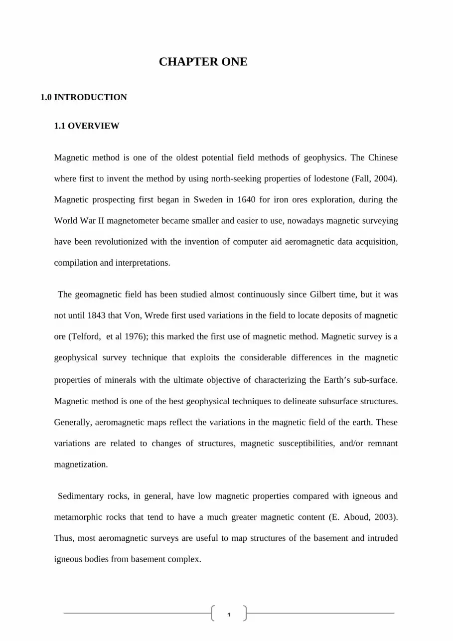
Magnetic method is one of the oldest potential field methods of geophysics. The Chinese

where first to invent the method by using north-seeking properties of lodestone (Fall, 2004).

Magnetic prospecting first began in Sweden in 1640 for iron ores exploration, during the

World War II magnetometer became smaller and easier to use, nowadays magnetic surveying

have been revolutionized with the invention of computer aid aeromagnetic data acquisition,

compilation and interpretations.

The geomagnetic field has been studied almost continuously since Gilbert time, but it was

not until 1843 that Von, Wrede first used variations in the field to locate deposits of magnetic

ore (Telford, et al 1976); this marked the first use of magnetic method. Magnetic survey is a

geophysical survey technique that exploits the considerable differences in the magnetic

properties of minerals with the ultimate objective of characterizing the Earth’s sub-surface.

Magnetic method is one of the best geophysical techniques to delineate subsurface structures.

Generally, aeromagnetic maps reflect the variations in the magnetic field of the earth. These

variations are related to changes of structures, magnetic susceptibilities, and/or remnant

magnetization.

Sedimentary rocks, in general, have low magnetic properties compared with igneous and

metamorphic rocks that tend to have a much greater magnetic content (E. Aboud, 2003).

Thus, most aeromagnetic surveys are useful to map structures of the basement and intruded

igneous bodies from basement complex.

2

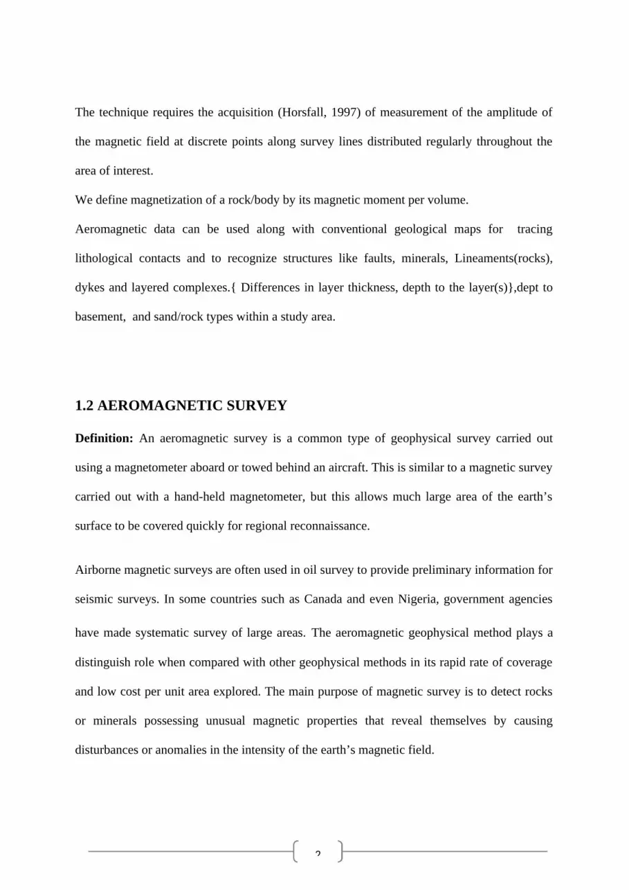
The technique requires the acquisition (Horsfall, 1997) of measurement of the amplitude of

the magnetic field at discrete points along survey lines distributed regularly throughout the

area of interest.

We define magnetization of a rock/body by its magnetic moment per volume.

Aeromagnetic data can be used along with conventional geological maps for tracing

lithological contacts and to recognize structures like faults, minerals, Lineaments(rocks),

dykes and layered complexes.{ Differences in layer thickness, depth to the layer(s)},dept to

basement, and sand/rock types within a study area.

1.2 AEROMAGNETIC SURVEY

Definition: An aeromagnetic survey is a common type of geophysical survey carried out

using a magnetometer aboard or towed behind an aircraft. This is similar to a magnetic survey

carried out with a hand-held magnetometer, but this allows much large area of the earth’s

surface to be covered quickly for regional reconnaissance.

Airborne magnetic surveys are often used in oil survey to provide preliminary information for

seismic surveys. In some countries such as Canada and even Nigeria, government agencies

have made systematic survey of large areas. The aeromagnetic geophysical method plays a

distinguish role when compared with other geophysical methods in its rapid rate of coverage

and low cost per unit area explored. The main purpose of magnetic survey is to detect rocks

or minerals possessing unusual magnetic properties that reveal themselves by causing

disturbances or anomalies in the intensity of the earth’s magnetic field.

3

The significance of aeromagnetic survey method in solving geologic and geologic related

problems cannot be over emphasized, this attributed to magnetic minerals being present in

(almost) all rock types and magnetic survey instruments can measure tiny magnetic signals

from these rock types.

Figure1.1: This shows a magnetometer towed by a helicopter for

geomagnetic data acquisition

The survey generally involves making series of parallel runs at a constant height and interval

of anywhere from a hundred meters to several kilometres (km). The plane is a source of

magnetism, so sensors are either mounted on a boom or towed behind on a cable.

There are other methods in geomagnetic prospecting, such as: Ground Based, ship borne,

spacecraft magnetic methods.

4

1.3 MAGNETISM OF THE EARTH

The geomagnetic field is composed of three main parts (Telford et al., 1976):

Figure 1.2: Magnetic Field Of The Earth

(Www.Earthexplorer.Com/Earthsfield).

1.)The main field, which varies relatively slowly and is of the internal origin. Spherical

harmonic analysis of the observed magnetic field shows that over 99% is due to sources

inside the Earth. The present theory is that the main field is caused by convection current of

conducting materials circulating in the liquid outer core (which extends from depth of 2,800

to 5,000 km). The earth’s core is assumed to be a mixture of Iron and Nickel, both are good

conductors.

5

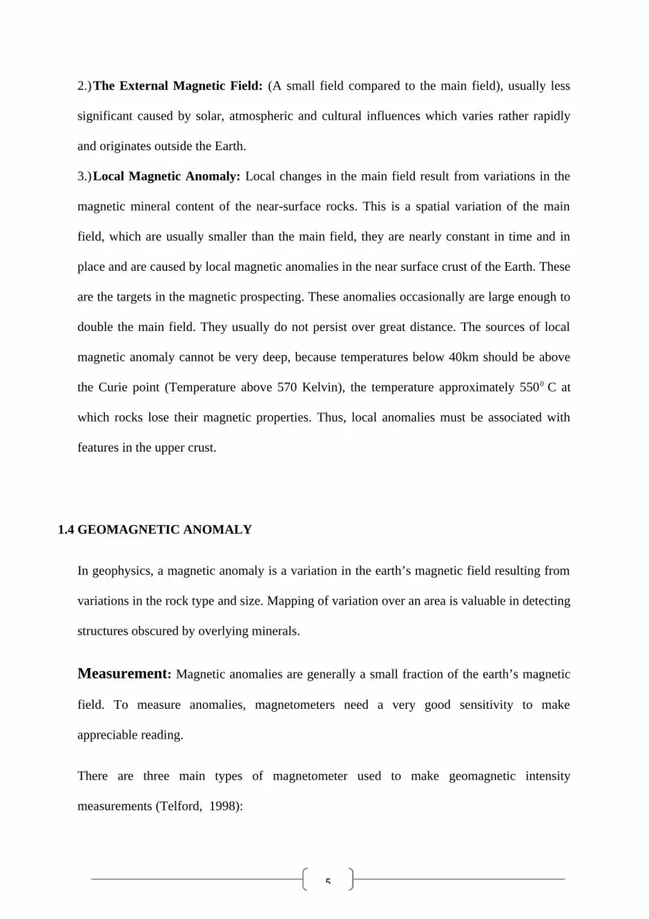
2.)The External Magnetic Field: (A small field compared to the main field), usually less

significant caused by solar, atmospheric and cultural influences which varies rather rapidly

and originates outside the Earth.

3.)Local Magnetic Anomaly: Local changes in the main field result from variations in the

magnetic mineral content of the near-surface rocks. This is a spatial variation of the main

field, which are usually smaller than the main field, they are nearly constant in time and in

place and are caused by local magnetic anomalies in the near surface crust of the Earth. These

are the targets in the magnetic prospecting. These anomalies occasionally are large enough to

double the main field. They usually do not persist over great distance. The sources of local

magnetic anomaly cannot be very deep, because temperatures below 40km should be above

the Curie point (Temperature above 570 Kelvin), the temperature approximately 5500 C at

which rocks lose their magnetic properties. Thus, local anomalies must be associated with

features in the upper crust.

1.4 GEOMAGNETIC ANOMALY

In geophysics, a magnetic anomaly is a variation in the earth’s magnetic field resulting from

variations in the rock type and size. Mapping of variation over an area is valuable in detecting

structures obscured by overlying minerals.

Measurement: Magnetic anomalies are generally a small fraction of the earth’s magnetic

field. To measure anomalies, magnetometers need a very good sensitivity to make

appreciable reading.

There are three main types of magnetometer used to make geomagnetic intensity

measurements (Telford, 1998):

6

1. Caesium Vapour Magnetometer,

Figure 1.2: A Caesium Vapour Magnetometer

1. The Proton Magnetometer, measure the strength of the field but not its direction, so it does

not need to be oriented. It is used in most ground surveys except the boreholes and high-

resolution gradiometer survey.

2. Optical Pumped Magnetometer, uses alkali gases (most commonly rubidium and caesium)

have high sample rate sensitivity of 0.001 or less, but are more expensive compared to other

types of magnetometers. They are used on satellites and in most

aeromagnetic survey.

7

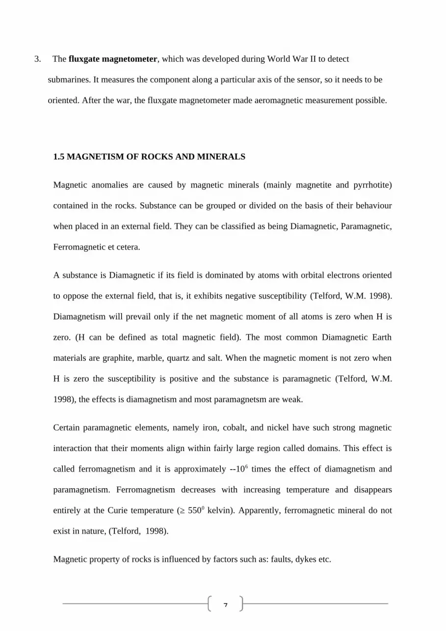
3. The fluxgate magnetometer, which was developed during World War II to detect

submarines. It measures the component along a particular axis of the sensor, so it needs to be

oriented. After the war, the fluxgate magnetometer made aeromagnetic measurement possible.

1.5 MAGNETISM OF ROCKS AND MINERALS

Magnetic anomalies are caused by magnetic minerals (mainly magnetite and pyrrhotite)

contained in the rocks. Substance can be grouped or divided on the basis of their behaviour

when placed in an external field. They can be classified as being Diamagnetic, Paramagnetic,

Ferromagnetic et cetera.

A substance is Diamagnetic if its field is dominated by atoms with orbital electrons oriented

to oppose the external field, that is, it exhibits negative susceptibility (Telford, W.M. 1998).

Diamagnetism will prevail only if the net magnetic moment of all atoms is zero when H is

zero. (H can be defined as total magnetic field). The most common Diamagnetic Earth

materials are graphite, marble, quartz and salt. When the magnetic moment is not zero when

H is zero the susceptibility is positive and the substance is paramagnetic (Telford, W.M.

1998), the effects is diamagnetism and most paramagnetsm are weak.

Certain paramagnetic elements, namely iron, cobalt, and nickel have such strong magnetic

interaction that their moments align within fairly large region called domains. This effect is

called ferromagnetism and it is approximately --106 times the effect of diamagnetism and

paramagnetism. Ferromagnetism decreases with increasing temperature and disappears

entirely at the Curie temperature (≥ 5500 kelvin). Apparently, ferromagnetic mineral do not

exist in nature, (Telford, 1998).

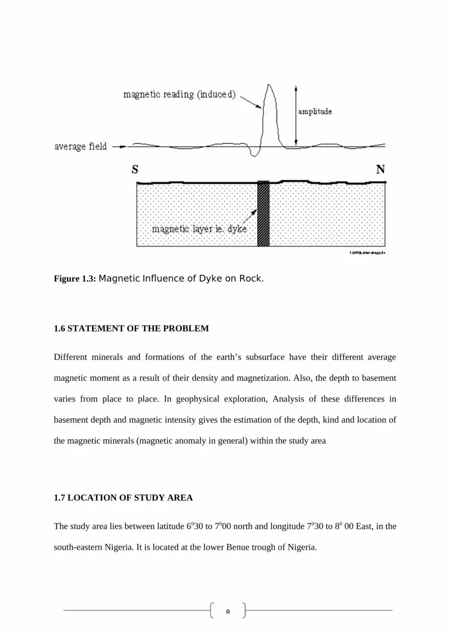
Magnetic property of rocks is influenced by factors such as: faults, dykes etc.

8

Figure 1.3: Magnetic Influence of Dyke on Rock.

1.6 STATEMENT OF THE PROBLEM

Different minerals and formations of the earth’s subsurface have their different average

magnetic moment as a result of their density and magnetization. Also, the depth to basement

varies from place to place. In geophysical exploration, Analysis of these differences in

basement depth and magnetic intensity gives the estimation of the depth, kind and location of

the magnetic minerals (magnetic anomaly in general) within the study area

1.7 LOCATION OF STUDY AREA

The study area lies between latitude 6030 to 7000 north and longitude 7030 to 80 00 East, in the

south-eastern Nigeria. It is located at the lower Benue trough of Nigeria.

9

1.8 SCOPE OF THE STUDY

The scope of this work is to collect and Interpret Aeromagnetic data of sheet_288 (Igunmale),

for delineation magnetic anomalies and depth to magnetic sources in the area.

1.9 AIM AND OBJECTIVES

The aim of this study is to delineate the magnetic sources along Enugu and some part of

Ebonyi using aeromagnetic data.

The objectives of this study are:

Determine magnetic anomalies in the study area.

To determine the thickness of the sediment (depth to basement) in the study area.

And to map basement faults and basic igneous intrusive.es

1.10 JUSTIFICATION OF THE STUDY

In order to delineate the mineral prospect of your area or a particular area, it is very necessary

to undertake such of this research, which showcases the mineral deposits, hydrocarbon

prospect and their respective locations within the study area.

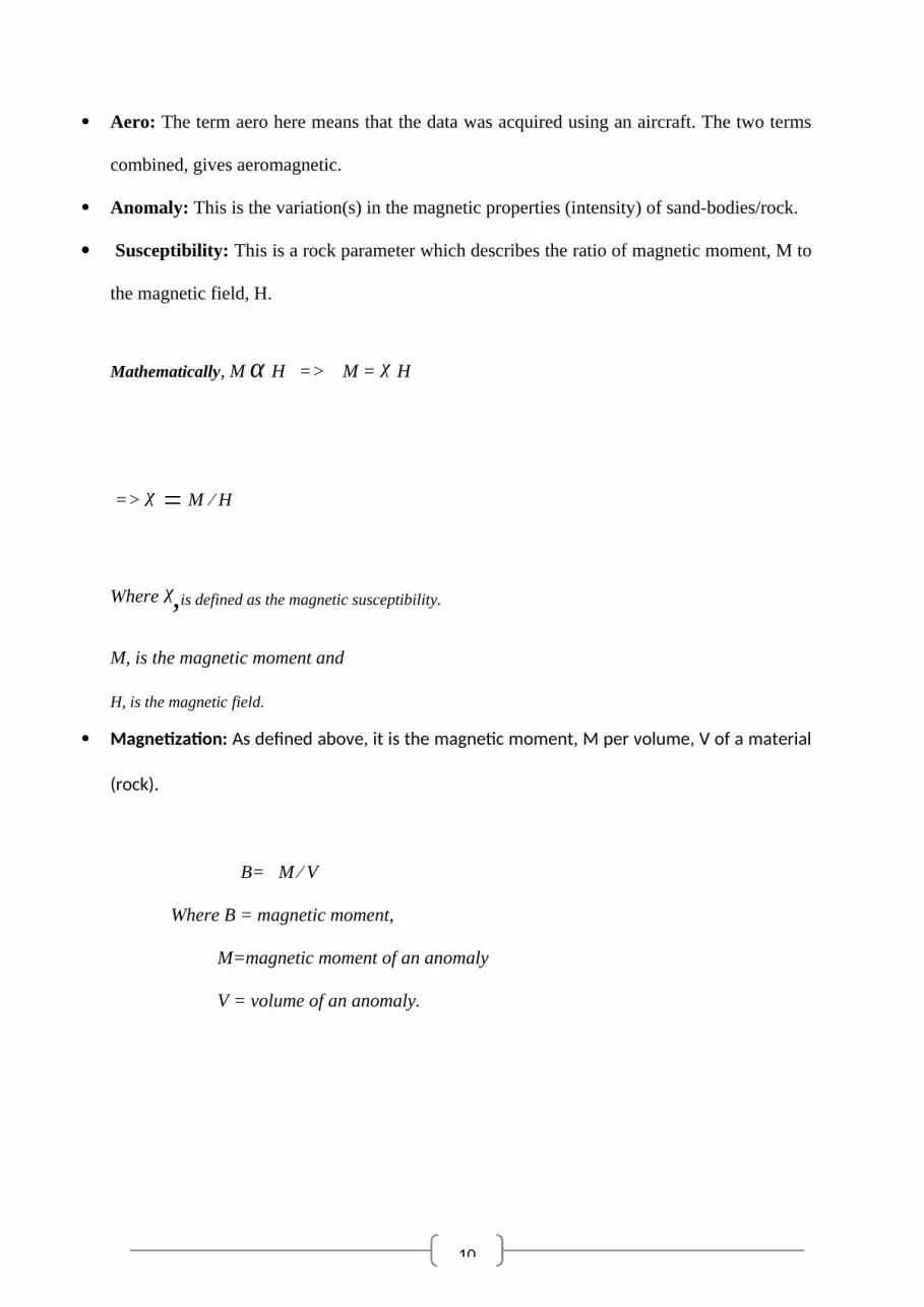
1.12 DEFINITION OF SOME TERMS USED

Magnetics: This is defined by the magnetic properties of sand bodies (creation of magnetic

field-repulsion and attraction).

10

Aero: The term aero here means that the data was acquired using an aircraft. The two terms

combined, gives aeromagnetic.

Anomaly: This is the variation(s) in the magnetic properties (intensity) of sand-bodies/rock.

Susceptibility: This is a rock parameter which describes the ratio of magnetic moment, M to

the magnetic field, H.

Mathematically, M α H =˃ M = ᵡ H

=˃ ᵡ = M ∕ H

Where ᵡ,is defined as the magnetic susceptibility.

M, is the magnetic moment and

H, is the magnetic field.

Magnetization: As defined above, it is the magnetic moment, M per volume, V of a material

(rock).

B= M ∕ V

Where B = magnetic moment,

M=magnetic moment of an anomaly

V = volume of an anomaly.

11

CHAPTER TWO

2.0 HISTORY AND GEOLOGICAL BACKGROUND

2.1 ORIGIN OF MAGNETIC SURVEY

The history of geomagnetism is concerned with the history of the study of Earth’s magnetic

field. It compasses the history of navigation using compasses, Studies of the prehistoric

magnetic field (archeomagnetism and paleomagnetism), and applications to plate tectonics.

Magnetism has been known since prehistory, but knowledge of the earth’s field developed

slowly. The horizontal direction of the earth’s field was first measured in the fourth century

BC but the vertical direction was not measured until 1544 AD and the intensity was first

measured in 1791.

At first, compasses were thought to point towards locations in the heavens, then towards

magnetic mountains. A modern experimental approach to understanding the earth’s field

began with de magnete, a book published by William Gilbert (1600). His experiment with a

magnetic model of the earth convinced him that the earth itself is a large magnet.

2.2 EARLY IDEAS OF MAGNETISM

The study of the earth’s magnetism is the oldest branch of geophysics. It has been studied for

more than three centuries that the earth behaves as a large and somewhat irregular magnet.

12

Sir William Gilbert (1540-1603) made the first scientific investigation of the terrestrial

magnetism, (Telford, W.M. 1998). He recorded in de Magnete that knowledge of the north-

seeking property of a magnetic splinter (a lodestone or leading stone) was brought to Europe

from China by Marco polo. Gilbert showed that the earth’s magnetic field was roughly

equivalent to that of a permanent magnet lying in a general north-south direction near the

earth’s rotational axis.

Karl Frederick Gauss made extensive studies of the Earth’s magnetic field from about 1830

to 1842, and most of his conclusions are still valid. He concluded from mathematical analysis

that; the magnetic field was entirely due to a source within the Earth rather than outside it,

and he noted a probable connection to the Earth’s rotation because the axis of the dipole that

accounts for most of the field is not far from the Earth’s rotational axis.

Von Wrede 1843 first used the variations (anomaly) in the field to locate deposits of

magnetic ore. The publication, in 1879, The examination Of Iron Ore Deposits By Magnetic

Measurement, by Thaleʹn marked the first use of the magnetic method.

Until the late 1940s, magnetic field measurements mostly were made with a magnetic balance

which measured only the vertical components of the Earth’s field.

2.3 LITERATURE REVIEW

The Benue Trough was formed by rifting of the central West African basement, beginning

at the start of the Cretaceous period. At first, the trough accumulated sediments deposited by

rivers and lakes. During the Late Early to Middle Cretaceous, the basin subsided rapidly and

was covered by the sea. Sea floor sediment accumulated, especially in the southern

Abakiliki Rift, under oxygen-deficient bottom conditions. In the Upper Cretaceous, the

13

Benue Trough probably formed the main link between the Gulf of Guinea and the Tethys

Ocean (predecessor of the Mediterranean Sea) via the Chad and Iullemmeden Basins.

Towards the end of this period the basin rose above sea level, and extensive coal forming

swamps developed, particularly in the Anambra Basin. The trough is estimated to contain

5,000 m of Cretaceous sediments and volcanic rocks.

Ofoegbu (1984), working in the lower Benue Trough found the thickness of sediments to

vary betwecn 0.5 and 7km. Estimates of the thickness of sedimentary rocks in the Benue

'Trough obtained from the interpretation of magnetic anomalies agree fairly with those

obtained through the analysis of the gravity field.

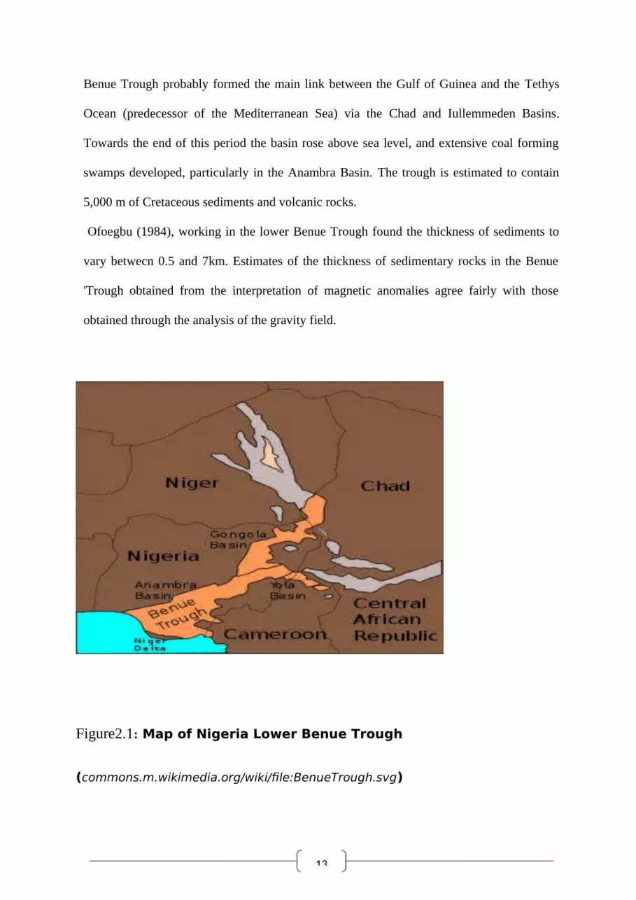
Figure2.1: Map of Nigeria Lower Benue Trough

(commons.m.wikimedia.org/wiki/file:BenueTrough.svg)

14

Onwuemesi (1998), used One-dimensional spectral analysis of aeromagnetic data over the

Anambra Basin, which is a subsidiary depression within the Benue Trough of Nigeria, to map

the sedimentary thickness variations and the Curie temperature isotherm. He concluded that

the Sedimentary thickness (=depth to the basement) varies between 0.9 and 5.6 km, while

depth to the Curie temperature isotherm varies between 16 and 30 km below the mean sea

level. The result also shows that the Curie temperature isotherm within the basin is not a

horizontal level surface, but is undulating, and the geothermal gradients associated with it

range between 20 and 35 °C/km.

Many other workers have analysed the aeromagnetic anomalies over igneous intrusions in the

lower parts of the Benue Trough. In 1986, Ofoegbu also transformed several aeromagnetic

profiles over the Benue Trough to the corresponding pseudo gravimetric profiles using the

equivalent layer method. A joint analysis of the magnetic, gravity and pseudo gravimetric

anomaly profiles confirmed that:

i. The short wavelength anomalies on the aeromagnetic profiles are caused by variation in

magnetization due to existence of very thin intrusions occurring at shallow depths.

ii. The medium and long wavelength anomalies on the aeromagnetic and pseudogravimetric

profiles are due to magnetization from deeply scaled intrusive bodies of asthenospheric

origin.

iii.

In addition to gravity and magnetic methods, other geophysical techniques have been applied

in the investigation for structures and economic resources in the lower Benue Trough.

15

Oil exploration activities have been going on for a long time in parts of the lower Benue

Trough, the Gongola arm and the Chad Basin. The seismic reflection method has been, used

extensively in these studies, but as is usual with such data, much of it is largely unpublished

and remains the property of the Nigerian National Petroleum Company [NNPC) or of the

company that acquires them. Oil was first discovered in the Anambra Basin in the Anambra

River-1 well (at Enugu Out) in 1967 by Safrap (now Elf Nigeria Limited), but since then,

despite large sums of money spent in acquiring more seismic data during the 1975-1985

period, no other significant discovery has been made. However, more information on the

basement morphology, geothermal gradient variations, heat flow and subsidence history of

the area has emerged from these studies (Onuoha, 1985; Onuoha and Ekine, 1988).

Several workers (Hoque and Ezepue, (1977); Nwajide (1979); Nwajide and Hoque, (1985);

Ibe and Akaolisa (2010) have studied the petrology of many of the sandstone units of lower

Benue Trough. The sandstone petrology shows a distinct basin-wide improvement in

compositional maturity of sandstone both in time and space.

Some mining companies in their search for uranium and other associated deposits in the

Benue Trough have also carried out Radiometry measurements. On the basis of these surveys,

a background radioactivity of 100-300 c.p.s, has been established for the Benue Trough

(Ajakaiye, 1981) with the cretaceous sediments having values of between 50-150 c.p.s. Local

occurrence of values as high as 500-20,000c.p.s. have been interpreted and indicating the

occurrence of rocks rich in uranium, potassium and thorium (Ajakaiye, I981).

The magnetic field over the Benue Trough is made up of contributions from short, medium

and long wavelength anomalies. The basement complex bordering the trough and outcropping

in some places within it is characterized by short wavelength anomalies, which arise from

16

either susceptibility changes within the basement, near surface intrusives in the basement or

their combined effects (Ofoegbu, 1984c). Ajakaiye (1981) and Ofoegbu (1984), analysed the

small amplitude, medium wavelength anomalies of general regular shapes and gentle

gradients on which are superimposed several locally occurring high frequency anomalies.

This characterizes the trough in terms of deep lying basement and highly magnetic intrusive

bodies either within the sediments or basement or both.

Nwogbo, (1997) mapped shallow magnetic sources in the Upper Benue Basin of Nigeria in

order to determine their structures, distribution and location at depths by employing

techniques based on the Fourier analysis of aeromagnetic fields. Spectral depth determination

to magnetic source in the region yield two distinct magnetic depth ranges. Mean depth values

in the range of 2.00-2.62km have been shown to correspond generally to the fine basement

surface, and indicates clearly the magnitude of the undulation of the basement topography in

the region. Mean depth to shallower magnetic sources in the region vary between 0.07 -

0.63km and may be attributed to shallow intrusive materials or some near surface basement

rocks. Some deeper intrusives occur within the basement at depths of up to 2.45km. The

numerous shallow intrusions in the basin however occur substantially outside the basement.

Depth results from the investigated blocks indicated that mean depth to the basement surface

in the region show a gentle general southward increase with mean depth values ranging from

2km in the northern area to 2.62km in the south.

2.4 GEOLOGY OF THE STUDY AREA

The study area lies between latitude 6030 to 7000 north and longitude 7030 to 80 00, in the

south-eastern Nigeria. It is located at the lower Benue trough of Nigeria, with the altitude of

350m above mean sea level .The study area consists of three major geologic formations

17

(Reyment, 1965); the Mamu, Ajali and Nsukka formations. The Mamu formation, previously

known as lower coal measures (Reyment, 1965), consists of fine-medium grained, white to

grey sandstones, shaly sandstones, sandy shales, grey mudstones, shales and coal seams. The

thickness is about 450m and it conformably underlies the Ajali formation. The Ajali

formation, also known as false bedded sandstone, consist of thick friable, poorly sorted

sandstones, typically white in colour but sometimes iron-stained. The thickness averages 300

m and is often overlain by considerable thickness of red earth, which consists of red, earthy

sands, formed by the weathering and ferruginisation of the formation. The Nsukka formation,

previously known as the upper coal measures (Reyment, 1965), lies conformably on the Ajali

sandstone. The lithology is very similar to that of Manu formation and consists of an

alternating succession of sandstone, dark shale and sandy shale, with thin coal seams at

various horizons.

2.5.1 ADVANTAGES OF AEROMAGNETIC TO OTHER MAGNETIC METHODS

(Airborne Magnetic)

Airborne surveying is extremely attractive for reconnaissance because of low cost per

kilometre and high speed (Telford, 1998). The speed not only reduces the cost, but also

decreases the effect of time variation of magnetic field.

18

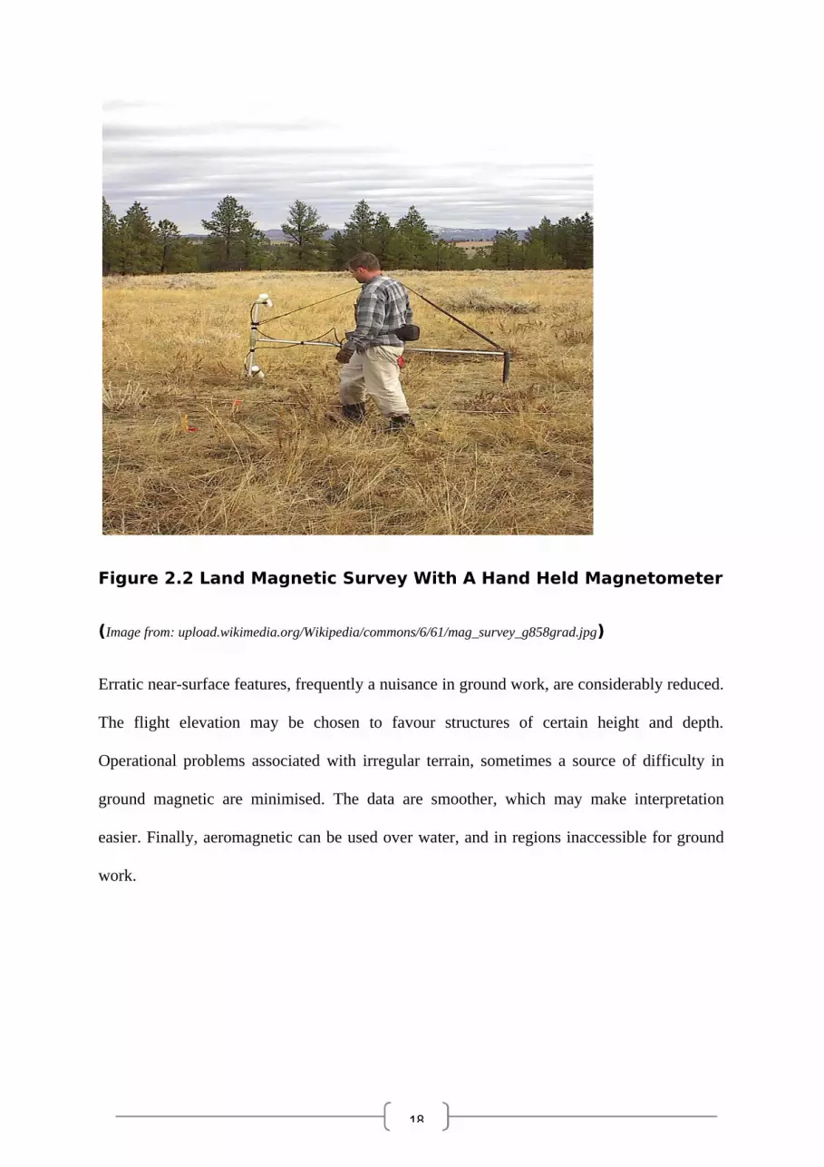
Figure 2.2 Land Magnetic Survey With A Hand Held Magnetometer

(Image from: upload.wikimedia.org/Wikipedia/commons/6/61/mag_survey_g858grad.jpg)

Erratic near-surface features, frequently a nuisance in ground work, are considerably reduced.

The flight elevation may be chosen to favour structures of certain height and depth.

Operational problems associated with irregular terrain, sometimes a source of difficulty in

ground magnetic are minimised. The data are smoother, which may make interpretation

easier. Finally, aeromagnetic can be used over water, and in regions inaccessible for ground

work.

19

2.5.2 DISADVANTAGE OF AEROMAGNETIC SURVEY

The disadvantage in aeromagnetic (airborne) apply mainly to mineral exploration (Telford,

W.M. 1998). The cost for surveying small area may be prohibited. The attenuations of near-

surface features apt to be the survey objective, becomes limitations in mineral search.

Other method in geomagnetic survey include; Ship-borne Magnetic Survey: In ship-borne

magnetic survey, a magnetometer is towed a few hundred meters behind the ship in a device

called fish. The sensor is kept at a constant depth of about 15m.

CHAPTER THREE

3.0 MATERIALS AND METHORDS

3.1 METHODS

20

The procedures employed in this research include:

1. Production of Total Magnetic Intensity (TMI) map of the study area in colour aggregate

using Oasis montaj software.

2. Computing the First Vertical Derivative of TMI

3. Computing the Horizontal Derivatives in the X,Y and Z directionsn n… n

4. Computing the Standard Euler Deconvolution equation using the Horizontal Derivatives

(DX, DY and DZ) to compute the Analytical Signal. This was done using Oasis montaj.

5. Computation of the source parameter imaging map of the study area.

6. Regional and Residual separation.

3.2 DATA CORRECTION

The primary data was collected at the Nigeria Geological Survey Agency, Abuja. Some of

the data corrections were made by the Agency.

`

Data reduction and processing involves series of step taken to remove both signal and

spurious noise from the data that are not related to the geology of the earth’s (upper) crust.

This process thereby prepares the dataset for interpretation by reducing the data to certain

signal relevant to the task.

To make accurate magnetic anomaly maps, temporal changes in the earth’s field during the

period of the survey must be considered. Normal changes during a day, sometimes called

diurnal drift, are a few tens of nT but changes of hundreds or thousands of nT may occur over

a few hours during magnetic storms. During severe magnetic storms, which occur

21

infrequently, magnetic surveys should not be made. The correction for diurnal drift can be

made by repeat measurements of a base station at frequent intervals. The measurements at

field stations are then corrected for temporal variations by assuming a linear change of the

field between repeat base station readings. Continuously recording magnetometers can also

be used at fixed base sites to monitor the temporal changes. If time is accurately recorded at

both base site and field location, the field data can be corrected by subtraction of the

variations at the base site.

Removal of IGRF: The Geomagnetic Reference Field Removal removes the strong

influence of the earth’s main field on the survey data. This is done because the main field is

dominantly influenced by dynamo action in the core and not related to the geology of the

(upper) crust. This achieved by subtracting a model of the main field from the survey data.

The IGRF for Nigeria is 32000nT (NGSA Abuja). The Australian or International

Geomagnetic Reference Field (AGRF or IGRF) is used for this purpose. This model accounts

for both the spatial and long period (>3years) temporal variation (secular variation) of the

main field (Lowis, 2000).

Once coefficients are available for the IGRF at the epoch of the survey it is possible to

calculate a value for the IGRF at every point where an airborne magnetometer reading is

made in a survey and subtract that value from the observed value to give the 'anomaly'

defined by the departure of the observed field from the global model (Reeves, 2005).

There are no significant consequences for the accuracy of processing if this gradient is

removed at the beginning or at the end of the data reduction sequence.

22

Magnetic Compensation: This removes the influence of the magnetic signature (remanent,

induced and electrical) of the aircraft on the recorded data (Ross, 2002). This is done on the

real time on-board the aircraft.

Reduction to Equator: This is a kind correction in the data processing with the software

were the viewed as if it was recorded from the earth’s equator. But in the case of Nigeria, we

are already at the earth’s equator. So the reduce to equator process is not required.

After all corrections have been made, magnetic survey data are usually displayed as

individual profiles contour maps (Figure 3.1). Identification of anomalies caused by cultural

features, such as railroads, pipelines, and bridges is commonly made using field observations

and maps showing such features.

3.3 SURVEY SPECIFICATIONS

Magnetic Data Recording Interval 0.1 seconds

Radiometric Data Recording Interval 1 second

Sensor Mean Terrain Clearance 80 meter

Flight Line Spacing 500 meters

Tie Line Spacing 2000 meters

Flight Line Trend 035 degrees

Tie Line Trend 125 degrees

23

3.4 EQUIPMENT SPECIFICATIONS

Magnetometers 3 x Scintrex CS3 Cesium Vapour

Data Acquisition System FASDAS

Magnetic Counter FASDAS

Radar Altimeter KING KR405/KING KR405B

Barometric Altimeter ENVIRO BARO/DIGIQUARTZ

Radiometric Crystal Volume-Down 32litres

Radiometric Crystal Volume-Up 8litres

Radiometric Crystals GPX 1024/256

Radiometric Data Acquisition GR-820-3

Aircraft Supplied By Fugro Airborne Surveys

Aircraft Cessna Caravan 208B ZS-FSA

Aircraft Cessna Caravan 208 ZS-MSJ

Aircraft Cessna 406 ZS-SSC

Survey Date 07/12/06 - 31/05/07

Data Acquisition by Fugro Airborne Surveys

Data Processing by Fugro Airborne Surveys.

24

3.5 INTERPRETATION MAPS

3.5.1 The Total Magnetic Field Intensity

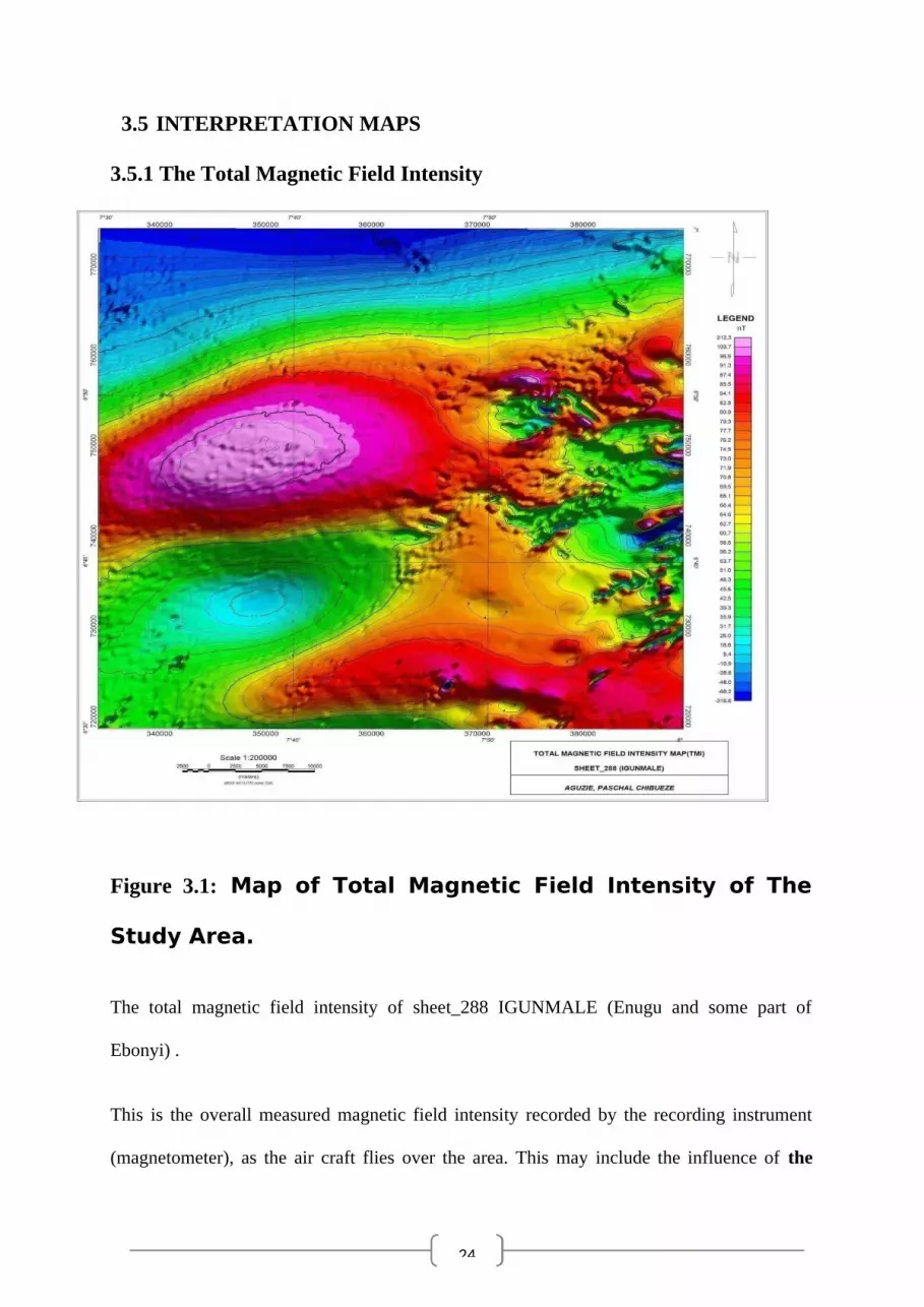
Figure 3.1: Map of Total Magnetic Field Intensity of The

Study Area.

The total magnetic field intensity of sheet_288 IGUNMALE (Enugu and some part of

Ebonyi) .

This is the overall measured magnetic field intensity recorded by the recording instrument

(magnetometer), as the air craft flies over the area. This may include the influence of the

25

earth main field, which varies relatively slowly and is of the internal origin and the Local

Magnetic Anomaly from variations in the magnetic mineral content of the near-surface

rocks.

3.5.2 SOURSE PARAMETER IMAGING (SPI)

Figure 3.2: Source Parameter Imaging Map 288_IGUNMALE

26

The SPI (SPI- Stands for Source Parameter Imaging) method is a technique using an

extension of the complex analytical signal to estimate magnetic depths using the Directional

derivatives and Tilt (Thurston and Smith, 1997). Oasis Montaj SPI menu was used to process

the data. The d/dx, d/dy, d/dz was computed manually using Magmap. Then SPI grid was

calculated using the derivatives. The directional and tilt derivative was computed in the Oasis

Montaj and SPI depth solutions was generated and gridded to produce the SPI depth map (Fig

3.2).

The basics are that for vertical contacts, the peaks of the local wave number define the inverse

of depth (Adetona A. and Abu M 2013).

The Source Parameter Imaging (SPI) method calculates source parameters from gridded

magnetic data. The method assumes either a 2D sloping contact or a 2.D dipping thin-sheet

model and is based on the complex analytic signal. Solution grids show the edge locations,

depths, dips, and susceptibility contrasts. Image processing of the source-parameter grids

enhances detail and provides maps that facilitate interpretation by no specialists.

. SPI (Thurston and Smith, 1997) is a procedure for automatic calculation of source depths

from gridded magnetic data. The depth solutions are saved in a database. These depth results

are independent of the magnetic inclination and declination, so it is not necessary to use a

pole-reduced input grid.

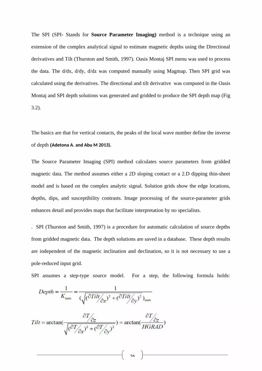
SPI assumes a step-type source model. For a step, the following formula holds:

27

Depth = 1/Kmax,

Where, Kmax is the peak value of the local wave number A over the step source.

K = sqrt( [dA/dx]**2 + [dA/dy]**2 ),

ANALYTICAL SIGNAL

28

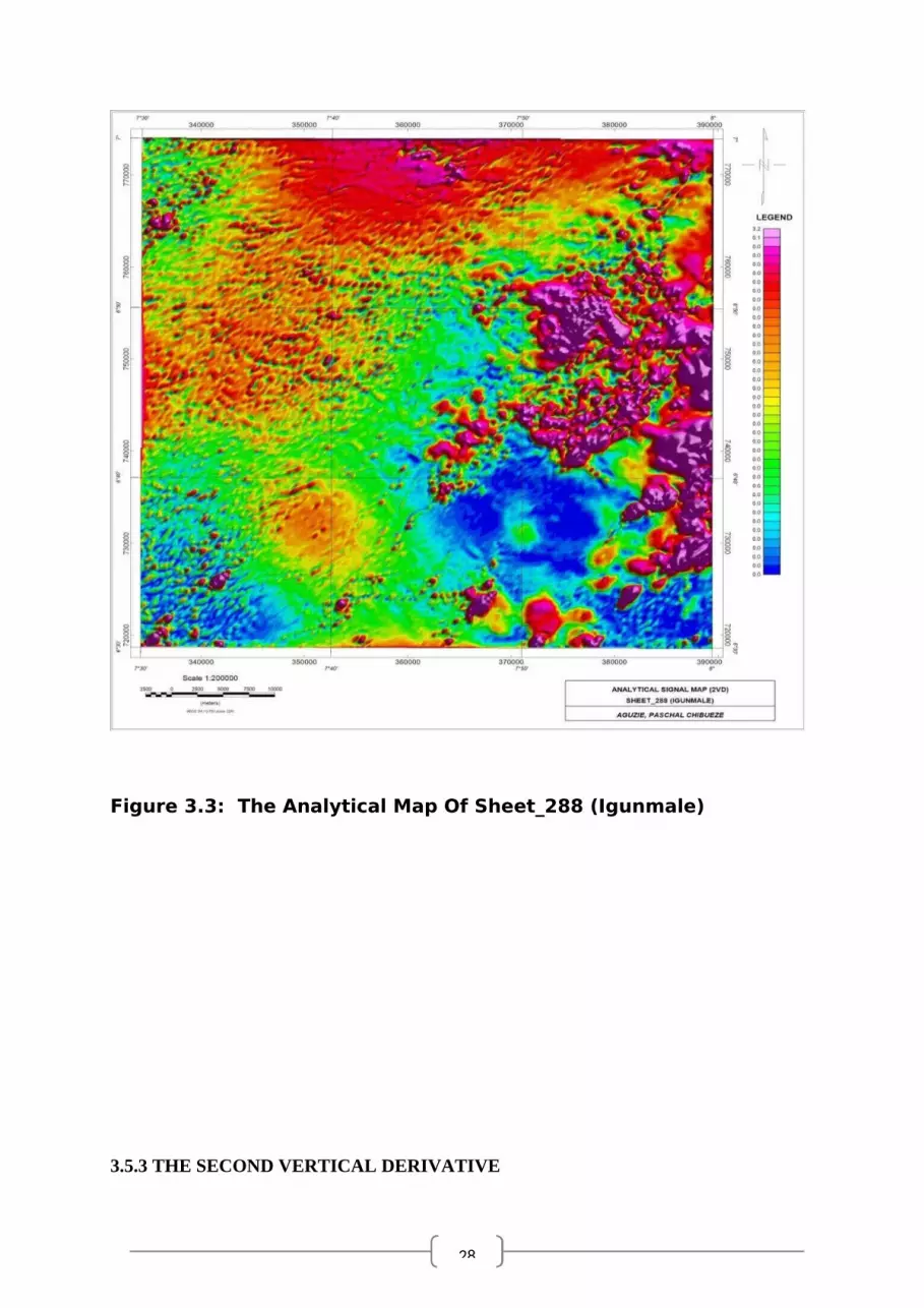
Figure 3.3: The Analytical Map Of Sheet_288 (Igunmale)

3.5.3 THE SECOND VERTICAL DERIVATIVE

29

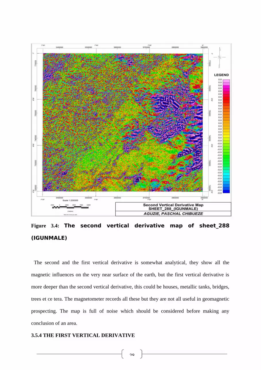
Figure 3.4: The second vertical derivative map of sheet_288

(IGUNMALE)

The second and the first vertical derivative is somewhat analytical, they show all the

magnetic influences on the very near surface of the earth, but the first vertical derivative is

more deeper than the second vertical derivative, this could be houses, metallic tanks, bridges,

trees et ce tera. The magnetometer records all these but they are not all useful in geomagnetic

prospecting. The map is full of noise which should be considered before making any

conclusion of an area.

3.5.4 THE FIRST VERTICAL DERIVATIVE

30

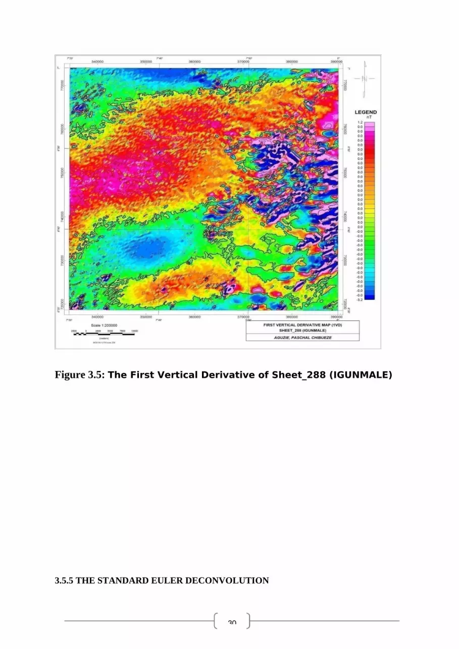
Figure 3.5: The First Vertical Derivative of Sheet_288 (IGUNMALE)

3.5.5 THE STANDARD EULER DECONVOLUTION

31

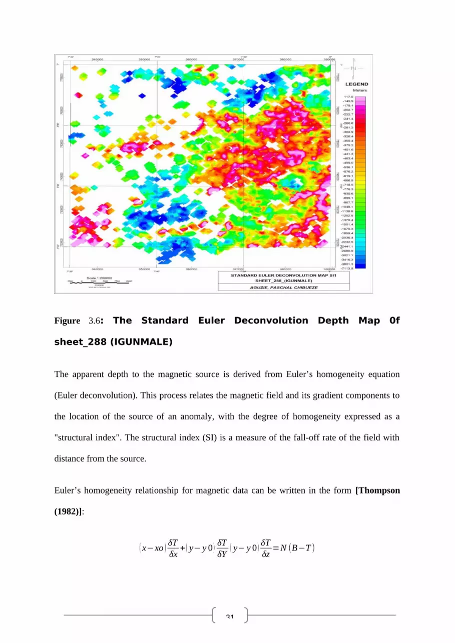
Figure 3.6: The Standard Euler Deconvolution Depth Map 0f

sheet_288 (IGUNMALE)

The apparent depth to the magnetic source is derived from Euler’s homogeneity equation

(Euler deconvolution). This process relates the magnetic field and its gradient components to

the location of the source of an anomaly, with the degree of homogeneity expressed as a

"structural index". The structural index (SI) is a measure of the fall-off rate of the field with

distance from the source.

Euler’s homogeneity relationship for magnetic data can be written in the form [Thompson

(1982)]:

( x−xo ) δTδx

+( y− y 0 ) δTδY

( y− y 0 ) δTδz

=N (B−T )

32

Where: (X0, y0, z0) is the position of the magnetic source whose total field (T) is detected at

(x, y, z,).

B is the regional magnetic field.

N is the measure of the fall-off rate of the magnetic field and may be interpreted as the structural

index (SI).

The Euler deconvolution process is applied at each solution. The method involves setting an

appropriate SI value and using least-squares inversion to solve the equation for an optimum

xo, yo, zo and B. As well, a square window size must be specified which consists of the

number of cells in the gridded dataset to use in the inversion at each selected solution

location. The window is centred on each of the solution locations. All points in the window

are used to solve Euler’s equation for solution depth, inversely weighted by distance from the

centre of the window. The window should be large enough to include each solution anomaly

of interest in the total field magnetic grid, but ideally not large enough to include any adjacent

anomalies.

33

CHAPTER FOUR

4.0 QUANTITATIVE DATA INTERPRETATION /ANALYSIS

4.1 THE TOTAL MAGNETIC INTENSITY

The total magnetic intensity of the study area (sheet 288_IGUNMALE) ranges from

Minimum value of -316.55nT to the Maximum value of 212.26nT and the average value of

51.06nT. The variations in the magnetic intensity is represented by different colours in the

map figure:3.1 and the values for each colour is arranged in the colour legend bar with blue

colour indicating highest magnetic intensity followed by green, yellow, red and Pink colour.

The study area is marked by both high and low magnetic signatures, which could be

attributed to several anomaly factors such as:

(1) Variation in depth and intrusion

(2) Difference in magnetic susceptibility of rocks,

(3) Difference in lithology, and

(4) Dykes and faults

Generally, total magnetic disturbances or anomalies are highly variable in shape and

amplitude; they are almost always asymmetrical, sometimes appear complex even from

simple sources, and usually portray the combined effects of several sources (UNU-GTP and

KenGen, 2007). An infinite number of possible sources can produce a given anomaly, giving

rise to the term ambiguity.

Individual magnetic anomalies - magnetic signatures different from the background- consist

of a high and a low (dipole) compared to the average field. The position and size of the

34

anomaly depend on the position and size of the magnetic body. A change in latitude will also

affect the positioning of anomalies over the magnetic body (UNU-GTP and KenGen, 2007).

This allows the geoscientists to interpret the position of the body which has caused the

anomalous reading. Often however the reading is complicated because of the position of the

body in relation to other rocks, its size, and what happens to the body at depth.

Data are usually displayed in the form of a contour map of the magnetic field as in Figure 1

above, but interpretation is often made on profiles. From these maps and profiles

geoscientists can locate magnetic bodies (even if they are not outcropping at the surface),

interpret the nature of geological boundaries at depth, find faults etc. Using the colour legend

bar, one can also locate the from the map the position of an anomaly with respect to the

coordinates labelled on the gridded map, the position of these anomalies can then be

ascertained using Global Positioning System (GPS) device in the site. Like all contoured

maps, when the lines are close together they represent a steep gradient or change in values.

When lines are widely spaced they represent shallow gradient or slow change in value. A

modern technique is to plot the magnetic data as a colour image (red=high, blue=low and all

the shades in between representing the values in between), (UNU-GTP and KenGen, at

Lake Naivasha, Kenya, 2-17 November, 2007). This gives an image which is easy to read.

When interpreting the aeromagnetic image it is useful to know that magnetite is found in

greater concentrations in igneous and metamorphic rocks. Magnetite can also be weathered or

leached from rocks and re-deposited in other locations, such as faults. In a geothermal

environment, this is a very useful feature as it may indicate the presence of faults, target for

drilling.

35

4.2 FIRST VERTICAL DERIVATIVE MAP SHOWING IDENTIFIED

STRUCTURES.

This is the influence that originates from the shallow subsurface. This is almost like that of

the second vertical derivative, but the noise is reduced as the vertical distance increases

(depth increase).

Mostly the southern and the eastern part of Figure 4 above of the IGUNMALE sheet-288

shows a lot of activity, as they are dotted by mixtures of both high and low magnetic

structures with features that are characteristics of surface to near surface structures such as

outcrops.

4.4 SOURCE PARAMETER IMAGING (SPI)

From the calculations of the source parameter imaging using the Oasis montaj software, the

depth to basement of the area varies between -0.0543 meters and -7.9863 meters, with 11639

data points, the maximum depth value is -0.0543 and the minimum depth value is -7.9863

with average value of -0.5205.

The negative sign means that distance is downwards.

In the figure 3.2 above, the SPI legend shows the variation in depth to basement with colours

which has blue colour indicating deepest to magnetic source followed by green, yellow and

red. Pink colour indicates intrusions.

4.5 THE EULER DECONVOLUTION ANALYSIS

The methods applicable to gridded data have become popular in recent years (Reeves, 2005),

largely on account of their implementation within user-friendly software packages, one of

36

which is known as Euler deconvolution (Reid et al, 1990) and exploits Euler’s inhomogeniety

relation to estimate source depths and positions from the maximum curvature of anomalies

present in an aeromagnetic survey grid. The Euler deconvolution filtering method is a good

method of depth determination geomagnetic processing and interpretation.

Depth to basement of the study area ( sheet 288_Igunmale) , using the Oasis montaj software

ranges between -12.0787km Minimum values to -0.0597km Maximum values with the

average of 0.9553 using the Euler deconvolution depth determination method. The negative

sign in the depth implies, it is bellow the earth surface, any area (as within the south-east

area of the study area) with positive value in the depth legend bar value of the standard

Euler deconvolution map, figure 3.6 above, implies that there is a rock protrusion/intrusive

above the earth level in the study area, blue colour indicating deepest to magnetic source

followed by green, yellow and red, pink colour indicates rock protrusion.

The result was calculated using Oasis montaj by geosoft V6.4.

The legend in Figure 3.5 above shows different colours and their values which represent the

depth to the basement in various positions on the gridded map with global coordinate. This

with the Global Positioning System (GPS) can be used for specific positioning.

37

4.6 QUALITATIVE ANALYSIS

The Regional Magnetic Map

FIGURE 4.1: Upward Continuation Map Of Sheet_288(Igunmale).

38

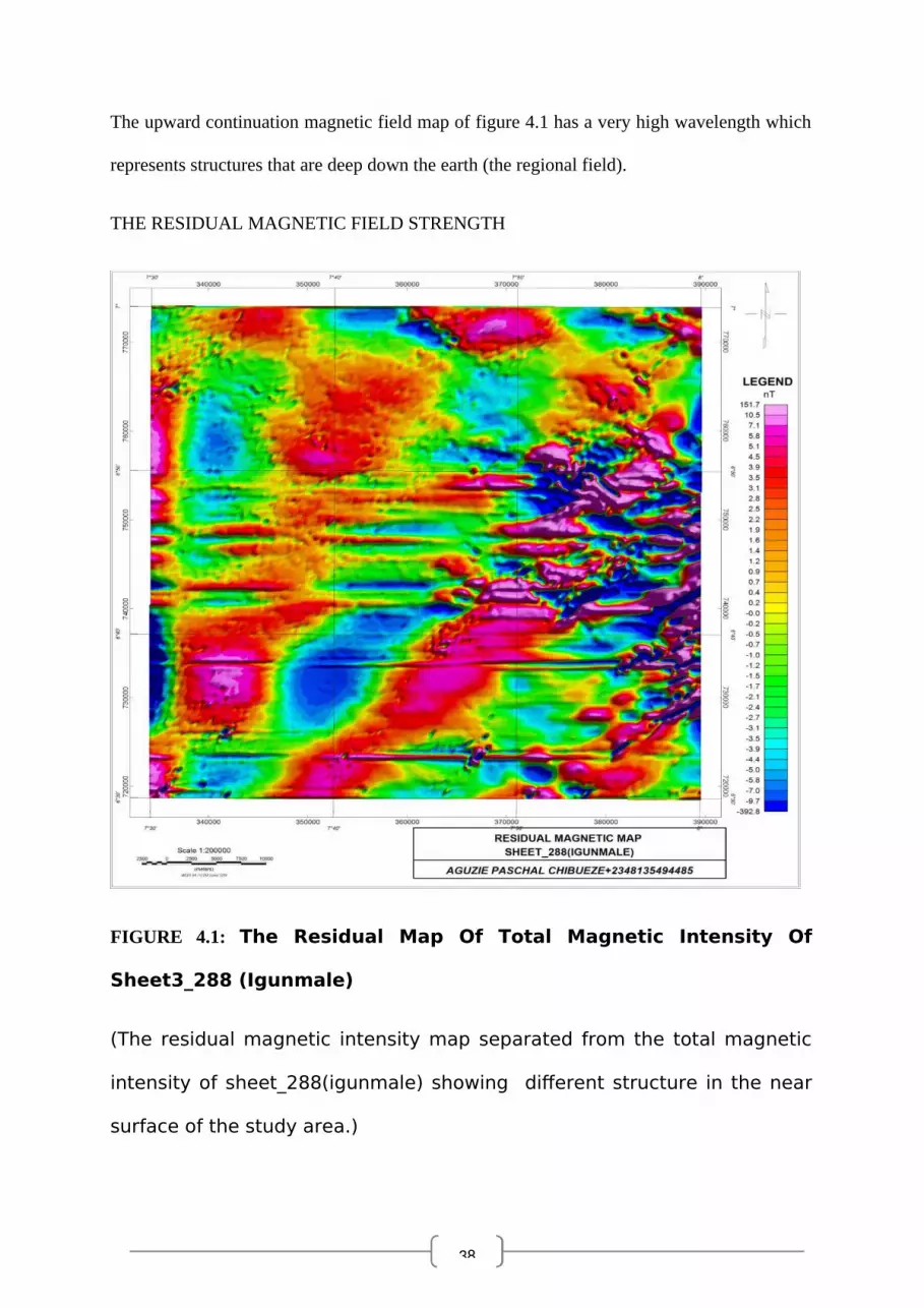
The upward continuation magnetic field map of figure 4.1 has a very high wavelength which

represents structures that are deep down the earth (the regional field).

THE RESIDUAL MAGNETIC FIELD STRENGTH

FIGURE 4.1: The Residual Map Of Total Magnetic Intensity Of

Sheet3_288 (Igunmale)

(The residual magnetic intensity map separated from the total magnetic

intensity of sheet_288(igunmale) showing different structure in the near

surface of the study area.)

39

The residual magnetic field intensity map of the study area (Figure 4.1) shows variations in

magnetic field strength, which is the main magnetic signature in geophysical exploration.

The map showcases structures that are diamagnetic with negative field strength. The

diamagnetic structures could be as a result of sediments. The study area is made up of mainly

a sedimentary bodies and strong magnetic rocks like magnetite and iron stones which may be

responsible for the very high magnetic field strength in the area. From the SPI and the Euler

deconvolution map above Figures 3.2and 3.5 respectively is seen that in their colour legend

bar there are value with positive sign, this is because they are calculated to be protrusion

(rock outgrowth/intrusive). Also in the TMI, Figure 3.1 above, tracing with the colour legend

bar the areas with high magnetic intensity are in agreement with what we have in the residual

magnetic map Figure 4.1(their value are in the range), the little variation there is due to the

earth’s main field influence.

40

CHAPTER FIVE

5.0 SUMMARY

5.1 DISCUSION AND CONCLUSION

The entire area can be divided into two lithology based on the signatures on Figure 4.1 above,

the sedimentary and the basement lithologies. The study area is occupied by shallow base

high frequency short wave anomalies which associated with basement signatures and

predominantly by basement signature which is associated with low magnetic intensity,

causing geomagnetic anomalies.

The qualitative interpretations of the residual map has identified two magnetic source depth;

the low frequency anomaly source depth for deep seated body and the high frequency

anomaly for the shallow seated bodies. The areas of deep seated bodies in the map are

possibly the magnetic basement depth; while the shallower are possibly magmatic intrusions

into the sedimentary basins which are possibly responsible for the mineralization found in the

area.

Analysis showed that the lower Benue Trough is mostly a sedimentary basin and a basement

basin, where the sedimentary sequences have been outlined. The basement sedimentary

boundary is fairly defined from the residual map and the intrusive bodies on the Analytical

Signal Map Fig: 3.3, based on the level of disruption of the field lines at the boundary. The

41

Lower Benue Trough which is genetically related to the entire Benue Trough which itself is

part of the west African Riff Subsystem.

The depth to basement varies between 0.0543 kilometres and 7.9863 kilometres

The earths subsurface have differences in their magnetic force. This is as a result of different

magnetic minerals and soil formations.

5.2 RECOMMENDATION

Subsequent study in the site (study area) as a confirmation should be undertaken in other to

ascertain the result from this work. Undertaking a study to delineate the rock type responsible

for these differences will go a long way in exploration of the mineral and hydrocarbon

prospects within you and understanding ones environment.

42

APPENDIXES

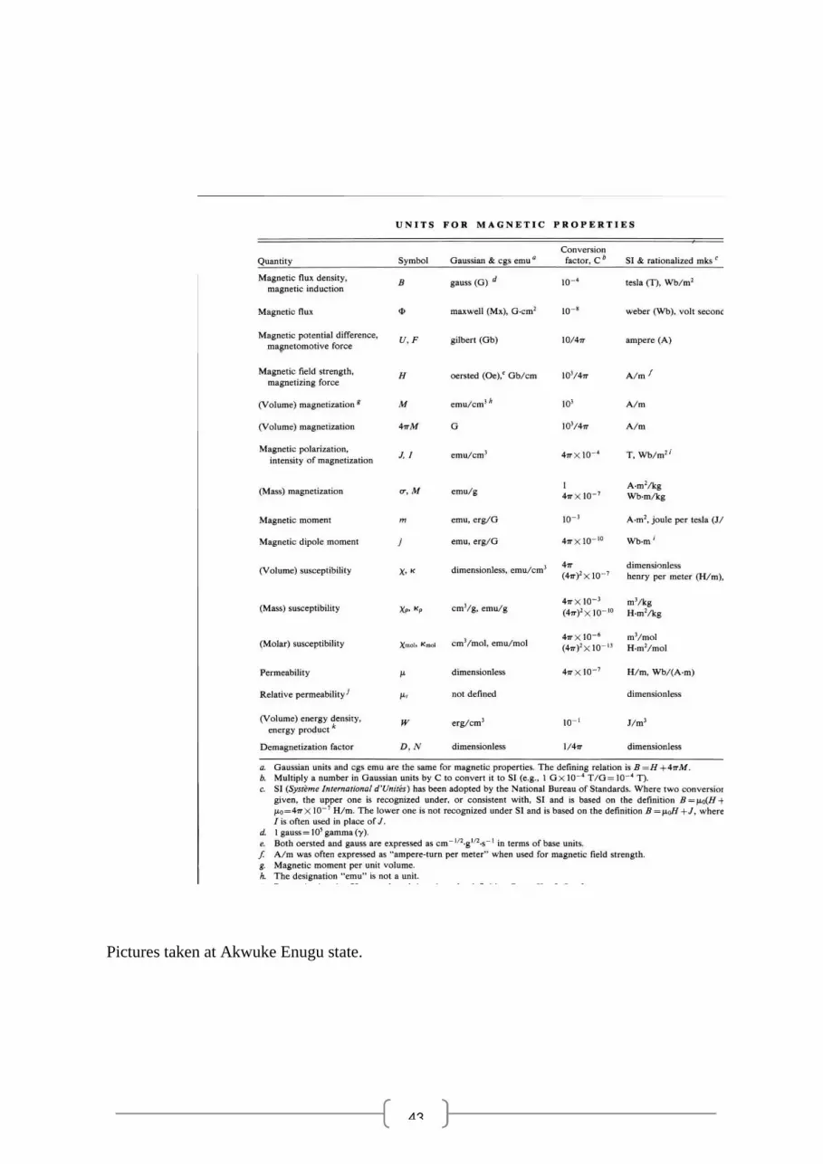
UNITS FOR MAGNETIC PROPERTIES

43

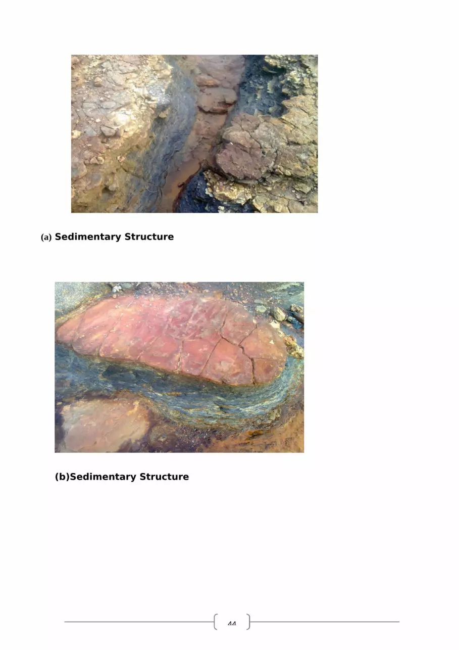
Pictures taken at Akwuke Enugu state.

44

(a) Sedimentary Structure

(b)Sedimentary Structure