Embed Size (px)
Citation preview
Delft University of Technology
A Mass-Conserving Hybrid interface capturing method for geometrically complicateddomains
Raees, Fahim
DOI10.4233/uuid:871b1879-d83c-47cb-9480-1cc3df37e3ebPublication date2016Document VersionFinal published version
Citation (APA)Raees, F. (2016). A Mass-Conserving Hybrid interface capturing method for geometrically complicateddomains. Delft. https://doi.org/10.4233/uuid:871b1879-d83c-47cb-9480-1cc3df37e3eb
Important noteTo cite this publication, please use the final published version (if applicable).Please check the document version above.
CopyrightOther than for strictly personal use, it is not permitted to download, forward or distribute the text or part of it, without the consentof the author(s) and/or copyright holder(s), unless the work is under an open content license such as Creative Commons.
Takedown policyPlease contact us and provide details if you believe this document breaches copyrights.We will remove access to the work immediately and investigate your claim.
This work is downloaded from Delft University of Technology.For technical reasons the number of authors shown on this cover page is limited to a maximum of 10.
A Mass-Conserving hybrid interface capturing
method for geometrically complicated domains
PROEFSCHRIFT
ter verkrijging van de graad van doctoraan de Technische Universiteit Delft,
op gezag van de Rector Magnificus Prof. ir. K.C.A.M. Luyben,voorzitter van het College voor Promoties, in het openbaar te verdedigen
op woensdag 15 juni 2016 om 10:00 uur
door
Fahim RAEESMaster of Science in Applied Mathematics,
University of Karachi, Pakistan
geboren te Karachi, Pakistan.
This dissertation has been approved by the promotor:Prof. dr. ir. C. Vuik
Composition of the doctoral committee:
Rector Magnificus, ChairmanProf. dr. ir. C. Vuik, Promotor, Delft University of TechnologyDr. ir. D. R. Van der Heul, Copromotor, Delft University of Technology
Independent members:
Prof. dr. A.E.P. Veldman, University of GroningenProf. dr. ir. B. Koren, Eindhoven University of TechnologyProf. dr. ir. R.A.W.M. Henkes, Delft University of TechnologyProf. dr. ir. B.J. Boersma, Delft University of TechnologyProf. dr. ir. B.G.M. van Wachem, Imperial College London
The work described in this thesis was financially supported by the NEDUniversity of Engineering and Technology, Karachi, Pakistan and Delft Uni-versity of Technology, Delft, The Netherlands.
A Mass-Conserving hybrid interface capturing method for geometricallycomplicated domains.Dissertation at Delft University of Technology.Copyright c© 2016 by Fahim RaeesISBN 978-94-6186-667-7
To my parents:Raees Hussain & Shahida Parveen

Contents
Summary ix
Samenvatting xii
1 Introduction 1
1.0.1 Modeling immiscible, incompressible two-phase flow 2
1.0.2 Interface capturing and interface tracking methods . 4
1.1 Simulation of two-phase flows in geometrically complex do-mains . . . . . . . . . . . . . . . . . . . . . . . . . . . . . . 6
1.2 Outline of the thesis . . . . . . . . . . . . . . . . . . . . . . 7
2 The Level-Set based interface capturing method 9
2.1 Introduction . . . . . . . . . . . . . . . . . . . . . . . . . . . 9
2.2 The Level-Set method . . . . . . . . . . . . . . . . . . . . . 9
2.3 The Level-Set method for modeling two-phase flow . . . . . 10
2.4 Discontinuous Galerkin discretisation of the Level-Set equation 12
2.4.1 Spatial discretization of the Level-Set equation . . . 13
2.4.2 Temporal Discretisation . . . . . . . . . . . . . . . . 15
2.5 Test Cases . . . . . . . . . . . . . . . . . . . . . . . . . . . . 17
v
vi CONTENTS
2.5.1 Linear translation of a circular interface . . . . . . . 18
2.5.2 Rotation of a circular interface . . . . . . . . . . . . 19
2.5.3 The reversed vortex test case . . . . . . . . . . . . . 20
2.6 The influence of the degree of the polynomial representationon mass conservation . . . . . . . . . . . . . . . . . . . . . . 24
2.7 Conclusions . . . . . . . . . . . . . . . . . . . . . . . . . . . 25
3 An overview of the LS and VoF hybrid methods 27
3.1 Introduction . . . . . . . . . . . . . . . . . . . . . . . . . . . 27
3.2 Hybrid Methods . . . . . . . . . . . . . . . . . . . . . . . . 28
3.2.1 CLSVOF method . . . . . . . . . . . . . . . . . . . . 28
3.2.2 Hybrid particle LS method . . . . . . . . . . . . . . 28
3.2.3 MCLS method . . . . . . . . . . . . . . . . . . . . . 29
3.2.4 VOSET method . . . . . . . . . . . . . . . . . . . . 29
3.3 Conclusions . . . . . . . . . . . . . . . . . . . . . . . . . . . 30
4 MCLS method for unstructured triangular meshes 31
4.1 Introduction . . . . . . . . . . . . . . . . . . . . . . . . . . . 31
4.2 Modeling the evolution of the interface . . . . . . . . . . . . 31
4.2.1 The Level-Set field . . . . . . . . . . . . . . . . . . . 31
4.2.2 Volume of Fluid field . . . . . . . . . . . . . . . . . . 32
4.2.3 Hybrid formulation of the MCLS method . . . . . . 32
4.3 Overview of the MCLS algorithm . . . . . . . . . . . . . . . 33
4.4 Efficient computation of the Volume of Fluid field from theLS field and vice versa . . . . . . . . . . . . . . . . . . . . . 34
4.4.1 Converting the LS field to the Volume of Fluid field 35
4.4.2 The Volume of Fluid function . . . . . . . . . . . . . 36
4.4.3 Combining the VoF functions for Case-1 and Case-2 43
4.5 Advection of the LS field . . . . . . . . . . . . . . . . . . . . 46
4.6 Advection of the Volume of Fluid field . . . . . . . . . . . . 47
4.6.1 Mass conserving advection of the Volume of Fluidfield for nonlinear velocity field . . . . . . . . . . . . 50
CONTENTS vii
4.7 Inverse function for the Level-Set correction . . . . . . . . . 55
4.8 Computational cost of the mass-conserving correction . . . 57
4.9 Test Cases . . . . . . . . . . . . . . . . . . . . . . . . . . . . 58
4.9.1 Conversion between level-set and volume of fluid rep-resentation . . . . . . . . . . . . . . . . . . . . . . . 58
4.9.2 Translation of circular region . . . . . . . . . . . . . 60
4.9.3 Rotation of circular region around the center of thedomain . . . . . . . . . . . . . . . . . . . . . . . . . 61
4.9.4 The reverse vortex test case . . . . . . . . . . . . . . 62
4.10 Conclusions . . . . . . . . . . . . . . . . . . . . . . . . . . . 63
5 Extension to tetrahedron control volumes 65
5.1 Introduction . . . . . . . . . . . . . . . . . . . . . . . . . . . 65
5.2 Volume of Fluid function in 3D . . . . . . . . . . . . . . . . 65
5.2.1 Coordinates of the point ξE . . . . . . . . . . . . . . 67
5.2.2 Coordinates of the points ξF and ξG . . . . . . . . . 67
5.2.3 Evaluation of the VoF from the LS function . . . . . 68
5.2.4 Case: When two vertices are aside . . . . . . . . . . 68
5.2.5 For point X1I . . . . . . . . . . . . . . . . . . . . . . 69
5.2.6 For point X2I . . . . . . . . . . . . . . . . . . . . . . 70
5.2.7 Extra volume . . . . . . . . . . . . . . . . . . . . . . 71
5.3 Inverse function in 3D . . . . . . . . . . . . . . . . . . . . . 72
5.4 Test Case: The 3D back and forth interface reconstruction . 73
5.5 Conclusions . . . . . . . . . . . . . . . . . . . . . . . . . . . 74
6 The Modified Level-Set method 75
6.1 Introduction . . . . . . . . . . . . . . . . . . . . . . . . . . . 75
6.2 The Modified Level-Set method . . . . . . . . . . . . . . . . 77
6.3 A vertex-based limiter for the modified level-set function . . 81
6.3.1 Limiter for linear polynomial expansion of the modi-fied level-set field . . . . . . . . . . . . . . . . . . . . 82
viii CONTENTS
6.3.2 Limiter for degree two polynomial expansion of thelevel-set field . . . . . . . . . . . . . . . . . . . . . . 83
6.4 Compressive velocity formulation . . . . . . . . . . . . . . . 85
6.5 Test Cases . . . . . . . . . . . . . . . . . . . . . . . . . . . . 86
6.5.1 Translation of the interface in one spatial dimension 87
6.5.2 Rotation of a circular interface in two spatial dimensions 91
6.5.3 The reversed vortex test case . . . . . . . . . . . . . 93
6.6 Conclusions . . . . . . . . . . . . . . . . . . . . . . . . . . . 96
7 Comparision of the LS, MCLS and MLS method 97
7.1 Introduction . . . . . . . . . . . . . . . . . . . . . . . . . . . 97
7.1.1 Advection of a bubble with a lens shaped cross section 98
7.1.2 Zalesak’s rotating disc . . . . . . . . . . . . . . . . . 102
7.2 Conclusions . . . . . . . . . . . . . . . . . . . . . . . . . . . 104
8 Conclusions and Future Prospects 107
8.1 Conclusions . . . . . . . . . . . . . . . . . . . . . . . . . . . 107
8.1.1 Mass conservation . . . . . . . . . . . . . . . . . . . 108
8.1.2 The Mass-Conserving Level-Set Method in relation toother hybrid interface capturing algorithms . . . . . 109
8.1.3 The modified Level-Set method in comparison to theLevel-Set method . . . . . . . . . . . . . . . . . . . . 109
8.2 Outlook . . . . . . . . . . . . . . . . . . . . . . . . . . . . . 109
Curriculum vitae 117
List of publications 118
Acknowledgements 121
Summary
In multiphase flow multiple phases, e.g. gasses, liquids and solids, occursimultaneously in the same flow domain, where they influence each other’sdynamics. Many industries, e.g. oil and gas recovery, (nuclear) power gen-eration, production of foods and chemicals rely on stable and predictableliquid-gas multiphase flows for safe transport and processing. Nowadays,cost-effective system design and operation rely indispensably on (flow) sim-ulation technology.
When only two different fluids are present in the same domain that donot mix, and the flow speed in either is much smaller than the local speed ofsound, such a multiphase flow is classified as immiscible incompressible two-phase flow. An important property of this type of flow is that the densityis constant along streamlines and only attains two values: the density ofeither of the two constituent phases.
Modeling the dynamics of two incompressible immiscible fluids is farmore challenging than modeling single phase flow because of the conflictingdemands imposed by very strict mass conservation and accurately predict-ing the position of the interface between the phases, for which the smooth-ness and sharpness have to be preserved. The latter is especially importantif the interface curvature and normal vector are required to model surfacetension. Furthermore, the solution needs to comply with the jump condi-tions that hold at the interface.
For Cartesian flow domains it is relatively straightforward to formu-late a finite volume discretisation of the flow equations that is discretelyconserving mass and momentum. However, when the flow domain has a
ix
x CONTENTS
more intricate geometry, this becomes very challenging. Development ofnumerical methods for solving the equations that describe the dynamics ofincompressible immiscible two-phase flow on generic domains are the veryactive field of research. In this thesis, three such methods will be comparedfor their accuracy, their ability to conserve mass and their efficiency:
• The (classic) Level-Set method,
• A newly developed extension of the Mass Conserving Level Set method,for discretisation on unstructured meshes consisting of triangular con-trol volumes.
• The modified Level-Set method.
In this comparison, the evolution of the interface is compared when advectedby an imposed two-dimensional velocity field. The interaction between theinterface evolution and the flow, as occurs in a complete model for two-phaseflow is not taken into account, to eliminate the influence of the specific modelchosen for this interaction.
In the Level-Set method, the interface is defined as the zero Level-Setof a signed-distance function and has notoriously poor mass conservation.Therefore, the evolution of the interface is described by a linear advectionequation for the Level-Set field. The discontinuous Galerkin method can beused to discretise this type of hyperbolic partial differential equation effi-ciently and with a high order of accuracy on unstructured simplex meshes.Numerical experiments show that mass-conservation improves upon hp-refinement, but is not comparable to what can be achieved using Volume ofFluid method on Cartesian meshes. This ’classic’ Level-Set method definesa baseline method that is used as starting point and reference for furtherdevelopment.
In the Mass-Conserving Level-Set method, that has originally been de-veloped for discretisation on structured Cartesian meshes, the interfacebetween both phases is described by a hybrid formulation that involvesboth the Level-Set field and the Volume of Fluid field that are congruent atall times. During the advection of the Level-Set field the Volume of Fluidfield is used to impose a mass-conserving correction on the former field.Simultaneously, the Level-Set field is used to formulate the fluxes for theVolume of Fluid advection equation more efficiently than would be possiblein the absence of this information. This synergy and the fact that explicitrelations can be derived to convert Volume of Fluid to Level-Set and viceversa make the method both very efficient and strictly mass conserving. In
CONTENTS xi
this thesis, the extension of this method to a discretisation on an unstruc-tured mesh of triangular control volumes is derived. Numerical experimentssupport the claim of exact mass conservation of the method.
An Arbitrary Eulerian-Lagrangian ’clipping’ algorithm is used for theadvection of the Volume of Fluid field in the proposed extension of theMass-Conserving Level-Set method that is exactly mass-conserving for lin-ear velocity fields, but makes the complete algorithm quite computationallyintensive. It is investigated how the accuracy and ability to conserve massof the modified Level-Set method compare to the corresponding propertiesof the Mass-Conserving Level-Set method. The latter can be used as astand-alone algorithm or as part of the Mass-Conserving Level-Set methodto replace the computationally intensive Volume of Fluid advection.
In the modified Level-Set method, that is often claimed to be more ac-curately mass-conserving than the classic Level-Set method, the interface isdefined as the Level-Set of a smooth indicator function that is an approxim-ation of the indicator function used in the Volume of Fluid method. Just asfor the classic Level-Set method the evolution of the interface is describedby a linear advection equation. To circumvent oscillations in the indicatorfunction in the vicinity of the interface, a limiter is added to the discontinu-ous Galerkin discretisation. By augmenting the imposed velocity field withan artificial compressive velocity field the interface remains sharply defined.
A number of test cases show that mass-conservation of the modifiedLevel-Set method is not significantly superior to the classic Level-Set methodin strict sense. The application of the limiter does not seem to affect theaccuracy of the solution.
Of all three methods, the newly developed Mass-Conserving Level-Setmethod is only one that is mass conserving up to machine precision, butalso the most computationally intensive of the three. For those applicationswhere strict mass conservation is of less importance the modified Level-Set presents an economical alternative to the Mass-Conserving Level-Setmethod.

Samenvatting
Een meerfasestroming onderscheidt zich van een enkelfasestroming doordatmeerdere fasen, bijvoorbeeld gassen, vloeistoffen en vaste stoffen, tegelij-kertijd door hetzelfde systeem stromen en elkaars dynamica beınvloeden.In heel veel industriele processen spelen zulke stromingen een belangrijkerol. Bij de winning van olie en gas, het opwekken van energie in een kern-reactor en in de chemische en voedingsmiddelenindustrie is het van hetgrootste belang dat de installaties op zo’n manier worden gedimensioneerddat gegarandeerd kan worden dat de verschillende fasen tegelijkertijd op eenefficiente, milieuvriendelijke, kosteneffectieve en vooral veilige manier doorde reactor, de koelinstallatie of het pijpleidingsysteem kunnen stromen.
Als slechts twee fluida in het systeem voorkomen die niet mengbaar zijnen stromen met een snelheid die veel kleiner is dan de lokale geluidssnel-heid wordt de meerfasestroming geclassificeerd als incompressible immisci-ble two-phase flow. Een belangrijke eigenschap van dit type stroming is datde dichtheid constant is langs stroomlijnen en slechts twee waarden aan kannemen: de dichtheid van de ene of van de andere fase.
Het onderwerp van dit proefschrift is de ontwikkeling van een numeriekemethode voor het efficient berekenen van nauwkeurige benaderingen van op-lossingen van de stromingsvergelijkingen die dit type stroming beschrijven.Terwijl numerieke methoden voor het simuleren van enkelfasestromingengrotendeels uitgekristalliseerd zijn geldt dit niet voor methoden voor de si-mulatie van meerfasestromingen. Dit is een gevolg van de conflicterendeeisen die in dit geval aan de oplossing worden gesteld en het discontinuekarakter van de oplossing zelf. Aan de ene kant moeten de stromings-variabelen voldoen aan de sprongrelaties die gelden op het scheidingsvlak
xiii
xiv CONTENTS
tussen beide fasen, terwijl aan de andere kant de oplossing in de buurt vanhet scheidingsvlak voldoende glad moet zijn om daaruit de richting van denormaalvector en de kromming van het scheidingsvlak te bepalen in het bij-zonder als ook oppervlaktespanning moet worden gemodelleerd. Daarnaastwordt grote waarde gehecht aan (bijna) volmaakt behoud van massa.
In die gevallen waar het stromingsdomein Cartesisch is, is het relatiefeenvoudig de stromingsvergelijkingen te discretiseren met een Eindige Volu-memethode die exact massa- en impulsbehoudend is. Heeft het stromings-domein een ingewikkelde vorm dan is dit veel moeilijker te realiseren. Deontwikkeling van numerieke methoden om de vergelijkingen die meerfase-stromingen beschrijven te discretiseren op een generiek domein zijn nogvolop in ontwikkeling. In dit proefschrift worden drie zulke methoden ver-geleken op basis van hun nauwkeurigheid, massabehoud en efficientie.
• De (klassieke) Level-Setmethode,
• Een nieuw ontwikkelde uitbreiding van de Mass Conserving Level-Setmethode naar een discretisatie op basis van driehoekige controle-volumes.
• De modified Level-Set methode.
In de vergelijking wordt gekeken naar de advectie van het scheidingsvlaktussen beide fasen in een twee-dimensionaal, opgelegd stromingsveld. Hier-bij wordt de wederzijdese beınvloeding van de stroming en het model voorhet scheidingsvlak, zoals die in een volledig model voor een tweefase stro-ming optreedt, buiten beschouwing gelaten om de invloed van de specifiekediscretisatie van deze koppeling te elimineren
Omdat bij de Level-Setmethode het scheidingsvlak wordt beschrevendoor de Level-Set van een signed-distancefunctie wordt de evolutie van hetscheidingsvlak beschreven door een lineaire advectievergelijking voor hetLevel-Setveld. Deze methode wordt gekenmerkt door zijn slechte massabe-houd. Door gebruik te maken van een nodal-based discontinuous Galerkin-methode kan deze vergelijking eenvoudig en efficient met een hoge orde vannauwkeurigheid worden gediscretiseerd op ongestructureerde roosters be-staande uit driehoekige controlevolumes. Uit numerieke experimenten komtnaar voren dat de mate waarin de methode massabehoudend is weliswaartoeneemt met hp-verfijning, maar dat het massabehoud niet vergelijkbaaris met dat van moderne methoden voor Cartesische roosters op basis vande Volume of Fluidmethode. Deze methode is het uitgangspunt voor deontwikkeling van de Mass Conserving Level-Setmethode.
CONTENTS xv
In de Mass Conserving Level-Setmethode, die oorspronkelijk ontwikkeldis voor een discretisatie op een gestructureerd rooster van Cartesische con-trolevolumes, wordt het scheidingsvlak tussen de beide fasen op een hybridemanier beschreven door zowel een Level-Set- als een Volume of Fluidvelddie beide in overeenstemming zijn. Bij de advectie van het Level-Setveldwordt het Volume of Fluidveld gebruikt om op het eerstgenoemde veld eenmassabehoudende correctie toe te passen. Tegelijkertijd maakt het Level-Setveld het mogelijk om het Volume of Fluidveld op een efficientere manierte advecteren dan in een standaard Volume of Fluidmethode. Deze syner-gie, gecombineerd met expliciete relaties waarmee beide velden naar elkaarkunnen worden geconverteerd, maakt de methode efficient en massabehou-dend. In dit proefschrift wordt de extensie van deze methode naar eendiscretisatie op basis van driehoekige controlevolumes beschreven. Nume-rieke experimenten ondersteunen dat de methode exact massabehoudendis.
Bij de advectiestap van het Volume of Fluidveld in de uitbreiding vande Mass Conserving Level-Setmethode wordt gebruik gemaakt van een Ar-bitrary Eulerian Lagrangian clipping-algoritme, dat weliswaar strict mas-sabehoudend is voor lineaire snelheidsvelden, maar relatief rekenintensief.Tenslotte is onderzocht hoe de nauwkeurigheid en het massbehoud van demodified Level-Setmethode zich verhouden tot die van de Mass ConservingLevel-Setmethode. De modified Level-Set kan als opzichzelfstaande me-thode of als onderdeel van de Mass Conserving Level-Setmethode kunnenworden gebruikt.
In de modified Level-Setmethode, waarvan wordt beweerd dat deze veelbeter massabehoudend is dan de klassieke Level-Setmethode, wordt hetscheidingsvlak beschreven door een Level-Set van een gladde indicatorfunc-tie die een benadering is van de indicatorfunctie die wordt gebruikt in deVolume of Fluidmethode. Ook bij de modified Level-Setmethode wordt deevolutie van het scheidingsvlak beschreven door een lineaire advectieverge-lijking. Om te voorkomen dat de numerieke oplossing oscillaties vertoontin de directe omgeving van het scheidingsvlak wordt een limiter toegevoegdaan de discontinuous Galerkindiscretisatie. Door ook een artificieel com-pressief snelheidsveld toe te voegen wordt voorkomen dat door het toepas-sen van de limiter het scheidingsvlak zijn scherpte verliest.
In verschillende testgevallen komt naar voren dat het massabehoud vande modified Level-Setmethode maar weinig beter is dan van de klassiekeLevel-Setmethode en dat het toepassen van de limiter geen gevolgen heeftvoor de nauwkeurigheid van de oplossing.
Van de drie methoden is de Mass Conserving Level-Setmethode de enige

xvi CONTENTS
die exact massbehoudend is, maar ook de meest rekenintensieve. Voor dietoepassingen waar massbehoud tot machinenauwkeurigheid niet relevant isvormt de modified Level-Setmethode een goedkoper alternatief.
List of Figures
1.1 Examples of two-phase flow . . . . . . . . . . . . . . . . . . 3
2.1 The level-set field and the corresponding zero-level contourof the interface. . . . . . . . . . . . . . . . . . . . . . . . . . 10
2.2 Control volume (Ωk). . . . . . . . . . . . . . . . . . . . . . . 13
2.3 The interface φ(x, t) = 0 for the linear translation test caseat time levels t = 0 (left) and t = T (right). . . . . . . . . . 18
2.4 Evolution of M(t)/M(0) for the translation of a LS repres-entation of a circular interface. . . . . . . . . . . . . . . . . 19
2.5 The interface φ(x, t) = 0 for the rotation test case at timelevels t = 0, t = 1
4T, t = 34T and t = T . . . . . . . . . . . . 20
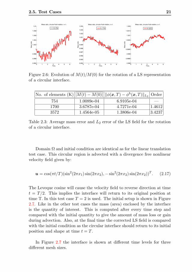
2.6 Evolution of M(t)/M(0) for the rotation of a LS representa-tion of a circular interface. . . . . . . . . . . . . . . . . . . . 21
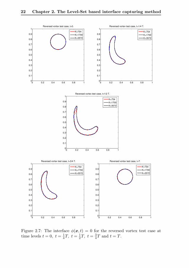
2.7 The interface φ(x, t) = 0 for the reversed vortex test case attime levels t = 0, t = 1
4T, t = 12T, t = 3
4T and t = T . . . . . 22
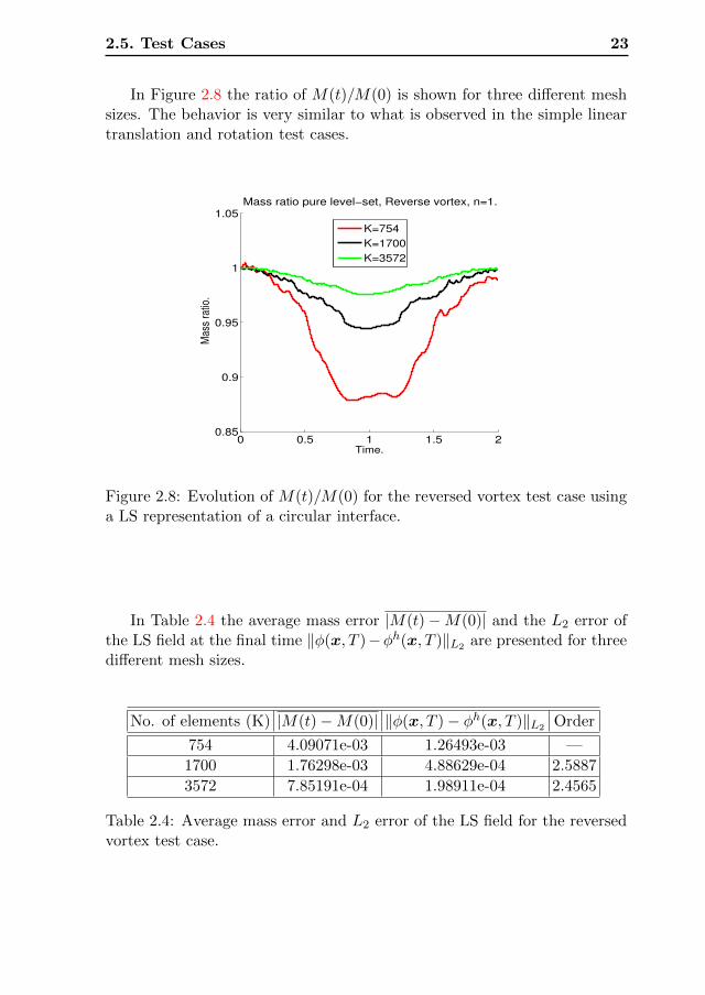
2.8 Evolution of M(t)/M(0) for the reversed vortex test caseusing a LS representation of a circular interface. . . . . . . 23
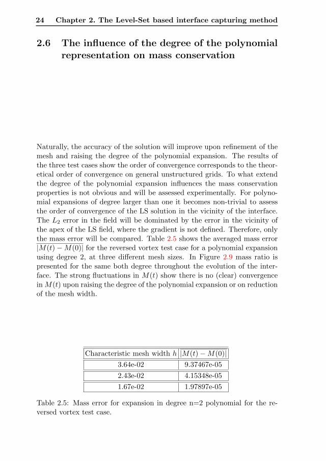
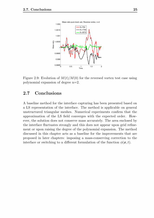
2.9 Evolution of M(t)/M(0) for the reversed vortex test caseusing polynomial expansion of degree n=2. . . . . . . . . . 25
xvii
xviii LIST OF FIGURES
4.1 The MCLS algorithm is presented in a flow chart to showthe transfer of information between the different componentsinvolved in advancing a single time step. . . . . . . . . . . . 34
4.2 Control volume (Ωk), cell centroid (Xk) and arbitrary point(X′). . . . . . . . . . . . . . . . . . . . . . . . . . . . . . . . 35
4.3 Case-1: Triangular domain of interest, where the vertex Xv3k
is mapped to the origin. . . . . . . . . . . . . . . . . . . . . 37
4.4 Interface passing through vertex (Xv1k ). . . . . . . . . . . . 40
4.5 Case-2: Mapping of two nodes a side. . . . . . . . . . . . . 41
4.6 Mapping of the interface parallel to one of its edge. . . . . . 44
4.7 VoF function for both Case-1 and Case-2. . . . . . . . . . . 44
4.8 Combination of two cases. . . . . . . . . . . . . . . . . . . . 45
4.9 Advection, remapping and distribution of the content of acontrol volume that is not intersected by the interface. . . . 49
4.10 Advection, remapping and distribution of the content of acontrol volume that is intersected by the interface. . . . . . 50
4.11 Straight-sided triangles remain straight-sided after being ad-vected by a linear velocity field (left). When advected by anonlinear velocity field this property is lost (right). . . . . . 51
4.12 The position of the interface in a mixed cell in the Lagrangianmesh is based on the advection of the extremities of the in-terface in the corresponding mixed cell in the Eulerian mesh. 53
4.13 For a nonlinear velocity field, the advected extremities of theinterface are first projected on the edges of the Lagrangiancontrol volume, before the appropriate interface position canbe determined. . . . . . . . . . . . . . . . . . . . . . . . . . 54
4.14 Initialization with the exact volume-of-fluid field leads to aslightly different initial position of the interface but elimin-ates the mass error incurred by initialization with the exactlevel-set field. . . . . . . . . . . . . . . . . . . . . . . . . . . 60
4.15 Time history of mass error for the circular fluid rotation case. 61
4.16 Time history of mass error for the reverse vortex test case. . 63
4.17 The evolution of the interface position for the reverse vortextest case. . . . . . . . . . . . . . . . . . . . . . . . . . . . . 64
LIST OF FIGURES xix
5.1 Tetrahedron control volume. . . . . . . . . . . . . . . . . . . 66
5.2 Case: where two vertices are aside. . . . . . . . . . . . . . . 69
5.3 The interface zero-contour after correction for the Zalesak’sslotted sphere. . . . . . . . . . . . . . . . . . . . . . . . . . 74
6.1 The influence of the parameter δ on the width of the interfacefor a fixed value of the parameter ε/h. . . . . . . . . . . . 79
6.2 The dimensionless width of the interface w/h for a fixeddefinition of the interface and different values of the dimen-sionless parameter ε/h. The vertical lines indicate the co-ordinate value xmin,max/h where |φεm(xmin,max)−(φm)min,max | <δ. . . . . . . . . . . . . . . . . . . . . . . . . . . . . . . . . . 80
6.3 LS, Modified LS for different ε and VoF . . . . . . . . . . . 81
6.4 Control volume Ωk and it’s neighbouring elements (dashededges) that contribute to the limited solution. . . . . . . . . 82
6.5 Translation of a circular region in ΩD ⊂ R. The solution isshown at the initial and final time. Clockwise from the topleft corner: Exact solution, numerical solution without ap-plication of a limiter, numerical solution based on the applic-ation of the vertex-based limiter, numerical solution based onthe application of the vertex-based limiter and a compressivevelocity field. . . . . . . . . . . . . . . . . . . . . . . . . . . 88
6.6 The interface φεm(x, t) = 0.5 for the rotation test case at timelevels t = 0, t = 1
4T, t = 34T and t = T . . . . . . . . . . . . 92
6.7 Evolution of M ε(t)/M ε(0) for the rotation of the MLS rep-resentation of a circular interface. . . . . . . . . . . . . . . . 93
6.8 The interface φm(x, t) = 0 for the reversed vortex test caseat time levels t = 0, t = 1
4T, t = 12T, t = 3
4T and t = T . . . 95
7.1 Initial position of the bubble with a lens shaped interface. . 99
7.2 Evolution of the mass ratio for the lens shaped interface ofLS and MLS for n = 1. . . . . . . . . . . . . . . . . . . . . . 100
7.4 Initial position of the interface in Zalesak’s rotating disc. . . 103
7.8 Evolution of the mass ratio M(t)/M(0) for Zalesak’s rotatingdisc test, for the LS (left) and MLS (right) field for n = 1. . 104
xx LIST OF FIGURES
7.3 The lens shaped interface at the final time t = T , for the LSand MLS for n = 1 (left) and n = 2 (right) and the MCLSfor n = 1. . . . . . . . . . . . . . . . . . . . . . . . . . . . . 105
7.5 Zalesak’s slotted disc at t = T , for the LS field, using n = 1. 106
7.6 Zalesak’s slotted disc at t = T , for the MCLS field, usingn = 1. . . . . . . . . . . . . . . . . . . . . . . . . . . . . . . 106
7.7 Zalesak’s slotted disc at t = T , for the MLS field, using n = 1.106
List of Tables
2.1 Coefficients of Low-Storage five-stage fourth-order ERK method. 16
2.2 Average mass error and L2 error of the LS field for the trans-lation of a circular interface. . . . . . . . . . . . . . . . . . . 19
2.3 Average mass error and L2 error of the LS field for the rota-tion of a circular interface. . . . . . . . . . . . . . . . . . . . 21
2.4 Average mass error and L2 error of the LS field for the re-versed vortex test case. . . . . . . . . . . . . . . . . . . . . . 23
2.5 Mass error for expansion in degree n=2 polynomial for thereversed vortex test case. . . . . . . . . . . . . . . . . . . . 24
4.1 Accuracy analysis of the interface back-and-forth conversiontest case. Initialization with the exact level-set field intro-duces a mass error that converges with second order accuracy. 59
4.2 Average mass error EnM and error in the level-set field EΦ(T )for the translation of a circular interface. . . . . . . . . . . . 61
4.3 Average mass error EnM and error in the level-set field EΦ(T )for the rotation of a circular interface. . . . . . . . . . . . . 62
4.4 Average mass error EnM and error in the level-set field EΦ(T )for the reverse vortex test case. . . . . . . . . . . . . . . . . 63
xxi
xxii LIST OF TABLES
6.1 Convection of the interface in one spatial dimension, masserror (|M(T )−M(0)|), L2-error of the modified LS field andestimated convergence rate without compressive velocity field(Kc = 0) for expansion in linear polynomial basis N = 1. . . 89
6.2 Convection of the interface in one spatial dimension, masserror (|M(T )−M(0)|), L2-error of the modified LS field andestimated convergence rate without compressive velocity field(Kc = 0) for expansion in quadratic polynomial basis N = 2. 90
6.3 Convection of the interface in one spatial dimension, masserror (|M(T )−M(0)| ), L2-error and estimated convergencerate of the modified LS field with compressive velocity field(Kc = 1e− 5) for expansion in linear polynomial basis N = 1. 90
6.4 Convection of the interface in one spatial dimension, masserror (|M(T )−M(0)| ), L2-error and estimated convergencerate of the modified LS field with compressive velocity field(Kc = 1e − 5) for expansion in quadratic polynomial basisN = 2. . . . . . . . . . . . . . . . . . . . . . . . . . . . . . . 90
6.5 Average mass error and L2 error of the MLS field for therotation of circular test case. . . . . . . . . . . . . . . . . . 93
6.6 Final mass error and L2 error of the MLS field for the re-versed vortex test case. . . . . . . . . . . . . . . . . . . . . . 96
7.1 Averaged mass error and L2-norm error for the MCLS fieldfor n = 1. . . . . . . . . . . . . . . . . . . . . . . . . . . . . 101
7.2 Averaged mass error and L2-norm error for the LS field forn = 1 and n = 2. . . . . . . . . . . . . . . . . . . . . . . . . 101
7.3 Averaged mass error and L2-norm error for the MLS field forn = 1 and n = 2. . . . . . . . . . . . . . . . . . . . . . . . . 101
7.4 Zalesak’s slotted disc test, average mass error and L2-normerror for the LS, MCLS and MLS field for n = 1. . . . . . . 103
CHAPTER 1
Introduction
In two-phase flow, two media with possibly very different properties and indifferent phases are present in a single domain. This type of flow plays avery important role in many industrial applications, ranging from petroleumindustry, chemical reactors, and the medical sciences.
The dynamics of two-phase flow can be very complex because of thefact that due to the movement of the interface between the two mediathe material properties strongly change in space and time. Furthermore, inmany cases the interface is not just advected by the local flow, but a possibleimbalance of inter molecular forces (surface tension) at the interface betweenthe two media leads to local acceleration of the flow.
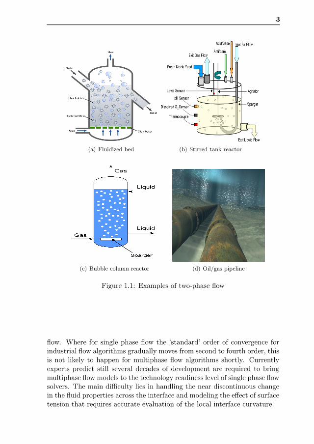
Based on the phases of the two media, two-phase flow can be categor-ised as: Liquid-Gas, Liquid-Liquid, Gas-Solid and Liquid-Solid. In all ofthese, sharp changes in material properties and the dynamics of the inter-face play an important role. Of these four, the Liquid-Gas and Gas-Solidflows present the larger challenges, because of the difference in (material)properties of both phases, e.g. density and viscosity. To illustrate how di-verse the nature of two-phase flow can be, an example of each type of flowwill be discussed briefly in the context of petroleum and process engineer-ing: a bubble column reactor, a fluidized bed reactor, a stirred tank reactorand an oil/gas pipeline, as shown in Fig. 1.1, taken from [1–4]
• Fluidized bed In the case a chemical reaction between two gasses
1
2 Chapter 1. Introduction
relies on the presence of a solid catalyst, it it of cardinal importance forthe efficiency of the reactor to disperse this catalyst as homogeneouslyas possible in the reactor vessel. A common approach is to form solid,nearly spherical particles from the catalyst and blow the gas-mixturethrough the reactor vessel. For a sufficiently large flow rate, the gas-solid mixture behaves like a fluid. This type of reactor is referred toas a fluidized bed.
• Stirred tank reactor When a chemical reaction involves two li-quids, use can be made of a stirred tank reactor. Optimization of thistwo-phase liquid-liquid flow aims at homogeneous mixing of the twoconstituents.
• Bubble column reactor Reactions between liquids and gasses, e.g.in oxidation processes and many bio-reactions, take place very ef-ficiently in a bubble column reactor. Proper engineering of the gasinjection in this gas-liquid flow guarantees finely dispersed gas bubbleswith the correct rise speed to complete the reaction.
• Oil/gas pipeline From the production well to the processing plant,natural gas and crude oil are transported simultaneously through asingle pipeline. When the gas and liquid flow rates are relativelysmall, gravity will separate the two phases into a stratified flow. Forlarger flow rates instabilities can grow on the oil/gas interface thatultimately lead to the formation of slugs. These are large chunks ofthe liquid phase, separated by gas bubbles. The mechanical impact ofslugs on delicate monitoring equipment can have catastrophic effectsand this type of gas-liquid flow has to be avoided. On the other handtwo-phase flow can be utilized to greatly reduce the required pumpingpower for heavy crude oil, using a special way of water-injection wherea thin film of water is formed surrounding a core of crude oil.
1.0.1 Modeling immiscible, incompressible two-phase flow
The research in this thesis is focused on the modeling of immiscible, incom-pressible gas-liquid and liquid-liquid two-phase flow: the two phases in thedomain are separated by a well-defined interface and both phases move atspeeds that are far smaller than the local speed of sound. The fact that thelocation of the interface is part of the solution, and the fact that at thisinterface a number of jump conditions have to be imposed on the solutionmakes two-phase flow considerably more hard to simulate than single-phase
3
(a) Fluidized bed (b) Stirred tank reactor
(c) Bubble column reactor (d) Oil/gas pipeline
Figure 1.1: Examples of two-phase flow
flow. Where for single phase flow the ’standard’ order of convergence forindustrial flow algorithms gradually moves from second to fourth order, thisis not likely to happen for multiphase flow algorithms shortly. Currentlyexperts predict still several decades of development are required to bringmultiphase flow models to the technology readiness level of single phase flowsolvers. The main difficulty lies in handling the near discontinuous changein the fluid properties across the interface and modeling the effect of surfacetension that requires accurate evaluation of the local interface curvature.
4 Chapter 1. Introduction
1.0.2 Interface capturing and interface tracking methods
Many methods have been designed to simulate two-phase flow. The largemajority of these are derived from one of the following archetypes of meth-ods:
• The Marker Particle method [45],
• The Volume of Fluid method (VOF) [24],
• The Level-Set method (LS) [40],
• The Modified Level-Set method [41],
• The Front-Tracking method [50],
Each of these methods has pros and cons. Some methods are easy to imple-ment, but do not conserve mass while others are mass conserving but havehigh computational complexity and this complexity further increases if themesh is unstructured.
The Marker Particle method is one of the earliest methods for the sim-ulation of the multiphase flow. It is based on a Lagrangian approach. Inthis method the initial interface is represented by a set of massless particlesthat are subsequently tracked while they are advected by the local velo-city. This method is not computationally efficient, because of the need totrack all individual particles and the need for regular particle distributionto avoid particle clusters and voids. This method alone is not a popularchoice any more, however, combined with other approaches it may be ad-vantageous [45]. The front-tracking method is another Lagrangian method.Instead of tracking fluid particles, the actual interface is tracked. Naturallythe interface is a lower dimensional manifold, requiring an order of mag-nitude less particles to be represented. However, different from the MarkerParticle method, the particles representing the interface are now connec-ted. Generally this connectivity is fixed and only the geometry and not theconnectivity of the interface can change.
If a continuous representation of the interface is required with the abilityto deform without any geometrical restrictions, two methods qualify forrepresenting the interface location: The Volume of Fluid method (VOF)and the Level-Set method. In the former, a color function is used to identifythe presence of either fluid. This color function has a value 1 in one fluidand 0 in the other fluid in order to distinguish between the two. In the VOFmethod the cell averaged value of the color function is used to represent the
5
quantity of either fluid present in a cell. This cell averaged value of the colorfunction lies by definition in the interval [0, 1] and is known as the Volumeof Fluid or the void-fraction. A cell which is completely filled with the fluidof interest has volume of fluid fraction value 1 and in the cell which is emptyi.e. not containing fluid of interest volume of fluid fraction defined to be 0.The interface location is only approximately defined: it will intersect thosecells that have intermediate value of the volume of fluid fraction between0 and 1, but its exact location is unknown. In each time step the positionof the interface is reconstructed within each cell that is intersected by theinterface, under the assumption that the interface is either aligned with theCartesian coordinate directions or locally planar, before it is advanced intime in a Lagrangian manner.
In the Level-Set method the interface position is indicated by the zeroLevel-Set of a signed distance function. The Level-Set field is advectedin time to get the position of the interface. As the Level-Set function iscontinuous and very smooth in the vicinity of the interface geometric char-acteristics, like gradient and curvature are easy to obtain. No techniquesexist to directly and exactly enforce the signed distance property on theLevel-Set field during the advection step. This property has to be reestab-lished a-posteriori in a process called reinitialization.
The VOF method is very accurately mass-conserving, but the inter-face reconstruction, and the approximation of the local curvature of theinterface to define surface tension effects are computationally intensive andinvolved. On the other hand, the Level-Set approach provides an exact (upto discretization order) representation of the interface and straightforwardevaluation of the local properties of the interface, but it is by definitionnot mass conserving: Exact conservation of the Level-Set function does notimply conservation of mass. The modified Level-Set method [41] is a relat-ively new approach in which a Level-Set function is chosen that resemblesthe color function of the Volume-of-Fluid method. By replacing the signed-distance function by a mollified Heaviside function, mass conservation isgreatly improved, but the large gradient of the modified Level-Set field atthe interface makes it harder to accurately compute the unit normal vectorand the curvature and to avoid oscillations in the solution, while keepingthe interface sharp.
In recent years an interest has developed in coupled VOF/LS meth-ods that combine the accurate mass conservation properties of the VOFmethod with the advantage of an exact representation of the interface by thelevel set method. For Example, the Combined Level Set Volume Of Fluid(CLSVOF) method of Sussman et al [48, 49, 56] and the Mass-Conserving
6 Chapter 1. Introduction
Level-Set (MCLS) method of Van der Pijl et al [53] for Cartesian grids.Although both examples seem to be very similar, the major difference isthat the CLSVOF method basically combines the work involved in boththe VOF and LS method, while the MCLS method avoids the computa-tionally intensive interface reconstruction step of the VOF method. This isaccomplished by the use of a volume of fluid function that directly relatesthe VOF color function to the LS function and its gradient, without theneed for an explicit reconstruction step.
1.1 Simulation of two-phase flows in geometricallycomplex domains
While simulating two-phase flow in simple Cartesian domains is challen-ging, applying the same models in geometrically intricate domains presentsa real challenge. However, because in many industrial applications such do-mains are more the rule than the exception, there is a strong drive for thedevelopment of such methods. To achieve optimal flexibility in discretizingthe flow equations in more intricate domains and resolve boundary layersefficiently and accurately state-of-the-art flow simulation algorithms relyon a discretisation of the domain in an unstructured set of non overlappingcontrol-volumes of mixed type: hexahedrons, tetrahedrons, pyramids andprisms or even more generically general convex polyhedra. A general convexpolyhedron is any oriented domain with bounded volume that is defined bya set of intersecting planes.
Contrary to the VOF method, the LS and modified-LS methods modelequations are relatively straightforward to discretize on tetrahedral cells.Using high order discontinuous Galerkin discretisation of the LS-equationmass loss can be significantly reduced with respect to second order meth-ods. Even so the mass conservation is still not comparable with that ofVOF methods that can can conserve mass nearly to machine precision.Extensions of the classic Piecewise Linear Interface Construction (PLIC)VOF method for tetrahedral control volumes currently available are veryrare. They are not very attractive because they rely on very complicatedgeometric reconstructions to position the interface and evaluate the fluxes,that impair their robustness. Furthermore, they are costly to apply.
In this thesis different approaches to simulating immiscible two-phaseflow in geometrically complex domain are proposed: The LS-method, themodified LS-method and the extension of the MCLS method of Van derPijl [53] . The accuracy of the solution, the mass loss and the work involvedin obtaining the solution are analyzed and compared.
1.2. Outline of the thesis 7
1.2 Outline of the thesis
In this thesis an extension is presented of the MCLS for a discretisationon a set of unstructured triangular and tetrahedral control volumes as astep-up towards the extension towards discretisation on general polygonaland polyhedral control volumes.
The key components of the MCLS will be shown to be:
• a discretisation of the linear transport equation for the LS field.
• a discretisation of the transport equation for the color function of theVOF method.
• an algorithm for the back-and-forth conversion of the LS field to theVOF field, that does not involve an explicit reconstruction of theinterface.
Furthermore, the performance of this extension is compared to two othermethods that are applicable for discretisation on triangular control volumes:the standard and the modified Level Set method.
The outline of this thesis is as follows:
In the second chapter of the thesis a higher-order discontinuous Galerkindiscretisation of the LS field is proposed. This discretisation is used in thestand-alone Level-Set method and as part of the extension of the Level-Setmethod. The chapter ends with an evaluation of the performance of thestand-alone LS method for three test cases.
Before presenting its extension, a concise review of the MCLS for struc-tured Cartesian control volumes is given in the third chapter. It is essentialto have a clear understanding of the MCLS to appreciate the details of theextension to triangular control volumes.
The extension of the MCLS method towards unstructured triangulargrid is presented in the fourth chapter. First the derivation of the conver-sion function and its inverse are presented for a triangular element that isintersected by the interface. Next the convection algorithm for the colorfunction is presented, formulated as an evolution equation for the VOFfield. Finally, the same test cases as presented in the second chapter arerepeated with the extension of the MCLS.
In the fifth chapter is discussed how the MCLS algorithm can be exten-ded from two to three dimensions. The conversion function for tetrahedralcontrol volumes is presented together with its inverse. On top of that an
8 Chapter 1. Introduction
extension of the two-dimensional algorithm is presented to handle generalpolygonal control volumes, that is based on a division of the computationalcells in triangular subcells.
Because of its relative simplicity and strict mass conservation propertiesthe modified LS method presents a viable alternative to the MCLS. Inthe before-last chapter a discretisation based on a limited discontinuousGalerkin scheme is presented and the merits of including a compressivevelocity field to enhance interface resolution are investigated.
The thesis concludes with a comparison of the performance of the threeproposed methods in the last chapter, followed by conclusions and recom-mendations how to further improve the MCLS method.
CHAPTER 2
The Level-Set based interface capturing method
2.1 Introduction
In this chapter an interface capturing model based on the solution of theLS equation is presented. The foundations of the LS model are discussedand a linear scalar transport equation for the LS field is derived. The latterequation is formulated in weak form and discretized in space using a dis-continuous Galerkin method on rectilinear triangular control volumes anda high order explicit Runge-Kutta method in time. Finally the algorithmis applied for a range of test cases, to set a benchmark for the solutions ofthe extension of the MCLS method and the modified-LS method that willbe presented in subsequent chapters of this thesis.
2.2 The Level-Set method
The LS method is a general approach to model interface evolution problemsin a very broad context ranging from solid and fluid mechanics to digitalimage processing. The method has been introduced by Sethian and Osher[29,40] in 1988, and is still actively developed. Because of its simplicity androbustness, the method is very popular and is included in many commercial
9
10 Chapter 2. The Level-Set based interface capturing method
simulation suites, e.g. COMSOL and OpenFOAM1.
2.3 The Level-Set method for modeling two-phaseflow
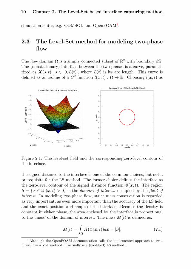
The flow domain Ω is a simply connected subset of R2 with boundary ∂Ω.The (nonstationary) interface between the two phases is a curve, paramet-rized as X(s, t), s ∈ [0, L(t)], where L(t) is its arc length. This curve isdefined as an isoline of a C2 function l(x, t) : Ω → R. Choosing l(x, t) as
0 0.2 0.4 0.6 0.8 1
0
0.5
1
−0.2
−0.1
0
0.1
0.2
0.3
0.4
0.5
0.6
x−axis.
Level−Set field of a circular interface.
y−axis.
Level−
Set valu
e.
x−axis.
y−
axis
.
Zero contour of the Level−Set field.
0 0.1 0.2 0.3 0.4 0.5 0.6 0.7 0.8 0.9 10
0.1
0.2
0.3
0.4
0.5
0.6
0.7
0.8
0.9
1
Figure 2.1: The level-set field and the corresponding zero-level contour ofthe interface.
the signed distance to the interface is one of the common choices, but not aprerequisite for the LS method. The former choice defines the interface asthe zero-level contour of the signed distance function Φ(x, t). The regionS = x ∈ Ω|(x, t) > 0 is the domain of interest, occupied by the fluid ofinterest. In modeling two-phase flow, strict mass conservation is regardedas very important, as even more important than the accuracy of the LS fieldand the exact position and shape of the interface. Because the density isconstant in either phase, the area enclosed by the interface is proportionalto the ’mass’ of the domain of interest. The mass M(t) is defined as:
M(t) =
∫ΩH(Φ(x, t))dx = |S|, (2.1)
1 Although the OpenFOAM documentation calls the implemented approach to two-phase flow a VoF method, it actually is a (modified) LS method.
2.3. The Level-Set method for modeling two-phase flow 11
where H(x) is the Heaviside function.
Due to this implicit definition of the interface, complex topology changes,for example merging of multiple or breaking up of a single interface are ac-commodated for. If the interface is a smooth curve, the smoothness of theLS function in the vicinity of the zero contour-line allows for a straightfor-ward computation of geometrical quantities of the interface by evaluatingderivatives of Φ(x, t) at the interface:
nα(x, t) =Φ,α(x, t)√
Φ,α(x, t)Φ,α(x, t), x ∈X(t), κ(x, t) = nα,α(x, t), x ∈X(t).
(2.2)where, nα is the unit normal vector (pointing outward from the domain ofinterest) and κ the curvature of a contour line of Φ(x, t) = 0. Because theinterface is by definition a contour line of the LS function, the followingequation holds at the interface:
d
dtΦ(x, t) = 0⇒ ∂Φ(x)
∂t+ uαΦ(x),α = 0,x ∈X(t), (2.3)
where uα is the velocity of the interface. Continuity conditions for massand momentum dictate the velocity field is continuous across the interfaceand therefore uniquely defined at the interface. The interface is advectedby the local flow.
In the LS method equation (2.3) is postulated to hold for all x ∈ Ω, butother choices are possible, as long as they are consistent with (2.3) and leadto a function that is at least C2 continuous in the vicinity of the interfaceto allow computation of the curvature. Following Osher [22,40] the velocityuα(x),x ∈ Ω \ X(t) can be chosen such that |∇Φ(x)| remains as closeas possible to unity, i.e. the LS function retains its property of being a(signed) distance function while being advected. Alternatively, the signed-distance property has to be re-established explicitly by a process calledreinitialization. For an overview of different reinitialization strategies andtheir merits, the reader is referred to [22,35,40,55].
Reinitialization or retaining the signed-distance property in a more gen-eral sense is important when the interface model is coupled to the flowequations. Regularization filters for the viscosity and the commonly usedContinuous Surface Model of Brackbill [9] for surface tension both use withthe LS field to determine the distance from a grid point to the interface.However, because the coupling to the flow equations will not be consideredin this research, reinitialization algorithms will not be considered.
For a solenodial velocity field uα the extension of (2.3) is given by
∂Φ(x)
∂t+ (uαΦ(x)),α = 0, x ∈ Ω. (2.4)
12 Chapter 2. The Level-Set based interface capturing method
This equation shows that the LS function is conserved. However, there isno reason why a conservative redistribution of the LS function maintainsthe area enclosed by the zero contour line, i.e. the interface. This is oneof the drawbacks associated with the LS method. Numerical experimentsindicate that to some extent this can be remedied by using higher order ap-proximations of the spatial differential operator, e.g. using ENO or WENOschemes in the context of a finite volume discretisation [26, 57], combinedwith higher order time-integration methods or by applying adaptive gridrefinement near the interface. Such a high order solution of the LS fieldis already required if the interface curvature is to be extracted from thisfield. In [Ref] it is shown the LS solution has to be discretized with fourthorder accuracy, if the interface curvature is to be recovered with secondorder accuracy. Although the latter is easily achieved on Cartesian meshes,this is not the case for unstructured grids of triangular or tetrahedral con-trol volumes, because it is not straightforward to combine information fromneighboring control volumes to obtain an approximation of the fluxes ofsufficient accuracy.
An approximation to the solution of (nearly) arbitrary order of accuracycan be obtained using the discontinuous Galerkin finite element method.The key property of this discretisation is the fact it is a completely localdiscretisation method, and the only information that has to be exchangedbetween neighboring control volumes is the solution at the inter-elementinterfaces. This makes the discretisation method straightforward to applyon unstructured triangular meshes as opposed to higher order finite volumediscretisation methods.
2.4 Discontinuous Galerkin discretisation of theLevel-Set equation
The discontinuous Galerkin discretisation combines the advantages of finitevolume and finite element discretisation techniques. The solution is expan-ded in a polynomial basis in each element. On each interface between twoelements the flux is uniquely defined (obviously, to have conservation) butthe solution is not. This implies the interface is only piecewise (element-wise) continuous together with the curvature and the interface normal vec-tor. Because the coupling of the interface model to the flow equations isoutside the scope of this thesis, the challenges presented by the handlingof the piecewise continuous curvature will not be considered and are leftfor future research. The proposed discretisation for the LS equation closelyfollows the algorithm described in [19,20,23,34].
2.4. Discontinuous Galerkin discretisation of the Level-Setequation 13
2.4.1 Spatial discretization of the Level-Set equation
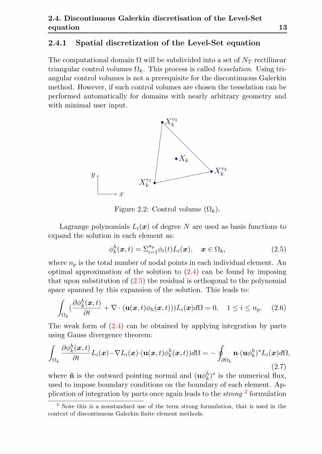
The computational domain Ω will be subdivided into a set of NT rectilineartriangular control volumes Ωk. This process is called tesselation. Using tri-angular control volumes is not a prerequisite for the discontinuous Galerkinmethod. However, if such control volumes are chosen the tesselation can beperformed automatically for domains with nearly arbitrary geometry andwith minimal user input.
Xv1k
Xv2k
Xv3k
y
x
Xk
Figure 2.2: Control volume (Ωk).
Lagrange polynomials Li(x) of degree N are used as basis functions toexpand the solution in each element as:
φhk(x, t) = Σnp
i=1φi(t)Li(x), x ∈ Ωk, (2.5)
where np is the total number of nodal points in each individual element. Anoptimal approximation of the solution to (2.4) can be found by imposingthat upon substitution of (2.5) the residual is orthogonal to the polynomialspace spanned by this expansion of the solution. This leads to:∫
Ωk
(∂φhk(x, t)
∂t+∇ · (u(x, t)φh(x, t)))Li(x)dΩ = 0, 1 ≤ i ≤ np. (2.6)
The weak form of (2.4) can be obtained by applying integration by partsusing Gauss divergence theorem:∫
Ωk
∂φhk(x, t)
∂tLi(x)−∇Li(x)·(u(x, t)φhk(x, t))dΩ = −
∮∂Ωk
n·(uφhk)∗Li(x)dΩ,
(2.7)where n is the outward pointing normal and (uφhk)∗ is the numerical flux,used to impose boundary conditions on the boundary of each element. Ap-plication of integration by parts once again leads to the strong 2 formulation
2 Note this is a nonstandard use of the term strong formulation, that is used in thecontext of discontinuous Galerkin finite element methods.
14 Chapter 2. The Level-Set based interface capturing method
of the weak form:∫Ωk
(∂φhk(x, t)
∂t+∇ · (uφhk(x, t))
)Li(x)dΩ =
∮∂Ωk
n·(uφhk−(uφhk)∗)Li(x)dΩ.
(2.8)For the discretisation of (2.4) the latter form is used, but either (2.8) or(2.7) can be used as a starting point. Instead of expanding the numericalsolution in a set of polynomial basis functions, the solution can be represen-ted, directly in the value of the solution at the collocation points or nodes.Both formulations are equivalent (related by a bijective mapping by meansof a Vandermonde matrix) and choosing either approach is a matter of pref-erence. In this case the latter approach is chosen, i.e. a nodal discontinuousformulation is used.
One important parameter in the definition of a discontinuous Galerkinmethod is the choice of the numerical flux function. For the scalar trans-port equation (2.4) there are only few options to consider. In [20] a centralapproximation and a Lax-Friedrichs approximation are assessed. Numericalexperiments show that oscillations will occur when a central flux approxim-ation is used, so the use of this approximation is discarded in this research.The Lax-Friedrichs flux formulation for the approximation of the numericalflux leads to the expected monotonic solution. This formulation uses a com-bination of a central approximation with a correction based on the jump inthe convected quantity at the face weighted by a parameter that dependson the magnitude of the velocity in the computational domain, given as:
(uφh)∗ =1
2
((uφh)− + (uφh)+
)− c
2
(φ+h − φ
−h
), (2.9)
where the + sign is used to represent the flux and the solution at the edge ofthe element under consideration and the − sign is used to represents the fluxand the solution at the edge of the neighboring element. The parameter c isused to weigh the jump across the edge in the formulation of the flux. Thisparameter is taken equal to the infinity norm of the velocity in the domain.Naturally, the fluxes at the edges that coincide with ∂Ω are determined bythe boundary conditions.
With the numerical flux approximation defined in Equation (2.8 ) cannow be cast in a linear system of equations. Imposing orthogonality for allindividual basis functions leads to a system of np linear equations for thesolution at the np nodal points:
Mk ∂Φ
∂t+ Sk · (uΦ) = F k (n · (uΦ− (uΦ)∗)) , (2.10)
2.4. Discontinuous Galerkin discretisation of the Level-Setequation 15
where Φ =φ1(t), φ2(t), ...., φnp(t)
and u =
u1(t),u2(t), .,unp(t)
are
the vectors of nodal values of φhk(x, t) and u(x, t) in element Ωk at time trespectively, Mk is the mass matrix, Sk is the stiffness matrix, and F k isthe boundary operator of the element. The latter are defined as:
Mkij =
∫Ωk
Lj(x)Li(x)dΩ, Skij =
∫Ωk
∇Lj(x)Li(x)dΩ,
F kij =
∮∂Ωk
Lj(x)Li(x)∂Ω.
Equation (2.10) is formulated for each element, but cannot be solved withoutconsidering the solution in the neighboring elements, because of the coup-ling by the fluxes at the common boundary defined through the boundaryoperator F k. All systems of dimension np × np can be assembled into onelinear system of ordinary differential equations that can be symbolicallyrepresented as:
AdΦ(t)
dt+BΦ(t) = g(t), (2.11)
where Φ =φ1(t), φ2(t), ...., φnp∗NT
(t)
and g(t) represents the contribu-tions of inhomogeneous boundary conditions. The approach to reduce apartial differential equation to a system of ordinary differential equations iscommonly referred to as the method-of-lines, in contrast to methods thatsimultaneously discretize in space and time. It is important to mentionedthat in our research we have focused more towards making the level-set fieldmass-conservative and we have adopted standard discretization practices forthe hyperbolic equation using DG method. Therefore, no new strategies forthe solution of the pure LS equation is given. Therefore, for further detailsregarding the discretization of the pure LS equation based on DG method,see [13,16,20,23,34].
2.4.2 Temporal Discretisation
To advance (2.11) in time an explicit Runge-Kutta method is used. Con-trary to a finite volume discretisation, the fact that the mass matrix isnondiagonal requires that even for an explicit time-stepping method a lin-ear system has to be solved in each time step. In the current project a directsolver has been used, because only problems with a very limited number ofdegrees of freedom are considered. For larger problems the specific proper-ties of the matrix A in (2.11) can be exploited to formulate a very efficient
16 Chapter 2. The Level-Set based interface capturing method
iterative solution method [6, 7].
Φ(t)
dt= A−1
(g(t)−BΦ(t)
)≡ Lh(Φ, t). (2.12)
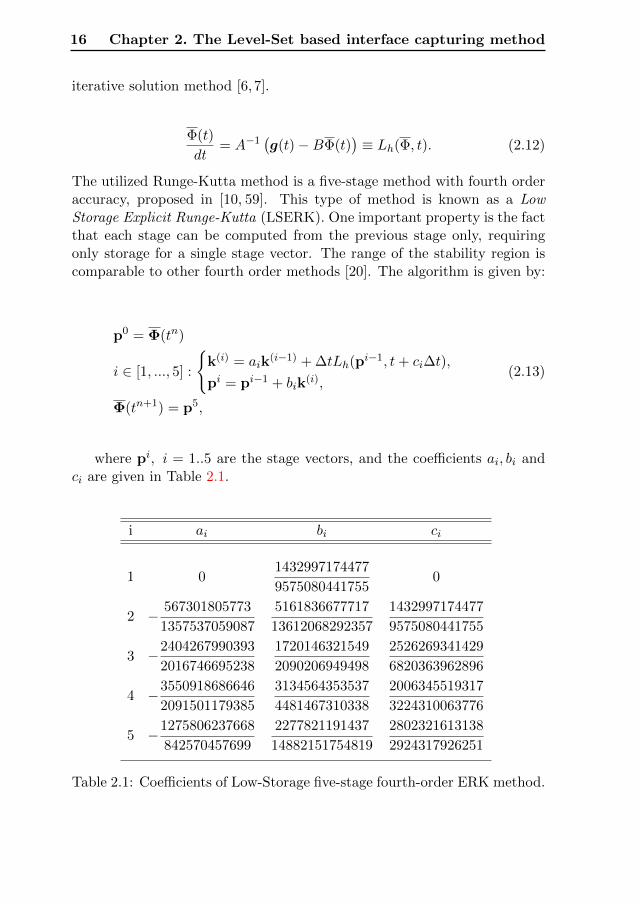
The utilized Runge-Kutta method is a five-stage method with fourth orderaccuracy, proposed in [10, 59]. This type of method is known as a LowStorage Explicit Runge-Kutta (LSERK). One important property is the factthat each stage can be computed from the previous stage only, requiringonly storage for a single stage vector. The range of the stability region iscomparable to other fourth order methods [20]. The algorithm is given by:
p0 = Φ(tn)
i ∈ [1, ..., 5] :
k(i) = aik
(i−1) + ∆tLh(pi−1, t+ ci∆t),
pi = pi−1 + bik(i),
Φ(tn+1) = p5,
(2.13)
where pi, i = 1..5 are the stage vectors, and the coefficients ai, bi andci are given in Table 2.1.
i ai bi ci
1 01432997174477
95750804417550
2 − 567301805773
1357537059087
5161836677717
13612068292357
1432997174477
9575080441755
3 −2404267990393
2016746695238
1720146321549
2090206949498
2526269341429
6820363962896
4 −3550918686646
2091501179385
3134564353537
4481467310338
2006345519317
3224310063776
5 −1275806237668
842570457699
2277821191437
14882151754819
2802321613138
2924317926251
Table 2.1: Coefficients of Low-Storage five-stage fourth-order ERK method.
2.5. Test Cases 17
2.5 Test Cases
The key characteristics of the method that need to be assessed are the massconservation property and the accuracy of the LS field. To accomplish this,three test cases are selected based on the properties of the imposed velocityfield; constant, linear or nonlinear functions of the spatial coordinates. In-cluding time-dependence of the velocity field is not necessary to assess theaccuracy of the discretisation. The test cases chosen are:
• (Solid body) translation of a circular interface with a constant velocityfield,
• (solid body) rotation of a circular interface,
• the reversed vortex test case [34, 56,60].
In all cases the problem is nondimensionalized by introducing a referencelength and reference velocity L = 1 m and T = 1 s, respectively.
The expansion of the solution can be done for polynomial basis functionsof a user defined degree, without any difficulty. However, the number ofnodal points increases with the degree of the basis functions and hence thenumber of degrees of freedom of the problem
In chapter 4 the extension of the MCLS to a discretisation on a setof unstructured triangular control volumes is presented. The discontinu-ous Galerkin discretisation of the LS equation is an integral part of thisalgorithm. However, in that application the basis functions are chosen aspolynomials of degree one, in accordance with the assumption of a piece-wise linear interface. For this reason, results are shown for an expansionin polynomials of order one for all test cases for three different mesh sizes.These results will be used to assess the improvement in the solution that canbe accomplished by imposing the mass conserving correction of the MCLSon a pure LS solution. This is also the reason for choosing separate testcases with a linear and a nonlinear velocity field. For the proposed discret-isation of the LS field the behavior of the solution will not be influencedby nonlinearity of the velocity field. However, for the MCLS method thenonlinearity does make a difference and it is worthwhile to consider thesecases separately.
To determine the effect of the degree of the polynomial basis on themass conservation properties of an uncorrected LS solution the mass lossis computed for three mesh sizes and using a degree one, two and threepolynomial expansion for the reversed vortex test case. The mass M can
18 Chapter 2. The Level-Set based interface capturing method
be computed up to machine precision when degree one polynomials are used,by a geometrical reconstruction of the domain of interest. However, for thedegree two and three polynomials it is approximated by a geometricallycomputed area (mass) enclosed by the fluid of interest. The details of thegeometrical method is given in appendix A.
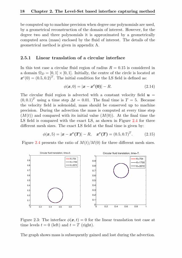
2.5.1 Linear translation of a circular interface
In this test case a circular fluid region of radius R = 0.15 is considered ina domain ΩD = [0, 1]× [0, 1]. Initially, the centre of the circle is located atxc(0) = (0.5, 0.2)T . The initial condition for the LS field is defined as:
φ(x, 0) = |x− xc(0)| −R. (2.14)
The circular fluid region is advected with a constant velocity field u =(0, 0.1)T using a time step ∆t = 0.01. The final time is T = 5. Becausethe velocity field is solenoidal, mass should be conserved up to machineprecision. During the advection the mass is computed at every time step(M(t)) and compared with its initial value (M(0)). At the final time theLS field is compared with the exact LS, as shown in Figure 2.4 for threedifferent mesh sizes. The exact LS field at the final time is given by:
φ(x, 5) = |x− xc(T )| −R, xc(T ) = (0.5, 0.7)T . (2.15)
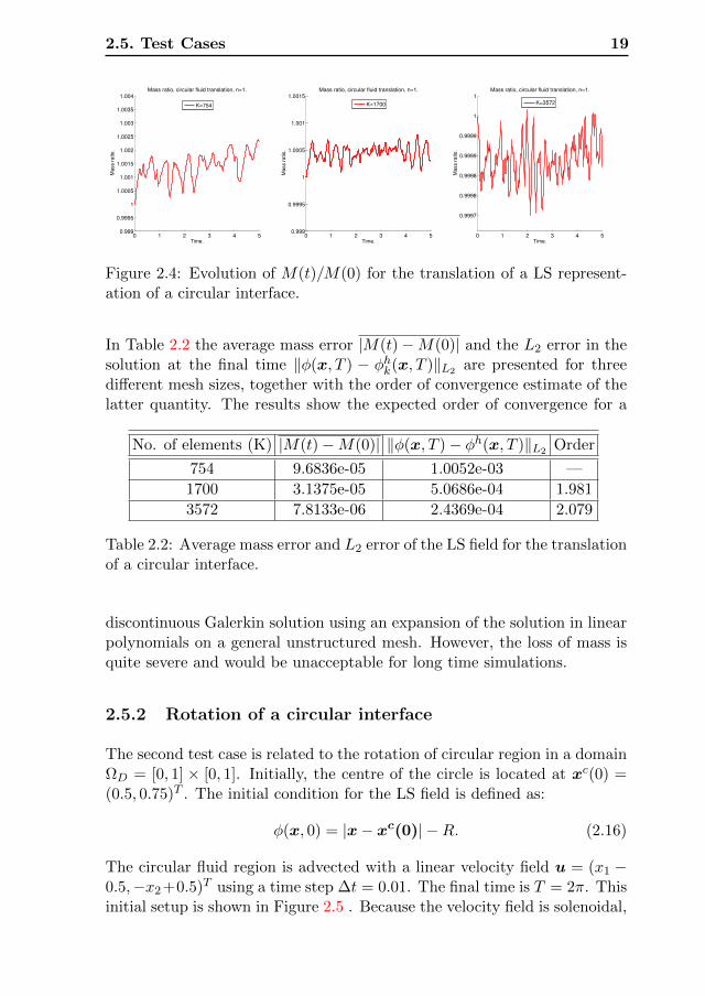
Figure 2.4 presents the ratio of M(t)/M(0) for three different mesh sizes.
Circular fluid translation, time=0.
0 0.2 0.4 0.6 0.8 10
0.1
0.2
0.3
0.4
0.5
0.6
0.7
0.8
0.9
1
K=754
K=1700
K=3572
Circular fluid translation, time=T.
0 0.2 0.4 0.6 0.8 10
0.1
0.2
0.3
0.4
0.5
0.6
0.7
0.8
0.9
1
K=754
K=1700
K=3572
Figure 2.3: The interface φ(x, t) = 0 for the linear translation test case attime levels t = 0 (left) and t = T (right).
The graph shows mass is subsequently gained and lost during the advection.
2.5. Test Cases 19
0 1 2 3 4 50.999
0.9995
1
1.0005
1.001
1.0015
1.002
1.0025
1.003
1.0035
1.004
Time.
Ma
ss r
atio
.
Mass ratio, circular fluid translation, n=1.
K=754
0 1 2 3 4 50.999
0.9995
1
1.0005
1.001
1.0015
Time.
Ma
ss r
atio
.
Mass ratio, circular fluid translation, n=1.
K=1700
0 1 2 3 4 5
0.9997
0.9998
0.9998
0.9999
0.9999
1
1
Time.
Ma
ss r
atio
.
Mass ratio, circular fluid translation, n=1.
K=3572
Figure 2.4: Evolution of M(t)/M(0) for the translation of a LS represent-ation of a circular interface.
In Table 2.2 the average mass error |M(t)−M(0)| and the L2 error in thesolution at the final time ‖φ(x, T ) − φhk(x, T )‖L2 are presented for threedifferent mesh sizes, together with the order of convergence estimate of thelatter quantity. The results show the expected order of convergence for a
No. of elements (K) |M(t)−M(0)| ‖φ(x, T )− φh(x, T )‖L2 Order
754 9.6836e-05 1.0052e-03 —
1700 3.1375e-05 5.0686e-04 1.981
3572 7.8133e-06 2.4369e-04 2.079
Table 2.2: Average mass error and L2 error of the LS field for the translationof a circular interface.
discontinuous Galerkin solution using an expansion of the solution in linearpolynomials on a general unstructured mesh. However, the loss of mass isquite severe and would be unacceptable for long time simulations.
2.5.2 Rotation of a circular interface
The second test case is related to the rotation of circular region in a domainΩD = [0, 1] × [0, 1]. Initially, the centre of the circle is located at xc(0) =(0.5, 0.75)T . The initial condition for the LS field is defined as:
φ(x, 0) = |x− xc(0)| −R. (2.16)
The circular fluid region is advected with a linear velocity field u = (x1 −0.5,−x2 +0.5)T using a time step ∆t = 0.01. The final time is T = 2π. Thisinitial setup is shown in Figure 2.5 . Because the velocity field is solenoidal,
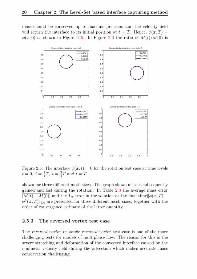
20 Chapter 2. The Level-Set based interface capturing method
mass should be conserved up to machine precision and the velocity fieldwill return the interface to its initial position at t = T . Hence, φ(x, T ) =φ(x, 0) as shown in Figure 2.5. In Figure 2.6 the ratio of M(t)/M(0) is
Circular fluid rotation test case, t=0.
0 0.2 0.4 0.6 0.8 10
0.1
0.2
0.3
0.4
0.5
0.6
0.7
0.8
0.9
1
K=754
K=1700
K=3572
Circular fluid rotation test case, t=1/4 T.
0 0.2 0.4 0.6 0.8 10
0.1
0.2
0.3
0.4
0.5
0.6
0.7
0.8
0.9
1
K=754
K=1700
K=3572
Circular fluid rotation test case, t=3/4 T.
0 0.2 0.4 0.6 0.8 10
0.1
0.2
0.3
0.4
0.5
0.6
0.7
0.8
0.9
1
K=754
K=1700
K=3572
Circular fluid rotation test case, t=T.
0 0.2 0.4 0.6 0.8 10
0.1
0.2
0.3
0.4
0.5
0.6
0.7
0.8
0.9
1
K=754
K=1700
K=3572
Figure 2.5: The interface φ(x, t) = 0 for the rotation test case at time levelst = 0, t = 1
4T, t = 34T and t = T .
shown for three different mesh sizes. The graph shows mass is subsequentlygained and lost during the rotation. In Table 2.3 the average mass error|M(t)−M(0)| and the L2 error in the solution at the final time‖φ(x, T )−φh(x, T )‖L2 are presented for three different mesh sizes, together with theorder of convergence estimate of the latter quantity.
2.5.3 The reversed vortex test case
The reversed vortex or single reversed vortex test case is one of the morechallenging tests for models of multiphase flow. The reason for this is thesevere stretching and deformation of the convected interface caused by thenonlinear velocity field during the advection which makes accurate massconservation challenging.
2.5. Test Cases 21
0 1 2 3 4 5 60.994
0.996
0.998
1
1.002
1.004
1.006
1.008
1.01
Time.
Ma
ss r
atio
.
Mass ratio, circular fluid rotation, n=1.
K=754
0 1 2 3 4 5 60.994
0.995
0.996
0.997
0.998
0.999
1
1.001
1.002
1.003
1.004
Time.
Ma
ss r
atio
.
Mass ratio, circular fluid rotation, n=1.
K=1700
0 1 2 3 4 5 60.998
0.9985
0.999
0.9995
1
1.0005
1.001
1.0015
1.002
Time.
Ma
ss r
atio
.
Mass ratio, circular fluid rotation, n=1.
K=3572
Figure 2.6: Evolution of M(t)/M(0) for the rotation of a LS representationof a circular interface.
No. of elements (K) |M(t)−M(0)| ‖φ(x, T )− φh(x, T )‖L2 Order
754 1.0089e-04 6.9105e-04 —
1700 3.6787e-04 4.7271e-04 1.4612
3572 1.4564e-05 1.3806e-04 3.4237
Table 2.3: Average mass error and L2 error of the LS field for the rotationof a circular interface.
Domain Ω and initial condition are identical as for the linear translationtest case. This circular region is advected with a divergence free nonlinearvelocity field given by:
u = cos(πt/T )(sin2(2πx1) sin(2πx2),− sin2(2πx2) sin(2πx2))T . (2.17)
The Leveque cosine will cause the velocity field to reverse direction at timet = T/2. This implies the interface will return to its original position attime T. In this test case T = 2 is used. The initial setup is shown in Figure2.7. Like in the other test cases the mass (area) enclosed by the interfaceis the quantity of interest. This is computed after every time step andcompared with the initial quantity to give the amount of mass loss or gainduring advection. Also, at the final time the corrected LS field is comparedwith the initial condition as the circular interface should return to its initialposition and shape at time t = T .
In Figure 2.7 the interface is shown at different time levels for threedifferent mesh sizes.
22 Chapter 2. The Level-Set based interface capturing method
Reversed vortex test case, t=0.
0 0.2 0.4 0.6 0.8 10
0.1
0.2
0.3
0.4
0.5
0.6
0.7
0.8
0.9
1
K=754
K=1700
K=3572
Reversed vortex test case, t=1/4 T.
0 0.2 0.4 0.6 0.8 10
0.1
0.2
0.3
0.4
0.5
0.6
0.7
0.8
0.9
1
K=754
K=1700
K=3572
Reversed vortex test case, t=1/2 T.
0 0.2 0.4 0.6 0.8 10
0.1
0.2
0.3
0.4
0.5
0.6
0.7
0.8
0.9
1
K=754
K=1700
K=3572
Reversed vortex test case, t=3/4 T.
0 0.2 0.4 0.6 0.8 10
0.1
0.2
0.3
0.4
0.5
0.6
0.7
0.8
0.9
1
K=754
K=1700
K=3572
Reversed vortex test case, t=T.
0 0.2 0.4 0.6 0.8 10
0.1
0.2
0.3
0.4
0.5
0.6
0.7
0.8
0.9
1
K=754
K=1700
K=3572
Figure 2.7: The interface φ(x, t) = 0 for the reversed vortex test case attime levels t = 0, t = 1
4T, t = 12T, t = 3
4T and t = T .
2.5. Test Cases 23
In Figure 2.8 the ratio of M(t)/M(0) is shown for three different meshsizes. The behavior is very similar to what is observed in the simple lineartranslation and rotation test cases.
0 0.5 1 1.5 20.85
0.9
0.95
1
1.05
Time.
Mas
s ra
tio.
Mass ratio pure level−set, Reverse vortex, n=1.
K=754
K=1700
K=3572
Figure 2.8: Evolution of M(t)/M(0) for the reversed vortex test case usinga LS representation of a circular interface.
In Table 2.4 the average mass error |M(t)−M(0)| and the L2 error ofthe LS field at the final time ‖φ(x, T )−φh(x, T )‖L2 are presented for threedifferent mesh sizes.
No. of elements (K) |M(t)−M(0)| ‖φ(x, T )− φh(x, T )‖L2 Order
754 4.09071e-03 1.26493e-03 —
1700 1.76298e-03 4.88629e-04 2.5887
3572 7.85191e-04 1.98911e-04 2.4565
Table 2.4: Average mass error and L2 error of the LS field for the reversedvortex test case.
24 Chapter 2. The Level-Set based interface capturing method
2.6 The influence of the degree of the polynomialrepresentation on mass conservation
Naturally, the accuracy of the solution will improve upon refinement of themesh and raising the degree of the polynomial expansion. The results ofthe three test cases show the order of convergence corresponds to the theor-etical order of convergence on general unstructured grids. To what extendthe degree of the polynomial expansion influences the mass conservationproperties is not obvious and will be assessed experimentally. For polyno-mial expansions of degree larger than one it becomes non-trivial to assessthe order of convergence of the LS solution in the vicinity of the interface.The L2 error in the field will be dominated by the error in the vicinity ofthe apex of the LS field, where the gradient is not defined. Therefore, onlythe mass error will be compared. Table 2.5 shows the averaged mass error|M(t)−M(0)| for the reversed vortex test case for a polynomial expansionusing degree 2, at three different mesh sizes. In Figure 2.9 mass ratio ispresented for the same both degree throughout the evolution of the inter-face. The strong fluctuations in M(t) show there is no (clear) convergencein M(t) upon raising the degree of the polynomial expansion or on reductionof the mesh width.
Characteristic mesh width h |M(t)−M(0)|3.64e-02 9.37467e-05
2.43e-02 4.15348e-05
1.67e-02 1.97897e-05
Table 2.5: Mass error for expansion in degree n=2 polynomial for the re-versed vortex test case.
2.7. Conclusions 25
0 0.5 1 1.5 20.9985
0.999
0.9995
1
1.0005
1.001
1.0015
1.002
Time.
Ma
ss r
atio
.
Mass ratio pure level−set, Reverse vortex, n=2.
K=754
K=1700
K=3572
Figure 2.9: Evolution of M(t)/M(0) for the reversed vortex test case usingpolynomial expansion of degree n=2.
2.7 Conclusions
A baseline method for the interface capturing has been presented based ona LS representation of the interface. The method is applicable on generalunstructured triangular meshes. Numerical experiments confirm that theapproximation of the LS field converges with the expected order. How-ever, the solution does not conserve mass accurately. The area enclosed bythe interface fluctuates strongly and this does not appear upon grid refine-ment or upon raising the degree of the polynomial expansion. The methoddiscussed in this chapter acts as a baseline for the improvements that areproposed in later chapters: imposing a mass-conserving correction to theinterface or switching to a different formulation of the function φ(x, t).

CHAPTER 3
An overview of the LS and VoF hybrid methods
3.1 Introduction
It is highlighted in the last chapter that apart from the geometrical flexibil-ity provided by the LS for the multiphase flow simulation, mass-conservationcan not be achieved from the pure LS field. Which is one of the key prob-lems associated with the LS method. To mitigate this problem as men-tioned earlier different solution procedures has been developed and are stilldeveloping. One of the popular choices is hybrid method, in which the LSmethod is combined with another simultaneously advected quantity thatused is to make the LS field mass conserving while keeping geometric flex-ibility provided by the pure LS field. The solution procedure varies fromthe coupling of LS field with particle approach [17] to LS coupling with VoFfield [49]. In general, the coupling is performed to correct the LS field suchthat it corresponds to the correct quantity of fluid of interest. Usually, thisis achieved by using a PLIC method in which the interface is represented bya line segment and then it is adjusted in a control volume such the it cor-responds to the exact quantity of the fluid of interest. This correction canbe an iterative based or direct i.e. that is without involving any iterativeprocess [43]. It is worthwhile to have an overview of the existing hybrid LSand VoF method for multiphase flow simulation in order to have a betterunderstanding of the proposed method of this research.
27
28 Chapter 3. An overview of the LS and VoF hybrid methods
3.2 Hybrid Methods
There exists a number of hybrid methods based on the application underconsideration. In the following, we have selected those methods that providethe guideline to develop another hybrid method.
3.2.1 CLSVOF method
The Coupled Level-Set Volume of Fluid (CLSVOF) method is proposed bySussman and Puckett [48,49], in 2000. In this method, the interface is con-structed using the LS field while mass is conserved by using simultaneouslyadvected volume of fluid, VoF PLIC method. PLIC is the extended versionof SLIC method in which the interface is assumed to be inclined with co-ordinates axes in a control volume, which is not a right assumption. In PLICmethod, the interface is represented by a line segment and can be orientedin any direction. The area enclosed in it represents the quantity of the fluidof interest. In CLSVOF method, there exists no straightforward relationbetween the LS field and the VoF field [52, 53]. The coupling between theLS and VoF field is done using a PLIC approach which not trivial and leadsto an iterative process and also the coupling becomes cumbersome whenthe grid is an unstructured Cartesian grid. It is also reported that massconservation of the CLSVOF method is comparable to VoF method [49,52].In spite, these limitations this method provides a solid guideline towardsthe coupling of the LS field and the VoF field.
3.2.2 Hybrid particle LS method
A hybrid particle Level-Set method is proposed by Enright et al. [17], in2002. In this method, the mass conservation property of the LS field canbe enhanced by passively advected particles of suitable radii with flow field.These particles are placed near the interface and their region of placementis marked by the sign of the LS field. This idea makes this method differ-ent from the traditional marker and particles approach in which particlesare placed in a whole domain [21,45]. The passively advected particles areused to reconstructed the interface in the region of sharp stretching andtearing of the interface. This approach seems suitable but the Lagrangiannature of the approach makes the algorithm computationally involved, asthese particles need tracking. These particles are used to track both thecharacteristics of the flow and also to reconstruct the interface in the re-gions where the LS method alone failed to accurately conserve mass. In
3.2. Hybrid Methods 29
this approach due to the passive nature of the particles they are allowedto overlap with each other, this makes algorithm computationally involvetowards interface reconstruction for the mass conservation.
3.2.3 MCLS method
The Mass-Conserving Level-Set (MCLS) method is presented by Pijl et.al [52, 53], in 2005. This method is based on the coupling between LS andVoF field by simultaneously advecting the LS and the VoF field. In thisapproach, the VoF field is only used for the mass conservation correctionto the LS field and it is not involved in the interface reconstruction apartfrom their counter methods [48, 49]. To achieve this goal i.e. to applyconservation without interface reconstruction of the interface from VoF fieldan explicit relation between LS and VoF field is obtained in the form ofan analytic function based on the assumption that the interface can berepresented by a piecewise line segment, which is very common practicein coupled methods. This analytic function is called the volume of fluidfunction. This idea is the key ingredient of the MCLS method. This methodis extendable to 3D. However, there is a limitation to this method as it isdesigned for Cartesian grids, so complicated geometries can not be handledat this moment. The rectification of this issue in the MCLS method is oneof the important research questions that has been answered in this thesis.
3.2.4 VOSET method
A coupled Volume of Fluid and Level-Set method (VOSET) of Sun andTao [46] is presented in 2010. This method works in different approach ascompared to above mentioned hybrid methods. In this method, the LS fieldis reconstructed from the VoF field. This methodology is contrary to theexisting LS and VoF coupled methods. It is important to incorporate thismethodology as well for a fair comparison. As the LS field is reconstructedfrom the VoF field the only quantity that is advected with the flow field isthe VoF field. This is an important difference with existing hybrid method,as this certainly computationally favourable. However, like VoF PLIC theinterface needs to be reconstructed and then using contour 0.5 value of theVoF fraction as reference interface the LS field is reconstructed by the geo-metrical iterative process in which distances are computed from the nearestpoints in order to get continues definition of the LS field. In general, thismethod seems simple as only one quantity needs to be advected. However,the interface reconstruction needs to be done twice once for the VoF fieldand then from VoF field to LS field needs to be reconstructed.
30 Chapter 3. An overview of the LS and VoF hybrid methods
3.3 Conclusions
In this chapter, a broader overview of the existing hybrid methods thatform the foundation to develop other methods for the simulation of multi-phase flow. These methods have their pros and cons. For example CLSVOFmethod seems plausible but the interface reconstruction based on the PLICapproach makes that method computationally involved and also the ex-tension to 3D is not so trivial. The flux approximation by using the fluxsplitting approach makes this method not suitable for non-Cartesian grids.In other words, to make this method robust extra information along withthe interface reconstruction needs to be done. In the hybrid particle methodtracking mass-less particle and the reconstructing the interface to make surethe LS is mass conserving is also computational involve and it increasesmore with 3D mesh and unstructured non-Cartesian grids. However, thismethod is suitable for the flow that involves large sharing and deformations.The VOSET method seems plausible as far as number quantity needs to beadvected, However, the interface reconstruction twice made in cumbersomefor 3D unstructured meshes as well and also the definition of VoF interfaceby a 0.5 contours of the VoF field is arbitrary.
If we analysis the MCLS method this method seems plausible in allrespect as the LS and the VoF field is needed to be advected independently,this step is similar to CLSVOF method, however, no need to reconstructthe interface, this makes MCLS method suitable for 3D control volumes,but it is designed for Cartesian grid only. Keeping our objective in mindthat is we need to formulate numerical methods for the multi-phase flowsimulation in geometrically complicated domains, we have decided to choosethe MCLS method as a guide to developed method. In order to achieve thisgoal, we have developed VoF function and inverse function for unstructured2D triangular and 3D tetrahedron grids. These are the key components ofthis thesis.
CHAPTER 4
MCLS method for unstructured triangular meshes
4.1 Introduction
In this chapter 1 proposed Mass-Conserving Level-Set method is presentedfor the 2D unstructured triangular grid.
4.2 Modeling the evolution of the interface
The MCLS algorithm is used to model the dynamics of two-phase immiscibleincompressible flow. It uses an ’hybrid’ description of the distribution ofthe two-phases, Phase0 and Phase1, using both the LS and the VoF field.
4.2.1 The Level-Set field
The interface between the two phases X(t) is defined as an isoline of a C2
function l(x, t) : Ω → R, where Ω ⊂ R2, and simply connected. Choosingl(x, t) as the signed distance to the interface is one of the common choices.
1This chapter is based on the article:F. Raees, D.R. van der Heul and C. Vuik, A mass-conserving level-set method for sim-ulation of multiphase flow in geometrically complicated domains, International Journalfor Numerical Methods in Fluids, 2015.
31
32 Chapter 4. MCLS method for unstructured triangular meshes
Consequently, this choice defines the interface as the zero-level contour ofthe signed distance function Φ(x, t). A signed distance function is a naturalchoice because it allows for accurate computation of the interface curvatureand normal vector. However, Olssson et al. propose a LS function thatresembles a mollified Heaviside function to improve the mass conservationproperties [14, 36, 38]. In the MCLS the LS function is chosen as a signeddistance function Φ(x, t). If Φ(x, t) < 0, Phase0 is present, while Phase1 ispresent when Φ(x, t) > 0. Due to this implicit definition of the interface,complex topology changes, for example merging of multiple or breakingup of a single interface are accommodated for. The smoothness of the LSfunction in the vicinity of the zero contour-line allows for a straightfor-ward computation of geometrical quantities of the interface by evaluatingderivatives of Φ(x, t) at the interface:
nα(x, t) =Φ,α(x, t)√
Φ,α(x, t)Φ,α(x, t), x ∈X(t), κ(x, t) = nα,α(x, t), x ∈X(t),
(4.1)where nα is the unit normal vector and κ the curvature of a contour line ofΦ(x, t) = 0.
4.2.2 Volume of Fluid field
The distribution of the fluids is represented by a C−1 color function c(x, t) :R→ 0, 1: If c(x, t) = 0, Phase0 is present, while Phase1 is present whenc(x, t) = 1. Based on the color function c(x, t) we can define the Volume ofFluid grid function Ψk : G→ [0, 1] as:
Ψk(t) =1
|Ωk|
∫Ωk
c(x, t)dΩ, (4.2)
where G is the set of all centers of the control volumes Ωk and |Ωk| theirarea. The fact that c(x, t) is C−1 continuous and Ψk(t) only discretelydefined, makes the computation of the interface curvature challenging andcomputationally intensive.
4.2.3 Hybrid formulation of the MCLS method
In the hybrid formulation the flow is described by both a LS and a VoFfield that are in agreement in each cell in the following way:
Ψk(t) =1
|Ωk|
∫Ωk
H(Φ(x, t))dΩ, (4.3)
4.3. Overview of the MCLS algorithm 33
where H(q) is the Heaviside function. This means that the LS field hasthe mass-conserving properties of the VoF field, while at the same time theinterface location is exactly defined by the LS field.
4.3 Overview of the MCLS algorithm
In this section an overview of the MCLS method is presented. The proposedalgorithm relies on the key idea that a mass-conserving correction can beimposed on the LS field that is based on a simultaneously advected VoFfield. The algorithm is visualised in Figure 4.1. Advancing the interfacewith the MCLS over a single time step consists of the following substeps,assuming the LS Φn and VoF field Ψn are known:
• The LS field and the VoF field are advected simultaneously. Afterthis advection step, the two fields do not correspond to each other,i.e. the fields do not comply with 4.3.
• The advected LS field Φ∗ is used to compute a corresponding VoFfield Ψ∗ by means of the VoF function.
• The difference between the advected VoF field Ψn+1 and the VoF fieldΨ∗ is determined.
• In an element, for which the difference is smaller than the prescribedtolerance no correction to the LS field is required. If the differenceexceeds the prescribed tolerance, a correction is imposed to the LSfield by means of the inverse VoF function to make the LS field massconserving up to a user specified tolerance.
• At time tn+1 a mass-conserving LS field Φn+1 has been obtained alongwith the VoF field Ψn+1.
In the following sections each of the components that are required for theproposed extension of the MCLS algorithm for an unstructured triangulargrid are presented. These are: the LS field and VoF field advection al-gorithms described in Sections 4.5 and refelvof, respectively, and the VoFfunction (Section 4.4) and its inverse (Section 4.7).
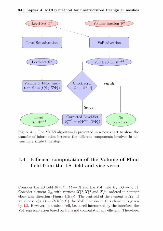
34 Chapter 4. MCLS method for unstructured triangular meshes
Level-Set Φn Volume fraction Ψn
Level-Set advection VoF advection
VoF fraction Ψn+1Level-Set Φ∗
Volume of Fluid func-tion Ψ∗ = f(Φ∗k,∇Φ∗k)
Check error|Ψ∗ −Ψn+1|
Corrected Level-SetΦn+1k = g(Ψn+1,∇Φ∗k)
Nocorrection
Level-Set Φn+1
small
large
Figure 4.1: The MCLS algorithm is presented in a flow chart to show thetransfer of information between the different components involved in ad-vancing a single time step.
4.4 Efficient computation of the Volume of Fluidfield from the LS field and vice versa
Consider the LS field Φ(x, t) : Ω → R and the VoF field Ψk : G → [0, 1].Consider element Ωk, with vertices Xv1
k ,Xv2k and Xv3
k , ordered in counterclock wise direction (Figure 4.2(a)). The centroid of the element is Xk. Ifwe choose c(x, t) = H(Φ(x, t)) the VoF function in this element is givenby 4.3. However, in a mixed cell, i.e. a cell intersected by the interface, theVoF representation based on 4.3 is not computationally efficient. Therefore,
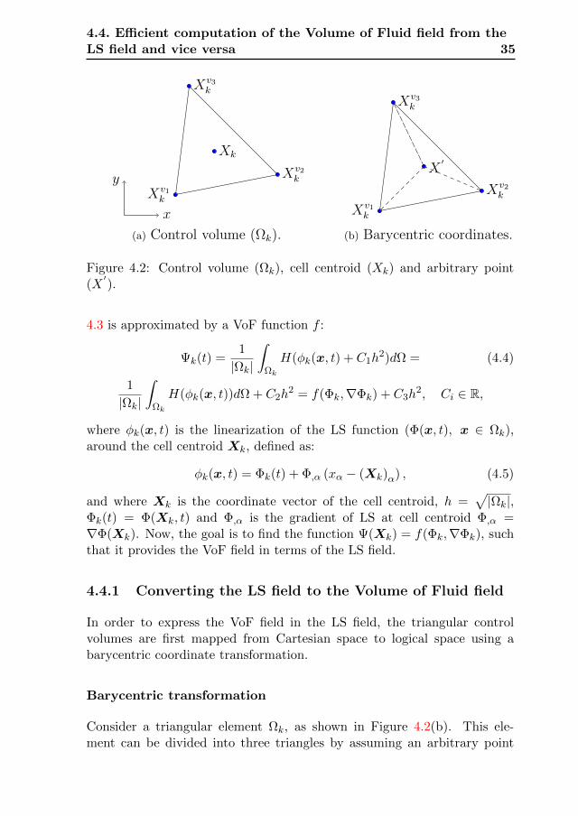
4.4. Efficient computation of the Volume of Fluid field from theLS field and vice versa 35
Xv1k
Xv2k
Xv3k
y
x
Xk
(a) Control volume (Ωk).
Xv1k
Xv2k
Xv3k
X′
(b) Barycentric coordinates.
Figure 4.2: Control volume (Ωk), cell centroid (Xk) and arbitrary point(X′).
4.3 is approximated by a VoF function f :
Ψk(t) =1
|Ωk|
∫Ωk
H(φk(x, t) + C1h2)dΩ = (4.4)
1
|Ωk|
∫Ωk
H(φk(x, t))dΩ + C2h2 = f(Φk,∇Φk) + C3h
2, Ci ∈ R,
where φk(x, t) is the linearization of the LS function (Φ(x, t), x ∈ Ωk),around the cell centroid Xk, defined as:
φk(x, t) = Φk(t) + Φ,α (xα − (Xk)α) , (4.5)
and where Xk is the coordinate vector of the cell centroid, h =√|Ωk|,
Φk(t) = Φ(Xk, t) and Φ,α is the gradient of LS at cell centroid Φ,α =∇Φ(Xk). Now, the goal is to find the function Ψ(Xk) = f(Φk,∇Φk), suchthat it provides the VoF field in terms of the LS field.
4.4.1 Converting the LS field to the Volume of Fluid field
In order to express the VoF field in the LS field, the triangular controlvolumes are first mapped from Cartesian space to logical space using abarycentric coordinate transformation.
Barycentric transformation
Consider a triangular element Ωk, as shown in Figure 4.2(b). This ele-ment can be divided into three triangles by assuming an arbitrary point
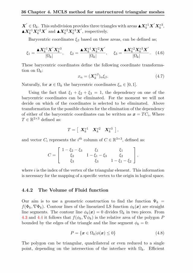
36 Chapter 4. MCLS method for unstructured triangular meshes
X′ ∈ Ωk. This subdivision provides three triangles with areas NXv1
k X′Xv3k ,
NXv1k X
v2k X
′and NXv2
k Xv3k X
′, respectively.
Barycentric coordinates ξβ based on these areas, can be defined as;
ξ1 =NXv1
k X′Xv3k
|Ωk|, ξ2 =
NXv1k X
v2k X
′
|Ωk|, ξ3 =
NXv2k X
v3k X
′
|Ωk|. (4.6)
These barycentric coordinates define the following coordinate transforma-tion on Ωk:
xα = (Xvβk )αξβ. (4.7)
Naturally, for x ∈ Ωk the barycentric coordinates ξα ∈ [0, 1].
Using the fact that ξ1 + ξ2 + ξ3 = 1, the dependency on one of thebarycentric coordinates can be eliminated. For the moment we will notdecide on which of the coordinates is selected to be eliminated. Abovetransformation for the possible choices for the elimination of the dependencyof either of the barycentric coordinates can be written as x = TCi, WhereT ∈ R2×3 defined as:
T =[Xv1k Xv2
k Xv3k
],
and vector Ci represents the ith column of C ∈ R3×3, defined as:
C =
1− ξ2 − ξ3 ξ1 ξ1
ξ2 1− ξ1 − ξ3 ξ2
ξ3 ξ3 1− ξ1 − ξ2
,where i is the index of the vertex of the triangular element. This informationis necessary for the mapping of a specific vertex to the origin in logical space.
4.4.2 The Volume of Fluid function
Our aim is to use a geometric construction to find the function Ψk =f(Φk,∇Φk). Contour lines of the linearized LS function φk(x) are straightline segments. The contour line φk(x) = 0 divides Ωk in two pieces. From4.3 and 4.4 it follows that f(φk,∇φk) is the relative area of the polygon Pbounded by the edges of the triangle and the line segment φk = 0:
P = x ∈ Ωk|φ(x) ≤ 0 (4.8)
The polygon can be triangular, quadrilateral or even reduced to a singlepoint, depending on the intersection of the interface with Ωk. Efficient
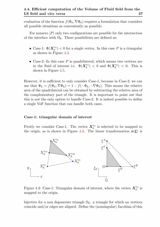
4.4. Efficient computation of the Volume of Fluid field from theLS field and vice versa 37
evaluation of the function f(Φk,∇Φk) requires a formulation that considersall possible situations as conveniently as possible.
For nonzero |P | only two configurations are possible for the intersectionof the interface with Ωk. These possibilities are defined as:
• Case-1: Φ(Xv3k ) < 0 for a single vertex. In this case P is a triangular
as shown in Figure 4.3.
• Case-2: In this case P is quadrilateral, which means two vertices arein the fluid of interest i.e. Φ(Xv3
k ) < 0 and Φ(Xv2k ) < 0. This is
shown in Figure 4.5.
However, it is sufficient to only consider Case-1, because in Case-2, we canuse that Ψk = f(Φk,∇Φk) = 1 − f(−Φk,−∇Φk). This means the relativearea of the quadrilateral can be obtained by subtracting the relative area ofthe complementary part of the triangle. It is important to point out thatthis is not the only option to handle Case-2. It is indeed possible to definea single VoF function that can handle both cases.
Case-1: triangular domain of interest
Firstly we consider Case-1. The vertex Xv3k is selected to be mapped to
the origin, as is shown in Figure 4.3. The linear transformation x(ξ) is
Xv1k
Xv2k
Xv3k
Xv31k Xv32
k
y
x
ξB
ξA
OξE
ξF
ξ1
ξ2
Figure 4.3: Case-1: Triangular domain of interest, where the vertex Xv3k is
mapped to the origin.
bijective for a non degenerate triangle Ωk: a triangle for which no verticescoincide and/or edges are aligned. Define the (nonsingular) Jacobian of this
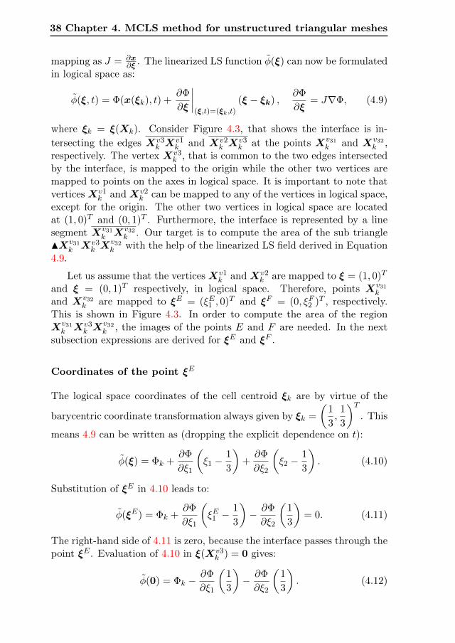
38 Chapter 4. MCLS method for unstructured triangular meshes
mapping as J = ∂x∂ξ . The linearized LS function φ(ξ) can now be formulated
in logical space as:
φ(ξ, t) = Φ(x(ξk), t) +∂Φ
∂ξ
∣∣∣∣(ξ,t)=(ξk,t)
(ξ − ξk) ,∂Φ
∂ξ= J∇Φ, (4.9)
where ξk = ξ(Xk). Consider Figure 4.3, that shows the interface is in-
tersecting the edges Xv3k X
v1k and Xv2
k Xv3k at the points Xv31
k and Xv32k ,
respectively. The vertex Xv3k , that is common to the two edges intersected
by the interface, is mapped to the origin while the other two vertices aremapped to points on the axes in logical space. It is important to note thatvertices Xv1
k and Xv2k can be mapped to any of the vertices in logical space,
except for the origin. The other two vertices in logical space are locatedat (1, 0)T and (0, 1)T . Furthermore, the interface is represented by a linesegment Xv31
k Xv32k . Our target is to compute the area of the sub triangle
NXv31k Xv3
k Xv32k with the help of the linearized LS field derived in Equation
4.9.
Let us assume that the vertices Xv1k and Xv2
k are mapped to ξ = (1, 0)T
and ξ = (0, 1)T respectively, in logical space. Therefore, points Xv31k
and Xv32k are mapped to ξE = (ξE1 , 0)T and ξF = (0, ξF2 )T , respectively.
This is shown in Figure 4.3. In order to compute the area of the regionXv31k Xv3
k Xv32k , the images of the points E and F are needed. In the next
subsection expressions are derived for ξE and ξF .
Coordinates of the point ξE
The logical space coordinates of the cell centroid ξk are by virtue of the
barycentric coordinate transformation always given by ξk =
(1
3,1
3
)T. This
means 4.9 can be written as (dropping the explicit dependence on t):
φ(ξ) = Φk +∂Φ
∂ξ1
(ξ1 −
1
3
)+∂Φ
∂ξ2
(ξ2 −
1
3
). (4.10)
Substitution of ξE in 4.10 leads to:
φ(ξE) = Φk +∂Φ
∂ξ1
(ξE1 −
1
3
)− ∂Φ
∂ξ2
(1
3
)= 0. (4.11)
The right-hand side of 4.11 is zero, because the interface passes through thepoint ξE . Evaluation of 4.10 in ξ(Xv3
k ) = 0 gives:
φ(0) = Φk −∂Φ
∂ξ1
(1
3
)− ∂Φ
∂ξ2
(1
3
). (4.12)
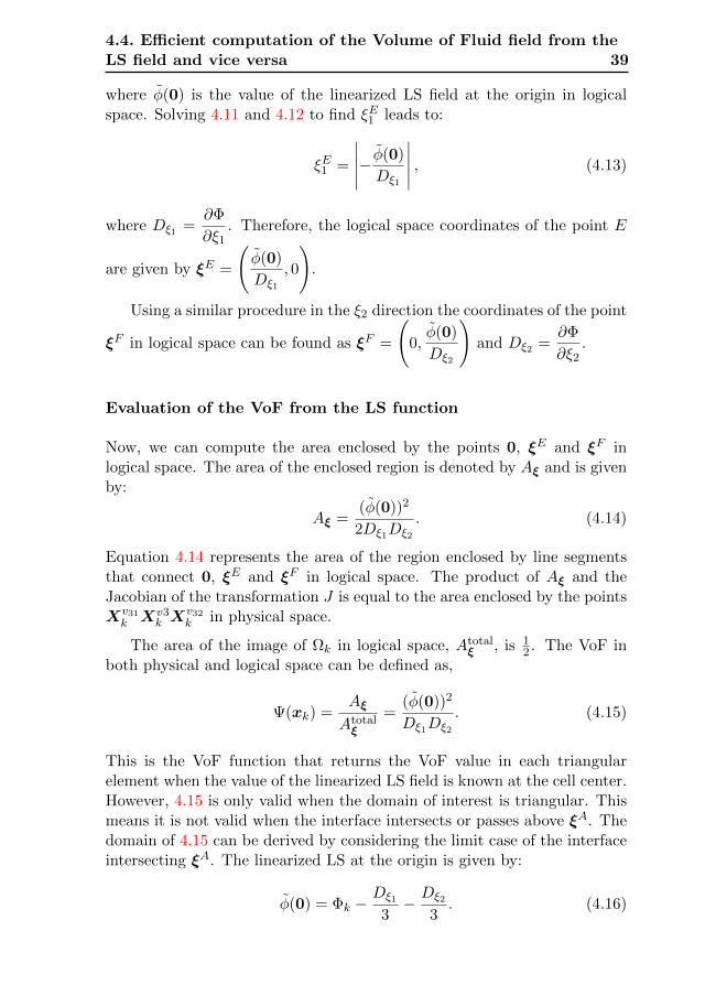
4.4. Efficient computation of the Volume of Fluid field from theLS field and vice versa 39
where φ(0) is the value of the linearized LS field at the origin in logicalspace. Solving 4.11 and 4.12 to find ξE1 leads to:
ξE1 =
∣∣∣∣∣− φ(0)
Dξ1
∣∣∣∣∣ , (4.13)
where Dξ1 =∂Φ
∂ξ1. Therefore, the logical space coordinates of the point E
are given by ξE =
(φ(0)
Dξ1
, 0
).
Using a similar procedure in the ξ2 direction the coordinates of the point
ξF in logical space can be found as ξF =
(0,φ(0)
Dξ2
)and Dξ2 =
∂Φ
∂ξ2.
Evaluation of the VoF from the LS function
Now, we can compute the area enclosed by the points 0, ξE and ξF inlogical space. The area of the enclosed region is denoted by Aξ and is givenby:
Aξ =(φ(0))2
2Dξ1Dξ2
. (4.14)
Equation 4.14 represents the area of the region enclosed by line segmentsthat connect 0, ξE and ξF in logical space. The product of Aξ and theJacobian of the transformation J is equal to the area enclosed by the pointsXv31k Xv3
k Xv32k in physical space.
The area of the image of Ωk in logical space, Atotalξ , is 1
2 . The VoF inboth physical and logical space can be defined as,
Ψ(xk) =Aξ
Atotalξ
=(φ(0))2
Dξ1Dξ2
. (4.15)
This is the VoF function that returns the VoF value in each triangularelement when the value of the linearized LS field is known at the cell center.However, 4.15 is only valid when the domain of interest is triangular. Thismeans it is not valid when the interface intersects or passes above ξA. Thedomain of 4.15 can be derived by considering the limit case of the interfaceintersecting ξA. The linearized LS at the origin is given by:
φ(0) = Φk −Dξ1
3−Dξ2
3. (4.16)
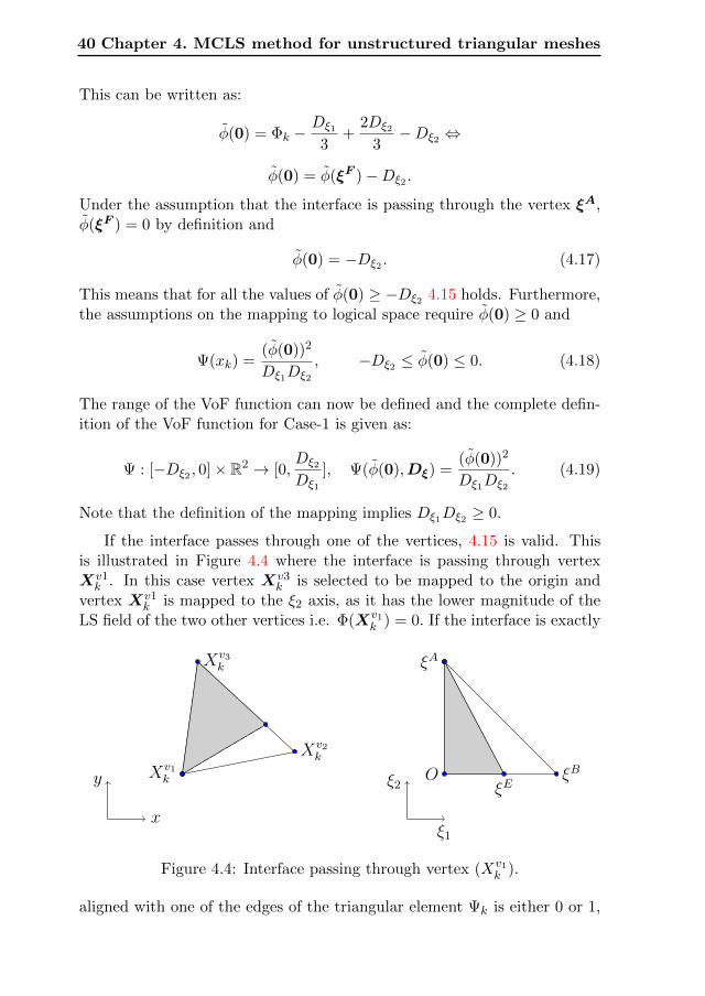
40 Chapter 4. MCLS method for unstructured triangular meshes
This can be written as:
φ(0) = Φk −Dξ1
3+
2Dξ2
3−Dξ2 ⇔
φ(0) = φ(ξF )−Dξ2 .
Under the assumption that the interface is passing through the vertex ξA,φ(ξF ) = 0 by definition and
φ(0) = −Dξ2 . (4.17)
This means that for all the values of φ(0) ≥ −Dξ2 4.15 holds. Furthermore,the assumptions on the mapping to logical space require φ(0) ≥ 0 and
Ψ(xk) =(φ(0))2
Dξ1Dξ2
, −Dξ2 ≤ φ(0) ≤ 0. (4.18)
The range of the VoF function can now be defined and the complete defin-ition of the VoF function for Case-1 is given as:
Ψ : [−Dξ2 , 0]× R2 → [0,Dξ2
Dξ1
], Ψ(φ(0),Dξ) =(φ(0))2
Dξ1Dξ2
. (4.19)
Note that the definition of the mapping implies Dξ1Dξ2 ≥ 0.
If the interface passes through one of the vertices, 4.15 is valid. Thisis illustrated in Figure 4.4 where the interface is passing through vertexXv1k . In this case vertex Xv3
k is selected to be mapped to the origin andvertex Xv1
k is mapped to the ξ2 axis, as it has the lower magnitude of theLS field of the two other vertices i.e. Φ(Xv1
k ) = 0. If the interface is exactly
Xv1k
Xv2k
Xv3k
y
x
ξB
ξA
OξE
ξ1
ξ2
Figure 4.4: Interface passing through vertex (Xv1k ).
aligned with one of the edges of the triangular element Ψk is either 0 or 1,
4.4. Efficient computation of the Volume of Fluid field from theLS field and vice versa 41
depending on the fluid of interest. In this case there is no need to use 4.19.The definition of the mapping excludes the possibility that the interface isaligned with one of the coordinate axes in logical space for Case-1. However,for Case-2 it is possible that the interface ends up aligned with one of theaxes in the logical space.
Case-2: quadrilateral domain of interest
Xv1k
Xv2k
Xv3k
y
x
ξB
ξA
OξE
ξI
ξF
ξ1
ξ2
Figure 4.5: Case-2: Mapping of two nodes a side.
An example of Case-2 is presented in Figure 4.5, where vertices Φ(Xv3k ) <
0 and Φ(Xv2k ) < 0 are now both located in the domain of interest. We as-
sume vertex Xv2k has a lower magnitude of the LS as compared to vertex
Xv3k . Therefore, vertex Xv2
k is mapped to the ξ2 axis and Xv3k to the ori-
gin in logical space. The fluid of interest is enclosed by the quadrilateral0, ξE , ξI , ξA (Figure 4.5). The vertex ξF is located outside the mappedregion and intersects the ξ2 axis, provided that the interface is not parallelto one of the edges of the triangle. This will only occur, when the interfaceis exactly equidistant from the vertices Xv3
k and Xv2k . This case will be
discussed separately in Section 4.4.2.
We can now use 4.14 to compute the area of the triangular region en-closed by vertices 0, ξE , ξI , ξF and ξA. Let us call this area Atri.. To findthe area of the quadrilateral region Aξ the area of the triangular regiondefined by the vertices ξF , ξI , ξA, which we will refer to as Aex., needs tobe subtracted from the area Atri.:
Aξ =(φ(0))2
2Dξ1Dξ2
−Aex.. (4.20)
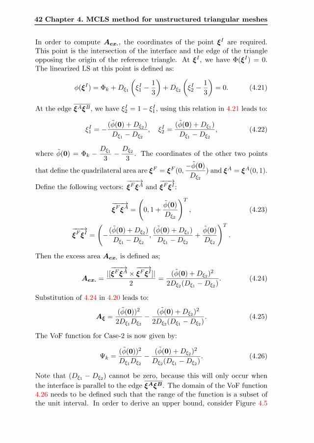
42 Chapter 4. MCLS method for unstructured triangular meshes
In order to compute Aex., the coordinates of the point ξI are required.This point is the intersection of the interface and the edge of the triangleopposing the origin of the reference triangle. At ξI , we have Φ(ξI) = 0.The linearized LS at this point is defined as:
φ(ξI) = Φk +Dξ1
(ξI1 −
1
3
)+Dξ2
(ξI2 −
1
3
)= 0. (4.21)
At the edge ξAξB, we have ξI2 = 1− ξI1 , using this relation in 4.21 leads to:
ξI1 = −(φ(0) +Dξ2)
Dξ1 −Dξ2
, ξI2 =(φ(0) +Dξ1)
Dξ1 −Dξ2
, (4.22)
where φ(0) = Φk −Dξ1
3−Dξ2
3. The coordinates of the other two points
that define the quadrilateral area are ξF = ξF (0,−φ(0)
Dξ2
) and ξA = ξA(0, 1).
Define the following vectors:−−−→ξF ξA and
−−−→ξF ξI :
−−−→ξF ξA =
(0, 1 +
φ(0)
Dξ2
)T, (4.23)
−−−→ξF ξI =
(−
(φ(0) +Dξ2)
Dξ1 −Dξ2
,(φ(0) +Dξ1)
Dξ1 −Dξ2
+φ(0)
Dξ2
)T.
Then the excess area Aex. is defined as;
Aex. =|[−−−→ξF ξA ×
−−−→ξF ξI ]|
2=
(φ(0) +Dξ2)2
2Dξ2(Dξ1 −Dξ2). (4.24)
Substitution of 4.24 in 4.20 leads to:
Aξ =(φ(0))2
2Dξ1Dξ2
−(φ(0) +Dξ2)2
2Dξ2(Dξ1 −Dξ2). (4.25)
The VoF function for Case-2 is now given by:
Ψk =(φ(0))2
Dξ1Dξ2
−(φ(0) +Dξ2)2
Dξ2(Dξ1 −Dξ2). (4.26)
Note that (Dξ1 − Dξ2) cannot be zero, because this will only occur when
the interface is parallel to the edge ξAξB. The domain of the VoF function4.26 needs to be defined such that the range of the function is a subset ofthe unit interval. In order to derive an upper bound, consider Figure 4.5
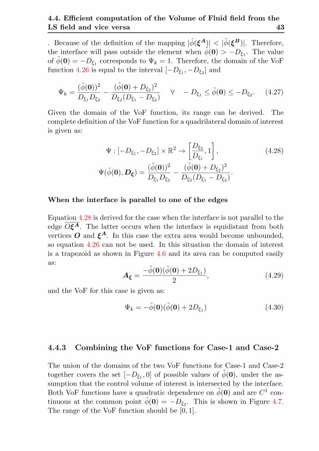
4.4. Efficient computation of the Volume of Fluid field from theLS field and vice versa 43
. Because of the definition of the mapping |φ(ξA)| < |φ(ξB)|. Therefore,the interface will pass outside the element when φ(0) > −Dξ1 . The valueof φ(0) = −Dξ1 corresponds to Ψk = 1. Therefore, the domain of the VoFfunction 4.26 is equal to the interval [−Dξ1 ,−Dξ2 ] and
Ψk =(φ(0))2
Dξ1Dξ2
−(φ(0) +Dξ2)2
Dξ2(Dξ1 −Dξ2)∀ −Dξ1 ≤ φ(0) ≤ −Dξ2 . (4.27)
Given the domain of the VoF function, its range can be derived. Thecomplete definition of the VoF function for a quadrilateral domain of interestis given as:
Ψ : [−Dξ1 ,−Dξ2 ]× R2 →[Dξ2
Dξ1
, 1
], (4.28)
Ψ(φ(0),Dξ) =(φ(0))2
Dξ1Dξ2
−(φ(0) +Dξ2)2
Dξ2(Dξ1 −Dξ2).
When the interface is parallel to one of the edges
Equation 4.28 is derived for the case when the interface is not parallel to theedge OξA. The latter occurs when the interface is equidistant from bothvertices O and ξA. In this case the extra area would become unbounded,so equation 4.26 can not be used. In this situation the domain of interestis a trapezoid as shown in Figure 4.6 and its area can be computed easilyas:
Aξ =−φ(0)(φ(0) + 2Dξ1)
2, (4.29)
and the VoF for this case is given as:
Ψk = −φ(0)(φ(0) + 2Dξ1) (4.30)
4.4.3 Combining the VoF functions for Case-1 and Case-2
The union of the domains of the two VoF functions for Case-1 and Case-2together covers the set [−Dξ1 , 0] of possible values of φ(0), under the as-sumption that the control volume of interest is intersected by the interface.Both VoF functions have a quadratic dependence on φ(0) and are C1 con-tinuous at the common point φ(0) = −Dξ2 . This is shown in Figure 4.7.The range of the VoF function should be [0, 1].
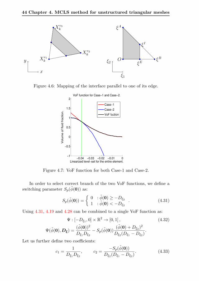
44 Chapter 4. MCLS method for unstructured triangular meshes
Xv1k
Xv2k
Xv3k
y
x
ξB
ξA
OξE
ξI
ξ1
ξ2
Figure 4.6: Mapping of the interface parallel to one of its edge.
−0.04 −0.03 −0.02 −0.01 0−1
−0.5
0
0.5
1
1.5
2
VoF function for Case−1 and Case−2.
Linearized level−set for the entire element.
Vo
lum
e o
f flu
id f
ractio
n.
Case−1
Case−2
VoF fuction
Figure 4.7: VoF function for both Case-1 and Case-2.
In order to select correct branch of the two VoF functions, we define aswitching parameter Sp(φ(0)) as:
Sp(φ(0)) =
0 : φ(0) ≥ −Dξ2
1 : φ(0) < −Dξ2
. (4.31)
Using 4.31, 4.19 and 4.28 can be combined to a single VoF function as:
Ψ : [−Dξ1 , 0]× R2 → [0, 1] , (4.32)
Ψ(φ(0),Dξ) =(φ(0))2
Dξ1Dξ2
− Sp(φ(0))(φ(0) +Dξ2)2
Dξ2(Dξ1 −Dξ2).
Let us further define two coefficients:
c1 =1
Dξ1Dξ2
, c2 =−Sp(φ(0))
Dξ2(Dξ1 −Dξ2). (4.33)
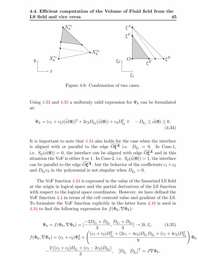
4.4. Efficient computation of the Volume of Fluid field from theLS field and vice versa 45
Xv1k
Xv2k
Xv3k
y
x
ξB
ξA
OξE
ξF
ξ1
ξ2
Figure 4.8: Combination of two cases.
Using 4.33 and 4.32 a uniformly valid expression for Ψk can be formulatedas:
Ψk = (c1 + c2)(φ(0))2 + 2c2Dξ2(φ(0)) + c2D2ξ2 ∀ −Dξ1 ≤ φ(0) ≤ 0.
(4.34)
It is important to note that 4.34 also holds for the case when the interfaceis aligned with or parallel to the edge OξA i.e. Dξ2 = 0. In Case-1,
i.e. Sp(φ(0)) = 0, the interface can be aligned with edge OξA and in thissituation the VoF is either 0 or 1. In Case-2, i.e. Sp(φ(0)) = 1, the interface
can be parallel to the edge OξA. but the behavior of the coefficients c1 + c2
and Dξ2c2 in the polynomial is not singular when Dξ2 = 0.
The VoF function 4.34 is expressed in the value of the linearized LS fieldat the origin in logical space and the partial derivatives of the LS functionwith respect to the logical space coordinates. However, we have defined theVoF function 4.4 in terms of the cell centroid value and gradient of the LS.To formulate the VoF function explicitly in the latter form 4.16 is used in4.34 to find the following expression for f(Φk,∇Φk):
Ψk = f(Φk,∇Φk) = [−2Dξ1 +Dξ2
3,Dξ1 +Dξ2
3]→ [0, 1], (4.35)
f(Φk,∇Φk) = (c1 + c2)Φ2k +
((c1 + c2)D2
ξ1+ (2c1 − 4c2)Dξ1Dξ2 + (c1 + 4c2)D2
ξ2
9
)Φk
−2 ((c1 + c2)Dξ1 + (c1 − 2c2)Dξ2)
3, [Dξ1 Dξ2 ]T = J∇Φk.
46 Chapter 4. MCLS method for unstructured triangular meshes
4.5 Advection of the LS field
Because the interface is by definition a contour line of the LS function, thefollowing equation holds at the interface:
d
dtΦ(x, t) = 0⇒ ∂Φ(x, t)
∂t+ uα(x, t)Φ(x, t),α = 0, x ∈X(t), t > 0.
(4.36)
In the MCLS method equation 4.36 is postulated to hold for all x ∈ Ω, butother choices are possible, as long as they are consistent with 4.36 and leadto a function that is at least C2 continuous in the vicinity of the interface toallow computation of the curvature. For a solenodial velocity field uα(x, t)the extension of (4.36) is given by (omitting the explicit dependence of xant t of uα(x, t)):
∂Φ(x, t)
∂t+ (uαΦ(x, t)),α = 0, x ∈ Ω, t > 0. (4.37)
This equation shows that the LS function is conserved. However, a con-servative redistribution of the LS function can lead to a change in the areaenclosed by the interface. This is one of the drawbacks associated withthe LS method. To some extent this can be remedied by using higher or-der approximations of the convection operator, e.g. using ENO or WENOschemes in the context of a finite volume discretisation [26, 57], combinedwith higher order time-integration methods or by applying adaptive gridrefinement near the interface. However, all the remedies are not computa-tionally efficient when 4.37 is discretised on an unstructured set of triangularcontrol volumes. In the current paper a higher-order discontinuous Galerkin(DG) finite element method is used for the discretization of 4.37. This ap-proach leads to a high order of accuracy boundary conforming discretisationfor domains with arbitrary geometrical complexity. For integration in timea low storage Runge-Kutta method is used. A brief description of the spa-tial and temporal discretization of 4.37 is presented, based on [19,20,23,34].The computational domain Ω is discretized into K non-overlapping, straightsided triangular elements Ωk. Lagrange polynomials Li(x) of degree N areused as basis functions to expand the solution in element Ωk as:
Φhk(x, t) = Σm
i=1φki (t)Li(x), x ∈ Ωk, t > 0, (4.38)
where m is the total number of nodal points in an element. In the DGframe work, the residual is made orthogonal to the polynomial space in Ωk,by requiring (omitting the explicit dependence of x ant t of Φh
k(x, t))∫Ωk
(∂Φh
k
∂t+ (uαΦh
k),α)Li(x)dΩ = 0, i = 1 . . .m. (4.39)
4.6. Advection of the Volume of Fluid field 47
The weak form of Equation 4.37 can be obtained by applying integrationby parts:∫
Ωk
∂Φhk
∂tLi(x)− Li,α(x)uαΦh
kdΩ = −∮∂Ωk
(nαuαΦh)∗Li(x)dΩ, i = 1 . . .m,
(4.40)where nα is the outward pointing unit normal and (uαΦh)∗ is the numericalflux, used to impose boundary conditions on each element. Integrating byparts once again leads to the strong formulation of the DG method:∫
Ωk
(∂Φh
∂t+ (uαΦh),α
)Li(x)dΩ =
∮∂Ωk
nα(uαΦh−(uαΦh)∗)Li(x)dΩ, i = 1 . . .m.
(4.41)In the MCLS 4.41 is combined with the Lax-Friedrichs approximation ofthe numerical flux [23]. The system ( 4.41) is formulated for all controlvolumes Ωk, k = 1 . . .K. All equations are coupled through the numericalflux function and advanced simultaneously.
4.6 Advection of the Volume of Fluid field
The MCLS algorithm uses a simultaneously advanced VoF field to impose acorrection on the LS field, to make the latter mass conserving. An evolutionequation for the VoF field is derived by taken the derivative of 4.3, withrespect to time:
dΨk(t)
dt=
d
dt
1
|Ωk|
∫Ωk
H(Φ(x, t))dΩ, (4.42)
Because H(Φ(x, t)) is a material property and assuming a solenoidal velo-city field uα(x, t), the right-hand side of 4.42 can be formulated as (droppingthe explicit dependences on x and t);
1
|Ωk|
∫Ωk
dH(Φ)
dtdΩ = − 1
|Ωk|
∫Ωk
H,α(Φ)uαdΩ = − 1
|Ωk|
∫∂Ωk
H(Φ)uαnαdS,
(4.43)where, nα is the normal vector on the boundary of the element. Therefore,the evolution of the VoF field is governed by:
dΨk
dt= − 1
|Ωk|
∫∂Ωk
H(Φ)uαnαdS (4.44)
The fact that H(Φ) is C−1 continuous on ∂Ω makes accurate discretisationof 4.44 very challenging. The application of ’standard’ schemes developed
48 Chapter 4. MCLS method for unstructured triangular meshes
for scalar hyperbolic equations leads either to strong oscillations in thesolution or unacceptable smearing of the interface, jeopardizing mass con-servation.
For Cartesian control volumes, accurate and efficient discretisation schemeshave been developed that utilize directional splitting, e.g. the schemepresented in [49] and its strictly mass conserving adaptation [58]. Apartfrom the latter scheme, strict mass conservation can only be achieved withvery intricate unsplit schemes. Also the method proposed by Jofre, Lluıs& et. al. [8, 12,27,28] can be suitable choice for the VoF advection but theinterface reconstruction based on the VoF field is computationally involved.
In this paper we propose to use a different approach for the advec-tion of the VoF field. This approach is also used in [60] and is known asEulerian-Lagrangian VoF evolution. The algorithm consists of three steps:Lagrangian advection of the color function, interface reconstruction, andremapping.
In the first step each mesh element is considered as a material elementand advected in a Lagrangian frame of reference. During this process thecolor function (a material property) is passively advected with the flow ineach element. Because the velocity field is solenodial each element retains itsVoF value while being deformed and rotated. Furthermore, if a divergencefree linear velocity field is assumed this ensures a straight sided triangleremains a straight sided triangle, irrespective of how the relative positionof the vertices changes (excluding folding). The assumption of a piecewiselinear velocity distribution is consistent with the linear approximation ofthe interface.
The approach is based on using two grids. The first one is a (fixed)Eulerian grid and the second one a Lagrangian grid that consists of the sameelements whose vertices have been translated. As the mesh elements areadvected such that their area remains the same, this advection is consistentwith Equation 4.43, i.e. the advection is mass conserving.
The coordinates of the vertices of the Lagrangian grid are obtained byusing a second order Runge-Kutta (RK) scheme, defined as,
Xv n+ 1
2kL
= XvkE
+∆t
2u(Xv
kE, tn), (4.45)
Xn+1kL
= XvkE
+ ∆tu(Xn+ 1
2kL
, tn+ 12 ), (4.46)
where, k = 1....., Nv and Nv is the total number of vertices. The Xv n+1kL
represent the vertices of the Lagrangian mesh, XvkE
the vertices of the Eu-lerian mesh. Because of the assumptions on the velocity field, the advection
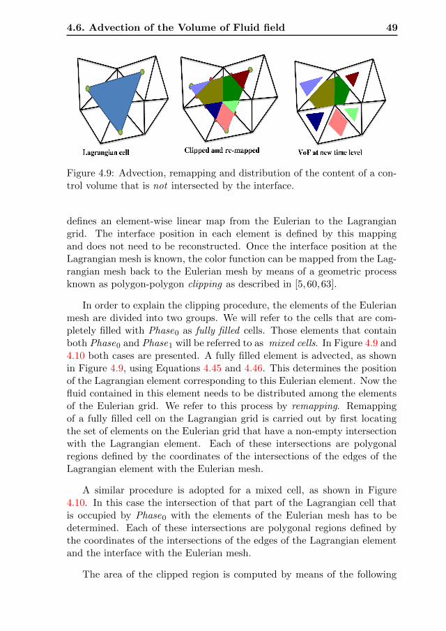
4.6. Advection of the Volume of Fluid field 49
Figure 4.9: Advection, remapping and distribution of the content of a con-trol volume that is not intersected by the interface.
defines an element-wise linear map from the Eulerian to the Lagrangiangrid. The interface position in each element is defined by this mappingand does not need to be reconstructed. Once the interface position at theLagrangian mesh is known, the color function can be mapped from the Lag-rangian mesh back to the Eulerian mesh by means of a geometric processknown as polygon-polygon clipping as described in [5, 60,63].
In order to explain the clipping procedure, the elements of the Eulerianmesh are divided into two groups. We will refer to the cells that are com-pletely filled with Phase0 as fully filled cells. Those elements that containboth Phase0 and Phase1 will be referred to as mixed cells. In Figure 4.9 and4.10 both cases are presented. A fully filled element is advected, as shownin Figure 4.9, using Equations 4.45 and 4.46. This determines the positionof the Lagrangian element corresponding to this Eulerian element. Now thefluid contained in this element needs to be distributed among the elementsof the Eulerian grid. We refer to this process by remapping. Remappingof a fully filled cell on the Lagrangian grid is carried out by first locatingthe set of elements on the Eulerian grid that have a non-empty intersectionwith the Lagrangian element. Each of these intersections are polygonalregions defined by the coordinates of the intersections of the edges of theLagrangian element with the Eulerian mesh.
A similar procedure is adopted for a mixed cell, as shown in Figure4.10. In this case the intersection of that part of the Lagrangian cell thatis occupied by Phase0 with the elements of the Eulerian mesh has to bedetermined. Each of these intersections are polygonal regions defined bythe coordinates of the intersections of the edges of the Lagrangian elementand the interface with the Eulerian mesh.
The area of the clipped region is computed by means of the following
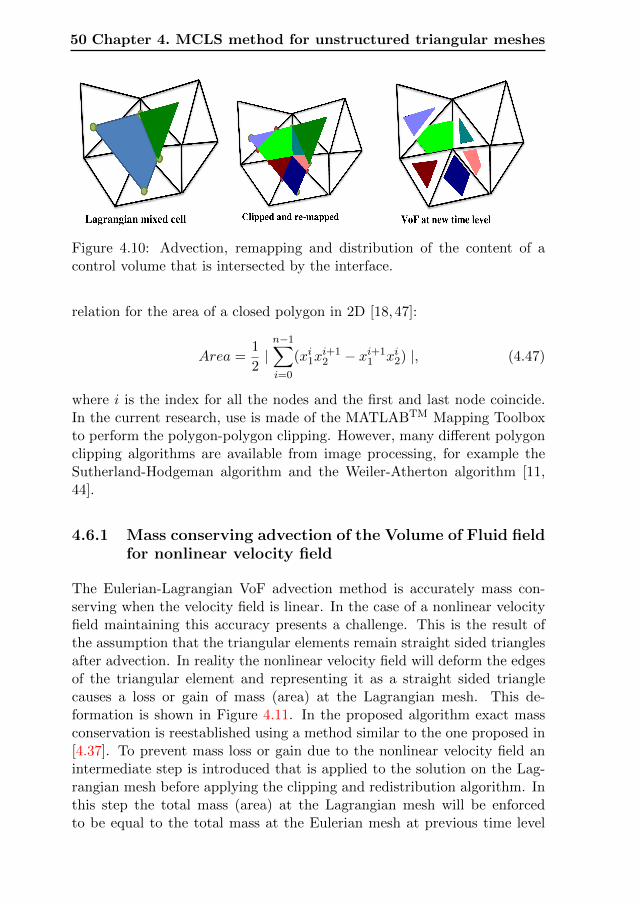
50 Chapter 4. MCLS method for unstructured triangular meshes
Figure 4.10: Advection, remapping and distribution of the content of acontrol volume that is intersected by the interface.
relation for the area of a closed polygon in 2D [18,47]:
Area =1
2|n−1∑i=0
(xi1xi+12 − xi+1
1 xi2) |, (4.47)
where i is the index for all the nodes and the first and last node coincide.In the current research, use is made of the MATLABTM Mapping Toolboxto perform the polygon-polygon clipping. However, many different polygonclipping algorithms are available from image processing, for example theSutherland-Hodgeman algorithm and the Weiler-Atherton algorithm [11,44].
4.6.1 Mass conserving advection of the Volume of Fluid fieldfor nonlinear velocity field
The Eulerian-Lagrangian VoF advection method is accurately mass con-serving when the velocity field is linear. In the case of a nonlinear velocityfield maintaining this accuracy presents a challenge. This is the result ofthe assumption that the triangular elements remain straight sided trianglesafter advection. In reality the nonlinear velocity field will deform the edgesof the triangular element and representing it as a straight sided trianglecauses a loss or gain of mass (area) at the Lagrangian mesh. This de-formation is shown in Figure 4.11. In the proposed algorithm exact massconservation is reestablished using a method similar to the one proposed in[4.37]. To prevent mass loss or gain due to the nonlinear velocity field anintermediate step is introduced that is applied to the solution on the Lag-rangian mesh before applying the clipping and redistribution algorithm. Inthis step the total mass (area) at the Lagrangian mesh will be enforcedto be equal to the total mass at the Eulerian mesh at previous time level
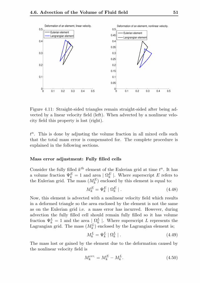
4.6. Advection of the Volume of Fluid field 51
0 0.1 0.2 0.3 0.4 0.50
0.1
0.2
0.3
0.4
0.5Deformation of an elememt, linear velocity.
Eulerian element
Langrangian element
0 0.1 0.2 0.3 0.4 0.50
0.05
0.1
0.15
0.2
0.25
0.3
0.35
0.4
0.45
0.5Deformation of an elememt, nonlinear velocity.
Eulerian element
Langrangian element
Figure 4.11: Straight-sided triangles remain straight-sided after being ad-vected by a linear velocity field (left). When advected by a nonlinear velo-city field this property is lost (right).
tn. This is done by adjusting the volume fraction in all mixed cells suchthat the total mass error is compensated for. The complete procedure isexplained in the following sections.
Mass error adjustment: Fully filled cells
Consider the fully filled kth element of the Eulerian grid at time tn. It hasa volume fraction ΨE
k = 1 and area | ΩEk |. Where superscript E refers to
the Eulerian grid. The mass (MEk ) enclosed by this element is equal to:
MEk = ΨE
k | ΩEk | . (4.48)
Now, this element is advected with a nonlinear velocity field which resultsin a deformed triangle so the area enclosed by the element is not the sameas on the Eulerian grid i.e. a mass error has incurred. However, duringadvection the fully filled cell should remain fully filled so it has volumefraction ΨL
k = 1 and the area | ΩLk |. Where superscript L represents the
Lagrangian grid. The mass (MLk ) enclosed by the Lagrangian element is;
MLk = ΨL
k | ΩLk | . (4.49)
The mass lost or gained by the element due to the deformation caused bythe nonlinear velocity field is
M err.k = ME
k −MLk . (4.50)
52 Chapter 4. MCLS method for unstructured triangular meshes
Where, M err.k is the mass error of the kth fully filled cell. If there are Nf
fully filled elements that are advected, using a nonlinear velocity field, thenthe total mass error (TM err.) caused by the fully filled cells can be definedas
TM err. =
Nf∑i=1
(MEi −ML
i
). (4.51)
The total mass error computed in Equation 4.51 is distributed evenly amongthe mixed cells. If there are Nm mixed cells then the average mass error(Mavg) can be defined as:
Mavg. =
Nf∑i=1
(MEi −ML
i
Nm
). (4.52)
This average mass error is added to each of the mixed cells to ensure globalmass conservation.
Mass error adjustment: Partially filled cells
In case of a partially filled or mixed cell a different procedure is adop-ted. The interface position is adjusted in each mixed control volume in theLagrangian grid such that the mass contained within is equal to the masscontained within the corresponding control volume on the Eulerian grid plusthe average mass error that follows from 4.52. Both the position and theorientation of the interface have to be determined. The orientation of theinterface can be determined from the LS field, but this approach would re-quire the interpolation of the LS field from the Eulerian to the Lagrangiangrid at time tn+1. This idea is not computationally efficient, for detailssee [60]. To mitigate this problem a different procedure is used, which isbased on the assumption that the interface can be reconstructed on theLagrangian element by advecting the two points that represent the inter-face in the corresponding Eulerian element. Naturally, this puts a thresholdon the size of the time step that can be taken. However, the idea is compu-tationally efficient and also in line with the idea of distributing the averagemass error to the mixed cells. The details of the interface adjustment forthe control volumes in the Lagrangian mesh are presented in the followingsubsection.
Interface adjustment for partially filled cells
Consider a partially filled cell at the Eulerian grid at time tn, as shown inFigure 4.12(a). The vertices of the element are Xv1
E , Xv2E and Xv3
E . The
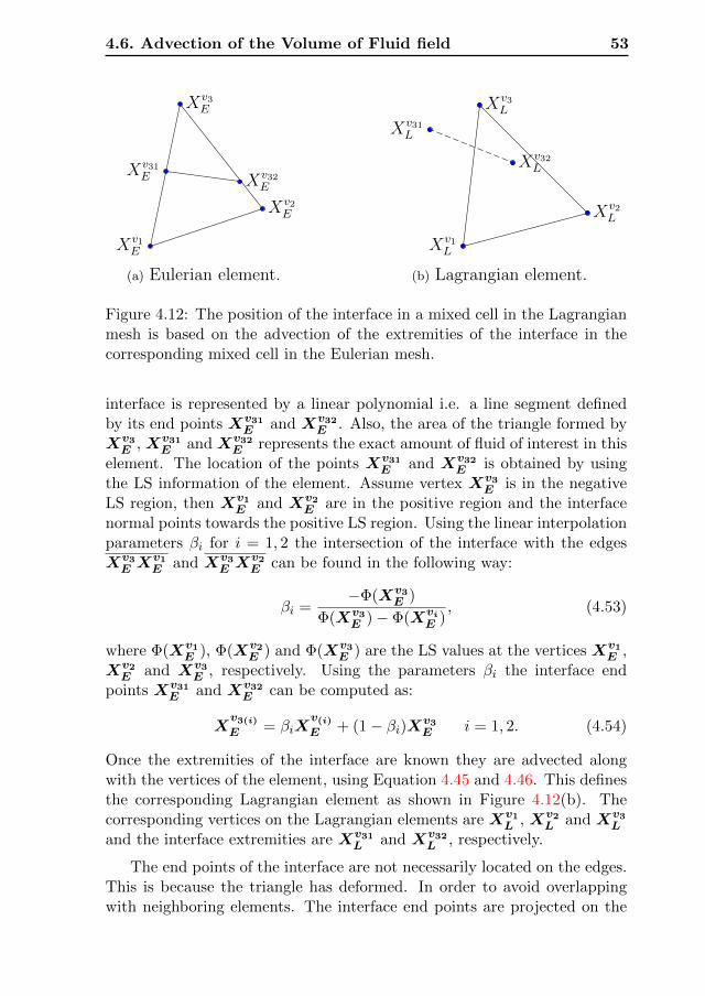
4.6. Advection of the Volume of Fluid field 53
Xv1E
Xv2E
Xv3E
Xv31E Xv32
E
(a) Eulerian element.
Xv1L
Xv2L
Xv3L
Xv31L
Xv32L
(b) Lagrangian element.
Figure 4.12: The position of the interface in a mixed cell in the Lagrangianmesh is based on the advection of the extremities of the interface in thecorresponding mixed cell in the Eulerian mesh.
interface is represented by a linear polynomial i.e. a line segment definedby its end points Xv31
E and Xv32E . Also, the area of the triangle formed by
Xv3E , Xv31
E and Xv32E represents the exact amount of fluid of interest in this
element. The location of the points Xv31E and Xv32
E is obtained by usingthe LS information of the element. Assume vertex Xv3
E is in the negativeLS region, then Xv1
E and Xv2E are in the positive region and the interface
normal points towards the positive LS region. Using the linear interpolationparameters βi for i = 1, 2 the intersection of the interface with the edgesXv3E X
v1E and Xv3
E Xv2E can be found in the following way:
βi =−Φ(Xv3
E )
Φ(Xv3E )− Φ(Xvi
E ), (4.53)
where Φ(Xv1E ), Φ(Xv2
E ) and Φ(Xv3E ) are the LS values at the vertices Xv1
E ,Xv2E and Xv3
E , respectively. Using the parameters βi the interface endpoints Xv31
E and Xv32E can be computed as:
Xv3(i)E = βiX
v(i)E + (1− βi)Xv3
E i = 1, 2. (4.54)
Once the extremities of the interface are known they are advected alongwith the vertices of the element, using Equation 4.45 and 4.46. This definesthe corresponding Lagrangian element as shown in Figure 4.12(b). Thecorresponding vertices on the Lagrangian elements are Xv1
L , Xv2L and Xv3
L
and the interface extremities are Xv31L and Xv32
L , respectively.
The end points of the interface are not necessarily located on the edges.This is because the triangle has deformed. In order to avoid overlappingwith neighboring elements. The interface end points are projected on the
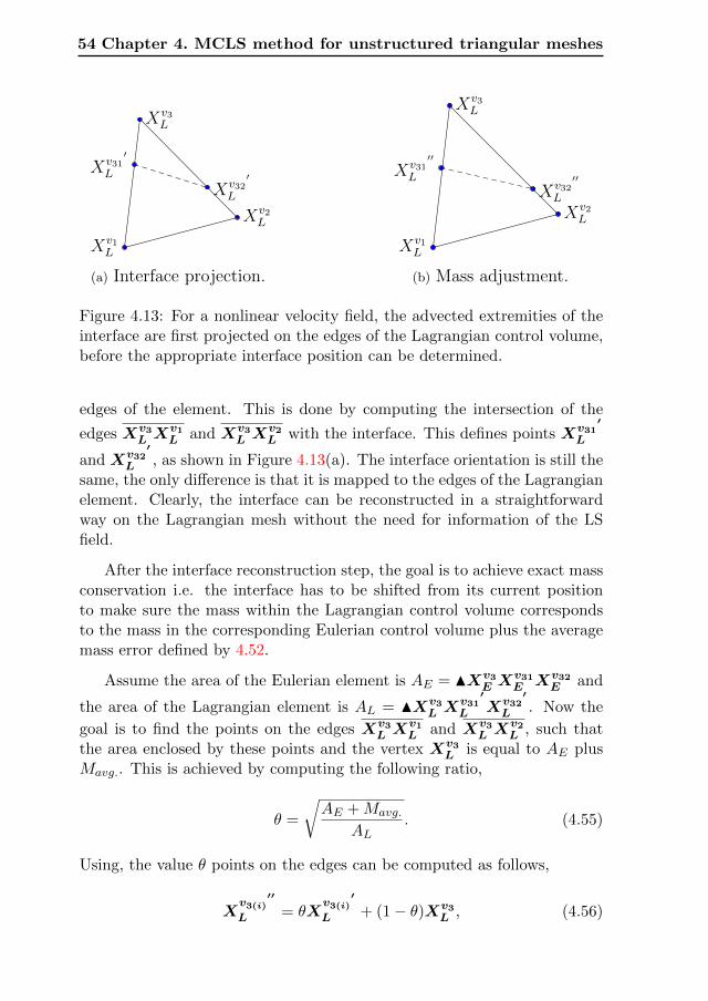
54 Chapter 4. MCLS method for unstructured triangular meshes
Xv1L
Xv2L
Xv3L
Xv31′
L
Xv32′
L
(a) Interface projection.
Xv1L
Xv2L
Xv3L
Xv31′′
L
Xv32′′
L
(b) Mass adjustment.
Figure 4.13: For a nonlinear velocity field, the advected extremities of theinterface are first projected on the edges of the Lagrangian control volume,before the appropriate interface position can be determined.
edges of the element. This is done by computing the intersection of the
edges Xv3L X
v1L and Xv3
L Xv2L with the interface. This defines points Xv31
′
L
and Xv32′
L , as shown in Figure 4.13(a). The interface orientation is still thesame, the only difference is that it is mapped to the edges of the Lagrangianelement. Clearly, the interface can be reconstructed in a straightforwardway on the Lagrangian mesh without the need for information of the LSfield.
After the interface reconstruction step, the goal is to achieve exact massconservation i.e. the interface has to be shifted from its current positionto make sure the mass within the Lagrangian control volume correspondsto the mass in the corresponding Eulerian control volume plus the averagemass error defined by 4.52.
Assume the area of the Eulerian element is AE = NXv3E X
v31E Xv32
E and
the area of the Lagrangian element is AL = NXv3L X
v31′
L Xv32′
L . Now the
goal is to find the points on the edges Xv3L X
v1L and Xv3
L Xv2L , such that
the area enclosed by these points and the vertex Xv3L is equal to AE plus
Mavg.. This is achieved by computing the following ratio,
θ =
√AE +Mavg.
AL. (4.55)
Using, the value θ points on the edges can be computed as follows,
Xv3(i)
′′
L = θXv3(i)
′
L + (1− θ)Xv3L , (4.56)
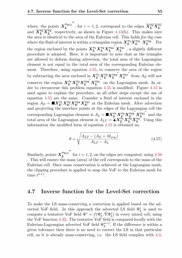
4.7. Inverse function for the Level-Set correction 55
where, the points Xv3(i)
′′
L , for i = 1, 2, correspond to the edges Xv3L X
v1L
and Xv3L X
v2L , respectively, as shown in Figure 4.13(b). This makes sure
the area is identical to the area of the Eulerian cell. This holds for the casewhere the fluid of interest is within a triangular regionXv3
L Xv31
′
L Xv32′
L . For
the region enclosed by the points Xv1L X
v2L X
v32′
L Xv31′
L , a slightly differentprocedure is adopted. Here, it is important to note that as the trianglesare allowed to deform during advection, the total area of the Lagrangianelement is not equal to the total area of the corresponding Eulerian ele-ment. Therefore, using equation 4.55, to conserve the area of the region
by subtracting the area enclosed in Xv1L X
v2L X
v32′
L Xv31′
L from AE will not
conserve the region Xv1L X
v2L X
v32′
L Xv31′
L on the Lagrangian mesh. In or-der to circumvent this problem equation 4.55 is modified. Figure 4.13 isused again to explain the procedure, as all other steps except the use ofequation 4.55 are the same. Consider a fluid of interest enclosed in theregion AE = Xv1
E Xv2E X
v32E Xv31
E at the Eulerian mesh. After advectionand projecting the interface points at the edges of the Lagrangian cell the
corresponding Lagrangian element is AL = Xv1L X
v2L X
v32′
L Xv31′
L and thetotal area of the Lagrangian element is ALT = NXv1
L Xv2L X
v3L . Using this
information the modified form of equation 4.55 is obtained as;
θ =
√ALT − (AE +Mavg.)
ALT −AL. (4.57)
Similarly, points Xv3(i)
′′
L for i = 1, 2, on the edges are computed, using 4.56. This will ensure the mass (area) of the cell corresponds to the mass of theEulerian cell. Once mass conservation is achieved at the Lagrangian mesh,the clipping procedure is applied to map the VoF to the Eulerian mesh fortime tn+1.
4.7 Inverse function for the Level-Set correction
To make the LS mass-conserving a correction is applied based on the ad-vected VoF field. In this approach the advected LS field Φ∗k is used tocompute a tentative VoF field Ψ∗ = f(Φ∗k,∇Φ∗k) in every mixed cell, usingthe VoF function 4.32. The tentative VoF field is compared locally with theEulerian-Lagrangian advected VoF field Ψn+1
k . If the difference is within agiven tolerance then there is no need to correct the LS in that particularcell, as it is already mass-conserving, i.e. the LS field complies with 4.3,
56 Chapter 4. MCLS method for unstructured triangular meshes
and Φn+1k = Φ∗k. However, if this difference exceeds the prescribed toler-
ance, a correction is required. In order to perform the correction the inverseof f(Φk,∇Φk) is required. This function is referred to as the inverse VoFfunction g(Ψk,∇Φk). This function is derived from 4.32.
Assume the value of the VoF field for Ωk is given by:
Ψn+1k = f(Φn+1
k ,∇Φn+1k ), (4.58)
for yet unknown Φn+1k . Because the mass conserving corrections that need
to be imposed in the MCLS are very small, the orientation of the interfaceis assumed to remain unchanged. Therefore, we can replace 4.58 by,
Ψn+1k = f(Φn+1
k ,∇Φ∗k). (4.59)
This means that in the conversion the height of the interface is adjustedwithout changing its orientation. For a triangular (or more generally aconvex) element there is a unique value of Φn+1
k that fulfills 4.59 for Ψk ∈[0, 1]. Therefore, the inverse of f(Φk,∇Φk) with respect to its first argumentcan be defined as
Φk = g(Ψk,∇Φk). (4.60)
In order to obtain a uniformly valid inverse function, a switching parametersimilar to 4.31 can be defined as:
S′p(Ψ
)k =
1 : Ψk ≥
Dξ2
Dξ1
0 : Ψk <Dξ2
Dξ1
. (4.61)
A critical value of the VoF is Ψk =Dξ2
Dξ1
, because for this value the interface
is passing through the vertex ξA, see Figure 4.8. Using 4.61, 4.27 can bewritten as:
Ψk =(φ(0))2
Dξ1Dξ2
− S′p(Ψk)(φ(0) +Dξ2)2
Dξ2(Dξ1 −Dξ2). (4.62)
Define the coefficients c′1,2 as:
c′1 =
1
Dξ1Dξ2
, c′2 =
−S′p(Ψk)
Dξ2(Dξ1 −Dξ2). (4.63)
Now φ(0) is the unique root of the following quadratic equation:
(c′1 + c
′2)(φn+1(0))2 + 2c
′2Dξ2(φn+1(0)) + c
′2D
2ξ2 −Ψk = 0, (4.64)
∀ Ψk ∈ [0, 1].
4.8. Computational cost of the mass-conserving correction 57
within the interval [−Dξ1 , 0]. This unique root is given by:
φ(0) = −(2c′2Dξ2)−
√(2c′2Dξ2)2 − 4(c
′1 + c
′2)(c
′2D
2ξ2−Ψk)
2(c′1 + c
′2)
. (4.65)
The inverse function g(Φk,∇Φk) can now be defined as:
Φk = g(Ψk,∇Φk) : [0, 1]→[−2Dξ1 +Dξ2
3,Dξ1 +Dξ2
3
], (4.66)
g(Ψk,∇Φk) = −(2c′2Dξ2)−
√(2c′2Dξ2)2 − 4(c
′1 + c
′2)(c
′2D
2ξ2−Ψk)
2(c′1 + c
′2)
) +Dξ1 +Dξ2
3.
Where, [Dξ1 Dξ2 ]T = J∇Φk. The conversion of LS to VoF depends onthe value and gradient of the LS at the center of the control volume. Keydifference between the original MCLS, and the proposed algorithm is thatin the latter, the discretisation of the LS field with a discontinuous Galer-kin method leads to a local, element-wise definition of the LS field. Thismeans that the LS field can be corrected locally, contrary to the originalMCLS algorithm where an iterative procedure is used to have both Φn+1
k
and ∇Φn+1k comply with 4.58. This is a major improvement with respect to
efficiency and robustness in comparison with the original MCLS algorithm.
4.8 Computational cost of the mass-conserving cor-rection
Accurately mass-conserving advection of the VoF field on a discretisationof general unstructured control volumes is very challenging but necessaryin many but certainly not all applications. Incorporating this correctionmakes the algorithm significantly more costly than a ’pure’ LS approach,but comparable in cost to algorithms that are based on an explicit recon-struction of the interface. The Eulerian-Lagrangian approach of advectionand the required ’clipping’ algorithm are computationally intensive. How-ever, these ’clipping’ type of algorithms are used extensively in computergraphics and under continuous development. Furthermore, they are highlyparallelizable and readily portable to GPU architectures. Alternative al-gorithms, for example based on the use of compressive schemes used formodified LS formulations are currently investigated. The use of a discon-tinuous Galerkin discretisation and the resulting locality of the mass con-serving correction lead to a significant gain in efficiency with respect to theoriginal formulation of the MCLS method.
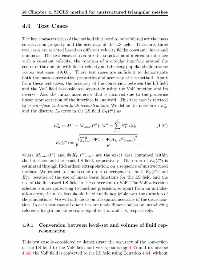
58 Chapter 4. MCLS method for unstructured triangular meshes
4.9 Test Cases
The key characteristics of the method that need to be validated are the massconservation property and the accuracy of the LS field. Therefore, threetest cases are selected based on different velocity fields; constant, linear andnonlinear. The test cases chosen are the translation of a circular interfacewith a constant velocity, the rotation of a circular interface around thecenter of the domain with linear velocity and the very popular single reversevortex test case [49, 60]. These test cases are sufficient to demonstrateboth the mass conservation properties and accuracy of the method. Apartfrom these test cases, the accuracy of the conversion between the LS fieldand the VoF field is considered separately using the VoF function and itsinverse. Also the initial mass error that is incurred due to the piecewiselinear representation of the interface is analysed. This test case is referredto as interface back and forth reconstruction. We define the mass error EnMand the discrete L2 error in the LS field EΨ(tn) as
EnM = Mn −Mexact(tn),Mn =
K∑k=1
Ψnk |Ωk|, (4.67)
EΦ(tn) =
√∑Kk=1
(ΦnK − Φ(Xk, tn)exact
)2K
,
where Mexact(tn) and Φ(Xk, t
n)exact are the exact area contained withinthe interface and the exact LS field, respectively. The order of EΦ(tn) isestimated through Richardson extrapolation, on a sequence of unstructuredmeshes. We expect to find second order convergence of both EΦ(tn) andEnM , because of the use of linear basis functions for the LS field and theuse of the linearized LS field in the conversion to VoF. The VoF advectionscheme is mass conserving to machine precision, so apart from an initializ-ation error, the mass loss should be virtually negligible over the duration ofthe simulations. We will only focus on the spatial accuracy of the discretisa-tion. In each test case all quantities are made dimensionless by introducingreference length and time scales equal to 1 m and 1 s, respectively.
4.9.1 Conversion between level-set and volume of fluid rep-resentation
This test case is considered to demonstrate the accuracy of the conversionof the LS field to the VoF field and vice versa using 4.35 and its inverse4.66: the VoF field is converted to the LS field using Equation 4.64, without
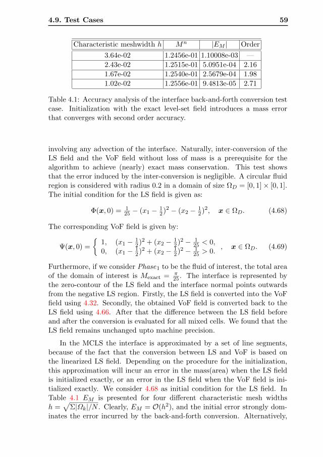
4.9. Test Cases 59
Characteristic meshwidth h Mn |EM | Order
3.64e-02 1.2456e-01 1.10008e-03 —
2.43e-02 1.2515e-01 5.0951e-04 2.16
1.67e-02 1.2540e-01 2.5679e-04 1.98
1.02e-02 1.2556e-01 9.4813e-05 2.71
Table 4.1: Accuracy analysis of the interface back-and-forth conversion testcase. Initialization with the exact level-set field introduces a mass errorthat converges with second order accuracy.
involving any advection of the interface. Naturally, inter-conversion of theLS field and the VoF field without loss of mass is a prerequisite for thealgorithm to achieve (nearly) exact mass conservation. This test showsthat the error induced by the inter-conversion is negligible. A circular fluidregion is considered with radius 0.2 in a domain of size ΩD = [0, 1]× [0, 1].The initial condition for the LS field is given as:
Φ(x, 0) = 125 − (x1 − 1
2)2 − (x2 − 12)2, x ∈ ΩD. (4.68)
The corresponding VoF field is given by:
Ψ(x, 0) =
1, (x1 − 1
2)2 + (x2 − 12)2 − 1
25 < 0,0, (x1 − 1
2)2 + (x2 − 12)2 − 1
25 > 0., x ∈ ΩD. (4.69)
Furthermore, if we consider Phase1 to be the fluid of interest, the total areaof the domain of interest is Mexact = π
25 . The interface is represented bythe zero-contour of the LS field and the interface normal points outwardsfrom the negative LS region. Firstly, the LS field is converted into the VoFfield using 4.32. Secondly, the obtained VoF field is converted back to theLS field using 4.66. After that the difference between the LS field beforeand after the conversion is evaluated for all mixed cells. We found that theLS field remains unchanged upto machine precision.
In the MCLS the interface is approximated by a set of line segments,because of the fact that the conversion between LS and VoF is based onthe linearized LS field. Depending on the procedure for the initialization,this approximation will incur an error in the mass(area) when the LS fieldis initialized exactly, or an error in the LS field when the VoF field is ini-tialized exactly. We consider 4.68 as initial condition for the LS field. InTable 4.1 EM is presented for four different characteristic mesh widthsh =
√Σ|Ωk|/N . Clearly, EM = O(h2), and the initial error strongly dom-
inates the error incurred by the back-and-forth conversion. Alternatively,
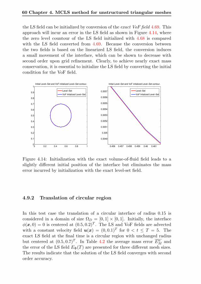
60 Chapter 4. MCLS method for unstructured triangular meshes
the LS field can be initialized by conversion of the exact VoF field 4.69. Thisapproach will incur an error in the LS field as shown in Figure 4.14, wherethe zero level countour of the LS field initialized with 4.68 is comparedwith the LS field converted from 4.69. Because the conversion betweenthe two fields is based on the linearized LS field, the conversion inducesa small movement of the interface, which can be shown to decrease withsecond order upon grid refinement. Clearly, to achieve nearly exact massconservation, it is essential to initialize the LS field by converting the initialcondition for the VoF field.
Initial Level−Set and VoF initialized Level−Set contour.
0 0.2 0.4 0.6 0.8 10
0.1
0.2
0.3
0.4
0.5
0.6
0.7
0.8
0.9
1
Level−Set
VoF Intialized Level−Set
Initial Level−Set and VoF initialized Level−Set contour.
0.456 0.457 0.458 0.459 0.46 0.461
0.3049
0.305
0.3051
0.3052
0.3053
0.3054
0.3055
0.3056
0.3057 Level−Set
VoF Intialized Level−Set
Figure 4.14: Initialization with the exact volume-of-fluid field leads to aslightly different initial position of the interface but eliminates the masserror incurred by initialization with the exact level-set field.
4.9.2 Translation of circular region
In this test case the translation of a circular interface of radius 0.15 isconsidered in a domain of size ΩD = [0, 1] × [0, 1]. Initially, the interfaceφ(x, 0) = 0 is centered at (0.5, 0.2)T . The LS and VoF fields are advectedwith a constant velocity field u(x) = (0, 0.1)T for 0 < t ≤ T = 5. Theexact LS field at the final time is a circular region with unchanged radiusbut centered at (0.5, 0.7)T . In Table 4.2 the average mass error EnM andthe error of the LS field EΦ(T ) are presented for three different mesh sizes.The results indicate that the solution of the LS field converges with secondorder accuracy.
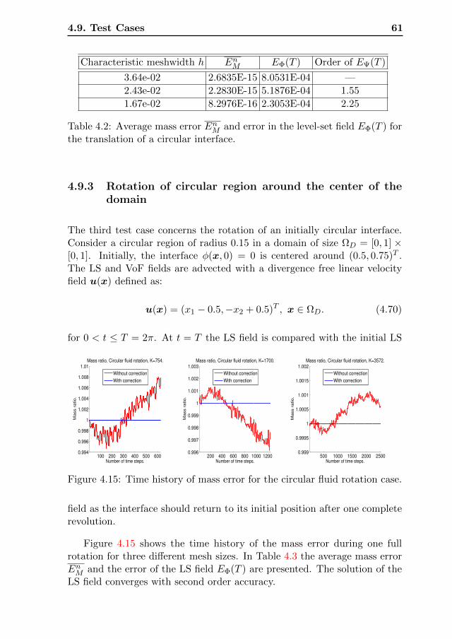
4.9. Test Cases 61
Characteristic meshwidth h EnM EΦ(T ) Order of EΨ(T )
3.64e-02 2.6835E-15 8.0531E-04 —
2.43e-02 2.2830E-15 5.1876E-04 1.55
1.67e-02 8.2976E-16 2.3053E-04 2.25
Table 4.2: Average mass error EnM and error in the level-set field EΦ(T ) forthe translation of a circular interface.
4.9.3 Rotation of circular region around the center of thedomain
The third test case concerns the rotation of an initially circular interface.Consider a circular region of radius 0.15 in a domain of size ΩD = [0, 1] ×[0, 1]. Initially, the interface φ(x, 0) = 0 is centered around (0.5, 0.75)T .The LS and VoF fields are advected with a divergence free linear velocityfield u(x) defined as:
u(x) = (x1 − 0.5,−x2 + 0.5)T , x ∈ ΩD. (4.70)
for 0 < t ≤ T = 2π. At t = T the LS field is compared with the initial LS
100 200 300 400 500 6000.994
0.996
0.998
1
1.002
1.004
1.006
1.008
1.01
Number of time steps.
Ma
ss r
atio
.
Mass ratio, Circular fluid rotation, K=754.
Without correction
With correction
200 400 600 800 1000 12000.996
0.997
0.998
0.999
1
1.001
1.002
1.003
Number of time steps.
Ma
ss r
atio
.
Mass ratio, Circular fluid rotation, K=1700.
Without correction
With correction
500 1000 1500 2000 25000.999
0.9995
1
1.0005
1.001
1.0015
1.002
Number of time steps.
Ma
ss r
atio
.
Mass ratio, Circular fluid rotation, K=3572.
Without correction
With correction
Figure 4.15: Time history of mass error for the circular fluid rotation case.
field as the interface should return to its initial position after one completerevolution.
Figure 4.15 shows the time history of the mass error during one fullrotation for three different mesh sizes. In Table 4.3 the average mass errorEnM and the error of the LS field EΦ(T ) are presented. The solution of theLS field converges with second order accuracy.
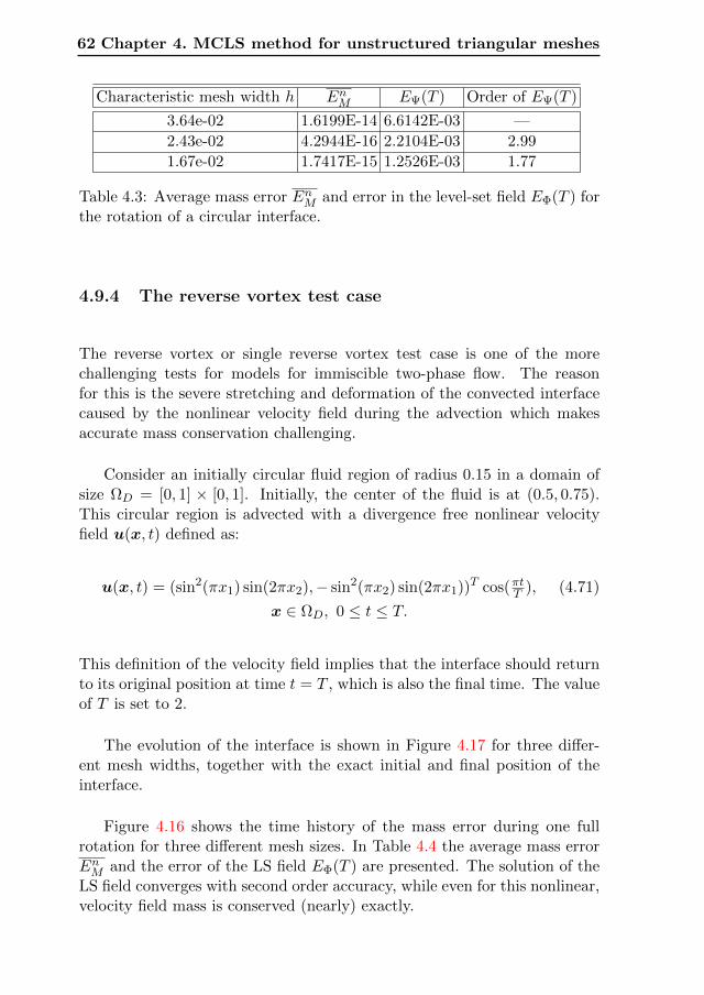
62 Chapter 4. MCLS method for unstructured triangular meshes
Characteristic mesh width h EnM EΨ(T ) Order of EΨ(T )
3.64e-02 1.6199E-14 6.6142E-03 —
2.43e-02 4.2944E-16 2.2104E-03 2.99
1.67e-02 1.7417E-15 1.2526E-03 1.77
Table 4.3: Average mass error EnM and error in the level-set field EΦ(T ) forthe rotation of a circular interface.
4.9.4 The reverse vortex test case
The reverse vortex or single reverse vortex test case is one of the morechallenging tests for models for immiscible two-phase flow. The reasonfor this is the severe stretching and deformation of the convected interfacecaused by the nonlinear velocity field during the advection which makesaccurate mass conservation challenging.
Consider an initially circular fluid region of radius 0.15 in a domain ofsize ΩD = [0, 1] × [0, 1]. Initially, the center of the fluid is at (0.5, 0.75).This circular region is advected with a divergence free nonlinear velocityfield u(x, t) defined as:
u(x, t) = (sin2(πx1) sin(2πx2),− sin2(πx2) sin(2πx1))T cos(πtT ), (4.71)
x ∈ ΩD, 0 ≤ t ≤ T.
This definition of the velocity field implies that the interface should returnto its original position at time t = T , which is also the final time. The valueof T is set to 2.
The evolution of the interface is shown in Figure 4.17 for three differ-ent mesh widths, together with the exact initial and final position of theinterface.
Figure 4.16 shows the time history of the mass error during one fullrotation for three different mesh sizes. In Table 4.4 the average mass errorEnM and the error of the LS field EΦ(T ) are presented. The solution of theLS field converges with second order accuracy, while even for this nonlinear,velocity field mass is conserved (nearly) exactly.
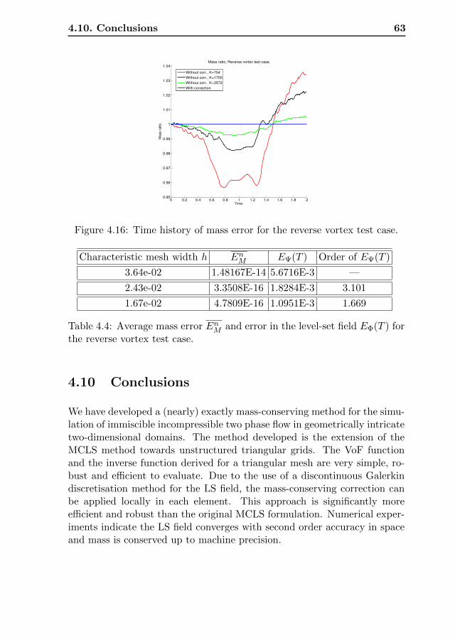
4.10. Conclusions 63
0 0.2 0.4 0.6 0.8 1 1.2 1.4 1.6 1.8 20.95
0.96
0.97
0.98
0.99
1
1.01
1.02
1.03
1.04
Time.
Ma
ss r
atio
.
Mass ratio, Reverse vortex test case.
Without corr., K=754
Without corr., K=1700
Without corr., K=3572
With correction
Figure 4.16: Time history of mass error for the reverse vortex test case.
Characteristic mesh width h EnM EΨ(T ) Order of EΨ(T )
3.64e-02 1.48167E-14 5.6716E-3 —
2.43e-02 3.3508E-16 1.8284E-3 3.101
1.67e-02 4.7809E-16 1.0951E-3 1.669
Table 4.4: Average mass error EnM and error in the level-set field EΦ(T ) forthe reverse vortex test case.
4.10 Conclusions
We have developed a (nearly) exactly mass-conserving method for the simu-lation of immiscible incompressible two phase flow in geometrically intricatetwo-dimensional domains. The method developed is the extension of theMCLS method towards unstructured triangular grids. The VoF functionand the inverse function derived for a triangular mesh are very simple, ro-bust and efficient to evaluate. Due to the use of a discontinuous Galerkindiscretisation method for the LS field, the mass-conserving correction canbe applied locally in each element. This approach is significantly moreefficient and robust than the original MCLS formulation. Numerical exper-iments indicate the LS field converges with second order accuracy in spaceand mass is conserved up to machine precision.
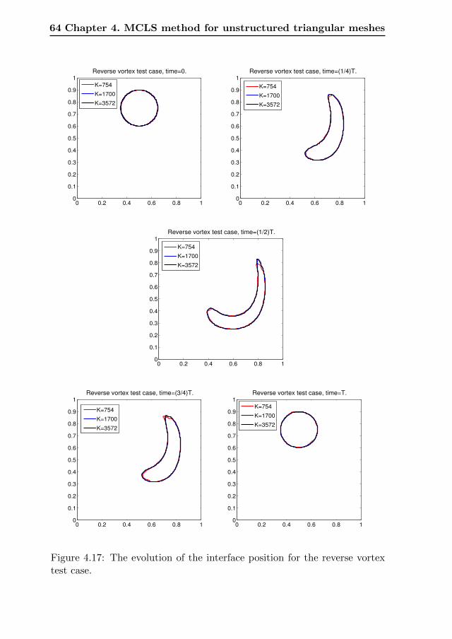
64 Chapter 4. MCLS method for unstructured triangular meshes
Reverse vortex test case, time=0.
0 0.2 0.4 0.6 0.8 10
0.1
0.2
0.3
0.4
0.5
0.6
0.7
0.8
0.9
1
K=754
K=1700
K=3572
Reverse vortex test case, time=(1/4)T.
0 0.2 0.4 0.6 0.8 10
0.1
0.2
0.3
0.4
0.5
0.6
0.7
0.8
0.9
1
K=754
K=1700
K=3572
Reverse vortex test case, time=(1/2)T.
0 0.2 0.4 0.6 0.8 10
0.1
0.2
0.3
0.4
0.5
0.6
0.7
0.8
0.9
1
K=754
K=1700
K=3572
Reverse vortex test case, time=(3/4)T.
0 0.2 0.4 0.6 0.8 10
0.1
0.2
0.3
0.4
0.5
0.6
0.7
0.8
0.9
1
K=754
K=1700
K=3572
Reverse vortex test case, time=T.
0 0.2 0.4 0.6 0.8 10
0.1
0.2
0.3
0.4
0.5
0.6
0.7
0.8
0.9
1
K=754
K=1700
K=3572
Figure 4.17: The evolution of the interface position for the reverse vortextest case.
CHAPTER 5
Extension to tetrahedron control volumes
5.1 Introduction
In Chapter 4, we have presented the proposed Mass-Conserving Level-Setmethod along with numerical results based on 2D triangular mesh. Basedon these results it is worthwhile to developed all the ingredients of theproposed method for 3D tetrahedral control volumes. This will pave the wayto demonstrate the capabilities of the proposed method for more complexdomains. In the light of the objective in this chapter, we have presented a3D Volume of Fluid function and its inverse function is presented.
5.2 Volume of Fluid function in 3D
Our approach is to use a geometric construction to find the function Ψ(Xk) =f(φk,∇φk) that can link VoF to the LS field by an analytic function. Theinterface LS function φk is segment of plane. Therefore, f(φk,∇φk) is therelative volume of the polygon bounded by the faces of the tetrahedral andthe plane φk = 0. The polygon can be either tetrahedral or quadrilateral oreven reduced to a single point, depending on the intersection of the inter-face plane with the tetrahedron, Ωk. An efficient evaluation of the functionf(φk,∇φk) requires a formulation that considers all possible situations asuniformly as possible.
65
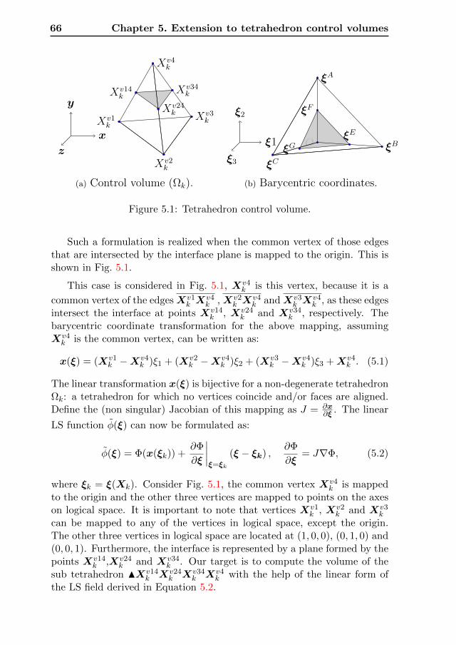
66 Chapter 5. Extension to tetrahedron control volumes
Xv1k
Xv3k
Xv4k
Xv2k
Xv14k
Xv24k
Xv34k
x
y
z
(a) Control volume (Ωk).
O ξB
ξA
ξC
ξF
ξGξE
ξ1
ξ2
ξ3
(b) Barycentric coordinates.
Figure 5.1: Tetrahedron control volume.
Such a formulation is realized when the common vertex of those edgesthat are intersected by the interface plane is mapped to the origin. This isshown in Fig. 5.1.
This case is considered in Fig. 5.1, Xv4k is this vertex, because it is a
common vertex of the edgesXv1k X
v4k ,Xv2
k Xv4k andXv3
k Xv4k , as these edges
intersect the interface at points Xv14k , Xv24
k and Xv34k , respectively. The
barycentric coordinate transformation for the above mapping, assumingXv4k is the common vertex, can be written as:
x(ξ) = (Xv1k −Xv4
k )ξ1 + (Xv2k −Xv4
k )ξ2 + (Xv3k −Xv4
k )ξ3 +Xv4k . (5.1)
The linear transformation x(ξ) is bijective for a non-degenerate tetrahedronΩk: a tetrahedron for which no vertices coincide and/or faces are aligned.Define the (non singular) Jacobian of this mapping as J = ∂x
∂ξ . The linear
LS function φ(ξ) can now be formulated as:
φ(ξ) = Φ(x(ξk)) +∂Φ
∂ξ
∣∣∣∣ξ=ξk
(ξ − ξk) ,∂Φ
∂ξ= J∇Φ, (5.2)
where ξk = ξ(Xk). Consider Fig. 5.1, the common vertex Xv4k is mapped
to the origin and the other three vertices are mapped to points on the axeson logical space. It is important to note that vertices Xv1
k , Xv2k and Xv3
k
can be mapped to any of the vertices in logical space, except the origin.The other three vertices in logical space are located at (1, 0, 0), (0, 1, 0) and(0, 0, 1). Furthermore, the interface is represented by a plane formed by thepoints Xv14
k ,Xv24k and Xv34
k . Our target is to compute the volume of thesub tetrahedron NXv14
k Xv24k Xv34
k Xv4k with the help of the linear form of
the LS field derived in Equation 5.2.
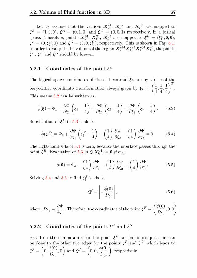
5.2. Volume of Fluid function in 3D 67
Let us assume that the vertices Xv1k , Xv2
k and Xv3k are mapped to
ξB = (1, 0, 0), ξA = (0, 1, 0) and ξC = (0, 0, 1) respectively, in a logicalspace. Therefore, points X14
k , X24k , X34
k are mapped to ξE = (ξE1 , 0, 0),ξF = (0, ξF2 , 0) and ξG = (0, 0, ξG3 ), respectively. This is shown in Fig. 5.1.In order to compute the volume of the regionXv14
k Xv24k Xv34
k Xv4k , the points
ξE , ξF and ξG should be known.
5.2.1 Coordinates of the point ξE
The logical space coordinates of the cell centroid ξk are by virtue of the
barycentric coordinate transformation always given by ξk =
(1
4,1
4,1
4
)T.
This means 5.2 can be written as;
φ(ξ) = Φk +∂Φ
∂ξ1
(ξ1 −
1
4
)+∂Φ
∂ξ2
(ξ2 −
1
4
)+∂Φ
∂ξ3
(ξ3 −
1
4
). (5.3)
Substitution of ξE in 5.3 leads to:
φ(ξE) = Φk +∂Φ
∂ξ1
(ξE1 −
1
4
)−(
1
4
)∂Φ
∂ξ2−(
1
4
)∂Φ
∂ξ3= 0. (5.4)
The right-hand side of 5.4 is zero, because the interface passes through thepoint ξE . Evaluation of 5.3 in ξ(Xv4
k ) = 0 gives:
φ(0) = Φk −(
1
4
)∂Φ
∂ξ1−(
1
4
)∂Φ
∂ξ2−(
1
4
)∂Φ
∂ξ3. (5.5)
Solving 5.4 and 5.5 to find ξE1 leads to:
ξE1 =
∣∣∣∣∣− φ(0)
Dξ1
∣∣∣∣∣ , (5.6)
where, Dξ1 =∂Φ
∂ξ1. Therefore, the coordinates of the point ξE =
(φ(0)
Dξ1
, 0, 0
).
5.2.2 Coordinates of the points ξF and ξG
Based on the computation for the point ξE , a similar computation canbe done to the other two edges for the points ξF and ξG, which leads to
ξF =
(0,φ(0)
Dξ2
, 0
)and ξG =
(0, 0,
φ(0)
Dξ3
), respectively.
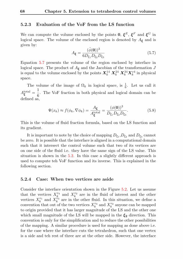
68 Chapter 5. Extension to tetrahedron control volumes
5.2.3 Evaluation of the VoF from the LS function
We can compute the volume enclosed by the points 0, ξE , ξF and ξG inlogical space. The volume of the enclosed region is denoted by Aξ and isgiven by:
Aξ =(φ(0))3
6Dξ1Dξ2Dξ3
(5.7)
Equation 5.7 presents the volume of the region enclosed by interface inlogical space. The product of Aξ and the Jacobian of the transformation Jis equal to the volume enclosed by the points X14
k X24k X34
k Xv4k in physical
space.
The volume of the image of Ωk in logical space, is 16 . Let us call it
Atotalξ =
1
6. The VoF fraction in both physical and logical domain can be
defined as,
Ψ(xk) ≈ f(φk,∇φk) =Aξ
Atotalξ
=(φ(0))3
Dξ1Dξ2Dξ3
. (5.8)
This is the volume of fluid fraction formula, based on the LS function andits gradient.
It is important to note by the choice of mapping Dξ1 ,Dξ2 and Dξ3 cannotbe zero. It is possible that the interface is aligned in a computational domainsuch that it intersect the control volume such that two of its vertices areon one side of the fluid i.e. they have the same sign of the LS value. Thissituation is shown in the 5.2. In this case a slightly different approach isused to compute teh VoF function and its inverse. This is explained in thefollowing section.
5.2.4 Case: When two vertices are aside
Consider the interface orientation shown in the Figure 5.2. Let us assumethat the vertices Xv4
k and Xv2k are in the fluid of interest and the other
vertices Xv1k and Xv3
k are in the other fluid. In this situation, we define aconvention that out of the two vertices Xv4
k and Xv2k anyone can be mapped
to origin provided that it has larger magnitude of the LS and the other onewhich small magnitude of the LS will be mapped in the ξ2 direction. Thisconvention is only for the simplification and to reduce the other possibilitiesof the mapping. A similar procedure is used for mapping as done above i.e.for the case where the interface cuts the tetrahedron, such that one vertexis a side and teh rest of three are at the other side. However, the interface
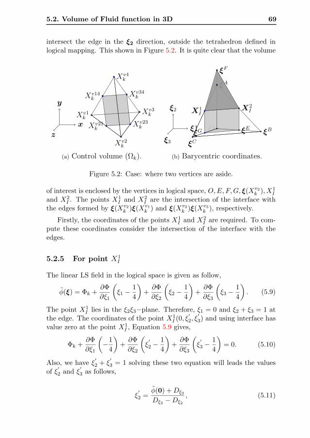
5.2. Volume of Fluid function in 3D 69
intersect the edge in the ξ2 direction, outside the tetrahedron defined inlogical mapping. This shown in Figure 5.2. It is quite clear that the volume
Xv1k
Xv3k
Xv4k
Xv2k
Xv14k
Xv21k
Xv23k
Xv34k
x
y
z
(a) Control volume (Ωk).
O ξB
ξA
ξC
X1I
ξG ξE
X2I
ξF
ξ1
ξ2
ξ3
(b) Barycentric coordinates.
Figure 5.2: Case: where two vertices are aside.
of interest is enclosed by the vertices in logical space, O,E, F,G, ξ(Xv2k ), X1
I
and X2I . The points X1
I and X2I are the intersection of the interface with
the edges formed by ξ(Xv2k )ξ(Xv1
k ) and ξ(Xv2k )ξ(Xv3
k ), respectively.
Firstly, the coordinates of the points X1I and X2
I are required. To com-pute these coordinates consider the intersection of the interface with theedges.
5.2.5 For point X1I
The linear LS field in the logical space is given as follow,
φ(ξ) = Φk +∂Φ
∂ξ1
(ξ1 −
1
4
)+∂Φ
∂ξ2
(ξ2 −
1
4
)+∂Φ
∂ξ3
(ξ3 −
1
4
). (5.9)
The point X1I lies in the ξ2ξ3−plane. Therefore, ξ1 = 0 and ξ2 + ξ3 = 1 at
the edge. The coordinates of the point X1I (0, ξ
′2, ξ
′3) and using interface has
value zero at the point X1I , Equation 5.9 gives,
Φk +∂Φ
∂ξ1
(−1
4
)+∂Φ
∂ξ2
(ξ′2 −
1
4
)+∂Φ
∂ξ3
(ξ′3 −
1
4
)= 0. (5.10)
Also, we have ξ′2 + ξ
′3 = 1 solving these two equation will leads the values
of ξ′2 and ξ
′3 as follows,
ξ′2 =
φ(0) +Dξ2
Dξ3 −Dξ2
, (5.11)
70 Chapter 5. Extension to tetrahedron control volumes
ξ′3 = −
(φ(0) +Dξ2
)Dξ3 −Dξ2
, (5.12)
where, Dξ2 =∂Φ
∂ξ2, Dξ3 =
∂Φ
∂ξ3and
φ(0) = Φk −(
1
4
)∂Φ
∂ξ1−(
1
4
)∂Φ
∂ξ2−(
1
4
)∂Φ
∂ξ3. (5.13)
This defines the coordinates of point X1I .
5.2.6 For point X2I
A similar procedure is adopted for the point X2I . The point X2
I lies in theξ2ξ1−plane. Therefore, ξ3 = 0 and ξ2 +ξ1 = 1 at the edge. The coordinatesof the point X2
I (ξ′1, ξ
′2, 0) and using the fact that interface has value zero at
the point X2I , Equation 5.9 gives.
Φk +∂Φ
∂ξ1
(ξ′1 −
1
4
)+∂Φ
∂ξ2
(ξ′2 −
1
4
)+∂Φ
∂ξ3
(−1
4
)= 0. (5.14)
Also, we have ξ′2 + ξ
′1 = 1 solving these two equation leads to the values of
ξ′2 and ξ
′1 as follows,
ξ′2 =
φ(0) +Dξ2
Dξ1 −Dξ2
, (5.15)
ξ′1 = −
(φ(0) +Dξ2
)Dξ1 −Dξ2
, (5.16)
where, Dξ1 =∂Φ
∂ξ1, Dξ2 =
∂Φ
∂ξ2and
φ(0) = Φk −(
1
4
)∂Φ
∂ξ1−(
1
4
)∂Φ
∂ξ2−(
1
4
)∂Φ
∂ξ3. (5.17)
This defines the coordinates of point X2I . The points X1
I and X2I are used
to compute the extra volume, explained in the next section.
5.2. Volume of Fluid function in 3D 71
5.2.7 Extra volume
The VoF fraction given by the VoF function derived in equation 5.7 givesthe volume enclosed by the interface and the tetrahedron and also the extravolume defined by the tetrahedron ξF , ξ(Xv2
k ), ξ(X1I ) and ξ(X2
I ). Let us callthe extra volume V extra
k . In order to get correct volume enclosed by theinterface in a cell, the volume V extra
k should be subtracted from the volumeobtained by VoF function. This can be noted as follows,
Vk =(φ(0))3
6Dξ1Dξ2Dξ3
− V extrak . (5.18)
Now, V extrak is needed to be determined and this can be computed by us-
ing the coordinates of the points ξF , ξ(Xv2k ), ξ(X1
I ), all of these points areknown and a simple needs to determine defined by these points. This isleads to,
V extrak =
∣∣∣∣∣ (φ(0) +Dξ2)3
6Dξ2(Dξ3 −Dξ2)(Dξ1 −Dξ2)
∣∣∣∣∣ . (5.19)
So, the volume fraction can be defined as,
Ψk =(φ(0))3
Dξ1Dξ2Dξ3
−(φ(0) +Dξ2)3
(Dξ1 −Dξ2)Dξ2(Dξ3 −Dξ2), (5.20)
where, φ(0) is the value of the LS at the origin in logical space and definedas;
φ(0) = Φk −(Dξ1 +Dξ2 +Dξ3
4
). (5.21)
The volume fraction equation can be further simplified to a simple cubicpolynomial equation for φ(0). To do this let us define two coefficients,
A =1
Dξ1Dξ2Dξ3
and B =1
(Dξ1 −Dξ2)Dξ2(Dξ3 −Dξ2). This will give us
volume fraction function in the simplest form as,
Ψk = aφ(0)3 + bφ(0)2 + cφ(0) + d, (5.22)
where, the coefficients are a = A − B, b = −3BDξ2 , c = −3BD2ξ2
and
d = −BD2ξ2
. This cubic polynomial representation of the VoF fraction isvery convenient in use and it is also used to derived the inverse function,explained in the next section.
72 Chapter 5. Extension to tetrahedron control volumes
5.3 Inverse function in 3D
In this section derivation of the inverse function is presented Φk = g(Ψk,∆Φk).This function is used to correct the LS field based on the given VoF fraction.This VoF fraction is obtained by advecting the VoF field parallel to the LSfield. In other words the inverse function is the analytic way to coupledthe LS field and the VoF field. The main objective of this coupling is tofind the cell centroid value of the LS Φc
k that corresponds to the given VoFfraction Ψc
k.
Consider Equation 5.22 and assume that the interface is corrected inthe direction of the normal to the interface. Therefore, we keep Dn+1
ξ1, Dn+1
ξ2
and Dn+1ξ3
as they are at time tn+1. Therefore, the inverse function can bedefined as,
aφ(0)3 + bφ(0)2 + cφ(0) + d−Ψck = 0. (5.23)
Above equation does not define the inverse function completely. First thevalue of φ(0) is computed for the given Ψc
k by solving cubic equation 5.23.Then the cell centroid value of the LS can be obtained as,
Φck = φ(0) +
(Dn+1ξ1
+Dn+1ξ2
+Dn+1ξ3
4
). (5.24)
This will give a corrected value of the LS field at the cell centroid.Here, corrected value of the LS field means that centroid value of the LSnow corresponds to the advected VoF fraction. This whole step is simpleand straight-forward, except that how to solve equation 5.23. There aretwo choices either solve it with cubic root finding analytic method or solveit numerically, like Newtons-Raphson iterative method for the non-linearequations. We have selected the iterative method to demonstrate the work-ing of the inverse function, however, any analytic method for finding cubicroots of the polynomial is applicable. In an iterative method initial guess isimportant and we have observed that, if we select the starting value equalto the lineraized value at the origin based on the non-corrected LS fieldand applying Newtons-Raphson method it appears to always converge tothe correct root value, which makes sure that the interface remains withinthe element and also corresponds to the correct VoF fraction. Let us as-sume that the starting value is φ(1), then the Newton-Raphson algorithmis presented as follows,
5.4. Test Case: The 3D back and forth interface reconstruction73
Algorithm 1 The inverse function solution, using the Newton-Raphsonmethod
Require: φ(1), a, b, c, d, tol, εwhile ε ≥ tol do
φ(i+1) = φ(i) − a(φ(i))3 + b(φ(i))2 + cφ(i) + d
3a(φ(i))2 + 2bφ(i) + c
ε = |φ(i+1) − φ(i)|φ(i+1) = φ(i)
end while
This has completed our discussion and overview of the MCLS methodwith respect to the tetrahedron control volumes. In the next section wehave only presented the result to demonstrate the working of VoF functionand the inverse function for the tetrahedron control volumes.
5.4 Test Case: The 3D back and forth interfacereconstruction
To demonstrate the accuracy of the conversion of the LS field to the VoFfield and then the VoF field back to the LS field using the inverse function.We have designed a test case in which in first step we convert the LS fieldinto the VoF field, using VoF function, equation 5.22 and in the second step,the converted VoF field is again converted back to the LS set field, using theinverse function 5.23. This is a basic step of the MCLS method to obtainedthe mass conservative LS field. However, in practice the VoF field in secondstep is obtained by advecting VoF filed along the LS field. In this test caseno advection of the interface is involved. Naturally, inter-conversion of theLS field and the VoF field without loss of mass is a prerequisite for thealgorithm to achieve (nearly) exact mass conservation. This test showsthat the absolute error (Err.) induced by the inter-conversion is nearlyzero. Steps involved in this test can expressed by the following equations,
Φk → f(Φk,∇Φk)︸ ︷︷ ︸Step-1: VOF function
→ Ψk → g(Ψk,∇Φk)︸ ︷︷ ︸Step-2: Inverse function
→ Φk, (5.25)
Err. = |Φk − Φk| ≈ 0.
In the light of the above test case, let us consider the interface topologyof the shape Zalesak’s slotted sphere. The interface is centered at xc =
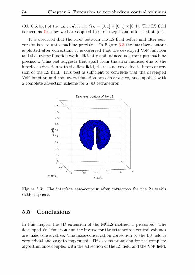
74 Chapter 5. Extension to tetrahedron control volumes
(0.5, 0.5, 0.5) of the unit cube, i.e. ΩD = [0, 1]× [0, 1]× [0, 1]. The LS fieldis given as Φk, now we have applied the first step-1 and after that step-2.
It is observed that the error between the LS field before and after con-version is zero upto machine precision. In Figure 5.3 the interface contouris plotted after correction. It is observed that the developed VoF functionand the inverse function work efficiently and induced no error upto machineprecision. This test suggests that apart from the error induced due to theinterface advection with the flow field, there is no error due to inter conver-sion of the LS field. This test is sufficient to conclude that the developedVoF function and the inverse function are conservative, once applied witha complete advection scheme for a 3D tetrahedron.
0 0.2 0.4 0.6 0.8 10
0.5
1
0
0.1
0.2
0.3
0.4
0.5
0.6
0.7
0.8
0.9
1
Zero level contour of the LS.
x−axis.y−axis.
z−
axis
.
Figure 5.3: The interface zero-contour after correction for the Zalesak’sslotted sphere.
5.5 Conclusions
In this chapter the 3D extension of the MCLS method is presented. Thedeveloped VoF function and the inverse for the tetrahedron control volumesare mass conservative. The mass-conservation correction to the LS field isvery trivial and easy to implement. This seems promising for the completealgorithm once coupled with the advection of the LS field and the VoF field.
CHAPTER 6
The Modified Level-Set method
6.1 Introduction
In the last two chapters the extension of the MCLS for Cartesian controlvolumes to triangular and tetrahedral control volumes has been presented.The hybrid formulation based on a congruent LS and VoF field combines theadvantages of the LS formulation with accurate mass conservation. How-ever, the Eulerian-Lagrangian approach to advect the VoF field is quiteinvolved and will be even more so when applied in three spatial dimensions.
For those cases for which the requirements of very strict mass conserva-tion can be relaxed an alternative approach has become very popular: Themodified Level-Set method introduced in the milestone paper by Olsson andKreis [15,37,39].
The concept is based on the use of a level-set function that is C∞ con-tinuous but closely resembles the color function [add reference to equationwhere this is defined]. For any continuous function φ(x, t) the ’mass’ M inthe domain is defined as the area of the region enclosed by the φ(x, t) = 0LS:
M(t) =
∫ΩH(φ(x, t))dΩ. (6.1)
Therefore, if the field φ(x, t) is conservatively advanced in time this doesnot guarantee conservation of mass unless either:
75
76 Chapter 6. The Modified Level-Set method
• Mass conservation is explicitly enforced after each advance in time.(e.g. as in the MCLS algorithm),
• ‖φ(x, t)−H(φ(x, t))‖ < ε.
It is the latter approach that is followed in the modified LS method. The’true’ color function is replaced by a mollified color function φm(x, t), wherethe change of φm(x, t) from the one to the other value of the color functiontakes place over a nonzero but small distance. How exactly this change oc-curs is arbitrary, but smoothness of the transition will improve the accuracyof the interface location and efficiency of the interface capturing model.
Clearly, the closer the modified LS function resembles the true colorfunction, the more accurately mass is conserved. However, simultaneously,accurate discretisation of the conservation equation for such a rapidly chan-ging and highly nonlinear function becomes more and more challenging.
The ability to easily accomodate changes in the topology of the interfacenecessary to model coalesence and break-up is shared by the LS and themodified LS. Also the evolution of both is described by the same simplelinear advection equation, which results in an efficient and robust algorithm.The discretisation of this advection equation is not complicated by the useof an unstructured tesselation of triangular or tetrahedral control volumes,instead of a set of Cartesian control volumes. Curvature and interfacenormal vector can be reconstructed from the modified LS field in exactlythe same way as for the LS field.
Up till recently, the finite volume methods and standard limited convec-tion schemes were used to discretise the modified LS equation. In [41] theuse of the discontinuous Galerkin method was introduced in this context.The aim of this research is to investigate the potential of the modified LSmethod in terms of accuracy of the interface location and mass conservationwhen state-of-the-art spatial discretisation techniques are used. Addition-ally, an artificial compressive velocity field is introduced to improve theinterface sharpness when it is aligned with the flow direction. This tech-nique is used in some finite volume schemes [51], but is now introduced inthe context of a discontinuous Galerkin discretisation of the modified LSequation. To circumvent the occurence of oscillations in the modified LSfield in the vicinity of the interface first and second order formulations of thelimiter proposed by Kuzmin et al. [31, 32] are used. The application of thelimiter succesfully suppresses any oscillations, but also leads to smearingout of the interface. The latter can now be corrected by the introductionof the artificial compressive velocity field. The key characteristics of theproposed algorithm can be summarized as:
6.2. The Modified Level-Set method 77
• The modified LS field is approximated by either a first or seconddegree piecewise polynomial function on a set of non overlapping tri-angular control volumes.
• To avoid oscillations in the solution of the LS field near the interfacedue to the nearly discontinuous behaviour a limiter is applied afterthe advection of the field.
• To retain an interface with nearly constant thickness an artificial com-pressive velocity field is introduced next to the physical velocity field.
In the following Sections these characteristics will be discussed in moredetail. Finally, computational results obtained with the proposed modifiedLS algorithm are presented for the test cases discussed in Chapter 2 andChapter 4. The proposed algorithm will be assessed on the accuracy of it’ssolutions, it’s mass conservation properties and it’s ability to maintain aninterface region of constant width.
6.2 The Modified Level-Set method
The main idea of the modified Level-Set method is to define an LS func-tion that mimicks the VoF field as close as is practically possible from acomputational point of view, to improve the mass conservation property ofthe former method. A commonly made choice for the modified LS functionis a scaled and translated tangent hyperbolic function of the (signed) dis-tance to the interface. Note that this definition of the modified LS functiononly explicitly appears in the initial condition of the initial boundary valueproblem for the modified LS function. This initialization is demonstratedfor a one-dimensional example.
Assume that the LS field is defined by the signed distance functionφ(x, t). The interface is the zero LS of φ(x, t), i.e. the interface I(x, t) isdefined as
I(x, t) = x ε Ω | φ(x, t) = 0. (6.2)
To improve the mass conservation property of the LS advection algorithm,the following modified LS field φεm(x, t) is defined:
φεm(x, t) = F εm(φ(x, t)), (6.3)
where
F εm(φ(x, t)) =1
2
(tanh
(φ(x, t)
2ε
)+ 1
). (6.4)
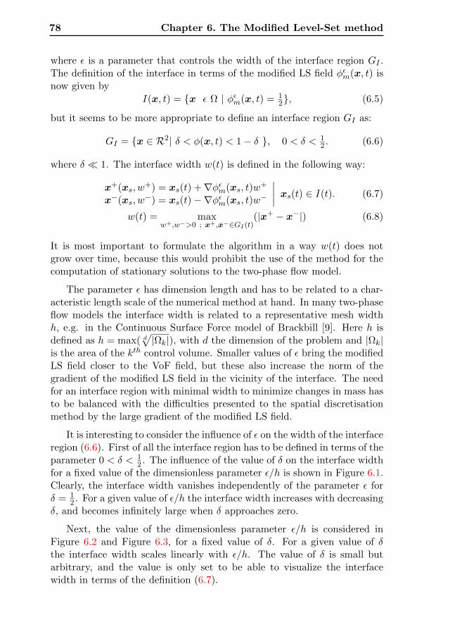
78 Chapter 6. The Modified Level-Set method
where ε is a parameter that controls the width of the interface region GI .The definition of the interface in terms of the modified LS field φεm(x, t) isnow given by
I(x, t) = x ε Ω | φεm(x, t) = 12, (6.5)
but it seems to be more appropriate to define an interface region GI as:
GI = x ∈ R2| δ < φ(x, t) < 1− δ , 0 < δ < 12 . (6.6)
where δ 1. The interface width w(t) is defined in the following way:
x+(xs, w+) = xs(t) +∇φεm(xs, t)w
+
x−(xs, w−) = xs(t)−∇φεm(xs, t)w
−
∣∣∣∣ xs(t) ∈ I(t). (6.7)
w(t) = maxw+,w−>0 ; x+,x−∈GI(t)
(|x+ − x−|) (6.8)
It is most important to formulate the algorithm in a way w(t) does notgrow over time, because this would prohibit the use of the method for thecomputation of stationary solutions to the two-phase flow model.
The parameter ε has dimension length and has to be related to a char-acteristic length scale of the numerical method at hand. In many two-phaseflow models the interface width is related to a representative mesh widthh, e.g. in the Continuous Surface Force model of Brackbill [9]. Here h isdefined as h = max( d
√|Ωk|), with d the dimension of the problem and |Ωk|
is the area of the kth control volume. Smaller values of ε bring the modifiedLS field closer to the VoF field, but these also increase the norm of thegradient of the modified LS field in the vicinity of the interface. The needfor an interface region with minimal width to minimize changes in mass hasto be balanced with the difficulties presented to the spatial discretisationmethod by the large gradient of the modified LS field.
It is interesting to consider the influence of ε on the width of the interfaceregion (6.6). First of all the interface region has to be defined in terms of theparameter 0 < δ < 1
2 . The influence of the value of δ on the interface widthfor a fixed value of the dimensionless parameter ε/h is shown in Figure 6.1.Clearly, the interface width vanishes independently of the parameter ε forδ = 1
2 . For a given value of ε/h the interface width increases with decreasingδ, and becomes infinitely large when δ approaches zero.
Next, the value of the dimensionless parameter ε/h is considered inFigure 6.2 and Figure 6.3, for a fixed value of δ. For a given value of δthe interface width scales linearly with ε/h. The value of δ is small butarbitrary, and the value is only set to be able to visualize the interfacewidth in terms of the definition (6.7).
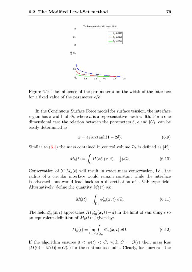
6.2. The Modified Level-Set method 79
0 0.1 0.2 0.3 0.4 0.50
0.5
1
1.5
2
2.5
3
δ.
w/h
.
Thickness variation with respect to δ.
ε1=0.0651
ε2=0.0326
ε3=0.0163
Figure 6.1: The influence of the parameter δ on the width of the interfacefor a fixed value of the parameter ε/h.
In the Continuous Surface Force model for surface tension, the interfaceregion has a width of 3h, where h is a representative mesh width. For a onedimensional case the relation between the parameters δ, ε and |GI | can beeasily determined as:
w = 4ε arctanh(1− 2δ). (6.9)
Similar to (6.1) the mass contained in control volume Ωk is defined as [42]:
Mk(t) =
∫ΩH(φεm(x, t)− 1
2)dΩ. (6.10)
Conservation of∑Mk(t) will result in exact mass conservation, i.e. the
radius of a circular interface would remain constant while the interfaceis advected, but would lead back to a discretisation of a VoF type field.Alternatively, define the quantity M ε
k(t) as:
M εk(t) =
∫Ωk
φεm(x, t) dΩ. (6.11)
The field φεm(x, t) approaches H(φεm(x, t)− 12) in the limit of vanishing ε so
an equivalent definition of Mk(t) is given by:
Mk(t) = limε→0
∫Ωk
φεm(x, t) dΩ. (6.12)
If the algorithm ensures 0 < w(t) < C, with C = O(ε) then mass loss|M(0)−M(t)| = O(ε) for the continuous model. Clearly, for nonzero ε the
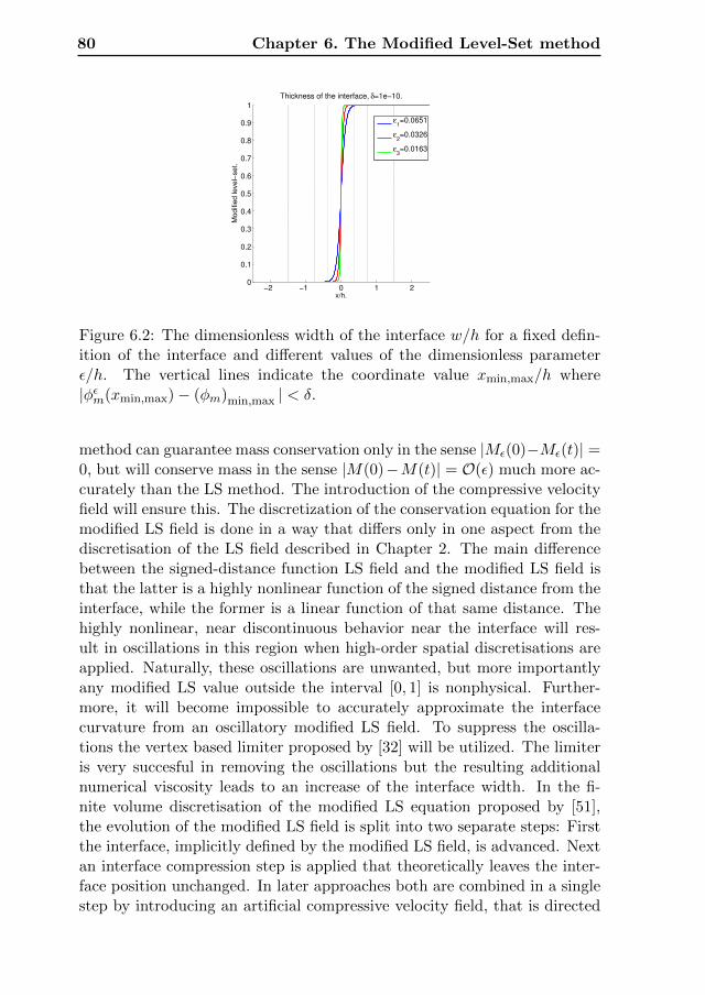
80 Chapter 6. The Modified Level-Set method
−2 −1 0 1 20
0.1
0.2
0.3
0.4
0.5
0.6
0.7
0.8
0.9
1
x/h.
Modifie
d level−
set.
Thickness of the interface, δ=1e−10.
ε1=0.0651
ε2=0.0326
ε3=0.0163
Figure 6.2: The dimensionless width of the interface w/h for a fixed defin-ition of the interface and different values of the dimensionless parameterε/h. The vertical lines indicate the coordinate value xmin,max/h where|φεm(xmin,max)− (φm)min,max | < δ.
method can guarantee mass conservation only in the sense |Mε(0)−Mε(t)| =0, but will conserve mass in the sense |M(0)−M(t)| = O(ε) much more ac-curately than the LS method. The introduction of the compressive velocityfield will ensure this. The discretization of the conservation equation for themodified LS field is done in a way that differs only in one aspect from thediscretisation of the LS field described in Chapter 2. The main differencebetween the signed-distance function LS field and the modified LS field isthat the latter is a highly nonlinear function of the signed distance from theinterface, while the former is a linear function of that same distance. Thehighly nonlinear, near discontinuous behavior near the interface will res-ult in oscillations in this region when high-order spatial discretisations areapplied. Naturally, these oscillations are unwanted, but more importantlyany modified LS value outside the interval [0, 1] is nonphysical. Further-more, it will become impossible to accurately approximate the interfacecurvature from an oscillatory modified LS field. To suppress the oscilla-tions the vertex based limiter proposed by [32] will be utilized. The limiteris very succesful in removing the oscillations but the resulting additionalnumerical viscosity leads to an increase of the interface width. In the fi-nite volume discretisation of the modified LS equation proposed by [51],the evolution of the modified LS field is split into two separate steps: Firstthe interface, implicitly defined by the modified LS field, is advanced. Nextan interface compression step is applied that theoretically leaves the inter-face position unchanged. In later approaches both are combined in a singlestep by introducing an artificial compressive velocity field, that is directed
6.3. A vertex-based limiter for the modified level-set function 81
0 0.01 0.02 0.03 0.04 0.05 0.06 0.070
0.5
1
1.5
2
2.5
3
ε/h.
w/h
.
Thickness variation with respect to ε/h.
δ1=1e−10
δ2=0.15
δ3=0.25
δ4=0.35
δ4=0.499
Figure 6.3: LS, Modified LS for different ε and VoF
orthogonal to and towards the interface location. Combining both stepsimproves efficiency, but defining an artificial compressive velocity field thatis independent of the problem to be solved and the time step size presentsto be a challenge.
The influence of the limiter and the compressive velocity field are studiedfor a one-dimensional problem. First a baseline solution without limiting ispresented. Next the particulars of the limiter are presented, followed by thelimited solution of the one dimensional problem. Finally, the compressivevelocity field is introduced and shown to have a significant influence on theinterface width.
A base line solution can be defined by applying the discontinuous Galer-kin discretisation to the conservation equation of the modified LS fieldwithout limiting for the one-dimensional problem defined in Chapter 2 ofthe LS field discretisation. Significant oscillations occur in the direct vicin-ity of the interface both up- and downstream Fig. 6.5.
6.3 A vertex-based limiter for the modified level-set function
To suppress the oscillations in the solution the vertex-based limiter proposedby Kuzmin [32] is applied. The limiter is an extension of the Barth-Jasperlimiter [25, 32] with enhanced accuracy and especially developed to be ap-plied to a solution of a discontinuous Galerkin discretisation. The limiteris guaranteed to bound the solution, but not necessarily within the interval[0, 1]. However, if the initial condition is within this interval, so will be the
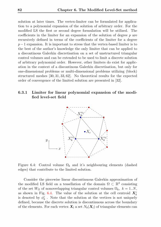
82 Chapter 6. The Modified Level-Set method
solution at later times. The vertex-limiter can be formulated for applica-tion to a polynomial expansion of the solution of arbitrary order. For themodified LS the first or second degree formulation will be utilized. Thecoefficients in the limiter for an expansion of the solution of degree p arerecursively defined in terms of the coefficients of the limiter for a degreep−1 expansion. It is important to stress that the vertex-based limiter is tothe best of the author’s knowledge the only limiter that can be applied toa discontinous Galerkin discretisation on a set of unstructured triangularcontrol volumes and can be extended to be used to limit a discrete solutionof arbitrary polynomial order. However, other limiters do exist for applic-ation in the context of a discontinous Galerkin discretisation, but only forone-dimensional problems or multi-dimensional problems utilizing (block)structured meshes [30, 31, 33, 62]. No theoretical results for the expectedorder of convergence of the limited solution are presented in [32].
6.3.1 Limiter for linear polynomial expansion of the modi-fied level-set field
Xv1k Xv2
k
Xv3k
y
x
Xc
Figure 6.4: Control volume Ωk and it’s neighbouring elements (dashededges) that contribute to the limited solution.
Consider the piecewise linear discontinuous Galerkin approximation ofthe modified LS field on a tessellation of the domain Ω ⊂ R2 consistingof the set WΩ of nonoverlapping triangular control volumes Ωk, k = 1..N ,as shown in Fig. 6.4. The value of the solution at the cell centroid Xc
k
is denoted by φck . Note that the solution at the vertices is not uniquelydefined, because the discrete solution is discontinuous across the boundaryof the elements. For each vertex Xl a set Nb(Xl) of triangular elements can
6.3. A vertex-based limiter for the modified level-set function 83
be defined, for which Xl is a common vertex:
Nb(Xl) =j ∈ N :
Xv1j ,X
v2j ,X
v3j
∩ Xl 6= ∅
. (6.13)
Unique values φkmax and φkmin can be defined as:
φkmax = maxj∈Nb(Xk)
φcj , φkmin = minj∈Nb(Xk)
φcj . (6.14)
Also define a mapping Mk, 1, 2, 3 → N that maps the local labels of thethree vertices to the global labels of the vertices in the tesselation in thefollowing way:
Xvik = XMk(i), i = 1, 2, 3. (6.15)
The first order Taylor expansion of the modified LS field with respect tothe cell centroid and with controlled gradient is defined as (dropping the εsuperscript to improve readability):
φhk(x) = φck + αk ∇φ|Xck
(x−Xck) , 0 6 αk 6 1, (6.16)
where αk is an (elementwise defined) parameter to restrict the value of thegradient to limit the flux. For the vertex based limiter it’s value is definedas:
αk = mini∈1,2,3
min
φMk(i) max − φck
φi − φck, 1
if φi − φck > 0,
1 if φi − φck = 0,
min
φMk(i) min − φck
φi − φck, 1
if φci − φck < 0.
Here, φi is the unconstrained solution in element Ωk at vertex Xvik , defined
as:
φi = φck + ∇φ|Xck
(Xvik −Xc). (6.17)
This generic formulation of the vertex-based limiter guarantees no new localextrema will occur in the solution for t > 0. Therefore, in this case it ensuresthe modified LS field will remain contained within the interval [0, 1].
6.3.2 Limiter for degree two polynomial expansion of thelevel-set field
More challenging is to guarantee the modified LS field remains containedwithin the interval [0, 1], when a higher order discontinous Galerkin dis-cretisation is applied to the conservation equation for the modified LS field.
84 Chapter 6. The Modified Level-Set method
The formulation of the vertex based limiter for a linear approximation ofthe solution presented in the previous section can be extended to be appliedto an approximation of arbitrary order [30,31].
This solution can be expanded in a Taylor polynomial of degree twowith respect to the cell center Xc
k of Ωk as,
φh = φc + ∇φ|Xck
(x−Xck) + (x−Xc
k)T H(φ)|Xc
k(x−Xc
k) , (6.18)
H(φ) = 12
(φ,11 φ,12
φ,21 φ,22
).
Introducing volume averaged quantities, (6.18) can be transformed to [32]:
φh = φc + ∇φ|Xck
(x−Xck) + (x−Xc
k)T H(φ)|Xc
k(x−Xc
k)− H(φ)|Xck
: Ik,
(6.19)
Ik = 12
(I11 I12
I21 I22
).
The volume average φc and tensor Ik are defined as:
φc =1
|Ωk|
∫Ωk
φhdΩ, I11 =1
|Ωk|
∫Ωk
(x1 − xc1)2 dΩ, (6.20)
I22 =1
|Ωk|
∫Ωk
(x2 − xc2)2 dΩ, I12 = I21 =1
|Ωk|
∫Ωk
(x1 − xc1) (x2 − xc2) dΩ.
(6.21)
I11, I22 and I12 are the second area moments of the control volume withrespect to the center of the element. These can be pre-computed for thecomplete mesh in advance of the solution of the time-stepping sequence.Both formulations (6.18) and (6.19) are equivalent approximations of thesolution, i.e. they have the same order of accuracy (add additional discus-sion of the alternative formulation based on averaging). Now both the firstand second degree contributions are limited by a factor 0 ≤ α(β) ≤ 1:
φh = φc + α(1)k (x−Xc
k)T H(φ)|Xc
k(x−Xc
k)− α(2)k H(φ)|Xc
k: Ik. (6.22)
The factor α(2)k defined as
α(2)k = minα(2)
k x1, α
(2)k x2, (6.23)
where α(2)k x1
and α(2)k x2
are used to limit corrections to the individual com-ponents of the gradient vector:
φ(2),1 = φ,1|Xc
k+ α
(2)k x1
φ,11|Xc
k(x1 − (Xc
k)1) + φ,12|Xck
(x2 − (Xck)2)
,
(6.24)
6.4. Compressive velocity formulation 85
φ(2),2 = φ,2|Xc
k+ α
(2)k x2
φ,21|Xc
k(x1 − (Xc
k)1) + φ,22|Xck
(x2 − (Xck)2)
.
(6.25)
The coefficients α(2)k are computed using the vertex-based limiter, described
in the previous section but based on a linear reconstruction of the first
derivatives in the vertices. The procedure for evaluation of α(1)k starts with
the procedure followed in the linear case, but is followed by a comparison
between α(1)k and α
(2)k , that resets α
(1)k as:
α(1)k := max(α
(1)k , α
(2)k ). (6.26)
Once the coefficients α(β)k are known the limited solution can be con-
structed in each element prior to advancing to the next time step. A moredetailed description of the limiting process is presented in [30,31,33,54,62].
6.4 Compressive velocity formulation
In order to keep the width of the interface region constant the use of acompressive, artificial, velocity field is proposed. The limiter will suppressoscillations in the modified LS field in the vicinity of the interface but thiswill simultaneously cause the width of the interface region to grow. Thecompressive velocity field will reduce the latter effect.
Although, this is a commonly applied augmentation of a finite volumediscretisation of the modified LS equation, it has not been introduced inthe context of a discontinous Galerkin discretisation, but for finite volumediscretisation it has been reported to improve the resolution of the inter-face. Additionally, in the implementation presented in [51], the compressivevelocity field is scaled in a (weakly) problem specific way.
The equation that describes the evolution of the modified LS field isgiven by:
∂φm(x)
∂t+ ((uα(x) + ucα(φm(x)))),α = 0, x ∈ Ω. (6.27)
where ucα denotes the artificial compressive velocity field defined as:
ucα(φm(x)) = Kcφm(x)(0.5− φm(x))(1− φm(x))φm,α(x)
|∇φm(x)|. (6.28)
The formulation of the compressive velocity field is chosen to accomplishthe following:
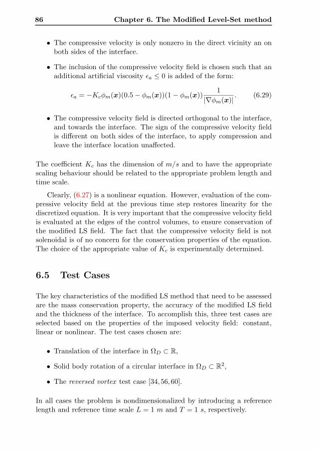
86 Chapter 6. The Modified Level-Set method
• The compressive velocity is only nonzero in the direct vicinity an onboth sides of the interface.
• The inclusion of the compressive velocity field is chosen such that anadditional artificial viscosity εa ≤ 0 is added of the form:
εa = −Kcφm(x)(0.5− φm(x))(1− φm(x))1
|∇φm(x)|. (6.29)
• The compressive velocity field is directed orthogonal to the interface,and towards the interface. The sign of the compressive velocity fieldis different on both sides of the interface, to apply compression andleave the interface location unaffected.
The coefficient Kc has the dimension of m/s and to have the appropriatescaling behaviour should be related to the appropriate problem length andtime scale.
Clearly, (6.27) is a nonlinear equation. However, evaluation of the com-pressive velocity field at the previous time step restores linearity for thediscretized equation. It is very important that the compressive velocity fieldis evaluated at the edges of the control volumes, to ensure conservation ofthe modified LS field. The fact that the compressive velocity field is notsolenoidal is of no concern for the conservation properties of the equation.The choice of the appropriate value of Kc is experimentally determined.
6.5 Test Cases
The key characteristics of the modified LS method that need to be assessedare the mass conservation property, the accuracy of the modified LS fieldand the thickness of the interface. To accomplish this, three test cases areselected based on the properties of the imposed velocity field: constant,linear or nonlinear. The test cases chosen are:
• Translation of the interface in ΩD ⊂ R,
• Solid body rotation of a circular interface in ΩD ⊂ R2,
• The reversed vortex test case [34,56,60].
In all cases the problem is nondimensionalized by introducing a referencelength and reference time scale L = 1 m and T = 1 s, respectively.
6.5. Test Cases 87
The expansion of the solution can be done for polynomial basis functionsof a user defined degree, without any difficulty. However, the number ofnodal points increases with the degree of the basis functions and hence thenumber of degrees of freedom of the problem. Because the vertex-basedlimiter discussed in Section 6.3 is derived for an expansion in linear andquadratic basis functions, only those bases will be used in the experiments.However, the frame work of the vertex based limiter permits to extend itto any arbitray order polynomial.
6.5.1 Translation of the interface in one spatial dimension
In the first test case the modified LS field is a scaled and mollified rectan-gular function, that is translated without any deformation. The LS field isinitialized in domain ΩD = [0, 2] as:
φ(x, 0) = |x− xc(0)| −R, (6.30)
where xc(0) = 12 andR = 1
5 . A uniform mesh of size h = 2/K is used, whereK is the number of control volumes. The interface thickness parameter isset as ε = 3
10h. The initial modified LS field can be given as:
φm(x, 0) =1
2
(tanh
(φ(x, 0)
2ε
)+ 1
). (6.31)
The velocity u1 = 1 and the final time for the solution is set to T = 1. Thismeans the solution for the LS field at the final time T is given as:
φ(x, T ) = |x− xc(T )| −R, (6.32)
where xc(T ) = 1.5. The corresponding modified LS field at the final timeis given by:
φεm(x, T ) =1
2
(tanh
(φ(x, T )
2ε
)+ 1
). (6.33)
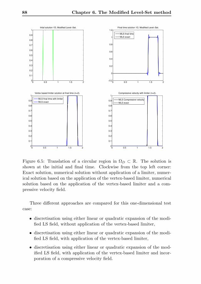
88 Chapter 6. The Modified Level-Set method
0 0.5 1 1.5 20
0.1
0.2
0.3
0.4
0.5
0.6
0.7
0.8
0.9
1
Intial solution 1D, Modified Level−Set.
0 0.5 1 1.5 2−0.2
0
0.2
0.4
0.6
0.8
1
1.2
Final time solution 1D, Modified Level−Set.
MLS final time
MLS exact
0 0.5 1 1.5 20
0.1
0.2
0.3
0.4
0.5
0.6
0.7
0.8
0.9
1Vertex based limiter solution at final time (n=2).
MLS final time with limiter
MLS exact
0 0.5 1 1.5 20
0.1
0.2
0.3
0.4
0.5
0.6
0.7
0.8
0.9
1Compressive velocity with limiter (n=2).
MLS Compressive velocity
MLS exact
Figure 6.5: Translation of a circular region in ΩD ⊂ R. The solution isshown at the initial and final time. Clockwise from the top left corner:Exact solution, numerical solution without application of a limiter, numer-ical solution based on the application of the vertex-based limiter, numericalsolution based on the application of the vertex-based limiter and a com-pressive velocity field.
Three different approaches are compared for this one-dimensional testcase:
• discretisation using either linear or quadratic expansion of the modi-fied LS field, without application of the vertex-based limiter,
• discretisation using either linear or quadratic expansion of the modi-fied LS field, with application of the vertex-based limiter,
• discretisation using either linear or quadratic expansion of the mod-ified LS field, with application of the vertex-based limiter and incor-poration of a compressive velocity field.
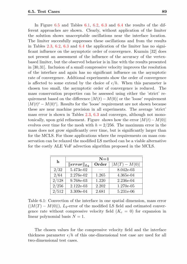
6.5. Test Cases 89
In Figure 6.5 and Tables 6.1, 6.2, 6.3 and 6.4 the results of the dif-ferent approaches are shown. Clearly, without application of the limiterthe solution shows unacceptable oscillations near the interface location.The limiter succesfully suppresses these oscillations and from the resultsin Tables 2.3, 6.2, 6.3 and 6.4 the application of the limiter has no signi-ficant influence on the asymptotic order of convergence. Kuzmin [32] doesnot present an assessment of the influence of the accuracy of the vertex-based limiter, but the observed behavior is in line with the results presentedin [30,31]. Inclusion of a small compressive velocity improves the resolutionof the interface and again has no significant influence on the asymptoticrate of convergence. Addtional experiments show the order of convergenceis affected to some extend by the choice of ε/h. When this parameter ischosen too small, the asymptotic order of convergence is reduced. Themass conservation properties can be assessed using either the ’strict’ re-quirement based on the difference |M(t)−M(0)| or the ’loose’ requirement|M(t)ε−M(0)ε|. Results for the ’loose’ requirement are not shown becausethese are near machine precision in all experiments. The average ’strict’mass error is shown in Tables 2.3, 6.3 and converges, although not mono-tonically, upon grid refinement. Figure shows how the error |M(t)−M(0)|evolves over time for the mesh with h = 2/256. The maximum error in themass does not grow significantly over time, but is significantly larger thanfor the MCLS. For those applications where the requirements on mass con-servation can be relaxed the modified LS method can be a viable alternativefor the costly ALE VoF advection algorithm proposed in the MCLS.
hN=1
‖error‖L2 Order |M(T )−M(0)|2/32 5.473e-02 — 8.042e-03
2/64 2.276e-02 1.265 4.365e-04
2/128 9.768e-03 1.220 2.236e-04
2/256 2.122e-03 2.202 1.270e-05
2/512 3.309e-04 2.681 5.231e-06
Table 6.1: Convection of the interface in one spatial dimension, mass error(|M(T ) −M(0)|), L2-error of the modified LS field and estimated conver-gence rate without compressive velocity field (Kc = 0) for expansion inlinear polynomial basis N = 1.
The chosen values for the compressive velocity field and the interfacethickness parameter ε/h of this one-dimensional test case are used for alltwo-dimensional test cases.
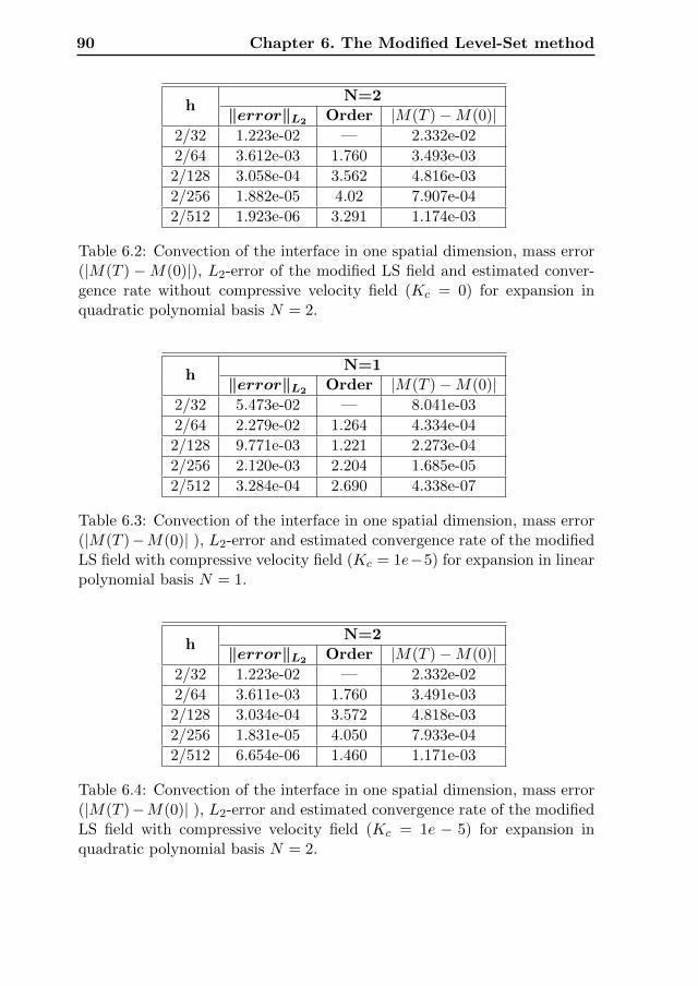
90 Chapter 6. The Modified Level-Set method
hN=2
‖error‖L2 Order |M(T )−M(0)|2/32 1.223e-02 — 2.332e-02
2/64 3.612e-03 1.760 3.493e-03
2/128 3.058e-04 3.562 4.816e-03
2/256 1.882e-05 4.02 7.907e-04
2/512 1.923e-06 3.291 1.174e-03
Table 6.2: Convection of the interface in one spatial dimension, mass error(|M(T ) −M(0)|), L2-error of the modified LS field and estimated conver-gence rate without compressive velocity field (Kc = 0) for expansion inquadratic polynomial basis N = 2.
hN=1
‖error‖L2 Order |M(T )−M(0)|2/32 5.473e-02 — 8.041e-03
2/64 2.279e-02 1.264 4.334e-04
2/128 9.771e-03 1.221 2.273e-04
2/256 2.120e-03 2.204 1.685e-05
2/512 3.284e-04 2.690 4.338e-07
Table 6.3: Convection of the interface in one spatial dimension, mass error(|M(T )−M(0)| ), L2-error and estimated convergence rate of the modifiedLS field with compressive velocity field (Kc = 1e−5) for expansion in linearpolynomial basis N = 1.
hN=2
‖error‖L2 Order |M(T )−M(0)|2/32 1.223e-02 — 2.332e-02
2/64 3.611e-03 1.760 3.491e-03
2/128 3.034e-04 3.572 4.818e-03
2/256 1.831e-05 4.050 7.933e-04
2/512 6.654e-06 1.460 1.171e-03
Table 6.4: Convection of the interface in one spatial dimension, mass error(|M(T )−M(0)| ), L2-error and estimated convergence rate of the modifiedLS field with compressive velocity field (Kc = 1e − 5) for expansion inquadratic polynomial basis N = 2.
6.5. Test Cases 91
6.5.2 Rotation of a circular interface in two spatial dimen-sions
The second test case is related to the rotation of circular interface in adomain ΩD = [0, 1] × [0, 1]. Initially, the centre of the circle is located atxc(0) = (1
2 ,34)T . The initial condition for the LS field is defined as:
φ(x, 0) = |x− xc(0)| −R, (6.34)
where R = 520 . The corresponding intial modified LS field is given as,
φεm(x, 0) =1
2
(tanh
(φl(x, 0)
2ε
)+ 1
). (6.35)
The circular interface is advected with a linear velocity field u = (x1 −12 ,−x2 + 1
2)T using a time step ∆t = 1100 . The final time is T = 2π. This
initial setup is shown in Figure 6.6. Because the velocity field is solenoidal,mass should be conserved up to machine precision and the velocity fieldwill return the interface to its initial position at t = T . Hence, φεm(x, T ) =φεm(x, 0) as shown in Figure 6.6.
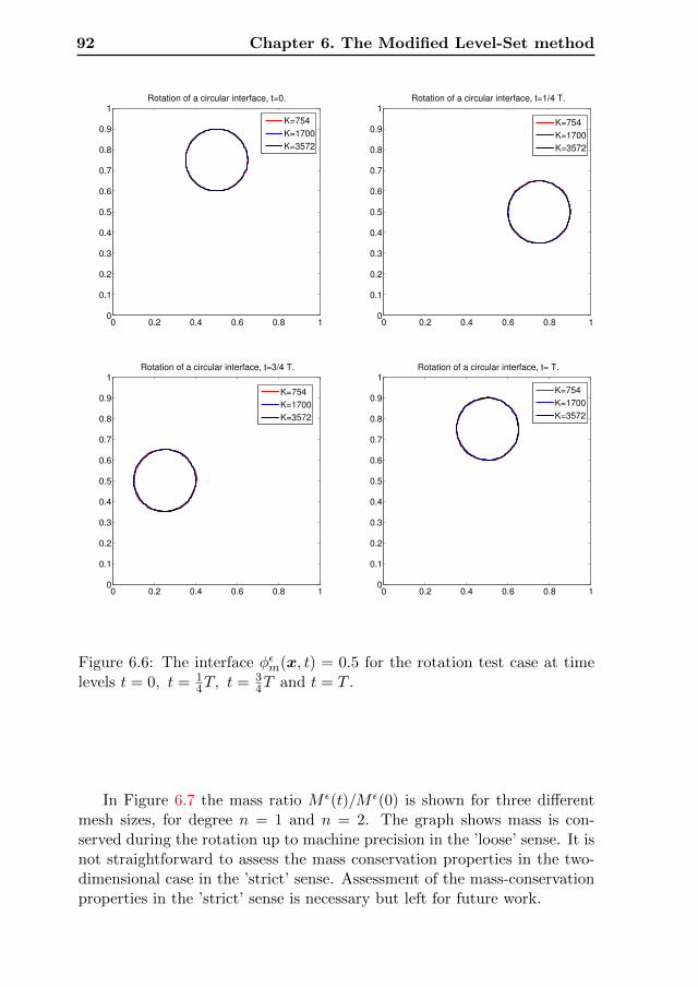
92 Chapter 6. The Modified Level-Set method
Rotation of a circular interface, t=0.
0 0.2 0.4 0.6 0.8 10
0.1
0.2
0.3
0.4
0.5
0.6
0.7
0.8
0.9
1
K=754
K=1700
K=3572
Rotation of a circular interface, t=1/4 T.
0 0.2 0.4 0.6 0.8 10
0.1
0.2
0.3
0.4
0.5
0.6
0.7
0.8
0.9
1
K=754
K=1700
K=3572
Rotation of a circular interface, t=3/4 T.
0 0.2 0.4 0.6 0.8 10
0.1
0.2
0.3
0.4
0.5
0.6
0.7
0.8
0.9
1
K=754
K=1700
K=3572
Rotation of a circular interface, t= T.
0 0.2 0.4 0.6 0.8 10
0.1
0.2
0.3
0.4
0.5
0.6
0.7
0.8
0.9
1
K=754
K=1700
K=3572
Figure 6.6: The interface φεm(x, t) = 0.5 for the rotation test case at timelevels t = 0, t = 1
4T, t = 34T and t = T .
In Figure 6.7 the mass ratio M ε(t)/M ε(0) is shown for three differentmesh sizes, for degree n = 1 and n = 2. The graph shows mass is con-served during the rotation up to machine precision in the ’loose’ sense. It isnot straightforward to assess the mass conservation properties in the two-dimensional case in the ’strict’ sense. Assessment of the mass-conservationproperties in the ’strict’ sense is necessary but left for future work.
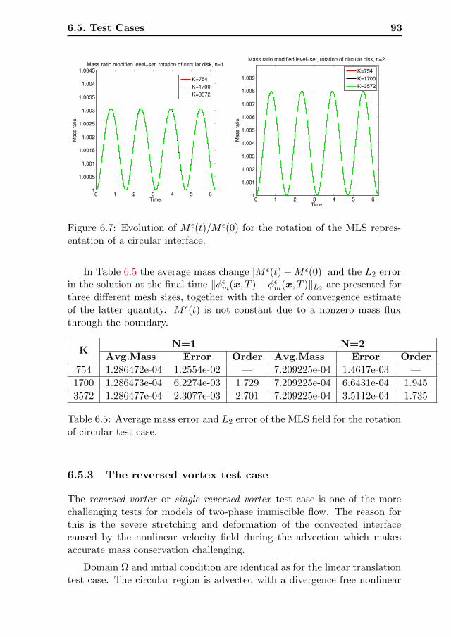
6.5. Test Cases 93
0 1 2 3 4 5 61
1.0005
1.001
1.0015
1.002
1.0025
1.003
1.0035
1.004
1.0045
Time.
Ma
ss r
atio
.
Mass ratio modified level−set, rotation of circular disk, n=1.
K=754
K=1700
K=3572
0 1 2 3 4 5 61
1.001
1.002
1.003
1.004
1.005
1.006
1.007
1.008
1.009
Time.
Ma
ss r
atio
.
Mass ratio modified level−set, rotation of circular disk, n=2.
K=754
K=1700
K=3572
Figure 6.7: Evolution of M ε(t)/M ε(0) for the rotation of the MLS repres-entation of a circular interface.
In Table 6.5 the average mass change |M ε(t)−M ε(0)| and the L2 errorin the solution at the final time ‖φεm(x, T )− φεm(x, T )‖L2 are presented forthree different mesh sizes, together with the order of convergence estimateof the latter quantity. M ε(t) is not constant due to a nonzero mass fluxthrough the boundary.
KN=1 N=2
Avg.Mass Error Order Avg.Mass Error Order
754 1.286472e-04 1.2554e-02 — 7.209225e-04 1.4617e-03 —
1700 1.286473e-04 6.2274e-03 1.729 7.209225e-04 6.6431e-04 1.945
3572 1.286477e-04 2.3077e-03 2.701 7.209225e-04 3.5112e-04 1.735
Table 6.5: Average mass error and L2 error of the MLS field for the rotationof circular test case.
6.5.3 The reversed vortex test case
The reversed vortex or single reversed vortex test case is one of the morechallenging tests for models of two-phase immiscible flow. The reason forthis is the severe stretching and deformation of the convected interfacecaused by the nonlinear velocity field during the advection which makesaccurate mass conservation challenging.
Domain Ω and initial condition are identical as for the linear translationtest case. The circular region is advected with a divergence free nonlinear
94 Chapter 6. The Modified Level-Set method
velocity field given by:
u = cos(πt/T )(sin2(2πx1) sin(2πx2),− sin2(2πx2) sin(2πx2))T . (6.36)
The cos(πt/T ) will cause the velocity field to reverse direction at time t =T/2. This implies the interface will return to its original position at timet = T . In this test case T = 2 is used. The initial setup is shown in Figure6.8. Like in the other test cases the mass (area) enclosed by the interfaceis the quantity of interest. This is computed after every time step andcompared with the initial quantity to give the amount of mass loss or gainduring advection. Also, at the final time the corrected LS field is comparedwith the initial condition as the circular interface should return to its initialposition and shape at time t = T .
In Figure 6.8 the interface is shown at different time levels for threedifferent mesh sizes.
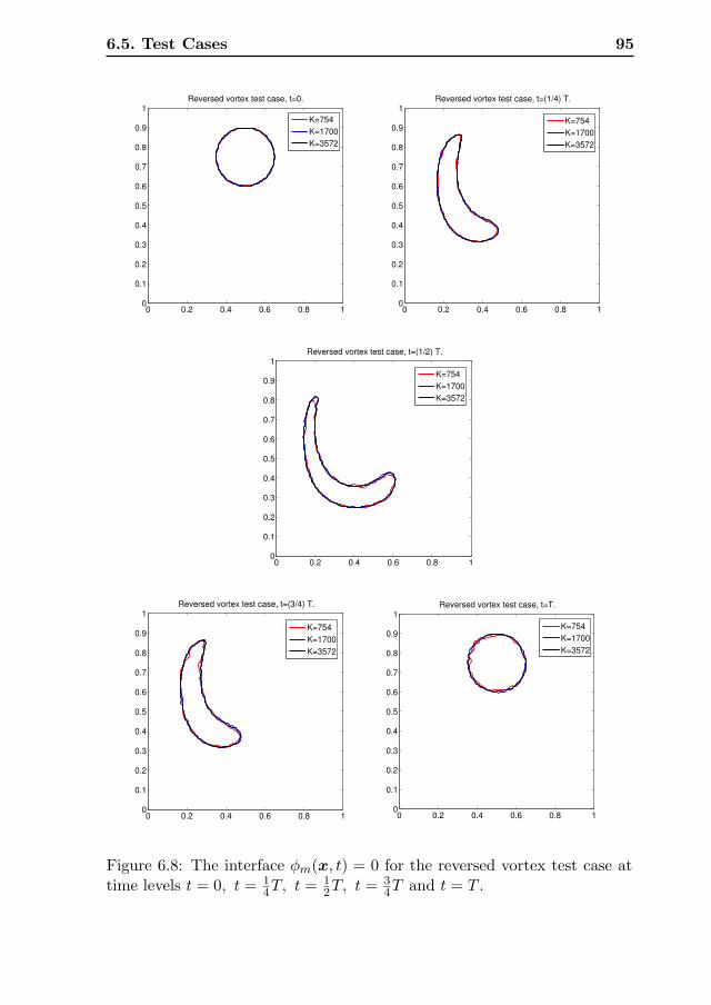
6.5. Test Cases 95
Reversed vortex test case, t=0.
0 0.2 0.4 0.6 0.8 10
0.1
0.2
0.3
0.4
0.5
0.6
0.7
0.8
0.9
1
K=754
K=1700
K=3572
Reversed vortex test case, t=(1/4) T.
0 0.2 0.4 0.6 0.8 10
0.1
0.2
0.3
0.4
0.5
0.6
0.7
0.8
0.9
1
K=754
K=1700
K=3572
Reversed vortex test case, t=(1/2) T.
0 0.2 0.4 0.6 0.8 10
0.1
0.2
0.3
0.4
0.5
0.6
0.7
0.8
0.9
1
K=754
K=1700
K=3572
Reversed vortex test case, t=(3/4) T.
0 0.2 0.4 0.6 0.8 10
0.1
0.2
0.3
0.4
0.5
0.6
0.7
0.8
0.9
1
K=754
K=1700
K=3572
Reversed vortex test case, t=T.
0 0.2 0.4 0.6 0.8 10
0.1
0.2
0.3
0.4
0.5
0.6
0.7
0.8
0.9
1
K=754
K=1700
K=3572
Figure 6.8: The interface φm(x, t) = 0 for the reversed vortex test case attime levels t = 0, t = 1
4T, t = 12T, t = 3
4T and t = T .
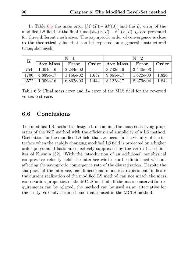
96 Chapter 6. The Modified Level-Set method
In Table 6.6 the mass error |M ε(T )−M ε(0)| and the L2 error of themodified LS field at the final time ‖φm(x, T ) − φhm(x, T )‖L2 are presentedfor three different mesh sizes. The asymptotic order of convergence is closeto the theoretical value that can be expected on a general unstructuredtriangular mesh.
KN=1 N=2
Avg.Mass Error Order Avg.Mass Error Order
754 1.004e-16 2.284e-02 — 3.743e-19 3.440e-03 —
1700 4.889e-17 1.166e-02 1.657 9.865e-17 1.622e-03 1.826
3572 1.009e-16 6.862e-03 1.444 3.122e-17 8.279e-04 1.842
Table 6.6: Final mass error and L2 error of the MLS field for the reversedvortex test case.
6.6 Conclusions
The modified LS method is designed to combine the mass-conserving prop-erties of the VoF method with the efficieny and simplicity of a LS method.Oscillations in the modified LS field that are occur in the vicinity of the in-terface when the rapidly changing modified LS field is projected on a higherorder polynomial basis are effectively suppressed by the vertex-based lim-iter of Kuzmin [32]. With the introduction of an additional nonphysicalcompressive velocity field, the interface width can be diminished withoutaffecting the asymptotic convergence rate of the discretisation. Despite thesharpness of the interface, one dimensional numerical experiments indicatethe current realization of the modified LS method can not match the massconservation properties of the MCLS method. If the mass conservation re-quirements can be relaxed, the method can be used as an alternative forthe costly VoF advection scheme that is used in the MCLS method.
CHAPTER 7
Comparision of the LS, MCLS and MLS method
7.1 Introduction
So far three different methods to simulate immcisible two-phase flows havebeen presented, namely the Level-Set method (LS), Mass-Conserving Level-set method (MCLS) and the modified Level-Set method (MLS). Each methodhas been discussed individually so far and the following key observationshave been made:
• The computational cost of the LS method is the lower of the three,but the method does not conserve mass accurately.
• The proposed MCLS method is exactly mass-conserving but it is com-putationally intensive as a result of the Eulerian-Lagrangian volumeof fluid advection.
• The MLS method is more computationally intensive than the LSmethod, due to the incorporation of a limiter, but less than the MCLS.
The convergence rate of the solutions obtained with the MLS method de-pend on the values of the interface width parameter and the magnitude ofthe compressive velocity. This means the MLS model depends on problemspecific parameters, contrary to the LS and MCLS method.
97
98 Chapter 7. Comparision of the LS, MCLS and MLS method
Based on these observations, the LS method is discarded as a viablealternative of the MCLS but the MLS requires further assessment. Theinterest in the MLS method is dual:
• As a stand-alone method that can challenge the MCLS method, be-cause of the relatively low computational cost of the former.
• As a replacement of the computationally intensive VoF advectionmodule of the MCLS.
Therefore, we decided to dedicate one more chapter for further compar-ison using slightly more difficult test cases, in which the interface repres-entation is more challenging. These test cases consist of;
• Advection of a bubble with a lens shaped cross section.
• Zalesak’s rotating disc.
Although the LS method is not considered a viable alternative to theMCLS, results for the former method are also included to put the resultsof the MLS and MCLS in perspective. Both testcases will be computed ona sequence of three meshes to determine the order of convergence of thesolution and the convergence rate of the mass error if this is more thanmachine precision.
7.1.1 Advection of a bubble with a lens shaped cross section
A very commonly studied test case for models for immiscible, incompressibletwo-phase flow is the rise of an initially circular bubble. Depending on thematerial properties of the liquid phase and the density ratio between bothphases, the bubble will change shape during its ascend to finally reach itsterminal spatial form. Accurate prediction of the rise speed is particularlychallenging when the terminal shape is lens-like with a very strong variationof the interface curvature: very low curvature near the symmetry line of thebubble and very high curvature near the extremities of the bubble, corres-ponding to the skirt of the bubble in the three dimensional case. Becausethe coupling between a flow solver and the interface model is outside thescope of this thesis, a model problem is studied where an interface, thatclosely resembles the shape of a skirted bubble is convected with a constantvelocity.
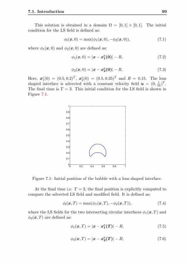
7.1. Introduction 99
This solution is obtained in a domain Ω = [0, 1] × [0, 1]. The initialcondition for the LS field is defined as:
φl(x, 0) = max(φ1(x, 0),−φ2(x, 0)), (7.1)
where φ1(x, 0) and φ2(x, 0) are defined as:
φ1(x, 0) = |x− xc1(0)| −R, (7.2)
φ2(x, 0) = |x− xc2(0)| −R. (7.3)
Here, xc1(0) = (0.5, 0.2)T , xc2(0) = (0.5, 0.35)T and R = 0.15. The lensshaped interface is advected with a constant velocity field u = (0, 1
10)T .The final time is T = 3. This initial condition for the LS field is shown inFigure 7.1.
0 0.2 0.4 0.6 0.8 10
0.1
0.2
0.3
0.4
0.5
0.6
0.7
0.8
0.9
1
Figure 7.1: Initial position of the bubble with a lens shaped interface.
At the final time i.e. T = 3, the final position is explicitly computed tocompare the advected LS field and modified field. It is defined as;
φl(x, T ) = max(φ1(x, T ),−φ2(x, T )), (7.4)
where the LS fields for the two intersecting circular interfaces φ1(x, T ) andφ2(x, T ) are defined as:
φ1(x, T ) = |x− xc1(T )| −R, (7.5)
φ2(x, T ) = |x− xc2(T )| −R, (7.6)
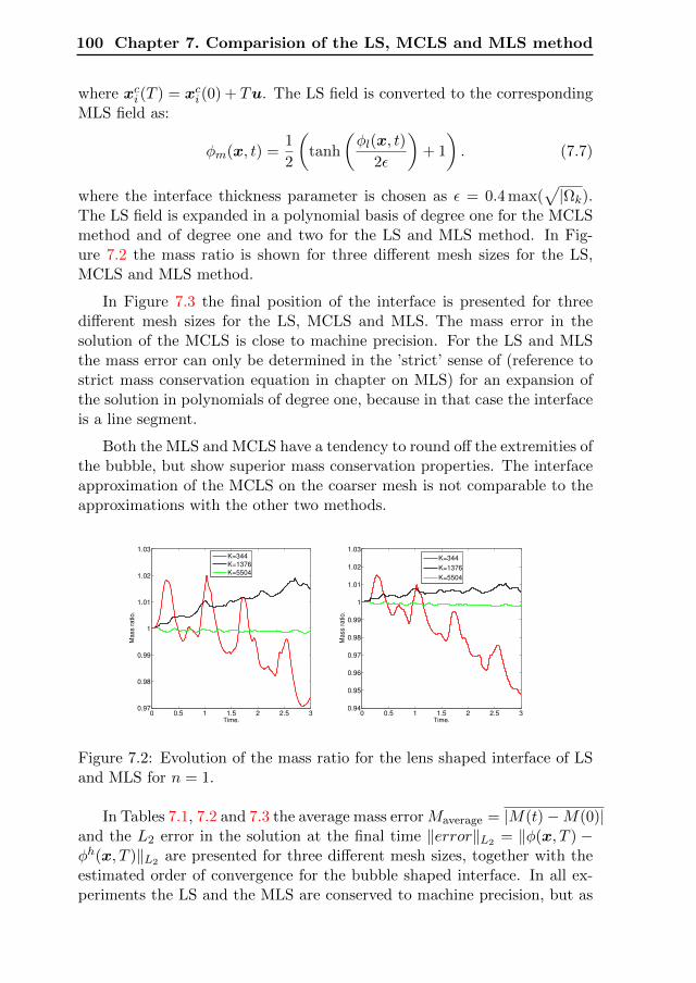
100 Chapter 7. Comparision of the LS, MCLS and MLS method
where xci (T ) = xci (0) + Tu. The LS field is converted to the correspondingMLS field as:
φm(x, t) =1
2
(tanh
(φl(x, t)
2ε
)+ 1
). (7.7)
where the interface thickness parameter is chosen as ε = 0.4 max(√|Ωk).
The LS field is expanded in a polynomial basis of degree one for the MCLSmethod and of degree one and two for the LS and MLS method. In Fig-ure 7.2 the mass ratio is shown for three different mesh sizes for the LS,MCLS and MLS method.
In Figure 7.3 the final position of the interface is presented for threedifferent mesh sizes for the LS, MCLS and MLS. The mass error in thesolution of the MCLS is close to machine precision. For the LS and MLSthe mass error can only be determined in the ’strict’ sense of (reference tostrict mass conservation equation in chapter on MLS) for an expansion ofthe solution in polynomials of degree one, because in that case the interfaceis a line segment.
Both the MLS and MCLS have a tendency to round off the extremities ofthe bubble, but show superior mass conservation properties. The interfaceapproximation of the MCLS on the coarser mesh is not comparable to theapproximations with the other two methods.
0 0.5 1 1.5 2 2.5 30.97
0.98
0.99
1
1.01
1.02
1.03
Time.
Mass r
atio.
K=344
K=1376
K=5504
0 0.5 1 1.5 2 2.5 30.94
0.95
0.96
0.97
0.98
0.99
1
1.01
1.02
1.03
Time.
Mass r
atio.
K=344
K=1376
K=5504
Figure 7.2: Evolution of the mass ratio for the lens shaped interface of LSand MLS for n = 1.
In Tables 7.1, 7.2 and 7.3 the average mass errorMaverage = |M(t)−M(0)|and the L2 error in the solution at the final time ‖error‖L2 = ‖φ(x, T ) −φh(x, T )‖L2 are presented for three different mesh sizes, together with theestimated order of convergence for the bubble shaped interface. In all ex-periments the LS and the MLS are conserved to machine precision, but as
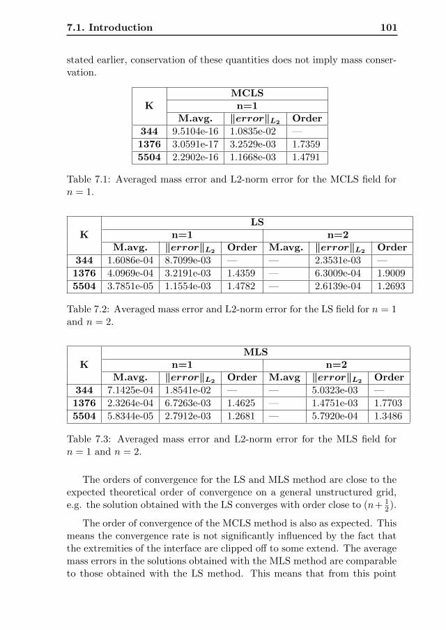
7.1. Introduction 101
stated earlier, conservation of these quantities does not imply mass conser-vation.
KMCLSn=1
M.avg. ‖error‖L2 Order
344 9.5104e-16 1.0835e-02 —
1376 3.0591e-17 3.2529e-03 1.7359
5504 2.2902e-16 1.1668e-03 1.4791
Table 7.1: Averaged mass error and L2-norm error for the MCLS field forn = 1.
KLS
n=1 n=2M.avg. ‖error‖L2 Order M.avg. ‖error‖L2 Order
344 1.6086e-04 8.7099e-03 — — 2.3531e-03 —
1376 4.0969e-04 3.2191e-03 1.4359 — 6.3009e-04 1.9009
5504 3.7851e-05 1.1554e-03 1.4782 — 2.6139e-04 1.2693
Table 7.2: Averaged mass error and L2-norm error for the LS field for n = 1and n = 2.
KMLS
n=1 n=2M.avg. ‖error‖L2 Order M.avg ‖error‖L2 Order
344 7.1425e-04 1.8541e-02 — — 5.0323e-03 —
1376 2.3264e-04 6.7263e-03 1.4625 — 1.4751e-03 1.7703
5504 5.8344e-05 2.7912e-03 1.2681 — 5.7920e-04 1.3486
Table 7.3: Averaged mass error and L2-norm error for the MLS field forn = 1 and n = 2.
The orders of convergence for the LS and MLS method are close to theexpected theoretical order of convergence on a general unstructured grid,e.g. the solution obtained with the LS converges with order close to (n+ 1
2).
The order of convergence of the MCLS method is also as expected. Thismeans the convergence rate is not significantly influenced by the fact thatthe extremities of the interface are clipped off to some extend. The averagemass errors in the solutions obtained with the MLS method are comparableto those obtained with the LS method. This means that from this point
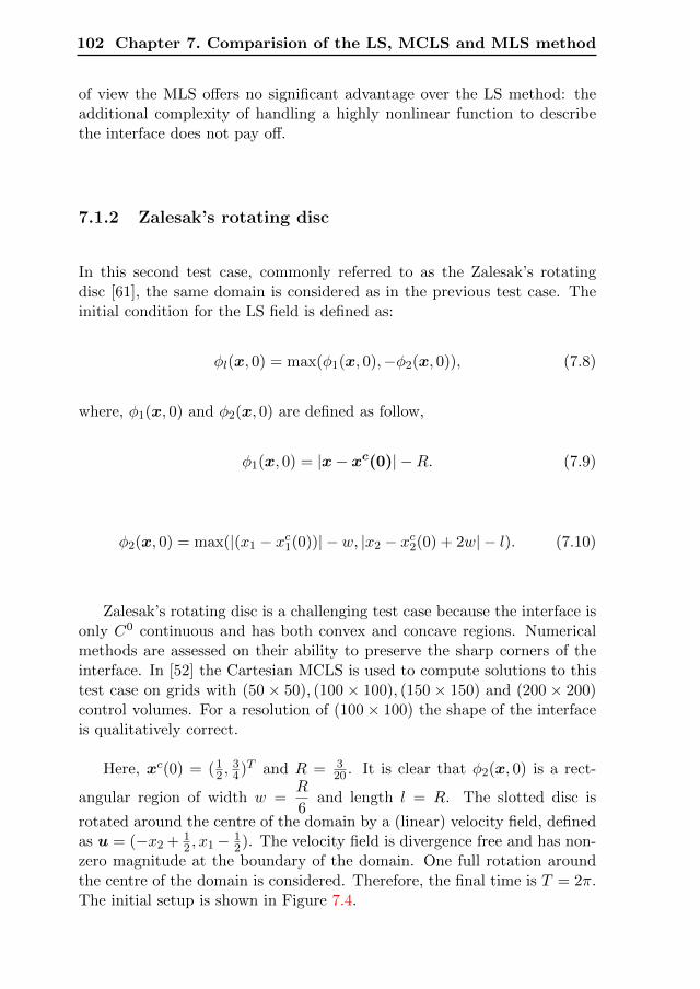
102 Chapter 7. Comparision of the LS, MCLS and MLS method
of view the MLS offers no significant advantage over the LS method: theadditional complexity of handling a highly nonlinear function to describethe interface does not pay off.
7.1.2 Zalesak’s rotating disc
In this second test case, commonly referred to as the Zalesak’s rotatingdisc [61], the same domain is considered as in the previous test case. Theinitial condition for the LS field is defined as:
φl(x, 0) = max(φ1(x, 0),−φ2(x, 0)), (7.8)
where, φ1(x, 0) and φ2(x, 0) are defined as follow,
φ1(x, 0) = |x− xc(0)| −R. (7.9)
φ2(x, 0) = max(|(x1 − xc1(0))| − w, |x2 − xc2(0) + 2w| − l). (7.10)
Zalesak’s rotating disc is a challenging test case because the interface isonly C0 continuous and has both convex and concave regions. Numericalmethods are assessed on their ability to preserve the sharp corners of theinterface. In [52] the Cartesian MCLS is used to compute solutions to thistest case on grids with (50 × 50), (100 × 100), (150 × 150) and (200 × 200)control volumes. For a resolution of (100× 100) the shape of the interfaceis qualitatively correct.
Here, xc(0) = (12 ,
34)T and R = 3
20 . It is clear that φ2(x, 0) is a rect-
angular region of width w =R
6and length l = R. The slotted disc is
rotated around the centre of the domain by a (linear) velocity field, definedas u = (−x2 + 1
2 , x1− 12). The velocity field is divergence free and has non-
zero magnitude at the boundary of the domain. One full rotation aroundthe centre of the domain is considered. Therefore, the final time is T = 2π.The initial setup is shown in Figure 7.4.
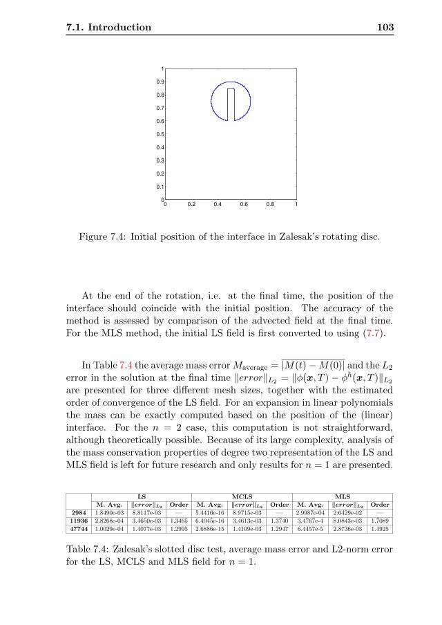
7.1. Introduction 103
0 0.2 0.4 0.6 0.8 10
0.1
0.2
0.3
0.4
0.5
0.6
0.7
0.8
0.9
1
Figure 7.4: Initial position of the interface in Zalesak’s rotating disc.
At the end of the rotation, i.e. at the final time, the position of theinterface should coincide with the initial position. The accuracy of themethod is assessed by comparison of the advected field at the final time.For the MLS method, the initial LS field is first converted to using (7.7).
In Table 7.4 the average mass errorMaverage = |M(t)−M(0)| and the L2
error in the solution at the final time ‖error‖L2 = ‖φ(x, T ) − φh(x, T )‖L2
are presented for three different mesh sizes, together with the estimatedorder of convergence of the LS field. For an expansion in linear polynomialsthe mass can be exactly computed based on the position of the (linear)interface. For the n = 2 case, this computation is not straightforward,although theoretically possible. Because of its large complexity, analysis ofthe mass conservation properties of degree two representation of the LS andMLS field is left for future research and only results for n = 1 are presented.
LS MCLS MLSM. Avg. ‖error‖L2 Order M. Avg. ‖error‖L2 Order M. Avg. ‖error‖L2 Order
2984 1.8490e-03 8.8117e-03 — 5.4416e-16 8.9715e-03 — 2.9987e-04 2.6429e-02 —
11936 2.8268e-04 3.4650e-03 1.3465 6.4045e-16 3.4613e-03 1.3740 3.4767e-4 8.0843e-03 1.7089
47744 1.0029e-04 1.4077e-03 1.2995 2.6886e-15 1.4109e-03 1.2947 6.4457e-5 2.8736e-03 1.4925
Table 7.4: Zalesak’s slotted disc test, average mass error and L2-norm errorfor the LS, MCLS and MLS field for n = 1.
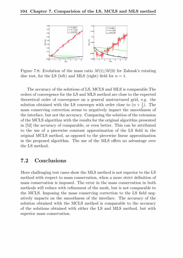
104 Chapter 7. Comparision of the LS, MCLS and MLS method
0 1 2 3 4 5 60.99
1
1.01
1.02
1.03
1.04
1.05
1.06
1.07
1.08
Time.
Ma
ss r
atio
.
K=2984
K=11936
K=47744
0 1 2 3 4 5 60.99
0.995
1
1.005
1.01
1.015
1.02
Time.
Ma
ss r
atio
.
K=2984
K=11936
K=47744
Figure 7.8: Evolution of the mass ratio M(t)/M(0) for Zalesak’s rotatingdisc test, for the LS (left) and MLS (right) field for n = 1.
The accuracy of the solutions of LS, MCLS and MLS is comparable.Theorders of convergence for the LS and MLS method are close to the expectedtheoretical order of convergence on a general unstructured grid, e.g. thesolution obtained with the LS converges with order close to (n + 1
2). Themass conserving correction seems to negatively impact the smoothness ofthe interface, but not the accuracy. Comparing the solution of the extensionof the MCLS algorithm with the results for the original algorithm presentedin [52] the accuracy of comparable, or even better. This can be attributedto the use of a piecewise constant approximation of the LS field in theoriginal MCLS method, as opposed to the piecewise linear approximationin the proposed algorithm. The use of the MLS offers no advantage overthe LS method.
7.2 Conclusions
More challenging test cases show the MLS method is not superior to the LSmethod with respect to mass conservation, when a more strict definition ofmass conservation is imposed. The error in the mass conservation in bothmethods will reduce with refinement of the mesh, but is not comparable tothe MCLS. Imposing the mass conserving correction to the LS field neg-atively impacts on the smoothness of the interface. The accuracy of thesolution obtained with the MCLS method is comparable to the accuracyof the solutions obtained with either the LS and MLS method, but withsuperior mass conservation.
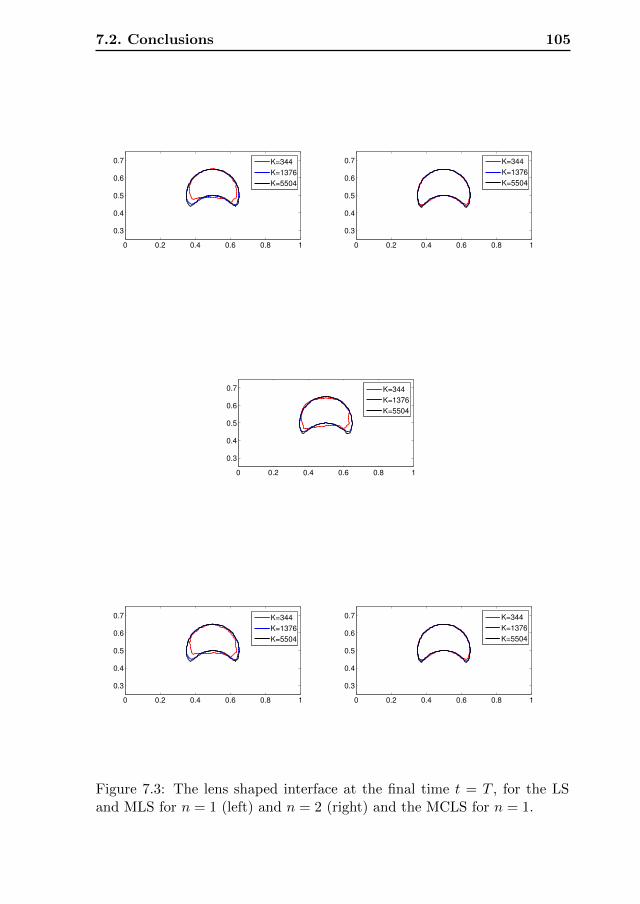
7.2. Conclusions 105
0 0.2 0.4 0.6 0.8 1
0.3
0.4
0.5
0.6
0.7 K=344
K=1376
K=5504
0 0.2 0.4 0.6 0.8 1
0.3
0.4
0.5
0.6
0.7 K=344
K=1376
K=5504
0 0.2 0.4 0.6 0.8 1
0.3
0.4
0.5
0.6
0.7 K=344
K=1376
K=5504
0 0.2 0.4 0.6 0.8 1
0.3
0.4
0.5
0.6
0.7 K=344
K=1376
K=5504
0 0.2 0.4 0.6 0.8 1
0.3
0.4
0.5
0.6
0.7 K=344
K=1376
K=5504
Figure 7.3: The lens shaped interface at the final time t = T , for the LSand MLS for n = 1 (left) and n = 2 (right) and the MCLS for n = 1.
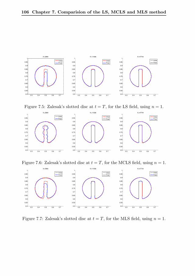
106 Chapter 7. Comparision of the LS, MCLS and MLS method
K=2984
0.3 0.4 0.5 0.6 0.70.5
0.55
0.6
0.65
0.7
0.75
0.8
0.85
0.9
0.95
1
Initial
Final
0.3 0.4 0.5 0.6 0.70.5
0.55
0.6
0.65
0.7
0.75
0.8
0.85
0.9
0.95
1
K=11936
Initial
Final
0.3 0.4 0.5 0.6 0.70.5
0.55
0.6
0.65
0.7
0.75
0.8
0.85
0.9
0.95
1
K=47744
Initial
Final
Figure 7.5: Zalesak’s slotted disc at t = T , for the LS field, using n = 1.
0.3 0.4 0.5 0.6 0.70.5
0.55
0.6
0.65
0.7
0.75
0.8
0.85
0.9
0.95
1
K=2984
Initial
Final
0.3 0.4 0.5 0.6 0.70.5
0.55
0.6
0.65
0.7
0.75
0.8
0.85
0.9
0.95
1
K=11936
Initial
Final
0.3 0.4 0.5 0.6 0.70.5
0.55
0.6
0.65
0.7
0.75
0.8
0.85
0.9
0.95
1
K=47744
Initial
Final
Figure 7.6: Zalesak’s slotted disc at t = T , for the MCLS field, using n = 1.
0.3 0.4 0.5 0.6 0.70.5
0.55
0.6
0.65
0.7
0.75
0.8
0.85
0.9
0.95
1
K=2984
Initial
Final
0.3 0.4 0.5 0.6 0.70.5
0.55
0.6
0.65
0.7
0.75
0.8
0.85
0.9
0.95
1
K=11936
Initial
Final
0.3 0.4 0.5 0.6 0.70.5
0.55
0.6
0.65
0.7
0.75
0.8
0.85
0.9
0.95
1
K=47744
Initial
Final
Figure 7.7: Zalesak’s slotted disc at t = T , for the MLS field, using n = 1.
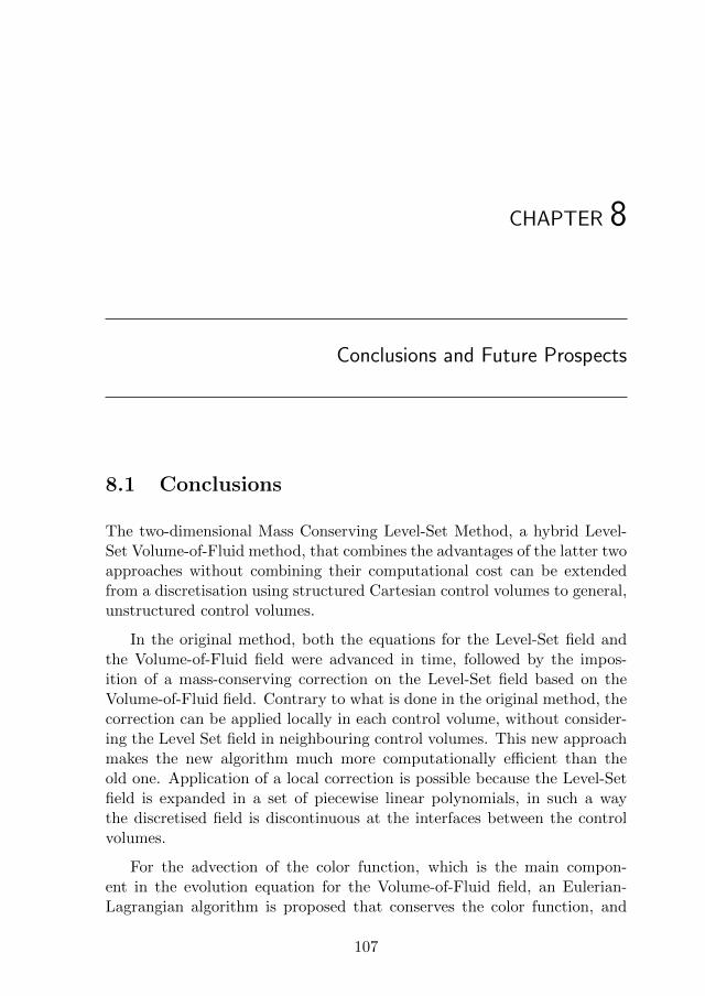
CHAPTER 8
Conclusions and Future Prospects
8.1 Conclusions
The two-dimensional Mass Conserving Level-Set Method, a hybrid Level-Set Volume-of-Fluid method, that combines the advantages of the latter twoapproaches without combining their computational cost can be extendedfrom a discretisation using structured Cartesian control volumes to general,unstructured control volumes.
In the original method, both the equations for the Level-Set field andthe Volume-of-Fluid field were advanced in time, followed by the impos-ition of a mass-conserving correction on the Level-Set field based on theVolume-of-Fluid field. Contrary to what is done in the original method, thecorrection can be applied locally in each control volume, without consider-ing the Level Set field in neighbouring control volumes. This new approachmakes the new algorithm much more computationally efficient than theold one. Application of a local correction is possible because the Level-Setfield is expanded in a set of piecewise linear polynomials, in such a waythe discretised field is discontinuous at the interfaces between the controlvolumes.
For the advection of the color function, which is the main compon-ent in the evolution equation for the Volume-of-Fluid field, an Eulerian-Lagrangian algorithm is proposed that conserves the color function, and
107
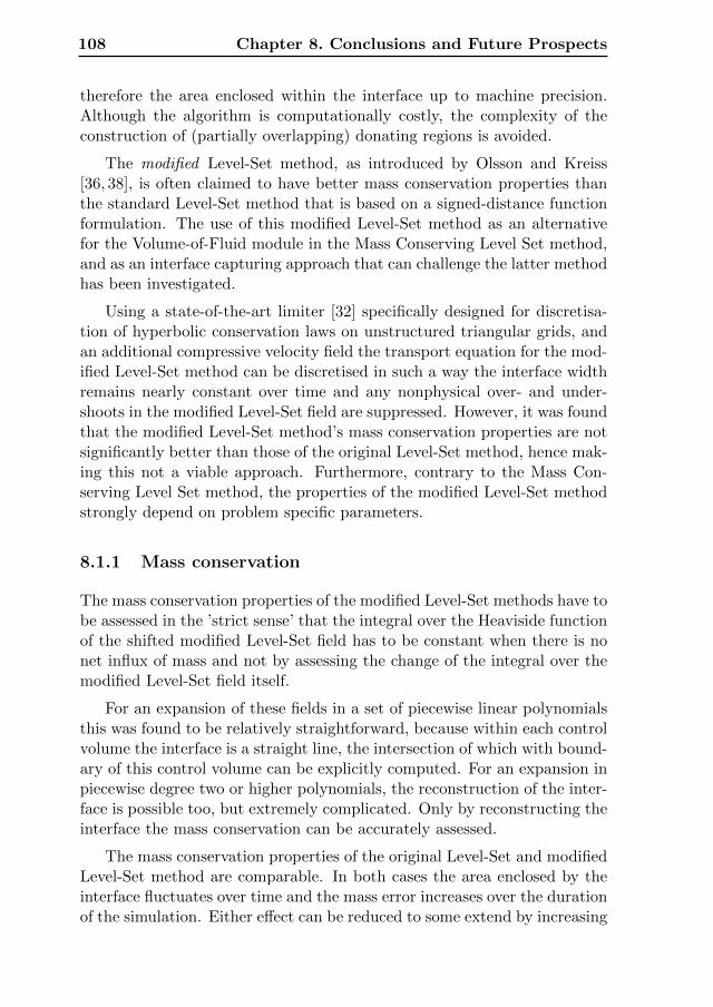
108 Chapter 8. Conclusions and Future Prospects
therefore the area enclosed within the interface up to machine precision.Although the algorithm is computationally costly, the complexity of theconstruction of (partially overlapping) donating regions is avoided.
The modified Level-Set method, as introduced by Olsson and Kreiss[36, 38], is often claimed to have better mass conservation properties thanthe standard Level-Set method that is based on a signed-distance functionformulation. The use of this modified Level-Set method as an alternativefor the Volume-of-Fluid module in the Mass Conserving Level Set method,and as an interface capturing approach that can challenge the latter methodhas been investigated.
Using a state-of-the-art limiter [32] specifically designed for discretisa-tion of hyperbolic conservation laws on unstructured triangular grids, andan additional compressive velocity field the transport equation for the mod-ified Level-Set method can be discretised in such a way the interface widthremains nearly constant over time and any nonphysical over- and under-shoots in the modified Level-Set field are suppressed. However, it was foundthat the modified Level-Set method’s mass conservation properties are notsignificantly better than those of the original Level-Set method, hence mak-ing this not a viable approach. Furthermore, contrary to the Mass Con-serving Level Set method, the properties of the modified Level-Set methodstrongly depend on problem specific parameters.
8.1.1 Mass conservation
The mass conservation properties of the modified Level-Set methods have tobe assessed in the ’strict sense’ that the integral over the Heaviside functionof the shifted modified Level-Set field has to be constant when there is nonet influx of mass and not by assessing the change of the integral over themodified Level-Set field itself.
For an expansion of these fields in a set of piecewise linear polynomialsthis was found to be relatively straightforward, because within each controlvolume the interface is a straight line, the intersection of which with bound-ary of this control volume can be explicitly computed. For an expansion inpiecewise degree two or higher polynomials, the reconstruction of the inter-face is possible too, but extremely complicated. Only by reconstructing theinterface the mass conservation can be accurately assessed.
The mass conservation properties of the original Level-Set and modifiedLevel-Set method are comparable. In both cases the area enclosed by theinterface fluctuates over time and the mass error increases over the durationof the simulation. Either effect can be reduced to some extend by increasing
8.2. Outlook 109
the mesh resolution, but not eliminated. In all applications of the MassConserving Level-Set method the area enclosed by the interface contour isconserved to machine precision.
For those applications for which requirements on mass-conservation canbe relaxed, the computational efficiency of the modified Level-Set methodremains attractive.
8.1.2 The Mass-Conserving Level-Set Method in relation toother hybrid interface capturing algorithms
The Mass Conserving Level-Set (MCLS) method introduced by Van der Pijl[52, 53] is not unique. The most well known competitors are the CLSVOFmethod of Sussmann et al. [48, 49] and the VOSET method of Sun [46].The main difference between CLSVOF and VOSET on one side and theoriginal MCLS is the use of a very efficient algorithm to establish congruencebetween the Level-Set field and the Volume-of-Fluid field, without explicitinterface reconstruction. A simple function relates the two fields within asingle Cartesian quadrilateral (2D) or hexahedral (3D) control volume. Inthe current thesis a similar relation has been defined for triangular controlvolumes. It is this key difference that makes the (extension of the) MCLSso competitive.
8.1.3 The modified Level-Set method in comparison to theLevel-Set method
The near-discontinuous behaviour of the modified Level-Set field in the vi-cinity of the interface makes accurate discretisation of the transport equa-tion for this field much more challenging and costly than for the Level-Setfield. The strong non-linearity of the field will also negatively impact theaccuracy of the computation of the interface normal vector and the inter-face curvature. For these reasons, and the fact that mass conservation is notsignificantly better than for the Level-Set method, the modified Level-Setmethod seems to offer little advantage over the original Level-Set method.
8.2 Outlook
A start has been made with the development of a model for two-dimensionalimmiscible incompressible two-phase flow in geometrically intricate domains.To complete the model the following steps are recommended to be taken.
110 Chapter 8. Conclusions and Future Prospects
• The extension of the Mass Conserving Level-Set method has to beembedded in a numerical method that can solve the incompressibleNavier-Stokes equations on the same type of control volumes utilizedby the proposed interface algorithm. A natural candidate would be adiscontinuous Galerkin method, using operator splitting, as proposedby Hesthaven [23].
• To model the effects of surface tension, the local curvature of theinterface and the interface normal vector have to be determined fromthe Level-Set field. It remains to be investigated how this is mostaccurately done for the piecewise continuous Level-Set field.
• To have even more flexibility for automatic tessellations of geometric-ally complicated domains, polygonal (2D) and polyhedral (3D) controlvolumes are preferred. It is worth-while to investigate the possibilityof extending the Mass-Conserving Level-Set method for a discretisa-tion using such control volumes, either directly or by using a subdivi-sion of the polyhedral control volumes in a set of tetrahedral controlvolumes. At least for convex polyhedral this subdivision is alwayspossible.
• Finally, it is recommended that alternatives to the computationallyintensive Volume-of-Fluid advection scheme are investigated.
Bibliography
[1] https://en.wikipedia.org/wiki/Bubble_column_reactor.
[2] https://en.wikipedia.org/wiki/Fluidized_bed_reactor.
[3] https://en.wikipedia.org/wiki/Fluidized_bed_reactor.
[4] http://synthoglasspiperepair.com/index.php/
ct-menu-item-3.html.
[5] Anthony Anderson, Xiaoming Zheng, and Vittorio Cristini. Adaptiveunstructured volume remeshing-I: The method. Journal of Computa-tional Physics, 208(2):616 – 625, 2005.
[6] Douglas N. Arnold, Franco Brezzi, Bernardo Cockburn, and L. Dona-tella Marini. Unified analysis of discontinuous galerkin methods forelliptic problems. SIAM Journal on Numerical Analysis, 39(5):1749–1779, 2002.
[7] Blanca AyusodeDios and Ludmil Zikatanov. Uniformly convergent it-erative methods fordiscontinuous galerkin discretizations. Journal ofScientific Computing, 40(1-3):4–36, 2009.
[8] Nestor Balcazar, Lluıs Jofre, Oriol Lehmkuhl, Jesus Castro, and Joa-quim Rigola. A finite-volume/level-set method for simulating two-phase flows on unstructured grids. International journal of multiphaseflow, 64:55–72, 2014.
111
112 BIBLIOGRAPHY
[9] J. U. Brackbill, D. B. Kothe, and C. Zemach. A continuum methodfor modeling surface tension. J. Comput. Phys., 100(2):335–354, June1992.
[10] John C. Butcher. A multistep generalization of runge-kutta methodswith four or five stages. J. ACM, 14(1):84–99, January 1967.
[11] Anurag Chakraborty. An extension of weiler-atherton algorithm tocope with the self-intersecting polygon. CoRR, abs/1403.0917, 2014.
[12] J Chiva, J Ventosa, O Lehmkuhl, and CD Perez-Segarra. Modeliza-tion of the low-mach navier stokes equations in unstructured meshes.Proceedings of the 7th International conference on computational heatand mass transfer, 2011.
[13] Bernardo Cockburn and Chi-Wang Shu. The runge–kutta discontinu-ous galerkin method for conservation laws v: multidimensional sys-tems. Journal of Computational Physics, 141(2):199–224, 1998.
[14] Olivier Desjardins, Vincent Moureau, and Heinz Pitsch. An accurateconservative level set/ghost fluid method for simulating turbulent at-omization. Journal of Computational Physics, 227(18):8395 – 8416,2008.
[15] Olivier Desjardins, Vincent Moureau, and Heinz Pitsch. An accur-ate conservative level set/ghost fluid method for simulating turbulentatomization. Journal of Computational Physics, 227(18):8395–8416,2008.
[16] A Runge-Kutta Discontinuous-Galerkin. Level-set method for un-steady com-pressible two-fluid flow.
[17] Douglas Enright, Ronald Fedkiw, Joel Ferziger, and Ian Mitchell. A hy-brid particle level set method for improved interface capturing. Journalof Computational Physics, 183(1):83 – 116, 2002.
[18] Allen Van Gelder. Efficient computation of polygon area and polyhed-ron volume. In Alan W. Paeth, editor, Graphics Gems V, pages 35–41.Academic Press, 1995.
[19] FX Giraldo, Jan S. Hesthaven, and T. Warburton. Nodal high-orderdiscontinuous Galerkin methods for the spherical shallow water equa-tions. Journal of Computational Physics, 181(2):499–525, 2002.
BIBLIOGRAPHY 113
[20] J. Grooss and J.S. Hesthaven. A level set discontinuous galerkinmethod for free surface flows. Computer Methods in Applied Mech-anics and Engineering, 195(25-28):3406–3429, 2006.
[21] Francis H. Harlow and J. Eddie Welch. Numerical calculation oftimedependent viscous incompressible flow of fluid with free surface.Physics of Fluids, 8(12), 1965.
[22] Daniel Hartmann, Matthias Meinke, and Wolfgang Schrder. Differen-tial equation based constrained reinitialization for level set methods.Journal of Computational Physics, 227(14):6821 – 6845, 2008.
[23] J. S. Hesthaven and T. Warburton. Discontinuous Galerkin methodsfor the time-domain Maxwell’s equations. ACES Newsletter, 19:10–29,2004.
[24] C.W Hirt and B.D Nichols. Volume of fluid VoF method for the dynam-ics of free boundaries. Journal of Computational Physics, 39(1):201 –225, 1981.
[25] Barth T. J. and Jespersen. The design and application of upwindschemes on unstructured meshes. AIAA Paper, 89-0366, 1989.
[26] Guang-Shan Jiang and Chi-Wang Shu. Efficient implementation ofweighted ENO schemes. Journal of Computational Physics, 126(1):202– 228, 1996.
[27] Lluıs Jofre, Oriol Lehmkuhl, Jesus Castro, and Assensi Oliva. A plic-vof implementation on parallel 3d unstructured meshes. Proc. of VEuropean Conference on Computational Fluid Dynamics, ECCOMASCFD, pages 1–15, 2010.
[28] Lluıs Jofre, Oriol Lehmkuhl, Jesus Castro, and Assensi Oliva. A 3-d volume-of-fluid advection method based on cell-vertex velocities forunstructured meshes. Computers & Fluids, 94:14–29, 2014.
[29] Ron Kimmel. The osher-sethian level set method. In Numerical Geo-metry of Images, pages 50–60. Springer New York, 2004.
[30] L. Krivodonova, J. Xin, J.-F. Remacle, N. Chevaugeon, and J.E. Fla-herty. Shock detection and limiting with discontinuous galerkin meth-ods for hyperbolic conservation laws. Applied Numerical Mathematics,48(34):323 – 338, 2004. Workshop on Innovative Time Integrators forPDEs.
114 BIBLIOGRAPHY
[31] Lilia Krivodonova. Limiters for high-order discontinuous galerkinmethods. Journal of Computational Physics, 226(1):879 – 896, 2007.
[32] Dmitri Kuzmin. A vertex-based hierarchical slope limiter for -adaptivediscontinuous galerkin methods. Journal of Computational and AppliedMathematics, 233(12):3077 – 3085, 2010. Finite Element Methods inEngineering and Science (FEMTEC 2009).
[33] Hong Luo, Joseph D. Baum, and Rainald Lhner. A discontinuousgalerkin method based on a taylor basis for the compressible flowson arbitrary grids. Journal of Computational Physics, 227(20):8875 –8893, 2008.
[34] Emilie Marchandise, Jean-Francois Remacle, and Nicolas Chevaugeon.A quadrature-free discontinuous galerkin method for the level set equa-tion. Journal of Computational Physics, 212(1):338 – 357, 2006.
[35] Jeremy O. Mccaslin and Olivier Desjardins. A localized re-initializationequation for the conservative level set method. J. Comput. Phys.,262:408–426, April 2014.
[36] Elin Olsson and Gunilla Kreiss. A conservative level set method fortwo phase flow. Journal of Computational Physics, 210(1):225 – 246,2005.
[37] Elin Olsson and Gunilla Kreiss. A conservative level set method fortwo phase flow. J. Comput. Phys., 210(1):225–246, November 2005.
[38] Elin Olsson, Gunilla Kreiss, and Sara Zahedi. A conservative level setmethod for two phase flow II. Journal of Computational Physics,225(1):785 – 807, 2007.
[39] Elin Olsson, Gunilla Kreiss, and Sara Zahedi. A conservative level setmethod for two phase flow ii. J. Comput. Phys., 225(1):785–807, July2007.
[40] Stanley Osher and James A Sethian. Fronts propagating withcurvature-dependent speed: Algorithms based on Hamilton-Jacobi for-mulations. Journal of Computational Physics, 79(1):12 – 49, 1988.
[41] Mark Owkes and Olivier Desjardins. A discontinuous galerkin conser-vative level set scheme for interface capturing in multiphase flows. J.Comput. Phys., 249:275–302, September 2013.
BIBLIOGRAPHY 115
[42] Mark Owkes and Olivier Desjardins. A discontinuous galerkin conser-vative level set scheme for interface capturing in multiphase flows. J.Comput. Phys., 249:275–302, September 2013.
[43] F. Raees, D. R. van der Heul, and C. Vuik. A mass-conserving level-setmethod for simulation of multiphase flow in geometrically complicateddomains. International Journal for Numerical Methods in Fluids, pagesn/a–n/a, 2015. fld.4188.
[44] Thomas Revesz. Clipping polygons with sutherland-hodgman’s al-gorithm. C Users J., 11(8):23–34, August 1993.
[45] W. Rider and D. Kothe. A marker particle method for interface track-ing. Proceedings of the Sixth International Symposium on Computa-tional Fluid Dynamics, pages 976–981, 1995.
[46] D.L. Sun and W.Q. Tao. A coupled volume-of-fluid and level set (voset)method for computing incompressible two-phase flows. InternationalJournal of Heat and Mass Transfer, 53(4):645 – 655, 2010.
[47] Daniel Sunday. Fast polygon area and newell normal computation.Journal of Graphics Tools, 7(2):9–13, 2002.
[48] Mark Sussman. A second order coupled level set and volume-of-fluidmethod for computing growth and collapse of vapor bubbles. Journalof Computational Physics, 187(1):110 – 136, 2003.
[49] Mark Sussman and Elbridge Gerry Puckett. A coupled level setand volume-of-fluid method for computing 3D and axisymmetric in-compressible two-phase flows. Journal of Computational Physics,162(2):301–337, 2000.
[50] G. Tryggvason, B. Bunner, A. Esmaeeli, D. Juric, N. Al-Rawahi,W. Tauber, J. Han, S. Nas, and Y.-J. Jan. A front-tracking methodfor the computations of multiphase flow. Journal of ComputationalPhysics, 169(2):708 – 759, 2001.
[51] O. Ubbink. Numerical prediction of the two fluid systems with sharpinterfaces. PhD Thesis,University of London, 1997.
[52] S.P. van der Pijl. Computation of bubbly flows with a mass-conservinglevel-set method. PhD Thesis, TU Delft, The Netherlands, 2005.
[53] S.P. van der Pijl, A. Segal, C. Vuik, and P. Wesseling. Computing three-dimensional two-phase flows with a mass-conserving level-set method.Comput. Visual Sci., 11:221–235, 2008.
116 BIBLIOGRAPHY
[54] V. Venkatakrishnan. Convergence to steady state solutions of the eulerequations on unstructured grids with limiters. Journal of Computa-tional Physics, 118(1):120 – 130, 1995.
[55] Tomasz Wacawczyk. A consistent solution of the re-initialization equa-tion in the conservative level-set method. Journal of ComputationalPhysics, 299:487 – 525, 2015.
[56] Y. Wang, S. Simakhina, and M. Sussman. A hybrid level set-volumeconstraint method for incompressible two-phase flow. Journal of Com-putational Physics, 231(19):6438 – 6471, 2012.
[57] Chi wang Shu. Essentially non-oscillatory and weighted essentiallynon-oscillatory schemes for hyperbolic conservation laws. In AdvancedNumerical Approximation of Nonlinear Hyperbolic Equations, volume1697 of Lecture Notes in Mathematics, pages 325–432. Springer, 1998.
[58] G.D. Weymouth and D.K.-P. Yue. Conservative volume-of-fluidmethod for free-surface simulations on Cartesian-grids. Journal ofComputational Physics, 229(8):2853 – 2865, 2010.
[59] Nazeeruddin Yaacob and Bahrom Sanugi. A fifth -order five-stagerk-method based on harmonic mean. In E. van Groesen and E. Soe-wono, editors, Differential Equations Theory, Numerics and Applica-tions, pages 381–389. Springer Netherlands, 1997.
[60] Xiaofeng Yang, Ashley J. James, John Lowengrub, Xiaoming Zheng,and Vittorio Cristini. An adaptive coupled level-set/volume-of-fluidinterface capturing method for unstructured triangular grids. Journalof Computational Physics, 217(2):364 – 394, 2006.
[61] Steven T Zalesak. Fully multidimensional flux-corrected transport al-gorithms for fluids. Journal of Computational Physics, 31(3):335 – 362,1979.
[62] H.W. Zheng. A new limiter for hybrid grid. Procedia Engineering,67:430 – 437, 2013. 7th Asian-Pacific Conference on Aerospace Tech-nology and Science, 7th APCATS 2013.
[63] Xiaoming Zheng, John Lowengrub, Anthony Anderson, and VittorioCristini. Adaptive unstructured volume remeshing-II: Application totwo- and three-dimensional level-set simulations of multiphase flow.Journal of Computational Physics, 208(2):626 – 650, 2005.
About the Author
Fahim Raees was born on 2nd December 1984 inKarachi, Pakistan. He obtained his High SchoolCertification with Pre-Engineering in 2002 fromD.J. Sindh Government Science college, Karachi.After that, he joined the Department of Mathem-atics of University of Karachi, Pakistan to pursueB.Sc. Honors in Mathematics. He graduated in2005 with the first division. After that, he com-pleted his M.Sc. in applied Mathematics from thesame university and graduated in 2006.
He started working as a Management Trainee Of-ficer in one of the leading banks in Pakistan. In
the beginning of 2008, he joined NED University of Engineering and Tech-nology, Karachi, as a lecturer in the department of Mathematics and BasicSciences, now known as Department of Mathematics. He worked therefor three years and taught different undergraduate courses. He was awar-ded a fully funded faculty development scholarship to pursue Ph.D. studiesabroad.
He joined Delft University of Technology, Delft, the Netherlands inDecember 2010. He started his doctoral research in the Numerical Ana-lysis group of Delft Institute of Applied Mathematics under the supervisionof Prof. dr. ir. Kees Vuik and assistant prof. dr. ir. Duncan van derHeul. He worked on the development of the efficient and robust method forthe simulation of the two-phase flow problems over complex domains. Heselected hybrid approach to combined the characteristics of the Level-Setand the Volume of Fluid method. He got many opportunities to presenthis Ph.D. research work on international conferences like ECCOMAS con-ference, 2012 in Vienna, Austria and the CFD meeting of APS, 2013 inPittsburgh, Pennsylvania, USA.
117

List of publications
Journal Publications
• F. Raees, D. R. van der Heul, and C. Vuik, A mass-conserving level-set method for simulation of multiphase flow in geometrically com-plicated domains. International Journal for Numerical Methods inFluids, 2015. fld.4188.
Abstract and Conference Proceedings
• F. Raees, D. R. van der Heul, and C. Vuik, Extension of the Mass-Conserving Level-Set method to unstructured polyhedral control volumesfor two-phase flows, Bulletin of the American Physical Society, 66thAnnual Meeting of the APS Division of Fluid Dynamics, Volume 58,Number 18, 2013. Pittsburgh, Pennsylvania, USA.
• F. Raees, D. R. van der Heul, and C. Vuik, The first step towardsextension of the Mass-Conserving Level-Set method to discretisationsusing general polyhedral control volumes,Proceedings of the 6th EuropeanCongress on Computational Methods in Applied Sciences and Engin-eering (ECCOMAS 2012), Vienna, Austria.
Technical Reports
• Evaluation of the interface-capturing algorithm of OpenFOAM forthe simulation of incompressible immiscible two-phase flow, Technical
119
120 BIBLIOGRAPHY
report no. 11-07, DIAM, 2011, TU Delft.
Presentations
• Research work presented at the 66th American Physical Society divi-sion of Computational Fluid Dynamics meeting, Pittsburgh, Pennsylvania,USA, 2013.
• Invited speaker at the Contactgroup Computational Fluid Dynamicsmeeting, Deltares, Delft, The Netherlands, 2013.
• Research work presented at the 6th ECCOMAS 2012 conference, Uni-versity of Vienna, Vienna, Austria.
• Tea Talks, Numerical Analysis group of DIAM, TU Delft.
• Poster presented at 36th, 37th, 38th, 39th Woudschoten Conference,held in Zeist, (2011-2014), The Netherlands.
Acknowledgements
First of all, I thank Allah (S.W.T) for having me this opportunity andguiding me in my low times during the course of this Ph.D. thesis.
This thesis is not possible without the help of many people; some of themare directly involved in the research and some are in the form of goodcompany. I would like to use this opportunity to thank all of you. However,I think it is not fair not to mention the name of those who have had helped,encouraged and guided me, during the period of my Ph.D. research.
I thank my promotor prof.dr.ir. Kees Vuik for his guidance. He alwaysadvised me to use a simple approach to sorting out/debug the big problem.I have found him really hard working and sincere person. I have learneda lot from him, including, how to do research and the importance of theresearch network.
I am also lucky to have a co-promotor dr.ir. Duncan Roy Van der Heul. Healways guided me in the right research direction. The discussion with himover the research problems always leads to some new inside and providesa better understanding of the problem. I thank him for his help and alsocritically reviewing my manuscripts. I have learned a lot from him aboutthe scientific writing.
I highly acknowledge NED University, Karachi, Pakistan for awarding mefaculty development scholarship, without this scholarship this thesis is im-possible to complete and I also thank TU Delft for partial funding myproject.
I acknowledge my former office mates, Dr. Ibrahim Daud and Dr. AbdulHanan Sheikh and current office mates Renaldo Astudillo, Behrouz Raftari
121

122 BIBLIOGRAPHY
and Baljinnyam Sereeter for providing me lively and friendly office environ-ment. I will never forget the memorable time, we have spent in our office.
I am greatful to have an opportunity to work with nice and hard workingpeople of the Numerical Analysis group. I like to thank Guido Oud, Manuelvan Baumann, Menel Rehrah, Dr. Denis de Ouden, Dr. Jing Zhao, Dr.Xiaozhou Li, Dr. Rohit Gupta, Dr. Yue Qiu, Peiyao Luo, Muhamed AlAbbassi, Luis Antonio, Diaz Gabriela, Zaza van der Have, Fei Cong, LisaWobbes, Virginia Roosi, Dr. Faraz Khatami and Thea Vuik for there sincerecooperation and nice working environment. I specially thank to Thea Vuikfor translating my propositions into Dutch. I also like to thank my friendfrom the Mathematical Analysis group, TU Delft, Rajab Ali Malookani,Dr. Sajad Sandilo, Dr. Haider Shah and Nick Gaiko.
I want to say special thank to my colleague and friend Joost van Zwietenfor his help during the research and also pursuing me to use Linux. I alwayshave a good discussion with you over research problems and also say mythank to Leonie Kah for having me over dinner.
I have enjoyed my stay in Delft due to the joys company of my friendsfrom Pakistan. I used to have BBQ with them and play cricket. Theircompany always keep me connected with my homeland. I like to thank,first the former Pakistani colleagues; Dr. M Faisal Nadeem, Dr. SeyabKhan, Dr. Fakhar Anjum, Dr. Shah Muhammad, Dr. Hamayun Zai,Dr. Iftikhar Faraz, Dr. Shahzad Gishkori, Dr. Adeel Javaid and KazmiSahab for providing me great company and guidance. I am also gratefulto have young Pakistani friends to whom with, I enjoyed delicious foodand play cricket a lot; Dr. Imran Ashraf, Dr. Waqas Hassan, Dr. HamidMushtaq, Nauman Ahmed, A Nadeem Tabish, Qasim Lone, Hussam Khaliq,Muhammad Farooq, Muneeb Yousaf, Muhammad Irfan, Saad Jahangir,Salman Khan, Noor Nabi Mujahid.
I cannot forget the memorable time spent with Sadar Usama Malik andUmar Ijaz Chaudrey. Thank you friends for your memorable company.
I thank my ex-house mate and best friend Devender Maheshwari and hiswife Rita Maheshwari for providing a good company away from my homeand special thanks to Rita for cooking nice and delicious vegetarian food.
I want to thank secretary of our group Deborah Dongor for her help inadministrative matters. You have helped me a lot. I also thank FrancaPost from CICAT for her help in organizing my initial stay in Delft andadministrative matters. I also acknowledge the time to time help of KeesLemmens for ICT support. You have a good command on Linux.
I also like to thank faculty members of my group Prof.dr.ir Martin van
BIBLIOGRAPHY 123
Gijzen, Dr.ir. Fred Vermolen, Dr. Jennifer Ryan, Dr.ir. Domenico La-haye, Dr. N.V. Budko, Ir. A. Segal and Ir. P. Sonneveld for their livelyconversation over a range of topics.
I thank my friends Charlie van Schoor and Anna, Albert, JP, Rubin andAndrew for having a good company over BBQ many times at my place. Ialso thank my current house mates for maintaining a friendly atmospherein our student house, Gijs, Jorn, Sharat, Tim, Micheal and Ingeborg.
I am grateful to have NED University colleagues, Tauqeer Ahmed Hashmi,Sohail Ahmed, Zakir Khan, Umar Faryaz, Muhammad Yousuf Tufail andDr. Bilal Ahmed Usmani. I especially convey my thank to Prof.dr. MirzaMahmood Baig for their administrative support during my stay aboard.
In last, I like to thank my parents for their continuous encouragement andmotivation during my stay aboard. I cannot be able to do anything withoutyour best wishes and prayers, thank you very much. May Allah bless youall!


