Passenger punctualityAn analysis of the method ofcalculation and describing models

G. J. Wolters

TechnischeUniversiteitDelft

Passenger punctualityAn analysis of the method of calculation

and describing models

by

G. J. Wolters

in partial fulfillment of the requirements for the degree of

Master of Sciencein Civil Engineering

at the Delft University of Technologyto be defended publicly on Monday March 7, 2016 at 11:00 AM.

Supervisor: Prof. dr. ir. S. P. HoogendoornThesis committee: Dr. R. M. P. Goverde, TU Delft

Ir. V. A. Weeda, ProRailDr. W. W. Veeneman, TU DelftIr. P. B. L. Wiggenraad, TU Delft

An electronic version of this thesis is available at http://repository.tudelft.nl/.

Preface

Before you lies the thesis ‘Passenger punctuality – An analysis of the method of calculation and de-scribing models’. It is the result of my research to fulfil the graduation requirements of the masterTransport and Planning of the faculty of Civil Engineering and Geosciences of the Delft University ofTechnology. The research is performed between June 2015 and February 2016.

For eight months I did my research as an intern at ProRail in Utrecht. Here were most resourcesavailable for me to analyse and answer the research questions properly. Nonetheless, I could notfully examine passenger punctuality without the data, sources and knowledge available at the NS.Fortunately it was no problem to conduct a part of my research there.

I want to thank several people for their help during my graduation. First of all I want to thank mygraduation committee: Serge Hoogendoorn, Rob Goverde and Paul Wiggenraad of the department ofTransport and Planning; Wijnand Veeneman of the faculty of Technology, Policy and Management; andVincent Weeda of ProRail. Their guidance, comments and suggestions were really helpful during myresearch and while writing my thesis.

Secondly I want to say thanks to the colleagues of the Prestatie Analyse Bureau at ProRail. Everyonewas always interested in my work and they included me from the very first day. Special thanks go toVincent Weeda. As my daily supervisor, Vincent was always prepared to answer questions, read andcomment my work and give advice where necessary. He really improved my research. Peter vanWaveren helped enormously in the formulating of my research question and guided me through myresearch. Jan-Martijn Egbers’ knowledge of the KPIs and the process indicators was essential to myresearch.

I could not have written this thesis without the help of some people of the NS, especially JohnTuithof. He was constantly interested in my work and I could always ask anything to him. Besides, heprovided me with data essential to this research. Marnix van den Broek was a big help as well. Hegave me a better insight in the method of calculating passenger punctuality.

Finally, I want to thank my fellow students with who I worked closely during my time in Delft. I wantsay thanks to my family and friends as well, for supporting me during my study. My deep gratitudegoes to my parents. Their interest, support and love throughout my entire time as a student wereessential. Lastly, I want to say thanks to Him, whose unconditional love still amazes me every day.

Geert-Jan WoltersDelft, February 2016

iii

Summary

The maintenance and control of the Dutch rail network is the responsibility of ProRail. ProRail worksclosely with the largest train operator, the Nederlandse Spoorwegen (the Dutch Railways, NS). Bothcompanies are accountable for their performance to the Dutch government. They measure their per-formance through Key Performance Indicators (KPI). In order to improve the performance of the railnetwork, ProRail and the NS adopted in 2015 the same KPI: passenger punctuality. The current defini-tion is: the percentage of passengers arriving at their final destination within 5 minutes of the plannedarrival time. The method of calculation is based on forecasts and the counting of passengers by trainconductors.

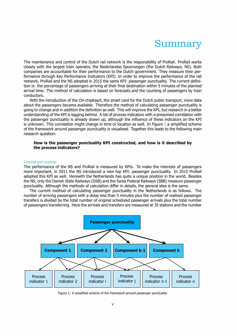
With the introduction of the OV-chipkaart, the smart card for the Dutch public transport, more dataabout the passengers became available. Therefore the method of calculating passenger punctuality isgoing to change and in addition the definition as well. This will improve the KPI, but research in a betterunderstanding of the KPI is lagging behind. A list of process indicators with a presumed correlation withthe passenger punctuality is already drawn up, although the influence of these indicators on the KPIis unknown. This correlation might change in time or location as well. In Figure 1 a simplified schemeof the framework around passenger punctuality is visualised. Together this leads to the following mainresearch question:

How is the passenger punctuality KPI constructed, and how is it described bythe process indicators?

Literature reviewThe performance of the NS and ProRail is measured by KPIs. To make the interests of passengersmore important, in 2011 the NS introduced a new top KPI: passenger punctuality. In 2015 ProRailadopted this KPI as well. Herewith the Netherlands has quite a unique position in the world. Besidesthe NS, only the Danish State Railways (DSB) and the Swiss Federal Railways (SBB) measure passengerpunctuality. Although the methods of calculation differ in details, the general idea is the same.

The current method of calculating passenger punctuality in the Netherlands is as follows. Thenumber of arriving passengers with a delay less than 5 minutes plus the number of realised passengertransfers is divided by the total number of original scheduled passenger arrivals plus the total numberof passengers transferring. Here the arrivals and transfers are measured at 35 stations and the number

Passenger punctuality

Component 2 Component k-1Component 1 Component k

Processindicator i

Processindicator 2

Processindicator 1

Processindicator j

Processindicator n-1

Processindicator n

Figure 1: A simplified scheme of the framework around passenger punctuality

v

vi Summary

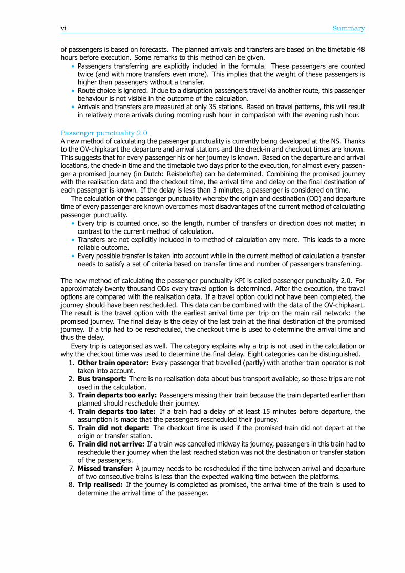
of passengers is based on forecasts. The planned arrivals and transfers are based on the timetable 48hours before execution. Some remarks to this method can be given.

• Passengers transferring are explicitly included in the formula. These passengers are countedtwice (and with more transfers even more). This implies that the weight of these passengers ishigher than passengers without a transfer.

• Route choice is ignored. If due to a disruption passengers travel via another route, this passengerbehaviour is not visible in the outcome of the calculation.

• Arrivals and transfers are measured at only 35 stations. Based on travel patterns, this will resultin relatively more arrivals during morning rush hour in comparison with the evening rush hour.

Passenger punctuality 2.0A new method of calculating the passenger punctuality is currently being developed at the NS. Thanksto the OV-chipkaart the departure and arrival stations and the check-in and checkout times are known.This suggests that for every passenger his or her journey is known. Based on the departure and arrivallocations, the check-in time and the timetable two days prior to the execution, for almost every passen-ger a promised journey (in Dutch: Reisbelofte) can be determined. Combining the promised journeywith the realisation data and the checkout time, the arrival time and delay on the final destination ofeach passenger is known. If the delay is less than 3 minutes, a passenger is considered on time.

The calculation of the passenger punctuality whereby the origin and destination (OD) and departuretime of every passenger are known overcomes most disadvantages of the current method of calculatingpassenger punctuality.

• Every trip is counted once, so the length, number of transfers or direction does not matter, incontrast to the current method of calculation.

• Transfers are not explicitly included in to method of calculation any more. This leads to a morereliable outcome.

• Every possible transfer is taken into account while in the current method of calculation a transferneeds to satisfy a set of criteria based on transfer time and number of passengers transferring.

The new method of calculating the passenger punctuality KPI is called passenger punctuality 2.0. Forapproximately twenty thousand ODs every travel option is determined. After the execution, the traveloptions are compared with the realisation data. If a travel option could not have been completed, thejourney should have been rescheduled. This data can be combined with the data of the OV-chipkaart.The result is the travel option with the earliest arrival time per trip on the main rail network: thepromised journey. The final delay is the delay of the last train at the final destination of the promisedjourney. If a trip had to be rescheduled, the checkout time is used to determine the arrival time andthus the delay.

Every trip is categorised as well. The category explains why a trip is not used in the calculation orwhy the checkout time was used to determine the final delay. Eight categories can be distinguished.1. Other train operator: Every passenger that travelled (partly) with another train operator is nottaken into account.

2. Bus transport: There is no realisation data about bus transport available, so these trips are notused in the calculation.

3. Train departs too early: Passengers missing their train because the train departed earlier thanplanned should reschedule their journey.

4. Train departs too late: If a train had a delay of at least 15 minutes before departure, theassumption is made that the passengers rescheduled their journey.

5. Train did not depart: The checkout time is used if the promised train did not depart at theorigin or transfer station.

6. Train did not arrive: If a train was cancelled midway its journey, passengers in this train had toreschedule their journey when the last reached station was not the destination or transfer stationof the passengers.

7. Missed transfer: A journey needs to be rescheduled if the time between arrival and departureof two consecutive trains is less than the expected walking time between the platforms.

8. Trip realised: If the journey is completed as promised, the arrival time of the train is used todetermine the arrival time of the passenger.

Summary vii

In the method of calculating passenger punctuality a lot of assumptions are made. In this research theassumptions are analysed and, if possible, the influence on the passenger punctuality is determined.Three assumptions stand out because the impact is large.

• Departure and arrival: If there is a disruption that causes large delays or the cancelling oftrains, passengers might check in or check out at stations that are not their planned departureor arrival stations. The assumptions are made that these cases are negligible: every passengerchecks in or out at his or her desired arrival or departure station. The overall impact of theseassumptions is hard to determine because it depends on the location, the time of day and theduration of the disruption. Nonetheless, per case an estimation of the impact can be determined.

• Walking time: The assumption is made that the walking time between the card reader (usedto check in or to check out) and the platform is 1 minute, independent of the station. If thiswalking time is specified per station, which implies more realistic walking times, the passengerpunctuality is expected to change 0.42 percentage point.

• Realisation data: Based on more than 5000 measurements by hand, the average deviationbetween the exact arrival and departure times of trains at each station and the determined arrivaland departure times used in the realisation data is 20 seconds. Moreover there are outliers ofmore than 1 minute. This difference between the realisation data and the exact realisation canlead to a maximum impact of 0.72 percentage point on the passenger punctuality KPI.

Altogether the estimation of the maximum impact of all assumptions on the passenger punctuality isabout 2 percentage points. This implies that the real passenger punctuality can be 2 percentage pointlower than the value of the KPI.

Breakdown of the passenger punctualityFrom a passengers’ perspective, the categories why a journey should be rescheduled are also reasonsfor a delay. These reasons, or components (see Figure 1), can give information about the performanceof the rail network. Therefore, in this research, an algorithm is developed that can breakdown thepassenger punctuality into the components. There are six components: the 5 rescheduling categories,where the final delay is at least a threshold value, and the component ’Train delayed’. This last com-ponent is within the trips categorized as ’Trip realised’, where the final delay is at least a thresholdvalue as well. An example of a resulting breakdown graph can be found in Figure 2. The size of thecomponents is scaled such that the sum of the components at a delay threshold of 180 seconds isequal to 100%.

The breakdown can also be done for a part of the rail network, like an OD, an arriving or transferstation or a train series. Figure 3 shows the passenger punctuality and the shares of the componentsfor passenger trips between stations Rotterdam Centraal and Breda. A sample of the data is taken tocreate this graph, so the 95% confidence interval is visualized by the two blue lines, just below andabove the passenger punctuality line.

Models to describe passenger punctualityBesides the new method of calculation, ProRail and the NS have created a model to describe passengerpunctuality in order to increase the passenger punctuality. Here passenger punctuality is related to thenumber of Explainable Train Deviations (in Dutch: Te Verklaren Treinafwijkingen, TVTA). A TVTA isa deviation of a train with respect to the timetable. For passenger trains this is mostly due to thecancellation or the delay of the train. The model implies that the more trains are delayed or cancelledthe lower the passenger punctuality is. In this research the correlation between the number of TVTAsand the passenger punctuality is calculated. For the business unit Transport control and Traffic control(TB / VL) the correlation is moderate. This implies that TB / VL do not have a large influence on thepassenger punctuality.

In the same model, the number of TVTAs is related to process indicators. These process indicatorsmeasure the performance of specific processes. If the performance of a process increases, the numberof TVTAs might go down and thus the passenger punctuality might improve. For the business unit TB/ VL 20 process indicators can be distinguished, whereby five are not yet fully developed and thereforeneglected in the remainder of the analysis. For four process indicators the correlation with the numberof TVTAs is moderate. For six process indicators the exact definition is wrong: there is a correlationwith the number of TVTAs but the value of the process indicator does not represent this. The remainingfive process indicators do not have any correlation with the number of TVTAs.

viii Summary

Figure 2: The passenger punctuality and the shares of the components on June 1, 2015

Figure 3: The passenger punctuality and the shares of the components for trips between stations Rotterdam Centraal and Breda

Summary ix

The largest disadvantage of this model is the use of TVTAs. TVTAs might not be very reliable and sometypes of TVTAs are not taken into account. The main drawback is the fact that TVTAs relate to trainsand not to passengers. In other words, the TVTAs are not weighted with the number of passengersinvolved. Therefore this research proposes another model where the passenger punctuality is split intocomponents. The process indicators are connected to the components and the passenger punctualityitself (see Figure 1). The process indicators are the same as in the model of ProRail and the NS.

The found correlations between the process indicators and the passenger punctuality in this newproposed model are comparable with the correlations between the process indicators and the numberof TVTAs in the model op ProRail and the NS. The explanation is that this new model misses a translationbetween involved trains and involved passengers as well. The process indicators are based on delayedor cancelled trains instead of delayed passengers.

Process indicators for a subset of the rail networkThe process indicators can only be calculated for the entire rail network. With the new method ofcalculating passenger punctuality, this can be calculated for subsets of the rail network, like a smallerregion, a train series or a period of time, such as during rush hours as well. This is why an algorithmwas developed in this research which is able to calculate the process indicators for a subset of the railnetwork as well.

In this algorithm the subset can be identified based on three options:1. Service control points (in Dutch: Dienstregelpunt) A region, section of single station of therail network can be identified via service control points, important geographical points in the railnetwork like a station or a place where a railway line branches off a main line.

2. Train series A single train series, in both or only one direction.3. Time of day The whole day, during rush hours, off-peak hours or another specified time period.

Case study: Utrecht - Leeuwarden / GroningenBoth models are applied in a case study. A breakdown of the passenger punctuality on the study areabetween station Utrecht Centraal and stations Leeuwarden and Groningen shows that more passengersarrive on time than on average for the entire rail network. This is mostly due to the fact that mosttransfers are realised and the percentage of passengers that is delayed because of a cancelled train isrelatively low.

Calculating the correlation for the study area between the process indicators and the number ofTVTAs and the components shows large similarities with the found correlation for the entire network.Nonetheless there are some significant differences, such as the correlation with the departure punc-tuality of empty rolling stock and the correct uses of train handling documents. For both processindicators the correlation in the study area is non-existing while a moderate correlation applies for theentire network. It might therefore be more efficient to steer on the process indicators in a subset ofthe rail network than nationwide to increase passenger punctuality.

Conclusions and recommendationsIn conclusion, the new method of calculating passenger punctuality is an improvement to the currentKPI. Every trip is used and the weight of every trip is the same. The result of the assumptions in thisnew method is a calculated passenger punctuality that might significantly differ from the real passengerpunctuality. A recommendation is to consider a couple of solutions to make the passenger punctualitymore reliable, such as taking rescheduling into account, use more realistic walking times and use adelay threshold of 5 minutes instead of the 3 minutes currently used.

The effect of both models describing passenger punctuality could be improved. First of all, for someprocess indicators the definition should change to reflect the correlation with the number of TVTAs orcomponents better. This will make steering more effective. In both models a translation betweendelayed and cancelled trains and delayed passengers is missing as well. Therefore a recommendationis to take the expected number of passengers involved into account in the definition of the processindicators. The last conclusion is that correlations might differ between subsets and the entire railnetwork.

Samenvatting

Het beheer en onderhoud van het Nederlandse spoornetwerk is de verantwoordelijkheid van ProRail.ProRail werkt nauw samen met de grootste reizigersvervoerder, de Nederlandse Spoorwegen (NS).Beide bedrijven moeten verantwoording voor hun prestaties afleggen bij de Nederlandse overheid.De presentaties worden gemeten via Kritieke Prestatie Indicatoren (KPI’s). Om de prestaties van hetspoornetwerk te verbeteren hebben ProRail en de NS in 2015 dezelfde KPI aangenomen: reizigers-punctualiteit. De huidige definitie is: Het percentage reizigers dat binnen 5 minuten van de geplandeaankomsttijd arriveert op hun eindbestemming. De berekeningswijze is gebaseerd op prognoses enreizigerstellingen door conducteurs.

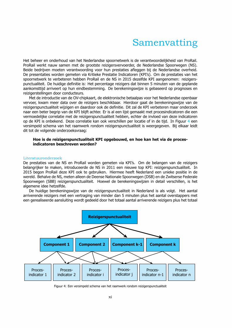
Met de introductie van de OV-chipkaart, de elektronische betaalpas voor het Nederlandse openbaarvervoer, kwam meer data over de reizigers beschikbaar. Hierdoor gaat de berekeningswijze van dereizigerspunctualiteit wijzigen en daardoor ook de definitie. Dit zal de KPI verbeteren maar onderzoeknaar een beter begrip van de KPI blijft achter. Er is al een lijst gemaakt met procesindicatoren die eenvermoedelijke correlatie met de reizigerspunctualiteit hebben, echter de invloed van deze indicatorenop de KPI is onbekend. Deze correlatie kan ook verschillen per locatie of in de tijd. In Figuur 4 eenversimpeld schema van het raamwerk rondom reizigerspunctualiteit is weergegeven. Bij elkaar leidtdit tot de volgende onderzoeksvraag:

Hoe is de reizigerspunctualiteit KPI opgebouwd, en hoe kan het via de proces-indicatoren beschreven worden?

LiteratuuronderzoekDe prestaties van de NS en ProRail worden gemeten via KPI’s. Om de belangen van de reizigersbelangrijker te maken, introduceerde de NS in 2011 een nieuwe top KPI: reizigerspunctualiteit. In2015 begon ProRail deze KPI ook te gebruiken. Hiermee heeft Nederland een unieke positie in dewereld. Behalve de NS, meten alleen de Deense Nationale Spoorwegen (DSB) en de Zwitserse FederaleSpoorwegen (SBB) reizigerspunctualiteit. Hoewel de berekeningswijzen in detail verschillen, is hetalgemene idee hetzelfde.

De huidige berekeningswijze van de reizigerspunctualiteit in Nederland is als volgt. Het aantalarriverende reizigers met een vertraging van minder dan 5 minuten plus het aantal overstappers meteen gerealiseerde aansluiting wordt gedeeld door het totaal aantal arriverende reizigers plus het totaal

Reizigerspunctualiteit

Component 2 Component k-1Component 1 Component k

Proces-indicator i

Proces-indicator 2

Proces-indicator 1

Proces-indicator j

Proces-indicator n-1

Proces-indicator n

Figuur 4: Een versimpeld schema van het raamwerk rondom reizigerspunctualiteit

xi

xii Samenvatting

aantal overstappers. De aankomsten en overstaps worden op 35 stations gemeten en de aantallenreizigers zijn gebaseerd op prognoses. De geplande aankomsten en overstaps zijn gebaseerd op dedienstregeling, 48 uur voor de uitvoering. Enkele opmerkingen op deze methode zijn:

• Overstappers zijn expliciet opgenomen in de formule. Deze reizigers worden twee keer geteld(en bij meer overstaps nog vaker). Dit houdt in dat het gewicht van deze reizigers hoger is danvoor reizigers zonder overstap.

• Routekeuze wordt genegeerd. Als er door een versperring reizigers via een andere route reizen,wordt dit gedrag niet weergegeven in de resultaten van de berekening.

• Aankomsten en overstaps worden op 35 stations gemeten. Gebaseerd op reisgedrag leidt dit totrelatief meer aankomsten in de ochtendspit dan in de avondspits.

Reizigerspunctualiteit 2.0Momenteel wordt er bij de NS een nieuwe berekeningswijze voor de reizigerspunctualiteit ontwikkeld.Dankzij de OV-chipkaart zijn de vertrek- en aankomststations en de check-in en check-uit tijden bekend.Dit suggereert dat voor elke reiziger zijn of haar reis bekend is. Via de vertrek- en aankomstlocaties, decheck-in tijd en de dienstregeling van twee dagen voor de uitvoering, kan voor bijna elke reizigers eenreisbelofte bepaald worden. Gecombineerd met de realisatiegegevens en de check-uit tijd wordt deaankomsttijd en vertraging op de uiteindelijke bestemming van elke reiziger bekend. Als de vertragingminder dan 3 minuten is, wordt de reiziger als op tijd beschouwd.

De berekening van de reizigerspunctualiteit waarbij de herkomst en bestemming (HB) en vertrektijdvan elke reiziger bekend zijn, ondervangt de meeste nadelen van de huidige berekeningswijze van dereizigerspunctualiteit.

• Elke trip wordt één keer meegeteld, dus de lengte, aantal overstaps of richting maakt niet uit, integenstelling tot de huidige berekeningswijze.

• Overstaps zijn niet meer expliciet opgenomen in de berekeningswijze. Dit leidt tot een betrouw-baarder uitkomst.

• Elke mogelijke overstap wordt meegenomen, terwijl in de huidige berekeningswijze een overstapaan meerdere criteria rondom overstaptijd en aantal overstappers moet voldoen.

De nieuwe berekeningswijze van de reizigerspunctualiteit KPI wordt reizigerspunctualiteit 2.0 genoemd.For circa twintig duizend HB’s wordt elke reismogelijkheid bepaald. Na de uitvoering worden de reis-mogelijkheden vergelijken met de realisatiegegevens. Als een reismogelijkheid niet voltooid kon wor-den, de reis zou herpland moeten worden. Deze gegevens kunnen gecombineerd worden met deOV-chipkaart data. Het resultaat is de reismogelijkheid met de vroegste aankomsttijd per trip op hethoofdrailnet: de reisbelofte. De uiteindelijke vertraging is de vertraging van de laatste trein op deeindbestemming van de reisbelofte. Als een trip herpland had moeten worden, wordt de check-uit tijdgebruikt om de aankomsttijd, en dus de vertraging, te bepalen.

Elke trip wordt ook gecategoriseerd. De categorie verklaard waarom een trip niet gebruikt wordt inde berekening of waarom de check-uit tijd was gebruikt om de vertraging te bepalen. Acht categorieënzijn te onderscheiden.1. Andere vervoerder: Elke reiziger die (gedeeltelijk) reist met een andere vervoerder wordt nietmeegerekend.

2. Busvervoer: Er zijn geen realisatiegegevens van busvervoer beschikbaar, en dus worden dezetrips niet meegenomen in de berekening.

3. Trein te vroeg vertrokken: Reizigers die hun trein missen doordat deze eerder dan geplandvertrokken is, moeten hun reis herplannen.

4. Trein te laat vertrokken: Als een trein voor vertrek minimaal 15 minuten vertraging had wordtde aanname gemaakt dat de reizigers hun reis herplannen.

5. Trein niet vertrokken: De check-uit tijd is gebruikt als de beloofde trein niet vertrok van hetherkomst- of overstapstation.

6. Trein niet aangekomen: Als een trein halverwege zijn reis opgeheven werd, moesten dereizigers in die trein hun reis herplannen, mits het laatste bereikte station niet hun eindbestem-ming of overstapstation was.

7. Overstap gemist: Een reis moet herpland worden als de tijd tussen aankomst en vertrek vantwee opeenvolgende treinen minder is dan de verwachte looptijd tussen de perrons.

Samenvatting xiii

8. Reis gerealiseerd: Al de reis is voltooid zoals beloofd dan wordt de aankomsttijd van de treingebruikt om de aankomsttijd van de reiziger te bepalen.

In de berekeningswijze van de reizigerspunctualiteit worden veel aannames gemaakt. In dit onderzoekzijn de aannames geanalyseerd en, indien mogelijk, is de invloed op de reizigerspunctualiteit bepaald.Drie aannames vallen op doordat de impact groot is.

• Vertrek en aankomst: Als er een verstoring is die leidt tot grote vertragingen of uitgevallentreinen, is het mogelijk dat reizigers in- of uitchecken op stations die niet de geplande vertrek-of aankomststations zijn. Aannames zijn gemaakt waardoor deze gevallen verwaarloosbaar zijn:Elke reiziger checkt in of uit op zijn of haar gewenste vertrek- of aankomststation. De algeheleimpact van de aannames is lastig te bepalen omdat het afhangt van de locatie, tijd en duur vande verstoring. Echter, per geval kan de impact geschat worden.

• Looptijd: De aanname is gemaakt dat de looptijd tussen kaartlezer (om in en uit te checken)en perron gelijk is aan 1 minuut, ongeacht het station. Als de looptijd gespecificeerd wordt perstation, wat meer realistische looptijen impliceert, is de verachting dat de reizigerspunctualiteit0.42 procentpunt veranderd.

• Realisatiegegevens: Gebaseerd op meer dan 5000 handmetingen is de gemiddelde afwijkingtussen de exacte aankomst- en vertrektijden van treinen op elk station en de bepaalde aankomst-en vertrektijden in de realisatiegegevens 20 seconden. Bovendien zijn er uitschieters van meerdan 1 minuut. Het verschil tussen de realisatiegegevens en de exacte realisatie kan tot eenmaximum impact van 0.72 procentpunt op de reizigerspunctualiteit KPI leiden.

Alles bij elkaar is de schatting van de maximum impact van alle aannames op de reizigerspunctualiteitongeveer 2 procentpunten. Dit betekend dat de echte reizigerspunctualiteit 2 procentpunten lager kanliggen dan de waarde van de KPI.

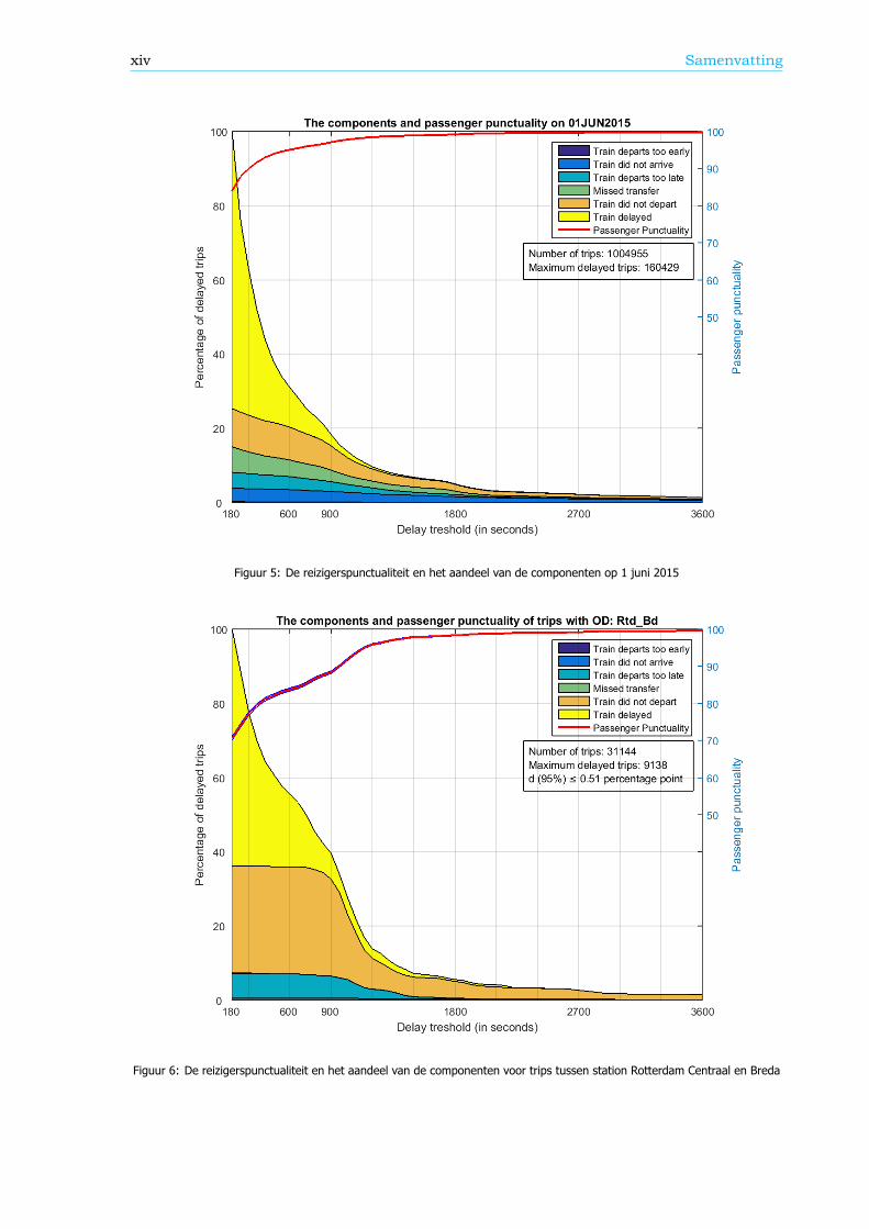
Uitsplitsing van de reizigerspunctualiteitVanuit een reizigersperspectief zijn de categorieën waarom een reis herpland moet worden ook redenenvoor een vertraging. Deze redenen, of componenten (zie Figuur 4), kunnen informatie geven over deprestaties op het spoornetwerk. Daarom is in dit onderzoek een algoritme ontwikkeld dat de reizigers-punctualiteit kan uitsplitsen naar de componenten. Er zijn zes componenten: de 5 herplan-categorieën,waar de uiteindelijke vertraging minimaal gelijk is aan een grenswaarde, en de component ‘Trein ver-traagd’. Deze laatste component valt binnen de trips met de categorie ‘Reis gerealiseerd’, waar ook hierde uiteindelijke vertraging gelijk is aan een grenswaarde. Een voorbeeld van een uitsplitsingsgrafiekstaat in Figuur 5. De grootte van de componenten is opgeschaald zodat de som van de componentenbij een grenswaarde van 180 seconden gelijk is aan 100%.

Een gedeelte van het spoornetwerk, zoals een HB, een aankomst- of overstapstation of een trein-serie, kan ook uitgesplitst worden. Figuur 6 geeft de reizigerspunctualiteit en het aandeel van decomponenten weer voor reizigers tussen station Rotterdam Centraal en Breda. Omdat een steekproefvan de data is genomen om deze grafiek te maken, is het 95% betrouwbaarheidsinterval weergegevenvia twee blauwe lijnen, net onder en boven de reizigerspunctualiteitlijn.

Modellen die de reizigerspunctualiteit beschrijvenBehalve de nieuwe berekeningswijze hebben ProRail en de NS ook een model gemaakt die de reizigers-punctualiteit beschrijft, om zo de reizigerspunctualiteit te verbeteren. Hierin is de reizigerspunctualiteitgerelateerd aan het aantal Te Verklaren Treinafwijkingen (TVTA). Een TVTA is een afwijking van eentrein ten opzichte van de dienstregeling. Voor reizigerstreinen is dit meestal door opheffing of ver-traging van de trein. Het model veronderstelt dat als er meer treinen vertraagd of opgeheven zijn, dereizigerspunctualiteit lager zal zijn. In dit onderzoek is de correlatie tussen het aantal TVTA’s en dereizigerspunctualiteit berekend. Voor de bedrijfseenheid Transportbesturing en Verkeersleiding (TB /VL) is de correlatie is matig. Dit betekend dat TB / VL geen grote invloed op de reizigerspunctualiteitheeft.

In hetzelfde model wordt het aantal TVTA’s gerelateerd aan procesindicatoren. Deze proces-indicatoren meten de prestaties van specifieke processen. As de prestaties van een proces verbetert,zal het aantal TVTA’s mogelijk minder worden en dus kan de reizigerspunctualiteit verbeterd worden.Voor de bedrijfseenheid TB / VL kunnen 20 procesindicatoren onderscheiden worden, waarvan 5 nogniet volledig ontwikkeld zijn en daardoor niet meegenomen zijn in het vervolg van de analyse. Voor

xiv Samenvatting

Figuur 5: De reizigerspunctualiteit en het aandeel van de componenten op 1 juni 2015

Figuur 6: De reizigerspunctualiteit en het aandeel van de componenten voor trips tussen station Rotterdam Centraal en Breda

Samenvatting xv

vier procesindicatoren is de correlatie met het aantal TVTA’s matig. Voor zes procesindicatoren is deprecieze definitie verkeerd: er is een correlatie met het aantal TVTA’s maar de waarde van de pro-cesindicator geeft dit niet weer. De overige vijf procesindicatoren hebben geen correlatie met hetaantal TVTA’s.

Het grootste nadeel aan dit model is het gebruik van de TVTA’s. TVTA’s zijn niet heel betrouwbaaren sommige TVTA’s zijn niet eens meegenomen. Het grootste bezwaar is het feit dat TVTA’s gerela-teerd zijn aan treinen en niet aan reizigers. Oftewel, de TVTA’s worden niet gewogen met het aantalbetrokken reizigers. Hierom wordt in dit onderzoek een ander model voorgesteld, waar de reizigers-punctualiteit is opgesplitst in componenten. De procesindicatoren zijn verbonden aan de componentenen aan de reizigerspunctualiteit zelf (zie Figuur 4). De procesindicatoren zijn hetzelfde als in het modelvan ProRail en de NS.

De gevonden correlaties tussen de procesindicatoren en de reizigerspunctualiteit in dit nieuwe modelzijn vergelijkbaar met de correlaties tussen de procesindicatoren en het aantal TVTA’s in het model vanProRail en de NS. De verklaring is dat dit nieuwe model ook een vertaalslag tussen betrokken treinenen betrokken reizigers mist. De procesindicatoren zijn gebaseerd op vertraagde of opgeheven treinenin plaats van vertraagde reizigers.

Procesindicatoren voor een deelgebied van het spoornetwerkDe procesindicatoren kunnen alleen berekend worden voor het hele spoornetwerk. Met de nieuweberekeningswijze voor reizigerspunctualiteit, kan dit ook berekend worden voor een deelgebied vanhet spoornetwerk, bijvoorbeeld een klein gebied, een treinserie of een tijdsperiode zoals spitsuur. Ditis waarom er in dit onderzoek een algoritme was ontwikkeld dat in staat is om procesindicators uit terekenen voor een deelgebied.

In dit algoritme het deelgebied kan geïdentificeerd worden via drie opties:1. Dienstregelpunt Een gebied, spoorsectie of enkel een station kan geïdentificeerd worden metdienstregelpunten, belangrijke geografische punten in het spoornetwerk, zoals een station of eenplek waar een zijspoorlijn afbuigt van een hoofdspoorlijn.

2. Treinserie Een treinserie, in beide of in een enkele richting.3. Tijdsmoment De hele dag, gedurende spitsuren, daluren of een andere aangegeven tijdsperi-ode.

Casestudie: Utrecht - Leeuwarden / GroningenBeide modellen zijn toegepast in een casestudie. Een uitsplitsing van de reizigers op het studiegebiedtussen station Utrecht Centraal en stations Leeuwarden en Groningen laat zien dat meer reizigers op tijdaankomen dan gemiddeld voor het hele spoornetwerk. Dit komt voornamelijk doordat meer overstapsgehaald worden en het percentage reizigers dat vertraagd is door dat een trein is opgeheven relatieflaag is.

De berekende correlaties voor het studiegebied tussen de procesindicatoren en het aantal TVTA’s ende componenten laat grote overeenkomsten met de gevonden correlaties in het hele spoornetwerk zien.Er zijn echter een paar significante verschillen, zoals de correlatie met de vertrekpunctualiteit van leegmaterieel en het correct uitvoeren van trein afhandelings documenten. Voor beide procesindicatorenis er geen correlatie in het studiegebied terwijl in het hele spoornetwerk een matige correlatie geldt.Het kan daardoor efficiënter zijn om op procesindicatoren in een deelgebied van het spoornetwerk testuren dan landelijk om de reizigerspunctualiteit te verbeteren.

Conclusies en aanbevelingenConcluderend, de nieuwe berekeningswijze van de reizigerspunctualiteit is een verbetering voor dehuidige KPI. Elke trip wordt gebruikt en het gewicht van elke trip is hetzelfde. Het resultaat van deaannames in deze nieuwe methode is een berekende reizigerspunctualiteit die significant verschilt vande echte reizigerspunctualiteit. Een aanbeveling is om enkele oplossingen om de reizigerspunctualiteitbetrouwbaarder te maken te overwegen, zoals het rekening houden met herplannen, meer realistis-che looptijden gebruiken en een grenswaarde van 5 minuten aanhouden in plaats van de 3 minutenwaarmee nu gewerkt wordt.

Het effect van beide modellen die reizigerspunctualiteit beschrijven kan verbeterd worden. Allereerst,voor sommige procesindicatoren moet de definitie veranderen om de correlatie met het aantal TVTA’s

xvi Samenvatting

of de componenten beter weer te geven. Dit kan sturen effectiever maken. In beide modellen mistook een vertaalslag tussen vertraagde en opgeheven treinen en vertraagde reizigers. Daarom eenaanbeveling is om de verwachte aantal betrokken reizigers mee te nemen in de definitie van de proces-indicatoren. De laatste conclusie is dat correlaties kunnen verschillen tussen deelgebieden en het helespoornetwerk.

Contents

Preface iii

Summary v

Samenvatting xi

1 Introduction 11.1 Problem definition . . . . . . . . . . . . . . . . . . . . . . . . . . . . . . . . . . . . . . 11.2 Research question and approach . . . . . . . . . . . . . . . . . . . . . . . . . . . . . 21.3 Relevance of the research . . . . . . . . . . . . . . . . . . . . . . . . . . . . . . . . . . 41.4 Outline of this report . . . . . . . . . . . . . . . . . . . . . . . . . . . . . . . . . . . . 5

2 Literature review 72.1 The rail network of the Netherlands. . . . . . . . . . . . . . . . . . . . . . . . . . . . 72.2 The origin of the passenger punctuality KPI . . . . . . . . . . . . . . . . . . . . . . . 92.3 Current state of research concerning passenger punctuality . . . . . . . . . . . . . 122.4 The Dutch methods of calculating passenger punctuality . . . . . . . . . . . . . . . 132.5 Conclusion . . . . . . . . . . . . . . . . . . . . . . . . . . . . . . . . . . . . . . . . . . 19

3 Passenger punctuality 2.0 213.1 The structure of the passenger punctuality calculation . . . . . . . . . . . . . . . . 213.2 The assumptions and their impact on the KPI. . . . . . . . . . . . . . . . . . . . . . 263.3 Conclusion . . . . . . . . . . . . . . . . . . . . . . . . . . . . . . . . . . . . . . . . . . 41

4 Breakdown of passenger punctuality 434.1 The components . . . . . . . . . . . . . . . . . . . . . . . . . . . . . . . . . . . . . . . 434.2 Delay threshold . . . . . . . . . . . . . . . . . . . . . . . . . . . . . . . . . . . . . . . . 454.3 Results . . . . . . . . . . . . . . . . . . . . . . . . . . . . . . . . . . . . . . . . . . . . . 454.4 Conclusion . . . . . . . . . . . . . . . . . . . . . . . . . . . . . . . . . . . . . . . . . . 57

5 Models to describe passenger punctuality 595.1 Introduction of the two models. . . . . . . . . . . . . . . . . . . . . . . . . . . . . . . 595.2 Introduction of the process indicators . . . . . . . . . . . . . . . . . . . . . . . . . . 655.3 Correlations in the two models. . . . . . . . . . . . . . . . . . . . . . . . . . . . . . . 715.4 Comparison of the two models . . . . . . . . . . . . . . . . . . . . . . . . . . . . . . . 81

6 Process indicators for a subset of the rail network 856.1 The options to create subsets . . . . . . . . . . . . . . . . . . . . . . . . . . . . . . . 856.2 The enriched data files . . . . . . . . . . . . . . . . . . . . . . . . . . . . . . . . . . . 86

7 Case study: Utrecht - Leeuwarden / Groningen 917.1 Description and the passenger punctuality of the study area. . . . . . . . . . . . . 917.2 The correlation with the process indicators . . . . . . . . . . . . . . . . . . . . . . . 927.3 Conclusion . . . . . . . . . . . . . . . . . . . . . . . . . . . . . . . . . . . . . . . . . . 97

8 Conclusions and recommendations 998.1 Answer to the research questions . . . . . . . . . . . . . . . . . . . . . . . . . . . . . 998.2 Conclusions . . . . . . . . . . . . . . . . . . . . . . . . . . . . . . . . . . . . . . . . . .1028.3 Reflection . . . . . . . . . . . . . . . . . . . . . . . . . . . . . . . . . . . . . . . . . . .1048.4 Recommendations . . . . . . . . . . . . . . . . . . . . . . . . . . . . . . . . . . . . . .105

xvii

xviii Contents

Bibliography 109

A Impact of the assumptions on the passenger punctuality 111

B Algorithms to create breakdown graphs 125

C Explainable Train Deviations 137

D Algorithms to calculate process indicators 139

1Introduction

Passenger punctuality is simply the percentage of passengers that arrive on time at their desired lo-cation. For the rail network, the Netherlands is one of the few countries calculating this performanceindicator. With the introduction of the OV-chipkaart, the smart card for public transport, the passengerpunctuality can be measured even more accurate. With the focus of the Nederlandse Spoorwegen(Dutch Railways, NS) to give interests of passengers the top priority, it becomes even more importantto achieve the best passenger punctuality as possible. However the correlation between the under-lying processes and the passenger punctuality is unknown. This makes steering and improving thepassenger punctuality difficult.

This first chapter is an introduction to the research. First, in paragraph 1.1, the problem regardingthe passenger punctuality, is defined. This problem definition ends with the drafting of the researchquestion. In paragraph 1.2 this main research question is given, as well as the research approachand the five sub questions. In paragraph 1.3 the relevance of this research in described. Finally, inparagraph 1.4 the outline of this report can be found.

1.1. Problem definitionThe responsibility of the Dutch rail network lies with ProRail. Operations include among others thedesign and building of new infrastructure, the maintenance and upgrading of the existing infrastructure,the building and improving of the timetables and the daily control of the trains on the network. ProRailworks closely with the NS. This is the largest rail operator on the rail network. Responsibilities includedomestic and international passenger rail transport, the purchase of new trains and the maintenanceof the existing trains and also the development of the stations.

Both ProRail and the NS have to answer for their performance to the Dutch government. They arebeing reviewed based on a set of Key Performance Indicators (KPIs) including train punctuality. Trainpunctuality is the percentage of trains arriving within a certain threshold on a certain set of stations.The exact definition differs between ProRail and the NS. This KPI has some drawbacks. For examplecancelled trains and the number of passengers per train are not included. Also not every station is beingreviewed. Therefore the NS introduced in 2011 a new KPI: passenger punctuality, the percentage ofpassengers arriving with a maximum delay of 4:59 minutes at their final destination. In 2015 ProRailstarted to use this KPI as well.

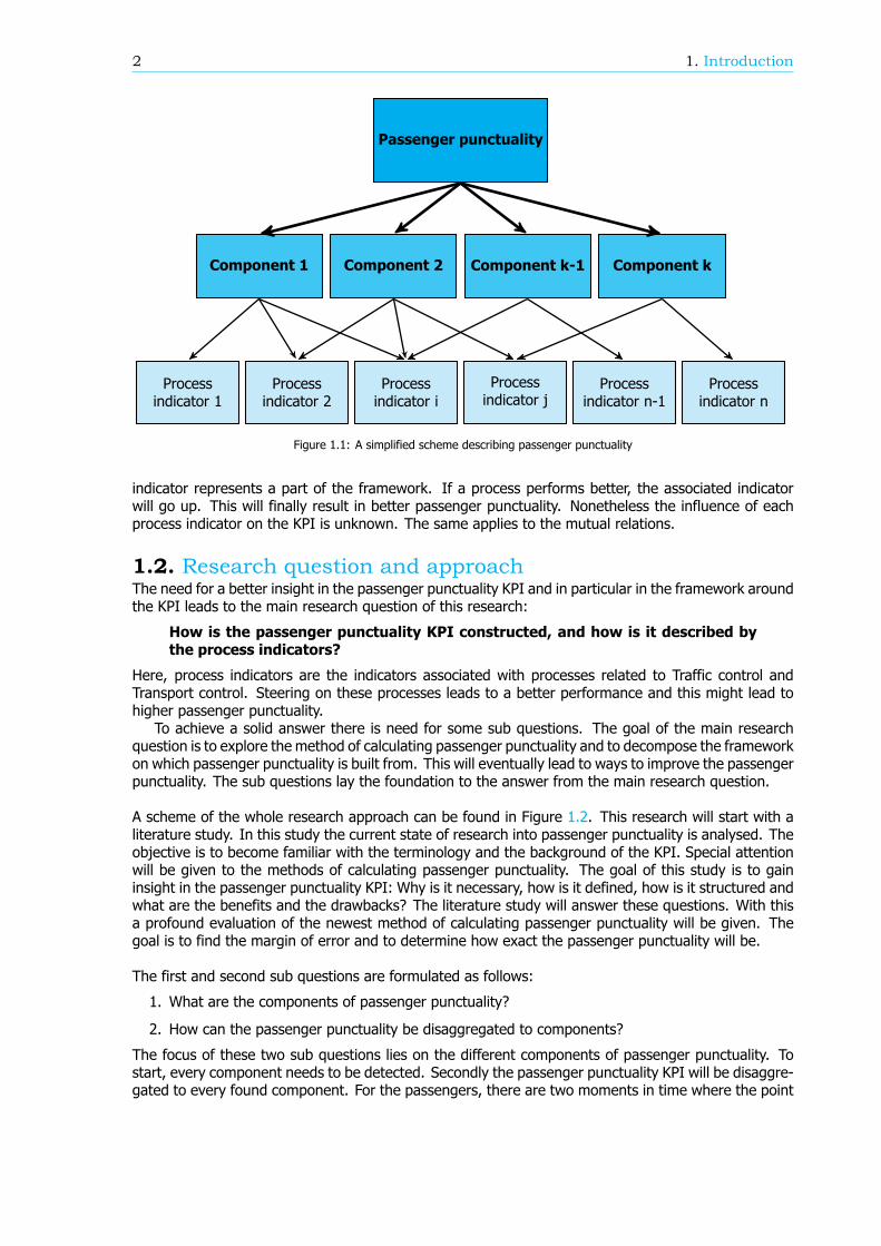
The goal of both ProRail and the NS is to describe the passenger punctuality KPI in order to improve it;however research to give a better understanding in this KPI is lagging behind. The components thatcause delays for individual passengers are for the greater part known (delayed or cancelled trains andmissed transfers) though in which degree the influence of each component extent is not known. Thisinfluence can change in time or location as well. In the framework around passenger punctuality thesecomponents compose the first layer below the KPI, see Figure 1.1.

The second layer consists of the process indicators. The process indicators are composed by theTraffic control of ProRail and the Transport control of the NS. They are representing the performance ofprocesses and can influence a component. The reasoning behind these indicators is as follows. Every

1

2 1. Introduction

Passenger punctuality

Component 2 Component k-1Component 1 Component k

Processindicator i

Processindicator 2

Processindicator 1

Processindicator j

Processindicator n-1

Processindicator n

Figure 1.1: A simplified scheme describing passenger punctuality

indicator represents a part of the framework. If a process performs better, the associated indicatorwill go up. This will finally result in better passenger punctuality. Nonetheless the influence of eachprocess indicator on the KPI is unknown. The same applies to the mutual relations.

1.2. Research question and approachThe need for a better insight in the passenger punctuality KPI and in particular in the framework aroundthe KPI leads to the main research question of this research:

How is the passenger punctuality KPI constructed, and how is it described bythe process indicators?

Here, process indicators are the indicators associated with processes related to Traffic control andTransport control. Steering on these processes leads to a better performance and this might lead tohigher passenger punctuality.

To achieve a solid answer there is need for some sub questions. The goal of the main researchquestion is to explore the method of calculating passenger punctuality and to decompose the frameworkon which passenger punctuality is built from. This will eventually lead to ways to improve the passengerpunctuality. The sub questions lay the foundation to the answer from the main research question.

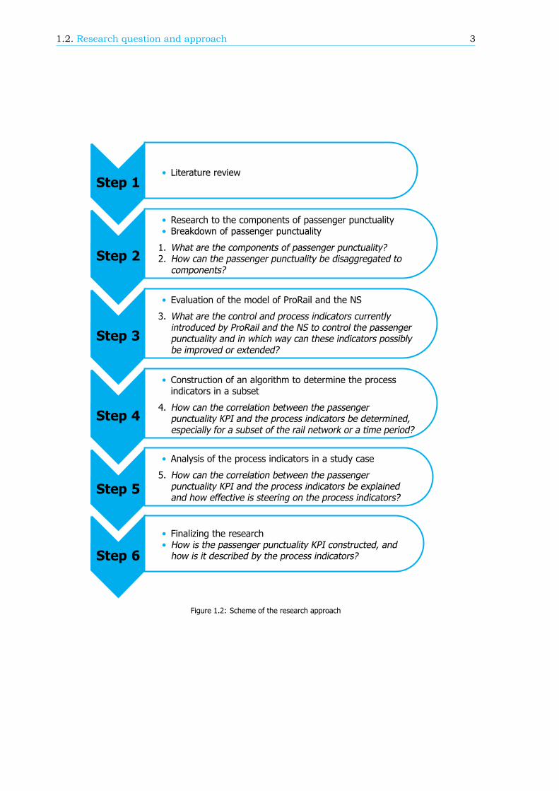
A scheme of the whole research approach can be found in Figure 1.2. This research will start with aliterature study. In this study the current state of research into passenger punctuality is analysed. Theobjective is to become familiar with the terminology and the background of the KPI. Special attentionwill be given to the methods of calculating passenger punctuality. The goal of this study is to gaininsight in the passenger punctuality KPI: Why is it necessary, how is it defined, how is it structured andwhat are the benefits and the drawbacks? The literature study will answer these questions. With thisa profound evaluation of the newest method of calculating passenger punctuality will be given. Thegoal is to find the margin of error and to determine how exact the passenger punctuality will be.

The first and second sub questions are formulated as follows:

1. What are the components of passenger punctuality?

2. How can the passenger punctuality be disaggregated to components?

The focus of these two sub questions lies on the different components of passenger punctuality. Tostart, every component needs to be detected. Secondly the passenger punctuality KPI will be disaggre-gated to every found component. For the passengers, there are two moments in time where the point

1.2. Research question and approach 3

Step 1• Literature review

Step 2

• Research to the components of passenger punctuality• Breakdown of passenger punctuality

1. What are the components of passenger punctuality?2. How can the passenger punctuality be disaggregated to

components?

Step 3

• Evaluation of the model of ProRail and the NS

3. What are the control and process indicators currentlyintroduced by ProRail and the NS to control the passengerpunctuality and in which way can these indicators possiblybe improved or extended?

Step 4

• Construction of an algorithm to determine the processindicators in a subset

4. How can the correlation between the passengerpunctuality KPI and the process indicators be determined,especially for a subset of the rail network or a time period?

Step 5

• Analysis of the process indicators in a study case

5. How can the correlation between the passengerpunctuality KPI and the process indicators be explainedand how effective is steering on the process indicators?

Step 6

• Finalizing the research• How is the passenger punctuality KPI constructed, andhow is it described by the process indicators?

Figure 1.2: Scheme of the research approach

4 1. Introduction

of view regarding their trip changes. The first moment is at a delay of 3 minutes. Before this momentthe average passenger is satisfied with the journey time, after this moment their judgement decreasesa bit. The second moment is at a delay of 15 minutes. After this moment, the judgement of theaverage passenger decreases strongly: their trip is disturbed. For both time moments, a breakdownof the passenger punctuality will be done. It is more desirable to improve the 15 minutes passengerpunctuality because of the judgement drop after a 15 minutes delay. On the other hand, ProRail andthe NS are not reviewed by the government based on the 15 minute passenger punctuality. Besidesit is fair to assume that the 3 minute passenger punctually is lower and possibly offers more room forimprovement.

In the next step, the focus will shift to the process indicators. These indicators are determined by theTraffic control of ProRail and the Transport control of the NS. First off, the indicators will be analysedto see how they are defined, how they are calculated and to which component they are related. Nextthey will be determined if they could be improved or otherwise be neglected. With this information thethird sub question can be answered:

3. What are the control and process indicators currently introduced by ProRail and the NS to con-trol the passenger punctuality and in which way can these indicators possibly be improved orextended?

The influence of every indicator might differ in time and place. Therefore it might be impossible tofind the correct correlation between every single process indicator and the passenger punctuality KPI.Nonetheless it is possible to construct an algorithm to find the value of each indicator and the passengerpunctuality for almost every subset. Herewith the correlations can be determined. This is the basis forthe fourth sub question:

4. How can the correlation between the passenger punctuality KPI and the process indicators bedetermined, especially for a subset of the rail network or a time period?

At this point, the focus of the research shifts to a specific subset of the passenger punctuality. Thissubset will be used to validate the algorithm. The correlation with the indicators and the passengerpunctuality in this subset are calculated as well. The results are analysed to determine the effectivenessof steering on the process indicators. With this the last sub question can be answered:

5. How can the correlation between the passenger punctuality KPI and the process indicators beexplained and how effective is steering on the process indicators?

1.3. Relevance of the researchThis research contributes in a better insight in the passenger punctuality KPI. First of the method ofcalculating passenger punctuality is examined. This will make clear where and when the calculatedpassenger punctuality differs from the actual passenger punctuality. It also points out if and where themethod can be improved to achieve a more reliable KPI.

From a passengers’ perspective, this research is also relevant. The causes of bad passenger punc-tuality are going to be decomposed. The result is not only a list of possible causes but also the degreeof influence. This could be on a national level but for a local train line as well. A distinction in timeis also possible. Difference between rush hours and off peak hours can be researched, but betweenwork and weekend days as well. Altogether this breakdown of the passenger punctuality leads to aclear insight in the causes: the causes itself but also in the influence of every cause.

The relations between the control indicators and the passenger punctuality itself are researched aswell. This offers a good insight in the control framework of influence to the passenger punctuality KPI.The influence of the indicators becomes known so a more optimal solution can be found to achieve thebest passenger punctuality possible. This applies particularly to specific situations, in time or location.This research will investigate such a situation to find the influence of the indicators concerned. For thefuture, this will help by analysing other situations with bad passenger punctuality.

1.4. Outline of this report 5

1.4. Outline of this reportThis research will start with a literature review in chapter 2. Here the history of the passenger punc-tuality KPI is explained, other relevant research is analysed and a brief overview of the methods ofcalculating passenger punctuality is given. Chapter 3 will examine the latest method of calculating pas-senger punctuality more closely. Special attention will be paid to the underlying assumptions. Herebythe margin of error could be determined and thus the reliability of the passenger punctuality KPI.

In chapter 4 the passenger punctuality is decomposed into components for different subsets of therail network. This can by a time period, but also an origin-destination combination, a train series or astation.

The analyses of the models to describe the passenger punctuality can be found in chapter 5. First themodel of the NS and ProRail is analysed. Attention goes to the control indicators and the ExplainableTrain Deviations (TVTAs). Second a new model is proposed. Here the components of the passengerpunctuality are used to connect the passenger punctuality with the process indicators. Next the processindicators are elaborated and the correlation with the TVTAs and the components is determined.

To perform a more detailed analysis of a subset of the rail network, an algorithm is created tocalculate the process indicators for such a subset. This algorithm is discussed in chapter 6. Finallya small case study is performed to validate the results of this algorithm (chapter 7). Hereby also ananalysis is performed to check the correlation between the process indicators and the TVTAs and thepassenger punctuality. This report ends with some conclusions and recommendations, in chapter 8.

Five appendixes are included in this report. Appendix A is an extension to chapter 3. It providessome additional analyses and summary tables used in this chapter. To perform the breakdowns of thepassenger punctuality a new type of graph is used. The algorithm to create these breakdown graphsis explained in appendix B. Appendix C provides a list of all the TVTAs in use by ProRail. The algorithmthat is made to calculate the process indicators is explained in appendix D.

2Literature review

This chapter describes the current developments regarding the passenger punctuality KPI (Key Perfor-mance Indicator). The focus will mainly be on the Netherlands, but when examining the current stateof the research concerning the passenger punctuality the view will be widened. Altogether this chapterwill provide some background information and will establish the starting point of the research.

First off, in paragraph 2.1, the origin of the rail network in the Netherlands, the NS and ProRail isexplained. Paragraph 2.2 elaborates on the origin of the passenger punctuality in the Netherlands. Themain question here will be: how is the passenger punctuality KPI originated? Not only the Netherlands,but also the Swiss and Denmark use passenger punctuality as a performance indicator. Research ofthese countries concerning passenger punctuality and more are reviewed in paragraph 2.3. Finally themethods to calculate the passenger punctuality in use in the Netherlands are explained and compared.This can be found in paragraph 2.4. This chapter ends with some conclusions (paragraph 2.5).

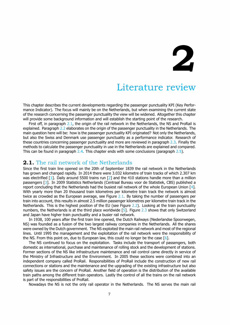
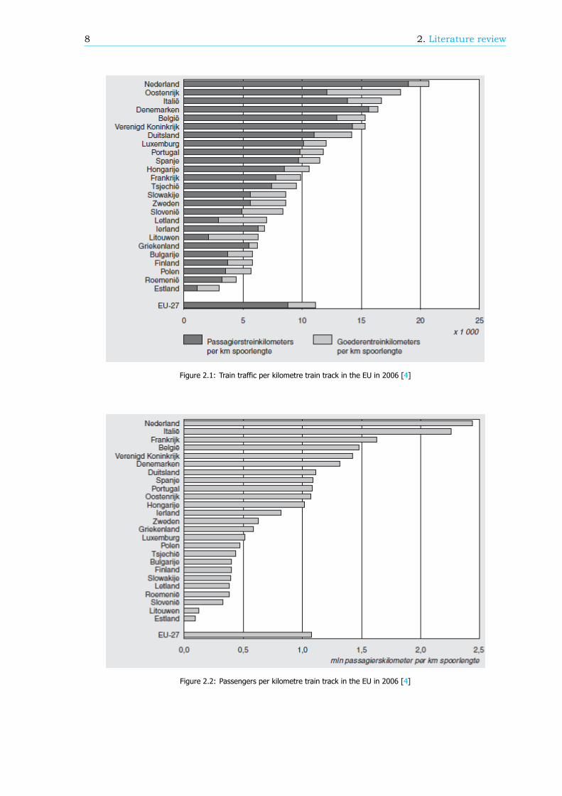
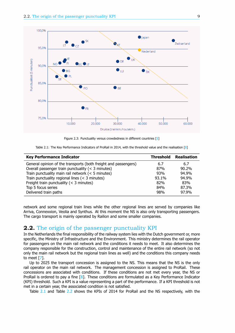
2.1. The rail network of the NetherlandsSince the first train line opened on the 20th of September 1839 the rail network in the Netherlandshas grown and changed rapidly. In 2014 there were 3.032 kilometre of train tracks of which 2.307 kmwas electrified [1]. Daily around 5500 trains run [2] and the 410 stations handle more than a millionpassengers [3]. In 2009 Statistics Netherlands (Centraal Bureau voor de Statistiek, CBS) published areport concluding that the Netherlands had the busiest rail network of the whole European Union [4].With yearly more than 20 thousand train kilometres per kilometre train track the network is almosttwice as crowded as the European average, see Figure 2.1. By taking the number of passengers pertrain into account, this results in almost 2.5 million passenger kilometres per kilometre train track in theNetherlands. This is the highest position of the EU (see Figure 2.2). Looking at the train punctualitynumbers, the Netherlands is at the third place worldwide [5]. Figure 2.3 shows that only Switzerlandand Japan have higher train punctuality and a busier rail network.

In 1938, 100 years after the first train line opened, the Dutch Railways (Nederlandse Spoorwegen,NS) was founded as a fusion of the two largest railway companies in the Netherlands. All the shareswere owned by the Dutch government. The NS exploited the main rail network and most of the regionallines. Until 1995 the management and the exploitation of the rail network were the responsibility ofthe NS. From this point on, due to European law, this could no longer be the case [6].

The NS continued to focus on the exploitation. Tasks include the transport of passengers, bothdomestic as international, purchase and maintenance of rolling stock and the development of stations.Former sections of the NS like infrastructure maintenance and rail control came directly in service ofthe Ministry of Infrastructure and the Environment. In 2005 these sections were combined into anindependent company called ProRail. Responsibilities of ProRail include the construction of new railconnections or stations and the maintenance and the upgrading of the existing infrastructure but alsosafety issues are the concern of ProRail. Another field of operation is the distribution of the availabletrain paths among the different train operators. Lastly the control of all the trains on the rail networkis part of the responsibilities of ProRail.

Nowadays the NS is not the only rail operator in the Netherlands. The NS serves the main rail

7

8 2. Literature review

Figure 2.1: Train traffic per kilometre train track in the EU in 2006 [4]

Figure 2.2: Passengers per kilometre train track in the EU in 2006 [4]

2.2. The origin of the passenger punctuality KPI 9

Figure 2.3: Punctuality versus crowdedness in different countries [5]

Table 2.1: The Key Performance Indicators of ProRail in 2014, with the threshold value and the realisation [8]

Key Performance Indicator Threshold Realisation

General opinion of the transports (both freight and passengers) 6.7 6.7Overall passenger train punctuality (< 3 minutes) 87% 90.2%Train punctuality main rail network (< 5 minutes) 93% 94.9%Train punctuality regional lines (< 3 minutes) 93.1% 94.9%Freight train punctuality (< 3 minutes) 82% 83%Top 5 focus series 84% 87.3%Delivered train paths 98% 97.9%

network and some regional train lines while the other regional lines are served by companies likeArriva, Connexxion, Veolia and Synthus. At this moment the NS is also only transporting passengers.The cargo transport is mainly operated by Railion and some smaller companies.

2.2. The origin of the passenger punctuality KPIIn the Netherlands the final responsibility of the railway system lies with the Dutch government or, morespecific, the Ministry of Infrastructure and the Environment. This ministry determines the rail operatorfor passengers on the main rail network and the conditions it needs to meet. It also determines thecompany responsible for the construction, control and maintenance of the entire rail network (so notonly the main rail network but the regional train lines as well) and the conditions this company needsto meet [7].

Up to 2025 the transport concession is assigned to the NS. This means that the NS is the onlyrail operator on the main rail network. The management concession is assigned to ProRail. Theseconcessions are associated with conditions. If these conditions are not met every year, the NS orProRail is ordered to pay a fine [8]. These conditions are formulated as a Key Performance Indicator(KPI) threshold. Such a KPI is a value representing a part of the performance. If a KPI threshold is notmet in a certain year, the associated condition is not satisfied.

Table 2.1 and Table 2.2 shows the KPIs of 2014 for ProRail and the NS respectively, with the

10 2. Literature review

Table 2.2: The Key Performance Indicators of the NS in 2014, with the threshold value and the realisation [8]

Key Performance Indicator Threshold Realisation

Passenger opinion on on-time-running 53.0% 49.9%Train (arrival) punctuality (< 5 minute threshold) 93.0% 94.9%Passenger punctuality 90.5% 92.3%Passenger opinion on travel information by 0 to 15 minute delay 91.0% 94.4%Passenger opinion on travel information by more than 15 minute delay 36.0% 39.0%Information in train by a disruption 60.0% 70.8%Information on the station by a disruption 80.0% 86.8%Chance of meeting a conductor 65.0% 64.3%Passenger opinion on cleanness train and station 55.0% 56.9%Quality of cleanness train and station 90.0% 90.6%Passenger opinion on social safety train and station 78.5% 80.2%Passenger opinion on seating capacity in the train during rush hour 70.0% 67.8%Transport capacity of passengers during rush hour 99.0% 98.9%

Figure 2.4: 5 minute train punctuality of the main rail network [10]

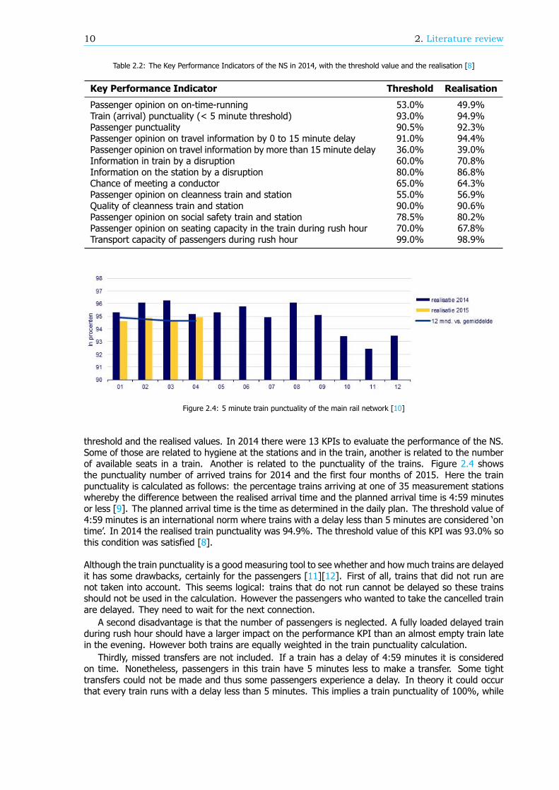
threshold and the realised values. In 2014 there were 13 KPIs to evaluate the performance of the NS.Some of those are related to hygiene at the stations and in the train, another is related to the numberof available seats in a train. Another is related to the punctuality of the trains. Figure 2.4 showsthe punctuality number of arrived trains for 2014 and the first four months of 2015. Here the trainpunctuality is calculated as follows: the percentage trains arriving at one of 35 measurement stationswhereby the difference between the realised arrival time and the planned arrival time is 4:59 minutesor less [9]. The planned arrival time is the time as determined in the daily plan. The threshold value of4:59 minutes is an international norm where trains with a delay less than 5 minutes are considered ‘ontime’. In 2014 the realised train punctuality was 94.9%. The threshold value of this KPI was 93.0% sothis condition was satisfied [8].

Although the train punctuality is a good measuring tool to see whether and how much trains are delayedit has some drawbacks, certainly for the passengers [11][12]. First of all, trains that did not run arenot taken into account. This seems logical: trains that do not run cannot be delayed so these trainsshould not be used in the calculation. However the passengers who wanted to take the cancelled trainare delayed. They need to wait for the next connection.

A second disadvantage is that the number of passengers is neglected. A fully loaded delayed trainduring rush hour should have a larger impact on the performance KPI than an almost empty train latein the evening. However both trains are equally weighted in the train punctuality calculation.

Thirdly, missed transfers are not included. If a train has a delay of 4:59 minutes it is consideredon time. Nonetheless, passengers in this train have 5 minutes less to make a transfer. Some tighttransfers could not be made and thus some passengers experience a delay. In theory it could occurthat every train runs with a delay less than 5 minutes. This implies a train punctuality of 100%, while

2.2. The origin of the passenger punctuality KPI 11

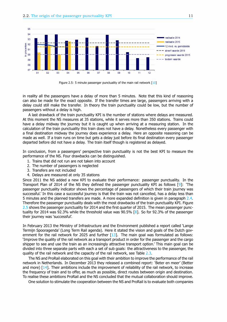
Figure 2.5: 5 minute passenger punctuality of the main rail network [10]

in reality all the passengers have a delay of more than 5 minutes. Note that this kind of reasoningcan also be made for the exact opposite. If the transfer times are large, passengers arriving with adelay could still make the transfer. In theory the train punctuality could be low, but the number ofpassengers without a delay is high.

A last drawback of the train punctuality KPI is the number of stations where delays are measured.At this moment the NS measures at 35 stations, while it serves more than 350 stations. Trains couldhave a delay midway the journey but it is caught up when arriving at a measuring station. In thecalculation of the train punctuality this train does not have a delay. Nonetheless every passenger witha final destination midway the journey does experience a delay. Here an opposite reasoning can bemade as well. If a train runs on time but gets a delay just before its final destination every passengerdeparted before did not have a delay. The train itself though is registered as delayed.

In conclusion, from a passengers’ perspective train punctuality is not the best KPI to measure theperformance of the NS. Four drawbacks can be distinguished.1. Trains that did not run are not taken into account2. The number of passengers is neglected3. Transfers are not included4. Delays are measured at only 35 stations

Since 2011 the NS added a new KPI to evaluate their performance: passenger punctuality. In theTransport Plan of 2014 of the NS they defined the passenger punctuality KPI as follows [9]: ‘Thepassenger punctuality indicator shows the percentage of passengers of which their train journey wassuccessful.’ In this case a successful journey is that the train was not cancelled, has a delay less than5 minutes and the planned transfers are made. A more expanded definition is given in paragraph 2.4.Therefore the passenger punctuality deals with the most drawbacks of the train punctuality KPI. Figure2.5 shows the passenger punctuality for 2014 and the first quarter of 2015. The mean passenger punc-tuality for 2014 was 92.3% while the threshold value was 90.5% [8]. So for 92.3% of the passengertheir journey was ‘successful’.

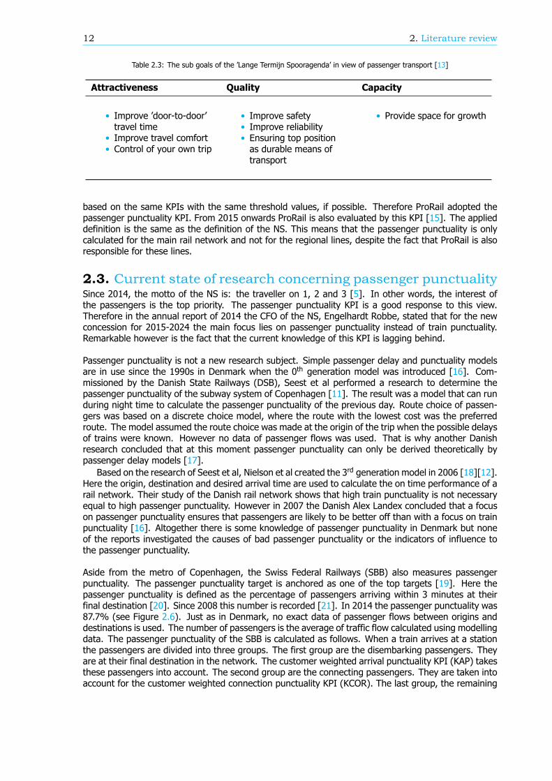
In February 2013 the Ministry of Infrastructure and the Environment published a report called ‘LangeTermijn Spooragenda’ (Long Term Rail agenda). Here it stated the vision and goals of the Dutch gov-ernment for the rail network for 2025 and further [13]. The main goal was formulated as follows:‘Improve the quality of the rail network as a transport product in order for the passenger and the cargoshipper to see and use the train as an increasingly attractive transport option.’ This main goal can bedivided into three separate parts with each a set of sub goals: the attractiveness to the passenger, thequality of the rail network and the capacity of the rail network, see Table 2.3.

The NS and ProRail elaborated on this goal with their ambition to improve the performance of the railnetwork in Netherlands. In December 2013 they released a combined report: ‘Beter en meer’ (Betterand more) [14]. Their ambitions include the improvement of reliability of the rail network, to increasethe frequency of train and to offer, as much as possible, direct routes between origin and destination.To realise these ambitions ProRail and the NS concluded that the mutual collaboration should improve.

One solution to stimulate the cooperation between the NS and ProRail is to evaluate both companies

12 2. Literature review

Table 2.3: The sub goals of the ’Lange Termijn Spooragenda’ in view of passenger transport [13]

Attractiveness Quality Capacity

• Improve ’door-to-door’travel time

• Improve travel comfort• Control of your own trip

• Improve safety• Improve reliability• Ensuring top positionas durable means oftransport

• Provide space for growth

based on the same KPIs with the same threshold values, if possible. Therefore ProRail adopted thepassenger punctuality KPI. From 2015 onwards ProRail is also evaluated by this KPI [15]. The applieddefinition is the same as the definition of the NS. This means that the passenger punctuality is onlycalculated for the main rail network and not for the regional lines, despite the fact that ProRail is alsoresponsible for these lines.

2.3. Current state of research concerning passenger punctualitySince 2014, the motto of the NS is: the traveller on 1, 2 and 3 [5]. In other words, the interest ofthe passengers is the top priority. The passenger punctuality KPI is a good response to this view.Therefore in the annual report of 2014 the CFO of the NS, Engelhardt Robbe, stated that for the newconcession for 2015-2024 the main focus lies on passenger punctuality instead of train punctuality.Remarkable however is the fact that the current knowledge of this KPI is lagging behind.

Passenger punctuality is not a new research subject. Simple passenger delay and punctuality modelsare in use since the 1990s in Denmark when the 0th generation model was introduced [16]. Com-missioned by the Danish State Railways (DSB), Seest et al performed a research to determine thepassenger punctuality of the subway system of Copenhagen [11]. The result was a model that can runduring night time to calculate the passenger punctuality of the previous day. Route choice of passen-gers was based on a discrete choice model, where the route with the lowest cost was the preferredroute. The model assumed the route choice was made at the origin of the trip when the possible delaysof trains were known. However no data of passenger flows was used. That is why another Danishresearch concluded that at this moment passenger punctuality can only be derived theoretically bypassenger delay models [17].

Based on the research of Seest et al, Nielson et al created the 3rd generation model in 2006 [18][12].Here the origin, destination and desired arrival time are used to calculate the on time performance of arail network. Their study of the Danish rail network shows that high train punctuality is not necessaryequal to high passenger punctuality. However in 2007 the Danish Alex Landex concluded that a focuson passenger punctuality ensures that passengers are likely to be better off than with a focus on trainpunctuality [16]. Altogether there is some knowledge of passenger punctuality in Denmark but noneof the reports investigated the causes of bad passenger punctuality or the indicators of influence tothe passenger punctuality.

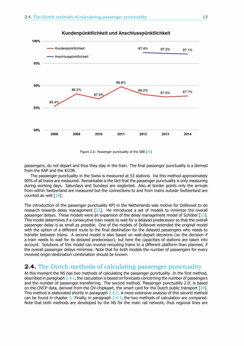
Aside from the metro of Copenhagen, the Swiss Federal Railways (SBB) also measures passengerpunctuality. The passenger punctuality target is anchored as one of the top targets [19]. Here thepassenger punctuality is defined as the percentage of passengers arriving within 3 minutes at theirfinal destination [20]. Since 2008 this number is recorded [21]. In 2014 the passenger punctuality was87.7% (see Figure 2.6). Just as in Denmark, no exact data of passenger flows between origins anddestinations is used. The number of passengers is the average of traffic flow calculated using modellingdata. The passenger punctuality of the SBB is calculated as follows. When a train arrives at a stationthe passengers are divided into three groups. The first group are the disembarking passengers. Theyare at their final destination in the network. The customer weighted arrival punctuality KPI (KAP) takesthese passengers into account. The second group are the connecting passengers. They are taken intoaccount for the customer weighted connection punctuality KPI (KCOR). The last group, the remaining

2.4. The Dutch methods of calculating passenger punctuality 13

Figure 2.6: Passenger punctuality of the SBB [20]

passengers, do not depart and thus they stay in the train. The final passenger punctuality is a derivedfrom the KAP and the KCOR.

The passenger punctuality in the Swiss is measured at 53 stations. Via this method approximately90% of all trains are measured. Remarkable is the fact that the passenger punctuality is only measuringduring working days. Saturdays and Sundays are neglected. Also at border points only the arrivalsfrom within Switzerland are measured but the connections to and from trains outside Switzerland arecounted as well [19].

The introduction of the passenger punctuality KPI in the Netherlands was motive for Dollevoet to doresearch towards delay management [22]. He introduced a set of models to minimize the overallpassenger delays. These models were an expansion of the delay management model of Schöbel [23].This model determines if a consecutive train needs to wait for a delayed predecessor so that the overallpassenger delay is as small as possible. One of the models of Dollevoet extended the original modelwith the option of a different route to the final destination for the delayed passengers who needs totransfer between trains. A second model is also based on wait-depart decisions (so the decision ifa train needs to wait for its delayed predecessor), but here the capacities of stations are taken intoaccount. Solutions of this model can involve rerouting trains to a different platform than planned, ifthe overall passenger delays minimise. Note that for both models the number of passengers for everyinvolved origin-destination combination should be known.

2.4. The Dutch methods of calculating passenger punctualityAt this moment the NS has two methods of calculating the passenger punctuality. In the first method,described in paragraph 2.4.1, the calculation is based on forecasts concerning the number of passengersand the number of passenger transferring. The second method, ’Passenger punctuality 2.0’, is basedon the OVCP data, derived from the OV-chipkaart, the smart card for the Dutch public transport [24].This method is elaborated shortly in paragraph 2.4.2. A more extensive analysis of this second methodcan be found in chapter 3. Finally, in paragraph 2.4.3, the two methods of calculation are compared.Note that both methods are developed by the NS for the main rail network, thus regional lines are

14 2. Literature review

neglected. Although ProRail manages all the rail lines in the Netherlands, both the network used bythe NS as by the other regional rail operators, the value of the passenger punctuality KPI of ProRail isthe same as the value of the NS.

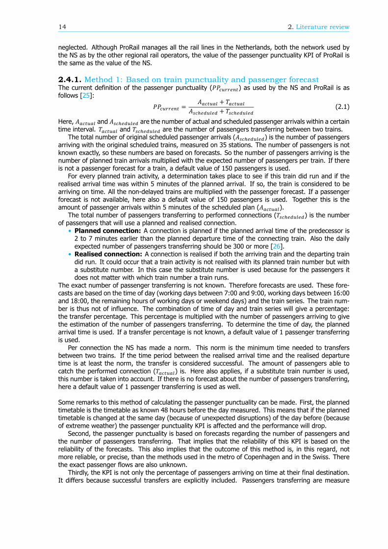
2.4.1. Method 1: Based on train punctuality and passenger forecastThe current definition of the passenger punctuality (𝑃𝑃 ) as used by the NS and ProRail is asfollows [25]:

𝑃𝑃 = 𝐴 + 𝑇𝐴 + 𝑇 (2.1)

Here, 𝐴 and 𝐴 are the number of actual and scheduled passenger arrivals within a certaintime interval. 𝑇 and 𝑇 are the number of passengers transferring between two trains.

The total number of original scheduled passenger arrivals (𝐴 ) is the number of passengersarriving with the original scheduled trains, measured on 35 stations. The number of passengers is notknown exactly, so these numbers are based on forecasts. So the number of passengers arriving is thenumber of planned train arrivals multiplied with the expected number of passengers per train. If thereis not a passenger forecast for a train, a default value of 150 passengers is used.

For every planned train activity, a determination takes place to see if this train did run and if therealised arrival time was within 5 minutes of the planned arrival. If so, the train is considered to bearriving on time. All the non-delayed trains are multiplied with the passenger forecast. If a passengerforecast is not available, here also a default value of 150 passengers is used. Together this is theamount of passenger arrivals within 5 minutes of the scheduled plan (𝐴 ).

The total number of passengers transferring to performed connections (𝑇 ) is the numberof passengers that will use a planned and realised connection.

• Planned connection: A connection is planned if the planned arrival time of the predecessor is2 to 7 minutes earlier than the planned departure time of the connecting train. Also the dailyexpected number of passengers transferring should be 300 or more [26].

• Realised connection: A connection is realised if both the arriving train and the departing traindid run. It could occur that a train activity is not realised with its planned train number but witha substitute number. In this case the substitute number is used because for the passengers itdoes not matter with which train number a train runs.

The exact number of passenger transferring is not known. Therefore forecasts are used. These fore-casts are based on the time of day (working days between 7:00 and 9:00, working days between 16:00and 18:00, the remaining hours of working days or weekend days) and the train series. The train num-ber is thus not of influence. The combination of time of day and train series will give a percentage:the transfer percentage. This percentage is multiplied with the number of passengers arriving to givethe estimation of the number of passengers transferring. To determine the time of day, the plannedarrival time is used. If a transfer percentage is not known, a default value of 1 passenger transferringis used.

Per connection the NS has made a norm. This norm is the minimum time needed to transfersbetween two trains. If the time period between the realised arrival time and the realised departuretime is at least the norm, the transfer is considered successful. The amount of passengers able tocatch the performed connection (𝑇 ) is. Here also applies, if a substitute train number is used,this number is taken into account. If there is no forecast about the number of passengers transferring,here a default value of 1 passenger transferring is used as well.

Some remarks to this method of calculating the passenger punctuality can be made. First, the plannedtimetable is the timetable as known 48 hours before the day measured. This means that if the plannedtimetable is changed at the same day (because of unexpected disruptions) of the day before (becauseof extreme weather) the passenger punctuality KPI is affected and the performance will drop.

Second, the passenger punctuality is based on forecasts regarding the number of passengers andthe number of passengers transferring. That implies that the reliability of this KPI is based on thereliability of the forecasts. This also implies that the outcome of this method is, in this regard, notmore reliable, or precise, than the methods used in the metro of Copenhagen and in the Swiss. Therethe exact passenger flows are also unknown.

Thirdly, the KPI is not only the percentage of passengers arriving on time at their final destination.It differs because successful transfers are explicitly included. Passengers transferring are measure

2.4. The Dutch methods of calculating passenger punctuality 15

at least twice. Also the number of passengers transferring is a percentage of the total number ofpassengers in a train. This fact has some influence on the KPI and the result is a slightly incorrectpassenger punctuality value.

A fourth remark to the method of calculation currently in use by the NS is the fact that route choiceis ignored. For example, if travelling from station Delft to station Utrecht Centraal, there are twopossibilities: via stations Den Haag or Rotterdam. The difference in travel time (and extra waiting timeat Delft) lies within the threshold of 5 minutes. When there are no disruptions, a part of the travellerswill travel via Den Haag and the other part will travel via Rotterdam. This passenger behaviour isincluded in the forecast for passengers transferring at stations Den Haag and Rotterdam. Howeverwhen there is a disruption at Den Haag, almost all passengers will travel via Rotterdam. All thesepassengers will travel without a delay and are able to make their transfer. Though in the passengerpunctuality calculation a part of the passengers will still travel via Den Haag and thus experiencesdelays and missed transfers.

Lastly, this method of calculating the passenger punctuality KPI deals with the most drawbacks ofthe train punctuality KPI (see paragraph 2.2). The impact for the passengers of trains that did not runare included in the KPI, because 𝐴 is the number of passengers that actually made a trip. TheKPI will go down if this number becomes smaller because trains did not run. Although the number ofpassengers is a forecast, it is taken into account in the calculation. The same applies for the passengerstransferring. If a transfer time is below the norm, transfers are not made and 𝑇 will drop. Theonly drawback still not handled is the number of measuring stations. The passenger punctuality KPI ismeasured only at the same 35 stations used for the train punctuality calculation. This means that theKPI is not as accurate as it could be. If a journey leads trough two or more measuring stations, thepassenger is calculated at least twice in the passenger punctuality. On the other hand if a trip doesnot pass a measuring station, that trip is not taken into account in the calculation. It implies that a triptowards a measuring station outweigh a trip departing at a measuring station.

2.4.2. Method 2: Based on OVCP dataAt this moment, the NS is developing a new method of calculating the passenger punctuality: ’passen-ger punctuality 2.0’ [26]. The goal was to implement this method on time so in 2016 the KPI couldbe calculated via this method. In July 2015 the decision was made to postpone the introduction withat least one year. This new method is this in developing, so some details can change. The methodcurrently is use has some drawbacks (see also paragraph 2.4.1) including:

• The number of passengers and the number of passengers transferring are forecasts.• The passenger punctuality is measured at only 35 stations.• Only planned transfers are taken into account• The ratio between InterCitys (long distance trains) and Sprinters (local trains) is disproportional:InterCitys stop relatively more often at measuring stations than Sprinters.

• The ratio between the morning and evening rush hour is disproportional: relatively more passen-gers arrive at a measuring station in the morning rush hour than in the evening rush hour.

Passenger punctuality 2.0 is designed to deal with these disadvantages. The new KPI can be calculatedas follows:

𝑃𝑃 . =𝑇𝑇 (2.2)

In this equation 𝑇 is the total number of trips. This number is determined via the OCVP data[24]. This data contains the origin and destination of every passenger so every trip made can bedetermined. It is amassed via the OV-chipkaart, the smart card of the public transport system of theNetherlands. At the start of a trip, the passenger has to check-in by holding the smart card against adedicated card reader. The location and time are registered. At the destination the passenger needsto do this again. Here also the location and time are registered. With this system the number of tripsper origin-destination combination is known, as well the start and end time of each trip.

With more than 400 stations in the Netherlands, the number of origin-destination (OD) combinationsis more than 160.000. Not all stations are always in use and most of the OD combinations are onlyin rare cases travelled on. Therefore a couple of conditions are drawn up to decrease the number ofpossible OD-combinations in the calculation of the passenger punctuality. First stations serviced onlyby other rail operators are neglected. OD combinations barely used are ignored [24] as well. Every

16 2. Literature review

quarter of a year a list is made with the most frequent used OD combinations. Here all combinationsare included with at least 100 trips in the last 100 days, spread out over at least 20 days. This preventsalso that event stations, like Rotterdam Stadion, are taken into account. These stations are onlyserviced during events and therefore not included in the general timetable. Altogether this will resultin approximately twenty thousand OD combinations used in the calculation. This implies that around87% of all OD combinations are not taken into account though still more than 98% of all trips in thenetwork are used in the calculation, see also paragraph 3.2.1.

𝑇 is the number of trips where the total travel time is within the promised travel time plusa certain delay threshold. The promised travel time is the travel time as shown in the timetable beforeunplanned disruptions are known. When there is an adapted timetable due to extreme weather theoriginal timetable is used for determining the planned arrival time as well. Although the delay thresholdcould be every value, at this moment 3 minutes is used in the official KPI. A threshold of 15 minutescould also be interesting [27], see also paragraph 4.2.

The calculation of 𝑇 is as follows [24]. The OVCP data is used to determine the originand destination and the check-in time of every trip. This check-in time is used to determine thepromised journey from the origin to the destination. This promised journey (in Dutch: Reisbelofte) isthe connection with the earliest possible arrival time with a departure after check-in time. Next therealisation data is examined. If a transfer was not made, or a train did not run or not arrive at thetransfers station or destination, the trip needs to be rescheduled. Otherwise the realised arrival timeis used to determine the final delay. If a trip needs be rescheduled, the checkout time is used todetermine the final delay. A more detailed explanation of the calculation is given in chapter 3.

Note that the passenger punctuality 2.0 deals with every drawback of the train punctuality, asdescribed in paragraph 2.2. Every trip is compared with the timetable, so trains that did not run aretaken into account. In large extend the number of passengers are also known. The same applies forthe number of passengers transferring. Finally, the delays are measured at every station for almostevery origin-destination combination and not only at the 35 measuring stations. This implies that thispassenger punctuality value gives a more realistic representation of the reality.

2.4.3. A comparison between the two methodsIn this paragraph a comparison between the two Dutch methods of calculating passenger punctualityis made. Method 1 is the method currently in use, where the passenger punctuality is a combination ofthe train punctuality at 35 stations and the forecast of the number of passengers. Method 2, passengerpunctuality 2.0, is based on the OVCP data. This method is still in development so details can changebefore the introduction. In an example the influence of the differences becomes clear. Here thepassenger punctuality is calculated via both methods for different situations.

1. The weight distribution among the trips in the network is different. In method 1, the weight ofa trip is dependent on the number of measuring stations passed and the number of transfers ata measuring station. In the worst case, this can imply that a trip is not taken into account atall, most common by the shorter journeys. On the other hand, the impact of longer journeys issevere. In method 2 every trip is weighted equally.

2. The transport plan of 2014 of the NS stated that passenger punctuality is the percentage ofsuccessful journeys, thus where all the trains run, all transfers are made and the final arrival timeis within 5 minutes of the planned arrival [9]. Method 1 calculates the passenger punctualityslightly different: transfers are explicitly included, see situation 8 of the example case on page19. In this example every passenger arrived with a delay. This implies that all the journeys werenot successful. Nonetheless the passenger punctuality was not 0% because the transfers weremade. In method 2 this is not possible. A journey is successful or not, but not partly because atransfer was made.

3. Method 1 uses forecasts of the number of passengers. These forecasts are based on passengercounting of conductors. Per train number and arrival a forecast is made. If such a forecast ifnot available, a default value of 150 passenger is used. Method 2 uses the exact number ofpassengers per train, retrieved from the OVCP data.

4. In method 1, the number of passenger transferring is a forecast. A percentage of all passengersarriving will transfer. Per train series and arrival stations there is a forecast of four percentages,

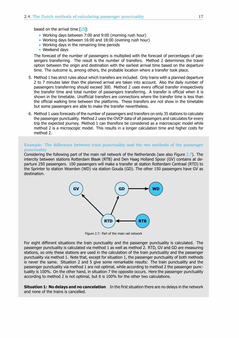
2.4. The Dutch methods of calculating passenger punctuality 17

based on the arrival time [25]:• Working days between 7:00 and 9:00 (morning rush hour)• Working days between 16:00 and 18:00 (evening rush hour)• Working days in the remaining time periods• Weekend days

The forecast of the number of passengers is multiplied with the forecast of percentages of pas-sengers transferring. The result is the number of transfers. Method 2 determines the traveloption between the origin and destination with the earliest arrival time based on the departuretime. The outcome is, among others, the probable location where a transfer took place.

5. Method 1 has strict rules about which transfers are included. Only trains with a planned departure2 to 7 minutes later than the planned arrival are taken into account. Also the daily number ofpassengers transferring should exceed 300. Method 2 uses every official transfer irrespectivelythe transfer time and total number of passengers transferring. A transfer is official when it isshown in the timetable. Unofficial transfers are connections where the transfer time is less thanthe official walking time between the platforms. These transfers are not show in the timetablebut some passengers are able to make the transfer nevertheless.

6. Method 1 uses forecasts of the number of passengers and transfers on only 35 stations to calculatethe passenger punctuality. Method 2 uses the OVCP data of all passengers and calculates for everytrip the expected journey. Method 1 can therefore be considered as a macroscopic model whilemethod 2 is a microscopic model. This results in a longer calculation time and higher costs formethod 2.

Example: The difference between train punctuality and the two methods of the passengerpunctualityConsidering the following part of the main rail network of the Netherlands (see also Figure 2.7). Theintercity between stations Rotterdam Blaak (RTB) and Den Haag Holland Spoor (GV) contains at de-parture 250 passengers. 100 passengers will make a transfer at station Rotterdam Centraal (RTD) tothe Sprinter to station Woerden (WD) via station Gouda (GD). The other 150 passengers have GV asdestination.

GV

RTD

GD WD

RTB

Figure 2.7: Part of the main rail network

For eight different situations the train punctuality and the passenger punctuality is calculated. Thepassenger punctuality is calculated via method 1 as well as method 2. RTD, GV and GD are measuringstations, so only these stations are used in the calculation of the train punctuality and the passengerpunctuality via method 1. Note that, except for situation 1, the passenger punctuality of both methodsis never the same. Situation 2 and 5 give some remarkable results: The train punctuality and thepassenger punctuality via method 1 are not optimal, while according to method 2 the passenger punc-tuality is 100%. On the other hand, in situation 7 the opposite occurs. Here the passenger punctualityaccording to method 2 is not optimal, but it is 100% for the other two calculations.

Situation 1: No delays and no cancelation In the first situation there are no delays in the networkand none of the trains is cancelled.

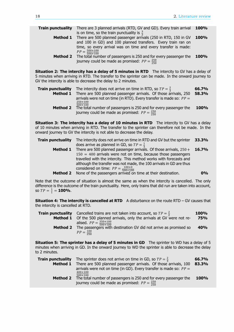
18 2. Literature review

Train punctuality There are 3 planned arrivals (RTD, GV and GD). Every train arrivalis on time, so the train punctuality is

100%

Method 1 There are 500 planned passenger arrivals (250 in RTD, 150 in GVand 100 in GD) and 100 planned transfers. Every train ran ontime, so every arrival was on time and every transfer is made:𝑃𝑃 =

100%

Method 2 The total number of passengers is 250 and for every passenger thejourney could be made as promised: 𝑃𝑃 =

100%

Situation 2: The intercity has a delay of 5 minutes in RTD The intercity to GV has a delay of5 minutes when arriving in RTD. The transfer to the sprinter can be made. In the onward journey toGV the intercity is able to decrease the delay to 2 minutes.

Train punctuality The intercity does not arrive on time in RTD, so 𝑇𝑃 = 66.7%Method 1 There are 500 planned passenger arrivals. Of those arrivals, 250

arrivals were not on time (in RTD). Every transfer is made so: 𝑃𝑃 =58.3%

Method 2 The total number of passengers is 250 and for every passenger thejourney could be made as promised: 𝑃𝑃 =

100%

Situation 3: The intercity has a delay of 10 minutes in RTD The intercity to GV has a delayof 10 minutes when arriving in RTD. The transfer to the sprinter can therefore not be made. In theonward journey to GV the intercity is not able to decrease the delay.

Train punctuality The intercity does not arrive on time in RTD and GV but the sprinterdoes arrive as planned in GD, so 𝑇𝑃 =

33.3%

Method 1 There are 500 planned passenger arrivals. Of those arrivals, 250+150 = 400 arrivals were not on time, because those passengerstravelled with the intercity. This method works with forecasts andalthough the transfer was not made, the 100 arrivals in GD are thusconsidered on time: 𝑃𝑃 =

16.7%

Method 2 None of the passengers arrived on time at their destination. 0%

Note that the outcome of situation is almost the same as when the intercity is cancelled. The onlydifference is the outcome of the train punctuality. Here, only trains that did run are taken into account,so 𝑇𝑃 = = 100%.

Situation 4: The intercity is cancelled at RTD A disturbance on the route RTD – GV causes thatthe intercity is cancelled at RTD.

Train punctuality Cancelled trains are not taken into account, so 𝑇𝑃 = 100%Method 1 Of the 500 planned arrivals, only the arrivals at GV were not re-

alised. 𝑃𝑃 =75%

Method 2 The passengers with destination GV did not arrive as promised so𝑃𝑃 =

40%

Situation 5: The sprinter has a delay of 5 minutes in GD The sprinter to WD has a delay of 5minutes when arriving in GD. In the onward journey to WD the sprinter is able to decrease the delayto 2 minutes.

Train punctuality The sprinter does not arrive on time in GD, so 𝑇𝑃 = 66.7%Method 1 There are 500 planned passenger arrivals. Of those arrivals, 100

arrivals were not on time (in GD). Every transfer is made so: 𝑃𝑃 =83.3%

Method 2 The total number of passengers is 250 and for every passenger thejourney could be made as promised: 𝑃𝑃 =

100%

2.5. Conclusion 19

Situation 6: The sprinter has a delay of 10 minutes in GD The sprinter to WD has a delay of10 minutes when arriving in GD. In the onward journey to WD the sprinter is not able to decrease thedelay.

Train punctuality The sprinter does not arrive on time in GD, so 𝑇𝑃 = 66.7%Method 1 There are 500 planned passenger arrivals. Of those arrivals, 100

where not on time, because those passengers travelled with thesprinter: 𝑃𝑃 =

83.3%

Method 2 The passengers with destination WD did not arrive on time: 𝑃𝑃 = 60%

Note that if the sprinter did not run at all, only the train punctuality would differ: 𝑇𝑃 = = 100%.

Situation 7: The sprinter is cancelled at GD A disturbance on the route GD – WD causes thatthe sprinter is cancelled at GD.

Train punctuality Cancelled trains are not taken into account, but WD is not a mea-suring station so 𝑇𝑃 =

100%

Method 1 Of the 500 planned arrivals, every arrival is realised because thepassenger with destination WD arrived on time in GD. 𝑃𝑃 =

100%

Method 2 The passengers with destination GW did not arrive on time aspromised, so 𝑃𝑃 =

60%

Situation 8: Both the intercity and the sprinter are delayed When arriving in RTD the intercityhas a delay of 10 minutes. A technical problem causes the sprinter to start its journey with a delay ofalso 10 minutes. Both trains are not able to decrease their delay further on their route.

Train punctuality Both trains are delayed, so 𝑇𝑃 = 0%Method 1 Of the 500 planned arrivals, none of those is on time. However the

transfer is made. 𝑃𝑃 =16.7%

Method 2 None of the passengers arrived on time as promised, so 𝑃𝑃 = 0%

2.5. ConclusionBoth the NS, as the rail operator on the main rail network, as ProRail, as the rail network manager,are under concession of the Ministry of Infrastructure and the Environment. To measure their perfor-mance, for both companies a list of Key Performance Indicators (KPIs) is created. Each KPI gives theperformance of a part of the operations of the NS or ProRail. If a value of a KPI is lower than a certainthreshold, the performance is not as good as it should be and ProRail or the NS have to pay a fine. Oneof the KPIs is passenger punctuality: the percentage of passengers with a successful journey. Initiallythis KPI belongs only to the NS, but in 2015 ProRail adopted this KPI as well.

In Swiss and by the metro of Copenhagen the passenger punctuality is calculated as well. Althoughthe exact calculation methods differ between the three countries, the basic idea is the same: therealisation data is combined with a forecast of the number of passengers. Together this leads to thepassenger punctuality. Until a few years ago in none of the countries the actual number of passengerswas known. Therefore more precise, microscopic, calculations were not possible.

With the introduction of the OV-chipkaart, data of almost every passenger in the Netherlands becameavailable. With this data, a possible journey for every passenger can be determined. This implies thepossibility of a more exact calculation of the passenger punctuality. Therefore the NS is developing anew method of calculating the passenger punctuality. Here the realised journeys of every passengeris compared with a promised journey, two days prior of the execution.

The NS made the passenger punctuality their most important KPI. It is therefore remarkable that atthis moment it is unknown how precise this new method of calculation is. With only a short explanationof the method of calculation, it is already clear that some large assumptions are made. Also it isunknown how the KPI can be described, based on the operations of ProRail and the NS. Steering onthe processes to improve the passenger punctuality is thus not possible.

3Passenger punctuality 2.0

In paragraph 2.4.2 the new method of calculating passenger punctuality is briefly explained. Passengerpunctuality 2.0 is the number of trips arriving with a delay less than a certain threshold, divided by allthe trips in the network. Chapter 2 stated that some large assumptions are made in this calculationas well. Therefore this chapter will examine the method of calculation even further. Special attentiongoes to the assumptions made in this method.

This chapter will start with an explanation of the structure of the algorithm to calculate passengerpunctuality, as developed at the NS. In paragraph 3.1 first the five modules that form the algorithmare explained. In the algorithm every trips gets categorised. These categories are also elaboratedon. A total of 22 assumptions can be distinguished in the method of calculation. The assumptions areanalysed in paragraph 3.2. If possible the impact of those assumptions is calculated as well. Someassumptions require an additional analysis. These analyses can be found in appendix A. Here anextensive overview of all assumptions and the calculated impact can be found as well (appendix A.6).The final concussions and some last remarks to the structure of the passenger punctuality calculationand the assumptions can be found in paragraph 3.3.

This chapter will provide a better insight in the method to calculate passenger punctuality. Moreoverit will give an estimation of the impact of the assumptions in the method on the passenger punctualityKPI. This will place the outcome of the breakdown of the passenger punctuality (chapter 4) and theresults of the models to describe passenger punctuality (chapter 5) in a more realistic perspective.

3.1. The structure of the passenger punctuality calculationThe NS has developed an algorithm to calculate the passenger punctuality 2.0 out of the raw data [24].This algorithm can be divided into five modules. These modules can be found in Table 3.1. All moduleshave their place in the algorithm, though the third module it not developed by the NS. In this moduletrips are being rescheduled. There are multiple alternatives for rescheduling trips, see also paragraph3.2.11. However the NS decided not to reschedule trips at all. Instead the checkout time is used todetermine the realised arrival time and thus the final delay. Nonetheless the structure of the algorithmis built in such way, that if the third module is still developed the integration of this module is relativelyeasy. In paragraph 3.1.1 the five modules are elaborated.

Table 3.1: The five modules of the algorithm to calculate the passenger punctuality [24]

Module Function

1 Retrieve and store travel options2 Combining travel options with realisation data3 Reschedule: Determine new travel option4 Combining OVCP data with travel options5 Generation data set

In the second module, every trip gets categorized. Based on the categorization, a trip is taken into

21

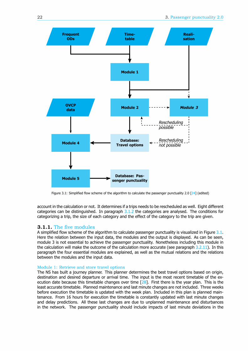
22 3. Passenger punctuality 2.0

OVCPdata

FrequentODs

Time-table

Reali-sation

Module 1

Module 2 Module 3

Database:Travel optionsModule 4

Module 5Database: Pas-

senger punctuality

Reschedulingpossible

Reschedulingnot possible

Figure 3.1: Simplified flow scheme of the algorithm to calculate the passenger punctuality 2.0 [24] (edited)

account in the calculation or not. It determines if a trips needs to be rescheduled as well. Eight differentcategories can be distinguished. In paragraph 3.1.2 the categories are analysed. The conditions forcategorizing a trip, the size of each category and the effect of the category to the trip are given.

3.1.1. The five modulesA simplified flow scheme of the algorithm to calculate passenger punctuality is visualized in Figure 3.1.Here the relation between the input data, the modules and the output is displayed. As can be seen,module 3 is not essential to achieve the passenger punctuality. Nonetheless including this module inthe calculation will make the outcome of the calculation more accurate (see paragraph 3.2.11). In thisparagraph the four essential modules are explained, as well as the mutual relations and the relationsbetween the modules and the input data.

Module 1: Retrieve and store travel optionsThe NS has built a journey planner. This planner determines the best travel options based on origin,destination and desired departure or arrival time. The input is the most recent timetable of the ex-ecution date because this timetable changes over time [28]. First there is the year plan. This is theleast accurate timetable. Planned maintenance and last minute changes are not included. Three weeksbefore execution the timetable is updated with the week plan. Included in this plan is planned main-tenance. From 16 hours for execution the timetable is constantly updated with last minute changesand delay predictions. All these last changes are due to unplanned maintenance and disturbancesin the network. The passenger punctuality should include impacts of last minute deviations in the

3.1. The structure of the passenger punctuality calculation 23

timetable but not the expected hindrance of planned maintenance. Therefore the travel options shouldbe determined from the journey planner between three weeks and 16 hours before execution. In thedocumentation this is often simplified as the timetable 48 hours before execution.

Once a week all the travel options for at least two days later are derived from the journey planner[24]. The result is stored in a database: the, so called, historic journey planner. Note that this onlyapplies for the travel options with an origin-destination (OD) combination frequently used. The list offrequent ODs is determined four times per year based on the OVCP data of the previous 100 days. AnOD is labelled frequent if two conditions are met:

• An OD should appear on average once a day.• An OD should appear on at least 20 different days

The result is a list of approximately twenty thousand different ODs. This list is updated every quarterof a year, so new stations can be included in the passenger punctuality and stations not in use anymorecan be filtered out.

Module 2: Combining travel options with realisation dataAfter the execution date the realisation data is available (NVGB data, see paragraph 3.2.9. This datacontains the realised arrival and departure times of the trains. For every travel option the moduleincludes if a train was cancelled, the last reached station and if a train was replaced with bus transportas well. Finally this module categorizes every travel option. The exact categories are given in paragraph3.1.2.

First a determination takes place to see if a travel option can be included in the passenger punc-tuality. A travel option cannot be included if it is (partly) serviced by another train operator or if atrain was replaced with a bus. In both cases the NS does not have the realised departure and arrivaltimes. This data is needed to determine if a travel option could be made as promised or if a traveloption should be rescheduled. The second step is to determine for every remaining travel option if thetravel option could be realised or not. A travel option is not realised if it is impossible to arrive at thefinal destination with the promised train. This could be due because a transfer could not be made ora promised train was cancelled. If so, the travel option should be rescheduled. The rescheduling ispart of module 3. It is necessary to determine the realised arrival time. Nonetheless module 3 is notdeveloped so no rescheduling is done. Instead the checkout time will be used to determine the finaldelay. This makes the whole process easier bus less accurate, see also paragraph 3.2.11.

The outcome is a database with every travel option combined with the realisation data. Every traveloption is categorized as well. If the category implies that the module was not able to determine therealised arrival time of the travel option, this information is neglected.

Module 4: Combining OVCP data with travel optionsThe OVCP data contains, among others, the origin, destination and check-in and checkout time of everytrip made. Based on the origin, destination and check-in time a travel option is found. The modulesearches per trip for all travel options with the same origin and destination. Each travel option musthave a planned departure at least 1 minute after the check-in time and at most 1 hour later. The traveloption arriving the earliest is the promised journey (in Dutch: Reisbelofte) for this trip. The thresholdof 1 minute is the expected walking time between card reader and platform. Note that there are tworeasons why a trip could not be combined with a travel option.

• The OD of the trip is not a frequent OD• There is no travel option between 1 minute and 1 hour after check-in

At this moment the last category can be assigned. If the time between check in and realised departureis less than 1 minute, the category of the trip will be ’Train departs too early’ (see paragraph 3.1.2). Inthis case it does not matter if the travel option had already a category. Note that this does not applyto trips not used in the passenger punctuality calculation, so trips without realisation data.

Based on the realised arrival time the final delay per trip can be calculated. This is the differencebetween the promised arrival time and the realised arrival time. No rescheduling is done, so forsome trips there is no realised arrival time. Here the checkout time is used. The delay is the differencebetween the promised arrival time and the checkout time minus 1 minute. This 1 minute is the expectedwalking time between platform and card reader.

24 3. Passenger punctuality 2.0

Module 5: Generation data setThis module takes the outcome of module 4 and stores it in a database. This database contains forevery trip the promised journey and the realisation of this promise. This includes a categorization andthe final delay. With this database the passenger punctuality can be calculated. That goes as follows.Take a time period. This can be for example a day or a year. Take also a delay threshold. If the goal isto calculate the 3 minute passenger punctuality this threshold is 180 seconds. Lastly count every tripwithin the chosen time period with a delay less than the chosen threshold and divide this with everytrip within the chosen time period. The result is the passenger punctuality. Note that trips (partly)serviced by another train operator and trips with bus transport needs to be neglected. Note also thatthe analysed trips could also be filtered by, among others, origin-destination combination, train seriesor departure or arrival station. This will lead to a passenger punctuality value for a part of the network.

3.1.2. The trip categories as defined by the NSAs stated in paragraph 3.1.1 every travel option gets categorized. The category can determine why atrip is not used in the passenger punctuality or it determines why a trip needs to be rescheduled. Forthe latter the expected arrival time is based on the checkout time. The last category (’Trip realised’)indicates that the trip can be realised as promised. The expected arrival time is the realised arrival timeof the last train of the journey. This section examines every category and analyses which conditionsmust apply. Also a determination is made to see which percentage of the trips ends up with theanalysed category.

Other train operatorIt could be that a passenger start and end his or her trip at a station serviced by the NS. Thereforethe passenger checks in and checks out by an OVCP card reader of the NS. However the found routeassociated with this trip involves another train operator. An example of such a trip could be betweenstations Amersfoort and Ede-Wageningen. This route is exploited by Valleilijn. However both stationsare also serviced by the NS. Passengers are able to check in and out by the NS but travel with theValleilijn. If this travel option is the fastest option as well, the trip gets the category: Other trainoperator.

The reason for this is that the NS does not have the realisation data of the other train operators.The realised departure and arrival times are therefore unknown. A correct determination whether apassenger arrives within a threshold value at the destination can thus not be made. Also the goal ofthe KPI is to give an indication of the performance of the NS. Using the trips made by another trainoperator is therefore not desirable. So trips with the component ‘Other train operator’ are not used inthe passenger punctuality calculation.

For the first 25 days of June 2015 21.318.027 different check-in checkout combinations could bedistinguished. Of those trips 99.61% (21.234.807) could be combined with a travel option. Of thosetrips with a promised journey, 80.555 (0.38%) were categorized as ‘Other train operator.’

Bus transportBy work activities or long term disruptions bus transport is used instead of trains. This means that thereis no realisation data available for these trips. Trips that encounter bus transport are categorized as‘Bus transport’. No realisation data is available, so rescheduling is not possible. Therefore this categoryis neglected in the passenger punctuality calculation. Passengers have an intent to check out beforethey get in the bus as well. Therefore the number of passengers with the category ‘Bus transport’ isnot representative of the total number of passengers experience bus transport.

For the first 25 days of June 2015, 38.646 trips were categorized as ‘Bus transport’. This is 0.18% ofthe total number of trips with a promised journey. ‘Bus transport’ and ‘Other train operator’ are the onlytwo categories not used in the passenger punctuality. Together with the trips with no promised journeythis means that 99.05% of all founded check-in checkout combinations are used in the calculation ofthe passenger punctuality.

Train departs too earlyThe earliest promised departure time is at least 1 minute (the walking time between card reader andplatform) later than the check-in time. It could occur that a train leaves too early. The trip is categorizedas ‘Train departs too early’ if the realised departure time is within 1 minute of the check-in time. The

3.1. The structure of the passenger punctuality calculation 25

assumption is made that the passenger was not able to catch the train and thus the realised arrivaltime of the train is not the realised arrival time of the passenger. This implies a new journey needs tobe planned. In this case the delay of the passenger is calculated via the checkout time. Here also awalking time of 1 minute is used. The delay of the passenger is the difference between the plannedarrival time and the checkout time minus 1 minute.

Between June 1 and June 25 2015 21.338 trips were categorized as ‘Train departs too early’. Thisis 0.10% of all trips used in the passenger punctuality calculation. Note that this category is only usedwhen the first train of the promised journey left too early. If a transfer is missed because a consecutivetrain departs too early, the category ‘Missed transfer’ is used.

Train departs too lateIt could occur that a promised train has a large delay. If this delay increases, the chance that passengerswill take another train is also increasing. The timespan when a route will be rescheduled depends on thelocation in the network. On some routes the next train in the same direction departs only 30 minuteslater while for other routes the maximum waiting time is 10 minutes or less. Therefore a default valueof 15 minutes is used. If a train departs with a delay of 15 minutes or more the assumption is madethat the passengers reschedule their trip. In this case the trip is categorized as ‘Train departs too late’.The realised arrival time of the original planned train cannot be used anymore so the checkout time isused as a reference for the arrival time. The arrival time is the checkout time minus 1 minute.

For the first 25 days of June 2015, 155.655 trips were categorized as ‘Train departs too late’. Thisis 0.73% off all the trips used in the calculation. Note that a train can depart too late at the origin ofthe trip but also at a transfer station.

Train did not departIf a train did not depart at the origin or at a transfer station, the trip is categorized as ‘Train did notdepart’. Enclosed in this categorization is the fact that a train can run with a different train numberas planned. Consider the following example. At the start of a route there is disturbance whereby theoriginal train is not able to depart. On a station further on the route a substitute train is deployed.This train gets the train number of the original train plus 300000. For passengers waiting on the firststation of the route, the train did not depart and their trips will be categorized as ‘Train did not depart’.However this is not the case for passengers departing further on the route. The fact that the traindeparting is not the original planned train does not matter. They do not need to reschedule their trip.If the trip needs to be rescheduled, the checkout time is used to determine the final delay.

1.86% of all the trips of the first 25 days of June 2015 used in the calculation of the passengerpunctuality has the category ‘Train did not depart’. This is a total of 392.180 trips.

Train did not arriveIn some cases a train is not able to serve the second part of the route. This can be due to a disturbancefurther down the route or because the train itself has technical problems. Whatever the cause maybe, passengers in this train are stranded on the last reached station. The planned trip needs to berescheduled so this trip gets the category ‘Train did not arrive’. The realised arrival time of every tripcannot be calculated based on the realisation data anymore so the checkout time is used. Note thatthe trips of the passengers waiting on the last reached station are getting the category ‘Train did notdepart’.

In the first 25 days of June 2015 129.646 trips were getting the category ‘Train did not arrive’. Thisis 0.61% of all the used trips in the calculation of the passenger punctuality.

Missed transferA transfer is made when the difference between the realised arrival time of the first train and therealised departure time of the second train is at least equal to the norm time for transferring. Thisnorm time is the walking time between the platforms. For the most stations and platforms, this isspecified per unique combination of the station and the two platforms involved. When such a platformspecific norm is not available, a station specific norm will be used. This is a norm time that differs onlyper station and not per platform combination. In the rare case such station norm is not available aswell, a default value of 5 minutes is used. Note that the platforms used in the determination of thenorm time are the planned platforms. The planned platforms are not necessarily the used platforms in

26 3. Passenger punctuality 2.0

the realisation. It is also possible that the arrival platform is equal to the departing platform. In sucha case a check is made if the time between the realised arrival time and the departure time is at least3 minutes. When the time difference is less, the conclusion is made that the planned platforms differsfrom the realisation. The minimum time between arrival and departure should be at least the specifiedstation norm time for such a transfer to be made.

If the time difference between arrival and departure is less than the norm time, the transfer is notmade. The trip is categorized as ‘Missed transfer’. This is the case for 532.555 trips in the 25 first daysof June 2015. This is 2.52% of all the used trips in the calculation. The transfer is missed, so the tripneeds to be rescheduled. The realisation data is therefore not useful and the realised arrival time atthe final destination is calculated based on the checkout time.

Trip realisedIf the first train of a trip did not depart within 1 minute after check-in; and if all the trains of a trip diddepart with a delay of less than 15 minutes; and if all the trains of a trip arrive at transfer stations or thedestination; and if all the transfers were made; and if there was no bus transport during the trip andif there was no other train operator involved, than the trip was realised as promised. The arrival timecan be derived from the realisation data. This does not mean that the departure and arrival times wereas promised, only that the passenger was able to catch the trains as promised without rescheduling.In this case the trip gets the category ‘Trip realised’.

By far the most trips get the category ‘Trip realised’. In the first 25 days of June 2015 19.884.232trips were ‘realised’. This is 94.17% of all the trips. Note that this does not mean that the passengerpunctuality is 94.17%. Trips with another category can still be on time and trips that are realised couldstill be delayed.

3.2. The assumptions and their impact on the KPIIn the method of calculating passenger punctuality 2.0 KPI 22 assumptions are made, see Table 3.2).These assumptions differ from passenger behaviour to the accuracy of the used data. This paragraphanalyses the assumptions. If some assumptions can be grouped, this group is examined together. Ifpossible the impact of the assumptions on the passenger punctuality KPI is calculated. A distinctionis made between the maximum impact and the expected impact. The maximum impact is based onevery trip influenced by the assumption. The expected impact is based on the trips influenced by theassumption and directly changes the passenger punctuality. For example, if due to an assumptionsome trips are considered delayed all those trips are the basis for the maximum impact value. On theother hand, only the trips with a final delay of more than 3 minutes are considered in the calculationof the expected impact value.

Some assumptions need additional analyses. If so, these analyses can be found in appendix A. Anoverall conclusion can be found in paragraph 3.3. An overview of all assumptions and the calculatedimpact values is given in appendix A.6.

3.2.1. The observed trips in the passenger punctuality calculation are repre-senting the average passenger

The NS already examined the assumption that the observed trips in the passenger punctuality calcu-lation are a correct representation of the average passenger on the main rail network [29]. A trip isa journey of a passenger where the origin is not the destination. The origin and destination are de-termined via the OVCP data. In the calculation of the passenger punctuality not all origin-destination(OD) combinations are taken into account. Every quarter of a year a selection is made to filter outthe stations that are not always served: the event stations like Rotterdam Stadium and HeerenveenIJsstadion. Also very rare OD combinations are filtered out to speed up the calculation time. An OD isselected if it satisfies two conditions:1. On average, in a period of 100 days at least once a day a passenger should make a trip with thisOD-combination.

2. On at least 20 of the 100 days a passenger needs to make a trip with this OD-combination.If both conditions are met, the OD is taken into the selection. The NS examined what the effect was onthe passenger punctuality when using the selection of OD combinations instead of all OD combinations.This test was done in 2014 when the second condition was a bit stricter: On at least 50 of the 100

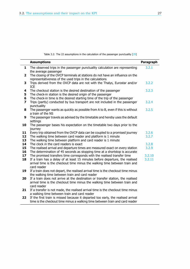
3.2. The assumptions and their impact on the KPI 27

Table 3.2: The 22 assumptions in the calculation of the passenger punctuality [29]

Assumptions Paragraph

1 The observed trips in the passenger punctuality calculation are representingthe average passenger

3.2.1

2 The closing of the OVCP terminals at stations do not have an influence on therepresentativeness of the used trips in the calculations

3 Trips derived from the OVCP data are not with the Thalys, Eurostar and/orICE

3.2.2

4 The checkout station is the desired destination of the passenger 3.2.35 The check-in station is the desired origin of the passenger6 The check-in time is the desired starting time of the trip of the passenger7 Trips (partly) conducted by bus transport are not included in the passenger

punctuality3.2.4

8 The passenger wants as quickly as possible from A to B, even if this is withouta train of the NS

3.2.5

9 The passenger travels as advised by the timetable and hereby uses the defaultsettings

10 The passenger bases his expectation on the timetable two days prior to thejourney

11 Every trip obtained from the OVCP data can be coupled to a promised journey 3.2.612 The walking time between card reader and platform is 1 minute 3.2.713 The walking time between platform and card reader is 1 minute14 The clock in the card readers is exact 3.2.815 The realised arrival and departure times are measured exact on every station 3.2.916 The determination of 45 seconds as stopping time at a shortstop is accurate17 The promised transfers time corresponds with the realised transfer time 3.2.1018 If a train has a delay of at least 15 minutes before departure, the realised

arrival time is the checkout time minus the walking time between train andcard reader

3.2.11

19 If a train does not depart, the realised arrival time is the checkout time minusthe walking time between train and card reader

20 If a train does not arrive at the destination or transfer station, the realisedarrival time is the checkout time minus the walking time between train andcard reader

21 If a transfer is not made, the realised arrival time is the checkout time minusa walking time between train and card reader

22 If the first train is missed because it departed too early, the realised arrivaltime is the checkout time minus a walking time between train and card reader

28 3. Passenger punctuality 2.0

days a passenger needs to make a trip with the OD-combination. For 100 days (between 2 June and 9September 2014) all the OD-combinations occurring were distinguished. The result was a list of 66.423different ODs. When applying the conditions a selection was made consisting of 19.755 ODs. Althoughthe number of ODs in the selection is only 29.7% of the total number of ODs, 98.36% of all the tripsare still taken into account in the calculation of the passenger punctuality.

For nine days the 3 minute passenger punctuality was calculated with and without the selectionof ODs. For eight days, the difference was between 0.02 and 0.06 percentage point, with a mean of0.05 percentage point. On one day (16 Augustus 2014) the difference was 0.15 percentage point. Thisoutlier can be explained by the fact that on that day maintenance was scheduled. When this calculationwas done, planned maintenance was not taken into account and could thus results in large outliers.Afterwards the method of calculation was adapted so planned maintenance is no reason for deviationof the passenger punctuality calculation anymore.

The second step is to check if every section of the main rail network is covered by the selection ofODs. If a section is not covered, disturbances on this section will not have an effect on the passengerpunctuality. With VISUM, an assignment model, for every OD of the selection a determination is madewhich sections of the network are used. Then the same is done for every other OD. A check tookplace to see if there were sections covered by ODs not in the selection but not covered by ODs in theselection. This was not the case. In fact this was still not the case when using only the top 2000ODs in the selection (instead of the original 19.755 ODs). When using the top 1000 ODs, only onesection (between stations Veenendaal-Centrum and Rhenen) was not covered. The first OD coveringthis section was in the 1017th place.

Note that this check took place with the used ODs between 2 June and 9 September 2014. Theselection of ODs can change over time. However the most frequent travelled ODs will stay in theselection. The fact that less than the top 1% of the selected ODs was enough was enough to coverthe whole main rail network indicates that also in the future the selected ODs are representative forthe whole network.

A third analysis to determine if the used trips are a correct representation of the average passenger isto check if the passengers using the OV-chipkaart are representative. Only the trips of the passengerswho check in and check out can be used in the passenger punctuality calculation. According to the NS,in October 2014 80% of the passenger kilometres was made with trips with a check-in and a checkout.

The other 20% can be divided into two groups. The first group is the trips made with a train ticketthat does not require a check-in or checkout: the unchipped train tickets, for example an internationaltrain ticket. Unfortunately the distribution of these tickets is not evenly in place and time. There is aslightly overrepresentation in the weekend and a small underrepresentation during rush hours. Notethat the mean travel distance of this group is larger than the overall mean travel distance, thus thepercentage of passenger kilometres travelled in this group is larger than the percentages of trips. Onthe other hand, the number of different unchipped train tickets is decreasing. The second group is theincomplete trips. A trip is incomplete if a check-in or checkout is missing. Research shows that betweenOctober 2012 and September 2013 2.0% of the train passengers did not check in or check out whilethis was required [30]. If these incomplete trips were evenly distributed among the network, this wouldbe no effect to the overall passenger punctuality. Nonetheless this research shows a variation in thepercentage of incomplete journeys among different regions as well (see Table 3.3). This means that thecalculated passenger punctuality is slightly off. Note that the number of closed stations is increasing.This means that a passenger cannot enter or leave the station without checking in or checking out.Hereby the percentage of incomplete trips will decrease.

So for both groups the number of involved trips will decrease over time. This implies that thepercentages of used trips in the passenger punctuality will increase. For now, the chance that a trainis not included in the passenger punctuality is almost zero. With only 6 passengers, the chance thatnone of those passengers did check in and check out, is less than 0.01%.

In conclusion, by using a selection of ODs in the calculation of the passenger punctuality the maximumdeviation will be approximately 0.05 percentage points. However every section of the main rail networkis covered by those ODs. This implies that every disturbance is included in the calculation. At thismoment, more than 80 per cent off all the trips in the network is used in the calculation and this

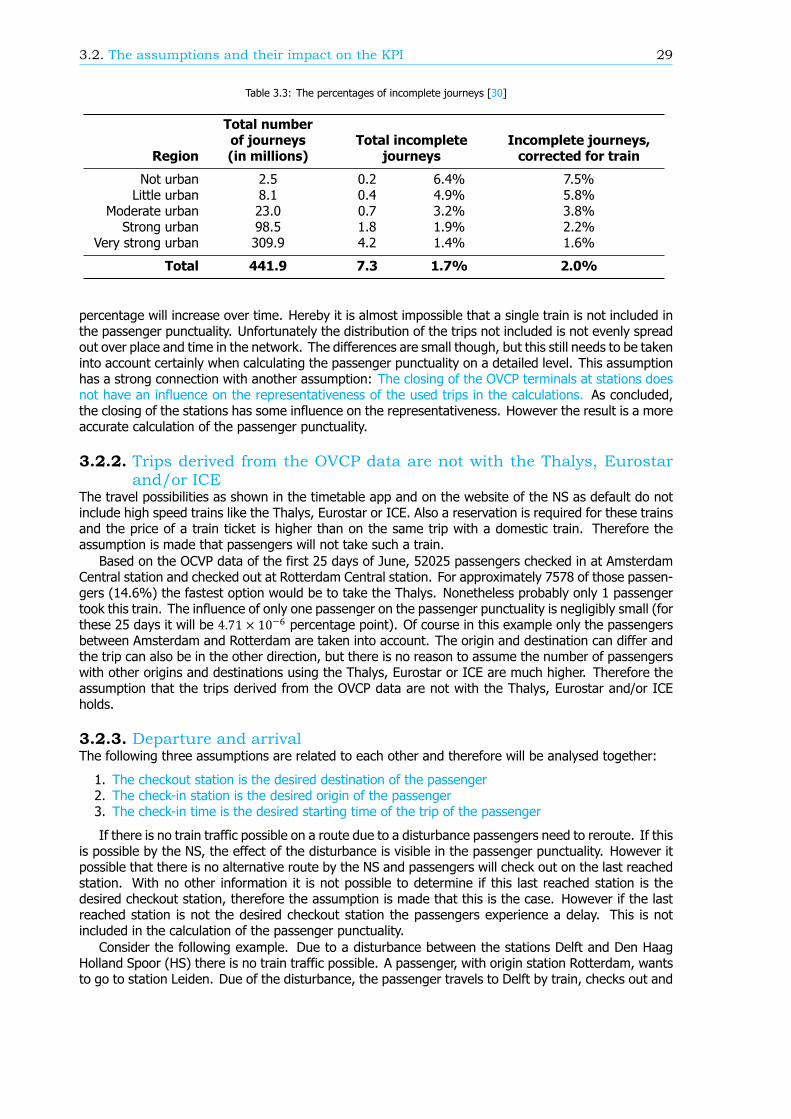
3.2. The assumptions and their impact on the KPI 29

Table 3.3: The percentages of incomplete journeys [30]

Region

Total numberof journeys(in millions)

Total incompletejourneys

Incomplete journeys,corrected for train

Not urban 2.5 0.2 6.4% 7.5%Little urban 8.1 0.4 4.9% 5.8%

Moderate urban 23.0 0.7 3.2% 3.8%Strong urban 98.5 1.8 1.9% 2.2%

Very strong urban 309.9 4.2 1.4% 1.6%

Total 441.9 7.3 1.7% 2.0%

percentage will increase over time. Hereby it is almost impossible that a single train is not included inthe passenger punctuality. Unfortunately the distribution of the trips not included is not evenly spreadout over place and time in the network. The differences are small though, but this still needs to be takeninto account certainly when calculating the passenger punctuality on a detailed level. This assumptionhas a strong connection with another assumption: The closing of the OVCP terminals at stations doesnot have an influence on the representativeness of the used trips in the calculations. As concluded,the closing of the stations has some influence on the representativeness. However the result is a moreaccurate calculation of the passenger punctuality.

3.2.2. Trips derived from the OVCP data are not with the Thalys, Eurostarand/or ICE

The travel possibilities as shown in the timetable app and on the website of the NS as default do notinclude high speed trains like the Thalys, Eurostar or ICE. Also a reservation is required for these trainsand the price of a train ticket is higher than on the same trip with a domestic train. Therefore theassumption is made that passengers will not take such a train.

Based on the OCVP data of the first 25 days of June, 52025 passengers checked in at AmsterdamCentral station and checked out at Rotterdam Central station. For approximately 7578 of those passen-gers (14.6%) the fastest option would be to take the Thalys. Nonetheless probably only 1 passengertook this train. The influence of only one passenger on the passenger punctuality is negligibly small (forthese 25 days it will be 4.71 × 10 percentage point). Of course in this example only the passengersbetween Amsterdam and Rotterdam are taken into account. The origin and destination can differ andthe trip can also be in the other direction, but there is no reason to assume the number of passengerswith other origins and destinations using the Thalys, Eurostar or ICE are much higher. Therefore theassumption that the trips derived from the OVCP data are not with the Thalys, Eurostar and/or ICEholds.

3.2.3. Departure and arrivalThe following three assumptions are related to each other and therefore will be analysed together:

1. The checkout station is the desired destination of the passenger2. The check-in station is the desired origin of the passenger3. The check-in time is the desired starting time of the trip of the passenger

If there is no train traffic possible on a route due to a disturbance passengers need to reroute. If thisis possible by the NS, the effect of the disturbance is visible in the passenger punctuality. However itpossible that there is no alternative route by the NS and passengers will check out on the last reachedstation. With no other information it is not possible to determine if this last reached station is thedesired checkout station, therefore the assumption is made that this is the case. However if the lastreached station is not the desired checkout station the passengers experience a delay. This is notincluded in the calculation of the passenger punctuality.

Consider the following example. Due to a disturbance between the stations Delft and Den HaagHolland Spoor (HS) there is no train traffic possible. A passenger, with origin station Rotterdam, wantsto go to station Leiden. Due of the disturbance, the passenger travels to Delft by train, checks out and

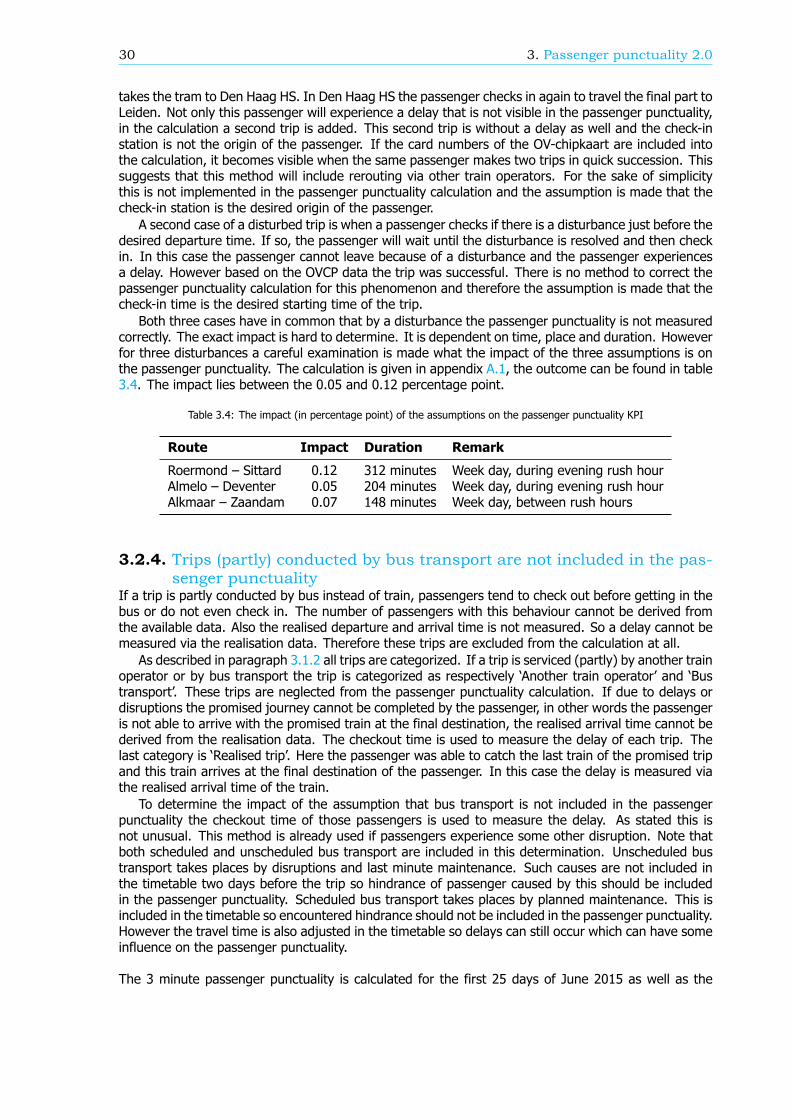
30 3. Passenger punctuality 2.0

takes the tram to Den Haag HS. In Den Haag HS the passenger checks in again to travel the final part toLeiden. Not only this passenger will experience a delay that is not visible in the passenger punctuality,in the calculation a second trip is added. This second trip is without a delay as well and the check-instation is not the origin of the passenger. If the card numbers of the OV-chipkaart are included intothe calculation, it becomes visible when the same passenger makes two trips in quick succession. Thissuggests that this method will include rerouting via other train operators. For the sake of simplicitythis is not implemented in the passenger punctuality calculation and the assumption is made that thecheck-in station is the desired origin of the passenger.

A second case of a disturbed trip is when a passenger checks if there is a disturbance just before thedesired departure time. If so, the passenger will wait until the disturbance is resolved and then checkin. In this case the passenger cannot leave because of a disturbance and the passenger experiencesa delay. However based on the OVCP data the trip was successful. There is no method to correct thepassenger punctuality calculation for this phenomenon and therefore the assumption is made that thecheck-in time is the desired starting time of the trip.

Both three cases have in common that by a disturbance the passenger punctuality is not measuredcorrectly. The exact impact is hard to determine. It is dependent on time, place and duration. Howeverfor three disturbances a careful examination is made what the impact of the three assumptions is onthe passenger punctuality. The calculation is given in appendix A.1, the outcome can be found in table3.4. The impact lies between the 0.05 and 0.12 percentage point.

Table 3.4: The impact (in percentage point) of the assumptions on the passenger punctuality KPI

Route Impact Duration Remark

Roermond – Sittard 0.12 312 minutes Week day, during evening rush hourAlmelo – Deventer 0.05 204 minutes Week day, during evening rush hourAlkmaar – Zaandam 0.07 148 minutes Week day, between rush hours

3.2.4. Trips (partly) conducted by bus transport are not included in the pas-senger punctuality

If a trip is partly conducted by bus instead of train, passengers tend to check out before getting in thebus or do not even check in. The number of passengers with this behaviour cannot be derived fromthe available data. Also the realised departure and arrival time is not measured. So a delay cannot bemeasured via the realisation data. Therefore these trips are excluded from the calculation at all.

As described in paragraph 3.1.2 all trips are categorized. If a trip is serviced (partly) by another trainoperator or by bus transport the trip is categorized as respectively ‘Another train operator’ and ‘Bustransport’. These trips are neglected from the passenger punctuality calculation. If due to delays ordisruptions the promised journey cannot be completed by the passenger, in other words the passengeris not able to arrive with the promised train at the final destination, the realised arrival time cannot bederived from the realisation data. The checkout time is used to measure the delay of each trip. Thelast category is ‘Realised trip’. Here the passenger was able to catch the last train of the promised tripand this train arrives at the final destination of the passenger. In this case the delay is measured viathe realised arrival time of the train.

To determine the impact of the assumption that bus transport is not included in the passengerpunctuality the checkout time of those passengers is used to measure the delay. As stated this isnot unusual. This method is already used if passengers experience some other disruption. Note thatboth scheduled and unscheduled bus transport are included in this determination. Unscheduled bustransport takes places by disruptions and last minute maintenance. Such causes are not included inthe timetable two days before the trip so hindrance of passenger caused by this should be includedin the passenger punctuality. Scheduled bus transport takes places by planned maintenance. This isincluded in the timetable so encountered hindrance should not be included in the passenger punctuality.However the travel time is also adjusted in the timetable so delays can still occur which can have someinfluence on the passenger punctuality.

The 3 minute passenger punctuality is calculated for the first 25 days of June 2015 as well as the

3.2. The assumptions and their impact on the KPI 31

passenger punctuality with bus transport included. If the checkout time is used to determine delaysthe difference between the planned arrival time and the checkout time is taken. Here 1 minute isabstracted. This 1 minute is the expected walking distance between platform and the card reader. Thesame methodology is applied to the trips categorized as ‘Bus transport’: The delay is the differencebetween the planned arrival time and the checkout time minus 1 minute. The results can be foundAppendix A.2. The impact of the assumption that bus transport is not included in the passengerpunctuality calculation is on average 0.07 percentage points. Note the large differences between June6, 7, 13 and 14 and the other days. On these days some large maintenance was scheduled. Thisresulted in a relatively large amount of trips with scheduled bus transport. Excluding these days fromthe calculation leads to an average impact of only 0.005 percentage point. On the other hand, theimpact of only those days is substantial: on average 0.42 percentage point. Trips categorized as ’Bustransport’ are not included in the passenger punctuality calculation, so the maximum impact is thesame as the expected impact.

The same calculation is done for the 15 minute passenger punctuality. Here the average impactwas 0.04 percentage point. Excluding the days with scheduled maintenance decreases the impact to0.002 percentage point. The average impact on June 6, 7, 13 and 14 is 0.25 percentage point.

In conclusion, the impact of bus transport on the passenger punctuality is on most days negligible.The reason is that the number of trips where bus transport is included is very small. If the share oftrips with bus transport is more extensive the impact on the passenger punctuality increases fast.

3.2.5. Passenger behaviour with respect to the planning of their journeyThere are multiple methods to plan a journey. All these methods lead to different choices concerningtravel time, route and train operator. To deal with all these possibilities three assumptions are made tomodel the passenger behaviour regarding journey planning.

1. The passenger wants as quickly as possible from A to B, even if this is without a train of the NS2. The passenger travels as advised by the timetable and hereby uses the default settings3. The passenger bases his expectation on the timetable two days prior to the journey

The NS has a journey planner on their website and in their app. This journey planner will searchfor the best (train) connections based on an origin and destination. Based on the desired departure orarrival time the best solutions are shown. The basis for this solution is the timetable. If there is moretime between the period of checking the journey planner and the actual journey, the solutions will beless accurate. The timetable gets a couple of updates towards the execution time [28]. For examplesmall deviations due to planned maintenance are added around three weeks before the execution.And only minutes before execution the timetable can change with predicted departure times based onreal time realisation data. Note the underlining assumption on all three analysed assumptions that thealgorithm, searching for travel possibilities, will always get the best solutions.

The first assumption can be split into two separate assumptions: The passenger wants as quickly aspossible from A to B and The passenger is willing to travel with another rail operator than the NS. To startwith the latter, the impact of this assumption is hard to measure. Check-in and checkout data of othertrain operators is needed, as well as their realisation data to determine the impact. An impact value istherefore not possible to calculate. However there is no direct reason to assume this assumption doesnot hold. Most of the time travelling with the NS is more expensive than with another train operator.Also on every origin-destination combination served by the NS and another train operator, the traveltime by the NS is equal or more than the travel time of the other train operator.

The impact of the assumption that the passenger wants as quickly as possible from A to B is lessstraight forward. Consider the route between stations Utrecht Centraal and Leiden. Sometimes thequickest route is via station Schiphol. Nonetheless, of all the passengers assumed to travel via Schiphol,84.40% was actual travelling via a different connection (see appendix A.3.1). This connection had lesstransfers while the arrival time was only 5 minutes later. This has a maximum impact on the dailypassenger punctuality KPI of 0.04 percentage points. The delay is measured via the realisation datawhen there is no disruption, so the actual impact is on average 0.01 percentage points. At this momentit is unclear which percentage of the passengers in the whole network takes not the quickest travelpossibility. And thus the total impact of this assumption on the passenger punctuality KPI is unclear.An alternative might be to calculate the costs of every possible travel options, where the number of

32 3. Passenger punctuality 2.0

transfers, the waiting time, the cancellation rate and the train punctuality is included. The assumptionthan will be that the passenger travels with the connection with the lowest costs.

The impact of the first half of the second assumption is impossible to determine: The passenger travelsas advised by the timetable. But assuming that the journey planner of the NS gives the most optimaloptions between origin and destination there is no reason for passenger to travel differently. Also if thepassenger does not travel as advised by the timetable the question arises whether the NS is responsiblewhen the passenger arrives with a delay. If there was another travel option, promoted by the NS viathe journey planner, is it the fault of the NS when the passenger decides to travel otherwise and endingup with a delay?

As explained, the journey planner finds the best train connections. However there are some settingsin the planner that can influence the outcome. The assumption is that every passenger uses the defaultsettings to find their promised journey. The different settings are as follows:

• Use high speed trains In the default settings this option is off. As shown in paragraph 3.2.2 thisis indeed the case in reality. Here all the passengers were observed who departed in Amsterdamand arrived in Rotterdam. Of those passengers, an determination took place who took the a highspeed train. Only one passengers did probably took this train.

• Use detours Some train tickets allows the passenger to travel unlimited. Default detours arenot shown in the options of the journey planner. However it could be beneficial to passengerswith such a train ticket. In appendix A.3.2 this option is analysed. Although the percentageof passenger taking a possible detour is significant, the impact on the passenger punctuality isnegligible. However more research on this travel option is necessary.

• Transfer time If the default settings are on, the journey planner will include travel options withthe smallest possible transfer time. It is possible to change the minimum transfer time into 5, 10,15 or 20 minutes. Given the available data, it is not possible to determine whether passengerschange this setting.

• Type of connection The algorithm behind the journey planner searches for the most optimalroute, which is a combination of travel time and number of transfers. This can be changed intothe connection with the least transfers and into the fastest connections. In practice this leadsto only a few minor changes. With the introduction of the new website of the NS in December2015, this option was omitted though in the app of the NS this option is still present.

Four different settings can be changed. For two of those, the use of high speed trains and the useof detours, the impact on the passenger punctuality can be determined. In both cases this impact isnegligible. For the other two setting, the transfer time and the type of connection, the impact cannotbe determined. However the expectation is that here the impact is also too small to have significantimpact. Therefore the assumption that the passengers use the default setting when using the journeyplanner holds.

As stated, the timetable used by the journey planner is updated several times before the execution.This means that with the same input, in time the journey planner can give different options. Thepassenger punctuality can thus change by using the timetable on different moment in time prior tothe execution because the travel options change. The third assumptions states that the time betweenchecking the journey planner and the trip itself is two days.

Consider the following. Every passenger checks the journey planner 10 minutes before departing.On that moment every disruption and delay is known so the promised journey is based on this infor-mation. The result is high passenger punctuality but this KPI does not give a correct indication on theperformance of the NS because the performance is worse than the KPI. The opposite is also possible.Every passenger checks the journey planner two weeks before departing. Scheduled maintenance isnot included yet so the promised journey takes this not into account. Although the NS clearly indi-cates in the two weeks prior to the execution that there is maintenance on the route, the passengerpunctuality is very low. The KPI shows a lower performance than in reality.

The threshold of two days between checking the journey planner and the actual departure ensuresthat planned deviations to the timetable are uncounted for in the passenger punctuality but disruptionsand last minutes changes due to extreme weather are included in the KPI. A higher threshold gives aworse KPI and a lower threshold gives a better KPI, while the performance of the NS stays the same.So in conclusion the assumption of a threshold of two days holds.

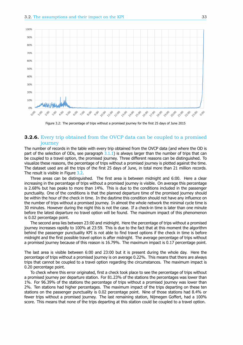
3.2. The assumptions and their impact on the KPI 33

Figure 3.2: The percentage of trips without a promised journey for the first 25 days of June 2015

3.2.6. Every trip obtained from the OVCP data can be coupled to a promisedjourney

The number of records in the table with every trip obtained from the OVCP data (and where the OD ispart of the selection of ODs, see paragraph 3.1.1) is always larger than the number of trips that canbe coupled to a travel option, the promised journey. Three different reasons can be distinguished. Tovisualize these reasons, the percentage of trips without a promised journey is plotted against the time.The dataset used are all the trips of the first 25 days of June, in total more than 21 million records.The result is visible in Figure 3.2.

Three areas can be distinguished. The first area is between midnight and 6:00. Here a clearincreasing in the percentage of trips without a promised journey is visible. On average this percentageis 2.68% but has peaks to more than 14%. This is due to the conditions included in the passengerpunctuality. One of the conditions is that the planned departure time of the promised journey shouldbe within the hour of the check in time. In the daytime this condition should not have any influence onthe number of trips without a promised journey. In almost the whole network the minimal cycle time is30 minutes. However during the night this is not the case. If a check-in time is later than one minutebefore the latest departure no travel option will be found. The maximum impact of this phenomenonis 0.02 percentage point.

The second area lies between 23:00 and midnight. Here the percentage of trips without a promisedjourney increases rapidly to 100% at 23:59. This is due to the fact that at this moment the algorithmbehind the passenger punctuality KPI is not able to find travel options if the check in time is beforemidnight and the first possible travel option is after midnight. The average percentage of trips withouta promised journey because of this reason is 16.79%. The maximum impact is 0.17 percentage point.

The last area is visible between 6:00 and 23:00 but it is present during the whole day. Here thepercentage of trips without a promised journey is on average 0.22%. This means that there are alwaystrips that cannot be coupled to a travel option regarding the circumstances. The maximum impact is0.20 percentage point.

To check where this error originated, first a check took place to see the percentage of trips withouta promised journey per departure station. For 81.23% of the stations the percentages was lower than1%. For 96.39% of the stations the percentage of trips without a promised journey was lower than2%. Ten stations had higher percentages. The maximum impact of the trips departing on these tenstations on the passenger punctuality is 0.02 percentage point. Nine of those stations had 8.4% orfewer trips without a promised journey. The last remaining station, Nijmegen Goffert, had a 100%score. This means that none of the trips departing at this station could be coupled to a travel option.

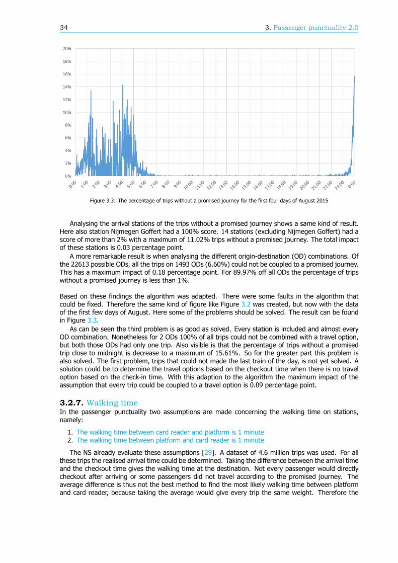
34 3. Passenger punctuality 2.0

Figure 3.3: The percentage of trips without a promised journey for the first four days of August 2015

Analysing the arrival stations of the trips without a promised journey shows a same kind of result.Here also station Nijmegen Goffert had a 100% score. 14 stations (excluding Nijmegen Goffert) had ascore of more than 2% with a maximum of 11.02% trips without a promised journey. The total impactof these stations is 0.03 percentage point.

A more remarkable result is when analysing the different origin-destination (OD) combinations. Ofthe 22613 possible ODs, all the trips on 1493 ODs (6.60%) could not be coupled to a promised journey.This has a maximum impact of 0.18 percentage point. For 89.97% off all ODs the percentage of tripswithout a promised journey is less than 1%.

Based on these findings the algorithm was adapted. There were some faults in the algorithm thatcould be fixed. Therefore the same kind of figure like Figure 3.2 was created, but now with the dataof the first few days of August. Here some of the problems should be solved. The result can be foundin Figure 3.3.

As can be seen the third problem is as good as solved. Every station is included and almost everyOD combination. Nonetheless for 2 ODs 100% of all trips could not be combined with a travel option,but both those ODs had only one trip. Also visible is that the percentage of trips without a promisedtrip close to midnight is decrease to a maximum of 15.61%. So for the greater part this problem isalso solved. The first problem, trips that could not made the last train of the day, is not yet solved. Asolution could be to determine the travel options based on the checkout time when there is no traveloption based on the check-in time. With this adaption to the algorithm the maximum impact of theassumption that every trip could be coupled to a travel option is 0.09 percentage point.

3.2.7. Walking timeIn the passenger punctuality two assumptions are made concerning the walking time on stations,namely:

1. The walking time between card reader and platform is 1 minute2. The walking time between platform and card reader is 1 minute

The NS already evaluate these assumptions [29]. A dataset of 4.6 million trips was used. For allthese trips the realised arrival time could be determined. Taking the difference between the arrival timeand the checkout time gives the walking time at the destination. Not every passenger would directlycheckout after arriving or some passengers did not travel according to the promised journey. Theaverage difference is thus not the best method to find the most likely walking time between platformand card reader, because taking the average would give every trip the same weight. Therefore the

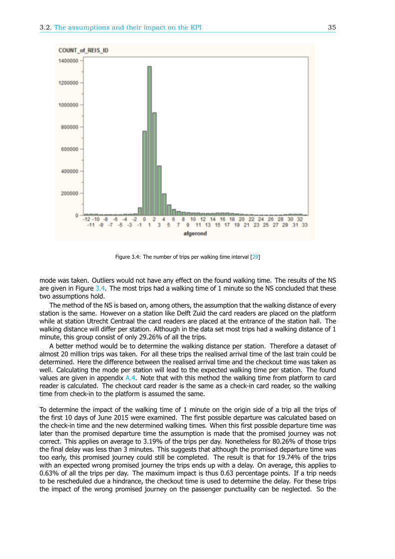
3.2. The assumptions and their impact on the KPI 35

Figure 3.4: The number of trips per walking time interval [29]

mode was taken. Outliers would not have any effect on the found walking time. The results of the NSare given in Figure 3.4. The most trips had a walking time of 1 minute so the NS concluded that thesetwo assumptions hold.

The method of the NS is based on, among others, the assumption that the walking distance of everystation is the same. However on a station like Delft Zuid the card readers are placed on the platformwhile at station Utrecht Centraal the card readers are placed at the entrance of the station hall. Thewalking distance will differ per station. Although in the data set most trips had a walking distance of 1minute, this group consist of only 29.26% of all the trips.

A better method would be to determine the walking distance per station. Therefore a dataset ofalmost 20 million trips was taken. For all these trips the realised arrival time of the last train could bedetermined. Here the difference between the realised arrival time and the checkout time was taken aswell. Calculating the mode per station will lead to the expected walking time per station. The foundvalues are given in appendix A.4. Note that with this method the walking time from platform to cardreader is calculated. The checkout card reader is the same as a check-in card reader, so the walkingtime from check-in to the platform is assumed the same.

To determine the impact of the walking time of 1 minute on the origin side of a trip all the trips ofthe first 10 days of June 2015 were examined. The first possible departure was calculated based onthe check-in time and the new determined walking times. When this first possible departure time waslater than the promised departure time the assumption is made that the promised journey was notcorrect. This applies on average to 3.19% of the trips per day. Nonetheless for 80.26% of those tripsthe final delay was less than 3 minutes. This suggests that although the promised departure time wastoo early, this promised journey could still be completed. The result is that for 19.74% of the tripswith an expected wrong promised journey the trips ends up with a delay. On average, this applies to0.63% of all the trips per day. The maximum impact is thus 0.63 percentage points. If a trip needsto be rescheduled due a hindrance, the checkout time is used to determine the delay. For these tripsthe impact of the wrong promised journey on the passenger punctuality can be neglected. So the

36 3. Passenger punctuality 2.0

expected impact on the passenger punctuality are the trips categorized as ‘Trip realised’ where thepromised departure time was too early and where the delay was at least 3 minutes. This applies to0.42% of the trips per day.

The impact of the walking time of 1 minute on the destination side is determined by analysing thefirst 25 days of June 2015. Note that only trips that need to be rescheduled are influenced by differentwalking times. Per trip the final delay is calculated based on the new walking times. Two groups oftrip can be distinguished.1. This group contains trips that have a delay of at least 3 minutes with a default walking of 1minute, but the delay is less than 3 minutes by a station specific walking time.

2. This group contains the trips without a delay of at least 3 minutes by a walking time of 1 minutebut with a delay of at least 3 minutes by a station specific walking time.

More than 21 million trips were analysed but group 1 consist on only 13 trips. Group 2 consist of morethan 24 thousand trips. The maximum trips impacted are the maximum of group 1 and group 2. Theexpected trips impacted are the difference between group 1 and group 2. Group 1 is very small, so themaximum and expected impact on the passenger punctuality is the same: on average 0.12 percentagepoints per day.

In this calculation, 28.91% of all the trips had a realised walking time of 1 minute. 38.99% had arealised walking time equal to the walking time associated by the station of destination. This percentagecan further increased by determining the walking time between platform and (group of) card readersper station. Data to calculate these walking times is already available at the NS.

3.2.8. The clock in the card readers is exactThe passenger punctuality is based on both the realisation data and the OVCP data. The clock on eachcard reader should run parallel with the realisation data to prevent mistakes. It could occur that theclock of a card reader is not exact. The expectation is that the impact of this error on the passengerpunctuality is negligible. Every card reader is calibrated at least once a day. Also there are alwaysmultiple card readers per station. If the clock on a card reader is not exact, this error is thus solvedwithin a day and the number of passengers involved is only a fraction of the total number of passengerchecking in or out at the station. Unfortunately the exact impact on the passenger punctuality is notcalculable.

3.2.9. The realised arrival and departures timesTwo assumptions are related to the realised arrival and departure times. Those assumptions are:

1. The realised arrival and departure times are measured exact on every station2. The determination of 45 seconds as stopping time at a shortstop is accurate

There are two systems that determine the arrival and departure times. The first system calculatesthe arrival and departure time based on the time a train passes a signal [31]. This system is used inthe calculation of the passenger punctuality. The arrival time is calculated as follows. The time a trainpasses the entry signal is registered. This passing time is added with a fixed correction factor basedon the combination of arrival track and platform track. This new time is the expected arrival time. Avisualisation of this method is given in Figure 3.5. The correction factor is the expected running time.Although this is a constant factor the actual running time can differ based on, among others, the speedof the train. This leads to an error in the calculated arrival time. Likewise if there is no correction factorfor a certain combination of arrival track and platform track, a default value of 0 seconds is used. Anexample is station Bovenkarspel Grootebroek. The correction factor is here 0 seconds while the realtime between signal and platform is approximately 2 minutes. The result of this is a calculated walkingtime between train and card reader of 3 minutes (see appendix A.4). This is much larger as expectedfor such a small station. Besides the departure time is calculated via the same method. Here the timethe train passes the exit signal is taken and subtracted with a fixed correction factor. The calculatedarrival and departure times are stored in the Nieuwe Vervoers Gegevens Bank (New Transport DataBank, NVGB).

Another drawback of the NVGB is that on shortstop stations the arrival time is not calculated at all.The arrival time is set equal to the departure time. At some locations this departure time is based onextrapolation of the measured delay on the last past service control point (in Dutch: Dienstregelpunt,an important geographical point in the rail network).

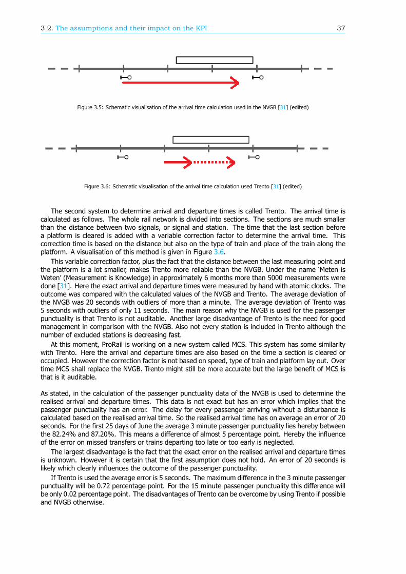
3.2. The assumptions and their impact on the KPI 37

Figure 3.5: Schematic visualisation of the arrival time calculation used in the NVGB [31] (edited)

Figure 3.6: Schematic visualisation of the arrival time calculation used Trento [31] (edited)

The second system to determine arrival and departure times is called Trento. The arrival time iscalculated as follows. The whole rail network is divided into sections. The sections are much smallerthan the distance between two signals, or signal and station. The time that the last section beforea platform is cleared is added with a variable correction factor to determine the arrival time. Thiscorrection time is based on the distance but also on the type of train and place of the train along theplatform. A visualisation of this method is given in Figure 3.6.

This variable correction factor, plus the fact that the distance between the last measuring point andthe platform is a lot smaller, makes Trento more reliable than the NVGB. Under the name ‘Meten isWeten’ (Measurement is Knowledge) in approximately 6 months more than 5000 measurements weredone [31]. Here the exact arrival and departure times were measured by hand with atomic clocks. Theoutcome was compared with the calculated values of the NVGB and Trento. The average deviation ofthe NVGB was 20 seconds with outliers of more than a minute. The average deviation of Trento was5 seconds with outliers of only 11 seconds. The main reason why the NVGB is used for the passengerpunctuality is that Trento is not auditable. Another large disadvantage of Trento is the need for goodmanagement in comparison with the NVGB. Also not every station is included in Trento although thenumber of excluded stations is decreasing fast.

At this moment, ProRail is working on a new system called MCS. This system has some similaritywith Trento. Here the arrival and departure times are also based on the time a section is cleared oroccupied. However the correction factor is not based on speed, type of train and platform lay out. Overtime MCS shall replace the NVGB. Trento might still be more accurate but the large benefit of MCS isthat is it auditable.

As stated, in the calculation of the passenger punctuality data of the NVGB is used to determine therealised arrival and departure times. This data is not exact but has an error which implies that thepassenger punctuality has an error. The delay for every passenger arriving without a disturbance iscalculated based on the realised arrival time. So the realised arrival time has on average an error of 20seconds. For the first 25 days of June the average 3 minute passenger punctuality lies hereby betweenthe 82.24% and 87.20%. This means a difference of almost 5 percentage point. Hereby the influenceof the error on missed transfers or trains departing too late or too early is neglected.

The largest disadvantage is the fact that the exact error on the realised arrival and departure timesis unknown. However it is certain that the first assumption does not hold. An error of 20 seconds islikely which clearly influences the outcome of the passenger punctuality.

If Trento is used the average error is 5 seconds. The maximum difference in the 3 minute passengerpunctuality will be 0.72 percentage point. For the 15 minute passenger punctuality this difference willbe only 0.02 percentage point. The disadvantages of Trento can be overcome by using Trento if possibleand NVGB otherwise.

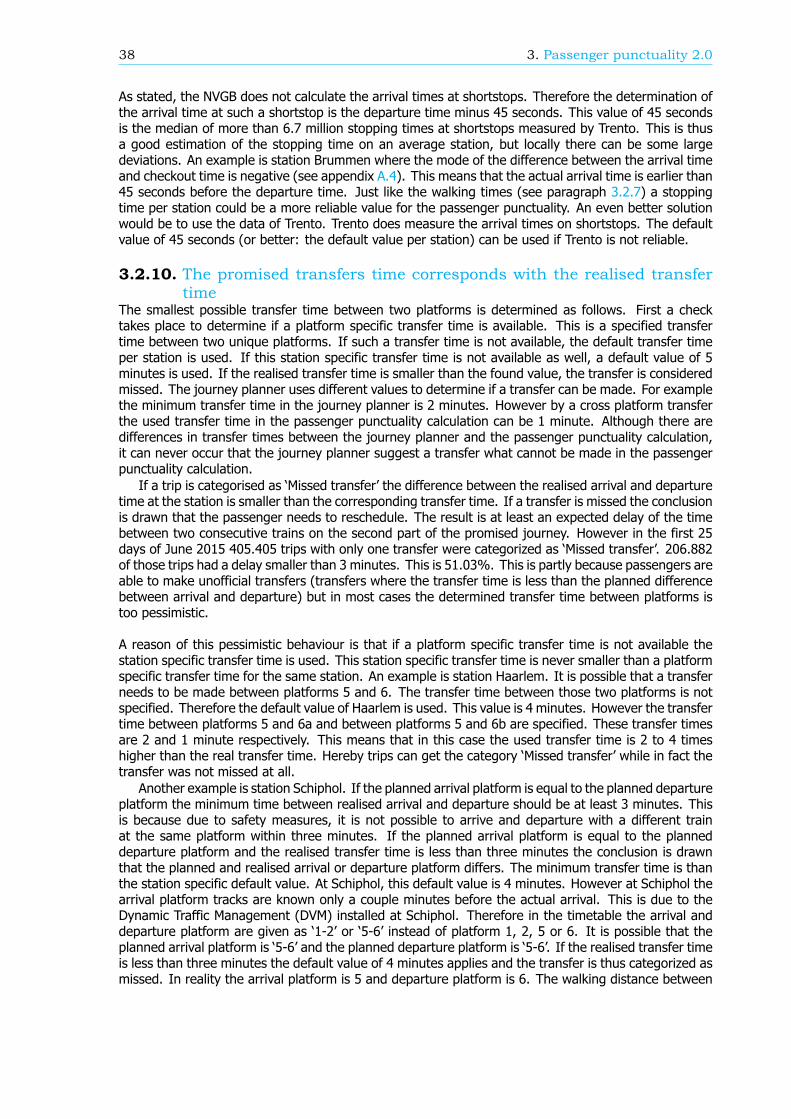
38 3. Passenger punctuality 2.0

As stated, the NVGB does not calculate the arrival times at shortstops. Therefore the determination ofthe arrival time at such a shortstop is the departure time minus 45 seconds. This value of 45 secondsis the median of more than 6.7 million stopping times at shortstops measured by Trento. This is thusa good estimation of the stopping time on an average station, but locally there can be some largedeviations. An example is station Brummen where the mode of the difference between the arrival timeand checkout time is negative (see appendix A.4). This means that the actual arrival time is earlier than45 seconds before the departure time. Just like the walking times (see paragraph 3.2.7) a stoppingtime per station could be a more reliable value for the passenger punctuality. An even better solutionwould be to use the data of Trento. Trento does measure the arrival times on shortstops. The defaultvalue of 45 seconds (or better: the default value per station) can be used if Trento is not reliable.

3.2.10. The promised transfers time corresponds with the realised transfertime

The smallest possible transfer time between two platforms is determined as follows. First a checktakes place to determine if a platform specific transfer time is available. This is a specified transfertime between two unique platforms. If such a transfer time is not available, the default transfer timeper station is used. If this station specific transfer time is not available as well, a default value of 5minutes is used. If the realised transfer time is smaller than the found value, the transfer is consideredmissed. The journey planner uses different values to determine if a transfer can be made. For examplethe minimum transfer time in the journey planner is 2 minutes. However by a cross platform transferthe used transfer time in the passenger punctuality calculation can be 1 minute. Although there aredifferences in transfer times between the journey planner and the passenger punctuality calculation,it can never occur that the journey planner suggest a transfer what cannot be made in the passengerpunctuality calculation.

If a trip is categorised as ‘Missed transfer’ the difference between the realised arrival and departuretime at the station is smaller than the corresponding transfer time. If a transfer is missed the conclusionis drawn that the passenger needs to reschedule. The result is at least an expected delay of the timebetween two consecutive trains on the second part of the promised journey. However in the first 25days of June 2015 405.405 trips with only one transfer were categorized as ‘Missed transfer’. 206.882of those trips had a delay smaller than 3 minutes. This is 51.03%. This is partly because passengers areable to make unofficial transfers (transfers where the transfer time is less than the planned differencebetween arrival and departure) but in most cases the determined transfer time between platforms istoo pessimistic.

A reason of this pessimistic behaviour is that if a platform specific transfer time is not available thestation specific transfer time is used. This station specific transfer time is never smaller than a platformspecific transfer time for the same station. An example is station Haarlem. It is possible that a transferneeds to be made between platforms 5 and 6. The transfer time between those two platforms is notspecified. Therefore the default value of Haarlem is used. This value is 4 minutes. However the transfertime between platforms 5 and 6a and between platforms 5 and 6b are specified. These transfer timesare 2 and 1 minute respectively. This means that in this case the used transfer time is 2 to 4 timeshigher than the real transfer time. Hereby trips can get the category ‘Missed transfer’ while in fact thetransfer was not missed at all.

Another example is station Schiphol. If the planned arrival platform is equal to the planned departureplatform the minimum time between realised arrival and departure should be at least 3 minutes. Thisis because due to safety measures, it is not possible to arrive and departure with a different trainat the same platform within three minutes. If the planned arrival platform is equal to the planneddeparture platform and the realised transfer time is less than three minutes the conclusion is drawnthat the planned and realised arrival or departure platform differs. The minimum transfer time is thanthe station specific default value. At Schiphol, this default value is 4 minutes. However at Schiphol thearrival platform tracks are known only a couple minutes before the actual arrival. This is due to theDynamic Traffic Management (DVM) installed at Schiphol. Therefore in the timetable the arrival anddeparture platform are given as ‘1-2’ or ‘5-6’ instead of platform 1, 2, 5 or 6. It is possible that theplanned arrival platform is ‘5-6’ and the planned departure platform is ‘5-6’. If the realised transfer timeis less than three minutes the default value of 4 minutes applies and the transfer is thus categorized asmissed. In reality the arrival platform is 5 and departure platform is 6. The walking distance between

3.2. The assumptions and their impact on the KPI 39

those platforms is only 1 minute and thereby the transfer is made. The underlying problem is that thedetermination of transfer times is based on the planned arrival and departure platforms. The realisationdata is derived from the NGVB (see paragraph 3.2.9). This system does not log the realised arrival anddeparture platforms. A solution is Trento. This system logs the realised arrival and departure platforms.

The impact of both causes on the large group of passengers without a missed transfer is hard todetermine. As stated 51.03% of the trips categorized as ‘Missed transfer’ had a delay less than 3minutes. For 42.44% of those trips the station specific transfer time is used instead of the platformspecific transfer time and for 1.89% of the trips the planned arrival platform is the same as the planneddeparture platform. Moreover, the percentage of trips where the station specific transfer time is usedinstead of the platform specific transfer time off all the trips categorized as ‘Missed transfer’ is 39.87%.For the transfers where the arrival platform is the same as the departure platform this is 2.54%.

So for 44.33% of the trips where the transfer was made but was categorized as ‘Missed transfer’the reason is one of above. Note that the only condition to assume if a transfer was made is if the finaldelay was less than 3 minutes. For the other 55.67% the reason is that the transfer times are possibletoo large and that the conditions used in the passenger punctuality calculations are too strict. Takefor example a transfer time of 2 minutes. If the difference between arrival time and departure time is1:59 minute the transfer is categorized as not made. Such a condition is harsh certainly when there isan error in the realised arrival and departure time of on average 20 seconds (see paragraph 3.2.9).

The difference between trips where the transfer was made and where the transfer was missed is thedetermination of the final delay. In the first case the realised arrival time is the basis for the delaycalculation, in the second case the checkout time is used. In paragraph 3.2.11 the impact of thisdifference is calculated. In conclusion, the assumption that the promised transfers time correspondswith the realised transfer time does not hold. However the delay calculation by rescheduling does nottake the reason of rescheduling into account. Hereby the mistakes made by wrongly categorizing tripsas ‘Missed transfer’ are corrected.

3.2.11. Reasons to rescheduleThere are five possible scenarios where a trip needs to be rescheduled, see paragraph 3.1.2. Instead ofdetermining the exact route a passenger took, the final delay is determined via the checkout time. Notethat in the official examination of the assumptions of the passenger punctuality only four reasons arementioned: the scenario ‘Train depart too early’ is not mentioned [29]. The corresponding assumptionsare as follows:

1. If a train has a delay of at least 15 minutes before departure, the realised arrival time is thecheckout time minus the walking time between train and card reader

2. If a train does not depart, the realised arrival time is the checkout time minus the walking timebetween train and card reader

3. If a train does not arrive at the destination or transfer station, the realised arrival time is thecheckout time minus the walking time between train and card reader

4. If a transfer is not made, the realised arrival time is the checkout time minus a walking timebetween train and card reader

5. If the first train is missed because it departed too early, the realised arrival time is the checkouttime minus a walking time between train and card reader

For the latter four scenarios (train did not depart, train did not arrive, missed transfer and train departtoo early) it is clear why a trips needs to be rescheduled. The passenger is not able to continue thetrip as promised. This is not necessarily the case when the train departs with a delay of at least15 minutes. The elaboration on the assumption that the threshold value of 15 minutes is correct isgiven in appendix A.5. In conclusion, the size of the initial delay on which the passengers starts toreschedule their trip differs per person, place and time. The chosen value of 15 minutes will resultsin an impact of approximately 0.09 percentage points on the 3 minute passenger punctuality and 0.18percentage points on the 15 minute passenger punctuality. For the current timetable a default value of15 minute as initial delay before rescheduling is acceptable because there is practically no route wherethe frequency of train series is more than 4 per hour. However if this changes a variable value, basedon the frequency of the train series, might be a better solution.

40 3. Passenger punctuality 2.0

If a trips needs to be rescheduled, five possible solutions can be distinguished [32]. These solutionsare listed below. The order is the accuracy, so the most accurate solution is the most upper solution.The effort involved to implement each solution is directly related to the accuracy. The more accurate,the more effort it takes to implement the solution into the passenger punctuality calculation.

1. Based on actual real time travel information Rescheduling takes always place last minute.The passenger is thus able to use real time travel information to reschedule. Conditions to thissolution are the need for the historic real time timetable of the journey planner and the time afterwhich a passenger is going to reschedule.

2. Based on the realisation data The realisation data combined with a shortest path algorithmcan lead to an alternative for the passenger. A condition is that the time after which a passenger isgoing to reschedule needs to be known. This solution uses hindrances further down the route toget the best alternative. However those hindrances are not necessarily known by the passengerwhile rescheduling.

3. Based on promised journeys of other passengers The available data consist of a list ofall travel options. If a trip needs to be rescheduled the best alternative travel option off all theavailable travel options is taken. Here also the time after which a passenger is going to resched-ule should be known. The largest disadvantage is that on the less frequent origin-destinationcombinations there is not always another travel option within a certain time limit, for example 1hour. The same applies to the night hours.

4. Promised journey based on the checkout time A promised journey is the travel option withthe earliest possible arrival time and where the first train departs after the check-in time. If atrip needs to be rescheduled, this new journey could be the travel option with the latest possibledeparture time where the last train arrives before the checkout time. The disadvantage is thatthe checkout time is not necessarily the actual arrival time.

5. No rescheduling This is the solutions currently in use. If a trips needs to be rescheduled, thecheckout time is used to determine the expected arrival time. Nonetheless the checkout time isnot necessarily the actual arrival time.

The rescheduling, in combination with the realisation data, is needed to determine the expectedarrival time. With this new expected arrival time the delay can be calculated by taking the differencebetween this arrival time and the original promised arrival time. The more accurate the reschedulingtakes place, the more accurate the delay can be calculated. The result is more accurate passengerpunctuality.

In the method currently in use trips will not be rescheduled. Instead the checkout time is used to calcu-late the expected arrival time (this is the checkout time mines the walking time between platform andcard reader). More than 5.6 million trips categorized as ‘Trip realised’ are examined. The advantagesof those trips are that both the realised arrival and the checkout time are known. 86.97% of the tripshad arrived within 3 minutes of the promised arrival time. If the arrival time based on the checkouttime is used, only 77.05% of the trips will arrive within 3 minutes. This is a decrease of 11.41%. Thiscould partly due to the fact that the used walking time of 1 minute might not be correct (see paragraph3.2.7) or that there is a deviation in the realisation data (see paragraph 3.2.9) but this does not explainthe whole difference. The same calculation can be done for a delay of 15 minutes. 99.36% of the tripsarrived within 15 minutes of the promised arrival time. Based on the checkout time this is 96.45%: adecrease of 2.93%.

These calculated deviations apply to by trips without a hindrance. Under assumptions that thesedeviations are the same for the trips that needs rescheduling the impact on the passenger punctualitycan be calculated. For the first 25 days of June the number of trips that needs rescheduling and witha delay of less than 3 minutes are determined. This delay is calculated via the checkout time. Theexpected number of trips with a delay less than 3 minutes is thus 11.41% higher. This expectationis added by the number of realised trips with a delay of less than 3 minute. The result is dividedby the total number of trips used in the passenger punctuality to achieve the 3 minute passengerpunctuality corrected for not rescheduling. The average result is a calculated passenger punctuality that

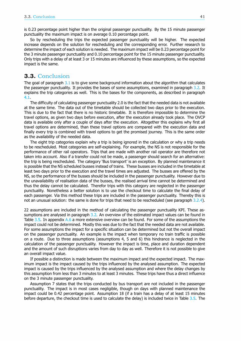
3.3. Conclusion 41

is 0.23 percentage point higher than the original passenger punctuality. By the 15 minute passengerpunctuality the maximum impact is on average 0.10 percentage point.

So by rescheduling the trips the expected passenger punctuality will be higher. The expectedincrease depends on the solution for rescheduling and the corresponding error. Further research todetermine the impact of each solution is needed. The maximum impact will be 0.23 percentage point forthe 3 minute passenger punctuality and 0.10 percentage point for the 15 minute passenger punctuality.Only trips with a delay of at least 3 or 15 minutes are influenced by these assumptions, so the expectedimpact is the same.

3.3. ConclusionThe goal of paragraph 3.1 is to give some background information about the algorithm that calculatesthe passenger punctuality. It provides the bases of some assumptions, examined in paragraph 3.2. Itexplains the trip categories as well. This is the bases for the components, as described in paragraph4.1.

The difficulty of calculating passenger punctuality 2.0 is the fact that the needed data is not availableat the same time. The data out of the timetable should be collected two days prior to the execution.This is due to the fact that there is no historic timetable. It is therefore impossible to determine thetravel options, as given two days before execution, after the execution already took place. The OVCPdata is available only after a couple of days after the execution. Altogether this explains why first alltravel options are determined, than these travel options are compared with the execution data andfinally every trip is combined with travel options to get the promised journey. This is the same orderas the availability of the needed data.

The eight trip categories explain why a trip is being ignored in the calculation or why a trip needsto be rescheduled. Most categories are self-explaining. For example, the NS is not responsible for theperformance of other rail operators. Trips that are made with another rail operator are therefore nottaken into account. Also if a transfer could not be made, a passenger should search for an alternative:the trip is being rescheduled. The category ‘Bus transport’ is an exception. By planned maintenance itis possible that the NS scheduled busses instead of trains. These busses are included in the timetable atleast two days prior to the execution and the travel times are adjusted. The busses are offered by theNS, so the performance of the busses should be included in the passenger punctuality. However due tothe unavailability of realisation data of the busses, the realised arrival time cannot be determined andthus the delay cannot be calculated. Therefor trips with this category are neglected in the passengerpunctuality. Nonetheless a better solution is to use the checkout time to calculate the final delay ofeach passenger. Via this method these trips are included in the passenger punctuality. Thereby this isnot an unusual solution: the same is done for trips that need to be rescheduled (see paragraph 3.2.4).

22 assumptions are included in the method of calculating the passenger punctuality KPI. These as-sumptions are analysed in paragraph 3.2. An overview of the estimated impact values can be found inTable 3.5. In appendix A.6 a more extensive overview can be found. For some of the assumptions theimpact could not be determined. Mostly this was due to the fact that the needed data are not available.For some assumptions the impact for a specific situation can be determined but not the overall impacton the passenger punctuality. An example is the impact when temporary no train traffic is possibleon a route. Due to three assumptions (assumptions 4, 5 and 6) this hindrance is neglected in thecalculation of the passenger punctuality. However the impact is time, place and duration dependentand the amount of such disruptions varies from day to day as well. Therefore it is not possible to givean overall impact value.

If possible a distinction is made between the maximum impact and the expected impact. The max-imum impact is the impact caused by the trips influenced by the analysed assumption. The expectedimpact is caused by the trips influenced by the analysed assumption and where the delay changes bythis assumption from less than 3 minutes to at least 3 minutes. These trips have thus a direct influenceon the 3 minute passenger punctuality.

Assumption 7 states that the trips conducted by bus transport are not included in the passengerpunctuality. The impact is in most cases negligible, though on days with planned maintenance theimpact could be 0.42 percentage point. Assumption 18 (if a train has a delay of at least 15 minutesbefore departure, the checkout time is used to calculate the delay) is included twice in Table 3.5. The

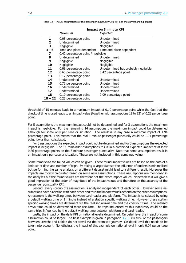
42 3. Passenger punctuality 2.0

Table 3.5: The 22 assumptions of the passenger punctuality 2.0 KPI and the corresponding impact

Impact on 3 minute KPIMaximum Expected

1 0.05 percentage point Undetermined2 Undetermined Undetermined3 Negligible Negligible

4 - 6 Time and place dependent Time and place dependent7 0.42 percentage point / negligible8 Undetermined Undetermined9 Negligible Negligible10 Negligible Negligible11 0.09 percentage point Undetermined but probably negligible12 0.63 percentage point 0.42 percentage point13 0.12 percentage point14 Undetermined Undetermined15 0.72 percentage point Undetermined16 Undetermined Undetermined17 Undetermined Undetermined18 0.10 percentage point 0.09 percentage point

18 – 22 0.23 percentage point

threshold of 15 minutes leads to a maximum impact of 0.10 percentage point while the fact that thecheckout time is used leads to an impact value (together with assumptions 19 to 22) of 0.23 percentagepoint.

For 5 assumptions the maximum impact could not be determined and for 3 assumptions the maximumimpact is negligible. For the remaining 14 assumptions the maximum impact could be determinedalthough for some only per case or situation. The result is in any case a maximal impact of 1.94percentage point. This means that the real 3 minute passenger punctually could be 1.94 percentagepoint lower than calculated.

For 8 assumptions the expected impact could not be determined and for 3 assumptions the expectedimpact is negligible. The 11 remainder assumptions result in a combined expected impact of at least0.86 percentage points on the 3 minute passenger punctuality. Note that some assumptions result inan impact only per case or situation. These are not included in this combined value.

Some remarks to the found values can be given. These found impact values are based on the data of alimit set of days and number of trips. By taking a larger dataset the influence of outliers is minimalizedbut performing the same analysis on a different dataset might lead to a different result. Moreover theimpacts are mostly calculated based on some new assumptions. These assumptions are mentioned inthe analyses but the found values are therefore not the exact impact values. Nonetheless it will give agood impression of the order of magnitude of the impact values and therefore on the accuracy of thepassenger punctuality KPI.

Second, every (group of) assumption is analysed independent of each other. However some as-sumptions have a relation with each other and thus the impact values depend on the other assumptions.An example is the walking times between card reader and platform. The impact is calculated by usinga default walking time of 1 minute instead of a station specific walking time. However these stationspecific walking times are determent via the realised arrival time and the checkout time. The realisedarrival time could be determined more accurate. The trips influenced by this inaccuracy could be thesame trips influenced by the default walking time between platform and card reader.

Lastly, the impact on the daily KPI on national level is determined. On detail level the impact of someassumption could be larger. The best example is given in paragraph 3.2.5. 84.40% of the passengersbetween Utrecht and Leiden do not travel via the promised journey. On detail level this needs to betaken into account. Nonetheless the impact of this example on national level in only 0.04 percentagepoint.

4Breakdown of passenger punctuality

In chapter 3 the structure of the new algorithm to calculate the passenger punctuality is described. Thisalgorithm is divided into five modules. The fifth module generates multiple output tables [24]. Withthese tables the passenger punctuality can be calculated but these tables provided more informationas well. This offers possibilities to additional analyses and performance checks of the rail network.This chapter will describe some of the output possibilities of the available data via performing differentbreakdowns of the passenger punctuality.

From a passengers’ perspective, the most important information stored in the data is the categori-sation of each trip (see paragraph 4.1). These categories form the basis of the components: reasonsfor the passengers why they are delayed. Therefore the passenger punctuality will be broken downinto these components. Paragraph 4.1 describes these components. With the data the places in therail network with the worst passenger punctuality can be found, as well as the places were the sizeof components is higher than on average in the rail network. A necessity is the need to know bywhich threshold a trip is delayed. Paragraph 4.2 will discuss two possible delay thresholds. Finallyin paragraph 4.3 the breakdown of the passenger punctuality is executed. Hereby different optionsto perform a break down are taken into account. The results of the breakdowns are visualised viabreakdown graphs. Appendix B describes how these graphs can be made. Finally in paragraph 4.4some final conclusions are made.

4.1. The componentsThe passenger punctuality can be broken down into reasons why a trip is delayed. These reasonsare based on the passengers’ perspective and called components. This paragraph will introduce thecomponents. In the first section the origin of the components and some background is described. Inthe second section the definitions of the components is gives, as used in this research.

4.1.1. The origin of the componentsAs stated in paragraph 3.1.2, all trips are categorized. Those categories are created to indicate why atrip should not be included or why a trip should be rescheduled. The categories for rescheduling are:

• If the time between check-in and departure is less than 1 minute the promised train could notmade: the train departs too early.

• The train departed from the origin station of the trip or from a transfer station with at least a 15minute delay: the train departs too late.

• The train did not depart at all.• The last reached station of the train was not the destination station of the trip or a transferstation: the train did not arrive.

• The time between arrival and departure at a transfer station was less than the specified transfertime: missed transfer.

If a trip is included in the calculation and requires no rescheduling the trip is categorized as ‘Triprealised’. Note that this does not mean that the trip is without any delays. However the final delay ofthe trip is the delay of the train at the final destination of the trip.

43

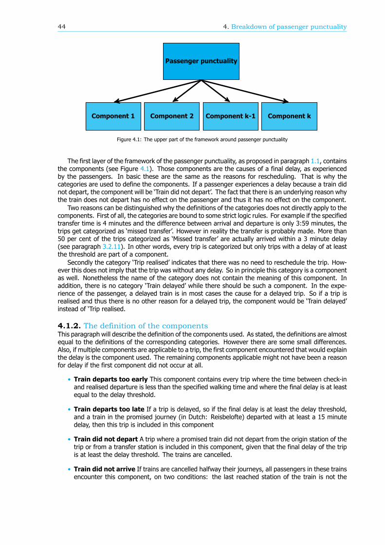
44 4. Breakdown of passenger punctuality

Passenger punctuality

Component 2 Component k-1Component 1 Component k

Figure 4.1: The upper part of the framework around passenger punctuality

The first layer of the framework of the passenger punctuality, as proposed in paragraph 1.1, containsthe components (see Figure 4.1). Those components are the causes of a final delay, as experiencedby the passengers. In basic these are the same as the reasons for rescheduling. That is why thecategories are used to define the components. If a passenger experiences a delay because a train didnot depart, the component will be ‘Train did not depart’. The fact that there is an underlying reason whythe train does not depart has no effect on the passenger and thus it has no effect on the component.

Two reasons can be distinguished why the definitions of the categories does not directly apply to thecomponents. First of all, the categories are bound to some strict logic rules. For example if the specifiedtransfer time is 4 minutes and the difference between arrival and departure is only 3:59 minutes, thetrips get categorized as ‘missed transfer’. However in reality the transfer is probably made. More than50 per cent of the trips categorized as ‘Missed transfer’ are actually arrived within a 3 minute delay(see paragraph 3.2.11). In other words, every trip is categorized but only trips with a delay of at leastthe threshold are part of a component.

Secondly the category ‘Trip realised’ indicates that there was no need to reschedule the trip. How-ever this does not imply that the trip was without any delay. So in principle this category is a componentas well. Nonetheless the name of the category does not contain the meaning of this component. Inaddition, there is no category ‘Train delayed’ while there should be such a component. In the expe-rience of the passenger, a delayed train is in most cases the cause for a delayed trip. So if a trip isrealised and thus there is no other reason for a delayed trip, the component would be ‘Train delayed’instead of ‘Trip realised.

4.1.2. The definition of the componentsThis paragraph will describe the definition of the components used. As stated, the definitions are almostequal to the definitions of the corresponding categories. However there are some small differences.Also, if multiple components are applicable to a trip, the first component encountered that would explainthe delay is the component used. The remaining components applicable might not have been a reasonfor delay if the first component did not occur at all.

• Train departs too early This component contains every trip where the time between check-inand realised departure is less than the specified walking time and where the final delay is at leastequal to the delay threshold.

• Train departs too late If a trip is delayed, so if the final delay is at least the delay threshold,and a train in the promised journey (in Dutch: Reisbelofte) departed with at least a 15 minutedelay, then this trip is included in this component

• Train did not depart A trip where a promised train did not depart from the origin station of thetrip or from a transfer station is included in this component, given that the final delay of the tripis at least the delay threshold. The trains are cancelled.

• Train did not arrive If trains are cancelled halfway their journeys, all passengers in these trainsencounter this component, on two conditions: the last reached station of the train is not the

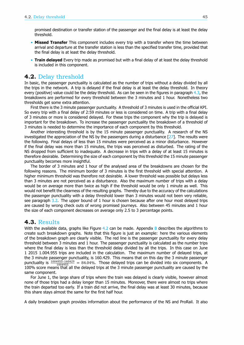
4.2. Delay threshold 45

promised destination or transfer station of the passenger and the final delay is at least the delaythreshold.

• Missed Transfer This component includes every trip with a transfer where the time betweenarrival and departure at the transfer station is less than the specified transfer time, provided thatthe final delay is at least the delay threshold.

• Train delayed Every trip made as promised but with a final delay of at least the delay thresholdis included in this component.

4.2. Delay thresholdIn basic, the passenger punctuality is calculated as the number of trips without a delay divided by allthe trips in the network. A trip is delayed if the final delay is at least the delay threshold. In theoryevery (positive) value could be the delay threshold. As can be seen in the figures in paragraph 4.3, thebreakdowns are performed for every threshold between the 3 minutes and 1 hour. Nonetheless twothresholds get some extra attention.

First there is the 3 minute passenger punctuality. A threshold of 3 minutes is used in the official KPI.So every trip with a final delay of 2:59 minutes or less is considered on time. A trip with a final delayof 3 minutes or more is considered delayed. For these trips the component why the trip is delayed isimportant for the breakdown. To increase the passenger punctuality the breakdown of a threshold of3 minutes is needed to determine the importance of each component by this threshold.

Another interesting threshold is by the 15 minute passenger punctuality. A research of the NSinvestigated the appreciation of the NS by the passengers during a disturbance [27]. The results werethe following. Final delays of less than 15 minutes were perceived as a minor disturbance. Howeverif the final delay was more than 15 minutes, the trips was perceived as disturbed. The rating of theNS dropped from sufficient to inadequate. A decrease in trips with a delay of at least 15 minutes istherefore desirable. Determining the size of each component by this threshold the 15 minute passengerpunctuality becomes more insightful.

The border of 3 minutes and 1 hour of the analysed area of the breakdowns are chosen for thefollowing reasons. The minimum border of 3 minutes is the first threshold with special attention. Ahigher minimum threshold was therefore not desirable. A lower threshold was possible but delays lessthan 3 minutes are not perceived as a disturbance. Also the maximum number of trips with a delaywould be on average more than twice as high if the threshold would be only 1 minute as well. Thiswould not benefit the clearness of the resulting graphs. Thereby due to the accuracy of the calculationsthe passenger punctuality with a delay threshold lower than 3 minutes would not been very reliable,see paragraph 3.2. The upper bound of 1 hour is chosen because after one hour most delayed tripsare caused by wrong check outs of wrong promised journeys. Also between 45 minutes and 1 hourthe size of each component decreases on average only 2.5 to 3 percentage points.

4.3. ResultsWith the available data, graphs like Figure 4.2 can be made. Appendix B describes the algorithms tocreate such breakdown graphs. Note that this figure is just an example: here the various elementsof the breakdown graph are clearly visible. The red line is the passenger punctuality for every delaythreshold between 3 minutes and 1 hour. The passenger punctuality is calculated as the number tripswhere the final delay is less than the threshold delay divided by all the trips. In this case on June1 2015 1.004.955 trips are included in the calculation. The maximum number of delayed trips, atthe 3 minute passenger punctuality, is 160.429. This means that on this day the 3 minute passengerpunctuality is – = 84.04%. Those delayed trips can be divided into six components. A100% score means that all the delayed trips at the 3 minute passenger punctuality are caused by thesame component.

For June 1, the large share of trips where the train was delayed is clearly visible, however almostnone of those trips had a delay longer than 15 minutes. Moreover, there were almost no trips wherethe train departed too early. If a train did not arrive, the final delay was at least 30 minutes, becausethis share stays almost the same for the first half hour.

A daily breakdown graph provides information about the performance of the NS and ProRail. It also

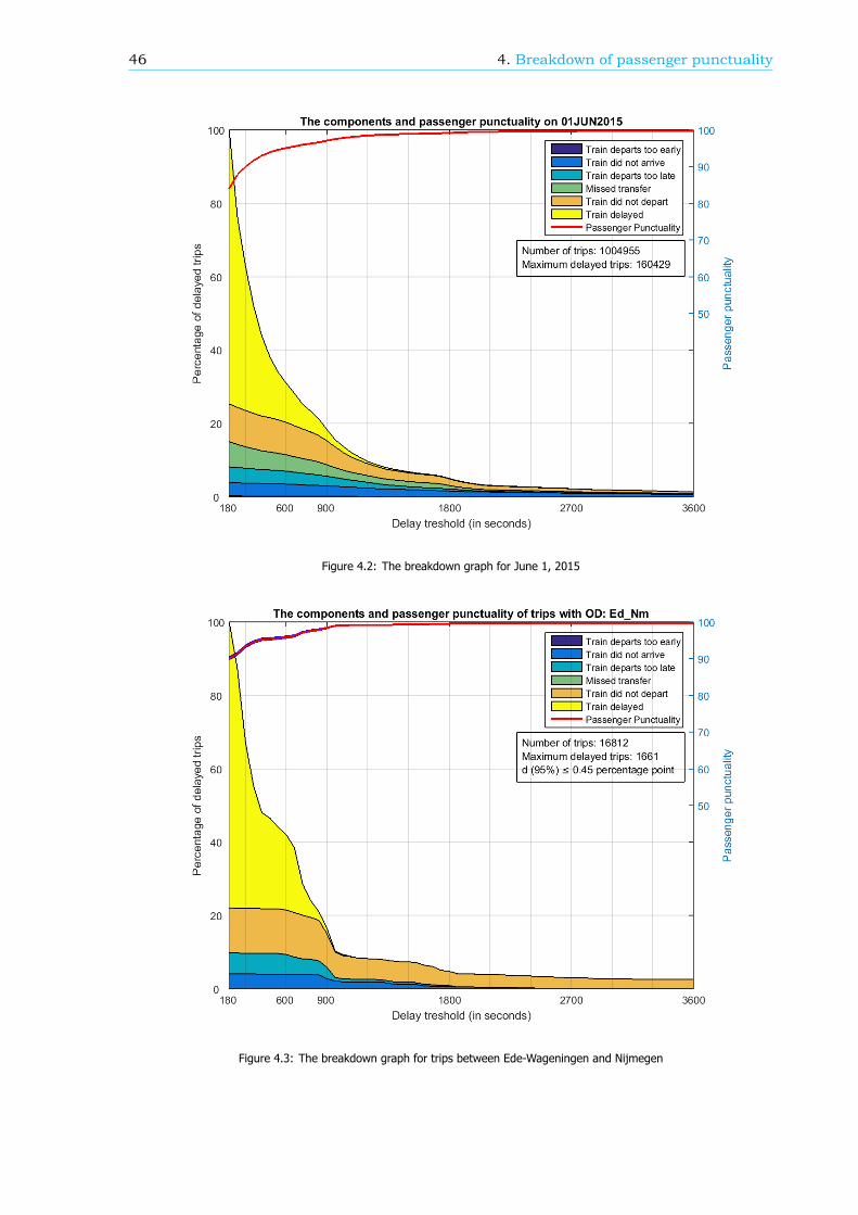
46 4. Breakdown of passenger punctuality

Figure 4.2: The breakdown graph for June 1, 2015

Figure 4.3: The breakdown graph for trips between Ede-Wageningen and Nijmegen

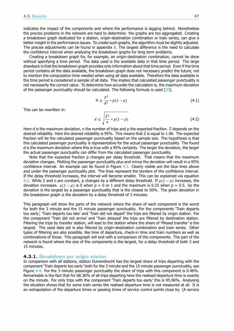
4.3. Results 47

indicates the impact of the components and where the performance is lagging behind. Nonethelessthe precise problems in the network are hard to determine: the graphs are too aggregated. Creatinga breakdown graph dedicated for a station, origin-destination combination or train series, can give abetter insight in the performance issues. To create such graphs, the algorithmmust be slightly adjusted.The precise adjustments can be found in appendix B. The largest difference is the need to calculatethe confidence interval when analysing the breakdown graphs for long term problems.

Creating a breakdown graph for, for example, an origin-destination combination, cannot be donewithout specifying a time period. The data used is the available data in that time period. The largedrawback is that the breakdown graph provides only information about that time period. Even if the timeperiod contains all the data available, the breakdown graph does not necessary predict the future, notto mention the computation time needed when using all data available. Therefore the data available inthe time period is considered a sample of all data. This implies that calculated passenger punctuality isnot necessarily the correct value. To determine how accurate the calculation is, the maximum deviationof the passenger punctuality should be calculated. The following formula is used [33].

𝑁 ≥ 𝑍𝑑 ∗ 𝑝(1 − 𝑝) (4.1)

This can be rewritten in:

𝑑 ≤ √𝑍𝑛 ∗ 𝑝(1 − 𝑝) (4.2)

Here d is the maximum deviation, n the number of trips and p the expected fraction. Z depends on thedesired reliability. Here the desired reliability is 95%. This means that Z is equal to 1.96. The expectedfraction will be the calculated passenger punctuality based on the sample size. The hypothesis is thatthis calculated passenger punctuality is representative for the actual passenger punctuality. The foundd is the maximum deviation where this is true with a 95% certainty. The larger the deviation, the largerthe actual passenger punctuality can differ from the calculated passenger punctuality.

Note that the expected fraction p changes per delay threshold. That means that the maximumdeviation changes. Plotting the passenger punctuality plus and minus the deviation will result in a 95%confidence interval. An example can be found in Figure 4.3. Clearly visible are the blue lines aboveand under the passenger punctuality plot. The lines represent the borders of the confidence interval.If the delay threshold increases, the interval will become smaller. This can be explained via equation4.2. While Z and n are constant, p changes by a different delay threshold. If 𝑝(1 − 𝑝) increases, thedeviation increases. 𝑝(1 − 𝑝) is 0 when p = 0 or 1 and the maximum is 0.25 when p = 0.5. So thedeviation is the largest by a passenger punctuality that is the closest to 50%. The given deviation inthe breakdown graph is the deviation by a delay threshold of 3 minutes.

This paragraph will show the parts of the network where the share of each component is the worstfor both the 3 minute and the 15 minute passenger punctuality. For the components ‘Train departstoo early’, ‘Train departs too late’ and ‘Train did not depart’ the trips are filtered by origin station. Forthe component ‘Train did not arrive’ and ‘Train delayed’ the trips are filtered by destination station.Filtering the trips by transfer station, will lead to the station where the share of ‘Missed transfer’ is thelargest. The used data set is also filtered by origin-destination combination and train series. Othertypes of filtering are also possible, like time of departure, check-in time and train numbers as well ascombinations of those. This paragraph will end with a comparison of the components. The part of thenetwork is found where the size of the components is the largest, for a delay threshold of both 3 and15 minutes.

4.3.1. Breakdown per origin stationIn comparison with all stations, station Duivendrecht has the largest share of trips departing with thecomponent ‘Train departs too early’ both for the 3 minute and the 15 minute passenger punctuality, seeFigure 4.4. For the 3 minute passenger punctuality the share of trips with this component is 0.46%.Remarkable is the fact that for 68.36% of all trips departing here the realised departure time is exactlyon the minute. For only trips with the component ‘Train departs too early’ this is 95.96%. Analysingthe situation shows that for some train series the realised departure time is not measured at all. It isan extrapolation of the departure times or passing times of service control points close by. (A service

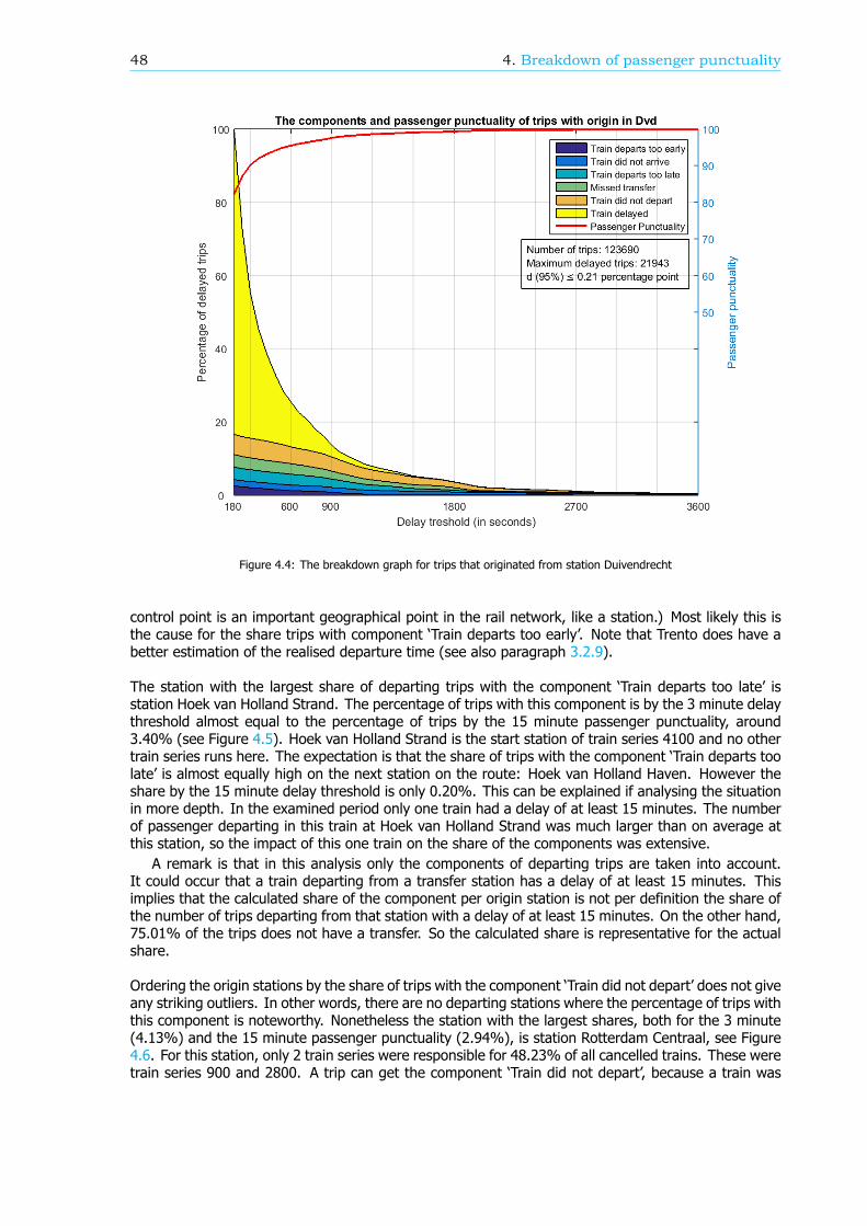
48 4. Breakdown of passenger punctuality

Figure 4.4: The breakdown graph for trips that originated from station Duivendrecht

control point is an important geographical point in the rail network, like a station.) Most likely this isthe cause for the share trips with component ‘Train departs too early’. Note that Trento does have abetter estimation of the realised departure time (see also paragraph 3.2.9).

The station with the largest share of departing trips with the component ‘Train departs too late’ isstation Hoek van Holland Strand. The percentage of trips with this component is by the 3 minute delaythreshold almost equal to the percentage of trips by the 15 minute passenger punctuality, around3.40% (see Figure 4.5). Hoek van Holland Strand is the start station of train series 4100 and no othertrain series runs here. The expectation is that the share of trips with the component ‘Train departs toolate’ is almost equally high on the next station on the route: Hoek van Holland Haven. However theshare by the 15 minute delay threshold is only 0.20%. This can be explained if analysing the situationin more depth. In the examined period only one train had a delay of at least 15 minutes. The numberof passenger departing in this train at Hoek van Holland Strand was much larger than on average atthis station, so the impact of this one train on the share of the components was extensive.

A remark is that in this analysis only the components of departing trips are taken into account.It could occur that a train departing from a transfer station has a delay of at least 15 minutes. Thisimplies that the calculated share of the component per origin station is not per definition the share ofthe number of trips departing from that station with a delay of at least 15 minutes. On the other hand,75.01% of the trips does not have a transfer. So the calculated share is representative for the actualshare.

Ordering the origin stations by the share of trips with the component ‘Train did not depart’ does not giveany striking outliers. In other words, there are no departing stations where the percentage of trips withthis component is noteworthy. Nonetheless the station with the largest shares, both for the 3 minute(4.13%) and the 15 minute passenger punctuality (2.94%), is station Rotterdam Centraal, see Figure4.6. For this station, only 2 train series were responsible for 48.23% of all cancelled trains. These weretrain series 900 and 2800. A trip can get the component ‘Train did not depart’, because a train was

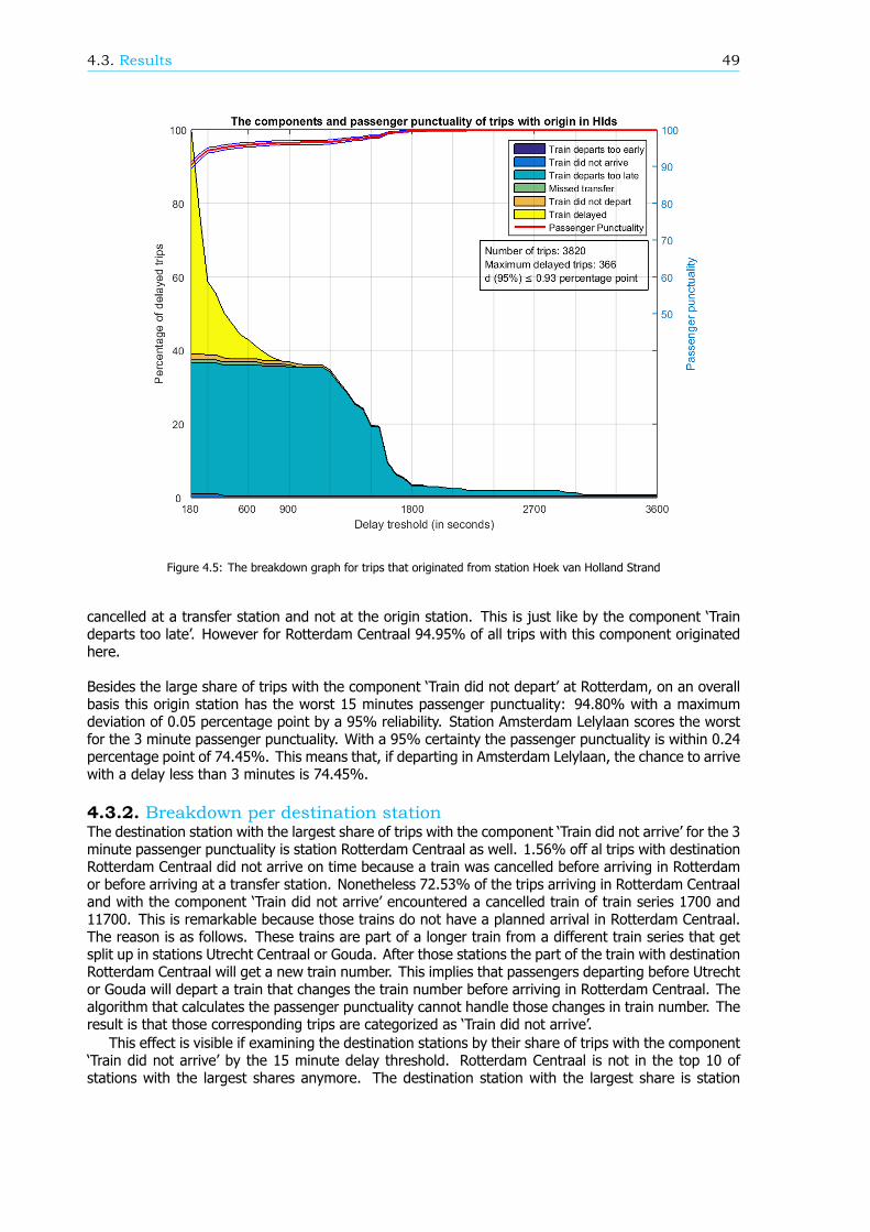
4.3. Results 49

Figure 4.5: The breakdown graph for trips that originated from station Hoek van Holland Strand

cancelled at a transfer station and not at the origin station. This is just like by the component ‘Traindeparts too late’. However for Rotterdam Centraal 94.95% of all trips with this component originatedhere.

Besides the large share of trips with the component ‘Train did not depart’ at Rotterdam, on an overallbasis this origin station has the worst 15 minutes passenger punctuality: 94.80% with a maximumdeviation of 0.05 percentage point by a 95% reliability. Station Amsterdam Lelylaan scores the worstfor the 3 minute passenger punctuality. With a 95% certainty the passenger punctuality is within 0.24percentage point of 74.45%. This means that, if departing in Amsterdam Lelylaan, the chance to arrivewith a delay less than 3 minutes is 74.45%.

4.3.2. Breakdown per destination stationThe destination station with the largest share of trips with the component ‘Train did not arrive’ for the 3minute passenger punctuality is station Rotterdam Centraal as well. 1.56% off al trips with destinationRotterdam Centraal did not arrive on time because a train was cancelled before arriving in Rotterdamor before arriving at a transfer station. Nonetheless 72.53% of the trips arriving in Rotterdam Centraaland with the component ‘Train did not arrive’ encountered a cancelled train of train series 1700 and11700. This is remarkable because those trains do not have a planned arrival in Rotterdam Centraal.The reason is as follows. These trains are part of a longer train from a different train series that getsplit up in stations Utrecht Centraal or Gouda. After those stations the part of the train with destinationRotterdam Centraal will get a new train number. This implies that passengers departing before Utrechtor Gouda will depart a train that changes the train number before arriving in Rotterdam Centraal. Thealgorithm that calculates the passenger punctuality cannot handle those changes in train number. Theresult is that those corresponding trips are categorized as ‘Train did not arrive’.

This effect is visible if examining the destination stations by their share of trips with the component‘Train did not arrive’ by the 15 minute delay threshold. Rotterdam Centraal is not in the top 10 ofstations with the largest shares anymore. The destination station with the largest share is station

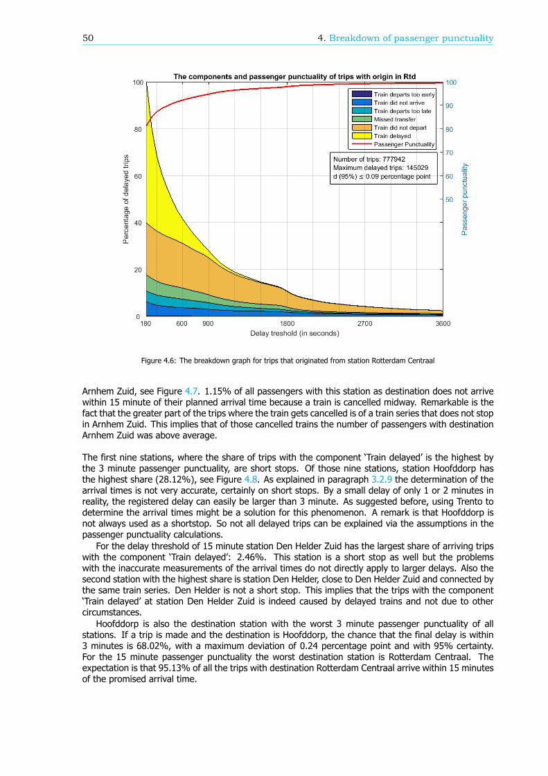
50 4. Breakdown of passenger punctuality

Figure 4.6: The breakdown graph for trips that originated from station Rotterdam Centraal

Arnhem Zuid, see Figure 4.7. 1.15% of all passengers with this station as destination does not arrivewithin 15 minute of their planned arrival time because a train is cancelled midway. Remarkable is thefact that the greater part of the trips where the train gets cancelled is of a train series that does not stopin Arnhem Zuid. This implies that of those cancelled trains the number of passengers with destinationArnhem Zuid was above average.

The first nine stations, where the share of trips with the component ‘Train delayed’ is the highest bythe 3 minute passenger punctuality, are short stops. Of those nine stations, station Hoofddorp hasthe highest share (28.12%), see Figure 4.8. As explained in paragraph 3.2.9 the determination of thearrival times is not very accurate, certainly on short stops. By a small delay of only 1 or 2 minutes inreality, the registered delay can easily be larger than 3 minute. As suggested before, using Trento todetermine the arrival times might be a solution for this phenomenon. A remark is that Hoofddorp isnot always used as a shortstop. So not all delayed trips can be explained via the assumptions in thepassenger punctuality calculations.

For the delay threshold of 15 minute station Den Helder Zuid has the largest share of arriving tripswith the component ‘Train delayed’: 2.46%. This station is a short stop as well but the problemswith the inaccurate measurements of the arrival times do not directly apply to larger delays. Also thesecond station with the highest share is station Den Helder, close to Den Helder Zuid and connected bythe same train series. Den Helder is not a short stop. This implies that the trips with the component‘Train delayed’ at station Den Helder Zuid is indeed caused by delayed trains and not due to othercircumstances.

Hoofddorp is also the destination station with the worst 3 minute passenger punctuality of allstations. If a trip is made and the destination is Hoofddorp, the chance that the final delay is within3 minutes is 68.02%, with a maximum deviation of 0.24 percentage point and with 95% certainty.For the 15 minute passenger punctuality the worst destination station is Rotterdam Centraal. Theexpectation is that 95.13% of all the trips with destination Rotterdam Centraal arrive within 15 minutesof the promised arrival time.

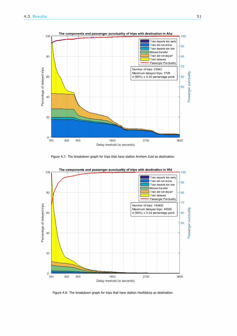
4.3. Results 51

Figure 4.7: The breakdown graph for trips that have station Arnhem Zuid as destination

Figure 4.8: The breakdown graph for trips that have station Hoofddorp as destination

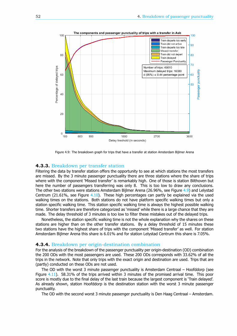
52 4. Breakdown of passenger punctuality

Figure 4.9: The breakdown graph for trips that have a transfer at station Amsterdam Bijlmer Arena

4.3.3. Breakdown per transfer stationFiltering the data by transfer station offers the opportunity to see at which stations the most transfersare missed. By the 3 minute passenger punctuality there are three stations where the share of tripswhere with the component ‘Missed transfer’ is remarkably high. One of those is station Bilthoven buthere the number of passengers transferring was only 8. This is too low to draw any conclusions.The other two stations were stations Amsterdam Bijlmer Arena (26.96%, see Figure 4.9) and LelystadCentrum (21.61%, see Figure 4.10). These high percentages can partly be explained via the usedwalking times on the stations. Both stations do not have platform specific walking times but only astation specific walking time. This station specific walking time is always the highest possible walkingtime. Shorter transfers are therefore categorized as ‘missed’ while there is a large chance that they aremade. The delay threshold of 3 minutes is too low to filter these mistakes out of the delayed trips.

Nonetheless, the station specific walking time is not the whole explanation why the shares on thesestations are higher than on the other transfer stations. By a delay threshold of 15 minutes thesetwo stations have the highest share of trips with the component ‘Missed transfer’ as well. For stationAmsterdam Bijlmer Arena this share is 6.01% and for station Lelystad Centrum this share is 7.05%.

4.3.4. Breakdown per origin-destination combinationFor the analysis of the breakdown of the passenger punctuality per origin-destination (OD) combinationthe 200 ODs with the most passengers are used. These 200 ODs corresponds with 33.62% of all thetrips in the network. Note that only trips with the exact origin and destination are used. Trips that are(partly) conducted on these ODs are not used.

The OD with the worst 3 minute passenger punctuality is Amsterdam Centraal – Hoofddorp (seeFigure 4.11). 58.31% of the trips arrived within 3 minutes of the promised arrival time. This poorscore is mostly due to the final delay of the last train because the largest component is ‘Train delayed’.As already shown, station Hoofddorp is the destination station with the worst 3 minute passengerpunctuality.

The OD with the second worst 3 minute passenger punctuality is Den Haag Centraal – Amsterdam.

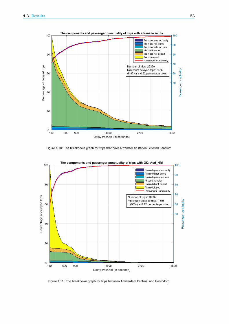
4.3. Results 53

Figure 4.10: The breakdown graph for trips that have a transfer at station Lelystad Centrum

Figure 4.11: The breakdown graph for trips between Amsterdam Centraal and Hoofddorp

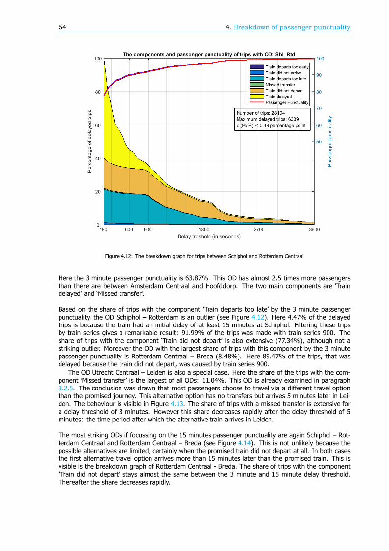
54 4. Breakdown of passenger punctuality

Figure 4.12: The breakdown graph for trips between Schiphol and Rotterdam Centraal

Here the 3 minute passenger punctuality is 63.87%. This OD has almost 2.5 times more passengersthan there are between Amsterdam Centraal and Hoofddorp. The two main components are ‘Traindelayed’ and ‘Missed transfer’.

Based on the share of trips with the component ‘Train departs too late’ by the 3 minute passengerpunctuality, the OD Schiphol – Rotterdam is an outlier (see Figure 4.12). Here 4.47% of the delayedtrips is because the train had an initial delay of at least 15 minutes at Schiphol. Filtering these tripsby train series gives a remarkable result: 91.99% of the trips was made with train series 900. Theshare of trips with the component ‘Train did not depart’ is also extensive (77.34%), although not astriking outlier. Moreover the OD with the largest share of trips with this component by the 3 minutepassenger punctuality is Rotterdam Centraal – Breda (8.48%). Here 89.47% of the trips, that wasdelayed because the train did not depart, was caused by train series 900.

The OD Utrecht Centraal – Leiden is also a special case. Here the share of the trips with the com-ponent ‘Missed transfer’ is the largest of all ODs: 11.04%. This OD is already examined in paragraph3.2.5. The conclusion was drawn that most passengers choose to travel via a different travel optionthan the promised journey. This alternative option has no transfers but arrives 5 minutes later in Lei-den. The behaviour is visible in Figure 4.13. The share of trips with a missed transfer is extensive fora delay threshold of 3 minutes. However this share decreases rapidly after the delay threshold of 5minutes: the time period after which the alternative train arrives in Leiden.

The most striking ODs if focussing on the 15 minutes passenger punctuality are again Schiphol – Rot-terdam Centraal and Rotterdam Centraal – Breda (see Figure 4.14). This is not unlikely because thepossible alternatives are limited, certainly when the promised train did not depart at all. In both casesthe first alternative travel option arrives more than 15 minutes later than the promised train. This isvisible is the breakdown graph of Rotterdam Centraal - Breda. The share of trips with the component’Train did not depart’ stays almost the same between the 3 minute and 15 minute delay threshold.Thereafter the share decreases rapidly.

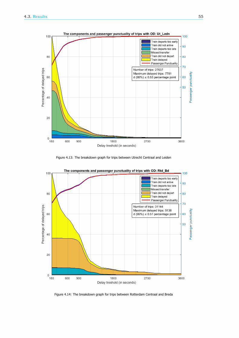
4.3. Results 55

Figure 4.13: The breakdown graph for trips between Utrecht Centraal and Leiden

Figure 4.14: The breakdown graph for trips between Rotterdam Centraal and Breda

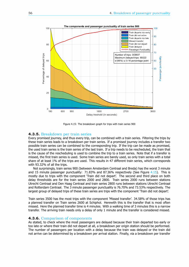
56 4. Breakdown of passenger punctuality

Figure 4.15: The breakdown graph for trips with train series 900

4.3.5. Breakdown per train seriesEvery promised journey, and thus every trip, can be combined with a train series. Filtering the trips bythese train series leads to a breakdown per train series. If a promised journey includes a transfer twopossible train series can be combined to the corresponding trip. If the trip can be made as promised,the used train series is the train series of the last train. If a trip needs to be rescheduled, the train thatis the cause of the rescheduling is used to combine the trip to a train series. Note that if a transfer ismissed, the first train series is used. Some train series are barely used, so only train series with a totalshare of at least 1% of the trips are used. This results in 47 different train series, which correspondswith 93.32% of all the trips.

Not surprisingly, train series 900 (between Amsterdam Centraal and Breda) has the worst 3 minuteand 15 minute passenger punctuality: 71.83% and 87.36% respectively (See Figure 4.15). This ismostly due to trips with the component ‘Train did not depart’. The second and third place on bothdelay thresholds are for the train series 2000 and 2800. Train series 2000 runs between stationsUtrecht Centraal and Den Haag Centraal and train series 2800 runs between stations Utrecht Centraaland Rotterdam Centraal. The 3 minute passenger punctuality is 76.70% and 73.53% respectively. Thelargest group of delayed trips of these train series are trips with the component ‘Train did not depart’.

Train series 3500 has the most trips with the component ’Missed transfer’. 34.58% of those trips hasa planned transfer on Train series 2600 at Schiphol. Herewith this is the transfer that is most oftenmissed. Here the planned transfer time is 4 minutes. With a walking time of 3 minutes this is a narrowtransfer. The arriving train needs only a delay of only 1 minute and the transfer is considered missed.

4.3.6. Comparison of componentsAs stated, to check where the most passengers are delayed because their train departed too early ortoo late or where their train did not depart at all, a breakdown per origin station should be performed.The number of passengers per location with a delay because the train was delayed or the train didnot arrive can be determined by a breakdown per arrival station. Finally, via a breakdown per transfer

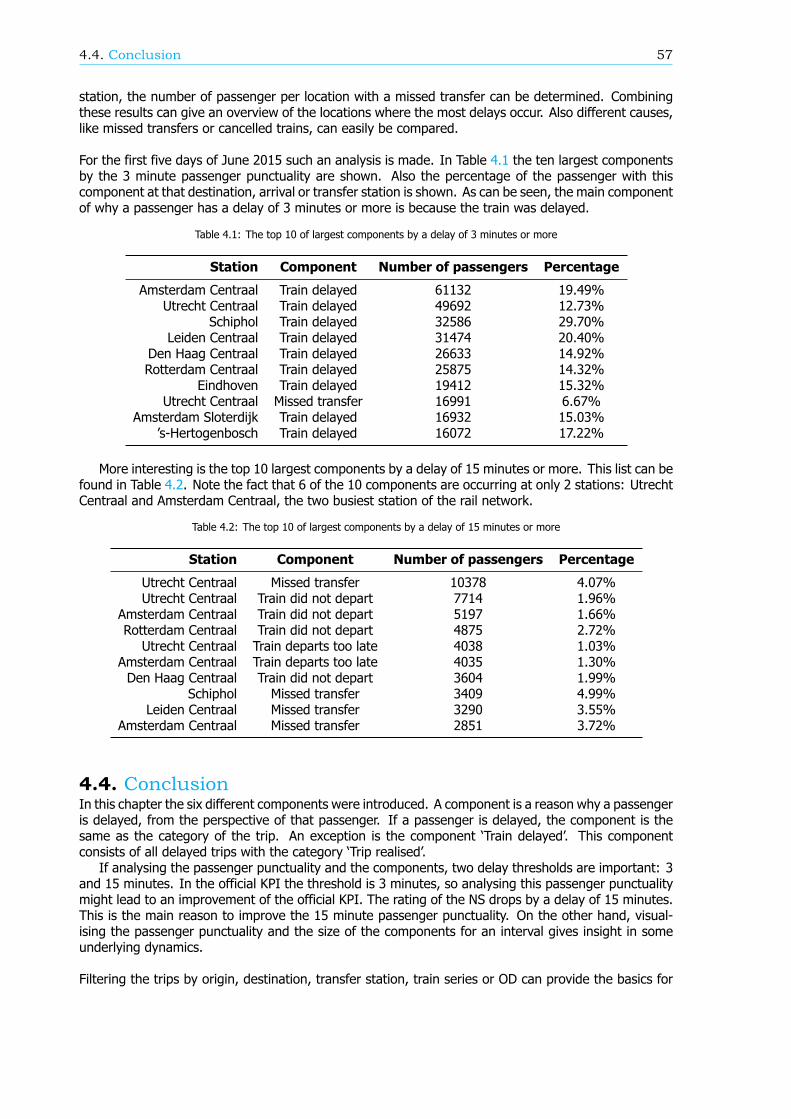
4.4. Conclusion 57

station, the number of passenger per location with a missed transfer can be determined. Combiningthese results can give an overview of the locations where the most delays occur. Also different causes,like missed transfers or cancelled trains, can easily be compared.

For the first five days of June 2015 such an analysis is made. In Table 4.1 the ten largest componentsby the 3 minute passenger punctuality are shown. Also the percentage of the passenger with thiscomponent at that destination, arrival or transfer station is shown. As can be seen, the main componentof why a passenger has a delay of 3 minutes or more is because the train was delayed.

Table 4.1: The top 10 of largest components by a delay of 3 minutes or more

Station Component Number of passengers Percentage

Amsterdam Centraal Train delayed 61132 19.49%Utrecht Centraal Train delayed 49692 12.73%

Schiphol Train delayed 32586 29.70%Leiden Centraal Train delayed 31474 20.40%

Den Haag Centraal Train delayed 26633 14.92%Rotterdam Centraal Train delayed 25875 14.32%

Eindhoven Train delayed 19412 15.32%Utrecht Centraal Missed transfer 16991 6.67%

Amsterdam Sloterdijk Train delayed 16932 15.03%’s-Hertogenbosch Train delayed 16072 17.22%

More interesting is the top 10 largest components by a delay of 15 minutes or more. This list can befound in Table 4.2. Note the fact that 6 of the 10 components are occurring at only 2 stations: UtrechtCentraal and Amsterdam Centraal, the two busiest station of the rail network.

Table 4.2: The top 10 of largest components by a delay of 15 minutes or more

Station Component Number of passengers Percentage

Utrecht Centraal Missed transfer 10378 4.07%Utrecht Centraal Train did not depart 7714 1.96%

Amsterdam Centraal Train did not depart 5197 1.66%Rotterdam Centraal Train did not depart 4875 2.72%Utrecht Centraal Train departs too late 4038 1.03%

Amsterdam Centraal Train departs too late 4035 1.30%Den Haag Centraal Train did not depart 3604 1.99%

Schiphol Missed transfer 3409 4.99%Leiden Centraal Missed transfer 3290 3.55%

Amsterdam Centraal Missed transfer 2851 3.72%

4.4. ConclusionIn this chapter the six different components were introduced. A component is a reason why a passengeris delayed, from the perspective of that passenger. If a passenger is delayed, the component is thesame as the category of the trip. An exception is the component ‘Train delayed’. This componentconsists of all delayed trips with the category ‘Trip realised’.

If analysing the passenger punctuality and the components, two delay thresholds are important: 3and 15 minutes. In the official KPI the threshold is 3 minutes, so analysing this passenger punctualitymight lead to an improvement of the official KPI. The rating of the NS drops by a delay of 15 minutes.This is the main reason to improve the 15 minute passenger punctuality. On the other hand, visual-ising the passenger punctuality and the size of the components for an interval gives insight in someunderlying dynamics.

Filtering the trips by origin, destination, transfer station, train series or OD can provide the basics for

58 4. Breakdown of passenger punctuality

the breakdowns of the passenger punctuality for subsets of the rail network. This is done in paragraph4.3. Analysing the outliers, thus parts of the network where the size of a components is much largerthan on average, lead most often to drawbacks of the algorithm that calculates passenger punctualitythan to actual performance problems in the rail network. An example is the stations where the sizeof the component ‘Train delayed’ by the 3 minute passenger punctuality is the largest. These stationsare all short stops. The actual arrival and departure times on these stations differ from the arrival anddeparture times used in the passenger punctuality calculation.

There is one remarkable drawback of the passenger punctuality calculation, found during the break-down analyses: the algorithm cannot handle trains that have multiple train numbers during a singlerun. This will lead to the wrong categorisation of trips. Not only has this an impact on the passen-ger punctuality, by small delay thresholds this will result in more trips with the component ‘Train didnot arrive’ than actually the case. This drawback is remarkable because it is not mentioned in thedocumentation of the algorithm [24] or in the assumptions (paragraph 3.2).

A last remark to the breakdown of the passenger punctuality is that the found results should alwaysrequire an explanation. The best example is the share of trips with the component ‘Trains depart toolate’, departing at station Hoek van Holland Strand. This share is the highest of all stations in the railnetwork. Although the data of almost a month used, the size of the share was mostly due to only 1train.

5Models to describe passenger

punctuality

Chapter 3 describes how the passenger punctuality is calculated. Based on the analyses of the as-sumptions, the calculation can be improved in order to achieve a more reliable KPI. Although a morereliable KPI would improve the passenger punctuality, it does not necessarily increase the passengerpunctuality. Nonetheless this is a goal of ProRail and the NS (see chapter 2). Higher passenger punc-tuality implies that the performance of ProRail and the NS increases. In paragraph 5.1 two modelsare discussed. These models are created to provide insight in the processes related to the passengerpunctuality.

The focus of the two models is the Transport control and Traffic control. Paragraph 5.2 analysesthe underlying processes through process indicators. The indicators give information about the per-formance of the processes. Both models suggest that if the performance of the processes increases,eventually the passenger punctuality will increase. In paragraph 5.3 the correlation in both modelsis calculated. This will give information whether steering on the process indicators will increase thepassenger punctuality or not. Finally in paragraph 5.4 the results of the two models are compared andsome conclusion can be made.

5.1. Introduction of the two modelsIn order to increase passenger punctuality ProRail and the NS created a model that describes passengerpunctuality. In this model the passenger punctuality is related to the delayed and cancelled trains(see paragraph 5.1.1). The processes of the Transport control and Traffic control should minimisethe number of delayed and cancelled trains. This will than result in higher passenger punctuality. Inparagraph 5.1.2 a second model is proposed. Here the delayed and cancelled trains are not used, mainlybecause it is unknown how many passengers every train contains. Instead the passenger punctuality isdivided into the components (see chapter 4). The components are roughly the percentage of delayedtrips because a train is delayed or cancelled.

5.1.1. Model 1: The model of ProRail and the NSProRail and the NS have developed a model where the passenger punctuality is related to underlyingprocesses in separate units within ProRail and the NS (see Figure 5.1). This model can be used todescribe passenger punctuality. In the top level, the management steers on passenger punctuality. Ahigher KPI means an improved performance of ProRail and the NS. To achieve this, on a lower level everyinvolved business unit steers on ‘Explainable Train Deviations’ (in Dutch: Te Verklaren Trein Afwijking,TVTA). The model anticipate on the idea that these TVTAs are the main cause for the dispunctuality:by decreasing the number of TVTAs, the punctuality will increase.

Another level lower, the individual units corresponding with the business unit steer on the processindicators. If the performance increases, the number of TVTAs occurring will decrease and thus thepassenger punctuality will become higher. An elaboration of the process indicators belonging to thebusiness unit Transport control and Traffic control (TB / VL) can be found in paragraph 5.2. The

59

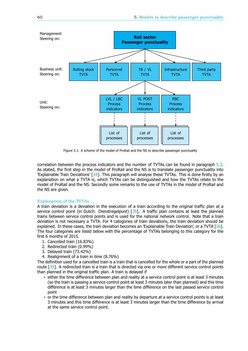
60 5. Models to describe passenger punctuality

Rail sectorPassenger punctuality

TB / VLTVTA

PersonnelTVTA

Rolling stockTVTA

InfrastructureTVTA

Third partyTVTA

VL POSTProcessindicators

LVL / LBCProcessindicators

RBCProcessindicators

List ofprocesses

List ofprocesses

List ofprocesses

Business unit:Steering on:

Management:Steering on:

Unit:Steering on:

Figure 5.1: A scheme of the model of ProRail and the NS to describe passenger punctuality

correlation between the process indicators and the number of TVTAs can be found in paragraph 5.3.As stated, the first step in the model of ProRail and the NS is to translate passenger punctuality into‘Explainable Train Deviations’ [34]. This paragraph will analyse these TVTAs. This is done firstly by anexplanation on what a TVTA is, which TVTAs can be distinguished and how the TVTAs relate to themodel of ProRail and the NS. Secondly some remarks to the use of TVTAs in the model of ProRail andthe NS are given.

Explanation of the TVTAsA train deviation is a deviation in the execution of a train according to the original traffic plan at aservice control point (in Dutch: Dienstregelpunt) [35]. A traffic plan contains at least the plannedtrains between service control points and is used for the national network control. Note that a traindeviation is not necessary a TVTA. For 4 categories of train deviations, the train deviation should beexplained. In these cases, the train deviation becomes an ’Explainable Train Deviation’, or a TVTA [36].The four categories are listed below with the percentage of TVTAs belonging to this category for thefirst 6 months of 2015.1. Cancelled train (16.83%)2. Redirected train (0.99%)3. Delayed train (73.42%)4. Realignment of a train in time (8.76%)

The definition used for a cancelled train is a train that is cancelled for the whole or a part of the plannedroute [35]. A redirected train is a train that is directed via one or more different service control pointsthan planned in the original traffic plan. A train is delayed if

• either the time difference between plan and reality at a service control point is at least 3 minutes(so the train is passing a service control point at least 3 minutes later than planned) and this timedifference is at least 3 minutes larger than the time difference on the last passed service controlpoint

• or the time difference between plan and reality by departure at a service control points is at least3 minutes and this time difference is at least 3 minutes larger than the time difference by arrivalat the same service control point.

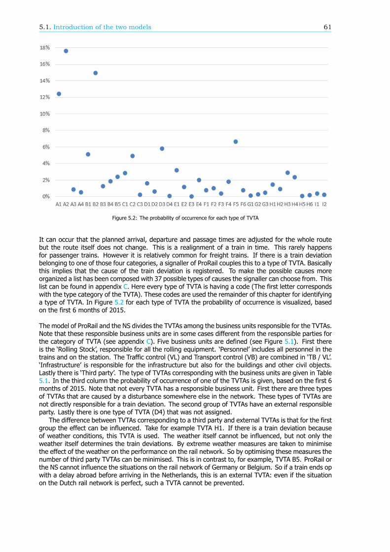
5.1. Introduction of the two models 61

Figure 5.2: The probability of occurrence for each type of TVTA

It can occur that the planned arrival, departure and passage times are adjusted for the whole routebut the route itself does not change. This is a realignment of a train in time. This rarely happensfor passenger trains. However it is relatively common for freight trains. If there is a train deviationbelonging to one of those four categories, a signaller of ProRail couples this to a type of TVTA. Basicallythis implies that the cause of the train deviation is registered. To make the possible causes moreorganized a list has been composed with 37 possible types of causes the signaller can choose from. Thislist can be found in appendix C. Here every type of TVTA is having a code (The first letter correspondswith the type category of the TVTA). These codes are used the remainder of this chapter for identifyinga type of TVTA. In Figure 5.2 for each type of TVTA the probability of occurrence is visualized, basedon the first 6 months of 2015.

The model of ProRail and the NS divides the TVTAs among the business units responsible for the TVTAs.Note that these responsible business units are in some cases different from the responsible parties forthe category of TVTA (see appendix C). Five business units are defined (see Figure 5.1). First thereis the ‘Rolling Stock’, responsible for all the rolling equipment. ‘Personnel’ includes all personnel in thetrains and on the station. The Traffic control (VL) and Transport control (VB) are combined in ‘TB / VL’.‘Infrastructure’ is responsible for the infrastructure but also for the buildings and other civil objects.Lastly there is ‘Third party’. The type of TVTAs corresponding with the business units are given in Table5.1. In the third column the probability of occurrence of one of the TVTAs is given, based on the first 6months of 2015. Note that not every TVTA has a responsible business unit. First there are three typesof TVTAs that are caused by a disturbance somewhere else in the network. These types of TVTAs arenot directly responsible for a train deviation. The second group of TVTAs have an external responsibleparty. Lastly there is one type of TVTA (D4) that was not assigned.

The difference between TVTAs corresponding to a third party and external TVTAs is that for the firstgroup the effect can be influenced. Take for example TVTA H1. If there is a train deviation becauseof weather conditions, this TVTA is used. The weather itself cannot be influenced, but not only theweather itself determines the train deviations. By extreme weather measures are taken to minimisethe effect of the weather on the performance on the rail network. So by optimising these measures thenumber of third party TVTAs can be minimised. This is in contrast to, for example, TVTA B5. ProRail orthe NS cannot influence the situations on the rail network of Germany or Belgium. So if a train ends opwith a delay abroad before arriving in the Netherlands, this is an external TVTA: even if the situationon the Dutch rail network is perfect, such a TVTA cannot be prevented.

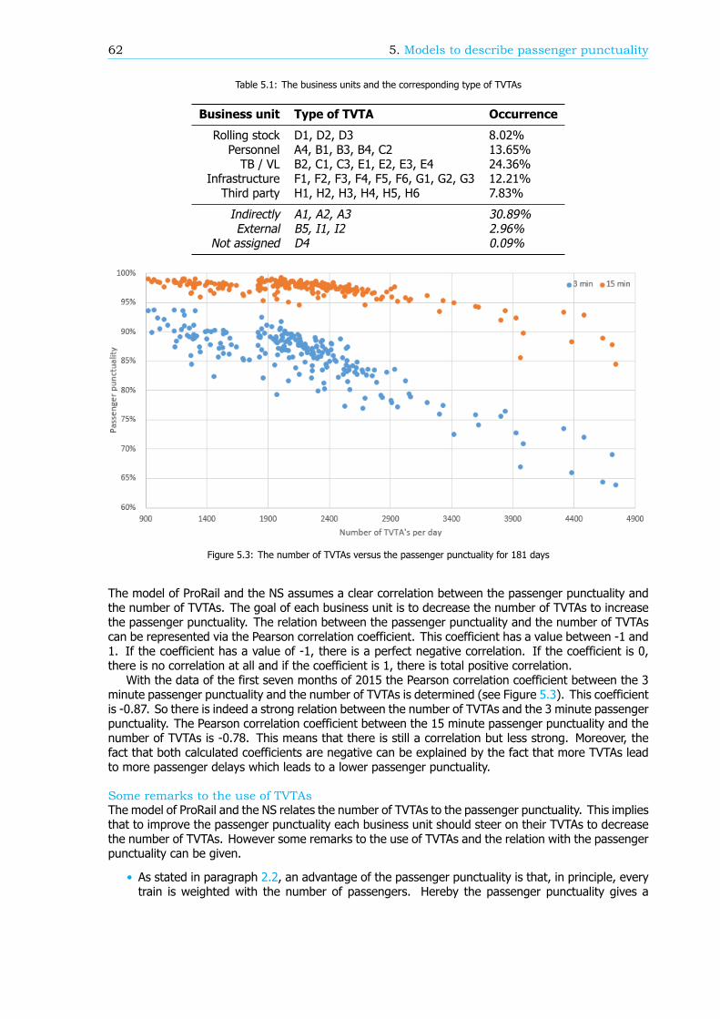
62 5. Models to describe passenger punctuality

Table 5.1: The business units and the corresponding type of TVTAs

Business unit Type of TVTA Occurrence

Rolling stock D1, D2, D3 8.02%Personnel A4, B1, B3, B4, C2 13.65%TB / VL B2, C1, C3, E1, E2, E3, E4 24.36%

Infrastructure F1, F2, F3, F4, F5, F6, G1, G2, G3 12.21%Third party H1, H2, H3, H4, H5, H6 7.83%

Indirectly A1, A2, A3 30.89%External B5, I1, I2 2.96%

Not assigned D4 0.09%

Figure 5.3: The number of TVTAs versus the passenger punctuality for 181 days

The model of ProRail and the NS assumes a clear correlation between the passenger punctuality andthe number of TVTAs. The goal of each business unit is to decrease the number of TVTAs to increasethe passenger punctuality. The relation between the passenger punctuality and the number of TVTAscan be represented via the Pearson correlation coefficient. This coefficient has a value between -1 and1. If the coefficient has a value of -1, there is a perfect negative correlation. If the coefficient is 0,there is no correlation at all and if the coefficient is 1, there is total positive correlation.

With the data of the first seven months of 2015 the Pearson correlation coefficient between the 3minute passenger punctuality and the number of TVTAs is determined (see Figure 5.3). This coefficientis -0.87. So there is indeed a strong relation between the number of TVTAs and the 3 minute passengerpunctuality. The Pearson correlation coefficient between the 15 minute passenger punctuality and thenumber of TVTAs is -0.78. This means that there is still a correlation but less strong. Moreover, thefact that both calculated coefficients are negative can be explained by the fact that more TVTAs leadto more passenger delays which leads to a lower passenger punctuality.

Some remarks to the use of TVTAsThe model of ProRail and the NS relates the number of TVTAs to the passenger punctuality. This impliesthat to improve the passenger punctuality each business unit should steer on their TVTAs to decreasethe number of TVTAs. However some remarks to the use of TVTAs and the relation with the passengerpunctuality can be given.

• As stated in paragraph 2.2, an advantage of the passenger punctuality is that, in principle, everytrain is weighted with the number of passengers. Hereby the passenger punctuality gives a

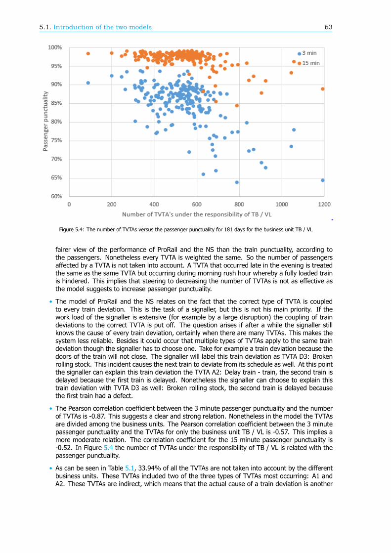
5.1. Introduction of the two models 63

Figure 5.4: The number of TVTAs versus the passenger punctuality for 181 days for the business unit TB / VL

fairer view of the performance of ProRail and the NS than the train punctuality, according tothe passengers. Nonetheless every TVTA is weighted the same. So the number of passengersaffected by a TVTA is not taken into account. A TVTA that occurred late in the evening is treatedthe same as the same TVTA but occurring during morning rush hour whereby a fully loaded trainis hindered. This implies that steering to decreasing the number of TVTAs is not as effective asthe model suggests to increase passenger punctuality.

• The model of ProRail and the NS relates on the fact that the correct type of TVTA is coupledto every train deviation. This is the task of a signaller, but this is not his main priority. If thework load of the signaller is extensive (for example by a large disruption) the coupling of traindeviations to the correct TVTA is put off. The question arises if after a while the signaller stillknows the cause of every train deviation, certainly when there are many TVTAs. This makes thesystem less reliable. Besides it could occur that multiple types of TVTAs apply to the same traindeviation though the signaller has to choose one. Take for example a train deviation because thedoors of the train will not close. The signaller will label this train deviation as TVTA D3: Brokenrolling stock. This incident causes the next train to deviate from its schedule as well. At this pointthe signaller can explain this train deviation the TVTA A2: Delay train - train, the second train isdelayed because the first train is delayed. Nonetheless the signaller can choose to explain thistrain deviation with TVTA D3 as well: Broken rolling stock, the second train is delayed becausethe first train had a defect.

• The Pearson correlation coefficient between the 3 minute passenger punctuality and the numberof TVTAs is -0.87. This suggests a clear and strong relation. Nonetheless in the model the TVTAsare divided among the business units. The Pearson correlation coefficient between the 3 minutepassenger punctuality and the TVTAs for only the business unit TB / VL is -0.57. This implies amore moderate relation. The correlation coefficient for the 15 minute passenger punctuality is-0.52. In Figure 5.4 the number of TVTAs under the responsibility of TB / VL is related with thepassenger punctuality.

• As can be seen in Table 5.1, 33.94% of all the TVTAs are not taken into account by the differentbusiness units. These TVTAs included two of the three types of TVTAs most occurring: A1 andA2. These TVTAs are indirect, which means that the actual cause of a train deviation is another

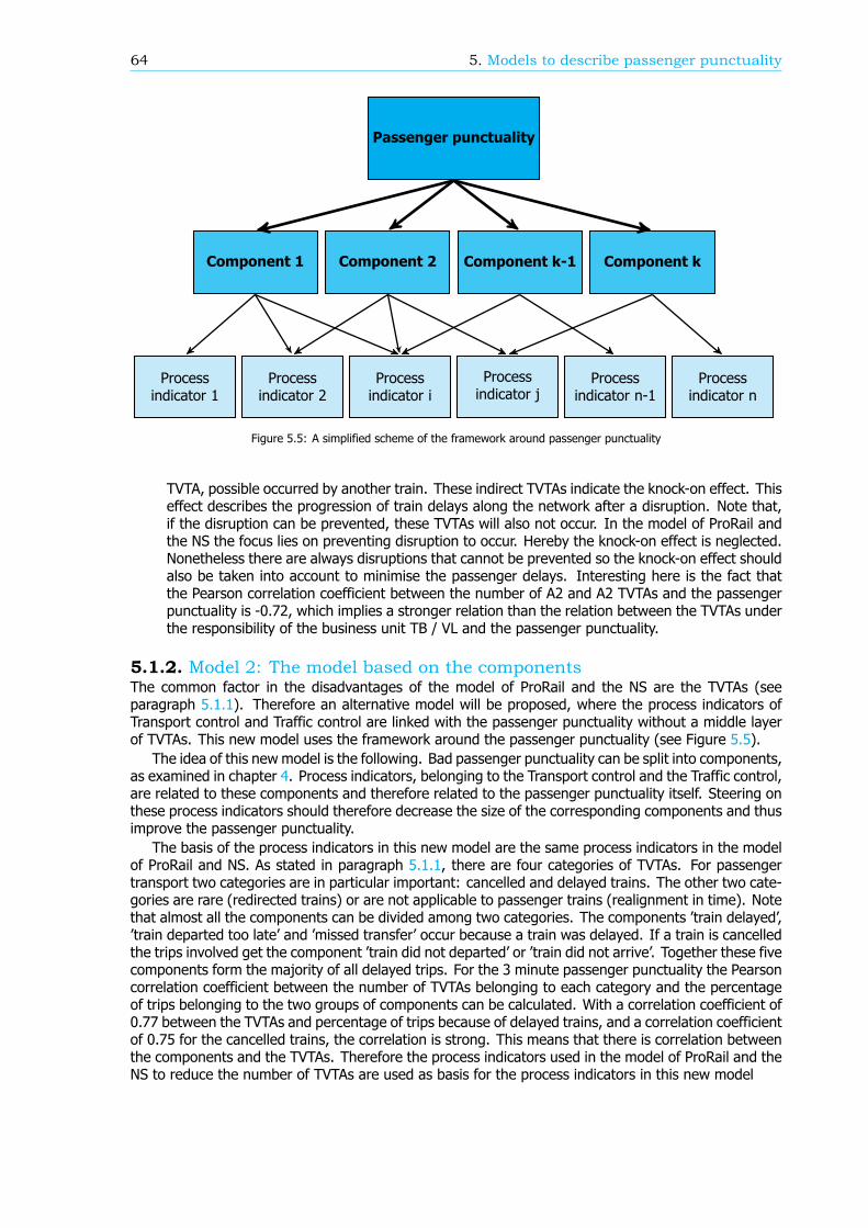
64 5. Models to describe passenger punctuality

Passenger punctuality

Component 2 Component k-1Component 1 Component k

Processindicator i

Processindicator 2

Processindicator 1

Processindicator j

Processindicator n-1

Processindicator n

Figure 5.5: A simplified scheme of the framework around passenger punctuality

TVTA, possible occurred by another train. These indirect TVTAs indicate the knock-on effect. Thiseffect describes the progression of train delays along the network after a disruption. Note that,if the disruption can be prevented, these TVTAs will also not occur. In the model of ProRail andthe NS the focus lies on preventing disruption to occur. Hereby the knock-on effect is neglected.Nonetheless there are always disruptions that cannot be prevented so the knock-on effect shouldalso be taken into account to minimise the passenger delays. Interesting here is the fact thatthe Pearson correlation coefficient between the number of A2 and A2 TVTAs and the passengerpunctuality is -0.72, which implies a stronger relation than the relation between the TVTAs underthe responsibility of the business unit TB / VL and the passenger punctuality.

5.1.2. Model 2: The model based on the componentsThe common factor in the disadvantages of the model of ProRail and the NS are the TVTAs (seeparagraph 5.1.1). Therefore an alternative model will be proposed, where the process indicators ofTransport control and Traffic control are linked with the passenger punctuality without a middle layerof TVTAs. This new model uses the framework around the passenger punctuality (see Figure 5.5).

The idea of this new model is the following. Bad passenger punctuality can be split into components,as examined in chapter 4. Process indicators, belonging to the Transport control and the Traffic control,are related to these components and therefore related to the passenger punctuality itself. Steering onthese process indicators should therefore decrease the size of the corresponding components and thusimprove the passenger punctuality.

The basis of the process indicators in this new model are the same process indicators in the modelof ProRail and NS. As stated in paragraph 5.1.1, there are four categories of TVTAs. For passengertransport two categories are in particular important: cancelled and delayed trains. The other two cate-gories are rare (redirected trains) or are not applicable to passenger trains (realignment in time). Notethat almost all the components can be divided among two categories. The components ’train delayed’,’train departed too late’ and ’missed transfer’ occur because a train was delayed. If a train is cancelledthe trips involved get the component ’train did not departed’ or ’train did not arrive’. Together these fivecomponents form the majority of all delayed trips. For the 3 minute passenger punctuality the Pearsoncorrelation coefficient between the number of TVTAs belonging to each category and the percentageof trips belonging to the two groups of components can be calculated. With a correlation coefficient of0.77 between the TVTAs and percentage of trips because of delayed trains, and a correlation coefficientof 0.75 for the cancelled trains, the correlation is strong. This means that there is correlation betweenthe components and the TVTAs. Therefore the process indicators used in the model of ProRail and theNS to reduce the number of TVTAs are used as basis for the process indicators in this new model

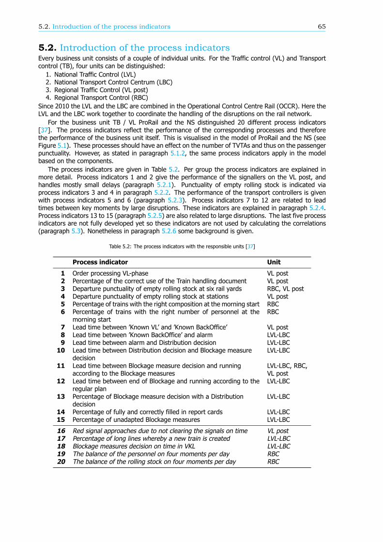
5.2. Introduction of the process indicators 65

5.2. Introduction of the process indicatorsEvery business unit consists of a couple of individual units. For the Traffic control (VL) and Transportcontrol (TB), four units can be distinguished:1. National Traffic Control (LVL)2. National Transport Control Centrum (LBC)3. Regional Traffic Control (VL post)4. Regional Transport Control (RBC)

Since 2010 the LVL and the LBC are combined in the Operational Control Centre Rail (OCCR). Here theLVL and the LBC work together to coordinate the handling of the disruptions on the rail network.

For the business unit TB / VL ProRail and the NS distinguished 20 different process indicators[37]. The process indicators reflect the performance of the corresponding processes and thereforethe performance of the business unit itself. This is visualised in the model of ProRail and the NS (seeFigure 5.1). These processes should have an effect on the number of TVTAs and thus on the passengerpunctuality. However, as stated in paragraph 5.1.2, the same process indicators apply in the modelbased on the components.

The process indicators are given in Table 5.2. Per group the process indicators are explained inmore detail. Process indicators 1 and 2 give the performance of the signallers on the VL post, andhandles mostly small delays (paragraph 5.2.1). Punctuality of empty rolling stock is indicated viaprocess indicators 3 and 4 in paragraph 5.2.2. The performance of the transport controllers is givenwith process indicators 5 and 6 (paragraph 5.2.3). Process indicators 7 to 12 are related to leadtimes between key moments by large disruptions. These indicators are explained in paragraph 5.2.4.Process indicators 13 to 15 (paragraph 5.2.5) are also related to large disruptions. The last five processindicators are not fully developed yet so these indicators are not used by calculating the correlations(paragraph 5.3). Nonetheless in paragraph 5.2.6 some background is given.

Table 5.2: The process indicators with the responsible units [37]

Process indicator Unit

1 Order processing VL-phase VL post2 Percentage of the correct use of the Train handling document VL post3 Departure punctuality of empty rolling stock at six rail yards RBC, VL post4 Departure punctuality of empty rolling stock at stations VL post5 Percentage of trains with the right composition at the morning start RBC6 Percentage of trains with the right number of personnel at the

morning startRBC

7 Lead time between ’Known VL’ and ’Known BackOffice’ VL post8 Lead time between ’Known BackOffice’ and alarm LVL-LBC9 Lead time between alarm and Distribution decision LVL-LBC

10 Lead time between Distribution decision and Blockage measuredecision

LVL-LBC

11 Lead time between Blockage measure decision and runningaccording to the Blockage measures

LVL-LBC, RBC,VL post

12 Lead time between end of Blockage and running according to theregular plan

LVL-LBC

13 Percentage of Blockage measure decision with a Distributiondecision

LVL-LBC

14 Percentage of fully and correctly filled in report cards LVL-LBC15 Percentage of unadapted Blockage measures LVL-LBC

16 Red signal approaches due to not clearing the signals on time VL post17 Percentage of long lines whereby a new train is created LVL-LBC18 Blockage measures decision on time in VKL LVL-LBC19 The balance of the personnel on four moments per day RBC20 The balance of the rolling stock on four moments per day RBC

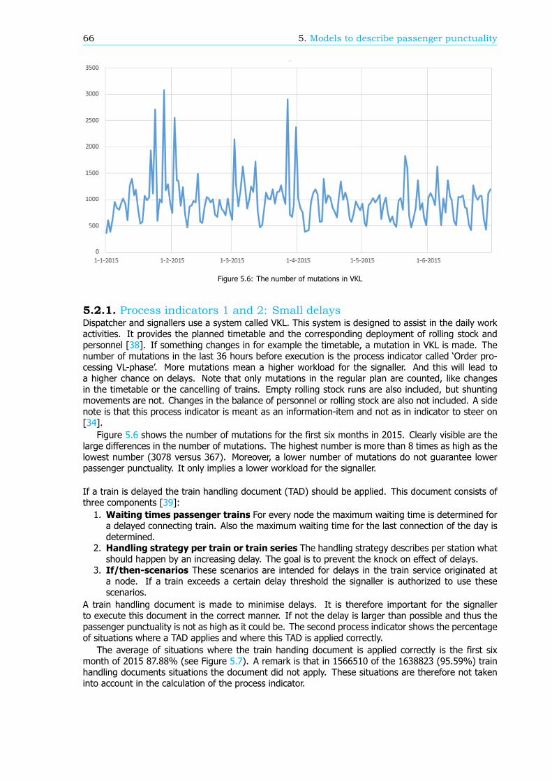
66 5. Models to describe passenger punctuality

Figure 5.6: The number of mutations in VKL

5.2.1. Process indicators 1 and 2: Small delaysDispatcher and signallers use a system called VKL. This system is designed to assist in the daily workactivities. It provides the planned timetable and the corresponding deployment of rolling stock andpersonnel [38]. If something changes in for example the timetable, a mutation in VKL is made. Thenumber of mutations in the last 36 hours before execution is the process indicator called ‘Order pro-cessing VL-phase’. More mutations mean a higher workload for the signaller. And this will lead toa higher chance on delays. Note that only mutations in the regular plan are counted, like changesin the timetable or the cancelling of trains. Empty rolling stock runs are also included, but shuntingmovements are not. Changes in the balance of personnel or rolling stock are also not included. A sidenote is that this process indicator is meant as an information-item and not as in indicator to steer on[34].

Figure 5.6 shows the number of mutations for the first six months in 2015. Clearly visible are thelarge differences in the number of mutations. The highest number is more than 8 times as high as thelowest number (3078 versus 367). Moreover, a lower number of mutations do not guarantee lowerpassenger punctuality. It only implies a lower workload for the signaller.

If a train is delayed the train handling document (TAD) should be applied. This document consists ofthree components [39]:1. Waiting times passenger trains For every node the maximum waiting time is determined fora delayed connecting train. Also the maximum waiting time for the last connection of the day isdetermined.

2. Handling strategy per train or train series The handling strategy describes per station whatshould happen by an increasing delay. The goal is to prevent the knock on effect of delays.

3. If/then-scenarios These scenarios are intended for delays in the train service originated ata node. If a train exceeds a certain delay threshold the signaller is authorized to use thesescenarios.

A train handling document is made to minimise delays. It is therefore important for the signallerto execute this document in the correct manner. If not the delay is larger than possible and thus thepassenger punctuality is not as high as it could be. The second process indicator shows the percentageof situations where a TAD applies and where this TAD is applied correctly.

The average of situations where the train handing document is applied correctly is the first sixmonth of 2015 87.88% (see Figure 5.7). A remark is that in 1566510 of the 1638823 (95.59%) trainhandling documents situations the document did not apply. These situations are therefore not takeninto account in the calculation of the process indicator.

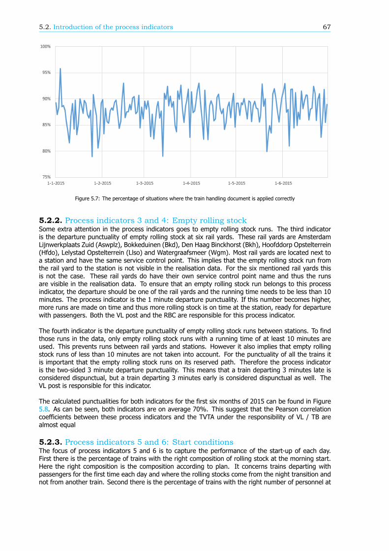
5.2. Introduction of the process indicators 67

Figure 5.7: The percentage of situations where the train handling document is applied correctly

5.2.2. Process indicators 3 and 4: Empty rolling stockSome extra attention in the process indicators goes to empty rolling stock runs. The third indicatoris the departure punctuality of empty rolling stock at six rail yards. These rail yards are AmsterdamLijnwerkplaats Zuid (Aswplz), Bokkeduinen (Bkd), Den Haag Binckhorst (Bkh), Hoofddorp Opstelterrein(Hfdo), Lelystad Opstelterrein (Llso) and Watergraafsmeer (Wgm). Most rail yards are located next toa station and have the same service control point. This implies that the empty rolling stock run fromthe rail yard to the station is not visible in the realisation data. For the six mentioned rail yards thisis not the case. These rail yards do have their own service control point name and thus the runsare visible in the realisation data. To ensure that an empty rolling stock run belongs to this processindicator, the departure should be one of the rail yards and the running time needs to be less than 10minutes. The process indicator is the 1 minute departure punctuality. If this number becomes higher,more runs are made on time and thus more rolling stock is on time at the station, ready for departurewith passengers. Both the VL post and the RBC are responsible for this process indicator.

The fourth indicator is the departure punctuality of empty rolling stock runs between stations. To findthose runs in the data, only empty rolling stock runs with a running time of at least 10 minutes areused. This prevents runs between rail yards and stations. However it also implies that empty rollingstock runs of less than 10 minutes are not taken into account. For the punctuality of all the trains itis important that the empty rolling stock runs on its reserved path. Therefore the process indicatoris the two-sided 3 minute departure punctuality. This means that a train departing 3 minutes late isconsidered dispunctual, but a train departing 3 minutes early is considered dispunctual as well. TheVL post is responsible for this indicator.

The calculated punctualities for both indicators for the first six months of 2015 can be found in Figure5.8. As can be seen, both indicators are on average 70%. This suggest that the Pearson correlationcoefficients between these process indicators and the TVTA under the responsibility of VL / TB arealmost equal

5.2.3. Process indicators 5 and 6: Start conditionsThe focus of process indicators 5 and 6 is to capture the performance of the start-up of each day.First there is the percentage of trains with the right composition of rolling stock at the morning start.Here the right composition is the composition according to plan. It concerns trains departing withpassengers for the first time each day and where the rolling stocks come from the night transition andnot from another train. Second there is the percentage of trains with the right number of personnel at

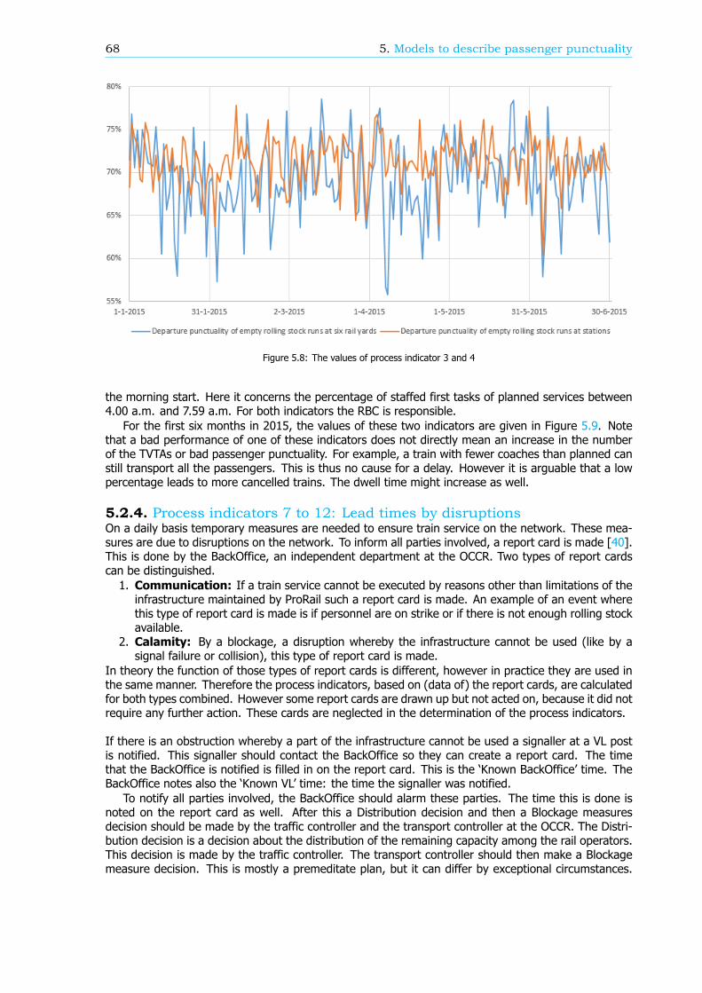
68 5. Models to describe passenger punctuality

Figure 5.8: The values of process indicator 3 and 4

the morning start. Here it concerns the percentage of staffed first tasks of planned services between4.00 a.m. and 7.59 a.m. For both indicators the RBC is responsible.

For the first six months in 2015, the values of these two indicators are given in Figure 5.9. Notethat a bad performance of one of these indicators does not directly mean an increase in the numberof the TVTAs or bad passenger punctuality. For example, a train with fewer coaches than planned canstill transport all the passengers. This is thus no cause for a delay. However it is arguable that a lowpercentage leads to more cancelled trains. The dwell time might increase as well.

5.2.4. Process indicators 7 to 12: Lead times by disruptionsOn a daily basis temporary measures are needed to ensure train service on the network. These mea-sures are due to disruptions on the network. To inform all parties involved, a report card is made [40].This is done by the BackOffice, an independent department at the OCCR. Two types of report cardscan be distinguished.1. Communication: If a train service cannot be executed by reasons other than limitations of theinfrastructure maintained by ProRail such a report card is made. An example of an event wherethis type of report card is made is if personnel are on strike or if there is not enough rolling stockavailable.

2. Calamity: By a blockage, a disruption whereby the infrastructure cannot be used (like by asignal failure or collision), this type of report card is made.

In theory the function of those types of report cards is different, however in practice they are used inthe same manner. Therefore the process indicators, based on (data of) the report cards, are calculatedfor both types combined. However some report cards are drawn up but not acted on, because it did notrequire any further action. These cards are neglected in the determination of the process indicators.

If there is an obstruction whereby a part of the infrastructure cannot be used a signaller at a VL postis notified. This signaller should contact the BackOffice so they can create a report card. The timethat the BackOffice is notified is filled in on the report card. This is the ‘Known BackOffice’ time. TheBackOffice notes also the ‘Known VL’ time: the time the signaller was notified.

To notify all parties involved, the BackOffice should alarm these parties. The time this is done isnoted on the report card as well. After this a Distribution decision and then a Blockage measuresdecision should be made by the traffic controller and the transport controller at the OCCR. The Distri-bution decision is a decision about the distribution of the remaining capacity among the rail operators.This decision is made by the traffic controller. The transport controller should then make a Blockagemeasure decision. This is mostly a premeditate plan, but it can differ by exceptional circumstances.

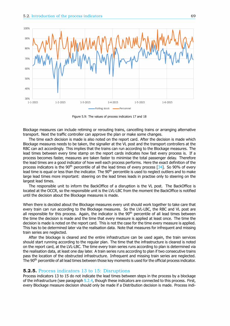
5.2. Introduction of the process indicators 69

Figure 5.9: The values of process indicators 17 and 18

Blockage measures can include retiming or rerouting trains, cancelling trains or arranging alternativetransport. Next the traffic controller can approve the plan or make some changes.

The time each decision is made is also noted on the report card. After the decision is made whichBlockage measures needs to be taken, the signaller at the VL post and the transport controllers at theRBC can act accordingly. This implies that the trains can run according to the Blockage measures. Thelead times between every time stamp on the report cards indicates how fast every process is. If aprocess becomes faster, measures are taken faster to minimise the total passenger delay. Thereforethe lead times are a good indicator of how well each process performs. Here the exact definition of theprocess indicators is the 90th percentile of all the lead times of every process [34]. So 90% of everylead time is equal or less than the indicator. The 90th percentile is used to neglect outliers and to makelarge lead times more important: steering on the lead times leads in practise only to steering on thelargest lead times.

The responsible unit to inform the BackOffice of a disruption is the VL post. The BackOffice islocated at the OCCR, so the responsible unit is the LVL-LBC from the moment the BackOffice is notifieduntil the decision about the Blockage measures is made.

When there is decided about the Blockage measures every unit should work together to take care thatevery train can run according to the Blockage measures. So the LVL-LBC, the RBC and VL post areall responsible for this process. Again, the indicator is the 90th percentile of all lead times betweenthe time the decision is made and the time that every measure is applied at least once. The time thedecision is made is noted on the report card. This is not the case for the time every measure is applied.This has to be determined later via the realisation data. Note that measures for infrequent and missingtrain series are neglected.

After the blockage is cleared and the entire infrastructure can be used again, the train servicesshould start running according to the regular plan. The time that the infrastructure is cleared is notedon the report card, at the LVL-LBC. The time every train series runs according to plan is determined viathe realisation data, at least one day later. A train series runs according to plan if two consecutive trainspass the location of the obstructed infrastructure. Infrequent and missing train series are neglected.The 90th percentile of all lead times between those key moments is used for the official process indicator.

5.2.5. Process indicators 13 to 15: DisruptionsProcess indicators 13 to 15 do not indicate the lead times between steps in the process by a blockageof the infrastructure (see paragraph 5.2.4, though these indicators are connected to this process. First,every Blockage measure decision should only be made if a Distribution decision is made. Process indi-

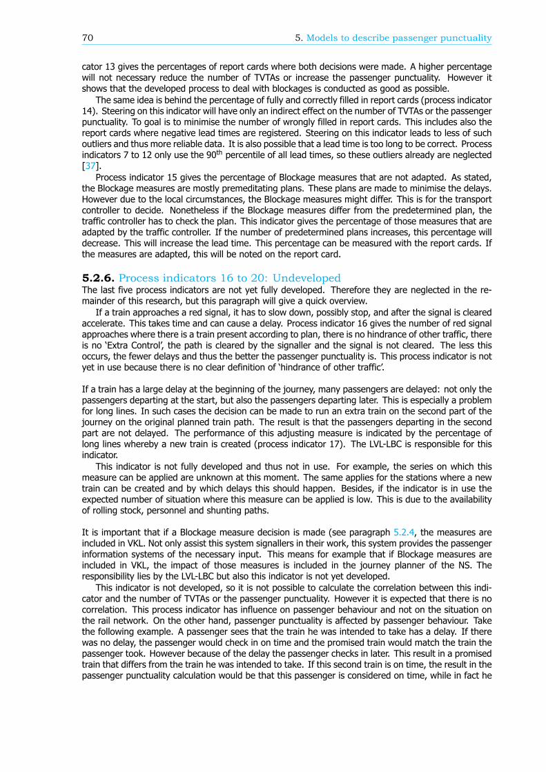
70 5. Models to describe passenger punctuality

cator 13 gives the percentages of report cards where both decisions were made. A higher percentagewill not necessary reduce the number of TVTAs or increase the passenger punctuality. However itshows that the developed process to deal with blockages is conducted as good as possible.

The same idea is behind the percentage of fully and correctly filled in report cards (process indicator14). Steering on this indicator will have only an indirect effect on the number of TVTAs or the passengerpunctuality. To goal is to minimise the number of wrongly filled in report cards. This includes also thereport cards where negative lead times are registered. Steering on this indicator leads to less of suchoutliers and thus more reliable data. It is also possible that a lead time is too long to be correct. Processindicators 7 to 12 only use the 90th percentile of all lead times, so these outliers already are neglected[37].

Process indicator 15 gives the percentage of Blockage measures that are not adapted. As stated,the Blockage measures are mostly premeditating plans. These plans are made to minimise the delays.However due to the local circumstances, the Blockage measures might differ. This is for the transportcontroller to decide. Nonetheless if the Blockage measures differ from the predetermined plan, thetraffic controller has to check the plan. This indicator gives the percentage of those measures that areadapted by the traffic controller. If the number of predetermined plans increases, this percentage willdecrease. This will increase the lead time. This percentage can be measured with the report cards. Ifthe measures are adapted, this will be noted on the report card.

5.2.6. Process indicators 16 to 20: UndevelopedThe last five process indicators are not yet fully developed. Therefore they are neglected in the re-mainder of this research, but this paragraph will give a quick overview.

If a train approaches a red signal, it has to slow down, possibly stop, and after the signal is clearedaccelerate. This takes time and can cause a delay. Process indicator 16 gives the number of red signalapproaches where there is a train present according to plan, there is no hindrance of other traffic, thereis no ‘Extra Control’, the path is cleared by the signaller and the signal is not cleared. The less thisoccurs, the fewer delays and thus the better the passenger punctuality is. This process indicator is notyet in use because there is no clear definition of ‘hindrance of other traffic’.

If a train has a large delay at the beginning of the journey, many passengers are delayed: not only thepassengers departing at the start, but also the passengers departing later. This is especially a problemfor long lines. In such cases the decision can be made to run an extra train on the second part of thejourney on the original planned train path. The result is that the passengers departing in the secondpart are not delayed. The performance of this adjusting measure is indicated by the percentage oflong lines whereby a new train is created (process indicator 17). The LVL-LBC is responsible for thisindicator.

This indicator is not fully developed and thus not in use. For example, the series on which thismeasure can be applied are unknown at this moment. The same applies for the stations where a newtrain can be created and by which delays this should happen. Besides, if the indicator is in use theexpected number of situation where this measure can be applied is low. This is due to the availabilityof rolling stock, personnel and shunting paths.

It is important that if a Blockage measure decision is made (see paragraph 5.2.4, the measures areincluded in VKL. Not only assist this system signallers in their work, this system provides the passengerinformation systems of the necessary input. This means for example that if Blockage measures areincluded in VKL, the impact of those measures is included in the journey planner of the NS. Theresponsibility lies by the LVL-LBC but also this indicator is not yet developed.

This indicator is not developed, so it is not possible to calculate the correlation between this indi-cator and the number of TVTAs or the passenger punctuality. However it is expected that there is nocorrelation. This process indicator has influence on passenger behaviour and not on the situation onthe rail network. On the other hand, passenger punctuality is affected by passenger behaviour. Takethe following example. A passenger sees that the train he was intended to take has a delay. If therewas no delay, the passenger would check in on time and the promised train would match the train thepassenger took. However because of the delay the passenger checks in later. This result in a promisedtrain that differs from the train he was intended to take. If this second train is on time, the result in thepassenger punctuality calculation would be that this passenger is considered on time, while in fact he

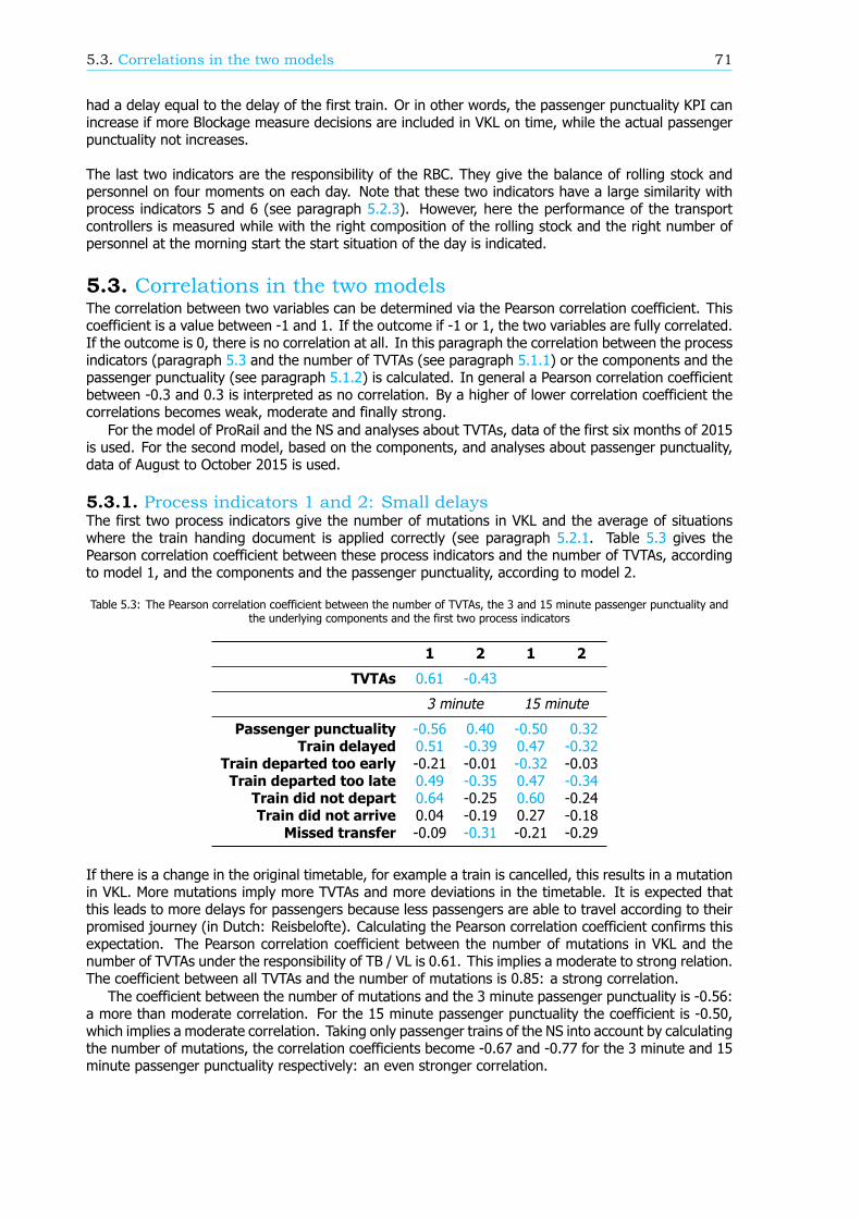
5.3. Correlations in the two models 71

had a delay equal to the delay of the first train. Or in other words, the passenger punctuality KPI canincrease if more Blockage measure decisions are included in VKL on time, while the actual passengerpunctuality not increases.

The last two indicators are the responsibility of the RBC. They give the balance of rolling stock andpersonnel on four moments on each day. Note that these two indicators have a large similarity withprocess indicators 5 and 6 (see paragraph 5.2.3). However, here the performance of the transportcontrollers is measured while with the right composition of the rolling stock and the right number ofpersonnel at the morning start the start situation of the day is indicated.

5.3. Correlations in the two modelsThe correlation between two variables can be determined via the Pearson correlation coefficient. Thiscoefficient is a value between -1 and 1. If the outcome if -1 or 1, the two variables are fully correlated.If the outcome is 0, there is no correlation at all. In this paragraph the correlation between the processindicators (paragraph 5.3 and the number of TVTAs (see paragraph 5.1.1) or the components and thepassenger punctuality (see paragraph 5.1.2) is calculated. In general a Pearson correlation coefficientbetween -0.3 and 0.3 is interpreted as no correlation. By a higher of lower correlation coefficient thecorrelations becomes weak, moderate and finally strong.

For the model of ProRail and the NS and analyses about TVTAs, data of the first six months of 2015is used. For the second model, based on the components, and analyses about passenger punctuality,data of August to October 2015 is used.

5.3.1. Process indicators 1 and 2: Small delaysThe first two process indicators give the number of mutations in VKL and the average of situationswhere the train handing document is applied correctly (see paragraph 5.2.1. Table 5.3 gives thePearson correlation coefficient between these process indicators and the number of TVTAs, accordingto model 1, and the components and the passenger punctuality, according to model 2.

Table 5.3: The Pearson correlation coefficient between the number of TVTAs, the 3 and 15 minute passenger punctuality andthe underlying components and the first two process indicators

1 2 1 2

TVTAs 0.61 -0.43

3 minute 15 minute

Passenger punctuality -0.56 0.40 -0.50 0.32Train delayed 0.51 -0.39 0.47 -0.32

Train departed too early -0.21 -0.01 -0.32 -0.03Train departed too late 0.49 -0.35 0.47 -0.34

Train did not depart 0.64 -0.25 0.60 -0.24Train did not arrive 0.04 -0.19 0.27 -0.18

Missed transfer -0.09 -0.31 -0.21 -0.29

If there is a change in the original timetable, for example a train is cancelled, this results in a mutationin VKL. More mutations imply more TVTAs and more deviations in the timetable. It is expected thatthis leads to more delays for passengers because less passengers are able to travel according to theirpromised journey (in Dutch: Reisbelofte). Calculating the Pearson correlation coefficient confirms thisexpectation. The Pearson correlation coefficient between the number of mutations in VKL and thenumber of TVTAs under the responsibility of TB / VL is 0.61. This implies a moderate to strong relation.The coefficient between all TVTAs and the number of mutations is 0.85: a strong correlation.

The coefficient between the number of mutations and the 3 minute passenger punctuality is -0.56:a more than moderate correlation. For the 15 minute passenger punctuality the coefficient is -0.50,which implies a moderate correlation. Taking only passenger trains of the NS into account by calculatingthe number of mutations, the correlation coefficients become -0.67 and -0.77 for the 3 minute and 15minute passenger punctuality respectively: an even stronger correlation.

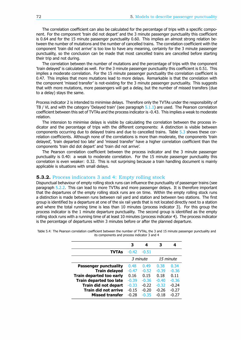
72 5. Models to describe passenger punctuality

The correlation coefficient can also be calculated for the percentage of trips with a specific compo-nent. For the component ’train did not depart’ and the 3 minute passenger punctuality this coefficientis 0.64 and for the 15 minute passenger punctuality 0.60. This implies an almost strong relation be-tween the number of mutations and the number of cancelled trains. The correlation coefficient with thecomponent ’train did not arrive’ is too low to have any meaning, certainly for the 3 minute passengerpunctuality, so the conclusion can be made that most cancelled trains are cancelled before startingtheir trip and not during.

The correlation between the number of mutations and the percentage of trips with the component’train delayed’ is calculated as well. For the 3 minute passenger punctuality this coefficient is 0.51. Thisimplies a moderate correlation. For the 15 minute passenger punctuality the correlation coefficient is0.47. This implies that more mutations lead to more delays. Remarkable is that the correlation withthe component ’missed transfer’ is not-existing for the 3 minute passenger punctuality. This suggeststhat with more mutations, more passengers will get a delay, but the number of missed transfers (dueto a delay) stays the same.

Process indicator 2 is intended to minimise delays. Therefore only the TVTAs under the responsibility ofTB / VL and with the category ‘Delayed train’ (see paragraph 5.1.1) are used. The Pearson correlationcoefficient between this set of TVTAs and the process indicator is -0.43. This implies a weak to moderaterelation.

The intension to minimise delays is visible by calculating the correlation between the process in-dicator and the percentage of trips with the different components: A distinction is visible betweencomponents occurring due to delayed trains and due to cancelled trains. Table 5.3 shows these cor-relation coefficients. Although none of the correlations is more than moderate, the components ’traindelayed’, ’train departed too late’ and ’missed transfer’ have a higher correlation coefficient than thecomponents ’train did dot depart’ and ’train did not arrive’.

The Pearson correlation coefficient between the process indicator and the 3 minute passengerpunctuality is 0.40: a weak to moderate correlation. For the 15 minute passenger punctuality thiscorrelation is even weaker: 0.32. This is not surprising because a train handling document is mainlyapplicable is situations with small delays.

5.3.2. Process indicators 3 and 4: Empty rolling stockDispunctual behaviour of empty rolling stock runs can influence the punctuality of passenger trains (seeparagraph 5.2.2. This can lead to more TVTAs and more passenger delays. It is therefore importantthat the departures of the empty rolling stock runs are on time. Within the empty rolling stock runsa distinction is made between runs between rail yard and station and between two stations. The firstgroup is identified by a departure at one of the six rail yards that is not located directly next to a stationand where the total running time is less than 10 minutes (process indicator 3). For this group theprocess indicator is the 1 minute departure punctuality. The second group is identified as the emptyrolling stock runs with a running time of at least 10 minutes (process indicator 4). The process indicatoris the percentage of departures within 3 minutes before or after the planned departure.

Table 5.4: The Pearson correlation coefficient between the number of TVTAs, the 3 and 15 minute passenger punctuality andits components and process indicator 3 and 4

3 4 3 4

TVTAs -0.42 -0.51

3 minute 15 minute

Passenger punctuality 0.48 0.49 0.38 0.34Train delayed -0.47 -0.52 -0.39 -0.36

Train departed too early 0.16 0.15 0.18 0.11Train departed too late -0.39 -0.36 -0.40 -0.36

Train did not depart -0.33 -0.22 -0.32 -0.24Train did not arrive -0.15 -0.20 -0.26 -0.27

Missed transfer -0.28 -0.35 -0.18 -0.27

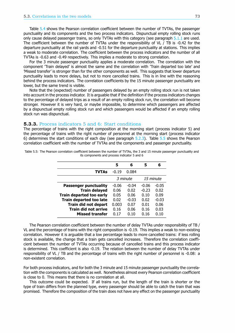
5.3. Correlations in the two models 73

Table 5.4 shows the Pearson correlation coefficient between the number of TVTAs, the passengerpunctuality and its components and the two process indicators. Dispunctual empty rolling stock runsonly cause delayed passenger trains, so only TVTAs with this category (see paragraph 5.1.1 are used.The coefficient between the number of TVTAs under the responsibility of VL / TB is -0.42 for thedeparture punctuality at the rail yards and -0.51 for the departure punctuality at stations. This impliesa weak to moderate correlation. The coefficient between the process indicators and the number of allTVTAs is -0.63 and -0.49 respectively. This implies a moderate to strong correlation.

For the 3 minute passenger punctuality applies a moderate correlation. The correlation with thecomponent ’Train delayed’ is almost the same and the correlation with ’Train departed too late’ and’Missed transfer’ is stronger than for the other components as well. This suggests that lower departurepunctuality leads to more delays, but not to more cancelled trains. This is in line with the reasoningbehind the process indicators. The correlation coefficients by the 15 minute passenger punctuality arelower, but the same trend is visible.

Note that the (expected) number of passengers delayed by an empty rolling stock run is not takeninto account in the process indicator. It is arguable that if the definition if the process indicators changesto the percentage of delayed trips as a result of an empty rolling stock run, the correlation will becomestronger. However it is very hard, or maybe impossible, to determine which passengers are affectedby a dispunctual empty rolling stock run and which passengers would be affected if an empty rollingstock run was dispunctual.

5.3.3. Process indicators 5 and 6: Start conditionsThe percentage of trains with the right composition at the morning start (process indicator 5) andthe percentage of trains with the right number of personnel at the morning start (process indicator6) determines the start conditions of each day (see paragraph 5.2.3). Table 5.5 shows the Pearsoncorrelation coefficient with the number of TVTAs and the components and passenger punctuality.

Table 5.5: The Pearson correlation coefficient between the number of TVTAs, the 3 and 15 minute passenger punctuality andits components and process indicator 5 and 6

5 6 5 6

TVTAs -0.19 0.084

3 minute 15 minute

Passenger punctuality -0.06 -0.04 -0.06 -0.05Train delayed 0.06 0.02 -0.23 0.02

Train departed too early 0.05 0.06 0.10 0.09Train departed too late 0.02 -0.03 0.02 -0.03

Train did not depart 0.003 0.07 0.01 0.06Train did not arrive 0.16 0.06 0.16 0.03

Missed transfer 0.17 0.10 0.16 0.10

The Pearson correlation coefficient between the number of delay TVTAs under responsibility of TB /VL and the percentage of trains with the right composition is -0.19. This implies a weak to non-existingcorrelation. However it is arguable that a low percentage leads to more cancelled trains: if less rollingstock is available, the change that a train gets cancelled increases. Therefore the correlation coeffi-cient between the number of TVTAs occurring because of cancelled trains and this process indicatoris determined. This coefficient is also -0.19. The relation between the number of delay TVTAs underresponsibility of VL / TB and the percentage of trains with the right number of personnel is -0.08: anon-existent correlation.

For both process indicators, and for both the 3 minute and 15 minute passenger punctuality the correla-tion with the components is calculated as well. Nonetheless almost every Pearson correlation coefficientis close to 0. This means that there is no correlation at all.

This outcome could be expected. If all trains run, but the length of the train is shorter or thetype of train differs from the planned type, every passenger should be able to catch the train that waspromised. Therefore the composition of the train does not have any effect on the passenger punctuality

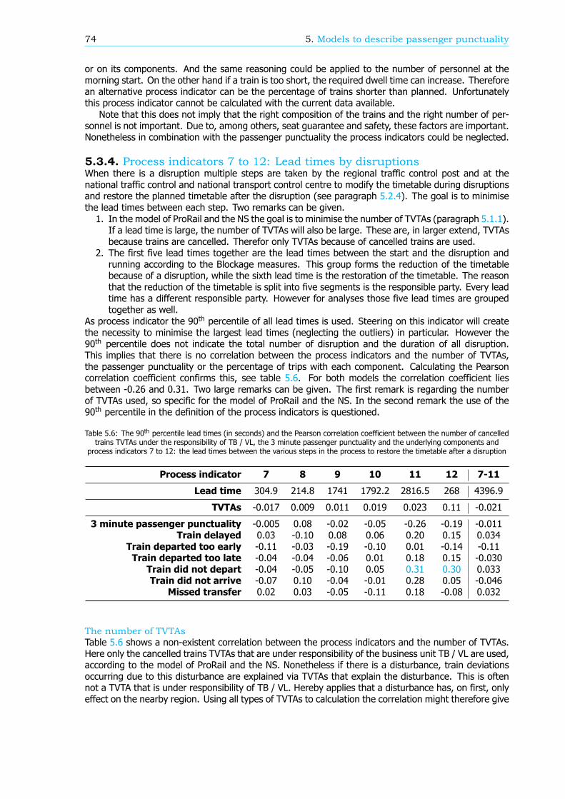
74 5. Models to describe passenger punctuality

or on its components. And the same reasoning could be applied to the number of personnel at themorning start. On the other hand if a train is too short, the required dwell time can increase. Thereforean alternative process indicator can be the percentage of trains shorter than planned. Unfortunatelythis process indicator cannot be calculated with the current data available.

Note that this does not imply that the right composition of the trains and the right number of per-sonnel is not important. Due to, among others, seat guarantee and safety, these factors are important.Nonetheless in combination with the passenger punctuality the process indicators could be neglected.

5.3.4. Process indicators 7 to 12: Lead times by disruptionsWhen there is a disruption multiple steps are taken by the regional traffic control post and at thenational traffic control and national transport control centre to modify the timetable during disruptionsand restore the planned timetable after the disruption (see paragraph 5.2.4). The goal is to minimisethe lead times between each step. Two remarks can be given.1. In the model of ProRail and the NS the goal is to minimise the number of TVTAs (paragraph 5.1.1).If a lead time is large, the number of TVTAs will also be large. These are, in larger extend, TVTAsbecause trains are cancelled. Therefor only TVTAs because of cancelled trains are used.

2. The first five lead times together are the lead times between the start and the disruption andrunning according to the Blockage measures. This group forms the reduction of the timetablebecause of a disruption, while the sixth lead time is the restoration of the timetable. The reasonthat the reduction of the timetable is split into five segments is the responsible party. Every leadtime has a different responsible party. However for analyses those five lead times are groupedtogether as well.

As process indicator the 90th percentile of all lead times is used. Steering on this indicator will createthe necessity to minimise the largest lead times (neglecting the outliers) in particular. However the90th percentile does not indicate the total number of disruption and the duration of all disruption.This implies that there is no correlation between the process indicators and the number of TVTAs,the passenger punctuality or the percentage of trips with each component. Calculating the Pearsoncorrelation coefficient confirms this, see table 5.6. For both models the correlation coefficient liesbetween -0.26 and 0.31. Two large remarks can be given. The first remark is regarding the numberof TVTAs used, so specific for the model of ProRail and the NS. In the second remark the use of the90th percentile in the definition of the process indicators is questioned.

Table 5.6: The 90th percentile lead times (in seconds) and the Pearson correlation coefficient between the number of cancelledtrains TVTAs under the responsibility of TB / VL, the 3 minute passenger punctuality and the underlying components and

process indicators 7 to 12: the lead times between the various steps in the process to restore the timetable after a disruption

Process indicator 7 8 9 10 11 12 7-11

Lead time 304.9 214.8 1741 1792.2 2816.5 268 4396.9

TVTAs -0.017 0.009 0.011 0.019 0.023 0.11 -0.021

3 minute passenger punctuality -0.005 0.08 -0.02 -0.05 -0.26 -0.19 -0.011Train delayed 0.03 -0.10 0.08 0.06 0.20 0.15 0.034

Train departed too early -0.11 -0.03 -0.19 -0.10 0.01 -0.14 -0.11Train departed too late -0.04 -0.04 -0.06 0.01 0.18 0.15 -0.030

Train did not depart -0.04 -0.05 -0.10 0.05 0.31 0.30 0.033Train did not arrive -0.07 0.10 -0.04 -0.01 0.28 0.05 -0.046

Missed transfer 0.02 0.03 -0.05 -0.11 0.18 -0.08 0.032

The number of TVTAsTable 5.6 shows a non-existent correlation between the process indicators and the number of TVTAs.Here only the cancelled trains TVTAs that are under responsibility of the business unit TB / VL are used,according to the model of ProRail and the NS. Nonetheless if there is a disturbance, train deviationsoccurring due to this disturbance are explained via TVTAs that explain the disturbance. This is oftennot a TVTA that is under responsibility of TB / VL. Hereby applies that a disturbance has, on first, onlyeffect on the nearby region. Using all types of TVTAs to calculation the correlation might therefore give

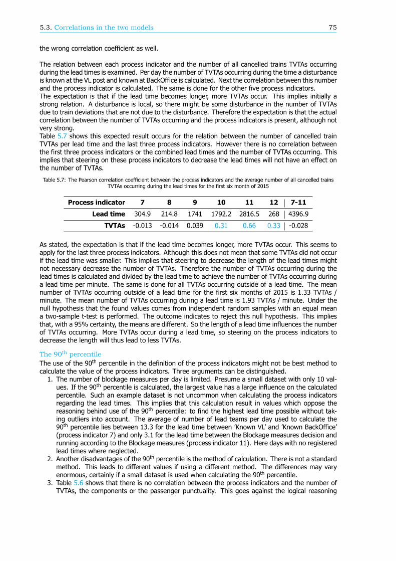
5.3. Correlations in the two models 75

the wrong correlation coefficient as well.

The relation between each process indicator and the number of all cancelled trains TVTAs occurringduring the lead times is examined. Per day the number of TVTAs occurring during the time a disturbanceis known at the VL post and known at BackOffice is calculated. Next the correlation between this numberand the process indicator is calculated. The same is done for the other five process indicators.The expectation is that if the lead time becomes longer, more TVTAs occur. This implies initially astrong relation. A disturbance is local, so there might be some disturbance in the number of TVTAsdue to train deviations that are not due to the disturbance. Therefore the expectation is that the actualcorrelation between the number of TVTAs occurring and the process indicators is present, although notvery strong.Table 5.7 shows this expected result occurs for the relation between the number of cancelled trainTVTAs per lead time and the last three process indicators. However there is no correlation betweenthe first three process indicators or the combined lead times and the number of TVTAs occurring. Thisimplies that steering on these process indicators to decrease the lead times will not have an effect onthe number of TVTAs.

Table 5.7: The Pearson correlation coefficient between the process indicators and the average number of all cancelled trainsTVTAs occurring during the lead times for the first six month of 2015

Process indicator 7 8 9 10 11 12 7-11

Lead time 304.9 214.8 1741 1792.2 2816.5 268 4396.9

TVTAs -0.013 -0.014 0.039 0.31 0.66 0.33 -0.028

As stated, the expectation is that if the lead time becomes longer, more TVTAs occur. This seems toapply for the last three process indicators. Although this does not mean that some TVTAs did not occurif the lead time was smaller. This implies that steering to decrease the length of the lead times mightnot necessary decrease the number of TVTAs. Therefore the number of TVTAs occurring during thelead times is calculated and divided by the lead time to achieve the number of TVTAs occurring duringa lead time per minute. The same is done for all TVTAs occurring outside of a lead time. The meannumber of TVTAs occurring outside of a lead time for the first six months of 2015 is 1.33 TVTAs /minute. The mean number of TVTAs occurring during a lead time is 1.93 TVTAs / minute. Under thenull hypothesis that the found values comes from independent random samples with an equal meana two-sample t-test is performed. The outcome indicates to reject this null hypothesis. This impliesthat, with a 95% certainty, the means are different. So the length of a lead time influences the numberof TVTAs occurring. More TVTAs occur during a lead time, so steering on the process indicators todecrease the length will thus lead to less TVTAs.

The 90th percentileThe use of the 90th percentile in the definition of the process indicators might not be best method tocalculate the value of the process indicators. Three arguments can be distinguished.1. The number of blockage measures per day is limited. Presume a small dataset with only 10 val-ues. If the 90th percentile is calculated, the largest value has a large influence on the calculatedpercentile. Such an example dataset is not uncommon when calculating the process indicatorsregarding the lead times. This implies that this calculation result in values which oppose thereasoning behind use of the 90th percentile: to find the highest lead time possible without tak-ing outliers into account. The average of number of lead teams per day used to calculate the90th percentile lies between 13.3 for the lead time between ’Known VL’ and ’Known BackOffice’(process indicator 7) and only 3.1 for the lead time between the Blockage measures decision andrunning according to the Blockage measures (process indicator 11). Here days with no registeredlead times where neglected.

2. Another disadvantages of the 90th percentile is the method of calculation. There is not a standardmethod. This leads to different values if using a different method. The differences may varyenormous, certainly if a small dataset is used when calculating the 90th percentile.

3. Table 5.6 shows that there is no correlation between the process indicators and the number ofTVTAs, the components or the passenger punctuality. This goes against the logical reasoning

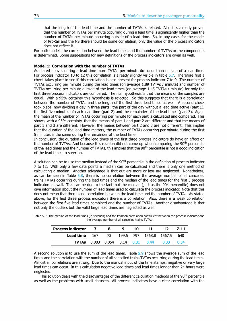
76 5. Models to describe passenger punctuality

that the length of the lead time and the number of TVTAs is related. Also it is already provedthat the number of TVTAs per minute occurring during a lead time is significantly higher than thenumber of TVTAs per minute occurring outside of a lead time. So, in any case, for the modelof ProRail and the NS there should be some correlation, only the value of the process indicatorsdoes not reflect it.

For both models the correlation between the lead times and the number of TVTAs or the componentsis determined. Some suggestions for new definitions of the process indicators are given as well.

Model 1: Correlation with the number of TVTAsAs stated above, during a lead time more TVTAs per minute do occur than outside of a lead time.For process indicator 10 to 12 this correlation is already slightly visible in table 5.7. Therefore first acheck takes place to see if this correlation is also present for process indicator 7 to 9. The number ofTVTAs occurring per minute during the lead times (on average 1.89 TVTAs / minute) and number ofTVTAs occurring per minute outside of the lead times (on average 1.45 TVTAs / minute) for only thefirst three process indicators are compared. The null hypothesis is that the means of the samples areequal. With a 95% certainty this hypothesis is rejected. So this suggests that there is a correlationbetween the number of TVTAs and the length of the first three lead times as well. A second checktook place, now dividing a day in three parts: the part of the day without a lead time active (part 1),the first five minutes of each lead time (part 2) and the remainder of the lead times (part 3). Againthe mean of the number of TVTAs occurring per minute for each part is calculated and compared. Thisshows, with a 95% certainty, that the means of part 1 and part 2 are different and that the means ofpart 1 and 3 are different. However, the means between part 2 and 3 are not different. This impliesthat the duration of the lead time matters, the number of TVTAs occurring per minute during the first5 minutes is the same during the remainder of the lead time.In conclusion, the duration of the lead times of the first three process indicators do have an effect onthe number of TVTAs. And because this relation did not come up when comparing the 90th percentileof the lead times and the number of TVTAs, this implies that the 90th percentile is not a good indicationof the lead times to steer on.

A solution can be to use the median instead of the 90th percentile in the definition of process indicator7 to 12. With only a few data points a median can be calculated and there is only one method ofcalculating a median. Another advantage is that outliers more or less are neglected. Nonetheless,as can be seen in Table 5.8, there is no correlation between the average number of all cancelledtrains TVTAs occurring during the lead times and the median of the lead times for the first 3 processindicators as well. This can be due to the fact that the median (just as the 90th percentile) does notgive information about the number of lead times used to calculate the process indicator. Note that thisdoes not mean that there is no correlation between the lead time and the number of TVTAs. As statedabove, for the first three process indicators there is a correlation. Also, there is a weak correlationbetween the first five lead times combined and the number of TVTAs. Another disadvantage is thatnot only the outliers but the valid large lead times are neglected as well.

Table 5.8: The median of the lead times (in seconds) and the Pearson correlation coefficient between the process indicator andthe average number of all cancelled trains TVTAs

Process indicator 7 8 9 10 11 12 7-11

Lead time 167 73 199.5 797 1568.8 1567.5 640

TVTAs 0.083 0.054 0.14 0.31 0.44 0.33 0.34

A second solution is to use the sum of the lead times. Table 5.9 shows the average sum of the leadtimes and the correlation with the number of all cancelled trains TVTAs occurring during the lead times.Almost all correlations are strong. Due to the manual input of the time stamps, negative or very largelead times can occur. In this calculation negative lead times and lead times longer than 24 hours wereneglected.

This solution deals with the disadvantages of the different calculation methods of the 90th percentileas well as the problems with small datasets. All process indicators have a clear correlation with the

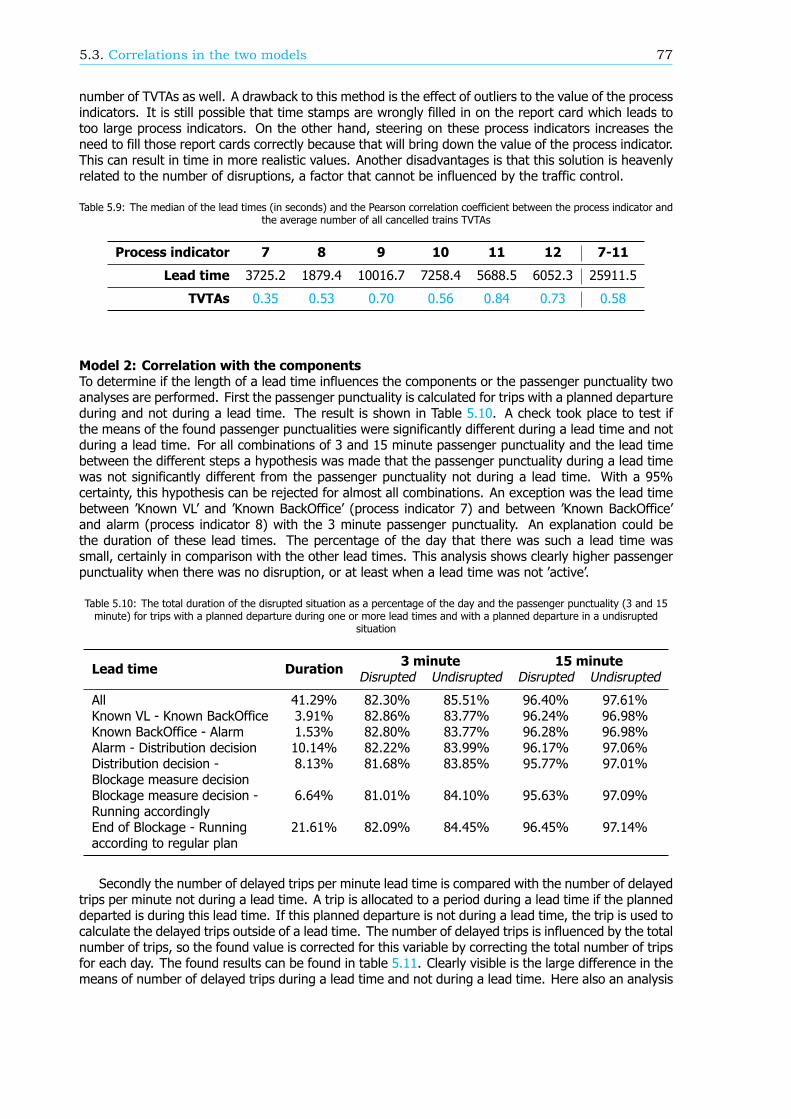
5.3. Correlations in the two models 77

number of TVTAs as well. A drawback to this method is the effect of outliers to the value of the processindicators. It is still possible that time stamps are wrongly filled in on the report card which leads totoo large process indicators. On the other hand, steering on these process indicators increases theneed to fill those report cards correctly because that will bring down the value of the process indicator.This can result in time in more realistic values. Another disadvantages is that this solution is heavenlyrelated to the number of disruptions, a factor that cannot be influenced by the traffic control.

Table 5.9: The median of the lead times (in seconds) and the Pearson correlation coefficient between the process indicator andthe average number of all cancelled trains TVTAs

Process indicator 7 8 9 10 11 12 7-11

Lead time 3725.2 1879.4 10016.7 7258.4 5688.5 6052.3 25911.5

TVTAs 0.35 0.53 0.70 0.56 0.84 0.73 0.58

Model 2: Correlation with the componentsTo determine if the length of a lead time influences the components or the passenger punctuality twoanalyses are performed. First the passenger punctuality is calculated for trips with a planned departureduring and not during a lead time. The result is shown in Table 5.10. A check took place to test ifthe means of the found passenger punctualities were significantly different during a lead time and notduring a lead time. For all combinations of 3 and 15 minute passenger punctuality and the lead timebetween the different steps a hypothesis was made that the passenger punctuality during a lead timewas not significantly different from the passenger punctuality not during a lead time. With a 95%certainty, this hypothesis can be rejected for almost all combinations. An exception was the lead timebetween ’Known VL’ and ’Known BackOffice’ (process indicator 7) and between ’Known BackOffice’and alarm (process indicator 8) with the 3 minute passenger punctuality. An explanation could bethe duration of these lead times. The percentage of the day that there was such a lead time wassmall, certainly in comparison with the other lead times. This analysis shows clearly higher passengerpunctuality when there was no disruption, or at least when a lead time was not ’active’.

Table 5.10: The total duration of the disrupted situation as a percentage of the day and the passenger punctuality (3 and 15minute) for trips with a planned departure during one or more lead times and with a planned departure in a undisrupted

situation

Lead time Duration 3 minute 15 minuteDisrupted Undisrupted Disrupted Undisrupted

All 41.29% 82.30% 85.51% 96.40% 97.61%Known VL - Known BackOffice 3.91% 82.86% 83.77% 96.24% 96.98%Known BackOffice - Alarm 1.53% 82.80% 83.77% 96.28% 96.98%Alarm - Distribution decision 10.14% 82.22% 83.99% 96.17% 97.06%Distribution decision -Blockage measure decision

8.13% 81.68% 83.85% 95.77% 97.01%

Blockage measure decision -Running accordingly

6.64% 81.01% 84.10% 95.63% 97.09%

End of Blockage - Runningaccording to regular plan

21.61% 82.09% 84.45% 96.45% 97.14%

Secondly the number of delayed trips per minute lead time is compared with the number of delayedtrips per minute not during a lead time. A trip is allocated to a period during a lead time if the planneddeparted is during this lead time. If this planned departure is not during a lead time, the trip is used tocalculate the delayed trips outside of a lead time. The number of delayed trips is influenced by the totalnumber of trips, so the found value is corrected for this variable by correcting the total number of tripsfor each day. The found results can be found in table 5.11. Clearly visible is the large difference in themeans of number of delayed trips during a lead time and not during a lead time. Here also an analysis

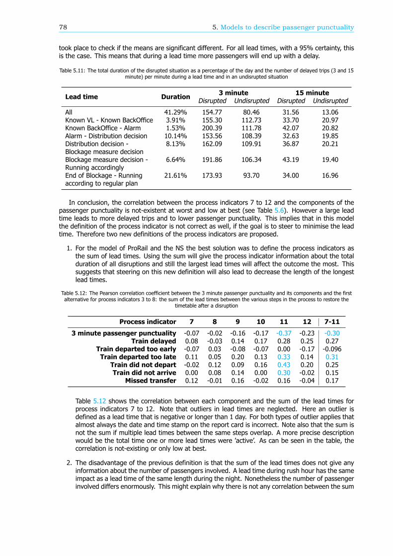
78 5. Models to describe passenger punctuality

took place to check if the means are significant different. For all lead times, with a 95% certainty, thisis the case. This means that during a lead time more passengers will end up with a delay.

Table 5.11: The total duration of the disrupted situation as a percentage of the day and the number of delayed trips (3 and 15minute) per minute during a lead time and in an undisrupted situation

Lead time Duration 3 minute 15 minuteDisrupted Undisrupted Disrupted Undisrupted

All 41.29% 154.77 80.46 31.56 13.06Known VL - Known BackOffice 3.91% 155.30 112.73 33.70 20.97Known BackOffice - Alarm 1.53% 200.39 111.78 42.07 20.82Alarm - Distribution decision 10.14% 153.56 108.39 32.63 19.85Distribution decision -Blockage measure decision

8.13% 162.09 109.91 36.87 20.21

Blockage measure decision -Running accordingly

6.64% 191.86 106.34 43.19 19.40

End of Blockage - Runningaccording to regular plan

21.61% 173.93 93.70 34.00 16.96

In conclusion, the correlation between the process indicators 7 to 12 and the components of thepassenger punctuality is not-existent at worst and low at best (see Table 5.6). However a large leadtime leads to more delayed trips and to lower passenger punctuality. This implies that in this modelthe definition of the process indicator is not correct as well, if the goal is to steer to minimise the leadtime. Therefore two new definitions of the process indicators are proposed.

1. For the model of ProRail and the NS the best solution was to define the process indicators asthe sum of lead times. Using the sum will give the process indicator information about the totalduration of all disruptions and still the largest lead times will affect the outcome the most. Thissuggests that steering on this new definition will also lead to decrease the length of the longestlead times.

Table 5.12: The Pearson correlation coefficient between the 3 minute passenger punctuality and its components and the firstalternative for process indicators 3 to 8: the sum of the lead times between the various steps in the process to restore the

timetable after a disruption

Process indicator 7 8 9 10 11 12 7-11

3 minute passenger punctuality -0.07 -0.02 -0.16 -0.17 -0.37 -0.23 -0.30Train delayed 0.08 -0.03 0.14 0.17 0.28 0.25 0.27

Train departed too early -0.07 0.03 -0.08 -0.07 0.00 -0.17 -0.096Train departed too late 0.11 0.05 0.20 0.13 0.33 0.14 0.31

Train did not depart -0.02 0.12 0.09 0.16 0.43 0.20 0.25Train did not arrive 0.00 0.08 0.14 0.00 0.30 -0.02 0.15

Missed transfer 0.12 -0.01 0.16 -0.02 0.16 -0.04 0.17

Table 5.12 shows the correlation between each component and the sum of the lead times forprocess indicators 7 to 12. Note that outliers in lead times are neglected. Here an outlier isdefined as a lead time that is negative or longer than 1 day. For both types of outlier applies thatalmost always the date and time stamp on the report card is incorrect. Note also that the sum isnot the sum if multiple lead times between the same steps overlap. A more precise descriptionwould be the total time one or more lead times were ’active’. As can be seen in the table, thecorrelation is not-existing or only low at best.

2. The disadvantage of the previous definition is that the sum of the lead times does not give anyinformation about the number of passengers involved. A lead time during rush hour has the sameimpact as a lead time of the same length during the night. Nonetheless the number of passengerinvolved differs enormously. This might explain why there is not any correlation between the sum

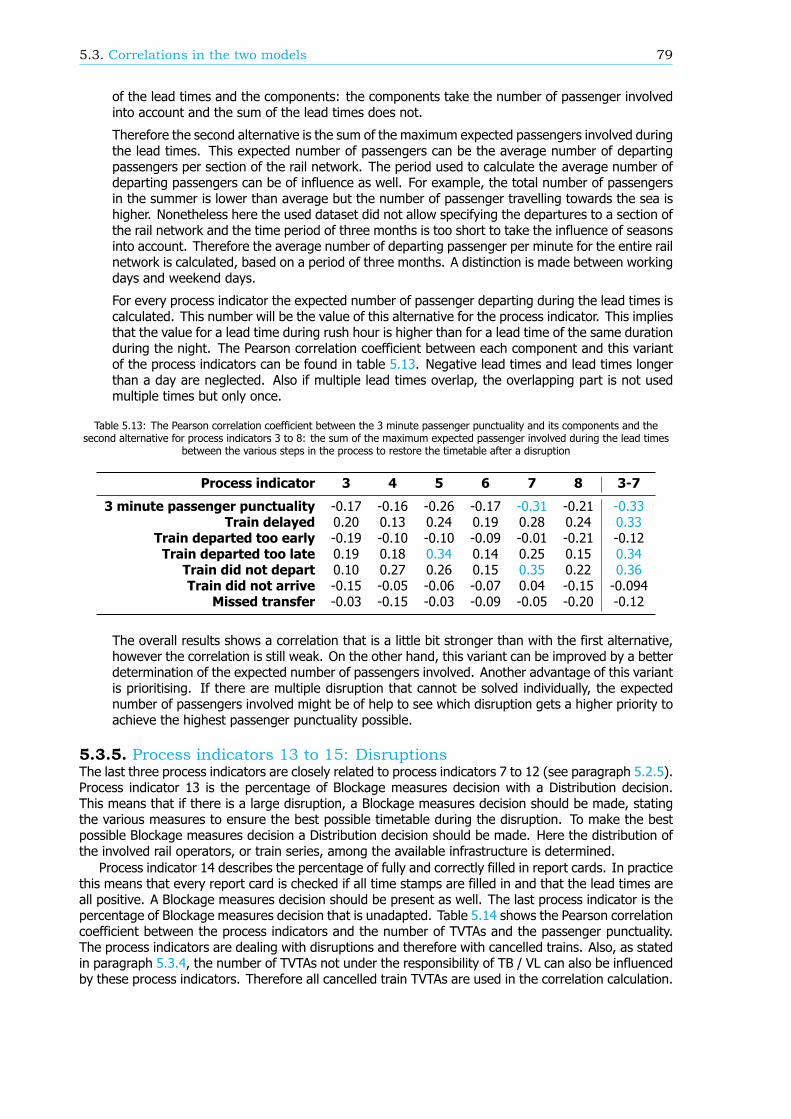
5.3. Correlations in the two models 79

of the lead times and the components: the components take the number of passenger involvedinto account and the sum of the lead times does not.

Therefore the second alternative is the sum of the maximum expected passengers involved duringthe lead times. This expected number of passengers can be the average number of departingpassengers per section of the rail network. The period used to calculate the average number ofdeparting passengers can be of influence as well. For example, the total number of passengersin the summer is lower than average but the number of passenger travelling towards the sea ishigher. Nonetheless here the used dataset did not allow specifying the departures to a section ofthe rail network and the time period of three months is too short to take the influence of seasonsinto account. Therefore the average number of departing passenger per minute for the entire railnetwork is calculated, based on a period of three months. A distinction is made between workingdays and weekend days.

For every process indicator the expected number of passenger departing during the lead times iscalculated. This number will be the value of this alternative for the process indicator. This impliesthat the value for a lead time during rush hour is higher than for a lead time of the same durationduring the night. The Pearson correlation coefficient between each component and this variantof the process indicators can be found in table 5.13. Negative lead times and lead times longerthan a day are neglected. Also if multiple lead times overlap, the overlapping part is not usedmultiple times but only once.

Table 5.13: The Pearson correlation coefficient between the 3 minute passenger punctuality and its components and thesecond alternative for process indicators 3 to 8: the sum of the maximum expected passenger involved during the lead times

between the various steps in the process to restore the timetable after a disruption

Process indicator 3 4 5 6 7 8 3-7

3 minute passenger punctuality -0.17 -0.16 -0.26 -0.17 -0.31 -0.21 -0.33Train delayed 0.20 0.13 0.24 0.19 0.28 0.24 0.33

Train departed too early -0.19 -0.10 -0.10 -0.09 -0.01 -0.21 -0.12Train departed too late 0.19 0.18 0.34 0.14 0.25 0.15 0.34

Train did not depart 0.10 0.27 0.26 0.15 0.35 0.22 0.36Train did not arrive -0.15 -0.05 -0.06 -0.07 0.04 -0.15 -0.094

Missed transfer -0.03 -0.15 -0.03 -0.09 -0.05 -0.20 -0.12

The overall results shows a correlation that is a little bit stronger than with the first alternative,however the correlation is still weak. On the other hand, this variant can be improved by a betterdetermination of the expected number of passengers involved. Another advantage of this variantis prioritising. If there are multiple disruption that cannot be solved individually, the expectednumber of passengers involved might be of help to see which disruption gets a higher priority toachieve the highest passenger punctuality possible.

5.3.5. Process indicators 13 to 15: DisruptionsThe last three process indicators are closely related to process indicators 7 to 12 (see paragraph 5.2.5).Process indicator 13 is the percentage of Blockage measures decision with a Distribution decision.This means that if there is a large disruption, a Blockage measures decision should be made, statingthe various measures to ensure the best possible timetable during the disruption. To make the bestpossible Blockage measures decision a Distribution decision should be made. Here the distribution ofthe involved rail operators, or train series, among the available infrastructure is determined.

Process indicator 14 describes the percentage of fully and correctly filled in report cards. In practicethis means that every report card is checked if all time stamps are filled in and that the lead times areall positive. A Blockage measures decision should be present as well. The last process indicator is thepercentage of Blockage measures decision that is unadapted. Table 5.14 shows the Pearson correlationcoefficient between the process indicators and the number of TVTAs and the passenger punctuality.The process indicators are dealing with disruptions and therefore with cancelled trains. Also, as statedin paragraph 5.3.4, the number of TVTAs not under the responsibility of TB / VL can also be influencedby these process indicators. Therefore all cancelled train TVTAs are used in the correlation calculation.

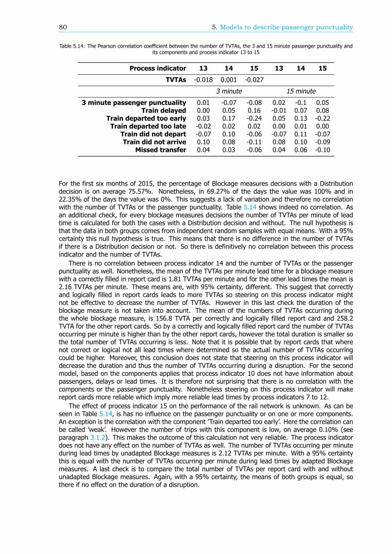
80 5. Models to describe passenger punctuality

Table 5.14: The Pearson correlation coefficient between the number of TVTAs, the 3 and 15 minute passenger punctuality andits components and process indicator 13 to 15

Process indicator 13 14 15 13 14 15

TVTAs -0.018 0.001 -0.027

3 minute 15 minute

3 minute passenger punctuality 0.01 -0.07 -0.08 0.02 -0.1 0.05Train delayed 0.00 0.05 0.16 -0.01 0.07 0.08

Train departed too early 0.03 0.17 -0.24 0.05 0.13 -0.22Train departed too late -0.02 0.02 0.02 0.00 0.01 0.00

Train did not depart -0.07 0.10 -0.06 -0.07 0.11 -0.07Train did not arrive 0.10 0.08 -0.11 0.08 0.10 -0.09

Missed transfer 0.04 0.03 -0.06 0.04 0.06 -0.10

For the first six months of 2015, the percentage of Blockage measures decisions with a Distributiondecision is on average 75.57%. Nonetheless, in 69.27% of the days the value was 100% and in22.35% of the days the value was 0%. This suggests a lack of variation and therefore no correlationwith the number of TVTAs or the passenger punctuality. Table 5.14 shows indeed no correlation. Asan additional check, for every blockage measures decisions the number of TVTAs per minute of leadtime is calculated for both the cases with a Distribution decision and without. The null hypothesis isthat the data in both groups comes from independent random samples with equal means. With a 95%certainty this null hypothesis is true. This means that there is no difference in the number of TVTAsif there is a Distribution decision or not. So there is definitively no correlation between this processindicator and the number of TVTAs.

There is no correlation between process indicator 14 and the number of TVTAs or the passengerpunctuality as well. Nonetheless, the mean of the TVTAs per minute lead time for a blockage measurewith a correctly filled in report card is 1.81 TVTAs per minute and for the other lead times the mean is2.16 TVTAs per minute. These means are, with 95% certainty, different. This suggest that correctlyand logically filled in report cards leads to more TVTAs so steering on this process indicator mightnot be effective to decrease the number of TVTAs. However in this last check the duration of theblockage measure is not taken into account. The mean of the numbers of TVTAs occurring duringthe whole blockage measure, is 156.8 TVTA per correctly and logically filled report card and 258.2TVTA for the other report cards. So by a correctly and logically filled report card the number of TVTAsoccurring per minute is higher than by the other report cards, however the total duration is smaller sothe total number of TVTAs occurring is less. Note that it is possible that by report cards that wherenot correct or logical not all lead times where determined so the actual number of TVTAs occurringcould be higher. Moreover, this conclusion does not state that steering on this process indicator willdecrease the duration and thus the number of TVTAs occurring during a disruption. For the secondmodel, based on the components applies that process indicator 10 does not have information aboutpassengers, delays or lead times. It is therefore not surprising that there is no correlation with thecomponents or the passenger punctuality. Nonetheless steering on this process indicator will makereport cards more reliable which imply more reliable lead times by process indicators 7 to 12.

The effect of process indicator 15 on the performance of the rail network is unknown. As can beseen in Table 5.14, is has no influence on the passenger punctuality or on one or more components.An exception is the correlation with the component ’Train departed too early’. Here the correlation canbe called ’weak’. However the number of trips with this component is low, on average 0.10% (seeparagraph 3.1.2). This makes the outcome of this calculation not very reliable. The process indicatordoes not have any effect on the number of TVTAs as well. The number of TVTAs occurring per minuteduring lead times by unadapted Blockage measures is 2.12 TVTAs per minute. With a 95% certaintythis is equal with the number of TVTAs occurring per minute during lead times by adapted Blockagemeasures. A last check is to compare the total number of TVTAs per report card with and withoutunadapted Blockage measures. Again, with a 95% certainty, the means of both groups is equal, sothere if no effect on the duration of a disruption.

5.4. Comparison of the two models 81

5.4. Comparison of the two modelsThe idea behind the model of ProRail and the NS to describe passenger punctuality is that steering onthe processes that minimise the number of Explainable Train Deviations (paragraph 5.1.1) would in-crease the passenger punctuality. These TVTAs indicates discrepancies between the planned timetableand the execution. A discrepancy could be a cancelled train but also a rerouted train or a delayed train.Three disadvantages of this model can be distinguished.1. As stated in paragraph 5.1.1, there is a very strong relation between this number and the 3 minutepassenger punctuality. The Pearson correlation coefficient drops a bit by the 15 minute passengerpunctuality, but still this correlation can be characterized as strong. However if focussing on onlythe business unit Transport control and Traffic control (TB / VL) this correlation between thepassenger punctuality and the number of TVTAs is only moderate. Not all TVTAs are takeninto account in de model as well, though the correlation between these neglected TVTAs and thepassenger punctuality is strong. This suggests that neglecting these TVTAs might not be effective: by neglecting these TVTAs, a part of the rail network that could be improved in order to improvethe passenger punctuality is neglected.

2. TVTAs are not weighted with the number of passengers affected by the TVTAs. This is a con-tradiction with the use of passenger punctuality above train punctuality: to make the interest ofpassengers top priority (see paragraph 2.3). As long as the TVTAs are not weighted with thenumber of passengers involved, steering to minimise the TVTAs is not the most effective methodto increase passenger punctuality.

3. The focus of a signaller is safety and not the allocation of types of TVTAs to train deviations, sothe TVTAs might not be very reliably. This is certainly the case by large disruptions, with manyTVTAs and many delayed passengers as well.

The common factor in these three disadvantages is the use of TVTAs. Therefore a new model isproposed, where TVTAs are neglected (see paragraph 5.1.2. In this new model the passenger punc-tuality is split into components. The share of the component is based on the number of trips withthat component, so the weight is included in this model. The process indicators relate to one or morecomponents. The sum of the components equals the passenger punctuality, so the process indicatorscan also directly be related with the passenger punctuality as well. This is in contrast to the model ofProRail and the NS. In that model the sum of all the TVTAs does not equal the passenger punctuality.A disadvantage of the new model regarding the model of ProRail and NS is that the performance of thebusiness units is not visible. Another drawback is that the correlation between the process indicatorsand the components or the passenger punctuality itself depends on the threshold value of a delay, sothe correlation between the process indicators and the 3 minute passenger punctuality differs from thecorrelation with the 15 minute passenger punctuality.

ProRail and the NS composed a list of 20 process indicators within the business unit TB / VL (see Table5.2). These process indicators are examined in paragraph 5.2. Steering on these indicators shouldaffect the number of TVTAs or the passenger punctuality. Five of those process indicators are not fullydeveloped yet and therefore not in use. A remark to process indicator 17 is that this indicator will nothave an influence on the number of TVTAs or size of the components, but on the behaviour of thepassengers. Steering on this indicator will therefore increase the passenger punctuality KPI but not thepassenger punctuality itself.

For the remaining 15 process indicators, the correlation with the number of TVTAs and the passengerpunctuality could be calculated. Note that the used TVTAs might differ between the process indicators,according to the goal of the process indicator. The results can be found in Table 5.15. Some specificnotes can be given:

1. The Pearson correlation coefficient for the first process indicator (the number of mutations inVKL) is almost similar for both models. It is the process indicator with the strongest correlationwith both the number of TVTAs and the passenger punctuality as well. Nonetheless this processindicator was intended to be an information-item and not an indicator that can be used to steeron [34].

2. Although for both models it is proven that a longer lead time leads to more TVTAs or morepassengers with a delay, process indicators 7 to 12 do not reflect this correlation. This is because

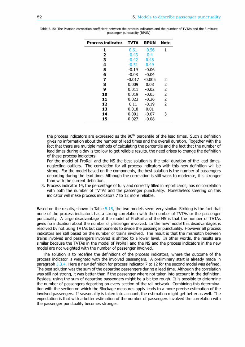
82 5. Models to describe passenger punctuality

Table 5.15: The Pearson correlation coefficient between the process indicators and the number of TVTAs and the 3 minutepassenger punctuality (RPUN)

Process indicator TVTA RPUN Note

1 0.61 -0.56 12 -0.43 0.43 -0.42 0.484 -0.51 0.495 -0.19 -0.066 -0.08 -0.047 -0.017 -0.005 28 0.009 0.08 29 0.011 -0.02 210 0.019 -0.05 211 0.023 -0.26 212 0.11 -0.19 213 0.018 0.0114 0.001 -0.07 315 0.027 -0.08

the process indicators are expressed as the 90th percentile of the lead times. Such a definitiongives no information about the number of lead times and the overall duration. Together with thefact that there are multiple methods of calculating the percentile and the fact that the number oflead times during a day is too low to get reliable results, the need arises to change the definitionof these process indicators.For the model of ProRail and the NS the best solution is the total duration of the lead times,neglecting outliers. The correlation for all process indicators with this new definition will bestrong. For the model based on the components, the best solution is the number of passengersdeparting during the lead time. Although the correlation is still weak to moderate, it is strongerthan with the current definition.

3. Process indicator 14, the percentage of fully and correctly filled in report cards, has no correlationwith both the number of TVTAs and the passenger punctuality. Nonetheless steering on thisindicator will make process indicators 7 to 12 more reliable.

Based on the results, shown in Table 5.15, the two models seem very similar. Striking is the fact thatnone of the process indicators has a strong correlation with the number of TVTAs or the passengerpunctuality. A large disadvantage of the model of ProRail and the NS is that the number of TVTAsgives no indication about the number of passenger involved. In the new model this disadvantages isresolved by not using TVTAs but components to divide the passenger punctuality. However all processindicators are still based on the number of trains involved. The result is that the mismatch betweentrains involved and passengers involved is shifted to a lower level. In other words, the results aresimilar because the TVTAs in the model of ProRail and the NS and the process indicators in the newmodel are not weighted with the number of passenger involved.

The solution is to redefine the definitions of the process indicators, where the outcome of theprocess indicator is weighted with the involved passengers. A preliminary start is already made inparagraph 5.3.4. Here a new definition for process indicator 7 to 12 for the second model was defined.The best solution was the sum of the departing passengers during a lead time. Although the correlationwas still not strong, it was better than if the passenger where not taken into account in the definition.Besides, using the sum of departing passengers might be a bit too rough. It is possible to determinethe number of passengers departing on every section of the rail network. Combining this determina-tion with the section on which the Blockage measures apply leads to a more precise estimation of theinvolved passengers. If seasonality is taken into account, the estimation might get better as well. Theexpectation is that with a better estimation of the number of passengers involved the correlation withthe passenger punctuality becomes stronger.

5.4. Comparison of the two models 83

As stated, based on the found correlations the both models are very similar. Besides, the found correla-tions are moderate at best. This makes it difficult to claim that one model does describe the passengerpunctuality better than the other. However the correlations in the model of ProRail and the NS are withthe number of TVTAs. Decreasing the number of TVTAs will not necessarily increase the passengerpunctuality with the same rate. This is in contrast to the model based on the components. If thesize of one or more component will decrease, the passenger punctuality will increase with the sameamount. This is an advantage the model of ProRail and the NS does not have. Nonetheless, as long asthe process indicators do not include the number of passengers involved and the correlations do notchange, the effect of both models can be improved.

For both models apply that the model is a simplification of the reality. The real performance of therail network, and especially the business unit Transport control and Traffic control, is in reality differentthan the process indicators suggest. This implies that steering on the process indicator will never leadto a perfect rail network, or a passenger punctuality of 100%. Nonetheless this is no reason not to usethese models. Correlations present in these models are also present in reality, although the Pearsoncorrelation coefficient might differ. Besides these models help to evaluate and steer more effectively onthe involved (business) units and are at this moment the best option to describe passenger punctuality.

6Process indicators for a subset of the

rail network

The official passenger punctuality KPI gives the performance of the whole network. Chapter 4 showedthat the passenger punctuality can also be calculated for subsets of the rail network. A subset can bea station, a train series or an origin-destination combination. By calculating the passenger punctualityfor a subset can reveal problems in the network that where not visible via the nationwide passengerpunctuality. In chapter 5 two models are discussed that can describe the passenger punctuality inorder to improve it. Both models use the process indicators, belonging to the Transport control and theTraffic control, to steer on the passenger punctuality. The correlation between these process indicatorsand the number of Explainable Train Deviations, the components and the passenger punctuality isdetermined. However this correlation is based on the entire network and might differ for a subset.Using the correlation of the entire network to steer on a subset of the network might therefore not bethe most effective method to increase the passenger punctuality. At this moment it is not possible tocalculate the process indicators for a subset of the rail network. Therefore an algorithm was createdthat is able to do this.

In order to calculate the process indicators, as described in paragraph 5.2, ProRail and the NSproduces several data files each day. With this data, the values of the process indicators of the previousday can be calculated. Combining these daily files can give a process indicator for a longer period oftime. The first part of the algorithm, created in this research, enriches each data file with someadditional data. This is necessary because the data files do not contain all the information needed tocalculate the process indicators for a subset of the rail network. This part of the algorithm is mostlywritten in MATLAB, but a small part is written in Structured Query Language. The second part of thealgorithm, written entirely in MATLAB, can calculate the process indicators for a specified subset. Inparagraph 6.1 the options to specify a subset are explained. Paragraph 6.2 describes in highlights theprocess to enrich the data files, which other data sources are needed and which part of the data canbe enriched. In appendix D the algorithm can be found.

6.1. The options to create subsetsA subset of the rail network can be a station, a (part of a) route or a moment in time. A combinationof these factors is possible as well. To ensure that for every subset every process indicator can becalculated, three options are distinguished. These options can be used to define the subset. Eachoption can add an additional constrain to the data used to calculate the process indicators. Altogetherthe constrains form the subset of the rail network.

1. Service control points: A service control point (in Dutch: Dienstregelpunt) is an importantgeographical point on the rail network. This can be a bridge, a rail yard, a place where a railwayline branches off a main line or a station. Via this option, a specific point of the rail network canbe examined. By the way of multiple points an area can be examined. In this last case, not everyservice control point in the area is needed, only the points at the border of the area and the

85

86 6. Process indicators for a subset of the rail network

arrival and departure station of every train series running in that area. However to minimise theerror, at least all stations in the area should also be included in the list of service control points.

An addition to this option is the possibility to define if one of these service control points is thestart point of a train series. This has only effect on the process indicators concerning the rightcomposition of the train and the right number of personnel at the morning start.

If multiple service control points are given instead of only one, at least two service control pointsshould match the service control points present in the data files of the process indicator to usethis data to calculate the process indicators. An exception is the data concerning train handlingdocuments (TAD). If a train handling document applies to only one station, the number of servicecontrol points involved is also one. This makes it impossible to have at least two service controlpoints in common with the examined area. As an addition, it is also possible to indicate that everyservice control point of the given area should be in common with data of the process indicators.

2. Train series: Via this option, the process indicators can be calculated for a single train seriesonly. The direction of the train series (even or uneven) can also be distinguished, although this isnot a prerequisite. It could occur that a disruption takes place during night time on a section thatis on the route of the examined train series. Nonetheless the disruption is at night, so the trainseries do not have a planned passage of the section. It is therefore arguable that this disruptionshould not be used in calculating the associated process indicators. Therefore as an addition, itcan be indicated if such situations should be taken into account or not. This applies not only todisruptions but also to the process indicators concerning empty rolling stock runs as well.

3. Time of day: A distinction can be made between the whole day, peak hours or off peak hours. Itis also possible to define a more specific time period. Note that this option does not apply to theprocess indicators regarding the right composition of the train and the right number of personnelat the morning start.

6.2. The enriched data filesThe process indicators can be calculated with data from six different data sources: VSM, PS, MS,TAD, VKL and VLM data. For all these data sources applies that the content of the data is enoughto calculate the process indicators for the whole rail network, but not for a subset. In other words,each data source needs to be enriched with additional information in order to calculate the processindicators for a subset of the rail network. The NS is responsible for the PS and the MS data. Thesystems that generate these data files are B@P and VKL MAT respectively. The basis for the other fourdata sources, under the responsibility of ProRail, is three systems, called VKL/VOS, TROTS and ISVL.Another program, Sherlock, combines the output of these systems to produce the VSM, TAD, VKL andVLM data.

This paragraph will describe each data source, in particular the information stored and the extrainformation needed to calculate the process indicators for each subset. For the enriching of the originaldata sources, three additional sources were used, though not every additional source is used to enrichevery original data source.1. The ribbon data (in Dutch: Lintdata) of each train number. This source, an output of Sherlock,contains the planned and realised route for each day and each train number. The route is repre-sented with a series of service control points, whereby every service control point the action ofthe train is shown: arrival, departure or passage. This data is available for ever train, so not onlythe passenger trains.

2. The ribbon data of each train series, as generated by Sherlock. If a train number is not known,this data source can be used. It contains per day the most frequent and the longest route of eachtrain series. A route is represented with a series of service control points, whereby every servicecontrol point the action of the train is shown: arrival, departure or passage. The longest route isthe route with the most service control points, not the route with the largest distance. This datais based on the realisation data only and not on the planned timetable. Using this informationsource instead of the ribbon data of each train number (see item 1) generates the assumptionthat the route of the individual train is the same as the most frequent route or the longest routeof the corresponding train series.

6.2. The enriched data files 87

3. The table ’EZ_D_RPU.FCT_RPUN_REISDEEL’, one of the output tables of the passenger punctu-ality calculation. In this table the planned and realised departure and arrival times of every trainnumber for every possible part of the route is stored. Note that this table only contains informa-tion of trains from the NS. This implies that if this data source is used, the process indicator doesnot contain data from other rail operators.

This paragraph ends with an overview of the percentage of data that can be enriched. The outcomedepends on the data source. The exact algorithm to enrich the data sources can be found in appendixD.1.

VSM dataNine process indicators can be calculated with the VSM data. This data contains information aboutthe report cards, used by large disruptions. With this data the lead times between key moments inthe process can be calculated. Also the percentage of Blockage measures decisions with a Distributiondecision, the percentage of fully and correctly filled in report cards and the percentage of unadaptedBlockage measures can be calculated.

Per report card the time period when the disruption occurred is known. Note that if the report cardin not filled in correctly, or if the time when all trains runs according to the Blockage measures or toregular plan is missing, this time period might be shorter than in reality. Also the two service controlpoints, giving the location of the disruption, is most of the time known. However it can occur that thisinformation is missing. In this case the corresponding data cannot be enriched.

Based on the location where the disruption happened and the ribbon data per train number, thenumbers of the trains passing the section of the disruption can be found. This information can becombined with the realisation data of all trains and the time the disruption occurred. The results arethe trains that run by the disruption or that were cancelled during the disruption. In this last case, theconclusion is made that the train was cancelled because of the disruption.

The final result is the VSM data enriched with the involved train numbers (and thus train series) foralmost every report card. Also the planned and realised route of each train number is known plus thefact if a train was cancelled.

PS data and MS dataThe process indicator that calculates the percentage of trains with the right number of personnel atthe morning start retrieves information from the PS data. The original data indicates per train seriesthe planned and realised number of staff members. This indicator is time independent, so informationabout time is not needed. This implies that the data needs only be enriched with the route of the trainseries. This route can be found with the ribbon data per train series.

The layout and content of the MS data is very similar with the PS data. The MS data is used tocalculate the percentage of trains with the right composition. Here also only the route of each trainseries needs to be known. For both data sets applies that the train series is used to find the routeinstead of every train number. If the actual route is not the most frequent or the longest route, thisinformation cannot be retrieved and thus a small discrepancy between the enriched data and the realityoccurs.

TAD dataThe TAD data contains all train handling document (TAD) situations. The relevant information is thename of the TAD and the train that triggers the use of a TAD. In the name of the TAD informationabout the involved train series and the location of route where the TAD applies can be found. Notethat information about time is not present. Another difficulty in enriching this data is the fact that it ispossible that not every train series present in the name of the TAD is involved.

One of the few certainties is the involvement of the train that triggers the TAD. With this trainnumber, the route of where the TAD applies and the ribbon data per train number the exact sectionof the TAD can be found. Next for every possible involved train series the arrival and departure timeson station in this section is determined, based on the realisation data from the passenger punctualitycalculation. Based on the time difference with the one certain train involved a determination can takeplace which train series or numbers are involved in the TAD. Here the planned arrival or departuretimes are used.

If all involved train numbers are known, the route for each train number can be found with theribbon data. The minimum of all departure and arrival times of the involved train numbers on the

88 6. Process indicators for a subset of the rail network

section where the TAD applies is the start time of the TAD. The maximum is the end time. Here adistinction is made between the planned departure and arrival times and the realised departure andarrival times.

At the end, the enriched TAD data consist of the expected route where the TAD applies, the involvedtrain numbers and train series and the time interval when the TAD applies. Note that because of thelittle available initial data, the data cannot be enriched without making some assumptions:

• Only the section of the route that all involved trains has in common is used to determine thearrival and departure times.

• If there are multiple trains from the same train series possible involved, the smallest difference inplanned departure or arrival time with the only train certainly involved is used to make a choicebetween the options.

• The most frequent route of a train series is used. If the section where the TAD applies does notlie on this route, the route of that train series with the most service control points is used. If thisroute is also a mismatch with the section of the TAD, the train series is neglected.

The planned and realised departure and arrival trains are used as well. This data is retrieved from the’EZ_D_RPU.FCT_RPUN_REISDEEL’-table. This table stores only data about trains from the NS.

VKL dataEvery mutation in the VKL system is stored in the VKL data. This mutation consists of the mutationtime and the involved train number. Only the location on the rail network is missing. So this additionalinformation is needed to use this data source to calculate the process indicator for a subset of the railnetwork.

The route of the train that had a mutation can be found via the train number and the ribbon data pertrain number. In comparison with the other data sources, the high number of train numbers without afound route is striking. A remark to this is the fact that most trains without a found route are freighttrains or empty rolling stock runs. Almost every passenger train can be linked with a ribbon of servicecontrol points.

VLM dataThe data about empty rolling stock runs can be found in the VLM data. With this data the departurepunctuality for empty rolling stock runs at rail yards and at stations can be found. The data consist ofa train number, the departure service control point, the planned and realised departure time and thedeparture delay.

With the train number and the ribbon data per train number the route of each empty rolling stockrun can be found. This route can be compared with every route of every passenger train in the ribbondata. If at least two service control points match, the conclusion is made that the passenger train didrun (partly) along the same route of the empty rolling stock run.

The next step is to make a determination which of the found passenger trains did run togetherwith the empty rolling stock. Hereby the planned and realised departure and arrival times are used.For each train the time period is calculated when the train did run on the same location as the emptyrolling stock. This time period is compared with the departure time of the empty rolling stock run. Ifthe departure time lies in the time period, the conclusion is drawn that the passenger train might beaffected by the empty rolling stock trip.

Note that the method to determine if a passenger train is affected by an empty rolling stock methodis not solid. If the matching section in the routes is at the end of the route of the empty rolling stock,the empty rolling stock run might pass this section long after its departure. It is unlikely that thepassenger train that did run during the departure time on that section is really affected by the emptyrolling stock run. Nonetheless the chance the corresponding train series is affected is higher. So thismethod distinguishes the train series affected by determining the train numbers possible affected.

Completeness of the enriched dataIt is possible that not every row of data can be enriched, or not fully enriched. A reason can be thatthe original data or the additional data is not complete or correct. It is also possible that information ofrail operators other than the NS is missing because this information is based on planned and realiseddeparture and arrival times. Note that this data was stored in the ’EZ_D_RPU.FCT_RPUN_REISDEEL’-table. This table contains only information about trains of the NS. A last reason can be a bug or a

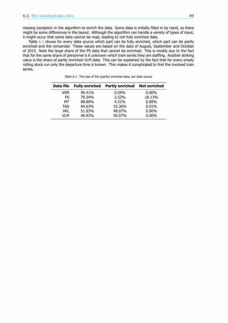
6.2. The enriched data files 89

missing exception in the algorithm to enrich the data. Some data is initially filled in by hand, so theremight be some differences in the layout. Although the algorithm can handle a variety of types of input,it might occur that some data cannot be read, leading to not fully enriched data.

Table 6.1 shows for every data source which part can be fully enriched, which part can be partlyenriched and the remainder. These values are based on the data of August, September and Octoberof 2015. Note the large share of the PS data that cannot be enriched. This is mostly due to the factthat for the same share of personnel is it unknown which train series they are staffing. Another strikingvalue is the share of partly enriched VLM data. This can be explained by the fact that for every emptyrolling stock run only the departure time is known. This makes it complicated to find the involved trainseries.

Table 6.1: The size of the (partly) enriched data, per data source

Data file Fully enriched Partly enriched Not enriched

VSM 99.41% 0.59% 0.00%PS 79.34% 2.53% 18.13%MT 88.80% 4.31% 6.89%TAD 84.63% 15.36% 0.01%VKL 51.93% 48.07% 0.00%VLM 40.93% 59.07% 0.00%

7Case study: Utrecht - Leeuwarden /

Groningen

In chapter 5 two models describing passenger punctuality were analysed. In the first model, as de-veloped by ProRail and the NS, the passenger punctuality is divided into “Explainable Train Deviations”(TVTAs), mostly cancelled and delayed trains. In the second model, the passenger punctuality is splitup in the components: the reason why passengers are delayed, according to their perspective. Forboth models applies that the TVTAs or the components are related to the process indicators under theresponsibility of Transport control and Traffic control (TB / VL). However this correlation is calculatedfor the entire network and might differ for a subset of the network.

Chapter 6 introduced an algorithm that is able to calculate the process indicators for a subset ofthe rail network. Such a subset can be a geographical area of the rail network, a train series or amoment in time, like rush hour. Herewith it becomes possible to determine the correlations in bothmodels these subsets. Therefor this chapter will focus on a subset of the rail network: the part of therail network between station Utrecht Centraal and stations Leeuwarden and Groningen. In paragraph7.1 this area is elaborated. A breakdown of the passenger punctuality (see chapter 4 of this study areais performed as well. In paragraph 7.2 the correlations between the process indicators and the numberof TVTAs, the components and the passenger punctuality are calculated. The outcome is comparedwith the correlations of the entire network. Finally some conclusions are drawn, described in paragraph7.3.

7.1. Description and the passenger punctuality of the study areaThe area of the case study is the main railway line to the north-east of the Netherlands. This line isschematically visualized in Figure 7.1. The line starts in the largest station in the Netherlands, UtrechtCentraal (Ut). After station Amersfoort and Zwolle the line splits into two branches near station Meppel(Mp). The western branch ends at station Leeuwarden (Lw) and the eastern branch ends at stationGroningen (Gn). At all 5 intercity stations there are side branches of the rail network in multipledirections. There are also two sections splitting off between stations Utrecht Centraal and Amersfoortand one just before station Groningen. These side branches are left out of the study area. Note thatnot every station in the area is visualized, but they are all taken into account.

A subset of the rail network is examined, so there is a complication when calculating the passengerpunctuality and the size of the components. Some passengers travel from a station in this study areato another station outside of the study area or vice versa. Three solutions can be distinguished.1. All passengers that travel in this study area are taken into account. This also means that passen-gers travelling only partly in the area are taken into account as well, even if they end up with adelay in another part of the rail network.

2. For every passenger the train that causes his or her delay is determined. If that train runs inthe study area, the passenger is taken into account in the punctuality calculation. If a passengerdoes not have a delay, their last train is used. This will result in lower passenger punctuality than

91

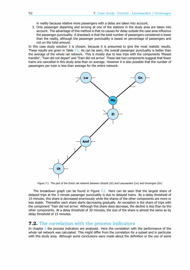
92 7. Case study: Utrecht - Leeuwarden / Groningen

in reality because relative more passengers with a delay are taken into account.3. Only passenger departing and arriving at one of the stations in the study area are taken intoaccount. The advantage of this method is that no causes for delay outside the case area influencethe passenger punctuality. A drawback is that the total number of passengers considered is lowerthan the reality, although the passenger punctuality is based on percentage of passengers andnot on the total amount.

In this case study solution 3 is chosen, because it is presumed to give the most realistic results.These results are given in Table 7.1. As can be seen, the overall passenger punctuality is better thanthe average of the whole rail network. This is mostly due to less trips with the components ’Missedtransfer’, ’Train did not depart’ and ’Train did not arrive’. These last two components suggest that fewertrains are cancelled in this study area than on average. However it is also possible that the number ofpassengers per train is less than average for the entire network.

Ut

Amf

Zl

Mp

Lw Gn

Figure 7.1: The part of the Dutch rail network between Utrecht (Ut) and Leeuwarden (Lw) and Groningen (Gn)

The breakdown graph can be found in Figure 7.2. Here can be seen that the largest share ofdelayed trips at the 3 minute passenger punctuality is due to delayed trains. By a delay threshold of15 minutes, this share is decreased enormously while the shares of the other components are more orless stable. Thereafter each share starts decreasing gradually. An exception is the share of trips withthe component ’Train did not arrive’. Although this share does decrease, the decline is less than by theother components. At a delay threshold of 30 minutes, the size of the share is almost the same as bydelay threshold of 15 minutes.

7.2. The correlation with the process indicatorsIn chapter 5 the process indicators are analysed. Here the correlation with the performance of thewhole rail network was calculated. This might differ from the correlation for a subset and in particularwith this study area. Although some conclusions were made about the definition or the use of some

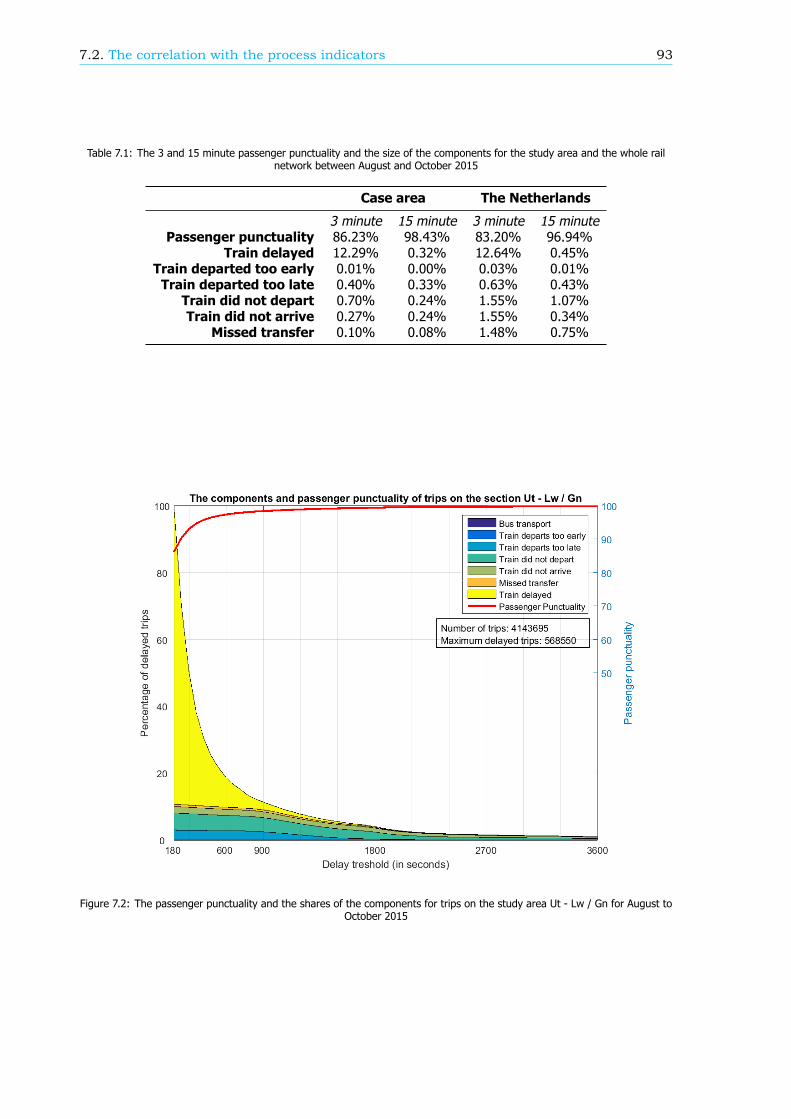
7.2. The correlation with the process indicators 93

Table 7.1: The 3 and 15 minute passenger punctuality and the size of the components for the study area and the whole railnetwork between August and October 2015

Case area The Netherlands

3 minute 15 minute 3 minute 15 minutePassenger punctuality 86.23% 98.43% 83.20% 96.94%

Train delayed 12.29% 0.32% 12.64% 0.45%Train departed too early 0.01% 0.00% 0.03% 0.01%Train departed too late 0.40% 0.33% 0.63% 0.43%

Train did not depart 0.70% 0.24% 1.55% 1.07%Train did not arrive 0.27% 0.24% 1.55% 0.34%

Missed transfer 0.10% 0.08% 1.48% 0.75%

Figure 7.2: The passenger punctuality and the shares of the components for trips on the study area Ut - Lw / Gn for August toOctober 2015

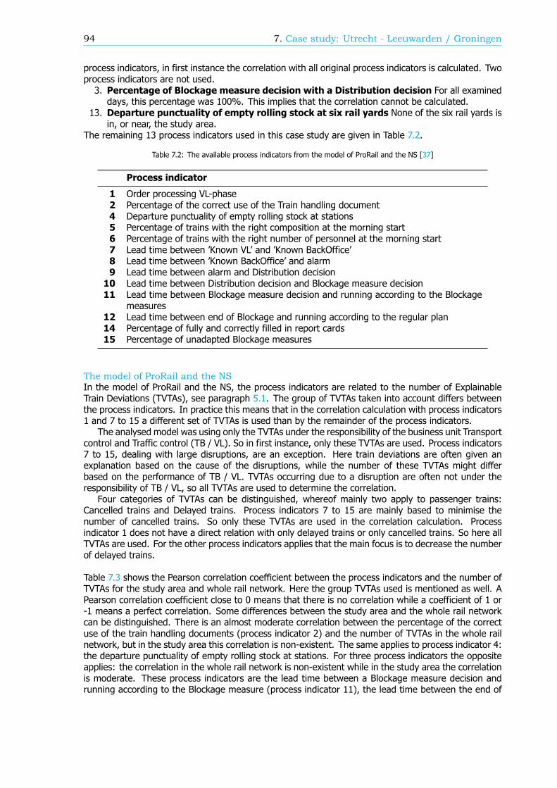
94 7. Case study: Utrecht - Leeuwarden / Groningen

process indicators, in first instance the correlation with all original process indicators is calculated. Twoprocess indicators are not used.3. Percentage of Blockage measure decision with a Distribution decision For all examineddays, this percentage was 100%. This implies that the correlation cannot be calculated.

13. Departure punctuality of empty rolling stock at six rail yards None of the six rail yards isin, or near, the study area.

The remaining 13 process indicators used in this case study are given in Table 7.2.

Table 7.2: The available process indicators from the model of ProRail and the NS [37]

Process indicator

1 Order processing VL-phase2 Percentage of the correct use of the Train handling document4 Departure punctuality of empty rolling stock at stations5 Percentage of trains with the right composition at the morning start6 Percentage of trains with the right number of personnel at the morning start7 Lead time between ’Known VL’ and ’Known BackOffice’8 Lead time between ’Known BackOffice’ and alarm9 Lead time between alarm and Distribution decision

10 Lead time between Distribution decision and Blockage measure decision11 Lead time between Blockage measure decision and running according to the Blockage

measures12 Lead time between end of Blockage and running according to the regular plan14 Percentage of fully and correctly filled in report cards15 Percentage of unadapted Blockage measures

The model of ProRail and the NSIn the model of ProRail and the NS, the process indicators are related to the number of ExplainableTrain Deviations (TVTAs), see paragraph 5.1. The group of TVTAs taken into account differs betweenthe process indicators. In practice this means that in the correlation calculation with process indicators1 and 7 to 15 a different set of TVTAs is used than by the remainder of the process indicators.

The analysed model was using only the TVTAs under the responsibility of the business unit Transportcontrol and Traffic control (TB / VL). So in first instance, only these TVTAs are used. Process indicators7 to 15, dealing with large disruptions, are an exception. Here train deviations are often given anexplanation based on the cause of the disruptions, while the number of these TVTAs might differbased on the performance of TB / VL. TVTAs occurring due to a disruption are often not under theresponsibility of TB / VL, so all TVTAs are used to determine the correlation.

Four categories of TVTAs can be distinguished, whereof mainly two apply to passenger trains:Cancelled trains and Delayed trains. Process indicators 7 to 15 are mainly based to minimise thenumber of cancelled trains. So only these TVTAs are used in the correlation calculation. Processindicator 1 does not have a direct relation with only delayed trains or only cancelled trains. So here allTVTAs are used. For the other process indicators applies that the main focus is to decrease the numberof delayed trains.

Table 7.3 shows the Pearson correlation coefficient between the process indicators and the number ofTVTAs for the study area and whole rail network. Here the group TVTAs used is mentioned as well. APearson correlation coefficient close to 0 means that there is no correlation while a coefficient of 1 or-1 means a perfect correlation. Some differences between the study area and the whole rail networkcan be distinguished. There is an almost moderate correlation between the percentage of the correctuse of the train handling documents (process indicator 2) and the number of TVTAs in the whole railnetwork, but in the study area this correlation is non-existent. The same applies to process indicator 4:the departure punctuality of empty rolling stock at stations. For three process indicators the oppositeapplies: the correlation in the whole rail network is non-existent while in the study area the correlationis moderate. These process indicators are the lead time between a Blockage measure decision andrunning according to the Blockage measure (process indicator 11), the lead time between the end of

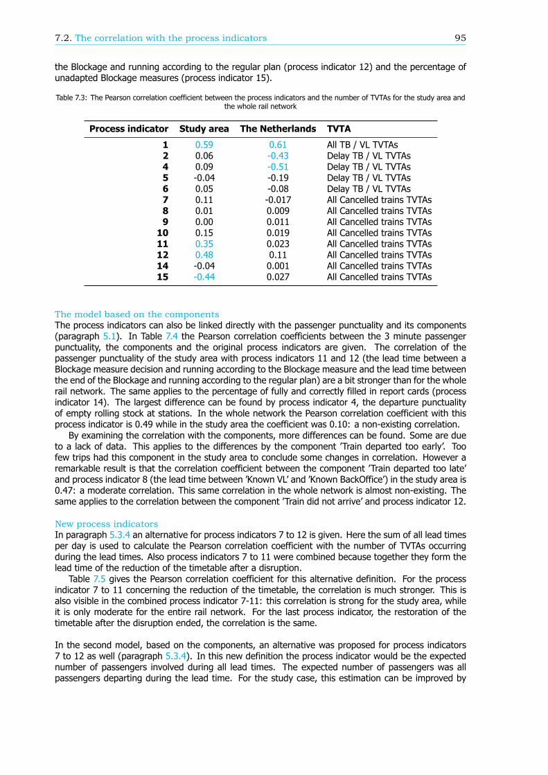
7.2. The correlation with the process indicators 95

the Blockage and running according to the regular plan (process indicator 12) and the percentage ofunadapted Blockage measures (process indicator 15).

Table 7.3: The Pearson correlation coefficient between the process indicators and the number of TVTAs for the study area andthe whole rail network

Process indicator Study area The Netherlands TVTA

1 0.59 0.61 All TB / VL TVTAs2 0.06 -0.43 Delay TB / VL TVTAs4 0.09 -0.51 Delay TB / VL TVTAs5 -0.04 -0.19 Delay TB / VL TVTAs6 0.05 -0.08 Delay TB / VL TVTAs7 0.11 -0.017 All Cancelled trains TVTAs8 0.01 0.009 All Cancelled trains TVTAs9 0.00 0.011 All Cancelled trains TVTAs

10 0.15 0.019 All Cancelled trains TVTAs11 0.35 0.023 All Cancelled trains TVTAs12 0.48 0.11 All Cancelled trains TVTAs14 -0.04 0.001 All Cancelled trains TVTAs15 -0.44 0.027 All Cancelled trains TVTAs

The model based on the componentsThe process indicators can also be linked directly with the passenger punctuality and its components(paragraph 5.1). In Table 7.4 the Pearson correlation coefficients between the 3 minute passengerpunctuality, the components and the original process indicators are given. The correlation of thepassenger punctuality of the study area with process indicators 11 and 12 (the lead time between aBlockage measure decision and running according to the Blockage measure and the lead time betweenthe end of the Blockage and running according to the regular plan) are a bit stronger than for the wholerail network. The same applies to the percentage of fully and correctly filled in report cards (processindicator 14). The largest difference can be found by process indicator 4, the departure punctualityof empty rolling stock at stations. In the whole network the Pearson correlation coefficient with thisprocess indicator is 0.49 while in the study area the coefficient was 0.10: a non-existing correlation.

By examining the correlation with the components, more differences can be found. Some are dueto a lack of data. This applies to the differences by the component ’Train departed too early’. Toofew trips had this component in the study area to conclude some changes in correlation. However aremarkable result is that the correlation coefficient between the component ’Train departed too late’and process indicator 8 (the lead time between ’Known VL’ and ’Known BackOffice’) in the study area is0.47: a moderate correlation. This same correlation in the whole network is almost non-existing. Thesame applies to the correlation between the component ’Train did not arrive’ and process indicator 12.

New process indicatorsIn paragraph 5.3.4 an alternative for process indicators 7 to 12 is given. Here the sum of all lead timesper day is used to calculate the Pearson correlation coefficient with the number of TVTAs occurringduring the lead times. Also process indicators 7 to 11 were combined because together they form thelead time of the reduction of the timetable after a disruption.

Table 7.5 gives the Pearson correlation coefficient for this alternative definition. For the processindicator 7 to 11 concerning the reduction of the timetable, the correlation is much stronger. This isalso visible in the combined process indicator 7-11: this correlation is strong for the study area, whileit is only moderate for the entire rail network. For the last process indicator, the restoration of thetimetable after the disruption ended, the correlation is the same.

In the second model, based on the components, an alternative was proposed for process indicators7 to 12 as well (paragraph 5.3.4). In this new definition the process indicator would be the expectednumber of passengers involved during all lead times. The expected number of passengers was allpassengers departing during the lead time. For the study case, this estimation can be improved by

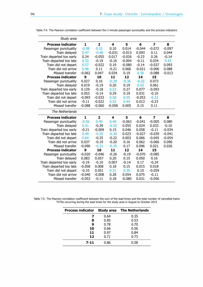
96 7. Case study: Utrecht - Leeuwarden / Groningen

Table 7.4: The Pearson correlation coefficient between the 3 minute passenger punctuality and the process indicators

Study area

Process indicator 1 2 4 5 6 7 8Passenger punctuality -0.58 0.33 0.10 0.014 -0.044 -0.072 -0.097

Train delayed 0.47 -0.40 -0.031 -0.013 0.093 0.11 0.044Train departed too early 0.24 -0.055 0.017 -0.026 -0.23 0.26 -0.14Train departed too late 0.32 -0.19 -0.16 -0.004 -0.11 0.034 0.43Train did not depart 0.57 -0.022 0.19 -0.080 -0.14 -0.037 0.093Train did not arrive 0.46 0.11 -0.21 0.066 -0.021 -0.006 0.088

Missed transfer -0.062 0.047 0.034 0.19 0.30 -0.088 -0.013Process indicator 9 10 11 12 14 15

Passenger punctuality 0.027 0.16 -0.39 -0.36 -0.32 0.073Train delayed 0.019 -0.19 0.20 0.19 0.43 0.061

Train departed too early 0.129 -0.18 0.53 0.27 0.077 -0.093Train departed too late 0.053 -0.14 0.29 0.19 0.031 -0.10Train did not depart -0.093 -0.033 0.58 0.55 -0.053 -0.32Train did not arrive -0.11 -0.022 0.53 0.44 0.013 -0.23

Missed transfer -0.088 -0.060 -0.058 0.005 0.15 0.11

The Netherlands

Process indicator 1 2 4 5 6 7 8Passenger punctuality -0.56 0.40 0.49 -0.063 -0.041 -0.005 0.080

Train delayed 0.51 -0.39 -0.52 0.055 0.024 0.033 -0.10Train departed too early -0.21 -0.009 0.15 0.046 0.058 -0.11 -0.034Train departed too late 0.49 -0.35 -0.36 0.023 -0.027 -0.039 -0.041Train did not depart 0.64 -0.25 -0.22 0.003 0.066 -0.045 -0.054Train did not arrive 0.037 -0.19 -0.20 0.16 0.062 -0.066 0.096

Missed transfer -0.090 -0.31 -0.35 0.17 0.096 0.021 0.026Process indicator 9 10 11 12 14 15

Passenger punctuality -0.020 -0.046 -0.26 -0.19 -0.070 -0.085Train delayed 0.083 0.057 0.20 0.15 0.050 0.16

Train departed too early -0.19 -0.10 0.007 -0.14 0.17 -0.24Train departed too late -0.058 0.008 0.18 0.15 0.015 0.018Train did not depart -0.10 0.051 0.31 0.30 0.10 -0.059Train did not arrive -0.040 -0.008 0.28 0.054 0.075 -0.11

Missed transfer -0.053 -0.11 0.18 -0.080 0.031 -0.056

Table 7.5: The Pearson correlation coefficient between the sum of the lead times and the total number of cancelled trainsTVTAs occurring during the lead times for the study area in August to October 2015

Process indicator Study area The Netherlands

7 0.64 0.358 0.85 0.539 0.78 0.70

10 0.66 0.5611 0.97 0.8412 0.71 0.73

7-11 0.86 0.58

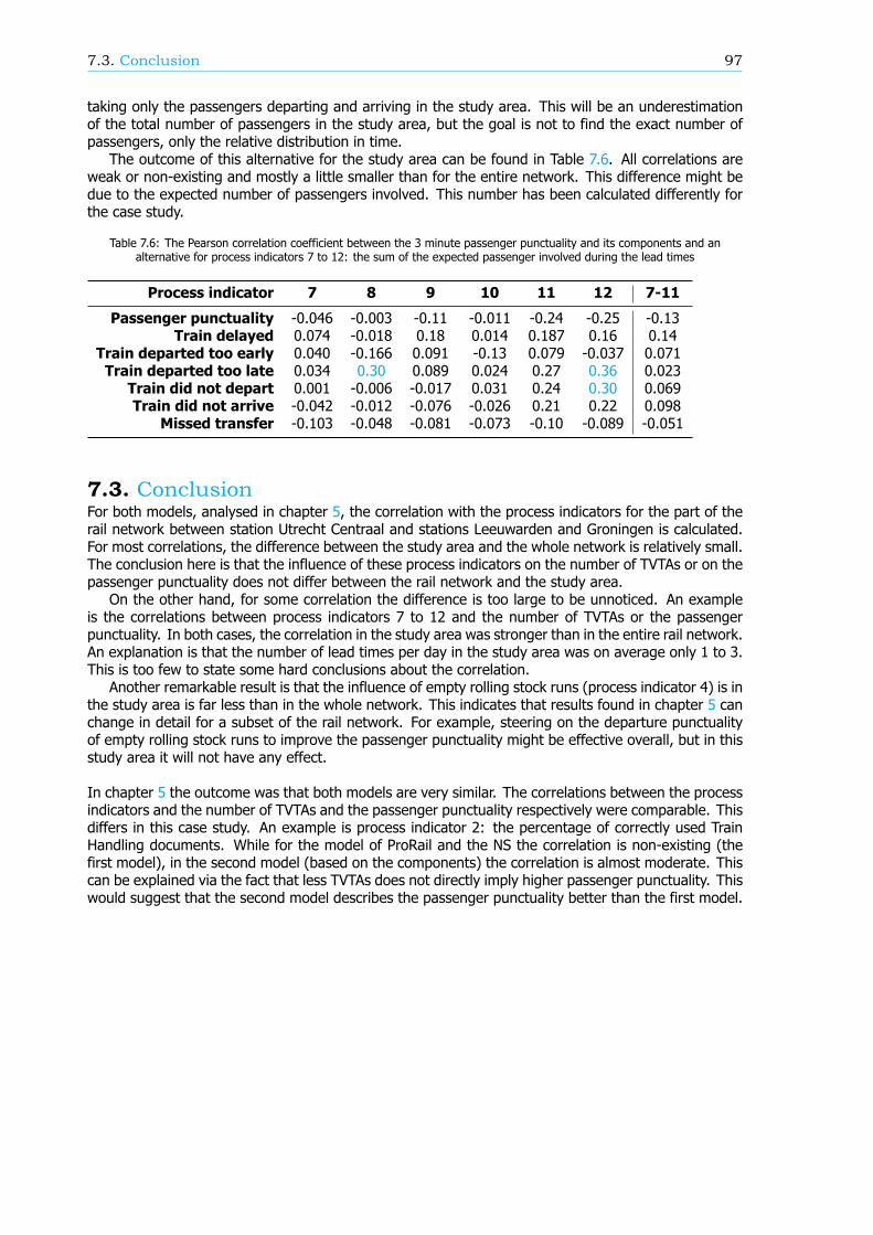
7.3. Conclusion 97

taking only the passengers departing and arriving in the study area. This will be an underestimationof the total number of passengers in the study area, but the goal is not to find the exact number ofpassengers, only the relative distribution in time.

The outcome of this alternative for the study area can be found in Table 7.6. All correlations areweak or non-existing and mostly a little smaller than for the entire network. This difference might bedue to the expected number of passengers involved. This number has been calculated differently forthe case study.

Table 7.6: The Pearson correlation coefficient between the 3 minute passenger punctuality and its components and analternative for process indicators 7 to 12: the sum of the expected passenger involved during the lead times

Process indicator 7 8 9 10 11 12 7-11

Passenger punctuality -0.046 -0.003 -0.11 -0.011 -0.24 -0.25 -0.13Train delayed 0.074 -0.018 0.18 0.014 0.187 0.16 0.14

Train departed too early 0.040 -0.166 0.091 -0.13 0.079 -0.037 0.071Train departed too late 0.034 0.30 0.089 0.024 0.27 0.36 0.023

Train did not depart 0.001 -0.006 -0.017 0.031 0.24 0.30 0.069Train did not arrive -0.042 -0.012 -0.076 -0.026 0.21 0.22 0.098

Missed transfer -0.103 -0.048 -0.081 -0.073 -0.10 -0.089 -0.051

7.3. ConclusionFor both models, analysed in chapter 5, the correlation with the process indicators for the part of therail network between station Utrecht Centraal and stations Leeuwarden and Groningen is calculated.For most correlations, the difference between the study area and the whole network is relatively small.The conclusion here is that the influence of these process indicators on the number of TVTAs or on thepassenger punctuality does not differ between the rail network and the study area.

On the other hand, for some correlation the difference is too large to be unnoticed. An exampleis the correlations between process indicators 7 to 12 and the number of TVTAs or the passengerpunctuality. In both cases, the correlation in the study area was stronger than in the entire rail network.An explanation is that the number of lead times per day in the study area was on average only 1 to 3.This is too few to state some hard conclusions about the correlation.

Another remarkable result is that the influence of empty rolling stock runs (process indicator 4) is inthe study area is far less than in the whole network. This indicates that results found in chapter 5 canchange in detail for a subset of the rail network. For example, steering on the departure punctualityof empty rolling stock runs to improve the passenger punctuality might be effective overall, but in thisstudy area it will not have any effect.

In chapter 5 the outcome was that both models are very similar. The correlations between the processindicators and the number of TVTAs and the passenger punctuality respectively were comparable. Thisdiffers in this case study. An example is process indicator 2: the percentage of correctly used TrainHandling documents. While for the model of ProRail and the NS the correlation is non-existing (thefirst model), in the second model (based on the components) the correlation is almost moderate. Thiscan be explained via the fact that less TVTAs does not directly imply higher passenger punctuality. Thiswould suggest that the second model describes the passenger punctuality better than the first model.

8Conclusions and recommendations

After the passenger punctuality KPI is analysed (chapter 3 and 4) and the models to describe the pas-senger punctuality are analysed (chapter 5 and 7) the answer to the main research question can beformulated. This is done in paragraph 8.1, where a small overview of the research is given as well.A deeper elaboration of the conclusion of this report can be found in paragraph 8.2. In the reflec-tion (paragraph 8.3) the scope of this research is widened. From new perspectives some commentsregarding the passenger punctuality and this research are given. This chapter ends with some recom-mendations regarding practical implication and further research of the passenger punctuality KPI andthe models in paragraph 8.4.

8.1. Answer to the research questionsIn order to achieve an answer to the main research question, five sub questions were formulated inchapter 1. The remainder of this report is an elaboration of these sub questions. This paragraph willformulate in short the answers to the sub questions to, in the end, find the answer to the main researchquestion.

1. What are the components of passenger punctuality?

Passenger punctuality is presented as the percentage of the passenger arriving on time at theirfinal destination (chapter 2). This slightly differs from the calculated passenger punctuality. This isthe percentage of promised journeys that could be completed and where the last train arrived ontime. A promised journey (in Dutch: Reisbelofte) is the travel option that a passenger was expectedto take. The difference is that a passenger might travel differently from the promised journey or thatthe promised journey starts or ends at stations that are not the desired departure or arrival stations.

In both definitions the phrase ’on time’ is used. The exact meaning can differ. In the Key Perfor-mance Indicator (KPI) currently in use, on time means within 5 minutes of the planned arrival time.In the new passenger punctuality KPI this threshold value is set at 3 minutes. So passengers arrivingwithin 3 minutes of the planned arrival are considered on time. Another interesting threshold value is15 minutes. By a delay of less than 15 minutes, the trip is considered delayed. If the delay exceedsthis threshold value, the trip becomes disturbed. In other words, the rating of the performance drops.

A component is a reason why a trip is delayed, from a passengers’ perspective (chapter 4). Delayedtrips belong to a component. This implies that the sum of the passenger punctuality and the compo-nents is 100%. In the calculation of the passenger punctuality every trip is categorized. If a delay isat least the delay threshold value, the trip will belong to the component that with the same name asits category. Hereby is one exception. If a trip can be made as promised, the category is ’Trip realised’while the corresponding component is ’Train delayed’. Two categories (’Other rail operator’ and ’Bustransport’) are not taken into account because these trips are not used to calculate the passengerpunctuality.

The six components of passenger punctuality are the following:

99

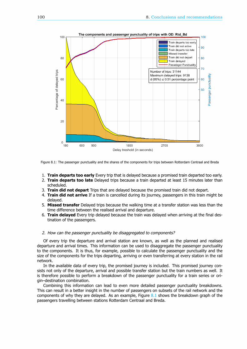
100 8. Conclusions and recommendations

Figure 8.1: The passenger punctuality and the shares of the components for trips between Rotterdam Centraal and Breda

1. Train departs too early Every trip that is delayed because a promised train departed too early.2. Train departs too late Delayed trips because a train departed at least 15 minutes later thanscheduled.

3. Train did not depart Trips that are delayed because the promised train did not depart.4. Train did not arrive If a train is cancelled during its journey, passengers in this train might bedelayed.

5. Missed transfer Delayed trips because the walking time at a transfer station was less than thetime difference between the realised arrival and departure.

6. Train delayed Every trip delayed because the train was delayed when arriving at the final des-tination of the passengers.

2. How can the passenger punctuality be disaggregated to components?

Of every trip the departure and arrival station are known, as well as the planned and realiseddeparture and arrival times. This information can be used to disaggregate the passenger punctualityto the components. It is thus, for example, possible to calculate the passenger punctuality and thesize of the components for the trips departing, arriving or even transferring at every station in the railnetwork.

In the available data of every trip, the promised journey is included. This promised journey con-sists not only of the departure, arrival and possible transfer station but the train numbers as well. Itis therefore possible to perform a breakdown of the passenger punctuality for a train series or ori-gin–destination combination.

Combining this information can lead to even more detailed passenger punctuality breakdowns.This can result in a better insight in the number of passengers on subsets of the rail network and thecomponents of why they are delayed. As an example, Figure 8.1 shows the breakdown graph of thepassengers travelling between stations Rotterdam Centraal and Breda.

8.1. Answer to the research questions 101

3. What are the control and process indicators currently introduced by ProRail and the NS to con-trol the passenger punctuality and in which way can these indicators possibly be improved orextended?

ProRail and the Dutch Railways (NS) created a model to describe the passenger punctuality (chapter5). Here the passenger punctuality is related to the number of train deviations (TVTAs): deviationsbetween the timetable and the realisation, mostly due to cancelled or delayed trains. These TVTAs canbe distributed among the responsible business units. In this research the focus lies by the businessunit Transport control and Traffic control (TB / VL). The numbers of TVTAs per business unit are thecontrol indicators.

In the next layer of the model, the number of TVTAs under the responsibility of TB / VL is relatedto 20 process indicators. Five of those process indicators are currently not fully developed. The other15 process indicators are as follows.1. Order processing VL-phase2. Percentage of the correct use of the Train handling document3. Departure punctuality of empty rolling stock at six rail yards4. Departure punctuality of empty rolling stock at stations5. Percentage of trains with the right composition at the morning start6. Percentage of trains with the right number of personnel at the morning start7. Lead time between ’Known VL’ and ’Known BackOffice’8. Lead time between ’Known BackOffice’ and alarm9. Lead time between alarm and Distribution decision10. Lead time between Distribution decision and Blockage measure decision11. Lead time between Blockage measure decision and running according to the Blockage measures12. Lead time between end of Blockage and running according to the regular plan13. Percentage of Blockage measure decision with a Distribution decision14. Percentage of fully and correctly filled in report cards15. Percentage of unadapted Blockage measuresNot all TVTAs are used in the model of ProRail and the NS, the reliability of the TVTAs cannot be

guaranteed and the number of TVTAs corresponds with the number of trains involved and not with thenumber of passengers involved. Therefore a second model is proposed. Here the process indicatorsare related to the components and therefore directly with the passenger punctuality. The TVTAs areneglected in this model.

4. How can the correlation between the passenger punctuality KPI and the process indicators bedetermined, especially for a subset of the rail network or a time period?

The passenger punctuality can be calculated for a subset of the rail network, offering potential toanalyse specific parts of the rail network or calculate the performance during a specific time period, likeduring rush hour. With the two models that describe the passenger punctuality, the process indicatorsunder the responsibility of TB / VL can be related to the passenger punctuality. Unfortunately it is notpossible to calculate the process indicators for a subset if the rail network. Therefore a new algorithmis created that can enrich the six data sources used to calculate the process indicators (chapter 6).With this enriched data, it becomes possible to calculate the process indicators for a subset or timeperiod.

5. How can the correlation between the passenger punctuality KPI and the process indicators beexplained and how effective is steering on the process indicators?

Calculating the correlation between the passenger punctuality and the process indicators via theTVTAs (in the model of ProRail and the NS) or directly (via the second model, based on the components)shows similar results (chapter 5). For only four process indicators (1 to 4) the correlation with thenumber of TVTAs and the passenger punctuality is moderate. Several remarks can be given:

• For six process indicators (7 to 12) there is no correlation with the number of TVTAs or thepassenger punctuality. However there is a correlation with the process itself, instead of theprocess indicator. This implies that the current definition of the process indicators is incorrect.For both models a new definition is proposed, which give better results.

102 8. Conclusions and recommendations

• Process indicator 14 does not have a correlation with the passenger punctuality. However steeringon this indicator to increase the performance leads to more reliable results of process indicators7 to 12.

• Decreasing the number of TVTAs does not, per definition, leads to higher passenger punctual-ity. The correlation between the number of TVTAs under the responsibility of TB / VL and thepassenger punctuality is only moderate.

The disadvantages of both models are the missing translation between the trains involved and thenumber of passengers involved. This is most clear in the number of TVTAs. These are trains that aredelayed or cancelled, not passengers. This is one of the reasons why the second model was proposed.Nonetheless the same kind of reasoning applies to the process indicators. Steering on the processeswill in first instance decrease the number of delayed or cancelled trains and not necessarily the numberof delayed passengers.

A case study is performed to calculate the correlation for a subset of the rail network (chapter 7). Asstudy area the main rail line between station Utrecht Centraal and stations Leeuwarden and Groningenis chosen. The found correlations are similar with the correlations of the entire rail network, althoughsome differences can be found. This can partly be due to small data sets for the study area. Nonethelessthis explains not all the differences. Some differences between the two models can be found aswell. Effective steering to increase passenger punctuality might therefore differ between the entire railnetwork and the study area.

The main research question is formulated as follows:

How is the passenger punctuality KPI constructed, and how is it described bythe process indicators?

The passenger punctuality is the percentage of promised journeys that can be completed on time.Here on time is within 3 minutes of the planned arrival time. The promised journeys are based on thedeparture and arrival stations and the check-in time of passengers: the registration of each passengerat their departure station. Via the realisation data the arrival times can be determined. If a journeycannot be completed as promised, the checkout time is used to determine the delay of the passenger.

In the calculation of the passenger punctuality every trip is categorized based on the realisation ofthe promised journey. These categories are based to determine the reasons (the components), froma passengers’ perspective, why a trip is delayed. In other words, the passenger punctuality can bebroken down into components. Each component is a percentage of trips that is delayed with a specificreason, like a missed transfer or a train that did not depart.

Fifteen process indicators give the performance of the business unit Transport control and Traffic con-trol. For most process indicators the correlation with the passenger punctuality is non-existent. Steer-ing on these process indicators does not increase the passenger punctuality. For six process indicatorsapplies that the current definition is not correct. The underlying process has a correlation with the pas-senger punctuality. Changing the definition can lead thus to more success in increasing the passengerpunctuality.

For a subset of the network the correlation with the passenger punctuality is for most processindicators similar with the entire network. Nonetheless, for certain process indicator the correlationcan change. The result is thus that specific steering by subsets of the rail network can lead to betterpassenger punctuality than steering on the same process indicator for the entire rail network.

8.2. ConclusionsThis research can roughly be divided into two parts. In the first part the passenger punctuality itselfis analysed: the origin, the calculation, the underlying assumptions and the breakdown to the com-ponents. In the second part two models to describe the passenger punctuality are examined. Thefocus lies by the correlation between the underlying process indicators and the train deviations or thepassenger punctuality itself. This paragraph describes both parts of this research and the conclusionfound. The main conclusions of this research are highlighted.

8.2. Conclusions 103

The analysis of the passenger punctuality itself started with an elaboration of the origin of the KPI inchapter 2. From a passengers’ perspective, the new method of calculation is an improvement relativeto the current method of calculation and certainly to the train punctuality. In the train punctualityevery train is weighted the same, while in the passenger punctuality every train is weighted with thenumber of passengers. This number is an estimation at 35 stations in the current passenger punctualitymethod. In the new passenger punctuality method the number of passengers per train is based ondata of all departure and arrival locations and times of every passenger. This method of calculationuses every trip only once while in the current method longer trips with more transfers have a largerimpact. Besides it is also possible that short trips are not used at all in the current method.

In the new method of calculation data from the OV-chipkaart (the smartcard for public transport inthe Netherlands) is used. This OVCP data contains the check-in and checkout times and locations. Thetimetable, as available two days before the execution, is combined with the realisation data of morethan 20.000 origin-destination combinations. The result is that for almost every possible travel optionthe realised arrival time, and thus the delay, can be calculated. With the OVCP data every passengerscan be combined with a travel option: the promised journey. If the realised arrival time is unknownthe checkout time is used to determine the delay. The result is that the passenger punctuality is thepercentage of promised journeys that can be completed with a delay less than 3 minutes.

In the new method of calculation 22 assumptions are made. These assumptions are analysed in chapter3. If possible the impact on the passenger punctuality is calculated as well. For some assumptions, theimpact is negligible. Nonetheless for other assumptions the impact can be more than 0.7 percentagepoint on the passenger punctuality. Combining all assumptions will result in a passenger punctualityKPI that can deviate almost 2 percentage points from the real passenger punctuality. In a subset of therail network, the difference can even be larger. Hereby applies that by a delay threshold of 3 minutesthe effect of the assumptions is more extensive than by a larger delay threshold.

The calculated passenger punctuality is based on the OVCP data and thus based on passengerbehaviour. This behaviour is different during disruptions than during a normal service: passengersmight check-in or checkout at stations that were not planned. Also the time a passenger checks inmight differ from the desired check-in time. Disruptions are not consistent, so the overall impactof disruptions on the passengers cannot be determined. Nevertheless, per case the impact can becalculated.

During the calculation of the passenger punctuality every trip is categorized. These categories canbe directly translated to components: reasons why passengers are delayed, like a train that did notdepart or a missed transfer. Every category is based on a couple of conditions. If a trip complies with allthose conditions, the trip is categorizes with the corresponding category. Here also some assumptionsare made. This implies that some trips will end up with the wrong category and thus with the wrongcomponent. Trips with the category ’Missed transfer’ are most often wrongly categorized: up to 51%of the trips categorized as ’Missed transfer’ did not have a missed transfer. A side-note is that by alarger delay threshold, the components will reflect the reality better.

Two models to describe the passenger punctuality are analysed in chapter 5. In the model of ProRailand the NS the passenger punctuality relates to the number of train deviations (TVTAs). Althoughthere is a correlation between the passenger punctuality and the number of TVTAs, this correlation isnot very strong. This is partly due because not every TVTA is included in the model. Another drawbackis the subjectivity of the TVTAs. A signaller can have multiple options by choosing the type of TVTA(and thus if the TVTA is included in the model). Also the priority of the signaller is not the TVTAs.Certainly by large disruptions this can lead to mismatching between the reality and the type of TVTAschosen. The last disadvantage of the TVTAs is the fact that TVTAs corresponds with trains, though thepassenger punctuality is based on the number of passengers in the train. This number is not consistentin time and location, so decreasing the number of TVTAs does not implicit means increasing passengerpunctuality.

The underlying process indicators give the performance of the business unit Transport control andTraffic control. Improving the corresponding processes should decrease the number of TVTAs. How-ever, steering on the process indicators is not as effective as presumed. As stated in paragraph 8.1, ofthe 15 process indicators currently in use, five do not have any correlation with the number of TVTAs.For six process indicators the current definitions do not show a correlation while the corresponding

104 8. Conclusions and recommendations

processes do have a correlation with the number of TVTAs. The remaining four process indicators haveonly a moderate correlation with the number of TVTAs. Steering on only the process indicators thatdo have a correlation with the number of TVTAs might give better results, but this will only decreasethe number of TVTAs. The correlation with the number of TVTAs and the passenger punctuality is notstrong, so the overall effect on the KPI might therefore not have the desired effect. A remark is theaccuracy of the passenger punctuality calculation. It is unknown to which extent this influences theresults.

The second model neglects the TVTAs. Here the passenger punctuality is broken down into the com-ponents. The found correlation between the process indicators and the passenger punctuality is com-parable with the correlations between the process indicators and the number of TVTAs. On the otherhand, the correlation between the process indicators and the components was often worse. This canbe due to the underlying assumptions of the components: the size of the components does not matchthe reality. Another explanation is the fact that most process indicators relates to more than onecomponent. For example, process indicators linked to delayed trains have a correlation with both thecomponent ’Train delayed’ and the component ’Missed transfer’.

Just as in the model of ProRail, the strongest correlation in the new model is moderate at best. Thiscan be explained with the fact that, just like the TVTAs, process indicators are related to trains and notto passengers. The translation between the trains and the passenger involved is missing.

The correlations in both models are calculated for the entire rail network of the Netherlands. Thismight differ from the correlations in a subset. Therefore in the case study of the route betweenstation Utrecht and stations Leeuwarden and Groningen (chapter 7 the correlations in both models arecalculated once again. For the majority of the process indicators the correlation with the number ofTVTAs or the passenger punctuality in the study area is similar with the entire network. Nonethelessthere were some significant differences. This suggest that steering on the process indicators with thestrongest correlation in the study area has a larger effect on the passenger punctuality than steeringon the process indicators with the largest correlation overall.

A remark to this conclusion is that the deviation between the calculated passenger punctuality andthe real passenger punctuality for a smaller area can be larger than for the entire rail network. Themargin of error by calculating process indicators for a subset of the rail network increases as wellbecause the neglected data increases.

Based on the found results there is no model that seems better in describing the passenger punctualitythan the other. Nonetheless, the second model has a preference above the model of ProRail andthe NS. The reason is that in this model the TVTAs are neglected. TVTAs are related to trains whilethe components are related to passengers. Besides, decreasing the size of a component will directlyincrease the passenger punctuality. This is in contrast to the model of ProRail and the NS: decreasingthe number of TVTAs will not necessarily increase the passenger punctuality.

8.3. ReflectionIn this research the passenger punctuality KPI, as defined by the NS, is analysed. In this definitionOVCP data is used to determine the promised journeys. There is no check to see if a passenger travelsaccording to this journey. If this is not the case, the calculated passenger punctuality leads to a wrongperformance value. With the help of additional data sources the allocation of promised journeys topassengers might lead to a higher reliability of the passenger punctuality.

A great additional data source might be the data originated from checking train tickets by the trainconductor. In addition with the check-in and checkout data, this can lead to better promised journey. Atthis moment the travel option with the earliest arrival time is chosen as the promised journey. Waitingtime, number of transfers and others aspects of influence are ignored. Calculating the costs of eachtravel option might lead to a better allocation of promised journeys to passengers. Not the travel optionwith the earliest arrival, but the travel option with the lowest costs will be the promised journey. Dataof the train conductors can help to fine tune this model and to find the costs for all aspects involved.

There are other methods to monitor the trips made on the rail network. Examples are GSM dataand Wi-Fi. Disadvantages of these methods are the privacy concerns, the contradiction with the basic

8.4. Recommendations 105

principle that every passenger is weighted the same in the passenger punctuality, the impossibility tocombine this data with the OVCP data and the fact that the GSM data does not belong to the NS orProRail.

An aspect what made this research complicated is the need for a delay threshold when calculating thepassenger punctuality. In every analysis a distinction is made between the 3 minute and 15 minutepassenger punctuality. An option is to neglect the passenger punctuality and to adopt a new KPI thatindicates the performance of the NS and ProRail while keeping the passengers’ interests in mind.

This alternative KPI could be ‘passenger delay minutes’: the sum of every delay of every passenger.The big advantage is that every delay is taken into account into the calculation. There is no needto specify a delay threshold. On the other hand, in the delay calculation of every trip some largeassumptions were made, for example regarding walking time and the promised journey. This results ina calculated delay that is a couple of minutes higher than the actual delay, leading to a large increasein the number of passengers with a small delay. The number of trips with a delay of 1 or 2 minutes is1.3 times as high as the number of trips with a delay of 3 minutes or more. If there is no thresholdvalue and the passenger delay minutes are calculated, trips with small delays will have an enormousinfluence on the outcome. This will make the final results unreliable.

Closely related is the fact that the delay threshold of 15 minutes might not be the best choice tocalculate the passenger punctuality. The main reason is that on the larger part of the rail network thefrequency of trains is 4 times per hour. If a train did not run, a passenger will take the next train andthe final delay is 15 minutes. However this delay is calculated via the checkout time. This implies somedeviation, because not every passenger checks out at the same moment and the used walking timemight differ from the actual walking time. This deviation is visible is the breakdown graphs. There isoften a larger decrease in the size of the components around the delay threshold of 15 minutes than bya delay threshold of 10 or 20 minutes. A good example can be found in Figure 8.2. Just after the delaythreshold of 900 seconds, the size of all components decreases more rapidly than before this thresholdand after a delay threshold of approximately 1000 seconds. Note that this same phenomenon can bespotted at a delay threshold of 1800 seconds (30 minutes).

The reason to use the 15 minute passenger punctuality is that after a delay of 15 minutes thepassenger rating of the performance of the NS decreases rapidly. If the rating drops by a delay of15 minutes, the threshold should be set at approximately 12 minutes to include all trips with a delayof least 15 minutes. If the rating drops after a delay of 15 minutes, the threshold should becomeapproximately 18 minutes. This will result that only trips with at least a 15 minute delay are used.

8.4. RecommendationsBased on the conclusions of this research, eight recommendations can be made regarding furtherresearch and the implementation of the passenger punctuality or de models to improve the passengerpunctuality. A distinction is made between recommendations regarding practical implication and furtherresearch.

Practical implication1. The effect of the assumptions of the passenger punctuality calculation on the 3 minute passengeris much larger than by a higher delay threshold. Changing the KPI into the 5 minute passengerpunctuality might create a more reliable KPI.

2. The passenger punctuality is the percentage of promised journeys that can be completed with adelay of less than 3 minutes. To create a reliable KPI, the promised journey should match thereal journeys of the passengers. Most of the times, only the check-in time and location and thecheckout location are not enough. Using more data sources can lead to a more reliable KPI.

3. The effect of disruptions on the passenger punctuality is larger than the KPI indicates. Disruptionsare irregular, so it is hard to determine the exact impact on the passenger punctuality. But if theKPI should represent the performance of the rail network, disruptions should be included.

4. The walking time between check-in and platform and between platform and checkout is set at 1minute, regardless the station or the location of the card readers. Also, the walking time between

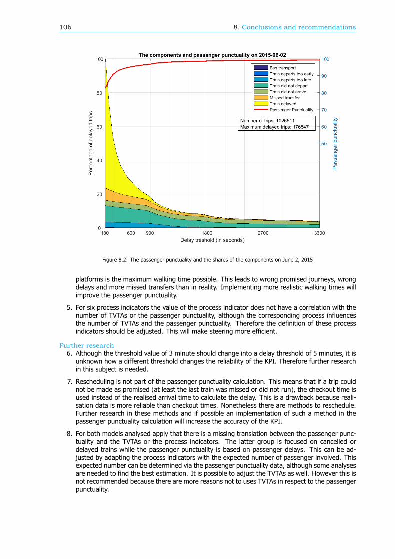
106 8. Conclusions and recommendations

Figure 8.2: The passenger punctuality and the shares of the components on June 2, 2015

platforms is the maximum walking time possible. This leads to wrong promised journeys, wrongdelays and more missed transfers than in reality. Implementing more realistic walking times willimprove the passenger punctuality.

5. For six process indicators the value of the process indicator does not have a correlation with thenumber of TVTAs or the passenger punctuality, although the corresponding process influencesthe number of TVTAs and the passenger punctuality. Therefore the definition of these processindicators should be adjusted. This will make steering more efficient.

Further research6. Although the threshold value of 3 minute should change into a delay threshold of 5 minutes, it isunknown how a different threshold changes the reliability of the KPI. Therefore further researchin this subject is needed.

7. Rescheduling is not part of the passenger punctuality calculation. This means that if a trip couldnot be made as promised (at least the last train was missed or did not run), the checkout time isused instead of the realised arrival time to calculate the delay. This is a drawback because reali-sation data is more reliable than checkout times. Nonetheless there are methods to reschedule.Further research in these methods and if possible an implementation of such a method in thepassenger punctuality calculation will increase the accuracy of the KPI.

8. For both models analysed apply that there is a missing translation between the passenger punc-tuality and the TVTAs or the process indicators. The latter group is focused on cancelled ordelayed trains while the passenger punctuality is based on passenger delays. This can be ad-justed by adapting the process indicators with the expected number of passenger involved. Thisexpected number can be determined via the passenger punctuality data, although some analysesare needed to find the best estimation. It is possible to adjust the TVTAs as well. However this isnot recommended because there are more reasons not to uses TVTAs in respect to the passengerpunctuality.

8.4. Recommendations 107

9. In the created algorithm to enrich data to calculate process indicators for a subset, it is possiblethat some parts of the data are not enriched or only partly enriched. This has an effect on theoutcome of the calculated process indicators, but the exact influence is unknown. This should beanalysed. A better option is to improve the algorithms to increase the part of the data that is fullyenriched. Related is the recommendation to analyse in more depth the correlations between theprocess indicators and the passenger punctuality in subsets of the rail network.

Bibliography

[1] CBS, Lengte van spoorwegen; spoorwegkenmerken, provincie, http://statline.cbs.nl/StatWeb/(2014), [Online; accessed 11-06-2015].

[2] NS, Veel gestelde vragen en antwoorden,http://www.ns.nl/over-ns/campagnes/dossier-seizoenen/veel-gestelde-vragen.html (2015),[Online; accessed 11-06-2015].

[3] NS, Facts figures, http://www.nsstations.nl/ns-stations/facts-figures.html (2014), [Online;accessed 11-06-2015].

[4] P. Ramaekers, T. De Wit and M. Pouwels, Hoe druk is het nu werkelijk op het Nederlandse spoor,Den Haag: CBS (2009).

[5] NS, Jaarverslag Nederlandse Spoorwegen 2014, Utrecht: NS Group NV (2015).

[6] ProRail, Geschiedenis, http://www.prorail.nl/reizigers/wie-zijn-we/geschiedenis (2015), [Online;accessed 11-06-2015].

[7] Rijksoverheid, Rol Rijksoverheid, NS en ProRail,http://www.rijksoverheid.nl/onderwerpen/openbaar-vervoer/rol-rijksoverheid-prorail-en-ns(2015), [Online; accessed 11-06-2015].

[8] W. J. Mansveld, Prestaties NS en ProRail 2014, Den Haag: Ministerie van Infrastructuur en Milieu(2015).

[9] NS, Vervoerplan Nederlande Spoorwegen 2014, Utrecht: NS Group NV (2013).

[10] NS, Punctualiteit hoofdrailnet, http://www.ns.nl/over-ns/wat-doen-wij/klantoordelen-en-prestaties/treinen-en-dienstregeling/punctualiteit-hoofdrailnet.html (2015), [Online; accessed11-06-2015].

[11] E. Seest, O. A. Nielsen and R. D. Frederiksen, Opg relse af passagerregularitet i S-tog, Aalborg:Trafikdage (2005).

[12] O. A. Nielsen, A. Landex and R. D. Frederiksen, Passenger Delay Models for Rail Networks,Schedule-Based Modeling of Transportation Networks: Theory and applications 46 (2008).

[13] IenM, Lange Termijn Spooragenda, Den Haag: Ministerie van Infrastructuur en Milieu (2013).

[14] NS and ProRail, Beter en meer, Utrecht: NS Group NV and ProRail (2013).

[15] ProRail, Beheerplan ProRail 2015, Utrecht: ProRail (2014).

[16] A. Landex, Tog-og passagerregularitet p jernbaner, in Conference paper presented atTrafikDage (Aalborg: Trafikdage, 2007).

[17] J. Parbo, O. A. Nielsen, A. Landex, and C. G. Prato, Measuring Robustness, Reliability andPunctuality within passenger railway transportation, KGS Lyngby, Denmark: Technical Universityof Denmark (2013).

[18] A. Landex, Gis analyses of railroad capacity and delays, in Proceedings of ESRI User Conference.San Diego, California, USA (San Diego: ESRI User Congerence, 2009).

[19] SBB, Customer Punctuality. Arriving on time with secure connections, Bern: SBB AG (2015).

109

110 Bibliography

[20] SBB, Kundenp nktlichkeit,http://www.sbb.ch/sbb-konzern/medien/dossier-medienschaffende/kundenpuenktlichkeit.html(2015), [Online; accessed 15-06-2015].

[21] SBB, Der SBB Franken 2011, Bern: SBB AG (2012).

[22] T. Dollevoet, Delay management and dispatching in railways, EPS-2013-272-LIS (Rotterdam:Erasmus Research Institute of Management (ERIM), 2013).

[23] A. Schöbel, A model for the delay management problem based on mixed-integer-programming,Electronic Notes in Theoretical Computer Science 50 (2001).

[24] T. Broersen, Functioneel ontwerp RPUN, Utrecht: NS Group NV (2014).

[25] B. v. d. Berg, Reizigerspunctualiteit 2013 definitie, Utrecht: NS Group NV (2013).

[26] NS, Definitie klantgedreven KPI’s op punctualiteit, Utrecht: NS Group NV (2014).

[27] NS, Klantonderzoek klantbegeleiding Q1 2015, Utrecht: NS Group NV (2015).

[28] M. Pelger, Memo Beloofd product en publicatiemomenten reisplanner, Utrecht: NS Group NV(2014).

[29] NS, Toetsdocument Aannames RPUN, Utrecht: NS Group NV (2014).

[30] B. Schepers and G. H. K. Zwart, Onderzoek incomplete transacties, Zoetermeer: Panteia (2014).

[31] P. Bruning, Trento – Nauwkeurige realisatiegegevens, Utrecht: ProRail (2012).

[32] T. Broersen, Memo afweging RFC voor herplannen, Utrecht: NS Group NV (2014).

[33] R.J. Verhaeghe, M. Minderhoud and K. Lindveld, Reader CIE4831 Empirical Analysis forTransport Planning, Delft: University of Technology (2014).

[34] R. Everhardt, Gezamelijke PI’s TB en VL, Utrecht: ProRail (2015).

[35] M. Claessens, F. Brouwers and E. Plettenburg, Spelregels Monitoring, Utrecht: ProRail (2011).

[36] CVB, Procesafspraken Monitoring, Utrecht: ProRail (2012).

[37] J. M. Egbers, Procesindicatoren in Qlikview, Utrecht: ProRail (2015).

[38] P. Reitsma and H. Van der Spek, VKL handleiding ProRail, Utrecht: ProRail (2007).

[39] ProRail Verkeersleiding, Werkwijze treindienstleider, Utrecht: ProRail (2015).

[40] P. Reitsma, ISVL Gebruikershandleiding, Utrecht: ProRail (2007).

AImpact of the assumptions on the

passenger punctuality

This appendix is an elaboration on paragraph 3.2. This paragraph analyses the assumptions in thecalculations of the passenger punctuality 2.0. In addition and if possible, the impact of this assumptionis calculated. A distinction is made between the maximum impact and the expected impact. ParagraphA.1 determines the impact of three assumptions concerning arrivals and departures of passengers bydisruptions. This is a completion of paragraph 3.2.3. Paragraph A.2 contains a table used in paragraph3.2.4. In paragraph A.3 the subject is passenger behaviour by the planning of their journey. This isa completion of paragraph 3.2.5. Paragraph 3.2.7 states that station specific walking times betweenplatform and card reader result in a more accurate passenger punctuality than the generic value of 1minute. In paragraph A.4 the calculated station specific walking time is given. Paragraph A.5 is anelaboration of the assumption that passengers starts to reschedule when a train has an initial delayof 15 minutes or more. This is part of paragraph 3.2.11. Finally in paragraph A.6 an overview of allassumptions and the calculated impact values is given.

A.1. Departure and arrivalIn the calculation of the passenger punctuality three assumptions are made to deal with passengerbehaviour by disturbances:1. The checkout station is the desired destination of the passenger2. The check-in station is the desired origin of the passenger3. The check-in time is the desired starting time of the trip of the passenger

The passenger punctuality cannot handle passengers not able to end their trip at their desired station,passengers rerouting by another rail operator and passengers leaving later than planned due to adisturbance on a part of the main rail network. These assumptions are made to deal with thesesituations. Unfortunately, hereby the passenger punctuality will reflect a better performance of the railnetwork than in reality.

The impact of these assumptions is time, place and duration dependent, so it is not possible to give ageneral impact number. Therefore three cases are examined. For every station on the route where thedistribution took place, the number of checkouts is counted for the entire duration of the distribution.This number is compared with a mean of the number of checkouts of 15 other days, for the samestation, same duration, same type of day (all working days) and without any other distribution. Theabsolute difference is the estimated number of passengers per station hindered by the disturbance.

If the difference is positive, if more passengers checked out than on an average day, the assumptionsis made that those passengers did not reached their final destination. If the difference is negativeless passengers than on average reached this station. These passengers could be the same as thepassengers that did not reached their final station, so the absolute difference per station cannot besummed to find the total number of hindered passengers.

In the most positive case, all the passengers that did not reached their final destination are the samepassengers that were missing on the other stations (where the difference was negative). Therefore to

111

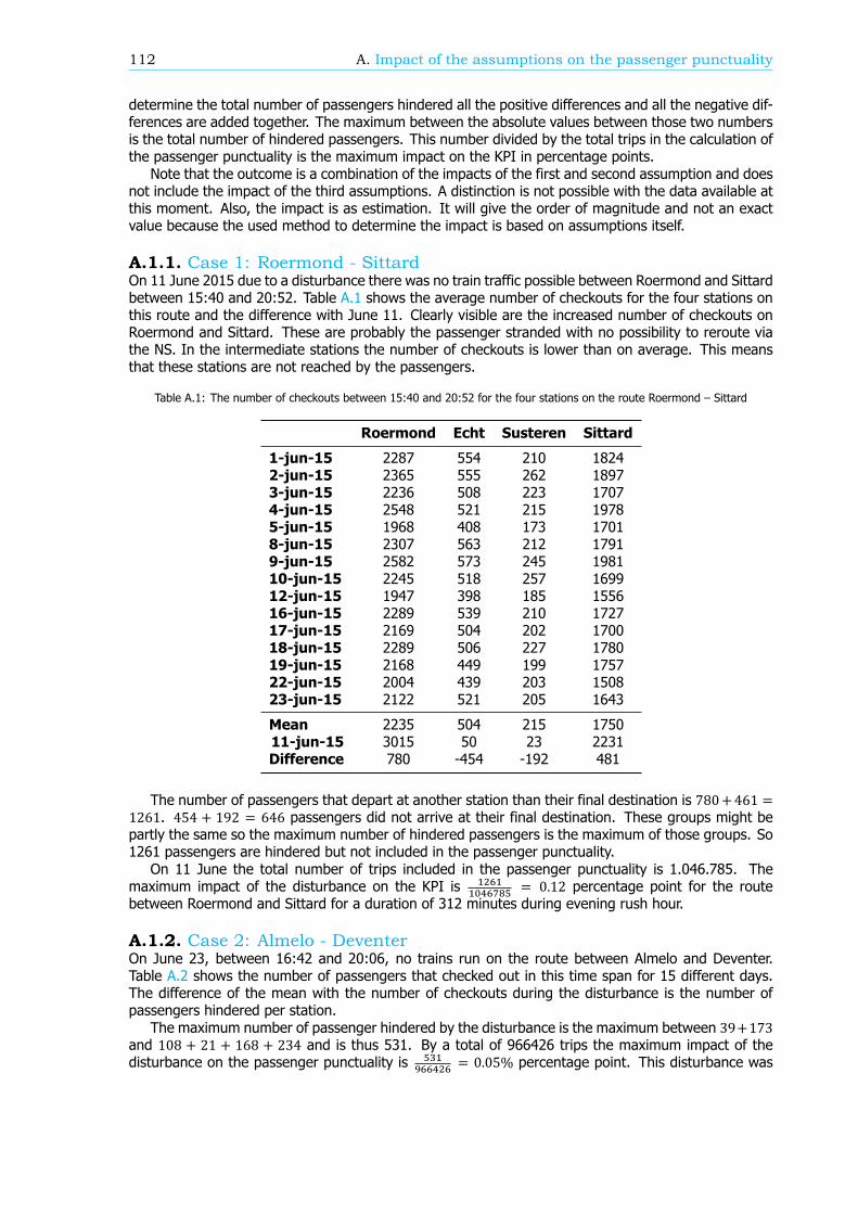
112 A. Impact of the assumptions on the passenger punctuality

determine the total number of passengers hindered all the positive differences and all the negative dif-ferences are added together. The maximum between the absolute values between those two numbersis the total number of hindered passengers. This number divided by the total trips in the calculation ofthe passenger punctuality is the maximum impact on the KPI in percentage points.

Note that the outcome is a combination of the impacts of the first and second assumption and doesnot include the impact of the third assumptions. A distinction is not possible with the data available atthis moment. Also, the impact is as estimation. It will give the order of magnitude and not an exactvalue because the used method to determine the impact is based on assumptions itself.

A.1.1. Case 1: Roermond - SittardOn 11 June 2015 due to a disturbance there was no train traffic possible between Roermond and Sittardbetween 15:40 and 20:52. Table A.1 shows the average number of checkouts for the four stations onthis route and the difference with June 11. Clearly visible are the increased number of checkouts onRoermond and Sittard. These are probably the passenger stranded with no possibility to reroute viathe NS. In the intermediate stations the number of checkouts is lower than on average. This meansthat these stations are not reached by the passengers.

Table A.1: The number of checkouts between 15:40 and 20:52 for the four stations on the route Roermond – Sittard

Roermond Echt Susteren Sittard

1-jun-15 2287 554 210 18242-jun-15 2365 555 262 18973-jun-15 2236 508 223 17074-jun-15 2548 521 215 19785-jun-15 1968 408 173 17018-jun-15 2307 563 212 17919-jun-15 2582 573 245 198110-jun-15 2245 518 257 169912-jun-15 1947 398 185 155616-jun-15 2289 539 210 172717-jun-15 2169 504 202 170018-jun-15 2289 506 227 178019-jun-15 2168 449 199 175722-jun-15 2004 439 203 150823-jun-15 2122 521 205 1643

Mean 2235 504 215 175011-jun-15 3015 50 23 2231Difference 780 -454 -192 481

The number of passengers that depart at another station than their final destination is 780+461 =1261. 454 + 192 = 646 passengers did not arrive at their final destination. These groups might bepartly the same so the maximum number of hindered passengers is the maximum of those groups. So1261 passengers are hindered but not included in the passenger punctuality.

On 11 June the total number of trips included in the passenger punctuality is 1.046.785. Themaximum impact of the disturbance on the KPI is = 0.12 percentage point for the routebetween Roermond and Sittard for a duration of 312 minutes during evening rush hour.

A.1.2. Case 2: Almelo - DeventerOn June 23, between 16:42 and 20:06, no trains run on the route between Almelo and Deventer.Table A.2 shows the number of passengers that checked out in this time span for 15 different days.The difference of the mean with the number of checkouts during the disturbance is the number ofpassengers hindered per station.

The maximum number of passenger hindered by the disturbance is the maximum between 39+173and 108 + 21 + 168 + 234 and is thus 531. By a total of 966426 trips the maximum impact of thedisturbance on the passenger punctuality is = 0.05% percentage point. This disturbance was

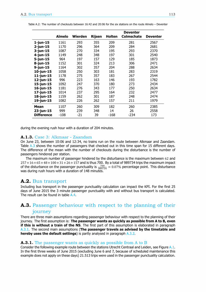
A.2. Bus transport 113

Table A.2: The number of checkouts between 16:42 and 20:06 for the six stations on the route Almelo – Deventer

Almelo Wierden Rijsen HoltenDeventerColmschate Deventer

1-jun-15 1161 293 355 209 281 25672-jun-15 1170 296 364 209 284 26813-jun-15 1087 270 334 195 293 23704-jun-15 1149 248 348 197 301 25405-jun-15 964 197 157 129 185 18738-jun-15 1152 301 324 213 306 24719-jun-15 1164 302 357 204 288 263410-jun-15 1058 250 303 181 283 231911-jun-15 1178 275 357 183 267 254412-jun-15 996 223 163 146 193 178215-jun-15 1092 247 370 180 273 243416-jun-15 1181 276 343 177 250 263417-jun-15 1014 237 295 164 232 247718-jun-15 1159 262 301 187 248 247419-jun-15 1082 226 262 157 211 1979

Mean 1107 260 309 182 260 238523-jun-15 999 239 348 14 26 2558Difference -108 -21 39 -168 -234 173

during the evening rush hour with a duration of 204 minutes.

A.1.3. Case 3: Alkmaar - ZaandamOn June 23, between 10:06 and 12:34, no trains run on the route between Alkmaar and Zaandam.Table A.3 shows the number of passengers that checked out in this time span for 15 different days.The difference of the mean with the number of checkouts during the disturbance is the number ofpassengers hindered per station.

The maximum number of passenger hindered by the disturbance is the maximum between 62 and257+16+65+48+100+31+26+157 and is thus 700. By a total of 989734 trips the maximum impactof the disturbance on the passenger punctuality is = 0.07% percentage point. This disturbancewas during rush hours with a duration of 148 minutes.

A.2. Bus transportIncluding bus transport in the passenger punctuality calculation can impact the KPI. For the first 25days of June 2015 the 3 minute passenger punctuality with and without bus transport is calculated.The result can be found in table A.4.

A.3. Passenger behaviour with respect to the planning of theirjourney

There are three main assumptions regarding passenger behaviour with respect to the planning of theirjourney. The first assumption is: The passenger wants as quickly as possible from A to B, evenif this is without a train of the NS. The first part of this assumption is elaborated in paragraphA.3.1. The second main assumptions (The passenger travels as advised by the timetable andhereby uses the default settings) is partly analysed in paragraph A.3.2.

A.3.1. The passenger wants as quickly as possible from A to BConsider the following example route between the stations Utrecht Centraal and Leiden, see Figure A.1.In the first three weeks of June 2015 (excluding June 6 and 7, because of scheduled maintenance thisexample does not apply on these days) 21.513 trips were used in the passenger punctuality calculation.

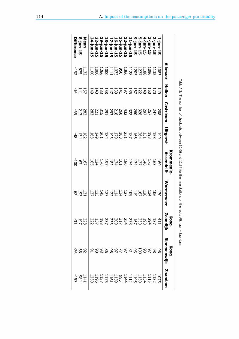
114 A. Impact of the assumptions on the passenger punctuality

TableA.3:

Thenum

berofcheckouts

between

10:06and

12:34for

thenine

stationsonthe

routeAlkm

aar–Zaandam

Alkm

aarHeiloo

Castricum

Uitgeest

Krom

menie-

Assendelft

Worm

erveerKoog-

ZaandijkKoog

Bloem

enwijk

Zaandam

1-jun-151083

149208

149160

170411

961075

2-jun-151132

170247

153163

106137

981132

3-jun-151096

160257

193173

134294

971115

4-jun-151188

148297

131146

128198

931154

5-jun-151277

122328

264177

167230

1001130

9-jun-151205

167260

166134

119167

931195

11-jun-151128

185322

187174

109278

811112

12-jun-151366

197432

231180

127254

971144

15-jun-15950

141260

188161

134217

77996

16-jun-151073

139218

179174

114209

971159

17-jun-151111

147293

193182

122233

981161

18-jun-151000

158291

184197

127237

861175

19-jun-151266

183315

201170

145193

931137

22-jun-151000

143221

149124

123137

901196

24-jun-151100

149283

163185

137222

911230

Mean

1132157

282182

167131

22892

11418-jun-15

875141

217134

67193

19766

984Difference

-257-16

-65-48

-10062

-31-26

-157

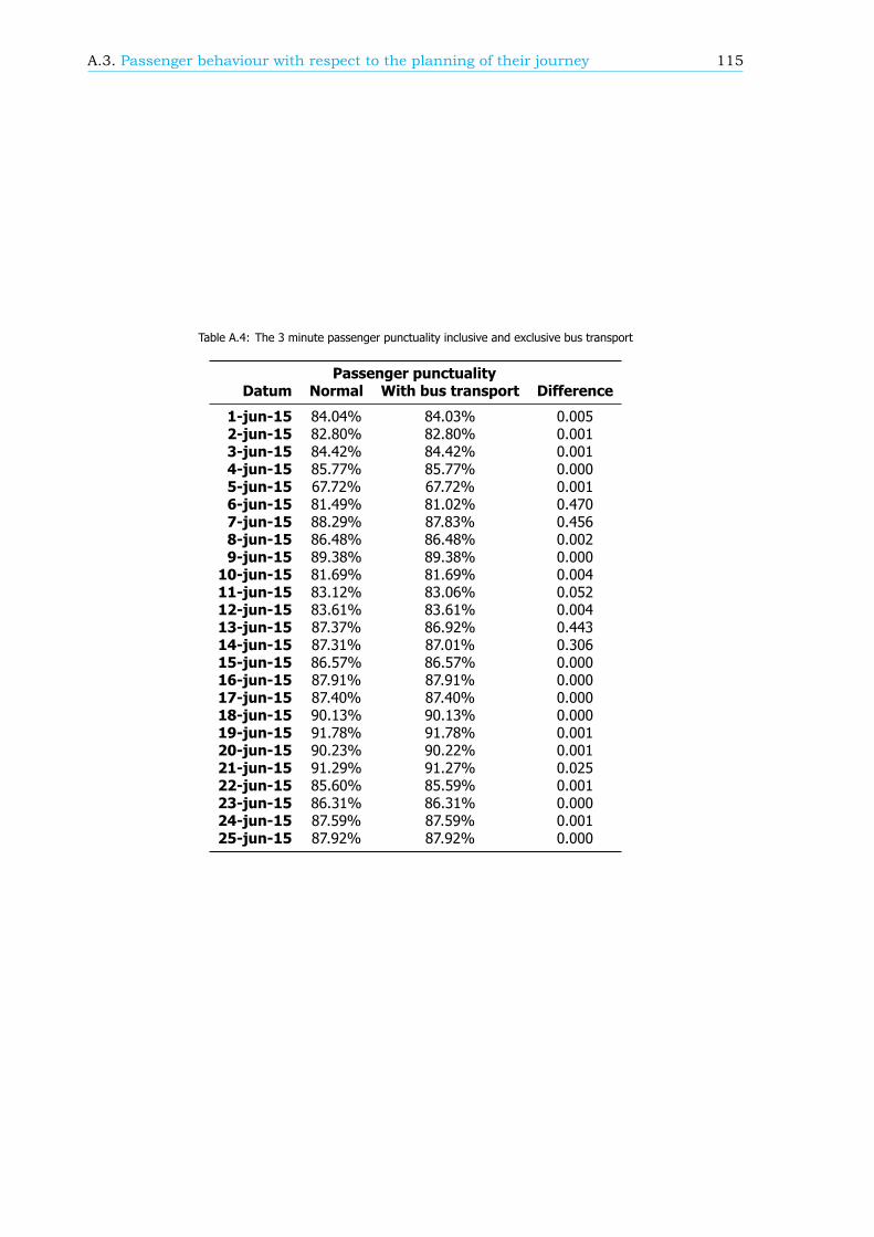
A.3. Passenger behaviour with respect to the planning of their journey 115

Table A.4: The 3 minute passenger punctuality inclusive and exclusive bus transport

Passenger punctualityDatum Normal With bus transport Difference

1-jun-15 84.04% 84.03% 0.0052-jun-15 82.80% 82.80% 0.0013-jun-15 84.42% 84.42% 0.0014-jun-15 85.77% 85.77% 0.0005-jun-15 67.72% 67.72% 0.0016-jun-15 81.49% 81.02% 0.4707-jun-15 88.29% 87.83% 0.4568-jun-15 86.48% 86.48% 0.0029-jun-15 89.38% 89.38% 0.000

10-jun-15 81.69% 81.69% 0.00411-jun-15 83.12% 83.06% 0.05212-jun-15 83.61% 83.61% 0.00413-jun-15 87.37% 86.92% 0.44314-jun-15 87.31% 87.01% 0.30615-jun-15 86.57% 86.57% 0.00016-jun-15 87.91% 87.91% 0.00017-jun-15 87.40% 87.40% 0.00018-jun-15 90.13% 90.13% 0.00019-jun-15 91.78% 91.78% 0.00120-jun-15 90.23% 90.22% 0.00121-jun-15 91.29% 91.27% 0.02522-jun-15 85.60% 85.59% 0.00123-jun-15 86.31% 86.31% 0.00024-jun-15 87.59% 87.59% 0.00125-jun-15 87.92% 87.92% 0.000

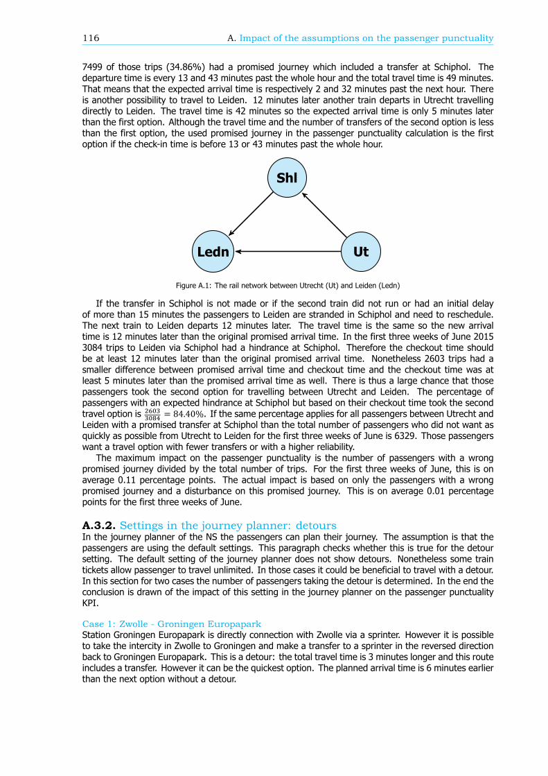
116 A. Impact of the assumptions on the passenger punctuality

7499 of those trips (34.86%) had a promised journey which included a transfer at Schiphol. Thedeparture time is every 13 and 43 minutes past the whole hour and the total travel time is 49 minutes.That means that the expected arrival time is respectively 2 and 32 minutes past the next hour. Thereis another possibility to travel to Leiden. 12 minutes later another train departs in Utrecht travellingdirectly to Leiden. The travel time is 42 minutes so the expected arrival time is only 5 minutes laterthan the first option. Although the travel time and the number of transfers of the second option is lessthan the first option, the used promised journey in the passenger punctuality calculation is the firstoption if the check-in time is before 13 or 43 minutes past the whole hour.

Shl

Ledn Ut

Figure A.1: The rail network between Utrecht (Ut) and Leiden (Ledn)

If the transfer in Schiphol is not made or if the second train did not run or had an initial delayof more than 15 minutes the passengers to Leiden are stranded in Schiphol and need to reschedule.The next train to Leiden departs 12 minutes later. The travel time is the same so the new arrivaltime is 12 minutes later than the original promised arrival time. In the first three weeks of June 20153084 trips to Leiden via Schiphol had a hindrance at Schiphol. Therefore the checkout time shouldbe at least 12 minutes later than the original promised arrival time. Nonetheless 2603 trips had asmaller difference between promised arrival time and checkout time and the checkout time was atleast 5 minutes later than the promised arrival time as well. There is thus a large chance that thosepassengers took the second option for travelling between Utrecht and Leiden. The percentage ofpassengers with an expected hindrance at Schiphol but based on their checkout time took the secondtravel option is = 84.40%. If the same percentage applies for all passengers between Utrecht andLeiden with a promised transfer at Schiphol than the total number of passengers who did not want asquickly as possible from Utrecht to Leiden for the first three weeks of June is 6329. Those passengerswant a travel option with fewer transfers or with a higher reliability.

The maximum impact on the passenger punctuality is the number of passengers with a wrongpromised journey divided by the total number of trips. For the first three weeks of June, this is onaverage 0.11 percentage points. The actual impact is based on only the passengers with a wrongpromised journey and a disturbance on this promised journey. This is on average 0.01 percentagepoints for the first three weeks of June.

A.3.2. Settings in the journey planner: detoursIn the journey planner of the NS the passengers can plan their journey. The assumption is that thepassengers are using the default settings. This paragraph checks whether this is true for the detoursetting. The default setting of the journey planner does not show detours. Nonetheless some traintickets allow passenger to travel unlimited. In those cases it could be beneficial to travel with a detour.In this section for two cases the number of passengers taking the detour is determined. In the end theconclusion is drawn of the impact of this setting in the journey planner on the passenger punctualityKPI.

Case 1: Zwolle - Groningen EuropaparkStation Groningen Europapark is directly connection with Zwolle via a sprinter. However it is possibleto take the intercity in Zwolle to Groningen and make a transfer to a sprinter in the reversed directionback to Groningen Europapark. This is a detour: the total travel time is 3 minutes longer and this routeincludes a transfer. However it can be the quickest option. The planned arrival time is 6 minutes earlierthan the next option without a detour.

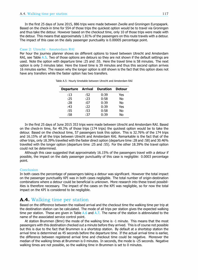
A.4. Walking time per station 117

In the first 25 days of June 2015, 886 trips were made between Zwolle and Groningen Europapark.Based on the check-in time for 554 of those trips the quickest option would be to travel via Groningenand thus take the detour. However based on the checkout time, only 10 of those trips were made withthe detour. This means that approximately 1.81% of the passengers on this route travels with a detour.The impact of this case on the daily passenger punctuality is 0.00005 percentage point.

Case 2: Utrecht - Amsterdam RAIPer hour the journey planner shows six different options to travel between Utrecht and AmsterdamRAI, see Table A.5. Two of those options are detours so they are not shown if the default settings areused. Note the option with departure time :25 and :55. Here the travel time is 58 minutes. The nextoption is only 3 minutes later. Here the travel time is 39 minutes and thus this second option arrives16 minutes earlier. The reason why the longer option is still shown is the fact that this option does nothave any transfers while the faster option has two transfers.

Table A.5: Hourly timetable between Utrecht and Amsterdam RAI

Departure Arrival Duration Detour

:13 :52 0:39 Yes:25 :23 0:58 No:28 :07 0:39 No:43 :22 0:39 Yes:55 :53 0:58 No:58 :37 0:39 No

In the first 25 days of June 2015 353 trips were made between Utrecht and Amsterdam RAI. Basedon the check-in time, for 49.3% of those trips (174 trips) the quickest option would be to take thedetour. Based on the checkout time, 57 passengers took this option. This is 32.76% of the 174 tripsand 16.15% of all the trips between Utrecht and Amsterdam RAI. Remarkable is the fact that of theother trips, only 18.39% travelled with the faster direct option (departure time :28 and :58) and 30.46%travelled with the longer option (departure time :25 and :55). For the other 18.39% the travel optioncould not be determined.

Although this case suggested that approximately 16.15% of the passengers travel with a detour ifpossible, the impact on the daily passenger punctuality of this case is negligible: 0.0003 percentagepoint.

ConclusionIn both cases the percentage of passengers taking a detour was significant. However the total impacton the passenger punctuality KPI was in both cases negligible. The total number of origin-destinationcombinations where a detour could be beneficial is unknown. More research into these travel possibil-ities is therefore necessary. The impact of the cases on the KPI was negligible, so for now the totalimpact on the KPI is considered to be negligible.

A.4. Walking time per stationBased on the difference between the realised arrival and the checkout time the walking time per trip atthe destination station can be calculated. The mode of all trips per station gives the expected walkingtime per station. These are given in Table A.6 and A.7. The name of the station is abbreviated to thename of the associated service control point.

At station Brummen (Bmn) the mode of the walking time is -1 minute. This means that the mostpassengers with this destination checked out a minute before they arrived. This is of course not possiblebut this is due to the fact that Brummen is a shortstop station. By default at a shortstop station thearrival time is determined as 45 seconds before the departure time. If the actual arrival time is earlier,the difference between registered arrival time and checkout time could be negative. Moreover themedian of the walking times at Brummen is 0 minutes. In seconds, the mode is -25 seconds. Negativewalking times are not possible, so the walking time in Brummen is set to 0 minutes.

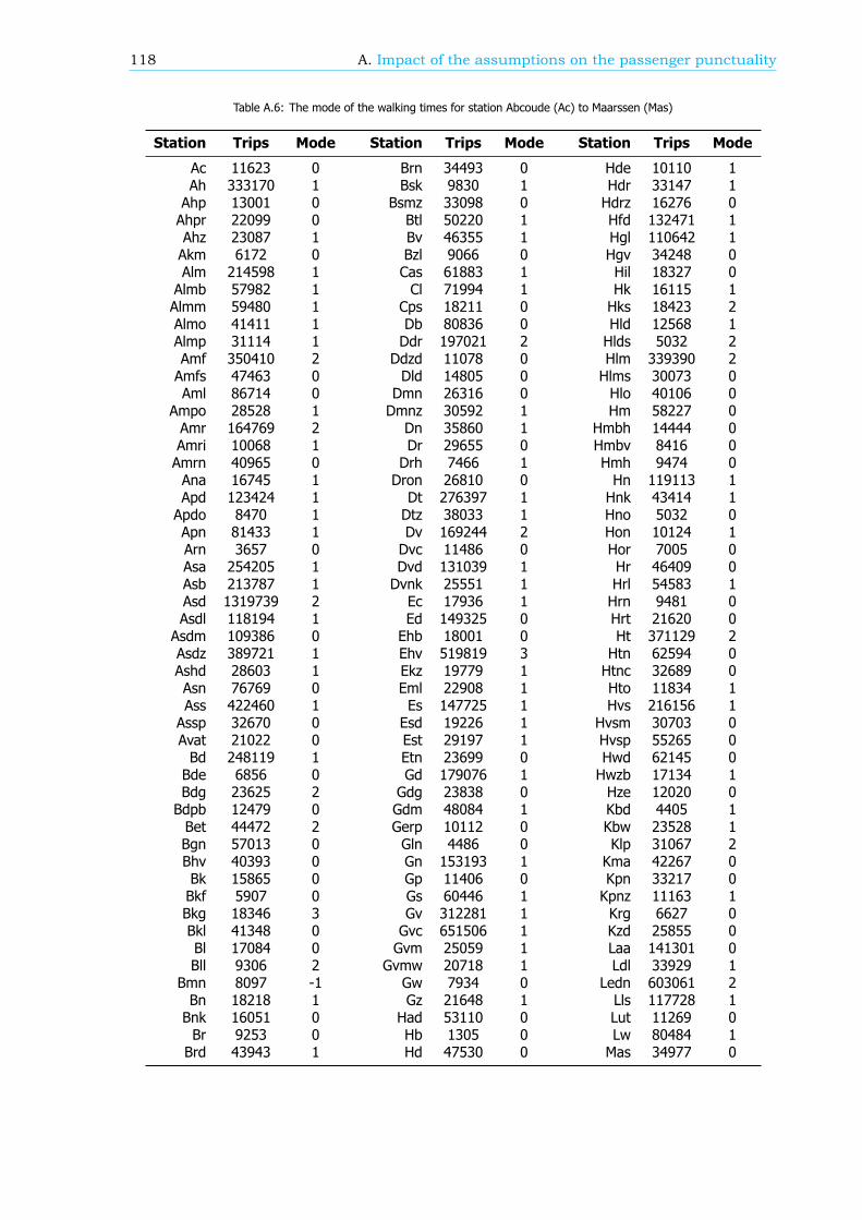
118 A. Impact of the assumptions on the passenger punctuality

Table A.6: The mode of the walking times for station Abcoude (Ac) to Maarssen (Mas)

Station Trips Mode Station Trips Mode Station Trips Mode

Ac 11623 0 Brn 34493 0 Hde 10110 1Ah 333170 1 Bsk 9830 1 Hdr 33147 1Ahp 13001 0 Bsmz 33098 0 Hdrz 16276 0Ahpr 22099 0 Btl 50220 1 Hfd 132471 1Ahz 23087 1 Bv 46355 1 Hgl 110642 1Akm 6172 0 Bzl 9066 0 Hgv 34248 0Alm 214598 1 Cas 61883 1 Hil 18327 0Almb 57982 1 Cl 71994 1 Hk 16115 1Almm 59480 1 Cps 18211 0 Hks 18423 2Almo 41411 1 Db 80836 0 Hld 12568 1Almp 31114 1 Ddr 197021 2 Hlds 5032 2Amf 350410 2 Ddzd 11078 0 Hlm 339390 2Amfs 47463 0 Dld 14805 0 Hlms 30073 0Aml 86714 0 Dmn 26316 0 Hlo 40106 0

Ampo 28528 1 Dmnz 30592 1 Hm 58227 0Amr 164769 2 Dn 35860 1 Hmbh 14444 0Amri 10068 1 Dr 29655 0 Hmbv 8416 0Amrn 40965 0 Drh 7466 1 Hmh 9474 0Ana 16745 1 Dron 26810 0 Hn 119113 1Apd 123424 1 Dt 276397 1 Hnk 43414 1Apdo 8470 1 Dtz 38033 1 Hno 5032 0Apn 81433 1 Dv 169244 2 Hon 10124 1Arn 3657 0 Dvc 11486 0 Hor 7005 0Asa 254205 1 Dvd 131039 1 Hr 46409 0Asb 213787 1 Dvnk 25551 1 Hrl 54583 1Asd 1319739 2 Ec 17936 1 Hrn 9481 0Asdl 118194 1 Ed 149325 0 Hrt 21620 0Asdm 109386 0 Ehb 18001 0 Ht 371129 2Asdz 389721 1 Ehv 519819 3 Htn 62594 0Ashd 28603 1 Ekz 19779 1 Htnc 32689 0Asn 76769 0 Eml 22908 1 Hto 11834 1Ass 422460 1 Es 147725 1 Hvs 216156 1Assp 32670 0 Esd 19226 1 Hvsm 30703 0Avat 21022 0 Est 29197 1 Hvsp 55265 0Bd 248119 1 Etn 23699 0 Hwd 62145 0Bde 6856 0 Gd 179076 1 Hwzb 17134 1Bdg 23625 2 Gdg 23838 0 Hze 12020 0Bdpb 12479 0 Gdm 48084 1 Kbd 4405 1Bet 44472 2 Gerp 10112 0 Kbw 23528 1Bgn 57013 0 Gln 4486 0 Klp 31067 2Bhv 40393 0 Gn 153193 1 Kma 42267 0Bk 15865 0 Gp 11406 0 Kpn 33217 0Bkf 5907 0 Gs 60446 1 Kpnz 11163 1Bkg 18346 3 Gv 312281 1 Krg 6627 0Bkl 41348 0 Gvc 651506 1 Kzd 25855 0Bl 17084 0 Gvm 25059 1 Laa 141301 0Bll 9306 2 Gvmw 20718 1 Ldl 33929 1

Bmn 8097 -1 Gw 7934 0 Ledn 603061 2Bn 18218 1 Gz 21648 1 Lls 117728 1Bnk 16051 0 Had 53110 0 Lut 11269 0Br 9253 0 Hb 1305 0 Lw 80484 1Brd 43943 1 Hd 47530 0 Mas 34977 0

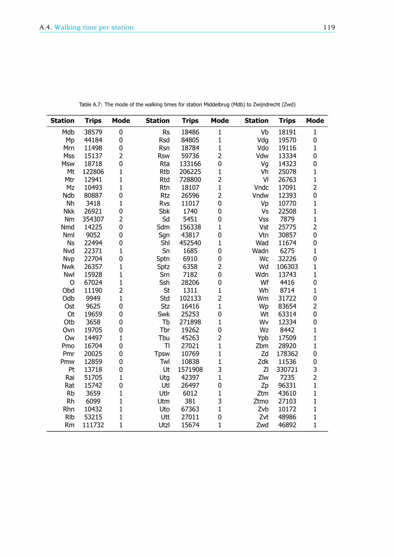
A.4. Walking time per station 119

Table A.7: The mode of the walking times for station Middelbrug (Mdb) to Zwijndrecht (Zwd)

Station Trips Mode Station Trips Mode Station Trips Mode

Mdb 38579 0 Rs 18486 1 Vb 18191 1Mp 44184 0 Rsd 84805 1 Vdg 19570 0Mrn 11498 0 Rsn 18784 1 Vdo 19116 1Mss 15137 2 Rsw 59736 2 Vdw 13334 0Msw 18718 0 Rta 133166 0 Vg 14323 0Mt 122806 1 Rtb 206225 1 Vh 25078 1Mtr 12941 1 Rtd 728800 2 Vl 26763 1Mz 10493 1 Rtn 18107 1 Vndc 17091 2Ndb 80887 0 Rtz 26596 2 Vndw 12393 0Nh 3418 1 Rvs 11017 0 Vp 10770 1Nkk 26921 0 Sbk 1740 0 Vs 22508 1Nm 354307 2 Sd 5451 0 Vss 7879 1Nmd 14225 0 Sdm 156338 1 Vst 25775 2Nml 9052 0 Sgn 43817 0 Vtn 30857 0Ns 22494 0 Shl 452540 1 Wad 11674 0Nvd 22371 1 Sn 1685 0 Wadn 6275 1Nvp 22704 0 Sptn 6910 0 Wc 32226 0Nwk 26357 1 Sptz 6358 2 Wd 106303 1Nwl 15928 1 Srn 7182 0 Wdn 13743 1O 67024 1 Ssh 28206 0 Wf 4416 0

Obd 11190 2 St 1311 1 Wh 8714 1Odb 9949 1 Std 102133 2 Wm 31722 0Ost 9625 0 Stz 16416 1 Wp 83654 2Ot 19659 0 Swk 25253 0 Wt 63314 0Otb 3658 0 Tb 271898 1 Wv 12334 0Ovn 19705 0 Tbr 19262 0 Wz 8442 1Ow 14497 1 Tbu 45263 2 Ypb 17509 1Pmo 16704 0 Tl 27021 1 Zbm 28920 1Pmr 20025 0 Tpsw 10769 1 Zd 178362 0Pmw 12859 0 Twl 10838 1 Zdk 11536 0Pt 13718 0 Ut 1571908 3 Zl 330721 3Rai 51705 1 Utg 42397 1 Zlw 7235 2Rat 15742 0 Utl 26497 0 Zp 96331 1Rb 3659 1 Utlr 6012 1 Ztm 43610 1Rh 6099 1 Utm 381 3 Ztmo 27103 1Rhn 10432 1 Uto 67363 1 Zvb 10172 1Rlb 53215 1 Utt 27011 0 Zvt 48986 1Rm 111732 1 Utzl 15674 1 Zwd 46892 1

120 A. Impact of the assumptions on the passenger punctuality

A.5. The waiting time before reschedulingThere are several reasons to reschedule a trip: a train did not depart, a train did not arrive at thedesired destination, a transfer is not made or the train departed too early. For those four reasons it isclear when the passenger starts rescheduling the trip. For the fifth and last reason this distinction is notso clear. The corresponding assumption is as follows: If a train has a delay of at least 15 minutesbefore departure, the realised arrival time is the checkout time minus the walking timebetween train and card reader. The focus of this paragraph is the first part of this assumption.It state that a trips needs to be rescheduled as the initial delay of a train is 15 minutes or more.This assumption is based on passenger behaviour and the characteristics of the main rail network.Most passengers will search for an alternative when the promised train has a certain initial delay. Thisthreshold delay, the turning point when passengers reschedule, is not known. On the other hand, onmost trajectories in the main rail network the frequency of trains is 4 times per hour, or 1 train per15 minutes. For most trips the first alternative journey will thus be 15 minutes later than the originaljourney. Therefore the limit between no reschedule and reschedule is set to 15 minutes.

This is no guarantee that this threshold of 15 minutes is always correct. For example, on manyroutes multiple trajectories can be taken to get to the final destination. The first alternative is thusless than 15 minutes later than the original route. On the other hand, on some other routes this is notpossible and the frequency is only 2 trains per hour. For the first 10 days of June the trips without atransfer and with the category ‘Train departs too late’ where examined. These are 90475 trips, whichis 1.02% of all trips during those days. For 21.78% of those examined trips the expected arrival timebased on the checkout time is later than the realised arrival time of the train. Most likely, the bestoption for those passengers was not to reschedule their journey. Also 22.40% of the examined tripshad a delay, based on the checkout time, smaller than 15 minutes and the expected arrival time basedon the checkout time was earlier than the arrival time of the train. These passengers probably took analternative train departing within 15 minutes of the promised departure time.

The maximum impact of the threshold of 15 minutes is calculated as follows. For all trips categorizedas ‘Train departs too late’ and with no transfers the delay is calculated via the realised arrival time andvia the checkout time. The next step is to determine for how many trips the delay based on checkouttime is less than 3 minutes but the delay based on the realised arrival time is at least 3 minutes (group1). These are the trips where the value of the threshold has an influence on the 3 minute passengerpunctuality. The opposite can also occur: trips where the delay based on the realised arrival time isless than 3 minutes and the delay based on the checkout time is 3 minutes or more (group 2). Themaximum impact is calculated by taking the maximum of group 1 and group 2. The examined trips donot have transfers, so the outcome should be corrected for all the trips with the category ‘Train departstoo late’. Dividing the result by all the trips used in the calculation of the passenger punctuality leads tothe maximum impact. This is on average 0.10 percentage points for the 3 minute passenger punctuality.To calculate the expected impact the difference of group 1 and group 2 is taken. The remainder ofthe calculation is the same. This leads to an expected impact on the passenger punctuality of 0.09percentage point.

The threshold is 15 minutes, so the impact on the 15 minute passenger punctuality is expected tobe larger. Calculating this impact shows that this expectation is true. The average maximum impactis 0.20 percentage point. The expected impact is 0.18 percentage point. Note that there will alwaysbe an impact on the passenger punctuality, independent of the threshold used. This is due to the factthat the time between planned departure and first alternative changes over time and place.

In Figure A.2 the impact by different thresholds before rescheduling is visualized. To calculate theimpact by a threshold of 14 minutes or lower the trips categorized as ‘Trip realised’ and without transfersare used. For these trips the realised arrival time is known as well as the corresponding checkout time.As can be seen, by a threshold of approximately 10 minutes or lower the impact is considerably. Aftera threshold of 10 minutes the impact flattens out. However the impact is still decreasing. This is dueto the fact that by a larger threshold more often trips are delayed based both on the checkout timeand based on the realised arrival time of the delayed train. Based on this information alone a thresholdcloser to the 30 minutes would therefore decrease the impact on the passenger punctuality.

On the other hand, increasing the threshold by which the passengers are expected to reschedulewill decrease the number of delayed trips with the correct category. This implies mostly to the tripscategorized as ‘Missed transfer’. More trips will get this category because the arriving train departed

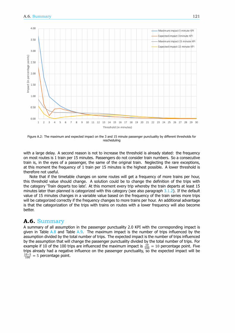
A.6. Summary 121

Figure A.2: The maximum and expected impact on the 3 and 15 minute passenger punctuality by different thresholds forrescheduling

with a large delay. A second reason is not to increase the threshold is already stated: the frequencyon most routes is 1 train per 15 minutes. Passengers do not consider train numbers. So a consecutivetrain is, in the eyes of a passenger, the same of the original train. Neglecting the rare exceptions,at this moment the frequency of 1 train per 15 minutes is the highest possible. A lower threshold istherefore not useful.

Note that if the timetable changes on some routes will get a frequency of more trains per hour,this threshold value should change. A solution could be to change the definition of the trips withthe category ‘Train departs too late’. At this moment every trip whereby the train departs at least 15minutes later than planned is categorized with this category (see also paragraph 3.1.2). If the defaultvalue of 15 minutes changes in a variable value based on the frequency of the train series more tripswill be categorized correctly if the frequency changes to more trains per hour. An additional advantageis that the categorization of the trips with trains on routes with a lower frequency will also becomebetter.

A.6. SummaryA summary of all assumption in the passenger punctuality 2.0 KPI with the corresponding impact isgiven in Table A.8 and Table A.9. The maximum impact is the number of trips influenced by theassumption divided by the total number of trips. The expected impact is the number of trips influencedby the assumption that will change the passenger punctuality divided by the total number of trips. Forexample if 10 of the 100 trips are influenced the maximum impact is = 10 percentage point. Fivetrips already had a negative influence on the passenger punctuality, so the expected impact will be

= 5 percentage point.

122 A. Impact of the assumptions on the passenger punctuality

Table A.8: The first 16 assumptions of the passenger punctuality 2.0 KPI and the corresponding impact

Impact on 3 minute KPIAssumption Maximum Expected Remark

1 The observed trips in the pas-senger punctuality calculation arerepresenting the average passen-ger

0.05 percent-age points

Undetermined Not all factors are in-cluded

2 The closing of the OVCP terminalsat stations does not have an influ-ence on the representativeness ofthe used trips in the calculations

Undetermined Undetermined The impact is unde-termined but the ef-fect is positive

3 Trips derived from the OVCP dataare not with the Thalys, Eurostarand/or ICE

Negligible Negligible

4 The checkout station is the de-sired destination of the passenger

Time and placedependent

Time and placedependent

For three examplesthe maximumimpact lies betweenthe 0.05 and 0.12percentage point

5 The check-in station is the desiredorigin of the passenger

6 The check-in time is the desiredstarting time of the trip of the pas-senger

7 Trips (partly) conducted by bustransport are not included in thepassenger punctuality

On days with planned bus trans-port: 0.42 percentage point.Otherwise negligible

The maximum andexpected impact arethe same

8 The passenger wants as quickly aspossible from A to B, even if thisis without a train of the NS

Undetermined Undetermined Per case the impactis calculable.

9 The passenger travels as advisedby the timetable and hereby usesthe default settings

Negligible Negligible The impact of twofactors could not bedetermined

10 The passenger bases his expec-tation on the timetable two daysprior to the journey

Negligible Negligible

11 Every trip obtained from the OVCPdata can be coupled to a promisedjourney

0.09 percent-age points

Undeterminedbut probablynegligible

The KPI will notchange by a largerdataset

12 The walking time between cardreader and platform is 1 minute

0.63 percent-age points

0.42 percent-age points

13 The walking time between plat-form and card reader is 1 minute

0.12 percentage point The maximum andexpected impact arethe same

14 The clock in the card readers is ex-act

Undetermined Undetermined Probably negligible

15 The realised arrival and departuretimes are measured exact on ev-ery station

0.72 percent-age points

Undetermined

16 The determination of 45 secondsas stopping time at a shortstop isaccurate

Undetermined Undetermined

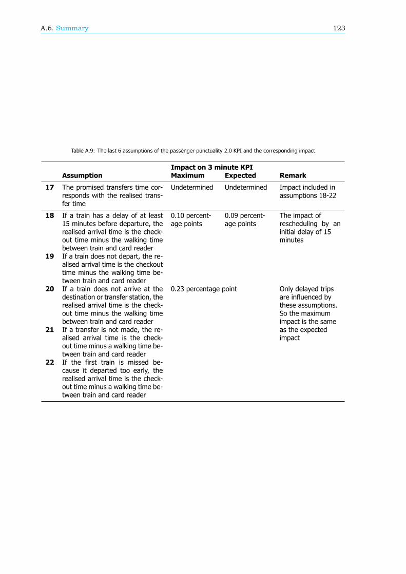
A.6. Summary 123

Table A.9: The last 6 assumptions of the passenger punctuality 2.0 KPI and the corresponding impact

Impact on 3 minute KPIAssumption Maximum Expected Remark

17 The promised transfers time cor-responds with the realised trans-fer time

Undetermined Undetermined Impact included inassumptions 18-22

18 If a train has a delay of at least15 minutes before departure, therealised arrival time is the check-out time minus the walking timebetween train and card reader

0.10 percent-age points

0.09 percent-age points

The impact ofrescheduling by aninitial delay of 15minutes

19 If a train does not depart, the re-alised arrival time is the checkouttime minus the walking time be-tween train and card reader

0.23 percentage point Only delayed tripsare influenced bythese assumptions.So the maximumimpact is the sameas the expectedimpact

20 If a train does not arrive at thedestination or transfer station, therealised arrival time is the check-out time minus the walking timebetween train and card reader

21 If a transfer is not made, the re-alised arrival time is the check-out time minus a walking time be-tween train and card reader

22 If the first train is missed be-cause it departed too early, therealised arrival time is the check-out time minus a walking time be-tween train and card reader

BAlgorithms to create breakdown

graphs

Out of the output data of the calculation of the passenger punctuality the, so called, breakdown graphscan be created. These graphs show the passenger punctuality and the share of each component by arange of delay thresholds. These components are the reasons why a trip is delayed. The sum of allcomponents is set equal to 100% by the delay threshold where the passenger punctuality is the lowest.These breakdown graphs show information about how much and why the investigated network is notpunctual and by which delay threshold. The components, the delay threshold and the outcome of thegraphs are discussed in chapter 4.

Two types of graphs can be distinguished. The first type is the ’Normal breakdown graph’. Thisbreakdown graph can be used to determine the passenger punctuality and the share of the componentsfor a certain time period. Here the time period is set on 1 day. The condition is that the data of all thetrips of that time period are available. The outcome of this graph is than exact for that examined timeperiod. The algorithm to create such a graph is explained in paragraph B.1.

It is also possible that the subject of an analysis is a station, train series or another part of thenetwork. To create a graph were the displayed information is exact can only be done when all the dataof all the trips is available. By using a sample size of the data however, an estimation can be madeof the passenger punctuality and the shares of the components. The larger the sample size, the moreaccurate the breakdown graph becomes. Such a ’Special breakdown graph’ is explained in paragraphB.2. This is a continuation of the previous paragraph.

B.1. Normal breakdown graphThis appendix describes the algorithm to create breakdown graphs for the daily passenger punctuality.In consist of two parts. The first part handles the data (paragraph B.1.1). In basis the data getssummarized into a small table. This is done via Structured Query Language (SQL). The resulting tableis the input for the second part. Here the graphs are created (paragraph B.1.2). This is done viaMATLAB. In theory MATLAB is able to deal with the actions of part 1, but because the size of the rawinput is very large SQL is used. This programming language is better and faster to deal with largedatabases.

B.1.1. Part 1: Data handlingIn paragraph 3.1 the structure of the passenger punctuality calculation is given. It consists of 5 mod-ules. The fifth module generates the output. One table is called: ’EZ_D_RPU.FCT_RPUN_REIS’ [24].This table contains every trip with a promised journey. Other information is, among others, the dateon which the trip was made, the final delay in seconds and the category of the trip (see paragraph3.1.2). Every trip is included in this table, so the size is extensive. On average on a normal workingday the number of entries is approximately one million (and less than half a million for a weekendday). Dedicated software is needed to handle such large tables. The NS uses SAS Enterprise Guide.

125

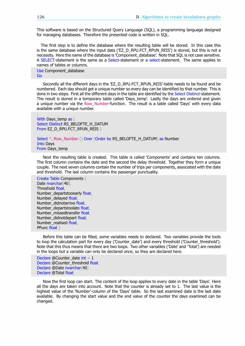
126 B. Algorithms to create breakdown graphs

This software is based on the Structured Query Language (SQL), a programming language designedfor managing databases. Therefore the presented code is written in SQL.

The first step is to define the database where the resulting table will be stored. In this case thisis the same database where the input data (’EZ_D_RPU.FCT_RPUN_REIS’) is stored, but this is not anecessity. Here the name of the database is ’Component_database’. Note that SQL is not case sensitive.A SELECT-statement is the same as a Select-statement or a select-statement. The same applies tonames of tables or columns.Use Component_databaseGo

Secondly all the different days in the ’EZ_D_RPU.FCT_RPUN_REIS’-table needs to be found and benumbered. Each day should get a unique number so every day can be identified by that number. This isdone in two steps. First all the different days in the table are identified by the Select Distinct-statement.The result is stored in a temporary table called ’Days_temp’. Lastly the days are ordered and givena unique number via the Row_Number-function. The result is a table called ’Days’ with every dataavailable with a unique number.;With Days_temp as (Select Distinct RS_BELOFTE_H_DATUMFrom EZ_D_RPU.FCT_RPUN_REIS )

Select *, Row_Number () Over (Order by RS_BELOFTE_H_DATUM) as NumberInto DaysFrom Days_temp

Next the resulting table is created. This table is called ’Components’ and contains ten columns.The first column contains the date and the second the delay threshold. Together they form a uniquecouple. The next seven columns contain the number of trips per components, associated with the dateand threshold. The last column contains the passenger punctuality.

Create Table Components (Date nvarchar(40),Threshold float,Number_departstooearly float,Number_delayed float,Number_didnotarrive float,Number_departstoolate float,Number_missedtransfer float,Number_didnotdepart float,Number_realised float,PPunc float )

Before this table can be filled, some variables needs to declared. Two variables provide the toolsto loop the calculation part for every day (’Counter_date’) and every threshold (’Counter_threshold’).Note that this thus means that there are two loops. Two other variables (’Date’ and ’Total’) are neededin the loops but a variable can only be declared once, so they are declared here.

Declare @Counter_date int = 1Declare @Counter_threshold floatDeclare @Date nvarchar(40)Declare @Total float

Now the first loop can start. The content of the loop applies to every date in the table ’Days’. Hereall the days are taken into account. Note that the counter is already set to 1. The last value is thehighest value of the ’Number’-column of the ’Days’ table. So the last examined date is the last dateavailable. By changing the start value and the end value of the counter the days examined can bechanged.

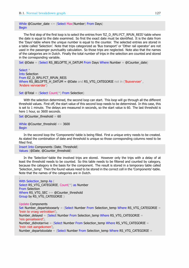
B.1. Normal breakdown graph 127

While @Counter_date <= (Select Max(Number) From Days)Begin

The first step of the first loop is to select the entries from ’EZ_D_RPU.FCT_RPUN_REIS’-table wherethe date is equal to the date examined. So first the exact date must be identified. It is the date fromthe ’Days’-table where the unique number is equal to the counter. The selected entries are stored ina table called ’Selection’. Note that trips categorized as ’Bus transport’ or ’Other rail operator’ are notused in the passenger punctuality calculation. So those trips are neglected. Note also that the namesof the categories are in Dutch. Finally the total number of trips in the selection are counted and storedin the corresponding variable.

Set @Date = (Select RS_BELOFTE_H_DATUM From Days Where Number = @Counter_date)

Select *Into SelectionFrom EZ_D_RPU.FCT_RPUN_REISWhere RS_BELOFTE_H_DATUM = @Date and RS_VTG_CATEGORIE not in (’Busvervoer’ ,’Andere vervoerder’)

Set @Total = (Select Count(*) From Selection)

With the selection determined, the second loop can start. This loop will go through all the differentthreshold values. First off, the start value of this second loop needs to be determined. In this case, thisis set to 1 minute. The delays are measured in seconds, so the start value is 60. The last threshold ishere 1 hour, so 3600 seconds.Set @Counter_threshold = 60

While @Counter_threshold <= 3600Begin

In the second loop the ’Components’-table is being filled. First a unique entry needs to be created.As stated the combination of date and threshold is unique so those corresponding columns need to befilled first.Insert Into Components (Date, Threshold)Values (@Date, @Counter_threshold)

In the ’Selection’-table the involved trips are stored. However only the trips with a delay of atleast the threshold needs to be counted. So this table needs to be filtered and counted by category,because the category is the basis for the component. The result is stored in a temporary table called’Selection_temp’. Then the found values need to be stored in the correct cell in the ’Components’-table.Note that the names of the categories are in Dutch.;With Selection_temp As (Select RS_VTG_CATEGORIE, Count(*) as NumberFrom SelectionWhere RS_VTG_SEC >= @Counter_thresholdGroup by RS_VTG_CATEGORIE )

Update ComponentsSet Number_departstooearly = (Select Number From Selection_temp Where RS_VTG_CATEGORIE =’trein te vroeg vertrokken’),Number_delayed = (Select Number From Selection_temp Where RS_VTG_CATEGORIE =’reis gerealiseerd’),Number_didnotarrive = (Select Number From Selection_temp Where RS_VTG_CATEGORIE =’trein niet aangekomen’),Number_departstoolate = (Select Number From Selection_temp Where RS_VTG_CATEGORIE =

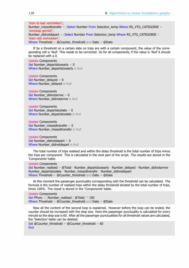
128 B. Algorithms to create breakdown graphs

’trein te laat vertrokken’),Number_missedtransfer = (Select Number From Selection_temp Where RS_VTG_CATEGORIE =’overstap gemist’),Number_didnotdepart = (Select Number From Selection_temp Where RS_VTG_CATEGORIE =’trein niet vertrokken’)Where Threshold = @Counter_threshold and Date = @Date

If by a threshold on a certain date no trips are with a certain component, the value of the corre-sponding cell is ’Null’. This needs to be corrected. So for all components, if the value is ’Null’ it shouldbe replaced with a 0.Update ComponentsSet Number_departstooearly = 0Where Number_departstooearly is Null

Update ComponentsSet Number_delayed = 0Where Number_delayed is Null

Update ComponentsSet Number_didnotarrive = 0Where Number_didnotarrive is Null

Update ComponentsSet Number_departstoolate = 0Where Number_departstoolate is Null

Update ComponentsSet Number_missedtransfer = 0Where Number_missedtransfer is Null

Update ComponentsSet Number_didnotdepart = 0Where Number_didnotdepart is Null

The total number of trips realised and within the delay threshold is the total number of trips minusthe trips per component. This is calculated in the next part of the script. The results are stored in the’Components’-table.Update ComponentsSet Number_realised = @Total - Number_departstooearly - Number_delayed - Number_didnotarrive -Number_departstoolate - Number_missedtransfer - Number_didnotdepartWhere Threshold = @Counter_threshold and Date = @Date

At this moment the passenger punctuality corresponding with the threshold can be calculated. Theformula is the number of realised trips within the delay threshold divided by the total number of trips,times 100%. The result is stored in the ’Components’-table.Update ComponentsSet PPunc = (Number_realised / @Total) * 100Where Threshold = @Counter_threshold and Date = @Date

Now all the content of the second loop is explained. However before the loop can be ended, thecounter should be increased with the step size. Here the passenger punctuality is calculated for everyminute so the step size is 60. After all the passenger punctualities for all threshold values are calculated,the ’Selection’-table can be deleted.Set @Counter_threshold = @Counter_threshold + 60End

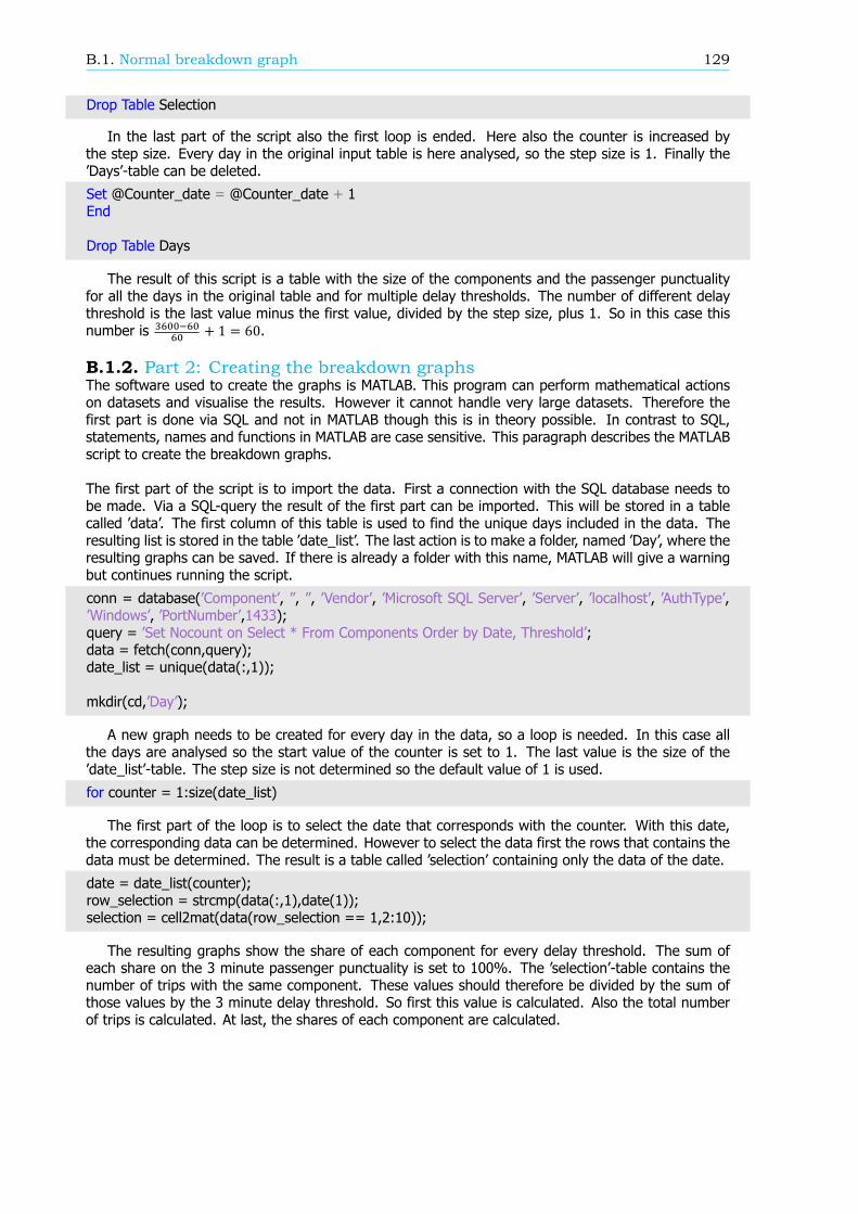
B.1. Normal breakdown graph 129

Drop Table Selection

In the last part of the script also the first loop is ended. Here also the counter is increased bythe step size. Every day in the original input table is here analysed, so the step size is 1. Finally the’Days’-table can be deleted.

Set @Counter_date = @Counter_date + 1End

Drop Table Days

The result of this script is a table with the size of the components and the passenger punctualityfor all the days in the original table and for multiple delay thresholds. The number of different delaythreshold is the last value minus the first value, divided by the step size, plus 1. So in this case thisnumber is + 1 = 60.

B.1.2. Part 2: Creating the breakdown graphsThe software used to create the graphs is MATLAB. This program can perform mathematical actionson datasets and visualise the results. However it cannot handle very large datasets. Therefore thefirst part is done via SQL and not in MATLAB though this is in theory possible. In contrast to SQL,statements, names and functions in MATLAB are case sensitive. This paragraph describes the MATLABscript to create the breakdown graphs.

The first part of the script is to import the data. First a connection with the SQL database needs tobe made. Via a SQL-query the result of the first part can be imported. This will be stored in a tablecalled ’data’. The first column of this table is used to find the unique days included in the data. Theresulting list is stored in the table ’date_list’. The last action is to make a folder, named ’Day’, where theresulting graphs can be saved. If there is already a folder with this name, MATLAB will give a warningbut continues running the script.

conn = database(’Component’, ”, ”, ’Vendor’, ’Microsoft SQL Server’, ’Server’, ’localhost’, ’AuthType’,’Windows’, ’PortNumber’,1433);query = ’Set Nocount on Select * From Components Order by Date, Threshold’;data = fetch(conn,query);date_list = unique(data(:,1));

mkdir(cd,’Day’);

A new graph needs to be created for every day in the data, so a loop is needed. In this case allthe days are analysed so the start value of the counter is set to 1. The last value is the size of the’date_list’-table. The step size is not determined so the default value of 1 is used.

for counter = 1:size(date_list)

The first part of the loop is to select the date that corresponds with the counter. With this date,the corresponding data can be determined. However to select the data first the rows that contains thedata must be determined. The result is a table called ’selection’ containing only the data of the date.

date = date_list(counter);row_selection = strcmp(data(:,1),date(1));selection = cell2mat(data(row_selection == 1,2:10));

The resulting graphs show the share of each component for every delay threshold. The sum ofeach share on the 3 minute passenger punctuality is set to 100%. The ’selection’-table contains thenumber of trips with the same component. These values should therefore be divided by the sum ofthose values by the 3 minute delay threshold. So first this value is calculated. Also the total numberof trips is calculated. At last, the shares of each component are calculated.

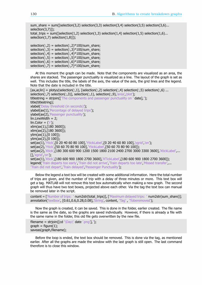
130 B. Algorithms to create breakdown graphs

sum_share = sum([selection(3,2) selection(3,3) selection(3,4) selection(3,5) selection(3,6)...selection(3,7)]);total_trips = sum([selection(1,2) selection(1,3) selection(1,4) selection(1,5) selection(1,6)...selection(1,7) selection(1,8)]);

selection(:,2) = selection(:,2)*100/sum_share;selection(:,3) = selection(:,3)*100/sum_share;selection(:,4) = selection(:,4)*100/sum_share;selection(:,5) = selection(:,5)*100/sum_share;selection(:,6) = selection(:,6)*100/sum_share;selection(:,7) = selection(:,7)*100/sum_share;

At this moment the graph can be made. Note that the components are visualized as an area, theshares are stacked. The passenger punctuality is visualized as a line. The layout of the graph is set aswell. This includes the title, the labels of the axis, the value of the axis, the grid lines and the legend.Note that the date is included in the title.[ax,ar,lin] = plotyy(selection(:,1), [selection(:,2) selection(:,4) selection(:,5) selection(:,6) ...selection(:,7) selection(:,3)], selection(:,1), selection(:,9),’area’,’plot’);titlestring = strjoin([’The components and passenger punctuality on ’ date],”);title(titlestring);xlabel(’Delay threshold (in seconds)’);ylabel(ax(1),’Percentage of delayed trips’);ylabel(ax(2),’Passenger punctuality’);lin.LineWidth = 2;lin.Color = (’r’);xlim(ax(1),[180 3600]);xlim(ax(2),[180 3600]);ylim(ax(1),[0 100]);ylim(ax(2),[0 100]);set(ax(1),’Ytick’,[0 20 40 60 80 100],’YtickLabel’,[0 20 40 60 80 100],’ygrid’,’on’);set(ax(2),’Ytick’,[50 60 70 80 90 100],’YtickLabel’,[50 60 70 80 90 100]);set(ax(2),’Xtick’,[180 300 600 900 1200 1500 1800 2100 2400 2700 3000 3300 3600],’XtickLabel’,...[],’xgrid’,’on’);set(ax(1),’Xtick’,[180 600 900 1800 2700 3600],’XTickLabel’,[180 600 900 1800 2700 3600]);legend(’Train departs too early’,’Train did not arrive’,’Train departs too late’,’Missed transfer’,...’Train did not depart’,’Train delayed’,’Passenger Punctuality’);

Below the legend a text box will be created with some additional information. Here the total numberof trips are given, and the number of trip with a delay of three minutes or more. This text box willget a tag. MATLAB will not remove this text box automatically when making a new graph. The secondgraph will thus have two text boxes, projected above each other. Via the tag the text box can manualbe removed later in the script.

content = [’Number of trips: ’ num2str(total_trips)], [’Maximum delayed trips: ’ num2str(sum_share)];annotation(’textbox’, [0.61,0.6,0.28,0.08],’String’, content, ’Tag’ , ’Toberemoved’);

Now the graph is created, it can be saved. This is done in the folder, earlier created. The file nameis the same as the date, so the graphs are saved individually. However, if there is already a file withthe same name in the folder, this old file gets overwritten by the new file.

filename = strjoin([cd ’\Day\’ date ’.png’],”);graph = figure(1);saveas(graph,filename);

Before the loop is ended, the text box should be removed. This is done via the tag, as mentionedearlier. After all the graphs are made the window with the last graph is still open. The last commandtherefore is to close this window.

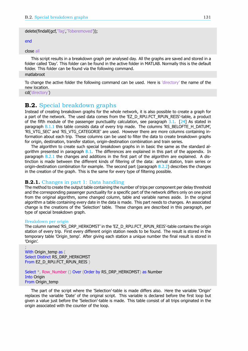
B.2. Special breakdown graphs 131

delete(findall(gcf,’Tag’,’Toberemoved’));

end

close all

This script results in a breakdown graph per analysed day. All the graphs are saved and stored in afolder called ’Day’. This folder can be found in the active folder in MATLAB. Normally this is the defaultfolder. This folder can be found via the following command.matlabroot

To change the active folder the following command can be used. Here is ’directory’ the name of thenew location.cd(’directory’)

B.2. Special breakdown graphsInstead of creating breakdown graphs for the whole network, it is also possible to create a graph fora part of the network. The used data comes from the ’EZ_D_RPU.FCT_RPUN_REIS’-table, a productof the fifth module of the passenger punctuality calculation, see paragraph 3.1. [24] As stated inparagraph B.1.1 this table consists data of every trip made. The columns ’RS_BELOFTE_H_DATUM’,’RS_VTG_SEC’ and ’RS_VTG_CATEGORIE’ are used. However there are more columns containing in-formation about each trip. These columns can be used to filter the data to create breakdown graphsfor origin, destination, transfer station, origin-destination combination and train series.

The algorithm to create such special breakdown graphs in in basic the same as the standard al-gorithm presented in paragraph B.1. The differences are explained in this part of the appendix. Inparagraph B.2.1 the changes and additions in the first part of the algorithm are explained. A dis-tinction is made between the different kinds of filtering of the data: arrival station, train series ororigin-destination combination for example. The second part (paragraph B.2.2) describes the changesin the creation of the graph. This is the same for every type of filtering possible.

B.2.1. Changes in part 1: Data handlingThe method to create the output table containing the number of trips per component per delay thresholdand the corresponding passenger punctuality for a specific part of the network differs only on one pointfrom the original algorithm, some changed column, table and variable names aside. In the originalalgorithm a table containing every date in the data is made. This part needs to changes. An associatedchange is the creations of the ’Selection’ table. These changes are described in this paragraph, pertype of special breakdown graph.

Breakdown per originThe column named ’RS_DRP_HERKOMST’ in the ’EZ_D_RPU.FCT_RPUN_REIS’-table contains the originstation of every trip. First every different origin station needs to be found. The result is stored in thetemporary table ’Origin_temp’. After giving each station a unique number the final result is stored in’Origin’.;With Origin_temp as (Select Distinct RS_DRP_HERKOMSTFrom EZ_D_RPU.FCT_RPUN_REIS )

Select *, Row_Number () Over (Order by RS_DRP_HERKOMST) as NumberInto OriginFrom Origin_temp

The part of the script where the ’Selection’-table is made differs also. Here the variable ’Origin’replaces the variable ’Date’ of the original script. This variable is declared before the first loop butgiven a value just before the ’Selection’-table is made. This table consist of all trips originated in theorigin associated with the counter of the loop.

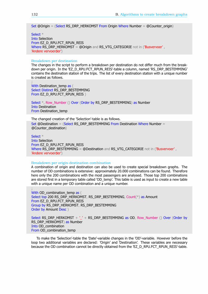
132 B. Algorithms to create breakdown graphs

Set @Origin = (Select RS_DRP_HERKOMST From Origin Where Number = @Counter_origin)

Select *Into SelectionFrom EZ_D_RPU.FCT_RPUN_REISWhere RS_DRP_HERKOMST = @Origin and RS_VTG_CATEGORIE not in (’Busvervoer’ ,’Andere vervoerder’)

Breakdown per destinationThe changes in the script to perform a breakdown per destination do not differ much from the break-down per origin. In the ’EZ_D_RPU.FCT_RPUN_REIS’-table a column, named ’RS_DRP_BESTEMMING’contains the destination station of the trips. The list of every destination station with a unique numberis created as follows.;With Destination_temp as (Select Distinct RS_DRP_BESTEMMINGFrom EZ_D_RPU.FCT_RPUN_REIS )

Select *, Row_Number () Over (Order by RS_DRP_BESTEMMING) as NumberInto DestinationFrom Destination_temp

The changed creation of the ’Selection’-table is as follows.Set @Destination = (Select RS_DRP_BESTEMMING From Destination Where Number =@Counter_destination)

Select *Into SelectionFrom EZ_D_RPU.FCT_RPUN_REISWhere RS_DRP_BESTEMMING = @Destination and RS_VTG_CATEGORIE not in (’Busvervoer’ ,’Andere vervoerder’)

Breakdown per origin-destination combinationA combination of origin and destination can also be used to create special breakdown graphs. Thenumber of OD combinations is extensive: approximately 20.000 combinations can be found. Thereforehere only the 200 combinations with the most passengers are analysed. Those top 200 combinationsare stored first in a temporary table called ’OD_temp’. This table is used as input to create a new tablewith a unique name per OD combination and a unique number.;With OD_combination_temp as (Select top 200 RS_DRP_HERKOMST, RS_DRP_BESTEMMING, Count(*) as AmountFrom EZ_D_RPU.FCT_RPUN_REISGroup by RS_DRP_HERKOMST, RS_DRP_BESTEMMINGOrder by Amount Desc )

Select RS_DRP_HERKOMST + ’_’ + RS_DRP_BESTEMMING as OD, Row_Number () Over (Order byRS_DRP_HERKOMST) as NumberInto OD_combinationFrom OD_combination_temp

To make the ’Selection’-table the ’Date’-variable changes in the ’OD’-variable. However before theloop two additional variables are declared: ’Origin’ and ’Destination’. These variables are necessarybecause the OD combination cannot be directly obtained from the ’EZ_D_RPU.FCT_RPUN_REIS’-table.

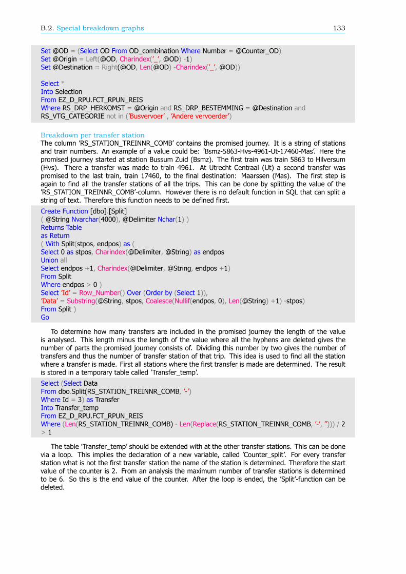
B.2. Special breakdown graphs 133

Set @OD = (Select OD From OD_combination Where Number = @Counter_OD)Set @Origin = Left(@OD, Charindex(’_’, @OD) -1)Set @Destination = Right(@OD, Len(@OD) -Charindex(’_’, @OD))

Select *Into SelectionFrom EZ_D_RPU.FCT_RPUN_REISWhere RS_DRP_HERKOMST = @Origin and RS_DRP_BESTEMMING = @Destination andRS_VTG_CATEGORIE not in (’Busvervoer’ , ’Andere vervoerder’)

Breakdown per transfer stationThe column ’RS_STATION_TREINNR_COMB’ contains the promised journey. It is a string of stationsand train numbers. An example of a value could be: ’Bsmz-5863-Hvs-4961-Ut-17460-Mas’. Here thepromised journey started at station Bussum Zuid (Bsmz). The first train was train 5863 to Hilversum(Hvs). There a transfer was made to train 4961. At Utrecht Centraal (Ut) a second transfer waspromised to the last train, train 17460, to the final destination: Maarssen (Mas). The first step isagain to find all the transfer stations of all the trips. This can be done by splitting the value of the’RS_STATION_TREINNR_COMB’-column. However there is no default function in SQL that can split astring of text. Therefore this function needs to be defined first.

Create Function [dbo].[Split]( @String Nvarchar(4000), @Delimiter Nchar(1) )Returns Tableas Return( With Split(stpos, endpos) as (Select 0 as stpos, Charindex(@Delimiter, @String) as endposUnion allSelect endpos +1, Charindex(@Delimiter, @String, endpos +1)From SplitWhere endpos > 0 )Select ’Id’ = Row_Number() Over (Order by (Select 1)),’Data’ = Substring(@String, stpos, Coalesce(Nullif(endpos, 0), Len(@String) +1) -stpos)From Split )Go

To determine how many transfers are included in the promised journey the length of the valueis analysed. This length minus the length of the value where all the hyphens are deleted gives thenumber of parts the promised journey consists of. Dividing this number by two gives the number oftransfers and thus the number of transfer station of that trip. This idea is used to find all the stationwhere a transfer is made. First all stations where the first transfer is made are determined. The resultis stored in a temporary table called ’Transfer_temp’.

Select (Select DataFrom dbo.Split(RS_STATION_TREINNR_COMB, ’-’)Where Id = 3) as TransferInto Transfer_tempFrom EZ_D_RPU.FCT_RPUN_REISWhere (Len(RS_STATION_TREINNR_COMB) - Len(Replace(RS_STATION_TREINNR_COMB, ’-’, ”))) / 2> 1

The table ’Transfer_temp’ should be extended with at the other transfer stations. This can be donevia a loop. This implies the declaration of a new variable, called ’Counter_split’. For every transferstation what is not the first transfer station the name of the station is determined. Therefore the startvalue of the counter is 2. From an analysis the maximum number of transfer stations is determinedto be 6. So this is the end value of the counter. After the loop is ended, the ’Split’-function can bedeleted.

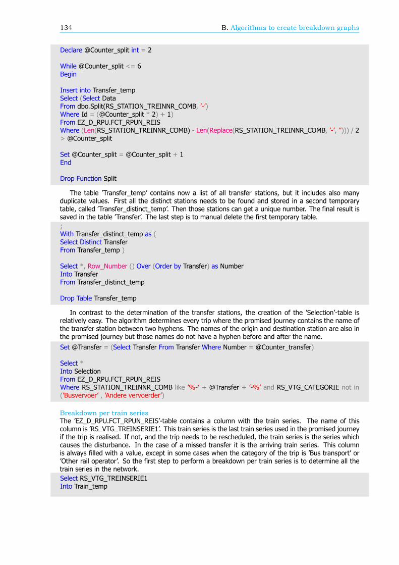
134 B. Algorithms to create breakdown graphs

Declare @Counter_split int = 2

While @Counter_split <= 6Begin

Insert into Transfer_tempSelect (Select DataFrom dbo.Split(RS_STATION_TREINNR_COMB, ’-’)Where Id = (@Counter_split * 2) + 1)From EZ_D_RPU.FCT_RPUN_REISWhere (Len(RS_STATION_TREINNR_COMB) - Len(Replace(RS_STATION_TREINNR_COMB, ’-’, ”))) / 2> @Counter_split

Set @Counter_split = @Counter_split + 1End

Drop Function Split

The table ’Transfer_temp’ contains now a list of all transfer stations, but it includes also manyduplicate values. First all the distinct stations needs to be found and stored in a second temporarytable, called ’Transfer_distinct_temp’. Then those stations can get a unique number. The final result issaved in the table ’Transfer’. The last step is to manual delete the first temporary table.;With Transfer_distinct_temp as (Select Distinct TransferFrom Transfer_temp )

Select *, Row_Number () Over (Order by Transfer) as NumberInto TransferFrom Transfer_distinct_temp

Drop Table Transfer_temp

In contrast to the determination of the transfer stations, the creation of the ’Selection’-table isrelatively easy. The algorithm determines every trip where the promised journey contains the name ofthe transfer station between two hyphens. The names of the origin and destination station are also inthe promised journey but those names do not have a hyphen before and after the name.

Set @Transfer = (Select Transfer From Transfer Where Number = @Counter_transfer)

Select *Into SelectionFrom EZ_D_RPU.FCT_RPUN_REISWhere RS_STATION_TREINNR_COMB like ’%-’ + @Transfer + ’-%’ and RS_VTG_CATEGORIE not in(’Busvervoer’ , ’Andere vervoerder’)

Breakdown per train seriesThe ’EZ_D_RPU.FCT_RPUN_REIS’-table contains a column with the train series. The name of thiscolumn is ’RS_VTG_TREINSERIE1’. This train series is the last train series used in the promised journeyif the trip is realised. If not, and the trip needs to be rescheduled, the train series is the series whichcauses the disturbance. In the case of a missed transfer it is the arriving train series. This columnis always filled with a value, except in some cases when the category of the trip is ’Bus transport’ or’Other rail operator’. So the first step to perform a breakdown per train series is to determine all thetrain series in the network.Select RS_VTG_TREINSERIE1Into Train_temp

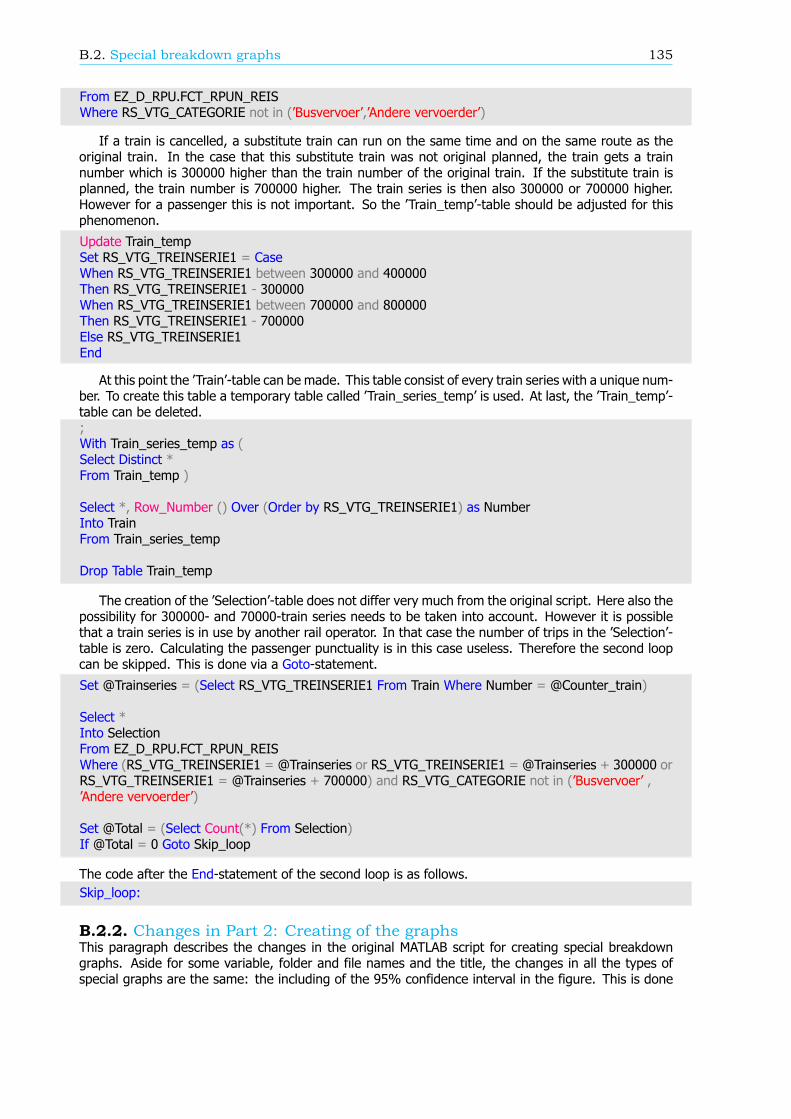
B.2. Special breakdown graphs 135

From EZ_D_RPU.FCT_RPUN_REISWhere RS_VTG_CATEGORIE not in (’Busvervoer’,’Andere vervoerder’)

If a train is cancelled, a substitute train can run on the same time and on the same route as theoriginal train. In the case that this substitute train was not original planned, the train gets a trainnumber which is 300000 higher than the train number of the original train. If the substitute train isplanned, the train number is 700000 higher. The train series is then also 300000 or 700000 higher.However for a passenger this is not important. So the ’Train_temp’-table should be adjusted for thisphenomenon.

Update Train_tempSet RS_VTG_TREINSERIE1 = CaseWhen RS_VTG_TREINSERIE1 between 300000 and 400000Then RS_VTG_TREINSERIE1 - 300000When RS_VTG_TREINSERIE1 between 700000 and 800000Then RS_VTG_TREINSERIE1 - 700000Else RS_VTG_TREINSERIE1End

At this point the ’Train’-table can be made. This table consist of every train series with a unique num-ber. To create this table a temporary table called ’Train_series_temp’ is used. At last, the ’Train_temp’-table can be deleted.;With Train_series_temp as (Select Distinct *From Train_temp )

Select *, Row_Number () Over (Order by RS_VTG_TREINSERIE1) as NumberInto TrainFrom Train_series_temp

Drop Table Train_temp

The creation of the ’Selection’-table does not differ very much from the original script. Here also thepossibility for 300000- and 70000-train series needs to be taken into account. However it is possiblethat a train series is in use by another rail operator. In that case the number of trips in the ’Selection’-table is zero. Calculating the passenger punctuality is in this case useless. Therefore the second loopcan be skipped. This is done via a Goto-statement.

Set @Trainseries = (Select RS_VTG_TREINSERIE1 From Train Where Number = @Counter_train)

Select *Into SelectionFrom EZ_D_RPU.FCT_RPUN_REISWhere (RS_VTG_TREINSERIE1 = @Trainseries or RS_VTG_TREINSERIE1 = @Trainseries + 300000 orRS_VTG_TREINSERIE1 = @Trainseries + 700000) and RS_VTG_CATEGORIE not in (’Busvervoer’ ,’Andere vervoerder’)

Set @Total = (Select Count(*) From Selection)If @Total = 0 Goto Skip_loop

The code after the End-statement of the second loop is as follows.Skip_loop:

B.2.2. Changes in Part 2: Creating of the graphsThis paragraph describes the changes in the original MATLAB script for creating special breakdowngraphs. Aside for some variable, folder and file names and the title, the changes in all the types ofspecial graphs are the same: the including of the 95% confidence interval in the figure. This is done

136 B. Algorithms to create breakdown graphs

by plotting the upper and lower bound of the interval and by giving the maximum deviation of the 3minute passenger punctuality.

The first step is to calculate the upper and lower bounds of the confidence interval of the passengerpunctuality. This is done via formula B.1.

𝑑 ≤ √𝑍𝑛 ∗ 𝑝(1 − 𝑝) (B.1)

Here is p the passenger punctuality, n the number of trips and Z is 1.96 by a reliability of 95%. Theupper bound of the interval is the passenger punctuality plus this deviation. However this cannot bemore than 100%. The lower bound of the passenger punctuality is the passenger punctuality minusthe deviation. Here the value cannot be smaller than 0%. The location of this part of the script is justbefore the graph is made.

p = selection(:,9)/100;d = sqrt((1.96ˆ2).*p.*(1-p)./total_trips)*100;upper = selection (:,9)+ d;upper(upper > 100) = 100;lower = selection (:,9)- d;lower(lower < 0) = 0;

The next step is to change the content of the text box. The maximum deviation of the 3 minutepassenger should be included. Note that thus the size and location of the text box also changes.

content = [’Number of trips: ’ num2str(total_trips)], [’Maximum delayed trips: ’ num2str(sum_share)],[’d (95%) ’ char(8804) ’ ’ num2str(round(d(3)*100)/100) ’ percentage point’];annotation(’textbox’, [0.61,0.57,0.28,0.11],’String’, content, ’Tag’ , ’Toberemoved’);

The last step is to plot the upper and lower bound of the confidence interval. This can be done justafter the previous change. The already created figure should not be deleted, so the ’hold on’-statementis used.hold on;plot(selection(:,1),lower,’b’);plot(selection(:,1),upper,’b’);hold off;

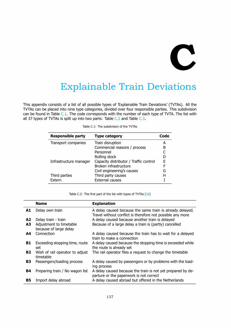
CExplainable Train Deviations

This appendix consists of a list of all possible types of ’Explainable Train Deviations’ (TVTAs). All theTVTAs can be placed into nine type categories, divided over four responsible parties. This subdivisioncan be found in Table C.1. The code corresponds with the number of each type of TVTA. The list withall 37 types of TVTAs is split up into two parts: Table C.2 and Table C.3.

Table C.1: The subdivision of the TVTAs

Responsible party Type category Code

Transport companies Train disruption ACommercial reasons / process BPersonnel CRolling stock D

Infrastructure manager Capacity distributor / Traffic control EBroken infrastructure FCivil engineering’s causes G

Third parties Third party causes HExtern External causes I

Table C.2: The first part of the list with types of TVTAs [36]

Name Explanation

A1 Delay own train A delay caused because the same train is already delayed.Travel without conflict is therefore not possible any more

A2 Delay train - train A delay caused because another train is delayedA3 Adjustment to timetable

because of large delayBecause of a large delay a train is (partly) cancelled

A4 Connection A delay caused because the train has to wait for a delayedtrain to make a connection

B1 Exceeding stopping time, routeset

A delay caused because the stopping time is exceeded whilethe route is already set

B2 Wish of rail operator to adjusttimetable

The rail operator files a request to change the timetable

B3 Passengers/loading process A delay caused by passengers or by problems with the load-ing process

B4 Preparing train / No wagon list A delay caused because the train is not yet prepared by de-parture or the paperwork is not correct

B5 Import delay abroad A delay caused abroad but offered in the Netherlands

137

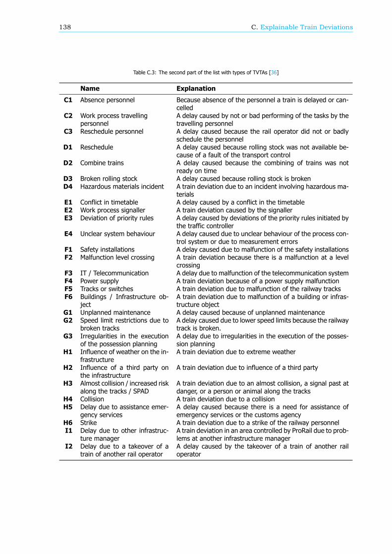
138 C. Explainable Train Deviations

Table C.3: The second part of the list with types of TVTAs [36]

Name Explanation

C1 Absence personnel Because absence of the personnel a train is delayed or can-celled

C2 Work process travellingpersonnel

A delay caused by not or bad performing of the tasks by thetravelling personnel

C3 Reschedule personnel A delay caused because the rail operator did not or badlyschedule the personnel

D1 Reschedule A delay caused because rolling stock was not available be-cause of a fault of the transport control

D2 Combine trains A delay caused because the combining of trains was notready on time

D3 Broken rolling stock A delay caused because rolling stock is brokenD4 Hazardous materials incident A train deviation due to an incident involving hazardous ma-

terialsE1 Conflict in timetable A delay caused by a conflict in the timetableE2 Work process signaller A train deviation caused by the signallerE3 Deviation of priority rules A delay caused by deviations of the priority rules initiated by

the traffic controllerE4 Unclear system behaviour A delay caused due to unclear behaviour of the process con-

trol system or due to measurement errorsF1 Safety installations A delay caused due to malfunction of the safety installationsF2 Malfunction level crossing A train deviation because there is a malfunction at a level

crossingF3 IT / Telecommunication A delay due to malfunction of the telecommunication systemF4 Power supply A train deviation because of a power supply malfunctionF5 Tracks or switches A train deviation due to malfunction of the railway tracksF6 Buildings / Infrastructure ob-

jectA train deviation due to malfunction of a building or infras-tructure object

G1 Unplanned maintenance A delay caused because of unplanned maintenanceG2 Speed limit restrictions due to

broken tracksA delay caused due to lower speed limits because the railwaytrack is broken.

G3 Irregularities in the executionof the possession planning

A delay due to irregularities in the execution of the posses-sion planning

H1 Influence of weather on the in-frastructure

A train deviation due to extreme weather

H2 Influence of a third party onthe infrastructure

A train deviation due to influence of a third party

H3 Almost collision / increased riskalong the tracks / SPAD

A train deviation due to an almost collision, a signal past atdanger, or a person or animal along the tracks

H4 Collision A train deviation due to a collisionH5 Delay due to assistance emer-

gency servicesA delay caused because there is a need for assistance ofemergency services or the customs agency

H6 Strike A train deviation due to a strike of the railway personnelI1 Delay due to other infrastruc-

ture managerA train deviation in an area controlled by ProRail due to prob-lems at another infrastructure manager

I2 Delay due to a takeover of atrain of another rail operator

A delay caused by the takeover of a train of another railoperator

DAlgorithms to calculate process

indicators

To calculate the process indicators (PI) for the entire network multiple data sources are used. Thesedata sources are tables where every row is unique. The information of each row is used to calculate theprocess indicator. To calculate the process indicators for a subset of the network, these data sourcesneed to be filtered. However not all the information needed is present in the data. So before theprocess indicators for a subset can be calculated, the raw data needs to be enriched. The algorithm todo this is described in paragraph D.1.

The actual algorithm to calculate the process indicators is described in paragraph D.2. Here theenriched data is loaded and filtered to retrieve only the data needed to calculate the process indicatorsfor a specific subset of the rail network.

D.1. Algorithm to enrich the PI dataThis paragraph describes the algorithm to enrich the raw data to calculate the process indicators (PI).It consists of a main algorithm (paragraph D.1.1) and multiple functions. A function is a part of thealgorithm in another file and can be called on in the main algorithm or in another function. The resultof this algorithm is six data files per examined day.

There are two reasons to have a function. The first reason is because the code in the function isrepetitive amongst the algorithm. To place this part of the code in a separate function, the overallalgorithm becomes less extensive and less complicated. The second reason is because of clearness.The total algorithm is long. To place certain parts of the algorithm in a separate function, the totalalgorithm stays more clear, certainty when such a function has a goal on its own.

The main part of the algorithm is written in MATLAB. However at certain points data out of the passengerpunctuality database is required. Here the output tables are quite extensive, so this data is stored in anSQL database. To retrieve the desired data, some parts of the algorithm are written in the StructuredQuery Language.

D.1.1. Main algorithmIn short the main algorithm is the user interface for the entire algorithm. Here the user can set someinput values, like the settings of the SQL server and the dates of which the data needs to be enriched.After some checks if the input data is correct, multiple function are called on. Every function enrichesthe data of a single data source.

In the first part of the algorithm the user can alter five settings. The first two are the start and end dateof the period of which the data needs to be enriched. The format of the input may vary. Correct valuesare ’01JUN2015’ or ’2015-06-01’. The last three settings are settings of the SQL-server. Secondly, theinputs are checked by comparing the start date with the end date and by trying to make a connectionwith the SQL database.

139

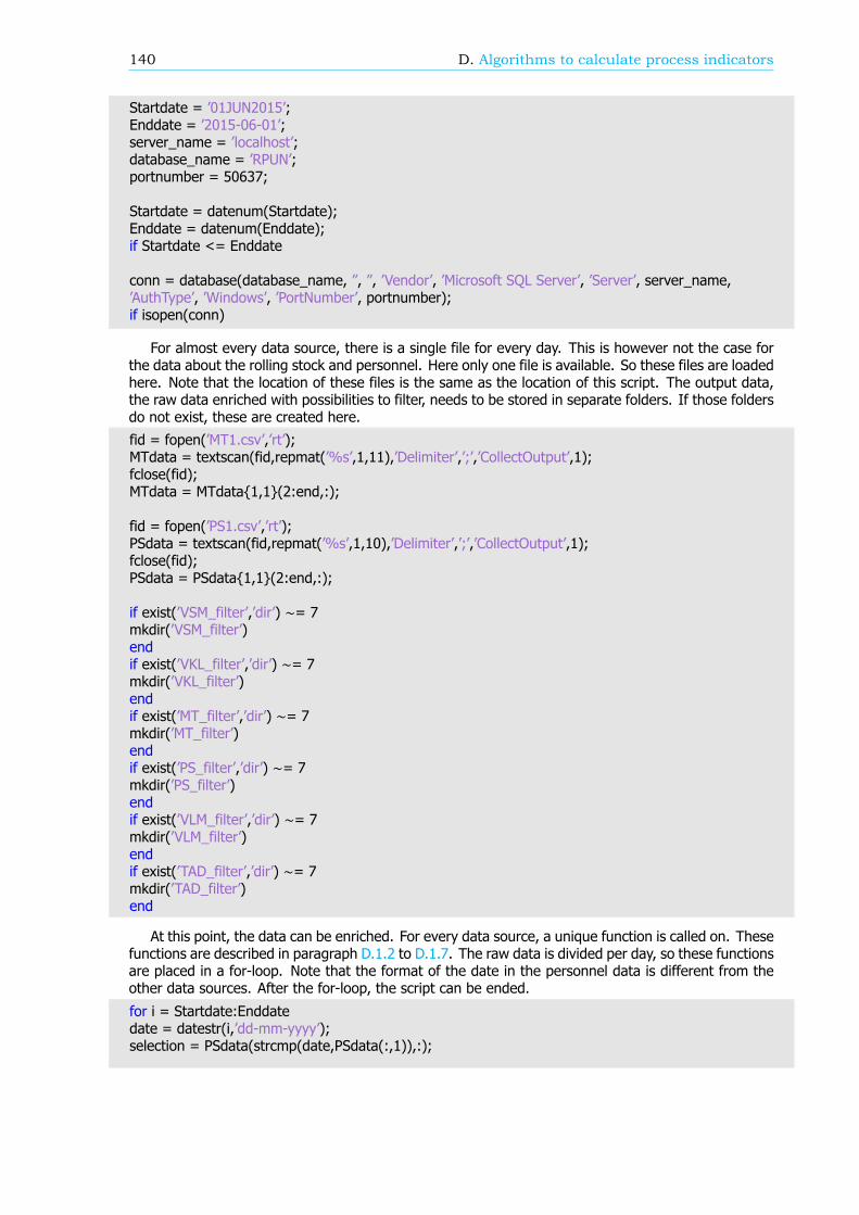
140 D. Algorithms to calculate process indicators

Startdate = ’01JUN2015’;Enddate = ’2015-06-01’;server_name = ’localhost’;database_name = ’RPUN’;portnumber = 50637;

Startdate = datenum(Startdate);Enddate = datenum(Enddate);if Startdate <= Enddate

conn = database(database_name, ”, ”, ’Vendor’, ’Microsoft SQL Server’, ’Server’, server_name,’AuthType’, ’Windows’, ’PortNumber’, portnumber);if isopen(conn)

For almost every data source, there is a single file for every day. This is however not the case forthe data about the rolling stock and personnel. Here only one file is available. So these files are loadedhere. Note that the location of these files is the same as the location of this script. The output data,the raw data enriched with possibilities to filter, needs to be stored in separate folders. If those foldersdo not exist, these are created here.

fid = fopen(’MT1.csv’,’rt’);MTdata = textscan(fid,repmat(’%s’,1,11),’Delimiter’,’;’,’CollectOutput’,1);fclose(fid);MTdata = MTdata{1,1}(2:end,:);

fid = fopen(’PS1.csv’,’rt’);PSdata = textscan(fid,repmat(’%s’,1,10),’Delimiter’,’;’,’CollectOutput’,1);fclose(fid);PSdata = PSdata{1,1}(2:end,:);

if exist(’VSM_filter’,’dir’) ∼= 7mkdir(’VSM_filter’)endif exist(’VKL_filter’,’dir’) ∼= 7mkdir(’VKL_filter’)endif exist(’MT_filter’,’dir’) ∼= 7mkdir(’MT_filter’)endif exist(’PS_filter’,’dir’) ∼= 7mkdir(’PS_filter’)endif exist(’VLM_filter’,’dir’) ∼= 7mkdir(’VLM_filter’)endif exist(’TAD_filter’,’dir’) ∼= 7mkdir(’TAD_filter’)end

At this point, the data can be enriched. For every data source, a unique function is called on. Thesefunctions are described in paragraph D.1.2 to D.1.7. The raw data is divided per day, so these functionsare placed in a for-loop. Note that the format of the date in the personnel data is different from theother data sources. After the for-loop, the script can be ended.

for i = Startdate:Enddatedate = datestr(i,’dd-mm-yyyy’);selection = PSdata(strcmp(date,PSdata(:,1)),:);

D.1. Algorithm to enrich the PI data 141

date = datestr(i,’yyyy-mm-dd’);PS_func(date,selection);VSM_func(date,conn);VKL_func(date);selection = MTdata(strcmp(date,MTdata(:,1)),:);MT_func(date,selection);VLM_func(date, conn);TAD_func(date, conn);end

elsedisp(’There is no connection with the SQL database’)endelsedisp(’The dates are not correct’);end

D.1.2. Function: PS_funcThis function enriches the data concerning personnel. This data consist per day and per train seriesthe number of planned staff members and the actual number of staff members. This data should beenlarged with the route of the train series. This route can change between the direction (odd or even),so a distinction between the directions should be made. The information about the route is stored ina datafile called ’list-linten_2015-06-01.dat’, where of course the date can change. This file containsper train series and direction the route that is most often run that day and the longest route of thatday. Here the route is presented as a list (a ribbon) of consecutive service control points and the action(arrival, departure or passage). The function starts with the loading of the data about the ribbons.

Next for every row in the data, the corresponding route should be found. This is done in multiplesteps. For every row in the ribbon data a check is made if the train series is a passenger train. Thenthe number of the train series of the ribbon is compared with the number of the train series of thepersonnel data. Lastly the direction is determined.

Following, the route should be placed in the right format in the right variable. As stated, in theribbon data per train series there are two routes: the most often travelled route and the longest route.At this point, the most often travelled route is used. Nonetheless if both routes are not the same, thelongest route should also be put in the right format in the right variable.

The involved service control points are the service control stops on the route whit a departure oran arrival. These service control points can be found by adding all possible routes per train series anddeleting those points with only a passage.

The found routes and the involved service control points should be added by the existing data.When this is done for every row in the personnel data, the enriched data should be exported to a newdata file. Note that the result is a file per day, instead of only one overall file, like the raw data. Thenames of the columns of the exported file are in Dutch, like in the raw data. The format of the outputfile can be found in Table D.1.

Table D.1: The format of the enriched PS-file

Column Content

1-10 Original PS data11 Involved stations12 Route, in the even direction13 Route, in the odd direction

D.1.3. Function: VSM_funcThere are nine process indicators concerning blockage measures. This function enriches the raw dataconcerning these measures. First of all, the lead times between the different steps between disruption

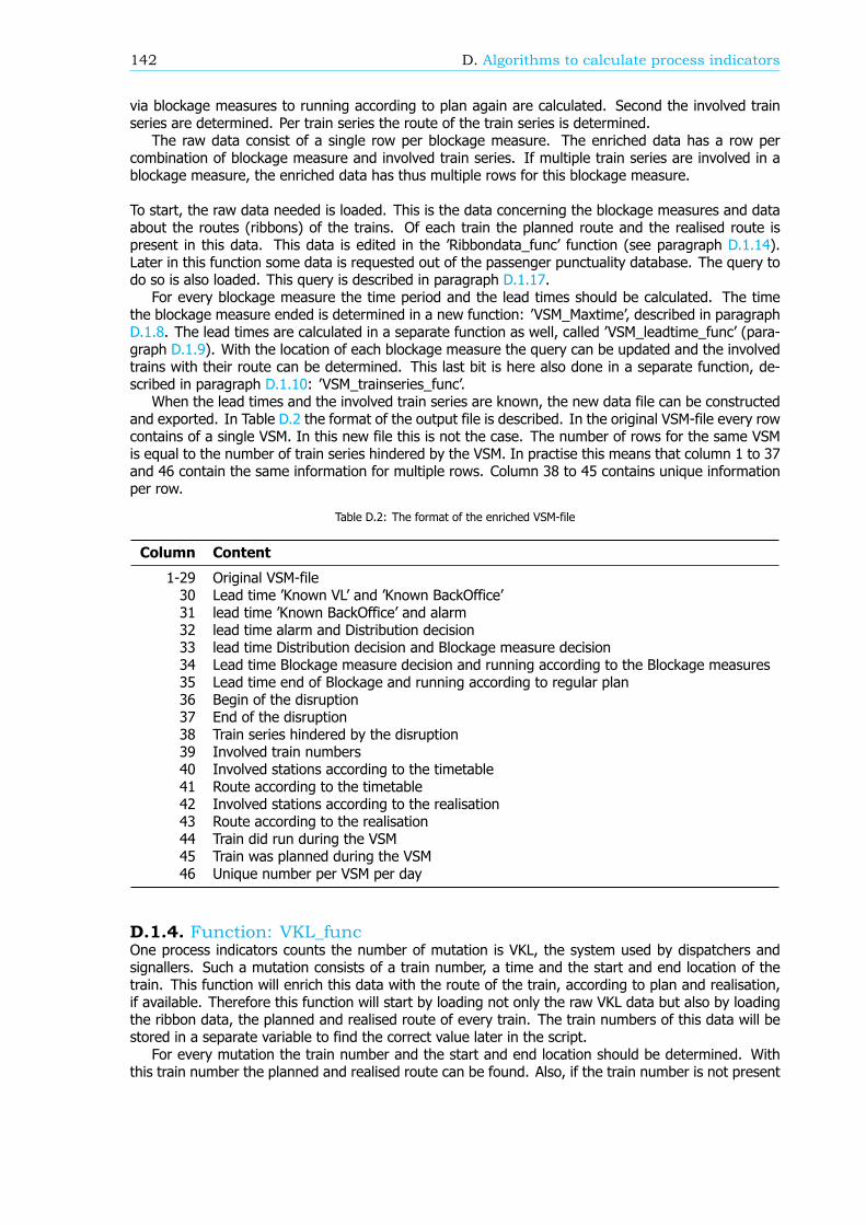
142 D. Algorithms to calculate process indicators

via blockage measures to running according to plan again are calculated. Second the involved trainseries are determined. Per train series the route of the train series is determined.

The raw data consist of a single row per blockage measure. The enriched data has a row percombination of blockage measure and involved train series. If multiple train series are involved in ablockage measure, the enriched data has thus multiple rows for this blockage measure.

To start, the raw data needed is loaded. This is the data concerning the blockage measures and dataabout the routes (ribbons) of the trains. Of each train the planned route and the realised route ispresent in this data. This data is edited in the ’Ribbondata_func’ function (see paragraph D.1.14).Later in this function some data is requested out of the passenger punctuality database. The query todo so is also loaded. This query is described in paragraph D.1.17.

For every blockage measure the time period and the lead times should be calculated. The timethe blockage measure ended is determined in a new function: ’VSM_Maxtime’, described in paragraphD.1.8. The lead times are calculated in a separate function as well, called ’VSM_leadtime_func’ (para-graph D.1.9). With the location of each blockage measure the query can be updated and the involvedtrains with their route can be determined. This last bit is here also done in a separate function, de-scribed in paragraph D.1.10: ’VSM_trainseries_func’.

When the lead times and the involved train series are known, the new data file can be constructedand exported. In Table D.2 the format of the output file is described. In the original VSM-file every rowcontains of a single VSM. In this new file this is not the case. The number of rows for the same VSMis equal to the number of train series hindered by the VSM. In practise this means that column 1 to 37and 46 contain the same information for multiple rows. Column 38 to 45 contains unique informationper row.

Table D.2: The format of the enriched VSM-file

Column Content

1-29 Original VSM-file30 Lead time ’Known VL’ and ’Known BackOffice’31 lead time ’Known BackOffice’ and alarm32 lead time alarm and Distribution decision33 lead time Distribution decision and Blockage measure decision34 Lead time Blockage measure decision and running according to the Blockage measures35 Lead time end of Blockage and running according to regular plan36 Begin of the disruption37 End of the disruption38 Train series hindered by the disruption39 Involved train numbers40 Involved stations according to the timetable41 Route according to the timetable42 Involved stations according to the realisation43 Route according to the realisation44 Train did run during the VSM45 Train was planned during the VSM46 Unique number per VSM per day

D.1.4. Function: VKL_funcOne process indicators counts the number of mutation is VKL, the system used by dispatchers andsignallers. Such a mutation consists of a train number, a time and the start and end location of thetrain. This function will enrich this data with the route of the train, according to plan and realisation,if available. Therefore this function will start by loading not only the raw VKL data but also by loadingthe ribbon data, the planned and realised route of every train. The train numbers of this data will bestored in a separate variable to find the correct value later in the script.

For every mutation the train number and the start and end location should be determined. Withthis train number the planned and realised route can be found. Also, if the train number is not present

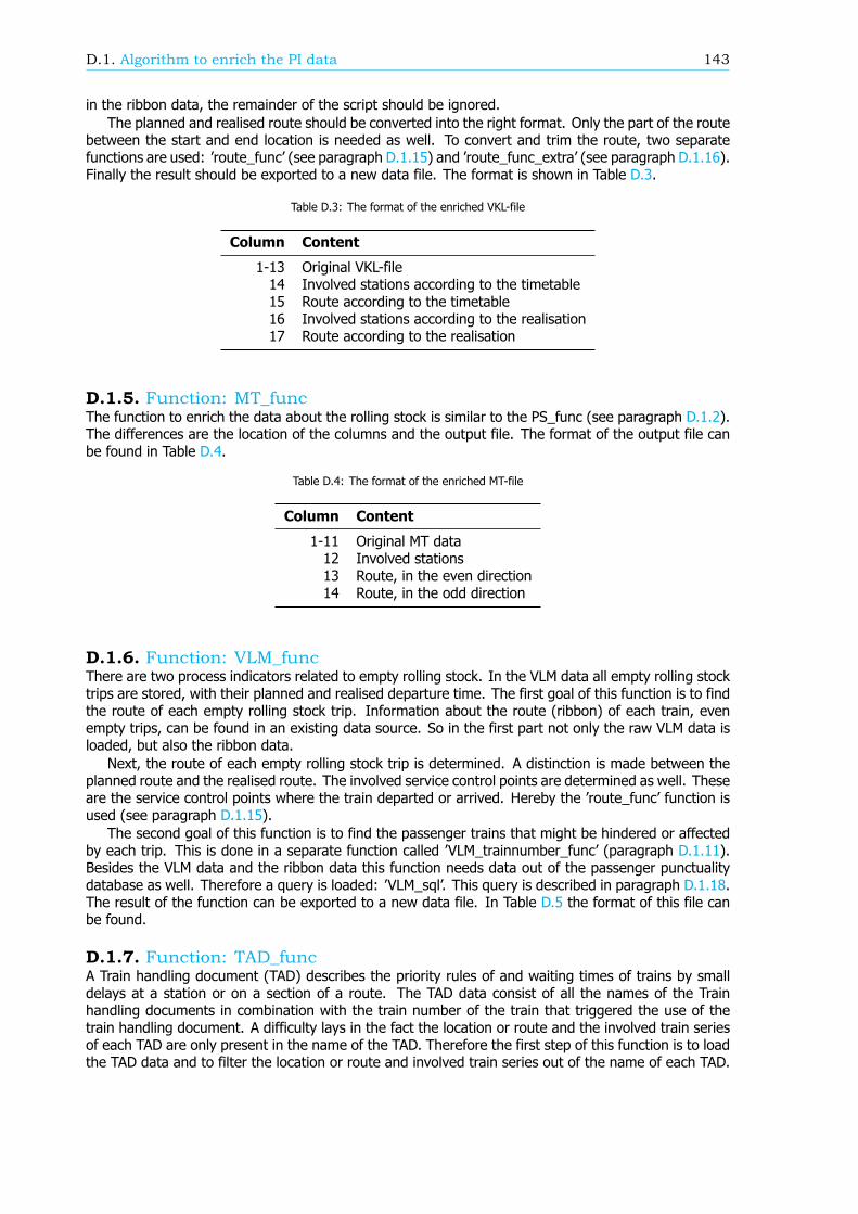
D.1. Algorithm to enrich the PI data 143

in the ribbon data, the remainder of the script should be ignored.The planned and realised route should be converted into the right format. Only the part of the route

between the start and end location is needed as well. To convert and trim the route, two separatefunctions are used: ’route_func’ (see paragraph D.1.15) and ’route_func_extra’ (see paragraph D.1.16).Finally the result should be exported to a new data file. The format is shown in Table D.3.

Table D.3: The format of the enriched VKL-file

Column Content

1-13 Original VKL-file14 Involved stations according to the timetable15 Route according to the timetable16 Involved stations according to the realisation17 Route according to the realisation

D.1.5. Function: MT_funcThe function to enrich the data about the rolling stock is similar to the PS_func (see paragraph D.1.2).The differences are the location of the columns and the output file. The format of the output file canbe found in Table D.4.

Table D.4: The format of the enriched MT-file

Column Content

1-11 Original MT data12 Involved stations13 Route, in the even direction14 Route, in the odd direction

D.1.6. Function: VLM_funcThere are two process indicators related to empty rolling stock. In the VLM data all empty rolling stocktrips are stored, with their planned and realised departure time. The first goal of this function is to findthe route of each empty rolling stock trip. Information about the route (ribbon) of each train, evenempty trips, can be found in an existing data source. So in the first part not only the raw VLM data isloaded, but also the ribbon data.

Next, the route of each empty rolling stock trip is determined. A distinction is made between theplanned route and the realised route. The involved service control points are determined as well. Theseare the service control points where the train departed or arrived. Hereby the ’route_func’ function isused (see paragraph D.1.15).

The second goal of this function is to find the passenger trains that might be hindered or affectedby each trip. This is done in a separate function called ’VLM_trainnumber_func’ (paragraph D.1.11).Besides the VLM data and the ribbon data this function needs data out of the passenger punctualitydatabase as well. Therefore a query is loaded: ’VLM_sql’. This query is described in paragraph D.1.18.The result of the function can be exported to a new data file. In Table D.5 the format of this file canbe found.

D.1.7. Function: TAD_funcA Train handling document (TAD) describes the priority rules of and waiting times of trains by smalldelays at a station or on a section of a route. The TAD data consist of all the names of the Trainhandling documents in combination with the train number of the train that triggered the use of thetrain handling document. A difficulty lays in the fact the location or route and the involved train seriesof each TAD are only present in the name of the TAD. Therefore the first step of this function is to loadthe TAD data and to filter the location or route and involved train series out of the name of each TAD.

144 D. Algorithms to calculate process indicators

Table D.5: The format of the enriched VLM-file

Column Content

1-14 Original VLM-file15 Involved stations according to the timetable16 Route according to the timetable17 Involved stations according to the realisation18 Route according to the realisation19 Trains that run during the empty rolling stock trip according to the timetable20 Trains that did not run during the empty rolling stock trip according to the timetable21 Trains that run during the empty rolling stock trip according to the realisation22 Trains that did not run during the empty rolling stock trip according to the realisation23 Train series that run during the empty rolling stock trip according to the timetable24 Train series that did not run during the empty rolling stock trip according to the

timetable25 Train series that run during the empty rolling stock trip according to the realisation26 Train series that did not run during the empty rolling stock trip according to the

realisation

In the name of the TAD the involved trains are listed. The timetable repeats itself every 15, 30 or 60minutes, so a TAD can be used multiple times in a day. In such cases not the involved train numbers,but the involved train series are listed. To determine the exact routes of the involved train series andtrain numbers, two data files are loaded. The first data file contains the routes (ribbons) of each trainseries. The second data file contains the route per train number. With these two data files for everyinvolved train number of series the route can be found.

Lastly the departure and arrival times of every train on every station needs to be known. Thisinformation is available in the passenger punctuality database. With a query (’TAD_sql’, see paragraphD.1.19) this data can be retrieved. To make calculations with this data easier the arrival and departuretimes (both according to plan and the realised time) are transformed to values. Also, the retrieveddata out of the SQL-server is very large. To make calculations faster, the data is split by train numberand stored in smaller tables. This implies that only smaller tables needs to be searched if departure orarrival times needs to be known.

The TAD data and ribbon data can be combined to find the exact route for each TAD. This is done ina separate function called ’TAD_route_func’ (see paragraph D.1.12). Next the, already enriched, TADdata is combined with the arrival and departure times to find the time period of each TAD. This is donein a separate function as well: ’TAD_time_func’ (paragraph D.1.13). Before the result can be exportedto a new data file, the involved train series should be converted to the right format. The format of thenew data file is shown in Table D.6.

Table D.6: The format of the enriched TAD-file

Column Content

1-7 Original TAD-file8 Borders of the TAD9 Possible involved train series10 Involved train series11 Involved stations12 Route13 Begin of the TAD according to the timetable14 End of the TAD according to the timetable15 Begin of the TAD according to the realisation16 End of the TAD according to the realisation

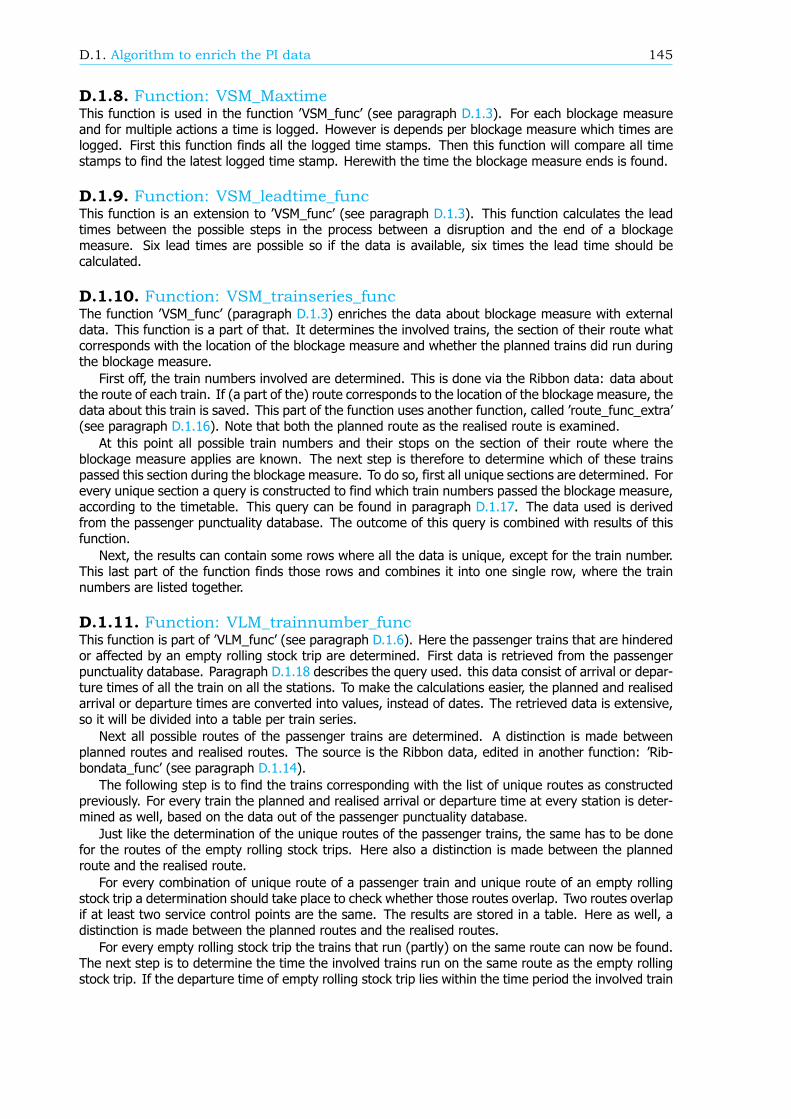
D.1. Algorithm to enrich the PI data 145

D.1.8. Function: VSM_MaxtimeThis function is used in the function ’VSM_func’ (see paragraph D.1.3). For each blockage measureand for multiple actions a time is logged. However is depends per blockage measure which times arelogged. First this function finds all the logged time stamps. Then this function will compare all timestamps to find the latest logged time stamp. Herewith the time the blockage measure ends is found.

D.1.9. Function: VSM_leadtime_funcThis function is an extension to ’VSM_func’ (see paragraph D.1.3). This function calculates the leadtimes between the possible steps in the process between a disruption and the end of a blockagemeasure. Six lead times are possible so if the data is available, six times the lead time should becalculated.

D.1.10. Function: VSM_trainseries_funcThe function ’VSM_func’ (paragraph D.1.3) enriches the data about blockage measure with externaldata. This function is a part of that. It determines the involved trains, the section of their route whatcorresponds with the location of the blockage measure and whether the planned trains did run duringthe blockage measure.

First off, the train numbers involved are determined. This is done via the Ribbon data: data aboutthe route of each train. If (a part of the) route corresponds to the location of the blockage measure, thedata about this train is saved. This part of the function uses another function, called ’route_func_extra’(see paragraph D.1.16). Note that both the planned route as the realised route is examined.

At this point all possible train numbers and their stops on the section of their route where theblockage measure applies are known. The next step is therefore to determine which of these trainspassed this section during the blockage measure. To do so, first all unique sections are determined. Forevery unique section a query is constructed to find which train numbers passed the blockage measure,according to the timetable. This query can be found in paragraph D.1.17. The data used is derivedfrom the passenger punctuality database. The outcome of this query is combined with results of thisfunction.

Next, the results can contain some rows where all the data is unique, except for the train number.This last part of the function finds those rows and combines it into one single row, where the trainnumbers are listed together.

D.1.11. Function: VLM_trainnumber_funcThis function is part of ’VLM_func’ (see paragraph D.1.6). Here the passenger trains that are hinderedor affected by an empty rolling stock trip are determined. First data is retrieved from the passengerpunctuality database. Paragraph D.1.18 describes the query used. this data consist of arrival or depar-ture times of all the train on all the stations. To make the calculations easier, the planned and realisedarrival or departure times are converted into values, instead of dates. The retrieved data is extensive,so it will be divided into a table per train series.

Next all possible routes of the passenger trains are determined. A distinction is made betweenplanned routes and realised routes. The source is the Ribbon data, edited in another function: ’Rib-bondata_func’ (see paragraph D.1.14).

The following step is to find the trains corresponding with the list of unique routes as constructedpreviously. For every train the planned and realised arrival or departure time at every station is deter-mined as well, based on the data out of the passenger punctuality database.

Just like the determination of the unique routes of the passenger trains, the same has to be donefor the routes of the empty rolling stock trips. Here also a distinction is made between the plannedroute and the realised route.

For every combination of unique route of a passenger train and unique route of an empty rollingstock trip a determination should take place to check whether those routes overlap. Two routes overlapif at least two service control points are the same. The results are stored in a table. Here as well, adistinction is made between the planned routes and the realised routes.

For every empty rolling stock trip the trains that run (partly) on the same route can now be found.The next step is to determine the time the involved trains run on the same route as the empty rollingstock trip. If the departure time of empty rolling stock trip lies within the time period the involved train

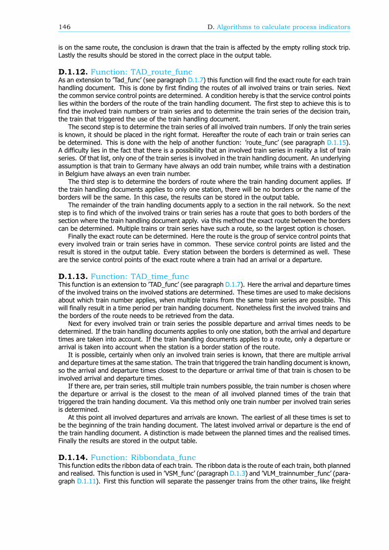
146 D. Algorithms to calculate process indicators

is on the same route, the conclusion is drawn that the train is affected by the empty rolling stock trip.Lastly the results should be stored in the correct place in the output table.

D.1.12. Function: TAD_route_funcAs an extension to ’Tad_func’ (see paragraph D.1.7) this function will find the exact route for each trainhandling document. This is done by first finding the routes of all involved trains or train series. Nextthe common service control points are determined. A condition hereby is that the service control pointslies within the borders of the route of the train handling document. The first step to achieve this is tofind the involved train numbers or train series and to determine the train series of the decision train,the train that triggered the use of the train handling document.

The second step is to determine the train series of all involved train numbers. If only the train seriesis known, it should be placed in the right format. Hereafter the route of each train or train series canbe determined. This is done with the help of another function: ’route_func’ (see paragraph D.1.15).A difficulty lies in the fact that there is a possibility that an involved train series in reality a list of trainseries. Of that list, only one of the train series is involved in the train handling document. An underlyingassumption is that train to Germany have always an odd train number, while trains with a destinationin Belgium have always an even train number.

The third step is to determine the borders of route where the train handing document applies. Ifthe train handling documents applies to only one station, there will be no borders or the name of theborders will be the same. In this case, the results can be stored in the output table.

The remainder of the train handling documents apply to a section in the rail network. So the nextstep is to find which of the involved trains or train series has a route that goes to both borders of thesection where the train handling document apply. via this method the exact route between the borderscan be determined. Multiple trains or train series have such a route, so the largest option is chosen.

Finally the exact route can be determined. Here the route is the group of service control points thatevery involved train or train series have in common. These service control points are listed and theresult is stored in the output table. Every station between the borders is determined as well. Theseare the service control points of the exact route where a train had an arrival or a departure.

D.1.13. Function: TAD_time_funcThis function is an extension to ’TAD_func’ (see paragraph D.1.7). Here the arrival and departure timesof the involved trains on the involved stations are determined. These times are used to make decisionsabout which train number applies, when multiple trains from the same train series are possible. Thiswill finally result in a time period per train handing document. Nonetheless first the involved trains andthe borders of the route needs to be retrieved from the data.

Next for every involved train or train series the possible departure and arrival times needs to bedetermined. If the train handling documents applies to only one station, both the arrival and departuretimes are taken into account. If the train handling documents applies to a route, only a departure orarrival is taken into account when the station is a border station of the route.

It is possible, certainly when only an involved train series is known, that there are multiple arrivaland departure times at the same station. The train that triggered the train handling document is known,so the arrival and departure times closest to the departure or arrival time of that train is chosen to beinvolved arrival and departure times.

If there are, per train series, still multiple train numbers possible, the train number is chosen wherethe departure or arrival is the closest to the mean of all involved planned times of the train thattriggered the train handing document. Via this method only one train number per involved train seriesis determined.

At this point all involved departures and arrivals are known. The earliest of all these times is set tobe the beginning of the train handing document. The latest involved arrival or departure is the end ofthe train handling document. A distinction is made between the planned times and the realised times.Finally the results are stored in the output table.

D.1.14. Function: Ribbondata_funcThis function edits the ribbon data of each train. The ribbon data is the route of each train, both plannedand realised. This function is used in ’VSM_func’ (paragraph D.1.3) and ’VLM_trainnumber_func’ (para-graph D.1.11). First this function will separate the passenger trains from the other trains, like freight

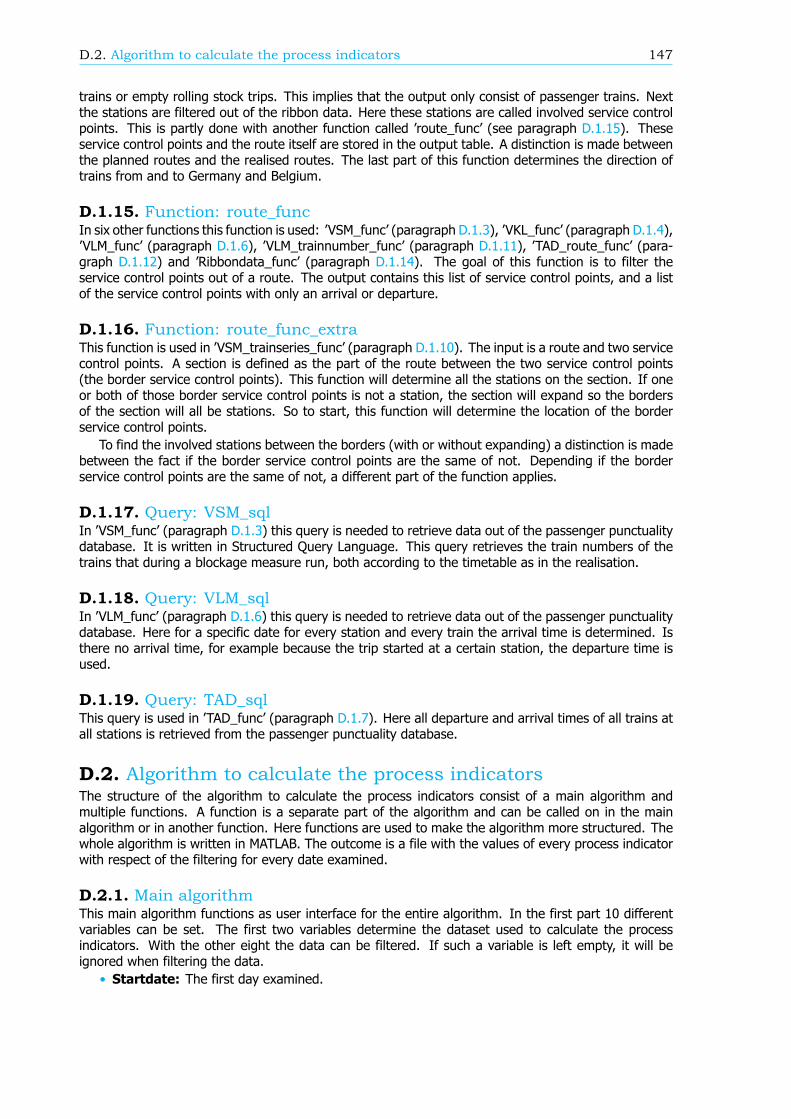
D.2. Algorithm to calculate the process indicators 147

trains or empty rolling stock trips. This implies that the output only consist of passenger trains. Nextthe stations are filtered out of the ribbon data. Here these stations are called involved service controlpoints. This is partly done with another function called ’route_func’ (see paragraph D.1.15). Theseservice control points and the route itself are stored in the output table. A distinction is made betweenthe planned routes and the realised routes. The last part of this function determines the direction oftrains from and to Germany and Belgium.

D.1.15. Function: route_funcIn six other functions this function is used: ’VSM_func’ (paragraph D.1.3), ’VKL_func’ (paragraph D.1.4),’VLM_func’ (paragraph D.1.6), ’VLM_trainnumber_func’ (paragraph D.1.11), ’TAD_route_func’ (para-graph D.1.12) and ’Ribbondata_func’ (paragraph D.1.14). The goal of this function is to filter theservice control points out of a route. The output contains this list of service control points, and a listof the service control points with only an arrival or departure.

D.1.16. Function: route_func_extraThis function is used in ’VSM_trainseries_func’ (paragraph D.1.10). The input is a route and two servicecontrol points. A section is defined as the part of the route between the two service control points(the border service control points). This function will determine all the stations on the section. If oneor both of those border service control points is not a station, the section will expand so the bordersof the section will all be stations. So to start, this function will determine the location of the borderservice control points.

To find the involved stations between the borders (with or without expanding) a distinction is madebetween the fact if the border service control points are the same of not. Depending if the borderservice control points are the same of not, a different part of the function applies.

D.1.17. Query: VSM_sqlIn ’VSM_func’ (paragraph D.1.3) this query is needed to retrieve data out of the passenger punctualitydatabase. It is written in Structured Query Language. This query retrieves the train numbers of thetrains that during a blockage measure run, both according to the timetable as in the realisation.

D.1.18. Query: VLM_sqlIn ’VLM_func’ (paragraph D.1.6) this query is needed to retrieve data out of the passenger punctualitydatabase. Here for a specific date for every station and every train the arrival time is determined. Isthere no arrival time, for example because the trip started at a certain station, the departure time isused.

D.1.19. Query: TAD_sqlThis query is used in ’TAD_func’ (paragraph D.1.7). Here all departure and arrival times of all trains atall stations is retrieved from the passenger punctuality database.

D.2. Algorithm to calculate the process indicatorsThe structure of the algorithm to calculate the process indicators consist of a main algorithm andmultiple functions. A function is a separate part of the algorithm and can be called on in the mainalgorithm or in another function. Here functions are used to make the algorithm more structured. Thewhole algorithm is written in MATLAB. The outcome is a file with the values of every process indicatorwith respect of the filtering for every date examined.

D.2.1. Main algorithmThis main algorithm functions as user interface for the entire algorithm. In the first part 10 differentvariables can be set. The first two variables determine the dataset used to calculate the processindicators. With the other eight the data can be filtered. If such a variable is left empty, it will beignored when filtering the data.

• Startdate: The first day examined.

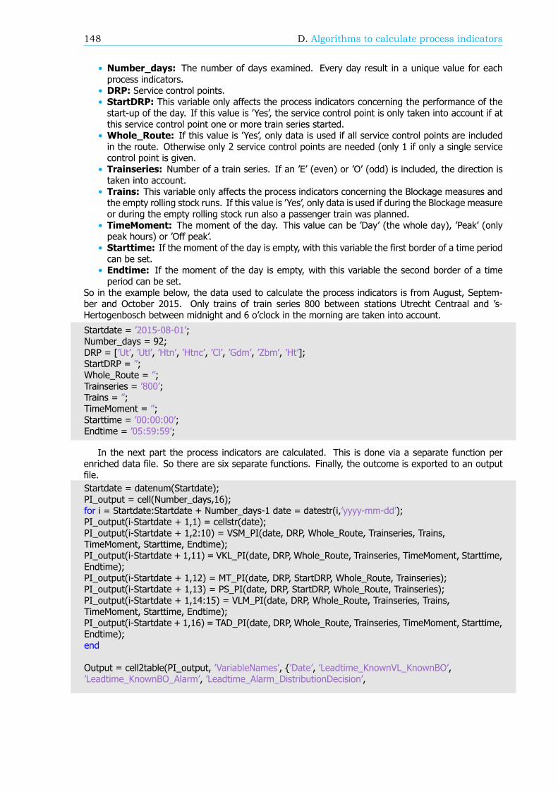
148 D. Algorithms to calculate process indicators

• Number_days: The number of days examined. Every day result in a unique value for eachprocess indicators.

• DRP: Service control points.• StartDRP: This variable only affects the process indicators concerning the performance of thestart-up of the day. If this value is ’Yes’, the service control point is only taken into account if atthis service control point one or more train series started.

• Whole_Route: If this value is ’Yes’, only data is used if all service control points are includedin the route. Otherwise only 2 service control points are needed (only 1 if only a single servicecontrol point is given.

• Trainseries: Number of a train series. If an ’E’ (even) or ’O’ (odd) is included, the direction istaken into account.

• Trains: This variable only affects the process indicators concerning the Blockage measures andthe empty rolling stock runs. If this value is ’Yes’, only data is used if during the Blockage measureor during the empty rolling stock run also a passenger train was planned.

• TimeMoment: The moment of the day. This value can be ’Day’ (the whole day), ’Peak’ (onlypeak hours) or ’Off peak’.

• Starttime: If the moment of the day is empty, with this variable the first border of a time periodcan be set.

• Endtime: If the moment of the day is empty, with this variable the second border of a timeperiod can be set.

So in the example below, the data used to calculate the process indicators is from August, Septem-ber and October 2015. Only trains of train series 800 between stations Utrecht Centraal and ’s-Hertogenbosch between midnight and 6 o’clock in the morning are taken into account.

Startdate = ’2015-08-01’;Number_days = 92;DRP = [’Ut’, ’Utl’, ’Htn’, ’Htnc’, ’Cl’, ’Gdm’, ’Zbm’, ’Ht’];StartDRP = ”;Whole_Route = ”;Trainseries = ’800’;Trains = ”;TimeMoment = ”;Starttime = ’00:00:00’;Endtime = ’05:59:59’;

In the next part the process indicators are calculated. This is done via a separate function perenriched data file. So there are six separate functions. Finally, the outcome is exported to an outputfile.Startdate = datenum(Startdate);PI_output = cell(Number_days,16);for i = Startdate:Startdate + Number_days-1 date = datestr(i,’yyyy-mm-dd’);PI_output(i-Startdate + 1,1) = cellstr(date);PI_output(i-Startdate + 1,2:10) = VSM_PI(date, DRP, Whole_Route, Trainseries, Trains,TimeMoment, Starttime, Endtime);PI_output(i-Startdate + 1,11) = VKL_PI(date, DRP, Whole_Route, Trainseries, TimeMoment, Starttime,Endtime);PI_output(i-Startdate + 1,12) = MT_PI(date, DRP, StartDRP, Whole_Route, Trainseries);PI_output(i-Startdate + 1,13) = PS_PI(date, DRP, StartDRP, Whole_Route, Trainseries);PI_output(i-Startdate + 1,14:15) = VLM_PI(date, DRP, Whole_Route, Trainseries, Trains,TimeMoment, Starttime, Endtime);PI_output(i-Startdate + 1,16) = TAD_PI(date, DRP, Whole_Route, Trainseries, TimeMoment, Starttime,Endtime);end

Output = cell2table(PI_output, ’VariableNames’, {’Date’, ’Leadtime_KnownVL_KnownBO’,’Leadtime_KnownBO_Alarm’, ’Leadtime_Alarm_DistributionDecision’,

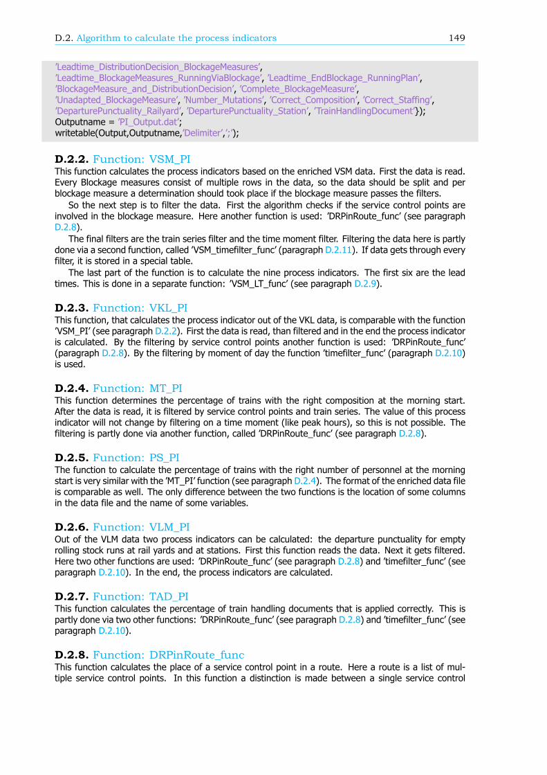
D.2. Algorithm to calculate the process indicators 149

’Leadtime_DistributionDecision_BlockageMeasures’,’Leadtime_BlockageMeasures_RunningViaBlockage’, ’Leadtime_EndBlockage_RunningPlan’,’BlockageMeasure_and_DistributionDecision’, ’Complete_BlockageMeasure’,’Unadapted_BlockageMeasure’, ’Number_Mutations’, ’Correct_Composition’, ’Correct_Staffing’,’DeparturePunctuality_Railyard’, ’DeparturePunctuality_Station’, ’TrainHandlingDocument’});Outputname = ’PI_Output.dat’;writetable(Output,Outputname,’Delimiter’,’;’);

D.2.2. Function: VSM_PIThis function calculates the process indicators based on the enriched VSM data. First the data is read.Every Blockage measures consist of multiple rows in the data, so the data should be split and perblockage measure a determination should took place if the blockage measure passes the filters.

So the next step is to filter the data. First the algorithm checks if the service control points areinvolved in the blockage measure. Here another function is used: ’DRPinRoute_func’ (see paragraphD.2.8).

The final filters are the train series filter and the time moment filter. Filtering the data here is partlydone via a second function, called ’VSM_timefilter_func’ (paragraph D.2.11). If data gets through everyfilter, it is stored in a special table.

The last part of the function is to calculate the nine process indicators. The first six are the leadtimes. This is done in a separate function: ’VSM_LT_func’ (see paragraph D.2.9).

D.2.3. Function: VKL_PIThis function, that calculates the process indicator out of the VKL data, is comparable with the function’VSM_PI’ (see paragraph D.2.2). First the data is read, than filtered and in the end the process indicatoris calculated. By the filtering by service control points another function is used: ’DRPinRoute_func’(paragraph D.2.8). By the filtering by moment of day the function ’timefilter_func’ (paragraph D.2.10)is used.

D.2.4. Function: MT_PIThis function determines the percentage of trains with the right composition at the morning start.After the data is read, it is filtered by service control points and train series. The value of this processindicator will not change by filtering on a time moment (like peak hours), so this is not possible. Thefiltering is partly done via another function, called ’DRPinRoute_func’ (see paragraph D.2.8).

D.2.5. Function: PS_PIThe function to calculate the percentage of trains with the right number of personnel at the morningstart is very similar with the ’MT_PI’ function (see paragraph D.2.4). The format of the enriched data fileis comparable as well. The only difference between the two functions is the location of some columnsin the data file and the name of some variables.

D.2.6. Function: VLM_PIOut of the VLM data two process indicators can be calculated: the departure punctuality for emptyrolling stock runs at rail yards and at stations. First this function reads the data. Next it gets filtered.Here two other functions are used: ’DRPinRoute_func’ (see paragraph D.2.8) and ’timefilter_func’ (seeparagraph D.2.10). In the end, the process indicators are calculated.

D.2.7. Function: TAD_PIThis function calculates the percentage of train handling documents that is applied correctly. This ispartly done via two other functions: ’DRPinRoute_func’ (see paragraph D.2.8) and ’timefilter_func’ (seeparagraph D.2.10).

D.2.8. Function: DRPinRoute_funcThis function calculates the place of a service control point in a route. Here a route is a list of mul-tiple service control points. In this function a distinction is made between a single service control

150 D. Algorithms to calculate process indicators

point as input, and multiple service control points. In the second case, the output is multiple places,corresponding with every service control point.

D.2.9. Function: VSM_LT_funcThis function is used in ’VSM_PI’ (paragraph D.2.2). Here the 90th percentile is calculated for a set oflead times.

D.2.10. Function: timefilter_funcThis function determines if a point in time lies within two time limits. This function is used in ’VKL_PI’(paragraph D.2.3), ’VLM_PI’ (paragraph D.2.6) and ’TAD_PI’ (paragraph D.2.7).

D.2.11. Function: VSM_timefilter_funcThis function is based on the ’timefilter_func’ function (paragraph D.2.10) and made especially for thefunction ’VSM_PI’ D.2.2). In this function a determination takes place to check if a (part of a) timeperiod lies within two time limits.