Embed Size (px)
Citation preview
Master of Science Thesis
Multiphase Pump Performance Assessment
Yu Tang1507915
20-01-2015
Faculty of Aerospace Engineering · Delft University of Technology


Multiphase Pump Performance Assessment
Master of Science Thesis
For obtaining the degree of Master of Science in AerospaceEngineering at Delft University of Technology
Yu Tang
20-01-2015
Faculty of Aerospace Engineering · Delft University of Technology

Copyright c© Yu TangAll rights reserved.
Delft University Of TechnologyDepartment Of
Flight Performance & Propulsion
The undersigned hereby certify that they have read and recommend to the Faculty ofAerospace Engineering for acceptance a thesis entitled “Multiphase Pump Perfor-mance Assessment” by Yu Tang in partial fulfillment of the requirements for thedegree of Master of Science.
Dated: 20-01-2015
University Supervisor:Dr. Arvind Rao
University Supervisor:Dr.Ir. Rene Pecnik
University Supervisor:Dr.Ir. Matteo Pini
Industrial Supervisor:Prof. Ian Bennett

Summary
The Oil and Gas industry has been using cutting edge technologies to increase the produc-tion for decades. For the exact same purpose Shell is planning to deploy two multiphasepumps into the Draugen field, located in the Norwegian Sea. A multiphase pump canincrease the pressure of a mixture of liquid and gas simultaneously. It is very desirable,since the content of an exploitable reservoir is frequently a mixture of oil and gas. Inorder to increase the reliability and efficiency of such pumps, a multiphase performancemodel will used to continuously monitor the pump performance during its operation. Un-fortunately, a multiphase pump performance model has not yet been developed withinShell Global Solutions. The purpose of this thesis is to investigate the key parameterswhich influence the pump performance and using this knowledge to create a multiphaseperformance model.
Based on the literature study carried out to investigate the multiphase pump performancebehaviour, it was found that an one dimensional two phase flow approach is most suitablefor developing a multiphase performance model. This approach has not only incorporatedthe key parameters such as volumetric flow, GVF and fluid density, but also the pumpgeometries such as the rotor diameter. Due to the complexity of the model, several as-sumptions were made to simplify the model. First of all, gas and liquid were assumed tofollow the same streamline. Secondly, the condensation of gas and vaporization of liquidare neglected. Finally, the temperature rise in the fluid is neglected as well (isothermalcondition is used), general speaking this assumption is valid for GVF conditions below60%. By applying Newton’s law of motion to the predefined control volume in the streamdirection, an one dimensional two phase flow governing equation can be derived. Usingconservation of mass, velocity triangles and computational tools like Solver within Mi-crosoft Excel, the governing equation can be solved and the pump performance can becalculated. An additional parameter , the blade angle, is required for the calculation,combining the blade angle with the slip factor, the predicted exit flow angle can be found.Unfortunately, this blade angle is not given by the vendor due to proprietary reasons.As a result, an empirical equation is developed to calculate the exit flow angle by usingdimensional analysis and the experimental data provided by the vendor. For validatingthe overall accuracy and applicability of the model, an additional set of data is required
v
vi Nomenclature
which is provided by the same vendor. This new set of data is generated by vendor’sown multiphase performance model rather from their experiments. The overall accuracyof the model is satisfying, with an maximum error of less than 20%, when the operationconditions are under 40% GVF. This range is sufficient for the purpose of this project,because the expected operation conditions will not exceed this GVF limit.
There are several explanations for the discrepancy of the model. The first one is thatthe discrepancy is caused by the empirical exit flow angle equation. This equation isdeveloped based on a set of experimental data where the maximum GVF is 30%. Theempirical equation is accurate only within that GVF range, for GVF range beyond 30%,the reliability of the model decreases significantly. It has been validated using additionalperformance data provided by the vendor that this empirical equation is applicable up to40% GVF. The second reason is that the separation of gas and liquid has not been takeninto account. The separation of gas and liquid occurs at high GVF conditions where gastends to accumulate on the suction side of the rotor blade. This will reduce the effectivestream area of the fluid, which will increase the fluid relative velocity in the impeller anddecrease the pump performance. The stream area is assumed to be constant for all theoperating conditions, and it is calculated based on the pump geometry. Thirdly, for thesimplicity of the analysis, the same exit flow angle is used for all the rotors. This is onlyvalid for low GVF conditions and near the design conditions. A different exit angle atthe impeller exit will result into a different impeller performance. These are the possiblemain reasons for the discrepancy of the mode.
There are several ways to further improve the model. First of all, to improve the empiricalexit flow angle equation by acquiring more experimental data, especially for the high GVFconditions such as 40% and 60%. It will be ideal if the actual blade angle can be disclosedby the vendor in the future, so the conventional methods can be applied to find the pumpperformance. Secondly, instead of doing an one dimensional analysis, do a two dimensionalmultiphase fluid analysis where the gas movement in the lateral direction (perpendicularto the stream direction) can be captured. This lateral gas movement causes the gasaccumulation at the high GVF conditions. Once the size of the gas pocket is known, theeffective stream area can be calculated. Thirdly, investigating how the exit flow anglechanges after leaving each stage. Finally, instead of using an isothermal assumption, apolytropic assumption can be used during the analysis and this assumption can extendthe GVF range of the model upto 90%. However it does required more gas and liquiddata such as specific heat capacity.
Contents
List of Figures x
List of Tables xi
Nomenclature xiii
1 Introduction 1
2 Introduction To Multiphase Pumps 3
2.1 Multiphase pumps . . . . . . . . . . . . . . . . . . . . . . . . . . . . . . . 3
2.2 Helico-axial multiphase pump . . . . . . . . . . . . . . . . . . . . . . . . . 4
2.3 Primary performance parameters . . . . . . . . . . . . . . . . . . . . . . . 5
2.4 Secondary performance parameters . . . . . . . . . . . . . . . . . . . . . . 6
3 Literature Survey 9
3.1 Centrifugal pumps . . . . . . . . . . . . . . . . . . . . . . . . . . . . . . . 9
3.1.1 Constant Head Device . . . . . . . . . . . . . . . . . . . . . . . . . 10
3.1.2 Pump Theory . . . . . . . . . . . . . . . . . . . . . . . . . . . . . . 10
Velocity Triangle . . . . . . . . . . . . . . . . . . . . . . . . . . . . 10
Impeller Inlet . . . . . . . . . . . . . . . . . . . . . . . . . . . . . . 10
Impeller Outlet . . . . . . . . . . . . . . . . . . . . . . . . . . . . . 11
Euler’s Pump Equation . . . . . . . . . . . . . . . . . . . . . . . . 12
3.1.3 Cavitation . . . . . . . . . . . . . . . . . . . . . . . . . . . . . . . . 13
3.1.4 Blade Angle . . . . . . . . . . . . . . . . . . . . . . . . . . . . . . . 13
3.1.5 Specific Speed . . . . . . . . . . . . . . . . . . . . . . . . . . . . . 14
3.1.6 Suction Specific Speed . . . . . . . . . . . . . . . . . . . . . . . . . 15
3.1.7 Slip . . . . . . . . . . . . . . . . . . . . . . . . . . . . . . . . . . . 15
3.1.8 Affinity Laws . . . . . . . . . . . . . . . . . . . . . . . . . . . . . . 16
vii
viii Contents
3.1.9 Pump Performance Losses . . . . . . . . . . . . . . . . . . . . . . . 17
3.1.10 Single Phase to Multiphase . . . . . . . . . . . . . . . . . . . . . . 18
3.2 Multiphase Pump . . . . . . . . . . . . . . . . . . . . . . . . . . . . . . . . 19
3.2.1 Introduction to Multiphase pump . . . . . . . . . . . . . . . . . . . 19
3.2.2 Existing Methodology description . . . . . . . . . . . . . . . . . . . 19
3.2.3 Empirical correlations based on experiments . . . . . . . . . . . . . 19
Empirical correlation factor . . . . . . . . . . . . . . . . . . . . . . 19
3.2.4 Analytical multiphase model . . . . . . . . . . . . . . . . . . . . . 20
Furuya: One Dimensional Control Volume Method . . . . . . . . . 20
Furuya: An Analytical Model For Prediction Two-Phase Condens-able Flow Case . . . . . . . . . . . . . . . . . . . . . . . . 24
Bratu : Rotodynamic Two-phase Pump Performance . . . . . . . . 25
Minemura: Prediction Of Air-Water Two Phase Flow Performance 26Poullikkas: Compressibility And Condensation Effects . . . . . . . 26
3.2.5 Empirical correlations using non-dimensional parameters . . . . . . 27
Two phase model developed by Sulzer based on the experimentalresults . . . . . . . . . . . . . . . . . . . . . . . . . . . . . 27
3.2.6 Using Computational Fluid Dynamics (CFD) tools . . . . . . . . . 28
3D flow modeling in one helical-axial multiphase pump stage throughCFD . . . . . . . . . . . . . . . . . . . . . . . . . . . . . 28
3.2.7 Comparison of various methods . . . . . . . . . . . . . . . . . . . . 29
4 One Dimensional Two Phase Control Volume Modelling 31
4.1 Fundamental equations for an one dimensional two phase model . . . . . 32
4.2 Using velocity triangles to reduce the unknowns . . . . . . . . . . . . . . . 34
4.3 Density of the mixed fluid at the rotor outlet . . . . . . . . . . . . . . . . 36
4.4 Pressure decrease calculation at pipe inlet . . . . . . . . . . . . . . . . . . 36
4.5 Pressure increase calculation at stator . . . . . . . . . . . . . . . . . . . . 374.6 Model inputs . . . . . . . . . . . . . . . . . . . . . . . . . . . . . . . . . . 38
4.6.1 Inlet conditions . . . . . . . . . . . . . . . . . . . . . . . . . . . . . 384.6.2 Pump geometry . . . . . . . . . . . . . . . . . . . . . . . . . . . . . 38
Rotor geometry . . . . . . . . . . . . . . . . . . . . . . . . . . . . . 38
Exit flow angle . . . . . . . . . . . . . . . . . . . . . . . . . . . . . 39
4.7 Pump pressure increase calculation flow diagram . . . . . . . . . . . . . . 40
4.7.1 General layout . . . . . . . . . . . . . . . . . . . . . . . . . . . . . 41
4.7.2 Rotor pressure increase calculation . . . . . . . . . . . . . . . . . . 41
4.8 Validation . . . . . . . . . . . . . . . . . . . . . . . . . . . . . . . . . . . . 414.8.1 Validation against the experimental results . . . . . . . . . . . . . 41
4.8.2 Finding the optimal exit flow angle for every operating condition . 44
4.8.3 Validation against the performance curves generated by the ven-dor’s tool . . . . . . . . . . . . . . . . . . . . . . . . . . . . . . . . 49
4.9 Stage by stage results . . . . . . . . . . . . . . . . . . . . . . . . . . . . . 52
5 Conclusion 55
References 57
List of Figures
2.1 Multiphase pump categorization . . . . . . . . . . . . . . . . . . . . . . . 3
2.2 Single compression stage of a helico-axial multiphase pump [1] . . . . . . 4
2.3 Sulzer multiphase pump [2] . . . . . . . . . . . . . . . . . . . . . . . . . . 4
2.4 A general Framo MPP performance map for a low GVF [3] . . . . . . . . 5
2.5 A general Framo MPP performance map for a high GVF [3] . . . . . . . . 6
3.1 Velocity Triangle [4] . . . . . . . . . . . . . . . . . . . . . . . . . . . . . . 11
3.2 Pump performance curves for different blade angles [5] . . . . . . . . . . . 14
3.3 Slip Velocity diagram [6] . . . . . . . . . . . . . . . . . . . . . . . . . . . . 16
3.4 Affinity Laws [7] . . . . . . . . . . . . . . . . . . . . . . . . . . . . . . . . 17
3.5 Control volume for one dimensional control volume method [8] . . . . . . 20
3.6 Force Diagram . . . . . . . . . . . . . . . . . . . . . . . . . . . . . . . . . 21
3.7 Geometry Diagram [8] . . . . . . . . . . . . . . . . . . . . . . . . . . . . . 21
3.8 Velocity Triangle[8] . . . . . . . . . . . . . . . . . . . . . . . . . . . . . . . 23
4.1 8 stage helico axial multiphase pump [24] . . . . . . . . . . . . . . . . . . 31
4.2 Control Volume . . . . . . . . . . . . . . . . . . . . . . . . . . . . . . . . 32
4.3 Force Diagram . . . . . . . . . . . . . . . . . . . . . . . . . . . . . . . . . 33
4.4 Velocity Triangles . . . . . . . . . . . . . . . . . . . . . . . . . . . . . . . . 34
4.5 Typical MPP cross section [9] . . . . . . . . . . . . . . . . . . . . . . . . . 36
4.6 Flow diagram . . . . . . . . . . . . . . . . . . . . . . . . . . . . . . . . . . 40
4.7 Pressure increase versus volumetric flow rate for 0% GVF . . . . . . . . . 42
4.8 Pressure increase versus volumetric flow rate for 15% GVF . . . . . . . . 42
4.9 Pressure increase versus volumetric flow rate for 30% GVF . . . . . . . . 43
4.10 Flow coefficient vs Exit flow angle . . . . . . . . . . . . . . . . . . . . . . 46
ix
x List of Figures
4.11 Flow coefficient vs Exit flow angle . . . . . . . . . . . . . . . . . . . . . . 47
4.12 Flow diagram . . . . . . . . . . . . . . . . . . . . . . . . . . . . . . . . . . 48
4.13 Pressure increase versus volumetric flow rate for 10% GVF . . . . . . . . 49
4.14 Pressure increase versus volumetric flow rate for 30% GVF . . . . . . . . 50
4.15 Pressure increase versus volumetric flow rate for 40% GVF . . . . . . . . 50
4.16 Pressure increase versus volumetric flow rate for 60% GVF . . . . . . . . 51
4.17 Pressure versus stage . . . . . . . . . . . . . . . . . . . . . . . . . . . . . 53
4.18 Pressure versus stage . . . . . . . . . . . . . . . . . . . . . . . . . . . . . 53
List of Tables
4.1 Estimated pump geometry based on the literature study . . . . . . . . . . 38
4.2 GVF 0%, liquid Density 998 kgm3 and Gas Density 20 kg
m3 . . . . . . . . . . 44
4.3 GVF 15%, liquid Density 998 kgm3 and Gas Density 14,3 kg
m3 . . . . . . . . . 45
4.4 GVF 30%, liquid Density 998 kgm3 and Gas Density 14,3 kg
m3 . . . . . . . . . 45
xi

xii List of Tables
Nomenclature
Latin Symbols
A Cross-section Area m2
b Width of the impeller m
C Absolute Velocity m/s
Cd Drag Coefficient −D Diameter m
f Force Newton
g Gravity of Earth m/s2
H Head m
m Mass kg
m Mass Flow kg/s
M Empirical correction factor for multiphase −n Rotational Speed rpm
n coordinate normal to the streamline coordinate length
Ns Specific Speed −P Power Coefficient −Ps Shaft Power watt
Q Flow Rate m3/h
R Gas constant Jmol·K
r Radius of the impeller m
S Suction Specific Speed −s streamline coordinate length
xiii
xiv Nomenclature
T Temperature K
T Torque Nm
t Time s
p Static Pressure Pa
U Tangential Velocity m/s
u Internal Energy watt
V Absolute Velocity m/s
v Velocity m/s
W Relative Velocity m/s
x Mass Fraction = Mass Gas / Mass Liquid −Z Height m
Greek Symbols
α Gas volume fraction −β′ Geometry Angle degree
β Blade Angle degree
β′ Exit flow angle degree
Γ Condensation Rate kg/s
γ Geometry Angle degree
ζ Work Coefficient −η Efficiency −ρ Density kg/m3
σ Slip Factor −φ Flow Coefficient −ψ Pressure Coefficient −ω Angular Speed rad/s
Subscripts
1 Inlet of the impeller
2 Outlet of the impeller
α void Fraction
b gas bubble
g gas
hyd Hydraulic
in Inlet of the pump

Nomenclature xv
isot isothermal
l liquid
mech Mechanical
mp Multiphase
m radial component of the absolute velocity
out Outlet of the pump
sl slip
sp Single Phase
st stage
s Shaft
tp Two Phase
T Total
u Tangential component of the absolute velocity
vol Volumetric
w Relative Velocity
w whirl velocity component

xvi Nomenclature
Chapter 1
Introduction
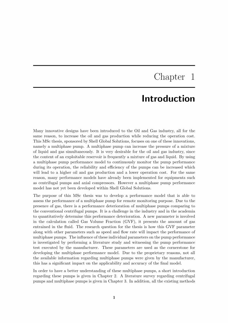
Many innovative designs have been introduced to the Oil and Gas industry, all for thesame reason, to increase the oil and gas production while reducing the operation cost.This MSc thesis, sponsored by Shell Global Solutions, focuses on one of these innovations,namely a multiphase pump. A multiphase pump can increase the pressure of a mixtureof liquid and gas simultaneously. It is very desirable for the oil and gas industry, sincethe content of an exploitable reservoir is frequently a mixture of gas and liquid. By usinga multiphase pump performance model to continuously monitor the pump performanceduring its operation, the reliability and efficiency of the pumps can be increased whichwill lead to a higher oil and gas production and a lower operation cost. For the samereason, many performance models have already been implemented for equipments suchas centrifugal pumps and axial compressors. However a multiphase pump performancemodel has not yet been developed within Shell Global Solutions.
The purpose of this MSc thesis was to develop a performance model that is able toassess the performance of a multiphase pump for remote monitoring purpose. Due to thepresence of gas, there is a performance deterioration of multiphase pumps comparing tothe conventional centrifugal pumps. It is a challenge in the industry and in the academiato quantitatively determine this performance deterioration. A new parameter is involvedin the calculation called Gas Volume Fraction (GVF), it presents the amount of gasentrained in the fluid. The research question for the thesis is how this GVF parameteralong with other parameters such as speed and flow rate will impact the performance ofmultiphase pumps. The influence of these individual parameters on the pump performanceis investigated by performing a literature study and witnessing the pump performancetest executed by the manufacturer. These parameters are used as the cornerstone fordeveloping the multiphase performance model. Due to the proprietary reasons, not allthe available information regarding multiphase pumps were given by the manufacturer,this has a significant impact on the applicability and accuracy of the final model.
In order to have a better understanding of these multiphase pumps, a short introductionregarding these pumps is given in Chapter 2. A literature survey regarding centrifugalpumps and multiphase pumps is given in Chapter 3. In addition, all the existing methods
1

2 Introduction
used to develop a multiphase pump performance model are elaborated in the same chapter.Using the knowledge obtained from the literature survey, a multiphase pump performancemodel is developed and validated using the performance data provided by the vendor inChapter 4. The final conclusion is given in Chapter 5.
Chapter 2
Introduction To Multiphase Pumps
2.1 Multiphase pumps
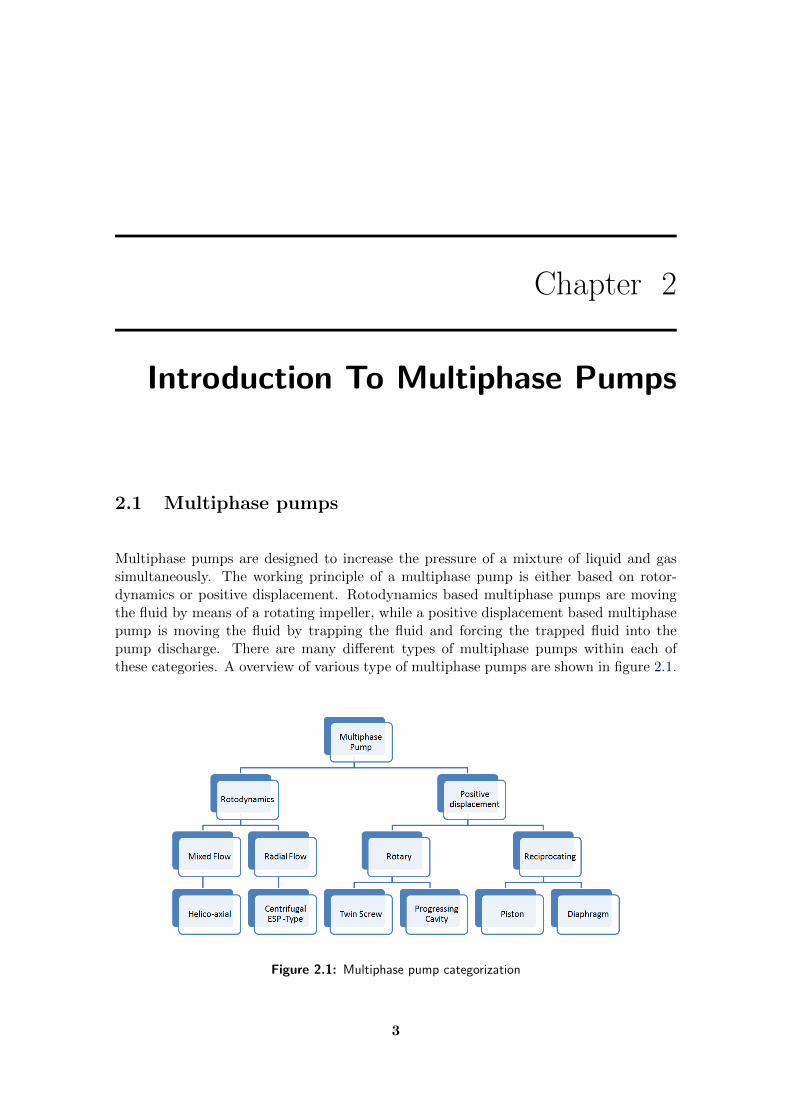
Multiphase pumps are designed to increase the pressure of a mixture of liquid and gassimultaneously. The working principle of a multiphase pump is either based on rotor-dynamics or positive displacement. Rotodynamics based multiphase pumps are movingthe fluid by means of a rotating impeller, while a positive displacement based multiphasepump is moving the fluid by trapping the fluid and forcing the trapped fluid into thepump discharge. There are many different types of multiphase pumps within each ofthese categories. A overview of various type of multiphase pumps are shown in figure 2.1.
Figure 2.1: Multiphase pump categorization
3
4 Introduction To Multiphase Pumps
2.2 Helico-axial multiphase pump
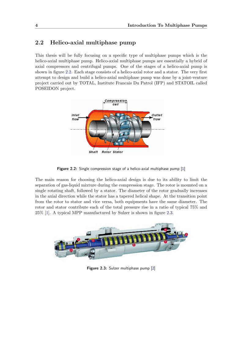
This thesis will be fully focusing on a specific type of multiphase pumps which is thehelico-axial multiphase pump. Helico-axial multiphase pumps are essentially a hybrid ofaxial compressors and centrifugal pumps. One of the stages of a helico-axial pump isshown in figure 2.2. Each stage consists of a helico-axial rotor and a stator. The very firstattempt to design and build a helico-axial multiphase pump was done by a joint-ventureproject carried out by TOTAL, Institute Francais Du Patrol (IFP) and STATOIL calledPOSEIDON project.
Figure 2.2: Single compression stage of a helico-axial multiphase pump [1]
The main reason for choosing the helico-axial design is due to its ability to limit theseparation of gas-liquid mixture during the compression stage. The rotor is mounted on asingle rotating shaft, followed by a stator. The diameter of the rotor gradually increasesin the axial direction while the stator has a tapered helical shape. At the transition pointfrom the rotor to stator and vice versa, both equipments have the same diameter. Therotor and stator contribute each of the total pressure rise in a ratio of typical 75% and25% [1]. A typical MPP manufactured by Sulzer is shown in figure 2.3.
Figure 2.3: Sulzer multiphase pump [2]
2.3 Primary performance parameters 5
2.3 Primary performance parameters
There are several key parameters and several secondary parameters which influence thepump performance. Primary parameters have the largest impact on the pump perfor-mance. These primary parameters are
• Gas Volume Fraction (GVF)
• Volumetric flow rate
• Rotational speed
• Liquid to gas density ratio
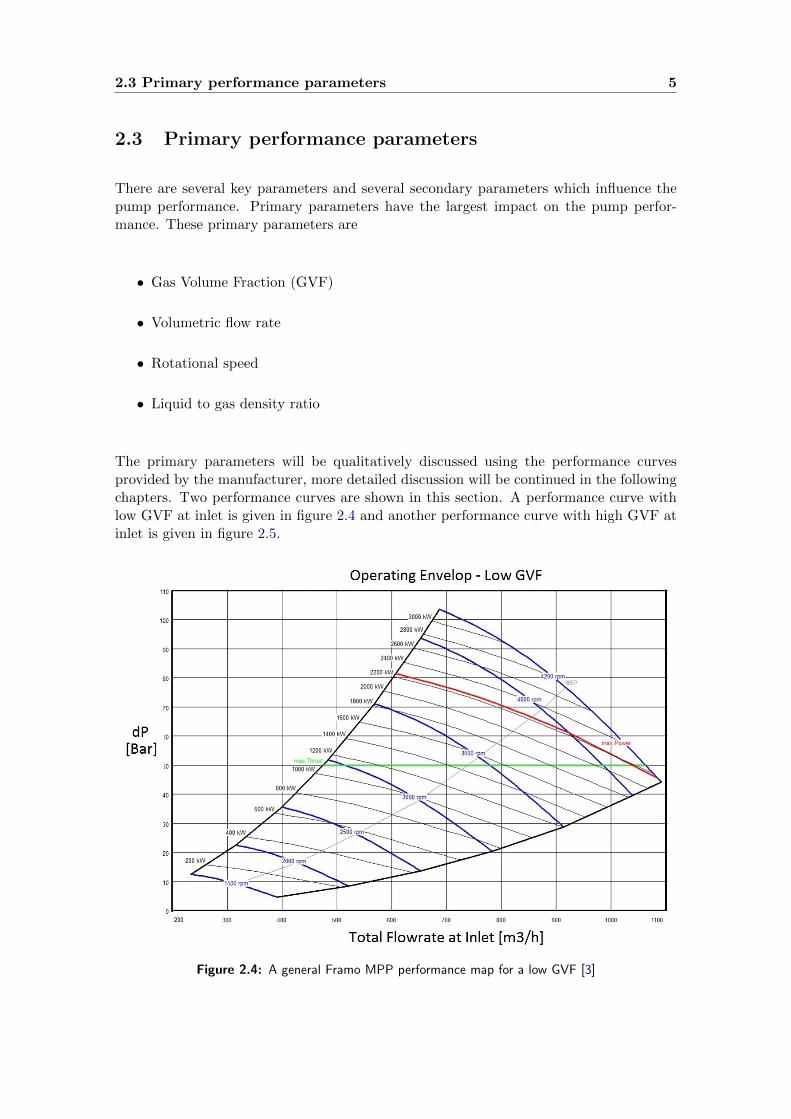
The primary parameters will be qualitatively discussed using the performance curvesprovided by the manufacturer, more detailed discussion will be continued in the followingchapters. Two performance curves are shown in this section. A performance curve withlow GVF at inlet is given in figure 2.4 and another performance curve with high GVF atinlet is given in figure 2.5.
Figure 2.4: A general Framo MPP performance map for a low GVF [3]
6 Introduction To Multiphase Pumps
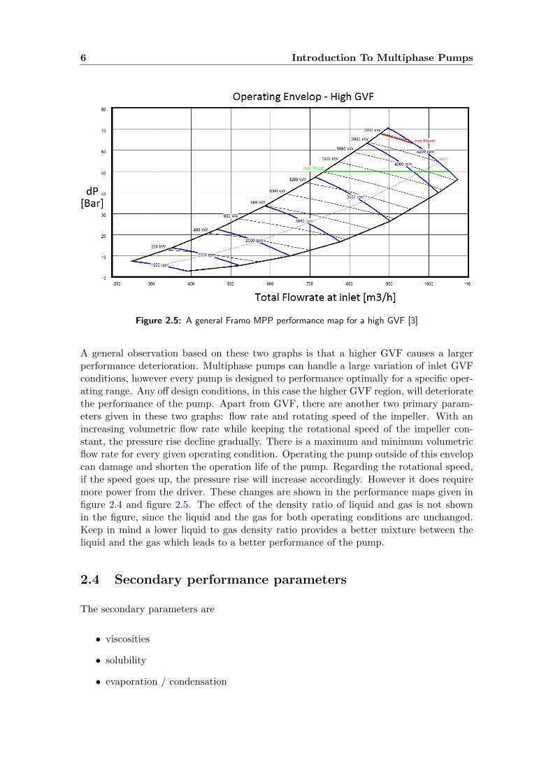
Figure 2.5: A general Framo MPP performance map for a high GVF [3]
A general observation based on these two graphs is that a higher GVF causes a largerperformance deterioration. Multiphase pumps can handle a large variation of inlet GVFconditions, however every pump is designed to performance optimally for a specific oper-ating range. Any off design conditions, in this case the higher GVF region, will deterioratethe performance of the pump. Apart from GVF, there are another two primary param-eters given in these two graphs: flow rate and rotating speed of the impeller. With anincreasing volumetric flow rate while keeping the rotational speed of the impeller con-stant, the pressure rise decline gradually. There is a maximum and minimum volumetricflow rate for every given operating condition. Operating the pump outside of this envelopcan damage and shorten the operation life of the pump. Regarding the rotational speed,if the speed goes up, the pressure rise will increase accordingly. However it does requiremore power from the driver. These changes are shown in the performance maps given infigure 2.4 and figure 2.5. The effect of the density ratio of liquid and gas is not shownin the figure, since the liquid and the gas for both operating conditions are unchanged.Keep in mind a lower liquid to gas density ratio provides a better mixture between theliquid and the gas which leads to a better performance of the pump.
2.4 Secondary performance parameters
The secondary parameters are
• viscosities
• solubility
• evaporation / condensation
2.4 Secondary performance parameters 7
The secondary parameters can not be actively controlled, they are dependant on thegas and liquid characteristics. Higher viscosities will result into higher deterioration.On the other side, having a higher viscosity helps to stabilize the bubble, however thedeterioration from higher viscosity still dominates. Higher solubility means more gascan be solved into the liquid, that decreases the GVF, hence improves the performance.Evaporation of gas will increase the GVF, condensation will decrease the GVF, both canhave either positive or negative effect on the pump performance. For the scope of thisthesis, these secondary parameters will be assumed to be constant.
Before we dive into the multiphase performance modelling, a literature survey is per-formed. The literature survey mainly focusses on two parts: the performance assessmentof conventional single liquid phase centrifugal pumps and the existing methods used toassess and predict the performance of helico-axial multiphase pumps.

8 Introduction To Multiphase Pumps
Chapter 3
Literature Survey
The knowledge obtained from literature regarding the centrifugal pumps and the multi-phase pumps are elaborated in this chapter. The findings regarding the centrifugal pumpswill be explained in section 3.1. In section 3.2, the focus will be shifted to multiphasepumps.
3.1 Centrifugal pumps
Centrifugal pumps are widely used all around the globe. The working principle of acentrifugal pump is as follow: angular momentum is created as the fluid is subjectedto centrifugal forces through an impeller, the momentum is then converted into pressurewhen fluid is slowed down and redirected through a stationary diffuser. The energy trans-fer equation for the pumps can be established through the first law of thermodynamics.Assuming the system is working at 100 % efficiency, the amount of mechanical energyput into the system through the shaft should be equal to the increase of hydraulic energy.Fluid flow through a centrifugal pump is essentially adiabatic and can be assumed to besteady across the boundaries of the control volume [7]. The pump equation derived fromthe first law of thermodynamics is shown below:
Ps = m
[(u+
p
ρ+V 2
2+ gZ
)out
−(u+
p
ρ+V 2
2+ gZ
)in
](3.1)
Where m is the mass flow, Ps is the shaft power, u+ pρ is the enthalpy and V 2
2 + gZdenote for kinetic and potential energy respectively. Unfortunately equation 3.1 is onlyvalid in the ideal world, since not all the mechanical energy is transferred into liquid due tomechanical and hydraulic losses. In addition, a small part of the energy ends up increasingthe internal energy of the fluid rather than being used for increasing the pressure. The
9
10 Literature Survey
overall efficiency of the pump is given in equation [3.1] and it can be decomposed intothree parts: mechanical efficiency, hydraulic efficiency and volumetric efficiency.
η =m[(
pρ + V 2
2 + gZ)out−(pρ + V 2
2 + gZ)in
]Ps
= ηmech · ηhyd · ηvol (3.2)
3.1.1 Constant Head Device
A centrifugal pump transforms mechanical energy from a rotating impeller into hydraulicenergy. The amount of mechanical energy used per kilo mass fluid is independent of thefluid itself. Therefore, the head generated by a given pump at certain speed and capacitywill remain constant for all fluids [7]. For instance, a heavier liquid would require moremechanical energy, however the head will be the same as for a light weight liquid. Due tothis phenomenon, a centrifugal pump is also called as a constant head device.
3.1.2 Pump Theory
In order to have a better understanding of the energy conversion process in a centrifugalpump, simple models such as velocity triangle are used to predict the pump performancefor various speed changes and impeller diameters.
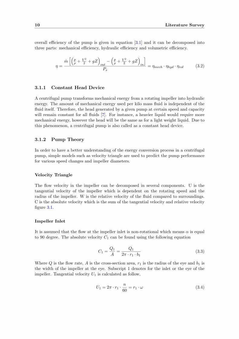
Velocity Triangle
The flow velocity in the impeller can be decomposed in several components. U is thetangential velocity of the impeller which is dependent on the rotating speed and theradius of the impeller. W is the relative velocity of the fluid compared to surroundings.C is the absolute velocity which is the sum of the tangential velocity and relative velocityfigure 3.1.
Impeller Inlet
It is assumed that the flow at the impeller inlet is non-rotational which means α is equalto 90 degree. The absolute velocity C1 can be found using the following equation
C1 =Q1
A=
Q1
2π · r1 · b1(3.3)
Where Q is the flow rate, A is the cross-section area, r1 is the radius of the eye and b1 isthe width of the impeller at the eye. Subscript 1 denotes for the inlet or the eye of theimpeller. Tangential velocity U1 is calculated as follow,
U1 = 2π · r1 ·n
60= r1 · ω (3.4)
3.1 Centrifugal pumps 11
Figure 3.1: Velocity Triangle [4]
Where n is the rotational speed of the impeller and ω is the angular speed of the impeller.Once U and C are found, the corresponding W can be calculated using Pythagoras theo-rem.
Impeller Outlet
The method used to calculate the inlet velocities can be used to calculate the the outletvelocities as well using a similar velocity triangle, see figure 3.1. The equations derivedfrom the velocity triangle are shown below
C2m =Q2
A2=
Q2
2π · r2 · b2(3.5)

12 Literature Survey
U2 = 2π · r2 ·n
60= r2 · ω (3.6)
Where subscripts m and 2 denote for the radial component of the absolute velocity andthe outlet of the impeller respectively. Assuming flow angle is the same as the blade angleβ2 . Based on that assumption, the relative velocity W and tangential velocity U at theoutlet can be calculated as follow.
W2 =C2m
sinβ2(3.7)
C2u = U2 −C2m
tanβ2(3.8)
Where subscript u denote for tangential component of the absolute velocity.
Euler’s Pump Equation
The Eulers pump equation is one of the most important equations in the pump design.The derivation is shown in this section. In order to derive Eulers pump equation, equationfor shaft power needs to be derived first. The derivation for the shaft power Ps is shownbelow [4],
Ps = T · ω = [m (r2 · C2u − r1 · C1u)] · ωPs = m (U2 · C2u − U1 · C1u)
(3.9)
Where T is the torque. Hydraulic power is equal to the pressure increase across theimpeller multiplied by the flow, so it can be rewritten as function of Head,
Phyd = ∆ptot ·Q = H · ρ · g ·Q (3.10)
Assuming the system is loss free, which means the mechanical power used should be thesame as the gained hydraulic power. Combining the equation 3.9 and 3.10, the Eulerequation can be derived as,
Ps = Phyd (3.11)
m (U2 · C2u − U1 · C1u) = H · ρ · g ·Q (3.12)
H =U2 · C2u − U1 · C1u
g(3.13)

3.1 Centrifugal pumps 13
Assuming there is no inlet rotation, C1u is 0, combining equation 3.5, 3.8 and 3.13 , thefinal equation becomes
H =U2 · C2u
g=U22
g− U2
π · 2r2 · b2 · g · tan(β2)·Q (3.14)
3.1.3 Cavitation
Cavitation is defined as flashing of liquid, it happens when the pressure in the suctiondrops below the vapor pressure of the pumping liquid. Cavitation can erode the pumpimpeller resulting in decrease of performance and higher vibration in the entire pump.The amount of energy can be utilized to suck the liquid into the pump is called the suctionhead. However to avoid the cavitation, the pressure at the inlet of the pump can not belower than the vapor head of the liquid. The available head is the suction head subtractsthe vapor head, which is called Net Positive Suction Head Available (NPSHA). For thesafety reasons the manufacturers added a safety margin to this NPSHA which is calledthe Net Positive Suction Head Required (NPSHR). NPSHA should always be larger thanNPSHR, otherwise cavitations will occur. There are several ways to increase the NPSHA[4]:
• subcool the liquid, that decreases the vapor head of the liquid
• use a booster pump, that increases the suction head
3.1.4 Blade Angle
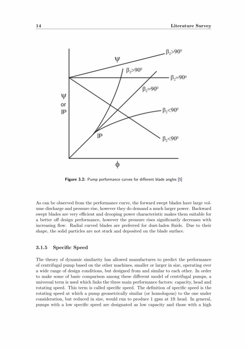
Depending on the blade angle, the impeller is divided into three subgroups, forward-sweptimpellers where the outlet angle β2 is larger than 90 degree, back-swept impellers wherethe outlet angle is smaller than 90 degree and radial impeller where the outlet angleis equal to 90 degree. In the forward-swept impeller, the blade curvature and the flowrotation are in the same direction, whereas in the back-swept impellers those are in theopposite direction. The differences between the back and forward swept blades in termsof the performance of the pump can explained using the figure 3.2
Non-dimensionalized parameters are used in the figure, ψ is the pressure coefficient, Pis the power coefficient and φ is the flow coefficient. These coefficients are calculated asfollow
ψ =∆P12ρU
22
(3.15)
φ =4Q
πD22U2
(3.16)
P = ψ · φ (3.17)
14 Literature Survey
Figure 3.2: Pump performance curves for different blade angles [5]
As can be observed from the performance curve, the forward swept blades have large vol-ume discharge and pressure rise, however they do demand a much larger power. Backwardswept blades are very efficient and drooping power characteristic makes them suitable fora better off design performance, however the pressure rises significantly decreases withincreasing flow. Radial curved blades are preferred for dust-laden fluids. Due to theirshape, the solid particles are not stuck and deposited on the blade surface.
3.1.5 Specific Speed
The theory of dynamic similarity has allowed manufactures to predict the performanceof centrifugal pump based on the other machines, smaller or larger in size, operating overa wide range of design conditions, but designed from and similar to each other. In orderto make some of basic comparison among these different model of centrifugal pumps, auniversal term is used which links the three main performance factors: capacity, head androtating speed. This term is called specific speed. The definition of specific speed is therotating speed at which a pump geometrically similar (or homologous) to the one underconsideration, but reduced in size, would run to produce 1 gpm at 1ft head. In general,pumps with a low specific speed are designated as low capacity and those with a high
3.1 Centrifugal pumps 15
specific speed are termed as high capacity. The specific speed is expressed as follow:
Ns =n√Q
(gH)3/4(3.18)
3.1.6 Suction Specific Speed
One big short coming of using specific speed is the fact that suction conditions were tieddirectly to the total head caused by the pump. A reduction in head by reducing theimpeller diameter will result in a proportional reduction in the net positive suction head[7]. Therefore, a new term called suction specific speed is used to identify the cavitationcharacteristics of the system. Suction specific speed is defined as the rotation speed atwhich a pump geometrically similar to the one under consideration, but reduced in size,would produce 1 gpm at 1 ft required NPSH. Unlike specific speed, suction specific speedis a criterion of a pump’s performance with regard to cavitation. The higher the number,the better the system is resisted against cavitation. The Equation for suction specificspeed is
S =n√Q
NPSHR3/4(3.19)
3.1.7 Slip
In the ideal world, the flow will exit the impeller with the exact same angle as the bladeangle. However in the real world that is not the case. The deviation of the flow exit angleand the blade angle is called slip. The exact cause of the slip within an impeller is notknown. However some general reasons can be given to the occurrence of this phenomenon[10]
• Flow circulation due to pressure gradient
• Boundary-layer development
• Leakage
• Number of vanes
Due the shape of the impeller blade, there will be a pressure difference between thetop side of the blade and the lower side of the blade, just like an airfoil. When youlook at an impeller passage enclosed by two adjacent blades, the flow is surrounded byhigh pressure on one side and low pressure on the other side. That causes a circulationmovement of the flow within the blade passage. As a result of this circulation, there willbe a velocity gradient at the impeller exit which has an impact on the flow exit angle.Due to boundary-layer development within the impeller passage, the exit area becomes
16 Literature Survey
smaller, the relative velocity of fluid has to increase if the mass flow is constant. Thisrelative velocity increase will impact the flow exit angle as well. Leakage is defined as themovement of the fluid from one side of the blade to the other side of the blade. It reducesthe energy transfer from the impeller to fluid which leads to a lower velocity increase.Finally, the number of blades can influence the magnitude of slip as well. The bladeloading is inversely proportional to the number of blades. Fluid closely follows the bladewhen the blade loading is small.
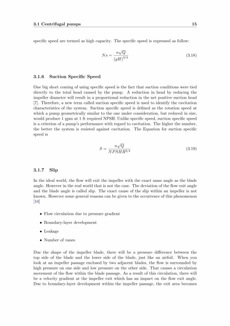
Many scientists have tried to predict the slip using a parameters called slip factor. Theslip factor σ is defined as the ratio of the actual and ideal values of the whirl velocitycomponents at the exit. The ideal whirl velocity components vw2 and the actual whirlvelocity component v′w2 are shown in figure 3.3.
Figure 3.3: Slip Velocity diagram [6]
σ =vw2v′w2
(3.20)
3.1.8 Affinity Laws
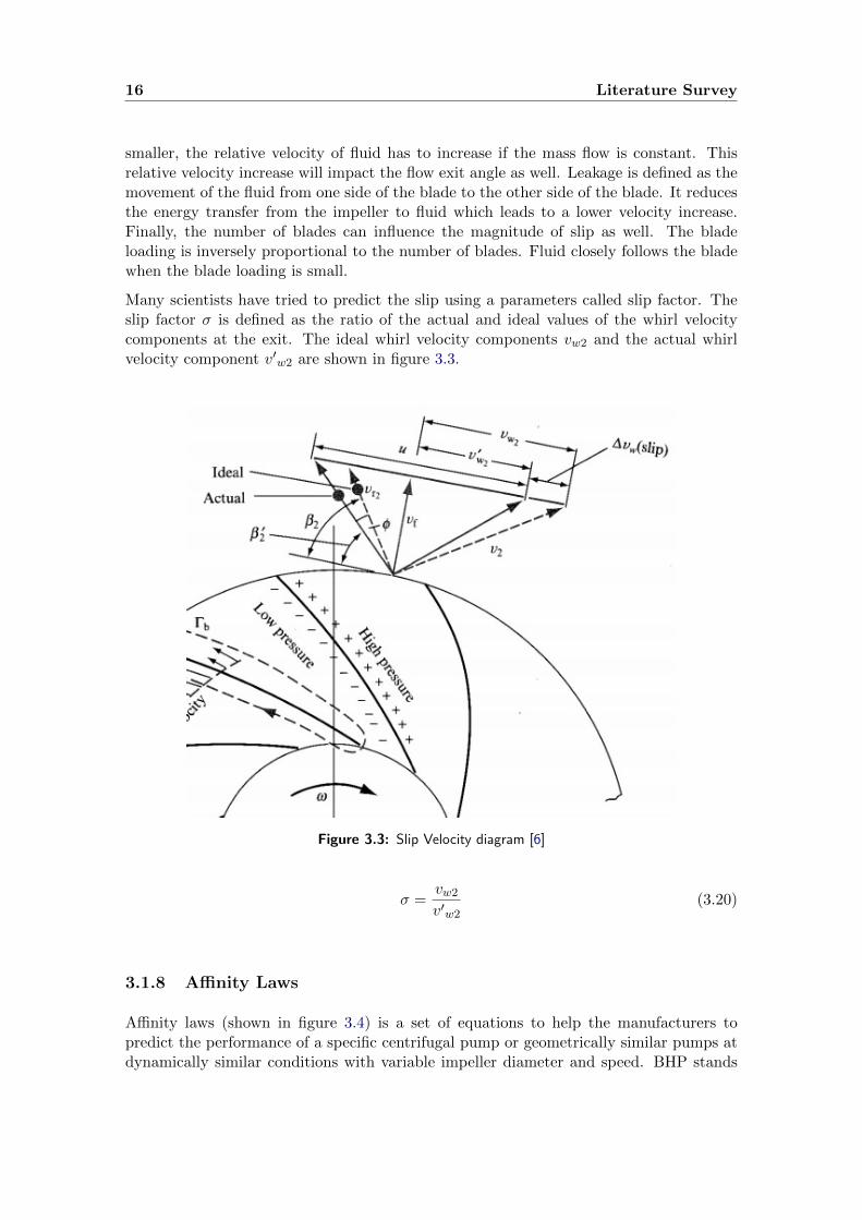
Affinity laws (shown in figure 3.4) is a set of equations to help the manufacturers topredict the performance of a specific centrifugal pump or geometrically similar pumps atdynamically similar conditions with variable impeller diameter and speed. BHP stands
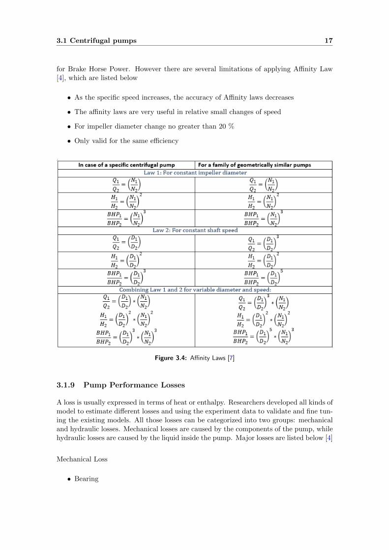
3.1 Centrifugal pumps 17
for Brake Horse Power. However there are several limitations of applying Affinity Law[4], which are listed below
• As the specific speed increases, the accuracy of Affinity laws decreases
• The affinity laws are very useful in relative small changes of speed
• For impeller diameter change no greater than 20 %
• Only valid for the same efficiency
Figure 3.4: Affinity Laws [7]
3.1.9 Pump Performance Losses
A loss is usually expressed in terms of heat or enthalpy. Researchers developed all kinds ofmodel to estimate different losses and using the experiment data to validate and fine tun-ing the existing models. All those losses can be categorized into two groups: mechanicaland hydraulic losses. Mechanical losses are caused by the components of the pump, whilehydraulic losses are caused by the liquid inside the pump. Major losses are listed below [4]
Mechanical Loss
• Bearing
18 Literature Survey
• Shaft Seal
Bearing and shaft seal losses, also called parasitic losses - are caused by friction. They areoften modelled as a constant which is added to the power consumption. The magnitudeof the loss varies with pressure and rotational speed.
Hydraulic Loss
• Flow friction
• Mixing loss
• Recirculation
• Incidence loss
• Disk Friction
• Leakage
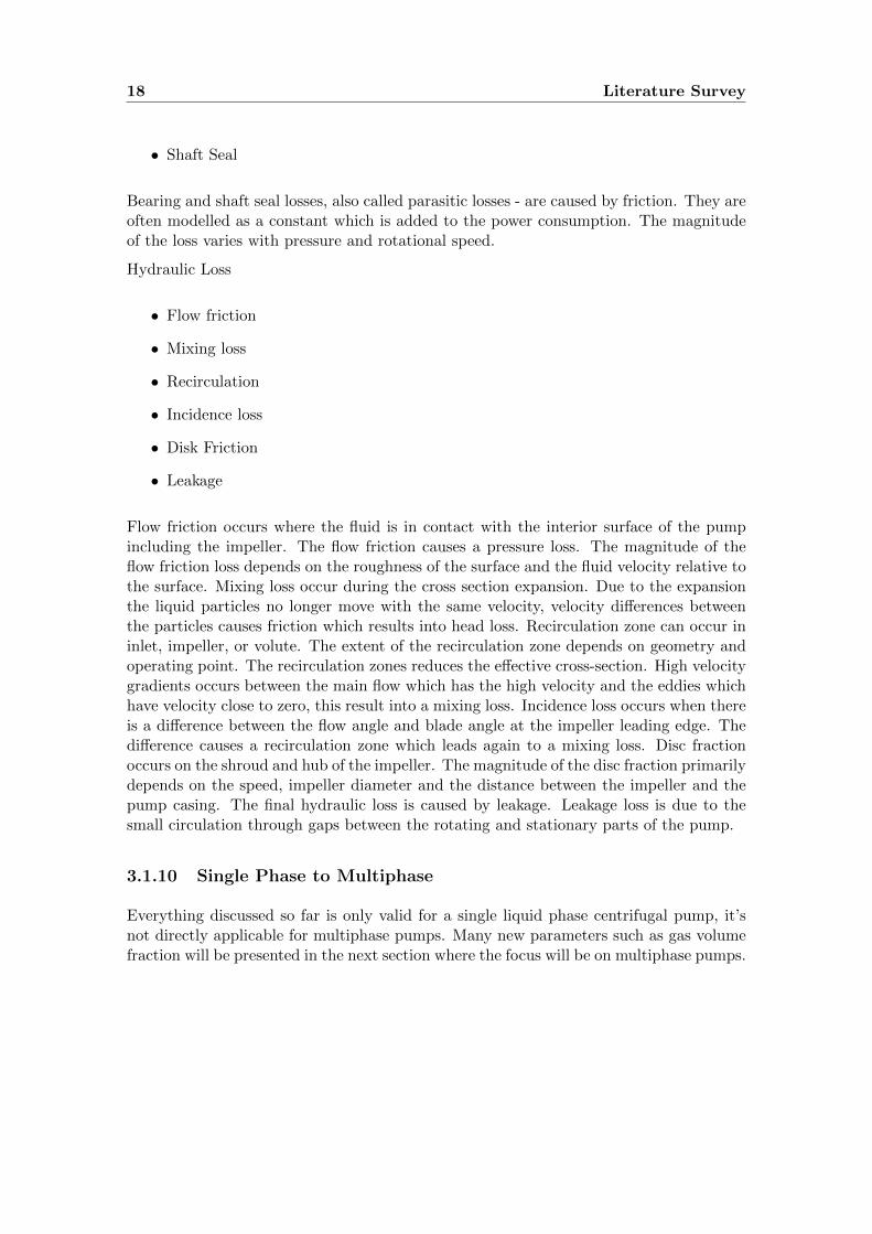
Flow friction occurs where the fluid is in contact with the interior surface of the pumpincluding the impeller. The flow friction causes a pressure loss. The magnitude of theflow friction loss depends on the roughness of the surface and the fluid velocity relative tothe surface. Mixing loss occur during the cross section expansion. Due to the expansionthe liquid particles no longer move with the same velocity, velocity differences betweenthe particles causes friction which results into head loss. Recirculation zone can occur ininlet, impeller, or volute. The extent of the recirculation zone depends on geometry andoperating point. The recirculation zones reduces the effective cross-section. High velocitygradients occurs between the main flow which has the high velocity and the eddies whichhave velocity close to zero, this result into a mixing loss. Incidence loss occurs when thereis a difference between the flow angle and blade angle at the impeller leading edge. Thedifference causes a recirculation zone which leads again to a mixing loss. Disc fractionoccurs on the shroud and hub of the impeller. The magnitude of the disc fraction primarilydepends on the speed, impeller diameter and the distance between the impeller and thepump casing. The final hydraulic loss is caused by leakage. Leakage loss is due to thesmall circulation through gaps between the rotating and stationary parts of the pump.
3.1.10 Single Phase to Multiphase
Everything discussed so far is only valid for a single liquid phase centrifugal pump, it’snot directly applicable for multiphase pumps. Many new parameters such as gas volumefraction will be presented in the next section where the focus will be on multiphase pumps.

3.2 Multiphase Pump 19
3.2 Multiphase Pump
3.2.1 Introduction to Multiphase pump
To develop an analytical multiphase performance model, the gas-liquid interaction oc-curring within the impeller must be identified and quantified. The gas bubble movingin the impeller is acted on by a number of forces: pressure gradient, centrifugal forcesand viscous drag between the gas bubble and surrounding fluid. The sum of these forcescause the gas bubble to accelerate or decelerate in the direction of the main flow andthe direction perpendicular to the main flow. That will result into a velocity differencebetween the gas and liquid in the fluid, and the velocity difference destroys the homo-geneity of the fluid and it causes gas accumulation in the impeller. It is the extent ofthis non homogeneity causes the performance deterioration. Assuming that the gas andliquid moving with the same speed within the impeller, the two phase performance willbe the same as the single phase. That can occur for the relative low GVF conditions. Forhigh GVF conditions, the performance drops off very fast. The flow regime changes withchanging GVF, low GVF conditions corresponds with bubbly flow where gas is equallydistributed in the flow. For the high GVF conditions, separated or slugged flow are morecommon where separation of gas and liquid has taken place. This results into a reductionof effective flow area due to the gas accumulation in the impeller channel. That willincrease the relative flow velocity, and deteriorate the pump performance. [11].
3.2.2 Existing Methodology description
The methodologies that have made a significant contribution to a better understandingof multiphase pumps will be elaborated. All the methodologies that have been developedso far can be sorted into 4 categories. These are
1. Empirical correlations based on experiments
2. Analytical multiphase model
3. Empirical correlations using non-dimensional parameters
4. Using Computational Fluid Dynamics (CFD) tools
3.2.3 Empirical correlations based on experiments
Empirical correlation factor
Babcock and Wilcox developed an empirical correlation factor to approximate the twophase pump performance in 1977 [11]. This empirical correlation factor is a function ofGas Volume Fraction (GVF), and is based purely on the experimental results. The simpleequation to estimate the pump head for two phase flow:
Hmp = Hsp ·M (α) (3.21)
20 Literature Survey
Where M is the correlation factor, α is the gas volume fraction and subscripts sp and mpdenote for single and multiphase. Unfortunately the accuracy and the range where thismethod can be applied are very limited.
3.2.4 Analytical multiphase model
Furuya: One Dimensional Control Volume Method
In 1985 Furuya developed an analytical model based on one dimensional control volumemethod for determining the performance of two-phase flow pumps [8]. This analyticalmethod has incorporated pump geometry, void fraction and flow slippage, but ignoredthe compressibility and condensation effects. The purpose of this model was to give theindustry a better understanding of basic mechanism of pump head degradation in twophase flow.
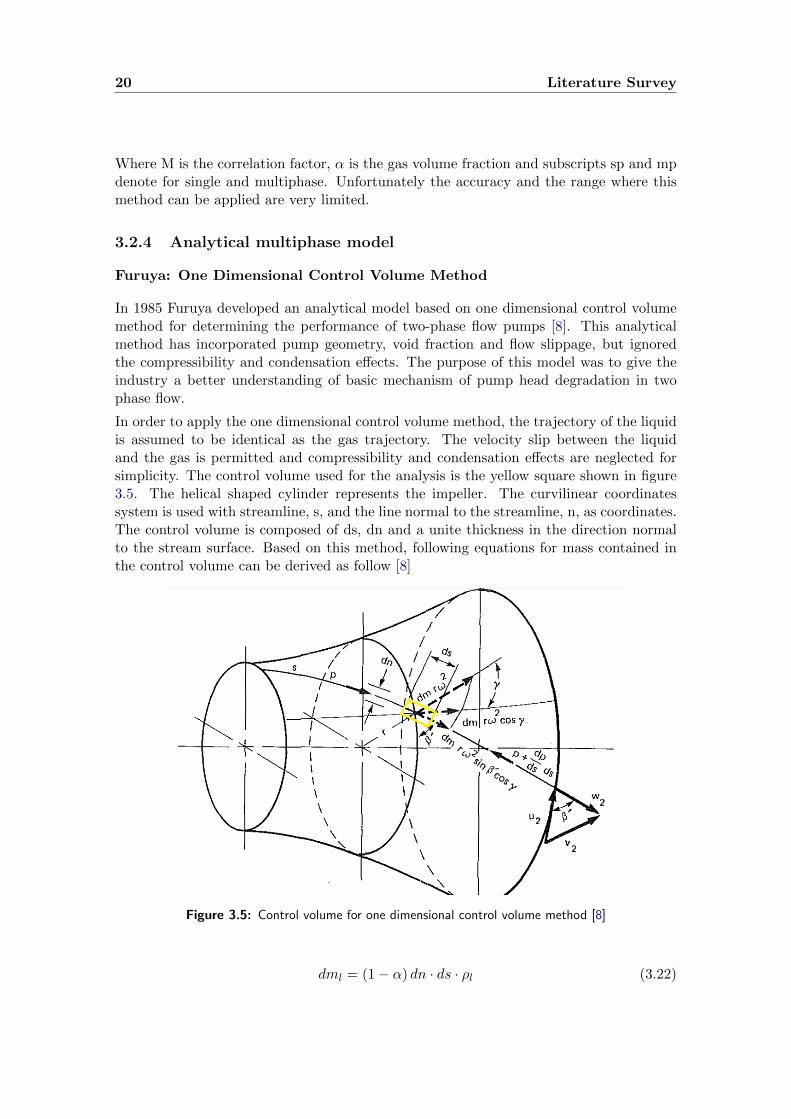
In order to apply the one dimensional control volume method, the trajectory of the liquidis assumed to be identical as the gas trajectory. The velocity slip between the liquidand the gas is permitted and compressibility and condensation effects are neglected forsimplicity. The control volume used for the analysis is the yellow square shown in figure3.5. The helical shaped cylinder represents the impeller. The curvilinear coordinatessystem is used with streamline, s, and the line normal to the streamline, n, as coordinates.The control volume is composed of ds, dn and a unite thickness in the direction normalto the stream surface. Based on this method, following equations for mass contained inthe control volume can be derived as follow [8]
Figure 3.5: Control volume for one dimensional control volume method [8]
dml = (1− α) dn · ds · ρl (3.22)
3.2 Multiphase Pump 21
dmg = α · dn · ds · ρg (3.23)
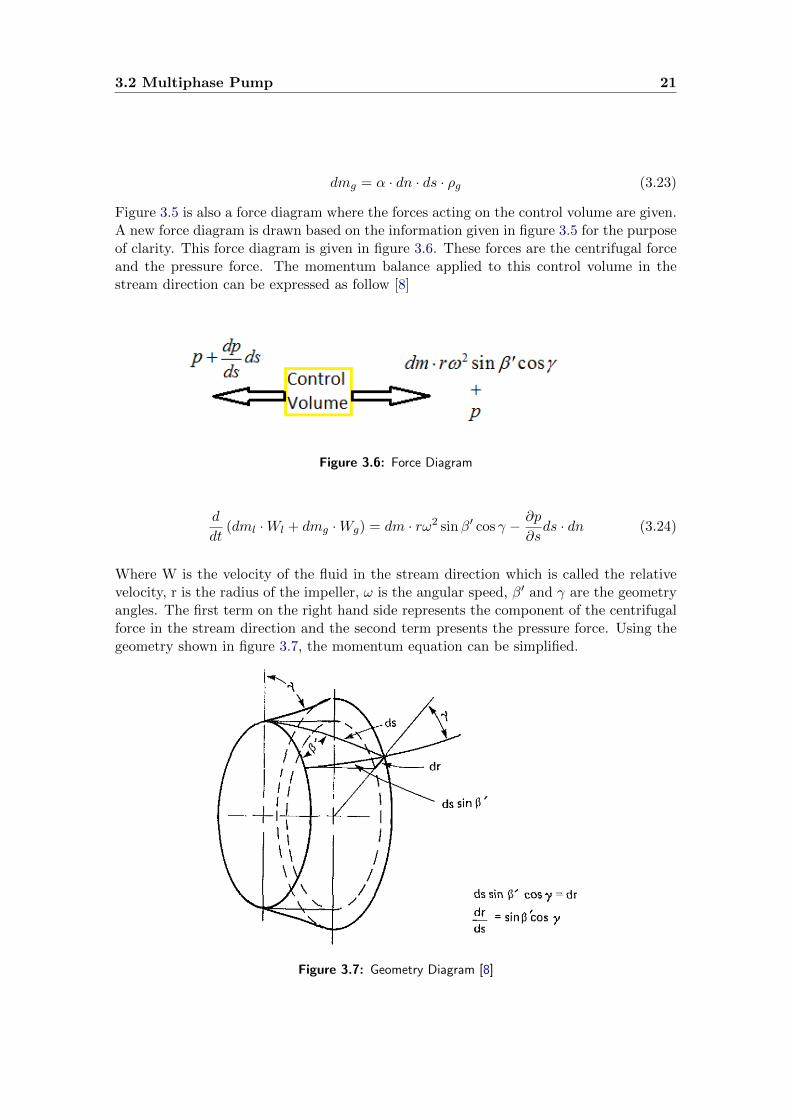
Figure 3.5 is also a force diagram where the forces acting on the control volume are given.A new force diagram is drawn based on the information given in figure 3.5 for the purposeof clarity. This force diagram is given in figure 3.6. These forces are the centrifugal forceand the pressure force. The momentum balance applied to this control volume in thestream direction can be expressed as follow [8]
Figure 3.6: Force Diagram
d
dt(dml ·Wl + dmg ·Wg) = dm · rω2 sinβ′ cos γ − ∂p
∂sds · dn (3.24)
Where W is the velocity of the fluid in the stream direction which is called the relativevelocity, r is the radius of the impeller, ω is the angular speed, β′ and γ are the geometryangles. The first term on the right hand side represents the component of the centrifugalforce in the stream direction and the second term presents the pressure force. Using thegeometry shown in figure 3.7, the momentum equation can be simplified.
Figure 3.7: Geometry Diagram [8]
22 Literature Survey
d
dt(dml ·Wl + dmg ·Wg) = dm · rω2dr
ds− ∂p
∂sds · dn (3.25)
Assuming the mass inside the control volume does not change over time, equation 3.25becomes
dml ·dWl
dt+ dmg ·
dWg
dt= dm · rω2dr
ds− ∂p
∂sds · dn (3.26)
Furthermore, assuming dWdt = ∂W
∂s W
dml ·∂Wl
∂sWl + dmg ·
∂Wg
∂sWg = dm · rω2dr
ds− ∂p
∂sds · dn (3.27)
Replacing dml and dmg terms by equation 3.22 and 3.23, and then dividing the wholeequation by ds · dn, the final equation becomes [8]
(1− α) ρl∂Wl
∂sWl + αρg
∂Wg
∂sWg = [(1− α) ρl + αρg] rω
2dr
ds− ∂p
∂s(3.28)
Based on the assumption that the gas volume fraction changes along the streamline s,equation 3.28 can be rewritten as
dds
[(1− α) ρl
Wl2
2 + αρgWg
2
2 − [(1− α) ρl + αρg](rω)2
2 + p]
+[ρlWl
2−(rω)22 − ρg Wg
2−(rω)22
]dαds = 0
(3.29)
The Bernoulli equation for rotating equipment operating under two phase flow is used asstarting point for deriving equations for the head degradation. The Bernoulli equationcan be obtained by taking the integral of equation 3.29 from suction side to dischargeside, denoted by subscript 1 and 2. The derived Bernoulli equation is given below
[(1− α2) ρl
W 22l−U
2
2 + α2ρgW 2
2g−U2
2 + p2
]−[(1− α1) ρl
W 21l−U
2
2 + α1ρgW 2
1g−U2
2 + p1
]+
2∫1
(ρlW 2l −U
2
2 − ρgW 2g−U2
2
)dαds ds = 0
(3.30)
Where U is the rotational velocity of the impeller. In equation 3.30 only the hydrauliclosses have been taken into account. Any mechanical losses such as friction drag has beenneglected. The total energy increase in the fluid is the sum of energy increase of liquidand gas. Assuming the flow is inviscid, incompressible and adiabatic, the total energyincrease can be written in terms of the static pressure increase and absolute velocityincrease between suction and discharge sides, then combining the pressure term for bothgas and liquid. The equation for total energy increase becomes
HT =p2 − p1gρavg
+V 22l − V 2
1l
2g(1− x) +
V 22g − V 2
1g
2gx (3.31)
3.2 Multiphase Pump 23
Where x =mgm , 1− x = ml
m , V is the absolute velocity, HT is the total head increase andsubscript avg denotes for the average density in the fluid. Substituting the term p2 − p1from Bernoulli equation [3.30] into equation [3.31], the final head increase equation canbe obtained. For the purpose of clarity, the final equation is expressed using the followingterms
Htp = Hsp −Hw −Hsl −Hα (3.32)
Where Htp represents the head increase for multiphase, Hsp is the head increase for singlephase, Hw is the head loss due to the increase of relative velocity, Hsl is the head loss dueto the velocity difference between liquid and gas, and finally Hα is the head loss due tovariation of the void fraction along the flow passage. These three head losses contributeto the degradation of the pump performance. The expressions for Hsp and Hw are givenbelow [8]
Hsp = (1− x) ·V 1φu2,l · U2 − V 1φ
u1,l · U1
g+ x ·
V 1φu2,g · U2 − V 1φ
u1,g · U1
g(3.33)
Hw = (1− x)∆Vu2,l · U2
g+ x
∆Vu2,g · U2
g(3.34)
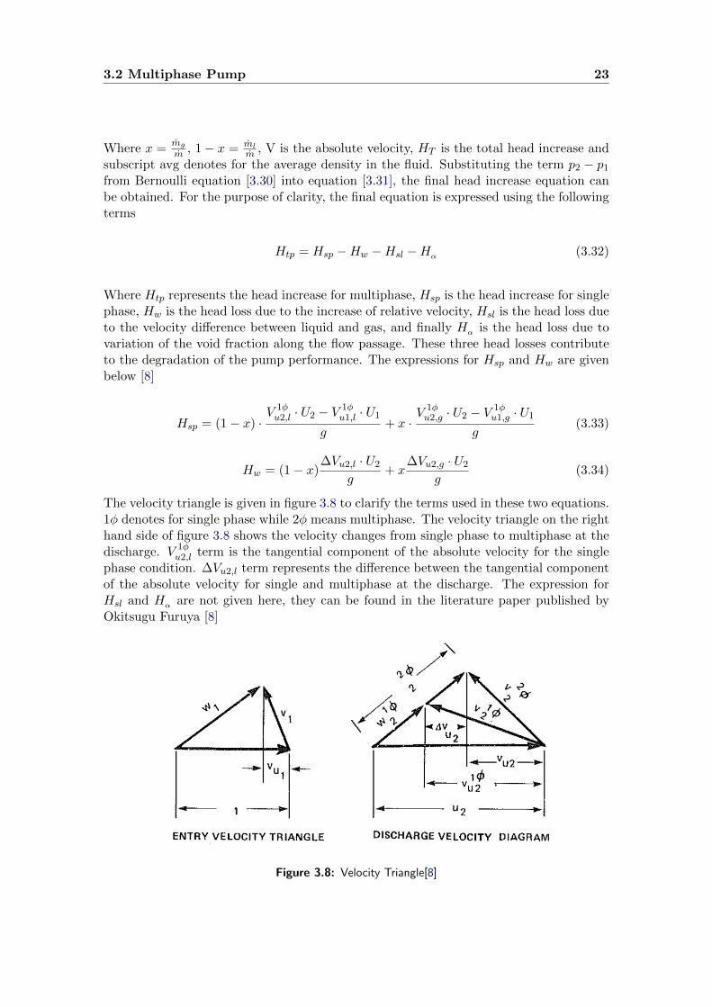
The velocity triangle is given in figure 3.8 to clarify the terms used in these two equations.1φ denotes for single phase while 2φ means multiphase. The velocity triangle on the righthand side of figure 3.8 shows the velocity changes from single phase to multiphase at thedischarge. V 1φ
u2,l term is the tangential component of the absolute velocity for the singlephase condition. ∆Vu2,l term represents the difference between the tangential componentof the absolute velocity for single and multiphase at the discharge. The expression forHsl and Hα are not given here, they can be found in the literature paper published byOkitsugu Furuya [8]
Figure 3.8: Velocity Triangle[8]

24 Literature Survey
After comparing this theoretical model with the experimental data, it showed that mea-sured head degradation is well presented by this model, particularly for the homogenousflow. However for the extreme off design conditions, some discrepancy between the an-alytical model and the test data exists. In addition, it has also been found that thecontribution of Hw to the head degradation is much larger than the sum of Hsl +Hα . Tofurther increase the accuracy of the model, the condensation and compressibility effectswill have to be properly incorporated.
Furuya: An Analytical Model For Prediction Two-Phase Condensable FlowCase
This is an extension of the previous work done by Furuya [8]. One of the assumptionsFuruya made during his previous analysis was either gas nor liquid is allowed to changeits phase through condensation or evaporation during the operation. In this paper Furuyahas created a mathematical model where the phase change of gas or liquid is permitted.One dimensional control volume method is used where the defined control volume is givenin his previous paper [8]. Using the mass conservation law, the condensation rate Γ withinthe control volume for gas is identified,
d
ds[(1− α) ρlWlA] = −ΓA (3.35)
d
ds[αρgWgA] = ΓA (3.36)
The momentum equation and equation of motion for a single gas bubble used in this anal-ysis are the same as the ones derived in his previous paper [8]. Based on the assumptionthat thermodynamic equilibrium exits throughout the entire pump, only one additionalenergy equation is required [12]. Using this energy equation with the momentum equa-tions, equation of motion for a single gas bubble and the two mass equation, condensationrate can be expressed as a function of
Γ = f(Hg,Hl, g,Wl,Wg, ρg, ρl,A,Cdrb, α, p) (3.37)
Where Cd is the drag coefficient of gas bubble and rb is the radius of the gas bubble. Theelaborated form of equation 3.37 can be found in his paper [12]. There are 5 unknownvariables, Γ, Wl, Wg, p and α and there are 2 mass equations (one for liquid one for gas),1 momentum equation, 1 equation of motion (for gas) and one equation for Γ. There areenough equations available to solve the variables by a typical numerical method such asRunge-Kutte method. Regarding the total head increase after taking condensation effectinto account, Furuya has obtained the following head equation by applying the energybalance between the inlet and outlet of the pump
HT =P2 − P1
gρavg+
1
2g
[V 22l (1− x2)− V 2
1l (1− x1)]
+1
2g
[V 22gx2 − V 2
1gx1]
(3.38)
3.2 Multiphase Pump 25
In case when x2 = x1, the entire equation can be reduced to the non condensable andincompressible head equation given in equation 3.31 As known from the previous work,the head degradation is mainly attributed due to the separation of liquid and the gasduring the compression phase. This separation will reduce the effective stream area ofthe main flow which will result into an increase of its relative velocity Wl at the outlet.This increase in relative velocity deteriorate the pump performance. After comparingthe calculated data with the experimental data, the same trend can be observed in thecondensable and incompressible flow as well, except the head degradation is much milder.That is due to the fact that the condensation of gas took place which led to a decrease ofvoid fraction. Based on the calculated results and the experiments data, it suggested thatthe mixed flow pump provides a better head degradation characteristic than the radialflow pump.
Bratu : Rotodynamic Two-phase Pump Performance
Using the same control volume as Furuya did[8], Bratu has derived a similar momentumequation in the stream direction. The only difference is that Bratu has added a friction
loss term(∂p∂s
)fl
to the equation [13]
(1− α) ρl∂Wl
∂sWl + αρg
∂Wg
∂sWg = [(1− α) ρl + αρg] rω
2dr
ds− ∂p
∂s−(∂p
∂s
)fl
(3.39)
This friction loss term is expressed using an empirical correlation developed by Wisman[13]
(∂p
∂s
)fl
=f
2
[(1− α)ρlW
2l + αρgW
2g
D+ FD
](3.40)
Where f is the friction coefficient, D is the diameter of the impeller and the subscript fldenotes for friction loss. The expression for the term FD is given as follow [13]
FD =3
8
Cdrbρsur (Wl −Wg) |Wl −Wg| (3.41)
Where Cd is the drag coefficient, rb is the radius of the gas bubble and ρsur is the densityof the surrounding fluid. Due to the density difference between liquid and gas, liquidwill experience a larger centrifugal force than gas. Consequently, the liquid will accel-erate faster than gas which leads to a velocity difference between liquid and gas. Thisdifference in velocity is called slip. As mentioned before, slip causes fluid separation andgas accumulation. This will result into an increased relative velocity of the fluid at thedischarge which is responsible for the head degradation. Furthermore, What Bratu diddifferently is instead of solving the differential equation numerically, he obtained a firstorder analytical approximation for the void fraction [13]
dα
ds=α (ρl + ρg) rω
2sinβ′cosγ
Q2l ρl
α(1−α)3 +Q2
gρg1α2
(3.42)

26 Literature Survey
The final results are validated with the experimental data, the effects such as flow strat-ification and inter-facial friction are observed. The effects of void fraction, flow rate onthe performance degradation are well predicted by this analytical model.
Minemura: Prediction Of Air-Water Two Phase Flow Performance
In 1998 Minemura extended the work done by Furuya by adding related losses at theimpeller exit and diffuser. He used the same control volume as Furuya. Based on thechosen control volume, the mass and momentum equations are derived. The severalassumptions he made for his calculation are shown below
• Steady flow, constant angular velocity
• Both phase has the same streamline
• Gas is assumed to be a perfect gas and change adiabatically, while liquid is incom-pressible
• Neither mass or heat transfer takes place between the phases
• The flow upstream of the impeller does not acquire prerotation
While fluid is exiting the impeller, several changes are happening simultaneously [14].The first one is the deflection of flow angle. Although the gas and the liquid exit theimpeller with the same blade angle, the actual exit flow angle will deviate from the bladeangle, the reason behind this has already been discussed in section 3.1.7. The magnitudeof this deviation is dependent on the relative velocity of the fluid at the discharge. Sincegas and liquid exit the impeller with different relative velocities, their exit flow angle willdiffer as well. The second change is the rapid expansion of flow area. At the exit, both gasand liquid encounter rapid expansion corresponding to the blade thickness, results intoa lower velocity for both phases and lower pressure due to losses causes by expansion.The pressure and velocity calculation is based on a theory developed by Chisholm andSutherland in 1969 [14]. The final subject was the flow mixing at the exit. The gas andthe liquid is mixing into a homogeneous flow after leaving the impeller exit which resultsinto a head loss. Once all the equations are acquired, a numerical calculation is executed.After validating the results with the experimental data, the head and the shaft powerobtained from this analysis are found to agree well with the measured values within 20% of the rated flow capacity.
Poullikkas: Compressibility And Condensation Effects
Poullikkas has extended the work that Furuya has done in his first paper regarding non-condensable two-phase flow [8]. He developed an improved model for calculating thetwo-phase pump head by taking phase separation, compressibility and condensation ef-fect into account. Two important assumptions are made at the beginning of his analysis.First one is that the trajectory for liquid and gas is identical, so that a control volumecan be bounded by two streamlines. The second assumption is that the gas is treated as
3.2 Multiphase Pump 27
a perfect gas undergoing an isothermal process. The momentum equation for the controlvolume used in his paper is taken from the paper written by Furuya [8]. In addition toFuruya’s work, he assumed that gas is undergoing isothermal change which gives that [15]
∂p
∂sdsdA =
∂
∂s(pdsdA) + dmgRT
d
ds(logp) (3.43)
Combining the momentum equation with the equation [3.43], then integrating it frominlet to discharge, denoted as 1 and 2 respectively, with respect to the streamline s. Afterrearranging the equation, the final total head equation for condensible and compressibletwo-phase flow model is derived as
HT =p2
gρ2avg− p1gρ1avg
+
[V 22l (1− x2)− V 2
1l (1− x1)]
2g+
[V 22gx2 − V 2
1gx1]
2g+RT
glog
px22px11
(3.44)
ρavg =(1− α) ρlRT + α
Wg
Wlp[
(1− α) + αWg
Wl
]RT
(3.45)
The first two terms on the right hand side represent the static pressure difference, thethird and the fourth represent the kinetic head difference for liquid and gas respectively,the final term on the right represents the compressibility of the gas. Due to the isothermalassumption, the obtained results are decent for low GVF conditions. However for highGVF inlet conditions, the model quickly losses its accuracy.
3.2.5 Empirical correlations using non-dimensional parameters
Two phase model developed by Sulzer based on the experimental results
Sulzer has developed an in-house two phase flow pump model to calculate the performanceof a MPP. The model is based on isothermal compression up to 60 % GVF. Above 60% GVF, isothermal compression is no longer valid, instead polytropic compression isapplied. Isothermal compression means that the temperature is assumed to be constantthroughout the process.
The methodology developed by Sulzer for multiphase pump performance assessment isshown in number of steps below [1]:
1. Performing experiments using pure liquid to create single phase performance maps.
2. The measured parameters are non-dimensionlized, non-dimensionlized single phaseperformance maps are created.
3. Performing experiments using liquid and gas to create multiphase performancemaps.
28 Literature Survey
4. The measured parameters are non-dimensionlized, non-dimensionlized multiphaseperformance maps are created.
5. Developing multiphase correction factors based on the these performance maps.
6. Use the similarity conditions to map the entire performance range
The equation used for non-dimensionlizing the flow is
ϕ =4Q
πD2U2(3.46)
Where Q is the flow rate and D is the diameter of the impeller.
The equation used for non-dimensionlizing the pressure rise for liquid phase and multi-phase is given as
ψisot = (1− x)p2 − p1ρl
+ xp1ρg
lnp2p1
(3.47)
Where p is the pressure, x is the gas mass fraction, ρ is the density and subscripts isot, land g denote for isothermal, liquid and gas respectively. In case of a single liquid phase,x is equal to zero, the equation can be reduced to
ψ =P2 − P1
ρl(3.48)
A new coefficient called work coefficient is introduced, it is expressed as a function of thepressure coefficient
ζ =2ψ
zstU22
(3.49)
The correction factor is a function of the work efficient and applicable for operatingconditions with the same flow coefficient
f =ζmpζsp
(3.50)
Where ζ is the work coefficient, zst is the number of stages, f is the correction factor andsubscripts mp and sp denote for multiphase and single phase.
3.2.6 Using Computational Fluid Dynamics (CFD) tools
3D flow modeling in one helical-axial multiphase pump stage through CFD
Up to the date, the development of helical-axial multiphase pumps has been based prin-cipally on experimental models. In the past decade, more and more Computational FluidDynamics (CFD) analysis are used as an additional tool in design and prediction of turbo

3.2 Multiphase Pump 29
machinery performances. The advantage of using CFD analysis is it reduces the time ofdesign and the cost. Many CFD analysis have been carried out for centrifugal pumps,mainly for single phase fluid. Only few have been done for helical-axial multiphase pumps,especially for the high GVF conditions. In order to have a better understanding of theflow behaviour in multiphase pumps, a CFD analysis for multiphase pumps with a highGVF inlet condition is necessary. In 2007, Roberto Faustini and Frank Kenyery havecarried out a CFD analysis for an one stage helical-axial multiphase pump under highGVF conditions [16].
A CFD commercial tool called CFX 5.7 is used to perform the analysis and to solve theNavier Stokes equation using finite volume technique. To simplify the problem, the fluiddynamics has to obey a series of hypotheses: permanent, isothermal and incompressibleflow, no phase changes and axisimetric geometry. In addition, for the multiphase model,gas is considered as the continuous phase while liquid is considered as the dispersed phase.Both phases can have different fields of speed and temperatures. For the turbulencemodelling, the k − ε model is used, since it allows the separation velocity fields for eachof the phase. This model is considered as the standard in the industry and has beenimplemented in most of the previous works.
The results obtained from their analysis was remarkable. For high GVF conditions(>60%), even though the fluid enters the rotor being homogeneous, the flow that comesout the rotor is stratified. The concentrated liquid is being pushed outwards against theshroud while gas stays close to the hub due to the centrifugal force and their density dif-ferences. In addition, an accumulation of gas takes place at the upper side of the blade,the suction side, while liquid is accumulated at the inner side of the blade, in betweenexits the mixture of liquid and gas. This phenomenon is caused by the pressure differ-ence between the upper and inner surface of two adjacent rotor blades. The accumulatedgas reduced the effective channel area for the liquid, that causes a higher relative liquidvelocity at the exit which is the main reason for head degradation. A higher flow rate fora given GVF diminishes the pure gas and liquid zone and increases the mixture zone, soit has a positive impact for the head increase. However a higher flow rate causes morelosses in the stator, the flow no longer obey to a pattern and the blades do not lead thefluid in a regular way through their channels, that causes performance loss in the stator.
3.2.7 Comparison of various methods
So far four different methods have been discussed. CFD analysis seems to be an excellentmethod when the flow behaviour inside the pump needs to be studied. However in orderto use CFD tools such as CFX, the exact geometry of the rotor and the stator need tobe known which includes the blade shape and angle. Without these information, CFDanalysis can not be performed. A small change of the geometry can greatly impact thehead degradation of the pump. Unfortunately, information such as the geometry data ofthe rotor and stator are not given by the manufacturers due to the proprietary reasons.For this reason CFD is being discarded for this thesis.
The experimental data are the foundation of the empirical correlation methods. Creatingperformance curves based on these experimental data and then developing a correctionfactor that represents the head degradation from single phase to multiphase. The cor-rection factor is only applicable when several conditions are met. For example the two
30 Literature Survey
operating conditions have to have the same flow coefficient. For this thesis, the final goalis to develop a tool that is able to create performance maps for the entire pump operat-ing range: different speed, GVF and flow rate. It will require hundreds of experimentsto cover its entire operating range and developing a correction factor for each of theseoperating conditions. Since I do not have the resource to accomplish that, this methodis discarded.
The last method discussed in the previous section is the analytical multiphase modelling.It is based on one dimensional control volume method where the pump geometry andthe operating condition are incorporated. This analytical method does not required aextensive amount of experiments and it has incorporated the operating condition in themodelling which means the model can be used to predict the pump performance for itsentire operating range. For these reasons, this method has been chosen to the startingpoint of this thesis. The final results will be validated with the several performance curvesprovided by the manufacturer to ensure the model accuracy and applicability.
Chapter 4
One Dimensional Two Phase ControlVolume Modelling
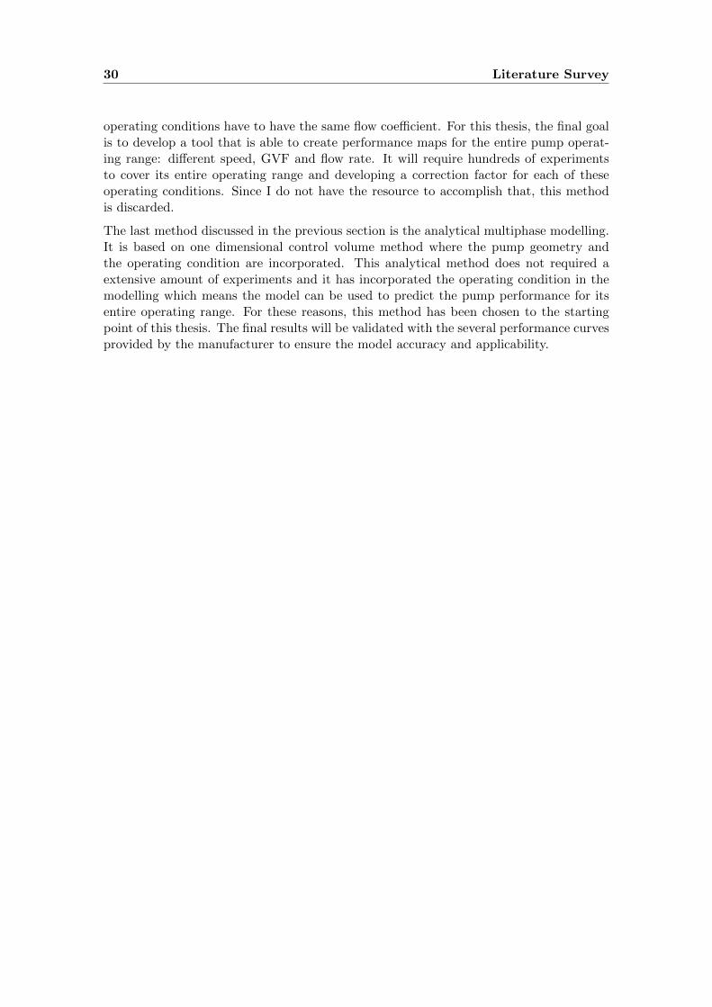
Using the knowledge obtained from the literature study, an approach called one dimen-sional two phase control volume will be used to develop a multiphase pump performancemodel. This performance model will be implemented for a 8 stage helico axial multiphasepump manufactured by Onesubsea. A computer drawing for the first 4 stages of the pumpshown in figure 4.1.
Figure 4.1: 8 stage helico axial multiphase pump [24]
31
32 One Dimensional Two Phase Control Volume Modelling
4.1 Fundamental equations for an one dimensional two phasemodel
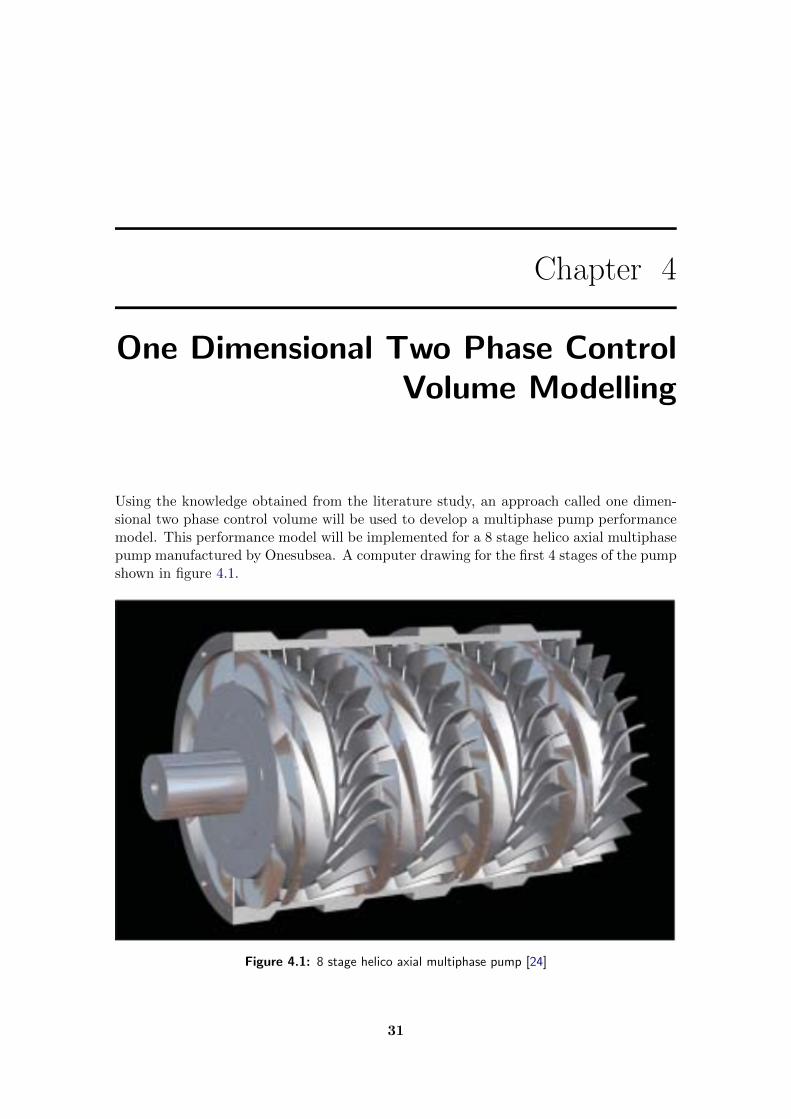
In order to apply this method the trajectory of the liquid and the gas are assumed tobe identical. A control volume used for this approach is shown in figure 4.2, where thestreamline, s, and the normal to the streamline n, are used as curvilinear coordinatesystem. The control volume is composed of ds, dn and a unit height.
Figure 4.2: Control Volume
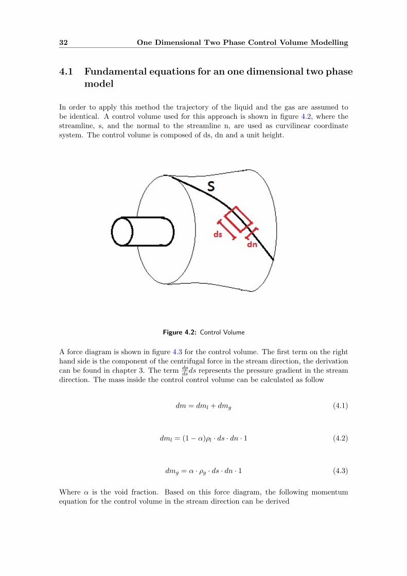
A force diagram is shown in figure 4.3 for the control volume. The first term on the righthand side is the component of the centrifugal force in the stream direction, the derivationcan be found in chapter 3. The term dp
dsds represents the pressure gradient in the streamdirection. The mass inside the control control volume can be calculated as follow
dm = dml + dmg (4.1)
dml = (1− α)ρl · ds · dn · 1 (4.2)
dmg = α · ρg · ds · dn · 1 (4.3)
Where α is the void fraction. Based on this force diagram, the following momentumequation for the control volume in the stream direction can be derived
4.1 Fundamental equations for an one dimensional two phase model 33
Figure 4.3: Force Diagram
d
dt(dml ·Wl + dmg ·Wg) = dm · rω2dr
ds− dp
dsdsdn (4.4)
Where m is the total mass, W is the relative velocity, r is the radius of the impeller, ω isthe angular velocity and p is the static pressure. The subscripts l and g denote for liquidand gas. Assuming a steady flow condition, so the mass flow for liquid and gas do notchange along the stream line, the momentum equation can be rewritten as
dmldWl
dt+ dmg
dWg
dt= dm · rω2dr
ds− dp
dsdsdn (4.5)
Replacing the dt term on the left hand side by ds/W, so the entire equation becomes aderivative with respect to s.
dmldWl
dsWl + dmg
dWg
dsWg = dm · rω2dr
ds− dp
dsdsdn (4.6)
Substituting equation 4.2 and 4.3 into equation 4.6 and the dividing the whole equationby dsdn, gives
(1− α)ρl2
dW 2l
ds+αρg2
dW 2g
ds= [(1− α)ρl + αρg] rω
2dr
ds− dp
ds(4.7)
Equation 4.7 can be rearranged and rewritten as
d
ds
[(1− α)ρl
W 2l
2+ αρg
W 2g
2− [(1− α)ρl + αρg]
r2ω2
2+ p
]= 0 (4.8)
Equation 4.8 can be further simplified and rearranged,
d
ds
[(1− α)ρl
W 2l − U2
2+ αρg
W 2g − U2
2+ p
]= 0 (4.9)
34 One Dimensional Two Phase Control Volume Modelling
Where r2ω2 = U2, integrating equation 4.9 from the inlet of the impeller to the dischargeof the impeller gives
(1−α2)ρlW 2
2l − U22
2+α2ρ2g
W 22g − U2
2
2+ p2 = (1−α1)ρl
W 21l − U2
1
2+α1ρ1g
W 21g − U2
1
2+ p1
(4.10)
4.2 Using velocity triangles to reduce the unknowns
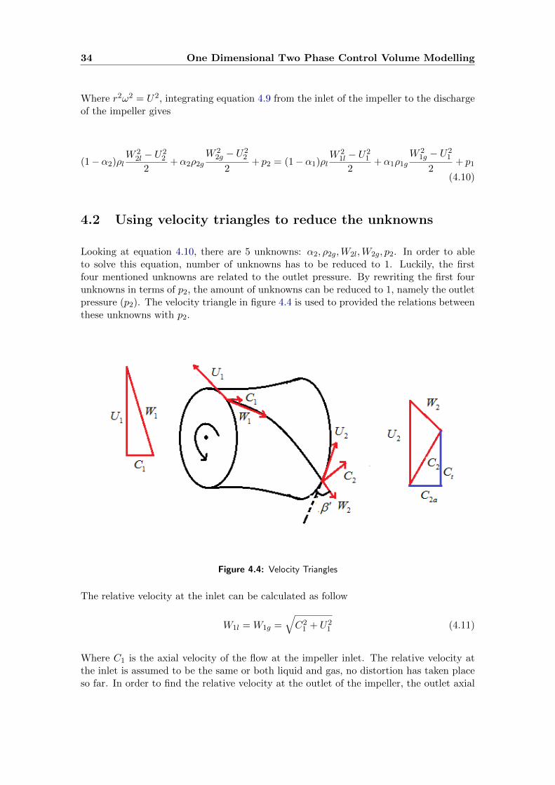
Looking at equation 4.10, there are 5 unknowns: α2, ρ2g,W2l,W2g, p2. In order to ableto solve this equation, number of unknowns has to be reduced to 1. Luckily, the firstfour mentioned unknowns are related to the outlet pressure. By rewriting the first fourunknowns in terms of p2, the amount of unknowns can be reduced to 1, namely the outletpressure (p2). The velocity triangle in figure 4.4 is used to provided the relations betweenthese unknowns with p2.
Figure 4.4: Velocity Triangles
The relative velocity at the inlet can be calculated as follow
W1l = W1g =√C21 + U2
1 (4.11)
Where C1 is the axial velocity of the flow at the impeller inlet. The relative velocity atthe inlet is assumed to be the same or both liquid and gas, no distortion has taken placeso far. In order to find the relative velocity at the outlet of the impeller, the outlet axial
4.2 Using velocity triangles to reduce the unknowns 35
velocity (C2a) for the liquid and the gas need to be found first. The conservation of massequation is used to find the axial velocity for the liquid and the gas at the outlet
ρ1g ·A1 · α1 · C1,g = ρ2g ·A2 · α2 · C2a,g (4.12)
ρl ·A1 · (1− α1) · C1,l = ρl ·A2 · (1− α2) · C2a,l (4.13)
The left hand side of equation 4.12 is known, since all the parameters are known at theinlet of the pipe. On the right hand side, density of the gas, GVF and axial velocity atthe outlet are still unknown. However we can write density of the gas and GVF at outletas a function of pressure.
ρ2g = ρ1gp2p1
(4.14)
Previous equation is derived assuming isothermal condition. GVF at outlet can be ex-pressed in terms of p2 as follow
α2 =
Q1g ·ρg1ρg2
Q1g ·ρg1ρg2
+Ql=
Q1gp1p2
Q1gp1p2
+Ql(4.15)
1− α2 =Ql
Q1gp1p2
+Ql(4.16)
Now C2g can be expressed as a function of p2 by substituting equation 4.14 and 4.15 intoequation 4.12.
C2a,g =mg
ρ1gp2p1·A2 ·
Q1gp1p2
Q1gp1p2
+Ql
(4.17)
Using the similar manner, C2l can be expresses as a function of p2 as well by substituting4.16 into 4.13.
C2a,l =ml
ρlA2Ql
Q1gp1p2
+Ql
(4.18)
Once C2a is know, the relative velocity can be calculated using the exit flow angle.
W2 =C2a
sinβ′(4.19)
The complete form of the relative velocity of gas and liquid at rotor outlet is given below
W2g =mg
ρ1gp2p1·A2 ·
Q1gp1p2
Q1gp1p2
+Ql· sinβ′
(4.20)
36 One Dimensional Two Phase Control Volume Modelling
W2l =ml
ρlA2Ql
Q1gp1p2
+Ql· sinβ′
(4.21)
All 4 unknowns α2, ρ2g,W2l,W2g are expressed as a function of p2. The total amount ofunknowns has been reduced to 1, namely p2. The governing equation 4.10 can be solved.
4.3 Density of the mixed fluid at the rotor outlet
Density of the mixed fluid at the rotor outlet can be calculated once the outlet pressureis known. The same equation for calculating the fluid density at the rotor inlet can beused,
ρ2mix = ρl · (1− α2) + ρ2g · α2 (4.22)
This equation can be rewritten as a function of p2 by substituting equation 4.14, 4.15 and4.16 into 4.22, which gives
ρ2mix = ρlQl
Q1gp1p2
+Ql+ ρ1g
p2p1
Q1gp1p2
Q1gp1p2
+Ql(4.23)
4.4 Pressure decrease calculation at pipe inlet
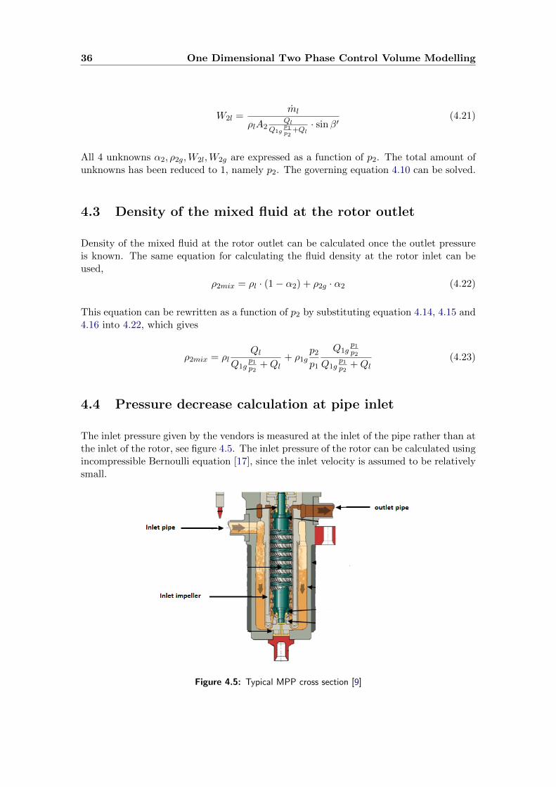
The inlet pressure given by the vendors is measured at the inlet of the pipe rather than atthe inlet of the rotor, see figure 4.5. The inlet pressure of the rotor can be calculated usingincompressible Bernoulli equation [17], since the inlet velocity is assumed to be relativelysmall.
Figure 4.5: Typical MPP cross section [9]

4.5 Pressure increase calculation at stator 37
The incompressible Bernoulli equation is given below
V 21
2+ gz1 +
p1ρmix
=V 22
2+ gz2 +
p2ρmix
(4.24)
Fluid velocity at the inlet is calculated using the following equation
V1 =Q1
A1(4.25)
Where Q is the volumetric flow and A is the cross section area of the inlet pipe. Thevelocity at the inlet of the rotor can be calculated using the mass conservation law wheredensity of the fluid is assumed to be constant
V2 =V1A1
A2(4.26)
Pressure at the inlet of the rotor can be found using equation 4.24.
4.5 Pressure increase calculation at stator
So far only the pressure calculation for the rotor is discussed, in this section the pressurecalculation through the stator will be elaborated. The incompressible Bernoulli equationis used to calculate the pressure increase through the diffuser. The inlet velocity for thediffuser is assumed to be the same as the outlet velocity of the rotor, hence the velocitytriangle in figure 4.4 can be used. The inlet velocity can be calculated using the followingequations
√C22a + C2
t = C1 (4.27)
Ct = U2 −W2 cosβ′ (4.28)
The outlet velocity at the stator can be calculated using conservation of mass. Since theflow is assumed to be incompressible, both gas density and gas volume density remainconstant. The following equation can be used to calculate the diffuser outlet velocity
Cout =m
ρ2 · α2 ·A1(4.29)
The fluid is assumed to leave the stator in the axial direction. When all the velocitiesare known, the pressure at the outlet of the stator can be calculated using incompress-ible Bernoulli equation. The final pressure increase for each stage will be the combinedpressure increase of the rotor and the stator. The outlet condition of the stator are usedas the inlet condition for the next stage rotor. The exact same calculation procedure willbe used to calculate the pressure increase of the next stage.
38 One Dimensional Two Phase Control Volume Modelling
4.6 Model inputs
4.6.1 Inlet conditions
The inlet conditions need to be given before the calculation can be carried out. Theseinlet conditions are
• Inlet pressure
• Inlet volumetric flow
• Inlet void fraction
• Inlet gas density
• Liquid density
• Rotational speed
4.6.2 Pump geometry
In addition, some of the pump geometry are required for the calculation.
• Casing diameter
• Rotor hub diameter
• Rotor tip diameter
• Exit flow angle
Rotor geometry
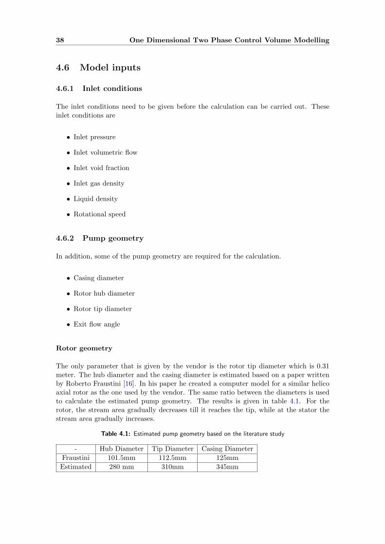
The only parameter that is given by the vendor is the rotor tip diameter which is 0.31meter. The hub diameter and the casing diameter is estimated based on a paper writtenby Roberto Fraustini [16]. In his paper he created a computer model for a similar helicoaxial rotor as the one used by the vendor. The same ratio between the diameters is usedto calculate the estimated pump geometry. The results is given in table 4.1. For therotor, the stream area gradually decreases till it reaches the tip, while at the stator thestream area gradually increases.
Table 4.1: Estimated pump geometry based on the literature study
- Hub Diameter Tip Diameter Casing Diameter
Fraustini 101.5mm 112.5mm 125mm
Estimated 280 mm 310mm 345mm
4.6 Model inputs 39
Exit flow angle
The first step in finding the exit flow angle is to calculate the slip factor. The slip factorcan be computed using the empirical equations developed by scientists such as Wiesnerand Stanitz. The slip factor shows the deviation of the exit flow angle from the bladeangle. However in this case, the exact blade angle is not given by the vendor due toproprietary reasons. Based on a drawing provided by the vendor, the blade angle isestimated between 10 and 20 degree. Since the exit flow angle should not deviate toomuch from the blade angle near the design conditions, for the simplicity, the exit flowangle is initially assumed to be 20 degree. This is of course not always true. For eachindividual operating condition, there is a corresponding exit flow angle. In addition, theexit flow angle is assumed to be the same for all the rotors within the pump. The 20degrees is used as the starting value. Using the iteration process, a new exit flow angle isdetermined which provides a better result.
40 One Dimensional Two Phase Control Volume Modelling
4.7 Pump pressure increase calculation flow diagram
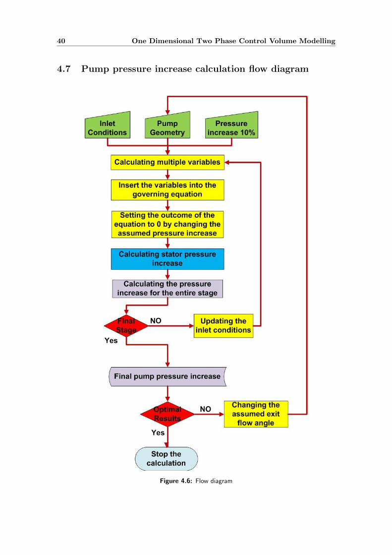
Figure 4.6: Flow diagram
4.8 Validation 41
4.7.1 General layout
The entire calculations methods can be explained using a flow diagram, figure 4.12. Thegreen boxes are the inputs, the inlet conditions and the pump geometry are alreadydiscussed in the previous section. The additional input, in this case an assumption, isthat the pressure increase in the rotor is 10 %. This assumption is crucial for solvingthe actual pressure increase in the rotor. This will be explained in section 4.7.2 Theyellow boxes are the calculations performed to find the actual pressure increase in therotor. The blue box represents the calculation done for the stator. Grey boxes representsthe final pressure obtained for each stage and the pump. After each stage, the sameprocedure will be repeated to calculated the pressure increase of the next stage until thefinal stage is reached. It is important to update the inlet condition for each stage, due thecompressibility of the gas, the gas density, GVF, flow rate, but also the inlet pressure willbe different from the previous stage. Once the calculation is performed for all the stages,the final results will be stored and the corresponding pump performance is calculated. Asdiscussed in the previous section, the exit flow angle is assumed to be 20 degree. Usingan iteration process, the optimal exit flow angle is found which gives the minimum errorwith the experimental data. The final exit flow angle has to be realistic, and it should bebetween 10 and 20 degree range.
4.7.2 Rotor pressure increase calculation
Equations from 4.11 to 4.21 can be performed once the inputs ( green boxes ) are given.By performing these equations, all the unknowns such as inlet and outlet relative veloc-ity, outlet gas density and outlet GVF can be found. By substituting these values intothe governing equation 4.10, the outcome of the governing equation can be found. Theoutcome of the governing equation is only equal to zero when the actual outlet pressure isused as an input. Since the exact outlet pressure is not known, an assumption is made atthe beginning of the calculation which is that the outlet pressure is 1.1 time bigger thanthe inlet pressure (the 10 % pressure increase). Using this assumption, the outcome of thegoverning equation is very likely not be 0, unless the assumed outlet pressure turns outto be the actual outlet pressure. A calculation tool called Solver within Microsoft Officeis used in case the outcome of the governing equation 4.10 is not equal to 0. In the solvertool box, the desired outcome of the equation can be chosen, and the parameter thatneeds to be changed to achieve the desired outcome can be identified. The real pressureincrease can be found by utilizing the Generalized Reduced Gradient algorithm withinthe Solver tool.
4.8 Validation
4.8.1 Validation against the experimental results
After using the iteration process, the optimal exit flow angle is found to be 15 degree.Using this 15 degree exit angle as input, several performance map are created for multipleGVFs( 0%, 15% and 30%). The performance maps are compared with the experimentaldata obtained from the vendor. The results are shown below.
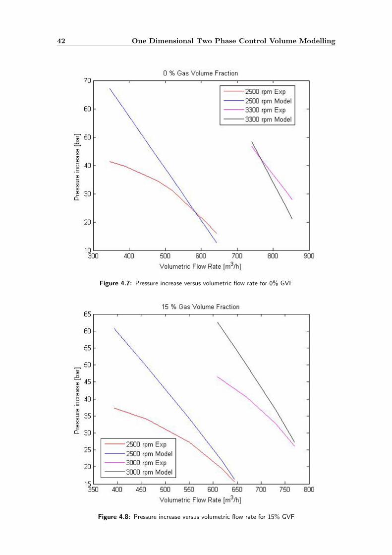
42 One Dimensional Two Phase Control Volume Modelling
Figure 4.7: Pressure increase versus volumetric flow rate for 0% GVF
Figure 4.8: Pressure increase versus volumetric flow rate for 15% GVF
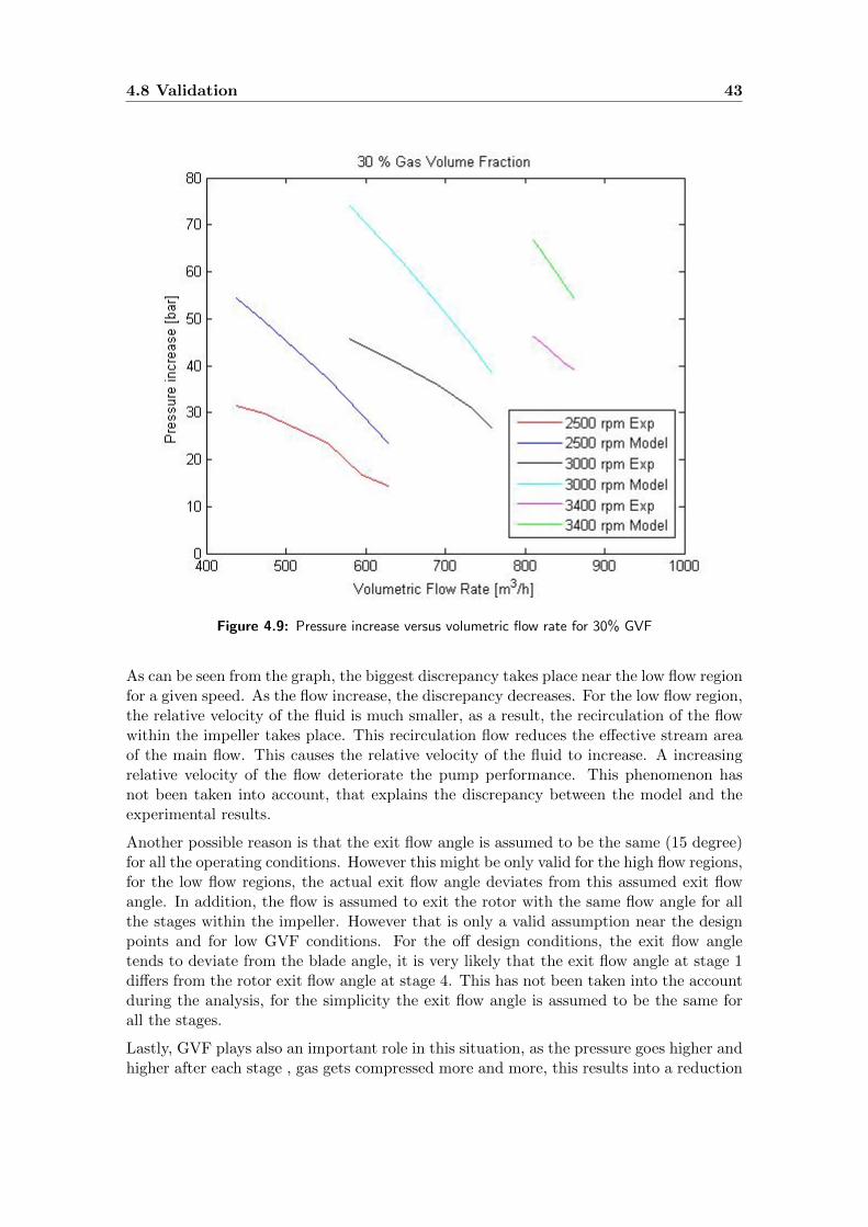
4.8 Validation 43
Figure 4.9: Pressure increase versus volumetric flow rate for 30% GVF
As can be seen from the graph, the biggest discrepancy takes place near the low flow regionfor a given speed. As the flow increase, the discrepancy decreases. For the low flow region,the relative velocity of the fluid is much smaller, as a result, the recirculation of the flowwithin the impeller takes place. This recirculation flow reduces the effective stream areaof the main flow. This causes the relative velocity of the fluid to increase. A increasingrelative velocity of the flow deteriorate the pump performance. This phenomenon hasnot been taken into account, that explains the discrepancy between the model and theexperimental results.
Another possible reason is that the exit flow angle is assumed to be the same (15 degree)for all the operating conditions. However this might be only valid for the high flow regions,for the low flow regions, the actual exit flow angle deviates from this assumed exit flowangle. In addition, the flow is assumed to exit the rotor with the same flow angle for allthe stages within the impeller. However that is only a valid assumption near the designpoints and for low GVF conditions. For the off design conditions, the exit flow angletends to deviate from the blade angle, it is very likely that the exit flow angle at stage 1differs from the rotor exit flow angle at stage 4. This has not been taken into the accountduring the analysis, for the simplicity the exit flow angle is assumed to be the same forall the stages.
Lastly, GVF plays also an important role in this situation, as the pressure goes higher andhigher after each stage , gas gets compressed more and more, this results into a reduction
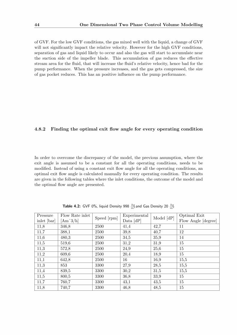
44 One Dimensional Two Phase Control Volume Modelling
of GVF. For the low GVF conditions, the gas mixed well with the liquid, a change of GVFwill not significantly impact the relative velocity. However for the high GVF conditions,separation of gas and liquid likely to occur and also the gas will start to accumulate nearthe suction side of the impeller blade. This accumulation of gas reduces the effectivestream area for the fluid, that will increase the fluid’s relative velocity, hence bad for thepump performance. When the pressure increases, and the gas gets compressed, the sizeof gas pocket reduces. This has an positive influence on the pump performance.
4.8.2 Finding the optimal exit flow angle for every operating condition
In order to overcome the discrepancy of the model, the previous assumption, where theexit angle is assumed to be a constant for all the operating conditions, needs to bemodified. Instead of using a constant exit flow angle for all the operating conditions, anoptimal exit flow angle is calculated manually for every operating condition. The resultsare given in the following tables where the inlet conditions, the outcome of the model andthe optimal flow angle are presented.
Table 4.2: GVF 0%, liquid Density 998 kgm3 and Gas Density 20 kg
m3
Pressureinlet [bar]
Flow Rate inlet[Amˆ3/h]
Speed [rpm]ExperimentalData [dP]
Model [dP]Optimal ExitFlow Angle [degree]
11,8 346,8 2500 41,4 42,7 11
11,7 388,1 2500 39,8 40,7 12
11,6 480,3 2500 34,5 35,9 14
11,5 519,6 2500 31,2 31,9 15
11,3 572,8 2500 24,9 25,6 15
11,2 609,6 2500 20,4 18,9 15
11,1 642,8 2500 16 16,9 15,5
11,3 853 3300 27,9 28,5 15,5
11,4 839,5 3300 30,2 31,5 15,5
11,5 800,5 3300 36,8 33,9 15
11,7 760,7 3300 43,1 43,5 15
11,8 740,7 3300 46,8 48,5 15
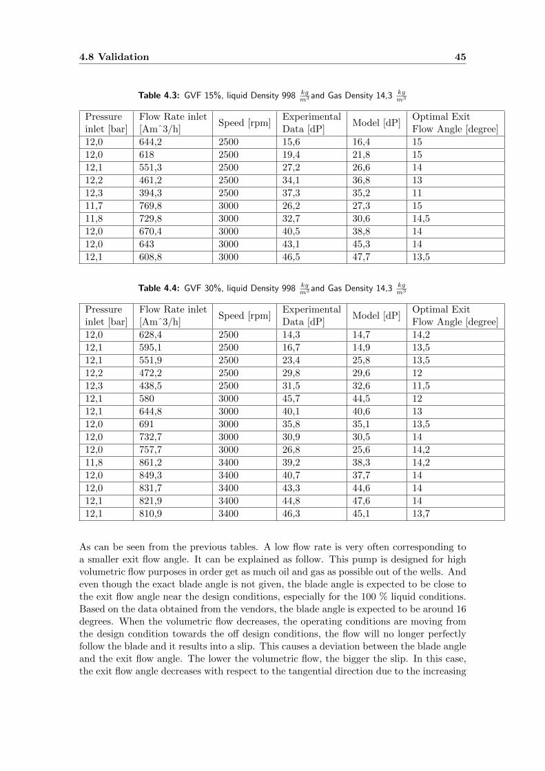
4.8 Validation 45
Table 4.3: GVF 15%, liquid Density 998 kgm3 and Gas Density 14,3 kg
m3
Pressureinlet [bar]
Flow Rate inlet[Amˆ3/h]
Speed [rpm]ExperimentalData [dP]
Model [dP]Optimal ExitFlow Angle [degree]
12,0 644,2 2500 15,6 16,4 15
12,0 618 2500 19,4 21,8 15
12,1 551,3 2500 27,2 26,6 14
12,2 461,2 2500 34,1 36,8 13
12,3 394,3 2500 37,3 35,2 11
11,7 769,8 3000 26,2 27,3 15
11,8 729,8 3000 32,7 30,6 14,5
12,0 670,4 3000 40,5 38,8 14
12,0 643 3000 43,1 45,3 14
12,1 608,8 3000 46,5 47,7 13,5
Table 4.4: GVF 30%, liquid Density 998 kgm3 and Gas Density 14,3 kg
m3
Pressureinlet [bar]
Flow Rate inlet[Amˆ3/h]
Speed [rpm]ExperimentalData [dP]
Model [dP]Optimal ExitFlow Angle [degree]
12,0 628,4 2500 14,3 14,7 14,2
12,1 595,1 2500 16,7 14,9 13,5
12,1 551,9 2500 23,4 25,8 13,5
12,2 472,2 2500 29,8 29,6 12
12,3 438,5 2500 31,5 32,6 11,5
12,1 580 3000 45,7 44,5 12
12,1 644,8 3000 40,1 40,6 13
12,0 691 3000 35,8 35,1 13,5
12,0 732,7 3000 30,9 30,5 14
12,0 757,7 3000 26,8 25,6 14,2
11,8 861,2 3400 39,2 38,3 14,2
12,0 849,3 3400 40,7 37,7 14
12,0 831,7 3400 43,3 44,6 14
12,1 821,9 3400 44,8 47,6 14
12,1 810,9 3400 46,3 45,1 13,7
As can be seen from the previous tables. A low flow rate is very often corresponding toa smaller exit flow angle. It can be explained as follow. This pump is designed for highvolumetric flow purposes in order get as much oil and gas as possible out of the wells. Andeven though the exact blade angle is not given, the blade angle is expected to be close tothe exit flow angle near the design conditions, especially for the 100 % liquid conditions.Based on the data obtained from the vendors, the blade angle is expected to be around 16degrees. When the volumetric flow decreases, the operating conditions are moving fromthe design condition towards the off design conditions, the flow will no longer perfectlyfollow the blade and it results into a slip. This causes a deviation between the blade angleand the exit flow angle. The lower the volumetric flow, the bigger the slip. In this case,the exit flow angle decreases with respect to the tangential direction due to the increasing

46 One Dimensional Two Phase Control Volume Modelling
slip. This explains why the low volumetric flow has a smaller exit flow angle.
After the optimal exit flow angle is found for each of the operating conditions, the nextstep is to find the relations between these exit angles and the inlet conditions. A goodstarting point will be using the non dimensionalized flow coefficient which was discussedin chapter 3. The equation for non dimensionalizing the flow is given below
ϕ =4Q
πD2U2 · 3600(4.30)
Where D is the tip diameter which is 0.31 meter. The flow coefficients are calculatedfor all the operating conditions and they are plotted against the corresponding exit flowangles. The results are shown in a graph.
Figure 4.10: Flow coefficient vs Exit flow angle
There are two important trends which can be observed from this graph. First of all isthat the flow coefficient is almost a linear function of the exit flow angle for a given GVF.Secondly, the ”trendline” for given GVF shifts towards the bottom right corner as theGVF increases. The second observation is not desired outcome. The biggest advantageof using a non dimensionalized flow coefficient is that multiple variables such as flow rate,diameter and rotating speed are transformed into a single parameter. When that happens,all the dots should lay on a single ’trendline ” which can be a linear or polynomial function.It works for single phase pump, however for multiphase pump an additional parameter is

4.8 Validation 47
involved in the calculation which is the GVF. This parameter has to be implemented intothe flow coefficient for a better results. The original flow coefficient is slightly modified
ϕ′ =4Q
πD2U2 · 3600· (1− α1
2.5) (4.31)
The only difference with the original flow coefficient is the multiplication of the (1− α12.5),
where α1 is the GVF at the inlet. Using this new flow coefficient, a new flow coefficientversus exit flow angle can be created. Based on the results, a trendline can be created.
Figure 4.11: Flow coefficient vs Exit flow angle
The equation for this trendline is generated using MS Excel. The equation is given below
β′ = −3489.4ϕ′2
+ 480ϕ′ − 0.785 (4.32)
Where β′ is the exit flow angle and ϕ′ is the new flow coefficient. Instead of assuminga constant exit flow angle as it was done previously, a new empirical equation can beused to calculated the exit flow angle. The original calculation flow diagram needs to beupdated.
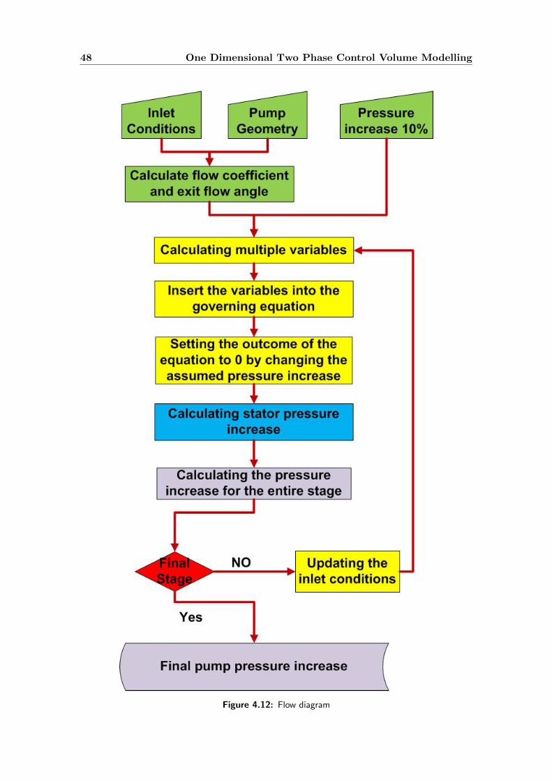
48 One Dimensional Two Phase Control Volume Modelling
Figure 4.12: Flow diagram
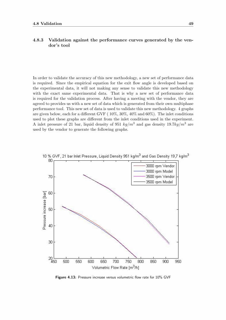
4.8 Validation 49
4.8.3 Validation against the performance curves generated by the ven-dor’s tool
In order to validate the accuracy of this new methodology, a new set of performance datais required. Since the empirical equation for the exit flow angle is developed based onthe experimental data, it will not making any sense to validate this new methodologywith the exact same experimental data. That is why a new set of performance datais required for the validation process. After having a meeting with the vendor, they areagreed to provides us with a new set of data which is generated from their own multiphaseperformance tool. This new set of data is used to validate this new methodology. 4 graphsare given below, each for a different GVF ( 10%, 30%, 40% and 60%). The inlet conditionsused to plot these graphs are different from the inlet conditions used in the experiment.A inlet pressure of 21 bar, liquid density of 951 kg/m3 and gas density 19.7kg/m3 areused by the vendor to generate the following graphs.
Figure 4.13: Pressure increase versus volumetric flow rate for 10% GVF

50 One Dimensional Two Phase Control Volume Modelling
Figure 4.14: Pressure increase versus volumetric flow rate for 30% GVF
Figure 4.15: Pressure increase versus volumetric flow rate for 40% GVF

4.8 Validation 51
Figure 4.16: Pressure increase versus volumetric flow rate for 60% GVF
The first observation is that as the GVF increases, the accuracy drops. Up to 40% GVF,the error is still acceptable, however in case of 60% GVF, the results are no longer reliable.There are several explanations for this observation.
The first one, also the most straight forward one, is that the empirical exit flow angleequation is developed based on the experimental data which covers a range from 0% GVFup to 30% GVF. It only provides a reasonable approximation of the exit flow angle withinthat range. For any cases that go beyond 30% GVF, such as 40% and 60%, the accuracythe empirical equation will decrease. A better empirical equation can be developed whenthe experimental data for 40% and 60% are available.
The second possible reason for the discrepancy is that during the analysis, the flow isassumed to exit the rotor with the same flow angle for all the stages within the pump.However this is only a valid assumptions for low GVF conditions. Due to the compress-ibility of gas, the volumetric volume of the fluid will decrease throughout the stages. Asresult, the relative flow velocity decreases, because the stream area is constant. For lowGVF inlet conditions, the relative flow velocity decrease is small, since the volumetricvolume change is small. However for high GVF inlet conditions, this effect can no longerbe ignored. This change of the relative velocity is big enough to have a significant im-pact on the flow exit angle. This causes the exit flow angle at the final stage differ fromthe initial stage. For the simplicity of the analysis, the exit flow angle is assumed to beconstant for all the stages.
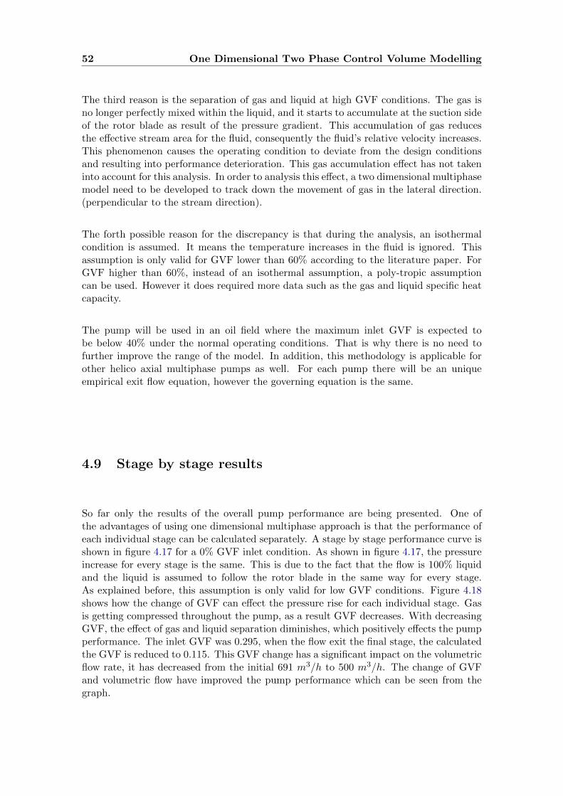
52 One Dimensional Two Phase Control Volume Modelling
The third reason is the separation of gas and liquid at high GVF conditions. The gas isno longer perfectly mixed within the liquid, and it starts to accumulate at the suction sideof the rotor blade as result of the pressure gradient. This accumulation of gas reducesthe effective stream area for the fluid, consequently the fluid’s relative velocity increases.This phenomenon causes the operating condition to deviate from the design conditionsand resulting into performance deterioration. This gas accumulation effect has not takeninto account for this analysis. In order to analysis this effect, a two dimensional multiphasemodel need to be developed to track down the movement of gas in the lateral direction.(perpendicular to the stream direction).
The forth possible reason for the discrepancy is that during the analysis, an isothermalcondition is assumed. It means the temperature increases in the fluid is ignored. Thisassumption is only valid for GVF lower than 60% according to the literature paper. ForGVF higher than 60%, instead of an isothermal assumption, a poly-tropic assumptioncan be used. However it does required more data such as the gas and liquid specific heatcapacity.
The pump will be used in an oil field where the maximum inlet GVF is expected tobe below 40% under the normal operating conditions. That is why there is no need tofurther improve the range of the model. In addition, this methodology is applicable forother helico axial multiphase pumps as well. For each pump there will be an uniqueempirical exit flow equation, however the governing equation is the same.
4.9 Stage by stage results
So far only the results of the overall pump performance are being presented. One ofthe advantages of using one dimensional multiphase approach is that the performance ofeach individual stage can be calculated separately. A stage by stage performance curve isshown in figure 4.17 for a 0% GVF inlet condition. As shown in figure 4.17, the pressureincrease for every stage is the same. This is due to the fact that the flow is 100% liquidand the liquid is assumed to follow the rotor blade in the same way for every stage.As explained before, this assumption is only valid for low GVF conditions. Figure 4.18shows how the change of GVF can effect the pressure rise for each individual stage. Gasis getting compressed throughout the pump, as a result GVF decreases. With decreasingGVF, the effect of gas and liquid separation diminishes, which positively effects the pumpperformance. The inlet GVF was 0.295, when the flow exit the final stage, the calculatedthe GVF is reduced to 0.115. This GVF change has a significant impact on the volumetricflow rate, it has decreased from the initial 691 m3/h to 500 m3/h. The change of GVFand volumetric flow have improved the pump performance which can be seen from thegraph.
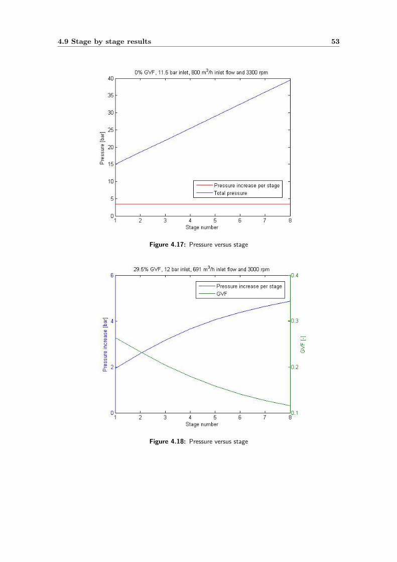
4.9 Stage by stage results 53
Figure 4.17: Pressure versus stage
Figure 4.18: Pressure versus stage

54 One Dimensional Two Phase Control Volume Modelling
Chapter 5
Conclusion
The purpose of this MSc thesis was to develop a performance model that is able to assessthe performance of a helico axial multiphase pump for remote monitory purpose. By usinga multiphase pump performance model to continuously monitor the pump performanceduring the operation, the reliability and efficiency of the pumps can be increased whichwill lead to higher production and lower operation cost. Therefore having a multiphasepump performance model can be extremely beneficial.
An one dimensional two phase flow control volume approach is used to develop the multi-phase performance model. This approach has not only incorporated the inlet conditionssuch as volumetric flow, GVF, gas and liquid density, but also the pump geometries suchas the rotor diameter. Applying the mass and the Newton’s law of motion to the pre-defined control volume, the governing one dimensional two phase flow equation can beobtained. Combining techniques such as velocity triangle with computational tools likeSolver within Microsoft Excel, the performance of a multiphase pump is predicted. Inaddition, an empirical equation is developed to calculate the exit flow angle, this empir-ical equation is developed based on the experimental data provided by the vendor andit is an essential part of the entire pump performance calculation. For validating theoverall accuracy and applicability of the model, an additional set of data is required andit is provided by the vendor. This additional set of data is generated using vendor’sown multiphase performance tool. The overall accuracy of the model is satisfying whenthe operation conditions under 40% GVF. This range is sufficient for the purpose of thisproject, because the expected operation conditions will not exceed this GVF limit.
There are several possible reasons to explain the discrepancy of the model. The first oneis that the discrepancy is caused by the empirical exit flow angle equation. This equationis developed based on a set of experimental data where the maximum GVF is 30%. Theempirical equation is accurate only within that GVF range, for GVF range beyond 30%,the reliability of the model decreases significantly. It turned out this empirical equation isapplicable up to 40% GVF, however the results are not longer reliable beyond that point.The second possible reason for this discrepancy is that during the analysis, the flow isassumed to exit the rotor with the same flow angle for all the stages. This assumption
55
56 Conclusion
is only valid for low GVF conditions and near the design conditions. A different exitangle will result into a different pressure increase. For the simplicity of the analysis, theexit flow angle is assumed to be constant for all the stages. The third reason is that theseparation of gas and liquid has not been taken into account. The separation of gas andliquid occurs at high GVF conditions where gas tends to accumulate on the suction sideof the rotor blade. This will reduce the effective stream area of the fluid, which will effectthe fluid relative velocity and the final pressure increase. The stream area is assumed tobe constant, and it is calculated based on the pump geometry. Another possible reasonfor the discrepancy is that isothermal condition is assumed during the analysis where thetemperature rise in the fluid is being neglected. This assumption is valid up to 60%.These are the possible reasons for causing the discrepancy of the mode.
There are several ways to improve the model. First of all, to improve the empirical exitflow angle equation by acquiring more experimental data, especially for the high GVFconditions such as 40% and 60%. It will be ideal if the actual blade angle can be disclosedby the vendor in the future, so the conventional methods can be applied to find thepump performance. Secondly, instead of doing an one dimensional analysis, do a twodimensional multiphase fluid analysis where the gas movement in the lateral direction( perpendicular to the stream direction) can be captured. This lateral gas movementcauses the gas accumulation at the high GVF conditions. Thirdly, investigating how theexit flow angle changes after each stage and what causes that change. Finally, instead ofusing an isothermal assumption, a polytropic assumption can be used during the analysis.However it does required more gas and liquid data such as specific heat capacity.

References
[1] Paul Ten Held. Development Release for Application of Sulzer’s Multi PhaseHelico-Axial Type Pump in OMEGA MEG Process. Shell Global Solutions, 2009.GS.09.53944.
[2] Sulzer Pumps. High performance multiphase pump. Brochure, 2013.
[3] OneSubsea. MPP Performance Curves. Technical report, 2014.
[4] Christian Brix Jacobsen. The Centrifugal Pump. Technical report, Grundfos Re-search And Technology.
[5] National Programme on Technology Enchance Learning. Fluid machinery: Lecture40.
[6] UTM Faculty of Mechnical Engineering. Fluid machine lecture.
[7] Igor J. Karassik, Joseph P. Messina, Paul Cooper, Charles C. Heald. Pump Handbook.McGraw Hill, 2008.
[8] Okitsugu Furuya. An Analytical Model for Prediction of Two-Phase (Noncondens-able) Flow Pump Performance . Journal of Fluids Engineering, 107:139–147, 1985.
[9] OneSubsea. Draugen 2013 Infill Drilling Project. Technical report, 2013.
[10] Meherwan P Boyce. Centrifugal compressors: a basic guide. 2003.
[11] S. Zakem. Determination of gas accumulation and two-phase slip velocity ratio in arotating impeller. In Polyphase Flow and Transport Technology.
[12] O. Furuya, S. Maekawa. An Analytical Model for Prediction of Two-Phase FlowPump Performance - Condensable Flow Case . In J.W. Hoyt, O. Furuya, editor,Cavitationand Multiphase Flow Furum - 1985.
[13] Christian Bratu. Rotodynamic two-phase pump performances. In Society ofPetroleum Engineers.
57

58 References
[14] Kiyoshi. Minemura, Tomomi. Uchiyama, Shinji Shoda, and Kazuyuki Egshira. Pre-diction of Air-Water Two-Phase Flow Performance of Centrifugal Pump Baed onOne-Dimensional Two-Fluid Model. Journal of Fluids Engineering, 120:327–334,1998.
[15] A. Poullikkas. Compressibility and Condensation Effects When Pumping Gas-LiquidMixtures . Fluid Dynamics Research.
[16] Roberto Fraustini and Frank Kenyery. 3D Flow Modeling In One Helical-Axial Mul-tiphase Pump Stage Through CFD . USB-LABCEM.
[17] Y. A. Cengel,J. M. Cimbala,R. H. Turner. Fundamentals of Thermal-Fluid ScienceSI 4th edition. McGraw-Hill, 2012.
[18] Garr M. Jones. Pump Station Design. Butterworth-Heinemann Ltdl, 2008.
[19] S. L. Dixon,C. A. Hall. Fluid Mechnical And Thermodynamics Of Turbomachinery.Elsevier Inc., 2010.
[20] Jose. Caridad, Miquel. Asuaje, Franck. Kenyery, Andres. Tremante, and OrlandoAguillon. Characterization of a centrifugal pump impeller under two-phase flowconditions. Journal of Petroleum Science and Engineering, 63:18–22, 2008.
[21] Jose A. Caridad and Frank Kenyery. Slip Factor For Centrifugal Impellers UnderSingle and Two-Phase Flow Conditions. Journal of Fluids Engineering, 127:317–321,2005.
[22] M. Van der Jagt. Separation Postponement by means of Periodic Surface Excitation.Master’s thesis, Delft University of Technology, Faculty of Aerospace Engineering,Chair of Aerodynamics, 2008.
[23] Grundfos Research and Technology. The Centrifugal Pumpl. Technical report,Grundfos Research And Technology, 1972. NASA TM X-2643.
[24] Framo Engineering AS. Framo multiphase pumps for offshore and land applications.Brochure, 2002.


