Embed Size (px)
Citation preview

ELSEVIER Finite Elements in Analysis and Design 25 (1997) 85-109
FINITE ELEMENTS IN ANALYSIS AND DESIGN
Delaunay mesh generation governed by metric specifications Part II. Applications
Houman Borouchaki*, Paul Louis George, Bijan Mohammadi INRIA, Domaine de Voluceau, Rocquencourt, BP 105, 78153 Le Chesnay Cedex, France
Abstract
This paper gives some application examples resulting from a governed Delaunay type mesh generation method. Isotropic and anisotropic cases are considered, these specifications being given via a metric map. The paper illustrates a study whose algorithmical aspects are described in a report referred to as part I. Academic examples as well as examples in CFD are discussed.
Keywords: Delaunay triangulation; Anisotropic mesh generation; Mesh adaption; A posteriori estimation
1. Introduction
A mesh generation method governed by a metric map has been proposed in the first part of this study [-1]. This method is an extension of the classical Delaunay mesh generation method in the case where a specification (specified by the above map) is given. The mesh generation method is governed by this map and the aim is to obtain an "optimal" mesh with respect to the map.
To validate the method, a prototype has been developed, the corresponding algorithms have been developed in C and For t ran 90 by H. Borouchaki (for the domain mesh generation part) and by P. Laug (for the boundary mesh generation part). This prototype is now applied to several examples, including both academic tests (Section 3) and typical applications in C F D (Section 4).
Before discussing these examples, a short summary of the mesh generation method is given (Section 2) whose detailed description can be found in [-1].
2. Outlines of the mesh generation method
The classical Delaunay mesh generation method (i.e. where an Euclidean space is used) is extended to the case where the resulting mesh must be "ideal" with respect to an isotropic or
* Corresponding author.
0168-874X/97/$17.00 © 1997 Elsevier Science B.V. All rights reserved PII S0 1 68 -874X(96)00065-0

86 H. Borouchaki et al.. Uinite Elements m Analysis and Design 25 (1997) ,~5 109
anisotropic map of specifications. It has been shown that the extension relies in "simply" consider- ing a Riemannian space and to extend within this context the different algorithms of the mesh generation process.
Two main basic procedures have been extended in the Riemannian situation: the incremental point insertion process, namely, the Delaunay kernel and the way in which the field points are created in the domain under consideration. As these two aspects are strongly based on length computations, it has been seen how to replace the notion of a length by the corresponding Riemannian notion.
The Riemannian space is defined by a metric map and the case where several metrics are specified at each point of the domain has led us to introduce the notion of metric intersection. Thus, it has been shown how to apply the mesh generation method when not only one metric is specified but when a series of metrics is entered as governing specification~ in this way multicriteria adaptation has been considered.
3. Academic test examples
Some academic examples are discussed in this section. The governing specification is given as an analytic function defined in [~2 The mesh generation process is iterative. First of all, a classical mesh of the domain is created (by means of the classical mesh generation method), then the value of the governing function at its vertices is computed. This discrete field specification provides metric information for the mesh generation algorithm to create the first adapted mesh.
The way in which the current mesh is more or less fine and the way in which the specification function varies result in a more or less fine capture of this function. As a consequence, the first mesh is not, in general, adapted within the whole domain but merely in some neighborhood of the vertices of the previous mesh. Thus, it is required to iterate the process while the specification is updated. The pair (mesh, map) constitutes the contro l space used in the next iteration. As will be seen, few iterations result in a stable output mesh such that the given governing function is globally satisfied. All the edges in the mesh enjoy a unit length with respect to the control space and, a new iteration will not modify the output in a significant way.
Four examples are now discussed, and for each of them one or several con t inuous metric maps are specified. For the first two, the map is isotropic while for the last two, it is anisotropic.
For each case, a loop of adaptations has been made. For each iteration the metric map is evaluated using the initial continuous map.
With each example, we present a table indicating, for iteration ni, the following parameters • np the number of points, • nt the number of triangles, • t the CPU time required for mesh generation (in seconds on a HP735/99 MHz) and • F the worst element quality (from 0 and 1).
The table also displays the values hmin and hmax showing, for each point, the minimal and the maximal sizes independent of the directions and, in the anisotropic case, the values rmin and rmax showing, for each point, the minimum and the maximum of the quantity h2 /h l , where hi (resp. hz) is the minimal (resp. maximal) size according to every possible direction.

H. Borouchaki et al./ Finite Elements in Analysis and Design 25 (1997) 85-109 87
For each example, the meshes corresponding to some iterations of the adaptation loop are shown. To help the reader to appreciate the resulting meshes, two diagrams are given. Let Ti be the mesh of iteration i governed by the control space (Ti- 1, Hi), where Hi is the metric map specified at the vertices of Ti- 1. The first (resp. second) diagram, noted as D1 (resp. D2) on the figures, reports the number of edges in mesh Ti- 1 (resp. Ti) with a given length in the control space (Ti- 1, Hi). The first diagram shows whether mesh Ti- 1 is satisfactory or not in control space (Ti- 1, Hi) and serves to decide if the adaptation loop needs to be pursued or not. The second diagram shows if mesh Ti is satisfactory or not in control space (Ti- 1, Hi) and illustrates the capabilities of the proposed mesh generation method.
The diagrams report the value of q ( f ) the quality of the edge. L e t f = I-P, Q] be an edge of mesh Ti or mesh T~_I, then, the quality q( f ) in the control space (Ti-1, Hi) is defined by
I l(P Q) q ( f ) = '1
if I(P, Q) >~ 1,
if I(P, Q) < 1
and the scale is considered as uniform with respect to q.
Remark. The gradation of the x axis, in the diagrams, must be understood as follows: • symmetry with respect to abscissa 100, • uniform variation of the lengths from 0 to 1 in the interval [0, 100], • uniform variation of the inverse of the lengths from 1 to vo in the interval [100, 200].
3.1. Isotropic case
Two isotropic examples follow.
3.1.1. Example 1
The first example corresponds to a case where only one metric map is specified in the domain. The domain is a rectangle of size 7 x 9. The map is defined in this rectangle by the function
f 1 .0 -½0 .95y if y~<2,
0.05 × 20 ~y- 2j/2.5 if 2 < y ~< 4.5,
h(x,y) = 0 . 2 ~y-4"5)/25 if 4.5 < y ~< 7,
0 . 2 + 0 . 8 ( ½ ( y - 7 ) ) 4 if 7 < y ~ < 9 .
Three iterations have been made in the adaptation loop, Fig. 1 displays the initial mesh (iteration 0) and iterations 1, 2 and 3. One can see the variation of the diagrams D 1 and D2 on Fig. 2 and 3.

88 H. Borouchaki et al./ Finite Elements in Anal)~is and Design 25 (1997) 85 109
I l e r o ( , on 0 / \ / \ /
/ "~\ / , / " \ /
- + y.
k ~ , . " \
I~ro~i on i
I ~ e r a on 2 I { e r o ~ i on 3
Fig. 1. Example 1 Ilsotropic case}.
We have seen that the final mesh has been obtained since iteration 2 by looking at Fig. l where the two meshes (in the lower part) are (almost) identical as well as by analysing the variation of the corresponding diagrams. Table 1 reporting the figures associated with the different meshes also shows this result.
The value of F is due to the fact that the size strongly varies within a short interval.

4 0
35
30
2 5
20
15
10
5
0
350
300
250
200
150
I00
SO
i m _ 1 I , I I
20 40 ~0 80 I00 120 140 160
i i
'DI' -- 'D2 ......
I 210 4 0
~, ~ i~: ,;\
60 80 100 120 140 160 180 200
Fig. 2. Diagrams D1 and D2, Example 1 (iteration 0).
"DI' 'D2 . . . . . .
H. Borouchaki et al./ Finite Elements in Analysis and Design 25 (1997) 85-109 89
I
180
Fig. 3. Diagrams D1 and D2, Example 1 (iteration 3).
2 0 0
Table 1 Output for Example 1
ni np nt t F hmin hmax
0 106 1 1754 2 2218 3 2227
206 0.05 0.83 1.0 1.0 3502 0.85 0.64 0.05 1.0 4430 1.30 0.70 0.05 1.0 4448 1.30 0.70 0.05 1.0

9 0 H. Borouchaki et al. : Finite Elements in Analysis and Design 25 (1997) 8 5 109
3.1.2. Example 2 The second example considers the case where two metric maps are specified in the domain. The
latter is a circle with radius 5 and whose centre is at the origin. The maps are defined, in this circle, by two functions, h~ and he of r and 0, the polar coordinates.
h~(r, 0) = 0.Sir - 0.201 + 0.02,
h2(r, 0) = 0.8fr + 0.20] + 0.05.
Fine elements are expected by the two curves
r = 0 . 2 0 and r = - 0 . 2 0
with a linear variation for the sizes between the two curves. It can be noticed that this problem includes a case where the first given metric intersects the other.
For this example five iterations have been performed in the adaptat ion loop. Fig. 4 displays the initial (iteration 0) and the iterations 1, 3 and 5 and Fig. 5 shows an enlargement of this last
II~ro{, on 0 ]-~ro[, on l
1 I i ~ r ~ t i Qn 3 Z l , ~ r 0 1 ~ t:n
Fig. 4. Example 2 dsotropic case).

H. Borouchaki et al./ Finite Elements in Analysis and Design 25 (1997) 85-109 91
Fig. 5. Example 2 (iteration 5).
50
45
40
35
30
25
20
1S
10
5
0 0
I
2O
i i i ,1 ! 1 i i
k ' D 1 ' - -
' D 2 . . . . . .
i 'i
40 60 80 i00 120 140 160 180 200
Fig, 6. Diagrams D1 and D2, Example 2 (iteration 0).
iteration. The variation of diagrams D1 and D2 are shown in Figs. 6 and 7. The converged result is obtained at iteration 5. Table 2 reports the characteristics associated with the different meshes.
The size variation is in the range of the 25.

92 H. Borouchaki et al./ Finite Elements in Analysis and Design 25 (1997) 85-109
1200
I000
BOO
600
400
200
0 i I t
0 20 40 180 200
f , , , , ,
' D 1 ' - -
1 ' D 2 . . . . . .
I
60 80 100 120 140 160
Fig. 7. Diagrams DI and D2, Example 2 iteration 5).
Table 2 Statistics for Example 2
ni np nt t F hmi. hmax
0 168 330 0.08 0.72 0.8 0.8 1 6497 12988 3.30 0.68 0.02 0.5 3 10715 21424 8.60 0.50 0.02 0.5 5 11430 22854 9.80 0.56 0.02 0.5
3.2. Anisotropic case
Two examples are now given for the anisotropic case.
3.2.1. Example 3 The third example considers the case where one anisotroplc map is specified in the domain. The
domain is a rectangle of size 7 x 9. Within this rectangle is given the metric map, which is defined by the diagonal matrix of order 2:

H. Borouchaki et al./ Finite Elements in Analysis and Design 25 (1997) 85-109 93
with
hi (x, y) =
1. - 0.95 ½x
0.05 x 20 (x - 2)/1.5
0 . 2 ( x - 3.5)/1.5
0.2 + o.8 (½(x - 5))'*
if x~<2 ,
if 2 < x ~< 3.5,
if 3.5 < x ~< 5,
if 5 < x ~ < 7 ,
h2(x, y) =
1.0 - ½ 0.95 y
0.05 X 20 (y - 2)/2.5
0 . 2 ( y -- 4.5)/2.5
0.2 + 0.8 (½(y - 7))'*
if y~<2,
i f 2 < y ~ < 4 . 5 ,
if 4.5 < y ~<7,
i f 7 < y ~ < 9 .
These data mean that the expected result must contain in the direction of the x-axis ele- ments whose size corresponds (via a mapping) to the discretization observed on the lower size of the rectangle and in the direction y-axis the size observed on the left side of the rectangle. Looking at the mesh of i teration 3, it is obvious to note that these requirements compare well with both the size and the aspect ratio of the elements. It can be noticed that the m a x i m u m stretching is about 20.
For this example, three iterations have been made in the adapta t ion loop. Fig. 8 displays the initial mesh (iteration 0) and iterations 1, 2 and 3. The variations of diagrams D1 and D2 are shown in Figs. 9 and 10. Table 3 reports the characteristics of the different meshes.
3.2.2. Example 4 The fourth example considers the case where two metric maps are specified in the domain,
a square centred at the origin and with size 8. The expected mesh must include stretched elements by the tangent of the curves whose equat ions are x 3 - y2 + 2 - 32x = 0 where 2 is the parameter. This parameter is compu ted at each point of the domain where it is defined. With respect to 2, the first metric at point (x, y) is given by hi, h2, the sizes, and 0, the angle of anisotropy, defined as follows:
~min(0.2(2 - - 1) 3 q- 0 .005 , 1.) if 2 ~ 1, hx(x, y) = [min(0.2(1 - - , ~ ) 2 ..t_ 0.01, 1.) if 2 < 1,
~min(0.2(2 - 1) 3 + 0.2, 1.) if 2 >~ 1, hi(x, y) = [min(0.2(1 - 2) 2 n t- 0.2, 1.) if 2 < 1,
- - 2 y 0 = arctan
3(x 2 -- 2)"

94 H. Borouchaki et al. ,,/Finite Elements in Analysis and Design 25 (1997) 85-109
p -
I{ero~, on 1
l[erol, or, 2 l~erol, on
Fig. 8. Example 3 (anisotropic case).
The second metric map is isotropic and given by h(x, y) = (x - 1) 2 n u y2 + 0.01, from which result a size of about 0.01 at the point (1, 0) and a quadratic variation elsewhere. The above point can be seen in Fig. 13 in the lower part at the right.
Seven iterations have been performed in the adaptation loop. Fig. 11 displays the initial mesh (iteration 0) and iterations 1, 3 and 7. Two enlargements are given, Fig. 12 for the entire mesh and,

H. Borouchaki et al./ Finite Elements in Analysis and Design 25 (1997) 85-109 95
14
12
I0
300
250
200
150
I00
50
'DI' -- 'D2 ' .....
I
| l
I
l 'If', ''e,l llll"
60 80 i00
"ii,i!iiA 120
I |
2 0 40 200 140 160 180
Fig. 9. Diagrams D1 and D2, Example 3 (iteration 0).
I I - I . I I
20 40 60 80 i00 120 140 160
i
'DI' ' D2 ......
I
180 200
Fig. 10. Diagrams D1 and D2, Example 3 (iteration 3).
Table 3 Statistics for Example 3
ni np nt t F hmin hm.~ rmi . rmax
0 52 98 1 815 1624 2 1328 2650 3 1298 2590
0.04 0.80 1.5 1.5 - - - - 0.5 0.45 0.02 1.5 1.0 9.7 1.0 0.44 0.02 1.5 1.0 19.5 1.0 0.43 0.02 1.5 1.0 19.5

96 H. Borouchaki et al./ Finite Elements in Analysis and Design 25 (1997) 85 109
I i
9 It~a{, on 7
Fig. 11. Example 4 (anisotropic case).
Fig. 13 for four local views. The variations of diagrams D1 and D2 are reported in Figs. 14 and 15. Table 4 lists the statistics corresponding to the different meshes.
4. CFD application examples
In this section are presented a series of complex compressible inviscid and viscous flow configurations in transonic and supersonic range.
The Navier-Stokes NSC2KE software is used [2]. This solver is based on a finite volume Galerkin technique where the unknowns are located at the nodes. This makes easier the treatment of the viscous terms as in finite element method. A four steps Runge-Kut ta method is used for time discretization.

H. Borouchaki et al./ Finite Elements in Analysis and Design 25 (1997) 85-109 97
Fig. 12. Example 4 (iteration 7).
The metric map is the intersection of the metrics associated with the conservative variables (p, pu, pv, p(Cv T + ½u12)) where p is the density, (u, v) the velocity and T the temperature. More precisely, for each of these conservative variables, noted as (ffi, i = 1 . . . . ,4), a metric tensor ~'~ (2, 2) is defined by the following algorithm:
1. Normalizat ion of ~O~ in 1-0, 1] (to avoid dimensional incompatibility). 2. Computat ion of the metric of ~ki, proportional to the Hessian of ffi, in a weak sense, for all
nodes is
1 ~t3~kg ~wi~ o/gi(j, l) = (3L2 Cis) ,] c~xj t3xt '
where wi~ is the p1 basis function at node is and Cis is the surface of the dual cell around node is. L defines the edge length in metric ~ ' i . Thus, all the edges have as length L in the metric.
3. Correction of the Hessian at the boundary nodes in the normal direction by using an average of the values over the field nodes.

98 H. Borouchaki et al./ Finite Elements in Analysis and Design 25 (1997) 85. 109
Fig. 13. Example 4 (iteration 7. enlargementj.
4. Limitation of the elgenvalues by ~.o1~,, = l/h~a~ and '~-max = l/h2ax where hmin and hmax are the external desired edge sizes.
5. Intersection of metric ..//; with metric -//k for k ¢ i using the algorithm described in [1].
4.1. Supersonic scram/et
This case consists of an Euler computation in a scramjet at Mach 3. The geometry is symmetric but the computat ion has been performed in the whole domain to see ifa symmetric solution can be obtained on an unstructured mesh.
The upper wall is defined by 6 points tdimensions in meter)
(0.0,3.5), (0.4,3.5), (4.9,2.9), (12.6,2.12), (14.25,1.92) and (16.9,1.7).

. . ~ . . ~ . t . o
~'~" ~'.~
r j ~
0 .
r~
:o
o
o i i i I I I I
i l I i
o 1 i , , ! , |
C~
o o " - . . : ~
o
I i I I . , I i l
t ~
I

100 H. Borouchaki et al./ Finite Elements in Analysis and Design 25 ('1997) 85-109
The lower obstacle is defined by 5 points
(4.9,1.4) (12.6,1.4k (14.25,1.2), (9.4,0.5) and (8A0.5).
The symmetry axis is defined by the segment
(0.0,0.0) and (16,9, 0.0).
Six adaptations have been made. Between each of them, up to 400 iterations of the Navier-Stokes solver have been performed. Although the mesh is unstructured, a symmetry is
l~vo~i oo @
"" ~i ~'"~\ . . . . . . ' J
F ig . 16. S c r a m j e t , m e s h e s .

H. Borouchaki et al./ Finite Elements in Analysis and Design 25 (1997) 85-109 101
Fig. 17. Scramjet, iso-density contours.
observed in the solution. It can be seen that the solver runs well with large distorsions in the mesh without producing oscillations. The adapta t ion coefficients are as follows
hmin = 5 x 10⁻³, hma x = 2., L = 10-3
Due to the complexity of the configuration, the same computa t ion with a structured mesh would require about 1 0 7 points meaning that elements of size hmln must be used to obtain the same accuracy. In our method, the finer mesh includes only 30 000 points (i.e. a ratio of 300). In addition,

102 H. Borouchaki et al. ,, FTnite Elements in Analvsis and Design 25 (1997) 85-109
/ , . " . - ? : . "= -7~"~ _ • 5 ? 5 - ~
, . d,~ ' ' - * - " ' ' " X . . ~ r L ' . ' > i ~ % . , ~ b - . : ~ - ~ , , ~ " '
" - , . " "%--,~ ,~" .)~ ~ _ - " g ~ J b K . . ' . ~ - - ~ " \ ~
~ . , , , , . . ~ . / , / ~ ' , ' , , . , ,~.
~-- ~ , ~-, ,
5g~
. . ~ \ X - ~ - x ~z -~ ' , - '~ ' - . .d ' , , :~ - -~- . . x- ~' ~.~- , ' /
. . . . . . . : , ¢ - . 11 /~ :¢?~,, ca _ ,
, -~ ~ - "~,
. - ._ ",~. I \ ~
Fig. 18. F ish ta i l • meshes and iso-density contours.
the adaptation of the mesh improves the convergence of the computation due to its multigrid effect. Thus, only 2400 explicit iterations have been used to reduce the residual by four orders of magnitude. Moreover, as a local time step strategy is used, we take advantage of an adapted mesh while, using a structured mesh, this effect would not be present.
Figs. 16 and 17 show the mesh and the iso-density contours at iterations 0 (initial), 2 and 6 (final). The initial mesh contains about 4000 points, at step 2, about 23000 points and, finally, about

H. Borouchaki et al./ Finite Elements in Analysis and Design 25 (1997) 85-109
/
/
/
Fig. 19. Fish tail, meshes and iso-density contours (continued).
103
30 000 points. The number of points is in practice almost constant in steps 4-6. At iteration 6, the maximal stretching is about 120 and the C P U time required for the mesh construct ion is about 30 s using an HP735/99 M H z (this corresponds to less than 10% of the total C P U time).

104 H. Borouchaki et al., Finite Elements in Analysis and Design 25 (1997) 85-109
. ,\ , , . J , /
•?,iii
f - ' ~
/
Fig, 20. Fish tail, mesh at iteration 6.
- - I x
4.2. Transonic viscous.flow around a Naca-O012
This example concerns a viscous computation around a wing profile at mach 0.95 and Reynolds number 5000. A fish tail configuration is obtained with a Von Karmann type instationarity resulting from the interaction between the strong shock and the wake.
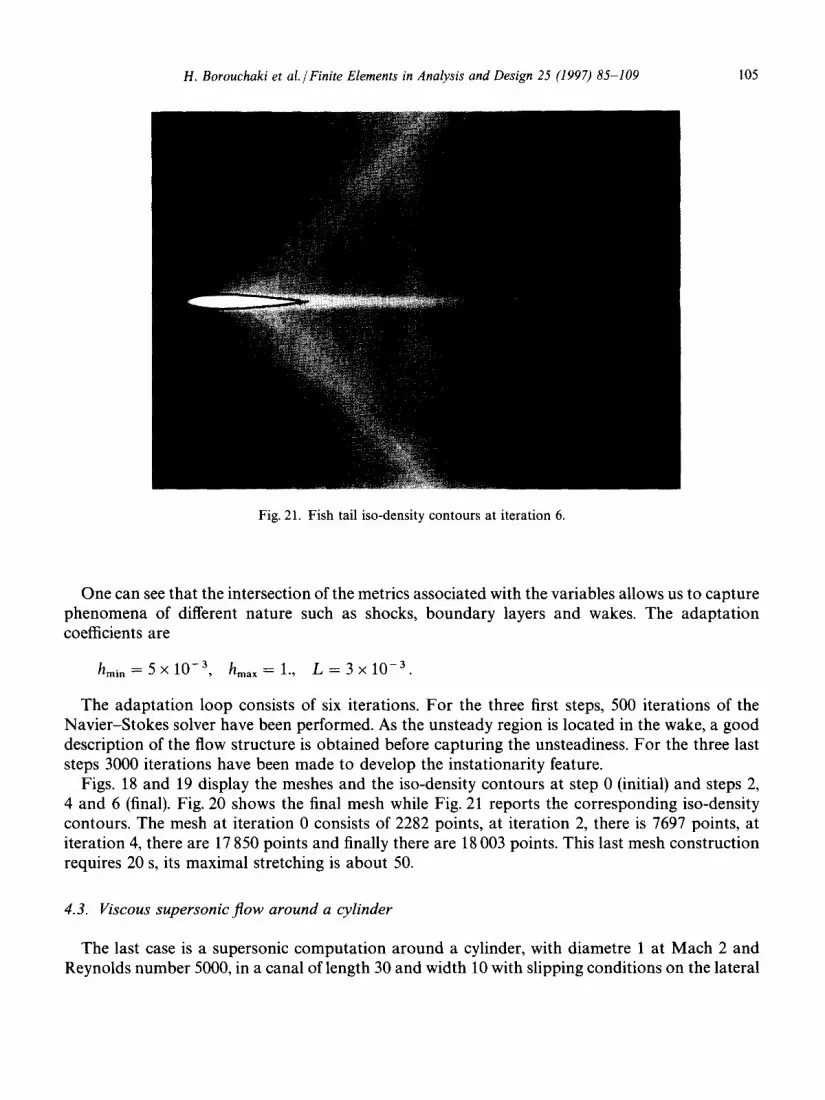
H. Borouchaki et al./ Finite Elements in Analysis and Design 25 (1997) 85-109 105
Fig. 21. Fish tail iso-density contours at iteration 6.
One can see that the intersection of the metrics associated with the variables allows us to capture phenomena of different nature such as shocks, boundary layers and wakes. The adaptation coefficients are
hmi n = 5 × 10 -3, hmax = 1., L = 3 × 10 - 3
The adaptation loop consists of six iterations. For the three first steps, 500 iterations of the Navier-Stokes solver have been performed. As the unsteady region is located in the wake, a good description of the flow structure is obtained before capturing the unsteadiness. For the three last steps 3000 iterations have been made to develop the instationarity feature.
Figs. 18 and 19 display the meshes and the iso-density contours at step 0 (initial) and steps 2, 4 and 6 (final). Fig. 20 shows the final mesh while Fig. 21 reports the corresponding iso-density contours. The mesh at iteration 0 consists of 2282 points, at iteration 2, there is 7697 points, at iteration 4, there are 17 850 points and finally there are 18 003 points. This last mesh construction requires 20 s, its maximal stretching is about 50.
4.3. Viscous supersonic f l ow around a cylinder
The last case is a supersonic computat ion around a cylinder, with diametre 1 at Mach 2 and Reynolds number 5000, in a canal of length 30 and width 10 with slipping conditions on the lateral

106 H. Borouchaki el al. : Finite Elements #7 Anah'sis and Design 25 (1997) 85 109
: ' ' - , : ~ ,-~_-: -~" ,' <7 ,'U---,~ ~ v) l J , -\~2_' , - r - - ~ 4
Fig. 22. M e s h a n d e n l a r g e m e n t at i t e r a t i o n 60 a r o u n d a cy l i nde r .
walls. This case is known to be very difficult as instationarities exist in the wake and as the shocks are not easy to properly locate. Here, the aim is to show the capability of the method to follow the shock fronts as, in this case and contrary to the previous, the instationarity is not limited to a limited region.
The adaptat ion coefficients are as follows:
hmi n = 5 × l 0 3 , hma ~ = 2., L = 3 x 10 3
Once again, the complexity of the configuration would lead to use elements of size hmi n in the case of a structured mesh to be able to achieve the same accuracy. Thus about 6 x 10⁷ points would be necessary (i.e. 30 x 10/5(5 x 10 ,~)2). With our method, the number of points remains almost stable and is about 50 000.
The adaptat ion loop includes 110 iterations. At each step, 500 iterations of the Navier-Stokes solver have been performed.

H. Borouchaki et al./ Finite Elements in Analysis and Design 25 (1997) 85-109 107
- _ _ . ~ , A i r .
Fig. 23. Mesh and enlargement at iteration 110 around a cylinder.
The meshes and the iso-density contours after 60 and 110 adaptations are shown in Figs. 22-25. One can see that the location of the shocks have been completely changed and that the adapted method follows this variation. Unfortunately, these configurations cannot be computed with a structured mesh and thus, no comparisons can be made. Once again, the metric intersection allows us to capture the shocks, boundary layers, wakes as well as the discontinuity in the contact. At iteration 60, the mesh includes 50 883 points and, at iteration 110, it has 54460 points, the CPU time required is 74 s and the maximal stretching is about 170.
5. Concluding remarks
The proposed mesh generation algorithm has been tested on different cases in ~2 domains including those described in this paper. These application examples showed the capabilities of the

108 H. Borouchaki et al. Finite Elements in Analysis and Design 25 (1997) 85-109
Fig. 24. Meshes at iterations 60 and 110 around a cylinder.
method and lead us to think that the two dimensional mesh generation problem seems to be almost satisfactorily solved. A priori, no special difficulties are expected to extend the proposed method to three dimensions. Nevertheless, some time must be spent to develop the corresponding software programs and to validate the output so obtained first by some academic examples and then by concrete and industrial applications.
As a final remark, it can be mentioned that the software package corresponding to the proposed mesh generation method is available freely (contact the authors).

H. Borouchaki et al./ Finite Elements in Analysis and Design 25 (1997) 85-109 109
, / ~ ~ ~ / , W . , . ' / , , . , " / , ' ." ' ~ " - Z I ~ " , . : ; L , " . /L, / / , / / ,.." / ,; ,' . , ' / - - > , > - x •
/ ~ , . /~. V/.,.~-".Z.4.9 / / . . ' / . . ' . , / / ,, ...~J..-., ~ ' . N
/ ~ 7 , ' . ' Y / . ; , . / . / 1 / I " ~ " ~ . ~ % / _ . J . / . / ~ ~ J ~ " / .~JJ)'~ ~ ; i ',
ll ........ ~., , .-,
X , ~ " , , X ' : ' , . . , X ' , " , - . , \ " , ' , '., \ '. \ '. "~.---' , " / ..
' k ' u ~ , X ' , . \ ' ~ V \ ' , \ ' , ' \ ' ! ' ! / ', ! } ) ) ) ,,' / " > - < " - - " <, ,,. / / "" ,sq-
Fig. 25. Iso-density contours at iterations 60 and 110 around a cylinder.
References
[1] H. Borouchaki, P.L. George, F. Hecht, P. Laug and E, Saltel, "Delaunay mesh generation governed by metric specification. Part I: Algorithms", Finite Elements Anal. and Des. (this issue).
[2] B. Mohammadi, Fluid dynamics computation with NSC2KE a user-Guide, Release 1.0, Rapport Technique INRIA, No. 164, 1994.
I3] H. Borouchaki and P. Laug, Le mailleur bidimensionnel BL2D: manuel d'utilisation et documentation, Rapport Technique INRIA, No. 0185, 1995 (in French),


