Comp. Part. Mech. (2014) 1:199–209DOI 10.1007/s40571-014-0022-7

On mesh-particle techniques

Rainald Löhner · Fernando Camelli · Joseph D. Baum ·Fumiya Togashi · Orlando Soto

Received: 22 December 2013 / Revised: 31 March 2014 / Accepted: 3 April 2014 / Published online: 9 May 2014© Springer International Publishing Switzerland 2014

Abstract The treatment of dilute solid (or liquid) phasesvia Lagrangian particles within mesh-based gas-dynamics(or hydrodynamic) codes is common in computational fluiddynamics. While these techniques work very well for a largespectrum of physical parameters, in some cases, notablyfor very light or very heavy particles, numerical instabili-ties appear. The present paper examines ways of mitigatingthese instabilities, and summarizes important implementa-tional issues.

Keywords Particle methods · Finite elements · Computa-tional fluid dynamics

1 Introduction

When solving the compressible two-phase equations, the gas,as a continuum, is best represented by a set of partial differen-tial equations (the Navier–Stokes equations) that are numer-ically solved on a mesh. Thus, the gas characteristics arecalculated at the mesh points within the flowfield. However,as the particles (or fragments) may be relatively sparse in theflowfield, they can be modeled by either:

Electronic supplementary material The online version of thisarticle (doi:10.1007/s40571-014-0022-7) contains supplementarymaterial, which is available to authorized users.

R. Löhner (B) · F. CamelliDepartment of Computational and Data Science M.S. 6A2,CFD Center, College of Science, George Mason University Fairfax,Fairfax, VA 22030-4444, USAe-mail: rlohner@gmu.edu

J. D. Baum · F. Togashi · O. SotoAdvanced Technology Group, SAIC, McLean, VA 22020, USA

(a) A continuum description, i.e. in the same manner as thefluid flow, or

(b) A particle (or Lagrangian) description, where individ-ual particles (or groups of particles) are monitored andtracked in the flow.

Although the continuum (so-called multi-fluid) method hasproven relatively successful for compressible two-phaseflows, the inherent assumptions of the continuum approachlead to several disadvantages which may be countered with aLagrangian treatment for dilute flows [15,16,23,30,70]. Thecontinuum assumption cannot robustly account for local dif-ferences in particle characteristics, particularly if the particlesare polydispersed. In addition, the only boundary conditionsthat can be considered in a straightforward manner are slip-ping and sticking, whereas reflection boundary conditions,such as specular and diffuse reflection, may be additionallyconsidered with a Lagrangian approach. Turbulent disper-sion can also be treated on a more fundamental basis. Finally,numerical diffusion of the particle density can be eliminatedby employing Lagrangian particles due to their pointwisespatial accuracy.

While a Lagrangian approach offers many potentialadvantages, this method also creates problems that shouldbe addressed by the model. For instance, large numbers ofparticles may cause a Lagrangian analysis to be memoryintensive. This problem is circumvented by treating parcelsof particles, i.e. doing the detailed analysis for one particleand then applying the effect of many. In addition, continu-ous mapping and remapping of particles to their respectiveelements may increase computational requirements, particu-larly for unstructured grids.

The present paper summarizes the procedures used, aswell as some of the difficulties encountered when implement-

123

200 Comp. Part. Mech. (2014) 1:199–209

ing a particle description of diluted phases in a flow solverbased on unstructured grids.

2 Equations describing the motion of particles

In order to describe the interaction of particles with the flow,the mass, forces and energy/ work exchanged between theflowfield and the particles must be defined. Before going on,we need to define the physical parameters involved. For thefluid, we denote by ρ, p, e, T, k, vi , μ, γ and cv the den-sity, pressure, specific total energy, temperature, conductiv-ity, velocity in direction xi , viscosity, ratio of specific heatsand the specific heat at constant volume. For the particles,we denote by ρp, Tp, vpi , d, cp and Q the density, temper-ature, velocity in direction xi , equivalent diameter, and heattransferred per unit volume. In what follows, we will refer toparticles, fragments, or chunks collectively as particles.

Making the classic assumptions that the particles may berepresented by an equivalent sphere of diameter d, the dragforces D acting on the particles will be due to the differenceof fluid and particle velocity:

D = πd2

4· cD · 1

2ρ|v − vp|(v − vp). (1)

The drag coefficient cD is obtained empirically from theReynolds-number Re:

Re = ρ|v − vp|dμ

(2)

as:

cD = max

(0.1,

24

Re

(1 + 0.15Re0.687

))

The lower bound of cD = 0.1 is required to obtain the properlimit for the Euler equations, where Re → ∞. The heattransferred between the particles and the fluid is given by

Q = πd2

4·[h · (T − Tp) + σ ∗ · (T 4 − T 4

p )], (3)

where h is the film coefficient andσ ∗ the radiation coefficient.For the class of problems considered here, the particle tem-perature and kinetic energy are such that the radiation coef-ficient σ ∗ may be ignored. The film coefficient h is obtainedfrom the Nusselt-Number Nu:

Nu = 2 + 0.459Pr0.333 Re0.55, (4)

where Pr is the Prandtl-number of the gas

Pr = k

μ, (5)

as

h = Nu · k

d. (6)

Having established the forces and heat flux, the particlemotion and temperature are obtained from Newton’s law andthe first law of thermodynamics. For the particle velocities,we have:

ρpπd3

6· dvp

dt= D . (7)

This implies that:

dvp

dt= 3ρ

4ρpd· cd |v−vp|(v−vp)=αv|v−vp|(v−vp). (8)

The particle positions are obtained from:

dxp

dt= vp. (9)

The temperature change in a particle is given by:

ρpcpπd3

6· dTp

dt= Q, (10)

which may be expressed as:

dTp

dt= 3k

4cpρpd2 · Nu · (T − Tp) = αT (T − Tp). (11)

Equations (8, 9, 11) may be formulated as a system of Ordi-nary Differential Equations (ODEs) of the form:

dup

dt= r(up, x, u f ), (12)

where up, x, u f denote the particle unknowns, the positionof the particle and the fluid unknowns at the position of theparticle.

3 Numerical integration

As seen above, the equations describing the position, velocityand temperature of a particle or fragment may be formulatedas a system of nonlinear Ordinary Differential Equations (seeabove) of the form:

dup

dt= r(up, x, u f ) . (13)

They can be integrated numerically in a variety of ways. Dueto its speed, low memory requirements and simplicity, wehave chosen the following k-step low-storage Runge-Kuttaprocedure to integrate them:

un+ip = un

p + αi�t · r(un+i−1p , xn+i−1, un+i−1

f ),

i = 1, k, �u0 = 0. (14)

For linear ODEs the choice

αi = 1

k + 1 − i, i = 1, k (15)

leads to a scheme that is k-th order accurate in time. Note thatin each step the location of the particle with respect to the

123

Comp. Part. Mech. (2014) 1:199–209 201

fluid mesh needs to be updated in order to obtain the propervalues for the fluid unknowns. The default number of stagesused is k = 4. This would seem unnecessarily high, giventhat the flow solver is of second-order accuracy, and that theparticles are integrated separately from the flow solver beforethe next (flow) timestep, i.e. in a staggered manner. However,it was found that the 4-stage particle integration preservesvery well the motion in vortical structures and leads to less‘wall sliding’ close to the boundaries of the domain. Thestability/ accuracy of the particle integrator should not be aproblem as the particle motion will always be slower thanthe maximum wave speed of the fluid (fluid velocity + speedof sound).

The transfer of forces and heat flux between the fluid andthe particles must be accomplished in a conservative way, i.e.whatever is added to the fluid must be subtracted from theparticles and vice-versa. The Finite Element Discretizationof the the fluid equations will lead to a system of ODE’s ofthe form:

M�u = r, (16)

where M,�u and r denote, respectively, the consistent massmatrix, increment of the unknowns vector and right-handside vector. Given the ‘host element’ of each particle, i.e.the fluid mesh element that contains the particle, we add theforces and heat transferred to r as follows:

riD =

∑elsurri

N i (xp)Dp. (17)

Here N i (xp) denotes the shape-function values of the hostelement for the point coordinates xp. As the sum of all shape-function values is unity at every point:∑

N i (x) = 1 ∀x, (18)

this procedure is strictly conservative.The change in momentum and energy for one particle is

given by:

fp = ρpπd3

6

(vn+1

p − vnp

)�t

, (19)

qp = ρpcppπd3

6

(T n+1

p − T np

)�t

. (20)

These quantities are multiplied by the number of particles ina packet in order to obtain the final values transmitted to thefluid. Before going on, we summarize the basic steps requiredin order to update the particles one timestep:

– Initialize Fluid Source-Terms: r = 0– DO: For Each Particle:

– DO: For Each Runge-Kutta Stage:– Find Host Element of Particle: IELEM, N i (x)

– Obtain Fluid Variables Required– Update Particle: Velocities, Position, Tempera-

ture, …

– – ENDDO– Transfer Loads to Element Nodes

– ENDDO

4 Particle parcels

For a large number of very small particles, it becomes impos-sible to carry every individual particle in a simulation. Thesolution to this dilemma is to:

(a) Agglomerate the particles into so-called packets of Np

particles;(b) Integrate the governing equations for one individual par-

ticle; and(c) Transfer back to the fluid Np times the effect of one par-

ticle.

Beyond a reasonable number of particles per element (typi-cally > 8), this procedure produces accurate results withoutany deterioration in physical fidelity.

4.1 Agglomeration/subdivision of particle parcels

As the fluid mesh may be adaptively refined and coarsenedin time, or the particle traverses elements of different sizes,it may be important to adapt the parcel concentrations aswell. This is necessary to ensure that there is sufficient parcelrepresentation in each element and yet, that there are not toomany parcels as to constitute an inefficient use of CPU andmemory. For example, as an element with parcels is refinedby one level (the maximum is typically four or five levelsof refinement) to yield eight new elements, the number ofparcels per new element will be significantly reduced if noparcel adaption is employed. This can lead to a reduction inlocal spatial accuracy, especially if no parcels are left in oneor more of the new elements.

In order to locally determine if a refinement or a coars-ening of parcels is to be performed, the number of parcelsin each element is checked and modified either after a setnumber of timesteps or after each mesh adaptation/ change.

5 Limiting during particle updates

As the particles are integrated independently from the flowsolver, it is not difficult to envision situations where for theextreme cases of very light or very heavy particles physicallymeaningless or unstable results may be obtained.

123

202 Comp. Part. Mech. (2014) 1:199–209

5.1 Small/light particles

In order to see the difficulties that can occur with very smalland/or light particles, consider an impulsive start from rest.This situation can happen when a shock enters a dusty zone.The friction forces are proportional to the difference of fluidand particle velocities to the 2nd power, and to the diameterof the particle to the 2nd power. The mass of the particle,however, is proportional to the diameter of the particle to the3rd power. If the timestep is large and the particle very light,after a timestep (or Runge-Kutta substep) the velocity of theparticle may exceed the velocity of the fluid. This is clearlyimpossible and is only due to the discretization error of thenumerical integration in time (i.e. the timestep is too large).The same can happen to the temperature (and diameter, inthe case of burning particles) of the particle.

It would be impractical (and unnecessary) to reduce thetimestep so as to achieve high temporal accuracy throughoutthe calculation. After all, for the case of a shock entering aquiescent dusty zone the timestep would have to be reduceduntil the shock has traversed the complete region. In orderto prevent this, the changes in particle velocities and tem-peratures are limited in order not to exceed the differencesin velocities and temperature between the particles and thefluid. Assume (in 1D) a difference of velocities at time t = tn :

�vn = vn − vnp. (21)

Furthermore, assume that the particles are updated before theflow. The particle velocity is then limited as follows:

– If: vnp < vn ⇒ vn+1

p ≤ vn

– If: vnp > vn ⇒ vn+1

p ≥ vn

This limiting procedure is applied to each of the Runge–Kuttastages.

5.2 Large/heavy/many particles

Consider now the opposite case as before. Assume that theparticles are started impulsively from rest (e.g. by a shockentering a quiescent dusty region), but that there are many orthese and/or they are large or heavy. In this case, when thedrag force is added back to the fluid, if the timestep is toolarge a flow reversal could occur (if the particles are acceler-ated the flow is decelerated). To prevent this unphysical (andunstable) phenomenon to happen, the source-terms are lim-ited. This is done by comparing the resulting source-termsfor the momentum and energy equations of the fluid withthe fluid velocities and temperature. Assuming we know thesource-terms for the particles sv, sT and the current timestep�t , the procedure is as follows:

– Obtain the average particle velocities and temperaturesat the points of the flow mesh vp, Tp.

– Obtain the change in flow velocities and temperatures ifonly the source-terms from the particles are added, e.g.for the velocities:

M ρ �v = sv; (22)

– Obtain the allowed increase/decrease factors from:

αv = |(vp − v) · �v|�v · �v

; αT = |(Tp − T )

�T; (23)

– Limit the allowed increase/decrease factor:

αv =max(0, min(1, αv)), αT =max(0, min(1, αT )).

(24)

This assures that the source-terms added to the momentumand energy equation remain bounded. While this procedureworks very well, avoiding instabilities, it is non-conservative.

6 Particle contact

In some situations, the density of the particles increases toa point that they basically occupy all the volume available.Although such high density situations are outside the scopeof the underlying theory, production runs require techniquesthat can cope with them. What happens physically is that atsome point particles contact with one another, thereby limit-ing the achievable density and volume-fill ratio of particles.

6.1 Particle forces due to contact

In order to approximate the forces exerted by the contact, thefirst measure that has to be obtained is the equivalent radius.After all, we are computing packets of particles. Some ofthese packets represent hundreds or thousands of actual parti-cles. Given n p particles of diameter dp, the volume occupiedby them is given by:

V = n p

αK

π

6d3

p, (25)

where αK is the maximum filling factor (whose theoreticallimit for spheres is the Kepler limit of αK ≈ 0.74). Theequivalent radius is therefore given by:

ra =[

3

4πV

]1/3

=[

n p

8αK

]1/3

dp. (26)

Given two particle packets with positions xi , x j , the overlapdistance is given by:

doi j = rai + ra

j − di j , di j = |xi − x j |. (27)

123

Comp. Part. Mech. (2014) 1:199–209 203

The average overlap betwen particles is then:

dosi j = doi j

1

2

(1

n pi

+ 1

n p j

). (28)

Defining a unit normal n in the direction i, j as:

ni j = xi − x j

|xi − x j | , (29)

the relative velocity of the particles defines a tangential direc-tion t:

vi j = v j − vi , vni j = vi j · ni j , vt

i j = vi j − vni j · ni j ,

ti j = vti j

|vti j |

. (30)

The normal and tangential forces are:

f ni j = 1

2

(ki + k j

)dos

i j , (31)

f ti j = 1

2

(hi + h j

)f ni j , (32)

where k, h refer to the stiffness and damping specified. Thetangential force is limited so as to avoid a reversal in relativetangential velocities:

f ti j = min

(f ti j ,

|vti j |

�t · max(mi , m j )

), (33)

A damping force is added in the normal direction in order toavoid ‘ringing’. This force is given by:

f ndi j = −vn

i j(hi + h j ) · (ki + k j )

(mi + m j ), (34)

and is limited to the lowest possible value of damping in orderto avoid revertion of contact force due to velocity damping:

f ndi j = max

(− f n

i j , f ndi j

). (35)

The complete force is then given by:

fi j = ( f ni j + f nd

i j ) · n + f ti j · t. (36)

The particles are stored in a bin in order to quickly find theparticles in the vicinity of any given particle.

6.2 Estimating contact stiffness and damping parameters

The estimation of the required particle contact stiffness anddamping parameters presents an interesting challenge. Themeasured values for contact stiffness may be very high, forc-ing a reduction of the allowable timestep. Therefore, anattempt was made to obtain values that would avoid pene-tration, yet allow the usual CFL-based flowfield timesteps tobe kept. Let us consider a stationary particle in a flow with

density ρ f and velocity v f . In this case the force exerted bythe fluid is given by:

D = πd2

4· cD · 1

2ρ f v

2f (37)

cD = max

(0.1,

24

Re

(1 + 0.15Re0.687

)), Re = ρ f v f d

μ.

(38)

The stiffness required in order to avoid a penetration distanceof ξd is then:

kξd = D, (39)

or

k = D

ξd. (40)

For the low and high Reynolds-number regimes, we obtain:

kRe<1 ≈ 3πμv

ξ, kRe>>1 ≈ 0.1πdρv2

8ξ. (41)

7 Accounting for void fractions

The amount the fluid can occupy in any given volume isreduced by the presence of particles. In the original derivationof the theory the assumption of a very dilute solid phaseswas made. This implied that all volume (or void fraction)effects could be neglected. As users keep pushing up thevoid fraction, these assumptions are no longer valid and theeffect of the void fraction has to be accounted for in the flowsolver. Given a volume V , occupied to the extent V f by afluid and Vp by particles, the void fraction ε is defined as:

ε = V f

V= V − Vp

V. (42)

The Navier–Stokes equations for the case of noticeable voidfractions are given by [28,69]:

u,t + ∇ · (Fa − Fv) = S, (43)

where

u = ε {ρ , ρvi , ρe} ,

Faj = ε

{ρv j , ρviv j + pδi j , v j (ρe + p)

},

Fvj = ε

{0 , σi j , vlσl j + kT, j

}. (44)

S = {0, pε,x + ερgx , pε,y

+ ερgy, pε,z + ερgz, (pε, j + ερg j )v j}. (45)

Here ρ, p, e, T, k, vi , gi denote the density, pressure, spe-cific total energy, temperature, conductivity, fluid velocityand gravity in direction xi respectively. This set of equationsis closed in the usual way by providing an equation of state forthe pressure, relating the stress tensor σi j to the deformationrate tensor.

123

204 Comp. Part. Mech. (2014) 1:199–209

A

B

Fig. 1 Particle tracing on unstructured grid

8 Particle tracking

A common feature of all particle-grid applications is thatthe particles do not move far between timesteps. This makesphysical sense: if a particle jumped ten gridpoints duringone timestep, it would have no chance to exchange informa-tion with the points along the way, leading to serious errors.Therefore, the assumption that the new host elements of theparticles are in the vicinity of the current ones is a valid one.For this reason, the most efficient way to search for the newhost elements is via the vectorized neighbour-to-neighbouralgorithm described in [33,45] (see Fig. 1). The idea is tosearch for the host elements of as many particles as possible.The obstacle to this approach is that not every particle willfind its host element in the same number of attempts or passesover the particles. The solution is to reorder the particles tobe interpolated after each pass so that all particles that havenot yet found their host element are at the top of the list.

9 Particles and shared memory parallel machines

For shared memory parallel machines, the ‘find host element’technique described above can be used directly. One only hasto make sure that sufficiently long vectors are obtained sothat even on tens of cores the procedure is efficient. For the‘particle loads to fluid nodes’ assembly, the particles loadsare first accumulated according to elements. Thereafter, theseelement loads are added to the fluid nodes using the standardmesh coloring techniques [45].

10 Particles and GPUs

Almost all physics subroutines employed by the authorsin the FEFLO code have been ported to GPUs using thesemi-automatic tool F2CUDA [49,51,58,59]. Particles onan unstructured mesh represent two ‘irregular’ data struc-tures. Therefore, it is not surprising that porting the particlemodules to GPUs required some effort. In order to pre-sortthese particles heavy use was made of the CUDA Thrust

library, in particular the thrust::copy_if option. A fur-ther algorithmic difficulty was encountered during the stepthat adds the source-terms (forces, source-terms) from parti-cles to points. After all, many particles could reside in an ele-ment, adding repeatedly to points. Such memory contentioninhibits straightforward parallelization directly over the par-ticles, necessitating a more advanced algorithm.

One solution is to use the colouring/grouping of elements(used to avoid memory conflicts during scatter-add opera-tions) and the host element information of each particle topresort the order in which the particle source-terms are added.The problem with this approach is that the number of parti-cles in each element is not the same. Therefore, besides beingdifficult to vectorize, large load imbalances may occur.

An alternative approach is to apply data-parallel algo-rithms provided by the Thrust library [29]. In particu-lar, prior to scattering particle-point contributions, theyare first written to a temporary array along with thepoint index to which the contributions should be scat-tered. Next, the contributions array is sorted by the pointindexes using thrust::sort_by_key, which is based onthe Merrill-radix-sort algorithm [57]. With particle-pointcontributions now arranged consecutively in memory, thenext step is to sum the contributions to each point using thethrust::reduce_by_key algorithm. Given that not nec-essarily all points will receive a contribution from particles,it is necessary to then perform a thrust::scatter to mapthe computed particle contributions to the appropriate points.While most of FEFLO is automatically ported to the GPU viaF2CUDA [49,51], this is one instance where this is not thecase. The employed translator allows for incorporating man-ual overrides of the original Fortran code. This is done hereby expressing the algorithms in terms of standardized data-parallel primitives. These primitives are highly non-trivial toimplement efficiently, but are easily accessible via the Thrustlibrary. An advantage of this approach is that future perfor-mance improvements to the Thrust library will be immedi-ately reflected in the GPU version of FEFLO.

We remark here, as we have done on several occasionsbefore, that favourable GPU timings require that all opera-tions be performed on the GPU.

11 Particles and distributed memory parallel machines

Porting particle tracing and particle/fluid interaction optionsto a distributed memory environment within a domaindecomposition framework/ approach requires the propertransfer of particles from one domain to the other, with theassociated extra coding. FEFLO uses overlap of domains thatis one layer thick. While this has many advantages, in the caseof particles one faces the problem that a particle could be in

123

Comp. Part. Mech. (2014) 1:199–209 205

several domains. In order to arrive at a fast particle transmis-sion algorithm, the following procedure was implemented:

– Obtain all the elements that border/overlap other domains;– Order these border elements according to the communi-

cation passes that exchange mesh information with neigh-bours;

– Obtain all the particles in each element;– In each exchange pass:

– From the list of border elements and the list of parti-cles in each element: assemble all particles that needto be sent to the neighbouring domain;

– Exchange the information of how many particles willbe sent and received in this pass;

– Send/receive the particles from the neighbouringdomains;

– Remove the duplicate particles residing in the domain.

A number of problems had to be overcome before thisprocedure would work reliably and without excessive CPUrequirements:

– Duplicate iarticles after exchanging the particles, the sameparticle may appear repeatedly in the same processor. Forexample, the particle may be moving along the borderof two domains, or may move slowly (which implies itwas also sent from the neighbouring domain in the pre-vious timestep). The best solution for this dilemma is toassign to each particle a so-called ‘unique universal num-ber’ (UUN). The particles are then traversed, and thosewhose UUN is already in the list are discarded.

– Particles with same location due to flow physics and/orgeometric singularities distinct particles may end up in thesame location. This is avoided by traversing all elements,finding the particles in each, and then separating in eachelement those that are too close together. This last step isdone by assigning a small random change to the shape-functions of the particles at the current location.

It was observed that the parallel particle update modulesrequired a considerable amount of CPU resources. For caseswhere the particle count per processor was in the millions(and this happens frequently), an update could take 2–3 min(!). After extensive recoding and optimization for both MPIand OMP, the same update was reduced to 2–3 s per update.

12 Examples

The techniques described above were implemented inFEFLO, a general-purpose CFD code based on the followinggeneral principles:

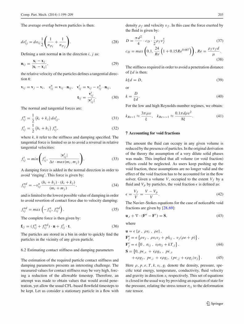
Fig. 2 a Tube with particles: fluid density. b Tube with particles: fluidvelocity. c Tube with particles: fluid pressure

– Use of unstructured grids (automatic grid generation andmesh refinement);

– Finite element discretization of space;– Separate flow modules for compressible and incompress-

ible flows;

123

206 Comp. Part. Mech. (2014) 1:199–209

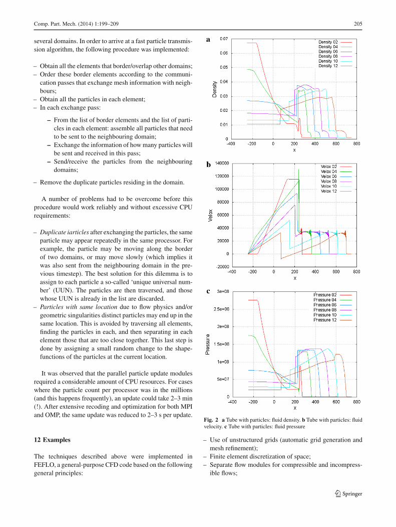
Fig. 3 a Tube with particles: fluid density. b Tube with particles: fluid velocity. c Tube with particles: fluid pressure. d Tube with particles: dustvelocity. e Tube with particles: dust density

– Edge-based data structures for speed;– Optimal data structures for different architectures;– Bottom-up coding from the subroutine level to assure an

open-ended, expandable architecture.

The code has had a long history of relevant applicationsinvolving compressible flow simulations in the areas of tran-sonic flow [37,52–56], store separation [4,7,9,11,12], blast–structure interaction [3,5,6,8,10,13,14,40,46,63,65,67],

123

Comp. Part. Mech. (2014) 1:199–209 207

incompressible flows [2,39,42,50,60,62,66], free-surfacehydrodynamics [36,43,44], dispersion [17–20,41], patient-based haemodynamics [1,21,22,37,47] and aeroacoustics[31]. The code has been ported to vector [38], shared mem-ory [35,64,68], distributed memory [34,48,60,61] and GPU-based [24–27,49] machines.

12.1 Shock into dust

This case considers a 60-cm-square rigid shaft, with theaxis running in the x-direction. The shaft is considered assemi-infinite starting at x = −250 cm. The gas is air,and treated as a perfect gas obeying p = ρ R T withR = 2.869 · 106 dynes − cm/g − K and γ = 1.4. Theair for x > 0 is initially at p = 1.01 · 106 dynes/cm2

and T = 15.15oC = 288.3o K . The air for x < 0 is ini-tially at p = 4000 psi = 2.7579 · 108 dynes/cm2 andT = 1430.6o K . Initially the region x > 250.0 cm is filledwith a mixture of air and uniformly distributed dust. The dustparticles have a density of ρp = 2.3 g/cm3 and D = 100 nm.The average mass loading of dust inside the disk is 0.1 g/cm3.The dust particles therefore occupy a volume fraction of0.1/2.3 = 0.0435 within the dusty region, sufficiently lowfor a dilute species assumption. At time t = 0 the gasesare allowed to begin interacting as in a Riemann problem,launching a shock wave propagating in the +x direction.Although the problem is one-dimensional, it was run usingthe 3-D code. The results obtained have been summarizedin Fig. 2a–c, which show the variables along the centerlineof the tube for different times. The emergence of the classi-cal Riemann problem is visible, followed by slowdown andpartial reflection due to the presence of the particles. Thisis a high-loading case (the density of the particles are 100xthe ambient density of air), and can lead to instabilities. Inorder to trigger these, we ran on a cartesian mesh split intotetrahedra, with 2 × 2 × 2 particles per cartesian cell. Notethe emergence of oscillations in the velocities as the shockenters the region of quiescent particles. Without the limitersdescribed above, this type of run would fail.

This case was repeated with 4x4x4 per cartesian cell. Theresults are shown in Fig. 3. Note that the oscillations havelargely disappeared.

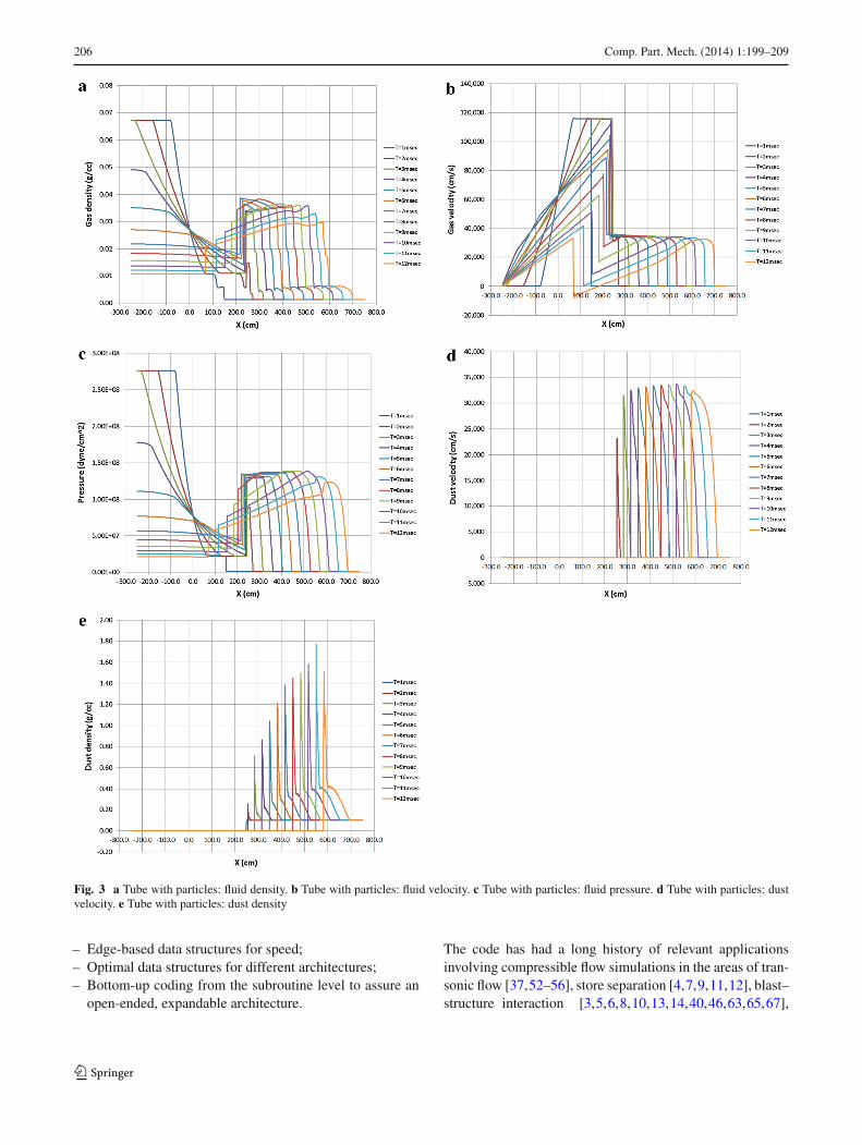
12.2 Blast in room with dilute material

This example considers the flow and particle transport result-ing from a blast in a room where dilute material has beendeposited. The powder-like material is modeled via particles.The geometry, together with the solution, can be discernedfrom Fig. 4.

The compressible Euler equations are solved using anedge-based FEM-FCT technique [32,45,52]. The initializa-tion was performed by interpolating the results of a very

Fig. 4 Blast in room: pressures and particle velocities

Table 1 Blast in room with dilute material

nelem CPU/GPU mvecl Time (sec)

4.0 M Xeon E5530 (1) 32 305

4.0 M Xeon E5530 (2) 32 178

4.0 M Xeon E5530 (4) 32 113

4.0 M Xeon E5530 (6) 32 79

4.0 M Xeon E5530 (8) 32 68

4.0 M Tesla C2070 51200 49

detailed 1D (spherically symmetric) run. The particles aretransported using a 4th order Runge-Kutta technique. Thetiming studies (summarized in Table 1) were carried out withthe following set of parameters:

– Compressible Euler– Ideal Gas EOS– Explicit FEM–FCT– Initialization from a 1D file– 4.0 Million elements, 93,552 particles– Run for 60 steps

13 Conclusions and outlook

The treatment of dilute solid (or liquid) phases via Lagrangianparticles within mesh-based gas-dynamics (or hydrody-namic) codes is common in computational fluid dynamics.While these techniques work very well for a large spectrumof physical parameters, in some cases, notably for very lightor very heavy particles, numerical instabilities appear. Thepresent paper has examined ways of mitigating these instabil-ities. Furthermore, important implementational issues weresummarized.

123

208 Comp. Part. Mech. (2014) 1:199–209

Current efforts are directed at porting all compressibleflow modules to account for volume blockage effects, andthe link to chemical reactions with burning particles.

Acknowledgments This research used resources of the Oak RidgeLeadership Computing Facility at the Oak Ridge National Laboratory,which is supported by the Office of Science of the U.S. Department ofEnergy under Contract No. DE-AC05-00OR22725, and also resourcesof the DoD High Performance Computing Modernization Program. Thissupport is gratefully acknowledged.

References

1. Appanaboyina S, Mut F, Löhner R, Putman CM, Cebral JR (2008)Computational fluid dynamics of stented intracranial aneurysmsusing adaptive embedded unstructured grids. Int J Numer MethodsFluids 57(5):475–493

2. Aubry R, Mut F, Löhner R, Cebral JR (2008) Deflated precondi-tioned conjugate gradient solvers for the pressure–poisson equa-tion. J Comput Phys 227(24):10196–10208

3. Baum JD, Löhner R (1991) Numerical simulation of shock inter-action with a modern main battlefield tank AIAA-91-1666.

4. Baum JD, Löhner R (1993) Numerical simulation of pilot/seat ejec-tion from an F-16 AIAA-93-0783.

5. Baum JD, Luo H, Löhner R (1993) Numerical simulation of a blastinside a boeing 747; AIAA-93-3091.

6. Baum JD, Luo H, Löhner R (1993) Numerical simulation of ablast withing a multi-room shelter. In: Proceedings of the MABS-13 conference. The Hague, pp 451–463

7. Baum JD, Luo H, Löhner R (1994) A new ALE adaptive unstruc-tured methodology for the simulation of moving bodies; AIAA-94-0414

8. Baum JD, Luo H, Löhner R (1995) Numerical simulation of blastin the world trade center; AIAA-95-0085

9. Baum JD, Luo H, Löhner R (1995) Validation of a new ALE, adap-tive unstructured moving body methodology for multi-store ejec-tion simulations; AIAA-95-1792

10. Baum JD, Luo H, Löhner R, Yang C, Pelessone D, Charman C(1996) Coupled fluid/structure modeling of shock interaction witha truck; AIAA-96-0795

11. Baum JD, Luo H, Löhner R, Goldberg E, Feldhun A (1997) Appli-cation of unstructured adaptive moving body methodology to thesimulation of fuel tank separation from an F-16 c/d fighter; AIAA-97-0166

12. Baum JD, Löhner R, Marquette TJ, Luo H (1997) Numerical sim-ulation of aircraft canopy trajectory; AIAA-97-1885

13. Baum JD, Luo H, Mestreau E, Löhner R, Pelessone D, CharmanC (1999) Coupled CFD/CSD methodology for modeling weapondetonation and fragmentation; AIAA-99-0794

14. Baum JD, Mestreau E, Luo H, Löhner R, Pelessone D, GiltrudME, Gran JK (2006) Modeling of near-field blast wave, evolution;AIAA-06-0191

15. Balakrishnan K, Menon S (2010) On the role of ambient reactiveparticles in the mixing and afterburn behind explosive blast waves.Combust Sci Technol 182:186–214

16. Benkiewicz K, Hayashi K (2003) Two-dimensional numerical sim-ulations of multi-headed detonations in oxygen–aluminum mix-tures using an adaptive mesh refinement. Shock Waves 12(5):385–402

17. Camelli F, Löhner R (2004) Assessing maximum possible damagefor contaminant release events. Eng Comput 21(7):748–760

18. Camelli F, Löhner R, Sandberg WC, Ramamurti R (2004) VLESstudy of ship stack gas, dynamics; AIAA-04-0072

19. Camelli F, Löhner R (2006) VLES study of flow and dispersionpatterns in heterogeneous urban areas; AIAA-06-1419.

20. Camelli F, Lien J, Dayong D, Wong DW, Rice M, Löhner R, YangC (2012) Generating seamless surfaces for transport and dispersionmodeling in GIS. GeoInformatica 16(2):207–327

21. Cebral JR, Löhner R (2001) From medical images to anatomicallyaccurate finite element grids. Int J Numer Methods Eng 51:985–1008

22. Cebral JR, Löhner R (2005) Efficient simulation of blood flowpast complex endovascular devices using an adaptive embeddingtechnique. IEEE Trans Med Imaging 24(4):468–476

23. Clift R, Grace JR, Weber ME (1978) Bubbles, drops and particles.Academic Press, New York

24. Corrigan A, Camelli F, Löhner R (2010) Porting of an edge-basedCFD solver to GPUs; AIAA-10-0523.

25. Corrigan A, Camelli F, Löhner R, Mut F (2010) Porting of FEFLOto GPUs. In: Proceedings of the ECCOMAS CFD 2010 conference.Lisbon, June 14–17.

26. Corrigan A, Camelli FF, Löhner R, Wallin J (2011) Runningunstructured grid based CFD solvers on modern graphics hard-ware. Int J Numer Methods Fluids 66:221–229

27. Corrigan A, Löhner R (2011) Porting of FEFLO to multi-GPUclusters; AIAA-11-0948.

28. Deen NG, Sint Annaland Mv, Kuipers JAM (2006) Direct numer-ical simulation of particle mixing in dispersed gas–liquid–solidflows using a combined volume of fluid and discrete parti-cle approach. In: Proceedings of the fifth international con-ference on CFD in the process industries CSIRO, Melbourne,13–15 Dec.

29. Hoberock J, Bell N (2010) Thrust: parallel template library. Version1:3

30. Kim CK, Moon JG, Hwang JS, Lai MC, Im KS (2008) Afterburningof TNT explosive products in air with aluminum particles; AIAA-2008-1029.

31. Liu J, Kailasanath K, Ramamurti R, Munday D, Gutmark E, LöhnerR (2009) Large-eddy simulations of a supersonic jet and its near-field acoustic properties. AIAA J 47(8):1849–1864

32. Löhner R, Morgan K, Peraire J, Vahdati M (1987) Finite elementflux-corrected transport (FEM-FCT) for the Euler and Navier–Stokes equations. Int J Numer Methods Fluids 7:1093–1109

33. Löhner R, Ambrosiano J (1990) A vectorized particle tracer forunstructured grids. J Comp Phys 91(1):22–31

34. Löhner R, Ramamurti R (1995) A load balancing algorithm forunstructured grids. Comput Fluid Dyn 5:39–58

35. Löhner R (1998) Renumbering strategies for unstructured-grid solvers operating on shared-memory, cache-based parallelmachines. Comput Methods Appl Mech Eng 163:95–109

36. Löhner R, Yang C, Oñate E (1998) Viscous free surface hydro-dynamics using unstructured grids. In: Proceedings of the 22ndSymposium Naval Hydrodynamics. Washington, D.C., Aug

37. Löhner R., Yang Chi, Cebral J, Soto O, Camelli F, Baum JD, Luo H,Mestreau E, Sharov D, Ramamurti R, Sandberg W, Oh Ch (2001)Advances in FEFLO; AIAA-01-0592.

38. Löhner R, Galle M (2002) Minimization of indirect addressing foredge-based field solvers. Commun Numer Methods Eng 18:335–343

39. Löhner R (2004) Multistage explicit advective prediction forprojection-type incompressible flow solvers. J Comput Phys195:143–152

40. Löhner R, Baum JD, Rice D (2004) Comparison of coarse andfine mesh 3D Euler predictions for blast loads on generic buildingconfigurations. In: Proceedings of the MABS-18 conference bad.Reichenhall, Germany, Sept

41. Löhner R, Camelli F (2005) Optimal placement of sensors for con-taminant detection based on detailed 3D CFD simulations. EngComput 22(3):260–273

123

Comp. Part. Mech. (2014) 1:199–209 209

42. Löhner R, Chi Yang JR, Camelli O Soto (2006) Improving thespeed and accuracy of projection-type incompressible flow solvers.Comput Methods Appl Mech Eng 195(23–24):3087–3109

43. Löhner R, Yang Chi (2006) On the simulation of flows with violentfree surface motion. Comput Methods Appl Mech Eng 195:5597–5620

44. Löhner R, Yang Chi (2007) Simulation of flows with violent freesurface motion and moving objects using unstructured grids. Int JNumer Methods Fluids 53:1315–1338

45. Löhner R (2008) Applied CFD techniques, 2nd edn. Wiley, NewYork

46. Löhner R, Luo H, Baum JD, Rice D (2008) Improvements in speedfor explicit, transient compressible flow solvers. Int J Numer Meth-ods Fluids 56(12):2229–2244

47. Löhner R, Cebral JR, Camelli FF, Appanaboyina S, Baum JD,Mestreau EL, Soto O (2008) Adaptive embedded and immersedunstructured grid techniques. Comput Methods Appl Mech Eng197:2173–2197

48. Löhner R, Mut F, Camelli FF (2011) Timings OF FEFLO on theSGI-ICE machines; AIAA-11-1064.

49. Löhner R, Corrigan A (2011) Semi-automatic porting if a generalfortran CFD code to GPUs: the difficult modules; AIAA-11-3219.

50. Löhner R, Mut F, Cebral JR, Aubry R, Houzeaux G (2011) Deflatedpreconditioned conjugate gradient solvers for the pressure–poissonequation: extensions and improvements. Int J Numer Methods Eng87(1–5):2–14

51. Löhner R (2012) F2GPU a general fortran to GPU translator. In:Proceedings of the NVIDIA GTC conference. San Jose, May

52. Luo H, Baum JD, Löhner R (1994) Edge-based finite elementscheme for the Euler equations. AIAA J 32(6):1183–1190

53. Luo H, Baum JD, Löhner R, Cabello J (1994) Implicit finite ele-ment schemes and boundary conditions for compressible flows onunstructured grids; AIAA-94-0816.

54. Luo H, Baum JD, Löhner R (1999) An accurate, fast, matrix-freeimplicit method for computing unsteady flows on unstructuredgrids; AIAA-99-0937.

55. Luo H, Sharov D, Baum JD, Löhner R (2000) A class of matrix-free implicit methods for compressible flows on unstructured grids.In: First international conference on computational fluid dynamics,Kyoto, July 10–14

56. Luo H, Baum JD, Löhner R (2001) A fast, matrix-free implicitmethod for computing low mach number flows on unstructuredgrids. Int J CFD 14:133–157

57. Merrill D, Grimshaw A (2010) Revisiting sorting for GPGPUstream architectures. UVA CS Report CS2010-03 Charlottesville.

58. NVIDIA Corporation. NVIDIA CUDA 3.2 Programming Guide(2010).

59. Peterson P (2009) F2PY: tool for connecting Fortran and pythonprograms. Int J Comput Sci Eng 4:296–305

60. Ramamurti R, Löhner R (1993) Simulation of flow past complexgeometries using a parallel implicit incompressible flow solver.In: Proceedings of the 11th AIAA CFD conference, Orlando, pp1049–1050

61. Ramamurti R, Löhner R (1996) A parallel implicit incompressibleflow solver using unstructured meshes. Comput Fluids 5:119–132

62. Ramamurti R, Sandberg WC, Löhner R (1999) Computation ofunsteady flow past deforming geometries. Int J Comput Fluid Dyn13:83–99

63. Rice DL, Baum JD, Togashi F, Löhner R, Amini A (2008) First-principles blast diffraction simulations on a notebook: accuracy,resolution and turn-around issues. In: Proceedings of the MABS-20 conference, Oslo

64. Sharov D, Luo H, Baum JD, Löhner R (2000) Implementationof untructured grid GMRES+LU-SGS method on shared-memory,cache-based parallel computers; AIAA-00-0927.

65. Stück A, Camelli F, Löhner R (2010) Adjoint-based design of shockmitigation devices. Int J Numer Methods Fluids 64:443–472

66. Tilch R, Tabbal A, Zhu M, Decker F, Löhner R (2008) Combinationof body-fitted and embedded grids for external vehicle aerodynam-ics. Eng Comput 25(1):28–41

67. Togashi F, Baum JD, Mestreau E, Löhner R, Sunshine D (2009)Numerical modeling of long-duration blast wave evolution in con-fined, facilities; AIAA-09-1531.

68. Tuszynski J, Löhner R (1998) Parallelizing the construction of indi-rect access arrays for shared-memory machines. Commun ApplNumer Methods Eng 14:773–781

69. Vreman AW, Geurts BJ, Deen NG, Kuipers JAM (2004) Large-eddy simulation of a particle laden turbulent channel flow. In: Pro-ceedings of the direct and large-eddy simulation V. ERCOFTACSeries 9, pp 271–278

70. Zhang F (ed.) (2009) Shock wave science and technology referencelibrary, vol. 4: heterogeneous detonation. Springer, New York.

123