Embed Size (px)
Citation preview
Deformation quantization of cosmological models
Ruben Cordero∗
Departamento de Fısica, Escuela Superior de Fısica y Matematicas del IPN
Unidad Adolfo Lopez Mateos, Edificio 9, 07738, Mexico D.F., Mexico
Hugo Garcıa-Compean†
Departamento de Fısica, Centro de Investigacion y de Estudios Avanzados del IPN
P.O. Box 14-740, 07000 Mexico D.F., Mexico
Francisco J. Turrubiates‡
Departamento de Fısica, Escuela Superior de Fısica y Matematicas del IPN
Unidad Adolfo Lopez Mateos, Edificio 9, 07738, Mexico D.F., Mexico.
(Dated: February 23, 2011)
Abstract
The Weyl-Wigner-Groenewold-Moyal formalism of deformation quantization is applied to cos-
mological models in the minisuperspace. The quantization procedure is performed explicitly for
quantum cosmology in a flat minisuperspace. The de Sitter cosmological model is worked out
in detail and the computation of the Wigner functions for the Hartle-Hawking, Vilenkin and
Linde wave functions are done numerically. The Wigner function is analytically calculated for
the Kantowski-Sachs model in (non)commutative quantum cosmology and for string cosmology
with dilaton exponential potential. Finally, baby universes solutions are described in this context
and the Wigner function is obtained.
PACS numbers: 03.65.-w, 03.65.Ca, 11.10.Ef, 03.65.Sq
∗Electronic address: [email protected]†Electronic address: [email protected]‡Electronic address: [email protected]
1
arX
iv:1
102.
4379
v1 [
hep-
th]
22
Feb
2011
I. INTRODUCTION
One of the fundamental problems of cosmology is the initial singularity. It is commonly
believed that near this singularity the physical evolution is governed by quantum mechanics.
In the quantum cosmology framework the whole universe is represented through a wave
function satisfying the Wheeler-DeWitt equation [1]. It is well known that it represents
the low energy approximation of string theory, however it contains some non-trivial leading
order information. The development of quantum cosmology started at the beginning of the
80’s of last century and one of its main ideas is that the universe could be spontaneously
nucleate out from nothing [2–10]. After nucleation the universe can enter into a phase of
inflationary expansion and continues its evolution to the present time. However, there are
several important questions that remain to be solved like the general definition of probability,
time and boundary conditions [11]. In order to find a unique solution of the Wheeler-
DeWitt equation it is necessary to impose boundary conditions. In the case of quantum
mechanics there is an external setup and the boundary conditions can be imposed safely,
however in 4-dimensional quantum cosmology there is nothing external to the universe and
the question of which one is the correct prescription for the boundary condition of the
universe is controversial [12]. There are several proposals for the correct boundary conditions
in quantum cosmology, for example, the no-boundary proposal of Hartle and Hawking [7], the
tunneling proposal of Vilenkin [10] and the proposal of Linde [8]. In a recent development
in quantum cosmology a principle of selection in the landscape of string vacua has been
proposed in [13], in the context of the minisuperspace. Moreover in [14] different cosmologies
were defined in terms of a wave function on a compact worldsheet of system of parafermions.
Much of the information is encoded in the wave function as function of the moduli space.
Another important issue is how to extract information of the Wheeler-DeWitt equation.
In general, the configuration space used in quantum cosmology is an infinite dimensional
space called superspace and it is not amenable to work with. In the study of homogeneous
universes the infinite dimensional space is truncated to finite degrees of freedom, therefore
obtaining a particular minisuperspace model. The reduction of superspace to minisuper-
space is not a rigorous approximation scheme, however there is the hope that minisuperspace
maintains some of the essential features of quantum cosmology. In classical cosmology ho-
mogeneity and isotropy are fundamental to describe the universe at large scale and therefore
2
it is expected to have a minisuperspace description in quantum cosmology.
At very early times of the universe, even before the Planck time, the universe should be
described by means of quantum cosmology that could take into account effects from string
theory, supersymmetry and noncommutativity. String cosmology [15], quantum wormholes,
baby universes and supersymmetric quantum cosmology has become very intensive research
areas in quantum cosmology. Quantum wormholes [16] are instanton solutions and are
important in the Euclidean path integral formulation. In the third quantization approach,
which is an adequate description of topology change in the path integral quantization, the
wave function is transformed into a quantum field operator which includes operators that
create and destroy the so called baby universes.
Supersymmetric quantum cosmology is one of the main research areas [17–20]. At the
time of quantum creation of the universe it is possible that supersymmetry would not yet
be broken and therefore could have very important consequences in the evolution of the
universe. Other very interesting effects that could arise in the very early universe are the
effects of noncommutativity [21].
At the end of the late 1980s and early 1990s quantum decoherence, the transition from
quantum physics to classical physics, was an active research area in quantum cosmology
[22, 23] (for more recent reviews see, [24, 25]). In Refs. [26–30], quantum cosmology is
developed in the phase space and the use of Wigner function is showed to be a very useful
approach to study decoherence. In fact, quantum mechanics in phase space is an appropriate
formalism to describe quantum mechanical systems (for a review see [31]). The description
using the Wigner function has been of considerable interest and usefulness in quantum optics,
nuclear and particle physics, condensed matter, statistical physics, etc. In particular, the
description of semiclassical properties and the analysis of the classical limit is more clear in
the Wigner function formalism. The classical limit from quantum cosmology was studied
also in [30, 32], where the use of Wigner function and quantum mechanics in phase space
is fundamental. It has been argued that quantum decoherence is achieved if the density
matrix is coarse grained, i.e. averaged over configuration or phase space variables, or in
an alternative way, if the system interact with some environment which is not monitored.
However the existence of classical correlations is another characteristic of the classical limit
and requires the presence of sharp peaks of the Wigner function, but a coarse graining
produces a spreading of the distribution in phase space. The former arguments demand a
3
subtle coarse graining in which there is a delicate balance between the existence of classical
correlations and decoherence. A coarse graining could be modeled by a Liouville equation
with friction and diffusion terms [30]. Some other further results are described in Refs.
[33, 34].
The quantum mechanics in phase space is only one part of a complete and consistent
type of quantization termed: deformation quantization. In this paper we formulate quantum
cosmology in terms of deformation quantization and rewrite some results of [30, 32] in the
context of this formalism. We will assume that the superspace (of 3-metrics) is flat and
a Fourier transform can be defined. This is fairly valid for the ample set of examples in
two dimensions that we present in this paper. The case of curved minisuperspace will be
discussed in a future communication.
The deformation quantization formalism is an alternative approach to the canonical and
path integral quantizations and has its origins in the seminal works by Weyl [35], Wigner
[36], Groenewold [37], Moyal [38], and Vey [39], and is based on the idea of treating with
quantum mechanics on the phase space. In 1978 Bayen, Flato, Fronsdal, Lichnerowicz
and Sternheimer [40] introduced its final form in which the quantization is understood as
a deformation of the classical algebra of observables instead of a change in the nature of
them. This quantization arises as a deformation of the usual product algebra of the smooth
functions on the classical phase space and then as a deformation of the Poisson bracket
algebra. The deformed product is called the ?−product which has been proved to exist
for any symplectic manifold [41], [42] and more recently shown by Kontsevich [43] that it
also exists for any Poisson manifold. These results in principle allow us to perform the
quantization of arbitrary Poissonian or symplectic systems and to obtain in an easier way
the classical limit due to the nature of the ?−product. Our aim is to introduce this formalism
in quantum cosmology and apply the results to simple models.
The structure of the paper is as follows. In section II we survey the canonical Hamiltonian
formalism of general relativity and its canonical quantization. In section III we construct the
Stratonovich-Weyl quantizer, the star-product and the Wigner functional. Section IV is de-
voted to apply the deformation quantization procedure to several minisuperspace models and
to obtain their Wigner function. In subsection IV.A we treat de Sitter model and calculate
numerically the Wigner function for the Hartle-Hawking, Vilenkin and Linde wave functions.
In subsection IV.B we calculate analytically the Wigner function for the Kantowski-Sachs
4
model in (non)commutative quantum cosmology and we interpret the results. In subsection
IV.C, we obtain the Wigner function for string cosmology with dilaton exponential potential
in terms of the Meijer’s function. Besides, in subsection IV.D the Wigner function for the
baby universes solutions is calculated by means of the Moyal product and the annihilation
and creation operators. Finally, in section V we give our final remarks.
II. CANONICAL FORMALISM OF GENERAL RELATIVITY
In this section we briefly overview the Hamiltonian formalism of general relativity. Our
presentation will not be complete and detailed information can be found in Ref. [1, 44].
Our intention is only to introduce the notation and conventions for future reference along
the paper.
A. Hamiltonian Formalism
We start from the ADM decomposition of general relativity and consider a pseudo Rie-
mannian manifold (M, g) which is globally hyperbolic. Thus, spacetime M can be decom-
posed as M = Σ × R where Σ is an spatial hypersurface and the metric of a foliation is:
ds2 = gµνdxµdxν = −(N2 − N iNi)dt
2 + 2Nidxidt + hijdx
idxj, with signature (−,+,+,+).
Here hij is the intrinsic metric on the hypersurface Σ, N is the lapse function and N i is the
shift vector.
The space of all Riemannian 3-metrics and scalar matter configurations Φ on Σ is the so
called superspace Riem(Σ) = hij(x), Φ(x)|x ∈ Σ. Let us denote the space of Riemannian
metrics on Σ as Met(Σ) = hij(x)|x ∈ Σ which is an infinite dimensional manifold. The
moduli space M, is then defined as the configuration space (superspace) modulo the group
of diffeomorphisms Diff(Σ) i.e. M = Riem(Σ)Diff(Σ)
or for pure gravity M = Met(Σ)Diff(Σ)
.
The corresponding phase space (Wheeler’s phase superspace) Γ∗ ∼= T ∗Met(Σ) is given
by the pairs Γ∗ = (hij(x), πij(x)), where πij = ∂LEH∂hij
and LEH is the Einstein-Hilbert
Lagrangian. In the following we will deal with fields at the moment t = 0 (on Σ) and we
put hij(x, 0) ≡ hij(x) and πij(x, 0) ≡ πij(x).
The dynamics of general relativity coupled to matter in this foliation is encoded in the
5
variation of the following action
S =
∫dtL =
1
16πGN
[ ∫M
d4x√−g
(4R(g)− 2Λ
)+ 2
∫∂M
d3x√hK
]+ Sm, (1)
where 4R(g) is the scalar curvature in four dimensions depending on the spacetime pseudo-
Riemannian metric gµν , g is the determinant of gµν , GN is the gravitational constant in N
dimensions, Λ is the cosmological constant, K is the trace of the extrinsic curvature Kii
compatible with hij and Sm is the matter action. For the case of scalar field matter subject
to a potential V (Φ) we have that
Sm =
∫M
d4x√−g(− 1
2gµν∂µΦ∂νΦ− V (Φ)
). (2)
The action (1) can then be written as
S =
∫dtd3x
(π0N + πiNi −NH⊥ −N iHi
), (3)
where H⊥ and Hi are given below. Thus the canonical Hamiltonian is given by
HC =
∫d3x
(π0N + πiNi + πijhij + πΦΦ
)− L
=
∫d3x
(π0N + πiNi +NH⊥ +N iHi
), (4)
where π0 = ∂L∂N
and πi = ∂L
∂N iand πΦ = ∂L
∂Φ. The corresponding equations of motion for N
and Ni yield the Hamiltonian constraint and the momentum constraint, respectively
H⊥(x) = h−1/2
(1
2π2 − πijπ
ji
)+√h 3R
= 4κ2Gijklπijπkl −
√h
4κ2
(3R− 2Λ
)+
1
2
√h
(π2
h+ hijΦ,iΦ,j + 2V (Φ)
)= 0 , (5)
Hi(x) =
√h
2κ2
(G0i − 2κ2T 0
i
)= −2πij|j + hijΦ,jπΦ = 0, (6)
where κ2 = 4πGN , 3R(h) is the scalar curvature of Σ, Gijkl = 12h−1/2
(hikhjl+hilhjk−hijhkl
),
|j denotes covariant derivative with respect to hij and h is its determinant.
In this way the Poisson bracket between hij and πkl is given by
hij(x), πkl(y)PB =1
2(δki δ
lj + δkj δ
li)δ(x− y) , (7)
which is one of the most important structures for quantization.
6
B. Canonical Quantization
The most employed formalism to quantize a physical system is the canonical quantization
which can be applied in general relativity. In this section we describe briefly the general
procedure to obtain the quantum equations. In the h-representation, the usual promotion of
canonical coordinates hij(x), Φ(x) and πij, πΦ to the operators can be done in the following
form: hij|hij,Φ〉 = hij|hij,Φ〉, πij|hij,Φ〉 = −i~ δδhij(x)
|hij,Φ〉, Φ|hij,Φ〉 = Φ(x)|hij,Φ〉 and
πΦ|hij,Φ〉 = −i~ δδΦ(x)|hij,Φ〉. These operators satisfy the commutation relations
[hij(x), πkl(y)] =i~2
(δki δlj + δkj δ
li)δ(x− y). (8)
The constraints (5) and (6) have to be imposed at the quantum level in the form
H⊥|Ψ〉 = 0, Hi|Ψ〉 = 0 . (9)
In the coordinate-representation we have[− 4κ2Gijkl
δ2
δhijδhkl+
√h
4κ2
(− 3R(h) + 2Λ + 4κ2T 00
)]Ψ[hij,Φ] = 0 , (10)
where 〈hij,Φ|Ψ〉 = Ψ[hij,Φ] and T 00 = − 12h
δ2
δΦ2 + 12hijΦ,iΦ,j+V (Φ). This constraint is called
the Wheeler-DeWitt equation. For pure gravity we have[− 4κ2Gijkl
δ2
δhijδhkl+
√h
4κ2
(− 3R(h) + 2Λ
) ]Ψ[hij] = 0, (11)
where 〈hij|Ψ〉 = Ψ[hij]. In the general case the Wheeler-DeWitt equation is not amenable
to extract physical information of the system. In order to obtain useful information it is a
common practice to reduce the number of degrees of freedom. In the following sections we
will consider models with one and two degrees of freedom.
III. DEFORMATION QUANTIZATION OF WHEELER’S PHASE-SUPERSPACE
In this section we work in a flat superspace with flat metric Gijkl. This case will allow
us to introduce the Weyl-Wigner-Groenewold-Moyal (WWGM) formalism for gravitational
systems in a direct way since the existence of the Fourier transform is warranted. The more
complicated cases of curved (mini)superspaces will be left for a future work. The deformation
quantization of gravity in ADM formalism and constrained systems is described in more
7
detail in Refs. [45]. We want to point out that in this section the calculations are formal
just as is the case of path integrals in field theory and in order to obtain some physical
results additional considerations need to be implemented depending on the specific system.
A. The Stratonovich-Weyl Quantizer
Let F [hij, πij; Φ, πΦ] be a functional on the phase space Γ∗ (Wheeler’s phase superspace)
and let F [µij, λij;µ, λ] be its Fourier transform. By analogy to the quantum mechanics case,
we define the Weyl quantization rule as follows [35–43, 45–53]
F =W(F [hij , πij ; Φ, πΦ]) :=
∫D(λij2π
)D(µij
2π
)D(λ
2π
)D( µ
2π
)F [µij , λij ;µ, λ]U [µij , λij ;µ, λ],
(12)
where the functional measures are given by Dhij =∏
x dhij(x) etc, U [µij, λij;µ, λ] :
(µij, λij;µ, λ) ∈ Γ∗ is the family of unitary operators given by
U [µij, λij;µ, λ] := exp
i
∫dx
(µij(x)hij(x)+λij(x)πij(x)+µ(x)Φ(x)+λ(x)πΦ(x)
), (13)
with hij, πij, Φ and πΦ being the field operators defined as
hij(x)|hij,Φ〉 = hij(x)|hij,Φ〉 and πij(x)|πij, πΦ〉 = πij(x)|πij, πΦ〉,
Φ(x)|hij,Φ〉 = Φ(x)|hij,Φ〉 and πΦ(x)|πij, πΦ〉 = πΦ(x)|πij, πΦ〉 . (14)
These states form basis satisfying the completeness relations while operators satisfy the
usual commutation rules. Using the well known Campbell-Baker-Hausdorff formula, the
completeness relations and the standard commutation rules we can write U [µij, λij;µ, λ] in
the following form
U [µij, λij;µ, λ] =
∫DhijDΦ exp
i
∫dx
(µij(x)hij(x) + µ(x)Φ(x)
)×∣∣∣∣hij − ~λij
2,Φ− ~λ
2
⟩⟨hij +
~λij2,Φ +
~λ2
∣∣∣∣. (15)
It is easy to show, from (15), that one can obtain the following properties:
Tr
U [µij, λij;µ, λ]
= δ[λij]δ
[~µij
2π
]· δ[λ]δ
[~µ2π
], (16)
Tr
U †[µij, λij;µ, λ]·U [µ′ij, λ′ij;µ
′, λ′]
= δ[λij−λ′ij]δ
[~2π
(µij − µ′ij)]·δ[λ−λ′]δ
[~2π
(µ− µ′)],
(17)
8
where Tr is the trace in some representation.
Equations (15) and (12) lead to write
F =
∫D(πij
2π~
)DhijD
( πΦ
2π~
)DΦF [hij, π
ij; Φ, πΦ]Ω[hij, πij; Φ, πΦ], (18)
where the operator Ω is given by
Ω[hij , πij ; Φ, πΦ] =
∫D(~λij2π
)DµijD
(~λ2π
)Dµ
× exp
− i∫dx
(µij(x)hij(x) + λij(x)πij(x) + µ(x)Φ(x) + λ(x)πΦ(x)
)U [µij , λij ;µ, λ]. (19)
It is evident that the operator Ω is the Stratonovich-Weyl quantizer. One can easily check
the following properties of Ω
(Ω[hij, π
ij; Φ, πΦ])†
=(Ω[hij, π
ij; Φ, πΦ]),
Tr
Ω[hij, πij; Φ, πΦ]
= 1,
Tr
Ω[hij, π
ij; Φ, πΦ] · Ω[h′ij, π′ij; Φ′, π′Φ]
= δ
[πij − π′ij
2π~
]δ[hij − h′ij] · δ
[πΦ − π′Φ
2π~
]δ[Φ−Φ′].
(20)
Now it is possible to obtain the inverse map of W by multiplying (12) by Ω[hij, πij; Φ, πΦ],
taking the trace of both sides and using (17) we get
F [hij, πij; Φ, πΦ] = Tr
Ω[hij, π
ij; Φ, πΦ]F
. (21)
One can also express Ω[hij, πij; Φ, πΦ] in a very useful form by inserting (15) into (19).
Thus one gets
Ω[hij, πij; Φ, πΦ] =
∫Dξij
∫Dξ exp
− i
~
∫dx
(ξij(x)πij(x) + ξ(x)πΦ(x)
)
×∣∣∣∣hij − ξij
2,Φ− ξ
2
⟩⟨hij +
ξij2,Φ +
ξ
2
∣∣∣∣. (22)
B. The Star-Product
Now we define the Moyal ?−product. Let F = F [hij, πij; Φ, πΦ] and G = G[hij, π
ij; Φ, πΦ]
be some functionals on Γ∗ that correspond to the field operators F and G respectively, i.e.
F [hij, πij; Φ, πΦ] = W−1(F ) = Tr
(Ω[hij, π
ij; Φ, πΦ]F)
and G[πij, hij; πΦ,Φ] = W−1(G) =
9
Tr(Ω[πij, hij; πΦ,Φ]G
). The functional corresponding to the product F G will be denoted by
(F ? G)[hij, πij; Φ, πΦ] and after some long but direct calculations we have that
(F ? G)[hij, πij; Φ, πΦ] :=W−1(F G) = Tr
Ω[hij, π
ij; Φ, πΦ]F G
, (23)
gives rise to(F ? G
)[hij, π
ij; Φ, πΦ] = F [hij, πij; Φ, πΦ] exp
i~2
↔PG[hij, π
ij; Φ, πΦ], (24)
where the operator↔P is defined as follows
↔P :=
∫dx
( ←δ
δhij(x)
→δ
δπij(x)−
←δ
δπij(x)
→δ
δhij(x)
)+
∫dx
( ←δ
δΦ(x)
→δ
δπΦ(x)−
←δ
δπΦ(x)
→δ
δΦ(x)
).
(25)
This is precisely the Moyal ?−product.
C. The Wigner Functional
In the deformation quantization formalism the Wigner function plays a very important
role and in the same way finally we are going to define the Wigner functional. Let ρ be the
density operator of a quantum state. The functional ρW [hij, πij; Φ, πΦ] corresponding to ρ
reads
ρW [hij, πij; Φ, πΦ] = Tr
Ω[hij, π
ij; Φ, πΦ]ρ
=
∫D(ξij
2π~
)D(
ξ
2π~
)exp
− i
~
∫dx
(ξij(x)πij(x) + ξ(x)πΦ(x)
)×⟨hij +
ξij2,Φ +
ξ
2
∣∣∣∣ρ∣∣∣∣hij − ξij2,Φ− ξ
2
⟩. (26)
For a pure state of the system ρ = |Ψ〉〈Ψ|, the equation (26) gives
ρW
[hij, πij; Φ, πΦ] =
∫D(ξij
2π~
)D(
ξ
2π~
)exp
− i
~
∫dx
(ξij(x)πij(x) + ξ(x)πΦ(x)
)×Ψ∗
[hij −
ξij2,Φ− ξ
2
]Ψ
[hij +
ξij2,Φ +
ξ
2
], (27)
where 〈hij,Φ|Ψ〉 = Ψ[hij,Φ] is the wave function of the universe.
The expected value of an arbitrary operator F can then be obtained by means of ρ as
〈F 〉 =Tr(ρF )
Tr(ρ)
=
∫D(πij
2π~
)DhijD
(πΦ
2π~
)DΦρ
W[hij, π
ij; Φ, πΦ]Tr(Ω[hij, πij; Φ, πΦ]F )∫
DπijDhijDπΦDΦρW
[hij, πij; Φ, πΦ]. (28)
10
It is now possible to write the equivalent of the constraints equations (9) in terms of the
?−product and the Wigner functional as
H⊥ ? ρW [hij, πij; Φ, πΦ] = 0, (29)
Hi ? ρW [hij, πij; Φ, πΦ] = 0, (30)
where H⊥ and Hi are given by (5) and (6) respectively. We term Eq. (29) the Wheeler-
DeWitt-Moyal equation. It is important to mention that the dynamics is completely gov-
erned by these equations and that their explicit form depends of the particular system
considered. These equations will be useful in the cosmological models which we will dis-
cuss in the following section. Also, we want to note that the real and imaginary parts of
Eq. (29), encoded in the ?−product, are the generalized mass condition and the Wheeler-
DeWitt-Vlasov transport equation presented in [29] for flat minisuperspace.
IV. DEFORMATION QUANTIZATION IN THE MINISUPERSPACE
Now we proceed to study the application of the deformation quantization construction
to some models in quantum cosmology. The general construction exposed in the previous
section in terms of functional integrals is defined in the whole superspace of 3-metrics and
is necessary in a general case , however as a first approach we will deal with some models
in the minisuperspace due to their simplicity and because they have been widely studied
in the literature by other methods. Our intention is to obtain the Wigner function for
these important cases and to motivate a further study using deformation quantization. We
consider that this first step is necessary in order to gain some experience to eventually
apply the deformation quantization formalism to curved phase-space. It is known that
this formalism has a natural extension to these situations (see [42, 43]) and allows another
suitable extensions or generalizations.
A. de Sitter cosmological model
As a first example we will deal with a minisuperspace model where the phase space is
bidimensional. We are going to calculate the Wigner function from the Wheeler-DeWitt-
Moyal equation and also from its integral expression. Let start with a minisuperspace (where
11
the degrees of freedom are reduced to just one represented by the scale factor of the universe)
corresponding to the Friedmann-Robertson-Walker metric
ds2 = l2p[−N2dt2 + a2(t)dΩ2
3
], (31)
where a is the scale factor of the universe, N is the lapse function, dΩ23 is the metric of the
unit three-sphere, lp = 2/3Lp and Lp denotes the Planck length. Introducing new variables
q = a2 and N = qN [54] the Hamiltonian H⊥ cast out in an easy form
H⊥ =1
2
(−4p2 + λq − 1
), (32)
where λ is the cosmological constant in Planck units. In the coordinate representation the
Hamiltonian acquires a simple form and its dynamics corresponds to a particle in a linear
potential. The Wheeler-DeWitt equation comes from the Hamiltonian constraint (10) and
is written as (42 d
2
dq2+ λq − 1
)Ψ(q) = 0 . (33)
Depending of the boundary conditions it can be found [11] the Vilenkin wave function
ΨV (q) =1
2Ai
(1− λq
(2λ)2/3
)+i
2Bi
(1− λq
(2λ)2/3
), (34)
the Hartle-Hawking wave function
ΨHH(q) = Ai
(1− λq
(2λ)2/3
), (35)
and the Linde wave function
ΨL(q) = −iBi
(1− λq
(2λ)2/3
), (36)
where Ai(x) and Bi(x) are the Airy functions of first and second class respectively.
One of the main differences between the Hartle-Hawking, Linde and Vilenkin wave func-
tions is their behavior in the region q > 1/λ. The Vilenkin tunneling wave function has the
following expression
ΨV = ψ−(q), (37)
the Hartle-Hawking wave function is
ΨHH = ψ+(q) + ψ−(q), (38)
12
and the Linde wave function is written as
ΨL = ψ+(q)− ψ−(q), (39)
where ψ−(q), ψ+(q) describe an expanding and contracting universe, respectively. In the
classical allowed region q > 1/λ the WKB solutions are
ψ± = [p(q)]−1/2 exp
[±i∫ q
1/λ
p(q′)dq′ ∓ iπ
4
], (40)
where p(a) = [−U(a)]1/2 = 12[λq − 1]1/2. From the WKB wave function (40) we have
pψ±(q) ≈ ±pψ±(q). (41)
Taking into account that
p = − q
4N, (42)
the Eq. (41) confirms the already given interpretation for ψ±(q), i.e. negative values of
p correspond to an expanding universe. Therefore, the Vilenkin wave function includes
only an expanding component while the Hartle-Hawking and Linde wave functions include
expanding and contracting universes with equal weight (for a different interpretation see
[55]). In fact, for large values of q these wave functions have the following expressions
ΨV (q) ≈ (2λ~)1/6
2[π2(λq − 1)]1/4e−iS, (43)
ΨHH(q) ≈ (2λ~)1/6
[π2(λq − 1)]1/4cosS =
(2λ~)1/6
2[π2(λq − 1)]1/4(eiS + e−iS
), (44)
ΨL(q) ≈ i(2λ~)1/6
[π2(λq − 1)]1/4sinS =
(2λ~)1/6
2[π2(λq − 1)]1/4(eiS − e−iS
), (45)
where
S =1
3λ~(λq − 1)3/2 − π
4. (46)
Now we proceed to calculate the Wigner function directly by solving the Wheeler-DeWitt-
Moyal equation (29)
H⊥ ? ρW = 0. (47)
where the corresponding Moyal ?−product is given by
? = exp
i2
↔P
= exp
i2 ←∂
∂q
→∂
∂p−←∂
∂p
→∂
∂q
. (48)
13
Taking in consideration the exponential power series expansion we have
1
2(−4p2 + λq − 1)
[∞∑n=0
1
n!
(i2
)n ↔Pn]ρW = 0 , (49)
which can be written as
(−4p2 + λq − 1)ρW +i2λ∂pρW + 4ip∂qρW + 2∂2
qρW = 0. (50)
If we define a new variable z = 4p2 − λq + 1 the imaginary part of the former equation is
identically zero and for the real part we obtain a new form of the equation (50)
2λ2d2ρWdz2
− zρW = 0 , (51)
whose solution is
ρW = c1Ai
(4p2 − λq + 1
(λ)2/3
). (52)
In order to obtain the last result the formalism assumes the existence of the Wigner trans-
form, where the range of integration in this transform is from minus to plus infinity in
the variable q. However, the valid range interval for the variable q is positive but still the
Wigner function is very similar to (52) because of the exponential decay for positive val-
ues of the argument of Ai(x). Last equation indeed admits another solution corresponding
to Bi(
4p2−λq+1(λ)2/3
), but in this case, the Airy function Bi(x) is divergent for positive x and
this part cannot be included as a suitable Wigner function. In fact, in order to obtain an
appropriate solution from (47), the potential could be complemented by an infinite barrier
avoiding the existence of negatives values for q. However the implementation of this proce-
dure is very cumbersome as it has been shown in [56] and [57] and it is not convenient to
develop it here.
Instead of this we can calculate the Wigner function using the following integral expression
[36]
ρW (q, p) =
∫ ∞−∞
dξ
2πexp
− i ξ
p
Ψ∗(q − ξ
2
)Ψ
(q +
ξ
2
). (53)
Employing the convolution theorem and the Fourier transform of the Airy function we get
the Wigner function for the Hartle-Hawking wave function
ρW (q, p) =21/3
π(~λ)1/3Ai
[4p2 − λq + 1
(~λ)2/3
]. (54)
The last result was obtained integrating out from minus to plus infinity in the variable q (in
fact this result was already derived in [30]). However, the wave function is only valid defined
14
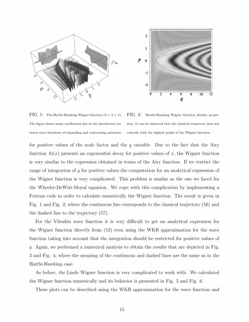
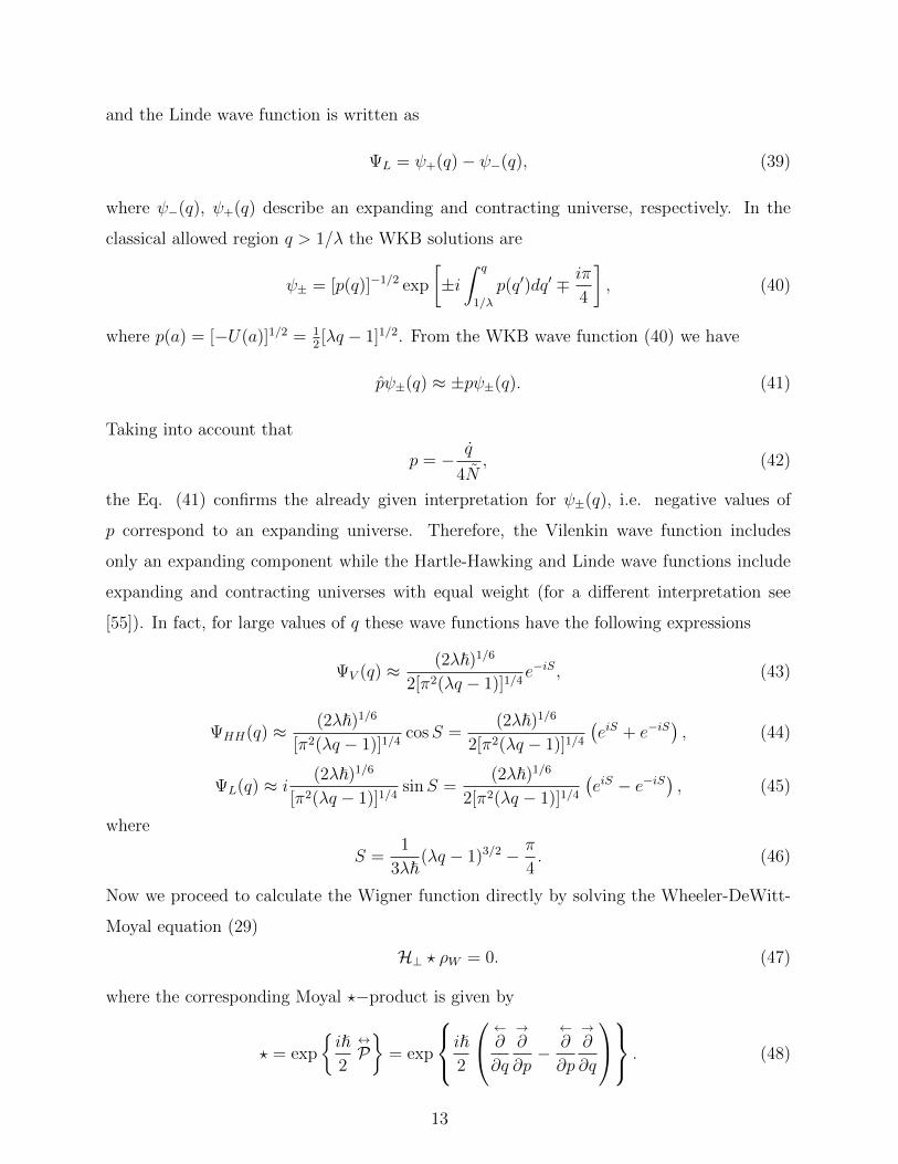
FIG. 1: The Hartle-Hawking Wigner function (~ = λ = 1).
The figure shows many oscillations due to the interference be-
tween wave functions of expanding and contracting universes.
FIG. 2: Hartle-Hawking Wigner function density projec-
tion. It can be observed that the classical trajectory does not
coincide with the highest peaks of the Wigner function.
for positive values of the scale factor and the q variable. Due to the fact that the Airy
function Ai(x) presents an exponential decay for positive values of x, the Wigner function
is very similar to the expression obtained in terms of the Airy function. If we restrict the
range of integration of q for positive values the computation for an analytical expression of
the Wigner function is very complicated. This problem is similar as the one we faced for
the Wheeler-DeWitt-Moyal equation. We cope with this complication by implementing a
Fortran code in order to calculate numerically the Wigner function. The result is given in
Fig. 1 and Fig. 2, where the continuous line corresponds to the classical trajectory (56) and
the dashed line to the trajectory (57).
For the Vilenkin wave function it is very difficult to get an analytical expression for
the Wigner function directly from (53) even using the WKB approximation for the wave
function taking into account that the integration should be restricted for positive values of
q. Again, we performed a numerical analysis to obtain the results that are depicted in Fig.
3 and Fig. 4, where the meaning of the continuous and dashed lines are the same as in the
Hartle-Hawking case.
As before, the Linde Wigner function is very complicated to work with. We calculated
the Wigner function numerically and its behavior is presented in Fig. 5 and Fig. 6.
These plots can be described using the WKB approximation for the wave function and
15
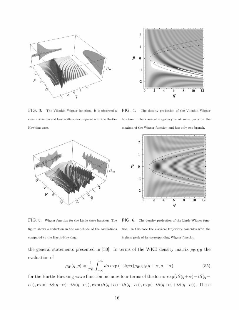
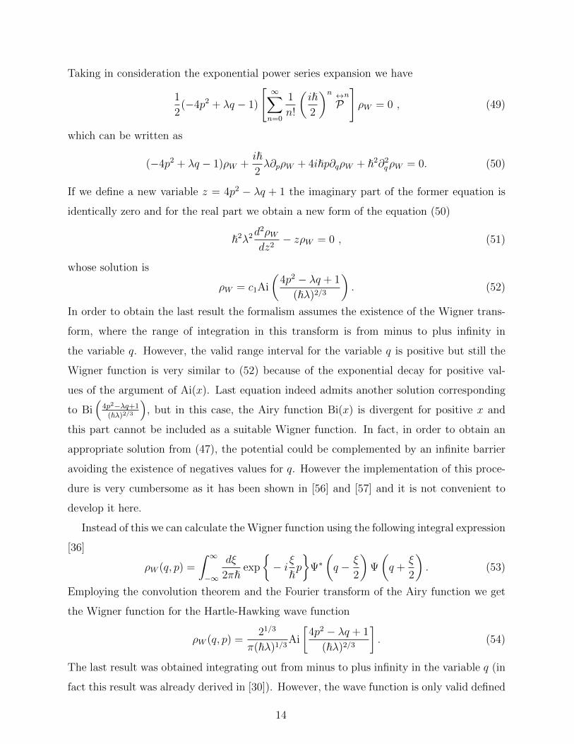
FIG. 3: The Vilenkin Wigner function. It is observed a
clear maximum and less oscillations compared with the Hartle-
Hawking case.
FIG. 4: The density projection of the Vilenkin Wigner
function. The classical trajectory is at some parts on the
maxima of the Wigner function and has only one branch.
FIG. 5: Wigner function for the Linde wave function. The
figure shows a reduction in the amplitude of the oscillations
compared to the Hartle-Hawking.
FIG. 6: The density projection of the Linde Wigner func-
tion. In this case the classical trajectory coincides with the
highest peak of its corresponding Wigner function.
the general statements presented in [30]. In terms of the WKB density matrix ρWKB the
evaluation of
ρW (q, p) ≈ 1
π~
∫ ∞−∞
dα exp (−2ipα)ρWKB(q + α, q − α) (55)
for the Hartle-Hawking wave function includes four terms of the form: exp(iS(q+α)−iS(q−
α)), exp(−iS(q+α)−iS(q−α)), exp(iS(q+α)+iS(q−α)), exp(−iS(q+α)+iS(q−α)). These
16
terms come from the products ψ+(q+α)ψ∗+(q−α), ψ−(q+α)ψ∗+(q−α), ψ+(q+α)ψ∗−(q−α),
ψ−(q + α)ψ∗−(q − α), respectively. By means of the stationary phase approximation, each
one of the former terms will contribute to the Wigner function in different regions bounded
by the classical trajectory
p2 =1
4(λq − 1), (56)
and by the trajectory
p2 =1
8(λq − 1), (57)
which corresponds to points where the path integral has a saddle point at zero momentum
[30], i.e. where the classical action changes sign. In the upper region of the phase space
between the classical trajectory and the dashed curve the Wigner function has contributions
mainly coming from the first term in the density matrix. The region inside the dashed curve
receives the principal contributions form the second and third terms of the density matrix.
The fourth term of the density matrix has a saddle point in the bottom part of phase space
between the classical trajectory and the dashed curve and as a consequence it contributes
predominantly in this region (see Fig. 2).
The Linde Wigner function has a similar structure like the Hartle-Hawking case but
there is one important difference: the interference terms between contracting and expanding
universes have an opposite sign with respect to Hartle-Hawking. The consequence of this
difference is the reduction of the amplitudes of the oscillations inside the classical trajectory
(see Fig. 5).
The Wigner function for the Vilenkin wave function only receives a contribution from
density matrix corresponding to ψ−(q+α)ψ∗−(q−α) and it has a predominantly contribution
only in the lower region of phase space between the classical trajectory and the dashed line.
This behavior is reflected in Fig. 4. It is important to mention that decoherence of the
Vilenkin Wigner function appears to be easier taking into account that large amplitude
terms due to interference between collapsing and expanding universes are not present near
p = 0.
We discuss now the interpretation of these numerical results. For the Hartle-Hawking
Wigner function we see an oscillatory behavior where the largest peaks are not on the
classical trajectory but away from it by a distance of O(~(2/3)), we can appreciate this fact
in the density plot. It should be remarked the existence of oscillations of the Wigner function
17
that are not near of the classical trajectory, however the heights of these peaks decreases
with the distance to the classical trajectory.
The Wigner function for the Linde wave function present a similar pattern, in general
terms, like the Hartle-Hawking wave function, however it is possible to see some differences.
We can appreciate more fluctuations of the Wigner function inside the region corresponding
to the classical trajectory than the Hartle-Hawking Wigner function. Furthermore, the
amplitude of the oscillations are smaller for the Linde wave function than for Hartle-Hawking.
The largest peaks of the Wigner function correspond to the classical trajectory.
In the case of the Wigner function for the Vilenkin wave function the classical trajectory
is at some parts of the curve at the middle of the largest peaks of the Wigner function, i.e.
the Vilenkin Wigner function has the largest peaks more closely to the classical trajectory
than the Hartle-Hawking Wigner function, but only in one part. This behavior is expected,
as we explained above, due to the fact that the Vilenkin wave function represents the tun-
neling wave function and as a consequence there is only one part of the classical trajectory
corresponding to negative values of the momenta (expanding universe).
B. Kantowski-Sachs model
Another interesting case to deal with under the deformation quantization procedure is
the cosmological Kantowski-Sachs model (KS) [58]. We consider the metric in the Misner
parametrization [59]
ds2 = −N2dt2 + e2√
3βdr2 + e−2√
3βe−2√
3Ω(dθ2 + sin2 θdϕ2). (58)
Choosing a particular factor ordering the Wheeler-DeWitt equation takes the following form(−P 2
Ω + P 2β − 48 exp(−2
√3Ω))
Ψ(Ω, β) = 0, (59)
where PΩ = −i~ ∂∂Ω
and Pβ = −i~ ∂∂β
. The solutions of the former equation are given by [59]
Ψ±ν (Ω, β) = e±iν√
3βKi ν~
(4
~e−√
3Ω
), (60)
where Kiν(x) is the MacDonald function of imaginary order. The normalized wave function
is
Ψν(Ω, β) =31/4
π~
√sinh
(πν~
)Ki ν~
(4
~e−√
3Ω
)(61)
18
which satisfy [60] ∫ ∞−∞
dΩdβΨ∗ν(Ω, β)Ψν′(Ω, β) = δ(ν2 − ν ′2). (62)
In order to write the Wheeler-DeWitt-Moyal equation (29) it is very useful to employ the
next relation
f(x, p) ? g(x, p) = f
(x+
i~2
→∂ p, p−
i~2
→∂ x
)g(x, p). (63)
In this way, we obtain the following equation(−(PΩ −
i~2
→∂Ω
)2
+
(Pβ −
i~2
→∂ β
)2
− 48e
(−2√
3
(Ω+ i~
2
→∂ PΩ
)))ρ(Ω, PΩ, β, Pβ) = 0, (64)
which can be split into two equations corresponding to its real part[−P 2
Ω +~2
4∂2
Ω + P 2β −
~2
4∂2β − 48e−2
√3Ω cos
(√3~∂PΩ
)]ρ = 0, (65)
and its imaginary part[~(PΩ∂Ω)− ~(Pβ∂β) + 48e−2
√3Ω sin
(√3~∂PΩ
)]ρ = 0. (66)
If we propose ρ(Ω, PΩ, β, Pβ) = ρΩ(Ω, PΩ)ρβ(β, Pβ), and taking into account that
ei√
3~∂xf(x) = f(x + i√
3~) and also that for free particle in the β parameter ∂βρβ = 0,
we get from equation (66)
∂2ΩρΩ = −48
√3i
~PΩ
e−2√
3Ω(ρ(Ω, PΩ + i√
3~)− ρ(Ω, PΩ − i√
3~))
−576
~2
e−2√
3Ω
P 2Ω + 3~2
[ρ(Ω, PΩ + 2i
√3~)− 2ρ(Ω, PΩ) + ρ(Ω, PΩ − 2i
√3~)
−i√
3~PΩ
(ρ(Ω, PΩ + 2i√
3~)− ρ(Ω, PΩ − 2i√
3~))
]. (67)
Using the last equation in (65) we finally obtain
− P 2ΩρΩ −
12√
3i~2e−2√
3Ω
PΩ
[ρΩ(Ω, PΩ + i
√3~)− ρΩ(Ω, PΩ − i
√3~)]
− 144~2e−4√
3Ω
(P 2Ω + 3~2)
[ρΩ(Ω, PΩ + 2i
√3~)− 2ρΩ(Ω, PΩ) + ρΩ(Ω, PΩ − 2i
√3~)]
+144√
3i~3e−4√
3Ω
PΩ(P 2Ω + 3~2)
[ρΩ(Ω, PΩ + 2i
√3~)− ρΩ(Ω, PΩ − 2i
√3~)]
− 24e−2√
3Ω[ρΩ(Ω, PΩ + i
√3~) + ρΩ(Ω, PΩ − i
√3~)]
= −P 2βρΩ. (68)
19
It is hard to obtain directly a solution to this equation, so we will follow a different approach
and will use the integral representation for the Wigner function. Using the following result
(see Sec. 19.6 formula (25) in [61] and the comment in [62])∫ ∞0
dw(wz)1/2wσ−1Kµ(a/w)Kν(wz) = 2−σ−5/2aσG4004
(a2z2
16
∣∣∣∣µ− σ2,−µ− σ
2,1
4+ν
2,1
4− ν
2
),
(69)
where G4004
(a2z2
16
∣∣∣∣µ−σ2, −µ−σ
2, 1
4+ ν
2, 1
4− ν
2
)is a special case of Meijer’s G function (see Sec.
5.3 in [63])
Gmnpq
z∣∣∣∣ ai, i = 1, ..., p
bj, j = 1, ..., q
, (70)
we calculate the Wigner function for the Ω part
ρΩ(Ω, PΩ) =31/2
2π4~2sinh
(πν~
)∫ ∞−∞
dyKi ν~
(4
~e−√
3(Ω− ~2y))e−iyPΩKi ν~
(4
~e−√
3(Ω+ ~2y)).
(71)
Then, we obtain the following expression for the Wigner function
ρΩ(Ω, PΩ) =sinh(πν/~)
π3
e√
3Ω
16~2
(2
~2e−√
3Ω
)− 2iPΩ√3~
×G4004
(16
~4e−4√
3Ω
∣∣∣∣14 + i
(ν
2~+
PΩ√3~
),1
4+ i
(−ν2~
+PΩ√3~
),1
4+iν
2~,1
4− iν
2~
).
(72)
Now, employing the Meijer’s function property
xσGmnpq
x∣∣∣∣ ai, i = 1, ..., p
bj, j = 1, ..., q
= Gmnpq
x∣∣∣∣ ai + σ, i = 1, ..., p
bj + σ, j = 1, ..., q
, (73)
the equation (72) can be written in the following form
ρΩ(Ω, PΩ) =sinh(πν/~)
π3
e√
3Ω
16~2
×G4004
(16
~4e−4√
3Ω
∣∣∣∣14 + i
(ν
2~+
PΩ
2√
3~
),
1
4+ i
(−ν2~
+PΩ
2√
3~
),
1
4+ i
(ν
2~− PΩ
2√
3~
),
1
4+ i
(−ν2~− PΩ
2√
3~
)).
(74)
It is possible to verify that the Wigner function indeed satisfy equation (68).
In order to extract physical information we plot the Wigner function for several values
of ν. We can say from Fig. 9 and Fig. 10 that the classical trajectory is near the highest
peaks of the Wigner function for values close to ν = 1. For values of ν smaller than one we
20
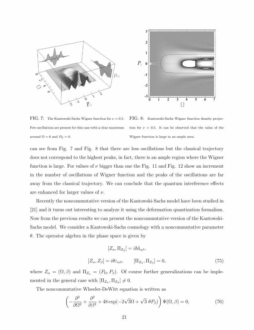
FIG. 7: The Kantowski-Sachs Wigner function for ν = 0.5.
Few oscillations are present for this case with a clear maximum
around Ω = 6 and PΩ = 0.
FIG. 8: Kantowski-Sachs Wigner function density projec-
tion for ν = 0.5. It can be observed that the value of the
Wigner function is large in an ample area.
can see from Fig. 7 and Fig. 8 that there are less oscillations but the classical trajectory
does not correspond to the highest peaks, in fact, there is an ample region where the Wigner
function is large. For values of ν bigger than one the Fig. 11 and Fig. 12 show an increment
in the number of oscillations of Wigner function and the peaks of the oscillations are far
away from the classical trajectory. We can conclude that the quantum interference effects
are enhanced for larger values of ν.
Recently the noncommutative version of the Kantowski-Sachs model have been studied in
[21] and it turns out interesting to analyze it using the deformation quantization formalism.
Now from the previous results we can present the noncommutative version of the Kantowski-
Sachs model. We consider a Kantowski-Sachs cosmology with a noncommutative parameter
θ. The operator algebra in the phase space is given by
[Zα,ΠZβ ] = i~δαβ,
[Zα, Zβ] = iθεαβ, [ΠZα ,ΠZβ ] = 0, (75)
where Zα = (Ω, β) and ΠZα = (PΩ, Pβ). Of course further generalizations can be imple-
mented in the general case with [ΠZα ,ΠZβ ] 6= 0.
The noncommutative Wheeler-DeWitt equation is written as(− ∂2
∂Ω2+
∂2
∂β2+ 48 exp(−2
√3Ω +
√3 θPβ)
)Ψ(Ω, β) = 0, (76)
21
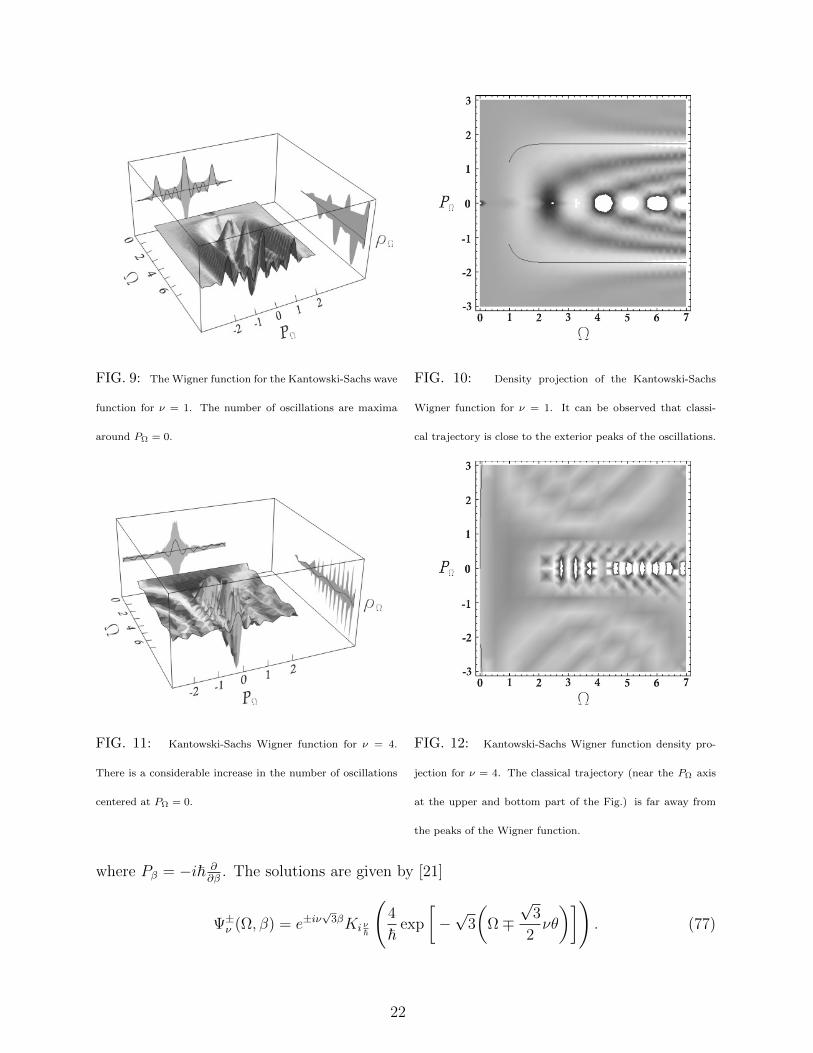
FIG. 9: The Wigner function for the Kantowski-Sachs wave
function for ν = 1. The number of oscillations are maxima
around PΩ = 0.
FIG. 10: Density projection of the Kantowski-Sachs
Wigner function for ν = 1. It can be observed that classi-
cal trajectory is close to the exterior peaks of the oscillations.
FIG. 11: Kantowski-Sachs Wigner function for ν = 4.
There is a considerable increase in the number of oscillations
centered at PΩ = 0.
FIG. 12: Kantowski-Sachs Wigner function density pro-
jection for ν = 4. The classical trajectory (near the PΩ axis
at the upper and bottom part of the Fig.) is far away from
the peaks of the Wigner function.
where Pβ = −i~ ∂∂β
. The solutions are given by [21]
Ψ±ν (Ω, β) = e±iν√
3βKi ν~
(4
~exp
[−√
3
(Ω∓
√3
2νθ
)]). (77)
22
The normalized wave function is
Ψ±(Ω, β) =31/4
π~
√sinh
(πν~
)Ki ν~
(4
~exp
[−√
3
(Ω∓
√3
2νθ
)])(78)
which satisfy ∫ ∞−∞
dΩdβΨ∗ν(Ω, β)Ψν(Ω, β) = δ(ν2 − ν ′2). (79)
Following a similar procedure as for the commutative case we are able to write the Wheeler-
DeWitt-Moyal equation in the following form−(PΩ −
i~2
→∂Ω
)2
+
(Pβ −
i~2
→∂ β
)2
− 48 exp
[− 2√
3
(Ω∓
√3
2νθ +
i~2
→∂PΩ
)]ρθ(Ω, PΩ, β, Pβ) = 0,
(80)
and the corresponding difference equation is
− P 2Ωρ
θΩ −
12√
3i~2e−2√
3(
Ω∓√
32νθ)
PΩ
[ρθΩ(Ω, PΩ + i
√3~)− ρθΩ(Ω, PΩ − i
√3~)]
− 144~2e−4√
3(
Ω∓√
32νθ)
(P 2Ω + 3~2)
[ρθΩ(Ω, PΩ + 2i
√3~)− 2ρθΩ(Ω, PΩ) + ρθΩ(Ω, PΩ − 2i
√3~)]
+144√
3i~3e−4√
3(
Ω∓√
32νθ)
PΩ(P 2Ω + 3~2)
[ρθΩ(Ω, PΩ + 2i
√3~)− ρθΩ(Ω, PΩ − 2i
√3~)]
− 24e−2√
3(
Ω∓√
32νθ) [ρθΩ(Ω, PΩ + i
√3~) + ρθΩ(Ω, PΩ − i
√3~)]
= −P 2βρ
θΩ. (81)
The solution to this equation is again difficult to obtain in a direct way but employing the
integral representation of the Wigner function we can calculate the corresponding noncom-
mutative Wigner function from
ρθ±Ω (Ω, PΩ) =31/2
2π4~2sinh
(πν~
)∫ ∞−∞
dyKi ν~
(4
~e±
32νθe−
√3(Ω− ~
2 y))e−iyPΩKi ν~
(4
~e±
32νθe−
√3(Ω+ ~
2 y)).
(82)
Thus we find
ρθ±Ω (Ω, PΩ) =sinh(πν/~)
π3
e√
3(
Ω∓√
32νθ)
16~2
(2
~2e−√
3(
Ω∓√
32νθ))− 2iPΩ√
3~
×G4004
(16
~4e−4√
3(
Ω∓√
32νθ)∣∣∣∣14 + i
(ν
2~+
PΩ√3~
),1
4+ i
(− ν
2~+
PΩ√3~
),1
4+iν
2~,1
4− iν
2~
).
(83)
23
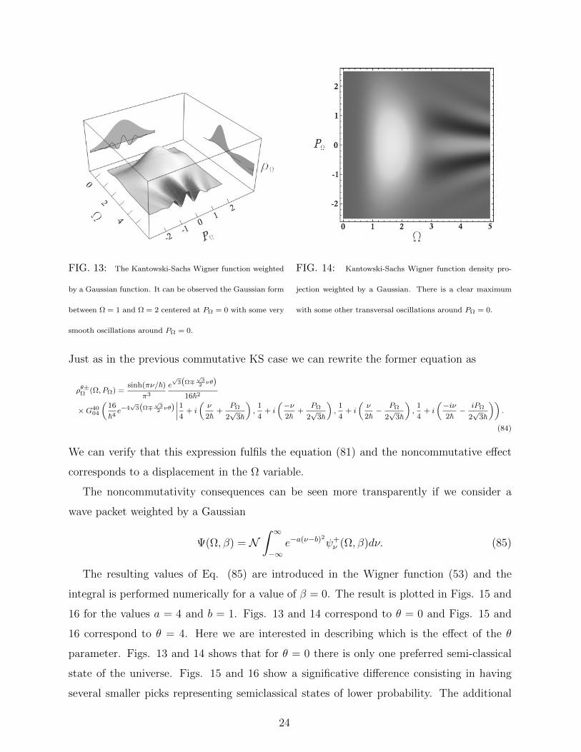
FIG. 13: The Kantowski-Sachs Wigner function weighted
by a Gaussian function. It can be observed the Gaussian form
between Ω = 1 and Ω = 2 centered at PΩ = 0 with some very
smooth oscillations around PΩ = 0.
FIG. 14: Kantowski-Sachs Wigner function density pro-
jection weighted by a Gaussian. There is a clear maximum
with some other transversal oscillations around PΩ = 0.
Just as in the previous commutative KS case we can rewrite the former equation as
ρθ±Ω (Ω, PΩ) =sinh(πν/~)
π3
e√
3(Ω∓
√3
2νθ)
16~2
×G4004
(16
~4e−4√
3(Ω∓
√3
2νθ)∣∣∣∣1
4+ i
(ν
2~+
PΩ
2√
3~
),
1
4+ i
(−ν2~
+PΩ
2√
3~
),
1
4+ i
(ν
2~−
PΩ
2√
3~
),
1
4+ i
(−iν2~−
iPΩ
2√
3~
)).
(84)
We can verify that this expression fulfils the equation (81) and the noncommutative effect
corresponds to a displacement in the Ω variable.
The noncommutativity consequences can be seen more transparently if we consider a
wave packet weighted by a Gaussian
Ψ(Ω, β) = N∫ ∞−∞
e−a(ν−b)2
ψ+ν (Ω, β)dν. (85)
The resulting values of Eq. (85) are introduced in the Wigner function (53) and the
integral is performed numerically for a value of β = 0. The result is plotted in Figs. 15 and
16 for the values a = 4 and b = 1. Figs. 13 and 14 correspond to θ = 0 and Figs. 15 and
16 correspond to θ = 4. Here we are interested in describing which is the effect of the θ
parameter. Figs. 13 and 14 shows that for θ = 0 there is only one preferred semi-classical
state of the universe. Figs. 15 and 16 show a significative difference consisting in having
several smaller picks representing semiclassical states of lower probability. The additional
24
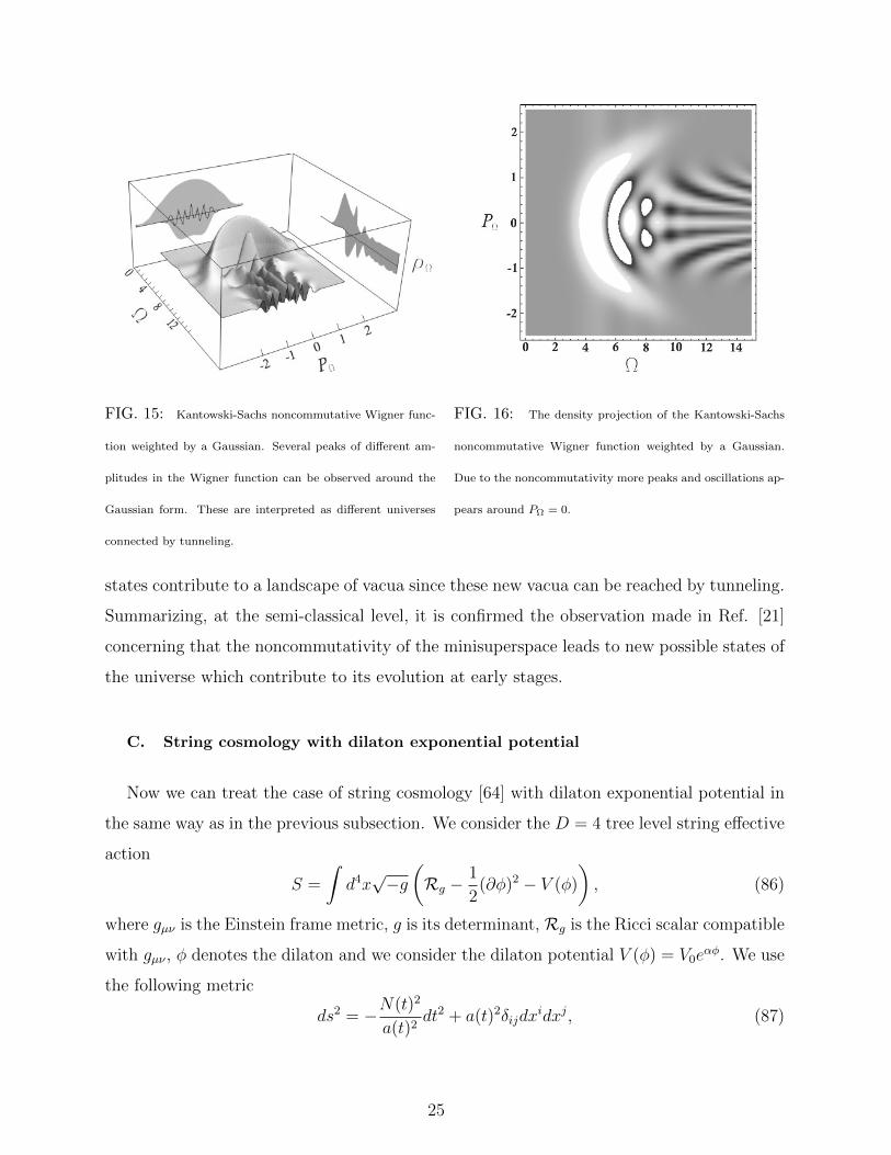
FIG. 15: Kantowski-Sachs noncommutative Wigner func-
tion weighted by a Gaussian. Several peaks of different am-
plitudes in the Wigner function can be observed around the
Gaussian form. These are interpreted as different universes
connected by tunneling.
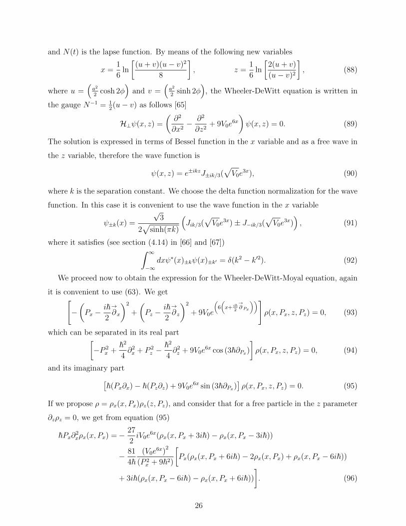
FIG. 16: The density projection of the Kantowski-Sachs
noncommutative Wigner function weighted by a Gaussian.
Due to the noncommutativity more peaks and oscillations ap-
pears around PΩ = 0.
states contribute to a landscape of vacua since these new vacua can be reached by tunneling.
Summarizing, at the semi-classical level, it is confirmed the observation made in Ref. [21]
concerning that the noncommutativity of the minisuperspace leads to new possible states of
the universe which contribute to its evolution at early stages.
C. String cosmology with dilaton exponential potential
Now we can treat the case of string cosmology [64] with dilaton exponential potential in
the same way as in the previous subsection. We consider the D = 4 tree level string effective
action
S =
∫d4x√−g(Rg −
1
2(∂φ)2 − V (φ)
), (86)
where gµν is the Einstein frame metric, g is its determinant, Rg is the Ricci scalar compatible
with gµν , φ denotes the dilaton and we consider the dilaton potential V (φ) = V0eαφ. We use
the following metric
ds2 = −N(t)2
a(t)2dt2 + a(t)2δijdx
idxj, (87)
25
and N(t) is the lapse function. By means of the following new variables
x =1
6ln
[(u+ v)(u− v)2
8
], z =
1
6ln
[2(u+ v)
(u− v)2
], (88)
where u =(a2
2cosh 2φ
)and v =
(a2
2sinh 2φ
), the Wheeler-DeWitt equation is written in
the gauge N−1 = 12(u− v) as follows [65]
H⊥ψ(x, z) =
(∂2
∂x2− ∂2
∂z2+ 9V0e
6x
)ψ(x, z) = 0. (89)
The solution is expressed in terms of Bessel function in the x variable and as a free wave in
the z variable, therefore the wave function is
ψ(x, z) = e±ikzJ±ik/3(√V0e
3x), (90)
where k is the separation constant. We choose the delta function normalization for the wave
function. In this case it is convenient to use the wave function in the x variable
ψ±k(x) =
√3
2√
sinh(πk)
(Jik/3(
√V0e
3x)± J−ik/3(√V0e
3x)), (91)
where it satisfies (see section (4.14) in [66] and [67])∫ ∞−∞
dxψ∗(x)±kψ(x)±k′ = δ(k2 − k′2). (92)
We proceed now to obtain the expression for the Wheeler-DeWitt-Moyal equation, again
it is convenient to use (63). We get[−(Px −
i~2
→∂ x
)2
+
(Pz −
i~2
→∂ z
)2
+ 9V0e
(6
(x+ i~
2
→∂ Px
))]ρ(x, Px, z, Pz) = 0, (93)
which can be separated in its real part[−P 2
x +~2
4∂2x + P 2
z −~2
4∂2z + 9V0e
6x cos (3~∂Px)]ρ(x, Px, z, Pz) = 0, (94)
and its imaginary part[~(Px∂x)− ~(Pz∂z) + 9V0e
6x sin (3~∂Px)]ρ(x, Px, z, Pz) = 0. (95)
If we propose ρ = ρx(x, Px)ρz(z, Pz), and consider that for a free particle in the z parameter
∂zρz = 0, we get from equation (95)
~Px∂2xρx(x, Px) =− 27
2iV0e
6x(ρx(x, Px + 3i~)− ρx(x, Px − 3i~))
− 81
4~(V0e
6x)2
(P 2x + 9~2)
[Px(ρx(x, Px + 6i~)− 2ρx(x, Px) + ρx(x, Px − 6i~))
+ 3i~(ρx(x, Px − 6i~)− ρx(x, Px + 6i~))
]. (96)
26
Using the former equation in (94) we finally obtain
−P 2z ρx(x, Px) =− P 2
xρx(x, Px) +27i~V0
4Pxe6x(ρx(x, Px + 3i~)− ρx(x, Px − 3i~))
+9V0
2e6x(ρx(x, Px + 3i~) + ρx(x, Px − 3i~))
− (9V0e6x)
2
42Px(P 2x + 9~2)
[(Px − 3i~)ρx(x, Px + 6i~)
− 2Pxρx(x, Px) + (Px + 3i~)ρx(x, Px − 6i~)]. (97)
This difference equation is complicated to solve in a direct way so as with the Kantowski-
Sachs case we use the integral representation of the Wigner function. Employing the follow-
ing result (see Sec. 19.3 formula (45) in [61]) we can calculate the Wigner function in terms
of the Meijer’s function∫ ∞0
xρ−1Jµ(ax)Jν(bx−1)dx = 2ρ−1a−ρG20
04
(a2b2
16
∣∣∣∣ν2 , ρ+ µ
2,ρ− µ
2,−ν
2
). (98)
Then we obtain,
ρx(x, Px) =1
8~π sin(πk)
[G20
04
(V 2
0 e12x
16~4
∣∣∣∣ i6(−k + Px),i
6(k − Px),
i
6(−k − Px),
i
6(k + Px)
)± G20
04
(V 2
0 e12x
16~4
∣∣∣∣ i6(−k + Px),i
6(−k − Px),
i
6(k − Px),
i
6(k + Px)
)± G20
04
(V 2
0 e12x
16~4
∣∣∣∣ i6(k + Px),i
6(k − Px),
i
6(−k − Px),
i
6(−k + Px)
)+ G20
04
(V 2
0 e12x
16~4
∣∣∣∣ i6(k + Px),ik
6(−k − Px),
i
6(k − Px),
i
6(−k + Px)
)]. (99)
We want to note, that it is also possible to write the Wigner function in terms of the
hypergeometric function 0F3 employing [68]. This is an straightforward but long calculation
that we will not present here.
It can be verified that ρx given by Eq. (99) satisfies the equation (97).
D. Baby Universes
In this subsection we will consider another example of the use of the deformation quan-
tization formalism to wormhole solutions in general relativity [69–71]. Here we will have a
system with two coordinates of the flat minisuperspace (2 degrees of freedom).
We are going to consider a baby universe with conformal matter φ0 and a three-metric
hij defined on a Cauchy hypersurface S of a closed wormhole universe. The matter is
27
represented by a conformal invariant scalar field expanded in hyper-spherical harmonics Qn
of the surface S given by φ0 = 1a
∑n fnQn, where a is the scale factor and fn are orthonormal
modes. The metric on S is given by hij = a2 · (Ωij + εij). Here Ωij is the metric of a unit
three-sphere S3 and εij =∑
n
(anΩijQn + bnPijn + cnSijn + dnGijn
). The Qn’s are the scalar
harmonics of the 3-sphere, Pijn is a suitable combination of Qn, Sijn is defined in terms of
the transverse vector harmonics and Gijn are the transverse traceless tensor harmonics on
S.
On the gravitational part, in a suitable gauge (an = bn = cn = 0) of hij on S and
considering the case without gravitons (dn = 0), one can express the three metric simply as:
hij = a2 ·Ωij. Thus, the wave function Ψ is a function of the scale factor a and the harmonic
modes of the scalar field fn. This wave function fulfills the Wheeler-DeWitt equation (10)
of the form
[∑n
(− ∂2
∂f 2n
+ n2f 2n
)−(− ∂2
∂a2+ a2
)]Ψ(a, fn) = 0, (100)
where we have implemented the canonical relation on the momenta pfn = −i~ ∂∂fn
and
pa = −i~ ∂∂a
.
In the context of quantum cosmology the solution factorizes in a purely gravitational
part and an purely matter part. Both of them correspond to harmonic oscillators and the
solution is given by
Ψ(a, fn) = AHm(a) exp
(−a
2
2
)·∏n
Hmn(fn√n) exp
(−nf
2n
2
), (101)
where Hm(x) are the Hermite polynomials and A is a normalization constant. This solution
satisfies the boundary conditions such that: ψ(a, fn) → 0 as a → ∞ and it is regular at
a = 0.
Here it is assumed, as in [70], that the zero-point energy of the gravitational sector
will precisely compensates the zero-point energy of the matter oscillators as it happens in a
supersymmetric theory. This solution represents a closed universe carrying m scalar particles
in the n-th mode. Thus the ground state |Ψ0〉 will correspond to m = 0 and n = 0, i.e., the
absence of matter particles and consequently excited states of the scale factor part.
The wave function factorization Ψ(a, fn) = ψ0(a)·∏
n ψn(fn) comes from the inner product
between 〈a, fn| and |ψ0, ψn〉. The ground state is given by |Ψ0〉 = |ψ0〉a ⊗ |ψ0〉f .
28
Let b and b† the annihilation and creation operators of the ma-th modes of the gravi-
tational sector defined by: b|0a,mf〉 = 0 and [b†]ma |Ψ0〉 = |ma,mf〉. Now, let d and d†
the annihilation and creation operators of the mf -th modes of scalar particles defined by:
d|ma, 0f〉 = 0 and [d†]mf |Ψ0〉 = |ma,mf〉. The combination yields b · d|0a, 0f〉 = 0 and
[b†]ma · [d†]mf |Ψ0〉 = |ma,mf〉.
In the WWGM formalism we have the following general stationary Wheeler-DeWitt-
Moyal equation
HB ? ρW (a, pa, fn, pfn) = 0, (102)
where ρW = ρW (a, pa, fn, pfn) is the Wigner function and HB stands for the baby universe
Hamiltonian
HB = Hf +Ha, (103)
where
Hf =∑n
(p2fn + ω2
nf2n
)(104)
with ωn = n and
Ha = p2a + a2. (105)
The Moyal product is given by
f ? g = f exp
(i~2
↔PB)g, (106)
where the corresponding Poisson operator has the following form
↔PB=
↔Pf +
↔Pa=
∑n
( ←∂
∂fn
→∂
∂pfn−
←∂
∂pfn
→∂
∂fn
)+
←∂
∂a
→∂
∂pa−
←∂
∂pa
→∂
∂a. (107)
We can write down ρW0 = ρaW0 · ρfW0 then we can separate (102) into two parts
Ha ? ρaW0(a, pa) = −EρaW0(a, pa), (108)
and
Hf ? ρfW0(f, pf ) = EρfW0(f, pf ). (109)
Therefore we have that the equation (102) at the order ~ can be written as
∑n
(ω2nfn ·
∂ρfW0
∂pfn− pfn ·
∂ρfW0
∂fn
)− a · ∂ρ
aW0
∂pa+ pa ·
∂ρaW0
∂a= 0, (110)
29
where ρW0 is the Wigner function for the ground state. Thus the solution to this equation
is given by
ρW0(pa, a, pfn , fn) = ρaW0(a, pa) · ρfW0(fn, pfn) = A exp
[−2
~(p2a + a2
)]·∏n
exp
[− 2
~(p2fn +ω2
nf2n
)].
(111)
The density matrix for all excited states is given by
ρr,s = [b†]r · [d†]s|Ψ0〉〈Ψ0|[d†]s · [b†]r. (112)
The WWGM formalism allows to compute from this density matrix the general Wigner
function for all excited states [53]
[ρW ]m,n = [b∗] ? · · · ? [b∗] ? [d∗] ? · · · ? [d∗] ? ρW0 ? [d∗] ? · · · ? [d∗] ? [b∗] ? · · · ? [b∗]. (113)
It is straightforward to show that it leads to the solution
ρW (pa, a, fn, pfn) = A exp
[−2
~(p2a + a2
)]Lm
(4
~(p2a + a2)
)·∏n
exp
[−2
~(p2fn+ω2
nf2n
)]Lmn
(4
~(p2fn + ω2
nf2n)
).
(114)
Here Lm(x) is the Laguerre polynomial of degree m. Remember that they are
related to the Hermite polynomials through the familiar formula Ln(x2 + y2) =
(−1)n2−2n∑n
m=01
m!(n−m)!H2m(x)H2n−2m(y). The case for the minimal coupling scalar matter
follows a similar treatment and will not be discussed here, but analogous formulas can be
obtained for this case.
V. FINAL REMARKS
In this paper we have constructed the WWGM formalism in the flat superspace (and phase
superspace). The WWGM correspondence is explicitly developed and the Stratonovich-Weyl
quantizer, the star product and the Wigner functional are obtained. These results can be
used in general situations but in a first approach we applied the formalism to some interesting
minisuperspace models widely studied in the literature, in particular, we used the Moyal star
product to describe some relevant cosmological models in phase space.
We studied de Sitter quantum cosmology using the Hartle-Hawking, Vilenkin and Linde
boundary conditions, where we have found numerically the Wigner function for all of these
cases.
30
For the Hartle-Hawking wave function the behavior of the Wigner function presents
many oscillations due to interference terms between the wave functions of expanding and
contracting universes. Similarly as in Ref. [30] our result shows that the highest peaks of
the Wigner function do not coincide with the classical trajectory of the universe.
The Linde Wigner function has a similar behavior to the Hartle-Hawking case, where there
are also expanding and contracting components of the wave function. The main difference
in their corresponding Wigner functions is just a sign in the interference terms between the
expanding and contracting wave functions and as a consequence it produces a reduction in
the amplitude of the oscillations inside the classical region.
In the case of the Vilenkin tunneling wave function we notice that the Wigner function
has less oscillations compared to the Hartle-Hawking Wigner function. This is explained by
the fact that there are less oscillation effects because there is only an outgoing wave. In this
case the classical trajectory corresponds almost to the maxima of the peaks of the Wigner
function.
However the classical limit for these three models is difficult to obtain due to the existence
of oscillations in the Wigner functions. It is important to note that decoherence of the
Vilenkin Wigner function is in principle simpler to obtain since the interference terms are
absent because there is only an expanding universe around p = 0.
For the Kantowski-Sachs cosmological model we found the Wheeler-DeWitt-Moyal equa-
tion which is equivalent to a differential-difference equation. We found its exact solution in
terms of the Meijer’s function. We observe that the classical trajectory corresponds to the
highest peaks of the Wigner function for values close to ν = 1. The situation for ν ≤ 1 in the
Wigner function corresponds to have less oscillations and the classical trajectory does not
correspond to the highest peaks. For values of ν ≥ 1 we have an increment in the number
of oscillations of the Wigner function and we do not have the peaks of the oscillations near
the classical trajectory. Thus it seems that ν could be regarded as a parameter encoding
the quantum interference effects.
We have also considered the noncommutative Kantowski-Sachs model. In a similar way
we obtain the analytic Wigner function and its differential-difference equation. This case
presents a noncommutative parameter θ deforming the Wheeler-DeWitt-Moyal equation.
The Wigner function is determined in terms of the above Meijer’s function with shifted ar-
gument by a factor proportional to θ. We have constructed numerically the Wigner function
31
with wave packet weighted by a Gaussian to see the effects of the noncommutativity. There
were found several peaks in the Wigner function around the Gaussian which can be inter-
preted as different universes connected by tunneling. Thus, at the semi-classical level, the
statement made in [21] about that the noncommutativity of the minisuperspace produces
new possible states of the universe at early stages is confirmed.
String cosmology with dilaton exponential potential is also discussed. We found the cor-
responding Wheeler-DeWitt-Moyal equation and the equivalent differential-difference equa-
tion. These equations have an exact solution in terms of the hypergeometric and Meijer’s
functions.
Baby universe solutions are also obtained in this context where the Wigner function is
calculated by finding the exact solution of its Wheeler-DeWitt-Moyal equation consisting in
two decoupled deformed harmonic oscillators in terms of Laguerre polynomials.
It is important to remark that this work opens the possibility of treating several im-
portant questions that remain unsolved in quantum cosmology with a novel approach. For
instance, deformation quantization allows to deal with systems having phase spaces with
nontrivial topology. In quantum cosmology, the existence of symmetries implies that the
phase-superspace and in particular, the phase-minisuperspace will be reduced by the im-
plementation of these symmetries leading to a non-trivial topological space with a non-flat
metric. Therefore, deformation quantization is able to treat these mentioned cases in a nat-
ural way. Moreover the extension to supersymmetric quantum cosmology [17, 19, 20] can
be also treated applying the results of [72].
Another point to remark is that the Wheeler-DeWitt-Moyal equation (29) proposed in
the present paper contains the generalized mass-shell equation and the Wheeler-DeWitt-
Vlasov transport equation in the flat minisuperspace [29] encoded in its real an imaginary
parts respectively. The former result was obtained using the Moyal ?−product and then all
the technics of deformation quantization developed for a long time can be apply to it. It
is known that the mass-shell equation and the Wheeler-DeWitt-Vlasov transport equation
admits a suitable generalization to curved minisuperspace [29]. It would be interesting to
deal with curved symplectic cases where the Fedosov’s approach could be applied in order
to find the Wheeler-DeWitt-Moyal equation in non-trivial phase superspaces and obtain
the mass-shell and the Wheeler-DeWitt-Vlasov equations. We will study this problem in a
further communication.
32
Besides, as was mentioned before, the problem of obtaining the classical limit by imple-
menting a coarse graining is relevant. It is possible to model a coarse graining through the
Liouville equation with friction and diffusion terms [30], this approach can be addressed in
the context of the deformation quantization formalism.
To conclude, we consider that deformation quantization possesses various advantages
in order to deal with more complicated problems in quantum cosmology for example, to
treat systems with non trivial topology or with curved minisuperspaces. For these cases
the canonical quantization could lead to the existence of nonhermitian operators which is
avoided in deformation quantization as a result of the use of classical objects instead of
operators. For these reasons more examples and further research is needed to develop this
approximation.
Acknowledgments
The work of R. C., H. G.-C. and F. J. T. was partially supported by SNI-Mexico, CONA-
CyT research grants: J1-60621-I, 103478 and 128761. In addition R. C. and F. J. T. were
partially supported by COFAA-IPN and by SIP-IPN grants 20100684 and 20100887. We
are indebted to Hector Uriarte for all his help in the elaboration of the figures presented in
the paper.
[1] B. S. DeWitt, Phys. Rev. 160, 1113 (1967).
[2] E.P. Tryon, Nature (London) 246, 396 (1973).
[3] P. I. Fomin, Dokl. Akad. Nauk Ukr. SSR 9A, 831 (1975).
[4] D. Atkatz and H. Pagels, Phys. Rev. D 25, 2065 (1982).
[5] A. Vilenkin, Phys. Lett. B 117, 25 (1982).
[6] L. P. Grishchuk and Ya. B. Zel’dovich, in Quantum Structure of Space and Time edited by
M. Duff and C. Isham, (Cambridge University Press, Cambridge, 1982).
[7] J. B. Hartle and S. W. Hawking, Phys. Rev. D 28, 2960 (1983).
[8] A. D. Linde, Lett. Nuovo Cimento 39, 401 (1984).
[9] V. A. Rubakov, Phys. Lett. B 148, 280 (1984).
33
[10] A. Vilenkin, Phys. Rev. D 30, 509 (1984).
[11] A. Vilenkin, Phys. Rev. D 50, 2581 (1994).
[12] R. Bousso and S. W. Hawking, Phys. Rev. D 54, 6312 (1996); J. Garriga and A. Vilenkin,
Phys. Rev. D 56, 2464 (1997); A. D. Linde, Phys. Rev. D 58, 083514, (1998); N. G. Turok,
S. W. Hawking, Phys. Lett. 432, 271 (1998); A. Vilenkin, Phys. Rev. D 58, 067301 (1998).
[13] R. Brustein and S. P. de Alwis, Phys. Rev. D 73, 046009 (2006). [arXiv:hep-th/0511093].
[14] C. Kounnas, N. Toumbas and J. Troost, JHEP 0708, 018 (2007). [arXiv:0704.1996 [hep-th]].
[15] M. Gasperini, Elements of string cosmology, Cambridge, UK: Cambridge University. Press.
(2007).
[16] A. Strominger, in Quantum Cosmology and Baby Universes, eds. S. Coleman, J. B. Hartle,
T. Piran and S. Weinberg, (World Scientific, Singapore, 1991), p. 269.
[17] A. Macias, O. Obregon and J. Socorro, Int. J. Mod. Phys. A 8, 4291 (1993).
[18] A. Csordas and R. Graham, Phys. Rev. Lett, 74, 4129 (1995).
[19] O. Obregon, J. J. Rosales and V. I. Tkach, Phys. Rev. D 53, 1750 (1996).
[20] P. D. D’Eath, Supersymmetric quantum cosmology , (Cambridge University Press, Cambridge,
England,1996), p. 252.
[21] H. Garcıa-Compean, O. Obregon and C. Ramırez, Phys. Rev. Lett. 88, 161301 (2002)
[arXiv:hep-th/0107250].
[22] J. B. Hartle, in Quantum Cosmology and Baby Universes, eds. S. Coleman, J. B. Hartle, T.
Piran and S. Weinberg, (World Scientific, Singapore, 1991), p. 65.
[23] J. J. Halliwell, J. Perez-Mercader, and W. H. Zrek (eds.), The physical Origins of Time
Asymmetry, (Cambridge University Press, 1994).
[24] J.C. Thorwart, Quantum Cosmology and the Dechoherent Histories Approach to Quantum
Theory, Ph.D. thesis, University of London, (2002).
[25] J. J. Halliwell, Contemp. Phys. 46, 93 (2005).
[26] J.J. Halliwell, Phys. Rev. D 36, 3626 (1987); Phys. Lett. B 196, 444 (1987).
[27] T. P. Singh and T. Padmanabhan, Ann. Phys. (N.Y.) 196, 296 (1989); Class. Quant. Grav.
5, 903 (1998).
[28] H. Kodama, in Fifth Marcel Grossman Meeting, proceedings, Perth, Australia, 1988, edited
by D.G. Blair and M.J. Buckingham (World Scientific, Singapore, 1989).
[29] E. Calzetta and B.L. Hu, Phys. Rev. D 40,380 (1989).
34
[30] S. Habib and R. Laflamme, Phys. Rev. D 42, 4056 (1990).
[31] M. Hillery, R.F. O’Connell, M.O. Scully and E. P. Wigner, Phys. Rep. 106, 121 (1984).
[32] S. Habib, Phys. Rev. D 42, 2566 (1990).
[33] R. Laflamme and J. Louko, Phys. Rev. D 43, 3317 (1991).
[34] J. J. Halliwell, Phys. Rev. D 46, 1610 (1992).
[35] H. Weyl, Group Theory and Quantum Mechanics, (Dover, New York, 1931).
[36] E. P. Wigner, Phys. Rev. 40, 749 (1932).
[37] A. Groenewold, Physica 12, 405-460 (1946).
[38] J. E. Moyal, Proc. Camb. Phil. Soc. 45, 99 (1949).
[39] J. Vey, Comment. Math. Helvet. 50, 421 (1964).
[40] F. Bayen, M. Flato, C. Fronsdal, A. Lichnerowicz and D. Sternheimer, Ann. Phys. 111, 61
(1978); Ann. Phys. 111, 111 (1978).
[41] M. De Wilde and P.B.A. Lecomte, Lett. Math. Phys. 7 (1983) 487; H. Omori, Y. Maeda and
A. Yoshioka, Adv. Math. 85, 224 (1991).
[42] B. Fedosov, J. Diff. Geom. 40, 213 (1994); Deformation Quantization and Index Theory
(Akademie Verlag, Berlin, 1996).
[43] M. Kontsevich, “Deformation Quantization of Poisson Manifolds I”. [q-alg/9709040]; Lett.
Math. Phys. 48, 35 (1999).
[44] D. L. Wiltshire, An introduction to quantum cosmology. [gr-qc/0101003].
[45] F. Antonsen, “Deformation quantisation of gravity,” [arXiv:gr-qc/9712012]; “Deformation
quantisation of constrained systems,” [arXiv:gr-qc/9710021].
[46] C.K. Zachos, “Deformation Quantization: Quantum Mechanics Lives and Works in Phase
Space”, Int. J. Mod. Phys. A 17 (2002) 297. [hep-th/0110114].
[47] A.C. Hirshfeld and P. Henselder, Am. J. Phys. 70, 537 (2002).
[48] G. Dito and D. Sternheimer, “Deformation Quantization: Genesis, Developments and Meta-
morphoses”, Deformation Quantization (Strasbourg 2001) Lect. Math. Theor. Phys. 1 Ed. de
Gruyter, Berlin, IRMA (2002) pp. 9-54.
[49] D. Sternheimer, “Quantizations and quantizations and introductory overview”, Contemp.
Math. 462, 41,(2008).
[50] N. Seiberg and E. Witten, JHEP 9909, 032 (1999). [arXiv:hep-th/9908142].
[51] R.L. Stratonovich, Sov. Phys. JETP 31, 1012 (1956); A. Grossmann, Commun. Math.
35
Phys.48, 191 (1976); J. M. Gracia Bondıa and J. C. Varilly, J. Phys. A: Math. Gen. 21,
L879 (1988), Ann. Phys. 190, 107 (1989); J. F. Carinena, J. M. Gracia Bondıa and J. C. Var-
illy, J. Phys. A: Math. Gen. 23, 901 (1990); M. Gadella, M. A. Martın, L. M. Nieto and M.
A. del Olmo, J. Math. Phys. 32, 1182 (1991); J. F. Plebanski, M. Przanowski and J. Tosiek,
Acta Phys. Pol. B27 1961 (1996).
[52] W. I. Tatarskii, Usp. Fiz. Nauk 139, 587 (1983).
[53] H. Garcıa-Compean, J. F. Plebanski, M. Przanowski and F. J. Turrubiates, Int. J. Mod. Phys.
A 16, 2533 (2001). [arXiv:hep-th/9909206].
[54] J. Luoko, Class. Quantum. Grav, 4, 581 (1987).
[55] V.A. Rubakov, Phys. Lett. B 214, 503 (1982).
[56] N. C. Dias and J. N. Prata, J. Math. Phys. 43, 4602 (2002).
[57] N. C. Dias and J. N. Prata, Ann. Phys. 321, 495 (2006).
[58] R. Kantowski and R. K. Sachs, J. Math. Phys. 7, 443 (1967), D. M. Solomons, P. Dunsby and
G. Ellis, Class. Quant. Grav. 23, 6585 (2006).
[59] C. Misner, in Magic Without Magic:John Archibald Wheeler (Freeman, San Francisco, 1972).
[60] R. Szmytkowski and S. Bielski, J. Math. Anal. Appl. 365, 195 (2010).
[61] A. Erdelyi et al., Tables of Integral Transform, Bateman Manuscript Project (McGarw-Hill,
New York, 1954).
[62] T. Curtright, D. Fairlie and C. Zachos, Phys. Rev. D, 58, 025002 (1998).
[63] A. Erdelyi et al., Higher Transcendental Functions, Bateman Manuscript Project (McGraw-
Hill, New York, 1953).
[64] J. E. Lidsey, D. Wands and E. J. Copeland, Phys. Rept. 337, 343 (2000).
[65] J. Maharana, Phys. Rev. D, 65, 103504 (2002).
[66] E. C. Titchmarsh, Eigenfunction Expansions, Second Edition, (Oxford at Clarendon Press,
Great Britain, 1962).
[67] S. Fulling, Phys. Rev. D, 7, 2850 (1973).
[68] I. S. Gradshteyn and I. M. Ryzhik, Table of Integrals, Series, and Products (Academic Press,
New York, 1980).
[69] S. W. Hawking, Phys. Rev. D 37, 904 (1988).
[70] S. W. Hawking, Mod. Phys. Lett. A 5, 453 (1990).
[71] A. Lyons and S. W. Hawking, Phys. Rev. D 44, 3802 (1991).
36
[72] I. Galaviz, H. Garcıa-Compean, M. Przanowski and F. J. Turrubiates, Annals Phys. 323, 267
(2008) [arXiv:hep-th/0612245].
37


