Quantization of Overcomplete Expansions

Vivek K Goyal, Martin Vetterli� Nguyen T. ThaoDept. of Electrical Engineering Dept. of Electrical & Electronic Eng.Univ. of California at Berkeley Hong Kong Univ. of Science & Tech.

fvkgoyal,marting@eecs.berkeley.edu eethao@ee.ust.hk

Abstract

The use of overcomplete sets of vectors (redundant bases or frames) togetherwith quantization is explored as an alternative to transform coding for signalcompression. The goal is to retain the computational simplicity of transformcoding while adding exibility like adaptation to signal statistics. We showresults using both �xed quantization in frames and greedy quantization usingmatching pursuit. An MSE slope of -6 dB/octave of frame redundancy is shownfor a particular tight frame and is veri�ed experimentally for another frame.

1 Introduction

Vector quantization and transform coding are the standard methods used in signalcompression. Vector quantization gives better rate-distortion performance, but it isdi�cult to implement and is computationally expensive. The computational aspectsmake transform coding very attractive. In particular, transform coding is ubiquitousin image compression.

For �ne quantization of a Gaussian signal with known statistics, the Karhunen-Loeve transform (KLT) is optimal for transform coding [2]. In general, signal statisticsare changing or not known a priori. Thus, one must either estimate the KLT from�nite length blocks of the signal or use a �xed, signal independent transform. Theformer case is computationally intensive and transmission of the KLT coe�cients canbe prohibitively expensive. The latter option is most commonly used, often with thediscrete cosine transform (DCT). As with any �xed transform, the DCT is nearlyoptimal for only a certain set of possible signals. There has been considerable work inthe area of adaptively choosing a transform from a library of orthogonal transforms,for example, using wavelet packets [5].

All varieties of transform coding represent a signal vector as a linear combinationof orthogonal basis vectors. In this paper, we present a method that represents asignal with respect to an overcomplete set of vectors which we call a dictionary.The representation is generated through greedy successive approximation. Much

�Work supported in part by the National Science Foundation under grant MIP-93-21302

1

as the KLT �nds the best representation \on average," this method �nds a goodrepresentation for the particular vector being coded. The overhead in using thismethod is that the indices of the dictionary elements used must be coded. Hencein choosing a dictionary size there is a tradeo� between increasing overhead andenhancing the ability to closely match signal vectors with a small number of iterations.

For a signal with correlated samples, we expect certain dictionary elements tobe chosen much more often than others. Thus entropy coding of the indices greatlyreduces the overhead in this representation. In particular, this method can be usedin a one-pass quantization system where the only adaptive component is a losslesscoder. We do not adapt the dictionary, which would be computationally expensive.Note that one step of our algorithm is related to gain-shape vector quantization, andthe overall scheme could be seen as a cascade form.

We begin in Section 2 with background material on frame representations andmethods of generating frames. In Section 3 we discuss quantization in tight frameswith no distributional assumptions and no adaptation to signal properties. Finally,in Section 4 we describe our quantization method based on matching pursuit. Anexample illustrates the exibility of this approach. Experimental results based on asimple design which employs no distributional assumptions are also presented.

Throughout we will limit our attention to quantization of vectors from a �nitedimensional Hilbert space H = C

N (or RN). We denote the inner product of x; y 2 Hby < x; y >, and denote the norm of x by jjxjj =< x; x >1=2.

2 Redundant Representations and Frames

Let f'kgMk=1 � H, whereM > N . If Span(f'kgMk=1) = H, there exist 0 < A � B <1so that, 8f 2 H,

Ajjf jj2 �MXk=1

j < f;'k > j2 � Bjjf jj2: (1)

We say that f'kgMk=1 is a frame or an overcomplete set of vectors with redundancy

ratio R = MN

[1]. Furthermore, if (1) holds for some A = B, we call the frame a tight

frame. If f'kgMk=1 is a tight frame such that jj'kjj = 1 8 k, then A = R.Since Span(f'kgMk=1) = H, any vector f 2 H can be written as

f =MXk=1

�k'k (2)

for some set of coe�cients f�kg � R which are not unique. We refer to (2) as aredundant representation, although it may be the case that only N of the �k's arenon-zero. De�ne the frame operator F associated with f'kgMk=1 to be the linearoperator from H to CM given by

(Ff)k =< f;'k > : (3)

Note that since H is �nite dimensional, this operation is a matrix multiplicationwhere F is a matrix with kth row equal to 'k. Using the frame operator, (1) can be

rewritten asAIN � F �F � BIN ; (4)

where IN is the N � N identity matrix. (The matrix inequality AIN � F �F meansthat F �F �AIN is a positive semide�nite matrix.) In particular, F �F = AIN showsthat f'kgMk=1 is a tight frame.

As an example, we will show that oversampling of a periodic, bandlimited signalcan be viewed as a frame operator applied to the signal, where the frame operatoris associated with a tight frame. If the samples are quantized, this is exactly thesituation of oversampled A/D conversion [7]. Let x = [X1 X2 � � � XN ]T 2 R

N. Wede�ne a corresponding continuous-time signal by

xc(t) = X1 +WXk=1

"X2k

p2 cos

2�kt

T+X2k+1

p2 sin

2�kt

T

#: (5)

(Any real-valued, T-period, bandlimited, continuous-time signal can be written inthis form.) De�ne a sampled version of xc(t) by xd[m] = xc(

mTM) and let y =

[xd(0) xd(1) � � � xd(M � 1)]T . Then we have y = Fx, where

F =

26666641

p2 0 � � � p

2 0

1p2 cos �

p2 sin � � � � p

2 cosW�p2 sinW�

......

......

...

1p2 cos(M 0�)

p2 sin(M 0�) � � � p

2 cos(WM 0�)p2 sin(WM 0�)

3777775 ; (6)

M 0 =M � 1, and � = 2�M. Using the orthogonality properties of sine and cosine, it is

easy to check that F �F = MIN , so F is an operator associated with a tight frame.Pairing terms and using the identity cos2 k�+sin2 k� = 1, we �nd that each row of Fhas norm

pN . Dividing F by

pN normalizes the frame and results in a frame bound

equal to the redundancy ratio R. Also note that R is the oversampling ratio withrespect to the Nyquist sampling frequency. Notice that multiplication by F can bedone e�ciently using an FFT-based algorithm. We will refer to generating a framein R

N for odd N using (6) as \Method I".A multitude of other families of frames can be found. For N = 3, 4, and 5,

Hardin, Sloane and Smith have numerically found arrangements of up to 130 pointson N -dimensional spheres that maximize the minimum Euclidean norm separation[3]. We refer to selecting one of these sets of points as \Method II".

A third method is to consider the corners of the hypercube [� 1pN; 1p

N]N . These

form a set of 2N symmetric points in RN. Taking the subset of points that have a pos-itive �rst coordinate gives a frame of size 2N�1. This frame has the feature that innerproducts can be computed by addition and subtraction without any multiplication.

3 Reconstruction from Frame Coe�cients

Let F 2 RM�N be a frame operator. Let x 2 R

N and y = Fx. Suppose y is quantizedas y = Q[y] according to some partition of RM. The uncertainty region associated

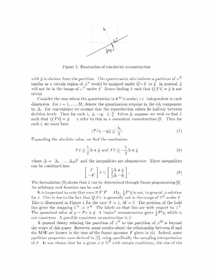
y

xx

y1−AF*

Figure 1: Illustration of consistent reconstruction

with y is obvious from the partition. This quantization also induces a partition of RN

insofar as a certain region of RN would be mapped under Q � F to y. In general, ywill not be in the image of RN under F . Hence �nding x such that Q[F x] = y is nottrivial.

Consider the case where the quantization in RM is scalar, i.e. independent in eachdimension. For i = 1; : : : ;M , denote the quantization stepsize in the ith componentby �i. For convenience we assume that the reproduction values lie halfway betweendecision levels. Then for each i, jyi � yij � �

2. Given y, suppose we wish to �nd x

such that Q[F x] = y. We refer to this as a consistent reconstruction [8]. Then foreach i, we must have

j(F x)i � yij � �i

2: (7)

Expanding the absolute value, we �nd the constraints

F x � 1

2� + y and F x � �1

2�+ y (8)

where � = [�1 : : : �M ]T and the inequalities are elementwise. These inequalitiescan be combined into "

F�F

#x �

"1

2�+ y

1

2�� y

#: (9)

The formulation (9) shows that x can be determined through linear programming [6].An arbitrary cost function can be used.

It is important to note that even if F �F = AIN ,1

AF �y is not, in general, a solution

for x. This is due to the fact that Q[Fx] is generally not in the image of RN under F .This is illustrated in Figure 1 for the case N = 1, M = 2. The position of the boldline gives the mapping RN ! R

M. The labels on that line are with respect to RN.

The quantized value of y = Fx is y. A \naive" reconstruction gives 1

AF �y, which is

not consistent. A possible consistent reconstruction is x.A general theory relating the partition of RN to the partition of RM is beyond

the scope of this paper. However, some results about the relationship between R andthe MSE are known in the case of the frame operator F given in (6). Indeed, somepartition properties were derived in [7], using speci�cally the sampling interpretationof F . It was shown that for a given x 2 R

N with certain conditions, the size of the

partition cell in RN diminishes with R as O(1=R2) in the MSE sense. The proof

explicitly uses the fact that y = Q[Fx] gives the sequence obtained by oversamplingand quantizing the continous-time signal xc(t) de�ned from x in (5). The conditionon x, however, is that xc(t) must cross the thresholds of the quantizer at least Ntimes in one period T . In the case N = 3 (W = 1), this is guaranteed for all

vector x = [X1 X2 X3]T such thatqX22 +X2

3 � �. In the three dimensional case,

a stronger result can in fact be shown. If we consider a given bounded region of R3

whose elements x satisfyqX22 +X2

3 � �, then all the cells of the partition within

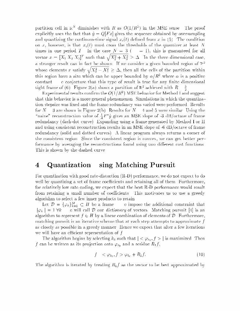
this region have a size which can be upper bounded by �=R2 where � is a positiveconstant. We conjecture that this type of result is true for any �nite dimensionaltight frame of (6). Figure 2(a) shows a partition of R2 achieved with R = 5

2.

Experimental results con�rm the O(1=R2) MSE behavior for Method I and suggestthat this behavior is a more general phenomenon. Simulations in which the quantiza-tion stepsize was �xed and the frame redundancy was varied were performed. Resultsfor N = 3 are shown in Figure 2(b). Results for N = 4 and 5 were similar. Using the\naive" reconstruction value of 1

AF �y gives an MSE slope of -3 dB/octave of frame

redundancy (dash-dot curve). Expanding using a frame generated by Method I or IIand using consistent reconstruction results in an MSE slope of -6 dB/octave of frameredundancy (solid and dotted curves). A linear program always returns a corner ofthe consistent region. Since the consistent region is convex, we can get better per-formance by averaging the reconstructions found using two di�erent cost functions.This is shown by the dashed curve.

4 Quantization Using Matching Pursuit

For quantization with good rate-distortion (R-D) performance, we do not expect to dowell by quantizing a set of frame coe�cients and retaining all of them. Furthermore,for relatively low rate coding, we expect that the best R-D performance would resultfrom retaining a small number of coe�cients. This motivates us to use a greedyalgorithm to select a few inner products to retain.

Let D = f'kgMk=1 � H be a frame . We impose the additional constraint thatjj'kjj = 1 8k. We will call D our dictionary of vectors. Matching pursuit [4] is analgorithm to represent f 2 H by a linear combination of elements of D. Furthermore,matching pursuit is an iterative scheme that at each step attempts to approximate fas closely as possible in a greedy manner. Hence we expect that after a few iterationswe will have an e�cient representation of f .

The algorithm begins by selecting k0 such that j < 'k0 ; f > j is maximized. Thenf can be written as its projection onto 'k0 and a residue R1f ,

f =< 'k0; f > 'k0 +R1f: (10)

The algorithm is iterated by treating R1f as the vector to be best approximated by

(0,-1,-1,0,0)

(-1,-1,-1,0,0)

(0,-1,-1,-1,0)(0,0,0,-1,-1)

(-1,0,0,-1,-1)

(-1,0,0,0,-1)

(0,-2,-2,0,1)

(1,-1,-2,-1,1)

(2,0,-2,-2,0)(1,1,-1,-2,-1)

(0,1,0,-2,-2)

(-1,1,1,-1,-2)

(-2,0,1,0,-2)

(-2,-1,1,1,-1) (-2,-2,0,1,0)

(-1,-2,-1,1,1)

(0,0,-1,-1,-1)

(0,0,-1,-1,0)

(-1,-1,0,0,0)

(-1,-1,0,0,-1)

0

3 3.5 4 4.5 5 5.5−70

−68

−66

−64

−62

−60

−58

−56

−54

−52

−50

log2(R)

MS

E (

dB

)

(a) (b)

Figure 2: (a) Partition of R2 induced by quantizing withR = 5

2tight frame. (b) Exper-

imental results for reconstruction from quantized frame expansion. Dash-dot curve:\naive" reconstruction. Dotted curve: consistent reconstruction from expansion I.Solid curve: consistent reconstruction from expansion II. Dashed curve: improvedconsistent reconstruction.

a multiple of 'k1 . Identifying R0f = f , we can write

f =n�1Xi=0

< 'ki; Rif > 'ki +Rnf: (11)

Hereafter we will denote < 'ki ; f > by �i. Notice that since �i is determined byprojection, �i'ki ? Ri+1f . Thus we have the \energy conversation" equation

jjRif jj2 = jjRi+1f jj2 + �2i : (12)

Since ki is selected to maximize j�ij, the energy in the residue is strictly decreasinguntil f is exactly represented.

To use matching pursuit for quantization, at the ith stage we quantize �i, yielding�i = Q[�i]. The quantized version is used in determining the residual so that quan-tization errors do not propagate to subsequent iterations. Note that the coe�cientquantization destroys the orthogonality of the projection and residual, so the analogof (12) does not hold.

At this point we have several design problems. We must choose a dictionary,design scalar quantizers, and decide how many quantized inner products to retain. Inprinciple, one could optimize each of these for a given source distribution, distortionmeasure and rate measure.

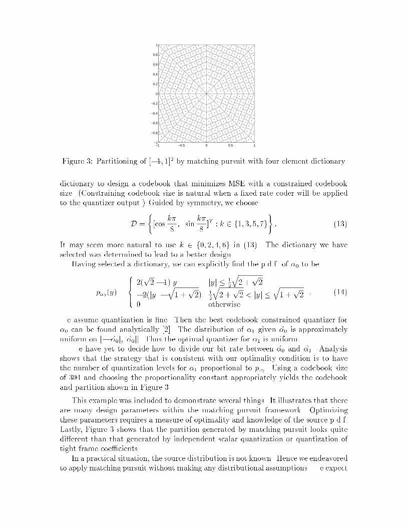
Example: Consider quantization of a source x = [X1; X2]T with a uniform

distribution on [�1; 1]2. Suppose we want to use matching pursuit with a four element

−1 −0.5 0 0.5 1−1

−0.8

−0.6

−0.4

−0.2

0

0.2

0.4

0.6

0.8

1

Figure 3: Partitioning of [�1; 1]2 by matching pursuit with four element dictionary

dictionary to design a codebook that minimizes MSE with a constrained codebooksize. (Constraining codebook size is natural when a �xed rate coder will be appliedto the quantizer output.) Guided by symmetry, we choose

D =

([cos

k�

8; sin

k�

8]T : k 2 f1; 3; 5; 7g

): (13)

It may seem more natural to use k 2 f0; 2; 4; 6g in (13). The dictionary we haveselected was determined to lead to a better design.

Having selected a dictionary, we can explicitly �nd the p.d.f. of �0 to be

p�0(y) =

8>><>>:

2(p2 � 1)jyj jyj � 1

2

q2 +

p2

�2(jyj �q1 +

p2) 1

2

q2 +

p2 < jyj �

q1 +

p2

0 otherwise

: (14)

We assume quantization is �ne. Then the best codebook constrained quantizer for�0 can be found analytically [2]. The distribution of �1 given �0 is approximatelyuniform on [�j�0j; j�0j]. Thus the optimal quantizer for �1 is uniform.

We have yet to decide how to divide our bit rate between �0 and �1. Analysisshows that the strategy that is consistent with our optimality condition is to havethe number of quantization levels for �1 proportional to p�0. Using a codebook sizeof 304 and choosing the proportionality constant appropriately yields the codebookand partition shown in Figure 3.

This example was included to demonstrate several things. It illustrates that thereare many design parameters within the matching pursuit framework. Optimizingthese parameters requires a measure of optimality and knowledge of the source p.d.f.Lastly, Figure 3 shows that the partition generated by matching pursuit looks quitedi�erent than that generated by independent scalar quantization or quantization oftight frame coe�cients.

In a practical situation, the source distribution is not known. Hence we endeavoredto apply matching pursuit without making any distributional assumptions. We expect

the best performance with a dictionary that is \evenly spaced" on the unit sphereor a hemisphere. We are purposely vague about the meaning of evenly spaced, sincethe importance of this is not yet clear. The three methods described in Section 2were used to generate dictionaries. Method I provides the most exibility. However,large dictionaries of this type are not \evenly" distributed because they lie in theintersection of the unit sphere with the plane x1 = 1p

N. We present experimental

results using each method.Our experiments all involve quantization of a zero mean Gaussian AR source with

correlation coe�cient � = 0:9. Source vectors are generated by forming blocks of Nsamples. All inner product quantization was scalar, uniform and equal in each dimen-sion. In addition to not relying on distributional assumptions, this is computationallyeasy and consistent with equally weighting the error in each direction. Distortion wasmeasured by MSE and rate by summing the (scalar) entropies of the ki's and �i'sretained. We denote the number of inner products retained by p and the quantizationstepsize by �.

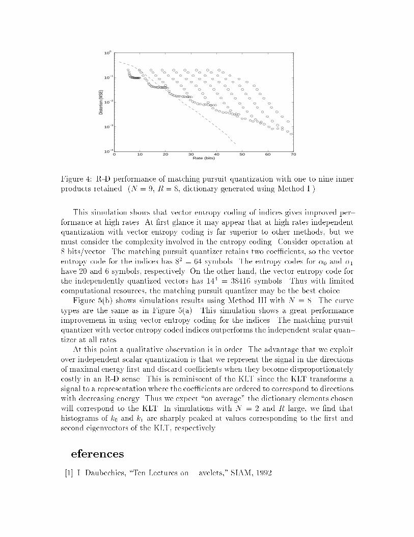
Figure 4 shows the D(R) points obtained using Method I with N = 9. Thedictionary redundancy ratio is R = 8. The dotted curves correspond to varying p,with the leftmost and rightmost curves corresponding to p = 1 and p = 9, respectively.The points along each dotted curve correspond various values of �. The dashed curveshows the performance of independently quantizing in each dimension.

The lower boundary of the region bounded below by one or more dotted curves isthe best R-D performance that can be achieved with this dictionary through choice pand �. The simulation results show that matching pursuit performs as well or betterthan independent scalar quantization for rates up to about 23 bits per vector (2.6bits per source sample).

The simulation described above does not explore the signi�cance of the R param-eter. Simulations as above were performed with R varied from 1 to 256. Redundancyfactors between 2 and 8 resulted in the best performance.

Simulations with N = 25 and R varied from 1 to 256 showed the best performancewas achieved with R between 2 and 4. The matching pursuit quantizer outperformedthe independent quantizer up to a rate of 75 bits per vector (3 bits per source sample).

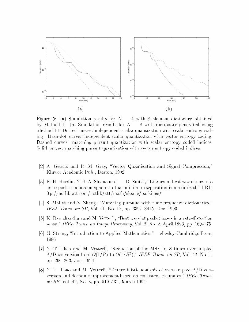
Consider use of Method II. We select a dictionary of size eight in R4 from [3].

Figure 5(a) shows the R-D performance of four quantizers. The dashed curve resultsfrom using matching pursuit with separate entropy coding of each index and eachcoe�cient. The solid curve shows the improvement resulting from vector entropycoding of the indices. The \knees" in these curves correspond to rates at which theoptimal number of coe�cients to retain changes. Independently quantizing in eachdimension and scalar entropy coding gives the dotted curve. Replacing the scalarentropy coding by vector entropy coding gives the dash-dot curve.

At rates up to about 6 bits per vector (1.5 bits per source sample), matchingpursuit quantization outperforms independent scalar quantization with either entropycoding method. At these rates, only one quantized inner product is retained. Thematching pursuit quantization does better than independent quantization with scalarentropy coding for rates up to about 12 bits per vector (3 bits per source sample).

0 10 20 30 40 50 60 7010

−4

10−3

10−2

10−1

100

Rate (bits)

Disto

rtion

(MSE

)

Figure 4: R-D performance of matching pursuit quantization with one to nine innerproducts retained. (N = 9, R = 8, dictionary generated using Method I.)

This simulation shows that vector entropy coding of indices gives improved per-formance at high rates. At �rst glance it may appear that at high rates independentquantization with vector entropy coding is far superior to other methods, but wemust consider the complexity involved in the entropy coding. Consider operation at8 bits/vector. The matching pursuit quantizer retains two coe�cients, so the vectorentropy code for the indices has 82 = 64 symbols. The entropy codes for �0 and �1have 20 and 6 symbols, respectively. On the other hand, the vector entropy code forthe independently quantized vectors has 144 = 38416 symbols. Thus with limitedcomputational resources, the matching pursuit quantizer may be the best choice.

Figure 5(b) shows simulations results using Method III with N = 8. The curvetypes are the same as in Figure 5(a). This simulation shows a great performanceimprovement in using vector entropy coding for the indices. The matching pursuitquantizer with vector entropy coded indices outperforms the independent scalar quan-tizer at all rates.

At this point a qualitative observation is in order. The advantage that we exploitover independent scalar quantization is that we represent the signal in the directionsof maximal energy �rst and discard coe�cients when they become disproportionatelycostly in an R-D sense. This is reminiscent of the KLT since the KLT transforms asignal to a representation where the coe�cients are ordered to correspond to directionswith decreasing energy. Thus we expect \on average" the dictionary elements chosenwill correspond to the KLT. In simulations with N = 2 and R large, we �nd thathistograms of k0 and k1 are sharply peaked at values corresponding to the �rst andsecond eigenvectors of the KLT, respectively.

References

[1] I. Daubechies, \Ten Lectures on Wavelets," SIAM, 1992.

0 2 4 6 8 10 12 14 16 18 20

10−3

10−2

10−1

Rate (bits)

Dis

tort

ion

(MS

E)

0 10 20 30 40 50 6010

−4

10−3

10−2

10−1

Rate (bits)

Dis

tort

ion

(MS

E)

(a) (b)

Figure 5: (a) Simulation results for N = 4 with 8 element dictionary obtainedby Method II. (b) Simulation results for N = 8 with dictionary generated usingMethod III. Dotted curves: independent scalar quantization with scalar entropy cod-ing. Dash-dot curve: independent scalar quantization with vector entropy coding.Dashed curves: matching pursuit quantization with scalar entropy coded indices.Solid curves: matching pursuit quantization with vector entropy coded indices.

[2] A. Gersho and R. M. Gray, \Vector Quantization and Signal Compression,"Kluwer Academic Pub., Boston, 1992.

[3] R. H. Hardin, N. J. A. Sloane and W. D. Smith, \Library of best ways known tous to pack n points on sphere so that minimum separation is maximized," URL:ftp://netlib.att.com/netlib/att/math/sloane/packings/

[4] S. Mallat and Z. Zhang, \Matching pursuits with time-frequency dictionaries,"IEEE Trans. on SP, Vol. 41, No. 12, pp. 3397{3415, Dec. 1993.

[5] K. Ramchandran and M. Vetterli, \Best wavelet packet bases in a rate-distortionsense," IEEE Trans. on Image Processing, Vol. 2, No. 2, April 1993, pp. 160{175.

[6] G. Strang, \Introduction to Applied Mathematics," Wellesley-Cambridge Press,1986.

[7] N. T. Thao and M. Vetterli, \Reduction of the MSE in R-times oversampledA/D conversion from O(1=R) to O(1=R2)," IEEE Trans. on SP, Vol. 42, No. 1,pp. 200{203, Jan. 1994.

[8] N. T. Thao and M. Vetterli, \Deterministic analysis of oversampled A/D con-version and decoding improvement based on consistent estimates," IEEE Trans.

on SP, Vol. 42, No. 3, pp. 519{531, March 1994.