9th International Conference of Modeling, Optimization and Simulation - MOSIM’12

June 06-08, 2012 – Bordeaux - France

“Performance, interoperability and safety for sustainable development”

DECISION-BASED GENETIC ALGORITHMS FOR SOLVING MULTI-

PERIOD PROJECT SCHEDULING WITH DYNAMICALLY EXPERIENCED

WORKFORCE

El-Awady ATTIA, Philippe DUQUENNE

UNIVERSITY OF TOULOUSE/INPT/ ENSIACET

LGC-UMR-CNRS 5503/PSI/ Génie Industriel

4 allée Emile Monso,

31030 Toulouse cedex 4, France

{Elawady.attia, Philippe.duquenne}@ensiacet.fr

Jean-Marc LE-LANN

UNIVERSITY OF TOULOUSE/INPT/ ENSIACET

LGC-UMR-CNRS 5503/PSI/ Génie Industriel

4 allée Emile Monso,

31030 Toulouse cedex 4, France

Jeanmarc.lelann@ensiacet.fr

ABSTRACT: The importance of the flexibility of resources increased rapidly with the turbulent changes in the

industrial context, to meet the customers’ requirements. Among all resources, the most important and considered as the

hardest to manage are human resources, in reasons of availability and/or conventions. In this article, we present an

approach to solve project scheduling with multi-period human resources allocation taking into account two flexibility

levers. The first is the annual hours and working time regulation, and the second is the actors’ multi-skills. The

productivity of each operator was considered as dynamic, developing or degrading depending on the prior allocation

decisions. The solving approach mainly uses decision-based genetic algorithms, in which, chromosomes don’t represent

directly the problem solution; they simply present three decisions: tasks’ priorities for execution, actors’ priorities for

carrying out these tasks, and finally the priority of working time strategy that can be considered during the specified

working period. Also the principle of critical skill was taken into account. Based on these decisions and during a serial

scheduling generating scheme, one can in a sequential manner introduce the project scheduling and the corresponding

workforce allocations.

KEYWORDS: human resources allocation, dynamic experience, annual-hours, versatility, project planning and

scheduling, genetic algorithms.

1 INTRODUCTION

Companies are constantly searching for shorter response

times, and this concern is all the more acute as competi-

tion between them is harder. Thus, they try to develop

reactivity towards changing environments. While flexi-

bility is always examined with respect to alternatives, it

can be characterised by a rapid and significant change

from one alternative to another, in function of short and

long terms strategies (Mitchell, 1995). Therefore, firms

are searching for agility and flexibility. Human resources

management is a key area, thanks to which firms can

create this flexibility: organizations should develop

multi-skilled, adaptable, and highly responsive work-

force that can deal with the non-routine circumstances

(Youndt et al. 1996). A vast of academic research has

focused towards workforce flexibility applications, for

example, the proposition of Vidal et al. (1999) to bal-

ance the fluctuation in workstation loads with respect to

the available workforce, by using flexibility levers such

as multi-skilled workforce, working time modulation, or

even external actors; or the model proposed by Franchini

et al. (2001) for the human resources planning and as-

signment, based on skills’ inventory. Later, the problem

was introduced as a multi-skill project scheduling prob-

lem by Bellenguez-Morineau and Néron (2007), which

optimizes the project duration in presence of precedence

and resources constraints. In such a problem, each task

requires a number of skills for its realization, each skill

can be carried out by one or more resource(s) at a time,

and in addition each actor may master one or more

skill(s). Duquenne et al. (2005) introduced an industrial

application methodology for workforce allocation, based

on their versatility, with task durations influenced by the

actors’ efficiencies. After while, Valls et al. (2009) ap-

plied this concept to service centres. When the human

resources are involved in a problem, they always come

with their working time regulations. Therefore, (Edi,

2007; Drezet and Billaut, 2008; Attia et al. 2012) pre-

sented their problems of scheduling multi-skilled actors

while complying with legislation constraints. On the

other hand, the annualized working time allows fluctuat-

ing time-tables in order to face seasonal variations. Many

researches have been conducted on workforce schedul-

ing with this new flexibility lever (for example, Hung,

1999; Grabot and Letouzey, 2000; Azmat, 2004;

Corominas et al. 2007; Hertz et al. 2010).

The model in Attia et al. (2012) presents the workforce

planning and scheduling problem, with the two levers of

flexibility at a time. In this model, tasks processing re-

MOSIM’12 - June 06-08, 2012 - Bordeaux - France

quires the fulfilment of some skills’ workloads. All the

jobs, for any skill in a task, should be started at the same

time, but there is flexibility for finishing them within a

time window limited by a minimum and a maximum

value imposed by the task definition. The tasks’ dura-

tions weren’t predetermined, provided they respect these

time windows. On the other side, each operator in the

company masters a list of skills with different productiv-

ity levels. In order to estimate these levels of productiv-

ities, Attia et al. (2011a) integrated the development of

experience as a result of practice, known as “learning-

by-doing”, and the skills’ erosion in case of interruption;

the actual duration needed to perform a given workload

depends on the efficiencies of the actors assigned. So the

duration and amount of work for each job are considered

as decision variables, and must be optimized when allo-

cating the workforce. Moreover, the working time modu-

lation permits the employees’ time-tables to change

weekly or even daily, depending on the variations of the

workload, provided they enforce labour legislation. So in

the model they produced, the number of working hours

per day for an actor is not defined in advance, since it

results from previous allocation decisions, and from the

resulting skills’ durations. With such a non-linear model,

one will encounter a huge optimization problem, with

both binary variables for the actors’ allocation decisions,

and integer variables representing the required work-

loads’ durations and their start dates, in addition to the

real dependant variables that represent the operators’

productivities, and their daily work.

As well known, evolutionary algorithms were success-

fully applied to industrial optimization problems (Gen

and Cheng, 2000). In the present article, we describe a

genetic algorithm (GA) with a serial allocation scheme

to solve this project scheduling problem, with multi-

period workforce allocation, taking into account the

temporal and versatility flexibilities, in addition to the

evolution of experience during the project horizon.

We organized our article as follows: in section 2, we

present the model’s mathematical formulation. Sections

3 and 4 introduce an approach to bring a solution: in

section 3, the GA will be presented, and in section 4, the

scheduling procedure based on the chromosomes will be

discussed. We present in section 5 the model validation,

and in section 6, a design of experiment intended at tun-

ing the model parameters. Finally, the conclusions and

directions for further research are presented in Section 7.

2 PROBLEM REPRESENTATION

The problem can be presented as follows: A project con-

sists of a set I of unique and original tasks. We only con-

sider one project at a time. The execution of each task i

I requires a given set of competences taken within a

group K of all the competences present in the company.

In the other side, our resources are a set A of human re-

sources, each individual or actor “a” being able to per-

form one or more competence(s) “nka” from the set K,

with a time-dependent performance – we consider the

actors as multi-skilled. The ability of each actor “a” to

practice a given competence “k”, is expressed by his

efficiency θa,k in the range [0,1]; if the actor has an effi-

ciency θa,k = 1, he is considered to have a nominal com-

petence in the skill “k”. So when this actor is allocated

for this skill on any task, he will perform the job in the

standard workload’s duration Ωi,k, whereas other actors,

whose efficiencies are lower than 1 for this skill, will

require a longer working time. The actual working time

ωi,k for this competence can be calculated from the effi-

ciency as follows: ωi,k = Ωi,k / θa,k > Ωi,k, resulting in an

increase of both execution time and labour cost (we as-

sume that actors’ wages are the same). From this point of

view, the actual execution duration of a task competence

di,k is not predetermined: it results from the decisions

about actors’ allocations. Indeed, in this model θa,k

[θmin,k, 1], where θmin,k represents the lower limit below

which an allocation will not be considered as acceptable,

for economic and/or quality reasons. We also adopted

dynamic actors’ efficiencies (Attia et al. 2011a): if an

actor is assigned to perform a given workload with a

given skill, his efficiency will increase as a result of

“learning by practice”. On the other hand, if the actor is

shifted away from practicing this skill, his efficiency will

decrease during the interruption period, as a result of the

forgetting effect. Of course, there is a relation between

the problem variables (the workforce allocation decision

variable a,i,k,j, di,k, ωa,i,,k,j , θa,k) , but this relation is sel-

dom linear: some competences may require more than

one actor for its completion, each actor having his own

efficiency. In addition to the actors’ versatility, we con-

sider that the company adopts a working time modula-

tion strategy: the timetables of its employees may be

changed according to the workloads to be done. Thus,

we aim simultaneously at four different targets: ensure a

balance between the workloads required and the actors’

availabilities; respect the processing and regulations con-

straints; maximise the actors’ efficiencies – and mini-

mize the execution cost: this can lead to a huge optimiza-

tion problem.

As a result, the problem consists in minimizing a cost

function, subject to a set of allocation, scheduling and

regulation constraints. First, the objective function is the

sum of five cost terms (f1,…f5), as shown in equation (1).

The first term (f1) represents the actual working cost of

workforce without overtime, with standard working

hourly cost rate “Ua”. The second term (f2) represents the

cost increase due to overtime, which can be computed by

applying a multiplier “u” to the standard hourly rate. The

third term (f3) represents a virtual cost associated to ac-

tors’ loss of flexibility at the end of the project, via a

virtual cost rate “UFa”: it is a function of the average

actors’ occupation rates, relative to the standard weekly

working hours “Cs0”, and it favours the solutions with

minimum working hours for the same workload: this is

intended at preserving the future flexibility of the com-

pany. The term (f4) charges a penalty cost to any activity

that would finish outside its flexible delivery time win-

MOSIM’12 - June 06-08, 2012 - Bordeaux - France

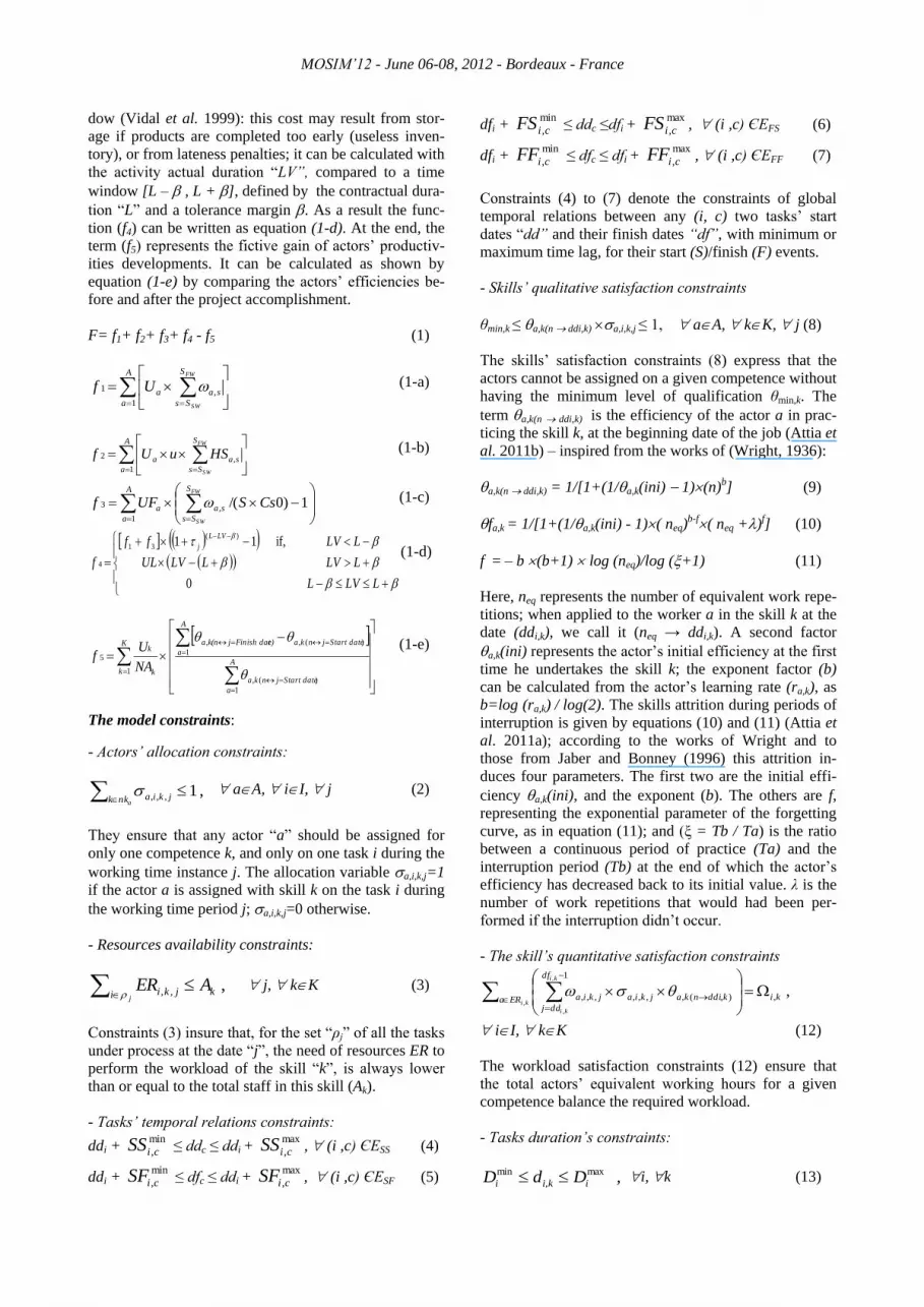
dow (Vidal et al. 1999): this cost may result from stor-

age if products are completed too early (useless inven-

tory), or from lateness penalties; it can be calculated with

the activity actual duration “LV”, compared to a time

window [L – , L + ], defined by the contractual dura-

tion “L” and a tolerance margin . As a result the func-

tion (f4) can be written as equation (1-d). At the end, the

term (f5) represents the fictive gain of actors’ productiv-

ities developments. It can be calculated as shown by

equation (1-e) by comparing the actors’ efficiencies be-

fore and after the project accomplishment.

F= f1+ f2+ f3+ f4 - f5 (1)

A

a

S

Ss

saa

FW

SW

Uf1

,1 (1-a)

A

a

S

Ss

saa

FW

SW

HSuUf1

,2 (1-b)

A

a

S

Ss

saa CsSUFfFW

SW1

,3 1)0/( (1-c)

LLVL

LLV

LLV

LLVUL

ff

f

LVL

j

if,

0

11)(

31

4

(1-d)

K

kA

a

Start datejnka

A

a

Start datejnkae)Finish datjk(na

k

k

NA

Uf

1

1

)(,

1

)(,,

5

(1-e)

The model constraints:

- Actors’ allocation constraints:

,1,,, ankk jkia aA, iI, j (2)

They ensure that any actor “a” should be assigned for

only one competence k, and only on one task i during the

working time instance j. The allocation variable a,i,k,j=1

if the actor a is assigned with skill k on the task i during

the working time period j; a,i,k,j=0 otherwise.

- Resources availability constraints:

,,, ki jki AERj

j, kK (3)

Constraints (3) insure that, for the set “ρj” of all the tasks

under process at the date “j”, the need of resources ER to

perform the workload of the skill “k”, is always lower

than or equal to the total staff in this skill (Ak).

- Tasks’ temporal relations constraints:

ddi + min

,ciSS ≤ ddc ≤ ddi + max

,ciSS , (i ,c) ЄESS (4)

ddi + min

,ciSF ≤ dfc ≤ ddi + max

,ciSF , (i ,c) ЄESF (5)

dfi + min

,ciFS ≤ ddc ≤dfi + max

,ciFS , (i ,c) ЄEFS (6)

dfi + min

,ciFF ≤ dfc ≤ dfi + max

,ciFF , (i ,c) ЄEFF (7)

Constraints (4) to (7) denote the constraints of global

temporal relations between any (i, c) two tasks’ start

dates “dd” and their finish dates “df”, with minimum or

maximum time lag, for their start (S)/finish (F) events.

- Skills’ qualitative satisfaction constraints

θmin,k ≤ a,k(n ddi,k) a,i,k,j ≤ 1, aA, kK, j (8)

The skills’ satisfaction constraints (8) express that the

actors cannot be assigned on a given competence without

having the minimum level of qualification θmin,k. The

term a,k(n ddi,k) is the efficiency of the actor a in prac-

ticing the skill k, at the beginning date of the job (Attia et

al. 2011b) – inspired from the works of (Wright, 1936):

a,k(n ddi,k) = 1/[1+(1/a,k(ini) 1)(n)b] (9)

fa,k = 1/[1+(1/a,k(ini) - 1)( neq)b-f( neq +)f] (10)

f = – b (b+1) log (neq)/log (+1) (11)

Here, neq represents the number of equivalent work repe-

titions; when applied to the worker a in the skill k at the

date (ddi,k), we call it (neq → ddi,k). A second factor

a,k(ini) represents the actor’s initial efficiency at the first

time he undertakes the skill k; the exponent factor (b)

can be calculated from the actor’s learning rate (ra,k), as

b=log (ra,k) / log(2). The skills attrition during periods of

interruption is given by equations (10) and (11) (Attia et

al. 2011a); according to the works of Wright and to

those from Jaber and Bonney (1996) this attrition in-

duces four parameters. The first two are the initial effi-

ciency a,k(ini), and the exponent (b). The others are f,

representing the exponential parameter of the forgetting

curve, as in equation (11); and (ξ = Tb / Ta) is the ratio

between a continuous period of practice (Ta) and the

interruption period (Tb) at the end of which the actor’s

efficiency has decreased back to its initial value. λ is the

number of work repetitions that would had been per-

formed if the interruption didn’t occur.

- The skill’s quantitative satisfaction constraints

,,

1

),(,,,,,,,,

,

,

kiERa

df

ddj

kddinkajkiajkiaki

ki

ki

iI, kK (12)

The workload satisfaction constraints (12) ensure that

the total actors’ equivalent working hours for a given

competence balance the required workload.

- Tasks duration’s constraints:

,DdD ii,ki

maxmin i, k (13)

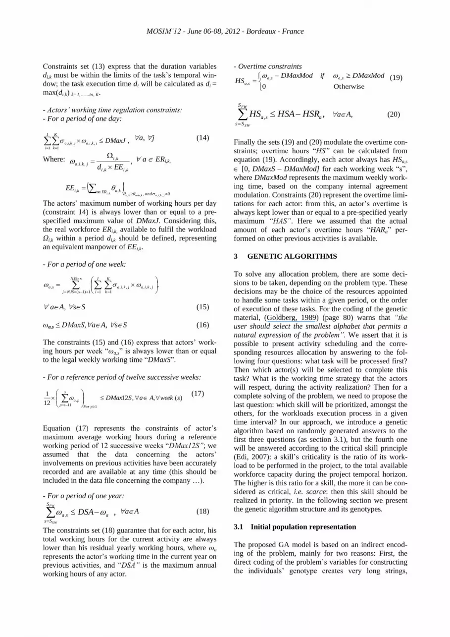
MOSIM’12 - June 06-08, 2012 - Bordeaux - France

Constraints set (13) express that the duration variables

di,k must be within the limits of the task’s temporal win-

dow; the task execution time di will be calculated as di =

max(di,k) k=1,……to, K.

- Actors’ working time regulation constraints:

- For a period of one day:

,1 1

,,,,,, DMaxJI

i

K

k

jkiajkia

a, j (14)

Where: ,,,

,

,,,

kiki

ki

jkiaEEd

a ERi,k,

0 ,

,,,,,min,,

, jkiakka

ki andERa kakiEE

The actors’ maximum number of working hours per day

(constraint 14) is always lower than or equal to a pre-

specified maximum value of DMaxJ. Considering this,

the real workforce ERi,k, available to fulfil the workload

Ωi,k within a period di,k should be defined, representing

an equivalent manpower of EEi,k.

- For a period of one week:

,1)1( 1 1

,,,,,,,

sNJS

sNJSj

I

i

K

k

jkiajkiasa

aA, sS (15)

ωa,s ≤ DMaxS,aA, sS (16)

The constraints (15) and (16) express that actors’ work-

ing hours per week “ωa,s” is always lower than or equal

to the legal weekly working time “DMaxS”.

- For a reference period of twelve successive weeks:

)( ,,1212

1

1 11

, sweekAaSDMax

pFor

s

sp

pa

(17)

Equation (17) represents the constraints of actor’s

maximum average working hours during a reference

working period of 12 successive weeks “DMax12S”; we

assumed that the data concerning the actors’

involvements on previous activities have been accurately

recorded and are available at any time (this should be

included in the data file concerning the company …).

- For a period of one year:

,, a

S

Ss

sa DSAFW

SW

aA (18)

The constraints set (18) guarantee that for each actor, his

total working hours for the current activity are always

lower than his residual yearly working hours, where ωa

represents the actor’s working time in the current year on

previous activities, and “DSA” is the maximum annual

working hours of any actor.

- Overtime constraints

Otherwise 0

,,

,

DMaxModifDMaxModHS

sasa

sa

(19)

,, a

S

Ss

sa HSRHSAHSFW

SW

aA, (20)

Finally the sets (19) and (20) modulate the overtime con-

straints; overtime hours “HS” can be calculated from

equation (19). Accordingly, each actor always has HSa,s

[0, DMaxS – DMaxMod] for each working week “s”,

where DMaxMod represents the maximum weekly work-

ing time, based on the company internal agreement

modulation. Constraints (20) represent the overtime limi-

tations for each actor: from this, an actor’s overtime is

always kept lower than or equal to a pre-specified yearly

maximum “HAS”. Here we assumed that the actual

amount of each actor’s overtime hours “HARa” per-

formed on other previous activities is available.

3 GENETIC ALGORITHMS

To solve any allocation problem, there are some deci-

sions to be taken, depending on the problem type. These

decisions may be the choice of the resources appointed

to handle some tasks within a given period, or the order

of execution of these tasks. For the coding of the genetic

material, (Goldberg, 1989) (page 80) warns that “the

user should select the smallest alphabet that permits a

natural expression of the problem”. We assert that it is

possible to present activity scheduling and the corre-

sponding resources allocation by answering to the fol-

lowing four questions: what task will be processed first?

Then which actor(s) will be selected to complete this

task? What is the working time strategy that the actors

will respect, during the activity realization? Then for a

complete solving of the problem, we need to propose the

last question: which skill will be prioritized, amongst the

others, for the workloads execution process in a given

time interval? In our approach, we introduce a genetic

algorithm based on randomly generated answers to the

first three questions (as section 3.1), but the fourth one

will be answered according to the critical skill principle

(Edi, 2007): a skill’s criticality is the ratio of its work-

load to be performed in the project, to the total available

workforce capacity during the project temporal horizon.

The higher is this ratio for a skill, the more it can be con-

sidered as critical, i.e. scarce: then this skill should be

realized in priority. In the following section we present

the genetic algorithm structure and its genotypes.

3.1 Initial population representation

The proposed GA model is based on an indirect encod-

ing of the problem, mainly for two reasons: First, the

direct coding of the problem’s variables for constructing

the individuals’ genotype creates very long strings,

MOSIM’12 - June 06-08, 2012 - Bordeaux - France

which increases the computing time. For example the

representation of a problem of 30 tasks, 82 actors, and 4

skills leads to chromosomes having 3,879 genes,

whereas with the indirect encoding presented further in

this paper, it drops down to 117 genes. The second rea-

son is the relations between the different problem’s deci-

sion variables, which can lead to the presence of “epista-

sis” (Gibbs et al. 2006): there are interactions between

some of the chromosome’s genes; some of their alleles

may affect other genes’ alleles. This phenomenon can be

illustrated by the equation of an actor’s number of daily

working hours, ωa,i,k,j = Ωi,k / (EEi,k di,k), that states a

relation between three variables: the equivalent work-

force EEi,k assigned to perform a given workload Ωi,k, the

duration di,k, and the corresponding actors’ daily working

hours. From this equation, any variable’s domain must

be consistent with each others’, in order to satisfy the

corresponding constraints. So, any change in a gene cor-

responding to actors’ allocation results in modifications

in actors’ equivalent productivities and in the domain of

possible durations, based on the working time constraints

and the actors’ availability: then any further modification

should be done randomly within this new modified do-

main during GA’s evolution process. With such a meth-

odology, finding a constraints–satisfying solution is

quite hard and may require larger CPU times. In addi-

tion, crossover and reproduction of new strings based on

the whole variables’ domains can produce more unfeasi-

ble genomes, so we waste a great amount of running

time for fixing the resulting distortions.

As mentioned above, our chromosomes will contain

three parts; the first one presents the priority of realizing

tasks. Thus, the number of genes in this part equals the

number of tasks in the project; the locus of the gene in

this sub-chromosome represents the task identification

number. But the value of the gene, or its allele (gener-

ated randomly), represents the corresponding task prior-

ity in the project. Based on this part of the chromosome

we can build a tasks’ priority list, by arranging these

numbers in a descending order, the position of the task in

the rearranged list represents its priority. Of course, in

the scheduling procedure that will be introduced in the

following section, the temporal relations between tasks

will be respected. The second sub-chromosome holds the

actors’ priorities for the allocation process. It is exactly

as the first part but instead of tasks, the genes represent

the actors. Thus, each gene’s locus represents the corre-

sponding actor identification number, and holds his pri-

ority indicator value as its allele, for the allocation proc-

ess. Based on this part we can construct the actors’ prior-

ity list for the project execution. Finally, the third part of

the chromosome represents the decision of what working

time strategy will be applied to the activity. From the

working time regulatory constraints, we have five inter-

vals (expressed in daily hours), which can be described

according to French regulations as follows:

[X, 7]: Represents the daily working time strategy within

the standard weekly hours C0s limits, where X can

represent a social willing of a minimum number of

working hours per day, under which the daily profit for

the actor can be considered as non-effective. Considering

that an employee would not appreciate to be called on

duty for a too little time, we arbitrarily fixed it at 4

hours. The second interval, represents the work above

the standard weekly hours Cs0 limits, and is limited by

the constraints of the company’s internal modulation of

weekly working time; we assumed it to be Cs0 = 39 hours

per week, which gives, in our example, the second

interval to be ]7, 7.8] hours per day for a 5-day week.

The next interval will then be limited by the constraints

of the maximum average weekly working time for a

period of 12 successive weeks; if we assume it to be 44

hours a week, according to French regulations, the third

interval will be ]7.8, 8.8] hours per day. The fourth

interval will then integrate the maximum number of

working hours per week; this number is of 48 hours per

week in France, and in this case we get ] 8.8, 9.6] hours

per day for our 4th interval. Finally, the last interval

considers the daily constraint of maximum working time

– if it is 10 hours per day, the 5th and mast interval will

be ]9.6, 10] hours per day.

Thus, considering the different working time constraints,

we get five time intervals for the decision of: what daily

rate actors will work with? These decisions are repre-

sented by the third sub-chromosome. Each gene position

in this part, exactly as for the two previous sub-

chromosomes, will represent the daily work range identi-

fication number, and its value represents the priority

assorted to each range. With the aid of this part we can

construct the time intervals priority list, which the actors

will work with respect to for the current simulation of

the problem. With this method, we are able to randomly

generate all the initial population individuals. Based on

this indirect encoding of the problem, we can gain some

benefits towards the feasibility of the chromosome after

the reproduction processes, and avoid some correction

procedures to the individuals, such as fixing the distor-

tions that could result from crossovers or mutations.

3.2 Individuals’ evaluations and fitness calculation

For each individual, the scheduling algorithm (described

in section 4) will take place, for decoding the chromo-

some, and designing the project schedule. The corre-

sponding objective function can be calculated as de-

scribed in section 2, equations (1); accordingly, and after

the normalization of different terms (f’i)s, we can get

individuals’ evaluations by assigning a given weight

(interest) to each term f’i. Considering that, in case of

violation of one or more of the soft constraint(s) (we

only consider working time constraints 17, 18 and 20 as

soft constraints), we should distinguish between the un-

feasible and feasible schedules: we will use penalties to

highlight and weight the unsatisfied constraints, if any.

For the violation of one of the hard constraints the pen-

alty (PHC) will be much larger compared to those of the

soft constraints (PSC). The sum of these penalties, ex-

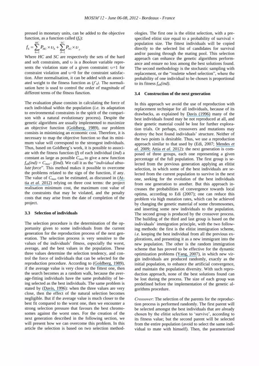
MOSIM’12 - June 06-08, 2012 - Bordeaux - France

pressed in monetary units, can be added to the objective

function, as a function called (f6):

SC

SC

HC

h

hHC PPf11

6

Where HC and SC are respectively the sets of the hard

and soft constraints, and is a Boolean variable repre-

sents the violation state of a given constraint: =1 for

constraint violation and =0 for the constraint satisfac-

tion. After normalisation, it can be added with an associ-

ated weight to the fitness function as (f’6). The normali-

sation here is used to control the order of magnitude of

different terms of the fitness function.

The evaluation phase consists in calculating the force of

each individual within the population (i.e. its adaptation

to environmental constraints in the spirit of the compari-

son with a natural evolutionary process). Despite the

genetic algorithms are usually implemented to maximize

an objective function (Goldberg, 1989), our problem

consists in minimizing an economic cost. Therefore, it is

necessary to map the objective function so that its mini-

mum value will correspond to the strongest individuals.

Thus, based on Goldberg’s work, it is possible to associ-

ate with the fitness function (f) of each individual (ind) a

constant as large as possible Cmax to give a new function

fab(ind) = Cmax– f(ind). We call it as the “individual abso-

lute force”. This method makes it possible to overcome

the problems related to the sign of the function, if any.

The value of Cmax can be estimated, as discussed in (At-

tia et al. 2012) relying on three cost terms: the project

realisation minimum cost, the maximum cost value of

the constraints that may be violated, and the penalty

costs that may arise from the date of completion of the

project.

3.3 Selection of individuals

The selection procedure is the determination of the op-

portunity given to some individuals from the current

generation for the reproduction process of the next gen-

eration. The selection process is very sensitive to the

values of the individuals’ fitness, especially the worst,

average, and the best values in the population. These

three values determine the selection tendency, and con-

trol the force of individuals that can be selected for the

reproduction procedure. According to (Goldberg, 1989),

if the average value is very close to the fittest one, then

the search becomes as a random walk, because the aver-

age-fitting individuals have the same probability of be-

ing selected as the best individuals. The same problem is

stated by (Davis, 1996): when the three values are very

close, then the effect of the natural selection becomes

negligible. But if the average value is much closer to the

best fit compared to the worst one, then we encounter a

strong selection pressure that favours the best chromo-

somes against the worst ones. For the creation of the

next generation described in the following section, we

will present how we can overcome this problem. In this

article the selection is based on two selection method-

ologies. The first one is the elitist selection, with a pre-

specified elitist size equal to a probability of survival

population size. The fittest individuals will be copied

directly to the selected list of candidates for survival

and/or passing through the mating pool. This selection

approach can enhance the genetic algorithms perform-

ance and ensure no loss among the best solutions found.

The second methodology is the stochastic sampling with

replacement, or the “roulette wheel selection”, where the

probability of one individual to be chosen is proportional

to its fitness fab(ind).

3.4 Construction of the next generation

In this approach we avoid the use of reproduction with

replacement technique for all individuals, because of its

drawbacks, as explained by Davis (1996) many of the

best individuals found may be not reproduced at all, and

their genetic material could be lost for further explora-

tion trials. Or perhaps, crossovers and mutations may

destroy the best found individuals’ structure. Neither of

the two points is desirable. Thus, we use a reproduction

approach similar to that used by (Edi, 2007; Mendes et

al. 2009; Attia et al. 2012): the next generation is com-

posed of three groups, each one representing a given

percentage of the full population. The first group is se-

lected from the previous generation applying an elitist

selection, in which some of the best individuals are se-

lected from the current population to survive in the next

one, seeking for the evolution of the best individuals

from one generation to another. But this approach in-

creases the probabilities of convergence towards local

optima, according to Edi (2007); one can reduce this

problem via high mutation rates, which can be achieved

by changing the genetic material of some chromosomes,

and inserting some new individuals to the population.

The second group is produced by the crossover process.

The building of the third and last group is based on the

individuals’ immigration principle, with the two follow-

ing methods: the first is the elitist immigration scheme,

i.e. keeping the best individual from all the previous ex-

plorations, and presenting it as a new immigrant into the

new population. The other is the random immigration

scheme that has proved to be effective for the dynamic

optimization problems (Yang, 2007), in which new vir-

gin individuals are produced randomly, exactly as the

initial population, to enhance the artificial convergence,

and maintain the population diversity. With such repro-

duction approach, none of the best solutions found can

be lost during the process. The size of each group was

predefined before the implementation of the genetic al-

gorithms procedure.

Crossover: The selection of the parents for the reproduc-

tion process is performed randomly. The first parent will

be selected amongst the best individuals that are already

chosen by the elitist selection to ‘survive’, according to

its fitness value; but the second parent will be selected

from the entire population (avoid to select the same indi-

vidual to mate with himself). Then, the parameterized

MOSIM’12 - June 06-08, 2012 - Bordeaux - France

uniform crossover of Mendes et al. (2009) takes it place,

in which a random number between [0, 1] is generated

for each gene in the chromosome. If this random number

is lower than a fixed value, then the allele of the first

parent (the best one) is used, otherwise the allele of the

second parent (the worst one) is used. The resulting child

is then directly copied into the new generation.

Mutation: After the selection, crossover, and reproduc-

tion processes, the mutation process takes place in the

evolution process. The mutation helps to prevent the

search to converge towards some local optima, by chang-

ing some of the population genetic materials. The uni-

form mutation is used, in which the value of the chosen

gene will be changed with a uniform random value as

generated in the initial population. Increasing the number

of mutated instances increases the algorithm’s ability to

search outside the currently explored region of the search

space - but if the mutation probability is set too high, the

search may become a random search.

3.5 Termination Procedure

As in any iterative algorithm, the implementation of ge-

netic algorithms requires the definition of a criterion by

which the exploration procedure decides whether to go

on searching or to stop. The termination criterion is

checked after each generation, to know if it is time to

stop or to complete the exploration. In our approach, we

define two termination criteria, and when any one of

them is valid, the exploration will be stopped:

- The first criterion is related to the average evolution of

the objective function, as it was used by Attia et al.

(2012). We call it ‘Average convergence’, in which the

convergence is the evolution or, more exactly, the non-

evolution, of the average value of the fitness for a num-

ber “Nbi” of the best individuals for successive genera-

tions: when the average fitness value no longer seems to

evolve during a given number g of generations, the proc-

ess is considered to have converged.

- The second termination procedure simply depends on

the number of generations that were produced and evalu-

ated. When this maximum number of generations has

been run, then the termination procedure occurs: this just

makes it possible to stop a search which does not seem

to be successful, or to maximise the procedure running

time.

4 SCHEDULING ALGORITHM

For each individual of the population, the scheduling

procedures is conducted, to translate the individuals’

genetic materials into the corresponding tasks’ schedule

and actors’ allocation. The following steps describe these

decoding procedures, starting from the first day of the

activity execution and based on the serial scheduling

generation scheme. This builds a feasible schedule by

sequentially adding the tasks one by one until a complete

schedule is obtained. The scheduling algorithm mainly

has two sub-procedures: search for sets of feasible tasks,

and workforce allocation. At each time instance (or day),

the feasible sets (fs) are generated, which represent the

group of the tasks that may be scheduled together ac-

cording to the temporal relations between tasks, re-

sources availability or even the workforce regulations.

4.1 Tasks feasible sets

The construction of this feasible set of tasks (fs) is con-

ducted in two steps. First, at each time instance of the

project partial schedule, we look for the task(s) that can

be performed without any violation of the temporal rela-

tions. After this search of all the tasks that can be con-

sidered as feasible (considering only the temporal con-

straints), they are grouped into a set of “the candidates

list”. With the aid of tasks priorities, which are hold by

the corresponding chromosomes, we can select the most

prioritized task. After that, other procedures of checking

feasibility based on resources availabilities, and regula-

tion constraints should be conducted. If ever the unfeasi-

bility was proven (because the need for resources ex-

ceeds their availabilities for example), the task with the

next maximum priority in the list is selected. We follow

this procedure until we can find the suitable task, then

we call the resources allocation procedures (as explained

in section 4.2). All tasks within the candidates list will be

checked, until we can find a feasible set of tasks, consid-

ering precedence relations, resources’ availabilities and

working time regulations, all together. Thus, first we are

looking for a feasible set fs, so that:

- For any pair of tasks (i, c) in the feasible set (fs),

there is no restriction for performing them simulta-

neously at the current time instance, considering the

precedence constraints.

- The workload requirements by the tasks within the

set (fs) must be satisfied, qualitatively as well as

quantitatively.

- The total resources requirement by the feasible set

must be lower than or equal to the resources avail-

abilities.

- Each actor always works without any violation of

the working time regulations.

4.2 Resources allocation

Having checked the resources availabilities, and written

the skills’ criticality list, we are now ready to conduct

actors’ allocation. By the end of actors’ allocation algo-

rithms, we should be able to assign a value to each vari-

able (ωa,i,k,j, EEi,k , di,k), according to the relation

kiki

ki

jkiaEEd ,,

,

,,,

. Therefore, we can construct all the

possibilities of every task’s workload durations di,k and

the resulting actors’ daily number of working hours

(ωa,i,k,j). Regarding the decision of the actors’ daily

working hours strategies that are hold by the chromo-

some, we can start a search for the actors’ values of daily

MOSIM’12 - June 06-08, 2012 - Bordeaux - France

working hours (ωa,i,k,j) which would satisfy the task time

window and the working time regulation constraints. By

the following procedure described by figure 1, we pre-

sent the workforce allocation algorithm. These proce-

dures for the scheduling generation scheme will be con-

tinued until all the tasks’ workloads are scheduled –

unless we state the failure of the corresponding chromo-

some to give rise to an acceptable schedule. In this case,

the chromosome will be penalized, by giving it a large

cost penalty, in order to reduce its probability to be re-

produced in the next generation.

- Sort the available actors according to their priorities

- Update the productivity levels a,k(n ddi,k) of the available actors,

- Sort workloads within the tasks according to skills’ criticality list.

While (all workloads of the current task have their team-works), do

While (all available actors are checked), do

Allocate (most prioritised actor with (θa,k ≥ θmin,k)), EEi,k=EEi,k + θa,k

Construct a matrix of ωa,i,k,j , di,k {Dimin, Di

max},

For (working interval = most prioritised working interval]

Search within the matrix for a value of ωa,i,k,j[working interval]

If it exists check working time constraints

If (working time constraints are feasible)

Store this allocation and mark actors as unavailable during the

period corresponding to di,k.. Fix the value of di,k., update all

variable that depends to this allocation.

Break to next workload

Next for

End while If (there are no available actors) break while with conclusion of: the

unavailability proven to realise the current task.

End while

Figure 1: Workforce allocation algorithm

5 APPROACH VALIDATION

In order to validate the ability of the proposed approach

to return a feasible solution, we randomly selected (and

modified) 20 projects from an open-access library

(PSPLib, 1996). The instances are taken with different

numbers of tasks (30, 60, 90, and 120), each instance

having its appropriate number of actors and tasks tempo-

ral relations. The validation procedures are simply based

on functional tests, i.e. we review the algorithm response

with what we expect from the data. Thus any contradic-

tion between the data entry and results will be concluded

as a failure of the functional test. In this way, we treated

the algorithm as a black box, as shown by figure 2: four

sets of inputs, such as tasks temporal relations, tasks

durations (Dmin, D, Dmax), tasks workload requirement

per skill, and the productivities, for each actor for each

of his/her skills. The simulation parameters of the ge-

netic algorithm are kept unchanged during the explora-

tion (as shown in table 1), because at this step we are

interested in validating the capability of the algorithm to

deliver a feasible and applicable schedule, not to study

its performance. Studying the performance of the algo-

rithm and tuning its parameters will be discussed in the

following sections. The parameters to be checked have

been classified into two groups according to the outputs

of the algorithm;

The project:

Tasks’ start and finish dates, tasks’ durations,

The tasks relations will be checked from their start and

finish dates,

The project workload per task and per skill should be

fulfilled with the required manpower, both quantita-

tively and qualitatively.

Human Resources:

Each actor should be assigned only once per each pe-

riod of his working timetable,

The assigned actors should master the required skills

with productivities higher than or equal to the mini-

mum prefixed qualifications,

The evolution of the actors’ experience (known from

their prior allocations) should be checked,

Each actor’s time table must satisfy the legal conditions

of working hours, especially the hard constraints.

Figure 2: treating the algorithm during the validation

We proved that the proposed model is capable to return a

feasible and applicable project schedule with the corre-

sponding workforce allocation. Here, the checking has

been carried out manually; all the hard constraints have

been checked and proved to be satisfied, in addition to

the soft constraints, thanks to workforce proposed flexi-

bility.

Max. generations = 400 generations

Population size (PI) = 50 individuals

Crossover probability = 0.7

Mutation probability = 0.01

Regeneration Probability = 0.2

Max. gen. without evolution = 100 generations

Size of “Nbi” = 10 individuals

Losing flexibility cost = 20 MU

Tolerance period (β) = 20 % ×L

Table 1: GA’s parameters used during validation

6 PARAMETERS TUNING

We then tested the performance and the robustness of the

algorithm. As discussed by Eiben and Smit (2011), an

algorithm performance measurement usually checks the

quality of the solutions, and the rapidity to return back

these solutions. The solution quality can be measured

from the individuals’ fitness. But the robustness consists

in checking the algorithm stability under the presence of

uncertainty conditions within the data input, e.g. chang-

ing randomly the problem instance – the parameter vec-

tor(s). However, one of the essential steps of any algo-

rithm is the parameters tuning that mainly depends on

the performance analysis. Then, and relying on “no free

lunch theorem” of Wolpert and Macready (1997), one

can use these parameters combination in solving other

MOSIM’12 - June 06-08, 2012 - Bordeaux - France

instances. Thus, here we designed an experiment to tune

the algorithm parameters in order to achieve the best

performance, in addition to study its robustness towards

changes of problem’s instances.

To tune the algorithm parameters, one should investigate

all the possible interactions between parameters combi-

nations, in order to adjust them and optimize the algo-

rithm performance; but investigating all parameters by

factorial design is almost impossible due to the cost re-

lated to running time, “time = levelsfactors numbers ”. To

avoid this drawback we adopted the fractional factorial,

by using one of surfaces response, such as “Taguchi

method”, “Central composite”, or ‘Box–Behnken de-

signs’. First we need to determine the parameters and the

associated ranges. Therefore, we conducted a survey for

the values used within literature as illustrated by table 2.

Population size (PI) [20 to 200]

Crossover probability [0.50 to 0.90]

Mutation probability [0.01 to 0.2]

Regeneration Probability [0.0 to 0.2]

Max. non developed generations [50 to 200]

Tolerance period (β) [0.0 to 60]% ×L

Table 2: Parameters ranges

According to the work of Ferreira et al. (2007) we

adopted the three levels design “Box–Behnken designs”,

and used the stochastic software “MiniTab-16” to gener-

ate the vectors of parameters combinations. As results,

we get 54 vectors to be tested. We selected randomly a

project instance of 30 tasks to be used during this inves-

tigation. In order to avoid the stochastic nature of genetic

algorithm, we decided to run each simulation at least 10

times, and to take the average of their results. The result

analysis indicates the best combination of the parame-

ters. According to “Pearson's correlation coefficient test”

we found that the running time is linearly related to the

population size, and number of non-convergence genera-

tions (stopping criterion). Regarding the objective func-

tion, we found that increasing the mutation rate increases

the returned project cost, and that increasing the project

tolerance period (β) linearly reduces its cost. As a sample

of the graphic representation, we display the effect of

some investigated parameters on figure 3 and 4.

Figure 3: The effect of PI and β on returned objective

Figure 4: The effect of SC and Pm on returned objective

As a result, we found the best combination of

parameters, showed it in table 3. With these

parameters, we proved the robustness of the proposed

approach when solving the different instances, with

different (tasks, actors, skills) combinations: (10, 30, 60,

90, 120) tasks, (10 : 193) actors, and 4 skills.

Population size (PI) [50, 100] according to

the problem size

Crossover probability = 0.7

Mutation probability (Pm) = 0.01

Regeneration Probability = 0.1

Maximum number of non-

evolved generations (SC)

= 100 generations

Tolerance period (β) = 20 % ×L

Table 3: Parameters corresponding values to be used

7 CONCLUSION

In this article, we presented a genetic algorithm-based

approach to solve our problem of project schedule with

workforce multi-periods allocations. The model takes

into account human resources flexible timetables, in ad-

dition to their dynamic versatility. The dynamic vision of

workforce productivities is relying on the development

thanks to learning-by-doing, and reciprocally, the depre-

ciation of their competences resulting from the lack of

practice in periods of work interruption. The produced

model is nonlinear, with a huge number of mixed vari-

ables. The proposed genetic algorithm relies mainly on

answering three questions based on the priority encod-

ing: what task will be processed first? Then which ac-

tor(s) will be allocated to realise this task? What is the

working time strategy that the actors will respect, during

the activity realization? The model has been validated,

moreover, its parameters has been tuned to give the best

performance. In addition, the model proved to be robust

towards changing instances to be solved. As future

works: this model will be used to conduct an investiga-

tion study to test the parameters affecting the develop-

ment of the actor’s skills. Moreover, we are looking to

upgrade this model with multi-criteria decision analysis.

MOSIM’12 - June 06-08, 2012 - Bordeaux - France

REFERENCES

Attia, E.-A., Duquenne, P. and Le-Lann, J.-M., 2011a.

Prise en compte des évolutions de compétences pour

les ressources humaines. In : 9ème Congrès

International de Génie Industriel (CIGI-2011). 12-14

octobre 2011, Saint-Sauveur, Québec, Canada.

Attia, E.-A., Duquenne, P. and Le-Lann, J.-M., 2011b.

Problème d’affectation flexible des ressources

humaines: Un modèle dynamique. In : 12ème

congrès annuel de la Société Française de Recherche

Opérationnelle et d’Aide à la Décision (ROADEF

2011). Saint-Etienne, France, p. 697-698.

Attia, E.-A., Edi, H.K. and Duquenne, P., 2012. Flexible

resources allocation techniques: characteristics and

modelling. Int. J. Operational Research, 14(2),

p.221-254.

Azmat, C., 2004. A case study of single shift planning

and scheduling under annualized hours: A simple

three-step approach. E. J. of Operational Research,

153(1), p.148-175.

Bellenguez-Morineau, O. and Néron, E., 2007. A

Branch-and-Bound method for solving Multi-Skill

Project Scheduling Problem. Operations Research,

41(2), p.155-170.

Corominas, A., Lusa, A. and Pastor, R., 2007. Planning

annualised hours with a finite set of weekly working

hours and cross-trained workers. E. J. of Operational

Research, 176(1), p.230-239.

Davis, L., 1996. Handbook of Genetic Algorithms,

International Thomson Computer Press.

Drezet, L. and Billaut, J., 2008. A project scheduling

problem with labour constraints and time-dependent

activities requirements. Int. J. of Prod. Economics,

112(1), p.217-225.

Duquenne, P., Edi, H.K. and Le-Lann, J.-M., 2005.

Characterization and modelling of flexible resources

allocation on industrial activities. In : 7th World

Congress of Chemical Engineering. Glasgow,

Scotland.

Edi, H.K., 2007. Affectation flexible des ressources dans

la planification des activités industrielles: prise en

compte de la modulation d’horaires et de la

polyvalence. Toulouse University, France.

Eiben A. E. and Smit S. K., 2011. Evolutionary

Algorithm Parameters and Methods to Tune them. Y.

Hamadi E. Monfroy and Saubion F. (eds.),

Autonomous Search , Springer.

Ferreira SL, Bruns RE, Ferreira HS, Matos GD, David

JM, Brandão GC, da Silva EG, Portugal LA, dos Reis

PS, Souza AS, dos Santos WN, 2007. Box-Behnken

design: An alternative for the optimization of

analytical methods. Analytica Chimica Acta, 597(2),

p.179-186.

Franchini, L., Caillaud, E., Nguyen, P., and Lacoste L.,

2001. Workload control of human resources to

improve production management. Int. J. of Prod.

Research, 39(7), p.1385-1403.

Gen, M. and Cheng, R., 2000. Genetic algorithms and

engineering optimization, Wiley-IEEE.

Gibbs, M.S.; Maier, H.R.; Dandy, G.C.; and Nixon,

J.B., 2006. Minimum Number of Generations

Required for Convergence of Genetic Algorithms. In:

IEEE Congress on Evolutionary Computation, CEC

2006. IEEE, p. 565-572.

Goldberg, D.E., 1989. Genetic Algorithms in Search,

Optimization and Machine Learning, Addison-

Wesley Longman Publishing Co., Inc.

Grabot, B. and Letouzey, A., 2000. Short-term

manpower management in manufacturing systems:

new requirements and DSS prototyping. Computers

in Industry, 43(1), p.11-29.

Hertz, A., Lahrichi, N. and Widmer, M., 2010. A

flexible MILP model for multiple-shift workforce

planning under annualized hours. E. J. of

Operational Research, 200(3), p.860-873.

Hung, R., 1999. A multiple shift workforce scheduling

model under annualized hours. Naval Research

Logistics (NRL), 46(6), p.726-736.

Jaber, M.Y. and Bonney, M.C., 1996. Production breaks

and the learning curve: the forgetting phenomenon.

Applied Mathematical Modelling, 20(2), p.162-169.

Mendes, J.J.M., Gonçalves, J.F., and Resende, M.G.C.,

2009. A random key based genetic algorithm for the

resource constrained project scheduling problem.

Computers and Operations Research, 36(1), p.92-

109.

Mitchell, C., 1995. Flexibility: Nature, Sources, and

Effects. The ANNALS of the American Academy of

Political and Social Science, 542(1), p.213-218.

PSPLib, 1996. PSPLIB: library for project scheduling

problems [online]. Available at: <http://129.187.

106.231/psplib/>, [Accessed 10 March 2011].

Valls, V., Perez, A., and Quintanilla, S., 2009. Skilled

workforce scheduling in Service Centres. E. J. of

Operational Research, 193(3), p.791-804.

Vidal, E., Duquenne, A., and Pingaud, H., 1999.

Optimisation des plans de charge pour un flow-shop

dans le cadre d’une production en Juste A Temps: 2-

Formulation mathématique. In : 3ème Congrès

Franco-Quebequois de Génie Industriel. Montréal,

Québec, Canada, p. 1175-1184.

Wolpert D.H. and Macready W.G., 1997. No free lunch

theorems for optimization. IEEE Transactions On

Evolutionary Computation, 1(1), p.67-82.

Wright, T., 1936. Factors Affecting the Cost of

Airplanes. J. of Aeronautical Sciences, 3, p.122-128.

Yang, S., 2007. Genetic algorithms with elitism-based

immigrants for changing optimization problems. In:

M. Giacobini, Applications of Evolutinary

Computing. Springer Berlin Heidelberg, p. 627-636.

Youndt M. A., Snell S. A., Dean J. W. Jr., Lepak D. P.,

1996. Human Resource Management, Manufacturing

Strategy, and Firm Performance. The Academy of

Management Journal, 39(4), p.836-866.