PLEASE SCROLL DOWN FOR ARTICLE

This article was downloaded by: [2007-2008 National Cheng Kung University]On: 13 August 2008Access details: Access Details: [subscription number 791473931]Publisher Taylor & FrancisInforma Ltd Registered in England and Wales Registered Number: 1072954 Registered office: Mortimer House,37-41 Mortimer Street, London W1T 3JH, UK

Engineering OptimizationPublication details, including instructions for authors and subscription information:http://www.informaworld.com/smpp/title~content=t713641621

The use of a grey-based Taguchi method for optimizing multi-responsesimulation problemsYiyo Kuo a; Taho Yang b; Guan-Wei Huang b

a Department of Technology Management, Hsing Kuo University of Management, Tainan, Taiwan b Institute ofManufacturing Engineering, National Cheng Kung University, Tainan, Taiwan

First Published:June2008

To cite this Article Kuo, Yiyo, Yang, Taho and Huang, Guan-Wei(2008)'The use of a grey-based Taguchi method for optimizing multi-response simulation problems',Engineering Optimization,40:6,517 — 528

To link to this Article: DOI: 10.1080/03052150701857645

URL: http://dx.doi.org/10.1080/03052150701857645

Full terms and conditions of use: http://www.informaworld.com/terms-and-conditions-of-access.pdf

This article may be used for research, teaching and private study purposes. Any substantial orsystematic reproduction, re-distribution, re-selling, loan or sub-licensing, systematic supply ordistribution in any form to anyone is expressly forbidden.

The publisher does not give any warranty express or implied or make any representation that the contentswill be complete or accurate or up to date. The accuracy of any instructions, formulae and drug dosesshould be independently verified with primary sources. The publisher shall not be liable for any loss,actions, claims, proceedings, demand or costs or damages whatsoever or howsoever caused arising directlyor indirectly in connection with or arising out of the use of this material.

Engineering OptimizationVol. 40, No. 6, June 2008, 517–528

The use of a grey-based Taguchi method for optimizingmulti-response simulation problems

Yiyo Kuoa*, Taho Yangb and Guan-Wei Huangb

aDepartment of Technology Management, Hsing Kuo University of Management, Tainan, Taiwan;bInstitute of Manufacturing Engineering, National Cheng Kung University, Tainan, Taiwan

(Received 24 January 2007, final version received 19 October 2007 )

Simulation modelling is a widely accepted tool in system design and analysis, particularly when the sys-tem or environment has stochastic and nonlinear behaviour. However, it does not provide a method foroptimization. In general, problems contain more than one response, which are often in conflict with eachother. This article proposes a grey-based Taguchi method to solve the multi-response simulation prob-lem. The grey-based Taguchi method is based on the optimizing procedure of the Taguchi method, andadopts grey relational analysis (GRA) to transfer multi-response problems into single-response problems.A practical case study from an integrated-circuit packaging company illustrates that differences in per-formance of the proposed grey-based Taguchi method and other methods found in the literature were notsignificant. The grey-based Taguchi method thus provides a new option when solving a multi-responsesimulation-optimization problem.

Keywords: grey relational analysis; integrated circuit packaging; multiple attribute decision making;simulation optimization; Taguchi method

1. Introduction

Simulation is a widely accepted tool in systems design and analysis (Fonseca et al. 2003). Itrequires a few simplifying assumptions, captures many of the true characteristics of the realsituation, and provides good insight into the interactions and relationships between qualitativeand quantitative variables (Fonseca and Navaresse 2002).

However, simulations are time consuming and are essentially trial-and-error approaches. Fur-thermore, simulation does not provide a method for optimization. There is thus a significant bodyof literature devoted to simulation optimization. In solving simulation-optimization problems,there are two general approaches—meta-heuristics and meta-modelling.

Meta-heuristics (such as simulated annealing, genetic algorithms, Tabu search, or scatter search)can be used as an embedded search algorithm associated with simulation software for a simulation-optimization problem. The search strategies proposed by meta-heuristics methodologies result initerative procedures that have the ability to escape local optimal points.

*Corresponding author. Email: yiyo@mail.hku.edu.tw

ISSN 0305-215X print/ISSN 1029-0273 online© 2008 Taylor & FrancisDOI: 10.1080/03052150701857645http://www.informaworld.com

Downloaded By: [2007-2008 National Cheng Kung University] At: 11:46 13 August 2008

518 Y. Kuo et al.

The simulation meta-model is a simpler model that approximates the simulation model (Hurrionand Birgil 1999). Optimizing a simulation model by meta-modelling methods is often carried outin three primary stages: (i) using a simulation model to generate a data set that contains inputand related output; (ii) developing a simulation meta-model by meta-modelling techniques suchas regression or neural networks; (iii) optimizing the simulation meta-model by optimizationprocedures.

When all decision variables are restricted to only a few viable discrete values and subject tothe inclusion of sampling variability, the simulation-optimization problem becomes a factorialdesign problem that is similar to Taguchi’s parameter-design method (Yang and Chou 2005).However, practical problems often embody many characteristics of a multi-response optimizationproblem, and these responses are frequently in conflict with each other. Tong and Su (1997)solved a multi-response robust design problem using a multi-attribute decision-making (MADM)method. They considered the quality loss of each response and then adopted a MADM methodto optimize the multi-response robust design problem. There are several common methodologiesfor MADM—simple additive weighting (SAW), technique for order preference by similarityto ideal solution (TOPSIS), analytical hierarchy process (AHP) (Yoon and Hwang 1995), dataenvelopment analysis (DEA), and so on.

Grey relational analysis (GRA) is part of grey system theory, which was proposed by Deng(1982), and is suitable for solving problems with complicated interrelationships between multiplefactors and variables (Morán et al. 2006). GRA solves MADM problems by combining theentire range of performance attribute values being considered for every alternative into one singlevalue. This reduces the original problem to a single-objective decision-making problem. Theprocess of combining attribute values into a single value is similar to the method adopted in SAWand TOPSIS. This article proposes a grey-based Taguchi method for optimizing multi-responsesimulation problems. A simulation model is optimized by the procedure of the Taguchi methodin which the multi-response values are processed by GRA.

The proposed grey-based Taguchi method has been used for some optimization prob-lems, such as machining parameters for wire electrical discharge machining (Huang and Liao2003), manufacturing process for fibre-reinforcement of polybutylene terephthalate compos-ites (Fung 2003), machining processes for electrical discharge (Lin and Lin 2002), processparameters for submerged arc welding (Tarng et al. 2002), and so on. However, the authorsof this article did not find literature reporting the grey-based Taguchi method for simulationoptimization.

The remainder of this article is organized a follows: the details of the proposed grey-basedTaguchi method are discussed in section 2. A brief introduction to the case study problem isprovided in section 3. Section 4 shows the empirical results. Finally, section 5 presents theconclusions.

2. The grey-based Taguchi method

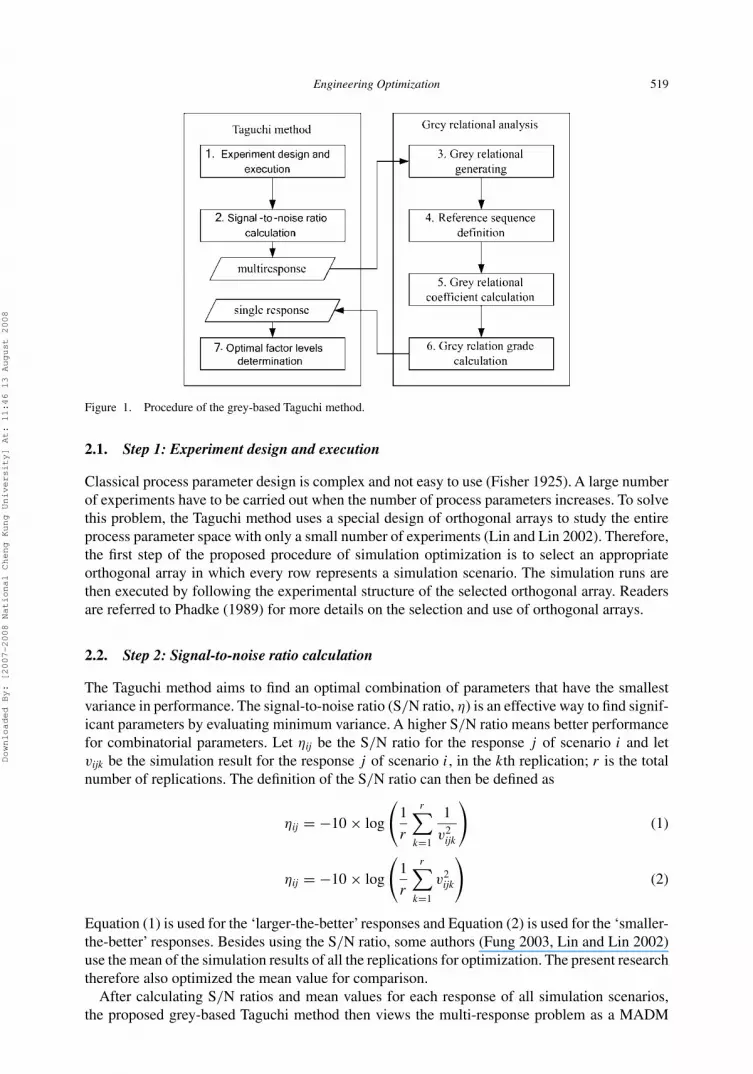
The proposed grey-based Taguchi method for simulation optimization follows the optimizationmethod (the Taguchi method) developed by Dr Genichi Taguchi. However, the Taguchi methodonly works for optimization of a single performance characteristic. The GRA procedure is used tocombine all the considered performance characteristics into a single value that can then be usedas the single characteristic in optimization problems. The procedure of the grey-based Taguchimethod is shown in Figure 1.

In Figure 1, steps 1, 2 and 7 are general procedures of the Taguchi method and steps 3 to 6 arethe procedure of GRA.

Downloaded By: [2007-2008 National Cheng Kung University] At: 11:46 13 August 2008

Engineering Optimization 519

Figure 1. Procedure of the grey-based Taguchi method.

2.1. Step 1: Experiment design and execution

Classical process parameter design is complex and not easy to use (Fisher 1925). A large numberof experiments have to be carried out when the number of process parameters increases. To solvethis problem, the Taguchi method uses a special design of orthogonal arrays to study the entireprocess parameter space with only a small number of experiments (Lin and Lin 2002). Therefore,the first step of the proposed procedure of simulation optimization is to select an appropriateorthogonal array in which every row represents a simulation scenario. The simulation runs arethen executed by following the experimental structure of the selected orthogonal array. Readersare referred to Phadke (1989) for more details on the selection and use of orthogonal arrays.

2.2. Step 2: Signal-to-noise ratio calculation

The Taguchi method aims to find an optimal combination of parameters that have the smallestvariance in performance. The signal-to-noise ratio (S/N ratio, η) is an effective way to find signif-icant parameters by evaluating minimum variance. A higher S/N ratio means better performancefor combinatorial parameters. Let ηij be the S/N ratio for the response j of scenario i and letvijk be the simulation result for the response j of scenario i, in the kth replication; r is the totalnumber of replications. The definition of the S/N ratio can then be defined as

ηij = −10 × log

(1

r

r∑k=1

1

v2ijk

)(1)

ηij = −10 × log

(1

r

r∑k=1

v2ijk

)(2)

Equation (1) is used for the ‘larger-the-better’ responses and Equation (2) is used for the ‘smaller-the-better’ responses. Besides using the S/N ratio, some authors (Fung 2003, Lin and Lin 2002)use the mean of the simulation results of all the replications for optimization. The present researchtherefore also optimized the mean value for comparison.

After calculating S/N ratios and mean values for each response of all simulation scenarios,the proposed grey-based Taguchi method then views the multi-response problem as a MADM

Downloaded By: [2007-2008 National Cheng Kung University] At: 11:46 13 August 2008

520 Y. Kuo et al.

problem. Different terminology is commonly used to describe MADM problems, and in thefollowing description some terms have been adjusted to conform with usual MADM usage. Thus‘response’was replaced by ‘attribute’, and ‘scenario’was replaced by ‘alternative’in the following.

2.3. Step 3: Grey relational generating

When the units in which performance is measured are different for different attributes, the influenceof some attributes may be neglected. This may also happen if some performance attributes have avery large range. In addition, if the goals and directions of these attributes are different, this willcause incorrect results in the analysis (Huang and Liao 2003). It is thus necessary to process allperformance values for every alternative into a comparability sequence, in a process analogousto normalization. This processing is called grey relational generating in GRA.

For a MADM problem, if there are m alternatives and n attributes, the ith alter-native can be expressed as Yi = (yi1,yi2, . . . , yij , . . . , yin), where yij is the performancevalue of attribute j of alternative i. The term Yi can be translated into the comparabil-ity sequence Xi = (xi1,xi2, . . . , xij , . . . , xin) by the use of one of Equations (3)–(5), whereyj = Max{yij , i = 1, 2, . . . , m} and yj = Min{yij , i = 1, 2, . . . , m}.

xij =yij − yj

yj − yj

; i = 1, 2, . . . , m j = 1, 2, . . . , n (3)

xij = yj − yij

yj − yj

; i = 1, 2, . . . , m j = 1, 2, . . . , n (4)

xij = 1 −∣∣∣yij − y∗

j

∣∣∣Max

{yj − y∗

j , y∗j − yj

} ; i = 1, 2, . . ., m j = 1, 2, . . . , n (5)

Equation (3) is used for larger-the-better attributes, Equation (4) is used for smaller-the-betterattributes, and Equation (5) is used for ‘closer-to-the-desired-value-y∗

j -the-better’ attributes. Notethat the S/N ratio that was calculated in step 2 is a larger-the-better attribute. Therefore, theproposed grey-based Taguchi method only uses Equation (3) for grey relational generating.

2.4. Step 4: Reference sequence definition

After the grey relational generating procedure, all performance values will be scaled into [0, 1]. Foran attribute jof alternative i, if the value xij that has been processed by grey relational generating isequal to 1, or nearer to 1 than the value for any other alternative, the performance of alternative i isthe best one for attribute j . Therefore, an alternative will be the best choice if all of its performancevalues are closest to or equal to 1. However, this kind of alternative does not usually exist. Thisarticle defines the reference sequence X0 as (x01,x02, . . . , x0j , . . . , x0n) = (1, 1, . . . , 1, . . . , 1),and then aims to find the alternative whose comparability sequence is the closest to the referencesequence.

2.5. Step 5: Grey relational coefficient calculation

The grey relational coefficient is used to determine how close xij is to x0j . The larger the greyrelational coefficient, the closer xij and x0j are. The grey relational coefficient can be calculated by

γ (x0j , xij ) = �min + ζ�max

�ij + ζ�max; i = 1, 2, . . . , m j = 1, 2, . . . , n (6)

Downloaded By: [2007-2008 National Cheng Kung University] At: 11:46 13 August 2008

Engineering Optimization 521

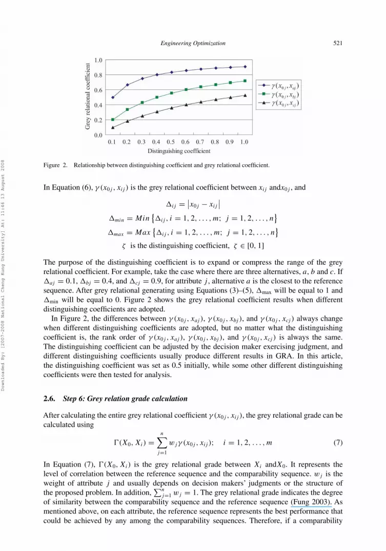
Figure 2. Relationship between distinguishing coefficient and grey relational coefficient.

In Equation (6), γ (x0j , xij ) is the grey relational coefficient between xij andx0j , and

�ij = ∣∣x0j − xij

∣∣�min = Min

{�ij , i = 1, 2, . . . , m; j = 1, 2, . . . , n

}�max = Max

{�ij , i = 1, 2, . . . , m; j = 1, 2, . . . , n

}ζ is the distinguishing coefficient, ζ ∈ [0, 1]

The purpose of the distinguishing coefficient is to expand or compress the range of the greyrelational coefficient. For example, take the case where there are three alternatives, a, b and c. If�aj = 0.1, �bj = 0.4, and �cj = 0.9, for attribute j , alternative a is the closest to the referencesequence. After grey relational generating using Equations (3)–(5), �max will be equal to 1 and�min will be equal to 0. Figure 2 shows the grey relational coefficient results when differentdistinguishing coefficients are adopted.

In Figure 2, the differences between γ (x0j , xaj ), γ (x0j , xbj ), and γ (x0j , xcj ) always changewhen different distinguishing coefficients are adopted, but no matter what the distinguishingcoefficient is, the rank order of γ (x0j , xaj ), γ (x0j , xbj ), and γ (x0j , xcj ) is always the same.The distinguishing coefficient can be adjusted by the decision maker exercising judgment, anddifferent distinguishing coefficients usually produce different results in GRA. In this article,the distinguishing coefficient was set as 0.5 initially, while some other different distinguishingcoefficients were then tested for analysis.

2.6. Step 6: Grey relation grade calculation

After calculating the entire grey relational coefficient γ (x0j , xij ), the grey relational grade can becalculated using

�(X0, Xi) =n∑

j=1

wjγ (x0j , xij ); i = 1, 2, . . . , m (7)

In Equation (7), �(X0, Xi) is the grey relational grade between Xi andX0. It represents thelevel of correlation between the reference sequence and the comparability sequence. wj is theweight of attribute j and usually depends on decision makers’ judgments or the structure ofthe proposed problem. In addition,

∑nj=1 wj = 1. The grey relational grade indicates the degree

of similarity between the comparability sequence and the reference sequence (Fung 2003). Asmentioned above, on each attribute, the reference sequence represents the best performance thatcould be achieved by any among the comparability sequences. Therefore, if a comparability

Downloaded By: [2007-2008 National Cheng Kung University] At: 11:46 13 August 2008

522 Y. Kuo et al.

sequence for an alternative gets the highest grey relational grade with the reference sequence, thecomparability sequence is most similar to the reference sequence and that alternative would bethe best choice.

2.7. Step 7: Determination of optimal factor levels

According to the principles of the Taguchi method, if the effects of the control factors on per-formance are additive, it is possible to predict the performance for a combination of levels ofthe control factors by knowing only the main effects of the control factor. For a factor A thathas two levels, 1 and 2, for example, the main effect of factor A at level 1 (mA1) is equal to theaverage grey relational grade whose factor A in experimental scenarios is at level 1, and the maineffect of factor A at level 2 (mA2) is equal to the average grey relational grade whose factor A inexperimental scenarios is at level 2. The higher the main effect is, the better the factor level is.Therefore, the optimal levels for factor A will be the one whose main effect is the highest amongall levels.

3. The case study

The case study is adapted from the work Yang and Tseng (2002). Company S is an anonymouscompany in Taiwan that provides integrated circuit (IC) packaging services to global customers.Its annual sales show that it has consistently been one of the top five companies in the world overthe past seven years.

In an IC packaging plant, the ink-marking machine (ink marker) has a significantly higherthroughput than the other processing machines. When periodic surges in demand result in abacklog of orders or in lost customers, there is a need to increase system throughput. If a newmachine is purchased in an attempt to resolve the problem, this often results in excess capacityas well as acquisition and operation costs. It is therefore preferable to improve the productivityof existing equipment rather than purchase new. This article reports on the proposed grey-basedTaguchi method to optimize throughput and cycle time performance for IC ink-marking machines.

For the case study, Yang and Tseng (2002) used a hybrid response surface method and alexicographical goal-programming approach to solve this multi-response simulation problem.The same case study has been reported by Yang and Chou (2005) and Yang et al. (2005). Yangand Chou (2005) solved this multi-response simulation problem with discrete variables by usinga MADM method (TOPSIS); Yang et al. (2005) used a dual-response system and scatter searchmethod. The results of those studies will be compared with the results of the present study.

4. Empirical illustrations

The simulation model of the case study problem was coded using commercial software (Arena2002), which was validated and used for the empirical illustrations. The two responses werethroughput and cycle time. The study horizon was 24 hours. The five control factors, togetherwith their respective bounds, are shown in Table 1. Note that the unit load for the ink-markingmachine is a ‘magazine’, which is a standard container for machine loading. (Readers are referredto Yang and Tseng (2002) for the raw data used in the model.)

Table 1 shows that there are five three-level control factors in the present study. The five factorsare denoted A, B, C, D, and E. Each factor has three levels: lower, middle, and upper bounds.Note that factor E represents the mean time between failures (MTBF); the longer the MTBF, the

Downloaded By: [2007-2008 National Cheng Kung University] At: 11:46 13 August 2008

Engineering Optimization 523

Table 1. Control variables.

Lower Middle UpperFactor Description (Unit) bound bound bound

A The process time for ten magazines for the bottleneckof earlier operations (min/10 magazines)

7 12 17

B The machine buffer size (magazines) 90 96 102C The time between ink adjustment (min) 251 321 391D The ratio of the adjusted process time to original

process time0.65 0.75 0.85

E The mean time between failures (min) 899 1,049 1,199

Table 2. Experimental results.

L18 Mean value S/N ratio

Scenario A B C D E Throughput Cycle time Throughput Cycle time

1 1 1 1 1 1 600.14 241.49 55.56 −47.662 1 2 2 2 2 592.07 264.27 55.45 −48.443 1 3 3 3 3 616.04 265.90 55.79 −48.504 2 1 1 2 2 586.20 238.55 55.36 −47.565 2 2 2 3 3 610.28 254.97 55.71 −48.136 2 3 3 1 1 612.64 265.07 55.74 −48.477 3 1 2 1 3 605.26 230.00 55.64 −47.248 3 2 3 2 1 613.10 230.69 55.75 −47.269 3 3 1 3 2 585.30 259.61 55.35 −48.29

10 1 1 3 3 2 606.76 245.98 55.66 −47.8311 1 2 1 1 3 605.70 271.05 55.64 −48.6612 1 3 2 2 1 610.65 274.41 55.71 −48.7713 2 1 2 3 1 612.60 235.36 55.74 −47.4414 2 2 3 1 2 622.54 249.08 55.88 −47.9315 2 3 1 2 3 593.46 273.41 55.46 −48.7416 3 1 3 2 3 614.12 223.61 55.76 −46.9917 3 2 1 3 1 581.69 256.26 55.29 −48.1818 3 3 2 1 2 602.58 264.13 55.60 −48.47

better the system throughput. However, there are costs to the improvement of MTBF performanceassociated with more frequent scheduled maintenance (better machine models, etc.). These costsare difficult to estimate and are not considered in this study.

4.1. Experiment design and execution

An L18(21 × 37) orthogonal array has the least number of treatments to account for more than fivethree-level control factors. Therefore, an L18(21 × 37) orthogonal array was used to collect theexperimental data. Columns 2–6 were used to represent the five control factors. The three levelsof all factors were denoted 1–3 (the lower, middle, and upper levels). The experimental scenariosare shown in columns 2–6 of Table 2.

4.2. Signal-to-noise ratio calculation

For each experimental scenario, there were ten replications. The mean values of each scenarioare show in columns 7 and 8 of Table 2. Because throughput is a larger-the-better response and

Downloaded By: [2007-2008 National Cheng Kung University] At: 11:46 13 August 2008

524 Y. Kuo et al.

cycle time is a smaller-the-better response, the S/N ratios of throughput were calculated by usingEquation (1), and the S/N ratios of cycle time were calculated by using Equation (2). The S/Nratios of each scenario are shown in columns 9 and 10 of Table 2.

4.3. Grey relational generating

The main purpose of grey relational generating is transferring the original data into comparabilitysequences. The mean value of throughput and S/N ratios are larger-the-better attributes and themean value of cycle time is a smaller-the-better attribute. Therefore the grey relational generatingprocess adopts Equation (3) for mean value of throughput and S/N ratios of both throughput andcycle time (columns 7, 9 and 10 of Table 2) and adopts Equation (4) for mean values of cycletime (column 8 of Table 2). The results are shown in Table 3.

4.4. Grey relational coefficient calculation

In Table 3, X0 is the reference sequence. After calculating �ij , �max , and �min, all grey relationalcoefficients can be calculated using Equation (6). For S/N ratios, for example, �11 = |1 − 0.46| =0.54, �max = 1 and �min = 0, if ζ = 0.5, then γ (x01, x11) = (0 + 0.5 × 1)/(0.54 + 0.5 × 1) =0.48. The results for the grey relational coefficient are shown in Table 4.

4.5. Grey relational grade calculation

According to the suggestion of Yang and Chou (2005), the weight of the attribute throughput wasset as 0.6 and cycle time was set as 0.4. Using Equation (7), the grey relational grade can becalculated and is shown in column 2 of Table 5.

Table 3. Results of grey relational generation.

Mean value S/N ratio

Scenario Throughput Cycle time Throughput Cycle time

X0 1.00 1.00 1.00 1.001 0.45 0.65 0.46 0.622 0.25 0.20 0.26 0.183 0.84 0.17 0.85 0.154 0.11 0.71 0.11 0.685 0.70 0.38 0.71 0.366 0.76 0.18 0.76 0.177 0.58 0.87 0.59 0.868 0.77 0.86 0.78 0.859 0.09 0.29 0.09 0.27

10 0.61 0.56 0.62 0.5311 0.59 0.07 0.60 0.0612 0.71 0.00 0.72 0.0013 0.76 0.77 0.76 0.7514 1.00 0.50 1.00 0.4715 0.29 0.02 0.29 0.0216 0.79 1.00 0.80 1.0017 0.00 0.36 0.00 0.3318 0.51 0.20 0.52 0.17

Downloaded By: [2007-2008 National Cheng Kung University] At: 11:46 13 August 2008

Engineering Optimization 525

Table 4. Results of grey relational coefficient.

Mean value S/N ratio

Scenario Throughput Cycle time Throughput Cycle time

1 0.48 0.59 0.48 0.572 0.40 0.38 0.40 0.383 0.76 0.38 0.76 0.374 0.36 0.63 0.36 0.615 0.62 0.45 0.63 0.446 0.67 0.38 0.68 0.387 0.54 0.80 0.55 0.788 0.68 0.78 0.69 0.779 0.35 0.41 0.36 0.41

10 0.56 0.53 0.57 0.5211 0.55 0.35 0.55 0.3512 0.63 0.33 0.64 0.3313 0.67 0.68 0.68 0.6714 1.00 0.50 1.00 0.4915 0.41 0.34 0.41 0.3416 0.71 1.00 0.72 1.0017 0.33 0.44 0.33 0.4318 0.51 0.39 0.51 0.38

Table 5. The results of grey relational analysis.

Scenario Mean value S/N ratio

1 0.52 0.522 0.39 0.393 0.61 0.614 0.47 0.465 0.55 0.556 0.56 0.567 0.64 0.648 0.72 0.729 0.38 0.38

10 0.55 0.5511 0.47 0.4712 0.51 0.5213 0.68 0.6714 0.80 0.7915 0.38 0.3816 0.82 0.8317 0.38 0.3718 0.46 0.46

4.6. Determination of optimal factor levels

By using the additive property, the average responses by factor levels can be solved. For example,in the case of the S/N ratio, estimation of the effect of factor A at level 1 (mA1) from Table 5 is

mA1 = 1

6(�(X0, X1) + �(X0, X2) + �(X0, X3) + �(X0, X10) + �(X0, X11) + �(X0, X12))

= 1

6(0.52 + 0.39 + 0.61 + 0.55 + 0.47 + 0.52) = 0.51 (8)

The resulting factor effects are summarized in Tables 6 and 7. The data in bold type show the pre-ferred design level for each factor. Their associated factor effect plots are shown in Figures 3 and 4.

Downloaded By: [2007-2008 National Cheng Kung University] At: 11:46 13 August 2008

526 Y. Kuo et al.

Table 6. Average grey relational grade by factorlevels (mean value).

Factor Level 1 Level 2 Level 3

A 0.5094 0.5708 0.5660B 0.6121 0.5512 0.4829C 0.4303 0.5396 0.6764D 0.5733 0.5511 0.5219E 0.5596 0.5054 0.5813

Table 7. Average grey relational grade by factorlevels (S/N ratio).

Factor Level 1 Level 2 Level 3

A 0.5100 0.5729 0.5672B 0.6144 0.5525 0.4820C 0.4321 0.5401 0.6767D 0.5745 0.5509 0.5234E 0.5608 0.5081 0.5799

Figure 3. Plots for factor effects (mean value).

Figure 4. Plots for factor effects (S/N ratio).

Since the effect value is a larger-the-better type, both Figures (3 and 4) led to the same final param-eter design of A2B1C3D1E3. The design is the same as the final result found by Yang and Chou(2005).

To illustrate the solution quality, the results from the proposed grey-based Taguchi method werecompared with those of Yang and Tseng (2002), Yang and Chou (2005), and Yang et al. (2005)

Downloaded By: [2007-2008 National Cheng Kung University] At: 11:46 13 August 2008

Engineering Optimization 527

Table 8. Solution comparison.

Throughput Cycle time

Method Simulation result Improvement (%) Simulation result Improvement (%)

Grey-based Taguchi method 623.77 — 263.70 —TOPSIS∗ 623.77 0 263.70 0Response surface method† 606.33 2.88 270.19 2.40Dual-response system‡ 629.59 −0.92 263.29 −0.16Scatter search‡ 632.47 −1.38 250.05 −5.46

∗Proposed by Yang and Chou (2005).†Proposed by Yang and Tseng (2002).‡Proposed by Yang et al. (2005).

(Table 8). The performance of parameter design in the method proposed here and in Yang andChou (2005) is better than that inYang and Tseng (2002), but worse than that inYang et al. (2005).However, the differences are very small.

This research also analysed the impact on the grey-based Taguchi method results when thedistinguishing coefficient was set at 0.1, 0.3, 0.5, 0.7 and 0.9. Figures 5 and 6 both show thatadjusting the distinguishing coefficient changes the average grey relational grade by factor levels.However, the impact of the distinguishing coefficient on the results of the proposed grey-basedTaguchi method is very small. They all led to the same final design of factor levels (A2B1C3D1E3),no matter what distinguishing coefficient was adopted.

Figure 5. Sensitivity analysis for different distinguishing coefficients (mean value).

Figure 6. Sensitivity analysis for different distinguishing coefficients (S/N ratio).

Downloaded By: [2007-2008 National Cheng Kung University] At: 11:46 13 August 2008

528 Y. Kuo et al.

5. Conclusion

This research proposed the grey-based Taguchi method to solve a multi-response simulation-optimization problem. Following the procedure of theTaguchi method, GRA was used to transforma multi-response problem into a single-response problem. A practical case study illustrated thatthe difference in performance between the proposed method and other methods identified in theliterature was not significant. However, the results of this study illustrate that the GRA procedure issimple and straightforward in calculations and optimization; it is therefore a very suitable methodfor solving multi-response simulation problems. In addition, the proposed method can easily beextended to problems that have more than two responses, even though the case study in this articlehas only two responses. The proposed method presents a new option for solving multi-responsesimulation-optimization problems.

Acknowledgements

The authors thank the anonymous company for providing the case study. This work was supported in part by the NationalScience Council of Taiwan, Republic of China, under grants NSC-94-2213-E-432-002 and NSC-94-2213-E-006-019.

References

Arena User’s Guide, 2002. Version 6.0, Rockwell Software Inc., West Allis, WI, USA.Deng, J., 1982. Control problems of grey systems. Systems and Control Letters, 1 (5), 288–294.Fisher, R.A., 1925. Statistical methods for research worker. London: Oliver and Boyd.Fonseca, D.J. and Navaresse, D.O., 2002. Artificial neural networks for job shop simulation. Advanced Engineering

Informatics, 16 (4), 241–246.Fonseca, D.J., Navaresse, D.O. and Moynihan, G.P., 2003. Simulation metamodeling through artificial neural networks.

Engineering Applications of Artificial Intelligence, 16 (3), 177–183.Fung, C.P., 2003. Manufacturing process optimization for wear property of fiber-reinforced polybutylene terephthalate

composites with grey relational analysis. Wear, 254 (3–4), 298–306.Huang, J.T. and Liao, Y.S., 2003. Optimization of machining parameters of wire-EDM based on grey relational and

statistical analyses. International Journal of Production Research, 41 (8), 1707–1720.Hurrion, R.D. and Birgil, S., 1999.A comparison of factorial and random experimental design methods for the development

of regression and neural network simulation metamodels. Journal of the Operational Research Society, 50 (10),1018–1033.

Lin, J.L. and Lin, C.L., 2002. The use of the orthogonal array with grey relational analysis to optimize the electricaldischarge machining process with multiple performance characteristics. International Journal of Machine Tool andManufacturing, 42 (2), 237–244.

Morán, J., Granada, E., Míguez, J. and Porteriro, 2006. Use of grey relational analysis to assess and optimize smallbiomass boilers. Fuel Processing Technology, 87 (2), 123–127.

Phadke, S.M., 1989. Quality Engineering Using Robust Design. Englewood Cliffs, NJ: Prentice-Hall.Tarng, T.S., Juang, S.C. and Chang, C.H., 2002. The use of grey-based Taguchi methods to determine submerged arc

welding process parameters in hardfacing. Journal of Materials Processing Technology, 128 (1–3), 1–6.Tong, L.I. and Su, C.T., 1997. Optimizing multi-response problems in the Taguchi method by fuzzy multiple attribute

decision making. Quality and Reliability Engineering International, 13 (1), 25–34.Yang, T. and Chou, P., 2005. Solving a multiresponse simulation-optimization problem with discrete variables using a

multiple-attribute decision-making method. Mathematics and Computers in Simulation, 68 (1), 9–21.Yang, T. and Tseng, L., 2002. Solving a multiple objective simulation model using a hybrid response surface method and

lexicographical goal programming approach-a case study on IC ink marking machines. Journal of the OperationalResearch Society, 53 (2), 211–221.

Yang, Y., Kuo, Y. and Chou, P., 2005. Solving a multiresponse simulation problem using a dual-response system andscatter search method. Simulation Modelling Practice and Theory, 13 (4), 356–369.

Yoon, K. and Hwang, C.L., 1995, Multiple Attribute Decision Making: an Introduction. Thousand Oaks, CA: Sage.

Downloaded By: [2007-2008 National Cheng Kung University] At: 11:46 13 August 2008