AN ALGORITHM FOR SOLVING RULE SETS-BASED BILEVEL DECISION PROBLEMS

Computational Intelligence, Volume 27, Number 2, 2011

AN ALGORITHM FOR SOLVING RULE SETS–BASED BILEVELDECISION PROBLEMS

GUANG-QUAN ZHANG,1 ZHENG ZHENG,2 JIE LU,1 AND QING HE3

1Decision Systems & e-Service Intelligence Lab, Centre for Quantum Computation & Intelligent Systems,School of Software, The Faculty of Information Technology, University of Technology, Sydney, Australia

2Beijing University of Aeronautics and Astronautics, Beijing, China3Key Laboratory of Intelligent Information Processing, Institute of Computing Technology,

Chinese Academy of Sciences, Beijing, China

Bilevel decision addresses the problem in which two levels of decision makers each tries to optimize theirindividual objectives under certain constraints, and to act and react in an uncooperative and sequential manner.Given the difficulty of formulating a bilevel decision problem by mathematical functions, a rule sets– based bileveldecision (RSBLD) model was proposed. This article presents an algorithm to solve a RSBLD problem. A case-basedexample is given to illustrate the functions of the proposed algorithm. Finally, a set of experiments is analyzed tofurther show the functions and the effectiveness of the proposed algorithm.

Key words: Decision-making model, rule sets, bilevel decision making, optimization algorithm.

1. INTRODUCTION

A bilevel decision problem can be viewed as a static version of the non-cooperative,two-player (decision maker) game (Stackelberg 1952). The decision maker at the upper levelis termed the leader, and at the lower level, the follower. In a bilevel decision problem, thecontrol for decision factors is divided among the decision makers who seek to optimize theirindividual objective functions (Aiyoshi and Shimizu 1981). Perfect information is assumedso that both the leader and the follower know the objective and feasible choices available to theother. The leader attempts to optimize his/her objective function but he/she must anticipateall possible responses of the follower (Lai 1996). The follower observes the leader’s decisionand then responds to it in a way that is personally optimal. For example, consider a logisticcompany making a decision on how to use commission as a means for its distributors toimprove product sale volume. The company, as the leader, attempts to maximize its benefitof product sale through offering a highly competitive commission to its distributors. Foreach of the possible commission strategies, the distributors, as the follower, will respond onproduct sale volume which is based on the maximized benefit obtained through product sale.Therefore, in such a bilevel decision problem described by a bilevel programming (BLP)model, a subset of the decision variables (like commission in the example) is constrainedto be a solution of a given optimization problem parameterized by the remaining variables(like sale volume) (Bard and Falk 1982; Anandalingam and Friesz 1992; Bard and Moore1992). In mathematical terms, a BLP problem consists of finding a solution for the upperlevel problem:

minx

F(x, y)

subject to A(x, y)T ≤ 0,

for each value of x, is the solution of the lower level problem:

miny

f (x, y)

Address correspondence to Jie Lu, Faculty of Information Technology, University of Technology, Sydney, Australia;e-mail: [email protected]

C© 2011 Wiley Periodicals, Inc.

236 COMPUTATIONAL INTELLIGENCE

subject to B(x, y)T ≤ 0,

where A and B are constraint coefficient matrixes of the upper and lower levels, respectively.The majority of BLP research has centered on the linear version of the problem. Candler

and Townsley (1982) first discussed a linear BLP problem with no upper level constraintsand with unique lower level solutions. Later, Bard (1984) and Bialas and Karwan (1984)proved this result under the assumption that the constraint region is bounded. Following theseresults, there have been nearly two dozen approaches and algorithms proposed for solvinglinear BLP problems, for example, the Kth-Best approach (Candler and Townsley 1982;Bialas and Karwan 1984), and the Kuhn–Tucker approach (Bard and Falk 1982; Bialas andKarwan 1982; Hansen, Jaumard, and Savard 1992). There have also been some intelligentapproaches to solve linear bilevel programming problems (Lan et al. 2007; Calvete, Gale,and Mateo 2008), as well as the Penalty function approach (Aiyoshi and Shimizu 1981;White and Anandalingam 1993), stability based approach (Liang and Sheng 1992), and aglobally convergent approach for solving nonlinear bilevel programming problems (Wang etal. 2007). Mathematicians, economists, engineers and other researchers and developers havedelivered contributions to this field.

BLP is the most suitable way to model a bilevel decision problem by assuming that (1)both the leader and the follower have perfect information about their objectives and con-straints, and (2) these objectives and constraints can be written into mathematics functions.However, in real situations, it is often very hard to describe these objectives and constraintsby mathematical functions including the determination of their parameters. Let us considerthe logistic company example mentioned above. The company can only estimate variousfeasible choices taken and various costs spent by its distributors through a survey. Therefore,in establishing a BLP model for the “commission” problem, we are hard-pressed to arriveat a formula for the objective functions and constraint functions (including their functiontypes and parameters) of the leader and the follower. Some researchers, such as Lai (1996),Sakawa, Nishizaki, and Uemura (2000a,b), Sakawa and Yauchi (2000), Sakawa and Nishizak(2001a,b, 2002), Shih, Lai, and Lee (1996), Zhang and Lu (2005, 2006) and Zhang, Lu, andDillon (2007a,b) have developed fuzzy BLP approaches to handle the difficulty in determin-ing the parameters in the objective and constraint functions of a BLP. However, they stillassumed that all these objective and constraint functions can be established and only theirparameters are uncertain. Obviously, this cannot solve the problem we proposed.

We have recently observed that in many bilevel decision problems, the leader’s attempts tooptimize his/her objectives and all the possible responses from the follower can be describedby a number of rules (Zheng et al. 2009). Therefore, when a bilevel problem cannot beformulated by a BLP model, we can explore the use of rule sets to describe its objectivefunctions and constrains. We thus proposed a rule sets–based bilevel decision (RSBLD)model. If a bilevel decision problem is modeled by a RSBLD, we call it a RSBLD problem.We have also developed a modeling approach to establish a RSBLD model (Zheng et al.2009). However, how to solve a RSBLD problem remains a challenge.

This study starts to explore a rule sets–based bilevel decision approach for solvinga RSBLD problem. We propose a transformation-based solution algorithm for RSBLDproblems. The main idea of the algorithm is to first transform a RSBLD model to a single-level decision model which has the same optimal solution as the original bilevel one, andthen obtain the optimal solution by solving the single-level decision model.

The article is organized as follows. Following this introduction, Section 2 introduces theconcepts and notions of information tables and rule sets, which are preliminaries in this study.Section 3 reviews our previous work including a RSBLD model and its modeling algorithm.How to transform a RSBLD problem into a single-level one is discussed in Section 4.

ALGORITHM FOR SOLVING RULE SETS 237

Section 5 presents a transformation-based algorithm based on the proposed transformationtheories. A case-based example is then shown in Section 6 for illustrating the functionsof the proposed algorithms. In Section 7, a set of experiment results is analyzed to showthe effectiveness and complexity of the proposed algorithms. Finally, the conclusion andproposals for future work are given in Section 8.

2. PRELIMINARIES

For the convenience of describing proposed models and algorithms, we first give somerelated definitions and theorems which will be used in subsequent sections.

2.1. Rules

As the basic concepts of this article, rules and their properties are introduced. Somerelated techniques, such as information tables and decision tables, are presented first. Ingeneral, an information table is a knowledge expressing system which can be used to representand process knowledge in machine learning, data mining and other related fields. It providesa convenient way to describe a finite set of objects called the universe by a finite set ofattributes (Pawlak 1991).

Definition 1 (Information table). (Pawlak 1991): An information table can be formulated asa tuple:

S = (U, At, L , {Va | a ∈ At}, {Ia | a ∈}}),

where U is a finite nonempty set of objects, At is a finite nonempty set of attributes, L is alanguage defined using attributes in At, Va is a nonempty set of values for a ∈ At, Ia :U→Va is an information function. Ia is a total function that maps an object of U to exactlyone value in Va .

A decision table is a special case of information table. It is commonly viewed as a func-tional description, which maps inputs (conditions) to outputs (actions) without necessarilyspecifying the manner in which the mapping is to be implemented.

Definition 2 (Decision table). (Pawlak 1991): A decision table is an information table forwhich the attributes in A are further classified into disjoint sets of condition attributes C anddecision attributes D, that is, At = C ∪ D, C ∩ D = �.

Note, decision attributes in a decision table can be unique or not. In the later case,the decision table can be converted to one with unique decision attributes (Wang 2001).Therefore, in this article, we assume that there is only one decision attribute in a decisiontable.

Usually, the knowledge implicated in information tables is expressed by rules, in whichformulas are their components.

Definition 3 (Formulas). (Yao and Yao 2002): In the language L of an information table, anatomic formula is given by (a, v), where a ∈ At and v ∈ Va . If φ and ϕ are formulas, then soare ¬φ, φ ∧ ϕ, and φ ∨ ϕ.


TABLE 1. An Information Table.

Object Height Hair Eyes Class

o1 Short Blond Blue +o2 Short Blond Brown −o3 Tall Dark Blue +o4 Tall Dark Blue −o5 Tall Dark Blue −o6 Tall Blond Blue +o7 Tall Dark Brown −o8 Short Blond Brown −

The semantics of the language L can be defined in Tarski’s style (Tarski 1956) throughthe notions of a model and satisfiability. The model is an information table S, which providesinterpretation for symbols and formulas of L.

Definition 4 (Satisfiability of formulas). (Yao and Yao 2002): The satisfiability of a formulaφ by an object x, written as x |= Sφ or in short x |= φ if S is understood, is defined by thefollowing conditions:

(1) x |= a = v iff Ia (x) = v;(2) x |= ¬φ iff not x |= φ;(3) x |= φ ∧ ϕ iff x |= φ and x |= ϕ;(4) x |= φ ∨ ϕ iff x |= φ or x |= ϕ.

If φ is a formula, the set mS (φ) = {x ∈ U | x |= φ} is called the meaning of the formula φ inS. If S is understood, we simply write m(φ).

The meaning of a formula φ is therefore the set of all objects having the propertyexpressed by the formula φ. In other words, φ can be viewed as the description of the set ofobjects m(φ). Thus, a connection between the formulas of L and subsets of U is established.Considering an information table given by Table 1 (Quinlan 1983), the following expressionsare some of the formulas of the language L:

(height, tall); (hair, dark); (height, tall) ∧ (hair, dark); (height, tall) ∨ (hair, dark).

The meanings of the formulas are given by:

m((height, tall)) = {o3, o4, o5, o6, o7}; m((hair, dark)) = {o4, o5, o7};m((height, tall) ∧ (hair, dark)) = {o4, o5, o7};

m((height, tall) ∨ (hair, dark)) = {o3, o4, o5, o6, o7}.Usually, the knowledge implicated in information tables is expressed by rules, which arestatements of the form: “if an object satisfies a formula, then the object must satisfy anotherformula.” The expression of rules can be formulated as follows (Pawlak 1991; Yao and Yao2002).

Definition 5 (Rules). Let S = (U, At, L, {Va | a ∈ At}, {Ia | a ∈ At}}) be an informationtable, then a rule r is a formula with the form φ ⇒ ϕ, where φ and ϕ are formulas ofinformation table, and S for any x ∈ U, x |= φ ⇒ ϕ iff x |= ¬ φ ∨ ϕ.


Definition 6 (Decision Rules). Let S = (U, C ∪ D, L, {Va | a ∈ At}, {Ia | a ∈ C ∪ D}})be a decision table, where C is the set of condition attributes and D is the set of decisionattributes. A decision rule dr is a rule with the form φ ⇒ ϕ, where φ, ϕ are both conjunctionof atomic formulas, for any atomic formula (c, v) in φ, c ∈ C, and for any atomic formula(d, v) in ϕ, d ∈ D.

It is obvious that each object in a decision table can be expressed by a decision rule. Therelationship between objects and rules can be defined by the following definition.

Definition 7 (Objects consistent or conflict with a rule). An object x is said to be consistentwith a rule dr: φ ⇒ ϕ, iff x |= φ and x |= ϕ; x is said to be conflict with dr, iff x |= φand x |= ¬ϕ.

2.2. Making Decisions with Rule Sets

Based on the above concepts, how to make decisions based on decision rules is exploredin this section by first defining decision rule set functions.

Given a decision table S = (U , At, L, {Va | a ∈ At}, {Ia | a ∈ At}}), where At = C ∪ D andD = {d}. Suppose x and y are two variables, where x ∈ X and X = Va1 × · · · × Vam , y ∈ Y andY = Vd . Vai is the set of attribute ai ’s values, ai ∈ C, i = 1 . . . m, m is the number of conditionattributes. RS is a decision rule set generated from S.

Definition 8 (Decision rule set function). A decision rule set function rs from X to Y is asubset of the Cartesian product X × Y, such that for each x in X , there is a unique y in Ygenerated with RS such that the ordered pair (x, y) is in rs. Here, x is called a conditionvariable, y is called a decision variable, X is the definitional domain, and Y is the valuedomain.

Calculating the value of a decision rule set function is to make decisions for objects withdecision rule sets. To present the calculating method, a definition about matching objects todecision rules is introduced first.

Definition 9 (An object matching a decision rule). An object o is said to be matching adecision rule φ ⇒ ϕ, if o |= φ.

Given a decision rule set RS, all decision rules in RS matched by object o are denoted asM Ro

RS . Consequently, a brief method for calculating a decision rule set function is developedas follows:

Step 1: Calculate MRoRS ;

Step 2: Select a decision rule dr from MRoRS , where

dr : ∧ {(a, va)} ⇒ (d, vd);

Step 3: Set the decision value of object o to be vd , that is, rs(o) = vd .

Here dr is called the final matching rule matched by object o in rule set RS. In Step 2,how to select a decision rule from M Ro

RS is the key task of the process. For example, thereis a decision rule set RS, including four rules:

RS = {(a, 1) ∧ (b, 2) ⇒ (d, 2); (a, 2) ∧ (b, 3) ⇒ (d, 1);

(b, 4) ⇒ (d, 2); (b, 3) ∧ (c, 2) ⇒ (d, 3)};


and an undecided object:

o = (a, 2) ∧ (b, 3) ∧ (c, 2).

With Step 1, M RoRS = {(a, 2)∧(b, 3) ⇒ (d, 1); (b, 3)∧(c, 2) ⇒ (d, 3)}.

With Step 2, if we select the final matching rule as (a, 2)∧(b, 3) ⇒ (d, 1), then withStep 3,

rs(o) = 1;if select the final matching rule as (b, 3)∧(c, 2) ⇒ (d, 3), then with Step 3,rs(o) = 3.

From the above example, we know that there may be more than one rule in M RoRS . In this

case, when the decision values of these rules are different, the result would be controlledaccording to the above method, known as the uncertainty of a decision rule-set function.The method of selecting the final rule from M Ro

RS is thus very important, and is called theuncertainty solution method. In our research, we use AID-based rule trees (Def. 11) to dealwith the problem.

2.3. Rule Trees

A rule tree is a compact and efficient structure for expressing a rule set. We first introducethe definition of rule trees in Zheng and Wang (2004) as follows. It is used in this article asthe expression form of rule sets for a bilevel decision model.

Definition 10 (Rule tree).

(1) A rule tree is composed of one root node, some leaf nodes and some middle nodes.(2) The root node represents the whole rule set.(3) Each path from the root node to a leaf node represents a rule.(4) Each middle node represents an attribute testing. Each possible value of an attribute in

a rule set is represented by a branch. Each branch generates a new child node. If anattribute is reduced in some rules, then a special branch is needed to represent it and thevalue of the attribute in this rule is supposed as “∗”, which is different from any possiblevalues of the attribute.

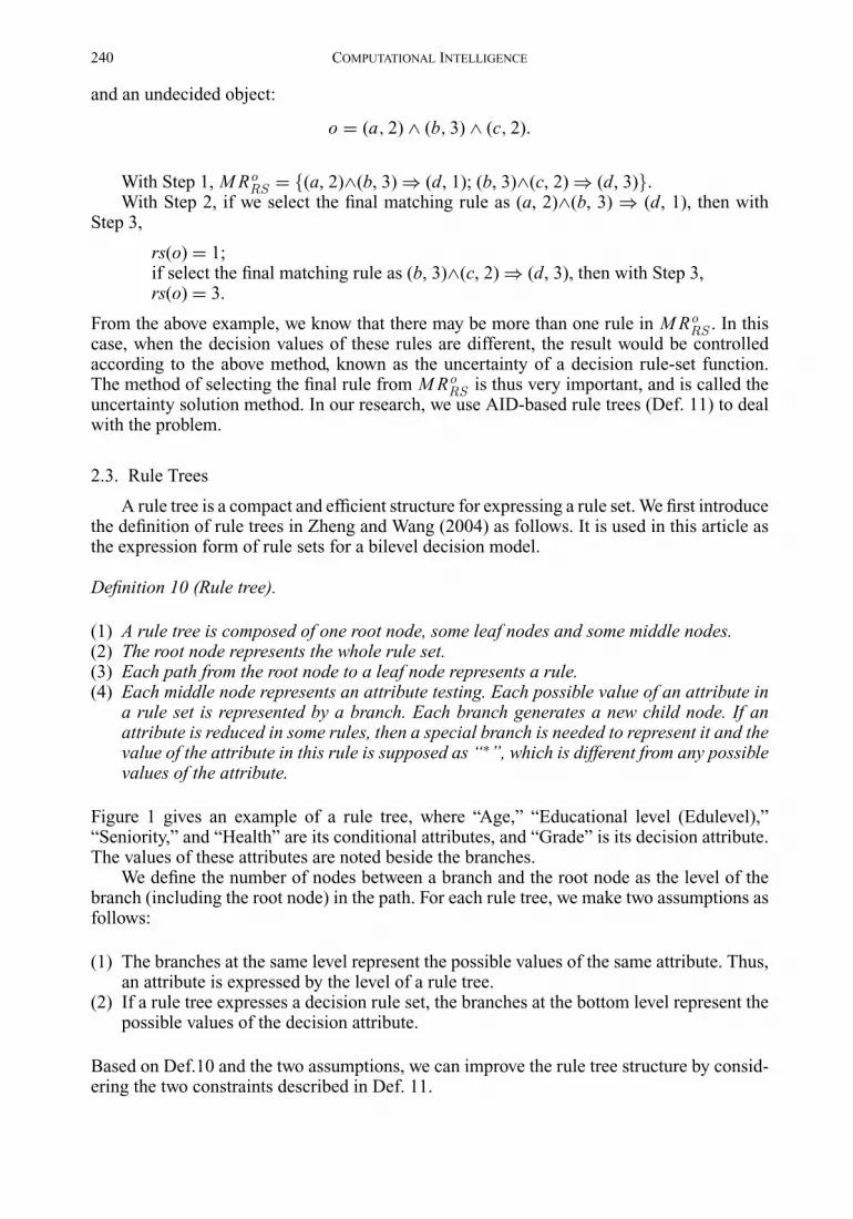
Figure 1 gives an example of a rule tree, where “Age,” “Educational level (Edulevel),”“Seniority,” and “Health” are its conditional attributes, and “Grade” is its decision attribute.The values of these attributes are noted beside the branches.

We define the number of nodes between a branch and the root node as the level of thebranch (including the root node) in the path. For each rule tree, we make two assumptions asfollows:

(1) The branches at the same level represent the possible values of the same attribute. Thus,an attribute is expressed by the level of a rule tree.

(2) If a rule tree expresses a decision rule set, the branches at the bottom level represent thepossible values of the decision attribute.

Based on Def.10 and the two assumptions, we can improve the rule tree structure by consid-ering the two constraints described in Def. 11.


Young Middle Old *

High

*

*

2

AgeEdulevel

SeniorityHealth

Grade

*

Long

Good

2

Short

Poor

3

*

*

4

* Short

*

*

4

FIGURE 1. An example of rule tree.

Definition 11 (Attribute importance degree (AID)–based rule tree). An AID-based rule treeis a rule tree, which satisfies the following two additional conditions:

(1) The conditional attribute expressed at the upper level is more important than thatexpressed at any lower level;

(2) Among the branches with the same start node, the value represented by the left branch ismore important (or better) than that represented by any right branch. And each possiblevalue is more important (or better) than the value “∗”.

In the rule tree illustrated in Figure 1, if we suppose

• ID(a) is the importance degree of attribute a, andID(Age) > ID(Edulevel) > ID(Seniority) > ID(Health);

• (Age, Young) is better than (Age, Middle), and (Age, Middle) is better than (Age, Old);• (Seniority, Long) is better than (Seniority, Short), and (Health, Good) is better than

(Health, Poor),

then the rule tree illustrated by Figure 1 is an AID-based rule tree.

Definition 12 (Comparison of rules). Suppose the condition attributes are ordered by theirimportance degrees as a1, . . . , ap . Rule dr1: ∧{(ai , va1i )} ⇒ (d1, vd1) is said to be betterthan rule dr2: ∧{(ai , va2i )}⇒ (d2, vd 2), if there exists an index k ∈ {1, . . . , p} that satisfies:

(1) va1k is better than va2k or the value of ak is deleted from rule dr2;(2) If k > 1, then for each j < k, va1j = va2j .

If for each attribute ai , va1i is with the same importance (or evaluation) degree as va2i , ruledr1 has the same importance (or evaluation) degree as rule dr2.

For example, we have two rules as follows:

dr1: (Age, Middle) ∧ (Working Seniority, Long) ⇒ 2,dr2: (Age, Middle) ∧ (Working Seniority, Short) ⇒ 3,


and the value “Long” is better than the value “Short” in the attribute “Working Seniority,”with Def. 12 we know dr1 is better than dr2.

Definition 13 (Rule confliction). Rule dr1 is said to be conflict with rule dr2, if

for ∀ x |= dr 1, x |= ¬ dr 2.

It can be proved that the following theorems hold from the definition of AID-based rule trees(Zheng et al. 2009).

Theorem 1. In an AID-based rule tree, the rule expressed by the left path is better than therule expressed by the right path.

Proof. Each branch in the left path is coincident with or on the left of the same level branchin the right path. Thus, from Def. 11 we know that the values represented by the branches inthe left path are at least not worse than those represented by the branches in the right path.Therefore, from Def. 12, the conclusion is reached, that is, the rule expressed by the left pathis better than the rule expressed by the right path. �

Theorem 2. After being transformed to an AID-based rule tree, the rules in a rule set aretotally in order, that is, every two rules can be compared.

Proof. The theorem holds from Def. 11 and Theorem 1. �Therefore, we can use an AID-based rule tree to solve the uncertainty problem of decision

rule set functions. For example, we can order the rules expressed by the rule tree shown inFigure 1 as follows:

(1) (Age, Young) ∧ (Edulevel, High) ⇒ 2,(2) (Age, Middle) ∧ (Working Seniority, Long) ⇒ 2,(3) (Age, Middle) ∧ (Working Seniority, Short) ⇒ 3,(4) (Age, Old) ⇒ 4,(5) (Edulevel, Short) ⇒ 4,

where rule i is better than rule i+1, i = 1, 2, 3, 4.

3. OUR PREVIOUS RELATED WORK

This section will introduce our previous related work including a RSBLD Model and anapproach for modeling bilevel decision problems by rule sets.

3.1. RSBLD Model

In principle, after emulating all possible situations in a decision domain, all objectivefunctions can be transformed into a set of decision tables, known as objective decision tables.As decision rule sets (Def. 6) have stronger knowledge expressing ability than decision tables(Def. 2), we use decision rule-set function (Def. 8) to represent the objectives of the leaderand follower of a bilevel decision problem in the proposed RSBLD model.

Similarly, after emulating all possible situations in a constraint field, the constraints canbe formulated to an information table. When the information table is too big to be processed,


it can be transformed to rule sets using the “Agrawal” methods provided by references(Agrawal, Imielinski, and Swami 1993; Agrawal and Srikant 1994).

By using rule sets, we have the following definition about constraint functions.

Definition 14 (Constraint Function). Suppose x is a decision variable and RS is a rule set,and then a constraint function cf (x, RS) is defined as

c f (x, RS) ={True, if for ∀r ∈ RS , x ∈ m(r )

False, else. (1)

The meaning of the constraint function cf (x, RS) is whether variable x belongs to theregion constrained by RS.

Now, we can describe a RSBLD model as follows.

Definition 15 (RSBLD model).

minx

fL(x, y)

subject tocf (x, GL ) = True

miny

fF (x, y)

subject to c f (y, G F ) = True(2)

where x and y are decision variables (vectors) of the leader and the follower, respectively; fLand fF are the objective decision rule set functions of the leader and the follower, respectively;cf is the constraint function; FL and GL are the objective decision rule set and constraintrule set of the leader; and FF and GF are the objective decision rule set and constraint ruleset of the follower, respectively.

3.2. An Approach for Modeling Bilevel Decision Problems by Rule Sets

For modeling a bilevel decision problem by rule sets, an approach was proposed in ourprevious study (Zheng et al. 2009) as follows.

Algorithm 1 (An approach for modeling bilevel decision problems by rule sets):

Input: A bilevel decision problem;Output: A RSBLD model;

Step 1: Transform the bilevel decision problem with rule sets (information tables are asspecial cases).

Step 2: Preprocess FL, such as delete reduplicate rules from the rule sets, eliminate noise,etc.

Step 3: If FL needs to be reduced, then using a reduction algorithm to reduce FL.Step 4: Preprocess GL, such as delete reduplicate rules from the rule sets, eliminate noise,

etc.Step 5: If GL needs to be reduced, then using reduction algorithm to reduce GL.Step 6: Preprocess FF , such as delete reduplicate rules from the rule sets, eliminate noise,

etc.Step 7: If FF needs to be reduced, then using a reduction algorithm to reduce FF .


Begin

Transform the problem with rule sets

Preprocess FL Preprocess GL Preprocess FF Preprocess GF

Reduce FL? Reduce GL? Reduce FF? Reduce GF?

Reduce FL Reduce GL Reduce FF Reduce GF

A Rule Sets-Based Bilevel Decision Model

End

Y Y Y YN N N N

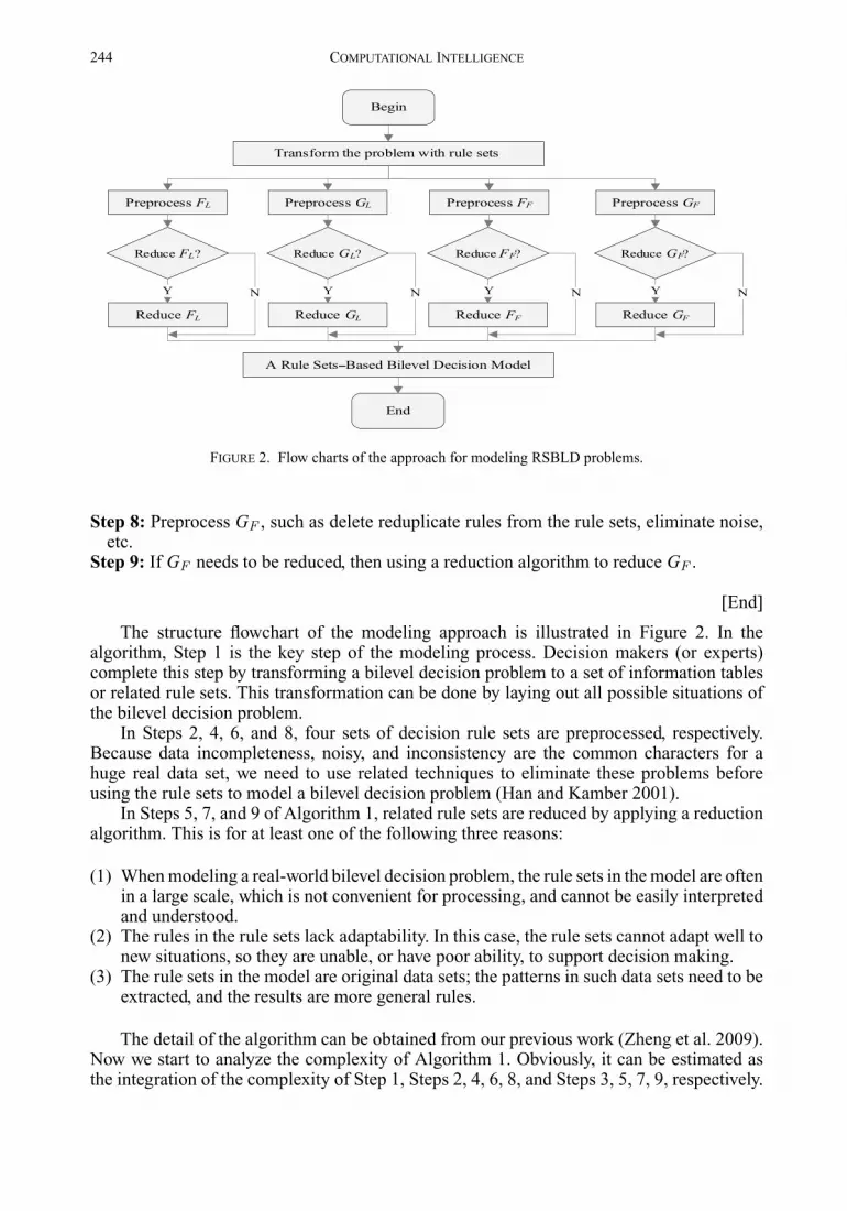
FIGURE 2. Flow charts of the approach for modeling RSBLD problems.

Step 8: Preprocess GF , such as delete reduplicate rules from the rule sets, eliminate noise,etc.

Step 9: If GF needs to be reduced, then using a reduction algorithm to reduce GF .

[End]

The structure flowchart of the modeling approach is illustrated in Figure 2. In thealgorithm, Step 1 is the key step of the modeling process. Decision makers (or experts)complete this step by transforming a bilevel decision problem to a set of information tablesor related rule sets. This transformation can be done by laying out all possible situations ofthe bilevel decision problem.

In Steps 2, 4, 6, and 8, four sets of decision rule sets are preprocessed, respectively.Because data incompleteness, noisy, and inconsistency are the common characters for ahuge real data set, we need to use related techniques to eliminate these problems beforeusing the rule sets to model a bilevel decision problem (Han and Kamber 2001).

In Steps 5, 7, and 9 of Algorithm 1, related rule sets are reduced by applying a reductionalgorithm. This is for at least one of the following three reasons:

(1) When modeling a real-world bilevel decision problem, the rule sets in the model are oftenin a large scale, which is not convenient for processing, and cannot be easily interpretedand understood.

(2) The rules in the rule sets lack adaptability. In this case, the rule sets cannot adapt well tonew situations, so they are unable, or have poor ability, to support decision making.

(3) The rule sets in the model are original data sets; the patterns in such data sets need to beextracted, and the results are more general rules.

The detail of the algorithm can be obtained from our previous work (Zheng et al. 2009).Now we start to analyze the complexity of Algorithm 1. Obviously, it can be estimated asthe integration of the complexity of Step 1, Steps 2, 4, 6, 8, and Steps 3, 5, 7, 9, respectively.


Suppose poL and poF are the numbers of the rules in the objective decision rule sets ofthe leader and the follower generated in Step 1, respectively, pcL, and pcF are the numbersof the rules in the constraint rule sets of the leader and the follower generated in Step 1,respectively, and mL and mF are the numbers of the condition attributes of the leader and thefollower. For Step 1, the complexity is

O((mL + m F )(poL + poF + pcL + pcF )).

For Steps 2, 4, 6, 8, different preprocess methods can cause different complexities. Forthe above-mentioned preprocess methods, the complexity is between O((mL + m F )p) andO((mL + m F )p2), where p = poL for Step 2, p = poF for Step 4, p = pcL for Step 6, andp = pcF for Step 8.

For Steps 3, 5, 7, and 9 the time complexity depends on the sizes of the processed rulesets. Using the methods mentioned above, it has complexity

O((mL + m F ) · p · (p − 1)),

where p = poL for Step 3, p = poF for Step 5, p = pcL for Step 7, and p = pcF for Step 9.Therefore, Algorithm 1 has the maximal time complexity

O((mL + m F )

(p2

oL + p2oF + p2

cL + p2cF

)).

In Section 6, we will use a case-based example to illustrate the modeling process of abilevel decision problem by using the proposed algorithm. In Section 7, a set of experimentsis designed to test the effectiveness and complexity of the algorithm.

4. TRANSFORMATION THEOREM FOR RSBLD PROBLEMS

In this section, we explore how to transform a RSBLD problem to a single-level one,where the two problems have the same optimal solution. A transformation theorem will beproposed to show the solution equivalence for the two problems. First, we give a definitionbelow.

Definition 16 (Combination rule of two decision rules). Suppose dr1: φ1 ⇒ (d1, v1) anddr2: φ2 ⇒ (d2, v2) are two decision rules and they are not conflict, then the combinationrule of them are denoted as dr1 ∩ dr2 with the form

φ1 ∧ φ2 ⇒ (d, (v1, v2)) , (3)

where d1, d2, and d are the decision attributes of dr1, dr2, and dr, respectively, v1, v2 and(v1, v2) are the decision values of dr1 and dr2, and dr, respectively.

Here, v1, v2 are called the leader decision and the follower decision of dr, respectively.For example, suppose

dr1: (Age, Young) ⇒ 2,dr2: (Working Seniority, Long) ⇒ 2,

then the combination of the two rules is

dr: (Age, Young)∧ (Working Seniority, Long)⇒ (d, (2, 2)).


Suppose the objective rule sets are expressed by AID-based rule trees, then the transfor-mation process can be presented as follows.

Step 1 (Initialization): Let CT be an empty attribute importance degree–based rule tree;Step 2 (Construct a new rule tree):

For each rule drL in FTL

For each decision rule drF in FTF

{If drL are not conflict with drF , thenAdd rule drL ∩ drF to CT ;}

[End]

Suppose the combined rule set is noted as F, then the single-level RSBLD problem canbe formulated as:

minx,y

f (x, y)

subject to c f (x, GL ) = True

c f (y, G F ) = True, (4)

where x and y are variables of the leader and the follower, respectively; f is the objectivedecision rule-set function; cf is the constraint function; F, GL, GF are the objective decisionrule set, leader’s constraint rule set and follower’s constraint rule set, respectively.

With the following theorem, we can prove the solution equivalence of the originalproblems and the transformed problem.

Theorem 3. The RSBLD model presented in equation (2) has an optimal solution (x, y), iff(x, y) is an optimal solution of its corresponding single-level decision model presented inequation (4).

Proof. Suppose x and y are variables of the leader and the follower, respectively, fLand fF are the objective rule-set functions of the leader and the follower, respectively, inequation (2), and f is the objective rule set function in equation (4). FL and FF are theobjective rule sets of the leader and the follower in the RSBLD model, and F is the objectiverule set in the single-level decision model.

(⇒)

If the optimal solution of the RSBLD model presented in equation (2) is (x, y), and

fL(x, y) = vL and fF(x, y) = vF.

Suppose the final matching rules (Section 2) of (x, y) in rule sets FL and FF are drL anddrF , respectively. Then, from the process of transformation, we know the rule drL ∩ drFbelongs to the combined rule set F.

Because (x, y) is the optimal solution of the RSBLD model, drL and drF must be thebest rules having the minimal decision values in FL and FF , respectively. Thus, dr = drL ∩drF must be the best rules matched by (x, y) in F. Besides, because (x, y) is the best objectsatisfying drL and drF both, thus (x, y) is the best object satisfying dr. Thus, (x, y) is theoptimal solution of the single-level decision model presented in equation (4).

The sufficient condition of the theorem is proved.

(⇐)


If the optimal solution of the single-level decision model presented in equation (4) is(x, y), and

f (x, y) = (d, (vLd, vFd)).

Suppose the final matching rule of (x, y) in rule set F is dr, then from the process oftransformation, there must be two decision rules drL in FL and drF in FF that dr = drL ∩drF . If there is more than one rule pair drL and drF satisfying that dr = drL ∩ drF , thenselect the best one among them.

Because (x, y) is the optimal solution of the single-level decision model, dr must bethe best rules having the minimal decision value in F. Thus, drL and drF must be the bestrules matched by (x, y) in FL and FF , respectively. Besides, because (x, y) is the best objectsatisfying dr, thus (x, y) is the best object satisfying drL and drF both. So, (x, y) is the optimalsolution of the bilevel decision model.

Thus, the necessary condition of the theorem is proved. �From Theorem 3, it is known that the solutions of the RSBLD problem presented in

equation (2) and its transformation problem shown in equation (4) are equivalent. Therefore,any RSBLD problem can be transformed into a single-level decision problem. Furthermore,a solution is arrived through solving the single-level decision problem. Note, although theoriginal bilevel decision problem and the transformed one level problem have the sameoptimal solution, they are not equivalent. Some information of the leader and the followerunrelated to the acquiring of the optimal solution is reduced during the transformingprocess, because the aim of transformation is only to generate a model which can beeasily solved but has the same optimal solution with the original bilevel decision model.

5. A TRANSFORMATION-BASED SOLUTION ALGORITHM FOR RSBLDPROBLEMS

Based on the transformation theory proposed, this section gives a transformation-basedsolution algorithm for RSBLD problems. To describe the algorithm clearly, some importantdefinitions are given.

Definition 17.

(a) Constraint region of a bilevel decision problem:

S = {(x, y) : c f (x, GL ) = True, c f (y, G F ) = True} (5)

(b) Feasible set for the follower for each fixed x:

S(x) = {y: (x, y) ∈ S} (6)

(c) Projection of S onto the leader’s decision space:

S(X) = {x :∃y, (x, y) ∈ S} (7)

(d) Follower’s rational reaction set for x ∈ S(X ):

P(x) = {y : y ∈ arg miny′

[ fF (x, y′) : y′ ∈ S(x)]} (8)


(e) Inducible region:

IR= {(x, y) : (x,y) ∈ S, y ∈ P(x)} (9)

From the features of the bilevel decision problem, it is obvious that once the leaderselects an x, the first term in the follower’s objective function becomes a constant and can beremoved from the problem. In this case, we replace fF (x, y) with fF (y).

To ensure that a RSBLD model is well posed, it is common to assume that S is nonemptyand compact, and that for all decisions taken by the leader, the follower has some roomto respond, that is, P(x)�= �. The rational reaction set P(x) defines the response while theinducible region IR represents the set over which the leader may optimize. Thus in terms ofthe above notation, the bilevel decision problem can be written as

min{ fL (x, y) : (x, y) ∈ IR}.

Now, we can give a description of the new algorithm. The algorithm has two stages. Itfirst transforms a bilevel decision problem described by a RSBLD model to a single-levelone. It then solves the single-level problem to get a solution. The solution obtained is ofthe original RSBLD problem. For simple description, suppose the importance degrees of theleader’s condition attributes are more than those of the follower’s. That means, the branchesrepresenting the possible values of the leader’s condition attributes are at higher levels ofAID-based rule trees than those of the follower’s. The detail of the transformation-basedalgorithm is as follows.

Algorithm 2 (A transformation-based solution algorithm for RSBLD problems):

Input: The objective decision rule set FL = {drL1 , . . . , drLp} and the constraint rule set GL

of the leader, the objective decision rule set FF = {drF1 , . . . , drFq} and the constraintrule set GF of the follower;

Output: An optimal solution of the RSBLD problem (ob);

Step 1: Construct the objective rule tree FTL of the leader by FL;Step 1.1: Arrange the condition attributes in ascending order according to the im-portance degrees. Let the attributes be the discernible attributes of levels from thetop to the bottom of the tree;Step 1.2: Initialize FTL to an empty AID-based rule tree;Step 1.3: For each rule R of the decision rule set FL {

Step 1.3.1: let CN = root node of the rule tree FTL;Step 1.3.2: For i = 1 to m /∗m is the number of levels in the rule tree∗/{If there is a branch of CN representing the ith discernible attribute value ofrule R, then

let CN = node I; /∗node I is the node generated by the branch∗/else {Create a branch of CN to represent the ith discernible attribute value;

According to the value order of the ith discernible attribute, put the createdbranch to the right place;Let CN = node J /∗node J is the end node of the branch∗/}}}

Step 2: Construct the objective rule tree FTF by FF ;The detail of Step 2 is similar to that in Step 1. What needs to be done is to replace FTL

with FTF and replace FL with FF in the sub-steps of Step 1.


Step 3: Transform the bilevel decision problem to a single-level one, and the resultantobjective rule tree is CT ;

Step 4: Use the constraint rule sets of both the leader and the follower to prune CT ;

Step 4.1: Generate an empty new AID-based rule tree CT ′;Step 4.2: For each rule dr in GL and GF ,

Add the rules in CT to CT ′ that are consistent with dr to FTL′;

Delete the rules in CT and CT ′ conflict with dr;

Step 4.3: CT = CT′;Step 5: Search for the leftmost rule dr in CT whose leader decision and follower decision

are both minimal;Step 6: If dr does not exist, then

There isn’t an optimal solution for the problem;Go to End;

Step 7: OB = {ob | ob |= dr and for ∀r∈GL∪GF , ob |= r};Step 8: If there is more than one object in OB, then

According to Def. 12, select the best or most important object ob;else

ob = the object in OB;Step 9: ob is the optimal solution of the RSBLD problem.

[End]

By this algorithm, we can obtain a solution for a bilevel decision problem through solvingthe transformed single-level problem. The time complexity of the new algorithm is

O (noLnoF (ncL + ncF ) (mL + m F )) ,

where noL, noF are numbers of the rules in the objective rule sets of the leader and thefollower, ncL, ncF are numbers of the rules in the constraint rule sets of the leader andthe follower, mL and mF are the numbers of the condition attributes of the leader and thefollower, respectively.

6. CASE STUDY

A factory’s human resource management system is distributed into two levels. Theupper level is the factory executive committee and the lower is the workshop managementcommittee. For the recruitment policy, the executive committee mainly considers how tomeet the overall business objectives with a long-term development plan, and the workshopmanagement committee concentrates on the current daily needs of workers. Obviously, theirobjectives are different. However, their objectives are transparent to each other though theymay operate in separate ways. A recruitment action will ultimately emerge that is the optimalresult for the company as a whole but will also consider current daily needs. This is a typicalbilevel decision problem, in which the company executive committee is as the leader, andthe workshop management committee, the follower.

When determining whether a person could be recruited for a particular position, thefactory executive committee mainly considers the following two factors, the “age” and“education level (edulevel)” of the person, and the workshop management committee mainlyconsiders another two factors, “seniority” and “health.” Suppose the condition attributes in


TABLE 2. Objective Rule Set of the Leader.

Age Edulevel Seniority Health Grade

Young High Middle Good 2Middle High Long Middle 2Young Short Short Poor 4Young Middle Middle Middle 2Middle Middle Short Middle 3Middle Middle Long Middle 2Old High Long Middle 3Young Short Middle Poor 2Middle Short Short Middle 4Old Short Middle Poor 4Middle Short Long Good 3Middle Short Long Middle 2Old High Middle Poor 3Old High Long Good 2Old Short Long Good 4Young High Long Good 4Young Short Long Middle 3

TABLE 3. Objective Decision Table of the Follower.

Age Edulevel Seniority Health Grade

Young High Long Good 2Old Short Short Good 4Young High Short Good 2Old High Long Middle 3Young Short Long Middle 4Middle High Middle Poor 3Middle Short Short Poor 4Old Short Short Poor 4Old High Long Good 2Young Short Long Good 2Young Short Middle Middle 3Middle Short Middle Good 3Old High Long Good 2Middle High Long Good 2Middle High Short Poor 4

ascending order according to the importance degree are “age,” “edulevel,” “seniority,” and“health.”

Obviously, it is hard for the two committees to express the conditions of the workerswho they want to recruit to linear or nonlinear functions. However, they have the data ofthe workers who have already been recruited in their databases. We can therefore build twodecision tables as shown in Tables 2 and 3, and then generate decision rule sets from the


tables to represent the objectives of the two committees. The condition attributes of thetwo decision tables are the factors; the decision attributes of the two decision tables areacceptance grades of the workers. The constraints of the two committees are expressed bysimple rule sets (equations 10, 11), which define the constraint regions.

Now, we use algorithm 1 to establish a RSBLD model from the problem.

Alg. 1-Step 1: Transform the problem with decision rule sets.

As indicated above, the objective rule sets and constraint rule sets of the leader and thefollower are described in Tables 2, 3, and equations (10), (11), respectively.

The constraint rule set of the leader is:

GL= {True ⇒ (Age, Young) ∨ (Age, Middle)} (10)

The constraint rule set of the follower is:

G F= {True ⇒ (Seniority, Long) ∨ (Seniority, Middle)} (11)

For the small scale of the data, the preprocess steps (Steps 2, 4, 6, and 8) are passedover. Besides, the constraint rule sets of the leader and the follower are brief enough, so thereduction steps of GL and GF (Step 5 and Step 9) can be ignored.

Alg. 1-Step 3 and Step 7: Reduce the objective rule sets of the leader and the follower.

After reducing the decision tables based on rough set theory, we can get the reducedobjective rule sets of the leader and the follower as shown in equations (12) and (13). Here,we use the decision matrices–based value reduction algorithm (Ziarko, Cercone, and Hu1996) in the RIDAS system (Wang, Zheng, and Zhang 2002).

The refined objective rule set of the leader is:

FL= {(Age, Young) ∧ (Seniority, Middle) ⇒ (Grade, 2)

(Age, Middle) ∧ (Edulevel, High) ⇒ (Grade, 2)

(Edulevel, Short) ∧ (Seniority, Short) ⇒ (Grade, 4)

(Edulevel, Middle) ∧ (Seniority, Short) ⇒ (Grade, 3)

(Edulevel, Middle) ∧ (Seniority, Long) ⇒ (Grade, 2)

(Age, Old) ∧ (Health, Middle) ⇒ (Grade, 3)

(Age, Old) ∧ (Edulevel, Short) ⇒ (Grade, 4)

(Age, Middle) ∧ (Health, Good) ⇒ (Grade, 3)

(Age, Middle) ∧ (Seniority, Long) ∧ (Health, Middle) ⇒ (Grade, 2)

(Age, Old) ∧ (Edulevel, High) ∧ (Health, Good) ⇒ (Grade, 2)

(Edulevel, High) ∧ (Health, Poor) ⇒ (Grade, 3)

(Age, Young) ∧ (Edulevel, High) ∧ (Seniority, Long) ⇒ (Grade, 4)

(Age, Young) ∧ (Edulevel, Short) ∧ (Seniority, Long) ⇒ (Grade, 3)}

(12)


The refined objective rule set of the follower is:

FF= {(Edulevel, High) ∧ (Health, Good) ⇒ (Grade, 2)

(Edulevel, Short) ∧ (Seniority, Short) ⇒ (Grade, 4)

(Age, Old) ∧ (Health, Middle) ⇒ (Grade, 3)

(Age, Young) ∧ (Seniority, Long) ∧ (Health, Middle) ⇒ (Grade, 4)

(Seniority, Middle) ⇒ (Grade, 3)

(Seniority, Long) ∧ (Health, Good) ⇒ (Grade, 2)

(Seniority, Short) ∧ (Health, Poor) ⇒ (Grade, 4)}

(13)

With the above steps, we get the RSBLD model of the decision problem as follows:

minx

fL (x, y)

subject to c f (x, GL ) = True (14)

miny

fF (x, y)

subject to c f (y, G F ) = True,

where fL, fF are the corresponding decision rule set functions of FL, FF , respectively.Now, we use the Alg. 2 to solve the RSBLD problem. We suppose the four condition

attributes are ordered as “age,” “edulevel,” “seniority,” and “health.”

Alg. 2-Step 1: Construct the objective rule tree FTL of the leader by FL, and the resultis illustrated by Figure 3.

Alg. 2-Step 2: Construct the objective rule tree FTF of the follower by FF , and the resultis illustrated by Figure 4.

Alg. 2-Step 3: Transform the bilevel decision problem to a single-level one, and theresulted objective rule tree CT is illustrated by Figure 5.

Alg. 2-Step 4: Use the constraint rule sets of both the leader and follower to prune CT ,and the result is illustrated by Figure 6.

Alg. 2-Step 5: Search for the leftmost rule dr in CT whose leader decision and followerdecision are both minimal, and the result is

dr : (Age, Young) ∧ (Edulevel, High) ∧ (Seniority, Middle) ∧ (Health, Good) ⇒ (d, (2, 2));

Alg. 2-Step 6: OB = {ob | ob is the object satisfying:

(Age, Young) ∧ (Edulevel, High) ∧ ((Seniority, Middle) ∧ (Health, Good);

Alg. 2-Step 7: ob = (Age, Young)∧(Edulevel, High)∧(Seniority, Middle)∧(Health,Good);

Alg. 2-Step 8: ob is the final solution of the RSBLD problem.

In Figure 3–6, the attribute values are represented by its first letter.


Y M O *

H S *

L L M

* * *

4 3 2

AgeHeight

SeniorityHealth

Grade

H

*

*

2

*

L

M

2

*

G

4

H S *

* * *

G * M

2 4 3

H M

* L S

P * *

3 2 3

S

S

*

4

FIGURE 3. Rule tree of the leader’s objective rule set.

Y O *

*

L

M

4

AgeHeight

SeniorityHealth

Grade

H S

* S L

G * G

2 4 2

*

M

*

3

*

*

M

3

S

P

4

FIGURE 4. Rule tree of the follower’s objective rule set.

7. EXPERIMENTS AND ANALYSIS

To test the effectiveness and complexity of the proposed RSBLD problem mod-eling algorithm (Algorithm 1) and solution algorithm (Algorithm 2), we implementedthese two algorithms within Matlab 6.5. We then used some classical data sets from theUCI database to test them by a set of experiments. UCI database (http://www.ics.uci.


Y M O *

H SM

L LL

G GM

4,2 3,22,4

AgeHeight

SeniorityHealth

Grade

H

L

G

2,2

*

L

G

4,2

H S

L LM

G G *

2,2 4,2 4,3

M

4,4

M

G

2,2

M

3,4

*

M

*

2,3

M

*

2,3

S

P

2,4

*

G

2,2

M

G

4,3

*

G

2,2

S

M

4,3

*

4,4

*

M

4,3

L S

M M

2,3 3,3

M H SM

MS

P P

3,3 3,4

L S

G P

2,2 3,4

S

P

4,4

*

4,4

P

4,4

FIGURE 5. Transformation result of the objective rule trees.

Y M *

H S M

L L L

G G M

4,2 3,2 2,4

AgeHeight

SeniorityHealth

Grade

H

L

G

2,2

*

L

G

4,2

M

4,4

M

G

2,2

M

3,4

*

M

*

2,3

M

*

2,3

*

G

2,2

M

G

4,3

H M

M

P

3,3

L

G

2,2

FIGURE 6. Combined objective rule trees after pruning by the constraint rules.


edu/∼mlearn/MLRepository.html) consists of many data sets that can be used by the de-cision systems and machine learning communities for the empirical analysis of algorithms.

For each data set we chose, we first selected half of a data set as the original objectiverule set of the leader, and the remaining as the original objective rule set of the follower. Weassumed that there are no constraints, which means all objects consistent with the objectiverule sets are in the constraint region. Additionally, we supposed the first half of the conditionattributes to be the ones for the leader and the others for the follower. The importance degreesof the condition attributes are in descending order from the first condition attribute to thelast condition attribute. The two experiments were processed on a computer with 2.33GHzCPU and 2G memory space. We describe the experiments as follows.

Experiment 1: Testing of Algorithm 1 with the data sets in the UCI database.

Step 1: Randomly choose 50% of the objects from the data set to be the original objectivedecision rule set of the leader, and the remaining 50% of the objects to be theoriginal objective decision rule set of the follower;

Step 2: Apply Algorithm 1 to construct a RSBLD model by using the chosen rule sets.Here, we use the decision matrices–based value reduction algorithm (Ziarko,Cercone, and Hu 1996) in the RIDAS system (Wang, Zheng, and Zhang 2002)to reduce the sizes of original rule sets.

Experiment 2: Testing of Algorithm 2 with the data sets in the UCI database.

Following Steps 1 and 2 in Experiment 1, we have

Step 3: Apply Algorithm 2 to get a solution from the generated RSBLD model inExperiment 1. Suppose object obj is the final solution.

minx

fL (x, y)

subject to c f (x, GL ) = True

miny

fF (x, y)

subject to c f (y, G F ) = True,

(15)

Experiment 3: Effectiveness Testing of Algorithm 1 and 2 in the UCI database.Following Steps 1, 2, 3 in Experiment 1 and 2, we have

Step 4: Let mark = 0;Step 5: Calculate fL(obj) and fF (obj);Step 6: If fL(obj) and fF (obj) are minimal, then

Step 6.1: Randomly generate 1000 objects, which are better than obj;Step 6.2: If all of the 1000 objects are not in the constraint fields or do not have the

minimal decisions by the decision rule set functions of the leader and the follower, then letmark = 1.

Experiments 1 and 2 are to calculate the final solution of a RSBLD problem. Experiment3 is to test the effectiveness of the two algorithms (algorithm 1 and 2). For a RSBLD problem,an object obj is its optimal solution if and only if obj satisfies the following two conditions:

(1) The decisions of obj, made by the objective decision rule sets of the leader and thefollower, are minimal;

(2) In the constraint field, obj is better than all objects with the same decisions.


TABLE 4. Testing Results of Algorithms 1 and 2.

Alg. 1 Alg. 2

Data sets pOL pOF mL mF nOL nOF t1(sec.) t2 (sec.) Mark∗

LENSES 12 12 2 3 6 3 <0.01 0.03 1HAYES-ROTH 50 50 2 3 21 24 <0.01 0.09 1AUTO-MPG 199 199 4 4 80 76 0.08 0.39 1BUPA 172 172 3 3 159 126 0.06 3.10 1PROCESSED_CLEVELAND 151 151 6 7 115 127 0.28 5.20 1BREAST-CANCER-WISCONSIN 349 349 5 5 47 47 0.51 0.63 1∗

Note, if mark = 1, the algorithms are effective on the corresponding data set.

The two conditions are tested by Step 5 and 6, respectively. Although the second conditioncannot be tested sufficiently by Step 6, it is verified if the number of randomly generatedobjects is great enough. Thus, from Experiment 3 we can conclude, if variable mark is equalto 1, the effectiveness of the two algorithms is confirmed.

The complexity of the two algorithms (Algorithm 1 and 2) is also tested through con-ducting these two experiments. As shown in Table 4, pOL and pOF are the numbers of objectsin the original decision rules of the leader and the follower, respectively (Refer to Step 1 ofAlgorithm 1), mL and mF are the condition attribute numbers of the leader and the follower,respectively, nOL and nOF are the numbers of the rules in the reduced objective decisionrule sets of the leader and the follower, respectively, t1 and t2 are the processing times ofAlgorithms 1 and 2, respectively.

From the results shown in Table 4 we can find that

(1) The modeling algorithm (Alg.1) and the transformation-based solution algorithm(Alg. 2) are effective;

(2) The processing time of Alg. 1 highly relates with the numbers of the rules in the originalobjective decision rule sets and the condition attribute numbers of the leader and thefollower, respectively, expressed by the symbols pOL, pOF , mL, and mF .

(3) The processing time of Alg. 2 highly relates with the numbers of the rules in the reducedobjective decision rule sets and the condition attribute numbers of the leader and thefollower, respectively, expressed by nOL, nOF , mL, and mF .

These are consistent with the complexity analysis results in Sections 3 and 5.

8. CONCLUSION AND FUTURE WORK

Bilevel decision making is a common issue in organizational management activities.As many bilevel decision problems are difficult to model with mathematical functions,RSBLD models were proposed, in which all objective functions and constraint functions wereexpressed by rule sets. Based on our previous research, this article presented a transformation-based algorithm to solve a RSBLD problem. Some experiments showed the effectivenessand complexity of the proposed solution algorithm.

In the traditional BLP model, Kuhn–Tucker conditions (Bard and Falk 1982; Bialasand Karwan 1982; Hansen et al. 1992) were used to transform a BLP model to a single-level one. The basic idea of the transformation proposed in this article is different from the


Kuhn–Tucher condition–based transformation. In the solution algorithm of the traditionalBLP problem, the follower’s problem was transformed to constraints, while in the solutionalgorithm proposed for RSBLP problems, the objective functions of the leader and the fol-lower were combined to one. Besides, the most important issue is that the two transformationssolve different bilevel problems, as one is a RSBLD problem and another is a bilevel linearprogramming.

Further study will include the development of approaches for multi-objectives or multi-followers RSBLD problems. A comprehensive bilevel decision support system is beingdeveloped to implement the proposed techniques for supporting real decision makers tosolve their bilevel decision problems effectively.

ACKNOWLEDGMENT

The work presented in this article was supported by Australian Research Council (ARC)under discovery grant DP0557154, Aviation Science Foundation of China (2008ZG51092),and National Natural Science Foundation of China (60904066, 60933004, 60975039).

REFERENCES

AGRAWAL, R., T. IMIELINSKI, and A. SWAMI. 1993. Mining association rules between sets of items in largedatabases. In Proceeding of The ACM SIGMOD Conference on Management of Data, pp. 207–216.

AGRAWAL, R., and R. SRIKANT. 1994. Fast algorithms for mining association rules. In Proceeding of 20thInternational Conference of Very Large Databases, pp. 487–499.

AIYOSHI, E., and K. SHIMIZU. 1981. Hierarchical decentralized systems and its new solution by a barrier method.IEEE Transactions on Systems, Man, and Cybernetics, 11:444–449.

ANANDALINGAM, G., and T. FRIESZ. 1992. Hierarchical optimization: An introduction. Annals of OperationsResearch, 34:1–11.

BARD, J. F. 1984. An investigation of the linear three level programming problem. IEEE Transactions on Systems,Man, and Cybernetics, 14:711–71.

BARD, J. F. 1998. Practical Bilevel Optimization: Algorithms and Applications. Kluwer Academic Publishers,Boston.

BARD, J. F., and J. E. FALK. 1982. An explicit solution to the multi-level programming problem. Computers &Operations Research, 9:77–100.

BARD, J. F., and J. T. MOORE. 1992. An algorithm for the discrete bilevel programming problem. Naval ResearchLogistics, 39:419–435.

BIALAS, W., and M. H. KARWAN. 1978. Multilevel linear programming. Technical Report 781, State Universityof New York at Buffalo, Operations Research Program.

BIALAS, W. F., and M. H. KARWAN. 1982. On two-level optimization. IEEE Transactions on Automatic Control,AC-26:211–214.

BIALAS, W., and M. H. KARWAN. 1984. Two-level linear programming. Management Science, 30:1004–1020.

CALVETE, H., I. C. GALE, and P. M. MATEO. 2008. A new approach for solving linear bilevel problems usinggenetic algorithms. European Journal of Operational Research, 188(1):14–28.

CANDLER, W., and R. TOWNSLEY. 1982. A linear two-level programming problem. Computers and OperationsResearch, 9:59–76.

CHEN, Y., M. FLORIAN, and S. WU. 1992. A descent dual approach for linear bilevel programs. Technical ReportCRT866, Centre de Recherche sur les Transports.

DEMPE, S. 1987. A simple algorithm for the linear bilevel programming problem. Optimization, 18:373–385.


HAN, J., and M. KAMBER. 2001. Data Mining Concepts and Techniques. Morgan Kaufmann, Palo Alto, CA.

HANSEN, P., B. JAUMARD, and G. SAVARD. 1992. An extended branch-and-bound rules for linear bilevel program-ming. SIAM Journal on Scientific and Statistical Computing, 13:1194–1217.

LAI, Y. J. 1996. Hierarchical optimization: a satisfactory solution. Fuzzy Sets and Systems, 77:321–335.

LAN, K. M., U. P. WEN, H. S. SHIH, and E. S. LEE. 2007. A hybrid neural network approach to bilevel programmingproblems. Applied Mathematics Letters, 20(8):880–884.

LIANG, L., and S. H. SHENG. 1992. The stability analysis of bilevel decision and its application. Decision AndDecision Support System, 2:63–70.

PAWLAK, Z. 1991. Rough Sets Theoretical Aspects of Reasoning about Data. Kluwer Academic Publishers,Boston.

QUINLAN, J. R. 1983. Learning efficient classification procedures and their application to chess end-games. InMachine Learning: An Artificial Intelligence Approach. Vol. 1. Edited by J. S. Michalski, J.G. Carbonell,and T.M. Mirchell. Morgan Kaufmann, Palo Alto, CA, pp. 463–482.

SAKAWA, M., and I. NISHIZAK. 2001a. Interactive fuzzy programming for two-level linear fractional programmingproblems. Fuzzy Sets and Systems, 119:31–40.

SAKAWA, M., and I. NISHIZAK. 2001b. Interactive fuzzy programming for decentralized two-level linear pro-gramming problems. Fuzzy Sets and Systems, 125:301–315.

SAKAWA, M., and I. NISHIZAK. 2002. Interactive fuzzy programming for two-level nonconvex programmingproblems with fuzzy parameters through genetic algorithms. Fuzzy Sets and Systems, 127:185–197.

SAKAWA, M., I. NISHIZAKI, and Y. UEMURA. 2000a. Interactive fuzzy programming for multilevel linear pro-gramming problems with fuzzy parameters. Fuzzy Sets and Systems, 109:3–19.

SAKAWA, M., I. NISHIZAKI, and Y. UEMURA. 2000b. Interactive fuzzy programming for two-level linear fractionalprogramming problems with fuzzy parameters. Fuzzy Sets and Systems, 115:93–103.

SAKAWA, M., and K. YAUCHI. 2000. Interactive decision making for multiobjective nonconvex programmingproblems with fuzzy numbers through coevolutionary genetic algorithms. Fuzzy Sets and Systems, 114:151–165.

SAVARD, G. 1989. Contributions a la programmation mathematique a deux niveaux. PhD thesis. Universite deMontreal, Ecole Polytechnique.

SHI, H. S., Y. J. LAI, and E. S. LEE. 1996. Fuzzy approach for multi-level programming problems. Computers &Operations Research, 23:73–91.

STACKELBERG, H. V. 1952. The Theory of Market Economy, Oxford University Press, Oxford.

TARSKI, A. 1956. The Concept of Truth in Formalized Language, Logic Semantics, Metamathematics. ClarendonPress, Oxford.

WANG, G. M., X. J. WANG, Z. P. WAN, and Y. B. LV. 2007. A globally convergent algorithm for a class of bilevelnonlinear programming problem. Applied Mathematics and Computation, 188(1):166–172.

WANG, G. Y. 2001. Rough Set Theory and Knowledge Acquisition. Press of Xi’an University of Communications.

WANG, G. Y., Z. ZHENG, and Y. ZHANG. 2002. RIDAS-a rough set based intelligent data analysis system. In theProceeding of the First International Conference on Machine Learning and Cybernetics, pp. 646–649.

WHITE, D., and G. ANANDALINGAM. 1993. A penalty function approach for solving bi-level linear programs.Journal of Global Optimization, 3:397–419.

YAO, Y. Y., and J. T. YAO. 2002. Granular computing as a basis for consistent classification problems. Commu-nications of Institute of Information and Computing Machinery (special issue of PAKDD’02 Workshop onToward the Foundation of Data Mining), 5:101–106.

ZHANG, G., and J. LU. 2005. The definition of optimal solution and an extended Kuhn–Tucker approach forfuzzy linear bilevel programming. IEEE Computational Intelligence Bulletin, 2(5):1–7.

ZHANG, G., and J. LU. 2006. Model and approach of fuzzy bilevel decision making for logistics planning problem.Journal of Enterprise Information Management, 20:178–197.


ZHANG, G., J. LU, and T. DILLON. 2007a. In Fuzzy linear bilevel optimization: Solution concepts, approachesand applications. In Fuzzy Logic—A Spectrum of Theoretical and Practical Issues. Edited by P. P. Wang, D.Ruan, and E. E. Kerre. Springer, Berlin, pp. 351–379.

ZHANG, G., J. LU, and T. DILLON. 2007b. Solution concepts and an approximation Kuhu–Tucker approach forfuzzy multi-objective linear bilevel programming. In Pareto Optimality, Game Theory and Equilibria. Editedby Panos Pardalos and Altannar Chinchuluun. Springer, Berlin, pp. 467–490.

ZHENG, Z., J. LU, G. ZHANG, and Q. HE. 2009. Rule sets based bilevel decision model and algorithm. ExpertSystems with Applications, 36:28–26.

ZHENG, Z., and G. Y. WANG. 2004. RRIA: A rough set and rule tree based incremental knowledge acquisitionalgorithm. Fundamenta Informaticae, 59:299–313.

ZIARKO, W., N. CERCONE, N. and X. HU. 1996. Rule discovery from databases with decision matrices. LectureNotes In Computer Science, 1079:653–662.

Documents

AN ALGORITHM FOR SOLVING RULE SETS-BASED BILEVEL DECISION PROBLEMS