Embed Size (px)
Citation preview
Data Mining Classification: Basic Concepts,
Lecture Notes for Chapter 4 - 5
Introduction to Data Mining by
Tan, Steinbach, Kumar
Classification: Definition
• Given a collection of records (training set ) – Each record contains a set of attributes, one of the
attributes is the class.
• Find a model for class attribute as a function of the values of other attributes.
• Goal: previously unseen records should be assigned a class as accurately as possible. – A test set is used to determine the accuracy of the
model. Usually, the given data set is divided into training and test sets, with training set used to build the model and test set used to validate it.
• When the class is numerical, the problem is a regression problem.
Classification: Definition
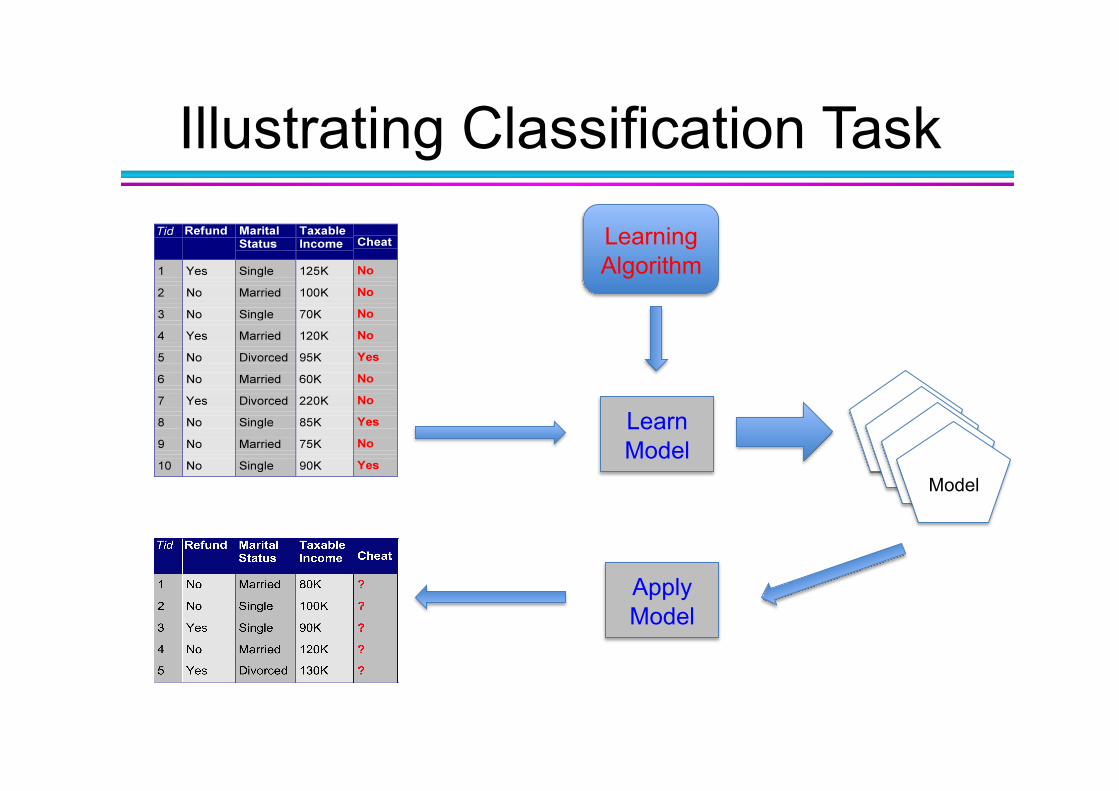
Illustrating Classification Task Learning Algorithm
Learn Model
Apply Model
Model
Examples of Classification Task • Predicting tumor cells as benign or malignant
• Classifying credit card transactions as legitimate or fraudulent
• Classifying secondary structures of protein as alpha-helix, beta-sheet, or random coil
• Categorizing news stories as finance, weather, entertainment, sports, etc
Classification Techniques
• Decision Tree • Naïve Bayes • Instance Based Learning • Rule-based Methods • Neural Networks • Bayesian Belief Networks • Support Vector Machines
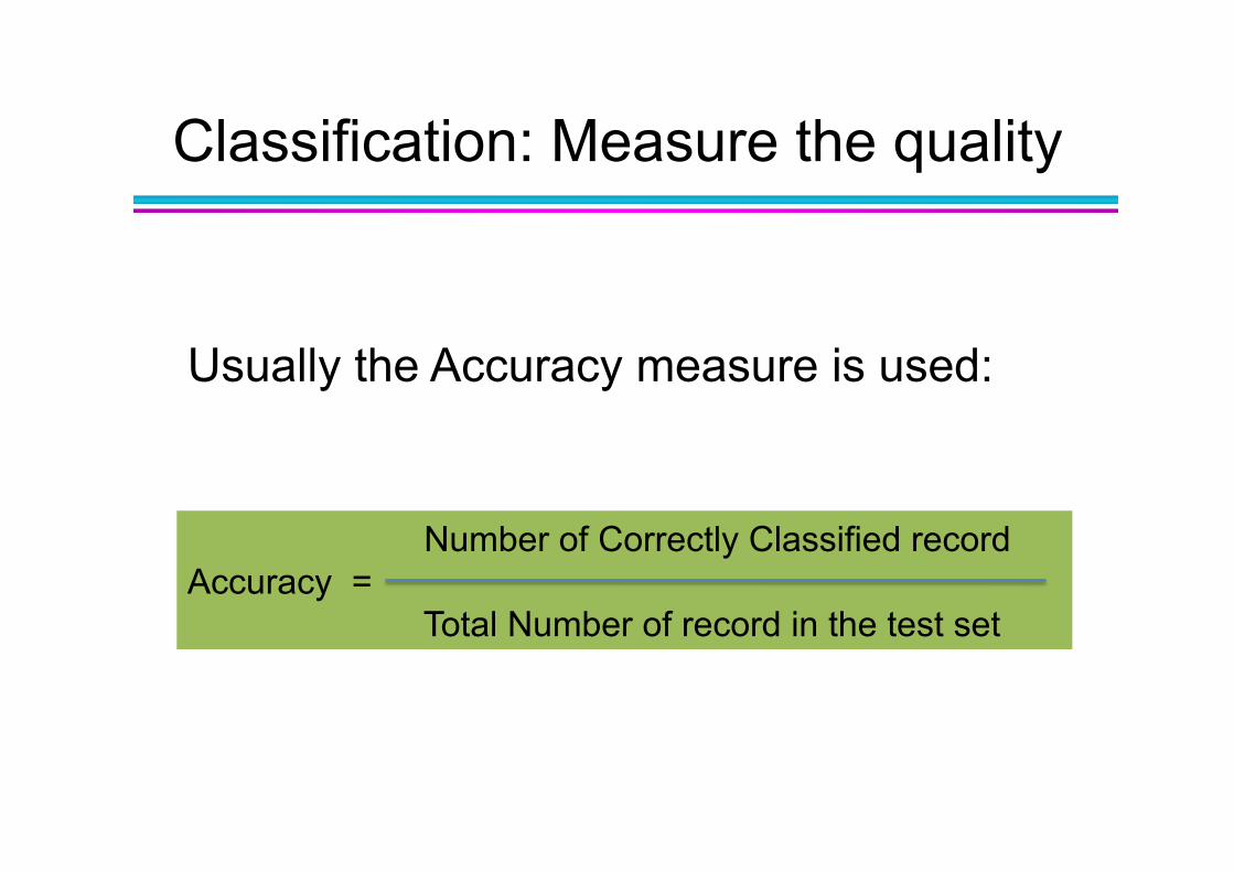
Usually the Accuracy measure is used:
Number of Correctly Classified record Accuracy =
Total Number of record in the test set
Classification: Measure the quality
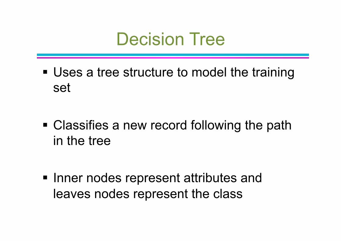
Decision Tree
Uses a tree structure to model the training set
Classifies a new record following the path in the tree
Inner nodes represent attributes and leaves nodes represent the class
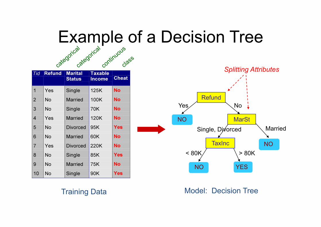
Example of a Decision Tree
Refund
MarSt
TaxInc
YES NO
NO
NO
Yes No
Married Single, Divorced
< 80K > 80K
Splitting Attributes
Training Data Model: Decision Tree
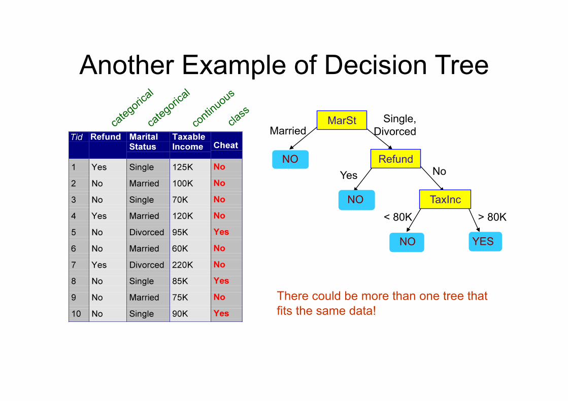
Another Example of Decision Tree
MarSt
Refund
TaxInc
YES NO
NO
NO
Yes No
Married Single,
Divorced
< 80K > 80K
There could be more than one tree that fits the same data!
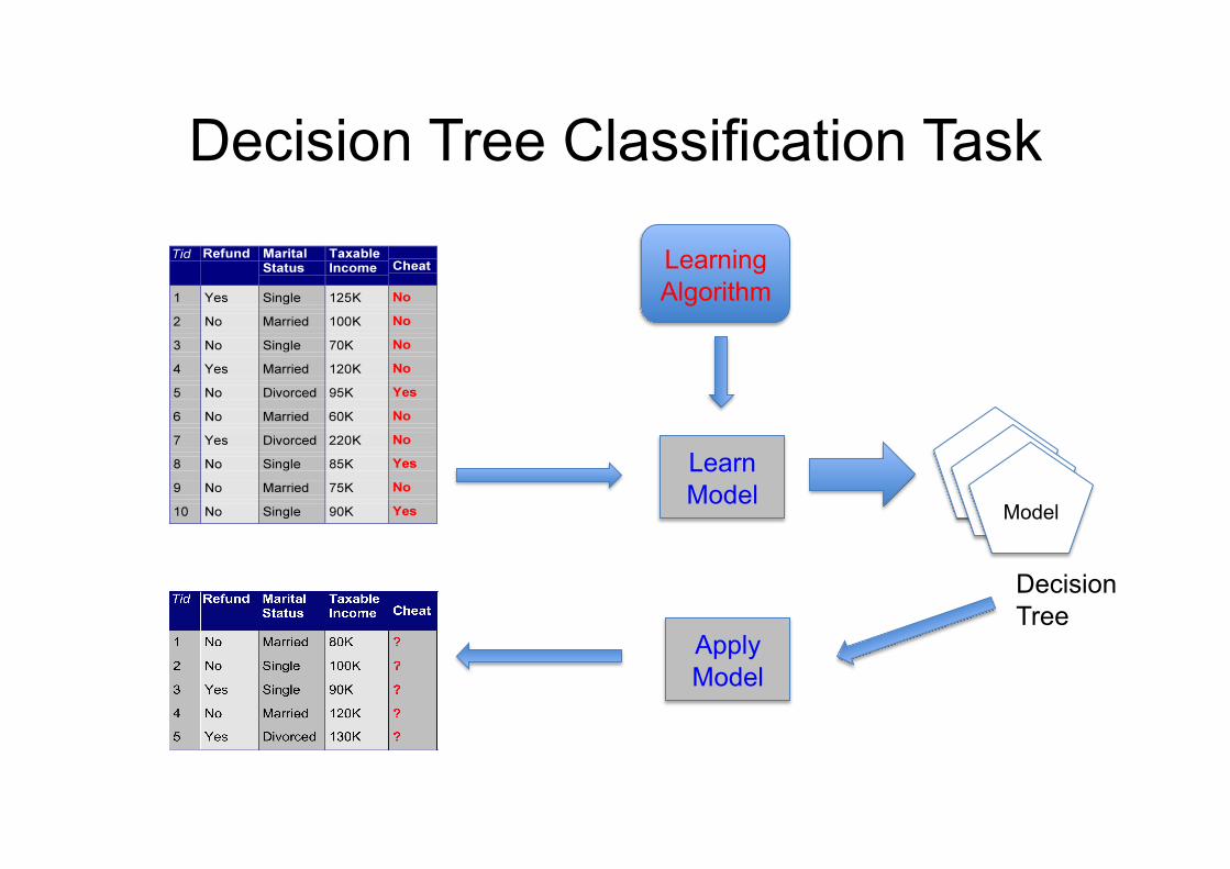
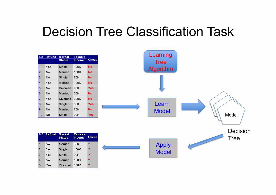
Decision Tree Classification Task
Decision Tree
Learning Algorithm
Learn Model
Apply Model
Model
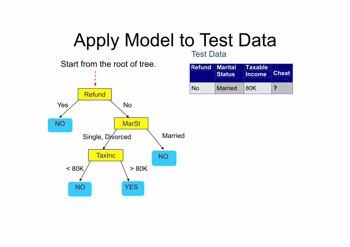
Apply Model to Test Data
Refund
MarSt
TaxInc
YES NO
NO
NO
Yes No
Married Single, Divorced
< 80K > 80K
Test Data Start from the root of tree.

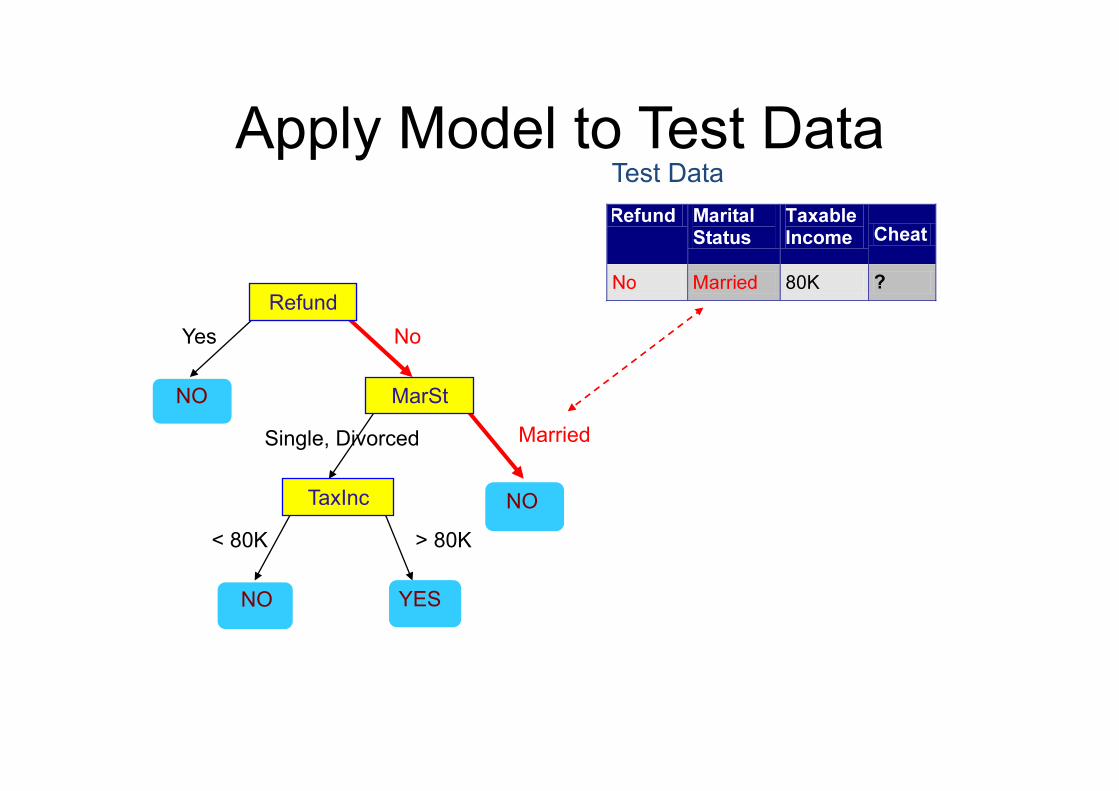
Apply Model to Test Data
Refund
MarSt
TaxInc
YES NO
NO
NO
Yes No
Married Single, Divorced
< 80K > 80K
Test Data

Apply Model to Test Data
Refund
MarSt
TaxInc
YES NO
NO
NO
Yes No
Married Single, Divorced
< 80K > 80K
Test Data

Apply Model to Test Data
Refund
MarSt
TaxInc
YES NO
NO
NO
Yes No
Married Single, Divorced
< 80K > 80K
Test Data
Apply Model to Test Data
Refund
MarSt
TaxInc
YES NO
NO
NO
Yes No
Married Single, Divorced
< 80K > 80K
Test Data
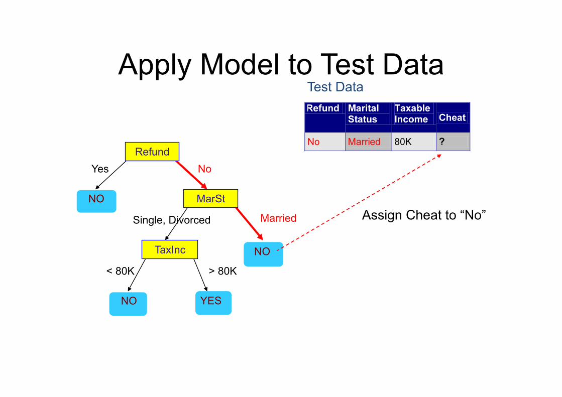
Apply Model to Test Data
Refund
MarSt
TaxInc
YES NO
NO
NO
Yes No
Married Single, Divorced
< 80K > 80K
Test Data
Assign Cheat to “No”
Decision Tree Classification Task Learning
Tree Algorithm
Learn Model
Apply Model
Model
Decision Tree
Decision Tree Induction
• Many Algorithms: – Hunt’s Algorithm (one of the earliest) – CART – ID3, C4.5 (J48 on WEKA) – SLIQ,SPRINT
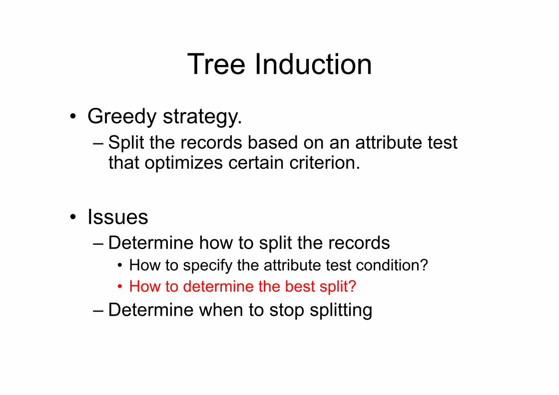
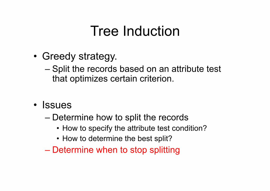
Tree Induction
• Greedy strategy. – Split the records based on an attribute test
that optimizes certain criterion.
• Issues – Determine how to split the records
• How to specify the attribute test condition? • How to determine the best split?
– Determine when to stop splitting
Tree Induction
• Greedy strategy. – Split the records based on an attribute test
that optimizes certain criterion.
• Issues – Determine how to split the records
• How to specify the attribute test condition? • How to determine the best split?
– Determine when to stop splitting
How to Specify Test Condition?
• Depends on attribute types – Nominal – Ordinal – Continuous
• Depends on number of ways to split – 2-way split – Multi-way split
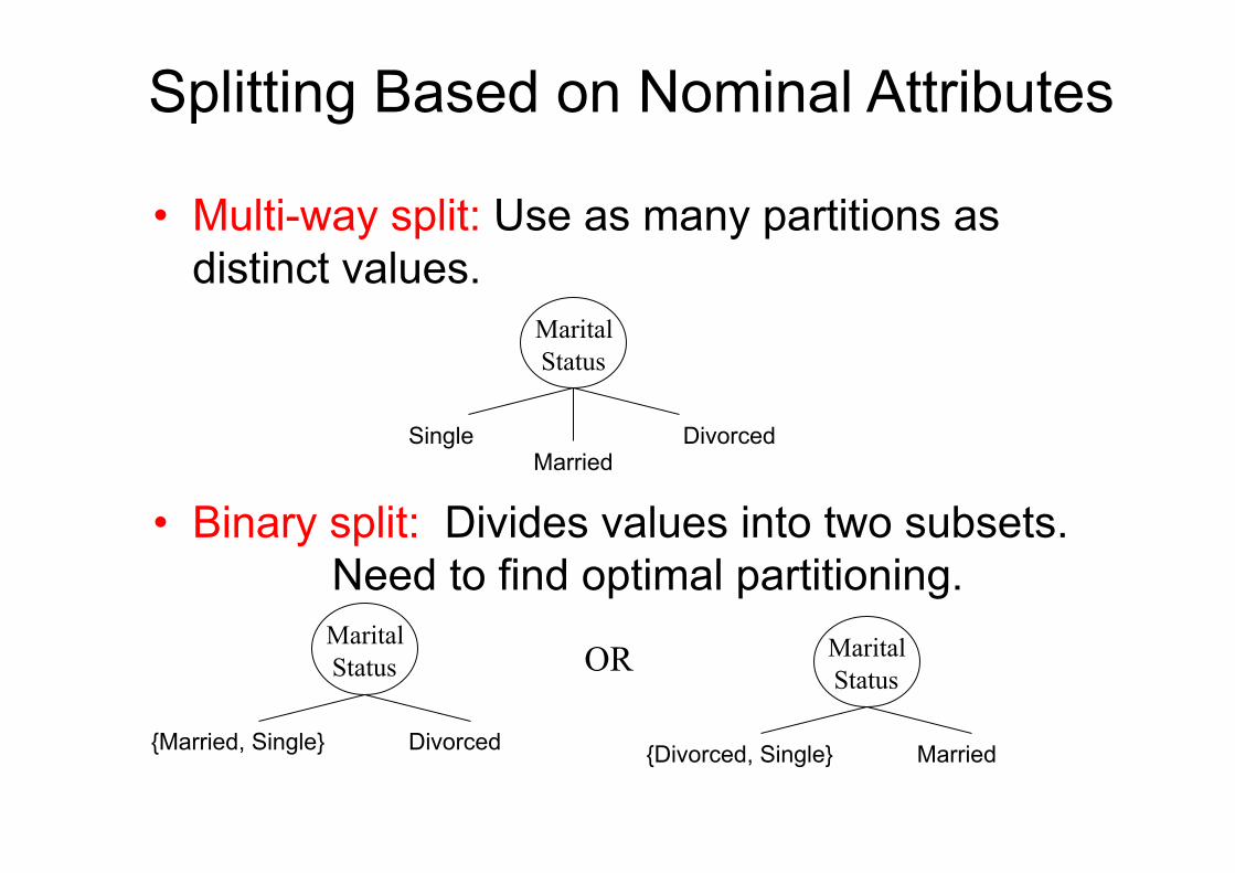
Splitting Based on Nominal Attributes
• Multi-way split: Use as many partitions as distinct values.
• Binary split: Divides values into two subsets. Need to find optimal partitioning.
Marital Status
Single Married
Divorced
OR Marital Status
{Married, Single} Divorced
Marital Status
{Divorced, Single} Married
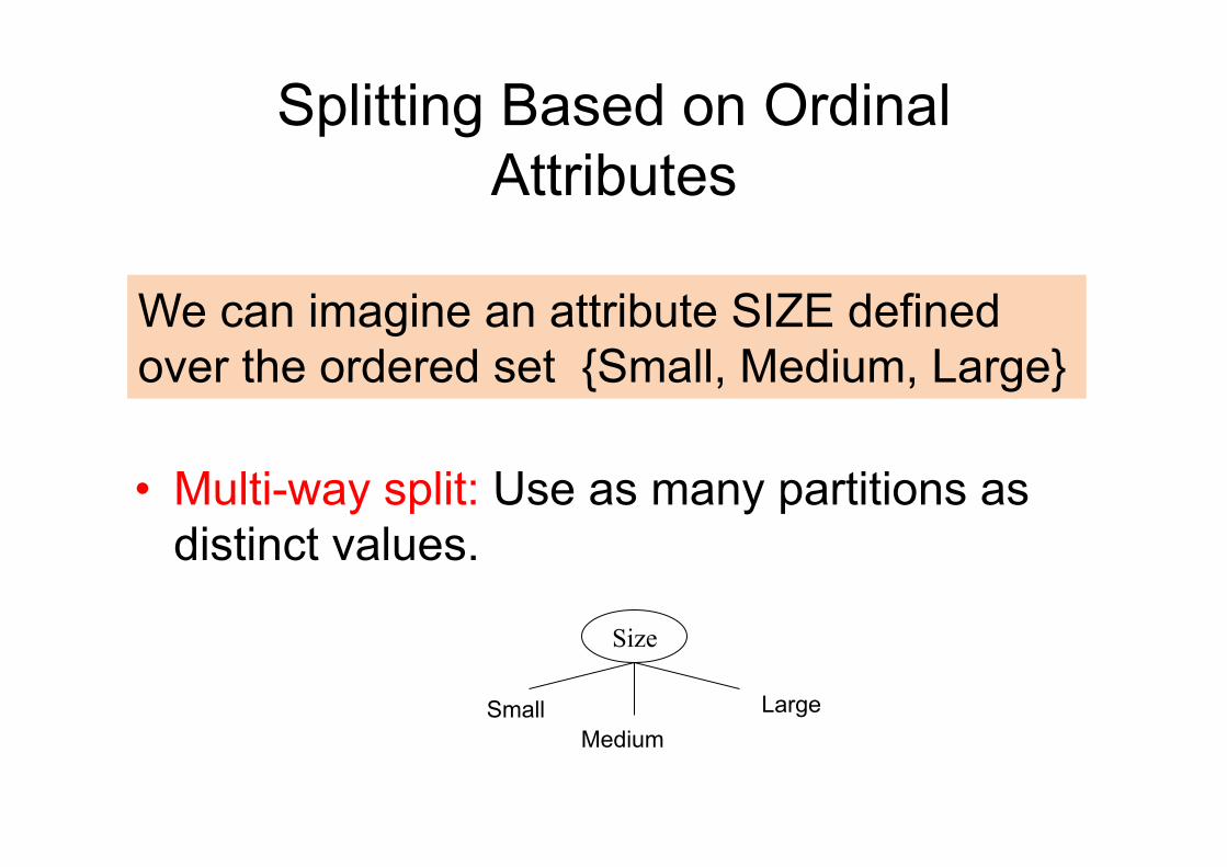
• Multi-way split: Use as many partitions as distinct values.
Splitting Based on Ordinal Attributes
Size
Small Medium
Large
We can imagine an attribute SIZE defined over the ordered set {Small, Medium, Large}
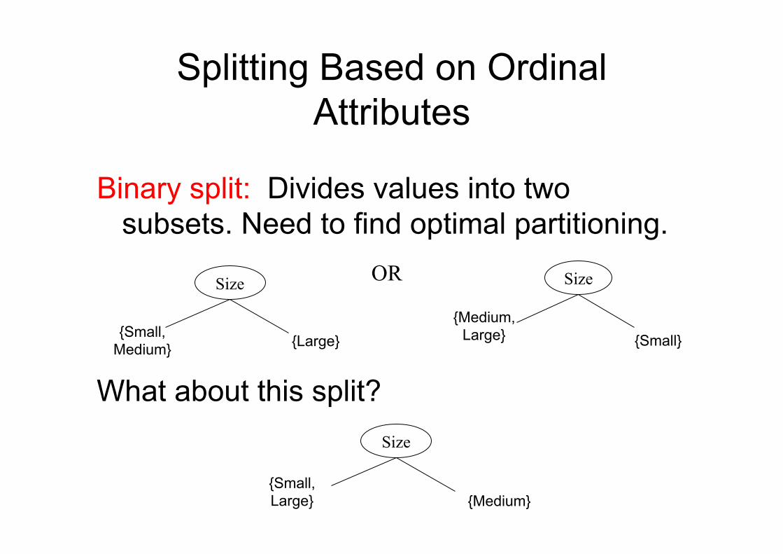
Size
{Medium, Large} {Small}
Size
{Small, Medium} {Large}
OR
Size
{Small, Large} {Medium}
Binary split: Divides values into two subsets. Need to find optimal partitioning.
What about this split?
Splitting Based on Ordinal Attributes
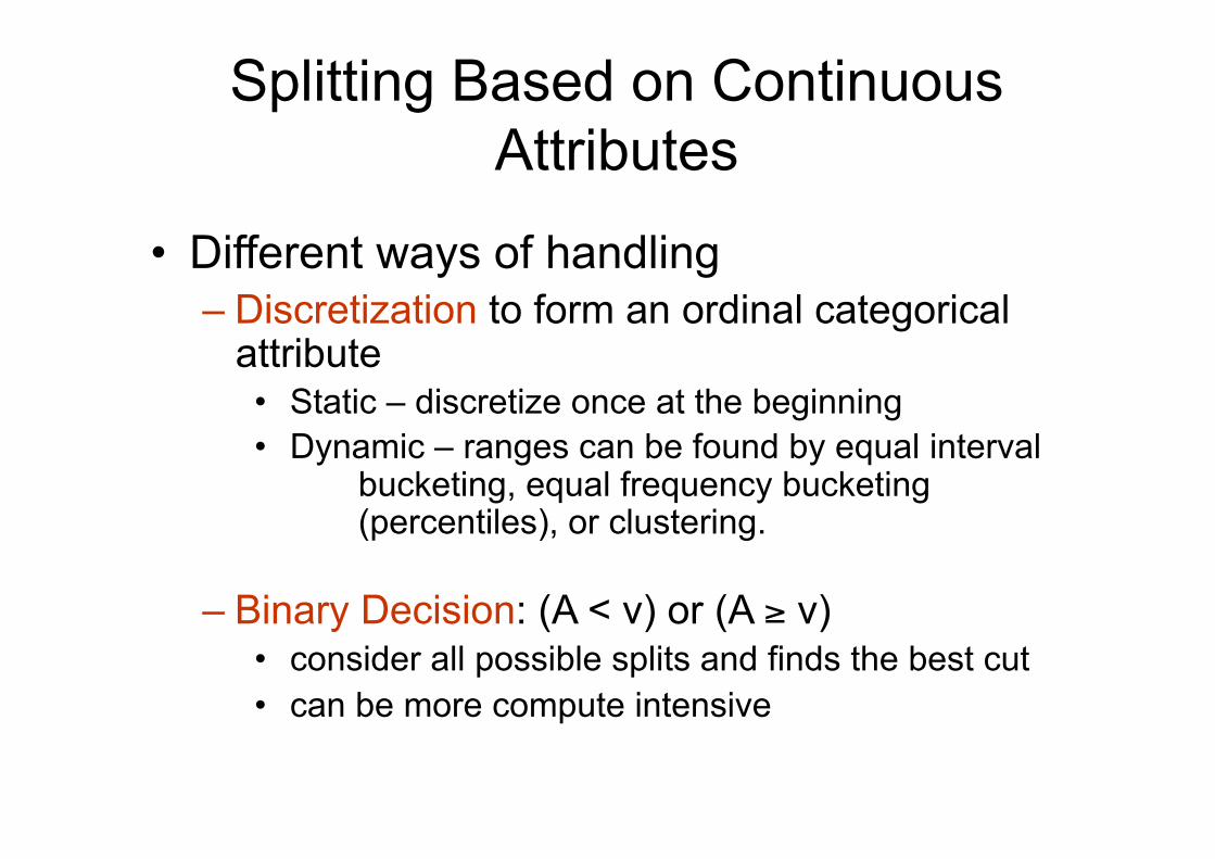
Splitting Based on Continuous Attributes
• Different ways of handling – Discretization to form an ordinal categorical
attribute • Static – discretize once at the beginning • Dynamic – ranges can be found by equal interval
bucketing, equal frequency bucketing (percentiles), or clustering.
– Binary Decision: (A < v) or (A ≥ v) • consider all possible splits and finds the best cut • can be more compute intensive
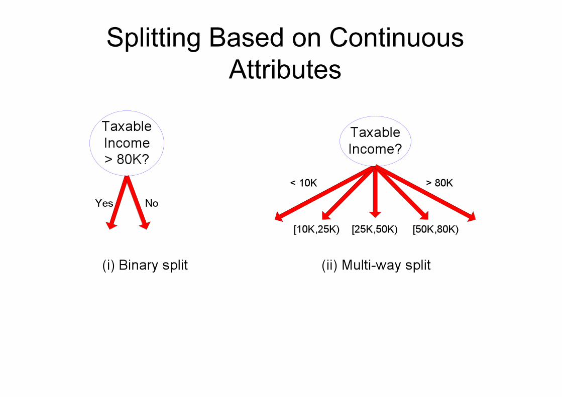
Splitting Based on Continuous Attributes
Tree Induction
• Greedy strategy. – Split the records based on an attribute test
that optimizes certain criterion.
• Issues – Determine how to split the records
• How to specify the attribute test condition? • How to determine the best split?
– Determine when to stop splitting
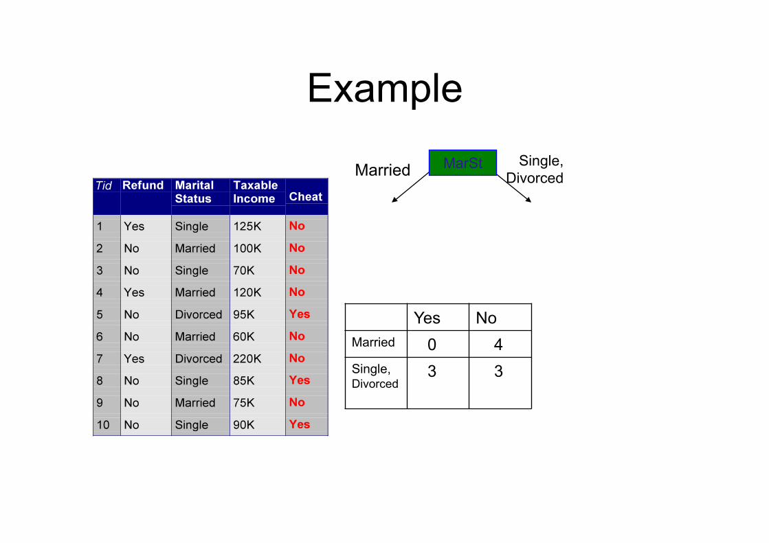
Example MarSt Single,
Divorced Married
Yes No Married 0 4 Single, Divorced
3 3

Example MarSt Single,
Divorced Married
NO
{NO:4, YES:0}
Refund Yes No
YES NO Single, Divorced
Refund = NO
3 1
Single, Divorced
Refund = Yes
0 2
MarSt Single, Divorced Married
NO
{NO:4, YES:0}
Refund Yes No
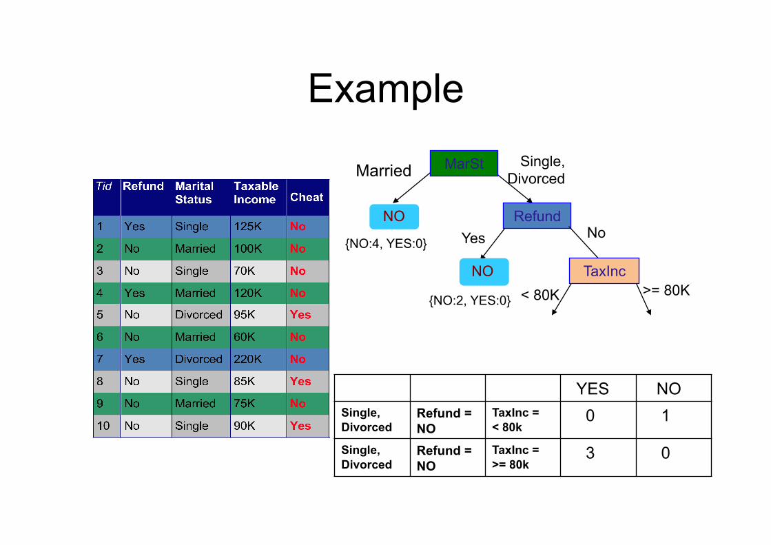
Example
NO
{NO:2, YES:0}
TaxInc < 80K >= 80K
YES NO Single, Divorced
Refund = NO
TaxInc = < 80k
0 1
Single, Divorced
Refund = NO
TaxInc = >= 80k
3 0
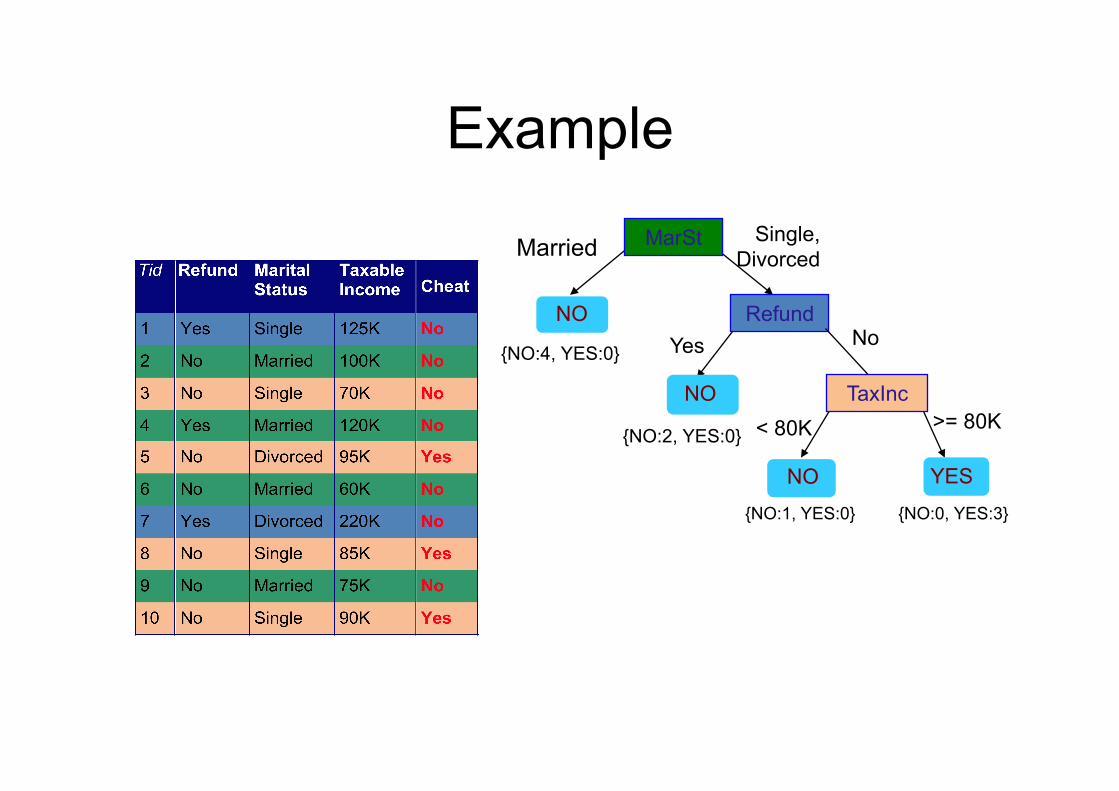
Example MarSt Single,
Divorced Married
NO
{NO:4, YES:0}
Refund Yes No
NO
{NO:2, YES:0}
TaxInc < 80K >= 80K
YES NO
{NO:1, YES:0} {NO:0, YES:3}
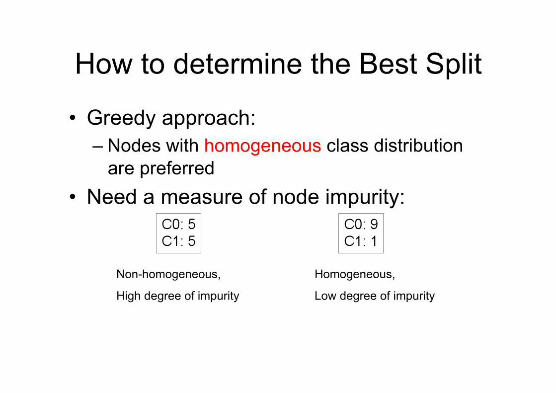
How to determine the Best Split
• Greedy approach: – Nodes with homogeneous class distribution
are preferred • Need a measure of node impurity:
Non-homogeneous,
High degree of impurity
Homogeneous,
Low degree of impurity
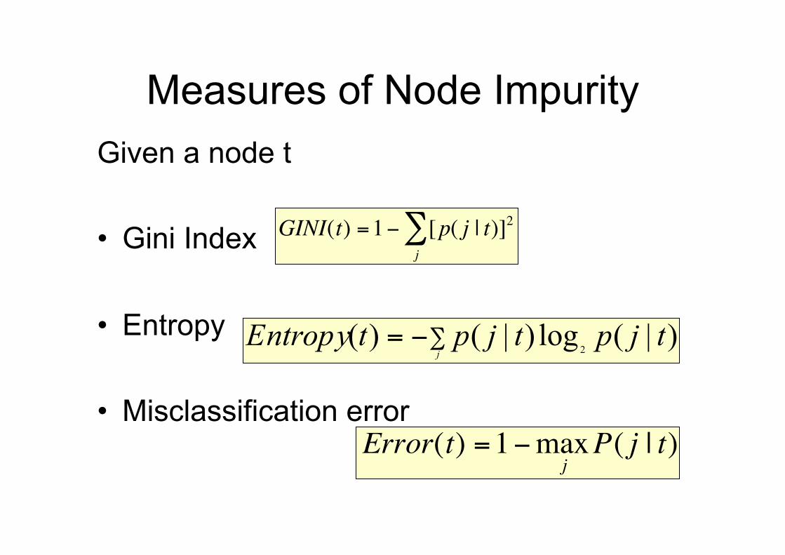
Measures of Node Impurity Given a node t
• Gini Index
• Entropy
• Misclassification error
€
Error(t) =1−maxjP( j | t)
€
GINI(t) =1− [p( j | t)]2j∑
Tree Induction
• Greedy strategy. – Split the records based on an attribute test
that optimizes certain criterion.
• Issues – Determine how to split the records
• How to specify the attribute test condition? • How to determine the best split?
– Determine when to stop splitting
Stopping Criteria for Tree Induction
• Stop expanding a node when all the records belong to the same class
• Stop expanding a node when all the records have similar attribute values
Decision Tree Based Classification
• Advantages:
– Inexpensive to construct
– Extremely fast at classifying unknown records
– Easy to interpret for small-sized trees
– Accuracy is comparable to other classification techniques for many simple data sets
Naive Bayes
Uses probability theory to model the training set
Assumes independence between attributes
Produces a model for each class
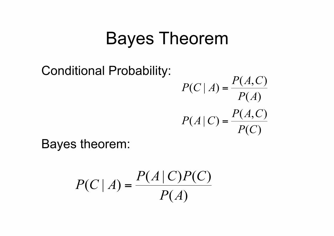
Conditional Probability:
Bayes theorem:
Bayes Theorem
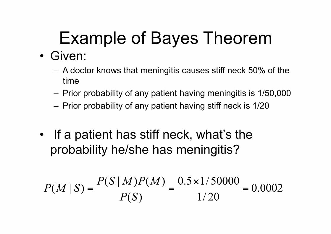
Example of Bayes Theorem • Given:
– A doctor knows that meningitis causes stiff neck 50% of the time
– Prior probability of any patient having meningitis is 1/50,000 – Prior probability of any patient having stiff neck is 1/20
• If a patient has stiff neck, what’s the probability he/she has meningitis?
Bayesian Classifiers • Consider each attribute and class label as
random variables
• Given a record with attributes (A1, A2,…,An) – Goal is to predict class C – Specifically, we want to find the value of C that
maximizes P(C| A1, A2,…,An )
• Can we estimate P(C| A1, A2,…,An ) directly from data?
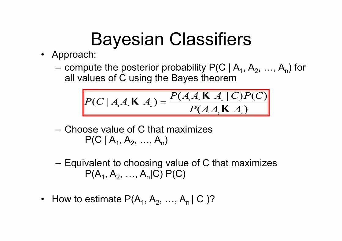
Bayesian Classifiers • Approach:
– compute the posterior probability P(C | A1, A2, …, An) for all values of C using the Bayes theorem
– Choose value of C that maximizes P(C | A1, A2, …, An)
– Equivalent to choosing value of C that maximizes P(A1, A2, …, An|C) P(C)
• How to estimate P(A1, A2, …, An | C )?
Naïve Bayes Classifier • Assume independence among attributes Ai when class is
given: – P(A1, A2, …, An |C) = P(A1| Cj) P(A2| Cj)… P(An| Cj)
– Can estimate P(Ai| Cj) for all Ai and Cj.
– New point is classified to Cj if P(Cj) Π P(Ai| Cj) is maximal.
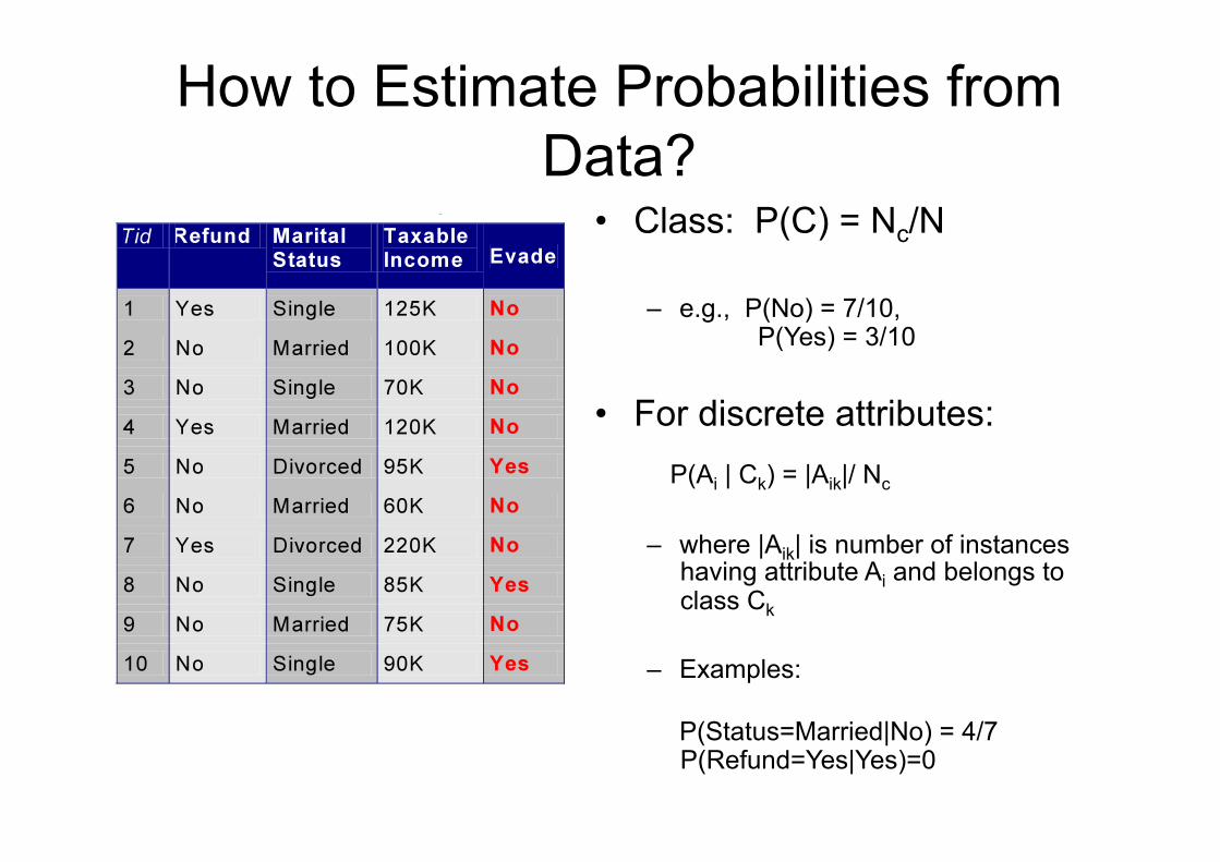
How to Estimate Probabilities from Data?
• Class: P(C) = Nc/N
– e.g., P(No) = 7/10, P(Yes) = 3/10
• For discrete attributes: P(Ai | Ck) = |Aik|/ Nc
– where |Aik| is number of instances having attribute Ai and belongs to class Ck
– Examples:
P(Status=Married|No) = 4/7 P(Refund=Yes|Yes)=0
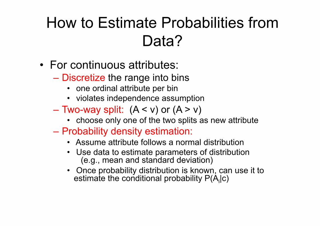
How to Estimate Probabilities from Data?
• For continuous attributes: – Discretize the range into bins
• one ordinal attribute per bin • violates independence assumption
– Two-way split: (A < v) or (A > v) • choose only one of the two splits as new attribute
– Probability density estimation: • Assume attribute follows a normal distribution • Use data to estimate parameters of distribution
(e.g., mean and standard deviation) • Once probability distribution is known, can use it to
estimate the conditional probability P(Ai|c)

How to Estimate Probabilities from Data?
P(Status=Married|Yes) = ?
P(Refund=Yes|No) = ?
P(Status=Divorced|Yes) = ?
P(TaxableInc > 80K|Yes) = ?
P(TaxableInc > 80K|NO) = ?
Compute:
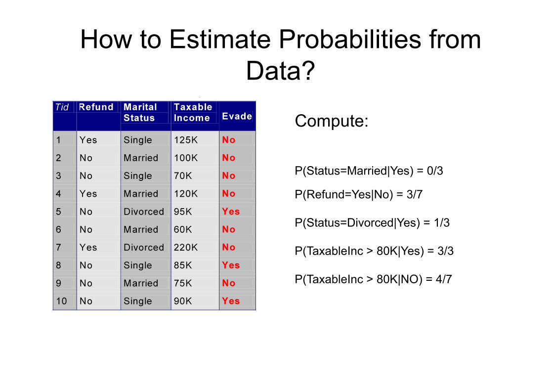
How to Estimate Probabilities from Data?
P(Status=Married|Yes) = 0/3
P(Refund=Yes|No) = 3/7
P(Status=Divorced|Yes) = 1/3
P(TaxableInc > 80K|Yes) = 3/3
P(TaxableInc > 80K|NO) = 4/7
Compute:
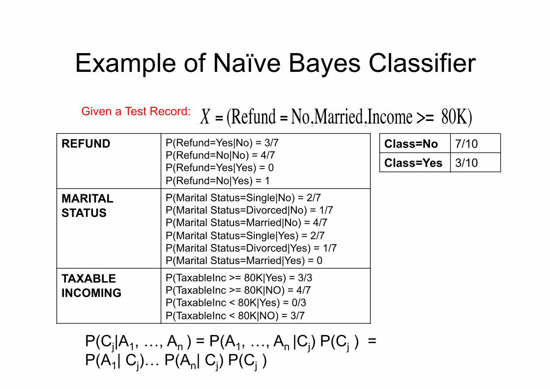
Example of Naïve Bayes Classifier
€
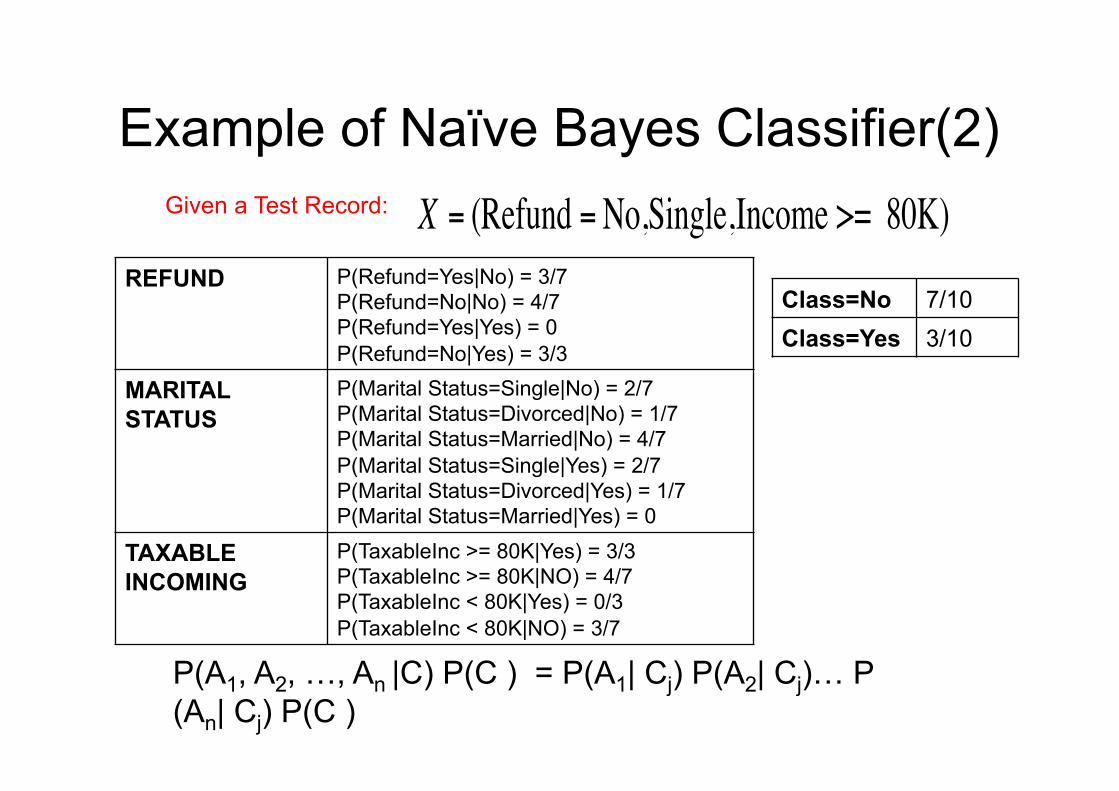
X = (Refund = No,Married,Income >= 80K)Given a Test Record:
REFUND P(Refund=Yes|No) = 3/7 P(Refund=No|No) = 4/7 P(Refund=Yes|Yes) = 0 P(Refund=No|Yes) = 1
MARITAL STATUS
P(Marital Status=Single|No) = 2/7 P(Marital Status=Divorced|No) = 1/7 P(Marital Status=Married|No) = 4/7 P(Marital Status=Single|Yes) = 2/7 P(Marital Status=Divorced|Yes) = 1/7 P(Marital Status=Married|Yes) = 0
TAXABLE INCOMING
P(TaxableInc >= 80K|Yes) = 3/3 P(TaxableInc >= 80K|NO) = 4/7 P(TaxableInc < 80K|Yes) = 0/3 P(TaxableInc < 80K|NO) = 3/7
Class=No 7/10 Class=Yes 3/10
P(Cj|A1, …, An ) = P(A1, …, An |Cj) P(Cj ) = P(A1| Cj)… P(An| Cj) P(Cj )
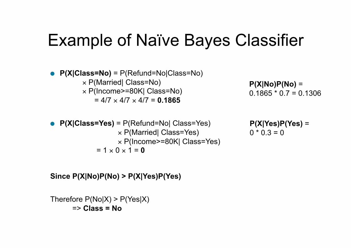
● P(X|Class=No) = P(Refund=No|Class=No) × P(Married| Class=No) × P(Income>=80K| Class=No) = 4/7 × 4/7 × 4/7 = 0.1865
● P(X|Class=Yes) = P(Refund=No| Class=Yes) × P(Married| Class=Yes) × P(Income>=80K| Class=Yes) = 1 × 0 × 1 = 0
Example of Naïve Bayes Classifier
P(X|No)P(No) = 0.1865 * 0.7 = 0.1306
P(X|Yes)P(Yes) = 0 * 0.3 = 0
Since P(X|No)P(No) > P(X|Yes)P(Yes)
Therefore P(No|X) > P(Yes|X) => Class = No
€
X = (Refund = No,Single,Income >= 80K)Given a Test Record:
Example of Naïve Bayes Classifier(2)
REFUND P(Refund=Yes|No) = 3/7 P(Refund=No|No) = 4/7 P(Refund=Yes|Yes) = 0 P(Refund=No|Yes) = 3/3
MARITAL STATUS
P(Marital Status=Single|No) = 2/7 P(Marital Status=Divorced|No) = 1/7 P(Marital Status=Married|No) = 4/7 P(Marital Status=Single|Yes) = 2/7 P(Marital Status=Divorced|Yes) = 1/7 P(Marital Status=Married|Yes) = 0
TAXABLE INCOMING
P(TaxableInc >= 80K|Yes) = 3/3 P(TaxableInc >= 80K|NO) = 4/7 P(TaxableInc < 80K|Yes) = 0/3 P(TaxableInc < 80K|NO) = 3/7
Class=No 7/10 Class=Yes 3/10
P(A1, A2, …, An |C) P(C ) = P(A1| Cj) P(A2| Cj)… P(An| Cj) P(C )
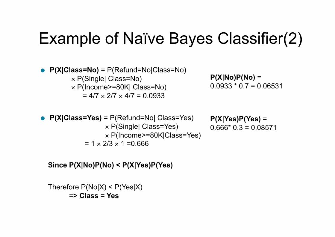
● P(X|Class=No) = P(Refund=No|Class=No) × P(Single| Class=No) × P(Income>=80K| Class=No) = 4/7 × 2/7 × 4/7 = 0.0933
● P(X|Class=Yes) = P(Refund=No| Class=Yes) × P(Single| Class=Yes) × P(Income>=80K|Class=Yes) = 1 × 2/3 × 1 =0.666
Example of Naïve Bayes Classifier(2)
P(X|No)P(No) = 0.0933 * 0.7 = 0.06531
P(X|Yes)P(Yes) = 0.666* 0.3 = 0.08571
Since P(X|No)P(No) < P(X|Yes)P(Yes)
Therefore P(No|X) < P(Yes|X) => Class = Yes
Naïve Bayes (Summary)
• Robust to isolated noise points
• Model each class separately
• Robust to irrelevant attributes
• Use the whole set of attribute to perform classification
• Independence assumption may not hold for some attributes
Instance-Based Classifier
Lazy approach to classification
Uses all the training set to peform classificaiton
Uses distances between training and test records
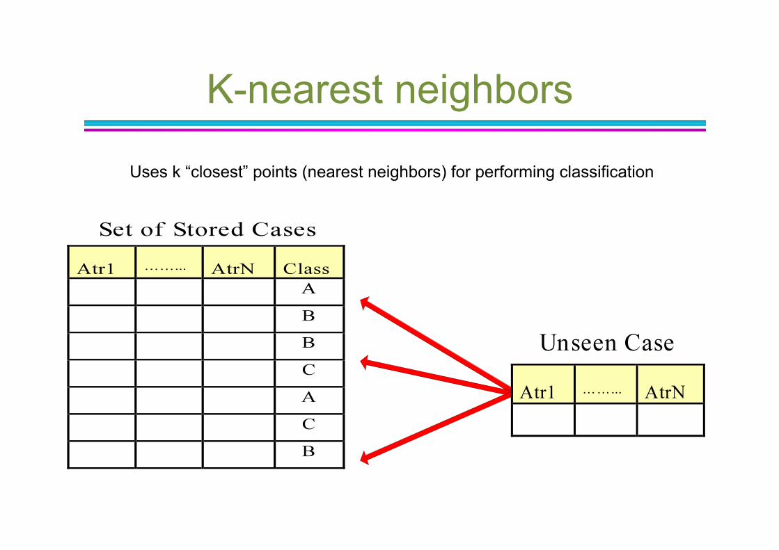
K-nearest neighbors
Uses k “closest” points (nearest neighbors) for performing classification
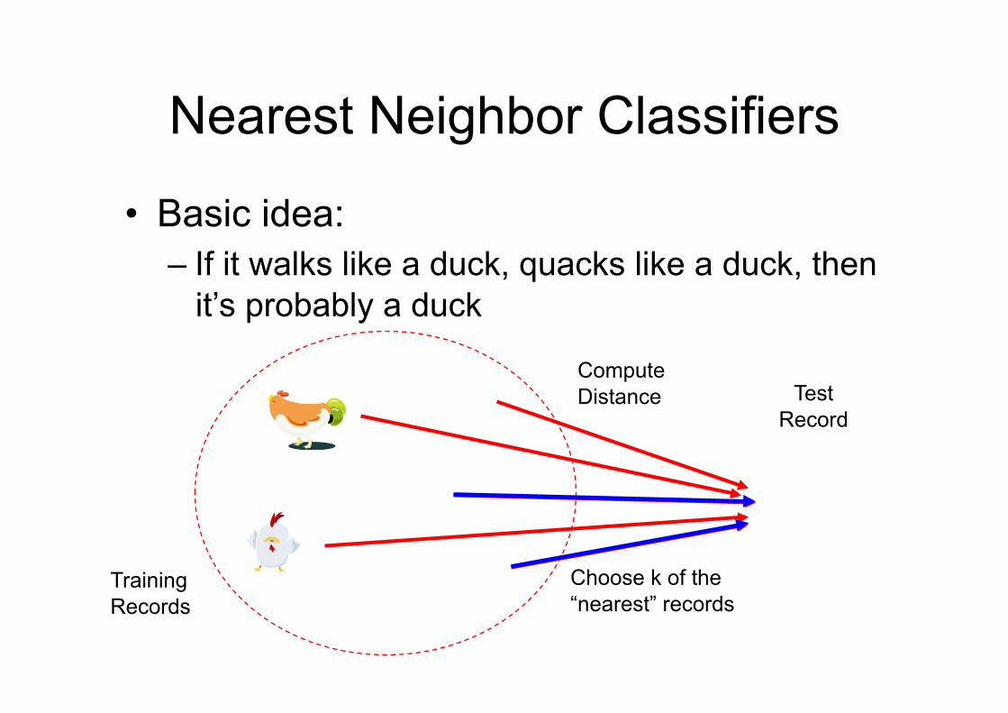
Nearest Neighbor Classifiers
• Basic idea: – If it walks like a duck, quacks like a duck, then
it’s probably a duck
Training Records
Test Record
Compute Distance
Choose k of the “nearest” records
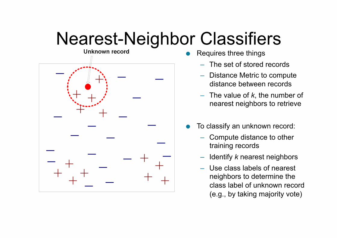
Nearest-Neighbor Classifiers ● Requires three things
– The set of stored records – Distance Metric to compute
distance between records – The value of k, the number of
nearest neighbors to retrieve
● To classify an unknown record: – Compute distance to other
training records – Identify k nearest neighbors – Use class labels of nearest
neighbors to determine the class label of unknown record (e.g., by taking majority vote)
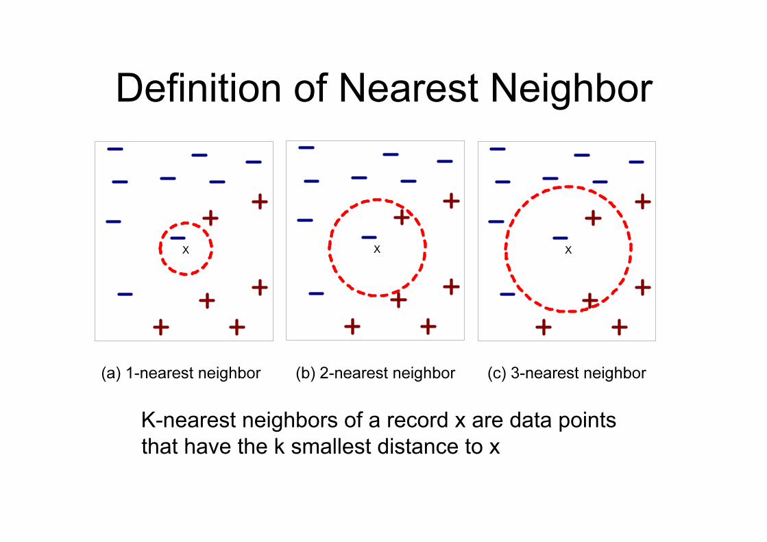
Definition of Nearest Neighbor
K-nearest neighbors of a record x are data points that have the k smallest distance to x
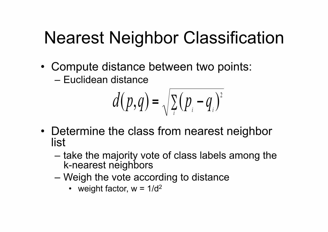
Nearest Neighbor Classification • Compute distance between two points:
– Euclidean distance
• Determine the class from nearest neighbor list – take the majority vote of class labels among the
k-nearest neighbors – Weigh the vote according to distance
• weight factor, w = 1/d2
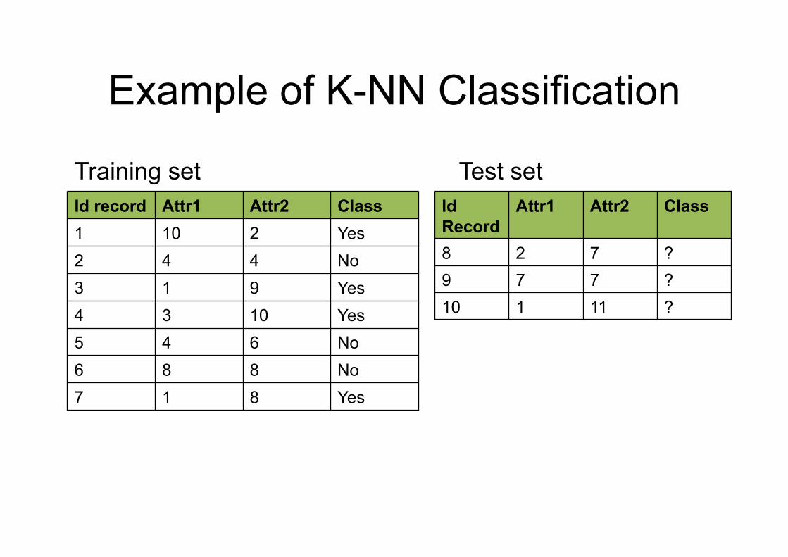
Example of K-NN Classification
Id record Attr1 Attr2 Class 1 10 2 Yes 2 4 4 No 3 1 9 Yes 4 3 10 Yes 5 4 6 No 6 8 8 No 7 1 8 Yes
Training set Id Record
Attr1 Attr2 Class
8 2 7 ? 9 7 7 ? 10 1 11 ?
Test set
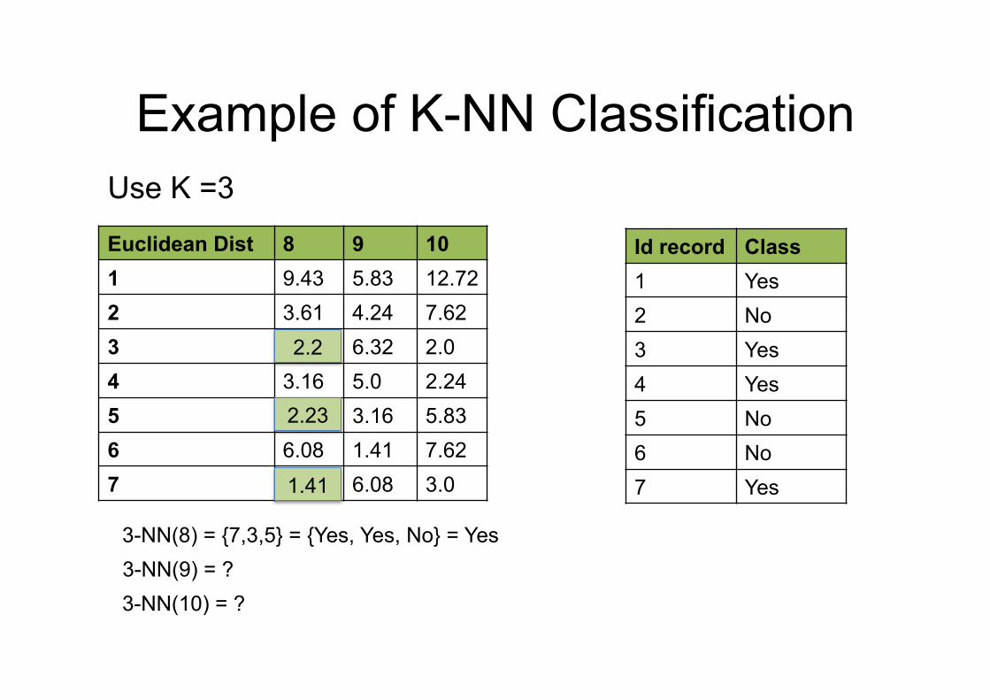
Example of K-NN Classification
Euclidean Dist 8 9 10 1 9.43 5.83 12.72 2 3.61 4.24 7.62 3 2.2 6.32 2.0 4 3.16 5.0 2.24 5 2.23 3.16 5.83 6 6.08 1.41 7.62 7 1.41 6.08 3.0
Id record Class 1 Yes 2 No 3 Yes 4 Yes 5 No 6 No 7 Yes
3-NN(9) = ? 3-NN(10) = ?
3-NN(8) = {7,3,5} = {Yes, Yes, No} = Yes
Use K =3
1.41
2.2
2.23
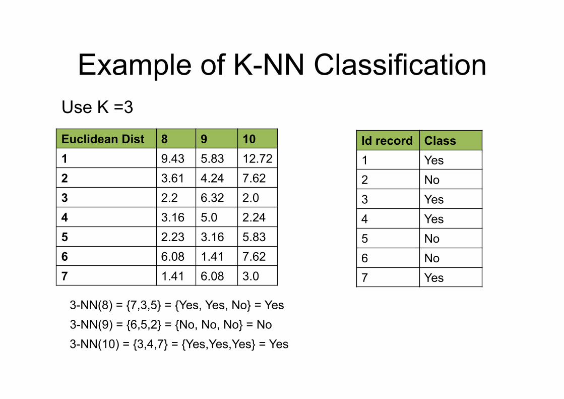
3-NN(9) = {6,5,2} = {No, No, No} = No 3-NN(10) = {3,4,7} = {Yes,Yes,Yes} = Yes
Example of K-NN Classification
3-NN(8) = {7,3,5} = {Yes, Yes, No} = Yes
Euclidean Dist 8 9 10 1 9.43 5.83 12.72 2 3.61 4.24 7.62 3 2.2 6.32 2.0 4 3.16 5.0 2.24 5 2.23 3.16 5.83 6 6.08 1.41 7.62 7 1.41 6.08 3.0
Id record Class 1 Yes 2 No 3 Yes 4 Yes 5 No 6 No 7 Yes
Use K =3
Example of K-NN Classification
Euclidean Dist 8 9 10 1 9.43 5.83 12.72 2 3.61 4.24 7.62 3 2.2 6.32 2.0 4 3.16 5.0 2.24 5 2.23 3.16 5.83 6 6.08 1.41 7.62 7 1.41 6.08 3.0
Id record Class 1 Yes 2 No 3 Yes 4 Yes 5 No 6 No 7 Yes
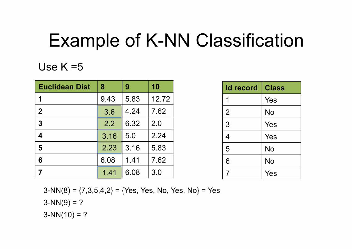
3-NN(9) = ? 3-NN(10) = ?
3-NN(8) = {7,3,5,4,2} = {Yes, Yes, No, Yes, No} = Yes
Use K =5
1.41
2.2
2.23
3.6
3.16
Example of K-NN Classification
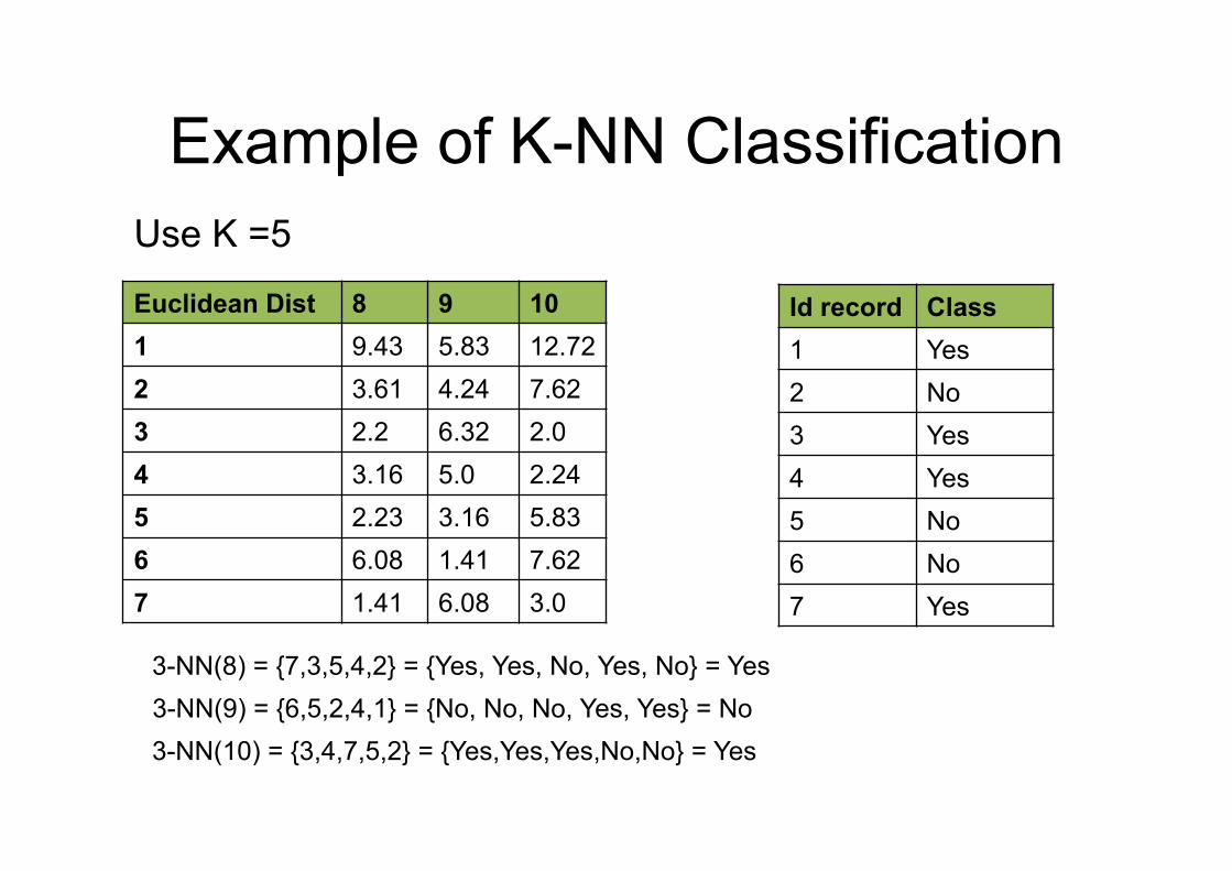
Euclidean Dist 8 9 10 1 9.43 5.83 12.72 2 3.61 4.24 7.62 3 2.2 6.32 2.0 4 3.16 5.0 2.24 5 2.23 3.16 5.83 6 6.08 1.41 7.62 7 1.41 6.08 3.0
Id record Class 1 Yes 2 No 3 Yes 4 Yes 5 No 6 No 7 Yes
Use K =5
3-NN(9) = {6,5,2,4,1} = {No, No, No, Yes, Yes} = No 3-NN(10) = {3,4,7,5,2} = {Yes,Yes,Yes,No,No} = Yes
3-NN(8) = {7,3,5,4,2} = {Yes, Yes, No, Yes, No} = Yes
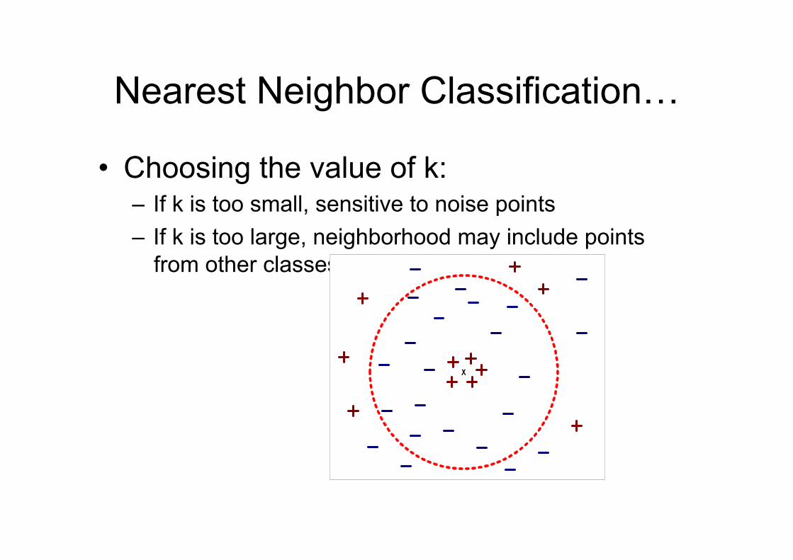
Nearest Neighbor Classification…
• Choosing the value of k: – If k is too small, sensitive to noise points – If k is too large, neighborhood may include points
from other classes
Nearest Neighbor Classification…
• Scaling issues – Attributes may have to be scaled to prevent
distance measures from being dominated by one of the attributes
– Example: • height of a person may vary from 1.5m to 1.8m • weight of a person may vary from 90lb to 300lb • income of a person may vary from $10K to $1M
Nearest neighbor Classification…
• k-NN classifiers are lazy learners – It does not build models explicitly – Unlike eager learners such as decision tree
induction and rule-based systems – Classifying unknown records are relatively
expensive
67
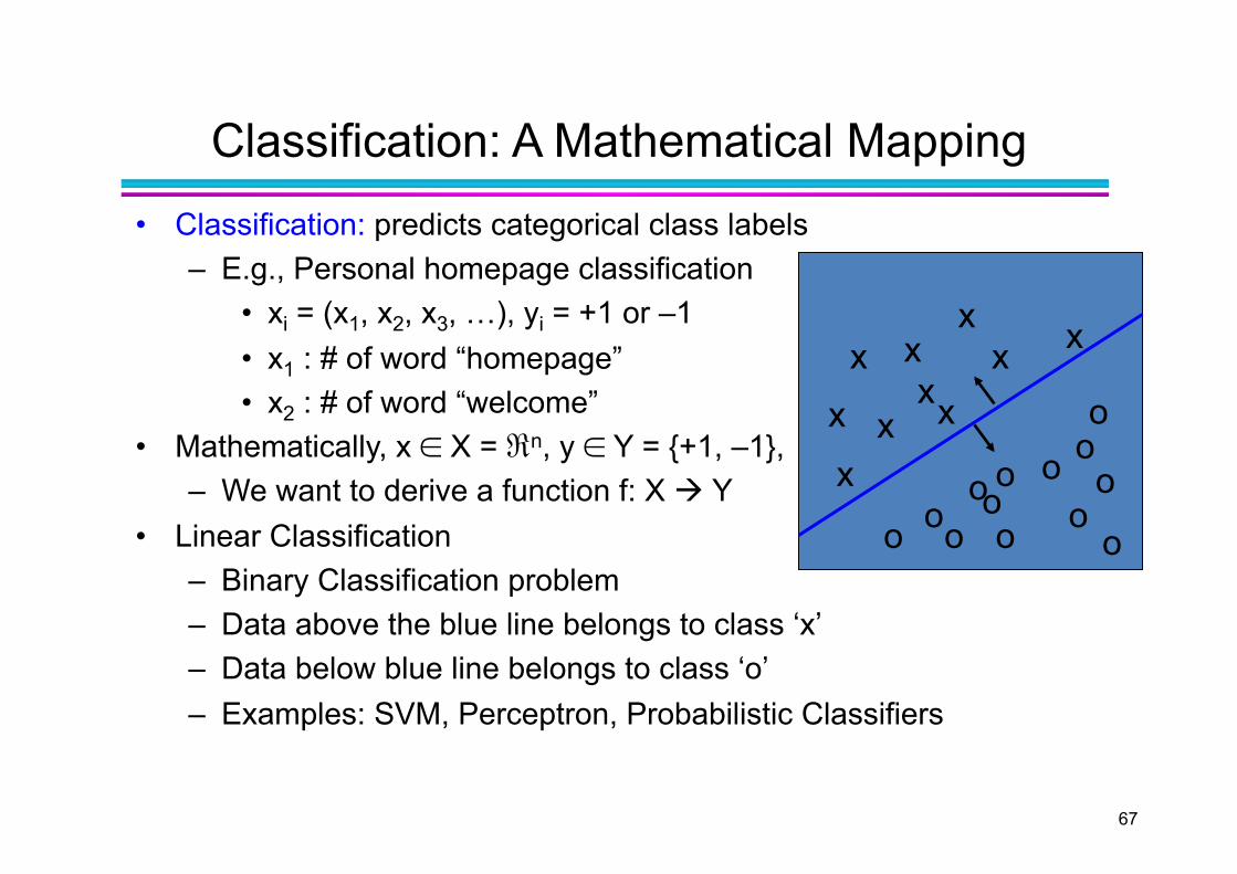
Classification: A Mathematical Mapping • Classification: predicts categorical class labels
– E.g., Personal homepage classification • xi = (x1, x2, x3, …), yi = +1 or –1 • x1 : # of word “homepage” • x2 : # of word “welcome”
• Mathematically, x ∈ X = ℜn, y ∈ Y = {+1, –1}, – We want to derive a function f: X Y
• Linear Classification – Binary Classification problem – Data above the blue line belongs to class ‘x’ – Data below blue line belongs to class ‘o’ – Examples: SVM, Perceptron, Probabilistic Classifiers
x
x x
x x x
x
x
x
x o o o
o o o
o o
o o o
o
o
68
SVM—Support Vector Machines • A relatively new classification method for both linear and nonlinear
data
• It uses a nonlinear mapping to transform the original training data into a higher dimension
• With the new dimension, it searches for the linear optimal separating hyperplane (i.e., “decision boundary”)
• With an appropriate nonlinear mapping to a sufficiently high dimension, data from two classes can always be separated by a hyperplane
• SVM finds this hyperplane using support vectors (“essential” training tuples) and margins (defined by the support vectors)
69
SVM—History and Applications
• Vapnik and colleagues (1992)—groundwork from Vapnik & Chervonenkis’ statistical learning theory in 1960s
• Features: training can be slow but accuracy is high owing to their ability to model complex nonlinear decision boundaries (margin maximization)
• Used for: classification and numeric prediction
• Applications: – handwritten digit recognition, object recognition, speaker
identification, benchmarking time-series prediction tests
70
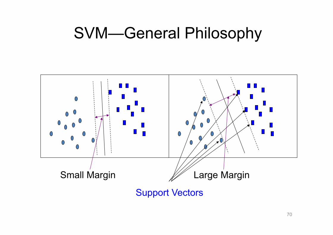
SVM—General Philosophy
Support Vectors
Small Margin Large Margin
29 février 2012 Data Mining: Concepts and Techniques 71
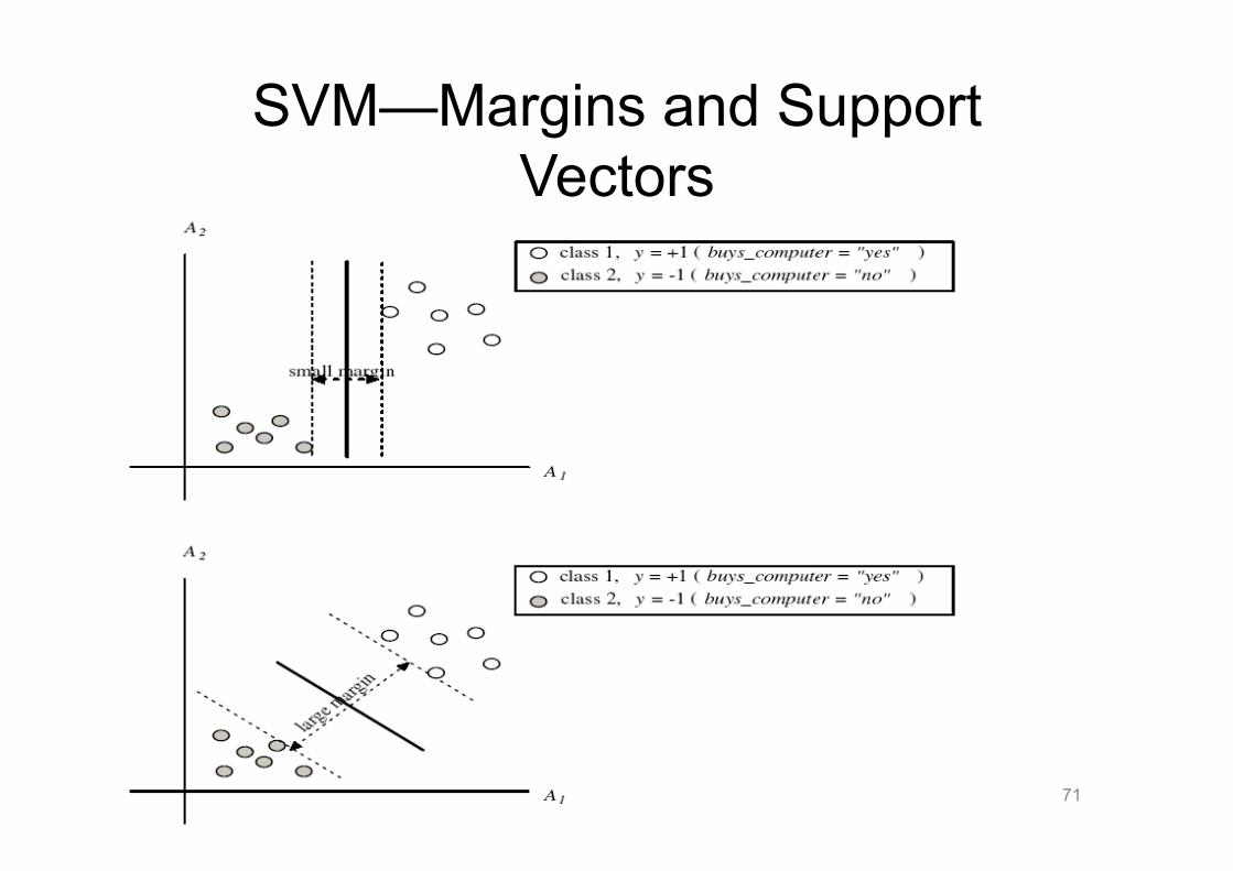
SVM—Margins and Support Vectors
72
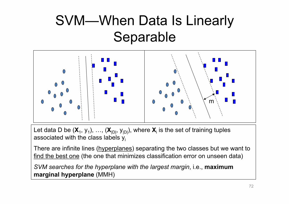
SVM—When Data Is Linearly Separable
m
Let data D be (X1, y1), …, (X|D|, y|D|), where Xi is the set of training tuples associated with the class labels yi
There are infinite lines (hyperplanes) separating the two classes but we want to find the best one (the one that minimizes classification error on unseen data)
SVM searches for the hyperplane with the largest margin, i.e., maximum marginal hyperplane (MMH)
73
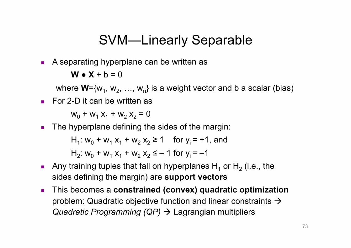
SVM—Linearly Separable A separating hyperplane can be written as
W ● X + b = 0 where W={w1, w2, …, wn} is a weight vector and b a scalar (bias)
For 2-D it can be written as w0 + w1 x1 + w2 x2 = 0
The hyperplane defining the sides of the margin: H1: w0 + w1 x1 + w2 x2 ≥ 1 for yi = +1, and H2: w0 + w1 x1 + w2 x2 ≤ – 1 for yi = –1
Any training tuples that fall on hyperplanes H1 or H2 (i.e., the sides defining the margin) are support vectors
This becomes a constrained (convex) quadratic optimization problem: Quadratic objective function and linear constraints Quadratic Programming (QP) Lagrangian multipliers
74
Why Is SVM Effective on High Dimensional Data? (I)
The complexity of trained classifier is characterized by the # of support
vectors rather than the dimensionality of the data
The support vectors are the essential or critical training examples —they lie
closest to the decision boundary (MMH)
If all other training examples are removed and the training is repeated, the
same separating hyperplane would be found
Why Is SVM Effective on High Dimensional Data? (II)
The number of support vectors found can be used to compute an
(upper) bound on the expected error rate of the SVM classifier, which
is independent of the data dimensionality
Thus, an SVM with a small number of support vectors can have good
generalization, even when the dimensionality of the data is high
76
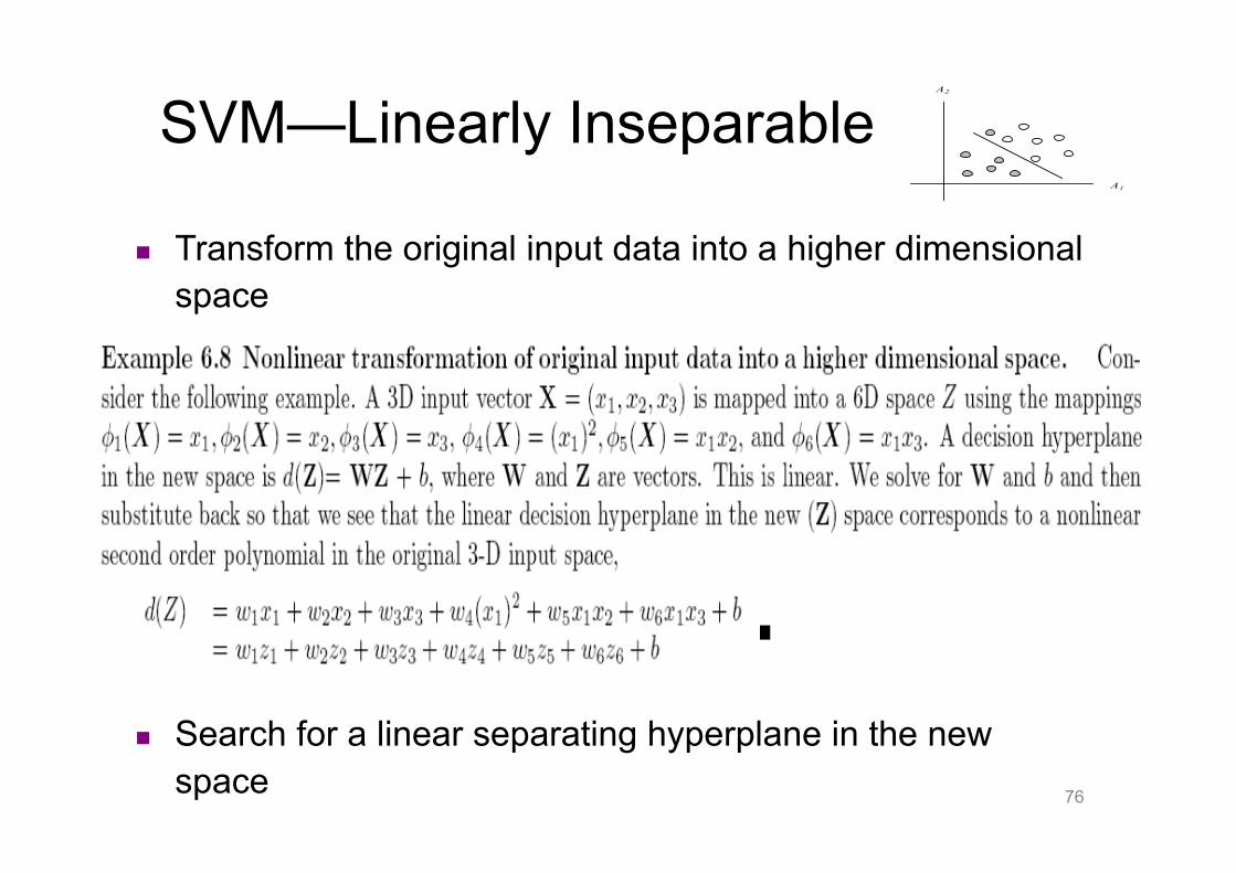
SVM—Linearly Inseparable
Transform the original input data into a higher dimensional space
Search for a linear separating hyperplane in the new space
77
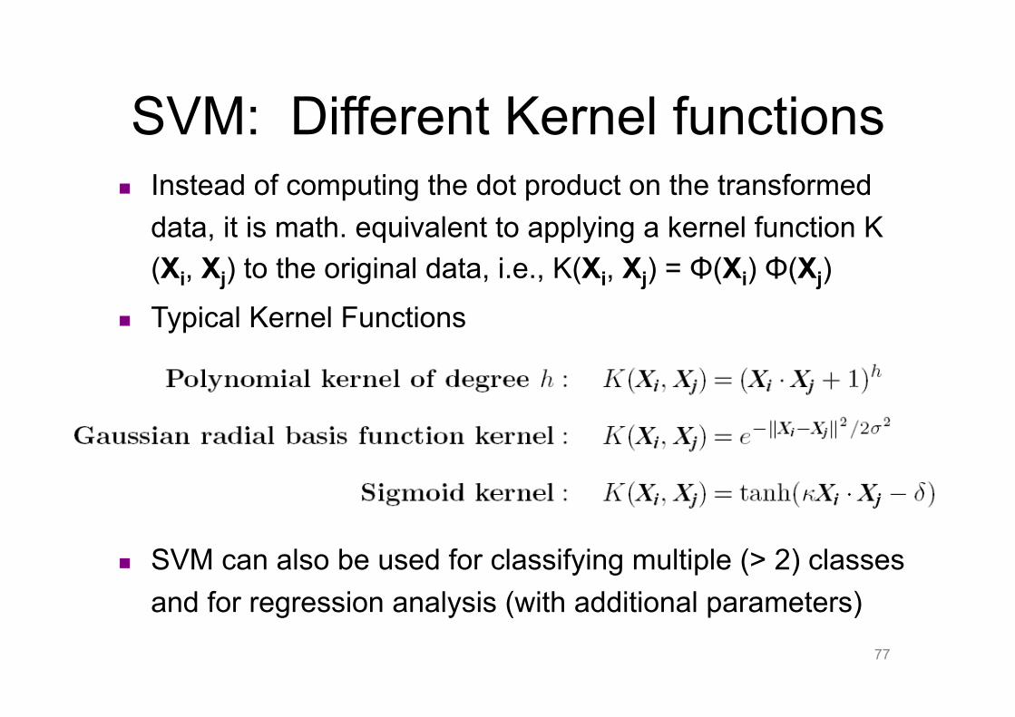
SVM: Different Kernel functions Instead of computing the dot product on the transformed
data, it is math. equivalent to applying a kernel function K(Xi, Xj) to the original data, i.e., K(Xi, Xj) = Φ(Xi) Φ(Xj)
Typical Kernel Functions
SVM can also be used for classifying multiple (> 2) classes and for regression analysis (with additional parameters)
SVM Classification…
Hard to learn – learned in batch mode using quadratic programming techniques
Using kernels can learn very complex functions
Deterministic algorithm
Nice generalization properties
79
Discriminative Classifiers • Advantages
– Prediction accuracy is generally high • As compared to Bayesian methods – in general
– Robust, works when training examples contain errors – Fast evaluation of the learned target function
• Criticism – Long training time – Difficult to understand the learned function (weights) – Not easy to incorporate domain knowledge
• Easy in the form of priors on the data or distributions
Model Evaluation
• Metrics for Performance Evaluation – How to evaluate the performance of a model?
• Methods for Performance Evaluation – How to obtain reliable estimates?
• Methods for Model Comparison – How to compare the relative performance
among competing models?
Model Evaluation
• Metrics for Performance Evaluation – How to evaluate the performance of a model?
• Methods for Performance Evaluation – How to obtain reliable estimates?
• Methods for Model Comparison – How to compare the relative performance
among competing models?
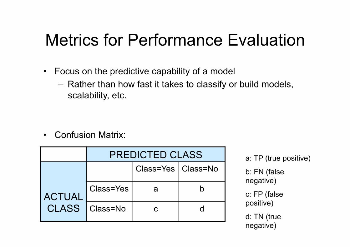
Metrics for Performance Evaluation
• Focus on the predictive capability of a model – Rather than how fast it takes to classify or build models,
scalability, etc.
• Confusion Matrix:
PREDICTED CLASS
ACTUAL CLASS
Class=Yes Class=No
Class=Yes a b
Class=No c d
a: TP (true positive)
b: FN (false negative)
c: FP (false positive)
d: TN (true negative)
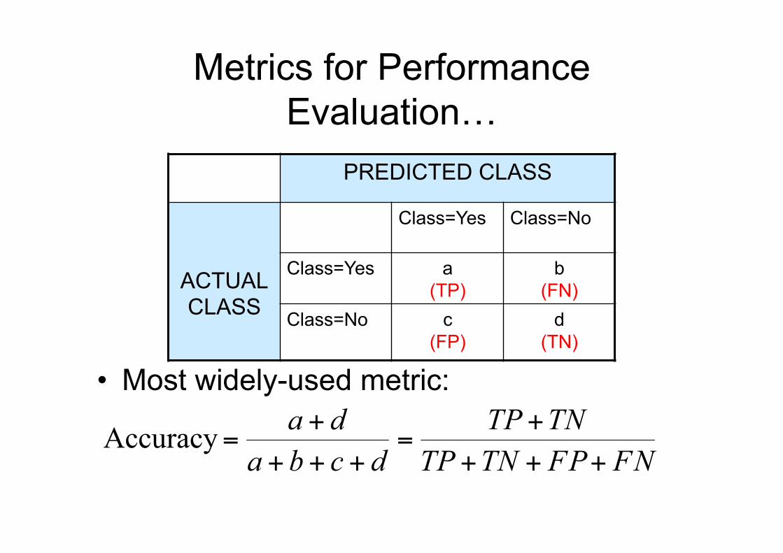
Metrics for Performance Evaluation…
• Most widely-used metric:
PREDICTED CLASS
ACTUAL CLASS
Class=Yes Class=No
Class=Yes a (TP)
b (FN)
Class=No c (FP)
d (TN)
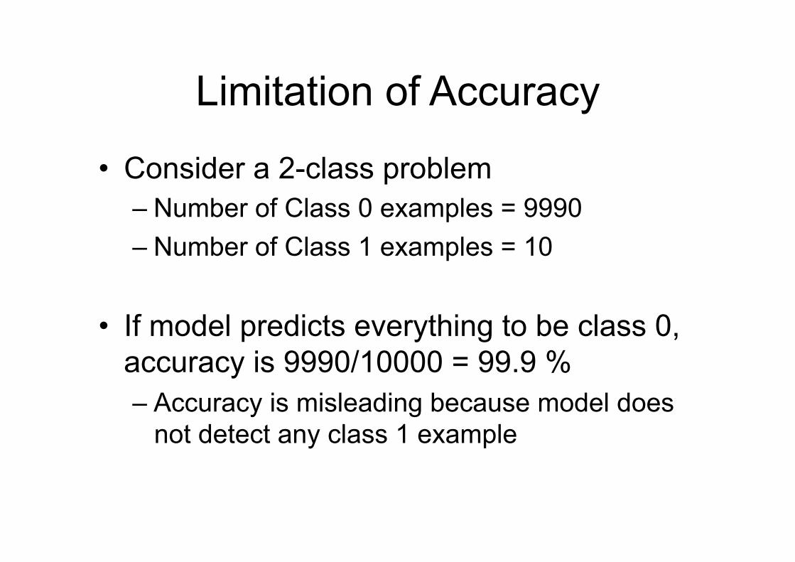
Limitation of Accuracy
• Consider a 2-class problem – Number of Class 0 examples = 9990 – Number of Class 1 examples = 10
• If model predicts everything to be class 0, accuracy is 9990/10000 = 99.9 % – Accuracy is misleading because model does
not detect any class 1 example
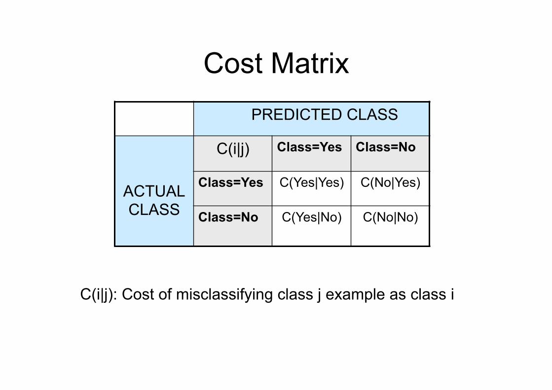
Cost Matrix PREDICTED CLASS
ACTUAL CLASS
C(i|j) Class=Yes Class=No
Class=Yes C(Yes|Yes) C(No|Yes)
Class=No C(Yes|No) C(No|No)
C(i|j): Cost of misclassifying class j example as class i
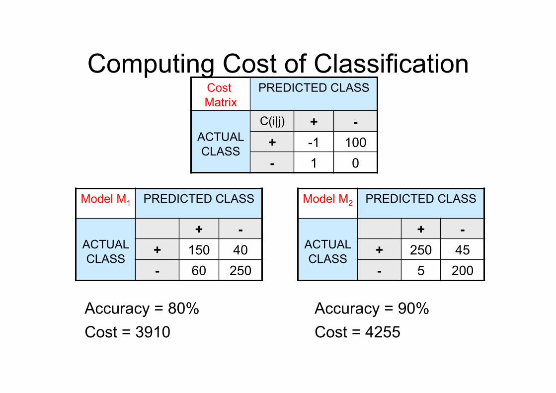
Computing Cost of Classification Cost Matrix
PREDICTED CLASS
ACTUAL CLASS
C(i|j) + - + -1 100 - 1 0
Model M1 PREDICTED CLASS
ACTUAL CLASS
+ - + 150 40 - 60 250
Model M2 PREDICTED CLASS
ACTUAL CLASS
+ - + 250 45 - 5 200
Accuracy = 80% Cost = 3910
Accuracy = 90% Cost = 4255
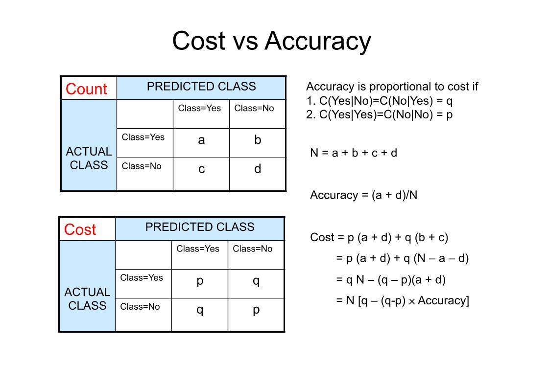
Cost vs Accuracy
Count PREDICTED CLASS
ACTUAL CLASS
Class=Yes Class=No
Class=Yes a b
Class=No c d
Cost PREDICTED CLASS
ACTUAL CLASS
Class=Yes Class=No
Class=Yes p q
Class=No q p
N = a + b + c + d
Accuracy = (a + d)/N
Cost = p (a + d) + q (b + c)
= p (a + d) + q (N – a – d)
= q N – (q – p)(a + d)
= N [q – (q-p) × Accuracy]
Accuracy is proportional to cost if 1. C(Yes|No)=C(No|Yes) = q 2. C(Yes|Yes)=C(No|No) = p
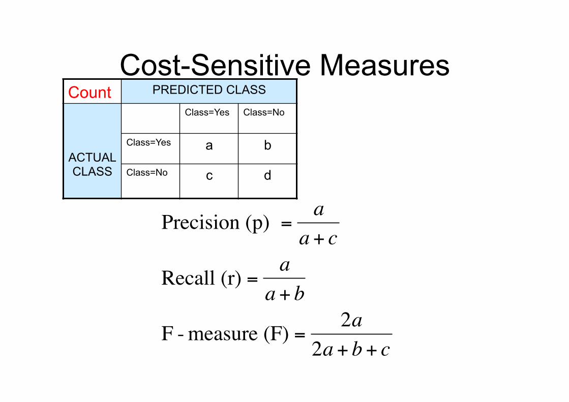
Cost-Sensitive Measures
€
Precision (p) =a
a + c
Recall (r) =a
a + b
F - measure (F) =2a
2a + b + c
Count PREDICTED CLASS
ACTUAL CLASS
Class=Yes Class=No
Class=Yes a b
Class=No c d
Model Evaluation
• Metrics for Performance Evaluation – How to evaluate the performance of a model?
• Methods for Performance Evaluation – How to obtain reliable estimates?
• Methods for Model Comparison – How to compare the relative performance
among competing models?
Methods for Performance Evaluation
• How to obtain a reliable estimate of performance?
• Performance of a model may depend on other factors besides the learning algorithm: – Class distribution – Cost of misclassification – Size of training and test sets
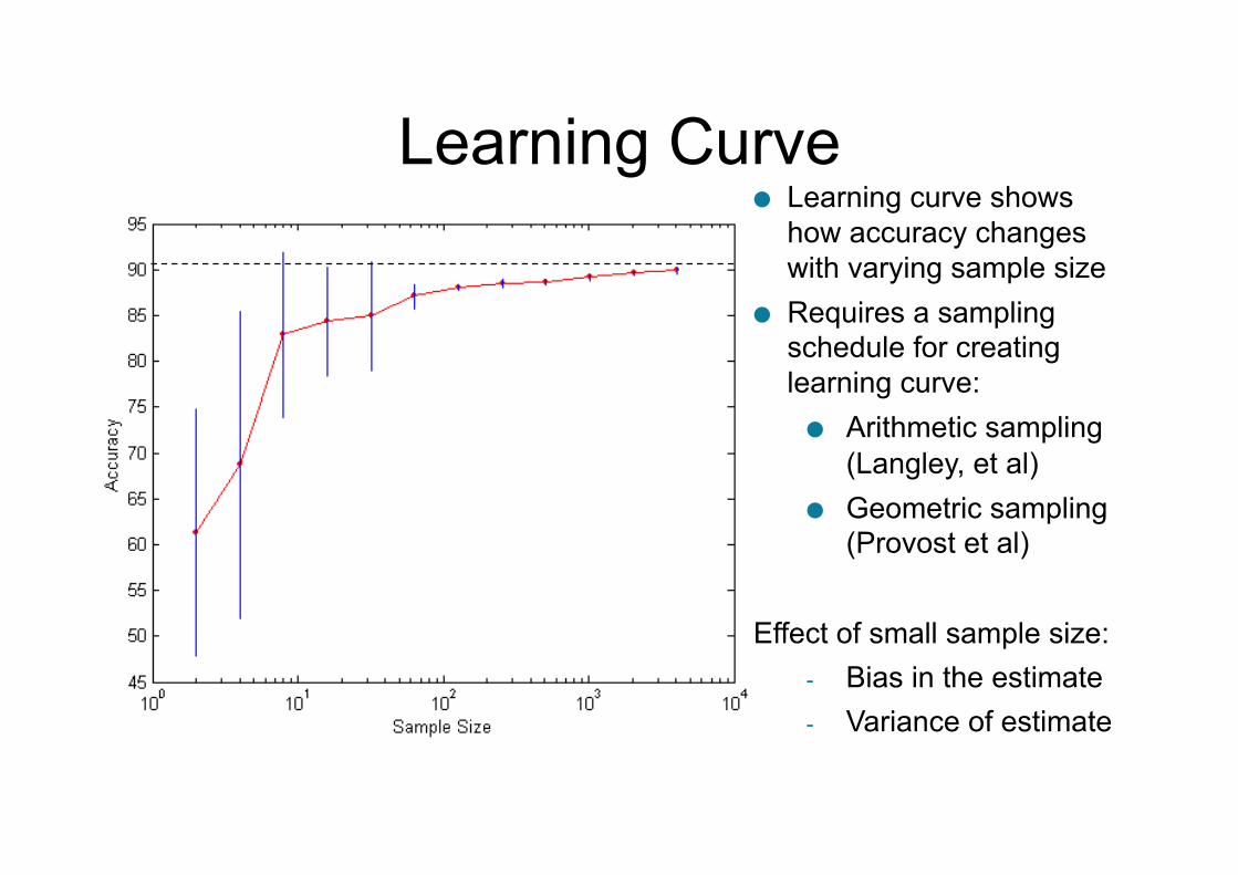
Learning Curve ● Learning curve shows
how accuracy changes with varying sample size
● Requires a sampling schedule for creating learning curve: ● Arithmetic sampling
(Langley, et al) ● Geometric sampling
(Provost et al)
Effect of small sample size: - Bias in the estimate - Variance of estimate
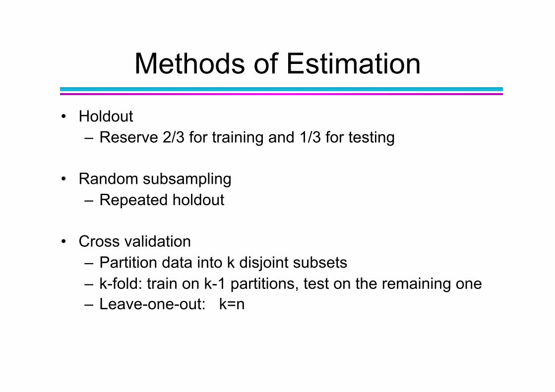
Methods of Estimation • Holdout
– Reserve 2/3 for training and 1/3 for testing
• Random subsampling – Repeated holdout
• Cross validation – Partition data into k disjoint subsets – k-fold: train on k-1 partitions, test on the remaining one – Leave-one-out: k=n
Model Evaluation
• Metrics for Performance Evaluation – How to evaluate the performance of a model?
• Methods for Performance Evaluation – How to obtain reliable estimates?
• Methods for Model Comparison – How to compare the relative performance
among competing models?
ROC (Receiver Operating Characteristic)
• Developed in 1950s for signal detection theory to analyze noisy signals – Characterize the trade-off between positive hits and false
alarms
• ROC curve plots TP (on the y-axis) against FP (on the x-axis)
• Performance of each classifier represented as a point on the ROC curve – changing the threshold of algorithm, sample distribution or
cost matrix changes the location of the point
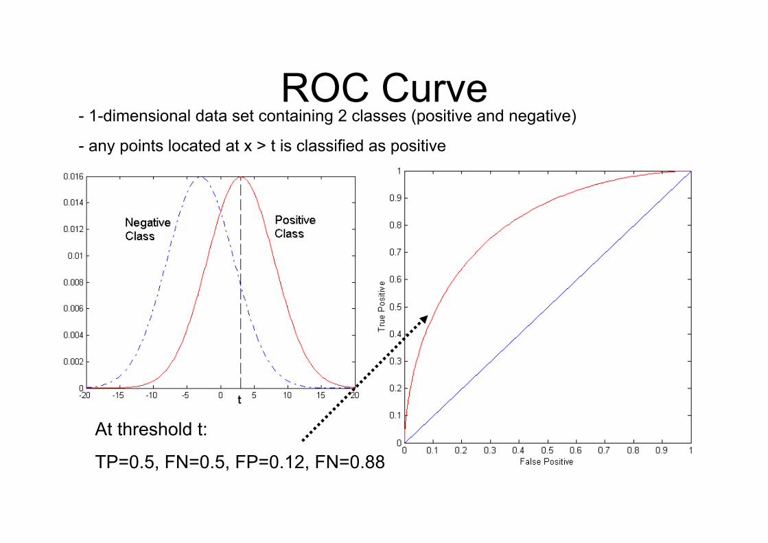
ROC Curve
At threshold t:
TP=0.5, FN=0.5, FP=0.12, FN=0.88
- 1-dimensional data set containing 2 classes (positive and negative)
- any points located at x > t is classified as positive
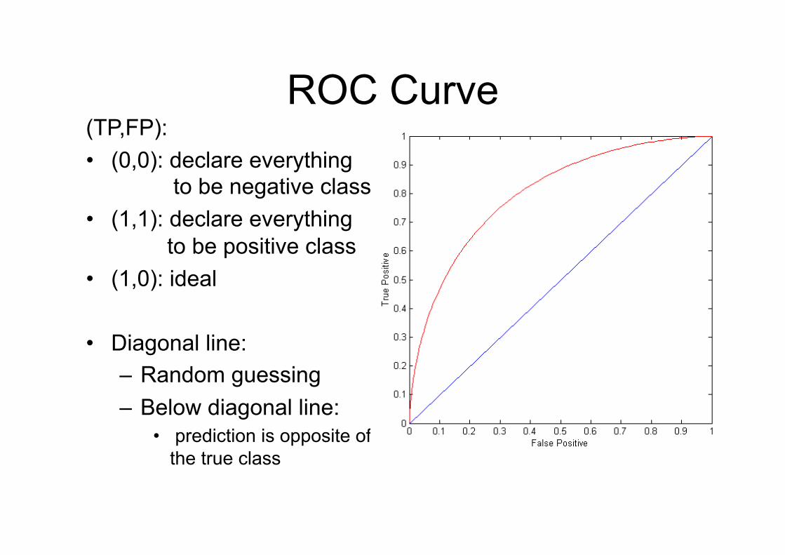
ROC Curve (TP,FP): • (0,0): declare everything
to be negative class • (1,1): declare everything
to be positive class • (1,0): ideal
• Diagonal line: – Random guessing – Below diagonal line:
• prediction is opposite of the true class
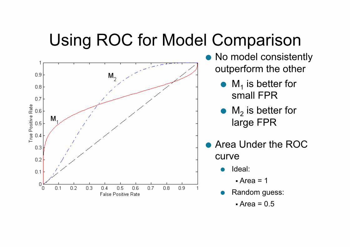
Using ROC for Model Comparison ● No model consistently
outperform the other ● M1 is better for
small FPR ● M2 is better for
large FPR
● Area Under the ROC curve ● Ideal:
Area = 1 ● Random guess:
Area = 0.5