Embed Size (px)
Citation preview

Textbook notes of herd management:Basic concepts
Dina Notat No. 48 August 1996
Anders R. Kristensen1 and Erik Jørgensen2
This report is also available as a PostScript file on World Wide Web at URL:ftp://ftp.dina.kvl.dk/pub/Dina-reports/notatXX.ps
1Dina KVL 2Dina FoulumDept. of Animal Science and Animal Health Department of Biometry and InformaticsRoyal Veterinary and Agricultural University Research Centre FoulumBülowsvej 13 P.O. Box 23DK-1870 Frederiksberg C DK-8830 TjeleTel: + 45 35 28 30 91 Tel: + 45 89 99 12 30Fax: +45 35 28 30 87 Fax: +45 89 99 16 69E-mail: [email protected] E-mail: [email protected]: http://www.dina.kvl.dk/~ark WWW: http://www.sp.dk/~ej

2 Dina Notat No. 48, August 1996
Contents:
1. A general framework for herd management. . . . . . . . . . . . . . . . . . . . . . . . . . . . . 3
2. Objectives of production: Farmer’s preferences. . . . . . . . . . . . . . . . . . . . . . . . . . 62.1. Common attributes of farmer’s utility functions. . . . . . . . . . . . . . . . . . . . . 7
2.1.1. Monetary gain. . . . . . . . . . . . . . . . . . . . . . . . . . . . . . . . . . . . . . 72.1.2. Leisure time. . . . . . . . . . . . . . . . . . . . . . . . . . . . . . . . . . . . . . . . 82.1.3. Animal welfare. . . . . . . . . . . . . . . . . . . . . . . . . . . . . . . . . . . . . . 82.1.4. Working conditions. . . . . . . . . . . . . . . . . . . . . . . . . . . . . . . . . . . 112.1.5. Environmental preservation. . . . . . . . . . . . . . . . . . . . . . . . . . . . . 112.1.6. Personal prestige. . . . . . . . . . . . . . . . . . . . . . . . . . . . . . . . . . . . . 122.1.7. Product quality. . . . . . . . . . . . . . . . . . . . . . . . . . . . . . . . . . . . . . 12
2.2. From attributes to utility. . . . . . . . . . . . . . . . . . . . . . . . . . . . . . . . . . . . . 132.2.1. Single attribute situation: Risk. . . . . . . . . . . . . . . . . . . . . . . . . . . 132.2.2. Multiple attribute situation. . . . . . . . . . . . . . . . . . . . . . . . . . . . . . 172.2.3. Operational representation of a farmer’s utility function. . . . . . . . . 20
3. The management cycle. . . . . . . . . . . . . . . . . . . . . . . . . . . . . . . . . . . . . . . . . . . 223.1. The elements of the cycle. . . . . . . . . . . . . . . . . . . . . . . . . . . . . . . . . . . . 223.2. Statistical evaluation of deviations identified during the control process. . . . 25
3.2.1. Example 1: Milk yield of dairy cows. . . . . . . . . . . . . . . . . . . . . . 253.2.2. Example 2: Daily gain for bull calves (or slaugther pigs). . . . . . . . . 263.2.3. Example 3: Reproduction in a dairy herd. . . . . . . . . . . . . . . . . . . . 283.2.4. Example 4: Diseases. . . . . . . . . . . . . . . . . . . . . . . . . . . . . . . . . . 283.2.5. Concluding remarks. . . . . . . . . . . . . . . . . . . . . . . . . . . . . . . . . . 29
3.3. Evaluation of deviations from a utility point of view. . . . . . . . . . . . . . . . . 29
4. Decisions and strategies: Framework and techniques. . . . . . . . . . . . . . . . . . . . . . 324.1. The framework of decision making in animal production. . . . . . . . . . . . . . 32
4.1.1. Information needs. . . . . . . . . . . . . . . . . . . . . . . . . . . . . . . . . . . . 324.1.2. Levels. . . . . . . . . . . . . . . . . . . . . . . . . . . . . . . . . . . . . . . . . . . . 334.1.3. Time horizons . . . . . . . . . . . . . . . . . . . . . . . . . . . . . . . . . . . . . . 34
4.2. Methods. . . . . . . . . . . . . . . . . . . . . . . . . . . . . . . . . . . . . . . . . . . . . . . . 354.2.1. Rule based expert systems. . . . . . . . . . . . . . . . . . . . . . . . . . . . . . 354.2.2. Linear programming with extensions. . . . . . . . . . . . . . . . . . . . . . . 374.2.3. Dynamic programming and Markov decision processes. . . . . . . . . . 384.2.4. Probabilistic Expert systems. . . . . . . . . . . . . . . . . . . . . . . . . . . . . 404.2.5. Influence diagrams. . . . . . . . . . . . . . . . . . . . . . . . . . . . . . . . . . . 414.2.6. Simulation. . . . . . . . . . . . . . . . . . . . . . . . . . . . . . . . . . . . . . . . . 43
References . . . . . . . . . . . . . . . . . . . . . . . . . . . . . . . . . . . . . . . . . . . . . . . . . . . . . 47

Kristensen & Jørgensen: Textbook notes of herd management: Basic concepts 3
1. A general framework for herd management
Several points of view may be taken if we want to describe a livestock production unit. Ananimal nutritionist would focus on the individual animal and describe how feeds aretransformed to meat, bones, tissues, skin, hair, embryos, milk, eggs, manure etc. Aphysiologist would further describe the roles of the various organs in this process and how thetransformations are regulated by hormones. A biochemist would even describe the basicprocesses at molecular level.
A completely different point of view is taken if we look at the production unit from a globalor national point of view. The individual production unit is regarded only as an arbitraryelement of the whole livestock sector, which serves the purpose of supplying the populationwith food and clothing as well as manager of natural resources. A description of a productionunit at this level would focus on its resource efficiency in food production and itssustainability from an environmental and animal welfare point of view.
Neither of these points of view are relevant to a herd management scientist even thoughseveral elements are the same. The herd management scientist also considers thetransformation of feeds to meat, bones, tissues, skin, hair, embryos, milk, eggs and manurelike the animal nutritionist, and he also regards the production as serving a purpose as we doat the global or national level. What differs, however, is the farmer. From the point of viewof a herd management scientist, the farmer is in focus and the purpose of the production isto provide the farmer (and maybe his family) with as much welfare as possible. In thisconnection welfare is regarded as a very subjective concept and has to be defined in eachindividual case. The only relevant source to be used in the determination of the definition isthe farmer himself.
The herd management scientist assumes that the farmer concurrently tries to organize theproduction in such a way that his welfare is maximized. In this process he has some optionsand he is subjected to some restraints. His options are to regulate the production in such a waythat his welfare is maximized given the restraints. The way in which he may regulateproduction is by deciding what factors he wants to use at what levels. A factor is somethingwhich is used in the production, i.e. the input of the transformation process. In livestockproduction, typical factors include buildings, animals, feeds, labor and medicine. During theproduction process, these factors are transformed into products which in this context includemeat, offspring, milk, eggs, fur, wool etc. The only way a farmer is able to regulate theproduction - and thereby try to maximize his welfare - is by adjustments of these factors.
Understanding the factors and the way they affect production (i.e. the products and theiramount and quality) is therefore essential in herd management. Understanding the restraintsis, however, just as important. What the restraints do is actually to limit the possible welfareof the farmer. If there were no restraints any level of welfare could be achieved. In a realworld situation the farmer faces many kinds of restraints. There are legal restraints regulatingaspects like use of hormones and medicine in production, storing and use of manure as wellas housing in general. He may also be restricted by production quotas. An other kind ofrestraints are of economic nature. The farmer only has a limited amount of capital at hisdisposal, and usually he has no influence on the prices of factors and products. Furthermore,

4 Dina Notat No. 48, August 1996
he faces some physical restraints like the capacity of his farm buildings or the land belongingto his farm, and finally his own education and skills may restrict his potential welfare.
In general, restraints are not static in the long run: Legal regulations may be changed, quotasystems may be abolished or changed, the farmer may increase or decrease his capital, extendhis housing capacity (if he can afford it), buy more land or increase his mental capacity bytraining or education. In some cases (e.g. legal restraints) the changes are beyond the controlof the farmer. In other cases (e.g. farm buildings or land) he may change the restraints in thelong run, but has to accept them at the short run.
We are now ready to define herd management:
Herd management is a discipline serving the purpose of concurrently ensuring thatthe factors are combined in such a way that the welfare of the individual farmeris maximized subject to the restraints imposed on his production.
The general welfare of the farmer depends on many aspects like monetary gain (profit), leisuretime, animal welfare, environmental sustainability etc. We shall denote these aspectsinfluencing the farmer’s welfare asattributes. It is assumed that the consequences of eachpossible combination of factors may be expressed by a finite number of such attributes andthat a uniquely determined level of welfare is associated with any complete set of values ofthese attributes. The level of welfare associated with a combination of factors is called theutility value. Thus the purpose of herd management is to maximize the utility value. Afunction returning the utility value of a given set of attributes is called autility function. InChapter 2, the concept of utility is discussed more thoroughly.
The most important factors in livestock production include:- farm buildings- animals- feeds- labor- medicine and general veterinary services- management information systems and decision support systems- energy
In order to be able to combine these factors in an optimal way it is necessary to know theirinfluence on production. As concerns this knowledge, the herd management scientist dependson results from other fields like agricultural engineering, animal breeding, nutrition andpreventive veterinary medicine. The knowledge may typically be expressed by a productionfunction, f, which in general for a givenstage(time interval),t, takes the form:
whereYs,t is a vector ofn products produced, fs,i is the production function,xs,t is a vector of
(1)
m factors used at staget andet is a vector ofn random terms. The function fs,i is valid for agiven production units, which may be an animal, a group or pen, a section or the entire herd.The characteristics of the production unit may vary over time, but the set of observedcharacteristics at staget are indicated by thestate of the unit denoted asi. The state

Kristensen & Jørgensen: Textbook notes of herd management: Basic concepts 5
specification contains all relevant information concerning the production unit in question. Ifthe function is defined at animal level the state might for instance contain information on theage of the animal, the health status, the stage of reproductive cycle, the production level etc.In some cases, it is also relevant to include information on the disease and/or productionhistory of the animal (for instance the milk yield ofpreviouslactation) in the state definition.
The total productionY t and factor consumptionxt is calculated simply as
and
(2)
whereS is the set off all production unitss at the same level.
(3)
Eq. (1) illustrates that the production is only partly under the control of the manager, whodecides the levels of the factors at various stages. The direct effects of the factors areexpressed by the production function f, but the actual production also depends on a numberof effects outside the control of the manager as for instance the weather conditions and anumber of minor or major random events like infection by contagious diseases. These effectsoutside the control of the manager will appear as random variations which are expressed byet. This is in agreement with the general experience in livestock production that even if exactlythe same factor levels were used in two periods, the production would nevertheless differbetween the periods.
An other important aspect illustrated by Eq. (1) is thedynamicnature of the herd managementproblem. The production at staget not only depends on the factor levels at the present stage,but it may very well also depend on the factor levels at previous stages. In other words, thedecisions made in the past will influence the present production. Obvious examples of sucheffects is the influence of feeding level on the production level of an individual animal. Indairy cattle, for instance, the milk yield of a cow is influenced by the feeding level during therearing period, and in sows the litter size at weaning depends on the feeding level in themating and gestation period.
The productionY t and factorsxt used at a stage are assumed to influence the attributesdescribing the welfare of the farmer. We shall assume thatk attributes are sufficient andnecessary to describe the welfare. If we denote the values of these attributes at a specific staget asu1,t,...,uk,t, we may logically assume that they are determined by the products and factorsof the stage. In other words, we have:
whereut = (u1,t,...,uk,t) is the vector of attributes. We shall denote h as theattribute function.
(4)
The over-all utility ofUN for N stages,t1,...,tN, may in turn be defined as a function of theseattributes:

6 Dina Notat No. 48, August 1996
where g is theutility function, andN is the relevant time horizon. If we substitute Eq. (4) into
(5)
Eq. (5), we arrive at:
From Eq. (6) we observe, that if we know the attribute function h and the utility function g
(6)
and, furthermore, the production and factor consumption at all stages have been recorded, weare able to calculate the utility relating to any time intervalin the past. Recalling the definitionof herd management, it is more relevant to focus on thefuture utility derived from theproduction. The only way in which the farmer is able to influence the utility is by makingdecisions concerning the factors. Having made these decisions, the factor levelsxt are knownalso for future stages. The production levelsY t, however, are unknown for future stages. Theproduction function may provide us with the expected level, but because of the random effectsrepresented byet of Eq. (1), the actual levels may very well deviate from the expected. Another source of random variation is the future statei of the production unit. This becomesclear if we substitute Eq. (1) into Eq. (5) (and for convenience assume that the productionfunction is defined at herd level so thats = S):
From Eq. (7) we conclude, that even if all functions (production function, attribute function
(7)
and utility function) are known, and decisions concerning factors have been made, we are notable to calculate numerical values of the utility relating to a future period. If, however, thedistributions of the random elements are known, thedistribution of the future utility may beidentified.
When the farmer makes decisions concerning the future use of factors he therefore does itwith incomplete knowledge. If, however, the distribution of the possible outcomes is knownhe may still be able to make rational decisions as discussed in the following chapters. Sucha situation is referred to asdecision making under risk.
2. Objectives of production: Farmer’s preferences
A general characteristic of an attribute is that it directly influences the farmer’s subjectivelydefined welfare and, therefore, is an element of the very purpose of production. This may beillustrated by a few examples. The average milk yield of the cows of a dairy herd isnot anattribute of a utility function, because such a figure has no direct influence on the farmer’swelfare. If, however, he is able to sell the milk under profitable conditions he will experiencea monetary gain, which certainly may increase his welfare and, therefore, may be an attribute.In other words, the purpose of production from the farmer’s point of view could never be toproduce a certain amount of milk, but it could very well be to attain a certain level ofmonetary gain.
Kristensen & Jørgensen: Textbook notes of herd management: Basic concepts 7
Animal welfare may in some cases be an attribute of the utility function. Whether or not itis in the individual case depends on the farmer’s reasons for considering this aspect. Anargument could be that animals at a high level of welfare probably also produce at a higherlevel and thereby increases the monetary gain. In that case, animal welfare is just consideredas a short cut to higher income, but it is not considered to be a quality by itself. Accordingly,it should not be considered to be an attribute. If, on the other hand, the farmer wants toincrease animal welfareeven ifit, to some extent, decreases the levels of other attributes likemonetary gain or leisure time then it is certainly relevant to consider it to be an attribute ofthe utility function.
This discussion also illustrates that attributes are individual. It is not possible to define a setof attributes that apply to all livestock farmers. In the following section, however, we shalltake a look at some examples oftypical attributes of farmers’ utility functions.
2.1. Common attributes of farmer’s utility functions
Typical attributes describing the welfare of a livestock farmer include:- Monetary gain- Leisure time- Animal welfare- Working conditions- Environmental preservation- Personal prestige- Product quality
In this section, we shall discuss each of these attributes and focus on how to define relevantattribute functions in each case and how to compare contributions from different stages.
2.1.1. Monetary gain
It seems very unlikely that monetary gain should not be an attribute of all professionalfarmers’ utility function. In many practical cases it is even the only one considered whendecisions are made. Usually, it is very easy to define the attribute function of monetary gain.If we assume product pricespy1,...,pyn and factor pricespx1,...,pxm to be fixed and known, thepartial attribute function simply becomes (assuming that monetary gain is the 1st attribute):
Monetary gains from different stages are not directly comparable. If a certain amount of
(8)
money is gained at the present stage, it is possible to invest it and earn interest, so that theamount has increased at the following stage. The usual way to account for that is bydiscounting, so that we deal with thepresent valueof future monetary gains. If we assumeall stages to be of equal length and the interest rate to be constant, the present value ofmonetary gains fromN stages is calculated as:

8 Dina Notat No. 48, August 1996
where 0 <β ≤ 1 is thediscount factorusually calculated as
(9)
wherer is the interest rate pr. stage. For further information on the theory and principles of
(10)
discounting, reference is made to textbooks on economics.
2.1.2. Leisure time
Just like monetary gain, leisure time is probably an attribute of all farmer’s utility function.It is, however, slightly more complicated to represent it, because not only the total value, butalso the distribution over time (day, week, year) is relevant. Since leisure time is thecounterpart of work, it may therefore be relevant to split up the factor labor into several sub-factors like for instance work on weekdays from 6 a.m. to 6 p.m.x1, work on weekdays from6 p.m. to 6 a.m.x2, work in weekends from 6 a.m. to 6 p.m.x3, work in weekends from 6p.m. to 6 a.m.x4 etc. These sub-factors are assumed to refer to the farmer’s own work,whereas the work by employees has to be represented by other sub-factors.
Using these sub-factors we may quite easily at any staget calculate corresponding sub-attributes like total leisure timeu2t1, leisure time in weekendsu2t2, during day timeu2t3 etc. Ifthe stage length in days is denoted asD, these sub-attributes are objectively calculated as forinstance total leisure time in hours:
and correspondingly for other sub-attributes. There exists no general over-all partial attribute
(11)
function h2 for leisure time, because the properties of that function depends on the farmer’sindividual (subjective) preferences. It seems however, reasonable to assume, that it maydefined in each individual case as a function of a number,ν, of objectively calculated sub-attributes like those discussed, i.e.
As concerns the comparison of values relating to different stages, the sub-attributes are to
(12)
some extent additive (e.g. total leisure time). In other cases it may be more relevant to lookat the average value (e.g. work load in weekends) and/or the maximum value. If, for instance,x3 and x4 are both zero, it means that the farmer does not have to work at all during theweekend, which some farmers would give a high priority. Correspondingly, ifu2t1 = 24D fora stage, it means that the farmer is able to have a vacation.
2.1.3. Animal welfare
While monetary gain and leisure time are probably attributes of all farmers’ utility functions

Kristensen & Jørgensen: Textbook notes of herd management: Basic concepts 9
(albeit that the relative weights may differ), the situation is different with animal welfare.There is no doubt that some farmers will include the attribute, but since the level of animalwelfare has no direct consequences for the farmer’s welfare it is probably ignored by others.It does not mean that the farmer necessarily ignores animal welfare, but the reason forconsidering it may only be for legal reasons or because it to some extend affects theproduction and consequently other attributes like monetary gain and/or labor. If that is thecase, animal welfare is only considered as far as to meet legal demands and not to affect theother attributes. In such a situation it should not be defined as a separate attribute of the utilityfunction.
Recalling Section 2.1.2. we note that monetary gain is an attribute which may objectively berepresented by a single numerical value. As concerns leisure time, we needed severalnumerical values (or sub-attributes) for an objective representation. If we want to express thatattribute as a single numerical value it is unavoidable a subjective personal value derived fromthe preferences of that particular farmer. An other farmer would probably attach differentweights to the various objective sub-attributes involved and, therefore, his over-all evaluationof the scenario would differ.
When it comes to an attribute like animal welfare, it is even a question whether objective sub-attributes exist. In general, the assessment of the very concept of animal welfare is a problem.In the literature many different definitions have been given. A few examples collected byKilgour & Dalton (1984) are listed for illustration:
- A wide term that embraces both the physical and mental wellbeing of the animal.(Brambell, 1965).
- Existence in reasonable harmony with the environment, both from an ethological andphysiological point of view.(Dutch National Council for Agricultural Research, 1977).
- Welfare can be satisfied if three questions can be answered in the affirmative: (a) Arethe animals producing normally? (b) Are they healthy and free from injury? (c) Is theanimal’s behaviour normal?(Adler, 1978).
- Welfare is a relative concept. Profit is a matter related to welfare and determining therelationship between welfare and profit is a scientific matter. Thechoice betweenwelfare and profit is an ethical matter.(Brantas, 1975).
- Considering that while an animal is producing protein without observable signs of pain,then it can be considered to be comfortable.Distress, strain, gross abuse and sufferingare used to describe unfavouable circumstances ... the presence of raw flesh or heavybruises would be classified this way, but callouses or hard skin caused by concretefloors and producing no pain would not be classed as distressing.(Randall, 1976).
- On a general level it is a state of complete mental and physical health where the animalis in harmony with its environment. On an empirical level it may be measured bystudying an animal in an environment which is assumed to be ideal, and then comparingit with an animal in the environment under investigation.(Hughes, 1976).
- Handling animals in the least disturbing manner with full consideration for their normalspecies-specific behaviour requirements.(Kilgour, 1987).
None of the definitions listed are appropriate in this context. A more consistent approachseems to be to consider animal welfare analogously to human welfare as discussed by Sandøe& Simonsen (1992). If we accept this approach, the welfare of an animal may be described

10 Dina Notat No. 48, August 1996
by a utility function involving a number of attributes each representing an element of animalwelfare. The principles are exactly the same as with the farmer’s utility function, but theattributes considered naturally differ. Animal welfare has nothing to do with monetary gain,environmental preservation or product quality. Instead, relevant attributes might be:
- Absence of hunger- Absence of pain- Thermal comfort- Absence of fear- Pleasure, joy
Just like the farmer’s utility, animal welfare may be controlled by the dynamic allocation offactors to the production processes. Obviously, absence of hunger is ensured by an appropriatesupply of feeds, but it is important to realize that what matters in relation to welfare is thesubjective experience by the animal. It is certainly possible to feed animals in such a way, thatall requirements for maintenance and production are satisfied, but the animal nevertheless feelshungry. Such a situation may occur if an animal is fed a very concentrated ration as it istypically the case with sows during the gestation period. Even though all physiologicalconcerns are met, the welfare of the animal may be violated.
As concerns pain, many factors are involved: Physical injuries caused by inapropriate housingconditions may expose the animal to pain. The same applies of course to injuries caused byother animals in the flock. An other source of pain is disease, which may be prevented orcured by drugs, vitamins, minerals or feeding in general as well as by the housing conditions.
By thermal comfort we mean that the animal neither feels cold or too warm. This may beachieved in many different ways involving many different factors. If an animal feels cold, wemay for instance install a heating system, reduce the ventilation, increase the number ofanimals per square meter, or supply the animal with straw for bedding.
It seems reasonably to assume that farm animals are able to experience fear. If we accept thisassumption we have to consider how to prevent it. The two most important factors in thisrespect are probably labor and other animals. A negative influence from labor is prevented byappropriate daily routines and the influence from other animals is regulated through flock sizesand re-grouping.
As concerns the last attribute mentioned (pleasure, joy) it is a question whether it makes sensein relation to animals, but according to Sandøe & Simonsen (1992) several researchers definethis attribute and even attributes like satisfaction and expectation as elements of animalwelfare.
Having identified the attributes is of course only half the way to an operational representationof animal welfare as a possible attribute of the farmer’s utility function in relation to herdmanagement. Since the attributes of animal welfare represent the animals’ subjectiveexperience, they cannot be measured directly. All that can be measured are physiological,behavioral, pathological and other objective parameters which may serve as evidence for theoccurrence of the relevant subjective experiences. Sandøe & Simonsen (1992) therefore arguethat animal welfare researchers have to find out which measurable parameters will serve as

Kristensen & Jørgensen: Textbook notes of herd management: Basic concepts 11
indicators of the occurrence of which experiences. This is an other example of a situationwhere the herd management scientist depends on results achieved in other research disciplines.What is actually measured are typically parameters like hormone levels, conflict and abnormalbehavior, results of various sorts of choice tests conducted and disease incidences. Sandøe &Simonsen (1992) refer to Dawkins (1980) and Fraser & Broom (1990) for a more full anddetailed account.
Reference is also made to Sandøe & Hurnik (1996) for a collection of articles discussingconcepts, theories and methods of measurement in relation to the welfare of domestic animals.
An other problem is how to combine the conclusions regarding individual attributes into theaggregate notion of over-all animal welfare, which is the possible attribute of the farmer’sutility function. Since, however, this problem is analogous to the problem of combining thevarious attributes of the farmer’s utility function, reference is made to Section 2.2., where thatissue is discussed.
2.1.4. Working conditions
Also the working conditions may affect the farmer’s welfare. When working in barns, dustmay contaminate the respiratory system and even damage the lungs. Correspondingly, veryhard work (heavy burdens etc.) may harm the back. It is probably not possible to express theworking conditions objectively by a single numerical attribute. It must, however, be assumedthat if the general working conditions are so bad that they are a threat to the farmerspermanent health condition improvements will have a very high priority in the utility function.When expressing the over-all value of the attribute over several stages it may therefore berelevant to define it as (assuming that the working conditions are the 4th attribute of the utilityfunction):
whereu4t, 1≤t≤N, is the resulting value at staget of the attribute representing the working
(13)
conditions. In words, Eq. (13) says that what matters to the farmer are theworst workingconditions experienced during theN stages.
2.1.5. Environmental preservation
Just like some of the previously discussed attributes it may also be relevant initially to definea number of sub-attributesu5t1,...,u5t each representing an aspect of environmental preservation.In most cases they may be objectively calculated as numerical figures even though theprecision may vary. An example of such a sub-attribute is according to Jensen & Sørensen(1996) the net loss of nutrients (e.g. nitrogen) to the environment which may be calculated as
wherecxi andcYi are the concentrations of the nutrient in question in theith factor and theith
(14)
product, respectively. Other relevant sub-attributes mentioned by Jensen & Sørensen (1996)

12 Dina Notat No. 48, August 1996
include the total consumption of energy and indicators of the risk of residues of pesticides inthe environment.
When dealing with the leisure time attribute we concluded that no general over-all partialattribute function exists. For an individual farmer, however, we assumed that such asubjectively defined function exists as illustrated by Eq. (12). As concerns environmentalpreservation, the aggregate attribute function probably also has to be subjectively defined, but,in this case the reason is merely lack of knowledge on the relative importance of the sub-attributes in relation to environmental preservation.
When the attribute is evaluated over several stages, calculation of average values of the sub-attributes are most often the relevant method.
2.1.6. Personal prestige
Already by using the word "personal" we suggest that we are dealing with a subjectivelydefined attribute. In many cases, personal prestige has something to do with a high level ofproductivity (e.g. milk yield per dairy cow or litter size per sow), the presence of a factor ofa particular kind (e.g. a milking parlor or a big tractor) implying that we are dealing with sub-attribute functions of the kind
(whereYti andxtj are, for instance, the total milk yield and the number of cows at staget) or
(15)
the kind
Even though the list of sub-attributes is highly subjective, the calculation of their numerical
(16)
values are, as illustrated, most often objective. Otherwise their worth as the basis of personalprestige would be lacking. Also the over-all partial attribute function h6 is subjectively definedas illustrated by Eq. (12).
2.1.7. Product quality
All farmers are probably interested in product quality to the extent that it influences the priceof the product (e.g. the hygienic status of milk). If, however, that is the only reason forconsidering product quality, it shouldnot be defined as an attribute of the farmer’s utilityfunction. If the farmer is interested in product quality also if it is independent of (or even inconflict with) monetary gain and other attributes already included then it is relevant toconsider it as an attribute of the utility function.
The relevant sub-attributes to consider will of course depend on the product, but typicalexamples when dealing with animal production are the hygienic status, the risk of residues ofmedicine or indicators of the nutritional value for humans (e.g. fat or protein percentage).

Kristensen & Jørgensen: Textbook notes of herd management: Basic concepts 13
2.2. From attributes to utility
Having identified the attributes of a farmer’s utility function we face the problem of how tocombine these single attributes into an aggregate over-all utility of the farmer. The examplesof the previos section clearly illustrate that typical attributes are very different in nature andmeasured in different units (e.g. monetary gain and animal welfare). When we use theattributes in a planning situation we furthermore face the problem that we are not able tocalculate exact values relating to future stages as discussed in relation to Eq. (7). We have toconsider the attributes (and thereby utilities) of future stages as random variables reflectingthat we are producing under risk. In other words, the farmer has to make decisions based ondistributionsof attributes and utilities rather than fixed values.
2.2.1. Single attribute situation: Risk
In the most simple case the farmer’s utility function only include one attribute, i.e.
whereuN is the aggregate value of the attribute overN stages. For convenience, we shall
(17)
assume that the attribute is monetary gain, but in principle it could be any attribute. In a realsituation it is hardly likely that a utility function only depends on one attribute, but theconsiderations below are also relevant if we consider a decision that only influences oneattribute, so that the remaining attributes may be considered as fixed.
In order to illustrate the nature of a typical single-attribute utility function we shall initiallyconsider a question:How do we feel about earning an extra fixed amount of money?We shalldenote our present annual income asa, and the potential extra income as∆a (where∆a > 0).There is probably no doubt that we would all prefer the total incomea + ∆a to a no matterthe actual values ofa and∆a. In other words, the utility function g must have the propertythat
for ∆a > 0.
(18)
In order to be able to answer the question more specificly, it is not sufficient information justto know that∆a is positive. We also have to know the value of not only∆a, but also of a.A simple example illustrates this. If our present annual income is a million (i.e.a = 1,000,000)we are probably rather indifferent to earning an extra amount of say ten thousand (i.e.∆a =10,000). If, on the other hand, our present annual income is only fifty thousand (a = 50,000),we would regard the same option as a considerable improvement of our situation. In otherwords, the marginal utility of the same monetary gain depends heavily on the present levelof income. This is illustrated in Figure 1 which shows the typical course of a single attributeutility function defined as
where most often 0 <α < 1. In Figure 1,α = 1/3. For a discussion of other common algebraic
(19)

14 Dina Notat No. 48, August 1996
representations of utility functions, reference is made to Anderson et al. (1977).
Figure 1. A typical single attribute utility function.
Now, assume that we have to choose between two alternative actions. Since actions alwaysrelate to the allotment of factors, we shall denote them asx1 andx2, respectively. The resultingproduction from these actions are correspondingly denoted asY1 andY2. Applying Eqs. (1)and (8) we may calculate the monetary gain under action 1 as:
where the random variableε1 is defined as
(20)
The monetary gain under action 2 is calculated correspondingly. Assuming fixed prices, the
(21)
only random elements of the monetary gains areε1 andε2. Without loss of generality, we mayassume that E(ε1) = E(ε2) = 0. Eq. (20) may therefore be written as

Kristensen & Jørgensen: Textbook notes of herd management: Basic concepts 15
Let us assume that E(u11) = 100 and E(u1
1) = 105. If the outcome is known with certainty (i.e.
(22)
P(ε1=0) = P(ε2=0) = 0), the choice between the two actions is easy. Using the utility functiondefined in Eq. (19) we may calculate the corresponding utilities asU1 = 1001/3 = 4.64 andU2
= 1051/3 = 4.72 implying that action 2 is preferred over action 1. This is certainly notsurprising, and in fact we only needed the logically deduced Eq. (18) in order to arrive at thesame conclusion.
If, however, risk is involved the situation is more complicated. By risk we mean that therandom variablesε1 and ε2 have known distributions with variances greater than zero. Asimple numerical example shall illustrate how this may influence the expected utilityassociated with each of the two alternative actions. In Table 1, the assumed distributions ofε1 and ε2 are specified, and the resulting expected utilities are calculated. It should beemphasized that the expected monetary gains under the two actions are still 100 and 105,respectively.
Table 1. Probability distributions and expected utilities of two alternative actions.
Action 1 Action 2
ε1 u11 P(ε1) U1 ε2 u1
2 P(ε2) U2
−10 90 0.25 4.48 -65 40 0.25 3.42
0 100 0.50 4.64 0 105 0.50 4.72
10 110 0.25 4.79 65 170 0.25 5.54
Expected utility, E(U1) 4.64 Expected utility, E(U2) 4.60
It may surprise to observe that even though the expected monetary gain under action 2 ishigher than under action 1, the opposite applies to the expected utilities. Thus in the examplewe should indeed prefer action 1 over action 2. The explanation is simply that action 2 ismore risky than action 1, and since the applied utility function only modestly rewardsoutcomes greater than the expected value but heavily punishes lower outcomes (cf. Figure 1),the expected utility of a risky action will always be lower than the expected utility of a lessrisky action having the same expected outcome.
The fact that maximization of expected utility is the relevant criterion for choosing betweenrisky actions follows from the so-calledexpected utility theoremwhich is discussed byAnderson et al. (1977, p 65-69). The theorem may be deduced from only three perfectlyreasonable axioms describing consistent human attitudes to risky choices. The same axiomsalso ensure the very existence of a unique subjective utility function.

16 Dina Notat No. 48, August 1996
A common numerical representation of the risk associated with an action is the variance ofthe outcomes. In the example we may directly calculate the variances from Table 1. Underaction 1 the variance is V1 = 0.25 × (−10)2 + 0.50 × 02 + 0.25 × 102 = 50. The correspondingvariance under action 2 is V2 = 0.25 × (−65)2 + 0.50 × 02 + 0.25 × 652 = 2112.5 indicatinga far more risky action.
In the single attribute situation, it is only because of random variation (i.e. risk) that we haveto consider the concept of utility and the shape of the function converting outcomes toutilities. In many cases it may therefore be more natural to use the expected monetary gainand the variance directly in the evaluation of risky actions. That approach is called (E,V)analysis. The idea is to draw so-called iso-utility curves in a diagram where the X axis is thevariance and the Y axis is the expected monetary gain. An iso-utiliti curve has the property,that all loci along the curve represent mean-variance combinations that yield the same levelof utility. Any risky action with known expected gain and variance may be plotted as a locusin the diagram. By comparing the loci of the actions with the course of the iso-utility curves,the action representing the highest expected utility may be chosen.
In Figure 2, iso-utility curves representing 3 constant levels of utility are shown in an (E,V)diagram. If we plot the two actions from the numerical example of Table 1 in the diagram(recalling that Action 1 had the lowest variance and the lowest expected monetary gain) weeasily see that action 1 represents the highest expected utility.
In the discussion of this section, we have implicitely assumed that the farmer in general
Figure 2. Iso-utility curves for 3 levels of utility. The two actions defined in Table 1 havebeen plotted in the diagram.
Kristensen & Jørgensen: Textbook notes of herd management: Basic concepts 17
regards risk as something that should be minimized. In other words we assume him to beriskaverter. The concave utility curve of Figure 1 represents a risk averter. At least in theory, afarmer may berisk preferrer. In that case his utility function is convex. Also in that case, Eq.(19) may be used as an algebraic representation of the utility function. For a risk preferrer,however, the parameterα has to be greater than 1. For a discussion of those aspects, referenceis made to Anderson et al. (1977), whom we also refer to for a discussion of how to identifya farmer’s utility function in practise.
2.2.2. Multiple attribute situation
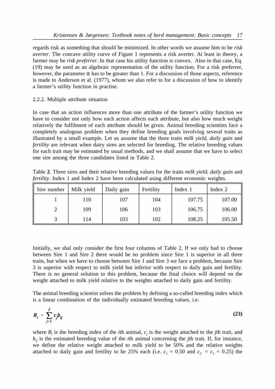
In case that an action influences more than one attribute of the farmer’s utility function wehave to consider not only how each action affects each attribute, but also how much weightrelatively the fulfilment of each attribute should be given. Animal breeding scientists face acompletely analogous problem when they define breeding goals involving several traits asillustrated by a small example. Let us assume that the three traitsmilk yield, daily gain andfertility are relevant when dairy sires are selected for breeding. The relative breeding valuesfor each trait may be estimated by usual methods, and we shall assume that we have to selectone sire among the three candidates listed in Table 2.
Initially, we shal only consider the first four columns of Table 2. If we only had to choose
Table2. Three sires and their relative breeding values for the traitsmilk yield, daily gainandfertility. Index 1 and Index 2 have been calculated using different economic weights.
Sire number Milk yield Daily gain Fertility Index 1 Index 2
1 110 107 104 107.75 107.00
2 109 106 103 106.75 106.00
3 114 103 102 108.25 105.50
between Sire 1 and Sire 2 there would be no problem since Sire 1 is superior in all threetraits, but when we have to choose between Sire 1 and Sire 3 we face a problem, because Sire3 is superior with respect to milk yield but inferior with respect to daily gain and fertility.There is no general solution to this problem, because the final choice will depend on theweight attached to milk yield relative to the weights attached to daily gain and fertility.
The animal breeding scientist solves the problem by defining a so-called breeding index whichis a linear combination of the individually estimated breeding values, i.e.
whereBi is the breeding index of theith animal,cj is the weight attached to thejth trait, and
(23)
bij is the estimated breeding value of theith animal concerning thejth trait. If, for instance,we define the relative weight attached to milk yield to be 50% and the relative weightsattached to daily gain and fertility to be 25% each (i.e.c1 = 0.50 andc2 = c3 = 0.25) the

18 Dina Notat No. 48, August 1996
breeding indexes of the three sires of the example become as shown underIndex 1in Table2. As it appears from the table, Sire 3 should be chosen. If on the other hand, the relativeweight attached to daily gain was 50% leaving 25% for each of the two remaining traits (i.e.c1 = c3 = 0.25 andc2 = 0.50) the breeding indexes become as shown underIndex 2leavingSire 1 as the superior one. This clearly illustrates that the relative importance attached to thetraits determines the mutual ranking of the animals.
In herd management science we do not choose among Sires but among alternative actionsrepresenting different factor allotments. Neither do we evaluate alternatives on breeding valuesbut on attributes of the farmer’s utility function. Nevertheless, if in the example we replacedSire by Action, trait by attribute (milk yield by monetary gain, daily gain by leisure time,fertility by animal welfare) and indexby utility, the example would still make sense. Also inherd management it is very likely that if we, for instance, rank actions on monetary gain theranking changes if we use leisure time as our criterion of evaluation instead. Also the multi-attribute utility function may be defined analogously with Eq. (23). Using the notation of theprevious sections, the utility function would just be a linear combination of the individualattribute functions:
wherec1,...,cJ are constant values which we may assume sum to 1 without loss of generality.
(24)
In the animal breeding example, Eq. (23) says that a higher breeding value concerning onetrait may compensate for a lower value concerning other traits. The same is expressed forattributes like monetary gain, leisure time and animal welfare in Eq. (24). This is certainly arealistic property of a utility function, but, nevertheless, if the utility function is defined as inEq. (24) we implicitly make some assumptions which by a closer look may seem unrealistic.In order to illustrate this we shall assume that only two attributes (monetary gainu1 andleisure timeu2) are relevant for the management problem considered. Eq. (24) thus reducesto
If we setU equal to some constantU’ , Eq. (25) may be rearranged into
(25)
implying that all combinations ofu1 and u2 yielding the same utilityU’ form a linear
(26)
relationship in a diagram. In Figure 3, three suchiso-utility curvesrepresenting a low, mediumand high fixed level of utilityU’ are shown. The course of the curves illustrate that decreasedleisure time may be compensated by increased monetary gain, and the linear relationshipimplies that the marginal rate of substitution between the two attributes is constant. In otherwords, a constant improvement∆u1 of the monetary gain may compensate a constant reduction∆u2 of leisure timeno matter whether the initial level of monetary gain or leisure time is highor low. From Eq. (26) we see that the constant marginal rate of substitution is:

Kristensen & Jørgensen: Textbook notes of herd management: Basic concepts 19
If we consider the situation of a real farmer, it is hardly likely that his marginal rate of
(27)
Figure 3. Iso-utility curves representing a low, medium and high fixed level of utilitycalculated according to Eq. (25).∆u2/∆u1 is constant.
substitution is constant. If, in his present situtation, he has a high level concerning leisure timeand a low level concerning monetary gain, an improvement concerning monetary gain willprobably be given very high priority. The farmer is probably willing to sacrify quite a bit ofhis leisure time in order to improve his income. In the opposite situation (high levelconcerning monetary gain and low level concerning leisure time) he is probably only willingto sacrify very little leisure time in order to improve his monetary gain.
In Figure 4, iso-utility curves illustrating varying marginal rates of substitution betweenattributes are shown. Again, three fixed levels of utility are represented in the diagram. Asshown in the figure, the marginal rate of substitution∆u21/∆u1 is very high if we are dealingwith a poor farmer with plenty of leisure time whereas it is very low (∆u22/∆u1) in the oppositesituation (a rich farmer working all the time).
A possible algebraic representation of a utility function having iso-utility curves like those ofFigure 4 is:

20 Dina Notat No. 48, August 1996
where (for the risk averter) 0 <α < 1 and 0 <β < 1. It should be noticed, that if one of the
Figure 4. Iso-utility curves corresponding to the utility function of Eq. (28).∆u21/∆u1
∆u22/∆u1.
(28)
attributes is left constant, Eq. (28) reduces to the single-attribute utility function of Eq. (19).For a discussion of other possible representations of a multi-attribute utility function, referenceis made to Anderson et al. (1977).
2.2.3. Operational representation of a farmer’s utility function
Tell me, how shall I feed my cows this winter?the farmer asks. The herd management scientistanswers him back:Let me know your utility function, and I shall tell you how to feed yourcows.From a theoretical point of view, the previous sections have illustrated that the herdmanagement scientist is right. In order to choose an optimal action among a set of alternatives,we need to know the farmer’s utility function. In other words we have to know what attributeshe includes and how they are weighted in a specific situation. On the other hand, the farmeris off course not able to specify his utility function, so what do we do? Does the dialogue endhere, or are we able to identify the utility function to an extent where it makes sense to makedecisions?
Even though for instance Anderson et al. (1977) to some extend describe how single- andmulti-attribute utility functions are identified in practice, it remains still a very difficult taskand even the representation of relevant attribute functions for attributes like animal welfare

Kristensen & Jørgensen: Textbook notes of herd management: Basic concepts 21
and working conditions may be a problem.
On the other hand, we may argue that it is not always necessary to know everything about theutility function when an action is chosen. In several cases we may logically conclude thatincomplete information is sufficient to choose an action:
- In some cases, an action only influences one attribute. If risk is involved, it is sufficientto know the single attribute utility function. In case of a decision not involving risk,even the attribute function is sufficient.
- Many actions (typically those with short time horizon) only marginally influence theattributes. It is therefore sufficient to know thelocal marginal rates of substitutionbetween attributes. In Figure 4, this may be illustrated by plotting thecurrentcombination of monetary gain and leisure time and draw a straight line with a slopeequal to the marginal rate of substitution through that locus. It is not claimed that thisconstant rate is universal, but for marginal changes the approximation may suffice. Thismeans that the simple additive Eq. (24) is used as a local approximation to atheoretically correct (but unknown) utility function with varying substitution rates.
- The utility function may only vary little over a rather large range of actions. It may besufficient to choose a satisfactory action rather than an optimal one. This is particularlythe case if a farmer’s single-attribute utility function has a course as illustrated inFigure 5. In that case it is important, that the value of the attribute in question is at leastas high as some satisfactory levelu*. Lower levels are punished by the utility function,but higher values are not rewarded. The attribute in question in Figure 5 could forinstance be animal welfare. Most farmers will probably try to improve it if it is verylow, but having reached a certain level, they do not worry about it anymore. When theymake decisions with long time horizon (for instance regarding housing facilities) theymake some decisions to ensure a satisfactory level, and afterwards they consider thematter of animal welfare to be out of concern.
An alternative to utility functions is the lexicographic utility concept which may be moreoperational in a real world situation. Instead of defining an aggregate multi-attribute utilityfunction the farmer has to rank attributes from the most important to the least important. Iffour attributes are relevant the ranking could for instance be as follows:
1. Monetary gain (u1)2. Working conditions (u2)3. Animal welfare (u3)4. Leisure time (u4)
In the pure form, the concept requires that actions are first evaluated entirely on the attributedgiven highest priority (in this case monetary gain), and action 1 is preferred to action 2 if andonly if u1
1 > u12 (no matter the values of the other attributes). Only ifu1
1 = u12 , the actions
are evaluated on the second attribute (working conditions) and, again, action 1 is preferred toaction 2 if, and only if,u2
1 > u22 and so on. Only ifu1
1 = u12, u2
1 = u22 andu3
1 = u32 the
actions are evaluated on the fourth attribute (leisure time).
The lexicographic concept may also be combined with definition of satisfactory levelsconcerning the most important attributes and then maximizing the least important one subjectto restraints on the others.

22 Dina Notat No. 48, August 1996
Finally, the obvious direct choice option should be mentioned. The farmer is just confronted
Figure 5. A single-attribute utility function reflecting the existence of a satisfactory level.
with the multi-attribute consequences of the alternative actions. In other words, he is told thataction 1 represents a monetary gain ofu1
1, working conditions expressed asu21, animal welfare
at the levelu31 and leisure time at the levelu4
1. Similar values concerning the other possibleactions are given, and based on this information the farmer chooses the preferred actiondirectly. This method has the obvious advantage that the advisor does not have to know thefarmer’s utility function, but only the relevant attributes.
3. The management cycle
3.1. The elements of the cycle
Herd management is a cyclic process as illustrated by Figure 6. The cycle is initiated byidentification of the farmer’s utility function as discussed in Chapter 2. Also the restraintshave to be identified no matter whether they are of the legal, economic, physical or personalkind discussed in Chapter 1. The number of restraints will depend heavily on the time horizonconsidered. If the time horizon is short, the farmer faces more restraints of economic, physicaland personal nature than when he is considering a long time horizon.
Having identified the farmer’s utility function and the relevant restraints, one or moregoalsmay be defined. It is very important not to confuse goals with the attributes of the utilityfunction. The attributes represent basic preferences of the farmer, and they are in principleinvariant, or - to be more precise - they only vary if the farmer’s preferences change (for

Kristensen & Jørgensen: Textbook notes of herd management: Basic concepts 23
instance he may give higher priority to leisure time or working conditions as he becomes
Figure 6. The elements of the management cycle.
older). Goals on the other hand may change as the conditions change. They are derived fromthe farmer’s preferences in combination with the restraints, and since we noted in Chapter 1that for instance legal restraints may very well change over time, the same of course apply togoals. The purpose of goals is only to set up some targets which (if they are met) ensure thatunder the circumstances defined by farmer’s preferences and the restraints the production willbe successful. In practice, goals may be expressed as a certain level of production, a certainefficiency etc.
It should be noticed, that goals are often defined as a result of planning under a longer timehorizon than the one considered. Traditionally three different time horizons (levels) aredistinguished. Thestrategiclevel refer to a long time horizon (several years), thetactical levelrefer to an intermediate time horizon (from a few months to a few years) and theoperationallevel refer to a short time horizon (days or weeks). Thus goals for the operational level aretypically defined at the tactical level.
When the goals have been defined the process ofplanningmay be initiated. The result of theprocess is of course aplan for the production. A plan is a set of decided actions eachconcerning the future allotment of one or more factors. Alternative actions are evaluated ontheir expected utility as discussed in Chapter 2. Accordingly, the expected resulting productionfrom each plan has to be known in order to be able to evaluate the utility (cf. Eq. (6)). So,what the plan actually contains is a detailed description of the factor allotment and theexpected resulting production.

24 Dina Notat No. 48, August 1996
The next element of the management cycle isimplementation. From a theoretical point ofview this element is trivial (but certainly not from a practical). Implementation is just to carryout the actions described in the plan, and during the production process the factors aretransformed into products.
During the production process, someregistrationsare performed. The registrations may referto factors as well as products. Based on the registrations, somekey figures(e.g. averagenumber of piglets per farrowing, average milk yield per cow) describing the performance ofproduction may be calculated. During thecontrol process these calculated key figures arecompared to the corresponding expected values known from the planning process.
The result of the comparison may either be that the production has passed off as expected orthat one ore more deviations are identified. In the first case, the production process iscontinued according to the plan. In the latter case, the deviations have to beanalyzed. Thepurpose of the analysis is to investigate whether the deviations are significant from (a) astatistical point of viewand (b) from a utility (often economic) point of view. Because of therandom elements of the production function (et of Eq. (1)) and because of observation errorsrelating to the method of measurement it may very well happen that even a considerableobserved deviation from a statistical point of view is insignificant. That depends on themagnitudes of the random elements and the sample size (for instance the number of animals).Even if a deviation is significant from a statistical point (because of small random variationand a large sample) it may still turn out to be insignificant from a utility point of view. In thefollowing section the statistical analysis is discussed in more details.
If it is concluded during the analysis that a deviation is significant from a statistical point ofview as well as a utility point of view, some kind of adjustment is necessary. Depending onthe nature of the deviation the adjustment may refer to the goals, the plan or theimplementation. If the deviation concerns the factor allotment, the implementation has to beadjusted. During the planning process certain factor levels were assumed, but during thecontrol it appeared that theactualfactor allotment was different. Accordingly, something wentwrong during the implementation of the plan.
If the deviation concerns the output level (i.e. the products), the conclusion depends onwhether or not a deviation concerning the factor levels was found simultaneously. In that case,the deviation in output level is probably only a result of the deviation in input level.Accordingly the adjustments should focus on the implementation process.
If, however, there is a deviation concerning output, but none concerning input, we really facea problem. During the planning process, we assumed that if we used the factors representedby the vectorx we could expect the production E(Y). Now, the control process show that theactual factor allotmentwas x, but the actual production wasY’ which differs significantlyfrom E(Y) both from a statistical and a utility point of view. If we consult Eq. (1), we haveto conclude, that the only possible explanation is that we have used a deficient productionfunction fs,i (in other words, thevalidation of the model used has been insufficient). Thereason may be that the statei of the production units differed from what we assumed duringthe planning process, or it may simply be because of lacking knowledge on the true courseof the production function. Under all circumstances, the situation calls for a new planningprocess where correct assumptions are made. Accordingly the adjustments refer to the plan.

Kristensen & Jørgensen: Textbook notes of herd management: Basic concepts 25
During the new planning process it may also turn up, that one or more goals are impossibleto meet, and in that case they have to be adjusted.
Finally, it should be emphasized that if any restraints (legal, economic, physical or personal)changes, new goals have to be defined and new plans have to be made.
3.2. Statistical evaluation of deviations identified during the control process
Whereas the analysis of a deviation from a utility point of view depends very much on thepreferences of the individual farmer, the anaslysis from a statistical point of view is moregeneral. In this section we shall briefly discuss some principles of this evaluation.
As mentioned in the previous section, the random variation associated with a calculated keyfigure has two sources: The observation error and the sample error. We shall denote the true(but unknown) value of the key figure askt and the calculated value askc. The relationbetween the two values may be expressed as
wherees is the sample error andeo is the observation error. Depending on the trait measured
(29)
by the key figure one or both of the error terms may be zero or at least insignificant inmagnitude. In the following, we shall investigate the consequences of (29) in relation to somepractical examples.
3.2.1. Example 1: Milk yield of dairy cows
In the Danish management information system for dairy cows, the average daily milk yieldof the cows during the first 24 weeks of lactation is calculated for first lactation cows andother cows, respectively. In the system, the farmer may compare the results to his own goals(expected values). The results in a herd were as shown in Table 3. We observe, that thecalculated result for all parities is lower than expected. The question is now, whether or notthe deviation is significant from a statistical point of view.
According to Kristensen (1986) the standard deviation ofcumulated milk yield (first 24
Table3. Average daily milk yield (ECM) during the first 24 weeks of the lactation in a herd.
Parity Goal (expected value) Calculated result No. of cows Acceptable result
1 23.5 20.4 10 21.7
≥ 2 27.8 26.0 12 25.6
weeks) between cows in the same herd is 490 kg milk for first lactation and 630 kg milk forother lactations. Since these standard deviations have been estimated from exatly the samekind of basic registrations as those of the management information system they actuallyrepresent the standard deviation of thesum of the error terms (i.e.es + eo). In order to usethem in relation to the results of Table 3 they have to be corrected to daily levels. Since 24

26 Dina Notat No. 48, August 1996
weeks are equal to 168 days, the standard deviation of daily milk yield between cows is490/168 = 2.92 kg for first lactation cows and 630/168 = 3.75 for others. Since the calculatedresults are average values of 10 and 12 observations, respectively, the standard deviations ofes + eo become 2.92 × 10-½ = 0.92 and 3.75 × 12-½ = 1.08. As a rule of thumb for normallydistributed data, a deviation is significant if it exceeds the standard deviation multiplied by 2,so in this case, acceptable results would be 23.5 − 2 × 0.92 = 21.7 and 27.8 − 2 × 1.08 = 25.6as indicated in the last column of Table 3.
Since the calculated result concerning first lactation cows is clearly below the deducedacceptable value, we conclude that the deviation is significant from a statistical point of view.On the other hand, the result concerning other cows is higher than the acceptable value, andaccordingly we have to accept the result as a possible consequence of usual random variation.In other words, the result concerning those cows doesnot call for any adjustments.
3.2.2. Example 2: Daily gain for bull calves (or slaugther pigs)
Usually, total gainyt for bull calves or slaugther pigs over a certain period is calculated asfollows:
wherex1 is the total live weight of all calves delivered during the period,x2 is the valuation
(30)
weight (total weight of all calves present in the herd) at the end of the period,x3 is thevaluation weight at the beginning of the period andx4 is the total weight of all calvesborn/inserted in the herd during the period. In order to arrive at thedaily gainyd, the total gainyt has to be divided by the total number of days in feedz, i.e. yd = yt /z, where days in feedare calculated as
whereH is the set ofall calves that have been in the herd during the period (or just a part of
(31)
the period), anddj is the number of days thejth animal has been in the herd. We shall assumethat the standard deviation in daily gain between calves of the same herd amounts to 200 g.The standard deviation of the sample errores (i.e. the standard deviation of the average resultin a herd with 100 animals) is therefore 200 × 100−½ = 20 g.
Based on the feeding and the housing conditions the goal for daily gain has been set to 1150g in a herd with approximately 100 bull calves. The actual results registered in the herd fora 3 month period appear from Table 4.
The standard deviation of the observation erroreo depends on the method used for registrationof the individual results of Table 4. We shall assume thatx1 has been calculated from actualweighings of all calves delivered to the slaughter house. Accordingly, we assume that noobservation error is associated with this figure. The uncertainty associated with the weight ofthe calves inserted will also be insignificant. What is left is only the valuation weight of allanimals at the beginning and the end of the period, respectively. The observation error onthese figures depends heavily on the method used. We shall assume the standard deviation of

Kristensen & Jørgensen: Textbook notes of herd management: Basic concepts 27
the observation error (onx2 andx3) it is zero if all animals (approximately 100) have actually
Table4. Results used for calculation of average daily gain in a herd.
Total live weight of 25 calves delivered, kg x1 12,500
Valuation weight at the end of the period, kg x2 21,159
Valuation weight at the beginning of the period, kg −x3 −23,441
Total weight of 20 calves inserted, kg −x4 −950
Total gain during the period, kg yt 9,268
Total days in feed z 8,827
Daily gain, g yd 1,050
been weighed. If the total weight is calculated by weighing only representative calves, thecorresponding standard deviation is assumed to be 5%. Finally, if the valuation weights arejust assessed by visual observations, the standard deviation is assumed to be 10%.
Based on these assumptions the variance and standard deviation of the observation error maybe calculated by standard methods as shown in Table 5, where also the total standarddeviations of the herd result under the three valuation methods appear.
If, again, we use the rule of thumb, that a deviation has to be larger than twice the standard
Table5. Error terms to be used in the calculation of the standard deviation of herd result.
Error term Valuation method
Weighing1 Sample2 Visual
Variance of observation error associated withyt 0 2,292,959 9,971,838
Standard deviation of observation error,yt 0 1579 3158
Standard deviation ofeo (observation error,yd) 0 179 358
Standard deviation ofes (sample error) 20 20 20
Variance ofes + eo 400 32,441 128,564
Standard deviation ofes + eo, g 20 180 3591 Weighing ofall calves at valuation.2 Weighing of a representative sample.
deviation in order to be significant, we conclude that acceptable results under the threevaluation methods are 1150 − 2 × 20 = 1110 g, 1150 − 2 × 180 = 790 g and 1150 − 2 × 359= 432 g, respectively. Accordingly, the calculated result of 1050 g is only significant from astatistical point of view if the valuation method has involved weighing ofall calves.

28 Dina Notat No. 48, August 1996
3.2.3. Example 3: Reproduction in a dairy herd
The previous examples referred to variables which might be regarded as at least approximatelynormally distributed. We now turn to examples involving categorical data, where otherdistributions are involved.
If N dairy cows are inseminated, the number of resulting pregnanciesn will be binomiallydistributed with parametersN andp, wherep is the conception rate. In a dairy herd, the goalconcerning the conception rate has been set to 0.5, wheras the actually calculated conceptionrate amounts to only 0.4. If we assume, that the state of a cow (pregnant or not pregnant) maybe determined with certainty (i.e. no observation error), the result may be evaluated by abinomial test using the hypothesisp = 0.5. The test variabletN is defined as:
whereno is the number of pregnancies observed. Whether or not the observed conception rate
(32)
differs significantly from the goal depends heavily on the number of inseminations behind thecalculation. In Table 6, the test variabletN has been calculated under assumption of threedifferent sample sizes.
As it appears from the table, the deviation is only close to be significant if the sample size is
Table6. Test of the hypothesis that the true conception rate is 0.5 given an observed rate of0.4 and the sample size (number of inseminations)N.
Number of inseminations,N Number of observed pregnancies,no Test variable,tN
10 4 0.17
20 8 0.13
50 20 0.06
50. If this figure is compared to usual herd sizes in European countries, we may conclude thatthe conception rate has to be calculated over a rather long period if shall pay any attention todeviations from the goal.
3.2.4. Example 4: Diseases
If the herd size and the disease incidence is constant, the number of cases of a specific diseasemay be represented by a Poisson distribution provided that individual cases appearindependently of each others (which isnot the case with contagious diseases). The actualnumber of cases may therefore be compared to the goal (or expected result) using probabilitiescalculated from a Poisson distribution taking the defined goal as it’s parameter. The testvariabletN is calculated as

Kristensen & Jørgensen: Textbook notes of herd management: Basic concepts 29
whereλ is the parameter of the Poisson distribution andno is the number of disease cases
(33)
observed.
3.2.5. Concluding remarks
It should be emphasizes that the kind of statistical "tests" illustrated in the previous sectionsare only of indicative nature. They may not be confused with tests performed on data fromcontrolled experiments. The purpose is only to provide a rough estimate of the significanceof an observed deviation. The message is, that a result calculated from actual registrations isoften associated with a rather big uncertainty as illustrated in the examples. In many cases itis possible to "estimate" that uncertainty rather precisely, but there is no correct level ofsignificance to use in the evaluation of results. In a true situation the relevant level will alsodepend on the significance from a utility point of view.
An other important observation is that in order to be able to evaluate the production we haveto perform some registrations relating to the production process. In an other note of this seriesthe process of transforming such registrations to useable information is discussed.
3.3. Evaluation of deviations from a utility point of view
The evaluation of deviations from a utility point of view is just as important as the statisticalanalysis. If may very well happen that a deviation is significant from a statistical point of view(where significance is merely a question of sample size), but insignificant from a utility pointof view (and vice versa). Adjustments are of course only relevant if the deviations observedare significant from both points of view.
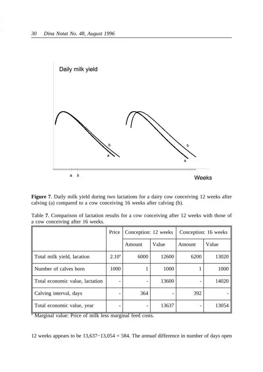
The evaluation from a utility point of view is complicated by the dynamics of production. If,for instance, the average number of days open in a dairy herd is higher than expected (and thestatistical analysis showed that it was a significant deviation) we have to consider what thedeviation means for the farmer’s utility. The direct consequences for production of a cowconceiving 16 weeks after calving (b) instead of 12 weeks after calving (a) are illustrated inFigure 7.
As it appears from the figure, the direct consequences include:
a. Next calving is delayed by 4 weeks.b. The milk yield towards the end of the lactation is slightly higher.c. The number of days in milk is increased by 4 weeks.d. The milk lactation curve of next lactation is shifted 4 weeks to the right.
Expressed numerically, the consequences might for instance be as indicated in Table 7, wherethe economical net returns are calculated initially on a lactation basis and afterwardsnormalized to annual figures per cow.
The economic value per cow per year of a decrease in the number of days open from 16 to
30 Dina Notat No. 48, August 1996
12 weeks appears to be 13,637−13,054 = 584. Theannualdifference in number of days open
Figure 7. Daily milk yield during two lactations for a dairy cow conceiving 12 weeks aftercalving (a) compared to a cow conceiving 16 weeks after calving (b).
Table7. Comparison of lactation results for a cow conceiving after 12 weeks with those ofa cow conceiving after 16 weeks.
Price Conception: 12 weeks Conception: 16 weeks
Amount Value Amount Value
Total milk yield, lacation 2.10a 6000 12600 6200 13020
Number of calves born 1000 1 1000 1 1000
Total economic value, lactation - - 13600 - 14020
Calving interval, days - 364 - 392 -
Total economic value, year - - 13637 - 13054
a Marginal value: Price of milk less marginal feed costs.

Kristensen & Jørgensen: Textbook notes of herd management: Basic concepts 31
per cow is 16×7×365/364 − 12×7×365/392 = 20 days. Assuming linearity, the cost of oneadditional day open is therefore 584/20 = 29.
Assume now, that in a herd with 100 cows, the average number of days open has beencalculated to 105 wheras the goal is 90. It would be very tempating to claim that the totaleconomic loss caused by this deviation is (105-90)×29×100 = 43,500, but nevertheless, itwould be a serious mistake. In order to reveal why, we shall consider the impliciteassumptions behind the calculations above. Those assumptions are:
- The marginal value of an improvement is assumed to be constant (i.e. independentof the initial level). In other words, a decrease from 200 days open to 199 days isassumed to be of the same value as a decrease from 30 to 29 days. Such an assumptionis certainlynot realistic.
- All cows are assumed to be identical in the sense that they all conceive exactly after12 (repectively 16) weeks.The real situation is very different. Even though an averageresult is for instance 105 days,individual results vary considerably among the cows ofa herd. Thus, if the assumption of constant marginal value does not hold, we need toknow the distribution of individual results in order to be able to estimate the economicconsequenses at herd level.
- All cows are assumed to be identical concerning milk yield. From the calculations itis obvious that a different level of milk yield would give us an other result.
- Conception is assumed to be independent of milk yield. In the real world, it is a wellknown problem that the conception rate of a high yielding cow is lower than that of alow yielding. It is therefore reasonable to assume that in particular the high yieldingcows are those that cause a high average number of days open.
- It is assumed that no cows are replaced. In practice annual replacement rates of 30to 50% are usual. It is obvious, that if a cow is replaced, the effects of delayed calvingand delayed new lactation are irrellevant.
- The farmer’s management is assumed not to interact with the observed result.Thefarmer probably has some policy concerning for instance replacement. If a cow is highyielding, he accepts more days open than if it is low yielding. If the number of daysopen grows, he probably also increases hes replacement rate.
- It is assumed that there is no milk quota.In case of a milk quota, the marginal valueof an increased milk yield is much lower than assumed in the example. The reason isthat if a higher milk yield is obtained (for instance because of improvements inreproduction) the farmer has to decrease the number of cows in order not to violate thequota (refer to Kristensen & Thysen, 1991, for a discussion). Presence of a milk quotamay reduce the costs of an additional day open by 60-70% as shown by Sørensen &Enevoldsen (1991)
These considerations clearly illustrate that calculations as those of the example are of littlevalue in the evaluation of results obtained in production. It is very important that randomvariation, interactions, management policies and restraints are taken into account in suchcalculations. The most obvious tool to apply is certainly simulation, but also some of the othertools discussed in Chapter 4 may be used in some cases. Evaluations from a utility point ofview remains, neverheless a true art.

32 Dina Notat No. 48, August 1996
4. Decisions and strategies: Framework and techniques
In this chapter we shall initially discuss general aspects of decision making in animalproduction with emphasis on information needs, time horizons and production units. Followingthat discussion, a general overview of techniques available in the determination of optimaldecisions and strategies is given.
4.1. The framework of decision making in animal production
During the planning process we have to make decisions. We shall define a decision as theallotment of some factor used in the production. The purpose of planning is of course to makeone or severaloptimal decisions so that the set of decisions making up the plan maximizesthe expected utility relating to the relevant time horizon as discussed in Chapter 2.
4.1.1. Information needs
From Eq. (7), we observe that in order to be able to make an optimal decision,in general,thefollowing information is necessary:
1. The state of the production unit atall stages of the planning horizon.2. The production function(s) and the distribution(s) of the random term(s).3. All attribute functions relevant to the farmer’s preferences.4. The utility function representing farmer’s preferences.
Recalling the discussion of Chapter 1, we have to add the following information:
5. All restraints of legal, economic, physical or personal kind.
As concerns item 1, it is obvious, that the future state of the production unit is not alwaysknown at the time of planning. The state represents all relevant information on the unit (i.e.the traits of the unit) and very often it varies at random over time. It is therefore likely, thatit is not possible to make decisions relating to all stages at the same time. Instead, we maychoose astrategy(or policy as it is also some times denoted) which is a map (or function)assigning to each possible state a decision. In other words, having chosen a strategy we mayat all stages observe the state of the unit and make the decision provided by the strategy.
The identification of an optimal strategy is complicated by the fact that decisions may alsoinfluence the future state of the unit as illustrated by the following example. Let us assumethat the unit is an animal, that the relevant information (the state) is the weighti of the animaland what we have to decide is the feeding levelx of the animal. It is obvios, that the optimallevel of x will depend on the weight of the animali, but it is also obvious, that the feedinglevel x will influence the future weightj of the animal.
A thorough inspection of Eq. (7) will unveil that the decision made may also influence thefuture production, but, since the statei is assumed to contain all relevant information on theproduction unit, we may just include information on previous decisions in the definition of thestate. Thus we do not need to consider that aspect further. Consider again the example of

Kristensen & Jørgensen: Textbook notes of herd management: Basic concepts 33
Chapter 1, where we noted that the feeding level of a heifer influences the future milkproduction as a dairy cow. If we denote the feeding level at various stages asx1, x2,... , thestage of first calving ask and the milk yield of stagen asyn we might express the productionfunction in the same manner as in Eq. (1):
where the statei for instance may be defined from combinations of traits like lactation
(34)
number, stage of lactation and body weight. Thus the state spaceΩ1 is defined as the set ofall possible combinations of those individual traits, and an individual statei ∈ Ω1 is anycombination of values representing the three traits. If, however, we redefine the state spaceto include also the feeding levels of previous stages (i.e.Ω2 = Ω1 ∪ x1,...,xk+n−1) exactly thesame information may be contained in the relation
where, now,i ∈ Ω2.
(35)
Eq. (35) illustrates that the state concept is very essential for the planning process. Theidentification of the state of the production unit is therefore a very important task. In order tobe able to identify the state we have to perform some registrations concerning the productionunit. It may some times happen that we are not able to observe the traits of the state spacedirectly, but only indirectly through other related traits. The precision of our knowledgeconcerning the true state may therefore vary, but Bayesian updating methods are available forhandeling such situations with imperfect knowledge. Those aspects are dealth with in a laterchapter.
We may now reformulate the information needs when choosing an optimal strategy:
1. A production function describing the immediate production given stage, state anddecision and the distribution of the possible random term(s).
2. The distribution of the future state given stage, state and decision.3. All attribute functions relevant to the farmer’s preferences.4. The utility function representing farmer’s preferences.5. All restraints of legal, economic, physical or personal kind.
As concerns items 3 and 4, the discussion of Section 2.2.3. should be remembered. Severaltechniques are available for identification of optimal strategies.
4.1.2. Levels
In herd management we face a hiearchy of decisions made at different levels with differenttime horizons. In this section, and the following section, we shall consider the implicationsof this hierarchy.
By level we mean the production unit considered. As discussed in Chapter 1 the unit may bean individual animal, a group or a pen, a section or even the entire herd. For instance thedecision to build a new barn is an example at herd level. Decisions concerning feeding are

34 Dina Notat No. 48, August 1996
typically made at group or section level wheras decisions concerning culling or medicaltreatment may be made at animal level.
As long as decisions at different levels are mutually independent we may solve a problem atone level without considering the other level. Unfortunately it is very rare that suchindependence exists as the following example shall illustrate.
We want to build a new barn for our dairy cows, and two alternatives,a1 anda2, are available.The two barns of course differ in several respects, but one of the differences is that barna1
allows for grouping of the cows wheras grouping is not possible in barna2. This differencemeans that in order to make an optimal decision concerning the kind of barn to build, we alsohave to consider how to feed the animals in each of the two systems, because the option ofgrouping makes other feeding strategies possible than if all cows are housed in a single group.It then turns out that feeding strategyα1 is optimal in barna1 whereas strategyα2 is optimalin barna2.
Unlessα1 has exactly the same utility consequences asα2, the differences must be taken intoacount when the optimal barn is chosen.
4.1.3. Time horizons
A general aspect of herd management under risk is that decisions have to be made withoutcertainty about the future state of the production unit. The uncertainty increases with the timehorizon of the decision, i.e. it is more prevalent at the tactical level than at the operationallevel. Having made a decision at the tactical level, the manager is restricted by theconsequences for the duration of the time horizon. It may very well later turn out, that theactual state of the production unit differs from the expected state at the time of the decision,but the only way the manager may adjust to the new situation is by making decisions at theoperational level. These decisions should be conditionally optimal given the tactical decisionmade and the current state of the production unit. In other words, the decisions at theoperational level may be regarded as a way of adjustment to risk and in that way compensatefor the incomplete knowledge on the future state of the production unit.
In general, it must be assumed that if decisiona1 is made at the tactical level, then strategyα1 is optimal for decisions at the operational level (a strategy is defined as a set of decisionsrelating to the set of possible states of the production unit). On the other hand, if decisiona2
is made at the tactical level, then strategyα2 is optimal at the operational level. It will be anexception, ifα1 = α2. In other words, it is not possible to choose an optimal decisiona’ at thetactical level, unless a conditionally optimal strategyα’ has been determined at the operationallevel (conditional given the tactical decision).
In case of a management problem with limited time horizon (for instance the duration of thetactical decision considered) the mutual dependency between decisions at the tactical andoperational level is not really a problem. We just have to determine optimal policies at theoperational level given each of the alternative tactical decisions and, afterwards, to choose thetactical decision maximizing the objective function. A problem corresponding to this situationis discussed by Jensen (1995), who considered optimal mildew management policies in winterwheat under different nitrogen fertilization strategies. In that example, the decision at the

Kristensen & Jørgensen: Textbook notes of herd management: Basic concepts 35
tactical level is to choose a nitrogen fertilization strategy and the decisions at the operationallevel are to treat the crop for mildew. The time horizon is limited to the growing season justlike the tactical decision. The problem was solved within the framework of a Bayesiannetwork in combination with a usual backwards dynamic programming algorithm.
If, however, the time horizon is unknown or at least very long as it is typically the case inanimal production, the situation is far more complicated. Examples of tactical decisionsinclude mating of a female animal with a male animal of a certain quality or choosing acertain feeding level for an animal. Such decisions have (depending on the animal species andother circumstances) a time horizon of a few months, but unlike the mildew managementproblem, the time horizon of the production is not limited to a growing season or the like.Instead the production is continuous, which is often modelled by an infinite time horizon. Inorder to cope with such a situation, the decisions at the tactical and operational level have tobe optimized simultaneously in order to ensure over-all optimality.
The terms "tactical" and "operational" are of course rather arbitrary. In general we have todeal with decisions at several levels having different time horizons.
4.2. Methods
The techniques will be described according to their ability to represent the various kinds ofnecessary information discussed in Chapter 4. Furthermore, their potentials for integration ofdecisions at different levels and time horizons are discussed. It is not the purpose to describethe various methods in details, but only to provide a general survey relating to the issues ofthe previous chapters. For each method, references to relevant literature is given.
4.2.1. Rule based expert systems
Research concerning expert system is a recent development within the area called ArtificialIntelligence (AI). The British Computer society has defined expert systems as follows:Anexpert system is regarded as the embodiment within a computer of a knowledge-basedcomponent from an expert skill in such a form that the system can offer intelligent advice ortake intelligent decision about a processing function. A desirable additional characteristic,which many would consider fundamental, is the capability of the system, on demand to justifyits own line of reasoning in a manner directly intelligible to the enquirer. The style adoptedto attain these characteristics is rule-based programming. (Cf Dindorph, 1992). This is justone of many proposed definitions of expert systems.
The fundamental difference between the rule based systems, and the approach that we havepresented until now, is that instead of trying to model a system, the rule based expert systemstries to model the expert, or rather the expert’s approach to problem solving. Originally, theambition within AI-research was to make general problem solvers that could be used for anyproblem area, but this was realized by most researchers within the area to be overambitious.The research efforts had, however, led to new approaches towards problem solving, and withinnarrow problem (expert) domains, the approach showed some promising results.
Rule based expert systems have three components: a knowledge base containing the expert’sknowledge of the domain, an inference engine that decides how and when to use the

36 Dina Notat No. 48, August 1996
knowledge, and a user interface.
The knowledge base contains knowledge of a problem domain, as it is described in text books,as well as and expert knowledge, e.g. exceptions to general rules, experiences from previousproblems, and time-efficient approaches on how to solve problems within the area. Theknowledge base is an enhanced data base that apart from data also contains logic rules for theconnection between the items in the knowledge base, e.gif x or y then z.
The inference machine contains the mechanism for deduction based on the logical rules in theknowledge base. The deduction can use different inference principles, such as backwardchaining and forward chaining. In the rule showed above, the inference machine would startout by finding the value ofz, and given the knowledge ofz establish the value ofx and y.Forward chaining would start out by establishing the values ofx andy and deduce the valueof z subsequently. In both cases the unknown values are found either by a question to the useror by combining other rules in the knowledge-base. The optimal choice of inference principledepends on the type of problem the expert system is supposed to solve. In very complexexpert systems, neither forward- or backward chaining is fast enough, and the so-calledheuristic search strategies are needed. These strategies work primarily by searching theknowledge base in an efficient order, focusing on areas, where a solution to the problem ismost likely to be found. Both general and problem specific heuristic strategies exist.
The questioning mechanism is a standard part of the user interface. Besides posing questions,the user interface is usually able to explain, why it asks the question, i.e. ’I’m trying toestablish the value ofz because I want to know if eitherx or y is true. Another facility is theexplanation facility, i.e. ’I know that neitherx is true nory is true becausez is not true.Usually the phrases are formulated more user friendly.
Programs for maintaining knowledge bases in connection with inference machine and userinterface as an integral part is sold as the so-called expert system shells. This conceptoriginates from the medical diagnosis system, MYCIN. The knowledge base in MYCIN wasemptied and the program sold as E-MYCIN (or empty mycin), and was thought to beapplicable to any problem domain. Very often these shells are programmed in programminglanguages where logic deduction can easily be represented, such as LISP or PROLOG, butstandard programming languages such as C and Pascal can of course be used.
Rule based expert system can be categorized into several areas (Hayes-Rothet al., 1996).Referring to Figure 6 they comprise the planning, control and analysis phase of the productioncycle.
In developing rule based expert systems two ’players’ are essential, of course the expert, butin addition the so-called knowledge engineer. The role of the knowledge engineer is to’extract’ the knowledge from the expert and to formulate the knowledge as rules that can serveas input to the knowledge base. Knowledge engineering has in fact become a research areain its own right.
To illustrate the problem of knowledge engineering, the first rule based expert systems werebased on very simple ’expert’ rules very much inspired by the diagnostic systems, e.g. ifindication a and b are observed then problem is probably c. Later on it was realized that the
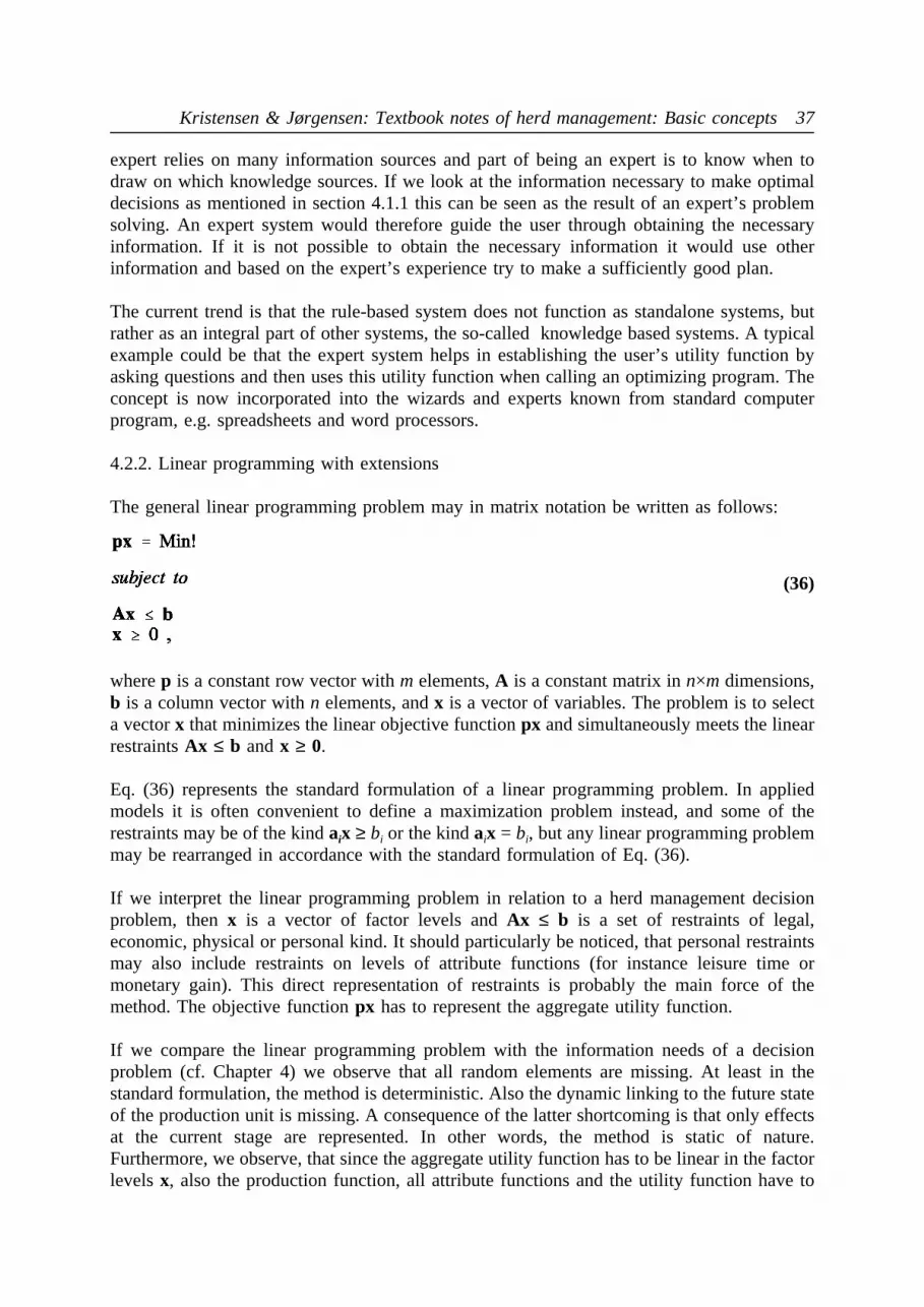
Kristensen & Jørgensen: Textbook notes of herd management: Basic concepts 37
expert relies on many information sources and part of being an expert is to know when todraw on which knowledge sources. If we look at the information necessary to make optimaldecisions as mentioned in section 4.1.1 this can be seen as the result of an expert’s problemsolving. An expert system would therefore guide the user through obtaining the necessaryinformation. If it is not possible to obtain the necessary information it would use otherinformation and based on the expert’s experience try to make a sufficiently good plan.
The current trend is that the rule-based system does not function as standalone systems, butrather as an integral part of other systems, the so-called knowledge based systems. A typicalexample could be that the expert system helps in establishing the user’s utility function byasking questions and then uses this utility function when calling an optimizing program. Theconcept is now incorporated into the wizards and experts known from standard computerprogram, e.g. spreadsheets and word processors.
4.2.2. Linear programming with extensions
The general linear programming problem may in matrix notation be written as follows:
wherep is a constant row vector withm elements,A is a constant matrix inn×m dimensions,
(36)
b is a column vector withn elements, andx is a vector of variables. The problem is to selecta vectorx that minimizes the linear objective functionpx and simultaneously meets the linearrestraintsAx ≤ b andx ≥ 0.
Eq. (36) represents the standard formulation of a linear programming problem. In appliedmodels it is often convenient to define a maximization problem instead, and some of therestraints may be of the kindaix ≥ bi or the kindaix = bi, but any linear programming problemmay be rearranged in accordance with the standard formulation of Eq. (36).
If we interpret the linear programming problem in relation to a herd management decisionproblem, thenx is a vector of factor levels andAx ≤ b is a set of restraints of legal,economic, physical or personal kind. It should particularly be noticed, that personal restraintsmay also include restraints on levels of attribute functions (for instance leisure time ormonetary gain). This direct representation of restraints is probably the main force of themethod. The objective functionpx has to represent the aggregate utility function.
If we compare the linear programming problem with the information needs of a decisionproblem (cf. Chapter 4) we observe that all random elements are missing. At least in thestandard formulation, the method is deterministic. Also the dynamic linking to the future stateof the production unit is missing. A consequence of the latter shortcoming is that only effectsat the current stage are represented. In other words, the method is static of nature.Furthermore, we observe, that since the aggregate utility function has to be linear in the factorlevelsx, also the production function, all attribute functions and the utility function have to
38 Dina Notat No. 48, August 1996
be linear. Examples of linear attibute functions are shown as Eqs. (8), (11) and (14), and alinear utility function is shown as Eq. (24). This demand for linear functions and linearrestraints is a serious weakness of the method.
Several of the shortcomings mentioned may be redressed or at least adapted by extensions tothe method: The linear objective function may be replaced by a quadratic one (quadraticprogramming); the static nature may be modified by introduction of stages and additionalrestraints ensuring dynamic links (dynamic linear programming); random terms may be addedto the elements ofA andb, and the corresponding restraints may be expressed as probabilities(stochastic programming); and often, non-linear functions may be approximated by pieces oflinear relations over short intervals. In particular, dynamic linear programming, may be usedto link decisions at different levels with different time horizons.
Herd management applications of linear programming are numerous. The most frequentapplication is no doubt for ration formulation, where least-cost rations meeting the nutrinionalrequirements of the animals in question are met. Most often such programs ignore the effectof feeding on production. An example of such a ration formulation program developed forteaching has been described by Kristensen (1993)1.
Also examples of application of linear programming for whole-farm planning may be foundin literature. Refer for instance to Hansen (1992) and Hardie (1996). Such models are oftenvery large containing thousands of variables and restraints, but since very efficient standardsoftware is available this is hardly a problem.
4.2.3. Dynamic programming and Markov decision processes
Consider a production unit which is observed over a number of stagesn = 1,...,N. At thebeginning of each stage, we observe the statei ∈ ωn of the unit. Having observed the state,we have to take an actiond ∈ Dn concerning the production unit. Usually, the state spaceωn
and the action space Dn are assumed to be finite sets. Depending on the stage, state and action,a reward is gained. The reward may very well be a random variable, but the expected valueri
d(n) has to be known. Also the state to be observed at the next stage is a random variable.We shall denote aspij
d(n) the conditional probability of observing statei at stagen+1 giventhat statei has been observed and actiond taken at stagen. Finally, a strategys is defined asa map assigning to each combination of stage and state an actions(n,i) ∈ Dn.
The purpose of dynamic programming is to determine a strategy which (in some sense) isoptimal. Several optimization techniques are available. The most commonly applied methodis calledvalue iterationwhere a value function representing the expected total rewards fromthe present stage until the end of the planning horizon (i.e. stageN) is maximized. Optimaldecisions depending on stage and state are determined backwards step by step as thosemaximizing the value function. This way of determining an optimalpolicy is based on theBellman principle of optimality which says: "An optimal policy has the property that whateverthe initial state and initial decision are, the remaining decisions must constitute an optimal
1 The program itself is available as a Zip-file on www at the following URL:http://www.prodstyr.husdyr.kvl.dk/Software/ah.html

Kristensen & Jørgensen: Textbook notes of herd management: Basic concepts 39
policy with regard to the state resulting from the first decision" (Bellman, 1957 p. 83). Valueiteration is often just denoted asdynamic programming.
If N is large, an infinite planning horizon is often assumed. A relevant optimization techniquefor infinite stage problems ispolicy iteration. This method was introduced by Howard (1960),who combined the dynamic programming technique with the mathematically well establishednotion of aMarkov chain. A natural consequence of the combination was to use the termMarkov decision processto describe the notion. The policy iteration method was a result ofthe application of the Markov chain environment and it was an important contribution to thedevelopment of optimization techniques.
The objective function being maximized during optimization depends on the circumstances.It may represent the total expected rewards, the total expecteddiscountedrewards, the averagerewards per stage or the average rewards over some kind of physical output.
If we compare the dynamic programming problem with the information needs of a decisionproblem (cf. Chapter 4) we observe that most aspects are covered. The rewards directlycorrespond to production functions; the conditional probabilitiespij
d(n) represent the dynamicrandom links to future stages; and the objective function represents the farmer’s utilityfunction. There are, however, some restrictions on the kind of utility function which can berepresented in a dynamic programming model. The restrictions concern the way in whichindividual stage attributes are aggregated into the over-all utility function as described by Eq.(5). In order to be able to use dynamic programming, we implicitely assume that theaggregation may be performed in such a way that we first aggregate attributes at the samestage into a stage specific utilityvn of the kind
(37)
where gn is a stage specific utility function of arbitrary kind. In the dynamic programmingcontext,vn is identical to the rewardri
d(n). The over-all utility (i.e. aggregation over stages)in turn must be calculated as a simple sum of the stage specific utilitiesvn, as a discountedsum (cf. Eq. (9)), as the average value over stagesor as the average value over some kindof physical output or input from production.
The most difficult kind of information to represent in dynamic programming models is theinformation on restraints. There is no general solution to that problem, but some times it maybe solved by using an objective function maximizing average rewards relative to the mostlimiting restriction. An example is maximization of average net returns per unit of milkproduced under a milk quota (Kristensen, 1989). In other cases combination of the methodwith methods like simulation (Ben-Ari & Gal, 1986; Kristensen, 1992) or genetic algorithms(Houben, 1995) may circumvent the restraint problem.
A major problem in relation to dynamic programming models is the so-calledcurse ofdimensionality. Since the state space is represented by discrete levels of a set of traits (statevariables), models tend to become very big. Thus a model presented by Houben et al. (1994)contained 6.8 million states. Despite the size of the model, optimization was still possible dueto a new notion of a hierarchic Markov process described by Kristensen (1987, 1991).

40 Dina Notat No. 48, August 1996
Numerous applications of dynamic programming are described in literature. A relevanttextbook concerning application in agriculture has been written by Kennedy (1986). The bookalso contains a survey of agricultural applications. In herd management, the technique hasmost often been applied for operational decisions like replacement, insemination and medicaltreatment of animals.
4.2.4. Probabilistic Expert systems
Another part of the research area named Artificial Intelligence are the so called probabilisticexpert systems that rely on the Bayesian network. The following description is based onLauritzen (1995).
In some areas where expert systems are appropriate, the task involves performing a sequenceof steps according to specified logical rules. However, other expert systems work in domainsthat are characterized by inherent uncertainty. This uncertainty is either due to imperfectunderstanding of the domain, incomplete knowledge of the state of the domain at the timewhere the task has to be performed, randomness in the mechanisms governing the behaviourof the domain or a combination of these. Within these domains probability and statistics canserve to represent and manipulate the uncertain aspect of domains having these characteristics.Probabilistic methods were for some time discarded in this context as requiring too complexspecification and computation. However, the work of Pearl (1988) and Lauritzen andSpiegelhalter (1988) demonstrated that these difficulties could be overcome, based on causalnetworks or as it is now usually termed Bayesian networks. There exist other formalisms forhandling uncertainty in expert system, such as the fuzzy sets, but these will not be discussedin the present context.
The rule based systems were mainly constructed through modelling of the behaviour of theexpert and the encoding this behaviour in terms of rules of various kind. In contrast,probabilistic expert systems are constructed by modelling the domain rather than the expert.The method is thus in close correspondence with the approach used in this book, where thedomain is modelled using production functions etc. The probabilistic expert systems specifya graphical model for the variables. The reasoning is then performed by updating theprobabilities of the domain in the light of the specific knowledge according to the laws ofconditional probability.
The graphical model captures association between entities in the domain, or rather lackthereof, in terms of conditional independence that in a systematic fashion are encoded in agraph or network with nodesrepresenting the entities themselves andedgesrepresentingassociations between them. Thenodesare represented as dots or circles. Theedgesare eitherdirected corresponding to influences of a causal nature and represented as arrows, orundirectedcorresponding to symmetric associations (e.g. correlations) and represented as lines.
The use of the graphic specification in the probabilistic expert systems plays several roles. Forexample, it gives a visual picture of the domain information; it gives a concise presentationof domain information in terms of conditional independence relations, and it enables rapidcomputation and revision of interesting probabilities.
The graphic method can also be used for several important tasks in the specification process.

Kristensen & Jørgensen: Textbook notes of herd management: Basic concepts 41
It can be used tolearn quantitative and structural aspects, or as it known within generalstatistics, estimation and model selection.
If we compare the probabilistic expert systems method with the information needs of thedecision problem, it is important to recognize that the method is inherently a static method,even though attempts have been made to model dynamic systems as well. For control andanalysis purposes it is ideal, i.e. the method can assign probabilities to observed deviations,whether they are random or not. It can also make a diagnosis in the analysis, that is, indicateprobabilities for different causes of the deviation. This can in turn serve as the necessary basisfor decisions concerning changes in production plan.
The expert systems can be build as recurrent time slices and can in this manner representdynamic production functions. And thus can predict the future state for given decisions. Therestraints concerning the production function can be modelled, but restraints may cause thesame problems as described under Dynamic Programming and Markov decision processes.
To represent decision in Bayesian networks the decision can be included as a random variablein the model, with the different decisions as level of the variables. When the decision is made,the corresponding level is assigned a probability of 1. This approach does not make any searchfor optimal decisions.
If decisions have to be included,Influence diagramsshould be used instead.Influencediagramscan in fact be fitted into the general frame work of Bayesian Networks.
4.2.5. Influence diagrams
Influence diagrams was introduced by Howard and Matheson (1981) as a formalism to modeldecision problems with uncertainty for a single decision maker. The influence diagrams gavea more compact graphical representation of a decision problem than the more traditionaldecision tree approach. The influence diagram is very similar to the Bayesian networkconsisting of chance node and arrows denoting causal effect. In addition two more node typesare introduced, the decision node shown as a square, and the value node shown as a diamond.
Originally, the influence diagrams was translated to a decision tree within the computer andthe standard "average-out and fold-back" algorithm were applied on that tree. In Shacter(1986) a method was suggested for solving the decision problem represented by the influencediagram directly, without the translation to a decision tree. This method transformed theinfluence diagram by successively removing nodes in the graph, until at last only one finalutility node remained, holding the utility of the optimal policy. In order to solve many similarproblems one therefore had to start from scratch every time. The transactions performed onthe diagram consisted of four simple transactions, the arc reversal (application of BayesTheorem), node removal by summing out, expectation of a value node with respect to achange node, and finally removal of a decision node into a value node by maximization.Initially problems were formulated with only one value node. By introducing the concept ofseparability of the utility function or value function, Tatman and Shachter (1990) showed thatthe Dynamic Programming Problems could be solved within the Influence Diagramframework, by introducing the separability of the utility function. The requirement forseparability is the same as the requirement that the overall utility is calculated as a simple

42 Dina Notat No. 48, August 1996
sum of stage specific responses as mentioned in section 4.2.3.
MPD
PD
RP
RP
FA
FA
FA
Y
Y
Y
N
Y
Y
N
N
N
N
N
Y
Y
N
Decision Tree Influence Diagram
UF
MPD
UD
PD
PS FA
RP
UR
Figure 8: Decision tree and Influence diagram representation of the pregnancy diagnosis andreplacement problem.
Shenoy (1992) proposed another algorithm that gave the solution to the influence diagramwithout disrupting the structure of the diagram. Then Jensenet al. (1994) showed how asimilar approach could be incorporated within the general framework of Bayesian Networks.This approach has been implemented in the Hugin expert system shell. The similarity betweeninfluence diagrams and Bayesian networks means, that several important improvements is tobe expected. This comprises, e.g approximate solutions by techniques such as Gibbs sampling(Bielzaet al. 1996; Charnes and Shenoy, 1996), easy representation of dynamic models as indHugin (Kjærulff, 1995) and easy calculation of promising strategies, e.g. the best N strategies(Nilsson, 1996).
As influence diagrams closely corresponds to Dynamic Programming the same commentsconcerning the information needs of the decision problems can be made. In addition, thecurrent version of influence diagrams are inherently static, and no algorithm corresponding topolicy iteration has been found (even though R.A. Howard’s research has been central for bothdevelopments). If stages of varying time length have to be modelled, time has to be includedin the model and the discounting factor has to be incorporated directly in the utility.Furthermore decision between qualitatively different subprocesses, such as in HierarchicMarkov processes is currently not possible. It should, however, be noted that it is a very activeresearch area, and continuous progress is to be expected.
Thus, the method has obvious possibilities for application within animal production, but so

Kristensen & Jørgensen: Textbook notes of herd management: Basic concepts 43
far the only example known to the author is an investigation of the value of using feedanalysis for feed composition in dairy cattle (Pedersen, 1996). Within crop protection a systemhas been made for decision making concerning mildew management in winter wheat (Jensen,1995).
4.2.6. Simulation
As the name implies, a simulation model is simply a model of a system. The model is usedfor the study of the real system’s behaviour under different conditions. Within animalproduction the term usually refers to computer based dynamic calculation models.
Formally, the simulation model is a computer representation of the production function, theattribute function, and/or the utility function. The degree of detail differs between the differentmodels.
The input to the model consists of two elements, a set of parameters,Φ, and a set of decisionrules,Θ. The decision rules specify the setting of input factors as well as other decisions inthe system. The termdecision ruleis used rather thandecision strategy, because usually nodirect mapping between the rule and the state of the whole system exists. Adecision rulecane.g be to use a dynamic programming model to specify a decision strategy every (simulated)year. Another example is to use some simple rule-of-thumb (heuristic) to make cullingdecisions. The set of parameters can be split in two,Φ=(Φ0,Φs•), whereΦ0 are the initial valuesof the parameters at the start of the calculation (State of Nature) andΦs•. is parameter valuesthat change during simulations. The elements ofΦs• are often called state variables, and canbe further split into time stages of the model i.e.Φs•=(Φs1,Φs2,...,Φst,....ΦsT), where T is thenumber of stages in the planning horizon. It is often convenient to refer to the set of outputvariablesΩ• that contains calculated values of input factors, production functions, attributesetc. The distinction between the elements ofΦs• andΩ• is not clear, usuallyΩ• is a subset ofΦs•. The elements inΩ• will usually be traits that at least in principle can be observed in thereal system. The termmodel inputusually refers to (Φ0,Θ).
The purpose of the models are to calculate the expected utility, i.e.,
where is the utility function. In general it can refer to any function of the output
(38)U(Θ) ⌡
⌠∞
∞
U(Θ,Φ φ )p(Φ φ )dφ ⌡⌠∞
∞⌡⌠∞
∞
U(Θ,φ s Φ0 φ 0) p(Φs φ s Φ0 φ 0) p(Φ0 φ 0) dφ s dφ 0
U(Θ)variables.
Simulation models are numerical methods for solving this integral.
Two different categories of simulation models have been implemented within animalproduction. Stochastic models and deterministic models, where the stochastic nature of thesystem is ignored (i.e. the underlying assumption is that P(Φ=φe)=1 for someφe e.g. estimatedfrom various experiments, or that U(Θ,Φ) is linear in the parameters). Examples ofdeterministic models can be found in Whittemore and Fawcett (1976; Black (1995); Arnold

44 Dina Notat No. 48, August 1996
and Bennett (1991); Danfær (1990). Stochastic models can be further subclassified intoProbabilistic Models and Monte Carlo models. Probabilistic models are models such asMarkov Chain models (see references under Dynamic Programming and in addition e.g.Jalvinghet al., 1993) and Bayesian Networks. Within the probabilistic models the distributionof the output variables can be directly found within a single run of the model. Reasonablecomplex models can be specified within this context, at least if the parameters and the traitsfollow the Gaussian (normal) distribution. Capacity restrictions, interactions between systemelements and the inclusion of decision variables will, however, make it impossible to specifythe distribution in closed form. Therefore, the Monte Carlo simulation technique is chosen.The Monte Carlo technique relies on the drawing of random numbers. Every time the modelencounters a stochastic variable, a (pseudo)-random variable is drawn from the appropriatedistribution and this value used in the subsequent calculations. Each completed calculation(simulation run) with the model represents a random drawing from the simultaneousdistribution of input and output variables. By increasing the number of calculations thedistribution of the output variables can be specified to any degree of precision. The expectedutility is found from:
whereφi is a random drawing from the multidimensional distribution of the parameters, and
U(Θ))≈ 1
k
k
i 1
U(Θ,φ i)
k is the number of random drawings (simulation runs). In addition the standard error on theestimated utility can be found by calculating the variance of U(Θ,φi). Thus, we can obtain ameasure of the precision of the estimated utility, and an indication of how many iterations thatare necessary. E.g. if standard error of the expected utility is 10% after 100 iterations, it willtake 10,000 iterations to obtain a standard error of 1%.
Examples of Monte Carlo simulation models are such models as Singh (1986); de Roo,(1987); Sørensenet al. (1992).
Simulation models can also be divided between physiological models of single animals,physiological models of whole herds, and models of whole herds with emphasis onmanagements strategies. The physiological model of whole herds is e.g. Tesset al. (1983);Pettigrewet al. (1986) and Finlaysonet al. (1995), while examples of current physiologicalmodels is found under the deterministic models, and the whole herd approach under thestochastic models mentioned above. Obviously, it is within the last category that the likelycandidates for decision support systems should be found. However, models from the firstcategory have been adapted to serve as decision support systems. The first two approaches areoften based on a description of the system with differential (or difference) equations, whilethe third approach relies more on the theory behind stochastic processes such as queuingmodels.
Compared to the other techniques, simulation models are much more flexible, and there is noconstraint on the degree of detail in the model. Especially when the so-called object orientedprogramming method is used, it is possible to achieve a very close correspondence betweenthe elements of the real system and the model. See e.g. Changet al. (1994), Skidmore andBeverly, (1995); and Jørgensen and Kristensen, (1995). Any model variable can be used asoutput variable and it is easy to represent capacity restrictions.

Kristensen & Jørgensen: Textbook notes of herd management: Basic concepts 45
Very often the purpose of simulation models is to improve the understanding of a system, i.e.to combine research results from different areas to obtain a comprehensive description of thesystem, the so-called holistic approach. This purpose should be seen as something differentfrom decision support. When simulation models are used to improve the understanding of thecomplex system, a fixed and known set of parameters are used for the initial state of nature,Φ0, and the expected value of the utility function or any other output variable is calculated as:
i.e. only the inner part of the integrand in (38) is solved.
(40)U(Θ Φo φ oj))≈1
N
N
i 1
U(Θ,φ si Φo φ oj)
The knowledge of the systems sensitivity to changes in the parameters is part of, what we callunderstanding of a system.
In contrast, when simulation models are used to determine ’optimal’ strategies we want to findthe optimal set of decision rules given the precision in our current knowledge of theparameters (state of nature). The parameters used in each simulation run should therefore bea sample from the apriori distribution ofΦ0 reflecting the precision in our current knowledge,and not fixed values.
The search for optimal strategies is included in linear programming, dynamic programmingand influence diagrams, (i.e. simplex algorithm, policy and value iteration). No such searchfacility is included in connection with simulation models. This is a major drawback of themethod.
Within simulation models the search for the optimal set of decision rules is treated as ageneral problem of multidimensional optimization. Several numerical methods exist that canhandle this (see e.g. Presset al., 1989). The choice of method should be made carefully. Theflexible form of the simulation models means that the behaviour of the expected utilityfunction is unknown, for example if there exist discontinuities and local optima. Suchphenomenons can make some of the methods go wrong. Another complication is that theexpected utility is only estimated with a precision depending on the number of simulation runswithin each treatment. The difference between to set of decision rules may therefore be justa matter of sampling error, rather than a difference in expected utility. The solution to thisproblem is to do more simulation runs. But there is a trade off between time spent improvingthe precision in the estimate of one set of decisions rules and the time spent searching for abetter. Guide lines to handle this problem is not available.
The search procedures are most easily demonstrated by borrowing terms from experimentalworld. A set of decision rule is termed a treatment. Expected values from a given treatmentare found by a number of replicates (N) or simulation runs. When searching for optimaldecision rules, we have to repeatedly specify new treatments and calculate expected utility forthe treatment. If we want to combine a set of treatments simultaneously, we design anexperiment with the different treatments included.
A well-established technique for well-behaved expected utility functions, especially withcontinuous variables in the decision rules, is the gradient search technique. First an experiment

46 Dina Notat No. 48, August 1996
is designed to initially explore the expected utility function, e.g. a response surface design.The result from this experiment is analysed and the response surface estimated. If the optimumis outside the current design, the path of steepest ascent of the response surface is estimated.Then an experiment is made with treatments on the steepest ascent path, until the optimaltreatment on this path is found. A new response surface design is made centred around thisoptimum point. This procedure is repeated until the optimum is found with sufficientprecision. Using this procedure, an (at least local) optimum will be found.
Other promising techniques are stochastic search techniques, such assimulated annealingandgenetic algorithms. These algorithms start with the selecting of a random initial set of decisionrules (treatment) as the current. The expected utility of this is calculated. Then the followingsteps are carried out iteratively. Select a new treatment candidate based on the currenttreatment by random permutation. Calculate expected utility for the treatment candidate.Decide randomly according to a specific rule (depending on the technique), whether to use thetreatment candidate as current candidate by drawing a random variable. Continue theiterations.
A third possibility is the group of so-called heuristic search strategies. Examples can be foundin Reeves (1993).
If we compare the simulation method with the information needs of the decision problem, allthe aspects can be covered, and the utility function and capacity restrictions can easily behandled. The curse of dimensionality is not felt immediately. The computation time of a singlerun of the model grows more or less linearly with the complexity of the model. The problemis the search for optimal solutions. The techniques mentioned are not as efficient as either thesimplex, value iteration or policy iteration methods. With the same complexity in the decisionrules as in e.g. dynamic programming the curse of dimensionality will be felt, e.g. if thedecision to cull an animal should include the states of all other animals in the herd. If therules are specified more heuristically, such as cull the worst animal, the problems becometractable, but no overall optimal solution is guarantied. Other decision rules might exist withhigher utility.
Probably because of this problem, published results from simulation model research usuallyhave only very few options in the decision rule, and the decision rules are often of a verygeneral nature. The use of simulation models for decision support is usually suggested to beof the what-if nature, i.e. the user of the model specifies some decision rules and the modelcalculates the expected output from these decision rules. This approach has advantages becausethere is no need to attempt to formulate the farmer’s utility function. The user of the modelcan simply look at the list of output variables for different set of decision-rules and decidewhich set to prefer. Anyhow, it seems that some kind of optimality search within thesimulation models would be the best.
The future developments within simulation modelling, will probably be in the area ofestimating model parameters, perhaps by directly using the model calculations. More efficientstrategies for sampling than the purely random approach, and improved search strategies areof interest, too. Finally, developments within the area of multicriteria optimisation, to obtaina better reflection of the farmers utility in the object function should not be overlooked.

Kristensen & Jørgensen: Textbook notes of herd management: Basic concepts 47
References
Adler, H.C. 1978. Animal welfare in farm animal production. In: D.W. Folsch (ed.):Ethologyand Ethics of Farm Animal Production. Basel and Stuttgart: Birkhauser.
Arnold, R.N. & G.L. Bennett. 1991. Evaluation of four simulation models of cattle growth andbody Composition: Part I - Comparison and characterization of the Models.AgriculturalSystems 35, 401-432.
Anderson, J.R., J.L. Dillon & J.B. Hardaker. 1977.Agricultural Decision Analysis.Ames,Iowa: The Iowa State University Press.
Bellman, R. E. (1957).Dynamic Programming. Princeton: Princeton University Press.Ben-Ari, Y. and Gal, S. 1986. Optimal replacement policy for multicomponent systems: An
application to a dairy herd.European Journal of Operational Research23, 213-221.Bielza, C., P. Muller, D. Insua & D.R. June. 1996. Monte Carlo Methods for Decision
Analysis with Applications to Influence Diagrams.. MCMC Preprint Service(http://www. statslab. cam. ac. uk/~mcms/html/).
Black, J.L. 1995. The Evolution of Animal Growth Models Modelling Energy Metabolism inthe Pig - Critical Evaluation of a Simple Reference Model. inModelling Growth in thePig (Series: Eaap Publication: 78). ( Moughan, P. J., Verstegen, M. W. A., andVisserreyneveld, M. I., Eds.) Wageningen Press, Stichting, Postbus 42, 6700AA,Wageningen, Netherlands. 3-9.
Brambell, F.W.R. 1965. (Chairman)Report of the Technical Committee to enquire into theWelfare of Animals kept under Intensive Livestock Husbandry Systems.London: HMSO,Command Paper No. 2836.
Brantas, G.C. 1975. Quoted in "Introduction to plenary session I. Intensive confinementfarming: Ethological, veterinary and ethical issues".Proceedings of the 1st WorldCongress of Ethology and Applied Zootech. Madrid, 1978.
Chang, W., D.H. Streeter, & L.R. Jones. 1994. An Object-Oriented Model for SimulatingMilking Parlor Operations.Journal of Dairy Science 77, 84-93.
Charnes, J.M. & P.P. Shenoy. 1996. A Forward Monte Carlo Method for Solving InfluenceDiagrams Using Local Computation (abstract). inProceedings of the First EuropeanConference on Highly Structured Stochastic Systems. 19.-24. may 1996. Rebild Denmark.
Danfær, A. 1990. A Dynamic Model of Nutrient Digestion and Metabolism in LactatingDairy Cows. Beretning fra Statens Husdyrbrugsforsøgs 671.
Dawkins, M. 1980.Animal Suffering. Chapman and Hall: London.de Roo, G. 1987. A stochastic model to study breeding schemes in a small pig population.
Agricultural Systems 25, 1-25.Dindorph, U. 1992. Agricultural applications of knowledge based system concepts -
exemplified by a prototype on weed control in organic farming. WEEDOF. Ph.D.dissertation. Tidsskrift for planteavls SprecialserieBeretning nr S 2201, pp. 1-97.
Dutch National Council for Agricultural Research. 1977.Report of Committee of Experts onAnimal Husbandry and Welfare: Policy Recommendations. The Hague.
Emmans, G.C. 1995. Problems in modelling the growth of poultry.World Poultry ScienceJournal 51, 77-89.
Finlayson, J.D., O.J. Cacho, & A.C. Bywater. 1995. A simulation model of grazing sheep: I.Animal Growth and Intake.Agricultural Systems 48, 1-25.
Fraser, A.F. & D.M. Broom. 1990.Farm Animal Behaviour and Welfare, 3rd edition.London:Baillière.

48 Dina Notat No. 48, August 1996
Hansen, J.P. 1992. ADAM-H - et beslutningsstøttesystem til fastlæggelse af optimalfoderforsyning og arealanvendelse i kvægbedriften.Beretning fra StatensHusdyrbrugsforsøg 718.
Hardie, A.J. 1996. Ph.D. thesis. University of Exeter.Hayes-Roth, F., D.A. Waterman & D.B. Lenat. 1996.Building Expert Systems,
Addison-Wesley.Houben, E.H.P., R.B.M. Huirne, A.A. Dijkhuizen and A.R. Kristensen. 1994. Optimal
replacement of mastitis cows determined by a hierarchic Markov process.Journal ofdairy Science 77, 2975-2993.
Houben, E.H.P., R.B.M. Huirne, A.A. Dijkhuizen & J.F. Schreinemakers.1995. Geneticalgorithm to link decisions at animal and herd level on dairy farms. In: Houben, E.H.P.1995. Economic optimization of decisions with respect to dairy cow health management.I Ph.D. thesis. Department of Farm Management, Wageningen Agricultural University.pp. 101-121.
Howard, R. A. 1960.Dynamic programming and Markov processes. Cambridge, Massachu-setts: The M.I.T. Press.
Howard, R.A. & J.E. Matheson. 1981. Influence Diagrams. In:Readings on the Principles andApplications of Decision Analysis. (Howard, R. A. & J.E. Matheson, Eds.) StrategicDecisions Group, Menlo Park, California. 719-762.
Hughes, B.O. 1976. Behaviour as an index of welfare.Proceedings 5th European Conference,Malta.
Jalvingh, A.W., J.A.M. van Arendonk & A.A. Dijkhuizen. 1993. Dynamic ProbabilisticSimulation of Dairy Herd Management Practices. 1. Model Description and Outcomeof Different Seasonal Calving Patterns.Livestock Production Science 37, 107-131.
Jensen, A.L. 1995. A probabilistic model based decision support system for mildewmanagement in winter wheat. Ph.D. thesis. Dina Research Report No. 39. URL:ftp://ftp.dina.kvl.dk/pub/Dina-reports/research39
Jensen, F., F.V. Jensen & S.L. Dittmer. 1994. From Influence Diagrams to Junction Trees. inProceedings of the 10th Conference on Uncertainty in Artificial Intelligence. SanFrancisco, July 1994. Morgan Kaufmann.( de Mantaras, R. L. and Poole, D. , Eds.)367-373.
Jensen, K.K. & J.T. Sørensen. 1996. The idea of ethical accounting for a livestock farm.Submitted for Journal Publication.
Jørgensen, E. & A.R. Kristensen. 1995. An object oriented simulation model of a pig herdwith emphasis on information flow. In:FACTs 95 March 7, 8, 9, 1995, OrlandoFlorida, Farm Animal Computer Technologies Conference. pp 206-215.
Kennedy, J. O. S. 1986.Dynamic programming. Applications to agriculture and natural re-sources.London and New York: Elsevier applied science publishers.
Kilgour, R. 1987. The application of animal behaviour and the humane care of farm animals.Journal of Animal Science 46, 1478-1486.
Kilgour, R. & C. Dalton. 1984.Livestock behaviour. A practical guide.London: Granada.Kjærulff, U. 1995. dHugin: A computational system for dynamic time-sliced Bayesian
Networks. International Journal of Forecasting. 1-29.Kristensen, A.R. 1987. Optimal replacement and ranking of dairy cows determined by a
hierarchic Markov process.Livestock Production Science 16, 131-144.Kristensen, A. R. 1989. Optimal replacement and ranking of dairy cows under milk quotas.
Acta Agriculturæ Scandinavica39, 311-318.

Kristensen & Jørgensen: Textbook notes of herd management: Basic concepts 49
Kristensen, A.R. 1991. Maximization of net revenue per unit of physical output in Markovdecision processes.European Review of Agricultural Economics 18, 231-244.
Kristensen, A. R. 1992. Optimal replacement in the dairy herd: A multi-component system.Agricultural Systems 39, 1-24.
Kristensen, A.R. 1993. A feed ration formulation program for PC to be used in education atuniversity level. In: E. Annevelink et al.:Proceedings XXV CIOSTA-CIGR V Congress.Farm Planning, Labour and labour conditions, Computers in farm management.pp 332-339.
Kristensen, A.R. & I. Thysen. 1991. Economic value of culling information in the presenceand absence of a milk quota.Acta Agriculturæ Scandinavica 41, 129-135.
Lauritzen, S. L. 1995. Probabilistic Expert Systems.Aalborg University. Insititute forElectronic Systems. Department of Mathematics and Computer Science. TechnicalReportR-95-2013, pp. 20.
Lauritzen, S. L. & D.J. Spiegelhalter. 1988. Local computations with probabilities on graphicalstructures and their application to expert system (with discussion).Journal of the RoyalStatististical Society B 50, 157-224.
Nilsson, D. 1996. An efficient algorithm for finding the M most probable configurations inBayesian networks.Aalborg University. Insititute for Electronic Systems. Departmentof Mathematics and Computer Science. Technical ReportR-96-2020, pp. 30.
Pearl, J. 1988.Probabilistic reasoning in intelligent systems, Morgan Kaufmann Publishers,San Mateo.
Pedersen, C. 1996.Kan det betale sig at analysere grovfoder. Opgave i faget Videregåendeproduktionsstyring., Institut for husdyrbrug of Husdyrsundhed, KVL, København.pp. 17.
Pettigrew, J.E., S.G. Cornelius, V.R. Eidman & R.L. Moser. 1986. Integration of factorsaffecting sow efficiency: A modelling approach.Journal of Animal Science 63,1314-1321.
Press, W.H., B.R. Flannery, S.A. Teukolsky & W.T. Vetterling. 1989.Numerical Recipes inPascal. The art of scientific computing, Cambridge University Press, Cambridge. pp.759.
Randall, J.M. 1976. Environmental and welfare aspects of intensive livestock housing: a reporton an American tour.National Institute of Agricultural Engineering Silsoe ReportNo.19.
Reeves, C.R (ed) (1993).Modern Heuristic techniques for combinatorial problems, HalstedSandøe, P. & F. Hurnik (eds). 1996. Welfare of domestic animals. Concepts, theories and
methods of measurement.Acta Agriculturæ Scandinavica, Section A, Animal Science.Supplementum 27.
Sandøe, P. & H.B. Simonsen. 1992. Assessing animal welfare: where does science end andphilosophy begin?Animal Welfare 1, 257-267.
Shachter, R.D. 1986. Evaluating Influence Diagrams.Operations Research 34, 871-882.Shenoy, P.P. 1992. Valuation-based systems for Bayesian decision analysis.Operations
Research 40, 463-484.Singh, D. 1986. Simulation of swine herd population dynamics.Agricultural Systems 22,
157-183.Skidmore, A.L. & R.W. Beverly. 1995. Utilizing Object-Oriented Analysis, Design, and
Programming Techniques to Develop a Dairy Herd Simulation Program. inFACTs 95March 7, 8, 9, 1995, Orlando Florida, Farm Animal Computer TechnologiesConference. pp. 190-195.

50 Dina Notat No. 48, August 1996
Sørensen, J.T. & C. Enevoldsen. 1991. Kvægsundhed, økonomi og mælkekvote.DanskVeterinærtidsskrift 74,298-302.
Sørensen, J.T., E.S. Kristensen & I. Thysen. 1992. A stochastic model simulating the dairyherd on a PC.Agricultural Systems 39, 177-200.
Tatman, J. A. & R.D. Shachter. 1990. Dynamic Programming and Influence Diagrams.IEEETransactions on Systems, Man, and Cybernetics 20, 365-379.
Tess, M.W., G.L. Bennett, & G.E. Dickerson. 1983. Simulation of Genetic changes in lifecycle efficiency of pork production. I. A Bioeconomic model.Journal of AnimalScience 56, 336-353.
Whittemore, C.T. & R.H. Fawcett. 1976. Theoretical Aspects of a flexible model to simulateprotein and lipid growth in pigs.Animal Production 22, 87.