Darboux coordinates, Yang-Yang functional, and gauge theory

arX

iv:1

103.

3919

v1 [

hep-

th]

21

Mar

201

1 Darboux coordinates, Yang-Yang functional, and gauge theory

N. Nekrasova,b∗,c†, A. Roslyb,d and S. Shatashvilia‡e,f

aIHES, 35 route de Chartres91440 Bures-sur-Yvette, FRANCE

bITEP, Bol. Cheremushkinskaya 25117259 Moscow, RUSSIA

cSimons Center for Geometry and Physics, Stony Brook University, Stony Brook NY 11794 USA

dLaboratory of Algebraic Geometry, SU-HSE, 7 Vavilova Str.,117312 Moscow, RUSSIA

eHamilton Mathematics Institute, Trinity College DublinDublin 2, IRELAND

fSchool of Mathematics, Trinity College DublinDublin 2, IRELAND

The moduli space of SL2 flat connections on a punctured Riemann surface Σ with the fixed conjugacy classes of

the monodromies around the punctures is endowed with a system of holomorphic Darboux coordinates, in which

the generating function of the variety of SL2-opers is identified with the universal part of the effective twisted

superpotential of the Gaiotto type four dimensional N = 2 supersymmetric theory subject to the two-dimensional

Ω-deformation. This allows to give a definition of the Yang-Yang functionals for the quantum Hitchin system in

terms of the classical geometry of the moduli space of local systems for the dual gauge group, and connect it to

the instanton counting of the four dimensional gauge theories, in the rank one case.

1. Introduction

The exact relation between the microscopic def-inition of a quantum field theory and its low en-ergy behavior is the major research subject. Inthe context of the supersymmetric gauge theoriesin four and two dimensions this relation touchesupon some unexpected domains of the mathemat-ical physics, such as the theory of classical andquantum integrable systems, and, in particular,the celebrated Bethe ansatz.

1.1. Bethe ansatz

Bethe ansatz is a useful technique for findingthe spectra of the quantum integrable systems,

∗On leave of absence†On leave of absence‡IHES Louis Michel Chair

such as the spin chains or the many-body sys-tems, or even the 1+1 dimensional quantum fieldtheories, see [1].Generally speaking, the ansatz consists in find-

ing a set of states Ψ(λ1, . . . , λN ) which are char-acterized using some algebraic structure, or interms of some functional equations, or other-wise. The physical meaning of the parametersλ1, . . . , λN may differ from context to context, yetoften they are the quasi-momenta of the quasi-free constituents.The condition that Ψ(λ1, . . . , λN ) actually be-

longs to the (Hilbert) space of states of the model,and it is the joint eigenstate of all the commutingHamiltonians translates to the set of N equationson the quasimomenta λ1, . . . , λN which, remark-

1

http://arxiv.org/abs/1103.3919v1

2 Nekrasov, Rosly, Shatashvili

ably, have the potential:

∂Y (λ)

∂λk= 2πink, k = 1, . . .N (1)

The function Y (λ) is often analytic multi-valued. We call it the Yang-Yang function, sinceC.N Yang and C.P. Yang used it for the analysisof the non-linear Schrodinger model [2] (see also[3]).

As an illustration, consider the simplest spinchain, the SU(2) Heisenberg magnet, with L spinsites. It can be solved with the help of the alge-braic Bethe ansatz, where the eigenstate of all thecommuting Hamiltonians is found in the form ofthe N ”quasiparticles”

B(λ1)B(λ2) . . . B(λN )|vac〉 (2)

where the quasimomenta λk solve the equation(1) with the function

Y (λ) =

N∑

i=1

L 12(λi) +

N∑

i<j

1(λi − λj) (3)

where s(λ) is a certain special function whoseexplicit form is known:

s(λ) =

(λ+ is) log (λ+ is)− (λ− is) log (λ− is) (4)

and B(λ) is the creation operator (see [4] for de-tails) of the quasiparticle of quasimomentum λ.The eigenvalues of all the commuting Hamiltoni-ans are written in terms of the solutions to (1). Inaddition, the function Y (λ), its derivatives withrespect to the parameters, or its Hessian enterin the explicit expressions for the norms of theBethe vectors (2), the correlation functions of lo-cal operators (see e. g. [5] and the referencesthere). Thus the function Y (λ) plays a centralrole in the concise formulation of the solution ofthe quantum system.

The universality of (1) is so far an experimentalfact about the world of the quantum integrability.It has been a somewhat puzzling (and thereforefor a long time abandonded) question as to whatis the meaning of the function Y (λ), why is the

spectrum of the quantum problem described bywhat looks like a classical equation (1)? why doesthe function Y (λ) look like a classical action ofsome classical mechanical system?The goal of this paper is to elucidate this point.

We shall show (in the restricted class of integrablesystems) that one can indeed associate to thequantum integrable system a classical mechani-cal model, i.e. a symplectic manifold and a La-grangian submanifold, and that the function Y (λ)is identified with the generating function of thissubmanifold, in the appropriate Darboux coordi-nates. Thus we give a geometric definition of theYang-Yang function for a large class of quantumintegrable systems.

1.2. Gauge theories and quantum integra-

bility

It turns out that quantum gauge theories arethe way to understand the correspondence be-tween the quantum integrability and classicalsymplectic geometry.In [6] a connection between a quantum inte-

grable system, the N -particle sector of the non-linear Schrodinger theory, and a topologicallytwisted two dimensional gauge theory, was ob-served. The coupling constant of the quantumintegrable system maps to the equivariant pa-rameter, the twisted mass of the gauge theory,i.e. to the bulk coupling. In [7], [8] this sub-ject was revived, by showing that the observationof [6] can be interpreted as the statement thatthe 2-observable [9] of the topological gauge the-ory of [6] descends from the Yang-Yang function[2] of the system of N non-relativistic particleson a circle with the δ-function pairwise potential(equivalent to the N -particle sector of the non-linear Schrodinger system). Together with theearlier work on the relation between the quantumintegrable many-body and spin systems of theCalogero-Moser-Sutherland type, harmonic anal-ysis, and the topological gauge theories in variousspacetime dimensions [10], [11], [12], [13] (wherethe strength of the interaction on the quantumsystem side corresponds to the parameters of theline defects on the gauge theory side) this stronglysuggested that the connection between the gaugetheory, the representation theory, and the quan-

Darboux, Yang-Yang, and Yang-Mills 3

tum integrable systems is universal.In all these cases the spectrum of the observ-

ables in gauge theory maps to the spectrum ofquantum Hamiltonians on the integrable theoryside.Eventually in [14], [15], [16] the precise form

of the Bethe/Gauge correspondence was formu-lated:The supersymmetric vacua of the gauge the-

ories with the two dimensional N = 2 super-Poincare invariance, with the generic twistedmasses and the superpotential, are the stationarystates (the common eigenstates of the commutingHamiltonians) of some quantum integrable sys-tem. The commuting Hamiltonians are the gen-erators of the twisted chiral ring of the gaugetheory. The quasimomenta of Bethe particlesare the special coordinates on quasiclassical mod-uli space of vacua (the genericity assumption onthe masses and superpotential implies this is aCoulomb branch). The Yang-Yang functional,generating the Bethe equations of the quantumsystem, is the effective twisted superpotential ofthe gauge theory. Thus, Bethe equations singleout the supersymmetric vacua of the gauge the-ory.This correspondence was checked for a large

class of spin systems including the XXX, XXZ,

XYZ spin chains for all spin groups and impuri-ties, and for some quantum algebraic integrablesystems as the elliptic Calogero-Moser, its rela-tivistic version and limits such as the periodicToda chain.The gauge theories with the two dimensional

super-Poincare invariance need not be two di-mensional. In fact, in [17] the four dimensionaltheories with four dimensional super-Poincare in-variance subject to the Ω-deformation in two di-mensions were studied, leading to the quantumintegrable systems whose classical limits are theSeiberg-Witten integrable systems [18], [19], [20],[21] describing the moduli space of vacua of theoriginal four dimensional N = 2 supersymmet-ric theory. The Ω-background in quantum fieldtheory was introduced in [22], the idea is basedon the earlier work [23], [24]. Its partition func-tion, Z-function, plays an important role in whatfollows.

1.3. Gauge theories from six dimensions

This paper will study a limited set of four di-mensional N = 2 gauge theories, namely thosewhich can be engineered by taking the six dimen-sional (0,2) superconformal theory (discovered in[25], [26]) and compactifying it with a partialtwist on a Riemann surface.The resulting theory can be analyzed in several

ways. One the one hand, by assuming the size ofΣ negligible one deals with the four dimensionalsuperconformal theory with N = 2 supersymme-try. The enhancement of the N = 2 supersym-metry to the superconformal symmetry is clearfrom the superconformal symmetry of the six di-mensional (0, 2) theory.Indeed, consider first the compactification of

the six dimensional theory on a finite size Rie-mann surface Σ, with the metric g2. Let the met-ric on the four dimensional spacetime X4 be g4.The Lagrangian of the theory on X4 depends ong2.If the six dimensional theory were a gauge the-

ory to begin with, then the resulting four di-mensional theory would have had the gauge cou-pling g6 depending on the symplectic, i.e. Kahler,moduli of Σ, e.g. g−2

4 = g−26 AreaΣ, where

AreaΣ =

∫

Σ

√

det(g2) (5)

However the (0, 2) theory in six dimensions is nota gauge theory, and the relation between the cou-plings in four dimensions and the geometry of Σ issubtle. To begin with, one gets not one, but sev-eral gauge group factors, depending on the topol-ogy of Σ, and their couplings remain finite evenwhen AreaΣ → 0. The couplings are determinedby the complex structure of Σ, determined by theconformal class [g2] of g2.The conformal transformation of the four di-

mensional metric on X4

g4 7→ l2g4 (6)

lifts to the conformal transformation of the sixdimensional metric

g6 = g2 ⊕ g4 7→ l2g6 = l2g2 ⊕ l2g4 (7)

on Σ×X4. If Σ has a finite size metric, then theresulting six dimensional metric in the right hand


side of (7) gives rise to a different metric on Σ.However, in the limit of vanishing area of Σ thedifference is negligible, hence the theory, in thislimit, becomes conformal in the four dimensionalsense.

It is not trivial to identify what this theory is, infour dimensional terms, e.g. describe the mattercontent and the Lagrangian.

When Σ is a two-torus, one can use the stringduality dictionary to conclude that this theory isthe N = 4 super-Yang-Mills theory, whose gaugegroup is determined by the type of the six dimen-sional superconformal theory we started with. Inparticular, for the A1 theory in six dimensions weget the SU(2) theory in four dimensions. WhenΣ is a genus g Riemann surface, Gaiotto argues[27] one gets theN = 2 super-Yang-Mills with thegauge group SU(2)3g−3 with 2g − 2 hypermulti-plets transforming in the tri-fundamental repre-sentations of some triples of SU(2)’s out of thetotal 3g − 3 factors. The precise assignment ofthese triplets is not unique, it is encoded in thetrivalent graph describing the maximal degenera-tion of the complex structure of Σ. In particular,the complexified gauge couplings of the SU(2)groups are identified with the usual asymptoticcomplex structure moduli corresponding to thepinched handles on the degenerate Riemann sur-face. In [27] more general theories, correspond-ing to the genus g complex curves with n punc-tures and some local data, assigning a complexnumber νk to the puncture zk, were proposed.In particular, the celebrated N = 2 SU(2) the-ory with Nf = 4 fundamental hypermultipletscorresponds to the genus 0 curve, a sphere, with4 punctures. The one-dimensional moduli spaceM0,4 ≈ CP1 of complex structures of the 4-punctured sphere parametrizes the gauge cou-pling of the SU(2) gauge group. Remarkably, thistheory already exhibits the non-trivial S-dualityof the N = 2 theory. There are three points ofthe maximal degeneration in M0,4. In the neigh-borhood of each point one identifies the gaugetheory with the SU(2) theory with four funda-mental hypers, however, the relation between thegauge couplings and the matter multiplet massesin the three respective weak coupling regions isnontrivial – these are not the same gauge groups

and not the same matter multiplets, as has beenalready observed in [28] at the level of the Seiberg-Witten curves. In particular, the triality exchang-ing the representations of the global SO(8) sym-metry group is identified in [27] with the modulargroup of M0,4.

1.4. The Ω-backgroundAny N = 2 supersymmetric theory in four di-

mensions can be subject to the Ω-deformation.This is achieved in three steps: i) given thefour dimensional theory T4 find a six dimensionalN = 1 supersymmetric gauge theory T6, whosedimensional reduction yields T4; ii) compactifyT6 on a manifold X6 which is an R4 vector bun-dle over the two-torus T2, of area r2 with a flatSpin(4) = SU(2)+ × SU(2)− connection, whoseholonomies around the two non-contractiblecycles are (e

ir2Re(ε1+ε2)σ3 , e

ir2Re(ε1−ε2)σ3) and

(eir2Im(ε1+ε2)σ3 , e

ir2Im(ε1−ε2)σ3), respectively. In

addition, embed the SU(2)+ part of the flat con-nection into the R-symmetry SU(2) of the six di-mensional theory; iii) take the limit r → 0 whilekeeping the complex numbers ε1, ε2 finite. In thisway we get the Ω-deformed theory on R4. Theparameters ε1, ε2 first appeared as the equivari-ant parameters in the integrals over the instantonand D-brane moduli spaces in [6], [29].The embedding of SU(2)+ into the R-

symmetry group is not unique when there arematter multiplets, as one can also embed SU(2)+in the global symmetry group. In other words,the masses of the four dimensional matter multi-plets can be shifted by the multiples of ε1 + ε2.Also, one can formulate the Ω-deformed the-

ories on more general four-manifolds X4, it suf-fices to have a U(1), or U(1)× U(1) isometry (itshould also be possible to extend this definitionto the manifolds with U(1)-invariant conformalstructure, but we shall not discuss this here). Theidea is to use the X4 bundle over T2 at the stepii.) of the procedure above, twisted by the ele-ments of the symmetry group of X4, which tendto identity as r → 0.In technical terms, this procedure amounts to

replacing the adjoint scalar σ in the N = 2 four


dimensional vector multiplet by the operator:

σ 7→ σ + ε1∇ϕ1+ ε2∇ϕ2

(8)

where ∂ϕ1and ∂ϕ2

are the two vector fields onX4 generating the U(1)× U(1) action.In this paper, as in [17], we shall be interested

in a particular case of the Ω-deformation, whereε2 = 0. In this case the four dimensional N = 2super-Poincare invariance is reduced to the twodimensional N = 2 super-Poincare. The param-eter ε1 = h is identified, in the spirit of [14],[16] with the Planck constant of a quantum in-tegrable system, obtained by the quantization ofthe Seiberg-Witten integrable system correspond-ing to T4.One can think about this correspondence as a

simplified version of the M-theory/string theorycorrespondence [30], in a sense that the Planckconstant of one theory is mapped to the geometricparameter of the other.

1.5. Two dimensional flat connections and

higher dimensional gauge theory

The moduli space Mg,n;ν of flat connections(or, which is the same, local systems) with thegauge group G, on a genus g Riemann surface Σwith a finite number n of punctures, with the pre-scribed conjugacy classes ν of the monodromiesaround the punctures, is a frequent player in thestudies of two, and three dimensional gauge theo-ries, such as the Yang-Mills theory in two dimen-sions [31], [9], and the Chern-Simons theory inthree dimensions [32]. In this context the case ofa compact group G is the most natural.In the attempts to describe the two [33], [34],

[35], [36] or three [37] dimensional quantum grav-ity using the formalism of vierbeins and spin con-nections the non-compact gauge groups, such asSL(2,R) or SL(2,C), become important.Despite some progress [38], [39] along these

lines the satisfactory gauge theory construction ofthe quantum gravity theory is still missing [40].Recently, the moduli spaces of flat connections

Mg,n;ν on a Riemann surface Σ, with or with-out punctures, with the complex gauge groups,such as SL(2,C) or PGL(2,C) became ubiqui-tous in the study of the four dimensional N = 2supersymmetric gauge theories, obtained by the

compactification of the six dimensional (0, 2)-superconformal theory of the A1 type, on a Rie-mann surface Σ. In what follows we shall oftenuse a shorter notation Mloc

Σ or Mloc for Mg,n;ν .A simple way of seeing the role of Mloc

Σ is tocompactify the theory on a circle S1

Ra, of radius

Ra. On the one hand, the analysis of [41] showsthat the effective description of the resulting the-ory is the three dimensional N = 4 supersym-metric sigma model on a manifold Mtot whichis the total space of the Seiberg-Witten fibrationover the moduli space of vacua of the four di-mensional theory, in other words, the complexphase space of the Seiberg-Witten integrable sys-tem. On the other hand, remembering the six di-mensional (0,2) origin of the theory in four dimen-sions, changing the order of compactification on Σand S1

R we arrive at the picture where the five di-mensional maximally supersymmetric Yang-Millstheory with the gauge group SU(2) (for the gen-eral A,D,E type (0,2) theory one gets the A,D,Etype Lie group as the gauge group), and the fivedimensional coupling

g25 = Ra

(so that the Yang-Mills instantons, which are thesolitons of the 4+ 1 dimensional theory, could beidentified with the Kaluza-Klein modes of the sixdimensional theory), is further compactified witha partial twist on Σ. The partial twist makes twoout of five adjoint scalars in the vector multipleta one-form on Σ valued in the adjoint bundle.In the limit of vanishing size of Σ we arrive

at the three dimensional theory which is clearlythe sigma model on the moduli space of the min-imal energy configurations, which are the com-plex connections, A = A + iφ, which are flat,F = dA + A ∧ A = 0, which are also D-flat,D∗

Aφ = 0, considered modulo gauge transforma-tions. The D-flatness condition and the compactgauge transformations together can be traded forthe invariance under the complex gauge transfor-mations. Thus, we end up with the sigma modelon the moduli space Mloc

Σ of complex flat connec-tions on Σ, also known as the GC-local systems.The kinetic term of this sigma model is propor-tional to 1

g25

= 1Ra

, thus we are led to the conclu-

sion, as in [41], that the Kahler class of the metric


on M as seen by the effective action is propor-tional to 1

Ra. The arguments of [41] involve the

electric-magnetic duality, and this is the way torelate the two points of view we just reviewed.

1.6. The hyperkahler structure

The two descriptions of the effective targetspace above are consistent. They just exhibit dif-ferent complex structures on the same manifold.The target space of the N = 4 sigma model inthree dimensions has to be a hyperkahler mani-fold. For the theories we consider this manifoldis the moduli space MH of solutions of Hitchin’sequations [42]:

Dzφz = 0, Dzφz = 0,Fzz + [φz , φz ] = 0

(9)

which is indeed hyperkahler (see [43] for the de-tailed review of its properties). In the complexstructure (which is conventionally denoted by I)where the components Az, φz of the gauge fieldand the twisted scalar are holomorphic, the spaceMH has the structure of the algebraic integrablesystem [44], with the base being the space of holo-morphic differentials of degrees d1, d2, . . . , dr, forr = rk(G), Pi(φz) ∈ H0(Σ,Kdi

Σ ) for the degreedi invariant polynomials on Lie(G), and the fiberbeing a (complement to a divisor in a) Jacobianof the spectral curve C ⊂ T ∗Σ, defined by theequation (for G = SU(N), for other Lie groupssee the review [45])

Det(φz − λ) = 0

In the complex structure J , where the holomor-phic coordinates are the components

Az = Az + iφz, Az = Az + iφz ,

MH is identified (up to the usual stability is-sues) with the moduli space of the complex GC-flat connections. Finally, K = IJ , and the K-holomorphic coordinates are

Az + φz , Az − φz

The complex structure J is natural, if one thinksof the three dimensional theory as coming fromthe compactification of the six dimensionalN = 1

gauge theory on a three manifold Σ× S1r′ , in the

limit r′ → ∞.To say that MH is hyperkahler means that

there exists the whole two-sphere of complexstructures,

I = aI + bJ + cK, I2 = −1,

for any (a, b, c), s.t. a2 + b2 + c2 = 1, and thetwo-sphere of the corresponding Kahler forms,

ωI = aωI + bωJ + cωK (10)

where

ωI =

∫

Σ

tr (δA ∧ δA− δφ ∧ δφ) (11)

ωJ =

∫

Σ

tr (δA ∧ ∗δφ) (12)

ωK =

∫

Σ

tr (δA ∧ δφ) (13)

For the compact Σ the form ωI realizes a non-trivial cohomology class of MH , while ωJ andωK are cohomologically trivial. We shall normal-ize the forms (10) in such a way that ωI realizesthe integral cohomology class, the restriction ofωI onto the subvariety BunG where φ = 0 is, upto the (2πi) multiple, the curvature of the canoni-cal Hermitian connection on the determinant linebundle L over BunG:

[ωI ]

∣

∣

∣

∣

BunG

= c1 (L) (14)

If the Riemann surface Σ has n > 0 punctures,then all three symplectic forms ωI,J,K on themoduli space of the solutions to Hitchin’s equa-tions with the sources are, in general, cohomolog-ically non-trivial.

1.7. From N = 2 4d gauge theory to 2d

N = (4, 4) sigma model

We can further compactify the theory on a cir-cle S1

Rb. On the one hand, this gives a two dimen-

sional N = (4, 4) sigma model with the same tar-get spaceMH , whose Kahler class is proportionalto Rb/Ra. More generally, if we start with the(0, 2) theory and compactify it on Eρ ×Σ, where


Eρ is the elliptic curve with the complex modulusρ, we would get the two dimensional sigma modelon MH with the complexified Kahler class

[] = ρ[ωI ] (15)

The two dimensional N = 2 sigma model can betopologically twisted to define an A model, whichdepends on the symplectic structure of the targetspace, or to define a B model, which depends onthe complex structure of the target space. TheN = (2, 2) theory can be twisted in an asymmet-ric manner, so that the left- and the right- chiral-ity worldsheet one-form fermions would transforminto the ∂-derivatives of the worldsheet bosonswhich are holomorphic in the target space in twodifferent complex structures (I+, I−) (there arealso the generalizations involving the generalizedcomplex structures but we shall not need them,see the discussion and the references in [43]).

1.8. Ω-deformation as the boundary condi-

tion

In topology, the G-equivariant cohomology of aspace Y with the free G-action is the ordinary co-homology of the quotient space Y/G. As a mod-ule over H∗(BG) (which is a polynomial ring)this is a pure torsion, and so, upon localizationbecomes trivial.Similarly, the Ω-deformation of the gauge the-

ory living on a spacetime X4 with the free actingU(1)×U(1) isometry is can be undone by a fieldredefinition, and a redefinition of the couplings,as explained, for X4 = T 2 × B2, in [46]. Onthe other hand, as we reviewed in the previoussection, the four dimensional gauge theory com-pactified on T 2, reduces, at low energy, to thesigma model on the total space of the Seiberg-Witten fibration. The relation (15) gets modified,as the effective Kahler parameter ρ and the effec-tive complex structure parameter τ (the asymp-totic gauge coupling) get mixed with the param-eters ε1, ε2 of the Ω-deformation.If U(1) × U(1) acts on the four-manifold X4

with the fixed points, then the transformationmapping the gauge theory to the sigma modelis valid approximately, outside the fixed locus.We can view the worldsheet B2 = X4/T 2 of thesigma model as a two-manifold with corners, per-

haps non-compact, and replace the effects of theΩ-deformation, which cannot be removed nearthe boundary ∂B2, by some boundary conditions,i.e. the branes in the sigma model.It is argued in [46] that at the smooth con-

nected component of the boundary ∂B2 the corre-sponding brane can be interpreted as a (A,B,A)brane, which, depending on the duality frame,is either the so-called canonical coisotropic brane(the cc-brane Bcc, for short), or a particular com-plex (in the complex structure J) Lagrangian(with respect to ωI and ωK) brane, known asthe brane of opers BOτ

, in the case of the SU(2)Hitchin moduli space MH . This brane dependson the complex structure τ of the Riemann sur-face Σ, while the topological field theory, in whichit is BRST invariant, does not.

The components at infinity ∂B2∞ = B

2\B2 also

come with some boundary conditions, both in thegauge theory, and in the effective sigma model. Itwas argued in [46] that the corresponding branesB∞γ also correspond to the middle-dimensional

complex Lagrangians Lγ of the (A,B,A)-type,which, unlike Oτ , are defined in topological terms(i.e. these do not depend on the complex struc-ture of Σ), yet may depend on some combinatorialdata γ.From now on we shall be discussing the Gaiotto

theories of A1 type. To describe the branesBcc,BOτ

,B∞γ in more detail we need to discuss

the geometry of the moduli space of flat connec-tions.

1.9. Two two dimensional theories

Suppose we study the four dimensional theoryon the manifold X4 = C2 ×S1×R1, where C2 istopologically a disk, with the cigar metric:

ds2C2 = dr2 + f(r)dϕ21 (16)

Where f(r) ∼ r2 for r → 0 and f(r) ∼ R2, forr → ∞, for some constant R. Let ϕ2 be the angu-lar coordinate on the second S1. The base B2 is,in this case, the half-plane R+ ×R. Suppose weturn on the Ω-deformation corresponding to theisometry rotating C2, i.e. the isometry generatedby ∂/∂ϕ1.On the one hand, we can relate this theory to

the sigma model with the worldsheet B2, as in


[46]. The sigma model brane corresponding tothe boundary r = 0 is Bcc or its T-dual BOτ

.The other ”boundary”, at r → ∞, leads to someasymptotic boundary condition, which we view asthe brane B∞, or B∞

γ if we want to specify thetype γ of the boundary conditions. We shall callthis viewpoint the theory Trt

On the other hand, we can view this theory asa two dimensional N = (2, 2) gauge theory withthe worldsheet S1×R1, with an infinite number offields, as in [17]. The Ω-deformation corresponds,in this two dimensional language, to turning onthe twisted mass ε, corresponding to the globalsymmetry U(1), which is the rotation of C2. Weshall call this two dimensional theory the theoryT2t.

The two dimensional theory has at low energies(in the sense of the theory on S1×R1) a descrip-tion of the sigma model on the complexified Car-tan subalgebra tC of the gauge group, with theeffective twisted superpotential Weff(σ; τ ;m, ε).Here σ denotes the flat coordinates on tC, τdenotes the four dimensional complexified gaugecouplings, which are identified, for the GaiottoA1 theories, with the complex moduli of Σ in asuitable parametrization, m denotes the massesof the matter multiplets in four dimensions, andfinally ε is the parameter of the Ω-backgroundwhich is viewed as the two dimensional twistedmass. This superpotential can be split as a sumof two contributions: a contribution of the fixedpoint in C2 and a contribution of the boundaryat infinity:

Weff(σ, τ,m, ε, γ) =

ε (WOτ(σ/ε,m/ε)−W∞(σ/ε,m/ε, γ))

(17)

The contribution WOτ(σ/ε;m/ε) of the fixed

point is computed from the asymptotics of theZ-function as follows [17]:

WOτ(α, ν) =

1

εLimε2→0 ε2logZ(αε, τ, νε; ε, ε2)

(18)

The left hand side is independent of ε, as follows

from the asymptotic conformal invariance of thegauge theory under consideration.The contribution of the region at infinity

W∞(α; ν, γ) is independent of τ . This is demon-strated by observing [22] that the gauge the-ory subject to the Ω-deformation is extremelyweakly coupled far away from the fixed pointsof the action of the isometry involved in the Ω-background. So we do not expect anything inter-esting to come from the bulk, however, if we cutthe cigar C2 at some finite value of r to have aninfrared regulator, then we may expect some ef-fective three dimensional supersymmetric gaugetheory to live on the product of the circle at in-finity S1

∞ and the cylinder S1 × R1, in analogywith the analysis of [47], [48]. Compared to thesituation studied there we have half the super-symmetry, so the three dimensional theory hasonly four supercharges, and upon compactifica-tion on S1

∞ generates a twisted superpotential, ofthe form studied in [14],[15]

W∞(α; ν, γ) ∼∑

ℓ

Li2(eℓ(α,ν)) (19)

where the sum is over the charged matter fields,and ℓ is the linear function of the gauge multipletscalar vevs and the masses. The degrees of free-dom living at S1

∞ depend on some combinatorialdata γ which we shall make more explicit later,but we shall not attempt to identify the bound-ary theory and the corresponding superpotentialmore precisely. Instead, we focus on WOτ

.

1.10. Twisted superpotential as the gener-

ating function

Our main conjecture is as follows:The effective twisted superpotential of the the-

ory on S1 ×R1 obtained by localizing at the fixedpoint in C2 is essentially the difference of the gen-erating functions of the Lagrangian subvarietiesOτ and Lγ in Mloc, defined with respect to theappropriate Darboux coordinate system on Mloc.The supersymmetric vacua of the theory T2t cor-respond to the intersection points v ∈ Oτ ∩ Lγ ,which are also the vacua of the theory Trt subjectto the appropriate D-brane boundary conditions.This statement can be viewed as the improve-

ment on the result of A. Beilinson and V. Drin-


feld. They show in [49] that upon the holomor-phic quantization of the Hitchin system for thegroup G the spectrum (in the sense of commuta-tive algebra) of twisted differential operators, e.g.the abstract quantum commuting Hamiltonians,identifies canonically with Oτ for the dual groupLG. In this paper we will concentrate on

G = PGL(2, C), LG = SL(2, C) .

Our point is that in the Darboux coordinate sys-tem (α, β) the generating function WOτ

(α, ν) ofthe variety of opers,

β =∂WOτ

(α, ν)

∂α(20)

is essentially the Yang-Yang function of thequantum Hitchin system. More precisely, theYang-Yang function Y(α, ν, τ, γ) of the quantumHitchin system depends on the complex structureτ of Σ (as does the Hitchin’s integrable system)and on the choice of the ”real slice”, which definesthe space of states Hγ . Our claim is:

Y(α, ν, τ ; γ) = WOτ(α, ν)−Wγ(α, ν) (21)

i.e. up to a τ -independent piece the twisted su-perpotential WOτ

(α, ν) computed by the four di-mensional instanton calculus (18) is the Yang-Yang function. Indeed, the coordinates (α, β) aredefined up to 2πiZ, so the Bethe equation

∂Y(α, ν, τ, γ)

∂αk= 2πink, nk ∈ Z (22)

determines the spectrum

Ek(~n) =∂Y(α, ν, τ, γ)

∂τk(23)

of the quantum Hitchin system. Let us clar-ify the meaning of (23). The classical Hamil-tonians of the A1 type Hitchin system are thequadratic differentials with the second order polesat the punctures, with the prescribed leadingsingularity. More precisely, given a basis µz

(k)z ,k = 1, . . . , 3g−3+n, of the Beltrami differentialswhich correspond to the variations of the complexstructure of the punctured Σ,

µz(k)z ↔

∂

∂τk(24)

we compute:

Hk =

∫

Σ

µz(k)zTrφ

2z (25)

Upon the deformation quantization Hk becomethe elements of the noncommutative ring (one hasto talk about the sheaf of D-modules to actu-ally see the noncommutative algebras, since theglobally defined objects form a commutative sub-algebra, [49]), whose spectrum we wish to de-termine. One has to specify the space of stateson which we represent both the noncommutativealgebra and its commutative subalgebra of thequantum integrals of motion. This is done (indi-rectly) by picking up a Lagrangian submanifoldLγ . At the moment it is hard to make this con-struction explicit, since it involves the T-dualityalong the fibers of the Hitchin fibration. See[50],[46] for more details. The formula (23) ac-tually makes sense even without specifying thespace of states. It reflects the canonical identifica-tion [49] of the spectrum of the commutative alge-bra of the quantized Hitchin’s Hamiltonians (thetwisted differential operators on BunG) with thevariety of opers. Indeed, Oτ is a Lagrangian sub-manifold in Mloc. As we vary the complex struc-ture τ infinitesimally, the corresponding variationof the Lagrangian submanifold is described by aclosed one-form defined on Oτ , i.e. a holomor-phic function, since the variety of opers is simply-connected. This function can be computed locallyusing the Hamilton-Jacobi equation which gives(23) in the ”static gauge” where to view the de-formation ofOτ while keeping α, the ”Lagrangianhalf of the monodromy data”, fixed.Let us conclude with a few comments. In the

context of the quantum integrable systems theYang-Yang function is defined as a potential forBethe equations, which is unique up to a con-stant which could be function of the parametersof the system, such as the complex structure pa-rameters τ in our case. This ambiguity can bepartly fixed by requiring that the derivatives ofthe Yang-Yang function with respect to the pa-rameters τk correspond to the suitably normal-ized operators Φk, forming a basis in the space ofquantum integrals of motion.The eigenvalue Ek(~n) in (23) is calculated on


the solutions of (22) and depends on the discreteparameters ~n. Obviously, the ambiguity we re-ferred to above does not affect the differencesEk(~n)− Ek(~n

′) of levels.

We would like to stress that both Eqs. (22),(23) make sense for any choice of the Darbouxcoordinates on Mloc, as they express in coordi-nates two geometric facts: i) The eigenstates ofthe quantum system correspond to the intersec-tion points v of two Lagrangian submanifolds inMloc; ii) the eigenvalues of the quantum Hamil-tonians are the functions on the variety of operswhich generate its deformations corresponding tothe variations of the complex structure of Σ, eval-uated at the intersection points v. In this sensethe equations Eqs. (22), (23) (which for the genuszero case were formally written in [51]) do not de-termine the Yang-Yang function Y(α, τ, ν, γ).

However, once both α and β coordinates arefixed, the Yang-Yang function is determined bythe Lagrangian submanifolds Oτ and Lγ , andthe claim that the τ -dependent piece coincideswith the localized four dimensional gauge theorytwisted superpotential (18) becomes quite non-trivial. It would not be true if instead of our(α, β) coordinates one took, e.g., Fock-Goncharovcoordinates [52], which are used in [53] with muchsuccess.

2. Geometry of the moduli space of flat

connections

Recall that we use the notations Mg,n;ν , MlocΣ

or Mloc interchangeably.

2.1. Moduli of flat connections: explicit

description

The moduli space Mg,n;ν of flat connectionsis the space of equivalence classes of the homo-morphisms of the fundamental group of the n-punctured genus g surface to the gauge group G,with the condition that the conjugacy class [gk]of the image of the simple loop gk surroundingthe k’th puncture lands in a particular conju-gacy class in G, which we label by νk. In caseG = SL(2,C) we view νk as a complex numbermodulo the action of the affine Weyl group whichflips the sign of νk and shifts it by an integer. The

invariant is the trace mk ∈ C of the monodromygk around the puncture zk:

mk = 2 cos(2πνk) = tr(gk) (26)

To be more precise we shall study the mod-uli space of flat G connections on a surfaceΣ with n small disks removed. This modulispace can be identified, very simply, with thespace of (2g + n)-tuples of the elements of G,(a1,b1, . . . , ag,bg; g1, . . . , gn), obeying:

gngn−1 . . . g2g1

g∏

l=1

albla−1l b−1

l = 1 (27)

considered up to a simultaneous conjugation:

(a1,b1, . . . , ag,bg; g1, . . . , gn) ∼ (28)

(h−1a1h, h−1b1h, . . . , h

−1agh, h−1bgh;

h−1g1h, . . . , h−1gnh),

for any h ∈ G, and with the fixed conjugacyclasses, which for G = SL(2,C) reads as tr(gk) =2 cos(2πνk).This identification depends upon the choice of

the generators of the fundamental group of thecomplement Σ\z1, . . . , zn, as in the Fig. 1:From now we assume (ν1, . . . , νn) which allowsus to think of the space of functions on Mg,n;ν asof the polynomial ring generated by the traces ofmonodromies around the noncontractible loops.This could be viewed as a definition of the Mg,n;ν

as of an affine variery.Alternatively, one could choose a subset of sta-

ble points. This choice depends, in turn, on then-tuple of real numbers r1, . . . , rn. To implementthis procedure properly one needs to use the fullset of Hitchin’s equations [42] with the delta func-tion sources (see, e.g. [12], [54], [55], [56], [57],[58]). We shall not discuss this any further.

2.2. The symplectic form

The moduli space of flat connections on a com-pact Riemann surface is a symplectic manifold[31], with the symplectic form written on thespace of all connections as:

Ω =

∫

Σ

Tr δA ∧ δA (29)


Figure 1. Generators of π1(

S2\z1, . . . , zn)

When one studies the moduli of flat connectionson a surface with boundaries, one may use thePoisson description. Also, in the finite dimen-sional description of the moduli space, e.g. asin (27) one can realize the Poisson structure onthe moduli space as descending from that on thespace of graph connections, [59],[60], [61]. Al-ternatively, one may use the formalism of [52] todescribe the symplectic form and some set of Dar-boux coordinates (which are different from the co-ordinates (α, β) which we introduce below!) asso-ciated with the triangulations of Σ with markedpoints (this formalism works if there is at leastone puncture). See also [62], [63], [64], [65].Using any of the formalisms above, or even

the basic formula (29) which defines the Pois-son structure on the space of all connections onededuces that the Poisson bracket of the Wilsonloops in the fundamental representation is givenby the ”skein-relations” [63], [64]:

trP exp

∮

γ1

A, trP exp

∮

γ2

A

=

(30)

1

2

∑

x∈γ1∩γ2

(

trP exp

∮

γ+

x,1,2

A− trP exp

∮

γ−

x,1,2

A

)

Figure 2. The intersecting loops γ1, γ2 and thesimple loops γ±x,1,2

where the loops γ±x,1,2 are obtained by removinga small neighborhood of the intersection point xand replacing it by two arcs making a single loop,as in the Fig.2:

2.2.1. The case of a sphere with four punc-

tures

Let us study first the case of g = 0, n = 4 insome detail. Let ν = (ν1, ν2, ν3, ν4). The modulispace M0,4;ν has the complex dimension two:

M0,4;ν =

(g1, g2, g3) ∈ G×3

∣

∣

∣

∣

tr(gi) = mi, i = 1, 2, 3tr(g3g2g1) = m4

/

G

(31)

where G acts by simultaneous conjugation(g1, g2, g3) 7→

(

h−1g1h, h−1g2h, h

−1g3h)

. Thegenerators of the coordinate ring of M0,4;ν canbe taken to be:

A = m12 = tr(g1g2),

B = m23 = tr(g2g3),

C = m13 = tr(g1g3)

(32)


Figure 3. The A and B loops

with one polynomial relation (which is easy toverify)

W0,4(A,B,C) = 0,

W0,4 = ABC +A2 +B2 + C2 − 4

−A(m3m4 +m1m2)

−B(m1m4 +m2m3)

−C(m1m3 +m2m4)

+m21 +m2

2 +m23 +m2

4 +m1m2m3m4

(33)

The application of the rule (30) to the loopsdrawn around the pairs of points z1, z2 and z2, z3,respectively, as in the Fig.3: gives rise to the dif-ference of two loops,

A,B = C+ − C−

drawn on Fig. 4, which can be expressed via A,B,and C as follows:

C+ = tr(g−12 g1g2g3) = (34)

−C −AB +m1m3 +m2m4,

C− = C

and also as the derivative of W0,4:

A,B =∂W0,4

∂C(35)

In arriving at (34) we used the following identity

Figure 4. The C+ and C− loops

for the SL(2) matrices:

tr(g)tr(h) = tr(gh) + tr(gh−1) (36)

which can also be expressed graphically: for anyx ∈ γ1 ∩ γ2:

trP exp

∮

γ1

A× trP exp

∮

γ2

A =

trP exp

∮

γ+

x12

A+ trP exp

∮

γ−

x12

A

We can parametrize A,B,C with the help ofthe Darboux coordinates on M0,4;ν , (α, β), i.e.α, β = 1,

A = eα + e−α ,

B(A2 − 4) + 2(m2m3 +m1m4)−A(m1m3 +m2m4)

= (eβ + e−β)√

c12(A)c34(A) ,

(2C +AB −m1m3 −m2m4)(

eα − e−α)

=

=(

eβ − e−β)√

c12(A)c34(A)

(37)

where

cij(A) = A2 +m2i +m2

j −Amimj − 4

2.2.2. The case of a torus with one punc-

ture

Now consider the case g = 1, n = 1. Themoduli space is:

M1,1;ν =


(g, h) ∈ G×2

∣

∣

∣

∣

tr(ghg−1h−1) = m

/

G (38)

and it can be coordinatized by

A = tr(g), B = tr(h), C = tr(gh), (39)

which obey the relation

W1,1(A,B,C) = 0

W1,1 = A2 +B2 + C2 −ABC −m− 2(40)

and the Poisson bracket of, e.g. A and B is easilycomputed to be

A,B = C −1

2AB (41)

Now the local coordinates α, β, on M1,1;ν , s.t.

A = eα + e−α ,

B =(

eβ/2 + e−β/2)

√

A2 −m− 2

A2 − 4

C =(

eα+β/2 + e−α−β/2)

√

A2 −m− 2

A2 − 4

(42)

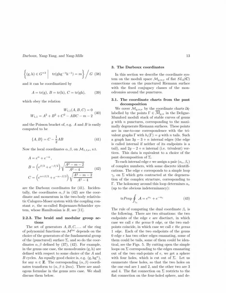
are the Darboux coordinates for (41). Inciden-tally, the coordinates α, β in (42) are the coor-dinate and momentum in the two-body relativis-tic Calogero-Moser system with the coupling con-stant ν, the so-called Rujsenaars-Schneider sys-tem, whose Hamiltonian is B, see [11].

2.2.3. The braid and modular group ac-

tions

The set of generators A,B,C, . . . of the ringof polynomial functions on Mloc depends on thechoice of the generators of the fundamental groupof the (punctured) surface Σ, and so do the coor-dinates α, β defined by (37), (42). For example,in the genus one case, the monodromies (g, h) aredefined with respect to some choice of the A andB cycles. An equally good choice is, e.g. (g, hgn),for any n ∈ Z. The corresponding (α, β) coordi-nates transform to (α, β ± 2nα). There are anal-ogous formulae in the genus zero case. We shalldiscuss them below.

3. The Darboux coordinates

In this section we describe the coordinate sys-tem on the moduli space Mg,n;ν of flat SL2(C)connections on the punctured Riemann surfacewith the fixed conjugacy classes of the mon-odromies around the punctures.

3.1. The coordinate charts from the pant

decomposition

We cover Mg,n;ν by the coordinate charts UΓ

labelled by the points Γ ∈ Mg,n in the Deligne-Mumford moduli stack of stable curves of genusg with n punctures, corresponding to the maxi-mally degenerate Riemann surfaces. These pointsare in one-to-one correspondence with the tri-valent graphs Γ with b1(Γ) = g with n tails. Sucha graph has 3g − 3 + n internal edges (the edgeis called internal if neither of its endpoints is atail), and 2g − 2 + n internal (i.e. trivalent) ver-tices. This data is equivalent to a choice of thepant decomposition of Σ.To each internal edge e we assign a pair (αe, βe)

of complex numbers, with some discrete identifi-cations. The edge e corresponds to a simple loopγe on Σ which gets contracted at the degenera-tion of the complex structure, corresponding toΓ. The holonomy around this loop determines αe

(up to the obvious indeterminancy):

trP exp

∮

γe

A = eαe + e−αe (43)

The rule of computing the dual coordinate βe isthe following. There are two situations: the twoendpoints of the edge e are disctinct, in whichcase we call e the genus 0 edge, or the two end-points coincide, in which case we call e the genus1 edge. Each of the two endpoints of the genus0 edge e has two other edges emanating, some ofthem could be tails, some of them could be iden-tical, see the Figs. 5. By cutting open the simpleloops on Σ corresponding to the edges emanatingout of the two end-points of e, we get a spherewith four holes, which is cut out of Σ. Let usenumerate these holes, so that the two holes onthe one end are 1 and 2, and the other two are 3and 4. The flat connection on Σ restricts to theflat connection on the four-holed sphere, and de-


Figure 5. The genus 0 edges

Figure 6. The genus 1 edges

fines the invariant functions, A, B, C, as in (32).Then, α and β defined by (37) are the αe and βe,corresponding to the edge e. We could have mis-labeled the two edges emanating from one end ofe. This would have replaced βe by βe ± αe.For the genus 1 edge the situation is similar,

except that there is only one simple loop to cut,which extracts out of Σ a one-holed torus. The re-striction of flat connection onto this torus definesthe invariant functions A,B and C as in (39).Then, using (42) we define the (αe, βe) pair forthe local genus 1 edge.

3.1.1. A little bit of geometry

In this section we shall review some stan-dard facts about the geometry of symplectic sur-faces, the complexification of the Euclidean andLobachevsky geometries, and the spaces of poly-gons.We shall construct a complex version of the

spherical and hyperbolic geometry of polygons inM3 = S3 orM3 = H3. It turns out that the Dar-boux coordinates α and β of the previous consid-erations can be viewed as describing the geometryof quadrangles in the M3

C ≈ G. The justificationfor the somewhat involved analysis of the simplegeometry is that the generalization of the Dar-boux coordinates for n > 4 turns out to describethe n-gons in G.Let us view the group G as the affine hypersur-

face in the four dimensional complex vector spaceV = C4 = Mat2(C) of the 2×2 complex matrices.We endow V with the complex metric:

〈X,Y 〉 =1

2(tr(XY )− trXtrY ) (44)

which is clearly invariant under the action of thegroup G×G:

X 7→ (gL, gR) ·X = gLXg−1R (45)

The group G is realized as a hypersurface:

〈g, g〉 = 1 ⇔ g ∈ G (46)

The metric (44) induces a complex metric on G:

ds2G =1

2trdg2−

1

2(trdg)2 = −

1

2tr(

g−1dg)2

(47)


where we used the identity in G ⊂ Mat2×2(C):

g + g−1 = trg · 1 (48)

The volume form dg11dg12dg21dg22 on V induces

the volume form volG = 18π2 tr

(

g−1dg)3

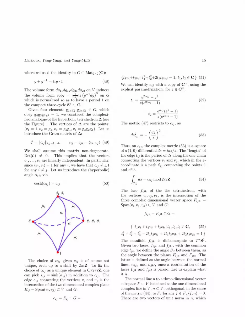
on Gwhich is normalized so as to have a period 1 onthe compact three-cycle S3 ⊂ G.Given four elements g1, g2, g3, g4 ∈ G, which

obey g4g3g2g1 = 1, we construct the complexi-fied analogue of the hyperbolic tetrahedron ∆ (seethe Figure) . The vertices of ∆ are the points:(v1 = 1, v2 = g1, v3 = g2g1, v4 = g3g2g1). Let usintroduce the Gram matrix of ∆:

C = ‖cij‖i,j=1...4, cij = cji = 〈vi, vj〉 (49)

We shall assume this matrix non-degenerate,Det(C) 6= 0. This implies that the vectorsv1, . . . , v4 are linearly independent. In particular,since 〈vi, vi〉 = 1 for any i, we have that cij 6= ±1for any i 6= j. Let us introduce the (hyperbolic)angle αij , via

cosh(αij) = cij (50)

The choice of αij given cij is of course notunique, even up to a shift by 2πiZ. To fix thechoice of αij as a unique element in C/2πiZ, onecan pick sij = sinh(αij) in addition to cij . Theedge eij connecting the vertices vi and vj is theintersection of the two dimensional complex planeEij = Span(vi, vj) ⊂ V and G:

eij = Eij ∩G =

t1vi+t2vj | t21+t

22+2t1t2cij = 1, t1, t2 ∈ C (51)

We can identify eij with a copy of C×, using theexplicit parametrization: for z ∈ C×,

t1 =e2αij − z2

z(e2αij − 1)(52)

t2 =eαij (z2 − 1)

z(e2αij − 1)

The metric (47) restricts to eij , as

ds2eij = −

(

dz

z

)2

. (53)

Thus, on eij , the complex metric (53) is a squareof a (1, 0)-differential ds = idz/z. The ”length” ofthe edge lij is the period of ds along the one-chainconnecting the vertices vi and vj , which in the z-coordinate is a path Cij connecting the points 1and eαij .

∫

Cij

ds = αij mod2πiZ (54)

The face fijk of the the tetrahedron, withthe vertices vi, vj , vk, is the intersection of thethree complex dimensional vector space Fijk =Span(vi, vj , vk) ⊂ V and G:

fijk = Fijk ∩G =

t1vi + t2vj + t3vk | t1, t2, t3 ∈ C, (55)

t21 + t22 + t23 + 2t1t2cij + 2t1t3cik + 2t2t3cjk = 1

The manifold fijk is diffeomorphic to T ∗S2.Given two faces, fijk and fjkl, with the commonedge ljk, we define the angle βil between them, asthe angle between the planes Fijk and Fjkl. Thelatter is defined as the angle between the normallines, nijk and njkl, once a coorientation of thefaces fijk and fjkl is picked. Let us explain whatit is.The normal line n to a three-dimensional vector

subspace F ⊂ V is defined as the one-dimensionalcomplex line in V , n ⊂ V , orthogonal, in the senseof the metric (44), to F : for any f ∈ F , 〈f, n〉 = 0.There are two vectors of unit norm in n, which


differ by a sign. A choice of one of these two unitnorm vectors is the choice of the coorientation ofF in V . We shall denote the unit norm vector inn by the same letter n.

Once the coorientation is fixed, the angle is de-fined via:

cosh(βil) = 〈nijk, njkl〉 (56)

A change of coorientation of one of the two planeschanges the angle β to πi− β. This ambiguity isin addition to the ambiguity β 7→ −β, and β 7→β + 2πik, k ∈ Z.

Let us now make the following useful obser-vation (cf. [66]): Let LC be the matrix of thehyperbolic cosines of the dihedral angles βij :

LC = ‖cosh(βij)‖4i,j=1 (57)

Then:

LC =1

√

C∨d

C∨ 1√

C∨d

(58)

where C∨ = Det(C)C−1 is the matrix of the mi-nors of C, and C∨

d is its diagonal part, e.g.

cosh(βij) =C∨ij

√

C∨iiC

∨jj

(59)

The coorientation ambiguity in the definition ofthe β angles is the reason for the square root am-biguity in (59). To demonstrate (59) let us notethat the vectors

v∨i =

4∑

j=1

C∨ijvj (60)

obey

〈v∨i , vk〉 = Det(C)δik (61)

and

〈v∨i , v∨j 〉 = Det(C)C∨

ij (62)

Therefore, we can choose the normal vectors tobe

nijk = εijklv∨l

√

Det(C)C∨ll

(63)

from which (59) follows immediately.We can interpret the matrix LC as the Gram

matrix of the dual tetrahedron

L∆ ⊂ LG = PGL(2,C)

whose vertices are the normals to the faces of ∆up to a choice of orientation. Now let us returnto the study of the moduli space M0,4;~ν . We as-sign to every point in a finite cover of M0,4;ν atetrahedron (perhaps, degenerate) in G, up to theaction of the group G×G of the isometries of themetric (44). The vertices of the tetrahedron canbe chosen to be:

(v1, v2, v3, v4) = (1, g1, g2g1, g3g2g1) (64)

The corresponding Gram matrix is readily com-puted:

C =1

2

2 m1 A m4

m1 2 m2 BA m2 2 m3

m4 B m3 2

(65)

which gives

−4C∨22 = c34(A), −4C∨

44 = c12(A),

8C∨24 = B(A2 − 4)−A(m1m3 +m2m4) (66)

+2(m2m3 +m1m4)

3.1.2. The Darboux coordinates for M0,4;ν

We are now in position to state the definitionof our coordinates in the case of the 4-puncturedsphere. There are three points of the maximaldegeneration of the complex structure which cor-respond to the s, t, and u channel tree scatteringgraphs. These degenerations collide the points1− 2, 3− 4, the points 1− 4, 2− 3 and the points1− 3, 2− 4, respectively, see the Fig. 7. We coverthe moduli space of flat connections by three co-ordinate charts. Each chart Ui has the coordi-nates (αi, βi), where i = s, t, u. The relation of(αs, βs), and (αt, βt) coordinates to the flat con-nection on the 4-punctured sphere with the basicholonomies g1,2,3 is depicted in the Fig. 8. The


Figure 7. The degeneration points in M0,4

Figure 8. The (αs, βs) and (αt, βt) coordinates

Figure 9. From the tree graph to the polygontriangulated by the diagonals

coordinates (αu, βu) are obtained by applying themodular group action:

(g1, g2, g3) 7→(

g2, g2g1g−12 , g3

)

(67)

which maps the tetrahedron with the vertices(1, g1, g2g1, g3g2g1) to the tetrahedron with thevertices (1, g2, g2g1, g3g2g1).

3.1.3. The Darboux coordinates for M0,n;ν

are defined analogously, and can be givena geometric interpretation in terms of thegeometry of a polygon with the vertices(1, g1, g2g1, . . . , gn−1gn−2 . . . g2g1) which is cut byn − 3 diagonals onto n − 2 (complexified hyper-bolic or spherical) triangles. The coordinate αi,i = 1, . . . , n− 3 is the hyperbolic length of the di-agonal di, while the coordinate βi is the dihedralangle between the two adjacent triangles, whichshare the common edge di, see Fig. 9 for the caseof n = 7.

3.1.4. The coordinate transformations

It is interesting to look at the coordinate trans-formations which glue our coordinate systems onthe overlaps UΓ ∩ UΓ′ . It suffices to discuss theoverlaps where the two graphs Γ and Γ′ differ inexactly one genus 0 edge, or in exactly one genus1 edge. In the first case the basic transformationis (αs, βs) 7→ (αt, βt) in the case of M0,4;ν. Re-call that the canonical transformations, i.e. thetransformations preserving the symplectic form,are generated by a function, the so-called gener-


ating function: S0,4(αs, αt;~ν), such that:

βs =∂S0,4

∂αs, βt =

∂S0,4

∂αt(68)

Using the formulae of [67] one can easily de-rive that S0,4(αs, αt, ν1, ν2, ν3, ν4) is the hyper-bolic volume of the tetrahedron L∆, which is dualto the tetrahedron ∆ (Fig. 8) whose edges havethe lengths

αs, αt, µ1, µ2, µ3, µ4 .

where µk = 2πiνk. The explicit formula can bederived using [66] (see also [67], [68], [69], [70]):Let

V1 = αs + µ1 + µ2

V2 = αs + µ3 + µ4

V3 = αt + µ1 + µ4

V4 = αt + µ2 + µ3

H1 = µ1 + µ2 + µ3 + µ4

H2 = αs + αt + µ1 + µ3

H3 = αs + αt + µ2 + µ4

H4 = 0

Then:

S0,4(αs, αt, ~ν) =

4∑

a=1

[

Li2(

w+eVa)

− Li2(

w−eVa)

−Li2(

w+eHa)

+ Li2(

w−eHa)]

(69)

where w± are the two different roots of the(quadratic in w) equation:

4∏

a=1

(1− weVa) =4∏

a=1

(1− weHa) (70)

For the genus 1 edge the formalism is similar andwe shall not present it here.

3.1.5. The Hamiltonian flows and bending

Fix Γ and consider the Hamiltonian flows gen-erated by the Poisson-commuting functions Ae =eαe + e−αe , for all edges e. These flows generate

a complexified integrable system. Its real slicesinclude the Fenchel-Nielsen twistings on the Te-ichmuller space and Goldman flows [65] on themoduli space of SU(2) flat connections.In our coordinates the flow generated by αe acts

very simply: βe is shifted while αe′ ’s and βe′ fore′ 6= e are unchanged. It is amusing to see theaction of this flow on the monodromy data of aflat connection A. We shall do it for the g =0, n = 4 case.Thus, let us take α as a Hamiltonian, and let

us try to find out what is the Hamiltonian flowUt generated by it. Of course, in the (α, β) co-ordinates this is trivial: Ut : (α, β) 7→ (α, β +t). Let us calculate the effect of this trans-formation on the flat connection A, which weparametrize by the gauge equivalence class of thetriple (g1, g2, g3, g4), with g4g3g2g1 = 1. Weclaim:

Ut : (g1, g2, g3, g4) 7→ (g1, g2, e−tJg3e

tJ , e−tJg4etJ)

(71)

where we have introduced a normalized Lie al-gebra element J , a traceless 2 × 2 matrix withthe eigenvalues ± 1

2 , trJ = 0, trJ2 = 12 , such

that:

g2g1 = e2αJ . (72)

Indeed, let

Bt = tr(g2e−tJg3e

tJ ) (73)

Using the identity for the SL2 matrices:

e2tαJ =sinh (1− t)α

sinhα+

sinh tα

sinhαe2αJ .

we can easily compute:

Bt(A2 − 4) + 2 (m2m3 +m1m4)−

A (m1m3 +m2m4) =

2 cosh(β + t)√

c12(A)c34(A)

which establishes (71).In the general g = 0 case, the Hamiltonian flow

generated by αe corresponding to the edge e, andthe corresponding diagonal de (as in the Fig. 9),


has a very simple geometric interpretation (mod-ulo the complexification): one simply bends thehyperbolic n-gon along the diagonal de. The an-gle of bending corresponding to Ut is equal to t.This is a complexified version of the constructionsin [63], [71], [72], [73].

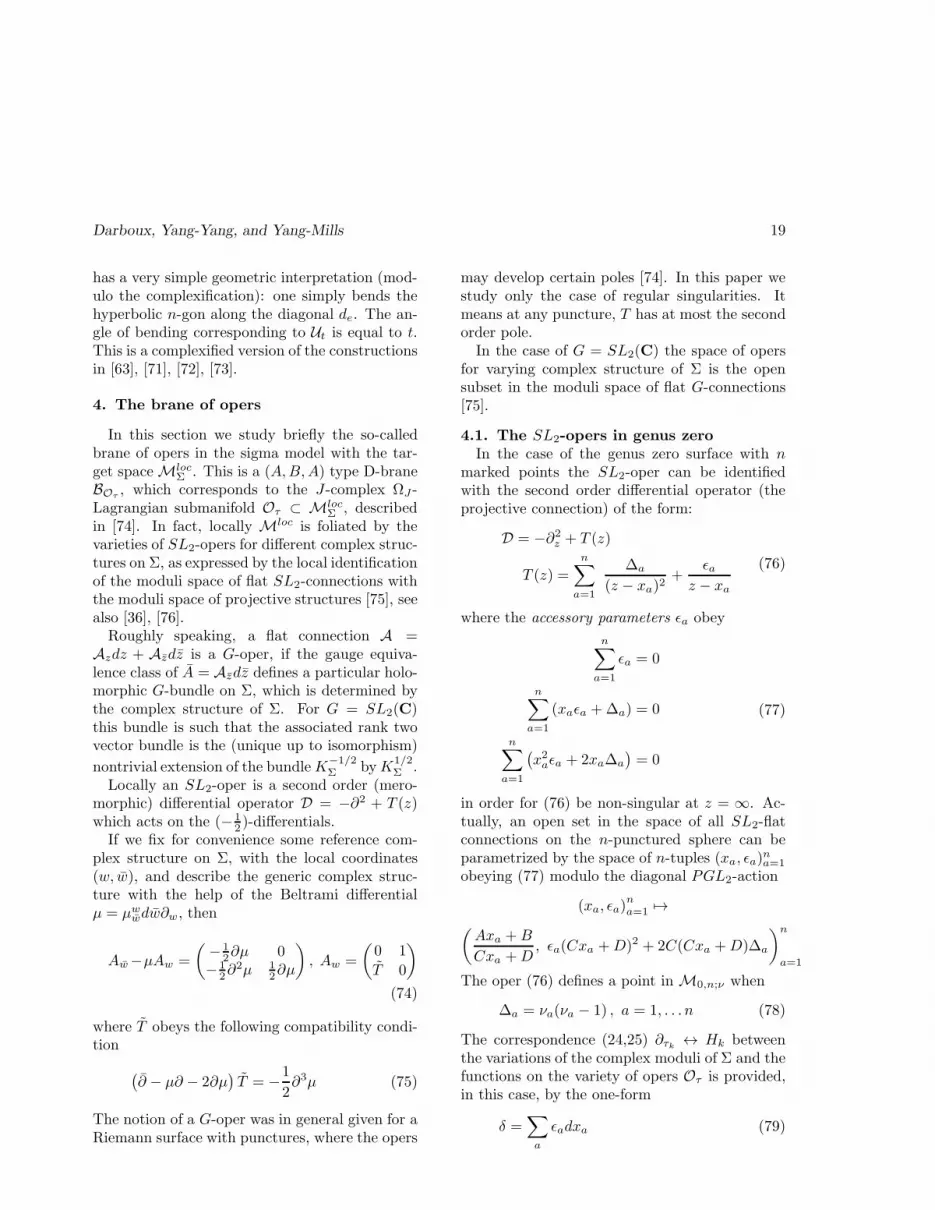
4. The brane of opers

In this section we study briefly the so-calledbrane of opers in the sigma model with the tar-get space Mloc

Σ . This is a (A,B,A) type D-braneBOτ

, which corresponds to the J-complex ΩJ -Lagrangian submanifold Oτ ⊂ Mloc

Σ , describedin [74]. In fact, locally Mloc is foliated by thevarieties of SL2-opers for different complex struc-tures on Σ, as expressed by the local identificationof the moduli space of flat SL2-connections withthe moduli space of projective structures [75], seealso [36], [76].Roughly speaking, a flat connection A =

Azdz + Azdz is a G-oper, if the gauge equiva-lence class of A = Azdz defines a particular holo-morphic G-bundle on Σ, which is determined bythe complex structure of Σ. For G = SL2(C)this bundle is such that the associated rank twovector bundle is the (unique up to isomorphism)

nontrivial extension of the bundleK−1/2Σ byK

1/2Σ .

Locally an SL2-oper is a second order (mero-morphic) differential operator D = −∂2 + T (z)which acts on the (− 1

2 )-differentials.If we fix for convenience some reference com-

plex structure on Σ, with the local coordinates(w, w), and describe the generic complex struc-ture with the help of the Beltrami differentialµ = µw

wdw∂w, then

Aw−µAw =

(

− 12∂µ 0

− 12∂

2µ 12∂µ

)

, Aw =

(

0 1

T 0

)

(74)

where T obeys the following compatibility condi-tion

(

∂ − µ∂ − 2∂µ)

T = −1

2∂3µ (75)

The notion of a G-oper was in general given for aRiemann surface with punctures, where the opers

may develop certain poles [74]. In this paper westudy only the case of regular singularities. Itmeans at any puncture, T has at most the secondorder pole.In the case of G = SL2(C) the space of opers

for varying complex structure of Σ is the opensubset in the moduli space of flat G-connections[75].

4.1. The SL2-opers in genus zero

In the case of the genus zero surface with nmarked points the SL2-oper can be identifiedwith the second order differential operator (theprojective connection) of the form:

D = −∂2z + T (z)

T (z) =

n∑

a=1

∆a

(z − xa)2+

ǫaz − xa

(76)

where the accessory parameters ǫa obey

n∑

a=1

ǫa = 0

n∑

a=1

(xaǫa +∆a) = 0

n∑

a=1

(

x2aǫa + 2xa∆a

)

= 0

(77)

in order for (76) be non-singular at z = ∞. Ac-tually, an open set in the space of all SL2-flatconnections on the n-punctured sphere can beparametrized by the space of n-tuples (xa, ǫa)

na=1

obeying (77) modulo the diagonal PGL2-action

(xa, ǫa)na=1 7→

(

Axa +B

Cxa +D, ǫa(Cxa +D)2 + 2C(Cxa +D)∆a

)n

a=1

The oper (76) defines a point in M0,n;ν when

∆a = νa(νa − 1) , a = 1, . . . n (78)

The correspondence (24,25) ∂τk ↔ Hk betweenthe variations of the complex moduli of Σ and thefunctions on the variety of opers Oτ is provided,in this case, by the one-form

δ =∑

a

ǫadxa (79)


Once a global coordinate z on the sphere is fixed,e.g. by requiring three out of n punctures to beat 0, 1,∞, the one-form δ becomes well-defined inthe tangent space to M0,n.

4.2. The SL2-opers in genus one

We can also describe quite explicitly the spaceof opers on an elliptic curve Eτ with regular sin-gularities at the points x1, . . . , xn ∈ Eτ :

D = −∂2z + T (z)

T (z) = u+

n∑

a=1

∆a℘(z − xa) + ǫaζ(z − xa)(80)

where∑

a ǫa = 0, u is a constant, and we usedthe Weierstrass ζ and ℘ = ζ′ functions. The cor-respondence ∂τk ↔ Hk is now represented by theone-form

δ =∑

a

ǫadxa + udτ (81)

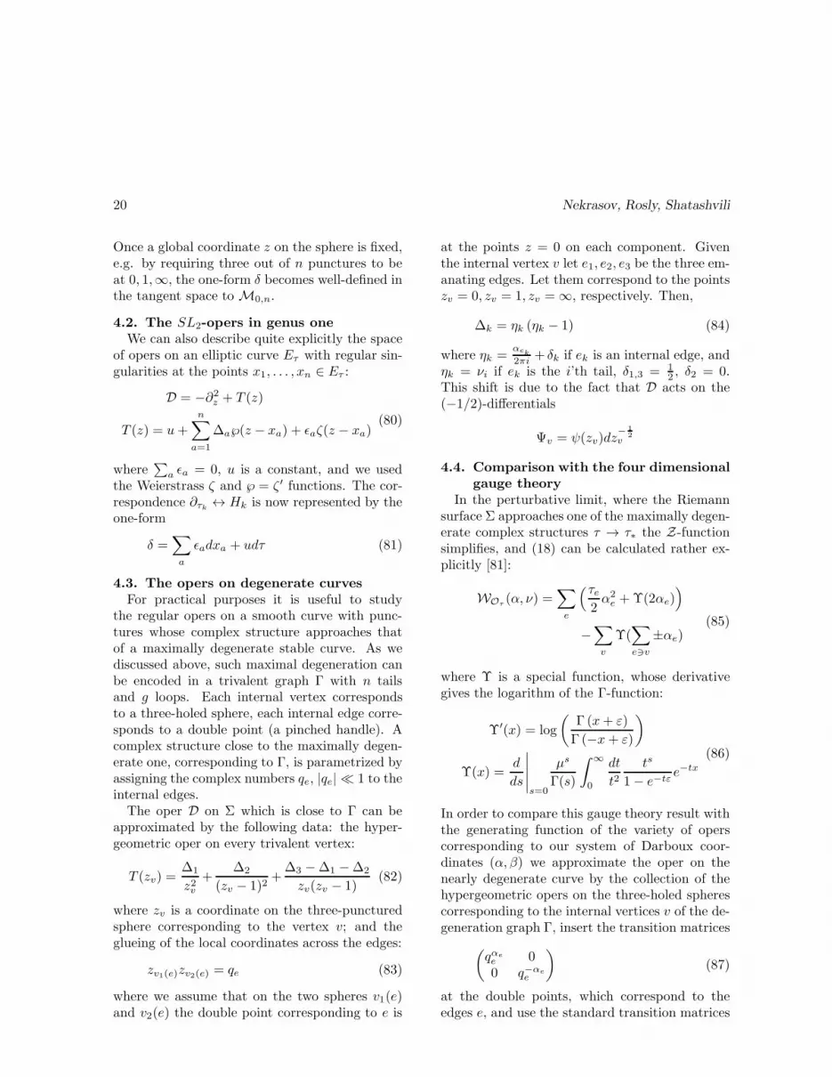
4.3. The opers on degenerate curves

For practical purposes it is useful to studythe regular opers on a smooth curve with punc-tures whose complex structure approaches thatof a maximally degenerate stable curve. As wediscussed above, such maximal degeneration canbe encoded in a trivalent graph Γ with n tailsand g loops. Each internal vertex correspondsto a three-holed sphere, each internal edge corre-sponds to a double point (a pinched handle). Acomplex structure close to the maximally degen-erate one, corresponding to Γ, is parametrized byassigning the complex numbers qe, |qe| ≪ 1 to theinternal edges.

The oper D on Σ which is close to Γ can beapproximated by the following data: the hyper-geometric oper on every trivalent vertex:

T (zv) =∆1

z2v+

∆2

(zv − 1)2+∆3 −∆1 −∆2

zv(zv − 1)(82)

where zv is a coordinate on the three-puncturedsphere corresponding to the vertex v; and theglueing of the local coordinates across the edges:

zv1(e)zv2(e) = qe (83)

where we assume that on the two spheres v1(e)and v2(e) the double point corresponding to e is

at the points z = 0 on each component. Giventhe internal vertex v let e1, e2, e3 be the three em-anating edges. Let them correspond to the pointszv = 0, zv = 1, zv = ∞, respectively. Then,

∆k = ηk (ηk − 1) (84)

where ηk =αek

2πi + δk if ek is an internal edge, andηk = νi if ek is the i’th tail, δ1,3 = 1

2 , δ2 = 0.This shift is due to the fact that D acts on the(−1/2)-differentials

Ψv = ψ(zv)dz− 1

2v

4.4. Comparison with the four dimensional

gauge theory

In the perturbative limit, where the Riemannsurface Σ approaches one of the maximally degen-erate complex structures τ → τ∗ the Z-functionsimplifies, and (18) can be calculated rather ex-plicitly [81]:

WOτ(α, ν) =

∑

e

(τe2α2e +Υ(2αe)

)

−∑

v

Υ(∑

e∋v

±αe)(85)

where Υ is a special function, whose derivativegives the logarithm of the Γ-function:

Υ′(x) = log

(

Γ (x+ ε)

Γ (−x+ ε)

)

Υ(x) =d

ds

∣

∣

∣

∣

∣

s=0

µs

Γ(s)

∫ ∞

0

dt

t2ts

1− e−tεe−tx

(86)

In order to compare this gauge theory result withthe generating function of the variety of operscorresponding to our system of Darboux coor-dinates (α, β) we approximate the oper on thenearly degenerate curve by the collection of thehypergeometric opers on the three-holed spherescorresponding to the internal vertices v of the de-generation graph Γ, insert the transition matrices

(

qαee 00 q−αe

e

)

(87)

at the double points, which correspond to theedges e, and use the standard transition matrices


for the solutions of the hypergeometric equation,to compute the monodromy matrices g1, g2, g3, g4for each genus zero edge, and the matrices g, h foreach genus one edge.One can also include the e2πiτe-corrections by

the usual quantum mechanical perturbation the-ory and verify the agreement with the instantoncalculations on the gauge theory side. We haveperformed these checks for low instanton numbersfor the two basic cases: SU(2) Nf = 4 theory(which corresponds to M0,4) and for the SU(2)N = 2∗ theory (which corresponds to M1,1).

4.5. The topological brane

The study of the separation of variables (pro-posed by E. Sklyanin [82]) for the quantumGaudin system, which is essentially the genus zerocase of the Hitchin system, suggests the followingdefinition of this second brane. We assume thatthe νk parameters are generic (and definitely nothalf-integral, as in [83]).Then we define a subvariety Lγ for any pair

γ = (Γ, or) which consists of the degenerationgraph Γ together with the choice of orientationor. For the oriented edge e we define the sources(e) and the target t(e) vertices in the obviousway.The definition of Lγ is the following: For ev-

ery internal genus zero egde e we require αe tobe equal to the sum of ±αe’s or ±νk’s (the signdepends on the orientation) corresponding to thetwo other edges which enter s(e)

αe =∑

e′,t(e′)=s(e)

ηe′ −∑

e′,s(e′)=s(e)

ηe′

where, as before ηe = αe ± δe if e is an internaledge, and ηe = νk if e is the k’th tail.In the coordinate patch UΓ′ the variety Lγ is

described by the generating function, which is asum of dilogarithms, as follows from (69).

5. Further directions and discussion

In this paper we have introduced a systemof holomorphic Darboux coordinates α, β on themoduli space Mloc

Σ of flat SL2(C)-connections ona punctured Riemann surface with fixed conju-gacy classes of the monodromies around the punc-

tures. The main claim about this coordinate sys-tem is the identification of the generating functionof the variety Oτ of SL2-opers with the effectivetwisted superpotential of the four dimensional A1

type Gaiotto theory corresponding to Σ, subjectto the two dimensional Ω-deformation.We also expressed the Yang-Yang function of

the quantum Hitchin system, using our coordi-nate system, as a difference of the generatingfunctions of the variety of opers Oτ , and thesecond Lagrangian submanifold Lγ , which deter-mines the space of states of the quantum Hitchinsystem. We presented a proposal for the construc-tion of Lγ in the genus zero case. We would like tostress that the Yang-Yang function we are talk-ing about here is different from the Yang-Yangfunctions of the finite dimensional Gaudin modelor spin chains, which can be derived by taking acritical level limit of the free field representationof the current algebra conformal blocks [77], [78],[79], [80], as explained in [14], [15], [16].The generating function WOτ

also has otherapplications. For example, it can be identifiedwith the classical conformal block of the Liouvilletheory [84], which makes the relation to the fourdimensional gauge theory natural in view of theconjecture [85]. It also provides the ”holomorphicpart” of the classical Liouville action, which isdiscussed in [33], [34], [86], [36], [87].Since the variety of opers is well-understood

for all Lie groups G, it is urgent to generalizeour Darboux coordinates for the case of generalG. This would allow us to compute the effec-tive twisted superpotentials of the exotic theo-ries which do not have a Lagrangian description(a general A,D,E type (0, 2) theory compacti-fied on a Riemann surface and subject to the Ω-deformation).In order to characterize the conformal blocks

of Liouville and Toda conformal theories, usingthe [85] relation, we need to turn on the genericΩ-deformation, with both ε1, ε2 non-vanishing.It was argued that this would effectively quan-tize the algebras of holomorphic functions onMloc

Σ (G) and MlocΣ (LG), with the deformation

quantization parameters h = ε2/ε1 and 1/h =ε1/ε2, respectively. The Z-function is then a vec-


tor in the representation of AhG × A

1/hLG

, whichcorresponds, quasiclassically, to Oτ . To find thisvector seems like an extremely important prob-lem. For the recent discussion of related problemssee [38], [88], [51], [46].

Finally, let us mention a couple more problemswe left out of this short note.

Our construction of the Darboux coordinates(α, β) and the description of the variety of op-ers Oτ must have an interesting quasiclassicallimit, corresponding to the ε → 0 limit of the Ω-background. In this limit one should recover theSeiberg-Witten geometry of the Hitchin system.

Also, a large mass, weak coupling limit of thegauge theory, as in e.g. [89], leading to the asymp-totically free gauge theory must have a counter-part in our construction. We believe extendingour Darboux coordinates to the case of the mod-uli spaces of flat connections with irregular sin-gularities will play an important role both in theanalysis of the four dimensional gauge theory, andin the extension of the Langlands duality to thecase of the wild ramification [90].

6. Acknowledgements

We are grateful to V. Fock, E. Frenkel,A. Gerasimov, Yu. Neretin, F. Smirnov forvaluable discussions. Research of NN waspartly supported by FASI RF 14.740.11.0347that of AR was partly supported by RFBR-09-02-00393, FASI RF 14.740.11.0347, RFBR-09-01-93106-NCNIL-a, and RF Government Grant-11.G34.31.0023, that of SS by SFI grant08/RFP/MTH1546 and by ESF grant ITGP. Partof the research was done while AR visited IHESin the summer of 2010. NN also thanks IlyaKhrzhanovsky for the opportunity to carry outsome of the research on the project at the ”DAU”Institute in Kharkiv, Ukraine, and to D. Kaledinand A. Losev for discussions.

The main conjecture about the generatingfunction of the variety of opers was announcedby one of the authors at the Simons Center work-shop on ”Perspectives, Open Problems & Appli-cations of Quantum Liouville Theory” (Mar 29-Apr 2, 2010). The results of this paper werealso reported at various seminars and conferences,

in particular, at the Institut Henri Poincare, atthe conferences ”Symmetry, Duality, and Cin-ema” (Jun 2010) and ”Advances in string the-ory, wall crossing, and quaternion-Kahler geom-etry” (Aug 30 - Sept 3, 2010), at the CargeseSummer School ”String Theory: Formal Devel-opments and Applications” (Jun 21-Jul 3, 2010)at the IAS (Princeton) seminar (Oct 29, 2010),at the DESY conference ”From Sigma Models toFour-dimensional QFT”, (Nov 29 - Dec 3, 2010),at the Hebrew Univeristy of Jerusalem IAS 15thMidrasha Mathematicae on Derived Categoriesof Algebro-Geometric Origin and Integrable sys-tems” (Dec 19 - 24, 2010). We thank all the or-ganizers and the audiences for the fruitful atmo-sphere and stimulating questions.

REFERENCES

1. L. D. Faddeev, “The Bethe Ansatz,” SFB-288-70 (1993);

2. C. N. Yang and C. P. Yang, J. Math. Phys.10, 1115 (1969).

3. C. N. Yang and C. P. Yang, Phys. Rev. 150,321 (1966).

4. L. D. Faddeev, E. K. Sklyanin andL. A. Takhtajan, Theor. Math. Phys. 40, 688(1980) [Teor. Mat. Fiz. 40, 194 (1979)].

5. M. Jimbo, T. Miwa, F. Smirnov, ”Hid-den Grassmann Structure in the XXZModel III: Introducing Matsubara direction,”arXiv:0811.0439, J.Phys. A 42 (2009) 304018

6. G. W. Moore, N. Nekrasov and S. Shatashvili,“Integrating over Higgs branches,”Commun. Math. Phys. 209, 97 (2000)[arXiv:hep-th/9712241].

7. A. A. Gerasimov and S. L. Shatashvili,“Higgs bundles, gauge theories and quantumgroups,” Commun. Math. Phys. 277, 323(2008) [arXiv:hep-th/0609024].

8. A. A. Gerasimov and S. L. Shatashvili, “Two-dimensional Gauge Theories and QuantumIntegrable Systems,” arXiv:0711.1472 [hep-th].

9. E. Witten, “Two dimensional gauge theoryrevisited”, arXiv:hep-th/9204083

10. A. Gorsky and N. Nekrasov, “Quantum inte-grable systems of particles as gauge theories,”

http://arxiv.org/abs/0811.0439

http://arxiv.org/abs/hep-th/9712241





Theor. Math. Phys. 100, 874 (1994) [Teor.Mat. Fiz. 100, 97 (1994)].

11. A. Gorsky and N. Nekrasov, “RelativisticCalogero-Moser Model As Gauged WZWTheory,” Nucl. Phys. B 436, 582 (1995)[arXiv:hep-th/9401017].

12. A. Gorsky and N. Nekrasov, “El-liptic Calogero-Moser System FromTwo-Dimensional Current Algebra,”arXiv:hep-th/9401021.

13. A. Gorsky and N. Nekrasov, “Hamilto-nian systems of Calogero type and two-dimensional Yang-Mills theory,” Nucl. Phys.B 414, 213 (1994) [arXiv:hep-th/9304047].

14. N. A. Nekrasov and S. L. Shatashvili, “Su-persymmetric vacua and Bethe ansatz,” Nucl.Phys. Proc. Suppl. 192-193, 91 (2009)[arXiv:0901.4744 [hep-th]].

15. N. Nekrasov and S. Shatashvili, “BetheAnsatz And Supersymmetric Vacua,” AIPConf. Proc. 1134, 154 (2009).

16. N. A. Nekrasov and S. L. Shatashvili,“Quantum integrability and supersymmetricvacua,” Prog. Theor. Phys. Suppl. 177, 105(2009) [arXiv:0901.4748 [hep-th]].

17. N. A. Nekrasov and S. L. Shatashvili, “Quan-tization of Integrable Systems and Four Di-mensional Gauge Theories,” arXiv:0908.4052[hep-th].

18. A. Gorsky, I. Krichever, A. Marshakov, A.Mironov, A. Morozov, “Integrability andSeiberg-Witten exact solution,” Phys. Lett.B355, 466-474 (1995). [hep-th/9505035].

19. E. Martinec and N. Warner, “Integrablesystems and supersymmetric gaugetheory“, ”Nucl.Phys.B459:97-112,1996,arXiv:hep-th/9509161

20. R. Donagi, E. Witten, “Supersymmet-ric Yang-Mills theory and integrable sys-tems,” Nucl. Phys. B460, 299-334 (1996).[hep-th/9510101].

21. R. Y. Donagi, “Seiberg-Witten integrable sys-tems,” [alg-geom/9705010].

22. N. A. Nekrasov, “Seiberg-Witten Pre-potential From Instanton Counting,”Adv. Theor. Math. Phys. 7, 831 (2004)[arXiv:hep-th/0206161].

23. A. Losev, N. Nekrasov and S. L. Shatashvili,

“Testing Seiberg-Witten solution,” InCargese 1997, Strings, branes and dualities,pp. 359-372, [arXiv:hep-th/9801061].

24. A. Losev, N. Nekrasov and S. L. Shatashvili,“Issues in topological gauge the-ory,” Nucl. Phys. B 534, 549 (1998)[arXiv:hep-th/9711108].

25. E. Witten, “Some comments on string dy-namics,” arXiv:hep-th/9507121.

26. A. Strominger, “Open p-branes,” Phys. Lett.B 383, 44 (1996) [arXiv:hep-th/9512059].

27. D. Gaiotto, “N=2 dualities,” arXiv:0904.2715[hep-th].

28. N. Seiberg and E. Witten, “Monopoles, dual-ity and chiral symmetry breaking in N=2 su-persymmetric Nucl. Phys. B 431, 484 (1994)[arXiv:hep-th/9408099].

29. G. W. Moore, N. Nekrasov and S. Shatashvili,“D-particle bound states and generalized in-stantons,” Commun. Math. Phys. 209, 77(2000) [arXiv:hep-th/9803265].

30. E. Witten, “String theory dynamics in variousdimensions,” Nucl. Phys. B 443, 85 (1995)[arXiv:hep-th/9503124].

31. M. Atiyah, R. Bott, “The Yang-Mills Equa-tions Over Riemann Surfaces”, Phil. Trans.R.Soc. London A 308, 523-615 (1982)

32. E. Witten, “Quantum field theory and theJones polynomial,” Commun. Math. Phys.,121 (1989) 351

33. A.M. Polyakov, ”Quantum Gravity in Two-Dimensions,” Mod. Phys. Lett.A2 (1987)893.

34. A. Alekseev and S. L. Shatashvili, Nucl. Phys.B 323, 719 (1989).

35. E. Verlinde, H. Verlinde, “A solution of twodimensional topological quantum gravity”,PUPT-1176, IASSNS-HEP-90/40, April 1990

36. H. Verlinde, Nucl. Phys. B337 (1990) 65237. E. Witten, “(2+1)-Dimensional Gravity as an

Exactly Soluble System,” Nucl. Phys. B 311,46 (1988).

38. L. Chekhov and V. V. Fock, “A quantum Te-ichmuller space,” Theor. Math. Phys. 120,1245 (1999) [Teor. Mat. Fiz. 120, 511 (1999)][arXiv:math/9908165].

39. L. O. Chekhov and V. V. Fock, “Observablesin 3D gravity and geodesic algebras,” Czech.










http://arxiv.org/abs/alg-geom/9705010










http://arxiv.org/abs/math/9908165


J. Phys. 50, 1201 (2000).40. E. Witten, “Three-Dimensional Gravity Re-

visited,” arXiv:0706.3359 [hep-th].41. N. Seiberg and E. Witten, “Gauge dynamics

and compactification to three dimensions,”arXiv:hep-th/9607163.

42. N. Hitchin, “The self-duality equations on aRiemann surface,” Proc. London Math. Soc.(3) 55 (1987) 59–126

43. A. Kapustin and E. Witten, “Electric-magnetic duality and the geometric Lang-lands program,” arXiv:hep-th/0604151.

44. N. Hitchin, “Stable bundles and integrablesystems,” Duke Math. J. 54 (1987) 91–114

45. R. Donagi, “Spectral Covers,”arXiv:alg-geom/9505009

46. N. Nekrasov and E. Witten, “The OmegaDeformation, Branes, Integrability, and Li-ouville Theory,” JHEP 1009, 092 (2010)[arXiv:1002.0888 [hep-th]].

47. D. Gaiotto, E. Witten, ”S-Duality Of Bound-ary Conditions in N = 4 Super Yang-MillsTheory,” arXiv:0807.3720v1 [hep-th]

48. D. Gaiotto, E. Witten, ”SupersymmetricBoundary Conditions in N = 4 Super Yang-Mills Theory,” arXiv:0804.2902v1 [hep-th]

49. A. Beilinson, V. Drinfeld, ”Quantization ofHitchin’s integrable system and Hecke eigen-sheaves”, preprint

50. S. Gukov, E. Witten, ”Branes And Quantiza-tion,” arXiv:0809.0305v2 [hep-th]

51. J. Teschner, ”Quantization of the Hitchinmoduli spaces, Liouville theory, and thegeometric Langlands correspondence I”,arXiv:1005.2846v2 [hep-th]

52. V. Fock, A. Goncharov, ”Moduli spaces oflocal systems and higher Teichmller theory”,Publ. Math. Inst. Hautes Etudes Sci. No. 103(2006), 1-211.

53. D. Gaiotto, G. W. Moore and A. Neitzke,“Wall-crossing, Hitchin Systems, and theWKB Approximation,” arXiv:0907.3987[hep-th].

54. N. Nekrasov, “Holomorphic bundles andmany body systems,” Commun. Math. Phys.180, 587 (1996) [arXiv:hep-th/9503157].

55. R. Donagi, E. Markman, “Spectral curves,algebraically completely integrable Hamil-

tonian systems, and moduli of bundles,”[alg-geom/9507017].

56. A. Kapustin and S. Sethi, “The Higgs branchof impurity theories,” Adv. Theor. Math.Phys. 2, 571 (1998) [arXiv:hep-th/9804027].

57. E. Markman, ”Spectral curves and integrablesystems”, Compositio Math. 93 (1994), no. 3,255-290

58. A. Gorsky, N. Nekrasov and V. Rubtsov,“Hilbert schemes, separated variables, andD-branes,” Commun. Math. Phys. 222, 299(2001) [arXiv:hep-th/9901089].

59. V. V. Fock and A. A. Rosly, “Poisson struc-ture on moduli of flat connections on Rie-mann surfaces and r-matrix,” preprint ITEP-72-92 (1992), AMS Transl. 191, 67 (1999)[arXiv:math/9802054].

60. V. V. Fock and A. A. Rosly, “Flat connectionsand polyubles,” Theor. Math. Phys. 95, 526(1993) [Teor. Mat. Fiz. 95, 228 (1993)].

61. V. V. Fock and A. A. Rosly, “Moduli space offlat connections as a Poisson manifold,” Int.J. Mod. Phys. B 11, 3195 (1997).

62. W. Goldman, “The symplectic nature of thefundamental group on surfaces,” Adv. Math.54, 200-225 (1984)

63. W. Goldman, “Invariant functions on Liegroups and Hamiltonian flows of surfacegroup representations,” Invent. math. 85,263-302 (1986)

64. V.G. Turaev, ”Skein quantization of Poissonalgebras of loops on surfaces”, Ann. Sci. EcoleNorm. Sup. (4) 24 (1991), no. 6, 635704

65. A. N. Tyurin, ”Quantization, Classical andQuantum FIeld Theory and Theta Func-tions”, CRM monograph series, Vol. 21, AMS, 2003.

66. D.A. Derevnin, A.D. Mednykh, A formula forthe volume of a hyperbolic tetrahedron, Russ.Math. Surv. 60 (2), (2005) 346-348

67. L. Schlafli, ”Theorie der vielfachen Konti-nuitat”, In: Gesammelte mathematishe Ab-handlungen, Basel: Birkhauser, 1950.

68. N. I. Lobatschefskij, ”Imaginare Geometrieund ihre Anwendung auf einige Integrale”,Deutsche aubersetzung von H.Liebmann,Leipzig: Teubner, 1904.

69. Yu. Cho, H. Kim, ”On the volume formula for

















hyperbolic tetrahedra”, Discrete and Compu-tational Geometry, 22, 1999, p.347-366.

70. J. Milnor, ”The Schlafli differential equality”in Collected Papers. I. Geometry (Publish orPerish, Houston, TX, 1994), pp. 281-295.

71. M. Kapovich, J. J. Millson, T. Treloar,arXiv:math/9907143

72. A.A. Klyachko, ”Spatial polygons and sta-ble configurations of points in the projectiveline,” Algebraic geometry and its applications(Yaroslavl, 1992), 6784, Aspects Math., E25,Vieweg, Braunschweig, 1994.

73. P. Foth, ”Polygons in Minkowski space andGelfand-Tsetlin for pseudounitary groups,”arXiv:math/0703525

74. A. Beilinson, V. Drinfeld, ”Opers”,math.AG/0501398

75. A. Bilal, I. Kogan, V. Fock, “On the origin ofW-algebras,” CERN-TH.5965/90

76. A. Gerasimov, A. Levin and A. Marshakov,”On W gravity in two-dimensions,” Nucl.Phys. B 360, 537 (1991).

77. A. Gerasimov, A. Morozov, M. Olshanetsky,A. Marshakov and S. L. Shatashvili, “Wess-Zumino-Witten model as a theory of freefields,” Int. J. Mod. Phys. A 5, 2495 (1990),preprints ITEP-89-64, ITEP-89-70, ITEP-89-72, ITEP-89-74, April 1989

78. A.Varchenko, V.Schechtman, ”Integral Rep-resentations of N-Point Conformal Correla-tors in the WZW Model,” Bonn, Max-PlanckInstitute (1989), 1-22.

79. N. Reshetikhin and A. Varchenko, “Quasi-classical asymptotics of solutions to the KZequations,” arXiv:hep-th/9402126.

80. G. Felder and A. Varchenko,arXiv:hep-th/9511120.

81. N. Nekrasov, V. Pestun, to appear82. E. Sklyanin, J. Sov. Math. 47 (1989) 2473-

248883. B. Feigin, E. Frenkel and N. Reshetikhin,

“Gaudin model, Bethe ansatz and cor-relation functions at the critical level,”Commun. Math. Phys. 166, 27 (1994)[arXiv:hep-th/9402022].

84. A. B. Zamolodchikov and A. B. Zamolod-chikov, ”Structure constants and conformalbootstrap in Liouville field theory”, Nucl.

Phys. B477 (1996) 577, hep-th/950613685. L. F. Alday, D. Gaiotto and Y. Tachikawa,

“Liouville Correlation Functions from Four-dimensional Gauge Theories,” Lett. Math.Phys. 91, 167 (2010) [arXiv:0906.3219 [hep-th]].

86. L.A. Takhtajan, P.G. Zograf, ”On Liouvilleequation, accessory parameters and the geom-etry of Teichmuller space for Riemann surfaceof genus 0”, Math. USSR Sbornik 60 (1988)143

87. E. Aldrovandi, L.A. Takhtajan, ”GeneratingFunctional in CFT on Riemann Surfaces II:Homological Aspects”, arXiv:math/0006147

88. L. F. Alday, D. Gaiotto, S. Gukov,Y. Tachikawa and H. Verlinde, JHEP 1001,113 (2010) [arXiv:0909.0945 [hep-th]].

89. D. Gaiotto, “Asymptotically free N=2theories and irregular conformal blocks,”arXiv:0908.0307 [hep-th].

90. E. Witten, “Gauge Theory And Wild Rami-fication,” arXiv:0710.0631 [hep-th].













Documents

Darboux coordinates, Yang-Yang functional, and gauge theory