Embed Size (px)
Citation preview
INCLUSION OF FATIGUE EFFECTS IN HUMAN RELIABILITY ANALYSIS
By
Candice D. Griffith
Dissertation
Submitted to the Faculty of the
Graduate School of Vanderbilt University
in partial fulfillment of the requirements
for the degree of
DOCTOR OF PHILOSOPHY
in
Interdisciplinary Studies: Human Reliability in Engineering Systems
May, 2013
Nashville, Tennessee
Approved by:
Professor Sankaran Mahadevan
Professor Mark Abkowitz
Professor Julie Adams
Professor Mark Lipsey
Professor Matthew Weinger
ii
Copyright © 2013 by Candice D. Griffith
All Rights Reserved

iii
To George, my favorite feline helper

iv
ACKNOWLEDGMENTS
I would like to acknowledge several people and organizations that have made this
research possible. I especially thank Dr. Mahadevan for his patience and support as my
dissertation committee chair and research advisor; and for the hours of sleep deprivation
he accrued reading about sleep deprivation. I would also like to thank my other
committee members: Dr. Mark Abkowitz, Dr. Julie Adams, Dr. Matthew Weinger, and
Dr. Mark Lipsey for their time and contributions.
This research was sponsored in part by a graduate fellowship funded by the
National Science Foundation (NSF) IGERT program at Vanderbilt University and by
Idaho National Laboratory’s Human Factors, Instrumentation, and Control Systems
Department through the Idaho National Laboratory Educational Programs. I am grateful
for the guidance of Dr. Bruce Hallbert and Dr. Harold Blackman of Idaho National
Laboratory during the grant period and additional research visits. I would also like to
acknowledge Jeffrey Joe and Dr. Ron Boring of Idaho National Laboratory for their
friendship and guidance throughout this research.
I had the opportunity to participate in an internship at the Nuclear Regulatory
Commission (NRC) and to work in my area of research. At the NRC, I would like to
thank Dr. J. Persensky, and especially, Dr. Erasmia Lois for her support and guidance.
I am grateful for the support of the students in the reliability and risk engineering
program and the support staff of the Department of Civil and Environmental Engineering
at Vanderbilt. Special thanks to Dr. Janey Smith Camp for her help and encouragement,

v
and to Karen Page, Dr. Robert Guratzsch, and Dr. Ned Mitchell for helping make this
process fun. I am grateful to my family and friends for their continued support
throughout my graduate career. I am especially thankful to my mother for her
proofreading, my brother’s printing and mailing services, and to my father for his support
and Tuesday phone calls. Finally, I would like to thank George, for being the best furball
ever.
vi
TABLE OF CONTENTS
Page
DEDICATION ............................................................................................................. iii ACKNOWLEDGMENTS ........................................................................................... iv LIST OF FIGURES ..................................................................................................... ix LIST OF TABLES ..................................................................................................... xiii ABBREVIATIONS .................................................................................................... xx Chapter I. INTRODUCTION ................................................................................................ 1
Background ...................................................................................................... 1 Research Objectives ......................................................................................... 6 Organization of the Dissertation ....................................................................... 7
II. FATIGUE RESEARCH AND HRA METHODS ............................................... 9
Fatigue ................................................................................................................ 9
Difficulties in Defining Fatigue .................................................................... 16 Measurement of Fatigue ............................................................................... 18 Measurement of Sleep Deprivation Effects on Performance ........................ 21
Probabilistic Risk Assessment (PRA) .............................................................. 26 Human Reliability Analysis (HRA) ................................................................. 29
THERP .......................................................................................................... 32 ATHEANA ................................................................................................... 35 SPAR-H ........................................................................................................ 37 PSFs in SPAR-H ........................................................................................... 38 Limitations in Current HRA Methods .......................................................... 40 Inclusion of Fatigue in HRA Methods .......................................................... 41
Summary .......................................................................................................... 43
III. SYNTHESIS OF SLEEP DEPRIVATION STUDIES ..................................... 44
Background on Meta-Analysis ....................................................................... 44 Procedure for Meta-Analysis .......................................................................... 46 Equations of Meta-Analysis ........................................................................... 47
Shortcomings of Meta-Analysis ................................................................. 50
vii
Variations among Sleep Deprivation Studies ............................................. 51 IV. RESEARCH METHODOLOGY ....................................................................... 58
Data Collection ............................................................................................... 58 Coding Applications ....................................................................................... 61
Data Resources............................................................................................ 61 Study Selection ........................................................................................... 62 Coding of Study Information ...................................................................... 64 Study Descriptors ........................................................................................ 65 Sample Descriptors ..................................................................................... 65 Experimental Conditions ............................................................................ 66 Task Characteristics .................................................................................... 68 Statistical Data ............................................................................................ 69 Data Collected ............................................................................................. 71
Data Analysis ................................................................................................. 77 Data Analyzed ............................................................................................. 78 Analysis Methodology ................................................................................ 79
Difference between Mean Values .......................................................... 79 Percentage Change ............................................................................... 80 Effect Size and Reliability Index Calculations ...................................... 81 Linear Regression ................................................................................. 83
PSF Derivation ............................................................................................ 84 Uncertainty Analysis ...................................................................................... 87 Summary of Methodology .............................................................................. 91
V. RESULTS........................................................................................................... 93
Resulting Data ................................................................................................ 93 Data on Number of Lapses ............................................................................. 98
Quantitative Effect of Sleep Deprivation on Number of Lapses ................ 98 Linear Regression for Number of Lapses ................................................. 105 Derivation of Probability Ratios for Number of Lapses ........................... 109
Uncertainty Analysis of Probability Ratios for Number of Lapses .............. 119 Data on Reaction Time ................................................................................. 122
Quantitative Effect of Sleep Deprivation on Reaction Time .................... 123 Reaction Time Regression ........................................................................ 131 Predictive Modeling of Reaction Time vs. Hours of Wakefulness .......... 137 Derivation of Probability Ratios for Reaction Time ................................. 143
Uncertainty Analysis of Probability Ratios for Reaction Time ................... 151 Data on Accuracy ......................................................................................... 154
Quantitative Effect of Sleep Deprivation on Accuracy ............................ 155 Sensitivity to Normal Assumption ............................................................... 157 Inter-rater Reliability .................................................................................... 158 Summary ...................................................................................................... 161
viii
VI. SUMMARY AND CONCLUSIONS .............................................................. 163
Summary of Accomplishments .................................................................... 163 Research Assumptions: ................................................................................ 165 Summary of Results ..................................................................................... 166 Practical Application .................................................................................... 169 Future Directions .......................................................................................... 173
BIBLIOGRAPHY ..................................................................................................... 175 Appendix A INTERESTING FATIGUE FACTS ............................................................... 196 B FATIGUE ACCIDENTS ................................................................................ 198 C IMPACT FACTOR OF JOURNALS ............................................................. 204 D ACCURACY ANALYSIS RESULTS............................................................ 206
Data on Accuracy ............................................................................................... 206 Data on Number Correct .................................................................................... 207 Data on Percentage Correct (% Correct) ............................................................ 212 Data on Number of Errors (# Errors) ................................................................. 219 Data on Percentage of Errors (% Errors) ............................................................ 225 Data on False Positives (False +) ....................................................................... 230 Summary and Conclusion for Accuracy Data .................................................... 235
E META-ANALYSIS CODING DATA ............................................................ 238 F INTER-RATER RELIABILITY DATA ......................................................... 291 G INITIAL SEARCH RESULTS (i.e., 600 STUDIES) ..................................... 294
ix
LIST OF FIGURES
Page
Figure 1: Fatigue Model...................................................................................................... 4
Figure 2: Fatigue as a Bucket (Grandjean, 1968) ............................................................. 17
Figure 3: Hours of Wakefulness Compared to BAC% ..................................................... 26
Figure 4: HRA Three-Step Process (INL HRA Course, 2004) ........................................ 30
Figure 5: Event-Tree for Two Tasks (A, B): Both Completed Correctly ........................ 34
Figure 6: Event-Tree for Two Tasks (A, B): Either One Completed Correctly ............... 34
Figure 7: Yerkes-Dodson Law Inverted U-graph (Yerkes and Dodson, 1908) ................ 40
Figure 8: Meta-Analysis Procedure Diagram ................................................................... 46
Figure 9: Normal Probability Distribution with Threshold Value (k) .............................. 85
Figure 10: Differences between the Means for Number of Lapses .................................. 99
Figure 11: Percentage Change for Number of Lapses .................................................... 101
Figure 12: Percentage Change for Number of Lapses (Outliers > 900% Removed)...... 102
Figure 13: ES and β for Number of Lapses .................................................................... 103
Figure 14: Probability P(T > C) for Number of Lapses .................................................. 104
Figure 15: Probability Ratios P(T>C)/0.5 for Number of Lapses vs. Hours of Wakefulness ............................................................................................................ 109
Figure 16: Probability Ratios for Number of Lapses vs. Hours of Wakefulness ........... 111
Figure 17: Probability Ratios for Number of Lapses (k = 9, 10) .................................... 112
Figure 18: Probability Ratios for Number of Lapses (k = 2) .......................................... 114
Figure 19: Probability Ratios for Number of Lapses (k = 1, 3, 6) .................................. 115
Figure 20: Mean Probability Ratios for Number of Lapses (k = 1) ................................ 120
x
Figure 21: Number of Lapses (Test) vs. Hours of Wakefulness ..................................... 122
Figure 22: Difference between the Means for Reaction Time (µT-µC) ........................... 124
Figure 23: Difference between the Means for Reaction Time (µT-µC) (Values > 100 and < -100 Removed)........................................................................................................ 125
Figure 24: Percentage Change for Reaction Time .......................................................... 127 Figure 25: ES and β for Reaction Time .......................................................................... 128
Figure 26: ES and β for Reaction Time (Values > 10 and < -10 Removed) .................. 130
Figure 27: Probability P(T > C) for Reaction Time ........................................................ 131
Figure 28: Regression of Reaction Time Data from Five Studies (77 Data Points) ....... 138
Figure 29: Simple Regression of 5 Studies with Reaction Time Data (≤ 24 Hours of Wakefulness)........................................................................................................... 142
Figure 30: Weighted Regression of 5 Studies with Reaction Time Data (≤ 24 Hours of
Wakefulness)........................................................................................................... 142 Figure 31: Probability Ratios for Reaction Time vs. Hours of Wakefulness ................. 144 Figure 32: Probability Ratios for Reaction Time (Values >10 Removed) ..................... 145
Figure 33: Probability Ratios for Reaction Time (k = 250, 400) .................................... 146
Figure 34: Probability Ratios for Reaction Time (k = 300) (Values >10 Removed) ...... 147
Figure 35: Probability Ratios for Reaction Time (k = 500, 750) (Values>10 Removed)148
Figure 36: Probability Ratios for Reaction Time (k = 1000) (Values >10 Removed) .... 150
Figure 37: Mean Probability Ratios and 95% Confidence Intervals of the Mean for Reaction Time (k = 500) ......................................................................................... 152
Figure 38: Reaction Times vs. Hours of Wakefulness (Test Condition Data) ............... 154 Figure 39: PSF Coefficients for k = 500 for Normal and Lognormal C and T ............... 158
Figure 40: Bland-Altman Plot Differences between Main and Auxiliary Coder (Control)................................................................................................................................. 160
Figure 41: Bland-Altman Plot Differences between Main and Auxiliary Coder (Test) . 161
xi
Figure 42: Effect Sizes for Number of Lapses................................................................ 167
Figure 43: Effect Sizes for Reaction Time Data ............................................................. 168
Figure 44: Difference between Mean Values (µT-µC) for Number Correct Data ........... 208
Figure 45: Percentage Change for Number Correct Accuracy Data ............................... 209
Figure 46: ES and β for Number Correct Accuracy Data ............................................... 210
Figure 47: Probability Ratio for Number Correct Data vs. Hours of Wakefulness ........ 212
Figure 48: Difference between the Mean Values (µT-µC) for Percentage Correct Data . 214
Figure 49: Percentage Change for Percentage Correct Accuracy Data .......................... 216
Figure 50: ES and β for Percentage Correct Accuracy Data .......................................... 217
Figure 51: Probability Ratio for Percentage Correct vs. Hours of Wakefulness ............ 218
Figure 52: Difference between the Mean Values (µC-µT) for Number of Errors Accuracy Data ......................................................................................................................... 220
Figure 53: Percentage Change for Number of Errors Accuracy Data ............................ 221 Figure 54: ES and β for Number of Errors Accuracy Data ............................................ 222
Figure 55: Probability Ratio for Number of Errors Accuracy Data vs. Hours of Wakefulness ............................................................................................................ 223
Figure 56: Difference between Mean Values (µC-µT) for Percentage Error Accuracy Data
................................................................................................................................. 226 Figure 57: Percentage Change for Percentage Error Accuracy Data .............................. 227 Figure 58: ES and β for Percentage Error Accuracy Data .............................................. 228
Figure 59: Probability Ratios for Percentage Error Accuracy Data vs. Hours of Wakefulness ............................................................................................................ 229
Figure 60: Difference between the Mean Values (µC-µT) for False Positive Accuracy Data
................................................................................................................................. 231 Figure 61: Percentage Change for False Positives Accuracy Data ................................. 232
xii
Figure 62: ES and β for False Positives Accuracy Data ................................................. 232
Figure 63: Probability Ratios for False Positives Accuracy Data vs. Hours of Wakefulness ............................................................................................................ 234
xiii
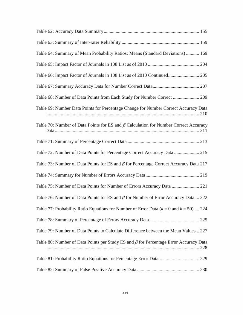
LIST OF TABLES
Page
Table 1: Estimation of Human Error Contributions as % of All Failures .......................... 2
Table 2: Incidents That List Human Fatigue as a Root Cause .......................................... 10
Table 3: Recent Nuclear Power Plant Fatigue Related Incidents ..................................... 15
Table 4: Factors That Differ in Sleep Deprivation Studies............................................... 22
Table 5: Hours of Wakefulness Compared to BAC% Levels........................................... 25
Table 6: THERP Table 20-14, Estimated HEPs in Detecting Stuck Locally Operated Valves (Swain and Guttman, 1983) .......................................................................... 33
Table 7: Interpreting Effect Size (Coe, 2000) ................................................................... 50 Table 8: Studies Using the PVT........................................................................................ 56
Table 9: List of 108 Studies .............................................................................................. 63
Table 10: Study and Sample Descriptors .......................................................................... 66
Table 11: Experimental Conditions .................................................................................. 67
Table 12: Characteristics of the Task................................................................................ 69
Table 13: Statistical Data .................................................................................................. 71
Table 14: Coding Example of Study Identifiers and Study Context Data ........................ 72
Table 15: Sample Descriptors and Experimental Condition Coding Example ................. 73
Table 16: Task Characteristics Coding Example .............................................................. 74
Table 17: Statistical Data .................................................................................................. 76
Table 18: Statistical Data Continued from Table 17 ........................................................ 76
Table 19: Desired Data for Collection .............................................................................. 77
xiv
Table 20: Data Used for Analysis ..................................................................................... 79
Table 21: Error Conditions ............................................................................................... 80
Table 22: Resulting Studies Used in Analysis .................................................................. 94
Table 23: Resulting Studies and Performance Variables Reported Part 1 ........................ 95
Table 24: Resulting Studies and Performance Variables Reported Part 2 ........................ 96
Table 25: Resulting Studies and Performance Variables Reported Part 3 ........................ 97
Table 26: Studies w.r.t. Data on Number of Lapses ......................................................... 98
Table 27: Number of Data Points for Differences between Means for Number of Lapses................................................................................................................................. 100
Table 28: Number of Data Points for ES Calculation (Number of Lapses) ................... 104 Table 29: Number of Lapses vs. Hours of Wakefulness: Within-Study Regression
Coefficients ............................................................................................................. 105 Table 30: Overall Number of Lapses Equation Based on Within-study Regression ...... 106 Table 31: Between-Studies Regression Coefficients for Number of Lapses vs. Hrs of
Wakefulness ............................................................................................................ 107 Table 32: Between-Studies Regression for Number of Lapses: Non-Significant Variables
Removed ................................................................................................................. 108 Table 33: Probability Ratios for Number of Lapses (k = 9, 10) ..................................... 113 Table 34: Probability Ratios for Number of Lapses (k = 2) ........................................... 115
Table 35: Probability Ratios for Number of Lapses (k = 1, 3, 6) ................................... 117
Table 36: Summary Data for Number of Lapses (k = 1, 2, 3, 6, 9, 10) .......................... 118
Table 37: Summary of Probability Ratios at 24 Hours of Wakefulness ......................... 118
Table 38: Descriptive Statistics for Number of Lapses Information .............................. 119
Table 39: Mean Probability Ratios for Number of Lapses and 95% CI (k = 1) ............. 120
Table 40: Probability Ratios for Number of Lapses: Means and Standard Deviations .. 121
xv
Table 41: Studies w.r.t. Data on Reaction Time ............................................................. 123
Table 42: Number of Data Points for Reaction Time ..................................................... 126
Table 43: Number of Data Points for Reaction Time Percentage Increase .................... 127
Table 44: Number of Data Points per Study for ES Calculation (Reaction Time) ......... 129
Table 45: Number of Data Points per Study for ES and β for Reaction Time (Values >10 Removed) ................................................................................................................ 130
Table 46: Reaction Time vs. Hours of Wakefulness: Within-Study Regression
Coefficients ............................................................................................................. 133 Table 47: Overall Reaction Time Equation Based on Within-Study Regression ........... 134
Table 48: Between-Studies Regression Coefficients for Reaction Time vs. Hours of Wakefulness ............................................................................................................ 135
Table 49: Between-Studies Regression for Reaction Time: Non-Significant Variables
Removed ................................................................................................................. 136 Table 50: Reaction Time Predictive Model: Within-Study Regression Results............. 137
Table 51: Leave-one-out Cross-Validation Results ........................................................ 139
Table 52: Summary of Within-Study Regression Data for ≤ 24 Hours of Wakefulness140
Table 54: Leave-one-out Cross-Validation Results ≤ 24 Hours of Wakefulness ........... 140
Table 54: Residual Mean Squared Values ≤ 24 Hours of Wakefulness ......................... 141
Table 55: Probability Ratios Regression Models for Reaction Time (k = 250, 400)...... 146
Table 56: Probability Ratios Regression Models for Reaction Time (k = 300) (Values >10 Removed) ......................................................................................................... 148
Table 57: Probability Ratios Regression Models for Reaction Time (k = 500, 750)...... 149
Table 58: Probability Ratio Regression Models for Reaction Time (k = 1000) ............. 150
Table 59: Descriptive Statistics for Reaction Time ........................................................ 152
Table 60: Mean Probability Ratios for Reaction Time and 95% CI (k = 500) ............... 153
Table 61: Probability Ratios for Reaction Time: Means and Standard Deviations ........ 153
xvi
Table 62: Accuracy Data Summary ................................................................................ 155
Table 63: Summary of Inter-rater Reliability ................................................................. 159
Table 64: Summary of Mean Probability Ratios: Means (Standard Deviations) ........... 169
Table 65: Impact Factor of Journals in 108 List as of 2010 ........................................... 204
Table 66: Impact Factor of Journals in 108 List as of 2010 Continued .......................... 205
Table 67: Summary Accuracy Data for Number Correct Data ....................................... 207
Table 68: Number of Data Points from Each Study for Number Correct ...................... 209
Table 69: Number Data Points for Percentage Change for Number Correct Accuracy Data................................................................................................................................. 210
Table 70: Number of Data Points for ES and β Calculation for Number Correct Accuracy
Data ......................................................................................................................... 211 Table 71: Summary of Percentage Correct Data ............................................................ 213
Table 72: Number of Data Points for Percentage Correct Accuracy Data ..................... 215
Table 73: Number of Data Points for ES and β for Percentage Correct Accuracy Data 217
Table 74: Summary for Number of Errors Accuracy Data ............................................. 219
Table 75: Number of Data Points for Number of Errors Accuracy Data ....................... 221
Table 76: Number of Data Points for ES and β for Number of Error Accuracy Data .... 222
Table 77: Probability Ratio Equations for Number of Error Data (k = 0 and k = 50) .... 224
Table 78: Summary of Percentage of Errors Accuracy Data .......................................... 225
Table 79: Number of Data Points to Calculate Difference between the Mean Values... 227
Table 80: Number of Data Points per Study ES and β for Percentage Error Accuracy Data................................................................................................................................. 228
Table 81: Probability Ratio Equations for Percentage Error Data .................................. 229 Table 82: Summary of False Positive Accuracy Data .................................................... 230
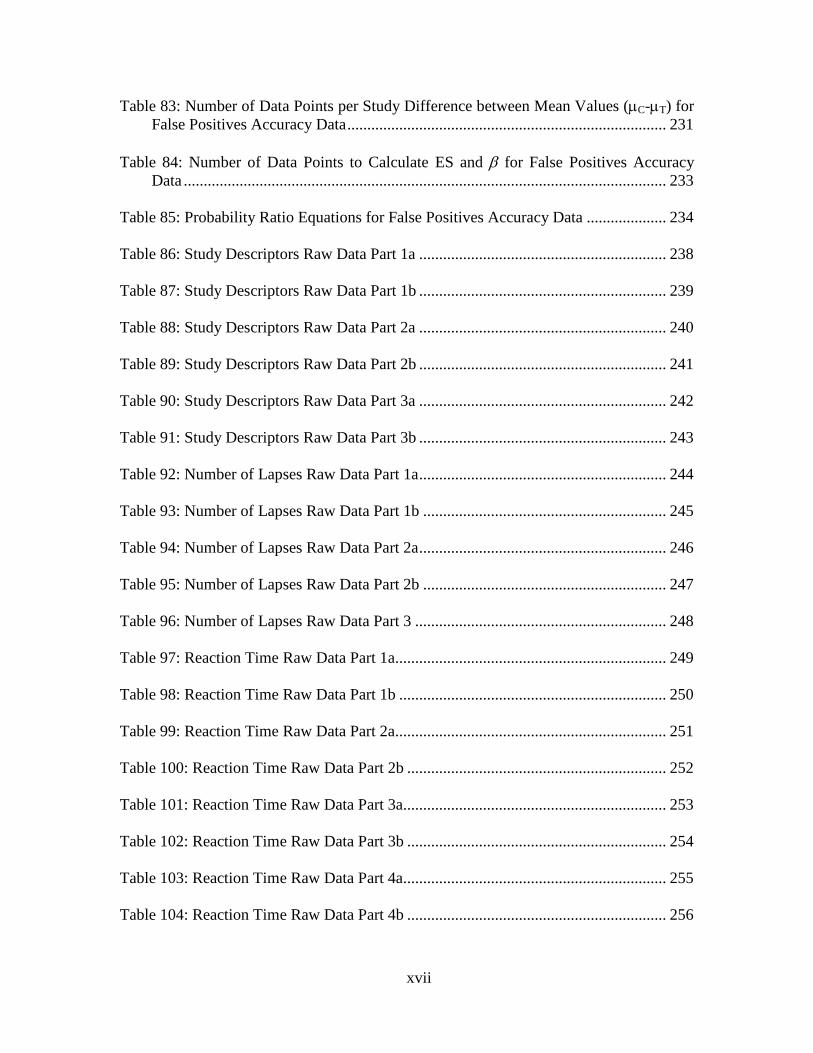
xvii
Table 83: Number of Data Points per Study Difference between Mean Values (µC-µT) for False Positives Accuracy Data ................................................................................ 231
Table 84: Number of Data Points to Calculate ES and β for False Positives Accuracy
Data ......................................................................................................................... 233 Table 85: Probability Ratio Equations for False Positives Accuracy Data .................... 234
Table 86: Study Descriptors Raw Data Part 1a .............................................................. 238
Table 87: Study Descriptors Raw Data Part 1b .............................................................. 239
Table 88: Study Descriptors Raw Data Part 2a .............................................................. 240
Table 89: Study Descriptors Raw Data Part 2b .............................................................. 241
Table 90: Study Descriptors Raw Data Part 3a .............................................................. 242
Table 91: Study Descriptors Raw Data Part 3b .............................................................. 243
Table 92: Number of Lapses Raw Data Part 1a .............................................................. 244
Table 93: Number of Lapses Raw Data Part 1b ............................................................. 245
Table 94: Number of Lapses Raw Data Part 2a .............................................................. 246
Table 95: Number of Lapses Raw Data Part 2b ............................................................. 247
Table 96: Number of Lapses Raw Data Part 3 ............................................................... 248
Table 97: Reaction Time Raw Data Part 1a.................................................................... 249
Table 98: Reaction Time Raw Data Part 1b ................................................................... 250
Table 99: Reaction Time Raw Data Part 2a.................................................................... 251
Table 100: Reaction Time Raw Data Part 2b ................................................................. 252
Table 101: Reaction Time Raw Data Part 3a.................................................................. 253
Table 102: Reaction Time Raw Data Part 3b ................................................................. 254
Table 103: Reaction Time Raw Data Part 4a.................................................................. 255
Table 104: Reaction Time Raw Data Part 4b ................................................................. 256
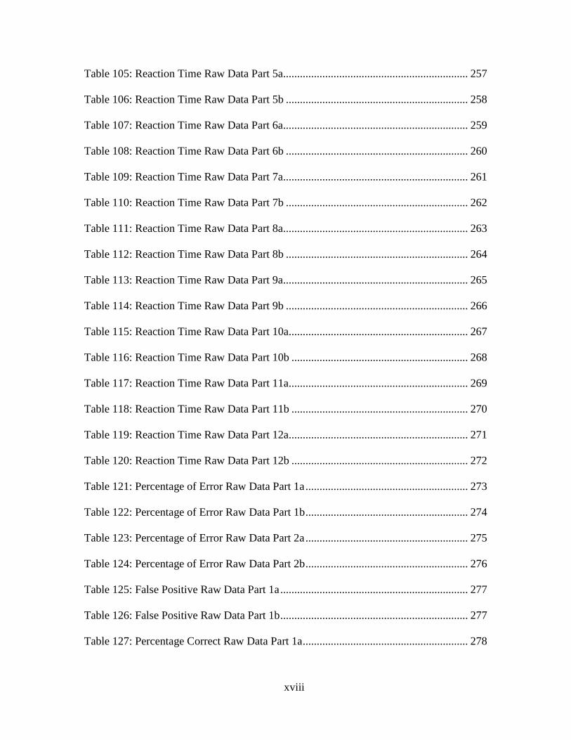
xviii
Table 105: Reaction Time Raw Data Part 5a.................................................................. 257
Table 106: Reaction Time Raw Data Part 5b ................................................................. 258
Table 107: Reaction Time Raw Data Part 6a.................................................................. 259
Table 108: Reaction Time Raw Data Part 6b ................................................................. 260
Table 109: Reaction Time Raw Data Part 7a.................................................................. 261
Table 110: Reaction Time Raw Data Part 7b ................................................................. 262
Table 111: Reaction Time Raw Data Part 8a.................................................................. 263
Table 112: Reaction Time Raw Data Part 8b ................................................................. 264
Table 113: Reaction Time Raw Data Part 9a.................................................................. 265
Table 114: Reaction Time Raw Data Part 9b ................................................................. 266
Table 115: Reaction Time Raw Data Part 10a................................................................ 267
Table 116: Reaction Time Raw Data Part 10b ............................................................... 268
Table 117: Reaction Time Raw Data Part 11a................................................................ 269
Table 118: Reaction Time Raw Data Part 11b ............................................................... 270
Table 119: Reaction Time Raw Data Part 12a................................................................ 271
Table 120: Reaction Time Raw Data Part 12b ............................................................... 272
Table 121: Percentage of Error Raw Data Part 1a .......................................................... 273
Table 122: Percentage of Error Raw Data Part 1b .......................................................... 274
Table 123: Percentage of Error Raw Data Part 2a .......................................................... 275
Table 124: Percentage of Error Raw Data Part 2b .......................................................... 276
Table 125: False Positive Raw Data Part 1a ................................................................... 277
Table 126: False Positive Raw Data Part 1b ................................................................... 277
Table 127: Percentage Correct Raw Data Part 1a ........................................................... 278
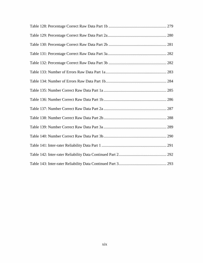
xix
Table 128: Percentage Correct Raw Data Part 1b .......................................................... 279
Table 129: Percentage Correct Raw Data Part 2a ........................................................... 280
Table 130: Percentage Correct Raw Data Part 2b .......................................................... 281
Table 131: Percentage Correct Raw Data Part 3a ........................................................... 282
Table 132: Percentage Correct Raw Data Part 3b .......................................................... 282
Table 133: Number of Errors Raw Data Part 1a ............................................................. 283
Table 134: Number of Errors Raw Data Part 1b............................................................. 284
Table 135: Number Correct Raw Data Part 1a ............................................................... 285
Table 136: Number Correct Raw Data Part 1b ............................................................... 286
Table 137: Number Correct Raw Data Part 2a ............................................................... 287
Table 138: Number Correct Raw Data Part 2b ............................................................... 288
Table 139: Number Correct Raw Data Part 3a ............................................................... 289
Table 140: Number Correct Raw Data Part 3b ............................................................... 290
Table 141: Inter-rater Reliability Data Part 1 ................................................................. 291
Table 142: Inter-rater Reliability Data Continued Part 2................................................ 292
Table 143: Inter-rater Reliability Data Continued Part 3................................................ 293
xx
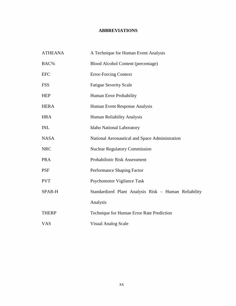
ABBREVIATIONS
ATHEANA A Technique for Human Event Analysis
BAC% Blood Alcohol Content (percentage)
EFC Error-Forcing Context
FSS Fatigue Severity Scale
HEP Human Error Probability
HERA Human Event Response Analysis
HRA Human Reliability Analysis
INL Idaho National Laboratory
NASA National Aeronautical and Space Administration
NRC Nuclear Regulatory Commission
PRA Probabilistic Risk Assessment
PSF Performance Shaping Factor
PVT Psychomotor Vigilance Task
SPAR-H Standardized Plant Analysis Risk – Human Reliability
Analysis
THERP Technique for Human Error Rate Prediction
VAS Visual Analog Scale
1
CHAPTER I
INTRODUCTION
Many industries experience significant losses due to human error. Despite years
of research, difficulties still exist in quantifying the direct contribution of human error to
incidents that result in disaster and/or losses. Human reliability analysis (HRA) attempts
to quantify human error probability under various situations. This information is useful
in probabilistic risk analysis (PRA) of large complex systems, such as nuclear power
plants. To date, HRA has mostly used expert opinion to quantify error probabilities
resulting in discrepancy of risk assessments from one analyst to another (Boring, 2007).
One way to improve the technical basis of HRA methods is to quantify the effects of
various performance shaping factors using empirical data. This dissertation investigates
methods to develop such an objective technical basis and focuses on fatigue resulting
from sleep deprivation. Information and data on sleep deprivation’s effect on
performance are not explicitly included in current HRA methods. This dissertation
develops a methodology for including sleep deprivation effects in human reliability
analysis (HRA).
Background
The degree to which fatigue impacts human performance ranges from slight to
catastrophic. In the case of large complex systems, it is possible for the fatigue-related
2
error of a single person working under sleep-deprived conditions to cause an industrial
accident that can kill thousands of people, cause major environmental damage and/or cost
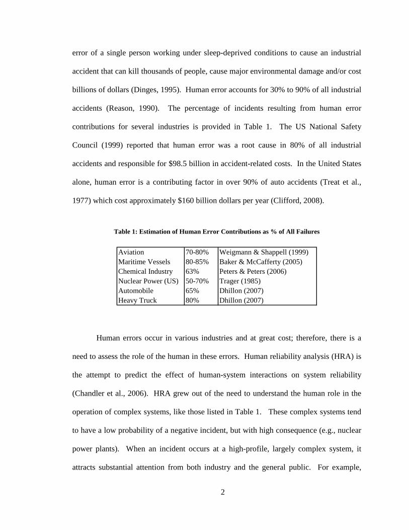
billions of dollars (Dinges, 1995). Human error accounts for 30% to 90% of all industrial
accidents (Reason, 1990). The percentage of incidents resulting from human error
contributions for several industries is provided in Table 1. The US National Safety
Council (1999) reported that human error was a root cause in 80% of all industrial
accidents and responsible for $98.5 billion in accident-related costs. In the United States
alone, human error is a contributing factor in over 90% of auto accidents (Treat et al.,
1977) which cost approximately $160 billion dollars per year (Clifford, 2008).
Table 1: Estimation of Human Error Contributions as % of All Failures
Aviation 70-80% Weigmann & Shappell (1999)Maritime Vessels 80-85% Baker & McCafferty (2005)Chemical Industry 63% Peters & Peters (2006)Nuclear Power (US) 50-70% Trager (1985)Automobile 65% Dhillon (2007)Heavy Truck 80% Dhillon (2007)
Human errors occur in various industries and at great cost; therefore, there is a
need to assess the role of the human in these errors. Human reliability analysis (HRA) is
the attempt to predict the effect of human-system interactions on system reliability
(Chandler et al., 2006). HRA grew out of the need to understand the human role in the
operation of complex systems, like those listed in Table 1. These complex systems tend
to have a low probability of a negative incident, but with high consequence (e.g., nuclear
power plants). When an incident occurs at a high-profile, largely complex system, it
attracts substantial attention from both industry and the general public. For example,
3
increased interest in occupational safety and human health resulted from the Three Mile
Island nuclear power plant disaster in 1979, the Chernobyl nuclear power plant explosion
in 1986, and the Challenger accident in 1986. These incidents have been the catalysts in
driving the development of HRA methods (Reason, 1990).
One option for obtaining quantitative data for use in HRA is to collect the number
of occurrences of events related to human performance (i.e., frequency data). However,
since adverse events in nuclear power plants and other industries are atypical, there are
not enough incidents to accurately use frequency data for HRA quantification while
producing statistically significant results. HRA practitioners currently use whatever data
exist (mostly expert opinion), updating when new information is obtained. The
infrequency of adverse events in nuclear power plants motivates the investigation into
other industries, such as aviation, medical, and the military, to gather field data.
To improve HRA, this research will explore and collate quantitative data on the
effect of fatigue on performance. Cognitive fatigue, as caused by hours of wakefulness
and measured through reaction time, accuracy, and the number of lapses, is evaluated in
this research. Physiological measures of fatigue (e.g., critical flicker frequency, blood
pressure, heart rate, etc.) are not investigated. Even though this research investigates
reaction time, which does have a physical component, in simple reaction time
experiments, the fatigue effect on performance has more to do with the draw on
attentional capacity rather than on muscle fatigue. Reaction time is often used as a
measure of cognitive performance throughout the psychological literature (Chee and
Choo, 2004; Choo et al., 2005; Kobbeltvedt et al., 2005; Nilsson et al., 2005; Thomas et
al., 2000; Williamson and Feyer, 2000). For the purposes of this research, fatigue will be
4
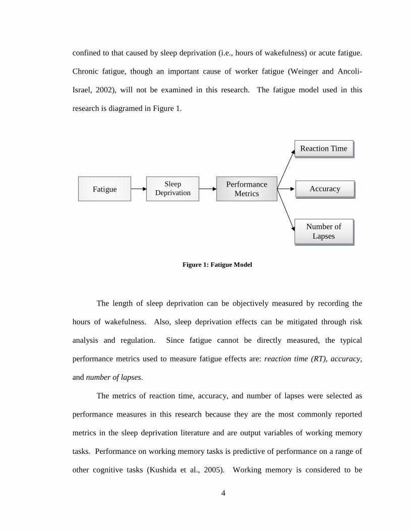
confined to that caused by sleep deprivation (i.e., hours of wakefulness) or acute fatigue.
Chronic fatigue, though an important cause of worker fatigue (Weinger and Ancoli-
Israel, 2002), will not be examined in this research. The fatigue model used in this
research is diagramed in Figure 1.
Figure 1: Fatigue Model
The length of sleep deprivation can be objectively measured by recording the
hours of wakefulness. Also, sleep deprivation effects can be mitigated through risk
analysis and regulation. Since fatigue cannot be directly measured, the typical
performance metrics used to measure fatigue effects are: reaction time (RT), accuracy,
and number of lapses.
The metrics of reaction time, accuracy, and number of lapses were selected as
performance measures in this research because they are the most commonly reported
metrics in the sleep deprivation literature and are output variables of working memory
tasks. Performance on working memory tasks is predictive of performance on a range of
other cognitive tasks (Kushida et al., 2005). Working memory is considered to be
Reaction Time
Accuracy
Number of Lapses
Performance Metrics
Sleep Deprivation Fatigue
5
fundamental to performance on virtually any neurocognitive task. The criteria for a
cognitive performance task to assess neurobehavioral performance capability should have
the following features: 1) uses basic expressions of performance (e.g., reaction time), 2)
is sensitive to homeostasis and circadian rhythms, 3) is easy to learn or perform, 4) has
sufficient task load (i.e., stimulus rate) to prevent boredom, 5) has sufficient re-test
reliability, and 6) reflects an aspect of real-world performance (Kushida et al., 2005).
Performance tasks, such as PVT (Dinges and Powell, 1985) and SRT have the above
features, and are useful in the tracking ability to access to the working memory of the
prefrontal cortex of the brain.
The metrics of reaction time, accuracy, and number of lapses are typically the
reported results of such working memory tasks. Reaction time, accuracy, and number of
lapses provide an index of the degree of functional impairment from sleep deprivation
that is meaningful and easily measurable outcome variables. Physical variables may also
be measured, such as temperature and cortisol levels; but these variables do not measure
performance decrements; which were the focus of this research.
These three metrics are measured through a variety of tasks in the literature, such
as: vigilance tasks, timed tasks, dual or multiple tasks, mental arithmetic tasks, memory
tasks, and others (Williamson and Feyer, 2000; Nilsson et al., 2005). New models are
needed to transform reaction time, accuracy and number of lapses into human error
probabilities (HEPs).
6
Research Objectives
The overall goal of this research is to improve the technical basis for including
sleep deprivation effects in human reliability analysis (HRA) methods used in
probabilistic risk assessment (PRA). Quantitative information to characterize the effect
of sleep deprivation on performance was considered. Data were collected from existing
psychological, medical, military, and transportation literature and in a structure that is
compatible with meta-analysis technique and the Human Event Response Analysis
(HERA) database being developed for the Nuclear Regulatory Commission (NRC), and
the NASA HRA database; both of which are being developed at Idaho National
Laboratory (INL).
The overall goal of this research can be divided into five sub-objectives:
1. Analyze existing HRA models and their treatment of cognitive fatigue; 2. Collect and analyze data with respect to the effect of sleep deprivation on
performance through the meta-analysis research synthesis procedure; 3. Evaluate the quantitative effect of sleep deprivation on performance; 4. Derive performance shaping factor coefficients based on quantitative data
to improve HRA models (e.g., SPAR-H); and 5. Conduct uncertainty analysis of the derived performance shaping factor
coefficients.
The first objective includes evaluation and analysis of existing HRA methods and
models, with a focus on how cognitive fatigue is covered, or not covered, in the existing
models. The models investigated are: THERP (Swain and Guttman, 1983), SPAR-H
(Gertman et al., 2005), and ATHEANA (USNRC, 2000). Fatigue was observed not to
have been explicitly covered in THERP (Swain and Guttman, 1983), SPAR-H (Gertman
et al., 2005), and ATHEANA (USNRC, 2000) HRA methods.
The second objective is to interpret and synthesize the fatigue data from research
literature, nuclear power plant-specific sources, and other industries with similar demands
7
on operating personnel. The meta-analysis technique of research synthesis is used for
this purpose.
In the third objective, the quantitative effect of sleep deprivation on performance
is evaluated. This is done by analyzing the data collected from objective two. For
example, the change in performance after sleep deprivation is evaluated using effect size,
percentage change, and failure probabilities. The results are segregated by reaction time,
accuracy and number of lapses.
The fourth objective derives performance shaping factor coefficient values based
on quantitative data gathered in objective two, based on the analysis in objective three.
This is done through ratios of the probability of failure between the test and control
conditions of performance.
The fifth objective is to conduct uncertainty analysis on the derived performance
shaping factor coefficient values. The calculated performance shaping factor coefficient
values show significant variability due to sparse data. Data were subdivided into twenty
hour intervals (i.e., < 20, 20-40, 40-60, 60-80, and > 80), and the mean and standard
deviation was used to find a confidence interval over the twenty hour time blocks. Also,
the uncertainty associated with the coding process of the quantitative data is evaluated by
calculating the inter-rater reliability.
Organization of the Dissertation
This dissertation is organized into six chapters. Chapter two includes a review of
HRA methods, the difficulties in defining fatigue, sleep deprivation literature, and the
shortcomings of current HRA methods with respect to the treatment of fatigue and sleep
8
deprivation. The third chapter discusses the meta-analysis technique of data collection
and the coding procedure. Chapter four develops the methodology used to evaluate the
quantitative effect of sleep deprivation on performance and to derive performance
shaping factor multipliers for modifying the base error probability. The fifth chapter
provides the results of the application of methodology and uncertainty analysis. Chapter
six discusses the conclusions drawn and future research needs.

9
CHAPTER II
FATIGUE RESEARCH AND HRA METHODS
This chapter provides a review of fatigue and sleep deprivation studies and
probabilistic risk assessment (PRA) and HRA methods. The difficulties in defining sleep
deprivation and the problems associated with sleep deprivation research studies are
discussed. Three HRA methods are explored in detail with respect to the inclusion of
fatigue effects. Incidents attributed to fatigue in the nuclear industry and other industries
are discussed. Also explored in this chapter are the effects of fatigue and sleep
deprivation in quantitative HRA.
Fatigue
Unlike chemical impairment due to alcohol or drugs, which can be detected by
biochemical tests, fatigue is more difficult to measure and discern as the cause of reduced
performance. Typically, fatigue must be inferred from the context of the situation. For
example, in the case of a single car accident, fatigue or even having fallen asleep, may
not be listed as the cause of the accident; instead only the end result, such as driving into
a ditch, might be listed, even when it is reasonable to assume fatigue as a root cause.
Despite this limitation, fatigue has increasingly been claimed as the primary cause of
numerous accidents (Mitler et al., 1988).
10
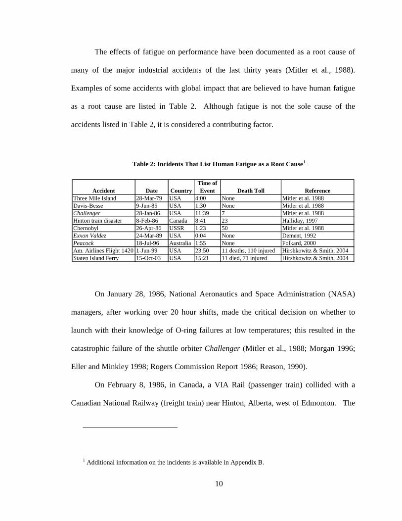
The effects of fatigue on performance have been documented as a root cause of
many of the major industrial accidents of the last thirty years (Mitler et al., 1988).
Examples of some accidents with global impact that are believed to have human fatigue
as a root cause are listed in Table 2. Although fatigue is not the sole cause of the
accidents listed in Table 2, it is considered a contributing factor.
Table 2: Incidents That List Human Fatigue as a Root Cause1
Three Mile Island 28-Mar-79 USA 4:00 None Mitler et al. 1988Davis-Besse 9-Jun-85 USA 1:30 None Mitler et al. 1988Challenger 28-Jan-86 USA 11:39 7 Mitler et al. 1988Hinton train disaster 8-Feb-86 Canada 8:41 23 Halliday, 1997Chernobyl 26-Apr-86 USSR 1:23 50 Mitler et al. 1988Exxon Valdez 24-Mar-89 USA 0:04 None Dement, 1992Peacock 18-Jul-96 Australia 1:55 None Folkard, 2000Am. Airlines Flight 1420 1-Jun-99 USA 23:50 11 deaths, 110 injured Hirshkowitz & Smith, 2004Staten Island Ferry 15-Oct-03 USA 15:21 11 died, 71 injured Hirshkowitz & Smith, 2004
Death Toll ReferenceAccident Date CountryTime of Event
On January 28, 1986, National Aeronautics and Space Administration (NASA)
managers, after working over 20 hour shifts, made the critical decision on whether to
launch with their knowledge of O-ring failures at low temperatures; this resulted in the
catastrophic failure of the shuttle orbiter Challenger (Mitler et al., 1988; Morgan 1996;
Eller and Minkley 1998; Rogers Commission Report 1986; Reason, 1990).
On February 8, 1986, in Canada, a VIA Rail (passenger train) collided with a
Canadian National Railway (freight train) near Hinton, Alberta, west of Edmonton. The
1 Additional information on the incidents is available in Appendix B.
11
accident was the result of the crew of the freight train having become incapacitated by
fatigue (Halliday, 1997).
On March 24, 1989, the Exxon Valdez oil tanker struck a reef in Prince William
Sound, Alaska, and spilled 11 to 32 million gallons of crude oil. The accident was
caused by the third mate improperly maneuvering the vessel. He had had only 6 hours of
sleep in the previous 48 hours, while the first mate had been working for 30 hours
continuously. The estimated cleanup cost was $2 billion dollars, including $41 million to
clean and rehabilitate approximately 800 birds and a few hundred sea otters (NSTB,
1989; NSTB, 1990; Dement, 1992; Hassen, 2008; Eller and Minkley, 1998; Exxon Valdez
Oil Spill Trustee Council, 2008).
At 01:55 a.m. on July 18, 1996, the Peacock, a cargo vessel carrying 605 tons of
heavy fuel oil, ran aground on the Great Barrier Reef at full speed. The inquiry to the
accident suggested that the pilot had fallen asleep fifteen minutes before the grounding.
Minor damage occurred to the reef and pollution was negligible (Folkard, 2000; Parker et
al., 1998). On October 15, 2003, the Staten Island Ferry, vessel Andrew J. Barberi,
piloted by the assistant captain, ran the ferry into the dock at full speed. The pilot made
no attempt to slow down because he had fallen asleep at the controls. Eleven were killed
and seventy-one injured (Hirshkowitz and Smith, 2004).
On June 1, 1999, an American Airlines Flight 1420 from Dallas, Texas, to Little
Rock, Arkansas, overran the runway upon landing and crashed; eleven were killed and
110 injured. Pilot fatigue and the resulting diminished judgment were listed as partial
causes for the crash. The crew had been on duty for about 13½ hours at the time of the
12
incident (Malnic, 2001; Hirshkowitz and Smith, 2004; National Transportation Safety
Board, 2001).
A sampling of human error with potentially severe detrimental impacts caused by
fatigue can be found when looking at the history of nuclear reactors. The Three Mile
Island incident occurred on March 28, 1979; nuclear reactor coolant escaped after the
pilot-operated relief valve failed to close properly. The mechanical failures were
compounded by the failure of operators to recognize that the plant was experiencing a
loss of coolant. When the situation was realized, the crew was not able to solve the
problem until the relief crew came on and took over for the fatigued crew. The incident
occurred in the morning between 04:00 and 06:00 a.m. (Reason, 1990; Harrison and
Horne, 2000; Monk, 2007; Mitler et al. 1988; USNRC, 1979). Another incident occurred
on June 9, 1985, at 01:30 a.m., when the Davis-Besse (Oak Harbor, Ohio) nuclear power
plant went into automatic shutdown after a loss of cooling water and then had a total loss
of the main feed-water. The incident was compounded when the operator pushed the
incorrect button and turned off the auxiliary feed-water system. The operator’s error was
discovered by workers coming on the next shift (Coren, 1996; Mitler et al. 1988;
USNRC, 1985).
On April 26, 1985, at approximately 01:30 a.m. at the Chernobyl nuclear power
facility in the Ukraine, workers turned off critical automatic safety systems causing the
reactor to begin to overheat. The sleep-deprived shift workers had turned off the cooling
system instead of turning on the automated safety systems. This caused the reactor to
overheat and led to the explosion that released 13 million curies of radioactive gases and
less than 20 curies of iodine-131 (Coren, 1996; Mitler et al., 1988; USNRC, 1987b;
13
Reason, 1990). These are only a few major incidents known to have been at least in part
caused by fatigue.
An example of an event resulting from fatigue that did not result in a major
accident, but posed a severe threat to public safety, occurred at the Peach Bottom Atomic
Energy Plant (USNRC, 1987a). In 1987, during a routine, but unannounced, inspection
of the Peach Bottom plant, U.S. Nuclear Regulatory Commission (NRC) inspectors found
control room operators asleep in their chairs. According to the USNRC report, the
management at Peach Bottom had a plan of willful circumvention of USNRC guidelines
by inventing its own mechanism to handle worker fatigue associated with the night shift
work: allowing control room operators to sleep during the night shift. Consequently, the
NRC ordered the power station shut down; this was a first in American nuclear power
history. Despite being a state-of-the-art and high-efficiency plant, management had
overlooked the effects of human limitations in 24 hour operations. Even though no
nuclear accident had occurred, the plant closure, which resulted from human inattention,
resulted in enormous costs.
Although the incident at Peach Bottom occurred in 1987, and guidelines were in
place at the time for limiting work shift hours (10-CFR26.20), similar events still occur at
nuclear power plants. Again, in 2007, at the Peach Bottom Plant, a video of sleeping
security guards was taken by a fellow guard and released to the media (Mufson, 2008).
Table 3 provides a list of events at nuclear power plants that involve similar situations of
sleeping or inattentive workers. Incidents, such as those in Table 3, occur because the
NRC procedures include only prescriptive and general guidelines on working hours and
shifts, aimed at limiting worker fatigue. The USNRC recognized that fatigue is an
14
important component to safe operations and that the fitness-for-duty guidelines (10-
CFR26.20) need to be more inclusive of fatigue effects and not just chemical impairment
(Persensky et al., 2002). The fitness-for-duty guidelines were changed in 2008,
increasing the minimum break between shifts, limiting the reasons for waivers for
overtime limits, and establishing training for fatigue management (Lenton, 2007). This
move addressed the fundamental issue of fatigue and its effects on overall human error
probability (HEP).
In several incidents, security officers have been found sleeping or inattentive
(Seabrook, 2002; Oyster Creek, 2003; Beaver Valley, (2004 and 2005); Three Mile
Island, 2007; Peach Bottom, 2007). In two incidents, security officers had fallen asleep
while driving (Millstone, 2002; Braidwood, 2004). In two others, control room operators
were found asleep at their stations (Massachusetts Institute of Technology, 2003; Pilgrim,
2004). Table 3 also includes incidents of work hour violations, (Susquehanna, 2002; St.
Lucie, 2003), along with a court case brought by an engineer who had been fired after
complaining about hours beyond the work limitations (D.C. Cook, 2004). Three reports
included security officers being threatened with disciplinary actions or being sent to a
psychiatrist when they complained of working their 6th day of 12 hour shifts (Indian
Point, 2003; Prairie Island, 2003; Wakenhut Security, 2003).
15
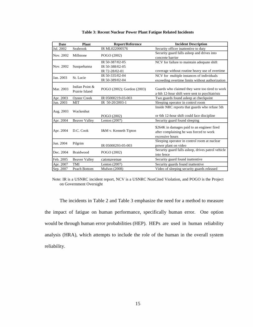
Table 3: Recent Nuclear Power Plant Fatigue Related Incidents
Date Plant Report/Reference Incident DescriptionJul. 2002 Seabrook IR ML022000576 Security officer inattentive to duty
Nov. 2002 Millstone POGO (2002)Security guard falls asleep and drives into concrete barrier
IR 50-387/02-05IR 50-388/02-05IR 72-28/02-01IR 50-335/02-04IR 50-389/02-04
Mar. 2003 Indian Point & Prairie Island POGO (2002); Gordon (2003) Guards who claimed they were too tired to work
a 6th 12-hour shift were sent to psychiatristsApr. 2003 Oyster Creek IR 05000219-03-003 Two guards found asleep at checkpointJun. 2003 MIT IR 50-20/2003-1 Sleeping operator in control room
Apr. 2004 Beaver Valley Lenton (2007) Security guard found sleeping
Jun. 2004 Pilgrim IR 05000293-05-003 Sleeping operator in control room at nuclear power plant on video
Dec. 2004 Braidwood POGO (2002)Security guard falls asleep, drives patrol vehicle into fence
Feb. 2005 Beaver Valley catonavenue Security guard found inattentiveApr. 2007 TMI Lenton (2007) Security guards found inattentiveSep. 2007 Peach Bottom Mufson (2008) Video of sleeping security guards released
Apr. 2004 D.C. Cook I&M v. Kenneth Tipton$264K in damages paid to an engineer fired after complaining he was forced to work excessive hours
Aug. 2003 WackenhutPOGO (2002)
Inside NRC reports that guards who refuse 5th
or 6th 12-hour shift could face discipline
Nov. 2002 SusquehannaNCV for failure to maintain adequate shift
coverage without routine heavy use of overtime
Jan. 2003 St. Lucie NCV for multiple instances of individuals exceeding overtime limits without authorization
Note: IR is a USNRC incident report, NCV is a USNRC NonCited Violation, and POGO is the Project
on Government Oversight
The incidents in Table 2 and Table 3 emphasize the need for a method to measure
the impact of fatigue on human performance, specifically human error. One option
would be through human error probabilities (HEP). HEPs are used in human reliability
analysis (HRA), which attempts to include the role of the human in the overall system
reliability.

16
Difficulties in Defining Fatigue
While fatigue is a major risk factor, it is not easy to define; few words have been
less adequately described or understood (Schmitt, 1976). Fatigue is used as the name of
the condition and the experience of feeling tired and weary (Bartley, 1957). Unlike
physical fatigue, mental fatigue can only be inferred from the context of the evidence;
which leads to fatigue often being defined in terms of its consequences rather than its
causes. Fatigue is a personal experience and is a function of the individual’s motivation
and past and present circumstances.2
Fatigue results not only from prolonged activity, but also from psychological,
socioeconomic, and environmental factors that affect the mind and body. Figure 2 shows
Grandjean’s (1968) analogy of fatigue being liquid filling a bucket. Grandjean compared
fatigue to the level of liquid in the container (bucket) that is being continuously filled by:
monotony of task, environment, intensity and length of work, psychological and physical
factors, and it can only be emptied by recovery or rest.
2 See Appendix A for additional information on fatigue.
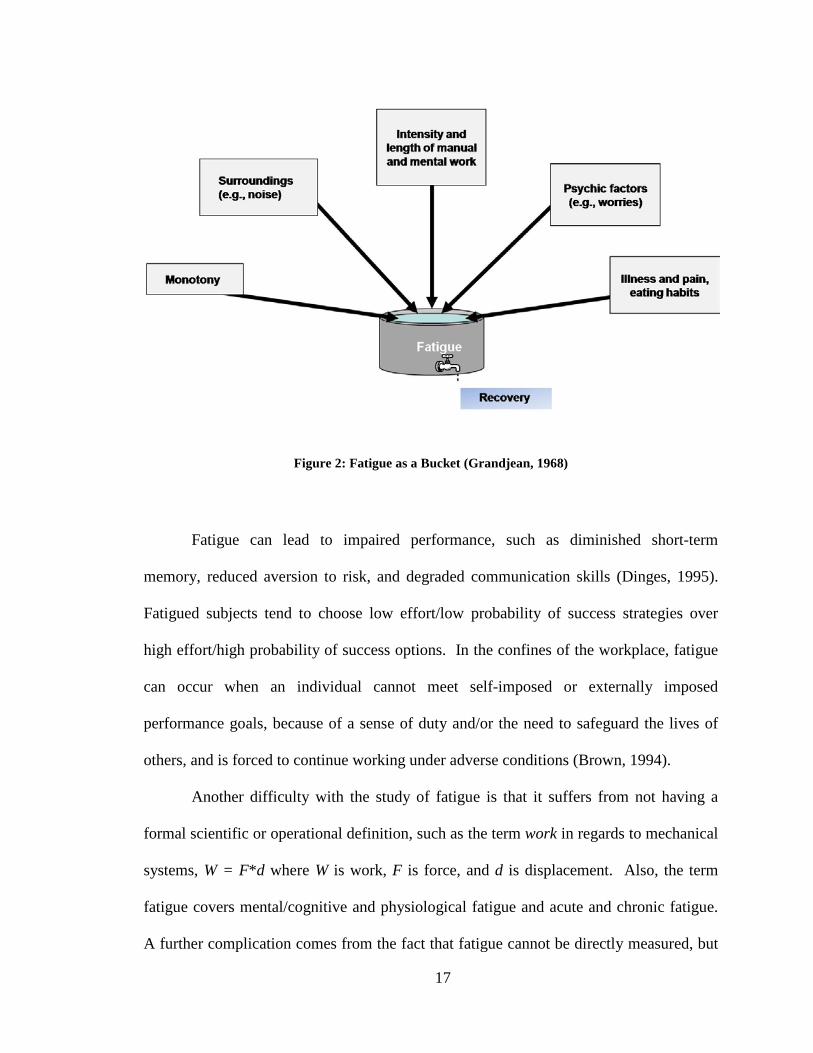
17
Figure 2: Fatigue as a Bucket (Grandjean, 1968)
Fatigue can lead to impaired performance, such as diminished short-term
memory, reduced aversion to risk, and degraded communication skills (Dinges, 1995).
Fatigued subjects tend to choose low effort/low probability of success strategies over
high effort/high probability of success options. In the confines of the workplace, fatigue
can occur when an individual cannot meet self-imposed or externally imposed
performance goals, because of a sense of duty and/or the need to safeguard the lives of
others, and is forced to continue working under adverse conditions (Brown, 1994).
Another difficulty with the study of fatigue is that it suffers from not having a
formal scientific or operational definition, such as the term work in regards to mechanical
systems, W = F*d where W is work, F is force, and d is displacement. Also, the term
fatigue covers mental/cognitive and physiological fatigue and acute and chronic fatigue.
A further complication comes from the fact that fatigue cannot be directly measured, but
18
instead must be inferred from changes in other conditions, such as reaction time, body
temperature, sleep latency (i.e., time taken to fall asleep), etc. (Boring et al., 2007).
Measurement of Fatigue
There is no direct objective measure of fatigue. There are subjective fatigue
scales that are used to indicate the level of fatigue. One of these is the fatigue severity
scale (FSS) by Krupps et al. (1989) that uses nine statements on a seven-point scale of
agreement; for example, one statement is how fatigue interferes with physical
functioning. The fatigue severity scale measures the impact of fatigue on specific types
of functioning, relating to behavioral consequences of fatigue rather than symptoms. The
other commonly used fatigue scale is the visual analog scale (VAS) by Bond and Lader
(1974). A 100-mm scale line, ranging from not at all to extremely fatigued, is used for
the subjects to describe the level of fatigue they are experiencing. These measures are
useful for the investigation of levels of fatigue, but are not appropriate for the study of
effects on performance.
Work scheduling programs such as Fatigue Avoidance Scheduling Tool (FAST)
(Hursh et al., 2004), Manpower and Personnel Integration (MANPRINT) (Army
Regulation 602-2, 2001), and Micro Saint (USNRC, 1995) consider the effect of fatigue
and sleep deprivation on performance. The software programs aid in limiting the
negative effect of fatigue caused by work schedules, but rely mostly on circadian
influences on performance for input. The effect of fatigue is not measured in these
programs but mitigated.
19
Performance moderator functions (PMFs) are used in modeling and simulation of
human behavior models. PMFs are similar to performance shaping factors (PSFs) used in
HRA. For example, for the Endocrine response to an acute psychological stress, the PMF
is continuous-time measurement of the plasma concentration level of sympathetic adrenal
and pituitary hormones (Richter et al., 1996). Performance moderator functions can be
used to represent the behavior or cognition that is needed in a simulation. PMFs are used
in SAFTE™, from which FAST™ is derived. Both software programs are used to aid in
operator scheduling, i.e., fatigue problems with sustained operation, but do not provide a
quantitative value for the effect of sleep deprivation performance. The result from
FAST™ is expressed in qualitative terms as a percentage of effectiveness.
The fatigue avoidance scheduling tool (FAST™) was designed by the US Air
Force Research Laboratory (AFRL) in 2000 to address the problem of fatigue associated
with aircrew flight scheduling (Eddy and Hursh, 2001). FAST™ is a Windows-based
program that quantifies the effects of various work-rest schedules on human performance.
The output from FAST™ produces a graphical display of cognitive performance
effectiveness (y-axis), using a scale from 0 to 100% effectiveness, as a function of time
(x-axis). The effectiveness rating represents a composite of human performance on a
number of tasks, but does not provide a numerical value of the effect of sleep deprivation
on performance (i.e., error probability). The goal of users is to manipulate the lengths of
work and rest periods to keep performance at or above the 90% effectiveness level.
Performance effectiveness is determined by: time of day, biological rhythms, time spent
awake (i.e., hours of wakefulness), and amount of sleep.
20
Fatigue predictions in FAST™ are derived from Sleep Activity, Fatigue, and Task
Effectiveness (SAFTE) (Hursh, 1998). SAFTE™ produces a three-process model of
human cognitive effectiveness by integrating quantitative information about: (1)
circadian rhythms in metabolic rate; (2) cognitive recovery rates related to sleep and
cognitive decay rates associated with wakefulness; (3) cognitive performance effects
associated with sleep inertia. The rating of cognitive effectiveness is dependent on the
current balance of the sleep regulation process, the circadian process, and sleep inertia.
The sleep regulation process is dependent on hours of sleep, hours of wakefulness,
current sleep debt, the circadian process, and sleep fragmentation (i.e., awakening during
sleep). In SAFTE™ the focus is on the circadian process, the cognitive effectiveness,
and sleep regulation.
FAST™ was used to evaluate data from US freight railroads and find a
correlation between effectiveness and number of human factor errors. The results found
that there exists a meaningful relationship between accident risk and effectiveness (Hursh
et al., 2006). Attempts to apply FAST™ to daily flying scheduling operations were
unsuccessful, due to the user interface having been designed for scientists and not for
operators. FAST™ has been used for operation risk management of fatigue effects, but is
not designed for use in HRA.
This dissertation sought to develop a method to derive PSF coefficients that will
modify the basic error probability, based on quantitative data. SAFTE™ and FAST™
are fatigue management tools trying to insure sufficient rest to maintain effective
performance. While useful in designing work schedules, they are not directly applicable
to HRA methods; i.e., they do not provide error probabilities or PSF coefficient values.
21
In further research it may be possible to extrapolate the output of FAST™ and SAFTE™
to validate the derived PSF coefficient values for sleep deprivation effects on error
probabilities. The types of tasks are also not delineated in FAST™. The developed PSF
coefficient derivation method can be adapted easily for specific types of tasks by using
the data on similar tasks to derive the PSF coefficient values; this is not possible with
FAST™.
The three main causes of cognitive fatigue are sleep deprivation, shift work, and
time on task. Sleep deprivation, or hours of wakefulness, lends itself best to research
studies because it is relatively simple to achieve and straightforward to measure. While
fatigue and sleepiness are often used interchangeably, they are different phenomena.
Sleepiness has to do with the propensity to fall asleep, while fatigue is a sense of
tiredness or exhaustion associated with impaired (i.e., depletion of capacity) physical
and/or cognitive functioning (Shen et al., 2006).
Fatigue effects on performance are measured indirectly through performance
metrics: typically reaction time, accuracy, and number of lapses. These three metrics are
measured through a variety of psycho-motor tasks in the literature, such as: vigilance
tasks, timed tasks, dual or multiple tasks, mental arithmetic tasks, memory tasks, and
others (Williamson and Feyer, 2000; Nilsson et al., 2005).
Measurement of Sleep Deprivation Effects on Performance
There is a wide body of research literature on the effects of fatigue on
performance in many different fields. The literature predominately focuses on sleep
deprivation due to its easy manipulation for study purposes as opposed to shift work and
22
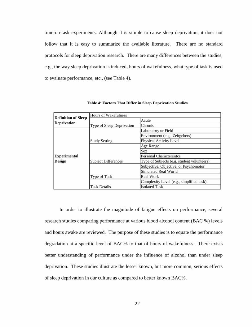
time-on-task experiments. Although it is simple to cause sleep deprivation, it does not
follow that it is easy to summarize the available literature. There are no standard
protocols for sleep deprivation research. There are many differences between the studies,
e.g., the way sleep deprivation is induced, hours of wakefulness, what type of task is used
to evaluate performance, etc., (see Table 4).
Table 4: Factors That Differ in Sleep Deprivation Studies
AcuteChronicLaboratory or FieldEnvironment (e.g., Zeitgebers)Physical Activity LevelAge RangeSexPersonal CharacterisitcsType of Subjects (e.g. student volunteers)Subjective, Objective, or PsychomotorSimulated Real WorldReal WorkComplexity Level (e.g., simplified task)Isolated Task
Definition of Sleep Deprivation
Experimental Design Subject Differences
Study Setting
Task Details
Type of Task
Hours of Wakefulness
Type of Sleep Deprivation
In order to illustrate the magnitude of fatigue effects on performance, several
research studies comparing performance at various blood alcohol content (BAC %) levels
and hours awake are reviewed. The purpose of these studies is to equate the performance
degradation at a specific level of BAC% to that of hours of wakefulness. There exists
better understanding of performance under the influence of alcohol than under sleep
deprivation. These studies illustrate the lesser known, but more common, serious effects
of sleep deprivation in our culture as compared to better known BAC%.
23
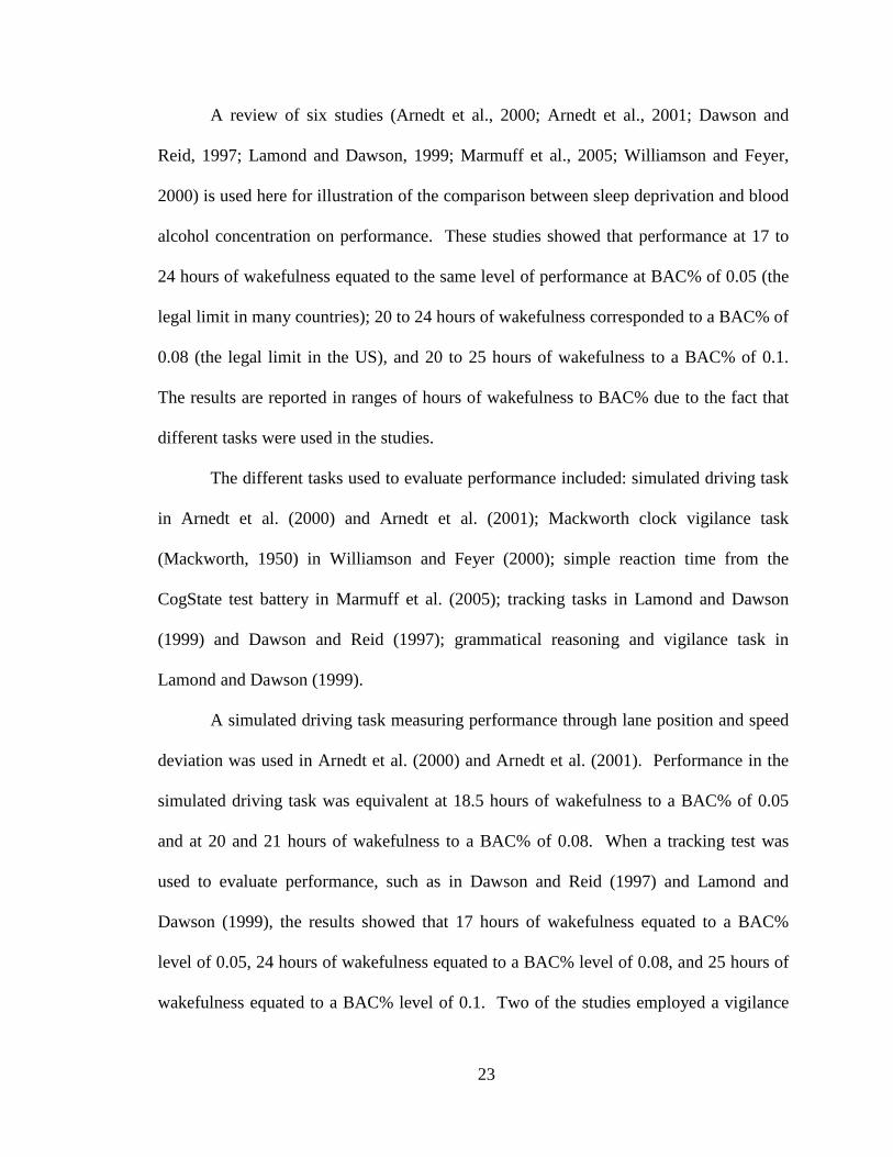
A review of six studies (Arnedt et al., 2000; Arnedt et al., 2001; Dawson and
Reid, 1997; Lamond and Dawson, 1999; Marmuff et al., 2005; Williamson and Feyer,
2000) is used here for illustration of the comparison between sleep deprivation and blood
alcohol concentration on performance. These studies showed that performance at 17 to
24 hours of wakefulness equated to the same level of performance at BAC% of 0.05 (the
legal limit in many countries); 20 to 24 hours of wakefulness corresponded to a BAC% of
0.08 (the legal limit in the US), and 20 to 25 hours of wakefulness to a BAC% of 0.1.
The results are reported in ranges of hours of wakefulness to BAC% due to the fact that
different tasks were used in the studies.
The different tasks used to evaluate performance included: simulated driving task
in Arnedt et al. (2000) and Arnedt et al. (2001); Mackworth clock vigilance task
(Mackworth, 1950) in Williamson and Feyer (2000); simple reaction time from the
CogState test battery in Marmuff et al. (2005); tracking tasks in Lamond and Dawson
(1999) and Dawson and Reid (1997); grammatical reasoning and vigilance task in
Lamond and Dawson (1999).
A simulated driving task measuring performance through lane position and speed
deviation was used in Arnedt et al. (2000) and Arnedt et al. (2001). Performance in the
simulated driving task was equivalent at 18.5 hours of wakefulness to a BAC% of 0.05
and at 20 and 21 hours of wakefulness to a BAC% of 0.08. When a tracking test was
used to evaluate performance, such as in Dawson and Reid (1997) and Lamond and
Dawson (1999), the results showed that 17 hours of wakefulness equated to a BAC%
level of 0.05, 24 hours of wakefulness equated to a BAC% level of 0.08, and 25 hours of
wakefulness equated to a BAC% level of 0.1. Two of the studies employed a vigilance
24
task (Lamond and Dawson, 1999; Williamson and Feyer, 2000). The findings for these
studies were that 17 hours of wakefulness equated to a BAC% of 0.05 and that 25 hours
of wakefulness on the latency component of the vigilance task and 22.3 hours of
wakefulness on the accuracy component of the vigilance task corresponded to a BAC%
of 0.1. A grammatical reasoning task (Baddeley, 1968) was used in Lamond and Dawson
(1999) that equated performance at the BAC% level of 0.1 to 20.3 hours.
When looking at the data from a complexity level, the more demanding the task is
cognitively, the fewer hours of wakefulness are needed to produce impairment equivalent
to higher BAC% levels. For example, the more complex task of grammatical reasoning
performance level for 20 hours of wakefulness was the same as at the BAC% of 0.1.
However, for the less cognitively demanding tracking task, performance after 25 hours of
wakefulness was the same as at the BAC% level of 0.1. The damaging effects of sleep
deprivation (extended hours of wakefulness) on performance is illustrated through these
studies by equating common legal limits of BAC% performance to that of hours of
wakefulness. Table 5 presents a summary of the hours of wakefulness that were
compared with BAC% and the type of task used.
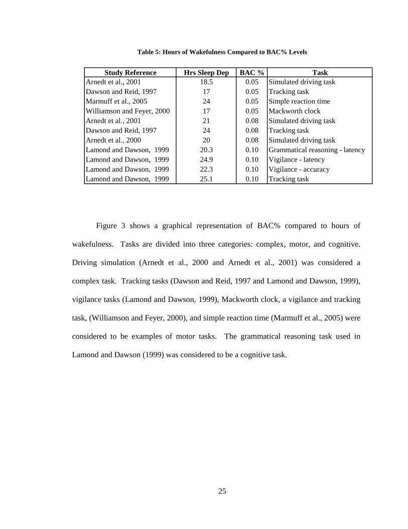
25
Table 5: Hours of Wakefulness Compared to BAC% Levels
Study Reference Hrs Sleep Dep BAC % TaskArnedt et al., 2001 18.5 0.05 Simulated driving taskDawson and Reid, 1997 17 0.05 Tracking taskMarmuff et al., 2005 24 0.05 Simple reaction timeWilliamson and Feyer, 2000 17 0.05 Mackworth clockArnedt et al., 2001 21 0.08 Simulated driving taskDawson and Reid, 1997 24 0.08 Tracking taskArnedt et al., 2000 20 0.08 Simulated driving taskLamond and Dawson, 1999 20.3 0.10 Grammatical reasoning - latencyLamond and Dawson, 1999 24.9 0.10 Vigilance - latencyLamond and Dawson, 1999 22.3 0.10 Vigilance - accuracyLamond and Dawson, 1999 25.1 0.10 Tracking task
Figure 3 shows a graphical representation of BAC% compared to hours of
wakefulness. Tasks are divided into three categories: complex, motor, and cognitive.
Driving simulation (Arnedt et al., 2000 and Arnedt et al., 2001) was considered a
complex task. Tracking tasks (Dawson and Reid, 1997 and Lamond and Dawson, 1999),
vigilance tasks (Lamond and Dawson, 1999), Mackworth clock, a vigilance and tracking
task, (Williamson and Feyer, 2000), and simple reaction time (Marmuff et al., 2005) were
considered to be examples of motor tasks. The grammatical reasoning task used in
Lamond and Dawson (1999) was considered to be a cognitive task.
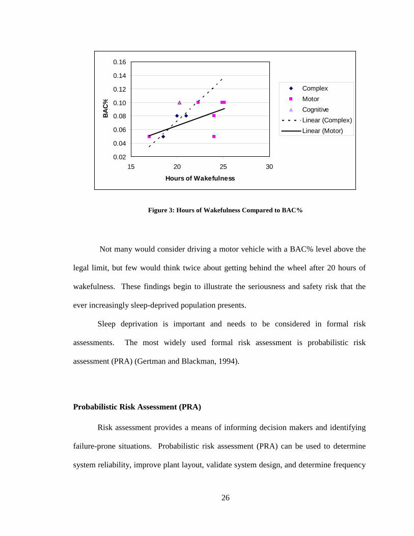
26
Figure 3: Hours of Wakefulness Compared to BAC%
Not many would consider driving a motor vehicle with a BAC% level above the
legal limit, but few would think twice about getting behind the wheel after 20 hours of
wakefulness. These findings begin to illustrate the seriousness and safety risk that the
ever increasingly sleep-deprived population presents.
Sleep deprivation is important and needs to be considered in formal risk
assessments. The most widely used formal risk assessment is probabilistic risk
assessment (PRA) (Gertman and Blackman, 1994).
Probabilistic Risk Assessment (PRA)
Risk assessment provides a means of informing decision makers and identifying
failure-prone situations. Probabilistic risk assessment (PRA) can be used to determine
system reliability, improve plant layout, validate system design, and determine frequency
0.02
0.04
0.06
0.08
0.10
0.12
0.14
0.16
15 20 25 30
Hours of Wakefulness
BAC%
ComplexMotorCognitiveLinear (Complex)Linear (Motor)
27
of error incidents. Risk assessment involves identifying the potential risks (i.e.,
understanding of the hazards), the likelihood of occurrences (i.e., frequency), and the
consequences when they do occur. Risk is the likelihood of a hazard-causing loss or
damage. Often risk is defined as the probability of an incident multiplied by its
consequence as in Equation 1:
Risk = P(Event) * Consequence (1)
Normally, a risk analyst is concerned with what can go wrong, how likely
something is to go wrong, and the consequences when something does go wrong. PRA
evolved from the need to estimate the frequencies of accidents in complex systems when
the data on actual incidents are very small and often zero (Bier, 1999). Typically, there
are failure rates for components of the system, for example pumps and valves, but not for
the overall system. These component failure rates are propagated through a fault-tree or
event-tree model to estimate an overall failure probability of the system (Bier, 1999).
The extreme cost of complex systems, such as nuclear power plants, made the initial
development of PRA techniques cost-effective, since a power plant may cost two billion
dollars while a full-scope PRA may cost only two million dollars. The resulting PRA
may establish safety improvements that are in the tens of thousands of dollars in cost,
while yielding large reductions in overall plant risk (Garrick, 1987).
The aim of PRA is to identify areas of significant risk and identify improvements
and quantify the overall risk to the plant. PRAs analyze the risk of entire systems by
decomposing the systems into their components (e.g., including hardware, software, and
human operators). A PRA is begun with an initiating event and is based on the sequence
28
of possible scenarios and possible resulting errors pursuant to that initiating event. PRA
is basically a logic-tree model of the plant and its functions (e.g., fault-trees) (Reason,
1990). The general structure of PRA was established from the 1975 Rasmussen Report
commonly referred to as WASH-1400 (Rasmussen, 1975).3 The steps are:
1) identify the source of the potential hazard, 2) identify the initiating events, 3) establish possible sequences stemming from various initiating events using event-
trees, 4) quantify each event sequence
a. frequency of the initiating event b. probability of failure of the relevant safety system when needed, and
5) determine overall plant risk (function of all possible accident sequences and their consequences).
Even though this structure depends on conditional probabilities, which are rarely
collected in practice and often independence of events is assumed, the development of a
standardized PRA method was a major step forward in reliability engineering (Reason,
1990).
One difficulty in PRA is that it is limited by the lack of empirical data; this makes
PRA hard to validate. This also creates a need to look for better resolution of the models.
One of the least data supported components of PRA is HRA. There is a significant need
to improve risk assessment in order to have a realistic risk informed approach. The
Nuclear Energy Association stated, “Any improvement in the current state of knowledge
… would have a positive impact on the confidence in probabilistic safety assessment
results” (NEA, 1998). There is a need to improve HRA to help with the continual
3 WASH-1400 was replaced with USNRC (1975) NUREG-75/014 and is now USNRC (1990) NUREG-1150.
29
improvement of PRA models, by increasing the level of detail and credibility while
decreasing the amount of conservativeness.
Human Reliability Analysis (HRA)
HRA enhances probabilistic risk assessment (PRA) by including the effects of
human error associated with complex systems. HRA provides a method to determine the
probability that a task or job requiring human action will be performed successfully
within the required time period and without extraneous human actions detrimental to
system performance. The inclusion of HRA in a PRA has many advantages, including
(Gertman and Blackman, 1994):
• providing quantitative estimates of human error probability, • identifying weaknesses in operator interaction with the system (by identifying
possible sources of error), • evaluating improvements in human interfaces, and • improving system evaluations by including human elements.
Human Reliability Analysis (HRA) grew out of the need to understand the human
role in the operation of complex systems, like those listed in Table 2. These complex
systems tend to have low probability of a negative incident but with high consequence.
Therefore, when one of these complex systems has an incident, it attracts substantial
industry wide attention. For example, an increased interest in occupational safety and
health resulted from the Three Mile Island nuclear power plant in 1979, the Chernobyl
nuclear power plant in 1986, and the Challenger accident in 1986 (Mitler et al. 1988).
These incidents have been the catalysts in driving the development of HRA methods
(Reason, 1990). Significant risk reductions and gains in the safety and performance of
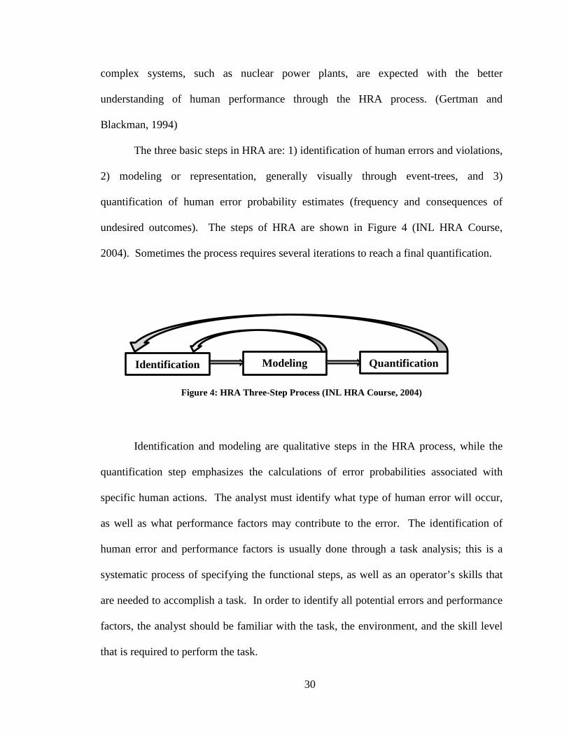
30
complex systems, such as nuclear power plants, are expected with the better
understanding of human performance through the HRA process. (Gertman and
Blackman, 1994)
The three basic steps in HRA are: 1) identification of human errors and violations,
2) modeling or representation, generally visually through event-trees, and 3)
quantification of human error probability estimates (frequency and consequences of
undesired outcomes). The steps of HRA are shown in Figure 4 (INL HRA Course,
2004). Sometimes the process requires several iterations to reach a final quantification.
Figure 4: HRA Three-Step Process (INL HRA Course, 2004)
Identification and modeling are qualitative steps in the HRA process, while the
quantification step emphasizes the calculations of error probabilities associated with
specific human actions. The analyst must identify what type of human error will occur,
as well as what performance factors may contribute to the error. The identification of
human error and performance factors is usually done through a task analysis; this is a
systematic process of specifying the functional steps, as well as an operator’s skills that
are needed to accomplish a task. In order to identify all potential errors and performance
factors, the analyst should be familiar with the task, the environment, and the skill level
that is required to perform the task.
Identification Modeling Quantification
31
The factors that influence human performance in complex systems are called
performance shaping factors (PSF). They are environmental, personal, or task-oriented
factors that influence the probability of human error. These factors are used in HRA
models to modify the base or nominal human error probability (HEP). Some examples of
psychological and physiological PSFs are task speed, distractions, monotonous work,
emergency situations, fatigue, discomfort, and high temperature (Kirwan, 1994). Other
examples of PSFs include: written procedures, training, personal skills, motivations,
expectations, environment, and equipment design (Gertman and Blackman, 1994). These
PSFs are an integral part of error modeling and characterization. A human error rate
applicable to a particular set of circumstances is obtained by modifying the nominal
human error probability, which is the base rate for an error to occur under normal
operating conditions, by the PSFs. After the HRA analyst has identified the PSFs that are
believed to affect performance in a particular situation, the corresponding multiplier
value is used to modify the nominal HEP in order to obtain the case-specific HEP.
Therefore, identifying and quantifying the effect of PSFs is a critical step in the HRA
process.
There are several different HRA methods available for use in probabilistic risk
assessments. Some methods are for quantification of human error rates, some are for
finding error-prone situations [i.e., error-forcing context), and some methods are
complete HRA models (quantification and error-forcing context) identification].
Three HRA methods are reviewed in greater detail. Those methods are
Technique for Human Error Rate Prediction (THERP) by Swain and Guttman (1983), A
Technique for Human Event Analysis (ATHEANA) developed in NUREG-1684
32
(USNRC, 2000), and Standardized Plant Analysis Risk – Human reliability analysis
(SPAR-H) by Gertman et al. (2005).
THERP
THERP, i.e., Technique for Human Error Rate Prediction (Swain and Guttman,
1983), is the most widely used first generation HRA method. This is due to its ease of
application and readily available numerical results for inclusion in a PRA. Other first
generation HRA methods include: Success Likelihood Index Method-Multi-Attribute
Utility Decomposition (SLIM-MAUD) from NUREG/CR-3518 (Embrey et al., 1983),
Human Cognitive Reliability model (HCR) (Hannaman et al., 1984), human error rate
assessment of intention-based errors (INTENT) (Gertman et al., 1990), and Human Error
Analysis and Reduction Technique (HEART) (Williams, 1986).
For multiple tasks, THERP uses event-tree modeling where each branch represents a
combination of human activities, influences upon these activities, and results of these
activities. Conditional probabilities are assigned for each branch along the tree (with the
possible exception of the first branch). The branches emit from binary decision points,
where only correct or incorrect performances are the options. The following are the four
basic steps in THERP.
1) Identify system functions that may be influenced by human error. 2) List and analyze related human operations (perform a task analysis). 3) Estimate the relevant error probabilities, using available data and expert
judgment. 4) Estimate the effects of human errors on the system failure events (integrate
HRA with PRA).
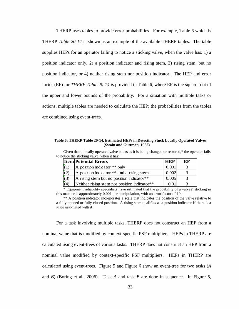
33
THERP uses tables to provide error probabilities. For example, Table 6 which is
THERP Table 20-14 is shown as an example of the available THERP tables. The table
supplies HEPs for an operator failing to notice a sticking valve, when the valve has: 1) a
position indicator only, 2) a position indicator and rising stem, 3) rising stem, but no
position indicator, or 4) neither rising stem nor position indicator. The HEP and error
factor (EF) for THERP Table 20-14 is provided in Table 6, where EF is the square root of
the upper and lower bounds of the probability. For a situation with multiple tasks or
actions, multiple tables are needed to calculate the HEP; the probabilities from the tables
are combined using event-trees.
Table 6: THERP Table 20-14, Estimated HEPs in Detecting Stuck Locally Operated Valves (Swain and Guttman, 1983)
Given that a locally operated valve sticks as it is being changed or restored,* the operator fails to notice the sticking valve, when it has:
Item Potential Errors HEP EF(1) A position indicator ** only 0.001 3(2) A position indicator ** and a rising stem 0.002 3(3) A rising stem but no position indicator** 0.005 3(4) Neither rising stem nor position indicator** 0.01 3 * Equipment reliability specialists have estimated that the probability of a valves’ sticking in
this manner is approximately 0.001 per manipulation, with an error factor of 10. ** A position indicator incorporates a scale that indicates the position of the valve relative to
a fully opened or fully closed position. A rising stem qualifies as a position indicator if there is a scale associated with it.
For a task involving multiple tasks, THERP does not construct an HEP from a
nominal value that is modified by context-specific PSF multipliers. HEPs in THERP are
calculated using event-trees of various tasks. THERP does not construct an HEP from a
nominal value modified by context-specific PSF multipliers. HEPs in THERP are
calculated using event-trees. Figure 5 and Figure 6 show an event-tree for two tasks (A
and B) (Boring et al., 2006). Task A and task B are done in sequence. In Figure 5,
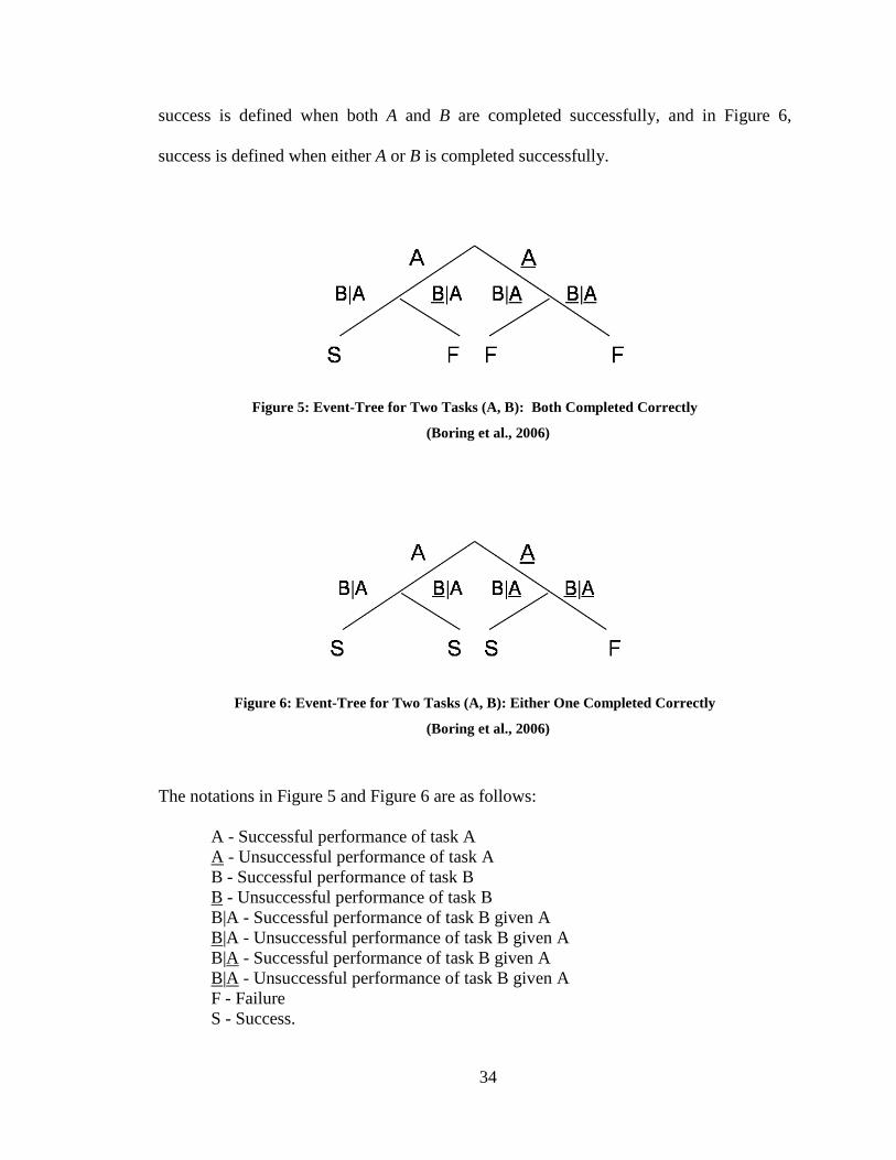
34
success is defined when both A and B are completed successfully, and in Figure 6,
success is defined when either A or B is completed successfully.
Figure 5: Event-Tree for Two Tasks (A, B): Both Completed Correctly
(Boring et al., 2006)
Figure 6: Event-Tree for Two Tasks (A, B): Either One Completed Correctly
(Boring et al., 2006)
The notations in Figure 5 and Figure 6 are as follows:
A - Successful performance of task A A - Unsuccessful performance of task A B - Successful performance of task B B - Unsuccessful performance of task B B|A - Successful performance of task B given A B|A - Unsuccessful performance of task B given A B|A - Successful performance of task B given A B|A - Unsuccessful performance of task B given A F - Failure S - Success.
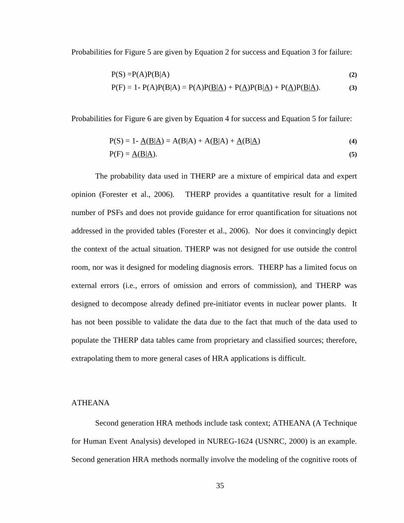
35
Probabilities for Figure 5 are given by Equation 2 for success and Equation 3 for failure:
P(S) =P(A)P(B|A) (2)
P(F) = 1- P(A)P(B|A) = P(A)P(B|A) + P(A)P(B|A) + P(A)P(B|A). (3)
Probabilities for Figure 6 are given by Equation 4 for success and Equation 5 for failure:
P(S) = 1- A(B|A) = A(B|A) + A(B|A) + A(B|A) (4)
P(F) = A(B|A). (5)
The probability data used in THERP are a mixture of empirical data and expert
opinion (Forester et al., 2006). THERP provides a quantitative result for a limited
number of PSFs and does not provide guidance for error quantification for situations not
addressed in the provided tables (Forester et al., 2006). Nor does it convincingly depict
the context of the actual situation. THERP was not designed for use outside the control
room, nor was it designed for modeling diagnosis errors. THERP has a limited focus on
external errors (i.e., errors of omission and errors of commission), and THERP was
designed to decompose already defined pre-initiator events in nuclear power plants. It
has not been possible to validate the data due to the fact that much of the data used to
populate the THERP data tables came from proprietary and classified sources; therefore,
extrapolating them to more general cases of HRA applications is difficult.
ATHEANA
Second generation HRA methods include task context; ATHEANA (A Technique
for Human Event Analysis) developed in NUREG-1624 (USNRC, 2000) is an example.
Second generation HRA methods normally involve the modeling of the cognitive roots of
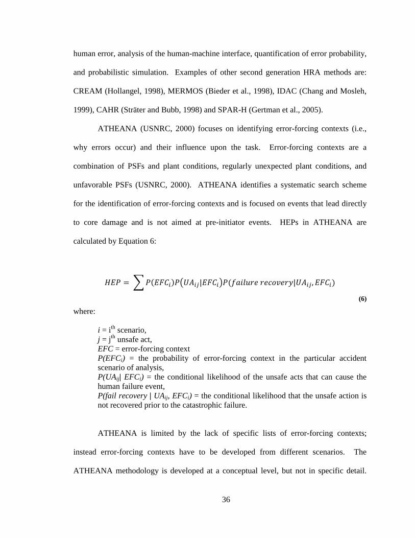
36
human error, analysis of the human-machine interface, quantification of error probability,
and probabilistic simulation. Examples of other second generation HRA methods are:
CREAM (Hollangel, 1998), MERMOS (Bieder et al., 1998), IDAC (Chang and Mosleh,
1999), CAHR (Sträter and Bubb, 1998) and SPAR-H (Gertman et al., 2005).
ATHEANA (USNRC, 2000) focuses on identifying error-forcing contexts (i.e.,
why errors occur) and their influence upon the task. Error-forcing contexts are a
combination of PSFs and plant conditions, regularly unexpected plant conditions, and
unfavorable PSFs (USNRC, 2000). ATHEANA identifies a systematic search scheme
for the identification of error-forcing contexts and is focused on events that lead directly
to core damage and is not aimed at pre-initiator events. HEPs in ATHEANA are
calculated by Equation 6:
𝐻𝐸𝑃 = �𝑃(𝐸𝐹𝐶𝑖)𝑃�𝑈𝐴𝑖𝑗|𝐸𝐹𝐶𝑖�𝑃(𝑓𝑎𝑖𝑙𝑢𝑟𝑒 𝑟𝑒𝑐𝑜𝑣𝑒𝑟𝑦|𝑈𝐴𝑖𝑗,𝐸𝐹𝐶𝑖)
(6)
where:
i = ith scenario, j = jth unsafe act, EFC = error-forcing context P(EFCi) = the probability of error-forcing context in the particular accident
scenario of analysis, P(UAij| EFCi) = the conditional likelihood of the unsafe acts that can cause the
human failure event, P(fail recovery | UAij, EFCi) = the conditional likelihood that the unsafe action is
not recovered prior to the catastrophic failure.
ATHEANA is limited by the lack of specific lists of error-forcing contexts;
instead error-forcing contexts have to be developed from different scenarios. The
ATHEANA methodology is developed at a conceptual level, but not in specific detail.
37
Also, there is no specific quantification method associated with ATHEANA; any
quantitative assessment to be used in PRA has to come from expert judgment informed
by the ATHEANA analysis (USNRC, 2000). Thus, a team of HRA specialists are
normally required to conduct an HRA when using ATHEANA.
SPAR-H
The Standardized Plant Analysis Risk – Human reliability analysis (SPAR-H)
method was developed to support plant-specific PRA and is discussed in NUREG/CR-
6883 (Gertman et al., 2005). SPAR-H is a replacement and revision of the NRC’s
accident sequence precursor analysis. SPAR-H is primarily a quantification method for
human error probability that assumes the human failure events have already been
identified. A strength of SPAR-H is that it provides guidance on assigning weights to the
PSFs and uses worksheets for analyst consistency and documentation. There are pre-
defined PSFs for SPAR-H (e.g., Time Available, Stress, Complexity, Experience and
Training, Procedures, Ergonomics, Fitness-for-Duty, and Work Process).
The SPAR-H method separates human error into two separate categories action
(e.g., errors of commission--active errors) and diagnosis (e.g., errors of omission--latent
errors). Separate worksheets are used for quantifying action and diagnosis errors.
Different PSF weights and nominal HEP values, which are pre-defined, are associated
with action and diagnosis errors in the SPAR-H method. Action errors have a nominal
probability of 1.0E-3, while the nominal probability for diagnosis is 1.0E-2. Therefore, in
SPAR-H under normal operating conditions, an individual has a 1 in 100 chance of
committing a cognitive error and 1 in 1000 of committing an action error. Human error
38
probabilities in SPAR-H are calculated by adjusting the nominal human error probability
by a standardized weighting factor attributed to the level of action by the PSF under
investigation. When the effect of PSFs is included, the overall probability is expressed
as:
𝐻𝐸𝑃 = 𝑃0 ∏ 𝑃𝑆𝐹𝑖8𝑖=1 (7)
where,
HEP = human error probability Po = nominal probability value PSFi = multiplier for performance shaping factor i in the situation
investigated.
SPAR-H uses standardized worksheets and is simple to implement; these
worksheets produce a mean estimate of the HEP. Although SPAR-H is relatively
straightforward and follows good practices for HRA, one weakness is that interactions
among the PSFs are not considered. SPAR-H is implicitly influenced by THERP for its
base (i.e., nominal) failure rates and dependency information. The main source of
uncertainty in SPAR-H comes from selecting the values for the PSFs; different users
might use different PSF values with the same data.
PSFs in SPAR-H
In the SPAR-H human reliability method, the nominal human error probabilities
are multiplied by PSF coefficient values. SPAR-H uses a pre-defined set of PSF
multipliers, which the analyst relates according to situational context. A literature review
of human behavioral sciences and HRA models was used to identify the following eight
PSFs that are used in the SPAR-H method (Gertman et al., 2005):
39
1) Time Available 2) Stress 3) Complexity
4) Experience and Training 5) Procedures 6) Ergonomics 7) Fitness-for-Duty 8) Work Process
The last five PSFs, experience and training, procedures, ergonomics, fitness-for-duty, and
work process, are event or personnel specific and are evaluated when analyzing a plant-
specific model. The first three SPAR-H PSFs, time available, stress, and complexity, are
evaluated immediately through HRA.
Another feature of SPAR-H is that it includes the positive influences of PSFs on
human performance; these follow the inverted-U graph of the arousal curve as shown in
Figure 7 and are referred to as the Yerkes-Dodson Law of arousal (Yerkes and Dodson,
1908). There is a positive influence on performance with added arousal (e.g., engaging
the worker and preventing errors of omission by inattention) until the peak is reached;
then there is a negative effect, as arousal/stress continues beyond the optimum point. The
term arousal in this sense is used as a synonym of stress or complexity. Arousal plays an
important role in determining what information is essential in a competitive environment
to allocate scarce attention and memory resources to critical events rather than to the
mundane (Christianson, 1992).
40
Figure 7: Yerkes-Dodson Law Inverted U-graph (Yerkes and Dodson, 1908)
Limitations in Current HRA Methods
There are four main sources of deficiencies in current HRA methods: 1) lack of
empirical data for model development and validation, 2) lack of inclusion of human
cognition (i.e., need for better human behavior modeling), 3) large variability in
implementation, i.e., HRA parameters are different depending on the method used,
(Sträter and Bubb, 1998), and 4) heavy reliance on expert judgment in selecting PSFs,
and the use of them to obtain the HEP in human reliability analysis. The theoretical basis
for many of the HRA methods is unclear (Blackman, 1998).
HRA methods are limited by the availability of relevant data. In order to address
the first deficiency, there are currently ongoing efforts to establish HRA databases.
These are available to HRA analysts and have the human error data with cited sources in
order to improve the validity and reproducibility of HRA results. Examples of the
databases are the Human Event Repository and Analysis (HERA) (Hallbert et al., 2006)
and the Human Factors Information System (HFIS) (USNRC, 2006).
Low Arousal High
Per
form
ance
Weak
Strong
Simple Task
Difficult Task
Low Arousal High
Per
form
ance
Weak
Strong
Simple Task
Difficult Task
41
In order to model human behavior with more fidelity, the effect of human
cognition and influences that significantly affect human performance, such as fatigue,
needs to be considered for inclusion into HRA. The more data available on human error,
especially in reference to contextual conditions, the greater the confidence in human
reliability analysis (Collier, 2005). Human actions can either improve or impede in
failure recovery. Researchers are beginning to include task context in HRA methods,
such as ATHEANA. This is an important step forward in human error analysis.
The third deficiency in current HRA methods is variability in model
implementation. There is one validation study of the THERP method that is widely cited,
but there is little else in the way of validation studies that have been published. How
much variance exists in HRA models that are currently being used is not clear. These
factors make it difficult to assess the predictive capability of current HRA methods.
The fourth limitation of HRA is the heavy reliance on expert opinion; the fact that
expert opinion is used to populate HEPs makes reproducing and validating the results
difficult. The dependency on expert judgments could be reduced with an improvement in
the quantitative basis for the data used to generate HEPs.
Inclusion of Fatigue in HRA Methods
Fatigue is not usually considered as a PSF in most commonly used HRA methods.
Nor do current HRA methods adequately include explicit quantitative measures for the
effects of fatigue. Typically, fatigue is assumed to be indirectly covered in PSFs such as
fitness-for-duty in the SPAR-H method. Fatigue is a dynamic PSF that does not remain
constant throughout an event, such as training would.
42
Fatigue is not explicitly covered in THERP. The tables of THERP deal with
HEPs of actual scenarios, for example, detecting stuck locally operated valves from Table
20-14 of Swain and Guttman (1983). In the case of ATHEANA, fatigue comes under the
error-forcing context (EFC) related to the effect of the initiator or accident sequence on
the capacity of action of the control room before the incident. For retrospective analysis
using ATHEANA (i.e., after the incident), fatigue effects could be considered as a sub-
factor under the PSF of human performance capabilities at a low point.
In SPAR-H, fatigue could be considered a sub-factor of the fitness-for-duty PSF.
However, it could be argued that fatigue would have some effect on several of the eight
PSFs given their generality. For example, SPAR-H PSFs such as stress, time available,
and complexity would be affected by fatigue through its competition for limited mental
resource capacity. However, the main PSF that would be affected would be fitness-for-
duty. The PSF fitness-for-duty is broken down into four levels in SPAR-H: unfit (which
gives the probability of human error as 1.0), degraded (weight of 5), and nominal (weight
of 1), with the additional option of selecting the category of insufficient information
(weight of 1). These three levels of duty fitness were initially designed with chemically
induced impairment in mind, not impairment due to fatigue (Whaley et al., 2011).
The refinement of current HRA methods can be done by focusing on specific
factors that contribute to human errors, and using empirical data for quantification. This
will lead to increased credibility of HRA, resulting in improved probabilistic risk
assessment (PRA). An improved PRA will allow for an increased understanding of the
safe operating bounds of human behavior in the twenty-four hour economy world. In
43
general, the inclusion of the quantitative and qualitative aspects of PSFs, such as fatigue,
need to be better understood and represented in the HRA methods.
Summary
Fatigue has been identified as the root cause in multiple accidents, including the
Challenger accident in 1986, the Staten Island Ferry crash in 2003, and multiple minor
incidents at nuclear power plants, for example, Peach Bottom in 1987 and 2003. Even
though fatigue is linked to many major and minor accidents, it is still a condition that
occurs daily. In order to illustrate the effect sleep deprivation has on simple reaction
time, hours of wakefulness have been experimentally equated to BAC% levels. These
experiments report that 17 hours of wakefulness (seven hours of sleep in a twenty-four
hour period) have the same effect as a BAC% of 0.05, which is the legal limit in much of
Europe. However, fatigue cannot be directly measured and must be measured through
indirect metrics. A way to address the pervasive influence of fatigue is to format known
information about fatigue into formal risk assessments. This research establishes a
method to extract quantitative data about fatigue and sleep deprivation to derive human
error probabilities for use in HRA.
In this chapter, HRA methods were presented along with their limitations
requiring improvement. Common HRA methods, including THERP, ATHEANA, and
SPAR-H, are lacking in the inclusion of fatigue and sleep deprivation effects on
performance. PRA utilizes information gained from HRA to represent the human
element of risk assessment.
44
CHAPTER III
SYNTHESIS OF SLEEP DEPRIVATION STUDIES
One way to deal with the multitude of differences in the sleep deprivation
literature is to use the meta-analysis research synthesis method. This chapter gives
background on meta-analysis, including the basic procedure and equations. The end
result of meta-analysis is the effect size or the degree of change in the variable under
study. Also, the basic differences in the sleep deprivation literature are reviewed. These
differences include variability in the subjects, experimental conditions, and performance
tasks. Three predefined performance tasks are discussed in greater detail, (i.e., Baddeley
logical reasoning, Mackworth clock, and the PVT).
Background on Meta-Analysis
Meta-analysis is a synthesis of available research about a topic. Meta-analysis
creates a structured format, through statistical procedures and a coding manual, to extract
information from selected studies for the purpose of combining the findings. Meta-
analysis is not a literature review, nor is it a vote counting method of available research
(Hunt, 1997).
The term meta-analysis was coined by Smith and Glass (1977) with respect to
studies on psychotherapy, beginning the now common practice of using quantitative
synthesis techniques in social science. The idea of combining results from multiple
45
studies was not originated by Glass, but was first introduced by Pearson in the early
1900’s (Pearson, 1904).
Meta-analysis provides explanations of causal relationships; the strength of
correlation suggests the causal chain of events leading to the outcome. With meta-
analysis, the sub-parts (the factors that play a role in the end effect studies) of the
outcome can be measured; this is a method that makes it possible to measure the
indirectly-measurable fatigue effects on worker performance. The main effects can be
identified and the quantitative change in effect size, due to substantive issues, can be
observed. The effect size is the degree to which the phenomenon under investigation is
present in the population. Effect size expresses the degree of difference from the null
hypothesis, where the null hypothesis is that there is no effect. Meta-analysis is used to
discover the underlying trends by integrating a large collection of analysis results from
individual studies for the purpose of integrating the findings. This method of analysis is
especially useful for studying humans, since human behavior is not easy to control for
study purposes; i.e., rarely does a single study provide sufficient information on which to
base policy.
A high quality meta-analysis depends on four main components: success in
locating studies, explicitness of criteria for selecting studies, accuracy in effect size
computations, and the adherence to the assumptions of meta-analysis statistics. At its
best, meta-analysis advances knowledge about a phenomenon by explicating its typical
patterns and showing when effect size is larger or smaller, negative or positive, and tests
theories about the phenomena (Hunt, 1997).
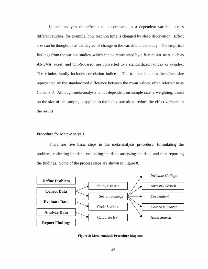
46
In meta-analysis the effect size is compared as a dependent variable across
different studies, for example, how reaction time is changed by sleep deprivation. Effect
size can be thought of as the degree of change in the variable under study. The empirical
findings from the various studies, which can be represented by different statistics, such as
ANOVA, t-test, and Chi-Squared, are converted to a standardized r-index or d-index.
The r-index family includes correlation indices. The d-index includes the effect size
represented by the standardized difference between the mean values, often referred to as
Cohen’s d. Although meta-analysis is not dependent on sample size, a weighting, based
on the size of the sample, is applied to the index statistic to reduce the effect variance in
the results.
Procedure for Meta-Analysis
There are five basic steps in the meta-analysis procedure: formulating the
problem, collecting the data, evaluating the data, analyzing the data, and then reporting
the findings. Some of the process steps are shown in Figure 8.
Figure 8: Meta-Analysis Procedure Diagram
Define Problem
Collect Data
Evaluate Data
Analyze Data
Report Findings
Invisible College
Ancestry Search
Descendent
Database Search
Hand Search
Study Criteria
Search Strategy
Code Studies
Calculate ES
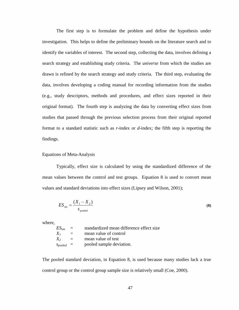
47
The first step is to formulate the problem and define the hypothesis under
investigation. This helps to define the preliminary bounds on the literature search and to
identify the variables of interest. The second step, collecting the data, involves defining a
search strategy and establishing study criteria. The universe from which the studies are
drawn is refined by the search strategy and study criteria. The third step, evaluating the
data, involves developing a coding manual for recording information from the studies
(e.g., study descriptors, methods and procedures, and effect sizes reported in their
original format). The fourth step is analyzing the data by converting effect sizes from
studies that passed through the previous selection process from their original reported
format to a standard statistic such as r-index or d-index; the fifth step is reporting the
findings.
Equations of Meta-Analysis
Typically, effect size is calculated by using the standardized difference of the
mean values between the control and test groups. Equation 8 is used to convert mean
values and standard deviations into effect sizes (Lipsey and Wilson, 2001);
pooledsm s
XXES )( 21 −= (8)
where, ESsm = standardized mean difference effect size X1 = mean value of control X2 = mean value of test spooled = pooled sample deviation.
The pooled standard deviation, in Equation 8, is used because many studies lack a true
control group or the control group sample size is relatively small (Coe, 2000).
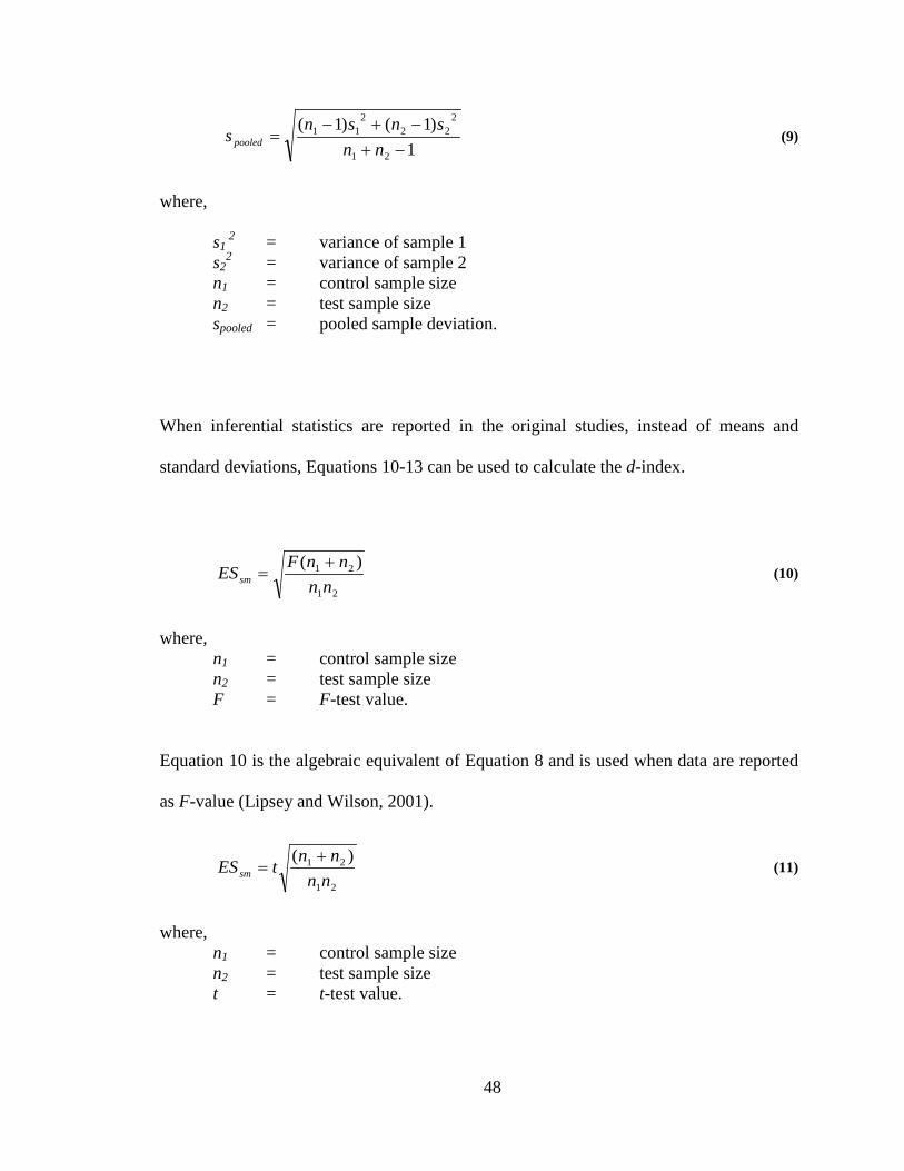
48
1)1()1(
21
222
211
−+−+−
=nn
snsns pooled (9)
where,
s1 2 = variance of sample 1
s22 = variance of sample 2
n1 = control sample size n2 = test sample size spooled = pooled sample deviation.
When inferential statistics are reported in the original studies, instead of means and
standard deviations, Equations 10-13 can be used to calculate the d-index.
21
21 )(nn
nnFESsm+
= (10)
where, n1 = control sample size n2 = test sample size F = F-test value.
Equation 10 is the algebraic equivalent of Equation 8 and is used when data are reported
as F-value (Lipsey and Wilson, 2001).
21
21 )(nn
nntESsm+
= (11)
where, n1 = control sample size n2 = test sample size t = t-test value.
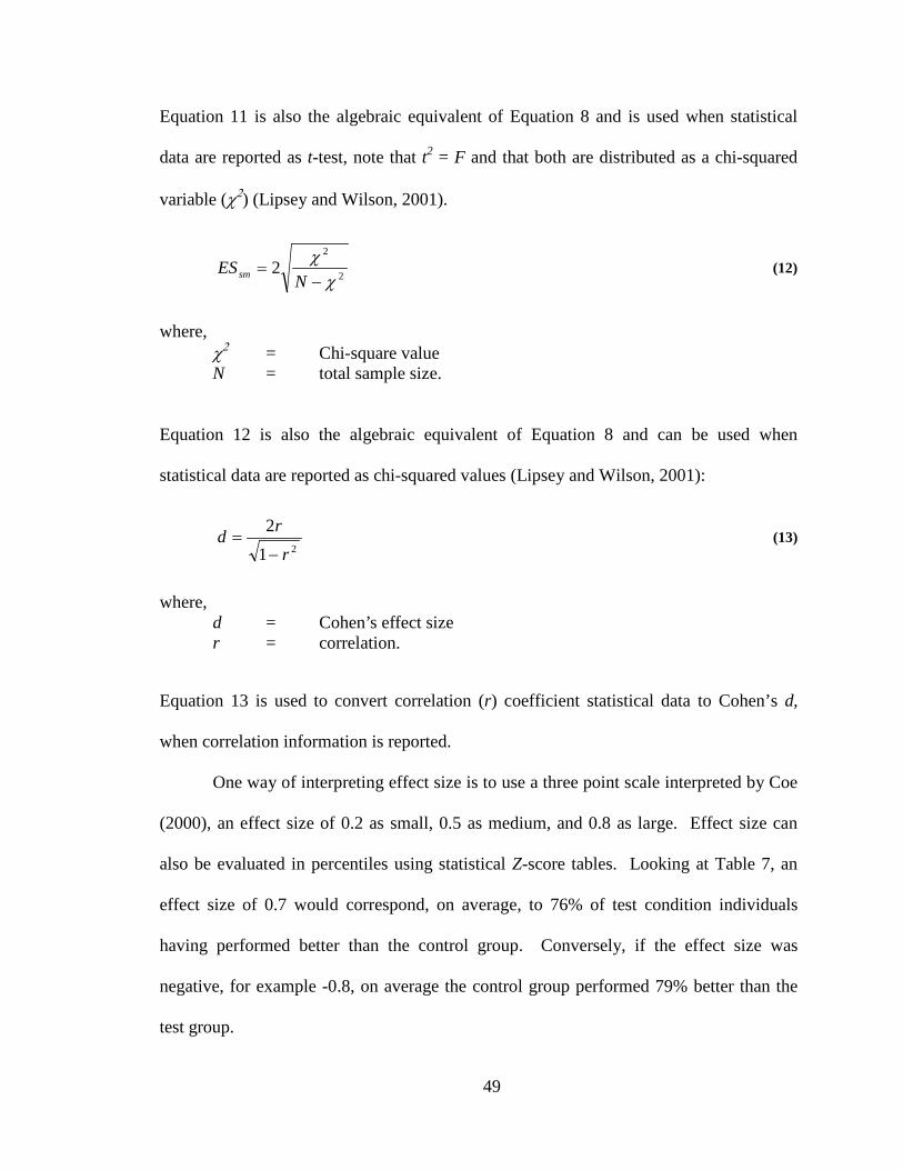
49
Equation 11 is also the algebraic equivalent of Equation 8 and is used when statistical
data are reported as t-test, note that t2 = F and that both are distributed as a chi-squared
variable (χ2) (Lipsey and Wilson, 2001).
2
2
2χ
χ−
=N
ESsm (12)
where, χ2 = Chi-square value N = total sample size.
Equation 12 is also the algebraic equivalent of Equation 8 and can be used when
statistical data are reported as chi-squared values (Lipsey and Wilson, 2001):
212
rrd
−= (13)
where, d = Cohen’s effect size r = correlation.
Equation 13 is used to convert correlation (r) coefficient statistical data to Cohen’s d,
when correlation information is reported.
One way of interpreting effect size is to use a three point scale interpreted by Coe
(2000), an effect size of 0.2 as small, 0.5 as medium, and 0.8 as large. Effect size can
also be evaluated in percentiles using statistical Z-score tables. Looking at Table 7, an
effect size of 0.7 would correspond, on average, to 76% of test condition individuals
having performed better than the control group. Conversely, if the effect size was
negative, for example -0.8, on average the control group performed 79% better than the
test group.
50
Table 7: Interpreting Effect Size (Coe, 2000)
Effect Size Percentage (%) Z-Table0.00 50% 0.50000.10 54% 0.53980.20 58% 0.57930.30 62% 0.61790.40 66% 0.65540.50 69% 0.69150.60 73% 0.72570.70 76% 0.75800.80 79% 0.78810.90 82% 0.81591.00 84% 0.84131.20 88% 0.88491.40 92% 0.91921.60 95% 0.94521.80 96% 0.96412.00 98% 0.97722.50 99% 0.99382.80 99.9% 0.9974
Shortcomings of Meta-Analysis
While there are many advantages to conducting a meta-analysis, there are also
some shortcomings associated with the procedure. One limitation is that meta-analysis
requires significant effort. Many studies can be identified using computer searches;
however, the actual data need to be coded manually. Meta-analysis is a labor intensive
activity that can sometimes take years depending on the topic under investigation and the
amount of literature that is available.
One pitfall in meta-analysis is the inclusion of blemished studies; a good meta-
analysis of bad studies will result in bad statistics. The meta-analyst is limited by the
quality of research in the available studies and often there is not enough information
reported in a study to determine if the statistics are correctly computed. There is need for
a balance between inclusion and exclusion of studies to maintain a quality analysis. The
51
meta-analyst is aided in limiting the inclusion of blemished studies in the synthesis by a
well-defined study criterion, while also being advised to err in the direction of being
broadly inclusive in research procedures in order to insure that a sufficient sample of
studies is located (Reis and Judd, 2000).
Another shortcoming is that there is a large publication bias towards significant
results. Non-significant findings are not often published or documented. This is often
described as the file drawer problem; i.e., there exists a file drawer in the back of a
researcher’s office that is overflowing with studies on the topic in question with non-
significant findings (Rosenthal, 1979). There must be a significant effort made to locate
this fugitive literature in order to increase the confidence in the effect size results.
Variations among Sleep Deprivation Studies
Many differences exist between studies in the sleep deprivation literature, for
example, the type of subjects used and study setting. Since the type of task used to
evaluate performance is not standardized, it also can differ from study to study.
Subject Variability
Subjects differ from study to study in terms of age, sex, and physical
characteristics (e.g., BMI). Older subjects have been shown to be more affected by sleep
deprivation in comparison to younger subjects (Lingenfelser et al., 1994; Steyvers and
Gaillard, 1993; Webb, 1985). Most studies seem to have more male than female
participants (Thomas et al., 2000). Differences between male and female subject
performances are not known. Some studies select appropriate subjects considering
physical characteristics including body mass index (BMI) or the presence of preexisting
52
sleep disorders (e.g., sleep apnea), while other studies make no mention of the personal
traits of the subjects. Another difference is the origination or background of the subjects
prior to the tests (i.e., education, career type, etc.). The majority of studies are conducted
in the laboratory, and often, the subjects are student volunteers (Babkoff et al., 2005).
However, some studies employ subjects from industry, such as medical residents (Saxena
and George, 2005).
Experimental Design
The differences in experimental design complicate the study of sleep deprivation
effects on performance. Differences in experimental design include study environment,
control of time cues, physical activity level, and tasks performed.
The physical settings for the experiments differ in that some studies are conducted
in the field, but most are conducted in laboratory settings. Field experiments have been
reported in military training sessions (May and Kline, 1987; Kobbeltvedt et al., 2005) or
on doctors after being on-call for long periods of time (Saxena and George, 2005).
Studies conducted in the lab are easier to control by limiting the number of influences of
parameters outside the study. Other study setting differences relate to the control of time
cues (zeitgebers) and the physical activity level of the subjects (Aschoff, 1965).
The control of zeitgebers is also different among studies; sometimes it is not
reported at all. For example, in Frey et al. (2004) subjects are removed from all time cues
(e.g., light level, temperature, and constant white noise). In Wesensten et al. (2005) all
time cues are kept constant. In Jones et al. (2006) and Roach et al. (2006), subjects are
not allowed access to caffeine to mitigate the effects of sleep deprivation, but have free
access to time cues.
53
Another difference in the procedure of sleep deprivation testing is the amount of
activity allowed the subjects. In some of the experiments, the subjects are subjected to
constant bed rest allowing for no activity while being kept awake (Caldwell et al., 2003;
Frey et al., 2004). Meanwhile, in others, subjects are asked to engage in light activity
such as TV, video and board games, and reading (Jones et al., 2006; Roach et al., 2006).
Yet, other studies engage the subjects in heavy activity such as military training
(Lieberman et al., 2005; Kobbeltvedt et al., 2005). Some studies report no information
on subject activity levels at all (Thorne et al., 2005).
Not only are the settings and procedures for the experiments different, the types of
tests that are used to evaluate performance may vary. There is no standard metric used to
evaluate performance; studies may use single metric or multiple metrics. Typical
performance evaluators could be subjective, physical, or psycho-motor. Subjective
measures, such as sleepiness scales, are more appropriate for sleepiness and fatigue
studies. Physical measures, such as temperature, electroencephalography (EEG), or
critical flicker frequency threshold, are better measures of arousal or alertness and are
very useful when investigating circadian influences (Czeisler et al. 1999). However, the
focus in this research is how sleep deprivation affects performance; consequently,
psychomotor tests are more appropriate. Psychomotor tests are based on mental
processes (cognition) that require a motor reaction (Kushida et al., 2005).
Currently, there are no definitive psychomotor tests for evaluating sleep
deprivation effects on performance. Some studies use simulated real world tasks, such as
simulated combat (Lieberman et al., 2005), laparoscopic surgery (Eastridge et al., 2003),
or driving simulator (Akerstedt et al., 2005; Langois et al., 1985). Other studies employ
54
real work activities or games (Venkatraman et al., 2007; Killgore et al., 2006). However,
most studies use simplified tasks that can be somewhat controlled. Three frequently
employed tests are the Logical Reasoning Task (Baddeley, 1968), Mackworth Vigilance
Task (Mackworth, 1950), and Psychomotor Vigilance Task - PVT (Dinges and Powell,
1985), with the PVT being the most frequently used (Gunzelmann et al., 2009). Each
type of test used is briefly described in the following discussion.
Baddeley Logical Reasoning Task
The logical reasoning task (Baddeley, 1968) is a three-minute test that measures
and emphasizes both speed and accuracy. The subject is presented with a series of short
sentences that employ different syntax structures that claim to describe the order between
two letters, such as AB. This test uses sentence comprehension as it is related to syntax
structure. For example, sentence understanding is faster for: a positive statement than a
negative one, an active faster than passive sentence, and a true sentence faster than a false
sentence. The subjects read the sentences that describe the 2-letter order and are asked to
identify the statements as true or false. For illustration of the task, the two letters A and B
are used in AB order. The following four sentences are all true. The first is an example of
a positive statement and an active sentence. The third sentence is an example of a
negative statement and a passive sentence.
1) A precedes B. 2) B follows A. 3) A does not follow B. 4) B does not come before A.
Normally this task uses sixty-four possible combinations of six different conditions; 1)
positive or negative, 2) active or passive, 3) true or false, 4) precedes or follows, 5)
whether A or B is mentioned first, and 6) either the AB or BA combination. Nine studies
55
out of the 108 utilized in the current study employ the Baddeley logical reasoning task
(Rosa and Colligan, 1988; Deaconson et al., 1988; Englund et al., 1985, Haslam, 1982;
Poulton et al., 1978; Rosa and Bonnet, 1993; Leonard et al., 1998; Lieberman et al.,
2005; Webb, 1985).
Mackworth Clock Vigilance Task
In the Mackworth clock vigilance task (Mackworth, 1950) subjects view a
circular display similar to a clock face. A pointer moves around the clock face at a steady
rate. The subject is asked to react (i.e., press a button) when the pointer double jumps or
skips over a point along the circle. This is a type of tracking task. The number of correct
responses, false positives, and reaction time are recorded. Studies using the Mackworth
clock vigilance task included Richter et al., (2005), Monk et al., (1997), and Williamson
and Feyer, (2000).
Psychomotor Vigilance Task
The PVT is a standardized task that uses a computer or hand-held device (Dinges
and Powell, 1985). The test is based on the Wilkinson simple visual reaction time device
(Wilkinson and Houghton, 1982). The PVT was developed as a neurocognitive test for
tracking to access the working memory of the prefrontal cortex of the brain; it is used to
measure the magnitude of attention deficits. Performance on working memory tasks is
observed to be predictive of performance on a range of other cognitive tasks (Kushida et
al., 2005). Working memory is considered to be fundamental to performance on virtually
any neurocognitive task. The PVT has a high level of reliability, validity, lack of
dependence on aptitude, and the ability to be repeatedly administered; this makes it useful
for quantifying the effects of sleep loss.
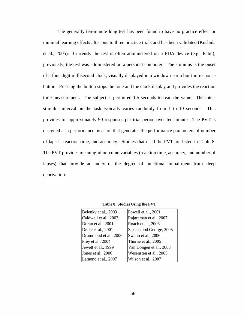
56
The generally ten-minute long test has been found to have no practice effect or
minimal learning effects after one to three practice trials and has been validated (Kushida
et al., 2005). Currently the test is often administered on a PDA device (e.g., Palm);
previously, the test was administered on a personal computer. The stimulus is the onset
of a four-digit millisecond clock, visually displayed in a window near a built-in response
button. Pressing the button stops the tone and the clock display and provides the reaction
time measurement. The subject is permitted 1.5 seconds to read the value. The inter-
stimulus interval on the task typically varies randomly from 1 to 10 seconds. This
provides for approximately 90 responses per trial period over ten minutes. The PVT is
designed as a performance measure that generates the performance parameters of number
of lapses, reaction time, and accuracy. Studies that used the PVT are listed in Table 8.
The PVT provides meaningful outcome variables (reaction time, accuracy, and number of
lapses) that provide an index of the degree of functional impairment from sleep
deprivation.
Table 8: Studies Using the PVT
Belenky et al., 2003 Powell et al., 2001Caldwell et al., 2003 Rajaraman et al., 2007Doran et al., 2001 Roach et al., 2006 Drake et al., 2001 Saxena and George, 2005Drummond et al., 2006 Swann et al., 2006Frey et al., 2004 Thorne et al., 2005Jewett et al., 1999 Van Dongen et al., 2003Jones et al., 2006 Wesensten et al., 2005Lamond et al., 2007 Wilson et al., 2007
57
The majority of the experiments are conducted in laboratory settings, where more
control can be used in excluding confounding factors. Therefore, tests are not being
conducted in realistic workplace settings and often use simplified tasks. This, in turn,
makes extrapolation of the results to real-world settings difficult and potentially
inaccurate. In addition, the tasks employed during laboratory tests are frequently
isolated, primary tasks, instead of being representative complex tasks faced in most jobs
today. The subject variability and differences in experimental design make direct
comparison between studies difficult.
The study differences of the sleep deprivation literature are coded through a meta-
analysis procedure. The change in performance due to sleep deprivation is the variable
under investigation. The differences between the studies in the sleep deprivation
literature are coded to look for causal relationships between the effect size and the study
design. This information may or may not be useful in evaluating the data. The type of
task used to evaluate performance can vary greatly between studies. It is important to
take note of the type of task used and the performance metrics evaluated through the task.
The data in this research are grouped by the performance metric reported (i.e., reaction
time, accuracy, and number of lapses). The data can be further divided by variables that
show some type of causal relationship, for example, task complexity level or the
experimental design. The study differences coded may also be useful for use in
extrapolating findings.
58
CHAPTER IV
RESEARCH METHODOLOGY
This chapter discusses the methodology used for data collection, data analysis,
and derivation of performance shaping factor coefficients. An initial search for sleep
deprivation studies evaluating performance was conducted. Data were identified through
reviewing journals for sleep deprivation studies from the search strategy. The selection
criteria were established and a group of 108 studies was identified. The statistical data,
study descriptors, and experimental conditions were coded. The data collected from the
identified studies were analyzed by looking at the difference between the mean values,
percentage change, effect size, and reliability index. Performance shaping factor
coefficient values were derived from the collected statistical data. The uncertainty
associated with the performance shaping factor coefficients and inter-rater reliability for
the coding was also calculated.
Data Collection
The data used for analysis were gathered through a meta-analysis approach. Data
collection involved defining a search strategy and establishing study criteria; these
criteria helped to limit or define the universe from which the studies were drawn. Studies
that were considered included published research studies on sleep deprivation and its
effect on performance, in a pretest-posttest design. A pretest and posttest experimental
59
design compares the performance before treatment (i.e., pretest) to the performance after
treatment (i.e., posttest).
The initial search strategy used computerized databases, (e.g., PubMed, Cochran,
MEDLINE, PsycINFO, and PsychLit) to locate relevant publications. Search terms
included fatigue, performance, sleep deprivation, shiftwork, reaction time, and accuracy.
The bibliographies of these papers were then used to find more possible studies in a
citation or descendent search. Authors that were found to frequently publish in the sleep
deprivation field were reviewed to find more studies in an ancestry search approach.
Journals, such as Sleep and Journal of Sleep Research, were searched manually for
studies on the topic after locating a study from the previous search methods.
The first sampling of studies included those that evaluated the effect of sleep
deprivation or fatigue on performance; these were primarily conducted in the areas of
military, medical, transportation, and psychology. The first requirement was that the
study was reported in English, due to the limitations of the researcher, and that all
subjects be adults. Studies conducted after the 1940’s were considered, since this is the
time frame for modern studies conducted after WWII, when technology became a part of
everyday work.
The quality of the studies was subjectively determined and relied on the peer
review process of journal publications and the reputations of the journals used. One way
to judge the suitability of the journals was to use the impact factor of the journal. The
impact factor can be used as a metric for a journal’s reputation, using the average number
of citations to articles published in science and social science journals. The impact
factors are calculated yearly and are part of Reuters. The top three journal impact factors
60
are New England Journal of Medicine (52.6), Lancet (28.6), and Journal of the American
Medical Association (JAMA) (25.6). However, the editor and chief of JAMA, Dr.
Catherine DeAngelis, said that the impact factor is, “the easiest manipulated number in
the world (Omanio, 2009). Since sleep research is a small subspace of science and social
science, the journals that have impact factors will not be large and many quality journals
in the field may not have an impact factor at all. Consequently, the impact factor was not
considered as a definitive level of quality, but was used to aid in the subjective evaluation
of journal suitability. The journals listed in Appendix C are those mentioned by the
European sleep research society as pertaining to sleep research. The journals are listed in
order of impact factor.
The studies selected for further review expressed the effect of sleep deprivation
(i.e., the independent variable) on performance through reaction time, accuracy, and or
number of lapses (i.e., the dependent variable). The studies used were collected from
multiple disciplines and journals. These journals included, but were not limited to:
Journal of Sleep Research (Nilsson et al., 2005; Thomas et al., 2000), Sleep (Mitler et al.,
1988; Jewett et al., 1999) Journal of Neuroscience (Chee and Choo, 2004), Behavior
Research Methods, Instruments, & Computers (Angus et al., 1985; Thorne et al., 2005),
Chronobiology (Langlois et al., 1985), Ergonomics (Rosa and Bonnet, 1993), Human
Factors (Wilkinson and Houghton, 1982), Journal of the American Medical Association
(JAMA) (Deaconson et al., 1988), Psychophysiology (Drake and Roehrs, 2001),
NeuroImage (Choo et al., 2005), Occupational Environmental Medicine (Williamson and
Feyer, 2000), and Organizational Behavior and Human Decision Processes (Kobbeltvedt
et al., 2005).
61
The data collection is limited by the quality of research reported and often there is
not enough information disclosed about a study in a journal publication to determine if
statistics are correctly computed. There is need for a balance between inclusion and
exclusion of studies in order to maintain a quality analysis and also ensure a sufficient
sample size of studies (Reis and Judd, 2000). Another limitation is the large publication
bias towards significant results. Commonly non-significant findings are not published or
documented (Rosenthal, 1979).
Coding Applications
The studies located from the search strategy were identified in a variety of fields.
Viable studies were identified by evaluating whether or not the studies examined a
change in performance due to sleep deprivation. A list of 108 studies was identified as
meeting the initial criteria. Information was extracted, coded, and then grouped by
experimental conditions, task characteristics, and statistical data.
Data Resources
The identification of sleep deprivation as a significant source of risk has led to
sleep deprivation studies being conducted in a variety of fields and settings. The majority
of data for use in this research comes from psychological experiments; many of which
have been conducted under the guidance of industries such as transportation [long haul
driving (Akerstedt et al., 2005), aviation (Wilson et al., 2007), railroad (Hildebrandt et
al., 1974)], medical (Deaconson et al., 1988), and military (Haslam, 1982). A search of
62
online resources and leading literature led to the discovery of studies focused on sleep
deprivation and its effects on human performance. While a vast number of studies were
identified, difficulties arose in utilizing much of the data presented in these studies for
HRA applications due to format, content, and reporting differences.
A method for collection and synthesis of the data reported in these studies is
needed. The data within the studies were reported in different ways and were found in
graphs, tables, and/or within the text. Each study identified was reviewed and available
data for synthesis and analysis were extracted. For example, if a study reported a change
in a performance variable on a task over an increase in the hours of wakefulness of the
subject, the mean values and variance of the initial and ending performance and the hours
of wakefulness could be extracted.
Study Selection
Originally, 600 studies (Appendix G) were considered to be viable options that
focused on sleep deprivation and its effect on performance (i.e., preliminary selection
criteria). The list was reduced by excluding studies that did not report continuous hours
of wakefulness (acute sleep deprivation) as the independent variable and one or more of
the dependent variables (reaction time, accuracy, and number of lapses) or the data were
not reported in a usable format (i.e., secondary selection criteria). For example,
subjective ratings on sleepiness or fatigue were reported by Minors and Waterhouse
(1987) and only time of day was reported by Mitler et al. (1988). Therefore, these studies
were excluded from the original sample. The resulting 108 studies are listed in Table 9.
63
The studies are listed by study identification number and primary author_year of
publication.
Table 9: List of 108 Studies
1 Nilsson_2005 37 Lenne_1997 73 Nag_19982 Thomas_2000 38 Sallinen_2004 74 MacDonald_19973 Choo_2005 39 Akerstedt_2005 75 Tilley_19824 Chee_2004 40 Boksem_2006 76 Rosa_19935 Williamson_2000 41 Monk_1997 77 Langois_19856 Kobbeltvedt_2005 42 Jones_2006 78 Akerstedt_19777 Robbins_1990 43 Hull_2003 79 Richter_20058 Angus_1985 44 Wright_2006 80 Hildebrandt_19749 Babkoff_2005 45 Halbach_2003 81 Donchin_1995
10 Swann_2006 46 Bliese_2006 82 Oginski_200011 Koslowsky_1992 47 Lamond_2007 83 Taffinder_199812 Pilcher_1996 48 Drummond_2006 84 Smith_199413 Belenky_2003 49 Eastridge_2003 85 Froberg_197714 Buck_1972 50 Engle-Friedman_2003 86 Philip_200415 Killgore_2006 51 Caldwell_2003 87 Powell_200116 Marmuff_2005 52 Rosa_1983 88 Fiorica_196817 Yoo_2007 53 Frey_2004 89 Cutler_197918 Babkoff_1985 54 Glenville_1979 90 Sharp_198819 Williams_1967 55 Webb_1982 91 Steyvers_199320 Williams_1959 56 Poulton_1978 92 Elkin_197421 Wilson_2007 57 Englund_1985 93 Webb_198622 Gundel_2007 58 Saxena_2005 94 Haslam_198323 Webb_1985 59 Richardson_1996 95 Sagaspe_200624 Dinges_1997 60 Christensen_1977 96 Scott_200625 Sanders_1982 61 Rosa_1988 97 Venkatraman_200726 Collins_1977 62 Hart_1987 98 Dinges_198827 Porcu_1998 63 Horne_1983 99 May_198728 Wojtczak_1978 64 Hoddes_1973 100 Lieberman_200529 Dorrian_2007 65 Webb_1984 101 Lamond_199930 Maury_1993 66 Haslam_1982 102 Thorne_200531 Borland_1986 67 Binks_1999 103 Doran_200132 Dawson_1997 68 Deaconson_1988 104 Wesenten_200533 Roach_2006 69 Leonard_1998 105 Jewett_199934 Reznick_1987 70 Storer_1989 106 Drake_200135 Daniel_1989 71 Lichtor_1989 107 Van Dongen_200336 Buck_1975 72 Linde_1999 108 Rajaraman_2007
ReferenceStudy Id # Reference
Study Id # Reference
Study Id #

64
A number of the viable studies among the 108 studies (Table 9) were not used in
the final analysis due to one or more of the reasons below:
1) Reported chronic sleep deprivation, not acute (e.g., Study Id # = 7, 13, 46, 58, 68, 75, 76,
79, 90)
2) Did not report hours of wakefulness (e.g., Study Id # = 83)
3) Did not report control and test conditions (e.g., Study Id # = 41, 44, 78)
4) Reported incidents related to time of day and not hours of wakefulness (e.g., Study Id # =
73, 74, 77, 80, 81, 82, 84, 86).
Some studies were used only in a limited basis when they did not report standard
deviation information (or standard error), but reported hours of wakefulness and test and
control conditions. When no baseline (control condition) was given, but test conditions
were reported for incremental times, the value at approximately 8 hours was used as the
control condition. The studies were further segregated based upon the variables reported
(reaction time, accuracy, and number of lapses). Some studies reported multiple
variables and others only reported single variables.
Coding of Study Information
The information coded for each study was broken up into four main sections: 1)
study descriptors, 2) sample descriptors, 3) experimental conditions and task information,
and 4) effect size information. If a qualifier of the study could not be determined, it was
coded as not available or NA.
65
Study Descriptors
The first step was to establish a method to identify each study. Each was assigned
an identification number in numeric succession as the study was identified along with the
last name of the principal author and the year of publication, in the format of last name of
first author_year. Next, the information of the study context was coded; this information
covered the type of publication (i.e., book, journal article, thesis or dissertation, technical
report, conference paper, other, and indiscernible), the discipline that conducted the study
(i.e., academic, medical, military, transportation, psychology, other, or indiscernible),
whether the study was conducted in the field or a laboratory setting, and the country in
which the study was conducted. This information is represented in Table 10.
Sample Descriptors
The next component coded from each study pertained to the description of the
subjects. Origin of the subjects (i.e., student volunteer, shift workers, medical residents,
nurses, and infantry soldiers) was recorded. Next recorded was the sex of the group (as
percentage male) [i.e., all males (>95%), mostly males (>60%), 50% to 60% male, some
males (<50%), and no males (0%)]. The age of the subjects was noted; this information
was usually given as a mean or a range. Additional information on the subjects was
necessary to identify whether subjects had special motivation or incentives; for example,
if the subject was paid for the number correct in performing a task. This would have put
a bias toward accuracy over reaction time. This information is represented in Table 10.
66
Table 10: Study and Sample Descriptors
JournalBookBook sectionThesis or dissertationTechnical reportConference proceedingGovernment documentOtherNot availableMedicalMilitaryTransportationAcademicOtherLabField
Student volunteersShift workersMedical residentsSoldiersNot availableOtherAll males (>95%), Mostly males (>60%)50 to 60% malesSome males (<50%), No males (<5%), Not available
Notes of Interest on Organization
Environment
Country
Sample Descriptors
From Where Subjects Pulled
Sex of Group
Mean Age of Subjects
Study Identifiers
Study Id #1st Author_Publication Year
Study Descriptors
Type of Publication
Industry or Discipline
Experimental Conditions
Information collected pertaining to the experimental conditions was identified and
coded. The experimental condition information included the type of comparison method
used for the pretest-posttest design, either repeated measures (denoted as RM) or two
group comparison (denoted as 2GC). The next category was the type of experiment
blinding (i.e., single blind subject is not informed of experiment goals or double-blind the
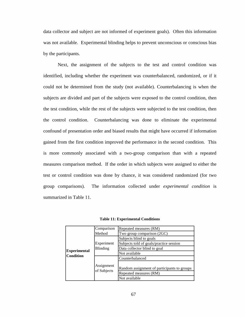
67
data collector and subject are not informed of experiment goals). Often this information
was not available. Experimental blinding helps to prevent unconscious or conscious bias
by the participants.
Next, the assignment of the subjects to the test and control condition was
identified, including whether the experiment was counterbalanced, randomized, or if it
could not be determined from the study (not available). Counterbalancing is when the
subjects are divided and part of the subjects were exposed to the control condition, then
the test condition, while the rest of the subjects were subjected to the test condition, then
the control condition. Counterbalancing was done to eliminate the experimental
confound of presentation order and biased results that might have occurred if information
gained from the first condition improved the performance in the second condition. This
is more commonly associated with a two-group comparison than with a repeated
measures comparison method. If the order in which subjects were assigned to either the
test or control condition was done by chance, it was considered randomized (for two
group comparisons). The information collected under experimental condition is
summarized in Table 11.
Table 11: Experimental Conditions
Repeated measures (RM)Two group comparison (2GC)Subjects blind to goalsSubjects told of goals/practice sessionData collector blind to goalNot availableCounterbalanced
Random assignment of participants to groupsRepeated measures (RM)Not available
Comparison Method
Experiment Blinding
Assignment of Subjects
Experimental Condition
68
Task Characteristics
Another group of study descriptors recorded were the characteristics of the task.
These included a description of the task, whether the task was self-paced or if the pace
was externally set (work pace). Additionally, whether the task was the only task
(primary) or if two tasks were performed at the same time (secondary) was recorded
whenever the data were available. The complexity level of the task was noted whenever
possible (e.g., simple or complex). Whether or not multiple performance metrics were
measured at the same time was also noted (i.e., if reaction time and accuracy were
recorded at the same time). The novelty of the task that subjects were asked to perform
was also indicated; either one designed specifically for the experiment or a predefined
task (e.g., PVT) was used. The name of the pre-defined task was used as the task
description. The length of the task was recorded when the information was available
(e.g., 10 minute PVT). Information on how the task was administered (e.g., use of pen
and paper or computer) and the number of times the task was administered (e.g., 20 times
over the test session) were recorded when available. This information is represented in
Table 12.
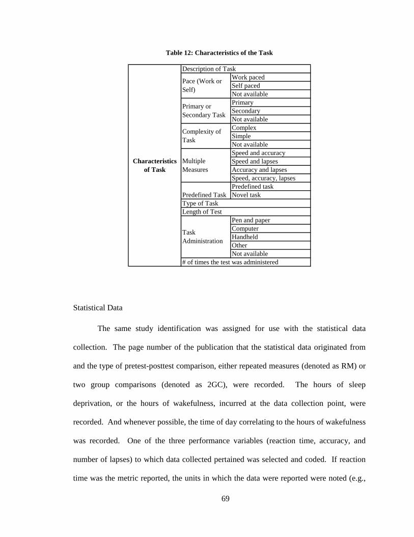
69
Table 12: Characteristics of the Task
Work pacedSelf pacedNot availablePrimarySecondaryNot availableComplexSimpleNot availableSpeed and accuracySpeed and lapsesAccuracy and lapsesSpeed, accuracy, lapsesPredefined taskNovel task
Pen and paperComputerHandheldOtherNot available
Predefined TaskType of TaskLength of Test
Task Administration
# of times the test was administered
Characteristics of Task
Description of Task
Pace (Work or Self)
Primary or Secondary Task
Complexity of Task
Multiple Measures
Statistical Data
The same study identification was assigned for use with the statistical data
collection. The page number of the publication that the statistical data originated from
and the type of pretest-posttest comparison, either repeated measures (denoted as RM) or
two group comparisons (denoted as 2GC), were recorded. The hours of sleep
deprivation, or the hours of wakefulness, incurred at the data collection point, were
recorded. And whenever possible, the time of day correlating to the hours of wakefulness
was recorded. One of the three performance variables (reaction time, accuracy, and
number of lapses) to which data collected pertained was selected and coded. If reaction
time was the metric reported, the units in which the data were reported were noted (e.g.,
70
seconds, milliseconds, or reciprocal of reaction time). How the data were presented in
the original study, either in the text, a table, or graphically was also noted. There will be
greater reliability in the data when presented in text or tables rather than when
interpretation of a graph is required to gather the data.
The statistical data needed to calculate the effect size (ES) were coded. The
sample size of pretest (control) and posttest (test) group and whether or not the number
initially assigned was the same number observed were recorded. If some subjects were
excluded or did not complete the experiment, the number of subjects completing the
study decreased. In repeated measure (RM) studies, the sample size was the same for the
control and test groups, since the same subjects were used as both the control and the test.
The mean value of the variable at the control and test condition (e.g., reaction time at
baseline and reaction time after sleep deprivation) and the standard deviation or standard
error were recorded. If the mean information was not reported, effect sizes can also be
computed through other descriptive statistics, such as proportions and frequencies (e.g.,
number of outcomes). An effect size was computed from significant test statistics if
adequate descriptive statistics were not available; in these cases the Independent-t,
dependent-t, F-value from one-way ANOVA, or χ2 (Chi-squared) was recorded. This
information is represented in Table 13.
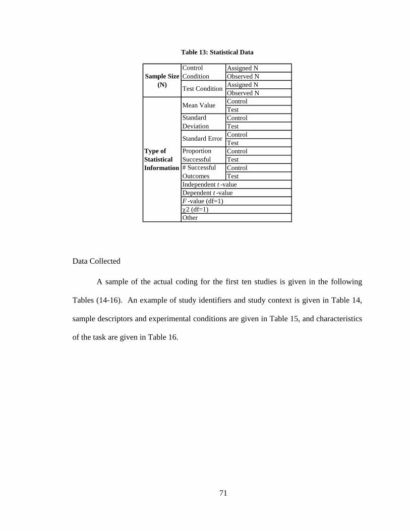
71
Table 13: Statistical Data
Assigned NObserved NAssigned NObserved NControlTestControlTestControlTestControlTestControlTest
Sample Size (N)
Control Condition
Test Condition
Type of Statistical Information
Mean Value
Standard Deviation
Standard Error
Proportion Successful# Successful OutcomesIndependent t -valueDependent t -valueF -value (df=1)χ2 (df=1)Other
Data Collected
A sample of the actual coding for the first ten studies is given in the following
Tables (14-16). An example of study identifiers and study context is given in Table 14,
sample descriptors and experimental conditions are given in Table 15, and characteristics
of the task are given in Table 16.
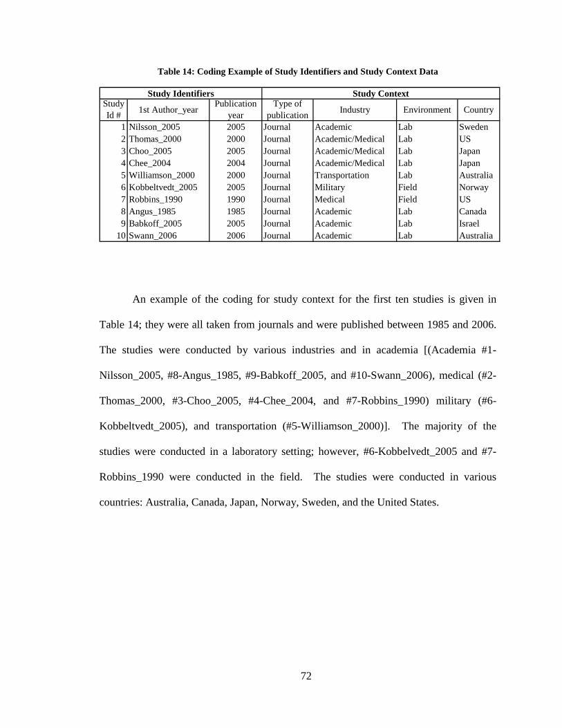
72
Table 14: Coding Example of Study Identifiers and Study Context Data
1 Nilsson_2005 2005 Journal Academic Lab Sweden2 Thomas_2000 2000 Journal Academic/Medical Lab US3 Choo_2005 2005 Journal Academic/Medical Lab Japan4 Chee_2004 2004 Journal Academic/Medical Lab Japan5 Williamson_2000 2000 Journal Transportation Lab Australia6 Kobbeltvedt_2005 2005 Journal Military Field Norway7 Robbins_1990 1990 Journal Medical Field US8 Angus_1985 1985 Journal Academic Lab Canada9 Babkoff_2005 2005 Journal Academic Lab Israel
10 Swann_2006 2006 Journal Academic Lab Australia
Study Identifiers Study ContextStudy Id # 1st Author_year
Publication year
Type of publication Industry Environment Country
An example of the coding for study context for the first ten studies is given in
Table 14; they were all taken from journals and were published between 1985 and 2006.
The studies were conducted by various industries and in academia [(Academia #1-
Nilsson_2005, #8-Angus_1985, #9-Babkoff_2005, and #10-Swann_2006), medical (#2-
Thomas_2000, #3-Choo_2005, #4-Chee_2004, and #7-Robbins_1990) military (#6-
Kobbeltvedt_2005), and transportation (#5-Williamson_2000)]. The majority of the
studies were conducted in a laboratory setting; however, #6-Kobbelvedt_2005 and #7-
Robbins_1990 were conducted in the field. The studies were conducted in various
countries: Australia, Canada, Japan, Norway, Sweden, and the United States.
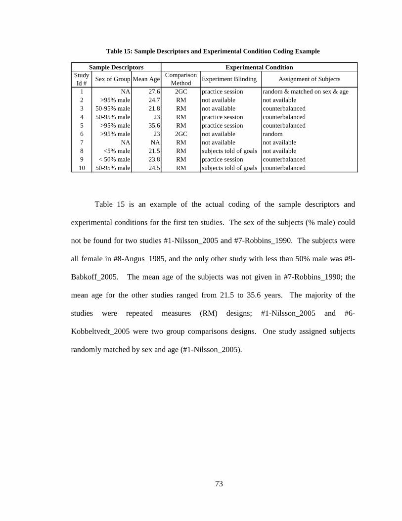
73
Table 15: Sample Descriptors and Experimental Condition Coding Example
1 NA 27.6 2GC practice session random & matched on sex & age2 >95% male 24.7 RM not available not available3 50-95% male 21.8 RM not available counterbalanced4 50-95% male 23 RM practice session counterbalanced5 >95% male 35.6 RM practice session counterbalanced6 >95% male 23 2GC not available random7 NA NA RM not available not available8 <5% male 21.5 RM subjects told of goals not available9 < 50% male 23.8 RM practice session counterbalanced10 50-95% male 24.5 RM subjects told of goals counterbalanced
Experimental ConditionStudy Id #
Sex of Group Mean Age Comparison Method Experiment Blinding Assignment of Subjects
Sample Descriptors
Table 15 is an example of the actual coding of the sample descriptors and
experimental conditions for the first ten studies. The sex of the subjects (% male) could
not be found for two studies #1-Nilsson_2005 and #7-Robbins_1990. The subjects were
all female in #8-Angus_1985, and the only other study with less than 50% male was #9-
Babkoff_2005. The mean age of the subjects was not given in #7-Robbins_1990; the
mean age for the other studies ranged from 21.5 to 35.6 years. The majority of the
studies were repeated measures (RM) designs; #1-Nilsson_2005 and #6-
Kobbeltvedt_2005 were two group comparisons designs. One study assigned subjects
randomly matched by sex and age (#1-Nilsson_2005).
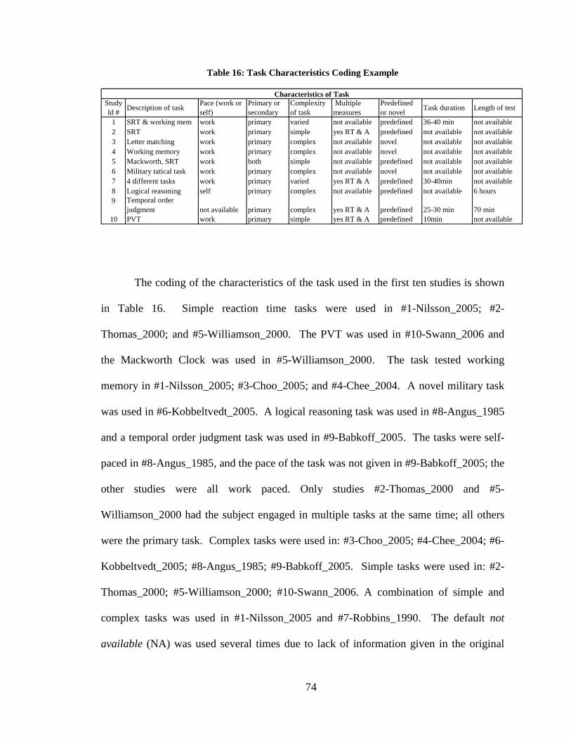
74
Table 16: Task Characteristics Coding Example
1 SRT & working mem work primary varied not available predefined 36-40 min not available2 SRT work primary simple yes RT & A predefined not available not available3 Letter matching work primary complex not available novel not available not available4 Working memory work primary complex not available novel not available not available5 Mackworth, SRT work both simple not available predefined not available not available6 Military tatical task work primary complex not available novel not available not available7 4 different tasks work primary varied yes RT & A predefined 30-40min not available8 Logical reasoning self primary complex not available predefined not available 6 hours
10 PVT work primary simple yes RT & A predefined 10min not available
Characteristics of TaskStudy Id # Description of task Pace (work or
self)Primary or secondary
Complexity of task
Multiple measures
Predefined or novel Task duration Length of test
70 mincomplex yes RT & A predefined 25-30 min9 Temporal order
judgment not available primary
The coding of the characteristics of the task used in the first ten studies is shown
in Table 16. Simple reaction time tasks were used in #1-Nilsson_2005; #2-
Thomas_2000; and #5-Williamson_2000. The PVT was used in #10-Swann_2006 and
the Mackworth Clock was used in #5-Williamson_2000. The task tested working
memory in #1-Nilsson_2005; #3-Choo_2005; and #4-Chee_2004. A novel military task
was used in #6-Kobbeltvedt_2005. A logical reasoning task was used in #8-Angus_1985
and a temporal order judgment task was used in #9-Babkoff_2005. The tasks were self-
paced in #8-Angus_1985, and the pace of the task was not given in #9-Babkoff_2005; the
other studies were all work paced. Only studies #2-Thomas_2000 and #5-
Williamson_2000 had the subject engaged in multiple tasks at the same time; all others
were the primary task. Complex tasks were used in: #3-Choo_2005; #4-Chee_2004; #6-
Kobbeltvedt_2005; #8-Angus_1985; #9-Babkoff_2005. Simple tasks were used in: #2-
Thomas_2000; #5-Williamson_2000; #10-Swann_2006. A combination of simple and
complex tasks was used in #1-Nilsson_2005 and #7-Robbins_1990. The default not
available (NA) was used several times due to lack of information given in the original
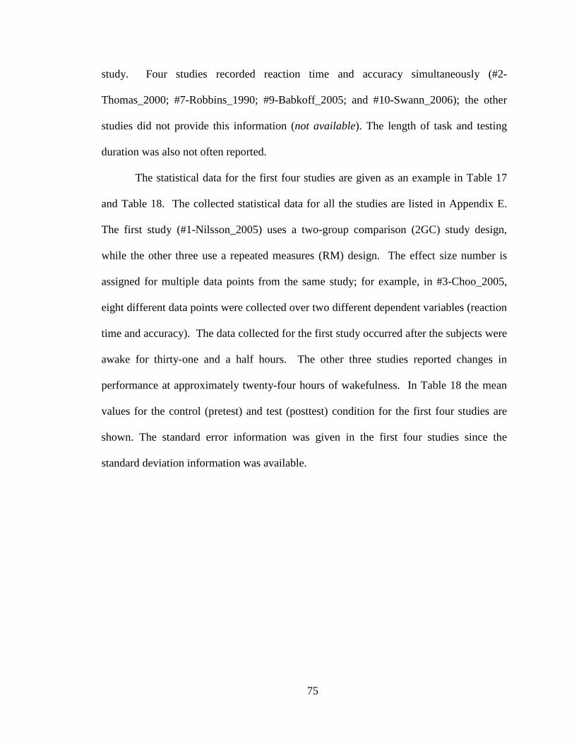
75
study. Four studies recorded reaction time and accuracy simultaneously (#2-
Thomas_2000; #7-Robbins_1990; #9-Babkoff_2005; and #10-Swann_2006); the other
studies did not provide this information (not available). The length of task and testing
duration was also not often reported.
The statistical data for the first four studies are given as an example in Table 17
and Table 18. The collected statistical data for all the studies are listed in Appendix E.
The first study (#1-Nilsson_2005) uses a two-group comparison (2GC) study design,
while the other three use a repeated measures (RM) design. The effect size number is
assigned for multiple data points from the same study; for example, in #3-Choo_2005,
eight different data points were collected over two different dependent variables (reaction
time and accuracy). The data collected for the first study occurred after the subjects were
awake for thirty-one and a half hours. The other three studies reported changes in
performance at approximately twenty-four hours of wakefulness. In Table 18 the mean
values for the control (pretest) and test (posttest) condition for the first four studies are
shown. The standard error information was given in the first four studies since the
standard deviation information was available.
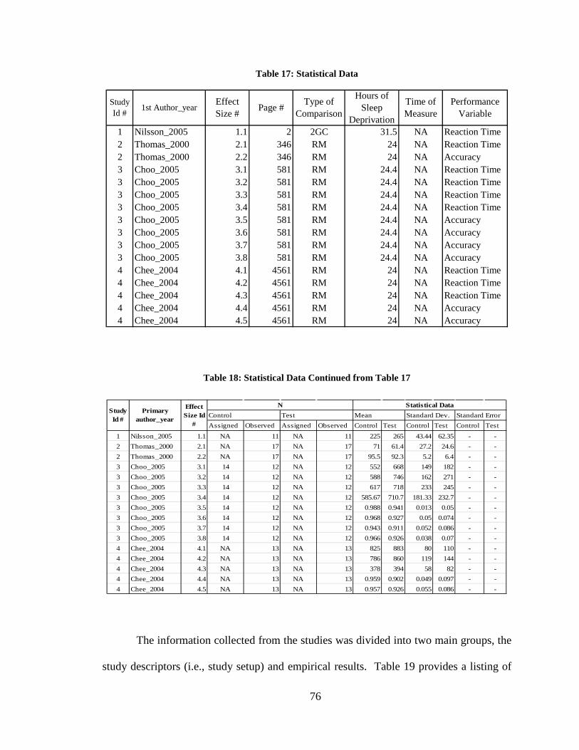
76
Table 17: Statistical Data
1 Nilsson_2005 1.1 2 2GC 31.5 NA Reaction Time2 Thomas_2000 2.1 346 RM 24 NA Reaction Time2 Thomas_2000 2.2 346 RM 24 NA Accuracy3 Choo_2005 3.1 581 RM 24.4 NA Reaction Time3 Choo_2005 3.2 581 RM 24.4 NA Reaction Time3 Choo_2005 3.3 581 RM 24.4 NA Reaction Time3 Choo_2005 3.4 581 RM 24.4 NA Reaction Time3 Choo_2005 3.5 581 RM 24.4 NA Accuracy3 Choo_2005 3.6 581 RM 24.4 NA Accuracy3 Choo_2005 3.7 581 RM 24.4 NA Accuracy3 Choo_2005 3.8 581 RM 24.4 NA Accuracy4 Chee_2004 4.1 4561 RM 24 NA Reaction Time4 Chee_2004 4.2 4561 RM 24 NA Reaction Time4 Chee_2004 4.3 4561 RM 24 NA Reaction Time4 Chee_2004 4.4 4561 RM 24 NA Accuracy4 Chee_2004 4.5 4561 RM 24 NA Accuracy
Type of Comparison
Hours of Sleep
Deprivation
Time of Measure
Performance Variable
Study Id # 1st Author_year
Effect Size # Page #
Table 18: Statistical Data Continued from Table 17
Assigned Observed Assigned Observed Control Test Control Test Control Test1 Nilsson_2005 1.1 NA 11 NA 11 225 265 43.44 62.35 - -2 Thomas_2000 2.1 NA 17 NA 17 71 61.4 27.2 24.6 - -2 Thomas_2000 2.2 NA 17 NA 17 95.5 92.3 5.2 6.4 - -3 Choo_2005 3.1 14 12 NA 12 552 668 149 182 - -3 Choo_2005 3.2 14 12 NA 12 588 746 162 271 - -3 Choo_2005 3.3 14 12 NA 12 617 718 233 245 - -3 Choo_2005 3.4 14 12 NA 12 585.67 710.7 181.33 232.7 - -3 Choo_2005 3.5 14 12 NA 12 0.988 0.941 0.013 0.05 - -3 Choo_2005 3.6 14 12 NA 12 0.968 0.927 0.05 0.074 - -3 Choo_2005 3.7 14 12 NA 12 0.943 0.911 0.052 0.086 - -3 Choo_2005 3.8 14 12 NA 12 0.966 0.926 0.038 0.07 - -4 Chee_2004 4.1 NA 13 NA 13 825 883 80 110 - -4 Chee_2004 4.2 NA 13 NA 13 786 860 119 144 - -4 Chee_2004 4.3 NA 13 NA 13 378 394 58 82 - -4 Chee_2004 4.4 NA 13 NA 13 0.959 0.902 0.049 0.097 - -4 Chee_2004 4.5 NA 13 NA 13 0.957 0.926 0.055 0.086 - -
Study Id #
Primary author_year
Effect Size Id
#
N Statistical DataControl Test Mean Standard Dev. Standard Error
The information collected from the studies was divided into two main groups, the
study descriptors (i.e., study setup) and empirical results. Table 19 provides a listing of
77
desired data for collection. Not all considered studies met these requirements. The data
collected from the various studies used in the current research were derived from tables
and graphs within each study. The hours of wakefulness, performance variable, and the
difference between the test and control conditions were considered necessary for analysis.
In some studies, the variation information was reported as standard error (SE) and had to
be converted to standard deviation (σ) using the sample size (N) for the study (Equation
14);
𝝈 = 𝑺𝑬 ∗ √𝑵 . (14)
Table 19: Desired Data for Collection
AcuteChronicLab/FieldEnvironment (e.g. Zeitgebers)Physical Activity LevelAge RangeSexPersonal CharacteristicsType of Subjects (e.g. student volunteers)Subjective, Objective, or PsychomotorSimulated Real-worldReal-work
Task Details Complexity Level (e.g. simplified task)
Reaction TimeAccuracyLapse
Definition of Sleep Deprivation Type of Sleep Deprivation
Experimental Design
Study Setting
Subject Differences
Type of Task
Empirical Data Collection
Hours of Wakefulness
Performance Variable
Mean of Test and Control ConditionStandard Deviation
Data Analysis
The previous section detailed the information that was collected. The current
section details the analysis method used to examine what information or trends can be
78
found from the collected data. This section includes a description of what data were
analyzed and by what means. The difference between the means, percentage change, and
effect size were calculated as a method to analyze the data. Also, a method to derive PSF
coefficient values from the data was developed.
Data Analyzed
The data were first segmented by the variable type (i.e., lapse, accuracy, and
reaction time). The accuracy data were further divided by the type of accuracy reported,
such as the number of false positives (false +), number correct (# correct), percentage
correct (% correct), number of errors (# errors), and the percentage of errors (% errors).
The data needed to calculate the difference between the mean values, effect sizes, and the
reliability indexes (β) are listed in Table 20. The data required are the mean values of the
test and control condition, the standard deviations or standard error of the test and control
condition, and the sample size. Not all data were available in each study.
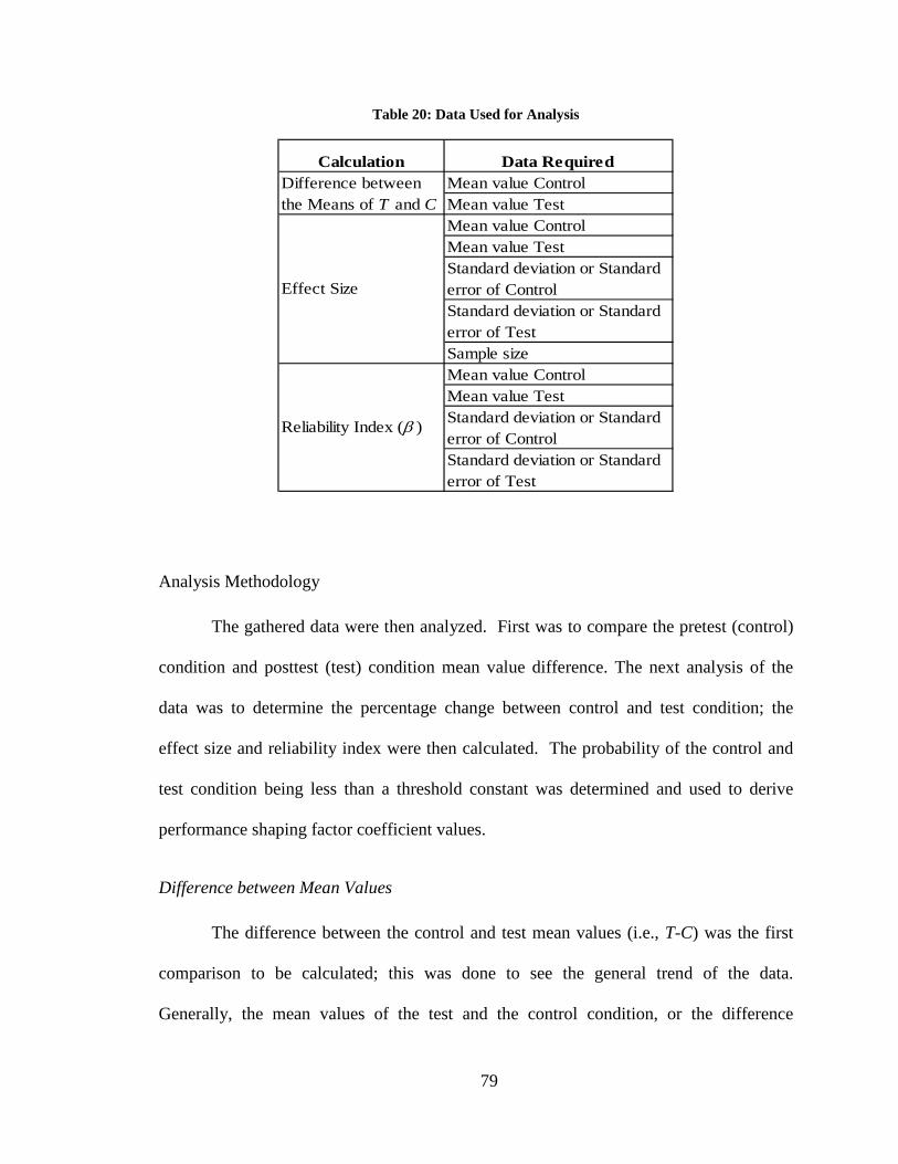
79
Table 20: Data Used for Analysis
Mean value ControlMean value TestMean value ControlMean value Test
Sample sizeMean value ControlMean value Test
Calculation Data RequiredDifference between the Means of T and C
Effect Size
Reliability Index (β )
Standard deviation or Standard error of ControlStandard deviation or Standard error of Test
Standard deviation or Standard error of ControlStandard deviation or Standard error of Test
Analysis Methodology
The gathered data were then analyzed. First was to compare the pretest (control)
condition and posttest (test) condition mean value difference. The next analysis of the
data was to determine the percentage change between control and test condition; the
effect size and reliability index were then calculated. The probability of the control and
test condition being less than a threshold constant was determined and used to derive
performance shaping factor coefficient values.
Difference between Mean Values
The difference between the control and test mean values (i.e., T-C) was the first
comparison to be calculated; this was done to see the general trend of the data.
Generally, the mean values of the test and the control condition, or the difference
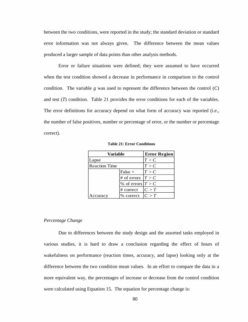
80
between the two conditions, were reported in the study; the standard deviation or standard
error information was not always given. The difference between the mean values
produced a larger sample of data points than other analysis methods.
Error or failure situations were defined; they were assumed to have occurred
when the test condition showed a decrease in performance in comparison to the control
condition. The variable g was used to represent the difference between the control (C)
and test (T) condition. Table 21 provides the error conditions for each of the variables.
The error definitions for accuracy depend on what form of accuracy was reported (i.e.,
the number of false positives, number or percentage of error, or the number or percentage
correct).
Table 21: Error Conditions
Error RegionT > CT > C
False + T > C# of errors T > C% of errors T > C# correct C > T% correct C > TAccuracy
LapseReaction Time
Variable
Percentage Change
Due to differences between the study design and the assorted tasks employed in
various studies, it is hard to draw a conclusion regarding the effect of hours of
wakefulness on performance (reaction times, accuracy, and lapse) looking only at the
difference between the two condition mean values. In an effort to compare the data in a
more equivalent way, the percentages of increase or decrease from the control condition
were calculated using Equation 15. The equation for percentage change is:
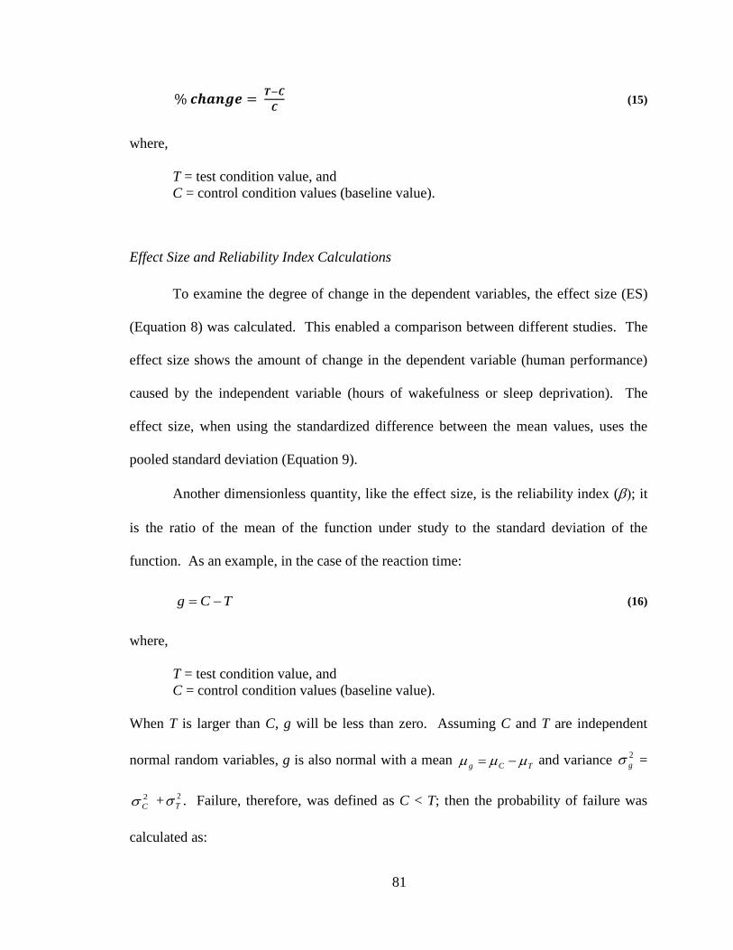
81
% 𝒄𝒉𝒂𝒏𝒈𝒆 = 𝑻−𝑪𝑪
(15)
where,
T = test condition value, and C = control condition values (baseline value).
Effect Size and Reliability Index Calculations
To examine the degree of change in the dependent variables, the effect size (ES)
(Equation 8) was calculated. This enabled a comparison between different studies. The
effect size shows the amount of change in the dependent variable (human performance)
caused by the independent variable (hours of wakefulness or sleep deprivation). The
effect size, when using the standardized difference between the mean values, uses the
pooled standard deviation (Equation 9).
Another dimensionless quantity, like the effect size, is the reliability index (β); it
is the ratio of the mean of the function under study to the standard deviation of the
function. As an example, in the case of the reaction time:
TCg −= (16)
where,
T = test condition value, and C = control condition values (baseline value).
When T is larger than C, g will be less than zero. Assuming C and T are independent
normal random variables, g is also normal with a mean TCg µµµ −= and variance 2gσ =
2Cσ + 2
Tσ . Failure, therefore, was defined as C < T; then the probability of failure was
calculated as:
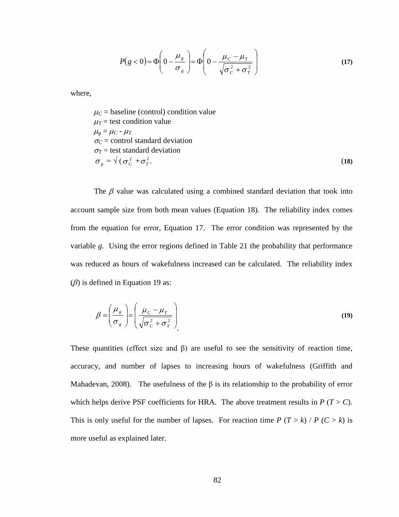
82
( )
+
−−Φ=
−Φ=<
22000
TC
TC
g
ggPσσ
µµσµ
(17)
where,
µC = baseline (control) condition value µT = test condition value µg = µC - µT σC = control standard deviation σT = test standard deviation
gσ = √ ( 2Cσ + 2
Tσ . (18)
The β value was calculated using a combined standard deviation that took into
account sample size from both mean values (Equation 18). The reliability index comes
from the equation for error, Equation 17. The error condition was represented by the
variable g. Using the error regions defined in Table 21 the probability that performance
was reduced as hours of wakefulness increased can be calculated. The reliability index
(β) is defined in Equation 19 as:
+
−=
=
22TC
TC
g
g
σσ
µµσµ
β
.
(19)
These quantities (effect size and β) are useful to see the sensitivity of reaction time,
accuracy, and number of lapses to increasing hours of wakefulness (Griffith and
Mahadevan, 2008). The usefulness of the β is its relationship to the probability of error
which helps derive PSF coefficients for HRA. The above treatment results in P (T > C).
This is only useful for the number of lapses. For reaction time P (T > k) / P (C > k) is
more useful as explained later.
83
Linear Regression
A linear regression for within study characteristics was performed using the
performance metric (number of lapses, reaction time, or accuracy) as the dependent
variable and the hours of wakefulness as the independent variable for linear and the
square of hours of wakefulness for the quadratic regression. An intercept (b0), linear
coefficient (b1), and curvilinear coefficient (b2) are calculated for each study. The
intercept and two coefficients are used to produce an equation for performance. To
correct for sample size, a weighted average also can be calculated by weighing each
study by the sample size over the total sample size for all the studies.
A between-studies regression was then performed to find the relationship among
between-study characteristics and the performance variable. A selection of study and
task descriptors was chosen to evaluate their effect on predicted performance for a
between-studies regression. Non-numeric data were coded as either yes (1) or no (0).
The effect of the industry in which the study was performed was evaluated in regards to
medical, military, general industry, and transportation with the default industry as
academic. Two subject characteristics were evaluated, the sex of the group, i.e.,
percentage of male subjects, and the age of subjects. Task characteristics were the next
group of study descriptors evaluated; these were: type of task (i.e., PVT, simple reaction
time, grammatical reasoning or real work), task complexity (i.e., simple or complex), task
pace (i.e., self or work paced), and whether the task was primary or secondary.
The variables that were identified as not having an effect on predicting
performance were removed and a new between-study regression was performed. The
resulting equation can be used to change the predicted performance measure to a different
84
variable space. For example, this enables a study that was conducted in the transportation
industry to be changed into the medical industry. This transformation allows for the data
to be evaluated on the same study characteristics.
PSF Derivation
A quantitative measure of the effect of sleep deprivation on performance (i.e.,
estimation of human error probabilities) is derived in this subsection by comparing the
probabilities of error in the control (pre-sleep deprivation) and test (post-sleep deprived)
conditions to obtain a PSF multiplier value.
The performance measure (e.g., reaction time) under test condition and control
condition can be compared to a threshold value k, in order to compute the error
probability under each condition. The threshold values are selected based on the
definition of a lapse for simple reaction time tasks, e.g., no response before 500 ms
(Anderson et al., 2010).
In the following discussion, error is defined as the performance measure being
larger than the threshold value. For example, error with respect to the control condition
reaction time (C) and for the test condition reaction time (T) are mathematically defined
as C > k and T > k. The reaction times under control condition and test condition are both
assumed to be normal random variables with a mean value µC and variance 2Cσ for the
control condition and a mean value µT and variance 2Tσ for the test condition. In Figure 9
the shaded area represents either PC or PT, the probability of error. Since error is defined
as C > k or T > k, the probability of error is calculated as:
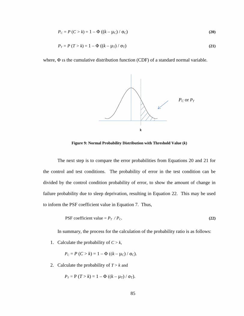
85
PC = P (C > k) = 1 – Φ ((k – µC) / σC) (20)
PT = P (T > k) = 1 – Φ ((k – µT) / σT) (21)
where, Φ ιs the cumulative distribution function (CDF) of a standard normal variable.
Figure 9: Normal Probability Distribution with Threshold Value (k)
The next step is to compare the error probabilities from Equations 20 and 21 for
the control and test conditions. The probability of error in the test condition can be
divided by the control condition probability of error, to show the amount of change in
failure probability due to sleep deprivation, resulting in Equation 22. This may be used
to inform the PSF coefficient value in Equation 7. Thus,
PSF coefficient value = PT / PC. (22)
In summary, the process for the calculation of the probability ratio is as follows:
1. Calculate the probability of C > k,
PC = P (C > k) = 1 – Φ ((k – µC) / σC).
2. Calculate the probability of T > k and
PT = P (T > k) = 1 – Φ ((k – µT) / σT).
PC or PT
86
3. Calculate the ratio of probability of the test condition to the control condition,
PT / PC.
The above treatment may also be used when the number of lapses is used as the
performance measure, by comparing the number of lapses in each condition to a
threshold value. However, there is also another way to derive PSF coefficient values for
the number of lapses or the number of errors (accuracy measure), without defining a
threshold value. For example, in the case of number of lapses, the probability that the
number of lapses for the test condition (TL) is greater than the number of lapses for the
control condition (CL) over the probability of TL equal to CL. PL is defined in Equation
23:
PL = P (TL > CL) / P (TL = CL) = P (TL > CL) / 0.5 (23)
where,
CL = control condition number of lapses TL = test condition number of lapses.
Outliers were removed from the analysis to reduce the PSF plots from being
skewed toward one or two studies that had markedly different observations from the rest
of the data (Grubbs, 1969). Outliers were also removed to prevent the ratio data (i.e.,
probability ratios to develop PSF coefficient values) from deviating markedly from the
values for the rest of the calculated PSF coefficients. In some cases, the PSF coefficients,
i.e., probability ratio (PT / PC), approach values greater than 10 when the error probability
for the control condition (i.e., denominator of the ratio) is small. These cases were
removed by assuming the small probabilities values to be zero and thereby removing
them from the data set.
87
The probability ratios calculated are used to represent PSF coefficient values. The
probability ratios can be used as direct measures of the PSF multiplier, as in the SPAR-H
HRA method, or can be used as a means to inform in the selection of an appropriate PSF
multiplier.
Uncertainty Analysis
The limited data for the PSF coefficient calculation results in significant
variability. To investigate the variability of the results, the data are divided into twenty
hour time blocks; the blocks were < 20, 20-40, 40-60, 60-80, and > 80 hours. A
confidence interval, for each k value over each twenty hour time block, can be reported to
express the variability in the derived PSF coefficient values. The 95% confidence
interval using a 2-tailed t-distribution was calculated for each k value (e.g., k = 500) over
each time block.
Another way to investigate the uncertainty of the results is to investigate the
sensitivity of the results to the assumed normal distribution. The variables C and T were
assumed to be normally distributed for the quantification analysis. To investigate the
sensitivity of the results to this assumption, the C and T for reaction time are assumed to
follow a lognormal distribution. The results are compared to the normally distributed C
and T results in the quantification analysis
In many of the studies, data have to be interpreted from graphical results. Since
there is some subjectivity associated with such a data collection method, the inter-rater
reliability was found for a sample of studies. Inter-rater reliability is the extent to which
two or more individuals (coders or raters) agree (i.e., if the coders recorded similar data).
88
Another source of uncertainty comes from the data being manually extracted. In
order to investigate this uncertainty, the inter-rater reliability was examined. Inter-rater
reliability quantifies the consistency or consensus of scores assigned by raters of the same
study (Gwet, 2008). There are several operational definitions of inter-rater reliability
depending on which statistics are appropriate (Saal et al., 1980). Some of the well-
known methods of calculating inter-rater reliability are: joint-probability of agreement,
Cohen’s kappa (κ) and Fleiss’ kappa (κ), correlation coefficients (e.g., Pearson’s r and
Spearman’s ρ), intra-class correlation, and limits of agreement.
Inter-rater reliability is needed because different raters can disagree about the
measurement results from the same object. The need for inter-rater reliability in this
research results from differences from reading numeric data from plots (not observing
data and assigning data to specific categories). This limits the type of inter-rater
reliability methods that would be appropriate, since most are designed to measure the
consistency of assigning data and not interpreting the results of the data.
Joint probability of agreement
Joint probability of agreement is the most simple, but least robust measure. It is
simply the number of times each rating is assigned by each rater and assumes that the
data are nominal. It does not take into account agreement by chance. Chance agreement
will be high with a small number of categories and joint probability of agreement will be
high even if there is no intrinsic agreement among raters (Cohen, 1960). Nominal data
use names or labels for certain characteristics, e.g., types of rocks can be categorized as
igneous, sedimentary, or metamorphic. Joint probability of agreement is used for
89
category study observer assignments, not numerical measurements or the reading of
numeric results from graphs.
Kappa statistics
Kappa statistics take into account agreement due to chance. Cohen’s kappa
(Cohen, 1968) is for two raters and Fleiss’ kappa (Shrout, and Fleiss, 1979) is a modified
version of Cohen’s kappa that works for multiple rates. The data are assumed to be
nominal (names or labels for certain characteristics); that is, there is no natural order to
the data.
Correlation coefficients
Correlation coefficients, such as Pearson’s (r) which assumes that the rating scale
is continuous and Spearman’s (ρ) which assumes that the scale is ordinal (i.e.,
measurements that describe order but not relative size), are used to measure pairwise
correlation (i.e., judge which observation is preferred) among raters on an ordered scale
and consider only relative position. For example, (1, 2, 1, 3) is considered perfectly
correlated with (2, 3, 2, 4). Ordinal scales describe order, but not relative size.
Intra-class correlation coefficient
The interclass correlation coefficient measures a bivariate relation among
variables (Kenneth et al., 1996). Intra-class correlation coefficient measures the
proportion of variance of observation due to between-study variability in the actual scores
(Koch, 1982). The intra-class correlation coefficient (ICC) ranges between 0.0 and 1.0;
the ICC will be larger, when there is little variation between rater scores. The ICC
considers the proportion of variability in a measure that is due to being part of a particular
group (i.e., the extent that members of the same group act alike (Szklo and Nieto, 2004)).
90
Limits of agreement (Bland-Altman Plot)
Another way to express rater consensus is to calculate the mean of the differences
between the two raters. Calculating a confidence limit around the mean provides insight
on the level of random variation that impacts the ratings. When the raters agree, the
mean will approach zero; however, if one rater is consistently higher than the other rater
the mean will be larger, but the confidence interval will be smaller. When raters differ
without a consistent pattern, the mean will be near zero, but the confidence interval will
be large.
The difference of the means can be displayed graphically in a Bland-Altman plot
(Bland and Altman, 1986). The mean difference with confidence limits (y-axis) is
plotted against the average of the two ratings (x-axis). The Bland-Altman plot displays
the degree of agreement between the raters, but also the level of agreement that is
depending on the size (underlying value) of the data observation. For example, raters
might closely agree on estimating the size of small values but disagree more with larger
values.
Joint probability of agreement, Cohen’s kappa, and Fleiss’ kappa are used with
nominal scales (category data) and are not applicable to this research data. Correlation
coefficients are not applicable because they describe ordinal scales. Intra-class
correlation (ICC) requires a true value to be known to compare to the observed data, a
true value is not known in this application, so ICC rater reliability methods are not
applicable. In this research, two raters were used to interpret reported results from
graphical outputs, and the data were not being assigned to observational categories.
91
Among the aforementioned methods, the limit of agreement using a Bland-Altman plot is
the most applicable for this research.
A random selection of studies is pulled from the pool of collected studies and
coded by another coder, i.e., auxiliary coder. The coding by the auxiliary is compared to
that of the main coder to compare for similar results. In this research, this most open for
coder interpretation data were taken from a graph within the original study.
Mean values, standard deviation, minimum value, maximum values, and number
of data points were calculated for the basic statistics of each overall performance metric
(i.e., number of lapses, reaction time, and accuracy). The uncertainty of the derived
performance shaping factor coefficients was calculated for each threshold value (i.e., k
values). The uncertainty (i.e., mean value, standard deviation, minimum value,
maximum values, and number of data points) was calculated for each k value derived
PSF coefficient for intervals of hours of wakefulness.
Summary of Methodology
The method of data analysis was provided in this chapter. This included the
method of data collection and types of information collected from the studies (e.g., study
descriptors, task characteristics, and statistical data). The types of analysis that were
applied to the data, along with the method of PSF coefficient derivation, were detailed.
Different threshold values (k values) were selected to define the error region for the
control and test condition values. The probability that the control or test condition was
greater than the selected threshold values was calculated. PSF coefficients were derived
by comparing the probability of failure (i.e., probability that the test metric is greater than

92
the threshold value) for the test condition in comparison to the control condition. Results
of the application of the methodology to the reported performance metrics of number of
lapses, reaction time, and accuracy are reported in the following chapter.
93
CHAPTER V
RESULTS
This chapter discusses the results of the application of the methodology; this
includes the analysis of the data including the difference between the mean values,
percentage change, effect size, reliability index (β), and probability ratio. The probability
ratio for different threshold values was calculated to find performance shaping factor
coefficients; the results were grouped by reaction time, accuracy, and number of lapses.
Resulting Data
The number of studies that provided data for use in the quantitative analysis for
each of the performance metrics (i.e., lapse, reaction time, and accuracy) is listed in Table
22. More studies reported reaction time information (65 studies) than accuracy (40
studies) and number of lapses data (18 studies). The number of studies that did not report
the standard deviation information of the test conditions limited the number of studies
that could be used for β, effect size, and probability calculations. These studies only
looked at the difference between the mean values. Studies that did not report the number
of hours of wakefulness were not usable in the analysis.
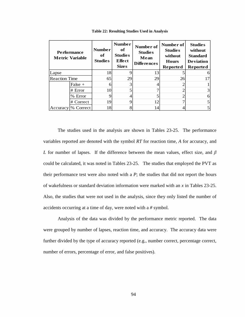
94
Table 22: Resulting Studies Used in Analysis
18 9 13 5 665 29 29 26 17
False + 6 3 4 2 1# Error 10 5 7 2 3% Error 9 4 5 2 6# Correct 19 9 12 7 5% Correct 18 8 14 4 5
Number of Studies without Hours
Reported
Number of Studies without
Standard Deviation Reported
LapseReaction Time
Accuracy
Performance Metric Variable
Number of
Studies
Number of
Studies Effect Sizes
Number of Studies Mean
Differences
The studies used in the analysis are shown in Tables 23-25. The performance
variables reported are denoted with the symbol RT for reaction time, A for accuracy, and
L for number of lapses. If the difference between the mean values, effect size, and β
could be calculated, it was noted in Tables 23-25. The studies that employed the PVT as
their performance test were also noted with a P; the studies that did not report the hours
of wakefulness or standard deviation information were marked with an x in Tables 23-25.
Also, the studies that were not used in the analysis, since they only listed the number of
accidents occurring at a time of day, were noted with a # symbol.
Analysis of the data was divided by the performance metric reported. The data
were grouped by number of lapses, reaction time, and accuracy. The accuracy data were
further divided by the type of accuracy reported (e.g., number correct, percentage correct,
number of errors, percentage of error, and false positives).
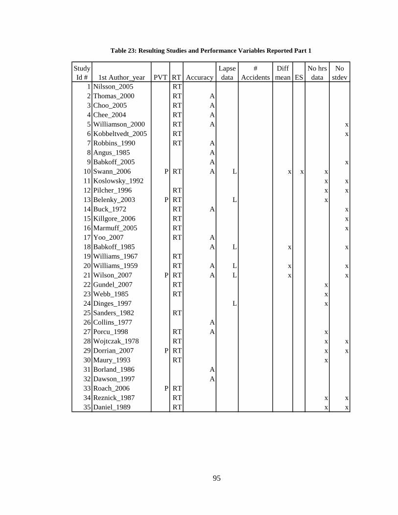
95
Table 23: Resulting Studies and Performance Variables Reported Part 1
1 Nilsson_2005 RT2 Thomas_2000 RT A3 Choo_2005 RT A4 Chee_2004 RT A5 Williamson_2000 RT A x6 Kobbeltvedt_2005 RT x7 Robbins_1990 RT A8 Angus_1985 A9 Babkoff_2005 A x
10 Swann_2006 P RT A L x x x11 Koslowsky_1992 x x12 Pilcher_1996 RT x x13 Belenky_2003 P RT L x14 Buck_1972 RT A x15 Killgore_2006 RT x16 Marmuff_2005 RT x17 Yoo_2007 RT A18 Babkoff_1985 A L x x19 Williams_1967 RT20 Williams_1959 RT A L x x21 Wilson_2007 P RT A L x x22 Gundel_2007 RT x23 Webb_1985 RT x24 Dinges_1997 L x25 Sanders_1982 RT26 Collins_1977 A27 Porcu_1998 RT A x28 Wojtczak_1978 RT x x29 Dorrian_2007 P RT x x30 Maury_1993 RT x31 Borland_1986 A32 Dawson_1997 A33 Roach_2006 P RT34 Reznick_1987 RT x x35 Daniel_1989 RT x x
Study Id # 1st Author_year PVT RT ES
No hrs data
No stdevAccuracy
Lapse data
# Accidents
Diff mean
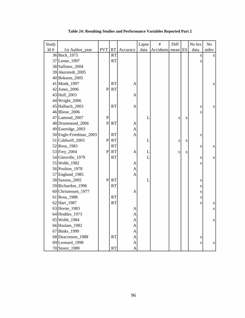
96
Table 24: Resulting Studies and Performance Variables Reported Part 2
36 Buck_1975 RT x x37 Lenne_1997 RT x38 Sallinen_200439 Akerstedt_200540 Boksem_200541 Monk_1997 RT A x42 Jones_2006 P RT43 Hull_2003 A44 Wright_200645 Halbach_2003 RT A x x46 Bliese_2006 x47 Lamond_2007 P L x x48 Drummond_2006 P RT A49 Eastridge_2003 A50 Engle-Friedman_2003 RT A x51 Caldwell_2003 P RT L x x52 Rosa_1983 RT x x53 Frey_2004 P RT A L x x54 Glenville_1979 RT L x x55 Webb_1982 A x56 Poulton_1978 A57 Englund_1985 A58 Saxena_2005 P RT L x59 Richardon_1996 RT x60 Christensen_1977 A x61 Rosa_1988 RT x62 Hart_1987 RT x x63 Horne_1983 A x64 Hoddes_1973 A65 Webb_1984 A x66 Haslam_1982 A67 Binks_1999 A68 Deaconson_1988 RT A x69 Leonard_1998 A x x70 Storer_1989 RT A
No hrs data
No stdevAccuracy
Lapse data
# Accidents
Diff mean
Study Id # 1st Author_year PVT RT ES
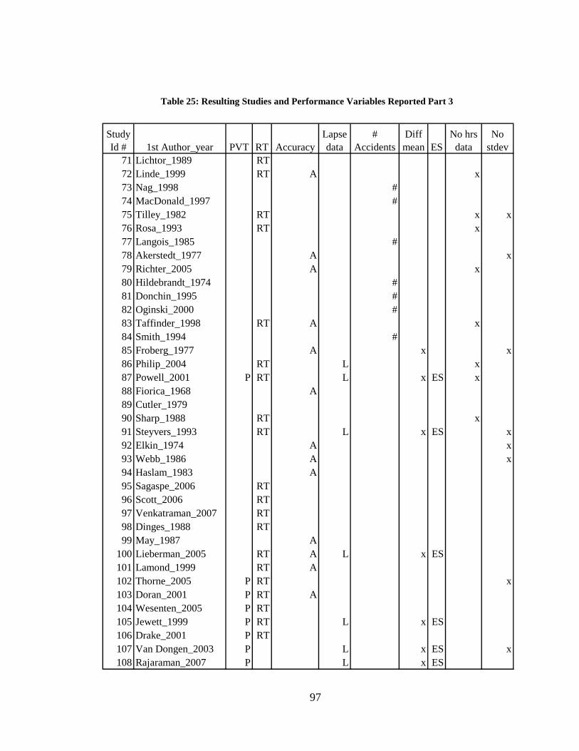
97
Table 25: Resulting Studies and Performance Variables Reported Part 3
71 Lichtor_1989 RT72 Linde_1999 RT A x73 Nag_1998 #74 MacDonald_1997 #75 Tilley_1982 RT x x76 Rosa_1993 RT x77 Langois_1985 #78 Akerstedt_1977 A x79 Richter_2005 A x80 Hildebrandt_1974 #81 Donchin_1995 #82 Oginski_2000 #83 Taffinder_1998 RT A x84 Smith_1994 #85 Froberg_1977 A x x86 Philip_2004 RT L x87 Powell_2001 P RT L x ES x88 Fiorica_1968 A89 Cutler_197990 Sharp_1988 RT x91 Steyvers_1993 RT L x ES x92 Elkin_1974 A x93 Webb_1986 A x94 Haslam_1983 A95 Sagaspe_2006 RT96 Scott_2006 RT97 Venkatraman_2007 RT98 Dinges_1988 RT99 May_1987 A
100 Lieberman_2005 RT A L x ES101 Lamond_1999 RT A102 Thorne_2005 P RT x103 Doran_2001 P RT A104 Wesenten_2005 P RT105 Jewett_1999 P RT L x ES106 Drake_2001 P RT107 Van Dongen_2003 P L x ES x108 Rajaraman_2007 P L x ES
No stdevAccuracy
Lapse data
# Accidents
Diff mean
Study Id # 1st Author_year PVT RT ES
No hrs data
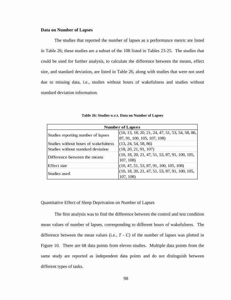
98
Data on Number of Lapses
The studies that reported the number of lapses as a performance metric are listed
in Table 26; these studies are a subset of the 108 listed in Tables 23-25. The studies that
could be used for further analysis, to calculate the difference between the means, effect
size, and standard deviation, are listed in Table 26, along with studies that were not used
due to missing data, i.e., studies without hours of wakefulness and studies without
standard deviation information.
Table 26: Studies w.r.t. Data on Number of Lapses
Studies without hours of wakefulness (13, 24, 54, 58, 86)Studies without standard deviation (18, 20, 21, 91, 107)
Effect size (10, 47, 51, 53, 87, 91, 100, 105, 108)
Studies used (10, 18, 20, 21, 47, 51, 53, 87, 91, 100, 105, 107, 108)
Number of Lapses
Studies reporting number of lapses (10, 13, 18, 20, 21, 24, 47, 51, 53, 54, 58, 86, 87, 91, 100, 105, 107, 108)
Difference between the means (10, 18, 20, 21, 47, 51, 53, 87, 91, 100, 105, 107, 108)
Quantitative Effect of Sleep Deprivation on Number of Lapses
The first analysis was to find the difference between the control and test condition
mean values of number of lapses, corresponding to different hours of wakefulness. The
difference between the mean values (i.e., T - C) of the number of lapses was plotted in
Figure 10. There are 68 data points from eleven studies. Multiple data points from the
same study are reported as independent data points and do not distinguish between
different types of tasks.
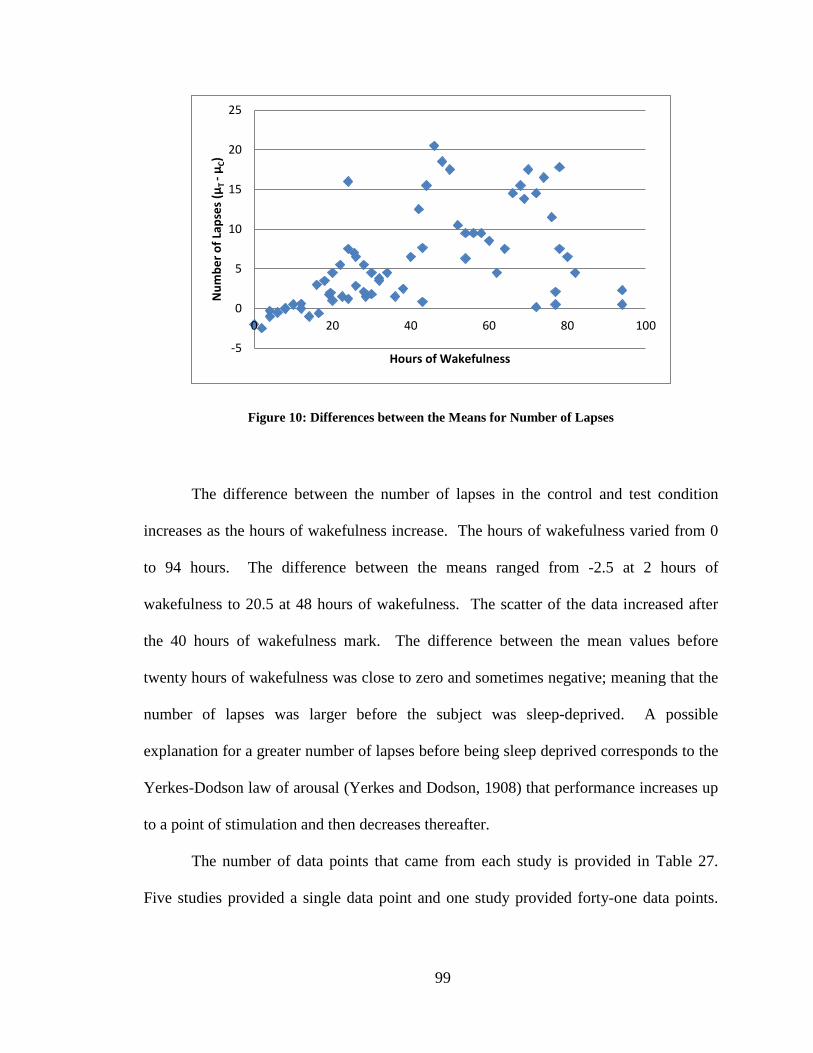
99
Figure 10: Differences between the Means for Number of Lapses
The difference between the number of lapses in the control and test condition
increases as the hours of wakefulness increase. The hours of wakefulness varied from 0
to 94 hours. The difference between the means ranged from -2.5 at 2 hours of
wakefulness to 20.5 at 48 hours of wakefulness. The scatter of the data increased after
the 40 hours of wakefulness mark. The difference between the mean values before
twenty hours of wakefulness was close to zero and sometimes negative; meaning that the
number of lapses was larger before the subject was sleep-deprived. A possible
explanation for a greater number of lapses before being sleep deprived corresponds to the
Yerkes-Dodson law of arousal (Yerkes and Dodson, 1908) that performance increases up
to a point of stimulation and then decreases thereafter.
The number of data points that came from each study is provided in Table 27.
Five studies provided a single data point and one study provided forty-one data points.
-5
0
5
10
15
20
25
0 20 40 60 80 100
Num
ber o
f Lap
ses
(μT
- μC)
Hours of Wakefulness
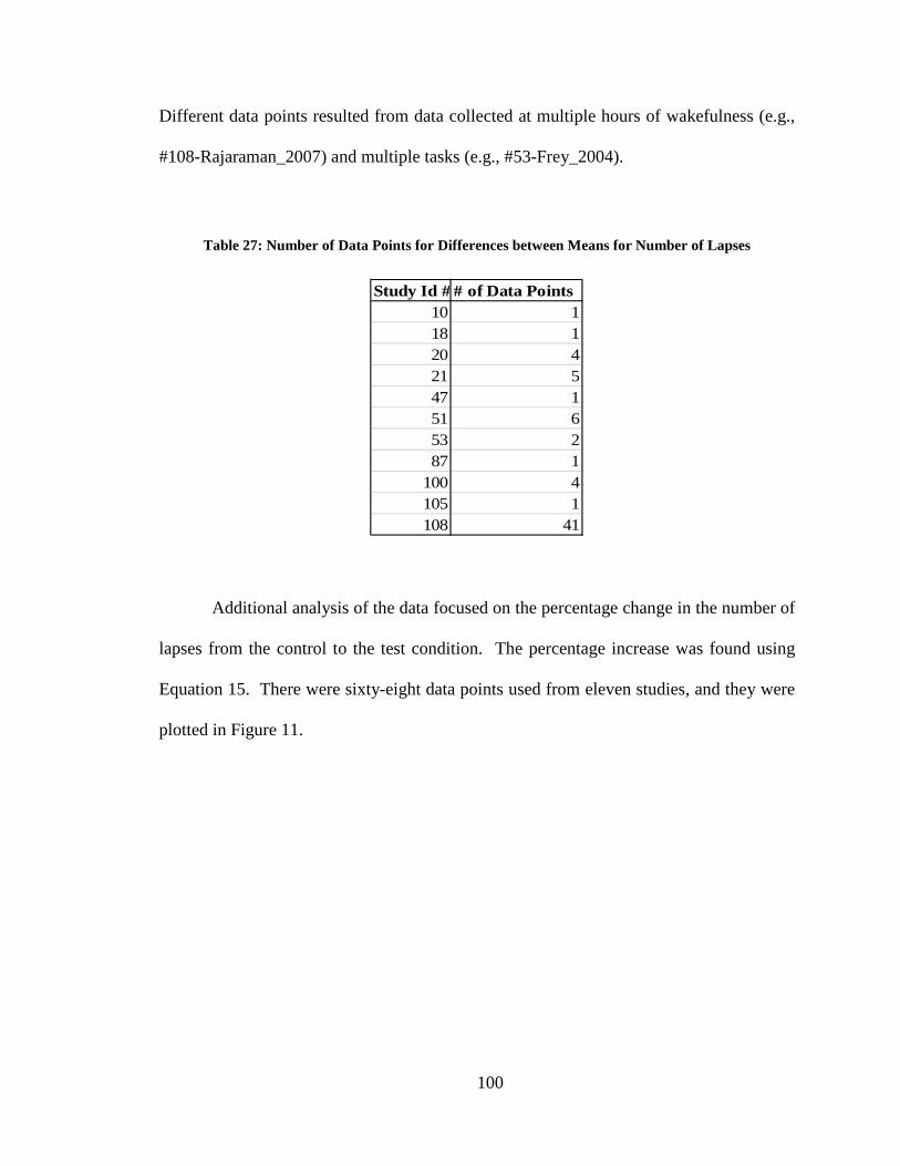
100
Different data points resulted from data collected at multiple hours of wakefulness (e.g.,
#108-Rajaraman_2007) and multiple tasks (e.g., #53-Frey_2004).
Table 27: Number of Data Points for Differences between Means for Number of Lapses
Study Id # # of Data Points10 118 120 421 547 151 653 287 1
100 4105 1108 41
Additional analysis of the data focused on the percentage change in the number of
lapses from the control to the test condition. The percentage increase was found using
Equation 15. There were sixty-eight data points used from eleven studies, and they were
plotted in Figure 11.
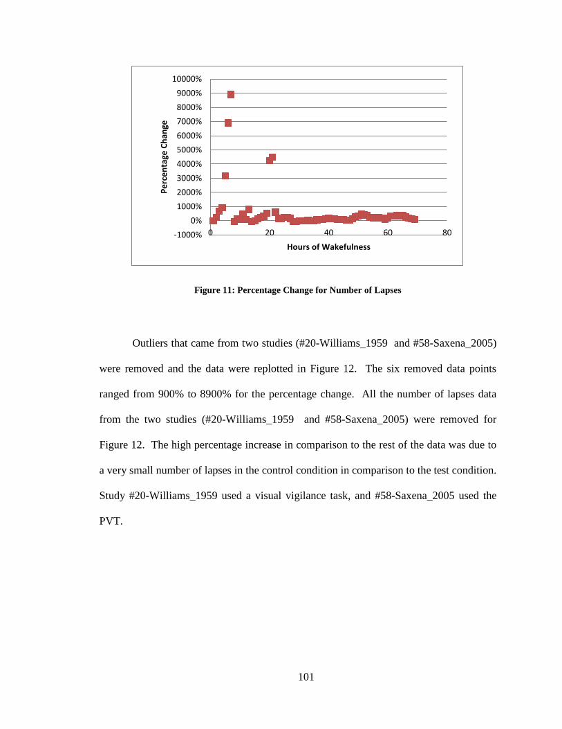
101
Figure 11: Percentage Change for Number of Lapses
Outliers that came from two studies (#20-Williams_1959 and #58-Saxena_2005)
were removed and the data were replotted in Figure 12. The six removed data points
ranged from 900% to 8900% for the percentage change. All the number of lapses data
from the two studies (#20-Williams_1959 and #58-Saxena_2005) were removed for
Figure 12. The high percentage increase in comparison to the rest of the data was due to
a very small number of lapses in the control condition in comparison to the test condition.
Study #20-Williams_1959 used a visual vigilance task, and #58-Saxena_2005 used the
PVT.
-1000%0%
1000%2000%3000%4000%5000%6000%7000%8000%9000%
10000%
0 20 40 60 80
Perc
enta
ge C
hang
e
Hours of Wakefulness
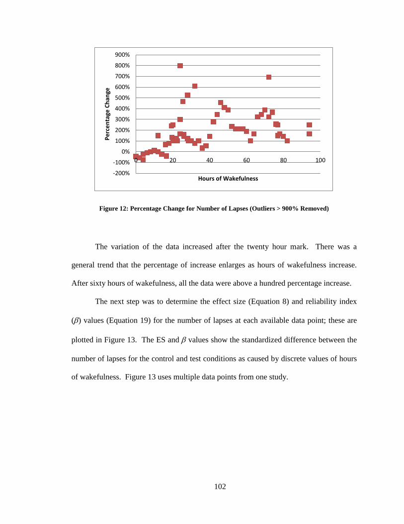
102
Figure 12: Percentage Change for Number of Lapses (Outliers > 900% Removed)
The variation of the data increased after the twenty hour mark. There was a
general trend that the percentage of increase enlarges as hours of wakefulness increase.
After sixty hours of wakefulness, all the data were above a hundred percentage increase.
The next step was to determine the effect size (Equation 8) and reliability index
(β) values (Equation 19) for the number of lapses at each available data point; these are
plotted in Figure 13. The ES and β values show the standardized difference between the
number of lapses for the control and test conditions as caused by discrete values of hours
of wakefulness. Figure 13 uses multiple data points from one study.
-200%
-100%
0%
100%
200%
300%
400%
500%
600%
700%
800%
900%
0 20 40 60 80 100
Perc
enta
ge C
hang
e
Hours of Wakefulness

103
Figure 13: ES and β for Number of Lapses
The ES and β values increased in the negative direction as hours of wakefulness
increased. A negative ES means the number of lapses increases as hours of wakefulness
increase, i.e., performance deterioration as hours of sleep deprivation increase. The
effect sizes ranged from (-0.732 to 1.594), and β values ranged from (-0.517 to 1.127).
There were fifty-eight data points from eight different studies; forty-one data points came
from one study (#108-Rajaraman_2007). The allocation of data points to studies is
provided in Table 28. The majority of the studies used the PVT as the task (e.g., #10-
Swann_2006, #47-Lamond_2007, #51-Caldwell_2003, #53-Frey_2004, #87-
Powell_2001, #105-Jewett_1999, and #108-Rajaraman_2007). A novel reaction time
test, in addition to the PVT, was used in #53-Frey_2004 and a four-choice reaction time
task and a grammatical reasoning task were used in #100-Lieberman_2005.
-2
-1.5
-1
-0.5
0
0.5
1
0 20 40 60 80 100Ef
fect
Siz
e
Hours of Wakefulness
ES
β
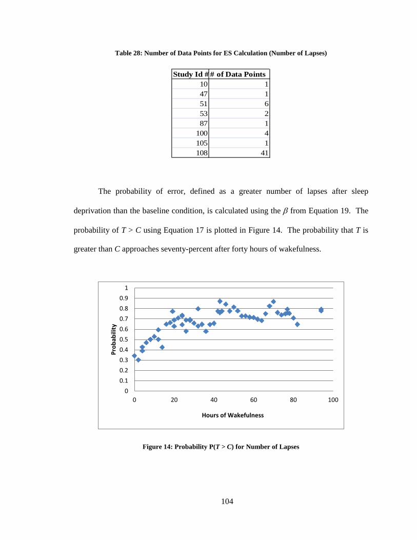
104
Table 28: Number of Data Points for ES Calculation (Number of Lapses)
Study Id # # of Data Points10 147 151 653 287 1
100 4105 1108 41
The probability of error, defined as a greater number of lapses after sleep
deprivation than the baseline condition, is calculated using the β from Equation 19. The
probability of T > C using Equation 17 is plotted in Figure 14. The probability that T is
greater than C approaches seventy-percent after forty hours of wakefulness.
Figure 14: Probability P(T > C) for Number of Lapses
00.10.20.30.40.50.60.70.80.9
1
0 20 40 60 80 100
Prob
abili
ty
Hours of Wakefulness
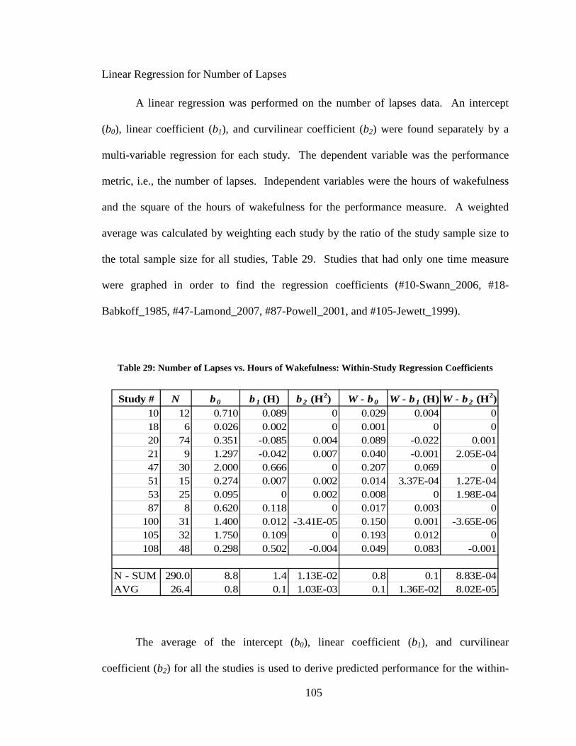
105
Linear Regression for Number of Lapses
A linear regression was performed on the number of lapses data. An intercept
(b0), linear coefficient (b1), and curvilinear coefficient (b2) were found separately by a
multi-variable regression for each study. The dependent variable was the performance
metric, i.e., the number of lapses. Independent variables were the hours of wakefulness
and the square of the hours of wakefulness for the performance measure. A weighted
average was calculated by weighting each study by the ratio of the study sample size to
the total sample size for all studies, Table 29. Studies that had only one time measure
were graphed in order to find the regression coefficients (#10-Swann_2006, #18-
Babkoff_1985, #47-Lamond_2007, #87-Powell_2001, and #105-Jewett_1999).
Table 29: Number of Lapses vs. Hours of Wakefulness: Within-Study Regression Coefficients
Study # N b0 b1 (H) b2 (H2) W - b0 W - b1 (H) W - b2 (H2)10 12 0.710 0.089 0 0.029 0.004 018 6 0.026 0.002 0 0.001 0 020 74 0.351 -0.085 0.004 0.089 -0.022 0.00121 9 1.297 -0.042 0.007 0.040 -0.001 2.05E-0447 30 2.000 0.666 0 0.207 0.069 051 15 0.274 0.007 0.002 0.014 3.37E-04 1.27E-0453 25 0.095 0 0.002 0.008 0 1.98E-0487 8 0.620 0.118 0 0.017 0.003 0
100 31 1.400 0.012 -3.41E-05 0.150 0.001 -3.65E-06105 32 1.750 0.109 0 0.193 0.012 0108 48 0.298 0.502 -0.004 0.049 0.083 -0.001
N - SUM 290.0 8.8 1.4 1.13E-02 0.8 0.1 8.83E-04AVG 26.4 0.8 0.1 1.03E-03 0.1 1.36E-02 8.02E-05
The average of the intercept (b0), linear coefficient (b1), and curvilinear
coefficient (b2) for all the studies is used to derive predicted performance for the within-
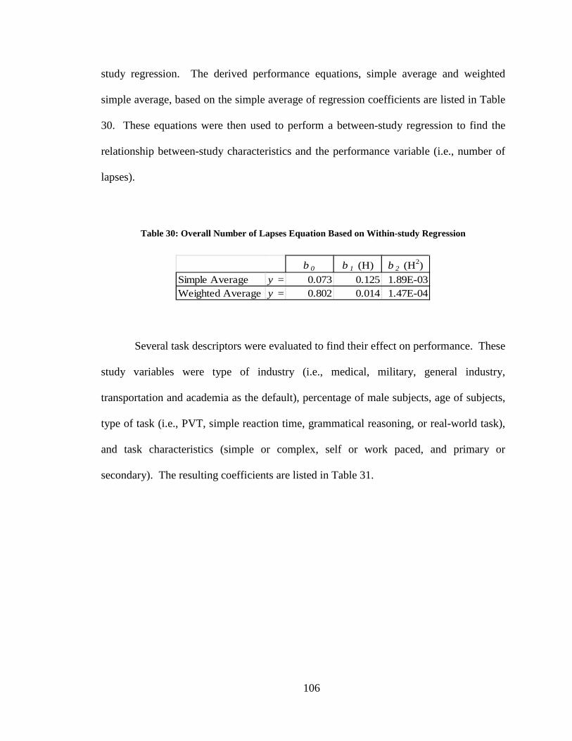
106
study regression. The derived performance equations, simple average and weighted
simple average, based on the simple average of regression coefficients are listed in Table
30. These equations were then used to perform a between-study regression to find the
relationship between-study characteristics and the performance variable (i.e., number of
lapses).
Table 30: Overall Number of Lapses Equation Based on Within-study Regression
b 0 b 1 (H) b 2 (H2)Simple Average y = 0.073 0.125 1.89E-03Weighted Average y = 0.802 0.014 1.47E-04
Several task descriptors were evaluated to find their effect on performance. These
study variables were type of industry (i.e., medical, military, general industry,
transportation and academia as the default), percentage of male subjects, age of subjects,
type of task (i.e., PVT, simple reaction time, grammatical reasoning, or real-world task),
and task characteristics (simple or complex, self or work paced, and primary or
secondary). The resulting coefficients are listed in Table 31.
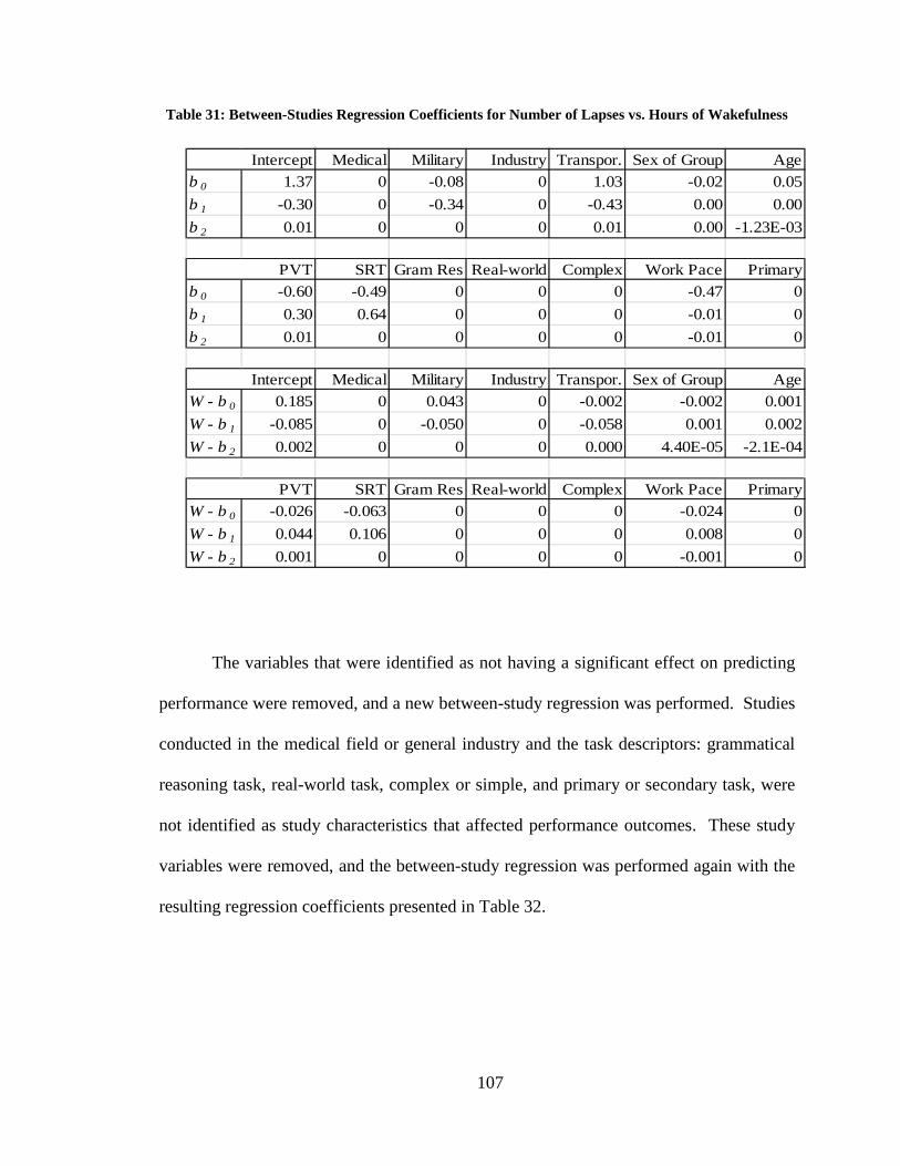
107
Table 31: Between-Studies Regression Coefficients for Number of Lapses vs. Hours of Wakefulness
Medical Military Industry Transpor. Sex of Group Ageb 0 1.37 0 -0.08 0 1.03 -0.02 0.05b 1 -0.30 0 -0.34 0 -0.43 0.00 0.00b 2 0.01 0 0 0 0.01 0.00 -1.23E-03
SRT Gram Res Real-world Complex Work Pace Primaryb 0 -0.60 -0.49 0 0 0 -0.47 0b 1 0.30 0.64 0 0 0 -0.01 0b 2 0.01 0 0 0 0 -0.01 0
Medical Military Industry Transpor. Sex of Group AgeW - b 0 0.185 0 0.043 0 -0.002 -0.002 0.001W - b 1 -0.085 0 -0.050 0 -0.058 0.001 0.002W - b 2 0.002 0 0 0 0.000 4.40E-05 -2.1E-04
SRT Gram Res Real-world Complex Work Pace PrimaryW - b 0 -0.026 -0.063 0 0 0 -0.024 0W - b 1 0.044 0.106 0 0 0 0.008 0W - b 2 0.001 0 0 0 0 -0.001 0
Intercept
PVT
Intercept
PVT
The variables that were identified as not having a significant effect on predicting
performance were removed, and a new between-study regression was performed. Studies
conducted in the medical field or general industry and the task descriptors: grammatical
reasoning task, real-world task, complex or simple, and primary or secondary task, were
not identified as study characteristics that affected performance outcomes. These study
variables were removed, and the between-study regression was performed again with the
resulting regression coefficients presented in Table 32.
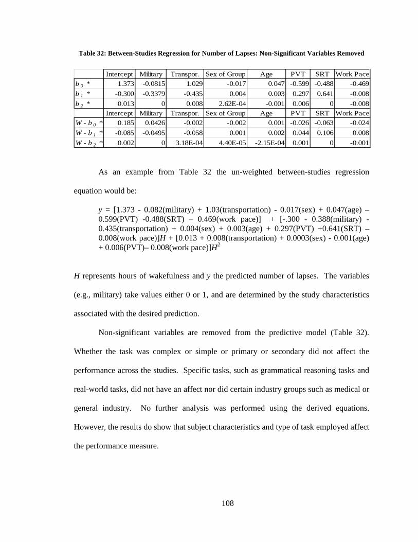
108
Table 32: Between-Studies Regression for Number of Lapses: Non-Significant Variables Removed
Intercept Military Transpor. Sex of Group Age PVT SRT Work Paceb 0 * 1.373 -0.0815 1.029 -0.017 0.047 -0.599 -0.488 -0.469b 1 * -0.300 -0.3379 -0.435 0.004 0.003 0.297 0.641 -0.008b 2 * 0.013 0 0.008 2.62E-04 -0.001 0.006 0 -0.008
Intercept Military Transpor. Sex of Group Age PVT SRT Work PaceW - b 0 * 0.185 0.0426 -0.002 -0.002 0.001 -0.026 -0.063 -0.024W - b 1 * -0.085 -0.0495 -0.058 0.001 0.002 0.044 0.106 0.008W - b 2 * 0.002 0 3.18E-04 4.40E-05 -2.15E-04 0.001 0 -0.001
As an example from Table 32 the un-weighted between-studies regression
equation would be:
y = [1.373 - 0.082(military) + 1.03(transportation) - 0.017(sex) + 0.047(age) – 0.599(PVT) -0.488(SRT) – 0.469(work pace)] + [-.300 - 0.388(military) - 0.435(transportation) + 0.004(sex) + 0.003(age) + 0.297(PVT) +0.641(SRT) – 0.008(work pace)]H + [0.013 + 0.008(transportation) + 0.0003(sex) - 0.001(age) + 0.006(PVT)– 0.008(work pace)]H2
H represents hours of wakefulness and y the predicted number of lapses. The variables
(e.g., military) take values either 0 or 1, and are determined by the study characteristics
associated with the desired prediction.
Non-significant variables are removed from the predictive model (Table 32).
Whether the task was complex or simple or primary or secondary did not affect the
performance across the studies. Specific tasks, such as grammatical reasoning tasks and
real-world tasks, did not have an affect nor did certain industry groups such as medical or
general industry. No further analysis was performed using the derived equations.
However, the results do show that subject characteristics and type of task employed affect
the performance measure.
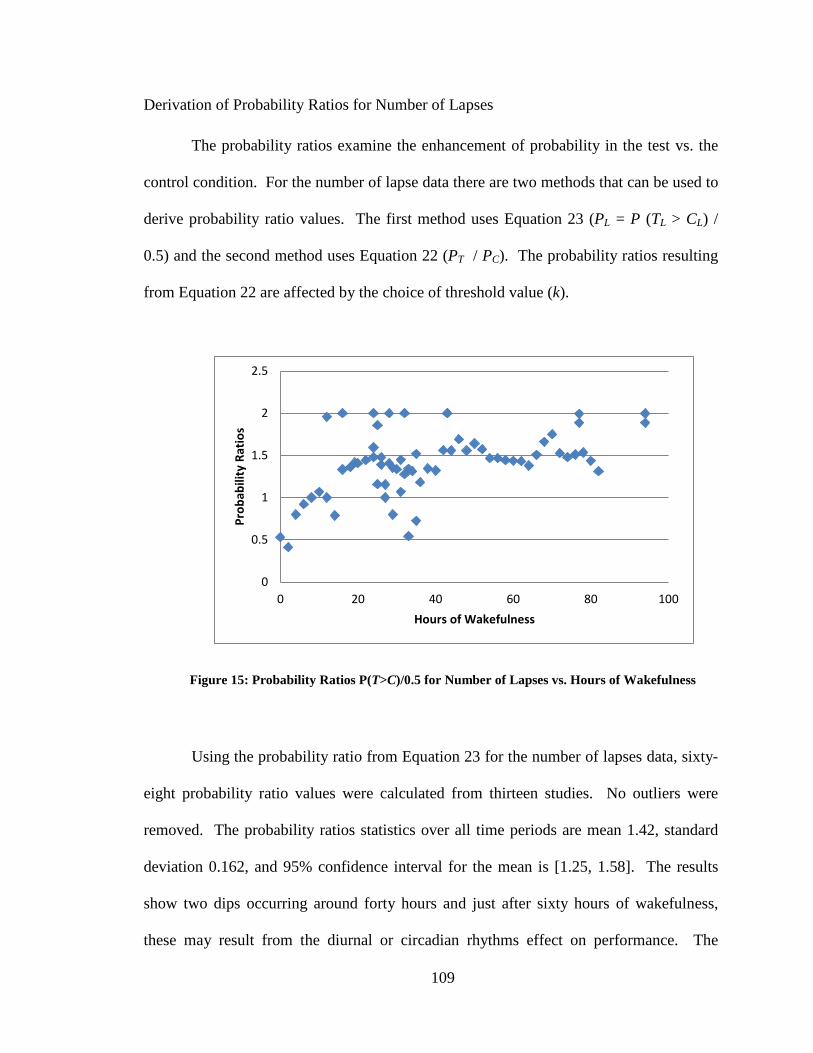
109
Derivation of Probability Ratios for Number of Lapses
The probability ratios examine the enhancement of probability in the test vs. the
control condition. For the number of lapse data there are two methods that can be used to
derive probability ratio values. The first method uses Equation 23 (PL = P (TL > CL) /
0.5) and the second method uses Equation 22 (PT / PC). The probability ratios resulting
from Equation 22 are affected by the choice of threshold value (k).
Figure 15: Probability Ratios P(T>C)/0.5 for Number of Lapses vs. Hours of Wakefulness
Using the probability ratio from Equation 23 for the number of lapses data, sixty-
eight probability ratio values were calculated from thirteen studies. No outliers were
removed. The probability ratios statistics over all time periods are mean 1.42, standard
deviation 0.162, and 95% confidence interval for the mean is [1.25, 1.58]. The results
show two dips occurring around forty hours and just after sixty hours of wakefulness,
these may result from the diurnal or circadian rhythms effect on performance. The
0
0.5
1
1.5
2
2.5
0 20 40 60 80 100
Prob
abili
ty R
atio
s
Hours of Wakefulness
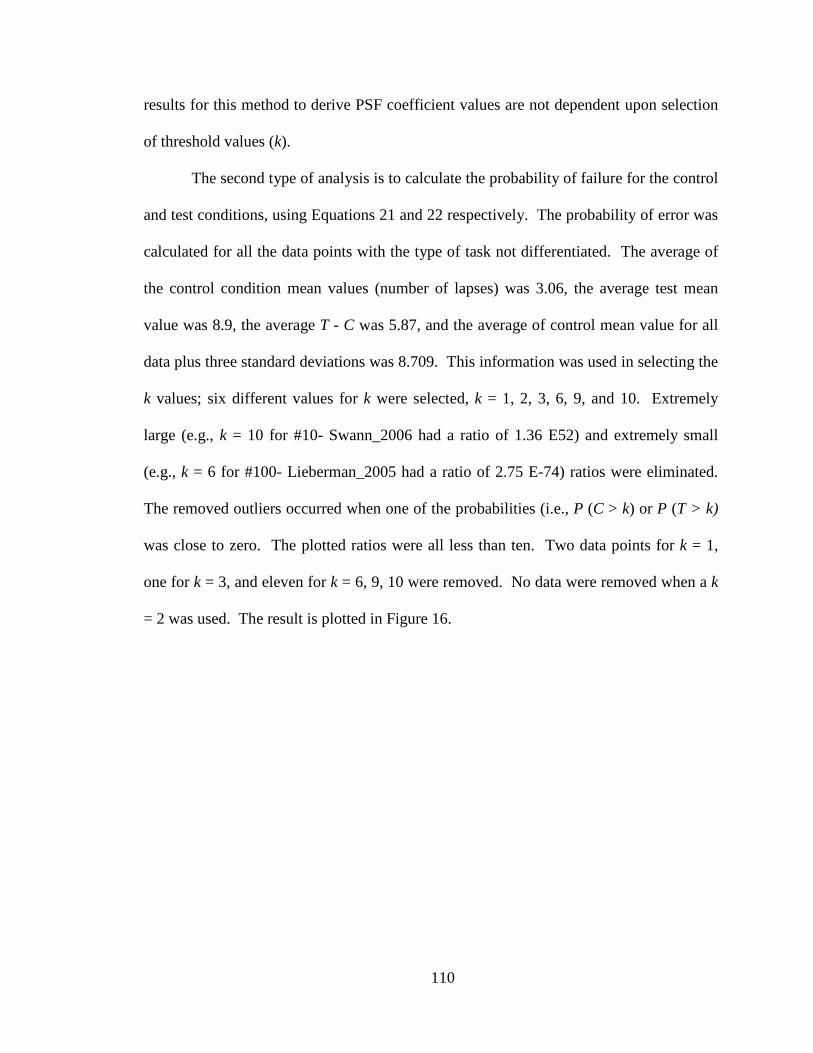
110
results for this method to derive PSF coefficient values are not dependent upon selection
of threshold values (k).
The second type of analysis is to calculate the probability of failure for the control
and test conditions, using Equations 21 and 22 respectively. The probability of error was
calculated for all the data points with the type of task not differentiated. The average of
the control condition mean values (number of lapses) was 3.06, the average test mean
value was 8.9, the average T - C was 5.87, and the average of control mean value for all
data plus three standard deviations was 8.709. This information was used in selecting the
k values; six different values for k were selected, k = 1, 2, 3, 6, 9, and 10. Extremely
large (e.g., k = 10 for #10- Swann_2006 had a ratio of 1.36 E52) and extremely small
(e.g., k = 6 for #100- Lieberman_2005 had a ratio of 2.75 E-74) ratios were eliminated.
The removed outliers occurred when one of the probabilities (i.e., P (C > k) or P (T > k)
was close to zero. The plotted ratios were all less than ten. Two data points for k = 1,
one for k = 3, and eleven for k = 6, 9, 10 were removed. No data were removed when a k
= 2 was used. The result is plotted in Figure 16.
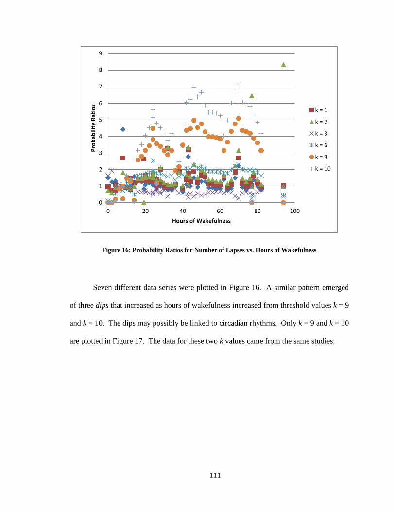
111
Figure 16: Probability Ratios for Number of Lapses vs. Hours of Wakefulness
Seven different data series were plotted in Figure 16. A similar pattern emerged
of three dips that increased as hours of wakefulness increased from threshold values k = 9
and k = 10. The dips may possibly be linked to circadian rhythms. Only k = 9 and k = 10
are plotted in Figure 17. The data for these two k values came from the same studies.
0
1
2
3
4
5
6
7
8
9
0 20 40 60 80 100
Prob
abili
ty R
atio
s
Hours of Wakefulness
k = 1
k = 2
k = 3
k = 6
k = 9
k = 10
112
Figure 17: Probability Ratios for Number of Lapses (k = 9, 10)
In order to find the best-fit line to describe the probability ratio values, a different
trend-line was fit to specific time intervals. The pattern of the probability ratios k = 9
and 10 showed three distinct dips; in order to best fit the data, the time intervals were
broken down into ten hour time blocks. The intervals were: less than ten hours, ten to
twenty hours, twenty to forty hours, forty to fifty hours, fifty to sixty hours, sixty to
seventy hours, and greater than seventy hours. The resulting equations and R2 values are
listed in Table 33. Equations for the interval of ten to twenty hours of wakefulness had
the lowest R2 value, k = 9 had a R2 of 0.76, and k = 10 had a R2 of 0.796. An exponential
fit for the interval of twenty to forty hours had the best fit. Polynomial equations were
the best-fit for the other time intervals.
0
1
2
3
4
5
6
7
8
0 20 40 60 80 100
Prob
abili
ty R
atio
s
Hours of Wakefulness
k = 9
k = 10
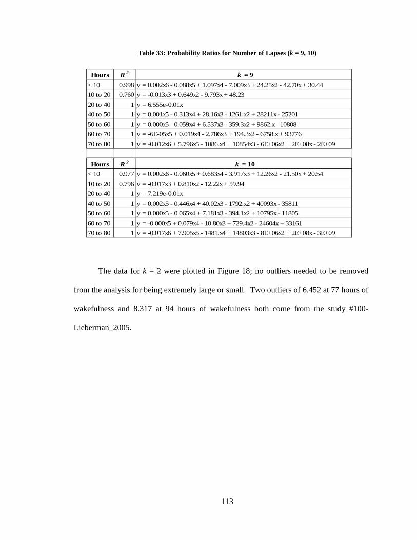
113
Table 33: Probability Ratios for Number of Lapses (k = 9, 10)
Hours R 2 k = 9< 10 0.998 y = 0.002x6 - 0.088x5 + 1.097x4 - 7.009x3 + 24.25x2 - 42.70x + 30.4410 to 20 0.760 y = -0.013x3 + 0.649x2 - 9.793x + 48.2320 to 40 1 y = 6.555e-0.01x40 to 50 1 y = 0.001x5 - 0.313x4 + 28.16x3 - 1261.x2 + 28211x - 2520150 to 60 1 y = 0.000x5 - 0.059x4 + 6.537x3 - 359.3x2 + 9862.x - 1080860 to 70 1 y = -6E-05x5 + 0.019x4 - 2.786x3 + 194.3x2 - 6758.x + 9377670 to 80 1 y = -0.012x6 + 5.796x5 - 1086.x4 + 10854x3 - 6E+06x2 + 2E+08x - 2E+09
Hours R 2 k = 10< 10 0.977 y = 0.002x6 - 0.060x5 + 0.683x4 - 3.917x3 + 12.26x2 - 21.50x + 20.5410 to 20 0.796 y = -0.017x3 + 0.810x2 - 12.22x + 59.9420 to 40 1 y = 7.219e-0.01x40 to 50 1 y = 0.002x5 - 0.446x4 + 40.02x3 - 1792.x2 + 40093x - 3581150 to 60 1 y = 0.000x5 - 0.065x4 + 7.181x3 - 394.1x2 + 10795x - 1180560 to 70 1 y = -0.000x5 + 0.079x4 - 10.80x3 + 729.4x2 - 24604x + 3316170 to 80 1 y = -0.017x6 + 7.905x5 - 1481.x4 + 14803x3 - 8E+06x2 + 2E+08x - 3E+09
The data for k = 2 were plotted in Figure 18; no outliers needed to be removed
from the analysis for being extremely large or small. Two outliers of 6.452 at 77 hours of
wakefulness and 8.317 at 94 hours of wakefulness both come from the study #100-
Lieberman_2005.
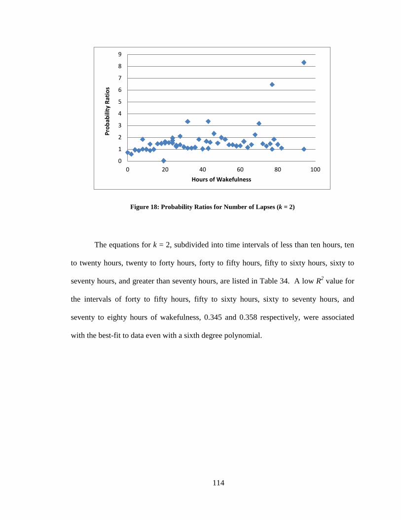
114
Figure 18: Probability Ratios for Number of Lapses (k = 2)
The equations for k = 2, subdivided into time intervals of less than ten hours, ten
to twenty hours, twenty to forty hours, forty to fifty hours, fifty to sixty hours, sixty to
seventy hours, and greater than seventy hours, are listed in Table 34. A low R2 value for
the intervals of forty to fifty hours, fifty to sixty hours, sixty to seventy hours, and
seventy to eighty hours of wakefulness, 0.345 and 0.358 respectively, were associated
with the best-fit to data even with a sixth degree polynomial.
0
1
2
3
4
5
6
7
8
9
0 20 40 60 80 100
Prob
abili
ty R
atio
s
Hours of Wakefulness
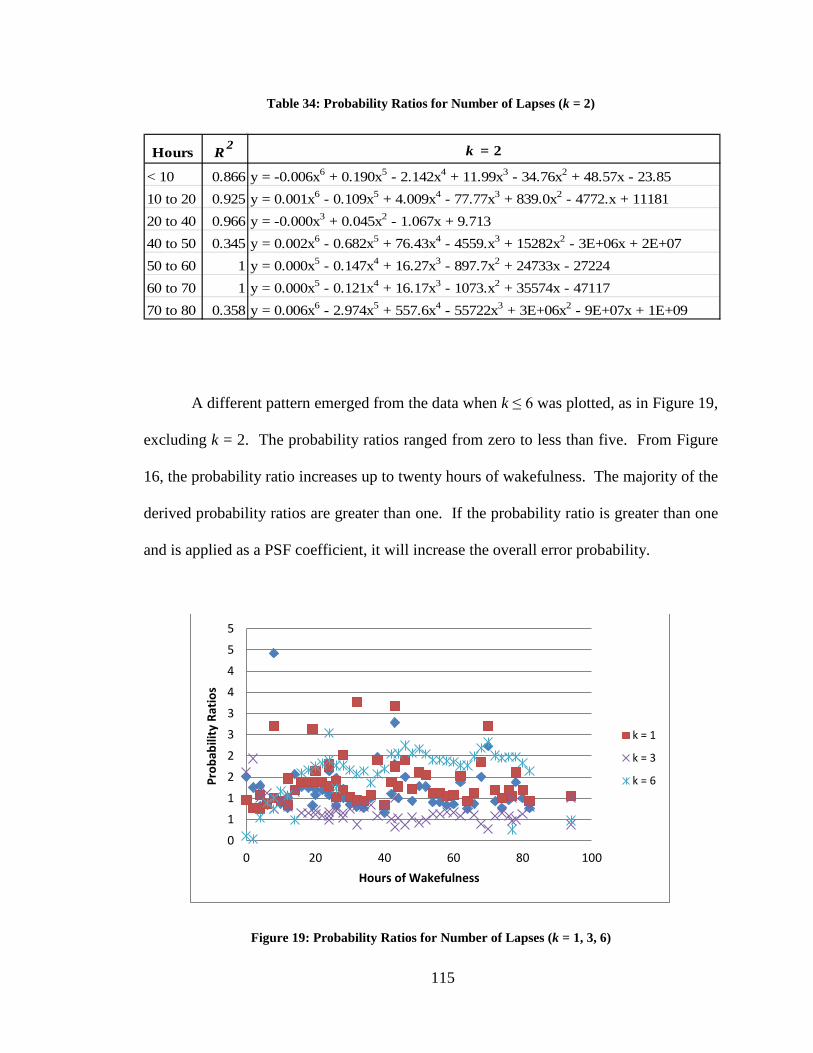
115
Table 34: Probability Ratios for Number of Lapses (k = 2)
Hours R 2 k = 2
< 10 0.866 y = -0.006x6 + 0.190x5 - 2.142x4 + 11.99x3 - 34.76x2 + 48.57x - 23.8510 to 20 0.925 y = 0.001x6 - 0.109x5 + 4.009x4 - 77.77x3 + 839.0x2 - 4772.x + 1118120 to 40 0.966 y = -0.000x3 + 0.045x2 - 1.067x + 9.71340 to 50 0.345 y = 0.002x6 - 0.682x5 + 76.43x4 - 4559.x3 + 15282x2 - 3E+06x + 2E+0750 to 60 1 y = 0.000x5 - 0.147x4 + 16.27x3 - 897.7x2 + 24733x - 2722460 to 70 1 y = 0.000x5 - 0.121x4 + 16.17x3 - 1073.x2 + 35574x - 4711770 to 80 0.358 y = 0.006x6 - 2.974x5 + 557.6x4 - 55722x3 + 3E+06x2 - 9E+07x + 1E+09
A different pattern emerged from the data when k ≤ 6 was plotted, as in Figure 19,
excluding k = 2. The probability ratios ranged from zero to less than five. From Figure
16, the probability ratio increases up to twenty hours of wakefulness. The majority of the
derived probability ratios are greater than one. If the probability ratio is greater than one
and is applied as a PSF coefficient, it will increase the overall error probability.
Figure 19: Probability Ratios for Number of Lapses (k = 1, 3, 6)
0
1
1
2
2
3
3
4
4
5
5
0 20 40 60 80 100
Prob
abili
ty R
atio
s
Hours of Wakefulness
k = 1
k = 3
k = 6
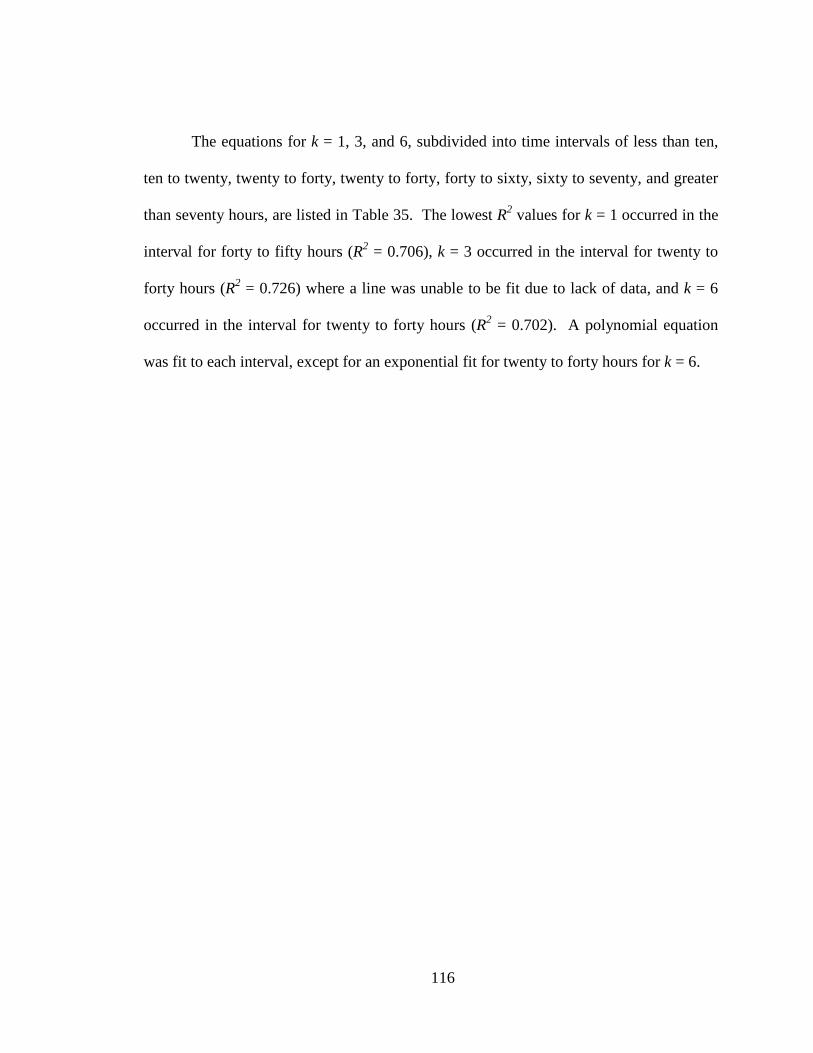
116
The equations for k = 1, 3, and 6, subdivided into time intervals of less than ten,
ten to twenty, twenty to forty, twenty to forty, forty to sixty, sixty to seventy, and greater
than seventy hours, are listed in Table 35. The lowest R2 values for k = 1 occurred in the
interval for forty to fifty hours (R2 = 0.706), k = 3 occurred in the interval for twenty to
forty hours (R2 = 0.726) where a line was unable to be fit due to lack of data, and k = 6
occurred in the interval for twenty to forty hours (R2 = 0.702). A polynomial equation
was fit to each interval, except for an exponential fit for twenty to forty hours for k = 6.
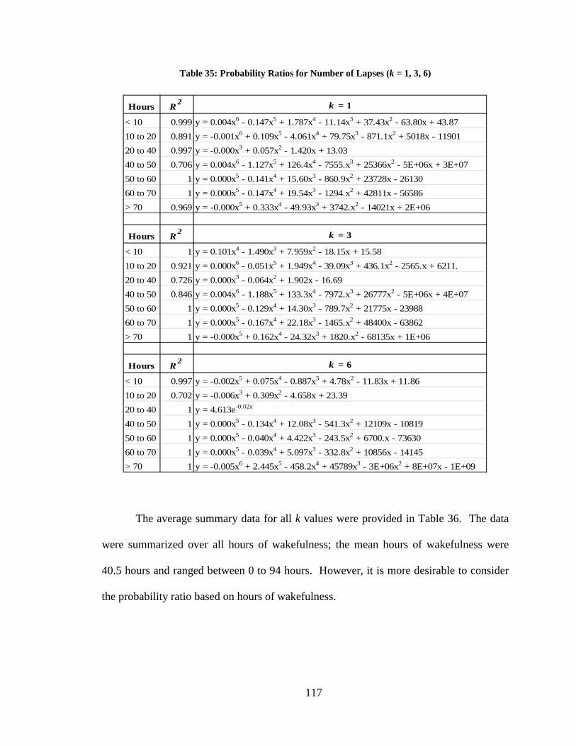
117
Table 35: Probability Ratios for Number of Lapses (k = 1, 3, 6)
Hours R 2 k = 1
< 10 0.999 y = 0.004x6 - 0.147x5 + 1.787x4 - 11.14x3 + 37.43x2 - 63.80x + 43.8710 to 20 0.891 y = -0.001x6 + 0.109x5 - 4.061x4 + 79.75x3 - 871.1x2 + 5018x - 1190120 to 40 0.997 y = -0.000x3 + 0.057x2 - 1.420x + 13.0340 to 50 0.706 y = 0.004x6 - 1.127x5 + 126.4x4 - 7555.x3 + 25366x2 - 5E+06x + 3E+0750 to 60 1 y = 0.000x5 - 0.141x4 + 15.60x3 - 860.9x2 + 23728x - 2613060 to 70 1 y = 0.000x5 - 0.147x4 + 19.54x3 - 1294.x2 + 42811x - 56586> 70 0.969 y = -0.000x5 + 0.333x4 - 49.93x3 + 3742.x2 - 14021x + 2E+06
Hours R 2 k = 3
< 10 1 y = 0.101x4 - 1.490x3 + 7.959x2 - 18.15x + 15.5810 to 20 0.921 y = 0.000x6 - 0.051x5 + 1.949x4 - 39.09x3 + 436.1x2 - 2565.x + 6211.20 to 40 0.726 y = 0.000x3 - 0.064x2 + 1.902x - 16.6940 to 50 0.846 y = 0.004x6 - 1.188x5 + 133.3x4 - 7972.x3 + 26777x2 - 5E+06x + 4E+0750 to 60 1 y = 0.000x5 - 0.129x4 + 14.30x3 - 789.7x2 + 21775x - 2398860 to 70 1 y = 0.000x5 - 0.167x4 + 22.18x3 - 1465.x2 + 48400x - 63862> 70 1 y = -0.000x5 + 0.162x4 - 24.32x3 + 1820.x2 - 68135x + 1E+06
Hours R 2 k = 6
< 10 0.997 y = -0.002x5 + 0.075x4 - 0.887x3 + 4.78x2 - 11.83x + 11.8610 to 20 0.702 y = -0.006x3 + 0.309x2 - 4.658x + 23.3920 to 40 1 y = 4.613e-0.02x
40 to 50 1 y = 0.000x5 - 0.134x4 + 12.08x3 - 541.3x2 + 12109x - 1081950 to 60 1 y = 0.000x5 - 0.040x4 + 4.422x3 - 243.5x2 + 6700.x - 7363060 to 70 1 y = 0.000x5 - 0.039x4 + 5.097x3 - 332.8x2 + 10856x - 14145> 70 1 y = -0.005x6 + 2.445x5 - 458.2x4 + 45789x3 - 3E+06x2 + 8E+07x - 1E+09
The average summary data for all k values were provided in Table 36. The data
were summarized over all hours of wakefulness; the mean hours of wakefulness were
40.5 hours and ranged between 0 to 94 hours. However, it is more desirable to consider
the probability ratio based on hours of wakefulness.
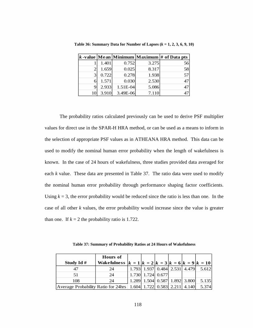
118
Table 36: Summary Data for Number of Lapses (k = 1, 2, 3, 6, 9, 10)
k -value Mean Minimum Maximum # of Data pts1 1.401 0.752 3.275 562 1.659 0.025 8.317 583 0.722 0.278 1.938 576 1.571 0.030 2.530 479 2.933 1.51E-04 5.086 47
10 3.910 3.49E-06 7.110 47
The probability ratios calculated previously can be used to derive PSF multiplier
values for direct use in the SPAR-H HRA method, or can be used as a means to inform in
the selection of appropriate PSF values as in ATHEANA HRA method. This data can be
used to modify the nominal human error probability when the length of wakefulness is
known. In the case of 24 hours of wakefulness, three studies provided data averaged for
each k value. These data are presented in Table 37. The ratio data were used to modify
the nominal human error probability through performance shaping factor coefficients.
Using k = 3, the error probability would be reduced since the ratio is less than one. In the
case of all other k values, the error probability would increase since the value is greater
than one. If k = 2 the probability ratio is 1.722.
Table 37: Summary of Probability Ratios at 24 Hours of Wakefulness
Study Id #Hours of
Wakefulness k = 1 k = 2 k = 3 k = 6 k = 9 k = 1047 24 1.793 1.937 0.484 2.531 4.479 5.61251 24 1.730 1.724 0.677108 24 1.289 1.504 0.587 1.892 3.800 5.135
Average Probability Ratio for 24hrs 1.604 1.722 0.583 2.211 4.140 5.374
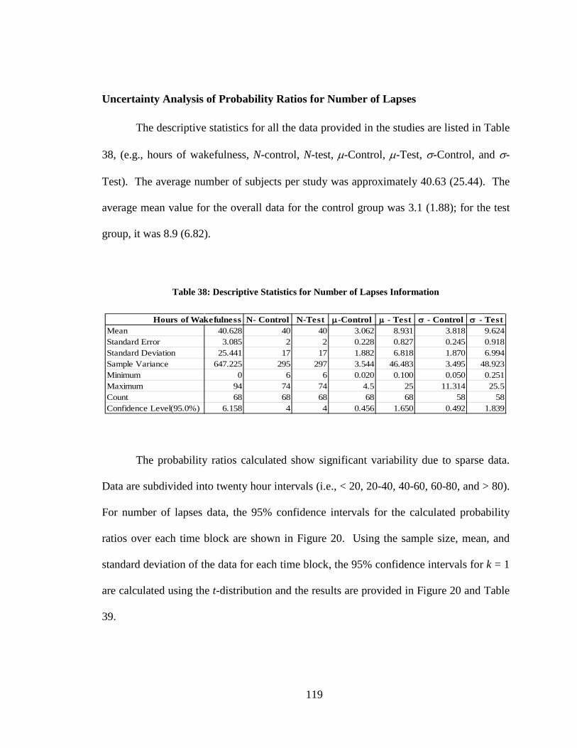
119
Uncertainty Analysis of Probability Ratios for Number of Lapses
The descriptive statistics for all the data provided in the studies are listed in Table
38, (e.g., hours of wakefulness, N-control, N-test, µ-Control, µ-Test, σ-Control, and σ-
Test). The average number of subjects per study was approximately 40.63 (25.44). The
average mean value for the overall data for the control group was 3.1 (1.88); for the test
group, it was 8.9 (6.82).
Table 38: Descriptive Statistics for Number of Lapses Information
Hours of Wakefulness N- Control N-Test µ-Control µ - Test σ - Control σ - TestMean 40.628 40 40 3.062 8.931 3.818 9.624Standard Error 3.085 2 2 0.228 0.827 0.245 0.918Standard Deviation 25.441 17 17 1.882 6.818 1.870 6.994Sample Variance 647.225 295 297 3.544 46.483 3.495 48.923Minimum 0 6 6 0.020 0.100 0.050 0.251Maximum 94 74 74 4.5 25 11.314 25.5Count 68 68 68 68 68 58 58Confidence Level(95.0%) 6.158 4 4 0.456 1.650 0.492 1.839
The probability ratios calculated show significant variability due to sparse data.
Data are subdivided into twenty hour intervals (i.e., < 20, 20-40, 40-60, 60-80, and > 80).
For number of lapses data, the 95% confidence intervals for the calculated probability
ratios over each time block are shown in Figure 20. Using the sample size, mean, and
standard deviation of the data for each time block, the 95% confidence intervals for k = 1
are calculated using the t-distribution and the results are provided in Figure 20 and Table
39.
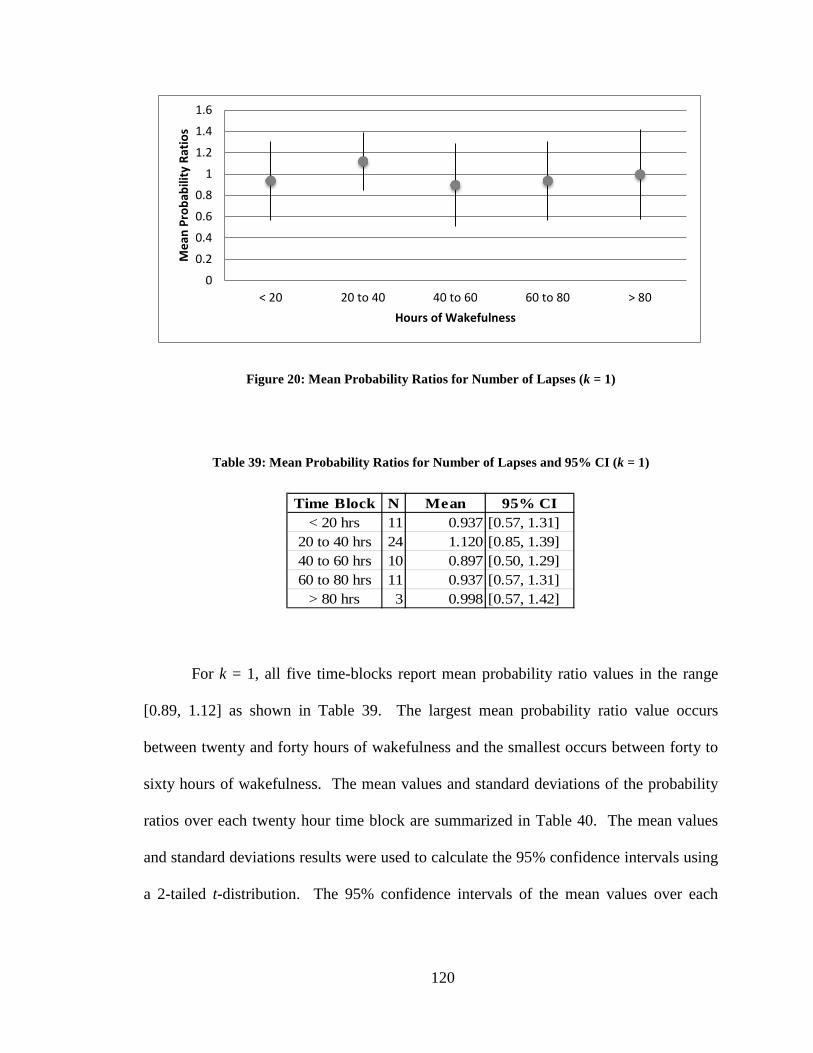
120
Figure 20: Mean Probability Ratios for Number of Lapses (k = 1)
Table 39: Mean Probability Ratios for Number of Lapses and 95% CI (k = 1)
Time Block N Mean 95% CI< 20 hrs 11 0.937 [0.57, 1.31]
20 to 40 hrs 24 1.120 [0.85, 1.39]40 to 60 hrs 10 0.897 [0.50, 1.29]60 to 80 hrs 11 0.937 [0.57, 1.31]
> 80 hrs 3 0.998 [0.57, 1.42]
For k = 1, all five time-blocks report mean probability ratio values in the range
[0.89, 1.12] as shown in Table 39. The largest mean probability ratio value occurs
between twenty and forty hours of wakefulness and the smallest occurs between forty to
sixty hours of wakefulness. The mean values and standard deviations of the probability
ratios over each twenty hour time block are summarized in Table 40. The mean values
and standard deviations results were used to calculate the 95% confidence intervals using
a 2-tailed t-distribution. The 95% confidence intervals of the mean values over each
0
0.2
0.4
0.6
0.8
1
1.2
1.4
1.6
< 20 20 to 40 40 to 60 60 to 80 > 80
Mea
n Pr
obab
ility
Rat
ios
Hours of Wakefulness
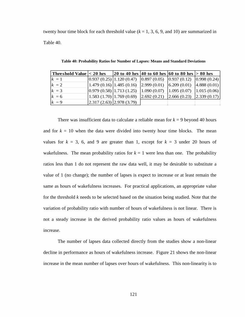
121
twenty hour time block for each threshold value (k = 1, 3, 6, 9, and 10) are summarized in
Table 40.
Table 40: Probability Ratios for Number of Lapses: Means and Standard Deviations
Threshold Value < 20 hrs 20 to 40 hrs 40 to 60 hrs 60 to 80 hrs > 80 hrsk = 1 0.937 (0.25) 1.120 (0.47) 0.897 (0.05) 0.937 (0.12) 0.998 (0.24)k = 2 1.479 (0.16) 1.485 (0.16) 2.999 (0.01) 6.209 (0.01) 4.888 (0.01)k = 3 0.979 (0.58) 1.713 (1.25) 1.090 (0.07) 1.095 (0.07) 1.015 (0.06)k = 6 1.583 (1.70) 1.769 (0.69) 2.692 (0.21) 2.666 (0.23) 2.339 (0.17)k = 9 2.317 (2.63) 2.978 (3.79)
There was insufficient data to calculate a reliable mean for k = 9 beyond 40 hours
and for k = 10 when the data were divided into twenty hour time blocks. The mean
values for k = 3, 6, and 9 are greater than 1, except for k = 3 under 20 hours of
wakefulness. The mean probability ratios for k = 1 were less than one. The probability
ratios less than 1 do not represent the raw data well, it may be desirable to substitute a
value of 1 (no change); the number of lapses is expect to increase or at least remain the
same as hours of wakefulness increases. For practical applications, an appropriate value
for the threshold k needs to be selected based on the situation being studied. Note that the
variation of probability ratio with number of hours of wakefulness is not linear. There is
not a steady increase in the derived probability ratio values as hours of wakefulness
increase.
The number of lapses data collected directly from the studies show a non-linear
decline in performance as hours of wakefulness increase. Figure 21 shows the non-linear
increase in the mean number of lapses over hours of wakefulness. This non-linearity is to
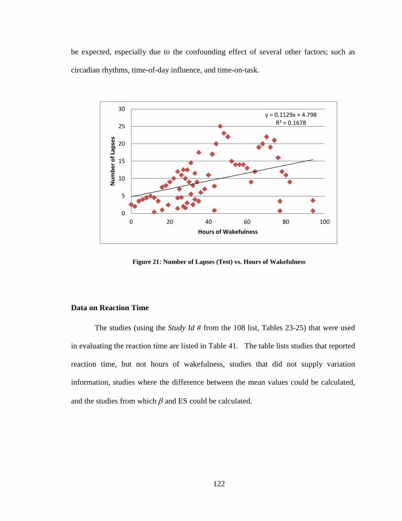
122
be expected, especially due to the confounding effect of several other factors; such as
circadian rhythms, time-of-day influence, and time-on-task.
Figure 21: Number of Lapses (Test) vs. Hours of Wakefulness
Data on Reaction Time
The studies (using the Study Id # from the 108 list, Tables 23-25) that were used
in evaluating the reaction time are listed in Table 41. The table lists studies that reported
reaction time, but not hours of wakefulness, studies that did not supply variation
information, studies where the difference between the mean values could be calculated,
and the studies from which β and ES could be calculated.
y = 0.1129x + 4.798 R² = 0.1678
0
5
10
15
20
25
30
0 20 40 60 80 100
Num
ber o
f Lap
ses
Hours of Wakefulness
123
Table 41: Studies w.r.t. Data on Reaction Time
Studies without hrs of wakefulness (10, 13, 29, 34, 45, 54, 58, 59, 61, 62, 72, 75, 76, 83, 86, 87, 90Studies without standard deviations (5, 6, 14, 15, 16, 20, 21, 28, 29, 34, 35, 36, 52, 54, 62, 75, 102)
Studies used (1, 2, 3, 4, 7, 17, 19, 23, 25, 33, 34, 41, 42, 48, 53, 70, 71, 76, 87, 95, 96, 97, 98, 100, 101, 103, 104, 105, 106)
Reaction Time
Studies reporting reaction time
(1, 2, 3, 4, 5, 6, 7, 10, 13, 14, 15, 16, 17, 19, 20, 21, 23, 25, 28, 29, 33, 34, 35, 36, 41, 42, 45, 48, 52, 53, 54, 58, 59, 61, 62, 70, 71, 72, 75, 76, 83, 86, 87, 95, 96, 97, 98, 100, 101, 102, 103, 104, 105, 106)
Difference between the mean values
(1, 2, 3, 4, 7, 17, 19, 23, 25, 33, 34, 41, 42, 48, 53, 70, 71, 76, 87, 95, 96, 97, 98, 100, 101, 103, 104, 105, 106)
Effect size (1, 2, 3, 4, 7, 17, 19, 23, 25, 33, 41, 42, 48, 53, 70, 71, 95, 96, 97, 98, 100, 101, 103, 104, 105, 106)
Quantitative Effect of Sleep Deprivation on Reaction Time
The initial analysis was to calculate the difference between the mean values of the
control and test conditions for each data point of hours of wakefulness provided. The
general trend of this data supports the hypothesis that as hours of wakefulness increase
the difference between the test condition and control condition increases. The data
plotted in Figure 22 have been converted to milliseconds.
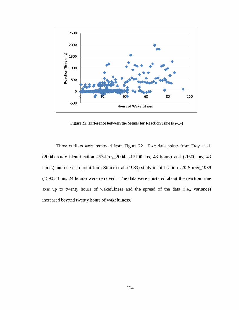
124
Figure 22: Difference between the Means for Reaction Time (µT-µC)
Three outliers were removed from Figure 22. Two data points from Frey et al.
(2004) study identification #53-Frey_2004 (-17700 ms, 43 hours) and (-1600 ms, 43
hours) and one data point from Storer et al. (1989) study identification #70-Storer_1989
(1590.33 ms, 24 hours) were removed. The data were clustered about the reaction time
axis up to twenty hours of wakefulness and the spread of the data (i.e., variance)
increased beyond twenty hours of wakefulness.
-500
0
500
1000
1500
2000
2500
0 20 40 60 80 100
Reac
tion
Tim
e (m
s)
Hours of Wakefulness
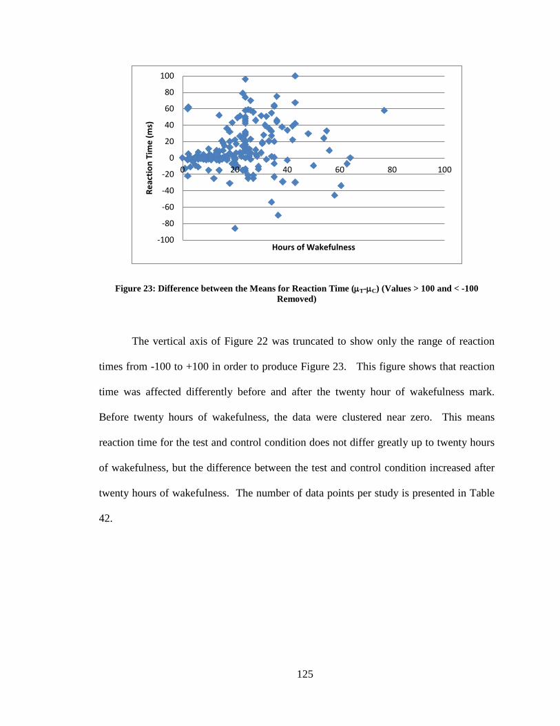
125
Figure 23: Difference between the Means for Reaction Time (µT-µC) (Values > 100 and < -100 Removed)
The vertical axis of Figure 22 was truncated to show only the range of reaction
times from -100 to +100 in order to produce Figure 23. This figure shows that reaction
time was affected differently before and after the twenty hour of wakefulness mark.
Before twenty hours of wakefulness, the data were clustered near zero. This means
reaction time for the test and control condition does not differ greatly up to twenty hours
of wakefulness, but the difference between the test and control condition increased after
twenty hours of wakefulness. The number of data points per study is presented in Table
42.
-100
-80
-60
-40
-20
0
20
40
60
80
100
0 20 40 60 80 100
Reac
tion
Tim
e (m
s)
Hours of Wakefulness
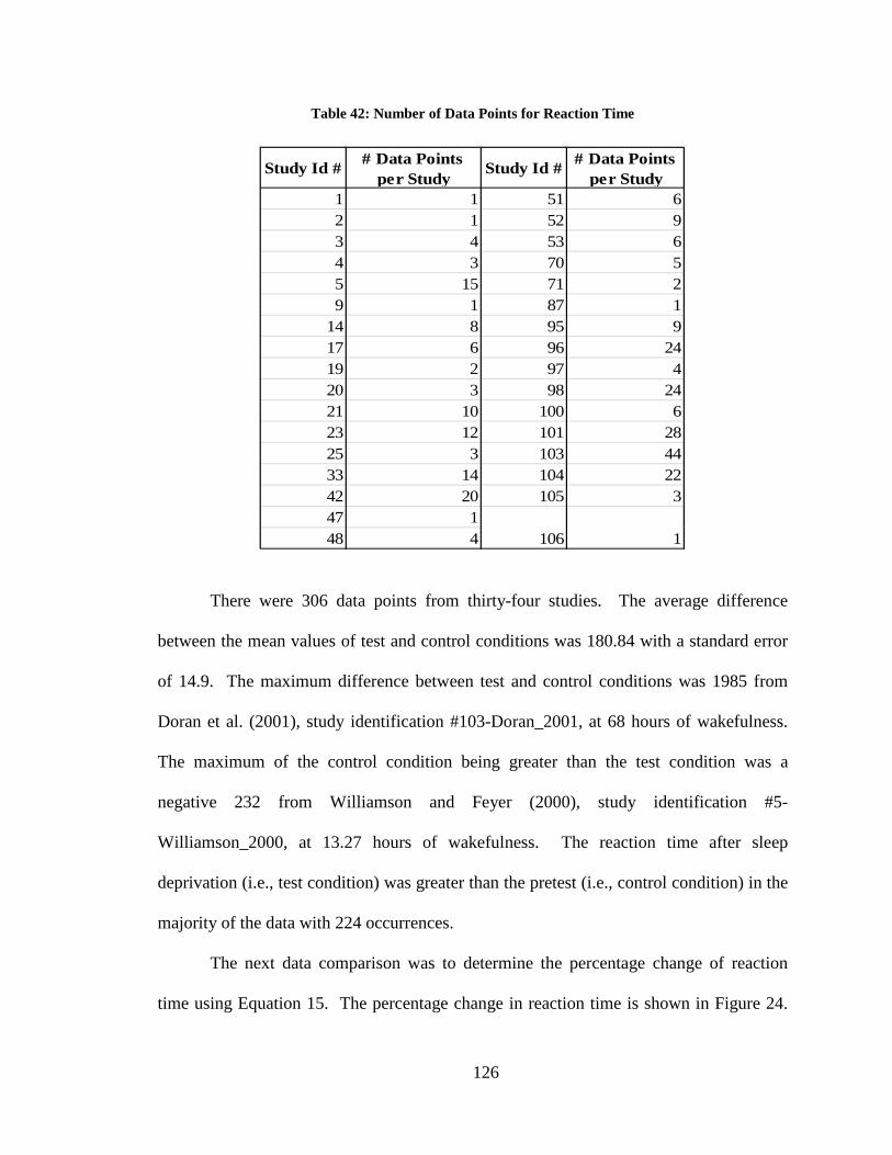
126
Table 42: Number of Data Points for Reaction Time
Study Id # # Data Points per Study
Study Id # # Data Points per Study
1 1 51 62 1 52 93 4 53 64 3 70 55 15 71 29 1 87 1
14 8 95 917 6 96 2419 2 97 420 3 98 2421 10 100 623 12 101 2825 3 103 4433 14 104 2242 20 105 347 148 4 106 1
There were 306 data points from thirty-four studies. The average difference
between the mean values of test and control conditions was 180.84 with a standard error
of 14.9. The maximum difference between test and control conditions was 1985 from
Doran et al. (2001), study identification #103-Doran_2001, at 68 hours of wakefulness.
The maximum of the control condition being greater than the test condition was a
negative 232 from Williamson and Feyer (2000), study identification #5-
Williamson_2000, at 13.27 hours of wakefulness. The reaction time after sleep
deprivation (i.e., test condition) was greater than the pretest (i.e., control condition) in the
majority of the data with 224 occurrences.
The next data comparison was to determine the percentage change of reaction
time using Equation 15. The percentage change in reaction time is shown in Figure 24.
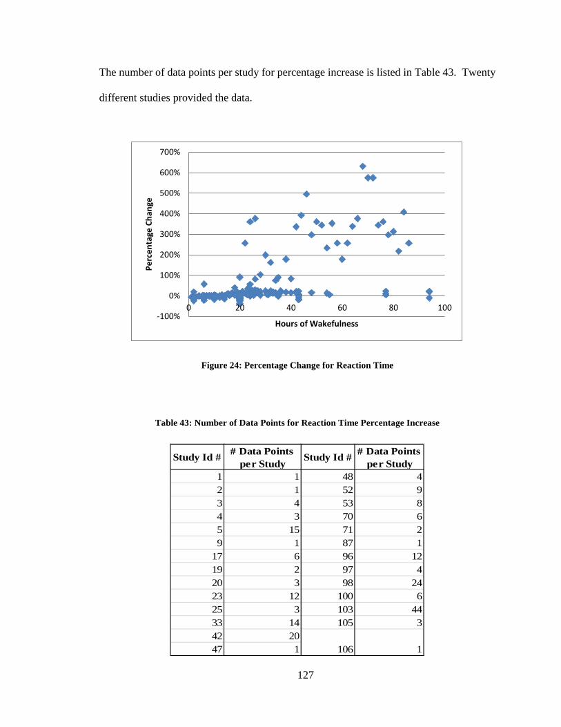
127
The number of data points per study for percentage increase is listed in Table 43. Twenty
different studies provided the data.
Figure 24: Percentage Change for Reaction Time
Table 43: Number of Data Points for Reaction Time Percentage Increase
Study Id # # Data Points per Study
Study Id # # Data Points per Study
1 1 48 42 1 52 93 4 53 84 3 70 65 15 71 29 1 87 1
17 6 96 1219 2 97 420 3 98 2423 12 100 625 3 103 4433 14 105 342 2047 1 106 1
-100%
0%
100%
200%
300%
400%
500%
600%
700%
0 20 40 60 80 100
Perc
enta
ge C
hang
e
Hours of Wakefulness
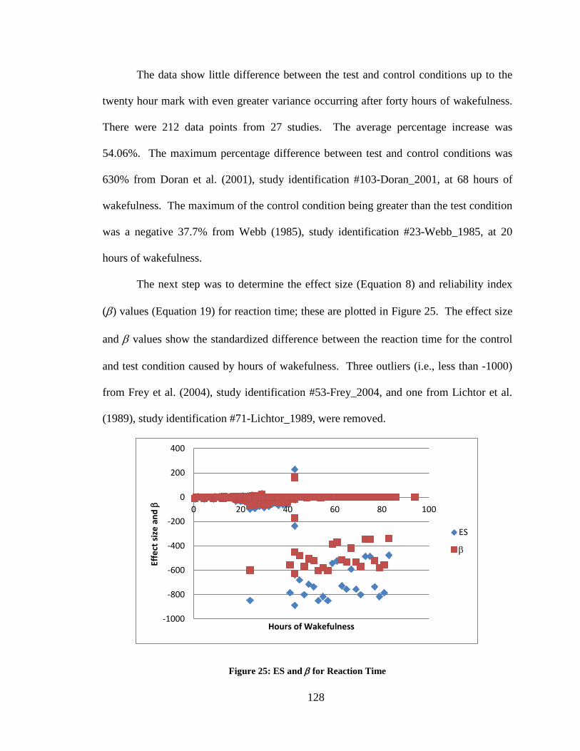
128
The data show little difference between the test and control conditions up to the
twenty hour mark with even greater variance occurring after forty hours of wakefulness.
There were 212 data points from 27 studies. The average percentage increase was
54.06%. The maximum percentage difference between test and control conditions was
630% from Doran et al. (2001), study identification #103-Doran_2001, at 68 hours of
wakefulness. The maximum of the control condition being greater than the test condition
was a negative 37.7% from Webb (1985), study identification #23-Webb_1985, at 20
hours of wakefulness.
The next step was to determine the effect size (Equation 8) and reliability index
(β) values (Equation 19) for reaction time; these are plotted in Figure 25. The effect size
and β values show the standardized difference between the reaction time for the control
and test condition caused by hours of wakefulness. Three outliers (i.e., less than -1000)
from Frey et al. (2004), study identification #53-Frey_2004, and one from Lichtor et al.
(1989), study identification #71-Lichtor_1989, were removed.
Figure 25: ES and β for Reaction Time
-1000
-800
-600
-400
-200
0
200
400
0 20 40 60 80 100
Effe
ct s
ize
and
β
Hours of Wakefulness
ES
β
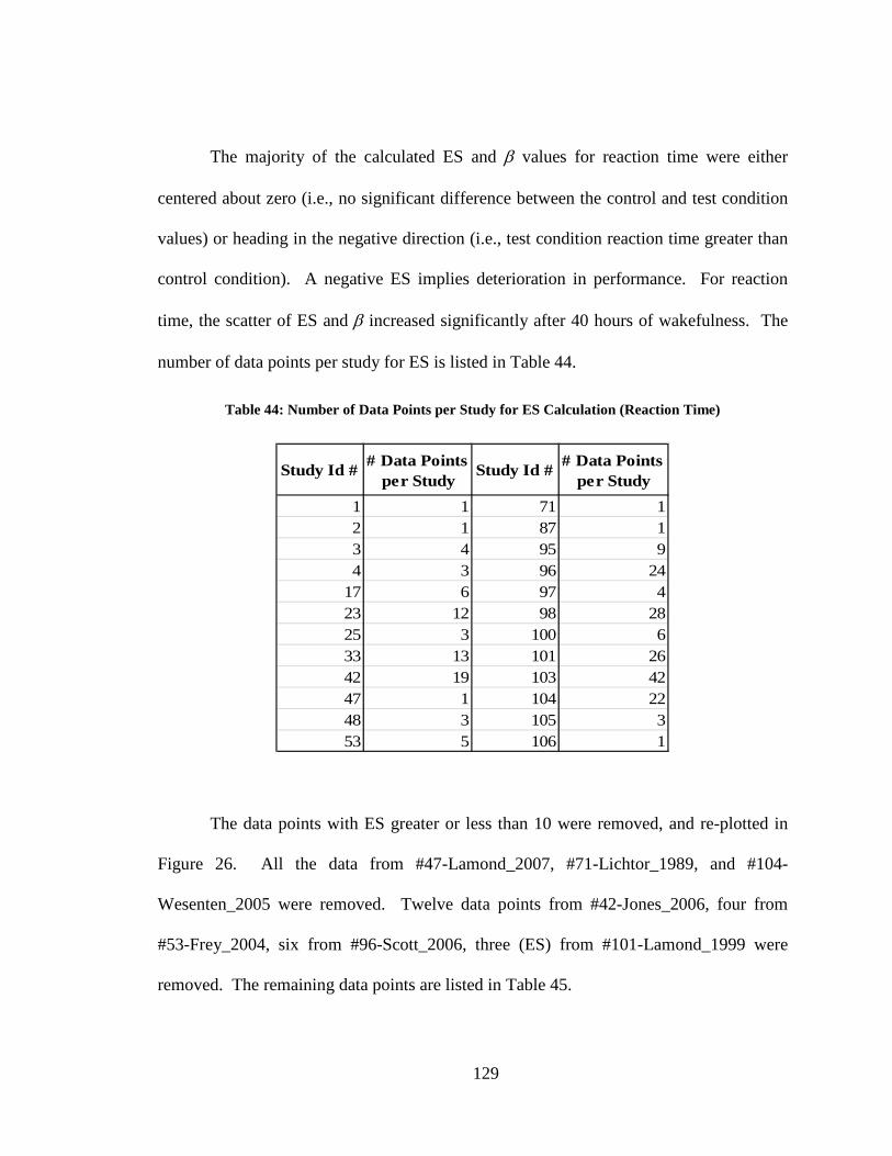
129
The majority of the calculated ES and β values for reaction time were either
centered about zero (i.e., no significant difference between the control and test condition
values) or heading in the negative direction (i.e., test condition reaction time greater than
control condition). A negative ES implies deterioration in performance. For reaction
time, the scatter of ES and β increased significantly after 40 hours of wakefulness. The
number of data points per study for ES is listed in Table 44.
Table 44: Number of Data Points per Study for ES Calculation (Reaction Time)
Study Id # # Data Points per Study
Study Id # # Data Points per Study
1 1 71 12 1 87 13 4 95 94 3 96 24
17 6 97 423 12 98 2825 3 100 633 13 101 2642 19 103 4247 1 104 2248 3 105 353 5 106 1
The data points with ES greater or less than 10 were removed, and re-plotted in
Figure 26. All the data from #47-Lamond_2007, #71-Lichtor_1989, and #104-
Wesenten_2005 were removed. Twelve data points from #42-Jones_2006, four from
#53-Frey_2004, six from #96-Scott_2006, three (ES) from #101-Lamond_1999 were
removed. The remaining data points are listed in Table 45.
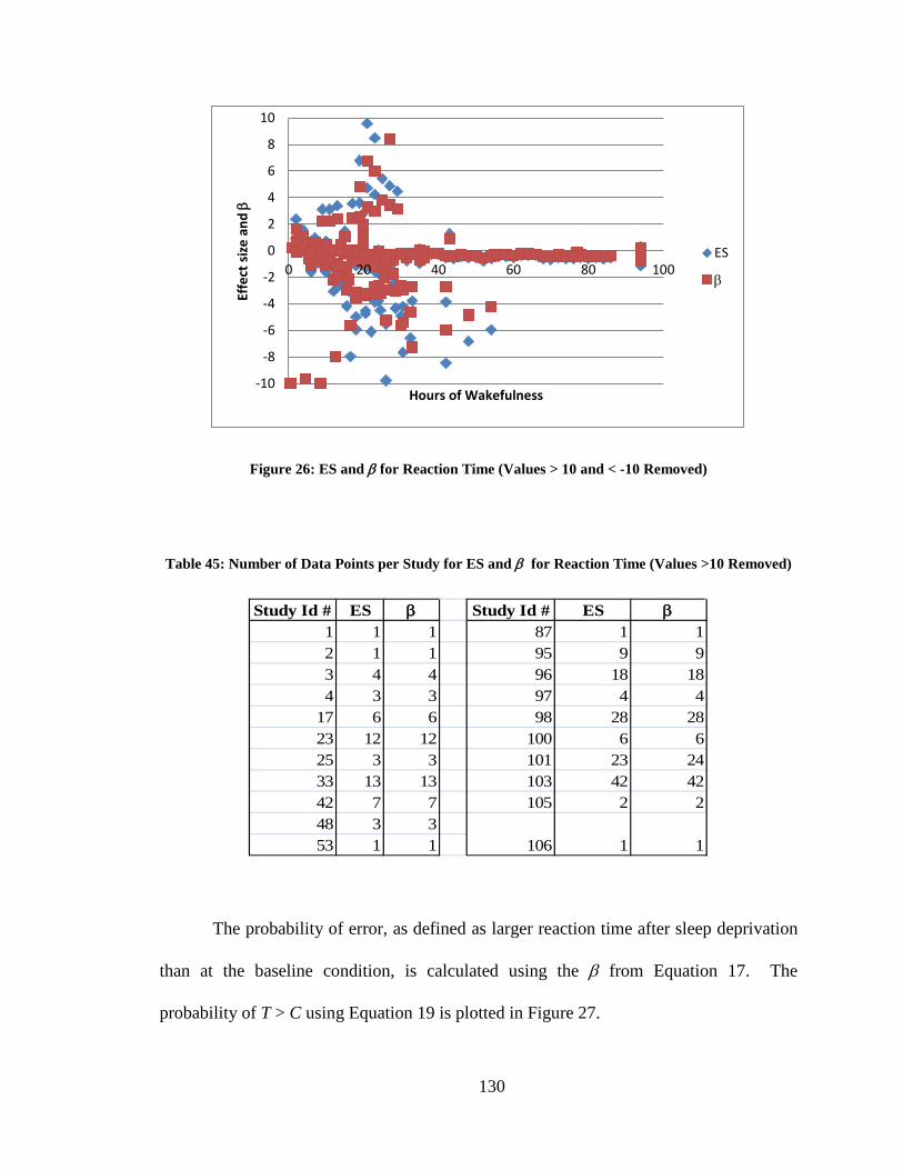
130
Figure 26: ES and β for Reaction Time (Values > 10 and < -10 Removed)
Table 45: Number of Data Points per Study for ES and β for Reaction Time (Values >10 Removed)
Study Id # ES β Study Id # ES β1 1 1 87 1 12 1 1 95 9 93 4 4 96 18 184 3 3 97 4 4
17 6 6 98 28 2823 12 12 100 6 625 3 3 101 23 2433 13 13 103 42 4242 7 7 105 2 248 3 353 1 1 106 1 1
The probability of error, as defined as larger reaction time after sleep deprivation
than at the baseline condition, is calculated using the β from Equation 17. The
probability of T > C using Equation 19 is plotted in Figure 27.
-10
-8
-6
-4
-2
0
2
4
6
8
10
0 20 40 60 80 100
Effe
ct s
ize
and
β
Hours of Wakefulness
ES
β
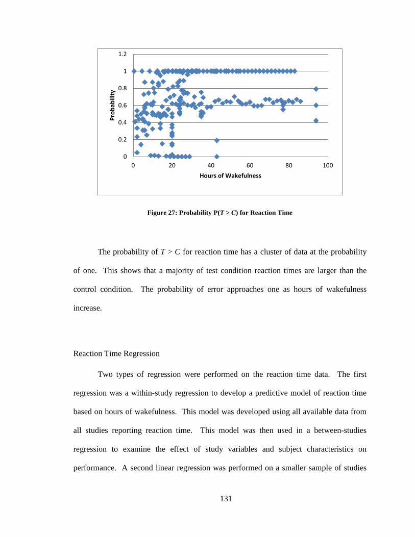
131
Figure 27: Probability P(T > C) for Reaction Time
The probability of T > C for reaction time has a cluster of data at the probability
of one. This shows that a majority of test condition reaction times are larger than the
control condition. The probability of error approaches one as hours of wakefulness
increase.
Reaction Time Regression
Two types of regression were performed on the reaction time data. The first
regression was a within-study regression to develop a predictive model of reaction time
based on hours of wakefulness. This model was developed using all available data from
all studies reporting reaction time. This model was then used in a between-studies
regression to examine the effect of study variables and subject characteristics on
performance. A second linear regression was performed on a smaller sample of studies
0
0.2
0.4
0.6
0.8
1
1.2
0 20 40 60 80 100
Prob
abili
ty
Hours of Wakefulness
132
(5 studies) that were similar in study design and investigated performance using a simple
reaction time task.
A linear regression was performed on the reaction time data. An intercept (b0),
linear coefficient (b1), and curvilinear coefficient (b2) of a quadratic model were found by
a multi-variate regression for each study separately. The hours of wakefulness were used
as the independent variable and reaction time was used as the dependent variable.
Studies that had only one time measure were graphed in order to find the regression
coefficients (#1-Nilsson_2005, #2-Thomas_2000, #7-Robbins_1990, #9-Babkoff_2005,
#10-Swann_2006, #14-Buck_1972, #23-Webb_1985, #47-Lamond_2007, and #106-
Drake_2001). The resulting coefficients are listed in Table 46.
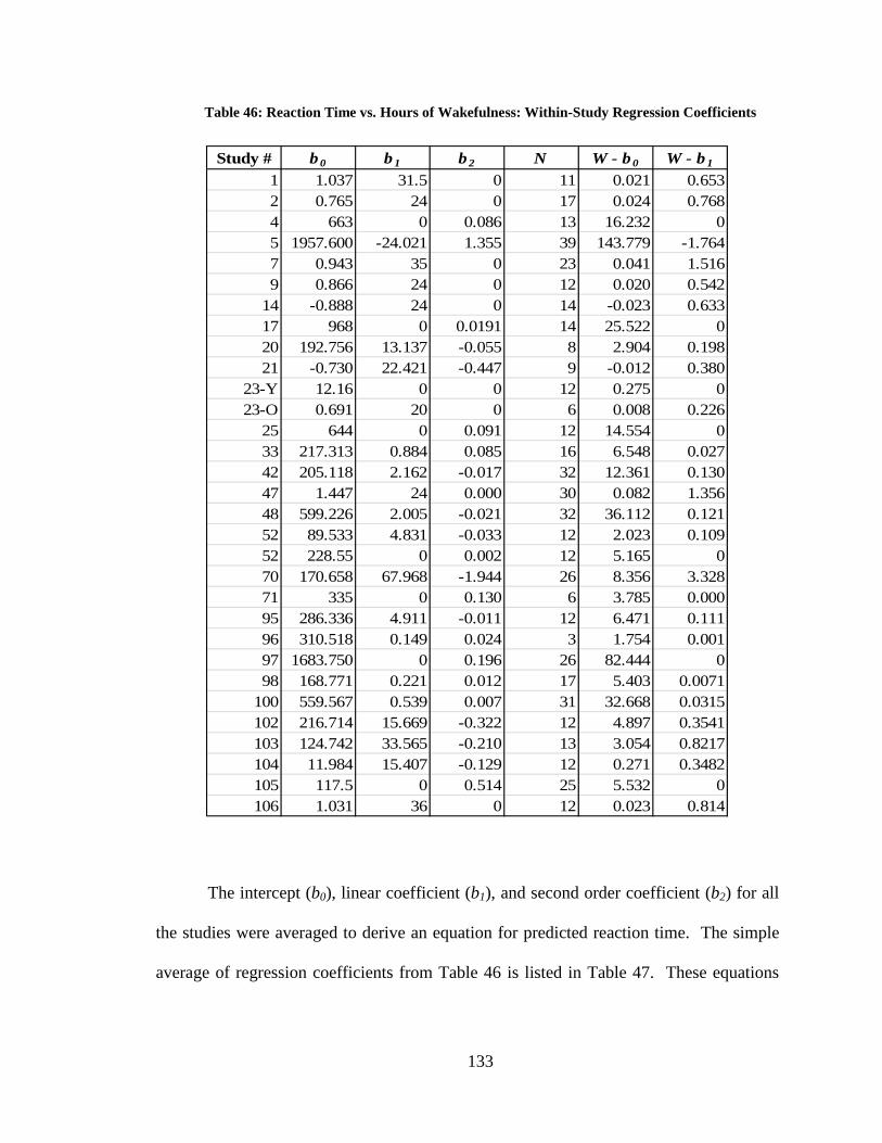
133
Table 46: Reaction Time vs. Hours of Wakefulness: Within-Study Regression Coefficients
Study # b0 b1 b2 N W - b0 W - b1
1 1.037 31.5 0 11 0.021 0.6532 0.765 24 0 17 0.024 0.7684 663 0 0.086 13 16.232 05 1957.600 -24.021 1.355 39 143.779 -1.7647 0.943 35 0 23 0.041 1.5169 0.866 24 0 12 0.020 0.542
14 -0.888 24 0 14 -0.023 0.63317 968 0 0.0191 14 25.522 020 192.756 13.137 -0.055 8 2.904 0.19821 -0.730 22.421 -0.447 9 -0.012 0.380
23-Y 12.16 0 0 12 0.275 023-O 0.691 20 0 6 0.008 0.226
25 644 0 0.091 12 14.554 033 217.313 0.884 0.085 16 6.548 0.02742 205.118 2.162 -0.017 32 12.361 0.13047 1.447 24 0.000 30 0.082 1.35648 599.226 2.005 -0.021 32 36.112 0.12152 89.533 4.831 -0.033 12 2.023 0.10952 228.55 0 0.002 12 5.165 070 170.658 67.968 -1.944 26 8.356 3.32871 335 0 0.130 6 3.785 0.00095 286.336 4.911 -0.011 12 6.471 0.11196 310.518 0.149 0.024 3 1.754 0.00197 1683.750 0 0.196 26 82.444 098 168.771 0.221 0.012 17 5.403 0.0071
100 559.567 0.539 0.007 31 32.668 0.0315102 216.714 15.669 -0.322 12 4.897 0.3541103 124.742 33.565 -0.210 13 3.054 0.8217104 11.984 15.407 -0.129 12 0.271 0.3482105 117.5 0 0.514 25 5.532 0106 1.031 36 0 12 0.023 0.814
The intercept (b0), linear coefficient (b1), and second order coefficient (b2) for all
the studies were averaged to derive an equation for predicted reaction time. The simple
average of regression coefficients from Table 46 is listed in Table 47. These equations
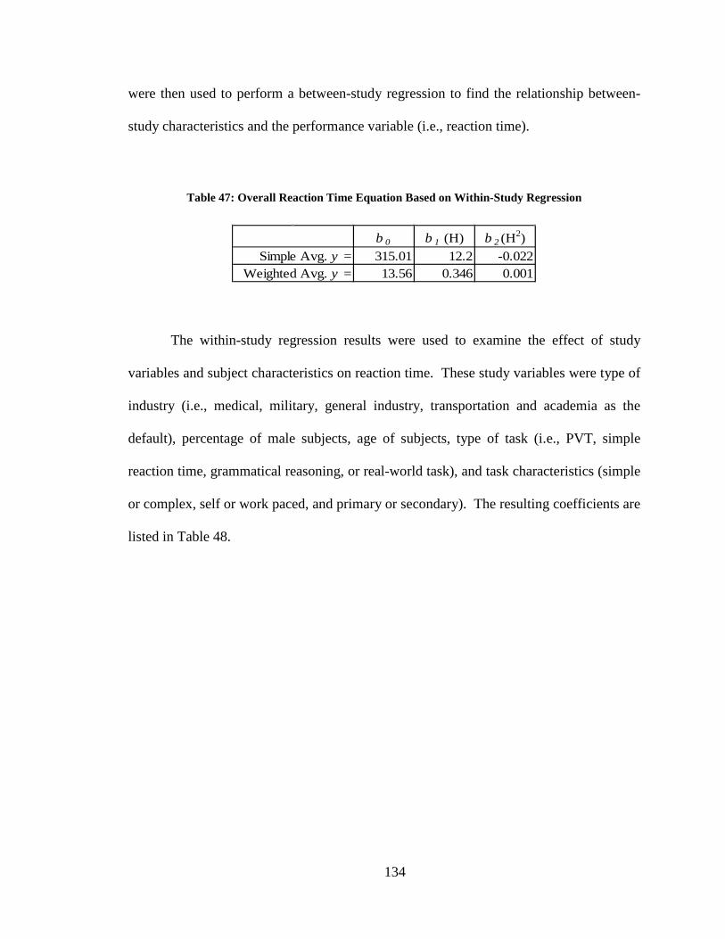
134
were then used to perform a between-study regression to find the relationship between-
study characteristics and the performance variable (i.e., reaction time).
Table 47: Overall Reaction Time Equation Based on Within-Study Regression
b 0 b 1 (H) b 2 (H2)315.01 12.2 -0.02213.56 0.346 0.001
Simple Avg. y =Weighted Avg. y =
The within-study regression results were used to examine the effect of study
variables and subject characteristics on reaction time. These study variables were type of
industry (i.e., medical, military, general industry, transportation and academia as the
default), percentage of male subjects, age of subjects, type of task (i.e., PVT, simple
reaction time, grammatical reasoning, or real-world task), and task characteristics (simple
or complex, self or work paced, and primary or secondary). The resulting coefficients are
listed in Table 48.
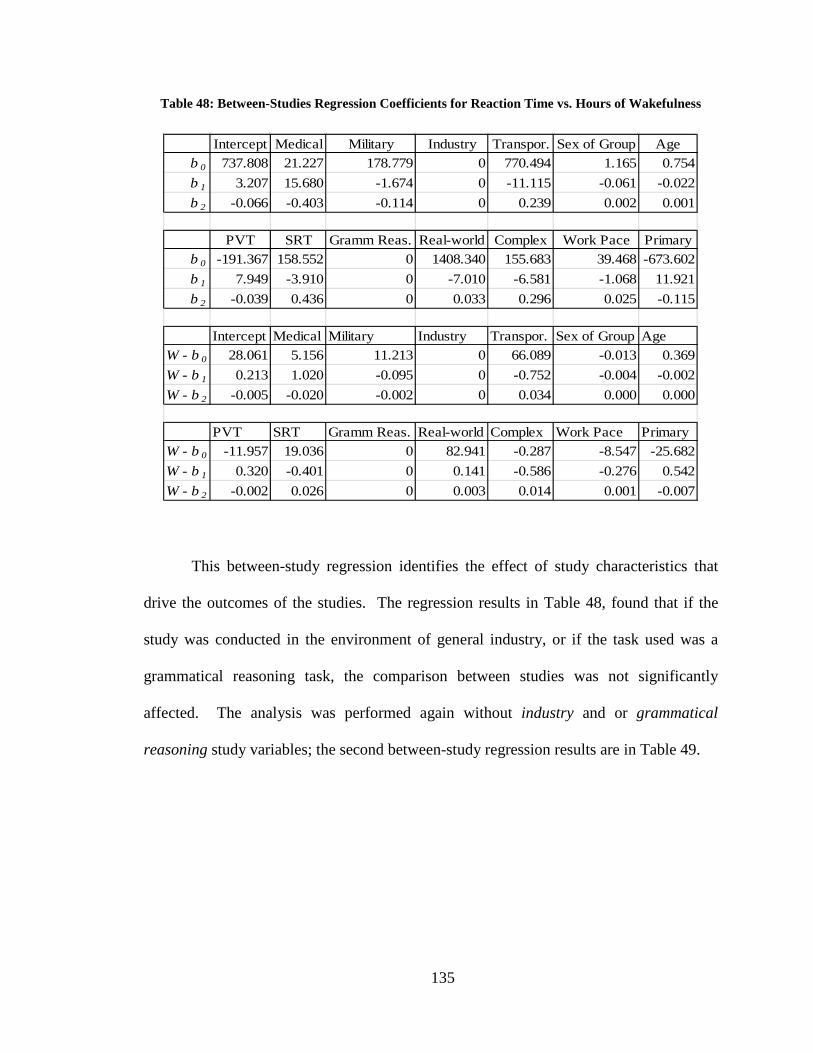
135
Table 48: Between-Studies Regression Coefficients for Reaction Time vs. Hours of Wakefulness
Intercept Medical Military Industry Transpor. Sex of Group Ageb 0 737.808 21.227 178.779 0 770.494 1.165 0.754b 1 3.207 15.680 -1.674 0 -11.115 -0.061 -0.022b 2 -0.066 -0.403 -0.114 0 0.239 0.002 0.001
PVT SRT Gramm Reas. Real-world Complex Work Pace Primaryb 0 -191.367 158.552 0 1408.340 155.683 39.468 -673.602b 1 7.949 -3.910 0 -7.010 -6.581 -1.068 11.921b 2 -0.039 0.436 0 0.033 0.296 0.025 -0.115
Intercept Medical Military Industry Transpor. Sex of Group AgeW - b 0 28.061 5.156 11.213 0 66.089 -0.013 0.369W - b 1 0.213 1.020 -0.095 0 -0.752 -0.004 -0.002W - b 2 -0.005 -0.020 -0.002 0 0.034 0.000 0.000
PVT SRT Gramm Reas. Real-world Complex Work Pace PrimaryW - b 0 -11.957 19.036 0 82.941 -0.287 -8.547 -25.682W - b 1 0.320 -0.401 0 0.141 -0.586 -0.276 0.542W - b 2 -0.002 0.026 0 0.003 0.014 0.001 -0.007
This between-study regression identifies the effect of study characteristics that
drive the outcomes of the studies. The regression results in Table 48, found that if the
study was conducted in the environment of general industry, or if the task used was a
grammatical reasoning task, the comparison between studies was not significantly
affected. The analysis was performed again without industry and or grammatical
reasoning study variables; the second between-study regression results are in Table 49.
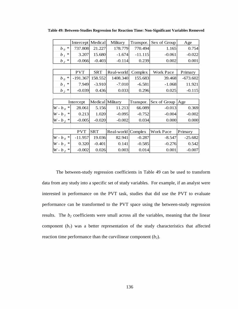
136
Table 49: Between-Studies Regression for Reaction Time: Non-Significant Variables Removed
Intercept Medical Military Transpor. Sex of Group Ageb 0 * 737.808 21.227 178.779 770.494 1.165 0.754b 1 * 3.207 15.680 -1.674 -11.115 -0.061 -0.022b 2 * -0.066 -0.403 -0.114 0.239 0.002 0.001
PVT SRT Real-world Complex Work Pace Primaryb 0 * -191.367 158.552 1408.340 155.683 39.468 -673.602b 1 * 7.949 -3.910 -7.010 -6.581 -1.068 11.921b 2 * -0.039 0.436 0.033 0.296 0.025 -0.115
Medical Military Transpor. Sex of Group AgeW - b 0 * 28.061 5.156 11.213 66.089 -0.013 0.369W - b 1 * 0.213 1.020 -0.095 -0.752 -0.004 -0.002W - b 2 * -0.005 -0.020 -0.002 0.034 0.000 0.000
SRT Real-world Complex Work Pace PrimaryW - b 0 * -11.957 19.036 82.941 -0.287 -8.547 -25.682W - b 1 * 0.320 -0.401 0.141 -0.585 -0.276 0.542W - b 2 * -0.002 0.026 0.003 0.014 0.001 -0.007
Intercept
PVT
The between-study regression coefficients in Table 49 can be used to transform
data from any study into a specific set of study variables. For example, if an analyst were
interested in performance on the PVT task, studies that did use the PVT to evaluate
performance can be transformed to the PVT space using the between-study regression
results. The b2 coefficients were small across all the variables, meaning that the linear
component (b1) was a better representation of the study characteristics that affected
reaction time performance than the curvilinear component (b2).
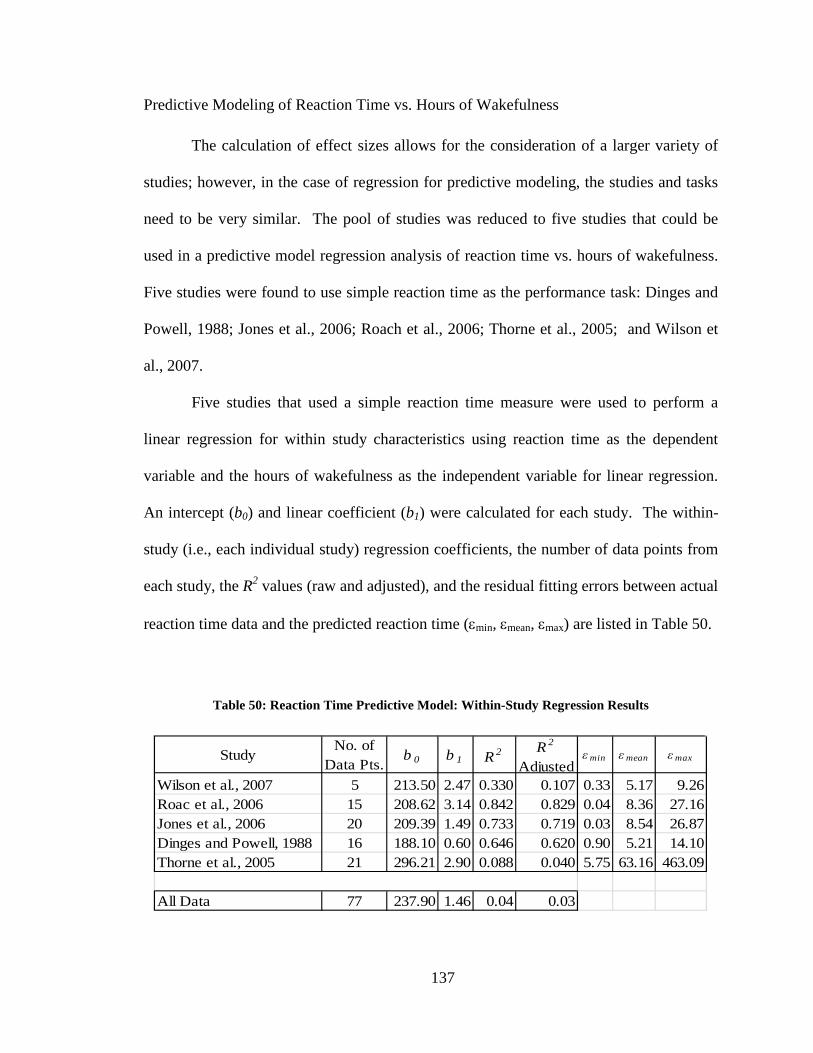
137
Predictive Modeling of Reaction Time vs. Hours of Wakefulness
The calculation of effect sizes allows for the consideration of a larger variety of
studies; however, in the case of regression for predictive modeling, the studies and tasks
need to be very similar. The pool of studies was reduced to five studies that could be
used in a predictive model regression analysis of reaction time vs. hours of wakefulness.
Five studies were found to use simple reaction time as the performance task: Dinges and
Powell, 1988; Jones et al., 2006; Roach et al., 2006; Thorne et al., 2005; and Wilson et
al., 2007.
Five studies that used a simple reaction time measure were used to perform a
linear regression for within study characteristics using reaction time as the dependent
variable and the hours of wakefulness as the independent variable for linear regression.
An intercept (b0) and linear coefficient (b1) were calculated for each study. The within-
study (i.e., each individual study) regression coefficients, the number of data points from
each study, the R2 values (raw and adjusted), and the residual fitting errors between actual
reaction time data and the predicted reaction time (εmin, εmean, εmax) are listed in Table 50.
Table 50: Reaction Time Predictive Model: Within-Study Regression Results
StudyNo. of
Data Pts.b 0 b 1 R 2 R 2
Adjustedεmin εmean εmax
Wilson et al., 2007 5 213.50 2.47 0.330 0.107 0.33 5.17 9.26Roac et al., 2006 15 208.62 3.14 0.842 0.829 0.04 8.36 27.16Jones et al., 2006 20 209.39 1.49 0.733 0.719 0.03 8.54 26.87Dinges and Powell, 1988 16 188.10 0.60 0.646 0.620 0.90 5.21 14.10Thorne et al., 2005 21 296.21 2.90 0.088 0.040 5.75 63.16 463.09
All Data 77 237.90 1.46 0.04 0.03
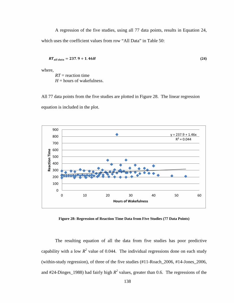
138
A regression of the five studies, using all 77 data points, results in Equation 24,
which uses the coefficient values from row “All Data” in Table 50:
𝑹𝑻𝒂𝒍𝒍 𝒅𝒂𝒕𝒂 = 𝟐𝟑𝟕.𝟗 + 𝟏.𝟒𝟔𝑯 (24)
where, RT = reaction time
H = hours of wakefulness. All 77 data points from the five studies are plotted in Figure 28. The linear regression
equation is included in the plot.
Figure 28: Regression of Reaction Time Data from Five Studies (77 Data Points)
The resulting equation of all the data from five studies has poor predictive
capability with a low R2 value of 0.044. The individual regressions done on each study
(within-study regression), of three of the five studies (#11-Roach_2006, #14-Jones_2006,
and #24-Dinges_1988) had fairly high R2 values, greater than 0.6. The regressions of the
y = 237.9 + 1.46x R² = 0.044
0
100
200
300
400
500
600
700
800
900
0 10 20 30 40 50 60
Reac
tion
Tim
e
Hours of Wakefulness
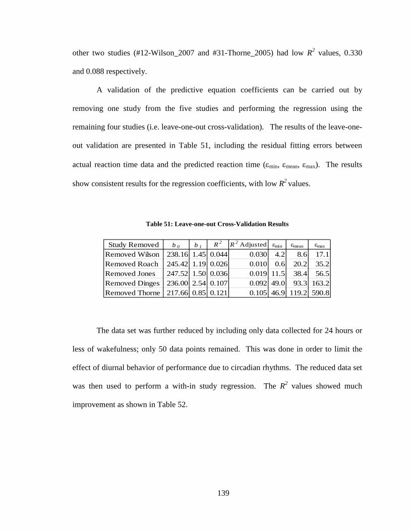
139
other two studies (#12-Wilson_2007 and #31-Thorne_2005) had low R2 values, 0.330
and 0.088 respectively.
A validation of the predictive equation coefficients can be carried out by
removing one study from the five studies and performing the regression using the
remaining four studies (i.e. leave-one-out cross-validation). The results of the leave-one-
out validation are presented in Table 51, including the residual fitting errors between
actual reaction time data and the predicted reaction time (εmin, εmean, εmax). The results
show consistent results for the regression coefficients, with low R2 values.
Table 51: Leave-one-out Cross-Validation Results
Study Removed b 0 b 1 R 2 R 2 Adjusted εmin εmean εmax
Removed Wilson 238.16 1.45 0.044 0.030 4.2 8.6 17.1Removed Roach 245.42 1.19 0.026 0.010 0.6 20.2 35.2Removed Jones 247.52 1.50 0.036 0.019 11.5 38.4 56.5Removed Dinges 236.00 2.54 0.107 0.092 49.0 93.3 163.2Removed Thorne 217.66 0.85 0.121 0.105 46.9 119.2 590.8
The data set was further reduced by including only data collected for 24 hours or
less of wakefulness; only 50 data points remained. This was done in order to limit the
effect of diurnal behavior of performance due to circadian rhythms. The reduced data set
was then used to perform a with-in study regression. The R2 values showed much
improvement as shown in Table 52.
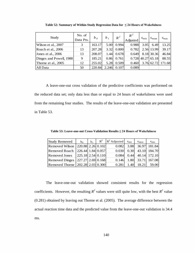
140
Table 52: Summary of Within-Study Regression Data for ≤ 24 Hours of Wakefulness
StudyNo. of
Data Pts.b 0 b 1 R 2 R 2
Adjustedεmin εmean εmax
Wilson et al., 2007 3 163.17 5.00 0.994 0.988 3.05 6.49 13.25Roach et al., 2006 13 207.28 3.32 0.800 0.782 2.56 13.99 39.17Jones et al., 2006 13 208.07 1.44 0.678 0.649 8.18 30.36 46.84Dinges and Powell, 1988 9 185.21 0.86 0.761 0.728 40.27 65.18 88.55Thorne et al., 2005 12 255.02 5.28 0.509 0.460 3.76 62.72 171.68All Data 50 220.84 2.246 0.107 0.089
A leave-one-out cross validation of the predictive coefficients was performed on
the reduced data set; only data less than or equal to 24 hours of wakefulness were used
from the remaining four studies. The results of the leave-one-out validation are presented
in Table 53.
Table 53: Leave-one-out Cross-Validation Results ≤ 24 Hours of Wakefulness
Study Removed b0 b1 R2 R2 Adjusted εmin εmean εmax
Removed Wilson 220.88 2.26 0.102 0.082 3.88 36.97 181.84Removed Roach 226.44 1.84 0.057 0.030 0.30 43.10 184.70Removed Jones 225.18 2.54 0.110 0.084 0.44 40.14 172.10Removed Dinges 227.27 2.69 0.168 0.146 1.80 33.71 167.08Removed Thorne 202.28 2.03 0.300 0.281 1.40 18.21 59.00
The leave-one-out validation showed consistent results for the regression
coefficients. However, the resulting R2 values were still quite low, with the best R2 value
(0.281) obtained by leaving out Thorne et al. (2005). The average difference between the
actual reaction time data and the predicted value from the leave-one-out validation is 34.4
ms.
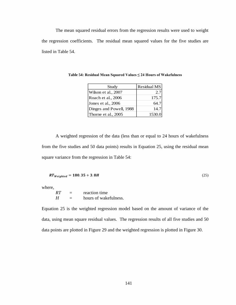
141
The mean squared residual errors from the regression results were used to weight
the regression coefficients. The residual mean squared values for the five studies are
listed in Table 54.
Table 54: Residual Mean Squared Values ≤ 24 Hours of Wakefulness
Study Residual MSWilson et al., 2007 2.7Roach et al., 2006 175.7Jones et al., 2006 64.7Dinges and Powell, 1988 14.7Thorne et al., 2005 1530.0
A weighted regression of the data (less than or equal to 24 hours of wakefulness
from the five studies and 50 data points) results in Equation 25, using the residual mean
square variance from the regression in Table 54:
𝑹𝑻𝑾𝒆𝒊𝒈𝒉𝒕𝒆𝒅 = 𝟏𝟖𝟎.𝟑𝟓 + 𝟑.𝟖𝑯 (25)
where, RT = reaction time
H = hours of wakefulness.
Equation 25 is the weighted regression model based on the amount of variance of the
data, using mean square residual values. The regression results of all five studies and 50
data points are plotted in Figure 29 and the weighted regression is plotted in Figure 30.
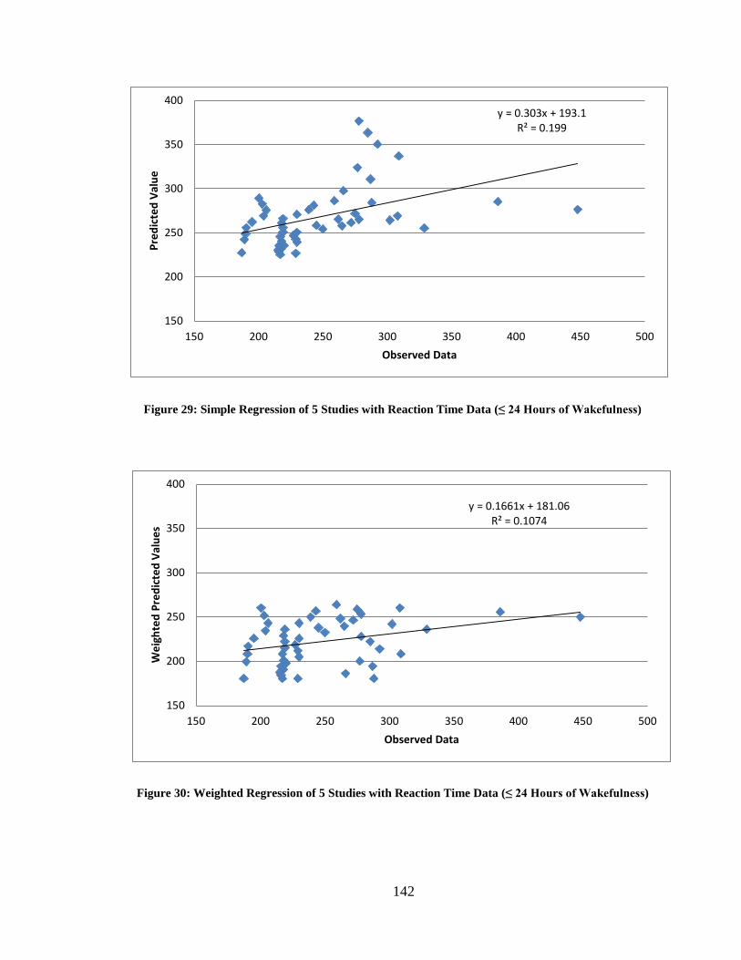
142
Figure 29: Simple Regression of 5 Studies with Reaction Time Data (≤ 24 Hours of Wakefulness)
Figure 30: Weighted Regression of 5 Studies with Reaction Time Data (≤ 24 Hours of Wakefulness)
y = 0.303x + 193.1 R² = 0.199
150
200
250
300
350
400
150 200 250 300 350 400 450 500
Pred
icte
d Va
lue
Observed Data
y = 0.1661x + 181.06 R² = 0.1074
150
200
250
300
350
400
150 200 250 300 350 400 450 500
Wei
ghte
d Pr
edic
ted
Valu
es
Observed Data
143
The low R2 values for both the non-weighted and weighted regression results of
0.199 (un-weighted) and 0.107 (weighted) imply that linear regression may not be the
best representation of the available data for predictive purposes. The individual study
regression (with-in study) had reasonably high R2 values; however, the predictability of
reaction time using all the data from Figures 29-30 has a low reliability (based on R2
values). Weighting does not seem to significantly improve the results. Overall, the
predictability of reaction time using the data from the five studies for hours of
wakefulness is not satisfactory.
Derivation of Probability Ratios for Reaction Time
The error under the control condition and test conditions were assumed to be C >
k and T > k respectively, where k (i.e., threshold value) was a selected constant and C and
T were reaction times for the control and test condition. The corresponding probabilities
of error were calculated using Equations 21 and 22. In simple reaction time psychomotor
tasks, a lapse is defined as failure to respond within 500 ms (Anderson et al., 2010); the k
values were selected using this knowledge; the threshold k values selected were: k = 250,
300, 400, 500, 750, and 1000. The probability ratios P(T > k) / P(C > k), signifying
deterioration in performance under the test condition, were plotted in Figure 31.
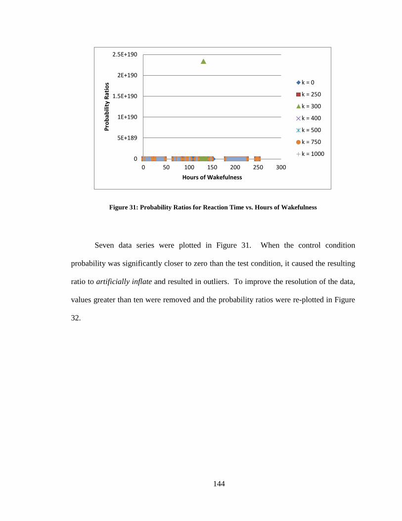
144
Figure 31: Probability Ratios for Reaction Time vs. Hours of Wakefulness
Seven data series were plotted in Figure 31. When the control condition
probability was significantly closer to zero than the test condition, it caused the resulting
ratio to artificially inflate and resulted in outliers. To improve the resolution of the data,
values greater than ten were removed and the probability ratios were re-plotted in Figure
32.
0
5E+189
1E+190
1.5E+190
2E+190
2.5E+190
0 50 100 150 200 250 300
Prob
abili
ty R
atio
s
Hours of Wakefulness
k = 0
k = 250
k = 300
k = 400
k = 500
k = 750
k = 1000
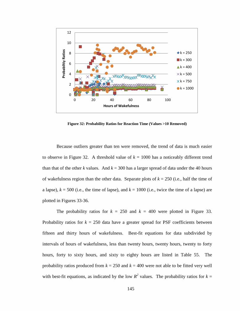
145
Figure 32: Probability Ratios for Reaction Time (Values >10 Removed)
Because outliers greater than ten were removed, the trend of data is much easier
to observe in Figure 32. A threshold value of k = 1000 has a noticeably different trend
than that of the other k values. And k = 300 has a larger spread of data under the 40 hours
of wakefulness region than the other data. Separate plots of k = 250 (i.e., half the time of
a lapse), k = 500 (i.e., the time of lapse), and k = 1000 (i.e., twice the time of a lapse) are
plotted in Figures 33-36.
The probability ratios for k = 250 and k = 400 were plotted in Figure 33.
Probability ratios for k = 250 data have a greater spread for PSF coefficients between
fifteen and thirty hours of wakefulness. Best-fit equations for data subdivided by
intervals of hours of wakefulness, less than twenty hours, twenty hours, twenty to forty
hours, forty to sixty hours, and sixty to eighty hours are listed in Table 55. The
probability ratios produced from k = 250 and k = 400 were not able to be fitted very well
with best-fit equations, as indicated by the low R2 values. The probability ratios for k =
0
2
4
6
8
10
12
0 20 40 60 80 100
Prob
abilt
iy R
atio
s
Hours of Wakefulness
k = 250
k = 300
k = 400
k = 500
k = 750
k = 1000
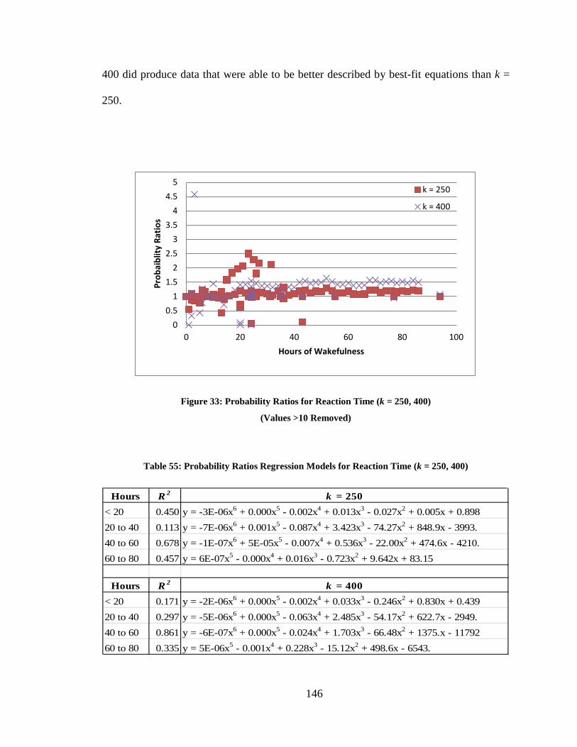
146
400 did produce data that were able to be better described by best-fit equations than k =
250.
Figure 33: Probability Ratios for Reaction Time (k = 250, 400)
(Values >10 Removed)
Table 55: Probability Ratios Regression Models for Reaction Time (k = 250, 400)
Hours R 2 k = 250< 20 0.450 y = -3E-06x6 + 0.000x5 - 0.002x4 + 0.013x3 - 0.027x2 + 0.005x + 0.89820 to 40 0.113 y = -7E-06x6 + 0.001x5 - 0.087x4 + 3.423x3 - 74.27x2 + 848.9x - 3993.40 to 60 0.678 y = -1E-07x6 + 5E-05x5 - 0.007x4 + 0.536x3 - 22.00x2 + 474.6x - 4210.60 to 80 0.457 y = 6E-07x5 - 0.000x4 + 0.016x3 - 0.723x2 + 9.642x + 83.15
Hours R 2 k = 400< 20 0.171 y = -2E-06x6 + 0.000x5 - 0.002x4 + 0.033x3 - 0.246x2 + 0.830x + 0.43920 to 40 0.297 y = -5E-06x6 + 0.000x5 - 0.063x4 + 2.485x3 - 54.17x2 + 622.7x - 2949.40 to 60 0.861 y = -6E-07x6 + 0.000x5 - 0.024x4 + 1.703x3 - 66.48x2 + 1375.x - 1179260 to 80 0.335 y = 5E-06x5 - 0.001x4 + 0.228x3 - 15.12x2 + 498.6x - 6543.
00.5
11.5
22.5
33.5
44.5
5
0 20 40 60 80 100
Prob
aibl
ity R
atio
s
Hours of Wakefulness
k = 250
k = 400
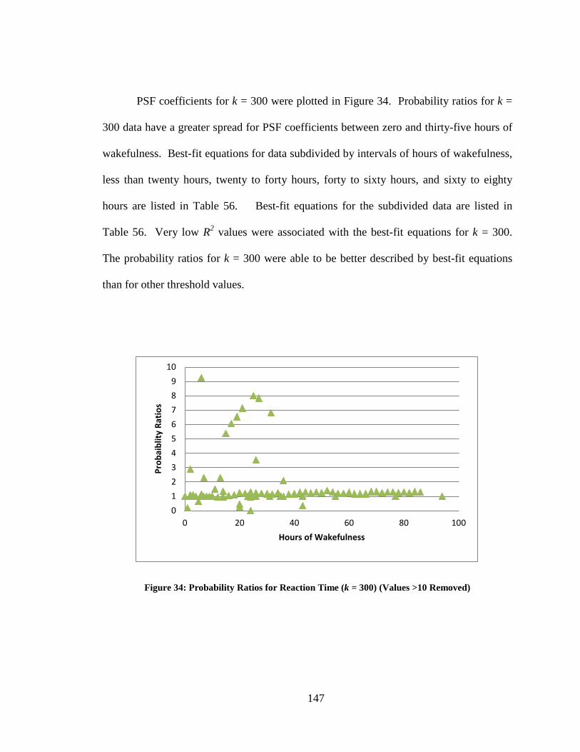
147
PSF coefficients for k = 300 were plotted in Figure 34. Probability ratios for k =
300 data have a greater spread for PSF coefficients between zero and thirty-five hours of
wakefulness. Best-fit equations for data subdivided by intervals of hours of wakefulness,
less than twenty hours, twenty to forty hours, forty to sixty hours, and sixty to eighty
hours are listed in Table 56. Best-fit equations for the subdivided data are listed in
Table 56. Very low R2 values were associated with the best-fit equations for k = 300.
The probability ratios for k = 300 were able to be better described by best-fit equations
than for other threshold values.
Figure 34: Probability Ratios for Reaction Time (k = 300) (Values >10 Removed)
0123456789
10
0 20 40 60 80 100
Prob
aibl
ity R
atio
s
Hours of Wakefulness
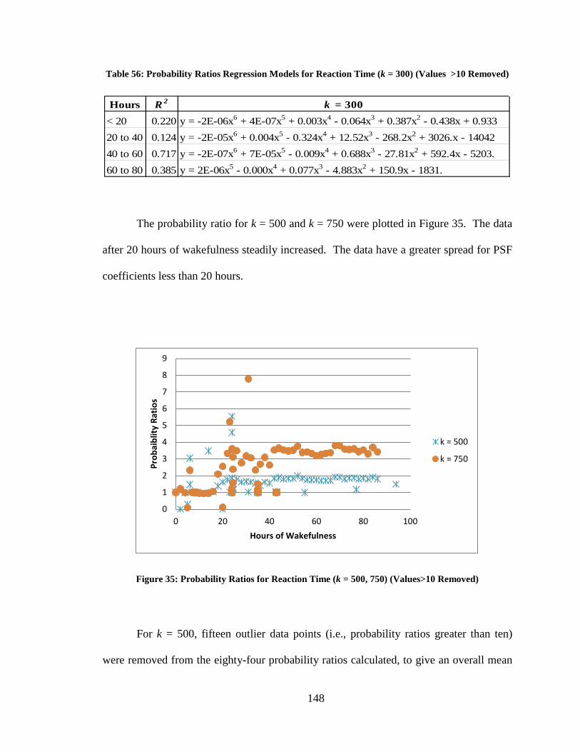
148
Table 56: Probability Ratios Regression Models for Reaction Time (k = 300) (Values >10 Removed)
Hours R 2 k = 300< 20 0.220 y = -2E-06x6 + 4E-07x5 + 0.003x4 - 0.064x3 + 0.387x2 - 0.438x + 0.93320 to 40 0.124 y = -2E-05x6 + 0.004x5 - 0.324x4 + 12.52x3 - 268.2x2 + 3026.x - 1404240 to 60 0.717 y = -2E-07x6 + 7E-05x5 - 0.009x4 + 0.688x3 - 27.81x2 + 592.4x - 5203.60 to 80 0.385 y = 2E-06x5 - 0.000x4 + 0.077x3 - 4.883x2 + 150.9x - 1831.
The probability ratio for k = 500 and k = 750 were plotted in Figure 35. The data
after 20 hours of wakefulness steadily increased. The data have a greater spread for PSF
coefficients less than 20 hours.
Figure 35: Probability Ratios for Reaction Time (k = 500, 750) (Values>10 Removed)
For k = 500, fifteen outlier data points (i.e., probability ratios greater than ten)
were removed from the eighty-four probability ratios calculated, to give an overall mean
0
1
2
3
4
5
6
7
8
9
0 20 40 60 80 100
Prob
aibl
ity R
atio
s
Hours of Wakefulness
k = 500
k = 750
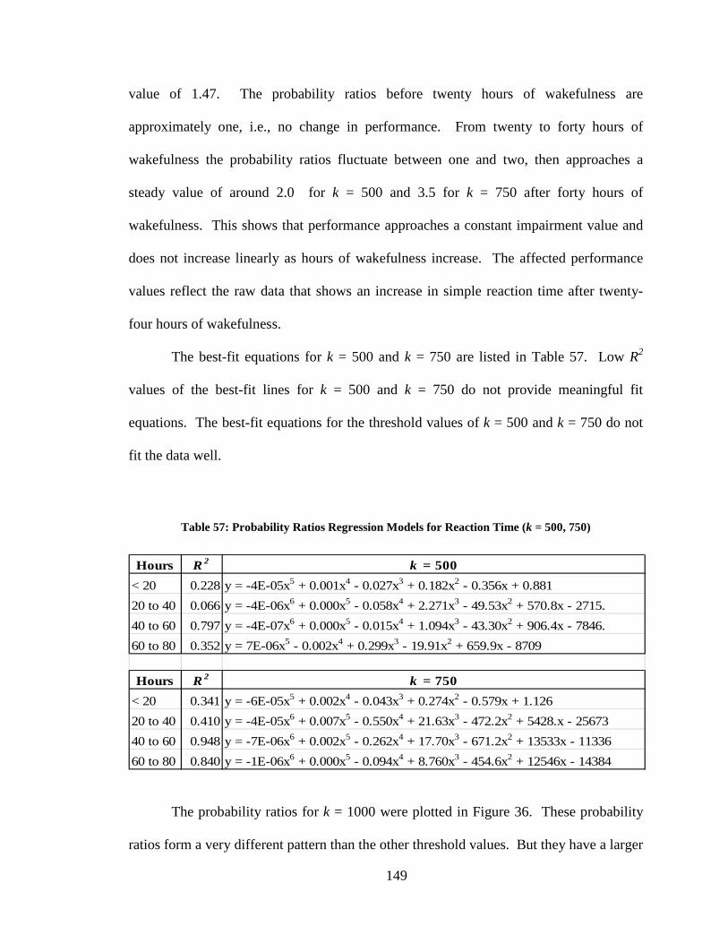
149
value of 1.47. The probability ratios before twenty hours of wakefulness are
approximately one, i.e., no change in performance. From twenty to forty hours of
wakefulness the probability ratios fluctuate between one and two, then approaches a
steady value of around 2.0 for k = 500 and 3.5 for k = 750 after forty hours of
wakefulness. This shows that performance approaches a constant impairment value and
does not increase linearly as hours of wakefulness increase. The affected performance
values reflect the raw data that shows an increase in simple reaction time after twenty-
four hours of wakefulness.
The best-fit equations for k = 500 and k = 750 are listed in Table 57. Low R2
values of the best-fit lines for k = 500 and k = 750 do not provide meaningful fit
equations. The best-fit equations for the threshold values of k = 500 and k = 750 do not
fit the data well.
Table 57: Probability Ratios Regression Models for Reaction Time (k = 500, 750)
Hours R 2 k = 500< 20 0.228 y = -4E-05x5 + 0.001x4 - 0.027x3 + 0.182x2 - 0.356x + 0.88120 to 40 0.066 y = -4E-06x6 + 0.000x5 - 0.058x4 + 2.271x3 - 49.53x2 + 570.8x - 2715.40 to 60 0.797 y = -4E-07x6 + 0.000x5 - 0.015x4 + 1.094x3 - 43.30x2 + 906.4x - 7846.60 to 80 0.352 y = 7E-06x5 - 0.002x4 + 0.299x3 - 19.91x2 + 659.9x - 8709
Hours R 2 k = 750< 20 0.341 y = -6E-05x5 + 0.002x4 - 0.043x3 + 0.274x2 - 0.579x + 1.12620 to 40 0.410 y = -4E-05x6 + 0.007x5 - 0.550x4 + 21.63x3 - 472.2x2 + 5428.x - 2567340 to 60 0.948 y = -7E-06x6 + 0.002x5 - 0.262x4 + 17.70x3 - 671.2x2 + 13533x - 1133660 to 80 0.840 y = -1E-06x6 + 0.000x5 - 0.094x4 + 8.760x3 - 454.6x2 + 12546x - 14384
The probability ratios for k = 1000 were plotted in Figure 36. These probability
ratios form a very different pattern than the other threshold values. But they have a larger
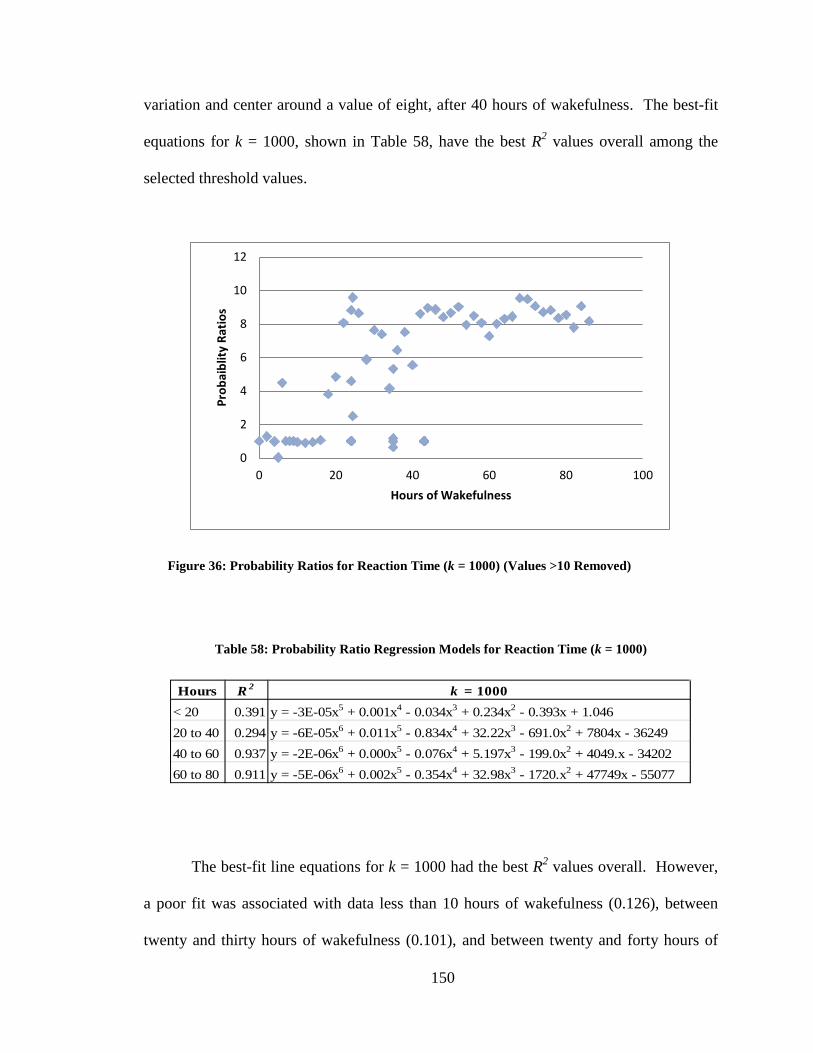
150
variation and center around a value of eight, after 40 hours of wakefulness. The best-fit
equations for k = 1000, shown in Table 58, have the best R2 values overall among the
selected threshold values.
Figure 36: Probability Ratios for Reaction Time (k = 1000) (Values >10 Removed)
Table 58: Probability Ratio Regression Models for Reaction Time (k = 1000)
Hours R 2 k = 1000< 20 0.391 y = -3E-05x5 + 0.001x4 - 0.034x3 + 0.234x2 - 0.393x + 1.04620 to 40 0.294 y = -6E-05x6 + 0.011x5 - 0.834x4 + 32.22x3 - 691.0x2 + 7804x - 3624940 to 60 0.937 y = -2E-06x6 + 0.000x5 - 0.076x4 + 5.197x3 - 199.0x2 + 4049.x - 3420260 to 80 0.911 y = -5E-06x6 + 0.002x5 - 0.354x4 + 32.98x3 - 1720.x2 + 47749x - 55077
The best-fit line equations for k = 1000 had the best R2 values overall. However,
a poor fit was associated with data less than 10 hours of wakefulness (0.126), between
twenty and thirty hours of wakefulness (0.101), and between twenty and forty hours of
0
2
4
6
8
10
12
0 20 40 60 80 100
Prob
aibl
ity R
atio
s
Hours of Wakefulness
151
wakefulness (0.294). The best-fit for less than 10 hours of wakefulness was found for k =
400 with an R2 = 0.301; the best-fit for between twenty and thirty hours of wakefulness
was found for k = 750 with an R2 = 0.471, and the best-fit for between twenty and forty
hours of wakefulness was found for k = 750 with an R2 = 0.410.
The threshold value of k = 1000 has a noticeably different trend than that of the
other k values. PSF coefficients calculated for k = 1000 have a larger variation and center
about a value of eight, after forty hours of wakefulness. The control/test condition
reaction time being greater than 1000 ms (twice the length of a lapse at 500 ms) should
occur less frequently than for example, k = 250. The higher PSF coefficient values
increase the nominal human error probability (HEP) to a greater degree than the other
selected threshold values (i.e., k = 250, 500, 750). Probability ratios for k = 250 data
have a greater spread for PSF coefficients between fifteen and thirty hours of
wakefulness.
Uncertainty Analysis of Probability Ratios for Reaction Time
The descriptive statistics data for all the data provided in the studies are listed in
Table 59, (e.g., hours of wakefulness, N-control, N-test, µ-Control, µ-Test, σ-Control,
and σ-Test). The average number of subjects per study was approximately 17.
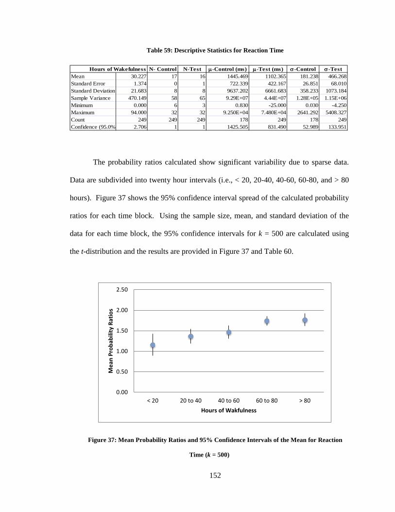
152
Table 59: Descriptive Statistics for Reaction Time
Hours of Wakefulness N- Control N-Test µ-Control (ms) µ-Test (ms) σ-Control σ-TestMean 30.227 17 16 1445.469 1102.365 181.238 466.268Standard Error 1.374 0 1 722.339 422.167 26.851 68.010Standard Deviation 21.683 8 8 9637.202 6661.683 358.233 1073.184Sample Variance 470.149 58 65 9.29E+07 4.44E+07 1.28E+05 1.15E+06Minimum 0.000 6 3 0.830 -25.000 0.030 -4.250Maximum 94.000 32 32 9.250E+04 7.480E+04 2641.292 5408.327Count 249 249 249 178 249 178 249Confidence (95.0% 2.706 1 1 1425.505 831.490 52.989 133.951
The probability ratios calculated show significant variability due to sparse data.
Data are subdivided into twenty hour intervals (i.e., < 20, 20-40, 40-60, 60-80, and > 80
hours). Figure 37 shows the 95% confidence interval spread of the calculated probability
ratios for each time block. Using the sample size, mean, and standard deviation of the
data for each time block, the 95% confidence intervals for k = 500 are calculated using
the t-distribution and the results are provided in Figure 37 and Table 60.
Figure 37: Mean Probability Ratios and 95% Confidence Intervals of the Mean for Reaction
Time (k = 500)
0.00
0.50
1.00
1.50
2.00
2.50
< 20 20 to 40 40 to 60 60 to 80 > 80
Mea
n Pr
obab
ility
Rat
ios
Hours of Wakfulness
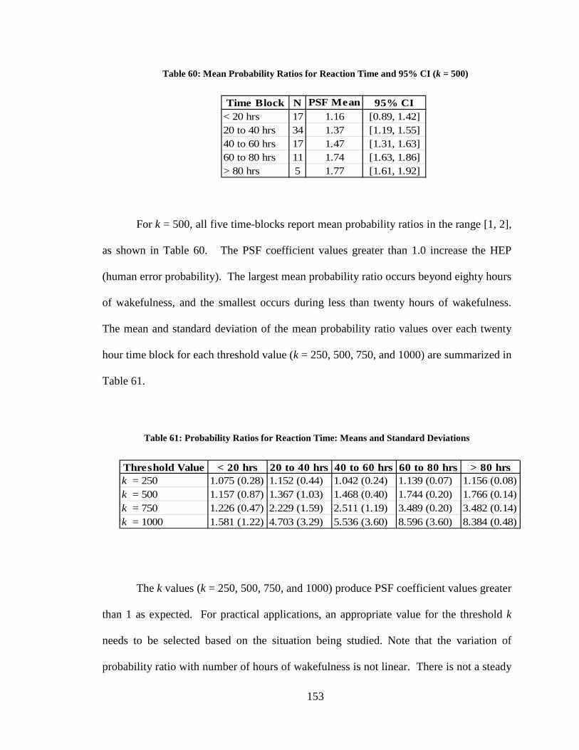
153
Table 60: Mean Probability Ratios for Reaction Time and 95% CI (k = 500)
Time Block N PSF Mean 95% CI< 20 hrs 17 1.16 [0.89, 1.42]20 to 40 hrs 34 1.37 [1.19, 1.55]40 to 60 hrs 17 1.47 [1.31, 1.63]60 to 80 hrs 11 1.74 [1.63, 1.86]> 80 hrs 5 1.77 [1.61, 1.92]
For k = 500, all five time-blocks report mean probability ratios in the range [1, 2],
as shown in Table 60. The PSF coefficient values greater than 1.0 increase the HEP
(human error probability). The largest mean probability ratio occurs beyond eighty hours
of wakefulness, and the smallest occurs during less than twenty hours of wakefulness.
The mean and standard deviation of the mean probability ratio values over each twenty
hour time block for each threshold value (k = 250, 500, 750, and 1000) are summarized in
Table 61.
Table 61: Probability Ratios for Reaction Time: Means and Standard Deviations
Threshold Value < 20 hrs 20 to 40 hrs 40 to 60 hrs 60 to 80 hrs > 80 hrsk = 250 1.075 (0.28) 1.152 (0.44) 1.042 (0.24) 1.139 (0.07) 1.156 (0.08)k = 500 1.157 (0.87) 1.367 (1.03) 1.468 (0.40) 1.744 (0.20) 1.766 (0.14)k = 750 1.226 (0.47) 2.229 (1.59) 2.511 (1.19) 3.489 (0.20) 3.482 (0.14)k = 1000 1.581 (1.22) 4.703 (3.29) 5.536 (3.60) 8.596 (3.60) 8.384 (0.48)
The k values (k = 250, 500, 750, and 1000) produce PSF coefficient values greater
than 1 as expected. For practical applications, an appropriate value for the threshold k
needs to be selected based on the situation being studied. Note that the variation of
probability ratio with number of hours of wakefulness is not linear. There is not a steady
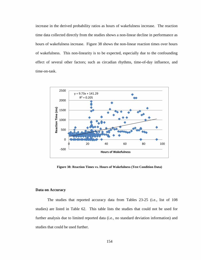
154
increase in the derived probability ratios as hours of wakefulness increase. The reaction
time data collected directly from the studies shows a non-linear decline in performance as
hours of wakefulness increase. Figure 38 shows the non-linear reaction times over hours
of wakefulness. This non-linearity is to be expected, especially due to the confounding
effect of several other factors; such as circadian rhythms, time-of-day influence, and
time-on-task.
Figure 38: Reaction Times vs. Hours of Wakefulness (Test Condition Data)
Data on Accuracy
The studies that reported accuracy data from Tables 23-25 (i.e., list of 108
studies) are listed in Table 62. This table lists the studies that could not be used for
further analysis due to limited reported data (i.e., no standard deviation information) and
studies that could be used further.
y = 9.73x + 141.29 R² = 0.205
-500
0
500
1000
1500
2000
2500
0 20 40 60 80 100
Reac
tion
Tim
e (m
s)
Hours of Wakefulness
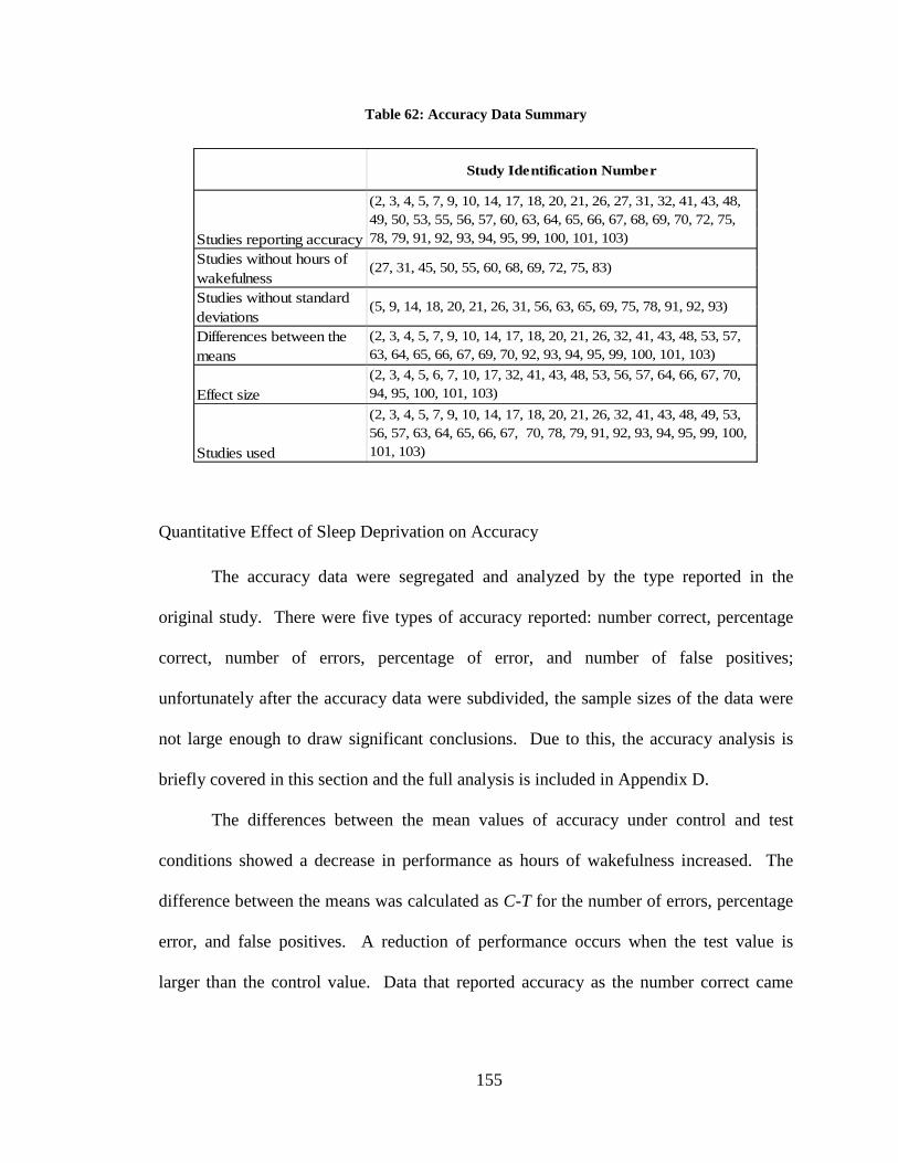
155
Table 62: Accuracy Data Summary
Study Identification Number
Studies used
(2, 3, 4, 5, 7, 9, 10, 14, 17, 18, 20, 21, 26, 32, 41, 43, 48, 49, 53, 56, 57, 63, 64, 65, 66, 67, 70, 78, 79, 91, 92, 93, 94, 95, 99, 100, 101, 103)
(2, 3, 4, 5, 7, 9, 10, 14, 17, 18, 20, 21, 26, 32, 41, 43, 48, 53, 57, 63, 64, 65, 66, 67, 69, 70, 92, 93, 94, 95, 99, 100, 101, 103)
Effect size(2, 3, 4, 5, 6, 7, 10, 17, 32, 41, 43, 48, 53, 56, 57, 64, 66, 67, 70, 94, 95, 100, 101, 103)
Differences between the means
(27, 31, 45, 50, 55, 60, 68, 69, 72, 75, 83)
(5, 9, 14, 18, 20, 21, 26, 31, 56, 63, 65, 69, 75, 78, 91, 92, 93)
Studies reporting accuracy
(2, 3, 4, 5, 7, 9, 10, 14, 17, 18, 20, 21, 26, 27, 31, 32, 41, 43, 48, 49, 50, 53, 55, 56, 57, 60, 63, 64, 65, 66, 67, 68, 69, 70, 72, 75, 78, 79, 91, 92, 93, 94, 95, 99, 100, 101, 103)
Studies without standard deviations
Studies without hours of wakefulness
Quantitative Effect of Sleep Deprivation on Accuracy
The accuracy data were segregated and analyzed by the type reported in the
original study. There were five types of accuracy reported: number correct, percentage
correct, number of errors, percentage of error, and number of false positives;
unfortunately after the accuracy data were subdivided, the sample sizes of the data were
not large enough to draw significant conclusions. Due to this, the accuracy analysis is
briefly covered in this section and the full analysis is included in Appendix D.
The differences between the mean values of accuracy under control and test
conditions showed a decrease in performance as hours of wakefulness increased. The
difference between the means was calculated as C-T for the number of errors, percentage
error, and false positives. A reduction of performance occurs when the test value is
larger than the control value. Data that reported accuracy as the number correct came
156
from fourteen different studies. For the number correct data, threshold values of k = 0,
23, 50, and 75 were used to derive PSF coefficient values.
Accuracy as reported as percent correct was found for fourteen studies. The
difference between the mean values centered about zero; i.e., there was a difference
between the control and test conditions. Threshold values of k = 0, 0.25, 0.5, and 1 were
used to derive the probability ratios for percentage correct.
Eight studies were found to report accuracy as number of errors, which increased
as hours of wakefulness increased. The differences between the mean values were
calculated as C-T. Threshold values of k = 0, 30, and 50 were used to derive PSF
coefficients.
Accuracy reported as percentage of errors was calculated from seven studies. The
difference between mean values centered on zero; i.e., there was no change from the
control to the test condition. Threshold values of k = 0, 0.25, 0.5, and 1 were used to
derive probability ratios for percentage of errors data.
The four studies that reported false positive data were analyzed. The number of
false positives, i.e., reacting when there was no signal, increased as hours of wakefulness
increased. Threshold values of k = 0, 1, 2, and 3 were selected.
In summary, accuracy is not affected as greatly as reaction time and number of
lapses under sleep-deprived conditions. The draw on cognitive capacity that results from
sleep deprivation may help increase arousal levels (Yerkes and Dodson, 1908) and help
to maintain, or even improve, performance on the simple tasks that were the primary
tasks employed in the studies under investigation.
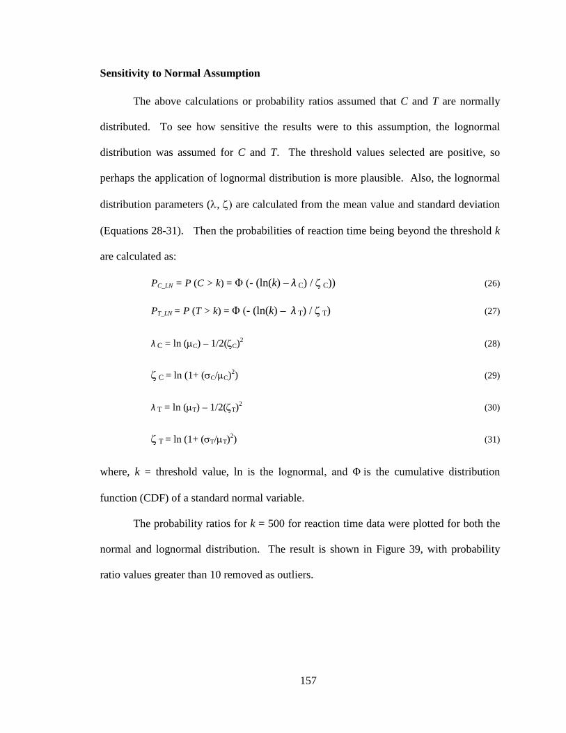
157
Sensitivity to Normal Assumption
The above calculations or probability ratios assumed that C and T are normally
distributed. To see how sensitive the results were to this assumption, the lognormal
distribution was assumed for C and T. The threshold values selected are positive, so
perhaps the application of lognormal distribution is more plausible. Also, the lognormal
distribution parameters (λ, ζ) are calculated from the mean value and standard deviation
(Equations 28-31). Then the probabilities of reaction time being beyond the threshold k
are calculated as:
PC_LN = P (C > k) = Φ (- (ln(k) – λ C) / ζ C)) (26)
PT_LN = P (T > k) = Φ (- (ln(k) – λ T) / ζ T) (27)
λ C = ln (µC) – 1/2(ζC)2 (28)
ζ C = ln (1+ (σC/µC)2) (29)
λ T = ln (µT) – 1/2(ζT)2 (30)
ζ T = ln (1+ (σT/µT)2) (31)
where, k = threshold value, ln is the lognormal, and Φ is the cumulative distribution
function (CDF) of a standard normal variable.
The probability ratios for k = 500 for reaction time data were plotted for both the
normal and lognormal distribution. The result is shown in Figure 39, with probability
ratio values greater than 10 removed as outliers.
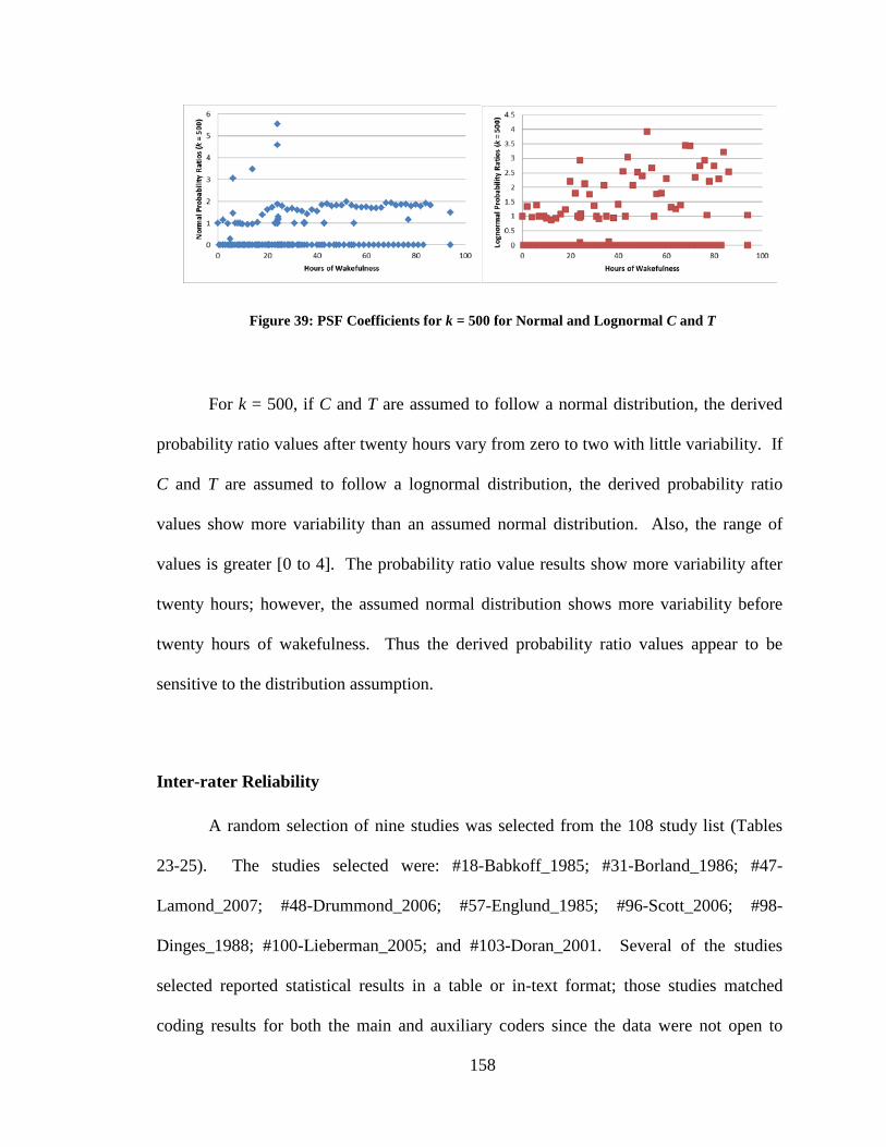
158
Figure 39: PSF Coefficients for k = 500 for Normal and Lognormal C and T
For k = 500, if C and T are assumed to follow a normal distribution, the derived
probability ratio values after twenty hours vary from zero to two with little variability. If
C and T are assumed to follow a lognormal distribution, the derived probability ratio
values show more variability than an assumed normal distribution. Also, the range of
values is greater [0 to 4]. The probability ratio value results show more variability after
twenty hours; however, the assumed normal distribution shows more variability before
twenty hours of wakefulness. Thus the derived probability ratio values appear to be
sensitive to the distribution assumption.
Inter-rater Reliability
A random selection of nine studies was selected from the 108 study list (Tables
23-25). The studies selected were: #18-Babkoff_1985; #31-Borland_1986; #47-
Lamond_2007; #48-Drummond_2006; #57-Englund_1985; #96-Scott_2006; #98-
Dinges_1988; #100-Lieberman_2005; and #103-Doran_2001. Several of the studies
selected reported statistical results in a table or in-text format; those studies matched
coding results for both the main and auxiliary coders since the data were not open to
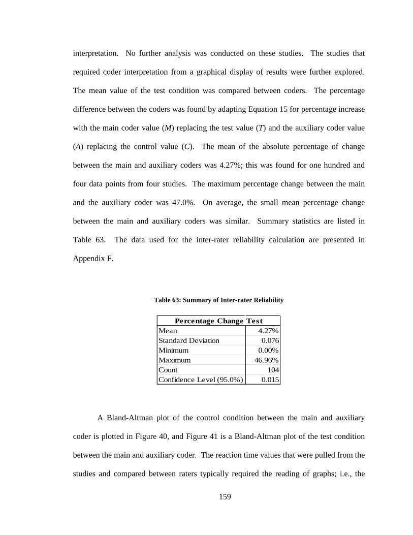
159
interpretation. No further analysis was conducted on these studies. The studies that
required coder interpretation from a graphical display of results were further explored.
The mean value of the test condition was compared between coders. The percentage
difference between the coders was found by adapting Equation 15 for percentage increase
with the main coder value (M) replacing the test value (T) and the auxiliary coder value
(A) replacing the control value (C). The mean of the absolute percentage of change
between the main and auxiliary coders was 4.27%; this was found for one hundred and
four data points from four studies. The maximum percentage change between the main
and the auxiliary coder was 47.0%. On average, the small mean percentage change
between the main and auxiliary coders was similar. Summary statistics are listed in
Table 63. The data used for the inter-rater reliability calculation are presented in
Appendix F.
Table 63: Summary of Inter-rater Reliability
Mean 4.27%Standard Deviation 0.076Minimum 0.00%Maximum 46.96%Count 104Confidence Level (95.0%) 0.015
Percentage Change Test
A Bland-Altman plot of the control condition between the main and auxiliary
coder is plotted in Figure 40, and Figure 41 is a Bland-Altman plot of the test condition
between the main and auxiliary coder. The reaction time values that were pulled from the
studies and compared between raters typically required the reading of graphs; i.e., the
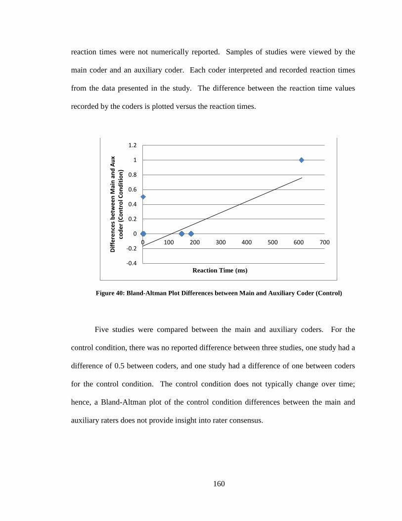
160
reaction times were not numerically reported. Samples of studies were viewed by the
main coder and an auxiliary coder. Each coder interpreted and recorded reaction times
from the data presented in the study. The difference between the reaction time values
recorded by the coders is plotted versus the reaction times.
Figure 40: Bland-Altman Plot Differences between Main and Auxiliary Coder (Control)
Five studies were compared between the main and auxiliary coders. For the
control condition, there was no reported difference between three studies, one study had a
difference of 0.5 between coders, and one study had a difference of one between coders
for the control condition. The control condition does not typically change over time;
hence, a Bland-Altman plot of the control condition differences between the main and
auxiliary raters does not provide insight into rater consensus.
-0.4
-0.2
0
0.2
0.4
0.6
0.8
1
1.2
0 100 200 300 400 500 600 700
Diffe
renc
es b
etw
een
Mai
n an
d Au
x co
der (
Cont
rol C
ondi
tion)
Reaction Time (ms)
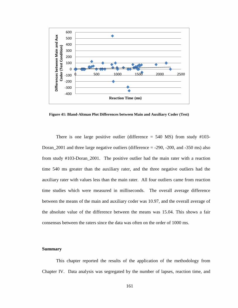
161
Figure 41: Bland-Altman Plot Differences between Main and Auxiliary Coder (Test)
There is one large positive outlier (difference = 540 MS) from study #103-
Doran_2001 and three large negative outliers (difference = -290, -200, and -350 ms) also
from study #103-Doran_2001. The positive outlier had the main rater with a reaction
time 540 ms greater than the auxiliary rater, and the three negative outliers had the
auxiliary rater with values less than the main rater. All four outliers came from reaction
time studies which were measured in milliseconds. The overall average difference
between the means of the main and auxiliary coder was 10.97, and the overall average of
the absolute value of the difference between the means was 15.04. This shows a fair
consensus between the raters since the data was often on the order of 1000 ms.
Summary
This chapter reported the results of the application of the methodology from
Chapter IV. Data analysis was segregated by the number of lapses, reaction time, and
-400
-300
-200
-100
0
100
200
300
400
500
600
0 500 1000 1500 2000 2500
Diffe
renc
es b
etw
een
Mai
n an
d Au
x Co
der (
Test
Con
ditio
n)
Reaction Time (ms)
162
accuracy. The data used in the analysis are provided in Appendix E. Analysis of the data
included finding the difference between the mean values, percentage change between test
and control conditions, and effect sizes. The data collected were used to derive
probability ratios based on empirical data. Equations for the probability ratios were
calculated for ten to twenty hour intervals of hours of wakefulness. Number of lapses
and reaction times were identified to be negatively affected by sleep deprivation.
Accuracy was not found to be consistently worse as hours of wakefulness increased.
The probability ratios could be used to inform the selection of PSF coefficients in
HRA models. Note however, that these ratios are different for different performance
measures (reaction time, accuracy, or number of lapses), and for different hours of
wakefulness. The selection of PSF coefficients in HRA may be guided by these
probability ratios in different ways, e.g., average over all three performance measures and
hours (not recommended), or use probability ratios from that performance measure that is
most relevant to the HRA situation of interest, varying with hours of sleep deprivation.
163
CHAPTER VI
SUMMARY AND CONCLUSIONS
Summary of Accomplishments
The main goal of this research was to develop a methodology to use empirical
data to inform PSF coefficient selection in order to improve current HRA methods. A
variety of studies in the available literature on sleep deprivation effects on performance
was synthesized for this purpose. This overarching research goal was achieved by
defining five subsidiary objectives and approaching these in a systematic fashion.
The first objective was to review current HRA methods, THERP (Swain and
Guttman, 1983), SPAR-H (Gertman et al., 2005), and ATHEANA (USNRC, 2000), to
determine how sleep deprivation effects on performance were included. Sleep
deprivation is not specifically addressed by any of the reviewed methods; therefore, a
method to address the effect of sleep deprivation is needed. THERP provides error
probabilities for specific situations, such as mis-turning a valve. ATHEANA does not
provide error probabilities for performance shaping factor coefficients, but does provide a
higher level of guidance in performing an HRA. SPAR-H has a given set of performance
shaping factors and PSF coefficients which do not include sleep deprivation. Sleep
deprivation is assumed to be included in the fitness-for-duty PSF of the SPAR-H method.
Since fatigue, in particular sleep deprivation, is found to be a contributing factor in so
164
many incidents, the importance of including sleep deprivation as a PSF needs to be
considered (Griffith and Mahadevan, 2011).
Next, data collection for the sleep deprivation effect on performance through a
meta-analysis synthesis method was performed. Literature from various sources was
reviewed; the majority came from laboratory test studies. Studies which provided data on
the performance metrics reaction time, accuracy, and number of lapses were mined for
data. The resulting 108 studies were more critically evaluated for statistical data and
were coded. The data were collected in a research synthesis procedure emulating the
meta-analysis technique with predefined coding information.
Qualitative information such as study design, information on the subjects,
experimental conditions, and task characteristics was collected. Quantitative information
was also coded from the studies; this information included pretest (control) and posttest
(test) mean values and standard deviation or standard error when available.
The data collected from the reviewed studies were evaluated to find the
quantitative effect of sleep deprivation on performance (e.g., reaction time, accuracy, and
number of lapses). The quantitative effect of sleep deprivation on performance was
determined by calculating the difference between mean values, effect size, percentage
change, and failure probabilities.
The fourth objective was to develop a method to derive PSF coefficients based on
the collected data from objective three. Error was defined to occur when the control or
test condition performance exceeded a threshold value (k). Assuming the defined error
measure had a normal distribution, the probability of error occurring was then calculated
(Equations 21 and 22).
165
Error probabilities were used to contrast the change in the performance under the
control condition vs. the test condition. The ratio of the error probabilities based on the
empirical data was used to derive PSF coefficients based on probability ratios. By
developing this method for selecting PSF coefficients using technical data, reliability and
reproducibility of HRA methods can be increased. The fifth objective in the research was
to analyze the uncertainty in the derived performance shaping factor coefficient values
and the inter-rater reliability for a sample of randomly selected studies.
Research Assumptions:
The effects of shift work, chronic sleep deprivation, napping (i.e., recovery),
circadian rhythms, time-of-day influence, and time-on-task were not considered in this
research, and the effect of acute sleep deprivation was assumed to be independent of
these factors. The influence of circadian rhythms was not taken into account (e.g., what
time of day that forty hour of wakefulness occurred) due to the infrequent recording of
the time of day when the data collection occurred, nor were the influences of shift work,
i.e., work hours that occurred outside of the standard 9 a.m.-5 p.m. daytime schedule, or
other schedules that included working outside of daytime hours. The tasks used to
evaluate performance were assumed to be equivalent between various studies (e.g., the
PVT was considered equivalent to simple reaction time (SRT) task). Also, the influence
of study differences was not considered in the final quantitative analysis of the data, but
was noted in the coding of the studies. Sleep deprivation was assumed independent of
other performance factors, i.e., the interaction of other performance shaping factors with
166
sleep deprivation was not considered, and the speed versus accuracy tradeoff was not
factored into the analysis.
The quantitative analysis had three assumptions. One was the calculation of the
error probabilities; performance measures under the control (C) and test (T) conditions
were assumed to be normally distributed. The performance measure of the number of
lapses was assumed to follow a normal distribution; even though it is a discrete variable.
The third quantitative assumption was that outliers greater than 10 (Probability ratio
values > 10) needed to be removed to prevent skewing the data.
Different tasks would necessarily require different lengths of time to complete;
for example, pushing a button for the PVT test would be expected to take less time than a
more complex task. This research has treated all the tasks as the same due to the data
limitations and since the majority of the studies used simplified tasks for experimentation
(e.g., PVT and SRT). The threshold performance values selected in this research were
not specifically selected for each task. The majority of the data came from PVT and SRT
tests, so the threshold selected values for k = 250, 500, 750, and 1000 for reaction time
and k = 1, 2, 3, 6, 9, and 10 for number of lapses. In practical applications of this
approach, a threshold value could be selected that is task specific.
Summary of Results
Many studies reported more than one performance metric (i.e., number of lapses,
reaction time, and accuracy). More studies reported reaction time (65) than accuracy (40)
or number of lapses (18). The control and test condition performance metric values were
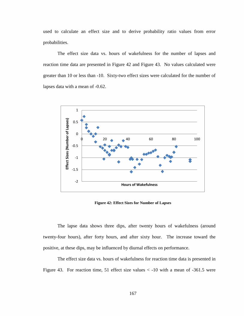
167
used to calculate an effect size and to derive probability ratio values from error
probabilities.
The effect size data vs. hours of wakefulness for the number of lapses and
reaction time data are presented in Figure 42 and Figure 43. No values calculated were
greater than 10 or less than -10. Sixty-two effect sizes were calculated for the number of
lapses data with a mean of -0.62.
Figure 42: Effect Sizes for Number of Lapses
The lapse data shows three dips, after twenty hours of wakefulness (around
twenty-four hours), after forty hours, and after sixty hour. The increase toward the
positive, at these dips, may be influenced by diurnal effects on performance.
The effect size data vs. hours of wakefulness for reaction time data is presented in
Figure 43. For reaction time, 51 effect size values < -10 with a mean of -361.5 were
-2
-1.5
-1
-0.5
0
0.5
1
0 20 40 60 80 100
Effe
ct S
izes
(Num
ber o
f Lap
ses)
Hours of Wakefulness
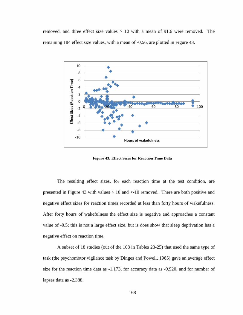
168
removed, and three effect size values > 10 with a mean of 91.6 were removed. The
remaining 184 effect size values, with a mean of -0.56, are plotted in Figure 43.
Figure 43: Effect Sizes for Reaction Time Data
The resulting effect sizes, for each reaction time at the test condition, are
presented in Figure 43 with values > 10 and <-10 removed. There are both positive and
negative effect sizes for reaction times recorded at less than forty hours of wakefulness.
After forty hours of wakefulness the effect size is negative and approaches a constant
value of -0.5; this is not a large effect size, but is does show that sleep deprivation has a
negative effect on reaction time.
A subset of 18 studies (out of the 108 in Tables 23-25) that used the same type of
task (the psychomotor vigilance task by Dinges and Powell, 1985) gave an average effect
size for the reaction time data as -1.173, for accuracy data as -0.920, and for number of
lapses data as -2.388.
-10
-8
-6
-4
-2
0
2
4
6
8
10
0 20 40 60 80 100
Effe
ct S
izes
(Rea
ctio
n Ti
me)
Hours of wakefulness
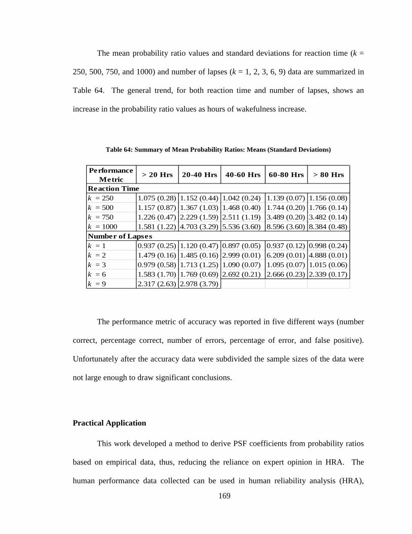
169
The mean probability ratio values and standard deviations for reaction time (k =
250, 500, 750, and 1000) and number of lapses (k = 1, 2, 3, 6, 9) data are summarized in
Table 64. The general trend, for both reaction time and number of lapses, shows an
increase in the probability ratio values as hours of wakefulness increase.
Table 64: Summary of Mean Probability Ratios: Means (Standard Deviations)
Performance Metric
> 20 Hrs 20-40 Hrs 40-60 Hrs 60-80 Hrs > 80 Hrs
k = 250 1.075 (0.28) 1.152 (0.44) 1.042 (0.24) 1.139 (0.07) 1.156 (0.08)k = 500 1.157 (0.87) 1.367 (1.03) 1.468 (0.40) 1.744 (0.20) 1.766 (0.14)k = 750 1.226 (0.47) 2.229 (1.59) 2.511 (1.19) 3.489 (0.20) 3.482 (0.14)k = 1000 1.581 (1.22) 4.703 (3.29) 5.536 (3.60) 8.596 (3.60) 8.384 (0.48)
k = 1 0.937 (0.25) 1.120 (0.47) 0.897 (0.05) 0.937 (0.12) 0.998 (0.24)k = 2 1.479 (0.16) 1.485 (0.16) 2.999 (0.01) 6.209 (0.01) 4.888 (0.01)k = 3 0.979 (0.58) 1.713 (1.25) 1.090 (0.07) 1.095 (0.07) 1.015 (0.06)k = 6 1.583 (1.70) 1.769 (0.69) 2.692 (0.21) 2.666 (0.23) 2.339 (0.17)k = 9 2.317 (2.63) 2.978 (3.79)
Reaction Time
Number of Lapses
The performance metric of accuracy was reported in five different ways (number
correct, percentage correct, number of errors, percentage of error, and false positive).
Unfortunately after the accuracy data were subdivided the sample sizes of the data were
not large enough to draw significant conclusions.
Practical Application
This work developed a method to derive PSF coefficients from probability ratios
based on empirical data, thus, reducing the reliance on expert opinion in HRA. The
human performance data collected can be used in human reliability analysis (HRA),
170
which is part of probabilistic risk assessment (PRA) applications. Typically, in HRA an
error probability is calculated based on performance shaping factors and a base human
error probability (HEP). Currently, SPAR-H (Gertman et al., 2005) uses fitness for duty
as a performance shaping factor (PSF) that perhaps indirectly includes the influence of
sleep deprivation on performance. In this research, it is shown how sleep deprivation test
data could be used to inform the quantitative treatment of sleep deprivation as a PSF, i.e.,
use the results to select appropriate PSF level/values if using a standardized HRA, e.g.,
SPAR-H fitness-for-duty. The methodology developed in this research can be similarly
applied to derive probability ratio values for other performance shaping factors used in
HRA.
However, the application of human performance data from controlled laboratory
studies to real-world applications is difficult due to several limitations. Two factors are
not typically reported: (1) motivation of the subjects, and (2) whether accuracy was
preferred to speed (reaction time) by the subjects. The tasks that are used in the existing
studies also create difficulty in the synthesis of the data. Studies typically use primary
tasks (i.e., one task at a time – no secondary task) and simplified tasks that can be better
controlled. The simplification and isolation of tasks in the literature are not
representative of general real-world tasks.
The need to have controlled experiments with simplified tasks in order to make
the studies possible presents a difficulty in making real-world use of the results of the
studies. This means that laboratory-based tests are not clear indicators of real-world
performance (Kushida et al., 2005). A cognitive laboratory task may track the direction
171
of the changes in function, but does not provide direct extrapolation estimates of ability
to perform everyday tasks.
Another complication in extrapolation from simplified tasks to real-world tasks is
that generally a single task is used in the laboratory. This enables the simplified test task
to be free from distractions and confounding factors that do not compete for attention
capacity. Testing is often done in isolation (i.e., one task at a time), but in real settings,
often, more than one task is performed simultaneously. When using the study data, it
cannot be determined how the reaction times, accuracy, and number of lapses would be
affected if there were additional draws on attention. These performance metrics (reaction
time, accuracy, and number of lapses) generally behave in accordance with the Yerkes-
Dodson law of arousal (1908) that shows an increase in performance as arousal increases
up to a point, after which the level of arousal performance starts to decrease. The
Yerkes-Dodson law even shows a leveling off of performance on simplified tasks even as
arousal (stress) increases (Yerkes and Dodson, 1908).
The laboratory tests generally report reaction time for simple tasks. The changes
in reaction time in these sleep deprivation studies are on the order of milliseconds. Many
real-world tasks do not require such immediate reaction to stimuli. Different tasks
demand different reaction times leading to errors. For example, in an automobile crash
there may be only a small window of time to react, unlike a control room setting where
employees may have several minutes to hours to respond to a cue or to perform a task.
Small changes in simple reaction times would not be significant if the time allowed to
complete the task before an error could occur was on the order of minutes to hours. The
172
effect of sleep deprivation on reaction time is more directly related to tasks that require
quick reactions.
Accuracy and number of lapses data also suffer from issues similar to reaction
time data. Sleep deprivation in general not only increases reaction time, but also affects
accuracy and the number of lapses. Accuracy tends to decrease as hours of wakefulness
increase; however, it is not clear how to extrapolate an increase in the number of false
positives to a simple stimulus in the laboratory setting to a real-world task. The
difference between the number of lapses after sleep deprivation (LT) and before (LC) was
observed to increase after forty hours of continuous wakefulness. This generally implies
that increased hours of wakefulness result in performance impairment. However, the
application of the data to the number of lapses, typically measured in milliseconds, to a
real-world task not requiring immediate action is not straightforward.
The differences in study methods and result collection techniques make it difficult
to synthesize the results of the studies. Even if these difficulties were resolved, there
remains the question of how to apply the results to real-world applications. Several other
complicating factors also need to be considered. The effects of motivation and context
on the laboratory tasks are not clearly addressed in the sleep deprivation studies. Another
serious limitation is the lack of knowledge about the tradeoff between speed and accuracy
during performance tasks. Speed-accuracy tradeoffs occur when speed (reaction time) is
sacrificed to improve accuracy, or when accuracy is traded to maintain or increase speed
(Fitts, 1954). The studies do not consistently mention if speed and accuracy were
measured at the same time or if one was emphasized over the other. Finally, a common
problem in the literature is bias against negative reporting, i.e., only studies that show
173
positive support for the hypothesis (in this case, sleep deprivation adversely affects
performance) tend to get reported.
Future Directions
This research focused on cognitive fatigue resulting from hours of wakefulness.
While this research establishes a procedure to derive PSF coefficients from probability
ratios for sleep deprivation effects on performance for HRA calculations of human error
probabilities, much is still left to be done to fully represent fatigue effects in HRA
methods. Recommendations for future research efforts, including the additional
investigation into the use of time-of-day and time-on-task as independent variables in
addition to hours of wakefulness, should be performed to better address the causes of
cognitive fatigue. Also, other qualitative information that was coded could be evaluated
for causal relationships. Another data collection means of establishing a relationship
between effect size (ES) and reliability index (β) could be used to increase the amount of
data available.
Future work should investigate and collect data in a similar method with time-of-
day and time-on-task as the independent variable. The qualitative information coded
could also be further evaluated to look for causal relationships between performance and
study design or subjects. The regression of the number of lapses and reaction time
studies identified some characteristics that drive performance outcomes, but not all study
characteristics were evaluated.
This research assumed that the performance metrics of number of lapses, reaction
time, and accuracy were normally distributed in the quantitative analysis. The results
174
were shown to be sensitive to this assumption. Other distributions should be investigated
to establish the best representation of the data.
Other PSFs that greatly impact human performance need to be investigated in a
similar method as sleep deprivation was in this research. This research methodology can
be used as a guideline for collecting data and deriving PSF coefficients for other PSFs.
The current trend in HRA methods is focusing on the context of errors. The ATHEANA
method is almost solely focused on defining error forcing situations. There is also a
desire by industry users to increase HRA reliability and reproducibility of results. If the
PSF coefficients are based on empirical data instead of expert judgment, the
reproducibility of the model should improve.
175
BIBLIOGRAPHY
10CFR26.205 - US Government Code of Federal Regulations (2010). “10-CFR 26.20 - Code of Federal Regulations – Title 10: Energy Part 26 Fitness for Duty Programs.” US Federal Government, Washington, DC.
Akerstedt, T. and Freberg, J. (1977). "Psychophysiological Circadian Rhythms in Women
during 72h of Sleep Deprivation." Waking and Sleeping 1: 387-394. Akerstedt, T., Peters, B., Anund, A. and Kecklund, G. (2005). "Impaired Alertness and
Performance Driving Home from the Night Shift: A Driving Simulator Study." Journal of Sleep Research 14: 17–20.
Anderson, C., Wales, A. and Horne, J. (2010). “PVT Lapses Differ According to Eyes Open, Closed, or Looking Away.” Sleep 33(2): 197–204. Angus, R., Helslegrave, R. and Myles, W. (1985). "Effects of Prolonged Sleep
Deprivation, with and without Chronic Physical Exercise, on Mood and Performance." Psychophysiology 22(3): 276-282.
Army-Regulation-602-2 (2001). Manpower and Personnel Integration (MANPRINT) in
the System Acquisition Process. Arnedt, J. Wilde, G., Munt, P. and MacLean, A. (2000). "Simulated Driving Performance
following Prolonged Wakefulness and Alcohol Consumption: Separate and Combined Contributions to Impairment." Journal of Sleep Research 9: 233-241.
Arnedt, J., Wilde, G., Munt, P. and MacLean, A. (2001). "How Do Prolonged
Wakefulness and Alcohol Compare in the Decrements They Produce on a Simulated Driving Task?" Accident Anal and Preven 33: 337-344.
Aschoff, J. (1965). "The Phase-Angle Difference in Circadian Periodicity." Circadian
Clocks. J. Aschoff. North Holland Press, Amsterdam, North Holland Press: 262–278.
Babkoff, H., Thorne, D., Sing, H., Genser, S., Taube, S. and Hegge, F. (1985). "Dynamic
Changes in Work/Rest Duty Cycles in a Study of Sleep Deprivation." Behavioral Research Methods, Instruments, & Computers 17(6): 604-613.
Babkoff, H., Zukerman, G., Fostick, L. and Ben-Artzi, E. (2005). "Effect of the Diurnal
Rhythm and 24-h of Sleep Deprivation on Dichotic Temporal Order Judgment." Journal of Sleep Research 14: 7-15.
176
Baddeley, A. (1968). "A 3-Minute Reasoning Test Based on Grammatical Transformation." Psychonomic Science 10: 341-342.
Baker, C. and McCafferty, D. (2005). "Accident Database Review of Human Element
Concerns: What Do the Results Mean for Classification?" Proceedings from the International Conference Human Factors in Ship Design and Operation, RINA Feb, 2005.
Bartley, S. (1957). "Fatigue and Inadequacy." Physiological Review 37: 301-324. Belenky, G., Wesensten, N., Thorne, D., Thomas, M. and Balkin, T. (2003). "Patterns of
Performance Degradation and Restoration during Sleep Restriction and Subsequent Recovery: A Sleep Dose-Response Study." Journal of Sleep Research 12(1): 1-12.
Bieder, C., Le-Bot, P., Desmares, E., Bonnet, J. and Cara, F. (1998). "MERMOS: EDF's
New Advanced HRA Method." Probabilistic Safety Assessment and Management. PSAM 4. New York, Springer-Verlag.
Bier, V. (1999). "Challenges to the Acceptance of Probabilistic Risk Analysis." Risk
Analysis 19(4): 703. Binks, P., Waters, W. and Hurry, M. (1999). "Short-term Total Sleep Deprivation Does
Not Selectively Impair Higher Cortical Functioning." Sleep 22: 328-334. Blackman, H. (1998). Introduction: A Course for Human Reliability Analysis. Human
Reliability Models: Theoretical and Practical Challenges. College Park, MD, University Printing Services.
Bland, J. and Altman, D. (1986).” Statistical Methods for Assessing Agreement between
Two Methods of Clinical Measurement.” Lancet i: 307–310. Bliese, P., Wesentsten, N. and Balking, T. (2006). "Age and Individual Variability in
Performance during Sleep Restriction." Journal of Sleep Research 15: 376-385. Boksem, M., Meijman, T. and Lorist, M. (2006). "Mental Fatigue, Motivation and Action
Monitoring." Biological Psychology 72: 123-132. Bond, A. and Lader, M. (1974). "The Use of the Analogue Scales in Rating Subjective
Feelings." British Journal of Psychology 4: 211-218. Boring, R., Tran, T., Joe, J., Whaley, A., Gertman, D., Keller, M., Thompson, R.,
Gerzewski, I., Griffith, C. and Anderson, T. (2006). "Users’ Guide for the NASA Human Reliability Database, INL/EXT-06-11944."
177
Boring, R. (2007). “A Review of Expertise and Judgment Processes for Risk Estimation INL/CON-07-12774, Idaho National Laboratory, Idaho Falls, Idaho.
Boring, R., Griffith, C., and Jeffrey, J. (2007). The Measure of Human Error: Direct and
Indirect Performance Shaping Factors. Official Proceedings of the Joint 8th IEEE Conference on Human Factors and Power Plants and the 13th Annual Workshop on Human Performance/Root Cause/Trending/Operating Experience/Self Assessment.
Borland, R., Rogers, A., Nicholson, A, Pascoe, P. and Spencer, M. (1986). "Performance
Overnight in Shift Workers Operating a Day-night Schedule." Aviation Space and Environmental Medicine 57: 241-249.
Brown, I. (1994). "Driver Fatigue." Human Factors 36(2): 298-314. Buck, L. (1975). "Sleep Loss Effects on Movement Time." Ergonomics 18(4): 415-425. Buck, L. and Gibbs, C. (1972). "Sleep Loss and Information Processing." Aspects of
Human Efficiency. W. P. Colquhoun. London, English University Press: 47-57. Caldwell, J., Prazinko, B. and Caldwell, J. (2003). "Body Posture Affects
Electroencephalographic Activity and Psychomotor Vigilance Task Performance in Sleep-Deprived Subjects." Clin Neurophysiol 114(1): 23-31.
Catonavenue.com (December 5, 2007). "Peach Bottom Nuclear Power Plant
Whistleblower Fired." Retrieved on July 16, 2010 from: www.catonave.com Chandler, F., Chang, Y., Mosleh, A., Marble, J., Boring, R. and Gertman, D. (2006).
"Human Reliability Analysis Methods: Selection Guidance for NASA." Washington, DC: NASA Office of Safety and Mission Assurance Technical Report.
Chang, Y. and Mosleh, A. (1999). "Cognitive Modeling and Dynamic Probabilistic
Simulation of Operating Crew Response to Complex System Accidents (ADS-IDACrew)." Reliability Engineering and System Safety 83: 241–253.
Chee, M. and Choo, W. (2004). "Functional Imaging of Working Memory after 24-Hr of
Total Sleep Deprivation." The Journal of Neuroscience 24(19): 4560-4567. Choo, W., Lee, W., Venkatraman, V., Sheu, F. and Chee, M. (2005). "Dissociation of
Cortical Regions Modulated by Both Working Memory Load and Sleep Deprivation and by Sleep Deprivation Alone." Neuroimage 25: 579-587.
Christensen, E., Dietz, G., Murray, R., and Moore, J. (1977). "The Effect of Fatigue on
Resident Performance." Radiology 125: 103-105.
178
Christianson, S. (1992). The Handbook of Emotion and Memory: Research and Theory. New York, Lawrence Erlbaum Associates.
Clifford, C. (2008). "U.S. Car Accident Cost: $164.2 Billion AAA Report Says Crashes
Are 2-1/2 Times More Costly Than Traffic Jams." CNNMoney.com. Coe, R. (2000). "What Is an ‘Effect Size'? A Brief Introduction," CEM Centre, Durham
University. Retrieved on May 6, 2007 from: www.cemcentre.org/renderpage.asp. Cohen, J. (1960). "A Coefficient of Agreement for Nominal Scales". Educational and
Psychological Measurement 20 (1): 37–46. Cohen, J. (1968). "Weighed Kappa: Nominal Scale Agreement with Provision for Scaled
Disagreement or Partial Credit." Psychological Bulletin 70 (4): 213–220. Collier, S. (2005). "HWR-811 HRA - Lessons-Learnt from Previous Experiments."
Halden Project. Collins, W. (1977). "Some Effects of Sleep Deprivation on Tracking Performance in
Static and Dynamic Environments." Journal of Applied Psychology 62: 567-573. Coren, S. (1996). Sleep Thieves: an Eye-Opening Exploration into the Science &
Mysteries of Sleep. New York, Free Press. Cutler, N. and Cohen, H. (1979). "The Effect of One Night's Sleep Loss on Mood and
Memory in Normal Subjects." Comprehensive Psychiatry 20(1): 61-66. Czeisler, C., Duffy, J. Shanahan, T., Brown, E., Mitchell, J., Rimmer, D., Ronda, J.,
Silva, E., Allan, J., Emens, J., Dijk, E. and Kronauer, R. (1999). "Stability, Precision and near 24 hour Period of the Human Circadian Pacemaker." Science 284(5423): 2177-2181.
Daniel, J. and Potasova, A. (1989). "Oral Temperature and Performance in 8 hour and 12
hour Shifts." Ergonomics 32(7): 689-696. Dawson, D. and Reid, K. (1997). "Fatigue, Alcohol, and Performance Impairment."
Nature 388(17): 235-237. Deaconson, T., O'Hair, D., Levy, M., Lee, M., Schueneman, A, and Condon, R. (1988).
"Sleep Deprivation and Resident Performance." JAMA 260: 1721-1727. Dement, W. (1992). The Sleep Watchers. Stanford, CA, Stanford Alumni Association. Dhillon, B. (2007). Human Reliability and Error in Transportation Systems, Ottawa,
CAN, Springer Series - Reliability Engineering.
179
Dinges, D. (1995). "An Overview of Sleepiness and Accidents." Journal of Sleep Research 4(s2): 4-14.
Dinges, D., Pack, F., Williams, K., Gillen, K., Powell, J., Ott, G., Aptowicz, C. and Pack,
A. (1997). "Cumulative Sleepiness, Mood Disturbance, and Psychomotor Vigilance Performance Decrements during a Week of Sleep Restricted to 4-5 Hours per Night." American Sleep Disorders Association and Sleep Research Society 20(4): 267-277.
Dinges, D. and Powell, J. (1985). "Microcomputer Analyses of Performance on a
Portable, Simple Visual RT Task during Sustained Operations." Behavior Research Methods, Instruments, & Computers 17: 652-655.
Dinges, D. and Powell, J. (1988). "Sleepiness is More Than Lapsing." Sleep Research 17:
84. Donchin, Y., Gopher, D., Oline, M., Badhihi, Y., Biesky, M., Sprung, C., Pizov, R. and
Cotev, S. (1995). "A Look into the Nature and Causes of Human Errors in the Intensive Care Unit." Critical Care Med 23: 294-300.
Doran, S., Van Dongen, H. and Dinges, D. (2001). "Sustained Attention Performance
during Sleep Deprivation: Evidence of State Instability." Archives Italiennes de Biologie 139: 253-267.
Dorrian, J., Roach, G., Fletcher, A. and Dawson, D. (2007). "Simulated Train Driving:
Fatigue, Self-awareness and Cognitive Disengagement." Applied Ergonomics 38(2): 155.
Drake, C., Roehrs, T., Burduvali, E., Bonahoom, A., Rosekind, M. and Roth, T. (2001).
"Effects of Rapid versus Slow Accumulation of Eight Hours of Sleep Loss." Psychophysiology 38: 979-987.
Drummond, S. and Brown, G. (2006). "The Effects of Total Sleep Deprivation on
Cerebral Responses to Cognitive Performance." Neuropsychopharmacology 25(5, Supplement 1): S68-S73.
Eastridge, B., Hamilton, E., O'Keefe, G., Rege, R., Valentine, R., Jones, D., Tesfay, S.
and Thal, E. (2003). "Effect of Sleep Deprivation on the Performance of Simulated Laparoscopic Surgical Skill." The American Journal of Surgery 186: 169-174.
Eddy, D. and Hursh, S. (2001) “Fatigue Avoidance Scheduling Tool (FAST).” Technical
Report No.AFRL-HE-BR-TR-2001-0140, Brooks AFB, TX, 2001 Elkin, A. and Murray, D. (1974). "The Effects of Sleep Loss on Short-Term Recognition
Memory." Canadian Journal of Psychology 28(2): 192-198.

180
Eller, S. and Minkley, P. (1998). "The High Price of Sleep Deprivation." Retrieved on
July 17, 2010 from: http://www.rtmagazine.com/issues/articles/1998. Embrey, D., Humphreys, P., Rosa, A., Kirwan, B. and Rea, K. (1983). "SLIM-MAUD:
An Approach to Assessing Human Error Probabilities Using Structured Expert." NUREG/CR-3518. U.S. Nuclear Regulatory Commission, Washington, DC.
Engle-Friedman, M., Riela, S., Golan, R., Ventuneac, A., Davis, C., Jefferson, A. and
Major, D. (2003). "The Effect of Sleep Loss on Next Day Effort." Journal of Sleep Research 12(2): 113-124.
Englund, C., Ryman, D., Naitoh, P. and Hodgdon, J. (1985). "Cognitive Performance
during Successive Sustained Physical Work Episodes." Behav Res Meth Instru Comp 17: 75-85.
Exxon Valdez Oil Spill Trustee Council (2008). "Frequently Asked Questions about the
Spill." Retrieved on September 21, 2008 from: http://www.evostc.state.ak.us/history/faq.cfm.
Fiorica, V., Higgins, E., Iampietro, P., Lategola, M. and Davis, A. (1968). "Physiological
Responses of Men during Sleep Deprivation." Journal of Appl Physiol 24: 167-176.
Folkard, S. (2000). "Transport: Rhythm and Blues." 10th Westminster Lecture on
Transport Safety. Parliamentary Advisory Council for Transport Safety. Forester, J., Kolaczkowski, A. et al. (2006). “Evaluation of Human Reliability Analysis
Methods against Good Practices.” NUREG-1842. U.S. Nuclear Regulatory Commission, Washington, DC.
Frey, D., Badia, P. and Wright, K. (2004). "Inter- and Intra-individual Variability in
Performance near the Circadian Nadir during Sleep Deprivation." Journal of Sleep Research 13(4): 305-315.
Froberg, J. (1977). "Twenty-four Hour Patterns in Human Performance, Subjective and
Physiological Variables and Differences between Morning and Evening Active Subjects." Biological Psychology 5: 119-134.
Garrick, B. (1987). "Examining the Realities of Risk Management." in L. Covello, L.,
Moshissi, A., and Uppuluri, V. (eds.) Uncertainty in Risk Assessment, Risk Management, and Decision Making. New York, Plenum.
Gertman, D., Blackman, H., Haney, L., Seidler, K., Sullivan, C., and Hahn, H. (1990).
“INTENT: A Method for Estimating Human Error Probabilities for Errors of
181
Intention, Rev. 1 (EGGSSRE-9178).” Idaho Falls, ID: Idaho National Engineering Laboratory.
Gertman, D. and Blackman, H. (1994). Human Reliability and Safety Analysis Data
Handbook. New York, John Wiley & Sons, Inc. Gertman, D., Blackman, H., Marble, J., Byers, J. and Smith, C. (2005). "The SPAR-H
Human Reliability Analysis Method." NUREG/CR-6883. U.S. Nuclear Regulatory Commission, Washington. DC.
Glenville, M. and Wilkinson, R. (1979). "Portable Devices for Measuring Performance in
the Field: The Effects of Sleep Deprivation and Night Shift on the Performance of Computer Operators." Ergonomics 22(8): 927-933.
Grandjean, E. (1968). "Fatigue: Its Physiological and Psychological Significance."
Ergonomics 11(5): 427-436. Griffith, C. and Mahadevan, S. (2008). The Use of Meta-Analysis Effect Size Data to
Derive PSF Multipliers. PSAM9, Hong Kong, China. Griffith, C. and Mahadevan, S. (2011). "Inclusion of Fatigue Effects in Human
Reliability Analysis." Reliability Engineering & System Safety 96(11): 1437-1447.
Grubbs, F (1969). “Procedures for Detecting Outlying Observations in Samples.”
Technometrics, 11(1): 1-21. Gordon, G. (2003). “Nuclear Plant Security Is under the Gun.” Minneapolis Star Tribune,
11 May 2003. http://www.startribune.com/stories/484/3875507.html. Gundel, A., Marsalek, K. and Radu, C. (2007). "Sleep-Related and Time-of-Day
Variations in Fatigue and Psychomotor Performance." Somnologie - Schlafforschung und Schlafmedizin 11(3): 186-191.
Gunzelmann, G., Gross, J., Gluck, K. and Dinges, D. (2009). "Sleep Deprivation and
Sustained Attention Performance: Integrating Mathematical and Cognitive Modeling." Cognitive Science.
Gwet, K. (2008). “Computing Inter-rater Reliability and Its Variance in the Presence of
High Agreement.” British Journal of Mathematical and Statistical Psychology 61: 29-48.
Gwet, K. (2010). Handbook of Inter-Rater Reliability (2nd Edition) Gaithersburg,
Advanced Analytics.
182
Halbach, M., Spann, C. and Egan, G. (2003). "Effect of Sleep Deprivation on Medical Resident and Student Cognitive Function: A Prospective Study." American Journal of Obstetrics and Gynecology 188(5): 1198-1201.
Haldar, A. and Mahadevan, S. (2000). Probability, Reliability, and Statistical Methods in
Engineering Design. New York, NY, John Wiley & Sons. Hallbert, B., Boring, R., Gertman, D., Dudenhoeffer, D., Whaley, A., Marble, J., Joe, J.
and Lois, E. (2006). "Human Event Repository and Analysis (HERA) System, Overview." NUREG/CR-6903 Vol. 1. U.S. Nuclear Regulatory Commission, Washington, DC.
Halliday, H. (1997). Wreck! Canada's Worst Railway Accidents. Toronto, Robin Brass
Studio. Hannaman, G., Spurgin, A. and Lukic, Y. (1984). Human Cognitive Reliability Model
for PRA Analysis, NUS-4531. Electric Power Research Institute (EPRI), Palo Alto, CA.
Harrison, Y. and Horne, J. (2000). "The Impact of Sleep Deprivation on Decision
Making: A Review." Journal of Experimental Psychology: Applied 6: 236-249. Hart, R., Buchsbaum, D., Wade, J., Hamer, R. and Kwentus, J. (1987). "Effect of Sleep
Deprivation on First-Year Residents' Response Times, Memory, and Mood." J Med Educ 62: 940-942.
Haslam, D. (1982). "Sleep Loss, Recovery Sleep, and Military Performance."
Ergonomics 25: 163-178. Haslam, D. (1983). "The Incentive Effect and Sleep Deprivation." Sleep 6(4): 362-368. Hassen, F. (Posted Sun 24 Feb 2008). "Sleep Deprivation: Effects on Safety, Health and
the Quality of Life." Retrieved on July 17, 2010 from: http://www.mclarenblog.com.
Hayes, A. and Krippendorff, K. (2007). “Answering the Call for a Standard Reliability
Measure for Coding Data.” Communication Methods and Measures, 1: 77-89. Hildebrandt, G., Rohmert, W. and Rutenfranz, J. (1974). "12 & 24-H Rhythms in Error
Frequency of Locomotive Drivers and the Influence of Tiredness." International Journal of Chronobiology 2: 175-180.
Hirshkowitz, M. and Smith, P. (2004) "Recognizing the Dangers of Sleep Deprivation." Retrieved on July 15, 2010 from: http://www.dummies.com/how- to/content/recognizing-the-dangers-of-sleep-deprivation.html
183
Hoddes, E., Zarcone, V., Smythe, H., Phillips, R. and Dement, W. (1973). "Qualification of Sleepiness: A New Approach." Psychophysiology 10: 431-436.
Hollangel, E. (1998). Cognitive Reliability and Error Analysis Method - CREAM.
Oxford, Elsevier Science. Horne, J., Anderson, N. and Wilkinson, R. (1983). "Effects of Sleep Deprivation on
Signal Detection Measures of Vigilance: Implications for Sleep Function." Sleep 6: 347-358.
Hull, J., Wright, K. and Czeisler, C. (2003). "The Influence of Subjective Alertness and
Motivation on Human Performance Independent of Circadian and Homeostatic Regulation." Journal of Biological Rhythms 18(4): 329-338.
Hunt, M. (1997). How Science Takes Stock: A History of Meta-Analysis. New York,
Russell Sage Foundation. Hursh, S. (1998). “Modeling Sleep and Performance within the Integrated Unit
Simulation System (IUSS).” Technical Report Natick/TR-98/026L. Science and Technology Directorate, Natick Research, Development and Engineering Center, United States Army Soldier Systems Command, Natick, Massachusetts 01760-5020.
Hursh, S., Redmond, D., Johnson, M., Thorne, D., Belenky, G., Balkin, T., Storm, W.,
Miller, J. and Eddy, D. (2004). "Fatigue Models for Applied Research in Warfighting." Aviat Space Environ Med 75(Suppl 3): A54-60.
Hursh, S., Raslear, T., Kaye, A., and Fanzone, J. (2006) “Validation and Calibration of a
Fatigue Assessment Tool for Railroad Work Schedules, Summary Report.” Technical report DOT/FRA/ORD-06/21, U.S. Department of Transportation, Federal Railroad Administration, Office of Research and Development.
Idaho National Laboratory (INL) (2004). HRA Course - Human Reliability Course taught
at the U.S. Nuclear Regulatory Commission, Washington, DC. Indiana Michigan Company v. U.S. Department of Labor v. Kenneth Tipton 0282N US
(6th Cir. 2008). Jewett, M., Dijk, Kronauer, R. and Dinges, D. (1999). "Dose-Response Relationship
between Sleep Duration and Human Psychomotor Vigilance and Subjective Alertness." Sleep 22(2): 171-179.
Jones, C., Dorrian, J., Jay, S., Lamond, N., Ferguson, S. and Dawson, D. (2006). "Self-
Awareness of Impairment and the Decision to Drive after an Extended Period of Wakefulness." Safety Science 23(6): 1253 - 1263.
184
Killgore, W., Balkin, T. and Wesensten, N. (2006). "Impaired Decision Making following 49-h of Sleep Deprivation." Journal of Sleep Research 15: 7-13.
Kirwan, B. (1994). A Guide to Practical Human Reliability Assessment. Bristol, PA,
Taylor & Francie. Kobbeltvedt, T., Brun, W. and Laberg, J. (2005). "Cognitive Processes in Planning and
Judgments under Sleep Deprivation and Time Pressure." Organizational Behavior and Human Decision Processes 98: 1-14.
Koch, G. (1982). "Intraclass Correlation Coefficient”. In Samuel Kotz and Norman L.
Johnson. Encyclopedia.4. New York: John Wiley & Sons. pp. 213–217. Koslowsky, M. and Babkoff, H. (1992). "Meta-Analysis of the Relationship between
Total Sleep Deprivation and Performance." Chronobiology International 9(2): 132-136.
Krupps, L., LaRocca, N., Muir-Nash, J. and Steinberg, A. (1989). "The Fatigue Severity
Scale. Application to Patients with Multiple Sclerosis and Systemic Lupus Erythematosus." Arch Neurol 46: 1121-1123.
Kushida, C., Littner, M., Morgenthaler, T., Alessi, C., Bailey, D., Coleman, J., Friedman,
L., Hirshkowitz, M, Kapen, S., Kramer, M., Lee-Chiong, T., Loube, D., Owens, J., Pancer, J. and Wise, M. (2005). "Practice Parameters for the Indications for Polysomnography and Related Procedures: An Update for 2005." Sleep 28: 499-521.
Lamond, N. and Dawson, D. (1999). "Quantifying the Performance Impairment
Associated with Fatigue." Journal of Sleep Research 8(4): 255–262. Lamond, N., Jay, S., Dorrian, J., Ferguson, S., Jones, C. and Dawson, D. (2007). "The
Dynamics of Neurobehavioral Recovery following Sleep Loss." Journal of Sleep Research 16: 33-34.
Langlois, P., Smolensky, M., His, B. and Weir, F. (1985). "Temporal Patterns of
Reported Single-Vehicle Car and Truck Accidents in Texas, U.S.A. during 1980-1983." Chronobiology International 2(2): 131-146.
Lenne, M., Triggs, T. and Redman, J. (1997). "Time of Day Variation in Driving
Performance." Accident Analysis and Prevention 29(4): 431-437. Lenton, G. (Posted April 26, 2007) "Work Hours to Be Limited for Some Nuclear Plant
Workers." Retrieved July 16, 2010 from:www.tmia.com/node/122.
185
Leonard, C., Fanning, N., Attwood, J. and Buckley, M. (1998). "The Effect of Fatigue, Sleep Deprivation and Onerous Working Hours on the Physical and Mental Well-Being of Pre-Registration House Officers." Ir J Med Sci 167: 22-25.
Lichtor, J., Nuotto, E., Hendren, M., Dohrn, C. and Korttila, K. (1989). "The Effect of
Sleep Deprivation on Psychomotor Performance in Anesthesia Residents." Anesth Analg 68.
Lieberman, H., Bathalon, G., Falco, C., Kramer, F., Morgan, C. and Niro, P. (2005).
"Severe Decrements in Cognition Function and Mood Induced by Sleep Loss, Heat, Dehydration, and Under-nutrition during Simulated Combat." Biological Psychiatry 57(4): 422-429.
Linde, L., Edland, A. and Bergstrom, M. (1999). "Auditory Attention and Multi-attribute
Decision-Making during a 33-h Sleep-Deprivation Period: Mean Performance and Between-Subject Dispersions." Ergonomics 42(5): 696-713.
Lingenfelser, T., Kaschel, R., Webber, A., Zaider-Kaschel, H., Jakober, B. and Kuper, J.
(1994). "Young Hospital Doctors after Night Duty: Their Task-Specific Cognitive Status and Emotional Condition." Medical Education 28(6): 566–572.
Lipsey, M. and Wilson, D. (2001). Practical Meta-Analysis. Thousand Oaks, CA, Sage
Publications. MacDonald, I., Smith, L., Lowe, S. and Folkard, S. (1997). "Effects on Accidents of
Time into Shift and of Short Breaks between Shifts." International Journal of Occupational Environmental Health 3(Suppl.2): S40-S45.
Mackworth, J. (1950). Vigilance and Attention: A Signal Detection Approach.
Harmondsworth, Penguin Books. Malnic, E. (2001). "Crew Fatigue Cited in Fatal 1999 Crash of Jetliner in Ark." Los
Angeles Times. Los Angeles. Marmuff, P., Falleti, M., Collie, A., Darby, D. and McStephen, M. (2005). "Fatigue-
Related Impairment in the Speed, Accuracy and Variability of Psychomotor Performance: Comparison with Blood Alcohol Levels." Journal of Sleep Research 14: 21–27.
Maury, P. and Queinnec, Y. (1993). "Qualitative Changes in Recall Memory during Day
and Night Shifts." Ergonomics 36(1-3): 289-297. May, J. and Kline, P. (1987). "Measuring the Effects upon Cognitive Abilities of Sleep
Loss during Continuous Operations." British Journal of Psychology 78: 443-455.
186
McGraw, K. and S. Wong (1996). “Forming Inferences about Some Intraclass Correlation Coefficients”. Psychological 1 (1): 30–46.
Minors, D. and Waterhouse, J. (1987). "The Role of Naps in Alleviating Sleepiness
during Irregular Sleep-Wake Schedule." Ergonomics 30(9): 1261-1273. Mitler, M., Carskadon, M., Czeisler, C., Dement, W., Dinges, D. and Graeber, R. (1988).
"Catastrophes, Sleep, and Public Policy: Consensus Report." Sleep 11: 100–109. Monk, T. (1997). "Circadian Rhythms in Human Performance and Mood under Constant
Conditions." Journal of Sleep Research 6: 9-18. Monk, T. (2007). "Practical Consequences of Fatigue-Related Performance Failures."
Sleep 30(11): 1402-1403. Morgan, D. (1996). Sleep Secrets for Shift Workers and People with Off-Beat Schedules.
Duluth, Minnesota, Whole Person Associates. Mufson, S. (2008). "Video of Sleeping Guards Shakes Nuclear Industry; Sight of Guards
Asleep Shakes Industry." Washington Post. Washington, DC. Nag, P. and Patel, V. (1998). "Work Accidents among Shiftworkers in Industry."
International Journal of Industrial Ergonomics 21: 275-281. National Safety Council (1999). "Accident Facts." National Safety Council. National Transportation Safety Board (March 4, 1989). "Grounding of the US Tankship
Exxon Valdez on Bligh Reef, Prince William Sound, Near Valdez, Alaska." National Transportation Safety Board (September 18, 1990). "Practices That Related to
the Exxon Valdez." M90-23-31, National Transportation and Safety Board, Washington, DC.
National Transportation Safety Board (2001). "Aircraft Accident Report: Runway
Overrun during Landing; American Airlines Flight 1420." McDonnell Douglas MD-82, N215AA; Little Rock, Arkansas; 1 June 1999. N. T. S. Board.
NEA - Nuclear Energy Agency (1998). "Critical Operator Actions: Human Reliability
Modeling and Data Issues. Principal Working Group No. 5 - Task 94-1." (NEA/CSNI/R(98)1) Paris, France.
Nilsson, J., Soderstrom, M., Karlsson, A., Lekander, M., Akerstedt, T., Limdroth, N. and
Axelsson, J. (2005). "Less Effective Executive Functioning after One Night’s Sleep Deprivation." Journal of Sleep Research 14: 1-6.
187
Oginski, A., Oginska, H. and Pokorski, J. (2000). "Internal and External Factors Influencing Time-Related Injury Risk in Continuous Shift Work." International Journal of Occupational Safety and Ergonomics: JOSE 6(3): 405-421.
Omanio, R. (2009, March 14). JAMA Editor's Guide to Publishing Research
www.Examiner.com. Retrieved Feb 18, 2013 from www.examiner.com/article/jama-editor-s-guide-to-publishing-research.
Parker, A., Briggs, L.,Hubinger, L., Folkard, S. and Green, S. (1998). "A Review of the
Work Practices of Marine Pilots." Australian Maritime Safety Authority. Pearson, K. (1904). "Report on Certain Enteric Fever Inoculation Statistics." British
Medical Journal: 1243-1246. Persensky, J., Hallbert, B. and Blackmon, H. (2002). New Century, New Trends. IEEE
Scottsdale, AZ. Peters, G. and Peters . B. (2006). Human Error Causes and Control Boca Raton, FL,
Taylor and Francis. Peterson, C. (1987). “Reactor Shutdown Ordered; Operators Asleep at Controls, NRC
Charges.” Washington Post, 1 April, final edition. Philip, P., Taillard, J., Sagaspe, P., Valtat, C., Sanchez-Ortuno, M., Moore, N., Charles,
A. and Bioulac, B. (2004). "Age, Performance and Sleep Deprivation." Journal of Sleep Research 13(2): 105–110.
Pilcher, J. and Huffcutt, A. (1996). "Effects of Sleep Deprivation on Performance: A
Meta-Analysis." Sleep 19(4): 318-326. POGO - Project on Government Oversight (2002). "Nuclear Power Plant Security:
Voices from inside the Fences, Project on Government Oversight." Retrieved Sept., 2007 from: http://www.pogo.org/pogo-files/reports/nuclear-security-safety/voices-from-inside-the-fences/.
Porcu, S., Bellatreccia, A., Ferrara, M and Casagrande, M. (1998). "Sleepiness, Alertness
and Performance during a Laboratory Simulation of an Acute Shift of the Wake-Sleep Cycle." Ergonomics 41(8): 1192-1202.
Poulton, E., Hunt, G., Carpenter, A. and Edwards, R. (1978). "The Performance of Junior
Hospital Doctors following Reduced Sleep and Long Hours of Work." Ergonomics 21: 279-295.
Powell, N., Schechtman, K., Riley, R., Li, K., Troell, R. and Guilleminault, C. (2001).
"The Road to Danger: The Comparative Risks of Driving While Sleepy." Laryngoscope 111(5): 887-893.
188
Rajaraman, S., Gribok, A., Wesensten, N., and Balkin, T. and Reifman, J. (2007).
"Individualized Performance Prediction of Sleep-Deprived Individuals with the Two-Process Model." Journal of Applied Physiology 104: 459-468.
Rasmussen, J. (1975). "WASH-1400, Reactor Safety Study: An Assessment of Accident
Risk in U.S. Commercial Nuclear Power Plants." NUREG-75/014. U.S. Nuclear Regulatory Commission, Washington, DC.
Reason, J. (1990). Human Error. New York, Cambridge University Press. Reis, H. and Judd, C. (2000). Handbook of Research Methods in Social Psychology.
London, Cambridge University Press. Reznick, R. and Folse, J. (1987). "Effect of Sleep Deprivation on the Performance of
Surgical Residents." The American Journal of Surgery 154: 520-525. Richardson, G., Wyatt, J., Sullivan, J., Orav, E., Ward, A., Wolf, M. and Czeisler, C.
(1996). "Objective Assessment of Sleep and Alertness in Medical House Staff and the Impact of Protected Time for Sleep." Sleep 19: 718-726.
Richter, S., Schurmeyer, T., Schedlowski, M., Hadicke, A., Tewes, U., Schmidt, R., and
Wagner, T. (1996) “Time Kinetics of the Endocrine Response to Acute Psychological Stress” Journal of Clinical Endocrinology and Metabolism 81(5): 1956-1960.
Richter, S., Marsalek, K., Glatz, C. and Gundel, (2005). "Task-Dependent Differences in
Subjective Fatigue Scores." Journal of Sleep Research 14: 393-400. Roach, G., Dawson, D. and Lamond, N. (2006). "Can a Shorter Psychomotor Vigilance
Task Be Used as a Reasonable Substitute for the Ten-Minute Psychomotor Vigilance Task." Chronobiology Int 23(6): 1379-87.
Robbins, J. and Gottlieb, F. (1990). "Sleep Deprivation and Cognitive Testing in Internal
Medicine House Staff." Western Journal Med 152: 82-86. Rogers-Commission-report (1986). "Report of the Presidential Commission on the Space
Shuttle Challenger Accident, Volume 1, chapter 2." Rosa, R. and Bonnet, M. (1993). "Performance and Alertness on 8-h and 12-h Rotating
Shifts at a Natural Gas Utility." Ergonomics 36(10): 1177-1193. Rosa, R., Bonnet, M. and Warm, J. (1983). "Recovery of Performance during Sleep
following Sleep Deprivation." Psychophysiology 20: 152-159.
189
Rosa, R. and Colligan, M. (1988). "Long Workdays versus Restdays: Assessing Fatigue and Alertness with a Portable Performance Battery." Human Factors 30(3): 305-317.
Rosenthal, R. (1979). "The File Drawer Problem and Tolerance for Null Results".
Psychological Bulletin 86 (3): 638–641. Saal, F., Downey, R., and Lahey, M. (1980) "Rating the Ratings: Assessing the
Psychometric Quality of Rating Data.” Psychological Bulletin 88(2): 413–428. Sagaspe, P., Sanchez-Ortuno, M., Charles, A., Taillard, J., Valtat, C., Bioulac, B., and
Philip, P. (2006). "Effects of Sleep Deprivation on Color-World, Emotional, and Specific Stroop Interference and on Self-Reported Anxiety." Brain and Cognition 60: 76-87.
Sallinen, M., Härmä, M., Akila, R, Holm, A., Luukkonen, R., Mikola, H., Muller, K. and
Virkkala, J. (2004). "The Effects of Sleep Debt and Monotonous Work on Sleepiness and Performance during a 12-h Dayshift." Journal of Sleep Research 13: 285-294.
Sanders, A. and Reitsma, W. (1982). "The Effect of Sleep-Loss on Processing
Information in the Functional Visual Field." Acta Psychologica 51(2): 149-162. Saxena, A. and George, C. (2005). "Sleep and Motor Performance in On-Call Internal
Medicine Residents." Sleep 28(11): 1386-1391. Schmitt, O. (1976). "Biophysical Models for Studying Work and Fatigue." Psychological
Aspects and Physiological Correlates of Work and Fatigue. Springfield, IL., Weiser: 43-52.
Scott, J., McNaughton, L. and Polman, R. (2006). "Effects of Sleep Deprivation and
Exercise on Cognitive, Motor Performance and Mood." Physiology and Behavior 87: 396-408.
Sharp, K., Vaughn, G. and Cosby, P. (1988). "Alterations of Temperature, Sleepiness,
Mood, and Performance in Residents Are Not Associated with Changes in Sulfatoxymelatonin Excretion." Journal of Pineal Research 5: 499-512.
Shen, J., Botly, L., Chung, S., Gibbs, A., Sabanadzovic, S. and Shapiro, C. (2006).
"Fatigue and Shift Work." Journal of Sleep Research 15: 1-5. Shrout, P. and Fleiss, J. (1979) "Intraclass Correlation: Uses in Assessing Rater
Reliability.” Psychological Bulletin 86(2): 420–428. Smith, L., Folkard, S. and Poole, C. (1994). "Increased Injuries on Night Shift." The
Lancet 344(8930): 1137-9.
190
Smith, M. and Glass, G. (1977). "Meta-Analysis of Psychotherapy Outcome Studies."
American Psychologist 32: 752–760. Steyvers, F. and Gaillard, A. (1993). "The Effects of Sleep Deprivation and Incentive on
Human Performance." Psychological Research 55(1): 64-70. Storer, J., Floyd, H., Gill, W., Giusti, C. and Ginsberg, H. (1989). "Effects of Sleep
Deprivation on Cognitive Ability and Skills of Pediatrics Residents." Acad Med 64: 29-32.
Sträter, O. and Bubb, H. (1998). "Assessment of Human Reliability Based on Evaluation
of Plant Experience: Requirements and Their Implementation." Reliability Engineering and System Safety 63(2): 199-219.
Swain, A. and Guttman, H. (1983). "A Handbook of Human Reliability Analysis with
Emphasis on Nuclear Power Plant Applications." NUREG/CR-1278. U.S. Nuclear Regulatory Commission, Washington, DC.
Swann, C., Yelland, G., Redman, J. and Rajaranam, S. (2006). "Chronic Partial Sleep
Loss Increases the Facilitory Role of a Masked Prime in a Word Recognition Task." Journal of Sleep Research 15: 23-29.
Taffinder, N., McManus, I., Gul, Y., Russell, R. and Darzi, A. (1998). "Effect of Sleep
Deprivation on Surgeons' Dexterity on Laparoscopy Simulator." Lancet 352: 1191.
Thomas, M., Sing, H., Belenky, G., Holcomb, H., Mayberg, H., Dannals, R., Wagner, H.,
Thorne, D., Popp, K., Rowland, L., Welsh, A., Balwinski, S. and Redmond, D. (2000). "Neural Basis of Alertness and Cognitive Performance Impairments during Sleepiness: Effects of 24-h of Sleep Deprivation on Waking Human Regional Brain Activity." Journal of Sleep Research 9: 335-352.
Thorne, D., Johnson, D., Redmond, D., Sing, H. and Belenky, G. (2005). "The Walter
Reed Palm-Held Psychomotor Vigilance Test." Behavior Research Methods 37(1): 111-118.
Tilley, A., Wilkinson, R., Watson, W. and Drud, M.et al. (1982). "The Sleep and
Performance of Shift Workers." Human Factors 24(6): 629-641. Trager, E. (1985). “Case Study Report on Loss of Safety System Function Events,
AEOD/C504.” U.S. Nuclear Regulatory Commission, Washington, DC. Treat, J., Tumbas, N., McDonald, S., Shinar, D., Hume, R., Mayer, R., Stanisfer, R. and
Castellan, N. (1977). "Tri-level Study of the Causes of Traffic Accidents." Report
191
No. DOT-HS-034-3-535-77 (Technical Advisory Committee). US Department of Transportation, Washington, DC.
USNRC (1975). "Reactor Safety Study: An Assessment of Accident Risks in U.S.
Commercial Nuclear Power Plants [NUREG-75/014 (WASH-1400)]." U.S. Nuclear Regulatory Commission, Washington, DC.
USNRC (1979). "Investigation into the March 28, 1979, Three Mile Island Accident by
the Office of Inspection and Enforcement (Investment Report No. 50-320/j79-10) NTIS." NUREG-0600. U.S. Nuclear Regulatory Commission, Washington, DC.
USNRC (1985). "Loss of Main and Auxiliary Feedwater Event at the Davis-Besse Plant
on June 9, 1985 (Investigative Report)." NUREG-1154. U.S. Nuclear Regulatory Commission, Washington, DC.
USNRC (1987a). "Report to Congress on Abnormal Occurrences, January – March 1987,
Vol.10, No.1." NUREG-0090. U.S. Nuclear Regulatory Commission, Washington, DC.
USNRC (1987b). "Report on the Accident at the Chernobyl Nuclear Power Station.
NTIS." NUREG 1250. U.S. Nuclear Regulatory Commission, Washington, DC. USNRC (1990). "Severe Accident Risks: An Assessment for Five U.S. Nuclear Power
Plants." NUREG-1150. U.S. Nuclear Regulatory Commission, Washington, DC. May.
USNRC (1995). "Using Micro Saint to Predict Performance in Nuclear Power Plant
Control Room." NUREG/CR-6159. U.S. Nuclear Regulatory Commission Washington, DC.
USNRC (2000). "Technical Basis and Implementation Guidelines for A Technique for
Human Event Analysis (ATHEANA)." NUREG-1624. U.S. Nuclear Regulatory Commission, Washington, DC.
USNRC (2002). Inspection report IR05000313-02-003 (Linda Smith) for Seabrook -
Accession Number ML022000576 (July 19, 2002), U.S. Nuclear Regulatory Commission, Washington, DC.
USNRC (2002). Inspection report IR 05000387-02-005 (A. Randolph Blough) for
Susquehanna - Accession Number ML023160228 (November 12, 2002), U.S. Nuclear Regulatory Commission, Washington, DC.
USNRC (2002). Inspection report IR 05000388-02-005 (A. Randolph Blough) for
Susquehanna - Accession Number ML023160228 (November 12, 2002), U.S. Nuclear Regulatory Commission, Washington, DC.
192
USNRC (2002). Inspection report IR 07200028-02-001 (A. Randolph Blough) for Susquehanna - Accession Number ML023160228 (November 12, 2002), U.S. Nuclear Regulatory Commission, Washington, DC.
USNRC (2003). Inspection report - IR 05000219-03-003 (Neil Perry) for Oyster Creek -
ML032100647 (July 29, 2003), U.S. Nuclear Regulatory Commission, Washington, DC.
USNRC (2003). Inspection report IR 50-20-03-203 for MIT –Accession Number
ML032901191 (October 31, 2003), U.S. Nuclear Regulatory Commission, Washington, DC.
USNRC (2003). Inspection report IR 05000335-02-004 (Joel T. Munday) for St. Lucie –
Accession Number ML030290253 (January 29, 2003), U.S. Nuclear Regulatory Commission, Washington, DC.
USNRC (2003). Inspection report IR 05000389-02-004 (David B. Matthews) for St.
Lucie – Accession Number ML030290253 (January 29, 2003), U.S. Nuclear Regulatory Commission, Washington, DC.
USNRC (2006). "Evaluation of Human Reliability Analysis Methods against Good
Practices." NUREG-1842. U.S. Nuclear Regulatory Commission, Washington, DC.
USNRC (2008). Inspection report - IR 05000293-05-003 (Clifford Anderson) for Pilgrim
– Accession Number ML052070351 (July 6, 2008), U.S. Nuclear Regulatory Commission, Washington, DC.
Van Dongen, H., Malslin, G., Mullington, J., and Dinges, D. (2003). "The Cumulative
Cost of Additional Wakefulness: Dose-Response Effects on Neurobehavioral Functions and Sleep Physiology from Chronic Sleep Restriction and Total Sleep Deprivation." Sleep 26(2): 117-124.
Venkatraman, V., Chuah, Y. and Huettle, S. (2007). "Sleep Deprivation Elevates
Expectation of Gains and Attenuates Response to Losses following Risky Decisions." Sleep 30: 603-609.
Vgontzas, A., Pejovic, S., Zoumakis, E., Lin, H., Bixler E., Basta, M., Fang, J.,
Sarrigiannidis, A. and Chrousos G. (2007). "Daytime Napping after a Night of Sleep Loss Decreases Sleepiness, Improves Performance, and Causes Beneficial Changes in Cortisol and Interleukin-6 Secretion." American Journal of Physiology Endocrinol Metab 292(1): E253.
Webb, W. (1982). "Sleep, Biological Rhythms, Performance Research: An Introduction."
Biological Rhythms, Sleep, and Performance. W. Webb. New York, John Wiley & Sons: 1-25.
193
Webb, W. (1985). "Experiments on Extended Performance: Repetition, Age, and Limited
Sleep Periods." Behavior Research Methods, Instruments, & Computers 17(1): 27-36.
Webb, W. (1986). "Sleep Deprivation and Reading Comprehension." Biological
Psychology 22: 169-172. Webb, W. and Levy, M. (1984). "Effects of Spaced and Repeated Total Sleep
Deprivation." Ergonomics 27: 45-58. Weigmann, S. and Shappell, D. (1999). “A Human Error Analysis of Commercial
Aviation Accidents Using the Human Factors Analysis and Classification System (HFACS) DOT/FAA/AM-01/3” Office of Aviation Medicine Washington, D.C.
Weinger, M. and Ancoli-Israel, S. (2002). "Sleep Deprivation and Clinical Performance."
Journal of the American Medical Association 287: 955-957. Wesensten, N., Killgore, W. and Balkin, T. (2005). "Performance and Alertness Effects
of Caffeine, Dextroamphetamine, and Modafinil during Sleep Deprivation." Journal of Sleep Research 14: 255–266.
Whaley, A., Kelly, D., Boring, R., and Galyean, W. (2011) “SPAR-H Step-by-Step
Guidance.”INL/EXT-10-18533, Rev. 2, Idaho National Laboratory, Idaho Falls, Idaho.
Wilkinson, R. and Houghton, D. (1982). "Field Test of Arousal: A Portable Reaction
Timer with Data Storage." Human Factors 24: 487-493. Williams, H. and Lubin, A. (1967). "Speeded Addition and Sleep Loss." J Exp Psychol
73: 313-317. Williams, H., Lubin, A. and Goodnow, J. (1959). "Impaired Performance with Acute
Sleep Loss." Psychol Monogr Gen Appl 73: 1-26. Williams, J. (1986). HEART (Human Error Analysis and Reduction Technique) - A
Proposed Method for Assessing and Reducing Human Error. 9th Advances in Reliability Technology Symposium, University of Bradford, U. K.
Williamson, A. and Feyer, A. (2000). "Moderate Sleep Deprivation Produces
Impairments in Cognitive and Motor Performance Equivalent to Legally Prescribed Levels of Alcohol Intoxication." Occupational Environmental Medicine 57: 649-655.
194
Wilson, G., Caldwell, J. and Russell, C. (2007). "Performance and Psychophysiological Measures of Fatigue Effects on Aviation Related Tasks of Varying Difficulty." The International Journal of Aviation Psychology 17(2): 219-247.
Wojtczak-Jaroszowa, J., Makowska, Z., Rzepecki, H., Banaszkiewicz, A. and Romejko,
A. (1978). "Changes in Psychomotor and Mental Task Performance following Physical Work in Standard Conditions, and in a Shift-working Situation." Ergonomics 21(10): 801-809.
Wright, J., Hull, T. and Czeisler, C. (2006). "Sleep and Wakefulness out of Phase with
Internal Biological Time Impairs Learning in Humans." J Cogn Neurosci 18(4): 508-21.
Yerkes, R. and Dodson, J. (1908). "The Relation of Strength of Stimulus to Rapidity of
Habit-Formation." Journal of Comparative Neurology and Psychology 18: 459–482.
Yoo, S., Hu, P., Gujar, N., Jolesz, F. and Walker, M. (2007). "A Deficit in the Ability to
Form New Human Memories without Sleep." Nature Neuroscience 10: 385-392.

195
APPENDICES
196
A INTERESTING FATIGUE FACTS
Longest Documented Time Awake
Randy Gardner stayed awake for 264 hours (11 days) of continuous wakefulness
not using any stimulants. He was a 17-year-old high school student in California. On the
4th day he experienced delusions (Ross, 1965).
Sleep Deprivation as a Treatment for Depression
Sleep deprivation has been shown to have a positive effect on depression.
Approximately 60% of patients showed an immediate recovery. However, most
depressed subjects relapsed the following night with sleep. The combination of sleep
deprivation and medication can lessen the number of relapses. Many anti-depressants
suppress REM sleep, which may be the link between improved mood in depressives and
sleep deprivation (Wirz-Justice, 1999).
Psychosis and Sleep Deprivation
In Goes et al. (2007), MRI scans of the brain revealed that sleep deprivation
caused the brain to become incapable of putting an emotional event into its proper
perspective and forming a controlled and suitable response to the event. In another study
in 2001, a link between mental illnesses, including psychosis and bipolar disorder, was
found.
Diabetes Correlation with Sleep Deprivation
197
A correlation between chronic sleep deprivation and Type 2 diabetes was found in
Gottlieb et al., 2005. In Spiegel et al. 2003, an impaired glucose tolerance (IGT) was
found under sleep-deprived conditions.
Bibliography for Interesting Fatigue Facts: Goes FS, Zandi PP, Miao K, et al. (February 2007). "Mood-incongruent Psychotic Features in Bipolar Disorder: Familial Aggregation and Suggestive Linkage to 2p11-q14 and 13q21-33". Am J Psychiatry 164 (2): 236–47. Gottlieb DJ, Punjabi NM, Newman AB, et al. (April 2005). "Association of Sleep Time with Diabetes Mellitus and Impaired Glucose Tolerance". Arch. Intern. Med. 165 (8): 863.
Ross, J., “Neurological Findings after Prolonged Sleep Deprivation,” (1965), Archives of Neurology 12:399-403. Spiegel, K., R. Leproult, and E. Van Cauter (1999-10-23). "Impact of Sleep Debt on Metabolic and Endocrine Function". The Lancet 354 (9188): 1435–9. Wirz-Justice, A. and Van den Hoofdakker, R. (August 1999). "Sleep Deprivation in Depression: What Do We Know, Where Do We Go?" Biol. Psychiatry 46 (4): 445–53.
198
B FATIGUE ACCIDENTS
Three Mile Island – United States (March 28, 1979)
Reactor coolant escaped after the pilot-operated relief valve (PORV) stuck open.
The mechanical failures were compounded with the failure of the operators to recognize
that the plant was experiencing a loss of coolant. When the situation was noticed, the
crew was not able to solve the problem until the relief crew came on and took over for the
fatigued crew. The incident occurred between 04:00 and 06:00.
References:
Harrison, Y. and J. Horne (2000). "The Impact of Sleep Deprivation on Decision Making: A Review." Journal of Experimental Psychology: Applied 6: 236-249. Mitler, M., M. Carskadon, et al. (1988). "Catastrophes, Sleep, and Public Policy: Consensus Report." Sleep 11: 100–109. Monk, T. (2007). "Practical Consequences of Fatigue-Related Performance Failures." Sleep 30(11): 1402-1403.
Reason, J. (1990). Human Error. New York, Cambridge University Press. USNRC (1979). " Investigation into the March 28, 1979, Three Mile Island Accident by the Office of Inspection and Enforcement (Investment Report No. 50-320/j79-10) NTIS NUREG-0600." U.S. Nuclear Regulatory Commission, Washington, DC.
Davis-Besse: United States (June 9, 1985)
At 01:30 the Davis-Besse (Oak Harbor, OH) nuclear power plant went into
automatic shutdown after a loss of cooler water and then the total loss of the main feed-
water. The incident was compounded because the operator pushed the incorrect button
and turned off the auxiliary feed-water system. The operator’s error was discovered by
workers coming on for the next shift.
199
References:
Coren, S. (1996). Sleep Thieves: An Eye-Opening Exploration into the Science & Mysteries of Sleep. New York, Free Press.
Mitler, M., M. Carskadon, et al. (1988). "Catastrophes, Sleep, and Public Policy: Consensus Report." Sleep 11: 100–109.
USNRC (1985). "Loss of Main and Auxiliary Feed-Water Event at the Davis-Besse Plant on June 9, 1985 (Investigative Report) NTIS NUREG-1154." U.S. Nuclear Regulatory Commission, Washington, DC.
Challenger – United States (January 28, 1986) - Poor decision making
NASA managers after working over 20 hour shifts made the critical decision on
whether to launch with their knowledge of O-ring failures at low temperature.
References:
Eller, S. and P. Minkley (1998). "The High Price of Sleep Deprivation." (Accessed July 17, 2010) http://www.rtmagazine.com/issues/articles/1998.
Hassen, F. (Posted Sun 24 Feb 2008). “Sleep Deprivation: Effects on Safety, Health and the Quality of Life.” Mitler, M., M. Carskadon, et al. (1988). "Catastrophes, Sleep, and Public Policy: Consensus Report." Sleep 11: 100–109. Morgan, D. (1996). Sleep Secrets for Shift Workers and People with Off-Beat Schedules. Duluth, Minnesota, Whole Person Associates.
Reason, J. (1990). Human Error. New York, Cambridge University Press. Rogers-Commission-report (1986). "Report of the Presidential Commission on the Space Shuttle Challenger Accident.” Volume 1, chapter 2.
200
Hinton Train Collision – Canada (February 8, 1986) - Operator incapacitated
On February 8, 1986, a VIA rail (passenger train) collided with a Canadian
National Railway (freight train) near Hinton, Alberta, which is west of Edmonton. The
accident was a result of the crew of the freight train becoming incapacitated, i.e., having
fallen asleep.
References:
Halliday, H. A. (1997). Wreck! Canada's Worst Railway Accidents. Toronto, Robin Brass Studio.
Chernobyl – Ukraine (April 26, 1986) - Poor decision making
What happened: Critical automatic safety systems were turned off, and the reactor
began to overheat at approximately 01:30. The sleep-deprived shift workers did not turn
back on the automated safety systems, but instead turned off the cooling system. This
caused the reactor to overheat and led to the explosion, which released radiation.
References:
Coren, S. (1996). Sleep Thieves: An Eye-Opening Exploration into the Science & Mysteries of Sleep. New York, Free Press. Hammon, C. (Quanta Dynamics Incorporated). “If You Don't Snooze, You Lose: Getting A Good Night's Sleep Is Critical to Productivity and Creativity.” Mitler, M., M. Carskadon, et al. (1988). "Catastrophes, Sleep, and Public Policy: Consensus Report." Sleep 11: 100–109.
Reason, J. (1990). Human Error. New York, Cambridge University Press. USNRC (1987). "Report on the Accident at the Chernobyl Nuclear Power Station. NTIS NUREG 1250." U.S. Nuclear Regulatory Commission, Washington, DC.
201
Exxon Valdez – United States (March 24, 1989) Sleep-deprived operator – poor decision
making
The Exxon Valdez oil tanker struck a reef in Prince William Sound, AK, and
spilled 11 to 32 million gallons of crude oil. The accident was caused by the third mate
not having maneuvered the vessel properly. The third mate only had had 6 hours sleep in
the previous 48 hours, while the first mate had been working for 30 hours continuously.
The estimated cleanup cost was $2 billion, including $41 million to help 800 birds and a
few hundred sea otters.
References:
Dement, W. C. (1992). The Sleep Watchers. Stanford, CA, Stanford Alumni Association. Eller, S. and P. Minkley (1998). "The High Price of Sleep Deprivation." (Accessed July 17, 2010 http://www.rtmagazine.com/issues/articles/1998.
Exxon Valdez Oil Spill Trustee Council (September 21, 2008). “Frequently Asked Questions about the Spill.” Hassen, F. (Posted Sun 24 Feb 2008). “Sleep Deprivation: Effects on Safety, Health and the Quality of Life.” National-Transportation-Safety-Board (September 18, 1990). “Practices That Related to the Exxon Valdez.” National-Transportation-Safety-Board (March 4, 1989). "Grounding of the US Tankship Exxon Valdez on Bligh Reef, Prince William Sound, near Valdez, Alaska."
American Airlines flight 1420– United States (June 1,1999) – Poor decision making
An American Airlines flight (1420) from Dallas, TX, to Little Rock, AR, overran
the runway upon landing and crashed. Eleven were killed and 110 injured. Pilot fatigue
and the resulting diminished judgment were given as part of the blame; the crew had been
on duty for about 13 ½ hours at the time of the crash.
202
References:
Hirshkowitz, M. and P. Smith (2004) “Recognizing the Dangers of Sleep Deprivation.” 2004. Web. 15 July 2010. Malnic, E. (2001). “Crew Fatigue Cited in Fatal 1999 Crash of Jetliner in Ark.” Los Angeles Times. Los Angeles. National-Transportation-Safety-Board (2001). “Aircraft Accident Report: Runway Overrun during Landing; American Airlines Flight 1420.” McDonnell Douglas MD-82, N215AA; Little Rock, Arkansas; 1 June 1999. N. T. S. Board.
Staten Island Ferry – United States (October 15, 2003) - Operator asleep
The assistant captain, while piloting the ferry, ran full speed into the dock. The
pilot made no attempt to slow the ferry because he had fallen asleep at the controls.
Eleven people died and seventy-one were injured.
References:
Hirshkowitz, M. and P. Smith (2004) “Recognizing the Dangers of Sleep Deprivation.” 2004. Web. 15 July 2010.
Accidents in General – United States
It has been estimated that the United States loses over $56 billion and 25,000 lives
each year because of sleep-related accidents. Driver fatigue is responsible for an
estimated 100,000 motor vehicle accidents and 1500 deaths each year, according to the
National Highway Traffic Safety Administration.
References:
203
Coren, Stanley. Sleep Thieves: an Eye-Opening Exploration into the Science & Mysteries of Sleep. New York: The Free Press, 1996. p. x, 241-4 Horne J, and L. Reyner. (1995) “Sleep Related Vehicle Accidents.” BMJ 310:565-567. Leger D. (1991) “The Cost of Sleep-Related Accidents: A Report for the National Commission on The Costs of Highway Crashes.” US Department of Transportation, Washington, DC.
Federal Highway Administration (1991). “FHWA-RD-91-055.” US Department of Transportation Federal Highway Administration, Washington, DC.
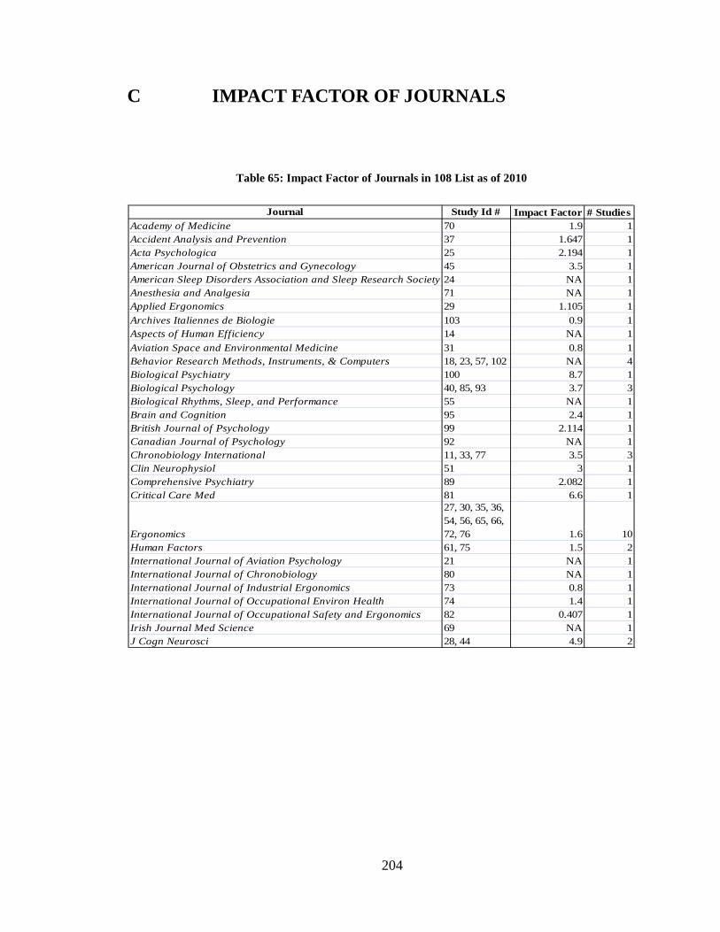
204
C IMPACT FACTOR OF JOURNALS
Table 65: Impact Factor of Journals in 108 List as of 2010
Journal Study Id # Impact Factor # StudiesAcademy of Medicine 70 1.9 1Accident Analysis and Prevention 37 1.647 1Acta Psychologica 25 2.194 1American Journal of Obstetrics and Gynecology 45 3.5 1American Sleep Disorders Association and Sleep Research Society 24 NA 1Anesthesia and Analgesia 71 NA 1Applied Ergonomics 29 1.105 1Archives Italiennes de Biologie 103 0.9 1Aspects of Human Efficiency 14 NA 1Aviation Space and Environmental Medicine 31 0.8 1Behavior Research Methods, Instruments, & Computers 18, 23, 57, 102 NA 4Biological Psychiatry 100 8.7 1Biological Psychology 40, 85, 93 3.7 3Biological Rhythms, Sleep, and Performance 55 NA 1Brain and Cognition 95 2.4 1British Journal of Psychology 99 2.114 1Canadian Journal of Psychology 92 NA 1Chronobiology International 11, 33, 77 3.5 3Clin Neurophysiol 51 3 1Comprehensive Psychiatry 89 2.082 1Critical Care Med 81 6.6 1
Ergonomics
27, 30, 35, 36, 54, 56, 65, 66, 72, 76 1.6 10
Human Factors 61, 75 1.5 2International Journal of Aviation Psychology 21 NA 1International Journal of Chronobiology 80 NA 1International Journal of Industrial Ergonomics 73 0.8 1International Journal of Occupational Environ Health 74 1.4 1International Journal of Occupational Safety and Ergonomics 82 0.407 1Irish Journal Med Science 69 NA 1J Cogn Neurosci 28, 44 4.9 2
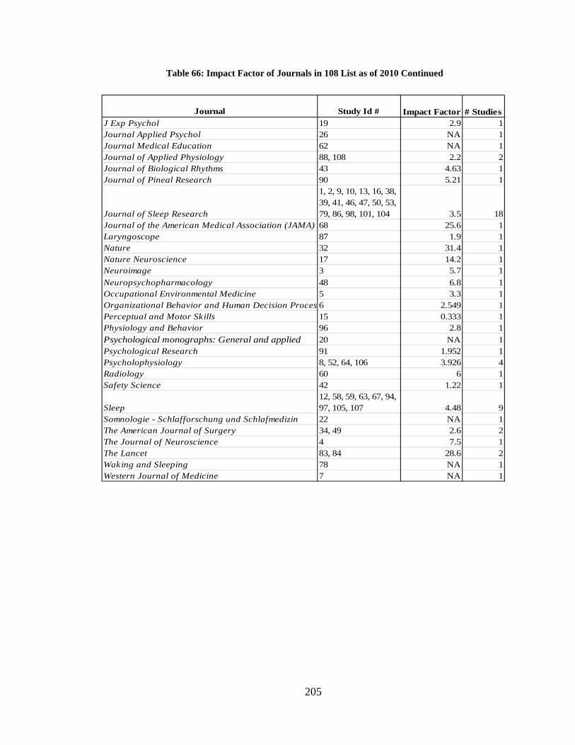
205
Table 66: Impact Factor of Journals in 108 List as of 2010 Continued
Journal Study Id # Impact Factor # StudiesJ Exp Psychol 19 2.9 1Journal Applied Psychol 26 NA 1Journal Medical Education 62 NA 1Journal of Applied Physiology 88, 108 2.2 2Journal of Biological Rhythms 43 4.63 1Journal of Pineal Research 90 5.21 1
Journal of Sleep Research
1, 2, 9, 10, 13, 16, 38, 39, 41, 46, 47, 50, 53, 79, 86, 98, 101, 104 3.5 18
Journal of the American Medical Association (JAMA) 68 25.6 1Laryngoscope 87 1.9 1Nature 32 31.4 1Nature Neuroscience 17 14.2 1Neuroimage 3 5.7 1Neuropsychopharmacology 48 6.8 1Occupational Environmental Medicine 5 3.3 1Organizational Behavior and Human Decision Process6 2.549 1Perceptual and Motor Skills 15 0.333 1Physiology and Behavior 96 2.8 1Psychological monographs: General and applied 20 NA 1Psychological Research 91 1.952 1Psycholophysiology 8, 52, 64, 106 3.926 4Radiology 60 6 1Safety Science 42 1.22 1
Sleep12, 58, 59, 63, 67, 94, 97, 105, 107 4.48 9
Somnologie - Schlafforschung und Schlafmedizin 22 NA 1The American Journal of Surgery 34, 49 2.6 2The Journal of Neuroscience 4 7.5 1The Lancet 83, 84 28.6 2Waking and Sleeping 78 NA 1Western Journal of Medicine 7 NA 1
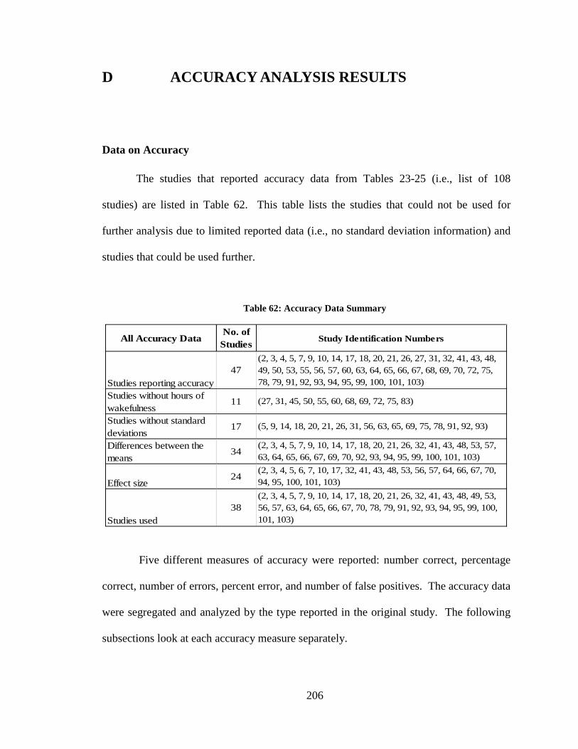
206
D ACCURACY ANALYSIS RESULTS
Data on Accuracy
The studies that reported accuracy data from Tables 23-25 (i.e., list of 108
studies) are listed in Table 62. This table lists the studies that could not be used for
further analysis due to limited reported data (i.e., no standard deviation information) and
studies that could be used further.
Table 62: Accuracy Data Summary
All Accuracy DataNo. of Studies Study Identification Numbers
(27, 31, 45, 50, 55, 60, 68, 69, 72, 75, 83)
(5, 9, 14, 18, 20, 21, 26, 31, 56, 63, 65, 69, 75, 78, 91, 92, 93)17
Studies reporting accuracy
(2, 3, 4, 5, 7, 9, 10, 14, 17, 18, 20, 21, 26, 27, 31, 32, 41, 43, 48, 49, 50, 53, 55, 56, 57, 60, 63, 64, 65, 66, 67, 68, 69, 70, 72, 75, 78, 79, 91, 92, 93, 94, 95, 99, 100, 101, 103)
Studies without standard deviations
47
11Studies without hours of wakefulness
Studies used
(2, 3, 4, 5, 7, 9, 10, 14, 17, 18, 20, 21, 26, 32, 41, 43, 48, 49, 53, 56, 57, 63, 64, 65, 66, 67, 70, 78, 79, 91, 92, 93, 94, 95, 99, 100, 101, 103)
(2, 3, 4, 5, 7, 9, 10, 14, 17, 18, 20, 21, 26, 32, 41, 43, 48, 53, 57, 63, 64, 65, 66, 67, 69, 70, 92, 93, 94, 95, 99, 100, 101, 103)
Effect size(2, 3, 4, 5, 6, 7, 10, 17, 32, 41, 43, 48, 53, 56, 57, 64, 66, 67, 70, 94, 95, 100, 101, 103)
34
24
38
Differences between the means
Five different measures of accuracy were reported: number correct, percentage
correct, number of errors, percent error, and number of false positives. The accuracy data
were segregated and analyzed by the type reported in the original study. The following
subsections look at each accuracy measure separately.
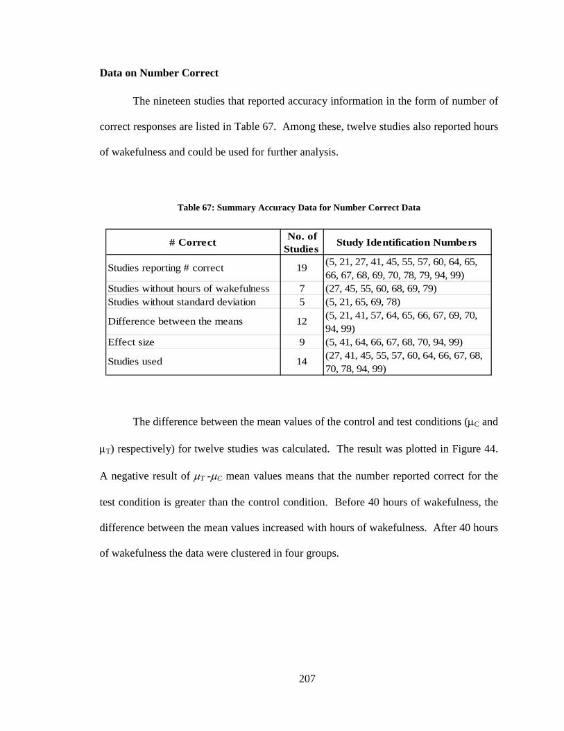
207
Data on Number Correct
The nineteen studies that reported accuracy information in the form of number of
correct responses are listed in Table 67. Among these, twelve studies also reported hours
of wakefulness and could be used for further analysis.
Table 67: Summary Accuracy Data for Number Correct Data
# Correct No. of Studies
Study Identification Numbers
Studies without hours of wakefulness 7 (27, 45, 55, 60, 68, 69, 79)Studies without standard deviation 5 (5, 21, 65, 69, 78)
Effect size 9 (5, 41, 64, 66, 67, 68, 70, 94, 99)
Studies used (27, 41, 45, 55, 57, 60, 64, 66, 67, 68, 70, 78, 94, 99)
Studies reporting # correct (5, 21, 27, 41, 45, 55, 57, 60, 64, 65, 66, 67, 68, 69, 70, 78, 79, 94, 99)
Difference between the means (5, 21, 41, 57, 64, 65, 66, 67, 69, 70, 94, 99)
19
12
14
The difference between the mean values of the control and test conditions (µC and
µT) respectively) for twelve studies was calculated. The result was plotted in Figure 44.
A negative result of µT -µC mean values means that the number reported correct for the
test condition is greater than the control condition. Before 40 hours of wakefulness, the
difference between the mean values increased with hours of wakefulness. After 40 hours
of wakefulness the data were clustered in four groups.
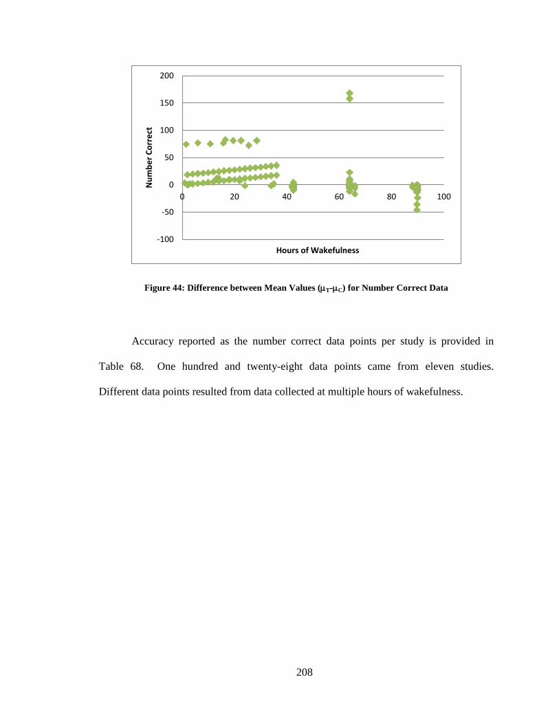
208
Figure 44: Difference between Mean Values (µT-µC) for Number Correct Data
Accuracy reported as the number correct data points per study is provided in
Table 68. One hundred and twenty-eight data points came from eleven studies.
Different data points resulted from data collected at multiple hours of wakefulness.
-100
-50
0
50
100
150
200
0 20 40 60 80 100
Num
ber C
orre
ct
Hours of Wakefulness
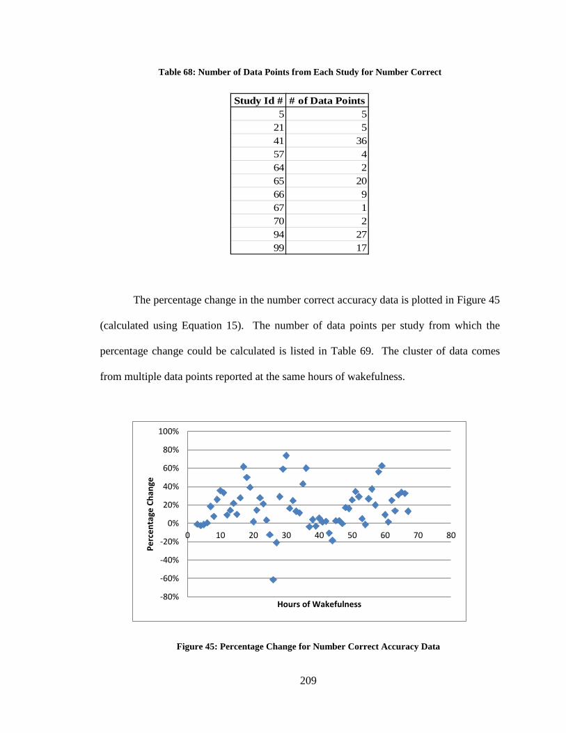
209
Table 68: Number of Data Points from Each Study for Number Correct
Study Id # # of Data Points5 5
21 541 3657 464 265 2066 967 170 294 2799 17
The percentage change in the number correct accuracy data is plotted in Figure 45
(calculated using Equation 15). The number of data points per study from which the
percentage change could be calculated is listed in Table 69. The cluster of data comes
from multiple data points reported at the same hours of wakefulness.
Figure 45: Percentage Change for Number Correct Accuracy Data
-80%
-60%
-40%
-20%
0%
20%
40%
60%
80%
100%
0 10 20 30 40 50 60 70 80
Perc
enta
ge C
hang
e
Hours of Wakefulness
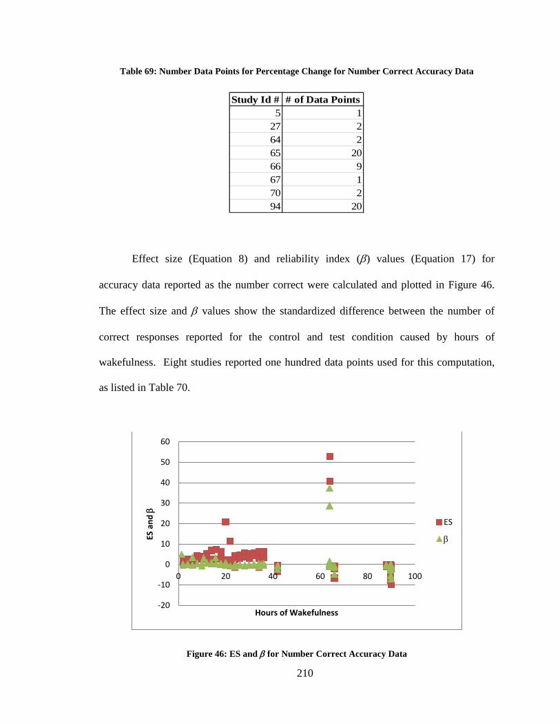
210
Table 69: Number Data Points for Percentage Change for Number Correct Accuracy Data
Study Id # # of Data Points5 1
27 264 265 2066 967 170 294 20
Effect size (Equation 8) and reliability index (β) values (Equation 17) for
accuracy data reported as the number correct were calculated and plotted in Figure 46.
The effect size and β values show the standardized difference between the number of
correct responses reported for the control and test condition caused by hours of
wakefulness. Eight studies reported one hundred data points used for this computation,
as listed in Table 70.
Figure 46: ES and β for Number Correct Accuracy Data
-20
-10
0
10
20
30
40
50
60
0 20 40 60 80 100
ES a
nd β
Hours of Wakefulness
ES
β
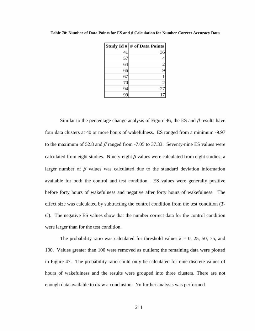
211
Table 70: Number of Data Points for ES and β Calculation for Number Correct Accuracy Data
Study Id # # of Data Points41 3657 464 266 967 170 294 2799 17
Similar to the percentage change analysis of Figure 46, the ES and β results have
four data clusters at 40 or more hours of wakefulness. ES ranged from a minimum -9.97
to the maximum of 52.8 and β ranged from -7.05 to 37.33. Seventy-nine ES values were
calculated from eight studies. Ninety-eight β values were calculated from eight studies; a
larger number of β values was calculated due to the standard deviation information
available for both the control and test condition. ES values were generally positive
before forty hours of wakefulness and negative after forty hours of wakefulness. The
effect size was calculated by subtracting the control condition from the test condition (T-
C). The negative ES values show that the number correct data for the control condition
were larger than for the test condition.
The probability ratio was calculated for threshold values k = 0, 25, 50, 75, and
100. Values greater than 100 were removed as outliers; the remaining data were plotted
in Figure 47. The probability ratio could only be calculated for nine discrete values of
hours of wakefulness and the results were grouped into three clusters. There are not
enough data available to draw a conclusion. No further analysis was performed.
212
Figure 47: Probability Ratio for Number Correct Data vs. Hours of Wakefulness
Data on Percentage Correct (% Correct)
The studies that reported accuracy performance in the form of percentage correct
are listed in Table 71. Percentage correct was reported in eighteen studies. Four studies
did not report hours of wakefulness and could not be used, leaving fourteen for further
analysis.
0.00
10.00
20.00
30.00
40.00
50.00
60.00
0 20 40 60 80 100
Prob
abili
ty R
atio
s
Hours of Wakefulness
k = 0
k = 25
k = 50
k = 75
k = 100
213
Table 71: Summary of Percentage Correct Data
% CorrectNo. of
Studies Study Identification Numbers
Studies without hours of wakefulness 4 (50, 55, 60, 72)Studies without standard deviaiton 5 (9, 18, 63, 92, 93)
Effect size 8 (2, 3, 4, 7, 17, 53, 57, 101)
Studies used (2, 3, 4, 7, 9, 17, 18, 53, 57, 63, 67, 92, 93, 101)
Studies reporting % correct (2, 3, 4, 7, 9, 17, 18, 50, 53, 55, 57, 60, 63, 67, 72, 92, 93, 101)
Difference between the means (2, 3, 4, 7, 9, 17, 18, 53, 57, 63, 67, 92, 93, 101)
16
14
14
The first analysis of the percentage correct accuracy data was to calculate the
difference between the mean values of the control and test conditions for each data point
of hours of wakefulness given, Figure 48. The spread of data is more variable after 45
hours of wakefulness. Before 40 hours of wakefulness, the difference between the
control and test conditions approaches zero; meaning that there is little or no change
between the mean value of control and test conditions.
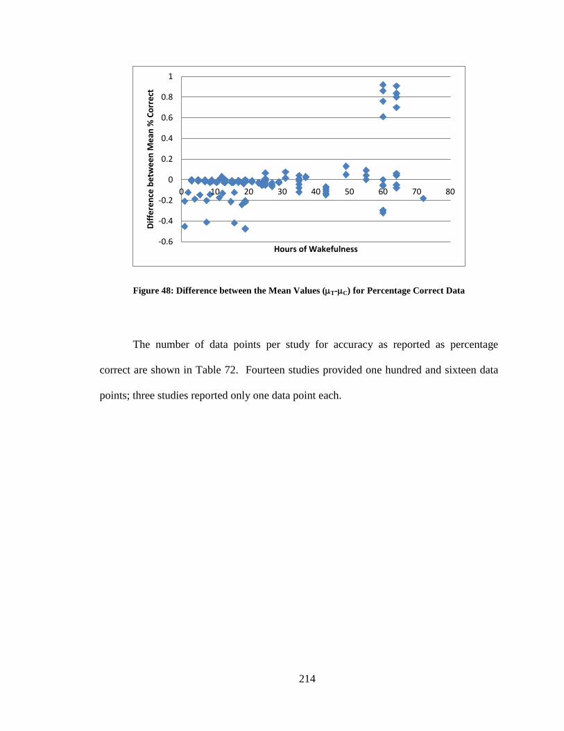
214
Figure 48: Difference between the Mean Values (µT-µC) for Percentage Correct Data
The number of data points per study for accuracy as reported as percentage
correct are shown in Table 72. Fourteen studies provided one hundred and sixteen data
points; three studies reported only one data point each.
-0.6
-0.4
-0.2
0
0.2
0.4
0.6
0.8
1
0 10 20 30 40 50 60 70 80
Diffe
renc
e be
twee
n M
ean
% C
orre
ct
Hours of Wakefulness
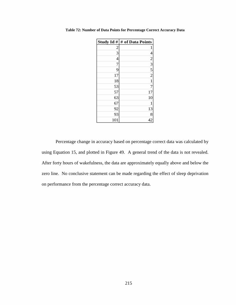
215
Table 72: Number of Data Points for Percentage Correct Accuracy Data
Study Id # # of Data Points2 13 44 27 39 5
17 218 153 757 1763 1067 192 1393 8
101 42
Percentage change in accuracy based on percentage correct data was calculated by
using Equation 15, and plotted in Figure 49. A general trend of the data is not revealed.
After forty hours of wakefulness, the data are approximately equally above and below the
zero line. No conclusive statement can be made regarding the effect of sleep deprivation
on performance from the percentage correct accuracy data.
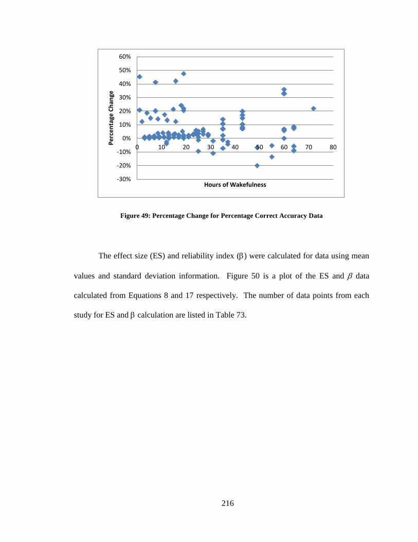
216
Figure 49: Percentage Change for Percentage Correct Accuracy Data
The effect size (ES) and reliability index (β) were calculated for data using mean
values and standard deviation information. Figure 50 is a plot of the ES and β data
calculated from Equations 8 and 17 respectively. The number of data points from each
study for ES and β calculation are listed in Table 73.
-30%
-20%
-10%
0%
10%
20%
30%
40%
50%
60%
0 10 20 30 40 50 60 70 80Perc
enta
ge C
hang
e
Hours of Wakefulness
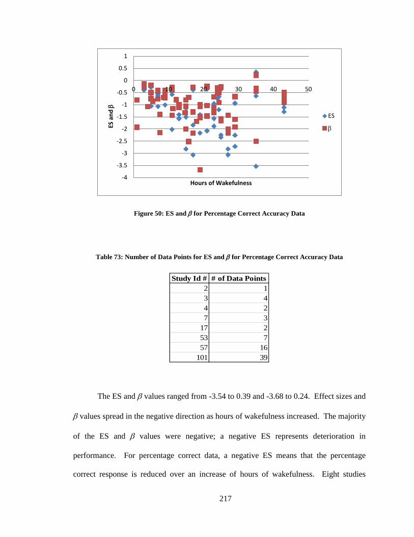
217
Figure 50: ES and β for Percentage Correct Accuracy Data
Table 73: Number of Data Points for ES and β for Percentage Correct Accuracy Data
Study Id # # of Data Points2 13 44 27 3
17 253 757 16
101 39
The ES and β values ranged from -3.54 to 0.39 and -3.68 to 0.24. Effect sizes and
β values spread in the negative direction as hours of wakefulness increased. The majority
of the ES and β values were negative; a negative ES represents deterioration in
performance. For percentage correct data, a negative ES means that the percentage
correct response is reduced over an increase of hours of wakefulness. Eight studies
-4
-3.5
-3
-2.5
-2
-1.5
-1
-0.5
0
0.5
1
0 10 20 30 40 50
ES
and
β
Hours of Wakefulness
ES
β
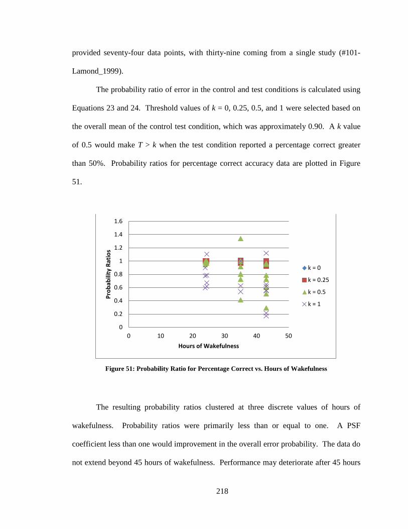
218
provided seventy-four data points, with thirty-nine coming from a single study (#101-
Lamond_1999).
The probability ratio of error in the control and test conditions is calculated using
Equations 23 and 24. Threshold values of k = 0, 0.25, 0.5, and 1 were selected based on
the overall mean of the control test condition, which was approximately 0.90. A k value
of 0.5 would make T > k when the test condition reported a percentage correct greater
than 50%. Probability ratios for percentage correct accuracy data are plotted in Figure
51.
Figure 51: Probability Ratio for Percentage Correct vs. Hours of Wakefulness
The resulting probability ratios clustered at three discrete values of hours of
wakefulness. Probability ratios were primarily less than or equal to one. A PSF
coefficient less than one would improvement in the overall error probability. The data do
not extend beyond 45 hours of wakefulness. Performance may deteriorate after 45 hours
0
0.2
0.4
0.6
0.8
1
1.2
1.4
1.6
0 10 20 30 40 50
Prob
abili
ty R
atio
s
Hours of Wakefulness
k = 0
k = 0.25
k = 0.5
k = 1
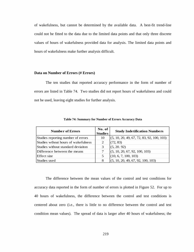
219
of wakefulness, but cannot be determined by the available data. A best-fit trend-line
could not be fitted to the data due to the limited data points and that only three discrete
values of hours of wakefulness provided data for analysis. The limited data points and
hours of wakefulness make further analysis difficult.
Data on Number of Errors (# Errors)
The ten studies that reported accuracy performance in the form of number of
errors are listed in Table 74. Two studies did not report hours of wakefulness and could
not be used, leaving eight studies for further analysis.
Table 74: Summary for Number of Errors Accuracy Data
Number of Errors No. of Studies
Study Indetification Numbers
Studies reporting number of errors 10 (5, 10, 20, 49, 67, 72, 83, 92, 100, 103)Studies wthout hours of wakefulness 2 (72, 83)Studies without standard deviaiton 3 (5, 20. 92)Difference between the means 7 (5, 10, 20, 67, 92, 100, 103)Effect size 5 (10, 6, 7, 100, 103)Studies used 8 (5, 10, 20, 49, 67, 92, 100, 103)
The difference between the mean values of the control and test conditions for
accuracy data reported in the form of number of errors is plotted in Figure 52. For up to
40 hours of wakefulness, the difference between the control and test conditions is
centered about zero (i.e., there is little to no difference between the control and test
condition mean values). The spread of data is larger after 40 hours of wakefulness; the
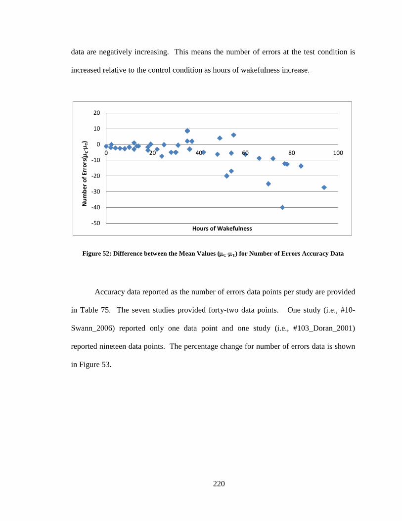
220
data are negatively increasing. This means the number of errors at the test condition is
increased relative to the control condition as hours of wakefulness increase.
Figure 52: Difference between the Mean Values (µC-µT) for Number of Errors Accuracy Data
Accuracy data reported as the number of errors data points per study are provided
in Table 75. The seven studies provided forty-two data points. One study (i.e., #10-
Swann_2006) reported only one data point and one study (i.e., #103_Doran_2001)
reported nineteen data points. The percentage change for number of errors data is shown
in Figure 53.
-50
-40
-30
-20
-10
0
10
20
0 20 40 60 80 100
Num
ber o
f Err
ors(
µ C-µ
T)
Hours of Wakefulness
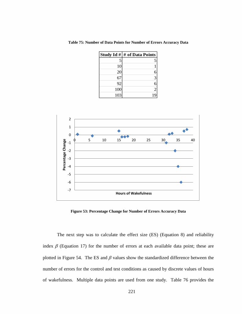
221
Table 75: Number of Data Points for Number of Errors Accuracy Data
Study Id # # of Data Points5 5
10 120 667 392 6
100 2103 19
Figure 53: Percentage Change for Number of Errors Accuracy Data
The next step was to calculate the effect size (ES) (Equation 8) and reliability
index β (Equation 17) for the number of errors at each available data point; these are
plotted in Figure 54. The ES and β values show the standardized difference between the
number of errors for the control and test conditions as caused by discrete values of hours
of wakefulness. Multiple data points are used from one study. Table 76 provides the
-7
-6
-5
-4
-3
-2
-1
0
1
2
0 5 10 15 20 25 30 35 40
Perc
enta
ge C
hang
e
Hours of Wakefulness
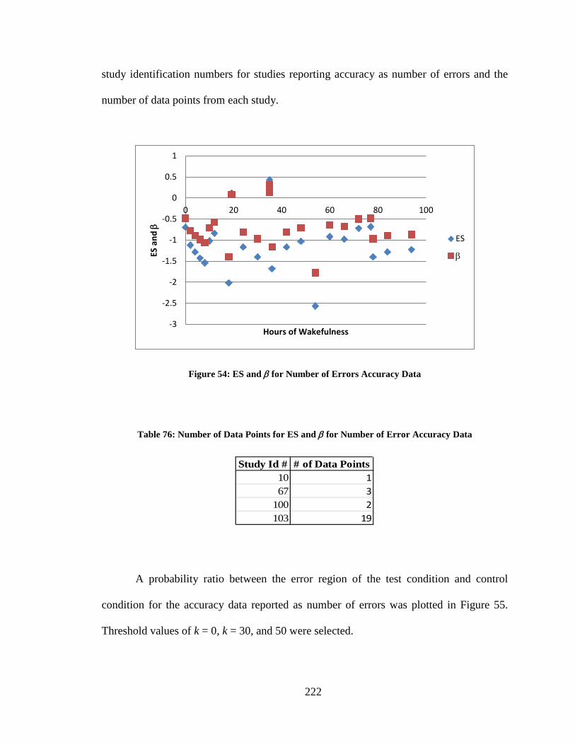
222
study identification numbers for studies reporting accuracy as number of errors and the
number of data points from each study.
Figure 54: ES and β for Number of Errors Accuracy Data
Table 76: Number of Data Points for ES and β for Number of Error Accuracy Data
Study Id # # of Data Points10 167 3
100 2103 19
A probability ratio between the error region of the test condition and control
condition for the accuracy data reported as number of errors was plotted in Figure 55.
Threshold values of k = 0, k = 30, and 50 were selected.
-3
-2.5
-2
-1.5
-1
-0.5
0
0.5
1
0 20 40 60 80 100
ES a
nd β
Hours of Wakefulness
ES
β
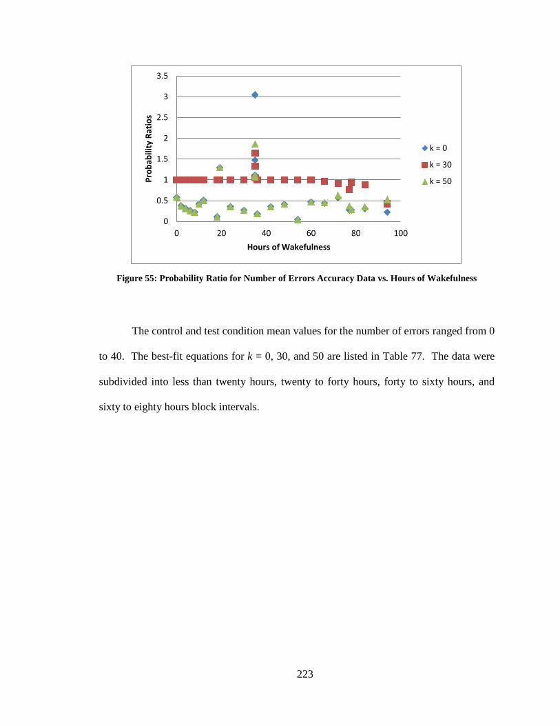
223
Figure 55: Probability Ratio for Number of Errors Accuracy Data vs. Hours of Wakefulness
The control and test condition mean values for the number of errors ranged from 0
to 40. The best-fit equations for k = 0, 30, and 50 are listed in Table 77. The data were
subdivided into less than twenty hours, twenty to forty hours, forty to sixty hours, and
sixty to eighty hours block intervals.
0
0.5
1
1.5
2
2.5
3
3.5
0 20 40 60 80 100
Prob
abili
ty R
atio
s
Hours of Wakefulness
k = 0
k = 30
k = 50
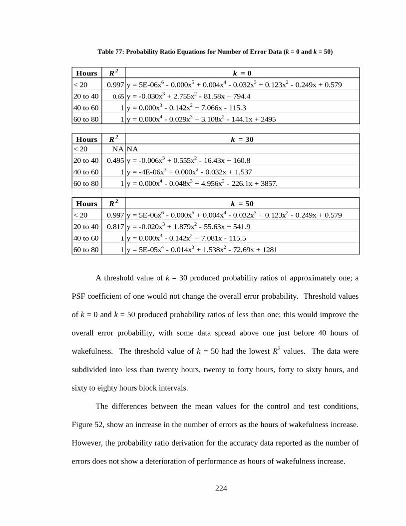
224
Table 77: Probability Ratio Equations for Number of Error Data (k = 0 and k = 50)
Hours R 2 k = 0< 20 0.997 y = 5E-06x6 - 0.000x5 + 0.004x4 - 0.032x3 + 0.123x2 - 0.249x + 0.57920 to 40 0.65 y = -0.030x3 + 2.755x2 - 81.58x + 794.440 to 60 1 y = 0.000x3 - 0.142x2 + 7.066x - 115.360 to 80 1 y = 0.000x4 - 0.029x3 + 3.108x2 - 144.1x + 2495
Hours R 2 k = 30< 20 NA NA20 to 40 0.495 y = -0.006x3 + 0.555x2 - 16.43x + 160.840 to 60 1 y = -4E-06x3 + 0.000x2 - 0.032x + 1.53760 to 80 1 y = 0.000x4 - 0.048x3 + 4.956x2 - 226.1x + 3857.
Hours R 2 k = 50< 20 0.997 y = 5E-06x6 - 0.000x5 + 0.004x4 - 0.032x3 + 0.123x2 - 0.249x + 0.57920 to 40 0.817 y = -0.020x3 + 1.879x2 - 55.63x + 541.940 to 60 1 y = 0.000x3 - 0.142x2 + 7.081x - 115.560 to 80 1 y = 5E-05x4 - 0.014x3 + 1.538x2 - 72.69x + 1281
A threshold value of k = 30 produced probability ratios of approximately one; a
PSF coefficient of one would not change the overall error probability. Threshold values
of k = 0 and k = 50 produced probability ratios of less than one; this would improve the
overall error probability, with some data spread above one just before 40 hours of
wakefulness. The threshold value of k = 50 had the lowest R2 values. The data were
subdivided into less than twenty hours, twenty to forty hours, forty to sixty hours, and
sixty to eighty hours block intervals.
The differences between the mean values for the control and test conditions,
Figure 52, show an increase in the number of errors as the hours of wakefulness increase.
However, the probability ratio derivation for the accuracy data reported as the number of
errors does not show a deterioration of performance as hours of wakefulness increase.
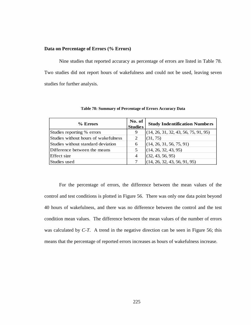
225
Data on Percentage of Errors (% Errors)
Nine studies that reported accuracy as percentage of errors are listed in Table 78.
Two studies did not report hours of wakefulness and could not be used, leaving seven
studies for further analysis.
Table 78: Summary of Percentage of Errors Accuracy Data
% Errors No. of Studies
Study Indentification Numbers
Studies reporting % errors 9 (14, 26, 31, 32, 43, 56, 75, 91, 95)Studies without hours of wakefulness 2 (31, 75)Studies without standard deviation 6 (14, 26, 31, 56, 75, 91)Difference between the means 5 (14, 26, 32, 43, 95)Effect size 4 (32, 43, 56, 95)Studies used 7 (14, 26, 32, 43, 56, 91, 95)
For the percentage of errors, the difference between the mean values of the
control and test conditions is plotted in Figure 56. There was only one data point beyond
40 hours of wakefulness, and there was no difference between the control and the test
condition mean values. The difference between the mean values of the number of errors
was calculated by C-T. A trend in the negative direction can be seen in Figure 56; this
means that the percentage of reported errors increases as hours of wakefulness increase.
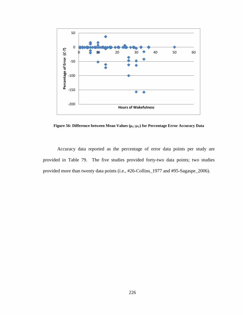
226
Figure 56: Difference between Mean Values (µC-µT) for Percentage Error Accuracy Data
Accuracy data reported as the percentage of error data points per study are
provided in Table 79. The five studies provided forty-two data points; two studies
provided more than twenty data points (i.e., #26-Collins_1977 and #95-Sagaspe_2006).
-200
-150
-100
-50
0
50
0 10 20 30 40 50 60
Perc
enta
ge o
f Err
or (
C-T)
Hours of Wakefulness
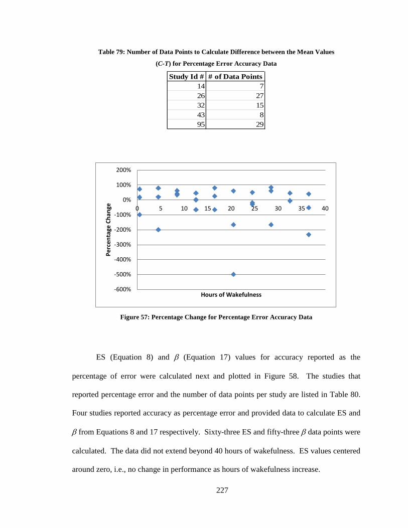
227
Table 79: Number of Data Points to Calculate Difference between the Mean Values
(C-T) for Percentage Error Accuracy Data
Study Id # # of Data Points14 726 2732 1543 895 29
Figure 57: Percentage Change for Percentage Error Accuracy Data
ES (Equation 8) and β (Equation 17) values for accuracy reported as the
percentage of error were calculated next and plotted in Figure 58. The studies that
reported percentage error and the number of data points per study are listed in Table 80.
Four studies reported accuracy as percentage error and provided data to calculate ES and
β from Equations 8 and 17 respectively. Sixty-three ES and fifty-three β data points were
calculated. The data did not extend beyond 40 hours of wakefulness. ES values centered
around zero, i.e., no change in performance as hours of wakefulness increase.
-600%
-500%
-400%
-300%
-200%
-100%
0%
100%
200%
0 5 10 15 20 25 30 35 40
Perc
enta
ge C
hang
e
Hours of Wakefulness
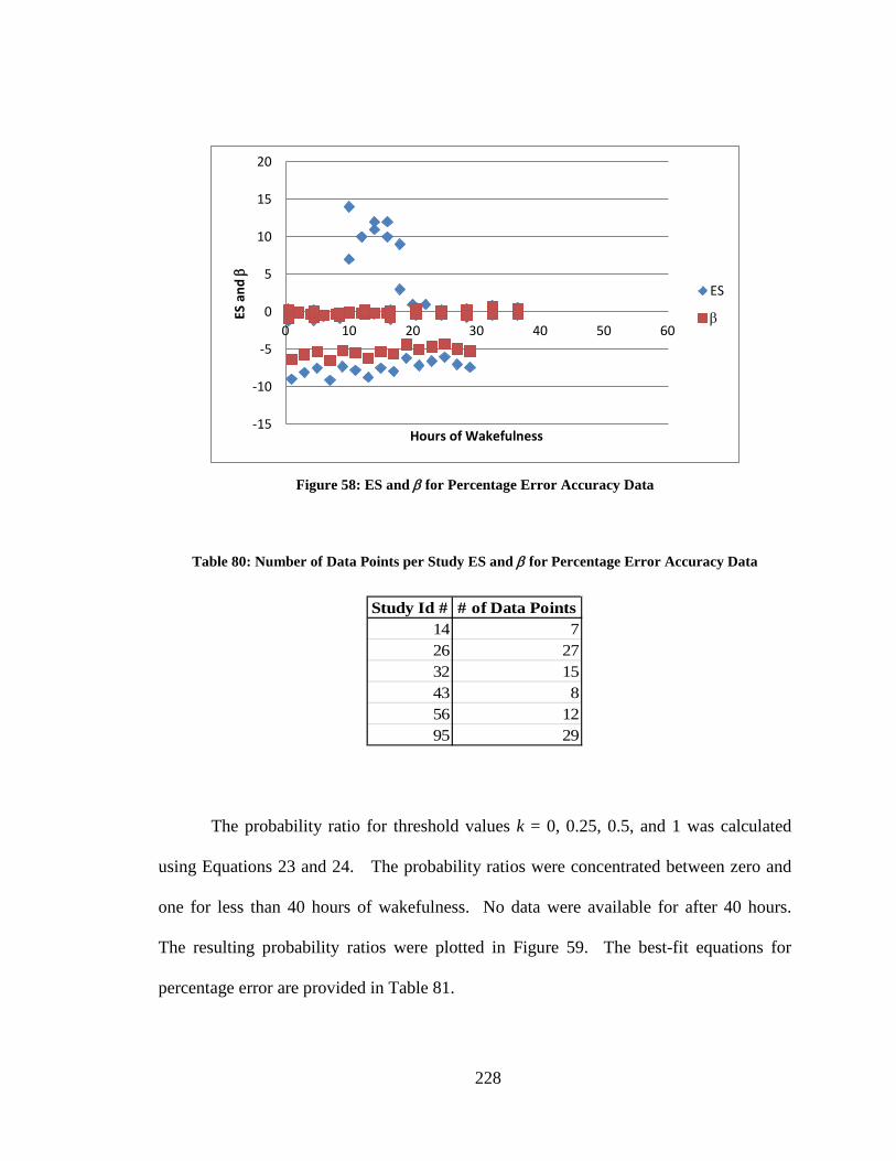
228
Figure 58: ES and β for Percentage Error Accuracy Data
Table 80: Number of Data Points per Study ES and β for Percentage Error Accuracy Data
Study Id # # of Data Points14 726 2732 1543 856 1295 29
The probability ratio for threshold values k = 0, 0.25, 0.5, and 1 was calculated
using Equations 23 and 24. The probability ratios were concentrated between zero and
one for less than 40 hours of wakefulness. No data were available for after 40 hours.
The resulting probability ratios were plotted in Figure 59. The best-fit equations for
percentage error are provided in Table 81.
-15
-10
-5
0
5
10
15
20
0 10 20 30 40 50 60
ES a
nd β
Hours of Wakefulness
ES
β
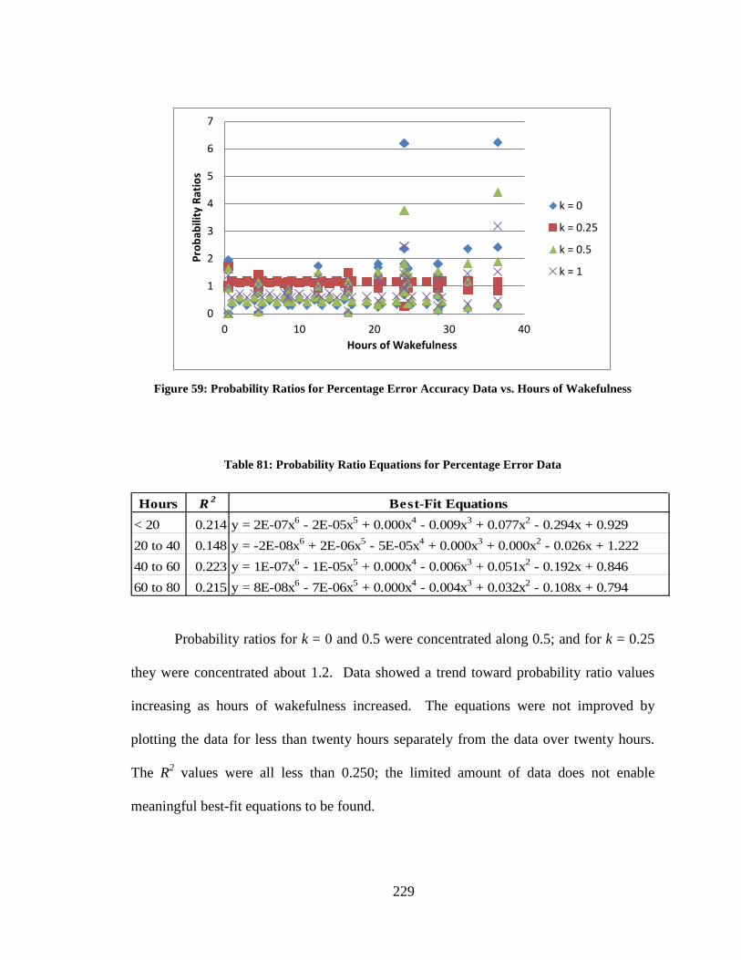
229
Figure 59: Probability Ratios for Percentage Error Accuracy Data vs. Hours of Wakefulness
Table 81: Probability Ratio Equations for Percentage Error Data
Hours R 2 Best-Fit Equations< 20 0.214 y = 2E-07x6 - 2E-05x5 + 0.000x4 - 0.009x3 + 0.077x2 - 0.294x + 0.92920 to 40 0.148 y = -2E-08x6 + 2E-06x5 - 5E-05x4 + 0.000x3 + 0.000x2 - 0.026x + 1.22240 to 60 0.223 y = 1E-07x6 - 1E-05x5 + 0.000x4 - 0.006x3 + 0.051x2 - 0.192x + 0.84660 to 80 0.215 y = 8E-08x6 - 7E-06x5 + 0.000x4 - 0.004x3 + 0.032x2 - 0.108x + 0.794
Probability ratios for k = 0 and 0.5 were concentrated along 0.5; and for k = 0.25
they were concentrated about 1.2. Data showed a trend toward probability ratio values
increasing as hours of wakefulness increased. The equations were not improved by
plotting the data for less than twenty hours separately from the data over twenty hours.
The R2 values were all less than 0.250; the limited amount of data does not enable
meaningful best-fit equations to be found.
0
1
2
3
4
5
6
7
0 10 20 30 40
Prob
abili
ty R
atio
s
Hours of Wakefulness
k = 0
k = 0.25
k = 0.5
k = 1
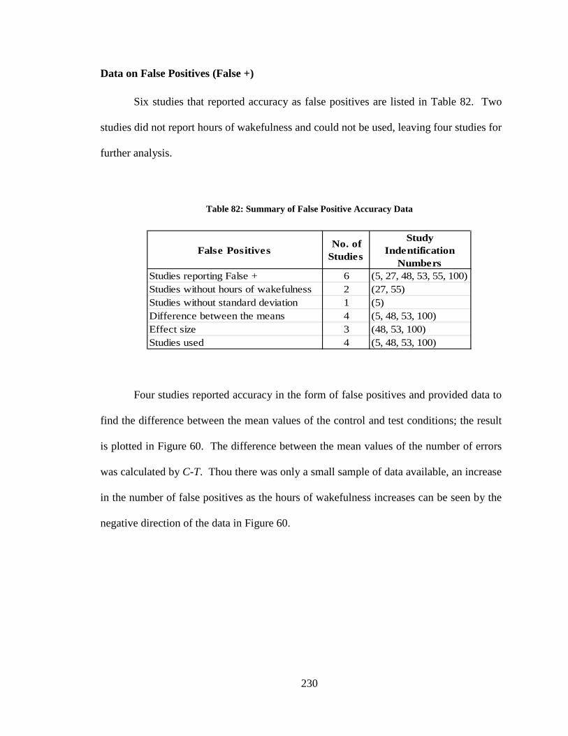
230
Data on False Positives (False +)
Six studies that reported accuracy as false positives are listed in Table 82. Two
studies did not report hours of wakefulness and could not be used, leaving four studies for
further analysis.
Table 82: Summary of False Positive Accuracy Data
False PositivesNo. of
Studies
Study Indentification
NumbersStudies reporting False + 6 (5, 27, 48, 53, 55, 100)Studies without hours of wakefulness 2 (27, 55)Studies without standard deviation 1 (5)Difference between the means 4 (5, 48, 53, 100)Effect size 3 (48, 53, 100)Studies used 4 (5, 48, 53, 100)
Four studies reported accuracy in the form of false positives and provided data to
find the difference between the mean values of the control and test conditions; the result
is plotted in Figure 60. The difference between the mean values of the number of errors
was calculated by C-T. Thou there was only a small sample of data available, an increase
in the number of false positives as the hours of wakefulness increases can be seen by the
negative direction of the data in Figure 60.
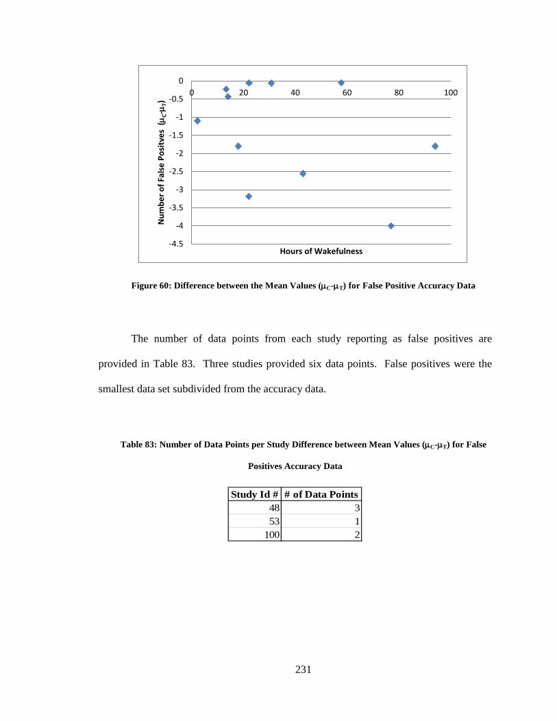
231
Figure 60: Difference between the Mean Values (µC-µT) for False Positive Accuracy Data
The number of data points from each study reporting as false positives are
provided in Table 83. Three studies provided six data points. False positives were the
smallest data set subdivided from the accuracy data.
Table 83: Number of Data Points per Study Difference between Mean Values (µC-µT) for False
Positives Accuracy Data
Study Id # # of Data Points48 353 1
100 2
-4.5
-4
-3.5
-3
-2.5
-2
-1.5
-1
-0.5
00 20 40 60 80 100
Num
ber o
f Fal
se P
ositv
es (
µ C-µ
T)
Hours of Wakefulness
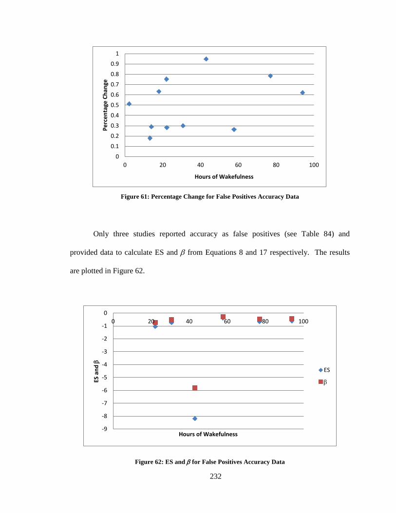
232
Figure 61: Percentage Change for False Positives Accuracy Data
Only three studies reported accuracy as false positives (see Table 84) and
provided data to calculate ES and β from Equations 8 and 17 respectively. The results
are plotted in Figure 62.
Figure 62: ES and β for False Positives Accuracy Data
0
0.1
0.2
0.3
0.4
0.5
0.6
0.7
0.8
0.9
1
0 20 40 60 80 100
Perc
enta
ge C
hang
e
Hours of Wakefulness
-9
-8
-7
-6
-5
-4
-3
-2
-1
00 20 40 60 80 100
ES a
nd β
Hours of Wakefulness
ES
β
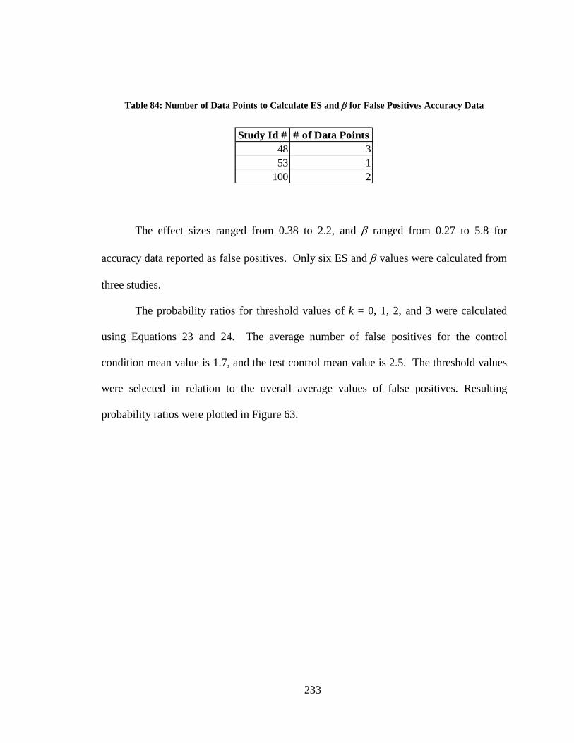
233
Table 84: Number of Data Points to Calculate ES and β for False Positives Accuracy Data
Study Id # # of Data Points48 353 1
100 2
The effect sizes ranged from 0.38 to 2.2, and β ranged from 0.27 to 5.8 for
accuracy data reported as false positives. Only six ES and β values were calculated from
three studies.
The probability ratios for threshold values of k = 0, 1, 2, and 3 were calculated
using Equations 23 and 24. The average number of false positives for the control
condition mean value is 1.7, and the test control mean value is 2.5. The threshold values
were selected in relation to the overall average values of false positives. Resulting
probability ratios were plotted in Figure 63.
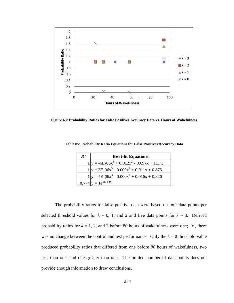
234
Figure 63: Probability Ratios for False Positives Accuracy Data vs. Hours of Wakefulness
Table 85: Probability Ratio Equations for False Positives Accuracy Data
R 2 Best-fit Equations1 y = -6E-05x3 + 0.012x2 - 0.697x + 11.731 y = 3E-06x3 - 0.000x2 + 0.011x + 0.8751 y = 4E-06x3 - 0.000x2 + 0.016x + 0.826
0.774 y = 1e2E-14x
The probability ratios for false positive data were based on four data points per
selected threshold values for k = 0, 1, and 2 and five data points for k = 3. Derived
probability ratios for k = 1, 2, and 3 before 80 hours of wakefulness were one; i.e., there
was no change between the control and test performance. Only the k = 0 threshold value
produced probability ratios that differed from one before 80 hours of wakefulness, two
less than one, and one greater than one. The limited number of data points does not
provide enough information to draw conclusions.
0
0.2
0.4
0.6
0.8
1
1.2
1.4
1.6
1.8
2
0 20 40 60 80 100
Prob
abili
ty R
atio
Hours of Wakefulness
k = 3
k = 2
k = 1
k = 0
235
The differences between the mean values of the control and test conditions show a
decrease in performance as hours of wakefulness increase. The difference between the
means was calculated by C-T for the number of errors, percentage of error, and false
positives. A reduction of performance occurs when the test condition is larger than the
control condition. Unfortunately after the accuracy data were subdivided by number
correct, percentage correct, number of errors, percentage of error, and false positives, the
sample sizes of data were not large enough to draw significant conclusions. The derived
probability ratios did not consistently predict an increase in error probability (for
accuracy data) as hours of wakefulness increase. Accuracy does not seem to be affected
as significantly as reaction time and number of lapses under sleep deprivation. However,
due to the sparseness in accuracy data, the statistics and inferences do not appear to be
significant.
Summary and Conclusion for Accuracy Data
Accuracy data were grouped by number correct, percentage correct, number of
errors, percentage of error, and false positives. Data that reported accuracy as the number
correct came from fourteen different studies. The differences between the means
increased up to 40 hours of wakefulness; after 40 hours of wakefulness the data clustered
and were not further analyzed. Threshold values of k = 0, 23, 50, and 75 were used to
derive probability ratio values. The data clustered about four points and were not further
analyzed.
Accuracy as reported as percentage correct was found in fourteen studies. The
difference between the mean values centered about zero; i.e., there was a difference
236
between the control and test conditions. Threshold values of k = 0, 0.25, 0.5, and 1 were
used to derive the probability ratios for percentage correct. Probability ratios less than
one were found for k = 0.25 and 0.5 and probability ratios of approximately one were
found for k = 0 and 1. A probability ratio of one does not change the overall error
probability, i.e., no change in performance under sleep deprivation.
Eight studies were found to report accuracy as number of errors. The number of
errors increased as hours of wakefulness increased. The differences between the mean
values were calculated by C - T. Threshold values of k = 0, 30, and 50 were used to
derive probability ratios. For k = 0 and k = 50, the probability ratios were less than one
and the probability ratio values were continuously close to one when a threshold value of
30 was used in the analysis.
Accuracy as reported as percentage of errors was calculated from seven studies.
The difference between mean values centered around zero, i.e., no change from the
control to the test condition. Threshold values of k = 0, 0.25, 0.5, and 1 were used to
derive probability ratios for percent of errors data. The probability ratios were centered
at 0.5 for k = 0 and k = 5 and 1.2 for k = 1.2. The probability ratios did not continuously
increase and remained consistent as hours of wakefulness increased.
The four studies that reported false positives data were analyzed. The number of
false positives, i.e., reacting when there was no signal, increased as hours of wakefulness
increased. Threshold values of k = 0, 1, 2, and 3 were selected. The produced probability
ratios centered around one; however k = 0 has some data spread.
In summary, accuracy is not as affected as reaction time and number of lapses
under sleep-deprived conditions. The draw on cognitive capacity that results from sleep
237
deprivation may help increase arousal levels (Yerkes and Dodson, 1908) and help to
maintain, or even improve, performance on the simple tasks that were the primary tasks
employed in the studies under investigation. Another reason why accuracy is not as
affected by sleep deprivation is the tradeoff between reaction time and accuracy (i.e.,
speed-accuracy tradeoff). Reaction time is often sacrificed to maintain or improve
accuracy (Fitts, 1954). The studies do not consistently mention if reaction time and
accuracy were measured at the same time or if one was emphasized over the other.
Accuracy was not reported in the same manner in each study. In the studies that reported
accuracy as a performance metric, accuracy was reported through several measures:
number of errors, number of false positives and hit rates, the number of false starts,
number of errors, and number of responses.
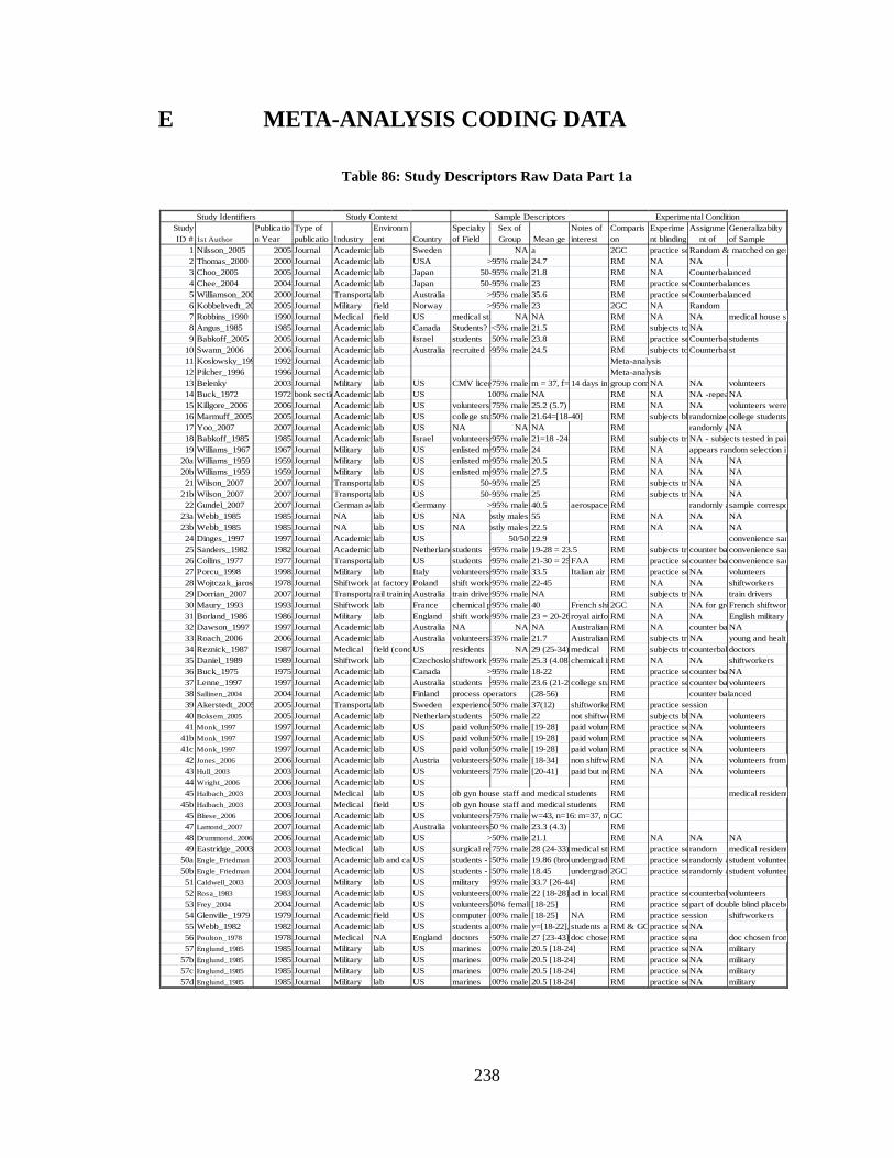
238
E META-ANALYSIS CODING DATA
Table 86: Study Descriptors Raw Data Part 1a
1 Nilsson_2005 2005 Journal Academic lab Sweden NA a 2GC practice seRandom & matched on gen 2 Thomas_2000 2000 Journal Academic/lab USA >95% male 24.7 RM NA NA3 Choo_2005 2005 Journal Academic/lab Japan 50-95% male 21.8 RM NA Counterbalanced4 Chee_2004 2004 Journal Academic/lab Japan 50-95% male 23 RM practice seCounterbalances5 Williamson_200 2000 Journal Transportalab Australia >95% male 35.6 RM practice seCounterbalanced6 Kobbeltvedt_20 2005 Journal Military field Norway >95% male 23 2GC NA Random7 Robbins_1990 1990 Journal Medical field US medical sta NA NA RM NA NA medical house st8 Angus_1985 1985 Journal Academic lab Canada Students? <5% male 21.5 RM subjects to NA9 Babkoff_2005 2005 Journal Academic lab Israel students 50% male 23.8 RM practice seCounterbalstudents
10 Swann_2006 2006 Journal Academic lab Australia recruited -95% male 24.5 RM subjects to Counterbalst11 Koslowsky_199 1992 Journal Academic lab Meta-analysis12 Pilcher_1996 1996 Journal Academic lab Meta-analysis13 Belenky 2003 Journal Military lab US CMV licen >75% male m = 37, f= 14 days in group comNA NA volunteers14 Buck_1972 1972 book sectioAcademic lab US 100% male NA RM NA NA -repea NA15 Killgore_2006 2006 Journal Academic/lab US volunteers 75% male 25.2 (5.7) RM NA NA volunteers were 16 Marmuff_2005 2005 Journal Academic lab US college stu<50% male 21.64=[18-40] RM subjects bli randomized college students 17 Yoo_2007 2007 Journal Academic lab US NA NA NA RM randomly a NA18 Babkoff_1985 1985 Journal Academic lab Israel volunteers>95% male 21=18 -24 RM subjects tra NA - subjects tested in pair19 Williams_1967 1967 Journal Military lab US enlisted me>95% male 24 RM NA appears random selection in
20a Williams_1959 1959 Journal Military lab US enlisted me >95% male 20.5 RM NA NA NA20b Williams_1959 1959 Journal Military lab US enlisted me >95% male 27.5 RM NA NA NA21 Wilson_2007 2007 Journal Transporta lab US 50-95% male 25 RM subjects tra NA NA
21b Wilson_2007 2007 Journal Transporta lab US 50-95% male 25 RM subjects tra NA NA22 Gundel_2007 2007 Journal German ae lab Germany >95% male 40.5 aerospace RM randomly a sample correspo
23a Webb_1985 1985 Journal NA lab US NA ostly males 55 RM NA NA NA23b Webb_1985 1985 Journal NA lab US NA ostly males 22.5 RM NA NA NA24 Dinges_1997 1997 Journal Academic lab US 50/50 22.9 RM convenience sam25 Sanders_1982 1982 Journal Academic lab Netherlandstudents >95% male 19-28 = 23.5 RM subjects tra counter ba convenience sam26 Collins_1977 1977 Journal Transportalab US students >95% male 21-30 = 25FAA RM practice secounter ba convenience sam27 Porcu_1998 1998 Journal Military lab Italy volunteers>95% male 33.5 Italian air fRM practice seNA volunteers28 Wojtczak_jaros 1978 Journal Shiftwork at factory Poland shift worke>95% male 22-45 RM NA NA shiftworkers29 Dorrian_2007 2007 Journal Transportarail training Australia train driver>95% male NA RM subjects tra NA train drivers30 Maury_1993 1993 Journal Shiftwork lab France chemical p>95% male 40 French shif2GC NA NA for gro French shiftwork31 Borland_1986 1986 Journal Military lab England shift worke>95% male 23 = 20-26royal airforRM NA NA English military r 32 Dawson_1997 1997 Journal Academic lab Australia NA NA NA Australian RM NA counter ba NA33 Roach_2006 2006 Journal Academic lab Australia volunteers<35% male 21.7 Australian RM subjects tra NA young and health34 Reznick_1987 1987 Journal Medical field (cond US residents NA 29 (25-34) medical RM subjects tracounterbala doctors35 Daniel_1989 1989 Journal Shiftwork lab Czechoslovshiftwork - >95% male 25.3 (4.08)chemical inRM NA NA shiftworkers36 Buck_1975 1975 Journal Academic lab Canada >95% male 18-22 RM practice secounter ba NA37 Lenne_1997 1997 Journal Academic lab Australia students >95% male 23.6 (21-26college stuRM practice secounter ba volunteers38 Sallinen_2004 2004 Journal Academic lab Finland process operators (28-56) RM counter balanced39 Akerstedt_2005 2005 Journal Transportalab Sweden experience 50% male 37(12) shiftworke RM practice session40 Boksem_2005 2005 Journal Academic lab Netherlandstudents >50% male 22 not shiftwoRM subjects bli NA volunteers41 Monk_1997 1997 Journal Academic lab US paid volunt>50% male [19-28] paid voluntRM practice seNA volunteers
41b Monk_1997 1997 Journal Academic lab US paid volunt>50% male [19-28] paid voluntRM practice seNA volunteers41c Monk_1997 1997 Journal Academic lab US paid volunt>50% male [19-28] paid voluntRM practice seNA volunteers42 Jones_2006 2006 Journal Academic lab Austria volunteers>50% male [18-34] non shiftwoRM NA NA volunteers from 43 Hull_2003 2003 Journal Academic/lab US volunteers 75% male [20-41] paid but no RM NA NA volunteers44 Wright_2006 2006 Journal Academic lab US RM45 Halbach_2003 2003 Journal Medical lab US ob gyn house staff and medical students RM medical resident
45b Halbach_2003 2003 Journal Medical field US ob gyn house staff and medical students RM45 Bliese_2006 2006 Journal Academic lab US volunteers>75% male w=43, n=16: m=37, n=GC47 Lamond_2007 2007 Journal Academic lab Australia volunteers 50 % male 23.3 (4.3) RM48 Drummond_2006 2006 Journal Academic lab US >50% male 21.1 RM NA NA NA49 Eastridge_2003 2003 Journal Medical lab US surgical res75% male 28 (24-33) medical stu RM practice serandom medical resident
50a Engle_Friedman 2003 Journal Academic lab and cal US students - u<50% male 19.86 (brok undergradu RM practice serandomly astudent voluntee50b Engle_Friedman 2004 Journal Academic lab US students - u<50% male 18.45 undergradu 2GC practice serandomly astudent voluntee51 Caldwell_2003 2003 Journal Military lab US military >95% male 33.7 [26-44] RM52 Rosa_1983 1983 Journal Academic lab US volunteers100% male 22 [18-28] ad in local RM practice secounterbala volunteers53 Frey_2004 2004 Journal Academic lab US volunteers50% femal [18-25] RM practice separt of double blind placebo 54 Glenville_1979 1979 Journal Academic field US computer o 100% male [18-25] NA RM practice session shiftworkers55 Webb_1982 1982 Journal Academic lab US students an 100% male y=[18-22], students an RM & GCpractice seNA56 Poulton_1978 1978 Journal Medical NA England doctors >50% male 27 [23-43] doc chosen RM practice sena doc chosen from 57 Englund_1985 1985 Journal Military lab US marines 100% male 20.5 [18-24] RM practice seNA military
57b Englund_1985 1985 Journal Military lab US marines 100% male 20.5 [18-24] RM practice seNA military57c Englund_1985 1985 Journal Military lab US marines 100% male 20.5 [18-24] RM practice seNA military57d Englund_1985 1985 Journal Military lab US marines 100% male 20.5 [18-24] RM practice seNA military
CountrySpecialty of Field
Sex of Group Mean ge
Notes of interest
Comparison
Study Identifiers Study Context Sample Descriptors Experimental ConditionStudy ID # 1st Author
Publication Year
Type of publicatio Industry
Environment
Experiment blinding
Assignment of
Generalizabilty of Sample
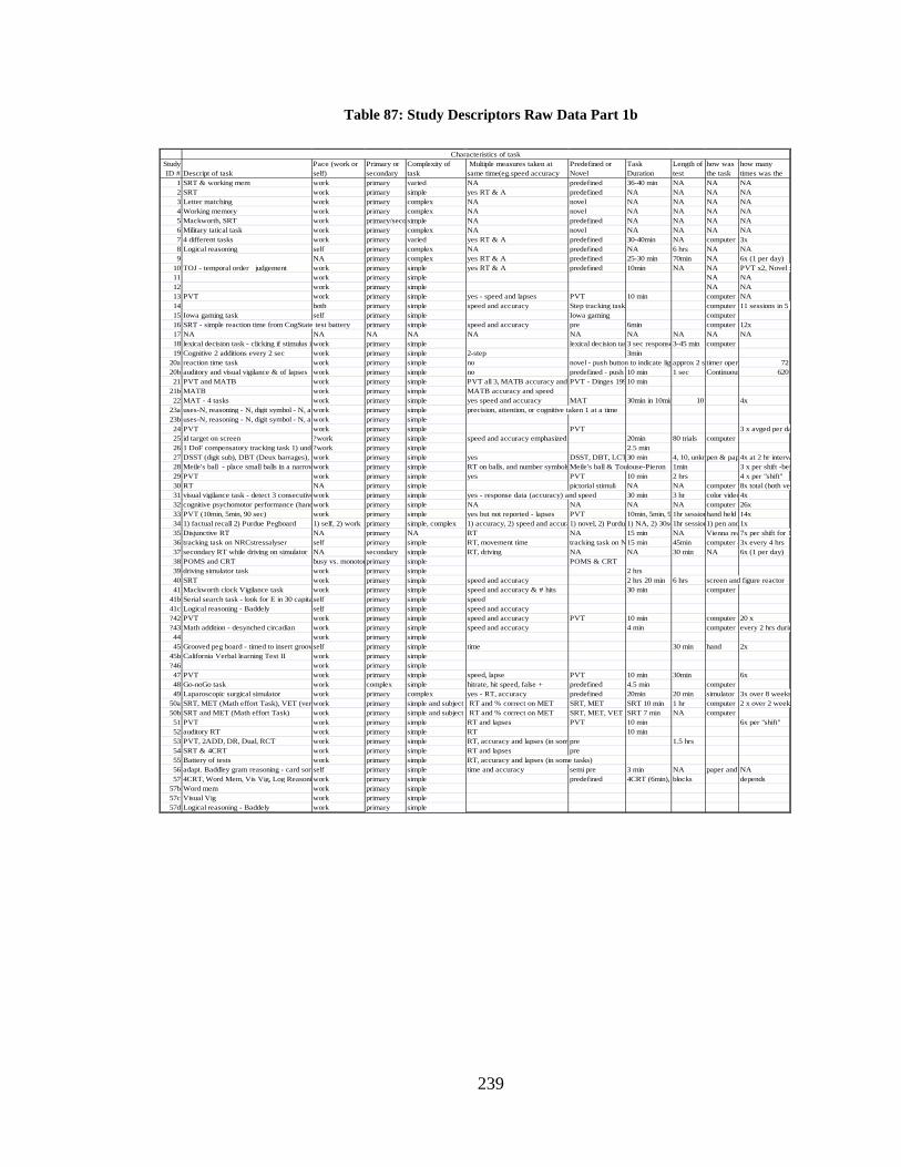
239
Table 87: Study Descriptors Raw Data Part 1b
1 SRT & working mem work primary varied NA predefined 36-40 min NA NA NA2 SRT work primary simple yes RT & A predefined NA NA NA NA3 Letter matching work primary complex NA novel NA NA NA NA4 Working memory work primary complex NA novel NA NA NA NA5 Mackworth, SRT work primary/secosimple NA predefined NA NA NA NA6 Military tatical task work primary complex NA novel NA NA NA NA7 4 different tasks work primary varied yes RT & A predefined 30-40min NA computer 3x8 Logical reasoning self primary complex NA predefined NA 6 hrs NA NA9 NA primary complex yes RT & A predefined 25-30 min 70min NA 6x (1 per day)
10 work primary simple yes RT & A predefined 10min NA NA PVT x2, Novel x11 work primary simple NA NA12 work primary simple NA NA13 PVT work primary simple yes - speed and lapses PVT 10 min computer NA14 both primary simple speed and accuracy Step tracking task computer 11 sessions in 5 r15 Iowa gaming task self primary simple Iowa gaming computer16 SRT - simple reaction time from CogState test battery primary simple speed and accuracy pre 6min computer 12x17 NA NA NA NA NA NA NA NA NA NA18 lexical decision task - clicking if stimulus is work primary simple lexical decision tas 3 sec response 3-45 min computer19 Cognitive 2 additions every 2 sec work primary simple 2-step 3min
20a reaction time task work primary simple no novel - push button to indicate ligh approx 2 s timer opera 7220b auditory and visual vigilance & of lapses work primary simple no predefined - push b 10 min 1 sec Continuous 62021 PVT and MATB work primary simple PVT all 3, MATB accuracy and PVT - Dinges 19910 min
21b MATB work primary simple MATB accuracy and speed22 MAT - 4 tasks work primary simple yes speed and accuracy MAT 30min in 10min 10 4x
23a uses-N, reasoning - N, digit symbol - N, an work primary simple precision, attention, or cognitive taken 1 at a time23b uses-N, reasoning - N, digit symbol - N, an work primary simple24 PVT work primary simple PVT 3 x avged per da25 id target on screen ?work primary simple speed and accuracy emphasized 20min 80 trials computer26 1 DoF compensatory tracking task 1) unde ?work primary simple 2.5 min27 DSST (digit sub), DBT (Deux barrages), L work primary simple yes DSST, DBT, LCT30 min 4, 10, unknpen & pap4x at 2 hr interva28 Meile's ball - place small balls in a narrow work primary simple RT on balls, and number symbols Meile's ball & Toulouse-Pieron 1min 3 x per shift -bef 29 PVT work primary simple yes PVT 10 min 2 hrs 4 x per "shift"30 RT NA primary simple pictorial stimuli NA NA computer 8x total (both ver 31 visual vigilance task - detect 3 consecutive work primary simple yes - response data (accuracy) and speed 30 min 3 hr color video 4x32 cognitive psychomotor performance (hand work primary simple NA NA NA NA computer 26x33 PVT (10min, 5min, 90 sec) work primary simple yes but not reported - lapses PVT 10min, 5min, 901hr sessionhand held d14x34 1) factual recall 2) Purdue Pegboard 1) self, 2) work primary simple, complex 1) accuracy, 2) speed and accura1) novel, 2) Purdue 1) NA, 2) 30se1hr session1) pen and 1x35 Disjunctive RT NA primary NA RT NA 15 min NA Vienna rea7x per shift for 1 36 tracking task on NRCstressalyser self primary simple RT, movement time tracking task on N15 min 45min computer a 3x every 4 hrs37 secondary RT while driving on simulator NA secondary simple RT, driving NA NA 30 min NA 6x (1 per day)38 POMS and CRT busy vs. monotonprimary simple POMS & CRT39 driving simulator task work primary simple 2 hrs40 SRT work primary simple speed and accuracy 2 hrs 20 min 6 hrs screen and figure reactor41 Mackworth clock Vigilance task work primary simple speed and accuracy & # hits 30 min computer
41b Serial search task - look for E in 30 capita self primary simple speed41c Logical reasoning - Baddely self primary simple speed and accuracy?42 PVT work primary simple speed and accuracy PVT 10 min computer 20 x?43 Math addition - desynched circadian work primary simple speed and accuracy 4 min computer every 2 hrs durin 44 work primary simple45 Grooved peg board - timed to insert groov self primary simple time 30 min hand 2x
45b California Verbal learning Test II work primary simple?46 work primary simple47 PVT work primary simple speed, lapse PVT 10 min 30min 6x48 Go-noGo task work complex simple hitrate, hit speed, false + predefined 4.5 min computer49 Laparoscopic surgical simulator work primary complex yes - RT, accuracy predefined 20min 20 min simulator 3x over 8 weeks
50a SRT, MET (Math effort Task), VET (verb work primary simple and subject c RT and % correct on MET SRT, MET SRT 10 min 1 hr computer 2 x over 2 week50b SRT and MET (Math effort Task) work primary simple and subject c RT and % correct on MET SRT, MET, VET ( SRT 7 min NA computer51 PVT work primary simple RT and lapses PVT 10 min 6x per "shift"52 auditory RT work primary simple RT 10 min53 PVT, 2ADD, DR, Dual, RCT work primary simple RT, accuracy and lapses (in som pre 1.5 hrs54 SRT & 4CRT work primary simple RT and lapses pre55 Battery of tests work primary simple RT, accuracy and lapses (in some tasks)56 adapt. Baddley gram reasoning - card sort self primary simple time and accuracy semi pre 3 min NA paper and NA57 4CRT, Word Mem, Vis Vig, Log Reasoniwork primary simple predefined 4CRT (6min), blocks depends
57b Word mem work primary simple57c Visual Vig work primary simple57d Logical reasoning - Baddely work primary simple
TOJ - temporal order judgement
Primary or secondary
Complexity of task
Multiple measures taken at same time(eg.speed accuracy
Predefined or Novel
Characteristics of taskStudy ID # Descript of task
Pace (work or self)
Length of test
how was the task
how many times was the
Task Duration
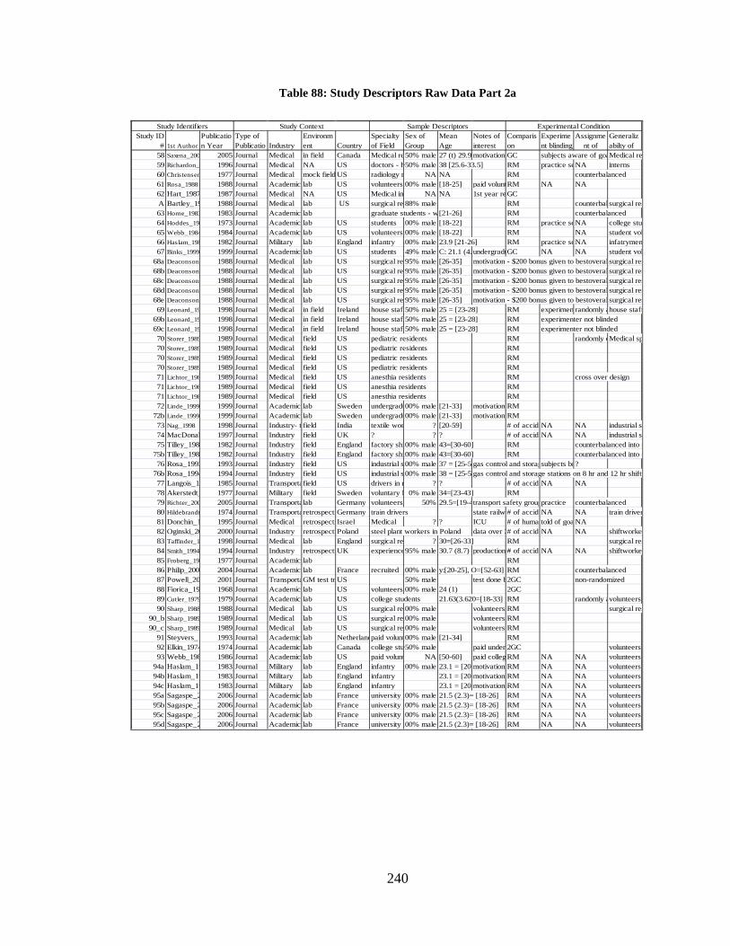
240
Table 88: Study Descriptors Raw Data Part 2a
58 Saxena_200 2005 Journal Medical in field Canada Medical re50% male 27 (t) 29.9 motivation GC subjects aware of goaMedical re59 Richardon_ 1996 Journal Medical NA US doctors - h >50% male 38 [25.6-33.5] RM practice seNA interns60 Christensen 1977 Journal Medical mock field US radiology r NA NA RM counterbalanced61 Rosa_1988 1988 Journal Academic lab US volunteers100% male [18-25] paid volunt RM NA NA62 Hart_1987 1987 Journal Medical NA US Medical int NA NA 1st year reGCA Bartley_19 1988 Journal Medical lab US surgical res88% male RM counterbalasurgical res63 Horne_1983 1983 Journal Academic lab graduate students - w [21-26] RM counterbalanced64 Hoddes_19 1973 Journal Academic lab US students 100% male [18-22] RM practice seNA college stud 65 Webb_1984 1984 Journal Academic lab US volunteers100% male [18-22] RM NA student vol66 Haslam_198 1982 Journal Military lab England infantry 100% male 23.9 [21-26] RM practice seNA infatrymen67 Binks_1999 1999 Journal Academic lab US students 49% male C: 21.1 (4. undergradu GC NA NA student vol
68a Deaconson_ 1988 Journal Medical lab US surgical re 95% male [26-35] motivation - $200 bonus given to bestoverallsurgical res68b Deaconson_ 1988 Journal Medical lab US surgical re 95% male [26-35] motivation - $200 bonus given to bestoverallsurgical res68c Deaconson_ 1988 Journal Medical lab US surgical re 95% male [26-35] motivation - $200 bonus given to bestoverallsurgical res68d Deaconson_ 1988 Journal Medical lab US surgical re 95% male [26-35] motivation - $200 bonus given to bestoverallsurgical res68e Deaconson_ 1988 Journal Medical lab US surgical re 95% male [26-35] motivation - $200 bonus given to bestoverallsurgical res69 Leonard_19 1998 Journal Medical in field Ireland house staff 50% male 25 = [23-28] RM experiment randomly a house staff
69b Leonard_19 1998 Journal Medical in field Ireland house staff 50% male 25 = [23-28] RM experimenter not blinded69c Leonard_19 1998 Journal Medical in field Ireland house staff 50% male 25 = [23-28] RM experimenter not blinded70 Storer_1989 1989 Journal Medical field US pediatric residents RM randomly d Medical sp 70 Storer_1989 1989 Journal Medical field US pediatric residents RM70 Storer_1989 1989 Journal Medical field US pediatric residents RM70 Storer_1989 1989 Journal Medical field US pediatric residents RM71 Lichtor_198 1989 Journal Medical field US anesthia residents RM cross over design71 Lichtor_198 1989 Journal Medical field US anesthia residents RM71 Lichtor_198 1989 Journal Medical field US anesthia residents RM72 Linde_1999 1999 Journal Academic lab Sweden undergradu 100% male [21-33] motivation RM
72b Linde_1999 1999 Journal Academic lab Sweden undergradu 100% male [21-33] motivation RM73 Nag_1998 1998 Journal Industry- tefield India textile wor ? [20-59] # of accideNA NA industrial s74 MacDonal 1997 Journal Industry field UK ? ? ? # of accideNA NA industrial s75 Tilley_198 1982 Journal Industry field England factory shi100% male 43=[30-60] RM counterbalanced into s
75b Tilley_198 1982 Journal Industry field England factory shi100% male 43=[30-60] RM counterbalanced into s76 Rosa_1993 1993 Journal Industry field US industrial s100% male 37 = [25-59gas control and storag subjects br ?
76b Rosa_1994 1994 Journal Industry field US industrial s100% male 38 = [25-59gas control and storage stations on 8 hr and 12 hr shifts77 Langois_1 1985 Journal Transportafield US drivers in r ? ? # of accideNA NA78 Akerstedt_ 1977 Journal Military field Sweden voluntary M 0% male 34=[23-43] RM79 Richter_200 2005 Journal Transportalab Germany volunteers 50% 29.5=[19-4transport safety grouppractice counterbalanced80 Hildebrandt 1974 Journal Transportaretrospecti Germany train drivers state railw # of accideNA NA train driver81 Donchin_1 1995 Journal Medical retrospecti Israel Medical ? ? ICU # of human told of goa NA82 Oginski_20 2000 Journal Industry retrospecti Poland steel plant workers in Poland data over 3 # of accideNA NA shiftworke83 Taffinder_1 1998 Journal Medical lab England surgical res ? 30=[26-33] RM surgical res84 Smith_1994 1994 Journal Industry retrospecti UK experience 95% male 30.7 (8.7) production # of accideNA NA shiftworker85 Froberg_19 1977 Journal Academic lab RM86 Philip_200 2004 Journal Academic lab France recruited 100% male y:[20-25], O=[52-63] RM counterbalanced87 Powell_20 2001 Journal TransportaGM test tr US 50% male test done b 2GC non-randomized88 Fiorica_19 1968 Journal Academic lab US volunteers100% male 24 (1) 2GC89 Cutler_1979 1979 Journal Academic lab US college students 21.63(3.620=[18-33] RM randomly avolunteers90 Sharp_1988 1988 Journal Medical lab US surgical re100% male volunteers RM surgical res
90_b Sharp_1989 1989 Journal Medical lab US surgical re100% male volunteers RM90_c Sharp_1989 1989 Journal Medical lab US surgical re100% male volunteers RM
91 Steyvers_1 1993 Journal Academic lab Netherlandpaid volunt100% male [21-34] RM92 Elkin_1974 1974 Journal Academic lab Canada college stu~50% male paid under 2GC volunteers93 Webb_198 1986 Journal Academic lab US paid volunt NA [50-60] paid colleg RM NA NA volunteers
94a Haslam_19 1983 Journal Military lab England infantry 100% male 23.1 = [20-motivation RM NA NA volunteers94b Haslam_19 1983 Journal Military lab England infantry 23.1 = [20-motivation RM NA NA volunteers94c Haslam_19 1983 Journal Military lab England infantry 23.1 = [20-motivation RM NA NA volunteers95a Sagaspe_2 2006 Journal Academic lab France university s100% male 21.5 (2.3)= [18-26] RM NA NA volunteers95b Sagaspe_2 2006 Journal Academic lab France university s100% male 21.5 (2.3)= [18-26] RM NA NA volunteers95c Sagaspe_2 2006 Journal Academic lab France university s100% male 21.5 (2.3)= [18-26] RM NA NA volunteers95d Sagaspe_2 2006 Journal Academic lab France university s100% male 21.5 (2.3)= [18-26] RM NA NA volunteers
CountrySpecialty of Field
Sex of Group
Mean Age
Notes of interest
Comparison
Study Identifiers Study Context Sample Descriptors Experimental ConditionStudy ID
# 1st AuthorPublication Year
Type of Publicatio Industry
Environment
Experiment blinding
Assignment of
Generalizabilty of
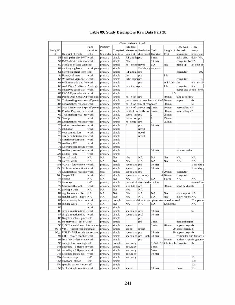
241
Table 89: Study Descriptors Raw Data Part 2b
58 5 min palm pilot PVT work primary simple RT and lappre 5 min palm pilot daily (NA 59 DAT-divided attention work primary simple NA 15 min computer ba NA60 Mock up of lung with self primary simple no - detect novel NA NA mock up 2x both con 61 auditory vigilance work pace primary simple Baddley gr depends62 Sternberg short term self primary simple RT and ac pre computer 192A Battery of tests work primary simple yes pre 1 hr63 Wilikinson vigilance tawork primary simple false repor pre computer 1264 Wilkinson add and Vi work primary simple pre Wil Add - 1hr 4 x per 16h 65 Aud Vig - Addition - Aud vig - w primary simple no - # corr pre 1 hr computer 5 x66 military tactical task - work primary simple paper and pencil - or eq 67 PASAT(paced audito work primary simple 2.5
68a Paced Aud Serial Ad work pace primary simple no - # of c pre 30 min tape recorde 6x68b Trail-making test - tes self paced primary simple yes - time to complete and # of 30 min paper 6x68c Grammatical reasoninwork primary simple no - # of correct responses 30 min 6x68d Mod Minnestota Pape self paced primary simple no - # of correct resp3 min 30 min assembling it?68e Purdue Pegboard - te work primary simple no # of correctly cons 3 min 30 min assembling it?69 Trail-making test - tes work primary simple score- time pre ? 25 min
69b Stroop work primary simple no- score i pre ? 25 min69c Grammatical reasoninwork primary simple no- score i pre ? 25 min70 written cogntive test work primary simple ? pre 20 min70 intubation work primary simple novel70 vein cannulation work primary simple novel70 artery catheterization work primary simple novel71 visual reaction time work primary simple71 Auditory RT work primary simple71 Coordination accurac work primary simple72 Auditory Attention taswork primary simple 30 min tape recorder
72b Coding Task work primary simple73 normal work NA NA NA NA NA NA NA NA NA74 normal work NA NA NA NA NA NA NA NA NA
75a 4CRT - four choice re work primary simple speed and pre 10 min 1 per day p 75b SRT- serial reaction twork primary simple speed pre 10 min 1 per day p 76 Grammatical reasonin work dual simple speed and pre 4 20 min computer
76b Simple RT work dual simple speed and accuracy 4 20 min computer77 driving NA NA NA NA NA NA 1 year NA NA78 Shooting self primary simple yes - # of shots and # of hits ~tested eve 79 Mackworth clock work primary simple # of hits an pre 60 min hand held pa8x80 driving a train NA NA NA NA NA81 regular work - filled o NA NA NA NA NA NA NA error report NA82 regular work - injury rNA NA NA NA NA NA NA injury report NA83 virtual reality laparosc work primary complex errors and time to complete, stress and arousal 20 x per se84 regular work NA NA NA NA NA NA 12 months NA85 work primary simple86 simple reaction time - work primary simple speed and pre? 10 min 6x87 simple reaction time - work primary simple speed and pre? 10 min88 Kugelmaschin - place self primary simple pre 89 memory test - list of 2 self primary simple pre 3 min pen and paper90 1) SST - serial search task - look primary simple speed 1 min 20 min apple compu4x
90_b VRT - verbal reasoning task - s primary simple speed preish 20 apple compu4x90_c USRT - Wilkinson's unprepared primary simple speed and pre 15 min 20 apple compu4x
91 CRT- choice reaction work primary simple speed and pre - tasko30 min tv monitor and buttons o 92 list of six 3-digit # aud work primary simple pre 35 min auditory - pe 6x (pace o 93 college level reading c self primary complex accuracy 1) 5 & 3, 2 4 hr test blcomputer 3x
94a encoding - 6 figure m work primary simple accuracy 5 min94b decoding - 6 figure m work primary simple accuracy 5min94c decoding messages work primary simple accuracy 10 min95a classic stroop self primary simple accuracy 10x95b emotional stroop self primary simple 10x95c specific stroop - word self primary simple 10x95d SRT - simple reaction work primary simple speed 10 min Palm 10x
How was the task administer
How many times was
Study ID #
Characteristics of task
Descript of Task
Pace (work or self)
Primary or Secondar
Complexity of task
Multiple Measures taken at
Predefined or novel
Task Duration
Length of Test
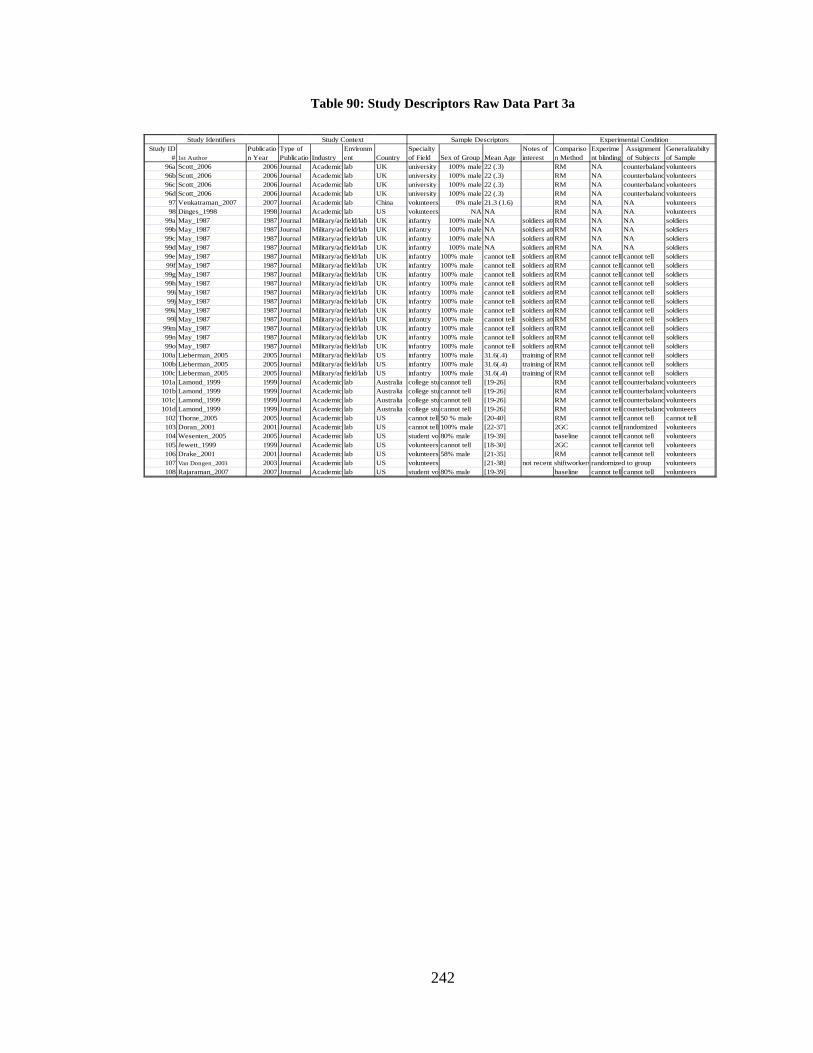
242
Table 90: Study Descriptors Raw Data Part 3a
96a Scott_2006 2006 Journal Academic lab UK university s 100% male 22 (.3) RM NA counterbalanc volunteers96b Scott_2006 2006 Journal Academic lab UK university s 100% male 22 (.3) RM NA counterbalanc volunteers96c Scott_2006 2006 Journal Academic lab UK university s 100% male 22 (.3) RM NA counterbalanc volunteers96d Scott_2006 2006 Journal Academic lab UK university s 100% male 22 (.3) RM NA counterbalanc volunteers97 Venkatraman_2007 2007 Journal Academic lab China volunteers 0% male 21.3 (1.6) RM NA NA volunteers98 Dinges_1998 1998 Journal Academic lab US volunteers NA NA RM NA NA volunteers
99a May_1987 1987 Journal Military/acfield/lab UK infantry 100% male NA soldiers att RM NA NA soldiers99b May_1987 1987 Journal Military/acfield/lab UK infantry 100% male NA soldiers att RM NA NA soldiers99c May_1987 1987 Journal Military/acfield/lab UK infantry 100% male NA soldiers att RM NA NA soldiers99d May_1987 1987 Journal Military/acfield/lab UK infantry 100% male NA soldiers att RM NA NA soldiers99e May_1987 1987 Journal Military/acfield/lab UK infantry 100% male cannot tell soldiers att RM cannot tell cannot tell soldiers99f May_1987 1987 Journal Military/acfield/lab UK infantry 100% male cannot tell soldiers att RM cannot tell cannot tell soldiers99g May_1987 1987 Journal Military/acfield/lab UK infantry 100% male cannot tell soldiers att RM cannot tell cannot tell soldiers99h May_1987 1987 Journal Military/acfield/lab UK infantry 100% male cannot tell soldiers att RM cannot tell cannot tell soldiers99i May_1987 1987 Journal Military/acfield/lab UK infantry 100% male cannot tell soldiers att RM cannot tell cannot tell soldiers99j May_1987 1987 Journal Military/acfield/lab UK infantry 100% male cannot tell soldiers att RM cannot tell cannot tell soldiers
99k May_1987 1987 Journal Military/acfield/lab UK infantry 100% male cannot tell soldiers att RM cannot tell cannot tell soldiers99l May_1987 1987 Journal Military/acfield/lab UK infantry 100% male cannot tell soldiers att RM cannot tell cannot tell soldiers
99m May_1987 1987 Journal Military/acfield/lab UK infantry 100% male cannot tell soldiers att RM cannot tell cannot tell soldiers99n May_1987 1987 Journal Military/acfield/lab UK infantry 100% male cannot tell soldiers att RM cannot tell cannot tell soldiers99o May_1987 1987 Journal Military/acfield/lab UK infantry 100% male cannot tell soldiers att RM cannot tell cannot tell soldiers
100a Lieberman_2005 2005 Journal Military/acfield/lab US infantry 100% male 31.6(.4) training of RM cannot tell cannot tell soldiers100b Lieberman_2005 2005 Journal Military/acfield/lab US infantry 100% male 31.6(.4) training of RM cannot tell cannot tell soldiers100c Lieberman_2005 2005 Journal Military/acfield/lab US infantry 100% male 31.6(.4) training of RM cannot tell cannot tell soldiers101a Lamond_1999 1999 Journal Academic lab Australia college stucannot tell [19-26] RM cannot tell counterbalanc volunteers101b Lamond_1999 1999 Journal Academic lab Australia college stucannot tell [19-26] RM cannot tell counterbalanc volunteers101c Lamond_1999 1999 Journal Academic lab Australia college stucannot tell [19-26] RM cannot tell counterbalanc volunteers101d Lamond_1999 1999 Journal Academic lab Australia college stucannot tell [19-26] RM cannot tell counterbalanc volunteers102 Thorne_2005 2005 Journal Academic lab US cannot tell 50 % male [20-40] RM cannot tell cannot tell cannot tell103 Doran_2001 2001 Journal Academic lab US cannot tell 100% male [22-37] 2GC cannot tell randomized volunteers104 Wesenten_2005 2005 Journal Academic lab US student vol80% male [19-39] baseline cannot tell cannot tell volunteers105 Jewett_1999 1999 Journal Academic lab US volunteers cannot tell [18-30] 2GC cannot tell cannot tell volunteers106 Drake_2001 2001 Journal Academic lab US volunteers 58% male [21-35] RM cannot tell cannot tell volunteers107 Van Dongen_2003 2003 Journal Academic lab US volunteers [21-38] not recent shiftworkersrandomized to group volunteers108 Rajaraman_2007 2007 Journal Academic lab US student vol80% male [19-39] baseline cannot tell cannot tell volunteers
Generalizabilty of SampleCountry
Specialty of Field Sex of Group Mean Age
Notes of interest
Comparison Method
Study Identifiers Study Context Sample Descriptors Experimental ConditionStudy ID
# 1st AuthorPublication Year
Type of Publicatio Industry
Environment
Experiment blinding
Assignment of Subjects
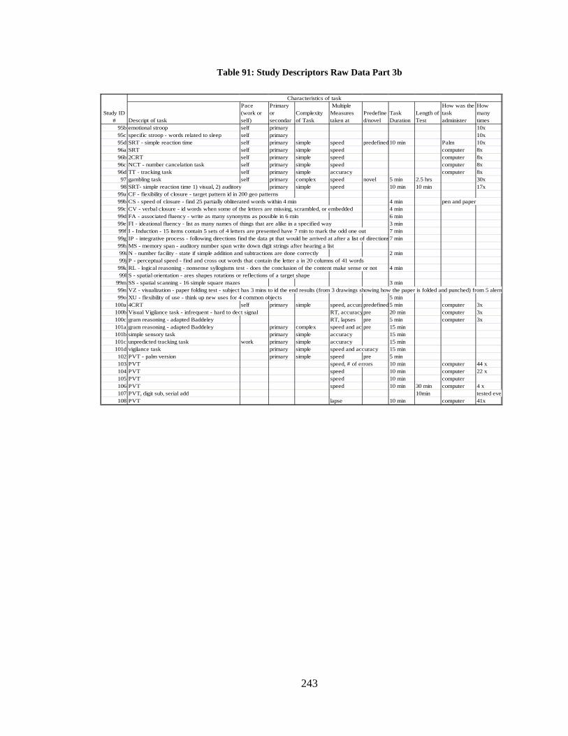
243
Table 91: Study Descriptors Raw Data Part 3b
95b emotional stroop self primary 10x95c specific stroop - words related to sleep self primary 10x95d SRT - simple reaction time self primary simple speed predefined10 min Palm 10x96a SRT self primary simple speed computer 8x96b 2CRT self primary simple speed computer 8x96c NCT - number cancelation task self primary simple speed computer 8x96d TT - tracking task self primary simple accuracy computer 8x97 gambling task self primary complex speed novel 5 min 2.5 hrs 30x98 SRT- simple reaction time 1) visual, 2) auditory primary simple speed 10 min 10 min 17x
99a CF - flexibility of closure - target pattern id in 200 geo patterns99b CS - speed of closure - find 25 partially obliterated words within 4 min 4 min pen and paper99c CV - verbal closure - id words when some of the letters are missing, scrambled, or embedded 4 min99d FA - associated fluency - write as many synonyms as possible in 6 min 6 min99e FI - ideational fluency - list as many names of things that are alike in a specified way 3 min99f I - Induction - 15 items contain 5 sets of 4 letters are presented have 7 min to mark the odd one out 7 min99g IP - integrative process - following directions find the data pt that would be arrived at after a list of directions7 min99h MS - memory span - auditory number span write down digit strings after hearing a list99i N - number facility - state if simple addition and subtractions are done correctly 2 min99j P - perceptual speed - find and cross out words that contain the letter a in 20 columns of 41 words
99k RL - logical reasoning - nonsense syllogisms test - does the conclusion of the content make sense or not 4 min99l S - spatial orientation - ares shapes rotations or reflections of a target shape
99m SS - spatial scanning - 16 simple square mazes 3 min99n VZ - visualization - paper folding test - subject has 3 mins to id the end results (from 3 drawings showing how the paper is folded and punched) from 5 alern99o XU - flexibility of use - think up new uses for 4 common objects 5 min
100a 4CRT self primary simple speed, accura predefined5 min computer 3x100b Visual Vigilance task - infrequent - hard to dect signal RT, accuracy pre 20 min computer 3x100c gram reasoning - adapted Baddeley RT, lapses pre 5 min computer 3x101a gram reasoning - adapted Baddeley primary complex speed and accpre 15 min101b simple sensory task primary simple accuracy 15 min101c unpredicted tracking task work primary simple accuracy 15 min101d vigilance task primary simple speed and accuracy 15 min102 PVT - palm version primary simple speed pre 5 min103 PVT speed, # of errors 10 min computer 44 x104 PVT speed 10 min computer 22 x105 PVT speed 10 min computer106 PVT speed 10 min 30 min computer 4 x10⁷ PVT, digit sub, serial add 10min tested ever 108 PVT lapse 10 min computer 41x
How was the task administer
How many times
Study ID #
Characteristics of task
Descript of task
Pace (work or self)
Primary or secondar
Complexity of Task
Multiple Measures taken at
Predefined/novel
Task Duration
Length of Test
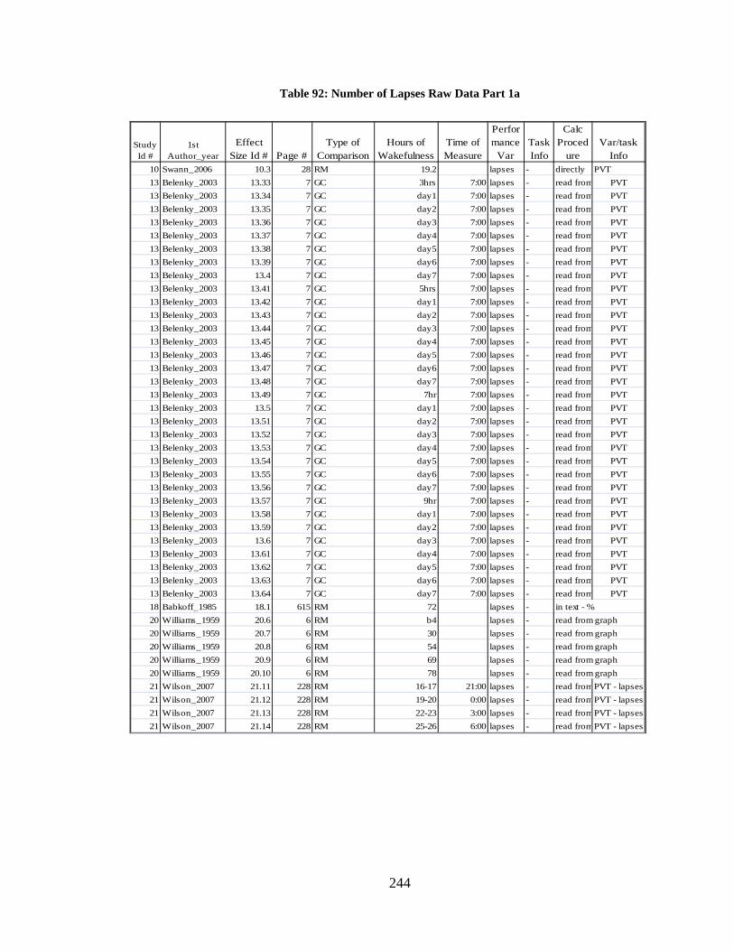
244
Table 92: Number of Lapses Raw Data Part 1a
10 Swann_2006 10.3 28 RM 19.2 lapses - directly PVT13 Belenky_2003 13.33 7 GC 3hrs 7:00 lapses - read from PVT13 Belenky_2003 13.34 7 GC day1 7:00 lapses - read from PVT13 Belenky_2003 13.35 7 GC day2 7:00 lapses - read from PVT13 Belenky_2003 13.36 7 GC day3 7:00 lapses - read from PVT13 Belenky_2003 13.37 7 GC day4 7:00 lapses - read from PVT13 Belenky_2003 13.38 7 GC day5 7:00 lapses - read from PVT13 Belenky_2003 13.39 7 GC day6 7:00 lapses - read from PVT13 Belenky_2003 13.4 7 GC day7 7:00 lapses - read from PVT13 Belenky_2003 13.41 7 GC 5hrs 7:00 lapses - read from PVT13 Belenky_2003 13.42 7 GC day1 7:00 lapses - read from PVT13 Belenky_2003 13.43 7 GC day2 7:00 lapses - read from PVT13 Belenky_2003 13.44 7 GC day3 7:00 lapses - read from PVT13 Belenky_2003 13.45 7 GC day4 7:00 lapses - read from PVT13 Belenky_2003 13.46 7 GC day5 7:00 lapses - read from PVT13 Belenky_2003 13.47 7 GC day6 7:00 lapses - read from PVT13 Belenky_2003 13.48 7 GC day7 7:00 lapses - read from PVT13 Belenky_2003 13.49 7 GC 7hr 7:00 lapses - read from PVT13 Belenky_2003 13.5 7 GC day1 7:00 lapses - read from PVT13 Belenky_2003 13.51 7 GC day2 7:00 lapses - read from PVT13 Belenky_2003 13.52 7 GC day3 7:00 lapses - read from PVT13 Belenky_2003 13.53 7 GC day4 7:00 lapses - read from PVT13 Belenky_2003 13.54 7 GC day5 7:00 lapses - read from PVT13 Belenky_2003 13.55 7 GC day6 7:00 lapses - read from PVT13 Belenky_2003 13.56 7 GC day7 7:00 lapses - read from PVT13 Belenky_2003 13.57 7 GC 9hr 7:00 lapses - read from PVT13 Belenky_2003 13.58 7 GC day1 7:00 lapses - read from PVT13 Belenky_2003 13.59 7 GC day2 7:00 lapses - read from PVT13 Belenky_2003 13.6 7 GC day3 7:00 lapses - read from PVT13 Belenky_2003 13.61 7 GC day4 7:00 lapses - read from PVT13 Belenky_2003 13.62 7 GC day5 7:00 lapses - read from PVT13 Belenky_2003 13.63 7 GC day6 7:00 lapses - read from PVT13 Belenky_2003 13.64 7 GC day7 7:00 lapses - read from PVT18 Babkoff_1985 18.1 615 RM 72 lapses - in text - %20 Williams_1959 20.6 6 RM b4 lapses - read from graph20 Williams_1959 20.7 6 RM 30 lapses - read from graph20 Williams_1959 20.8 6 RM 54 lapses - read from graph20 Williams_1959 20.9 6 RM 69 lapses - read from graph20 Williams_1959 20.10 6 RM 78 lapses - read from graph21 Wilson_2007 21.11 228 RM 16-17 21:00 lapses - read from PVT - lapses21 Wilson_2007 21.12 228 RM 19-20 0:00 lapses - read from PVT - lapses21 Wilson_2007 21.13 228 RM 22-23 3:00 lapses - read from PVT - lapses21 Wilson_2007 21.14 228 RM 25-26 6:00 lapses - read from PVT - lapses
Hours of Wakefulness
Study Id #
1st Author_year
Effect Size Id # Page #
Type of Comparison
Time of Measure
Performance
VarTask Info
Calc Proced
ureVar/task
Info
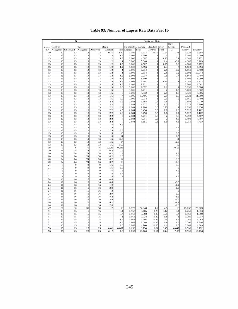
245
Table 93: Number of Lapses Raw Data Part 1b
Diff Mean
Assigned Observed Assigned Observed Control Test Control Test Control Test T-C10 12 12 12 12 0.71 2.42 0.589 2.217 0.17 0.64 1.71 1.622 2.29413 13 13 13 13 1.2 1.2 3.606 3.606 1 1 0 3.606 5.09913 13 13 13 13 1.2 1.3 3.606 4.507 1 1.25 0.1 4.081 5.77213 13 13 13 13 1.2 1 3.606 5.048 1 1.4 -0.2 4.386 6.20313 13 13 13 13 1.2 1.5 3.606 4.507 1 1.25 0.3 4.081 5.77213 13 13 13 13 1.2 1.2 3.606 8.653 1 2.4 0 6.629 9.37413 13 13 13 13 1.2 1 3.606 9.014 1 2.5 -0.2 6.865 9.70813 13 13 13 13 1.2 1 3.606 9.374 1 2.6 -0.2 7.102 10.04413 13 13 13 13 1.2 1.6 3.606 9.014 1 2.5 0.4 6.865 9.70813 13 13 13 13 1.5 1.5 3.606 3.606 1 1 0 3.606 5.09913 13 13 13 13 1.5 1.6 3.606 4.507 1 1.25 0.1 4.081 5.77213 13 13 13 13 1.5 1.5 3.606 7.211 1 2 0 5.701 8.06213 13 13 13 13 1.5 2.5 3.606 7.572 1 2.1 1 5.930 8.38613 13 13 13 13 1.5 3 3.606 7.211 1 2 1.5 5.701 8.06213 13 13 13 13 1.5 3 3.606 7.572 1 2.1 1.5 5.930 8.38613 13 13 13 13 1.5 4 3.606 10.456 1 2.9 2.5 7.821 11.06013 13 13 13 13 1.5 3.5 3.606 9.014 1 2.5 2 6.865 9.70813 13 13 13 13 2.2 2.2 2.884 2.884 0.8 0.8 0 2.884 4.07913 13 13 13 13 2.2 3 2.884 4.327 0.8 1.2 0.8 3.677 5.20013 13 13 13 13 2.2 3.2 2.884 2.704 0.8 0.75 1 2.796 3.95413 13 13 13 13 2.2 4.5 2.884 6.490 0.8 1.8 2.3 5.022 7.10213 13 13 13 13 2.2 4.9 2.884 6.490 0.8 1.8 2.7 5.022 7.10213 13 13 13 13 2.2 6 2.884 7.211 0.8 2 3.8 5.492 7.76713 13 13 13 13 2.2 7 2.884 7.211 0.8 2 4.8 5.492 7.76713 13 13 13 13 2.2 7 2.884 6.851 0.8 1.9 4.8 5.256 7.43313 13 13 13 13 1.5 1.5 013 13 13 13 13 1.5 4 2.513 13 13 13 13 1.5 5.5 413 13 13 13 13 1.5 10 8.513 13 13 13 13 1.5 11 9.513 13 13 13 13 1.5 12.5 1113 13 13 13 13 1.5 14 12.513 13 13 13 13 1.5 17.5 1618 6 6 6 6 0.026 0.206 0.1820 74 74 74 74 0.2 0.2 020 74 74 74 74 0.2 2 1.820 74 74 74 74 0.2 6.5 6.320 74 74 74 74 0.2 14 13.820 74 74 74 74 0.2 18 17.821 9 9 9 9 1.5 0.9 -0.621 9 9 9 9 1.5 3.5 221 9 9 9 9 1.5 3 1.521 9 9 9 9 1.5 8.5 721 9 9 9 9 1.5 3 1.524 16 16 16 16 0.824 16 16 16 16 0.8 -0.824 16 16 16 16 1.2 -1.224 16 16 16 16 2.9 -2.924 16 16 16 16 3 -324 16 16 16 16 2.9 -2.924 16 16 16 16 3.2 -3.224 16 16 16 16 2.9 -2.924 16 16 16 16 4.1 -4.124 16 16 16 16 2.8 -2.847 30 30 30 30 2 18 6.573 24.648 1.2 4.5 16 18.037 25.50951 15 15 15 15 0.1 0.968 0.465 0.25 0.12 0.1 0.759 1.07451 15 15 15 15 0.4 0.968 0.968 0.25 0.25 0.4 0.968 1.36951 15 15 15 15 1 0.968 2.324 0.25 0.6 1 1.780 2.51751 15 15 15 15 1.4 0.968 2.905 0.25 0.75 1.4 2.165 3.06251 15 15 15 15 1.6 0.968 3.098 0.25 0.8 1.6 2.295 3.24651 15 15 15 15 2.5 0.968 4.260 0.25 1.1 2.5 3.089 4.36953 25 25 25 25 0.02 0.867 0.050 0.750 0.01 0.15 0.847 0.532 0.75253 25 25 25 25 0.17 7.8 0.850 10.700 0.17 2.14 7.63 7.590 10.734
Study Id #
N Statistical Data
Control Test Mean Standard Deviation Standard Error Poooled Stdev B Stdev
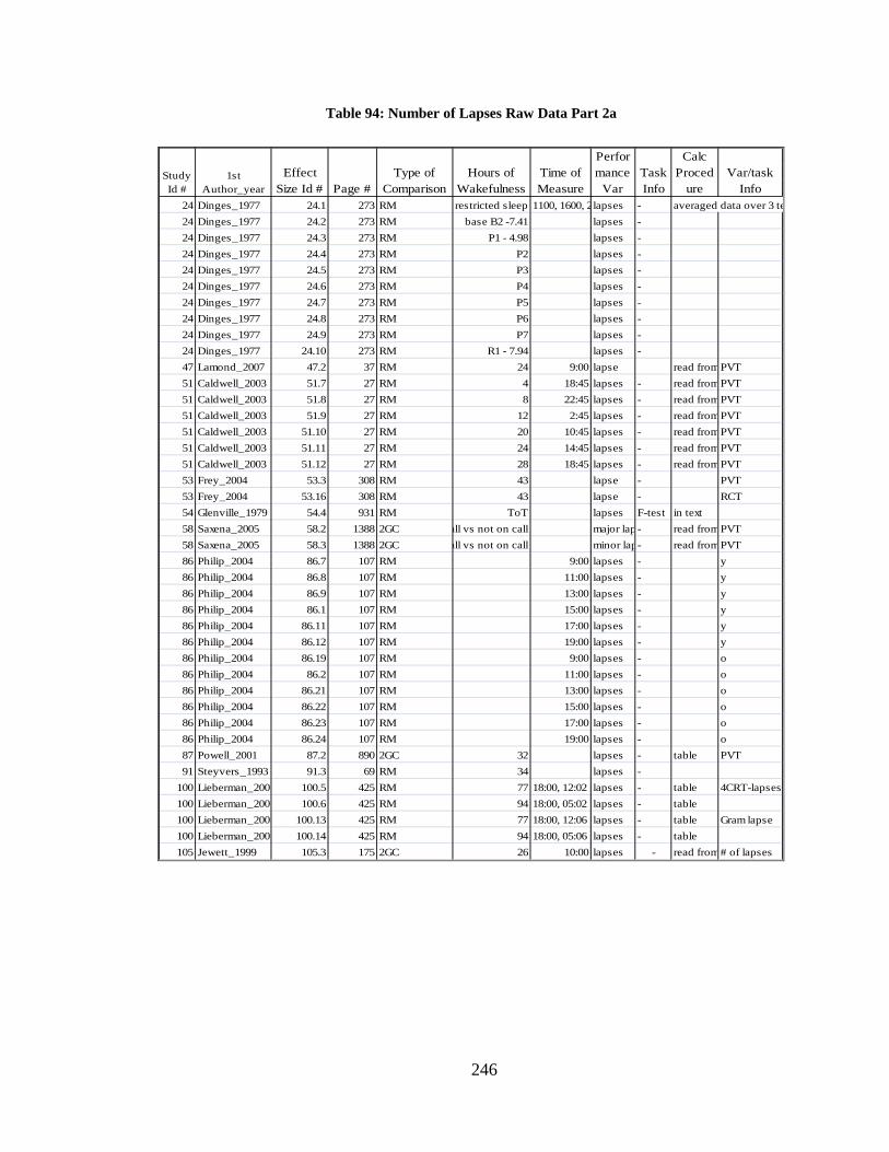
246
Table 94: Number of Lapses Raw Data Part 2a
24 Dinges_1977 24.1 273 RM restricted sleep 1100, 1600, 2lapses - averaged data over 3 te24 Dinges_1977 24.2 273 RM base B2 -7.41 lapses -24 Dinges_1977 24.3 273 RM P1 - 4.98 lapses -24 Dinges_1977 24.4 273 RM P2 lapses -24 Dinges_1977 24.5 273 RM P3 lapses -24 Dinges_1977 24.6 273 RM P4 lapses -24 Dinges_1977 24.7 273 RM P5 lapses -24 Dinges_1977 24.8 273 RM P6 lapses -24 Dinges_1977 24.9 273 RM P7 lapses -24 Dinges_1977 24.10 273 RM R1 - 7.94 lapses -47 Lamond_2007 47.2 37 RM 24 9:00 lapse read from PVT51 Caldwell_2003 51.7 27 RM 4 18:45 lapses - read from PVT51 Caldwell_2003 51.8 27 RM 8 22:45 lapses - read from PVT51 Caldwell_2003 51.9 27 RM 12 2:45 lapses - read from PVT51 Caldwell_2003 51.10 27 RM 20 10:45 lapses - read from PVT51 Caldwell_2003 51.11 27 RM 24 14:45 lapses - read from PVT51 Caldwell_2003 51.12 27 RM 28 18:45 lapses - read from PVT53 Frey_2004 53.3 308 RM 43 lapse - PVT53 Frey_2004 53.16 308 RM 43 lapse - RCT54 Glenville_1979 54.4 931 RM ToT lapses F-test in text58 Saxena_2005 58.2 1388 2GC all vs not on call major lap - read from PVT58 Saxena_2005 58.3 1388 2GC all vs not on call minor lap- read from PVT86 Philip_2004 86.7 107 RM 9:00 lapses - y86 Philip_2004 86.8 107 RM 11:00 lapses - y86 Philip_2004 86.9 107 RM 13:00 lapses - y86 Philip_2004 86.1 107 RM 15:00 lapses - y86 Philip_2004 86.11 107 RM 17:00 lapses - y86 Philip_2004 86.12 107 RM 19:00 lapses - y86 Philip_2004 86.19 107 RM 9:00 lapses - o86 Philip_2004 86.2 107 RM 11:00 lapses - o86 Philip_2004 86.21 107 RM 13:00 lapses - o86 Philip_2004 86.22 107 RM 15:00 lapses - o86 Philip_2004 86.23 107 RM 17:00 lapses - o86 Philip_2004 86.24 107 RM 19:00 lapses - o87 Powell_2001 87.2 890 2GC 32 lapses - table PVT91 Steyvers_1993 91.3 69 RM 34 lapses -
100 Lieberman_2005 100.5 425 RM 77 18:00, 12:02 lapses - table 4CRT-lapses100 Lieberman_2005 100.6 425 RM 94 18:00, 05:02 lapses - table100 Lieberman_2005 100.13 425 RM 77 18:00, 12:06 lapses - table Gram lapse100 Lieberman_2005 100.14 425 RM 94 18:00, 05:06 lapses - table105 Jewett_1999 105.3 175 2GC 26 10:00 lapses - read from # of lapses
Time of Measure
Performance
VarTask Info
Calc Proced
ureVar/task
InfoHours of
WakefulnessStudy Id #
1st Author_year
Effect Size Id # Page #
Type of Comparison

247
Table 95: Number of Lapses Raw Data Part 2b
Diff Mean
Assigned Observed Assigned Observed Control Test Control Test Control Test T-C54 11 11 11 11 F-stat58 7 7 13 13 1.53 2.5 0.920 103.000 0.97 84.101 103.00458 7 7 13 13 1.5 2.9 0.910 2.200 1.4 1.872 2.38186 10 10 10 10 1 7 4.048 12.333 1.28 3.9 6 9.178 12.98086 10 10 10 10 1 2 4.902 15.558 1.55 4.92 1 11.534 16.31286 10 10 10 10 1 3 5.629 12.681 1.78 4.01 2 9.810 13.87486 10 10 10 10 2 5.5 3.036 18.310 0.96 5.79 3.5 13.124 18.56086 10 10 10 10 1.5 4 4.838 17.108 1.53 5.41 2.5 12.572 17.77986 10 10 10 10 1 3.5 6.894 8.918 2.18 2.82 2.5 7.970 11.27286 10 10 10 10 5 7 21.788 22.927 6.89 7.25 2 22.365 31.62886 10 10 10 10 12.5 12.5 21.946 23.844 6.94 7.54 0 22.915 32.40686 10 10 10 10 15.5 12.5 20.681 30.864 6.54 9.76 -3 26.271 37.15286 10 10 10 10 13.5 14.5 25.994 25.330 8.22 8.01 1 25.664 36.29486 10 10 10 10 20 11.5 27.069 34.943 8.56 11.05 -8.5 31.255 44.20186 10 10 10 10 23 17.5 27.607 40.699 8.73 12.87 -5.5 34.774 49.17887 8 8 8 8 0.62 4.4 0.600 4.500 3.78 3.210 4.54091 16 16 16 16 0 0.000 0.000
100 31 31 31 31 1.4 3.5 2.784 1.122 0.5 0.6 2.1 2.122 3.002100 31 31 31 31 1.4 3.7 2.784 1.154 0.5 0.6 2.3 2.131 3.014100 31 31 31 31 0.2 0.7 0.557 0.251 0.1 0.3 0.5 0.432 0.611100 31 31 31 31 0.2 0.7 0.557 0.251 0.1 0.3 0.5 0.432 0.611105 32 32 25 25 1.75 4.6 11.314 8.579 2 4 2.85 10.211 14.199107 12 12 13 13 8 8 0.000 0.000107 12 12 13 13 13 13 0.000 0.000107 12 12 13 13 15 15 0.000 0.000108 48 48 48 48 2.5 2.000 2.5 1.414 2.000108 48 48 48 48 2 1.750 2 1.237 1.750108 48 48 48 48 3.5 3.000 3.5 2.121 3.000108 48 48 48 48 4 4.500 4 3.182 4.500108 48 48 48 48 4.5 2.500 4.5 1.768 2.500108 48 48 48 48 5 5.500 5 3.889 5.500108 48 48 48 48 4.5 5.500 4.5 3.889 5.500108 48 48 48 48 3.5 2.750 3.5 1.945 2.750108 48 48 48 48 7.5 6.500 7.5 4.596 6.500108 48 48 48 48 8 7.000 8 4.950 7.000108 48 48 48 48 9 8.000 9 5.657 8.000108 48 48 48 48 10 9.000 10 6.364 9.000108 48 48 48 48 12 11.500 12 8.132 11.500108 48 48 48 48 11 12.500 11 8.839 12.500108 48 48 48 48 10 10.000 10 7.071 10.000108 48 48 48 48 9 10.000 9 7.071 10.000108 48 48 48 48 8 9.500 8 6.718 9.500108 48 48 48 48 9 11.000 9 7.778 11.000108 48 48 48 48 6 6.000 6 4.243 6.000108 48 48 48 48 7 5.000 7 3.536 5.000108 48 48 48 48 11 15.500 11 10.960 15.500108 48 48 48 48 17 16.000 17 11.314 16.000108 48 48 48 48 20 20.000 20 14.142 20.000108 48 48 48 48 25 20.000 25 14.142 20.000108 48 48 48 48 23 24.000 23 16.971 24.000108 48 48 48 48 22 19.000 22 13.435 19.000108 48 48 48 48 15 13.000 15 9.192 13.000108 48 48 48 48 14 15.000 14 10.607 15.000108 48 48 48 48 14 15.000 14 10.607 15.000108 48 48 48 48 14 16.000 14 11.314 16.000108 48 48 48 48 13 14.500 13 10.253 14.500108 48 48 48 48 9 7.500 9 5.303 7.500108 48 48 48 48 12 15.000 12 10.607 15.000108 48 48 48 48 19 21.000 19 14.849 21.000108 48 48 48 48 20 16.000 20 11.314 16.000108 48 48 48 48 22 15.000 22 10.607 15.000108 48 48 48 48 19 20.000 19 14.142 20.000108 48 48 48 48 21 25.500 21 18.031 25.500108 48 48 48 48 16 16.500 16 11.667 16.500108 48 48 48 48 12 10.000 12 7.071 10.000108 48 48 48 48 11 11.000 11 7.778 11.000108 48 48 48 48 9 11.000 9 7.778 11.000
Study Id #
N Statistical Data
Control Test Mean Standard Deviation Standard Error Poooled Stdev B Stdev
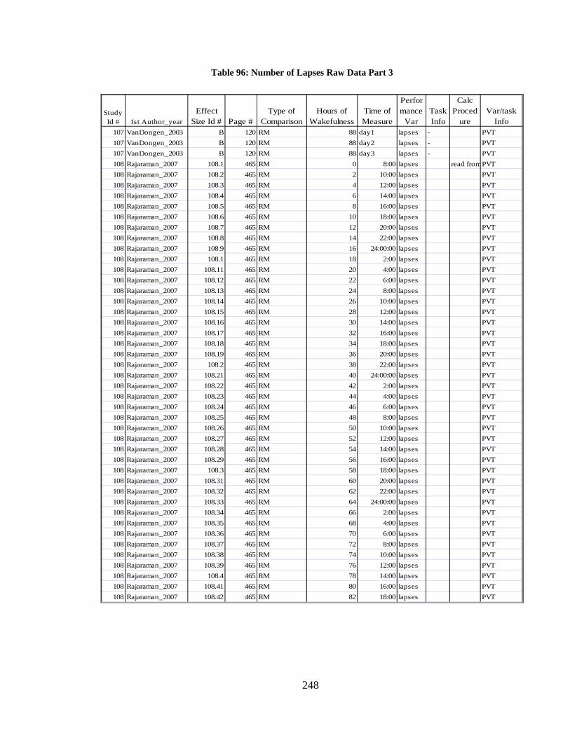
248
Table 96: Number of Lapses Raw Data Part 3
107 VanDongen_2003 B 120 RM 88 day1 lapses - PVT107 VanDongen_2003 B 120 RM 88 day2 lapses - PVT107 VanDongen_2003 B 120 RM 88 day3 lapses - PVT108 Rajaraman_2007 108.1 465 RM 0 8:00 lapses read from PVT108 Rajaraman_2007 108.2 465 RM 2 10:00 lapses PVT108 Rajaraman_2007 108.3 465 RM 4 12:00 lapses PVT108 Rajaraman_2007 108.4 465 RM 6 14:00 lapses PVT108 Rajaraman_2007 108.5 465 RM 8 16:00 lapses PVT108 Rajaraman_2007 108.6 465 RM 10 18:00 lapses PVT108 Rajaraman_2007 108.7 465 RM 12 20:00 lapses PVT108 Rajaraman_2007 108.8 465 RM 14 22:00 lapses PVT108 Rajaraman_2007 108.9 465 RM 16 24:00:00 lapses PVT108 Rajaraman_2007 108.1 465 RM 18 2:00 lapses PVT108 Rajaraman_2007 108.11 465 RM 20 4:00 lapses PVT108 Rajaraman_2007 108.12 465 RM 22 6:00 lapses PVT108 Rajaraman_2007 108.13 465 RM 24 8:00 lapses PVT108 Rajaraman_2007 108.14 465 RM 26 10:00 lapses PVT108 Rajaraman_2007 108.15 465 RM 28 12:00 lapses PVT108 Rajaraman_2007 108.16 465 RM 30 14:00 lapses PVT108 Rajaraman_2007 108.17 465 RM 32 16:00 lapses PVT108 Rajaraman_2007 108.18 465 RM 34 18:00 lapses PVT108 Rajaraman_2007 108.19 465 RM 36 20:00 lapses PVT108 Rajaraman_2007 108.2 465 RM 38 22:00 lapses PVT108 Rajaraman_2007 108.21 465 RM 40 24:00:00 lapses PVT108 Rajaraman_2007 108.22 465 RM 42 2:00 lapses PVT108 Rajaraman_2007 108.23 465 RM 44 4:00 lapses PVT108 Rajaraman_2007 108.24 465 RM 46 6:00 lapses PVT108 Rajaraman_2007 108.25 465 RM 48 8:00 lapses PVT108 Rajaraman_2007 108.26 465 RM 50 10:00 lapses PVT108 Rajaraman_2007 108.27 465 RM 52 12:00 lapses PVT108 Rajaraman_2007 108.28 465 RM 54 14:00 lapses PVT108 Rajaraman_2007 108.29 465 RM 56 16:00 lapses PVT108 Rajaraman_2007 108.3 465 RM 58 18:00 lapses PVT108 Rajaraman_2007 108.31 465 RM 60 20:00 lapses PVT108 Rajaraman_2007 108.32 465 RM 62 22:00 lapses PVT108 Rajaraman_2007 108.33 465 RM 64 24:00:00 lapses PVT108 Rajaraman_2007 108.34 465 RM 66 2:00 lapses PVT108 Rajaraman_2007 108.35 465 RM 68 4:00 lapses PVT108 Rajaraman_2007 108.36 465 RM 70 6:00 lapses PVT108 Rajaraman_2007 108.37 465 RM 72 8:00 lapses PVT108 Rajaraman_2007 108.38 465 RM 74 10:00 lapses PVT108 Rajaraman_2007 108.39 465 RM 76 12:00 lapses PVT108 Rajaraman_2007 108.4 465 RM 78 14:00 lapses PVT108 Rajaraman_2007 108.41 465 RM 80 16:00 lapses PVT108 Rajaraman_2007 108.42 465 RM 82 18:00 lapses PVT
Time of Measure
Performance
VarTask Info
Calc Proced
ureVar/task
InfoHours of
WakefulnessStudy Id # 1st Author_year
Effect Size Id # Page #
Type of Comparison
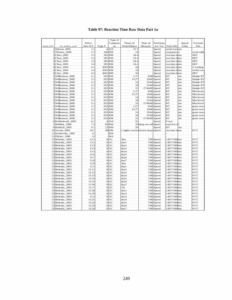
249
Table 97: Reaction Time Raw Data Part 1a
1 Nilsson_2005 1.1 4 2GC 31.5 Speed serial react ms2 Thomas_2000 2.1 346 RM 24 Speed responses/x serial addit 3 Choo_2005 3.1 581 RM 24.4 Speed reaction timms SRT3 Choo_2005 3.2 581 RM 24.4 Speed reaction timms SRT3 Choo_2005 3.3 581 RM 24.4 Speed reaction timms SRT3 Choo_2005 3.4 581 RM 24.4 Speed reaction timms SRT4 Chee_2004 4.1 4561 RM 24 Speed reaction timms 2 working m4 Chee_2004 4.2 4561 RM 24 Speed reaction timms verbal wor 4 Chee_2004 4.3 4561 RM 24 Speed reaction timms SRT5 Williamson_2000 5.1 652 RM 2.27 8:00 Speed RT ms Simple RT 5 Williamson_2000 5.1 652 RM 13.27 19:00 Speed RT ms Simple RT 5 Williamson_2000 5.1 652 RM 14 19:44 Speed RT ms Simple RT 5 Williamson_2000 5.1 652 RM 18 23:44 Speed RT ms Simple RT 5 Williamson_2000 5.1 652 RM 22 27:44:00 Speed RT ms Simple RT 5 Williamson_2000 5.1 652 RM 2.27 8:00 speed RT ms Mackworth 5 Williamson_2000 5.1 652 RM 13.27 19:00 speed RT ms Mackworth 5 Williamson_2000 5.1 652 RM 14 19:44 Speed RT ms Mackworth 5 Williamson_2000 5.1 652 RM 18 23:44 Speed RT ms Mackworth 5 Williamson_2000 5.1 652 RM 22 27:44:00 Speed RT ms Mackworth 5 Williamson_2000 5.1 652 RM 2.27 8:00 Speed RT ms gram reaso 5 Williamson_2000 5.1 652 RM 13.27 19:00 Speed RT ms gram reaso 5 Williamson_2000 5.1 652 RM 14 19:44 Speed RT ms gram reaso 5 Williamson_2000 5.1 652 RM 18 23:44 Speed RT ms gram reaso 5 Williamson_2000 5.1 652 RM 22 27:44:00 Speed RT ms gram reaso 6 Kobbeltvedt_2005 6.1 4 2GC 52 Speed F-test7 Robbins_1990 7.2 83 RM 35 sleep on-call Speed total test tim?9 Babkoff_2005 9.1 12 RM 24 Speed RT ms
10 Swann_2005 10.1 28 RM 2 nights restrict stricted sleep Speed reaction timms PVT11 Koslowsky_1992 11 MA -12 Pilcher_1996 12 MA -13 Belenky_2003 13.1 6 GC 3hrs 7:00 Speed 1/RT*1000ms PVT13 Belenky_2003 13.2 6 GC day1 7:00 Speed 1/RT*1000ms PVT13 Belenky_2003 13.3 6 GC day2 7:00 Speed 1/RT*1000ms PVT13 Belenky_2003 13.4 6 GC day3 7:00 Speed 1/RT*1000ms PVT13 Belenky_2003 13.5 6 GC day4 7:00 Speed 1/RT*1000ms PVT13 Belenky_2003 13.6 6 GC day5 7:00 Speed 1/RT*1000ms PVT13 Belenky_2003 13.7 6 GC day6 7:00 Speed 1/RT*1000ms PVT13 Belenky_2003 13.8 6 GC day7 7:00 Speed 1/RT*1000ms PVT13 Belenky_2003 13.9 6 GC 5hrs 7:00 Speed 1/RT*1000ms PVT13 Belenky_2003 13.1 6 GC day1 7:00 Speed 1/RT*1000ms PVT13 Belenky_2003 13.11 6 GC day2 7:00 Speed 1/RT*1000ms PVT13 Belenky_2003 13.12 6 GC day3 7:00 Speed 1/RT*1000ms PVT13 Belenky_2003 13.13 6 GC day4 7:00 Speed 1/RT*1000ms PVT13 Belenky_2003 13.14 6 GC day5 7:00 Speed 1/RT*1000ms PVT13 Belenky_2003 13.15 6 GC day6 7:00 Speed 1/RT*1000ms PVT13 Belenky_2003 13.16 6 GC day7 7:00 Speed 1/RT*1000ms PVT13 Belenky_2003 13.17 6 GC 7hr 7:00 Speed 1/RT*1000ms PVT13 Belenky_2003 13.18 6 GC day1 7:00 Speed 1/RT*1000ms PVT13 Belenky_2003 13.19 6 GC day2 7:00 Speed 1/RT*1000ms PVT13 Belenky_2003 13.2 6 GC day3 7:00 Speed 1/RT*1000ms PVT13 Belenky_2003 13.21 6 GC day4 7:00 Speed 1/RT*1000ms PVT13 Belenky_2003 13.22 6 GC day5 7:00 Speed 1/RT*1000ms PVT13 Belenky_2003 13.23 6 GC day6 7:00 Speed 1/RT*1000ms PVT13 Belenky_2003 13.24 6 GC day7 7:00 Speed 1/RT*1000ms PVT
Hours of WakefulnessStudy Id # 1st Author_year
Effect Size Id # Page #
Type of Comparis
onTime of Measure
Performance Var Task Info
Speed Units
Var/task Info
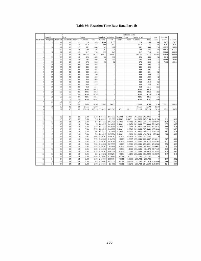
250
Table 98: Reaction Time Raw Data Part 1b
Assigned Observed Assigned Observed Control Test Control Test Control Test Control Test1 11 11 11 11 225 265 43.44 62.35 225 265 40 53.73 75.992 17 17 17 17 61.4 71 24.6 27.2 61.4 71 9.6 25.93 36.673 12 12 12 12 552 668 149 182 552 668 116 166.32 235.213 12 12 12 12 588 746 162 271 588 746 158 223.25 315.733 12 12 12 12 617 718 233 245 617 718 101 239.08 338.103 12 12 12 12 585.67 710.7 181.33 232.67 585.67 710.7 125.03 208.59 294.984 13 13 13 13 825 883 80 110 825 883 58 96.18 136.014 13 13 13 13 786 860 119 144 786 860 74 132.09 186.814 13 13 13 13 378 394 58 82 378 394 16 71.02 100.445 39 39 39 39 489 494 - - 489 494 55 39 39 39 39 489 495 - - 489 495 65 39 39 39 39 489 497 - - 489 497 85 39 39 39 39 489 521 - - 489 521 325 39 39 39 39 489 540 - - 489 540 515 39 39 39 39 958 1020 - - 958 1020 625 39 39 39 39 958 964 - - 958 964 65 39 39 39 39 958 1010 - - 958 1010 525 39 39 39 39 958 1225 - - 958 1225 2675 39 39 39 39 958 1511 - - 958 1511 5535 39 39 39 39 4286 4413 - - 4286 4413 1275 39 39 39 39 4286 4054 - - 4286 4054 -2325 39 39 39 39 4286 4128 - - 4286 4128 -1585 39 39 39 39 4286 4255 - - 4286 4255 -315 39 39 39 39 4286 4182 - - 4286 4182 -1046 21 21 69 69 - - - -7 31 23 31 23 5000 4750 359.69 748.15 5000 4750 -250 586.99 830.129 18 12 18 12 57.61 73.93 57.61 73.93 16.32
10 15 12 15 12 251.15 285.29 33.60179 41.91563 9.7 12.1 251.15 285.29 34.14 37.99 53.7211 012 013 13 13 13 13 3.83 3.83 1.814313 1.814313 0.5032 0.5032 261.0966 261.0966 013 13 13 13 13 3.83 3.5 1.814313 2.51379 0.5032 0.6972 261.0966 285.7143 24.61768 2.19 3.1013 13 13 13 13 3.83 3.4 1.814313 2.672435 0.5032 0.7412 261.0966 294.1176 33.02104 2.28 3.2313 13 13 13 13 3.83 3 1.814313 3.414818 0.5032 0.9471 261.0966 333.3333 72.23673 2.73 3.8713 13 13 13 13 3.83 2.87 1.814313 3.839191 0.5032 1.0648 261.0966 348.4321 87.33545 3.00 4.2513 13 13 13 13 3.83 2.75 1.814313 3.440778 0.5032 0.9543 261.0966 363.6364 102.5398 2.75 3.8913 13 13 13 13 3.83 2.6 1.814313 3.31891 0.5032 0.9205 261.0966 384.6154 123.5188 2.67 3.7813 13 13 13 13 3.83 2.3 1.814313 3.652784 0.5032 1.0131 261.0966 434.7826 173.686 2.88 4.0813 13 13 13 13 3.95 3.95 2.586262 2.586262 0.7173 0.7173 253.1646 253.1646 013 13 13 13 13 3.95 3.75 2.586262 3.124931 0.7173 0.8667 253.1646 266.6667 13.50211 2.87 4.0613 13 13 13 13 3.95 3.72 2.586262 2.936361 0.7173 0.8144 253.1646 268.8172 15.65265 2.77 3.9113 13 13 13 13 3.95 3.55 2.586262 3.217955 0.7173 0.8925 253.1646 281.6901 28.52558 2.92 4.1313 13 13 13 13 3.95 3.45 2.586262 3.54606 0.7173 0.9835 253.1646 289.8551 36.69052 1.83 2.5913 13 13 13 13 3.95 3.28 2.586262 3.974039 0.7173 1.1022 253.1646 304.878 51.71349 3.35 4.7413 13 13 13 13 3.95 3.35 2.586262 3.863348 0.7173 1.0715 253.1646 298.5075 45.34291 3.29 4.6513 13 13 13 13 3.95 3.3 2.586262 3.659274 0.7173 1.0149 253.1646 303.0303 49.86575 3.17 4.4813 14 14 14 14 3.88 3.88 2.136861 2.136861 0.5711 0.5711 257.732 257.732 013 14 14 14 14 3.88 3.88 2.136861 1.996174 0.5711 0.5335 257.732 257.732 0 2.07 2.9213 14 14 14 14 3.88 3.8 2.136861 1.973724 0.5711 0.5275 257.732 263.1579 5.425936 2.06 2.9113 14 14 14 14 3.88 3.78 2.136861 2.34789 0.5711 0.6275 257.732 264.5503 6.818306 2.24 3.17
Diff MeansStudy Id #
NControl Test Mean Standard Deviation Standard Error
Statistical DataMean in ms Poooled
Stdev B Stdev
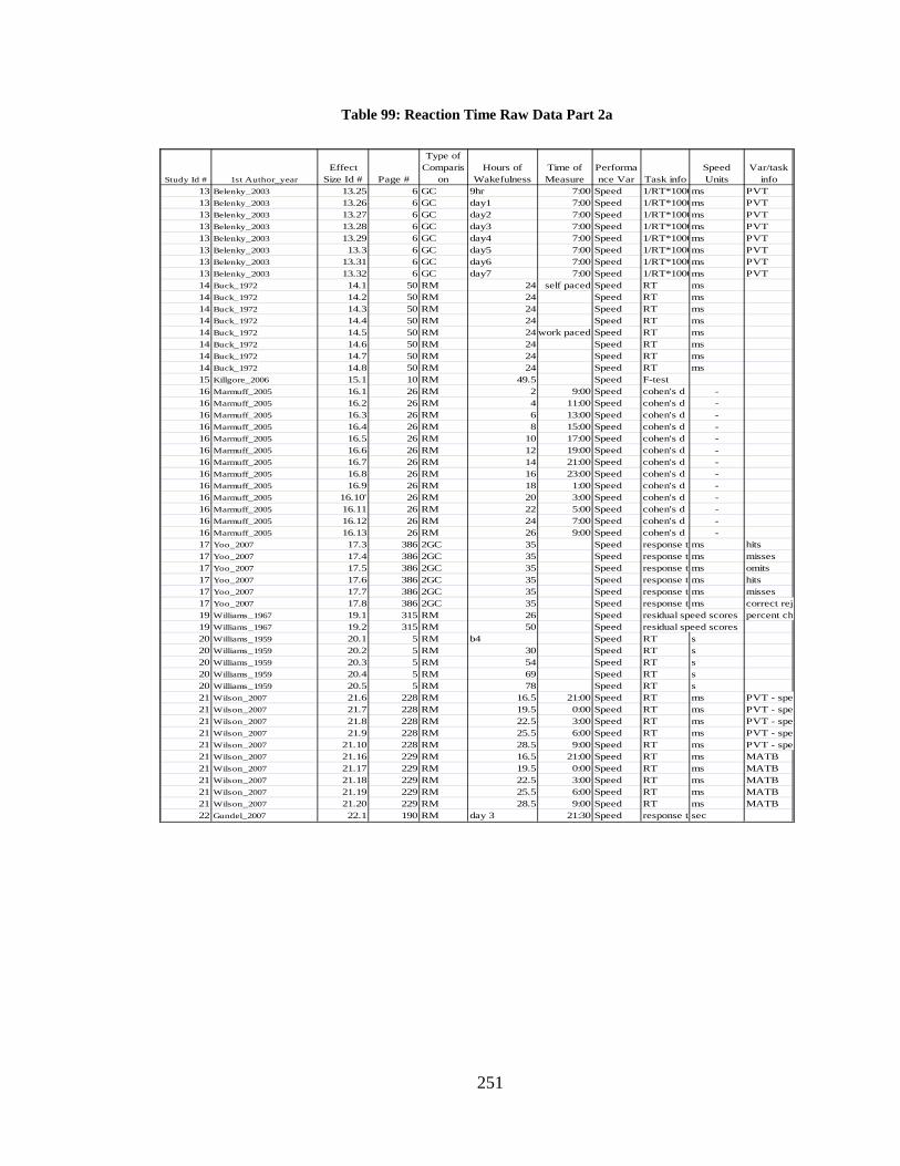
251
Table 99: Reaction Time Raw Data Part 2a
13 Belenky_2003 13.25 6 GC 9hr 7:00 Speed 1/RT*1000ms PVT13 Belenky_2003 13.26 6 GC day1 7:00 Speed 1/RT*1000ms PVT13 Belenky_2003 13.27 6 GC day2 7:00 Speed 1/RT*1000ms PVT13 Belenky_2003 13.28 6 GC day3 7:00 Speed 1/RT*1000ms PVT13 Belenky_2003 13.29 6 GC day4 7:00 Speed 1/RT*1000ms PVT13 Belenky_2003 13.3 6 GC day5 7:00 Speed 1/RT*1000ms PVT13 Belenky_2003 13.31 6 GC day6 7:00 Speed 1/RT*1000ms PVT13 Belenky_2003 13.32 6 GC day7 7:00 Speed 1/RT*1000ms PVT14 Buck_1972 14.1 50 RM 24 self paced Speed RT ms14 Buck_1972 14.2 50 RM 24 Speed RT ms14 Buck_1972 14.3 50 RM 24 Speed RT ms14 Buck_1972 14.4 50 RM 24 Speed RT ms14 Buck_1972 14.5 50 RM 24 work paced Speed RT ms14 Buck_1972 14.6 50 RM 24 Speed RT ms14 Buck_1972 14.7 50 RM 24 Speed RT ms14 Buck_1972 14.8 50 RM 24 Speed RT ms15 Killgore_2006 15.1 10 RM 49.5 Speed F-test16 Marmuff_2005 16.1 26 RM 2 9:00 Speed cohen's d -16 Marmuff_2005 16.2 26 RM 4 11:00 Speed cohen's d -16 Marmuff_2005 16.3 26 RM 6 13:00 Speed cohen's d -16 Marmuff_2005 16.4 26 RM 8 15:00 Speed cohen's d -16 Marmuff_2005 16.5 26 RM 10 17:00 Speed cohen's d -16 Marmuff_2005 16.6 26 RM 12 19:00 Speed cohen's d -16 Marmuff_2005 16.7 26 RM 14 21:00 Speed cohen's d -16 Marmuff_2005 16.8 26 RM 16 23:00 Speed cohen's d -16 Marmuff_2005 16.9 26 RM 18 1:00 Speed cohen's d -16 Marmuff_2005 16.10' 26 RM 20 3:00 Speed cohen's d -16 Marmuff_2005 16.11 26 RM 22 5:00 Speed cohen's d -16 Marmuff_2005 16.12 26 RM 24 7:00 Speed cohen's d -16 Marmuff_2005 16.13 26 RM 26 9:00 Speed cohen's d -17 Yoo_2007 17.3 386 2GC 35 Speed response tims hits17 Yoo_2007 17.4 386 2GC 35 Speed response tims misses17 Yoo_2007 17.5 386 2GC 35 Speed response tims omits17 Yoo_2007 17.6 386 2GC 35 Speed response tims hits17 Yoo_2007 17.7 386 2GC 35 Speed response tims misses17 Yoo_2007 17.8 386 2GC 35 Speed response tims correct reje19 Williams_1967 19.1 315 RM 26 Speed residual speed scores percent ch 19 Williams_1967 19.2 315 RM 50 Speed residual speed scores20 Williams_1959 20.1 5 RM b4 Speed RT s20 Williams_1959 20.2 5 RM 30 Speed RT s20 Williams_1959 20.3 5 RM 54 Speed RT s20 Williams_1959 20.4 5 RM 69 Speed RT s20 Williams_1959 20.5 5 RM 78 Speed RT s21 Wilson_2007 21.6 228 RM 16.5 21:00 Speed RT ms PVT - spe21 Wilson_2007 21.7 228 RM 19.5 0:00 Speed RT ms PVT - spe21 Wilson_2007 21.8 228 RM 22.5 3:00 Speed RT ms PVT - spe21 Wilson_2007 21.9 228 RM 25.5 6:00 Speed RT ms PVT - spe21 Wilson_2007 21.10 228 RM 28.5 9:00 Speed RT ms PVT - spe21 Wilson_2007 21.16 229 RM 16.5 21:00 Speed RT ms MATB21 Wilson_2007 21.17 229 RM 19.5 0:00 Speed RT ms MATB21 Wilson_2007 21.18 229 RM 22.5 3:00 Speed RT ms MATB21 Wilson_2007 21.19 229 RM 25.5 6:00 Speed RT ms MATB21 Wilson_2007 21.20 229 RM 28.5 9:00 Speed RT ms MATB22 Gundel_2007 22.1 190 RM day 3 21:30 Speed response tisec
Time of Measure
Performance Var Task info
Speed Units
Var/task info
Hours of WakefulnessStudy Id # 1st Author_year
Effect Size Id # Page #
Type of Comparis
on
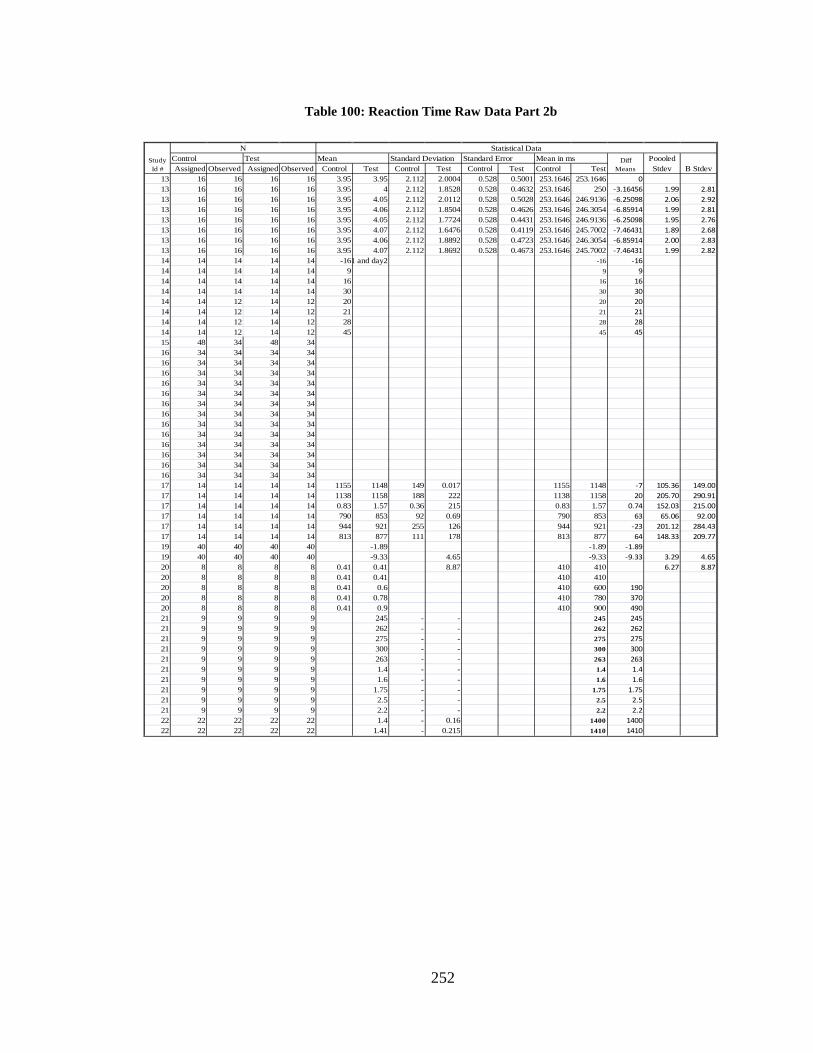
252
Table 100: Reaction Time Raw Data Part 2b
Assigned Observed Assigned Observed Control Test Control Test Control Test Control Test13 16 16 16 16 3.95 3.95 2.112 2.0004 0.528 0.5001 253.1646 253.1646 013 16 16 16 16 3.95 4 2.112 1.8528 0.528 0.4632 253.1646 250 -3.16456 1.99 2.8113 16 16 16 16 3.95 4.05 2.112 2.0112 0.528 0.5028 253.1646 246.9136 -6.25098 2.06 2.9213 16 16 16 16 3.95 4.06 2.112 1.8504 0.528 0.4626 253.1646 246.3054 -6.85914 1.99 2.8113 16 16 16 16 3.95 4.05 2.112 1.7724 0.528 0.4431 253.1646 246.9136 -6.25098 1.95 2.7613 16 16 16 16 3.95 4.07 2.112 1.6476 0.528 0.4119 253.1646 245.7002 -7.46431 1.89 2.6813 16 16 16 16 3.95 4.06 2.112 1.8892 0.528 0.4723 253.1646 246.3054 -6.85914 2.00 2.8313 16 16 16 16 3.95 4.07 2.112 1.8692 0.528 0.4673 253.1646 245.7002 -7.46431 1.99 2.8214 14 14 14 14 -16 1 and day2 -16 -1614 14 14 14 14 9 9 914 14 14 14 14 16 16 1614 14 14 14 14 30 30 3014 14 12 14 12 20 20 2014 14 12 14 12 21 21 2114 14 12 14 12 28 28 2814 14 12 14 12 45 45 4515 48 34 48 3416 34 34 34 3416 34 34 34 3416 34 34 34 3416 34 34 34 3416 34 34 34 3416 34 34 34 3416 34 34 34 3416 34 34 34 3416 34 34 34 3416 34 34 34 3416 34 34 34 3416 34 34 34 3416 34 34 34 3417 14 14 14 14 1155 1148 149 0.017 1155 1148 -7 105.36 149.0017 14 14 14 14 1138 1158 188 222 1138 1158 20 205.70 290.9117 14 14 14 14 0.83 1.57 0.36 215 0.83 1.57 0.74 152.03 215.0017 14 14 14 14 790 853 92 0.69 790 853 63 65.06 92.0017 14 14 14 14 944 921 255 126 944 921 -23 201.12 284.4317 14 14 14 14 813 877 111 178 813 877 64 148.33 209.7719 40 40 40 40 -1.89 -1.89 -1.8919 40 40 40 40 -9.33 4.65 -9.33 -9.33 3.29 4.6520 8 8 8 8 0.41 0.41 8.87 410 410 6.27 8.8720 8 8 8 8 0.41 0.41 410 41020 8 8 8 8 0.41 0.6 410 600 19020 8 8 8 8 0.41 0.78 410 780 37020 8 8 8 8 0.41 0.9 410 900 49021 9 9 9 9 245 - - 245 24521 9 9 9 9 262 - - 262 26221 9 9 9 9 275 - - 275 27521 9 9 9 9 300 - - 300 30021 9 9 9 9 263 - - 263 26321 9 9 9 9 1.4 - - 1.4 1.421 9 9 9 9 1.6 - - 1.6 1.621 9 9 9 9 1.75 - - 1.75 1.7521 9 9 9 9 2.5 - - 2.5 2.521 9 9 9 9 2.2 - - 2.2 2.222 22 22 22 22 1.4 - 0.16 1400 140022 22 22 22 22 1.41 - 0.215 1410 1410
Diff Means
Study Id #
NControl Test Mean Standard Deviation Standard Error
Statistical DataMean in ms Poooled
Stdev B Stdev
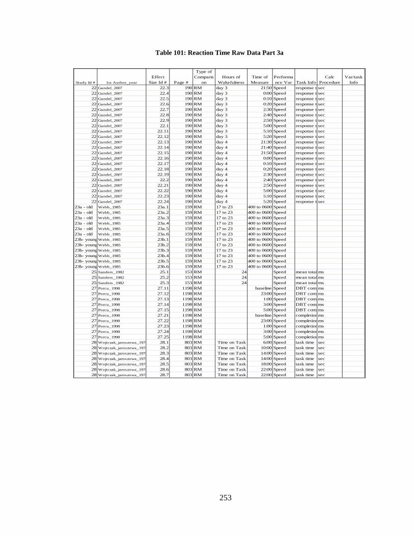
253
Table 101: Reaction Time Raw Data Part 3a
22 Gundel_2007 22.3 190 RM day 3 21:50 Speed response tisec22 Gundel_2007 22.4 190 RM day 3 0:00 Speed response tisec22 Gundel_2007 22.5 190 RM day 3 0:10 Speed response tisec22 Gundel_2007 22.6 190 RM day 3 0:20 Speed response tisec22 Gundel_2007 22.7 190 RM day 3 2:30 Speed response tisec22 Gundel_2007 22.8 190 RM day 3 2:40 Speed response tisec22 Gundel_2007 22.9 190 RM day 3 2:50 Speed response tisec22 Gundel_2007 22.1 190 RM day 3 5:00 Speed response tisec22 Gundel_2007 22.11 190 RM day 3 5:10 Speed response tisec22 Gundel_2007 22.12 190 RM day 3 5:20 Speed response tisec22 Gundel_2007 22.13 190 RM day 4 21:30 Speed response tisec22 Gundel_2007 22.14 190 RM day 4 21:40 Speed response tisec22 Gundel_2007 22.15 190 RM day 4 21:50 Speed response tisec22 Gundel_2007 22.16 190 RM day 4 0:00 Speed response tisec22 Gundel_2007 22.17 190 RM day 4 0:10 Speed response tisec22 Gundel_2007 22.18 190 RM day 4 0:20 Speed response tisec22 Gundel_2007 22.19 190 RM day 4 2:30 Speed response tisec22 Gundel_2007 22.2 190 RM day 4 2:40 Speed response tisec22 Gundel_2007 22.21 190 RM day 4 2:50 Speed response tisec22 Gundel_2007 22.22 190 RM day 4 5:00 Speed response tisec22 Gundel_2007 22.23 190 RM day 4 5:10 Speed response tisec22 Gundel_2007 22.24 190 RM day 4 5:20 Speed response tisec
23a - old Webb_1985 23a.1 159 RM 17 to 23 2400 to 0600 Speed23a - old Webb_1985 23a.2 159 RM 17 to 23 2400 to 0600 Speed23a - old Webb_1985 23a.3 159 RM 17 to 23 2400 to 0600 Speed23a - old Webb_1985 23a.4 159 RM 17 to 23 2400 to 0600 Speed23a - old Webb_1985 23a.5 159 RM 17 to 23 2400 to 0600 Speed23a - old Webb_1985 23a.6 159 RM 17 to 23 2400 to 0600 Speed23b- youngWebb_1985 23b.1 159 RM 17 to 23 2400 to 0600 Speed23b- youngWebb_1985 23b.2 159 RM 17 to 23 2400 to 0600 Speed23b- youngWebb_1985 23b.3 159 RM 17 to 23 2400 to 0600 Speed23b- youngWebb_1985 23b.4 159 RM 17 to 23 2400 to 0600 Speed23b- youngWebb_1985 23b.5 159 RM 17 to 23 2400 to 0600 Speed23b- youngWebb_1985 23b.6 159 RM 17 to 23 2400 to 0600 Speed
25 Sanders_1982 25.1 153 RM 24 Speed mean total ms25 Sanders_1982 25.2 153 RM 24 Speed mean total ms25 Sanders_1982 25.3 153 RM 24 Speed mean total ms27 Porcu_1998 27.11 1198 RM baseline Speed DBT comp ms27 Porcu_1998 27.12 1198 RM 23:00 Speed DBT comp ms27 Porcu_1998 27.13 1198 RM 1:00 Speed DBT comp ms27 Porcu_1998 27.14 1198 RM 3:00 Speed DBT comp ms27 Porcu_1998 27.15 1198 RM 5:00 Speed DBT comp ms27 Porcu_1998 27.21 1198 RM baseline Speed completion ms27 Porcu_1998 27.22 1198 RM 23:00 Speed completion ms27 Porcu_1998 27.23 1198 RM 1:00 Speed completion ms27 Porcu_1998 27.24 1198 RM 3:00 Speed completion ms27 Porcu_1998 27.25 1198 RM 5:00 Speed completion ms28 Wojtczak_jaroszowa_1978 28.1 803 RM Time on Task 6:00 Speed task time sec28 Wojtczak_jaroszowa_1978 28.2 803 RM Time on Task 10:00 Speed task time sec28 Wojtczak_jaroszowa_1978 28.3 803 RM Time on Task 14:00 Speed task time sec28 Wojtczak_jaroszowa_1978 28.4 803 RM Time on Task 14:00 Speed task time sec28 Wojtczak_jaroszowa_1978 28.5 803 RM Time on Task 18:00 Speed task time sec28 Wojtczak_jaroszowa_1978 28.6 803 RM Time on Task 22:00 Speed task time sec28 Wojtczak_jaroszowa_1978 28.7 803 RM Time on Task 22:00 Speed task time sec
Time of Measure
Performance Var Task Info
Calc Procedure
Var/task Info
Hours of WakefulnessStudy Id # 1st Author_year
Effect Size Id # Page #
Type of Comparis
on
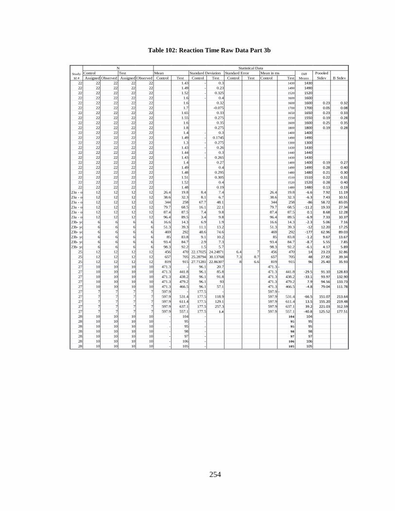
254
Table 102: Reaction Time Raw Data Part 3b
Assigned Observed Assigned Observed Control Test Control Test Control Test Control Test22 22 22 22 22 1.43 - 0.3 1430 143022 22 22 22 22 1.49 - 0.23 1490 149022 22 22 22 22 1.52 - 0.325 1520 152022 22 22 22 22 1.6 - 0.4 1600 160022 22 22 22 22 1.6 0.32 1600 1600 0.23 0.3222 22 22 22 22 1.7 -0.075 1700 1700 0.05 0.0822 22 22 22 22 1.65 0.33 1650 1650 0.23 0.3322 22 22 22 22 1.55 0.275 1550 1550 0.19 0.2822 22 22 22 22 1.6 0.35 1600 1600 0.25 0.3522 22 22 22 22 1.8 0.275 1800 1800 0.19 0.2822 22 22 22 22 1.4 - 0.3 1400 140022 22 22 22 22 1.49 - 0.1745 1490 149022 22 22 22 22 1.3 - 0.275 1300 130022 22 22 22 22 1.43 - 0.26 1430 143022 22 22 22 22 1.44 - 0.3 1440 144022 22 22 22 22 1.43 - 0.265 1430 143022 22 22 22 22 1.4 0.27 1400 1400 0.19 0.2722 22 22 22 22 1.49 0.4 1490 1490 0.28 0.4022 22 22 22 22 1.48 0.295 1480 1480 0.21 0.3022 22 22 22 22 1.51 0.305 1510 1510 0.22 0.3122 22 22 22 22 1.52 0.4 1520 1520 0.28 0.4022 22 22 22 22 1.48 0.19 1480 1480 0.13 0.19
23a - ol 12 12 12 12 26.4 19.8 8.4 7.4 26.4 19.8 -6.6 7.92 11.1923a - ol 12 12 12 12 38.6 32.3 8.1 6.7 38.6 32.3 -6.3 7.43 10.5123a - ol 12 12 12 12 344 258 67.7 48.1 344 258 -86 58.72 83.0523a - ol 12 12 12 12 79.7 68.5 16.1 22.1 79.7 68.5 -11.2 19.33 27.3423a - ol 12 12 12 12 87.4 87.5 7.4 9.8 87.4 87.5 0.1 8.68 12.2823a - ol 12 12 12 12 96.4 89.5 3.4 9.8 96.4 89.5 -6.9 7.33 10.3723b- yo 6 6 6 6 16.6 14.3 6.9 1.9 16.6 14.3 -2.3 5.06 7.1623b- yo 6 6 6 6 51.3 39.3 11.1 13.2 51.3 39.3 -12 12.20 17.2523b- yo 6 6 6 6 469 292 48.6 74.6 469 292 -177 62.96 89.0323b- yo 6 6 6 6 85 83.8 9.1 10.2 85 83.8 -1.2 9.67 13.6723b- yo 6 6 6 6 93.4 84.7 2.9 7.3 93.4 84.7 -8.7 5.55 7.8523b- yo 6 6 6 6 98.3 92.2 1.5 5.7 98.3 92.2 -6.1 4.17 5.89
25 12 12 12 12 456 470 22.17025 24.24871 6.4 7 456 470 14 23.23 32.8625 12 12 12 12 657 705 25.28794 30.13768 7.3 8.7 657 705 48 27.82 39.3425 12 12 12 12 819 915 27.71281 22.86307 8 6.6 819 915 96 25.40 35.9327 10 10 10 10 471.3 - 96.1 20.7 471.3 -27 10 10 10 10 471.3 441.8 96.1 85.8 471.3 441.8 -29.5 91.10 128.8327 10 10 10 10 471.3 438.2 96.1 91.8 471.3 438.2 -33.1 93.97 132.9027 10 10 10 10 471.3 479.2 96.1 93 471.3 479.2 7.9 94.56 133.7327 10 10 10 10 471.3 466.5 96.1 57.1 471.3 466.5 -4.8 79.04 111.7827 7 7 7 7 597.9 - 177.5 - 597.9 -27 7 7 7 7 597.9 531.4 177.5 118.9 597.9 531.4 -66.5 151.07 213.6427 7 7 7 7 597.9 611.4 177.5 129.1 597.9 611.4 13.5 155.20 219.4827 7 7 7 7 597.9 637.1 177.5 257.3 597.9 637.1 39.2 221.03 312.5927 7 7 7 7 597.9 557.1 177.5 1.4 597.9 557.1 -40.8 125.52 177.5128 10 10 10 10 - 104 - 104 10428 10 10 10 10 - 95 - 95 9528 10 10 10 10 - 95 - 95 9528 10 10 10 10 - 98 - 98 9828 10 10 10 10 - 97 - 97 9728 10 10 10 10 - 106 - 106 10628 10 10 10 10 - 105 - 105 105
Diff Means
Study Id #
NControl Test Mean Standard Deviation Standard Error
Statistical DataMean in ms Poooled
Stdev B Stdev
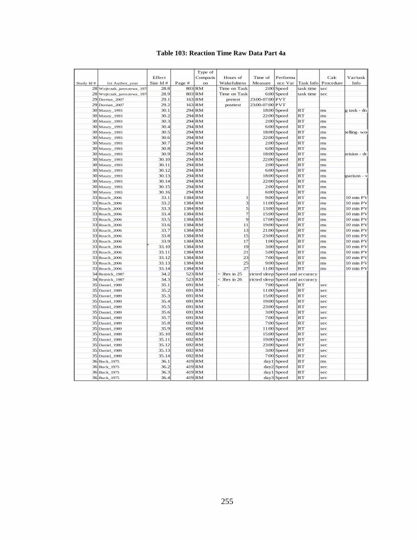
255
Table 103: Reaction Time Raw Data Part 4a
28 Wojtczak_jaroszowa_1978 28.8 803 RM Time on Task 2:00 Speed task time sec28 Wojtczak_jaroszowa_1978 28.9 803 RM Time on Task 6:00 Speed task time sec29 Dorrian_2007 29.1 163 RM pretest 23:00-07:00 PVT29 Dorrian_2007 29.2 163 RM posttest 23:00-07:00 PVT30 Maury_1993 30.1 294 RM 18:00 Speed RT ms ng task - dra 30 Maury_1993 30.2 294 RM 22:00 Speed RT ms30 Maury_1993 30.3 294 RM 2:00 Speed RT ms30 Maury_1993 30.4 294 RM 6:00 Speed RT ms30 Maury_1993 30.5 294 RM 18:00 Speed RT ms pelling- wor30 Maury_1993 30.6 294 RM 22:00 Speed RT ms30 Maury_1993 30.7 294 RM 2:00 Speed RT ms30 Maury_1993 30.8 294 RM 6:00 Speed RT ms30 Maury_1993 30.9 294 RM 18:00 Speed RT ms arision - dra30 Maury_1993 30.10 294 RM 22:00 Speed RT ms30 Maury_1993 30.11 294 RM 2:00 Speed RT ms30 Maury_1993 30.12 294 RM 6:00 Speed RT ms30 Maury_1993 30.13 294 RM 18:00 Speed RT ms mparison - w30 Maury_1993 30.14 294 RM 22:00 Speed RT ms30 Maury_1993 30.15 294 RM 2:00 Speed RT ms30 Maury_1993 30.16 294 RM 6:00 Speed RT ms33 Roach_2006 33.1 1384 RM 1 9:00 Speed RT ms 10 min PV33 Roach_2006 33.2 1384 RM 3 11:00 Speed RT ms 10 min PV33 Roach_2006 33.3 1384 RM 5 13:00 Speed RT ms 10 min PV33 Roach_2006 33.4 1384 RM 7 15:00 Speed RT ms 10 min PV33 Roach_2006 33.5 1384 RM 9 17:00 Speed RT ms 10 min PV33 Roach_2006 33.6 1384 RM 11 19:00 Speed RT ms 10 min PV33 Roach_2006 33.7 1384 RM 13 21:00 Speed RT ms 10 min PV33 Roach_2006 33.8 1384 RM 15 23:00 Speed RT ms 10 min PV33 Roach_2006 33.9 1384 RM 17 1:00 Speed RT ms 10 min PV33 Roach_2006 33.10 1384 RM 19 3:00 Speed RT ms 10 min PV33 Roach_2006 33.11 1384 RM 21 5:00 Speed RT ms 10 min PV33 Roach_2006 33.12 1384 RM 23 7:00 Speed RT ms 10 min PV33 Roach_2006 33.13 1384 RM 25 9:00 Speed RT ms 10 min PV33 Roach_2006 33.14 1384 RM 27 11:00 Speed RT ms 10 min PV34 Reznick_1987 34.2 523 RM < 3hrs in 25 tricted sleep Speed and accuracy34 Reznick_1987 34.3 523 RM < 3hrs in 26 tricted sleep Speed and accuracy35 Daniel_1989 35.1 691 RM - 7:00 Speed RT sec35 Daniel_1989 35.2 691 RM 11:00 Speed RT sec35 Daniel_1989 35.3 691 RM 15:00 Speed RT sec35 Daniel_1989 35.4 691 RM 19:00 Speed RT sec35 Daniel_1989 35.5 691 RM 23:00 Speed RT sec35 Daniel_1989 35.6 691 RM 3:00 Speed RT sec35 Daniel_1989 35.7 691 RM 7:00 Speed RT sec35 Daniel_1989 35.8 692 RM 7:00 Speed RT sec35 Daniel_1989 35.9 692 RM 11:00 Speed RT sec35 Daniel_1989 35.10 692 RM 15:00 Speed RT sec35 Daniel_1989 35.11 692 RM 19:00 Speed RT sec35 Daniel_1989 35.12 692 RM 23:00 Speed RT sec35 Daniel_1989 35.13 692 RM 3:00 Speed RT sec35 Daniel_1989 35.14 692 RM 7:00 Speed RT sec36 Buck_1975 36.1 419 RM day1 Speed RT ms36 Buck_1975 36.2 419 RM day2 Speed RT sec36 Buck_1975 36.3 419 RM day1 Speed RT sec36 Buck_1975 36.4 419 RM day3 Speed RT sec
Time of Measure
Performance Var Task Info
Calc Procedure
Var/task Info
Hours of WakefulnessStudy Id # 1st Author_year
Effect Size Id # Page #
Type of Comparis
on
256
Table 104: Reaction Time Raw Data Part 4b
Assigned Observed Assigned Observed Control Test Control Test Control Test Control Test28 10 10 10 10 - 113 - 113 11328 10 10 10 10 - 109 - 109 10929 20 20 20 2029 20 20 20 2030 15 15 15 15 540 540 37.5 37.5 540 540 0 37.50 53.0330 15 15 15 15 540 600 37.5 65 540 600 60 53.06 75.0430 15 15 15 15 540 490 37.5 30 540 490 -50 33.96 48.0230 15 15 15 15 540 560 37.5 45 540 560 20 41.42 58.5830 14 14 14 14 480 480 25 25 480 480 0 25.00 35.3630 14 14 14 14 480 500 25 22.5 480 500 20 23.78 33.6330 14 14 14 14 480 495 25 27.5 480 495 15 26.28 37.1730 14 14 14 14 480 460 25 25 480 460 -20 25.00 35.3630 15 15 15 15 210 210 20 20 210 210 0 20.00 28.2830 15 15 15 15 210 200 20 20 210 200 -10 20.00 28.2830 15 15 15 15 210 205 20 20 210 205 -5 20.00 28.2830 15 15 15 15 210 212 20 17.5 210 212 2 18.79 26.5830 14 14 14 14 150 150 10 10 150 150 0 10.00 14.1430 14 14 14 14 150 140 10 12.5 150 140 -10 11.32 16.0130 14 14 14 14 150 170 10 17.5 150 170 20 14.25 20.1630 14 14 14 14 150 160 10 20 150 160 10 15.81 22.3633 16 16 16 16 229 216 44 36 11 9 229 216 -13 40.20 56.8533 16 16 16 16 229 218 44 52 11 13 229 218 -11 48.17 68.1233 16 16 16 16 229 220 44 44 11 11 229 220 -9 44.00 62.2333 16 16 16 16 229 230 44 60 11 15 229 230 1 52.61 74.4033 16 16 16 16 229 229 44 44 11 11 229 229 0 44.00 62.2333 16 16 16 16 229 227 44 52 11 13 229 227 -2 48.17 68.1233 16 16 16 16 229 230 44 60 11 15 229 230 1 52.61 74.4033 16 16 16 16 229 250 44 88 11 22 229 250 21 69.57 98.3933 16 16 16 16 229 265 44 76 11 19 229 265 36 62.10 87.8233 16 16 16 16 229 272 44 72 11 18 229 272 43 59.67 84.3833 16 16 16 16 229 278 44 72 11 18 229 278 49 59.67 84.3833 16 16 16 16 229 308 44 72 11 18 229 308 79 59.67 84.3833 16 16 16 16 229 288 44 64 11 16 229 288 59 54.92 77.6733 16 16 16 16 229 285 44 72 11 18 229 285 56 59.67 84.3834 21 12 21 12 -34 21 12 21 1235 18 18 18 18 3.8 3.8 3.835 18 18 18 18 3.6 3.6 3.635 18 18 18 18 3.3 3.3 3.335 18 18 18 18 3.45 3.45 3.4535 18 18 18 18 3.34 3.34 3.3435 18 18 18 18 3.38 3.38 3.3835 18 18 18 18 3.8 3.8 3.835 16 16 16 16 3.45 3.45 3.4535 16 16 16 16 2.95 2.95 2.9535 16 16 16 16 2.95 2.95 2.9535 16 16 16 16 2.6 2.6 2.635 16 16 16 16 2.9 2.9 2.935 16 16 16 16 2.9 2.9 2.935 16 16 16 16 3.65 3.65 3.6536 20 20 20 20 241 244 - - 241 244 336 20 20 20 20 229 233 - - 229 233 436 8 8 8 8 207 214 - - 207 214 736 8 8 8 8 202 228 - - 202 228 26
Diff Means
Study Id #
NControl Test Mean Standard Deviation Standard Error
Statistical DataMean in ms Poooled
Stdev B Stdev
257
Table 105: Reaction Time Raw Data Part 5a
36 Buck_1975 36.5 419 RM day1 Speed RT sec36 Buck_1975 36.6 419 RM day2 Speed RT sec36 Buck_1975 36.7 419 RM day1 Speed RT sec36 Buck_1975 36.8 419 RM day3 Speed RT sec37 Lenne_1997 37.1 434 RM 6:00 Speed RT sec37 Lenne_1997 37.2 434 RM 10:00 Speed RT sec37 Lenne_1997 37.3 434 RM 14:00 Speed RT sec37 Lenne_1997 37.4 434 RM 18:00 Speed RT sec37 Lenne_1997 37.5 434 RM 22:00 Speed RT sec37 Lenne_1997 37.6 434 RM 2:00 Speed RT sec41 Monk_1997 41.19 15 RM 2 9:00 Speed residuals sec Vigilance S 41 Monk_1997 41.2 15 RM 4 11:00 Speed residuals sec Vigilance S 41 Monk_1997 41.21 15 RM 6 13:00 Speed residuals sec Vigilance S 41 Monk_1997 41.22 15 RM 8 15:00 Speed residuals sec Vigilance S 41 Monk_1997 41.23 15 RM 10 17:00 Speed residuals sec Vigilance S 41 Monk_1997 41.24 15 RM 12 19:00 Speed residuals sec Vigilance S 41 Monk_1997 41.25 15 RM 14 21:00 Speed residuals sec Vigilance S 41 Monk_1997 41.26 15 RM 16 23:00 Speed residuals sec Vigilance S 41 Monk_1997 41.27 15 RM 18 1:00 Speed residuals sec Vigilance S 41 Monk_1997 41.28 15 RM 20 3:00 Speed residuals sec Vigilance S 41 Monk_1997 41.29 15 RM 22 5:00 Speed residuals sec Vigilance S 41 Monk_1997 41.3 15 RM 24 7:00 Speed residuals sec Vigilance S 41 Monk_1997 41.31 15 RM 26 9:00 Speed residuals sec Vigilance S 41 Monk_1997 41.32 15 RM 28 11:00 Speed residuals sec Vigilance S 41 Monk_1997 41.33 15 RM 30 13:00 Speed residuals sec Vigilance S 41 Monk_1997 41.34 15 RM 32 15:00 Speed residuals sec Vigilance S 41 Monk_1997 41.35 15 RM 34 17:00 Speed residuals sec Vigilance S 41 Monk_1997 41.36 15 RM 36 19:00 Speed residuals sec Vigilance S 41 Monk_1997 41.37 14 RM 2 9:00 Speed residuals sec Search Spe 41 Monk_1997 41.38 14 RM 4 11:00 Speed residuals sec Search Spe 41 Monk_1997 41.39 14 RM 6 13:00 Speed residuals sec Search Spe 41 Monk_1997 41.4 14 RM 8 15:00 Speed residuals sec Search Spe 41 Monk_1997 41.41 14 RM 10 17:00 Speed residuals sec Search Spe 41 Monk_1997 41.42 14 RM 12 19:00 Speed residuals sec Search Spe 41 Monk_1997 41.43 14 RM 14 21:00 Speed residuals sec Search Spe 41 Monk_1997 41.44 14 RM 16 23:00 Speed residuals sec Search Spe 41 Monk_1997 41.45 14 RM 18 1:00 Speed residuals sec Search Spe 41 Monk_1997 41.46 14 RM 20 3:00 Speed residuals sec Search Spe 41 Monk_1997 41.47 14 RM 22 5:00 Speed residuals sec Search Spe 41 Monk_1997 41.48 14 RM 24 7:00 Speed residuals sec Search Spe 41 Monk_1997 41.49 14 RM 26 9:00 Speed residuals sec Search Spe 41 Monk_1997 41.5 14 RM 28 11:00 Speed residuals sec Search Spe 41 Monk_1997 41.51 14 RM 30 13:00 Speed residuals sec Search Spe 41 Monk_1997 41.52 14 RM 32 15:00 Speed residuals sec Search Spe 41 Monk_1997 41.53 14 RM 34 17:00 Speed residuals sec Search Spe 41 Monk_1997 41.54 14 RM 36 19:00 Speed residuals sec Search Spe 41 Monk_1997 41.55 14 RM 2 9:00 Speed residuals sec Reasoning 41 Monk_1997 41.56 14 RM 4 11:00 Speed residuals sec Reasoning 41 Monk_1997 41.57 14 RM 6 13:00 Speed residuals sec Reasoning 41 Monk_1997 41.58 14 RM 8 15:00 Speed residuals sec Reasoning 41 Monk_1997 41.59 14 RM 10 17:00 Speed residuals sec Reasoning 41 Monk_1997 41.6 14 RM 12 19:00 Speed residuals sec Reasoning 41 Monk_1997 41.61 14 RM 14 21:00 Speed residuals sec Reasoning 41 Monk_1997 41.62 14 RM 16 23:00 Speed residuals sec Reasoning
Time of Measure
Performance Var Task Info
Calc Procedure
Var/task Info
Hours of WakefulnessStudy Id # 1st Author_year
Effect Size Id # Page #
Type of Comparis
on
258
Table 106: Reaction Time Raw Data Part 5b
Assigned Observed Assigned Observed Control Test Control Test Control Test Control Test36 20 20 20 20 374 369 - - 374 369 -536 20 20 20 20 354 379 - - 354 379 2536 8 8 8 8 304 305 - - 304 305 136 8 8 8 8 277 343 - - 277 343 6637 11 11 11 11 0.88 0.15754 0.0475 880 880 0.11 0.1637 11 11 11 11 0.8 0.132665 0.04 800 800 0.09 0.1337 11 11 11 11 0.925 0.505785 0.1525 925 925 0.36 0.5137 11 11 11 11 0.81 0.140957 0.0425 810 810 0.10 0.1437 11 11 11 11 0.78 0.116082 0.035 780 780 0.08 0.1237 11 11 11 11 0.92 0.140957 0.0425 920 920 0.10 0.1441 17 17 17 17 0 1.841 17 17 17 17 -1 2.1541 17 17 17 17 -0.6 1.541 17 17 17 17 3 1.841 17 17 17 17 1 1.541 17 17 17 17 3 1.541 17 17 17 17 3.3 2.141 17 17 17 17 0.5 1.541 17 17 17 17 -4.5 2.341 17 17 17 17 -2 1.541 17 17 17 17 -3.8 1.7541 17 17 17 17 -3.7 2.541 17 17 17 17 -0.4 1.641 17 17 17 17 -3.8 1.841 17 17 17 17 2.8 2.341 17 17 17 17 0 1.541 17 17 17 17 2 1.541 17 17 17 17 3.9 2.341 17 17 17 17 0 0.27541 17 17 17 17 0.35 0.4541 17 17 17 17 -0.4 0.27541 17 17 17 17 -0.8 0.27541 17 17 17 17 0.5 0.27541 17 17 17 17 1 0.27541 17 17 17 17 0.15 0.4541 17 17 17 17 0.9 0.4541 17 17 17 17 0.5 0.4541 17 17 17 17 -0.5 0.4541 17 17 17 17 -1.2 0.82541 17 17 17 17 -1.3 0.8241 17 17 17 17 -0.6 0.4541 17 17 17 17 0 0.541 17 17 17 17 -0.15 0.27541 17 17 17 17 0.1 0.541 17 17 17 17 0.3 0.241 17 17 17 17 1 0.4541 17 17 17 17 -1.5 0.641 17 17 17 17 -0.5 0.441 17 17 17 17 0.2 0.641 17 17 17 17 0.8 0.441 17 17 17 17 0.2 0.541 17 17 17 17 1.8 0.641 17 17 17 17 1.15 0.641 17 17 17 17 1 0.5
Diff Means
Study Id #
NControl Test Mean Standard Deviation Standard Error
Statistical DataMean in ms Poooled
Stdev B Stdev
259
Table 107: Reaction Time Raw Data Part 6a
41 Monk_1997 41.63 14 RM 18 1:00 Speed residuals sec Reasoning Speed (VR 41 Monk_1997 41.64 14 RM 20 3:00 Speed residuals sec Reasoning Speed (VR 41 Monk_1997 41.65 14 RM 22 5:00 Speed residuals sec Reasoning Speed (VR 41 Monk_1997 41.66 14 RM 24 7:00 Speed residuals sec Reasoning Speed (VR 41 Monk_1997 41.67 14 RM 26 9:00 Speed residuals sec Reasoning Speed (VR 41 Monk_1997 41.68 14 RM 28 11:00 Speed residuals sec Reasoning Speed (VR 41 Monk_1997 41.69 14 RM 30 13:00 Speed residuals sec Reasoning Speed (VR 41 Monk_1997 41.7 14 RM 32 15:00 Speed residuals sec Reasoning Speed (VR 41 Monk_1997 41.71 14 RM 34 17:00 Speed residuals sec Reasoning Speed (VR 41 Monk_1997 41.72 14 RM 36 19:00 Speed residuals sec Reasoning Speed (VR 42 Jones_2006 42.1 1259 RM 2 9:00 Speed 1/RT ms42 Jones_2006 42.1 1259 RM 4 11:00 Speed 1/RT ms42 Jones_2006 42.1 1259 RM 6 13:00 Speed 1/RT ms42 Jones_2006 42.1 1259 RM 8 15:00 Speed 1/RT ms42 Jones_2006 42.1 1259 RM 10 17:00 Speed 1/RT ms42 Jones_2006 42.1 1259 RM 12 19:00 Speed 1/RT ms42 Jones_2006 42.1 1259 RM 14 21:00 Speed 1/RT ms42 Jones_2006 42.1 1259 RM 16 23:00 Speed 1/RT ms42 Jones_2006 42.1 1259 RM 18 1:00 Speed 1/RT ms42 Jones_2006 42.1 1259 RM 20 3:00 Speed 1/RT ms42 Jones_2006 42.1 1259 RM 22 5:00 Speed 1/RT ms42 Jones_2006 42.1 1259 RM 24 7:00 Speed 1/RT ms42 Jones_2006 42.1 1259 RM 26 9:00 Speed 1/RT ms42 Jones_2006 42.1 1259 RM 28 11:00 Speed 1/RT ms42 Jones_2006 42.1 1259 RM 30 13:00 Speed 1/RT ms42 Jones_2006 42.1 1259 RM 32 15:00 Speed 1/RT ms42 Jones_2006 42.1 1259 RM 34 17:00 Speed 1/RT ms42 Jones_2006 42.1 1259 RM 36 19:00 Speed 1/RT ms42 Jones_2006 42.1 1259 RM 38 21:00 Speed 1/RT ms42 Jones_2006 42.1 1259 RM 40 23:00 Speed 1/RT ms45 Halbach_2003 45.1 1200 RM one night on caltricted sleep Speed groove peg sec peg board - dominant45 Halbach_2003 45.2 1200 RM one night on call Speed groove peg sec peg board - non-domina47 Lamond_2007 47.1 RM 24 9:00 Speed 1/RT ms PVT48 Drummond_2006 48.9 263 RM 7 Speed hit RT ms PVT48 Drummond_2006 48.10 263 RM 23 Speed hit RT ms PVT48 Drummond_2006 48.11 263 RM 31 Speed hit RT ms PVT48 Drummond_2006 48.12 263 RM 55 Speed hit RT ms PVT49 Eastridge_2003 49.2 172 RM - Speed mean RT sec50 Engle_Friedman 50.1 115 RM 1 night 8:00 to16:00 Speed mean RT sec50 Engle_Friedman 50.3 121 2GC 1 night 9:00 to 10:30 Speed mean RT sec50 Engle_Friedman 50.4 121 2GC 2 night 9:00 to 10:31 Speed mean RT sec50 Engle_Friedman 50.6 121 2GC 4 night 9:00 to 10:33 Speed mean RT sec51 Caldwell_2003 51.1 27 RM 4 18:45 Speed 1/RT ms reaction time51 Caldwell_2003 51.2 27 RM 8 22:45 Speed 1/RT ms51 Caldwell_2003 51.3 27 RM 12 2:45 Speed 1/RT ms51 Caldwell_2003 51.4 27 RM 20 10:45 Speed 1/RT ms51 Caldwell_2003 51.5 27 RM 24 14:45 Speed 1/RT ms51 Caldwell_2003 51.6 27 RM 28 18:45 Speed 1/RT ms52 Rosa_1983 52 156 RM 32 23:30 Speed 1/RT sec52 Rosa_1983 52.1 156 RM 34 1:30 Speed 1/RT sec52 Rosa_1983 52.2 156 RM 36.5 4:00 Speed 1/RT sec52 Rosa_1983 52.3 156 RM 38.25 6:15 Speed 1/RT sec52 Rosa_1983 52.3 156 RM 40 8:30 Speed 1/RT sec52 Rosa_1983 52.4 156 RM 56 23:30 Speed 1/RT sec
Hours of WakefulnessStudy Id # 1st Author_year
Effect Size Id # Page #
Type of Comparis
onTime of Measure
Performance Var Task Info
Calc Procedure Var/task Info
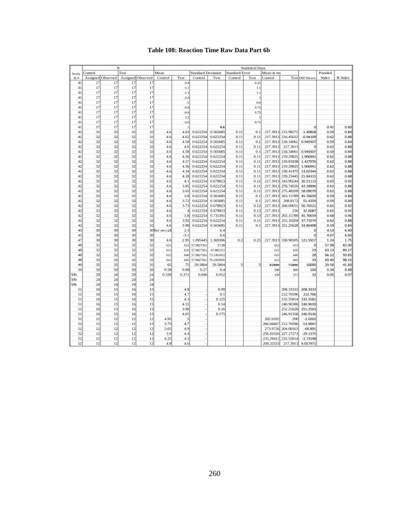
260
Table 108: Reaction Time Raw Data Part 6b
Assigned Observed Assigned Observed Control Test Control Test Control Test Control Test41 17 17 17 17 0.4 0.2541 17 17 17 17 -1.1 1.141 17 17 17 17 -1.3 1.141 17 17 17 17 -2.4 141 17 17 17 17 -1 0.641 17 17 17 17 -0.8 0.7541 17 17 17 17 -0.6 0.7541 17 17 17 17 2.2 141 17 17 17 17 -0.6 0.7541 17 17 17 17 1 0.6 0 0.42 0.6042 32 32 32 32 4.6 4.63 0.622254 0.565685 0.11 0.1 217.3913 215.98272 -1.40858 0.59 0.8442 32 32 32 32 4.6 4.62 0.622254 0.622254 0.11 0.11 217.3913 216.45022 -0.94109 0.62 0.8842 32 32 32 32 4.6 4.58 0.622254 0.565685 0.11 0.1 217.3913 218.34061 0.949307 0.59 0.8442 32 32 32 32 4.6 4.6 0.622254 0.622254 0.11 0.11 217.3913 217.3913 0 0.62 0.8842 32 32 32 32 4.6 4.58 0.622254 0.565685 0.11 0.1 217.3913 218.34061 0.949307 0.59 0.8442 32 32 32 32 4.6 4.56 0.622254 0.622254 0.11 0.11 217.3913 219.29825 1.906941 0.62 0.8842 32 32 32 32 4.6 4.57 0.622254 0.622254 0.11 0.11 217.3913 218.81838 1.427076 0.62 0.8842 32 32 32 32 4.6 4.56 0.622254 0.622254 0.11 0.11 217.3913 219.29825 1.906941 0.62 0.8842 32 32 32 32 4.6 4.34 0.622254 0.622254 0.11 0.11 217.3913 230.41475 13.02344 0.62 0.8842 32 32 32 32 4.6 4.18 0.622254 0.622254 0.11 0.11 217.3913 239.23445 21.84315 0.62 0.8842 32 32 32 32 4.6 4.1 0.622254 0.678823 0.11 0.12 217.3913 243.90244 26.51113 0.65 0.9242 32 32 32 32 4.6 3.85 0.622254 0.622254 0.11 0.11 217.3913 259.74026 42.34896 0.62 0.8842 32 32 32 32 4.6 3.63 0.622254 0.622254 0.11 0.11 217.3913 275.48209 58.09079 0.62 0.8842 32 32 32 32 4.6 3.8 0.622254 0.565685 0.11 0.1 217.3913 263.15789 45.76659 0.59 0.8442 32 32 32 32 4.6 3.72 0.622254 0.565685 0.11 0.1 217.3913 268.8172 51.4259 0.59 0.8442 32 32 32 32 4.6 3.73 0.622254 0.678823 0.11 0.12 217.3913 268.09651 50.70521 0.65 0.9242 32 32 32 32 4.6 4 0.622254 0.678823 0.11 0.12 217.3913 250 32.6087 0.65 0.9242 32 32 32 32 4.6 3.8 0.622254 0.735391 0.11 0.13 217.3913 263.15789 45.76659 0.68 0.9642 32 32 32 32 4.6 3.92 0.622254 0.622254 0.11 0.11 217.3913 255.10204 37.71074 0.62 0.8842 32 32 32 32 4.6 3.98 0.622254 0.565685 0.11 0.1 217.3913 251.25628 33.86498 0.59 0.8445 30 30 30 30 fter on-call 2.3 6.4 0 4.53 6.4045 30 30 30 30 -3.1 6.6 0 4.67 6.6047 30 30 30 30 4.6 2.95 1.095445 1.369306 0.2 0.25 217.3913 338.98305 121.5917 1.24 1.7548 32 32 32 32 612 612 57.9827561 57.98 612 612 0 57.98 82.0048 32 32 32 32 612 635 57.9827561 67.882251 612 635 23 63.13 89.2748 32 32 32 32 612 640 57.9827561 73.5391052 612 640 28 66.22 93.6548 32 32 32 32 612 645 57.9827561 79.1959595 612 645 33 69.40 98.1549 35 35 35 35 65 75 29.5804 29.5804 5 5 65000 75000 10000 29.58 41.8350 50 50 50 50 0.58 0.68 0.27 0.4 580 680 100 0.34 0.48
50b 29 24 29 24 0.339 0.371 0.046 0.052 339 371 32 0.05 0.0750b 24 24 24 2450b 24 24 24 24
51 16 15 16 15 4.8 - 0.09 208.33333 208.333351 16 15 16 15 4.7 - 0.1 212.76596 212.76651 16 15 16 15 4.3 - 0.125 232.55814 232.558151 16 15 16 15 4.15 - 0.14 240.96386 240.963951 16 15 16 15 3.98 - 0.16 251.25628 251.256351 16 15 16 15 4.05 - 0.175 246.91358 246.913652 12 12 12 12 4.95 5 - 202.0202 200 -2.020252 12 12 12 12 3.75 4.7 - 266.66667 212.76596 -53.900752 12 12 12 12 3.65 4.9 - 273.9726 204.08163 -69.89152 12 12 12 12 3.9 4.4 - 256.41026 227.27273 -29.137552 12 12 12 12 4.25 4.3 - 235.29412 232.55814 -2.7359852 12 12 12 12 4.8 4.6 - 208.33333 217.3913 9.057971
Diff MeansStudy Id #
NControl Test Mean Standard Deviation Standard Error
Statistical DataMean in ms Poooled
Stdev B Stdev
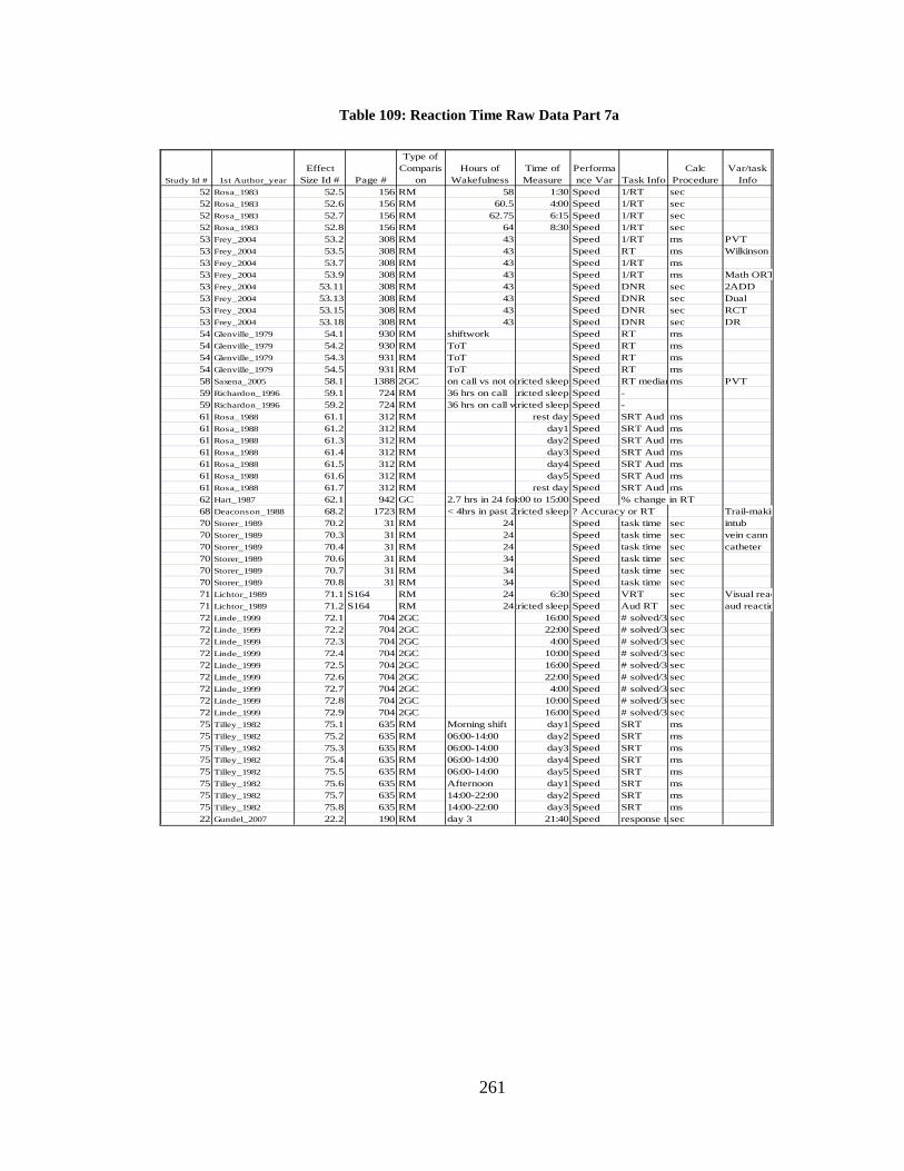
261
Table 109: Reaction Time Raw Data Part 7a
52 Rosa_1983 52.5 156 RM 58 1:30 Speed 1/RT sec52 Rosa_1983 52.6 156 RM 60.5 4:00 Speed 1/RT sec52 Rosa_1983 52.7 156 RM 62.75 6:15 Speed 1/RT sec52 Rosa_1983 52.8 156 RM 64 8:30 Speed 1/RT sec53 Frey_2004 53.2 308 RM 43 Speed 1/RT ms PVT53 Frey_2004 53.5 308 RM 43 Speed RT ms Wilkinson53 Frey_2004 53.7 308 RM 43 Speed 1/RT ms53 Frey_2004 53.9 308 RM 43 Speed 1/RT ms Math ORT53 Frey_2004 53.11 308 RM 43 Speed DNR sec 2ADD53 Frey_2004 53.13 308 RM 43 Speed DNR sec Dual53 Frey_2004 53.15 308 RM 43 Speed DNR sec RCT53 Frey_2004 53.18 308 RM 43 Speed DNR sec DR54 Glenville_1979 54.1 930 RM shiftwork Speed RT ms54 Glenville_1979 54.2 930 RM ToT Speed RT ms54 Glenville_1979 54.3 931 RM ToT Speed RT ms54 Glenville_1979 54.5 931 RM ToT Speed RT ms58 Saxena_2005 58.1 1388 2GC on call vs not on tricted sleep Speed RT medianms PVT59 Richardon_1996 59.1 724 RM 36 hrs on call tricted sleep Speed -59 Richardon_1996 59.2 724 RM 36 hrs on call w tricted sleep Speed -61 Rosa_1988 61.1 312 RM rest day Speed SRT Aud ms61 Rosa_1988 61.2 312 RM day1 Speed SRT Aud ms61 Rosa_1988 61.3 312 RM day2 Speed SRT Aud ms61 Rosa_1988 61.4 312 RM day3 Speed SRT Aud ms61 Rosa_1988 61.5 312 RM day4 Speed SRT Aud ms61 Rosa_1988 61.6 312 RM day5 Speed SRT Aud ms61 Rosa_1988 61.7 312 RM rest day Speed SRT Aud ms62 Hart_1987 62.1 942 GC 2.7 hrs in 24 for 4:00 to 15:00 Speed % change in RT68 Deaconson_1988 68.2 1723 RM < 4hrs in past 2tricted sleep ? Accuracy or RT Trail-makin70 Storer_1989 70.2 31 RM 24 Speed task time sec intub70 Storer_1989 70.3 31 RM 24 Speed task time sec vein cann70 Storer_1989 70.4 31 RM 24 Speed task time sec catheter70 Storer_1989 70.6 31 RM 34 Speed task time sec70 Storer_1989 70.7 31 RM 34 Speed task time sec70 Storer_1989 70.8 31 RM 34 Speed task time sec71 Lichtor_1989 71.1 S164 RM 24 6:30 Speed VRT sec Visual reac71 Lichtor_1989 71.2 S164 RM 24tricted sleep Speed Aud RT sec aud reactio 72 Linde_1999 72.1 704 2GC 16:00 Speed # solved/32sec72 Linde_1999 72.2 704 2GC 22:00 Speed # solved/32sec72 Linde_1999 72.3 704 2GC 4:00 Speed # solved/32sec72 Linde_1999 72.4 704 2GC 10:00 Speed # solved/32sec72 Linde_1999 72.5 704 2GC 16:00 Speed # solved/32sec72 Linde_1999 72.6 704 2GC 22:00 Speed # solved/32sec72 Linde_1999 72.7 704 2GC 4:00 Speed # solved/32sec72 Linde_1999 72.8 704 2GC 10:00 Speed # solved/32sec72 Linde_1999 72.9 704 2GC 16:00 Speed # solved/32sec75 Tilley_1982 75.1 635 RM Morning shift day1 Speed SRT ms75 Tilley_1982 75.2 635 RM 06:00-14:00 day2 Speed SRT ms75 Tilley_1982 75.3 635 RM 06:00-14:00 day3 Speed SRT ms75 Tilley_1982 75.4 635 RM 06:00-14:00 day4 Speed SRT ms75 Tilley_1982 75.5 635 RM 06:00-14:00 day5 Speed SRT ms75 Tilley_1982 75.6 635 RM Afternoon day1 Speed SRT ms75 Tilley_1982 75.7 635 RM 14:00-22:00 day2 Speed SRT ms75 Tilley_1982 75.8 635 RM 14:00-22:00 day3 Speed SRT ms22 Gundel_2007 22.2 190 RM day 3 21:40 Speed response tisec
Time of Measure
Performance Var Task Info
Calc Procedure
Var/task Info
Hours of WakefulnessStudy Id # 1st Author_year
Effect Size Id # Page #
Type of Comparis
on
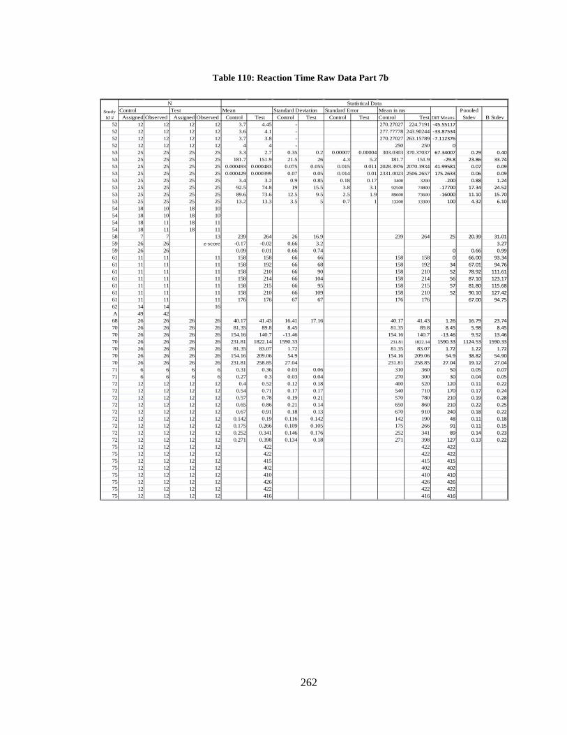
262
Table 110: Reaction Time Raw Data Part 7b
Assigned Observed Assigned Observed Control Test Control Test Control Test Control Test52 12 12 12 12 3.7 4.45 - 270.27027 224.7191 -45.5511752 12 12 12 12 3.6 4.1 - 277.77778 243.90244 -33.8753452 12 12 12 12 3.7 3.8 - 270.27027 263.15789 -7.11237652 12 12 12 12 4 4 - 250 250 053 25 25 25 25 3.3 2.7 0.35 0.2 0.00007 0.00004 303.0303 370.37037 67.34007 0.29 0.4053 25 25 25 25 181.7 151.9 21.5 26 4.3 5.2 181.7 151.9 -29.8 23.86 33.7453 25 25 25 25 0.000493 0.000483 0.075 0.055 0.015 0.011 2028.3976 2070.3934 41.99581 0.07 0.0953 25 25 25 25 0.000429 0.000399 0.07 0.05 0.014 0.01 2331.0023 2506.2657 175.2633 0.06 0.0953 25 25 25 25 3.4 3.2 0.9 0.85 0.18 0.17 3400 3200 -200 0.88 1.2453 25 25 25 25 92.5 74.8 19 15.5 3.8 3.1 92500 74800 -17700 17.34 24.5253 25 25 25 25 89.6 73.6 12.5 9.5 2.5 1.9 89600 73600 -16000 11.10 15.7053 25 25 25 25 13.2 13.3 3.5 5 0.7 1 13200 13300 100 4.32 6.1054 18 10 18 1054 18 10 18 1054 18 11 18 1154 18 11 18 1158 7 7 13 239 264 26 16.9 239 264 25 20.39 31.0159 26 26 z-score -0.17 -0.02 0.66 3.2 3.2759 26 26 0.09 0.01 0.66 0.74 0 0.66 0.9961 11 11 11 158 158 66 66 158 158 0 66.00 93.3461 11 11 11 158 192 66 68 158 192 34 67.01 94.7661 11 11 11 158 210 66 90 158 210 52 78.92 111.6161 11 11 11 158 214 66 104 158 214 56 87.10 123.1761 11 11 11 158 215 66 95 158 215 57 81.80 115.6861 11 11 11 158 210 66 109 158 210 52 90.10 127.4261 11 11 11 176 176 67 67 176 176 67.00 94.7562 14 14 16A 49 4268 26 26 26 26 40.17 41.43 16.41 17.16 40.17 41.43 1.26 16.79 23.7470 26 26 26 26 81.35 89.8 8.45 81.35 89.8 8.45 5.98 8.4570 26 26 26 26 154.16 140.7 -13.46 154.16 140.7 -13.46 9.52 13.4670 26 26 26 26 231.81 1822.14 1590.33 231.81 1822.14 1590.33 1124.53 1590.3370 26 26 26 26 81.35 83.07 1.72 81.35 83.07 1.72 1.22 1.7270 26 26 26 26 154.16 209.06 54.9 154.16 209.06 54.9 38.82 54.9070 26 26 26 26 231.81 258.85 27.04 231.81 258.85 27.04 19.12 27.0471 6 6 6 6 0.31 0.36 0.03 0.06 310 360 50 0.05 0.0771 6 6 6 6 0.27 0.3 0.03 0.04 270 300 30 0.04 0.0572 12 12 12 12 0.4 0.52 0.12 0.18 400 520 120 0.11 0.2272 12 12 12 12 0.54 0.71 0.17 0.17 540 710 170 0.17 0.2472 12 12 12 12 0.57 0.78 0.19 0.21 570 780 210 0.19 0.2872 12 12 12 12 0.65 0.86 0.21 0.14 650 860 210 0.22 0.2572 12 12 12 12 0.67 0.91 0.18 0.13 670 910 240 0.18 0.2272 12 12 12 12 0.142 0.19 0.116 0.142 142 190 48 0.11 0.1872 12 12 12 12 0.175 0.266 0.109 0.105 175 266 91 0.11 0.1572 12 12 12 12 0.252 0.341 0.146 0.176 252 341 89 0.14 0.2372 12 12 12 12 0.271 0.398 0.134 0.18 271 398 127 0.13 0.2275 12 12 12 12 422 422 42275 12 12 12 12 422 422 42275 12 12 12 12 415 415 41575 12 12 12 12 402 402 40275 12 12 12 12 410 410 41075 12 12 12 12 426 426 42675 12 12 12 12 422 422 42275 12 12 12 12 416 416 416
Diff MeansStudy Id #
NControl Test Mean Standard Deviation Standard Error
Statistical DataMean in ms Poooled
Stdev B Stdev
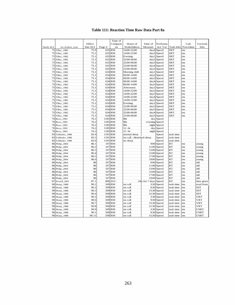
263
Table 111: Reaction Time Raw Data Part 8a
75 Tilley_1982 75.9 635 RM 14:00-22:00 day4 Speed SRT ms75 Tilley_1982 75.1 635 RM 14:00-22:00 day5 Speed SRT ms75 Tilley_1982 75.1 635 RM Evening day1 Speed SRT ms75 Tilley_1982 75.1 635 RM 22:00-06:00 day2 Speed SRT ms75 Tilley_1982 75.1 635 RM 22:00-06:00 day3 Speed SRT ms75 Tilley_1982 75.1 635 RM 22:00-06:00 day4 Speed SRT ms75 Tilley_1982 75.1 635 RM 22:00-06:00 day5 Speed SRT ms75 Tilley_1982 75.1 634 RM Morning shift day1 Speed SRT ms75 Tilley_1982 75.1 634 RM 06:00-14:00 day2 Speed SRT ms75 Tilley_1982 75.1 634 RM 06:00-14:00 day3 Speed SRT ms75 Tilley_1982 75.1 634 RM 06:00-14:00 day4 Speed SRT ms75 Tilley_1982 75.1 634 RM 06:00-14:00 day5 Speed SRT ms75 Tilley_1982 75.1 634 RM Afternoon day1 Speed SRT ms75 Tilley_1982 75.1 634 RM 14:00-22:00 day2 Speed SRT ms75 Tilley_1982 75.1 634 RM 14:00-22:00 day3 Speed SRT ms75 Tilley_1982 75.1 634 RM 14:00-22:00 day4 Speed SRT ms75 Tilley_1982 75.1 634 RM 14:00-22:00 day5 Speed SRT ms75 Tilley_1982 75.1 634 RM Evening day1 Speed SRT ms75 Tilley_1982 75.1 634 RM 22:00-06:00 day2 Speed SRT ms75 Tilley_1982 75.1 634 RM 22:00-06:00 day3 Speed SRT ms75 Tilley_1982 75.1 634 RM 22:00-06:00 day4 Speed SRT ms75 Tilley_1982 75.1 634 RM 22:00-06:00 day5 Speed SRT ms76 Rosa_1993 76.1 1185 RM 8hr day Speed76 Rosa_1993 76.2 1185 RM 8hr evening Speed76 Rosa_1993 76.2 1185 RM 8hr night Speed76 Rosa_1993 76.2 1185 RM 12 -hr day Speed76 Rosa_1993 76.2 1185 RM 12 -hr night Speed83 Taffinder_1998 83.4 1191 RM normal sleep Speed task time83 Taffinder_1998 83.5 1191 RM on call - disturbed sleep Speed task time83 Taffinder_1998 83.6 1191 RM no sleep Speed task time86 Philip_2004 86.1 107 RM 9:00 Speed RT ms young86 Philip_2004 86.2 107 RM 11:00 Speed RT ms young86 Philip_2004 86.3 107 RM 13:00 Speed RT ms young86 Philip_2004 86.4 107 RM 15:00 Speed RT ms young86 Philip_2004 86.5 107 RM 17:00 Speed RT ms young86 Philip_2004 86.6 107 RM 19:00 Speed RT ms young86 Philip_2004 86 107 RM 9:00 Speed RT ms old86 Philip_2004 86 107 RM 11:00 Speed RT ms old86 Philip_2004 86 107 RM 13:00 Speed RT ms old86 Philip_2004 86 107 RM 15:00 Speed RT ms old86 Philip_2004 86 107 RM 17:00 Speed RT ms old86 Philip_2004 86 107 RM 19:00 Speed RT ms old87 Powell_2001 87.1 890 2GC 24 rs for 7 days Speed RT ms data given 90 Sharp_1988 90.1 509 RM on call 3:30 Speed task time ms read from 90 Sharp_1988 90.2 509 RM on call 9:30 Speed task time ms SST90 Sharp_1988 90.3 509 RM on call 15:30 Speed task time ms SST90 Sharp_1988 90.4 509 RM on call 21:30 Speed task time ms SST90 Sharp_1988 90.5 509 RM on call 3:30 Speed task time ms VRT90 Sharp_1988 90.6 509 RM on call 9:30 Speed task time ms VRT90 Sharp_1988 90.7 509 RM on call 15:30 Speed task time ms VRT90 Sharp_1988 90.8 509 RM on call 21:30 Speed task time ms VRT90 Sharp_1988 90.9 509 RM on call 3:30 Speed task time ms USRT90 Sharp_1988 90.1 509 RM on call 9:30 Speed task time ms USRT90 Sharp_1988 90.11 509 RM on call 15:30 Speed task time ms USRT
Time of Measure
Performance Var Task Info
Calc Procedure
Var/task Info
Hours of WakefulnessStudy Id # 1st Author_year
Effect Size Id # Page #
Type of Comparis
on
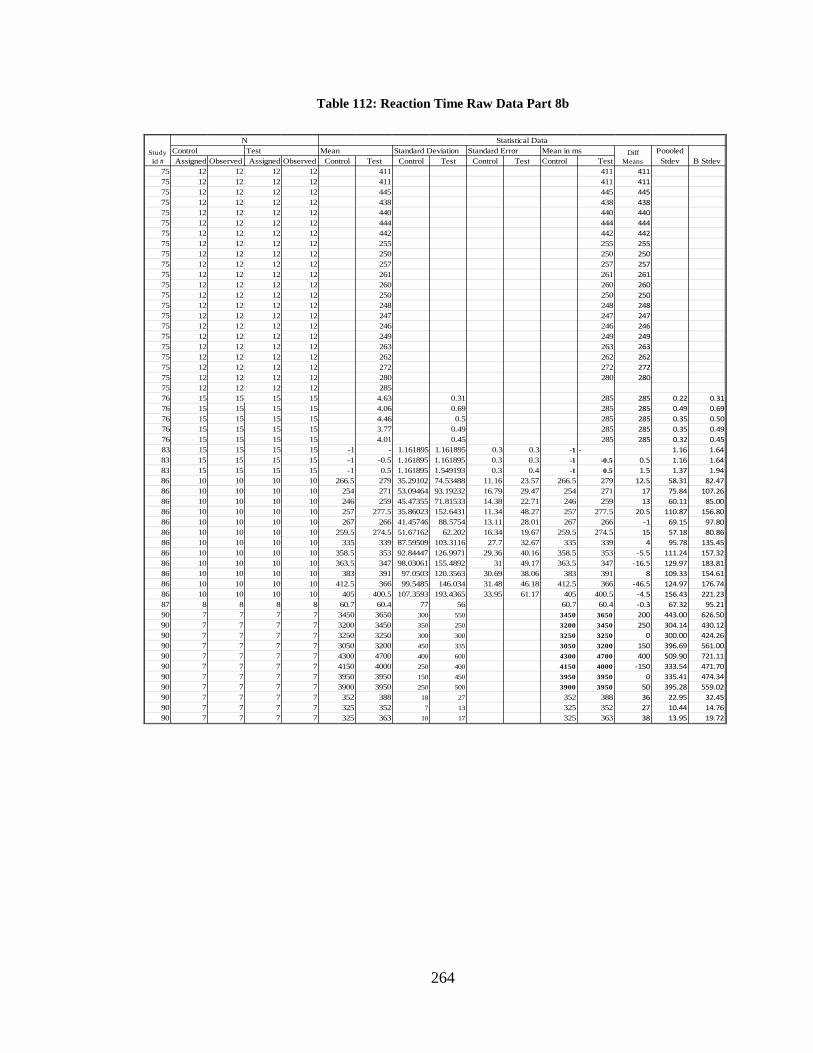
264
Table 112: Reaction Time Raw Data Part 8b
Assigned Observed Assigned Observed Control Test Control Test Control Test Control Test75 12 12 12 12 411 411 41175 12 12 12 12 411 411 41175 12 12 12 12 445 445 44575 12 12 12 12 438 438 43875 12 12 12 12 440 440 44075 12 12 12 12 444 444 44475 12 12 12 12 442 442 44275 12 12 12 12 255 255 25575 12 12 12 12 250 250 25075 12 12 12 12 257 257 25775 12 12 12 12 261 261 26175 12 12 12 12 260 260 26075 12 12 12 12 250 250 25075 12 12 12 12 248 248 24875 12 12 12 12 247 247 24775 12 12 12 12 246 246 24675 12 12 12 12 249 249 24975 12 12 12 12 263 263 26375 12 12 12 12 262 262 26275 12 12 12 12 272 272 27275 12 12 12 12 280 280 28075 12 12 12 12 28576 15 15 15 15 4.63 0.31 285 285 0.22 0.3176 15 15 15 15 4.06 0.69 285 285 0.49 0.6976 15 15 15 15 4.46 0.5 285 285 0.35 0.5076 15 15 15 15 3.77 0.49 285 285 0.35 0.4976 15 15 15 15 4.01 0.45 285 285 0.32 0.4583 15 15 15 15 -1 - 1.161895 1.161895 0.3 0.3 -1 - 1.16 1.6483 15 15 15 15 -1 -0.5 1.161895 1.161895 0.3 0.3 -1 -0.5 0.5 1.16 1.6483 15 15 15 15 -1 0.5 1.161895 1.549193 0.3 0.4 -1 0.5 1.5 1.37 1.9486 10 10 10 10 266.5 279 35.29102 74.53488 11.16 23.57 266.5 279 12.5 58.31 82.4786 10 10 10 10 254 271 53.09464 93.19232 16.79 29.47 254 271 17 75.84 107.2686 10 10 10 10 246 259 45.47355 71.81533 14.38 22.71 246 259 13 60.11 85.0086 10 10 10 10 257 277.5 35.86023 152.6431 11.34 48.27 257 277.5 20.5 110.87 156.8086 10 10 10 10 267 266 41.45746 88.5754 13.11 28.01 267 266 -1 69.15 97.8086 10 10 10 10 259.5 274.5 51.67162 62.202 16.34 19.67 259.5 274.5 15 57.18 80.8686 10 10 10 10 335 339 87.59509 103.3116 27.7 32.67 335 339 4 95.78 135.4586 10 10 10 10 358.5 353 92.84447 126.9971 29.36 40.16 358.5 353 -5.5 111.24 157.3286 10 10 10 10 363.5 347 98.03061 155.4892 31 49.17 363.5 347 -16.5 129.97 183.8186 10 10 10 10 383 391 97.0503 120.3563 30.69 38.06 383 391 8 109.33 154.6186 10 10 10 10 412.5 366 99.5485 146.034 31.48 46.18 412.5 366 -46.5 124.97 176.7486 10 10 10 10 405 400.5 107.3593 193.4365 33.95 61.17 405 400.5 -4.5 156.43 221.2387 8 8 8 8 60.7 60.4 77 56 60.7 60.4 -0.3 67.32 95.2190 7 7 7 7 3450 3650 300 550 3450 3650 200 443.00 626.5090 7 7 7 7 3200 3450 350 250 3200 3450 250 304.14 430.1290 7 7 7 7 3250 3250 300 300 3250 3250 0 300.00 424.2690 7 7 7 7 3050 3200 450 335 3050 3200 150 396.69 561.0090 7 7 7 7 4300 4700 400 600 4300 4700 400 509.90 721.1190 7 7 7 7 4150 4000 250 400 4150 4000 -150 333.54 471.7090 7 7 7 7 3950 3950 150 450 3950 3950 0 335.41 474.3490 7 7 7 7 3900 3950 250 500 3900 3950 50 395.28 559.0290 7 7 7 7 352 388 18 27 352 388 36 22.95 32.4590 7 7 7 7 325 352 7 13 325 352 27 10.44 14.7690 7 7 7 7 325 363 10 17 325 363 38 13.95 19.72
Diff Means
Study Id #
NControl Test Mean Standard Deviation Standard Error
Statistical DataMean in ms Poooled
Stdev B Stdev
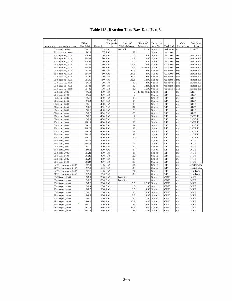
265
Table 113: Reaction Time Raw Data Part 9a
90 Sharp_1988 90.12 509 RM on call 21:30 Speed task time ms USRT91 Steyvers_1993 91.1 67 RM 32 Speed reaction timx95 Sagaspe_2006 95.31 80 RM 0.5 8:00 Speed reaction timsec motor RT95 Sagaspe_2006 95.32 80 RM 4.5 12:00 Speed reaction timsec motor RT95 Sagaspe_2006 95.33 80 RM 8.5 16:00 Speed reaction timsec motor RT95 Sagaspe_2006 95.34 80 RM 12.5 20:00 Speed reaction timsec motor RT95 Sagaspe_2006 95.35 80 RM 16.5 24:00:00 Speed reaction timsec motor RT95 Sagaspe_2006 95.36 80 RM 20.5 4:00 Speed reaction timsec motor RT95 Sagaspe_2006 95.37 80 RM 24.5 8:00 Speed reaction timsec motor RT95 Sagaspe_2006 95.38 80 RM 28.5 12:00 Speed reaction timsec motor RT95 Sagaspe_2006 95.39 80 RM 32.5 16:00 Speed reaction timsec motor RT95 Sagaspe_2006 95.4 80 RM 12 8:00 Speed reaction timsec motor RT95 Sagaspe_2006 95.41 80 RM 12 12:00 Speed reaction timsec motor RT95 Sagaspe_2006 95.42 80 RM 12 16:00 Speed reaction timsec motor RT96 Scott_2006 96.1 400 RM 2 30 hrs total Speed RT ms SRT96 Scott_2006 96.2 400 RM 6 Speed RT ms SRT96 Scott_2006 96.3 400 RM 10 Speed RT ms SRT96 Scott_2006 96.4 400 RM 14 Speed RT ms SRT96 Scott_2006 96.5 400 RM 18 Speed RT ms SRT96 Scott_2006 96.6 400 RM 22 Speed RT ms SRT96 Scott_2006 96.7 400 RM 26 Speed RT ms SRT96 Scott_2006 96.8 400 RM 30 Speed RT ms SRT96 Scott_2006 96.9 400 RM 2 Speed RT ms 2-CRT96 Scott_2006 96.1 400 RM 6 Speed RT ms 2-CRT96 Scott_2006 96.11 400 RM 10 Speed RT ms 2-CRT96 Scott_2006 96.12 400 RM 14 Speed RT ms 2-CRT96 Scott_2006 96.13 400 RM 18 Speed RT ms 2-CRT96 Scott_2006 96.14 400 RM 22 Speed RT ms 2-CRT96 Scott_2006 96.15 400 RM 26 Speed RT ms 2-CRT96 Scott_2006 96.16 400 RM 30 Speed RT ms 2-CRT96 Scott_2006 96.17 400 RM 2 Speed RT ms NCT96 Scott_2006 96.18 400 RM 6 Speed RT ms NCT96 Scott_2006 96.19 400 RM 10 Speed RT ms NCT96 Scott_2006 96.2 400 RM 14 Speed RT ms NCT96 Scott_2006 96.21 400 RM 18 Speed RT ms NCT96 Scott_2006 96.22 400 RM 22 Speed RT ms NCT96 Scott_2006 96.23 400 RM 26 Speed RT ms NCT96 Scott_2006 96.24 400 RM 30 Speed RT ms NCT97 Venkatraman_2007 97.1 606 RM 24 Speed RT ms certain/low97 Venkatraman_2007 97.2 606 RM 24 Speed RT ms certain/low97 Venkatraman_2007 97.3 606 RM 24 Speed RT ms low/high97 Venkatraman_2007 97.4 606 RM 24 Speed RT ms low/high98 Dinges_1988 98.1 366 RM baseline Speed VRT ms VRT98 Dinges_1988 98.2 366 RM baseline Speed VRT ms VRT98 Dinges_1988 98.3 366 RM 5.5 22:30 Speed VRT ms VRT98 Dinges_1988 98.4 366 RM 8 1:00 Speed VRT ms VRT98 Dinges_1988 98.5 366 RM 10.5 3:30 Speed VRT ms VRT98 Dinges_1988 98.6 366 RM 13 6:00 Speed VRT ms VRT98 Dinges_1988 98.7 366 RM 15.5 8:30 Speed VRT ms VRT98 Dinges_1988 98.8 366 RM 18 11:00 Speed VRT ms VRT98 Dinges_1988 98.9 366 RM 20.5 13:30 Speed VRT ms VRT98 Dinges_1988 98.10 366 RM 23 16:00 Speed VRT ms VRT98 Dinges_1988 98.11 366 RM 25.5 18:30 Speed VRT ms VRT98 Dinges_1988 98.12 366 RM 28 21:00 Speed VRT ms VRT
Hours of WakefulnessStudy Id # 1st Author_year
Effect Size Id # Page #
Type of Comparis
onTime of Measure
Performance Var Task Info
Calc Procedure
Var/task Info
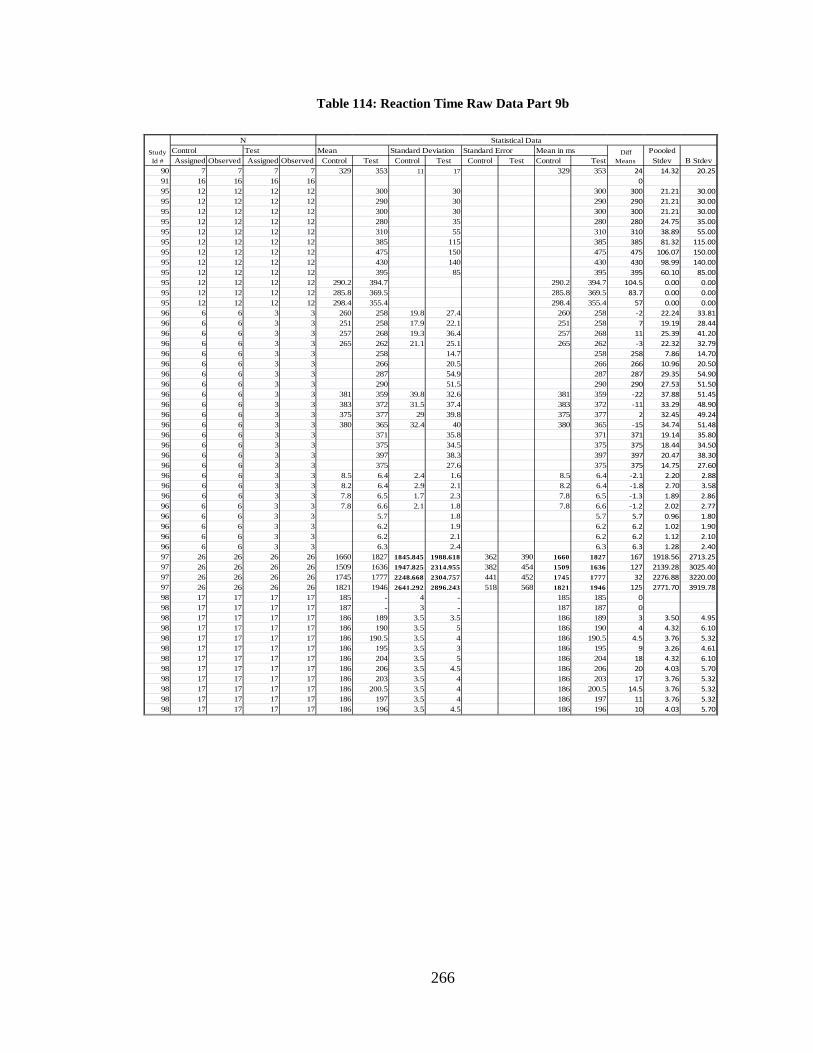
266
Table 114: Reaction Time Raw Data Part 9b
Assigned Observed Assigned Observed Control Test Control Test Control Test Control Test90 7 7 7 7 329 353 11 17 329 353 24 14.32 20.2591 16 16 16 16 095 12 12 12 12 300 30 300 300 21.21 30.0095 12 12 12 12 290 30 290 290 21.21 30.0095 12 12 12 12 300 30 300 300 21.21 30.0095 12 12 12 12 280 35 280 280 24.75 35.0095 12 12 12 12 310 55 310 310 38.89 55.0095 12 12 12 12 385 115 385 385 81.32 115.0095 12 12 12 12 475 150 475 475 106.07 150.0095 12 12 12 12 430 140 430 430 98.99 140.0095 12 12 12 12 395 85 395 395 60.10 85.0095 12 12 12 12 290.2 394.7 290.2 394.7 104.5 0.00 0.0095 12 12 12 12 285.8 369.5 285.8 369.5 83.7 0.00 0.0095 12 12 12 12 298.4 355.4 298.4 355.4 57 0.00 0.0096 6 6 3 3 260 258 19.8 27.4 260 258 -2 22.24 33.8196 6 6 3 3 251 258 17.9 22.1 251 258 7 19.19 28.4496 6 6 3 3 257 268 19.3 36.4 257 268 11 25.39 41.2096 6 6 3 3 265 262 21.1 25.1 265 262 -3 22.32 32.7996 6 6 3 3 258 14.7 258 258 7.86 14.7096 6 6 3 3 266 20.5 266 266 10.96 20.5096 6 6 3 3 287 54.9 287 287 29.35 54.9096 6 6 3 3 290 51.5 290 290 27.53 51.5096 6 6 3 3 381 359 39.8 32.6 381 359 -22 37.88 51.4596 6 6 3 3 383 372 31.5 37.4 383 372 -11 33.29 48.9096 6 6 3 3 375 377 29 39.8 375 377 2 32.45 49.2496 6 6 3 3 380 365 32.4 40 380 365 -15 34.74 51.4896 6 6 3 3 371 35.8 371 371 19.14 35.8096 6 6 3 3 375 34.5 375 375 18.44 34.5096 6 6 3 3 397 38.3 397 397 20.47 38.3096 6 6 3 3 375 27.6 375 375 14.75 27.6096 6 6 3 3 8.5 6.4 2.4 1.6 8.5 6.4 -2.1 2.20 2.8896 6 6 3 3 8.2 6.4 2.9 2.1 8.2 6.4 -1.8 2.70 3.5896 6 6 3 3 7.8 6.5 1.7 2.3 7.8 6.5 -1.3 1.89 2.8696 6 6 3 3 7.8 6.6 2.1 1.8 7.8 6.6 -1.2 2.02 2.7796 6 6 3 3 5.7 1.8 5.7 5.7 0.96 1.8096 6 6 3 3 6.2 1.9 6.2 6.2 1.02 1.9096 6 6 3 3 6.2 2.1 6.2 6.2 1.12 2.1096 6 6 3 3 6.3 2.4 6.3 6.3 1.28 2.4097 26 26 26 26 1660 1827 1845.845 1988.618 362 390 1660 1827 167 1918.56 2713.2597 26 26 26 26 1509 1636 1947.825 2314.955 382 454 1509 1636 127 2139.28 3025.4097 26 26 26 26 1745 1777 2248.668 2304.757 441 452 1745 1777 32 2276.88 3220.0097 26 26 26 26 1821 1946 2641.292 2896.243 518 568 1821 1946 125 2771.70 3919.7898 17 17 17 17 185 - 4 - 185 185 098 17 17 17 17 187 - 3 - 187 187 098 17 17 17 17 186 189 3.5 3.5 186 189 3 3.50 4.9598 17 17 17 17 186 190 3.5 5 186 190 4 4.32 6.1098 17 17 17 17 186 190.5 3.5 4 186 190.5 4.5 3.76 5.3298 17 17 17 17 186 195 3.5 3 186 195 9 3.26 4.6198 17 17 17 17 186 204 3.5 5 186 204 18 4.32 6.1098 17 17 17 17 186 206 3.5 4.5 186 206 20 4.03 5.7098 17 17 17 17 186 203 3.5 4 186 203 17 3.76 5.3298 17 17 17 17 186 200.5 3.5 4 186 200.5 14.5 3.76 5.3298 17 17 17 17 186 197 3.5 4 186 197 11 3.76 5.3298 17 17 17 17 186 196 3.5 4.5 186 196 10 4.03 5.70
Diff Means
Study Id #
NControl Test Mean Standard Deviation Standard Error
Statistical DataMean in ms Poooled
Stdev B Stdev
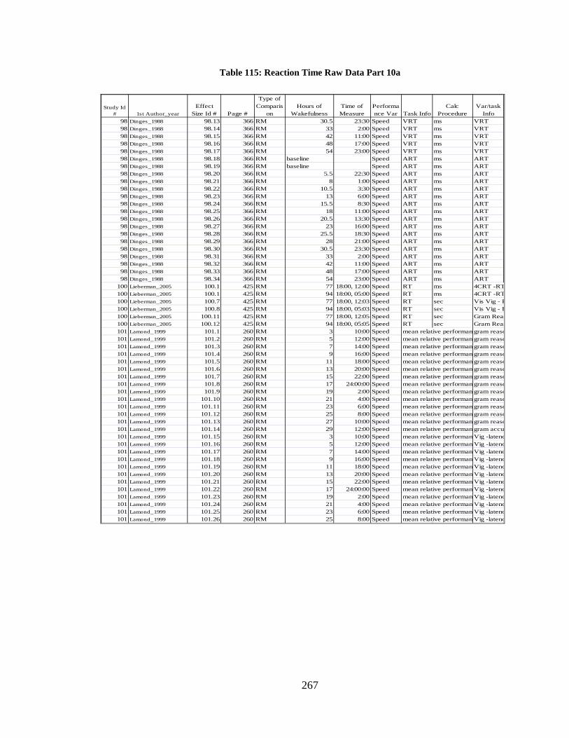
267
Table 115: Reaction Time Raw Data Part 10a
98 Dinges_1988 98.13 366 RM 30.5 23:30 Speed VRT ms VRT98 Dinges_1988 98.14 366 RM 33 2:00 Speed VRT ms VRT98 Dinges_1988 98.15 366 RM 42 11:00 Speed VRT ms VRT98 Dinges_1988 98.16 366 RM 48 17:00 Speed VRT ms VRT98 Dinges_1988 98.17 366 RM 54 23:00 Speed VRT ms VRT98 Dinges_1988 98.18 366 RM baseline Speed ART ms ART98 Dinges_1988 98.19 366 RM baseline Speed ART ms ART98 Dinges_1988 98.20 366 RM 5.5 22:30 Speed ART ms ART98 Dinges_1988 98.21 366 RM 8 1:00 Speed ART ms ART98 Dinges_1988 98.22 366 RM 10.5 3:30 Speed ART ms ART98 Dinges_1988 98.23 366 RM 13 6:00 Speed ART ms ART98 Dinges_1988 98.24 366 RM 15.5 8:30 Speed ART ms ART98 Dinges_1988 98.25 366 RM 18 11:00 Speed ART ms ART98 Dinges_1988 98.26 366 RM 20.5 13:30 Speed ART ms ART98 Dinges_1988 98.27 366 RM 23 16:00 Speed ART ms ART98 Dinges_1988 98.28 366 RM 25.5 18:30 Speed ART ms ART98 Dinges_1988 98.29 366 RM 28 21:00 Speed ART ms ART98 Dinges_1988 98.30 366 RM 30.5 23:30 Speed ART ms ART98 Dinges_1988 98.31 366 RM 33 2:00 Speed ART ms ART98 Dinges_1988 98.32 366 RM 42 11:00 Speed ART ms ART98 Dinges_1988 98.33 366 RM 48 17:00 Speed ART ms ART98 Dinges_1988 98.34 366 RM 54 23:00 Speed ART ms ART
100 Lieberman_2005 100.1 425 RM 77 18:00, 12:00 Speed RT ms 4CRT -RT100 Lieberman_2005 100.1 425 RM 94 18:00, 05:00 Speed RT ms 4CRT -RT100 Lieberman_2005 100.7 425 RM 77 18:00, 12:03 Speed RT sec Vis Vig - R100 Lieberman_2005 100.8 425 RM 94 18:00, 05:03 Speed RT sec Vis Vig - R100 Lieberman_2005 100.11 425 RM 77 18:00, 12:05 Speed RT sec Gram Reas 100 Lieberman_2005 100.12 425 RM 94 18:00, 05:05 Speed RT sec Gram Reas 101 Lamond_1999 101.1 260 RM 3 10:00 Speed mean relative performan gram reaso 101 Lamond_1999 101.2 260 RM 5 12:00 Speed mean relative performan gram reaso 101 Lamond_1999 101.3 260 RM 7 14:00 Speed mean relative performancgram reaso 101 Lamond_1999 101.4 260 RM 9 16:00 Speed mean relative performancgram reaso 101 Lamond_1999 101.5 260 RM 11 18:00 Speed mean relative performancgram reaso 101 Lamond_1999 101.6 260 RM 13 20:00 Speed mean relative performancgram reaso 101 Lamond_1999 101.7 260 RM 15 22:00 Speed mean relative performancgram reaso 101 Lamond_1999 101.8 260 RM 17 24:00:00 Speed mean relative performan gram reaso 101 Lamond_1999 101.9 260 RM 19 2:00 Speed mean relative performan gram reaso 101 Lamond_1999 101.10 260 RM 21 4:00 Speed mean relative performan gram reaso 101 Lamond_1999 101.11 260 RM 23 6:00 Speed mean relative performan gram reaso 101 Lamond_1999 101.12 260 RM 25 8:00 Speed mean relative performan gram reaso 101 Lamond_1999 101.13 260 RM 27 10:00 Speed mean relative performan gram reaso 101 Lamond_1999 101.14 260 RM 29 12:00 Speed mean relative performan gram accur101 Lamond_1999 101.15 260 RM 3 10:00 Speed mean relative performan Vig -latenc101 Lamond_1999 101.16 260 RM 5 12:00 Speed mean relative performan Vig -latenc101 Lamond_1999 101.17 260 RM 7 14:00 Speed mean relative performan Vig -latenc101 Lamond_1999 101.18 260 RM 9 16:00 Speed mean relative performan Vig -latenc101 Lamond_1999 101.19 260 RM 11 18:00 Speed mean relative performan Vig -latenc101 Lamond_1999 101.20 260 RM 13 20:00 Speed mean relative performan Vig -latenc101 Lamond_1999 101.21 260 RM 15 22:00 Speed mean relative performancVig -latenc101 Lamond_1999 101.22 260 RM 17 24:00:00 Speed mean relative performancVig -latenc101 Lamond_1999 101.23 260 RM 19 2:00 Speed mean relative performancVig -latenc101 Lamond_1999 101.24 260 RM 21 4:00 Speed mean relative performancVig -latenc101 Lamond_1999 101.25 260 RM 23 6:00 Speed mean relative performan Vig -latenc101 Lamond_1999 101.26 260 RM 25 8:00 Speed mean relative performan Vig -latenc
Hours of Wakefulness
Study Id # 1st Author_year
Effect Size Id # Page #
Type of Comparis
onTime of Measure
Performance Var Task Info
Calc Procedure
Var/task Info
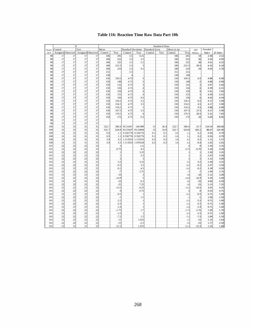
268
Table 116: Reaction Time Raw Data Part 10b
Assigned Observed Assigned Observed Control Test Control Test Control Test Control Test98 17 17 17 17 186 205 3.5 0.25 186 205 19 2.48 3.5198 17 17 17 17 186 222 3.5 3.5 186 222 36 3.50 4.9598 17 17 17 17 186 225 3.5 5.5 186 225 39 4.61 6.5298 17 17 17 17 186 215.5 3.5 5 186 215.5 29.5 4.32 6.1098 17 17 17 17 186 210 3.5 4.5 186 210 24 4.03 5.7098 17 17 17 17 151 - 5.5 - 151 15198 17 17 17 17 149 - 4 - 149 14998 17 17 17 17 150 150.5 4.75 5 150 150.5 0.5 4.88 6.9098 17 17 17 17 150 148 4.75 5 150 148 -2 4.88 6.9098 17 17 17 17 150 152 4.75 3 150 152 2 3.97 5.6298 17 17 17 17 150 156 4.75 4 150 156 6 4.39 6.2198 17 17 17 17 150 159 4.75 6 150 159 9 5.41 7.6598 17 17 17 17 150 155 4.75 4 150 155 5 4.39 6.2198 17 17 17 17 150 156 4.75 4.5 150 156 6 4.63 6.5498 17 17 17 17 150 156.5 4.75 3.5 150 156.5 6.5 4.17 5.9098 17 17 17 17 150 154.5 4.75 3.5 150 154.5 4.5 4.17 5.9098 17 17 17 17 150 154.5 4.75 5 150 154.5 4.5 4.88 6.9098 17 17 17 17 150 167.5 4.75 3.5 150 167.5 17.5 4.17 5.9098 17 17 17 17 150 170.5 4.75 6 150 170.5 20.5 5.41 7.6598 17 17 17 17 150 172 4.75 6.5 150 172 22 5.69 8.0598 17 17 17 1798 17 17 17 17
100 31 31 31 31 522.7 580.4 83.51647 146.989 15 26.4 522.7 580.4 57.7 119.54 169.06100 31 31 31 31 522.7 624.8 83.51647 93.53844 15 16.8 522.7 624.8 102.1 88.67 125.40100 31 31 31 31 0.9 1.1 0.556776 0.556776 0.1 0.1 0.9 1.1 0.2 0.56 0.79100 31 31 31 31 0.9 1.1 0.556776 0.556776 0.1 0.1 0.9 1.1 0.2 0.56 0.79100 31 31 31 31 3.9 4.1 1.113553 1.113553 0.2 0.2 3.9 4.1 0.2 1.11 1.57100 31 31 31 31 3.9 3.5 1.113553 1.670329 0.2 0.3 3.9 3.5 -0.4 1.42 2.01101 22 22 22 22 0 3.25 0 0 2.30 3.25101 22 22 22 22 -0.75 4.5 -0.75 -0.75 3.18 4.50101 22 22 22 22 1 3.25 1 1 2.30 3.25101 22 22 22 22 1 3.5 1 1 2.47 3.50101 22 22 22 22 2 3 2 2 2.12 3.00101 22 22 22 22 3.5 3.25 3.5 3.5 2.30 3.25101 22 22 22 22 -0.2 3.5 -0.2 -0.2 2.47 3.50101 22 22 22 22 -0.2 4.5 -0.2 -0.2 3.18 4.50101 22 22 22 22 -7 2.75 -7 -7 1.94 2.75101 22 22 22 22 -10 3 -10 -10 2.12 3.00101 22 22 22 22 -14.9 5 -14.9 -14.9 3.54 5.00101 22 22 22 22 -25 6.5 -25 -25 4.60 6.50101 22 22 22 22 -25 7.25 -25 -25 5.13 7.25101 22 22 22 22 -13.5 -4.25 -13.5 -13.5 3.01 4.25101 22 22 22 22 0 0.75 0 0 0.53 0.75101 22 22 22 22 -0.5 1 -0.5 -0.5 0.71 1.00101 22 22 22 22 -1 1.5 -1 -1 1.06 1.50101 22 22 22 22 -2.2 1 -2.2 -2.2 0.71 1.00101 22 22 22 22 -2.2 1 -2.2 -2.2 0.71 1.00101 22 22 22 22 -2.4 1 -2.4 -2.4 0.71 1.00101 22 22 22 22 -1.75 1.7 -1.75 -1.75 1.20 1.70101 22 22 22 22 -2.5 1 -2.5 -2.5 0.71 1.00101 22 22 22 22 -7.2 1.5 -7.2 -7.2 1.06 1.50101 22 22 22 22 -11 1.625 -11 -11 1.15 1.63101 22 22 22 22 -15 -2.5 -15 -15 1.77 2.50101 22 22 22 22 -21.5 1.875 -21.5 -21.5 1.33 1.88
Diff Means
Study Id #
NControl Test Mean Standard Deviation Standard Error
Statistical DataMean in ms Poooled
Stdev B Stdev
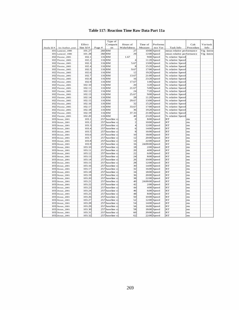
269
Table 117: Reaction Time Raw Data Part 11a
101 Lamond_1999 101.27 260 RM 27 10:00 Speed mean relative performance Vig -latenc101 Lamond_1999 101.28 260 RM 29 12:00 Speed mean relative performance Vig -latenc102 Thorne_2005 102.1 116 RM 1.67 9:00 Speed % relative Speed102 Thorne_2005 102.2 116 RM 4 11:20 Speed % relative Speed102 Thorne_2005 102.3 116 RM 5.67 13:00 Speed % relative Speed102 Thorne_2005 102.4 116 RM 8 15:20 Speed % relative Speed102 Thorne_2005 102.5 116 RM 9.67 17:00 Speed % relative Speed102 Thorne_2005 102.6 116 RM 12 19:20 Speed % relative Speed102 Thorne_2005 102.7 116 RM 13.67 21:00 Speed % relative Speed102 Thorne_2005 102.8 116 RM 16 23:20 Speed % relative Speed102 Thorne_2005 102.9 116 RM 17.67 1:00 Speed % relative Speed102 Thorne_2005 102.10 116 RM 20 3:20 Speed % relative Speed102 Thorne_2005 102.11 116 RM 21.67 5:00 Speed % relative Speed102 Thorne_2005 102.12 116 RM 24 7:20 Speed % relative Speed102 Thorne_2005 102.13 116 RM 25.67 9:00 Speed % relative Speed102 Thorne_2005 102.14 116 RM 28 11:20 Speed % relative Speed102 Thorne_2005 102.15 116 RM 29.67 13:00 Speed % relative Speed102 Thorne_2005 102.16 116 RM 32 15:20 Speed % relative Speed102 Thorne_2005 102.17 116 RM 33.67 17:00 Speed % relative Speed102 Thorne_2005 102.18 116 RM 36 19:20 Speed % relative Speed102 Thorne_2005 102.19 116 RM 37.33 21:00 Speed % relative Speed102 Thorne_2005 102.20 116 RM 40 23:20 Speed % relative Speed103 Doran_2001 103.1 257 baseline co 0 8:00 Speed RT ms103 Doran_2001 103.2 257 baseline co 2 10:00 Speed RT ms103 Doran_2001 103.3 257 baseline co 4 12:00 Speed RT ms103 Doran_2001 103.4 257 baseline co 6 14:00 Speed RT ms103 Doran_2001 103.5 257 baseline co 8 16:00 Speed RT ms103 Doran_2001 103.6 257 baseline co 10 18:00 Speed RT ms103 Doran_2001 103.7 257 baseline co 12 20:00 Speed RT ms103 Doran_2001 103.8 257 baseline co 14 22:00 Speed RT ms103 Doran_2001 103.9 257 baseline co 16 24:00:00 Speed RT ms103 Doran_2001 103.10 257 baseline co 18 2:00 Speed RT ms103 Doran_2001 103.11 257 baseline co 20 4:00 Speed RT ms103 Doran_2001 103.12 257 baseline co 22 6:00 Speed RT ms103 Doran_2001 103.13 257 baseline co 24 8:00 Speed RT ms103 Doran_2001 103.14 257 baseline co 26 10:00 Speed RT ms103 Doran_2001 103.15 257 baseline co 28 12:00 Speed RT ms103 Doran_2001 103.16 257 baseline co 30 14:00 Speed RT ms103 Doran_2001 103.17 257 baseline co 32 16:00 Speed RT ms103 Doran_2001 103.18 257 baseline co 34 18:00 Speed RT ms103 Doran_2001 103.19 257 baseline co 36 20:00 Speed RT ms103 Doran_2001 103.20 257 baseline co 38 22:00 Speed RT ms103 Doran_2001 103.21 257 baseline co 40 24:00:00 Speed RT ms103 Doran_2001 103.22 257 baseline co 42 2:00 Speed RT ms103 Doran_2001 103.23 257 baseline co 44 4:00 Speed RT ms103 Doran_2001 103.24 257 baseline co 46 6:00 Speed RT ms103 Doran_2001 103.25 257 baseline co 48 8:00 Speed RT ms103 Doran_2001 103.26 257 baseline co 50 10:00 Speed RT ms103 Doran_2001 103.27 257 baseline co 52 12:00 Speed RT ms103 Doran_2001 103.28 257 baseline co 54 14:00 Speed RT ms103 Doran_2001 103.29 257 baseline co 56 16:00 Speed RT ms103 Doran_2001 103.30 257 baseline co 58 18:00 Speed RT ms103 Doran_2001 103.31 257 baseline co 60 20:00 Speed RT ms103 Doran_2001 103.32 257 baseline co 62 22:00 Speed RT ms
Time of Measure
Performance Var Task Info
Calc Procedure
Var/task Info
Hours of WakefulnessStudy Id # 1st Author_year
Effect Size Id # Page #
Type of Comparis
on
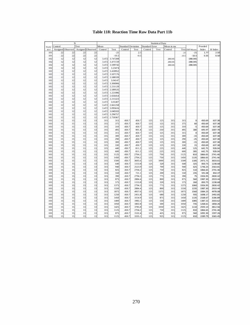
270
Table 118: Reaction Time Raw Data Part 11b
Assigned Observed Assigned Observed Control Test Control Test Control Test Control Test101 22 22 22 22 -21 2.5 -21 -21 1.77 2.50101 22 22 22 22 -10.5 -0.5 -10.5 -10.5 0.35 0.50102 12 12 12 12 3.472 3.747208 288.045 -288.045102 12 12 12 12 3.472 3.475729 288.045 -288.045102 12 12 12 12 3.472 3.599742 288.045 -288.045102 12 12 12 12 3.472 3.23474102 12 12 12 12 3.472 3.418952102 12 12 12 12 3.472 3.507176102 12 12 12 12 3.472 3.588339102 12 12 12 12 3.472 3.04147102 12 12 12 12 3.472 3.306906102 12 12 12 12 3.472 2.231129102 12 12 12 12 3.472 2.589535102 12 12 12 12 3.472 1.221086102 12 12 12 12 3.472 2.656454102 12 12 12 12 3.472 2.215323102 12 12 12 12 3.472 3.01407102 12 12 12 12 3.472 2.661258102 12 12 12 12 3.472 3.095616102 12 12 12 12 3.472 3.049183102 12 12 12 12 3.472 3.296757102 12 12 12 12 3.472 2.750367103 15 15 13 13 315 315 450.7 450.7 125 125 315 315 0 450.69 637.38103 15 15 13 13 315 375 450.7 450.7 125 125 315 375 60 450.69 637.38103 15 15 13 13 315 310 450.7 450.7 125 125 315 310 -5 450.69 637.38103 15 15 13 13 315 495 450.7 901.4 125 250 315 495 180 695.97 1007.78103 15 15 13 13 315 315 450.7 450.7 125 125 315 315 0 450.69 637.38103 15 15 13 13 315 300 450.7 450.7 125 125 315 300 -15 450.69 637.38103 15 15 13 13 315 290 450.7 450.7 125 125 315 290 -25 450.69 637.38103 15 15 13 13 315 300 450.7 450.7 125 125 315 300 -15 450.69 637.38103 15 15 13 13 315 330 450.7 450.7 125 125 315 330 15 450.69 637.38103 15 15 13 13 315 440 450.7 811.2 125 225 315 440 125 642.75 928.04103 15 15 13 13 315 600 450.7 811.2 125 225 315 600 285 642.75 928.04103 15 15 13 13 315 1125 450.7 2704.2 125 750 315 1125 810 1866.65 2741.46103 15 15 13 13 315 1450 450.7 2704.2 125 750 315 1450 1135 1866.65 2741.46103 15 15 13 13 315 1500 450.7 3605.6 125 1000 315 1500 1185 2471.71 3633.61103 15 15 13 13 315 640 450.7 1153.8 125 320 315 640 325 850.75 1238.68103 15 15 13 13 315 940 450.7 2523.9 125 700 315 940 625 1746.25 2563.81103 15 15 13 13 315 825 450.7 2704.2 125 750 315 825 510 1866.65 2741.46103 15 15 13 13 315 550 450.7 721.1 125 200 315 550 235 591.08 850.37103 15 15 13 13 315 390 450.7 2794.3 125 775 315 390 75 1926.95 2830.42103 15 15 13 13 315 875 450.7 2884.4 125 800 315 875 560 1987.30 2919.44103 15 15 13 13 315 575 450.7 1153.8 125 320 315 575 260 850.75 1238.68103 15 15 13 13 315 1375 450.7 2794.3 125 775 315 1375 1060 1926.95 2830.42103 15 15 13 13 315 1550 450.7 2884.4 125 800 315 1550 1235 1987.30 2919.44103 15 15 13 13 315 1875 450.7 4957.6 125 1375 315 1875 1560 3384.25 4978.08103 15 15 13 13 315 1250 450.7 2451.8 125 680 315 1250 935 1698.17 2492.85103 15 15 13 13 315 1450 450.7 3154.9 125 875 315 1450 1135 2168.67 3186.89103 15 15 13 13 315 1400 450.7 1983.1 125 550 315 1400 1085 1387.22 2033.62103 15 15 13 13 315 1050 450.7 1802.8 125 500 315 1050 735 1268.61 1858.26103 15 15 13 13 315 1425 450.7 3785.8 125 1050 315 1425 1110 2593.14 3812.56103 15 15 13 13 315 1125 450.7 2704.2 125 750 315 1125 810 1866.65 2741.46103 15 15 13 13 315 875 450.7 1532.4 125 425 315 875 560 1092.30 1597.26103 15 15 13 13 315 1125 450.7 3335.1 125 925 315 1125 810 2289.79 3365.45
Diff MeansStudy Id #
NControl Test Mean Standard Deviation Standard Error
Statistical DataMean in ms Poooled
Stdev B Stdev
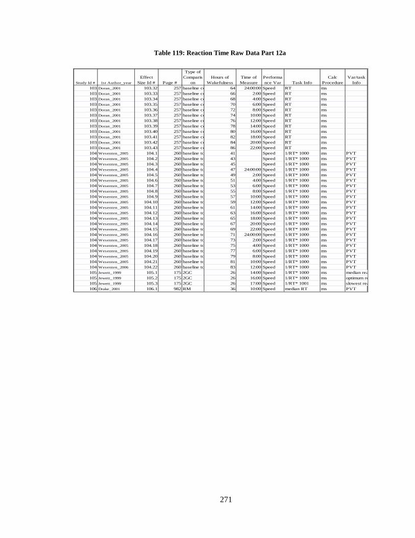
271
Table 119: Reaction Time Raw Data Part 12a
103 Doran_2001 103.32 257 baseline co 64 24:00:00 Speed RT ms103 Doran_2001 103.33 257 baseline co 66 2:00 Speed RT ms103 Doran_2001 103.34 257 baseline co 68 4:00 Speed RT ms103 Doran_2001 103.35 257 baseline co 70 6:00 Speed RT ms103 Doran_2001 103.36 257 baseline co 72 8:00 Speed RT ms103 Doran_2001 103.37 257 baseline co 74 10:00 Speed RT ms103 Doran_2001 103.38 257 baseline co 76 12:00 Speed RT ms103 Doran_2001 103.39 257 baseline co 78 14:00 Speed RT ms103 Doran_2001 103.40 257 baseline co 80 16:00 Speed RT ms103 Doran_2001 103.41 257 baseline co 82 18:00 Speed RT ms103 Doran_2001 103.42 257 baseline co 84 20:00 Speed RT ms103 Doran_2001 103.43 257 baseline co 86 22:00 Speed RT ms104 Wesenten_2005 104.1 260 baseline to 41 Speed 1/RT* 1000 ms PVT104 Wesenten_2005 104.2 260 baseline to 43 Speed 1/RT* 1000 ms PVT104 Wesenten_2005 104.3 260 baseline to 45 Speed 1/RT* 1000 ms PVT104 Wesenten_2005 104.4 260 baseline to 47 24:00:00 Speed 1/RT* 1000 ms PVT104 Wesenten_2005 104.5 260 baseline to 49 2:00 Speed 1/RT* 1000 ms PVT104 Wesenten_2005 104.6 260 baseline to 51 4:00 Speed 1/RT* 1000 ms PVT104 Wesenten_2005 104.7 260 baseline to 53 6:00 Speed 1/RT* 1000 ms PVT104 Wesenten_2005 104.8 260 baseline to 55 8:00 Speed 1/RT* 1000 ms PVT104 Wesenten_2005 104.9 260 baseline to 57 10:00 Speed 1/RT* 1000 ms PVT104 Wesenten_2005 104.10 260 baseline to 59 12:00 Speed 1/RT* 1000 ms PVT104 Wesenten_2005 104.11 260 baseline to 61 14:00 Speed 1/RT* 1000 ms PVT104 Wesenten_2005 104.12 260 baseline to 63 16:00 Speed 1/RT* 1000 ms PVT104 Wesenten_2005 104.13 260 baseline to 65 18:00 Speed 1/RT* 1000 ms PVT104 Wesenten_2005 104.14 260 baseline to 67 20:00 Speed 1/RT* 1000 ms PVT104 Wesenten_2005 104.15 260 baseline to 69 22:00 Speed 1/RT* 1000 ms PVT104 Wesenten_2005 104.16 260 baseline to 71 24:00:00 Speed 1/RT* 1000 ms PVT104 Wesenten_2005 104.17 260 baseline to 73 2:00 Speed 1/RT* 1000 ms PVT104 Wesenten_2005 104.18 260 baseline to 75 4:00 Speed 1/RT* 1000 ms PVT104 Wesenten_2005 104.19 260 baseline to 77 6:00 Speed 1/RT* 1000 ms PVT104 Wesenten_2005 104.20 260 baseline to 79 8:00 Speed 1/RT* 1000 ms PVT104 Wesenten_2005 104.21 260 baseline to 81 10:00 Speed 1/RT* 1000 ms PVT104 Wesenten_2006 104.22 260 baseline to 83 12:00 Speed 1/RT* 1000 ms PVT105 Jewett_1999 105.1 175 2GC 26 14:00 Speed 1/RT* 1000 ms median rea 105 Jewett_1999 105.2 175 2GC 26 16:00 Speed 1/RT* 1000 ms optimum re 105 Jewett_1999 105.3 175 2GC 26 17:00 Speed 1/RT* 1001 ms slowest rea 106 Drake_2001 106.1 982 RM 36 10:00 Speed median RT ms PVT
Time of Measure
Performance Var Task Info
Calc Procedure
Var/task Info
Hours of WakefulnessStudy Id # 1st Author_year
Effect Size Id # Page #
Type of Comparis
on
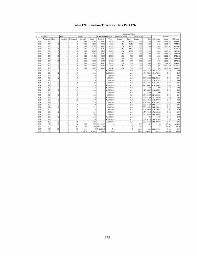
272
Table 120: Reaction Time Raw Data Part 12b
Assigned Observed Assigned Observed Control Test Control Test Control Test Control Test103 15 15 13 13 315 1380 450.7 4506.9 125 1250 315 1380 1065 3079.67 4529.42103 15 15 13 13 315 1500 450.7 4723.3 125 1310 315 1500 1185 3225.83 4744.73103 15 15 13 13 315 2300 450.7 4506.9 125 1250 315 2300 1985 3079.67 4529.42103 15 15 13 13 315 2125 450.7 4056.2 125 1125 315 2125 1810 2775.45 4081.21103 15 15 13 13 315 2125 450.7 5408.3 125 1500 315 2125 1810 3689.09 5427.07103 15 15 13 13 315 1400 450.7 2704.2 125 750 315 1400 1085 1866.65 2741.46103 15 15 13 13 315 1450 450.7 2704.2 125 750 315 1450 1135 1866.65 2741.46103 15 15 13 13 315 1250 450.7 2704.2 125 750 315 1250 935 1866.65 2741.46103 15 15 13 13 315 1300 450.7 2433.7 125 675 315 1300 985 1686.16 2475.13103 15 15 13 13 315 1000 450.7 1892.9 125 525 315 1000 685 1327.83 1945.83103 15 15 13 13 315 1600 450.7 2884.4 125 800 315 1600 1285 1987.30 2919.44103 15 15 13 13 315 1125 450.7 2091.2 125 580 315 1125 810 1458.69 2139.23104 12 12 12 12 2.6 0.6928203 0.2 384.61538 384.61538 0.49 0.69104 12 12 12 12 2.3 0.6928203 0.2 434.78261 434.78261 0.49 0.69104 12 12 12 12 2 1.0392305 0.3 500 500 0.73 1.04104 12 12 12 12 1.7 1.0392305 0.3 588.23529 588.23529 0.73 1.04104 12 12 12 12 1.9 1.0392305 0.3 526.31579 526.31579 0.73 1.04104 12 12 12 12 1.85 1.0392305 0.3 540.54054 540.54054 0.73 1.04104 12 12 12 12 2.4 0.6928203 0.2 416.66667 416.66667 0.49 0.69104 12 12 12 12 2.5 0.6928203 0.2 400 400 0.49 0.69104 12 12 12 12 2.4 0.6928203 0.2 416.66667 416.66667 0.49 0.69104 12 12 12 12 2.5 1.0392305 0.3 400 400 0.73 1.04104 12 12 12 12 2.6 1.0392305 0.3 384.61538 384.61538 0.73 1.04104 12 12 12 12 2.8 0.6928203 0.2 357.14286 357.14286 0.49 0.69104 12 12 12 12 2.7 0.6928203 0.2 370.37037 370.37037 0.49 0.69104 12 12 12 12 2.3 1.0392305 0.3 434.78261 434.78261 0.73 1.04104 12 12 12 12 1.8 1.0392305 0.3 555.55556 555.55556 0.73 1.04104 12 12 12 12 1.7 1.0392305 0.3 588.23529 588.23529 0.73 1.04104 12 12 12 12 2.1 1.3856406 0.4 476.19048 476.19048 0.98 1.39104 12 12 12 12 2.1 1.3856406 0.4 476.19048 476.19048 0.98 1.39104 12 12 12 12 1.85 1.0392305 0.3 540.54054 540.54054 0.73 1.04104 12 12 12 12 2.5 0.6928203 0.2 400 400 0.49 0.69104 12 12 12 12 2.6 0.6928203 0.2 384.61538 384.61538 0.49 0.69104 12 12 12 12 2.85 1.0392305 0.3 350.87719 350.87719 0.73 1.04105 32 32 25 25 235 305 62.225397 90 11 18 235 305 70 75.61 109.42105 32 32 25 25 192 215 11.313708 15 2 3 192 215 23 13.05 18.79105 32 32 25 25 2.9 1.6 5.6568542 7.5 1 1.5 344.83 625 280.17241 6.53 9.39106 28 12 28 12 266.3 310.07 54.01 68.9 266.3 310.07 43.77 61.90 87.55
Diff MeanStudy Id #
NControl Test Mean Standard Deviation Standard Error
Statistical DataMean in ms Poooled
Stdev B Stdev
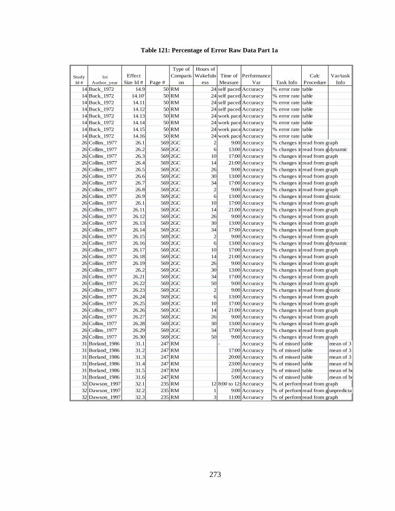
273
Table 121: Percentage of Error Raw Data Part 1a
14 Buck_1972 14.9 50 RM 24 self paced Accuracy % error rate table14 Buck_1972 14.10' 50 RM 24 self paced Accuracy % error rate table14 Buck_1972 14.11 50 RM 24 self paced Accuracy % error rate table14 Buck_1972 14.12 50 RM 24 self paced Accuracy % error rate table14 Buck_1972 14.13 50 RM 24 work pace Accuracy % error rate table14 Buck_1972 14.14 50 RM 24 work pace Accuracy % error rate table14 Buck_1972 14.15 50 RM 24 work pace Accuracy % error rate table14 Buck_1972 14.16 50 RM 24 work pace Accuracy % error rate table26 Collins_1977 26.1 569 2GC 2 9:00 Accuracy % changes in read from graph26 Collins_1977 26.2 569 2GC 6 13:00 Accuracy % changes in read from g dynamic26 Collins_1977 26.3 569 2GC 10 17:00 Accuracy % changes in read from graph26 Collins_1977 26.4 569 2GC 14 21:00 Accuracy % changes in read from graph26 Collins_1977 26.5 569 2GC 26 9:00 Accuracy % changes in read from graph26 Collins_1977 26.6 569 2GC 30 13:00 Accuracy % changes in read from graph26 Collins_1977 26.7 569 2GC 34 17:00 Accuracy % changes in read from graph26 Collins_1977 26.8 569 2GC 2 9:00 Accuracy % changes in read from graph26 Collins_1977 26.9 569 2GC 6 13:00 Accuracy % changes in read from g static26 Collins_1977 26.1 569 2GC 10 17:00 Accuracy % changes in read from graph26 Collins_1977 26.11 569 2GC 14 21:00 Accuracy % changes in read from graph26 Collins_1977 26.12 569 2GC 26 9:00 Accuracy % changes in read from graph26 Collins_1977 26.13 569 2GC 30 13:00 Accuracy % changes in read from graph26 Collins_1977 26.14 569 2GC 34 17:00 Accuracy % changes in read from graph26 Collins_1977 26.15 569 2GC 2 9:00 Accuracy % changes in read from graph26 Collins_1977 26.16 569 2GC 6 13:00 Accuracy % changes in read from g dynamic26 Collins_1977 26.17 569 2GC 10 17:00 Accuracy % changes in read from graph26 Collins_1977 26.18 569 2GC 14 21:00 Accuracy % changes in read from graph26 Collins_1977 26.19 569 2GC 26 9:00 Accuracy % changes in read from graph26 Collins_1977 26.2 569 2GC 30 13:00 Accuracy % changes in read from graph26 Collins_1977 26.21 569 2GC 34 17:00 Accuracy % changes in read from graph26 Collins_1977 26.22 569 2GC 50 9:00 Accuracy % changes in read from graph26 Collins_1977 26.23 569 2GC 2 9:00 Accuracy % changes in read from g static26 Collins_1977 26.24 569 2GC 6 13:00 Accuracy % changes in read from graph26 Collins_1977 26.25 569 2GC 10 17:00 Accuracy % changes in read from graph26 Collins_1977 26.26 569 2GC 14 21:00 Accuracy % changes in read from graph26 Collins_1977 26.27 569 2GC 26 9:00 Accuracy % changes in read from graph26 Collins_1977 26.28 569 2GC 30 13:00 Accuracy % changes in read from graph26 Collins_1977 26.29 569 2GC 34 17:00 Accuracy % changes in read from graph26 Collins_1977 26.30 569 2GC 50 9:00 Accuracy % changes in read from graph31 Borland_1986 31.1 247 RM - Accuracy % of missed table mean of 3 31 Borland_1986 31.2 247 RM 17:00 Accuracy % of missed table mean of 3 31 Borland_1986 31.3 247 RM 20:00 Accuracy % of missed table mean of 3 31 Borland_1986 31.4 247 RM 23:00 Accuracy % of missed table mean of bo 31 Borland_1986 31.5 247 RM 2:00 Accuracy % of missed table mean of bo 31 Borland_1986 31.6 247 RM 5:00 Accuracy % of missed table mean of bo 32 Dawson_1997 32.1 235 RM 12 8:00 to 12:0Accuracy % of perform read from graph32 Dawson_1997 32.2 235 RM 1 9:00 Accuracy % of perform read from g unpredictab 32 Dawson_1997 32.3 235 RM 3 11:00 Accuracy % of perform read from graph
Time of Measure
Performance Var Task Info
Calc Procedure
Var/task Info
Hours of Wakefuln
essStudy Id #
1st Author_year
Effect Size Id # Page #
Type of Comparis
on
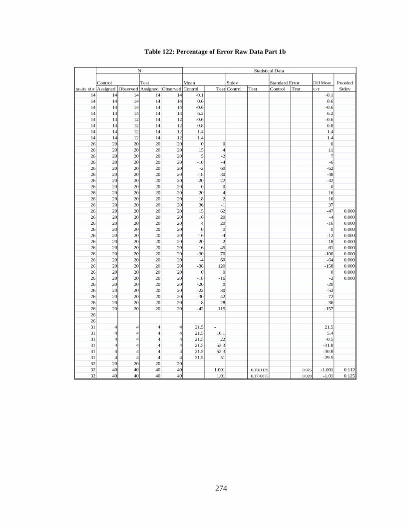
274
Table 122: Percentage of Error Raw Data Part 1b
Standard Error Diff MeanAssigned Observed Assigned Observed Control Test Control Test Control Test C-T
14 14 14 14 14 -0.1 -0.114 14 14 14 14 0.6 0.614 14 14 14 14 -0.6 -0.614 14 14 14 14 6.2 6.214 14 12 14 12 -0.6 -0.614 14 12 14 12 0.8 0.814 14 12 14 12 1.4 1.414 14 12 14 12 1.4 1.426 20 20 20 20 0 0 026 20 20 20 20 15 4 1126 20 20 20 20 5 -2 726 20 20 20 20 -10 -4 -626 20 20 20 20 -2 60 -6226 20 20 20 20 -18 30 -4826 20 20 20 20 -20 22 -4226 20 20 20 20 0 0 026 20 20 20 20 20 4 1626 20 20 20 20 18 2 1626 20 20 20 20 36 -1 3726 20 20 20 20 15 62 -47 0.00026 20 20 20 20 16 20 -4 0.00026 20 20 20 20 4 20 -16 0.00026 20 20 20 20 0 0 0 0.00026 20 20 20 20 -16 -4 -12 0.00026 20 20 20 20 -20 -2 -18 0.00026 20 20 20 20 -16 45 -61 0.00026 20 20 20 20 -30 70 -100 0.00026 20 20 20 20 -4 60 -64 0.00026 20 20 20 20 -38 120 -158 0.00026 20 20 20 20 0 0 0 0.00026 20 20 20 20 -18 -16 -2 0.00026 20 20 20 20 -20 0 -2026 20 20 20 20 -22 30 -5226 20 20 20 20 -30 42 -7226 20 20 20 20 -8 28 -3626 20 20 20 20 -42 115 -157262631 4 4 4 4 21.5 - 21.531 4 4 4 4 21.5 16.1 5.431 4 4 4 4 21.5 22 -0.531 4 4 4 4 21.5 53.3 -31.831 4 4 4 4 21.5 52.3 -30.831 4 4 4 4 21.5 51 -29.532 20 20 20 2032 40 40 40 40 1.001 0.1581139 0.025 -1.001 0.11232 40 40 40 40 1.01 0.1770875 0.028 -1.01 0.125
Study Id #
N Statistical Data
Control Test Mean Stdev Poooled Stdev
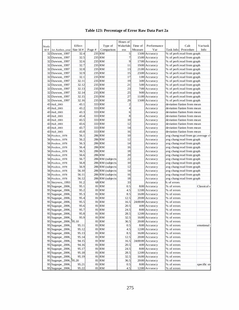
275
Table 123: Percentage of Error Raw Data Part 2a
32 Dawson_1997 32.4 235 RM 5 13:00 Accuracy % of perfo read from graph32 Dawson_1997 32.5 235 RM 7 15:00 Accuracy % of perfo read from graph32 Dawson_1997 32.6 235 RM 9 17:00 Accuracy % of perfo read from graph32 Dawson_1997 32.7 235 RM 11 19:00 Accuracy % of perfo read from graph32 Dawson_1997 32.8 235 RM 13 21:00 Accuracy % of perfo read from graph32 Dawson_1997 32.9 235 RM 15 23:00 Accuracy % of perfo read from graph32 Dawson_1997 32.1 235 RM 17 1:00 Accuracy % of perfo read from graph32 Dawson_1997 32.11 235 RM 19 3:00 Accuracy % of perfo read from graph32 Dawson_1997 32.12 235 RM 21 5:00 Accuracy % of perfo read from graph32 Dawson_1997 32.13 235 RM 23 7:00 Accuracy % of perfo read from graph32 Dawson_1997 32.14 235 RM 25 9:00 Accuracy % of perfo read from graph32 Dawson_1997 32.15 235 RM 27 11:00 Accuracy % of perfo read from graph32 Dawson_1997 32.16 235 RM 29 13:00 Accuracy % of perfo read from graph43 Hull_2003 43.1 333 RM 2 Accuracy deviation f viation from mean43 Hull_2003 43.2 333 RM 4 Accuracy deviation fr viation from mean43 Hull_2003 43.3 333 RM 6 Accuracy deviation fr viation from mean43 Hull_2003 43.4 333 RM 8 Accuracy deviation fr viation from mean43 Hull_2003 43.5 333 RM 10 Accuracy deviation fr viation from mean43 Hull_2003 43.6 333 RM 12 Accuracy deviation f viation from mean43 Hull_2003 43.7 333 RM 14 Accuracy deviation f viation from mean43 Hull_2003 43.8 333 RM 16 Accuracy deviation f viation from mean56 Poulton_1978 56.1 286 RM 10 Accuracy avg change read from graaverage ch 56 Poulton_1978 56.2 286 RM 12 Accuracy avg change read from graph56 Poulton_1978 56.3 286 RM 14 Accuracy avg change read from graph56 Poulton_1978 56.4 286 RM 16 Accuracy avg change read from graph56 Poulton_1978 56.5 286 RM 18 Accuracy avg change read from graph56 Poulton_1978 56.6 286 RM 20 Accuracy avg change read from graph56 Poulton_1978 56.7 286 RM (subjects 22 Accuracy avg change read from graph56 Poulton_1978 56.8 286 RM (subjects 10 Accuracy avg change read from graph56 Poulton_1978 56.9 286 RM (subjects 12 Accuracy avg change read from graph56 Poulton_1978 56.10 286 RM (subjects 14 Accuracy avg change read from graph56 Poulton_1978 56.11 286 RM (subjects 16 Accuracy avg change read from graph56 Poulton_1978 56.12 286 RM (subjects 18 Accuracy avg change read from graph91 Steyvers_1993 91.2 68 RM 33 Accuracy % of errors95 Sagaspe_2006_ 95.1 81 RM 0.5 8:00 Accuracy % of errors Classical s95 Sagaspe_2006_ 95.2 81 RM 4.5 12:00 Accuracy % of errors95 Sagaspe_2006_ 95.3 81 RM 8.5 16:00 Accuracy % of errors95 Sagaspe_2006_ 95.4 81 RM 12.5 20:00 Accuracy % of errors95 Sagaspe_2006_ 95.5 81 RM 16.5 24:00:00 Accuracy % of errors95 Sagaspe_2006_ 95.6 81 RM 20.5 4:00 Accuracy % of errors95 Sagaspe_2006_ 95.7 81 RM 24.5 8:00 Accuracy % of errors95 Sagaspe_2006_ 95.8 81 RM 28.5 12:00 Accuracy % of errors95 Sagaspe_2006_ 95.9 81 RM 32.5 16:00 Accuracy % of errors95 Sagaspe_2006_ 95.10 81 RM 36.5 20:00 Accuracy % of errors95 Sagaspe_2006_ 95.11 81 RM 0.5 8:00 Accuracy % of errors emotional s95 Sagaspe_2006_ 95.12 81 RM 4.5 12:00 Accuracy % of errors95 Sagaspe_2006_ 95.13 81 RM 8.5 16:00 Accuracy % of errors95 Sagaspe_2006_ 95.14 81 RM 12.5 20:00 Accuracy % of errors95 Sagaspe_2006_ 94.15 81 RM 16.5 24:00:00 Accuracy % of errors95 Sagaspe_2006_ 94.16 81 RM 20.5 4:00 Accuracy % of errors95 Sagaspe_2006_ 95.17 81 RM 24.5 8:00 Accuracy % of errors95 Sagaspe_2006_ 95.18 81 RM 28.5 12:00 Accuracy % of errors95 Sagaspe_2006_ 95.19 81 RM 32.5 16:00 Accuracy % of errors95 Sagaspe_2006_ 95.20 81 RM 36.5 20:00 Accuracy % of errors95 Sagaspe_2006_ 95.21 81 RM 0.5 8:00 Accuracy % of errors specific str95 Sagaspe_2006_ 95.22 81 RM 4.5 12:00 Accuracy % of errors
Time of Measure
Performance Var Task Info
Calc Procedure
Var/task Info
Hours of Wakefuln
essStudy Id # 1st Author_year
Effect Size Id # Page #
Type of Comparison
276
Table 124: Percentage of Error Raw Data Part 2b
Standard Error Diff MeanAssigned Observed Assigned Observed Control Test Control Test Control Test C-T
32 40 40 40 40 1.009 0.1897367 0.03 -1.009 0.13432 40 40 40 40 1.02 0.1581139 0.025 -1.02 0.11232 40 40 40 40 1.01 0.1960612 0.031 -1.01 0.13932 40 40 40 40 1.01 0.1834121 0.029 -1.01 0.13032 40 40 40 40 1.015 0.1644384 0.026 -1.015 0.11632 40 40 40 40 1.007 0.1897367 0.03 -1.007 0.13432 40 40 40 40 0.995 0.1770875 0.028 -0.995 0.12532 40 40 40 40 0.968 0.2213594 0.035 -0.968 0.15732 40 40 40 40 0.96 0.1897367 0.03 -0.96 0.13432 40 40 40 40 0.942 0.2023858 0.032 -0.942 0.14332 40 40 40 40 0.945 0.2213594 0.035 -0.945 0.15732 40 40 40 40 0.97 0.1960612 0.031 -0.97 0.13932 40 40 40 40 0.995 0.1897367 0.03 -0.995 0.13443 15 15 15 15 71 0.71 7.7459667 0.07746 2 -71 5.50043 15 15 15 15 70.75 0.7075 1.9364917 0.019365 0.5 -70.75 1.45843 15 15 15 15 70.5 0.705 1.5491933 0.015492 0.4 -70.5 1.20443 15 15 15 15 69 0.69 1.9364917 0.019365 0.5 -69 1.45443 15 15 15 15 69.75 0.6975 5.809475 0.058095 1.5 -69.75 4.13743 15 15 15 15 69.75 0.6975 3.8729833 0.03873 1 -69.75 2.78343 15 15 15 15 69 0.69 3.8729833 0.03873 1 -69 2.78243 15 15 15 15 68 0.68 3.8729833 0.03873 1 -68 2.78156 7 7 7 756 10 10 10 1056 11 11 11 1156 12 12 12 1256 3 3 3 356 1 1 1 156 1 1 1 156 14 14 14 1456 10 10 10 1056 12 12 12 1256 10 10 10 1056 9 9 9 991 16 16 16 1695 12 12 12 12 1 3.5 1.5 2.4 -2.5 2.00195 12 12 12 12 0.5 2.3 0.9 2 -1.8 1.55195 12 12 12 12 0.5 1.3 0.9 0.9 -0.8 0.90095 12 12 12 12 0.6 1.1 0.9 1.9 -0.5 1.48795 12 12 12 12 0.5 2.5 0.9 2.7 -2 2.01295 12 12 12 12 0.6 1.5 1.7 2.4 -0.9 2.08095 12 12 12 12 0.8 1.6 1.8 1.8 -0.8 1.80095 12 12 12 12 0.8 2 1.5 2.2 -1.2 1.88395 12 12 12 12 1.6 1.5 1.8 1.5 0.1 1.65795 12 12 12 12 1.1 1.8 1.3 2.1 -0.7 1.74695 12 12 12 12 0.5 0.6 0.9 1.3 -0.1 1.11895 12 12 12 12 0.8 1 1 1.3 -0.2 1.16095 12 12 12 12 0.3 0.5 0.7 0.9 -0.2 0.80695 12 12 12 12 1 1 1.8 1.3 0 1.57095 12 12 12 12 0.5 0.3 0.9 0.7 0.2 0.80695 12 12 12 12 0.8 0.3 1.3 0.7 0.5 1.04495 12 12 12 12 1.3 1 1.5 1.3 0.3 1.40495 12 12 12 12 0.8 0.3 1.5 0.7 0.5 1.17095 12 12 12 12 0.8 0 1.3 0 0.8 0.91995 12 12 12 12 1 0.3 1.5 0.7 0.7 1.17095 12 12 12 12 1 0.5 1.5 1.2 0.5 1.35895 12 12 12 12 0.3 0.1 1.1 0.5 0.2 0.85495 12 12 12 12 1 1.5 1.8 1.2 -0.5 1.53095 12 12 12 12 1 0.6 1.5 1.3 0.4 1.40495 12 12 12 12 0.6 0.8 0.9 1.3 -0.2 1.11895 12 12 12 12 0.6 0.1 1.3 0.5 0.5 0.98595 12 12 12 12 0.6 0.5 0.9 0.9 0.1 0.90095 12 12 12 12 0.1 0.6 0.5 0.9 -0.5 0.72895 12 12 12 12 1.1 2 2.3 2.4 -0.9 2.35195 12 12 12 12 2.3 1.5 2.8 2.2 0.8 2.518
Study Id #
N Statistical Data
Control Test Mean Stdev Poooled Stdev
277
Table 125: False Positive Raw Data Part 1a
5 Williamson_2000 5.21 652 RM 2.27 8:00 Accuracy false + table Mackworth a 5 Williamson_2000 5.22 652 RM 13.27 19:00 Accuracy false + table Mackworth a 5 Williamson_2000 5.23 652 RM 14 19:44 Accuracy false + table Mackworth a 5 Williamson_2000 5.24 652 RM 18 23:44 Accuracy false + table Mackworth a 5 Williamson_2000 5.25 652 RM 22 27:44:00 Accuracy false + table Mackworth a
27 Porcu_1998 27.26 1198 RM baseline Accuracy false + DBT27 Porcu_1998 27.27 1198 RM 23:00 Accuracy false + DBT27 Porcu_1998 27.28 1198 RM 1:00 Accuracy false + DBT27 Porcu_1998 27.29 1198 RM 3:00 Accuracy false + DBT27 Porcu_1998 27.30 1198 RM 5:00 Accuracy false + DBT27 Porcu_1998 27.31 1198 RM baseline Accuracy false + LCT27 Porcu_1998 27.32 1198 RM 23:00 Accuracy false + LCT27 Porcu_1998 37.33 1198 RM 1:00 Accuracy false + LCT27 Porcu_1998 27.34 1198 RM 3:00 Accuracy false + LCT27 Porcu_1998 27.35 1198 RM 5:00 Accuracy false + LCT48 Drummond_2006 48.5 263 RM 7 Accuracy false + PVT48 Drummond_2006 48.6 263 RM 22.15 Accuracy false + PVT48 Drummond_2006 48.7 263 RM 30.75 Accuracy false + PVT48 Drummond_2006 48.8 263 RM 57.75 Accuracy false + PVT53 Frey_2004 53.1 308 RM 43 02:00 to 08 Accuracy false start PVT55 Webb_1982 55.5 274 RM Accuracy false + table AVI f +55 Webb_1982 55.6 274 RM Accuracy false + table AVI f +
100 Lieberman_2005 100.9 425 RM 77 18:00, 12:04Accuracy false + table Vis Vig - fals 100 Lieberman_2005 100.1 425 RM 94 18:00, 05:04Accuracy false + table Vis Vig - fals
Time of Measure
Performance Var Task Info
Calc Procedure
Var/task Info
Hours of Sleep
DeprivatiStudy Id # 1st Author_year
Effect Size Id # Page #
Type of Comparison
Table 126: False Positive Raw Data Part 1b
Standard ErrorDiff Means
Assigned Observed Assigned Observed Control Test Control Test Control Test C-T5 39 39 39 39 1.05 2.15 -1.15 39 39 39 39 1.05 1.28 -0.235 39 39 39 39 1.05 1.48 -0.435 39 39 39 39 1.05 2.85 -1.85 39 39 39 39 1.05 4.24 -3.19
27 10 10 10 1027 10 10 10 10 0.78 0.46 1.03 1.092 0.32 1.061 1.50127 10 10 10 10 0.78 0.46 1.03 0.96 0.32 0.996 1.40827 10 10 10 10 0.78 0.78 1.03 0.69 0 0.877 1.24027 10 10 10 10 0.78 0.56 1.03 1.13 0.22 1.081 1.52927 7 7 7 727 7 7 7 7 0.43 0.29 0.79 0.68 0.14 0.737 1.04227 7 7 7 7 0.43 0.71 0.79 0.49 -0.28 0.657 0.93027 7 7 7 7 0.43 1 0.79 1.1 -0.57 0.958 1.35427 7 7 7 7 0.43 1 0.79 1 -0.57 0.901 1.27448 36 36 36 36 0.14 0.14 0.045 0.045 0.0075 0.0075 0 0.045 0.06448 36 36 36 36 0.14 0.195 0.045 0.06 0.0075 0.01 -0.055 0.053 0.07548 36 36 36 36 0.14 0.2 0.045 0.105 0.0075 0.0175 -0.06 0.081 0.11448 36 36 36 36 0.14 0.19 0.045 0.18 0.0075 0.03 -0.05 0.131 0.18653 25 25 25 25 0.14 2.7 0.04 0.44 -2.56 0.312 0.44255 13.5 14.8 10 8.2 -1.3 9.144 12.93255 11.3 11.8 20 24.7 -0.5 22.473 31.782
100 31 31 31 31 1.1 5.1 1.6703293 8.3516465 0.3 1.5 -4 6.022 8.517100 31 31 31 31 1.1 2.9 1.6703293 3.8974351 0.3 0.7 -1.8 2.998 4.240
Study Id #
N Statistical Data
Control Test Mean Standard Deviation Poooled Stdev B Stdev
278
Table 127: Percentage Correct Raw Data Part 1a
2 Thomas_2000 2.2 346 RM 24 Accuracy % correct worse directly serial addit 3 Choo_2005 3.5 581 RM 24.4 Accuracy % correct worse directly SRT3 Choo_2005 3.6 581 RM 24.4 Accuracy % correct worse directly SRT3 Choo_2005 3.7 581 RM 24.4 Accuracy % correct worse directly SRT3 Choo_2005 3.8 581 RM 24.4 Accuracy % correct worse directly SRT4 Chee_2004 4.4 RM 24 Accuracy % correct worse directly4 Chee_2004 4.5 RM 24 Accuracy % correct worse directly7 Robbins_1990 7.1 83 RM 35 end of bein Accuracy % correct worse read from graph7 Robbins_1990 7.3 83 RM 35 Accuracy % correct worse read from graph7 Robbins_1990 7.4 83 RM 35 Accuracy % correct worse read from graph7 Robbins_1990 7.5 83 RM 35 Accuracy % correct better? read from graph9 Babkoff_2005 9.2 11 RM 8.5 0.354167 Accuracy % of correct responseread from graph9 Babkoff_2005 9.3 11 RM 10.5 0.4375 Accuracy % of correct responseread from graph9 Babkoff_2005 9.4 11 RM 12.75 0.53125 Accuracy % of correct responseread from graph9 Babkoff_2005 9.5 11 RM 15.5 0.645833 Accuracy % of correct responseread from graph9 Babkoff_2005 9.6 11 RM 18.5 0.770833 Accuracy % of correct responseread from graph
17 Yoo_2007 17.1 386 2GC 35 0.75 Accuracy proportion worse read from proportion 17 Yoo_2007 17.2 386 2GC 35 0.75 Accuracy proportion of correct rejections proportion 18 Babkoff_1985 18.2 616 RM 72 Accuracy % correct worse in text50 Engle_Friedman 50.2 115 RM 1night Accuracy % correct worse in text50 Engle_Friedman 50.5 121 2GC 3 night 09:00 to 10Accuracy % correct table50 Engle_Friedman 50.7 121 2GC 5 night 09:00 to 10Accuracy % correct table53 Frey_2004 53.4 308 RM 43 Accuracy % correct Wilkinson53 Frey_2004 53.6 308 RM 43 Accuracy % correct Manikin53 Frey_2004 53.8 308 RM 43 Accuracy % correct Math accu53 Frey_2004 53.10 308 RM 43 Accuracy % correct 2ADD53 Frey_2004 53.12 308 RM 43 Accuracy % correct Dual53 Frey_2004 53.14 308 RM 43 Accuracy % correct RCT53 Frey_2004 53.17 308 RM 43 Accuracy % correct DR55 Webb_1982 53.27 274 RM Accuracy % correct table REA - %55 Webb_1982 55.1 274 RM Accuracy % correct table57 Englund_1985 57.1 81 RM 2 0.375 Accuracy % correct table 4CRT57 Englund_1985 57.2 81 RM 5.5 0.520833 Accuracy % correct table 4CRT57 Englund_1985 57.3 81 RM 8.5 0.645833 Accuracy % correct table 4CRT57 Englund_1985 57.4 81 RM 12.25 0.802083 Accuracy % correct table 4CRT57 Englund_1985 57.5 81 RM 15.75 0.947917 Accuracy % correct table 4CRT57 Englund_1985 57.6 81 RM 19 0.083333 Accuracy % correct table 4CRT57 Englund_1985 57.7 81 RM 1 0.333333 Accuracy % recall table word mem57 Englund_1985 57.8 81 RM 7.5 0.604167 Accuracy % recall table word mem57 Englund_1985 57.9 81 RM 15.75 0.947917 Accuracy % recall table word mem57 Englund_1985 57.10 81 RM 19 0.083333 Accuracy % recall table word mem57 Englund_1985 57.15 81 RM 1 0.333333 Accuracy % correct table logical reas57 Englund_1985 57.16 81 RM 4 0.458333 Accuracy % correct table logical reas57 Englund_1985 57.17 81 RM 7.5 0.604167 Accuracy % correct table logical reas57 Englund_1985 57.18 81 RM 11.25 0.760417 Accuracy % correct table logical reas57 Englund_1985 57.19 81 RM 14.75 0.90625 Accuracy % correct table logical reas57 Englund_1985 57.20 81 RM 18 0.041667 Accuracy % correct table logical reas57 Englund_1985 57.21 81 RM 19 0.083333 Accuracy % correct table logical reas
Var/task Info
Study Id # 1st Author_year
Effect Size Id # Page #
Type of Comparis
on
Hours of Sleep
DeprivatiTime of Measure
Performance Var Task Info
Performance
Direction CalcPpro
cedure
279
Table 128: Percentage Correct Raw Data Part 1b
Standard ErrorDiff Means
Assigned Observed Assigned Observed Control Test Control Test Control Test T-C2 - 17 - 17 0.955 0.923 0.052 0.064 -0.032 0.05831 0.0824623 14 12 - 0.988 0.941 0.013 0.05 -0.047 #NUM! 0.0516623 14 12 - 0.968 0.927 0.05 0.074 -0.041 0.04693 0.0893083 14 12 - 0.943 0.911 0.052 0.086 -0.032 0.047274 0.1004993 14 12 - 0.966 0.926 0.038 0.07 -0.04 0.033142 0.0796494 13 13 13 13 0.959 0.902 0.049 0.097 -0.057 0.076844 0.1086744 13 13 13 13 0.957 0.926 0.055 0.086 -0.031 0.072184 0.1020837 31 23 31 23 0.65 0.605 0.0575 0.0815 -0.045 0.070528 0.0997427 31 23 31 23 0.75 0.67 0.0911 0.2254 -0.08 0.171907 0.2431147 31 23 31 23 23.95 22.25 4.1723 4.556 -1.7 4.368365 6.1778017 31 23 31 23 0.54 0.58 0.1247 0.1103 0.04 0.11772 0.1664829 20 18 20 18 0.764 0.735 -0.0299 20 18 20 18 0.76 0.73 -0.039 20 18 20 18 0.745 0.715 -0.039 20 18 20 18 0.743 0.719 -0.0249 20 18 20 18 0.768 0.729 -0.039
17 14 14 14 14 0.86 0.74 0.019 0.044 -0.12 0.03389 0.04792717 14 14 14 14 0.91 0.92 0.021 0.044 0.01 0.034475 0.04875418 10 6 10 6 0.827 0.646 -0.18150 50 50 50 50 0.6998 0.6408 0.1448 0.1817 -0.059 0.164289 0.2323450 50 50 50 5050 50 50 50 5053 25 25 25 25 0.977 0.908 0.02 0.085 0.004 0.017 -0.069 0.061745 0.08732153 25 25 25 25 0.916 0.822 0.1 0.145 0.02 0.029 -0.094 0.124549 0.17613953 25 25 25 25 0.909 0.775 0.085 0.12 0.017 0.024 -0.134 0.103983 0.14705453 25 25 25 25 0.855 0.709 0.115 0.185 0.023 0.037 -0.146 0.154029 0.2178353 25 25 25 25 0.98 0.911 0.035 0.095 0.007 0.019 -0.069 0.071589 0.10124253 25 25 25 25 0.913 0.839 0.085 0.125 0.017 0.025 -0.074 0.106888 0.15116253 25 25 25 25 0.571 0.458 0.15 0.16 0.03 0.032 -0.113 0.155081 0.21931755 0.76 0.843 0.362 0.206 0.083 0.294517 0.41650955 0.422 0.399 0.086 0.093 -0.023 0.089568 0.12666957 22 22 22 22 1 0.877 -0.123 0 057 22 22 22 22 1 0.852 0.173 -0.148 0.17357 22 22 22 22 1 0.858 0.203 -0.142 0.20357 22 22 22 22 1 0.867 0.168 -0.133 0.16857 22 22 22 22 1 0.876 0.176 -0.124 0.17657 22 22 22 22 1 0.795 0.189 -0.205 0.18957 22 22 22 22 1 0.547 0.235 -0.453 0.23557 22 22 22 22 1 0.588 0.192 -0.412 0.19257 22 22 22 22 1 0.58 0.167 -0.42 0.16757 22 22 22 22 1 0.787 0.16 -0.213 0.1657 22 22 22 22 1 0.758 0.144 -0.242 0.14457 22 22 22 22 1 0.781 0.148 -0.219 0.148
Poooled Stdev B Stdev
Study Id #
N
Control Test Mean Stdev
Statistical Data
280
Table 129: Percentage Correct Raw Data Part 2a
60 Christensen_1977 60.2 105 RM worked at least 15hr accuracy % detecte table logical reasoning63 Horne_1983 63.1 352 RM 60 1 accuracy % hits read from glogical reasoning63 Horne_1983 63.2 352 RM 60 0.166667 accuracy % hits read from glogical reasoning63 Horne_1983 63.3 352 RM 60 0.375 accuracy % hits read from glogical reasoning63 Horne_1983 63.4 352 RM 60 0.583333 accuracy % hits read from glogical reasoning63 Horne_1983 63.5 352 RM 60 0.791667 accuracy % hits read from glogical reasoning63 Horne_1983 63.6 352 RM 60 1 accuracy % hits read from glogical reasoning63 Horne_1983 63.7 352 RM 60 0.166667 accuracy % hits read from glogical reasoning63 Horne_1983 63.8 352 RM 60 0.375 accuracy % hits read from glogical reasoning63 Horne_1983 63.9 352 RM 60 0.583333 accuracy % hits read from glogical reasoning63 Horne_1983 63.1 352 RM 60 0.791667 accuracy % hits read from glogical reasoning67 Binks_1999 67.1 331 2GC 35 0.75 accuracy % of corre table PASAT % - Aud serial add72 Linde_1999 72.2 704 2GC 0.916667 accuracy % correct = table72 Linde_1999 72.21 704 2GC 0.166667 accuracy % correct = table72 Linde_1999 72.22 704 2GC 0.416667 accuracy % correct = table72 Linde_1999 72.23 704 2GC 0.666667 accuracy % correct = table72 Linde_1999 72.24 704 2GC 0.916667 accuracy % correct = table72 Linde_1999 72.25 704 2GC 0.166667 accuracy % correct = table72 Linde_1999 72.26 704 2GC 0.416667 accuracy % correct = table72 Linde_1999 72.27 704 2GC 0.666667 accuracy % correct = table92 Elkin_1974 92.1 194 2GC 55 0.625 accuracy % correct - immediate recognition92 Elkin_1974 92.2 195 2GC 12 0.875 accuracy % correct - immediate recognition92 Elkin_1974 92.3 195 2GC 25 0.375 accuracy % correct - immediate recognition92 Elkin_1974 92.4 195 2GC 31 0.625 accuracy % correct - immediate recognition92 Elkin_1974 92.5 195 2GC 37 0.875 accuracy % correct - immediate recognition92 Elkin_1974 92.6 195 2GC 49 0.375 accuracy % correct - immediate recognition92 Elkin_1974 92.7 195 2GC 55 0.625 accuracy % correct - immediate recognition92 Elkin_1974 92.8 195 2GC 12 0.875 accuracy % correct - recognition after 20 sec92 Elkin_1974 92.9 195 2GC 25 0.375 accuracy % correct - recognition after 20 sec92 Elkin_1974 92.1 195 2GC 31 0.625 accuracy % correct - recognition after 20 sec92 Elkin_1974 92.11 195 2GC 37 0.875 accuracy % correct - recognition after 20 sec92 Elkin_1974 92.12 195 2GC 49 0.375 accuracy % correct - recognition after 20 sec92 Elkin_1974 92.13 195 2GC 55 0.625 accuracy % correct - recognition after 20 sec93 Webb_1986 93.1 171 RM 64 0.208333 accuracy % correct table93 Webb_1986 93.2 171 RM 64 accuracy % correct table93 Webb_1986 93.3 171 RM 64 accuracy % correct table93 Webb_1986 93.4 171 RM 64 accuracy % correct table93 Webb_1986 93.5 171 RM 64 0.208333 accuracy reading ra table task 1a93 Webb_1986 93.6 171 RM 64 accuracy reading ra table task 1b93 Webb_1986 93.7 171 RM 64 accuracy reading ra table task 293 Webb_1986 93.8 171 RM 64 accuracy reading ra table task 3
101 Lamond_1999 101.1 260 RM 3 0.416667 accuracy mean rela read from gsimple sensory 101 Lamond_1999 101.2 260 RM 5 0.5 accuracy mean rela read from gsimple sensory 101 Lamond_1999 101.3 260 RM 7 0.583333 accuracy mean rela read from gsimple sensory 101 Lamond_1999 101.4 260 RM 9 0.666667 accuracy mean rela read from gsimple sensory 101 Lamond_1999 101.5 260 RM 11 0.75 accuracy mean rela read from gsimple sensory 101 Lamond_1999 101.6 260 RM 13 0.833333 accuracy mean rela read from gsimple sensory 101 Lamond_1999 101.7 260 RM 15 0.916667 accuracy mean rela read from gsimple sensory 101 Lamond_1999 101.8 260 RM 17 1 accuracy mean rela read from gsimple sensory 101 Lamond_1999 101.9 260 RM 19 0.083333 accuracy mean rela read from gsimple sensory 101 Lamond_1999 101.1 260 RM 21 0.166667 accuracy mean rela read from gsimple sensory 101 Lamond_1999 101.11 260 RM 23 0.25 accuracy mean rela read from gsimple sensory 101 Lamond_1999 101.12 260 RM 25 0.333333 accuracy mean rela read from gsimple sensory 101 Lamond_1999 101.13 260 RM 27 0.416667 accuracy mean rela read from gsimple sensory 101 Lamond_1999 101.14 260 RM 29 0.5 accuracy mean rela read from gsimple sensory 101 Lamond_1999 101.29 259 RM 3 0.416667 accuracy mean rela read from ggram accuracy101 Lamond_1999 101.3 259 RM 5 0.5 accuracy mean rela read from ggram accuracy101 Lamond_1999 101.31 259 RM 7 0.583333 accuracy mean rela read from ggram accuracy101 Lamond_1999 101.32 259 RM 9 0.666667 accuracy mean rela read from ggram accuracy101 Lamond_1999 101.34 259 RM 11 0.75 accuracy mean rela read from ggram accuracy101 Lamond_1999 101.35 259 RM 13 0.833333 accuracy mean rela read from ggram accuracy101 Lamond_1999 101.36 259 RM 15 0.916667 accuracy mean rela read from ggram accuracy101 Lamond_1999 101.37 259 RM 17 1 accuracy mean rela read from ggram accuracy101 Lamond_1999 101.38 259 RM 19 0.083333 accuracy mean rela read from ggram accuracy101 Lamond_1999 101.39 259 RM 21 0.166667 accuracy mean rela read from ggram accuracy101 Lamond_1999 101.4 259 RM 23 0.25 accuracy mean rela read from ggram accuracy
Study Id # 1st Author_yearEffect
Size Id # Page #
Type of Comparis
on Var/task Info
Hours of Sleep
DeprivatiTime of Measure
Performance Var Task Info
Calc Procedure
281
Table 130: Percentage Correct Raw Data Part 2b
Standard ErrorDiff Means
Assigned Observed Assigned Observed Control Test Control Test Control Test T-C60 14 14 14 14 0.614 0.607 0.614 0.429214 0.60763 8 8 8 8 0.92 0.92 0 063 8 8 8 8 0.86 0.86 0 063 8 8 8 8 0.88 0.82 -0.06 0 063 8 8 8 8 0.83 0.83 0 0 063 8 8 8 8 0.87 0.82 -0.05 0 063 8 8 8 8 0.76 0.76 0 063 8 8 8 8 0.61 0.61 0 063 8 8 8 8 0.89 0.57 -0.32 0 063 8 8 8 8 0.91 0.61 -0.3 0 063 8 8 8 8 0.9 0.605 -0.295 0 067 32 32 32 29 0.573 0.561 0.153 0.147 -0.012 0.150182 0.21217472 11 11 11 11 0.965 0.948 0.07 0.092 -0.017 0.067112 0.11560372 11 11 11 11 0.956 0.929 0.044 0.119 -0.027 0.024035 0.12687472 11 11 11 11 0.0954 0.92 0.075 0.131 0.8246 0.065903 0.1509572 11 11 11 11 0.983 0.93 0.012 0.128 -0.053 #NUM! 0.12856172 10 10 10 10 0.009 0.005 0.026 0.044 -0.004 0.022771 0.05110872 9 9 9 9 0.014 -0.013 0.031 0.078 -0.027 0.015137 0.08393472 10 10 10 10 0.002 -0.023 0.08 0.117 -0.025 0.074087 0.14173672 10 10 10 10 0.031 -0.012 0.057 0.139 -0.043 0.035214 0.15023392 20 20 20 20 0 0 092 20 20 20 20 0.76 0.79 0.03 0 092 20 20 20 20 0.79 0.8 0.01 0 092 20 20 20 20 0.785 0.8 0.015 0 092 20 20 20 20 0.76 0.78 0.02 0 092 20 20 20 20 0.74 0.79 0.05 0 092 20 20 20 20 0.75 0.79 0.04 0 092 20 20 20 20 0.75 0.77 0.02 0 092 20 20 20 20 0.685 0.75 0.065 0 092 20 20 20 20 0.685 0.76 0.075 0 092 20 20 20 20 0.7 0.73 0.03 0 092 20 20 20 20 0.65 0.78 0.13 0 092 20 20 20 20 0.66 0.75 0.09 0 093 10 8 10 8 0.69 0.73 0.04 0 093 10 6 10 6 0.67 0.73 0.06 0 093 10 6 10 6 0.94 0.86 -0.08 0 093 10 6 10 6 0.68 0.63 -0.05 0 093 10 8 10 8 0.906977 0.906977 0 093 10 6 10 6 0.835938 0.835938 0 093 10 6 10 6 0.8 0.8 0 093 10 6 10 6 0.7 0.7 0 0
101 22 22 22 22 1 0.99 0.0775 7.75 -0.01 0.054801 0.0775101 22 22 22 22 1 0.995 0.025 2.5 -0.005 0.017678 0.025101 22 22 22 22 1 0.981 0.025 2.5 -0.019 0.017678 0.025101 22 22 22 22 1 0.9875 0.025 2.5 -0.0125 0.017678 0.025101 22 22 22 22 1 0.991 0.0325 3.25 -0.009 0.022981 0.0325101 22 22 22 22 1 1 0.036 3.6 0 0.025456 0.036101 22 22 22 22 1 0.97 0.037 3.7 -0.03 0.026163 0.037101 22 22 22 22 1 0.989 0.04 4 -0.011 0.028284 0.04101 22 22 22 22 1 1 0.0355 3.55 0 0.025102 0.0355101 22 22 22 22 1 0.99 0.04 4 -0.01 0.028284 0.04101 22 22 22 22 1 0.971 0.043 4.3 -0.029 0.030406 0.043101 22 22 22 22 1 0.99 0.0375 3.75 -0.01 0.026517 0.0375101 22 22 22 22 1 0.95 0.035 3.5 -0.05 0.024749 0.035101 22 22 22 22 1 0.97 0.045 4.5 -0.03 0.03182 0.045101 22 22 22 22 1 0.995 0.0175 1.75 -0.005 0.012374 0.0175101 22 22 22 22 1 0.985 0.02 2 -0.015 0.014142 0.02101 22 22 22 22 1 0.99 0.023 2.3 -0.01 0.016263 0.023101 22 22 22 22 1 0.99 0.025 2.5 -0.01 0.017678 0.025101 22 22 22 22 1 0.991 0.022 2.2 -0.009 0.015556 0.022101 22 22 22 22 1 0.975 0.0225 2.25 -0.025 0.01591 0.0225101 22 22 22 22 1 0.975 0.0125 1.25 -0.025 0.008839 0.0125101 22 22 22 22 1 0.975 0.0115 1.15 -0.025 0.008132 0.0115101 22 22 22 22 1 0.977 0.015 1.5 -0.023 0.010607 0.015101 22 22 22 22 1 0.978 0.015 1.5 -0.022 0.010607 0.015101 22 22 22 22 1 0.975 0.0225 2.25 -0.025 0.01591 0.0225101 22 22 22 22 1 0.965 0.022 2.2 -0.035 0.015556 0.022
Study Id #
N Statistical Data
Control Test Mean Stdev Poooled Stdev B Stdev
282
Table 131: Percentage Correct Raw Data Part 3a
101 Lamond_1999 101.42 259 RM 27 0.416667 accuracy mean relative pe read from grgram accuracy101 Lamond_1999 101.43 259 RM 29 0.5 accuracy mean relative pe read from grgram accuracy101 Lamond_1999 101.44 259 RM 3 0.416667 accuracy mean relative pe read from grVig- accuracy101 Lamond_1999 101.15 259 RM 5 0.5 accuracy mean relative pe read from grVig- accuracy101 Lamond_1999 101.46 259 RM 7 0.583333 accuracy mean relative pe read from grVig- accuracy101 Lamond_1999 101.47 259 RM 9 0.666667 accuracy mean relative pe read from grVig- accuracy101 Lamond_1999 101.48 259 RM 11 0.75 accuracy mean relative pe read from grVig- accuracy101 Lamond_1999 101.49 259 RM 13 0.833333 accuracy mean relative pe read from grVig- accuracy101 Lamond_1999 101.5 259 RM 15 0.916667 accuracy mean relative pe read from grVig- accuracy101 Lamond_1999 101.51 259 RM 17 1 accuracy mean relative pe read from grVig- accuracy101 Lamond_1999 101.52 259 RM 19 0.083333 accuracy mean relative pe read from grVig- accuracy101 Lamond_1999 101.53 259 RM 21 0.166667 accuracy mean relative pe read from grVig- accuracy101 Lamond_1999 101.54 259 RM 23 0.25 accuracy mean relative pe read from grVig- accuracy101 Lamond_1999 101.55 259 RM 25 0.333333 accuracy mean relative pe read from grVig- accuracy101 Lamond_1999 101.56 259 RM 27 0.416667 accuracy mean relative pe read from grVig- accuracy101 Lamond_1999 101.57 259 RM 29 0.5 accuracy mean relative pe read from grVig- accuracy
Var/task InfoStudy Id # 1st Author_year
Effect Size Id # Page #
Type of Comparis
on
Hours of Sleep
DeprivatiTime of Measure
Performance Var Task Info
Calc Procedure
Table 132: Percentage Correct Raw Data Part 3b
Standard ErrorDiff Means
Assigned Observed Assigned Observed Control Test Control Test Control Test T-C101 22 22 22 22 1 0.97 0.015 1.5 -0.03 0.010607 0.015101 22 22 22 22 1 0.98 0.0125 1.25 -0.02 0.008839 0.0125101 22 22 22 22 1 1 0.003 0.3 0 0.002121 0.003101 22 22 22 22 1 0.999 0.002 0.2 -0.001 0.001414 0.002101 22 22 22 22 1 0.998 0.005 0.5 -0.002 0.003536 0.005101 22 22 22 22 1 0.995 0.007 0.7 -0.005 0.00495 0.007101 22 22 22 22 1 0.99 0.007 0.7 -0.01 0.00495 0.007101 22 22 22 22 1 0.99 0.01 1 -0.01 0.007071 0.01101 22 22 22 22 1 0.992 0.0075 0.75 -0.008 0.005303 0.0075101 22 22 22 22 1 0.9935 0.005 0.5 -0.0065 0.003536 0.005101 22 22 22 22 1 0.985 0.015 1.5 -0.015 0.010607 0.015101 22 22 22 22 1 0.981 0.0185 1.85 -0.019 0.013081 0.0185101 22 22 22 22 1 0.968 0.024 2.4 -0.032 0.016971 0.024101 22 22 22 22 1 0.947 0.032 3.2 -0.053 0.022627 0.032101 22 22 22 22 1 0.935 0.03 3 -0.065 0.021213 0.03101 22 22 22 22 1 0.975 0.013 1.3 -0.025 0.009192 0.013
Study Id #
N Statistical Data
Control Test Mean Stdev Poooled Stdev B Stdev
283
Table 133: Number of Errors Raw Data Part 1a
5 Williamson_2000 5.6 652 RM 2.27 8:00 Accuracy misses table RT accura5 Williamson_2000 5.7 652 RM 13.27 19:00 Accuracy misses table RT accura5 Williamson_2000 5.8 652 RM 14 19:44 Accuracy misses table RT accura5 Williamson_2000 5.9 652 RM 18 23:44 Accuracy misses table RT accura5 Williamson_2000 5.1 652 RM 22 27:44:00 Accuracy misses table RT accura
10 Swann_2006 10.2 28 RM 19.2 Accuracy total errorsdirectly PVT20 Williams_1959 20.11 13 RM b4 Accuracy # of errorsread from graph20 Williams_1959 20.12 13 RM 28 Accuracy # of errorsread from graph20 Williams_1959 20.13 13 RM 52 Accuracy # of errorsread from graph20 Williams_1959 20.14 13 RM 76 Accuracy # of errorsread from graph20 Williams_1959 20.15 13 RM b4 Accuracy # of errorsread from graph20 Williams_1959 20.16 13 RM 30 Accuracy # of errorsread from graph20 Williams_1959 20.17 13 RM 54 Accuracy # of errorsread from graph20 Williams_1959 20.18 13 RM 70 Accuracy # of errorsread from graph49 Eastridge_2003 49.1 172 RM - 08:00 to 11 Accuracy # of errorsread from graph67 Binks_1999 67.2 331 2GC 35 18:00 Accuracy # of incorr table BFCT err67 Binks_1999 67.3 332 2GC 35 18:00 Accuracy total error table WSCT tota 67 Binks_1999 67.4 332 2GC 35 18:00 Accuracy error table WSCT per 72 Linde_1999 72.1 703 2GC 16:00 Accuracy # error table72 Linde_1999 72.2 703 2GC 22:00 Accuracy # error table72 Linde_1999 72.3 703 2GC 4:00 Accuracy # error table72 Linde_1999 72.4 703 2GC 10:00 Accuracy # error table72 Linde_1999 72.5 703 2GC 16:00 Accuracy # error table72 Linde_1999 72.6 703 2GC 22:00 Accuracy # error table72 Linde_1999 72.7 703 2GC 4:00 Accuracy # error table72 Linde_1999 72.8 703 2GC 10:00 Accuracy # error table72 Linde_1999 72.9 703 2GC 16:00 Accuracy # error table92 Elkin_1974 92.14 195 2GC 12 21:00 Accuracy median # copying errormedian # c 92 Elkin_1974 92.15 195 2GC 25 9:00 Accuracy median # copying errors92 Elkin_1974 92.16 195 2GC 31 15:00 Accuracy median # copying errors92 Elkin_1974 92.17 195 2GC 37 21:00 Accuracy median # copying errors92 Elkin_1974 92.18 195 2GC 49 9:00 Accuracy median # copying errors92 Elkin_1974 92.19 195 2GC 55 15:00 Accuracy median # copying errors
100 Lieberman_2005 100.3 425 RM 77 18:00, 12:01Accuracy # incorrect table 4CRT-erro100 Lieberman_2005 100.4 425 RM 94 18:00, 05:01Accuracy # incorrect table103 Doran_2001 103.45 257 RM 0 8:00 Accuracy # of errorsread from graph103 Doran_2001 103.46 257 RM 2 10:00 Accuracy # of errorsread from graph103 Doran_2001 103.47 257 RM 4 12:00 Accuracy # of errorsread from graph103 Doran_2001 103.48 257 RM 6 14:00 Accuracy # of errorsread from graph103 Doran_2001 103.49 257 RM 8 16:00 Accuracy # of errorsread from graph103 Doran_2001 103.5 257 RM 10 18:00 Accuracy # of errorsread from graph103 Doran_2001 103.51 257 RM 12 20:00 Accuracy # of errorsread from graph103 Doran_2001 103.54 257 RM 18 2:00 Accuracy # of errorsread from graph103 Doran_2001 103.57 257 RM 24 8:00 Accuracy # of errorsread from graph103 Doran_2001 103.6 257 RM 30 14:00 Accuracy # of errorsread from graph103 Doran_2001 103.63 257 RM 36 18:00 Accuracy # of errorsread from graph103 Doran_2001 103.66 257 RM 42 24:00:00 Accuracy # of errorsread from graph103 Doran_2001 103.69 257 RM 48 6:00 Accuracy # of errorsread from graph103 Doran_2001 103.72 257 RM 54 12:00 Accuracy # of errorsread from graph103 Doran_2001 103.75 257 RM 60 16:00 Accuracy # of errorsread from graph103 Doran_2001 103.78 257 RM 66 22:00 Accuracy # of errorsread from graph103 Doran_2001 103.81 257 RM 72 4:00 Accuracy # of errorsread from graph103 Doran_2001 103.84 257 RM 78 10:00 Accuracy # of errorsread from graph103 Doran_2001 103.87 257 RM 84 16:00 Accuracy # of errorsread from graph
Time of Measure
Performance Var Task Info
Calc Procedure
Var/task Info
Hours of Wakefulness
Study Id # 1st Author_year
Effect Size Id # Page #
Type of Comparis
on

284
Table 134: Number of Errors Raw Data Part 1b
Standard ErrorDiff Means
Assigned Observed Assigned Observed Control Test Control Test Control Test T-C5 39 39 39 39 0.36 0.39 -0.035 39 39 39 39 1.08 -1.085 39 39 39 39 0.98 -0.985 39 39 39 39 1.67 -1.675 39 39 39 39 3.1 -3.1
10 12 12 12 12 0.88 0.79 0.762102 0.796743 0.22 0.23 0.09 0.779615 1.10254320 74 74 74 74 0 - visual vigilance20 74 74 74 74 0 5 -520 74 74 74 74 0 20 -2020 74 74 74 74 0 40 -4020 74 74 74 74 0 -20 74 74 74 74 0 5 -520 74 74 74 74 0 17 -1720 74 74 74 74 0 25 -2549 35 35 35 35 6 12 2.366432 3.549648 0.4 0.6 -6 3.016621 4.26614667 32 32 29 29 43.8 35 20.1 20.6 8.8 20.33882 28.7814267 32 32 29 29 43.5 35.1 28.8 27 8.4 27.96021 39.4770867 32 32 29 29 13.4 11.3 12.4 11.2 2.1 11.84567 16.7092872 12 12 12 12 27.2 24.5 18 16.9 2.7 18.10632 24.6902872 12 12 12 12 14.6 15.7 18.6 13.1 -1.1 19.06292 22.7501672 12 12 12 12 8.5 16.1 9.7 20.3 -7.6 7.892401 22.4984472 12 12 12 12 5.8 14.2 4.7 23.3 -8.4 23.7693172 12 12 12 12 4.3 11.6 3.4 20.3 -7.3 20.5827672 12 12 12 12 0.58 0.37 0.29 0.35 0.21 0.283302 0.45453372 12 12 12 12 0.74 0.33 0.16 0.56 0.41 0.58240972 12 12 12 12 0.77 0.43 0.16 0.62 0.34 0.64031272 12 12 12 12 0.83 0.5 0.11 0.65 0.33 0.65924292 20 20 20 20 2 1 192 20 20 20 20 2 2.2 -0.292 20 20 20 20 2 2.5 -0.592 20 20 20 20 3 1 292 20 20 20 20 5 1 492 20 20 20 20 7 1 6
100 31 31 31 31 12.5 24.7 18.9304 16.70329 3.4 3 -12.2 17.85161 25.24599100 31 31 31 31 12.5 39.8 18.9304 25.05494 3.4 4.5 -27.3 22.20484 31.40239103 15 15 15 13 1.25 1.25 2.25347 -1.25 1.784684 2.576941103 15 15 15 13 2 1.25 2.25347 -2 1.784684 2.576941103 15 15 15 13 2.3 1.25 2.25347 -2.3 1.784684 2.576941103 15 15 15 13 2.55 1.25 2.25347 -2.55 1.784684 2.576941103 15 15 15 13 2.75 1.25 2.25347 -2.75 1.784684 2.576941103 15 15 15 13 1.75 1.2 2.163331 -1.75 1.713296 2.473863103 15 15 15 13 3 2.5 4.506939 -3 3.569368 5.153882103 15 15 15 13 3.75 1.3 2.343608 -3.75 1.856071 2.680019103 15 15 15 13 7.5 4.5 8.11249 -7.5 6.424862 9.276988103 15 15 15 13 5 2.5 4.506939 -5 3.569368 5.153882103 15 15 15 13 3 1.25 2.25347 -3 1.784684 2.576941103 15 15 15 13 5 3 5.408327 -5 4.283241 6.184658103 15 15 15 13 6.25 4.25 7.661796 -6.25 6.067925 8.761599103 15 15 15 13 5.5 1.5 2.704163 -5.5 2.141621 3.092329103 15 15 15 13 6.25 4.75 8.563184 -6.25 6.781798 9.792376103 15 15 15 13 8.75 6.25 11.26735 -8.75 8.923419 12.88471103 15 15 15 13 9 8.75 15.77429 -9 12.49279 18.03859103 15 15 15 13 12.5 6.25 11.26735 -12.5 8.923419 12.88471103 15 15 15 13 13.75 7.5 13.52082 -13.75 10.7081 15.46165
Study Id #
N Statistical Data
Control Test Mean Stdev Poooled Stdev B Stdev
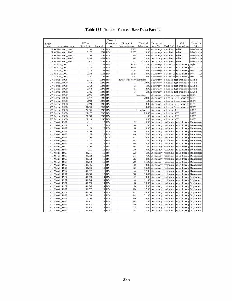
285
Table 135: Number Correct Raw Data Part 1a
5 Williamson_2000 5.16 652 RM 2.27 8:00 accuracy Mackwort table Mackworth 5 Williamson_2000 5.17 652 RM 13.27 19:00 accuracy Mackwort table Mackworth 5 Williamson_2000 5.18 652 RM 14 19:44 accuracy Mackwort table Mackworth 5 Williamson_2000 5.19 652 RM 18 23:44 Accuracy Mackwort table Mackworth 5 Williamson_2000 5.2 652 RM 22 27:44:00 Accuracy Mackwort table Mackworth
21 Wilson_2007 21.1 228 RM 16.5 21:00 accuracy # of respon read from graph21 Wilson_2007 21.2 228 RM 19.5 0:00 accuracy # of respon read from grPVT - acc21 Wilson_2007 21.3 228 RM 22.5 3:00 accuracy # of respon read from grPVT - acc21 Wilson_2007 21.4 228 RM 25.5 6:00 accuracy # of respon read from grPVT - acc21 Wilson_2007 21.5 228 RM 28.5 9:00 accuracy # of respon read from grPVT - acc27 Porcu_1998 27.1 1198 RM acute shift of w baseline accuracy # hits in digit symbol su DSST27 Porcu_1998 27.2 1198 RM 1 23:00 accuracy # hits in digit symbol su DSST27 Porcu_1998 27.3 1198 RM 3 1:00 accuracy # hits in digit symbol su DSST27 Porcu_1998 27.4 1198 RM 5 3:00 accuracy # hits in digit symbol su DSST27 Porcu_1998 27.5 1198 RM 7 5:00 accuracy # hits in digit symbol su DSST27 Porcu_1998 27.6 1198 RM baseline Accuracy # hits in Deux barragesDBT27 Porcu_1998 27.7 1198 RM 23:00 Accuracy # hits in Deux barragesDBT27 Porcu_1998 27.8 1198 RM 1:00 Accuracy # hits in Deux barragesDBT27 Porcu_1998 27.9 1198 RM 3:00 Accuracy # hits in Deux barragesDBT27 Porcu_1998 27.10 1198 RM 5:00 Accuracy # hits in Deux barragesDBT27 Porcu_1998 27.16 1198 RM baseline Accuracy # hits in LCT LCT27 Porcu_1998 27.17 1198 RM 23:00 Accuracy # hits in LCT LCT27 Porcu_1998 27.18 1198 RM 1:00 Accuracy # hits in LCT LCT27 Porcu_1998 27.19 1198 RM 3:00 Accuracy # hits in LCT LCT41 Monk_1997 41.1 15 RM 2 9:00 Accuracy residuals read from grReasoning 41 Monk_1997 41.2 15 RM 4 11:00 Accuracy residuals read from grReasoning 41 Monk_1997 41.3 15 RM 6 13:00 Accuracy residuals read from grReasoning 41 Monk_1997 41.4 15 RM 8 15:00 Accuracy residuals read from grReasoning 41 Monk_1997 41.5 15 RM 10 17:00 Accuracy residuals read from grReasoning 41 Monk_1997 41.6 15 RM 12 19:00 Accuracy residuals read from grReasoning 41 Monk_1997 41.7 15 RM 14 21:00 Accuracy residuals read from grReasoning 41 Monk_1997 41.8 15 RM 16 23:00 Accuracy residuals read from grReasoning 41 Monk_1997 41.9 15 RM 18 1:00 Accuracy residuals read from grReasoning 41 Monk_1997 41.1 15 RM 20 3:00 Accuracy residuals read from grReasoning 41 Monk_1997 41.11 15 RM 22 5:00 Accuracy residuals read from grReasoning 41 Monk_1997 41.12 15 RM 24 7:00 Accuracy residuals read from grReasoning 41 Monk_1997 41.13 15 RM 26 9:00 Accuracy residuals read from grReasoning 41 Monk_1997 41.14 15 RM 28 11:00 Accuracy residuals read from grReasoning 41 Monk_1997 41.15 15 RM 30 13:00 Accuracy residuals read from grReasoning 41 Monk_1997 41.16 15 RM 32 15:00 Accuracy residuals read from grReasoning 41 Monk_1997 41.17 15 RM 34 17:00 Accuracy residuals read from grReasoning 41 Monk_1997 41.18 15 RM 36 19:00 Accuracy residuals read from grReasoning 41 Monk_1997 41.73 14 RM 2 9:00 Accuracy residuals read from grVigilance h41 Monk_1997 41.74 14 RM 4 11:00 Accuracy residuals read from grVigilance h41 Monk_1997 41.75 14 RM 6 13:00 Accuracy residuals read from grVigilance h41 Monk_1997 41.76 14 RM 8 15:00 Accuracy residuals read from grVigilance h41 Monk_1997 41.77 14 RM 10 17:00 Accuracy residuals read from grVigilance h41 Monk_1997 41.78 14 RM 12 19:00 Accuracy residuals read from grVigilance h41 Monk_1997 41.79 14 RM 14 21:00 Accuracy residuals read from grVigilance h41 Monk_1997 41.8 14 RM 16 23:00 Accuracy residuals read from grVigilance h41 Monk_1997 41.81 14 RM 18 1:00 Accuracy residuals read from grVigilance h41 Monk_1997 41.82 14 RM 20 3:00 Accuracy residuals read from grVigilance h41 Monk_1997 41.83 14 RM 22 5:00 Accuracy residuals read from grVigilance h41 Monk_1997 41.84 14 RM 24 7:00 Accuracy residuals read from grVigilance h
Time of Measure
Performance Var Task Info
Calc Procedure
Var/task Info
Hours of Wakefulness
Study Id # 1st Author_year
Effect Size Id # Page #
Type of Comparis
on
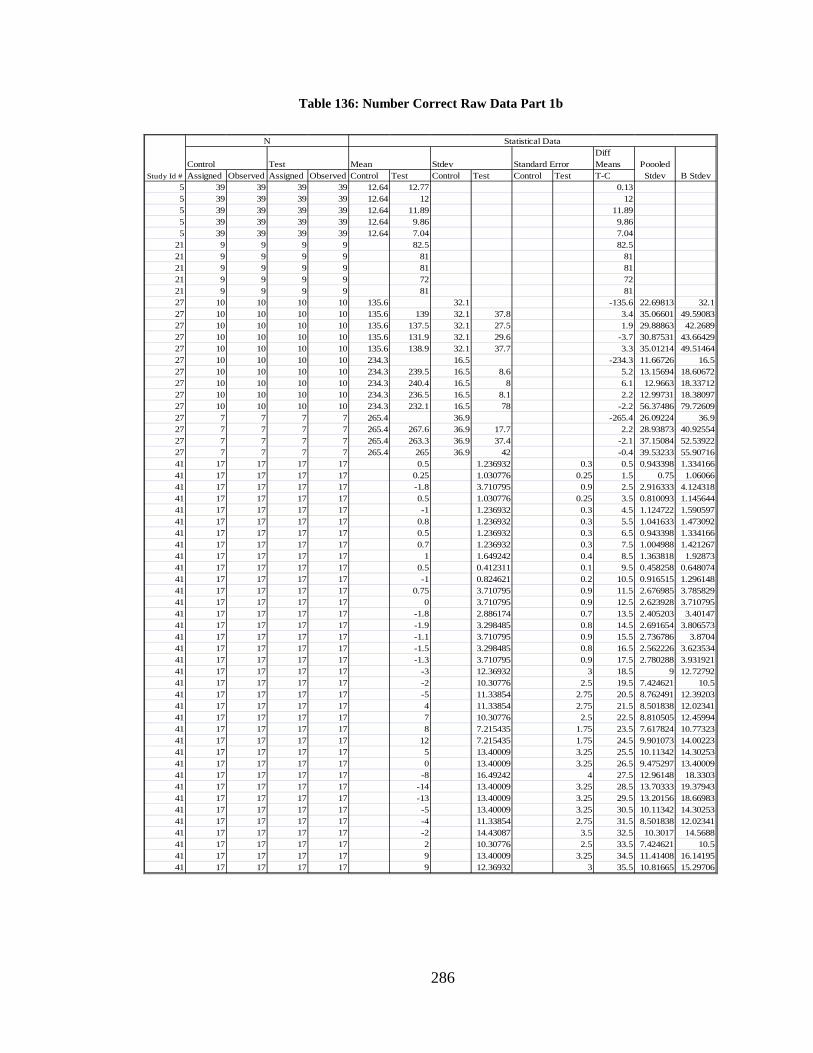
286
Table 136: Number Correct Raw Data Part 1b
Standard ErrorDiff Means
Assigned Observed Assigned Observed Control Test Control Test Control Test T-C5 39 39 39 39 12.64 12.77 0.135 39 39 39 39 12.64 12 125 39 39 39 39 12.64 11.89 11.895 39 39 39 39 12.64 9.86 9.865 39 39 39 39 12.64 7.04 7.04
21 9 9 9 9 82.5 82.521 9 9 9 9 81 8121 9 9 9 9 81 8121 9 9 9 9 72 7221 9 9 9 9 81 8127 10 10 10 10 135.6 32.1 -135.6 22.69813 32.127 10 10 10 10 135.6 139 32.1 37.8 3.4 35.06601 49.5908327 10 10 10 10 135.6 137.5 32.1 27.5 1.9 29.88863 42.268927 10 10 10 10 135.6 131.9 32.1 29.6 -3.7 30.87531 43.6642927 10 10 10 10 135.6 138.9 32.1 37.7 3.3 35.01214 49.5146427 10 10 10 10 234.3 16.5 -234.3 11.66726 16.527 10 10 10 10 234.3 239.5 16.5 8.6 5.2 13.15694 18.6067227 10 10 10 10 234.3 240.4 16.5 8 6.1 12.9663 18.3371227 10 10 10 10 234.3 236.5 16.5 8.1 2.2 12.99731 18.3809727 10 10 10 10 234.3 232.1 16.5 78 -2.2 56.37486 79.7260927 7 7 7 7 265.4 36.9 -265.4 26.09224 36.927 7 7 7 7 265.4 267.6 36.9 17.7 2.2 28.93873 40.9255427 7 7 7 7 265.4 263.3 36.9 37.4 -2.1 37.15084 52.5392227 7 7 7 7 265.4 265 36.9 42 -0.4 39.53233 55.9071641 17 17 17 17 0.5 1.236932 0.3 0.5 0.943398 1.33416641 17 17 17 17 0.25 1.030776 0.25 1.5 0.75 1.0606641 17 17 17 17 -1.8 3.710795 0.9 2.5 2.916333 4.12431841 17 17 17 17 0.5 1.030776 0.25 3.5 0.810093 1.14564441 17 17 17 17 -1 1.236932 0.3 4.5 1.124722 1.59059741 17 17 17 17 0.8 1.236932 0.3 5.5 1.041633 1.47309241 17 17 17 17 0.5 1.236932 0.3 6.5 0.943398 1.33416641 17 17 17 17 0.7 1.236932 0.3 7.5 1.004988 1.42126741 17 17 17 17 1 1.649242 0.4 8.5 1.363818 1.9287341 17 17 17 17 0.5 0.412311 0.1 9.5 0.458258 0.64807441 17 17 17 17 -1 0.824621 0.2 10.5 0.916515 1.29614841 17 17 17 17 0.75 3.710795 0.9 11.5 2.676985 3.78582941 17 17 17 17 0 3.710795 0.9 12.5 2.623928 3.71079541 17 17 17 17 -1.8 2.886174 0.7 13.5 2.405203 3.4014741 17 17 17 17 -1.9 3.298485 0.8 14.5 2.691654 3.80657341 17 17 17 17 -1.1 3.710795 0.9 15.5 2.736786 3.870441 17 17 17 17 -1.5 3.298485 0.8 16.5 2.562226 3.62353441 17 17 17 17 -1.3 3.710795 0.9 17.5 2.780288 3.93192141 17 17 17 17 -3 12.36932 3 18.5 9 12.7279241 17 17 17 17 -2 10.30776 2.5 19.5 7.424621 10.541 17 17 17 17 -5 11.33854 2.75 20.5 8.762491 12.3920341 17 17 17 17 4 11.33854 2.75 21.5 8.501838 12.0234141 17 17 17 17 7 10.30776 2.5 22.5 8.810505 12.4599441 17 17 17 17 8 7.215435 1.75 23.5 7.617824 10.7732341 17 17 17 17 12 7.215435 1.75 24.5 9.901073 14.0022341 17 17 17 17 5 13.40009 3.25 25.5 10.11342 14.3025341 17 17 17 17 0 13.40009 3.25 26.5 9.475297 13.4000941 17 17 17 17 -8 16.49242 4 27.5 12.96148 18.330341 17 17 17 17 -14 13.40009 3.25 28.5 13.70333 19.3794341 17 17 17 17 -13 13.40009 3.25 29.5 13.20156 18.6698341 17 17 17 17 -5 13.40009 3.25 30.5 10.11342 14.3025341 17 17 17 17 -4 11.33854 2.75 31.5 8.501838 12.0234141 17 17 17 17 -2 14.43087 3.5 32.5 10.3017 14.568841 17 17 17 17 2 10.30776 2.5 33.5 7.424621 10.541 17 17 17 17 9 13.40009 3.25 34.5 11.41408 16.1419541 17 17 17 17 9 12.36932 3 35.5 10.81665 15.29706
Study Id #
N Statistical Data
Control Test Mean Stdev Poooled Stdev B Stdev
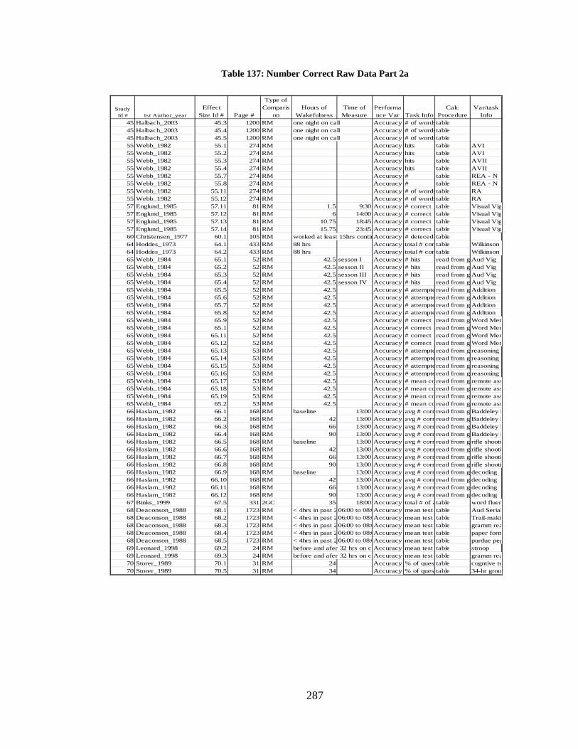
287
Table 137: Number Correct Raw Data Part 2a
45 Halbach_2003 45.3 1200 RM one night on call Accuracy # of words table45 Halbach_2003 45.4 1200 RM one night on call Accuracy # of words table45 Halbach_2003 45.5 1200 RM one night on call Accuracy # of words table55 Webb_1982 55.1 274 RM Accuracy hits table AVI55 Webb_1982 55.2 274 RM Accuracy hits table AVI55 Webb_1982 55.3 274 RM Accuracy hits table AVII55 Webb_1982 55.4 274 RM Accuracy hits table AVII55 Webb_1982 55.7 274 RM Accuracy # table REA - N55 Webb_1982 55.8 274 RM Accuracy # table REA - N55 Webb_1982 55.11 274 RM Accuracy # of words table RA55 Webb_1982 55.12 274 RM Accuracy # of wordstable RA57 Englund_1985 57.11 81 RM 1.5 9:30 Accuracy # correct table Visual Vig57 Englund_1985 57.12 81 RM 6 14:00 Accuracy # correct table Visual Vig57 Englund_1985 57.13 81 RM 10.75 18:45 Accuracy # correct table Visual Vig57 Englund_1985 57.14 81 RM 15.75 23:45 Accuracy # correct table Visual Vig60 Christensen_1977 60.1 105 RM worked at least 15hrs continAccuracy # deteced table64 Hoddes_1973 64.1 433 RM 88 hrs Accuracy total # corrtable Wilkinson A64 Hoddes_1973 64.2 433 RM 88 hrs Accuracy total # corrtable Wilkinson V65 Webb_1984 65.1 52 RM 42.5 sesson I Accuracy # hits read from grAud Vig65 Webb_1984 65.2 52 RM 42.5 sesson II Accuracy # hits read from grAud Vig65 Webb_1984 65.3 52 RM 42.5 sesson III Accuracy # hits read from grAud Vig65 Webb_1984 65.4 52 RM 42.5 sesson IV Accuracy # hits read from grAud Vig65 Webb_1984 65.5 52 RM 42.5 Accuracy # attempteread from grAddition65 Webb_1984 65.6 52 RM 42.5 Accuracy # attempteread from grAddition65 Webb_1984 65.7 52 RM 42.5 Accuracy # attempteread from grAddition65 Webb_1984 65.8 52 RM 42.5 Accuracy # attempteread from grAddition65 Webb_1984 65.9 52 RM 42.5 Accuracy # correct read from grWord Mem65 Webb_1984 65.1 52 RM 42.5 Accuracy # correct read from grWord Mem65 Webb_1984 65.11 52 RM 42.5 Accuracy # correct read from grWord Mem65 Webb_1984 65.12 52 RM 42.5 Accuracy # correct read from grWord Mem65 Webb_1984 65.13 53 RM 42.5 Accuracy # attempteread from grreasoning65 Webb_1984 65.14 53 RM 42.5 Accuracy # attempteread from grreasoning65 Webb_1984 65.15 53 RM 42.5 Accuracy # attempteread from grreasoning65 Webb_1984 65.16 53 RM 42.5 Accuracy # attempteread from grreasoning65 Webb_1984 65.17 53 RM 42.5 Accuracy # mean co read from grremote ass65 Webb_1984 65.18 53 RM 42.5 Accuracy # mean co read from grremote ass65 Webb_1984 65.19 53 RM 42.5 Accuracy # mean co read from grremote ass65 Webb_1984 65.2 53 RM 42.5 Accuracy # mean co read from grremote ass66 Haslam_1982 66.1 168 RM baseline 13:00 Accuracy avg # corr read from grBaddeley l 66 Haslam_1982 66.2 168 RM 42 13:00 Accuracy avg # corr read from grBaddeley l 66 Haslam_1982 66.3 168 RM 66 13:00 Accuracy avg # corr read from grBaddeley l 66 Haslam_1982 66.4 168 RM 90 13:00 Accuracy avg # corr read from grBaddeley l 66 Haslam_1982 66.5 168 RM baseline 13:00 Accuracy avg # corr read from grrifle shootin 66 Haslam_1982 66.6 168 RM 42 13:00 Accuracy avg # corr read from grrifle shootin 66 Haslam_1982 66.7 168 RM 66 13:00 Accuracy avg # corr read from grrifle shootin 66 Haslam_1982 66.8 168 RM 90 13:00 Accuracy avg # corr read from grrifle shootin 66 Haslam_1982 66.9 168 RM baseline 13:00 Accuracy avg # corr read from grdecoding66 Haslam_1982 66.10 168 RM 42 13:00 Accuracy avg # corr read from grdecoding66 Haslam_1982 66.11 168 RM 66 13:00 Accuracy avg # corr read from grdecoding66 Haslam_1982 66.12 168 RM 90 13:00 Accuracy avg # corr read from grdecoding67 Binks_1999 67.5 331 2GC 35 18:00 Accuracy total # of a table word fluen68 Deaconson_1988 68.1 1723 RM < 4hrs in past 206:00 to 08:0Accuracy mean test table Aud Serial 68 Deaconson_1988 68.2 1723 RM < 4hrs in past 206:00 to 08:0Accuracy mean test table Trail-makin68 Deaconson_1988 68.3 1723 RM < 4hrs in past 206:00 to 08:0Accuracy mean test table gramm rea68 Deaconson_1988 68.4 1723 RM < 4hrs in past 206:00 to 08:0Accuracy mean test table paper form68 Deaconson_1988 68.5 1723 RM < 4hrs in past 206:00 to 08:0Accuracy mean test table purdue peg69 Leonard_1998 69.2 24 RM before and afer 32 hrs on caAccuracy mean test table stroop69 Leonard_1998 69.3 24 RM before and afer 32 hrs on caAccuracy mean test table gramm rea70 Storer_1989 70.1 31 RM 24 Accuracy % of quest table cogntive te70 Storer_1989 70.5 31 RM 34 Accuracy % of quest table 34-hr group
Time of Measure
Performance Var Task Info
Calc Procedure
Var/task Info
Hours of Wakefulness
Study Id # 1st Author_year
Effect Size Id # Page #
Type of Comparis
on
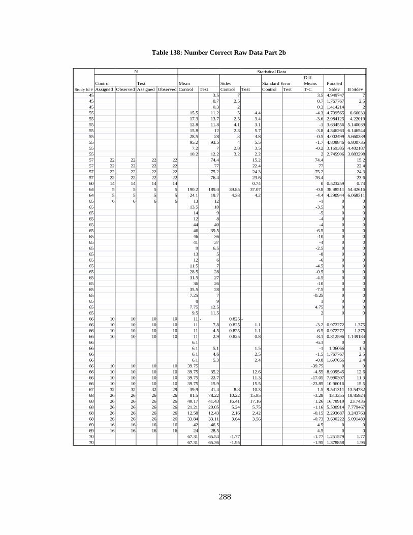
288
Table 138: Number Correct Raw Data Part 2b
Standard ErrorDiff Means
Assigned Observed Assigned Observed Control Test Control Test Control Test T-C45 3.5 7 3.5 4.949747 745 0.7 2.5 0.7 1.767767 2.545 0.3 2 0.3 1.414214 255 15.5 11.2 5 4.4 -4.3 4.709565 6.6603355 17.3 13.7 2.5 3.4 -3.6 2.984125 4.2201955 12.8 11.8 4.1 3.1 -1 3.634556 5.14003955 15.8 12 2.3 5.7 -3.8 4.346263 6.14654455 28.5 28 3 4.8 -0.5 4.002499 5.66038955 95.2 93.5 4 5.5 -1.7 4.808846 6.80073555 7.2 7 2.8 3.5 -0.2 3.169385 4.48218755 10.2 12.2 3.2 2.2 2 2.745906 3.88329857 22 22 22 22 74.4 15.2 74.4 15.257 22 22 22 22 77 22.4 77 22.457 22 22 22 22 75.2 24.3 75.2 24.357 22 22 22 22 76.4 23.6 76.4 23.660 14 14 14 14 0.74 0 0.523259 0.7464 5 5 5 5 190.2 189.4 39.85 37.07 -0.8 38.48511 54.4261664 5 5 5 5 24.1 19.7 4.38 4.2 -4.4 4.290944 6.06831165 6 6 6 6 13 12 -1 0 065 13.5 10 -3.5 0 065 14 9 -5 0 065 12 8 -4 0 065 44 40 -4 0 065 46 39.5 -6.5 0 065 46 36 -10 0 065 41 37 -4 0 065 9 6.5 -2.5 0 065 13 5 -8 0 065 12 6 -6 0 065 11.5 7 -4.5 0 065 28.5 28 -0.5 0 065 31.5 27 -4.5 0 065 36 26 -10 0 065 35.5 28 -7.5 0 065 7.25 7 -0.25 0 065 8 9 1 0 065 7.75 12.5 4.75 0 065 9.5 11.5 2 0 066 10 10 10 10 11 - 0.825 -66 10 10 10 10 11 7.8 0.825 1.1 -3.2 0.972272 1.37566 10 10 10 10 11 4.5 0.825 1.1 -6.5 0.972272 1.37566 10 10 10 10 11 2.9 0.825 0.8 -8.1 0.812596 1.14918466 6.1 -6.1 0 066 6.1 5.1 1.5 -1 1.06066 1.566 6.1 4.6 2.5 -1.5 1.767767 2.566 6.1 5.3 2.4 -0.8 1.697056 2.466 10 10 10 10 39.75 -39.75 0 066 10 10 10 10 39.75 35.2 12.6 -4.55 8.909545 12.666 10 10 10 10 39.75 22.7 11.3 -17.05 7.990307 11.366 10 10 10 10 39.75 15.9 15.5 -23.85 10.96016 15.567 32 32 32 29 39.9 41.4 8.8 10.3 1.5 9.541311 13.5473268 26 26 26 26 81.5 78.22 10.22 15.85 -3.28 13.3355 18.8592468 26 26 26 26 40.17 41.43 16.41 17.16 1.26 16.78919 23.743568 26 26 26 26 21.21 20.05 5.24 5.75 -1.16 5.500914 7.77946768 26 26 26 26 12.58 12.43 2.16 2.42 -0.15 2.293687 3.24376368 26 26 26 26 33.84 33.11 3.64 3.56 -0.73 3.600222 5.09148369 16 16 16 16 42 46.5 4.5 0 069 16 16 16 16 24 28.5 4.5 0 070 67.31 65.54 -1.77 -1.77 1.251579 1.7770 67.31 65.36 -1.95 -1.95 1.378858 1.95
Study Id #
N Statistical Data
Control Test Mean Stdev Poooled Stdev B Stdev
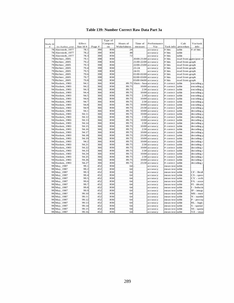
289
Table 139: Number Correct Raw Data Part 3a
78 Akerstedt_1977 78.1 390 RM 24 accuracy # hits table # of hits78 Akerstedt_1977 78.2 390 RM 48 accuracy # hits table78 Akerstedt_1977 78.3 390 RM 72 accuracy # hits table79 Richter_2005 79.1 398 RM 20:00-21:00 accuracy # hits read from grpre/post of 79 Richter_2005 79.2 398 RM 21:00-22:00 accuracy # hits read from graph79 Richter_2005 79.3 398 RM 22:00-23:00 accuracy # hits read from graph79 Richter_2005 79.4 398 RM 23-24 accuracy # hits read from graph79 Richter_2005 79.5 398 RM 24-01 accuracy # hits read from graph79 Richter_2005 79.6 398 RM 01:00-02:00 accuracy # hits read from graph79 Richter_2005 79.7 398 RM 02:00-03:00 accuracy # hits read from graph79 Richter_2005 79.8 398 RM 03:00-04:00 accuracy # hits read from graph94 Haslam_1983 94.1 366 RM 89.75 10am - baseaccuracy # correct table encoding g94 Haslam_1983 94.2 366 RM 89.75 10:00 accuracy # correct table encoding g94 Haslam_1983 94.3 366 RM 89.75 2:30 accuracy # correct table encoding g94 Haslam_1983 94.4 366 RM 89.75 10:00 accuracy # correct table encoding g94 Haslam_1983 94.5 366 RM 89.75 2:30 accuracy # correct table encoding g94 Haslam_1983 94.6 366 RM 89.75 10:00 accuracy # correct table encoding g94 Haslam_1983 94.7 366 RM 89.75 2:30 accuracy # correct table encoding g94 Haslam_1983 94.8 366 RM 89.75 10:00 accuracy # correct table encoding g94 Haslam_1983 94.9 366 RM 89.75 23:30 accuracy # correct table encoding g94 Haslam_1983 94.1 366 RM 89.75 10:00 accuracy # correct table decoding g94 Haslam_1983 94.11 366 RM 89.75 10:00 accuracy # correct table decoding g94 Haslam_1983 94.12 366 RM 89.75 2:30 accuracy # correct table decoding g94 Haslam_1983 94.13 366 RM 89.75 10:00 accuracy # correct table decoding g94 Haslam_1983 94.14 366 RM 89.75 2:30 accuracy # correct table decoding g94 Haslam_1983 94.15 366 RM 89.75 10:00 accuracy # correct table decoding g94 Haslam_1983 94.16 366 RM 89.75 2:30 accuracy # correct table decoding g94 Haslam_1983 94.17 366 RM 89.75 10:00 accuracy # correct table decoding g94 Haslam_1983 94.18 366 RM 89.75 23:30 accuracy # correct table decoding g94 Haslam_1983 94.19 366 RM 89.75 10:00 accuracy # correct table decoding m94 Haslam_1983 94.2 366 RM 89.75 10:00 accuracy # correct table decoding m94 Haslam_1983 94.21 366 RM 89.75 2:30 accuracy # correct table decoding m94 Haslam_1983 94.22 366 RM 89.75 10:00 accuracy # correct table decoding m94 Haslam_1983 94.23 366 RM 89.75 2:30 accuracy # correct table decoding m94 Haslam_1983 94.24 366 RM 89.75 10:00 accuracy # correct table decoding m94 Haslam_1983 94.25 366 RM 89.75 2:30 accuracy # correct table decoding m94 Haslam_1983 94.26 366 RM 89.75 10:00 accuracy # correct table decoding m94 Haslam_1983 94.27 366 RM 89.75 23:30 accuracy # correct table decoding m99 May_1987 99.1 452 RM 64 - accuracy mean test stable99 May_1987 99.2 452 RM 64 accuracy mean test stable99 May_1987 99.3 452 RM 64 accuracy mean test stable CF - flexib 99 May_1987 99.4 452 RM 64 accuracy mean test stable CS - speed 99 May_1987 99.5 452 RM 64 accuracy mean test stable CV - verba 99 May_1987 99.6 452 RM 64 accuracy mean test stable FA - assoc 99 May_1987 99.7 452 RM 64 accuracy mean test stable FI - ideatio 99 May_1987 99.8 452 RM 64 accuracy mean test stable I - Inductio 99 May_1987 99.9 452 RM 64 accuracy mean test stable IP - integra 99 May_1987 99.10 452 RM 64 accuracy mean test stable MS - mem 99 May_1987 99.11 452 RM 64 accuracy mean test stable N - numbe 99 May_1987 99.12 452 RM 64 accuracy mean test stable P - percept 99 May_1987 99.13 452 RM 64 accuracy mean test stable RL - logica 99 May_1987 99.14 452 RM 64 accuracy mean test stable S - spatial o 99 May_1987 99.15 452 RM 64 accuracy mean test stable SS - spatia 99 May_1987 99.16 452 RM 64 accuracy mean test stable VZ - visua
Time of measure
Performance Var Task info
Calc procedure
Var/task info
Hours of Wakefulness
Study Id # 1st Author_year
Effect Size Id # Page #
Type of Comparis
on
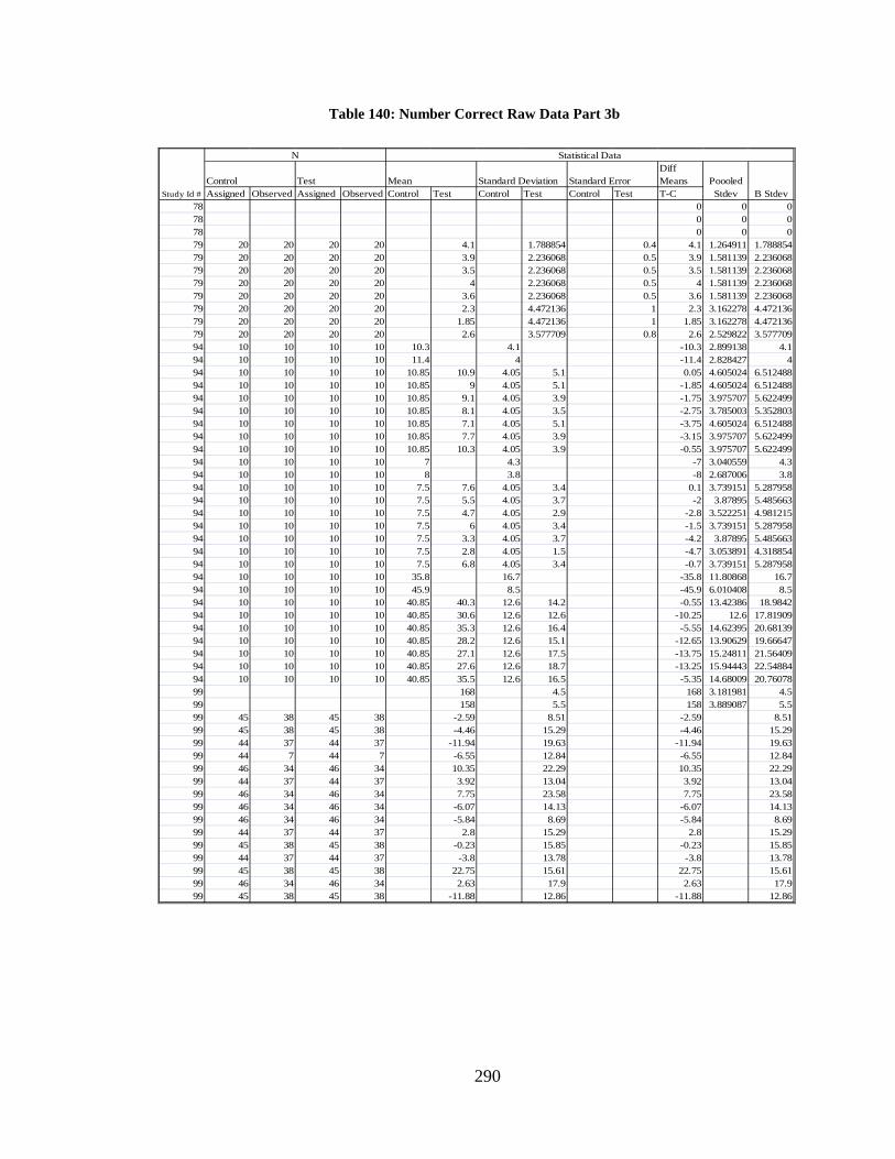
290
Table 140: Number Correct Raw Data Part 3b
Standard ErrorDiff Means
Assigned Observed Assigned Observed Control Test Control Test Control Test T-C78 0 0 078 0 0 078 0 0 079 20 20 20 20 4.1 1.788854 0.4 4.1 1.264911 1.78885479 20 20 20 20 3.9 2.236068 0.5 3.9 1.581139 2.23606879 20 20 20 20 3.5 2.236068 0.5 3.5 1.581139 2.23606879 20 20 20 20 4 2.236068 0.5 4 1.581139 2.23606879 20 20 20 20 3.6 2.236068 0.5 3.6 1.581139 2.23606879 20 20 20 20 2.3 4.472136 1 2.3 3.162278 4.47213679 20 20 20 20 1.85 4.472136 1 1.85 3.162278 4.47213679 20 20 20 20 2.6 3.577709 0.8 2.6 2.529822 3.57770994 10 10 10 10 10.3 4.1 -10.3 2.899138 4.194 10 10 10 10 11.4 4 -11.4 2.828427 494 10 10 10 10 10.85 10.9 4.05 5.1 0.05 4.605024 6.51248894 10 10 10 10 10.85 9 4.05 5.1 -1.85 4.605024 6.51248894 10 10 10 10 10.85 9.1 4.05 3.9 -1.75 3.975707 5.62249994 10 10 10 10 10.85 8.1 4.05 3.5 -2.75 3.785003 5.35280394 10 10 10 10 10.85 7.1 4.05 5.1 -3.75 4.605024 6.51248894 10 10 10 10 10.85 7.7 4.05 3.9 -3.15 3.975707 5.62249994 10 10 10 10 10.85 10.3 4.05 3.9 -0.55 3.975707 5.62249994 10 10 10 10 7 4.3 -7 3.040559 4.394 10 10 10 10 8 3.8 -8 2.687006 3.894 10 10 10 10 7.5 7.6 4.05 3.4 0.1 3.739151 5.28795894 10 10 10 10 7.5 5.5 4.05 3.7 -2 3.87895 5.48566394 10 10 10 10 7.5 4.7 4.05 2.9 -2.8 3.522251 4.98121594 10 10 10 10 7.5 6 4.05 3.4 -1.5 3.739151 5.28795894 10 10 10 10 7.5 3.3 4.05 3.7 -4.2 3.87895 5.48566394 10 10 10 10 7.5 2.8 4.05 1.5 -4.7 3.053891 4.31885494 10 10 10 10 7.5 6.8 4.05 3.4 -0.7 3.739151 5.28795894 10 10 10 10 35.8 16.7 -35.8 11.80868 16.794 10 10 10 10 45.9 8.5 -45.9 6.010408 8.594 10 10 10 10 40.85 40.3 12.6 14.2 -0.55 13.42386 18.984294 10 10 10 10 40.85 30.6 12.6 12.6 -10.25 12.6 17.8190994 10 10 10 10 40.85 35.3 12.6 16.4 -5.55 14.62395 20.6813994 10 10 10 10 40.85 28.2 12.6 15.1 -12.65 13.90629 19.6664794 10 10 10 10 40.85 27.1 12.6 17.5 -13.75 15.24811 21.5640994 10 10 10 10 40.85 27.6 12.6 18.7 -13.25 15.94443 22.5488494 10 10 10 10 40.85 35.5 12.6 16.5 -5.35 14.68009 20.7607899 168 4.5 168 3.181981 4.599 158 5.5 158 3.889087 5.599 45 38 45 38 -2.59 8.51 -2.59 8.5199 45 38 45 38 -4.46 15.29 -4.46 15.2999 44 37 44 37 -11.94 19.63 -11.94 19.6399 44 7 44 7 -6.55 12.84 -6.55 12.8499 46 34 46 34 10.35 22.29 10.35 22.2999 44 37 44 37 3.92 13.04 3.92 13.0499 46 34 46 34 7.75 23.58 7.75 23.5899 46 34 46 34 -6.07 14.13 -6.07 14.1399 46 34 46 34 -5.84 8.69 -5.84 8.6999 44 37 44 37 2.8 15.29 2.8 15.2999 45 38 45 38 -0.23 15.85 -0.23 15.8599 44 37 44 37 -3.8 13.78 -3.8 13.7899 45 38 45 38 22.75 15.61 22.75 15.6199 46 34 46 34 2.63 17.9 2.63 17.999 45 38 45 38 -11.88 12.86 -11.88 12.86
Study Id #
N Statistical Data
Control Test Mean Standard Deviation Poooled Stdev B Stdev
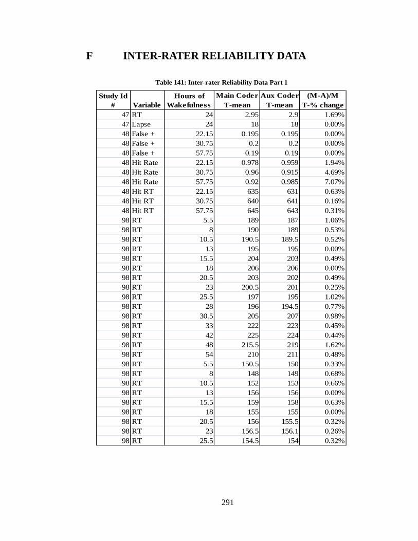
291
F INTER-RATER RELIABILITY DATA
Table 141: Inter-rater Reliability Data Part 1
Main Coder Aux Coder (M-A)/MT-mean T-mean T-% change
47 RT 24 2.95 2.9 1.69%47 Lapse 24 18 18 0.00%48 False + 22.15 0.195 0.195 0.00%48 False + 30.75 0.2 0.2 0.00%48 False + 57.75 0.19 0.19 0.00%48 Hit Rate 22.15 0.978 0.959 1.94%48 Hit Rate 30.75 0.96 0.915 4.69%48 Hit Rate 57.75 0.92 0.985 7.07%48 Hit RT 22.15 635 631 0.63%48 Hit RT 30.75 640 641 0.16%48 Hit RT 57.75 645 643 0.31%98 RT 5.5 189 187 1.06%98 RT 8 190 189 0.53%98 RT 10.5 190.5 189.5 0.52%98 RT 13 195 195 0.00%98 RT 15.5 204 203 0.49%98 RT 18 206 206 0.00%98 RT 20.5 203 202 0.49%98 RT 23 200.5 201 0.25%98 RT 25.5 197 195 1.02%98 RT 28 196 194.5 0.77%98 RT 30.5 205 207 0.98%98 RT 33 222 223 0.45%98 RT 42 225 224 0.44%98 RT 48 215.5 219 1.62%98 RT 54 210 211 0.48%98 RT 5.5 150.5 150 0.33%98 RT 8 148 149 0.68%98 RT 10.5 152 153 0.66%98 RT 13 156 156 0.00%98 RT 15.5 159 158 0.63%98 RT 18 155 155 0.00%98 RT 20.5 156 155.5 0.32%98 RT 23 156.5 156.1 0.26%98 RT 25.5 154.5 154 0.32%
Hours of Wakefulness
Study Id # Variable
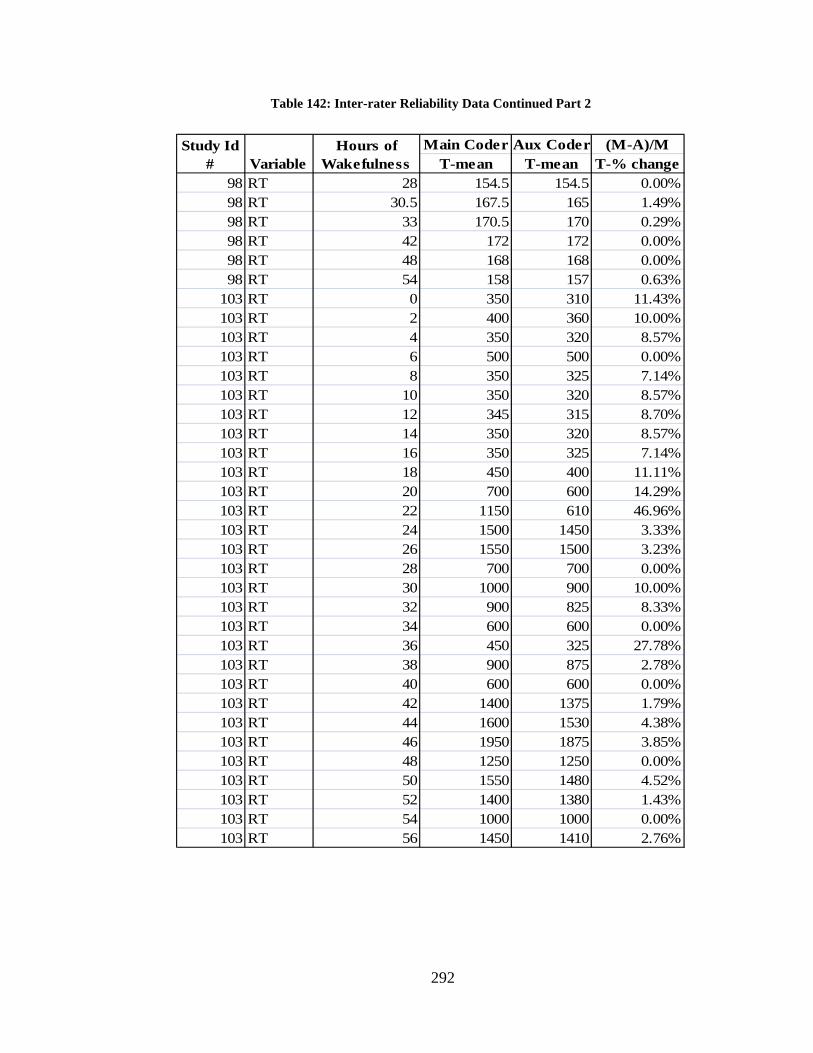
292
Table 142: Inter-rater Reliability Data Continued Part 2
Main Coder Aux Coder (M-A)/MT-mean T-mean T-% change
98 RT 28 154.5 154.5 0.00%98 RT 30.5 167.5 165 1.49%98 RT 33 170.5 170 0.29%98 RT 42 172 172 0.00%98 RT 48 168 168 0.00%98 RT 54 158 157 0.63%
103 RT 0 350 310 11.43%103 RT 2 400 360 10.00%103 RT 4 350 320 8.57%103 RT 6 500 500 0.00%103 RT 8 350 325 7.14%103 RT 10 350 320 8.57%103 RT 12 345 315 8.70%103 RT 14 350 320 8.57%103 RT 16 350 325 7.14%103 RT 18 450 400 11.11%103 RT 20 700 600 14.29%103 RT 22 1150 610 46.96%103 RT 24 1500 1450 3.33%103 RT 26 1550 1500 3.23%103 RT 28 700 700 0.00%103 RT 30 1000 900 10.00%103 RT 32 900 825 8.33%103 RT 34 600 600 0.00%103 RT 36 450 325 27.78%103 RT 38 900 875 2.78%103 RT 40 600 600 0.00%103 RT 42 1400 1375 1.79%103 RT 44 1600 1530 4.38%103 RT 46 1950 1875 3.85%103 RT 48 1250 1250 0.00%103 RT 50 1550 1480 4.52%103 RT 52 1400 1380 1.43%103 RT 54 1000 1000 0.00%103 RT 56 1450 1410 2.76%
Study Id # Variable
Hours of Wakefulness
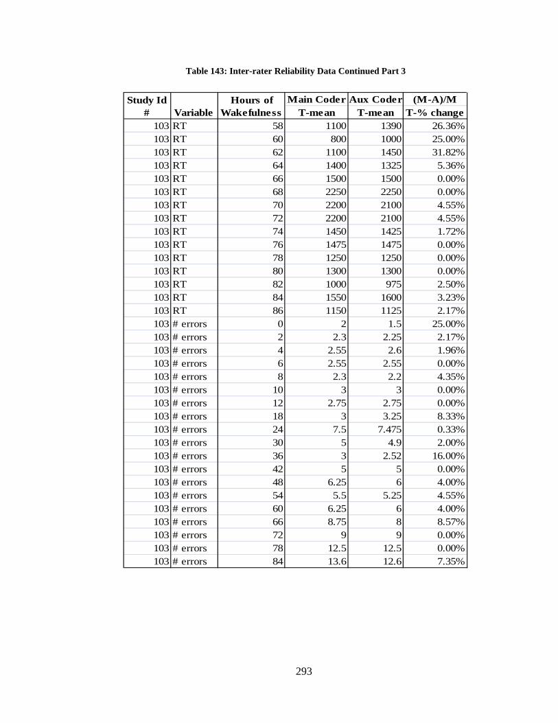
293
Table 143: Inter-rater Reliability Data Continued Part 3
Main Coder Aux Coder (M-A)/MT-mean T-mean T-% change
103 RT 58 1100 1390 26.36%103 RT 60 800 1000 25.00%103 RT 62 1100 1450 31.82%103 RT 64 1400 1325 5.36%103 RT 66 1500 1500 0.00%103 RT 68 2250 2250 0.00%103 RT 70 2200 2100 4.55%103 RT 72 2200 2100 4.55%103 RT 74 1450 1425 1.72%103 RT 76 1475 1475 0.00%103 RT 78 1250 1250 0.00%103 RT 80 1300 1300 0.00%103 RT 82 1000 975 2.50%103 RT 84 1550 1600 3.23%103 RT 86 1150 1125 2.17%103 # errors 0 2 1.5 25.00%103 # errors 2 2.3 2.25 2.17%103 # errors 4 2.55 2.6 1.96%103 # errors 6 2.55 2.55 0.00%103 # errors 8 2.3 2.2 4.35%103 # errors 10 3 3 0.00%103 # errors 12 2.75 2.75 0.00%103 # errors 18 3 3.25 8.33%103 # errors 24 7.5 7.475 0.33%103 # errors 30 5 4.9 2.00%103 # errors 36 3 2.52 16.00%103 # errors 42 5 5 0.00%103 # errors 48 6.25 6 4.00%103 # errors 54 5.5 5.25 4.55%103 # errors 60 6.25 6 4.00%103 # errors 66 8.75 8 8.57%103 # errors 72 9 9 0.00%103 # errors 78 12.5 12.5 0.00%103 # errors 84 13.6 12.6 7.35%
Study Id # Variable
Hours of Wakefulness
294
G INITIAL SEARCH RESULTS (i.e., 600 STUDIES)
Aboukhalil, A., M. Shelhamer, et al. (2004). "Acquisition of Context-specific Adaptation Is Enhanced with Rest Intervals between Changes in Context State, Suggesting a New Form of Motor Consolidation." Neuroscience Letters 369: 162–167.
AbuALRub, R. (2004). "Job Stress, Job Performance, and Social Support among Hospital
Nurses." Journal of Nursing Scholarship 36(1): 73-78. Achermann, P. (2004). "The Two-process Model of Sleep Regulation Revisited."
Aviation Space and Environmental Medicine 75(Suppl. 3): A37–A43. Achermann, P. and A. Borbély (1994). "Simulation of Daytime Vigilance by the Additive
Interaction of a Homeostatic and a Circadian Process." Biol Cybern 71: 115–121. Adams, G., V. Caiozzo, et al. (2003). "Skeletal Muscle Unweighting: Spaceflight and
Ground-based Models." Journal of Appl Physiol 95(6): 2185-2201. Aguzzi, J., N. Bullock, et al. (2006). "Spontaneous Internal Desynchronization of
Locomotor Activity and Body Temperature Rhythms from Plasma Melatonin Rhythm in Rats Exposed to Constant Dim Light." Journal of Circadian Rhythms 4(1): 6.
Akerstedt, T. (1995). "Work Hours, Sleepiness and Accidents." Journal of Sleep
Research 4(Suppl.2): 4-14. Akerstedt, T. (2007). "Altered Sleep/wake Patterns and Mental Performance." Physiology
& Behavior 90(2-3): 209-218. Akerstedt, T., D. Dinges, et al. (1994). "Accidents and Sleepiness: A Consensus
Statement from the International Conference on Work Hours, Sleepiness and Accidents, Stockholm, 8-10 September 1994." J. Sleep Res. (3): 1994.
Akerstedt, T. and S. Folkard (1993). "Sleep/Wake Regulation." Light and Biological
Rhythms in Man. W. L., Pergamon Press: 237-245. Akerstedt, T., S. Folkard, et al. (2004). "Predictions from the Three-process Model of
Alertness." Aviation Space and Environmental Medicine 75(Suppl. 3): A75–A83. Akerstedt, T. and J. Freberg (1977). "Psychophysiological Circadian Rhythms in Women
during 72h of Sleep Deprivation." Waking and Sleeping 1: 387-394. Akerstedt, T. and M. Gillberg (1981). "The Circadian Variation of Experimentally
Displaced Sleep." Sleep 4(2): 159–169.
295
Akerstedt, T. and M. Gillberg (1982). "Displacement of the Sleep Period and Sleep
Deprivation." Human Neurobiol 1: 163–171. Akerstedt, T. and M. Gillberg (1982). "Experimentally Displaced Sleep: Effects on
Sleepiness." Electroencephalography and Clinical Neurophysiology 54: 220–226. Akerstedt, T. and M. Gillberg (1990). "Subjective and Objective Sleepiness in the Active
Individual." Int J Neurosci 52: 29–37. Akerstedt, T., G. Kechlund, et al. (1998). "Subjective Sleepiness in Shift Work."
Biological Clocks. Mechanisms and Applications, Elsevier Science. Akerstedt, T. and U. Landstrom (1998). "Work Place Countermeasures of Night Shift
Fatigue." International Journal of Industrial Ergonomics 21: 167-178. Akerstedt, T., B. Peters, et al. (2005). "Impaired Alertness and Performance Driving
Home from the Night Shift: A Driving Simulator Study." Journal of Sleep Research 14: 17–20.
Akerstedt, T., L. Torsvall, et al. (1982). "Sleepiness and Shift Work: Field Studies."
Sleep 5: S95-S106. Ancoli-Israel, S. and T. Roth (1999). "Characteristics of Insomnia in the United States:
Results of the 1991 National Sleep Foundation Survey. I." Sleep 22(Suppl 2): S347-S353.
Angus, R., R. Helslegrave, et al. (1985). "Effects of Prolonged Sleep Deprivation, with
and without Chronic Physical Exercise, on Mood and Performance." Psychophysiology 22(3): 276-282.
Arnedt, J., G. Wilde, et al. (2001). "How Do Prolonged Wakefulness and Alcohol
Compare in the Decrements They Produce on a Simulated Driving Task?" Accident Anal and Preven 33: 337-344.
Arnedt, J., G. Wilde, et al. (2000). "Simulated Driving Performance following Prolonged
Wakefulness and Alcohol Consumption: Separate and Combined Contributions to Impairment." Journal of Sleep Research 9: 233-241.
Arnedt, J., J. Owen, et al. (2005). "Neurobehavioral Performance of Residents after
Heavy Night Call vs. after Alcohol Ingestion. 294(9), 1025-1033." Journal of American Medical Association 294(9): 1025-1033.
Arnold, P., L. Hartley, et al. (1997). "Hours of Work, and Perceptions of Fatigue among
Truck Drivers." Accid. Anal. and Prev. 29(4): 471-477.
296
Arora, V., C. Dunphy, et al. (2006). "The Effects of On-duty Napping on Intern Sleep Time and Fatigue." Annals of Internal Medicine 144(11): 792–798.
Asch, D. and R. Parker (1988). "The Libby Zion Case. One Step forward or Two Steps
Backward?" New Engl J Med 318: 771-775. Asken, M. and D. Raham (1983). "Resident Performance and Sleep Deprivation: A
Review." J Med Educ 58(5): 382-388. Ayas, N., L. Barger, et al. (2006). "Extended Work Duration and the Risk of Self-
reported Percutaneous Injuries in Interns." JAMA 296(9): 1055-62. Aykin, N. and T. Aykin (1987). "Complex Task Performance under Speed-accuracy
Tradeoffs Single Task versus Dual Task." Proceedings of The Human Factors Society - 31st Annual Meeting 1: 161-165.
Babkoff, H. (1985). "The Effects of Progressive Sleep Loss on a Lexical Decision Task:
Response Lapses and Response Accuracy." Behavioral Research Methods, Instruments, & Computers 17(6): 614-622.
Babkoff, H., D. Thorne, et al. (1985). "Dynamic Changes in Work/rest Duty Cycles in a
Study of Sleep Deprivation." Behavioral Research Methods, Instruments, & Computers 17(6): 604-613.
Babkoff, H., G. Zukerman, et al. (2005). "Effect of the Diurnal Rhythm and 24-h of Sleep
Deprivation on Dichotic Temporal Order Judgment." Journal of Sleep Research 14: 7-15.
Baker, K. and J. Olson (1994). "Work Practices, Fatigue, and Nuclear Power Plant Safety
Performance." Human Factors 36(2): 244-257. Baldwin, D. and S. Daugherty (2004). "Sleep Deprivation and Fatigue in Residency
Training: Results of a National Survey of First- and Second-year Residents." Sleep 27(2): 217-23.
Baldwin, P., M. Dodd, et al. (1997). "Young Doctors' Health--I. How Do Working
Conditions Affect Attitudes, Health and Performance?" Soc Sci Med 45: 35-40. Baldwin, P., M. Dodd, et al. (1998). "Junior Doctors Making Mistakes." Lancet 351: 804. Banks, S., P. Catcheside, et al. (2005). "The Maintenance of Wakefulness Test and
Driving Simulator Performance." Sleep 28(22): 1381-1385. Barger, L., N. Ayas, et al. (2006) “Impact of Extended-duration Shifts on Medical Errors,
Adverse Events, and Attentional Failures." PLOS Medicine 3(12): e487.
297
Barger, L., B. Cade, et al. (2005). "Extended Work Shifts and the Risk of Motor Vehicle Crashes among Interns." New Engl J Med 352(2): 125-34.
Barger, L., K. Wright, et al. (2004). “Daily Exercise Facilitates Phase Delays of
Circadian Melatonin Rhythm in Very Dim Light." Am J Physiol Regul Integr Comp Physiol 286(6): R1077-84.
Barnes-Farrell, J., K. Davies-Schrils, et al. (2008). "What Aspects of Shiftwork Influence
Off-shift Well-being of Healthcare Workers?" Applied Ergonomics 39(5): 589-596.
Bartle, E., J. Sun, et al. (1988). "The Effects of Acute Sleep Deprivation during
Residency Training." Surgery 104: 311-316. Barton, J. and S. Folkard (1993). "Advancing versus Delaying Shift Systems."
Ergonomics 36(1-3): 59-64. Bayer, E. (1999). "The Compilation of Items and Calibration for a Survey of Infant
Motor Behavior." United States -- Indiana, Indiana University. Beatty, J., S. Ahern, et al. (1977). Sleep Deprivation and the Vigilance of
Anesthesiologists during Simulated Surgery, Vigilance: Theory, Operational Performance, and Physiological Correlates. New York, Plenum.
Belenky, G., N. Wesensten, et al. (2003). "Patterns of Performance Degradation and
Restoration during Sleep Restriction and Subsequent Recovery: A Sleep Dose-response Study." Journal of Sleep Research 12(1): 1-12.
Belyavin, A. and M. Spencer (2004). "Modeling Performance and Alertness: The QinetiQ
Approach." Aviation Space and Environmental Medicine 75(Suppl. 3): A93–A103.
Benedetti, F., A. Bernasconi, et al. (2007). "Neural and Genetic Correlates of
Antidepressant Response to Sleep Deprivation: a Functional Magnetic Resonance Imaging Study of Moral Valence Decision in Bipolar Depression." Archives of General Psychiatry 64(2): 179.
Benuzzi, F., G. Basso, et al. (2005). "Temporal Production and Visuospatial Processing."
Percept Mot Skills 101(3): 737-758. Bergman, A. B., C. D. DeAngelis, et al. (1990). "Regulation of Working Hours for
Pediatric Residents." The Journal of Pediatrics 116(3): 478-483. Bertram, D. (1988). "Characteristics of Shifts and Second-year Resident Performance in
an Emergency Department." NY State J Med 88: 10-14.
298
Bey, L. and M. Hamilton (2003). "Suppression of Skeletal Muscle Lipoprotein Lipase Activity during Physical Inactivity: a Molecular Reason to Maintain Daily Low-intensity Activity." J Physiol (London) 551(Pt 2): 673-682.
Binks, P., W. Waters, et al. (1999). "Short-term Total Sleep Deprivations Does Not
Selectively Impair Higher Cortical Functioning." Sleep 22: 328-334. Blagrove, M., C. Alexander, et al. (1994). "The Effects of Chronic Sleep Reduction on
the Performance of Cognitive Tasks Sensitive to Sleep Deprivation." Appl Cog Psychol 9: 21-40.
Blatter, K., P. Graw, et al. (2006). "Gender and Age Differences in Psychomotor
Vigilance Performance under Differential Sleep Pressure Conditions." Behavioral Brain Research 168(2): 312-317.
Blatter, K., K. Opwis, et al. (2005). "Sleep Loss-related Decrements in Planning
Performance in Healthy Elderly Depend on Task Difficulty." Journal of Sleep Research 14: 409-417.
Bliese, P., N. Wesentsten, et al. (2006). "Age and Individual Variability in Performance
during Sleep Restriction." Journal of Sleep Research 15: 376-385. Bobko, N., A. Karpenko, et al. (1998). "The Mental Performance of Shiftworkers in
Nuclear and Heat Power Plants of Ukraine." International Journal of Industrial Ergonomics 21: 333-340.
Bohnen, H. and A. Gaillard (1994). "The Effects of Sleep Loss in a Combined Tracking
and Time Estimation Task." Ergonomics 37(6): 1021-1030. Boksem, M., T. Meijman, et al. (2006). "Mental Fatigue, Motivation and Action
Monitoring." Biological Psychology 72: 123-132. Bond, V., B. Balkissoon, et al. (1986). "Effects of Sleep Deprivation on Performance
during Submaximal Exercise." Journal of Sports Medicine 26: 169-174. Bonnet, M. (1985). "Effect of Sleep Disruption on Sleep, Performance, and Mood." Sleep
8(1): 11-19. Bonnet, M. (1986). "Performance and Sleepiness following Moderate Sleep Disruption
and Slow Wave Sleep Deprivation." Physiology & Behavior 37(6): 915-918. Bonnet, M. (1989). "The Effect of Sleep Fragmentation on Sleep and Performance in
Younger and Older Subjects." Neurobiology of Aging 10(1): 21-25. Bonnet, M. (1991). "The Effect of Varying Prophylactic Naps on Performance, Alertness
and Mood throughout a 52 Hour Continuous Operation." Sleep 14: 307-315.
299
Bonnet, M. (1994). "Sleep Deprivation." Principles and Practice of Sleep Medicine. M.
Kryger, T. Roth and W. Dement. Philadelphia, WB Saunders: 50-67. Bonnet, M. (2000). "Sleep Deprivation." Principles and Practice of Sleep Medicine. M.
Kryger, T. Roth and W. Dement. Philadelphia, W.B. Saunders: 53-71. Bonnet, M. and D. Arand (1995). "We Are Chronically Sleep Deprived." Sleep 18: 908-
911. Bonnet, M. and D. Arand (1998). "Sleepiness as Measured by Modified Multiple Sleep
Latency Testing Varies as a Function of Preceding Activity." Sleep 21: 477-483. Bonnet, M. and D. Arand (2005). "Sleep Latency Testing as a Time Course Measure of
State of Arousal." Journal of Sleep Research 14: 387-392. Bonnet, M. and J. Alter (1982). "Effects of Irregular versus Regular Sleep Schedules on
Performance, Mood and Body Temperature." Biological Psychology 14(3-4): 287-296.
Borbely, A. and P. Achermann (1999). "Sleep Homeostasis and Models of Sleep
Regulation." Journal of Biological Rhythms 14(6): 559-568. Borg, G. (1977). "Simple Rating Methods for Estimation of Perceived Exertion."
Physical Work and Effort. G. Borg. Oxford, England, Permagon Press: 39-47. Borland, R., A. Rogers, et al. (1986). "Performance Overnight in Shift Workers
Operating a Day-night Schedule." Aviation Space and Environmental Medicine 57: 241-249.
Bourgeois-Bougrine S, Carbon P, et al. (2003). "Perceived Fatigue for Short- and Long-
haul Flights: a Survey of 739 Airline Pilots." Aviation, Space, and Environmental Medicine 74(10): 1072-1076.
Brazzini-poisson, V., R. Godbout, et al. (2006). "Differential Modulation of Frontal and
Parietal Attentional Processes by Total Sleep Deprivation: An Event-related Potentials Study." Journal of Sleep Research 15(Suppl. 1): 1-253.
Brown, E., Y. Luithard, et al. (2000). "A Statistical Model of the Human Core-
temperature Circadian Rhythm." American Journal Physiol Endocrinal Metab 279(3): E669-E683.
Brown, I. (1994). "Driver Fatigue." Human Factors 36(2): 298-314. Bruck, D. and D. Pisani (1999). "The Effects of Sleep Inertia on Decision-making
Performance." Journal of Sleep Research 8: 95-103.
300
Buck, L. (1977). "Circadian Rhythms in Step-input Pursuit Tracking." Ergonomics 20(1):
19-31. Buck, L. and C. Gibbs (1972). "Sleep Loss and Information Processing." Aspects of
Human Efficiency. W. P. Colquhoun. London, English University Press: 47-57. Butterfield, P. (1988). "The Stress of Residency: A Review of the Literature." Archives
of Internal Medicine 148: 1428-1435. Buysse, D., Barzansky, B., et al. (2003). “Sleep Fatigue, and Medical Training: Setting
an Agenda for Optimal Learning and Patient Care.” Sleep. 26(2):218-25. Cabon, P., A. Coblentz, et al. (1993). "Human Vigilance in Railway and Long-haul Flight
Operation." Ergonomics 36: 1019-1033. Caiozzo, V. J., C. Rose-Gottron, et al. (2004). "Hemodynamic and Metabolic Responses
to Hypergravity on a Human-powered Centrifuge." Aviation Space and Environmental Medicine 75(2): 101-108.
Cajochen, C., M. Imai, et al. (2006). "Age-related Changes in the Dynamics of Frontal
Low-EEG Activity during Sustained Wakefulness." Journal of Sleep Research 15(Suppl. 1): 1-253.
Cajochen, C., M. Jewett, et al. (2003). "Human Circadian Melatonin Rhythm Phase
Delay during a Fixed Sleep–wake Schedule Interspersed with Nights of Sleep Deprivation." J Pineal Res 35: 149-157.
Cajochen, C., S. Khalsa, et al. (1999). "EEG and Ocular Correlates of Circadian
Melatonin Phase and Human Performance Decrements during Sleep Loss." Am J Physiol Regul Integr Comp Physiol 277(3): R640-R649.
Caldwell, J. (2001). "The Impact of Fatigue in Air, Medical, and Other Types of
Operations: A Review of Fatigue Facts and Potential Countermeasures." Air Medical Journal 20(1): 25-32.
Caldwell, J., B. Prazinko, et al. (2003). "Body Posture Affects Electroencephalographic
Activity and Psychomotor Vigilance Task Performance in Sleep-deprived Subjects." Clinical Neurophysiology 114(1): 23-31.
Campbell, S. and D. Dawson (1990). "Enhancement of Nighttime Alertness and
Performance with Bright Ambient Light." Phsiol Behav 48: 317-320. Carskadon, M. and W. Dement (1981). "Cumulative Effects of Sleep Restriction on
Daytime Sleepiness." Psychophysiology 18: 107-13.
301
Carskadon, M. and W. Dement (1982). "Nocturnal Determinants of Daytime Sleepiness." Sleep 5: s73-81.
Carskadon, M., W. Dement, et al. (1986). "Guidelines for the Multiple Sleep Latency
Test (MSLT): A Standard Measure of Sleepiness." Sleep 9(4): 519-524. Carskadon, M. and T. Roth (1991). "Sleep Restriction". Sleep, Sleepiness and
Performance. T. H. Monk. New York, John Wiley & Sons: 155-167. Cary, J. and J. Fishburne (1989). "A Method to Limit Working Hours and Reduce Sleep
Deprivation in an Obstetrics and Gynecology Residency Program." Obstetrics & Gynecol 74: 668-672.
Chee, M. and W. Choo (2004). "Functional Imaging of Working Memory after 24 HR of
Total Sleep Deprivation." The Journal of Neuroscience 24(19): 4560-4567. Chiles, W., E. Alluisi, et al. (1968). "Work Schedules and Performance during
Confinement." Human Factors 10(2): 143-196. Choo, W., W. Lee, et al. (2005). "Dissociation of Cortical Regions Modulated by Both
Working Memory Load and Sleep Deprivation and by Sleep Deprivation Alone." NeuroImage 25: 579-587.
Christensen, E., G. Dietz, et al. (1977). "The Effect of Fatigue on Resident Performance."
Radiology 125: 103-105. Colford, J. and S. McPhee (1989). "The Reveled Sleeve of Care Managing the Stresses of
Residency Training." JAMA 261: 889-893. Collins, W. (1977). "Some Effects of Sleep Deprivation on Tracking Performance in
Static and Dynamic Environments." J Appl Psychol 62: 567-573. Colquhoun, W., M. Blake, et al. (1968). "Experimental Studies of Shift-work II:
Stabilized 8 Hour Shift System." Ergonomics 11(6): 527-546. Colquhoun, W., M. Blake, et al. (1969). "Experimental Studies of Shift-work III:
Stabilized 12 Hour Shift Systems." Ergonomics 12(6): 865-882. Conway, P., P. Campanini, et al. (2008). "Main and Interactive Effects of Shiftwork,
Age, and Work Stress on Health in an Italian Sample of Healthcare Workers." Applied Ergonomics 39(5): 630-639.
Corfitsen, M. (1996). "Enhanced Tiredness among Young Impaired Male Nighttime
Drivers." Accid. Anal. and Prev. 28(2): 155-162.
302
Craig, A. (1979). "Discrimination, Temperature, and Time of Day." Human Factors 21(1): 61-68.
Croon, E., R. Blonk, et al. (2007). "Job Stress, Fatigue, and Job Dissatisfaction in Dutch
Lorry Drivers: towards an Occupation Specific Model of Job Demands and Control." Occup Environ Med 59: 356-361.
Cutler, N. and H. Cohen (1979). "The Effect of One Night's Sleep Loss on Mood and
Memory in Normal Subjects." Comprehensive Psychiatry 20(1): 61-66. Czeisler, C., J. Allan, et al. (1986). "Bright Light Resets the Human Circadian Pacemaker
Independent of the Timing of the Sleep-wake Cycle." Science 233: 667-671. Czeisler, C., E. Weitzman, et al. (1980). "Human Sleep: Its Duration and Organization
depend on Its Circadian Phase." Science 210: 1264-1267. Czeisler, C., J. Duffy, et al. (1999). "Stability, Precision, and Near 24 Hour Period of the
Human Circadian Pacemaker." Science 284(5423): 2177-2181.
Daan, S., D. Beersma, et al. (1984). "Timing of Human Sleep: Recovery Process Gated by a Circadian Pacemaker." AM J Physiol 246: R161–R183.
Dalziel, J. and R. Job (1997). "Motor Vehicle Accidents, Fatigue and Optimism Bias in
Taxi Drivers." Accid Anal Prev 29(4): 489 494. Daniel, J. and A. Potasova (1989). "Oral Temperature and Performance in 8-hour and 12-
hour Shifts." Ergonomics 32(7): 689-696. Darwent, D., N. Lamond, et al. (2008). "The Sleep and Performance of Train Drivers
during an Extended Freight-haul Operation." Applied Ergonomics 39(5): 614-622.
Daugherty, S. and D. Baldwin (1996). "Sleep Deprivation in Senior Medical Students and
First-year Residents." Acad Emerg Med 71: S93-S95. Daugherty, S., D. Baldwin, et al. (1998). " Learning, Satisfaction, and Mistreatment
during Medical Internship: A National Survey of Working Conditions." JAMA 279: 1194-1199.
Davies, A. and D. Davies (1975). "The Effects of Noise and Time of Day upon Age
Differences in Performance at Two Checking Tasks." Ergonomics 18(3): 321-336.
Dawson, D. and K. Reid (1997). "Fatigue, Alcohol, and Performance Impairment."
Nature 388(17): 235-237.
303
Deaconson, T., D. O'Hair, et al. (1988). "Sleep Deprivation and Resident Performance." JAMA 260: 1721-1727.
Deary, I. and R. Tait (1987). "Effects of Sleep Disruption on Cognitive Performance and
Mood in Medical House Officers." British Medical Journal, 295: 1513-1516. Dement, W. and M. Mitler (1993). "It's Time to Wake up to the Importance of Sleep
Disorders." JAMA 269: 1548-1550. Dement, W., W. Seidel, et al. (1986). "Sleep and Wakefulness in Aircrew before and
after Transoceanic Flights." Aviation, Space, and Environmental Medicine 57: B14-B28.
Denisco, R., J. Drummond, et al. (1987). "The Effect of Fatigue on the Performance of a
Simulated Anesthetic Monitoring Task." Journal of Clinical Monitoring 3(1): 22-24.
Desanctis, M. (1982). "The Biopsychology of the Weather Matrix: An Evaluation of
Psychomotor Behavior and Mood States as a Function of Ionization, Polarity, and Cognitive-personality Dimensions." United States -- Texas, Texas Tech University.
Desmond, P., P. Hancock, et al. (1998). "Fatigue and Automation-induced Impairments
in Simulated Driving Performance." Transportation Research Record 1628: 8-14. Desmond, P. and T. Hoyes (1996). "Workload Variation, Intrinsic Risk and Utility in a
Simulate Air Traffic Control Task: Evidence for Compensatory Effects." Safety Science 22(1-3): 87-101.
Desmond, P. A. and G. Matthews (1997). "Implications of Task-induced Fatigue Effects
for In-vehicle Countermeasures to Driver Fatigue." Accident Analysis and Prevention 29(4): 515-523.
Dijk, D., D. Neri, et al. (2001). "Sleep, Performance, Circadian Rhythms, and Light-dark
Cycles during Two Space Shuttle Flights." American Journal of Physiology Regulatory Integrative Comp Physiology 281: R1647–R1664.
Dilts, P. and S. Dilts (1987). "Stress in Residency: Proposals for Solution." OB/
GYN(157): 1093-1096. Dinges, D. (1992). "Probing the Limits of Functional Capability: The Effects of Sleep
Loss on Short-duration Tasks." Sleep, Arousal, and Performance. R. Broughton and R. Ogilvie. Boston, Birkhauser: 177-188.
Dinges, D. (1995). "An Overview of Sleepiness and Accidents." Journal of Sleep
Research 4(Suppl.2): 4-14.
304
Dinges, D. (2001). "Stress, Fatigue, and Behavioral Energy." Nutrition Reviews 59(1):
S30. Dinges, D. (2004). "Critical Research Issues in Development of Biomathematical Models
of Fatigue and Performance." Aviation, Space, and Environmental Medicine 75 Dinges, D., S. Douglas, et al. (1994). "Leukocytosis and Natural Killer Cell Function
Parallel Neurobehavioral Fatigue Induced by 64 Hours of Sleep Deprivation." Journal of Clinical Investigation 93: 1930-1939.
Dinges, D. and N. Kribbs (1991). Performing While Sleepy: Effects of Experimentally-
induced Sleepiness. Sleep, Sleepiness, and Performance. T. H. Monk. New York, John Wiley & Sons: 97-128.
Dinges, D., M. Orne, et al. (1987). "Temporal Placement of a Nap for Alertness:
Contributions of Circadian Phase and Prior Wakefulness." Sleep 10: 313-329. Dinges, D., F. Pack, et al. (1997). "Cumulative Sleepiness, Mood Disturbance, and
Psychomotor Vigilance Performance Decrements during a Week of Sleep Restricted to 4-5 Hours per Night." American Sleep Disorders Association and Sleep Research Society 20(4): 267-277.
Dinges, D. and J. Powell (1985). "Microcomputer Analyses of Performance on a
Portable, Simple Visual RT Task during Sustained Operations." Behavior Research Methods, Instruments, and Computers 17: 652-655.
Dinges, D. and J. Powell (1989). "Sleepiness Impairs Optimum Response Capability --
It's Time to Move beyond the Lapse Hypothesis." Sleep Research 18: 399. Dodge, R. (1982). "Circadian Rhythms and Fatigue: A Discrimination of Their Effects on
Performance." Aviation Space and Environmental Medicine 53: 1131-1136. Donchin Y, Gopher D, et al. (1995). "A Look into the Nature and Causes of Human
Errors in the Intensive Care Unit." Critical Care Med 23: 294-300. Donnell, J. (1969). "Performance Decrement as a Function of Total Sleep Loss and Task
Duration." Percept Mot Skills 29(711-714). Doran, S., H. Van Dongen, et al. (2001). "Sustained Attention Performance during Sleep
Deprivation: Evidence of State Instability." Archives Italiennes de Biologie 139: 253-267.
Dorrian J., F. Hussey, et al. (2007). "Train Driving Efficiency and Safety: Examining the
Cost of Fatigue." Journal of Sleep Research 16: 1–11.
305
Dorrian, J., K. Kandelaars, et al. (2006). "Tormentum Vigilae? A Case Study Illustrating the Hallucinatory Effects of Four Days of Sleep Deprivation." Japanese Society of Sleep Research(Sleep across Time and Age): A39.
Dorrian, J., G. Roach, et al. (2006). "The Effects of Fatigue on Train Handling during
Speed Restrictions." Transportation Research Part F 9: 243-257. Dorrian, J., G. Roach, et al. (2007). "Simulated Train Driving: Fatigue, Self-awareness
and Cognitive Disengagement." Applied Ergonomics 38(2): 155. Dorrian, J., C. Tolley, et al. (2008). "Sleep and Errors in a Group of Australian Hospital
Nurses at Work and during the Commute." Applied Ergonomics 39(5): 605-613. Drake, C., T. Roehrs, et al. (2001). "Effects of Rapid versus Slow Accumulation of Eight
Hours of Sleep Loss." Psycholophysiology 38: 979-987. Drummond, S., M. Paulus, et al. (2006). "Effects of Two Nights Sleep Deprivation and
Two Nights Recovery Sleep on Response Inhibition." Journal of Sleep Research 15: 261-265.
Drummond, S., L. Ayalon, et al. (2006). "Individual Differences Predict Compensatory
Recruitment with Sleep Deprivation." Journal of Sleep Research 15(Suppl. 1): 1-253.
Drummond, S. and G. Brown (2001). "The Effects of Total Sleep Deprivation on
Cerebral Responses to Cognitive Performance." Neuropsychopharmacology 25(5, Supplement 1): S68-S73.
Duchon, J. (1992). "The Effects of Extended Workdays in an Underground Mine:
Analysis of Psychomotor and Physiological Functioning." Illinois Institute of Technology. Illinois, IN.
Duchon, J., C. Keran, et al. (1994). "Extended Workdays in an Underground Mine: A
Work Performance Analysis." Human Factors 36(2): 258-268. Dula, D., N. Dula, et al. (2001). "The Effect of Working Serial Night Shifts on Cognitive
Functioning of Emergency Physicians." Annals of Emergency Med 38: 152-155. Dumont, M., J. Montplaisir, et al. (1997). "Sleep Quality of Former Night-shift Workers."
International Journal of Occup Environ Health 3(3): S10-S14.
Eastridge, B., E. Hamilton, et. al (2003). "Effect of Sleep Deprivation on the Performance of Simulated Laparoscopic Surgical Skill." The American Journal of Surgery 186: 169-174.
306
Echeverria, D. (1987). "Acute Neurobehavioral Effects of Toluene and Ethanol in Humans." United States -- Michigan, University of Michigan.
Elkin, A. and D. Murray (1974). "The Effects of Sleep Loss on Short-term Recognition
Memory." Canadian Journal of Psychology 28(2): 192-198. Ellman, P., M. Law, et al. (2004). "Sleep Deprivation Does Not Affect Operative Results
in Cardiac Surgery." The Society of Thoracic Surgeons: 906-911. Elmenhorst, D., E. Elmenhorst, et al. (2008) "Performance Impairment during Four Days
Partial Sleep Deprivation Compared with the Acute Effects of Alcohol and Hypoxia." Sleep Medicine. 10(2):189-97.
Elwood, J. and R. Barr (1973). "A New Work Schedule for Interns: Aimed at Reducing
Sleep Deprivation." The Lancet 302(7825): 371-372. Endsley, M. (1995). "Measurement of Situation Awareness in Dynamic Systems."
Human Factors 37: 65-84. Engel, W., R. Seime, et al. (1987). "Clinical Performance of Interns after Being on Call."
So Med J 80: 761-763. Engle-Friedman, M., S. Riela, et al. (2003). "The Effect of Sleep Loss on Next Day
Effort." Journal of Sleep Research 12(2): 113-124. Englund, C., D. Ryman, et al. (1985). "Cognitive Performance during Successive
Sustained Physical Work Episodes." Behav Res Meth Instru Comp 17: 75-85. Eric, A. B. (2003). "Use of Amphetamines in the Military Environment." The Lancet
362: S18. Everson, C. (2006). "Splenic Lymphocyte Changes Correspond to Sleep Deprivation and
Recovery in Rats." Journal of Sleep Research 15(Suppl. 1): 1-253. Eysenck, M. and M. Eysenck (1979). "Processing Depth, Elaboration of Encoding,
Memory Stores, and Expending Processing Capacity." J Exper Psychol: Human Learn Memory 5: 472-484.
Fairclough, S. and R. Graham (1999). "Impairment of Driving Performance Causes."
Human Factors 41(1): 118-128. Ferguson, C., A. Shandall, et al. (1994). "Out-of hours Workload of Junior and Senior
House Surgeons in a District General Hospital." Ann R Coll Surg Engl 76: 53-56.
307
Feyer, A., A. Williamson, et al. (1997). "Balancing Work and Rest to Combat Driver Fatigue: An Investigation of Two-up Driving in Australia." Accident Analysis and Prevention 29(4): 541-553.
Finkelman, J. (1994). "A Large Database Study of the Factors Associated with Work-
induced Fatigue." Human Factors 36(2): 232-243. Fiorica, V., E. Higgins, et al. (1968). "Physiological Responses of Men during Sleep
Deprivation." Journal of Applied Physiology 24: 167-176. Firth-Cozens, J. and J. Greenhalgh (1997). "Doctors' Perceptions of the Links between
Stress and Lowered Clinical Care." Soc Sci Med 44: 1017-1022. Fletcher, A. and D. Dawson (2001). "Field-based Validations of a Work-related Fatigue
Model Based on Hours of Work." Transportation Research Part F 4: 75-88. Fletcher, A. and D. Dawson (2001). "A Quantitative Model of Work-related Fatigue:
Empirical Evaluations." Ergonomics 44(5): 475-488. Folkard, S. (1997). "Black Times: Temporal Determinants of Transport Safety." Accident
Analysis and Prevention 29(4): 417-430. Folkard, S. and T. Akerstedt (2004). "Trends in the Risk of Accidents and Injuries and
Their Implications for Models of Fatigue and Performance." Aviation, Space, and Environmental Medicine 75(Suppl.3): A161–A167.
Folkard, S., T. Akerstedt, et al. (1999). "Beyond the Three-process Model of Alertness:
Estimating Phase, Time on Shift, and Successive Night Effects." Journal of Biological Rhythms 14(6): 579-587.
Folkard, S. and J. Barton (1993). "Does the ‘Forbidden Zone’ for Sleep Onset Influence
Morning Shift Sleep Duration?" Ergonomics 36(1-3): 85-91. Folkard, S. and D. A. Lombardi (2004). "Toward a 'Risk Index' to Assess Work
Schedules." Chronobiology International 21(6): 1063-1072. Folkard, S., T. Monk, et al. (1979). "Towards a Predictive Test of Adjustment to Shift
Work." Ergonomics 22(1): 79-91. Ford, C. and D. Wentz (1984). "The Internship Year: A Study of Sleep, Mood States, and
Psychophysiologic Parameters." So Med J 77: 435-1442. Ford, C. and D. Wentz (1986). "Internship: What Is Stressful?" So Med J 79: 595-599. Foster, R. G. and K. Wulff (2005). "The Rhythm of Rest and Excess." Nat Rev Neurosci
6(5): 407-14.
308
Frey, D., P. Badia, et al. (2004). "Inter- and Intra-Individual Variability in Performance
Near the Circadian Nadir during Sleep Deprivation." Journal of Sleep Research 13(4): 305-315.
Frey, D., M. Fleshner, et al. (2007). "The Effects of 40 Hours of Total Sleep Deprivation
on Inflammatory Markers in Healthy Young Adults." Brain, Behavior, and Immunity 21(8): 1050-1057.
Friedl, K., M. Mallis, et al. (2004). "Research Requirements for Operational Decision-
making Using Models of Fatigue and Performance." Aviation, Space, and Environmental Medicine 75(3): A192-A199.
Friedman, R., J. Bigger, et al. (1971). "The Intern and Sleep Loss." New Engl J Med 285:
201-203. Friedmann, J., G. Globus, et al. (1977). "Performance and Mood during and after Gradual
Sleep Reduction." Psychophysiology 14(3): 245-250. Friedmann, R., D. Kornfeld, et al. (1973). "Psychological Problems Associated with
Sleep Deprivation in Interns." J Med Educ 48: 436-441. Froberg, J. (1977). "Twenty-four Hour Patterns in Human Performance, Subjective and
Physiological Variables and Differences between Morning and Evening Active Subjects." Biological Psychology 5: 119-134.
Froberg, J., C. Karlsson, et al. (1975). "Circadian Rhythms of Catecholamine Excretion,
Shooting Range Performance and Self-ratings of Fatigue during Sleep Deprivation." Biological Psychology 2: 175.
Fucci, R., J. Gradner, et al. (2005). "Toward Optimizing Lighting as a Countermeasure to
Sleep and Circadian Disruption in Space Flight." Acta Astronautica 56(9-12): 1017-24.
Fuller, P., T. Jones, et al. (2002). "Neurovestibular Modulation of Circadian and
Homeostatic Regulation: Vestibulohypothalamic Connection?" Proc Natl Acad Sci 99(24): 15723-15728.
Gaba, D. (1998). "Physician Work Hours: The 'Sore Thumb' of Organizational Safety in
Tertiary Health Care." Enhancing Patient Safety and Reducing Errors in Health Care. A. Scheffler, Zipperer, LA: 302-305.
Gaba, D., K. Fish, et al. (1994). Crisis Management in Anesthesiology. New York,
Churchill Livingstone.
309
Gaba, D. and S. Howard (2002). "Fatigue among Clinicians and the Safety of Patients." New England Journal of Medicine 347(16): 1249-1255.
Gaba, D., S. Howard, et al. (1995). "Situation Awareness in Anesthesiology." Human
Factors 37: 20-31. Gander, P., H. Purnell, et al. (2007). "Work Patterns and Fatigue-related Risk among
Junior Doctors." Occup Environ Med 64(11): 733-738. George, C., A. Boudreau, et al. (1996). "Comparison of Simulated Driving Performance
in Narcolepsy and Sleep Apnea Patients." Sleep 19(9): 711-717. Gillberg, M. and T. Akerstedt (1998). "Sleep Loss and Performance: No 'Safe' Duration
of a Monotonous Task." Physiology & Behavior 64(5): 599-604. Gilmore, G., F. Royer, et al. (1983). "Age Differences in Symbol-digit Substitution Task
Performance." J Clin Psychol 39: 114-124. Glenn, F. W., A. C. John, et al. (2007). "Performance and Psychophysiological Measures
of Fatigue Effects on Aviation Related Tasks of Varying Difficulty." The International Journal of Aviation Psychology 17(2): 219.
Glenville, M., R. Broughton, et al. (1978). "Effects of Sleep Deprivation on Short
Duration Performance Tests Compared to the Wilkinson Auditory Vigilance Task." Sleep 1(160): 176.
Glenville, M. and R. Wilkinson (1979). "Portable Devices for Measuring Performance in
the Field: The Effects of Sleep Deprivation and Night Shift on the Performance of Computer Operators." Ergonomics 22(8): 927-933.
Goetz, R., D. Goetz, et al. (1983). "Spindle Characteristics in Prepubertal Major
Depressives during an Episode and after Sustained Recovery: A Controlled Study." Sleep 6(4): 369-375.
Goldman, L., M. McDonough, et al. (1972). "Stresses Affecting Surgical Performance
and Learning: I. Correlation of Heart Rate, Electrocardiogram, and Operation Simultaneously Recorded on Videotapes." J Surg Res 12: 83-86.
Gottlieb, D., C. Parenti, et al. (1991). "Effect of a Change in House Staff Work Schedule
on Resource Utilization and Patient Care." Arch Intern Med 151: 2065-2070. Gottselig, J., M. Adam, et al. (2006). "Random Number Generation during Sleep
Deprivation: Effects of Caffeine on Response Maintenance and Stereotypy." Journal of Sleep Research: 31-40.
310
Grandjean, E. (1968). "Fatigue: Its Physiological and Psychological Significance." Ergonomics 11(5): 427-436.
Gravenstein, J., J. Cooper, et al. (1990). "Work and Rest Cycles in Anesthesia Practice."
Anesthesiology 72: 737-742. Gundel, A., K. Marsalek, et al. (2007). "Sleep-related and Time-of-day Variations in
Fatigue and Psychomotor Performance." Somnologie-Schlafforschung und Schlafmedizin 11(3): 186-191.
Halbach, M., C. Spann, et al. (2003). "Effect of Sleep Deprivation on Medical Resident
and Student Cognitive Function: A Prospective Study." American Journal of Obstetrics and Gynecology 188(5): 1198-1201.
Hamelin, P. (1987). "Lorry Driver’s Time Habits in Work and Their Involvement in
Traffic Accidents1323-1333." Ergonomics 30(9): 1323-1333. Hancock, P. (1984). "Stressor Induced Attentional Narrowing: Implications for Design
and Operation of Person-machine Systems." Proc Human Factors Soc Canada 16: 19-21.
Hanifin, J., K. Stewart, et al. (2006). "High-intensity Red Light Suppresses Melatonin."
Chronobiology International 23(1-2): 251-68. Hansen, M., I. Janssen, et al. (2005). "The Impact of School Daily Schedule on
Adolescent Sleep." Pediatrics 115(6): 1555. Harma, M., T. Hakola, et al. (1994). "Age and Adjustment to Night Work." Occupational
and Environmental Medicine 51: 568-573. Harma, M., P. Knauth, et al. (1989). "Daytime Napping and Its Effects on Alertness and
Short-term Memory Performance in Shiftworkers." Occupational-Environmental Health 61: 341-345.
Harrah, C. J. (1984). "Effects of Sleep Deprivation on Neuroposychological Functioning
of Medical and Surgical Residents." P. Dissertation, Calif, Fuller Theological Seminary.
Harris, R., J. Tole, et al. (1982). "Visual Scanning Behavior and Pilot Workload."
Aviation Space and Environmental Medicine 53: 1067-1072. Harrison, Y. and J. Horne (2000). "The Impact of Sleep Deprivation on Decision Making:
A Review." Journal of Experimental Psychology: Applied 6(3): 236-249. Hart, R., D. Buchsbaum, et al. (1987). "Effect of Sleep Deprivation on First-year
Residents' Response Times, Memory, and Mood." J Med Educ 62: 940-942.
311
Harvey, R., P. Jarrett, et al. (1994). "Patterns of Paging Medical Interns during Night
Calls at Two Teaching Hospitals." Can Med Assoc J 151: 307-311. Haslam, D. (1982). "The Military Performance of Soldiers in Sustained Operations."
Aviat Space Environ Med. 1984:216-221. Haslam, D. (1982). "Sleep Loss, Recovery Sleep, and Military Performance."
Ergonomics 25: 163-178. Haslam, D. (1983). "The Incentive Effect and Sleep Deprivation." Sleep 6(4): 362-368. Haslam, D. (1985). "Sustained Operations and Military Performance." Behavior Research
Methods, Instruments, and Computers 17: 90-95. Haug, H. (1992). "Prediction of Sleep Deprivation Outcome by Diurnal Variation of
Mood." Biological Psychiatry 31(3): 271-278. Hawkins, M., D. Vichick, et al. (1985). "Sleep and Nutritional Deprivation and
Performance on House Officers." Journal of Medical Education 60: 530-535. Henry, M., B. Silverman, et al. (2005). "The Impact of the 80 Hour Workweek on
Pediatric Surgical Training: An Association of Pediatric Surgery Program Directors-sponsored Study." Journal of Pediatric Surgery 40(1): 60-68.
Heslegrave, R. and R. Angus (1985). "The Effects of Task Duration and Work-session
Location on Performance Degradation Induced by Sleep Loss and Sustained Cognitive Work." Behav Res Meth Instru Comp 17: 592-603.
Hienz, R., J. Brady, et al. (2005). "Distributed Communication and Psychosocial
Performance in Simulated Space Dwelling Groups." Acta Astronautica 56: 937 – 948.
Hildebrandt, G., W. Rohmert, et al. (1974). "12 & 24-h Rhythms in Error Frequency of
Locomotive Drivers and the Influence of Tiredness." International Journal of Chronobiology 2: 175-180.
Hildebrandt, G., W. Rohmert, et al. (1975). "The Influence of Fatigue and Rest Period on
the Circadian Variation of Error Frequency in Shift Workers (Engine Drivers)." International Symposium on Night and Shift Work (3rd): 174-187.
Hillary, B. (1995). "Caffeine Dose Effects at Rest and during Stress on Heavy and Light
Chronic Caffeine Consumers." United States -- New York, Hofstra University.
312
Hockey, R., D. Westell, et al. (1998). "Effects of Sleep Deprivation and User Interface on Complex Performance: a Multilevel Analysis of Compensatory Control." Human Factors 40: 233-253.
Hoddes, E., V. Zarcone, et al. (1973). "Qualification of Sleepiness: A New Approach."
Psychophysiology 10: 431-436. Horne, J. (1985). "Sleep Function, with Particular Reference to Sleep Deprivation." Ann
Clin Res 17: 199-208. Horne, J. (1988). "Sleep Loss and 'Divergent' Thinking Ability." Sleep 11(6): 528-536. Horne, J. (1988). Why We Sleep: The Functions of Sleep in Humans and Other
Mammals. New York, Oxford University Press. Horne, J. (1991). "Dimensions in Sleepiness." Sleep Sleepiness and Performance. T. H.
Monk. New York, John Wiley and Sons: 169-196. Horne, J., N. Anderson, et al. (1983). "Effects of Sleep Deprivation on Signal Detection
Measures of Vigilance: Implications for Sleep Function." Sleep 6: 347-358. Horne, J. and L. Reyner (1995). "Sleep Related Vehicle Accidents." BMJ 310: 565-567. Horne, J. and L. Reyner (1995). "Driver Sleepiness." Journal of Sleep Research 4(2): 23-
29.
Horwitz, I and B. McCall (2004). "The Impact of Shift Work on the Risk and Severity of Injuries for Hospital Employees: An Analysis Using Oregon Workers' Compensation Data." Occup Med (Lond) 54(8): 556-563.
Howard, S., D. Gaba, et al. (2002). "Excessive Daytime Sleepiness in Resident
Physicians: Risks, Intervention, and Implication." Acad Med 77: 1019-25. Howard, S., M. Rosekind, et al. (2002). "Fatigue in Anesthesia." Anesthesiology 97:
1281-1294. Howes, P. (1988). "Effects of Sleep Disruption on Cognitive Performance and Mood in
Medical House Officers" Journal of Emergency Medicine 6(5): 458-25. Hull, J., K. Wright, et al. (2003). "The Influence of Subjective Alertness and Motivation
on Human Performance Independent of Circadian and Homeostatic Regulation." Journal of Biological Rhythms 18(4): 329-338.
Huntley, M. and T. Centybear (1974). "Alcohol, Sleep Deprivation and Driving Speed
Effects upon Control Use during Driving." Human Factors 16: 19-28.
313
Hursh, S., D. Redmond, et al. (2004). "Fatigue Models for Applied Research in Warfighting." Aviat Space Environ Med 75(Suppl 3): A54-60.
Iliffe, S. and U. Haug (1991). "Out of Hours Work in General Practice." BMJ 302: 1584-
1586. Indic, P., D. Forger, et al. (2005). "Comparison of Amplitude Recovery Dynamics of
Two Limit Cycle Oscillator Models of the Human Circadian Pacemaker." Chronobiology International 22(4): 613-629.
Ingre, M., T. Akerstedt, et al. (2006). "Subjective Sleepiness, Simulated Driving
Performance and Blink Duration: Examining Individual Differences." Journal of Sleep Research 15: 47-53.
Jacques, C., J. Lynch, et al. (1990). "The Effects of Sleep Loss on Cognitive Performance
of Resident Physicians." Journal of Family Practice 30(Feb): 223-227. Jansen, N., I. Kant, et al. (2003). "Need for Recovery from Work: Evaluating Short-term
Effects of Working Hours, Patterns, and Schedules." Ergonomics 46(7): 664-680. Jay, S., D. Dawson, et al. (2008). "Driver Fatigue during Extended Rail Operations."
Applied Ergonomics 39(5): 623-629. Jewett, M., D. Dijk, et al. (1999). "Dose-response Relationship between Sleep Duration
and Human Psychomotor Vigilance and Subjective Alertness." Sleep 22(2): 171-179.
Jewett, M. and R. Kronauer (1999). "Interactive Mathematical Models of Subjective
Alertness and Cognitive Throughput in Humans." J Biol Rhythms 14: 588–597. Jha, A., B. Duncan, et al. (2001). "Fatigue, Sleepiness, and Medical Errors." Making
Health Care Safer: A Critical Analysis of Patient Safety Practices. K. Shojania, B. Duncan, K. McDonald and R. Wachter, Agency for Healthcare Research and Quality. 01-E058.
Johns, M. (1991). "A New Method of Measuring Daytime Sleepiness: The Epworth
Sleepiness Scale." Sleep 14: 54--545. Johnson, A. (2006). The Influence of Sleep Deprivation on Performance and the
Occurrence of Error in Staff Nurses Who Work the Night Shift. United States -- Alabama, The University of Alabama at Birmingham.
Johnson, L. (1982). "Sleep Deprivation and Performance." Biological Rhythms, Sleep,
and Performance. W. Webb. Chichester, Wiley: 111-141.
314
Johnson, L. and P. Naitoh (1974). "The Operational Consequence of Sleep Deprivation and Sleep Deficit." NATO, Argardograph-AGARD-AG.
Jones, C., J. Dorrian, et al. (2005). "Working Hours Regulations and Fatigue in
Transportation: A Comparative Analysis." Safety Science 43: 225–252. Jones, C., J. Dorrian, et al. (2006). "Self-awareness of Impairment and the Decision to
Drive after an Extended Period of Wakefulness." Safety Science 23(6): 1253 - 1263.
Jones, J., B. Barge, et al. (1988). "Stress and Medical Malpractice: Organizational Risk
Assessment and Intervention." J Appl Psyc 73: 727-735. Kay, G., B. Berman, et al. (1997). "Initial and Steady-state Effects of Diphenhydramine
and Loratadine on Sedation, Cognition, Mood, and Psychomotor Performance." Archives of Internal Medicine 157(20): 2350.
Kecklund, G. and T. Akerstedt (1993). "Sleepiness in Long Distance Truck Driving: An
Ambulatory EEG Study of Night Driving." Ergonomics 36(9): 1007-1017. Kecklund, G., T. Akerstedt, et al. (1994). "Sleep and Early Morning Work." Journal of
Sleep Research 3: 248. Kecklund, G., T. Akerstedt, et al. (1997). "Morning Work: Effects of Early Rising on
Sleep and Alertness." Sleep 20(3): 215. Kecklund, G., C. Eriksen, et al. (2008). "Police Officers Attitude to Different Shift
Systems: Association with Age, Present Shift Schedule, Health and Sleep/wake Complaints." Applied Ergonomics 39(5): 565-571.
Killgore, W., T. Balkin, et al. (2006). "Impaired Decision Making following 49-h of
Sleep Deprivation." Journal of Sleep Research 15: 7-13. Killgore, W., A. Kendall, et al. (2007). "Lack of Degradation in Visuospatial Perception
of Orientation after One Night of Sleep Loss." Perceptual and Motor Skills 105(1): 276.
Killgore, W., D. Killgore, et al. (2006). "Trait-anger Enhances Effects of Caffeine on
Psychomotor Vigilance Performance." Perceptual and Motor Skills 103(3): 883. Kim, H., B. Caldwell, et al. (1999). "Sleep-disordered Breathing (SDB), Daytime
Sleepiness, and Complex Monitoring Task Performance." Automation Technology and Human Performance: Current Research and Trends.
Klein, G. (1989). "Recognition Primed Decisions." Adv Man-Machine Sys Res 5: 47-92.
315
Klein, K. (1968). "Circadian Rhythm in Indices of Human Performance, Physical Fitness and Stress Resistance." Aerospace Medicine 39(5): 512-518.
Klein, K. (1970). "Circadian Rhythm of Pilots' Efficiency and Effects of Multiple Time
Zones Travel." Aerospace Medicine 41(2): 125-132. Klein, K. (1972). "Desynchronization of Body Temperature and Performance Circadian
Rhythms as a Result of Outgoing and Home-going Transmeridian Flights." Aerospace Medicine 43(2): 119-132.
Klein, M., J. Heimans, et al. (2002). "Effect of Radiotherapy and Other Treatment-related
Factors on Mid-term to Long-term Cognitive Sequelae in Low-grade Gliomas: A Comparative Study." The Lancet 360(9343): 1361.
Klerman, E., G. Adler, et al. (2003). "A Statistical Model of the Human Core-temperature
Circadian Rhythm." American Journal Physiol Endocrinol Metab 285(3): E1118-E1126.
Klose, K., G. Wallace-Barnhill, et al. (1985). "Performance Test Results for Anesthesia
Residents over a Five-day Week including On-call Duty." Anesthesiology 63(3A): A485.
Knauth, P., K. Landau, et al. (1980). "Duration of Sleep depending on the Type of Shift
Work." Arch Occup Environ Health 46: 167-177. Kobbeltvedt, T., W. Brun, et al. (2005). "Cognitive Processes in Planning and Judgments
under Sleep Deprivation and Time Pressure." Organizational Behavior and Human Decision Processes 98: 1-14.
Kogi, K. and T. Ohta (1975). "Incidence of Near Accidental Drowsing in Locomotive
Driving during a Period of Rotation." J Human Ergol 4: 65-76. Kohen-Raz, R., M. Himmelfarb, et al. (1996). "An Initial Evaluation of Work Fatigue
and Circadian Changes as Assessed by Multiplate Posturography." Perceptual and Motor Skills 82(2): 547.
Kollar, E., N. Namerow, et al. (1968). "Neurological Findings during Prolonged Sleep
Deprivation." Neurology 18: 836-840. Kollar, E., G. Slater, et al. (1966). "Stress in Subjects Undergoing Sleep Deprivation."
Psychosomatic Med 28: 101-113. Koslowsky, M. and H. Babkoff (1992). "Meta-analysis of the Relationship between Total
Sleep Deprivation and Performance." Chronobiology International 9(2): 132-136.
316
Krieg, E., D. Chrislip, et al. (2001). "Neurobehavioral Test Performance in the Third National Health and Nutrition Examination Survey." Neurotoxicol Teratol 23: 569-589.
Kristal-Boneh, E., P. Froom, et al. (1996). "Fatigue among Israeli Industrial Employees."
Journal of Occupational and Environmental Medicine 38(11): 1145-1150. Kushida, C., M. Littner, et al. (2005). "Practice Parameters for the Indications for
Polysomnography and Related Procedures: An Update for 2005." Sleep 28: 499-521.
Laine, C., L. Goldman, et al. (1993). "The Impact of a Regulation Restricting Medical
House Staff Working Hours on the Quality of Patient Care." JAMA 269(3): 374-378.
Lamberg, L. (2002). "Long Hours, Little Sleep: Bad Medicine for Physicians-in-
training?" JAMA 287: 303-307. Lamond, N. and D. Dawson (1999). "Quantifying the Performance Impairment
Associated with Fatigue." Journal of Sleep Research 8(4): 255–262. Lamond, N., J. Dorrian, et al. (2004). "Adaptation of Performance during a Week of
Simulated Night Work." Ergonomics 47(2): 154. Lamond, N., S. Jay, et al. (2007). "The Dynamics of Neurobehavioral Recovery
following Sleep Loss." Journal of Sleep Research 16: 33-34. Landrigan, C., L. Barger, et al. (2006). "Interns’ Compliance with Accreditation Council
for Graduate Medical Education Work Hour Limits." JAMA 296(9): 1063-70. Landrigan, C., J. Rothschild, et al. (2004). "Effect of Reducing Interns’ Work Hours on
Serious Medical Errors in Intensive Care Units." New Engl J Med 351(18): 1838-48.
Langlois, P., M. Smolensky, et al. (1985). "Temporal Patterns of Reported Single-vehicle
Car and Truck Accidents in Texas, U.S.A. during 1980-1983." Chronobiology International 2(2): 131-146.
Ledger, H. (1994). "The Cost of Sleep Related Accidents: A Report for the National
Commission on Sleep Disorders Research." Sleep 17(1): 84-93. LeDuc, P., J. Greig, et al. (2005). "Involuntary Eye Responses as Measures of Fatigue in
U.S. Army Apache Aviators." Aviation Space and Environmental Medicine 76(Suppl. 7): C86–91.
317
Lee, S., G. Heo, et al. (2006) "Prediction of the Human Response Time with the Similarity and Quantity of Information." Reliability Engineering and System Safety 91: 728–734.
Lees, D. (1988). "New York State Regulations to Be Implemented: Work Hours,
Resident Supervision, Anesthesia Monitors Mandated." APSF Newsletter 3: 18-24.
Legg, S. and J. Patton (1987). "Effects of Sustained Manual Work and Partial Sleep
Deprivation on Muscular Strength and Endurance." Eur J Appl Physiol 56: 64-68. Leighton, K. and M. Livingston (1983). "Fatigue in Doctors, Letter." Lancet 1: 1280. Lenne, M., T. Triggs, et al. (1997). "Time of Day Variation in Driving Performance."
Accident Analysis and Prevention 29(4): 431-437. Leonard, C., N. Fanning, et al. (1998). "The Effect of Fatigue, Sleep Deprivation and
Onerous Working Hours on the Physical and Mental Wellbeing of Pre-registration House Officers." Irish J Med Sci 167: 22-25.
Leung, L. and C. Becker (1992). "Sleep Deprivation and House Staff Performance."
Journal of Medicine 34: 1153-1160. Levin L, Oler J, et al. (1985). "Injury Incidence Rates in Paint Company on Rotating
Production Shifts." 17(1): 67-73. Levin, R. (1988). "Beyond the Men of Steel--The Origins and Significance of House
Staff Training Stress." Gen Hosp Psychol 10: 114-121. Lewittes, L. and V. Marshall (1989). "Fatigue and Concerns about Quality Care among
Ontario Interns and Residents." Can Med Assoc J 140: 21-24. Lichtor, J., E. Nuotto, et al. (1989). "The Effect of Sleep Deprivation on Psychomotor
Performance in Anesthesia Residents." Anesth Analg 68. Lieberman, H., G. Bathalon, et al. (2005). "Severe Decrements in Cognition Function and
Mood Induced by Sleep Loss, Heat, Dehydration, and Undernutrition during Simulated Combat." Biological Psychiatry 57(4): 422-429.
Lieberman, H., F. Kramer, et al. (2007). "Field Assessment and Enhancement of
Cognitive Performance: Development of an Ambulatory Vigilance." Aerospace Medical Association 78(Supplement 1): B268-B275.
Light, A., J. Sun, et al. (1989). "The Effects of Acute Sleep Deprivation on Level of
Resident Training." Current Surgery 46(1): 29-30.
318
Lim, S., J. Paik, et al. (2007). "S49.C Sleep Deprivation and Traffic Accident Involved Professional Truck Drivers in Korea." Sleep Medicine 8(Supplement 1): S46-218.
Linde, L., A. Edland, et al. (1999). "Audiattention and Multiattribute Decision-making
during a 33 H Sleep-deprivation Period: Mean Performance and Between-subject Dispersions." Ergonomics 42(5): 696-713.
Lindsjo, U. (1974). "Working Hours and Working Conditions of Physicians (II): Entirely
Old-Fashioned Working Conditions for Many Older Hospital Physicians." Lakartidningen 71: 803-804.
Lisper, H. and A. Kjellberg (1972). "Effects of 24 Hour Sleep Deprivation on Rate of
Decrement in a 10-minute Auditory Reaction Time Task." J Exper Psyc. 96: 287-290.
Lockley, S., J. Cronin, et al. (2004). "Effect of Reducing Interns’ Weekly Work Hours on
Sleep and Attentional Failures." New Engl J Med 351(18): 1829-37. Lofgren, R., D. Gottlieb, et al. (1990). "Post-call Transfer of Resident Responsibility: Its
Effect on Patient Care." Journal of General Internal Medicine: 501-505. Loudoun, R. (2008). "Balancing Shiftwork and Life outside Work: Do 12-h Shifts Make
a Difference?" Applied Ergonomics 39(5): 572-579. Loudoun, R. and C. Allan (2008). "The Effect of Time of Day on Injury Patterns amongst
Adolescents in Australia." Applied Ergonomics 39(5): 663-670. Lyznicki, J., T. Doeage, et al. (1998). "Sleepiness Vehicle Crashes." JAMA 279: 1908-
1913.
MacDonald, I., L. Smith, et al. (1997). "Effects on Accidents of Time into Shift and of Short Breaks between Shifts." International Journal of Occup Environ Health 3(Suppl.2): S40-S45.
Mallis, M. and C. DeRoshia (2005). "Circadian Rhythms, Sleep, and Performance in
Space." Aviat Space Environ Med 76(Suppl 6): B94-107. Mallis, M. (1999). "Evaluation of Techniques for Drowsiness Detection: Experiment on
Performance-based Validation of Fatigue-tracking Technologies." United States -- Pennsylvania, Drexel University.
Mallis, M., S. Mejdal, et al. (2004). "Summary of the Key Features of Seven
Biomathematical Models of Human Fatigue and Performance." Aviation, Space, and Environmental Medicine 75(Suppl 3): A4-14.
319
Manacci, C., K. Rogers, et al. (1999). "Efficacy of 24 Hour Shifts: Prepared or Impaired? A Prospective Study." Air Medical Journal 18(1): 20-25.
Marchetti, L., S. Biello, et al. (2006). " Who Is Pre-occupied with Sleep? A Comparison
of Attention Bias in People with Psychophysiological Insomnia, Delayed Sleep Phase Syndrome and Good Sleepers Using the Induced Change Blindness Paradigm." Journal of Sleep Research 15(2): 212-221.
Marcus, C. and G. Loughlin (1996). "Effect of Sleep Deprivation on Driving Safety in
Housestaff." Sleep 19: 763-766. Marmuff, P., M. Falleti, et al. (2005). "Fatigue-related Impairment in the Speed,
Accuracy and Variability of Psychomotor Performance: Comparison with Blood Alcohol Levels." Journal of Sleep Research 14: 21–27.
Marqueze, E., G. Voltz, et al. (2008). "A 2-year Follow-up Study of Work Ability among
College Educators." Applied Ergonomics 39(5): 640-645. Martin, B. and G. Gaddis (1981). "Exercise after Sleep Deprivation." Medicine and
Science in Sports and Exercise 12: 220-223. Martin, S. (1999). "'Is Everyone as Tired as I Am?' The CMA's Physician Survey
Results." JAMA 161: 1020-121. Matousek, M., I. Petersen, et al. (1984) "Spontaneous Vigilance Fluctuations in the
Daytime." The Society for Psychophysiological Research, Inc 21(2). Matuszczak, Y., M. Farid, et al. (2005). "Effects of N-acetylcysteine on Glutathione
Oxidation and Fatigue during Handgrip Exercise." Muscle Nerve 32(5): 633-638. Maury, P. and Y. Queinnec (1993). "Qualitative Changes in Recall Memory during Day
and Night Shifts." Ergonomics 36(1-3): 289-297. May, J. and P. Kline (1987). "Measuring the Effects upon Cognitive Abilities of Sleep
Loss during Continuous Operations." British Journal of Psychology 78: 443-455. McCall, T. (1988). "The Impact of Long Working Hours on Resident Physicians." New
Engl J Med 318: 775-778. McCall, T. (1989). "No Turning Back: A Blueprint for Residency Reform." JAMA 261:
909-910. McCombe, A. (1995). "Junior Doctors' Hours. Wong Was Right." BMJ (Clinical
Research Ed.) 311: 1094.
320
McManus, I., D. Lockwood, et al. (1977). "The Preregistration Year: Chaos by Consensus." Lancet 1: 413-416.
McMorris, T., J. Sproule, et al. (2000). "Performance of a Psychomotor Skill following
Rest, Exercise at the Plasma Epinephrine Threshold and Maximal Intensity Exercise." Perceptual and Motor Skills 91(2): 553.
Meerlo, P., M. Koehl, et al. (2002). "Sleep Restriction Alters the Hypothalamic-pituitary-
adrenal Response to Stress." J Neuroendocrinol 14(5): 397-402. Meerlo, P. and V. Roman (2006). "Consequences of Chronic Partial Sleep Deprivation:
Alterations in Serotonin Signaling and Emotionality." Journal of Sleep Research 15(Suppl. 1): 1-253.
Meijman, T., O. van der Mer, et al. (1993). "The After-effects of Night Work on Short-
term Memory Performance." Ergonomics 36(1-3): 37-42. Mertens, H. and W. Collins (1986). "The Effects of Age, Sleep Deprivation, and
Attitudes on Complex Performance." Human Factors 27: 67-77. Metz, B., G. Scharf, et al. (1961). "Psychophysiological Effects of Sleep-deprivation."
Acta Psychologica 19: 801-803. Mikulincer, M., H. Babkoff, et al. (1990). "The Impact of Cognitive Interference on
Performance during Prolonged Sleep Loss." Psychological Research 52: 80-86. Milia, L., P. Bohle, et al. (2008). "Contemporary Research Findings in Shiftwork."
Applied Ergonomics 39(5): 539-540. Minors, D. and J. Waterhouse (1981). "Rhythms in Mental Performance." Circadian
Rhythms and the Human. Bristol, Wright -PSG: 120-139. Minors, D. and J. Waterhouse (1987). "The Role of Naps in Alleviating Sleepiness during
Irregular Sleep-wake Schedule." Ergonomics 30(9): 1261-1273. Miró, E., M. Cano-Lozano, et al. (2002). "Electrodermal Activity during Total Sleep
Deprivation and Its Relationship with Other Activation and Performance Measures." Journal of Sleep Research 11(2): 105-112.
Mitler, M., J. Miller, et al. (1997). "The Sleep of Long-Haul Truck Drivers." New
England Journal of Medicine 337: 755-761. Mittal, V. and W. Ross (1988). "The Impact of Positive and Negative Affect and Issue
Framing on Issue Interpretation and Risk Taking." Organ Behav Human Decis Process 76: 298-324.
321
Moller, J., N. Johannessen, et al. (1993). "Randomized Evaluation of Pulse Eximetry in 20,802 Patients: II. Perioperative Events and Postoperative Complications." Anesthesiology 78: 445-453.
Monk, T. (1987). "Subjective Ratings of Sleepiness--The Underlying Circadian
Mechanisms." Sleep 10: 343-353. Monk, T. (1991). Sleep, Sleepiness, and Performance. New York, Wiley. Monk, T., D. Buysse, et al. (1997). "Circadian Rhythms in Human Performance and
Mood under Constant Conditions." Journal of Sleep Research 6(1): 9-18. Monk, T. and M. Conrad (1979). "Time of Day Effects in a Range of Clerical Tasks."
Human Factors 21(2): 191-194. Monk, T., P. Knauth, et al. (1978). "Memory Based Performance Measures in Studies of
Shiftwork." Ergonomics 21(10): 819-826. Moore-Ede, M., A. Heitmann, et al. (2004). "Circadian Alertness Simulator for Fatigue
Assessment in Transportation: Application to Reduce Frequency and Severity of Truck Accidents." Aviation Space and Environmental Medicine 75(Suppl. 3): A107–A118.
Morgan, B., B. Brown, et al. (1974). "Effects on Sustained Performance of 48 Hours of
Continuous Work and Sleep Loss." Human Factors 16: 406-414. Morris, G. and R. Morris (2000). " Anesthesia and Fatigue: An Analysis of the First 10-
Years of the Australian Incident Monitoring Study 1987-1997." Anaesth Inten Care 28: 300-304.
Morris, G. and M. Singer (1966). "Sleep Deprivation: The Context of Consciousness." J
Nervous and Mental Disease 143: 291-303. Mosko, S., K. Knipher, et al. (1984). "Middle Latency Auditory Evoked Potentials Sleep
Apneics during Waking and as a Function of Arterial Oxygen Saturation during Apneas." Sleep 7(3): 239-246.
Motohashi, Y., A. Reinberg, et al. (1987). "Auxiliary Temperature: A Circadian Maker
Rhythm for Shift workers." Ergonomics 30(9): 1235-1247. Mulder, T. and W. Hulstijn (1984). "The Effects of Fatigue and Task Repetition on the
Surface Electromyographic Signal." Psychophysiology 21(5): 528–534. Mullaney, D., L. Johnson, et al. (1977). "Sleep during and after Gradual Sleep
Reduction." Psychophysiology 14: 243-244.
322
Mullaney, D., D. Kripke, et al. (1983). "Sleep Loss and Nap Effects on Sustained Continuous Performance." Psychophysiology 20: 643-651.
Murphy, T., M. Richard, et al. (2006). "The Effect of Sleepiness on Performance
Monitoring: I Know What I Am Doing, but Do I Care?" Journal of Sleep Research 15: 15-21.
Murray, D. and C. Dodds (2003). "The Effect of Sleep Disruption on Performance of
Anesthetists - A Pilot Study." Anesthesia 58: 520-525. Murray, S. and B. Caldwell (1996). "Human Performance and Control of Multiple
Systems." Human Factors 38(2): 323-329. Myles, P., J. Hunt, et al. (1999). "Development and Psychometric Testing of a Quality of
Recovery Score after General Anesthesia and Surgery in Adults." Anesth Analg 88: 83-90.
Myles, W. (1985). "Sleep Deprivation, Physical Fatigue, and the Perception of Exercise
Intensity." Medicine and Science in Sports and Medicine 17(5): 580-584.
Nag, P. and V. Patel (1998). "Work Accidents among Shiftworkers in Industry." International Journal of Industrial Ergonomics 21: 275-281.
Naitoh, P. (1976). "Sleep Deprivation in Human Subjects: A Reprisal." Waking and
Sleeping 1: 53-60. Naitoh, P. (1983). "Signal Detection Theory as Applied to Vigilance Performance of
Sleep-deprived Subjects." Sleep 6: 359-361. Naitoh, P. (1992). "Minimal Sleep to Maintain Performance: The Search for Sleep
Quantum in Sustained Operations." Why We Nap: Evolution, Chronobiology, and Function of Polyphasic and Ultrashort Sleep. C. Stampi. Boston, Birhauser: 199-216.
Naitoh, P. and R. Townsend (1970). "The Role of Sleep Deprivation Research in Human
Factors." Human Factors 12: 575-585. Nakano, T., K. Araki, et al. (2000). "Temporal Order of Sleepiness, Performance and
Physiological Indices during 19-h Sleep Deprivation." Psychiatry and Clinical Neurosciences 54(3): 280–282.
Narang, V. and J. Laycock (1986). "Psychomotor Testing of On-call Anesthetists."
Anesthesia 41: 868-869. Natale, V., M. Martoni, et al. (2007). "Circadian Motor Asymmetries before and after
Prolonged Wakefulness in Humans." Neuroscience Letters 423: 216-218.
323
Nelson, C., K. Dell'Angela, et al. (1995). "Residents' Performance before and after Night
Call as Evaluated by an Indicator of Creative Thought." J Am Osteopath Assoc 95: 600-603.
Nicholson, A. (1987). "Sleep and Wakefulness of the Airplane Pilot." Aviation Space and
Environmental Medicine 58: 395-401. Nicholson, A., P. Pascoe, et al. (1985). "Sustained Performance with Short Evening and
Morning Sleeps." Aviation Space and Environmental Medicine 56: 105-114. Nilsson, J., M. Soderstrom, et al. (2005). "Less Effective Executive Functioning after
One Night’s Sleep Deprivation." Journal of Sleep Research 14: 1-6. Noble, K. (2007). "Fatigue: When the 'Little Engine That Could' Just Can't Anymore!"
Journal of Peri-Anesthesia Nursing 22(6): 430-434. Noel, G., D. Cope, et al. (1984). Symposium: Stress in Clinical Training: Causes,
Recognition and Intervention. Proc Annu Conf Res Med Educ. Nutt, J., J. Carter, et al. (2007). "Effects of Methylphenidate on Response to Oral
Levodopa." Archives of Neurology 64(3): 319. Ogilvie, R. and R. Wilkinson (1984). "The Detection of Sleep Onset: Behavioral and
Physiological Convergence." Psychophysiology 21(1): 510-520. Oginski, A., H. Oginska, et al. (2000). "Internal and External Factors Influencing Time-
related Injury Risk in Continuous Shift Work." Occupational Safety and Ergonomics 6(3): 405-421.
Oginska, H., J. Pokorski, et al. (1993). "Gender, Ageing, and Shiftwork Intolerance."
Ergonomics 36(1-3): 161-168. Okawa, M., M. Matousek, et al. (1984). "Spontaneous Vigilance in the Daytime." The
Society for Psychophysiological Research, Inc. 2(2): 207-211. Oken, B. and M. Salinsky (2007). "Sleeping and Driving: Not a Safe Dual-task." Clinical
Neurophysiology 118(9): 1899-1900. Orton, D. and J. Gruzelier (1989). "Adverse Changes in Mood and Cognitive
Performance of House Officers after Night Duty." BMJ 298: 21-23. Otmani, S., T. Pebayle, et al. (2005). "Effect of Driving Duration and Partial Sleep
Deprivation on Subsequent Alertness and Performance of Car Drivers." Physiology & Behavior 84(5): 715-724.
324
Owens, W., J. Felts, et al. (1978). "ASA Physical Status Classifications: A Study of Consistency of Ratings." Anesthesiology 49: 239-243.
Owens, J., S. Veasey, et al. (2001). "Physician, Heal Thyself: Sleep, Fatigue, and Medical
Education." Sleep 24: 493-495. Paley, M., J. Price, et al. (1998). "The Impact of a Change in Rotating Shift Schedules: A
Comparison of the Effects of 8, 10 and 14-h Work Shifts." International Journal of Industrial Ergonomics 21(3-4): 293-305.
Paley, M. and D. Tepas (1994). "Fatigue and the Shiftworker: Firefighters Working on a
Rotating Shift Schedule." Human Factors 36(2): 269-284. Parker, J. (1987). "The Effects of Fatigue on Physician Performance - An Underestimated
Cause of Physician Impairment and Increased Patient Risk." Can Med Assoc J 34: 489-495.
Paul, G. (1994). "Meal Timing and Composition Alter Plasma Amino Acid and Skeletal
Muscle Protein Metabolism after Exercise." United States -- Illinois, University of Illinois at Urbana-Champaign.
Peacock, B., R. Glube, et al. (1983). "Police Officer’s Responses to 8 and 12 Hour Shift
Schedules." Ergonomics 26(5): 497-493. Peeke, S., E. Callaway, et al. (1980). "Combined Effects of Alcohol and Sleep
Deprivation in Normal Young Adults." Psychopharmacology 67: 279-287. Peiris, M.., R. Jones, et al. (2006). "Frequent Lapses of Responsiveness during an
Extended Visuomotor Tracking Task in Non-sleep-deprived Subjects." Journal of Sleep Research 15: 291-300.
Peirson, S. and R. G. Foster (2006). "Melanopsin: Another Way of Signaling Light."
Neuron 49(3): 331-339. Persson, J., K. Welsh, et al. (2007). "Cognitive Fatigue of Executive Processes:
Interaction between Interference Resolution Tasks." Neuropsychologia 45: 1571-1579.
Peterson, P., A. Pheley, et al. (1998). "A Preliminary Placebo-controlled Crossover Trial
of Fludrocortisone for Chronic Fatigue Syndrome." Archives of Internal Medicine 158(8): 908.
Petrilli, R., G. Roach, et al. (2006). "The Sleep, Subjective Fatigue, and Sustained
Attention of Commercial Airline Pilots during an International Pattern." Chronobiology Int 23(6): 1357-1362.
325
Philip, P. and T. Akerstedt (2006). "Transport and Industrial Safety, How Are They Affected by Sleepiness and Sleep Restriction?" Sleep Medicine Reviews 10(5): 347-356.
Philip, P., I. Ghorayeb, et al. (1996). "Determinants of Sleepiness in Automobile
Drivers." Journal of Psychosomatic Research 41(3): 279-288. Philip, P., J. Taillard, et al. (2003). "Effect of Fatigue on Performance Measured by a
Driving Simulator in Automobile Drivers." Journal of Psychosomatic Research 55: 197– 200.
Philip, P., J. Taillard, et al. (2004). "Age, Performance and Sleep Deprivation." Journal of
Sleep Research 13(2): 105–110. Phillips, R. (2000). "Sleep, Watch-keeping and Accidents: A Content Analysis of
Incident at Sea Reports." Transportation Research Part F: Traffic Psychology and Behavior 3(4): 229-240.
Piikivi, L. (1989). "Health Effects of Low-level, Long-term Exposure to Mercury (Hg(o))
Vapor." Finland, Oulun Yliopisto (Finland). Pilcher, J. and M. Coplens (2000). "Work/rest Cycles in Railroad Operations: Effects of
Shorter than 24-h Work Schedules and On-call Schedules on Sleep." Ergonomics 43(5): 573-588.
Pilcher, J. and A. Huffcutt (1996). "Effects of Sleep Deprivation on Performance: A
Meta-analysis." Sleep 19(4): 318-326. Pisarski, A., S. Lawrence, et al. (2008). "Organizational Influences on the Work Life
Conflict and Health of Shiftworkers." Applied Ergonomics 39(5): 580-588. Porcu, S., A. Bellatreccia, et al. (1998). "Sleepiness, Alertness and Performance during a
Laboratory Simulation of an Acute Shift of the Wake-sleep Cycle." Ergonomics 41(8): 1192-1202.
Poulton, E., G. Hunt, et al. (1978). "The Performance of Junior Hospital Doctors
following Reduced Sleep and Long Hours of Work." Ergonomics 21: 279-295. Powell, N., K. Schechtman, et al. (2001). "The Road to Danger: The Comparative Risks
of Driving while Sleepy." Laryngoscope 111(5): 887-893. Purnell, M., A. Feyer, et al. (2002). "The Impact of a Nap Opportunity during the Night
Shift on the Performance and Alertness of 12-h Shift Workers." Journal of Sleep Research 11(3): 219-227.
326
Quant, J. (1992). "The Effect of Sleep Deprivation on Sustained Military Operations on Near Visual Performance." Aviation Space and Environmental Medicine 63(172-176).
Quarck, G., J. Ventre, et al. (2006). "Total Sleep Deprivation Can Increase Vestibulo-
ocular Responses." Journal of Sleep Research 15: 369-375. Quillian, R. (1994). "Neuropsychological Functioning in Chronic Fatigue Syndrome."
United States -- Florida, University of Miami. Rajaraman, S., A. Gribok, et al. (2008). "Individualized Performance Prediction of Sleep-
deprived Individuals with the Two-process Model." Journal of Applied Physiology 104: 459-468.
Reid, K., A. Chang, et al. (2004). "Circadian Rhythm Sleep Disorders." Medical Clinics
of North America 88(3): 631-651. Reyner, L. and J. Horne (1998). "Evaluation of 'In-car' Countermeasures to Sleepiness:
Cold Air and Radio." Sleep 21: 46-50. Reznick, R. and J. Folse (1987). "Effect of Sleep Deprivation on the Performance of
Surgical Residents." The American Journal of Surgery 154: 520-525. Rice, V. (1990). "Complex Cognitive Performance and Antihistamine Use." United
States -- Virginia, Virginia Polytechnic Institute and State University. Richardson, G., J. Wyatt, et al. (1996). "Objective Assessment of Sleep and Alertness in
Medical House Staff and the Impact of Protected Time for Sleep." Sleep 19: 718-726.
Richter, S., K. Marsalek, et al. (2005). "Task-dependent Differences in Subjective
Fatigue Scores." Journal of Sleep Research 14: 393-400. Riemersma, J., P. Biesta, et al. (1977). Fatigue and Stress Due to Prolonged Driving and
Changing Task Demands. Society of Automotive Engineers International Automotive Engineering Congress and Exposition, Detroit, MI.
Roach, G., D. Dawson, et al. (2006). "Can a Shorter Psychomotor Vigilance Task Be
Used as a Reasonable Substitute for the Ten-minute Psychomotor Vigilance Task." Chronobiology Int 23(6): 1379-87.
Roach, G., J. Dorrian, et al. (2001). "Comparing the Effects of Fatigue and Alcohol
Consumption on Locomotive Engineers' Performance in a Rail Simulator." Journal of Human Ergol. 30: 125-130.
327
Robbins, J. and F. Gottlieb (1990). "Sleep Deprivation and Cognitive Testing in Internal Medicine House Staff." Western Journal Med 152: 82-86.
Robert, E. and Y. Oester (1970). "Nerve Impulses and Trophic Effect." Archives of
Neurology 22: 57. Roehrs, T., D. Beare, et al. (1994). "Sleepiness and Ethanol Effects on Simulated
Driving." Alcohol Clin Exp Res 18: 154-158. Rogers, P. (1999). "Podium: Is That First Cup of Coffee Really a Pick-me-up?" Extract
from a speech given by Bristol University's senior lecturer in psychology to the British Association Festival of Science. The Independent: 4.
Rosa, R. (1993). "Performance and Alertness on 8-H and 12-H Rotating Shifts at a
Natural Gas Utility." Ergonomics 36(10): 1177-1193. Rosa, R., M. Bonnet, et al. (1983). "Recovery of Performance during Sleep following
Sleep Deprivation." Psychophysiology 20: 152-159. Rosa, R. and M. Colligan (1988). "Long Workdays versus Restdays: Assessing Fatigue
and Alertness with a Portable Performance Battery." Human Factors 30(3): 305-317.
Rosekind, M., R. Smith, et al. (1995). "Alertness Management: Strategic Naps in
Operational Settings." Journal of Sleep Research 4: 62-66. Rosekind, M., P. Gander, et al. (1994). "Fatigue in Operational Settings: Examples from
the Aviation Environment." Human Factors 36(2): 327-338. Rosenthal, L., T. Roehrs, et al. (1993). "Level of Sleepiness and Total Sleep Time
following Various Times in Bed Condition." Sleep 16: 226-232.B Rotenberg, L., L. Portela, et al. (2008). "A Gender Approach to Work Ability and Its
Relationship to Professional and Domestic Work Hours among Nursing Personnel." Applied Ergonomics 39(5): 646-652.
Roth, T. and S. Ancoli-Israel (1999). "Daytime Consequences and Correlates of Insomnia
in the United States: Results of the 1991 National Sleep Foundation Survey. II." Sleep 22(Suppl 2): S354-S358.
Rubin, R., P. Orris, et al. (1991). "Neurobehavioral Effects of the On-call Experience in
Housestaff Physicians." Journal of Occupational Medicine 33: 13-18. Rundell, G. and H. Williams (1979). "Alcohol and Speed-accuracy Tradeoff." Human
Factors 21(4): 433-443.
328
Rupp, T. (2006). "Consequences of Late Nights with and without Alcohol on Simulated Driving, Reaction Time, and Sleepiness in Young Adults." United States -- Rhode Island, Brown University.
Rupp, T., J. Arnedt, et al. (2004). "Performance on a Dual Driving Simulation and
Subtraction Task following Sleep Restriction." Perceptual and Motor Skills 99(3): 739.
Sabri, M. and K. Cambell (2005). "Is the Failure to Detect Stimulus Deviance during
Sleep Due to a Rapid Fading of Sensory Memory or a Degradation of Stimulus Encoding?" Journal of Sleep Research 12: 113-122.
Sagaspe, P., M. Sanchez-Ortuno, et al. (2006). "Effects of Sleep Deprivation on Color-
World, Emotional, and Specific Stroop Interference and on Self-reported Anxiety." Brain and Cognition 60: 76-87.
Sakamoto, K., C. Liu, et al. (2005). "Dopamine Regulates Melanopsin mRNA Expression
in Intrinsically Photosensitive Retinal Ganglion Cells." European Journal of Neuroscience 22(12): 3129-36.
Sakamoto, K., C. Liu, et al. (2006). "Intraocular Injection of Kainic Acid Does Not
Abolish the Circadian Rhythm of Arylalkylamine N-acetyltransferase mRNA in Rat Photoreceptors." Mol Vis 12: 117-24.
Sallinen, M., M. Härmä, et al. (2004). "The Effects of Sleep Debt and Monotonous Work
on Sleepiness and Performance during a 12-h Dayshift." Journal of Sleep Research 13(4): 285-294.
Samel, A., H. Wegmann, et al. (1997). "Aircrew Fatigue in Long-Haul Operations."
Accident Analysis & Prevention 29(4): 439-452. Samel, A., H. Wegmann, et al. (1997). "Two-crew Operations: Stress and Fatigue during
Long-haul Night Flights." Aviation Space and Environmental Medicine 68(8): 679-687.
Samkoff, J. and C. Jacques (1991). "A Review of Studies concerning Effects of Sleep
Deprivation and Fatigue on Residents' Performance." Academic Medicine 66: 687-693.
Samn, S. and L. Perelli (1982). "Estimating Aircrew Fatigue: A Technique with
Implications to Airlift Operations." Technical Report No SAM-TR-82–21. Brooks, Texas.
Samuels, C. (2008). "Sleep, Recovery, and Performance: The New Frontier in High-
Performance Athletics." Neurologic Clinics 26(1): 169-180.
329
Sanders, A. and W. Reitsman (1982). "The Effect of Sleep-loss on Processing Information in the Functional Visual Field." Acta Psychologica 51(2): 149-162.
Santos, E., M. De Mello, et al. (2004). "Sleep and Sleepiness among Brazilian Shift-
working Bus Drivers." Chronobiology International 21(6): 881-888. Sapira, J. (1977). "Dysphoria and Impaired Mentation in Young Physicians." So Med J
70: 1305-1307. Saxena, A. and C. George (2005). "Sleep and Motor Performance in On-call Internal
Medicine Residents." Sleep 28(11): 1386-1391. Schott, E. (2006). "Effects on Cognition of Sleep Loss, Abstinence from Chronic Cocaine
Use, and the Interaction of Sleep and Drug Abuse with Specific Focus on State-dependent Fluctuations in Executive Function." United States -- Massachusetts, Boston University.
Scott, J., L. McNaughton, et al. (2006). "Effects of Sleep Deprivation and Exercise on
Cognitive, Motor Performance and Mood." Physiology and Behavior 87: 396-408.
Sean, P., J. Drummond, et al. (2001). "Increased Cerebral Response during a Divided
Attention Task following Sleep Deprivation." Journal of Sleep Research 10(2): 85-92.
See, W., C. Cooper, et al. (1993). "Predictors of Laparoscopic Complications after
Formal Training in Laparoscopic Surgery." JAMA 270: 2689-2692. Seidel, W., S. Ball, et al. (1984). "Daytime Alertness in Relation to Mood, Performance,
and Nocturnal Sleep in Chronic Insomniacs and Noncomplaining Sleepers." Sleep 7(3): 230-238.
Sharp, K., G. Vaughn, et al. (1988). "Alterations of Temperature, Sleepiness, Mood, and
Performance in Residents Are Not Associated with Changes in Sulfatoxymelatonin Excretion." Journal of Pineal Research 5: 499-512.
Shen, J., L. Botly, et al. (2006). "Fatigue and Shift Work." Journal of Sleep Research 15:
1-5. Sicard, B., E. Jouve, et al. (2001). "Risk Propensity Assessment in Military Special
Operations." Military Medicine 166: 871-874. Silberger, A., S. Than, et al. (1988). "The Changing Environment of Resident
Physicians." Health Aff Suppl: 121-133.
330
Slagle, J., M. Weinger, et al. (2002). "Intra- and Inter-rater Reliability of a Clinical Task Analysis Methodology." Anesthesiology 96: 1129-1139.
Small, G. (1981). "House Officer Stress Syndrome." Psychosomatic Med 22: 860-869. Smiley, A. (1998). "Fatigue Management: Lessons from Research, Managing Fatigue in
Transportation." L. Hartley. Oxford, Elsevier Science Ltd.: 1-23. Smith, L., Folkard S, et al. (1994). "Increased Injuries on Night Shift." Lancet
344(8930): 1137-9. Smith-Coggins, R., M. Rosekind, et al. (1994). "Relationship of Day versus Night Sleep
to Physician Performance and Mood." Annals of Emergency Med 24: 928-934. Smith-Coggins, R., M. Rosekind, et al. (1997). "Rotating Shiftwork Schedules: Can We
Enhance Physician Adaptation to Night Shifts?" Acad Emerg Med 4: 951-961. Smithers, F. (1995). "The Pattern and Effect of an On-call Work in Transplant
Coordinators in the United Kingdom." Int J Nurs Stud 32: 469-483. Sneddon, A., K. Mearns, et al. (2006). "Situation Awareness and Safety in Offshore Drill
Crews." Cogn Tech Work 8:255-267. Speier, C., I. Vessey, et al. (2003) "The Effects of Interruptions, Task Complexity, and
Information Presentation on Computer-supporter Decision-making Performance." Decision Sciences 34(4).
Spiegel, K., R. Leproult, et al. (1999). "Impact of Sleep Debt on Metabolic and Endocrine
Function." Lancet 354: 1435-1439. Spitzer, R., M. Terman, et al. (1977). "Jet Lag: Clinical Features, Validation of a New
Syndrome-specific Scale, and Lack of Response to Melatonin in a Randomized, Double-blind Trial." So Med J 70: 1305-1307.
Squires, B. (1989). "Fatigue and Stress in Medical Students, Interns, and Residents: It's
Time to Act." Can Med Assoc J 140: 18-19. Steele, M., O. Ma, et al. (1999). "The Occupational Risk of Motor Vehicle Collisions for
Emergency Medicine Residents." Acad Emerg Med 6: 1050-1053. Steiger, A., P. Schussler, et al. (2006). "Growth Hormone-releasing Hormone and
Corticotrophin-releasing Hormone Enhance Sleep after Sleep Deprivation." Journal of Sleep Research 15(Suppl. 1): 1-253.
331
Steyvers, F. and A. Gaillard (1993). "The Effects of Sleep Deprivation and Incentives on Human Performance." Psychological Research Psychologische Forschung 55: 64-70.
Storer, J., H. Floyd, et al. (1989). "Effects of Sleep Deprivation on Cognitive Ability and
Skills of Pediatrics Residents." Academic Medicine 64: 29-32. Strangman, G., J. Thompson, et al. (2005). "Functional Brain Imaging of a Complex
Navigation Task following One Night of Total Sleep Deprivation: A Preliminary Study." Journal of Sleep Research 14: 369-375.
Summala, H. and T. Mikkola (1994). "Fatal Accidents among Car and Truck Drivers:
Effects of Fatigue, Age and, Alcohol Consumption." Human Factors and Ergonomics Society 36(2): 315-326.
Surani, S., S. Subramanian, et al. (2007). "Sleepiness in Medical Residents: Impact of
Mandated Reduction in Work Hours." Sleep Medicine 8(1): 90-93. Suvanto, S., M. Harma, et al. (1993). "Effects of 10-h Time Zone Changes on Female
Flight Attendants' Circadian Rhythms of Body Temperature, Alertness, and Visual Search." Ergonomics 36(6): 613-625.
Swaen, G., L. van Amelsovoort, et al. (2003). "Fatigue as a Risk Factor for Being Injured
in an Occupational Accident: Results from the Maastricht Cohort Study." Occup Environ Med 60: 88-92.
Swann, C., G. Yelland, et al. (2006). "Chronic Partial Sleep Loss Increases the
Facilitatory Role of a Masked Prime Word Recognition Task." Journal of Sleep Research 15: 23-29.
Symons, J., D. Bell, et al. (1988). "Physical Performance and Physiological Responses
following 60 Hours of Sleep Deprivation." Med Sci Sports Exerc 20: 374-380. Szuba, M., L. Baxter, et al. (1991). "Effects of Partial Sleep Deprivation on the Diurnal
Variation of Mood and Motor Activity in Major Depression." Biological Psychiatry 30(8): 817-829.
Taffinder, N., I. McManus, et al. (1998). "Effect of Sleep Deprivation on Surgeons'
Dexterity on Laparoscopy Simulator." Lancet 352: 1191. Taillard J., Moore N., et al. (2006). "Nocturnal Sustained Attention during Sleep
Deprivation Can Be Predicted by Specific Periods of Subjective Daytime Alertness in Normal Young Humans." Journal of Sleep Research 15: 41-45.
Takahashi, M., K. Iwakiri, et al. (2008). "Work Schedule Differences in Sleep Problems
of Nursing Home Caregivers." Applied Ergonomics 39(5): 597-604.
332
Tassi, P., A. Nicolas, et al. (1993). "Interaction of the Alerting Effect of Noise with
Partial Sleep Deprivation and Circadian Rhythmicity of Vigilance." Percept Mot Skills 77: 1239-1248.
Taub, J. and R. Berger (1973). "Performance and Mood following Variations in Length
and Timing of Sleep." Psychophysiology 10: 559-570. Teran-Santos, J., A. Jimenez-Gomez, et al. (1999). "The Association between Sleep
Apnea and the Risk of Traffic Accidents. Cooperative Group Burgos-santander." New Engl J Med 340: 847-851.
Thayer, R. (1978). "Toward a Psychological Theory of Multidimensional Activation
(Arousal)." Motivation and Emotion 2(1): 1. Thomas, M., H. Sing, et al. (2000). "Neural Basis of Alertness and Cognitive
Performance Impairments during Sleepiness. I Effects of 24-h of Sleep Deprivation on Waking Human Regional Brain Activity." Journal of Sleep Research 9: 335-352.
Thorndike, E. (1900). "Mental Fatigue." Psychology Review: 466-482. Thorne, D. (2006). "Throughput: A Simple Performance Index with Desirable
Characteristics." Behavior Research Methods 38(4): 569. Thorne, D., D. Johnson, et al. (2005). "The Walter Reed Palm-held Psychomotor
Vigilance Test." Behavior Research Methods 37(1): 111-118. Tietzel, A. and L. Lack (2001). "The Short-term Benefits of Brief and Long Naps
following Nocturnal Sleep Restriction." Sleep 24(3): 293-300. Tietzel, A. and L. Lack (2002). "The Recuperative Value of Brief and Ultra-brief Naps
on Alertness and Cognitive Performance." Journal of Sleep Research 11(3): 213-218.
Tilley, A. and P. Warren (1984). " Retrieval from Semantic Memory during a Night
without Sleep." The Quarterly Journal of Experimental Psychology: Human Experimental Psychology 36A: 281-289.
Tilley, A., R. T. Wilkinson, et al. (1982). "The Sleep and Performance of Shift Workers."
Human Factors 24(6): 629-641. Timoshanko, A., C. Stough, et al. (2001). "A Preliminary Investigation on the Acute
Pharmacodynamic Effects of Hypericum on Cognitive and Psychomotor Performance." Behav Pharmacol 12: 635-640.
333
Todres, I., M. Howell, et al. (1974). "Physicians' Reactions to Training in a Pediatric Intensive Care Unit." Pediatrics 53: 375-383.
Torrance, E. (1974). Torrance Tests of Creative Thought - Norms and Technical Manual.
Benseville, III, Scholastic Testing Service. Torsvall, L., T. Akerstedt, et al. (1989). "Sleep on the Night Shift: 24 Hour EEG
Monitoring of Spontaneous Sleep/Wake Behavior." Psychophysiology 26(3): 352-358.
Tosini, G. and C. Fukuhara (2003). "Photic and Circadian Regulation of Retinal
Melatonin in Mammals." J Neuroendocrinol 15(4): 364-369. Totterdell, P., E. Spelten, et al. (1995). "Recovery from Work Shifts: How Long Does It
Take?" Journal of Applied Psychology 80(1): 43–57. Tucker, P., A. Dahlgren, et al. (2008). "The Impact of Free-time Activities on Sleep,
Recovery and Well-being." Applied Ergonomics 39(5): 653-662. Tucker, P. and S. Knowles (2008). "Review of Studies That Have Used the Standard
Shiftwork Index: Evidence for the Underlying Model of Shiftwork and Health." Applied Ergonomics 39(5): 550-564.
Turnbull, R. (1998). "Diurnal Cycles and Work-rest Scheduling in Unusual
Environments." Clin Rehabil 12: 304-318. Turner-Stokes, L., P. Tonge, et al. (1998). "The Northwick Park Dependency Score
(NPDS): a Measure of Nursing Dependency in Rehabilitation." Clin Rehabil 12: 304-318.
Turner, T., S. Drummond, et al. (2007). "Effects of 42-Hr of Total Sleep Deprivation on
Component Processes of Verbal Working Memory." Neuropsychology 21(6): 787-795.
Van den Berg, J. and G. Neely (2006). "Performance on a Simple Reaction Time Task
while Sleep Deprived." Percept Mot Skills 102(2): 589-599. Van Dongen, H. and D. Dinges (2003). "Investigating the Interaction between the
Homeostatic and Circadian Processes of Sleep-wake Regulation for the Prediction of Waking Neurobehavioral Performance." Journal of Sleep Research 12(3): 181-187.
Van Dongen, H., G. Maislin, et al. (2001). "Repeated Assessment of the Endogenous 24
Hour Profile of Blood Pressure under Constant Routine." Chronobiology International 18(1): 85-98.
334
Van Dongen, H., G. Maislin, et al. (2003). "The Cumulative Cost of Additional Wakefulness: Dose-response Effects on Neurobehavioral Functions and Sleep Physiology from Chronic Sleep Restriction and Total Sleep Deprivation Sleep." Sleep 26(2): 117-126.
Van Duinen, H., R. Renken, et al. (2007). "Effects of Motor Fatigue on Human Brain
Activity, an fMRI Study." Neuroimage 35(4): 1438-49. VanHelder, T. and Radomski (1989). "Sleep Deprivation and the Effect on Exercise and
Performance." Sports Medicine 7: 235-247. Varughese, J. and R. Allen (2001). "Fatal Accidents following Changes in Daylight
Savings Time: The American Experience." Sleep Medicine 2(1): 31-36. Veasey, S., R. Rosen, et al. (2002). "Sleep Loss and Fatigue in Residency Training: A
Reappraisal." JAMA 288: 1116-1124. Vein, A., I. Dallakyan, et al. (1982). "Physiological and Psychological Consequences of
Single Sleep Deprivation." Human Physiology 8: 392-396. Venkatraman, V., Y. Chuah, et al. (2007). "Sleep Deprivation Elevates Expectation of
Gains and Attenuates Response to Losses following Risky Decisions." Sleep 30: 603-609.
Verhaegen, P., R. Cober, et al. (1987). "The Adaptation of Night Nurses to Different
Work Schedules." Ergonomics 30(9): 1301-1309. Versace, F., C. Cavallero, et al. (2006). "Effects of Sleep Reduction on Spatial
Attention." Biological Psychology 71(3): 248-255. Vgontzas, A., S. Pejovic, et al. (2007). "Daytime Napping after a Night of Sleep Loss
Decreases Sleepiness, Improves Performance, and Causes Beneficial Changes in Cortisol and Interleukin-6 Secretion." American Journal of Physiology Endocrinol Metab 292(1): E253.
Volle, M., G. Brisson, et al. (1979). "Compressed Work-week: Psychophysiological and
Physiological Repercussions." Ergonomics 22(9): 1001-1010. Vredenburgh, A., M. Weinger, et al. (2000). Developing a Technique to Measure
Anesthesiologists’ Real-time Workload. Proc IEA/HFES Congress.
Wadsworth, E., S. Moss, et al. (2006). "Cannabis Use, Cognitive Performance and Mood in a Sample of Workers." Journal of Psychopharmacology 20(1): 14.
335
Wallace-Barnhill, G., G. Florez, et al. (1983). "The Effect of 24 Hour Duty on the Performance of Anesthesiology Residents on Vigilance, Mood and Memory Tasks." Anesthesiology 59: A460.
Walsh, J., M. Muehlbach, et al. (1990). "Effect of Caffeine on Physiological Sleep
Tendency and Ability to Sustain Wakefulness at Night." Psychopharmacology 101: 271-273.
Webb, W. (1982). "Sleep, Biological Rhythms, Performance Research: An Introduction."
Biological Rhythms, Sleep, and Performance. W. Webb. New York, John Wiley & Sons: 1-25.
Webb, W. (1985). "Experiments on Extended Performance: Repetition, Age, and Limited
Sleep Periods." Behavior Research Methods, Instruments, & Computers 17(1): 27-36.
Webb, W. (1985). "A Further Analysis of Age and Sleep Deprivation Effects."
Psychophysiology 22: 159-162. Webb, W. (1986). "Sleep Deprivation and Reading Comprehension." Biological
Psychology 22: 169-172. Webb, W. and H. Agnew (1974). "The Effects of a Chronic Limitation of Sleep Length."
Psychophysiology 11: 265-274. Webb, W. and C. Levy (1982). "Age Sleep Deprivation and Performance."
Psychophysiology 19: 272-276. Webb, W. and M. Levy (1984). "Effects of Spaced and Repeated Total Sleep
Deprivation." Ergonomics 27: 45-58. Wehrle, R., P. Samann, et al. (2006). "Mapping Effects of Sleep Deprivation with
Combined fMRI/EEG." Journal of Sleep Research 15(Suppl.1): 1-253. Weinger, M. and S. Ancoli-Israel (2002). "Sleep Deprivation and Clinical Performance."
Journal of the American Medical Association 287: 955-957. Weinger, M., O. Herndon, et al. (1997). "The Effect of Electronic Record Keeping and
Transesophageal Echocardiography on Task Distribution, Workload, and Vigilance during Cardiac Anesthesia." Anesthesiology 87: 144-155.
Weinger, M., O. Herndon, et al. (1994). "Objective Task Analysis and Workload
Assessment of Anesthesia Providers." Anesthesiology 80: 77-92. Weinger, M., C. Pantiskas, et al. (1998). "Incorporating Human Factors in the Design of
Medical Devices." J Am Med Assoc 280: 1484.
336
Weinger, M., S. Vora, et al. (1998). Evaluation of the Effects of Fatigue and Sleepiness
on Clinical Performance in On-call Anesthesia Residents during Actual Nighttime Cases and in Simulated Cases, Enhancing Patient Safety and Reducing Errors in Health Care. Chicago, IL, National Patient Safety Foundation.
Weinger, M., S. Vora, et al. (1998). Changes in Task Patterns, Workload, and Mood of
Fatigued Resident Physicians Performing Night-time Anesthesia Cases (abstract). Proc Human Factors Ergo Soc Ann Mtg.
Wertz, A., K. Wright, et al. (2006). "Effects of Sleep Inertia on Cognition." JAMA
295(2): 163-4. Wesensten, N. (2006). "Effects of Modafinil on Cognitive Performance and Alertness
during Sleep." Current Pharmaceutical Design 12: 2457-2471. Wesensten, N., D. Killgore, et al. (2005). "Performance and Alertness Effects of
Caffeine, Dextroamphetamine, and Modafinil during Sleep Deprivation." Journal of Sleep Research 14: 255–266.
Wetterberg, L. (1993). Light and Biological Rhythms in Man. Stockholm, Pergamon
Press. Wichniak, A., P. Geisler, et al. (2002). "The Influence of Polysomnography on the
Multiple Sleep Latency Test and Other Measures of Daytime Sleepiness." Physiology & Behavior 75: 183-188.
Wiker, S. (1986). "Effects of Relative Hand Location upon Movement and Fatigue
(Workplace, Posture, Shoulder)." United States -- Michigan, University of Michigan.
Wilkinson, R. (1961). "Interaction of Lack of Sleep with Knowledge of Results,
Repeated Testing, and Individual Differences." J Exp Psychol 62: 263-271. Wilkinson, R. (1964). "Effects of up to 60 Hours of Sleep Deprivation on Different Types
of Work." Ergonomics 7: 175-186. Wilkinson, R. (1968). "Sleep Deprivation: Performance Tests for Partial and Selective
Sleep Deprivation." Progress in Clinical Psychology: 28-43. Wilkinson, R., P. Tyler, et al. (1975). "Duty Hours of Young Hospital Doctors: Effects on
the Quality of Work." J Occup Psyc 48: 219-229. Wilkinson, R. (1959). "The Effects of Lack of Sleep on Performance." Acta Psychologica
15: 226-803.
337
Wilkinson, R. (1992). "How Fast Should the Night Shift Rotate?" Ergonomics 33(12): 1425-1446.
Wilkinson, R. and W. Coloquhoun (1968). "Interaction of Alcohol with Incentive and
Sleep Deprivation." J Exp Psychol 76: 629-632. Williams, H. and A. Lubin (1967). "Speeded Addition and Sleep Loss." J Exp Psychol
73: 313-317. Williams, H., A. Lubin, et al. (1959). "Impaired Performance with Acute Sleep Loss."
Psychol Monogr Gen Appl 73: 1-26. Williams, H., J. Hammack, et al. (1964). "Responses to Auditory Stimulation, Sleep Loss
and the EEG Stages of Sleep." Electroencephalography and Clinical Neurophysiology 16(3): 269-279.
Williams, M. (2002). "Tired Surgical Trainees. Sleep Deprivation Affects Psychomotor
Function." British Medical Journal 324(7346): 1154. Williamson, A. and A. Feyer (2000). "Moderate Sleep Deprivation Produces Impairments
in Cognitive and Motor Performance Equivalent to Legally Prescribed Levels of Alcohol Intoxication." Occupational Environmental Medicine 57: 649-655.
Williamson, A., A. Feyer, et al. (2001). "Developing Measures of Fatigue Using an
Alcohol Comparison to Validate the Effects of Fatigue on Performance." Accid Anal Prev 33: 313-326.
Wilson, G., J. Caldwell, et al. (2007). "Performance and Psychophysiological Measures
of Fatigue Effects on Aviation Related Tasks of Varying Difficulty." The International Journal of Aviation Psychology 17(2): 219-247.
Winer, B. (1971). Statistical Principles in Experimental Design. New York, McGraw-
Hill. Wojtczak-Jaroszowa, J., Z. Makowska, et al. (1978). "Changes in Psychomotor and
Mental Task Performance following Physical Work in Standard Conditions, and in a Shift-working Situation." Ergonomics 21(10): 801-809.
Wong, C. (1995). "Junior Doctors' Hours. Committee Response Was Ignorant." BMJ
(Clinical Research Ed.) 311: 1093. Woodrow, S., C. Segouin, et al. (2006). "Duty Hours Reforms in the United States,
France, and Canada: Is It Time to Refocus Our Attention on Education?" Academic Medicine 81: 1045-1051.
338
Wright, J., J. Hull, et al. (2002). "Relationship between Alertness, Performance and Body Temperature in Humans." American Journal Physiol Endocrinol Metab 283(6): R1370-R1377.
Wright, K., D. Frey, et al. (2006). "The Effects of Chronic Sleep Loss and Sleep
Extension on Selective Attention and Executive Function." Journal of Sleep Research 15(Suppl. 1): 56.
Wright, J., J. Hull, et al. (2006). "Sleep and Wakefulness out of Phase with Internal
Biological Time Impairs Learning in Humans." J Cogn Neurosci 18(4): 508-21. Wu, C., J. Gillin, et al. (2006). "Frontal Lobe Metabolic Decreases with Sleep
Deprivation Not Totally Reversed by Recovery Sleep." Neuropsychopharmacology 31: 2783-2792.
Yajima, K., K. Lkeda, et al. (1976). Fatigue in Automobile Drivers Due to Long Time
Driving. Automotive Engineering Congress and Exposition, Detroit, Michigan. Yogev, S. and S. Harris (1983). "Women Physicians during Residency Years: Workload,
Work Satisfaction and Self Concept." Soc Sci Med 17: 837-841. Yoo, S., P. Hu, et al. (2007). "A Deficit in the Ability to Form New Human Memories
without Sleep." Nature Neuroscience 10: 385-392. Zeitzer, J., S. Khalsa, et al. (2005). "Temporal Dynamics of Late-night Photic Stimulation
of the Human Circadian Timing System." Am J Physiol Regul Integr Comp Physiol 289(3): R839–R844.
Zenger, B. and M. Fahle (1997). "Missed Targets Are More Frequent Than False Alarms:
A Model for Error Rates in Visual Search." Journal of Experimental Psychology: Human Perception and Performance 23(6): 1783-1791.
Zohar, D., O. Tzischinsky, et al. (2005). "The Effects of Sleep Loss on Medical
Residents' Emotional Reactions to Work Events: a Cognitive-Energy Model." Sleep 28(1): 47-54.