Embed Size (px)
Citation preview
ii
Cotton Quality - Fibre to Fabric
FIBRE PROPERTIES RELATIONSHIPS TO FABRIC QUALITY
by
Patricia Damian Bel
Student Number: D99325022
A thesis submitted for the degree of Doctorate of Philosophy in Agricultural Engineering
Specializing in Textile Engineering
University of Southern Queensland
2004
Approved by __________________________________________________ Principal Supervisor: Dr. Mark Porter (USQ)
Supervisors:
_________________________________________________
Dr. Devron Thibodeaux (SRRC1)
_________________________________________________
Dr. D. Grant Roberts (NCEA2/USQ)
Southern Regional Research Center, United States Department of Agriculture,
Agricultural Research Service, New Orleans, LA, USA
2National Centre for Engineering in Agriculture, USQ campus, Toowoomba, Queensland, Australia
iii
ABSTRACT
COTTON QUALITY – FIBRE TO FABRIC
FIBER PROPERTIES RELATIONSHIP
TO FABRIC QUALITY
By
Patricia Bel
University of Southern Queensland
Chairperson of the Supervisory Committee:
Professor Mark Porter
Department of Agricultural Engineering
The textile industry has a recurrent white speck nep problem in cotton. “White
specks” are immature clusters of fibres that are not visible as defects until dyeing,
after which they remain white on the surface of a darkly dyed fabric, or appear as
non-uniform streaks in the fabric. Both results render the fabric unsuitable for
commercial fashion fabrics. The white speck potential of cotton is difficult to predict
except in extremely immature cottons. Competitive synthetic fibres are uniform in
length and strength and never have a maturity problem resulting in dye defects. They
are much more predictable in the mill. As a result, cotton faces the risk of being
replaced by synthetic fibres. Industry requires a method to predict fabric quality from
cotton bale fibre properties to minimize this risk.
This research addresses the problem of predicting white specks in dyed cotton
fabrics. It is part of a large study, which is supported jointly by US and Australian
iv
agencies. The main objective is to predict fabric quality from bale fibre properties
given controlled gin and mill processing. Gin and mill processing must be controlled
so that field and varietal effects can be seen without the interaction of mechanical
processing differences. This results in achieving other objectives, including the
provision of baseline data for Australian varieties, ginning effects and comparison of
ring and open-end spinning.
Initially a reliable method for measuring white specks had to be found. Several
systems have been evaluated and are reported here. The systems accuracy was
compared using fabrics from the US Extreme Variety Study (EVS), which was
grown specifically to have different levels of white specks. The fabrics made from
the US (Leading Variety Study 1993 (LVS) and The American Textile
Manufacturers Institute (ATMI) Cotton Variety Processing Trials, 2001) and the
Australian (1998 & 1999) variety studies were analysed using AutoRate-2-03, the
best of the image analysis systems studied. The final release of AutoRate (February
2003) was developed by Dr. Bugao Xu to measure white specks on dark fabrics in
conjunction with this research. This final analysis of these studies results in white
speck prediction equations from high-speed fibre measurement systems. This
information should be immediately useful to as a tool to measure the effects of field
and ginning practices on the levels of white specks without having to carry the
research out to finished fabrics. Cotton breeders will be able to use the equations in
the development of new varieties with low white speck potential, by eliminating
varieties with high white speck potential early on. The research will continue on a
much larger scale in the US and hopefully a WSP (White Speck Potential) value will
be incorporated into the US Cotton Grading System.
v
Certification of Dissertation
I certify that the ideas, experimental work, results, analyses, software and
conclusions reported in thesis dissertation are entirely my own effort, except
where otherwise acknowledged. I also certify that the work is original and
has not been previously submitted for any other award, except where
otherwise acknowledged.
_______________________________ ________
Signature of Candidate Date
ENDORSEMENT
Signature of Supervisors:
________________________________ ________
Principal Supervisor: Dr. Mark Porter (USQ) Date
________________________________ ________
Dr. Devron Thibodeaux (SRRC) Date
vi
ACKNOWLEDGEMENTS The author wishes to thank Dr. Mark Porter and Dr. Grant Robert, my Thesis Advisors, for their assistance and
recommendations with this thesis, especially Dr Porter’s extra efforts on my proposal and thesis and all of Dr.
Roberts’ special efforts with ginning and his coordination of research efforts in planning, collecting, and
overseeing the ginning aspects of the Australian. This work could not have been done without him; I needed both
his brains and muscle. Thanks to Dr. Devron Thibodeaux, my US Thesis Advisor, who provided very positive
suggestions and support during my research. Thanks to Dr. Bugao Xu for all of his research efforts in developing
computer image analysis systems for the evaluation of cross sections and white specks. The tools he has
developed will be invaluable to the cotton industry. Thanks to Cotton Incorporated for their support of my white
speck research efforts from the beginning, starting with the use of their analysis system.
Thanks to Dr. John Patrick Jordan, my Director at SRRC, for backing me on this project from the start and for all
of the support he’s provided and to Dr. Alfred French, my Research Leader, for his tireless efforts editing and his
support. Deborah Boykin of the Mid South Area, USDA was also instrumental in assisting with the statistical
analysis. In addition, I’d like to thank Wilton Goynes and Bruce Ingber of the Southern Regional Research Center
who provided many of the photomicrographs. Melanie Smith, Denise Burthlong, Amy Nunenmacher, Mia
Schexnayder, Kitty Pusateri, Jason Hamide, and Terri Von Hoven of the Southern Regional Research Center for
their the invaluable assistance and tireless efforts.
Appreciation is expressed to cottons and to Queensland Cotton and Namoi Gins for custom ginning the AU98 &
AU99 cottons and Robert McLaughlin of IFC for processing the AU99 cottons. Appreciation is also expressed to
David McAlister for coordinating the US2001 field to yarn study, along with personnel of the Cotton Quality
Research Station, ARS, USDA, and Clemson, SC for processing for the LVS, AU98, and US2001 cottons. The
careful efforts of the SRRC Textile personnel who wove and dyed all of the fabrics were key to the research and
their efforts are much appreciated, as are the efforts of all SRRC personnel who were involved in fibre, yarn and
fabric testing.
Thanks to Dr. Barry Bavister for his long hours of editing, his invaluable assistance, moral support, and
especially for making me take time out to relax when I was too stressed.
Finally, thanks to Kenny Berger for his support, especially in the beginning, I wouldn’t have pursued this path
without his encouragement.
vii
TABLE OF CONTENTS ABSTRACT.........................................................................................................iii Certification of Dissertation ..................................................................... v ACKNOWLEDGEMENTS ......................................................................... vi 1. INTRODUCTION........................................................................................ 1
1.1 Project Overview................................................................................................ 4 1.2 Project Aims....................................................................................................... 4 1.3 Previous Work.................................................................................................... 5 1.4 Justification ........................................................................................................ 6 1.5 What is a Nep? ................................................................................................... 7
2. FIBRE PROPERTIES............................................................................... 12 2.1 Fibre Fineness .................................................................................................. 13 2.2 Fibre Maturity .................................................................................................. 14 2.3 Fibre Length ..................................................................................................... 17 2.4 Fibre Strength................................................................................................... 17 2.5 Fibre Elongation, Stiffness and Buckling Coefficient ..................................... 18 2.6 Fibre Impurities................................................................................................ 18 2.7 Neps ................................................................................................................. 18
2.7.1 Nep Formation .......................................................................................... 19 2.7.1.1 Biological Neps.................................................................................. 19 2.7.1.2 Mechanical Neps................................................................................ 20 2.7.1.3 Coalesced Neps .................................................................................. 20 2.7.1.4 White Speck Neps.............................................................................. 22
2.8 Fibre Measurement Systems ............................................................................ 25 3. HIGH SPEED FIBRE MEASUREMENT SYSTEMS............ 27
3.1 HVI................................................................................................................... 27 3.1.1 Instrumental Determinations (Cotton Program AMS USDA, 2001) ................. 28
3.1.1.1 Fibre Length ....................................................................................... 28 3.1.1.2 Length Uniformity ............................................................................. 29 3.1.1.3 Fibre Strength..................................................................................... 30 3.1.1.4 Micronaire .......................................................................................... 31 3.1.1.5 Colour Grade...................................................................................... 32 3.1.1.6 Trash................................................................................................... 33
3.1.2 Classer Determinations ............................................................................. 34 3.1.2.1 Leaf Grade.......................................................................................... 34 3.1.2.2 Preparation ......................................................................................... 35 3.1.2.3 Extraneous Matter .............................................................................. 35
3.2 Other High-Speed Maturity Measurements. .................................................... 35 3.2.1 FMT .......................................................................................................... 36 3.2.2 AFIS - Advanced Fiber Information System ............................................ 40 3.2.3 Lintronics .................................................................................................. 42
3.2.3.1 FQT .................................................................................................... 43 3.2.3.2 FCT .................................................................................................... 43
3.3 Hand count ....................................................................................................... 45 4. IMAGE ANALYSIS SYSTEMS........................................................ 47
4.1 Introduction...................................................................................................... 47 4.2 Extreme Variety Experimental program .......................................................... 50
4.2.1 EVS Processing Methodology .................................................................. 51
viii
4.2.1.1 Mill Processing .................................................................................. 52 4.2.1.2 Dyeing Procedure for Fibre Evaluation ............................................. 53 4.2.1.3 Dyeing Procedure for Fabric Evaluation............................................ 54
4.2.2 White Speck Evaluation............................................................................ 55 4.2.2.1 Cotton Incorporated’s Image Analysis system .................................. 57 4.2.2.2 Cambridge Instruments Quantimet 970(Von Hoven, 1996) .............. 58 4.2.2.3 Optimas 4.0 and the Upgraded Optimas 5.2 Image Analysis System 59
4.2.2.3.1 Optimas 5.2 Image Analysis System –White Speck Size ........... 60 4.2.2.4 Xu Image Analysis System................................................................ 61
4.2.3 EVS Results .............................................................................................. 64 4.2.3.1 Hand Counting and Cotton Incorporated’s Image Analysis System . 65 4.2.3.2 Cambridge Image Analysis System ................................................... 65 4.2.3.3 Optimas Image Analysis System ....................................................... 66 4.2.3.4 AutoRate Image Analysis System...................................................... 68
5. LARGE SCALE VARIETY WHITE SPECK STUDIES...... 73 5.1 Large scale variety white speck studies ........................................................... 73
5.1.1 Neps result from growth, harvesting or ginning and processing (Wegener, 1980) .................................................................................................................. 74 5.1.2 Harvesting and Ginning ............................................................................ 76 5.1.3 Mill Processing ......................................................................................... 81
5.1.3.1 Carding............................................................................................... 81 5.1.3.2 Combing............................................................................................. 84 5.1.3.3 Spinning ............................................................................................. 86 5.13.4 Winding............................................................................................... 89
5.2 White Speck Variety studies Methodology ............................................... 90 5.2.1 US Leading Variety Study – (LVS).......................................................... 94 5.2.2 Australian Field Study 1998 (AU98) ........................................................ 95 5.2.3 Australian Field Study 1999 (AU99) ........................................................ 99 5.2.4 US 2001 Variety Study (U.S. 2001) ...................................................... 103
6. RESULTS OF FIELD STUDIES ..................................................... 105 6.1 Results - LVS ................................................................................................. 105 6.2 Results AU98 & AU99 White Speck Studies ................................................ 107
6.2.1 Yarn Spinning System ............................................................................ 107 6.2.2 Yarn Size................................................................................................. 108 6.2.3 Lint Cleaner Treatments.......................................................................... 109 6.2.4 Winding................................................................................................... 112
6.3 Results U.S. 2001........................................................................................... 113 6.3.1 Harvesting Method.................................................................................. 113 6.3.2 Spinning Systems .................................................................................... 114
6.4 Field Studies’ Conclusions............................................................................. 115 7. WHITE SPECK MODEL DEVELOPMENT ............................ 120
7.1 Introduction.................................................................................................... 120 7.2 Methodology .................................................................................................. 122 7.3 Model Results ................................................................................................ 125
7.3.1 FMT ........................................................................................................ 125 7.3.2 HVI.......................................................................................................... 126 7.3.3 AFIS ........................................................................................................ 129
7.3.3.1 Version 2 .......................................................................................... 129 7.3.3.2 Version 4 .......................................................................................... 131
ix
7.3.3.3 Version 5 .......................................................................................... 132 7.3.4 Lintronics ................................................................................................ 134
8. CONCLUSIONS...................................................................................... 135 REFERENCES ................................................................................................ 138 APPENDIX A .................................................................................................. 143 Processing Flow Charts ........................................................................................... 143
EVS Flow Chart ................................................................................................... 144 LVS Flow Chart ................................................................................................... 145 Au98 Flow Chart.................................................................................................. 145 Au99 Flow Chart.................................................................................................. 146 US 2001 Flow Chart ............................................................................................ 146
APPENDIX B .................................................................................................. 149 Fabric White Speck Data & Fibre Data ................................................................... 149
Fabric White Speck AutoRate (AR-02-03) Data ................................................. 150 EVS 40’s Ring ................................................................................................. 150 LVS 36’s Ring ................................................................................................. 151 Au98 36’s Ring ................................................................................................ 152 Au98 36’s Ring (continued)............................................................................. 153 Au98 22’s Ring ................................................................................................ 154 Au98 22’s Ring (continued)............................................................................. 155 Au98 22’s OE................................................................................................... 156 Au98 22’s OE (continued) ............................................................................... 157 Au98 10’s OE................................................................................................... 158 Au98 10’s OE (continued) ............................................................................... 159 Au99 28’s Ring ................................................................................................ 160 Au99 28’s Ring ................................................................................................ 161 US01 30’s Ring................................................................................................ 162 US01 20’s OE .................................................................................................. 163 US01 20’s Vortex............................................................................................. 164
Fibre Data............................................................................................................. 165 HVI (US 2001 & EVS) .................................................................................... 165 HVI (LVS) ....................................................................................................... 166 HVI (Au 1998Continued) ................................................................................ 168 HVI (Au 1999) ................................................................................................. 169 HVI (Au 1999 Continued) ............................................................................... 170 AFIS Versions 2 & 4 (US 2001 & EVS) ......................................................... 171 AFIS Versions 2 & 4 (LVS) ............................................................................ 172 AFIS Versions 2 & 4 (Au 1998) ...................................................................... 173 AFIS Versions 2 & 4 (Au 1998 Continued) .................................................... 174 AFIS Versions 2 & 4 (Au 1999 Continued) .................................................... 176 AFIS-V5 (US 2001 & EVS) ............................................................................ 177 AFIS-V5 - Au98............................................................................................... 178 AFIS Versions 5 (Au 1998 Continued)............................................................ 179 AFIS-V5 – Au99.............................................................................................. 180 Lintronics (US 2001 & EVS)........................................................................... 182 Lintronics - LVS .............................................................................................. 183 Lintronics - Au98 ............................................................................................. 184 Lintronics – Au98 (continued) ......................................................................... 185 Lintronics – Au99 ............................................................................................ 186

x
Lintronics – Au99 (continued) ......................................................................... 187
xi
LIST OF FIGURES FIGURE 1.1: COTTON PRODUCTION, IMPORTS, EXPORTS, MILL USE AND ENDING STOCK
IN CHINA, THE U.S. AND AUSTRALIA FOR 1989 TO 2003 . .................................... 1 FIGURE 1.2: AUSTRALIAN COTTON IS GROWN MAINLY IN CENTRAL AND
NORTHWESTERN NSW AND CENTRAL AND SOUTHERN QUEENSLAND. POTENTIAL COTTON GROWING AREAS ARE SHOWN IN THE NORTH(COTTON AUSTRALIA, 2003)............................................................................................................................... 2
FIGURE 1.3: IN THE US, COTTON IS GROWN IN 17 STATES, ACROSS THE COTTON BELT (SOUTHERN PART OF THE US FROM THE EAST COAST TO THE WEST COAST. (NATIONAL COTTON COUNCIL, 2003)................................................................... 3
FIGURE 1.4: US LEADING VARIETY STUDY INDICATES THAT PROCESSING DIFFERENCES ARE DISCERNABLE AND FUTURE STUDIES SHOULD HAVE CONTROLLED GINNING... 5
FIGURE 1.5: MECHANICAL NEP (PHOTOMICROGRAPH BY BRUCE INGBER)................... 8 FIGURE 1.6: COALESCED WHITE SPECK NEP ON FABRIC SURFACE (LOW
MAGNIFICATION) (PHOTOMICROGRAPH BY BRUCE INGBER). ................................ 9 FIGURE 1.7: HIGH MAGNIFICATION OF A WHITE SPECK NEP (NOTE THE EXTREMELY
IMMATURE FIBRES CREATE A REFLECTIVE SURFACE) (PHOTOMICROGRAPH BY BRUCE INGBER). ................................................................................................. 10
FIGURE 1.8: (LEFT) ORIGINAL SCAN AND (RIGHT) SCAN BRIGHTENED TO 120 AND IMAGE ANALYSED ON AUTORATE........................................................................ 11
FIGURE 2.1: COTTONSEED AND FIBRE DEVELOPMENT (D. P. THIBODEAUX AND J. P. EVANS, TEXTILE RESEARCH JOURNAL, FEBRUARY 1986)................................... 15
FIGURE 2.2: MATURITY OF THE COTTON FIBRE CROSS-SECTION IS DEPENDENT ON ITS CELL WALL DEVELOPMENT (FROM DEVRON THIBODEAUX)................................. 16
FIGURE 2.4: A) COALESCED NEP ON A DYED YARN AND B) ITS CROSS-SECTION. C) 21-DAY POST ANTHESIS COTTON FIBRES FROM A GROWTH STUDY BY GOYNES ET AL, (GOYNES –B, 1995). ............................................................................................ 22
FIGURE 2.5: WHITE SPECKS AS SEEN BY THE NAKED EYE ON FABRIC AND MAGNIFIED SHOWING FIBRE ENTANGLEMENTS OR CLUSTERS OF IMMATURE FIBRE ................ 23
FIGURE 2.6: WHITE SPECK - HIGH MAGNIFICATION (PHOTOMICROGRAPH BY BRUCE INGBER) .............................................................................................................. 24
FIGURE 3.1: RELATIONSHIP OF MICRONAIRE READINGS TO MARKET VALUE IN STANDARD COTTON CLASSING SCHEME. .............................................................. 31
FIGURE 3.2: COTTON CLASSING.................................................................................. 32 FIGURE 3.3 THE SHIRLEY DEVELOPMENTS LTD. MICROMAT FINENESS AND MATURITY
TESTER (FMT), A DUAL-COMPRESSION INSTRUMENT (ASTM, 1994). PHOTO SUPPLIED BY J. MONTALVO (MONTALVO, 2002)................................................. 38
FIGURE 3.4 UPGRADED MICROMAT AT THE SOUTHERN REGIONAL RESEARCH CENTER INCLUDES HEADSPACE RESISTANCE STANDARDS (HRS) AND LEAK DETECTOR MODULE (LDM) AND AIRFLOW. PL AND PH ARE THE INITIAL AND SECOND STAGE PRESSURE DROPS, RESPECTIVELY. (MONTALVO, 2002)......................................... 39
FIGURE 3.5: AFIS, BY ZELLWEGER USTER, UTILIZED AN ELECTRO-OPTICAL SENSOR TO DETECT FIBRE PROPERTIES AND THEIR DISTRIBUTIONS. ....................................... 41
FIGURE 3.6: LINTRONICS FIBERLAB MEASURES LENGTH, STRENGTH STICKINESS, TRASH, SEED COAT FRAGMENTS AND NEPS (MOR, 2003)..................................... 43
FIGURE 3.7: FCT TESTING SCHEMATIC (MOR, 2003).................................................. 44 FIGURE 3.8: LINTRONICS MEASURES MECHANICAL NEPS AND SEED COAT FRAGMENTS,
WHICH ARE DETECTED USING IMAGE ANALYSIS ON THE WEB IT GENERATES FROM THE COTTON SAMPLE (MOR, 2003). .................................................................... 45
xii
FIGURE 4.1: THE TWO VARIETIES ARE FROM A BREEDING PROGRAM WHERE THE EAC-30 WAS BRED TO MATURE EARLY. (NOTE: HIGH LEVEL OF FLAT, IMMATURE FIBRES IN EAC-32). HARDY CROSS-SECTIONS AND PHOTOMICROGRAPHS PROVIDED BY JARREL CARRA (SRRC)................................................................ 49
FIGURE 4.2: FIBRE PROPERTIES OF THE FOUR EVS COTTONS. ILLUSTRATION BASED ON CROSS-SECTIONAL DATA. .................................................................................... 50
FIGURE 4.3: SAMPLE OF BALE COTTON FIBRES DYED RED FROM GOLDTHWAIT’S MATURITY DYE TEST AND SPREAD OUT ON BLACK VELVET. IMMATURE FIBRE IS PRESENT AS SMALL AND LARGE CLUMPS. MATURE FIBRES ABSORB DYE, WHILE THE IMMATURE FIBRES REMAIN WHITE................................................................ 54
FIGURE 4.4: CARD SETTINGS SIGNIFICANTLY AFFECT THE LEVEL OF WHITE SPECKS ON DYED FABRICS. .................................................................................................... 55
FIGURE 4.5: FOUR VARIETIES GROWN TO SHOW DIFFERENT LEVELS OF WHITE SPECKS ON FABRIC. .......................................................................................................... 56
FIGURE 4.6: TYPICAL IMAGE ANALYSIS SYSTEM: CAMERA WITH UNIFORM LIGHTING OR SCANNER TO CAPTURE IMAGE, COMPUTER WITH PROGRAM TO EVALUATE FABRICS AND MONITOR TO VISUALLY EVALUATE IMAGES. ................................................ 57
FIGURE 4.7: MEASURING WHITE SPECK SIZE USING OPTIMAS VERSION 5.2. ............... 61 FIGURE 4.8: FOUR 5” X 5” FABRICS ARE SCANNED (IMAGE ON LEFT). THE IMAGE IS
CONVERTED INTO PIXELS, AND THEN ADJUSTED TO 120 BRIGHTNESS IN XU’S AUTORATE PROGRAM; MINIMUM SIZE IS SET TO THREE PIXELS. FABRICS ARE MEASURED AND ANALYSED RESULTING IN WHITE SPECK COUNT, SIZE AND % WHITE (IMAGE ON RIGHT).................................................................................... 63
FIGURE 4.9: IMAGE ANALYSIS BY COTTON INCORPORATED’S SYSTEM TRACKS HAND COUNTED WHITE SPECKS ..................................................................................... 65
FIGURE 4.10: EVS RESULTS BY CAMBRIDGE % WHITE VALUES FOR FIVE TEST DATES............................................................................................................................. 66
FIGURE 4.11: EVS RESULTS BY OPTIMAS % WHITE VALUES FOR FOUR TEST DATES. . 68 FIGURE 4.12: WHITE SPECKS (%WHITE) MEASURED ON FOUR IMAGE ANALYSIS
SYSTEMS. ............................................................................................................ 69 FIGURE 4.13: WHITE SPECK COUNT PER SQUARE METER MEASURED ON THREE IMAGE
ANALYSIS SYSTEMS AND COMPARED TO HAND COUNTING................................... 70 FIGURE 4.14: ACCURACY OF WHITE SPECK SIZE MEASUREMENTS............................... 71 FIGURE 5.1: DIFFERENT TYPES AND LEVELS OF TRASH SEEN IN SPINDLE PICKED AND
STRIPPER PICKED COTTON. .................................................................................. 77 FIGURE 5.2: SPINDLE PICKING COTTON(NANCE, 2002). COTTON STRIPPER HARVESTING
COTTON(WRIGHT, 2000). .................................................................................... 77 FIGURE 5.3: TYPICAL SAW GINNING SYSTEM FOR SPINDLE AND STRIPPER PICKED
COTTONS (ANTHONY, 1994)................................................................................ 79 FIGURE 5.4: SEEDCOTTON AND GINNED COTTON - COTTON ON THE RIGHT HAS BEEN
GINNED AND IS READY FOR CONVERSION INTO YARN AT A TEXTILE MILL (AGRICULTURE RESEARCH SERVICE IMAGE GALLERY, 2003). ........................... 80
FIGURE 5.5: CARD WIRE AND LEVELS OF LINT CLEANING IN THE GIN AFFECTS THE WHITE SPECK CONTENT IN DYED FABRICS (BEL-BERGER, 1997). ........................ 80
FIGURE 5.6: CARDING IN THE MILL (MARVIN, 1973). ................................................. 82 FIGURE 5.7: COMBING AT THE MILL (ANTHONY, 1994). ............................................. 85 FIGURE 5.8: RING SPINNING –ROVING IS DRAWN OUT INTO A TINY STRAND OF FIBRES
AND TWISTED INTO A YARN. ................................................................................ 86
xiii
FIGURE 5.9: OPEN END SPINNING – CARD SLIVER IS OPENED, CLEANED, AND REDUCED INTO INDIVIDUALIZED FIBRES THAT ARE LAID INTO THE GROOVE OF THE ROTOR AND TWISTED INTO A YARN AS IT LEAVES THE ROTOR. ........................................ 87
FIGURE 5.10: VORTEX SPINNING – DRAWN SLIVER IS REDUCED TO A SMALL CONTINUOUS STRAND OF FIBRES AND FED THROUGH AN AIR-JET NOZZLE WITH ROTATING JETS OF AIR WHICH TWISTS THE FIBRES TOGETHER AND FORM A YARN............................................................................................................................. 88
FIGURE 5.11: WINDING IN THE MILL........................................................................... 89 FIGURE 5.12: FIVE HARNESS, FILLING-FACE SATEEN FABRIC CONSTRUCTION (POTTER,
1967). ................................................................................................................. 92 FIGURE 5.13: CALCULATING SURFACE COVERAGE OF THE EXPERIMENTAL YARNS...... 93 FIGURE 6.1: AFIS BALE DATA VS. WHITE SPECK FOR THE US 26 LEADING VARIETIES
AND THE 5 CONTROLS ....................................................................................... 105 FIGURE 6.3: OE SPINNING HAS MINIMAL LEVELS OF WHITE SPECKS AS COMPARED TO
RING SPINNING. ................................................................................................. 108 FIGURE 6.4: YARN SIZE EFFECT ON % WHITE AND DATA ADJUSTED ON BASIS OF
WEIGHT. ............................................................................................................ 109 FIGURE 6.5: LINT CLEANER EFFECTS ON WHITE SPECKS FOR 1998 AND 1999 FIELD
STUDIES............................................................................................................. 111 FIGURE 6.6: STRIPPER AND SPINDLE PICKING EFFECTS ON WHITE SPECK LEVELS....... 114 FIGURE 6.7: OE AND VORTEX SPINNING REMOVE WHITE SPECKS. THE RESULTANT
FABRICS ARE SIGNIFICANTLY LOWER IN WHITE SPECKS LEVELS THAN FABRICS MADE FROM RING SPUN YARNS.......................................................................... 115
FIGURE 6.8: % WHITE ON FABRICS FOR FIVE STUDIES. DATA HAS BEEN ADJUSTED TO ACCOUNT FOR YARN SIZE, FABRIC CONSTRUCTION AND EXTRAPOLATED TO 100% SURFACE COVERAGE BY EXPERIMENTAL YARNS. .............................................. 116
FIGURE 7.1: MICRONAIRE PREDICTS 87% OF WHITE SPECKS FOR THE US 2001 STUDY. MICRONAFIS BY AFIS VERSION 2 ONLY PREDICTS 61% OF THE WHITE SPECKS.121
FIGURE 7.2: % WHITE PREDICTED FROM FMT (MATURITY RATIO AND FINENESS) DATA........................................................................................................................... 126
FIGURE 7.3: % WHITE PREDICTED FROM HVI BUCKLING COEFFICIENT, UNIFORMITY RATIO AND RD. ................................................................................................ 128
FIGURE 7.4: WHITE SPECK PREDICTED FROM AFIS VERSION 2 USING NEPS/GRAM, SFC(N) AND THETA CV. ................................................................................... 130
FIGURE 7.5: WHITE SPECK PREDICTED FROM AFIS VERSION 2 USING IFF, NEPS/GRAM, SFC(N) AND THETA CV. ................................................................................... 131
FIGURE 7.6: WHITE SPECK PREDICTED FROM AFIS VERSION 4 USING IFC, NEPS/GRAM, AND SFC(N) ...................................................................................................... 132
FIGURE 7.7: WHITE SPECK PREDICTED FROM AFIS VERSION 5 USING NEPS/GRAM, NEP SIZE, SEED COATS SIZE AND SFC(W). ............................................................... 133
FIGURE 7.8: WHITE SPECK PREDICTED FROM AFIS VERSION 5 USING FINENESS, NEPS/GRAM, SEED COATS/GRAM AND SFC(N).................................................. 133
FIGURE 7.9: WHITE SPECK PREDICTED FROM LINTRONIC’S FIBERLAB USING NEPS (AREA/GRAM), SEED COATS NEPS SIZE, AND MATURITY .................................. 134
FIGURE A-1: EXTREME VARIETY STUDY PROCESSING CHART.................................. 144 FIGURE A-2: US’S 1987 LEADING VARIETY STUDY PROCESSING CHART................. 145 FIGURE A-3: AUSTRALIA’S 1998 FIELD STUDY PROCESSING CHART........................ 145 FIGURE A-4: AUSTRALIA’S 1999 FIELD STUDY PROCESSING CHART........................ 146 FIGURE A-5: US’S 2001 VARIETY STUDY PROCESSING CHART ................................ 146
xiv
LIST OF TABLES TABLE 3.1: STANDARD LENGTH CONVERSION CHART FOR COTTON CLASSING SYSTEMS:
............................................................................................................................ 29 TABLE 3.2: DEGREE OF UNIFORMITY INDICATED BY HVI INDEX ............................... 30 TABLE 3.3: DEGREE OF STRENGTH OF COTTON FIBRE AS INDICATED BY HVI
MEASUREMENTS.................................................................................................. 31 TABLE 3.4: COLOUR GRADES OF UPLAND COTTON.................................................... 33 TABLE 3.5: RELATIONSHIP OF TRASH MEASUREMENT TO CLASSER’S LEAF GRADE ..... 34 TABLE 3.6: HVI AND FMT FIBRE DATA SHOW THAT MICRONAIRE IS AN INDIRECT
ESTIMATE OF FIBRE FINENESS AND MATURITY (MONTALVO, 1989)..................... 40 TABLE 4.1: EVS RESULTS BY OPTIMAS % WHITE VALUES FOR FOUR TEST DATES ... 67 (VERSIONS 4.0 AND 5.2).............................................................................................. 67 TABLE 5.1: US LVS HAS SEVERAL SUBGROUPS. STANDARD US COTTONS, COTTONS
WITH HEAVY CLEANING AT THE GIN, COMBED COTTONS AND THE 1987 EVS COTTONS. THE SECOND COLUMN IDENTIFIES EACH COTTON (STUDY -YARN SIZE AND TYPE- ID NUMBER). ..................................................................................... 95
TABLE 5.2: IDENTIFICATION OF THE AU 98 COTTONS USING ONE LINT CLEANER (LC) AT THE GIN. ......................................................................................................... 98
TABLE 5.3: CONTINUATION OF THE IDENTIFICATION OF THE AU 98 COTTONS - TWO LINT CLEANERS (LC) AT THE GIN. ....................................................................... 99
TABLE 5.4: IDENTIFICATION OF THE AU 99 COTTONS USING 0 & 2 LINT CLEANERS (LC) AT THE GIN. ....................................................................................................... 102
TABLE 5.5: MILL PROCESSING PROTOCOL FOR THE US 2001 COTTONS.................... 103 TABLE 5.6: IDENTIFICATION OF THE US 2001 COTTONS. ......................................... 104
1. INTRODUCTION
Improving the quality and marketability of cotton fabrics through improved fibre
quality measurement technology could enhance the economic viability of cotton. In
this dissertation, I set out a starting point for such improved technology. It is based
on a program of field experiments conducted with the cooperation and assistance of
leading fibre research groups in the U.S. and Australia. No other countries are
producing the controlled conditions for growing and processing samples that are
necessary for this project. The global and country specific context to the studies is
explained in this introduction.
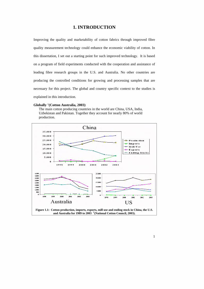
Globally 1(Cotton Australia, 2003) The main cotton producing countries in the world are China, USA, India, Uzbekistan and Pakistan. Together they account for nearly 80% of world production.
Figure 1.1: Cotton production, imports, exports, mill use and ending stock in China, the U.S.
and Australia for 1989 to 2003 2(National Cotton Council, 2003).
1
World consumption of cotton is estimated at more than 91 million bales per year, each bale weighing about 227kg (500 lbs). This cotton is produced on a total global growing area of 31.6 million hectares. It is grown in over 90 countries, 75 of which are developing nations.
Of the major producers, China’s mill use has increased in recent years while that in the U.S. has decreased, and in conjunction with this, China’s imports have increased and the U.S. exports have increased (Figure 1.1).
Australia 3(Cotton Australia, 2003)
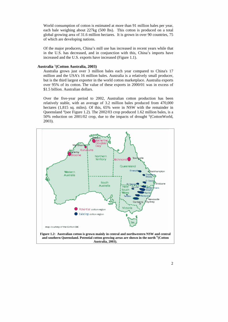
Australia grows just over 3 million bales each year compared to China's 17 million and the USA's 16 million bales. Australia is a relatively small producer, but is the third largest exporter in the world cotton marketplace. Australia exports over 95% of its cotton. The value of these exports in 2000/01 was in excess of $1.5 billion. Australian dollars.
Over the five-year period to 2002, Australian cotton production has been relatively stable, with an average of 3.2 million bales produced from 470,000 hectares (1,815 sq. miles). Of this, 65% were in NSW with the remainder in Queensland 4(see Figure 1.2). The 2002/03 crop produced 1.62 million bales, is a 50% reduction on 2001/02 crop, due to the impacts of drought 5(CottonWorld, 2003).
Figure 1.2: Australian cotton is grown mainly in central and northwestern NSW and central
and southern Queensland. Potential cotton growing areas are shown in the north 6(Cotton Australia, 2003).
2
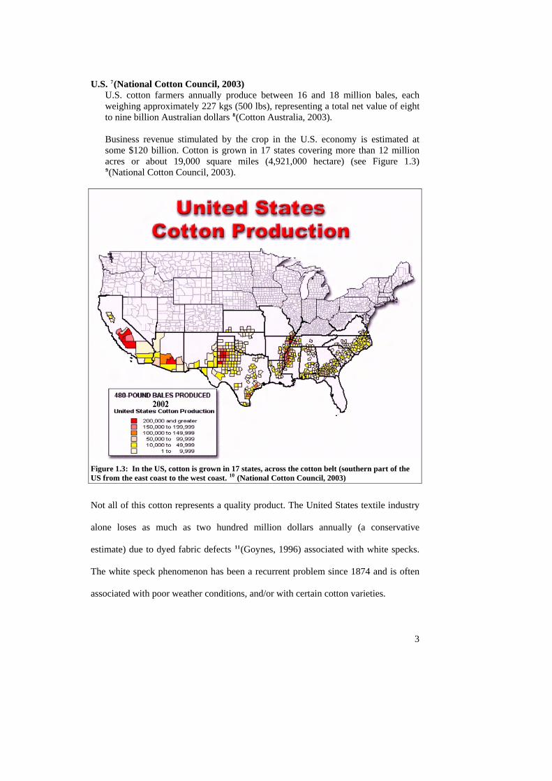
U.S. 7(National Cotton Council, 2003) U.S. cotton farmers annually produce between 16 and 18 million bales, each weighing approximately 227 kgs (500 lbs), representing a total net value of eight to nine billion Australian dollars 8(Cotton Australia, 2003).
Business revenue stimulated by the crop in the U.S. economy is estimated at some $120 billion. Cotton is grown in 17 states covering more than 12 million acres or about 19,000 square miles (4,921,000 hectare) (see Figure 1.3) 9(National Cotton Council, 2003).
Figure 1.3: In the US, cotton is grown in 17 states, across the cotton belt (southern part of the US from the east coast to the west coast. 10 (National Cotton Council, 2003)
Not all of this cotton represents a quality product. The United States textile industry
alone loses as much as two hundred million dollars annually (a conservative
estimate) due to dyed fabric defects 11(Goynes, 1996) associated with white specks.
The white speck phenomenon has been a recurrent problem since 1874 and is often
associated with poor weather conditions, and/or with certain cotton varieties.
3
4
1.1 Project Overview White specks are a specific type of fibre defect that result in high financial losses to
the cotton industry. Fibre entanglements are called neps. Neps that involve immature
fibres do not dye properly and appear as white specks on the dyed fabric. This
dissertation presents an experimentally derived link between the properties of baled
cotton and the quality of resulting fabrics (indicated by the level of white specks in
the fabric). The results are presented as predictive equations for different fibre
measurement systems, with the intention of providing a White Speck Potential
(WSP) that can be incorporated into cotton grading systems used for marketing.
The equations are derived from a database of measured cotton parameters that was
accumulated during a six-year research program (sixteen years when including initial
research) on two continents (North America and Australia). A number of
measurement techniques were developed during the course of the project to acquire
the data, and these are explained.
The international cotton industry uses non-standard, U.S. units of measurement, and
so these units have been adopted in this dissertation. SI units are also provided where
appropriate throughout the dissertation
1.2 Project Aims The aims of this project are:
i) To develop reliable systems for measuring white speck in fabric samples;
ii) To produce a database of measured fibre properties and white speck values;
and
iii) To produce regression equations that will allow white speck potential in
fabrics to be estimated from fibre properties.
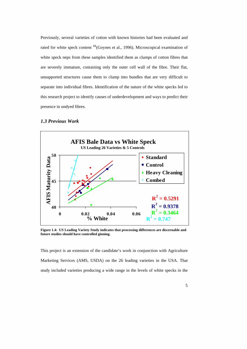
Previously, several varieties of cotton with known histories had been evaluated and
rated for white speck content 12(Goynes et al., 1996). Microscopical examination of
white speck neps from these samples identified them as clumps of cotton fibres that
are severely immature, containing only the outer cell wall of the fibre. Their flat,
unsupported structures cause them to clump into bundles that are very difficult to
separate into individual fibres. Identification of the nature of the white specks led to
this research project to identify causes of underdevelopment and ways to predict their
presence in undyed fibres.
1.3 Previous Work
AFIS Bale Data vs White SpeckUS Leading 26 Varieties & 5 Controls
40
45
50
0 0.02 0.04 0.06% White
AFI
S M
atur
ity D
ata
R2 = 0.3464R2 = 0.9378
R2 = 0.747
StandardControlHeavy CleaningCombed
R2 = 0.5291
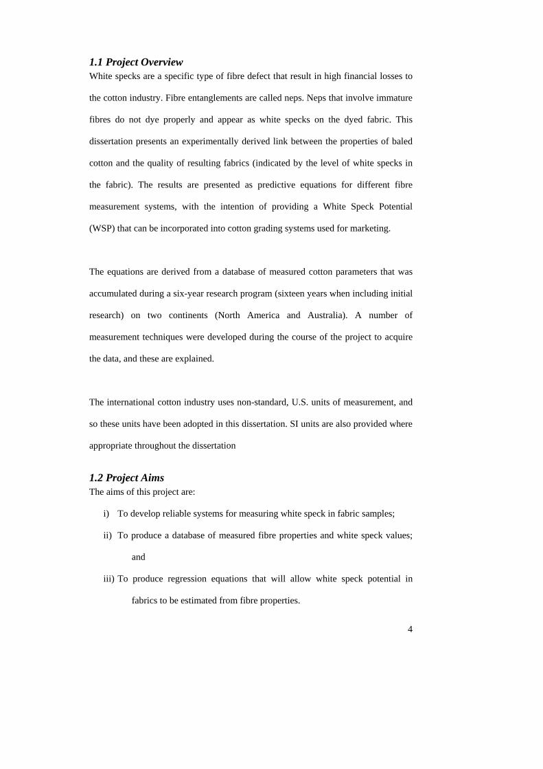
Figure 1.4: US Leading Variety Study indicates that processing differences are discernable and future studies should have controlled ginning.
This project is an extension of the candidate’s work in conjunction with Agriculture
Marketing Services (AMS, USDA) on the 26 leading varieties in the USA. That
study included varieties producing a wide range in the levels of white specks in the
5
6
finished fabrics and resulted in a scale (% white) for the quality of fabric with respect
to white speck. True varietal differences were not readily discernable in the study
results because of the processing interaction shown in Figure 1.4. The varieties were
collected from different gins and therefore had been processed differently. Such
interactions must be quantified before the extent of white speck formation can be
established.
1.4 Justification Constant demands to improve competitiveness through increased productivity are
driving the cotton textile industry to continually upgrade equipment and increase the
intensity and speed of processing. However as speeds increase in cotton processing,
so does the number of neps, especially white speck neps. It has become increasingly
important to know the white speck potential of a bale of cotton before processing it.
HVI data provide a basis for controlling the properties that are important to a
particular operation. However, definitive guidelines are needed so that testing
methods and sampling techniques give statistically sound white speck and fibre
maturity data. In previous studies, the candidate defined minimum sample sizes and
developed techniques for this purpose using both AFIS 13(Bel-Berger, 1999) and
image analysis techniques 14(Bel-Berger, 1998), which together provide the tools to
undertake this research.
Cotton breeders would like to improve fibre quality to improve future varieties, and
the mills need to know what measurable fibre properties are considered the most vital
for quality during processing. Producers and ginners also need to be aware of these
fibre properties, but often receive contradictory responses from the textile mills.
Breeding programs have been geared towards producing longer, stronger, and finer
7
cottons, but with a primary emphasis on yield. Other elements, such as the percent
immature fibres or strength of seed coat attachment, often change along with the
targeted fibre property. Seed coat attachment is strongly related to variety. From 14
to 24 % of white specks are from seed coat fragments that have short immature fibres
attached. A series of field studies conducted from 1997 to 2001 (sixteen years when
including initial my research from 1987 to 1997) is presented in this dissertation to
identify measurable fibre properties that can be used to predict white speck neps
using high-speed fibre measurement systems.
1.5 What is a Nep? A technical description of neps is presented in Section 2.7. However, they are the
cause of the problem addressed in this thesis and a general understanding is required
in this introduction.
Neps are small tangled knots of lint hairs that appear after ginning in manufactured
cotton products. In cloth, they appear as specks. In dyed cloth, the specks are usually
lighter than the background 15(Brown & Ware 1958) and are classically considered to
be of two different types: mechanical or biological neps. Recent studies have defined
coalesced neps as a third and very important type. Mechanical neps only contain
fibres and have their origin in the manipulation of those fibres during processing
16(van der Sluijs, 1999), whereas biological neps include foreign material such as
seed coat fragments, leaf or stem material 17(Hebert, 1988). In coalesced neps, the
immature fibres appear to have grown together in the boll. Mechanical and biological
neps involving immature fibres create undyed spots in the finished fabric 18(Hebert,
1988). The coalesced neps, composed solely of immature fibres, always appear as
white spots on dyed fabric when they survive processing to the fabric stage.
More than 90% of neps in finished fabric incorporate immature fibre 19(Hebert,
1988). These undyeable spots are known as white speck neps, or more commonly,
white specks. Not all neps are white specks, but all white specks are neps, and they
contain immature fibres. Some are tangles of immature and mature fibres while many
are tight masses of immature fibres. White specks were reported as long ago as 1855.
Crum20 (Crum, 1855) examined a sample of calico, which contained white spots after
dyeing. He wrote: “On placing it under the microscope, I found the cotton which had
thus resisted the dye to consist of very thin and remarkably transparent blades, some
of which were marked or spotted while others were so clear as to be almost invisible,
except at the edges. They seem to be particularly numerous during years with
weather problems such as occurred with the 1987 U.S. crop. Long, fine, immature
fibres have a propensity to nep during processing, so any field condition, harvesting
method, gin, or mill processing that increases the level of immature fibres will
increase neps in yarns and fabrics.
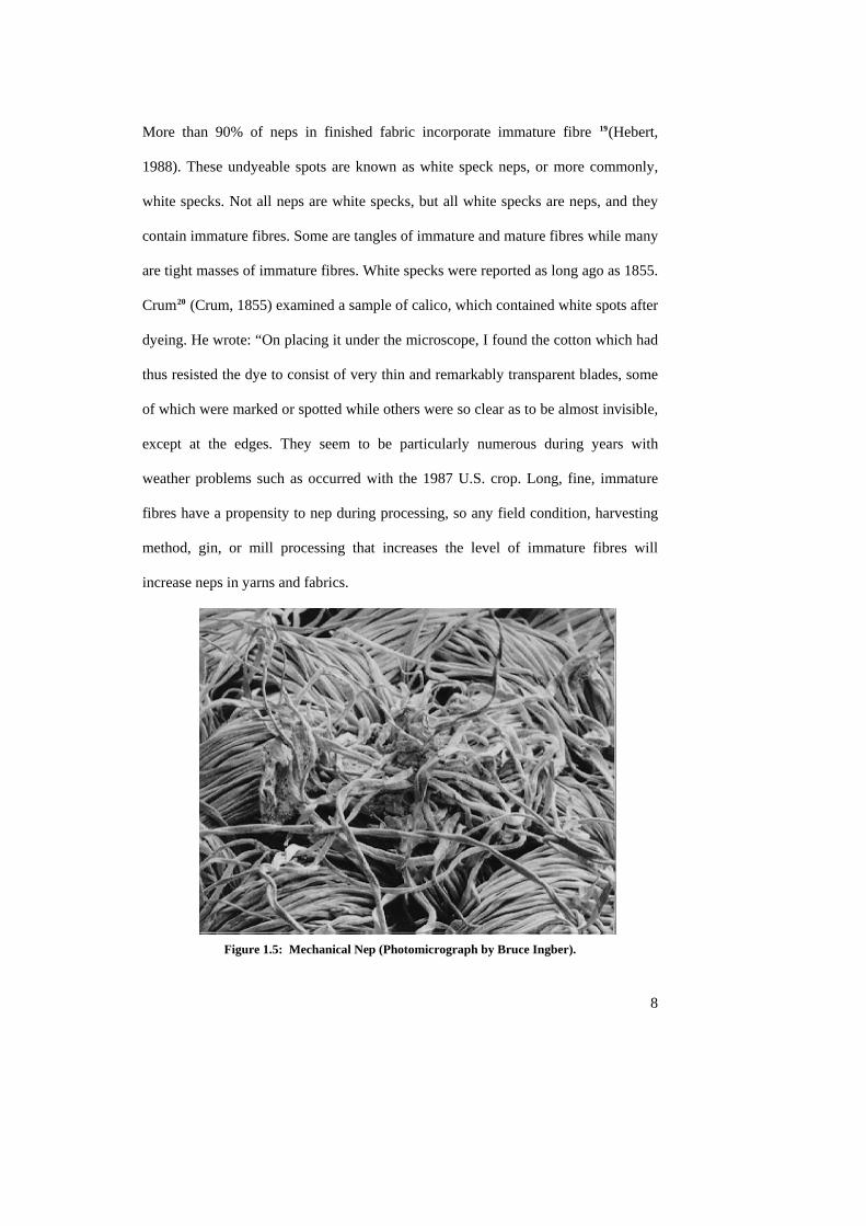
Figure 1.5: Mechanical Nep (Photomicrograph by Bruce Ingber).
8
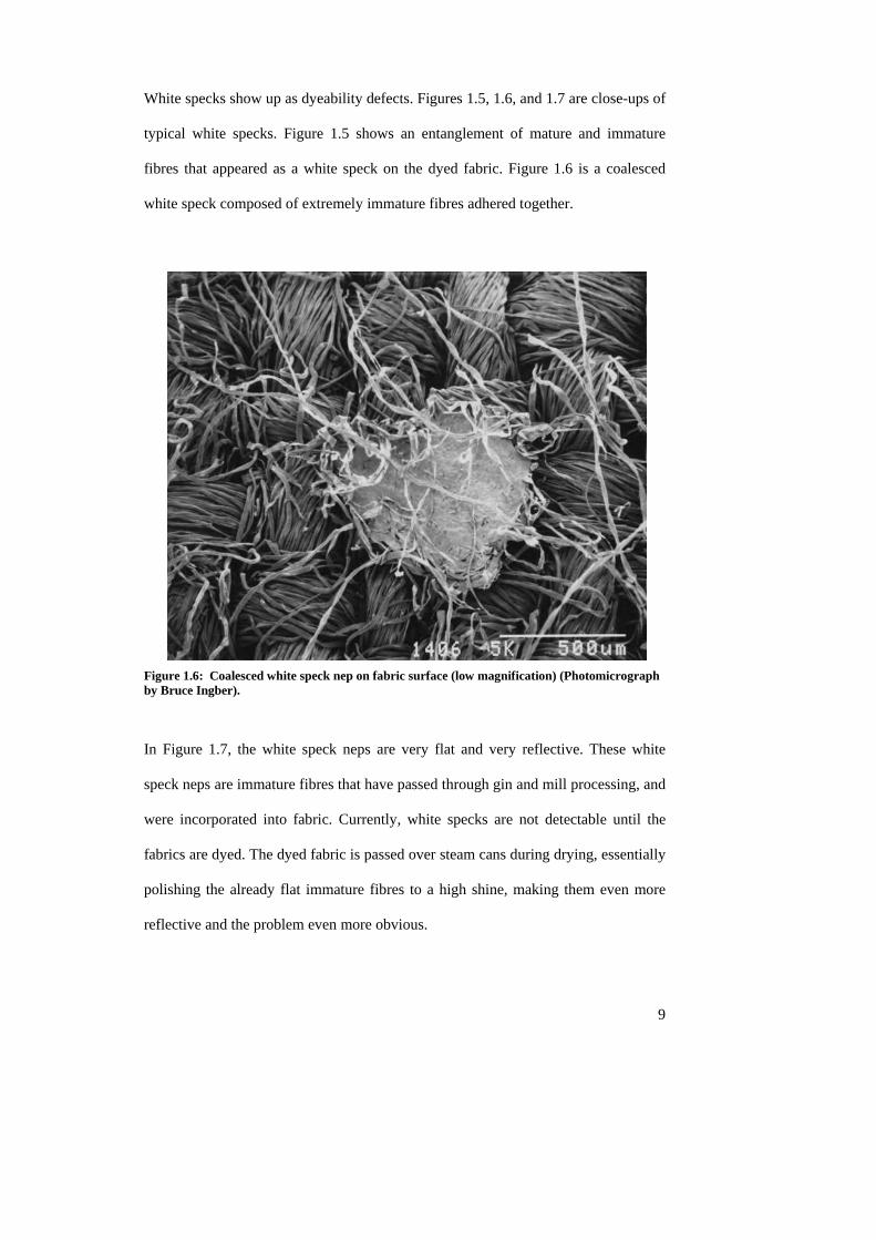
White specks show up as dyeability defects. Figures 1.5, 1.6, and 1.7 are close-ups of
typical white specks. Figure 1.5 shows an entanglement of mature and immature
fibres that appeared as a white speck on the dyed fabric. Figure 1.6 is a coalesced
white speck composed of extremely immature fibres adhered together.
Figure 1.6: Coalesced white speck nep on fabric surface (low magnification) (Photomicrograph by Bruce Ingber).
In Figure 1.7, the white speck neps are very flat and very reflective. These white
speck neps are immature fibres that have passed through gin and mill processing, and
were incorporated into fabric. Currently, white specks are not detectable until the
fabrics are dyed. The dyed fabric is passed over steam cans during drying, essentially
polishing the already flat immature fibres to a high shine, making them even more
reflective and the problem even more obvious.
9
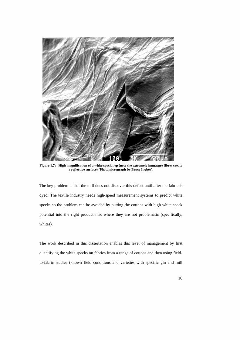
Figure 1.7: High magnification of a white speck nep (note the extremely immature fibres create a reflective surface) (Photomicrograph by Bruce Ingber).
The key problem is that the mill does not discover this defect until after the fabric is
dyed. The textile industry needs high-speed measurement systems to predict white
specks so the problem can be avoided by putting the cottons with high white speck
potential into the right product mix where they are not problematic (specifically,
whites).
The work described in this dissertation enables this level of management by first
quantifying the white specks on fabrics from a range of cottons and then using field-
to-fabric studies (known field conditions and varieties with specific gin and mill
10
processing through fabric) to develop predictive equations.
Before it is decided which values from high-speed fibre measurement systems are
most predictive of white specks, the level of white specks in dyed fabric and/or the
amount of immature fibres needs to be quantified by a consistent method. Several
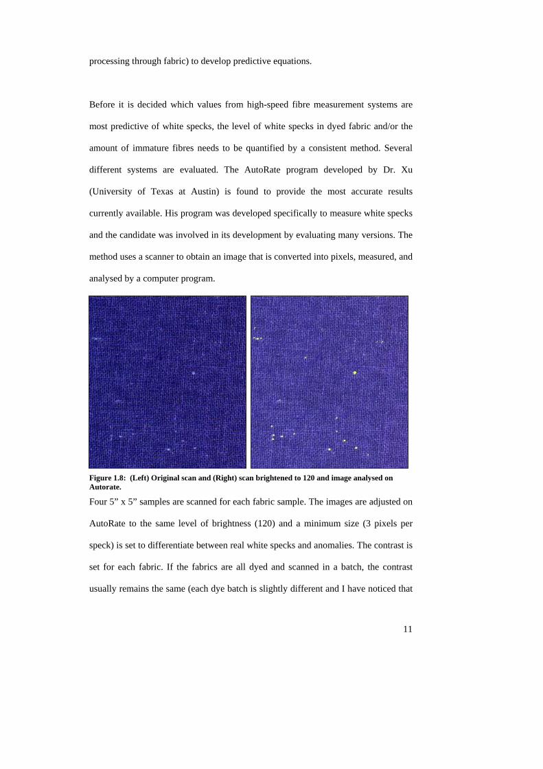
different systems are evaluated. The AutoRate program developed by Dr. Xu
(University of Texas at Austin) is found to provide the most accurate results
currently available. His program was developed specifically to measure white specks
and the candidate was involved in its development by evaluating many versions. The
method uses a scanner to obtain an image that is converted into pixels, measured, and
analysed by a computer program.
Figure 1.8: (Left) Original scan and (Right) scan brightened to 120 and image analysed on Autorate.
Four 5” x 5” samples are scanned for each fabric sample. The images are adjusted on
AutoRate to the same level of brightness (120) and a minimum size (3 pixels per
speck) is set to differentiate between real white specks and anomalies. The contrast is
set for each fabric. If the fabrics are all dyed and scanned in a batch, the contrast
usually remains the same (each dye batch is slightly different and I have noticed that
11
12
the scanner contrast has a slight drift over time). Figure 1.8 shows the fabric’s
original scan and the altered image after it is brightened and analysed. This analysis
results in a white speck count, the size of the white specks, and the percent white on
the fabric.
2. FIBRE PROPERTIES
Cotton fibre is a truly remarkable biological entity, being formed from a single
epidermal cell on the surface of a fertilized cottonseed. As the seed develops the
seed hair-cell continues to lengthen in the form of a circular cylinder, continues to
lengthen. The cell wall diameter is determined early in the growth cycle and is
chiefly a genetic or varietal property.
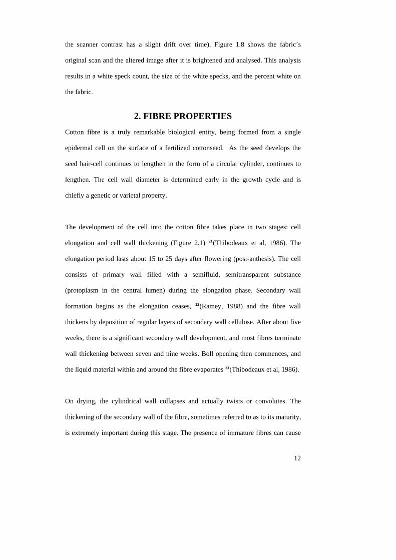
The development of the cell into the cotton fibre takes place in two stages: cell
elongation and cell wall thickening (Figure 2.1) 21(Thibodeaux et al, 1986). The
elongation period lasts about 15 to 25 days after flowering (post-anthesis). The cell
consists of primary wall filled with a semifluid, semitransparent substance
(protoplasm in the central lumen) during the elongation phase. Secondary wall
formation begins as the elongation ceases, 22(Ramey, 1988) and the fibre wall
thickens by deposition of regular layers of secondary wall cellulose. After about five
weeks, there is a significant secondary wall development, and most fibres terminate
wall thickening between seven and nine weeks. Boll opening then commences, and
the liquid material within and around the fibre evaporates 23(Thibodeaux et al, 1986).
On drying, the cylindrical wall collapses and actually twists or convolutes. The
thickening of the secondary wall of the fibre, sometimes referred to as to its maturity,
is extremely important during this stage. The presence of immature fibres can cause
13
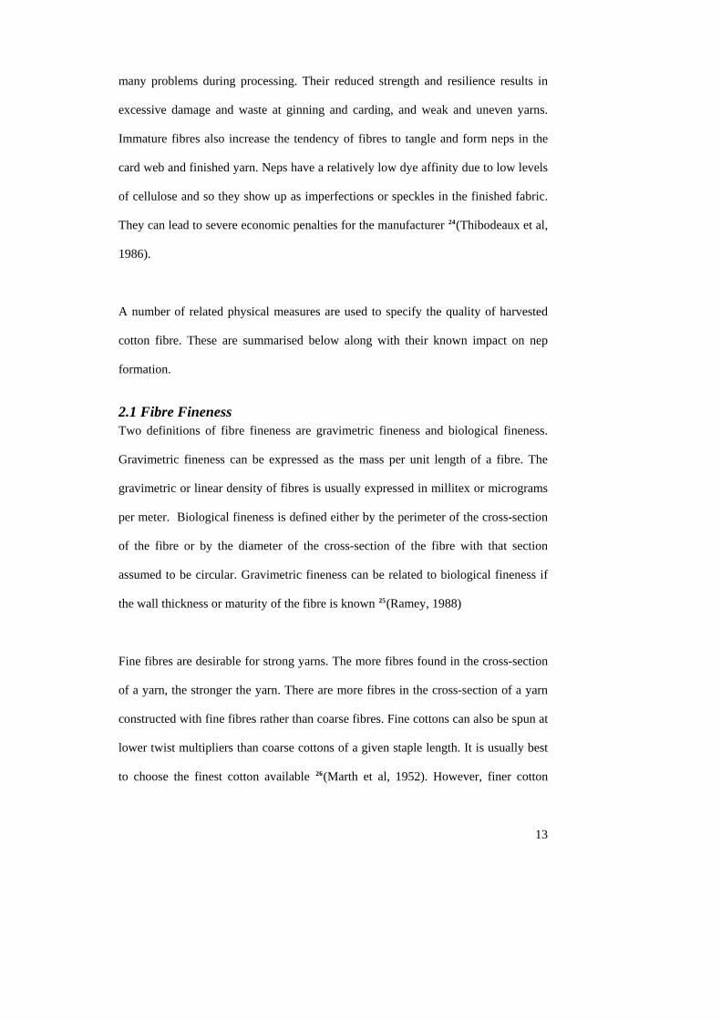
many problems during processing. Their reduced strength and resilience results in
excessive damage and waste at ginning and carding, and weak and uneven yarns.
Immature fibres also increase the tendency of fibres to tangle and form neps in the
card web and finished yarn. Neps have a relatively low dye affinity due to low levels
of cellulose and so they show up as imperfections or speckles in the finished fabric.
They can lead to severe economic penalties for the manufacturer 24(Thibodeaux et al,
1986).
A number of related physical measures are used to specify the quality of harvested
cotton fibre. These are summarised below along with their known impact on nep
formation.
2.1 Fibre Fineness Two definitions of fibre fineness are gravimetric fineness and biological fineness.
Gravimetric fineness can be expressed as the mass per unit length of a fibre. The
gravimetric or linear density of fibres is usually expressed in millitex or micrograms
per meter. Biological fineness is defined either by the perimeter of the cross-section
of the fibre or by the diameter of the cross-section of the fibre with that section
assumed to be circular. Gravimetric fineness can be related to biological fineness if
the wall thickness or maturity of the fibre is known 25(Ramey, 1988)
Fine fibres are desirable for strong yarns. The more fibres found in the cross-section
of a yarn, the stronger the yarn. There are more fibres in the cross-section of a yarn
constructed with fine fibres rather than coarse fibres. Fine cottons can also be spun at
lower twist multipliers than coarse cottons of a given staple length. It is usually best
to choose the finest cotton available 26(Marth et al, 1952). However, finer cotton
14
fibres tend to form neps more easily than coarser fibres because the former are more
easily bent, buckled, and entangled during mechanical manipulation. Several studies
have shown that cottons with a lower micronaire (a general measure of maturity and
fineness) produce neppy, low-grade yarn, whereas cottons with a higher micronaire
produce less neppy, higher quality yarns 27(van der Sluijs, 1999).
Nep formation becomes more frequent and more detrimental in its consequences
with the spinning of fine yarns from fine fibres. Neps are more noticeable in fine
yarns because their size becomes comparable to that of the yarn diameter 28(Ramey,
1988).
2.2 Fibre Maturity The term “fibre maturity” has not been standardized in the cotton industry. Common
measures used 29, 30(Peirce and Lord, 1939; Lord and Heap, 1988) are: wall thickness,
degree of thickening, maturity ratio, causticaire maturity index, and dye maturity.
Wall thickness is the absolute value of the fibre wall thickness (μm). Degree of
thickening (θ) is defined by area of fibre wall/area of circle having same perimeter.
Maturity ratio is given by θ/0.577 and is the most widely used term in the literature.
As a rough guide, immature fibres have a wall thickness below 2.7μm. Montalvo and
Faught (1996) suggested a further measure called percent wall thickness.
Dead cotton consists of fibres that are very immature, where the secondary wall is
completely missing. The fibres with intermediate development (between the dead
and normal fibres) are described as thin walled; the dead and thin walled fibres may
be classed together as immature. The mature cottons are fairly ridged and have a
kidney bean shaped cross-section. The fibres collapse as the boll opens and immature
fibres collapse to a ribbon-like section and are comparatively floppy. It is because of
this lack of rigidity that the immature fibres tangle during processing 31(Midgley,
1933). These neps consist of mostly immature or dead fibres 32(Furter, 1992) that
collapse into extremely flat ribbons, which are highly reflective and thus appear as
white specks in the dyed fabric 33(Peter et al, 1989). These fibres are therefore called
‘shiny neps’.
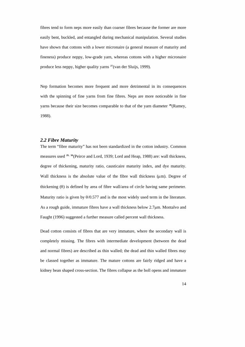
Figure 2.1: Cottonseed and fibre development (D. P. Thibodeaux and J. P. Evans, Textile Research Journal, February 1986).
Cellulose fills in the cell wall as the fibre develops and increases the maturity of the
cotton. Mature fibre has a more circular in shape as illustrated in Figure 2.2 (a perfect
circle would have θ = 1, while the smaller θ becomes, the less circular and the flatter
the cross-section becomes). Cotton immaturity results when the normal wall
thickening process is interrupted or slowed down by factors such as frost, bad
15
weather, insects, drought stress, premature opening because of mineral deficiencies,
plant diseases, injury to the foliage, stem or roots. 34(van der Sluijs, 1999).
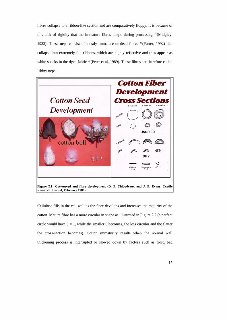
Figure 2.2: Maturity of the cotton fibre cross-section is dependent on its cell wall development (from Devron Thibodeaux).
Cottons of high fibre maturity are likely to give less neppy yarns than those of lower
maturity. Fibre maturity is partly determined by genetic factors which may produce
markedly consistent differences in cottons grown under varying environmental
conditions, even when those conditions are uniformly favourable to a high degree of
development of secondary thickening 35(Lord, 1948).
Immature fibres are finer, flatter, and more elastic than fully mature fibres of the
same genotype because the fibre walls are thinner and the fibres are incompletely
‘filled’ with secondary wall cellulose. Consequently, immature fibres tend to stretch
elastically, rather than break, when tension is applied. Upon release of tension, they
can recoil into tangled snarls. The snarls and knots formed during fibre processing
often contain entrapped mature fibres, and these tangled fibre masses appear in yarn
and finished fabric as nep visible to the unaided eye. Furthermore, the lower
16
17
cellulosic content of the cell walls of the immature fibre results in decreased dye
uptake, which is seen as undesirable colour shadings or barré. When fibres of
markedly different maturities are combined, ‘white specks” develop when the
immature and mature fibres in a nep mass do not dye evenly and to the same degree
36(Bradow, 1998).
2.3 Fibre Length The effect of the staple length on the tendency towards nep formation has been under
debate. Some think that an increase in the tendency towards nep formation can be
correlated with an increase in the staple length of the cotton, since a long-staple
cotton frequently has a greater mean fibre fineness than a short-staple one
37(Wegener, 1980). Neps may also form due to the breaking of excessively long
fibres, or lack of fibre orientation. However, a useful MSc dissertation by van der
Sluijs, 38(van der Sluijs, 1996) showed that there was a low correlation between the
cotton fibre length characteristics and neps, with the 50% (mean) span length playing
a more significant role than the 2.5% (longest) span length 39(van der Sluijs, 1996).
2.4 Fibre Strength Strong cottons usually exhibit fewer problems and fewer neps during processing than
weaker cottons. Improvement in average strength reduces fibre breakage and
therefore short fibre content and nep content; the same result can also be achieved by
improving the uniformity of the cotton. Fibre tenacity is related to nep formation.
Cotton with a low strength will result in the generation of fibre neps due to fibre
damage in the carding process. A link between fibre strength and stiffness could also
be reflected in a trend towards fewer neps40 (van der Sluijs, 1999).
18
2.5 Fibre Elongation, Stiffness and Buckling Coefficient An increase in fibre elongation tends to lead to an increase in nep formation with
card and draw-frame sliver. At a constant fibre tenacity, an increase in fibre
elongation is indicative of a decrease in fibre stiffness and an increase in buckling
potential, and consequently of an increase in nep formation. Stiffer fibres form fewer
neps. The stress build up and sudden release mechanism or Buckling Coefficient
41(Alon, 1978), which induces buckling along the fibre length, is probably a cause for
the neps that are present in finished fabrics 42(van der Sluijs, 1999). Fibres, which are
stretched during processing, accumulate elastic energy. If one end of the fibre is
suddenly released from the tensile load, that energy is converted to kinetic energy.
As the fibre cannot stand compressive stress, buckling results 43(Alon, 1978).
2.6 Fibre Impurities The tendency towards nep formation increases with increasing amounts of impurities
such as husk, leaf, stalk, and seed coat fragments. This is largely due to the fact that
the higher the trash content, the greater the number of cleaning points required
during ginning and opening, which in turn leads to more neps, fibre breakage and
short fibre content, causing a deterioration in spinning performance and yarn quality
44(van der Sluijs, 1999).
2.7 Neps The ASTM definition is “Neps are small knot-like aggregates of tightly entangled
cotton fibres not usually larger than a common pinhead, which are difficult to
remove. Neps usually appear to be more numerous in cotton after subjection to
considerable handling and to some manner of processing, as certain ginning and
manufacturing operations” 45(ASTM, 1947). A nep is therefore a small cluster of
entangled fibres consisting either entirely of fibres (i.e., a mechanical or coalesced
19
rdi - a, 1985).
fibre nep) or of foreign matter (e.g., a seed-coat fragment) entangled with fibres. In
most cases, fibrous neps are found to contain at least five fibres, with the average
number being 16 or more 46(van der Sluijs, 1999). Neps are distinct from certain
other imperfections found in cotton, including fibres still attached to parts of seeds.
One of these imperfections is the “mote”, which consists of a whole undeveloped
seed of any size or age, covered with fuzzy and short fibres, certain of which bear
mature lint fibres. Seed coat and mote fragments with lint or fuzz fibres attached are
not neps. Neps are created during development, harvesting, ginning and yarn
manufacturing phases of production 47(Mangiala
2.7.1 Nep Formation Neps can be classified by the differences in formation. Biological neps are neps that
contain foreign material, whether the material is a seed coat fragment, leaf, or stem
material 48(Hebert, 1988). Mechanical neps are those that contain only fibres and
have their origin in the manipulation of the fibres during processing 49(van der Sluijs,
1999). The coalesced neps make a third type of nep in that they are an intermediate
between biological and mechanical neps (see 2.7.1.3), in that they are entirely
formed from fibres, but biologically produced. In addition, most important to this
research, is the fourth type of nep, white speck neps, which cause dye defects in the
finished fabric.
2.7.1.1 Biological Neps Biological neps are caused by biological components of the cotton plant forming
contaminants in the fabric; two examples are shown in Figure 2.3. Undeveloped
seeds, motes, small bits of seed coat, particles of leaf or bract can all be entangled in
the cotton during harvesting or subsequent processing. They result in small dark
specks in the greige (just off the loom without chemical finishing) fabric, but are
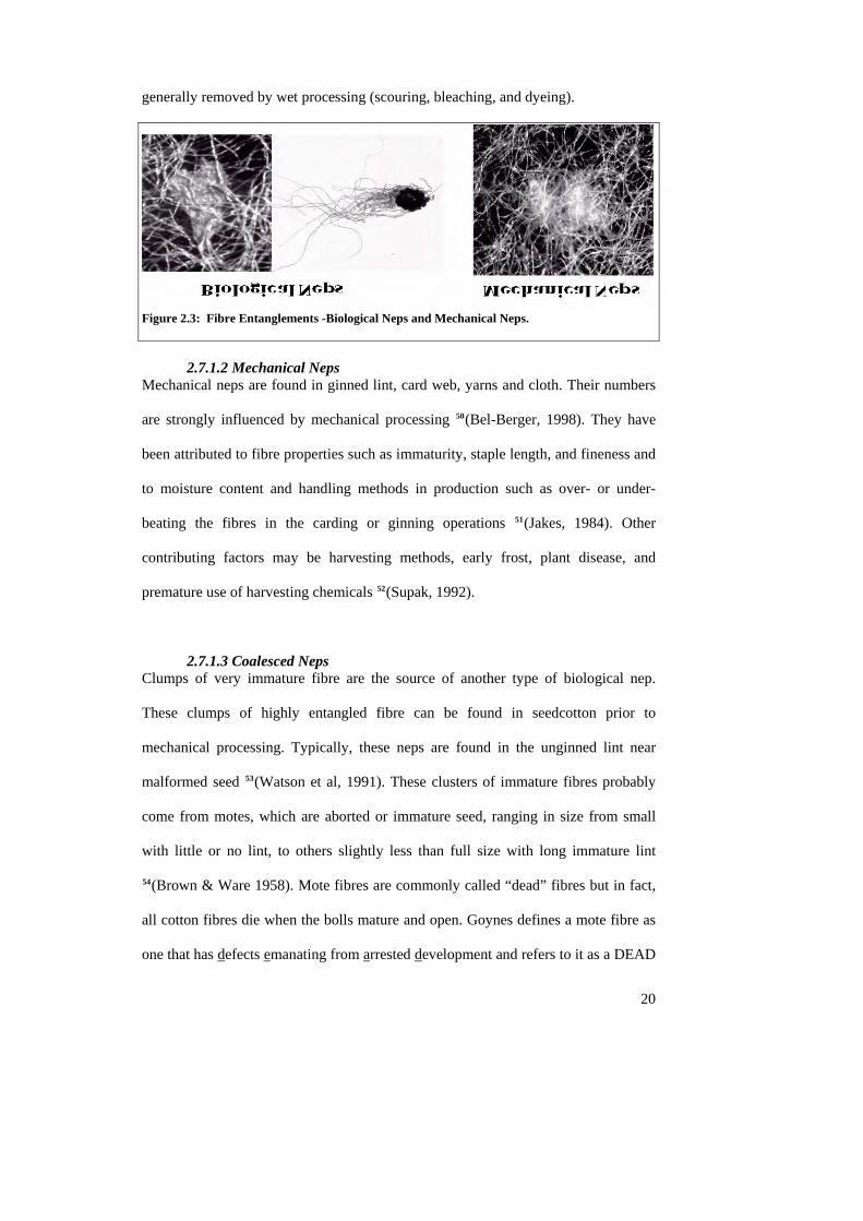
generally removed by wet processing (scouring, bleaching, and dyeing).
Figure 2.3: Fibre Entanglements -Biological Neps and Mechanical Neps.
2.7.1.2 Mechanical Neps Mechanical neps are found in ginned lint, card web, yarns and cloth. Their numbers
are strongly influenced by mechanical processing 50(Bel-Berger, 1998). They have
been attributed to fibre properties such as immaturity, staple length, and fineness and
to moisture content and handling methods in production such as over- or under-
beating the fibres in the carding or ginning operations 51(Jakes, 1984). Other
contributing factors may be harvesting methods, early frost, plant disease, and
premature use of harvesting chemicals 52(Supak, 1992).
2.7.1.3 Coalesced Neps Clumps of very immature fibre are the source of another type of biological nep.
These clumps of highly entangled fibre can be found in seedcotton prior to
mechanical processing. Typically, these neps are found in the unginned lint near
malformed seed 53(Watson et al, 1991). These clusters of immature fibres probably
come from motes, which are aborted or immature seed, ranging in size from small
with little or no lint, to others slightly less than full size with long immature lint
54(Brown & Ware 1958). Mote fibres are commonly called “dead” fibres but in fact,
all cotton fibres die when the bolls mature and open. Goynes defines a mote fibre as
one that has defects emanating from arrested development and refers to it as a DEAD
20
21
fibre 55(Goynes - a, 1995). These neps are formed from immature fibres that are
damaged while there is still considerable biological material in the lumen or the boll.
The biological material from the lumen adheres the immature fibres together, leaving
a flat shiny clump of immature fibres.
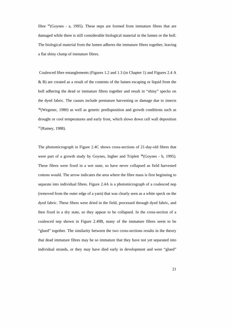
Coalesced fibre entanglements (Figures 1.2 and 1.3 (in Chapter 1) and Figures 2.4 A
& B) are created as a result of the contents of the lumen escaping or liquid from the
boll adhering the dead or immature fibres together and result in “shiny” specks on
the dyed fabric. The causes include premature harvesting or damage due to insects
56(Wegener, 1980) as well as genetic predisposition and growth conditions such as
drought or cool temperatures and early frost, which slows down cell wall deposition
57(Ramey, 1988).
The photomicrograph in Figure 2.4C shows cross-sections of 21-day-old fibres that
were part of a growth study by Goynes, Ingber and Triplett 58(Goynes - b, 1995).
These fibres were fixed in a wet state, so have never collapsed as field harvested
cottons would. The arrow indicates the area where the fibre mass is first beginning to
separate into individual fibres. Figure 2.4A is a photomicrograph of a coalesced nep
(removed from the outer edge of a yarn) that was clearly seen as a white speck on the
dyed fabric. These fibres were dried in the field, processed through dyed fabric, and
then fixed in a dry state, so they appear to be collapsed. In the cross-section of a
coalesced nep shown in Figure 2.49B, many of the immature fibres seem to be
“glued” together. The similarity between the two cross-sections results in the theory
that dead immature fibres may be so immature that they have not yet separated into
individual strands, or they may have died early in development and were “glued”
together by the protoplasm in the boll. If the ultra-immature (biologically
underdeveloped) or coalesced fibres have loose edges, they can entangle with mature
fibres during processing, trapping the cluster in the yarn and appearing as white
specks on the dye fabric (with out any dark foreign matter). Therefore, from this it
can be seen that coalesced neps could also be considered mechanical or biological
neps. They are also white speck neps, which are discussed in the next section.
Figure 2.4: A) Coalesced nep on a dyed yarn and B) its cross-section. C) 21-day post anthesis cotton fibres from a growth study by Goynes et al, 59(Goynes –b, 1995).
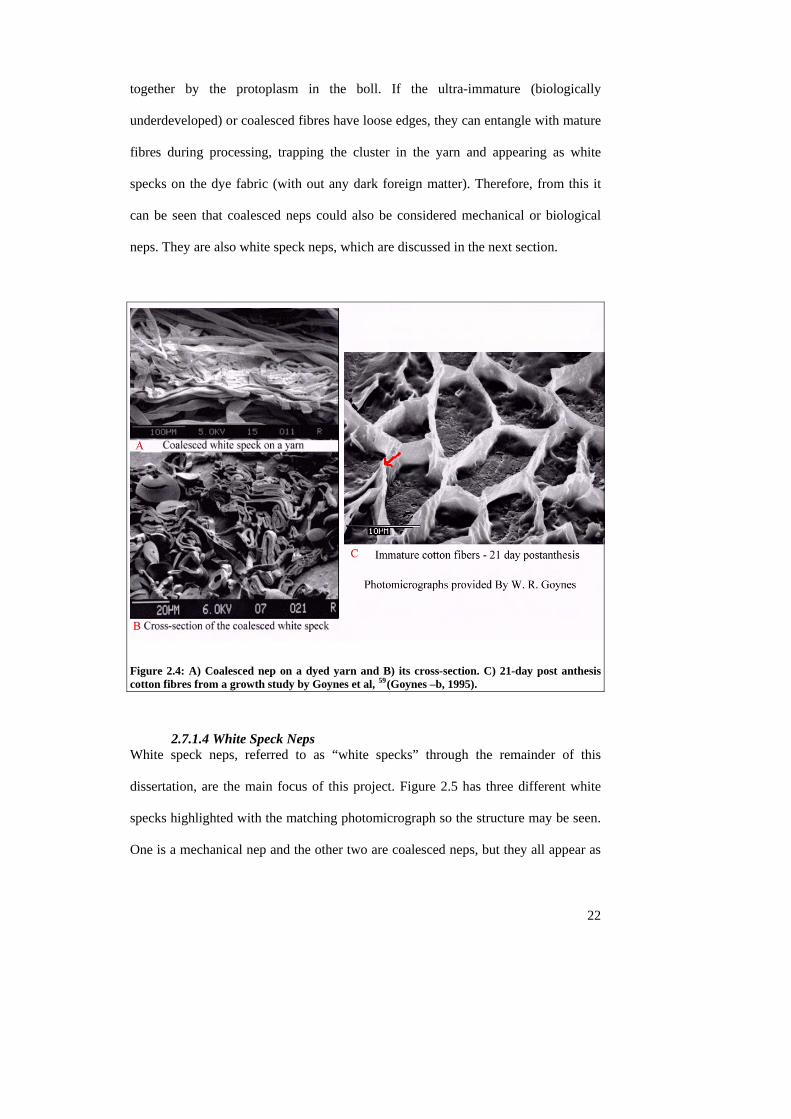
2.7.1.4 White Speck Neps White speck neps, referred to as “white specks” through the remainder of this
dissertation, are the main focus of this project. Figure 2.5 has three different white
specks highlighted with the matching photomicrograph so the structure may be seen.
One is a mechanical nep and the other two are coalesced neps, but they all appear as
22
white specks on the dyed fabric.
Figure 2.5: White specks as seen by the naked eye on fabric and magnified showing fibre entanglements or clusters of immature fibre
A shiny nep is found on the surface of dyed fabrics; they appear as light or white
spots and occur only in the finished fabric 60(Hebert, 1988). Many people have called
white specks “shiny neps” due to their reflective appearance (Figure 2.6). When
immature fibres die, they collapse into flat ribbons. In dyed fabric, these flat ribbons
are passed over steam cans, essentially polishing the already flat immature fibres to a
high shine. This makes them even more reflective and the problem becomes even
more obvious (Figure 2.6).
23
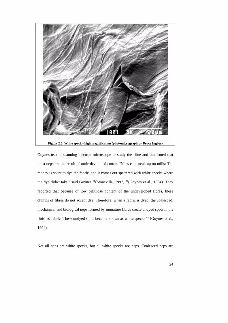
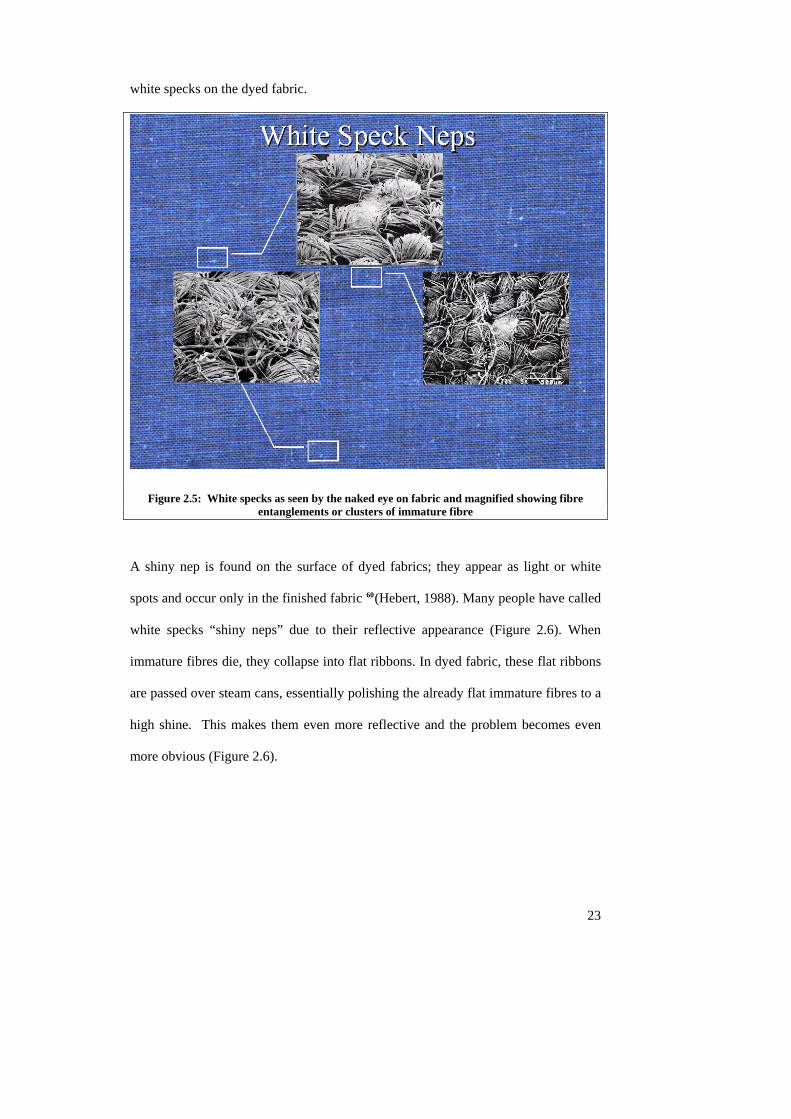
Figure 2.6: White speck - high magnification (photomicrograph by Bruce Ingber)
Goynes used a scanning electron microscope to study the fibre and confirmed that
most neps are the result of underdeveloped cotton. ''Neps can sneak up on mills: The
money is spent to dye the fabric, and it comes out spattered with white specks where
the dye didn't take,'' said Goynes 61(Stoneville, 1997) 62(Goynes et al., 1994). They
reported that because of low cellulose content of the undeveloped fibres, these
clumps of fibres do not accept dye. Therefore, when a fabric is dyed, the coalesced,
mechanical and biological neps formed by immature fibres create undyed spots in the
finished fabric. These undyed spots became known as white specks 63 (Goynes et al.,
1994).
Not all neps are white specks, but all white specks are neps. Coalesced neps are
24
25
composed solely of immature fibre clusters. They always appear white or light, and
therefore are always white specks. Biological and mechanical neps can be white
speck neps if they involve immature fibres, thus appearing white in dyed fabrics, but
many of these neps have only mature fibres and appear as a thick and/or a dark spot
on yarn and wouldn’t be considered white specks. The more general term of “white
specks” refers to all nep formations that appear white on the surface of the fabric
(Figure 2.5).
2.8 Fibre Measurement Systems High-speed fibre measurements are now being used to provide the main indication of
crop quality. All US and Australian cotton is graded with the industry standard High
Volume Instrumentation (HVI) system, which quantifies length, strength, trash,
colour and micronaire. The candidate’s previous work showed that little correlation
could be established between any of these measurements and the degree of white
speck nep potential, unless the processing history was known.
While HVI is the industry standard commercial instrumentation system, other
systems are available. One commercially available instrument purchased by many
textile mills is the Advanced Fibre Information System (AFIS). This machine can be
fitted with an optional F&M (Fineness and Maturity) module, which provides the
strongest fibre to white speck data relationships available to industry from high-
speed measurement systems.
Lintronics FiberLab is the latest contender for commercial acceptance in the
measurement of neps and maturity. It is different from the above systems in that it
26
actually makes a web and attempts to simulate the real world conditions of the card.
High-speed near-infrared spectroscopy (NIRS) is another new and promising method
of predicting the white speck potential of bale fibre, but it is still under development
and not yet available commercially for fibre maturity measurements.
Part of the investigation described in this dissertation was intended to identify the
high-speed systems that have the most potential for accurately predicting fabric
quality from fibre quality. A large set of samples was required to do this. Samples
with known ginning and growth environment history were needed to better establish
the correlations with HVI, AFIS, NIRS, and other high-speed measurements of
cotton fibre properties. Finally, the measured values are used to establish best-fit
relationships between high-speed fibre data and fabric white specks.
27
3. HIGH SPEED FIBRE MEASUREMENT SYSTEMS High-speed fibre measurement systems are beginning to influence the way cotton is
being ginned in Australia and the U.S.A. The High Volume Instrumentation (HVI)
system is well accepted in the Australian and North American ginning industries,
while the advantages of several other systems are becoming increasingly well
known. This chapter describes the HVI system and other high-speed fibre measuring
systems and details the potential benefit of these systems for improving fibre quality.
3.1 HVI Ginners are more conscious today of what is being done to cotton fibre during the
ginning process following widespread acceptance of HVI measurements in recent
years. The biggest offences in ginning have been over-drying and over-machination
64(Norman, 1991). Until recently, the grower and the ginner produced cotton “for the
grade”. Ginning “for the grade” produces cotton that is visually appealing but gives
less than optimum results in the spinning mill. Over-drying may result in reduced
trash and a raised grade, but it breaks down large particles into pepper trash. It also
makes neps, reduces average fibre length, increases “ends down” in spinning
(number of broken ends/spindle hour), lowers yarn evenness, and lowers yarn
strength. Cotton quality should be maintained or only minimally reduced during
processing. A robust testing and marketing system would encourage breeding,
variety selection and ginning for higher quality. Quality is the key, but what fibre
qualities should be rewarded financially? Currently the marketing system tends to
reward white, clean, but overprocesed cottons with qualities that can cause
processing problems and defects in the mill. The grading system was based on hand
picked cottons and was very valid in its day. However, today cottons are
mechanically harvested and ginned at high speeds which affect cotton quality in
28
ways that hand picking doesn’t. Mills would now rather pay for long, strong, fine,
but mature cotton with large trash particles (easily removed in the mill) that process
well, producing yarns and fabrics with low defects and high strength. Objective
approaches to improving cotton quality are possible, based on:
1) Developing methods to measure all the important properties for textile processing (trash particle size and shape, short fibre content, colour [grey versus yellow], fibre maturity/ fibre fineness, and undyeable neps);
2) Adapting these methods for grading cotton; and
3) Developing ways to reduce damage in processing and so maintain the natural quality produced by the cotton plant; and make allowing the fibre as long and strong as possible 65(Werber, 1994).
The impact of HVI on the ginning process follows from the ginners becoming more
aware of gin equipment and conditions that affect the HVI data on cottons that they
ginned. The HVI measurements have heightened ginners’ awareness of the need to
calibrate machinery controls: automatic calibration is available that allows for
multiple temperature and /or moisture sensing inputs for improved process control.
Lint cleaners at the gin are being bypassed for improved quality, and single stage lint
cleaning is being discussed 66(Anthony, 1986). All these effects of the HVI grading
system positively affect the cotton fibre and its associated nepping.
3.1.1 Instrumental Determinations 67(Cotton Program AMS USDA, 2001) Measurements for the following quality factors are performed by high volume,
precision instruments, commonly referred to as "HVI" (High Volume
Instrumentation). The specifics outlined in this section are provided by the USDA
publication “The Classification of Cotton” 68(Cotton Program AMS USDA, 2001).
3.1.1.1 Fibre Length Fibre length is the average length of the longer one half of the fibres (upper half
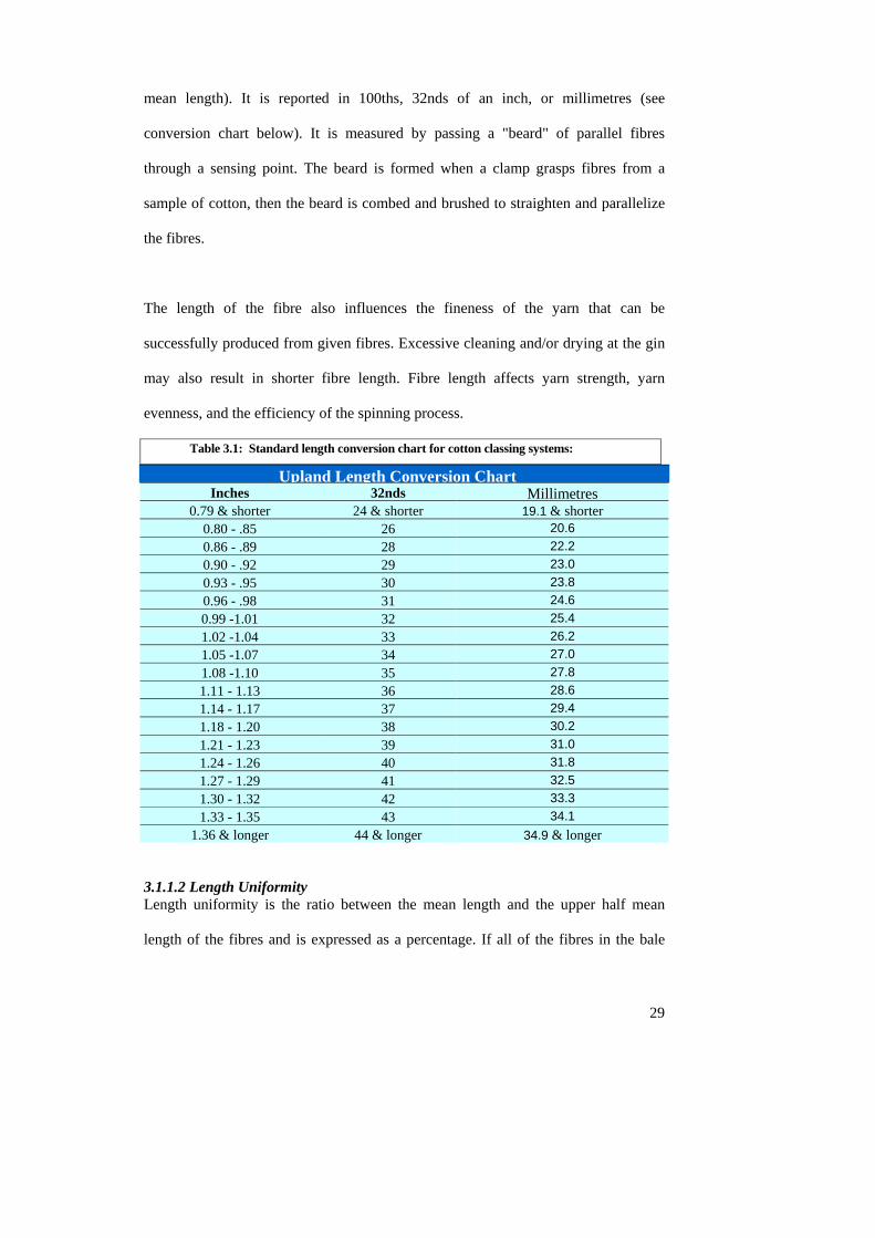
29
mean length). It is reported in 100ths, 32nds of an inch, or millimetres (see
conversion chart below). It is measured by passing a "beard" of parallel fibres
through a sensing point. The beard is formed when a clamp grasps fibres from a
sample of cotton, then the beard is combed and brushed to straighten and parallelize
the fibres.
The length of the fibre also influences the fineness of the yarn that can be
successfully produced from given fibres. Excessive cleaning and/or drying at the gin
may also result in shorter fibre length. Fibre length affects yarn strength, yarn
evenness, and the efficiency of the spinning process.
Table 3.1: Standard length conversion chart for cotton classing systems:
Upland Length Conversion ChartInches 32nds Millimetres
0.79 & shorter 24 & shorter 19.1 & shorter0.80 - .85 26 20.6 0.86 - .89 28 22.2 0.90 - .92 29 23.0 0.93 - .95 30 23.8 0.96 - .98 31 24.6 0.99 -1.01 32 25.4 1.02 -1.04 33 26.2 1.05 -1.07 34 27.0 1.08 -1.10 35 27.8 1.11 - 1.13 36 28.6 1.14 - 1.17 37 29.4 1.18 - 1.20 38 30.2 1.21 - 1.23 39 31.0 1.24 - 1.26 40 31.8 1.27 - 1.29 41 32.5 1.30 - 1.32 42 33.3 1.33 - 1.35 43 34.1
1.36 & longer 44 & longer 34.9 & longer 3.1.1.2 Length Uniformity Length uniformity is the ratio between the mean length and the upper half mean
length of the fibres and is expressed as a percentage. If all of the fibres in the bale
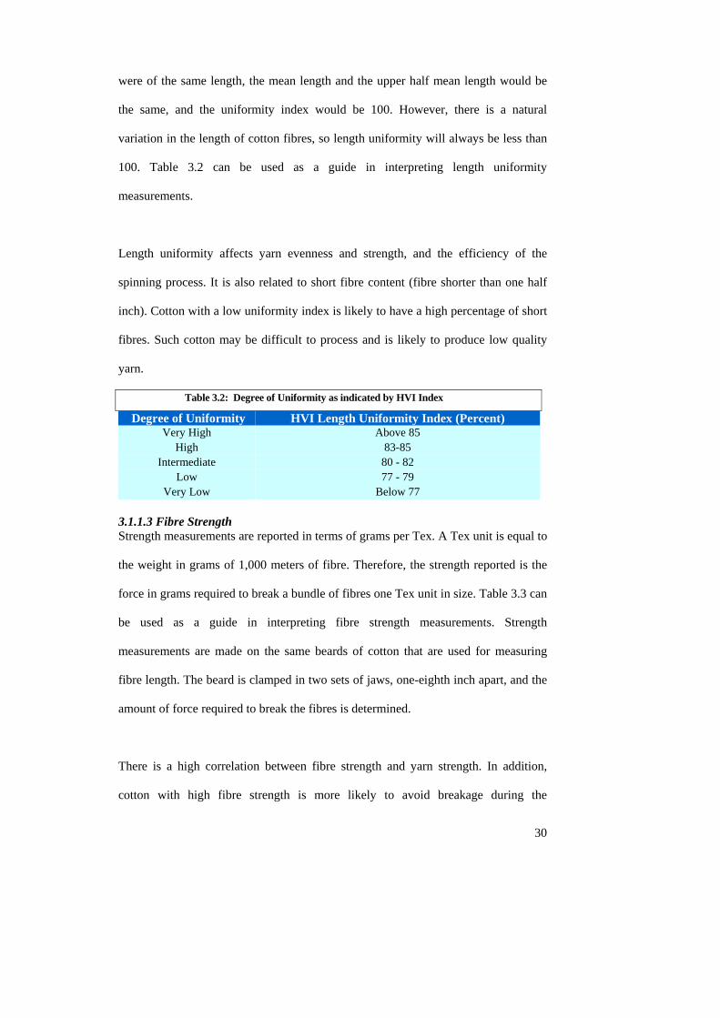
30
were of the same length, the mean length and the upper half mean length would be
the same, and the uniformity index would be 100. However, there is a natural
variation in the length of cotton fibres, so length uniformity will always be less than
100. Table 3.2 can be used as a guide in interpreting length uniformity
measurements.
Length uniformity affects yarn evenness and strength, and the efficiency of the
spinning process. It is also related to short fibre content (fibre shorter than one half
inch). Cotton with a low uniformity index is likely to have a high percentage of short
fibres. Such cotton may be difficult to process and is likely to produce low quality
yarn.
Table 3.2: Degree of Uniformity as indicated by HVI Index
Degree of Uniformity HVI Length Uniformity Index (Percent) Very High Above 85
High 83-85Intermediate 80 - 82
Low 77 - 79Very Low Below 77
3.1.1.3 Fibre Strength Strength measurements are reported in terms of grams per Tex. A Tex unit is equal to
the weight in grams of 1,000 meters of fibre. Therefore, the strength reported is the
force in grams required to break a bundle of fibres one Tex unit in size. Table 3.3 can
be used as a guide in interpreting fibre strength measurements. Strength
measurements are made on the same beards of cotton that are used for measuring
fibre length. The beard is clamped in two sets of jaws, one-eighth inch apart, and the
amount of force required to break the fibres is determined.
There is a high correlation between fibre strength and yarn strength. In addition,
cotton with high fibre strength is more likely to avoid breakage during the
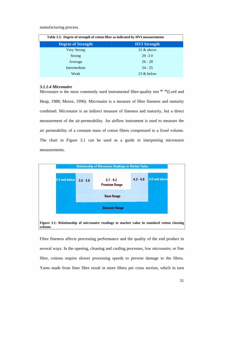
manufacturing process.
Table 3.3: Degree of strength of cotton fibre as indicated by HVI measurements
Degree of Strength HVI Strength
31
Very Strong 31 & aboveStrong 29 -3 0
Average 26 - 28Intermediate 24 - 25
Weak 23 & below
3.1.1.4 Micronaire Micronaire is the most commonly used instrumental fibre-quality test 69 70(Lord and
Heap, 1988; Moore, 1996). Micronaire is a measure of fibre fineness and maturity
combined. Micronaire is an indirect measure of fineness and maturity, but a direct
measurement of the air-permeability. An airflow instrument is used to measure the
air permeability of a constant mass of cotton fibres compressed to a fixed volume.
The chart in Figure 3.1 can be used as a guide in interpreting micronaire
measurements.
Figure 3.1: Relationship of micronaire readings to market value in standard cotton classing scheme.
Fibre fineness affects processing performance and the quality of the end product in
several ways. In the opening, cleaning and carding processes, low micronaire, or fine
fibre, cottons require slower processing speeds to prevent damage to the fibres.
Yarns made from finer fibre result in more fibres per cross section, which in turn
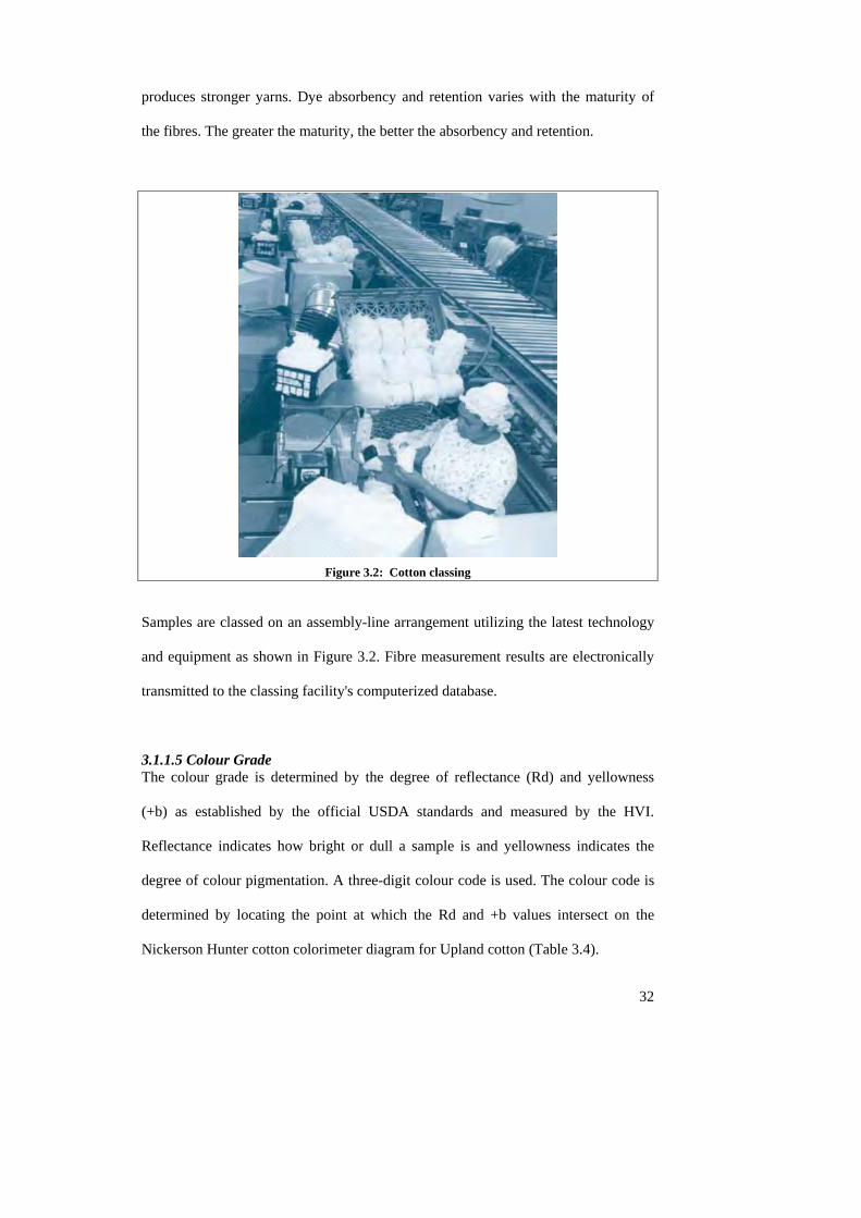
produces stronger yarns. Dye absorbency and retention varies with the maturity of
the fibres. The greater the maturity, the better the absorbency and retention.
Figure 3.2: Cotton classing
Samples are classed on an assembly-line arrangement utilizing the latest technology
and equipment as shown in Figure 3.2. Fibre measurement results are electronically
transmitted to the classing facility's computerized database.
3.1.1.5 Colour Grade The colour grade is determined by the degree of reflectance (Rd) and yellowness
(+b) as established by the official USDA standards and measured by the HVI.
Reflectance indicates how bright or dull a sample is and yellowness indicates the
degree of colour pigmentation. A three-digit colour code is used. The colour code is
determined by locating the point at which the Rd and +b values intersect on the
Nickerson Hunter cotton colorimeter diagram for Upland cotton (Table 3.4).
32

33
The colour of cotton fibres can be affected by genetics, rainfall, freezes, insects and
fungi, and by staining through contact with soil, grass, or the cotton plant's leaf.
Excessive moisture and temperature levels also can affect colour while cotton is
being stored, both before and after ginning. As the colour of cotton deteriorates
(greys) due to non-optimal environmental conditions, especially bacterial growth, the
probable processing efficiency is reduced. Colour deterioration is an indication of the
fibres’ reduced ability to absorb and hold dyes and finishes.
Table 3.4: Colour Grades of Upland Cotton
Colour Grades of Upland Cotton Effective 1993
White Light Spotted Spotted Tinged Yellow Stained
Good Middling 11* 12 13 -- -- Strict Middling 21* 22 23* 24 25 Middling 31* 32 33* 34* 35 Strict Low Middling 41* 42 43* 44* -- Low Middling 51* 52 53* 54* -- Strict Good Ordinary 61* 62 63* -- -- Good Ordinary 71* -- -- -- -- Below Grade 81 82 83 84 85
*Physical Standards. All others are descriptive
There are 25 official colour grades for American Upland cotton, plus five categories
of below grade colour, as shown in the tabulation below. The USDA maintains
physical standards for 15 of the colour grades. The others are descriptive standards.
3.1.1.6 Trash Trash is a measure of the amount of non-lint material (such as leaf and bark from the
cotton plant) in the cotton. The surface of the cotton sample is scanned by a video
camera and the percentage of the surface area occupied by trash particles is
automatically calculated. Although the resulting trash determination is not the same
as classer's leaf grade, there is a correlation between the two as shown in Table 3.5
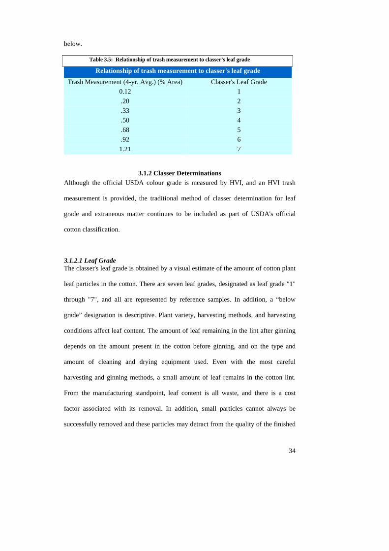
34
below.
Table 3.5: Relationship of trash measurement to classer’s leaf grade
Relationship of trash measurement to classer's leaf grade
Trash Measurement (4-yr. Avg.) (% Area) Classer's Leaf Grade 0.12 1 .20 2 .33 3 .50 4 .68 5 .92 6 1.21 7
3.1.2 Classer Determinations Although the official USDA colour grade is measured by HVI, and an HVI trash
measurement is provided, the traditional method of classer determination for leaf
grade and extraneous matter continues to be included as part of USDA's official
cotton classification.
3.1.2.1 Leaf Grade The classer's leaf grade is obtained by a visual estimate of the amount of cotton plant
leaf particles in the cotton. There are seven leaf grades, designated as leaf grade "1"
through "7", and all are represented by reference samples. In addition, a “below
grade” designation is descriptive. Plant variety, harvesting methods, and harvesting
conditions affect leaf content. The amount of leaf remaining in the lint after ginning
depends on the amount present in the cotton before ginning, and on the type and
amount of cleaning and drying equipment used. Even with the most careful
harvesting and ginning methods, a small amount of leaf remains in the cotton lint.
From the manufacturing standpoint, leaf content is all waste, and there is a cost
factor associated with its removal. In addition, small particles cannot always be
successfully removed and these particles may detract from the quality of the finished
35
product.
3.1.2.2 Preparation Preparation is a term used to describe the degree of smoothness or roughness of the
ginned cotton lint. Various methods of harvesting, handling, and ginning cotton
produce differences in roughness or smoothness of fibre (preparation) that sometimes
are very apparent. Abnormal preparation in Upland cotton has greatly diminished in
recent years due to improvements in harvesting and ginning practices, and now
occurs in less than one-half of 1 percent of the crop. If the cotton has abnormal
preparation, that is noted under extraneous matter on the classification record.
3.1.2.3 Extraneous Matter Extraneous matter is any substance in the cotton other than fibre or leaf. Examples of
extraneous matter are bark, grass, spindle twist, seed coat fragments, dust, and oil.
The classer notes the kinds of extraneous matter, and an indication of the amount
(light or heavy), on the classification document.
In 1993, the classer grading system was changed. Under the old system of grading,
the classer determined a composite grade of colour and trash content. Bales that
contained bark and grass were reduced one or more grade levels. Under the current
system, the classer determines a colour grade, a leaf (trash) grade and notes whether
there is bark or grass present in the bale, factors that do not influence the grade. Each
colour grade percentage will include all levels of leaf 71(Cotton Program AMS USDA,
2001).
3.2 Other High-Speed Maturity Measurements. Fast methods of high-speed maturity measurements other than the HVI (High
36
Volume Instrument) include the Fineness and Maturity Tester (FMT), Lintronics
FiberLab and the Advanced Fiber and Information System (AFIS). The FMT is
based on airflow resistance to cotton (Lord and Heap, 1988). Lintronics
measurements of micronaire, fineness, and maturity are based on double
compression airflow resistance and are made by image analysis of data from the web
that the system makes and analyses for neps and seed coat fragments. AFIS is based
on the amount of radiation (NIR) sensed by two detectors as a single cotton fibre
moves across the incident beam 72(Gordon et al., 1997). Benchmark analysis speeds,
exclusive of sample preparation, for FMT, FiberLab and AFIS are, respectively 20,
55 and 60 seconds 73(Mor, 2003). Although, these are high-speed systems, industry
does not consider them high volume instrumentation.
3.2.1 FMT The first dual-compression airflow instrument for estimating both fibre fineness and
fibre maturity from airflow rates through untreated raw cotton was the Arealometer,
developed by Special Instruments Laboratories Inc (Knoxville, TN)74, 75(ASTM,
1976; Lord and Heap, 1988). The Arealometer provides an indirect measurement of
the specific surface area of loose cotton fibres, that is, the external area of fibres per
unit volume (approximately 200-mg samples in four to five replicates). Empirical
formulae were developed for calculating the approximate maturity ratio and the
average perimeter, wall thickness, and weight per inch from the specific surface area
data. The precision and accuracy of Arealometer determinations were sensitive to
variations in sample preparation, to repeated sample handling, and to previous
mechanical treatment of the fibres, e.g., conditions during harvesting, blending, and
opening. The Arealometer was never approved for acceptance testing, and the ASTM
method was withdrawn in 1977 without replacement 76(Bradow, 2000).
37
The variations in biological fineness and relative maturity of cotton fibres cause the
porous plugs used in air-compression measurements to respond differently to
compression and, consequently, to airflow 77(Lord and Heap, 1988). The IIC-Shirley
Fineness/Maturity Tester (Shirley FMT), a dual-compression instrument, was
developed to compensate for this plug-variation effect 78(ASTM, 1994). The Shirley
FMT is considered suitable for research, but is not used for acceptance testing
(grading) due to low precision and accuracy. Instead of fineness and maturity, the
combination micronaire value has become the standard estimate in the USDA-AMS
classing offices.
The need continues for a reliable reference method that can analyse, in about 30
seconds, several grams of cotton for fineness and maturity. The Shirley
Developments LTD. Micromat Fineness and Maturity Tester (FMT) provides a
reference method that meets this need. The method is based on the resistance to air
flowing through cleaned cotton in a short pipe. Montalvo et al. 79(1995) identified a
number of biases in data produced by the FMT and performed experiments to define
acceptable limits. Montalvo and Faught 80 81(1998; 1999) developed the theory and
reduced to practice physical standards for calibrating, control and elimination of drift
in the FMT. To calibrate the upgraded FMT (Figures 3.3 and 3.4) with cotton, a
dozen new FMT standard cottons were produced, analysed by a combination of
independent reference methods including image analysis 82(Montalvo et al., 2001).
Combining data from independent methods is the approach used by the National
Institute of Standards and Technology (NIST) in developing certified reference
materials 83(Schiller and Eberhardt, 1991).
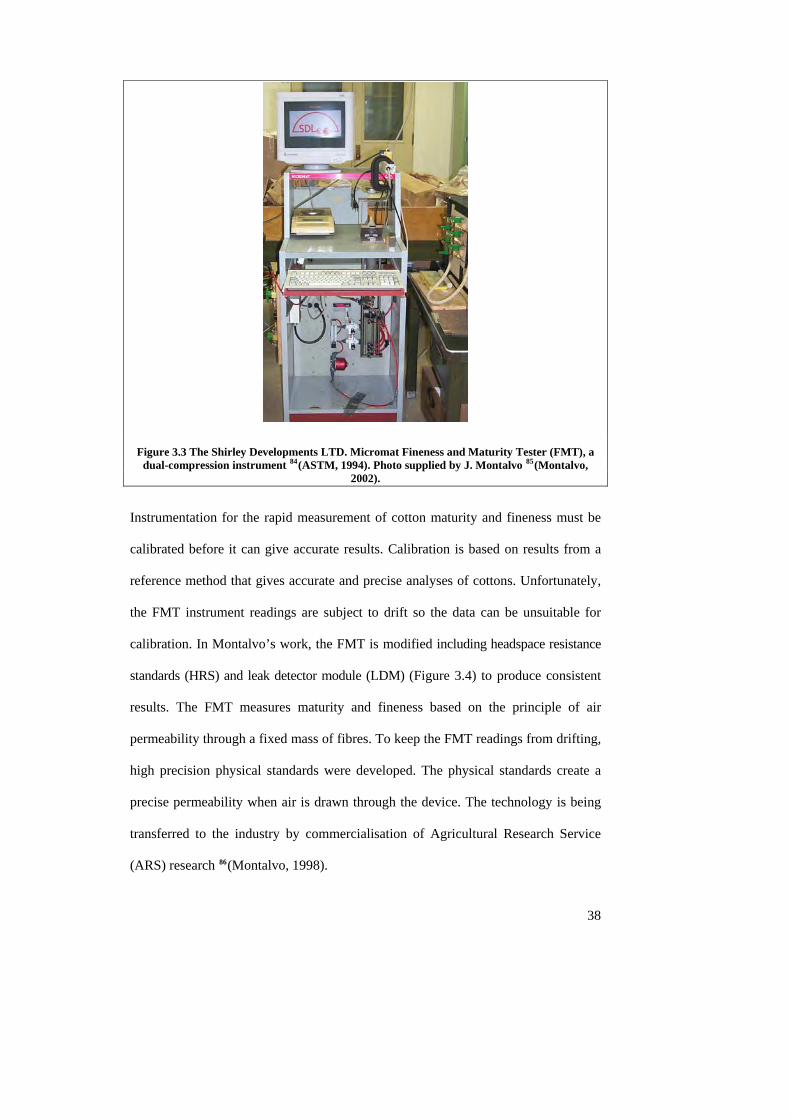
Figure 3.3 The Shirley Developments LTD. Micromat Fineness and Maturity Tester (FMT), a dual-compression instrument 84(ASTM, 1994). Photo supplied by J. Montalvo 85(Montalvo,
2002).
Instrumentation for the rapid measurement of cotton maturity and fineness must be
calibrated before it can give accurate results. Calibration is based on results from a
reference method that gives accurate and precise analyses of cottons. Unfortunately,
the FMT instrument readings are subject to drift so the data can be unsuitable for
calibration. In Montalvo’s work, the FMT is modified including headspace resistance
standards (HRS) and leak detector module (LDM) (Figure 3.4) to produce consistent
results. The FMT measures maturity and fineness based on the principle of air
permeability through a fixed mass of fibres. To keep the FMT readings from drifting,
high precision physical standards were developed. The physical standards create a
precise permeability when air is drawn through the device. The technology is being
transferred to the industry by commercialisation of Agricultural Research Service
(ARS) research 86(Montalvo, 1998).
38
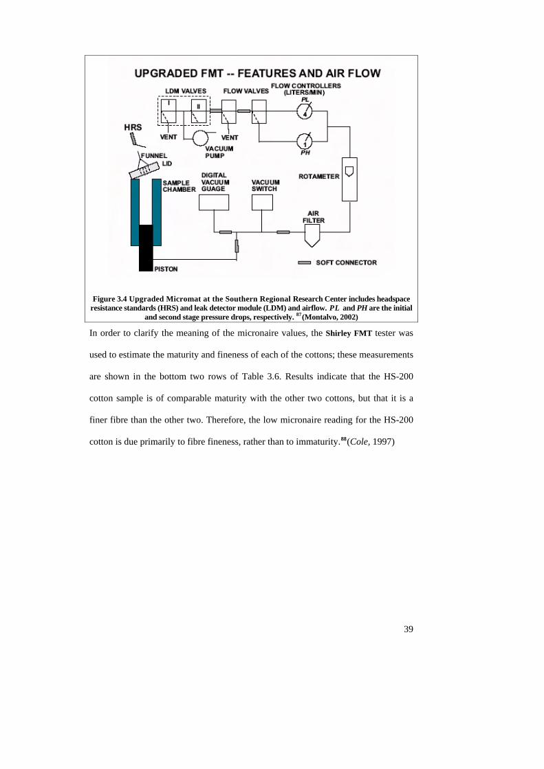
Figure 3.4 Upgraded Micromat at the Southern Regional Research Center includes headspace resistance standards (HRS) and leak detector module (LDM) and airflow. PL and PH are the initial
and second stage pressure drops, respectively. 87(Montalvo, 2002)
In order to clarify the meaning of the micronaire values, the Shirley FMT tester was
used to estimate the maturity and fineness of each of the cottons; these measurements
are shown in the bottom two rows of Table 3.6. Results indicate that the HS-200
cotton sample is of comparable maturity with the other two cottons, but that it is a
finer fibre than the other two. Therefore, the low micronaire reading for the HS-200
cotton is due primarily to fibre fineness, rather than to immaturity.88(Cole, 1997)
39
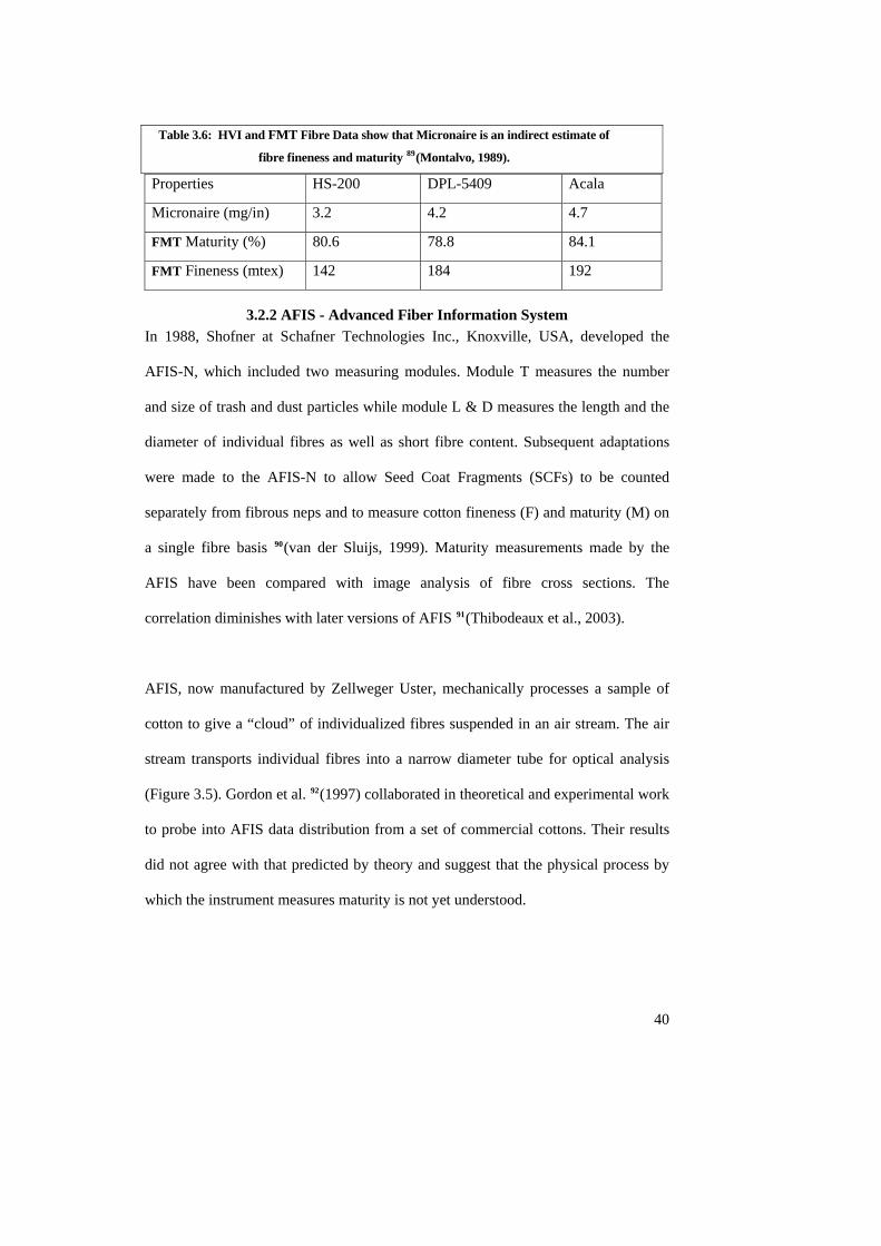
40
Table 3.6: HVI and FMT Fibre Data show that Micronaire is an indirect estimate of
fibre fineness and maturity 89(Montalvo, 1989).
Properties HS-200 DPL-5409 Acala
Micronaire (mg/in) 3.2 4.2 4.7
FMT Maturity (%) 80.6 78.8 84.1
FMT Fineness (mtex) 142 184 192
3.2.2 AFIS - Advanced Fiber Information System In 1988, Shofner at Schafner Technologies Inc., Knoxville, USA, developed the
AFIS-N, which included two measuring modules. Module T measures the number
and size of trash and dust particles while module L & D measures the length and the
diameter of individual fibres as well as short fibre content. Subsequent adaptations
were made to the AFIS-N to allow Seed Coat Fragments (SCFs) to be counted
separately from fibrous neps and to measure cotton fineness (F) and maturity (M) on
a single fibre basis 90(van der Sluijs, 1999). Maturity measurements made by the
AFIS have been compared with image analysis of fibre cross sections. The
correlation diminishes with later versions of AFIS 91(Thibodeaux et al., 2003).
AFIS, now manufactured by Zellweger Uster, mechanically processes a sample of
cotton to give a “cloud” of individualized fibres suspended in an air stream. The air
stream transports individual fibres into a narrow diameter tube for optical analysis
(Figure 3.5). Gordon et al. 92(1997) collaborated in theoretical and experimental work
to probe into AFIS data distribution from a set of commercial cottons. Their results
did not agree with that predicted by theory and suggest that the physical process by
which the instrument measures maturity is not yet understood.
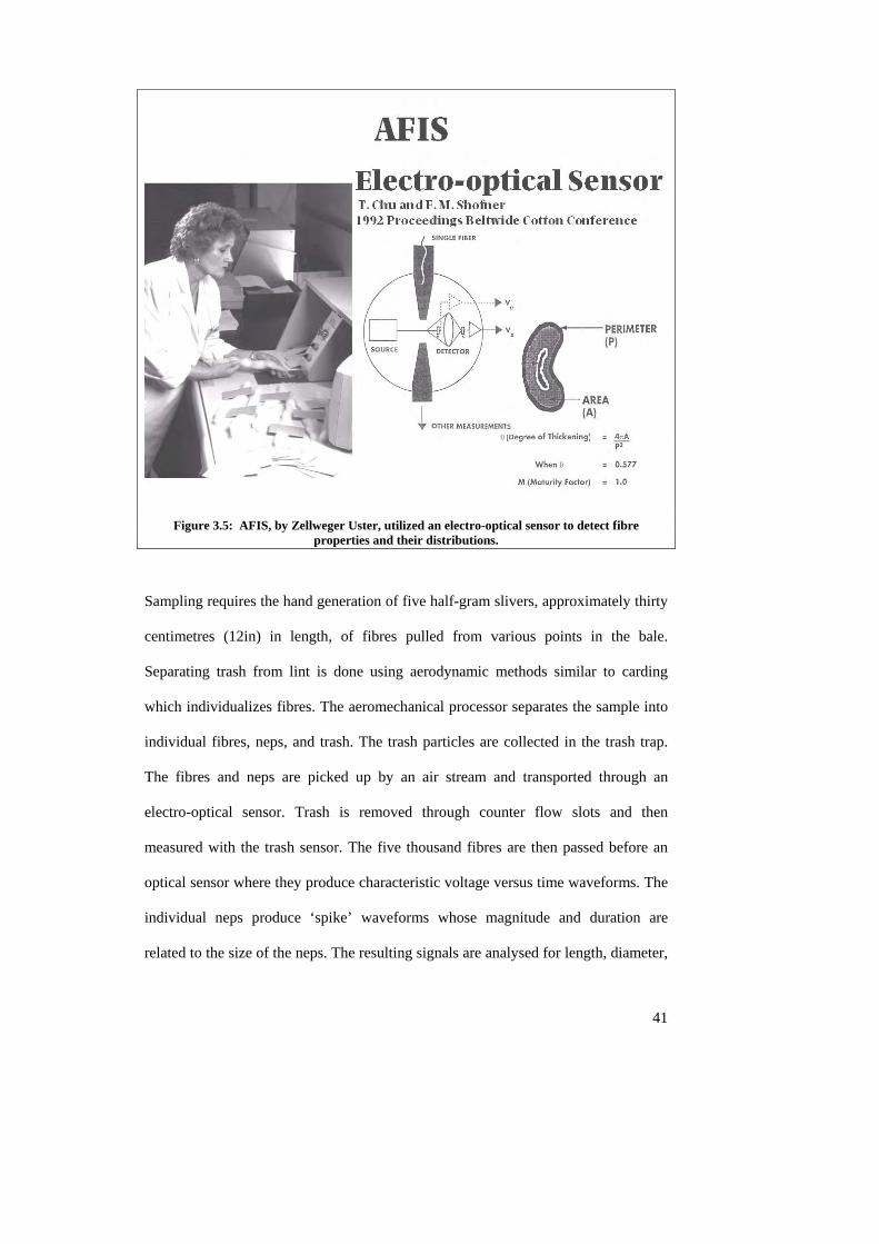
Figure 3.5: AFIS, by Zellweger Uster, utilized an electro-optical sensor to detect fibre properties and their distributions.
Sampling requires the hand generation of five half-gram slivers, approximately thirty
centimetres (12in) in length, of fibres pulled from various points in the bale.
Separating trash from lint is done using aerodynamic methods similar to carding
which individualizes fibres. The aeromechanical processor separates the sample into
individual fibres, neps, and trash. The trash particles are collected in the trash trap.
The fibres and neps are picked up by an air stream and transported through an
electro-optical sensor. Trash is removed through counter flow slots and then
measured with the trash sensor. The five thousand fibres are then passed before an
optical sensor where they produce characteristic voltage versus time waveforms. The
individual neps produce ‘spike’ waveforms whose magnitude and duration are
related to the size of the neps. The resulting signals are analysed for length, diameter,
41
maturity and fineness.
The F & M module, currently unavailable to industry, enabled the fineness and
maturity measurements to be undertaken at SRRC (Versions 2 and 4) and Zellweger
(Version 5). Five repetitions of the five slivers were utilized on these systems to
calculate the mean, standard deviation, and percent coefficient of variation for each
parameter. The parameters relevant to this project include Micronafis (similar to
micronaire), which measures fineness and maturity in micrograms of one inch of
fibre, and Theta (θ), which represents the circularity, or the degree of thickening, as,
calculated by the equation:
42
θ = 4 2PAπ .
Where A = the cross-sectional area, and
P = perimeter of the fibre cross section
Most importantly, Immature Fibre Fraction (IFF) measured the percentage of fibre
with values of theta less than 0.25. In every case, there was an inverse correlation
between the fraction IFF and Micronafis, and Theta. An increase in IFF resulted in a
decrease in the values of Micronafis and Theta. Since white specks are primarily
immature fibre clusters, % IFF was seen as a possible prediction tool for indicating a
potential white speck problem.
3.2.3 Lintronics FiberLab (Figure 3.6 shows the combination of FCT (Fibre Contamination Tester)
and FQT (Fibre Quality Tester)) works at ginning production speeds, and is very
easy to operate. FiberLab is designed to measure impurities such as neps and to test
the stickiness of cotton.
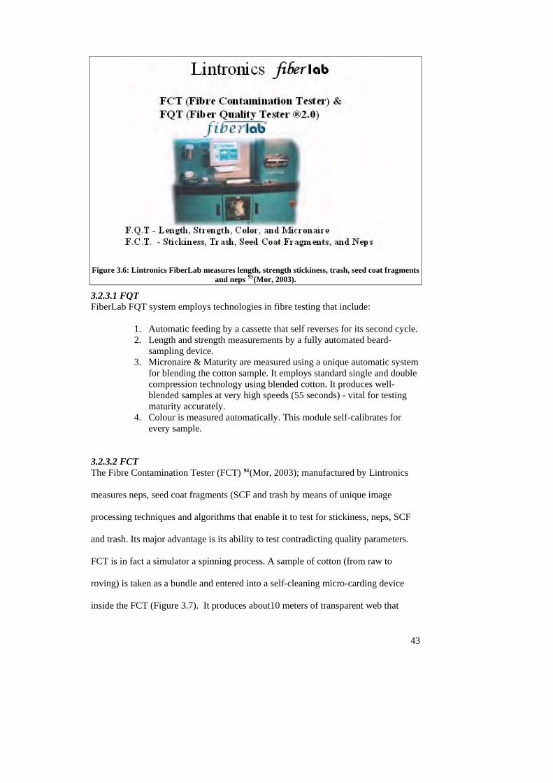
Figure 3.6: Lintronics FiberLab measures length, strength stickiness, trash, seed coat fragments and neps 93(Mor, 2003).
3.2.3.1 FQT FiberLab FQT system employs technologies in fibre testing that include:
1. Automatic feeding by a cassette that self reverses for its second cycle. 2. Length and strength measurements by a fully automated beard-
sampling device. 3. Micronaire & Maturity are measured using a unique automatic system
for blending the cotton sample. It employs standard single and double compression technology using blended cotton. It produces well-blended samples at very high speeds (55 seconds) - vital for testing maturity accurately.
4. Colour is measured automatically. This module self-calibrates for every sample.
3.2.3.2 FCT The Fibre Contamination Tester (FCT) 94(Mor, 2003); manufactured by Lintronics
measures neps, seed coat fragments (SCF and trash by means of unique image
processing techniques and algorithms that enable it to test for stickiness, neps, SCF
and trash. Its major advantage is its ability to test contradicting quality parameters.
FCT is in fact a simulator a spinning process. A sample of cotton (from raw to
roving) is taken as a bundle and entered into a self-cleaning micro-carding device
inside the FCT (Figure 3.7). It produces about10 meters of transparent web that
43
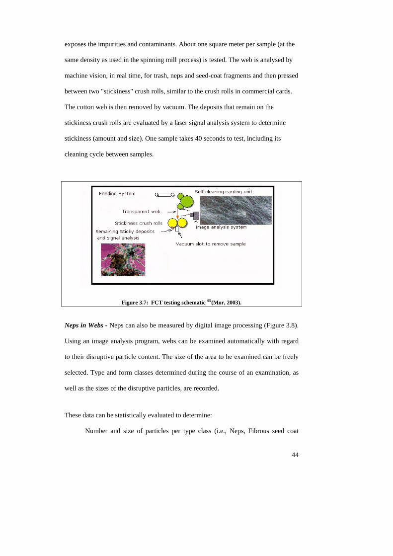
exposes the impurities and contaminants. About one square meter per sample (at the
same density as used in the spinning mill process) is tested. The web is analysed by
machine vision, in real time, for trash, neps and seed-coat fragments and then pressed
between two "stickiness" crush rolls, similar to the crush rolls in commercial cards.
The cotton web is then removed by vacuum. The deposits that remain on the
stickiness crush rolls are evaluated by a laser signal analysis system to determine
stickiness (amount and size). One sample takes 40 seconds to test, including its
cleaning cycle between samples.
Figure 3.7: FCT testing schematic 95(Mor, 2003).
Neps in Webs - Neps can also be measured by digital image processing (Figure 3.8).
Using an image analysis program, webs can be examined automatically with regard
to their disruptive particle content. The size of the area to be examined can be freely
selected. Type and form classes determined during the course of an examination, as
well as the sizes of the disruptive particles, are recorded.
These data can be statistically evaluated to determine:
Number and size of particles per type class (i.e., Neps, Fibrous seed coat
44
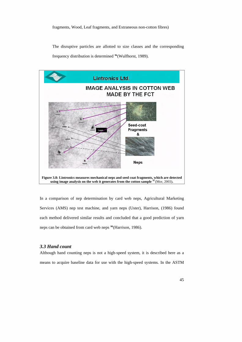
fragments, Wood, Leaf fragments, and Extraneous non-cotton fibres)
The disruptive particles are allotted to size classes and the corresponding
frequency distribution is determined 96(Wulfhorst, 1989).
Figure 3.8: Lintronics measures mechanical neps and seed coat fragments, which are detected using image analysis on the web it generates from the cotton sample 97(Mor, 2003).
In a comparison of nep determination by card web neps, Agricultural Marketing
Services (AMS) nep test machine, and yarn neps (Uster), Harrison, (1986) found
each method delivered similar results and concluded that a good prediction of yarn
neps can be obtained from card web neps 98(Harrison, 1986).
3.3 Hand count Although hand counting neps is not a high-speed system, it is described here as a
means to acquire baseline data for use with the high-speed systems. In the ASTM
45
46
D3216 - 78 method (Grading Cotton Card Webs for Appearance), specimens of a
web are placed on a dark background, with particular care taken to preserve the
original condition of the web, as it would be immediately after leaving the web-
detaching device on the card. The web specimens are compared with photographs of
web representing five levels of web quality. The grade is based on the appearance
and nep content of the specimens in comparison to the photographs 99(ASTM Codes,
1978).
For the manual counting method, specimens of web are extracted on flat supports
and covered with templates containing a number of small holes or cells of equal
cross-sectional area. For each specimen a count is made of the number of cells
containing neps. The average number of cells with neps per template is converted
into neps per unit area of web on the assumption that neps follow a Poisson
distribution. Templates should be no larger than 150mm x 300mm and should
contain 20 to 40 holes each of 1 square inch in area 100(Verschraege, 1989).
47
4. IMAGE ANALYSIS SYSTEMS AND
THE U.S. EXTREME VARIETY WHITE SPECK STUDY This chapter sets out the experimental work and analysis undertaken to develop and
validate a system for reliably quantifying the amount of white specks in a woven
fabric. An automatic system was required to enable the collection of a large number
of measurements so that adequate amounts of data could be obtained in the work
described in subsequent chapters.
4.1 Introduction It has been estimated that 40% of white specks are caused by processing and 30% by
the cotton variety 101(Bragg, 1992). Varietal tests indicate that cotton varieties that
have a strong tendency to nep usually have high levels of immature fibre. Varieties
mature at different rates. Some mature quickly and there is only a limited “tail” (the
time period when most bolls have fully matured but some are still maturing). Others
mature more slowly, and the “tail” drags out longer. These differences increase the
range of maturities in harvested bolls. It was concluded that nep formation is
heritable; and that nep levels are influenced by fibre fineness and maturity
102(Miravelle, 1984).
The genotype influences the tendency of fibres to form neps and the occurrence of
seed coat fragments (SCF) and motes. Motes are found in genetically disposed
cultivars that have expressed, to some extent, a defect in the pollination process or
environmental conditions at anthesis 103(van der Sluijs, 1999). White specks,
although primarily immature fibre neps, may also result from seed coat fragments
that have short fibres attached that resist dye. Often, these seed coats appear as dark
48
e seed.
specks in the dyed fabric with white specks around the SCF, due to their attached
short, immature fibres. These SCFs are portions of immature or mature seeds that
have disintegrated during mechanical processing. In addition, the seed coat has a
weakness at the chalazal (point at which the nucleus and seed coat of an ovule are
united) portion of the seed. This portion easily peels and is generally believed to be
the source of the seed coat fragment problem. SCFs are produced by cultivars that
have a high fibre-to-seed attachment force, a strong shank and loose tissue at the
chalazal end of th
Some individual varieties have particularly strong tendencies to produce high levels
of immature cotton. It is likely that in the future this tendency will have a greater
importance in the selection of new varieties. Breeding programs have been geared to
producing longer, stronger and finer cottons, but other elements often change without
control while the breeder seeks the desired property. Breeders could reduce the nep
formation potential of cotton by selecting for further development those varieties and
fibre properties that are consistently associated with low nep count and seed coat
fragment levels in ginned lint, yarn and fabric.
The two varieties shown in Figure 4.1 are from a breeding program in California
where the EAC-30 variety was bred to mature early from the EAC-32 line. The
cottons were grown in the same field, and were harvested and ginned identically.
These photomicrographs show that the EAC-32 cotton has a much higher level of
immature fibres than the EAC-30. EAC-32 produced very high levels of white
specks (see Figure 4.5) in the dyed fabric while the EAC-30 had minimal levels. This
is not surprising when fibre properties such as the cell wall thickness and Buckling
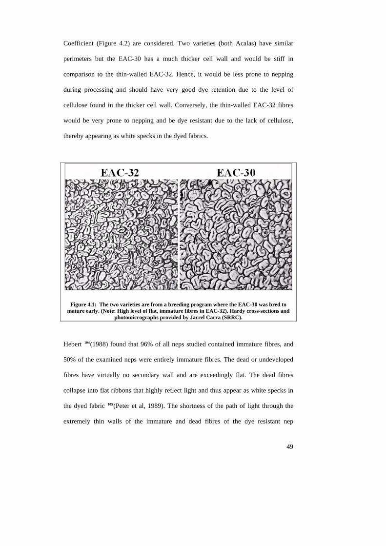
Coefficient (Figure 4.2) are considered. Two varieties (both Acalas) have similar
perimeters but the EAC-30 has a much thicker cell wall and would be stiff in
comparison to the thin-walled EAC-32. Hence, it would be less prone to nepping
during processing and should have very good dye retention due to the level of
cellulose found in the thicker cell wall. Conversely, the thin-walled EAC-32 fibres
would be very prone to nepping and be dye resistant due to the lack of cellulose,
thereby appearing as white specks in the dyed fabrics.
Figure 4.1: The two varieties are from a breeding program where the EAC-30 was bred to mature early. (Note: High level of flat, immature fibres in EAC-32). Hardy cross-sections and
photomicrographs provided by Jarrel Carra (SRRC).
Hebert 104(1988) found that 96% of all neps studied contained immature fibres, and
50% of the examined neps were entirely immature fibres. The dead or undeveloped
fibres have virtually no secondary wall and are exceedingly flat. The dead fibres
collapse into flat ribbons that highly reflect light and thus appear as white specks in
the dyed fabric 105(Peter et al, 1989). The shortness of the path of light through the
extremely thin walls of the immature and dead fibres of the dye resistant nep
49
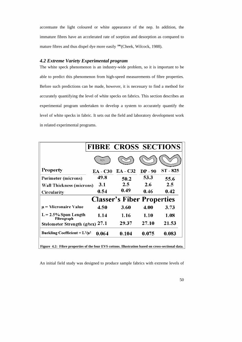
accentuate the light coloured or white appearance of the nep. In addition, the
immature fibres have an accelerated rate of sorption and desorption as compared to
mature fibres and thus dispel dye more easily 106(Cheek, Wilcock, 1988).
4.2 Extreme Variety Experimental program The white speck phenomenon is an industry-wide problem, so it is important to be
able to predict this phenomenon from high-speed measurements of fibre properties.
Before such predictions can be made, however, it is necessary to find a method for
accurately quantifying the level of white specks on fabrics. This section describes an
experimental program undertaken to develop a system to accurately quantify the
level of white specks in fabric. It sets out the field and laboratory development work
in related experimental programs.
Figure 4.2: Fibre properties of the four EVS cottons. Illustration based on cross-sectional data.
An initial field study was designed to produce sample fabrics with extreme levels of
50
51
white specks. It was named the U.S. Extreme Variety Study (EVS). Varietal
influences on white specks were examined to eliminate as many confounding
variables as possible, such as weathering, soil conditions and maturity. Standard
processing was employed from field to fabric and full warps were made for each
variety, so the final fabrics reflected varietal differences only.
For the EVS study, four extremely different U.S. cotton varieties were grown under
irrigated conditions in the same field in the San Joaquin valley in California. The
cottons included two typically rain grown and two irrigated varieties. DP-90 is a
commercial Delta Upland fibre, while ST-825 is a Mississippi hybrid variety. EAC30
(experimentally bred to mature early from the EAC-32 line) and EAC-32 (Prema) are
Acala cottons (Figure 4.2).
4.2.1 EVS Processing Methodology Full size production equipment was used throughout the study. The EVS cottons
were spindle picked and then ginned, to remove the seeds, at Mesilla Park, NM, with
the lint cleaned by two saw-type lint cleaners. Three bales were produced for each
variety. The bales were opened and processed into yarn and then woven into fabric
and dyed. See Appendix A - Figure A1- 1) Samples of the fabric were dyed and the
white specks were counted both manually and with image analysis systems. All of
these processes were standardized as much as possible to allow future comparisons
with the EVS results. The ginned fibre samples were evaluated using the following:
Fibrograph, Stelometer, Arealometer, Peyer, microscopic cross sections with image
analysis, and the complete ranges of HVI (Motion Control 3500 and Spinlab 9000),
AFIS and Lintronics tests. Figure 4.2 shows some of the results from these
measurements.
52
4.2.1.1 Mill Processing The cotton was processed using mill equipment at the USDA, Southern Regional
Research Center (SRRC). Three bales were used for each variety. Equal amounts
were taken from each of the three bales to make four lots of equal weight per variety
for processing. All sixteen lots underwent the same opening process. They passed
through a hopper, Superior Cleaner, and two beater sections of the picker and then
were chute fed to the cards. Two of the four lots from each variety were single
carded, while the other two were tandem carded. The international cotton industry
uses non-standard, U.S. units of measurement, and so these units have been adopted
in this dissertation. SI units are also provided where appropriate throughout the
dissertation. A 30 Ne, 30/1 or 30’s yarn all indicate a 30 cotton count yarn, which
means that it would take 30 x 840 yards or 25,200 yards to weigh one pound. ASTM
has identified tex yarn number as the standard measure of yarn. Tex determines the
yarn number by determining the weight in grams of 1 kilometre (1000 meters) of
yarn 107(Joseph, 1986). For clarity, both cotton count and tex will be given.
The first drawing had eight doublings to 55 grains/yard (3.99g/m) and the second
drawing had eight doublings to 55 grains/yard. (3.99g/m) Roving was 1.25 hank (472
tex) with medium soft twist. Both 30’s (19.7 tex) and 40’s (14.8 tex) yarns with a 3.8
T.M. (twist multiplier - the ratio of turns per inch to the square root of the yarn
count) were spun on a Roberts Arrow 240 spindle spinning frame with spindle speed
of 9500 rpm. Warp yarns with a 4.2 T.M. 30’s (19.7 tex) were also spun for fabrics
with 40’s (14.8 tex) filling for all varieties.
53
4.2.1.2 Dyeing Procedure for Fibre Evaluation Fibre dyeing (Goldwaithe108 maturity test, using red dye portion only) allowed the
overall number of neps and the white specks in the fibre to be identified. A 0.2 g
sample was sandwiched between two pieces of 160cm2 (25 in2) fibreglass screening
and clamped tightly within a 100 cm (4 in) diameter polymer embroidery hoop (or
tambour frame). The webs were opened up slightly by hand before mounting in the
screening to minimize fibre clumping. This ensured free access of the dye liquor to
the fibre without any possible loss of fibre through the web.
The web in its tambour frame was submerged in a 250 ml (cc) dyebath in a 15 cm
diameter pan. CI Direct Red 81 was selected for this dyeing procedure due to a
known lack of affinity for immature fibres 109, 110 (Mangliardi, 1990 and Bragg, 1992)
and poor coverage of immature fibre neps in fibre and fabric. The dyeing pan was
placed on a hotplate equipped with a magnetic stirrer and a thermistor probe. The
dyebath included 0.015% (owb [on weight of bath]) dye, 0.1% owb NaCl, and 0.01%
of non-ionic surfactant (Triton X-100, Rohm and Haas). Dyeing was carried out at
60°C for one hour with constant stirring, with the salt added in equal portions at three
15-minute intervals.
The dried web was spread out on a 25 x 10 cm panel of clear Plexiglas, and the fibres
teased into a thin layer of uniform density as shown in Figure 4.3. A second panel of
Plexiglas was put on top of the fibres, rendering them immobile. The composite
assembly was then put onto a piece of black velvet fabric and examined under a
magnifying lamp (Figure 4.3). The number of undyed neps on each 0.2 g web was
counted. Five webs were examined for each fibre variety and the total counts were
recorded as the number of white specks per gram.
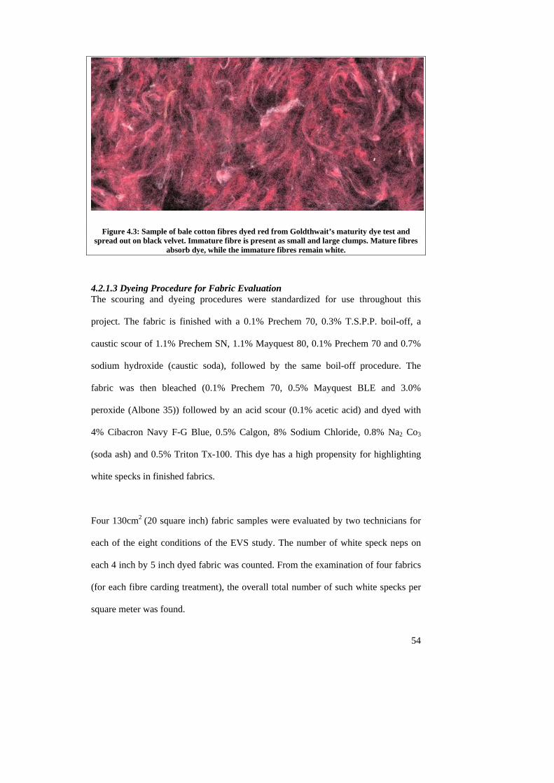
Figure 4.3: Sample of bale cotton fibres dyed red from Goldthwait’s maturity dye test and spread out on black velvet. Immature fibre is present as small and large clumps. Mature fibres
absorb dye, while the immature fibres remain white.
4.2.1.3 Dyeing Procedure for Fabric Evaluation The scouring and dyeing procedures were standardized for use throughout this
project. The fabric is finished with a 0.1% Prechem 70, 0.3% T.S.P.P. boil-off, a
caustic scour of 1.1% Prechem SN, 1.1% Mayquest 80, 0.1% Prechem 70 and 0.7%
sodium hydroxide (caustic soda), followed by the same boil-off procedure. The
fabric was then bleached (0.1% Prechem 70, 0.5% Mayquest BLE and 3.0%
peroxide (Albone 35)) followed by an acid scour (0.1% acetic acid) and dyed with
4% Cibacron Navy F-G Blue, 0.5% Calgon, 8% Sodium Chloride, 0.8% Na2 Co3
(soda ash) and 0.5% Triton Tx-100. This dye has a high propensity for highlighting
white specks in finished fabrics.
Four 130cm2 (20 square inch) fabric samples were evaluated by two technicians for
each of the eight conditions of the EVS study. The number of white speck neps on
each 4 inch by 5 inch dyed fabric was counted. From the examination of four fabrics
(for each fibre carding treatment), the overall total number of such white specks per
square meter was found.
54
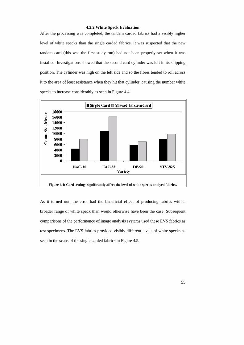
4.2.2 White Speck Evaluation After the processing was completed, the tandem carded fabrics had a visibly higher
level of white specks than the single carded fabrics. It was suspected that the new
tandem card (this was the first study run) had not been properly set when it was
installed. Investigations showed that the second card cylinder was left in its shipping
position. The cylinder was high on the left side and so the fibres tended to roll across
it to the area of least resistance when they hit that cylinder, causing the number white
specks to increase considerably as seen in Figure 4.4.
Figure 4.4: Card settings significantly affect the level of white specks on dyed fabrics.
As it turned out, the error had the beneficial effect of producing fabrics with a
broader range of white speck than would otherwise have been the case. Subsequent
comparisons of the performance of image analysis systems used these EVS fabrics as
test specimens. The EVS fabrics provided visibly different levels of white specks as
seen in the scans of the single carded fabrics in Figure 4.5.
55
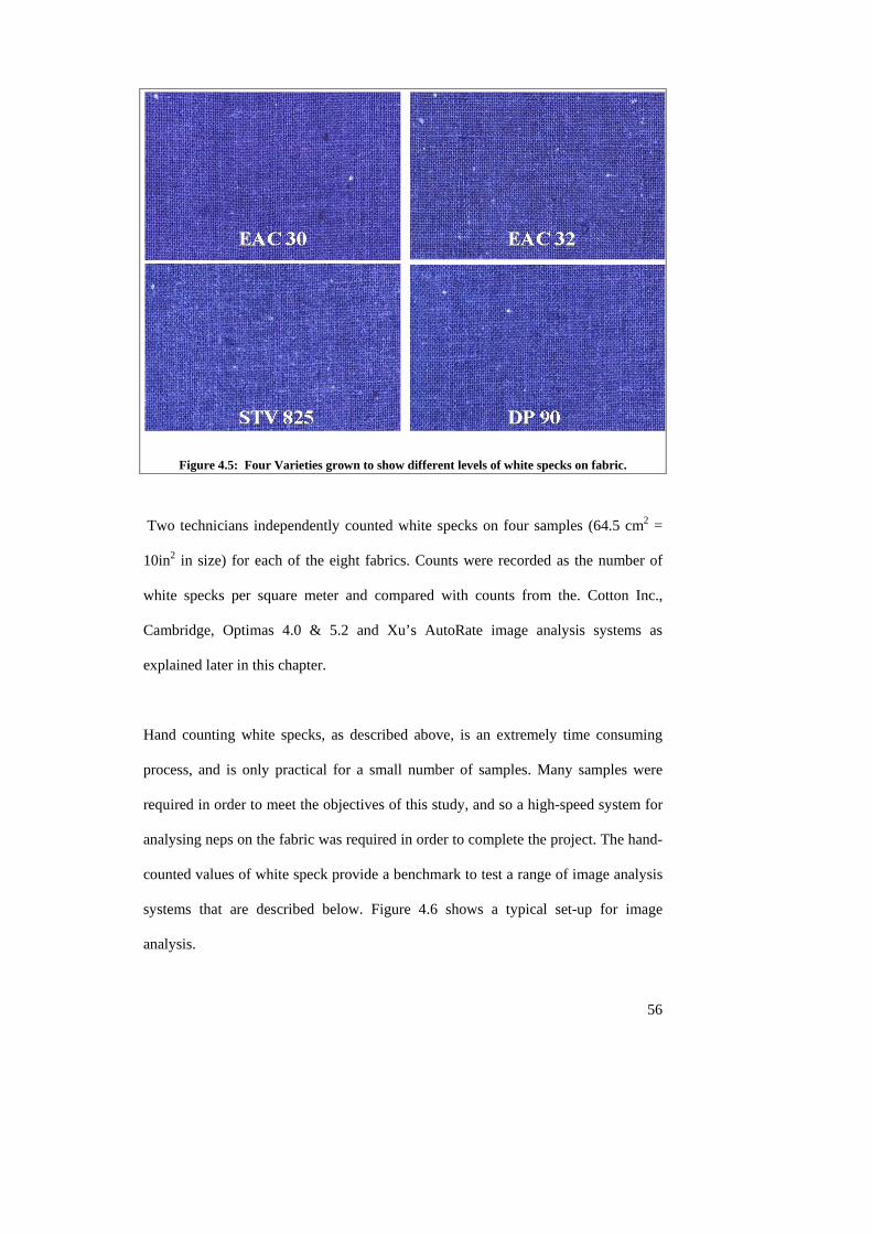
Figure 4.5: Four Varieties grown to show different levels of white specks on fabric.
Two technicians independently counted white specks on four samples (64.5 cm2 =
10in2 in size) for each of the eight fabrics. Counts were recorded as the number of
white specks per square meter and compared with counts from the. Cotton Inc.,
Cambridge, Optimas 4.0 & 5.2 and Xu’s AutoRate image analysis systems as
explained later in this chapter.
Hand counting white specks, as described above, is an extremely time consuming
process, and is only practical for a small number of samples. Many samples were
required in order to meet the objectives of this study, and so a high-speed system for
analysing neps on the fabric was required in order to complete the project. The hand-
counted values of white speck provide a benchmark to test a range of image analysis
systems that are described below. Figure 4.6 shows a typical set-up for image
analysis.
56
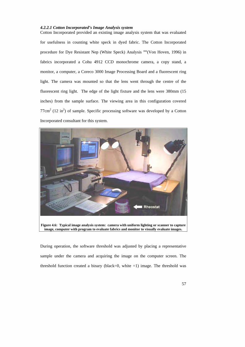
4.2.2.1 Cotton Incorporated’s Image Analysis system Cotton Incorporated provided an existing image analysis system that was evaluated
for usefulness in counting white speck in dyed fabric. The Cotton Incorporated
procedure for Dye Resistant Nep (White Speck) Analysis 111(Von Hoven, 1996) in
fabrics incorporated a Cohu 4912 CCD monochrome camera, a copy stand, a
monitor, a computer, a Coreco 3000 Image Processing Board and a fluorescent ring
light. The camera was mounted so that the lens went through the centre of the
fluorescent ring light. The edge of the light fixture and the lens were 380mm (15
inches) from the sample surface. The viewing area in this configuration covered
77cm2 (12 in2) of sample. Specific processing software was developed by a Cotton
Incorporated consultant for this system.
Figure 4.6: Typical image analysis system: camera with uniform lighting or scanner to capture image, computer with program to evaluate fabrics and monitor to visually evaluate images.
During operation, the software threshold was adjusted by placing a representative
sample under the camera and acquiring the image on the computer screen. The
threshold function created a binary (black=0, white =1) image. The threshold was
57
58
manually adjusted until all of the white specks were visible to the operator, with a
minimum amount of noise in the image. Once the threshold was set, the minimum
size (in pixels) was determined visually to differentiate between white specks and
noise. The threshold and minimum pixel size were set and maintained throughout the
duration of the testing to remove noise from the image, leaving the white specks
highlighted. The number of "events" was then automatically counted with the
number of pixels determining the size of each "event". The count per square meter
and “% white" (the actual percent of the fabric that was white rather than dyed blue)
were calculated. Twenty-four readings were taken from each of the fabrics. The
samples were manipulated so that there was no overlap of the sample viewing area.
Cotton Incorporated tested the samples and then the system was shipped to SRRC for
further evaluation. It must have been damaged in shipping because a drift was noted
in the data when the system was used at SRRC. The system was focused on one
fabric, which was taped into place, then tested every half hour with the same settings
to see if there was any change over time. The recorded number of white speck
increased significantly over an 8-hour period. The problem could not be resolved and
it started the search for other imaging systems to evaluate white specks. Only one
complete data set for this study using this image analysis system was gathered at
Cotton, Inc. when the fabrics were sent there for analysis. This data, was used for
comparison purposes to compare % White values obtained by the other systems
evaluated.
4.2.2.2 Cambridge Instruments Quantimet 970112(Von Hoven, 1996) The fabrics were also analysed using a Cambridge Instruments Quantimet 970 at
SRRC. Before testing, the operator determined the camera settings for the Cambridge
Instruments’ Chalnican camera, which resulted in a sharp image of the white speck
59
fabric. The Cambridge Instruments Chalnican camera was placed on the arm of a
Cambridge Instruments stand fifteen inches above the surface of the stand, thus the
camera was twelve and one half inches above the fabric sample. A ring light was
used in order to provide uniform lighting and was placed eight and one half inches
above the fabric sample. The equipment was then allowed to equilibrate for
approximately an hour to permit stabilization of lighting and equipment. The room
was blackened so that the only source of light was that of the Image Analysis system.
After stabilization, shading correction was implemented to eliminate any unevenness
in lighting. Acceptance values were set to place size limits on what was to be
detected as a white speck while eliminating noise or false positives that were
typically smaller than white specks. These parameters were set once, and all tests
were performed consecutively under the same conditions so that reliable
comparisons and correlations could be made. The system was calibrated at the start
of every analysis procedure to ensure correct measurements.
The equipment was programmed to sample seven approximately 60cm2 (9 square
inch) sections of fabric, measure the size and area of the white specks, and count the
number of specks detected in that area. The image size was 600 by 500 pixels, with
one pixel edge equivalent to 0.138mm2 (0.00543 in2). An average size, count and
area were determined for each of the seven samples. The tests were then replicated
five times. The same operator tested all samples on the same day, to eliminate any
operator or lighting variation influencing the results. The operator manipulated the
fabric sample to avoid detecting the same area more than once 113(Von Hoven, 1996).
4.2.2.3 Optimas 4.0 and the Upgraded Optimas 5.2 Image Analysis System Two versions (4.0 and 5.2) of the Optimas system for image analysis were also
60
evaluated for use in the project. The Optimas system used a Gateway 2000 P5-75
computer with a dual monitor set up with a Sony Trinitron RGB Monitor and an
Imaging Technologies frame grabber. A Microimage Video Systems
RGB/YC/NTSC colour camera was mounted on a camera stand. The F-stop on the
camera was set to a value of four, and the lens was located 47cm (18.5 in) above the
fabric surface.
The original setup (Version 4.0) used a low level of lighting with only two 15 W
fluorescent lamps. This was subsequently revised to use a brighter and more uniform
light source using four tungsten 120 V 300W flood photography lights that could be
adjusted by a rheostat. A digital light meter was used to measure luminance (visible
flux density). The light sensor was mounted over the lens of the video camera and
pointed towards the fabric. The rheostat was adjusted until the light meter luminance
reading was 234±1 lm/m2 (234±1 Lux). For white speck measurements, the lights
were set on high and the rheostat was used to maintain a constant reflected light
measurement of 11 EV with ASA set at 800. This is the lighting procedure used for
the data reported for both Versions of Optimas.
Thirty different sections, regions of interest (ROI), of the fabric were analysed with a
total area of 2320cm2 (360 in2) of fabric. The operator manipulated the fabric sample
so that the same area was not tested more than once and area covered was sequential.
4.2.2.3.1 Optimas 5.2 Image Analysis System –White Speck Size To determine which system was most accurately measuring the size of the white
specks, forty photomicrographs were taken of white specks from each of the eight
EVS fabrics and measured using the area protocol from Optimas version 5.2.

Optimas was developed for medical purposes and is considered very accurate for
measuring cell areas. A Bausch & Lomb stereomicroscope fitted with a Hitachi KP-
D50 colour digital camera with an extension tube (which increased the
magnification) RS Photometric’s CoolSNAP was used to create digital
photomicrographic images of white specks. Most of the white specks were
photographed at a magnification of four, but some larger white specks had to use a
magnification factor of three.
The Optimas system also changes the scale of the photomicrograph, depending on
the monitor size, and the image appears as shown in Figure 4.7. The system is
calibrated and then:
1) The scanned photomicrograph is opened,
2) The operator draws the perimeter of the white speck using the mouse and
3) Optimas determines the sizes of the white speck in square microns.
Figure 4.7: Measuring white speck size using Optimas Version 5.2.
4.2.2.4 Xu Image Analysis System The AutoRate System was designed and developed by Dr. Bugao Xu of the
University of Texas at Austin specifically to measure white specks. The candidate
61
62
assisted Dr Xu throughout this development process. Initially, we used a camera and
lighting set-up (as reported for Optimas) with this system but found that it was very
sensitive to lighting and picked up “hot spots” for each of the four lamps. Next, a
scanner was used to acquire an image. It gave the uniform lighting necessary for this
imaging system. The reset control tool of the HP Scan Jet 6300C flatbed scanner was
used to reset all tools except dimensions to their automatic settings. The scanning
Region of Interest (ROI) was set at 5 inches by 5 inches with four adjacent fabric
images analysed to give a total viewing area of 100 square inches. The images were
converted into pixels by the AutoRate program Version AR-02-03 (February 2003).
The scanner contrast was found to drift slightly over time, so brightness was adjusted
to 120 in the AutoRate program so the images would be consistent. A minimum size
of three pixels was adopted to differentiate between real white specks and anomalies.
The contrast setting was used to dictate what is detected as white and so it affects the
percent white of the sampled area. The contrast can be set for each fabric. If the
fabrics were all dyed and scanned in a batch, the contrast usually remained the same,
but each dye batch is slightly different. Figure 4.8 shows the original scan of a fabric
and the altered image after it was brightened and analysed. In this case, the operator
found that a contrast of 20 was good for all of the EVS fabrics. The analysis results
in two values: white speck count and area that is white in pixels. The size of the
white specks and the percent white on the fabric are calculated.
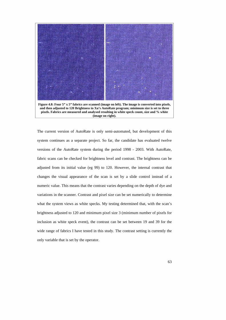
Figure 4.8: Four 5” x 5” fabrics are scanned (image on left). The image is converted into pixels, and then adjusted to 120 Brightness in Xu’s AutoRate program; minimum size is set to three pixels. Fabrics are measured and analysed resulting in white speck count, size and % white
(image on right).
The current version of AutoRate is only semi-automated, but development of this
system continues as a separate project. So far, the candidate has evaluated twelve
versions of the AutoRate system during the period 1998 - 2003. With AutoRate,
fabric scans can be checked for brightness level and contrast. The brightness can be
adjusted from its initial value (eg 99) to 120. However, the internal contrast that
changes the visual appearance of the scan is set by a slide control instead of a
numeric value. This means that the contrast varies depending on the depth of dye and
variations in the scanner. Contrast and pixel size can be set numerically to determine
what the system views as white specks. My testing determined that, with the scan’s
brightness adjusted to 120 and minimum pixel size 3 (minimum number of pixels for
inclusion as white speck event), the contrast can be set between 19 and 39 for the
wide range of fabrics I have tested in this study. The contrast setting is currently the
only variable that is set by the operator.
63
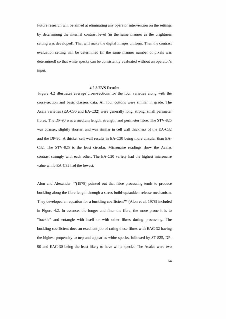
64
Future research will be aimed at eliminating any operator intervention on the settings
by determining the internal contrast level (in the same manner as the brightness
setting was developed). That will make the digital images uniform. Then the contrast
evaluation setting will be determined (in the same manner number of pixels was
determined) so that white specks can be consistently evaluated without an operator’s
input.
4.2.3 EVS Results Figure 4.2 illustrates average cross-sections for the four varieties along with the
cross-section and basic classers data. All four cottons were similar in grade. The
Acala varieties (EA-C30 and EA-C32) were generally long, strong, small perimeter
fibres. The DP-90 was a medium length, strength, and perimeter fibre. The STV-825
was coarser, slightly shorter, and was similar in cell wall thickness of the EA-C32
and the DP-90. A thicker cell wall results in EA-C30 being more circular than EA-
C32. The STV-825 is the least circular. Micronaire readings show the Acalas
contrast strongly with each other. The EA-C30 variety had the highest micronaire
value while EA-C32 had the lowest.
Alon and Alexander 114(1978) pointed out that fibre processing tends to produce
buckling along the fibre length through a stress build-up/sudden release mechanism.
They developed an equation for a buckling coefficient115 (Alon et al, 1978) included
in Figure 4.2. In essence, the longer and finer the fibre, the more prone it is to
“buckle” and entangle with itself or with other fibres during processing. The
buckling coefficient does an excellent job of rating these fibres with EAC-32 having
the highest propensity to nep and appear as white specks, followed by ST-825, DP-
90 and EAC-30 being the least likely to have white specks. The Acalas were two
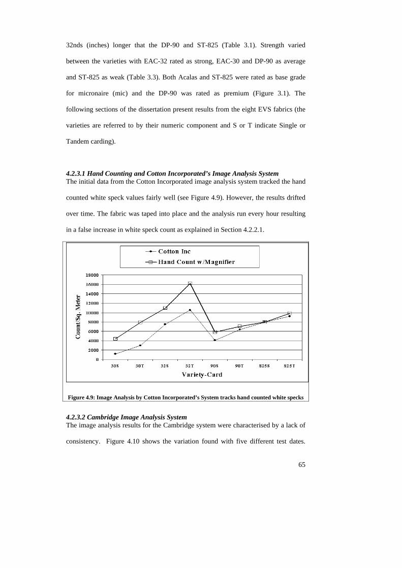
32nds (inches) longer that the DP-90 and ST-825 (Table 3.1). Strength varied
between the varieties with EAC-32 rated as strong, EAC-30 and DP-90 as average
and ST-825 as weak (Table 3.3). Both Acalas and ST-825 were rated as base grade
for micronaire (mic) and the DP-90 was rated as premium (Figure 3.1). The
following sections of the dissertation present results from the eight EVS fabrics (the
varieties are referred to by their numeric component and S or T indicate Single or
Tandem carding).
4.2.3.1 Hand Counting and Cotton Incorporated’s Image Analysis System The initial data from the Cotton Incorporated image analysis system tracked the hand
counted white speck values fairly well (see Figure 4.9). However, the results drifted
over time. The fabric was taped into place and the analysis run every hour resulting
in a false increase in white speck count as explained in Section 4.2.2.1.
Figure 4.9: Image Analysis by Cotton Incorporated’s System tracks hand counted white specks
4.2.3.2 Cambridge Image Analysis System The image analysis results for the Cambridge system were characterised by a lack of
consistency. Figure 4.10 shows the variation found with five different test dates.
65
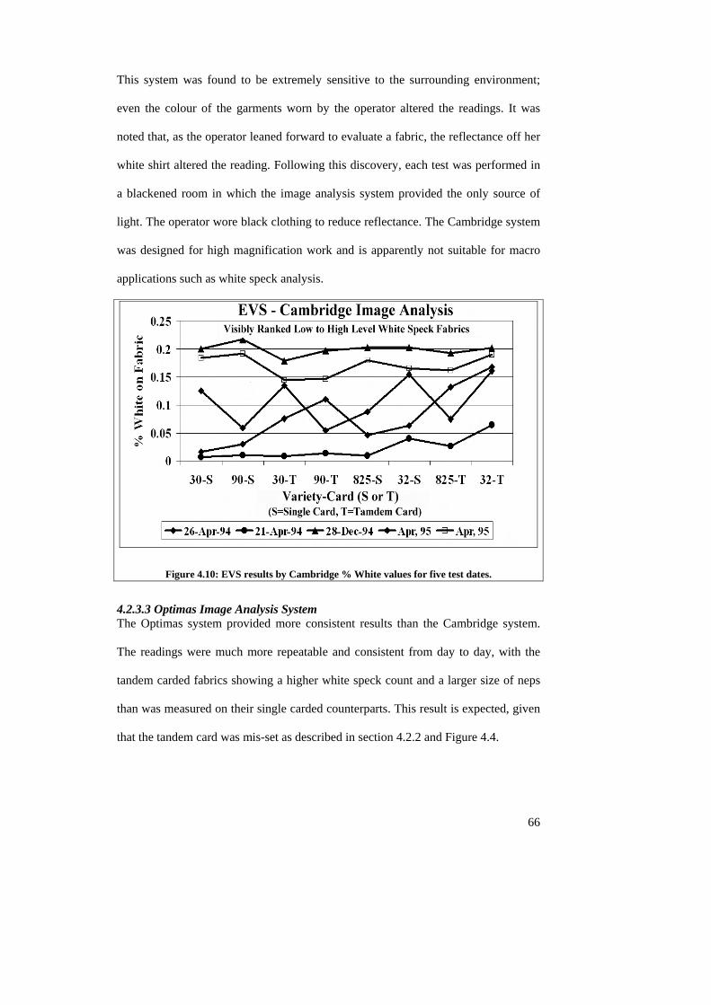
This system was found to be extremely sensitive to the surrounding environment;
even the colour of the garments worn by the operator altered the readings. It was
noted that, as the operator leaned forward to evaluate a fabric, the reflectance off her
white shirt altered the reading. Following this discovery, each test was performed in
a blackened room in which the image analysis system provided the only source of
light. The operator wore black clothing to reduce reflectance. The Cambridge system
was designed for high magnification work and is apparently not suitable for macro
applications such as white speck analysis.
Figure 4.10: EVS results by Cambridge % White values for five test dates.
4.2.3.3 Optimas Image Analysis System The Optimas system provided more consistent results than the Cambridge system.
The readings were much more repeatable and consistent from day to day, with the
tandem carded fabrics showing a higher white speck count and a larger size of neps
than was measured on their single carded counterparts. This result is expected, given
that the tandem card was mis-set as described in section 4.2.2 and Figure 4.4.
66
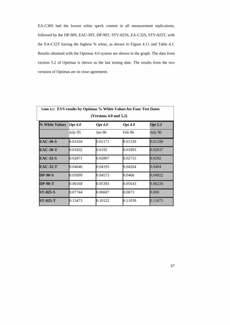
67
EA-C30S had the lowest white speck content in all measurement replications,
followed by the DP-90S, EAC-30T, DP-90T, STV-825S, EA-C32S, STV-825T, with
the EA-C32T having the highest % white, as shown in Figure 4.11 and Table 4.1.
Results obtained with the Optimas 4.0 system are shown in the graph. The data from
version 5.2 of Optimas is shown as the last testing date. The results from the two
versions of Optimas are in close agreement.
Table 4.1: EVS results by Optimas % White Values for Four Test Dates
(Versions 4.0 and 5.2)
% White Values Opt 4.0 Opt 4.0 Opt 4.0 Opt 5.2
July 95 Jan 96 Feb 96 July 96
EAC-30-S 0.01418 0.01171 0.01339 0.01188
EAC-30-T 0.01832 0.0192 0.01893 0.02037
EAC-32-S 0.02871 0.02807 0.02755 0.0292
EAC-32-T 0.04646 0.04195 0.04264 0.0494
DP-90-S 0.05099 0.04573 0.0468 0.04922
DP-90-T 0.06168 0.05393 0.05643 0.06226
ST-825-S 0.07744 0.06607 0.0673 0.069
ST-825-T 0.13473 0.10122 0.11039 0.11675
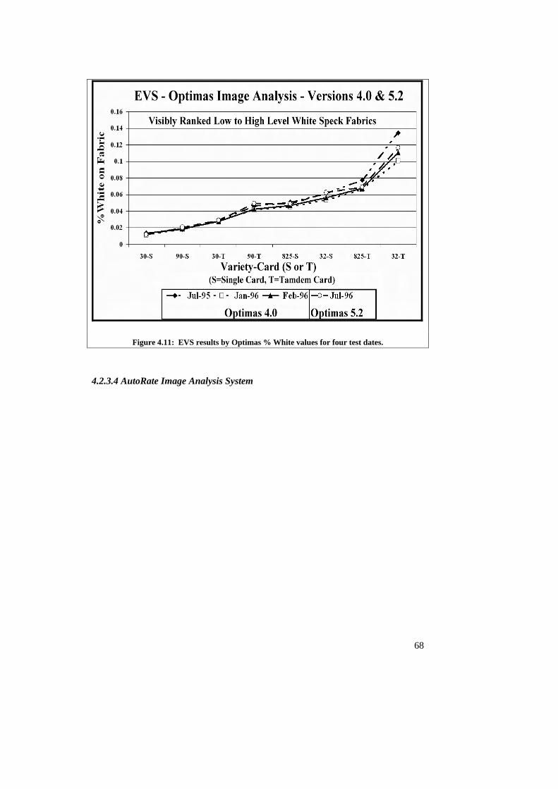
Figure 4.11: EVS results by Optimas % White values for four test dates.
4.2.3.4 AutoRate Image Analysis System
68
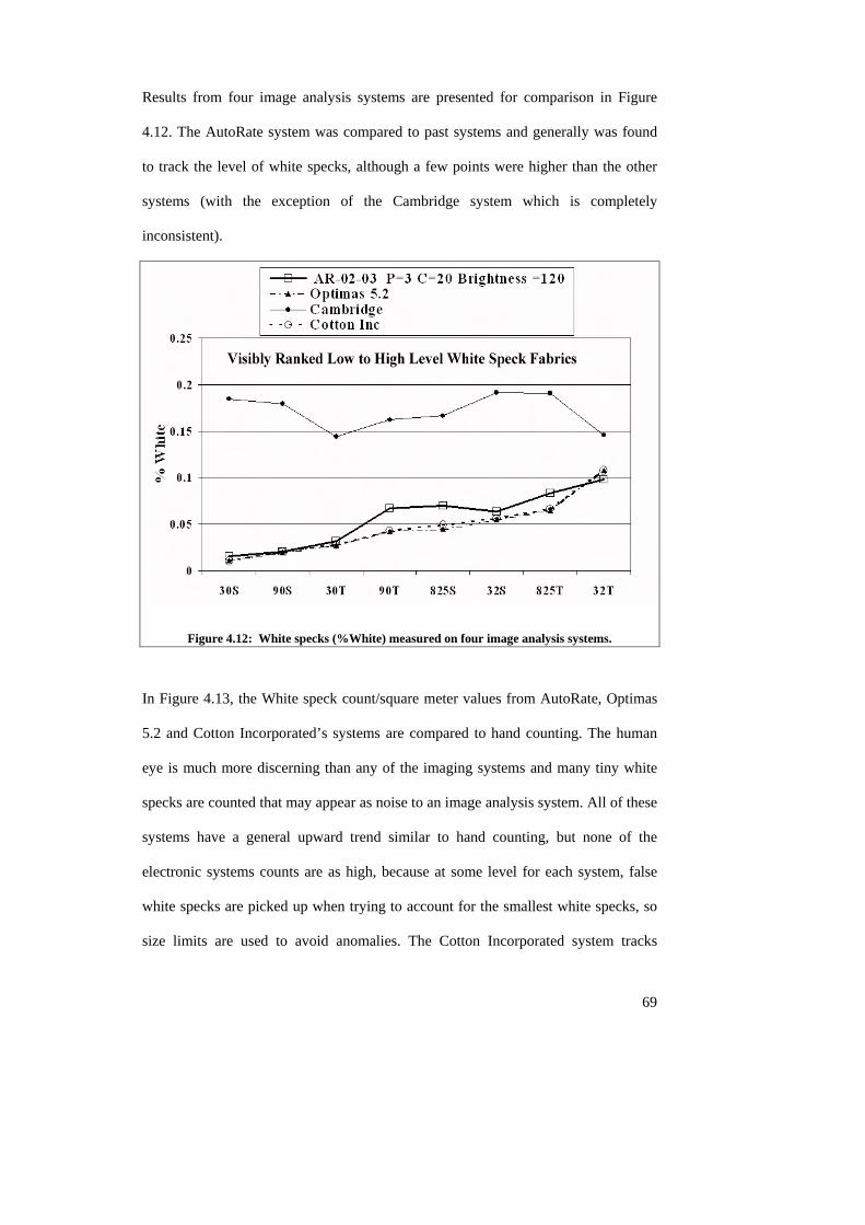
Results from four image analysis systems are presented for comparison in Figure
4.12. The AutoRate system was compared to past systems and generally was found
to track the level of white specks, although a few points were higher than the other
systems (with the exception of the Cambridge system which is completely
inconsistent).
Figure 4.12: White specks (%White) measured on four image analysis systems.
In Figure 4.13, the White speck count/square meter values from AutoRate, Optimas
5.2 and Cotton Incorporated’s systems are compared to hand counting. The human
eye is much more discerning than any of the imaging systems and many tiny white
specks are counted that may appear as noise to an image analysis system. All of these
systems have a general upward trend similar to hand counting, but none of the
electronic systems counts are as high, because at some level for each system, false
white specks are picked up when trying to account for the smallest white specks, so
size limits are used to avoid anomalies. The Cotton Incorporated system tracks
69
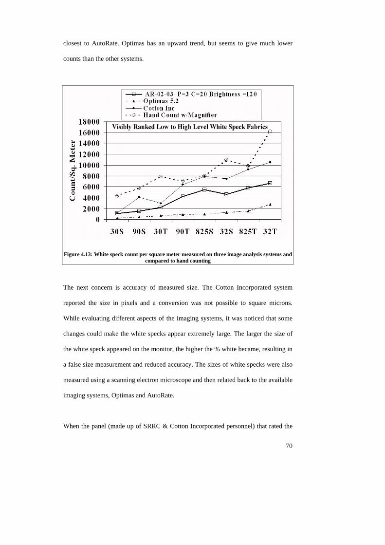
closest to AutoRate. Optimas has an upward trend, but seems to give much lower
counts than the other systems.
Figure 4.13: White speck count per square meter measured on three image analysis systems and compared to hand counting
The next concern is accuracy of measured size. The Cotton Incorporated system
reported the size in pixels and a conversion was not possible to square microns.
While evaluating different aspects of the imaging systems, it was noticed that some
changes could make the white specks appear extremely large. The larger the size of
the white speck appeared on the monitor, the higher the % white became, resulting in
a false size measurement and reduced accuracy. The sizes of white specks were also
measured using a scanning electron microscope and then related back to the available
imaging systems, Optimas and AutoRate.
When the panel (made up of SRRC & Cotton Incorporated personnel) that rated the
70
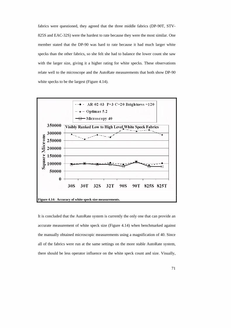
fabrics were questioned, they agreed that the three middle fabrics (DP-90T, STV-
825S and EAC-32S) were the hardest to rate because they were the most similar. One
member stated that the DP-90 was hard to rate because it had much larger white
specks than the other fabrics, so she felt she had to balance the lower count she saw
with the larger size, giving it a higher rating for white specks. These observations
relate well to the microscope and the AutoRate measurements that both show DP-90
white specks to be the largest (Figure 4.14).
Figure 4.14: Accuracy of white speck size measurements.
It is concluded that the AutoRate system is currently the only one that can provide an
accurate measurement of white speck size (Figure 4.14) when benchmarked against
the manually obtained microscopic measurements using a magnification of 40. Since
all of the fabrics were run at the same settings on the more stable AutoRate system,
there should be less operator influence on the white speck count and size. Visually,
71
72
the counts from the AutoRate system appear realistic, while the Optimas system
appears to undercount and significantly oversize the white specks. The combination
results in very similar % white for both systems, but the AutoRate system obviously
measures size more accurately than the Optimas system. Testing fabrics for white
specks can take as much as an hour per fabric using the manual Optimas system. The
candidate reduced the required time to ten minutes per fabric with the current
AutoRate system. A fully automated system should result from Dr. Xu’s current
work and this would further reduce this time significantly.
Only data from the latest version of AutoRate (AR-02-03) are presented in the
remainder of this dissertation using the adopted configuration (fabrics scanned using
the reset control tool, minimum pixel size = 3, brightness =120 and contrast varied as
needed), which seemed visually most accurate.
73
5. LARGE SCALE VARIETY WHITE SPECK STUDIES AND
PROCESSING EFFECTS ON WHITE SPECK LEVELS
Both Australia and the U.S. mechanically harvest and gin their cottons and both
countries are perceived by buyers to have nep problems. White specks are the most
expensive nep defect problem. Many growing regions (usually small areas but
sometimes whole countries) are often avoided by individual cotton buyers if the
previous year produced high white speck problems for their mills. This project was
undertaken at sites in the U.S. and Australia to provide baseline data on the level of
white specks in Australian and U.S. cotton. Previously published studies do not cover
fabric neps but focus on yarn quality, which makes it particularly important to
determine the factors that affect white speck levels in fabrics. After all, cotton is
ultimately valued in fabric form. This chapter sets out the experimental work and
analysis undertaken in U.S. and Australian field studies. The AutoRate system was
used to evaluate the large number of fabric samples. Processing effects on the level
of white specks in the dyed fabrics are also described.
5.1 Large scale variety white speck studies Several field studies in the U.S. and Australia were used to investigate varietal
differences as well as processing influences on white speck levels. The U.S. Leading
Variety Study (LVS) consisted of 26 bales from across the U.S. cotton belt and were
part of an annual variety study conducted by AMS (Agricultural Marketing Service).
Two years of field studies in Australia with known harvesting and ginning were used
to derive more information about processing effects on white speck levels. This was
74
followed by an investigation of 21 varieties from three states in the U.S. All of these
studies had the same mill processing.
5.1.1 Neps result from growth, harvesting or ginning and processing 116(Wegener, 1980)
Imperfections in lint cotton, particularly neps and seed coat fragments, reduce
processing efficiency in the textile mill and detract from appearance of yarns and
fabrics, ultimately causing financial losses. Breeders can help to reduce the nep
formation potential of cotton by selecting for further development those varieties
with fibre properties that are consistently associated with low nep count and seed-
coat fragment levels in ginned lint, yarn and fabric. Neps are often the result of
immature fibre growth as influenced by climate, over-watering, coalescence, and
pests. These growth neps contain predominantly dead and immature fibres. Fibres
damaged by insects will no longer mature and the escaping lumen cellular fluid
causes these immature fibres to coalesce 117(Wegener, 1980). If a plant is stressed
during certain critical periods, for example by a shortage of water, some of the
immature seeds within a boll are aborted. The immature fibres attached to those
seeds have the primary wall laid down, but lack secondary wall that other living
seeds on the plant produce. Growth period, which is related to growing conditions
prior to harvest, has an impact on the number of neps and other imperfections found
in ginned lint, yarn and fabric 118(Mangialardi, 1987). It is possible that a crop of
cotton that “just makes it” through a bad season may not have “made it” at all, and a
white speck problem is likely to occur.
The susceptibility of cotton to form neps is dependent upon the nature of the cotton
itself. Fibre properties such as fineness and maturity determine to a large degree the
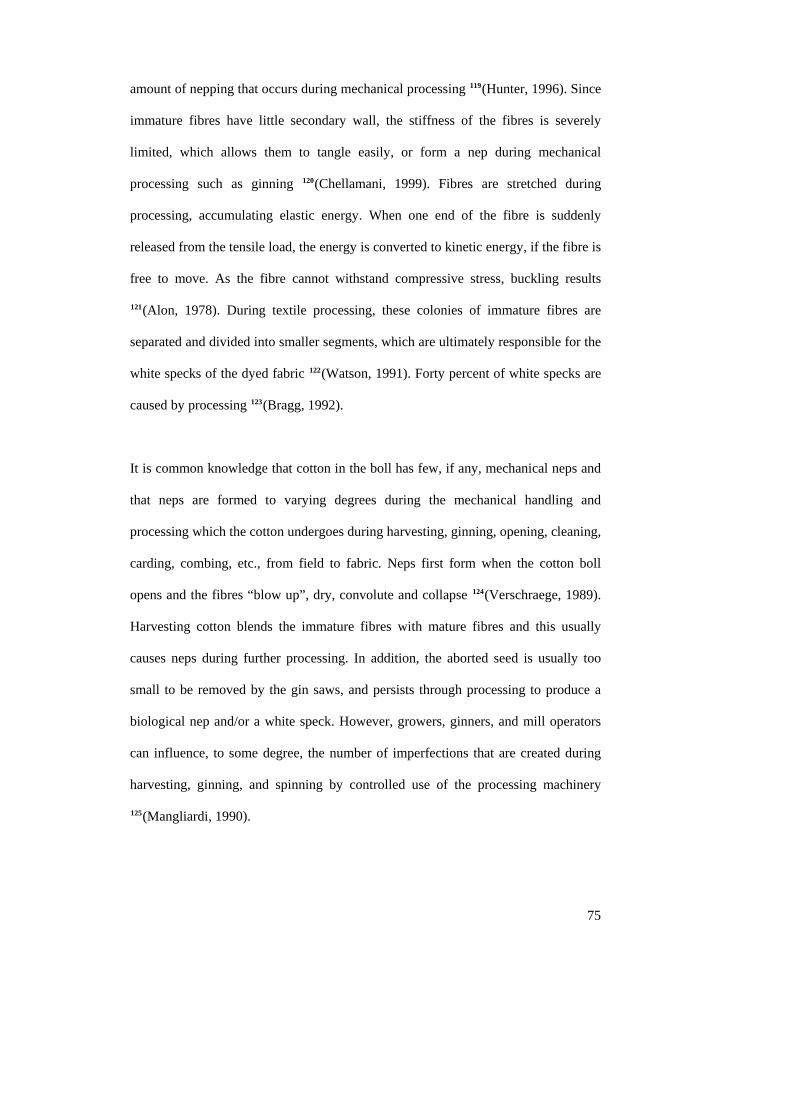
75
amount of nepping that occurs during mechanical processing 119(Hunter, 1996). Since
immature fibres have little secondary wall, the stiffness of the fibres is severely
limited, which allows them to tangle easily, or form a nep during mechanical
processing such as ginning 120(Chellamani, 1999). Fibres are stretched during
processing, accumulating elastic energy. When one end of the fibre is suddenly
released from the tensile load, the energy is converted to kinetic energy, if the fibre is
free to move. As the fibre cannot withstand compressive stress, buckling results
121(Alon, 1978). During textile processing, these colonies of immature fibres are
separated and divided into smaller segments, which are ultimately responsible for the
white specks of the dyed fabric 122(Watson, 1991). Forty percent of white specks are
caused by processing 123(Bragg, 1992).
It is common knowledge that cotton in the boll has few, if any, mechanical neps and
that neps are formed to varying degrees during the mechanical handling and
processing which the cotton undergoes during harvesting, ginning, opening, cleaning,
carding, combing, etc., from field to fabric. Neps first form when the cotton boll
opens and the fibres “blow up”, dry, convolute and collapse 124(Verschraege, 1989).
Harvesting cotton blends the immature fibres with mature fibres and this usually
causes neps during further processing. In addition, the aborted seed is usually too
small to be removed by the gin saws, and persists through processing to produce a
biological nep and/or a white speck. However, growers, ginners, and mill operators
can influence, to some degree, the number of imperfections that are created during
harvesting, ginning, and spinning by controlled use of the processing machinery
125(Mangliardi, 1990).
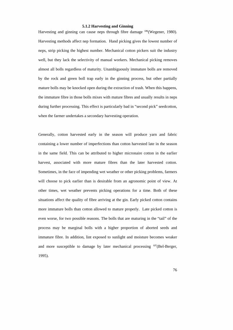
76
5.1.2 Harvesting and Ginning Harvesting and ginning can cause neps through fibre damage 126(Wegener, 1980).
Harvesting methods affect nep formation. Hand picking gives the lowest number of
neps, strip picking the highest number. Mechanical cotton pickers suit the industry
well, but they lack the selectivity of manual workers. Mechanical picking removes
almost all bolls regardless of maturity. Unambiguously immature bolls are removed
by the rock and green boll trap early in the ginning process, but other partially
mature bolls may be knocked open during the extraction of trash. When this happens,
the immature fibre in those bolls mixes with mature fibres and usually results in neps
during further processing. This effect is particularly bad in “second pick” seedcotton,
when the farmer undertakes a secondary harvesting operation.
Generally, cotton harvested early in the season will produce yarn and fabric
containing a lower number of imperfections than cotton harvested late in the season
in the same field. This can be attributed to higher micronaire cotton in the earlier
harvest, associated with more mature fibres than the later harvested cotton.
Sometimes, in the face of impending wet weather or other picking problems, farmers
will choose to pick earlier than is desirable from an agronomic point of view. At
other times, wet weather prevents picking operations for a time. Both of these
situations affect the quality of fibre arriving at the gin. Early picked cotton contains
more immature bolls than cotton allowed to mature properly. Late picked cotton is
even worse, for two possible reasons. The bolls that are maturing in the “tail” of the
process may be marginal bolls with a higher proportion of aborted seeds and
immature fibre. In addition, lint exposed to sunlight and moisture becomes weaker
and more susceptible to damage by later mechanical processing 127(Bel-Berger,
1995).
Figure 5.1: Different types and levels of trash seen in spindle picked and stripper picked cotton.
Figure 5.1 shows samples of spindle-harvested, conventionally grown cotton (left)
and stripper-harvested cotton. Cotton harvested with a stripper harvester contains
more stems and leaves 128(Greb , 2000) than spindle picked cotton.
Figure 5.2: Spindle picking cotton129(Nance, 2002). Cotton stripper harvesting cotton130(Wright, 2000).
Figures 5.2 compares the field impacts of the two types of cotton harvesting
machines. There is very little cotton left in the field behind the stripper harvester,
emphasizing that all of the cotton is taken by the stripper, both mature and immature.
77
78
Figure 5.3 depicts the processing sequence followed by seedcotton from module to
bale. Many stages can be bypassed or heat levels changed at the discretion of the
ginner. Ginning increases the number of neps, saw-ginning more so than roller
ginning. The more violent the ginning method, the more neps and seed coat
fragments are formed 131(Mangialardi, 1987).
The ginner’s job is to remove the lint from the seed and to clean the cotton (Figure
5.4) in order to get the best price for the grower for his cotton based on the grading
system. The grading system was set up on hand picked cotton and discounts heavily
if the cotton is not “white and clean”, as this was a major indication of quality
problems in the days of hand picked cotton.
The gin stands and saw cylinder lint cleaners are major points of cleaning and
formation of neps. Using three saw cylinder lint cleaners in the ginning sequence
instead of one lint cleaner can increase the number of neps by 54% 132(Mangialardi -
b, 1985). Lint cleaning in the gin does take out motes and seed coat fragments
(SCF), but the cleaning efficiency depends somewhat on the differential weight
between cotton and trash, so the heavier, larger motes and seed coat fragments are
more likely to come out than smaller, pinhead motes. As the severity of the
machining is increased, the smaller motes are just as likely to be broken up and
scattered through the lint rather than being removed 133(Hughs, 1988). The number of
neps also increases with increased SFC and coefficient of length variation
134(Frydrych, 2001), both of which are good indicators of excessive ginning
conditions.
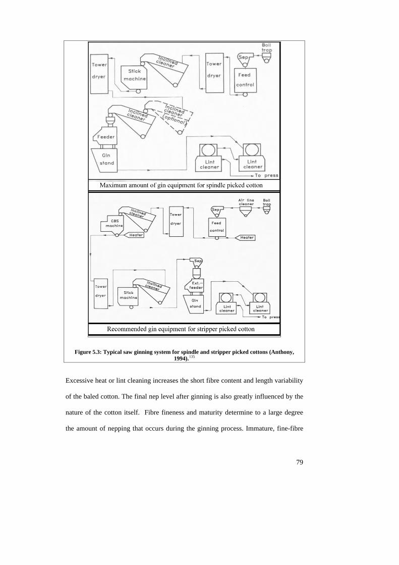
Figure 5.3: Typical saw ginning system for spindle and stripper picked cottons (Anthony, 1994).135
Excessive heat or lint cleaning increases the short fibre content and length variability
of the baled cotton. The final nep level after ginning is also greatly influenced by the
nature of the cotton itself. Fibre fineness and maturity determine to a large degree
the amount of nepping that occurs during the ginning process. Immature, fine-fibre
79
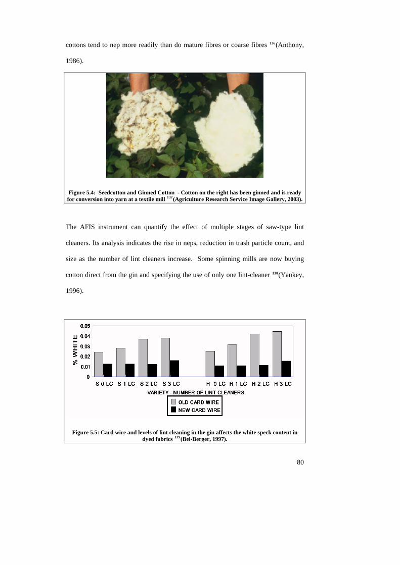
cottons tend to nep more readily than do mature fibres or coarse fibres 136(Anthony,
1986).
Figure 5.4: Seedcotton and Ginned Cotton - Cotton on the right has been ginned and is ready for conversion into yarn at a textile mill 137(Agriculture Research Service Image Gallery, 2003).
The AFIS instrument can quantify the effect of multiple stages of saw-type lint
cleaners. Its analysis indicates the rise in neps, reduction in trash particle count, and
size as the number of lint cleaners increase. Some spinning mills are now buying
cotton direct from the gin and specifying the use of only one lint-cleaner 138(Yankey,
1996).
Figure 5.5: Card wire and levels of lint cleaning in the gin affects the white speck content in dyed fabrics 139(Bel-Berger, 1997).
80
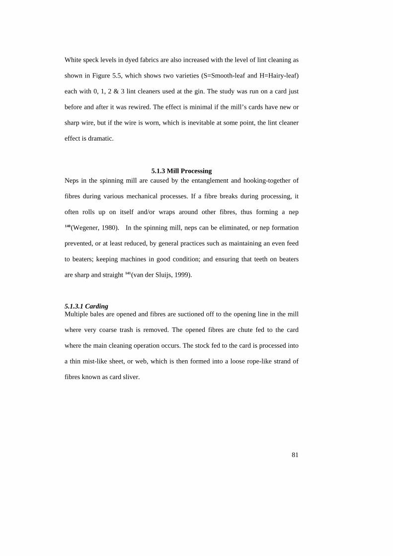
81
White speck levels in dyed fabrics are also increased with the level of lint cleaning as
shown in Figure 5.5, which shows two varieties (S=Smooth-leaf and H=Hairy-leaf)
each with 0, 1, 2 & 3 lint cleaners used at the gin. The study was run on a card just
before and after it was rewired. The effect is minimal if the mill’s cards have new or
sharp wire, but if the wire is worn, which is inevitable at some point, the lint cleaner
effect is dramatic.
5.1.3 Mill Processing Neps in the spinning mill are caused by the entanglement and hooking-together of
fibres during various mechanical processes. If a fibre breaks during processing, it
often rolls up on itself and/or wraps around other fibres, thus forming a nep
140(Wegener, 1980). In the spinning mill, neps can be eliminated, or nep formation
prevented, or at least reduced, by general practices such as maintaining an even feed
to beaters; keeping machines in good condition; and ensuring that teeth on beaters
are sharp and straight 141(van der Sluijs, 1999).
5.1.3.1 Carding Multiple bales are opened and fibres are suctioned off to the opening line in the mill
where very coarse trash is removed. The opened fibres are chute fed to the card
where the main cleaning operation occurs. The stock fed to the card is processed into
a thin mist-like sheet, or web, which is then formed into a loose rope-like strand of
fibres known as card sliver.
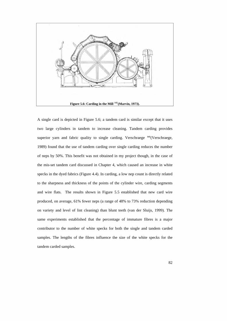
Figure 5.6: Carding in the Mill 142(Marvin, 1973).
A single card is depicted in Figure 5.6; a tandem card is similar except that it uses
two large cylinders in tandem to increase cleaning. Tandem carding provides
superior yarn and fabric quality to single carding. Verschraege 143(Verschraege,
1989) found that the use of tandem carding over single carding reduces the number
of neps by 50%. This benefit was not obtained in my project though, in the case of
the mis-set tandem card discussed in Chapter 4, which caused an increase in white
specks in the dyed fabrics (Figure 4.4). In carding, a low nep count is directly related
to the sharpness and thickness of the points of the cylinder wire, carding segments
and wire flats. The results shown in Figure 5.5 established that new card wire
produced, on average, 61% fewer neps (a range of 48% to 73% reduction depending
on variety and level of lint cleaning) than blunt teeth (van der Sluijs, 1999). The
same experiments established that the percentage of immature fibres is a major
contributor to the number of white specks for both the single and tandem carded
samples. The lengths of the fibres influence the size of the white specks for the
ndem carded samples. ta
82
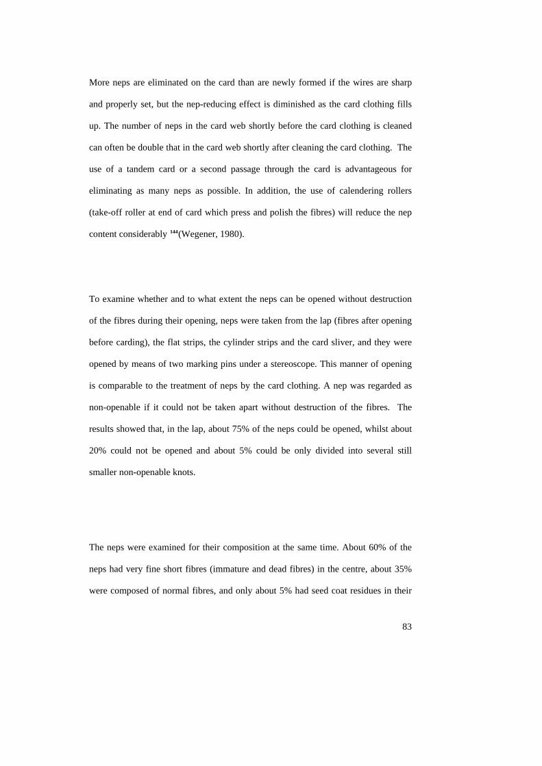
83
and polish the fibres) will reduce the nep
ontent considerably 144(Wegener, 1980).
d about 5% could be only divided into several still
smaller non-openable knots.
More neps are eliminated on the card than are newly formed if the wires are sharp
and properly set, but the nep-reducing effect is diminished as the card clothing fills
up. The number of neps in the card web shortly before the card clothing is cleaned
can often be double that in the card web shortly after cleaning the card clothing. The
use of a tandem card or a second passage through the card is advantageous for
eliminating as many neps as possible. In addition, the use of calendering rollers
(take-off roller at end of card which press
c
To examine whether and to what extent the neps can be opened without destruction
of the fibres during their opening, neps were taken from the lap (fibres after opening
before carding), the flat strips, the cylinder strips and the card sliver, and they were
opened by means of two marking pins under a stereoscope. This manner of opening
is comparable to the treatment of neps by the card clothing. A nep was regarded as
non-openable if it could not be taken apart without destruction of the fibres. The
results showed that, in the lap, about 75% of the neps could be opened, whilst about
20% could not be opened an
The neps were examined for their composition at the same time. About 60% of the
neps had very fine short fibres (immature and dead fibres) in the centre, about 35%
were composed of normal fibres, and only about 5% had seed coat residues in their
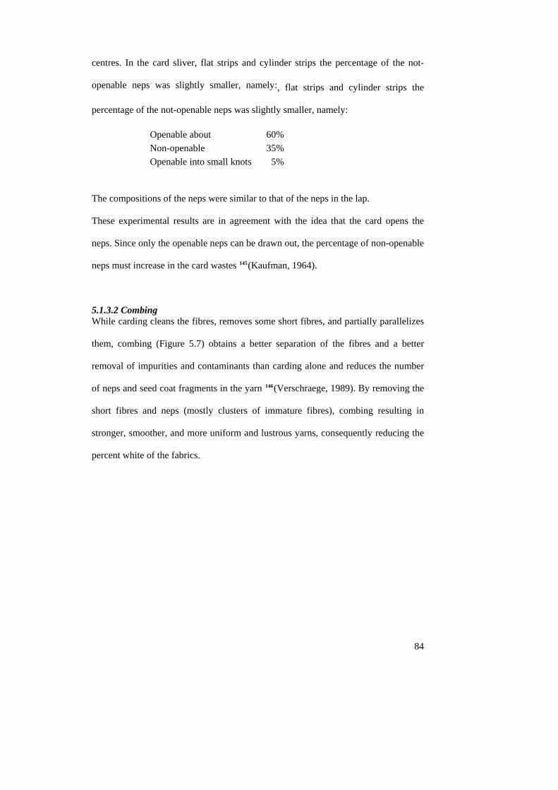
84
linder strips the
percentage of the not-openable neps as slig aller, namely:
Non-openable 35% Openable into small knots 5%
ercentage of non-openable
eps must increase in the card wastes 145(Kaufman, 1964).
5.1.3.2 Combing
uniform and lustrous yarns, consequently reducing the
percent white of the fabrics.
centres. In the card sliver, flat strips and cylinder strips the percentage of the not-
openable neps was slightly smaller, namely:, flat strips and cy
w htly sm
Openable about 60%
The compositions of the neps were similar to that of the neps in the lap.
These experimental results are in agreement with the idea that the card opens the
neps. Since only the openable neps can be drawn out, the p
n
While carding cleans the fibres, removes some short fibres, and partially parallelizes
them, combing (Figure 5.7) obtains a better separation of the fibres and a better
removal of impurities and contaminants than carding alone and reduces the number
of neps and seed coat fragments in the yarn 146(Verschraege, 1989). By removing the
short fibres and neps (mostly clusters of immature fibres), combing resulting in
stronger, smoother, and more
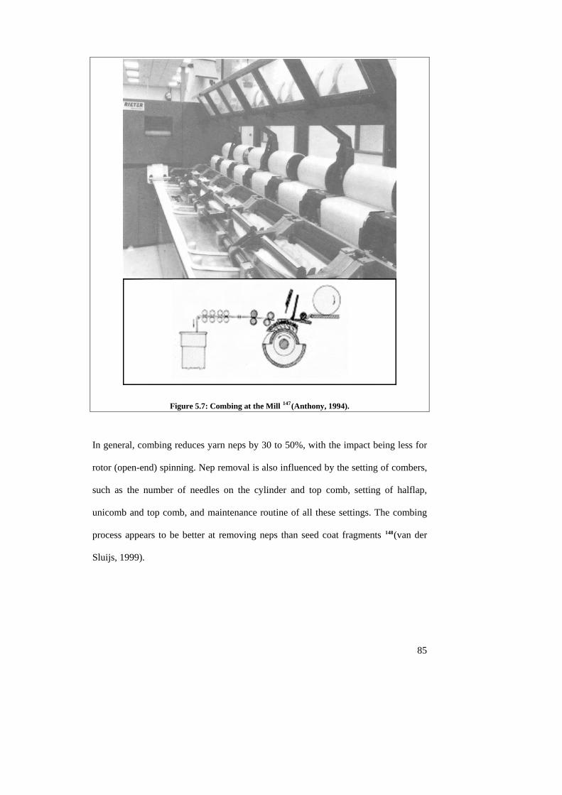
Figure 5.7: Combing at the Mill 147(Anthony, 1994).
In general, combing reduces yarn neps by 30 to 50%, with the impact being less for
rotor (open-end) spinning. Nep removal is also influenced by the setting of combers,
such as the number of needles on the cylinder and top comb, setting of halflap,
unicomb and top comb, and maintenance routine of all these settings. The combing
process appears to be better at removing neps than seed coat fragments 148(van der
Sluijs, 1999).
85
5.1.3.3 Spinning High quality cotton is traditionally spun using the ring spinning system (Figure 5.8)
at a typical speed of 20 metres per minute. This produces high quality, fine yarns
with excellent mechanical properties and a soft, smooth feel. The other technology
commonly used in cotton processing, the open end (OE) spinning system (also
known as rotor spinning) (Figure 5.9), has a productivity in the region of 150 metres
per minute and is more suited to coarser yarns. By comparison, the new Murata
Vortex Spinning (MVS) (Figure 5.10) system produces 400 metres per minute and
can produce fine yarns of high quality, similar to that of a ring spun yarn. Based on
the quantity of yarn produced, open end spinning dominates. Even though there are
only one-third as many positions of rotors installed, rotor spinning is so much faster
that they spin three times more yarn than ring spinning 149(Naylor, 2002).
Figure 5.8: Ring Spinning –roving is drawn out into a tiny strand of fibres and twisted into a yarn.
86
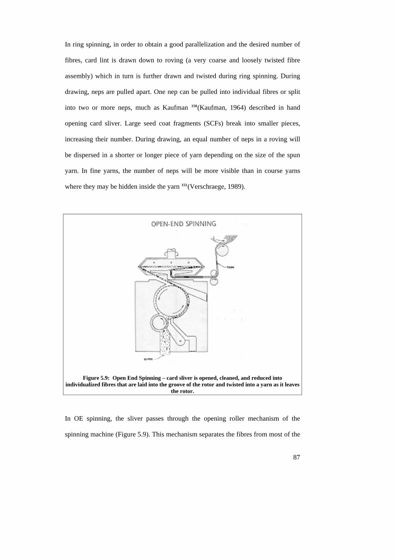
In ring spinning, in order to obtain a good parallelization and the desired number of
fibres, card lint is drawn down to roving (a very coarse and loosely twisted fibre
assembly) which in turn is further drawn and twisted during ring spinning. During
drawing, neps are pulled apart. One nep can be pulled into individual fibres or split
into two or more neps, much as Kaufman 150(Kaufman, 1964) described in hand
opening card sliver. Large seed coat fragments (SCFs) break into smaller pieces,
increasing their number. During drawing, an equal number of neps in a roving will
be dispersed in a shorter or longer piece of yarn depending on the size of the spun
yarn. In fine yarns, the number of neps will be more visible than in course yarns
where they may be hidden inside the yarn 151(Verschraege, 1989).
Figure 5.9: Open End Spinning – card sliver is opened, cleaned, and reduced into individualized fibres that are laid into the groove of the rotor and twisted into a yarn as it leaves
the rotor.
In OE spinning, the sliver passes through the opening roller mechanism of the
spinning machine (Figure 5.9). This mechanism separates the fibres from most of the
87
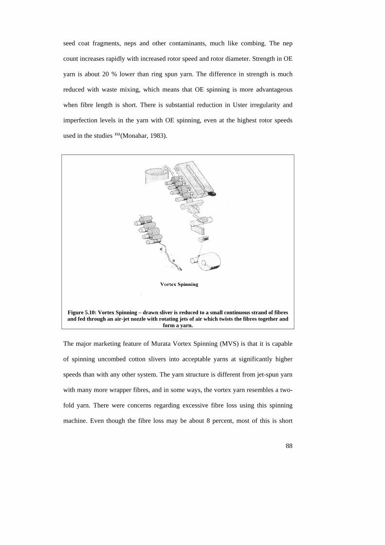
seed coat fragments, neps and other contaminants, much like combing. The nep
count increases rapidly with increased rotor speed and rotor diameter. Strength in OE
yarn is about 20 % lower than ring spun yarn. The difference in strength is much
reduced with waste mixing, which means that OE spinning is more advantageous
when fibre length is short. There is substantial reduction in Uster irregularity and
imperfection levels in the yarn with OE spinning, even at the highest rotor speeds
used in the studies 152(Monahar, 1983).
Figure 5.10: Vortex Spinning – drawn sliver is reduced to a small continuous strand of fibres and fed through an air-jet nozzle with rotating jets of air which twists the fibres together and
form a yarn.
The major marketing feature of Murata Vortex Spinning (MVS) is that it is capable
of spinning uncombed cotton slivers into acceptable yarns at significantly higher
speeds than with any other system. The yarn structure is different from jet-spun yarn
with many more wrapper fibres, and in some ways, the vortex yarn resembles a two-
fold yarn. There were concerns regarding excessive fibre loss using this spinning
machine. Even though the fibre loss may be about 8 percent, most of this is short
88
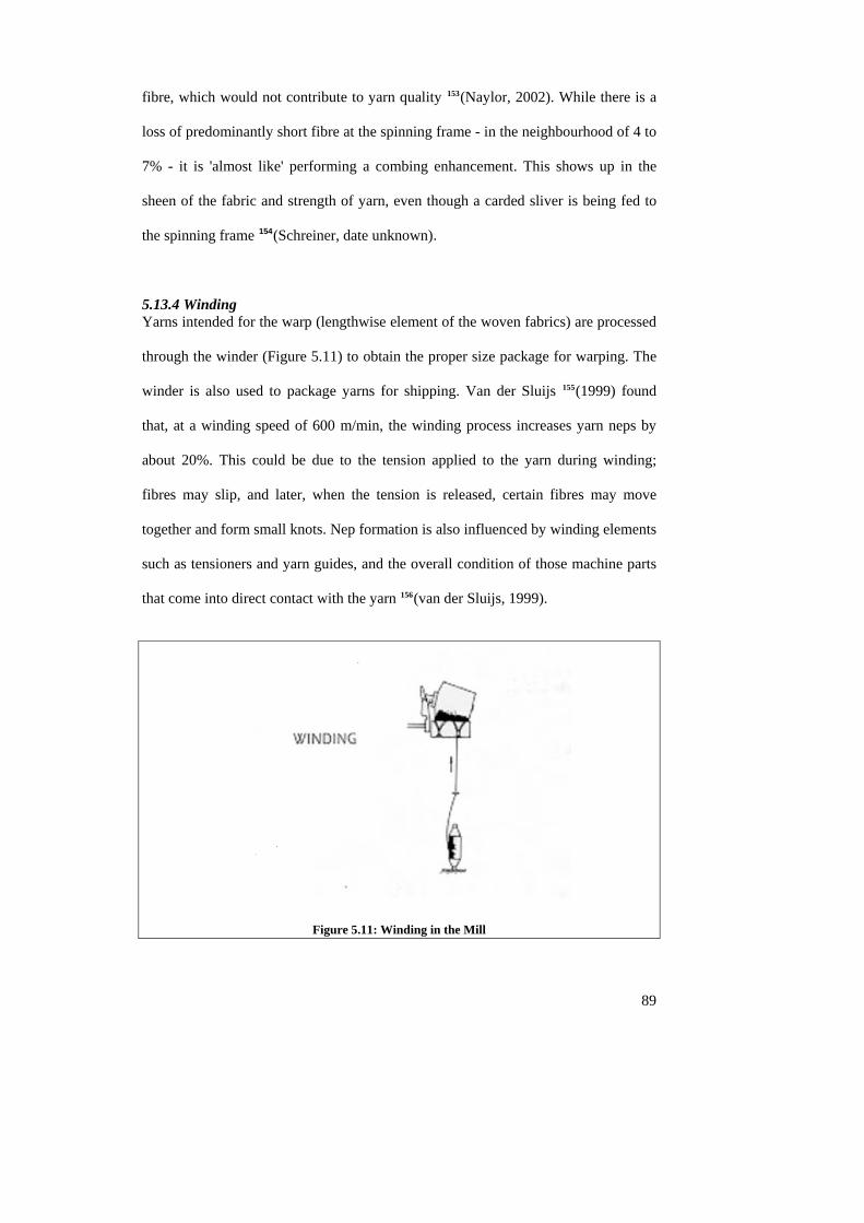
fibre, which would not contribute to yarn quality 153(Naylor, 2002). While there is a
loss of predominantly short fibre at the spinning frame - in the neighbourhood of 4 to
7% - it is 'almost like' performing a combing enhancement. This shows up in the
sheen of the fabric and strength of yarn, even though a carded sliver is being fed to
the spinning frame 154(Schreiner, date unknown).
5.13.4 Winding
9).
Yarns intended for the warp (lengthwise element of the woven fabrics) are processed
through the winder (Figure 5.11) to obtain the proper size package for warping. The
winder is also used to package yarns for shipping. Van der Sluijs 155(1999) found
that, at a winding speed of 600 m/min, the winding process increases yarn neps by
about 20%. This could be due to the tension applied to the yarn during winding;
fibres may slip, and later, when the tension is released, certain fibres may move
together and form small knots. Nep formation is also influenced by winding elements
such as tensioners and yarn guides, and the overall condition of those machine parts
that come into direct contact with the yarn 156(van der Sluijs, 199
Figure 5.11: Winding in the Mill
89
90
5.2 White Speck Variety studies Methodology The first experimental study conducted with AMS (USDA’s Agricultural Marketing
Service) retained little history about the bale, except the region where it was grown,
the variety, the gin used, and the general processing levels (number of lint cleaners)
at the gins. The last three studies exercised greater control over the cotton and
ginning. Samples were identified in the field and agronomic data were collected. The
samples were then ginned under certain settings, and samples of lint were collected
from the bale press. Fibres were evaluated by classing, HVI, FMT, AFIS, Lintronics
and cross-section image analysis. The mill processing for these three studies
followed the same protocols as the first study except for yarn size. In addition, the
final study increased carding production from 70 lbs/hour to 150 lbs/hour to be more
in line with industrial standards. The yarns for all of these studies were woven into a
common combed warp, producing a filling faced sateen fabric at SRRC (Figure
5.12). The experimental yarns cover approximately 84% to 92% of the fabric surface,
a factor that is considered when comparing studies (Figure 5.13). The fabrics were
dyed and image analysed for white specks at SRRC using the AutoRate Program
(Version AR-04-03 [April 2003]) as described at the end of Chapter 4. Most studies
do not cover fabric neps, they usually conclude with yarn quality, which makes these
studies unusual in design, as the primary results are fabric appearance.
Dyeing of Fabric The fabric was finished with a 0.1% Prechem 70, 0.3% T.S.P.P. (tetrasodium
phosphate) boiloff, a caustic scour of 1.1% Prechem SN, 1.1% Mayquest 80, 0.1%
Prechem 70 and 0.7% sodium hydroxide (caustic soda), followed by the same boiloff
procedure. It was then bleached (0.1% Prechem 70, 0.5% Mayquest BLE and 3.0%

91
Peroxide (Albone 35) and dyed with 4% Cibacron Navy F-G Blue 184 (owf-on
weight of fabric), 0.5% Calgon, 8% NaCl, 0.8% Na2CO3 (soda ash) and 0.5% Triton
X-100. This reactive dye (Colour Index Reactive Blue184) effectively highlights
white specks in finished fabrics.
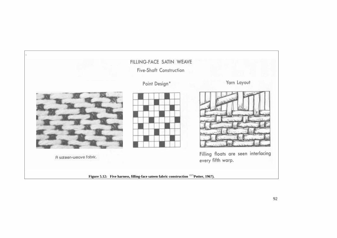
.
Figure 5.12: Five harness, filling-face sateen fabric construction 157(Potter, 1967).
92
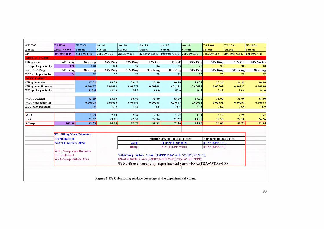
93
Figure 5.13: Calculating surface coverage of the experimental yarns.
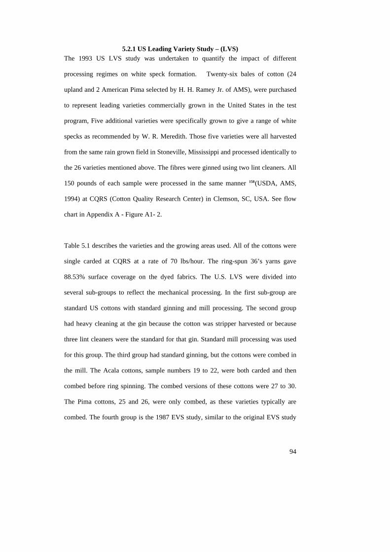
94
5.2.1 US Leading Variety Study – (LVS) The 1993 US LVS study was undertaken to quantify the impact of different
processing regimes on white speck formation. Twenty-six bales of cotton (24
upland and 2 American Pima selected by H. H. Ramey Jr. of AMS), were purchased
to represent leading varieties commercially grown in the United States in the test
program, Five additional varieties were specifically grown to give a range of white
specks as recommended by W. R. Meredith. Those five varieties were all harvested
from the same rain grown field in Stoneville, Mississippi and processed identically to
the 26 varieties mentioned above. The fibres were ginned using two lint cleaners. All
150 pounds of each sample were processed in the same manner 158(USDA, AMS,
1994) at CQRS (Cotton Quality Research Center) in Clemson, SC, USA. See flow
chart in Appendix A - Figure A1- 2.
Table 5.1 describes the varieties and the growing areas used. All of the cottons were
single carded at CQRS at a rate of 70 lbs/hour. The ring-spun 36’s yarns gave
88.53% surface coverage on the dyed fabrics. The U.S. LVS were divided into
several sub-groups to reflect the mechanical processing. In the first sub-group are
standard US cottons with standard ginning and mill processing. The second group
had heavy cleaning at the gin because the cotton was stripper harvested or because
three lint cleaners were the standard for that gin. Standard mill processing was used
for this group. The third group had standard ginning, but the cottons were combed in
the mill. The Acala cottons, sample numbers 19 to 22, were both carded and then
combed before ring spinning. The combed versions of these cottons were 27 to 30.
The Pima cottons, 25 and 26, were only combed, as these varieties typically are
combed. The fourth group is the 1987 EVS study, similar to the original EVS study
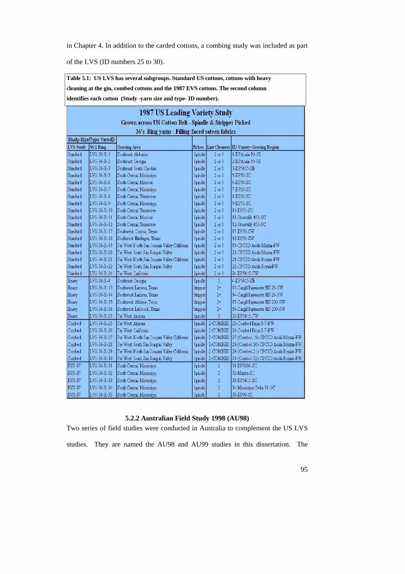
in Chapter 4. In addition to the carded cottons, a combing study was included as part
of the LVS (ID numbers 25 to 30).
Table 5.1: US LVS has several subgroups. Standard US cottons, cottons with heavy
cleaning at the gin, combed cottons and the 1987 EVS cottons. The second column
identifies each cotton (Study -yarn size and type- ID number).
5.2.2 Australian Field Study 1998 (AU98) Two series of field studies were conducted in Australia to complement the US LVS
studies. They are named the AU98 and AU99 studies in this dissertation. The
95
96
objective of these studies was to isolate variety and environmental effects from
machinery effects on nep formation.
The AU98 study was conducted first, and 30 cotton samples were collected from
across Australia to include eight different Australian varieties, with four locations or
irrigation conditions (two varieties only have three locations, due to timing
problems). Each sample had a known history regarding variety and growing issues
such as drought, flood, cloud cover, high-low temperatures, or specific field
problems. For example, if the white speck data for one variety has lower values at
one location than another, the field history would show if the high white speck data
were influenced by drought, flooding, or low sun days. It would be obvious that it
was a weather problem rather than a varietal problem. For the purposes of
quantifying the tendency of the variety to form white specks, the low white speck
data would be used, but both the high and low white speck data are used for the fibre
to fabric prediction study detailed in Chapter 6. By using all of the fibre data,
including field conditions that increased immature fibre production, useful
information could be obtained to help reduce white specks in the future and
prediction equations for yarns and fabrics from fibre properties without processing
interactions can be determined.
Thirty samples of seedcotton, each 1500 kg in weight, were baled using a small wool
bale press in the field. Each sample was split into two 750 kg samples at Queensland
Cotton’s Emerald Gin and ginned (approximately 5 bales/hr to assist in sampling;
normal gin production is about 6 bales/hr) using one lint cleaner on one set and two
lint cleaners on the second set of samples. All of the samples were processed through
97
one gin in one line with common equipment settings, preserving the individual
identities of the lots. The bulk of the ginned cottons were sold, reserving 50 lbs. of
each of the 60 samples, which were sent to CQRS (Cotton Quality Research Station,
Clemson SC, US). The 60 cotton bale samples were processed into 36’s and 22’s
ring yarns and 22’s and 10’s OE yarns using the same processing protocol as the U.S
LVS program. The full-scale equipment at CQRS is able to handle a minimum of 50
lbs. See flow chart in Appendix A - Figure A1- 3.
Cotton Seed Distributors (CSD) in Wee Waa furnishes 90% of seed planted in
Australia and Deltapine provide 10% of the seed planted in Australia. Ninety % of
CSD’s sales come from five lines - SiCala V2 and V2i, SiOkra V15 and V15i, and
SiCot 189. Deltapine seed is mostly Delta Pearl. These were included in the study
together with an Inguard line of genetically modified cotton called NuCOTN.
One CSD variety, CS50, tends to have low micronaire, depending on the growing
season. It is a long season variety that yields well, but our crop experienced a cold
start to the growing season. One CS50 sample in Emerald experienced heavy rainfall
twice following irrigation, so the urea fertiliser leached down slope. As a result, the
upper end of the field ran out of nitrogen in early January. We would expect that
cotton from the upper end would have the worst problem with white speck.
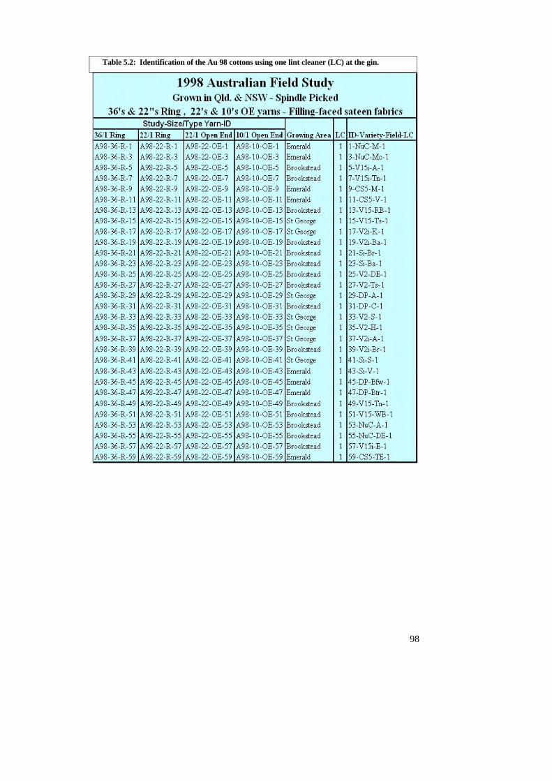
Table 5.2: Identification of the Au 98 cottons using one lint cleaner (LC) at the gin.
98
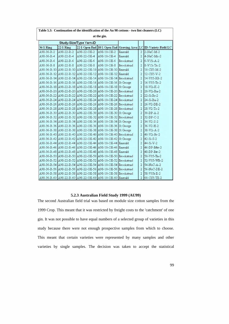
Table 5.3: Continuation of the identification of the Au 98 cottons - two lint cleaners (LC)
at the gin.
5.2.3 Australian Field Study 1999 (AU99) The second Australian field trial was based on module size cotton samples from the
1999 Crop. This meant that it was restricted by freight costs to the 'catchment' of one
gin. It was not possible to have equal numbers of a selected group of varieties in this
study because there were not enough prospective samples from which to choose.
This meant that certain varieties were represented by many samples and other
varieties by single samples. The decision was taken to accept the statistical
99
100
constraints on comparisons between varieties in order to get the benefits of having
more samples overall for wider comparisons. Namoi Co-op's Wathagar gin, east of
Moree was selected for processing the samples. Cotton was selected in the field, and
harvested normally by spindle picking. At harvest, the cotton was specially tagged
and diverted to stand with the other sample modules until a suitable time. The 36
modules comprised 540 tonnes of seedcotton and required about 20 hours running
time for the Wathagar gin. A rain front arrived after the first 12 hours of ginning,
changing the ambient atmospheric conditions. The decision was then made to break
the ginning after the 13th sample module. This was done assuming that fewer
problems would be caused by the break in continuity than were likely to be caused
by ginning under markedly different atmospheric conditions. The ginning of the
remaining 23 sample modules resumed 21 days later under conditions similar to
those existing for the first 13. All ginning was done during a 'day' shift, which is 12
hours from 8 a.m. to 8 p.m. The equipment was being used in the main run of the
season's cotton at the time the samples were ginned. No changes were made for the
sample modules except for the number of lint cleaners brought into use.
In this AU99 trial, the gin’s operation had to be continuously managed. The first half
of each module was ginned using two lint cleaners, which was standard for that gin
in that season. The flow of seedcotton from the module feeder was then stopped, and
a bale of cotton fibre was pressed. A lint sample was taken at this time and
adjustments were made to the equipment so that both lint cleaners were by-passed.
The flow of seedcotton was resumed until a second bale was pressed. A sample of
this 'zero lint cleaner' cotton was then removed in the same way as the previous
sample, and the two lint cleaners were brought back into use. The flow of seedcotton
101
then resumed to complete ginning of that module and start the sequence again with
the next sample module. Each 25kg lint sample was weighed, and then pressed into
woolpacks (small bales) in a nearby wool press. Four samples were pressed into each
woolpack. The lint samples in woolpacks were transported and stored for further
processing. Smaller lint samples were taken for laboratory analysis. After ginning,
the lint was freighted to the International Fibre Centre (IFC), Melbourne, Victoria,
Australia, to be spun on a ring spinning frame to a nominal yarn size of 30's Ne (19.7
Tex). The spinning specifications were set up to match the U.S. LVS mill processing
protocol. See flow chart in Appendix A - Figure A1- 4.
The processing of yarns from this study into fabrics experienced technical problems.
Initially, the yarns were woven and dyed by ITC, International Textile Center,
Lubbock, Texas, U. S., for a fee, using a common combed warp, in a filling faced
sateen for dyeing and white speck evaluation. The yarns were backwound before
weaving and there was a large amount of “fly” in the air during rewinding. The
fabrics all appeared relatively free of white specks. When the fabrics were tested on
AutoRate, there was no significant difference among these fabrics for white speck,
even though the fibre data indicated it should be significant. The yarns were sent to
USDA and rewoven on the same warp as was used in previous studies. The fabrics
were visibly different as can be seen in the results section (Figure 6.5).
All of the cottons from this trial were CSD and DP smooth leaf Upland varieties.
Varieties with “i” as the last letter in their variety name are Inguard varieties, single
BT gene (same as US Bollguard™). The 666 and Line XXXi are alternative names
for an experimental variety from CSD. S189i (ct) distinguishes that module from
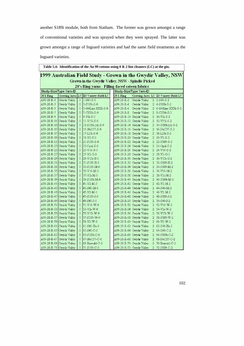
another S189i module, both from Statham. The former was grown amongst a range
of conventional varieties and was sprayed when they were sprayed. The latter was
grown amongst a range of Inguard varieties and had the same field treatments as the
Inguard varieties.
Table 5.4: Identification of the Au 99 cottons using 0 & 2 lint cleaners (LC) at the gin.
102
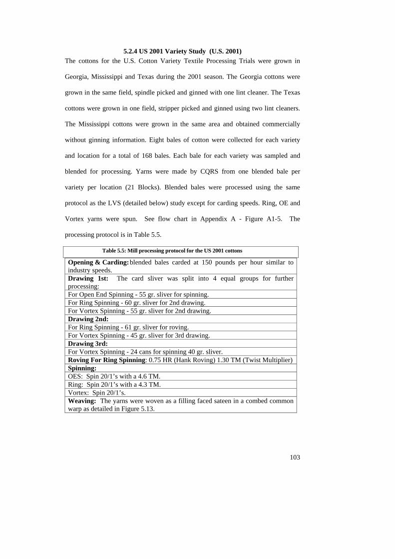
103
5.2.4 US 2001 Variety Study (U.S. 2001) The cottons for the U.S. Cotton Variety Textile Processing Trials were grown in
Georgia, Mississippi and Texas during the 2001 season. The Georgia cottons were
grown in the same field, spindle picked and ginned with one lint cleaner. The Texas
cottons were grown in one field, stripper picked and ginned using two lint cleaners.
The Mississippi cottons were grown in the same area and obtained commercially
without ginning information. Eight bales of cotton were collected for each variety
and location for a total of 168 bales. Each bale for each variety was sampled and
blended for processing. Yarns were made by CQRS from one blended bale per
variety per location (21 Blocks). Blended bales were processed using the same
protocol as the LVS (detailed below) study except for carding speeds. Ring, OE and
Vortex yarns were spun. See flow chart in Appendix A - Figure A1-5. The
processing protocol is in Table 5.5.
Table 5.5: Mill processing protocol for the US 2001 cottons
Opening & Carding: blended bales carded at 150 pounds per hour similar to industry speeds. Drawing 1st: The card sliver was split into 4 equal groups for further processing: For Open End Spinning - 55 gr. sliver for spinning. For Ring Spinning - 60 gr. sliver for 2nd drawing. For Vortex Spinning - 55 gr. sliver for 2nd drawing. Drawing 2nd: For Ring Spinning - 61 gr. sliver for roving. For Vortex Spinning - 45 gr. sliver for 3rd drawing. Drawing 3rd: For Vortex Spinning - 24 cans for spinning 40 gr. sliver. Roving For Ring Spinning: 0.75 HR (Hank Roving) 1.30 TM (Twist Multiplier) Spinning: OES: Spin 20/1’s with a 4.6 TM. Ring: Spin 20/1’s with a 4.3 TM. Vortex: Spin 20/1’s. Weaving: The yarns were woven as a filling faced sateen in a combed common warp as detailed in Figure 5.13.
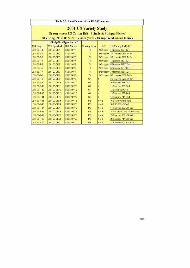
Table 5.6: Identification of the US 2001 cottons.
104
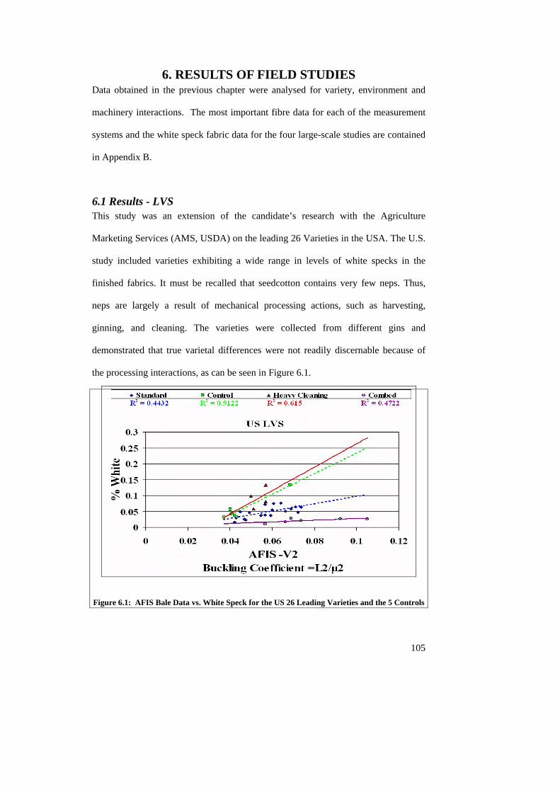
6. RESULTS OF FIELD STUDIES Data obtained in the previous chapter were analysed for variety, environment and
machinery interactions. The most important fibre data for each of the measurement
systems and the white speck fabric data for the four large-scale studies are contained
in Appendix B.
6.1 Results - LVS This study was an extension of the candidate’s research with the Agriculture
Marketing Services (AMS, USDA) on the leading 26 Varieties in the USA. The U.S.
study included varieties exhibiting a wide range in levels of white specks in the
finished fabrics. It must be recalled that seedcotton contains very few neps. Thus,
neps are largely a result of mechanical processing actions, such as harvesting,
ginning, and cleaning. The varieties were collected from different gins and
demonstrated that true varietal differences were not readily discernable because of
the processing interactions, as can be seen in Figure 6.1.
Figure 6.1: AFIS Bale Data vs. White Speck for the US 26 Leading Varieties and the 5 Controls
105
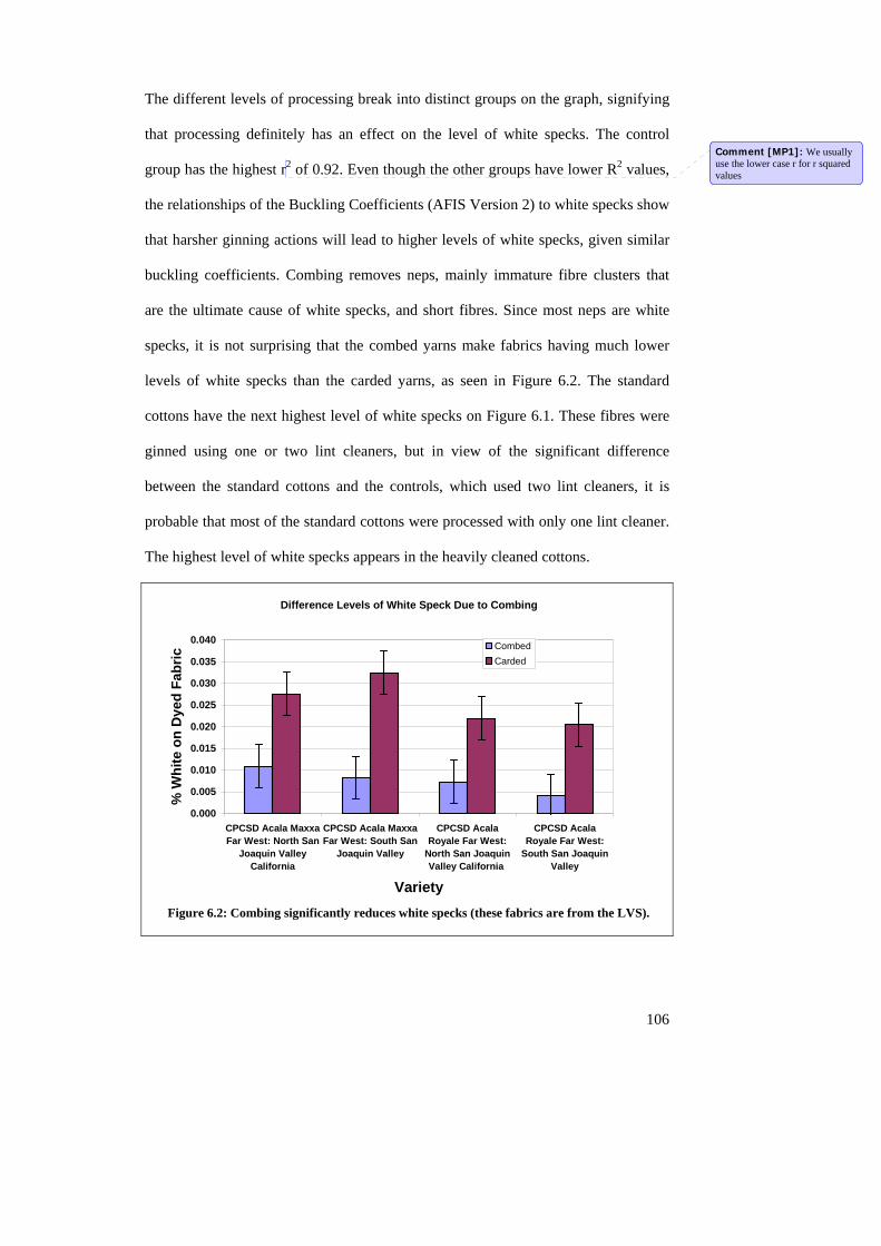
The different levels of processing break into distinct groups on the graph, signifying
that processing definitely has an effect on the level of white specks. The control
group has the highest r2 of 0.92. Even though the other groups have lower R2 values,
the relationships of the Buckling Coefficients (AFIS Version 2) to white specks show
that harsher ginning actions will lead to higher levels of white specks, given similar
buckling coefficients. Combing removes neps, mainly immature fibre clusters that
are the ultimate cause of white specks, and short fibres. Since most neps are white
specks, it is not surprising that the combed yarns make fabrics having much lower
levels of white specks than the carded yarns, as seen in Figure 6.2. The standard
cottons have the next highest level of white specks on Figure 6.1. These fibres were
ginned using one or two lint cleaners, but in view of the significant difference
between the standard cottons and the controls, which used two lint cleaners, it is
probable that most of the standard cottons were processed with only one lint cleaner.
The highest level of white specks appears in the heavily cleaned cottons.
Comment [MP1]: We usually use the lower case r for r squared values
Difference Levels of White Speck Due to Combing
0.035
0.040
0.000
0.005
0.010
0.015
0.020
0.025
0.030
CPCSD Acala MaxxaFar West: North San
Joaquin ValleyCalifornia
CPCSD Acala MaxxaFar West: South San
Joaquin Valley
CPCSD AcalaRoyale Far West:
North San JoaquinValley California
CPCSD AcalaRoyale Far West:
South San JoaquinValley
Variety
% W
hite
on
Dye
d Fa
bric
CombedCarded
Figure 6.2: Combing significantly reduces white specks (these fabrics are from the LVS).
106
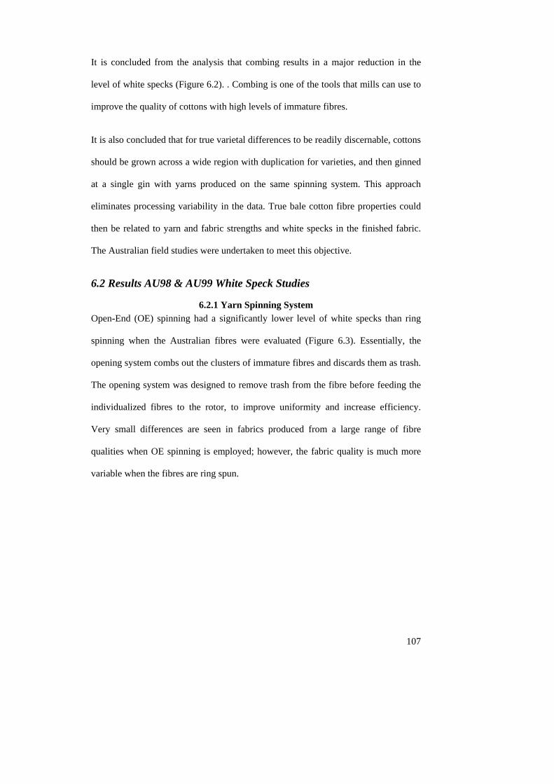
107
It is concluded from the analysis that combing results in a major reduction in the
level of white specks (Figure 6.2). . Combing is one of the tools that mills can use to
improve the quality of cottons with high levels of immature fibres.
It is also concluded that for true varietal differences to be readily discernable, cottons
should be grown across a wide region with duplication for varieties, and then ginned
at a single gin with yarns produced on the same spinning system. This approach
eliminates processing variability in the data. True bale cotton fibre properties could
then be related to yarn and fabric strengths and white specks in the finished fabric.
The Australian field studies were undertaken to meet this objective.
6.2 Results AU98 & AU99 White Speck Studies
6.2.1 Yarn Spinning System Open-End (OE) spinning had a significantly lower level of white specks than ring
spinning when the Australian fibres were evaluated (Figure 6.3). Essentially, the
opening system combs out the clusters of immature fibres and discards them as trash.
The opening system was designed to remove trash from the fibre before feeding the
individualized fibres to the rotor, to improve uniformity and increase efficiency.
Very small differences are seen in fabrics produced from a large range of fibre
qualities when OE spinning is employed; however, the fabric quality is much more
variable when the fibres are ring spun.
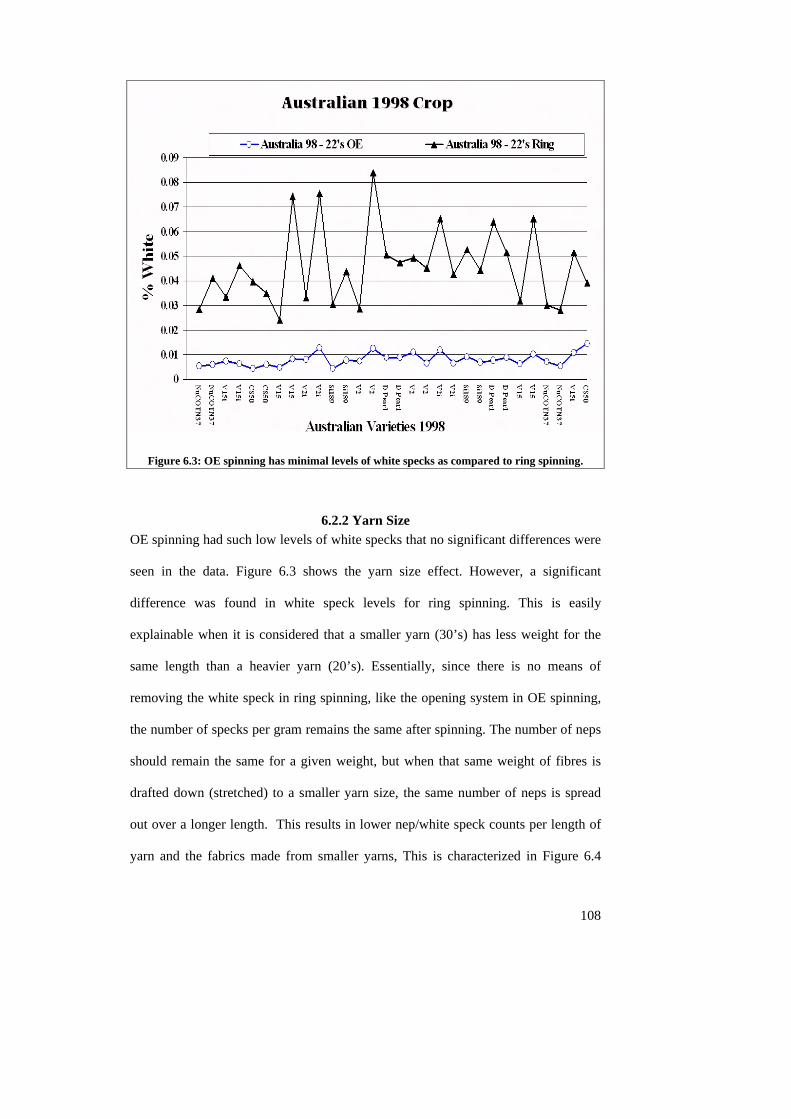
Figure 6.3: OE spinning has minimal levels of white specks as compared to ring spinning.
6.2.2 Yarn Size OE spinning had such low levels of white specks that no significant differences were
seen in the data. Figure 6.3 shows the yarn size effect. However, a significant
difference was found in white speck levels for ring spinning. This is easily
explainable when it is considered that a smaller yarn (30’s) has less weight for the
same length than a heavier yarn (20’s). Essentially, since there is no means of
removing the white speck in ring spinning, like the opening system in OE spinning,
the number of specks per gram remains the same after spinning. The number of neps
should remain the same for a given weight, but when that same weight of fibres is
drafted down (stretched) to a smaller yarn size, the same number of neps is spread
out over a longer length. This results in lower nep/white speck counts per length of
yarn and the fabrics made from smaller yarns, This is characterized in Figure 6.4
108
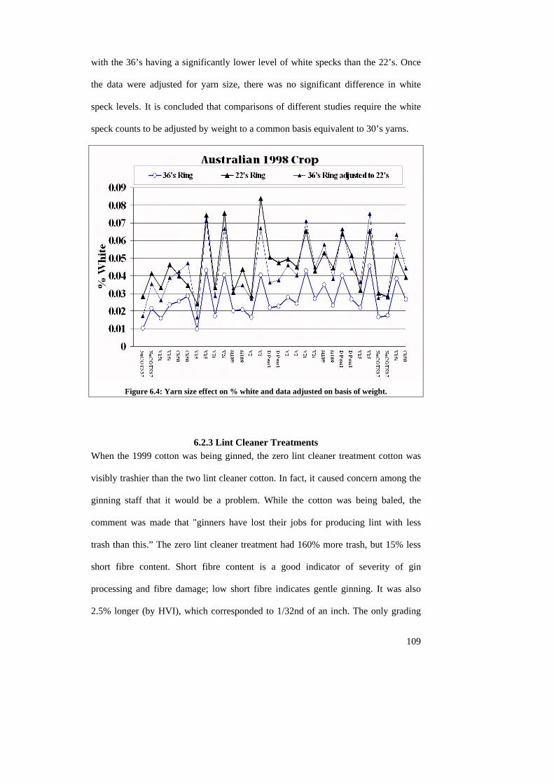
with the 36’s having a significantly lower level of white specks than the 22’s. Once
the data were adjusted for yarn size, there was no significant difference in white
speck levels. It is concluded that comparisons of different studies require the white
speck counts to be adjusted by weight to a common basis equivalent to 30’s yarns.
Figure 6.4: Yarn size effect on % white and data adjusted on basis of weight.
6.2.3 Lint Cleaner Treatments When the 1999 cotton was being ginned, the zero lint cleaner treatment cotton was
visibly trashier than the two lint cleaner cotton. In fact, it caused concern among the
ginning staff that it would be a problem. While the cotton was being baled, the
comment was made that "ginners have lost their jobs for producing lint with less
trash than this.” The zero lint cleaner treatment had 160% more trash, but 15% less
short fibre content. Short fibre content is a good indicator of severity of gin
processing and fibre damage; low short fibre indicates gentle ginning. It was also
2.5% longer (by HVI), which corresponded to 1/32nd of an inch. The only grading
109
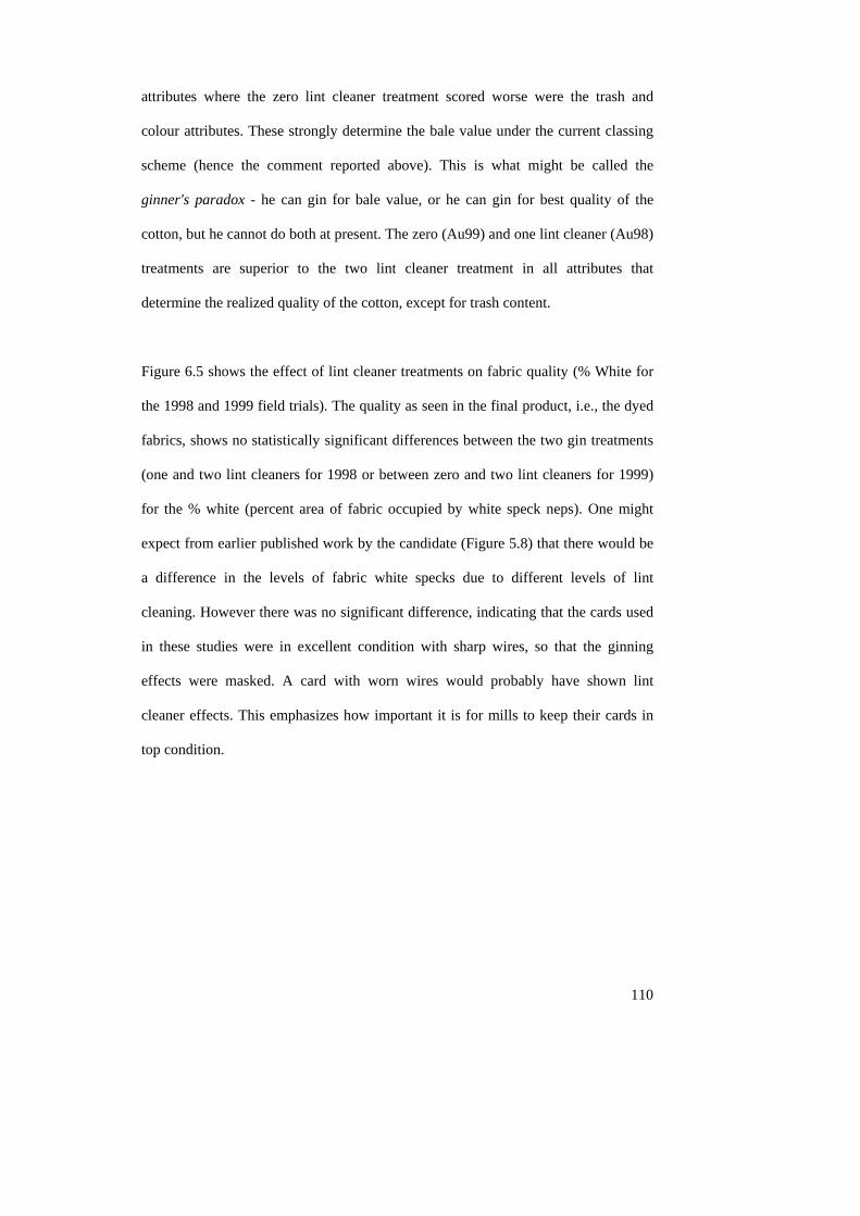
110
attributes where the zero lint cleaner treatment scored worse were the trash and
colour attributes. These strongly determine the bale value under the current classing
scheme (hence the comment reported above). This is what might be called the
ginner's paradox - he can gin for bale value, or he can gin for best quality of the
cotton, but he cannot do both at present. The zero (Au99) and one lint cleaner (Au98)
treatments are superior to the two lint cleaner treatment in all attributes that
determine the realized quality of the cotton, except for trash content.
Figure 6.5 shows the effect of lint cleaner treatments on fabric quality (% White for
the 1998 and 1999 field trials). The quality as seen in the final product, i.e., the dyed
fabrics, shows no statistically significant differences between the two gin treatments
(one and two lint cleaners for 1998 or between zero and two lint cleaners for 1999)
for the % white (percent area of fabric occupied by white speck neps). One might
expect from earlier published work by the candidate (Figure 5.8) that there would be
a difference in the levels of fabric white specks due to different levels of lint
cleaning. However there was no significant difference, indicating that the cards used
in these studies were in excellent condition with sharp wires, so that the ginning
effects were masked. A card with worn wires would probably have shown lint
cleaner effects. This emphasizes how important it is for mills to keep their cards in
top condition.
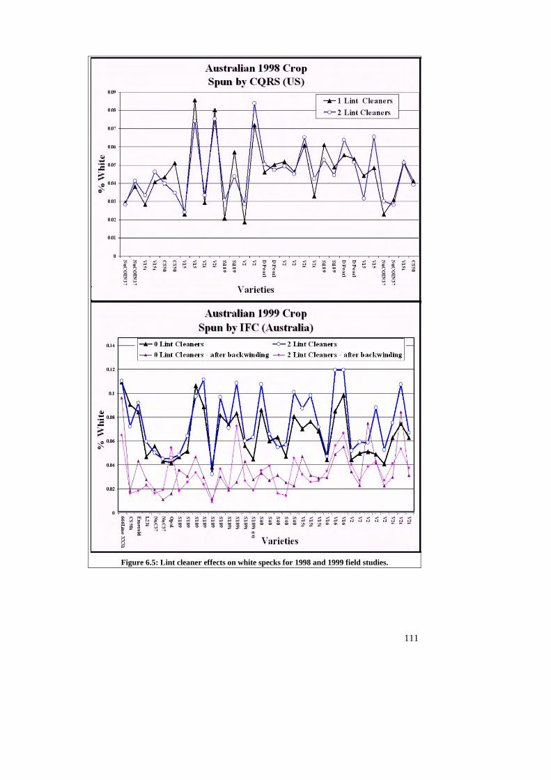
111
Figure 6.5: Lint cleaner effects on white specks for 1998 and 1999 field studies.
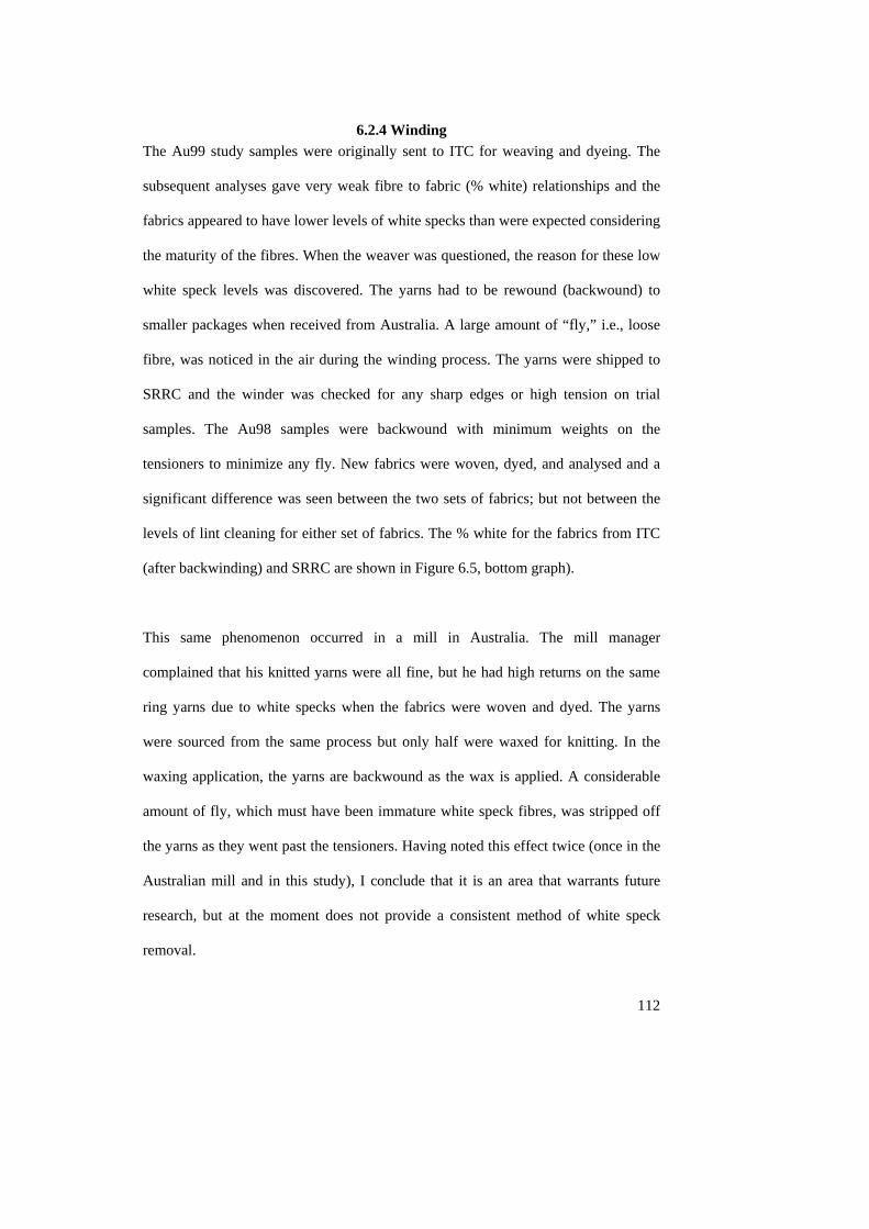
112
6.2.4 Winding The Au99 study samples were originally sent to ITC for weaving and dyeing. The
subsequent analyses gave very weak fibre to fabric (% white) relationships and the
fabrics appeared to have lower levels of white specks than were expected considering
the maturity of the fibres. When the weaver was questioned, the reason for these low
white speck levels was discovered. The yarns had to be rewound (backwound) to
smaller packages when received from Australia. A large amount of “fly,” i.e., loose
fibre, was noticed in the air during the winding process. The yarns were shipped to
SRRC and the winder was checked for any sharp edges or high tension on trial
samples. The Au98 samples were backwound with minimum weights on the
tensioners to minimize any fly. New fabrics were woven, dyed, and analysed and a
significant difference was seen between the two sets of fabrics; but not between the
levels of lint cleaning for either set of fabrics. The % white for the fabrics from ITC
(after backwinding) and SRRC are shown in Figure 6.5, bottom graph).
This same phenomenon occurred in a mill in Australia. The mill manager
complained that his knitted yarns were all fine, but he had high returns on the same
ring yarns due to white specks when the fabrics were woven and dyed. The yarns
were sourced from the same process but only half were waxed for knitting. In the
waxing application, the yarns are backwound as the wax is applied. A considerable
amount of fly, which must have been immature white speck fibres, was stripped off
the yarns as they went past the tensioners. Having noted this effect twice (once in the
Australian mill and in this study), I conclude that it is an area that warrants future
research, but at the moment does not provide a consistent method of white speck
removal.
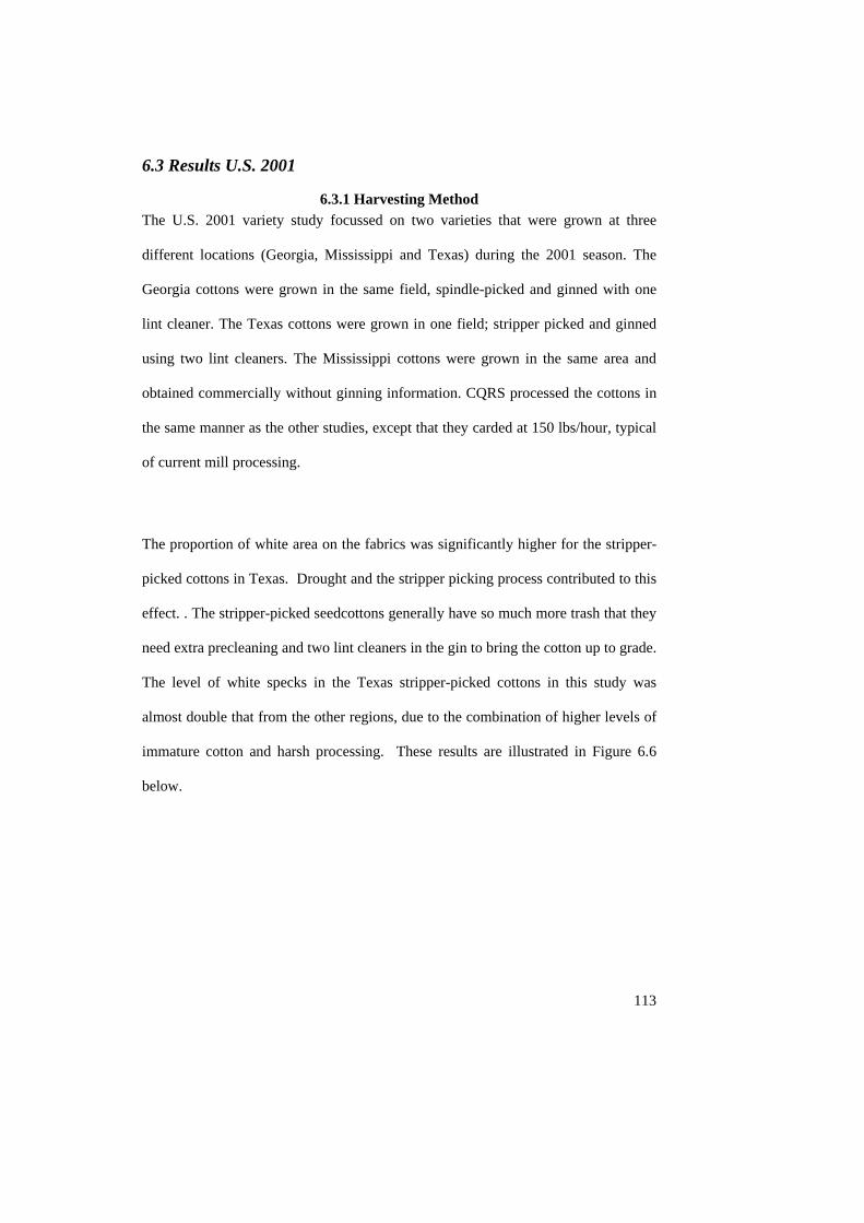
113
6.3 Results U.S. 2001
6.3.1 Harvesting Method The U.S. 2001 variety study focussed on two varieties that were grown at three
different locations (Georgia, Mississippi and Texas) during the 2001 season. The
Georgia cottons were grown in the same field, spindle-picked and ginned with one
lint cleaner. The Texas cottons were grown in one field; stripper picked and ginned
using two lint cleaners. The Mississippi cottons were grown in the same area and
obtained commercially without ginning information. CQRS processed the cottons in
the same manner as the other studies, except that they carded at 150 lbs/hour, typical
of current mill processing.
The proportion of white area on the fabrics was significantly higher for the stripper-
picked cottons in Texas. Drought and the stripper picking process contributed to this
effect. . The stripper-picked seedcottons generally have so much more trash that they
need extra precleaning and two lint cleaners in the gin to bring the cotton up to grade.
The level of white specks in the Texas stripper-picked cottons in this study was
almost double that from the other regions, due to the combination of higher levels of
immature cotton and harsh processing. These results are illustrated in Figure 6.6
below.
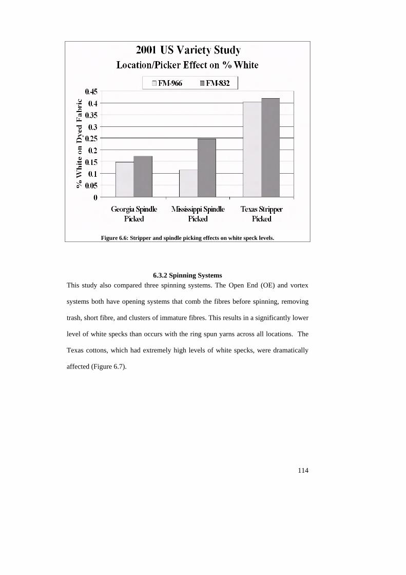
Figure 6.6: Stripper and spindle picking effects on white speck levels.
6.3.2 Spinning Systems This study also compared three spinning systems. The Open End (OE) and vortex
systems both have opening systems that comb the fibres before spinning, removing
trash, short fibre, and clusters of immature fibres. This results in a significantly lower
level of white specks than occurs with the ring spun yarns across all locations. The
Texas cottons, which had extremely high levels of white specks, were dramatically
affected (Figure 6.7).
114
Figure 6.7: OE and Vortex spinning remove white specks. The resultant fabrics are significantly
lower in white specks levels than fabrics made from ring spun yarns
6.4 Field Studies’ Conclusions To put all of the studies in perspective and so enable direct comparisons, the data
were adjusted for each study to allow for fabric structure and yarn size as if all yarns
were 30/1 and the fabrics were 100% experimental yarns. Visually the fabrics can be
broken into several groups, based on my judgment from the hundreds of fabrics I
analysed in this project.
Excellent fabrics < 0.03 %W Acceptable fabrics < 0.07 %W Poor fabrics > 0.09 %W
Figure 6.8 shows the results from the five different white speck studies described in
this thesis.
115
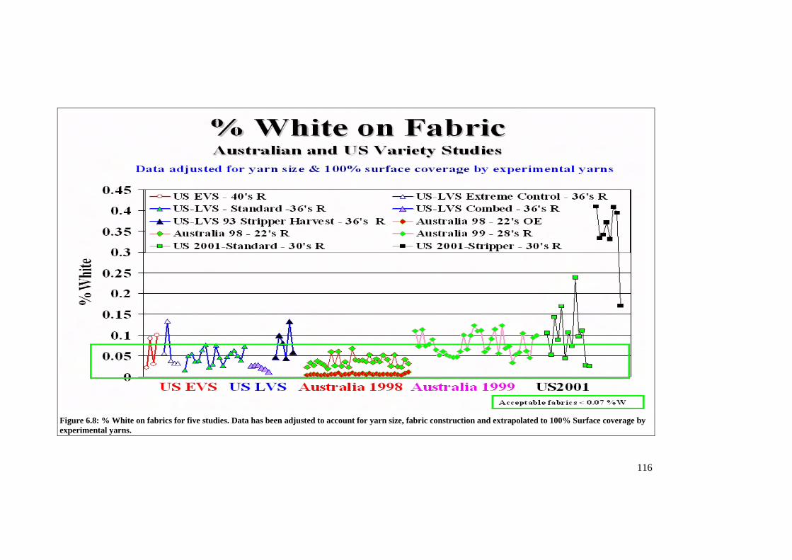
Figure 6.8: % White on fabrics for five studies. Data has been adjusted to account for yarn size, fabric construction and extrapolated to 100% Surface coverage by experimental yarns.
116
117
The initial study (U.S. EVS) is the only one that used a full warp and filling for each
fabric from the experimental fibres. The remaining studies have a common combed
warp (to remove the white specks) and the experimental filling yarns are used to
weave a filling faced sateen fabric that has approximately 85% surface coverage
from the experimental yarns. The white speck data have been adjusted for yarn size
and fabric construction as if all fabrics were 100% surface coverage with 30’s filling
yarns, so the results can be evaluated on the same basis. The coloured lines are to
help identify the individual studies. The first study, U.S. EVS, is simply the first four
data points indicated by the white circles (red lines). DP90 and EAC-30 both yielded
excellent fabrics, while the STV825 and EAC-32 were visibly poor fabrics due to the
high level of white specks. The results were as expected, with the level of white
specks being extremely low and extremely high for the two Acala varieties (see
Chapter 4).
The next study, U.S. LVS (triangles and blue lines), also included a control with
varieties that were expected to range from extremely low to extremely high levels of
white specks. All of the cottons were processed identically in the mill by CQRS. The
five white triangles indicate the extreme control varieties in the study for that year.
The extreme control group was also grown in the same field and processed
identically to those in the previous extreme study. The green triangles indicate the
varieties with one and two lint cleaners. The purple triangles indicate the varieties
that were combed and have very low levels of white specks. Finally, the black
triangles are for the varieties that were heavily cleaned (stripper harvested with 2 or 3
lint cleaners).
118
The LVS data show significant differences in levels of white specks due to
processing. Most of the cottons in the LVS fall within a range that is visibly
acceptable. The green box indicates the range (% White < 0.07%) representing
acceptable levels of white speck. Any value greater than this is likely to be
problematic. The combed cottons are nice and clean, below the 0.05 percent level.
In the third study, Australia 1998 (diamonds) cotton was considered one of the best
crop years in Australian history. The cotton had excellent fibre properties and as
shown in Fig 5.24, produced excellent fabrics, many of which were as good as
combed cottons. The seedcottons were brought to the same gin and both 1 and 2 lint
cleaners were used. This particular crop year produced very mature fibres and no
significant difference was seen due to lint cleaning. This study showed there was a
difference due to yarn sizes and type of spinning system. OE spinning combined with
one of Australia’s best crop years produced fabrics that had the lowest white speck
levels of all the studies.
The fourth study, Australia’s 1999 crop (green diamonds, pink lines), had maturity
problems due to drought and the levels of white specks were significantly higher than
for the 1998 crop. The Australian 1999 crop yield was less than anticipated due to
late planting, high insect pressure and harvest rains, all of which contributed to a
smaller, lower quality crop. There were unusually wet conditions before planting,
and a summer that was not exceptionally hot; in addition, aphid numbers were much
higher than usual. In addition to these problems, some areas of the Australian cotton
crop suffered from an unidentified disease or virus, which seemed to be associated
with the presence of aphids early in the season. The disease resulted in low numbers
119
of bolls, and small bolls containing only 5-6 seeds (usually 9 or 10) 159(Southern
Hemisphere Crop report 4/26/1999). The report states, “Fortunately, the quality of
this cotton has not been affected, only yields. All parameters have been more than
adequate, with all merchants extremely satisfied with the quality outruns160(Southern
Hemisphere Crop report 4/26/1999).” This illustrates that what appears to be a good
crop by HVI standards may in fact be a poor quality crop when the final product
(dyed fabric) is judged. The 1999 crop resulted in white speck problems in the mills
in 2000.
The Australia 1999 crop’s higher white speck levels are more similar to the standard
cottons in the final study, i.e., the U.S. 2001 study (shown as black lines, with green
squares for the standard cottons and black squares for the stripper-harvested cottons),
which also experienced weather problems that affected maturity. The higher white
speck level is also due to higher carding rates (150 lbs per hour as compared to 70 lbs
per hour). High cylinder speeds are known to increase nep levels. The stripper-
harvested crops are black squares for the US 2001 crop and black triangles for the
U.S. LVS crop; in both cases, the excess cleaning significantly increased the level of
white specks compared to the varieties with standard cleaning for those years. The
higher carding rates make the U.S.2001 stripper samples the most extreme (highest
% White) in the study. When all of this information is analysed, the measurements of
immaturity can be evaluated to predict levels of the white speck phenomenon. Many
measurement systems are attempting to characterize maturity. Results obtained from
several of these systems will be presented in the next chapter.
120
7. WHITE SPECK MODEL DEVELOPMENT PREDICTING WHITE SPECKS FROM
HIGH-SPEED FIBRE MEASUREMENT SYSTEMS This chapter combines and analyses the results and knowledge presented in the
previous chapters to develop prediction equations of white speck from fibre data
measured by several high-speed fibre measurement systems.
7.1 Introduction The studies undertaken in this project provide an enormous amount of insight into
mechanical processing effects on white specks, but only the last study was processed
at the higher speeds used by industry. The US 2001 cottons are therefore considered
to provide the best set of data to develop prediction equations of white specks in
fabrics from fibre properties. Not only did the US 2001 study have higher carding
rates, it also had the widest range in white speck levels of all of the studies. Some
white speck levels were as low as those found in some of the combed cottons in the
LVS study. The stripper-harvested cottons from regions with drought problems had
the highest white speck levels in all of the studies.
Ring, Open End and Vortex yarns were spun for this study, but the OE and Vortex
spinning removed the bulk of the white specks, so the prediction equations are based
on data from the fabrics made with ring spun filling. Cross-sections, FMT, HVI,
AFIS, and Lintronics provided measured fibre properties from the bale.
The present cotton marketing system is based on average values of fibre length,
strength, micronaire, colour and trash. The commercial price only reflects fibre value
on a broad basis. With increased processing speeds, more cleaning of fibre, new
varieties, field treatments and other improvements such as genetically engineered
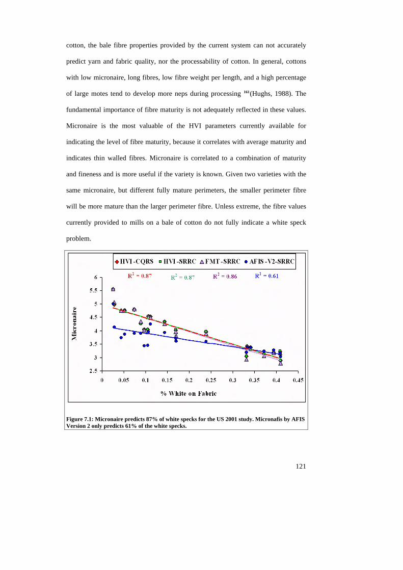
cotton, the bale fibre properties provided by the current system can not accurately
predict yarn and fabric quality, nor the processability of cotton. In general, cottons
with low micronaire, long fibres, low fibre weight per length, and a high percentage
of large motes tend to develop more neps during processing 161(Hughs, 1988). The
fundamental importance of fibre maturity is not adequately reflected in these values.
Micronaire is the most valuable of the HVI parameters currently available for
indicating the level of fibre maturity, because it correlates with average maturity and
indicates thin walled fibres. Micronaire is correlated to a combination of maturity
and fineness and is more useful if the variety is known. Given two varieties with the
same micronaire, but different fully mature perimeters, the smaller perimeter fibre
will be more mature than the larger perimeter fibre. Unless extreme, the fibre values
currently provided to mills on a bale of cotton do not fully indicate a white speck
problem.
Figure 7.1: Micronaire predicts 87% of white specks for the US 2001 study. Micronafis by AFIS Version 2 only predicts 61% of the white specks.
121
122
Immature fibres are the ultimate cause of white specks and micronaire is the
measurement that has been classically used to judge maturity. Graph 7.1 shows that
micronaire as measured by HVI and FMT predicts approximately 87% of the white
specks seen on the dyed fabric. Micronafis is the Micronaire measurement provided
by AFIS Version 2 but it tends to be lower (only 61%) than the classical
measurements.
7.2 Methodology This study was designed from the standpoint that cotton is ultimately valued at the
consumer product level, so the best way to gauge the effects of a particular factor in
cotton processing is to analyse its effect on realised quality, that is, quality seen at the
fabric stage. However, since quality of cotton is based on fibre quality, fibre
measurements from different testing systems must be correlated with levels of white
specks on the fabrics. Multiple regressions were used to investigate the relationship
between several independent or predictor variables and the dependent or criterion
variable, % white, by using the "least squares" method to fit a line through a set of
observations. Multiple linear regressions are used to analyse how a single dependent
variable is affected by the values of one or more independent variables.
Multiple regression designs contain the separate simple regression designs for two or
more continuous predictor variables. The regression equation for a multiple
regression design for the first-order effects of three continuous predictor variables P,
Q, and R would be
Y = b0 + b1P + b2Q + b3R.
The regression line expresses the best prediction of the dependent variable (Y) in this
123
case % White, given the independent variables (X), fibre properties. However, nature
is rarely (if ever) perfectly predictable, and usually there is substantial variation of
the observed points around the fitted regression line. The deviation of a particular
point from the regression line (its predicted value) is called the residual value. The
difference between unity (1.0) and the ratio of the residual variability of the Y
variable to the original variance is referred to as R-square (R2) or the coefficient of
determination. If we have an R2 of 0.4 then we know that the variability of the Y
values around the regression line is 1-0.4 times the original variance; in other words,
we have explained 40% of the original variability, and are left with 60% residual
variability. Ideally, we would like to explain most if not all of the original variability.
The R2 value is an indicator of how well the model fits the data (e.g., an R2 close to
1.0 indicates that we have accounted for almost all of the variability with the
variables specified in the model) 162(StatSoft, 2004).
Choice of the Number of Variables. Multiple regression is a seductive
technique: "plug in" as many predictor variables as you can think of and usually at
least a few of them will come out as being significant. This is because one is
capitalizing on chance when simply including as many variables as one can think of
as predictors of some other variable of interest. This problem is compounded when
the number of observations is relatively low. Intuitively, it is clear that one can
hardly draw conclusions from an analysis of 100 questionnaire items based on 10
respondents. Most authors recommend that one should have at least 10 to 20 times as
many observations (cases, respondents) as one has variables, otherwise the estimates
of the regression line are probably very unstable and unlikely to replicate if one were
to do the study over.
124
For these regressions, all of the fabric data was adjusted to compensate for yarn size,
and fabric structure. All % white data was based on 30’s ring spun yarns with 100%
surface coverage of experimental yarns. Because the sample set (US2001 study) is
only 21 fabrics, it was extremely important to minimise the number of variables in
the predictions. % White for each of the 21 fabrics were analysed in linear
regressions with each variable for each system. The variable with the highest R-
square was considered the starting point for the multiple regressions developed for
each system. The other variables were systematically added in and regressed against
% white. The variable that showed the largest improvement in the adjusted R2 was
then entered as the second variable and this process continued until reductions were
seen in the adjusted R2. If the adjusted R2 drops from .89 to .85 even though the R2
may have improved from .90 to .95, it indicates that the improvement in R2 isn’t
valid and the variable should be dropped as part of the final regression. Knowledge
of the subject is also important in ensuring that the result is meaningful. In AFIS,
perhaps both average length by number and average length by weight may improve
the R2, but only one would be needed and the one which raises the adjusted R2 the
most would be the preferred choice. Between statistical and logical evaluation, the
final fibre properties that had the best regressions for each test were used to make the
final predictions. SAS/STAT® Analysis software, (Version 8.02 of the SAS System
for Windows TS Level 02M0 Copyright, SAS Institute Inc. SAS and all other SAS
Institute Inc. product or service names are registered trademarks or trademarks of
SAS Institute Inc., Cary, NC, USA.) was also used to evaluate stepwise regressions
and forward regression selections. Once the final predictions were developed, they
were compared to regressions of the same fibre properties across all studies to
125
validate their legitimacy.
7.3 Model Results The fibre and white speck data for the following relationships can be found in
Appendix B. Forward selection model and stepwise regressions were run on fibre
and white speck data for all studies in SAS to verify the adjusted R-square method.
7.3.1 FMT Maturity ratio and fineness were the best predictors of white speck for FMT.
Maturity ratio alone had an R-square of 0.58 and fineness increased the R-square to
0.62 and an adjusted R-square of 0.61. The FMT (maturity ratio and fineness) data in
Figure 7.2 show a strong relation to white specks for the 2001 study, but when
evaluating all of the studies together, the R-square drops down from 0.86 (adjusted
R2 = 0.85) to 0.62, which may be explained by the variations between studies such as
card condition and speeds. The % white prediction for the 2001 fabrics is slightly
higher than the predicted % white based on all studies. This is due to the increase in
carding rates for the 2001 study. As cylinder speeds increase, nep levels increase
making this 2001 study more accurate for current mill processing rates. It also has a
much higher R-square explaining approximately 86 % of the variability of white
specks. FMT only measures maturity. Although maturity is the predominant factor
for white specks, it doesn’t tell the whole story as can be seen in analysis of some of
the other fibre measurement systems, which indicates that the FMT is not sufficient
as a basis for predicting white specks.
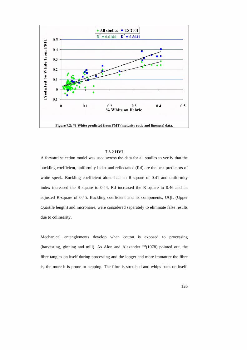
Figure 7.2: % White predicted from FMT (maturity ratio and fineness) data.
7.3.2 HVI A forward selection model was used across the data for all studies to verify that the
buckling coefficient, uniformity index and reflectance (Rd) are the best predictors of
white speck. Buckling coefficient alone had an R-square of 0.41 and uniformity
index increased the R-square to 0.44, Rd increased the R-square to 0.46 and an
adjusted R-square of 0.45. Buckling coefficient and its components, UQL (Upper
Quartile length) and micronaire, were considered separately to eliminate false results
due to colinearity.
Mechanical entanglements develop when cotton is exposed to processing
(harvesting, ginning and mill). As Alon and Alexander 163(1978) pointed out, the
fibre tangles on itself during processing and the longer and more immature the fibre
is, the more it is prone to nepping. The fibre is stretched and whips back on itself,
126
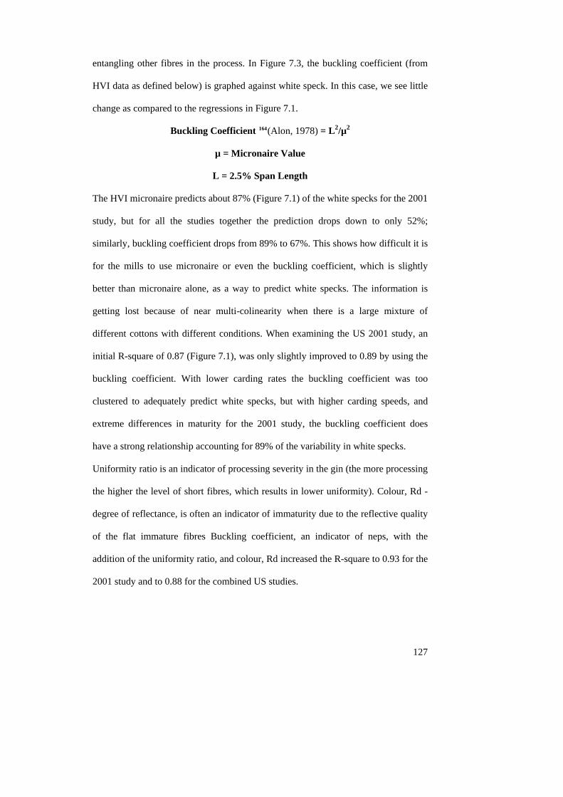
127
entangling other fibres in the process. In Figure 7.3, the buckling coefficient (from
HVI data as defined below) is graphed against white speck. In this case, we see little
change as compared to the regressions in Figure 7.1.
Buckling Coefficient 164(Alon, 1978) = L2/µ2
µ = Micronaire Value
L = 2.5% Span Length
The HVI micronaire predicts about 87% (Figure 7.1) of the white specks for the 2001
study, but for all the studies together the prediction drops down to only 52%;
similarly, buckling coefficient drops from 89% to 67%. This shows how difficult it is
for the mills to use micronaire or even the buckling coefficient, which is slightly
better than micronaire alone, as a way to predict white specks. The information is
getting lost because of near multi-colinearity when there is a large mixture of
different cottons with different conditions. When examining the US 2001 study, an
initial R-square of 0.87 (Figure 7.1), was only slightly improved to 0.89 by using the
buckling coefficient. With lower carding rates the buckling coefficient was too
clustered to adequately predict white specks, but with higher carding speeds, and
extreme differences in maturity for the 2001 study, the buckling coefficient does
have a strong relationship accounting for 89% of the variability in white specks.
Uniformity ratio is an indicator of processing severity in the gin (the more processing
the higher the level of short fibres, which results in lower uniformity). Colour, Rd -
degree of reflectance, is often an indicator of immaturity due to the reflective quality
of the flat immature fibres Buckling coefficient, an indicator of neps, with the
addition of the uniformity ratio, and colour, Rd increased the R-square to 0.93 for the
2001 study and to 0.88 for the combined US studies.
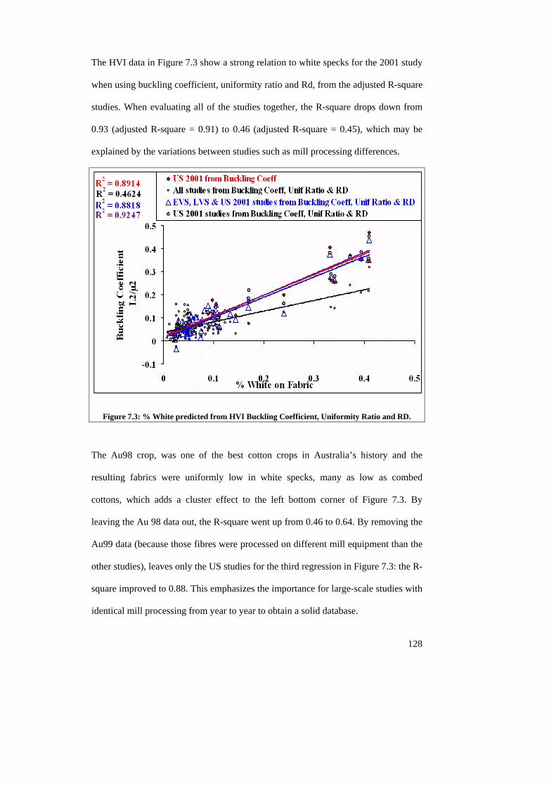
The HVI data in Figure 7.3 show a strong relation to white specks for the 2001 study
when using buckling coefficient, uniformity ratio and Rd, from the adjusted R-square
studies. When evaluating all of the studies together, the R-square drops down from
0.93 (adjusted R-square = 0.91) to 0.46 (adjusted R-square = 0.45), which may be
explained by the variations between studies such as mill processing differences.
Figure 7.3: % White predicted from HVI Buckling Coefficient, Uniformity Ratio and RD.
The Au98 crop, was one of the best cotton crops in Australia’s history and the
resulting fabrics were uniformly low in white specks, many as low as combed
cottons, which adds a cluster effect to the left bottom corner of Figure 7.3. By
leaving the Au 98 data out, the R-square went up from 0.46 to 0.64. By removing the
Au99 data (because those fibres were processed on different mill equipment than the
other studies), leaves only the US studies for the third regression in Figure 7.3: the R-
square improved to 0.88. This emphasizes the importance for large-scale studies with
identical mill processing from year to year to obtain a solid database.
128
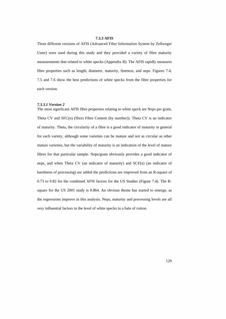
129
7.3.3 AFIS Three different versions of AFIS (Advanced Fiber Information System by Zellweger
Uster) were used during this study and they provided a variety of fibre maturity
measurements that related to white specks (Appendix B). The AFIS rapidly measures
fibre properties such as length, diameter, maturity, fineness, and neps. Figures 7.4,
7.5 and 7.6 show the best predictions of white specks from the fibre properties for
each version.
7.3.3.1 Version 2 The most significant AFIS fibre properties relating to white speck are Neps per gram,
Theta CV and SFC(n) (Short Fibre Content (by number)). Theta CV is an indicator
of maturity. Theta, the circularity of a fibre is a good indicator of maturity in general
for each variety, although some varieties can be mature and not as circular as other
mature varieties, but the variability of maturity is an indication of the level of mature
fibres for that particular sample. Neps/gram obviously provides a good indicator of
neps, and when Theta CV (an indicator of maturity) and SCF(n) (an indicator of
harshness of processing) are added the predictions are improved from an R-square of
0.73 to 0.82 for the combined AFIS factors for the US Studies (Figure 7.4). The R-
square for the US 2001 study is 0.864. An obvious theme has started to emerge, as
the regressions improve in this analysis. Neps, maturity and processing levels are all
very influential factors in the level of white specks in a bale of cotton.
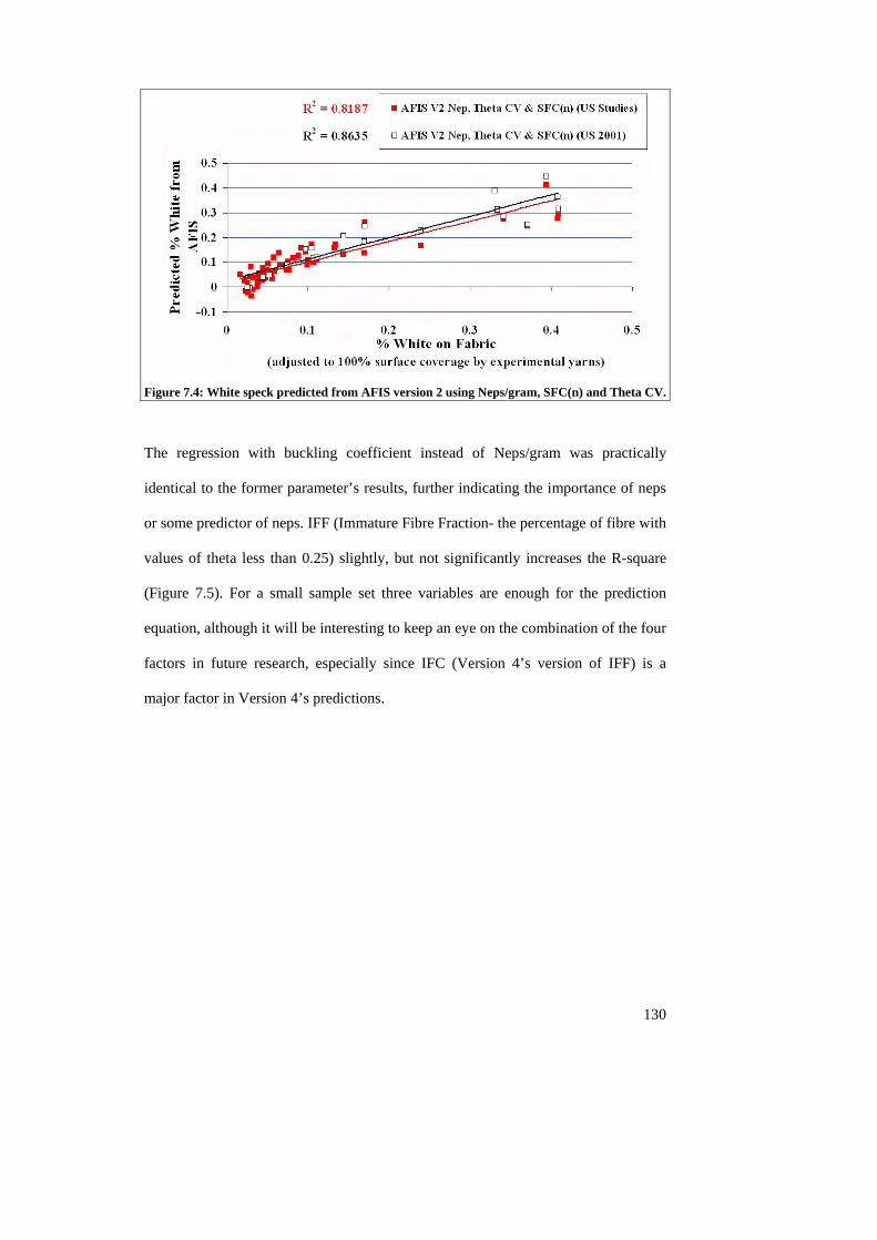
Figure 7.4: White speck predicted from AFIS version 2 using Neps/gram, SFC(n) and Theta CV.
The regression with buckling coefficient instead of Neps/gram was practically
identical to the former parameter’s results, further indicating the importance of neps
or some predictor of neps. IFF (Immature Fibre Fraction- the percentage of fibre with
values of theta less than 0.25) slightly, but not significantly increases the R-square
(Figure 7.5). For a small sample set three variables are enough for the prediction
equation, although it will be interesting to keep an eye on the combination of the four
factors in future research, especially since IFC (Version 4’s version of IFF) is a
major factor in Version 4’s predictions.
130
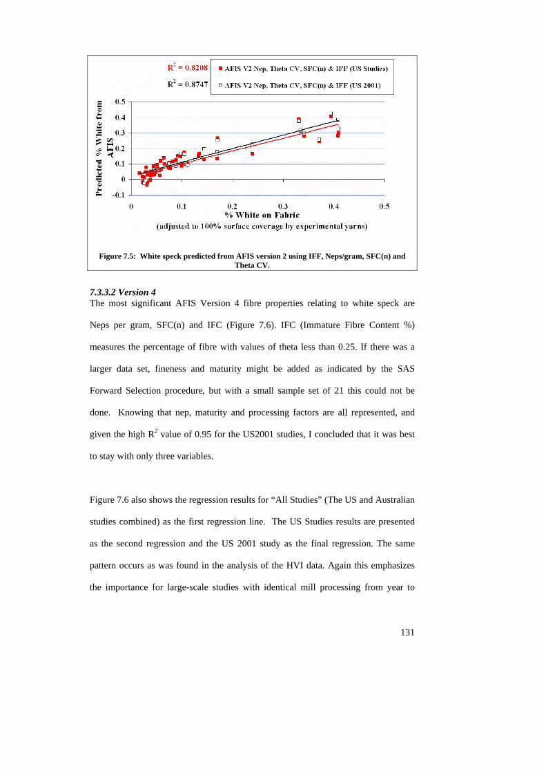
Figure 7.5: White speck predicted from AFIS version 2 using IFF, Neps/gram, SFC(n) and Theta CV.
7.3.3.2 Version 4 The most significant AFIS Version 4 fibre properties relating to white speck are
Neps per gram, SFC(n) and IFC (Figure 7.6). IFC (Immature Fibre Content %)
measures the percentage of fibre with values of theta less than 0.25. If there was a
larger data set, fineness and maturity might be added as indicated by the SAS
Forward Selection procedure, but with a small sample set of 21 this could not be
done. Knowing that nep, maturity and processing factors are all represented, and
given the high R2 value of 0.95 for the US2001 studies, I concluded that it was best
to stay with only three variables.
Figure 7.6 also shows the regression results for “All Studies” (The US and Australian
studies combined) as the first regression line. The US Studies results are presented
as the second regression and the US 2001 study as the final regression. The same
pattern occurs as was found in the analysis of the HVI data. Again this emphasizes
the importance for large-scale studies with identical mill processing from year to
131
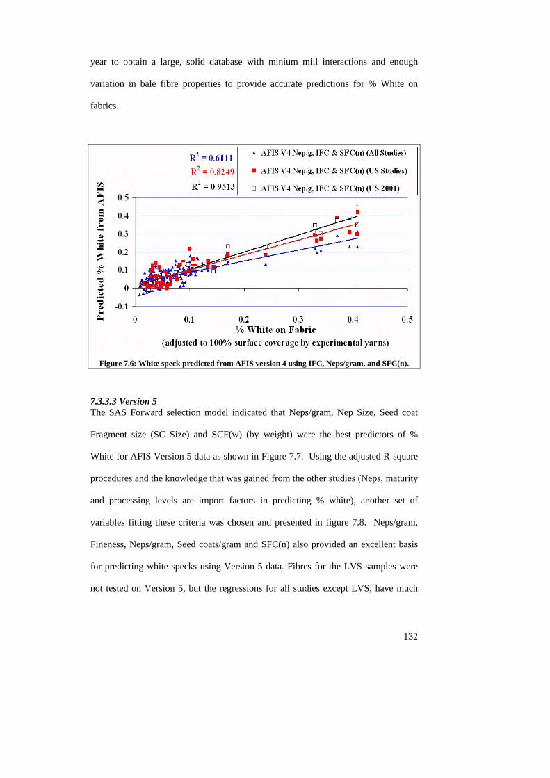
year to obtain a large, solid database with minium mill interactions and enough
variation in bale fibre properties to provide accurate predictions for % White on
fabrics.
Figure 7.6: White speck predicted from AFIS version 4 using IFC, Neps/gram, and SFC(n).
7.3.3.3 Version 5 The SAS Forward selection model indicated that Neps/gram, Nep Size, Seed coat
Fragment size (SC Size) and SCF(w) (by weight) were the best predictors of %
White for AFIS Version 5 data as shown in Figure 7.7. Using the adjusted R-square
procedures and the knowledge that was gained from the other studies (Neps, maturity
and processing levels are import factors in predicting % white), another set of
variables fitting these criteria was chosen and presented in figure 7.8. Neps/gram,
Fineness, Neps/gram, Seed coats/gram and SFC(n) also provided an excellent basis
for predicting white specks using Version 5 data. Fibres for the LVS samples were
not tested on Version 5, but the regressions for all studies except LVS, have much
132
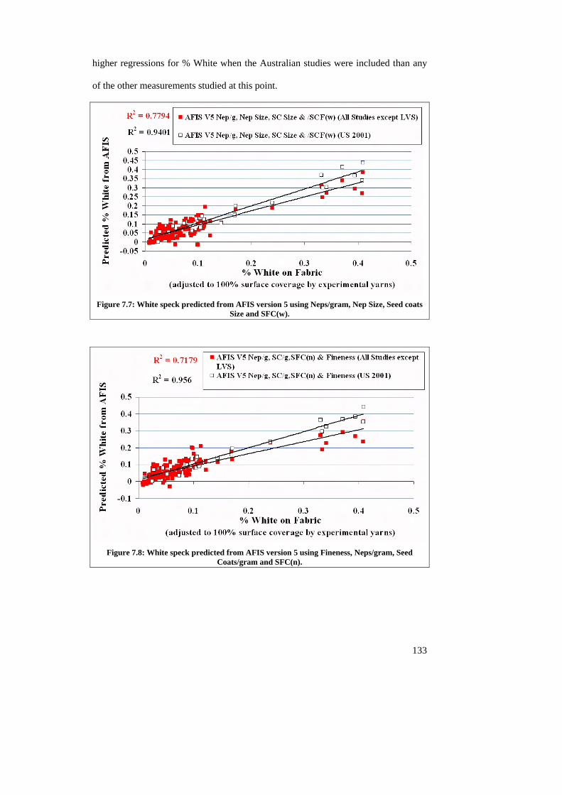
higher regressions for % White when the Australian studies were included than any
of the other measurements studied at this point.
Figure 7.7: White speck predicted from AFIS version 5 using Neps/gram, Nep Size, Seed coats
Size and SFC(w).
Figure 7.8: White speck predicted from AFIS version 5 using Fineness, Neps/gram, Seed
Coats/gram and SFC(n).
133
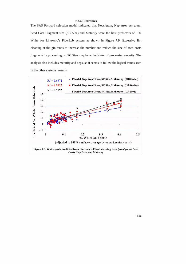
7.3.4 Lintronics The SAS Forward selection model indicated that Neps/gram, Nep Area per gram,
Seed Coat Fragment size (SC Size) and Maturity were the best predictors of %
White for Lintronic’s FiberLab system as shown in Figure 7.9. Excessive lint
cleaning at the gin tends to increase the number and reduce the size of seed coats
fragments in processing, so SC Size may be an indicator of processing severity. The
analysis also includes maturity and neps, so it seems to follow the logical trends seen
in the other systems’ results.
Figure 7.9: White speck predicted from Lintronic’s FiberLab using Neps (area/gram), Seed
Coats Neps Size, and Maturity
134
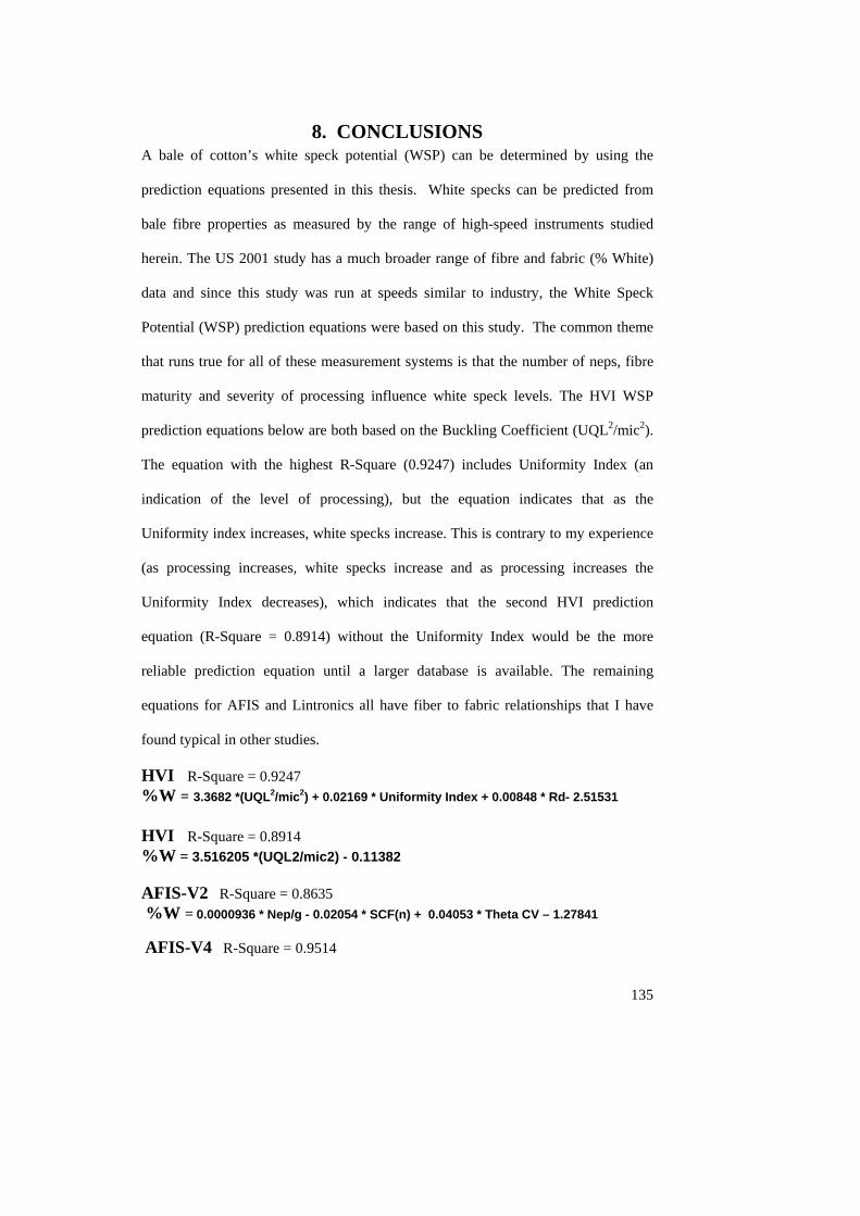
135
8. CONCLUSIONS A bale of cotton’s white speck potential (WSP) can be determined by using the
prediction equations presented in this thesis. White specks can be predicted from
bale fibre properties as measured by the range of high-speed instruments studied
herein. The US 2001 study has a much broader range of fibre and fabric (% White)
data and since this study was run at speeds similar to industry, the White Speck
Potential (WSP) prediction equations were based on this study. The common theme
that runs true for all of these measurement systems is that the number of neps, fibre
maturity and severity of processing influence white speck levels. The HVI WSP
prediction equations below are both based on the Buckling Coefficient (UQL2/mic2).
The equation with the highest R-Square (0.9247) includes Uniformity Index (an
indication of the level of processing), but the equation indicates that as the
Uniformity index increases, white specks increase. This is contrary to my experience
(as processing increases, white specks increase and as processing increases the
Uniformity Index decreases), which indicates that the second HVI prediction
equation (R-Square = 0.8914) without the Uniformity Index would be the more
reliable prediction equation until a larger database is available. The remaining
equations for AFIS and Lintronics all have fiber to fabric relationships that I have
found typical in other studies.
HVI R-Square = 0.9247 %W = 3.3682 *(UQL2/mic2) + 0.02169 * Uniformity Index + 0.00848 * Rd- 2.51531 HVI R-Square = 0.8914 %W = 3.516205 *(UQL2/mic2) - 0.11382 AFIS-V2 R-Square = 0.8635 %W = 0.0000936 * Nep/g - 0.02054 * SCF(n) + 0.04053 * Theta CV – 1.27841 AFIS-V4 R-Square = 0.9514
136
%W = 0.000484 * Neps/g + 0.07983 * IFC – 0.01006 * SFC(n) - 0.13291 AFIS-V5 R-Square = 0.9401 %W = 0.000904 * Nep Size + 0.00047 * Nep/g + 0.00059 * SC Size + 0.2283 * SFC(w) – 1.0662 Lintronic’s FiberLab R-Square = 0.9192 %W =- 0.97314 * Maturity + 0.000353 * Nep Area/g – 0.51652 * SC Size + 1.367854
These equations should be seen as providing preliminary predictions of white specks
from fibre measurements. They are based on mechanically harvested cottons and are
only the beginning of a larger scale research project. It’s clear that more studies are
required to provide a large enough database of collected fibre and fabric
measurements to improve the prediction equations. The database should have an
international fibre set including hand picked cottons, considering the world market
today, and the confusion as to the meaningfulness of high-speed fibre measurements.
The most important factor for the success of these future studies is that testing and
mill processing must be standardised from year to year. The mill equipment must
have proper settings, and consistent card wires.
This thesis has successfully provided an initial basis for the cotton industry to
quantify white speck potential from high-speed fibre data. It has also successfully
provided a foundation for continuing long-term studies to refine this basis. The US
2001 fibres and fabric have already been adopted as the first year of a continuing
follow-on study to this project. When the long-term study that is being undertaken by
SRRC and CQRS is completed, the White Speck Potential (WSP) can be confidently
expected to provide the required nep management tool for mills and breeders. The
breeders will be able to eliminate varieties that have a propensity to white speck
early on. In addition, when there is a drought situation that will result in white
specks, the affected bales can be identified. If these high WSP cottons are used in the

137
right product line, where dyeability is not a problem (such as whites), both the
producers and the mills will have solved a major economic problem. Shirting,
undergarments, and sheets and towelling are big markets that consume large
quantities of cotton, which could handle white speck cottons, without any losses due
to defects. There is a place for these cottons, where they will not cause a problem; it
just needs to be identified. Alternatively, if a mill does find it has a white speck
problem they can minimize it. First, the mill may want to check their card settings
and wire condition, if the cards are in good running order, the mills may comb it or
using open-end or vortex spinning to minimize the problem.
138
REFERENCES Agriculture Research Service Image Gallery. (2003) Image Number K4844-9
http://www.ars.usda.gov/is/graphics/photos/k4844-9.htm. Date accessed 10/5/2003
Alon, Gan, and Alexander, Ernst. (1978) “Mechanism of Nep Formation“, Melliand Textilberichte. American Society for Testing and Materials. (1947) “ASTM Standards on Textile Materials”, Annual. Book of ASTM Standards (pp. 210-211). Philadelphia, PA: ASTM. American Society for Testing and Materials. (1978) “ASTM D3216 – 78 “Grading Cotton Card Webs for Appearance”, Annual. Book of ASTM Standards (pp.641-644). Philadelphia, PA: ASTM. American Society for Testing and Materials. (1994) “ASTM Standard D 3818-92. 07.02 - Standard test method for linear density and maturity index of cotton fibers (IIC-Shirley Fineness/Maturity Tester”, Annual. Book of ASTM Standards (pp.143-146). Philadelphia, PA: ASTM. Anthony, W.S., Baker, R.V., Hughs, S.E. (1986) “Ginning for Maximum Grade without Excessive Short Fibers, Neps and Trash”, The Cotton Gin and Oil Mill Press, 14-17. Anthony, W.S., and Mayfield, W. D. (1994) “Cotton Ginners Handbook”, U.S. Department of Agriculture - Agricultural Handbook, 503. Bel-Berger PD, Vinyard BT, Thibodeaux DT. (1995) “Effect of Harvesting Times on White Specks: A Study of Field to Fabric Properties.” Proceedings of the Beltwide Cotton Production Conference, 2, 1440-1444. Bel-Berger, P. and Von Hoven, T. (1997) “Effects of Mechanical Cleaning on Cotton Fibers. Part III: Effects of Card Wire Condition on White Specks”, Textile Research Journal 67, 12 857-865. Bel-Berger, P. and Roberts, G. (1998) “Neps: How Do They Impact Cotton Quality” Proceedings of the Ninth Australian Cotton Conference, 1, 721-729. Bel-Berger, P.D., Von Hoven T., Cui, X., Davidonis, G and Pusateri, K. (1998) “The Importance of Sampling in White Speck Analysis.” Book of Papers, AATCC International Conference, 2, 600. Bel-Berger, P.D., Von Hoven T,, Cui, X., Davidonis, G and Pusateri, K. (1999) “Comparison of Sampling, Methods and Versions of AFIS”, Proceedings of the Beltwide Cotton Production Conference, 1, 681-684. Bradow, J. M., Davidonis, G. H., Bauer, P. J., Sassenrath-Cole, G. F. and Johnson, R. M. (1998) “Mapping Variability in Cotton Fiber Maturity.” Proceedings of the Beltwide Cotton Conference, 2, 1463-1465. Bradow, J. M. and Davidonis, G. H. (2000) “Quantification of Fiber Quality and the Cotton Production-Processing Interface: A Physiologist's Perspective.” The Journal of Cotton Science, 4, 34-64. Brown, H. B. and Ware, J. O. (1958) Cotton (3rd Ed) McGraw Hill Book Company, Inc. Bragg, C.K. and Simpson, C.L. (1992) “Solving Cotton Quality Problems: White Specks and Bark in Textile Products.” Proceedings of the Beltwide Cotton Production Conference, 1, 97-99. Cheek, L. and Wilcock, A, (1988) “Relationship between Direct Dye Characteristics and Coverage of Immature Fiber Neps in Dyed Cotton Fabric, J. Soc. Dyers and Colorists. 104, 477. Chellamani K. P., Chattopadhyay D. and Thanabal V. (1999) “Indian Cottons and Influence of Mechanical Processing on Nep Generation”, Asian Textile Journal, 120-126.
139
Cole, William D. (1997) “Examination of Effects of Drafting Rates o Yarn Quality”, Textile Topics, InternationalTextileCenter, http://www.depts.ttu.edu/itc/acrobat%20files/ttw98.pdf, Date accessed 11/8/2003. Cotton Program Agricultural Marketing Service U.S. Department of Agriculture. (2001) “The Classification of Cotton”, USDA Publication, http://www.cottoninc.com/CottonClassification/homepage.cfm?PAGE=646, Date accessed 10/15/2003. Cotton World. (2003) “Growers at the top of cotton game”, http://www.cottonworld.com.au/articles.php3?rc=574 Date accessed 10/24/2003. Crum, W., Phil. Soc. Glasgow Proc. On a Peculiar Fiber of Cotton Which is Incapable of Being Dyed (1848-1855. 3:61-64.1855. EconCentral. (2003) National Cotton Council, http://agriculture.about.com/gi/dynamic/offsite.htm?site=http%3A%2F%2Fwww.cotton.org%2F Date accessed 10/23/2003. Frydrych, I., Matusiak, M. and Swiech, T. (2001) “Cotton Maturity and Its Influence on Nep Formation”. Textile Research Journal, 595 - 604. Furter, R. (1992) “Reducing Neps.” Cotton International. 113-117. Golthwaite, C.F.; Smith, H. O. and Barnitt, M. P. (1947) “New Dye Technique Shows Maturity of cotton”. Textile World, 97, 105-108. Gordon, S.G.; Montalvo, J.G. Jr.; Faught, S. E.; Grimball, R.T.; and Watkins, T. A. (1997) “Theoretical and experimental profiles of fiber fineness and maturity using the Shirley Micromat and the Zellweger Uster advanced fiber information system module”. Text. Res. J. 67 (8): 545-555. Goynes, W.R., B.F. Ingber, and D.P. Thibodeaux. (1994) “White specks: A Microscopic Profile”. Proceedings of Cotton Beltwide Cotton Conference, 1994. Goynes, W. R., Ingber, B. F., and Thibodeaux D. P., (1995) “Introductory Study of Structures of Cotton Motes and Mote Fibers.” Textile Research Journal, 65, 4 219-225. Goynes, W. R., Ingber, B. F., and Triplett, B, (1995) “Cotton Fibers Secondary Wall Development – Time versus Thickness.” Textile Research Journal, 65, 7 400-408. Goynes, W. R., Bel-Berger, P. D., Blanchard, E. I., Ingber, B. F. Graves, E.E., Dastoor, P., Von Hoven, T. M. (1996) “Identification, Quantification and Elimination of White Speck Defects on Dyed Cotton Fabrics.” American Association of Textile Chemists and Colorists Conference Paper, 9-16. Greb, Peggy. (2000) Image Number K8706-7, http://www.ars.usda.gov/is/graphics/photos/jan00/k8706-7.htm. Date accessed 11/15/2003. Harrison, R.E, Bargeron III, J.D. (1986) “Comparison of Several Nep Determination Methods.” Textile Research Journal, 56, 2 77-79. Hebert, J.J., Boylston, E.K., and Thibodeaux, D.P. (1988) “Anatomy of a Nep.” Textile Research Journal, 58, 7 380-382. Hughs, S.E., Lalor, W.F., Wahba, F.T. (1988) “Relationship of Ginning and Fiber Properties to Dyeing Imperfections”, Textile Research Journal, 58, 10 557-564. Hunter L. and van der Sluijs, M. H. J. (1996) “Neps in Cotton Lint”, Melliand English, E81 - E82. Jakes, K. A.; Unble, B. A. (1984) “Chemical and physical structure of neps selected in non woven fabrics.” Textile Research Journal, 54, 644-648.
140
Joseph, L. M. (1986) Introductory Textile Science (Fifth Edition). New York: CBS College Publishing. Kaufman, D. (1964) Studies on the Revolving Flat Card. U. S. D. A., 42. Lord, E., and S.A. Heap. (1988) “The Origin and Assessment of Cotton Fiber Maturity”, International Institution for Cotton, Manchester, UK. Mangialardi Jr., G.J. (1985) “Neps in Ginned Lint: A Review of Research”, Beltwide Cotton Production Research Conferences, 358-362. Mangialardi Jr., G.J. (1985) “An Evaluation of Nep Formation at the Cotton Gin” Textile Research Journal, 55, 12 756-761. Mangialardi Jr., G. J., Lalor, W.F., Bassett, D. M., and Miravalle, R.J. (1987)“Influence of Growth Period on Neps in Cotton”, Textile Research Journal, 57, 7 421-427. Mangliardi, G. J. and Lalor, W. F. (1990) “Propensity of Cotton Varieties to Neppiness”, Transactions of the ASAE, 36, 6 1748-1758. Manohar, J. S., Rakshit, A. K. and Balasubramanian, N. (1983) “Influence of Rotor Speed, Rotor Diameter, and Card Conditions on Yarn Quality in Open-End Spinning”, Textile Research Journal, 497-502. Marth, Charles T., Arthur, Harry E., and Berkley, Earl E. (1952) “Fiber Fineness (Micronaire), Neps in Card Web, and Yarn Appearance Grades”, Textile Research Journal, 22, 9 561-566. Marvin, (1973) Textile Processing Vol. 1, State Dept. of Education South Carolina and Clemson University. Midgley, E. (1933) “Defects in Dyed Cotton Goods; a Consideration of the Causes”, Textile Weekly, 11, 261 20-21. Miravaille, R. J., Mangialardi, G.J., Lalor, W.F. (1986) “Neps in cotton genotypes grown in six locations across the cotton belt in 1984”, Proceedings of the Beltwide Cotton Production Research Conference, 426-428. Montalvo, J.G., Jr., and Faught, S. E. (1995) “Determination of Maturity/Fineness by FMT and Diode-Array HVI. Part I. FMT (Micromat Model) Procedure of Optimization”, Proceedings of the Beltwide Cotton Production Research Conference 1276-1278. Montalvo, Jr., J.G., Joseph, J. R. and Faught, S. E. (1998) “Headspace Resistance Standards for the Shirley Developments Limited Micromat Tester”, The Journal of Cotton Science, 4, 269-277. Montalvo, J.G. Jr., Faught, S.E. and Buco, S.M. (1989) “An Investigation of the Relationship Between Cotton Fineness and Light-Scattering from Thin Webs as Measured by Near-Infrared Transmission spectroscopy”, Applied Spectroscopy, 43, 1459-1471. Montalvo, J.G., Jr. (2001). Theory of single and independent reference methods for cotton fineness and maturity. Presented to the Cotton Research Planning meeting, SRRC, New Orleans, Louisiana. Montalvo, Jr., J.G., Faught, S. E. and Buco, S. M. (2002) “Sensitivity of the Shirley Developments Ltd. Micromat Tester to Operators and Sample Preparations”, The Journal of Cotton Science, 6, 133–142. Moore, J.F. (1996) “Cotton Classification and Quality”. In E.H. Glade Jr., L.A. Meyer, and H. Stults (Ed) The Cotton Industry in the United States (pp. 51-57). Washington, DC: USDA-ERS Agric. Econ. Rep. 739. U.S. Gov. Print. Office.
141
Mor, U. (2003) “A New Generation of Fast Fiber Testers Gives Hope to a Major Improvement in the Field of Fiber Quality Control at the Spinning and Ginning Mills”, http://www.lintronics.com/articale2.htm, Date accessed 11/28/2003. Nance, David (date unknown) “Cotton Harvesting”, Image Number K5927-2, http://www.ars.usda.gov/is/graphics/photos/may02/k5927-21.htm, Date accessed 11/28/2003. National Cotton Council. (2003) The World of Cotton, Economics, http://agriculture.about.com/gi/dynamic/offsite.htm?site=http%3A%2F%2Fwww.cotton.org%2F, Date accessed 11/4/2003 Naylor, G.R.S., (2002), “Murata Vortex Spinning: A New Spin on Textile Processing” The Australian Cottongrower, 23(1), p26-27. Norman, B.M. (1991) “HVI Classing and its Effects on Ginning.” The Fourth Annual Engineered Fiber Selection Conference. Charlotte, North Carolina. Peirce, F. T. and Lord, E., (1939) “The Fineness and Maturity of Cotton”, Journal of the Textile Institute, 30, T173-T210. Peter, U. and Bowes, Q. (1989) “Quality Variations in Cotton and Their Effects on Bleaching, Dyeing and Finishing”, Melliand Textilberichte, 70, 135-137. Potter, M. D. and Corbman, B. P. (1967) “Textiles: Fiber to Fabric”, Fourth Edition, McGraw-Hill, Inc. Ramey Jr., H. H. (1988) “The Meaning and Assessment of Cotton Fiber Fineness”, International Institute for Cotton, 1-19. Schiller, Susannah and Eberhardt, Keith. (1991). "Combining Data from Several Chemical Analytic Techniques." Spectrochimica Acta Acta, Vol. 46B, No. 12. Schreiner, (date unknown) http://www.cottoninc.com/insideout/homepage.cfm?PAGE=2643, Date accessed 8/24/2003. Southern Hemisphere Crop report April 26, (1999) http://cotton.net/AustCrop.htm 7/21/99). StatSoft, Inc. (2004). Electronic Statistics Textbook. Tulsa, OK: StatSoft. WEB: http://www.statsoft.com/textbook/stathome.html. Date accessed 12/2/2003. STONEVILLE, Miss. (AP). (1997) “Scientist finds miniscule flaws in cotton fibers.” Copyright Lubbock Avalanche-Journal, http://www.lubbockonline.com/news/072697/scientis.htm Date accessed 8/13/2003. Supak, J. R. (1986) “Solving Cotton Quality Problems: White Speck and Barky Cotton.” Proceedings of the Beltwide Production Conference, 1, 94-96. Thibodeaux, D. P., and Evans, J.P. (1986) “ Cotton Fiber Maturity by Image Analysis”, Textile Research Journal, 56, 2 130-139. Thibodeaux, D. P, Montalvo, J. Jr., Davidonis, G.and McAlister, D. (2003) Effects of Location on Distributions of Fiber Quality. Proceedings of the Beltwide Cotton Conferences, 2580 - 2588. USDA, (1994)“Fiber and Processing Tests, Survey of Leading Cotton Varieties, Crop of 1993”, US Department of Agriculture Agricultural Marketing Service, Cotton Division. van der Sluijs, M. H. J. and Hunter, L. (1999) “Neps in Cotton Lint.” Textile Progress, 28, 4 1-51. van der Sluijs, M. H. J. (1996) “The Influence of Fiber Properties on Neps in South African Cotton”,

142
MSc Dissertation, University of Port Elizabeth. Verschraege, L. (1989) “Cotton Fibre Impurities: Neps, Motes and Seed Coat Fragments.” ICAC Review Articles on Cotton Production Research No.1. Von Hoven, Terri. (1996) “Comparison of Image Analysis Systems for their Ability to Detect the White Speck Phenomenon.” MSc Dissertation Georgia Institute of Technology. Watson, M. D., Carter, F. L. and Cloninger, Jr., A. E. (1991) “An Update on New Chemical Test Methods to Detect Dye Resistant Neps in Raw Cotton." Proceedings of the Beltwide Cotton Production Conference, I, 878-879. Wegener, W. (1980) “Nature, Formation, and Reduction of Neps and Slubs”, Textil Praxis International, 35, 2 130-135. Werber, F. X. and Backe, E.E. (1994) “Textile Industry Needs”, Agriculture Handbook, USDA, 503, 293-306. Wright, David. (date unknown) “Cotton stripper harvesting UNR cotton near Altha, Florida”, Image Number K8719-1, http://www.ars.usda.gov/is/graphics/photos/jan00/k8719-1.htm, Date accessed 11/28/2003. Wulfhorst, B. and Bergmann, J. (1989) “Detection of Disruptive Particles in Cotton Fibre Webs Using Digital Image Processing”, Melliand Textilberichte. 70, 12 377-379. Yankey, Joseph M. (1996) “The Value of Fiber Testing in the Ginning Industry.” Beltwide Cotton Conferences, 1654-1657.
143
APPENDIX A
Processing Flow Charts
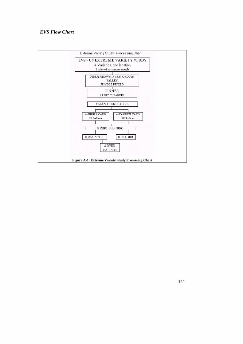
EVS Flow Chart
Figure A-1: Extreme Variety Study Processing Chart
144
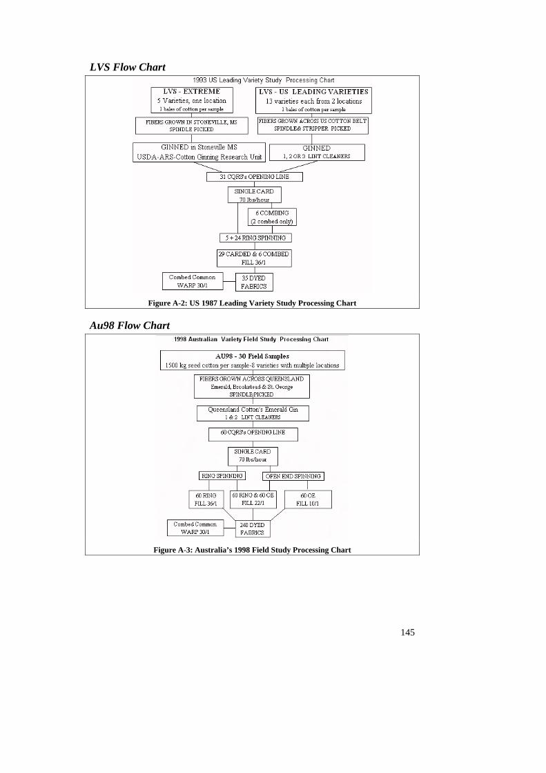
LVS Flow Chart
Figure A-2: US 1987 Leading Variety Study Processing Chart
Au98 Flow Chart
Figure A-3: Australia’s 1998 Field Study Processing Chart
145
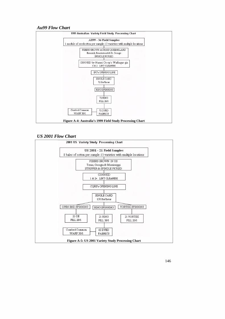
Au99 Flow Chart
Figure A-4: Australia’s 1999 Field Study Processing Chart
US 2001 Flow Chart
Figure A-5: US 2001 Variety Study Processing Chart
146

147
Opening & Carding: 2 - 300 pound blended bales were carded at 150 pounds per hour similar to industry speeds.
Drawing 1st: The card sliver was split into 4 equal groups for further processing:
1. For Open End Spinning - Used RSB 51 - Made 55 gr. sliver for spinning.
2. For Ring Spinning - Used RSB 951 - Made 60 gr. sliver for 2nd drawing.
3. For Vortex Spinning - Used RSB 951 - Made 55 gr. sliver for 2nd drawing.
Drawing 2nd:
1. For Ring Spinning - Used RSB51 -Made 61 gr. sliver for roving. 2. For Vortex Spinning - Used RSB 951 -Made 45 gr. sliver for 3rd drawing.
Drawing 3rd:
1. For Vortex Spinning - Used RSB 51 -Made 24 cans for spinning 40 gr.
sliver.
Roving For Ring Spinning: Made 0.75 HR (Hank Roving) with a 1.30 TM (Twist Multiplier) for spinning.
Spinning:
1. OES: Spin 20/1’s with a 4.6 TM. 2. Ring: Spin 20/1’s with a 4.3 TM. 3. Vortex: Spin 20/1’s.
Weaving: The yarns were woven at 90 picks per inch as a 4/1 filling faced sateen (a 5 harness sateen with a 2 move sateen pattern) in a combed common warp (30/1 ring yarns, 72 ends/inch).

149
APPENDIX B
Fabric White Speck Data & Fibre Data
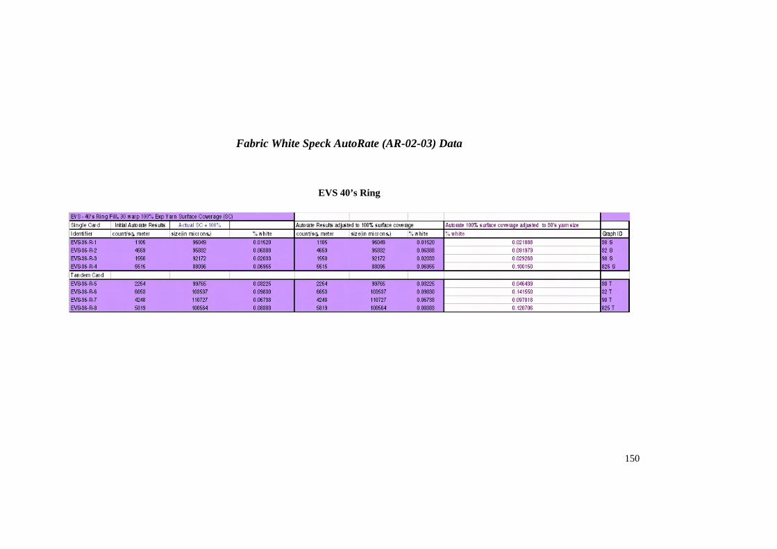
Fabric White Speck AutoRate (AR-02-03) Data
EVS 40’s Ring
150
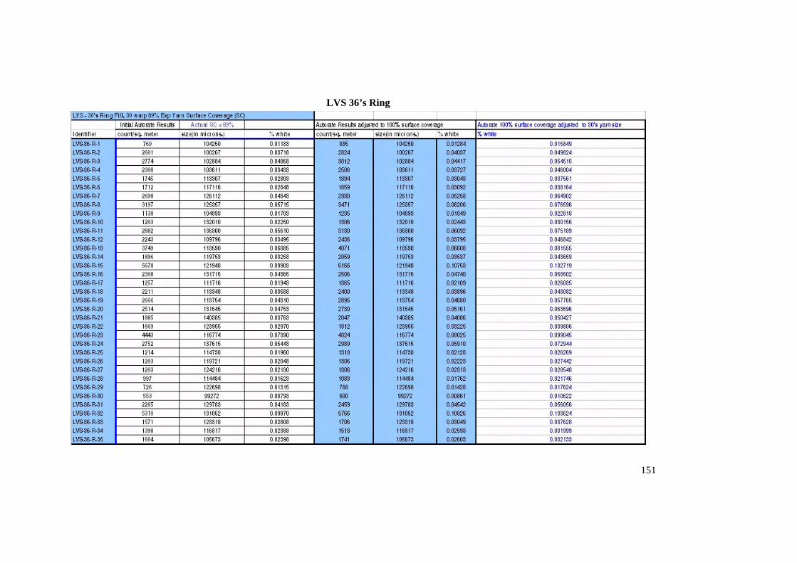
LVS 36’s Ring
151

Au98 36’s Ring
152
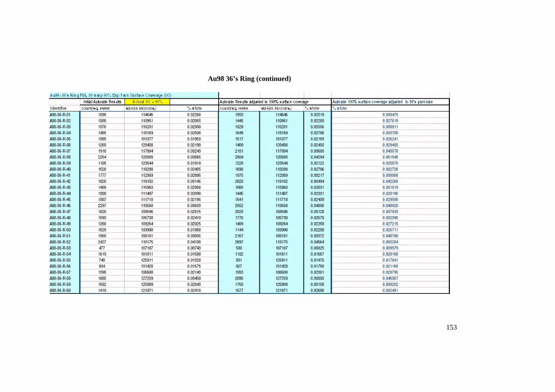
Au98 36’s Ring (continued)
153

Au98 22’s Ring
154
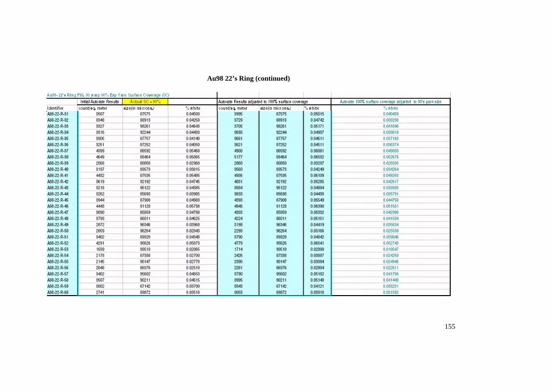
Au98 22’s Ring (continued)
155
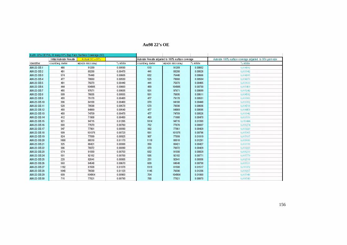
Au98 22’s OE
156
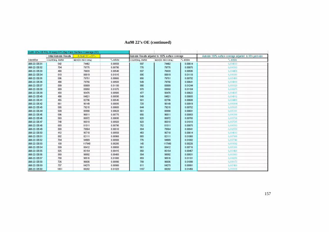
Au98 22’s OE (continued)
157
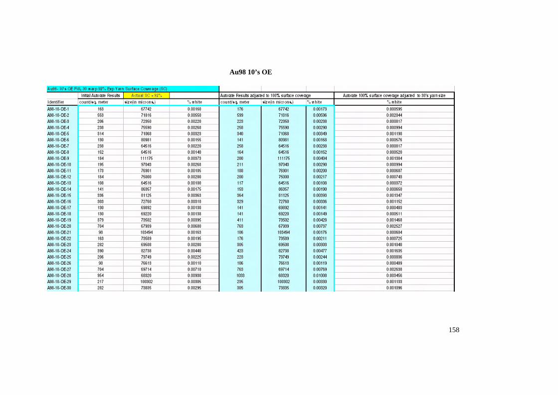
Au98 10’s OE
158
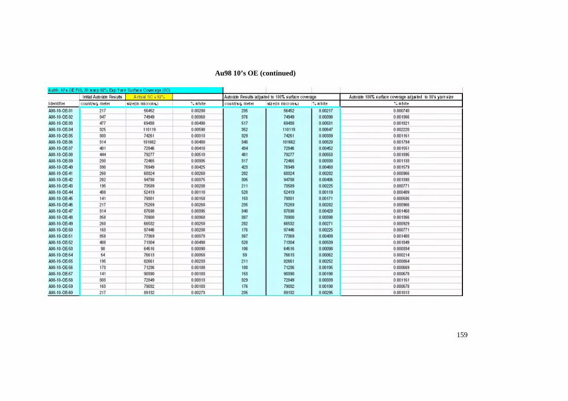
Au98 10’s OE (continued)
159

Au99 28’s Ring
160
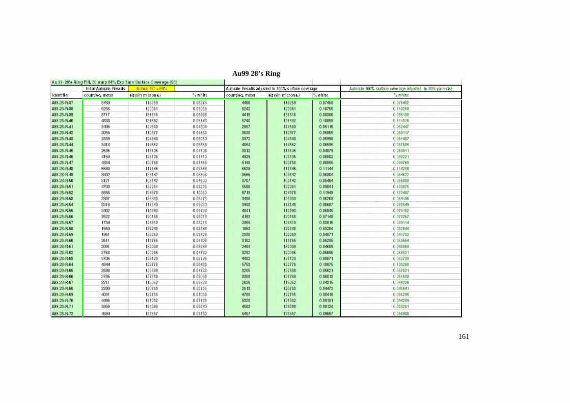
Au99 28’s Ring
161
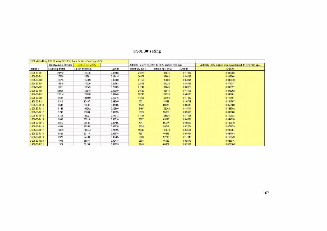
US01 30’s Ring
162
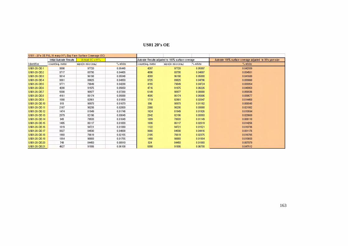
US01 20’s OE
163
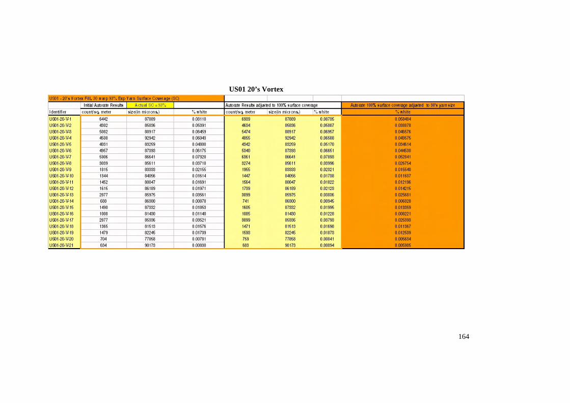
US01 20’s Vortex
164
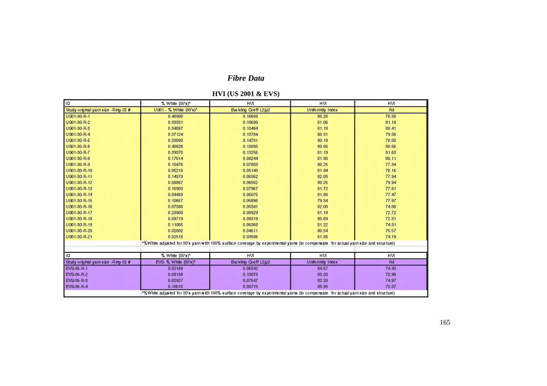
Fibre Data
HVI (US 2001 & EVS)
165
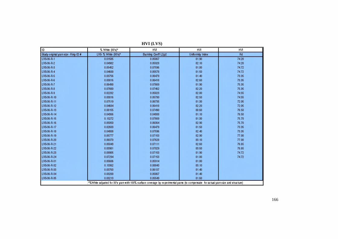
HVI (LVS)
166
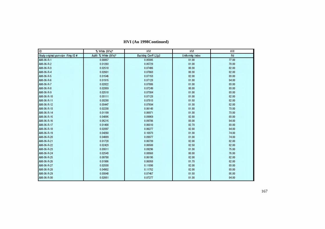
HVI (Au 1998Continued)
167
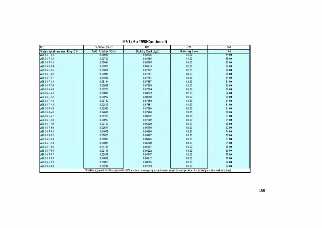
HVI (Au 1998Continued)
168
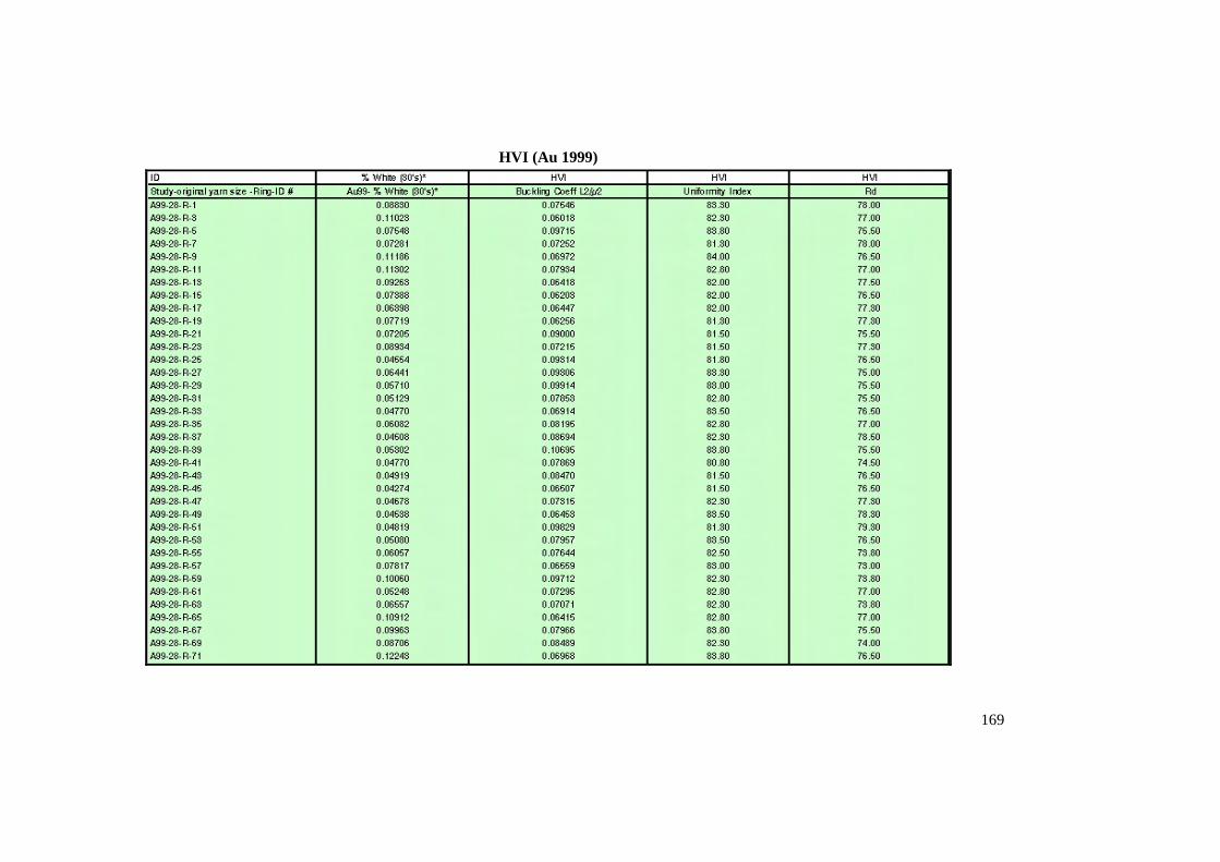
HVI (Au 1999)
169
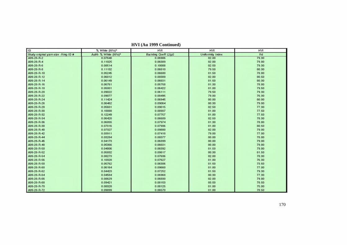
HVI (Au 1999 Continued)
170
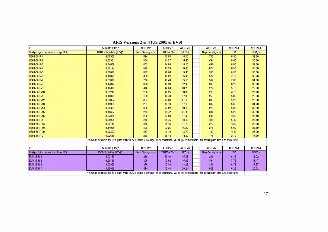
AFIS Versions 2 & 4 (US 2001 & EVS)
171
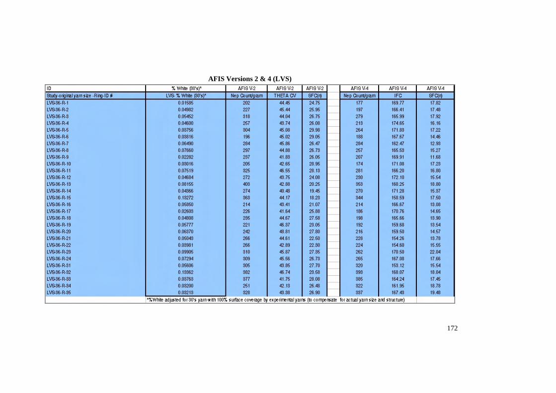
AFIS Versions 2 & 4 (LVS)
172
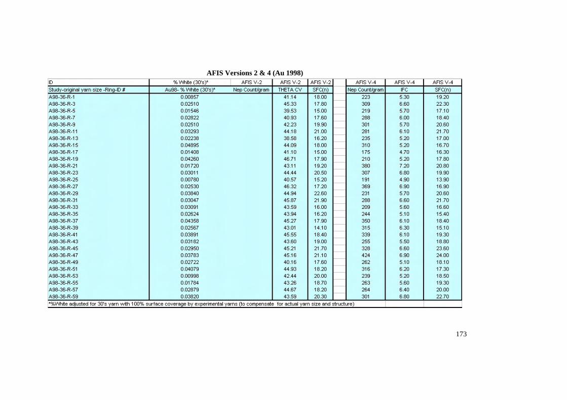
AFIS Versions 2 & 4 (Au 1998)
173
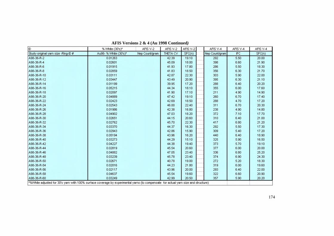
AFIS Versions 2 & 4 (Au 1998 Continued)
174
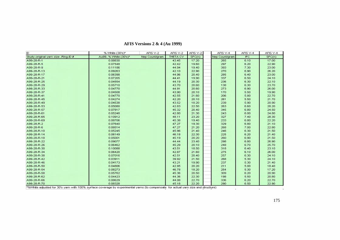
175
AFIS Versions 2 & 4 (Au 1999)
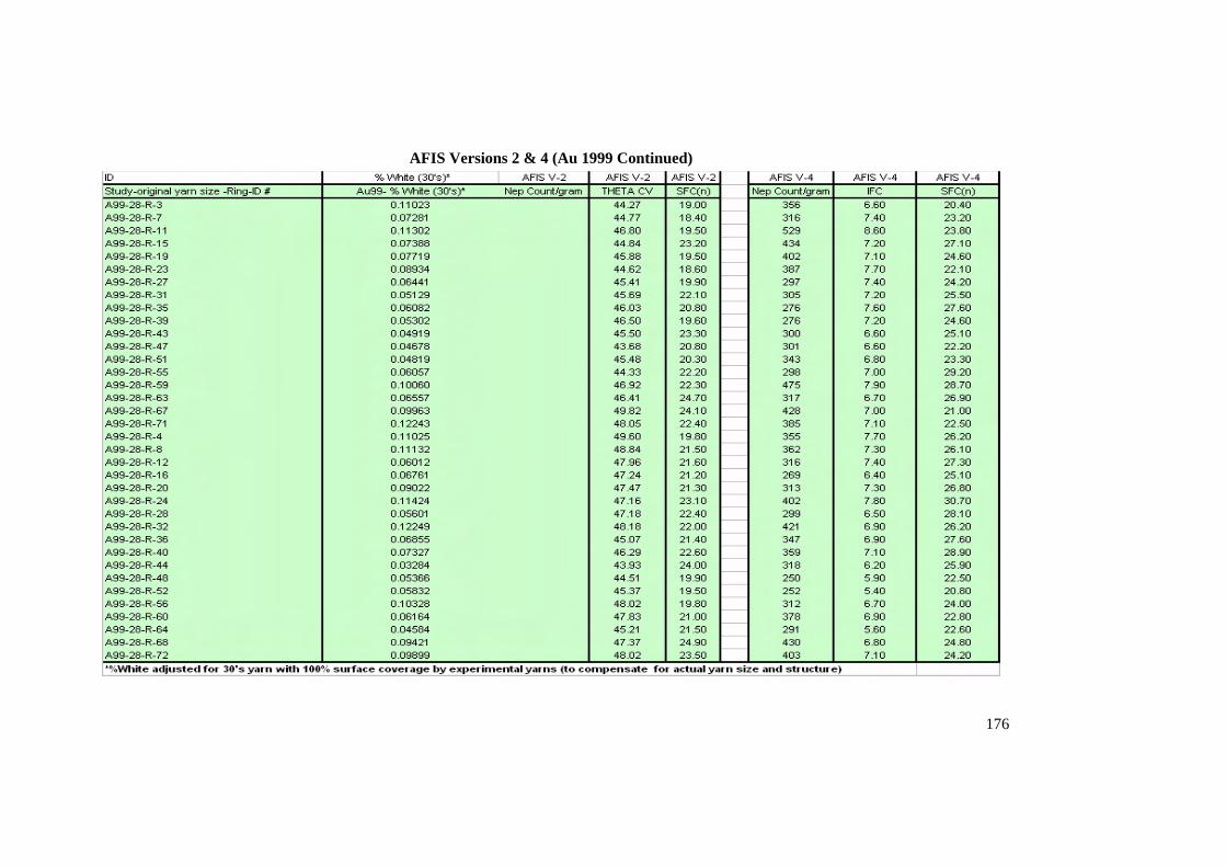
AFIS Versions 2 & 4 (Au 1999 Continued)
176
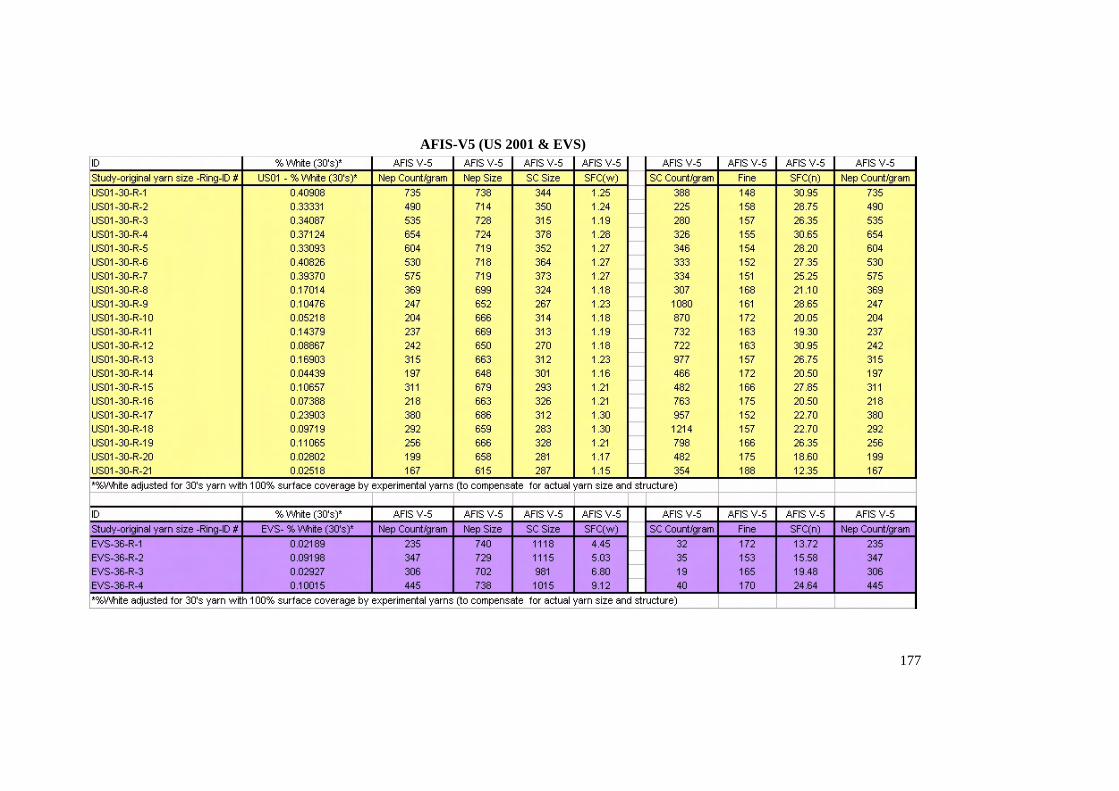
AFIS-V5 (US 2001 & EVS)
177
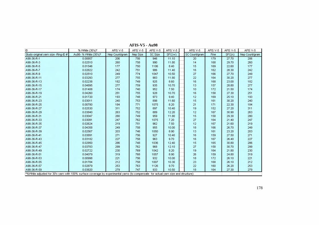
AFIS-V5 - Au98
178
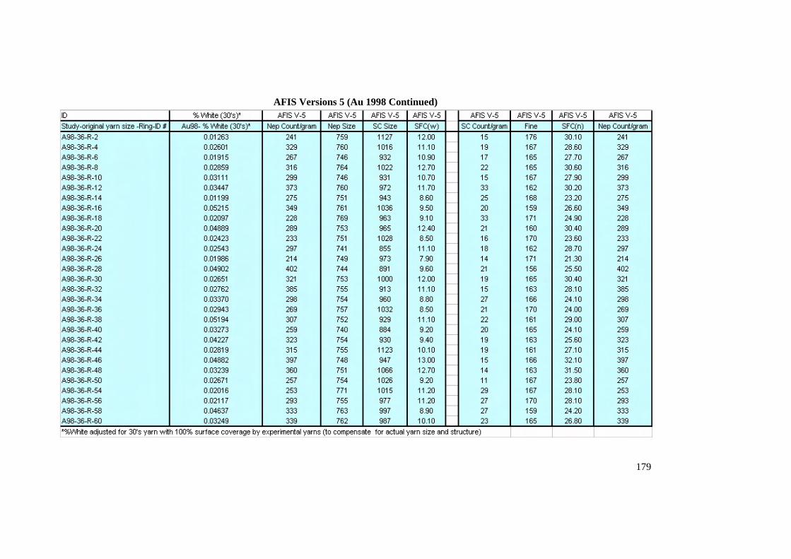
AFIS Versions 5 (Au 1998 Continued)
179
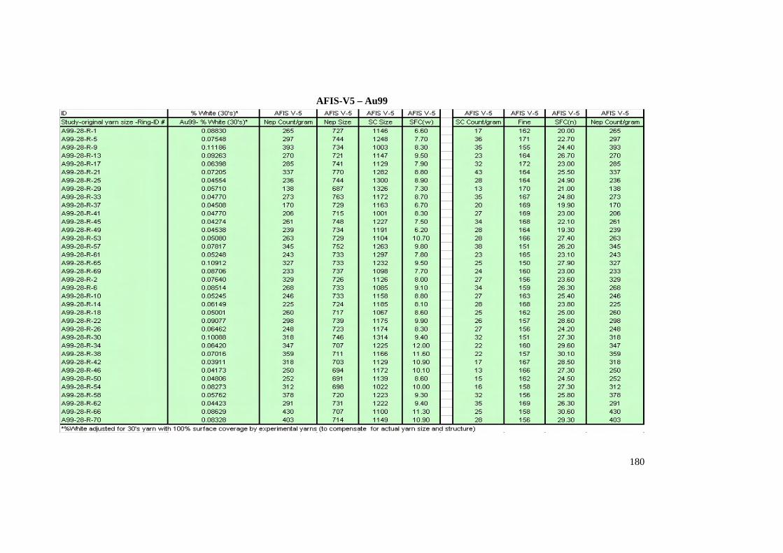
AFIS-V5 – Au99
180
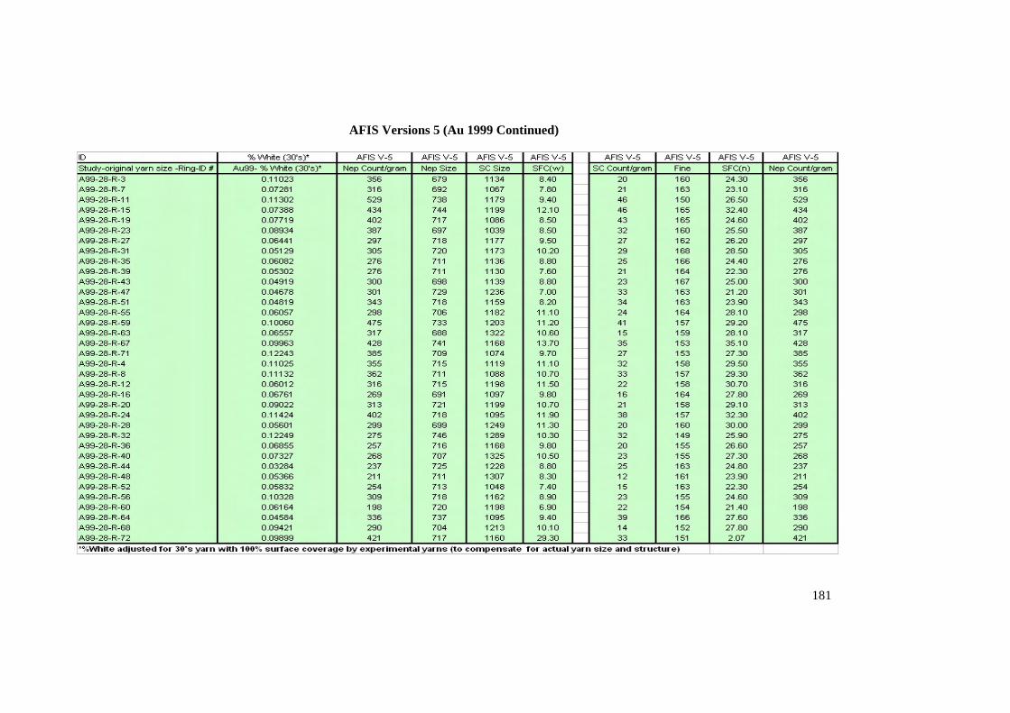
AFIS Versions 5 (Au 1999 Continued)
181
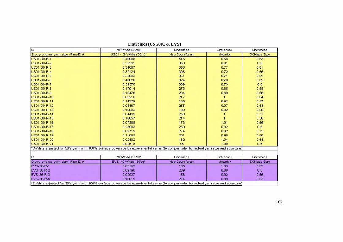
Lintronics (US 2001 & EVS)
182
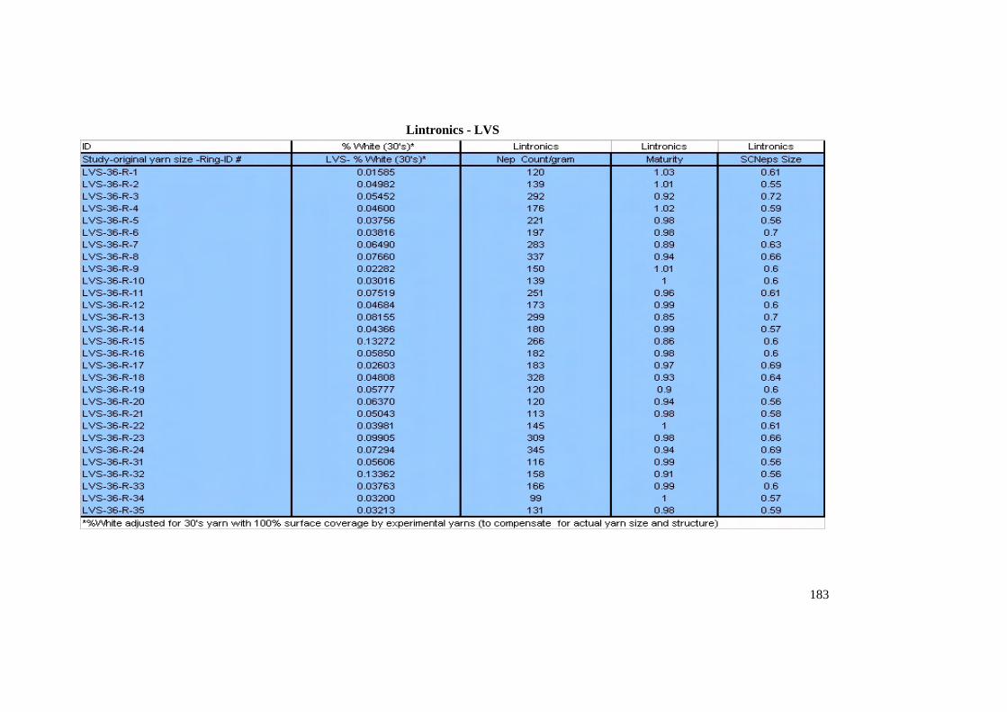
Lintronics - LVS
183
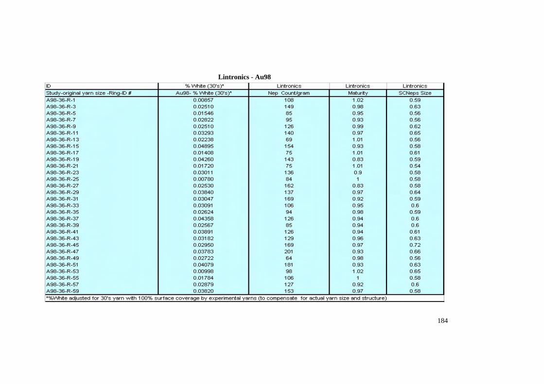
Lintronics - Au98
184
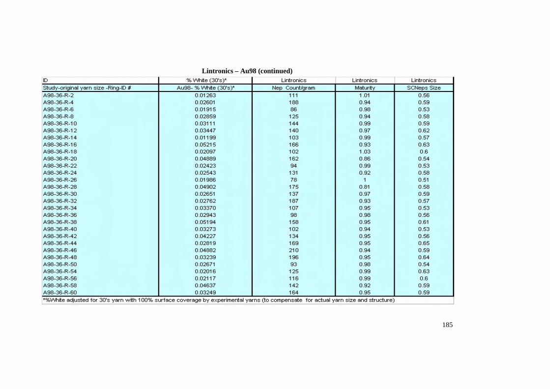
Lintronics – Au98 (continued)
185
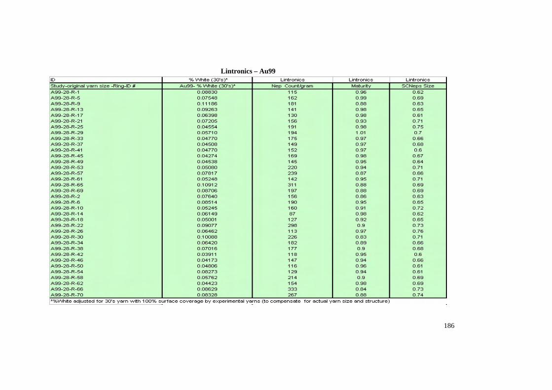
Lintronics – Au99
186
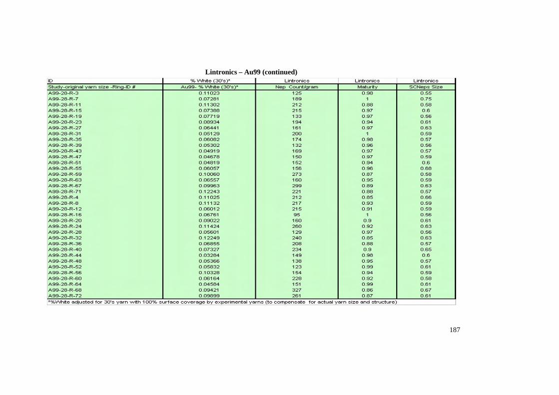
187
Lintronics – Au99 (continued)
188
References by Number
1 CottonAustralia (2003) “Where is Cotton Grown?” http://www.cottonaustralia.com.au/aboutindex.html,, Date accessed 10/24/2003. 2 EconCentral. (2003) National Cotton Council, http://agriculture.about.com/gi/dynamic/offsite.htm?site=http%3A%2F%2Fwww.cotton.org%2F Date accessed 10/23/2003. 3 CottonAustralia (2003) “Where is Cotton Grown?” http://www.cottonaustralia.com.au/aboutindex.html, Date accessed 10/24/2003. 4 CottonAustralia (2003) “Where is Cotton Grown?” http://www.cottonaustralia.com.au/aboutindex.html, Date accessed 10/24/2003. 5 Cotton World. (2003) “Growers at the top of cotton game”, http://www.cottonworld.com.au/articles.php3?rc=574 Date accessed 10/24/2003. 6 CottonAustralia (2003) “Where is Cotton Grown?” http://www.cottonaustralia.com.au/aboutindex.html, Date accessed 10/24/2003. 7 National Cotton Council. (2003) The World of Cotton, Economics, http://agriculture.about.com/gi/dynamic/offsite.htm?site=http%3A%2F%2Fwww.cotton.org%2F, Date accessed 11/4/2003. 8 CottonAustralia (2003) “Where is Cotton Grown?” http://www.cottonaustralia.com.au/aboutindex.html, Date accessed 10/24/2003. 9 National Cotton Council. (2003) The World of Cotton, Economics, http://agriculture.about.com/gi/dynamic/offsite.htm?site=http%3A%2F%2Fwww.cotton.org%2F, Date accessed 11/4/2003. 10 National Cotton Council. (2003) The World of Cotton, Economics, http://agriculture.about.com/gi/dynamic/offsite.htm?site=http%3A%2F%2Fwww.cotton.org%2F, Date accessed 11/4/2003. 11 Goynes, W. R., Bel-Berger, P. D., Blanchard, E. I., Ingber, B. F. Graves, E.E., Dastoor, P., Von Hoven, T. M. (1996) “Identification, Quantification and Elimination of White Speck Defects on Dyed Cotton Fabrics.” American Association of Textile Chemists and Colorists Conference Paper, 9-16. 12 Goynes, W. R., Bel-Berger, P. D., Blanchard, E. I., Ingber, B. F. Graves, E.E., Dastoor, P., Von Hoven, T. M. (1996) “Identification, Quantification and Elimination of White Speck Defects on Dyed Cotton Fabrics.” American Association of Textile Chemists and Colorists Conference Paper, 9-16. 13 Bel-Berger, P.D., Von Hoven T,, Cui, X., Davidonis, G and Pusateri, K. (1999) “Comparison of Sampling, Methods and Versions of AFIS”, Proceedings of the Beltwide Cotton Production Conference, 1, 681-684. 14 Bel-Berger, P.D., Von Hoven T., Cui, X., Davidonis, G and Pusateri, K. (1998) “The Importance of Sampling in White Speck Analysis.” Book of Papers, AATCC International Conference, 2, 600. 15 Brown, H. B. and Ware, J. O. (1958) Cotton (3rd Ed) McGraw Hill Book Company, Inc., 1958. 16 van der Sluijs, M. H. J. and Hunter, L. (1999) “Neps in Cotton Lint.” Textile Progress, 28, 4 1-51. 17 Hebert, J.J., Boylston, E.K., and Thibodeaux, D.P. (1988) “Anatomy of a Nep.” Textile Research Journal, 58, 7 380-382. 18 Hebert, J.J., Boylston, E.K., and Thibodeaux, D.P. (1988) “Anatomy of a Nep.” Textile Research Journal, 58, 7 380-382. 19 Hebert, J.J., Boylston, E.K., and Thibodeaux, D.P. (1988) “Anatomy of a Nep.” Textile Research Journal, 58, 7 380-382. 20 Crum, W., Phil. Soc. Glasgow Proc. On a Peculiar Fiber of Cotton Which is Incapable of Being Dyed (1848-1855. 3:61-64.1855. 21 Thibodeaux, D. P., and Evans, J.P. (1986) “ Cotton Fiber Maturity by Image Analysis”, Textile Research Journal, 56, 2 130-139. 22 Ramey Jr., H. H. (1988) “The Meaning and Assessment of Cotton Fiber Fineness”, International Institute for Cotton, 1-19. 23 Thibodeaux, D. P., and Evans, J.P. (1986) “ Cotton Fiber Maturity by Image Analysis”, Textile Research Journal, 56, 2 130-139. 24 Thibodeaux, D. P., and Evans, J.P. (1986) “ Cotton Fiber Maturity by Image Analysis”, Textile Research Journal, 56, 2 130-139. 25 Ramey Jr., H. H. (1988) “The Meaning and Assessment of Cotton Fiber Fineness”, International Institute for Cotton, 1-19. 26 Marth, Charles T., Arthur, Harry E., and Berkley, Earl E. (1952) “Fiber Fineness (Micronaire),
189
Neps in Card Web, and Yarn Appearance Grades”, Textile Research Journal, 22, 9 561-566. 27 van der Sluijs, M. H. J. and Hunter, L. (1999) “Neps in Cotton Lint.” Textile Progress, 28, 4 1-51. 28 Ramey Jr., H. H. (1988) “The Meaning and Assessment of Cotton Fiber Fineness”, International Institute for Cotton, 1-19. 29 Peirce, F. T. and Lord, E., (1939) “The Fineness and Maturity of Cotton”, Journal of the Textile Institute, 30, T173-T210. 30 Lord, E., and S.A. Heap. (1988) “The Origin and Assessment of Cotton Fiber Maturity”, International Institution for Cotton, Manchester, UK. 31 Midgley, E. (1933) “Defects in Dyed Cotton Goods; a Consideration of the Causes”, Textile Weekly, 11, 261 20-21. 32 Furter, R. (1992) “Reducing Neps.” Cotton International. 113-117. 33 Peter, U. and Bowes, Q. (1989) “Quality Variations in Cotton and Their Effects on Bleaching, Dyeing and Finishing”, Melliand Textilberichte, 70, 135-137. 34 van der Sluijs, M. H. J. and Hunter, L. (1999) “Neps in Cotton Lint.” Textile Progress, 28, 4 1-51. 35 Lord, E., and S.A. Heap. (1988) “The Origin and Assessment of Cotton Fiber Maturity”, International Institution for Cotton, Manchester, UK. 36 Bradow, J. M., Davidonis, G. H., Bauer, P. J., Sassenrath-Cole, G. F. and Johnson, R. M. (1998) “Mapping Variability in Cotton Fiber Maturity.” Proceedings of the Beltwide Cotton Conference, 2, 1463-1465. 37 Wegener, W. (1980) “Nature, Formation, and Reduction of Neps and Slubs”, Textil Praxis International, 35, 2 130-135. 38 van der Sluijs, M. H. J. (1996) “The Influence of Fiber Properties on Neps in South African Cotton”, MSc Dissertation, University of Port Elizabeth. 39 van der Sluijs, M. H. J. and Hunter, L. (1999) “Neps in Cotton Lint.” Textile Progress, 28, 4 1-51. 40 van der Sluijs, M. H. J. and Hunter, L. (1999) “Neps in Cotton Lint.” Textile Progress, 28, 4 1-51. 41 Alon, Gan, and Alexander, Ernst. (1978) “Mechanism of Nep Formation“, Melliand Textilberichte. 42 van der Sluijs, M. H. J. and Hunter, L. (1999) “Neps in Cotton Lint.” Textile Progress, 28, 4 1-51. 43 Alon, Gan, and Alexander, Ernst. (1978) “Mechanism of Nep Formation“, Melliand Textilberichte. 44 van der Sluijs, M. H. J. and Hunter, L. (1999) “Neps in Cotton Lint.” Textile Progress, 28, 4 1-51. 45 American Society for Testing and Materials. (1947) “ASTM Standards on Textile Materials”, Annual. Book of ASTM Standards (pp. 210-211). Philadelphia, PA: ASTM. 46 van der Sluijs, M. H. J. and Hunter, L. (1999) “Neps in Cotton Lint.” Textile Progress, 28, 4 1-51. 47 Mangialardi Jr., G.J. (1985) “Neps in Ginned Lint: A Review of Research”, Beltwide Cotton Production Research Conferences, 358-362. 48 Hebert, J.J., Boylston, E.K., and Thibodeaux, D.P. (1988) “Anatomy of a Nep.” Textile Research Journal, 58, 7 380-382. 49 van der Sluijs, M. H. J. and Hunter, L. (1999) “Neps in Cotton Lint.” Textile Progress, 28, 4 1-51. 50 Bel-Berger, P. and Roberts, G. (1998) “Neps: How Do They Impact Cotton Quality” Proceedings of the Ninth Australian Cotton Conference, 1, 721-729. 51 Jakes, K. A.; Unble, B. A. (1984) “Chemical and physical structure of neps selected in non woven fabrics.” Textile Research Journal, 54, 644-648. 52 Supak, J. R. (1986) “Solving Cotton Quality Problems: White Speck and Barky Cotton.” Proceedings of the Beltwide Production Conference, 1, 94-96. 53 Watson, M. D., Carter, F. L. and Cloninger, Jr., A. E. (1991) “An Update on New Chemical Test Methods to Detect Dye Resistant Neps in Raw Cotton." Proceedings of the Beltwide Cotton Production Conference, I, 878-879. 54 Brown, H. B. and Ware, J. O. (1958) Cotton (3rd Ed) McGraw Hill Book Company, Inc., 1958. 55 Goynes, W. R., Ingber, B. F., and Thibodeaux D. P., (1995) “Introductory Study of Structures of Cotton Motes and Mote Fibers.” Textile Research Journal, 65, 4 219-225. 56 Wegener, W. (1980) “Nature, Formation, and Reduction of Neps and Slubs”, Textil Praxis International, 35, 2 130-135. 57 Ramey Jr., H. H. (1988) “The Meaning and Assessment of Cotton Fiber Fineness”, International Institute for Cotton, 1-19. 58 Goynes, W. R., Ingber, B. F., and Triplett, B, (1995) “Cotton Fibers Secondary Wall Development – Time versus Thickness.” Textile Research Journal, 65, 7 400-408. 59 Goynes, W. R., Ingber, B. F., and Triplett, B, (1995) “Cotton Fibers Secondary Wall Development – Time versus Thickness.” Textile Research Journal, 65, 7 400-408. 60 Hebert, J.J., Boylston, E.K., and Thibodeaux, D.P. (1988) “Anatomy of a Nep.” Textile Research Journal, 58, 7 380-382.
190
61 STONEVILLE, Miss. (AP). (1997) “Scientist finds miniscule flaws in cotton fibers.” Copyright Lubbock Avalanche-Journal, http://www.lubbockonline.com/news/072697/scientis.htm Date accessed 8/13/2003. 62 Goynes, W. R., Ingber, B. F., and Triplett, B, (1995) “Cotton Fibers Secondary Wall Development – Time versus Thickness.” Textile Research Journal, 65, 7 400-408. 63 Goynes, W.R., B.F. Ingber, and D.P. Thibodeaux. (1994) “White specks: A Microscopic Profile”. Proceedings of Cotton Beltwide Cotton Conference, 1994. 64 Norman, B.M. (1991) “HVI Classing and its Effects on Ginning.” The Fourth Annual Engineered Fiber Selection Conference. Charlotte, North Carolina. 65 Werber, F. X. and Backe, E.E. (1994) “Textile Industry Needs”, Agriculture Handbook, USDA, 503, 293-306. 66 Anthony, W.S., Baker, R.V., Hughs, S.E. (1986) “Ginning for Maximum Grade without Excessive Short Fibers, Neps and Trash”, The Cotton Gin and Oil Mill Press, 14-17. 67 Cotton Program Agricultural Marketing Service U.S. Department of Agriculture. (2001) “The Classification of Cotton”, USDA Publication, http://www.cottoninc.com/CottonClassification/homepage.cfm?PAGE=646, Date accessed 10/15/2003. 68 Cotton Program Agricultural Marketing Service U.S. Department of Agriculture. (2001) “The Classification of Cotton”, USDA Publication, http://www.cottoninc.com/CottonClassification/homepage.cfm?PAGE=646, Date accessed 10/15/2003. 69 Lord, E., and S.A. Heap. (1988) “The Origin and Assessment of Cotton Fibre Maturity”, International Institution for Cotton, Manchester, UK. 70 Moore, J.F. (1996) “Cotton Classification and Quality”. In E.H. Glade Jr., L.A. Meyer, and H. Stults (Ed) The Cotton Industry in the United States (pp. 51-57). Washington, DC: USDA-ERS Agric. Econ. Rep. 739. U.S. Gov. Print. Office. 71 Cotton Program Agricultural Marketing Service U.S. Department of Agriculture. (2001) “The Classification of Cotton”, USDA Publication, http://www.cottoninc.com/CottonClassification/homepage.cfm?PAGE=646, Date accessed 10/15/2003. 72 Gordon, S.G.; Montalvo, J.G. Jr.; Faught, S. E.; Grimball, R.T.; and Watkins, T. A. (1997) “Theoretical and experimental profiles of fiber fineness and maturity using the Shirley Micromat and the Zellweger Uster advanced fiber information system module”. Text. Res. J. 67 (8): 545-555. 73 Mor, U. (2003) “A New Generation of Fast Fiber Testers Gives Hope to a Major Improvement in the Field of Fiber Quality Control at the Spinning and Ginning Mills”, http://www.lintronics.com/articale2.htm, Date accessed 11/28/2003. 74 American Society for Testing and Materials. (1978) “ASTM D3216 – 78 “Grading Cotton Card Webs for Appearance”, Annual. Book of ASTM Standards (pp.641-644). Philadelphia, PA: ASTM. 75 Lord, E., and S.A. Heap. (1988) “The Origin and Assessment of Cotton Fibre Maturity”, International Institution for Cotton, Manchester, UK. 76 Bradow, J. M. and Davidonis, G. H. (2000) “Quantification of Fiber Quality and the Cotton Production-Processing Interface: A Physiologist's Perspective.” The Journal of Cotton Science, 4, 34-64. 77 Lord, E., and S.A. Heap. (1988) “The Origin and Assessment of Cotton Fibre Maturity”, International Institution for Cotton, Manchester, UK. 78 American Society for Testing and Materials. (1994) “ASTM Standard D 3818-92. 07.02 - Standard test method for linear density and maturity index of cotton fibers (IIC-Shirley Fineness/Maturity Tester”, Annual. Book of ASTM Standards (pp.143-146). Philadelphia, PA: ASTM. 79 Montalvo, J.G., Jr., and Faught, S. E. (1995) “Determination of Maturity/Fineness by FMT and Diode-Array HVI. Part I. FMT (Micromat Model) Procedure of Optimization”, Proceedings of the Beltwide Cotton Production Research Conference 1276-1278. 80 Montalvo, Jr., J.G., Joseph, J. R. and Faught, S. E. (1998) “Headspace Resistance Standards for the Shirley Developments Limited Micromat Tester”, The Journal of Cotton Science, 4, 269-277. 81 Montalvo, J.G., Jr., and Faught, S. E. (1999) “Headspace Resistance Standards for the Shirley Developments Ltd. Micromat Tester”, ”. Text. Res. J. 69 (4): 269-277. 82 Montalvo, J.G., Jr. (2001). Theory of single and independent reference methods for cotton fineness and maturity. Presented to the Cotton Research Planning meeting, SRRC, New Orleans, Louisiana. 83 Schiller, Susannah and Eberhardt, Keith. (1991). "Combining Data from Several Chemical Analytic Techniques." Spectrochimica Acta Acta, Vol. 46B, No. 12.
191
84 American Society for Testing and Materials. (1994) “ASTM Standard D 3818-92. 07.02 - Standard test method for linear density and maturity index of cotton fibers (IIC-Shirley Fineness/Maturity Tester”, Annual. Book of ASTM Standards (pp.143-146). Philadelphia, PA: ASTM. 85 Montalvo, Jr., J.G., Faught, S. E. and Buco,S. M. (2002) “Sensitivity of the Shirley Developments Ltd. Micromat Tester to Operators and Sample Preparations”, The Journal of Cotton Science, 6, 133–142. 86 Montalvo, Jr., J.G., Joseph, J. R. and Faught, S. E. (1998) “Headspace Resistance Standards for the Shirley Developments Limited Micromat Tester”, The Journal of Cotton Science, 4, 269-277. 87 Montalvo, Jr., J.G., Faught, S. E. and Buco,S. M. (2002) “Sensitivity of the Shirley Developments Ltd. Micromat Tester to Operators and Sample Preparations”, The Journal of Cotton Science, 6, 133–142. 88 Cole, William D. (1997) “Examination of Effects of Drafting Rates o Yarn Quality”, Textile Topics, InternationalTextileCenter, http://www.depts.ttu.edu/itc/acrobat%20files/ttw98.pdf, Date accessed 11/8/2003. 89 Montalvo, J.G. Jr., Faught, S.E. and Buco, S.M. (1989) “An Investigation of the Relationship Between Cotton Fineness and Light-Scattering from Thin Webs as Measured by Near-Infrared Transmission spectroscopy”, Applied Spectroscopy, 43, 1459-1471. 90 van der Sluijs, M. H. J. and Hunter, L. (1999) “Neps in Cotton Lint.” Textile Progress, 28, 4 1-51. 91 Devron Thibodeaux, Joseph Montalvo, Jr., Gayle Davidonis, and David McAlister (2003) Effects of Location on Distributions of Fiber Quality. Proceedings of the Beltwide Cotton Conferences, 2580 - 2588. 92 Gordon, S.G.; Montalvo, J.G. Jr.; Faught, S. E.; Grimball, R.T.; and Watkins, T. A. (1997) “Theoretical and experimental profiles of fiber fineness and maturity using the Shirley Micromat and the Zellweger Uster advanced fiber information system module”. Text. Res. J. 67 (8): 545-555. 93 Mor, U. (2003) “A New Generation of Fast Fiber Testers Gives Hope to a Major Improvement in the Field of Fiber Quality Control at the Spinning and Ginning Mills”, http://www.lintronics.com/articale2.htm, Date accessed 11/28/2003. 94 Mor, U. (2003) “A New Generation of Fast Fiber Testers Gives Hope to a Major Improvement in the Field of Fiber Quality Control at the Spinning and Ginning Mills”, http://www.lintronics.com/articale2.htm, Date accessed 11/28/2003. 95 Mor, U. (2003) “A New Generation of Fast Fiber Testers Gives Hope to a Major Improvement in the Field of Fiber Quality Control at the Spinning and Ginning Mills”, http://www.lintronics.com/articale2.htm, Date accessed 11/28/2003. 96 Wulfhorst, B. and Bergmann, J. (1989) “Detection of Disruptive Particles in Cotton Fibre Webs Using Digital Image Processing”, Melliand Textilberichte. 70, 12 377-379. 97 Mor, U. (2003) “A New Generation of Fast Fiber Testers Gives Hope to a Major Improvement in the Field of Fiber Quality Control at the Spinning and Ginning Mills”, http://www.lintronics.com/articale2.htm, Date accessed 11/28/2003. 98 Harrison, R.E, Bargeron III, J.D. (1986) “Comparison of Several Nep Determination Methods.” Textile Research Journal, 56, 2 77-79. 99 American Society for Testing and Materials. (1978) “ASTM D3216 – 78 “Grading Cotton Card Webs for Appearance”, Annual. Book of ASTM Standards (pp.641-644). Philadelphia, PA: ASTM. 100 Verschraege, L. (1989) “Cotton Fibre Impurities: Neps, Motes and Seed Coat Fragments.” ICAC Review Articles on Cotton Production Research No.1. 101 Bragg, C.K. and Simpson, C.L. (1992) “Solving Cotton Quality Problems: White Specks and Bark in Textile Products.” Proceedings of the Beltwide Cotton Production Conference, 1, 97-99. 102 Miravaille, R. J., Mangialardi, G.J., Lalor, W.F. (1986) “Neps in cotton genotypes grown in six locations across the cotton belt in 1984”, Proceedings of the Beltwide Cotton Production Research Conference, 426-428. 103 van der Sluijs, M. H. J. and Hunter, L. (1999) “Neps in Cotton Lint.” Textile Progress, 28, 4 1-51. 104 Hebert, J.J., Boylston, E.K., and Thibodeaux, D.P. (1988) “Anatomy of a Nep.” Textile Research Journal, 58, 7 380-382. 105 Peter, U. and Bowes, Q. (1989) “Quality Variations in Cotton and Their Effects on Bleaching, Dyeing and Finishing”, Melliand Textilberichte, 70, 135-137. 106 Cheek, L. and Wilcock, A, (1988) “Relationship between Direct Dye Characteristics and Coverage of Immature Fiber Neps in Dyed Cotton Fabric, J. Soc. Dyers and Colorists. 104, 477. 107 Joseph, L. M. (1986) Introductory Textile Science (Fifth Edition). New York: CBS College Publishing. 108 Golthwaite, C.F.; Smith, H. O. and Barnitt, M. P. (1947) “New Dye Technique Shows Maturity of
192
cotton”. Textile World, 97, 105-108. 109 Mangliardi, G. J. and Lalor, W. F. (1990) “Propensity of Cotton Varieties to Neppiness”, Transactions of the ASAE, 36, 6 1748-1758. 110 Bragg, C.K. and Simpson, C.L. (1992) “Solving Cotton Quality Problems: White Specks and Bark in Textile Products.” Proceedings of the Beltwide Cotton Production Conference, 1, 97-99. 111 Von Hoven, Terri. (1996) “Comparison of Image Analysis Systems for their Ability to Detect the White Speck Phenomenon.” MSc Dissertation Georgia Institute of Technology. 112 Von Hoven, Terri. (1996) “Comparison of Image Analysis Systems for their Ability to Detect the White Speck Phenomenon.” MSc Dissertation Georgia Institute of Technology. 113 Von Hoven, Terri. (1996) “Comparison of Image Analysis Systems for their Ability to Detect the White Speck Phenomenon.” MSc Dissertation Georgia Institute of Technology. 114 Alon, Gan, and Alexander, Ernst. (1978) “Mechanism of Nep Formation“, Melliand Textilberichte. 115 Alon, Gan, and Alexander, Ernst. (1978) “Mechanism of Nep Formation“, Melliand Textilberichte. 116 Wegener, W. (1980) “Nature, Formation, and Reduction of Neps and Slubs”, Textil Praxis International, 35, 2 130-135. 117 Wegener, W. (1980) “Nature, Formation, and Reduction of Neps and Slubs”, Textil Praxis International, 35, 2 130-135. 118 Mangialardi Jr., G. J., Lalor, W.F., Bassett, D. M., and Miravalle, R.J. (1987)“Influence of Growth Period on Neps in Cotton”, Textile Research Journal, 57, 7 421-427. 119 Hunter L. and van der Sluijs, M. H. J. (1996) “Neps in Cotton Lint”, Melliand English, E81 - E82. 120 Chellamani K. P., Chattopadhyay D. and Thanabal V. (1999) “Indian Cottons and Influence of Mechanical Processing on Nep Generation”, Asian Textile Journal, 120-126. 121 Alon, Gan, and Alexander, Ernst. (1978) “Mechanism of Nep Formation“, Melliand Textilberichte. 122 Watson, M. D., Carter, F. L. and Cloninger, Jr., A. E. (1991) “An Update on New Chemical Test Methods to Detect Dye Resistant Neps in Raw Cotton." Proceedings of the Beltwide Cotton Production Conference, I, 878-879. 123 Bragg, C.K. and Simpson, C.L. (1992) “Solving Cotton Quality Problems: White Specks and Bark in Textile Products.” Proceedings of the Beltwide Cotton Production Conference, 1, 97-99. 124 Verschraege, L. (1989) “Cotton Fibre Impurities: Neps, Motes and Seed Coat Fragments.” ICAC Review Articles on Cotton Production Research No.1. 125 Mangliardi, G. J. and Lalor, W. F. (1990) “Propensity of Cotton Varieties to Neppiness”, Transactions of the ASAE, 36, 6 1748-1758. 126 Wegener, W. (1980) “Nature, Formation, and Reduction of Neps and Slubs”, Textil Praxis International, 35, 2 130-135. 127 Bel-Berger PD, Vinyard BT, Thibodeaux DT. (1995) “Effect of Harvesting Times on White Specks: A Study of Field to Fabric Properties.” Proceedings of the Beltwide Cotton Production Conference, 2, 1440-1444 128 Greb, Peggy. (2000) Image Number K8706-7, http://www.ars.usda.gov/is/graphics/photos/jan00/k8706-7.htm. Date accessed 11/15/2003. 129 Nance, David (date unknown) “Cotton Harvesting”, Image Number K5927-2, http://www.ars.usda.gov/is/graphics/photos/may02/k5927-21.htm, Date accessed 11/28/2003. 130 Wright, David. (date unknown) “Cotton stripper harvesting UNR cotton near Altha, Florida”, Image Number K8719-1, http://www.ars.usda.gov/is/graphics/photos/jan00/k8719-1.htm, Date accessed 11/28/2003. 131 Mangialardi Jr., G. J., Lalor, W.F., Bassett, D. M., and Miravalle, R.J. (1987)“Influence of Growth Period on Neps in Cotton”, Textile Research Journal, 57, 7 421-427. 132 Mangialardi Jr., G.J. (1985) “An Evaluation of Nep Formation at the Cotton Gin” Textile Research Journal, 55, 12 756-761. 133 Hughs, S.E., Lalor, W.F., Wahba, F.T. (1988) “Relationship of Ginning and Fiber Properties to Dyeing Imperfections”, Textile Research Journal, 58, 10 557-564. 134Frydrych, I., Matusiak, M. and Swiech, T. (2001) “Cotton Maturity and Its Influence on Nep Formation”. Textile Research Journal, 595 - 604. 135 Anthony, W.S., and Mayfield, W. D. (1994) “Cotton Ginners Handbook”, U.S. Department of Agriculture - Agricultural Handbook, 503. 136 Anthony, W.S., Baker, R.V., Hughs, S.E. (1986) “Ginning for Maximum Grade without Excessive Short Fibers, Neps and Trash”, The Cotton Gin and Oil Mill Press, 14-17. 137 Agriculture Research Service Image Gallery. (2003) Image Number K4844-9 http://www.ars.usda.gov/is/graphics/photos/k4844-9.htm. Date accessed 10/5/2003.
193
138 Yankey, Joseph M. (1996) “The Value of Fiber Testing in the Ginning Industry.” Beltwide Cotton Conferences, 1654-1657. 139 Bel-Berger, P. and Von Hoven, T. (1997) “Effects of Mechanical Cleaning on Cotton Fibers. Part III: Effects of Card Wire Condition on White Specks”, Textile Research Journal 67, 12 857-865. 140 Wegener, W. (1980) “Nature, Formation, and Reduction of Neps and Slubs”, Textil Praxis International, 35, 2 130-135. 141 van der Sluijs, M. H. J. and Hunter, L. (1999) “Neps in Cotton Lint.” Textile Progress, 28, 4 1-51. 142 Marvin, (1973) Textile Processing Vol. 1, State Dept. of Education South Carolina and Clemson University. 143 Verschraege, L. (1989) “Cotton Fibre Impurities: Neps, Motes and Seed Coat Fragments.” ICAC Review Articles on Cotton Production Research No.1. 144 Wegener, W. (1980) “Nature, Formation, and Reduction of Neps and Slubs”, Textil Praxis International, 35, 2 130-135. 145 Kaufman, D. (1964) Studies on the Revolving Flat Card. U. S. D. A., 42. 146 Verschraege, L. (1989) “Cotton Fibre Impurities: Neps, Motes and Seed Coat Fragments.” ICAC Review Articles on Cotton Production Research No.1. 147 Anthony, W.S., and Mayfield, W. D. (1994) “Cotton Ginners Handbook”, U.S. Department of Agriculture - Agricultural Handbook, 503. 148 van der Sluijs, M. H. J. and Hunter, L. (1999) “Neps in Cotton Lint.” Textile Progress, 28, 4 1-51. 149 Naylor, G.R.S., (2002), “Murata Vortex Spinning: A New Spin on Textile Processing” The Australian Cottongrower, 23(1), p26-27. 150 Kaufman, D. (1964) Studies on the Revolving Flat Card. U. S. D. A., 42. 151 Verschraege, L. (1989) “Cotton Fibre Impurities: Neps, Motes and Seed Coat Fragments.” ICAC Review Articles on Cotton Production Research No.1. 152 Manohar, J. S., Rakshit, A. K. and Balasubramanian, N. (1983) “Influence of Rotor Speed, Rotor Diameter, and Card Conditions on Yarn Quality in Open-End Spinning”, Textile Research Journal, 497-502. 153 Naylor, G.R.S., (2002), “Murata Vortex Spinning: A New Spin on Textile Processing” The Australian Cottongrower, 23(1), p26-27. 154 Schreiner, (date unknown) http://www.cottoninc.com/insideout/homepage.cfm?PAGE=2643, Date accessed 8/24/2003. 155 van der Sluijs, M. H. J. and Hunter, L. (1999) “Neps in Cotton Lint.” Textile Progress, 28, 4 1-51. 156 van der Sluijs, M. H. J. and Hunter, L. (1999) “Neps in Cotton Lint.” Textile Progress, 28, 4 1-51. 157 Potter, M. D. and Corbman, B. P. (1967) “Textiles: Fiber to Fabric”, Fourth Edition, McGraw-Hill, Inc. 158 “Fiber and Processing Tests, Survey of Leading Cotton Varieties, Crop of 1993”, US Department of Agriculture Agricultural Marketing Service, Cotton Division June 1994. 159 Southern Hemisphere Crop report April 26, (1999) http://cotton.net/AustCrop.htm 7/21/99). 160 Southern Hemisphere Crop report April 26, (1999) http://cotton.net/AustCrop.htm 7/21/99). 161 Hughs, S.E., Lalor, W.F., Wahba, F.T. (1988) “Relationship of Ginning and Fibre Properties to Dyeing Imperfections”, Textile Research Journal, 58, 10 557-564. 162 StatSoft, Inc. (2004). Electronic Statistics Textbook. Tulsa, OK: StatSoft. WEB: http://www.statsoft.com/textbook/stathome.html. Date accessed 12/2/2003. 163 Alon, Gan, and Alexander, Ernst. (1978) “Mechanism of Nep Formation“, Melliand Textilberichte. 164 Alon, Gan, and Alexander, Ernst. (1978) “Mechanism of Nep Formation“, Melliand Textilberichte