Embed Size (px)
Citation preview
Chapter 6
Cost-Volume-Profit Relationships
Learning Objectives
LO1. Explain how changes in activity affect contribution marginand net operating income.
LO2. Prepare and interpret a cost-volume-profit (CVP) graph.LO3. Use the contribution margin ratio (CM ratio) to compute
changes in contribution margin and net operating incomeresulting from changes in sales volume.
LO4. Show the effects on contribution margin of changes invariable costs, fixed costs, selling price, and volume.
LO5. Compute the break-even point in unit sales and salesdollars.
LO6. Determine the level of sales needed to achieve a desiredtarget profit.
LO7. Compute the margin of safety and explain its significance.LO8. Compute the degree of operating leverage at a particular
level of sales, and explain how the degree of operatingleverage can be used to predict changes in net operatingincome.
LO9. Compute the break-even point for a multiple product companyand explain the effects of shifts in the sales mix oncontribution margin and the break-even point.
New in this Edition• Several new In Business boxes have been added.• A number of new exercises have been added, each of which focuses on a single
learning objective.
Chapter Overview
333
A. The Basics of Cost-Volume-Profit (CVP) Analysis.(Exercises 6-1, 6-10, 6-14, and 6-15.) Cost-volume-profit (CVP)analysis is a key step in many decisions. CVP analysis involvesspecifying a model of the relations among the prices ofproducts, the volume or level of activity, unit variable costs,total fixed costs, and the sales mix. This model is used topredict the impact on profits of changes in those parameters.
1. Contribution Margin. Contribution margin is the amountremaining from sales revenue after variable expenses havebeen deducted. It contributes towards covering fixed costsand then towards profit.
2. Unit Contribution Margin. The unit contribution margin can beused to predict changes in total contribution margin as aresult of changes in the unit sales of a product. To do this,the unit contribution margin is simply multiplied by thechange in unit sales. Assuming no change in fixed costs, thechange in total contribution margin falls directly to thebottom line as a change in profits.
3. Contribution Margin Ratio. The contribution margin (CM) ratiois the ratio of the contribution margin to total sales. Itshows how the contribution margin is affected by a givendollar change in total sales. The contribution margin ratiois often easier to work with than the unit contributionmargin, particularly when a company has many products. Thisis because the contribution margin ratio is denominated insales dollars, which is a convenient way to express activityin multi-product firms.
B. Some Applications of CVP Concepts. (Exercises 6-4, 6-10,6-11, 6-12, 6-13, and 6-16.) CVP analysis is typically used toestimate the impact on profits of changes in selling price,variable cost per unit, sales volume, and total fixed costs. CVPanalysis can be used to estimate the effect on profit of achange in any one (or any combination) of these parameters. Avariety of examples of applications of CVP are provided in thetext.
C. CVP Relationships in Graphic Form. (Exercises 6-2 and 6-11.) CVP graphs can be used to gain insight into the behavior of
334
expenses and profits. The basic CVP graph is drawn with dollarson the vertical axis and unit sales on the horizontal axis.Total fixed expense is drawn first and then variable expense isadded to the fixed expense to draw the total expense line.Finally, the total revenue line is drawn. The total profit (orloss) is the vertical difference between the total revenue andtotal expense lines. The break-even occurs at the point wherethe total revenue and total expenses lines cross.
D. Break-Even Analysis and Target Profit Analysis.(Exercises 6-5, 6-6, 6-11, 6-12, and 6-15.) Target profitanalysis is concerned with estimating the level of salesrequired to attain a specified target profit. Break-evenanalysis is a special case of target profit analysis in whichthe target profit is zero.
1. Basic CVP equations. Both the equation and contribution(formula) methods of break-even and target profit analysisare based on the contribution approach to the incomestatement. The format of this statement can be expressed inequation form as:
Profits = Sales Variable expenses Fixed expenses
In CVP analysis this equation is commonly rearranged andexpressed as:
Sales = Variable expenses + Fixed expenses + Profits
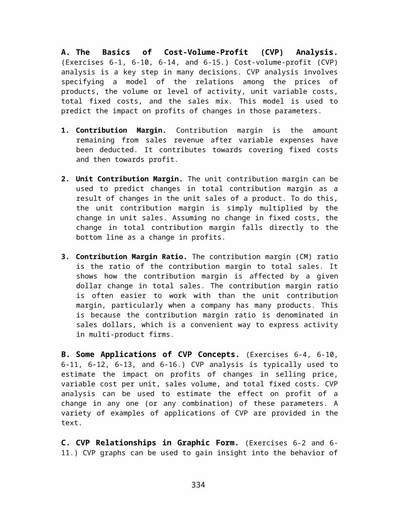
a. The above equation can be expressed in terms of unit salesas follows:
Price Unit sales = Unit variable cost Unit sales + Fixedexpenses + Profits
Unit contribution margin Unit sales = Fixed expenses + Profits
Unit sales =
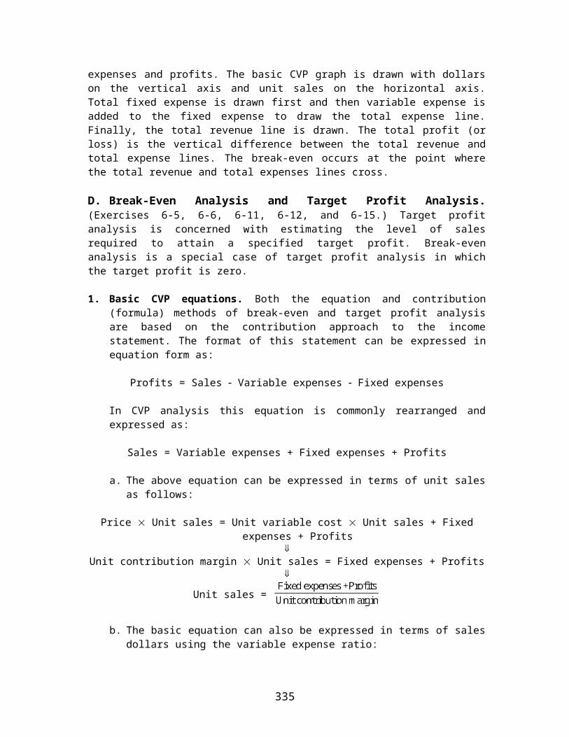
b. The basic equation can also be expressed in terms of salesdollars using the variable expense ratio:
335
Sales = Variable expense ratio Sales + Fixed expenses +Profits
(1 Variable expense ratio) Sales = Fixed expenses + Profits
Contribution margin ratio* Sales = Fixed expenses + Profits
Sales =
* 1 Variable expense ratio = 1
=
= = Contribution margin ratio
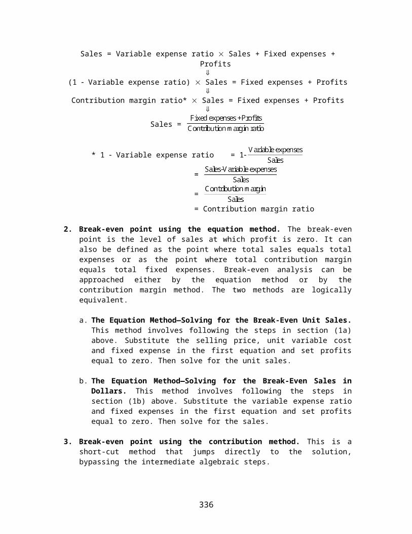
2. Break-even point using the equation method. The break-evenpoint is the level of sales at which profit is zero. It canalso be defined as the point where total sales equals totalexpenses or as the point where total contribution marginequals total fixed expenses. Break-even analysis can beapproached either by the equation method or by thecontribution margin method. The two methods are logicallyequivalent.
a. The Equation Method—Solving for the Break-Even Unit Sales.This method involves following the steps in section (1a)above. Substitute the selling price, unit variable costand fixed expense in the first equation and set profitsequal to zero. Then solve for the unit sales.
b. The Equation Method—Solving for the Break-Even Sales inDollars. This method involves following the steps insection (1b) above. Substitute the variable expense ratioand fixed expenses in the first equation and set profitsequal to zero. Then solve for the sales.
3. Break-even point using the contribution method. This is ashort-cut method that jumps directly to the solution,bypassing the intermediate algebraic steps.
336
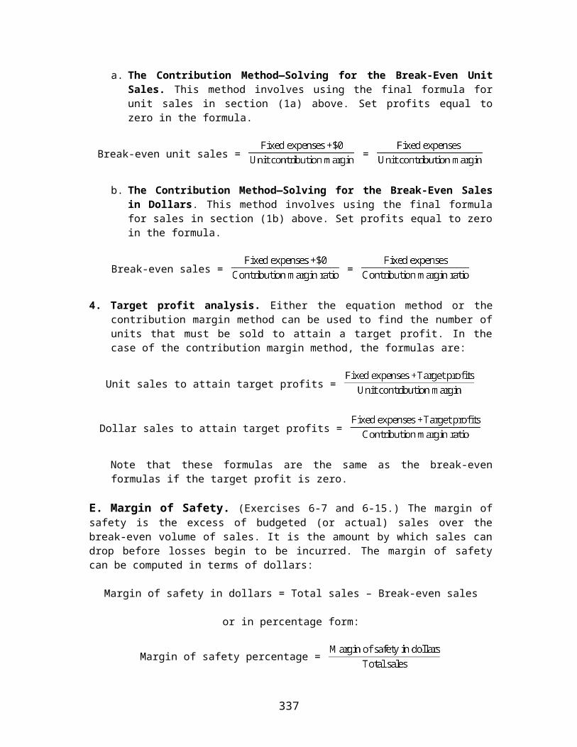
a. The Contribution Method—Solving for the Break-Even UnitSales. This method involves using the final formula forunit sales in section (1a) above. Set profits equal tozero in the formula.
Break-even unit sales = =
b. The Contribution Method—Solving for the Break-Even Salesin Dollars. This method involves using the final formulafor sales in section (1b) above. Set profits equal to zeroin the formula.
Break-even sales = =
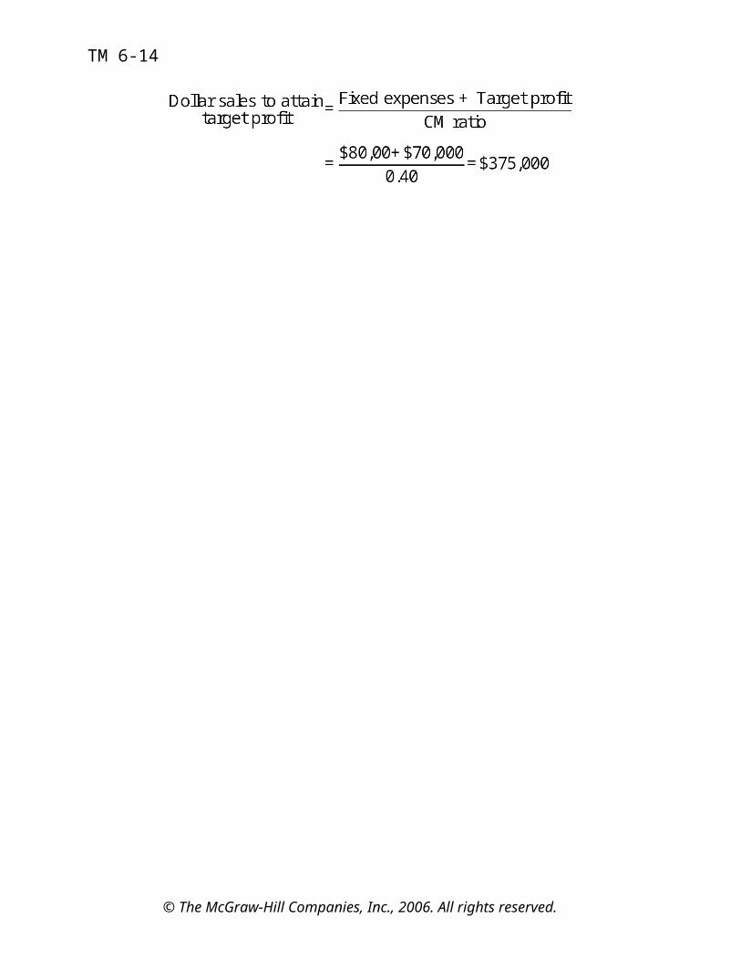
4. Target profit analysis. Either the equation method or thecontribution margin method can be used to find the number ofunits that must be sold to attain a target profit. In thecase of the contribution margin method, the formulas are:
Unit sales to attain target profits =
Dollar sales to attain target profits =
Note that these formulas are the same as the break-evenformulas if the target profit is zero.
E. Margin of Safety. (Exercises 6-7 and 6-15.) The margin ofsafety is the excess of budgeted (or actual) sales over thebreak-even volume of sales. It is the amount by which sales candrop before losses begin to be incurred. The margin of safetycan be computed in terms of dollars:
Margin of safety in dollars = Total sales – Break-even sales
or in percentage form:
Margin of safety percentage =
337
F. Cost Structure. Cost structure refers to the relativeproportion of fixed and variable costs in an organization.Understanding a company’s cost structure is important fordecision-making as well as for analysis of performance.
G. Operating Leverage. (Exercises 6-8 and 6-16.) Operatingleverage is a measure of how sensitive net operating income isto a given percentage change in sales.
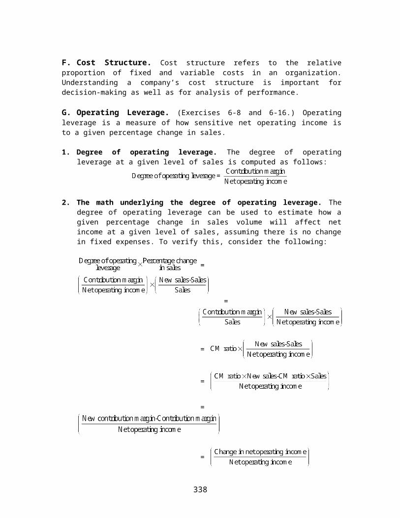
1. Degree of operating leverage. The degree of operatingleverage at a given level of sales is computed as follows:
2. The math underlying the degree of operating leverage. Thedegree of operating leverage can be used to estimate how agiven percentage change in sales volume will affect netincome at a given level of sales, assuming there is no changein fixed expenses. To verify this, consider the following:
=
=
=
=
=
=
338
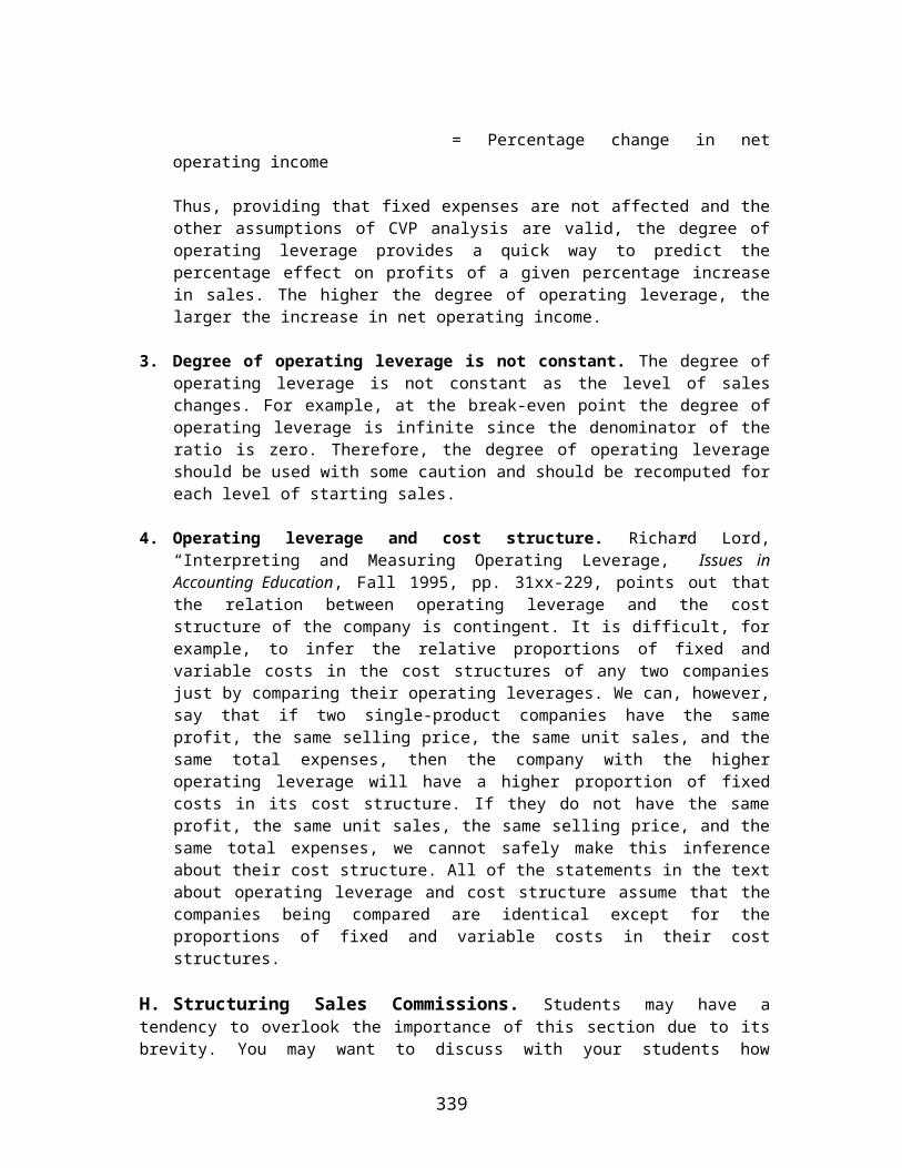
= Percentage change in netoperating income
Thus, providing that fixed expenses are not affected and theother assumptions of CVP analysis are valid, the degree ofoperating leverage provides a quick way to predict thepercentage effect on profits of a given percentage increasein sales. The higher the degree of operating leverage, thelarger the increase in net operating income.
3. Degree of operating leverage is not constant. The degree ofoperating leverage is not constant as the level of saleschanges. For example, at the break-even point the degree ofoperating leverage is infinite since the denominator of theratio is zero. Therefore, the degree of operating leverageshould be used with some caution and should be recomputed foreach level of starting sales.
4. Operating leverage and cost structure. Richard Lord,“Interpreting and Measuring Operating Leverage,” Issues inAccounting Education, Fall 1995, pp. 31xx-229, points out thatthe relation between operating leverage and the coststructure of the company is contingent. It is difficult, forexample, to infer the relative proportions of fixed andvariable costs in the cost structures of any two companiesjust by comparing their operating leverages. We can, however,say that if two single-product companies have the sameprofit, the same selling price, the same unit sales, and thesame total expenses, then the company with the higheroperating leverage will have a higher proportion of fixedcosts in its cost structure. If they do not have the sameprofit, the same unit sales, the same selling price, and thesame total expenses, we cannot safely make this inferenceabout their cost structure. All of the statements in the textabout operating leverage and cost structure assume that thecompanies being compared are identical except for theproportions of fixed and variable costs in their coststructures.
H. Structuring Sales Commissions. Students may have atendency to overlook the importance of this section due to itsbrevity. You may want to discuss with your students how
339
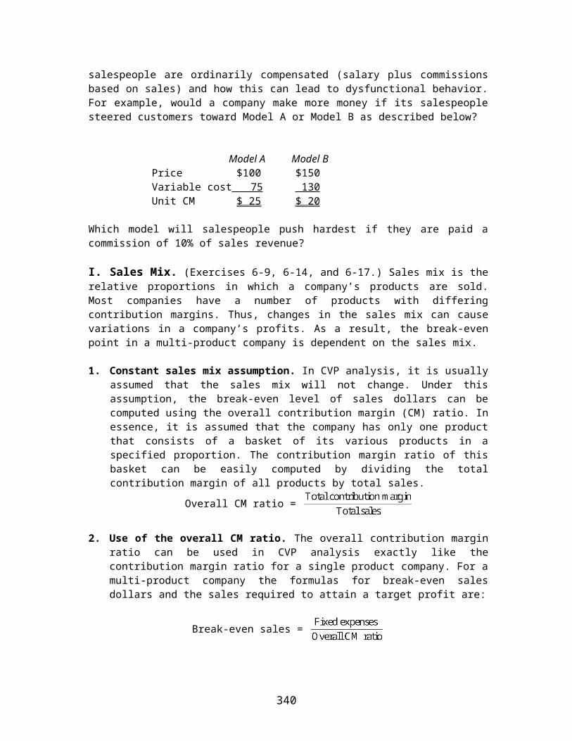
salespeople are ordinarily compensated (salary plus commissionsbased on sales) and how this can lead to dysfunctional behavior.For example, would a company make more money if its salespeoplesteered customers toward Model A or Model B as described below?
Model A Model BPrice $100 $150Variable cost 75 130Unit CM $ 25 $ 20
Which model will salespeople push hardest if they are paid acommission of 10% of sales revenue?
I. Sales Mix. (Exercises 6-9, 6-14, and 6-17.) Sales mix is therelative proportions in which a company’s products are sold.Most companies have a number of products with differingcontribution margins. Thus, changes in the sales mix can causevariations in a company’s profits. As a result, the break-evenpoint in a multi-product company is dependent on the sales mix.
1. Constant sales mix assumption. In CVP analysis, it is usuallyassumed that the sales mix will not change. Under thisassumption, the break-even level of sales dollars can becomputed using the overall contribution margin (CM) ratio. Inessence, it is assumed that the company has only one productthat consists of a basket of its various products in aspecified proportion. The contribution margin ratio of thisbasket can be easily computed by dividing the totalcontribution margin of all products by total sales.
Overall CM ratio =
2. Use of the overall CM ratio. The overall contribution marginratio can be used in CVP analysis exactly like thecontribution margin ratio for a single product company. For amulti-product company the formulas for break-even salesdollars and the sales required to attain a target profit are:
Break-even sales =
340
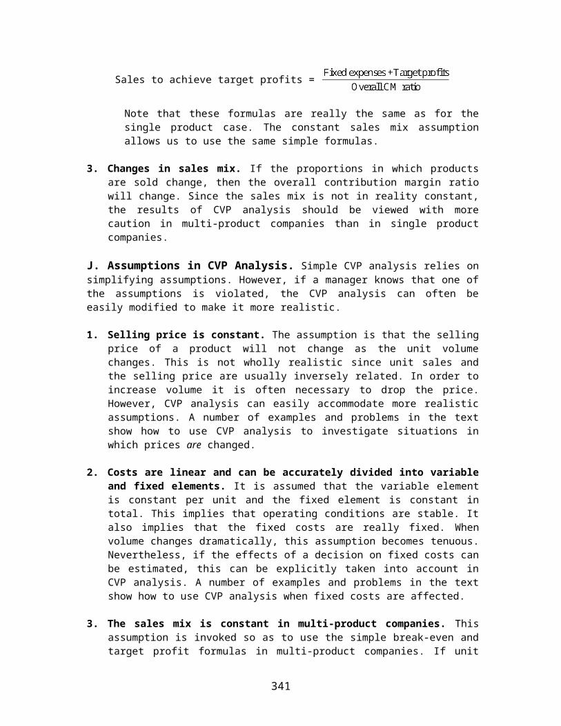
Sales to achieve target profits =
Note that these formulas are really the same as for thesingle product case. The constant sales mix assumptionallows us to use the same simple formulas.
3. Changes in sales mix. If the proportions in which productsare sold change, then the overall contribution margin ratiowill change. Since the sales mix is not in reality constant,the results of CVP analysis should be viewed with morecaution in multi-product companies than in single productcompanies.
J. Assumptions in CVP Analysis. Simple CVP analysis relies onsimplifying assumptions. However, if a manager knows that one ofthe assumptions is violated, the CVP analysis can often beeasily modified to make it more realistic.
1. Selling price is constant. The assumption is that the sellingprice of a product will not change as the unit volumechanges. This is not wholly realistic since unit sales andthe selling price are usually inversely related. In order toincrease volume it is often necessary to drop the price.However, CVP analysis can easily accommodate more realisticassumptions. A number of examples and problems in the textshow how to use CVP analysis to investigate situations inwhich prices are changed.
2. Costs are linear and can be accurately divided into variableand fixed elements. It is assumed that the variable elementis constant per unit and the fixed element is constant intotal. This implies that operating conditions are stable. Italso implies that the fixed costs are really fixed. Whenvolume changes dramatically, this assumption becomes tenuous.Nevertheless, if the effects of a decision on fixed costs canbe estimated, this can be explicitly taken into account inCVP analysis. A number of examples and problems in the textshow how to use CVP analysis when fixed costs are affected.
3. The sales mix is constant in multi-product companies. Thisassumption is invoked so as to use the simple break-even andtarget profit formulas in multi-product companies. If unit
341
contribution margins are fairly uniform across products,violations of this assumption will not be important. However,if unit contribution margins differ a great deal, thenchanges in the sales mix can have a big impact on the overallcontribution margin ratio and hence on the results of CVPanalysis. If a manager can predict how the sales mix willchange, then a more refined CVP analysis can be performed inwhich the individual contribution margins of products arecomputed.
4. In manufacturing companies, inventories do not change. It isassumed that everything the company produces is sold in thesame period. Violations of this assumption result indiscrepancies between financial accounting net operatingincome and the profits calculated using the contributionapproach. This topic is covered in detail in the chapter onvariable costing.
342
Assignment Materials
Assignment TopicLevel of
DifficultySuggeste
d TimeExercise 6-1
Preparing a contribution margin format income statement...........................Basic 20 min.
Exercise 6-2
Prepare a cost-volume-profit (CVP) graph.....Basic 30 min.
Exercise 6-3
Computing and using the CM ratio.............Basic 10 min.
Exercise 6-4
Changes in variable costs, fixed costs, selling price, and volume..................Basic 20 min.
Exercise 6-5
Compute the break-even point.................Basic 20 min.
Exercise 6-6
Compute the level of sales required to attain a target profit.....................Basic 10 min.
Exercise 6-7
Compute the margin of safety.................Basic 10 min.
Exercise 6-8
Compute and use the degree of operating leverage...................................Basic 20 min.
Exercise 6-9
Compute the break-even point for a multi-product company......................Basic 20 min.
Exercise 6-10
Using a contribution format income statement..................................Basic 20 min.
Exercise 6-11
Break-even analysis and CVP graphing.........Basic 30 min.
Exercise 6-12
Break-even and target profit analysis........Basic 30 min.
Exercise 6-13
Break-even and target profit analysis........Basic 30 min.
Exercise 6-14
Missing data; basic CVP concepts.............Basic 20 min.
Exercise 6-15
Break-even analysis; target profit; margin of safety; CM ratio.................Basic 30 min.
Exercise 6-16
Operating leverage...........................Basic 15 min.
Exercise 6-17
Multi-product break-even analysis............Basic 30 min.
Problem 6-18
Basic CVP analysis; graphing.................Basic 60 min.
Problem 6-19
Basics of CVP analysis; cost structure.......Basic 60 min.
Problem Basics of CVP analysis.......................Basic 60 min.
343
6-20Problem 6-21
Sales mix; multi-product break-even analysis...................................Basic 30 min.
Problem 6-22
Break-even analysis; pricing.................Medium 45 min.
Problem 6-23
Interpretive questions on the CVP graph......Medium 30 min.
Problem 6-24
Various CVP questions; break-even point;cost structure; target sales...............Medium 75 min.
Problem 6-25
Graphing; incremental analysis; operating leverage.........................Medium 60 min.
Problem 6-26
Changes in fixed and variable costs; break-even and target profit analysis......Medium 30 min.
Problem 6-27
Break-even and target profit analysis........Medium 30 min.
Problem 6-28
Changes in cost structure; break-even analysis; operating leverage; margin of safety..................................Medium 60 min.
Problem 6-29
Sales mix; break-even analysis; margin of safety..................................Medium 45 min.
Problem 6-30
Sales mix; multi-product break-even analysis...................................Medium 60 min.
Case 6-31 Detailed income statement; CVP analysis......Difficult 60 min.
Case 6-32 Missing data; break-even analysis; target profit; margin of safety; operating leverage.........................
Difficult 90 min.
Case 6-33 Cost structure; break-even; target profits....................................
Difficult 75 min.
Case 6-34 Break-even analysis with step fixed costs......................................
Difficult 75 min.
Case 6-35 Break-evens for individual products in amulti-product company......................
Difficult 60 min.
Essential Problems: Problem 6-18 or Problem 6-25, Problem 6-19 or Problem 6-20, Problem 6-21, Problem 6-24
Supplementary Problems: Problem 6-22, Problem 6-23, Problem 6-26, Problem 6-27, Problem 6-28, Problem 6-29, Problem 6-30, Case 6-31, Case 6-32, Case 6-33, Case 6-34, Case 6-35
344

345
1 2
346
Chapter 6Lecture Notes
Helpful Hint: Before beginning the lecture, show students the sixth segment from the first tape of the McGraw-Hill/Irwin Managerial/Cost Accounting video library. This segment introducesstudents to many of the concepts discussed in chapter 6. The lecture notes reinforce the concepts introduced in the video.
Chapter theme: Cost-volume-profit (CVP)analysis helps managers understand the interrelationships among cost, volume, and profit by focusing their attention on the interactions among the prices ofproducts, volume of activity, per unit variable costs, total fixed costs, and mix of products sold. It is a vital tool used in many business decisions such as deciding what products to manufacture or sell, what pricing policy to follow, what marketing
347
strategy to employ, and what type of productive facilities to acquire.
I. The basics of cost-volume-profit (CVP) analysis
A.The contribution income statement is helpful to managers in judging the impact on profits of changes in selling price, cost, or volume. For example, let's look at a hypotheticalcontribution income statement for Racing Bicycle Company (RBC). Notice:
i. The emphasis on cost behavior.Variable costs are separate from fixed costs.
ii. The contribution margin defined as the amount remaining from sales revenue after variable expenses have been deducted.
3 4 5
348
6 7 8
349
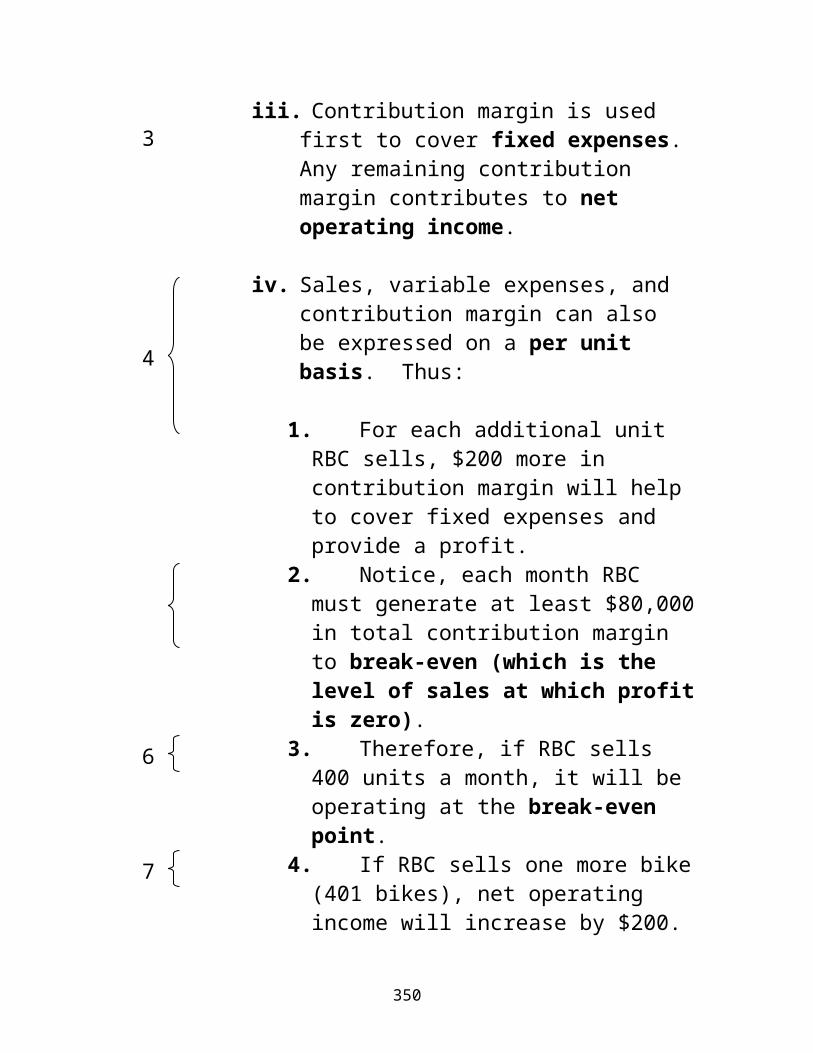
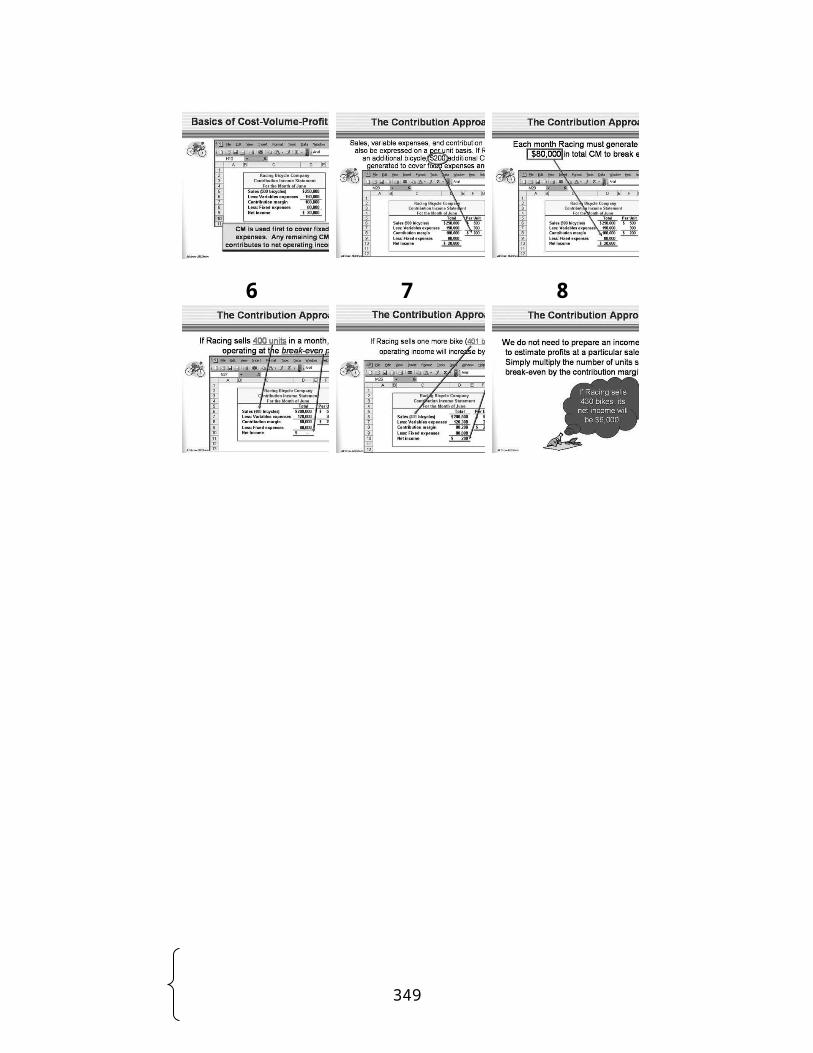
iii. Contribution margin is used first to cover fixed expenses.Any remaining contribution margin contributes to net operating income.
iv. Sales, variable expenses, and contribution margin can also be expressed on a per unit basis. Thus:
1. For each additional unit RBC sells, $200 more in contribution margin will help to cover fixed expenses and provide a profit.
2. Notice, each month RBC must generate at least $80,000in total contribution margin to break-even (which is the level of sales at which profitis zero).
3. Therefore, if RBC sells 400 units a month, it will be operating at the break-even point.
4. If RBC sells one more bike(401 bikes), net operating income will increase by $200.
350
3
4
6
7
v. You do not need to prepare
an income statement to estimate profits at a particular sales volume. Simply multiply the number of units sold above break-even bythe contribution margin per unit.
1. For example, if RBC sells 430 bikes, its net operating income will be $6,000.
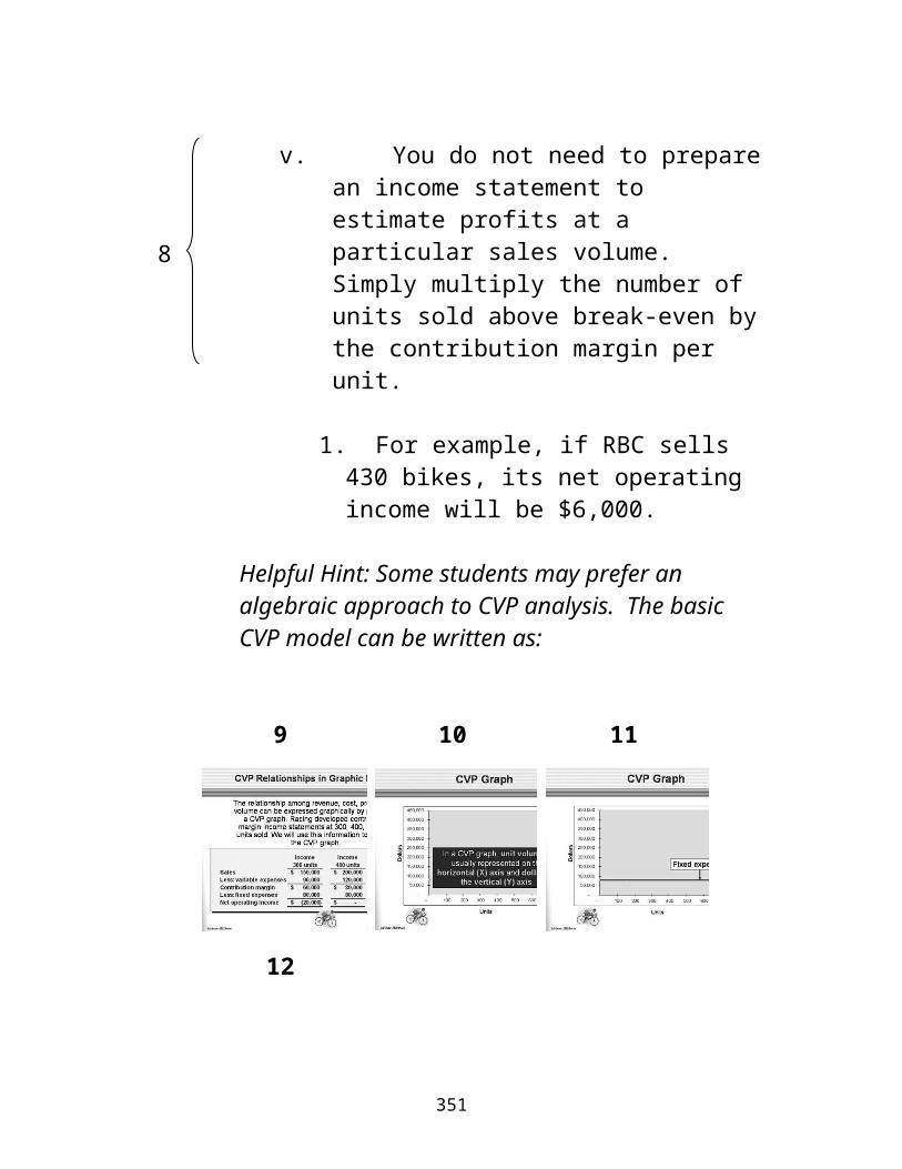
Helpful Hint: Some students may prefer an algebraic approach to CVP analysis. The basic CVP model can be written as:
9 10 11
12
351
8
Profit = (p – v)q – For
Profit = cm × q – F
352
Where p is the unit selling price, v is the variable cost per unit, q is the unit sales, F is the fixed cost, and cm is the unit contribution margin.
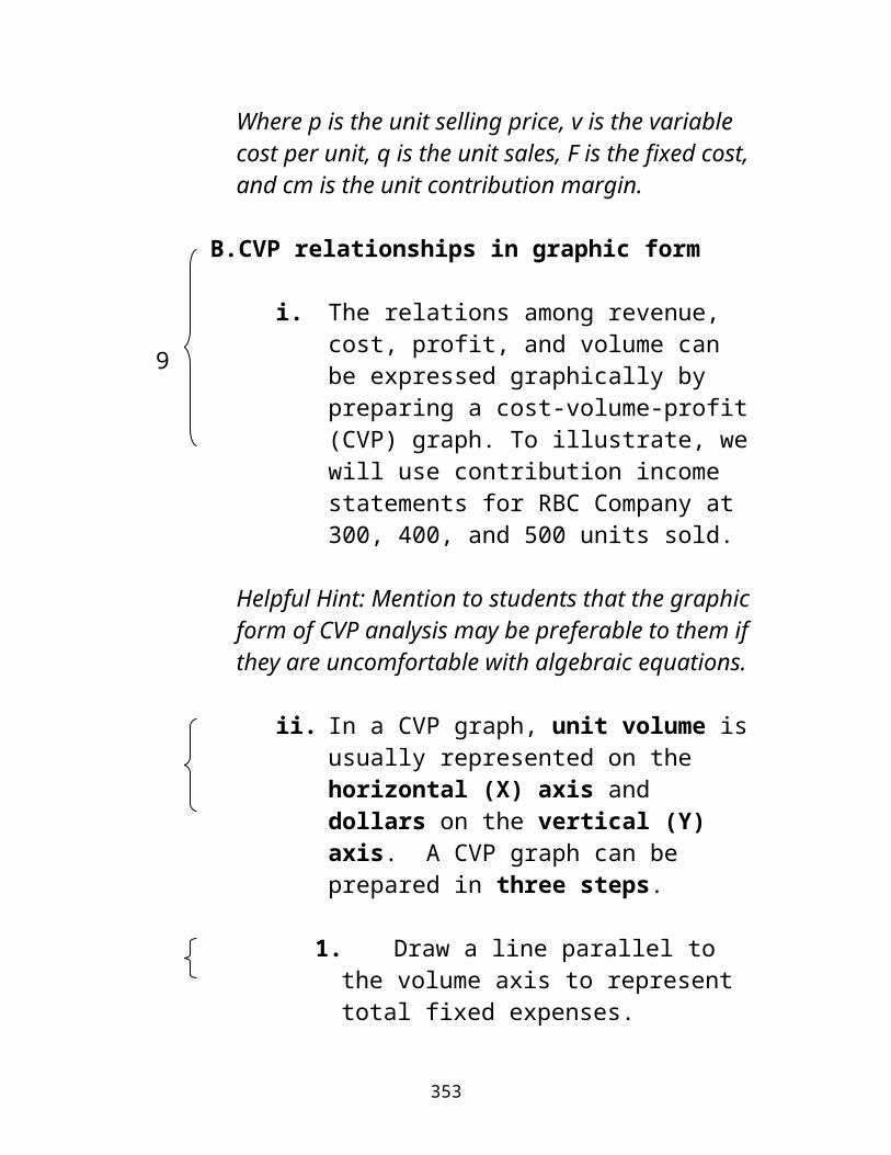
B.CVP relationships in graphic form
i. The relations among revenue, cost, profit, and volume can be expressed graphically by preparing a cost-volume-profit(CVP) graph. To illustrate, wewill use contribution income statements for RBC Company at 300, 400, and 500 units sold.
Helpful Hint: Mention to students that the graphic form of CVP analysis may be preferable to them if they are uncomfortable with algebraic equations.
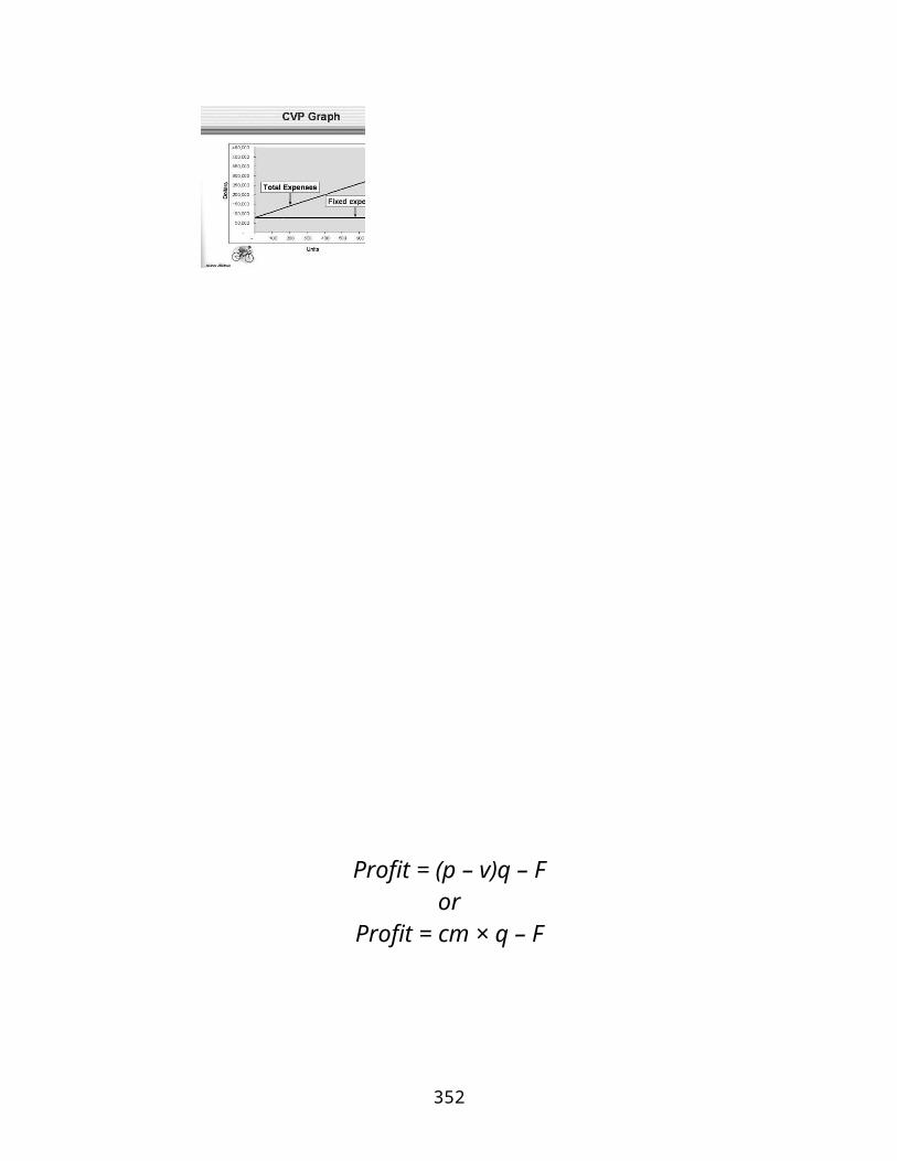
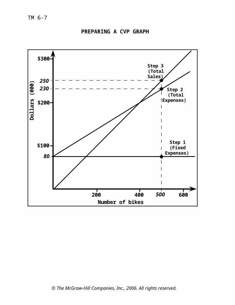
ii. In a CVP graph, unit volume isusually represented on the horizontal (X) axis and dollars on the vertical (Y) axis. A CVP graph can be prepared in three steps.
1. Draw a line parallel to the volume axis to represent total fixed expenses.
353
9
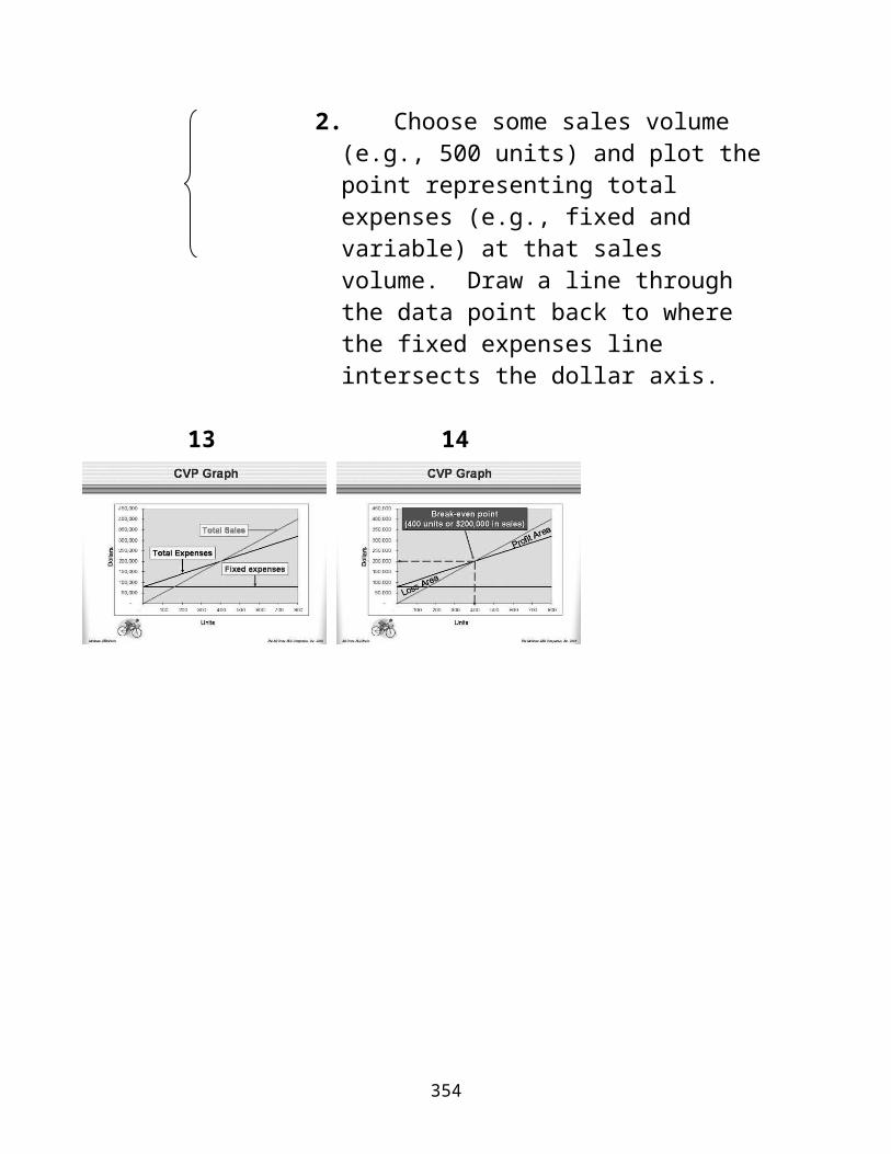
2. Choose some sales volume (e.g., 500 units) and plot thepoint representing total expenses (e.g., fixed and variable) at that sales volume. Draw a line through the data point back to where the fixed expenses line intersects the dollar axis.
13 14
354
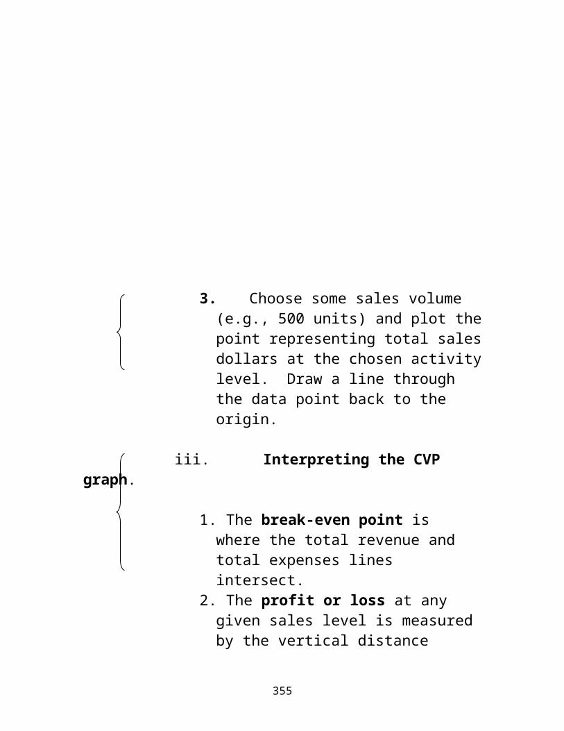
3. Choose some sales volume (e.g., 500 units) and plot thepoint representing total salesdollars at the chosen activitylevel. Draw a line through the data point back to the origin.
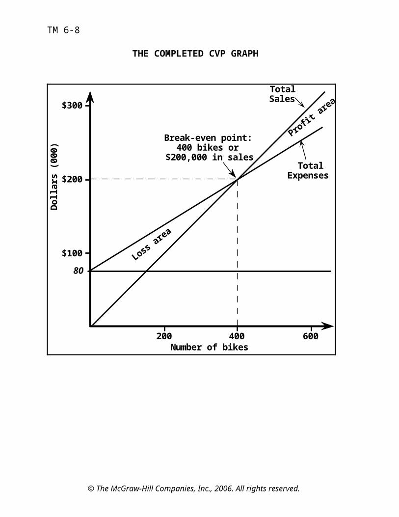
iii. Interpreting the CVP graph.
1. The break-even point is where the total revenue and total expenses lines intersect.
2. The profit or loss at any given sales level is measured by the vertical distance
355
between the total revenue and the total expenses lines.
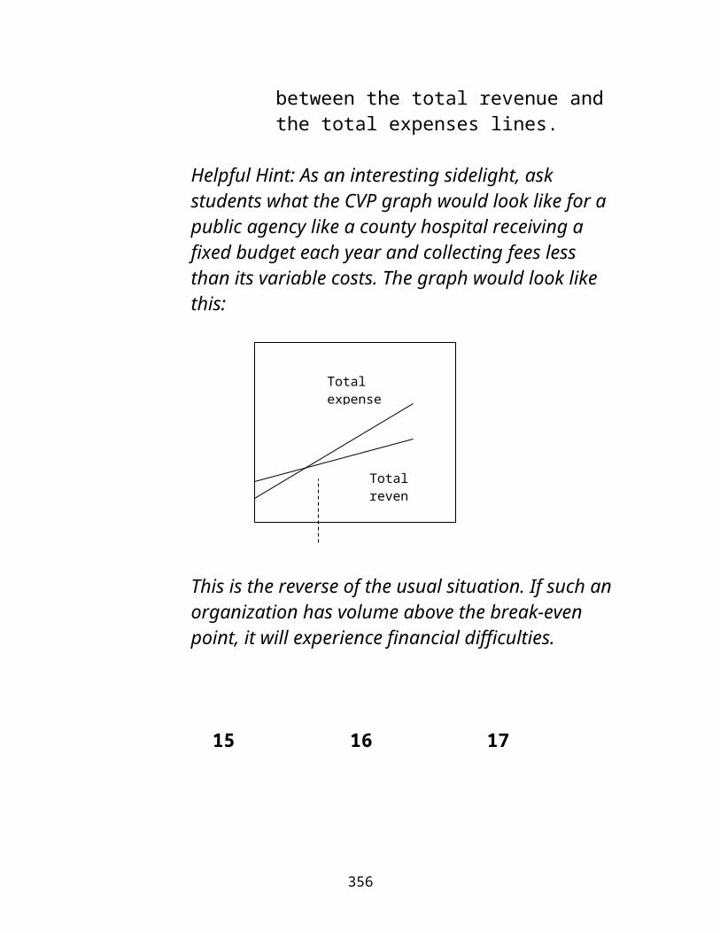
Helpful Hint: As an interesting sidelight, ask students what the CVP graph would look like for a public agency like a county hospital receiving a fixed budget each year and collecting fees less than its variable costs. The graph would look like this:
This is the reverse of the usual situation. If such anorganization has volume above the break-even point, it will experience financial difficulties.
15 16 17
356
Totalexpense
Totalreven
18 19
357
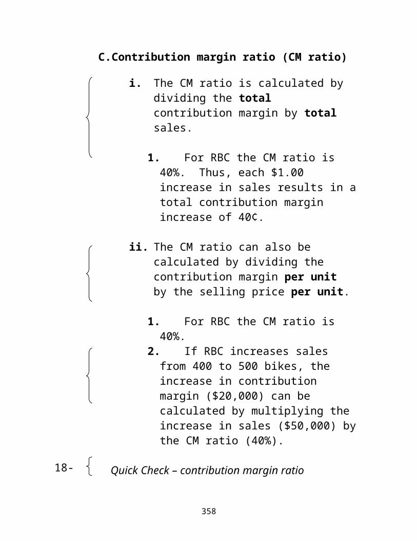
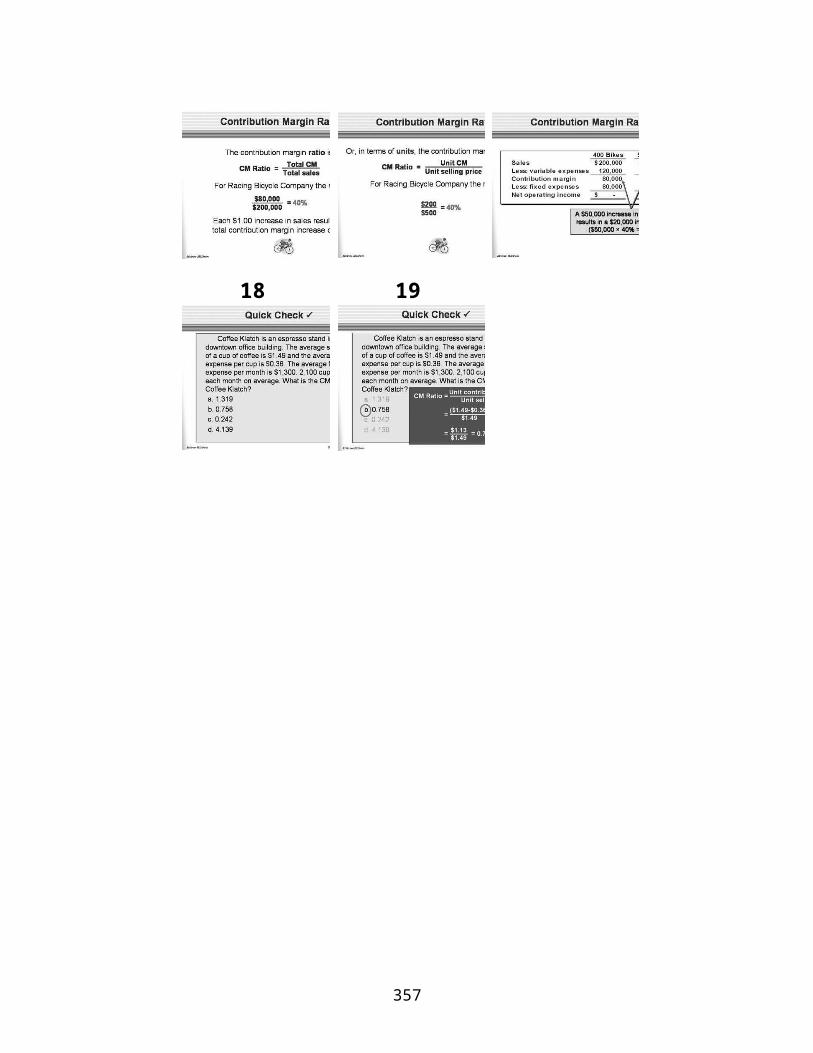
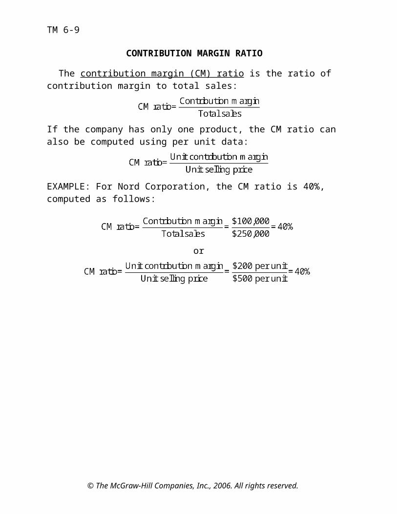
C.Contribution margin ratio (CM ratio)
i. The CM ratio is calculated by dividing the total contribution margin by total sales.
1. For RBC the CM ratio is 40%. Thus, each $1.00 increase in sales results in atotal contribution margin increase of 40¢.
ii. The CM ratio can also be calculated by dividing the contribution margin per unit by the selling price per unit.
1. For RBC the CM ratio is 40%.
2. If RBC increases sales from 400 to 500 bikes, the increase in contribution margin ($20,000) can be calculated by multiplying the increase in sales ($50,000) bythe CM ratio (40%).
Quick Check – contribution margin ratio
358
18-
D.Applications of CVP concepts
Helpful Hint: The five examples that are forthcoming should indicate to students the rangeof uses of CVP analysis. In addition to assisting management in determining the level of sales thatis needed to break-even or generate a certain dollar amount of profit, the examples illustrate how the results of alternative decisions can be quickly determined.
20 21 22
23 24 25
359
26
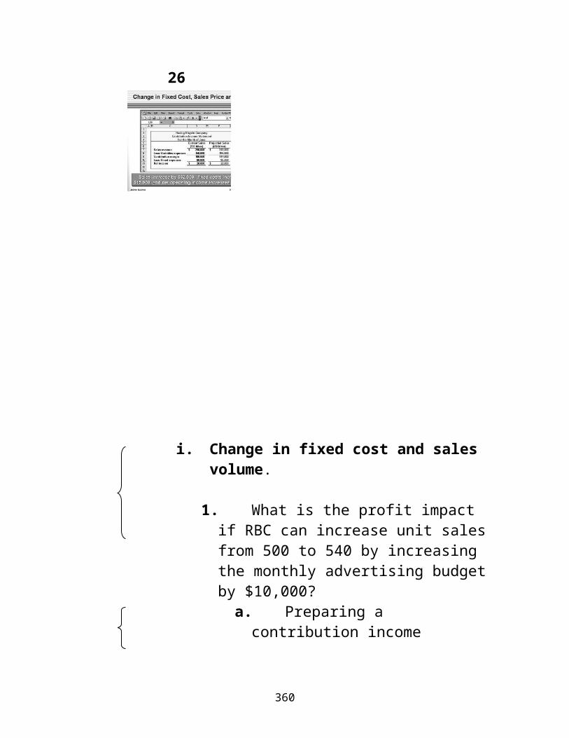
i. Change in fixed cost and salesvolume.
1. What is the profit impact if RBC can increase unit salesfrom 500 to 540 by increasing the monthly advertising budgetby $10,000?a. Preparing a contribution income
360
statement reveals a $2,000decrease in profits.
b. A shortcut solution using incremental analysisalso reveals a $2,000 decrease in profits.
ii. Change in variable costs and sales volume.
1. What is the profit impact if RBC can use higher quality raw materials, thus increasingvariable costs per unit by $10, to generate an increase in unit sales from 500 to 580?a. A shortcut solution reveals a $10,200 increasein profits.
iii. Change in fixed cost, sales price, and sales volume.
1. What is the profit impact if RBC: (1) cuts its selling price $20 per unit, (2) increases its advertising budget by $15,000 per month, and (3) increases unit sales
361
from 500 to 650 units per month? a. A shortcut solution reveals a $2,000 increase in profits.
27 28 29
30
362
iv. Change in variable cost, fixedcost, and sales volume.
1. What is the profit impact if RBC: (1) pays a $15 sales commission per bike sold instead of paying salespersonsflat salaries that currently total $6,000 per month, and (2) increases unit sales from 500 to 575 bikes? a. A shortcut solution reveals a $12,375 increasein profits.
v. Change in regular sales price.
1. If RBC has an opportunity to sell 150 bikes to a wholesaler without disturbing
363
sales to other customers or fixed expenses, what price should it quote to the wholesaler if it wants to increase monthly profits by $3,000?a. The price quote shouldbe $320.
In Business InsightsReal companies regularly manage the CVP levers in an effort to increase profits. For example:
“Playing the CVP Game” (page 250) In 2002, General Motors (GM) gave away
almost $2,600 per vehicle in customer incentives such as price cuts and 0% financing.
GM reported that “The pricing sacrifices have been more than offset by volume gains.” Lehman Brothers analysts estimated that GMwould sell an additional 395,000 trucks and SUVs and an extra 75,000 cars in 2002.
31 32 33
364
34
365
The trucks earn an average contribution margin of $7,000 per vehicle, while the cars earn about $4,000 per vehicle.
All told, the volume gains were expected to bring in an additional $3 billion in profits for GM.
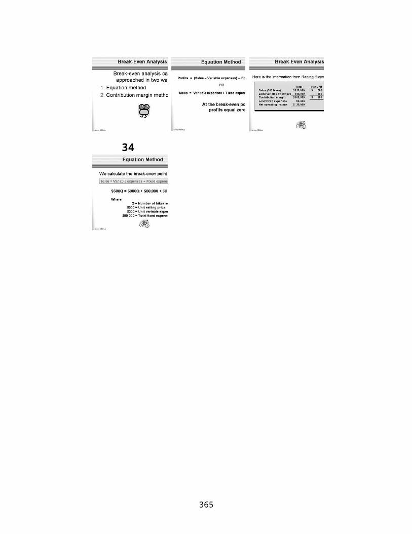
II. Break-even analysis
A.The breakeven point can be computed using either the equation method or the contribution margin method.
i. The equation method is based on the contribution approach income statement.
1. The equation can be statedin one of two ways:
Profits = (Sales – Variable expenses) – Fixed Expenses
or
Sales = Variable expenses + Fixed expenses + Profits
366
32
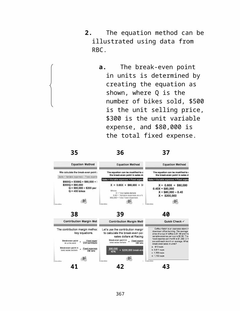
2. The equation method can beillustrated using data from RBC.
a. The break-even point in units is determined by creating the equation as shown, where Q is the number of bikes sold, $500is the unit selling price,$300 is the unit variable expense, and $80,000 is the total fixed expense.
35 36 37
38 39 40
41 42 43
367
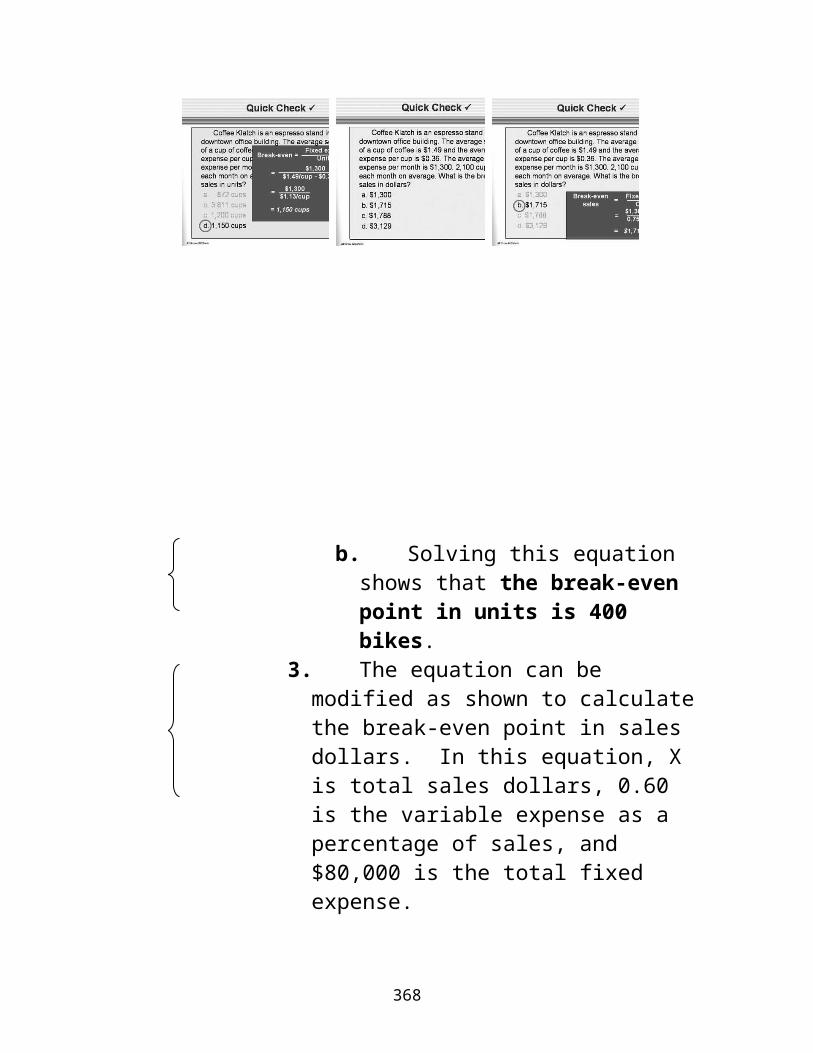
b. Solving this equation shows that the break-even point in units is 400 bikes.
3. The equation can be modified as shown to calculatethe break-even point in sales dollars. In this equation, X is total sales dollars, 0.60 is the variable expense as a percentage of sales, and $80,000 is the total fixed expense.
368
a. Solving this equation shows that the break-even point is sales dollars is $200,000.
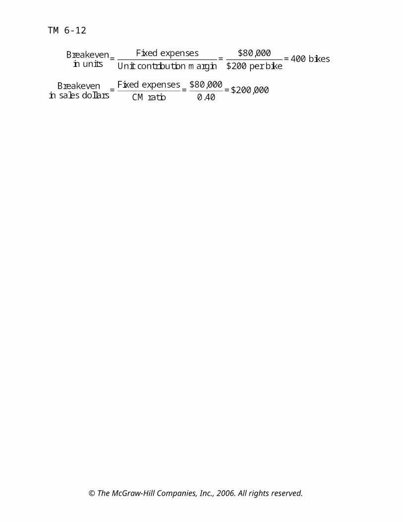
ii. The contribution margin methodhas two key equations:
Break-even point in units sold = Fixed expenses
CMper unit
Break-even point in sales dollars = Fixed expenses
CM ratio
1. The contribution margin method can be illustrated using data from RBC.a. The break-even point in unit sales (400 bikes) and sales dollars ($200,000) is the same as shown for the equation method.
Quick Check – break-even calculations
369
40-
44
370
In Business InsightsThe concept of a breakeven point is critically important to dot.com companies. For example:
“Buying on the GoA Dot.com Tale” (page 240) *CD is a company that allows customers to
order music CDs on their cell phones. Suppose you hear a cut from a CD on your car radio that you would like to own. Pick up your cell phone, punch “*CD,” enter the radio station’s frequency, and the time you heard the song, and the CD will soon be on its way to you.
*CD charges about $17 per CD, including shipping. The company pays its suppliers about $13 per CD.
*CD expects to lose $1.5 million on sales of $1.5 million in its first year of operations. That assumes the company sells 88,000 CDs.
Working backwards, it would appear the company’s fixed costs are about $1,850,000 per year. This means the company would
371
need to sell over 460,000 CDs per year just to break-even!
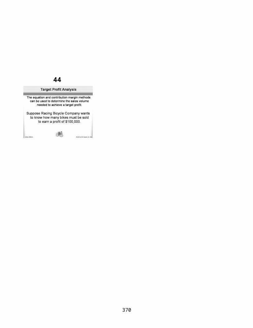
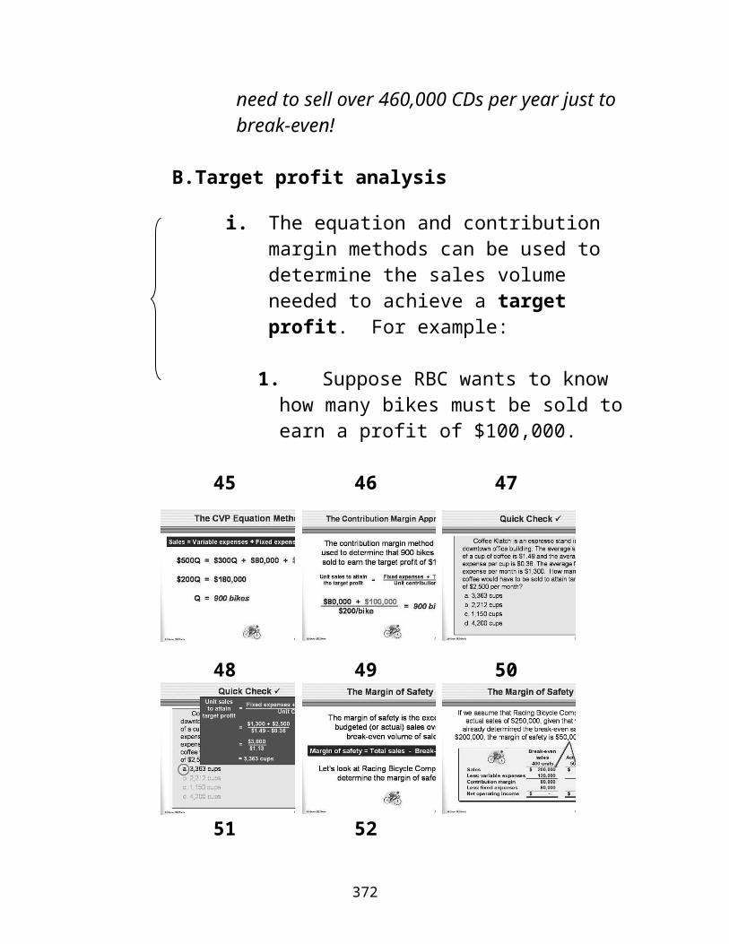
B.Target profit analysis
i. The equation and contribution margin methods can be used to determine the sales volume needed to achieve a target profit. For example:
1. Suppose RBC wants to know how many bikes must be sold toearn a profit of $100,000.
45 46 47
48 49 50
51 52
372
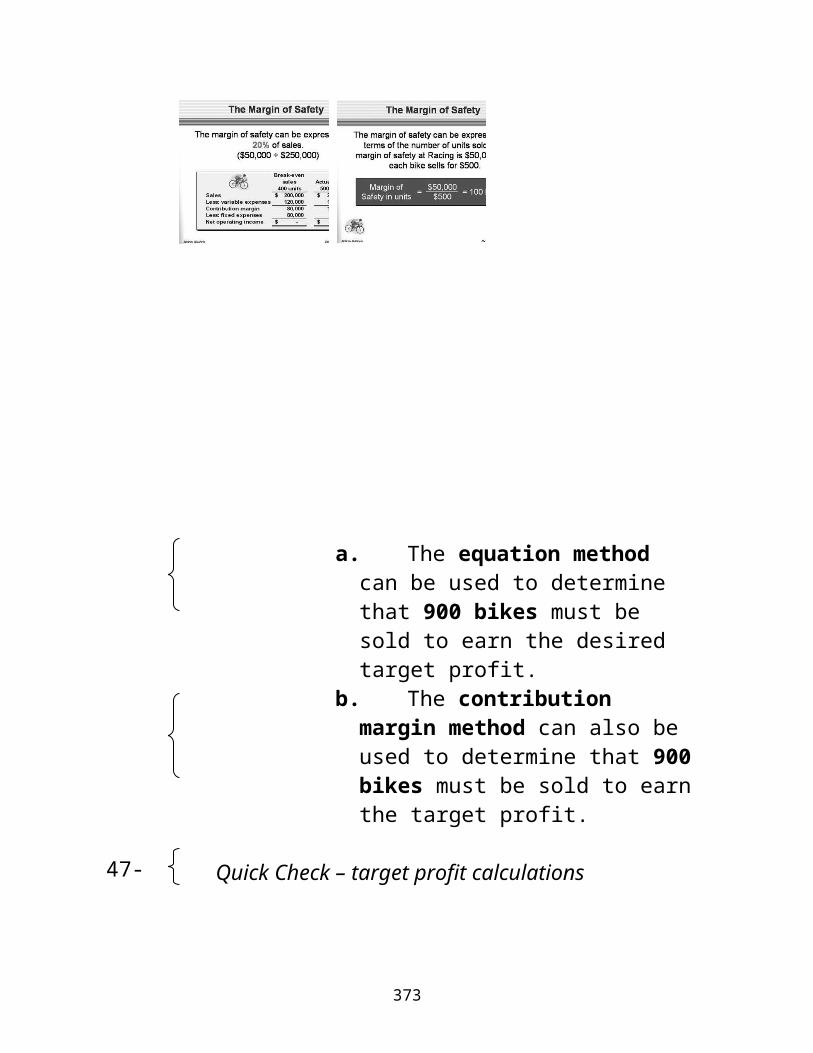
a. The equation method can be used to determine that 900 bikes must be sold to earn the desired target profit.
b. The contribution margin method can also be used to determine that 900bikes must be sold to earnthe target profit.
Quick Check – target profit calculations
373
47-
C.The margin of safety
i. The margin of safety is the excess of budgeted (or actual)sales over the break-even volume of sales. For example:1. If we assume that RBC has actual sales of $250,000, given that we have already determined the break-even sales to be $200,000, the margin of safety is $50,000.
2. The margin of safety can be expressed as a percent of sales. For example:a. RBC’s margin of safetyis 20% of sales.
3. The margin of safety can be expressed in terms of the number of units sold. For example:a. RBC’s margin of safetyis 100 bikes.
374
53 54 55
56
375
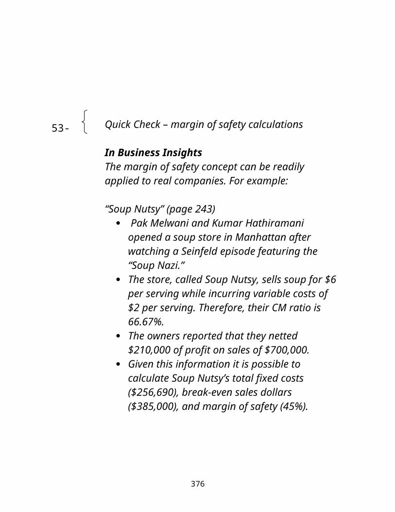
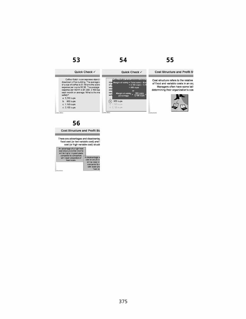
Quick Check – margin of safety calculations
In Business InsightsThe margin of safety concept can be readily applied to real companies. For example:
“Soup Nutsy” (page 243) Pak Melwani and Kumar Hathiramani
opened a soup store in Manhattan after watching a Seinfeld episode featuring the “Soup Nazi.”
The store, called Soup Nutsy, sells soup for $6per serving while incurring variable costs of $2 per serving. Therefore, their CM ratio is 66.67%.
The owners reported that they netted $210,000 of profit on sales of $700,000.
Given this information it is possible to calculate Soup Nutsy’s total fixed costs ($256,690), break-even sales dollars ($385,000), and margin of safety (45%).
376
53-
III. CVP considerations in choosing a coststructure
A. Cost structure and profit stability
i. Cost structure refers to the relative proportion of fixed and variable costs in an organization. Managers often have some latitude in determining their organization's cost structure.
ii. There are advantages and disadvantages to high fixed cost (or low variable cost) and low fixed cost (or high variable cost) structures.
56
377
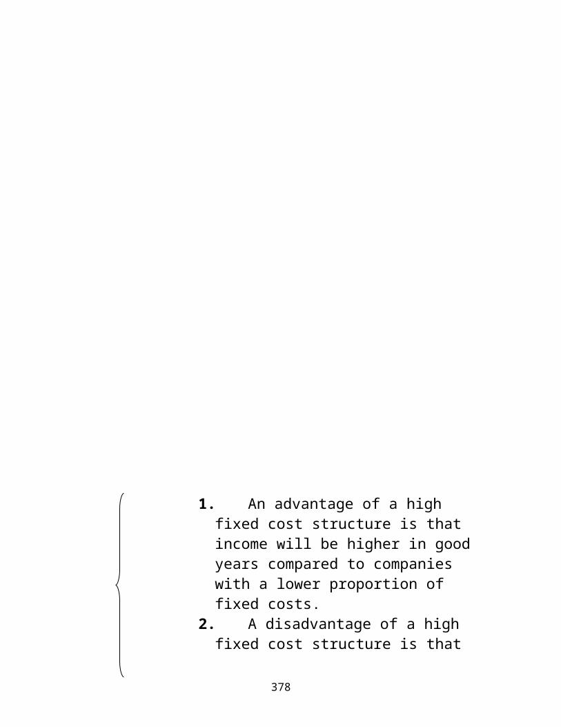
1. An advantage of a high fixed cost structure is that income will be higher in good years compared to companies with a lower proportion of fixed costs.
2. A disadvantage of a high fixed cost structure is that
378
income will be lower in bad years compared to companies with a lower proportion of fixed costs.
3. Companies with low fixed cost structures enjoy greater stability in income across good and bad years.
In Business InsightsCompanies frequently compete with one another based on their cost structures. For example:
“A Losing Cost Structure” (page 245) Both JetBlue and United Airlines use an
Airbus 235 to fly from Dulles International airport near Washington D.C., to Oakland, California. Both planes have a pilot, copilot, and four flight attendants.
Based on 2002 data, the pilot on the United Flight earned $16,350 to $18,000 per month compared to $6,800 per month for the JetBlue pilot.
United’s senior flight attendants earned more than $41,000 per year; whereas the Jet Blue attendants were paid $16,800 to $27,000 per year.
Due to intense fare competition from JetBlue and other low-cost carriers, United was
379
unable to cover its higher operating costs onthis and many
57 58 59
60 61 62
63 64 65
380
other flights. Consequently, United went into bankruptcy at the end of 2002.
B.Operating leverage
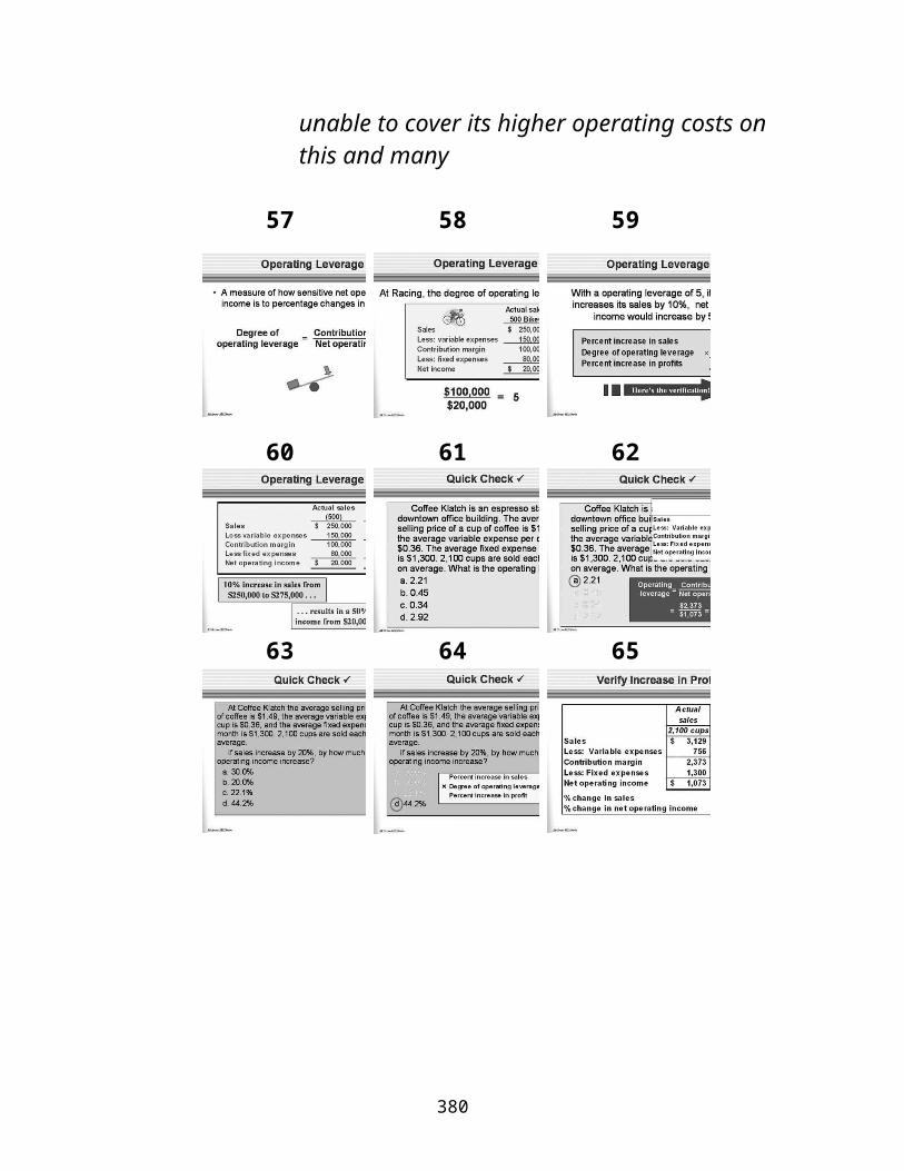
i. Operating leverage is a measure of how sensitive net operating income is to percentage changes in sales.
ii. The degree of operating leverage is a measure, at any given level of sales, of how apercentage change in sales volume will affect profits. Itis computed as follows:
Degree of operating leverage = Contribution margin
Net operating income
iii. To illustrate, let’s revisit the contribution income statement for RBC:
381
1. RBC’s degree of operating leverage is 5 ($100,000/$20,000).
2. With an operating leverageof 5, if RBC increases its sales by 10%, net operating income would increase by 50%.a. The 50% increase can be verified by preparing acontribution approach income statement.
Quick Check – operating leverage calculations
In Business InsightsOperating leverage is an important concept that managers need to understand. Failure to understand this concept can cause serious problems. For example:
66
382
61-
“Fan Appreciation” (page 247) Jerry Colangelo, the managing partner of the
Arizona Diamondbacks professional baseball team, spent over $100 million to sign six free agents.
The doubling of the team’s payroll coupled with servicing the debt on the team’s new
383
stadium, raised the D-backs annual operating expenses to about $100 million. Accordingly, the team needed to average 40,000 fans per game to break-even.
In an effort to boost revenue, Colangelo decided, during Fan Appreciation Weekend, to raise ticket prices by 12%. Attendance for the season dropped by 15%, turning what should have been a $20 million profit into a loss of over $10 million.
Note that a drop in attendance of 15% did not cut profits just by 15% – that’s the magic of operating leverage at work.
Helpful Hint: Emphasize that the degree of operating leverage is not a constant like unit variable cost or unit contribution margin that a manager can apply with confidence in a variety of situations. The degree of operating leverage depends on the level of sales and must be recomputed each time the sales level changes. Also, note that operating leverage is greatest at sales levels near the break-even point and it decreases as sales and profits rise.
IV. Structuring sales commissions
384
A.Companies generally compensate salespeople by paying them either a commission based on sales or a salaryplus a sales commission. Commissions based
385
66 67 68
69
386
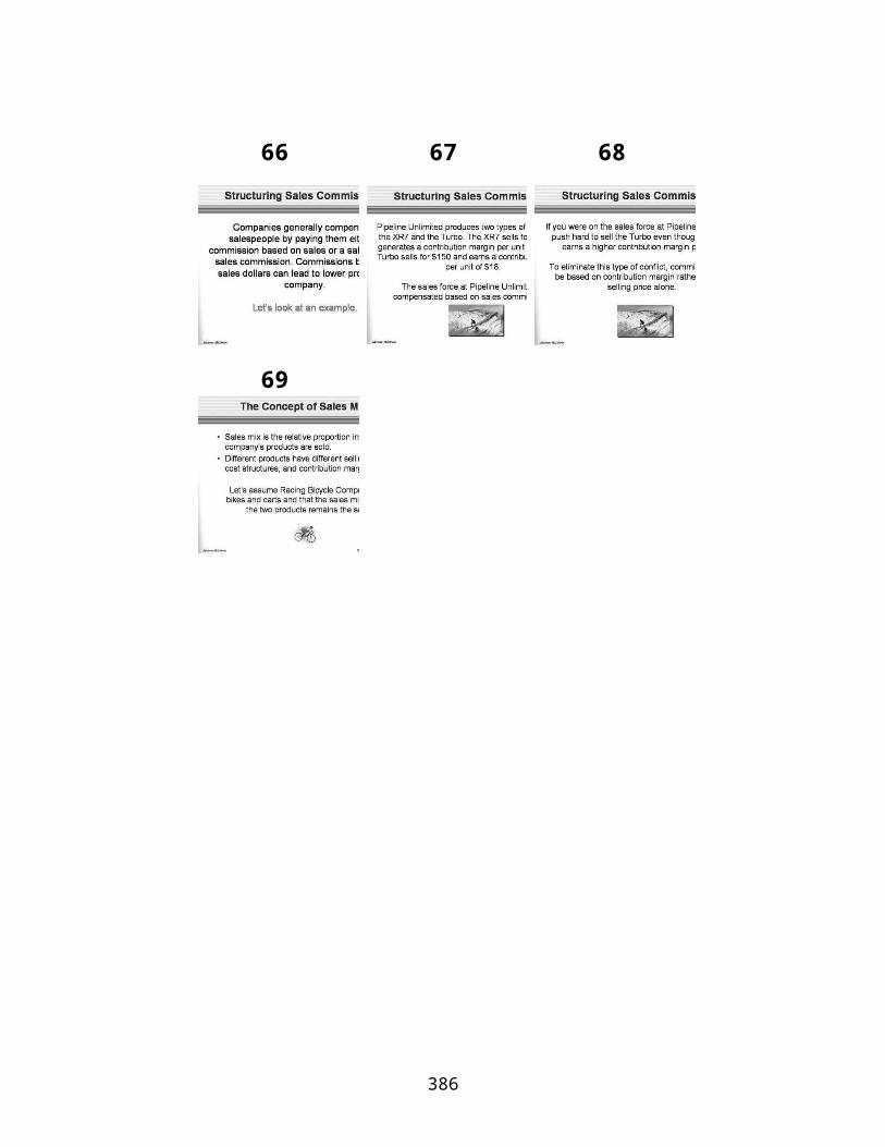
on sales dollars can lead to lower profits in a company. Consider the following illustration:
i. Pipeline unlimited produces two types of surfboards, the XR7 and the Turbo. The XR7 sells for $100 and generates acontribution margin per unit of $25. The Turbo sells for $150 and earns a contribution margin per unit of $18.
ii. Salespeople compensated based on sales commission will push hard to sell the Turbo even-though the XR7 earns a higher contribution margin per unit.
iii. To eliminate this type of conflict, commissions can be based on contribution margin rather than on selling price alone.
V. The concept of sales mix
387
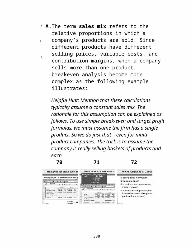
A.The term sales mix refers to the relative proportions in which a company’s products are sold. Since different products have different selling prices, variable costs, and contribution margins, when a company sells more than one product, breakeven analysis become more complex as the following example illustrates:
Helpful Hint: Mention that these calculations typically assume a constant sales mix. The rationale for this assumption can be explained as follows. To use simple break-even and target profitformulas, we must assume the firm has a single product. So we do just that – even for multi-product companies. The trick is to assume the company is really selling baskets of products and each 70 71 72
388
basket always contains the various products in thesame proportions.
i. Assume the RBC sells bikes andcarts. The bikes comprise 45% of the company’s total sales revenue and the carts comprise
389
the remaining 55%. The contribution margin ratio for both products combined is 48.2%.
ii. The break-even point in sales would be $352,697. The bikes would account for 45% of this amount, or $158,714. The cartswould account for 55% of the break-even sales, or $193,983.
1. Notice a slight rounding error of $176.
VI. Assumptions of CVP analysis
A.Four key assumptions underlie CVP analysis:
i. Selling price is constant.
ii. Costs are linear and can be accurately divided into variable and fixed elements. The variable element is constant per unit, and the fixed element is constant in
390
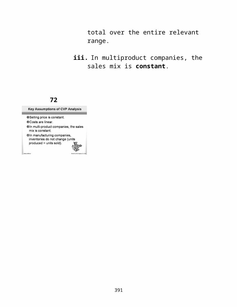
total over the entire relevantrange.
iii. In multiproduct companies, thesales mix is constant.
72
391
iv. In manufacturing companies, inventories do not change. Thenumber of units produced equals the number of units sold.
Helpful Hint: Point out that nothing is sacred about these assumptions. When violations of theseassumptions are significant, managers can and domodify the basic CVP model. Spreadsheets allow practical models that incorporate more realistic assumptions. For example, nonlinear cost functions with step fixed costs can be modeled using “If…Then” functions.
392

Chapter 6Transparency Masters
393
TM 6-1
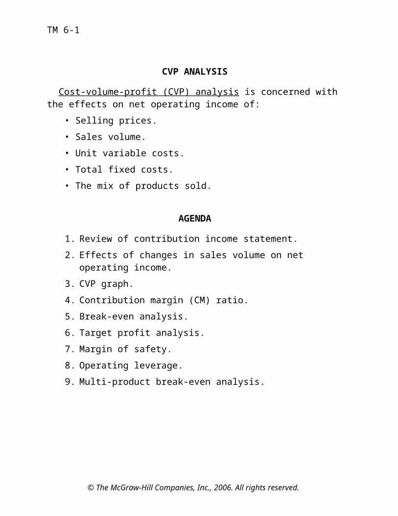
CVP ANALYSIS
Cost-volume-profit (CVP) analysis is concerned with the effects on net operating income of:
• Selling prices.• Sales volume.• Unit variable costs.• Total fixed costs.• The mix of products sold.
AGENDA
1. Review of contribution income statement.2. Effects of changes in sales volume on net
operating income.3. CVP graph.4. Contribution margin (CM) ratio.5. Break-even analysis.6. Target profit analysis.7. Margin of safety.8. Operating leverage.9. Multi-product break-even analysis.
© The McGraw-Hill Companies, Inc., 2006. All rights reserved.
TM 6-2
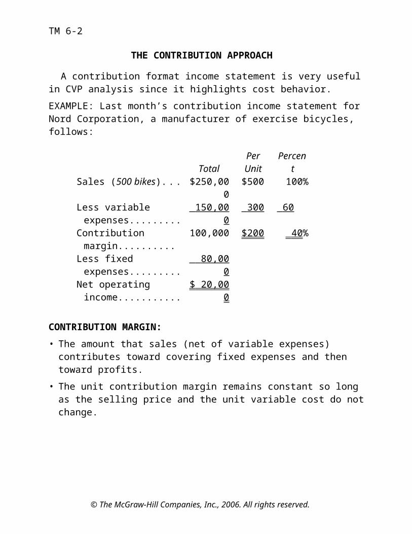
THE CONTRIBUTION APPROACH
A contribution format income statement is very usefulin CVP analysis since it highlights cost behavior.EXAMPLE: Last month’s contribution income statement forNord Corporation, a manufacturer of exercise bicycles, follows:
TotalPerUnit
Percent
Sales (500 bikes)... $250,000
$500 100%
Less variable expenses.........
150,00 0
300 60
Contribution margin..........
100,000 $200 40 %
Less fixed expenses.........
80,00 0
Net operating income...........
$ 20,00 0
CONTRIBUTION MARGIN:• The amount that sales (net of variable expenses) contributes toward covering fixed expenses and then toward profits.
• The unit contribution margin remains constant so long as the selling price and the unit variable cost do notchange.
© The McGraw-Hill Companies, Inc., 2006. All rights reserved.
TM 6-3
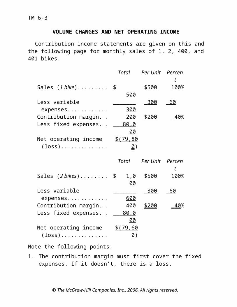
VOLUME CHANGES AND NET OPERATING INCOME
Contribution income statements are given on this and the following page for monthly sales of 1, 2, 400, and 401 bikes.
Total Per Unit Percent
Sales (1 bike)......... $ 500
$500 100%
Less variable expenses............
300
300 60
Contribution margin. . 200 $200 40 %Less fixed expenses. . 80,0
00Net operating income (loss)..............
$(79,800)
Total Per Unit Percent
Sales (2 bikes)........ $ 1,000
$500 100%
Less variable expenses............
600
300 60
Contribution margin. . 400 $200 40 %Less fixed expenses. . 80,0
00Net operating income (loss)..............
$(79,600)
Note the following points:1. The contribution margin must first cover the fixed
expenses. If it doesn’t, there is a loss.
© The McGraw-Hill Companies, Inc., 2006. All rights reserved.
TM 6-4
2. As additional units are sold, fixed expenses are whittled down until they have all been covered.
© The McGraw-Hill Companies, Inc., 2006. All rights reserved.
TM 6-5
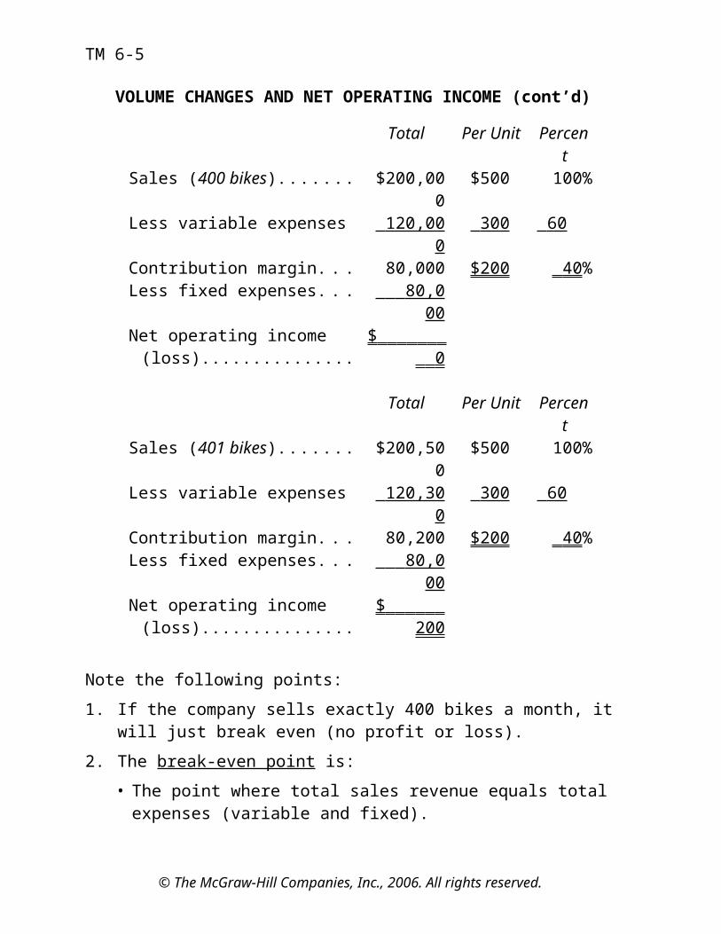
VOLUME CHANGES AND NET OPERATING INCOME (cont’d)
Total Per Unit Percent
Sales (400 bikes)....... $200,000
$500 100%
Less variable expenses 120,00 0
300 60
Contribution margin. . . 80,000 $200 40 %Less fixed expenses. . . 80,0
00Net operating income (loss)...............
$ 0
Total Per Unit Percent
Sales (401 bikes)....... $200,500
$500 100%
Less variable expenses 120,30 0
300 60
Contribution margin. . . 80,200 $200 40 %Less fixed expenses. . . 80,0
00Net operating income (loss)...............
$ 200
Note the following points:1. If the company sells exactly 400 bikes a month, it
will just break even (no profit or loss).2. The break-even point is:
• The point where total sales revenue equals total expenses (variable and fixed).
© The McGraw-Hill Companies, Inc., 2006. All rights reserved.
TM 6-6
• The point where total contribution margin equals total fixed expenses.
3. Each additional unit sold increases net operating income by the amount of the unit contribution margin.
© The McGraw-Hill Companies, Inc., 2006. All rights reserved.
TM 6-7
PREPARING A CVP GRAPH
$200
$100
$300
Dollars (000)
Number of bikes200 400 600500
250230
80
Step 1 (Fixed
Expenses)
Step 3 (Total Sales)
Step 2 (Total
Expenses)
© The McGraw-Hill Companies, Inc., 2006. All rights reserved.
TM 6-8
THE COMPLETED CVP GRAPH
.
$200
$100
$300
Dollars (000)
Number of bikes200 400 600
80
Break-even point:400 bikes or
$200,000 in sales
TotalSales
TotalExpenses
Profit
area
Loss a
rea
© The McGraw-Hill Companies, Inc., 2006. All rights reserved.
TM 6-9
CONTRIBUTION MARGIN RATIO
The contribution margin (CM) ratio is the ratio of contribution margin to total sales:
If the company has only one product, the CM ratio can also be computed using per unit data:
EXAMPLE: For Nord Corporation, the CM ratio is 40%, computed as follows:
or
© The McGraw-Hill Companies, Inc., 2006. All rights reserved.
TM 6-10
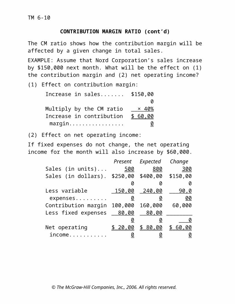
CONTRIBUTION MARGIN RATIO (cont’d)
The CM ratio shows how the contribution margin will be affected by a given change in total sales.EXAMPLE: Assume that Nord Corporation’s sales increase by $150,000 next month. What will be the effect on (1) the contribution margin and (2) net operating income?(1) Effect on contribution margin:
Increase in sales....... $150,000
Multiply by the CM ratio × 40% Increase in contributionmargin.................
$ 60,00 0
(2) Effect on net operating income:If fixed expenses do not change, the net operating income for the month will also increase by $60,000.
Present Expected ChangeSales (in units)... 500 800 300Sales (in dollars). $250,00
0$400,00
0$150,00
0Less variable expenses.........
150,00 0
240,00 0
90,0 00
Contribution margin 100,000 160,000 60,000Less fixed expenses 80,00
0 80,00
0
0 Net operating income...........
$ 20,00 0
$ 80,00 0
$ 60,00 0
© The McGraw-Hill Companies, Inc., 2006. All rights reserved.
TM 6-11
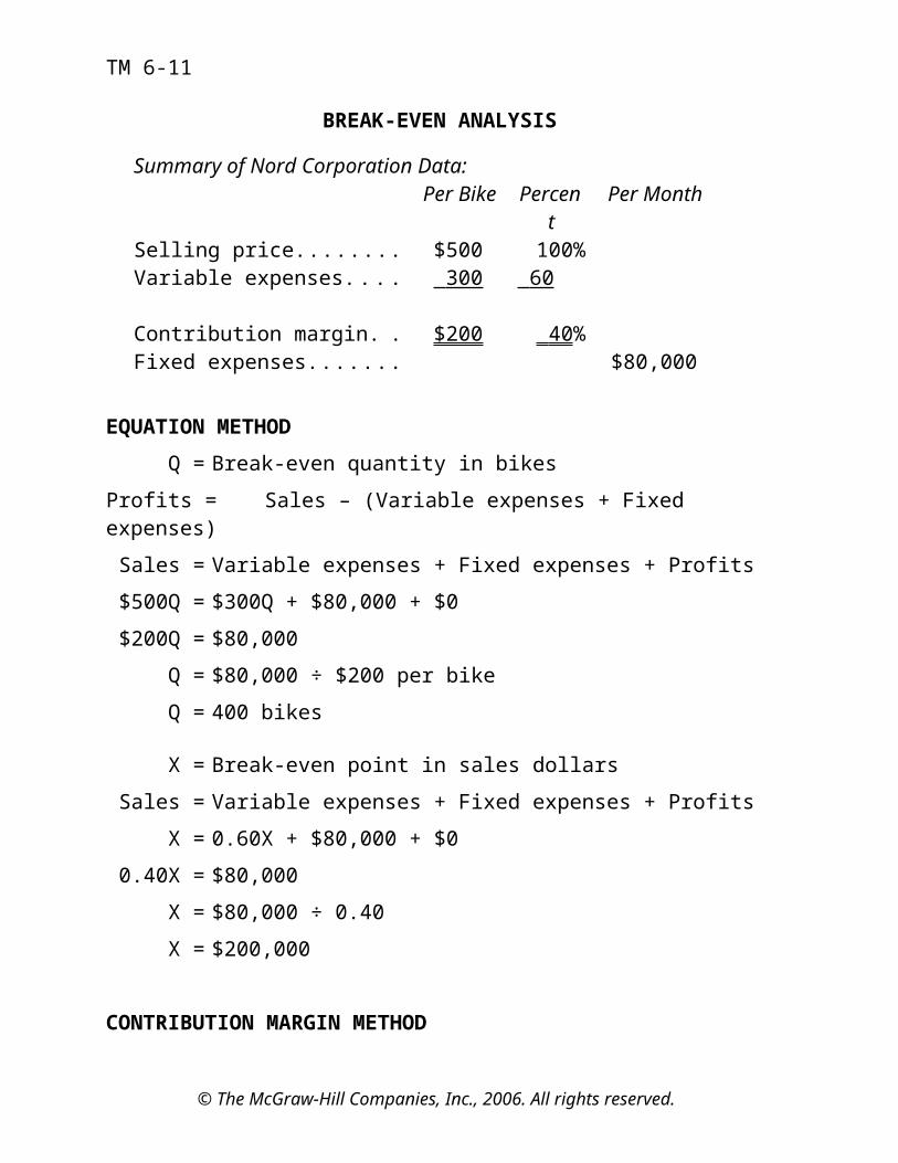
BREAK-EVEN ANALYSIS
Summary of Nord Corporation Data:Per Bike Percen
tPer Month
Selling price........ $500 100%Variable expenses.... 300 60
Contribution margin. . $200 40 %Fixed expenses....... $80,000
EQUATION METHODQ = Break-even quantity in bikes
Profits = Sales – (Variable expenses + Fixed expenses)Sales = Variable expenses + Fixed expenses + Profits $500Q = $300Q + $80,000 + $0$200Q = $80,000
Q = $80,000 ÷ $200 per bikeQ = 400 bikes
X = Break-even point in sales dollarsSales = Variable expenses + Fixed expenses + Profits
X = 0.60X + $80,000 + $00.40X = $80,000
X = $80,000 ÷ 0.40X = $200,000
CONTRIBUTION MARGIN METHOD
© The McGraw-Hill Companies, Inc., 2006. All rights reserved.
TM 6-12
© The McGraw-Hill Companies, Inc., 2006. All rights reserved.
TM 6-13
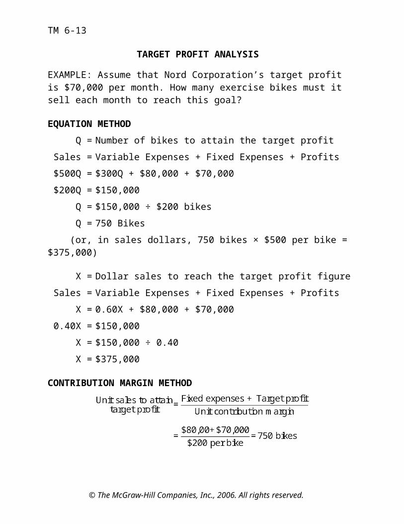
TARGET PROFIT ANALYSIS
EXAMPLE: Assume that Nord Corporation’s target profit is $70,000 per month. How many exercise bikes must it sell each month to reach this goal?
EQUATION METHODQ = Number of bikes to attain the target profit
Sales = Variable Expenses + Fixed Expenses + Profits$500Q = $300Q + $80,000 + $70,000$200Q = $150,000
Q = $150,000 ÷ $200 bikesQ = 750 Bikes
(or, in sales dollars, 750 bikes × $500 per bike = $375,000)
X = Dollar sales to reach the target profit figureSales = Variable Expenses + Fixed Expenses + Profits
X = 0.60X + $80,000 + $70,0000.40X = $150,000
X = $150,000 ÷ 0.40X = $375,000
CONTRIBUTION MARGIN METHOD
© The McGraw-Hill Companies, Inc., 2006. All rights reserved.
TM 6-14
© The McGraw-Hill Companies, Inc., 2006. All rights reserved.
TM 6-15
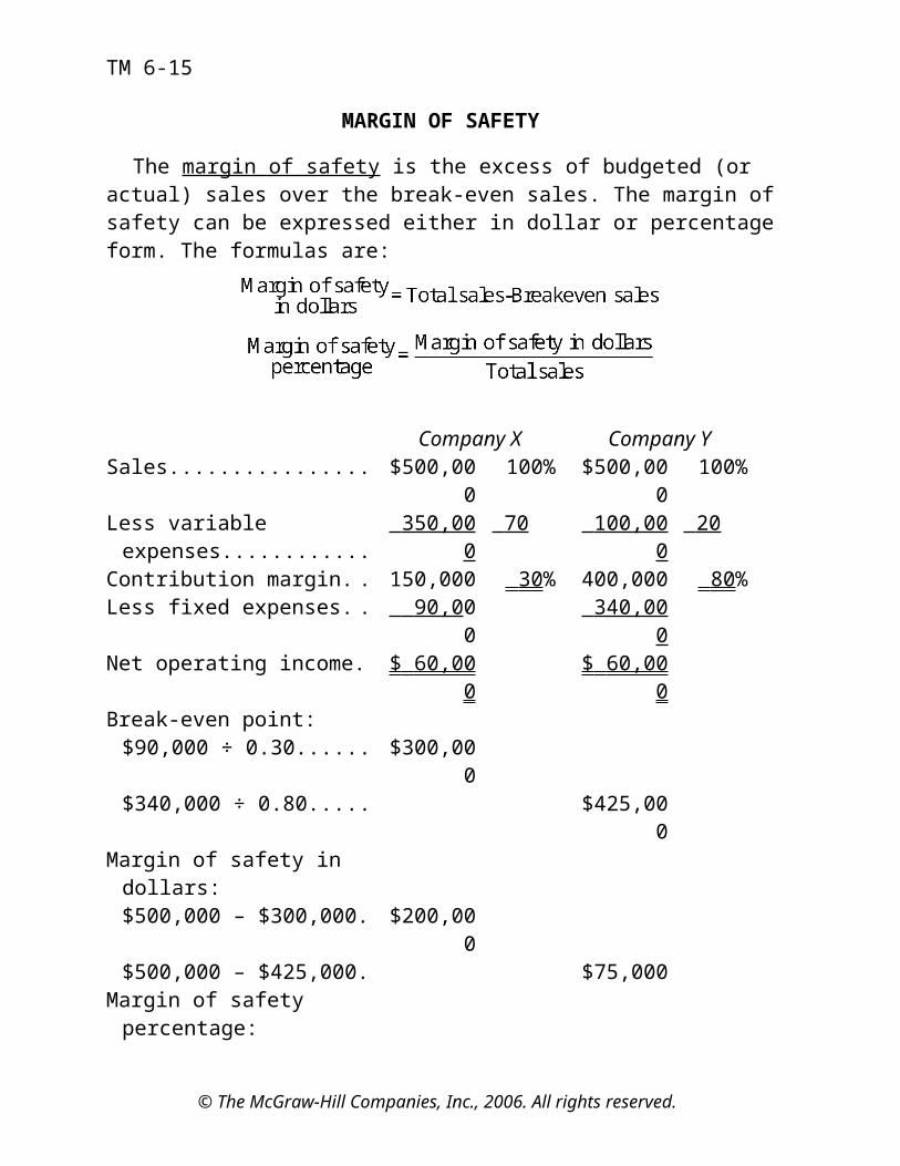
MARGIN OF SAFETY
The margin of safety is the excess of budgeted (or actual) sales over the break-even sales. The margin of safety can be expressed either in dollar or percentage form. The formulas are:
Company X Company YSales................ $500,00
0100% $500,00
0100%
Less variable expenses............
350,00 0
70 100,00 0
20
Contribution margin. . 150,000 30 % 400,000 80 %Less fixed expenses. . 90,0 0
0 340,00
0Net operating income. $ 60,00
0$ 60,00
0Break-even point: $90,000 ÷ 0.30...... $300,00
0$340,000 ÷ 0.80..... $425,00
0Margin of safety in dollars:$500,000 – $300,000. $200,00
0$500,000 – $425,000. $75,000
Margin of safety percentage:
© The McGraw-Hill Companies, Inc., 2006. All rights reserved.
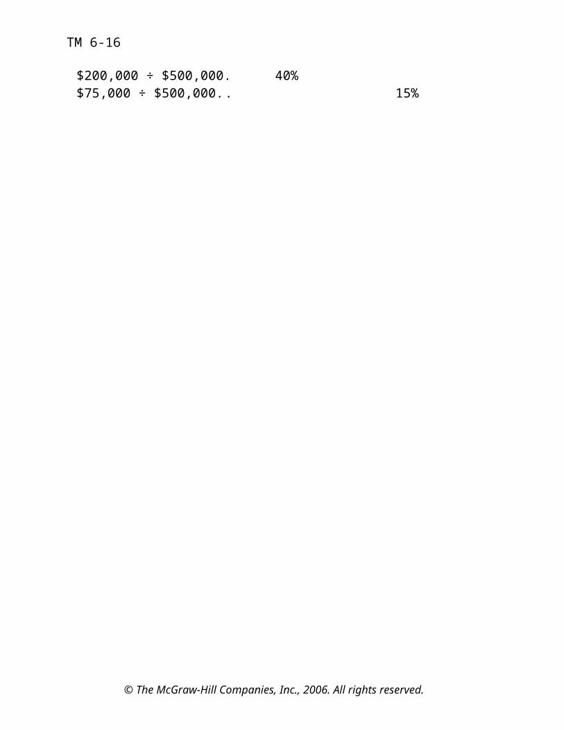
TM 6-16
$200,000 ÷ $500,000. 40%$75,000 ÷ $500,000.. 15%
© The McGraw-Hill Companies, Inc., 2006. All rights reserved.
TM 6-17
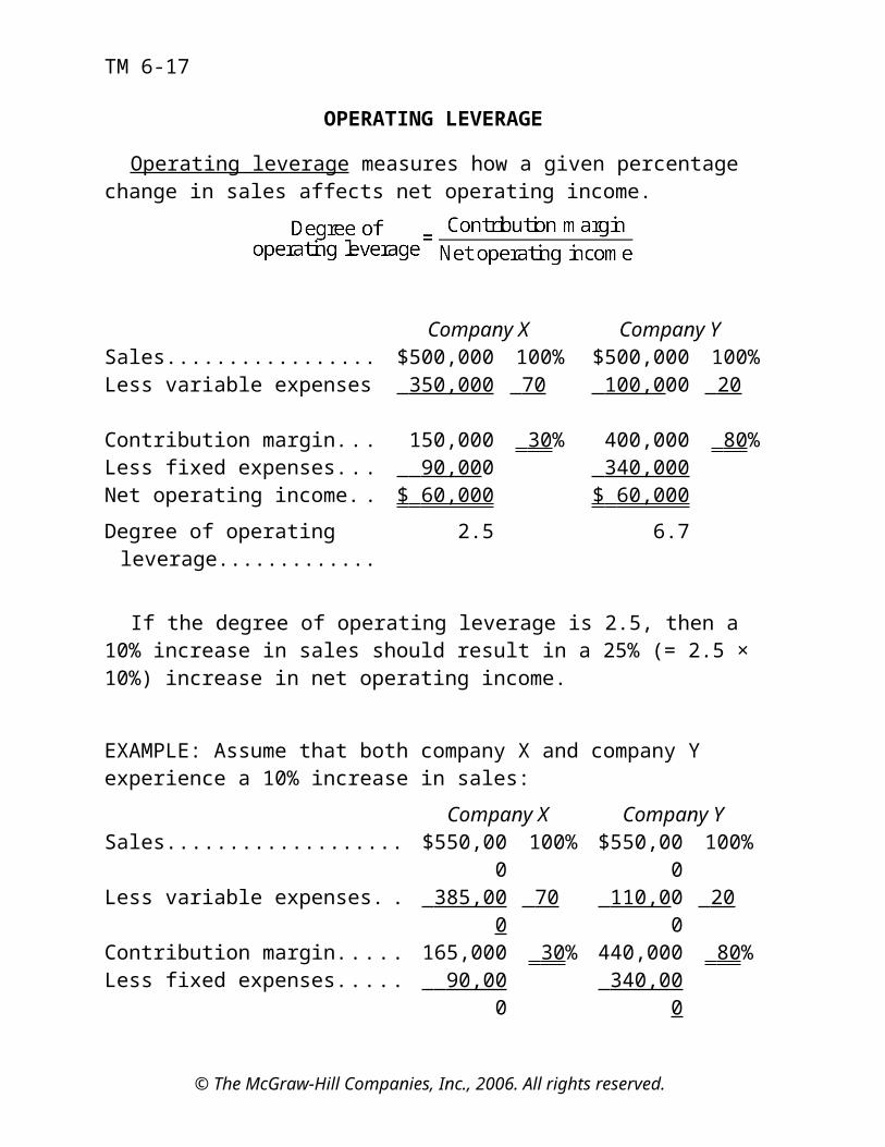
OPERATING LEVERAGE
Operating leverage measures how a given percentage change in sales affects net operating income.
Company X Company YSales................. $500,000 100% $500,000 100%Less variable expenses 350,000 70
100,0 00 20
Contribution margin... 150,000 30 % 400,000 80 %Less fixed expenses... 90,00 0 340,000 Net operating income. . $ 60,000 $ 60,000 Degree of operating leverage.............
2.5 6.7
If the degree of operating leverage is 2.5, then a 10% increase in sales should result in a 25% (= 2.5 × 10%) increase in net operating income.
EXAMPLE: Assume that both company X and company Y experience a 10% increase in sales:
Company X Company YSales................... $550,00
0100% $550,00
0100%
Less variable expenses. . 385,00 0
70
110,0 00
20
Contribution margin..... 165,000 30 % 440,000 80 %Less fixed expenses..... 90,00
0 340,00
0
© The McGraw-Hill Companies, Inc., 2006. All rights reserved.
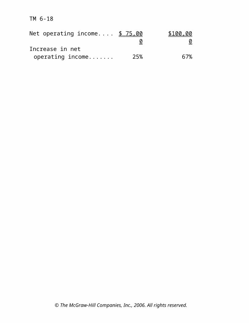
TM 6-18
Net operating income.... $ 75,00 0
$100,000
Increase in net operating income....... 25% 67%
© The McGraw-Hill Companies, Inc., 2006. All rights reserved.
TM 6-19
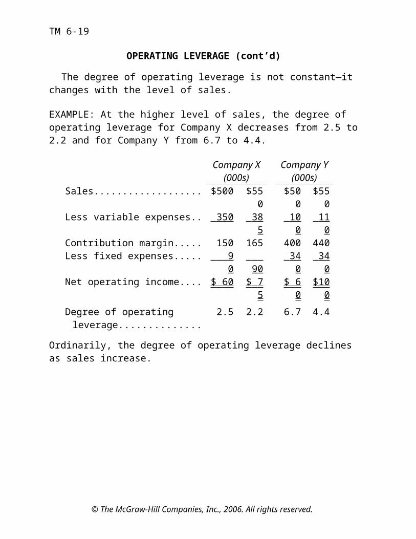
OPERATING LEVERAGE (cont’d)
The degree of operating leverage is not constant—it changes with the level of sales.
EXAMPLE: At the higher level of sales, the degree of operating leverage for Company X decreases from 2.5 to 2.2 and for Company Y from 6.7 to 4.4.
Company X(000s)
Company Y(000s)
Sales................... $500 $550
$500
$550
Less variable expenses.. 350 38 5
10 0
11 0
Contribution margin..... 150 165 400 440Less fixed expenses..... 9
0 90
34 0
34 0
Net operating income.... $ 60 $ 7 5
$ 6 0
$100
Degree of operating leverage..............
2.5 2.2 6.7 4.4
Ordinarily, the degree of operating leverage declines as sales increase.
© The McGraw-Hill Companies, Inc., 2006. All rights reserved.
TM 6-20
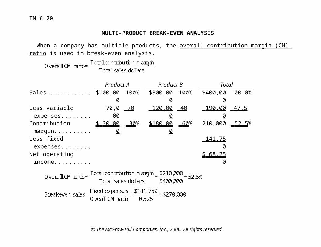
MULTI-PRODUCT BREAK-EVEN ANALYSIS
When a company has multiple products, the overall contribution margin (CM) ratio is used in break-even analysis.
Product A Product B TotalSales............. $100,00
0100% $300,00
0100% $400,00
0100.0%
Less variable expenses........
70,000
70
120,00 0
40
190,00 0
47.5
Contribution margin..........
$ 30,00 0
30 % $180,000
60 % 210,000 52.5 %
Less fixed expenses........
141,75 0
Net operating income..........
$ 68,25 0
© The McGraw-Hill Companies, Inc., 2006. All rights reserved.
TM 6-21
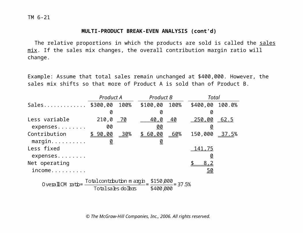
MULTI-PRODUCT BREAK-EVEN ANALYSIS (cont’d)
The relative proportions in which the products are sold is called the salesmix. If the sales mix changes, the overall contribution margin ratio will change.
Example: Assume that total sales remain unchanged at $400,000. However, the sales mix shifts so that more of Product A is sold than of Product B.
Product A Product B TotalSales............. $300,00
0100% $100,00
0100% $400,00
0100.0%
Less variable expenses........
210,000
70
40,0 00
40
250,00 0
62.5
Contribution margin..........
$ 90,00 0
30 % $ 60,00 0
60 % 150,000 37.5 %
Less fixed expenses........
141,75 0
Net operating income..........
$ 8,2 50
© The McGraw-Hill Companies, Inc., 2006. All rights reserved.
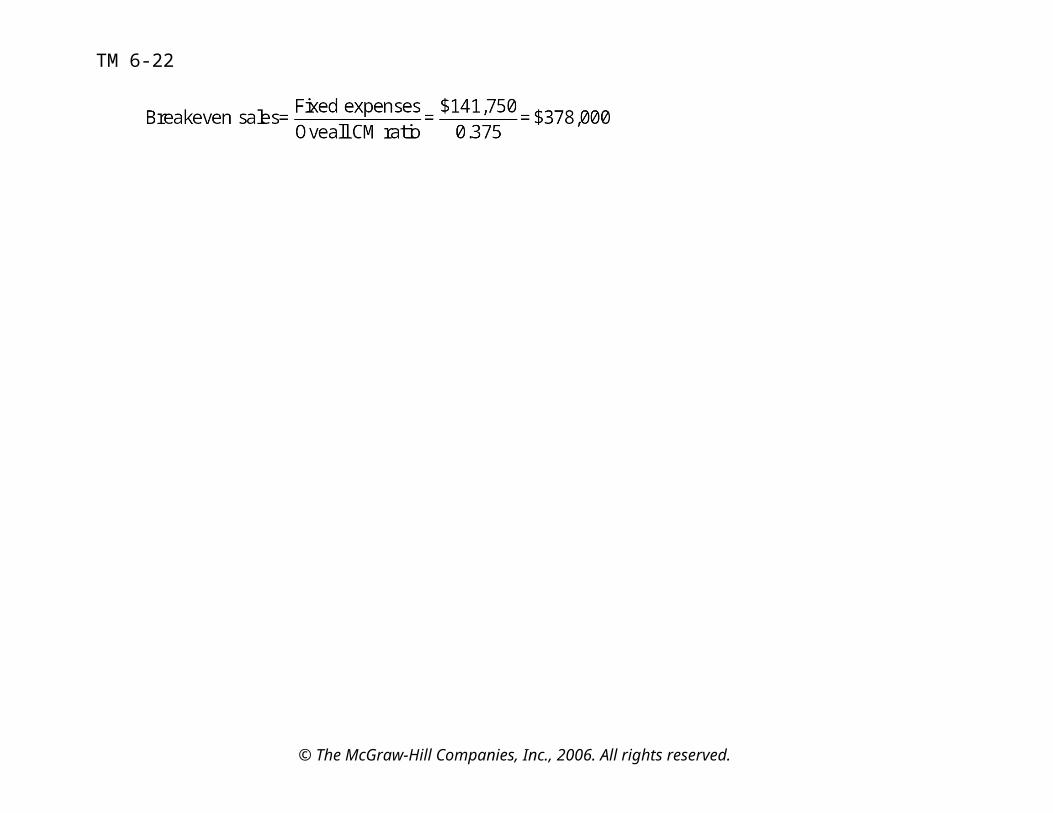
TM 6-22
© The McGraw-Hill Companies, Inc., 2006. All rights reserved.
TM 6-16
MAJOR ASSUMPTIONS OF CVP ANALYSIS
1. Selling price is constant. The price does not changeas volume changes.
2. Costs are linear and can be accurately split into fixed and variable elements. The total fixed cost isconstant and the variable cost per unit is constant.
3. The sales mix is constant in multi-product companies.
4. In manufacturing companies, inventories do not change. The number of units produced equals the number of units sold.
© The McGraw-Hill Companies, Inc., 2006. All rights reserved.