Cost Savings from Allowance Trading in the 1990 Clean Air Act:

Estimates from a Choice-Based Model∗

Nathaniel O. Keohane†

Yale School of Management

Forthcoming in Charles E. Kolstad and Jody Freeman, eds., Moving to Markets in

Environmental Regulation: Lessons from Twenty Years of Experience (New York: Oxford

University Press, 2006).

Abstract

Title IV of the 1990 Clean Air Act instituted a nationwide system of tradeable pollution

permits for sulfur dioxide emitted by electric power plants.This paper provides new estimates

of the cost savings from allowance trading, utilizing an econometric model of abatement choices

made by electric utilities under various policy regimes

My baseline estimate of abatement cost under the allowance market is $747 million during

each year of Phase I, which lasted from 1995 to 1999. I estimate that annual abatement costs

would have been $150 million to $180 million greater under performance standards, holding

aggregate abatement constant. These figures correspond to cost savings from trading of 17

to 20 percent. Alternatively, the allowance trading program yielded an estimated increase

in abatement of 10% relative to performance standard with equal costs. A technology-based

standard, requiring the use of a scrubber, would have been roughly three and a half times more

costly than the market outcome. These estimates demonstrate the usefulness of a choice-based

approach, relative to the assumption of cost-minimizing behavior made by prior studies.

∗ An earlier version of a portion of the work here appeared in a 2003 working paper titled “What Did theMarket Buy?: Cost Savings Under the U.S.Tradeable Permits Program for Sulfur Dioxide.” I am grateful to manyfor helpful comments, including Denny Ellerman, Erin Mansur, Robert Mendelsohn, Juan-Pablo Montero, SheilaOlmstead, Chris Timmins, seminar participants at the University of California Energy Institute, participants at theconference on “Twenty Years of Market-based Instruments for Environmental Protection” at UC-Santa Barbara, andan anonymous referee. All remaining errors, of course, are my own.

†Yale School of Management, P.O. Box 208200, 135 Prospect St., New Haven, CT 06520-8200;nathaniel.keohane@yale.edu; tel (203) 432 6024; fax (203) 432 6974.

1

1 Introduction

Title IV of the Clean Air Act of 1990 represented a major innovation in environmental policy

in the United States. Before 1990, clean-air regulations for electric power plants in the U. S.

were exclusively prescriptive in nature — requiring individual units to meet strict performance

standards or even to install particular abatement technologies. Title IV took a much different tack:

it instituted a market for sulfur dioxide emissions. Utilities affected by the regulation were allocated

a certain number of “allowances,” with each allowance representing one ton of SO2 emissions.

Utilities which reduced their emissions could sell their excess allowances to other utilities, or bank

them for future use.

Economists have long asserted the virtues of such market-based environmental policies over

traditional prescriptive or “command-and-control” regulation such as performance or technology

standards. In theory, market-based instruments are cost-effective: that is, they can achieve a given

level of abatement for the least possible total cost.1 Title IV offers the first major test of how a

market-based instrument can perform in practice.

Overall, this “grand policy experiment” (Stavins, 1999) has been overwhelmingly successful

to date. After a slow start, allowance trading has been vigorous. The utilities’ ability to bank

allowances, meanwhile, led to deeper-than-expected cuts in emissions during Phase I, with con-

comitant environmental benefits.2 Surprisingly, however, a consensus has yet to emerge on the

actual cost savings realized from the allowance market. Expectations of cost savings certainly ran

high before the program began. Studies done in the early 1990s by the General Accounting Of-

fice and by the Environmental Protection Agency anticipated cost savings between $250 and $470

million annually during Phase I (cited in Table 10.8 of Ellerman et al. 2000). The two major ex

post analyses of cost savings from allowance trading, however, have reached opposite conclusions.

Curtis Carlson, Dallas Burtraw, Maureen Cropper, and Karen L. Palmer (2000; henceforth CBCP)

find that the costs of abatement during Phase I were higher than they would have been under pre-

scriptive regulation. On the other hand, a study by A. Denny Ellerman, Paul L. Joskow, Richard

Schmalensee, Juan-Pablo Montero, and Elizabeth M. Bailey (2000; henceforth MCA after the title

of their volume, Markets for Clean Air) estimates that the use of allowance trading led to savings

of hundreds of millions of dollars per year.

1For a comprehensive discussion of the economics of environmental policy, see Baumol and Oates (1988).2For broader assessments of the performance of Title IV and associated lessons for policy, see Ellerman et al.

(2000) and Stavins (1999).

2

This chapter offers a comprehensive assessment of the cost savings over the first five years of

the allowance trading program. The current study has two methodological advantages over the

previous ones. The first is the completeness of the data used. Like the two previous studies, this

study estimates scrubber costs from costs reported in survey data, although the current study is

able to use cost data from the full five years of Phase I. The data on coal prices used here is much

more detailed than that in the other two studies, allowing for plant-level estimates of sulfur premia

and of counterfactual sulfur content.

The second and more significant advantage of the current study is methodological. I employ an

econometric model of the abatement choices actually made by utilities to simulate the decisions that

would have been made under prescriptive regulation. Thus abatement costs under counterfactual

policies are estimated on the basis of observed behavior under actual policy regimes, rather than

on the basis of engineering estimates or least-cost algorithms.

Using observed behavior to estimate costs is critical for two reasons. First, it allows for a

“warts-and-all” comparison of policies as they would actually have been implemented, rather than

comparing an actual outcome with an idealized counterfactual. Indeed, because we can estimate the

idealized outcomes as well, the model demonstrates the importance of taking compliance behavior

into account in estimating the consequences of policy choice.

Second, this approach incorporates differences in the incentives provided by policy regimes

for the adoption of abatement technologies. Market-based instruments in theory offer regulated

firms greater incentives to install technologies with low marginal costs (Downing and White 1986;

Milliman and Prince 1989; Kerr and Newell 2003). In the context of sulfur dioxide regulation, this

effect implies that the decisions made by utilities whether or not to install scrubbers should differ

systematically by policy regime (Keohane 2004). Thus an explicit model of decision making under

different policy instruments also accounts for differences in how those policy regimes reward the

adoption of low-marginal-cost methods of pollution control.3

As a starting point, I use the econometric choice model to generate a “baseline scenario” cor-

responding to predicted outcomes under the actual policy. I focus on the set of units that were

required to participate in the allowance market — the “Table A” units, named after the table that

3In addition to affecting adoption incentives, the policy regime may also affect technological innovation and thusthe costs of scrubbing (see Bellas (1998) and Lange and Bellas (2004) for discussions of technological change inscrubbing as a result of sulfur dioxide regulation.) Those innovation effects are not explicitly addressed in this paper;to the extent they were present in Phase I, therefore, this paper understates the cost savings associated with the useof a market-based instrument.

3

listed them in the legislation. Aggregate abatement at Table A units under the baseline scenario

is 4.2 million tons annually, while abatement costs total $747 million per year. These model pre-

dictions accord closely with estimates of abatement and cost based on actual choices.

The richness of my data and the flexibility of the econometric model allow me to compare the

actual policy with a wide range of counterfactual scenarios. My central comparison is between the

baseline scenario and a counterfactual uniform emissions rate standard that would have achieved

the same total amount of abatement among all units that were required to participate in the trading

program. I estimate that under such an emissions standard the aggregate costs of compliance would

have been $153 million greater during each year of Phase I — an increase of 20 percent over the

model’s baseline prediction. This estimate corresponds to cost savings of 17 percent. I estimate

a similar percentage increase in costs for a more stringent emissions standard calibrated to the

abatement actually achieved among all Phase I units, including voluntary participants.

Other plausible prescriptive policies would have been even costlier. I estimate that costs would

have been 25 percent higher under source-specific emissions limits pegged to the allowance allo-

cations under Title IV (and scaled to achieve the same 4.2 million tons of abatement as under

the baseline scenario). Because this scenario mimics actual allowance allocations without allowing

trading, it represents an alternative “pure” measure of the gains from trade.

Costs would have been astronomically high under a technology-forcing policy requiring utilities

to install scrubbers — soaring by $1.8 billion dollars per year. The enormous increase in estimated

cost under a technology standard relative to a performance standard underscores the importance

of giving polluters flexibility in how to reduce emissions.

As a final assessment of alternative “real-world” policies, I estimate the additional abatement

attributable to the allowance market, relative to a performance standard with the same aggregate

cost. Computing the “pollution savings” in this way involves the obverse of the “cost savings”

question usually asked; but in some ways it is more relevant to policy debates. It is also a novel

contribution of this study, since it requires a model that can predict abatement costs and choices

under a variety of counterfactual scenarios. I estimate that the trading program achieved 10 percent

more abatement during Phase I than could have been realized by a uniform standard with the same

total cost.

My econometric model relies on observed abatement choices to predict what would have hap-

pened under alternative policy regimes. Alternatively, we can assess the performance of the al-

lowance trading system against two theoretical benchmarks that assume least-cost compliance at

4

every unit. First, I estimate the theoretical minimum cost of abating 4.2 million tons to be $315

million/year. The wide gap between this figure and the baseline cost estimate suggests that the

choices actually made by managers did not minimize costs, at least over the span of Phase I. Thus

while the allowance market achieved considerable cost savings over alternative policies, it appears

— not surprisingly, perhaps — to have fallen short of its theoretical potential.

In its examination of pollution control decisions and its comparison of market-based policies with

conventional prescriptive regulation, this paper is heir to a line of comparative studies that thrived

in the 1970s and early 1980s (e.g., Atkinson and Lewis 1974; Seskin et al. 1983; Kolstad 1986;

Krupnick 1986). These studies compared actual or imminent prescriptive air pollution regulation

with hypothetical market-based regimes. The Title IV allowance trading program, along with two

decades of prescriptive regulations involving the same pollutant from the same types of sources,

allows a comparison of marked-based and prescriptive policy instruments that is grounded in actual

experience with both.

Note that this chapter focuses exclusively on the costs of abatement, rather than net benefits.

Estimates of overall net benefits from the Title IV program have been overwhelmingly positive

(e.g., Burtraw et al., 1998). Burtraw and Mansur (1999) and Shadbegian et al. (2004) study the

net benefits of trading relative to a counterfactual command-and-control alternative, taking into

account the distribution of emissions reductions and resulting environmental benefits.

The next section briefly reviews the regulatory context for the current study. Section 3 describes

the econometric analysis used to generate the “baseline” scenario representing the performance of

the actual tradeable permits regime. Section 4 compares the baseline scenario with the range of

alternative outcomes. Section 5 compares the results from this study with the findings in CBCP

and MCA. Section 6 concludes.

2 Regulation of sulfur dioxide emissions

Emissions regulations apply at the level of the generating unit — i.e., a individual electric turbine,

powered by steam produced by an associated boiler burning coal or another fuel. A typical power

plant will have more than one unit — usually two or three and sometimes a half-dozen or more,

often built at different times and thus subject to regulations of different form and stringency. The

primary means of reducing sulfur dioxide emissions are installing end-of-pipe devices called “flue-gas

desulfurization units” (better known as scrubbers) and switching to fuel with lower sulfur content.

5

Federal regulation of SO2 emissions from power plants began under the Clean Air Act Amend-

ments (CAAA) of 1970. Generating units built after August 17, 1971 were subject to New Source

Performance Standards (NSPS), which imposed a maximum allowable emissions rate of 1.2 pounds

of SO2 per million Btus. In response to concerns from coal interests and environmentalists, Congress

strengthened these regulations in the Clean Air Act Amendments of 1977.4 Starting in Septem-

ber 1978, new generating units were required not only to meet the existing emissions rate of 1.2

lbs/mmBtus, but also to do so by removing a certain percentage of SO2 from the flue gases — a de

facto scrubbing requirement.

By the late 1980s, growing concern over acid rain (to which SO2 emissions are a major contribu-

tor) led Congress to consider imposing regulations on the power plants built before 1971, which had

been “grandfathered” out of the earlier federal regulations. The result was the allowance trading

program provision of Title IV. Phase I of the program lasted from 1995 to 1999. It applied directly

to the 263 largest, dirtiest existing generating units, listed on Table A of the legislation. In addition,

utilities that owned Table A units could voluntarily enroll other generating units in the allowance

market during Phase I. This “substitution and compensation” provision, however, invited adverse

selection: units that chose to enroll would almost certainly have reduced their emissions anyway

(Montero 1999). Phase II of the program started in 2000 and extended the allowance market to

every fossil-fired power plant greater than 25 MWe in generating capacity.

Alongside this federal regulatory structure exists a patchwork of emissions standards imposed

by state governments, who must comply with federal National Ambient Air Quality Standards

(NAAQS). Since power plants are a prominent source of air pollution, they are natural targets of

state regulation. These state-level regulations are always prescriptive in nature; for the most part,

they specify unit-level maximum allowable emissions rates.5

This paper seeks to use observed behavior to generate counterfactual estimates of what abate-

ment and cost at Table A plants would have been under alternative policies. By definition, all of

the Table A units were built decades before the allowance market took effect. Similarly, nearly all

units regulated at the state level were built before the passage of air pollution laws. For all these

units, therefore, scrubbers had to be retrofitted onto the existing boilers. Retrofitting a unit is

more costly than building the scrubber and boiler simultaneously. Moreover, the decision whether

or not to retrofit an old boiler is likely to differ in fundamental ways from the decision whether to

4Ackerman and Hassler (1981) provide a fascinating account of the politics behind the 1977 CAAA.5See Keohane and Lee (2004) for an analysis of state-level regulation of SO2 emissions from power plants.

6

build a scrubber at a newly constructed unit. Hence I restrict attention to retrofitted units only,

and leave the NSPS units out of the analysis entirely.6

3 The model of technique choice and the baseline scenario

3.1 The choice of abatement technique

3.1.1 Econometric model

The simulation of counterfactual policies is based on the econometric model of technique choice

under different policy regimes presented in Keohane (2004). The model has two stages. In the

first stage, scrubbing costs are estimated with a maximum-likelihood Heckman model (Heckman

1974). This approach controls for potential selection bias by estimating a model of scrubber choice

simultaneously with scrubber costs. This approach provides consistent estimates of what scrubber

costs would have been at units that did not install them. In the second stage, these predicted

scrubbing costs are entered into a probit model of the scrubbing decision, along with predicted

price premia for low-sulfur coal and a number of other explanatory variables.

Our interest in the choice estimation here is purely instrumental: the goal is to predict the choices

that utilities would have made under counterfactual policies. Accordingly, I simply summarize how

the costs were estimated and then briefly report the results from the probit choice model. The

reader interested in the full choice model is referred to Keohane (2004).

In that analysis, average scrubbing cost (in dollars per ton of SO2 abated) is modeled as a log-

linear function of the nameplate capacity of the unit (MW of electricity at maximum output); the

“capacity factor” or percent utilization of the unit; the sulfur content of the coal used (expressed

for convenience in the emissions rate that would result from burning the coal unabated); annual

heat input (in millions of British thermal units, or Btus);7 a dummy variable for units that share a

stack, along with interactions between that dummy and measures of generating capacity and heat

consumption on the common stack; the vintage of the scrubber; a dummy variable for the boiler

6A handful of state-regulated plants were required to install scrubbers; these are dropped from the analysis. Notethat an earlier version of this paper included NSPS-D units as well; acquisition of data on retrofitted state-regulatedunits made those unnecessary.

7Ellerman and his colleagues demonstrate inMCA that heat input rose sharply among Table A units with scrubbers(MCA, ch. 5). Units with scrubbers have lower variable costs (inclusive of abatement costs) than units that buymore expensive lower-sulfur coal, and hence are utilized more. To overcome this endogeneity problem, I use 1990heat input and utilization factors for all Table A units in estimating scrubbing cost.

7

type (specifically, whether the boiler has a “wet bottom”); and a dummy variable for the North

Atlantic region, where anecdotal evidence suggests that construction and even operating costs are

systematically high. Finally, the model interacts the logarithm of sulfur content with the log of

vintage and nameplate capacity. The average cost of scrubbing is estimated simultaneously with

the decision to have a scrubber (described in the next paragraph), and the estimated coefficients

employed to predict scrubbing cost at all units.

The scrubber decision is then estimated by probit, as a function of the estimated cost of scrub-

bing relative to the cost of switching to low-sulfur coals, taking into account a range of other factors.

The decision of whether or not to install a scrubber is modeled as taking place at a particular point

in time, corresponding to the year in which the scrubber would have first operated.8 The primary

measure of the cost of switching to low-sulfur coal is the estimated price premium for low-sulfur coal

relative to the cheapest available coal at a given unit. Since transportation costs make up a large

fraction of the delivered price of coal, the premium for low-sulfur coal varies widely among power

plants. Units that lack a viable source of low-sulfur coal are accounted for by an indicator variable,

as are units that were already burning low-sulfur coal at the time of the scrubber decision.9

I also include a range of other factors: applicable state-level emissions regulations; a dummy

variable for units that were already burning low-sulfur coal at the time of the scrubber decisions; a

dummy variable for plants located adjacent to a coal mine; a dummy variable for plants larger than

the median plant; a dummy for Table A units located in states which enacted rules to encourage

scrubbing, as determined by Lile and Burtraw (1998); and (for Table A units) the number of other

Phase I units under common ownership, which reflects the scope of interutility trading. For Table

A units, I also include the expected sulfur content in five years’ time and the extent of long-term

contracts, as reported by the power plants five years before the beginning of Phase I. Finally, to

account for the differences in policy regimes, I also include a dummy for Table A status, and interact

it with several of the variables in the choice equation. In particular, I allow the scrubbing cost,

low-sulfur coal premium, performance standard, and plant size variables to vary with the policy

regime.

8For Table A units I use 1995, the year the allowance market took effect. For retrofitted units regulated by thestates, I use the year in which state-level regulations were tightened (if such a year exists), or else 1985 (which is thefirst year for which I have scrubber operation data). See the discussion in Keohane (2004).

9For state-regulated units that installed scrubbers before 1985 (the first year of the data), I set this indicatorvariable equal to 1 for units where low-sulfur coal is the cheapest available coal.

8

3.1.2 Data

Data for the estimation are discussed in more detail in Keohane (2004). They are drawn from

two primary sources. Form EIA-767, an annual survey of electric power plants administered by the

Energy Information Administration of the Department of Energy, provides data on unit-level oper-

ation, including the costs and operating performance of scrubbers, the amounts and characteristics

of coal burned, and applicable state and federal emissions regulations. I use these data to estimate

emissions and abatement at the unit level.10

The second principal data source is FERC Form 423, a survey of fuel purchases at power plants

conducted by the Federal Energy Regulatory Commission. I supplement these coal delivery data

with plant-level information on transportation options and actual rail and barge distances to coal

districts. By regressing coal prices on rail and barge distances and plant characteristics, I am able

to estimate coal prices at every plant in the data for a variety of coals, and thus can estimate

price premia for low-sulfur coal even at plants that purchase only one type of coal. The low-sulfur

coal premium used in the choice model represents the difference between the predicted price of the

cheapest available coal and that of the most attractive low-sulfur coal. Moreover, the estimated

prices of low-sulfur coal take into account the costs of adjusting existing boilers to burn coal with

lower sulfur.11

The entire dataset includes observations on 846 units, of which 247 were listed on Table A

and thus subject to the tradeable permits regime. Table 1 gives summary statistics. In this data,

average scrubbing costs are actual costs for units with scrubbers. For units without scrubbers, I

use the predicted scrubbing costs from the first-stage Heckman model. Finally, for the handful of

units with scrubbers that lack cost data, I use the predicted scrubbing cost, conditional on having

a scrubber.

10Emissions estimates at the unit level were computed on a mass-balance basis. I employed the estimation formulaeused by the Energy Information Administration, taking into account the design of the boiler and the sulfur content ofthe coal used; for scrubbed units, I incorporated information on hours of scrubber operation and removal efficiency.The mass-balance calculations were used because the data include a range of units that began operation well beforethe advent of Continuous Emissions Monitoring Systems (CEMS) in place since 1996, which measure emissions inreal time. For the years available, however, my computed emissions estimated agree very well with these data. Atthe unit level, the correlation between the emissions measures is 0.97; I present aggregate comparisons in the textbelow.11I use different capital costs for adjustment to bituminous and to sub-bituminous (i.e., Powder River Basin) coals.

I use the estimated adjustment costs reported in MCA. Again, details can be found in Keohane (2004).

9

Table 1: Summary statistics for scrubber choice estimation

StandardVariable Mean deviation Minimum Maximum

State-regulated units(599 units, 41 scrubbed)Est. avg. scrubbing cost ($/ton) 2166.62 8171.79 77.95 159753.9Price premium for low-sulfur coal (cents/mmBtus) 12.72 12.59 0 97.90Low-S coal infeasible 0.03 0.18 0 1Minemouth location 0.03 0.17 0 1Already burning low-sulfur coal 0.10 0.30 0 1SO2 emissions standard(lbs/mmBtus) 2.87 1.81 0.1 9.5Large plant 0.53 0.49 0 1

Table A units(247 units, 27 scrubbed)Est. avg. scrubbing cost ($/ton) 729.94 923.70 173.60 8156.07Price premium for low-sulfur coal (cents/mmBtus) 16.81 16.16 0 96.40Low-S coal infeasible 0 0 0 0Minemouth location 0.09 0.29 0 1Already burning low-sulfur coal 0.03 0.18 0 1SO2 emissions standard(lbs/mmBtus) 4.95 1.84 1.2 12Large plant 0.52 0.50 0 1Large Table A plant 0.41 0.49 0 1Expected sulfur content in 5 yrs 1.29 1.02 0 4.1Pct. of coal under long-term contract 0.28 0.39 0 1.84Capital-intensive statutory bias 0.57 0.49 0 1Number of commonly owned Phase I units 19.29 16.31 1 59

10

3.1.3 Results

Table 2 presents the estimated coefficients from the choice model.12 Overall, units were significantly

less likely to install scrubbers when scrubbing was relatively expensive. Moreover, variation in

average scrubbing cost had a much greater effect for units governed by the tradeable permits

regime. As discussed in Keohane (2004), this finding is consistent with the theoretical literature

on the incentives for technology adoption under various policy instruments. For Table A units, the

probability of scrubbing also rises with the cost of low-sulfur coal, although the effect is weak. The

estimates suggest that state-regulated units, however, are more likely to have a scrubber when low-

sulfur coal is inexpensive — a perverse effect, albeit a weak one. Other measures of sulfur content

and low-sulfur coal availability have the expected effects. A lack of feasible sources of low-sulfur

coal increases the likelihood of scrubbing significantly, as does minemouth location. The expected

sulfur content of coal is also a significant predictor of scrubbing, implying that units with readily

available high-sulfur coal were more likely to scrub.

For units regulated by prescriptive regulation, scrubbing is much more likely when regulation is

more stringent (thus the negative sign on ln (SO2 PERFORMANCE STANDARDi)). The effect

of performance standards vanishes for Table A units. This accords with expectations: although

Table A units remained subject to state-level emissions standards, those standards became less

salient in the scrubbing decision than the allowance market was. Surprisingly, state biases towards

capital-intensive compliance with Title IV have no discernible effect.13 Finally, scrubbing is more

likely at Table A units, all else equal, although this effect diminishes at larger plants.

3.2 Estimating costs and abatement under the “baseline scenario”

3.2.1 Methodology

I use the results from the choice estimation to predict scrubber choices under the allowance regime.

Predicted scrubbers are those for which the probit model assigns a probability of scrubbing greater

than a certain cutoff. I used a cut point of 0.35, which maximizes the percentage of correct

predictions among all units. This cut point also results in the same number of predicted scrubbers

as actual scrubbers, among the 247 Table A units included in the choice model. The model correctly

12Standard errors are not corrected for the use of econometrically estimated regressors. The t-statistics on thevariables of greatest interest are sufficiently large, however, that one might reasonably expect them to remain signif-icant even accounting for the generation of the regressors. Note too that the correct standard errors need not belarger than the ones presented here: the bias can go in either direction. See Murphy and Topel (1985).13Elizabeth M. Bailey (1998) reached a similar conclusion in a more detailed analysis of state regulations.

11

Table 2: Results from probit estimation of scrubber choice

Dependent variable: Equals 1 if unit has scrubber

ln(Avg. scrubbing cost) -0.705 ***(0.233)

ln(Avg. scrubbing cost) × Table A -2.007 ***(0.627)

ln(Low-S price premium) -0.228 *(0.135)

ln(Low-S price premium) × Table A 0.535 *(0.312)

Low-sulfur coal infeasible 3.489 ***(1.068)

Minemouth location 1.659 ***(0.478)

Already burning low-sulfur coal -0.641(0.392)

ln(SO2 performance standard) -3.144 ***(0.469)

ln(SO2 performance standard) × Table A 3.067 ***(0.623)

Large plant -0.157(0.264)

Table A unit 8.289 **(3.738)

Expected sulfur content in 5 yrs 0.682 ***(0.191)

Pct. of coal under long-term contract -0.044(0.436)

Capital-intensive statutory bias 0.189(0.379)

Large Table A plant -1.887 ***(0.609)

No. of commonly owned Phase I units -0.027 *(0.015)

Constant 5.016 ***(1.754)

Number of units 846Number of scrubbed units 68Log likelihood -81Wald statistic χ2(16) 310

(p < 0.001)

Notes: * denotes significance at 10% level at 5 % level *** at 1 % level

12

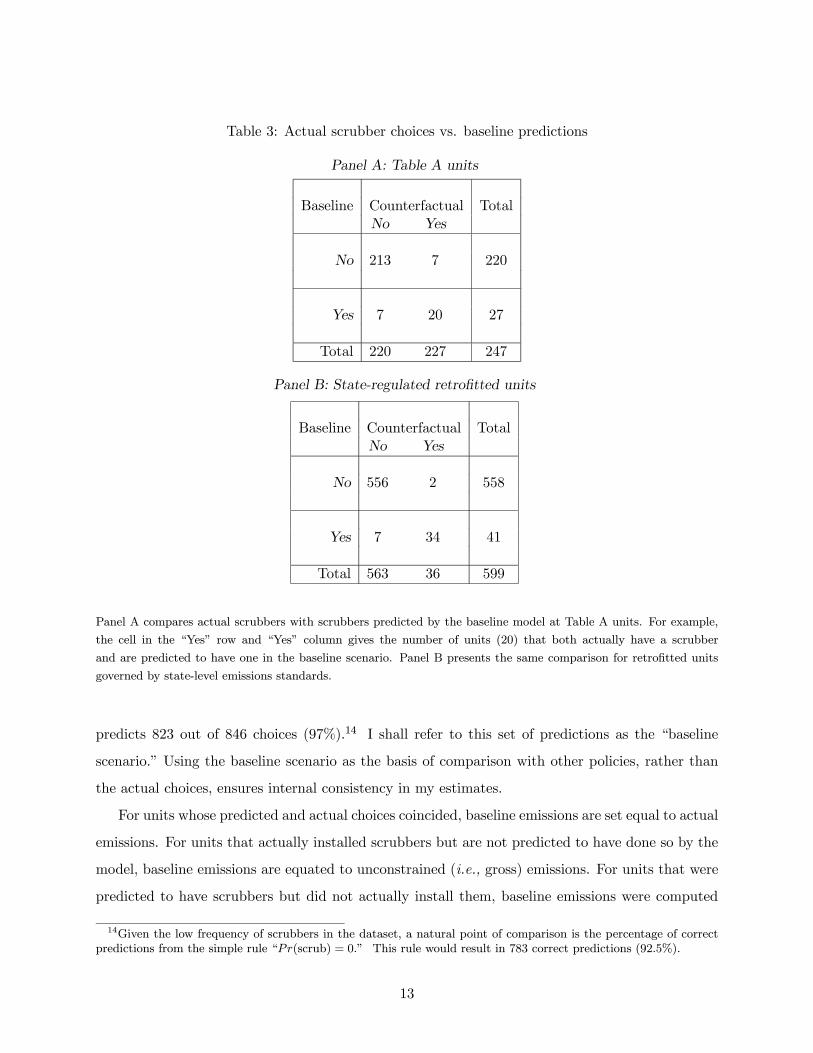
Table 3: Actual scrubber choices vs. baseline predictions

Panel A: Table A units

Baseline Counterfactual TotalNo Yes

No 213 7 220

Yes 7 20 27

Total 220 227 247

Panel B: State-regulated retrofitted units

Baseline Counterfactual TotalNo Yes

No 556 2 558

Yes 7 34 41

Total 563 36 599

Panel A compares actual scrubbers with scrubbers predicted by the baseline model at Table A units. For example,

the cell in the “Yes” row and “Yes” column gives the number of units (20) that both actually have a scrubber

and are predicted to have one in the baseline scenario. Panel B presents the same comparison for retrofitted units

governed by state-level emissions standards.

predicts 823 out of 846 choices (97%).14 I shall refer to this set of predictions as the “baseline

scenario.” Using the baseline scenario as the basis of comparison with other policies, rather than

the actual choices, ensures internal consistency in my estimates.

For units whose predicted and actual choices coincided, baseline emissions are set equal to actual

emissions. For units that actually installed scrubbers but are not predicted to have done so by the

model, baseline emissions are equated to unconstrained (i.e., gross) emissions. For units that were

predicted to have scrubbers but did not actually install them, baseline emissions were computed

14Given the low frequency of scrubbers in the dataset, a natural point of comparison is the percentage of correctpredictions from the simple rule “Pr(scrub) = 0.” This rule would result in 783 correct predictions (92.5%).

13

using the average operating removal rate among Table A units, which was 91%.15

To estimate the abatement attributable to Title IV requires an estimate of what emissions

would been in the absence of any federal regulation on Table A units — that is, the “business-as-

usual” (BAU) outcome. BAU emissions are computed by multiplying an estimate of each unit’s

unconstrained emissions rate by a counterfactual estimate of the unit’s heat input, absent Title

IV. As an estimate of the unconstrained emissions rate for scrubbed units, I simply use the sulfur

content of the coal actually burned, since that is presumably the cheapest coal available. For

unscrubbed units, the sulfur content of the cheapest available coal (as determined by the same coal

price regressions used to estimate low-sulfur coal premia, as discussed in section 3.1.2) is taken as a

“benchmark rate” in determining a unit’s unconstrained emissions. I use the emissions rate in 1992

(i.e., just in advance of any changes made in anticipation of Title IV) when that rate is less than

the benchmark rate and the state emissions standard is non-binding (meaning that the estimated

cheapest available coal would satisfy it). Finally, I use the observed average emissions rate during

Phase I, when that is greater than the benchmark rate. Thus my approach relies on actual choices

to the extent possible.

As demonstrated in MCA, heat input rose at Table A units that installed scrubbers as well as

those that were close to the Powder River Basin; meanwhile, it fell at other Table A units (relative

to non-Table A units). To account for these effects of regime, scrubbers, and location, I estimate a

fixed-effects regression on panel data for 1985-1999 for 820 units, regressing annual heat input on

unit-level fixed effects; year effects; dummies for each Phase I year; total state electricity demand

in each year; scrubber status (by itself as well as interacted with a dummy for the Phase I period

and another for Table A units during Phase I); and a dummy variable indicating that coal from

the Powder River Basin is estimated to be the cheapest available coal (again, entering by itself as

well as interacted with Table A status).16 The predicted BAU heat input is computed from these

coefficients by setting the scrubber dummy and all the Table A variables equal to zero. Multiplying

15This mean removal efficiency takes into account the fraction of hours that the scrubber was in operation. As analternative, the removal efficiency could be predicted from data. For the Table A units, however, such a predictionyields virtually no improvement over the mean. Moreover, a Heckman estimation of removal efficiencies yielded noevidence of selection.16MCA estimates a similar regression on emissions (see chapter 5 in that volume), and I follow their lead in choosing

the right-hand side variables for the regression. Likewise, I follow them in using as my sample generating units fromall states east of the Mississippi, not including North or South Carolina, along with Kansas, Missouri, Iowa, andMinnesota. One difference is that my more detailed data on coal prices allows me to use a direct measure of theattractiveness of PRB coal (namely, whether it was the cheapest available coal) rather than relying on the crudermeasure of distance from the PRB. Moreover, my data includes only coal-fired units, so I cannot estimate (as theydo) the shift from oil- and gas-fired units to coal-fired units, although I can identify changes that affected Table Aunits differently than other coal-fired units.

14

this heat input by the corresponding BAU emissions rate results in total BAU emissions of 8.56

million tons.

Predicted emissions at the unit level account for the effects of scrubbing on heat input, using

the fixed-effects regression just described. For example, predicted heat input exceeds actual heat

input at units that are predicted to have scrubbers but did not actually install them. Predicted

abatement is then the difference between BAU and predicted emissions.

The estimated cost at units without predicted scrubbers is simply the low-sulfur coal premium

used in the choice model, expressed per ton of SO2, multiplied by predicted abatement conditional

on not having a scrubber. Estimating abatement cost at units predicted to have scrubbers requires

two further adjustments. First, for units with binding state regulations, the abatement cost due to

Title IV is estimated as the total cost of scrubbing minus the cost of meeting the state regulation by

burning low-sulfur coal. Doing so accounts for the abatement costs that units would have incurred

in the absence of Title IV, while recognizing that scrubbers would not have been used simply to

meet existing state standards. Second, I add the estimated cost of “parasitic power loss” — that

is, the electricity used by the scrubber. Parasitic power loss accounts for roughly 5 percent of total

average scrubbing costs. It is computed by multiplying reported electricity usage by the average

wholesale electricity price for the parent utility. For units without scrubbers, I use the average

percentage of “parasitic power loss” among scrubbed units, and then use the units’ own electricity

prices.

3.2.2 Baseline estimates

Table 4 summarizes aggregate outcomes predicted by the model, along with estimates based on

actual choices. The set of units includes the 846 units in the choice model, plus one more: Yates

Y1BR, which is excluded from the choice model because it was a demonstration unit partially

funded by DOE and designed to test a scrubber on a unit burning relatively low-sulfur coal.

Total emissions among the 248 Table A units in the baseline scenario are 4.33 million tons per

year (see the third entry of the first row of the table). Aggregate abatement under the baseline

scenario is 4.23 million tons. The estimated cost of this abatement is $747 million annually, in con-

stant 1995 dollars. As Table 4 shows, the baseline estimates corresponding to predicted scrubbing

choices agree well with estimates based on actual choices, presented in column (2) of the table. The

model slightly understates emissions and overstates abatement, but the difference is less than one

percent. Baseline abatement cost is even closer to estimated cost.

15

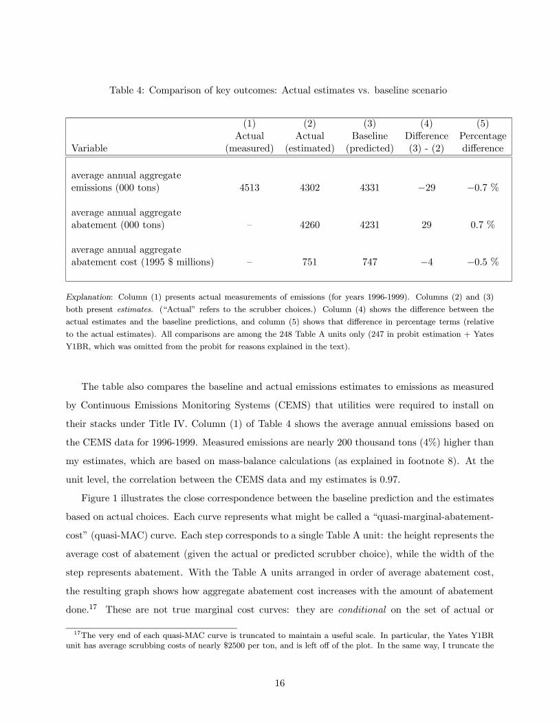
Table 4: Comparison of key outcomes: Actual estimates vs. baseline scenario

(1) (2) (3) (4) (5)Actual Actual Baseline Difference Percentage

Variable (measured) (estimated) (predicted) (3) - (2) difference

average annual aggregateemissions (000 tons) 4513 4302 4331 −29 −0.7 %

average annual aggregateabatement (000 tons) — 4260 4231 29 0.7 %

average annual aggregateabatement cost (1995 $ millions) — 751 747 −4 −0.5 %

Explanation: Column (1) presents actual measurements of emissions (for years 1996-1999). Columns (2) and (3)

both present estimates. (“Actual” refers to the scrubber choices.) Column (4) shows the difference between the

actual estimates and the baseline predictions, and column (5) shows that difference in percentage terms (relative

to the actual estimates). All comparisons are among the 248 Table A units only (247 in probit estimation + Yates

Y1BR, which was omitted from the probit for reasons explained in the text).

The table also compares the baseline and actual emissions estimates to emissions as measured

by Continuous Emissions Monitoring Systems (CEMS) that utilities were required to install on

their stacks under Title IV. Column (1) of Table 4 shows the average annual emissions based on

the CEMS data for 1996-1999. Measured emissions are nearly 200 thousand tons (4%) higher than

my estimates, which are based on mass-balance calculations (as explained in footnote 8). At the

unit level, the correlation between the CEMS data and my estimates is 0.97.

Figure 1 illustrates the close correspondence between the baseline prediction and the estimates

based on actual choices. Each curve represents what might be called a “quasi-marginal-abatement-

cost” (quasi-MAC) curve. Each step corresponds to a single Table A unit: the height represents the

average cost of abatement (given the actual or predicted scrubber choice), while the width of the

step represents abatement. With the Table A units arranged in order of average abatement cost,

the resulting graph shows how aggregate abatement cost increases with the amount of abatement

done.17 These are not true marginal cost curves: they are conditional on the set of actual or

17The very end of each quasi-MAC curve is truncated to maintain a useful scale. In particular, the Yates Y1BRunit has average scrubbing costs of nearly $2500 per ton, and is left off of the plot. In the same way, I truncate the

16

predicted choices (which may not have been cost-minimizing), and they end at total abatement (4.2

million tons) by construction. They are best seen as descriptions of the distribution of abatement

costs among units: the flatter the curve, the more similar are per-ton abatement costs across a

range of units.

4 The cost savings from Title IV

In this section I estimate the cost savings from Title IV, relative to a range of alternative plausible

policies. I start by comparing the predictions in the baseline scenario to a uniform performance

standard that would have achieved the same aggregate emissions and abatement among Table A

units. This comparison measures the savings due to trading alone, since the performance standard

would have allowed individual units flexibility in determining how to abate. In other words, it

estimates of the gains from a market-based policy, relative to what some observers (such as CBCP)

call “enlightened command-and-control.”

Following this central comparison, I estimate abatement costs under a range of other counter-

factual scenarios. The first three alternatives represent plausible prescriptive policies that could

have been enacted in place of the allowance market: a uniform standard tied to total Phase I

abatement (including that by units that participated voluntarily); a set of source-specific standards

tied to Table A allowance allocations; and a technology standard requiring most firms to install

a scrubber. I also estimate the abatement achieved by a uniform performance standard with the

same cost as the baseline, to derive an alternative measure of the gains from trading. Finally, I

estimate the costs of two theoretical benchmarks — the cost-effective outcome and the minimum

cost of meeting a uniform emissions standard. These scenarios provide an alternative yardstick

with which to measure the performance of the actual policy.

4.1 Comparisons with performance-based standards

4.1.1 Uniform emissions rate standard: Table A abatement

The counterfactual uniform standard is chosen so that the aggregate abatement predicted by the

counterfactual scenario for all Table A units equals the aggregate abatement among the same

units under the baseline scenario. I assume that such a federal standard — like actual standards

plotted quasi-MAC curves under prescriptive regulation. In all cases, the truncation applies only to the graph: thesehigh-cost units (including Yates) are included in the estimates of aggregate abatement and cost.

17

— would not have superseded more stringent state regulations where they exist. Thus under the

counterfactual uniform emissions rate scenario, each Table A unit is assigned an emissions rate

standard equal to the minimum of its actual state-imposed regulation and 2.3 lbs/mmBtus. This

particular standard yielded the closest fit with predicted baseline abatement, among the set of

all emissions rate standards in increments of 0.01 lbs/mmBtus. By comparison, the “benchmark”

emissions rate under Title IV, embodied in the basic allowance allocation rule, was 2.5 lbs/mmBtus;

and even this was more stringent than the eventual reality, since the benchmark rate did not

incorporate the numerous bonus allowances granted during Phase I. More abatement was done

than was required to meet the cap, largely due to the effect of banking, as has been documented

in detail in MCA and elsewhere.

The coefficients from the probit estimation of scrubber choice (Table 2) were then used to

generate predicted choice probabilities, conditional on the counterfactual regime. The actual

emissions standard for each unit was replaced with the counterfactual emissions standard; coefficient

estimates for state-regulated units were used for scrubbing and switching costs and for the emissions

standard (i.e., the interaction terms with Table A status were dropped); and the coefficients on

Table A status, Table A plant size, and capital-intensive bias were dropped.18 The premium for low-

sulfur coal was also reestimated, taking the counterfactual standard into account; thus low-sulfur

coals with sulfur content above the standard (which might profitably have been burned under Title

IV) were dropped from each unit’s choice set. A unit was predicted to have a scrubber under the

counterfactual if its predicted choice probability exceeded the cut point of 0.35.

Importantly, my model allows units with scrubbers to over-comply with the uniform standard,

just as they actually do (Oates, Portney, and McGartland 1989). Each unit without a scrubber

was assigned a predicted removal rate based on observed behavior at actual scrubbed units subject

to state regulations.19 An alternative would be to assume that units governed by a prescriptive

regulation meet it exactly. Estimating removal efficiencies as a function of observed characteristics

is attractive not only because it more faithfully mimics observed behavior, but also because it

better matches the econometric estimates of scrubber cost, which are based on actual patterns of

18The coefficients on expected sulfur content and coal under long-term contract were retained, however, since thesame expectations and contracts would have been in place regardless of regime.19The predicted removal rates were generated using coefficients from an OLS regression of the operating removal

rate on sulfur content, emissions regulations, nameplate capacity, and scrubber vintage. The sample for the regressioncomprised the 38 state-regulated scrubbers; the regression R-squared was 0.73, and all the variables were significantat at least the 5% level.

18

Table 5: Predicted scrubber choices under baseline scenario and uniform (Table A) emissionsstandard

Baseline Counterfactual TotalNo Yes

No 212 9 221

Yes 12 15 27

Total 224 24 248

scrubber utilization.

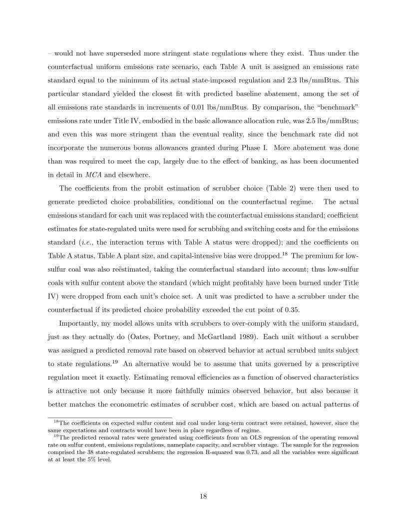
Table 5 provides an overview of the scrubber choice predictions from the simulation. The number

of units predicted to install scrubbers decreases slightly under the emissions standard, falling from

26 under the baseline scenario to 24 under the counterfactual. Of the twenty-four counterfactual

scrubbers, fifteen have scrubbers under the baseline (of which fourteen actually have scrubbers).

Table 6 compares the model predictions for aggregate abatement and cost under this coun-

terfactual policy with the estimates from the baseline scenario. By construction, emissions and

abatement are nearly identical under the two scenarios. The predicted annual aggregate abatement

cost is considerably greater under the uniform emissions-rate standard, however. The estimated

increase in cost is $153 million per year — an increase of 20 percent over the baseline scenario.

Equivalently, the tradeable allowances regime resulted in cost savings of 17 percent relative to a

uniform emissions-rate standard.

Figure 2 compares the “quasi-MAC” curves under the baseline and counterfactual scenarios.

The same caveats apply as in Figure 1. Recall that these curves are drawn conditional on a particular

set of choices, and thus on a particular policy. In particular, unlike a true marginal cost curve, they

do not provide a direct estimate of what marginal or total costs would have been at a lower level

of abatement (such as 3 million tons). For the same reason, the prescriptive-regulation curve does

not necessarily lie everywhere below the baseline cost curve. (On the other hand, the total areas

under the curve do correspond to the total costs of abatement.)

19

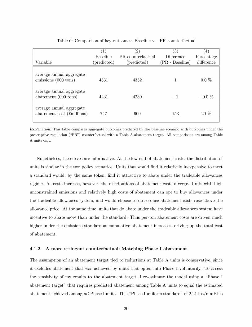
Table 6: Comparison of key outcomes: Baseline vs. PR counterfactual

(1) (2) (3) (4)Baseline PR counterfactual Difference Percentage

Variable (predicted) (predicted) (PR - Baseline) difference

average annual aggregateemissions (000 tons) 4331 4332 1 0.0 %

average annual aggregateabatement (000 tons) 4231 4230 −1 −0.0 %

average annual aggregateabatement cost ($millions) 747 900 153 20 %

Explanation: This table compares aggregate outcomes predicted by the baseline scenario with outcomes under the

prescriptive regulation (“PR”) counterfactual with a Table A abatement target. All comparisons are among Table

A units only.

Nonetheless, the curves are informative. At the low end of abatement costs, the distribution of

units is similar in the two policy scenarios. Units that would find it relatively inexpensive to meet

a standard would, by the same token, find it attractive to abate under the tradeable allowances

regime. As costs increase, however, the distributions of abatement costs diverge. Units with high

unconstrained emissions and relatively high costs of abatement can opt to buy allowances under

the tradeable allowances system, and would choose to do so once abatement costs rose above the

allowance price. At the same time, units that do abate under the tradeable allowances system have

incentive to abate more than under the standard. Thus per-ton abatement costs are driven much

higher under the emissions standard as cumulative abatement increases, driving up the total cost

of abatement.

4.1.2 A more stringent counterfactual: Matching Phase I abatement

The assumption of an abatement target tied to reductions at Table A units is conservative, since

it excludes abatement that was achieved by units that opted into Phase I voluntarily. To assess

the sensitivity of my results to the abatement target, I re-estimate the model using a “Phase I

abatement target” that requires predicted abatement among Table A units to equal the estimated

abatement achieved among all Phase I units. This “Phase I uniform standard” of 2.21 lbs/mmBtus

20

Table 7: Comparison of key outcomes: Baseline vs. PR counterfactual (Phase I abatement target)

(1) (2) (3) (4)Baseline PR counterfactual Difference Percentage

Variable (predicted) (predicted) (PR - Baseline) difference

average annual aggregateabatement (000 tons) 4417 4413 −4 −0.1 %

average annual aggregateabatement cost ($millions) 779 941 162 21 %

Explanation: This table compares aggregate outcomes under the baseline scenario and the alternative prescriptive

regulation counterfactual, in which abatement is scaled to total Phase I abatement. Thus the “Baseline” estimate

aggregates abatement and abatement cost across all 312 Phase I units in the sample. The “PR Counterfactual,” in

contrast, sums over Table A units only.

accounts for emissions reductions that were accomplished by voluntary units as well as those directly

subject to the regulation.

Table 7 summarizes the key results. The total annual abatement cost under the counterfactual

is now estimated to be $162 million higher than under the baseline. Of course, the baseline cost

has also risen, since it now represents the total abatement cost among all Phase I units. Hence

in percentage terms, the difference is similar to that for the Table A abatement target. The cost

increase is 21 percent of the baseline (Phase I) costs, corresponding to cost savings of 17 percent.

4.1.3 Unit-specific emissions standards

An alternative counterfactual policy is a set of source-specific emissions limitations. Although

prescriptive regulation at the federal level has generally taken the form of uniform standards,

state-level regulation commonly involves source-specific standards. Moreover, allowance allocations

varied widely among units, so that the application of the actual policy was far from uniform.

The simplest approach would limit emissions at each Table A unit to that unit’s allowance

allocation under Table A.20 The estimated costs of such an approach turn out to be 3 percent less

20Actual allowance allocations diverged from those listed on Table A: nearly one million bonus and extensionallowances were handed out each year for the first two years, as a result of political horsetrading or as an incentivefor adopting scrubbers (MCA, p. 41). These were awarded on the basis of provisions written in general terms in theAct itself, but specifically administered by the EPA. Because I lack the data on the actual allocations that resulted,however, I use the figures from Table A.

21

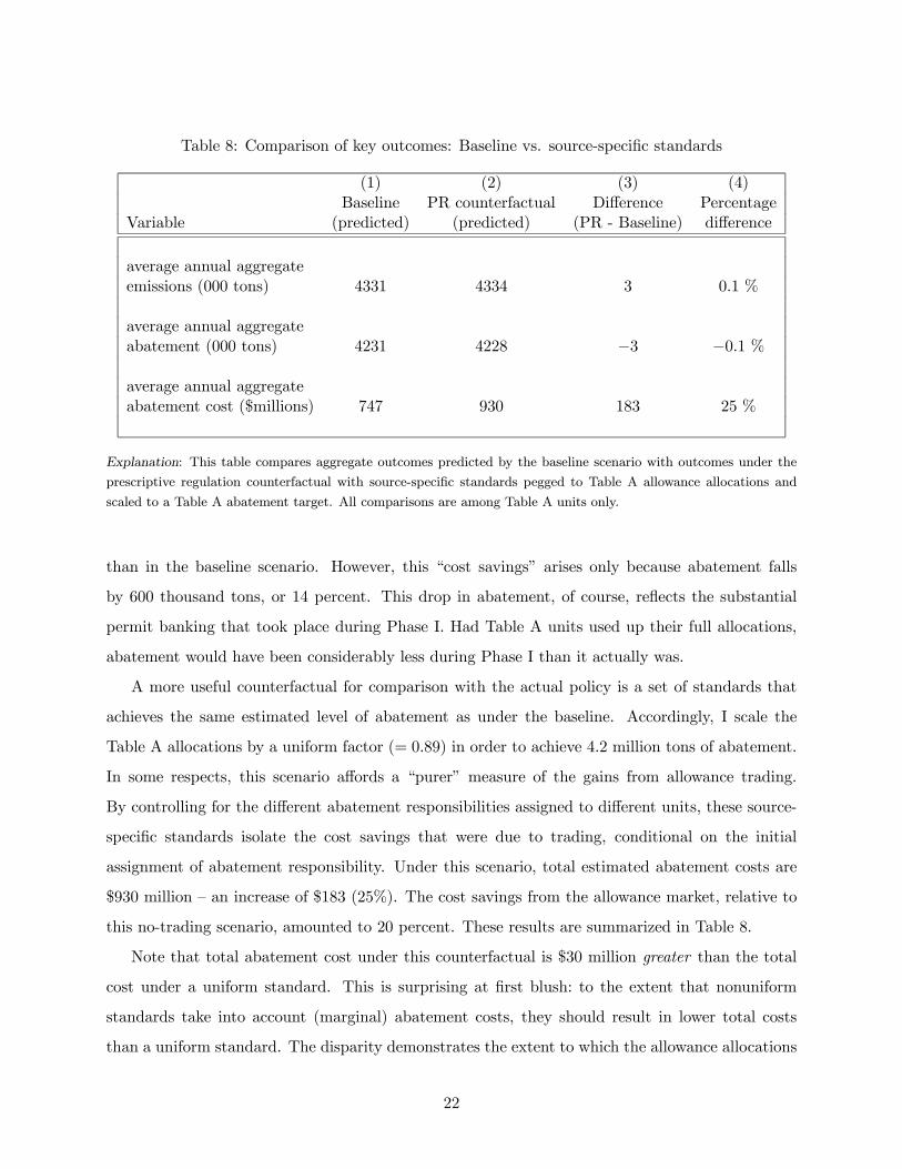
Table 8: Comparison of key outcomes: Baseline vs. source-specific standards

(1) (2) (3) (4)Baseline PR counterfactual Difference Percentage

Variable (predicted) (predicted) (PR - Baseline) difference

average annual aggregateemissions (000 tons) 4331 4334 3 0.1 %

average annual aggregateabatement (000 tons) 4231 4228 −3 −0.1 %

average annual aggregateabatement cost ($millions) 747 930 183 25 %

Explanation: This table compares aggregate outcomes predicted by the baseline scenario with outcomes under the

prescriptive regulation counterfactual with source-specific standards pegged to Table A allowance allocations and

scaled to a Table A abatement target. All comparisons are among Table A units only.

than in the baseline scenario. However, this “cost savings” arises only because abatement falls

by 600 thousand tons, or 14 percent. This drop in abatement, of course, reflects the substantial

permit banking that took place during Phase I. Had Table A units used up their full allocations,

abatement would have been considerably less during Phase I than it actually was.

A more useful counterfactual for comparison with the actual policy is a set of standards that

achieves the same estimated level of abatement as under the baseline. Accordingly, I scale the

Table A allocations by a uniform factor (= 0.89) in order to achieve 4.2 million tons of abatement.

In some respects, this scenario affords a “purer” measure of the gains from allowance trading.

By controlling for the different abatement responsibilities assigned to different units, these source-

specific standards isolate the cost savings that were due to trading, conditional on the initial

assignment of abatement responsibility. Under this scenario, total estimated abatement costs are

$930 million — an increase of $183 (25%). The cost savings from the allowance market, relative to

this no-trading scenario, amounted to 20 percent. These results are summarized in Table 8.

Note that total abatement cost under this counterfactual is $30 million greater than the total

cost under a uniform standard. This is surprising at first blush: to the extent that nonuniform

standards take into account (marginal) abatement costs, they should result in lower total costs

than a uniform standard. The disparity demonstrates the extent to which the allowance allocations

22

were motivated by distributional politics rather than efficiency. Allowance allocations under Title

IV were determined not by a cost-minimizing regulator, but by an explicitly political process, as

detailed by Joskow and Schmalensee (1998). The higher estimates of compliance costs suggest

that the political process resulted in a negative correlation between abatement cost and allowance

allocations: units that could abate more cheaply tended to receive more allowances. Of course, one

of the well-known attractions of tradeable allowances as a policy instrument is that the equilibrium

outcome — and thus the aggregate abatement cost — is robust to the initial allocation, as long as

transactions costs are low.21 Thus the allowance allocations might well have been different (since

their distributional implications would have been so) if a different policy instrument had been

chosen.

4.2 Comparison with a technology-based counterfactual

Next, I contemplate a technology standard achieving the same aggregate abatement as the baseline

scenario. This comparison provides a direct estimate of the cost savings from a market-based policy

relative to what might be termed “unenlightened command-and-control.” Consider a policy requir-

ing units with unconstrained emissions above 2.5 lbs/mmBtus to install scrubbers. (Under this

counterfactual policy, units whose cheapest available coal would meet or beat the 2.5 lbs/mmBtus

emissions rate standard would not be required to install a scrubber, or indeed even to abate at all.)

I then apply a uniform percentage-removal requirement to these units, chosen to yield the aggregate

abatement target. This counterfactual policy is modeled on the actual New Source Performance

Standards in the 1977 Clean Air Act Amendments. Because it exempts units with unconstrained

emissions below 2.5 lbs/mmBtus, it represents a relatively low-cost technology standard. More-

over, note that (unlike the 1977 NSPS) this technology standard is constructed to achieve the same

amount of abatement as under the baseline scenario. I estimate that such a technology requirement

would have cost $2.6 billion annually — an increase of $1.8 billion over than the baseline scenario.

This represents a more than three-fold increase in abatement cost. Judged against this alternative,

the tradeable allowances system yielded cost savings of 71 percent.

Of perhaps equal interest is the comparison between this technology standard and the uni-

form performance standard discussed above. Both achieve the same aggregate abatement, and

both represent prescriptive regulation imposed at the unit level. The crucial difference is that the

21Of course, when transactions costs exist in the permit market, the initial allocation may well distort the finaloutcome. See Stavins (1995) for a discussion of transactions costs in permits markets.

23

performance standard allows units the choice of how to comply. The estimated savings from in-

creased flexibility are enormous: $1.7 billion per year, or 65 percent of the costs under the scrubbing

requirement.

This comparison — between “enlightened” and “unenlightened” command-and-control regula-

tions — underscores the relative importance of regulatory flexibility versus trading per se. While

the allowance market yielded sizeable gains relative to a uniform performance standard, those gains

are less than one-tenth the size of the estimated gains from regulating emissions rather than tech-

nology. In other words, allowing intra-unit flexibility in compliance was much more significant than

allowing inter-unit flexibility, although both yielded substantial cost savings. In this respect, my

findings accord with arguments made early in the allowance trading program by Burtraw (1996).

4.3 “Pollution savings” as an alternative measure of gains from trade

Thus far we have equated aggregate abatement and compared the resulting costs. Next, I return to

the uniform performance standard counterfactual — but rather than matching aggregate abatement

with the baseline predictions, I match aggregate abatement cost. Doing so provides an alternative

measure of the gains from a market-based policy: namely, the increased abatement made possible

by the allowance trading system, relative to an equally costly prescriptive regulation.

This measure of “pollution savings” (rather than cost savings) may be the more relevant one

from a political perspective, since increasing environmental protection may be more rhetorically

compelling than reducing cost. Certainly this is the more salient strategic question for environmen-

tal advocacy groups. Hahn and Stavins (1991), for example, describe the role of the Environmental

Defense Fund (EDF) in proposing and supporting the use of tradeable allowances in Title IV. Such

market-based environmental policies had previously been anathema to environmentalists. EDF,

however, argued that the cost savings from such an approach would make possible greater cuts in

emissions. In essence, EDF supported the Bush Administration’s favored market-based proposal

in return for a more ambitious target for SO2 abatement than the Administration would have

otherwise contemplated.

My model suggests that a uniform performance standard of 2.47 lbs/mmBtus would have

matched the cost of the actual outcome. I estimate that such an equal-cost policy would have

resulted in 3.8 million tons of abatement — 400 thousand tons less than the baseline scenario. Thus

the use of the market-based instrument resulted in an increase in abatement of roughly ten percent.

Interestingly, this “pollution savings” based on equal-cost outcomes is considerably smaller, in

24

percentage terms, than the cost savings estimated on the basis of scenarios with equal abatement.

While the current model provides only a single instance, there is reason to believe that this asym-

metry is general. It results from the different effects of an increase in abatement on total costs

under different policy instruments. At lax levels of a standard, many regulated units can comply

by burning low-sulfur coal of varying sulfur content. As the stringency of a standard increases,

some sources of low-sulfur coal no longer satisfy the standard, forcing units that would otherwise

burn low-sulfur coal to install scrubbers instead. This effect intensifies as the standard tightens

further, so that total costs rise more than proportionally with abatement. Under a market-based

instrument, on the other hand, much of an increase in abatement can be achieved by units with

relatively low costs. While tightening the overall cap drives permit prices up, this results in a

smoothly increasing incentive to install a scrubber, rather than the kind of “threshold effect” cre-

ated by a performance standard that requires all units to reduce emissions. As a result, costs rise

less steeply with abatement, relative to the case of prescriptive regulation.

Hence the relative cost savings of a market-based instrument are higher, the more stringent is

the abatement target. A direct implication is the asymmetry found above: the percentage increase

in abatement achieved by a market-based instrument, relative to a performance standard with equal

cost, will be less than the percentage increase in cost under a performance standard relative to a

market-based instrument with equal abatement.

4.4 Theoretical benchmarks

Thus far, we have assessed the allowance market against plausible alternative policies. We can also

ask: How well did the tradeable allowances program perform relative to what theory would predict?

Two natural benchmarks stand out for comparison. The first is the cost-effective outcome. With

the considerable benefit of hindsight, what is the minimum total cost for which baseline level of

abatement could have been achieved?

I estimate the cost-effective outcome to be $315 million annually — less than half the baseline

cost. This suggests that the allowance market fell far short of what theory predicts. Of course,

there are a range of explanations for why units may not appear to have minimized abatement

costs during Phase I. For example, abatement decisions in the first few years of the program may

have been made with an eye towards Phase II, when allowance allocations were ratcheted down.

In particular, some investment in scrubbers may have been motivated by longer time horizons.

Pessimistic expectations about market liquidity could also have given rise to scrubbing decisions

25

that turned out not to be optimal.22

Indeed, ample evidence suggesting that utilities overinvested in scrubbers during Phase I. Eller-

man and Montero (1998) argue that an abundance of scrubbers (due partly to inflated expectations

about allowance prices) contributed to the downward pressure on allowance prices during Phase

I, along with lower-than expected prices of low-sulfur coal from Wyoming. In the dataset used in

the present study, average total costs of scrubbing at Table A units with scrubbers are clustered

between $200 and $450 per ton — higher than actual Phase I allowance prices, but lower than pub-

lished forecasts of allowance prices. These data suggest that scrubbing decisions may have been

individually rational given ex ante expectations; but since those expectations turned out to be

wrong, the scrubbers that were installed did not minimize costs ex post.

Whatever the reason for the failure of utilities to behave as perfect cost-minimizers during

Phase I, it is evident in the disparity between the theoretical least-cost outcome and the baseline

estimate. Even allowing for considerable uncertainty in the least-cost estimate, the magnitude of

the gap suggests that the actual market fell well short of theoretical cost-effectiveness. From a

methodological point of view, this result underscores the importance of taking actual behavior into

account, rather than assuming perfect foresight and cost-minimization by unit managers.

The second theoretical benchmark is an “ideal prescriptive regulation” scenario, in which pre-

dicted abatement decisions at the unit level are made to minimize abatement costs, subject to

compliance with a uniform standard.23 This scenario is no more realistic than the cost-effective

outcome, since it assumes perfectly rational (and foresighted) utility managers. Nonetheless, it

remains useful as the appropriate behavioral analogue to the theoretical least-cost scenario. The

estimated cost under this scenario is $546 million annually.

The difference in costs between the “ideal prescriptive regulation” scenario and the least-cost

outcome provides a second measure of the gains from trade — one based on theoretical cost-

minimizing behavior, rather than on our predictions of what would have occurred under alternative

policies. Figure 3 illustrates the comparison. The top curve, corresponding to the ideal prescriptive

regulation, is conditional on the choice of emissions standard. The least-cost estimate (the lower

curve) is now a true marginal cost curve, since it assumes cost-minimization; thus it extends beyond

22I thank an anonymous referee for suggesting these explanations.23The counterfactual emissions standard (achieving the same level of abatement as under the baseline) is now

2.02 lbs/mmBtus. It is lower than the uniform standard used earlier because fewer scrubbers are installed in thecost-minimizing case for any given standard, and because units are now assumed to meet abatement requirementsexactly (rather than overcomplying).

26

actual total abatement. The area between the two curves, up to the total abatement of 4.2 million

tons, represents the theoretical cost savings from trading — $231 million annually, or 42 percent of

the costs under the ideal prescriptive regulation.

Table 9 summarizes the abatement cost estimates under six of the scenarios just discussed,

relative to the baseline prediction. The central comparison with the counterfactual corresponding

to a uniform emissions standard and a Table A abatement target is in boldface type.

5 Comparisons across studies

The bottom three rows of Table 9 present the cost savings from Title IV estimated by the two major

prior studies, MCA and CBCP.24 A glance at the table shows considerable agreement among the

three studies with respect to the baseline cost estimates. The estimated cost savings, however, are

strikingly different among the three studies. The MCA study estimates cost savings of $358 million

to $626 million annually, while CBCP estimate that compliance costs under the actual policy were

10 percent greater than they would have been under a performance standard.

Two differences are worth noting about the data used in the present study. First, I have re-

stricted attention to Table A units, on the grounds that because those were the units directly

identified by Congress for regulation, they are the natural group to perform on which to counter-

factual analysis. Both the MCA and CBCP analyses, in contrast, comprise all affected units — i.e.,

voluntary Phase I participants as well as Table A units. Second, this study draws on data from all

five years of Phase I. CBCP used only the first two years, while MCA used actual data for 1995-

1997 and extrapolated to the remaining two years in estimating Phase I averages. This is relevant

because the number of voluntary participants declined during each year of Phase I; thus the sets

of units used by CBCP and MCA are both larger than the set of Phase I units that participated

throughout the program.25 This change in the number of units affected also argues in favor of

focusing on the Table A units, which were required to participate throughout the program.

The difference in the units considered, however, does not explain the large differences in esti-

mated cost savings. The difference in approach is reflected in the counterfactual estimates as well

24A third study of cost savings, in a working paper by Burtraw and Mansur (1999), found cost savings of $97million (relative to an estimate of Phase I costs of $650 million) from trading during Phase I. In percentage terms,that estimate (13% cost savings) is quite close to the “preferred estimate” presented here, despite being based on astate-level model employing engineering estimates of abatement cost and a least-cost choice algorithm.25As explained in MCA, an important incentive for units to participate voluntarily in Phase I was to receive

exemption from subsequent NOx emissions regulations. To receive this exemption a unit had to opt into the programin 1995 — but did not have to remain in subsequent years. See MCA, ch. 8.

27

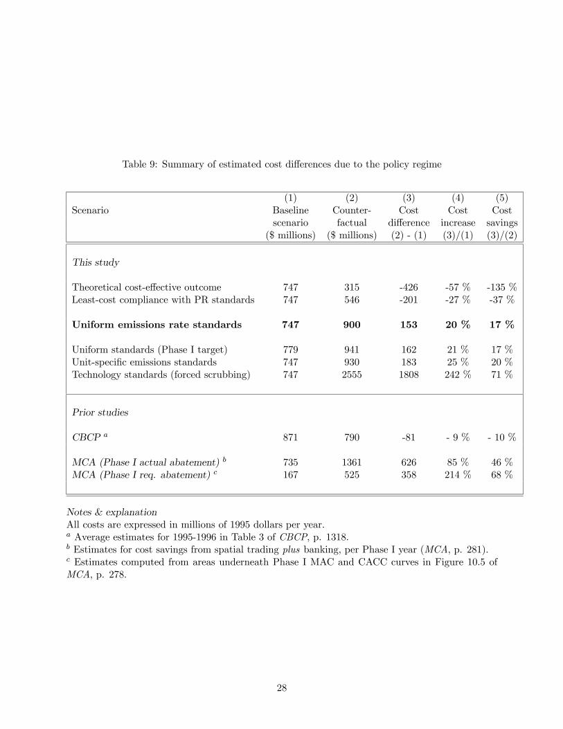
Table 9: Summary of estimated cost differences due to the policy regime

(1) (2) (3) (4) (5)Scenario Baseline Counter- Cost Cost Cost

scenario factual difference increase savings($ millions) ($ millions) (2) - (1) (3)/(1) (3)/(2)

This study

Theoretical cost-effective outcome 747 315 -426 -57 % -135 %Least-cost compliance with PR standards 747 546 -201 -27 % -37 %

Uniform emissions rate standards 747 900 153 20 % 17 %

Uniform standards (Phase I target) 779 941 162 21 % 17 %Unit-specific emissions standards 747 930 183 25 % 20 %Technology standards (forced scrubbing) 747 2555 1808 242 % 71 %

Prior studies

CBCP a 871 790 -81 - 9 % - 10 %

MCA (Phase I actual abatement) b 735 1361 626 85 % 46 %MCA (Phase I req. abatement) c 167 525 358 214 % 68 %

Notes & explanationAll costs are expressed in millions of 1995 dollars per year.a Average estimates for 1995-1996 in Table 3 of CBCP, p. 1318.b Estimates for cost savings from spatial trading plus banking, per Phase I year (MCA, p. 281).c Estimates computed from areas underneath Phase I MAC and CACC curves in Figure 10.5 ofMCA, p. 278.

28

as in the baseline scenario. Moreover, we have already seen that in percentage terms the choice

of baseline has little effect on the estimated cost savings. And the greatest divergence is between

the MCA and CBCP estimates, which rely on the same set of units (and nearly the same years of

data).

In the remainder of this section, I examine the CBCP and MCA estimates more closely. The

sources of the differences are varied, but two stand out. First, the two studies compare the actual

policy to counterfactual scenarios that differ in subtle but crucial respects from each other and

from that used here. Second, the MCA group — lacking a direct means of estimating the costs of

prescriptive regulation — employs a short cut which appears benign but in fact leads it to overstate

the cost savings from Phase I by nearly a factor of two.

5.1 Comparison with CBCP

The striking result in CBCP is that costs were higher during the first few years Phase I than they

would have been under an equivalent command-and-control scenario. The authors cast their finding

in strong terms: “[T]he fact that our estimate of actual compliance costs exceeds our estimate of

the cost of command and control suggests that the uniform performance standard would have been

no less efficient than the actual pattern of emissions chosen by utilities” (p. 1318). Their finding

has been similarly interpreted by other analysts, such as Ellerman (2003). CBCP attribute their

surprising finding in part to their focus on the first two years of the program, when the allowance

market was just getting underway. Their key argument, however, concerns the behavior of utilities

under the allowance market. They write: “Adjustment costs associated with changing fuel contracts

and capital expenditures as well as regulatory policies may make it appear that firms have failed

to minimize costs when they have actually done so” (p. 1318).

A simpler explanation is that CBCP compare the actual policy to an idealized version of

command-and-control. As in the present study, CBCP specify as their counterfactual a uniform

emissions rate standard chosen to achieve an equivalent level of emissions as under the actual

outcome. However, they assume cost-minimizing behavior by the utilities. The appropriate com-

parison with my estimates, therefore, is to my “ideal prescriptive regulation” scenario. Like CBCP,

I estimate that the costs under such a scenario would have been lower than they were under the

actual policy. Indeed, my estimate of costs under such a scenario is even lower (relative to actual

costs) than the CBCP estimate.26

26CBCP use estimates of actual emissions that accord well with those in MCA and in this study. To calculate what

29

The importance of assumed behavior can also be seen in CBCP’ s estimates of the long-run

cost savings from trading. CBCP estimate gains from trade of $780 million in the final year

of Phase II (2010), relative to estimated costs under prescriptive regulation of $1.8 billion. In

making this long-run comparison, of course, CBCP assume cost-minimizing behavior under both

policy regimes. Note that their estimated long-run cost savings amount to 43 percent of the costs

under the counterfactual policy. This is virtually identical (in percentage terms) to the difference

between the “ideal prescriptive regulation” and cost-effective scenarios I considered in section 4.4,

which incorporate the same assumption about decision making.

CBCP adopt the assumption of cost-minimizing behavior because it is theoretically and practi-

cally attractive: it accords with economic reasoning and it can easily be implemented by a least-cost

algorithm. But the assumption of cost-minimization skews their results, since they end up com-

paring an idealized version of one policy with the actual implementation of another. There is

considerable irony in CBCP ’s assertion that the allowance market was more costly (in the short

run) than prescriptive regulation would have been. When the early articles in this line of lit-

erature were written, prescriptive regulation was the norm, and the counterfactual policies were

market-based. In that context, it was the cost savings from trading programs that were inevitably

overstated.

In summary, my data confirm CBCP ’s finding that abatement costs under the allowance market

were higher than they would have been under a uniform standard with cost-minimizing behavior.

But that is not really the right benchmark for comparison. Using actual behavior by electric utilities

under other policy regimes as a guide, a prescriptive approach would also have ended up costing

much more in practice than we would predict on the basis of cost-minimizing behavior. A consistent

approach compares the costs under the actual program with the costs that a performance standard

would actually have entailed.

5.2 Comparison with MCA

Of the three studies,MCA calculates the largest cost savings from the allowance market — estimating

that trading saved $358 million per year of Phase I. The dramatically higher cost savings are not

emissions would have been absent Title IV, they multiply actual emissions rates in 1993 by electricity generation in1995 and 1996. For Table A units, this method yields unconstrained emissions of 7.5 million tons — well below myestimate of 8.6 million tons. Thus their estimates appear to significantly underestimate actual abatement — a factthat helps explain why their estimated counterfactual cost is relatively close to their estimated cost of the actualprogram.

30

due to differences in abatement or baseline cost estimates.MCA estimates actual abatement to have

been 4.2 million tons, identical to the estimate in this study, and the estimated baseline abatement

cost of $735 million is very close to my estimate. Rather, these high cost savings can be attributed

to how the MCA group calculates costs under the command-and-control counterfactual.

To understand this point, it helps to consider their methodology. An important contribution

of the MCA study is its conceptualization of the “cost savings attributable to trading.” MCA

partitions cost savings into the gains from spatial trading and those from intertemporal trading.

The gains from spatial trading represent the reduced costs of achieving required (rather than actual)

abatement through the allowance market, relative to a counterfactual prescriptive regulation. Gains

from intertemporal trading result from overcompliance in early years, with the extra abatement

banked for Phase II. Indeed, the $358 million figure cited above represents only the first of these

types of savings. If the intertemporal savings from Phase I abatement are credited to the first phase

of the program as well, the MCA estimate of total cost savings rises to $626 million annually.

In contrast, the approach taken in the body of this paper (as well as by CBCP) compares the

costs of actual abatement with the estimated costs of reaching the same level of abatement under a

counterfactual scenario. The appeal of this latter approach is that it can be estimated on the basis

of actual data, rather than requiring extrapolation about future costs (i.e., costs under either policy

regime in Phase II). The strength of the MCA approach, on the other hand, is that it explicitly

addresses the dynamic nature of the allowance program. The drawback is that to do so it must

rely on conjectures about costs during Phase II.

To identify the cost savings from spatial trading, MCA first estimates the abatement that was

effectively required by Phase I of the program — that is, the difference between the total number

of allowances and what emissions would have been in the absence of regulation. MCA estimates

required abatement for all Phase I units together to be 2 million tons annually. Using actual data,

MCA then estimates a linear quasi-MAC curve corresponding to the tradeable allowances regime.

The actual policy is compared to a particular counterfactual scenario: a set of source-specific

standards based on actual allowance allocations and summing to required abatement. To estimate

costs under this counterfactual, the MCA group assume that actual behavior under the allowance

market was cost-minimizing, allowing them to infer that costs under the counterfactual would have

been at least as high. Under the additional assumption of a linear relationship between cumulative

abatement and average cost at the marginal unit, they posit a linear “command-and-control cost”

curve (with much the same interpretation as the “quasi-MAC curves” drawn in figures 1-3 above).

31

The area between the posited “command-and-control cost” (CACC) curve and the quasi-MAC

curve under the actual policy corresponds to the estimated cost savings from spatial trading of

$358 million.

The derivation of the CACC curve turns out to be the source of the very high estimate of cost

savings. To demonstrate this, I first use my model to estimate the costs of achieving required

abatement among Table A units via a set of source-specific standards based on Table A allocations.

That required abatement was 2.25 million tons annually.27 The increase in required abatement

relative to the MCA estimate stems from the fact that I focus on Table A units only, rather than

all Phase I units. Although it might seem paradoxical at first, the abatement required of Table A

units exceeded the abatement required of the larger set of all Phase I units. The reason is simple:

in the absence of Title IV, emissions at units that participated in Phase I voluntarily would have

been less than the allowances those units were allocated. This gap, between required abatement

at Table A units and that at all Phase I units, neatly demonstrates the adverse selection problem

(and the resulting loosening of the cap) created by the “opt-in” program (Montero 1999).

I estimate the total costs of exactly meeting the 2.25 million tons requirement to be $346

million annually. The cost of achieving the same amount of abatement under the baseline was

$165 million. Thus the estimated cost savings of achieving required abatement under the allowance

market, on the basis of my model, was $181 million — just half of the $358 million estimated in

MCA.28 Figure 4 plots the Phase I CACC and MAC curves used in MCA along with the quasi-

MAC curves corresponding to my estimates of the costs under the baseline scenario and under the

required-abatement counterfactual.29

For the actual policy, the linear approximation used by MCA coincides reasonably well with

my estimated quasi-MAC curve. Thus, as the MCA group point out, the linearity assumption has

only a small effect on estimated costs under the baseline. Their CACC curve, however, diverges

significantly from my econometrically-based estimate. In Figure 4, the area under the linear CACC

27Table 5.2 of MCA reports that an average of 6.31 million total allowances per year allocated to Table A plantsduring Phase I (using the 1997 figure for years 1998 and 1999). I estimate unconstrained emissions as 8.56 milliontons per year. The difference is my estimate of required abatement.28This figure of $181 million is not directly comparable to the cost savings estimates derived earlier on the basis

of actual abatement, for two reasons. The estimate of counterfactual costs is high, since it entails source-specificstandards. On the other hand, the estimated cost of meeting required abatement under the allowance market(computed by finding the area under the baseline quasi-MAC curve up to 2.25 million tons of abatement) is low,since estimated marginal cost under the baseline is relatively flat at low levels of abatement and rises more steeplyat higher levels.29The MCA MAC curve is a ray from the origin through the point (4.2,$350); the MCA CACC curve passes from

the origin through the point (2.0,$525).

32

curve (up to 2.25 million tons) is $664 million — much greater than the $346 million represented

by the area under the curve estimated by my model. Far from being linear, the actual curve is

rather flat at first and then turns sharply up. This shape is not accidental: it is driven by the wide

variation in abatement costs under prescriptive regulation. As argued above, the quasi-MAC curve

is best thought of as representing the distribution of abatement costs under a particular policy.

Because units must comply with a performance standard even if it is very costly, the highest-cost

units under such a policy are likely to have very high costs indeed, even while costs at the low end

of the distribution may correspond closely with costs under the tradeable allowances regime.

Of course, a linear approximation to the actual quasi-MAC curve exists that will preserve the

area below it. One might alternatively identify the particular linear approximation selected byMCA

as the source of the inflated estimate of cost savings. Regardless of how we frame the argument,

Figure 4 makes clear that the curve they posit has a dramatic (and unappreciated) effect.

The strength of the MCA approach is that it takes into account the intertemporal equilibrium.

To preserve this strength while correcting for their ad hoc estimate of costs under prescriptive

regulation, I replicate their analysis drawing on the data used here. Figure 5 presents the same

four curves as in Figure 10.3 of MCA, drawn to match the data here. The solid Phase I curves

correspond to my model estimates; the dashed lines correspond to linear approximations that

preserve the area underneath the curves.30 As the MCA group points out, if one assumes that

observed Phase I abatement reflected optimal intertemporal behavior by utilities, then the cost of

the last ton of abatement during Phase I should equal the abatement cost at the margin during

Phase II. Accordingly, as in MCA, I have drawn the Phase II MAC curve as a straight line from

the end of the Phase I curve down to a right-hand origin. The horizontal distance equals the

total allowances available during Phase II, averaged over the five years of Phase I (yielding 15.04

million tons, as in MCA).31 Finally, continuing to follow the approach taken by MCA, the “Phase

II CACC” (line O2D) in Figure 5 is drawn so that the ratio of its slope to that of the “Phase

II MAC” equals the ratio of the slopes of the linear approximations to the corresponding Phase I

curves (1.64). This embodies an assumption that the ratio of prescriptive regulation costs to costs

under the trading regime is constant over time.

30Thus the dashed line O1B in Figure 6 runs from the origin to the point (2.25, $308), encompassing an area equalto that under the quasi-MAC curve corresponding to the required-abatement scenario with no trading. Similarly, theray from the origin to the point labeled E, (4.23, $353), is a linear approximation of the baseline prediction — drawnso that the area underneath equals the estimated $747 aggregate cost of Phase I abatement.31Of course, one might be more concerned about the assumption of optimal intertemporal behavior given the

evidence already presented that utility decisions did not minimize costs during Phase I.

33

We can now compute the various types of cost savings. Annual cost savings from spatial

trading during Phase I — the area between the Phase I curves to 2.25 million tons — amount to

$181 million, as already discussed. Annual cost savings from banking correspond to the area below

the Phase II quasi-MAC and above the Phase I quasi-MAC, computed over the 1.98-million-ton

difference between required and actual abatement. This gain is $169 million for each year of Phase

I. Alternatively, using the straight-line approximations to the Phase I curves yields estimated cost

savings of $134 million for spatial trading (area O1AB) and $216 for banking (area ACE). The

effect of the straight-line approximations is to increase the cost savings from spatial trading by $47

million, and reduce the cost savings from banking by the same amount. This “smoothing” results

because the linear approximation lies above the cost curve at low levels of abatement and below it

at higher levels.

These estimated cost savings from abatement during Phase I are well below the corresponding

figures in MCA. The $169 million in gains from banking, for example, is nearly $100 million less

thanMCA’s estimate of $268 million per Phase I year. Overall, the combined estimated cost savings

from spatial and intertemporal trading during Phase I equals $350 million — somewhat over half

the corresponding MCA estimate of $626 million.

FollowingMCA, we can also use Figure 5 to estimate cost savings during Phase II. In particular,

the area of triangle O2CD corresponds to the spatial trading gains during Phase II. This area is

$2.0 billion per Phase I year. Assuming (with MCA) that the allowance bank will be exhausted in

2007, this estimate represents an annual cost savings of $1.2 billion for each of those eight years —

far below the MCA estimate of $2.1 billion.

In fairness, any estimate of cost savings must rely on a particular choice of counterfactual.

What the comparison in this section highlights is the importance of that choice. Indeed, in a

thorough sensitivity analysis MCA shows that their estimates of the gains from trading are most

sensitive to the assumed costs under prescriptive regulation (MCA, p. 290). For example, their

lower-bound estimate of cost savings during Phase II, based on an alternative assumption that

prescriptive regulation would be less costly relative to the trading regime during Phase II, is $1.1

billion annually — much closer to my estimate.

While the cost savings estimated in MCA appear to have been inflated, their analysis provides

a useful alternative framework for thinking about cost savings. Because the drawback of their

approach is its reliance on conjectures about Phase II, it will be even more attractive when direct

estimates of Phase II costs can be made from actual data. The apparent overestimates in MCA

34

also illuminate the usefulness of paying more careful and direct attention to modeling the actual

behavior of utilities under various policy regimes.

6 Conclusion

This chapter has used an econometric model of decisions made by utilities to estimate total costs of

abatement under the Title IV program as well as a range of counterfactual prescriptive regulations.

The allowance trading program resulted in estimated annual cost savings of $150 million (17%)

during Phase I, relative to a uniform performance standard that would have achieved the same

aggregate abatement. Holding estimated abatement costs constant, the allowance market achieved

roughly 10 percent more abatement than would have been possible under a uniform standard.

Estimated cost savings are somewhat higher — $180 million — relative to a counterfactual policy

of source-specific standards based on Table A allowance allocations. The cost of a technology

standard, meanwhile, would have been astronomically high — nearly three and a half times the cost

of the actual policy. The wide gap between the technology standard and the performance standard

illustrates that allowing flexibility in compliance within regulated units (by regulating emissions

rather than technology) is even more consequential than allowing flexibility among regulated units

through trading.

The results of this study demonstrate the usefulness of estimating abatement costs on the

basis of actual behavior. Previous studies were dependent on assumptions of cost minimization or

relatively ad hoc estimates of costs under command-and-control. In contrast, the current study

incorporates information about decisions made by utilities under varying forms of environmental

regulation. This approach both allows for systematic deviations between actual decisions and those

that would appear to minimize costs, and incorporates the differences among policy regimes in the

incentives for installing pollution control technologies.

35

References

[1] Ackerman, Bruce A., and William T. Hassler. Clean Coal/Dirty Air. New Haven: Yale Uni-

versity Press, 1981.

[2] Atkinson, Scott E., and David H. Lewis. 1974. “A Cost-Effectiveness Analysis of Alternative

Air Quality Control Strategies,” Journal of Environmental Economics and Management 1:

237-50.

[3] Bailey, Elizabeth M. 1998. “Allowance Trading Activity and State Regulatory Rulings: Evi-

dence from the U. S. Acid Rain Program.” MIT-CEEPR Working Paper 98-005 WP (March).

[4] Baumol, William J, and Wallace E. Oates. 1988. The Theory of Environmental Policy, 2nd

ed. (New York: Cambridge University Press).

[5] Bellas, Allen. 1998. “Empirical Advances in Scrubbing Technology.” Resource and Energy

Economics 20: 327-343.

[6] Burtraw, Dallas. 1996. “The SO2 Emissions Trading Program: Cost Savings Without Allowance

Trades.” Contemporary Economic Policy 14: 79-94.

[7] Burtraw, Dallas, Alan J. Krupnick, Erin Mansur, David Austin, and Deirdre Farrell. 1998.

“The Costs and Benefits of Reducing Air Pollutants Related to Acid Rain.” Contemporary

Economic Policy 16: 379-400.

[8] Burtraw, Dallas, and Erin Mansur. 1999. “The Effects of Trading and Banking in the SO2

Allowance Market.” Resources for the Future Discussion Paper 99-25.

[9] Burtraw, Dallas, and Erin Mansur. 1999. “The Environmental Effects of SO2 Trading and

Banking.” Environmental Science and Technology 33: 3489-3494.

[10] Busse, Meghan, and Nathaniel O. Keohane. 2004. “Market Effects of Environmental Regula-

tion: Coal, Railroads, and the 1990 Clean Air Act.” Working paper, Yale University, available

at www.som.yale.edu/faculty/nok4.

[11] Carlson, Curtis, Dallas Burtraw, Maureen Cropper, and Karen L. Palmer. 2000. “Sulfur Diox-

ide Control by Electric Utilities: What are the Gains from Trade?” Journal of Political Econ-

omy 108: 1292-1326.

36

[12] Downing, P. B. and L. J. White. 1986. “Innovation in Pollution Control.” Journal of Environ-

mental Economics and Management 13: 18-29.

[13] Ellerman, A. Denny. 2003. “Ex Post Evaluation of Tradeable Permits: The U. S. Cap-and-Trade

Program.” Paper prepared for the National Policies Division of the Environmental Directorate

of the OECD.

[14] Ellerman, A. Denny, Paul L. Joskow, Richard M. Schmalensee, Juan-Pablo Montero, and

Elizabeth M. Bailey. 2000. Markets for Clean Air. Cambridge: Cambridge, UK.

[15] Ellerman, A. Denny, and Juan-Pablo Montero. 1998. “The Declining Trend in Sulfur Diox-

ide Emissions: Implications for Allowance Prices.” Journal of Environmental Economics and

Management 36: 26-45.

[16] Fischer, Carolyn, Ian W. H. Parry, and William A. Pizer. 2003. “Instrument choice for en-

vironmental protection when technological change is endogenous.” Journal of Environmental

Economics and Management 45: 523-545.

[17] Hahn, Robert W., and Robert N. Stavins. 1991. “Incentive-Based Environmental Regulation:

A New Era from an Old Idea.” Ecology Law Quarterly 1: 24.

[18] Heckman, James J. 1974. “Shadow prices, market wages, and labor supply.” Econometrica

42(4): 679-694.

[19] Joskow, Paul L, and Richard Schmalensee. 1998. “The Political Economy of Market-Based

Environmental Policy: The U. S. Acid Rain Program.” Journal of Law and Economics 41:

37-83.

[20] Keohane, Nathaniel O. 2004. “Environmental Policy and the Choice of Abatement Tech-

nique: Evidence from Coal-Fired Power Plants.” Working paper, Yale University, available

at www.som.yale.edu/faculty/nok4.

[21] Keohane, Nathaniel O., and Christine T. Lee. 2004. “How Responsive is Environmental Reg-

ulation to Costs and Benefits? Evidence from State Regulation of Sulfur Dioxide Emissions.”

Working paper, Yale University, available at www.som.yale.edu/faculty/nok4.

[22] Kerr, Suzi, and Richard G. Newell. 2003. “Policy-Induced Technology Adoption: Evidence

from the U. S. Lead Phasedown.” Journal of Industrial Economics 51: 317-343.

37

[23] Kolstad, Charles D. 1986. “Empirical Properties of Economic Incentives and Command-and-

Control Regulations for Air Pollution Control.” Land Economics 62: 250-268.

[24] Krupnick, A. J. 1986. “Costs of Alternative Policies for the Control of Nitrogen Dioxide in

Baltimore.” Journal of Environmental Economics and Management 13 (189-197).

[25] Lange, Ian, and Allen Bellas. 2004. “Secondary Benefits of Market-Based Regulation:

The Case of Scrubbers.” Working paper, University of Washington, downloaded from

http://students.washington.edu/ilange1/adobes/lange paper1.pdf.

[26] Lile, Ron, and Dallas Burtraw. 1998. “State-level policies and regulatory guidance for com-

pliance in the early years of the SO2 emission allowance trading program.” RFF Discussion

Paper 98-35 (May). Washington, D.C.: Resources for the Future.

[27] Milliman, S. R., and R. Prince. 1989. “Firm Incentives to Promote Technological Change in

Pollution Control.” Journal of Environmental Economics and Management 17: 247-265.

[28] Montero, Juan-Pablo. 1999. “Voluntary Compliance with Market-Based Environmental Policy:

Evidence from the U. S. Acid Rain Program.” Journal of Political Economy 107: 998-1033.

[29] Murphy, Kevin M., and Robert H. Topel. 1985. “Estimation and inference in two-step econo-

metric models.” Journal of Business and Economic Statistics 3(4): 370-379.

[30] Oates, Wallace E., Paul R. Portney, and Albert M. McGartland. 1989. “The Net Benefits

of Incentive-Based Regulation: A Case Study of Environmental Standard Setting.” American

Economic Review 79: 1233-42.

[31] Seskin, E. P., Anderson, R. J., Jr., and R. O. Reid. 1983. “An Empirical Analysis of Economic

Strategies for Controlling Air Pollution.” Journal of Environmental Economics and Manage-

ment 10: 112-124.

[32] Shadbegian, Ronald J., Wayne Gray, and Cynthia Morgan. 2004. “The 1990 Clean

Air Act Amendments: Who Got Cleaner Air — And Who Paid for It?” Working

paper (July). Downloaded from http://www.clarku.edu/faculty/wgray/personalwebpage/-

currentpapers/whopaid04.pdf.

[33] Stavins, Robert N. 1995. “Transactions Costs and Tradeable Permits.” Journal of Environ-

mental Economics and Management 29: 133-148.

38

[34] Stavins, Robert N. 1999. “What Can We Learn from the Grand Policy Experiment? Lessons

from SO2 Trading.” Journal of Economic Perspectives 12: 69-88.

39

Figure 1: Baseline and estimated "quasi-MAC" curves

0

200

400

600

800

0 500 1000 1500 2000 2500 3000 3500 4000 4500 5000Annual abatement (000 tons)

Abat

emen

t cos

t ($/t

on)

Baseline prediction

Total abatement4.2 m tons

Estimated (actual choices)

Figure 2: Baseline and counterfactual "quasi-MAC" curves

0

200

400

600

800

0 500 1000 1500 2000 2500 3000 3500 4000 4500 5000Annual abatement (000 tons)

Abat

emen

t cos

t ($/t

on)

PR counterfactual

Baseline prediction

Total abatement4.2 m tons

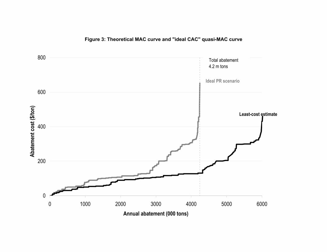
Figure 3: Theoretical MAC curve and "ideal CAC" quasi-MAC curve

0

200

400

600

800

0 1000 2000 3000 4000 5000 6000Annual abatement (000 tons)

Abat

emen

t cos

t ($/t

on)

Ideal PR scenario

Total abatement4.2 m tons

Least-cost estimate

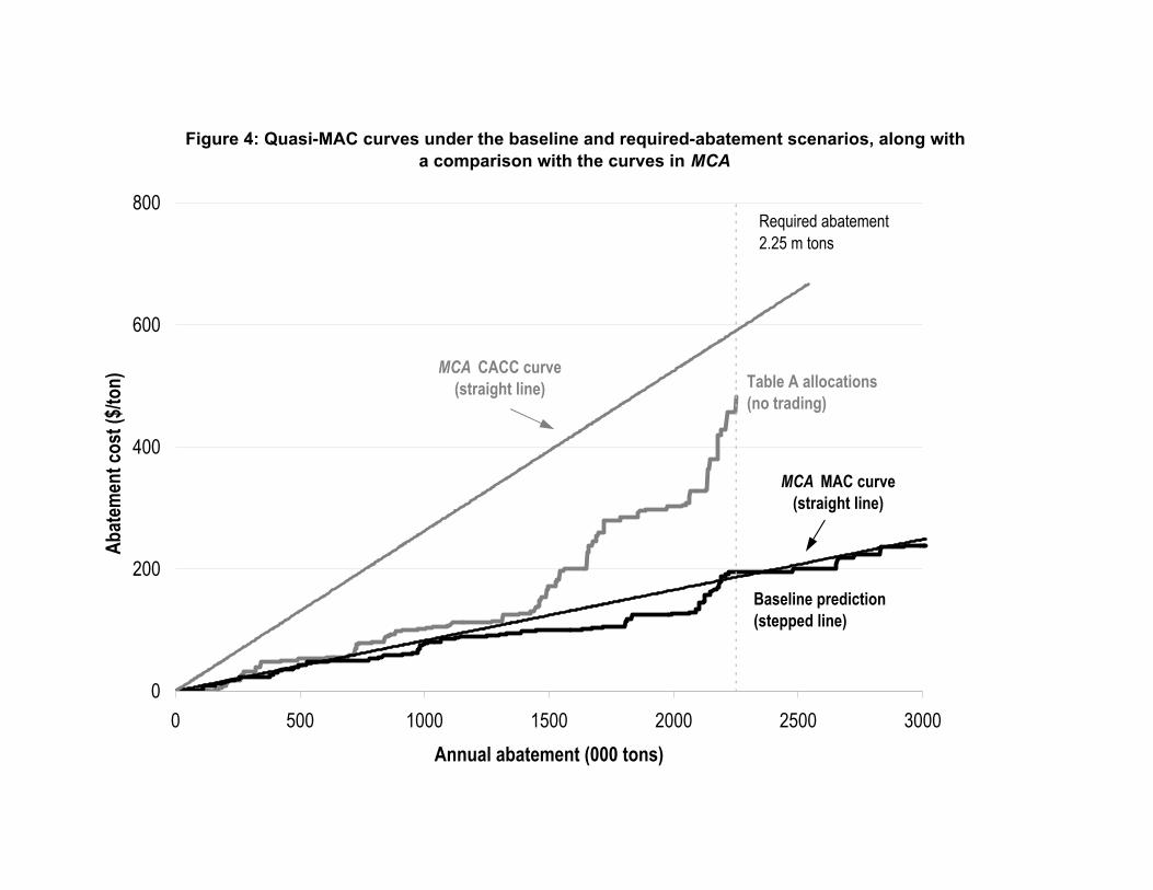
Figure 4: Quasi-MAC curves under the baseline and required-abatement scenarios, along with a comparison with the curves in MCA

0

200

400

600

800

0 500 1000 1500 2000 2500 3000Annual abatement (000 tons)

Abat

emen

t cos

t ($/t

on) Table A allocations

(no trading)

Required abatement2.25 m tons

Baseline prediction (stepped line)

MCA CACC curve(straight line)

MCA MAC curve(straight line)

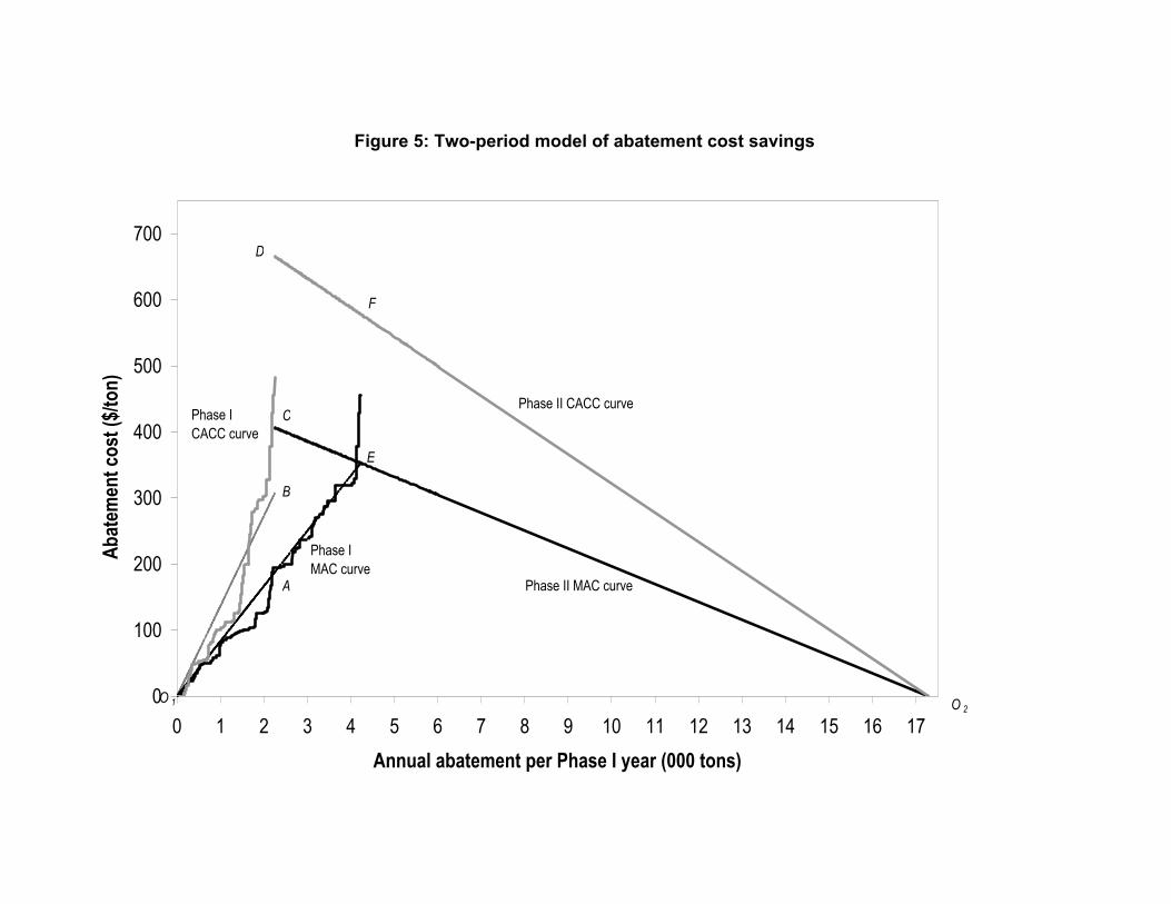
Figure 5: Two-period model of abatement cost savings

0

100

200

300

400

500

600

700

0 1 2 3 4 5 6 7 8 9 10 11 12 13 14 15 16 17Annual abatement per Phase I year (000 tons)

Abat

emen

t cos

t ($/t

on)

A

E

B

C

D

O 1 O 2

F

Phase II CACC curve

Phase II MAC curve

Phase ICACC curve

Phase IMAC curve