Embed Size (px)
Citation preview

Clean Energy Project Analysis
Third Edition
RETScreen® Engineering & Cases Textbook

Clean Energy Project Analysis: RETScreen Engineering & Cases is an electronic textbook for professionals and university students who are interested in learning how to better analyze the technical and financial viability of possible clean energy projects.
The Introduct ion chapter provides an overview of clean energy technologies and their implementation, and introduces the RETScreen International Clean Energy Project Analysis Software. The remaining chapters cover a number of the technologies in the RETScreen Software, including a background of these technologies and a detailed description of the algorithms found in the RETScreen Clean Energy Technology Models.

Introduction to Clean Energy Project Analysis
INTRO Wind Energy Project Analysis
WIND Small Hydro Project Analysis
HYDRO Photovoltaic Project Analysis
PV Combined Heat & Power Project Analysis
CHP Biomass Heating Project Analysis
BIOH Solar Air Heating Project Analysis
SAH Solar Water Heating Project Analysis
SWH Passive Solar Heating Project Analysis
PSH Ground-Source Heat Pump Project Analysis
GSHP
CCHAPTERSCHAPTERS

Reproduction
This report may be reproduced in whole or in part and in any form for educational or non-profit uses, without special permission, provided acknowledgement of the source is made. Natural Resources Can-ada would appreciate receiving a copy of any publication that uses this report as a source. However, some of the materials and elements found in this report are subject to copyrights held by other organisations. In such cases, some restrictions on the reproduction of materials or graphical elements may apply; it may be necessary to seek permission from the author or copyright holder prior to reproduction. To obtain information concerning copyright ownership and restrictions on reproduction, please contact RETScreen Customer Support.
Disclaimer
This publication is distributed for informational purposes only and does not necessarily reflect the views of the Government of Canada nor constitute an endorsement of any commercial product or person. Neither Canada, nor its ministers, officers, employees and agents make any warranty in respect to this publication nor assume any liability arising out of this publication.
September 2005© Minister of Natural Resources Canada 2001-2005.
Cette publication est disponible en français sous le titre « Analyse de projets d’énergies propres : Manuel d’ingénierie et d’études de cas RETScreen® ».
C

INTRODUCTIONTO CLEAN ENERGY PROJECT ANALYSISCHAPTER
CLEAN ENERGY PROJECT ANALYSIS:RETSCREEN® ENGINEERING & CASES TEXTBOOK
DisclaimerThis publication is distributed for informational purposes only and does not necessarily reflect the v iews of the Government of Canada nor constitute an endorsement of any commercial product or person. Nei ther Canada, nor i ts ministers, officers, employees and agents makeany warranty in respect to this publication nor a s s u m e a n y l i a b i l i t y a r i s i n g o u t o f t h i s publication.
© Minister of Natural Resources Canada 2001 - 2005.
www.retscreen.net
RETScreen® InternationalClean Energy Decision Support Centre

ISBN: 0-662-39191-8Catalogue no.: M39-112/2005E-PDF
© Minister of Natural Resources Canada 2001-2005.

INTRO.3
TABLE OF CONTENTS
1 CLEAN ENERGY PROJECT ANALYSIS BACKGROUND . . . . . . . . . . . . . . . . . . . . . . 5
1.1 Clean Energy Technologies . . . . . . . . . . . . . . . . . . . . . . . . . . . . . . . . . . . . . . . . . . . 71.1.1 Energy effi ciency versus renewable energy technologies . . . . . . . . . . . . . . . . . . . . . . . . . 7
1.1.2 Reasons for the growing interest in clean energy technologies . . . . . . . . . . . . . . . . . . . . 10
1.1.3 Common characteristics of clean energy technologies . . . . . . . . . . . . . . . . . . . . . . . . . . 13
1.1.4 Renewable energy electricity generating technologies . . . . . . . . . . . . . . . . . . . . . . . . . . 14
1.1.5 Renewable energy heating and cooling technologies . . . . . . . . . . . . . . . . . . . . . . . . . . . 17
1.1.6 Combined Heat and Power (CHP) technologies . . . . . . . . . . . . . . . . . . . . . . . . . . . . . . 23
1.1.7 Other commercial and emerging technologies . . . . . . . . . . . . . . . . . . . . . . . . . . . . . . . 25
1.2 Preliminary Feasibility Studies . . . . . . . . . . . . . . . . . . . . . . . . . . . . . . . . . . . . . . . 301.2.1 Favourable project conditions . . . . . . . . . . . . . . . . . . . . . . . . . . . . . . . . . . . . . . . . . . 33
1.2.2 Project viability factors . . . . . . . . . . . . . . . . . . . . . . . . . . . . . . . . . . . . . . . . . . . . . . . 34
2 RETSCREEN CLEAN ENERGY PROJECT ANALYSIS SOFTWARE . . . . . . . . . . . . . 35
2.1 RETScreen Software Overview . . . . . . . . . . . . . . . . . . . . . . . . . . . . . . . . . . . . . . . 352.1.1 Five step standard project analysis . . . . . . . . . . . . . . . . . . . . . . . . . . . . . . . . . . . . . . . 36
2.1.2 Common platform for project evaluation & development . . . . . . . . . . . . . . . . . . . . . . . . 38
2.1.3 Clean energy technology models . . . . . . . . . . . . . . . . . . . . . . . . . . . . . . . . . . . . . . . . 40
2.1.4 Clean energy related international databases . . . . . . . . . . . . . . . . . . . . . . . . . . . . . . . . 41
2.1.5 Online manual and training material . . . . . . . . . . . . . . . . . . . . . . . . . . . . . . . . . . . . . . 49
2.2 Greenhouse Gas (GHG) Emission Reduction Analysis Model . . . . . . . . . . . . . . . . . 512.2.1 GHG for electricity generating technology models . . . . . . . . . . . . . . . . . . . . . . . . . . . . . 53
2.2.2 GHG for heating and cooling technology models . . . . . . . . . . . . . . . . . . . . . . . . . . . . . 55
2.3 Financial Analysis Model . . . . . . . . . . . . . . . . . . . . . . . . . . . . . . . . . . . . . . . . . . . . 572.3.1 Debt payments . . . . . . . . . . . . . . . . . . . . . . . . . . . . . . . . . . . . . . . . . . . . . . . . . . . . 58
2.3.2 Pre-tax cash fl ows . . . . . . . . . . . . . . . . . . . . . . . . . . . . . . . . . . . . . . . . . . . . . . . . . . 58
2.3.3 Asset depreciation . . . . . . . . . . . . . . . . . . . . . . . . . . . . . . . . . . . . . . . . . . . . . . . . . . 59
2.3.4 Income tax . . . . . . . . . . . . . . . . . . . . . . . . . . . . . . . . . . . . . . . . . . . . . . . . . . . . . . . 61
2.3.5 Loss carry forward . . . . . . . . . . . . . . . . . . . . . . . . . . . . . . . . . . . . . . . . . . . . . . . . . . 62
2.3.6 After-tax cash fl ow . . . . . . . . . . . . . . . . . . . . . . . . . . . . . . . . . . . . . . . . . . . . . . . . . . 62
2.3.7 Financial feasibility indicators . . . . . . . . . . . . . . . . . . . . . . . . . . . . . . . . . . . . . . . . . . . 63
Introduction to Clean Energy Project Analysis Chapter
INTRO.4
2.4 Sensitivity and Risk Analysis Models . . . . . . . . . . . . . . . . . . . . . . . . . . . . . . . . . . . 662.4.1 Monte Carlo simulation . . . . . . . . . . . . . . . . . . . . . . . . . . . . . . . . . . . . . . . . . . . . . . . 66
2.4.2 Impact graph . . . . . . . . . . . . . . . . . . . . . . . . . . . . . . . . . . . . . . . . . . . . . . . . . . . . . 68
2.4.3 Median & confi dence interval . . . . . . . . . . . . . . . . . . . . . . . . . . . . . . . . . . . . . . . . . . 69
2.4.4 Risk analysis model validation . . . . . . . . . . . . . . . . . . . . . . . . . . . . . . . . . . . . . . . . . . 70
2.5 Summary . . . . . . . . . . . . . . . . . . . . . . . . . . . . . . . . . . . . . . . . . . . . . . . . . . . . . . . 73
REFERENCES . . . . . . . . . . . . . . . . . . . . . . . . . . . . . . . . . . . . . . . . . . . . . . . . . . . . 75
APPENDIX A – RETSCREEN DEVELOPMENT TEAM & EXPERTS . . . . . . . . . . . . . . . 77

INTRO.5
INTRODUCTION TO CLEAN ENERGY PROJECT ANALYSIS CHAPTERClean Energy Project Analysis: RETScreen® Engineering & Cases is an electronic textbook for professionals and uni-versity students. This chapter introduces the analysis of potential clean energy projects, including a status of clean energy technologies, a presentation of project analysis using the RETScreen® International Clean Energy Project Analysis Software, a brief review of the weather and product data available with the RETScreen® Software and a detailed description of the al-gorithms for the greenhouse gas analysis, the fi nancial analysis and the sensitivity and risk analysis found in the RETScreen® Software. A collection of project case studies, with assignments, worked-out solutions and information about how the projects fared in the real world, is available at the RETScreen® International Clean Energy Decision Support Centre Website www.retscreen.net.
1 CLEAN ENERGY PROJECT ANALYSIS BACKGROUND1
The use of clean energy technologies—that is, energy efficient and renewable energy technologies (RETs)—has increased greatly over the past several decades. Technologies once considered quaint or exotic are now commercial realities, providing cost-effective alternatives to conventional, fossil fuel-based systems and their associated problems of greenhouse gas emissions, high operating costs, and local pollution.
In order to benefit from these technologies, potential users, decision and policy makers, planners, project financiers, and equipment vendors must be able to quickly and easily as-sess whether a proposed clean energy technology project makes sense. This analysis allows for the minimum investment of time and effort and reveals whether or not a potential clean energy project is sufficiently promising to merit further investigation.
The RETScreen International Clean Energy Project Analysis Software is the leading tool specifically aimed at facilitating pre-feasibility and feasibility analysis of clean energy tech-nologies. The core of the tool consists of a standardised and integrated project analysis software which can be used worldwide to evaluate the energy production, life-cycle costs and greenhouse gas emission reductions for various types of proposed energy efficient and renewable energy technologies. All clean energy technology models in the RETScreen Software have a common look and follow a standard approach to facilitate decision-mak-ing – with reliable results2. Each model also includes integrated product, cost and weather databases and a detailed online user manual, all of which help to dramatically reduce the time and cost associated with preparing pre-feasibility studies. The RETScreen Software is perhaps the quickest and easiest tool for the estimation of the viability of a potential clean energy project.
1. Some of the text in this chapter comes from the following reference: Leng, G., Monarque, A., Graham, S., Higgins,
S., and Cleghorn, H., RETScreen® International: Results and Impacts 1996-2012, Natural Resources Canada’s
CETC-Varennes, ISBN 0-662-11903-7, Cat. M39-106/2004F-PDF, 44 pp, 2004.
2. All RETScreen models have been validated by third-party experts and the results are published in the RETScreen
Engineering e-Textbook technology chapters.
1. Clean Energy Project Analysis Background

Introduction to Clean Energy Project Analysis Chapter
INTRO.6
Since RETScreen International contains so much information and so many useful features, its utility extends beyond pre-feasibility and feasibility assessment. Someone with no prior knowledge in wind energy, for example, could gain a good understanding of the capa-bilities of the technology by reading through relevant sections of this e-textbook and the RETScreen Software’s built-in “Online Manual.” An engineer needing to know the monthly solar energy falling on a sloped surface at a building site could find this very quickly using the solar resource calculator. An architect investigating energy efficient windows for a new project could use the product database integrated into the RETScreen Passive Solar Heating Project Model to find windows vendors which have certain thermal properties. An investor or banker could use the sensitivity and risk analysis capabilities available in the model to evaluate the risk associated with an investment in the project. The RETScreen Software is very flexible, letting the user focus on those aspects that are of particular interest to him or her.
This e-textbook complements the RETScreen Software, serving the reader in three ways:
It familiarizes the reader with some of the key clean energy technologies covered by RETScreen International;
It introduces the RETScreen Software framework for clean energy project analysis; and
It serves as a reference for the assumptions and methods underlying each RETScreen Clean Energy Technology Model.
The e-textbook progresses from a general overview of clean energy technologies and project analysis to a more detailed examination of each of these technologies and how they are modeled in the RETScreen Software. To this end, the Introduction Chapter first explains the reasons for the mounting interest in clean energy technology and provides a quick synopsis of how these technologies work, as well as their applications and markets. The chapter then proceeds to discuss the importance of pre-feasibility and feasibility analy-sis in the project implementation cycle. Finally, it describes the methods common to all RETScreen Clean Energy Technology Models: the use of climate and renewable energy resource data, the greenhouse gas emission reduction calculation, the financial analysis, and the sensitivity and risk analysis.
Each of the subsequent chapters is dedicated to one of the key clean energy technologies addressed by RETScreen International. Background information on the technology itself expands on the synopsis of the Introduction Chapter; each chapter then continues with a detailed description of the algorithms used in the clean energy model, including assump-tions, equations, and limitations of the approach. The last section of each chapter recounts the various ways that the accuracy of the model has been investigated and validated, nor-mally through third party comparisons with other simulations or measured data.

1. Clean Energy Project Analysis Background
INTRO.7
The combination of the RETScreen Software and its associated tools, which are all avail-able free-of-charge via the RETScreen Website, provide a complete package to guide and inform, distilled from the experience of over 210 experts3 from industry, government and academia, that will be useful to all those interested in the proper technical and financial analysis of potential clean energy projects.
1.1 Clean Energy Technologies
This section introduces clean energy technologies by first comparing renewable energy technologies with energy efficiency measures, then presenting reasons for their growing interest worldwide, and by describing their overall common characteristics. The text then presents an overview of some of the clean energy technologies considered directly by the RETScreen International Clean Energy Project Analysis Software; more in-depth informa-tion is available in the individual chapters dedicated to each technology. Finally, other commercial and emerging clean energy technologies are briefly overviewed.
1.1.1 Energy effi ciency versus renewable energy technologies
Clean energy technologies consist of energy efficient and renewable energy technologies (RETs). Both of these reduce the use of energy from “conventional” sources (e.g. fossil fuels) but they are dissimilar in other respects.
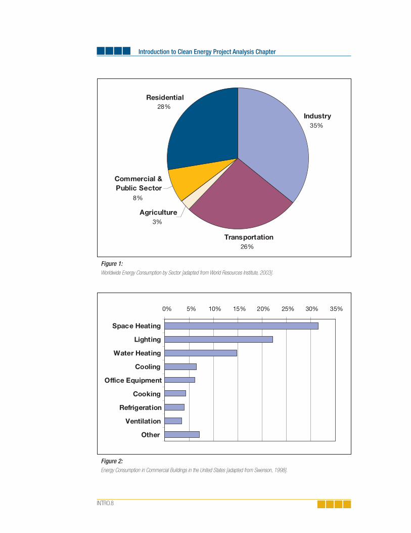
“Energy efficiency measures” refers to methods and means for reducing the energy con-sumed in the provision of a given good or service, especially compared to conventional or standard approaches. Often the service being provided is heating, cooling, or electricity generation. Efficient refrigeration systems with waste heat recovery are an example of such an energy efficient technology: they can provide the same level of cooling as conventional refrigeration technologies, but require significantly less energy. Energy efficiency measures can be applied to various sectors and applications (see Figure 1 and Figure 2).
Clean energy technologies that fall into the energy efficiency category typically include combined heat and power systems, efficient refrigeration technologies, efficient lighting systems, ventilation heat recovery systems, variable speed motors for compressors and ventilation fans, improved insulation, high performance building envelopes and windows, and other existing and emerging technologies.
Renewable energy technologies transform a renewable energy resource into useful heat, cooling, electricity or mechanical energy. A renewable energy resource is one whose use does not affect its future availability. For example, every unit of natural gas burned in order to heat a building results in one less unit of natural gas for future needs. In contrast, using solar energy to heat the building does nothing to reduce the future supply of sunshine. Some renewable energy resources cease to be renewable when they are abused: trees can provide a renewable supply of biomass for combustion, for example, but not if the rate of harvest leads to deforestation.
3. See Appendix A for a detailed list of experts involved in RETScreen International.
Introduction to Clean Energy Project Analysis Chapter
INTRO.8
Industry35%
Transportation26%
Agriculture3%
Commercial & Public Sector
8%
Residential28%
Figure 1:Worldwide Energy Consumption by Sector [adapted from World Resources Institute, 2003].
0% 5% 10% 15% 20% 25% 30% 35%
Space Heating
Lighting
Water Heating
Cooling
Office Equipment
Cooking
Refrigeration
Ventilation
Other
Figure 2:Energy Consumption in Commercial Buildings in the United States [adapted from Swenson, 1998].

1. Clean Energy Project Analysis Background
INTRO.9
RETs include systems that convert sunshine into electricity, heating, and cooling; that generate electricity from the power in wind, falling water (i.e. hydroelectric generation), waves, or tides; and that extract heat from the ground or that provide cooling by rejecting heat to the ground.
Normally, project planners should apply cost-effective energy efficiency measures first, and then consider RETs. Typically there are inefficiencies that can be reduced with fairly minimal investments, yielding significant reductions in energy consumption; achieving the same reductions with RETs is often more costly. Furthermore, by reducing the energy that must be supplied by the RETs, the efficiency measure permits a smaller renewable energy system to be used. Since RETs tend to have high initial costs, the investment in efficiency can make RETs more financially attractive.
As an example, consider a hypothetical house, similar to the one shown in Figure 3, con-nected to the electric grid, in a cold climate. If the objective is to reduce consumption of conventional energy, the first consideration should be the building envelope: high lev-els of insulation, minimal thermal bridging, and airtight construction reduce heat losses throughout the winter. Then, heating and cooling systems should be designed and appli-ances selected so as to minimize energy use. Finally, renewable energy technologies such as solar water heating and photovoltaics (the generation of electricity directly from sunlight) can be considered.
A photovoltaic system installed on the roof of this house would garner more attention from neighbours than improving the building envelope, but would contribute far less to the goal of reducing energy consumption, at a much higher cost.
In many projects, commercially available efficiency measures can halve energy consumption compared to standard practices. Then the use of cost-effective renewable energy technolo-gies can cut, or even eliminate, the remaining conventional energy consumption further.
Figure 3:Effi ciency Measures, Passive Solar
Design and a Solar Water Heating
System Combined in a Residential
Application in Canada.
Photo Credit: Waterloo Green Home

Introduction to Clean Energy Project Analysis Chapter
INTRO.10
Sometimes, the distinction between energy efficient technologies and RETs becomes blurred. In the case of the house just discussed, high performance windows (i.e. permit-ting minimal heat loss) could be considered as part of the envelope and thus an efficiency measure. But if they are oriented towards the equator and properly shaded to avoid summer overheating inside the house, these windows permit sunshine to heat the house only in the winter—making them a RET as well (i.e. passive solar heating). Similarly, a ground-source heat pump, which extracts heat from the ground, is an efficient way to use electricity (which drives the heat pump) to heat the house. But the heat from the ground is ultimately provided by solar energy. Fortunately, the distinction is not that important: the goal, to save money and reduce conventional energy consumption, is the same regardless of the nature of the clean energy technology.
1.1.2 Reasons for the growing interest in clean energy technologies
Clean energy technologies are receiving increasing attention from governments, industry, and consumers. This interest reflects a growing awareness of the environmental, economic, and social benefits that these technologies offer.
Environmental reasons
Environmental concern about global warming and local pollution is the primary impetus for many clean energy technologies in the 21st century. Global warming is the phenomenon of rising average temperatures observed worldwide in recent years. This warming trend is generally attributed to increased emission of certain gases, known as greenhouse gasses, which include carbon dioxide, methane, nitrous oxide, water vapour, ozone, and several classes of halocarbons (compounds containing carbon in combination with fluorine, bromine, and/or chlorine). Greenhouse gasses are so-called because their presence in the atmosphere does not block sunlight from reach-ing the earth’s surface, but does slow the escape of heat from the earth. As a result, heat becomes trapped, as in a greenhouse, and temperatures rise (see Figure 4).
Global warming has the potential to cause massive ecological and human devasta-tion. In the past, drastic, rapid changes in climate have resulted in extinction for large numbers of animal and plant species. Sea levels will rise as ice caps melt, inundating low-lying areas around the world. While average temperatures will rise, extreme weather events, including winter storms and extreme cold, are expected to increase in frequency. Some areas will experience more flooding, while other areas will suffer drought and desertification, straining the remaining agricultural land. Changing climate may permit tropical diseases such as malaria to invade temperate zones, including Europe and North America. Societies whose lifestyle is closely tied to certain ecosystems, such as Aboriginal peoples, are expected to be hit particularly hard by the environmental effects of global warming.

1. Clean Energy Project Analysis Background
INTRO.11
There is a strong consensus among the scientists who study climate that the global warming now observed is caused by human activity, especially the combustion of fossil fuels. When oil, gas, or coal are burned to propel cars, generate electricity or provide heat, the products of the combustion include carbon dioxide, nitrous oxide, and methane. Thus, our conventional energy systems are in large measure responsible for this impending environmental problem (IPCC, 2001). Clean energy technologies address this problem by reducing the amount of fossil fuels combusted. The RETScreen Clean Energy Project Analysis Software allows the user to estimate the reduction in greenhouse gas emissions associated with using a clean energy technology in place of a conventional energy technology.
Global warming is not the only environmental concern driving the growth in clean energy technologies. Conventional energy systems pollute on a local, as well as global, scale. Combustion releases compounds and particulates that exacerbate res-piratory conditions, such as the smog that envelops many cities; sulphur-containing coal causes acid rain when it is burned. Furthermore, local pollution is not limited to combustion emissions: for small systems, noise and visual pollution can be just as significant to people living and working nearby, and fuel spills result in serious damage to the local environment and costly clean-ups. For example, consider a power system for a warden’s residence in a remote park. If a diesel-burning engine were used to drive a generator, the wardens and visitors would hear the drone of the engine (noise pollution) and see the fuel containers (visual pollution), and the system operator would have to be very careful not to contaminate the area with spilled diesel fuel. These concerns could be reduced or eliminated through the use of photovoltaic or wind power, two clean energy technologies.
Figure 4: Absorption of solar energy heats up the earth.
Photo Credit: NASA Goddard Space Flight Center (NASA-GSFC)

Introduction to Clean Energy Project Analysis Chapter
INTRO.12
Economic reasons
Much of the recent growth in clean energy technology sales has been driven by sales to customers for whom environmental concerns are not necessarily the prime motivation for their decision to adopt clean energy technology. Instead, they are basing their decision on the low “life-cycle costs,” or costs over the lifetime of the project, associated with clean energy technologies. As will be discussed in the next section, over the long term, clean energy technologies are often cost-competitive, or even less costly, when compared to conventional energy technologies.
It is not merely the expense of conventional energy that make conventional energy systems unattractive; often the uncertainty associated with this expense is even more troublesome. Conventional energy prices rise and fall according to local, national, continental, and global conditions of supply and demand. Several times over the past decade, unforeseen spikes in the price of conventional energy—elec-tricity, natural gas, and oil—have caused severe financial difficulties for individuals, families, industry, and utilities. This is not just of concern to consumers, but also to the governments which are often held accountable for the state of the economy.
There are good reasons for believing that conventional energy costs will rise in the coming decades. Throughout much of the world, the rate of discovery of new oil reserves is declining, while at the same time, demand is rising. Remaining conven-tional reserves, while vast, are concentrated in a few countries around the world. Large unconventional reserves, such as oil sands, exist in Canada, Venezuela and other regions, but the manufacture of usable fuel (or “synthetic crude”) from these sources is more expensive than conventional methods and emits additional green-house gasses. Rising energy prices and the risk of price shocks makes clean energy technologies more attractive.
Integral to the RETScreen Software are sophisticated but easy-to-use financial anal-ysis and sensitivity & risk analysis worksheets that helps determines the financial viability and risks of a clean energy project. The user can investigate the influence of a number of financial parameters, including the rate at which the price of energy may escalate.
Social reasons
Clean energy technologies are associated with a number of social benefits that are of particular interest to governments. Firstly, clean energy technologies gener-ally require more labour per unit of energy produced than conventional energy technologies, thus creating more jobs. Secondly, conventional energy technologies exploit concentrated energy resources in a capital-intensive manner and require the constant exploration for new sources of energy. In contrast, energy efficiency measures focus on maximizing the use of existing resources and RETs “harvest” more dispersed, dilute energy resources. This generally requires more human inter-vention, either in applying the technology or in manufacturing and servicing the equipment. The additional cost of the labour required by clean energy technologies is offset by the lower cost of energy inputs. For example, in the case of solar and wind energy, the energy input is free.

1. Clean Energy Project Analysis Background
INTRO.13
Fossil fuel imports drain money from the local economy. On the other hand, energy efficiency measures are applied to local systems and RETs make use of local resourc-es. Therefore, transactions tend to be between local organizations. When money stays within the local area, its “multiplier effect” within that area is increased. For example, compare a biomass combustion system making use of waste woodchips to a boiler fired with imported oil. In the latter case, fuel purchases funnel money to oil companies located far from the community; in the former, woodchip collection, quality assurance, storage, and delivery are handled by a local company that will use local labour and that will then spend a portion of its revenues at local stores and service providers and the money will circulate within the community. Globally, this may or may not be advantageous, but it is certainly of interest to local governments, and a driver for their interest in clean energy technologies.
Another social and economic reason for the interest in clean energy technologies is simply the growing demand for energy. The International Energy Agency (IEA) has forecast that, based on historical trends and economic growth, worldwide energy demand will have tripled by 2050 (IEA, 2003). Industries have seen the potential of this expansion, and governments the need for new technologies and fuels to meet this demand. This has stimulated interest in clean energy technologies.
1.1.3 Common characteristics of clean energy technologies
Several characteristics shared by clean energy technologies become apparent when they are compared to conventional energy technologies; these have already been mentioned in passing, but deserve further emphasis.
First, clean energy technologies tend to be environmentally preferable to conventional technologies. This is not to say that they have no environmental impact, nor that they can be used without heed for the environment. All heating systems, power generators, and, by extension, energy consumers, have some environmental impact. While this cannot be eliminated, it must be minimized, and clean energy technologies have been built to address the most pressing environmental problems. When used responsibly and intelligently, they provide energy benefits at an environmental cost far below that of conventional technolo-gies, especially when the conventional technology relies on fossil fuel combustion.
Second, clean energy technologies tend to have higher initial costs (i.e., costs incurred at the outset of the project) than competing conventional technologies. This has led some to conclude that clean energy technologies are too expensive. Unfortunately, this view ignores the very real costs that are incurred during operation and maintenance of any energy sys-tem, whether clean or conventional.
Third, clean energy technologies tend to have lower operating costs than conventional technologies. This makes sense, because efficiency measures reduce the energy require-ment and RETs make use of renewable energy resources often available at little or no marginal cost.

Introduction to Clean Energy Project Analysis Chapter
INTRO.14
So how can the high initial costs and low operating costs of clean energy technologies be compared with the low initial costs and high operating costs of conventional technologies? The key is to consider all costs over the lifetime of the project. These include not just the initial costs (feasibility assessment, engineering, development, equipment purchase, and installation) but also:
Annual costs for fuel and operation and maintenance;
Costs for major overhauls or replacement of equipment;
Costs for decommissioning of the project (which can be very signifi cant for technologies that pollute a site, through fuel spills, for example); and
The costs of fi nancing the project, such as interest charges.
All these costs must then be summed, taking into account the time value of money, to determine the overall “lifecycle cost” of the project.
This leads to the fourth characteristic common to clean energy technologies: despite their higher initial costs, they are often cost-effective compared with conventional technolo-gies on a lifecycle cost basis, especially for certain types of applications. The RETScreen Clean Energy Project Analysis Software has been developed specifically to facilitate the identification and tabulation of all costs and to perform the lifecycle analysis, so that a just comparison can reveal whether clean energy technologies make sense for a given project.
1.1.4 Renewable energy electricity generating technologies
RETScreen International addresses a number of renewable energy electricity generating technologies. The four most widely applied technologies are discribed here. These are wind energy, photovoltaics, small hydro, and biomass combustion power technologies. The first three technologies are briefly introduced in the sections that follow and the fourth technology is introduced later as part of the combined heat and power technology section. More in-depth information is also available in the chapters specifically dedicated to each of these technologies.
Wind energy systems
Wind energy systems convert the kinetic energy of moving air into electricity or mechanical power. They can be used to provide power to central grids or isolated grids, or to serve as a remote power supply or for water pumping. Wind turbines are commercially available in a vast range of sizes. The turbines used to charge bat-teries and pump water off-grid tend to be small, ranging from as small as 50 W up to 10 kW. For isolated grid applications, the turbines are typically larger, ranging from about 10 to 200 kW. As of 2005, the largest turbines are installed on central grids and are generally rated between 1 and 2 MW, but prototypes designed for use in shallow waters offshore have capacities of up to 5 MW.

1. Clean Energy Project Analysis Background
INTRO.15
A good wind resource is criti-cal to the success of a commer-cial wind energy project. The energy available from the wind increases in proportion to the cube of the wind speed, which typically increases with height above the ground. At mini-mum, the annual average wind speed for a wind energy project should exceed 4 m/s at a height of 10 m above the ground. Cer-tain topographical features tend to accelerate the wind, and wind turbines are often located along these features. These include the crests of long, gradual slopes (but not cliffs), passes between moun-tains or hills, and valleys that channel winds. In addition, areas that present few obstructions to winds, such as the sea surface adjacent to coastal regions and flat, grassy plains, may have a good wind resource.
Since the early 1990s, wind energy technology has emerged as the fastest growing electricity generation technology in the world. This reflects the steady decline in the cost of wind energy production that has accompanied the maturing of the technol-ogy and industry: where a good wind resource and the central grid intersect, wind energy can be among the lowest cost provider of electricity, similar in cost to natural gas combined-cycle electricity generation.
Small hydro systems
Small hydro systems convert the potential and kinetic energy of moving water into electricity, by using a turbine that drives a generator. As water moves from a higher to lower elevation, such as in rivers and waterfalls, it carries energy with it; this energy can be harnessed by small hydro systems. Used for over one hundred years, small hydro systems are a reliable and well-understood technology that can be used to provide power to a central grid, an isolated grid or an off-grid load, and may be either run-of-river systems or include a water storage reservoir.
Most of the world’s hydroelectricity comes from large hydro projects of up to sev-eral GW that usually involve storage of vast volumes of water behind a dam. Small hydro projects, while benefiting from the knowledge and experience gleaned from the construction of their larger siblings, are much more modest in scale with installed capacities of less than 50 MW. They seldom require the construction of a large dam, except for some isolated locations where the value of the electricity is very high due to few competing power options. Small hydro projects can even be less than 1 kW in capacity for small off-grid applications.
Figure 5:
Wind Energy System.
Photo Credit: NRCan

Introduction to Clean Energy Project Analysis Chapter
INTRO.16
An appreciable, constant flow of water is critical to the success of a commercial small hydro project. The energy available from a hydro turbine is proportional to the quantity of water passing through the turbine per unit of time (i.e. the flow), and the vertical difference between the turbine and the surface of the water at the water inlet (i.e. the head)4. Since the majority of the cost of a small hydro project stems from up front expenses in construction and equipment purchase, a hydro project can generate large quantities of electricity with very low operating costs and modest maintenance expenditures for 50 years or longer.
In many parts of the world, the opportunities for further large hydro developments are dwindling and smaller sites are being examined as alternatives giving significant growth potential for the small hydro market (e.g. China).
Photovoltaic systems
Photovoltaic systems convert energy from the sun directly into electricity. They are composed of photovoltaic cells, usually a thin wafer or strip of semiconductor material, that generates a small current when sunlight strikes them. Multiple cells can be assembled into modules that can be wired in an array of any size. Small photovoltaic arrays are found in wristwatches and calculators; the largest arrays have capacities in excess of 5 MW.
Photovoltaic systems are cost-effective in small off-grid applications, provid-ing power, for example, to rural homes in developing countries, off-grid cottages and motor homes in industrialised countries, and remote telecommunications, monitoring and control systems worldwide. Water pumping is also a notable off-grid application of photovoltaic systems that are used for domestic water supplies, agriculture and, in developing countries, provision of water to villages. These power systems are relatively simple, modular, and highly reliable due to the lack of moving parts. Photovoltaic systems can be combined with fossil fuel-driven generators in
4. In reality, this must be adjusted for various losses.
Figure 6:Small Hydro System.
Photo Credit: SNC-Lavalin.

1. Clean Energy Project Analysis Background
INTRO.17
applications having higher energy demands or in climates characterized by extend-ed periods of little sunshine (e.g. winter at high latitudes) to form hybrid systems.
Photovoltaic systems can also be tied to isolated or central grids via a specially configured inverter. Unfortunately, without subsidies, on-grid (central grid-tied) applications are rarely cost-effective due to the high price of photovoltaic modules, even if it has declined steadily since 1985. Due to the minimal maintenance of pho-tovoltaic systems and the absence of real benefits of economies of scale during con-struction, distributed generation is the path of choice for future cost-effective on-grid applications. In distributed electricity generation, small photovoltaic systems would be widely scattered around the grid, mounted on buildings and other structures and thus not incurring the costs of land rent or purchase. Such applications have been facilitated by the development of technologies and practices for the integration of photovoltaic systems into the building envelope, which offset the cost of conven-tional material and/or labour costs that would have otherwise been spent.
Photovoltaic systems have seen the same explosive growth rates as wind turbines, but starting from a much smaller installed base. For example, the worldwide installed pho-tovoltaic capacity in 2003 was around 3,000 MW, which represents less than one-tenth that of wind, but yet is growing rapidly and is significant to the photovoltaic industry.
1.1.5 Renewable energy heating and cooling technologies
RETScreen International addresses a number of renewable energy heating and cooling technologies that have the potential to significantly reduce the planet’s reliance on con-ventional energy resources. These proven technologies are often cost-effective and have enormous potential for growth. The main ones described here include: biomass heating, solar air heating, solar water heating, passive solar heating, and ground-source heat pump technologies. They are briefly introduced in the sections that follow, with more in-depth information available in the chapters specifically dedicated to each of these technologies.
Figure 7: Photovoltaic System at Oberlin
College’s Adam Joseph Lewis Center
for Environmental studies (USA); the panels
cover 4,682 square feet on the buildings
south-facing curved roof.
Photo Credit:Robb Williamson/NREL Pix.

Introduction to Clean Energy Project Analysis Chapter
INTRO.18
Biomass heating systems
Biomass heating systems burn organic matter—such as wood chips, agricultural residues or even municipal waste—to generate heat for buildings, whole commu-nities, or industrial processes. More sophisticated than conventional woodstoves, they are highly efficient heating systems, achieving near complete combustion of the biomass fuel through control of the fuel and air supply, and often incorporating automatic fuel handling systems.
Biomass heating systems consist of a heating plant, a heat distribution system, and a fuel supply operation. The heating plant typically makes use of multiple heat sources, including a waste heat recovery system, a biomass combustion system, a peak load heating system, and a back-up heating system. The heat distribution system conveys hot water or steam from the heating plant to the loads that may be located within the same building as the heating plant, as in a system for a single institutional or industrial building, or, in the case of a “district heating” system, clusters of buildings located in the vicinity of the heating plant.
Biomass fuels include a wide range of materials (e.g. wood residues, agricultural residues, municipal solid waste, etc.) that vary in their quality and consistency far more than liquid fossil fuels. Because of this, the fuel supply operation for a biomass plant takes on a scale and importance beyond that required for most fossil fuels and it can be considered a “component” of the biomass heating system. Biomass heat-ing systems have higher capital costs than conventional boilers and need diligent operators. Balancing this, they can supply large quantities of heat on demand with very low fuel costs, depending on the provenance of the fuel.
Today, 11% of the world’s Total Primary Energy Supply (TPES)5 comes from biomass combustion, accounting for over 20,000 MW (68,243 million Btu/h) of installed capacity worldwide [Langcake, 2003]. They are a major source of energy, mainly for cooking and heating, in developing countries, representing, for example, 50% of the African continent’s TPES [IEA Statistics, 2003].
5. A measure of the total energy used by humans.
Figure 8: Biomass Heating System
Photo Credit: NRCan

1. Clean Energy Project Analysis Background
INTRO.19
Solar air heating systems
Solar air heating systems use solar energy to heat air for building ventilation or industrial processes such as drying. These systems raise the temperature of the out-side air by around 5 to 15ºC (41 to 59ºF) on average, and typically supply a portion of the required heat, with the remainder being furnished by conventional heaters.
A solar air heating system currently considered by RETScreen consists of a transpired collector, which is a sheet of steel or aluminium perforated with numerous tiny holes, through which outside air is drawn. Mounted on an equator-facing building wall, the transpired collector absorbs incident sunshine and warms the layer of air adjacent to it. A fan draws this sun-warmed air through the perforations, into the air space behind the collector and then into the ducting within the building, which distributes the heated air through the building or the industrial processes. Controls regulate the temperature of the air in the building by adjusting the mix of recirculated and fresh air or by modulating the output of a conventional heater. When heat is not required, as in summertime, a damper bypasses the collector. The system also provides a measure of insulation, recuperates heat lost through the wall it covers and can reduce stratification, the pooling of hot air near the ceiling of voluminous buildings. The result is an inexpensive, robust and simple system with virtually no maintenance requirements and efficiencies as high as 80%.
Solar air heating systems tend to be most cost-effective in new construction, when the net cost of the installation of the transpired collector is offset by the cost of the traditional weather cladding it supplants. Also, new-construction gives the designer more latitude in integrating the collector into the building’s ventilation system and aesthetics. Installation of a transpired collector also makes sense as a replacement for aging or used weather cladding.
Given the vast quantities of energy used to heat ventilation air, the use of perforated collectors for solar air heating has immense potential. In general, the market is strongest where the heating season is long, ventilation requirements are high, and conventional heating fuels are costly. For these reasons, industrial buildings constitute the biggest market, followed by commercial and institutional buildings, multi-unit residential build-ings, and schools. Solar air heating also has huge potential in industrial processes which need large volumes of heated air, such as in the drying of agricultural products.
Figure 9: Solar Air Heating System.
Photo Credit: Conserval Engineering

Introduction to Clean Energy Project Analysis Chapter
INTRO.20
Solar water heating systems
Solar water heating systems use solar energy to heat water. Depending on the type of solar collector used, the weather conditions, and the hot water demand, the temper-ature of the water heated can vary from tepid to nearly boiling. Most solar systems are meant to furnish 20 to 85% of the annual demand for hot water, the remainder being met by conventional heating sources, which either raise the temperature of the water further or provide hot water when the solar water heating system cannot meet demand (e.g. at night).
Solar systems can be used wherever moderately hot water is required. Off-the-shelf packages provide hot water to the bathroom and kitchen of a house; custom systems are designed for bigger loads, such as multi-unit apartments, restaurants, hotels, motels, hospitals, and sports facilities. Solar water heating is also used for industrial and commercial processes, such as car washes and laundries.
Worldwide, there are millions of solar collectors in existence, the largest portion installed in China and Europe. The North American market for solar water heating has traditionally been hampered by low conventional energy costs, but a strong demand for swimming pool heating has led unglazed technology to a dominant sales position on the continent. Solar water heating technology has been embraced by a number of developing countries with both strong solar resources and costly or unreliable conventional energy supplies.
Passive solar heating systems
Passive solar heating is the selective use of solar energy to provide space heating in buildings by using properly oriented, high-performance windows, and selected interior building materials that can store heat from solar gains during the day and release it at night. In so doing, passive solar heating reduces the conventional energy required to heat the building. A building employing passive solar heating maintains a comfortable interior temperature year round and can reduce a building’s space heating requirement by 20 to 50%.
Figure 10: Solar Water Heating System.
Photo Credit: NRCan

1. Clean Energy Project Analysis Background
INTRO.21
Improvements to commercial window technologies have facilitated passive solar heating by reducing the rate of heat escape while still admitting much of the inci-dent solar radiation. Due to their good thermal properties, a high-performance window allows the building designer to make better use of daylight since their size and placement are less restricted than conventional windows. The use of high-per-formance windows is becoming standard practice in the building industry today.
Passive solar heating tends to be very cost effective for new construction since at this stage many good design practices—orientation, shading, and window upgrades—can be implemented at little or no additional cost compared to conventional design. Depending on the level of performance desired, specifying windows that perform better than standard wood frame windows with double-glazing adds 5 to 35% to their cost. Reduced energy expenditures rarely justify the replacement of existing windows that are still in good condition, but a window upgrade (e.g. from single to double-glazing) should be considered whenever windows are replaced.
Passive solar heating is most cost-effective when the building’s heating load is high compared to its cooling load. Both climate and the type of building determine this. Cold and moderately cold climates are most promising for passive solar heating design. Low-rise residential construction is more easily justified than commercial and industrial buildings, where internal heat gains may be very high, decreas-ing the required heating load. On the other hand, such buildings may require perimeter heating even when the building’s net heat load is zero or negative; if high-performance windows obviate the need for this perimeter heating they may be very cost-effective.
Figure 11: Passive Solar Heating System.
Photo Credit: McFadden, Pam DOE/NREL

Introduction to Clean Energy Project Analysis Chapter
INTRO.22
Ground-source heat pumps
Ground-source heat pumps provide low temperature heat by extracting it from the ground or a body of water and provide cooling by reversing this process. Their prin-cipal application is space heating and cooling, though many also supply domestic hot water. They can even be used to maintain the integrity of building foundations in permafrost conditions, by keeping them frozen through the summer.
A ground-source heat pump (GSHP) system has three major components: the earth connection, a heat pump, and the heating or cooling distribution system. The earth connection is where heat transfer occurs. One common type of earth connection comprises tubing buried in horizontal trenches or vertical boreholes, or alternatively, submerged in a lake or pond. An antifreeze mixture, water or another heat-transfer fluid is circulated from the heat pump, through the tubing, and back to the heat pump in a “closed loop.” “Open loop” earth connections draw water from a well or a body of water, transfer heat to or from the water, and then return it to the ground (e.g. a second well) or the body of water.
Since the energy extracted from the ground exceeds the energy used to run the heat pump, GSHP “efficiencies” can exceed 100%, and routinely average 200 to 500% over a season. Due to the stable, moderate temperature of the ground, GSHP systems are more efficient than air-source heat pumps, which exchange heat with the outside air. GSHP systems are also more efficient than conventional heating and air-conditioning technologies, and typically have lower maintenance costs. They require less space, especially when a liquid building loop replaces voluminous air ducts, and, since the tubing is located underground, are not prone to vandalism like conventional rooftop units. Peak electricity consumption during cooling sea-son is lower than with conventional air-conditioning, so utility demand charges may be reduced.
Figure 12: Ground-Source
Heat Pump System.

1. Clean Energy Project Analysis Background
INTRO.23
Heat pumps typically range in cooling capacity from 3.5 to 35 kW (1 to 20 tons of cooling). A single unit in this range is sufficient for a house or small commercial building. Larger commercial and institutional buildings often employ multiple heat pumps (perhaps one for each zone) attached to a single earth connection. This allows for greater occupant control of the conditions in each zone and facilitates the transfer of heat from zones needing cooling to zones needing heating. The heat pump usually generates hot or cold air to be distributed locally by conventional ducts.
Strong markets for GSHP systems exist in many industrialised countries where heating and cooling energy requirements are high. Worldwide, 800,000 units total-ling nearly 10,000 MW of thermal capacity (over 843,000 tons of cooling) have been installed so far with an annual growth rate of 10% [Lund, 2003].
1.1.6 Combined Heat and Power (CHP) technologies
The principle behind combined heat and power (or “cogeneration”) is to recover the waste heat generated by the combustion of a fuel6 in an electricity generation system. This heat is often rejected to the environment, thereby wasting a significant portion of the energy avail-able in the fuel that can otherwise be used for space heating and cooling, water heating, and industrial process heat and cooling loads in the vicinity of the plant. This cogeneration of electricity and heat greatly increases the overall efficiency of the system, anywhere from 25-55% to 60-90%, depending on the equipment used and the application.
6. Such as fossil fuels (e.g. natural gas, diesel, coal, etc.), renewable fuels (wood residue, biogas, agricultural byproducts,
bagasse, landfi ll gas (LFG), etc.), hydrogen, etc.
Figure 13: Gas Turbine.
Photo Credit: Rolls-Royce plc

Introduction to Clean Energy Project Analysis Chapter
INTRO.24
Combined heat and power systems can be implemented at nearly any scale, as long as a suitable thermal load is present. For example, large scale CHP for community energy sys-tems and large industrial complexes can use gas turbines (Figure 13), steam turbines, and reciprocating engines with electrical generating capacities of up to 500 MW. Independent energy supplies, such as for hospitals, universities, or small communities, may have capaci-ties in the range of 10 MW. Small-scale CHP systems typically use reciprocating engines to provide heat for single buildings with smaller loads. CHP energy systems with electrical capacities of less than 1 kW are also commercially available for remote off-grid operation, such as on sailboats. When there is a substantial cooling load in the vicinity of the power plant, it can also make sense to integrate a cooling system into the CHP project7. Cooling loads may include industrial process cooling, such as in food processing, or space cooling and dehumidification for buildings.
The electricity generated can be used for loads close to the CHP system, or located else-where by feeding the electric grid. Since heat is not as easily transported as electricity over long distances, the heat generated is normally used for loads within the same building, or located nearby by supplying a local district heating network. This often means that electric-ity is produced closer to the load than centralized power production. This decentralized or “distributed” energy approach allows for the installation of geographically dispersed generating plants, reducing losses in the transmission of electricity, and providing space & process heating and/or cooling for single or multiple buildings (Figure 14).
A CHP installation comprises four subsystems: the power plant, the heat recovery and distribution system, an optional system for satisfying heating8 and/or cooling9 loads and a control system. A wide range of equipment can be used in the power plant, with the sole restriction being that the power equipment10 rejects heat at a temperature high enough
7. In such case, the CHP project becomes a “combined cooling, heating and power project”.
8. Heating equipment such as waste heat recovery, boiler, furnace, heater, heat pump, etc.
9. Cooling equipment such as compressor, absorption chiller, heat pump, etc.
10. Power equipment such as gas turbine, steam turbine, gas turbine-combined cycle, reciprocating engine, fuel cell, etc.
Figure 14: Combined Heat & Power
Kitchener’s City Hall, Ontario, Canada.
Photo Credit: Urban Ziegler, NRCan

1. Clean Energy Project Analysis Background
INTRO.25
to be useful for the thermal loads at hand. In a CHP system, heat may be recovered and distributed as steam (often required in thermal loads that need high temperature heat, such as industrial processes) or as hot water (conveyed from the plant to low temperature thermal loads in pipes for domestic hot water, or for space heating.)
Worldwide, CHP systems with a combined electrical capacity of around 240 GW are presently in operation. This very significant contribution to the world energy supply is even more impressive when one considers that CHP plants generate significantly more heat than power. Considering that most of the world’s electricity is generated by rotating machinery that is driven by the combustion of fuels, CHP systems have enormous poten-tial for growth. This future growth may move away from large industrial systems towards a multitude of small CHP projects, especially if a decentralized energy approach is more widely adopted and the availability of commercial products targeted at this market.
1.1.7 Other commercial and emerging technologies
A number of other clean energy technologies addressed by RETScreen International are also commercially available or in various stages of development. Some of these commercial and emerging technologies are briefly introduced in this section. Further RETScreen de-velopment is also underway or forthcoming for several of these technologies not currently covered by the software.
Commercial technologies
Many other commercial clean energy technologies and fuels are presently available. Some are described here.
Biofuels (ethanol and bio-diesel): Fermentation of certain agricultural products, such as corn and sugar cane, generates ethanol, a type of alcohol. In many regions of the world, and especially in Brazil, ethanol is being used as a transportation fuel that is often blended with conventional gasoline for use in regular car engines. In this way, biomass fuel is substituted for fossil fuels. Researchers are working on pro-ducing ethanol from cellulose, with the goal of converting wood waste into liquid
Figure 15: Biofuel - Agriculture
Waste Fuel Supply.
Photo Credit: David and Associates DOE/NREL

Introduction to Clean Energy Project Analysis Chapter
INTRO.26
fuel. Similarly, plant and animal oils, such as soybean oil and used cooking grease, can be used as fuel in diesel engines. Normally, such biomass oil is mixed with fossil fuels, resulting in less air pollution than stand-ard diesel, although the biomass oils have a tendency to congeal at low temperatures. Often, waste oils are used. When crops are purpose-grown for their oils or alcohols, the agricultural practices must be sustainable in order to be considered as a renewable energy fuel. Regular biofuel supplies (Figure 15) should be secured first and be more widely available before these new biofuel technolo-gies are more widely used11.
Ventilation heat recovery & efficient refrigeration systems: Heating, cooling and ventilation consume vast amounts of energy, but a number of efficiency measures can reduce their consumption. Simultaneous heating and cooling loads are often found within large buildings, in specialized facili-ties such as supermarkets and arenas, and in industrial complexes. For example, efficient refrigeration systems can transfer heat from the areas needing cooling to those needing heating (Figure 16). In absorption cool-ing systems and desiccant dehumidifiers, heat is used to drive the cooling equip-ment. This is a promising application for waste heat. Heat which is normally lost when ventilation air is exhausted from a building can be recuperated and used to preheat the fresh air drawn into the building. Such ventilation heat recovery systems routinely recuperate 50% of the sensible heat; new technologies are improving this and recuperating some latent heat as well, all while maintaining good air quality.
Variable speed motors: Motors consume much of the world’s electricity. For example, energy use in motors represents around 65% of total industrial electric-ity consumption in Europe. The rotational speed of a traditional motor is directly related to the frequency of the electric grid. Variable speed drives result from the combination of traditional motors and power electronics. The power electronics analyze the load and generate a signal to optimize the motor at the speed required by the application. For example, when only a reduced airflow is required, the speed of a ventilation air motor can be reduced, resulting in a more efficient system.
11. ATLAS Website. European Communities.
Figure 16: Secondary loop pumping system for recovery
of heat rejected by the refrigeration systems
in a supermarket.
Photo Credit: NRCan

1. Clean Energy Project Analysis Background
INTRO.27
Daylighting & efficient lighting systems: Lighting is another major consumer of electricity that has been made more efficient by new technologies. High intensity discharge (HID) lamps, fluorescent tubes, and electronic ballasts (for operating HID and fluorescent tubes) have made incremental improvements in the efficiency of light-ing. In commercial buildings, which tend to overheat, more efficient lighting reduces the cooling load, a further energy benefit. Facilitated by improved windows and even transparent insulation, designers are also making better use of daylight to lower artificial lighting energy consumption. This better of use of daylight is especially appropriate for office blocks (Figure 17), where working hours coincide well with day-light availability, but is generally limited to building retrofit and new construction.
Emerging technologies
The worldwide growing concerns about energy security and climate change, and the expected depletion of worldwide fossil fuels (and the associated rise of their selling price) have propelled the research and development of new energy technologies. A number of them are presently in the prototype or pilot stage and may eventually become commercially viable. Some of them are briefly introduced below.
Solar-thermal power: Several large-scale solar thermal power projects, which gen-erate electricity from solar energy via mechanical processes, have been in operation for over two decades. Some of the most successful have been based on arrays of mirrored parabolic troughs (Figure18). Through the 1980’s, nine such commer-cial systems were built in the Mohave Desert of California, in the United States. The parabolic troughs focus sunlight on a collector tube, heating the heat transfer fluid in the collector to 390ºC (734ºF). The heated fluid is used to generate steam that drives a turbine. The combined electric capacity of the nine plants is around 350 MW, and their average output is over 100 MW. The systems have functioned reliably and the most recently constructed plants generate power at a cost of around $0.10/kWh. Several studies have identified possible cost reductions.
Figure 17:Daylighting & Effi cient Lighting.
Photo Credit:Robb Williamson/ NREL Pix

Introduction to Clean Energy Project Analysis Chapter
INTRO.28
Another approach to solar thermal power is based on a large field of relatively small mirrors that track the sun, focussing its rays on a receiver tower in the centre of the field (Figure 19). The concentrated sunlight heats the receiver to a high temperature (e.g., up to 1,000ºC, or 1,800ºF), which generates steam for a turbine. Prototype plants with electrical capacities of up to 10 MW have been built in the United States, the Ukraine (as part of the former USSR), Israel, Spain, Italy, and France.
A third solar thermal power technology combines a Stirling cycle heat engine with a parabolic dish. Solar energy, concentrated by the parabolic dish, supplies heat to the engine at temperatures of around 600ºC. Prototype systems have achieved high efficiencies.
Figure 18:Parabolic-Trough Solar
Power Plant.
Photo Credit: Gretz, Warren DOE/NREL
Figure 19:Central Receiver Solar Power Plant.
Photo Credit:Sandia National Laboratories DOE/NREL

1. Clean Energy Project Analysis Background
INTRO.29
All three of the above technologies can also be co-fired by natural gas or other fossil fuels, which gives them a firm capacity and permits them to be used as peak power providers. This makes them more attractive to utilities, and gives them an advantage over photovoltaics, which cannot necessarily provide power whenever it is required. On the other hand, they utilize only that portion of sunlight that is direct beam and require much dedicated land area. Solar thermal power is still at the development stage: the costs of the technology should be reduced together with the associated risks, and experience under real operating conditions should be a further gain.
Ocean-thermal power: Electricity can be generated from the ocean in several ways, as demonstrated by a number of pilot projects around the world. In ocean thermal electrical conversion (OTEC), a heat engine is driven by the vertical temperature gradient found in the ocean. In tropical oceans, the solar-heated surface water may be over 20ºC warmer than the water found a kilometre or so below the surface. This temperature difference is sufficient to generate low-pressure steam for a turbine. Pilot plants with a net power output of up to 50 kW have been built in Hawaii (USA) and Japan. High production costs, possible negative impacts on near-shore marine ecosystems and a limited number of suitable locations worldwide have so far limited the development of this technology which needs further demonstration before commercial deployment.
Tidal power: Narrow basins experiencing very high tides can be dammed such that water flowing into and out of the basin with the changing tides is forced through a turbine. Such “barrage” developments have been constructed in eastern Cana-da, Russia, and France, where a 240 MW project has been operating since 1966. While technically feasible, the initial costs are high and environmental impacts may include sedimentation of the basin, flooding of the nearby coastline and difficult-to-predict changes in the local ecosystems. Tidal power technology raises many technical questions (e.g. configuration, reliability, safe deployment and recovery, grid connection, operation and maintenance) and market barriers that limit the deployment of this technology.
Wave power: Waves have enormous power, and a range of prototypes harnessing this power have been constructed. These include shore-based and offshore devices, both floating and fixed to land or the ocean floor. Most utilize either turbines, driven with air compressed by the oscillating force of the waves, or the relative motion of linked floats as waves pass under them. Pilot plants with capacities of up to 3 MW have been built; the major barrier to commercialization has been the harsh ocean environment. It is crucial that the current prototypes and demonstration projects are successful to overcome barriers to further deployment.
Ocean current power: Just as wind flows in the atmosphere, so ocean currents exist in the ocean; ocean currents can also be generated by tides. It has been pro-posed that underwater turbines (Figure 20), not unlike wind turbines, could be used to generate electricity in areas experiencing especially strong currents. Some pilot projects investigating the feasibility of this concept have been launched.

Introduction to Clean Energy Project Analysis Chapter
INTRO.30
1.2 Preliminary Feasibility Studies
Energy project proponents, investors, and financers continually grapple with questions like “How accurate are the estimates of costs and energy savings or production and what are the possibilities for cost over-runs and how does the project compare financially with other competitive options?” These are very difficult to answer with any degree of confi-dence, since whoever prepared the estimate would have been faced with two conflicting requirements:
Keep the project development costs low in case funding cannot be secured, or in case the project proves to be uneconomic when compared with other energy options.
Spend additional money and time on engineering to more clearly delineate potential project costs and to more precisely estimate the amount of energy produced or energy saved.
For both conventional and clean energy project implementation, the usual procedure for tackling this dilemma is to advance the project through several steps as shown in Figure 21. At the completion of each step, a “go/no-go” decision is usually made by the project proponent as to whether to proceed to the next step of the development process. High quality, but low-cost, pre-feasibility and feasibility studies are critical to helping the project proponent “screen out” projects that do not make financial sense, as well as to help focus development and engineering efforts prior to construction.
Figure 20:Artist’s impression of MCT pile mounted
twin rotor tidal turbine.
Photo Credit:MCT Ltd. 2003 Director

1. Clean Energy Project Analysis Background
INTRO.31
Typical Energy Project Implementation Process
Pre-feasibility Analysis: A quick and inexpensive initial examination, the pre-feasibility analysis determines whether the proposed project has a good chance of satisfying the proponent’s require-ments for profitability or cost-effectiveness, and therefore merits the more serious investment of time and resources required by a feasibility analysis. It is characterized by the use of readily available site and resource data, coarse cost estimates, and simple calculations and judgements often involving rules of thumb. For large projects, such as for hydro projects, a site visit may be required. Site visits are not usually necessary for small projects involving lower capital costs, such as for a residential solar water heating project.
Feasibility Analysis: A more in-depth analysis of the project’s prospects, the feasibility study must provide information about the physical characteristics, financial viability, and environ-mental, social, or other impacts of the project, such that the proponent can come to a decision about whether or not to proceed with the project. It is characterized by the collection of refined site, resource, cost and equipment data. It typically involves site visits, resource monitoring, energy audits, more detailed computer simulation, and the solicitation of price information from equipment suppliers.
Engineering and Development: If, based on the feasibility study, the project proponent decides to proceed with the project, then engineering and development will be the next step. Engineering includes the design and planning of the physical aspects of the project. Development involves the planning, arrangement, and negotiation of financial, regulatory, contractual and other non-physical aspects of the project. Some development activities, such as training, customer relations, and community consultations extend through the subsequent project stages of construction and operation. Even following significant investments in engineering and development, the project may be halted prior to construction because financing cannot be arranged, environmental ap-provals cannot be obtained, the pre-feasibility and feasibility studies “missed” important cost items, or for other reasons.
Construction and Commissioning: Finally, the project is built and put into service. Certain construction activities can be started before completion of engineering and development, and the two conducted in parallel.
Figure 21: Typical steps in energy project implementation process.
GO?
NO GO?
Pre-feasibilityAnalysis
FeasibilityAnalysis
Engineering& Development
Construction &Commissioning
NO GO?
NO GO?
GO?
GO?
Introduction to Clean Energy Project Analysis Chapter
INTRO.32
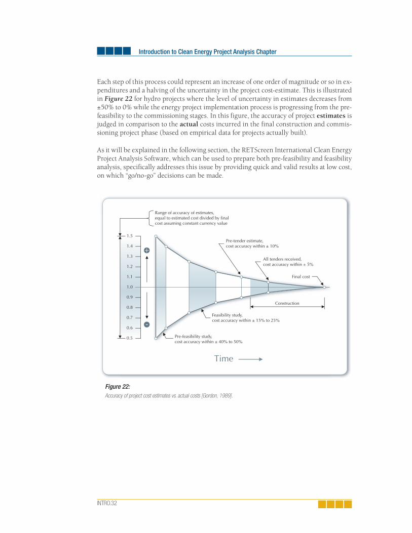
Each step of this process could represent an increase of one order of magnitude or so in ex-penditures and a halving of the uncertainty in the project cost-estimate. This is illustrated in Figure 22 for hydro projects where the level of uncertainty in estimates decreases from ±50% to 0% while the energy project implementation process is progressing from the pre-feasibility to the commissioning stages. In this figure, the accuracy of project estimates is judged in comparison to the actual costs incurred in the final construction and commis-sioning project phase (based on empirical data for projects actually built).
As it will be explained in the following section, the RETScreen International Clean Energy Project Analysis Software, which can be used to prepare both pre-feasibility and feasibility analysis, specifically addresses this issue by providing quick and valid results at low cost, on which “go/no-go” decisions can be made.
Time
1.5
1.4
1.3
1.2
1.1
1.0
0.9
0.8
0.7
0.6
0.5
Range of accuracy of estimates, equal to estimated cost divided by final cost assuming constant currency value
Pre-tender estimate,cost accuracy within ± 10%
All tenders received,cost accuracy within ± 5%
Final cost
Construction
Feasibility study,cost accuracy within ± 15% to 25%
Pre-feasibility study,cost accuracy within ± 40% to 50%
Figure 22: Accuracy of project cost estimates vs. actual costs [Gordon, 1989].

1. Clean Energy Project Analysis Background
INTRO.33
1.2.1 Favourable project conditions
Typically, decision-makers are often not familiar with clean energy technologies. Thus, they have not normally developed an intuition for identifying when clean energy tech-nologies are promising and should be expressly included in a pre-feasibility study. As an initial guide, the conditions indicating good potential for successful clean energy project implementation typically include:
Need for energy system: Proposing an energy system while there is an energy need is a strong favourable prerequisite to any energy project, and especially so for clean energy projects where awareness barriers are often the main stumbling blocks.
New construction or planned renovation: Outfi tting buildings and other facilities with clean energy technologies is often more cost-effective when done as part of an existing construction project. The initial costs of the clean energy technology may be offset by the costs of the equipment or materials it supplants, and early planning can facilitate the integration of the clean energy technology into the rest of the facility.
High conventional energy costs: When the conventional energy options are expensive, the usually higher initial costs of clean energy technologies can be overcome by the lower fuel costs, in comparison with the high conventional energy costs.
Interest by key stakeholders: Seeing a project through to completion can be a protracted, arduous affair involving a number of key stakeholders. If even just one key stakeholder is opposing the project, even the most fi nancially and environmentally attractive projects could be prevented from moving to successful implementation.
Hassle-free approvals process: Development costs are minimised when approvals are possible and easily obtained. Local, regional or national legislation and policy may not be sensitive to the differences between conventional and clean energy technologies, and as such may unfairly disadvantage clean energy technologies.
Easy access to funding and fi nancing: With access to fi nancing, subsidies, and grants, the higher initial costs of clean energy technologies need not present a major hurdle.
Adequate local clean energy resources: A plentiful resource (e.g. wind) will make clean energy technologies much more fi nancially attractive.
Assessing these favourable conditions first could serve as valuable criteria for finding opportunities for clean energy project implementation. As part of an initial filtering or pre-screening process, they could also be used to prioritize clean energy projects, and to select which ones to invest in a pre-feasibility analysis.

Introduction to Clean Energy Project Analysis Chapter
INTRO.34
1.2.2 Project viability factors
Carefully considering the key factors which make a clean energy project financially viable can save a significant amount of time and money for the project’s proponents. Some of the viability factors related to clean energy projects are listed below, with examples for a wind energy project:
Energy resource available at project site (e.g. wind speed)
Equipment performance (e.g. wind turbine power curve)
Initial project costs (e.g. wind turbines, towers, engineering)
“Base case” credits (e.g. diesel generators for remote sites)
On-going and periodic project costs (e.g. cleaning of wind turbine blades)
Avoided cost of energy (e.g. wholesale electricity price)
Financing (e.g. debt ratio & term, interest rate)
Taxes on equipment & income (or savings)
Environmental characteristics of energy displaced (e.g. coal, natural gas, oil, large hydro, nuclear)
Environmental credits and/or subsidies(e.g. greenpower rates, GHG credits, grants)
Decision-maker’s defi nition of cost-effective (e.g. payback period, IRR, NPV, Energy production costs)
The RETScreen Clean Energy Project Analysis Software, as described in the next section, has a number of features to make this focus on key factors relatively straight-forward.

2. RETScreen Clean Energy Project Analysis Software
INTRO.35
2 RETSCREEN CLEAN ENERGY PROJECT ANALYSIS SOFTWARE
The RETScreen International Clean Energy Project Analysis Software can be used worldwide to evaluate the energy production, life-cycle costs and greenhouse gas emission reductions for various types of proposed energy efficient and renewable energy technologies (RETs).
The RETScreen Software has been developed to overcome the barriers to clean energy tech-nology implementation at the preliminary feasibility stage. It provides a proven methodol-ogy for comparing conventional and clean energy technologies. The analyst can therefore focus on the pre-feasibility study, rather than developing the methodology; combined with the tool’s minimal data input requirements and built-in weather and product databases, this results in fast, accurate analyses that cost roughly one-tenth the amount of pre-feasibil-ity studies with custom-developed methodologies. This permits the screening of multiple potential projects, such that the most promising ones can be identified and implemented. It also facilitates the sharing of information by way of a standardised, internationally ac-cepted platform.
All clean energy technology models in the RETScreen Software have a common look and follow a standard approach to facilitate decision-making – with reliable results. Each model also includes integrated product, cost and weather databases and a detailed online user manual, all of which help to dramatically reduce the time and costs associated with pre-paring pre-feasibility studies.
RETScreen has been designed to help not just with the task of carrying out a project analysis, but also to provide useful information about the clean energy technologies, thus building awareness of their capabilities and applications. This should assist the user in developing a good sense for when a given technology should be considered; it also makes RETScreen an excellent resource for teaching and information dissemination.
This section presents the RETScreen Software, including the project analysis approach, and some of the clean energy technology models, databases and complementary resources that come with the software. While the methodology and algorithms specific to a RETScreen Clean Energy Technology Model are presented in-depth in their respective chapters, the methodologies and algorithms common to all models are presented in this section. These include the greenhouse gas analysis, the financial analysis and the sensitivity & risk analy-sis methodologies.
2.1 RETScreen Software Overview
Fundamental to the RETScreen Software is a comparison between a “base case”—typically the conventional technology or measure—and a “proposed case”—the clean energy tech-nology. This has very important implications for how the user specifies costs: RETScreen is ultimately not concerned with the absolute costs, but rather the incremental costs—the costs of the proposed case that are in excess of those for the base case. The user can either enter incremental costs directly or enter both the full cost associated with the proposed case and any credits stemming from base case costs made unnecessary by the proposed technology.

Introduction to Clean Energy Project Analysis Chapter
INTRO.36
In the RETScreen Software, the energy benefits are the same for both the base case and the proposed case. If, for example, a proposed on-grid wind farm generates 50,000 MWh per year, then this compared to 50,000 MWh of electricity from conventional sources available through the grid. On the other hand, the costs will not, in general, be the same for the base case and the proposed case: typically, the proposed case will have higher initial costs and lower annual costs (i.e. savings). Thus RETScreen’s analysis task is to determine whether or not the balance of costs and savings over the life of the project make for a financially attractive proposition. This is reflected in the various financial indicators and the cash flows calculated by the RETScreen Software.
RETScreen’s greenhouse gas emission reduction analysis adheres to this same analysis ap-proach: it reports the reduction in GHG emission associated with changing from the base case to the proposed case technology.
2.1.1 Five step standard project analysis
While a different RETScreen Clean Energy Technology Model is used for each of the technologies covered by RETScreen, the same five step standard analysis procedure is common to all of them. As a result, the user who has learned how to use RETScreen with one technology should have no problem using it for another. Since the RETScreen Software is developed in Microsoft® Excel, each of the five steps in the standardised analy-sis procedure is associated with one or more Excel worksheets. Figure 23 presents the RETScreen Software Model Flow Chart’s Five Step Standard Project Analysis, which are further described below:
Figure 23:RETScreen Software Model Flow Chart: A Five Step Standard Analysis.

INTRO.37
STEP 1 - Energy Model (and sub-worksheet(s)): In this worksheet, the user specifies pa-rameters describing the location of the energy project, the type of system used in the base case, the technology for the proposed case, the loads (where applicable), and the renewable energy resource (for RETs). In turn, the RETScreen Software calculates the annual energy production or energy savings. Often a resource worksheet (such as the “Solar Resource” or the “Hydrology and Load” worksheet) or an “Equipment Data” worksheet—or both—ac-companies the Energy Model worksheet as sub-worksheet(s). The algorithms used in each technology’s Energy Model worksheet along with their validations can be found in the respective chapters of this textbook.
STEP 2 - Cost Analysis: In this worksheet, the user enters the initial, annual, and periodic costs for the proposed case system as well as credits for any base case costs that are avoided in the proposed case (alternatively, the user can enter the incremental costs directly). The user has the choice between performing a pre-feasibility or a feasibility study. For a “Pre-feasibility analysis,” less detailed and less accurate information is typically required while for a “Feasibility analysis,” more detailed and more accurate information is usually required. Since the calculations performed by the RETScreen Software for this step are straightforward and relatively simple (addition and multiplication), the information found in the online manual for each input and output cell should be sufficient for a complete understanding of this worksheet.
STEP 3– Greenhouse Gas (GHG) Analysis (optional): This optional worksheet helps determine the annual reduction in the emission of greenhouse gases stemming from using the proposed technology in place of the base case technology. The user has the choice between performing a simplified, standard or custom analysis, and can also indicate if the project should be evaluated as a potential Clean Development Mechanism (CDM) project12. RETScreen automatically assesses whether or not the project can be considered as a small-scale CDM project to take advantage of the simplified baseline methods and other rules and procedures for small-scale CDM projects. The methodology and algorithms used in the RETScreen Software for this step are described in detail in Section 2.2.
STEP 4 - Financial Summary: In this worksheet, the user specifies financial parameters related to the avoided cost of energy, production credits, GHG emission reduction credits, incentives, inflation, discount rate, debt, and taxes. From this, RETScreen calculates a vari-ety of financial indicators (e.g. net preset value, etc.) to evaluate the viability of the project. A cumulative cash flow graph is also included in the financial summary worksheet. The methodology and algorithms used in the RETScreen Software for this step are described in detail in Section 2.3.
STEP 5 - Sensitivity & Risk Analysis (optional): This optional worksheet assists the user in determining how uncertainty in the estimates of various key parameters may affect the financial viability of the project. The user can perform either a sensitivity analysis or a risk analysis, or both. The methodology and algorithms used in the RETScreen Software for this step are described in detail in Section 2.4.
12. The Kyoto Protocol has established three mechanisms (the Clean Development Mechanism (CDM), Joint Implementation (JI),
and Emissions Trading) which allow Parties to pursue opportunities to cut emissions, or enhance carbon sinks, abroad.
2. RETScreen Clean Energy Project Analysis Software

Introduction to Clean Energy Project Analysis Chapter
INTRO.38
2.1.2 Common platform for project evaluation & development
The RETScreen Software facilitates project implementation by providing a common evalua-tion and development platform for the various stakeholders involved in a project. For exam-ple, numerous people around the world report using RETScreen for a variety of purposes, including: feasibility studies; project lender due-diligence; market studies; policy analysis; information dissemination; training; sales of products and/or services; project development & management; and product development/R&D.
To further illustrate how this works, the RETScreen Software files can be electronically shared (e.g. e-mail) among the various project stakeholders (see Figure 24). For example, a consultant may be asked to prepare a RETScreen study for the project owner, such as an independent power producer (IPP). The IPP may then want to change input values as part of a sensitivity analysis of key parameters such as return on investment. The IPP may in turn be asked by the potential lender to submit the file to them so that they can perform the project due-diligence review. In parallel, the utility regulator may want the project file to verify the GHG emission reduction estimates, and so on.
Figure 24: Common Platform for Project Evaluation & Development.

2. RETScreen Clean Energy Project Analysis Software
INTRO.39
The reporting capability of the RETScreen Software also facilitates decision-making by allowing one to see all the key information used to prepare a study. This allows for easier project due-diligence and comparison amongst different options or propositions by all the parties involved in an energy project. It particularly helps reduce the costs of studies by decreasing the effort normally dedicated to write the project assessment report. Indeed, the printout of a RETScreen study constitutes, by itself, a report that is often sufficient at the early stage of the project imple-mentation process. The box entitled “Reducing the Cost of Pre-feasibility Studies” shows how this capability has already been instrumental for a project identification initiative.
A language switch allows the analy-sis to be set to one of many languages available in RETScreen13 and facili-tates the communication between stakeholders. It allows partners who speak different languages to easily evaluate a project by removing the need to translate reports and results, thus repeating the analysis in each language; the language switch auto-matically translates the entire analy-sis. For example, a project proponent from France might want to prepare a RETScreen analysis in French for a potential clean energy project in China, which might result in GHG production credits as a clean devel-opment mechanism (CDM) project as defined in the Kyoto Protocol. By using the RETScreen language switch, the analysis initially pre-pared in French can automatically be translated into Simplified Chinese for potential Chinese partners, and also into English for the required CDM related project analysis.
The overall time and cost savings attributable to RETScreen are very important in terms of accelerating clean energy project implementation and market expansion. According to an independent impact assessment of RETScreen International14, the user savings attrib-uted to the RETScreen Software between 1998 and 2004 are estimated to be $600 million worldwide, and are expected to grow exponentially to reach $7.9 billion by 2012.
13. As of September, 1st 2005, the languages available include: Arabic, Bengali, Chinese, Danish, Dutch, English, Finnish,
French, German, Greek, Hindi, Italian, Japanese, Korean, Polish, Portuguese, Romanian, Russian, Spanish, Swedish,
and Telugu. Additional product translations for these languages and additional translations in other languages are
expected to be available in RETScreen.
14. Graham, Stephen and Steve Higgins, SGA Energy Ltd., An Impact Assessment of RETScreen® International 1998-2012, Final Report to NRCan’s CETC-Varennes, April 2004.
REDUCING THE COST OF PRE-FEASIBILITY STUDIES
RETScreen was instrumental in helping Natural Resources Canada’s (NRCan) CETC-Varennes and a team of eleven consulting firms prepare studies for 56 potential RET projects in Canada’s 300 remote communities at a cost of less than $2,000 each. Of these, 27 projects offered commercial potential with-out government incentives. Similar studies would otherwise have cost in the order of 5 to 10 times this amount! As a result, money saved is now being used to develop a number of these projects, with several projects already built, such as the 35 m2 solar air heating collector shown here [Alward, 1999].
Solar Air Heating Technology, Yellowknife, NWT, Canada.

Introduction to Clean Energy Project Analysis Chapter
INTRO.40
2.1.3 Clean energy technology models
The RETScreen Software can be used to evaluate industrial, commercial, institutional, community, residential and utility applications. Some of the RETScreen clean energy tech-nology models are as follows15:
Wind Energy Project Model for central-grid and isolated-grid con-nected projects, ranging in size from large-scale multi-turbine wind farms to small-scale single-turbine wind-diesel hybrid systems.
Small Hydro Project Model for central-grid and isolated-grid con-nected projects, ranging in size from multi-turbine small and mini hydro installations to single-turbine micro hydro systems.
Photovoltaic Project Model for on-grid (central-grid and isolated-grid PV systems); off-grid (stand-alone (PV-battery) and hybrid (PV-battery-genset) systems; and water pumping applications (PV-pump systems).
Biomass Heating Project Model for biomass and/or waste heat recov-ery (WHR) heating projects, from large-scale developments for clusters of buildings to individual building applications. The model can be used to evaluate three basic heating systems using: waste heat recovery; bio-mass; and biomass and waste heat recovery combined.
Solar Air Heating Project Model for ventilation air heating and process air heating applications of transpired-plate solar collectors, from small residential to larger commercial/industrial-scale ventilation systems, as well in the air-drying processes for various crops.
Solar Water Heating Project Model for domestic hot water, industrial process heat and swimming pools (indoor and outdoor), ranging in size from small residential systems to large scale commercial, institutional and industrial systems.
15. NRCan continues to develop the RETScreen Software, including new energy effi ciency models. See the RETScreen
Website (www.retscreen.net) for the latest developments.

2. RETScreen Clean Energy Project Analysis Software
INTRO.41
Passive Solar Heating Project Model for passive solar designs and/or energy efficient window use in low-rise residential and small commercial building applications, for either retrofit or new construc-tion projects.
Ground-Source Heat Pump Project Model for heating and/or cooling of residential, commercial, institutional and industrial buildings, for both retrofit and new construction projects using either ground-coupled (horizontal and vertical closed loop) or groundwater heat pumps.
Combined Heat & Power (CHP) Project Model for any one or combina-tion of the following applications: power; heating; cooling; single buildings or multiple buildings; industrial processes; communities; district heating and district cooling; with a wide range of renewable and non-renewable fuels (which can be used in parallel), including landfill gas; biomass; ba-gasse; biodiesel; hydrogen; natural gas; oil/diesel; coal; municipal waste, etc.; and using multiple types of power, heating and/or cooling equipment, including reciprocating engines; gas turbines; gas turbine - combined cycle; steam turbines; geothermal systems; fuel cells; wind turbines; hydro tur-bines; photovoltaic modules; boilers; heat pumps; biomass systems; heaters; furnaces; compressors; absorption chillers, etc., all working under various operating conditions (base load, intermediate load and/or peak load).
For the above clean energy technologies, a detailed description of the algorithms found in the RETScreen Software is available in the respective chapters of this textbook covering each of these technologies.
2.1.4 Clean energy related international databases
The RETScreen Software uses both meteorological and product performance data as input to the various technology models to help determine the amount of energy that can be delivered (or saved) by a project, or to help calculate other important parameters, such as heating loads. Additional data regarding costs and other financial parameters is necessary to determine various financial aspects of the project. Gathering this sort of data for an individual project can be very time consuming and expensive. The RETScreen Software integrates a series of databases to help overcome this deployment barrier and to facilitate the implementation of clean energy projects around the world. However, the user can, at any time, enter data from other sources where needed.
This section introduces the origin of the meteorological data used in RETScreen, both for the ground-based meteorological data and NASA’s satellite-derived meteorological data sets, both of which provide weather (climate) data for the entire surface of the planet. An overview of the hydrology, product and cost data that are also included with the RETScreen Software is also provided below.

Introduction to Clean Energy Project Analysis Chapter
INTRO.42
Worldwide ground-based meteorological data
Worldwide Ground-based Meteorological Data has been incorporated directly into the RETScreen Software. This integrated RETScreen International Online Weather Database includes ground-based observation averages for over 4,700 sites16 around the world, compiled from over 20 different sources for the 1961-1990 period. A map displaying all ground-based weather stations used in RETScreen is shown in Figure 25, and an example of the integrated weather database in the Solar Water Heating Project Model is presented in Figure 26.
16. The RETScreen Combined Heat & Power Model Version 3.2 and subsequent versions of the RETScreen Software
integrate data for over 4,720 ground-monitoring stations. Earlier version have 1,000 weather stations.
Figure 25: Worldwide location of ground-based weather stations in RETScreen.
Figure 26: Example of the Integrated Weather Database to the RETScreen Solar Water Heating Project Model.

2. RETScreen Clean Energy Project Analysis Software
INTRO.43
These data are compiled from a number of different sources. As a consequence, the original data is not presented, but rather data from the various sources are gathered into a single, coherent repository. For example, the data is homogenised so that SI units are used for all locations, regardless of the original units. Also, depending on the station, some variables are calculated from other quantities; for example, the rela-tive humidity may be calculated from the minimum and maximum humidity levels.
Over 20 different sources were used to compile the database. However, not all sources contributed equally. For example, some sources had limited spatial cover-age (i.e. covered only one country), or proved less reliable than other sources for the same location and were thus used only as a last resort in the absence of other, more reliable data. The most significant sources were:
1. Environment Canada (1993). Canadian Climate Normals, 1961-1990. Ottawa: Minister of Supply and Services Canada. This six-volume book includes a wealth of meteorological information for Canada and was used for most Canadian stations (except for solar radiation and wind data, see below).
2. Environment Canada (1998). The Canadian renewable energy wind and solar resource (CERES). Ottawa: Minister of Supply and Services Canada. This CD-ROM contains wind and solar radiation information for all available Canadian sites.
3. Numerical Logics Inc. (1998). Monthly averages of solar radiation and sunshine derived from data from the World Radiation Data Centre (WRDC) Online Archive (1964-1993). Averages for solar radiation were calculated from data stored at the WRDC; only stations having more than fi ve years of data were included in the RETScreen database.
4. National Climatic Data Center and National Renewable Energy Laboratory (1993). Solar And Meteorological Surface Observation Network (SAMSON) 1961-1990. Version 1.0. These 3 CD-ROMs were the primary source for climate data, including solar radiation, for sites in the United States. Monthly averages were calculated from hourly values contained in the CD-ROM.
5. World Meteorological Organization (1996). Climatological Normals (CLINO) for the period 1961-1990. WMO/OMM-No.847. Geneva: Secretariat of the World Meteorological Organization. This very large document contains information that was supplied by member countries on various climatological parameters. The number of parameters included depends on the reporting country. Some less developed countries may contain only one parameter, whereas more developed countries tend to report values for all parameters required for the RETScreen database.
A detailed description of the meteorological variables used in the RETScreen Soft-ware is found in the Online Manual.

Introduction to Clean Energy Project Analysis Chapter
INTRO.44
NASA’s satellite-derived meteorological data set
NASA’s Satellite-derived Meteorological Data for any location on earth is pro-vided for use with the RETScreen Software via the NASA Surface Meteorology and Solar Energy (SSE) Data Set. This data set, developed by NASA in collaboration with RETScreen International, is a useful alternative when ground-based data or detailed resource maps are not available for the project location. A direct link to the NASA Website is provided from within the RETScreen Software; the user may simply copy the relevant data from the Website and paste it into the relevant worksheets of the RETScreen Software.
The SSE data set is derived mainly from several other data sets developed by NASA, including the Goddard Earth Observing Systems Version 1 (GEOS-1) and, for solar radiation data, the International Satellite Cloud Climatology Project Version D (ISCCP D-1), using an atmospheric model constrained to satellite and sounding observations. These data sets, in turn, were derived from the analysis of observa-tions made by earth-orbiting satellites: the Geostationary Operational Environmen-tal Satellites (GOES) and Polar-Orbiting Environmental Satellites (POES) from the US National Oceanic & Atmospheric Administration (NOAA), the Meteorological Satellites (Meteosat) operated by the European Space Agency, and the Geostationary Meteorological Satellites (GMS) operated by the Japan Meteorological Agency.
Satellite-derived data provide a much greater coverage than ground-based data. Unlike the RETScreen ground-based meteorological database, the SSE is not limited to any particular station and is able to provide climatic variables for any location on earth. This is important since many ground measurement stations are located near populated areas; the SSE may therefore be a valuable resource – and sometimes the only resource – for isolated and remote locations. On the other hand, the resolution of the grid used by the SSE may be insufficient to catch local peculiarities of the climate; natural or human (urban effect) microclimates are not taken into account, and the SSE data alone is not appropriate where there are large topographic features within a cell of the grid. Certain climate parameters may be sensitive to variations within the cell boundaries (i.e. wind speed) whereas others are ideally suited to this resolution (i.e. insolation); higher resolution data for these parameters will have a negligible or no effect on the final energy analysis. Examples of maps generated from average (1983-1992) SSE data for the month of July are shown in Figure 27 for insolation (solar radiation), 50 m wind speed, and earth skin temperature.
The NASA SSE data set is formulated from data gathered for the 10-year period from July 1983 to June 1993. The original satellite and GEOS-1 data are calculated using a 1-degree grid size which covers the entire globe (64,800 regions). At mid-latitudes (45°), the cell size is therefore approximately 80×110 km. Figure 28 shows a detailed sample of the grid covering the United Kingdom and Ireland. The 1-degree data is generated using the NASA Goddard Earth Observing System - Version 1 (GEOS-1) Multiyear Assimilation Timeseries Data.

2. RETScreen Clean Energy Project Analysis Software
INTRO.45
A description of the algorithms used to derive the SSE is beyond the scope of this textbook. A fairly complete description of the Staylor algorithm used to calculate solar insolation is found in the Surface Radiation Budget (SRB) Langley DAAC Data Set Document, available on-line17. NASA’s methodology and other relevant additional information can also be found on the NASA’s Surface meteorology and Solar Energy Website.
17. http://charm.larc.nasa.gov/GUIDE/dataset_documents/srb.html
Figure 27: Example of global maps derived
from average NASA SSE data
for the month of July.
Figure 28: Example of the grid covering the United Kingdom
and Ireland, used by NASA.
Source: NASA’s Surface Meteorology
and Solar Energy (release 5.1) Website.

Introduction to Clean Energy Project Analysis Chapter
INTRO.46
Hydrology data
In the RETScreen Small Hydro Project Model, hydrological data are specified by a flow-duration curve, which is assumed to represent the flow conditions in the river being studied over the course of an average year. For reservoir storage projects, data must be manually entered by the user and should represent the regulated flow that results from operating a reservoir. For run-of-river projects, the required flow-duration curve data can be entered either manually or by using the specific run-off method and data contained in the RETScreen Online Weather Database.
Hydrology Data from Environment Canada for more than 500 Canadian river gauges are available in the Weather Database included in the RETScreen Small Hydro Project Model (see Figure 29), including regional flow-duration curves and specific run-off maps prepared using Water Survey of Canada data (see Figure 30).
Flow-duration curve data, required to run the model, are available for a large num-ber of stream flow gauging stations. For example, stream flow data for the United Kingdom and Spain are available from the Centre for Hydrology and Ecology via a database called HYDATA. The actual weather database integrated in the RETScreen Small Hydro Project Model currently includes a flow-duration curve dataset that has been calculated from the HYDAT hydrological database, available from Environ-ment Canada18. For project locations outside of Canada, hydrology data from other sources can be entered manually.
18. http://www.wsc.ec.gc.ca
Figure 29: Example of the integrated Weather (Hydrology) Database to the RETScreen Small Hydro Project Model,
which includes 500 Canadian river gauges (from Environment Canada).

2. RETScreen Clean Energy Project Analysis Software
INTRO.47
Product data
The product data incorporated directly into the RETScreen Software provides access to over 6,000 pertinent product performance and specification data needed to describe the performance of the proposed clean energy system in the first step of the RETScreen analysis (i.e. in the Energy Model and accompanying worksheets).
The data for these products can be pasted into the relevant cells direct-ly in the clean energy technology model as shown in Figure 31. This figure shows an example of the integrated product database includ-ed in the RETScreen Photovoltaic Project Model. The RETScreen Product Database provides data for the power, heating and cooling sys-tems listed in Table 1 and more.
In addition, the product database provides access, via website links within the software, to contact information for clean energy tech-nology manufacturers around the globe so that the user interested in getting more information (e.g. a quotation) can contact the prod-uct supplier directly.
0.000 - 0.0020.002 - 0.0040.004 - 0.0080.008 - 0.0160.016 - 0.0320.032 - 0.0640.064 +
Canadian Specific Run-off Map
Figure 30: Example of the
RETScreen Canadian
Specifi c Run-Off
Map for Small
Hydro Projects.
Figure 31: Example of the Integrated Product Database
in the RETScreen Software.
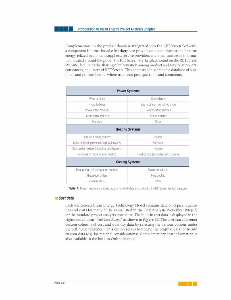
Introduction to Clean Energy Project Analysis Chapter
INTRO.48
Complementary to the product database integrated into the RETScreen Software, a companion Internet-based e-Marketplace provides contact information for clean energy related equipment suppliers, service providers and other sources of informa-tion located around the globe. The RETScreen Marketplace found on the RETScreen Website, facilitates the sharing of information among product and service suppliers, consumers, and users of RETScreen. This consists of a searchable database of sup-pliers and on-line forums where users can post questions and comments.
Power Systems
Wind turbines Gas turbines
Hydro turbines Gas turbines – combined cycle
Photovoltaic modules Reciprocating engines
Geothermal systems Steam turbines
Fuel cells Other
Heating Systems
Biomass heating systems Boilers
Solar air heating systems (e.g. Solarwall®) Furnaces
Solar water heaters (including pool heaters) Heaters
Windows for passive solar heating Heat pumps (air and ground-source)
Cooling Systems
Heat pumps (air and ground-source) Desiccant wheels
Absorption chillers Free cooling
Compressors Other
Table 1: Power, heating and cooling systems for which data are provided in the RETScreen Product Database.
Cost data
Each RETScreen Clean Energy Technology Model contains data on typical quanti-ties and costs for many of the items listed in the Cost Analysis Worksheet (Step 2) for the standard project analysis procedure. The built-in cost data is displayed in the rightmost column “Unit Cost Range,” as shown in Figure 32. The user can also enter custom columns of cost and quantity data by selecting the various options under the cell “Cost reference.” This option serves to update the original data, or to add custom data (e.g. for regional considerations). Complementary cost information is also available in the built-in Online Manual.

2. RETScreen Clean Energy Project Analysis Software
INTRO.49
2.1.5 Online manual and training material
A number of additional resources have been developed to help users learn how to use the RETScreen Software quickly, effectively, and accurately. These resources are:
Online manual: Within the RETScreen Software is an extensive Online User Manual (see Figure 33). For every cell displaying an output or requiring user input, there is an associated page in the online manual that explains what the cell means. This is helpful for new users and experts alike. New users can step through the spreadsheet, seeking guidance from the online manual for every input cell they encounter. Expert users can rely on the manual for clarifi cation of conventions and to help them remember pricing, sizing, and other details. The manual also provides background on both the clean energy technologies and the RETScreen methodology. This further enhances RETScreen’s utility in education and information dissemination. The manual is also available from the RETScreen Website for download as an Adobe Acrobat (pdf) format fi le, for those users who wish to print the entire manual.
Figure 32: Example of the Integrated Cost Data in the RETScreen Software.
Figure 33: Example of the integrated online manual in the RETScreen
Photovoltaic Project Model.

Introduction to Clean Energy Project Analysis Chapter
INTRO.50
Training material: Training material for a modular case study-based Clean Energy Project Analysis Course has been created for use by recognised educational centres and training organisations around the globe, as well as for use by professionals and college/university students in “self-study” distance learning format. Each module can be presented as a separate seminar or workshop for professionals, or as a section of a college/university course. All the modules combined can be presented either as a one to two week long intensive course for professionals or as a one to two semester long course for college/university students. The course material, including slide presentations (see Figure 34) and an instructor’s voice-over, has also been made available on the RETScreen Website for download, free-of-charge.
Engineering textbook: the electronic textbook Clean Energy Project Analysis: RETScreen Engineering & Cases (which you are currently reading) is written for professionals and university students who are interested in learning how to better analyse the technical and fi nancial viability of possible clean energy projects. It covers each of the technologies in the RETScreen Software, including a background of these technologies and a detailed description of the algorithms found in some of the RETScreen software clean energy technology models (see Figure 35). This textbook has also been made available on the RETScreen Website for download, free-of-charge.
Case studies: a collection of clean energy project case studies is also provided to complement the training material and to facilitate the use of the RETScreen Software. Available free-of-charge on the RETScreen website, these case studies typically include assignments, worked-out solutions (e.g. RETScreen Studies) and information about how the projects fared in the real world (see Figure 36).
Figure 34: Example of the complementary training course material (Slides) available with the RETScreen Software.

2. RETScreen Clean Energy Project Analysis Software
INTRO.51
The methodologies and algorithms common to all models are presented in detail in the following section. These include the greenhouse gas analysis, the financial analysis and the sensitivity & risk analysis methodologies.
2.2 Greenhouse Gas (GHG) Emission Reduction Analysis Model
The RETScreen Greenhouse Gas (GHG) Emission Reduction Analysis Model found in the GHG Analysis worksheet of the RETScreen Software, helps the user estimate the green-house gas emission reduction (mitigation) potential of a proposed clean energy project. The GHG analysis model is common to all RETScreen Clean Energy Technology Models. It calculates the GHG emission profile for a Base Case System (Baseline), and for the Proposed Case System (clean energy project). The GHG emission reduction potential is obtained by combining the difference of the GHG emission factors with other information calculated by RETScreen, such as the annual energy delivered.
Figure 35: Example of the complementary Engineering
Textbook “Clean Energy Project Analysis:
RETScreen Engineering & Cases” available
with the RETScreen Software.
Figure 36: Example of the complementary Case Studies
available with the RETScreen Software.

Introduction to Clean Energy Project Analysis Chapter
INTRO.52
The methodology implemented in the RETScreen Software to calculate the GHG emis-sion reductions associated with a clean energy project, has been developed by Natural Resources Canada in collaboration with the United Nations Environment Programme (UNEP), the UNEP Collaborating Centre on Energy and Environment at the RISØ National Laboratory, and the World Bank’s Prototype Carbon Fund (PCF). It has been validated by a team of experts from government and industry (see Appendix A).
There are some challenges that may arise in the basic calculations associated with a GHG analysis. The following items are taken into consideration by the RETScreen Software in addition to the Base Case/Proposed Case comparison:
Combustion produces not just carbon dioxide, but also methane and nitrous oxide. The RETScreen Software uses carbon dioxide, the most common GHG, as a common currency: methane and nitrous oxide emissions are converted into their equivalent carbon dioxide emission according to their “global warming potential” (GWP). International scientifi c committees such as the International Panel on Climate Change [IPCC, 1996] have proposed GWP factors for these gasses. These factors are built into the RETScreen Software as default conversion values used in the standard GHG analysis type.
The transmission and distribution (T & D) losses in electrical systems that feed into a grid must be considered. When electricity is generated in one place but consumed in another, a certain fraction of the electricity is lost as heat from the transmission and distribution lines connecting the two. Modern, industrialized grids tend to have losses of around 8 to 10 %. Thus, electricity destined for a grid (i.e. not consumed directly on-site) produced by either the base case system or the proposed case system must include these losses when calculating the energy delivered to the end user. The RETScreen Software permits the user to specify the expected “T & D losses”.
The number of credits that accrue to the project may be reduced if a percentage has to be paid annually as a transaction fee to a crediting agency (e.g. the United Nations Framework Convention on Climate Change - UNFCCC) or the country hosting the project, or both. The RETScreen Software includes an input cell entitled “GHG credits transaction fee” where the user can specify this percentage.
The RETScreen Software takes into account the emerging rules from the Kyoto Protocol that are associated with three specific flexibility mechanisms: the Clean Development Mecha-nism (CDM), Joint Implementation (JI), and Emissions Trading. These allow Parties to the Kyoto Protocol to pursue opportunities to cut emissions, or enhance carbon sinks, abroad.
This section presents the equations used in the RETScreen GHG Emission Reduction Analysis Model. The model works slightly differently depending on whether the clean energy system under consideration generates electricity or provides heating or cooling; the main difference lies in transmission and distribution losses, which are incurred only by electricity generating systems.
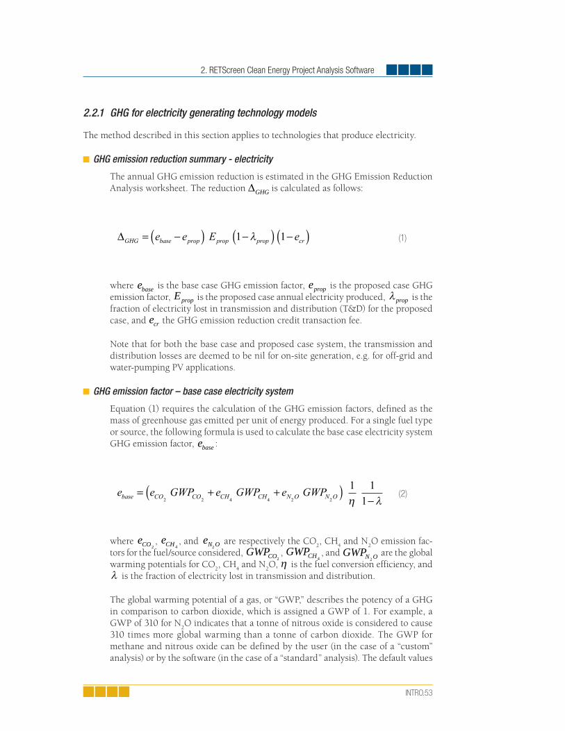
2. RETScreen Clean Energy Project Analysis Software
INTRO.53
2.2.1 GHG for electricity generating technology models
The method described in this section applies to technologies that produce electricity.
GHG emission reduction summary - electricity
The annual GHG emission reduction is estimated in the GHG Emission Reduction Analysis worksheet. The reduction ΔGHG is calculated as follows:
where ebase is the base case GHG emission factor, eprop is the proposed case GHG emission factor, Eprop is the proposed case annual electricity produced, λprop
is the fraction of electricity lost in transmission and distribution (T&D) for the proposed case, and ecr the GHG emission reduction credit transaction fee.
Note that for both the base case and proposed case system, the transmission and distribution losses are deemed to be nil for on-site generation, e.g. for off-grid and water-pumping PV applications.
GHG emission factor – base case electricity system
Equation (1) requires the calculation of the GHG emission factors, defined as the mass of greenhouse gas emitted per unit of energy produced. For a single fuel type or source, the following formula is used to calculate the base case electricity system GHG emission factor, ebase :
where eCO 2, eCH 4
, and eN O2 are respectively the CO
2, CH
4 and N
2O emission fac-
tors for the fuel/source considered, GWPCO2, GWPCH 4
, and GWPN O2 are the global
warming potentials for CO2, CH
4 and N
2O, η is the fuel conversion efficiency, and
λ is the fraction of electricity lost in transmission and distribution.
The global warming potential of a gas, or “GWP,” describes the potency of a GHG in comparison to carbon dioxide, which is assigned a GWP of 1. For example, a GWP of 310 for N
2O indicates that a tonne of nitrous oxide is considered to cause
310 times more global warming than a tonne of carbon dioxide. The GWP for methane and nitrous oxide can be defined by the user (in the case of a “custom” analysis) or by the software (in the case of a “standard” analysis). The default values
(1)
(2)

Introduction to Clean Energy Project Analysis Chapter
INTRO.54
used by RETScreen are shown in Table 2; these values can be found in the Revised Intergovernmental Panel on Climate Change (IPCC) Guidelines for Greenhouse Gas Inventories, 1996.
The GHG emission factor will vary according to the type and quality of the fuel, and the type and size of the power plant. Emission factors are defined by the user (in the case of a “custom” analysis) or by the software (in the case of a “standard” analysis).
Greenhouse gas GWPCO2
1
CH 21
N2O 310
Table 2: Global warming potentials of greenhouse gases.
In cases for which there are a number of fuel types or sources, the GHG emission factor ebase for the electricity mix is calculated as the weighted sum of emission factors calculated for each individual fuel source:
where n is the number of fuels/sources in the mix, fi is the fraction of end-use electricity coming from fuel/source i, and ebase i, is the emission factor for fuel i, calculated through a formula similar to equation (2):
where
,
, and are respectively the CO2, CH
4 and N
2O emission
factors for fuel/source i, ηi is the fuel conversion efficiency for fuel i, and λi is fraction of electricity lost in transmission and distribution for fuel i.
Alternatively, the GHG emission factor for the electricity mix, before transmission and distribution losses are applied, can be entered directly by the user, in case of a “user-defined” analysis.
(3)
(4)

2. RETScreen Clean Energy Project Analysis Software
INTRO.55
Note that the GHG emission factor for the electricity mix will apply from year 1 up to the year of change in baseline, as specified by the user, unless no changes are specified; in this case, the emission factor will apply throughout the life of the project. When a change in the baseline emission factor is specified, the new factor for the year that the change in baseline takes place, and the years that follow will be determined by (e*):
where rchange is the percentage change in the base case (baseline) GHG emission factor for the year that the change in baseline takes place, and the years that follow.
GHG emission factor – proposed case electricity system
The calculation of the proposed case electricity system GHG emission factor, eprop ,
is similar to that of the base case GHG emission factor, with the exception that for off-grid systems the fraction of electricity lost in transmission and distribution is set to zero.
eprop is therefore calculated through equation (2) with λ = 0 , in the
case of a single fuel/source, or through equations (3) and (4) with all λi = 0 , in the case of a mix of fuel/sources.
Alternatively, the proposed case GHG emission factor, before transmission and dis-tribution losses are applied, can be entered directly by the user, in case of a “user-defined” analysis.
2.2.2 GHG for heating and cooling technology models
The method described in this section applies to heating and cooling technologies.
GHG emission reduction summary – heating and cooling
The annual GHG emission reduction is estimated in the GHG Emission Reduction Analysis Worksheet. The reduction ΔGHG hc, is calculated as follows:
where ΔGHG heat, and
ΔGHG cool, are the annual GHG emission reductions from heat-ing and cooling. These are calculated as:
(5)
(6)

Introduction to Clean Energy Project Analysis Chapter
INTRO.56
where ebase heat, and ebase cool, are the base case GHG emission factors for heating and for cooling, and eprop heat, and
eprop cool, are the proposed case GHG emission
factors for heating and for cooling. Eprop heat, is the proposed case end-use annual
heating energy delivered and Eprop cool, is the proposed case end-use annual cool-
ing energy delivered.
GHG emission factor – base case electricity system
Some applications require the definition of a base case electricity system to account for the GHG emissions from electricity that can be emitted for heating, for air con-ditioning or to drive auxiliary equipment such as fans and pumps (for example, a solar water heating system may require an electric pump to circulate water through the collectors). The corresponding GHG emission factor is calculated through equa-tion (2) in the case of a single fuel/source, or through equations (3) and (4) in the case of a mix of fuel/sources.
GHG emission factor – base case and proposed case heating and cooling systems
For a single fuel type or source, the GHG emission factor e (for example ebase cool, , ebase heat, , etc.) is calculated through an equation very similar to equation (2), except that there are no transmission and distribution losses (since heating or air-condi-tioning systems are considered to be at the site of use):
where η is the fuel conversion efficiency and all other variables have the same mean-ing as in equation (2). If there are a number of fuel types or sources, the GHG emis-sion factor is calculated as the weighted sum of emission factors calculated for each individual fuel source:
(8)
(9)
(10)
(7)

2. RETScreen Clean Energy Project Analysis Software
INTRO.57
where n is the number of fuels/sources in the mix,
fi is the fraction of end-use energy coming from fuel/source i, and ei is the emission factor for fuel i, calculated through a formula similar to equation (9):
where ηi is the fuel conversion efficiency for fuel i.
For heating systems, the calculation of the emission factor for the proposed case requires special attention because of the presence of parasitic electric energy. For example the electricity required to run the pump of a solar collector does not con-tribute to the clean energy delivered by the system, but it does contribute to its GHG emissions. To take this into account, the following quantity, epara , is added to the GHG emission factor calculated through equations (9) and (10):
where eelec is the emission factor for the base case electricity system, Eprop para, is the parasitic electrical energy used in the proposed case, and Eprop heat, is, as before, the proposed case end-use annual heating energy delivered.
2.3 Financial Analysis Model
The RETScreen Financial Analysis Model, found in the Financial Summary worksheet of the RETScreen Software, allows the user to input various financial parameters, such as discount rates, etc., and to automatically calculate key financial feasibility indicators, such as internal rate of return, simple payback, net present value, etc.
This section presents the equations used in the RETScreen Financial Analysis Model. The formulae used are based on standard financial terminology that can be found in most fi-nancial textbooks, such as Brealey and Myers (1991) or Garrison et al. (1990). The model makes the following assumptions:
The initial investment year is year 0;
The costs and credits are given in year 0 terms, thus the infl ation rate (or the escalation rate) is applied from year 1 onwards; and
The timing of cash fl ows occurs at the end of the year.
(11)
e eEEpara elec
prop para
prop heat
= ,
,
(12)

Introduction to Clean Energy Project Analysis Chapter
INTRO.58
2.3.1 Debt payments
Debt payments are a constant stream of regular payments that last for a fixed number of years (known as the debt term). The yearly debt payment D is calculated using the fol-lowing formula:
(13)
where C is the total initial cost of the project, fd is the debt ratio, id is the effective annual debt interest rate, and N ′ is the debt term in years. The yearly debt payment, as given by equation (13), can be broken down into payment towards the principal Dp n,
and payment of interest Di n, :
(14)
Both Dp n, and Di n, vary from year to year; they are calculated by standard functions built
into Microsoft® Excel.
2.3.2 Pre-tax cash fl ows
The calculation of cash flows keeps track, on a yearly basis, of all expenses (outflows) and in-comes (inflows) generated by the clean energy project. This sub-section presents the formu-lae used in RETScreen to determine the cash flows of a project, before considering taxes.
Cash outfl ows
For year zero, the pre-tax cash outflow Cout ,0 is equal to the project equity, that is, the portion of the total investment required to finance the project that is funded directly and therefore not incorporated in the financial leverage (e.g. not included in the debt):
(15)
For subsequent years, the pre-tax cash outflow Cout n, is calculated as:
(16)

2. RETScreen Clean Energy Project Analysis Software
INTRO.59
where n is the year, CO M& is the yearly operation and maintenance costs incurred by the clean energy project, ri is the inflation rate, C fuel is the annual cost of fuel or electricity, re is the energy cost escalation rate, D is the annual debt payment (equation 13), and Cper is the periodic costs or credits incurred by the system.
Cash infl ows
For year zero, the pre-tax cash inflow Cin,0 is simply equal to the incentives and grants IG :
(17)
For subsequent years, the pre-tax cash inflow Cin n, is calculated as:
(18)
where n is the year, Cener is the annual energy savings or income, Ccapa is the annual capacity savings or income, CRE is the annual renewable energy (RE) production credit income, rRE the RE credit escalation rate, CGHG is the GHG reduction income, rGHG is the GHG credit escalation rate. For the last year, the end-of-project life credit, incremented by inflation, is added to the right-hand side of equation (18).
Pre-tax cash fl ows
The pre-tax cash flow Cn for year n is simply the difference between the pre-tax cash inflow and the pre-tax cash outflow:
(19)
2.3.3 Asset depreciation
The calculation of asset depreciation (or capital cost allowance) depends on the deprecia-tion method chosen by the user in the Financial Summary Worksheet: choices are “None,” “Declining balance,” or “Straight-line.” The yearly depreciation of assets is used in the model in the calculation of income taxes and after-tax financial indicators. The user should select the method which most closely resembles the methods used by the tax departments in the jurisdiction of the project. At the end of the project life, the difference between the “End of project life” value and its undepreciated capital costs is treated as income if posi-tive and as a loss if negative.
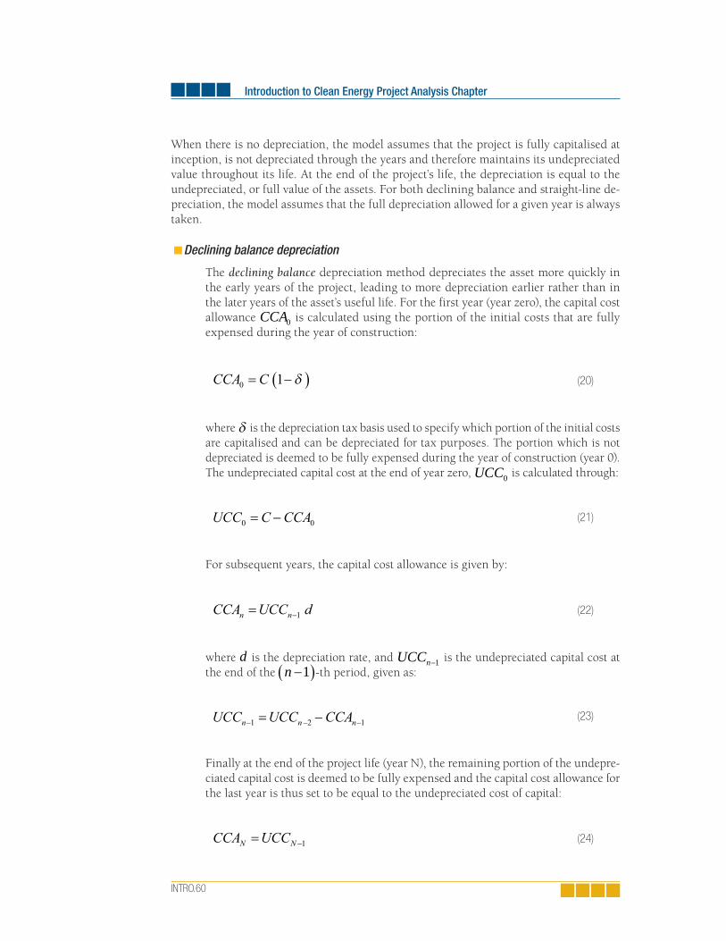
Introduction to Clean Energy Project Analysis Chapter
INTRO.60
When there is no depreciation, the model assumes that the project is fully capitalised at inception, is not depreciated through the years and therefore maintains its undepreciated value throughout its life. At the end of the project’s life, the depreciation is equal to the undepreciated, or full value of the assets. For both declining balance and straight-line de-preciation, the model assumes that the full depreciation allowed for a given year is always taken.
Declining balance depreciation
The declining balance depreciation method depreciates the asset more quickly in the early years of the project, leading to more depreciation earlier rather than in the later years of the asset’s useful life. For the first year (year zero), the capital cost allowance CCA0 is calculated using the portion of the initial costs that are fully expensed during the year of construction:
(20)
where δ is the depreciation tax basis used to specify which portion of the initial costs are capitalised and can be depreciated for tax purposes. The portion which is not depreciated is deemed to be fully expensed during the year of construction (year 0). The undepreciated capital cost at the end of year zero, UCC0 is calculated through:
(21)
For subsequent years, the capital cost allowance is given by:
(22)
where d is the depreciation rate, and UCCn 1 is the undepreciated capital cost at the end of the n( )1 -th period, given as:
(23)
Finally at the end of the project life (year N), the remaining portion of the undepre-ciated capital cost is deemed to be fully expensed and the capital cost allowance for the last year is thus set to be equal to the undepreciated cost of capital:
(24)

2. RETScreen Clean Energy Project Analysis Software
INTRO.61
so that the undepreciated capital cost at the end of that year becomes zero:
(25)
Straight-line depreciation
With the straight-line depreciation method, the financial analysis model assumes that the capitalised costs of the project, as specified by the depreciation tax basis, are depreciated with a constant rate over the depreciation period. The portion of initial costs not capitalised is deemed to be expensed during the year of construction, i.e. year 0. In this method, the following formulae are used:
(26)
for year zero, and for subsequent years within the depreciation period:
(27)
where Nd is the user-defined depreciation period in years.
2.3.4 Income tax
The income tax analysis allows the financial analysis model to calculate after-tax cash flows and after-tax financial indicators. The tax rate used in the RETScreen Financial Summary worksheet is the effective equivalent rate, and is specified by the user. It is the rate at which the net income from the project is taxed. In all cases, the financial analysis model assumes a single income tax rate valid and constant throughout the project life and applied to net income.
Net taxable income is derived from the project cash inflows and outflows assuming that all revenues and expenses are paid at the end of the year in which they are earned or incurred. The amount of tax Tn for year n is equal to the effective income tax rate t , specified by the user, multiplied by the net income for that year, In :
(28)

Introduction to Clean Energy Project Analysis Chapter
INTRO.62
The net income for years one and beyond is calculated as:
(29)
where Cn is the pre-tax annual cash flow (equation 19), Dp n, is the payment on the prin-cipal (equation 14), and CCAn is the capital cost allowance (equations 20 or 25 depending on the asset depreciation method selected). For year 0, the net income is simply:
(30)
where IG is the value of incentives and grants.
2.3.5 Loss carry forward
A loss (e.g. a negative net income) in a given year can sometimes be used, according to some taxation rules, to lower taxes owed in that same year. According to other taxation rules, it can be deferred to offset profits from future years. A third alternative is that the loss cannot be used in the same year nor in the future, and is thus lost from a tax perspective. The Loss Carry Forward option in the Financial Summary worksheet allows the user to select which of the three rules apply to the project being analysed. If the Loss Carry Forward option is selected, losses are carried forward and applied against net income in the following years, thereby reducing taxes in the following year(s). If the option is not selected, losses are not carried forward nor applied against other income, but are effectively lost as a tax offset. If the Flow-through option is selected, losses are not carried forward but used to generate a refundable tax credit in the year in which the loss occurs.
2.3.6 After-tax cash fl ow
Considering the pre-tax cash flows, the asset depreciation, the income tax, and the loss carry forward discussed in the previous sections, the after-tax cash flow nC~ is calculated as follows:
(31)
where Cn is net cash flow (equation 19) and Tn the yearly taxes (equation 28).
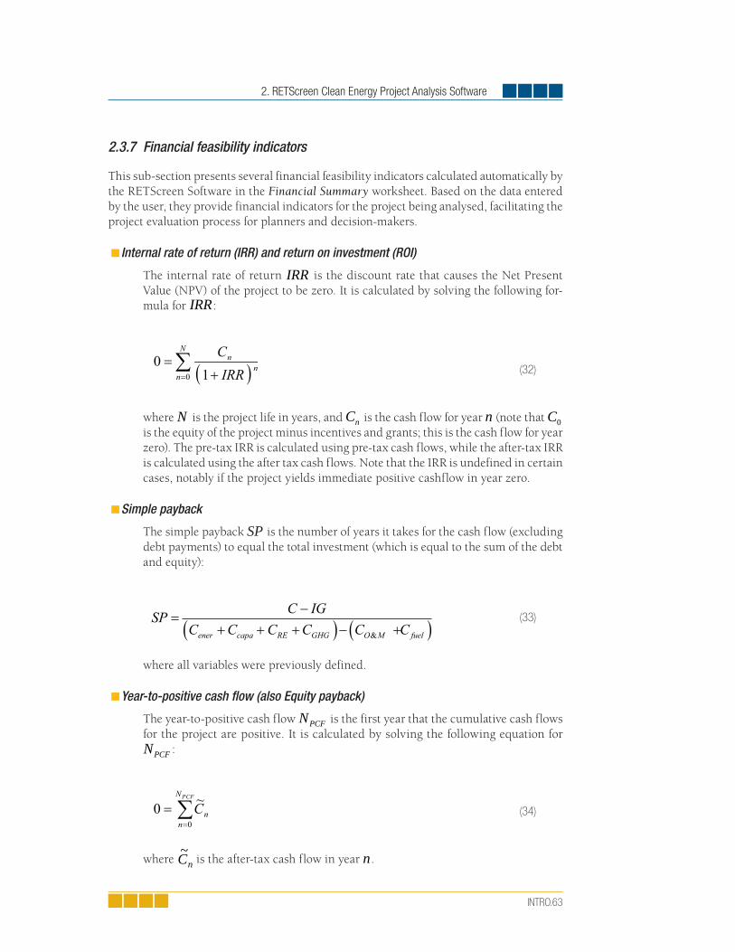
2. RETScreen Clean Energy Project Analysis Software
INTRO.63
2.3.7 Financial feasibility indicators
This sub-section presents several financial feasibility indicators calculated automatically by the RETScreen Software in the Financial Summary worksheet. Based on the data entered by the user, they provide financial indicators for the project being analysed, facilitating the project evaluation process for planners and decision-makers.
Internal rate of return (IRR) and return on investment (ROI)
The internal rate of return IRR is the discount rate that causes the Net Present Value (NPV) of the project to be zero. It is calculated by solving the following for-mula for IRR:
(32)
where N is the project life in years, and Cn is the cash flow for year n (note that C0 is the equity of the project minus incentives and grants; this is the cash flow for year zero). The pre-tax IRR is calculated using pre-tax cash flows, while the after-tax IRR is calculated using the after tax cash flows. Note that the IRR is undefined in certain cases, notably if the project yields immediate positive cashflow in year zero.
Simple payback
The simple payback SP is the number of years it takes for the cash flow (excluding debt payments) to equal the total investment (which is equal to the sum of the debt and equity):
(33)
where all variables were previously defined.
Year-to-positive cash fl ow (also Equity payback)
The year-to-positive cash flow NPCF is the first year that the cumulative cash flows for the project are positive. It is calculated by solving the following equation for NPCF :
(34)
where nC~ is the after-tax cash flow in year n.
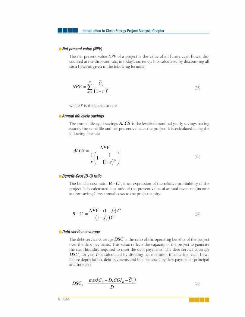
Introduction to Clean Energy Project Analysis Chapter
INTRO.64
Net present value (NPV)
The net present value NPV of a project is the value of all future cash flows, dis-counted at the discount rate, in today’s currency. It is calculated by discounting all cash flows as given in the following formula:
(35)
where r is the discount rate.
Annual life cycle savings
The annual life cycle savings ALCS is the levelised nominal yearly savings having exactly the same life and net present value as the project. It is calculated using the following formula:
(36)
Benefi t-Cost (B-C) ratio
The benefit-cost ratio, B C , is an expression of the relative profitability of the project. It is calculated as a ratio of the present value of annual revenues (income and/or savings) less annual costs to the project equity:
(37)
Debt service coverage
The debt service coverage DSC is the ratio of the operating benefits of the project over the debt payments. This value reflects the capacity of the project to generate the cash liquidity required to meet the debt payments. The debt service coverage DSCn for year n is calculated by dividing net operation income (net cash flows before depreciation, debt payments and income taxes) by debt payments (principal and interest):
(38)

2. RETScreen Clean Energy Project Analysis Software
INTRO.65
where COIn is the cumulative operating income for year n, defined as:
(39)
The Financial Analysis model calculates the debt service coverage for each year of the project and reports the lowest ratio encountered throughout the term of debt.
Energy production cost
The energy production cost is the avoided cost of energy that brings the net present value to zero. This parameter is not included in the Combined Heat & Power Model, since there are potentially many types of energy produced, each potentially having a distinct production cost . The energy production cost, Cprod , is thus obtained by solving for:
(40)
where
(41)
(42)
(43)
GHG emission reduction cost
The GHG Emission reduction cost GRC represents the levelised nominal cost to be incurred for each tonne of GHG avoided. It is calculated by:
(44)
where ALCS is the annual life cycle savings calculated in equation 36, and GHG is the annual GHG emission reduction, calculated in the GHG Analysis worksheet (equation 1).

Introduction to Clean Energy Project Analysis Chapter
INTRO.66
2.4 Sensitivity and Risk Analysis Models
The RETScreen Sensitivity and Risk Analysis Models, found in the Sensitivity and Risk Analysis worksheet of the RETScreen Software, help the user estimate the sensitivity of important financial indicators in relation to key technical and financial parameters. This worksheet contains two main sections: Sensitivity Analysis and Risk Analysis. Each analy-sis provides information on the relationship between the technical and financial param-eters and the financial indicators, showing the parameters which have the greatest impact on the financial indicators. Both the sensitivity and the risk analyses are optional, and the related inputs or outputs do not affect results in other worksheets.
The Sensitivity and Risk Analysis worksheet varies slightly from one Clean Energy Technol-ogy Model to the next, reflecting the different key parameters that are important to each technology. Nevertheless, all share a common underlying algorithm, described below. This sub-section presents the methodology and the equations used, together with a validation of the accuracy of the “Risk Analysis” portion of this model. The “Sensitivity Analysis” portion of this model consists of a series of tables, similar to the one shown in Figure 37, which show the effect of varying a pair of input parameters on the financial feasibility indicators. This method is relatively straightforward and is not described in detail here.
2.4.1 Monte Carlo simulation
The Risk Analysis Model in RETScreen is based on a “Monte Carlo simulation,” which is a method whereby the distribution of possible financial indicator outcomes is generated by using randomly selected sets of values as input parameters, within a predetermined range, to simulate possible outcomes.
In the RETScreen Software Monte Carlo simulation, the input parameters relate to several pre-selected technical and financial parameters, and the output indicators relate to key financial indicators (see Table 3). The simulation consists of two steps:
32,54636,61440,68244,75048,619
Avoided cost of energy ($/kWh)RE delivered
(MWh)
-20%-10%0%
10%20%
7.2%10.2%13.3%16.6%20.0%
9.8%13.1%16.7%20.4%24.4%
12.4%16.1%20.1%24.4%28.9%
14.9%19.2%23.7%28.5%33.6%
17.6%22.3%27.4%32.8%38.4%
0.0760-20%
0.0855-10%
0.09500%
0.104510%
0.114020%
Figure 37: Example of a Sensitivity Analysis Chart from the default built-in example of the Wind Energy Project Model. The analysis is performed
on the after-tax IRR and ROI, with a sensitivity range of 20% and a threshold of 15%. The three original values used in the analysis
are indicated in bold.

2. RETScreen Clean Energy Project Analysis Software
INTRO.67
1. For each input parameter, 500 random values are generated using a normal (Guassian) distribution with a mean of 0 and a standard deviation of 0.33 using the Random Number Generation function in Microsoft® Excel’s Data Analysis ToolPack. Once generated, these random numbers are fi xed.
2. Each random value is then multiplied by the related percentage of variability (range) specifi ed by the user in the Sensitivity and Risk Analysis worksheet. The result is a 500 x 9 matrix containing percentages of variation that will be applied to input parameters’ initial value in order to obtain 500 results for the output fi nancial indicators.
Since the set of random numbers is fixed, whenever the same input parameters are speci-fied in the RETScreen Clean Energy Project Model and the same ranges of variability are used, the user will obtain exactly the same results from the Risk Analysis Model.
Technical and Financial Parameters(Input parameters)
Financial Indicators(Output indicators)
Avoided cost of energy
Fuel cost – proposed case
Fuel cost – base case
Renewable energy (RE) delivered
Initial costs
Annual costs (O&M)
Debt ratio
Debt interest rate
Debt term
GHG emission reduction credit
Net GHG reduction – credit duration
RE production credit (CE production credit)
Customer premium income – rebate
Electricity export rate
After-tax internal rate of return (IRR)and return on investment (ROI)
After-tax IRR – equity
After-tax IRR – assets
Year-to-positive cash fl ow (equity payback)
Net present values (NPV)
Table 3: Input Parameters and Output Indicators associated with the Monte Carlo simulation performed
in the RETScreen Risk Analysis Model.
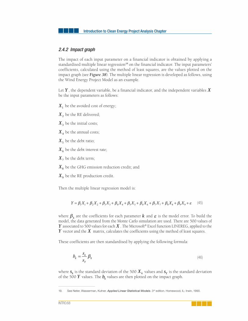
Introduction to Clean Energy Project Analysis Chapter
INTRO.68
2.4.2 Impact graph
The impact of each input parameter on a financial indicator is obtained by applying a standardised multiple linear regression19 on the financial indicator. The input parameters’ coefficients, calculated using the method of least squares, are the values plotted on the impact graph (see Figure 38). The multiple linear regression is developed as follows, using the Wind Energy Project Model as an example.
Let Y , the dependent variable, be a financial indicator, and the independent variables X be the input parameters as follows:
X1 be the avoided cost of energy;
X 2 be the RE delivered;
X 3 be the initial costs;
X 4 be the annual costs;
X 5 be the debt ratio;
X 6 be the debt interest rate;
X 7 be the debt term;
X8 be the GHG emission reduction credit; and
X 9 be the RE production credit.
Then the multiple linear regression model is:
(45)
where βk are the coefficients for each parameter k and ε is the model error. To build the model, the data generated from the Monte Carlo simulation are used. There are 500 values of Y associated to 500 values for each X . The Microsoft® Excel function LINEREG, applied to the Y vector and the X matrix, calculates the coefficients using the method of least squares.
These coefficients are then standardised by applying the following formula:
(46)
where sk is the standard deviation of the 500 X k values and sY is the standard deviation of the 500 Y values. The bk values are then plotted on the impact graph.
19. See Neter, Wasserman, Kutner. Applied Linear Statistical Models. 3rd edition. Homewood, IL: Irwin, 1990.

2. RETScreen Clean Energy Project Analysis Software
INTRO.69
2.4.3 Median & confi dence interval
The median of a financial indicator is the 50th percentile of the 500 values generated by the Monte Carlo simulation. The median is given by the Microsoft® Excel function MEDIAN, and is calculated by first ordering the 500 financial indicator values from the smallest to the biggest. The median is the average of the 250th and 251st ordered values.
The confidence interval is the range of values within which the Monte Carlo simulation falls. A 90% confidence interval indicates that 90% of the 500 financial indicator values will fall within a certain range. The user specifies the level of risk, or the percentage of values which will fall outside the confidence interval (e.g. a 90% confidence interval has a 10% level of risk).
The minimum level of confidence for a financial indicator is given by the percentile cor-responding to half the level of risk defined by the user. This percentile is given by the PERCENTILE function in Microsoft® Excel. For example, for a level of risk of 10%, the minimum level of confidence will be the 5th percentile of the 500 values generated by the Monte Carlo simulation. It is calculated by ordering the 500 financial indicator values in ascending order. The 5th percentile is the average of the 25th and 26th values. Similarly, the maximum level of confidence is the percentile corresponding to one minus half the level of risk. Using the above example, the maximum level of confidence would be the 95th percentile, obtained by taking the average of the 475th and 476th values.
-0.800 -0.600 -0.400 -0.200 0.000 0.200 0.400 0.600
Impact on After-tax IRR and ROI
Effect of increasing the value of the parameter
Initial costs
RE delivered
Debt interest rate
Debt ratio
Avoided cost of energy
RE production credit
Annual costs
GHG emission reduction credit
Dept term
So
rted
by
the
imp
act
Figure 38: Impact Chart (Tornado Graph) that shows the relative effect of parameters variation over the After-Tax IRR and ROI in the Risk Analysis
Model; example from the default built-in example of the Wind Energy Project Model (Sensitivity and Risk Analysis Worksheet).

Introduction to Clean Energy Project Analysis Chapter
INTRO.70
2.4.4 Risk analysis model validation
A validation of the Risk Analysis Model was performed to assess the accuracy of the impact statistics, the median, and the maximum and minimum level of confidence. The validation also investigated the effect of the number of observations used in the Monte Carlo simu-lation on the precision of the impact results. The validation was done by comparing the statistical results obtained from RETScreen to JMP, a statistical software from the company SAS. The default example of the RETScreen Wind Energy Project Model was used as the test case.
Number of observations effect
All the results presented in the Risk analysis section are obtained from a Monte Carlo simulation using 500 randomly generated observations. It is well known that the larger the number of observations generated, the more precise the estimates obtained from the simulation will be. The drawback is an increase in the time it takes to perform the calculations. To assess the effect the number of observations used in the Monte Carlo simulation has on the precision of the impact results, the following calculations were performed.
For each financial indicator output, a multiple linear regression analysis was per-formed using subsets of the 500 values generated from the Monte Carlo simulation. The subsets were obtained using the last 50 observations, last 100 observations, and so on, up to the last 450 observations and the full set of 500 observations. For each of these subsets, multiple linear regression coefficients and their estimation error were used as the input parameters for the JMP statistical software. The estimation errors were then standardised according to their standard deviation:
(47)
where Z p i, is the standardised error for the input parameter p and subset i (e.g. the subset of the last 50 observations, last 100 observations, etc.), Qp i, is the error in the estimate of parameter p when using subset i, Qp is the average for all values of i of the error Qp i, , and σ p is the standard deviation of the set of Qp i, for the parameter p over all values of i (i.e., 50 observations, 100 observations, etc.).
The values of Z p i, are plotted in Figures 39, 40, and 41. Note that with standardised errors, a negative value does not mean underestimation; rather, it means that the error is lower than average. As the number of observations in the Monte Carlo simu-lation increases, the standardised error of the regression coefficients decreases. The slope of the standardised error usually flattens as the number of observations gets closer to 500. This pattern is more obvious for NPV and after-tax IRR and ROI than for the year-to-positive cash flow.
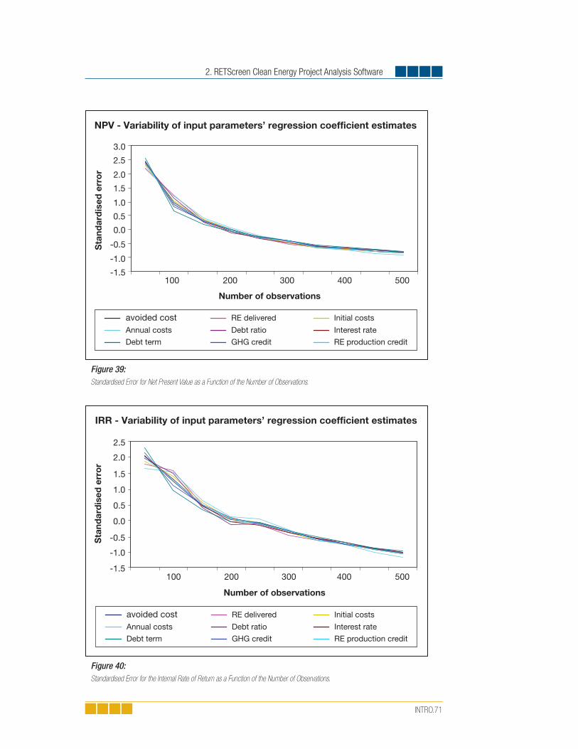
2. RETScreen Clean Energy Project Analysis Software
INTRO.71
NPV - Variability of input parameters’ regression coefficient estimates
-1.5
-1.0
-0.5
0.0
0.5
1.0
1.5
2.0
2.5
3.0
100 200 300 400 500
Number of observations
Sta
ndar
dis
ed e
rro
r
avoided cost RE delivered Initial costs
Annual costs Debt ratio Interest rate
Debt term GHG credit RE production credit
Figure 39:Standardised Error for Net Present Value as a Function of the Number of Observations.
IRR - Variability of input parameters’ regression coefficient estimates
-1.5
-1.0
-0.5
0.0
0.5
1.0
1.5
2.0
2.5
100 200 300 400 500
Number of observations
Sta
ndar
dis
ed e
rro
r
avoided cost RE delivered Initial costs
Annual costs Debt ratio Interest rate
Debt term GHG credit RE production credit
Figure 40: Standardised Error for the Internal Rate of Return as a Function of the Number of Observations.

Introduction to Clean Energy Project Analysis Chapter
INTRO.72
Statistical results accuracy
Using the test case (the default values in the Wind Energy Project Model), three different risk analysis scenarios were generated. The accuracy of impact, median, maximum and minimum level of confidence was checked against the JMP statistical software. For after-tax IRR and ROI, and year-to-positive cash flow, three decimals of precision were used; for the NPV, results were expressed to the nearest integer.
For all three scenarios, RETScreen’s values for the impacts and the medians were identi-cal to those of the JMP software. The RETScreen Risk Analysis Model’s maximum and minimum within level of confidence values never differed more than 0.7% from those of JMP, as summarized in Table 4. The average ratio of the difference between RETScreen and JMP over the financial output indicators range for all three scenarios is 0.24% for the minimum level of confidence and -0.30% for the maximum level of confidence.
On average, the RETScreen Risk Analysis Model gives a higher minimum within level of confidence and a lower maximum within level of confidence resulting in a confidence interval that is narrower than the JMP software. The average differ-ence between RETScreen and JMP increases with increasing range of the financial indicator (e.g. the difference between the maximum and minimum values from the 500 calculations in the Monte Carlo simulation). Overall, the differences are insig-nificant and illustrate the adequacy of the RETScreen Sensitivity and Risk Analysis Model for pre-feasibility studies.
Year - Variability of input parameters’ regression coefficient estimates
100 200 300 400 500
Number of observations
Sta
ndar
dis
ed e
rro
r
-2.0-1.5
-1.0-0.5
0.00.5
1.01.52.0
2.53.0
avoided cost RE delivered Initial costs
Annual costs Debt ratio Interest rate
Debt term GHG credit RE production credit
Figure 41: Standardised Error for Year-to-Positive Cash Flow as a Function of the Number of Observations.

2. RETScreen Clean Energy Project Analysis Software
INTRO.73
Average differences(RETScreen vs JMP)
Ratio of average differences
over results range
Within level of confi dence Within level of confi dence
Financial output Results range Minimum Maximum Minimum Maximum
Scenario 1 IRR 22.686% 0.041% -0.044% 0.179% -0.193%
Year 12.1504 0.0086 -0.0768 0.071% -0.632%
NPV 23,104,673 48,910 -29,881 0.212% -0.129%
Average 0.154% -0.318%
Scenario 2 IRR 1.813% 0.009% -0.005% 0.474% -0.302%
Year 0.7125 0.0008 -0.0019 0.112% -0.270%
NPV 1,797,879 8,634 -3,685 0.480% -0.205%
Average 0.355% -0.259%
Scenario 3 IRR 123.357% 0.028% -0.490% 0.023% -0.398%
Year - N/A N/A - -
NPV 74,231,343 282,884 -201,811 0.381% -0.272%
Average 0.202% -0.335%
Average of Scenario 1, 2 and 3 0.240% -0.301%
Table 4: Comparison of RETScreen and JMP for Minimum and Maximum within Level of Confi dence.
2.5 Summary
This introductory chapter has first explained the reasons for the mounting interest in clean energy technologies and has provided a quick synopsis of the operation of these technolo-gies and their applications and markets. It has then proceeded to discuss the importance of pre-feasibility analysis within the project implementation cycle. Finally, it has described the methods common to all RETScreen Clean Energy Technology Models: the use of cli-mate and renewable energy resource data (e.g. weather data), the greenhouse gas emission reduction calculation, the financial analysis, and the sensitivity and risk analysis.
Clean energy technologies have received increasing attention over the last decade as one response to the challenges of global warming, increasing demand for energy, high fuel costs, and local pollution. Commercial technologies for power, heating and cooling enjoy stong markets, with substantial opportunities for future expansion around the world. To benefit from these technologies, energy project proponents and stakeholders must be able to assess on a life cycle cost basis whether a particular proposed project makes sense. Therefore, using the minimum investment of time and effort to determine the most finan-cially attractive option, competing energy options have to be screened early in the project planning stages.

Introduction to Clean Energy Project Analysis Chapter
INTRO.74
The RETScreen International Clean Energy Project Analysis Software facilitates this deci-sion process, and can be used worldwide to evaluate the energy production, life-cycle costs and greenhouse gas emission reductions for various types of proposed energy efficient and renewable energy technologies (RETs). Its use significantly reduces the cost and increases the precision of pre-feasibility studies and contributes to the formulation of more fully informed decisions prior to project implementation. The RETScreen Software is increasing and improving access to clean energy technologies, building awareness & capacity, and helping to identify opportunities that facilitate the implementation of energy projects that save money, while reducing greenhouse gas emissions.

INTRO.75
REFERENCES
Al Homoud, M.S., Variable-Base Heating and Cooling Degree-Day Data for 24 Saudi Arabian Cities, ASHRAE Transactions, 104-2, 1998.
Alward, R., Remote Community Renewable Energy Technology Project Identifi cation Initiative (RETPII), Natural Resources Canada’s CANMET Energy Diversifi cation Research Laboratory (CEDRL), Varennes, QC, Canada, Initiative Summary (Abstract), 6 pp, 1999.
American Wind Energy Association (AWEA), Global Wind Power Growth Continues to Strengthen, 2005.
ASHRAE, Commercial/Institutional Ground-Source Heat Pump Engineering Manual, American Society of Heating, Refrigerating and Air-Conditioning Engineers, Inc., 1791 Tullie Circle, N.E., Atlanta, GA 30329, USA, 1995.
ASHRAE, Handbook of Fundamentals, SI Edition, American Society of Heating, Refrigerating and Air-Conditioning Engineers, Inc., 1791 Tullie Circle, N.E., Atlanta, GA 30329, USA, 1997.
Beaumert, K. and Selman, M., Data Note: Heating and Cooling Degree Days, World Resources Institute, 2003.
Chandler, W.S., Brown, D.E., Whitlock, C.H., and Stackhouse, P.W., NASA Climatological Data for Renewable Energy Assessment, Submitted to ISEC 2003 International Solar Energy Conference, 16-18 March 2003, Mauna Kea Resort, HI, USA, 2003.
Danish Wind Industry Association, 2004.
Eliasson, B., Renewable Energy: Status and Prospects 1998, Baden-Dättwil, Switzerland: ABB Corporate Research, Ltd., 1998.
Environment Canada, Canadian Weather Energy and Engineering Data Sets (CWEEDS), 1993.
European Commission, European Network of Energy Agencies ATLAS, 2005.
European Wind Energy Association (EWEA), Wind Power Installed In Europe by end of 2003, 2005.
ESTIF, A Solar Thermal Strategy: Sun in Action II, Renewable Energy World, pp. 200-209, July-August 2003.
Gipe, P., The BTM Wind Report: World Market Update, Renewable Energy World, pp. 66-83, July-August 2003.
IEA, Energy to 2050—Scenarios for a Sustainable Future, International Energy Agency (IEA), Paris, France, 2003.
IEA Statistics, Renewables Information, IEA, Paris, France, 2003.
International Small Hydro Atlas, Small-Scale Hydro Annex of the International Energy Agency (IEA)’s Implementing Agreement for Hydropower Technologies & Programmes, 2004.

Introduction to Clean Energy Project Analysis Chapter
INTRO.76
IPCC, IPCC Third Assessment Report—Climate Change 2001: Summary for Policy Makers, Intergovernmental Panel on Climate Change (IPCC), Geneva, Switzerland, 2001.
Langcake, P., Getting a Clear View: Strategic Perspectives for Renewable Energy Companies, Renewable Energy World, pp. 29-37, March-April 2003.
Leng, G., Monarque, A., Graham, S., Higgins, S., and Cleghorn, H., RETScreen® International: Results and Impacts 1996-2012, Natural Resources Canada’s CETC-Varennes, ISBN 0-662-11903-7, Cat. M39-106/2004F-PDF, 44 pp, 2004.
Lund, J., Ground-source Heat Pumps: A World Overview, Renewable Energy World, pp. 218-227, July-August 2003.
Marine Current Turbines, Bristol, UK, 2005.
Maycock, P., Boomer, PVNews, May 2004.
Maycock, P., PV Market Update, Renewable Energy World, pp. 84-101, July-August 2003.
Microsoft Online Help and Support, Microsoft, 2005.
National Aeronautics and Space Administration (NASA), USA, 2005.
National Renewable Energy Laboratory (NREL), Golden, CO, USA, 2005.
NCDC, International Surface Weather Observations (ISWO), Available from the National Climatic Data Centre, 151 Patton Ave., Asheville, NC, 28801-5001, USA, 1997.
Strahler, A.H. and Strahler, A.N., Modern physical geography, New York: John Wiley and Sons, 1992.
Swenson, A., Energy Consumption by End Use, Energy Information Administration, U.S. Department of Energy, USA, 1998.
Thevenard, D.J. and Brunger, A.P., The Development of Typical Weather Years for International Locations: Part I, Algorithms, and Part II: Production, ASHRAE Transactions, 108, 2, 376-383 and 480-486, 2002.
Whitlock, C., Brown, D., Chandler, W., DiPasquale, R., Meloche, N., Leng, G.J., Gupta, S., Wilber, A., Ritchey, N., Carlson, A., Kratz, D., Stackhouse, P., Release 3 NASA Surface Meteorology and Solar Energy Data Set for Renewable Energy Industry Use, Rise & Shine 2000 – The 26th Annual Conference of the Solar Energy Society of Canada Inc. (SESCI), Halifax, NS, Canada, October 21st to 24th, 2000.
Windpower Monthly News Magazine, The Windicator, Windpower Monthly, January 2004.
World Resources Institute, Earth Trends: Energy Consumption by Economic Sector, 2003.

APPENDIX A - RETScreen Development Team & Experts
INTRO.77
APPENDIX A - RETSCREEN DEVELOPMENT TEAM & EXPERTS
A core team at CETC-Varennes provides the technical knowledge and management of RETScreen International, and a large network of experts from industry, government and academia provide technical support on a contracted or task-shared basis. This approach pro-vides RETScreen International with access to a broad array of expert skills that are needed for specialised tasks. The RETScreen International core team is presented in Figure 42.
More than 221 people have been directly involved in the development and support of RETScreen International, with 20 to 50 people working with the core RETScreen team during the course of a year. They include professional staff from the RETScreen partner organisations such as UNEP, NASA, the World Bank, and other Government of Canada programs; plus experts from a number of private-sector firms, including GPCo, Enermodal Engineering, Numerical Logics, TN Conseil, Ottawa Engineering, Econoler International, IT Power India, Umen, Cybercat and Projet Bleu, to name but a few.
The core team and network of experts include energy modeling specialists who help de-velop the individual technology computer simulation models, cost engineering experts who have extensive hands-on experience with project installations, greenhouse gas modeling and baseline specialists with broad experience in economic and environmental analysis, and financial and risk analysis professionals with considerable experience in evaluating and financing projects.
Farah SheriffProject Engineer
Software Integration(Electrical Engineer)
Ron AlwardSenior Engineer
Capacity Building(Mechanical Engineer)
Amélie RichardInformation OfficerCustomer Support(Communications)
Co-op
Engineering Student(s)Software Testing
Contract Position
Project EngineerQuality Control
Kevin BourqueProject Engineer
Technical Support(Mining Engineer)
Alexandre MonarqueProject Manager
Outreach & Training(Civil Engineer)
Gregory J. LengSection Head
RETScreen International(Energy Engineer)
Urban T. ZieglerSenior Engineer
Model Development(Civil Engineer)
Co-op/Interns
Marketing Student(s)Client Outreach
Nathalie MelocheProject Manager
Software Development(Chemical Engineer)
Figure 42: RETScreen International Core Team.

Introduction to Clean Energy Project Analysis Chapter
INTRO.78
Other experts include the team developing the ground station and satellite weather data-bases, as well as the product databases. Additional experts validate the work done by the core development team of experts and others provide testing and debugging of the final products, as well as preparing case studies, e-Textbook chapters and training material for the course.
The team also includes numerous people involved in the overall software completion and website development and a dedicated group involved in customer support and outreach.
Finally, hundreds of other people provide comments and suggestions for improvements to the RETScreen software on an on-going basis, and a growing international network of RET-Screen trainers provide local training and technical support to users around the globe.
The following is an alphabetical listing of the people who have been directly involved in the development and support of RETScreen International to-date:
Richard AdamsonSouthern Research Institute
Kim Ah-YouNRCan/CETC-Varennes
Gerard AllengUniversity of Delaware
Ron AlwardNRCan/CETC-Varennes
Tommy AndersonNRCan/CETC-Varennes
Louis AugerGPCo
Josef AyoubNRCan/CETC-Varennes
Pierre-Luc BeaupréProjet Bleu
Vadim BelotserkovskyGPCo
Kearon J. BennettOttawa Engineering
Jocelyn BenoitNRCan/CETC-Varennes
Jocelyn BérubéGraphiscan
S. C. BhattacharyaAsian Institute of Technology (AIT)
Mariusz BogackiPolish Foundation for Energy Effi ciency (FEWE)
Daniel BolinuNRCan/CETC-Ottawa
Julie BosséNRCan/CETC-Varennes
Isabelle BouchardNRCan/CETC-Varennes
Lucie BourgoinNRCan/CETC-Varennes
Kevin BourqueNRCan/CETC-Varennes
Ron BraatenNRCan/CETC-Ottawa
Rob BrandonNRCan/CETC-Ottawa
Abeeku Brew-HammondGlobal Village Energy Partnership (GVEP)
Pascale BrièreAcres International
Carl BrothersAtlantic Wind Test Site
Ève-Line BrouillardGPCo
Alexander BrownNRCan/CETC-Varennes
Donald E. Brown, IIScience Applications International Corporation (SAIC)
Douglas CaneCaneta Research
Martin CarignanBezeau Carignan
Stephen CarpenterEnermodal Engineering
André ChalifourNRCan/CETC-Varennes
Jasmin ChampagneNRCan/CETC-Varennes

INTRO.79
APPENDIX A - RETScreen Development Team & Experts
Bill ChandlerScience Applications International Corporation (SAIC)
Dominique ChartierUmen Innovation
Simon ChartrandNRCan/CETC-Varennes
Salim ChemanedjiGPCo
William ChenCanadian Solar Inc. (CSI)
Koshy Cherail Consultant
John ChinFVB Energy
Mo ChungYeungnam University
Lyn CiavagliaNRCan/CETC-Ottawa
Roland ClarkeCaribbean Renewable Energy Development Programme (CREDP)
Harry CleghornCleghorn & Associates
Jean-Philippe CossetteNRCan/CETC-Varennes
Rada CraciunAzitrad RSL
Stephen DanielsEnermodal Engineering
Barbara DederkoConsultant
Bengt DegermanÖsterlens Kraft AB
Jaime Agredano DiazInstituto de Investigaciones Electricas (IIE)
Lisa Dignard-BaileyNRCan/CETC-Varennes
Roberta C. DiPasqualeScience Applications International Corporation (SAIC)
Stephen DixonTdS Dixon
Anton DriesseQueen’s University
Éric DubucNRCan/CETC-Varennes
Christian DugasProjet Bleu
Richard EckmanNASA Langley Research Center
Jason EdworthyVision Quest Windelectric
Joergen FenhannUNEP-Risoe
André FilionNRCan/CETC-Varennes
Guido FlorIntermic
Kirsi-Maaria ForssellMotiva
Lionel FretzEcoSecurities
Ryoko FukuharaUNEP-GEF Networks
Benjamin GarantCyberCat
Shirish GarudThe Energy and Resources Institute (TERI)
Olivier GaumondUmen Innovation
Renka GesingCleghorn & Associates
Neila GhribiNRCan/CETC-Varennes
Dionysios GiannakopoulosNational Technical University of Athens
Helene GichenjeNRCan/CETC-Varennes
Daniel GiguèreNRCan/CETC-Varennes
James GordonConsultant
Anil GoyalIndia Desein Private Limited
Stephen GrahamSGA Energy
Vasile GrasinSC ECO-ERG Technologie Service S.R.L
Sandra GreinerWorld Bank Prototype Carbon Fund (PCF)
François GrenierÉdumicro
Vanessa GrimmWuppertal Institute
Martin HamelGPCo
Tom HamlinUNEP/SWERA

Introduction to Clean Energy Project Analysis Chapter
INTRO.80
Abdelaziz HammacheNRCan/CETC-Varennes
Skip HaydenNRCan/CETC-Ottawa
Gajanana HegdeIT Power India
Johannes HeisterWorld Bank Prototype Carbon Fund (PCF)
Gabriel HernandezOrganización Latinoamericana de Energía (OLADE)
Steve HigginsSGA Energy
William HindsBarbados Ministry of Energy and Public Utilities (MEPU)
Hans HofEurope’s Energy Point
John HollickConserval Engineering
Pierre HosatteTN Conseil
Sophie HosatteNRCan/CETC-Varennes
Robin HuguesTREC North
Seppo Kalevi HulkkonenMotiva
Fenny HumNRCan/CETC-Varennes
Frederick IsaacEnergy & Advanced Control Technologies
Gilles JeanNRCan/CETC-Varennes
Annie JenkinsNRCan/CETC-Varennes
Emmanuelli KakarasNational Technical University of Athens
Tara Chandra KandpalIndian Institute of Technology (IIT-Delhi)
Socrates N. KaplanisTechnological Educational Institute of Patras
Celia KirlewNRCan/REED
Harley E. KelseyConsultant
Steve KempEnermodal Engineering
Björn KjellströmLuleå University of Technical
John KokkoEnermodal Engineering
Kerstin Kramer Premier Focus Inc.
Amit KumarThe Energy and Resources Institute (TERI)
Hertsel LabibNRCan/AMD
Maxime LagacéNRCan/CETC-Varennes
Nathalie LagdenProjet Bleu
Pierre LangloisEconoler International
Steve LappSGA Energy
Ingvar LarssonFVB AB
Catherine LavigneUmen Innovation
Marius LavoieNRCan/CETC-Varennes
Franck LecocqWorld Bank Prototype Carbon Fund (PCF)
E. J. LeeKorea Institute of Energy Research (KIER)
Norbert LegrosÉdumicro
Gregory J. LengNRCan/CETC-Varennes
Nadya LevtchenkoConsultant
Vladimir LikhachevRussian Academy of Sciences
Szymon LiszkaPolish Foundation for Energy Effi ciency (FEWE)
Baiqi LiuGroupe Sinordev International
Malcolm LodgeAtlantic Orient Corporation (AOC)
Carolyn LuceSolea
Benedict T. LumbyIT Power India
Per Lundsager UNEP-Risoe
Bouabdellah MahmoudNRCan/CETC-Varennes

APPENDIX A - RETScreen Development Team & Experts
INTRO.81
Jacques MailhotSNC-Lavalin
Nana-Osei MainooKumasi Institute of Technology and Environment (KITE)
Robin MajumdarNRCan/CETC-Varennes
Vladimir MalafeevRussian Academy of Sciences
Loreti MarcoConsultant
Robert M. MarshallArctic Energy Alliance
Sylvain MartelNRCan/CETC-Varennes
Eduardo Antunez de Mayolo RamisConsultant
Bruce McCallumEnsight Consulting
Bernard McNelisIT Power
Nathalie MelocheNRCan/CETC-Varennes
Svend Erik Mikkelsen COWI A/S
Swapan Das Modak Consultant
Alexandre MonarqueNRCan/CETC-Varennes
Rick MosherConestoga Rovers Associates
Paritosh NandiJadavpur University
Joop NeindersIngenieursbureau ter Horst
Vladimir NikiforovConserval Engineering
Lucie NolinNRCan/CETC-Varennes
Stéphanie NourEconoler International
Matti NuutilaFinnish District Heating Association (FDHA)
Peter OstrowskiUniversity of Northern British Columbia (UNBC)
Guy PainchaudGPCo
Michel ParentTechnosim Consulting Group
S.H. ParkKorea Institute of Energy Research (KIER)
Jean-Michel ParouffeGPCo
Slawomir PasierbKogen Polska Polski Klub Kogeneracji
Binu ParthanRenewable Energy and Energy Effi ciency Partnership (REEEP)
Marcelle PayeurNRCan/CETC-Varennes
Lotte Lykke PedersenCOWI A/S
Paulo da Silva Filho PedroConsultant
Francis PelletierGPCo
Samuel PelletierCyberCat
Michael PeltonEnermodal Engineering
Geneviève PerronUmen Innovation
Julien PoirierNRCan/CETC-Varennes
Florin PopEnergoBit
Stephen PopeNRCan/CETC-Ottawa
Alexander PotterConsultant
Frédéric PouyotGPEKS Constructions
Chuck PriceDirk and Price Engineering
Mark RadkaUNEP/DTIE
Dineka RayasamNRCan/CETC-Varennes
Beeram Rami ReddiConsultant
Amélie RichardNRCan/CETC-Varennes
Sonia RinguetteNRCan/CETC-Varennes
Frank RittnerUNEP-GEF Networks
Michael RossGPCo

Introduction to Clean Energy Project Analysis Chapter
INTRO.82
Nicolas RossCyberCat
Jimmy RoyerNRCan/REED
Matthew SalkedTaylor Munro Energy Systems
Mario SamsonNRCan/CETC-Varennes
Stéphanie SanchezNRCan/CETC-Varennes
Dominique SanschagrinUmen Innovation
Massimiliano Santini Baxterenergy Engineering
Flavio SantosTurbec
John P. ScottNRCan/CETC-Varennes
Pippa SellersSGA Energy
Mabrouk SghaierSociété Tunisienne de Gérance de L’Énergie (STGE)
Farah SheriffNRCan/CETC-Varennes
Reynaldo Sigiliao da CostaConsultant
Philippe SimardNRCan/CETC-Varennes
Ioana SiposEnergobit
Bard SkagestadFVB Energy
Doug SmithEntropic Energy
Paul StackhouseNASA Langley Research Center
John StephensonFVB Energy
Benoît St-GermainNRCan/CETC-Varennes
Ian B. StoreyI.B. Storey Professional Energy Solutions
Roberto SunyeNRCan/CETC-Varennes
Jean-Michel SurprenantNRCan/CETC-Varennes
Gunnar SvahnTac Strategy
Brian SykesEnvironment Canada
Jessica TanNRCan/CETC-Varennes
Didier ThevenardLevelton Consultants
Joe ThwaitesTaylor Munro Energy Systems
Natalia TischenkoConsultant
Fukuda ToruResearch Institute for Systems Technology
Michel TremblaySNC-Lavalin
William TrowerConsultant
Sébastien TrudelGPCo
Haruki TsuchiyaResearch Institute for Systems Technology
Dave TurcotteNRCan/CETC-Varennes
Eric UsherUNEP/DTIE
Normand VallièresTN Conseil
Marine Van HoofConsultant
Jari VayrynenWorld Bank Prototype Carbon Fund (PCF)
Martin VézinaProjet Bleu
Chris WeyellSigma Engineering
Charles H. WhitlockScience Applications International Corporation (SAIC)
Eric M. WilsonConsultant
Matthias WissnerWuppertal Institute
Ronald G. WroblewskiProductive Energy Solutions
Hakim ZaharEconoler International
Khaled ZaharConsultant
Urban ZieglerNRCan/CETC-Varennes

APPENDIX A - RETScreen Development Team & Experts
INTRO.83
ACKNOWLEDGEMENTS
A great number of other people have provided information and/or guidance during the development of RETScreen International. We apologise in advance to anyone who may have helped with the development with this tool, but is inadvertently not acknowledged here. The authors would also like to thank the numerous individuals from government, industry, academia and non-government organisations (NGOs) for their assistance.
As part of the various alpha and beta tests conducted since 1997, numerous other organisations provided comments and suggestions for improvements to the RETScreen International. Their efforts are gratefully acknowledged.


WIND ENERGYPROJECT ANALYSIS CHAPTER
CLEAN ENERGY PROJECT ANALYSIS:RETSCREEN® ENGINEERING & CASES TEXTBOOK
DisclaimerThis publication is distributed for informational purposes only and does not necessarily reflect the views of the Government of Canada nor constitute an endorsement of any commercial product or person. Neither Canada, nor its ministers, officers, employees and agents makeany warranty in respect to this publication nor a s s u m e a n y l i a b i l i t y a r i s i n g o u t o f t h i s publication.
© Minister of Natural Resources Canada 2001 - 2004.
www.retscreen.net
RETScreen® InternationalClean Energy Decision Support Centre

ISBN: 0-662-35670-5Catalogue no.: M39-97/2003E-PDF
© Minister of Natural Resources Canada 2001 - 2004.

WIND.3
TABLE OF CONTENTS
1 WIND ENERGY BACKGROUND. . . . . . . . . . . . . . . . . . . . . . . . . . . . . . . . . . . . . . . 5
1.1 Description of Wind Turbines . . . . . . . . . . . . . . . . . . . . . . . . . . . . . . . . . . . . . . . . . 7
1.2 Wind Energy Application Markets . . . . . . . . . . . . . . . . . . . . . . . . . . . . . . . . . . . . . . 81.2.1 Off-grid applications. . . . . . . . . . . . . . . . . . . . . . . . . . . . . . . . . . . . . . . . . . . . . . . . . . 8
1.2.2 On-grid applications. . . . . . . . . . . . . . . . . . . . . . . . . . . . . . . . . . . . . . . . . . . . . . . . . . 9
2 RETSCREEN WIND ENERGY PROJECT MODEL . . . . . . . . . . . . . . . . . . . . . . . . . 13
2.1 Unadjusted Energy Production . . . . . . . . . . . . . . . . . . . . . . . . . . . . . . . . . . . . . . . 142.1.1 Wind speed distribution . . . . . . . . . . . . . . . . . . . . . . . . . . . . . . . . . . . . . . . . . . . . . . 14
2.1.2 Energy curve . . . . . . . . . . . . . . . . . . . . . . . . . . . . . . . . . . . . . . . . . . . . . . . . . . . . . 15
2.1.3 Unadjusted energy production . . . . . . . . . . . . . . . . . . . . . . . . . . . . . . . . . . . . . . . . . . 16
2.2 Gross Energy Production . . . . . . . . . . . . . . . . . . . . . . . . . . . . . . . . . . . . . . . . . . . 16
2.3 Renewable Energy Delivered . . . . . . . . . . . . . . . . . . . . . . . . . . . . . . . . . . . . . . . . 172.3.1 Renewable energy collected . . . . . . . . . . . . . . . . . . . . . . . . . . . . . . . . . . . . . . . . . . . 17
2.3.2 Absorption rate and renewable energy delivered. . . . . . . . . . . . . . . . . . . . . . . . . . . . . . 18
2.3.3 Excess renewable energy available. . . . . . . . . . . . . . . . . . . . . . . . . . . . . . . . . . . . . . . 19
2.3.4 Specifi c yield . . . . . . . . . . . . . . . . . . . . . . . . . . . . . . . . . . . . . . . . . . . . . . . . . . . . . 19
2.3.5 Wind plant capacity factor. . . . . . . . . . . . . . . . . . . . . . . . . . . . . . . . . . . . . . . . . . . . . 20
2.4 Validation . . . . . . . . . . . . . . . . . . . . . . . . . . . . . . . . . . . . . . . . . . . . . . . . . . . . . . . 202.4.1 Validation of wind energy model compared with an hourly model . . . . . . . . . . . . . . . . . . 20
2.4.2 Validation of wind energy model compared with monitored data . . . . . . . . . . . . . . . . . . . 24
2.5 Summary . . . . . . . . . . . . . . . . . . . . . . . . . . . . . . . . . . . . . . . . . . . . . . . . . . . . . . . 25
REFERENCES . . . . . . . . . . . . . . . . . . . . . . . . . . . . . . . . . . . . . . . . . . . . . . . . . . . . 27


1. Wind Energy Background
WIND.5
WIND ENERGY PROJECT ANALYSIS CHAPTERClean Energy Project Analysis: RETScreen® Engineering & Cases is an electronic textbook for professionals and uni-versity students. This chapter covers the analysis of potential wind energy projects using the RETScreen® International Clean Energy Project Analysis Software, including a technology background and a detailed description of the algorithms found in the RETScreen® Software. A collection of project case studies, with assignments, worked-out solutions and information about how the projects fared in the real world, is available at the RETScreen® International Clean Energy Decision Support Centre Website www.retscreen.net.
1 WIND ENERGY BACKGROUND1
The kinetic energy in the wind is a promising source of renewable energy with significant potential in many parts of the world. The energy that can be captured by wind turbines is highly dependent on the local average wind speed. Regions that normally present the most attractive potential are located near coasts, inland areas with open terrain or on the edge of bodies of water. Some mountainous areas also have good potential. In spite of these geographical limitations for wind energy project siting, there is ample terrain in most areas of the world to provide a significant portion of the local electricity needs with wind energy projects (Rangi et al., 1992).
1. Some of the text in this “Background” description comes from the following two CANMET supported reports: Wind Energy Basic Information, Backgrounder published by the Canadian Wind Energy Association (CanWEA), and, Rangi, R., Templin, J., Carpentier, M. and Argue, D., Canadian Wind Energy Technical and Market Potential, EAETB, Energy, Mines and Resources Canada (CANMET), ON, Canada, October 1992.
Figure 1:39.6 MW Central-Grid Windfarm in Spain.
Photo Credit:Photo © BONUS Energy A/S

Wind Energy Project Analysis Chapter
WIND.6
The world-wide demand for wind turbines has been growing rapidly over the last 15 years. During 2001 alone the wind energy industry installed close to 5,500 MW of new generating capacity. More than 24,000 MW of wind energy capacity is now estimated to be in opera-tion around the world (Wind Power Monthly, 2001). Much of this demand has been driven by the need for electric power plants that use “cleaner fuels.” Windfarms that use multiple turbines are being constructed in the multi-megawatt range, as depicted in Figure 1. Over the last decade, typical individual turbine sizes have increased from around 100 kW to 1 MW or more of electricity generation capacity, with some wind energy projects now even being developed offshore, as shown in Figure 2. The result of all this progress is that, in some areas of the world, large-scale wind energy projects now generate electricity at costs competitive with conventional power plants (e.g. nuclear, oil and coal).
In addition to these larger scale applications, there are a number of other applications for wind turbines, such as medium scale applications on isolated-grids and off-grid uses for pumping water and providing smaller amounts of electricity for stand-alone battery charging applications.
Wind energy projects are generally more financially viable in “windy” areas. This is due to the fact that the power potential in the wind is related to the cube of the wind speed. However, the power production performance of a practical wind turbine is typically more proportional to the square of the average wind speed. The difference is accounted for by the
Figure 2:2 MW Wind Turbines at 40 MW Offshore
Windfarm in Denmark.
Photo Credit:Photo © BONUS Energy A/S

1. Wind Energy Background
WIND.7
aerodynamic, mechanical and electrical conversion characteristics and efficiencies of the wind turbines. This means that the energy that may be produced by a wind turbine will increase by about 20% for each 10% increase in wind speed. Wind energy project siting is critical to a financially viable venture. It is important to note that since the human sensory perception of the wind is usually based on short-term observations of climatic extremes such as wind storms and wind chill impressions, either of these “wind speeds” might be wrongly interpreted as representative of a windy site. Proper wind resource assessment is a standard and important component for most wind energy project developments.
1.1 Description of Wind Turbines
Wind turbine technology has reached a mature status during the past 15 years as a result of international commercial competition, mass production and continuing technical success in research and development (R&D). The earlier concerns that wind turbines were expen-sive and unreliable have largely been allayed. Wind energy project costs have declined and wind turbine technical availability is now consistently above 97%. Wind energy project plant capacity factors have also improved from 15% to over 30% today, for sites with a good wind regime (Rangi et al., 1992).
Modern wind energy systems operate automatically. The wind turbines depend on the same aerodynamic forces created by the wings of an aeroplane to cause rotation. An an-emometer that continuously measures wind speed is part of most wind turbine control systems. When the wind speed is high enough to overcome friction in the wind turbine drivetrain, the controls allow the rotor to rotate, thus producing a very small amount of power. This cut-in wind speed is usually a gentle breeze of about 4 m/s. Power output increases rapidly as the wind speed rises. When output reaches the maximum power the machinery was designed for, the wind turbine controls govern the output to the rated power. The wind speed at which rated power is reached is called the rated wind speed of the turbine, and is usually a strong wind of about 15 m/s. Eventually, if the wind speed increases further, the control system shuts the wind turbine down to prevent damage to the machinery. This cut-out wind speed is usually around 25 m/s.
The major components of modern wind energy systems typically consist of the following:
Rotor, with 2 or 3 blades, which converts the energy in the wind into mechanical energy onto the rotor shaft;
Gearbox to match the slowly turning rotor shaft to the electric generator;
Tall tower which supports the rotor high above the ground to capture the higher wind speeds;
Solid foundation to prevent the wind turbine from blowing over in high winds and/or icing conditions (CanWEA, 1996); and
Control system to start and stop the wind turbine and to monitor proper operation of the machinery.

Wind Energy Project Analysis Chapter
WIND.8
Figure 3 illustrates the configuration of a typical “Horizontal Axis Wind Turbine” or HAWT wind energy system. A “Vertical Axis Wind Turbine” or VAWT is an equally viable alternative design, although it is not as common as the HAWT design in recent projects implemented around the world.
1.2 Wind Energy Application Markets
Wind energy markets can be classified based on the end-use application of the technology. Wind energy projects are common for off-grid applications. However, the largest market potential for wind energy projects is with on-grid (or grid-connected) applications.
1.2.1 Off-grid applications
Historically, wind energy was most competitive in remote sites, far from the electric grid and requiring relatively small amounts of power, typically less than 10 kW. In these off-grid applications, wind energy is typically used in the charging of batteries that store the energy captured by the wind turbines and provides the user with electrical energy on demand, as depicted in Figure 4. Water pumping, where water, rather than energy, can
Figure 3: Wind Energy System Schematic.
RotorDiameter
Swept Areaof Blades
Underground ElectricalConnections(Front View)
Nacelle withGearbox and
Generator
RotorBlade
Tower
HubHeight
Foundation(Side View)

1. Wind Energy Background
WIND.9
be stored for future use, is also a key historical application of wind energy. The key com-petitive area for wind energy in remote off-grid power applications is against electric grid extension, primary (disposable) batteries, diesel, gas and thermoelectric generators. Wind energy is also competitive in water pumping applications (Leng et al., 1996).
1.2.2 On-grid applications
In on-grid applications the wind energy system feeds electrical energy directly into the electric utility grid. Two on-grid application types can be distinguished.
1. Isolated-grid electricity generation, with wind turbine generation capacity typically ranging from approximately 10 kW to 200 kW.
2. Central-grid electricity generation, with wind turbine generation capacity typically ranging from approximately 200 kW to 2 MW.
Figure 4:10 kW Off-Grid Wind Turbine in Mexico.
Photo Credit:Charles Newcomber/NREL Pix
RETScreen® InternationalWind Energy Project Model
The RETScreen® International Wind Energy Project Model can be used world-wide to easily evaluate the energy production, life-cycle costs and greenhouse gas emissions reduction for central-grid, isolated-grid and off-grid wind energy projects, ranging in size from large scale multi-turbine wind farms to small scale single-turbine wind-diesel hybrid systems.

Wind Energy Project Analysis Chapter
WIND.10
Isolated-grids
Isolated-grids are common in remote areas. Electricity generation is often relatively expensive due to the high cost of transporting diesel fuel to these isolated sites. However, if the site has good local winds, a small wind energy project could be installed to help supply a portion of the electricity requirements. These wind energy projects are normally referred to as wind-diesel hybrid systems. The wind energy system’s primary role is to help reduce the amount of diesel fuel consumption. A wind-diesel hybrid system is shown in Figure 5.
Figure 5:50 kW Isolated-Grid Wind Turbine in the Arctic.
Photo Credit:
Phil Owens/Nunavut Power Corp.

1. Wind Energy Background
WIND.11
Central-grids
Central-grid applications for wind energy projects are becoming more common. In relatively windy areas, larger scale wind turbines are clustered together to create a windfarm with capacities in the multi-megawatt range. The land within the wind-farm is usually used for other purposes, such as agriculture or forestry. Another common approach for wind energy project development includes the installation of one or more larger scale wind turbines by individuals, businesses or co-operatives.
A windfarm, as depicted in Figure 6, consists of a number of wind turbines (which are often installed in rows perpendicular to the wind direction), access roads, electrical interconnections and a substation, a monitoring and control system and a maintenance building for the larger farms. The development of a wind energy project includes the determination of the wind resource, the acquisition of all authorisations and permits, the design and specification of the civil, electrical and mechanical infrastructure, the layout of the wind turbines, the purchasing of the equipment, the construction and the commissioning of the installation. Con-struction involves preparing the site, grading roads, building turbine foundations, installing the electrical collection lines and transformers, erecting the turbines, and construction of the substation and building.
Figure 6:Components of a Windfarm in the United States.
Photo Credit:Warren Gretz/NREL Pix

Wind Energy Project Analysis Chapter
WIND.12
The wind resource assessment and approvals for a windfarm are often the longest activities in the development of the wind energy project. These can take up to 4 years in the case of a large windfarm requiring a comprehensive environmental impact study. The construction itself can normally be completed within one year. The precise determination of the wind resource at a given site is one of the most important aspects in the development of a wind energy project as the available wind resource at the project site can dramatically impact the cost of wind energy production. In the case where a pre-feasibility study indicates that a proposed wind energy project could be financially viable, it is typically recommended that a project developer take at least a full year of wind measurements at the exact location where the wind energy project is going to be installed (Brothers, 1993), (CanWEA, 1996) and (Lynette et al., 1992). Figure 7 shows the installation of a 40 m tall meteorologi-cal mast at the CANMET Energy Technology Centre - Varennes in Canada.
For very small-scale projects (e.g. off-grid battery charging and water pumping), the cost of wind monitoring could actually be higher than the cost to purchase and install a small wind turbine. In this case a detailed wind resource assessment would normally not be completed.
Figure 7:Installation of a 40 m Meteorological Mast.
Photo Credit:GPCo Inc.
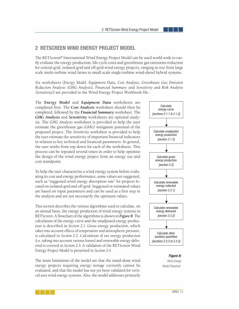
2. RETScreen Wind Energy Project Model
WIND.13
2 RETSCREEN WIND ENERGY PROJECT MODEL
The RETScreen® International Wind Energy Project Model can be used world-wide to eas-ily evaluate the energy production, life-cycle costs and greenhouse gas emissions reduction for central-grid, isolated-grid and off-grid wind energy projects, ranging in size from large scale multi-turbine wind farms to small scale single-turbine wind-diesel hybrid systems.
Six worksheets (Energy Model, Equipment Data, Cost Analysis, Greenhouse Gas Emission Reduction Analysis (GHG Analysis), Financial Summary and Sensitivity and Risk Analysis (Sensitivity)) are provided in the Wind Energy Project Workbook file.
The Energy Model and Equipment Data worksheets are completed first. The Cost Analysis worksheet should then be completed, followed by the Financial Summary worksheet. The GHG Analysis and Sensitivity worksheets are optional analy-sis. The GHG Analysis worksheet is provided to help the user estimate the greenhouse gas (GHG) mitigation potential of the proposed project. The Sensitivity worksheet is provided to help the user estimate the sensitivity of important financial indicators in relation to key technical and financial parameters. In general, the user works from top-down for each of the worksheets. This process can be repeated several times in order to help optimise the design of the wind energy project from an energy use and cost standpoint.
To help the user characterise a wind energy system before evalu-ating its cost and energy performance, some values are suggested, such as “suggested wind energy absorption rate” for projects lo-cated on isolated-grid and off-grid. Suggested or estimated values are based on input parameters and can be used as a first step in the analysis and are not necessarily the optimum values.
This section describes the various algorithms used to calculate, on an annual basis, the energy production of wind energy systems in RETScreen. A flowchart of the algorithms is shown in Figure 8. The calculation of the energy curve and the unadjusted energy produc-tion is described in Section 2.1. Gross energy production, which takes into account effects of temperature and atmospheric pressure, is calculated in Section 2.2. Calculation of net energy production (i.e. taking into account various losses) and renewable energy deliv-ered is covered in Section 2.3. A validation of the RETScreen Wind Energy Project Model is presented in Section 2.4.
The main limitations of the model are that the stand-alone wind energy projects requiring energy storage currently cannot be evaluated, and that the model has not yet been validated for verti-cal axis wind energy systems. Also, the model addresses primarily
Figure 8: Wind Energy
Model Flowchart.
Calculateenergy curve
[sections 2.1.1 & 2.1.2]
Calculate unadjustedenergy production
[section 2.1.3]
Calculate grossenergy production
[section 2.2]
Calculate renewableenergy collected[section 2.3.1]
Calculate renewableenergy delivered[section 2.3.2]
Calculate otherauxiliary quantities
[sections 2.3.3 to 2.3.5]

Wind Energy Project Analysis Chapter
WIND.14
“low penetration” technologies. To properly evaluate “high penetration” technologies cur-rently under development for isolated diesel-grid applications, the user will need to carefully evaluate the “wind energy absorption rate” used and will likely require further information. However, for the majority of the wind energy capacity being installed around the world today, these limitations are without consequence.
2.1 Unadjusted Energy Production
RETScreen calculates the unadjusted energy production from the wind turbines. It is the energy that one or more wind turbines will produce at standard conditions of temperature and atmospheric pressure. The calculation is based on the energy production curve of the selected wind turbine (entered in the Equipment Data worksheet) and on the average wind speed at hub height for the proposed site.
2.1.1 Wind speed distribution
Wind speed distribution, when required in the model (see Section 2.1.2), is calculated in RETScreen as a Weibull probability density function. This distribution is often used in wind energy engineering, as it conforms well to the observed long-term distribution of mean wind speeds for a range of sites. In some cases the model also uses the Rayleigh wind speed distribution, which is a special case of the Weibull distribution, where the shape factor (described below) is equal to 2.
The Weibull probability density function expresses the probability p x( ) to have a wind speed x during the year, as follows (Hiester and Pennell, 1981):
This expression is valid for k >1, x ≥ 0, and C > 0. k is the shape factor, specified by the user. The shape factor will typically range from 1 to 3. For a given average wind speed, a lower shape factor indicates a relatively wide distribution of wind speeds around the aver-age while a higher shape factor indicates a relatively narrow distribution of wind speeds around the average. A lower shape factor will normally lead to a higher energy production for a given average wind speed. C is the scale factor, which is calculated from the following equation (Hiester and Pennell, 1981):
where x is the average wind speed value and Γ is the gamma function.
p x kC
xC
xC
k k
( ) =
−
−1
exp (1)
C x
k
=+
Γ 1 1 (2)

2. RETScreen Wind Energy Project Model
WIND.15
In some cases, the model will calculate the wind speed distribution from the wind power density at the site rather than from the wind speed. The relations between the wind power density WPD and the average wind speed v are:
where is the air density and p(x) is the probability to have a wind speed x during the year.
2.1.2 Energy curve
The energy curve data is the total amount of energy a wind turbine produces over a range of annual average wind speeds. In RETScreen, the energy curve is specified over the range of 3 to 15 m/s annual average wind speed, and is displayed graphically in the Equipment Data worksheet.
The user can specify the energy curve data by choosing among the three following data sources: Standard, Custom and User-defined. For the standard and custom cases, the model uses the wind turbine power curve data entered by the user and the Weibull probability function described in Section 2.1.1 to calculate the energy curve data. In the User-defined case, the user directly enters the energy curve data.
In the Standard and Custom cases, the user specifies the wind turbine power curve as a function of wind speed in increments of 1 m/s, from 0 m/s to 25 m/s. Each point on the energy curve, Ev , is then calculated as:
where v is the mean wind speed considered (v =3, 4, …, 15 m/s), Px is the turbine power at wind speed x, and p x( ) is the Weibull probability density function for wind speed x , calculated for an average wind speed v .
(5)
(3)
(4)

Wind Energy Project Analysis Chapter
WIND.16
2.1.3 Unadjusted energy production
The unadjusted energy production is the energy produced by the turbines at standard conditions of temperature and atmospheric pressure. The calculation is based on the average wind speed at hub height for the proposed site. Wind speed at hub height is usually significantly higher than wind speed measured at anemometer height due to wind shear. The model uses the following power law equation to calculate the average wind speed at hub height [Gipe, 1995]:
where V is the average wind speed at hub height H, V0 is the wind speed at anemometer height H0, and α is the wind shear exponent. Values of H, H0, V0 and α are specified by the user2.
Once the annual average wind speed at hub height V is calculated, the unadjusted energy production EU is calculated simply by interpolating the energy curve from Section 2.1.2 at the value V .
2.2 Gross Energy Production
Gross energy production is the total annual energy produced by the wind energy equip-ment, before any losses, at the wind speed, atmospheric pressure and temperature con-ditions at the site. It is used in RETScreen to determine the renewable energy delivered (Section 2.3). Gross energy production EG is calculated through:
where EU is the unadjusted energy production, and cH and cT are the pressure and tem-perature adjustment coefficients. cH and cT are given by:
E E c cG U H T= (7)
VV
HH0 0
=
α
(6)
2. The same equation is used to calculate wind speed at the 10-meter level, with H set to 10 m. This latter value has no bearing on the energy calculation procedure; it is calculated in order to provide a common basis to compare two sites for which the wind speed has been measured at different heights.
c PPH =
0
(8)

2. RETScreen Wind Energy Project Model
WIND.17
where P is the annual average atmospheric pressure at the site, P0 is the standard atmospheric pressure of 101.3 kPa, T is the annual average absolute temperature at the site, and T0 is the standard absolute temperature of 288.1 K.
2.3 Renewable Energy Delivered
The RETScreen Wind Energy Project Model calculates the renewable energy delivered to the electricity grid, taking into account various losses. In the special case of isolated-grid and off-grid applications, the amount of wind energy that can be absorbed by the grid or the load is also considered.
2.3.1 Renewable energy collected
Renewable energy collected is equal to the net amount of energy produced by the wind energy equipment:
where EG is the gross energy production, and cL is the losses coefficient, given by:
where λa is the array losses, λs i& is the airfoil soiling and icing losses, λd is the downtime losses, and λm is the miscellaneous losses. Coefficients λa , λs i& , λd , and λm are specified by the user in the Energy Model worksheet.
E E cC G L= (10)
cL a s i d m= −( ) −( ) −( ) −( )&λ λ1 1 λ λ1 1 (11)
c TTT = 0 (9)
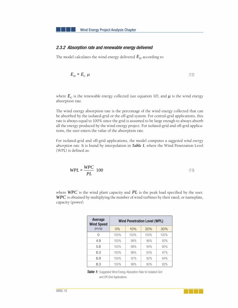
Wind Energy Project Analysis Chapter
WIND.18
2.3.2 Absorption rate and renewable energy delivered
The model calculates the wind energy delivered ED according to:
where EC is the renewable energy collected (see equation 10), and µ is the wind energy absorption rate.
The wind energy absorption rate is the percentage of the wind energy collected that can be absorbed by the isolated-grid or the off-grid system. For central-grid applications, this rate is always equal to 100% since the grid is assumed to be large enough to always absorb all the energy produced by the wind energy project. For isolated-grid and off-grid applica-tions, the user enters the value of the absorption rate.
For isolated-grid and off-grid applications, the model computes a suggested wind energy absorption rate. It is found by interpolation in Table 1, where the Wind Penetration Level (WPL) is defined as:
where WPC is the wind plant capacity and PL is the peak load specified by the user. WPC is obtained by multiplying the number of wind turbines by their rated, or nameplate, capacity (power).
Average Wind Speed
(m/s)
Wind Penetration Level (WPL)
0% 10% 20% 30%
0 100% 100% 100% 100%
4.9 100% 98% 96% 93%
5.6 100% 98% 94% 90%
6.3 100% 98% 93% 87%
6.9 100% 97% 92% 84%
8.3 100% 96% 90% 82%
Table 1: Suggested Wind Energy Absorption Rate for Isolated-Grid
and Off-Grid Applications.
WPL WPCPL
= 100 (13)
E ED C= µ (12)

2. RETScreen Wind Energy Project Model
WIND.19
As illustrated in Table 1, the suggested wind energy absorption rate varies according to the average wind speed and the wind penetration level. Note that it is based on the wind speed at the wind turbine hub height. Table 1 values are derived from simulations conducted to establish the amount of wind energy delivered from windfarms installed in remote communities (i.e. isolated-grid and off-grid applications). The simulations considered combinations of wind regime, load profiles and equipment performance curves. Detailed results can be found in Rangi et al. (1992).
The model only provides suggested values for wind penetration levels less than 25%. How-ever, if the wind penetration level is greater than 3% and the wind speed at hub height is 8.3 m/s or higher, then the model does not provide suggested values. Under these circum-stances, the wind energy absorption rates will vary widely depending on the configuration of the system and on the control strategies adopted.
2.3.3 Excess renewable energy available
Excess renewable energy available EX is simply the difference between the wind energy collected EC and the wind energy delivered ED :
2.3.4 Specifi c yield
The specific yield Y is obtained by dividing the renewable energy collected EC by the swept area of the turbines:
where N is the number of turbines and A is the area swept by the rotor of a single wind turbine.
Y EN A
C= (15)
E E EX C D= − (14)

Wind Energy Project Analysis Chapter
WIND.20
2.3.5 Wind plant capacity factor
The wind plant capacity factor PCF represents the ratio of the average power produced by the plant over a year to its rated power capacity. It is calculated as follows [Li and Priddy, 1985]:
where EC is the renewable energy collected, expressed in kWh, WPC is the wind plant capacity, expressed in kW, and hY is the number of hours in a year.
2.4 Validation
Numerous experts have contributed to the development, testing and validation of the RETScreen Wind Energy Project Model. They include wind energy modelling experts, cost engineering experts, greenhouse gas modelling specialists, financial analysis professionals, and ground station and satellite weather database scientists.
This section presents two examples of the validations completed. First, predictions of the RETScreen Wind Energy Project Model are compared to results from an hourly simulation program. Then, model predictions are compared to yearly data measured at a real wind energy project site.
2.4.1 Validation of wind energy model compared with an hourly model
In this section predictions of the RETScreen Wind Energy Project Model are compared with an hourly model. The hourly model used is HOMER, an optimisation model for de-signing stand-alone electric power systems (NREL, 2001). HOMER uses hourly simulations to optimise the design of hybrid power systems. HOMER can model any combination of wind turbines, photovoltaic panels, diesel generation, and battery storage. The present vali-dation does not make use of the optimisation capabilities of HOMER; the program is used only as a simulation tool. Two configurations were tested: a small windfarm connected to an isolated-grid and a large windfarm connected to a central-grid.
Small windfarm
The system configuration used for the first test is based on a real wind power project in Kotzebue, Alaska, a small coastal community about 50 km North of the Arctic Circle (CADDET, 2001). The system comprises 10 turbines with a combined rated capacity of 500 kW; it is a joint undertaking between the US Department of Energy, the Electric Power Research Institute (EPRI), and the Alaska Energy Authority-Alaska Industrial Development Export Authority (AEA/AIDEA). The system services a small local grid, with a total population of 3,500. The system is designed to meet about 6% of the total electrical demand of the town. The system configuration is summarised in Table 2.
C h
100PCF E
WPC
Y
=
(16)

2. RETScreen Wind Energy Project Model
WIND.21
Turbines
Atlantic Orient Corporation AOC 15/50
Number of turbines 10
Rotor diameter 15 m
Swept area 177 m2
Hub height 24 m
Grid type Isolated local grid
Local grid peak load 3.6 MW
Table 2: Kotzebue Wind System Confi guration.
The power output curve of the AOC 15/50 is shown in Figure 9. The same data were used for both software programs.
Weather data from the RETScreen online weather database for Kotzebue/Wien, AK, was used. RETScreen and HOMER differ in the type of wind speed they require. HOMER requires monthly wind speed values (shown in Table 3) and stochastically estimates hourly values from these. RETScreen simply requires the annual average wind speed, which is equal to 5.8 m/s (all wind values are measured at 9.4 m). In both models, a Weibull wind distribution was used, with a shape factor of 2.0. The annual average atmospheric pressure is 101.1 kPa and the annual average tempera-ture is -6°C.
Figure 9: AOC 15/50 Turbine Power Curve.
0
10
20
30
40
50
60
70
0 5 10 15 20 25
Wind speed (m/s)
Po
wer
out
put
(kW
)
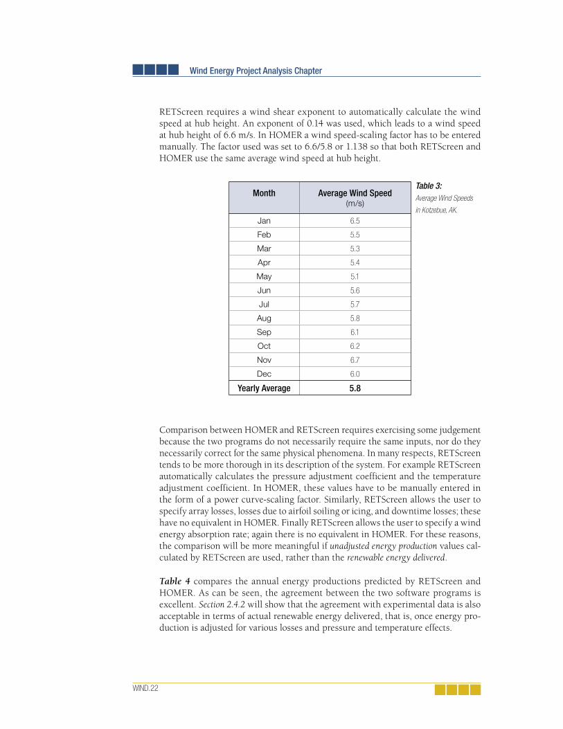
Wind Energy Project Analysis Chapter
WIND.22
RETScreen requires a wind shear exponent to automatically calculate the wind speed at hub height. An exponent of 0.14 was used, which leads to a wind speed at hub height of 6.6 m/s. In HOMER a wind speed-scaling factor has to be entered manually. The factor used was set to 6.6/5.8 or 1.138 so that both RETScreen and HOMER use the same average wind speed at hub height.
Month
Average Wind Speed (m/s)
Jan 6.5
Feb 5.5
Mar 5.3
Apr 5.4
May 5.1
Jun 5.6
Jul 5.7
Aug 5.8
Sep 6.1
Oct 6.2
Nov 6.7
Dec 6.0
Yearly Average 5.8
Comparison between HOMER and RETScreen requires exercising some judgement because the two programs do not necessarily require the same inputs, nor do they necessarily correct for the same physical phenomena. In many respects, RETScreen tends to be more thorough in its description of the system. For example RETScreen automatically calculates the pressure adjustment coefficient and the temperature adjustment coefficient. In HOMER, these values have to be manually entered in the form of a power curve-scaling factor. Similarly, RETScreen allows the user to specify array losses, losses due to airfoil soiling or icing, and downtime losses; these have no equivalent in HOMER. Finally RETScreen allows the user to specify a wind energy absorption rate; again there is no equivalent in HOMER. For these reasons, the comparison will be more meaningful if unadjusted energy production values cal-culated by RETScreen are used, rather than the renewable energy delivered.
Table 4 compares the annual energy productions predicted by RETScreen and HOMER. As can be seen, the agreement between the two software programs is excellent. Section 2.4.2 will show that the agreement with experimental data is also acceptable in terms of actual renewable energy delivered, that is, once energy pro-duction is adjusted for various losses and pressure and temperature effects.
Table 3: Average Wind Speeds
in Kotzebue, AK.

2. RETScreen Wind Energy Project Model
WIND.23
RETScreenUnadjusted Energy Production
(MWh)
HOMERTotal Energy Production
(MWh)Difference
1,532 1,515 +1.12%
Table 4: Comparison of Predicted Annual Energy Production – Small Windfarm.
Large windfarm
The second test configuration represents a large windfarm connected to a central-grid. The main parameters of the system are as follows:
76 Vestas V47-600kW turbines (hub height 55 m, diameter 47 m).
Annual average wind speed: 8.1 m/s.
Annual average temperature: 12°C.
Altitude of site: 250 m, annual average atmospheric pressure: 98.4 kPa.
Wind speed distribution: Weibull, shape factor: 1.8.
Wind shear exponent: 0.14.
The power output curve of the Vestas V47-600kW turbine is shown in Figure 10. The same data were used for both software programs.
According to RETScreen the average wind speed at hub height is 10.3 m/s. As in the small windfarm case, a wind speed-scaling factor equal to 10.3/8.1 or 1.272 had to be entered manually in HOMER so that both programs use the same average wind speed at hub height.
As before, unadjusted energy production values calculated by RETScreen are used, rather than the actual renewable energy delivered, to facilitate comparison with HOMER. The comparison is shown in Table 5. Once again, the agreement between the two software programs is excellent.
RETScreenUnadjusted Energy Production
(GWh)
HOMERTotal Energy Production
(GWh)Difference
258.2 265.2 -2.64%
Table 5: Comparison of Predicted Annual Energy Production – Large Windfarm.
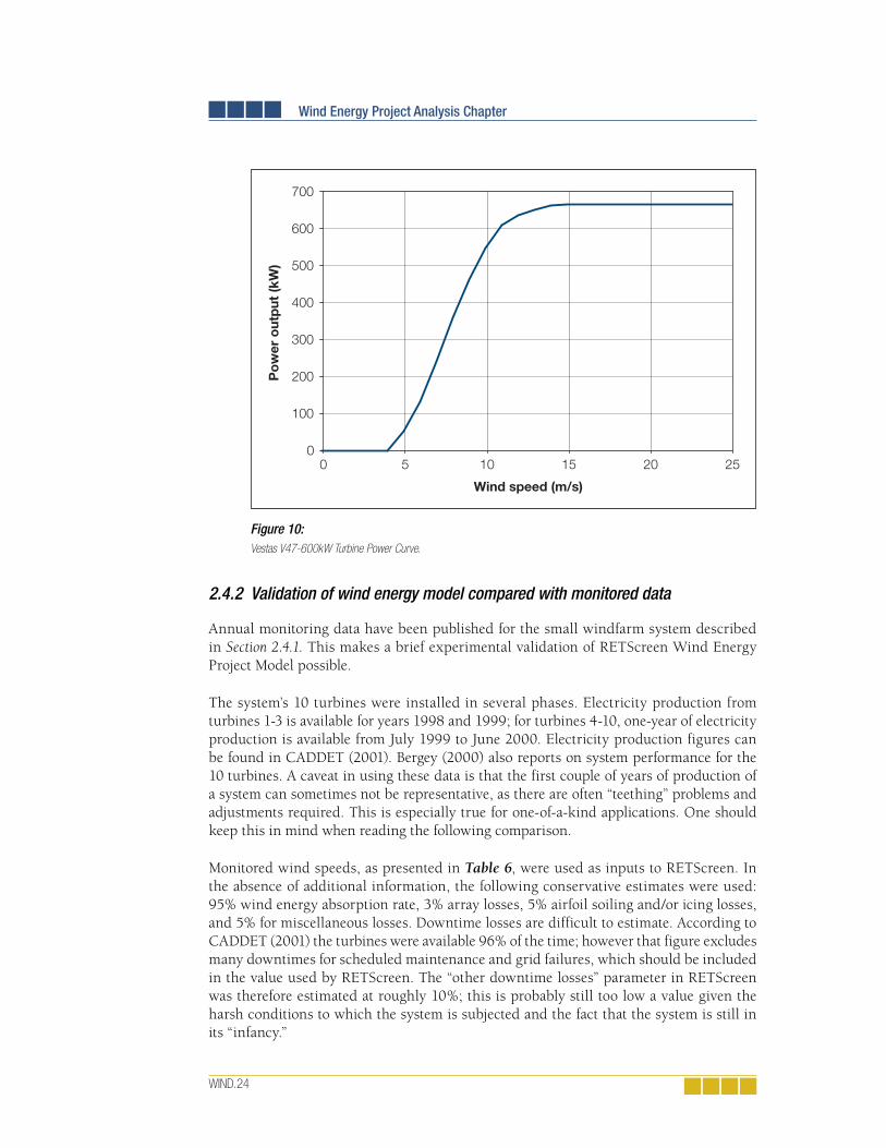
Wind Energy Project Analysis Chapter
WIND.24
2.4.2 Validation of wind energy model compared with monitored data
Annual monitoring data have been published for the small windfarm system described in Section 2.4.1. This makes a brief experimental validation of RETScreen Wind Energy Project Model possible.
The system’s 10 turbines were installed in several phases. Electricity production from turbines 1-3 is available for years 1998 and 1999; for turbines 4-10, one-year of electricity production is available from July 1999 to June 2000. Electricity production figures can be found in CADDET (2001). Bergey (2000) also reports on system performance for the 10 turbines. A caveat in using these data is that the first couple of years of production of a system can sometimes not be representative, as there are often “teething” problems and adjustments required. This is especially true for one-of-a-kind applications. One should keep this in mind when reading the following comparison.
Monitored wind speeds, as presented in Table 6, were used as inputs to RETScreen. In the absence of additional information, the following conservative estimates were used: 95% wind energy absorption rate, 3% array losses, 5% airfoil soiling and/or icing losses, and 5% for miscellaneous losses. Downtime losses are difficult to estimate. According to CADDET (2001) the turbines were available 96% of the time; however that figure excludes many downtimes for scheduled maintenance and grid failures, which should be included in the value used by RETScreen. The “other downtime losses” parameter in RETScreen was therefore estimated at roughly 10%; this is probably still too low a value given the harsh conditions to which the system is subjected and the fact that the system is still in its “infancy.”
Figure 10: Vestas V47-600kW Turbine Power Curve.
0
100
200
300
400
500
600
700
0 5 10 15 20 25
Wind speed (m/s)
Po
wer
out
put
(kW
)

2. RETScreen Wind Energy Project Model
WIND.25
Table 6 summarises RETScreen predictions versus actual energy production. RETScreen reasonably predicts the actual electricity production, except in 1999 where the energy production of the monitored project appears to have under-performed. For example, when comparing production of turbines 1-3 in 1998 and in 1999, it appears that the 3 turbines actually only produced 23% less energy in 1999 although the average wind was 10% higher than in 1998. Also, average production per turbine for a 5.4 m/s wind speed was 69.5 MWh in 1999 according to CADDET (2001) whereas it was 117.0 MWh (or 68% more) in 1999/2000 for the same 5.4 m/s average wind speed according to Bergey (2000). Again these discrepancies may be due to problems experienced by the installed wind energy system in its first few years of operation, and solved since then. The comparison of RETScreen predictions with real data is nevertheless acceptable and this, together with the model-to-model comparison of Section 2.4.1, confirms the adequacy of RETScreen for pre-feasibility studies of wind energy projects.
Period TurbinesAverage
Wind Speed(m/s)
RETScreenPrediction
(MWh)
Actual ElectricityProduction
(MWh)Difference
1998* 1-3 4.9 250 270.9 -8%
1999* 1-3 5.4 317 208.6 +52%
July 1999-June 2000* 4-10 5.1 646 546.9 +18%
1999-2000** 1-10 5.4 1,057 ≈1,170 -10%
* From CADDET (2001). ** From Bergey (2000).
Table 6: Comparison of RETScreen Predictions against Monitored Data for Kotzebue, AK.
2.5 Summary
In this section the algorithms used by the RETScreen Wind Energy Project Model have been shown in detail. The model uses a user-specified power curve and a Weibull wind speed probability distribution function to calculate the energy curve of the turbine. Energy production is then adjusted for pressure and temperature effects, as well as for various user-specified losses. In the case of isolated-grid and off-grid applications, the calculation of wind energy delivered takes into account the wind energy absorption rate. Comparison of the RETScreen model predictions against results of an hourly simulation program and against monitored data shows that the accuracy of the RETScreen Wind Energy Project Model is excellent in regards to the preparation of pre-feasibility studies, particularly given the fact that RETScreen only requires 1 point of wind speed data versus 8,760 points of data for most hourly simulation models.


WIND.27
REFERENCES
Bergey, M., Small Wind Systems For Rural Energy Supply, Village Power 2000, Washington, DC, USA, 2000.
Brothers, C., Wind Generation Systems for Remote Communities - Market Assessment and Guidelines for Wind Turbines Selection, Canadian Electrical Association, Project no. 9123 G 880, 1993.
CADDET, Technical Bulletin no. 143, 2001.
Canadian Wind Energy Association (CanWEA), Wind Energy Basic Information, Backgrounder Published with Support from CANMET, 1996.
Conover, K., Wind Energy Financial Due Diligence, R. Lynette & Associates, Seminar on Opportunities for Finance and Investment in Wind Energy, 1994.
Elliot, D. et al., Wind Energy Resource Atlas of the United States, SERI, 1986.
Gipe, P., Wind Energy Comes of Age, John Wiley & Sons, Inc., New York, NY, USA, 1995.
Hiester, T.R. and Pennell, W.T., The Siting Handbook for Large Wind Energy Systems, WindBooks, New York, NY, USA, 1981.
Le Gouriérès, D., Wind Power Plants: Theory and Design, Pergamon Press, 1982.
Leng, G., Dignard-Bailey, L., Bragagnolo, J., Tamizhmani, G. and Usher, E., Overview of the Worldwide Photovoltaic Industry, Report no. 96-41-A1 (TR), CANMET Energy Diversifi cation Research Laboratory, Natural Resources Canada, Varennes, QC, Canada, J3X 1S6, 1996.
Li, K.W. and Priddy, A.P., Power Plant System Design, John Wiley & Sons, Inc., New York, NY, USA, 1985.
Lynette, R. and Ass., Technical and Economic Potential for Wind Energy Development in Ontario, Prepared for Independent Power Producers’ Society of Ontario, 1992.
NREL, HOMER, The Hybrid Optimization Model for Electric Renewables, Available from National Renewable Energy Laboratory, 1617 Cole Boulevard, Golden, CO 80401-3393, USA, 2001.
Rangi, R., Templin, J., Carpentier, M. and Argue, D., Canadian Wind Energy Technical and Market Potential, EAETB, Energy, Mines and Resources Canada, 1992.
Reid, R., Application de l’éolien aux réseaux non-reliés, Hydro-Québec, Congrès de l’ACFAS, Montreal, QC, Canada, 1996.
SunMedia GmbH, Wind Turbine Market: Types, Technical Characteristics, Prices, 1999.
Vesterdal, J., The Potential of Wind Farms, ELSAM, 1992.
WECTEC, Évaluation du potentiel éolien du Québec, Report Prepared for the Ministère des Ressources naturelles du Québec, 1996.

WIND.28
Wind Power Monthly, The Windicator-Operational Wind Power Capacity Worldwide, 2001.
Winkra-Recom, Wind Turbine Market - Types, Technical Characteristics, Prices, 1995/96.
Zond, Wind Power Economics, Seminar on Opportunities for Finance and Investment in Wind Energy, 1994.


SMALL HYDROPROJECT ANALYSIS CHAPTER
CLEAN ENERGY PROJECT ANALYSIS:RETSCREEN® ENGINEERING & CASES TEXTBOOK
DisclaimerThis publication is distributed for informational purposes only and does not necessarily reflect the views of the Government of Canada nor constitute an endorsement of any commercial product or person. Neither Canada, nor its ministers, officers, employees and agents makeany warranty in respect to this publication nor a s s u m e a n y l i a b i l i t y a r i s i n g o u t o f t h i s publication.
© Minister of Natural Resources Canada 2001 - 2004.
www.retscreen.net
RETScreen® InternationalClean Energy Decision Support Centre

ISBN: 0-662-35671-3Catalogue no.: M39-98/2003E-PDF
© Minister of Natural Resources Canada 2001 - 2004.

HYDRO.3
TABLE OF CONTENTS
1 SMALL HYDRO BACKGROUND . . . . . . . . . . . . . . . . . . . . . . . . . . . . . . . . . . . . . . 5
1.1 Description of Small Hydro Power Plants . . . . . . . . . . . . . . . . . . . . . . . . . . . . . . . . 61.1.1 Civil works . . . . . . . . . . . . . . . . . . . . . . . . . . . . . . . . . . . . . . . . . . . . . . . . . . . . . . . . 6
1.1.2 Electrical and mechanical equipment . . . . . . . . . . . . . . . . . . . . . . . . . . . . . . . . . . . . . . 8
1.2 Small Hydro Project Development. . . . . . . . . . . . . . . . . . . . . . . . . . . . . . . . . . . . . 101.2.1 Types of small hydro developments . . . . . . . . . . . . . . . . . . . . . . . . . . . . . . . . . . . . . . 11
1.2.2 Hydro project engineering phases . . . . . . . . . . . . . . . . . . . . . . . . . . . . . . . . . . . . . . . 13
2 RETSCREEN SMALL HYDRO PROJECT MODEL . . . . . . . . . . . . . . . . . . . . . . . . . 15
2.1 Hydrology . . . . . . . . . . . . . . . . . . . . . . . . . . . . . . . . . . . . . . . . . . . . . . . . . . . . . . . 172.1.1 Flow-duration curve . . . . . . . . . . . . . . . . . . . . . . . . . . . . . . . . . . . . . . . . . . . . . . . . . 18
2.1.2 Available fl ow . . . . . . . . . . . . . . . . . . . . . . . . . . . . . . . . . . . . . . . . . . . . . . . . . . . . . 19
2.1.3 Firm fl ow . . . . . . . . . . . . . . . . . . . . . . . . . . . . . . . . . . . . . . . . . . . . . . . . . . . . . . . . 19
2.2 Load. . . . . . . . . . . . . . . . . . . . . . . . . . . . . . . . . . . . . . . . . . . . . . . . . . . . . . . . . . . 192.2.1 Energy demand. . . . . . . . . . . . . . . . . . . . . . . . . . . . . . . . . . . . . . . . . . . . . . . . . . . . 20
2.2.2 Average load factor . . . . . . . . . . . . . . . . . . . . . . . . . . . . . . . . . . . . . . . . . . . . . . . . . 21
2.3 Energy Production . . . . . . . . . . . . . . . . . . . . . . . . . . . . . . . . . . . . . . . . . . . . . . . . 212.3.1 Turbine effi ciency curve . . . . . . . . . . . . . . . . . . . . . . . . . . . . . . . . . . . . . . . . . . . . . . 21
2.3.2 Power available as a function of fl ow . . . . . . . . . . . . . . . . . . . . . . . . . . . . . . . . . . . . . 22
2.3.3 Plant capacity . . . . . . . . . . . . . . . . . . . . . . . . . . . . . . . . . . . . . . . . . . . . . . . . . . . . . 23
2.3.4 Power-duration curve. . . . . . . . . . . . . . . . . . . . . . . . . . . . . . . . . . . . . . . . . . . . . . . . 24
2.3.5 Renewable energy available . . . . . . . . . . . . . . . . . . . . . . . . . . . . . . . . . . . . . . . . . . . 25
2.3.6 Renewable energy delivered - central-grid. . . . . . . . . . . . . . . . . . . . . . . . . . . . . . . . . . 25
2.3.7 Renewable energy delivered - isolated-grid and off-grid . . . . . . . . . . . . . . . . . . . . . . . . 25
2.3.8 Small hydro plant capacity factor . . . . . . . . . . . . . . . . . . . . . . . . . . . . . . . . . . . . . . . . 28
2.3.9 Excess renewable energy available. . . . . . . . . . . . . . . . . . . . . . . . . . . . . . . . . . . . . . . 28
2.4 Project Costing . . . . . . . . . . . . . . . . . . . . . . . . . . . . . . . . . . . . . . . . . . . . . . . . . . . 28
2.5 Validation . . . . . . . . . . . . . . . . . . . . . . . . . . . . . . . . . . . . . . . . . . . . . . . . . . . . . . . 292.5.1 Turbine effi ciency . . . . . . . . . . . . . . . . . . . . . . . . . . . . . . . . . . . . . . . . . . . . . . . . . . 29
2.5.2 Plant capacity and annual renewable energy delivered. . . . . . . . . . . . . . . . . . . . . . . . . . 31
2.5.3 Project costs. . . . . . . . . . . . . . . . . . . . . . . . . . . . . . . . . . . . . . . . . . . . . . . . . . . . . . 32
2.6 Summary . . . . . . . . . . . . . . . . . . . . . . . . . . . . . . . . . . . . . . . . . . . . . . . . . . . . . . . 34
REFERENCES . . . . . . . . . . . . . . . . . . . . . . . . . . . . . . . . . . . . . . . . . . . . . . . . . . . . 35
APPENDIX A - TURBINE EFFICIENCY FORMULAE . . . . . . . . . . . . . . . . . . . . . . . . . 37
APPENDIX B - FORMULAE FOR FORMULA COSTING METHOD . . . . . . . . . . . . . . . 41


1. Small Hydro Background
HYDRO.5
SMALL HYDRO PROJECT ANALYSIS CHAPTERClean Energy Project Analysis: RETScreen® Engineering & Cases is an electronic textbook for professionals and uni-versity students. This chapter covers the analysis of potential small hydro projects using the RETScreen® International Clean Energy Project Analysis Software, including a technology background and a detailed description of the algorithms found in the RETScreen® Software. A collection of project case studies, with assignments, worked-out solutions and information about how the projects fared in the real world, is available at the RETScreen® International Clean Energy Decision Support Centre Website www.retscreen.net.
1 SMALL HYDRO BACKGROUND1
Hydroelectricity is one of the most mature forms of renewable energy, providing more than 19% of the world’s electricity consumption from both large and small power plants. Coun-tries such as Brazil, the United States, Canada and Norway produce significant amounts of electricity from very large hydroelectric facilities. However, there are also many regions of the world that have a significant number of small hydro power plants in operation, such as the one depicted in Figure 1. In China, for example, more than 19,000 MW of electricity is produced from 43,000 small hydro facilities.
1. Some of the text in this “Background” description comes from the following reference: Bennett, K., Small Hydro in Canada: An Overview, prepared for Industry, Science and Technology Canada, Aboriginal Economic Programs, 1990.
Figure 1: 2.6 MW Small Hydro Power
Project in Canada.
Photo Credit: SNC-Lavalin

Small Hydro Project Analysis Chapter
HYDRO.6
There is no universally accepted definition of the term “small hydro” which, depending on local definitions can range in size from a few kilowatts to 50 megawatts or more of rated power output. Internationally, “small” hydro power plant capacities typically range in size from 1 MW to 50 MW, with projects in the 100 kW to 1 MW range sometimes referred to as “mini” hydro and projects under 100 kW referred to as “micro” hydro. Installed capac-ity, however, is not always a good indicator of the size of a project. For example, a 20 MW, low-head “small” hydro plant is anything but small as low-head projects generally use much larger volumes of water, and require larger turbines as compared with high-head projects.
1.1 Description of Small Hydro Power Plants
A small hydro generating station can be described under two main headings: civil works, and electrical and mechanical equipment. Refer to Figure 2 below for a schematic of a typical small hydro power plant.
1.1.1 Civil works
The main civil works of a small hydro development are the diversion dam or weir, the water passages and the powerhouse as depicted in Figure 3. The diversion dam or weir directs the water into a canal, tunnel, penstock or turbine inlet. The water then passes through the turbine, spinning it with enough force to create electricity in a generator. The water then flows back into the river via a tailrace. Generally, small hydro projects built for applica-tion at an isolated area are run-of-river developments, meaning that water is not stored in a reservoir and is used only as it is available. The cost of large water storage dams cannot normally be justified for small waterpower projects and consequently, a low dam or diver-sion weir of the simplest construction is normally used. Construction can be of concrete, wood, masonry or a combination of these materials. Considerable effort continues to be spent to lower the cost of dams and weirs for small hydro projects, as the cost of this item alone frequently renders a project not financially viable.
Figure 2:Small Hydro Project
System Schematic.

1. Small Hydro Background
HYDRO.7
The water passages of a small hydro project comprise the following:
An intake which includes trashracks, a gate and an entrance to a canal, penstock or directly to the turbine depending on the type of development. The intake is generally built of reinforced concrete, the trashrack of steel, and the gate of wood or steel.
A canal, tunnel and/or penstock, which carries the water to the power-house in developments where the powerhouse is located at a distance downstream from the intake. Canals are generally excavated and followthe contours of the existing terrain. Tunnels are underground and exca-vated by drilling and blasting or by using a tunnel-boring machine. Pen-stocks, which convey water under pressure, can be made of steel, iron, fi breglass, plastics, concrete or wood.
The entrance and exit of the turbine, which include the valves and gates necessary to shut off fl ow to the turbine for shutdown and maintenance. These components are generally made of steel or iron. Gates downstream of the turbine, if required for maintenance, can be made of wood.
Figure 3:Civil Works for a 700 kW Mini Hydro Project.
Photo Credit: Ottawa Engineering

Small Hydro Project Analysis Chapter
HYDRO.8
A tailrace, which carries the water from the turbine exit back to the river. The tailrace, like the canal, is exca-vated.
The powerhouse contains the turbine or tur-bines and most of the mechanical and electri-cal equipment as depicted in Figure 4. Small hydro powerhouses are generally kept to the minimum size possible while still provid-ing adequate foundation strength, access for maintenance, and safety. Construction is of concrete and other local building materials.
Simplicity in design, with an emphasis on practical, easily constructed civil structures is of prime concern for a small hydro project in order to keep costs at a minimum.
1.1.2 Electrical and mechanical equipment
The primary electrical and mechanical components of a small hydro plant are the turbine(s) and generator(s).
A number of different types of turbines have been designed to cover the broad range of hy-dropower site conditions found around the world. Turbines used for small hydro applications are scaled-down versions of turbines used in conventional large hydro developments.
Turbines used for low to medium head applications are usually of the reaction type and include Francis and fixed and variable pitch (Kaplan) propeller turbines. The runner or turbine “wheel” of a reaction turbine is completely submersed in water. Turbines used for high-head applications are generally referred to as impulse turbines. Impulse turbines include the Pelton (see Figure 5), Turgo and crossflow designs. The runner of an impulse turbine spins in the air and is driven by a high-speed jet of water.
Small hydro turbines can attain efficiencies of about 90%. Care must be given to selecting the preferred turbine design for each application as some turbines only operate efficiently over a limited flow range (e.g. propeller turbines with fixed blades and Francis turbines). For most run-of-river small hydro sites where flows vary considerably, turbines that operate efficiently over a wide flow range are usually preferred (e.g. Kaplan, Pelton, Turgo and crossflow de-signs). Alternatively, multiple turbines that operate within limited flow ranges can be used.
There are two basic types of generators used in small hydro plants - synchronous or induction (asynchronous). A synchronous generator can be operated in isolation while an induction generator must normally be operated in conjunction with other generators. Synchronous generators are used as the primary source of power produced by utilities and for isolated diesel-grid and stand-alone small hydro applications. Induction generators with
Figure 4:Small Hydro Powerhouse Containing Francis Turbine.
Photo Credit: PO Sjöman Hydrotech Consulting

1. Small Hydro Background
HYDRO.9
capacities less than about 500 kW are generally best suited for small hydro plants provid-ing energy to a large existing electricity grid.
Other mechanical and electrical components of a small hydro plant include:
Speed increaser to match the ideal rotational speed of the turbine to that of the generator (if required);
Water shut-off valve(s) for the turbine(s);
River by-pass gate and controls (if required);
Hydraulic control system for the turbine(s) and valve(s);
Electrical protection and control system;
Electrical switchgear;
Transformers for station service and power transmission;
Station service including lighting and heating and power to run control systems and switchgear;
Water cooling and lubricating system (if required);
Ventilation system;
Backup power supply;
Telecommunication system;
Fire and security alarm systems (if required); and
Utility interconnection or transmission and distribution system.
Figure 5:Pelton Turbine.
Photo Credit: PO Sjöman Hydrotech Consulting

Small Hydro Project Analysis Chapter
HYDRO.10
1.2 Small Hydro Project Development
The development of small hydro projects typically takes from 2 to 5 years to complete, from conception to final commissioning. This time is required to undertake studies and design work, to receive the necessary approvals and to construct the project. Once constructed, small hydro plants require little maintenance over their useful life, which can be well over 50 years. Normally, one part-time operator can easily handle operation and routine maintenance of a small hydro plant, with periodic maintenance of the larger components of a plant usually requiring help from outside contractors.
The technical and financial viability of each potential small hydro project are very site specific. Power output depends on the available water (flow) and head (drop in elevation). The amount of en-ergy that can be generated depends on the quantity of water available and the variability of flow throughout the year. The economics of a site depends on the power (capacity) and the energy that a project can produce, whether or not the energy can be sold, and the price paid for the energy. In an isolated area (off-grid and isolated-grid applications) the value of energy generated for consumption is generally significantly more than for systems that are connected to a central-grid. However, isolated areas may not be able to use all the available energy from the small hydro plant and, may be unable to use the energy when it is available because of seasonal variations in water flow and energy consumption.
A conservative, “rule-of-thumb” relationship is that power for a hydro project is equal to seven times the product of the flow (Q) and gross head (H) at the site (P = 7QH). Produc-ing 1 kW of power at a site with 100 m of head will require one-tenth the flow of water that a site with 10 m of head would require. The hydro turbine size depends primarily on the flow of water it has to accommodate. Thus, the generating equipment for higher-head, lower-flow installations is generally less expensive than for lower-head, higher-flow plants. The same cannot necessarily be said for the civil works components of a project which are related much more to the local topography and physical nature of a site.
RETScreen® InternationalSmall Hydro Project Model
The RETScreen® International Small Hydro Project Model can be used world-wide to easily evaluate the energy production, life-cycle costs and greenhouse gas emissions reduction for central-grid, isolated-grid and off-grid small hydro projects, ranging in size from multi-turbine small and mini hydro installations to single-turbine micro hydro systems.

1. Small Hydro Background
HYDRO.11
1.2.1 Types of small hydro developments
Small hydro projects can generally be categorised as either “run-of-river developments” or “water storage (reservoir) developments,” which are described in more detail below.
Run-of-river developments
“Run-of-river” refers to a mode of operation in which the hydro plant uses only the water that is available in the natural flow of the river, as depicted in Figure 6. “Run-of-river” implies that there is no water storage and that power fluctuates with the stream flow.
The power output of run-of-river small hydro plants fluctuates with the hydrologic cycle, so they are often best suited to provide energy to a larger electricity system. Individually, they do not generally provide much firm capacity. Therefore, isolated areas that use small hydro resources often require supplemental power. A run-of-river plant can only supply all of the electrical needs of an isolated area or industry if the minimum flow in the river is sufficient to meet the load’s peak power requirements.
Run-of-river small hydro can involve diversion of the flow in a river. Diversion is often required to take advantage of the drop in elevation that occurs over a distance in the river. Diversion projects reduce the flow in the river between the intake and the powerhouse. A diversion weir or small dam is usually required to divert the flow into the intake.
Figure 6:Run-of-River Small
Hydro Project in a
Remote Community.
Photo Credit: Robin Hughes/PNS

Small Hydro Project Analysis Chapter
HYDRO.12
Water storage (reservoir) developments
For a hydroelectric plant to provide power on demand, either to meet a fluctuating load or to provide peak power, water must be stored in one or more reservoirs2. Unless a natural lake can be tapped, providing storage usually requires the con-struction of a dam or dams and the creation of new lakes. This impacts the local environment in both negative and positive ways, although the scale of development often magnifies the negative impacts. This often presents a conflict, as larger hydro projects are attractive because they can provide “stored” power during peak demand periods. Due to the economies of scale and the complex approval process, storage schemes tend to be relatively large in size.
The creation of new storage reservoirs for small hydro plants is generally not financially viable except, possibly, at isolated locations where the value of energy is very high. Storage at a small hydro plant, if any, is generally limited to small volumes of water in a new head pond or existing lake upstream of an existing dam. Pondage is the term used to describe small volumes of water storage. Pondage can provide benefits to small hydro plants in the form of increased energy production and/or increased revenue.
Another type of water storage development is “pumped storage” where water is “recy-cled” between downstream and upstream storage reservoirs. Water is passed through turbines to generate power during peak periods and pumped back to the upper reser-voir during off-peak periods. The economics of pumped storage projects depends on the difference between the values of peak and off-peak power. Due to the inefficiencies involved in pumping versus generating, the recycling of water results in a net consump-tion of energy. Energy used to pump water has to be generated by other sources.
The environmental impacts that can be associated with small hydro developments can vary significantly depending on the location and configuration of the project.
The effects on the environment of developing a run-of-river small hydro plant at an exist-ing dam are generally minor and similar to those related to the expansion of an existing facility. Development of a run-of-river small hydro plant at an undeveloped site can pose additional environmental impacts. A small dam or diversion weir is usually required. The most economical development scheme might involve flooding some rapids upstream of the new small dam or weir.
The environmental impacts that can be associated with hydroelectric developments that incorporate water storage (typically larger in size) are mainly related to the creation of a water storage reservoir. The creation of a reservoir involves the construction of a relatively large dam, or the use of an existing lake to impound water. The creation of a new reservoir with a dam involves the flooding of land upstream of the dam. The use of water stored in the reservoir behind a dam or in a lake results in the fluctuation of water levels and flows in the river downstream. A rigorous environmental assessment is typically required for any project involving water storage.
2. Except in the run-of-river case where the minimum fl ow in the river can provide the peak power requirement.

1. Small Hydro Background
HYDRO.13
1.2.2 Hydro project engineering phases
According to Gordon (1989), there are normally four phases for engineering work required to develop a hydro project. Note, however, that for small hydro, the engineering work is often reduced to three phases in order to reduce costs. Generally, a preliminary investiga-tion is undertaken that combines the work involved in the first two phases described below. The work, however, is completed to a lower level of detail in order to reduce costs. While reducing the engineering work increases the risk of the project not being financially viable, this can usually be justified due to the lower costs associated with smaller projects.
Reconnaissance surveys and hydraulic studies
This first phase of work frequently covers numerous sites and includes: map studies; delineation of the drainage basins; preliminary estimates of flow and floods; and a one day site visit to each site (by a design engineer and geologist or geotechnical engineer); preliminary layout; cost estimates (based on formulae or computer data); a final ranking of sites based on power potential; and an index of cost.
Pre-feasibility study
Work on the selected site or sites would include: site mapping and geological inves-tigations (with drilling confined to areas where foundation uncertainty would have a major effect on costs); a reconnaissance for suitable borrow areas (e.g. for sand and gravel); a preliminary layout based on materials known to be available; preliminary selection of the main project characteristics (installed capacity, type of development, etc.); a cost estimate based on major quantities; the identification of possible envi-ronmental impacts; and production of a single volume report on each site.
Feasibility study
Work would continue on the selected site with a major foundation investigation pro-gramme; delineation and testing of all borrow areas; estimation of diversion, design and probable maximum floods; determination of power potential for a range of dam heights and installed capacities for project optimisation; determination of the project design earthquake and the maximum credible earthquake; design of all structures in sufficient detail to obtain quantities for all items contributing more than about 10% to the cost of individual structures; determination of the dewatering sequence and project schedule; optimisation of the project layout, water levels and components; production of a detailed cost estimate; and finally, an economic and financial evalu-ation of the project including an assessment of the impact on the existing electrical grid along with a multi-volume comprehensive feasibility report.
System planning and project engineering
This work would include studies and final design of the transmission system; inte-gration of the transmission system; integration of the project into the power network to determine precise operating mode; production of tender drawings and specifi-cations; analysis of bids and detailed design of the project; production of detailed construction drawings and review of manufacturer’s equipment drawings. However, the scope of this phase would not include site supervision nor project management, since this work would form part of the project execution costs.


2. RETScreen Small Hydro Project Model
HYDRO.15
2 RETSCREEN SMALL HYDRO PROJECT MODEL
The RETScreen Small Hydro Project Model provides a means to assess the available energy at a potential small hydro site that could be provided to a central-grid or, for isolated loads, the portion of this available energy that could be harnessed by a local electric utility (or used by the load in an off-grid system). The model addresses both run-of-river and reser-voir developments, and it incorporates sophisticated formulae for calculating efficiencies of a wide variety of hydro turbines.
The Small Hydro model can be used to evaluate small hydro projects typically classified under the following three names:
Small hydro;
Mini hydro; and
Micro hydro.
The Small Hydro Project Model has been developed primarily to determine whether work on the small hydro project should proceed further or be dropped in favour of other alter-natives. Each hydro site is unique, since about 75% of the development cost is determined by the location and site conditions. Only about 25% of the cost is relatively fixed, being the cost of manufacturing the electromechanical equipment.
Seven worksheets (Energy Model, Hydrology Analysis and Load Calculation (Hydrology & Load), Equipment Data, Cost Analysis, Greenhouse Gas Emission Reduction Analysis (GHG Analysis), Financial Summary and Sensitivity and Risk Analysis (Sensitivity)) are provided in the Small Hydro Project Workbook file.
The Energy Model, Hydrology & Load and Equipment Data worksheets are completed first. The Cost Analysis worksheet should then be completed, followed by the Financial Summary worksheet. The GHG Analysis and Sensitivity worksheets are optional analy-sis. The GHG Analysis worksheet is provided to help the user estimate the greenhouse gas (GHG) mitigation potential of the proposed project. The Sensitivity worksheet is provided to help the user estimate the sensitivity of important financial indicators in relation to key technical and financial parameters. In general, the user works from top-down for each of the worksheets. This process can be repeated several times in order to help optimise the design of the small hydro project from an energy use and cost standpoint.
The RETScreen Small Hydro Project Model provides the user with two different methods for estimating project costs: the “Formula” and the “Detailed” costing methods. All the hydro cost equations used in the “Formula” costing method are empirical, based on data collected over 20 years for both large and small hydro facilities. They have been extended to include more site data for this analysis (Gordon, 1989 & 1991). If used correctly, the “Formula” costing method will provide a baseline, or minimum, cost estimate for a proposed project.

Small Hydro Project Analysis Chapter
HYDRO.16
The “Detailed” costing method allows the user to estimate costs based on estimated quanti-ties and unit costs. The use of this costing method requires that the user estimate the size and the layout of the required structures. If the user chooses to use this method, the results should be compared with results from the “Formula” costing method.
In order to use the RETScreen Small Hydro Project Model, the user may require certain information that can be obtained from available topographic maps. Topographic maps can be purchased or ordered from most map stores. In cases where a previous hydrologic assessment has been undertaken for the site in question, the pertinent data from this as-sessment can be used in the model. The user should be aware that if the available head, or drop in elevation, at a site is unknown, a site visit will be required to measure the head unless detailed mapping is available. The measurement of head can be done easily using simple surveying techniques.
This section describes the various algorithms used to calculate, on an annual basis, the energy production of small hydro power plants in RETScreen. A flowchart of the algo-rithms is shown in Figure 7. User inputs include the flow-duration curve (Section 2.1) and, for isolated-grid and off-grid applications, the load-duration curve (Section 2.2). Turbine efficiency is calculated at regular intervals on the flow-duration curve (Sections 2.3.1 and 2.3.2 and Appendix A). Plant capacity is then calculated (Section 2.3.3) and the power-dura-tion curve is established (Section 2.3.4). Available energy is simply calculated by integrating the power-duration curve (Section 2.3.5). In the case of a central-grid, the energy delivered is equal to the energy available (Section 2.3.6). In the case of an isolated-grid or off-grid ap-plication, the procedure is slightly more complicated and involves both the power-duration curve and the load-duration curve (Section 2.3.7). The Formula Costing Method (Section 2.4) is described in detail in Appendix B and a validation of the RETScreen Small Hydro Project Model is presented in Section 2.5.
There are some limitations associated with the Small Hydro Project Model. First, the model has been designed primarily to evaluate run-of-river small hydro projects. The evaluation of storage projects is possible, however, a number of assumptions are required. Variations in gross head due to changes in reservoir water level cannot be simulated. The model re-quires a single value for gross head and, in the case of reservoir projects, an appropriate av-erage value must be entered. The determination of the average head must be done outside of the model and will require an understanding of the effects of variations in head on annual energy production. Second, for isolated-grid and off-grid applications in isolated areas, the energy demand has been assumed to follow the same pattern for every day of the year. For isolated locations where energy demand and available energy vary significantly over the course of a year, adjustments will have to be made to the estimated amount of renewable energy delivered. This is done by changing the “Available flow adjustment factor” in the Energy Model worksheet. These limitations aside, the model is fairly easy to understand and use. As will be seen in the next sections, the model condenses in an easy-to-use format a wealth of information, and it should be of great assistance to engineers involved in the preliminary evaluation of small hydro projects.

2. RETScreen Small Hydro Project Model
HYDRO.17
2.1 Hydrology
In RETScreen, hydrological data are specified as a flow-duration curve, which is assumed to represent the flow conditions in the river being studied over the course of an average year. For storage projects, data must be entered manually by the user and should represent the regulated flow that results from operating a reservoir; at present, the head variation with storage drawdown is not included in the model. For run-of-river projects, the required flow-duration curve data can be entered either manually or by using the specific run-off method and data contained in the RETScreen Online Weather Database.
Load-duration curve[section 2.2]
Flow-duration curve[section 2.1]
Calculation ofturbine efficiency curve[sections 2.3.1 & 2.3.2]
Calculation ofplant capacity[section 2.3.3]
Calculation of power-duration curve[section 2.3.4]
Calculation of renewableenergy available[section 2.3.5]
Calculation of renewableenergy delivered
(isolated-grid and off-grid)[section 2.3.7]
Calculation of renewable energy delivered
(central-grid)[section 2.3.6]
Figure 7:Small Hydro Energy
Model Flowchart.
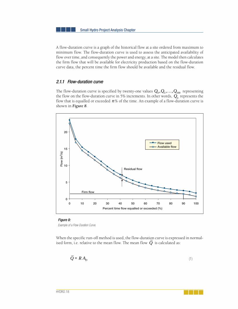
Small Hydro Project Analysis Chapter
HYDRO.18
A flow-duration curve is a graph of the historical flow at a site ordered from maximum to minimum flow. The flow-duration curve is used to assess the anticipated availability of flow over time, and consequently the power and energy, at a site. The model then calculates the firm flow that will be available for electricity production based on the flow-duration curve data, the percent time the firm flow should be available and the residual flow.
2.1.1 Flow-duration curve
The flow-duration curve is specified by twenty-one values Q Q Q0 5 100, , ,… representing the flow on the flow-duration curve in 5% increments. In other words, Qn represents the flow that is equalled or exceeded n% of the time. An example of a flow-duration curve is shown in Figure 8.
When the specific run-off method is used, the flow-duration curve is expressed in normal-ised form, i.e. relative to the mean flow. The mean flow Q is calculated as:
Figure 8: Example of a Flow-Duration Curve.
0
5
10
15
20
0 10 20 30 40 50 60 70 80 90 100
Percent time flow equalled or exceeded (%)
Flo
w (m
3 /s)
Flow usedAvailable flow
Residual flow
Firm flow
Q R AD= (1)

2. RETScreen Small Hydro Project Model
HYDRO.19
where R is the specific run-off and AD is the drainage area. Then the actual flow data Qn ( n =0,5,…,100) is computed from the normalised flow data qn extracted from the weather database through:
2.1.2 Available fl ow
Often, a certain amount of flow must be left in the river throughout the year for environ-mental reasons. This residual flow Qr is specified by the user and must be subtracted from all values of the flow-duration curve for the calculation of plant capacity, firm capacity and renewable energy available, as explained further on in this chapter. The available flow ′Qn (n = 0, 5, …, 100) is then defined by:
The available flow-duration curve is shown in Figure 8, with as an example Qr set to 1 m3/s.
2.1.3 Firm fl ow
The firm flow is defined as the flow being available p% of the time, where p is a percent-age specified by the user and usually equal to 95%. The firm flow is calculated from the available flow-duration curve. If necessary, a linear interpolation between 5% intervals is used to find the firm flow. In the example of Figure 8 the firm flow is equal to 1.5 m3/s with p set to 90%.
2.2 Load
The degree of sophistication used to describe the load depends on the type of grid consid-ered. If the small hydro power plant is connected to a central-grid, then it is assumed that the grid absorbs all of the energy production and the load does not need to be specified. If on the other hand the system is off-grid or connected to an isolated-grid, then the por-tion of the energy that can be delivered depends on the load. The RETScreen Small Hydro Project Model assumes that the daily load demand is the same for all days of the year and can be represented by a load-duration curve. An example of such a curve is shown in Fig-ure 9. As for the flow-duration curve of Section 2.1.1, the load-duration curve is specified by twenty-one values L L L0 5 100, , ,… defining the load on the load-duration curve in 5% increments: Lk represents the load that is equalled or exceeded k % of the time.
Q q Qn n= (2)
′ = −( )Q Q Qn n rmax ,0 (3)
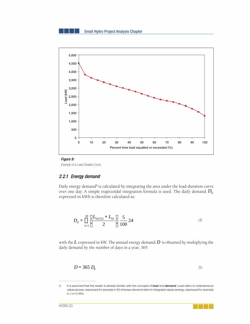
Small Hydro Project Analysis Chapter
HYDRO.20
2.2.1 Energy demand
Daily energy demand3 is calculated by integrating the area under the load-duration curve over one day. A simple trapezoidal integration formula is used. The daily demand Dd expressed in kWh is therefore calculated as:
with the L expressed in kW. The annual energy demand D is obtained by multiplying the daily demand by the number of days in a year, 365:
DL L
dk k
k=
+
−
=∑ 5 1 5
1
20
25
10024( ) (4)
3. It is assumed that the reader is already familiar with the concepts of load and demand. Load refers to instantaneous values (power, expressed for example in W) whereas demand refers to integrated values (energy, expressed for example in J or in Wh).
Figure 9: Example of a Load-Duration Curve.
0
500
1,000
1,500
2,000
2,500
3,000
3,500
4,000
4,500
5,000
0 10 20 30 40 50 60 70 80 90 100
Percent time load equalled or exceeded (%)
Load
(kW
)
D Dd= 365 (5)

2. RETScreen Small Hydro Project Model
HYDRO.21
2.2.2 Average load factor
The average load factor L is the ratio of the average daily load (Dd 24) to the peak load (L0):
This quantity is not used by the rest of the algorithm but is simply provided to the user to give an indication of the variability of the load.
2.3 Energy Production
The RETScreen Small Hydro Project Model calculates the estimated renewable energy delivered (MWh) based on the adjusted available flow (adjusted flow-duration curve), the design flow, the residual flow, the load (load-duration curve), the gross head and the efficiencies/losses. The calculation involves comparing the daily renewable energy available to the daily load-duration curve for each of the flow-duration curve values.
2.3.1 Turbine effi ciency curve
Small hydro turbine efficiency data can be entered manually or can be calculated by RETScreen. Calculated efficiencies can be adjusted using the Turbine manufacture/design coefficient and Efficiency adjustment factor in the Equipment Data worksheet of the model. Standard turbine efficiencies curves have been developed for the following turbine types:
Kaplan (reaction turbine)
Francis (reaction turbine)
Propellor (reaction turbine)
Pelton (impulse turbine)
Turgo (impulse turbine)
Cross-fl ow (generally classifi ed as an impulse turbine).
The type of turbine is selected based on its suitability to the available head and flow conditions. The calculated turbine efficiency curves take into account a number of fac-tors including rated head (gross head less maximum hydraulic losses), runner diameter (calculated), turbine specific speed (calculated for reaction turbines) and the turbine manufacture/design coefficient. The efficiency equations were derived from a large number of manufacture efficiency curves for different turbine types and head and flow conditions. The turbine efficiency equations are described in Appendix A.
L DLd= 24
0
(6)
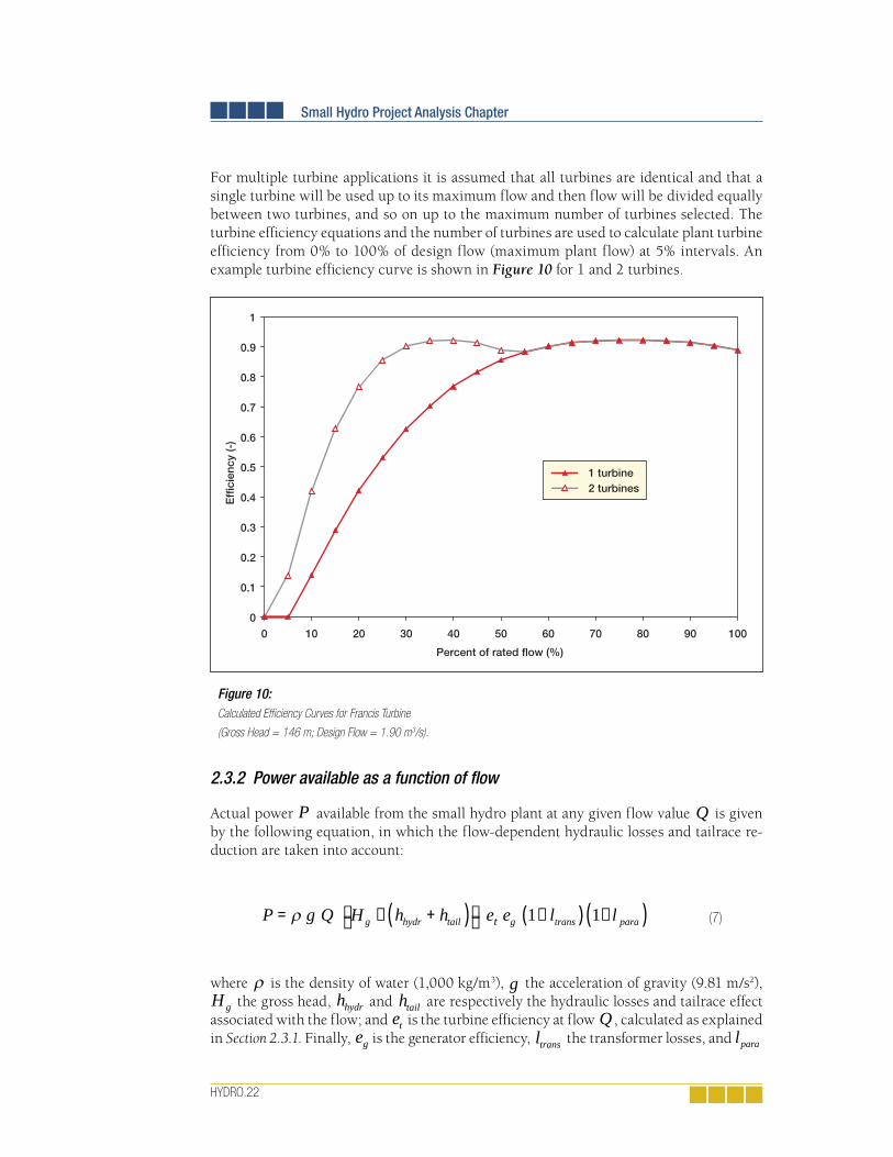
Small Hydro Project Analysis Chapter
HYDRO.22
For multiple turbine applications it is assumed that all turbines are identical and that a single turbine will be used up to its maximum flow and then flow will be divided equally between two turbines, and so on up to the maximum number of turbines selected. The turbine efficiency equations and the number of turbines are used to calculate plant turbine efficiency from 0% to 100% of design flow (maximum plant flow) at 5% intervals. An example turbine efficiency curve is shown in Figure 10 for 1 and 2 turbines.
2.3.2 Power available as a function of fl ow
Actual power P available from the small hydro plant at any given flow value Q is given by the following equation, in which the flow-dependent hydraulic losses and tailrace re-duction are taken into account:
where ρ is the density of water (1,000 kg/m3), g the acceleration of gravity (9.81 m/s2), Hg the gross head, hhydr and htail are respectively the hydraulic losses and tailrace effect associated with the flow; and et is the turbine efficiency at flow Q , calculated as explained in Section 2.3.1. Finally, eg is the generator efficiency, ltrans the transformer losses, and lpara
P g Q H h h e e l lg hydr tail t g trans para= − +( ) −( ) −( )ρ 1 1 (7)
Figure 10: Calculated Effi ciency Curves for Francis Turbine
(Gross Head = 146 m; Design Flow = 1.90 m3/s).
0
0.1
0.2
0.3
0.4
0.5
0.6
0.7
0.8
0.9
1
0 10 20 30 40 50 60 70 80 90 100
Percent of rated flow (%)
Eff
icie
ncy
(-)
1 turbine2 turbines

2. RETScreen Small Hydro Project Model
HYDRO.23
the parasitic electricity losses; eg , ltrans , and lpara are specified by the user in the Energy
Model worksheet and are assumed independent from the flow considered.
Hydraulic losses are adjusted over the range of available flows based on the following relationship:
where lhydr max, is the maximum hydraulic losses specified by the user, and Qdes the design flow. Similarly the maximum tailrace effect is adjusted over the range of available flows with the following relationship:
where htail max, is the maximum tailwater effect, i.e. the maximum reduction in available gross head that will occur during times of high flows in the river. Qmax is the maximum river flow, and equation (9) is applied only to river flows that are greater than the plant design flow (i.e. when Q Qdes> ).
2.3.3 Plant capacity
Plant capacity Pdes is calculated by re-writing equation (7) at the design flow Qdes . The equation simplifies to:
where Pdes is the plant capacity and et des, the turbine efficiency at design flow, calculated as explained in Section 2.3.1.
The small hydro plant firm capacity is calculated again with equation (7), but this time using the firm flow and corresponding turbine efficiency and hydraulic losses at this flow. If the firm flow is greater than the design flow, firm plant capacity is set to the plant capac-ity calculated through equation (10).
h H l QQhydr g hydr max
des
= ,
2
2 (8)
(9)
(10)

Small Hydro Project Analysis Chapter
HYDRO.24
2.3.4 Power-duration curve
Calculation of power available as a function of flow using equation (7) for all 21 values of the available flow ′ ′ ′Q Q Q0 5 100, , ,… used to define the flow-duration curve, leads to 21 values of available power P P P0 1 100, , ,… defining a power-duration curve. Since the design flow is defined as the maximum flow that can be used by the turbine, the flow values used in equations (7) and (8) are actually Qn used, defined as4:
An example power-duration curve is shown in Figure 11, with the design flow equal to 3 m3/s.
Q Q Qn used n des, min ,= ′( ) (11)
Figure 11: Example of a Power-Duration Curve.
0
5
10
15
20
25
0 10 20 30 40 50 60 70 80 90 100
Percent of time flow equalled or exceeded (%)
Flo
w (m
3 /s)
0
500
1,000
1,500
2,000
2,500
3,000
3,500
4,000
4,500
5,000
Po
wer
(kW
)
Available flowFlow usedAvailable power
4. In equation (9), however, neither the residual fl ow nor the maximum fl ow should be taken into account, and it is indeed Qn that should be used, not Qn used, .
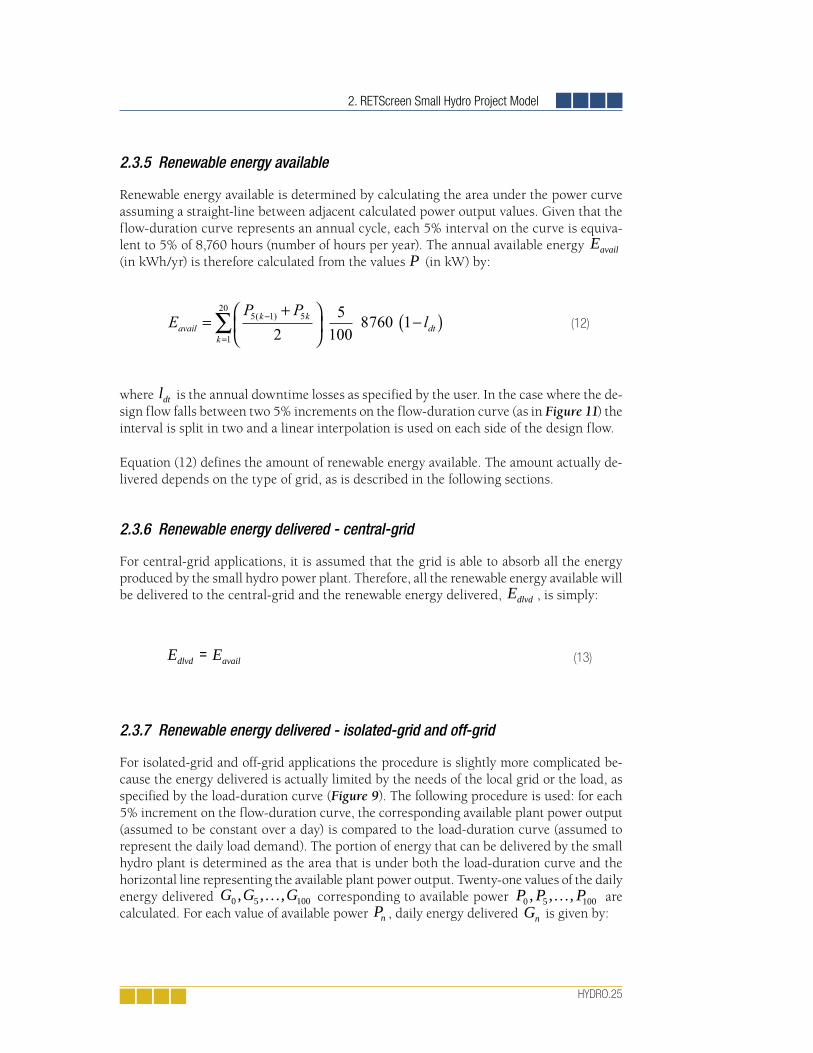
2. RETScreen Small Hydro Project Model
HYDRO.25
2.3.5 Renewable energy available
Renewable energy available is determined by calculating the area under the power curve assuming a straight-line between adjacent calculated power output values. Given that the flow-duration curve represents an annual cycle, each 5% interval on the curve is equiva-lent to 5% of 8,760 hours (number of hours per year). The annual available energy Eavail (in kWh/yr) is therefore calculated from the values P (in kW) by:
where ldt is the annual downtime losses as specified by the user. In the case where the de-sign flow falls between two 5% increments on the flow-duration curve (as in Figure 11) the interval is split in two and a linear interpolation is used on each side of the design flow.
Equation (12) defines the amount of renewable energy available. The amount actually de-livered depends on the type of grid, as is described in the following sections.
2.3.6 Renewable energy delivered - central-grid
For central-grid applications, it is assumed that the grid is able to absorb all the energy produced by the small hydro power plant. Therefore, all the renewable energy available will be delivered to the central-grid and the renewable energy delivered, Edlvd , is simply:
2.3.7 Renewable energy delivered - isolated-grid and off-grid
For isolated-grid and off-grid applications the procedure is slightly more complicated be-cause the energy delivered is actually limited by the needs of the local grid or the load, as specified by the load-duration curve (Figure 9). The following procedure is used: for each 5% increment on the flow-duration curve, the corresponding available plant power output (assumed to be constant over a day) is compared to the load-duration curve (assumed to represent the daily load demand). The portion of energy that can be delivered by the small hydro plant is determined as the area that is under both the load-duration curve and the horizontal line representing the available plant power output. Twenty-one values of the daily energy delivered G G G0 5 100, , ,… corresponding to available power P P P0 5 100, , ,… are calculated. For each value of available power Pn , daily energy delivered Gn is given by:
(12)
E Edlvd avail= (13)

Small Hydro Project Analysis Chapter
HYDRO.26
where ′Pn k, is the lesser of load Lk and available power Pn :
In the case where the available power
′Pn k, falls between two 5% increments on the load-duration curve, the interval is split in two and a linear interpolation is used on each side of the available power.
The procedure is illustrated by an example, using the load-duration curve from Figure 9 and values from the power-duration curve shown in Figure 11. The purpose of the example is to determine the daily renewable energy
G75 delivered for a flow that is exceeded 75% of the time. One first refers to Figure 11 to determine the corresponding power level:
Then one reports that number as a horizontal line on the load-duration curve, as shown in Figure 12. The area that is both under the load-duration curve and the horizontal line is the renewable energy delivered per day for the plant capacity that corresponds to flow Q75 ; integration with formula (14) gives the result:
The procedure is repeated for all values P P P0 5 100, , ,… to obtain twenty one values of
the daily renewable energy delivered G G G0 5 100, , ,… as a function of percent time the flow is exceeded as shown in Figure 13. The annual renewable energy delivered
Edlvd is
obtained simply by calculating the area under the curve of Figure 13, again with a trap-ezoidal rule:
where, as before, ldt is the annual downtime losses as specified by the user.
(14)
′ = ( )P P Ln k n k, min , (15)
P75 = 2,630 kW (16)
G75 = 56.6 MWh/d (17)
(18)
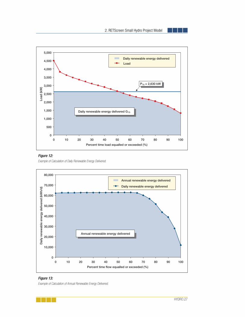
2. RETScreen Small Hydro Project Model
HYDRO.27
Figure 12: Example of Calculation of Daily Renewable Energy Delivered.
0
500
1,000
1,500
2,000
2,500
3,000
3,500
4,000
4,500
5,000
0 10 20 30 40 50 60 70 80 90 100
Percent time load equalled or exceeded (%)
Load
(kW
)
Daily renewable energy delivered
Load
P75 = 2,630 kW
Daily renewable energy delivered G75
Figure 13: Example of Calculation of Annual Renewable Energy Delivered.
0
10,000
20,000
30,000
40,000
50,000
60,000
70,000
80,000
0 10 20 30 40 50 60 70 80 90 100
Percent time flow equalled or exceeded (%)
Dai
ly r
enew
able
ene
rgy
del
iver
ed (k
Wh/
d)
Annual renewable energy delivered
Daily renewable energy delivered
Annual renewable energy delivered
Small Hydro Project Analysis Chapter
HYDRO.28
2.3.8 Small hydro plant capacity factor
The annual capacity factor K of the small hydro power plant is a measure of the available flow at the site and how efficiently it is used. It is defined as the average output of the plant compared to its rated capacity:
where the annual renewable energy delivered Edlvd calculated through (13) or (18) is ex-pressed in kWh, and plant capacity calculated through (10) is expressed in kW.
2.3.9 Excess renewable energy available
Excess renewable energy available Eexcess is the difference between the renewable energy available Eavail and the renewable energy delivered Edlvd :
Eavail is calculated through equation (12) and Edlvd through either (13) or (18).
2.4 Project Costing
The Small Hydro Project Model is unique among RETScreen technology models in that it offers two methods for project costing: the detailed costing method, or alternatively, the formula costing method.
The detailed costing method is described in the online user manual. The formula costing method is based on empirical formulae that have been developed to relate project costs to key project parameters. The costs of numerous projects have been used to develop the formulae. The formulae are described in Appendix B.
K EP
dlvd
des
=8760
(19)
E E Eexcess avail dlvd= − (20)

2. RETScreen Small Hydro Project Model
HYDRO.29
2.5 Validation
Numerous experts have contributed to the development, testing and validation of the RETScreen Small Hydro Project Model. They include small hydro modelling experts, cost engineering experts, greenhouse gas modelling specialists, financial analysis professionals, and ground station (hydrology) and satellite weather database scientists.
This section presents three examples of the validations completed. In Section 2.5.1, a turbine efficiency curve as calculated by RETScreen is compared to manufacturer’s efficiency data for an installed unit with the same characteristics. Then, the annual renewable energy de-livered and plant capacity calculated by RETScreen are compared to values calculated by another software program in Section 2.5.2. And finally, project costs, as calculated by the formula costing method, are compared to the as-built costs of one small hydro project in Section 2.5.3.
2.5.1 Turbine effi ciency
Small hydro turbine efficiency as calculated by RETScreen was compared to the manufac-turer guaranteed turbine efficiency for the Brown Lake Hydro Project in British Columbia, Canada.
The following provides a summary of the Brown Lake project and the turbine performance data as provided by the manufacturer:
Project name: Brown Lake Hydro Project
Project location: Approximately 40 km south of Prince Rupert, British Columbia on the confl uence of Brown Creek and Ecstall River.
Project features: 600 m rock tunnel tapping into Brown Lake, 50 m of 1.5 m diameter steel penstock, single horizontal Francis turbine, horizontal synchronous genera-tor, 1,500 m of submarine power cable, substation and connection to BC Hydro at 69 kV. Automatic operation and remote monitoring.
Date commissioned: December 1996
Turbine manufacturer: GEC Alsthom (runner by Neyrpic)
Turbine type: Francis
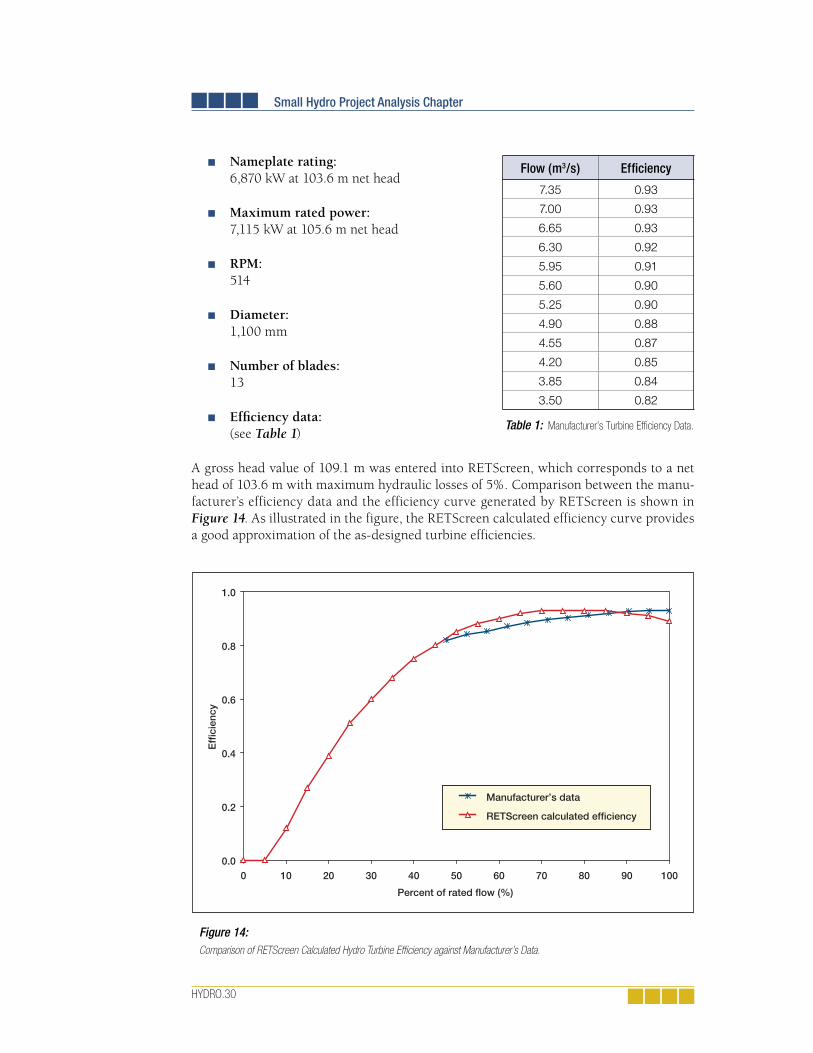
Small Hydro Project Analysis Chapter
HYDRO.30
Nameplate rating: 6,870 kW at 103.6 m net head
Maximum rated power: 7,115 kW at 105.6 m net head
RPM: 514
Diameter: 1,100 mm
Number of blades: 13
Effi ciency data:(see Table 1)
A gross head value of 109.1 m was entered into RETScreen, which corresponds to a net head of 103.6 m with maximum hydraulic losses of 5%. Comparison between the manu-facturer’s efficiency data and the efficiency curve generated by RETScreen is shown in Figure 14. As illustrated in the figure, the RETScreen calculated efficiency curve provides a good approximation of the as-designed turbine efficiencies.
Flow (m3/s) Effi ciency
7.35 0.93
7.00 0.93
6.65 0.93
6.30 0.92
5.95 0.91
5.60 0.90
5.25 0.90
4.90 0.88
4.55 0.87
4.20 0.85
3.85 0.84
3.50 0.82
Figure 14: Comparison of RETScreen Calculated Hydro Turbine Effi ciency against Manufacturer’s Data.
0.0
0.2
0.4
0.6
0.8
1.0
0 10 20 30 40 50 60 70 80 90 100
Percent of rated flow (%)
Eff
icie
ncy
Manufacturer’s data
RETScreen calculated efficiency
Table 1: Manufacturer’s Turbine Effi ciency Data.
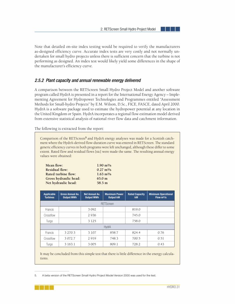
2. RETScreen Small Hydro Project Model
HYDRO.31
Note that detailed on-site index testing would be required to verify the manufacturers as-designed efficiency curve. Accurate index tests are very costly and not normally un-dertaken for small hydro projects unless there is sufficient concern that the turbine is not performing as designed. An index test would likely yield some differences in the shape of the manufacturer’s efficiency curve.
2.5.2 Plant capacity and annual renewable energy delivered
A comparison between the RETScreen Small Hydro Project Model and another software program called HydrA is presented in a report for the International Energy Agency – Imple-menting Agreement for Hydropower Technologies and Programmes entitled “Assessment Methods for Small-hydro Projects” by E.M. Wilson, D.Sc., FICE, FASCE, dated April 2000. HydrA is a software package used to estimate the hydropower potential at any location in the United Kingdom or Spain. HydrA incorporates a regional flow estimation model derived from extensive statistical analysis of national river flow data and catchment information.
The following is extracted from the report:
Comparison of the RETScreen5 and HydrA energy analyses was made for a Scottish catch-ment where the HydrA-derived flow-duration curve was entered in RETScreen. The standard generic efficiency curves in both programs were left unchanged, although these differ to some extent. Rated flow and residual flows [sic] were made the same. The resulting annual energy values were obtained:
Mean fl ow: 1.90 m³/sResidual fl ow: 0.27 m³/sRated turbine fl ow: 1.63 m³/sGross hydraulic head: 65.0 mNet hydraulic head: 58.5 m
Applicable Turbines
Gross Annual Av. Output MWh
Net Annual Av. Output MWh
Maximum Power Output kW
Rated Capacity kW
Minimum Operational Flow m³/s
RETScreen
Francis 3 092 819.0
Crossfl ow 2 936 745.0
Turgo 3 125 758.0
HydrA
Francis 3 270.3 3 107 858.7 824.4 0.76
Crossfl ow 3 072.7 2 919 748.3 700.5 0.51
Turgo 3 163.1 3 005 809.1 728.2 0.43
It may be concluded from this simple test that there is little difference in the energy calcula-tions.
5. A beta version of the RETScreen Small Hydro Project Model Version 2000 was used for the test.

Small Hydro Project Analysis Chapter
HYDRO.32
2.5.3 Project costs
Project costs as calculated by RETScreen using the Formula Costing Method were com-pared to a detailed as-built cost evaluation prepared for the existing 6 MW Rose Blanche hydroelectric development in Newfoundland, Canada.
The key parameters of the Rose Blanche project are summarised below:
Project name: Rose Blanche Hydroelectric Development
Owner/developer: Newfoundland Power
Project location: Rose Blanche Brook, approximately 45 km east of Channel Port Aux Basques.
Date commissioned: December 1998
Project type: Run-of-river (with several days’ storage)
Installed capacity: 6 MW
Design net head: 114.2 m
Rated fl ow: 6.1 m3/s
Turbine/generator: Twin Francis turbines connected to a single generator.
Other project features:Small dam with minimal storage, 1,300 m penstock, short transmission line (approximately 3 km).
The data inputs for the RETScreen Formula Costing Method and the results are shown in Figure 15, and a comparison of the costs as calculated by RETScreen and the detailed cost evaluation for the real project is presented in Figure 16. The detailed project costs estimated in 1998 have been converted to 2000 values using an inflation factor of 1.03.
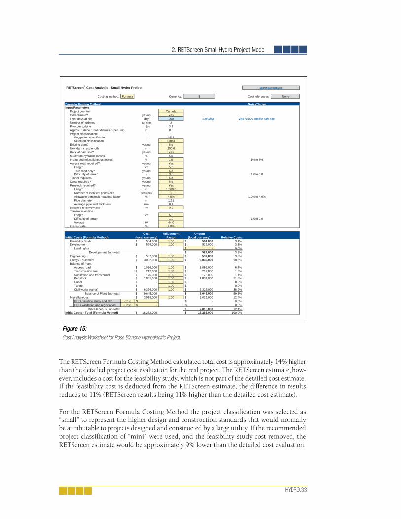
2. RETScreen Small Hydro Project Model
HYDRO.33
The RETScreen Formula Costing Method calculated total cost is approximately 14% higher than the detailed project cost evaluation for the real project. The RETScreen estimate, how-ever, includes a cost for the feasibility study, which is not part of the detailed cost estimate. If the feasibility cost is deducted from the RETScreen estimate, the difference in results reduces to 11% (RETScreen results being 11% higher than the detailed cost estimate).
For the RETScreen Formula Costing Method the project classification was selected as “small” to represent the higher design and construction standards that would normally be attributable to projects designed and constructed by a large utility. If the recommended project classification of “mini” were used, and the feasibility study cost removed, the RETScreen estimate would be approximately 9% lower than the detailed cost evaluation.
Figure 15: Cost Analysis Worksheet for Rose Blanche Hydroelectric Project.
Costing method: Formula Currency: $ Cost references: NoneSecond currency: USA Rate: $/USD 1,47730
Formula Costing Method Notes/RangeInput Parameters
Project country CanadaCold climate? yes/no YesFrost days at site day 200 See Map Visit NASA satellite data siteNumber of turbines turbine 2Flow per turbine m‡/s 3.1Approx. turbine runner diameter (per unit) m 0.8Project classification:
Suggested classification - MiniSelected classification - Small
Existing dam? yes/no NoNew dam crest length m 250.0Rock at dam site? yes/no YesMaximum hydraulic losses % 5%Intake and miscellaneous losses % 1% 1% to 5%Access road required? yes/no Yes
Length km 5.0Tote road only? yes/no NoDifficulty of terrain - 3.0 1.0 to 6.0
Tunnel required? yes/no NoCanal required? yes/no NoPenstock required? yes/no Yes
Length m 1,300.0Number of identical penstocks penstock 1Allowable penstock headloss factor % 4.0% 1.0% to 4.0%Pipe diameter m 1.61Average pipe wall thickness mm 8.1
Distance to borrow pits km 3.0Transmission line
Length km 5.0Difficulty of terrain - 1.0 1.0 to 2.0Voltage kV 44.0
Interest rate % 9.0%
Cost Adjustment AmountInitial Costs (Formula Method) (local currency) Factor (local currency) Relative Costs
Feasibility Study $ 504,000 1.00 $ 504,000 3.1% 0% -USD Development $ 529,000 1.00 $ 529,000 3.3% 0% -USD
Land rights $ - 0.0% 0% -USD Development Sub-total: $ 529,000 3.3% 0% -USD
Engineering $ 537,000 1.00 $ 537,000 3.3% 0% -USD Energy Equipment $ 3,032,000 1.00 $ 3,032,000 18.6% 100% 564 543USD Balance of Plant
Access road $ 1,096,000 1.00 $ 1,096,000 6.7% 0% -USD Transmission line $ 217,000 1.00 $ 217,000 1.3% 100% 146 890USD Substation and transformer $ 175,000 1.00 $ 175,000 1.1% 100% 29 107USD Penstock $ 1,831,000 1.00 $ 1,831,000 11.3% 100% 726 325USD Canal $ - 1.00 $ - 0.0% 100% -USD Tunnel $ - 1.00 $ - 0.0% 100% -USD Civil works (other) $ 6,326,000 1.00 $ 6,326,000 38.9% 0% -USD
Balance of Plant Sub-total: $ 9,645,000 $ 9,645,000 59.3% 26% 902 322USD Miscellaneous $ 2,015,000 1.00 $ 2,015,000 12.4% 0% -USD
GHG baseline study and MP Cost -$ -$ 0.0% 100% -USD GHG validation and registration Cost -$ -$ 0.0% 100% -USD
Miscellaneous Sub-total: $ 2,015,000 12.4% 0% -USD Initial Costs - Total (Formula Method) $ 16,262,000 $ 16,262,000 100.0% 28% USD 1 466 865
Search Marketplace RETScreenfi Cost Analysis - Small Hydro Project
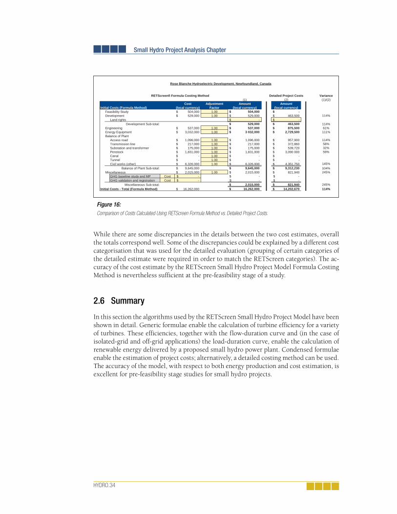
Small Hydro Project Analysis Chapter
HYDRO.34
While there are some discrepancies in the details between the two cost estimates, overall the totals correspond well. Some of the discrepancies could be explained by a different cost categorisation that was used for the detailed evaluation (grouping of certain categories of the detailed estimate were required in order to match the RETScreen categories). The ac-curacy of the cost estimate by the RETScreen Small Hydro Project Model Formula Costing Method is nevertheless sufficient at the pre-feasibility stage of a study.
2.6 Summary
In this section the algorithms used by the RETScreen Small Hydro Project Model have been shown in detail. Generic formulae enable the calculation of turbine efficiency for a variety of turbines. These efficiencies, together with the flow-duration curve and (in the case of isolated-grid and off-grid applications) the load-duration curve, enable the calculation of renewable energy delivered by a proposed small hydro power plant. Condensed formulae enable the estimation of project costs; alternatively, a detailed costing method can be used. The accuracy of the model, with respect to both energy production and cost estimation, is excellent for pre-feasibility stage studies for small hydro projects.
Figure 16: Comparison of Costs Calculated Using RETScreen Formula Method vs. Detailed Project Costs.
Detailed Project Costs Variance(1) (2) (1)/(2)
Cost Adjustment Amount AmountInitial Costs (Formula Method) (local currency) Factor (local currency) (local currency)
Feasibility Study $ 504,000 1.00 $ 504,000 $ - Development $ 529,000 1.00 $ 529,000 $ 463,500 114%
Land rights $ - $ - Development Sub-total: $ 529,000 $ 463,500 114%
Engineering $ 537,000 1.00 $ 537,000 $ 875,500 61%Energy Equipment $ 3,032,000 1.00 $ 3 032,000 $ 2,729,500 111%Balance of Plant
Access road $ 1,096,000 1.00 $ 1,096,000 $ 957,900 114%Transmission line $ 217,000 1.00 $ 217,000 $ 372,860 58%Substation and transformer $ 175,000 1.00 $ 175,000 $ 539,720 32%Penstock $ 1,831,000 1.00 $ 1,831,000 $ 3,090 000 59%Canal $ - 1.00 $ - $ - Tunnel $ - 1.00 $ - $ - Civil works (other) $ 6,326,000 1.00 $ 6,326,000 $ 4,351,750 145%
Balance of Plant Sub-total: $ 9,645,000 $ 9,645,000 $ 9,312,230 104%Miscellaneous $ 2,015,000 1.00 $ 2,015,000 $ 821,940 245%
GHG baseline study and MP Cost -$ -$ -$ GHG validation and registration Cost -$ -$ -$
Miscellaneous Sub-total: $ 2,015,000 $ 821,940 245%Initial Costs - Total (Formula Method) $ 16,262,000 $ 16,262,000 $ 14,202,670 114%
RETScreenfi Formula Costing Method
Rose Blanche Hydroelectric Development, Newfoundland, Canada

HYDRO.35
REFERENCES
Acres International Limited, Hydrologic Design Methodologies for Small-Scale Hydro at Ungauged Sites - Phase I, Prepared for Environment Canada, Inland Waters Directorate, Executed for Energy, Mines and Resources Canada, 1984.
Bennett, K., Small Hydro in Canada: An Overview, Prepared for Industry, Science and Technology Canada, Aboriginal Economic Programs, 1990.
Energy, Mines and Resources Canada (EMR), Small Power Production in Remote Communities: A Shared Opportunity, 1988.
Gordon, J. L., What We Must Not Forget, 1991.
Gordon, J. L., Black Boxing Hydro Costs, 1989.
Gulliver, J.S., Arndt, E.A., Hydropower Engineering Handbook, 1991.
Leopold, L.B., Water: A Primer, 1974.
Wilson, E.M., Assessment Methods for Small-Hydro Projects, International Energy Agency – Implementing Agreement for Hydropower Technologies and Programs, April 2000.

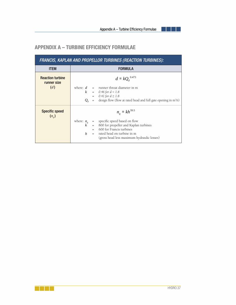
Appendix A – Turbine Effi ciency Formulae
HYDRO.37
ITEM FORMULA
Reaction turbine runner size
( )
d kQd= 0 473.
where: = = = =
runner throat diameter in m0.46 for d < 1.80.41 for d ≥ 1.8design fl ow (fl ow at rated head and full gate opening in m3/s)
Specifi c speed ( )
n khq = −0 5.
where: = = ==
specifi c speed based on fl ow800 for propeller and Kaplan turbines600 for Francis turbinesrated head on turbine in m (gross head less maximum hydraulic losses)
dkQ
kQd
nqkh
FRANCIS, KAPLAN AND PROPELLOR TURBINES (REACTION TURBINES):
d
nq
APPENDIX A – TURBINE EFFICIENCY FORMULAE
Appendix A – Turbine Effi ciency Formulae
kh

Small Hydro Project Analysis Chapter
HYDRO.38
ITEM FORMULA
Specifi c speed adjustment to peak
effi ciency ( )
^ /e nnq q= −( ){ }56 2562
Runner size adjustment to peak
effi ciency ( )
Turbine peak effi ciency
( )
e e e Rp nq d m= − +( ) − +0 919 0 0305 0 005. ^ ^ . .where: = turbine manufacture/design coeffi cient
(2.8 to 6.1; default = 4.5). Refer to online manual.
Peak effi ciency fl ow ( ) Q Q np d q= 0 65 0 05. .
Effi ciencies at fl ows below peak
effi ciency fl ow ( )
eQ Q
Qqp
p
nq
= −−( )
−( )1 1 25
3 94 0 0195
.. .
ep
Drop in effi ciency at full load
( )
Effi ciency at full load ( )
Effi ciencies at fl ows above peak
effi ciency fl ow ( )
FRANCIS TURBINES:
Rm
^enq
ep
Qp
eq
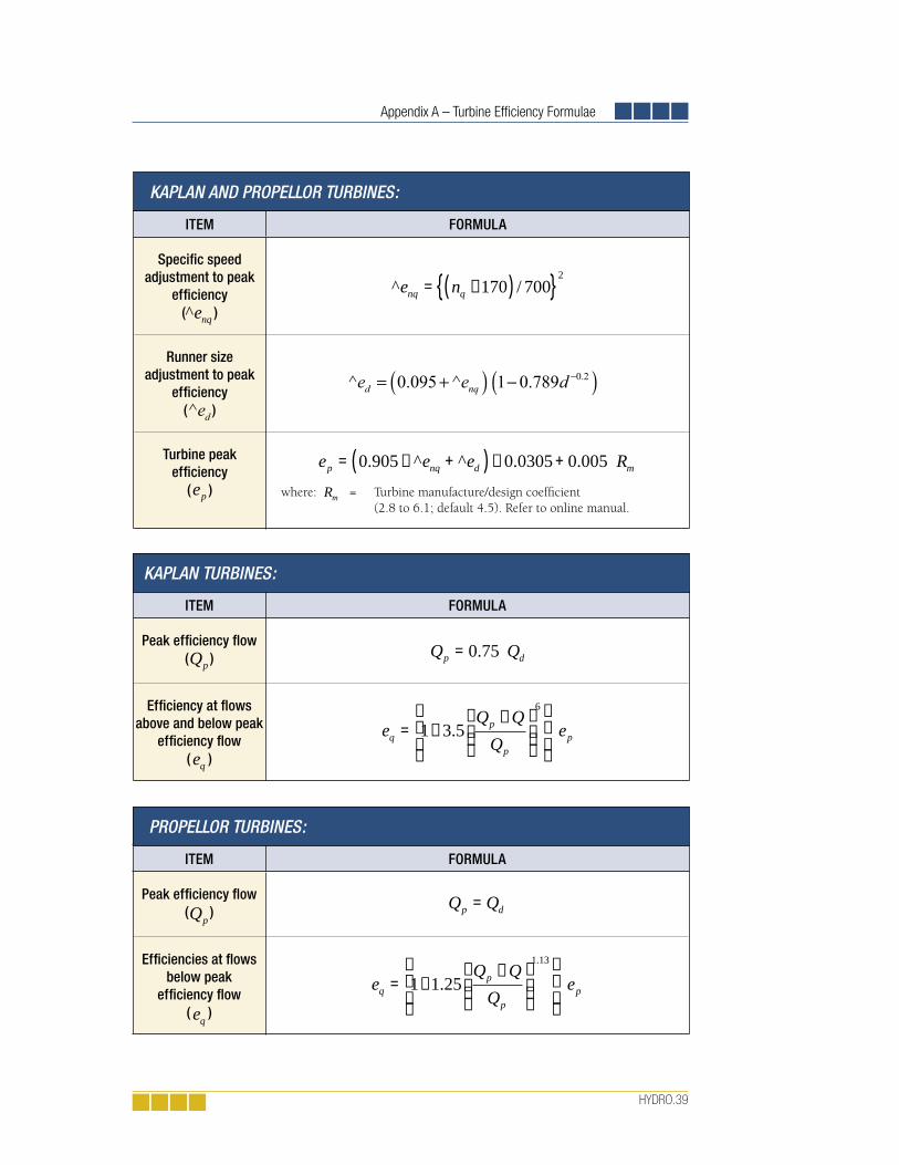
Appendix A – Turbine Effi ciency Formulae
HYDRO.39
ITEM FORMULA
Peak effi ciency fl ow ( ) Q Qp d=
Effi ciencies at fl ows below peak
effi ciency fl ow ( )
eQ Q
Qeq
p
pp= −
−
1 1 251 13
..
PROPELLOR TURBINES:
Qp
eq
ITEM FORMULA
Peak effi ciency fl ow ( ) Q Qp d= 0 75.
Effi ciency at fl ows above and below peak
effi ciency fl ow ( )
eQ Q
Qeq
p
pp= −
−
1 3 56
.
KAPLAN TURBINES:
Qp
eq
ITEM FORMULA
Specifi c speed adjustment to peak
effi ciency ( )
^ /e nnq q= −( ){ }170 7002
Runner size adjustment to peak
effi ciency ( )
Turbine peak effi ciency
( )
e e e Rp nq d m= − +( ) − +0 905 0 0305 0 005. ^ ^ . .
where: = Turbine manufacture/design coeffi cient
(2.8 to 6.1; default 4.5). Refer to online manual.
KAPLAN AND PROPELLOR TURBINES:
Rmep
^enq

Small Hydro Project Analysis Chapter
HYDRO.40
ITEM FORMULA
Rotational speed ( ) n h Q
jd=
31
0 5.
where: = Number of jets (user-selected value from 1 to 6)
Outside diameter of runner
( )
Turbine peak effi ciency
( )e dp = 0 864 0 04. .
Peak effi ciency fl ow ( )
Effi ciency at fl ows above and below
peak effi ciency fl ow ( )
PELTON TURBINES:
j
n
ep
ITEM FORMULA
Effi ciency ( ) Pelton effi ciency minus 0.03
TURGO TURBINES:
ITEM FORMULA
Peak effi ciency fl ow ( ) Q Qp d=
Effi ciency ( ) e Q Q
QQ Q
Qqd
p
d
p
= − −
− −
0 79 0 15 1 37
14
. . .
CROSS-FLOW TURBINES:
Qp
eq
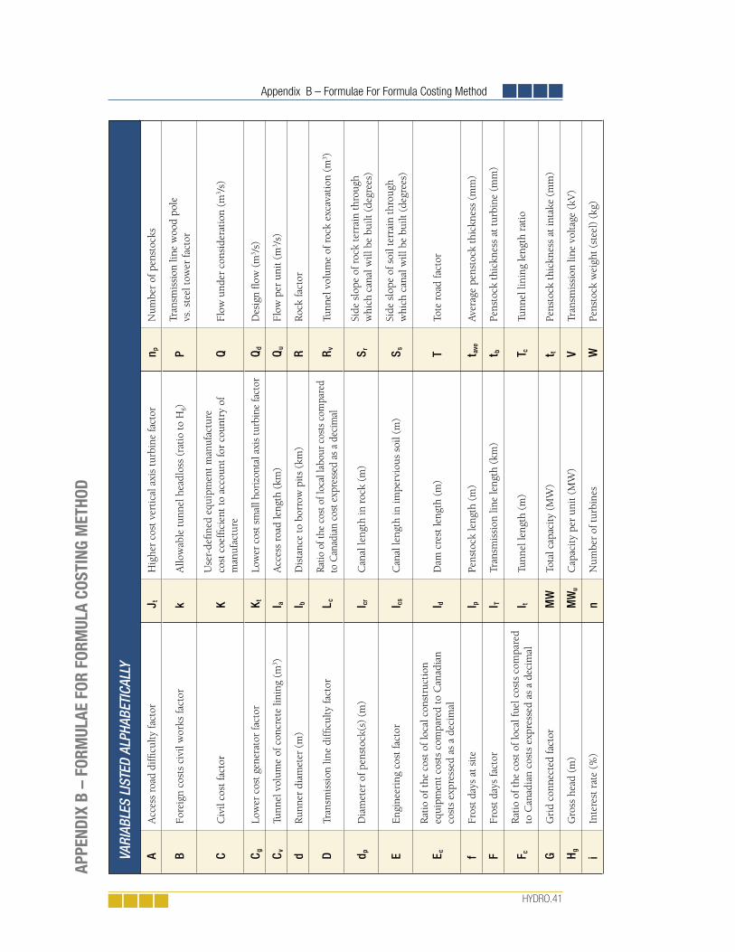
Appendix B – Formulae For Formula Costing Method
HYDRO.41
APPE
NDIX
B –
FOR
MUL
AE F
OR F
ORM
ULA
COST
ING
MET
HOD
A A
cces
s ro
ad d
iffi c
ulty
fact
orJ t
Hig
her
cost
ver
tica
l axi
s tu
rbin
e fa
ctor
n p
Num
ber
of p
enst
ocks
B Fo
reig
n co
sts
civi
l wor
ks fa
ctor
kA
llow
able
tun
nel h
eadl
oss
(rat
io t
o H
g)P
Tran
smis
sion
line
woo
d po
le
vs. s
teel
tow
er fa
ctor
C C
ivil
cost
fact
orK
Use
r-de
fi ned
equ
ipm
ent
man
ufac
ture
co
st c
oeffi
cien
t to
acc
ount
for
coun
try
of
man
ufac
ture
Q Fl
ow u
nder
con
side
rati
on (
m3 /
s)
C g
Low
er c
ost
gene
rato
r fa
ctor
K tLo
wer
cos
t sm
all h
oriz
onta
l axi
s tu
rbin
e fa
ctor
Qd
Des
ign
fl ow
(m
3 /s)
Cv
Tunn
el v
olum
e of
con
cret
e lin
ing
(m3 )
l aA
cces
s ro
ad le
ngth
(km
)Q
u Fl
ow p
er u
nit
(m3 /
s)
d R
unne
r di
amet
er (
m)
l bD
ista
nce
to b
orro
w p
its
(km
)R
Roc
k fa
ctor
D Tr
ansm
issi
on li
ne d
iffi c
ulty
fact
orL c
Ratio
of t
he c
ost o
f loc
al la
bour
cos
ts c
ompa
red
to C
anad
ian
cost
exp
ress
ed a
s a
deci
mal
R v
Tunn
el v
olum
e of
roc
k ex
cava
tion
(m
3 )
d p
Dia
met
er o
f pen
stoc
k(s)
(m
)l cr
Can
al le
ngth
in r
ock
(m)
S r
Side
slo
pe o
f roc
k te
rrai
n th
roug
h w
hich
can
al w
ill b
e bu
ilt (
degr
ees)
E E
ngin
eeri
ng c
ost
fact
orl cs
Can
al le
ngth
in im
perv
ious
soi
l (m
)S s
Si
de s
lope
of s
oil t
erra
in t
hrou
gh
whi
ch c
anal
will
be
built
(de
gree
s)
E c
Rat
io o
f the
cos
t of
loca
l con
stru
ctio
n eq
uipm
ent
cost
s co
mpa
red
to C
anad
ian
cost
s ex
pres
sed
as a
dec
imal
l dD
am c
rest
leng
th (
m)
T To
te r
oad
fact
or
f Fr
ost
days
at
site
l p Pe
nsto
ck le
ngth
(m
)t a
ve
Aver
age
pens
tock
thi
ckne
ss (
mm
)
FFr
ost
days
fact
orl T
Tran
smis
sion
line
leng
th (
km)
t b
Pens
tock
thi
ckne
ss a
t tu
rbin
e (m
m)
F cR
atio
of t
he c
ost
of lo
cal f
uel c
osts
com
pare
d to
Can
adia
n co
sts
expr
esse
d as
a d
ecim
all t
Tunn
el le
ngth
(m
)T c
Tu
nnel
lini
ng le
ngth
rat
io
GG
rid
conn
ecte
d fa
ctor
MW
Tota
l cap
acit
y (M
W)
t t Pe
nsto
ck t
hick
ness
at
inta
ke (
mm
)
Hg
Gro
ss h
ead
(m)
MW
uC
apac
ity
per
unit
(M
W)
V Tr
ansm
issi
on li
ne v
olta
ge (
kV)
iIn
tere
st r
ate
(%)
nN
umbe
r of
tur
bine
sW
Pe
nsto
ck w
eigh
t (s
teel
) (k
g)
VARI
ABLE
S LI
STED
ALP
HABE
TICA
LLY

Small Hydro Project Analysis Chapter
HYDRO.42
ITEM
SMAL
LM
INI
MIC
RO
Desi
gn fl
ow (m
axim
um fl
ow u
sed
by
gene
ratin
g st
atio
n) in
m3 /
s (
)
Use
r-de
fi ned
val
ue
Reco
mm
ende
d cl
assi
fi cat
ion
Qd
>12
8.12
80
4.
.≥
>Q
dQ
d≤
04.
Sele
cted
cla
ssifi
catio
nU
ser-
defi n
ed v
alue
bas
ed o
n ac
cept
able
ris
k (fl
ood
, etc
.).
Qd
≤0
4.
Num
ber o
f tur
bine
s(
)U
ser-
defi n
ed v
alue
1
Flow
per
turb
ine
in m
3 /s
(
)=
Qn
d=
Qd
Appr
ox. t
urbi
ne ru
nner
dia
met
er in
m(
)=
048
20
45.
.Q
Gros
s he
ad in
m(
)
Use
r-de
fi ned
val
ue
MW
/uni
t in
MW
(hid
den)
(
)
Tota
l Cap
acity
in M
W (h
idde
n)(
)=
MW
nu
=M
Wu
BASI
C PA
RAM
ETER
S
Qd n
0Q Qd
MW
u
MW
u

Appendix B – Formulae For Formula Costing Method
HYDRO.43
ITEM
SMAL
LM
INI
MIC
RO
Engi
neer
ing
cost
fact
or (h
idde
n)
(E)
= 0.
67 if
exi
stin
g da
m=
1.0
if no
dam
as s
peci
fi ed
by y
es/n
o se
lect
ion
Grid
-con
nect
ed fa
ctor
to a
ccou
nt fo
r the
us
e of
indu
ctio
n ge
nera
tors
(hid
den)
(G
)=
0.9
if M
W <
1.5
and
cen
tral
-gri
d co
nnec
ted
Fact
or to
acc
ount
for u
se o
f low
er-c
ost
mot
ors
as g
ener
ator
s fo
r pro
ject
s be
low
10
MW
(hid
den)
(C
g)
= 0.
75 if
MW
< 1
0=
1.0
if M
W ≥
10
Fact
or to
acc
ount
for c
ost i
ncre
ase
with
ve
rtic
al a
xis
Kapl
an, F
ranc
is a
nd P
rope
ller
units
at h
eads
abo
ve 2
5 m
(hid
den)
(J t)
= 1
if H
g ≤ 2
5=
1.1
if H
g > 2
5
Fact
or to
acc
ount
for c
ost d
ecre
ase
with
sm
all h
oriz
onta
l Kap
lan,
Fra
ncis
and
Pr
opel
ler a
xis
units
(hid
den)
(K
t)
= 0.
9 if
d <
1.8
= 1.
0 if
d ≥
1.8
Fact
or to
adj
ust a
cces
s ro
ad c
osts
to re
fl ect
lo
wer
-cos
t tot
e ro
ad c
onst
ruct
ion
(hid
den)
(T
)
= 0.
25 if
tote
roa
d=
1.0
othe
rwis
eas
spe
cifi e
d by
yes
/no
sele
ctio
n
Acce
ss ro
ad d
iffi c
ulty
of t
erra
in fa
ctor
(A
)U
ser-
defi n
ed fa
ctor
with
rec
omm
ende
d ra
nge
of 1
to 6
Leng
th o
f acc
ess
road
in m
(l a)
Use
r-de
fi ned
val
ue
OTHE
R VA
RIAB
LES
AND
COST
ING
FACT
ORS
(IN O
RDER
OF
USE
IN F
ORM
ULAE
)

Small Hydro Project Analysis Chapter
HYDRO.44
ITEM
SMAL
LM
INI
MIC
RO
Tran
smis
sion
line
diffi
cul
ty o
f ter
rain
fact
or
(D)
Use
r-de
fi ned
fact
or w
ith r
ecom
men
ded
rang
e of
1 to
2
Leng
th o
f tra
nsm
issi
on li
ne in
km
(l t)
Use
r-de
fi ned
val
ue
Tran
smis
sion
line
vol
tage
in k
V (V
)U
ser-
defi n
ed v
alue
Fact
or to
refl e
ct c
ost o
f woo
d po
le v
s. s
teel
to
wer
con
stru
ctio
n (h
idde
n)
(P)
= 0.
85 if
V <
69
= 1.
0 if
V ≥
69
Civi
l cos
t fac
tor (
hidd
en)
(C)
= 0.
44 if
exi
stin
g da
m=
1.0
if no
dam
as s
peci
fi ed
by y
es/n
o se
lect
ion
Rock
fact
or (h
idde
n)(R
)
= 1
if ro
ck a
t dam
site
= 1.
05 if
no
rock
as s
peci
fi ed
by y
es/n
o se
lect
ion
N/A
Dist
ance
to a
bor
row
pit
in k
m
(l b)U
ser-
defi n
ed v
alue
Leng
th o
f dam
cre
st in
m
(l d)U
ser-
defi n
ed v
alue
Num
ber o
f ide
ntic
al p
enst
ocks
(n
p)U
ser-
defi n
ed v
alue
Wei
ght o
f pen
stoc
k(s)
in k
g (h
idde
n)(W
)C
alcu
late
d va
lue
(pen
stoc
k co
st fo
rmul
a)
Diam
eter
of p
enst
ock(
s) in
m
(dp)
Cal
cula
ted
valu
e (p
enst
ock
cost
form
ula)
Leng
th o
f pen
stoc
k(s)
in m
(l p)
Use
r-de
fi ned
val
ue
OTHE
R VA
RIAB
LES
AND
COST
ING
FACT
ORS
(IN O
RDER
OF
USE
IN F
ORM
ULAE
)

Appendix B – Formulae For Formula Costing Method
HYDRO.45
ITEM
SMAL
LM
INI
MIC
RO
Aver
age
pipe
wal
l thi
ckne
ss
of p
enst
ock(
s) in
mm
(t av
e)C
alcu
late
d va
lue
(pen
stoc
k co
st fo
rmul
a)
Pens
tock
pip
e w
all t
hick
ness
at
inta
ke in
mm
(hid
den)
(t t)
Cal
cula
ted
valu
e (p
enst
ock
cost
form
ula)
Pens
tock
pip
e w
all t
hick
ness
at t
urbi
ne
in m
m (h
idde
n)
(t b)C
alcu
late
d va
lue
(pen
stoc
k co
st fo
rmul
a)
Terr
ain
side
slo
pe o
f soi
l thr
ough
whi
ch
cana
l is
to b
e co
nstr
ucte
d in
deg
rees
(S
s)U
ser-
defi n
ed v
alue
Leng
th o
f can
al to
be
cons
truc
ted
in s
oil i
n m
(l cs
)U
ser-
defi n
ed v
alue
Terr
ain
side
slo
pe o
f roc
k th
roug
h w
hich
ca
nal i
s to
be
cons
truc
ted
in d
egre
es
(Sr)
Use
r-de
fi ned
val
ue
Leng
th o
f can
al to
be
cons
truc
ted
in
rock
in m
(l cr
)U
ser-
defi n
ed v
alue
Tunn
el ro
ck e
xcav
atio
n vo
lum
e in
m3 (h
idde
n)
(Rv)
Cal
cula
ted
valu
e (t
unne
l cos
t for
mul
a)N
/A
Tunn
el c
oncr
ete
linin
g vo
lum
e in
m3 (h
idde
n)
(Cv)
Cal
cula
ted
valu
e (t
unne
l cos
t for
mul
a)N
/A
Leng
th o
f tun
nel i
n m
(l t)
Use
r-de
fi ned
val
ueN
/A
OTHE
R VA
RIAB
LES
AND
COST
ING
FACT
ORS
(IN O
RDER
OF
USE
IN F
ORM
ULAE
)

Small Hydro Project Analysis Chapter
HYDRO.46
ITEM
SMAL
LM
INI
MIC
RO
Allo
wab
le tu
nnel
hea
dlos
s ex
pres
sed
as a
ratio
to th
e gr
oss
head
(k
)U
ser-
defi n
ed v
alue
N/A
Perc
ent l
engt
h of
tunn
el th
at is
line
d fa
ctor
(Tc)
Use
r-de
fi ned
val
ue w
ith r
ecom
men
ded
rang
e of
15%
(e
xcel
lent
roc
k) to
100
% (
poor
roc
k)N
/A
Inte
rest
rate
(i)
Use
r-de
fi ned
val
ue
Num
ber o
f day
s w
ith fr
ost a
t site
(f
)U
ser-
defi n
ed v
alue
Fros
t-da
ys fa
ctor
(hid
den)
(F)
=−11
036
50
9(
).f
Loca
l vs.
Can
adia
n eq
uipm
ent c
osts
ratio
(E
c)U
ser-
defi n
ed v
alue
Loca
l vs.
Can
adia
n fu
el c
osts
ratio
(F
c)U
ser-
defi n
ed v
alue
Loca
l vs.
Can
adia
n la
bour
cos
ts ra
tio
(Lc)
Use
r-de
fi ned
val
ue
Civi
l wor
ks fo
reig
n co
st fa
ctor
(hid
den)
. Us
ed in
pro
gram
to d
eter
min
e lo
cal c
ost o
f the
civ
il w
orks
co
mpo
nent
s of
fore
ign
proj
ects
(B
)
Equi
pmen
t man
ufac
ture
cos
t coe
ffi ci
ent
(K)
Use
r-de
fi ned
val
ue w
ith r
ecom
men
ded
rang
e of
0.5
to 1
.0
OTHE
R VA
RIAB
LES
AND
COST
ING
FACT
ORS
(IN O
RDER
OF
USE
IN F
ORM
ULAE
)
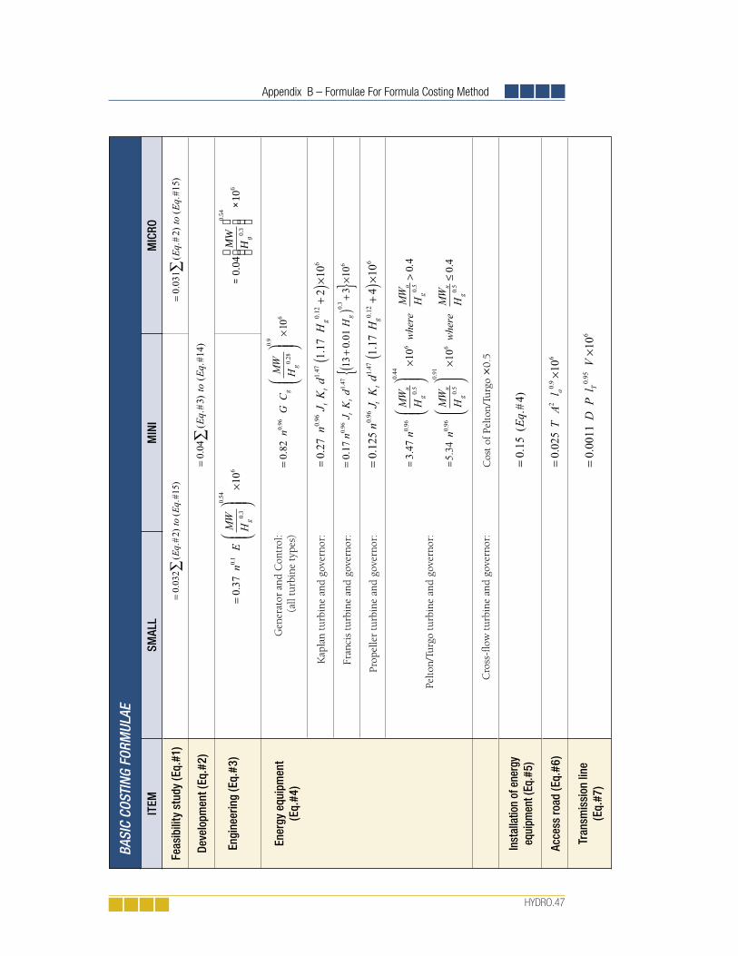
Appendix B – Formulae For Formula Costing Method
HYDRO.47
ITEM
SMAL
LM
INI
MIC
RO
Feas
ibili
ty s
tudy
(Eq.
#1)
Deve
lopm
ent (
Eq.#
2)
Engi
neer
ing
(Eq.
#3)
=
×
004
100
3
054
6.
.
.M
WH
g
Ener
gy e
quip
men
t (E
q.#4
)G
ener
ator
and
Con
trol
:(a
ll tu
rbin
e ty
pes)
Kap
lan
turb
ine
and
gove
rnor
:
Fran
cis
turb
ine
and
gove
rnor
:
Prop
elle
r tu
rbin
e an
d go
vern
or:
Pelt
on/T
urgo
tur
bine
and
gov
erno
r:
Cro
ss-fl
ow
tur
bine
and
gov
erno
r:C
ost
of P
elto
n/Tu
rgo
×0.5
Inst
alla
tion
of e
nerg
y eq
uipm
ent (
Eq.#
5)
Acce
ss ro
ad (E
q.#6
)
Tran
smis
sion
line
(E
q.#7
)
BASI
C CO
STIN
G FO
RMUL
AE
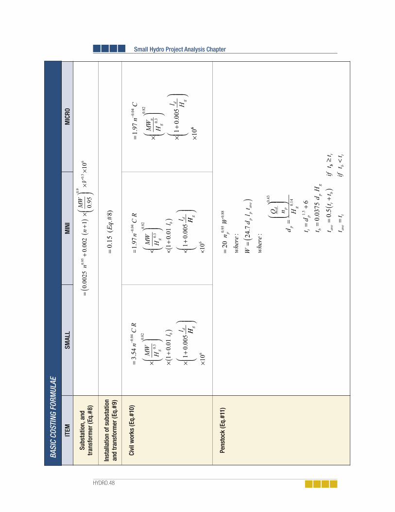
Small Hydro Project Analysis Chapter
HYDRO.48
ITEM
SMAL
LM
INI
MIC
RO
Subs
tatio
n, a
nd
tran
sfor
mer
(Eq.
#8)
Inst
alla
tion
of s
ubst
atio
n an
d tr
ansf
orm
er (E
q.#9
)
Civi
l wor
ks (E
q.#1
0)
Pens
tock
(Eq.
#11)
BASI
C CO
STIN
G FO
RMUL
AE
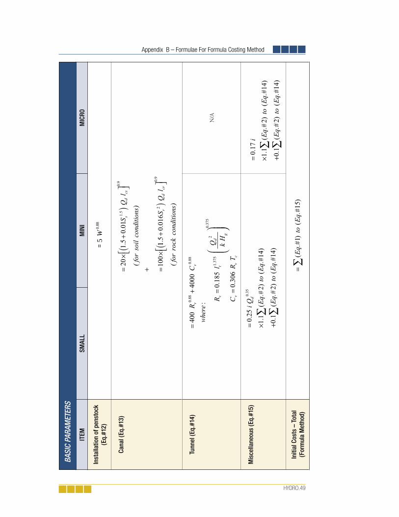
Appendix B – Formulae For Formula Costing Method
HYDRO.49
ITEM
SMAL
LM
INI
MIC
RO
Inst
alla
tion
of p
enst
ock
(Eq.
#12)
=5
088
W.
Cana
l (Eq
.#13
)
Tunn
el (E
q.#1
4)
N/A
Mis
cella
neou
s (E
q.#1
5)
Initi
al C
osts
– T
otal
(F
orm
ula
Met
hod)
BASI
C PA
RAM
ETER
S

Small Hydro Project Analysis Chapter
HYDRO.50
Cana
dian
Pro
ject
sNo
n-Ca
nadi
an P
roje
cts
Cost
ing
Cate
gory
Appl
y “F
” Fa
ctor
% L
ocal
Com
pone
ntAp
ply
“F”
to L
ocal
Appl
y “B
” to
Loc
alAp
ply
“K”
to F
orei
gn
Feas
ibili
ty s
tudy
(Eq.
#1)
15%
Deve
lopm
ent (
Eq.#
2)50
%
Engi
neer
ing
(Eq.
#3)
Yes
40%
Yes
Yes
Ener
gy e
quip
men
t (Eq
.#4)
0%Ye
s
Inst
alla
tion
of e
nerg
y eq
uipm
ent (
Eq.#
5)Ye
s10
0%Ye
sYe
s
Acce
ss (E
q.#6
) Ye
s10
0%Ye
sYe
s
Tran
smis
sion
line
(Eq.
#7)
Yes
60%
if V
< 6
940
% if
V ≥
69
Yes
Yes
Yes
Subs
tatio
n an
d tr
ansf
orm
er
(Eq.
#8)
0%Ye
s
Inst
alla
tion
of s
ubst
atio
n an
d tr
ansf
orm
er (E
q.#9
)Ye
s10
0%Ye
sYe
s
Civi
l wor
ks (E
q.#1
0)Ye
s85
%Ye
sYe
sYe
s
Pens
tock
(Eq.
#11)
0%Ye
s
Inst
alla
tion
of p
enst
ock
(Eq.
#12)
Yes
100%
Yes
Yes
Cana
l (Eq
.#13
)Ye
s10
0%Ye
sYe
s
Tunn
el (E
q.#1
4)Ye
s85
%Ye
sYe
sYe
s
Mis
cella
neou
s (E
q.#1
5)
CANA
DIAN
AND
NON
-CAN
ADIA
N PR
OJEC
TS -
APPL
ICAT
ION
OF “
F,” “
B,”
AND
“K”
FACT
ORS

Appendix B – Formulae For Formula Costing Method
HYDRO.51
Cost
Cat
egor
yFo
rmul
a(e)
num
ber(
s)
Feas
ibili
ty S
tudy
1
Deve
lopm
ent
2
Engi
neer
ing
3
Ener
gy E
quip
men
t 4
Bala
nce
of p
lant
Acce
ss ro
ad6
Tran
smis
sion
line
7
Subs
tatio
n an
d tr
ansf
orm
er8
Pens
tock
11
Cana
l13
Tunn
el14
Civi
l wor
ks (o
ther
)5
+ 9
+ 10
+ 1
2
Subt
otal
Mis
cella
neou
s15
RETS
cree
n FO
RMUL
A CO
STIN
G M
ETHO
D CO
ST C
ATEG
ORIE
S


PHOTOVOLTAIC PROJECT ANALYSIS CHAPTER
CLEAN ENERGY PROJECT ANALYSIS:RETSCREEN® ENGINEERING & CASES TEXTBOOK
DisclaimerThis publication is distributed for informational purposes only and does not necessarily reflect the views of the Government of Canada nor constitute an endorsement of any commercial product or person. Neither Canada, nor its ministers, officers, employees and agents makeany warranty in respect to this publication nor a s s u m e a n y l i a b i l i t y a r i s i n g o u t o f t h i s publication.
© Minister of Natural Resources Canada 2001 - 2004.
www.retscreen.net
RETScreen® InternationalClean Energy Decision Support Centre

ISBN: 0-662-35672-1Catalogue no.: M39-99/2003E-PDF
© Minister of Natural Resources Canada 2001 - 2004.

PV.3
TABLE OF CONTENTS
1 PHOTOVOLTAIC BACKGROUND . . . . . . . . . . . . . . . . . . . . . . . . . . . . . . . . . . . . . . 5
1.1 Description of Photovoltaic Systems . . . . . . . . . . . . . . . . . . . . . . . . . . . . . . . . . . . . . 61.1.1 PV modules . . . . . . . . . . . . . . . . . . . . . . . . . . . . . . . . . . . . . . . . . . . . . . . . . . . . . . . 71.1.2 Batteries . . . . . . . . . . . . . . . . . . . . . . . . . . . . . . . . . . . . . . . . . . . . . . . . . . . . . . . . . 81.1.3 Power conditioning . . . . . . . . . . . . . . . . . . . . . . . . . . . . . . . . . . . . . . . . . . . . . . . . . . 81.1.4 Generators . . . . . . . . . . . . . . . . . . . . . . . . . . . . . . . . . . . . . . . . . . . . . . . . . . . . . . . . 91.1.5 Pumps. . . . . . . . . . . . . . . . . . . . . . . . . . . . . . . . . . . . . . . . . . . . . . . . . . . . . . . . . . . 9
1.2 Photovoltaic Application Markets . . . . . . . . . . . . . . . . . . . . . . . . . . . . . . . . . . . . . . 101.2.1 On-grid applications. . . . . . . . . . . . . . . . . . . . . . . . . . . . . . . . . . . . . . . . . . . . . . . . . 101.2.2 Off-grid applications. . . . . . . . . . . . . . . . . . . . . . . . . . . . . . . . . . . . . . . . . . . . . . . . . 121.2.3 Water pumping applications . . . . . . . . . . . . . . . . . . . . . . . . . . . . . . . . . . . . . . . . . . . 13
2 RETSCREEN PHOTOVOLTAIC PROJECT MODEL . . . . . . . . . . . . . . . . . . . . . . . . . 15
2.1 Basics of Solar Energy . . . . . . . . . . . . . . . . . . . . . . . . . . . . . . . . . . . . . . . . . . . . . . 172.1.1 Declination . . . . . . . . . . . . . . . . . . . . . . . . . . . . . . . . . . . . . . . . . . . . . . . . . . . . . . . 172.1.2 Solar hour angle and sunset hour angle . . . . . . . . . . . . . . . . . . . . . . . . . . . . . . . . . . . 172.1.3 Extraterrestrial radiation and clearness index . . . . . . . . . . . . . . . . . . . . . . . . . . . . . . . . 18
2.2 Tilted Irradiance Calculation . . . . . . . . . . . . . . . . . . . . . . . . . . . . . . . . . . . . . . . . . . 182.2.1 Description of algorithm . . . . . . . . . . . . . . . . . . . . . . . . . . . . . . . . . . . . . . . . . . . . . . 192.2.2 Calculation of hourly global and diffuse irradiance . . . . . . . . . . . . . . . . . . . . . . . . . . . . . 192.2.3 Calculation of hourly irradiance in the plane of the PV array . . . . . . . . . . . . . . . . . . . . . . 212.2.4 Summation. . . . . . . . . . . . . . . . . . . . . . . . . . . . . . . . . . . . . . . . . . . . . . . . . . . . . . . 21
2.3 PV Array Model . . . . . . . . . . . . . . . . . . . . . . . . . . . . . . . . . . . . . . . . . . . . . . . . . . . . 212.3.1 Calculation of average effi ciency . . . . . . . . . . . . . . . . . . . . . . . . . . . . . . . . . . . . . . . . 222.3.2 Other corrections. . . . . . . . . . . . . . . . . . . . . . . . . . . . . . . . . . . . . . . . . . . . . . . . . . . 23
2.4 On-Grid Model . . . . . . . . . . . . . . . . . . . . . . . . . . . . . . . . . . . . . . . . . . . . . . . . . . . . 23
2.5 Off-Grid Model . . . . . . . . . . . . . . . . . . . . . . . . . . . . . . . . . . . . . . . . . . . . . . . . . . . . 242.5.1 Overview . . . . . . . . . . . . . . . . . . . . . . . . . . . . . . . . . . . . . . . . . . . . . . . . . . . . . . . . 242.5.2 Load calculation . . . . . . . . . . . . . . . . . . . . . . . . . . . . . . . . . . . . . . . . . . . . . . . . . . . 252.5.3 Utilisability method . . . . . . . . . . . . . . . . . . . . . . . . . . . . . . . . . . . . . . . . . . . . . . . . . . 262.5.4 Energy going through the battery . . . . . . . . . . . . . . . . . . . . . . . . . . . . . . . . . . . . . . . . 292.5.5 Array, battery and genset sizing . . . . . . . . . . . . . . . . . . . . . . . . . . . . . . . . . . . . . . . . . 32
2.6 Water Pumping Model . . . . . . . . . . . . . . . . . . . . . . . . . . . . . . . . . . . . . . . . . . . . . . 33
2.7 Validation . . . . . . . . . . . . . . . . . . . . . . . . . . . . . . . . . . . . . . . . . . . . . . . . . . . . . . . . 342.7.1 Validation of tilted irradiance calculation compared with an hourly model . . . . . . . . . . . . . 342.7.2 Validation of off-grid model compared with an hourly model. . . . . . . . . . . . . . . . . . . . . . 41
2.8 Summary . . . . . . . . . . . . . . . . . . . . . . . . . . . . . . . . . . . . . . . . . . . . . . . . . . . . . . . . 44
REFERENCES . . . . . . . . . . . . . . . . . . . . . . . . . . . . . . . . . . . . . . . . . . . . . . . . . . . . 45


1. Photovoltaic Background
PV.5
PHOTOVOLTAIC PROJECT ANALYSIS CHAPTERClean Energy Project Analysis: RETScreen® Engineering & Cases is an electronic textbook for professionals and uni-versity students. This chapter covers the analysis of potential photovoltaic projects using the RETScreen® International Clean Energy Project Analysis Software, including a technology background and a detailed description of the algorithms found in the RETScreen® Software. A collection of project case studies, with assignments, worked-out solutions and information about how the projects fared in the real world, is available at the RETScreen® International Clean Energy Decision Support Centre Website www.retscreen.net.
1 PHOTOVOLTAIC BACKGROUND1
The world-wide demand for solar electric power systems has grown steadily over the last 20 years. The need for reliable and low cost electric power in isolated areas of the world is the primary force driving the world-wide photovoltaic (PV) industry today. For a large number of applications, PV technology is simply the least-cost option. Typical applications of PV in use today include stand-alone power systems for cottages and remote residences, navigational aides for the Coast Guard, remote telecommunication sites for utilities and the military, water pumping for farmers, and emergency call boxes for highways and col-lege campuses, to name just a few. An example of a centralised hybrid photovoltaic system is presented in Figure 1.
Significant growth in demand for PV systems is expected to occur in developing countries to help meet the basic electrical needs of the 2 billion people without access to conven-tional electricity grids. In addition to this demand for cost effective off-grid power systems, environmental and longer-term fuel supply concerns by governments and electric utilities
1. Much of the text in this “Background” description comes from the following reference: Leng, G., Dignard-Bailey, L., Bragagnolo, J., Tamizhmani, G. and Usher, E., Overview of the Worldwide Photovoltaic Industry, Report no. 96- 41- A1 (TR), CANMET Energy Diversifi cation Research Laboratory, Natural Resources Canada, Varennes, QC, Canada, June 1996.
Figure 1: Centralised Hybrid Photovoltaic
System in Escuain
(Puertolas, Aragon, Spain)
Parque Natural de Ordesa
y el Monte Perdido.
Photo Credit: Sylvain Martel

Photovoltaic Project Analysis Chapter
PV.6
are beginning to help accelerate the market for demonstration programs for PV systems connected to central electric grids in industrialised countries.
During 1999, the estimated annual world-wide shipments of photovoltaic modules by manufacturers were approximately 200 megawatts (MWp) with annual PV industry sales exceeding the 3 billion dollar mark for complete systems. In comparison, roughly 23 MWp were shipped during 1985 which means that the industry has grown over 850% in just 14 years. This growth has lead to an installed base of PV electric generation capacity of greater than 1,000 MWp world-wide at the beginning of 2000 as described in Leng et al. (1996) and Maycock (2000).
This background section describes photovoltaic systems (PV modules, batteries, power conditioning, generators, and pumps) and discusses the photovoltaic markets including on-grid, off-grid and water pumping applications.
1.1 Description of Photovoltaic Systems
The primary article of commerce in the PV market is the PV module. PV modules are rated on the basis of the power delivered under Standard Testing Conditions (STC) of 1 kW/m² of sunlight and a PV cell temperature of 25 degrees Celsius (°C). Their output measured under STC is expressed in terms of “peak Watt” or Wp nominal capacity. Note that annual industry shipments of 165 MWp indicates that PV manufacturers made modules with the ability to generate 165 MWp of electric power (nameplate capacity) under STC of 1 kW/m² of sunlight, 25°C cell temperature, and an air mass of 1.5.
PV modules are integrated into systems designed for specific applications. The compo-nents added to the module constitute the “balance of system” or BOS. Balance of system components can be classified into four categories:
Batteries - store electricity to provide energy on demand at night or on overcast days;
Inverters - required to convert the DC power produced by the PV module into AC power;
Controllers - manage the energy storage to the battery and deliver power to the load; and
Structure - required to mount or install the PV modules and other components.
Not all systems will require all these components. For example in systems where no AC load is present an inverter is not required. For on-grid systems, the utility grid acts as the storage medium and batteries are not required. Batteries are typically not required for PV water pumping systems, where a water reservoir “buffers” short-term demand and supply differences. Some systems also require other components which are not strictly related
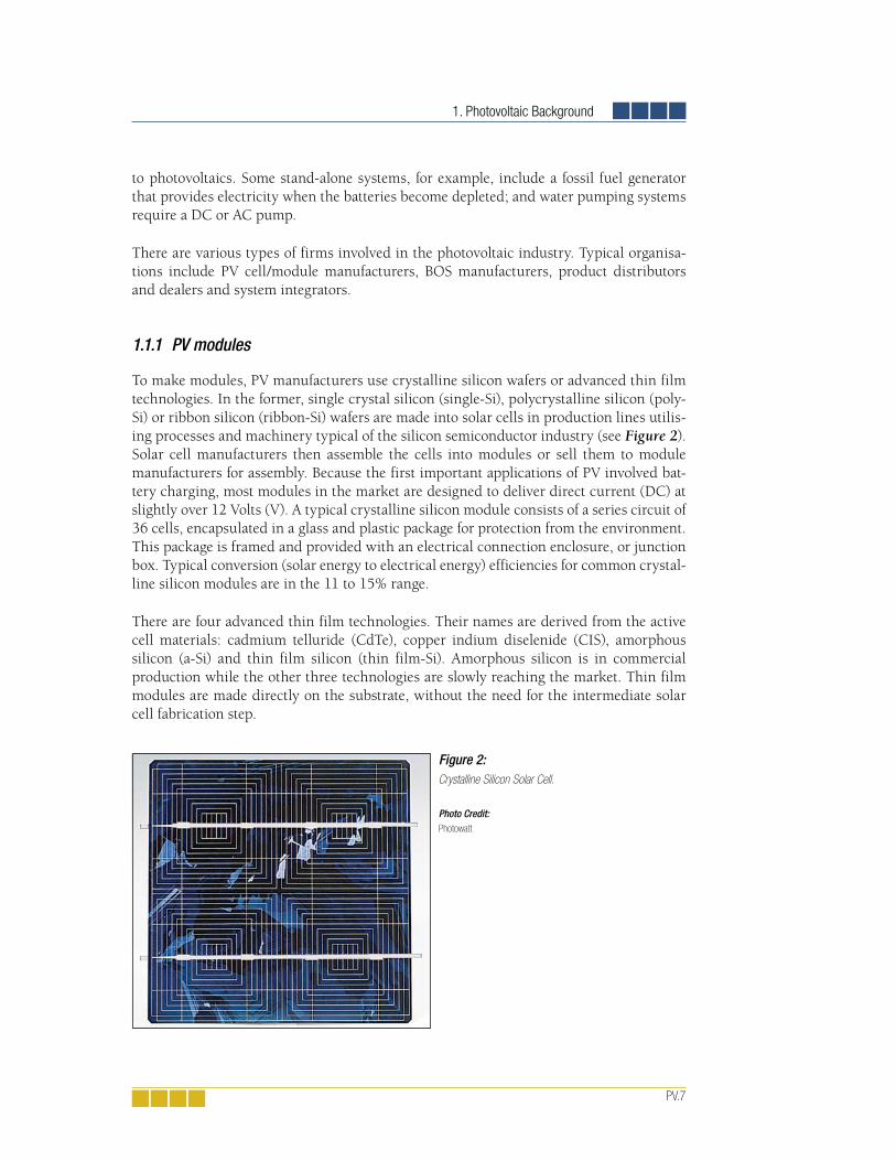
1. Photovoltaic Background
PV.7
to photovoltaics. Some stand-alone systems, for example, include a fossil fuel generator that provides electricity when the batteries become depleted; and water pumping systems require a DC or AC pump.
There are various types of firms involved in the photovoltaic industry. Typical organisa-tions include PV cell/module manufacturers, BOS manufacturers, product distributors and dealers and system integrators.
1.1.1 PV modules
To make modules, PV manufacturers use crystalline silicon wafers or advanced thin film technologies. In the former, single crystal silicon (single-Si), polycrystalline silicon (poly-Si) or ribbon silicon (ribbon-Si) wafers are made into solar cells in production lines utilis-ing processes and machinery typical of the silicon semiconductor industry (see Figure 2). Solar cell manufacturers then assemble the cells into modules or sell them to module manufacturers for assembly. Because the first important applications of PV involved bat-tery charging, most modules in the market are designed to deliver direct current (DC) at slightly over 12 Volts (V). A typical crystalline silicon module consists of a series circuit of 36 cells, encapsulated in a glass and plastic package for protection from the environment. This package is framed and provided with an electrical connection enclosure, or junction box. Typical conversion (solar energy to electrical energy) efficiencies for common crystal-line silicon modules are in the 11 to 15% range.
There are four advanced thin film technologies. Their names are derived from the active cell materials: cadmium telluride (CdTe), copper indium diselenide (CIS), amorphous silicon (a-Si) and thin film silicon (thin film-Si). Amorphous silicon is in commercial production while the other three technologies are slowly reaching the market. Thin film modules are made directly on the substrate, without the need for the intermediate solar cell fabrication step.
Figure 2: Crystalline Silicon Solar Cell.
Photo Credit: Photowatt

Photovoltaic Project Analysis Chapter
PV.8
Some manufacturers are developing PV modules that concentrate sunlight onto small area high efficiency PV cells using lenses. The concept here is that the lens material will be less expensive per unit area than conventional silicon modules thus resulting in a $/Wp advantage. To ensure that the concentrating lenses are always focused on the PV cells, these modules must always be directed at the sun and therefore must be used in conjunc-tion with sun trackers. These modules are limited to areas of the world where there is a considerable amount of direct beam sunlight, such as in desert regions.
1.1.2 Batteries
If an off-grid PV system must provide energy on demand rather than only when the sun is shining, a battery is required as an energy storage device. The most common battery types are lead-calcium and lead-antimony. Nickel-cadmium batteries can also be used, in particular when the battery is subject to a wide range of temperatures. Because of the vari-able nature of solar radiation, batteries must be able to go through many cycles of charge and discharge without damage. The amount of battery capacity that can be discharged without damaging the battery depends on the battery type. Lead-calcium batteries are suitable only in “shallow cycle” applications where less than 20% discharge occurs each cycle. Nickel-cadmium batteries and some lead-antimony batteries can be used in “deep cycle” applications where the depth of discharge can exceed 80%.
Depending on site conditions, and on the presence of a backup generator, battery banks are sized to provide a period of system autonomy ranging from a few days to a couple of weeks (in some very specific applications such as systems above the arctic circle). Batteries are characterised by their voltage, which for most applications is a multiple of 12 V, and their capacity, expressed in Ampere-hours (Ah). For example a 50 Ah, 48 V battery will store 50 × 48 = 2,400 Wh of electricity under nominal conditions.
Note that optimising battery size is critical in obtaining good battery life, suitable system performance, and optimal system life-cycle costs. Unnecessary battery replacement is costly, particularly for remote applications.
1.1.3 Power conditioning
Several electronic devices are used to control and modify the electrical power produced by the photovoltaic array. These include:
Battery charge controllers - regulate the charge and discharge cycles of the battery;
Maximum power point trackers (MPPT) - maintain the operating voltage of the array to a value that maximises array output;

1. Photovoltaic Background
PV.9
Inverters - convert the direct current (DC) output of the array or the battery into alternating current (AC). AC is required by many appliances and motors; it is also the type of power used by utility grids and therefore on-grid systems always require the use of an inverter;
Rectifi ers (battery chargers) - convert the AC current produced by a generator into the DC current needed to charge the batteries.
1.1.4 Generators
For off-grid applications it is also possible to have both a photovoltaic system and a fossil-fuel generator running in parallel. The use of a generator eliminates the need to oversize the photovoltaic array and the battery bank in order to provide power during periods with little sunshine. The photovoltaic array and the generator supplement each other, the PV array reduces the fuel use and maintenance cost of the generator and the generator replaces the part of the photovoltaic system that would need to be oversized to ensure an uninterrupted supply of power.
Generators can use a variety of fossil fuels, such as gasoline, #2 oil (diesel), propane or natural gas. The requirement for a generator, and the fraction of the load met respectively by the photovoltaic system and the generator, will depend on many factors, including the capital cost of the PV array, operating costs of the generator, system reliability, and envi-ronmental considerations (e.g. noise of the generator, emission of fumes, etc.).
1.1.5 Pumps
For water pumping applications, several types of pumps may be used. They can be cate-gorised according to their design type (rotating or positive displacement pumps), to their location (surface or submersible), or to the type of motor they use (AC or DC). Rotating pumps (e.g. centrifugal pumps) are usually preferred for deep wells or boreholes and large water requirements. The use of displacement pumps is usually limited to low volumes. Positive displacement pumps (e.g. diaphragm pumps, piston pumps and progressive ca vity pumps) usually have good lift capabilities but are less accessible than surface pumps and are more sensitive to dirt in the water. Figure 3, which is adapted from Barlow et al. (1993), suggests possible pump choices as a function of the head (total height the water has to be lifted) and the daily water requirement.
Finally the choice between a DC and an AC motor to drive the pump will depend on many factors, including price, reliability and technical support available. DC motors are usually very efficient and are easier to match with the photovoltaic array. AC motors, on the other hand, are cheaper and more readily available, but they require an inverter to be connected to the array.

Photovoltaic Project Analysis Chapter
PV.10
1.2 Photovoltaic Application Markets
Photovoltaic markets can be classified based on the end-use application of the technology. The most common PV projects are off-grid applications. Water pumping also represents an important application of PV, particularly in developing countries. The largest long-term market potential for PV, in volume of sales, is with on-grid applications.
1.2.1 On-grid applications
In grid-connected applications, also called “On-grid” applications, the PV system feeds electrical energy directly into the electric utility grid (this includes central-grids and isolated-grids). Two application types can be distinguished, distributed and central power plant generation. An example of a distributed grid-connected ap-plication is building inte grated PV for individual residences or commercial buildings. The system size for resi-dences is typically in the 2 to 4 kWp range. For commercial buildings, the system size can range up to 100 kWp
Figure 3: Pump Type Selection [adapted from Barlow et al., 1993].
RETScreen® International Photovoltaic Project Model
The RETScreen®
International
Photovoltaic Project Model can be used world-wide to easily evaluate the energy production, life-cycle costs and greenhouse gas emissions reduction for three basic PV applications: on-grid; off-grid; and water pumping. For on-grid applications the model can be used to evaluate both central-grid and isolated-grid PV systems. For off-grid applications the model can be used to evaluate both stand-alone (PV-battery) and hybrid (PV-battery-genset) systems. For water pumping applications the model can be used to evaluate PV-pump systems.

1. Photovoltaic Background
PV.11
or more. Batteries are not necessary when the system is grid-connected. Another applica-tion is the installation of “PV generators” by utilities at power substations and “end-of-line” sites. These applications can be on the threshold of cost competitiveness for PV, depending on location. For example, the Sacramento Municipal Utility District (SMUD) in California has been implementing a plan to install more than 1 MWp per year of distributed PV in its service area. Distributed grid-connected PV systems and a central PV power plant are shown in Figure 4, which is adapted from Ross and Royer (1999).
The benefits of grid-connected PV power generation are generally evaluated based on its potential to reduce costs for energy production and generator capacity, as well as its environmental benefits. For distributed generation, the electric generators (PV or other) are located at or near the site of electrical consumption. This helps reduce both energy (kWh) and capacity (kW) losses in the utility distribution network. In addition, the uti-lity can avoid or delay upgrades to the transmission and distribution network where the average daily output of the PV system corresponds with the utility’s peak demand period (e.g. afternoon peak demand during summer months due to air conditioning loads) as described in Leng and Martin (1994). PV manufacturers are also developing PV modules which can be incorporated into buildings as standard building components such as roof-ing tiles and curtain walls. This helps reduce the relative cost of the PV power system by the cost of the conventional building materials, and allows the utility and/or building owner to capture distributed generation benefits. The use of PV in the built environment is expanding with demonstration projects in industrialised countries.
Figure 4: Grid-Connected PV System Schematic [adapted from Ross and Royer, 1999].

Photovoltaic Project Analysis Chapter
PV.12
Central generation applications are not currently cost-competitive for PV. Several multi-megawatt central generation systems have however been installed as demonstration projects, designed to help utilities acquire experience in the management of central PV power plants. Installations of central PV generation, like distributed grid connected PV, represent a long-term strategy by governments and utilities to support the development of PV as a clean energy with a guaranteed fuel supply.
1.2.2 Off-grid applications
Currently, PV is most competitive in isolated sites, away from the electric grid and requir-ing relatively small amounts of power, typically less than 10 kWp. In these off-grid applica-tions, PV is frequently used in the charging of batteries, thus storing the electrical energy produced by the modules and providing the user with electrical energy on demand.
The key competitive arena for PV in remote off-grid power applications is against electric grid extension; primary (disposable) batteries; or diesel, gasoline and thermoelectric generators. The cost of grid extension in the US, estimated by the Utility Photovoltaic Group (UPVG) ranges from $20,000 to $80,000 per mile. Thus, PV competes particu-larly well against grid extension for small loads, far from the utility grid. Compared to
Figure 5: Stand-Alone Off-Grid PV
System Schematic
[adapted from Ross and Royer, 1999].
Figure 6: Hybrid Off-Grid PV System Schematic
[adapted from Ross and Royer, 1999].
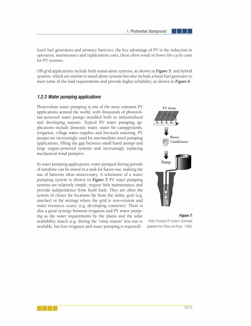
1. Photovoltaic Background
PV.13
fossil fuel generators and primary batteries, the key advantage of PV is the reduction in operation, maintenance and replacement costs; these often result in lower life-cycle costs for PV systems.
Off-grid applications include both stand-alone systems, as shown in Figure 5; and hybrid systems, which are similar to stand-alone systems but also include a fossil fuel ge nerator to meet some of the load requirements and provide higher reliability, as shown in Figure 6.
1.2.3 Water pumping applications
Photovoltaic water pumping is one of the most common PV applications around the world, with thousands of photovol-taic-powered water pumps installed both in industrialised and developing nations. Typical PV water pumping ap-plications include domestic water, water for campgrounds, irrigation, village water supplies and livestock watering. PV pumps are increasingly used for intermediate sized pumping applications, filling the gap between small hand pumps and large engine-powe red systems and increasingly replacing mech anical wind pumpers.
In water pumping applications, water pumped during periods of sunshine can be stored in a tank for future use, making the use of batteries often unnecessary. A schematic of a water pumping system is shown in Figure 7. PV water pumping systems are relatively simple, require little maintenance, and provide independence from fossil fuels. They are often the system of choice for locations far from the utility grid (e.g. ranches) or for settings where the grid is non-existent and water resources scarce (e.g. developing countries). There is also a good synergy between irrigation and PV water pump-ing as the water requirements by the plants and the solar availability match (e.g. during the “rainy season” less sun is available, but less irrigation and water pumping is required).
Figure 7: Water Pumping PV System Schematic
[adapted from Ross and Royer, 1999].


2. Photovoltaic Project Model
PV.15
2 RETSCREEN PHOTOVOLTAIC PROJECT MODEL
The RETScreen Photovoltaic Project Model can be used to evaluate the energy production and financial performance of photovoltaic projects, from small-scale water pum ping sys-tems to intermediate residential off-grid systems to large grid-connected systems, anywhere in the world. There are three basic applications that can be evaluated with the PV model:
On-grid applications, which cover both central-grid and isolated-grid systems;
Off-grid applications, which include both stand-alone (PV-battery) systems and hybrid (PV-battery-genset) systems; and
Water pumping applications, which include PV-pump systems.
Six worksheets (Energy Model, Solar Resource & System Load Calculation (SR&SLC), Cost Analysis, Greenhouse Gas Emission Reduction Analysis (GHG Analysis), Financial Summary and Sensitivity Analysis) are provided in the Photovoltaic Project Workbook file. The SR&SLC worksheet is used to specify the kind of system under consideration, and calcu-late the monthly energy load. This worksheet also computes the annual solar radiation on the tilted PV array for any array orientation, using monthly values of solar radiation on a horizontal surface.
To help the user characterise a photovoltaic system before evaluating its cost and energy performance, some values are suggested for component sizing (e.g. “Nominal PV array power”). Suggested or estimated values are based on input parameters and can be used as a first step in the analysis and are not necessarily the optimum values.
The Energy Model and SR&SLC worksheets are completed first. The Cost Analysis work-sheet should then be completed and finally the Financial Summary worksheet should be completed. The GHG Analysis and Sensitivity & Risk Analysis worksheets are an optional analysis. The GHG Analysis worksheet is provided to help the user estimate the greenhouse gas (GHG) mitigation potential of the proposed project. The Sensitivity & Risk Analysis worksheet is provided to help the user estimate the sensitivity of important financial indicators in rela-tion to key technical and financial parameters. In general, the user works from top-down for each of the worksheets. This process can be repeated several times in order to help optimise the design of the photovoltaic project from an energy use and cost standpoint.
This section describes the various algorithms used to calculate, on a month-by-month basis, the energy production of PV systems in RETScreen. A flowchart of the algorithms is shown in Figure 8. The basics of solar energy are covered in Section 2.1. Section 2.2 describes the tilted radiation calculation algorithm which is common to all three application models (i.e. on-grid, off-grid and water pumping applications). It is used to calculate solar radiation in the plane of the PV array, as a function of its orientation, given monthly mean daily solar radiation on a horizontal surface. Section 2.3 presents the photovoltaic array model, which calculates PV array energy production given ambient temperature and available solar ra-diation. This algorithm is also common to all three application models. Then three different application models are used to evaluate the interaction of the va rious components of the PV system and predict how much energy (or water, in the case of a pumping system) can be
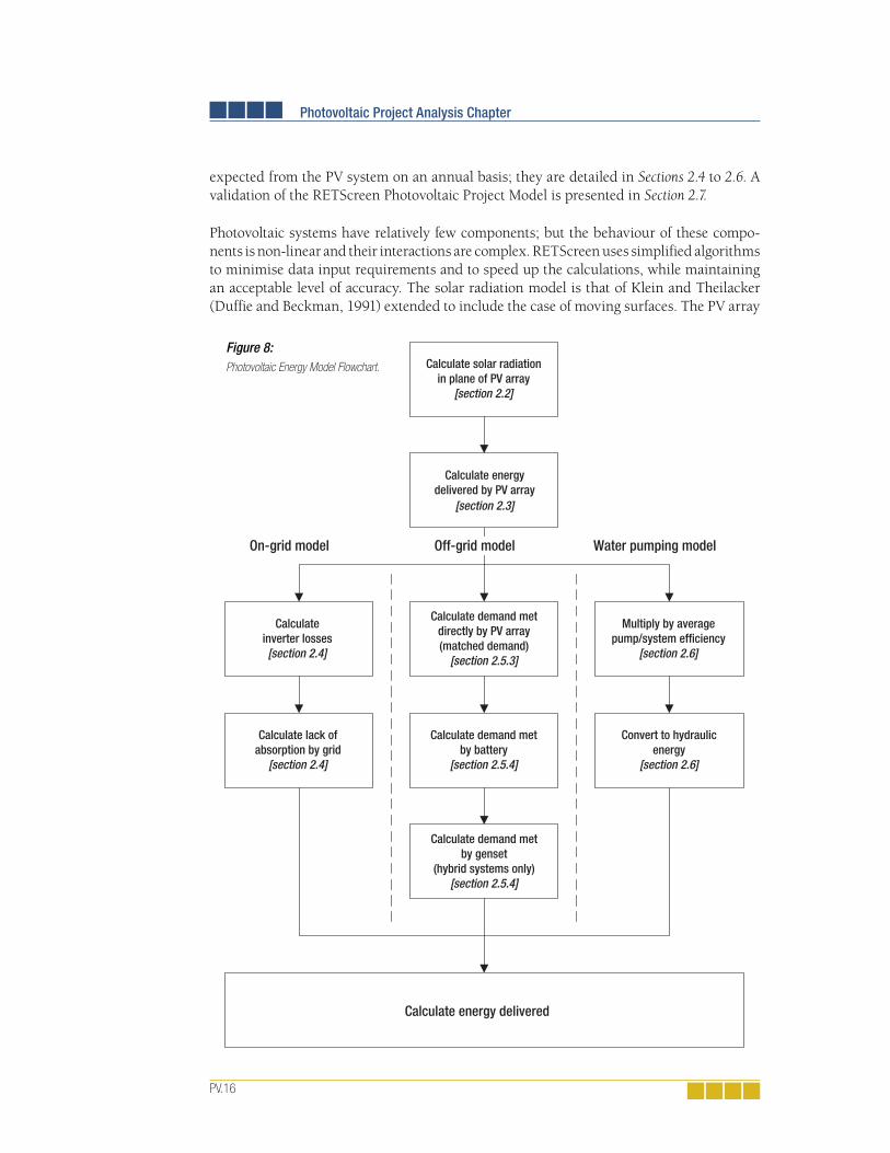
Photovoltaic Project Analysis Chapter
PV.16
expected from the PV system on an annual basis; they are detailed in Sections 2.4 to 2.6. A validation of the RETScreen Photovoltaic Project Model is presented in Section 2.7.
Photovoltaic systems have relatively few components; but the behaviour of these compo-nents is non-linear and their interactions are complex. RETScreen uses simplified algorithms to minimise data input requirements and to speed up the calculations, while maintaining an acceptable level of accuracy. The solar radiation model is that of Klein and Theilacker (Duffie and Beckman, 1991) extended to include the case of moving surfaces. The PV array
Figure 8: Photovoltaic Energy Model Flowchart. Calculate solar radiation
in plane of PV array[section 2.2]
Calculate energydelivered by PV array
[section 2.3]
Calculateinverter losses[section 2.4]
Multiply by averagepump/system efficiency
[section 2.6]
Convert to hydraulicenergy
[section 2.6]
Calculate demand metdirectly by PV array(matched demand)
[section 2.5.3]
Calculate demand metby battery
[section 2.5.4]
Calculate demand metby genset
(hybrid systems only)[section 2.5.4]
Calculate lack ofabsorption by grid
[section 2.4]
Calculate energy delivered
On-grid model Off-grid model Water pumping model
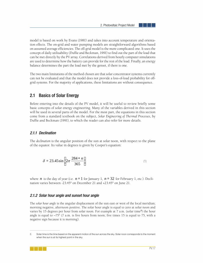
2. Photovoltaic Project Model
PV.17
model is based on work by Evans (1981) and takes into account temperature and orienta-tion effects. The on-grid and water pumping models are straightforward algorithms based on assumed average efficiencies. The off-grid model is the more complicated one. It uses the concept of daily utilisability (Duffie and Beckman, 1991) to find out the part of the load that can be met directly by the PV array. Correlations derived from hourly computer simulations are used to determine how the battery can provide for the rest of the load. Finally, an energy balance determines the part the load met by the genset, if there is one.
The two main limitations of the method chosen are that solar concentrator systems currently can not be evaluated and that the model does not provide a loss-of-load probability for off-grid systems. For the majority of applications, these limitations are without consequence.
2.1 Basics of Solar Energy
Before entering into the details of the PV model, it will be useful to review briefly some basic concepts of solar energy engineering. Many of the variables derived in this section will be used in several parts of the model. For the most part, the equations in this section come from a standard textbook on the subject, Solar Engineering of Thermal Processes, by Duffie and Beckman (1991), to which the reader can also refer for more details.
2.1.1 Declination
The declination is the angular position of the sun at solar noon, with respect to the plane of the equator. Its value in degrees is given by Cooper’s equation:
δ π= +
23 45 2 284365
. sin n
(1)
where n is the day of year (i.e. n =1 for January 1, n = 32 for February 1, etc.). Decli-nation varies between -23.45° on December 21 and +23.45° on June 21.
2.1.2 Solar hour angle and sunset hour angle
The solar hour angle is the angular displacement of the sun east or west of the local meri dian; morning negative, afternoon positive. The solar hour angle is equal to zero at solar noon and varies by 15 degrees per hour from solar noon. For example at 7 a.m. (solar time2) the hour angle is equal to –75° (7 a.m. is five hours from noon; five times 15 is equal to 75, with a negative sign because it is morning).
2. Solar time is the time based on the apparent motion of the sun across the sky. Solar noon corresponds to the moment when the sun is at its highest point in the sky.

Photovoltaic Project Analysis Chapter
PV.18
The sunset hour angle ωs is the solar hour angle corresponding to the time when the sun sets.
It is given by the following equation:
cos tan tanω ψ δs = −
(2)
where δ is the declination, calculated through equation (1), and ψ is the latitude of the site, specified by the user.
2.1.3 Extraterrestrial radiation and clearness index
Solar radiation outside the earth’s atmosphere is called extraterrestrial radiation. Daily extraterrestrial radiation on a horizontal surface,
H0 , can be computed for day n from
the following equation:
H G nscs s0
86400 1 0 033 2365
= +
+
ππ ψ δ ω ω. cos cos cos sin sinn sinψ δ( )
(3)
where Gsc is the solar constant equal to 1,367 W/m2, and all other variables have the same meaning as before.
Before reaching the surface of the earth, radiation from the sun is attenuated by the atmo-sphere and the clouds. The ratio of solar radiation at the surface of the earth to extrater-restrial radiation is called the clearness index. Thus the monthly average clearness index, K T , is defined as:
K HHT =
0
(4)
where H is the monthly average daily solar radiation on a horizontal surface and H0 is the monthly average extraterrestrial daily solar radiation on a horizontal surface. K T values depend on the location and the time of year considered; they are usually between 0.3 (for very overcast climates) and 0.8 (for very sunny locations).
2.2 Tilted Irradiance Calculation
Radiation in the plane of the PV array is computed using a method similar to the Klein and Theilacker algorithm (Duffie and Beckman, 1991, section 2.20). However the algorithm is extended to tracking surfaces and, for that reason, is implemented in a slightly different form than what is described in Duffie and Beckman (1991).

2. Photovoltaic Project Model
PV.19
2.2.1 Description of algorithm
The algorithm can be described as a succession of three basic steps (see Figure 9):
Calculate hourly global and diffuse irradiance on an horizontal surface for all hours of an “average day” having the same daily global radiation as the monthly average;
Calculate hourly values of global irradiance on the tilted (or tracking) surface for all hours of the day; and then
Sum the hourly tilted values to obtain the average daily irradiance in the plane of the PV array.
2.2.2 Calculation of hourly global and diffuse irradiance
Solar radiation can be broken down into two components: beam radiation, which emanates from the solar disk, and diffuse radiation, which emanates from the rest of the sky. The tilting algorithm used in RETScreen requires the knowledge of beam and diffuse radiation for every hour of an “average day” (for the concept of average day, see Duffie and Beckman, 1991).
First, monthly average daily diffuse radiation Hd is calculated from monthly average daily global radiation H using the Erbs et al. correlation3 (Duffie and Beckman, 1991):
HH
K K KdT T T= − + −1 391 3 560 4 189 2 1372 3. . . .
(5)
when the sunset hour angle for the average day of the month is less than 81.4º, and:
HH
K K KdT T T= − + −1 311 3 022 3 427 1 8212 3. . . .
(6)
when the sunset hour angle is greater than 81.4º (the monthly average clearness index, K T is calculated through equation 4).
Figure 9: Flowchart for Tilted
Irradiance Calculation.
Calculation ofhourly beam anddiffuse irradiance
Calculation ofhourly tiltedirradiance
Summation
H
db HH ,
tH
tH
3. Note that both equations are valid only for 0 3 0 8. .≤ ≤KT . A special work-around has to be used when KT falls outside that range, for example in situations near polar night.

Photovoltaic Project Analysis Chapter
PV.20
Then, average daily radiation is then broken down into hourly values. This is done with formulae from Collares-Pereira and Rabl for global irradiance:
r a bts
s s s
= +( ) −−
πω
ω ωω ω ω24
cos cos cossin cos
(7)
a s= + −
0 409 0 50163
. . sin ωπ
(8)
b s= − −
0 6609 0 47673
. . sin ωπ
(9)
where rt is the ratio of hourly total to daily total global radiation, with ωs the sunset hour angle, expressed in radians (see equation 2), and ω the solar hour angle for the midpoint of the hour for which the calculation is made, also expressed in radians (see Section 2.1); and with the formula from Liu and Jordan for diffuse irradiance:
rds
s s s
= −−
π ω ωω ω ω24
cos cossin cos
(10)
where rd is the ratio of hourly total to daily total diffuse radiation. For each hour of the “average day”, global horizontal irradiance H and its diffuse and beam components Hd and Hb are therefore given by:
H r Ht=
(11)
H r Hd d d=
(12)
H H Hb d= −
(13)

2. Photovoltaic Project Model
PV.21
2.2.3 Calculation of hourly irradiance in the plane of the PV array
Calculation of hourly irradiance in the plane of the PV array, Ht , is done using a simple isotropic model, described in section 2.15 of Duffie and Beckman (1991). This is not the most accurate model available, however this is amply sufficient at the pre-feasibility stage:
H H R H Ht b b d= + +
+ −
12
12
cos cosβρ
β
(14)
where ρ represents the diffuse reflectance of the ground (also called ground albedo) and β represents the slope of the PV array. Ground albedo is set to 0.2 if the average monthly temperature is greater than 0°C, 0.7 if it is less than –5°C, with a linear interpolation for temperatures between these values. Rb is the ratio of beam radiation on the PV array to that on the horizontal, which can be expressed as:
Rbz
= coscos
θθ
(15)
where θ is the incidence angle of beam irradiance on the array and θ z is the zenith angle of the sun.
The advantage of the algorithm above is that it can accommodate situations where the posi-tion of the array varies through the day, as is the case with tracking arrays. For tracking surfaces, the slope β of the array and the incidence angle θ for every hour are determined by equations from Braun and Mitchell (1983).
2.2.4 Summation
Once tilted irradiance for all hours of the day is computed, the daily total Ht is obtained by summing individual hours. A special case is that of months near polar night, where the above algorithm fails; in that case tilted irradiance is set equal to global horizontal irradiance.
2.3 PV Array Model
The PV array model is shown in Figure 10. It is based on work by Evans (1981) and is common to all types of PV applications represented in RETScreen.
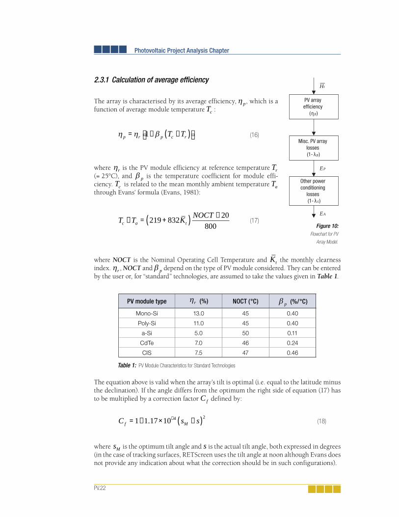
Photovoltaic Project Analysis Chapter
PV.22
2.3.1 Calculation of average effi ciency
The array is characterised by its average efficiency, ηp, which is a function of average module temperature
Tc :
η η βp r p c rT T= − −( ) 1 (16)
where ηr is the PV module efficiency at reference temperature Tr(= 25°C), and β p
is the temperature coefficient for module effi-ciency.
Tc is related to the mean monthly ambient temperature Ta
through Evans’ formula (Evans, 1981):
T T K NOCTc a t− = +( ) −219 832 20
800 (17)
where NOCT is the Nominal Operating Cell Temperature and Kt the monthly clearness index. ηr , NOCT and
β p depend on the type of PV module considered. They can be entered
by the user or, for “standard” technologies, are assumed to take the values given in Table 1.
PV module type ηr (%) NOCT (°C) β p (%/°C)
Mono-Si 13.0 45 0.40
Poly-Si 11.0 45 0.40
a-Si 5.0 50 0.11
CdTe 7.0 46 0.24
CIS 7.5 47 0.46
Table 1: PV Module Characteristics for Standard Technologies
The equation above is valid when the array’s tilt is optimal (i.e. equal to the latitude minus the declination). If the angle differs from the optimum the right side of equation (17) has to be multiplied by a correction factor C f
defined by:
C s sf M= − × −( )−1 1 17 10 4 2.
(18)
where sM is the optimum tilt angle and s is the actual tilt angle, both expressed in degrees (in the case of tracking surfaces, RETScreen uses the tilt angle at noon although Evans does not provide any indication about what the correction should be in such configurations).
PV arrayefficiency
(ηp)
Other powerconditioning
losses(1- λc)
Misc. PV arraylosses(1- λp)
EP
Ht
EA
Figure 10:Flowchart for PV
Array Model.
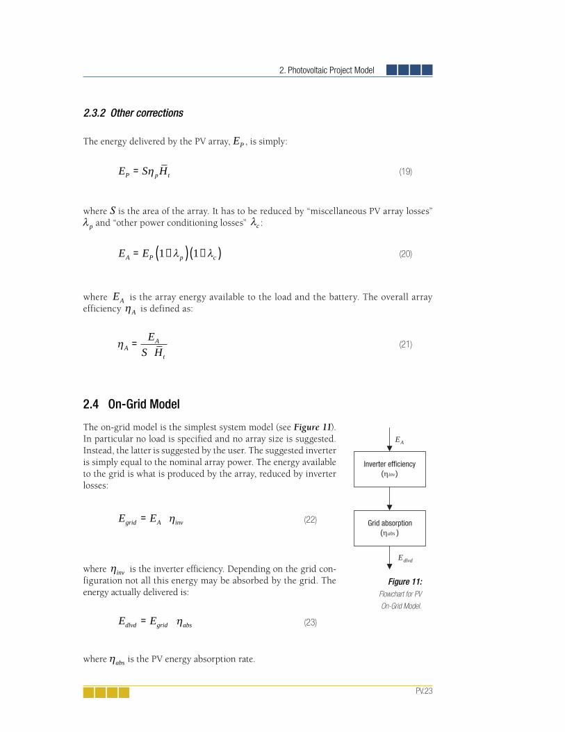
2. Photovoltaic Project Model
PV.23
2.3.2 Other corrections
The energy delivered by the PV array, EP , is simply:
E S HP p t= η
(19)
where S is the area of the array. It has to be reduced by “miscellaneous PV array losses” λp and “other power conditioning losses”
λc :
E EA P p c= −( ) −( )1 1λ λ (20)
where EA is the array energy available to the load and the battery. The overall array efficiency ηA is defined as:
ηAA
t
ES H
=
(21)
2.4 On-Grid Model
The on-grid model is the simplest system model (see Figure 11). In particular no load is specified and no array size is suggested. Instead, the latter is suggested by the user. The suggested inverter is simply equal to the nominal array power. The energy available to the grid is what is produced by the array, reduced by inverter losses:
E Egrid A inv= η
(22)
where ηinv is the inverter efficiency. Depending on the grid con-figuration not all this energy may be absorbed by the grid. The energy actually delivered is:
E Edlvd grid abs= η
(23)
where ηabs is the PV energy absorption rate.
Figure 11:Flowchart for PV
On-Grid Model.
Inverter efficiency(ηinv)
Edlvd
EA
Grid absorption(ηabs )
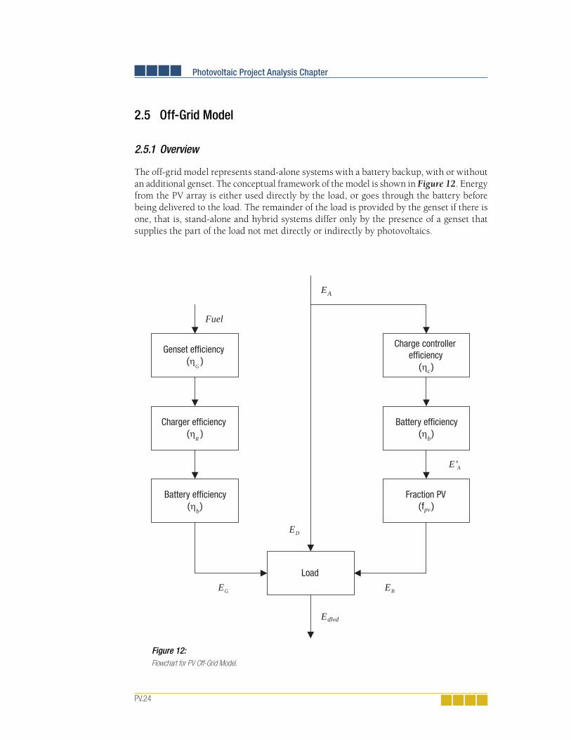
Photovoltaic Project Analysis Chapter
PV.24
2.5 Off-Grid Model
2.5.1 Overview
The off-grid model represents stand-alone systems with a battery backup, with or without an additional genset. The conceptual framework of the model is shown in Figure 12. Energy from the PV array is either used directly by the load, or goes through the battery before being delivered to the load. The remainder of the load is provided by the genset if there is one, that is, stand-alone and hybrid systems differ only by the presence of a genset that supplies the part of the load not met directly or indirectly by photovoltaics.
Figure 12: Flowchart for PV Off-Grid Model.
Charge controllerefficiency
(ηc)
Battery efficiency(ηb)
Fraction PV(fpv)
Load
Genset efficiency(η
G)
EA
E’A
EBEG
ED
Fuel
Charger efficiency(η
R)
Battery efficiency(ηb)
Edlvd

2. Photovoltaic Project Model
PV.25
2.5.2 Load calculation
Equivalent DC demand
The user specifies the total DC demand, DDC , and the total AC demand, DAC (both are expressed in kWh/d). AC energy demand is converted to a DC equivalent by dividing it by the inverter efficiency. Hence the total equivalent DC equivalent DDC equ, is:
D D DDC equ DC
AC
inv, = +
η
(24)
where ηinv is the efficiency of the inverter.
Types of loads
RETScreen carefully considers the correlation between load and solar resource. In some cases, part of the energy demand can be met directly by the photovoltaic system without any energy flowing through the battery (this has some important consequences in terms of energy delivered by the system, because inefficiencies in the battery storage can then be ignored). How much of the energy demand can be met directly depends on the solar-load correlation specified by the user:
Positive. This is, for example, the case of a fan connected directly to a PV module; the fan works only when there is solar energy to power it (water pumping also falls into that category, although a separate model is used – see Section 2.6);
Zero. This is treated in RETScreen as the case of a constant load, i.e. a load that has the same value throughout the day. This of course requires the use of a battery. Examples are cathodic protection or monitoring systems; and
Negative. In this case all the energy fl ows through the battery fi rst before being delivered to the load. This corresponds to all cases not falling into the Positive and Zero categories. Note that daytime intermittent loads (e.g. refrigerator) also fall into this category.
The final result of this calculation is a division of the DC equivalent electrical demand in three parts:
D D D DDC equ matched continuous battery, = + +
(25)

Photovoltaic Project Analysis Chapter
PV.26
where:
Dmatched is the part of the demand that is met directly by the PV modules whenever there is enough energy produced;
Dcontinuous is the part of the demand that is constant throughout the day; and
Dbattery is the part of the demand that will be met primarily by the battery.
Note that Dcontinuous will be met either directly by the PV modules (during the day when there is enough sunshine) or through the battery (at night, or when there is not enough sunshine). The method used to calculate this is described in the next section. It makes use of the critical PV absorption level Pcrit , defined as the load cor-responding to the constant energy demand:
P Dcrit
continuous=24
(26)
where Dcontinuous is expressed in Wh and Pcrit is expressed in W.
2.5.3 Utilisability method
As exposed in Section 2.5.2 the load may be considered in part or in whole as constant. Finding which part of that constant load can be met directly by the photovoltaic array, without first being stored in the battery, is the object of this section. The utilisability method is used to perform the calculation. The method is explained in detail in chapters 2 and 21 of Duffie and Beckman (1991) and is briefly summarised here.
Monthly average daily utilisability
A critical radiation level ITc , defined as the level of radiation that must be exceed-ed in order for the PV array to produce more energy than can be immediately used by the constant load, is:
I PSTc
crit
A
=η
(27)
where Pcrit is the critical PV absorption level (see equation 26), ηA is the overall
array efficiency (see equation 21), and S is the area of the PV array.

2. Photovoltaic Project Model
PV.27
The monthly average critical radiation level Xc , defined as the ratio of the critical radiation level to the noon radiation level on a day of the month in which the day’s radiation is the same as the monthly average, is equal to:
X Ir R Hc
Tc
t n n
=,
(28)
The meaning of rt n, and Rn will be explained later. Finally, the monthly average daily utilisability
φ , i.e. the sum for a month, over all hours and days, of the radia-tion incident upon the array that is above the critical level, divided by the monthly radiation, is:
φ = +
+
exp a b RR
X cXnc c
2
(29)
with:
a K KT T= − +2 943 9 271 4 031 2. . . (30)
b K KT T= − + −4 345 8 853 3 602 2. . . (31)
c K KT T= − − +0 170 0 306 2 936 2. . . (32)
where R will be explained later, and K T is the monthly average clearness index.
Intermediate quantities
Quantities of interest that appear in equations (28) and (29) are:
R , the monthly ratio of radiation in the plane of the array to that on a horizontal surface
( )R H Ht= ;
Rn , the ratio for the hour centred at noon of radiation on the tilted surface to that on a horizontal surface for an average day of the month. This is expressed as:

Photovoltaic Project Analysis Chapter
PV.28
Rr Hr H
Rr Hr Hn
d n d
t nb n
d n d
t n
= −
+
+
1 12
,
,,
,
,
cos β + −
ρβ
g1
2cos
(33)
where rt n, and rd n, are the ratio of hourly total to daily total radiation and the ratio of hourly diffuse to daily diffuse radiation, both for the hour centred around solar noon. This formula is computed for an “average day of month”, i.e. a day with daily global radiation H equal to the monthly average daily global radiation H ; Hd is the monthly average daily diffuse radiation for that “average day” (see equations 5 and 6), ρg is the average ground albedo, and β is the slope of the array (for track-ing surfaces, the slope at noon is used);
rt n, is computed by the Collares-Pereira and Rabl equation, written for solar noon (equation 7 with ω = 0 ); and
rd n, is computed by the Liu and Jordan equation, written for solar noon (equation 10 with ω = 0 ).
Energy breakdown
The energy delivered directly to the continuous load is simply:
E Econtinuous A= −( )1 φ (34)
where EA is the energy available from the array; and the energy delivered to the matched load is:
E D E Ematched matched A continuous= −( )min , (35)
The energy delivered directly to the load is therefore:
E E ED continuous matched= +
(36)
and the energy delivered to the battery is:
E EA D− (37)

2. Photovoltaic Project Model
PV.29
2.5.4 Energy going through the battery
The fraction of the load that a system with battery backup will provide depends on two variables: the array size and the battery size. The probability that the system will fail to meet the load is called the loss of load probability (LOLP).
Several methods for LOLP calculation exist in the literature, in particular the ones of Bucciarelli (1986) and Klein et al. (1987). Unfortunately none of these are suitable for RETScreen. One critical parameter required by Bucciarelli’s method, the standard devia-tion of array output, is not readily available, whereas the method of Klein et al. is too com-putationally intensive. A third method, based on Markov transition matrices (Bucciarelli, 1999) would also likely be too complicated – although it would probably lead to more accurate results.
A simpler approach was taken. A number of computer simulations were run for a dummy stand-alone system with night-only load (the program used was WATSUN-PV, a stan-dard hourly simulation program for photovoltaic systems developed by the University of Waterloo; see Watsun, 1999). Six Typical Meteorological Year (TMY; Watsun, 1993) files corresponding to a variety of climates were used (Toronto, Vancouver, Edmonton, Phoenix, Miami, Denver). Various array sizes were used and the battery capacity was varied from one to six days of storage. The output of the simulations provided, on a monthly basis, the fraction of the load met by the PV system, given the storage/load ratio and the array/load ratio (this latter varying on a monthly basis depending on PV array output). Main relevant parameters of the simulation were:
Load = 2,400 Wh/day, night only;
PV array = from 4 to 20 modules rated at 72 W; and
Batteries = from 4 to 24 batteries rated at 12 V, 50 Ah and maintained at a constant temperature.
The average battery efficiency during the simulations, as revealed by an analysis of all simulation results, was at 85%. The array/load ratios were multiplied by this quantity to reflect the loss of energy in the batteries, the idea here being that, since all the energy deli-vered to the load has to go through the battery first (night-only load), the effective energy produced by the array has to be reduced by battery inefficiencies.
Figure 13 shows in graphical form the output of the simulation providing, on a monthly basis, the fraction of the load met by the PV system, fPV , given the storage/load ratio SLR and the array/load ratio ALR. These are defined mathematically as:
ALR E LA= ′ ′ (38)
SLR Q LU= ′ (39)
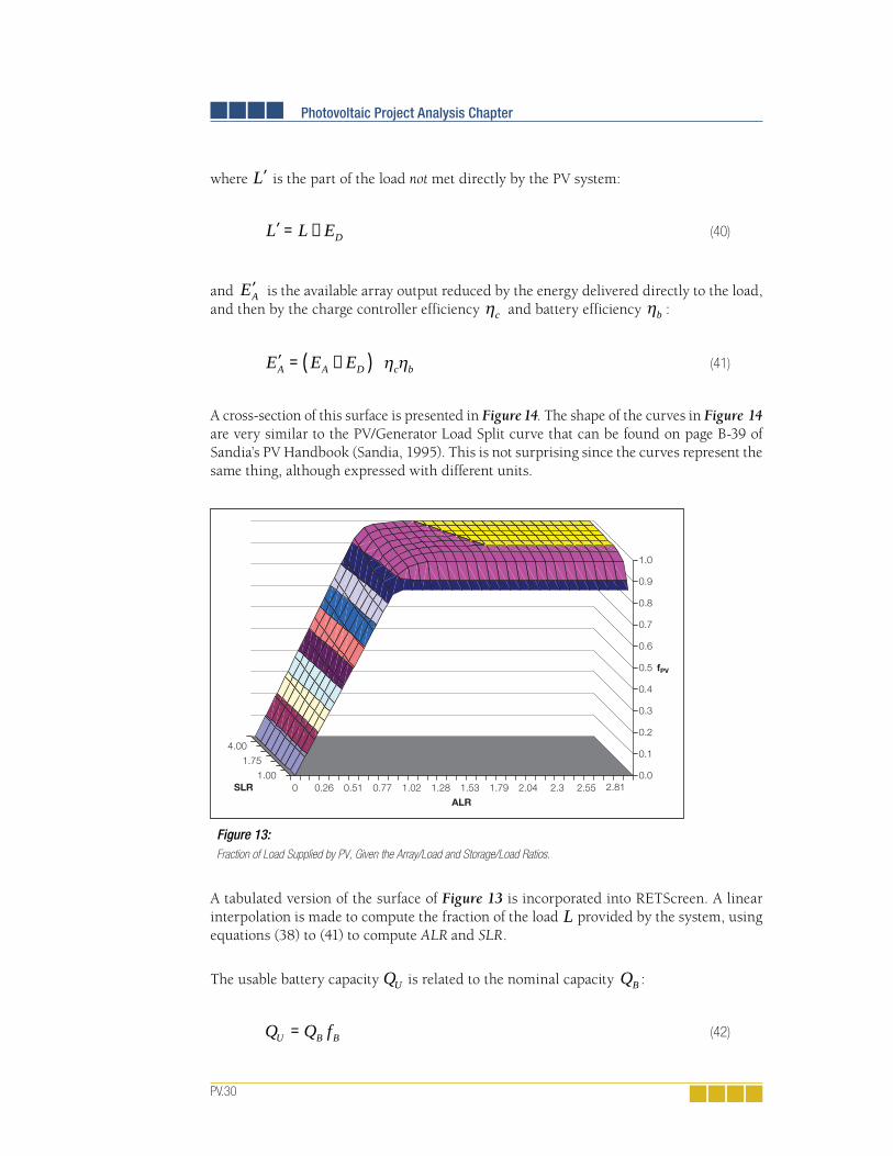
Photovoltaic Project Analysis Chapter
PV.30
where ′L is the part of the load not met directly by the PV system:
′ = −L L ED (40)
and ′EA is the available array output reduced by the energy delivered directly to the load, and then by the charge controller efficiency ηc and battery efficiency ηb :
′ = −( )E E EA A D c bη η (41)
A cross-section of this surface is presented in Figure 14. The shape of the curves in Figure 14 are very similar to the PV/Generator Load Split curve that can be found on page B-39 of Sandia’s PV Handbook (Sandia, 1995). This is not surprising since the curves represent the same thing, although expressed with different units.
A tabulated version of the surface of Figure 13 is incorporated into RETScreen. A linear interpolation is made to compute the fraction of the load L provided by the system, using equations (38) to (41) to compute ALR and SLR.
The usable battery capacity QU is related to the nominal capacity QB :
Q Q fU B B=
(42)
Figure 13: Fraction of Load Supplied by PV, Given the Array/Load and Storage/Load Ratios.
0.0
0.1
0.2
0.3
0.4
0.5
0.6
0.7
0.8
0.9
1.0
fPV
0 0.26 0.51 0.77 1.02 1.28 1.53 1.79 2.04 2.3 2.55 2.811.00
1.75
4.00
ALR
SLR
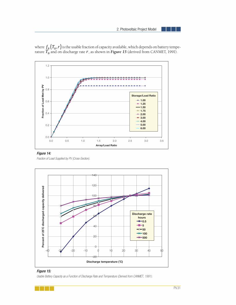
2. Photovoltaic Project Model
PV.31
where f T rB B ,( ) is the usable fraction of capacity available, which depends on battery tempe-rature TB and on discharge rate r , as shown in Figure 15 (derived from CANMET, 1991).
Figure 14: Fraction of Load Supplied by PV (Cross-Section).
0.0
0.2
0.4
0.6
0.8
1.0
1.2
0.0 0.5 1.0 1.5 2.0 2.5 3.0 3.5
Array/Load Ratio
Frac
tio
n o
f Lo
ad M
et b
y P
V
1.001.251.501.752.003.004.005.006.00
Storage/Load Ratio
Figure 15: Usable Battery Capacity as a Function of Discharge Rate and Temperature (Derived from CANMET, 1991).
Discharge temperature (˚C)
Per
cent
of
25˚C
dis
char
ged
cap
acit
y d
eliv
ered
0.5550100500
Discharge rate hours
0
20
40
60
80
100
120
140
-40 -30 -20 -10 0 10 20 30 40 50
-20

Photovoltaic Project Analysis Chapter
PV.32
The average discharge rate is taken as 24n where n is the number of days of autonomy.
Energy delivered by the genset is simply the difference between the load and what can be provided by the PV array, either directly or through the battery:
E L E EG D B= − −
(43)
This quantity is capped by the actual size of the generator, i.e. the generator cannot deliver more than 24CG Rη Wh per day, where CG is the capacity of the generator in W, and ηR the charger efficiency.
The energy used by the genset, QG , expressed either in L/d or m3/d, is simply:
Q EG
G
R G b
=η η η
(44)
where ηG is the average genset efficiency. The presence of the battery efficiency,ηb, in the denominator of equation (44) simply accounts for the fact that most of the energy from the genset will be stored in the battery before reaching the load.
2.5.5 Array, battery and genset sizing
RETScreen suggests values of array, battery and genset size to the user 4. The underlying sizing methods are relatively crude and are intended to provide a starting point which the user can work from.
For stand-alone systems, the array is sized so that its output as defined in Section 2.2 is greater than 1.2 times the load for all months of the year. For hybrid system, the suggested array size is 25% of that for the stand-alone system; in addition the size is capped so that the array never provides more than 75% of the load.
Battery sizing is based on the desired number of days of autonomy. If L is the equivalent DC load, n the number of days of autonomy and d the maximum depth of discharge, the usable battery capacity should be:
Q LndU
B
=η
(45)
where ηB is the battery efficiency. As seen before the usable fraction of capacity available depends on battery temperature TB and on discharge rate r . If f T rB B ,( ) if the usable fraction of capacity available, then the design battery capacity is:
4. RETScreen also suggests a value for inverter size, which is simply the AC peak load (in kW) specifi ed by the user.

2. Photovoltaic Project Model
PV.33
Q QfB
U
B
=
(46)
This quantity is calculated on a monthly basis and the maximum over the year is taken as the suggested battery size.
Finally, the suggested genset capacity is taken as the maximum of the AC demand and:
18
QB
Rη
(47)
where ηR is the charger efficiency. This corresponds to the power required to charge the battery in 8 hours.
2.6 Water Pumping Model
The water pumping model is based on the simple equations found in Royer et al. (1998) and is shown schematically in Figure 16. The daily hydraulic energy demand Ehydr , in J, corresponding to lifting water to a height h (in m) with a daily volume Q (in m3/d) is:
E g Q hhydr f= +( )86400 1ρ η (48)
where g is the acceleration of gravity (9.81 m s-2), ρ the density of water (1000 kg/m-3), and η f is a factor accounting for friction losses in the piping. This hydraulic energy translates into an elec-trical energy requirement Epump :
EE
pumphydr
pump
=η
(49)
where ηpump is the pump system efficiency. If the pump is AC, this equation has to be modified to take into account the inverter efficiency ηinv :
EE
pumphydr
pump inv
=η η
(50)
Figure 16: Flowchart for PV
Water Pumping Model.
Average pumpefficiency(ηpump )
Edlvd
EA
Conversion tohydraulic energy
(ρ g Q η)
Epump

Photovoltaic Project Analysis Chapter
PV.34
Energy delivered is simply:
E E Edlvd pump pump A= ( )η min , (51)
where EA is the energy available from the array (this quantity should be multiplied by ηinv in the case of an AC pump), and daily water delivered is obtained from:
Q Eg hdlvd
dlvd
f
=+( )86400 1ρ η
(52)
Suggested array size is calculated simply by inverting the above equations and is therefore equal to Epump Aη where ηA is the overall array efficiency (see equation 21). This quantity is calculated on a monthly basis and the maximum over the season of use is the suggested array dimension.
In the case of an AC pump, suggested inverter capacity is simply taken equal to the nomi-nal array power. This is the only method possible since it is assumed that the pump power rating is not known (only the energy demand is known).
2.7 Validation
Numerous experts have contributed to the development, testing and validation of the RETScreen Photovoltaic Project Model. They include PV modelling experts, cost engi-neering experts, greenhouse gas modelling specialists, financial analysis professionals, and ground station and satellite weather database scientists.
This section presents two examples of validation against other models. The first example deals exclusively with the tilted radiation calculation model. The second example is a sys-tem test and compares the predicted energy production of a PV/Diesel hybrid system by the RETScreen model against results from an hourly simulation program.
2.7.1 Validation of tilted irradiance calculation compared with an hourly model
Methodology
The algorithm of Section 2.2 was validated in several ways. First, hourly calcula-tions for different tracking configurations were run with Typical Meteorological Year (TMY) weather data as input5. Six sites were considered: Iqaluit (63.75°N), Vancouver (49.20°N), Toronto (43.67°N), Denver (39.8°N), Phoenix (33.43°N), and
5. All are TMY fi les from the Watsun Simulation Laboratory, except Singapore which is an artifi cial fi le created with the WATGEN program. See Watsun (1992, 1993).

2. Photovoltaic Project Model
PV.35
Singapore (1.37°N). Monthly mean daily tilted radiation calculated from hourly values was compared with tilted radiation values computed with the RETScreen algorithm. The configurations considered were:
1. Fixed array facing south, tilted at latitude (see Figure 17a).
2. Fixed vertical array facing south (see Figure 17b).
3. Fixed vertical array facing west (see Figure 17c).
4. Fixed vertical array facing east (see Figure 17d).
5. One-axis tracking with horizontal axis N-S (see Figure 18a).
6. One-axis tracking with sloped axis N-S tilted at latitude (see Figure 18b).
7. Two-axis tracking (see Figure 18c).
8. Azimuth tracking with array sloped at latitude (see Figure 18d).
Second, for fixed surfaces, the RETScreen algorithm was compared to the Liu and Jordan algorithm, which was used in the previous version of the RETScreen PV model, and is still used in the RETScreen Solar Water Heating Model.
Finally, the calculations made in the Northern Hemisphere were duplicated in the Southern Hemisphere, using the same input data as for northern locations but shifted by six months.
Validation results
Figure 17 and Figure 18 show the results of comparisons with values derived from hourly calculations. The agreement between values derived from hourly calcula-tions and values obtained with the RETScreen algorithm is good. For fixed sur-faces, the RETScreen algorithm tends to outperform the Liu and Jordan algorithm. Table 2 summarises the mean bias error and root mean square error of the algo-rithms with respect to values derived from hourly calculations (the results for all stations are aggregated together). The table confirms that for all configurations the model performs well (compared to hourly calculations) and that for fixed surfaces, the RETScreen algorithms always outperforms the Liu and Jordan algorithm – and particularly so for East or West-facing surfaces.
Finally, Figure 19 compares calculations in the Northern and Southern Hemi-sphere. As would be expected the results are identical, except for a few points where the differences can be traced back to small differences in declination or extraterrestrial irradiance (the winter in the Southern Hemisphere is not quite equivalent, mathematically speaking, to the summer in the Northern Hemisphere, hence small differences which get amplified by the model’s equations).

Photovoltaic Project Analysis Chapter
PV.36
Figure 17a and 17b: Performance of RETScreen Radiation Algorithm for Fixed Surfaces.
Fixed, slope = lat, due south
0
5
10
15
20
25
30
0 5 10 15 20 25 30
Monthly mean daily radiation calculated from hourly values [MJ/m2/d]
Mo
nthl
y m
ean
dai
ly r
adia
tio
n ca
lcul
ated
fro
m
mo
nthl
y va
lues
[M
J/m
2 /d
]
Vert. facing south (RETScreen) Vert. facing south (Liu-Jordan)
Fixed, slope = vert, south facing
0
2
4
6
8
10
12
14
16
18
20
Monthly mean daily radiation calculated from hourly values [MJ/m2/d]
Mo
nthl
y m
ean
dai
ly r
adia
tio
n ca
lcul
ated
fro
m
mo
nthl
y va
lues
[M
J/m
2 /d
]
Vert. facing south (RETScreen) Vert. facing south (Liu-Jordan)
0 2 4 6 108 12 14 16 18 20
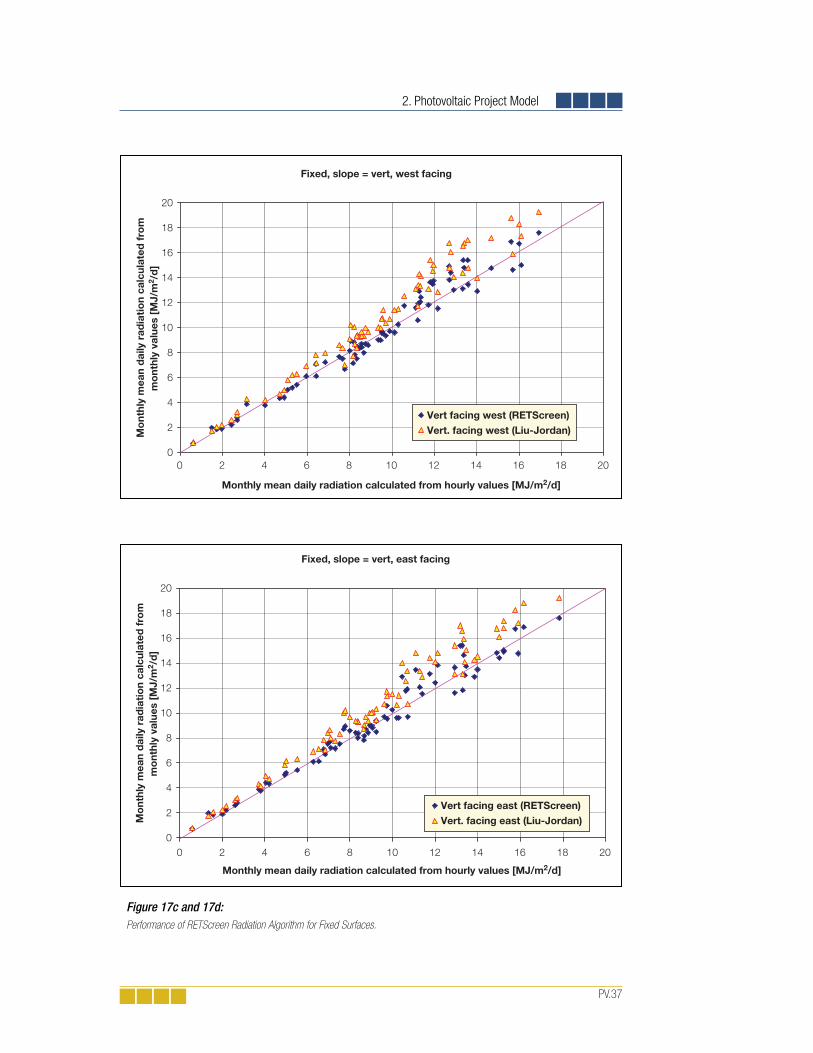
2. Photovoltaic Project Model
PV.37
Fixed, slope = vert, west facing
0
2
4
6
8
10
12
14
16
18
20
Monthly mean daily radiation calculated from hourly values [MJ/m2/d]
Mo
nthl
y m
ean
dai
ly r
adia
tio
n ca
lcul
ated
fro
m
mo
nthl
y va
lues
[M
J/m
2 /d
]
Vert facing west (RETScreen)Vert. facing west (Liu-Jordan)
0 2 4 6 108 12 14 16 18 20
Fixed, slope = vert, east facing
0
2
4
6
8
10
12
14
16
18
20
0 2 4 6 8 10 12 14 16 18 20
Monthly mean daily radiation calculated from hourly values [MJ/m2/d]
Mo
nthl
y m
ean
dai
ly r
adia
tio
n ca
lcul
ated
fro
m
mo
nthl
y va
lues
[M
J/m
2 /d
]
Vert facing east (RETScreen)Vert. facing east (Liu-Jordan)
Figure 17c and 17d: Performance of RETScreen Radiation Algorithm for Fixed Surfaces.

Photovoltaic Project Analysis Chapter
PV.38
Figure 18a and 18b: Performance of RETScreen Radiation Algorithm for Tracking Surfaces.
One-axis, slope = 0, due south
0
5
10
15
20
25
30
35
40
45
0 5 10 15 20 25 30 35 40 45
Monthly mean daily radiation calculated from hourly values [MJ/m2/d]
Mo
nthl
y m
ean
dai
ly r
adia
tio
n ca
lcul
ated
fro
m
mo
nthl
y va
lues
[M
J/m
2 /d
]
One-axis, slope = lat, due south
0
5
10
15
20
25
30
35
40
45
0 5 10 15 20 25 30 35 40 45
Monthly mean daily radiation calculated from hourly values [MJ/m2/d]
Mo
nthl
y m
ean
dai
ly r
adia
tio
n ca
lcul
ated
fro
m
mo
nthl
y va
lues
[M
J/m
2 /d
]
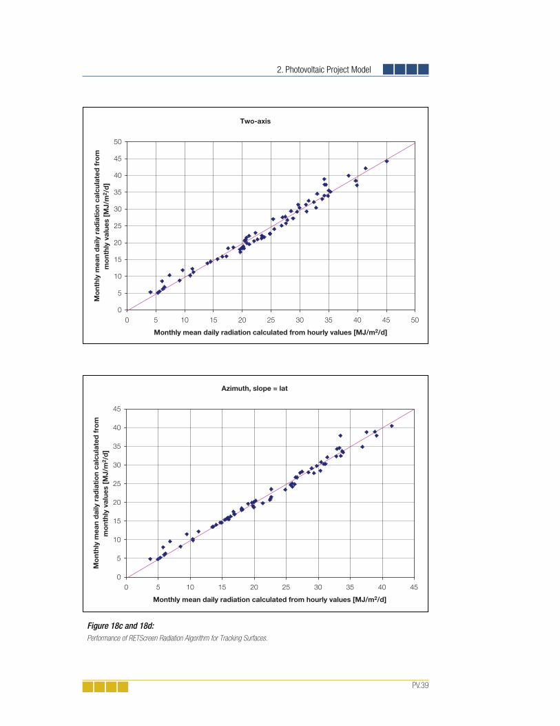
2. Photovoltaic Project Model
PV.39
Two-axis
0
5
10
15
20
25
30
35
40
45
50
0 5 10 15 20 25 30 35 40 45 50
Monthly mean daily radiation calculated from hourly values [MJ/m2/d]
Mo
nthl
y m
ean
dai
ly r
adia
tio
n ca
lcul
ated
fro
m
mo
nthl
y va
lues
[M
J/m
2 /d
]
Azimuth, slope = lat
0
5
10
15
20
25
30
35
40
45
0 5 10 15 20 25 30 35 40 45
Monthly mean daily radiation calculated from hourly values [MJ/m2/d]
Mo
nthl
y m
ean
dai
ly r
adia
tio
n ca
lcul
ated
fro
m
mo
nthl
y va
lues
[M
J/m
2 /d
]
Figure 18c and 18d: Performance of RETScreen Radiation Algorithm for Tracking Surfaces.
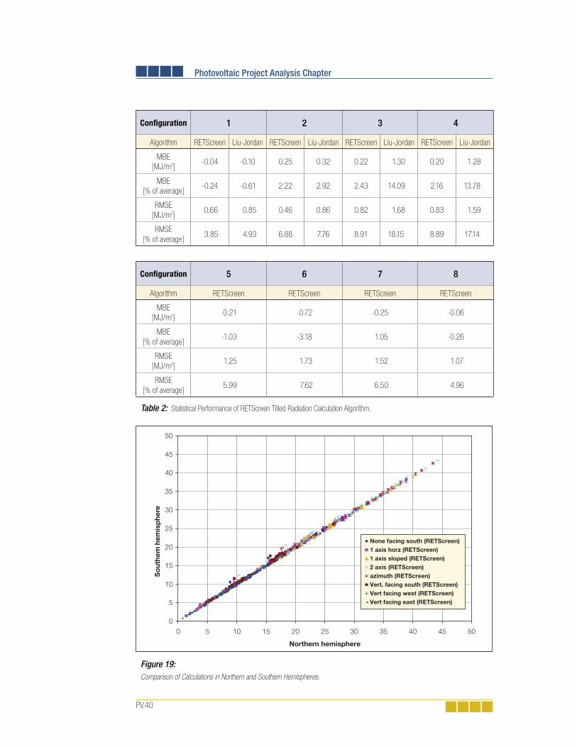
Photovoltaic Project Analysis Chapter
PV.40
Confi guration 1 2 3 4
Algorithm RETScreen Liu-Jordan RETScreen Liu-Jordan RETScreen Liu-Jordan RETScreen Liu-Jordan
MBE [MJ/m2]
-0.04 -0.10 0.25 0.32 0.22 1.30 0.20 1.28
MBE [% of average]
-0.24 -0.61 2.22 2.92 2.43 14.09 2.16 13.78
RMSE [MJ/m2]
0.66 0.85 0.46 0.86 0.82 1.68 0.83 1.59
RMSE [% of average]
3.85 4.93 6.88 7.76 8.91 18.15 8.89 17.14
Confi guration 5 6 7 8
Algorithm RETScreen RETScreen RETScreen RETScreen
MBE [MJ/m2]
-0.21 -0.72 -0.25 -0.06
MBE [% of average]
-1.03 -3.18 1.05 -0.26
RMSE [MJ/m2]
1.25 1.73 1.52 1.07
RMSE [% of average]
5.99 7.62 6.50 4.96
Table 2: Statistical Performance of RETScreen Titled Radiation Calculation Algorithm.
Figure 19: Comparison of Calculations in Northern and Southern Hemispheres.
0
5
10
15
20
25
30
35
40
45
50
0 5 10 15 20 25 30 35 40 45 50
Northern hemisphere
So
uthe
rn h
emis
phe
re
None facing south (RETScreen)1 axis horz (RETScreen)1 axis sloped (RETScreen)2 axis (RETScreen)azimuth (RETScreen)Vert. facing south (RETScreen) Vert facing west (RETScreen)Vert facing east (RETScreen)

2. Photovoltaic Project Model
PV.41
2.7.2 Validation of off-grid model compared with an hourly model
In this section the predictions of the RETScreen off-grid model are tested against calcu-lations by an hourly model. The hourly model used is HOMER, an optimisation model for designing stand-alone electric power systems (see NREL, 2001). HOMER uses hourly simulations to optimise the design of hybrid power systems. HOMER can model com-binations of wind turbines, photovoltaic panels, diesel generators, and battery storage. The present validation does not make use of the optimisation capabilities of HOMER; the program is used only as a simulation tool.
The system configuration is close to the default off-grid PV/batteries/genset worked-out example one finds when opening the RETScreen PV model. The system modelled is a tele-com station located near Neuquen, Argentina (latitude 39°S). Horizontal solar radiation and average air temperature are shown in Table 3. Main parameters of the system are:
Load: 500 W, continuous, AC load (the choice of an AC load is to make the comparison with HOMER easier since HOMER deals only with AC loads) 6.
PV array: 1 kWp mono-Si array; miscellaneous PV array losses are set to 10%. The array is tilted at 50° facing North.
Battery: 24 V, 2,500 Ah nominal capacity with 80% round trip effi ciency and 40% maximum depth of discharge. The HOMER simulations were set up using the “Cycle charging” option, which means that whenever the genset is needed it runs at full capacity, with surplus power going to charge the batteries. The “Setpoint State of Charge” option was also used, which means that the genset will not stop charging the battery bank until it reaches the specifi ed state of charge.
Inverter: 1 kW, 90% average effi ciency.
Genset: 7.5 kW, with a specifi c fuel consumption 0.46 L/kWh.
Charger effi ciency is 95%.
For HOMER, monthly results were obtained by exporting hourly simulation data and per-forming a summation. Obtaining monthly results with RETScreen was trickier and required setting all “fraction of month used” to 0 for all months with the exception of one, and repea-ting the procedure for all months of the year7.
6. HOMER allows a randomization of the load to induce artifi cial variations on an hourly and daily basis. This feature was turned off for the comparison.
7. Inside RETScreen, all energy calculations are performed on a monthly basis before being summed as a yearly fi gure, so the trick mentioned here only reveals fi gures calculated internally by the program prior to the yearly summation displayed in the Energy Model sheet. From a validation point of view, it is interesting to use monthly data since yearly totals could mask seasonal variations in the performance of the models.

Photovoltaic Project Analysis Chapter
PV.42
Global solar
KW/m2/d
Average Temp.
°C
Incident Solar RadiationkW/m2/d
PV Energy Production
kWh
Genset FuelConsumption
L
HOMER RETScreen HOMER RETScreen HOMER RETScreen
Jan 6.33 23.3 4.98 4.94 139 129 164 172
Feb 5.89 22.0 5.23 5.21 132 123 141 152
Mar 4.58 18.3 4.99 4.82 139 127 172 173
Apr 3.36 13.2 4.58 4.39 124 114 170 173
May 2.33 9.2 3.88 3.88 108 106 187 186
Jun 1.78 6.1 3.23 3.27 87 88 191 189
Jul 2.00 5.6 3.51 3.51 98 98 195 191
Aug 2.93 8.0 4.36 4.32 122 119 175 178
Sep 3.72 11.2 4.34 4.17 117 110 176 176
Oct 5.28 15.3 5.14 4.93 143 132 169 170
Nov 6.33 19.3 5.06 5.08 137 130 166 163
Dec 6.36 22.2 4.83 4.81 135 127 174 174
Year 4.23 14.5 4.51 4.44 1,480 1,404 2,079 2,096
Table 3: Summary of Calculation Results with RETScreen and HOMER.
The results of the comparison are summarised in Table 3. On a yearly basis RETScreen predicts slightly less PV energy production than HOMER does (1,404 vs. 1,480 kWh, or a difference of 5%). Part of this difference (around 2%) is attributable to differences in the calculations of inci-dent solar radiation, as shown in the table. Contributions from the genset, reported in Table 3 as fuel consumption, are virtually identical (2,096 vs. 2,079 L). Overall, these diffe rences are insignificant and illustrate the adequacy of the RETScreen PV model for pre-feasibility studies. A graphical comparison of the results are presented in Figure 20 to Figure 22.
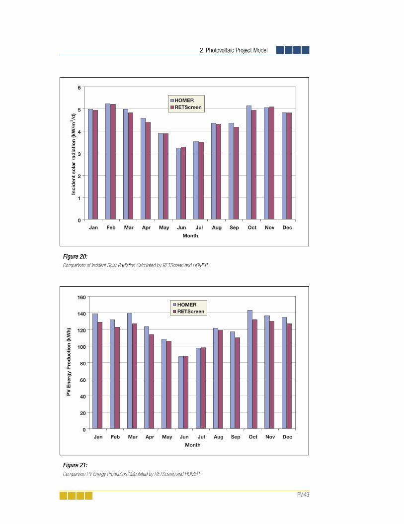
2. Photovoltaic Project Model
PV.43
Figure 20: Comparison of Incident Solar Radiation Calculated by RETScreen and HOMER.
0
1
2
3
4
5
6
Jan Feb Mar Apr May Jun Jul Aug Sep Oct Nov Dec
Month
Inci
den
t so
lar
rad
iati
on
(kW
/m2 /d
)
HOMERRETScreen
Figure 21: Comparison PV Energy Production Calculated by RETScreen and HOMER.
0
20
40
60
80
100
120
140
160
Jan Feb Mar Apr May Jun Jul Aug Sep Oct Nov Dec
Month
PV
Ene
rgy
Pro
duc
tio
n (k
Wh)
HOMERRETScreen

Photovoltaic Project Analysis Chapter
PV.44
2.8 Summary
In this section the algorithms used by the RETScreen Photovoltaic Project Model have been shown in detail. The tilted irradiance calculation algorithm and the PV array model are common to all applications. The tilted irradiance calculation uses an hourly model extended to take into account tracking surfaces. The PV array model takes into account changes in array performance induced by ambient temperature. The On-grid model and the Water pumping model are relatively simple models based on assumed average efficien-cies. The Off-grid model is more complex and allows for a distinction between matched, continuous and intermittent loads which may have an influence on the amount of energy going through the battery.
Figure 22: Comparison of Genset Fuel Consumption Calculated by RETScreen and HOMER.
0
50
100
150
200
250
Jan Feb Mar Apr May Jun Jul Aug Sep Oct Nov Dec
Month
Gen
set
Fuel
Co
nsum
pti
on
(L)
HOMERRETScreen

PV.45
REFERENCES
Barlow, R., McNelis, B. and Derrick, A., Solar Pumping: An Introduction and Update on the Technology, Performance, Costs and Economics, Intermediate Technology Publications and The World Bank, Washington, DC, USA, 1993.
Braun, J.E. and Mitchell, J.C., Solar Geometry for Fixed and Tracking Surfaces, Solar Energy 31,5, 439-444, 1983.
Bucciarelli, L., The Effect of Day-to-Day Correlation in Solar Radiation on the Probability of Loss-of-Power in a Stand-alone Photovoltaic Energy System, Solar Energy 36,1, 11-14, 1986.
Bucciarelli, L., “Personal communication,” 1999.
CANMET, Photovoltaic Systems Design Manual, Available from Natural Resources Canada, CANMET, 580 Booth Street, Ottawa, ON, Canada, K1A 0E4, 1991.
Duffi e, J.A. and Beckman, W.A., Solar Engineering of Thermal Processes, 2nd Edition, John Wiley & Sons, 1991.
ECOTEC Research and Consulting Limited, ECD Energy and Environment, Newcastle Photovoltaics Applications Centre, The Potential Market for PV Building Products, Report no. ETSU: S/P2/00277/00/00, 1998.
Evans, D.L., Simplifi ed Method for Predicting Photovoltaic Array Output, Solar Energy 27,6, 555-560, 1981.
Klein, S.A. and Beckman, W.A., Loss-of-load Probabilities for Stand-Alone Photovoltaic Systems, Solar Energy 39, 6, 499-512, 1987.
Leng, G., Dignard-Bailey, L., Bragagnolo, J., Tamizhmani, G. and Usher, E ., Overview of the Worldwide Photovoltaic Industry, Report no. 96-41-A1 (TR), CANMET Energy Diversifi cation Research Laboratory, Natural Resources Canada, Varennes, QC, Canada, June 1996.
Leng, G., and Martin, J., Distributed Photovoltaic Demand-Side Generation: An Economic Evaluation For Electric Utilities, IEEE First World Conference On Photovoltaic Energy Conversion, December 1994.
Leng, G., Distributed Photovoltaic Demand-Side Generation: An Economic Evaluation for Electric Utilities - Master Degree Thesis, University of Massachusetts Lowell, MA, USA, November 1993.
Markvart, T. (ed.), Solar Electricity, 2nd Edition, John Wiley & Sons, 2000.
Maycock, P.D., Photovoltaic News, February 2000.
NREL, HOMER, The Hybrid Optimization Model for Electric Renewables, Available from National Renewable Energy Laboratory, 1617 Cole Boulevard, Golden, CO 80401-3393, USA, 2001.
Ross, M. and Royer, J., Photovoltaics in Cold Climates, James and James Ltd., 1999.

Photovoltaic Project Analysis Chapter
PV.46
Royer, J., Djiako, T., Schiller, E. and Sy, B.S., Le pompage photovoltaïque: manuel de cours à l’intention des ingénieurs et des techniciens, Institut de l’Énergie des Pays ayant en commun l’usage du Français, 56, rue Saint-Pierre, 3e étage, Québec, QC, Canada, G1K 4A1, 1998.
Royer, J., “Personal Communication,” Solener Inc., 1999.
Sandia National Laboratories, Stand-alone Photovoltaic Systems – A Handbook of Recommended Design Practices, Available from National Technical Information Service, US Department of Commerce, 5285 Port Royal Road, Springfi eld, VA 22161, USA, 1995.
United Nations Population Information Network, Population and Water Resources, Web Site.
Watsun, WATGEN - A Synthetic Radiation Data Generator, User’s Manual and Program Documentation, Version 1.0, Watsun Simulation Laboratory, University of Waterloo, Waterloo, ON, Canada, N2L 3G1, 1992.
Watsun, Typical Meteorological Year (TMY) Weather Files for the WATSUN Family of Programs, Watsun Simulation Laboratory, University of Waterloo, Waterloo, ON, Canada, N2L 3G1, 1993.
Watsun, WATSUN-PV - A Computer Program for Simulation of Solar Photovoltaic Systems, User’s Manual and Program Documentation, Version 6.1, Watsun Simulation Laboratory, University of Waterloo, Waterloo, ON, Canada, N2L 3G1, 1999.


BIOMASS HEATING PROJECT ANALYSIS CHAPTER
CLEAN ENERGY PROJECT ANALYSIS:RETSCREEN® ENGINEERING & CASES TEXTBOOK
DisclaimerThis publication is distributed for informational purposes only and does not necessarily reflect the views of the Government of Canada nor constitute an endorsement of any commercial product or person. Neither Canada, nor its ministers, officers, employees and agents makeany warranty in respect to this publication nor a s s u m e a n y l i a b i l i t y a r i s i n g o u t o f t h i s publication.
© Minister of Natural Resources Canada 2001 - 2005.
www.retscreen.net
RETScreen® InternationalClean Energy Decision Support Centre

ISBN: 0-662-39150-0Catalogue no.: M39-110/2005E-PDF
© Minister of Natural Resources Canada 2001 - 2005.

BIOH.3
TABLE OF CONTENTS
1 BIOMASS HEATING BACKGROUND . . . . . . . . . . . . . . . . . . . . . . . . . . . . . . . . . . . 5
1.1 Description of Biomass Heating Systems . . . . . . . . . . . . . . . . . . . . . . . . . . . . . . . . 71.1.1 Heating plant . . . . . . . . . . . . . . . . . . . . . . . . . . . . . . . . . . . . . . . . . . . . . . . . . . . . . . 7
1.1.2 Heat distribution system . . . . . . . . . . . . . . . . . . . . . . . . . . . . . . . . . . . . . . . . . . . . . . 10
1.1.3 Biomass fuel supply operation . . . . . . . . . . . . . . . . . . . . . . . . . . . . . . . . . . . . . . . . . . 12
1.2 Biomass Heating Application Markets . . . . . . . . . . . . . . . . . . . . . . . . . . . . . . . . . . 141.2.1 Community energy systems . . . . . . . . . . . . . . . . . . . . . . . . . . . . . . . . . . . . . . . . . . . 14
1.2.2 Individual institutional and commercial buildings . . . . . . . . . . . . . . . . . . . . . . . . . . . . . . 15
1.2.3 Process heat . . . . . . . . . . . . . . . . . . . . . . . . . . . . . . . . . . . . . . . . . . . . . . . . . . . . . 16
1.3 Biomass Heating Project Considerations . . . . . . . . . . . . . . . . . . . . . . . . . . . . . . . . 17
2 RETSCREEN BIOMASS HEATING PROJECT MODEL . . . . . . . . . . . . . . . . . . . . . . 19
2.1 Site Conditions . . . . . . . . . . . . . . . . . . . . . . . . . . . . . . . . . . . . . . . . . . . . . . . . . . . 202.1.1 Design temperature and degree-days . . . . . . . . . . . . . . . . . . . . . . . . . . . . . . . . . . . . . 21
2.1.2 Equivalent degree-days for domestic hot water heating . . . . . . . . . . . . . . . . . . . . . . . . . 21
2.1.3 Load and demand duration curves . . . . . . . . . . . . . . . . . . . . . . . . . . . . . . . . . . . . . . . 23
2.1.4 Equivalent full-load hours . . . . . . . . . . . . . . . . . . . . . . . . . . . . . . . . . . . . . . . . . . . . . 30
2.2 Heating Load . . . . . . . . . . . . . . . . . . . . . . . . . . . . . . . . . . . . . . . . . . . . . . . . . . . . 302.2.1 Peak heating load . . . . . . . . . . . . . . . . . . . . . . . . . . . . . . . . . . . . . . . . . . . . . . . . . . 30
2.2.2 Annual heating energy demand . . . . . . . . . . . . . . . . . . . . . . . . . . . . . . . . . . . . . . . . . 31
2.2.3 Fuel consumption (base case system) . . . . . . . . . . . . . . . . . . . . . . . . . . . . . . . . . . . . 31
2.3 Energy Delivered and Fuel Consumption . . . . . . . . . . . . . . . . . . . . . . . . . . . . . . . . 322.3.1 Energy mix determination . . . . . . . . . . . . . . . . . . . . . . . . . . . . . . . . . . . . . . . . . . . . . 32
2.3.2 Heating fuel requirements . . . . . . . . . . . . . . . . . . . . . . . . . . . . . . . . . . . . . . . . . . . . . 34
2.3.3 Biomass annual fuel requirements . . . . . . . . . . . . . . . . . . . . . . . . . . . . . . . . . . . . . . . 34
2.4 District Heating Network Design . . . . . . . . . . . . . . . . . . . . . . . . . . . . . . . . . . . . . . 36
2.5 Validation . . . . . . . . . . . . . . . . . . . . . . . . . . . . . . . . . . . . . . . . . . . . . . . . . . . . . . . 382.5.1 Validation of load duration curve . . . . . . . . . . . . . . . . . . . . . . . . . . . . . . . . . . . . . . . . 39
2.5.2 Validation of as-fi red calorifi c value (heating value) algorithm . . . . . . . . . . . . . . . . . . . . . 42
2.5.3 Validation of district heating network design . . . . . . . . . . . . . . . . . . . . . . . . . . . . . . . . . 43
2.6 Summary . . . . . . . . . . . . . . . . . . . . . . . . . . . . . . . . . . . . . . . . . . . . . . . . . . . . . . . 45
REFERENCES . . . . . . . . . . . . . . . . . . . . . . . . . . . . . . . . . . . . . . . . . . . . . . . . . . . . 47


BIOH.5
BIOMASS HEATING PROJECT ANALYSIS CHAPTERClean Energy Project Analysis: RETScreen® Engineering & Cases is an electronic textbook for professionals and univer-sity students. This chapter covers the analysis of potential biomass heating projects using the RETScreen® International Clean Energy Project Analysis Software, including a technology background and a detailed description of the algorithms found in the RETScreen® Software. A collection of project case studies, with assignments, worked-out solutions and information about how the projects fared in the real world, is available at the RETScreen® International Clean Energy Decision Support Centre Website www.retscreen.net.
1 BIOMASS HEATING BACKGROUND1
Biomass heating systems burn plant or other organic matter—such as wood chips, agri-cultural residues or even municipal waste—to generate heat. This heat can be transported and used wherever it is needed—for the ventilation and space heating requirements of buildings or whole communities, or for industrial processes. Biomass heating systems differ from conventional wood-burning stoves and fireplaces in that they typically control the mix of air and fuel in order to maximize efficiency and minimize emissions, and they include a heat distribution system to transport heat from the site of combustion to the heat load. Many biomass heating systems incorporate a sophisticated automatic fuel handling system. Figure 1 shows a small commercial biomass heating system.
Figure 1: Small Commercial Biomass
Heating System.
Photo Credit: Credit: Grove Wood Heat
1. Biomass Heating Background
1. Some of the text in this “Background” description comes from the following two Natural Resources Canada (NRCan)
supported reports: Buyer’s Guide To Small Commercial Biomass Combustion Systems, NRCan, 2002, and,
McCallum, B., Small-Scale Automated Biomass Energy Heating Systems: A Viable Option For Remote Canadian Communities?, NRCan/CFS’s Great Lake Forestry Centre and NRCan’s CEDRL, 1997.

Biomass Heating Project Analysis Chapter
BIOH.6
Biomass heating technology is not new. For many years people have used stoves and fur-naces, fed with cut roundwood, for space heating. The development of automated biomass heating systems began in Scandinavia in the 1970s, when oil prices skyrocketed. Today, there are thousands of these systems in operation around the world, using a multitude of different types of biomass fuels, or “feedstock”. Despite this, much of the general public and many heating professionals are unaware of the benefits of this cost-effective, proven, and reliable source of energy. The recent emphasis on renewable energy resources as re-placements for conventional fuels, spurred by concerns about greenhouse gas (GHG) emis-sions, is causing a resurgence of interest in biomass heating, where the biomass is harvested in a sustainable manner.
Biomass heating offers a number of compelling advantages, both for the system owner and, in the case of district heating systems, for the local community. It can supplant expensive conventional energy sources such as fossil fuels and electricity with local biomass re-sources, which is often available at little or no cost as waste or low-value by-products from various industries (e.g. forestry and agriculture). In doing so, overall levels of pollution and greenhouse gases are reduced, the purchaser is insulated from fossil fuel price shocks, and local jobs are created in the collection, preparation, and delivery of the feedstock. In addition, the heat distribution system of the biomass heating plant facilitates the use of waste heat from on-site power generation or thermal processes (i.e. waste heat recovery, or “WHR”) and can be extended to service clusters of buildings or even whole communities in a “district energy system”.
Biomass heating systems tend to have higher initial costs than conventional fossil fuel-burning systems. Furthermore, the quality of biomass feedstock is highly variable in com-parison with the relatively standardized commercially available fossil fuels. Feedstock delivery, storage, and handling are more complex as a result, and often more physical space is required. All these factors require a high level of operator involvement and diligence.
Therefore, biomass heating systems are most attractive where conventional energy costs are high and biomass feedstock costs are low. This occurs when: electricity or some other costly form of energy is used for space and water heating; and biomass residues are available on-site or nearby at zero cost or, if there is a disposal fee for the biomass residues, at a discount.
Because of their size and complexity, the use of automated biomass combustion systems is largely limited to the industrial, commercial, institutional and community sectors. They tend to be located in rural and industrial areas, where restrictions on the types of pol-lutants they emit may be less severe, truck access for feedstock delivery may be in place, feedstock-handling equipment such as loaders may already be available, and the labour and expertise required to operate an industrial type boiler system may be easier to find.
Biomass combustion systems are often well suited to industrial process loads. Many indus-trial process loads have constant heat requirements and biomass heating systems operate most efficiently, and with the fewest operational challenges, when they supply a relatively constant quantity of heat, near their rated capacity, throughout the year. This also maxi-mizes fuel savings by displacing a large amount of expensive conventional fuel, justifying the higher initial capital and ongoing labour costs of the system.

1. Biomass Heating Background
BIOH.7
This background section describes biomass heating systems, discusses the biomass heating markets including community energy systems, individual, institutional and commercial building, and process heat applications, and presents general biomass heating project considerations.
1.1 Description of Biomass Heating Systems
A biomass heating system consists of a heating plant, a heat distribution system, and a biomass fuel supply operation. These three parts are described in detail in the following section.
1.1.1 Heating plant
Biomass heating plants typically comprise a number of different heating units. This en-sures that there will be sufficient heating capacity to meet the heating load (by turning on additional units when the load increases), reduces the risk that a fuel supply interruption will endanger the supply of heat (other units can compensate for the lack of fuel in the primary unit), and maximizes the use of the lowest-cost heat sources (by using the least ex-pensive sources first, and activating more expensive sources only as needed). As described by Arkay and Blais (1996), the four types of heat sources that may be found in a biomass heating plant are, in increasing order of typical cost per unit of heat produced:
1) Waste heat recovery: The lowest-cost heat will typically be that provided by a waste heat recovery system. Some biomass heating plants can be situated near electricity generation equipment (e.g. a reciprocating engine driving a generator) or a thermal process that rejects heat to the environment. This heat, which would otherwise be wasted, can often be captured by a waste heat recovery system, at little or no additional cost.
2) Biomass combustion system (BCS): The BCS is the unit that generates heat through combustion of biomass feedstock, and is thus by defi nition the heart of a biomass heating plant. If a low-cost feedstock is used, and the system is operated at a relatively constant loading near its rated capacity, the unit cost of heat produced by the BCS will be relatively low; the BCS will supply the portion of the heat load that is not met by waste heat recovery, up to the capacity of the BCS.
3) Peak load heating system: Due to its operational characteristics and higher capital costs, the biomass combustion system may be sized to provide suffi cient heat to meet typical heat loads, but too small to satisfy occasional peaks in the heating load. The peak load heating system will provide that small portion of the annual heating load that cannot be furnished by the BCS. Often it will rely on conventional energy sources, and be characterized by lower capital costs and higher fuel costs. In some cases the peak load heating system is also used during times of very low heat load; under such conditions, the biomass combustion system would be very ineffi cient or generate unacceptable levels of emissions (smoke).

Biomass Heating Project Analysis Chapter
BIOH.8
4) Backup heating system: Used in the case where one or more of the other heat sources are shutdown, either due to maintenance or an interruption in the fuel supply, the backup heating system will tend to share the peak load system’s characteristics of lower capital costs and higher fuel costs. Often the peak load system serves as the backup to the biomass combustion system, and no additional backup heating system is included.
In the biomass combustion system (BCS), the principal interest in a heating plant, the biomass fuel or feedstock moves through the BCS in a number of stages, many of which are illustrated in Figure 2 and described here:
Biomass Fuel (Feedstock) Delivery: if not available on site, the biomass fuel is delivered to a fuel receiving area, which must be large enough to accommodate the delivery vehicles.
Biomass Fuel (Feedstock) Storage: the biomass fuel in the storage area must be suffi cient to fi re the plant over the longest interval between deliveries. The fuel can be stored in an outdoor pile, a protective shed, or inside a bin or silo. Outdoor storage, though inexpensive, permits precipitation and dirt to contaminate feedstock.
Biomass Fuel (Feedstock) Reclaim: this refers to the movement of the biomass fuel from storage to the combustion chamber. It can be effected manually, as in the loading of outdoor furnaces with cut logs; fully automated, using augers or conveyors; or rely on both operator and machinery. Fully automatic systems can be vulnerable to biomass fuel variability and detritus, such as frozen or irregularly shaped clumps, wire, or gloves.
Biomass Fuel (Feedstock) Transfer: this is the movement of the biomass fuel into the combustion chamber. In automated systems, a screw auger or similar device moves the biomass fuel and a metering bin measures the fl ow into the combustion chamber.
Combustion Chamber: the biomass fuel is injected into an enclosed combustion chamber, where it burns under controlled conditions. To this end, a control system regulates the infl ow of air in response to heat demand; in automated BCSs, biomass fuel fl ow is also regulated. Refractory materials keep the heat of combustion inside the chamber. Many combustion chambers support the burning feedstock on a grate, enabling airfl ow up through and over the burning biomass fuel, facilitating complete combustion. In more sophisticated systems, the grate moves in order to evenly distribute the fi re bed, convey the biomass fuel through zones of different under-fi re airfl ow, and to push the ash to the end of the combustion chamber. Hot exhaust gases exit the combustion chamber and either pass through a heat exchanger, into a secondary combustion chamber containing a heat exchanger, or, if the heat exchanger is in or around the combustion chamber, directly into an exhaust system.

1. Biomass Heating Background
BIOH.9
Heat Exchanger: the heat from combustion is transferred to the heat distribution system via a heat exchanger. In simple outdoor furnaces, an insulated water jacket around the combustion chamber serves as the heat exchanger. Larger BCSs use boilers, with water, steam, or thermal oil as the heat transfer medium.
Ash Removal and Storage: this involves voiding the BCS of bottom ash, which remains in the combustion chamber, and fl y ash, which is transported by the exhaust gases. Bottom ash may be removed manually or automatically, depending on the system. Fly ash may deposit in the secondary combustion chamber or the heat exchanger (necessitating cleaning), escape out the fl ue, or be taken out of suspension by a particulate collection device (exhaust scrubber).
Exhaust System and Stack: this vents the spent combustion gases to the atmosphere. Small systems use the natural draft resulting from the buoyancy of the warm exhaust; larger systems rely on the fans feeding air into the combustion chamber to push out the exhaust gases, or draw the exhaust gases out with a fan at the base of the chimney.
In addition to the equipment described above, instrumentation and control systems of varying sophistication oversee the operation of a BCS, modulate the feed of air and, in automated BCSs, fuel, in response to demand, and maintain safe operating conditions.
BiomassFuel Delivery
BiomassFuel Reclaim
Backup andPeaking Boiler
BiomassFuel Transfer
Ash Removal and StorageCombustionChamber
Hot WaterSupply
ParticulateCollection
Heat Exchanger
Exhaust Systemand Stack
BiomassFuel
Storage
Figure 2:Biomass Combustion System – General Layout
[adapted from NRCan’s Buyer’s Guide To Small Commercial Biomass Combustion Systems, 2002].

Biomass Heating Project Analysis Chapter
BIOH.10
Biomass combustion systems cover a wide range of equipment, distinguished by variations in fuel and air delivery, design of combustion chamber and grate, type of heat exchanger, and handling of exhaust gas and ash. Other than very large heating plants, BCS installations can generally be classified within three broad feed system categories, based on their capacity:
Small manual feed systems (50-280 kW): typically are outdoor furnaces burning blocks of wood and distributing heat with hot water.
Small automatic feed systems (50-500 kW): use particulate biomass fuel (feedstock), typically utilising a two-stage combustor (i.e. with a secondary combustion chamber) and incorporating a fi re-tube hot water boiler (i.e. a tube that carries hot combustion gases through the water that is to be heated).
Moderate-sized feed systems (400 kW and up): have fully automated feeding of particulate biomass fuel (feedstock), typically utilising a moving or fi xed grate combustor with integral or adjacent fi re-tube boiler for hot water, steam or thermal oil.
In addition to these general types, there is a wide variety of specialty biomass combustion systems configured to meet specific fuel characteristics or specific heating requirements.
The sizing of the biomass combustion system relative to that of the peak load heating sys-tem is a crucial design decision. The overriding objective is to minimize the total life-cycle cost of the heat supply. There are two common approaches to BCS system sizing: base load design and peak load design. The choice of design method will depend on the variability of the load, the cost of biomass and conventional fuels, the availability of capital, and other factors specific to the application. Peak load sizing is more common in large installations with high continuous energy demands. Base load sizing is often applied to smaller instal-lations serving exclusively space heating or variable loads. The two approaches to system design are compared in Table 1.
For applications exhibiting strong seasonal variation in the heat load, such as year round process loads augmented by space heating requirements in the winter, two BCSs may be used. A small unit operates in the summer, a larger unit sized for the typical winter load runs during wintertime, and both units operate simultaneously during periods of peak demand. This arrangement facilitates the operation of each BCS at a loading close to its rated capacity, raising efficiency and reducing emissions. Moreover, it is still possible to provide some heat when one system is shut down for maintenance.
1.1.2 Heat distribution system
The heat distribution system transports heat from the heating plant to the locations where it is required. This may be within the same building as the BCS, in a nearby building, or in a cluster of buildings located in the vicinity of the plant in the case of a district heating system. In most systems, a network of insulated piping conveys water at temperatures up to 90ºC away from the plant and returns the cooled water back to the plant for reheating; in some industrial systems, heat is distributed by steam or thermal oil.

1. Biomass Heating Background
BIOH.11
Within a building, heat is typically distributed by baseboard hot water radiators, under-floor or in-floor hot water piping, or hot air ducting. Between build-ings, a network of insulated underground piping transports heat. Small distribution networks utilize low cost coils of plastic pipe. In larger networks, a pipe-within-a-pipe arrangement is common: the inner carrier pipe is generally steel, the outer casing is polyethylene, and the cavity between the carrier pipe and the casing is filled with polyurethane foam. Piping is usually buried 60 to 80 cm below ground surface, as depicted in Figure 3; it is not necessary to bury the pipes below the frost line since the pipes are insulated and circulate hot water.
Approaches To Biomass Combustion System Sizing
BASE LOAD DESIGN PEAK LOAD DESIGN
Description (Design philosophy)
Maximise cost effectiveness by ‘undersizing’ the BCS to handle only the major (or base) portion of the heating load. Use a lower capital cost, smaller fossil fuel system to handle peaks.
Determine the peak (or maximum) heating load, then oversize the system by a contingency factor to ensure that unanticipated extreme loads can be satisfi ed.
Advantages
BCS is running at or near its full (optimum) capacity most of the time, which will provide highest seasonal effi ciency;
Capital costs signifi cantly reduced; and
Better system control for effi cient performance and lower emissions.
Minimizes use of fossil fuel;
Maximizes use of biomass;
Provides the possibility for increased energy use at marginal cost (if biomass fuel cost is low); and
Provides a built-in capacity surplus for future load expansion.
Disadvantages
A conventional system is required for peak heating loads;
Fossil fuel use will be increased;
Future load expansion will affect base load; and
Increased energy use must be supplemented by more expensive conventional fuels.
A larger system greatly increases capital cost (and labour operating costs);
With variable loads (as in heating applications), the BCS must be operated at part load much of the time. This reduces operating effi ciency, resulting in an increase in biomass fuel consumption; and
When operated at low load, BCSs are prone to higher emissions (smoke) and often unstable combustion.
Table 1: Approaches To Biomass Combustion System Sizing
[adapted from NRCan’s Buyer’s Guide To Small Commercial Biomass Combustion Systems, 2002].
Figure 3: Water Pipes in District Heating System.
Photo Credit: SweHeat

Biomass Heating Project Analysis Chapter
BIOH.12
In a district heating system, a central biomass plant provides heat to a number of consum-ers located around the area near the central plant. The consumers will often be grouped in clusters of public, commercial, and residential buildings located within a few hundred meters of each other. District heating systems offer a number of advantages over the use of individual heating plants in each building. A single, large plant will have a level of so-phistication, efficiency, and automation that would not be possible in the smaller plants. In addition, individual consumers will not need the equipment or expertise needed to successfully operate their individual biomass combustion system, further encouraging the substitution of biomass over fossil fuels. Additionally, fuel consumption, labour require-ments, and emissions will be reduced, waste heat may be used more effectively, and the system will be operated more safely, all because the plant is centralized.
Heat distribution systems can often be expanded to accommodate new loads if the main distribution piping has sufficient capacity. Additional buildings within a reasonable dis-tance can be connected to the system until its capacity is reached. If sufficient space is allocated in the heating plant building, additional burners can be installed at a later date to increase capacity.
Since the initial costs of a district heating system are high, it is cheaper to be integrated into newly constructed areas. Finally, a biomass combustion and district heating system requires a high level of dedication and organization than simple fossil fuel-fired systems.
1.1.3 Biomass fuel supply operation
The biomass fuel supply operation is the sequence of activities that results in the delivery of biomass fuel (feedstock) to the heating plant. Since the proper functioning of the plant is intimately related to the timely supply of appropriate biomass fuel, and since this operation often entails local activity rather than decisions made at a distant refinery, the fuel supply operation is considered a “component” of the plant.
A reliable, low-cost, long-term supply of biomass fuel is essential to the successful opera-tion of a biomass heating plant. Fossil fuel products are relatively standardized, generally available, and easy to transport and handle. In contrast, many biomass fuels are highly variable in terms of moisture content, ash content, heating value, bulk consistency, and geographical availability. Biomass combustion systems—and especially their fuel handling sub-systems—may be designed to operate with only one type of biomass of a certain qual-ity, and may require modification or operate poorly when used with a different biomass fuel. Thus, the installation of a biomass heating plant must be preceded by a thorough assessment of the quality and quantity of the biomass resource that is available, the reli-ability of the suppliers, the fuel handling requirements imposed by the characteristics of the available biomass fuel, and possible changes in the future demand for the targeted biomass resource. For example, if an alternative use is discovered, that may increase the price of the biomass resource. Therefore, long-term supply contracts should be negotiated whenever possible.

1. Biomass Heating Background
BIOH.13
A wide range of low-cost material can be used as biomass fuel such as wood and wood resi-dues in chunk, sawdust, chip, or pellet form; agricultural residues such as straw, chaff, husks, animal litter, and manure; fast-grow-ing energy crops planted specifically for bio-mass combustion, including willow, switch-grass, and hybrid poplar; and municipal solid waste. Figures 4 and 5 show two examples of low-cost biomass fuel. Whatever the biomass resource, it can be considered a renewable re-source only if it is harvested in a sustainable manner.
The price of the biomass fuel depends on the source. If the biomass fuel is a waste prod-uct that must be disposed of, it may have a negative cost since tipping fees are reduced. Residuals, such as bark from a sawmill, which do not need to be disposed of but have no alternative use, are often available at no cost. By-products, such as shavings and sawdust, have a low-value alternative use and there-fore will typically be available at a low cost. Plant biomass, which is harvested or purpose-grown specifically for use as a biomass fuel, will normally have higher costs, and prepared fuels, such as briquettes, may cost more than fossil fuels. These prepared fuels may have stable, uniform characteristics, however, mak-ing them convenient for use in small systems with simple fuel handling systems, where minimum operator involvement is a neces-sity. For example, prepared wood pellets have achieved considerable success in Europe.
In many countries that have embraced bio-mass heating, woodchips and other wood products are the principal biomass resource. The goal of every forestry operation should be to maximize the utilisation of harvested trees and to provide for the establishment of a new crop of productive trees. In the forestry industry, harvested trees should be sorted so that a range of products reflecting the qual-ity of the trees can be produced: timber from the boles of spruce or pine and firewood or woodchips from small diameter, dead, diseased and otherwise unusable trees. A commu-nity logging operation can integrate woodchip fuel production into their product offering. Figure 6 shows a wood biomass fuel supply being harvested in a commercial operation.
Figure 4: Walnut Shells for Biomass Combustion.
Photo Credit: Warren Gretz/NREL Pix
Figure 5: Bagasse for Biomass Combustion.
Photo Credit: Warren Gretz/NREL Pix

Biomass Heating Project Analysis Chapter
BIOH.14
The size of wood that can be chipped is limited by the size of the chipper selected. Large-diameter trees require a large chipper with a powerful engine. Because of the high costs for large chippers, most small-scale chipping operations employ small-scale chippers, often powered by farm tractors that can chip trees up to about 23 cm (10 inches) in diameter. Larger, second-hand industrial chippers are sometimes available at a reasonable cost.
Chipping can take place at the logging site. However, in isolated areas where winter roads may be used for transport, a significant quantity of chipping material can be stockpiled near the heating plant and chipped as it is required. If there is no logging operation nearby, a stand-alone operation to supply wood and produce chips will need to be established.
Woodchips must be of good quality, and free of dirt and oversized sticks, which are pro-duced when chipping knives get dull. Sticks can cause jamming and shutdowns of the fuel-feed system; dirt causes excessive wear as well.
1.2 Biomass Heating Application Markets
Biomass heating markets can be classified by the end-use application of the technology. The three major markets are community energy systems, institutional and commercial buildings, and process heat applications.
1.2.1 Community energy systems
Community energy systems make use of a biomass heating plant and a district heating system to service clusters of buildings or even an entire community, as seen in Figure 7. Such community energy systems can provide space heating, heating of ventilation air, water heating, and process heat. These can be supplied to individual buildings, such as in-stitutional (e.g. hospitals, schools, sports complexes), commercial (e.g. offices, warehouses, stores), residential (e.g. apartments) and industrial buildings. They can also provide heat to individual homes, especially if the houses are newly constructed and in groups.
Figure 6:Wood Biomass Fuel Harvesting.
Photo Credit: Bruce McCallum [1995]

1. Biomass Heating Background
BIOH.15
Small community energy systems em-ploy fully automated, highly sophisti-cated, “small-industrial” biomass heat-ing plants, usually with a capacity of 1 MW or higher. They have large fuel storage bins, computerized control sys-tems, burners with automated de-ashing augers, and smoke venting systems that are usually equipped with particulate collectors and induced draft fans.
1.2.2 Individual institutional and commercial buildings
Individual buildings can satisfy their heating requirements with biomass combustion systems, as seen in Figure 8. Since substantial fuel savings must be achieved in order to offset the higher ini-tial costs and annual labour operational requirements of the biomass system, it is rare that a building as small as an individual house would use a biomass heating plant as described in the previous sub-section. Rather, biomass heating is found in institutional buildings such as schools, hospitals, and municipal buildings; commercial buildings like stores, garages, factories, workshops, and hotels; and even agricultural buildings, such as greenhouses.
RETScreen® InternationalBiomass Heating Project Model
The RETScreen® International Biomass Heat-ing Project Model can be used world-wide to easily evaluate the energy production (or sav-ings), life-cycle costs and greenhouse gas emis-sions reduction for biomass and/or waste heat recovery (WHR) heating projects, ranging in size from large scale developments for clusters of buildings to individual building applications. The model can be used to evaluate three basic heating systems using: waste heat recovery; biomass; and biomass and waste heat recovery combined. It also allows for a “peak load heat-ing system” to be included (e.g. oil-fired boiler). The model is designed to analyse a wide range of systems with or without district heating.
Note that the RETScreen Combined Heat and Power Project Model can also be used to evaluate these and a large number of other project types.
Figure 7:Biomass-Fired District Heating
System at the Cree Community
of Oujé-Bougamou in Northern
Quebec, Canada.
Photo Credit: NRCan

Biomass Heating Project Analysis Chapter
BIOH.16
The biomass heating plants in individual buildings tend to be of the “small-commercial” or “commercial” variety. For plants with capacity of 75 to 250 kW, small-commercial systems are common. These automated, relatively simple plants have low initial costs compared to larger, more sophisticated systems. Fuel hoppers are typically quite small, and the opera-tor must fill them about twice a day. The ash must also be raked off the grate once a day; larger systems use automatic ash handling systems. Electronic controls regulate airflow and fuel feed.
Commercial (also called “intermediate-scale”) biomass heating systems, sized from 200 to 400 kW, have characteristics of both small-commercial and industrial biomass heat-ing systems. They employ larger fuel storage bins and have more elaborate fuel feeding mechanisms than small-commercial systems, but they have simple low cost control pan-els—some have fixed burner grates that require manual de-ashing. Usually they do not have dust collectors or induced draft fans. They are common in countries such as Sweden and Denmark, where they are found in institutional buildings and small industry, such as sawmill kilns.
1.2.3 Process heat
Small industrial biomass heating plants are also used to provide process heat to industry, especially in those sectors where biomass waste is produced. These include sawmills, sugar plants, alcohol plants, furniture manufacturing sites, and drying sites for agricultural proc-esses. Industrial processes will usually require substantial quantities of heat year round, thus justifying the higher capital costs of biomass heating through substantial savings in fuel costs. Figure 9 depicts an industrial application of biomass heating. These applica-tions benefit from having skilled labour on-site, loading and storage infrastructure, and free feedstock material.
Figure 8: An Institutional Building Heated
with Biomass.
Photo Credit: ECOMatters Inc.

1. Biomass Heating Background
BIOH.17
1.3 Biomass Heating Project Considerations
Selecting a conventional gas or oil heating system is relatively straightforward. Bids from different sup-pliers are comparable because fuel quality is stand-ardised, systems are simple and designs are similar. Different bids often offer the same quality of heat service and the same level of operating convenience, leaving price as the sole deciding factor.
Biomass combustion systems, on the other hand, are more complex than conventional systems and offer wide variations in design, leading to different feed-stock and operating requirements (see Figure 10). Comparing BCSs to conventional plants requires a careful evaluation of life-cycle costs and savings; even comparing bids from different biomass heat-ing system suppliers calls for diligence.
Figure 9: A Brazilian Mill that Makes
Use of Bagasse, a Byproduct
of Sugar Refi ning.
Photo Credit: Ralph Overend/NREL Pix
Figure 10: A Specialized Biomass Feedstock
Handling System.
Photo Credit: Ken Sheinkopf/Solstice CREST

Biomass Heating Project Analysis Chapter
BIOH.18
In such comparisons, the following particularities associated with biomass heating systems should be considered:
These special considerations must be weighed against the many advantages of biomass heating systems. In addition to those already described, such as reduced life-cycle costs, the following may be important:
Physical size Biomass fuel systems are much larger than conventional heating systems. They often require access for direct truck delivery of fuel, space for fuel storage, and a larger boiler room to house the mechanical fuel delivery and ash removal systems.
Fuel Unlike gas and oil, biomass fuels are generally not standardised, homogeneous fuels backed by large national suppliers. As a result, fuel quality, consistency and supply reliability are concerns. Energy content varies signifi cantly depending on the type of biomass used for fuel.
Operation Biomass combustion systems typically require more frequent maintenance and greater operator attention than conventional systems. As a result, operator dedication is critical.
Mechanical complexity
Biomass combustion systems are more complex than conventional heating systems, especially when it comes to fuel storage, fuel handling and combustion. The complexity arises due to the different characteristics of biomass fuel compared to fossil fuels. The increased complexity means capital costs that are both higher and more diffi cult to estimate.
Local pollution Biomass combustion generates emissions that can affect local air quality and that may be subject to regulation. These include particulates, also known as soot, gaseous pollutants such as carbon monoxide, sulphur oxides, nitrogen oxides, and hydrocarbons, and low levels of carcinogens. The emissions generated by the system will depend on the type of fuel as well as the size and nature of the combustion system. Local emission regulations may be different depending on the fuel type and combustion system. In addition, ash must be discarded according to local regulations.
Combustion hazards
Biomass combustion systems often require additional fi re insurance premiums and special attention to general safety issues.
Local economic benefi ts
Biomass fuel (feedstock) is often harvested, collected, and delivered by local operators; in contrast, fossil fuels are generally imported from outside the community. Furthermore, the preparation and delivery of biomass fuel is more labour intensive than is the case with fossil fuels. As a result, expenditures on biomass have a stronger “multiplier effect” for the local economy: money tends to stay within the community rather than leave, creating local jobs and improving the local tax base.
Heating comfort
Low-cost biomass fuels make raising thermostats a more welcome proposition than with more expensive fossil fuels, resulting in warmer, more comfortable buildings.
Flexibility Biomass combustion systems are highly fl exible. Solid-fuel systems can be easily converted to burn almost any conceivable fuel (solid, liquid or gaseous) thus providing the user with great fl exibility for the future.
Environment Plant material that is harvested in a sustainable manner is considered a renewable energy resource since it will last indefi nitely. Since growing biomass removes the same amount of carbon from the atmosphere as is released during combustion, so there is no net increase in the greenhouse gases that cause climate change. Most biomass fuels have negligible sulphur content and thus do not contribute to acid rain.
Price stability Biomass fuel prices tend to be relatively stable and locally controlled; this is in marked contrast to the price for fossil fuels, which fl uctuates widely and unpredictably in response to worldwide supply and demand.

2. RETScreen Biomass Heating Project Model
BIOH.19
2 RETSCREEN BIOMASS HEATING PROJECT MODEL
The RETScreen Biomass Heating Project Model can be used world-wide to easily evaluate the energy production (or savings), life-cycle costs and greenhouse gas emissions reduction for biomass and/or waste heat recovery (WHR) heating projects, ranging in size from large scale developments for clusters of buildings to individual building applications. The model can be used to evaluate three basic heating systems using: waste heat recovery; biomass; and biomass and waste heat recovery combined. It also allows for a “peak load heating system” to be included (e.g. oil-fired boiler). The model is designed to analyse a wide range of systems with or without district heating.
Six worksheets (Energy Model, Heating Load Calculation & District Heating Network Design (Heating Load & Network), Cost Analysis, Greenhouse Gas Emission Reduction Analysis (GHG Analysis), Financial Summary, and Sensitivity and Risk Analysis (Sensitivity)) are provided in the Biomass Heating Project Workbook file. The Heating Load & Network worksheet is used with the Energy Model worksheet to estimate the heating load and cost of the distribution system and energy transfer stations for the potential biomass and/or WHR heating system.
The Energy Model and Heating Load & Network worksheets are completed first. The Cost Analysis worksheet should then be completed, followed by the Financial Summary worksheet. The GHG Analysis and Sensitivity worksheet are optional analysis. The GHG Analysis worksheet is provided to help the user estimate the greenhouse gas (GHG) miti-gation potential of the proposed project. The Sensitivity worksheet is provided to help the user estimate the sensitivity of important financial indicators in relation to key technical and financial parameters. In general, the user works from top-down for each of the work-sheets. This process can be repeated several times in order to help optimize the design of the biomass heating project from an energy use and cost standpoint. In general, the user works from top-down for each of the worksheets.
This section describes the various algorithms used to calculate, on a month-by-month basis, the energy production of biomass heating systems in RETScreen. A flowchart of the algorithms is shown in Figure 11. The calculation of the load and demand duration curves is presented in Section 2.1 followed by the description of the peak heating load and total energy demand calculation in Section 2.2. The evaluation of the energy mix (energy deliv-ered) that will meet the load, as well as fuel consumption (biomass or otherwise) are shown in Section 2.3. District heating network considerations are covered in Section 2.4. Finally a validation of the RETScreen Biomass Heating Project Model is presented in Section 2.5.
The Biomass Heating Project Model contains two sub-models. The first sub-model calcu-lates the portion of the energy requirements that can be met by the various heating systems (waste heat recovery, biomass, peak load heating system) and establishes the correspond-ing energy use. The second sub-model guides the user through the design of a district heating network (if there is one); this sub-model is included so that the user can perform a preliminary sizing of the pipes and costing of the installation, but has no influence on the annual energy production calculations, at least at the pre-feasibility stage of a project.
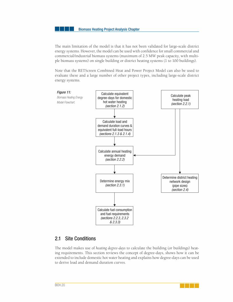
Biomass Heating Project Analysis Chapter
BIOH.20
The main limitation of the model is that it has not been validated for large-scale district energy systems. However, the model can be used with confidence for small commercial and commercial/industrial biomass systems (maximum of 2.5 MW peak capacity, with multi-ple biomass systems) on single building or district heating systems (1 to 100 buildings).
Note that the RETScreen Combined Heat and Power Project Model can also be used to evaluate these and a large number of other project types, including large-scale district energy systems.
2.1 Site Conditions
The model makes use of heating degree-days to calculate the building (or buildings) heat-ing requirements. This section reviews the concept of degree-days, shows how it can be extended to include domestic hot water heating and explains how degree-days can be used to derive load and demand duration curves.
Calculate equivalentdegree-days for domestic
hot water heating(section 2.1.2)
Calculate load anddemand duration curves &equivalent full-load hours(sections 2.1.3 & 2.1.4)
Calculate peakheating load
(section 2.2.1)
Calculate annual heatingenergy demand(section 2.2.2)
Determine energy mix(section 2.3.1)
Calculate fuel consumptionand fuel requirements(sections 2.2.3, 2.3.2
& 2.3.3)
Determine district heatingnetwork design
(pipe sizes)(section 2.4)
Figure 11:Biomass Heating Energy
Model Flowchart.

2. RETScreen Biomass Heating Project Model
BIOH.21
2.1.1 Design temperature and degree-days
Site conditions are defined through two user-entered parameters: the heating design tem-perature, and the monthly heating degree-days. The former corresponds to the temperature of an exceptionally cold day in the area. It is often specified by the local building code. For example, ASHRAE (1997) defines it as the minimum temperature that has been measured for a frequency level of at least 1% over the year for the specified location. In Sweden, it is defined as the coldest temperature that is expected once every 20 years. The design heat-ing temperature is used to determine the total peak heating load (see Section 2.2.1) and to size the heating system.
Heating degree-days help determine the heating demand2. Heating degree-days are defined as the difference between a set temperature (usually 18°C) and the average daily tempera-ture. Mathematically:
where DDi is the monthly degree-days for month i , Ni is the number of days in month i , Tset is the set temperature, and Ta k, is the average daily temperature for day k of month i . The annual degree-days, DD , is calculated by adding the monthly degree days:
The main advantage of using degree-days is that, as a first approximation, the heating demand of a building can be assumed to be proportional to the number of heating degree-days. Degree-days can also be used to describe hot water consumption, as will be seen in the next Section 2.1.2.
2.1.2 Equivalent degree-days for domestic hot water heating
The RETScreen Biomass Heating Project Model allows the user to include domestic hot water as part of the energy demand met by the heating system3. The hot water demand is supposed constant throughout the year and is expressed by the user as a fraction d of the annual total demand. Thus if Q is the annual total energy demand and QH the part of the
2. It is assumed that the user is already familiar with the concepts of load and demand. Load refers to instantaneous
values (power, expressed in W) whereas demand refers to integrated values (energy, expressed in J or in Wh).
3. The hot water demand can also be used to simulate non-weather dependent process demands.
(1)
(2)
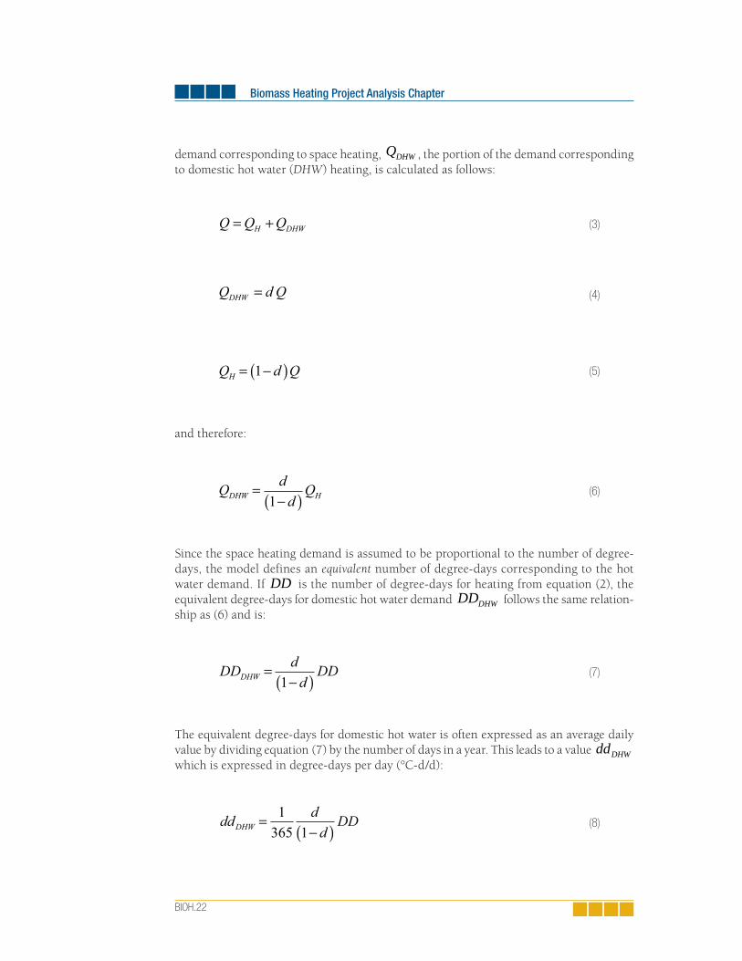
Biomass Heating Project Analysis Chapter
BIOH.22
demand corresponding to space heating, QDHW , the portion of the demand corresponding to domestic hot water (DHW) heating, is calculated as follows:
and therefore:
Since the space heating demand is assumed to be proportional to the number of degree-days, the model defines an equivalent number of degree-days corresponding to the hot water demand. If DD is the number of degree-days for heating from equation (2), the equivalent degree-days for domestic hot water demand
DDDHW follows the same relation-ship as (6) and is:
The equivalent degree-days for domestic hot water is often expressed as an average daily value by dividing equation (7) by the number of days in a year. This leads to a value
ddDHW
which is expressed in degree-days per day (°C-d/d):
(3)
(4)
(5)
(6)
(7)
(8)
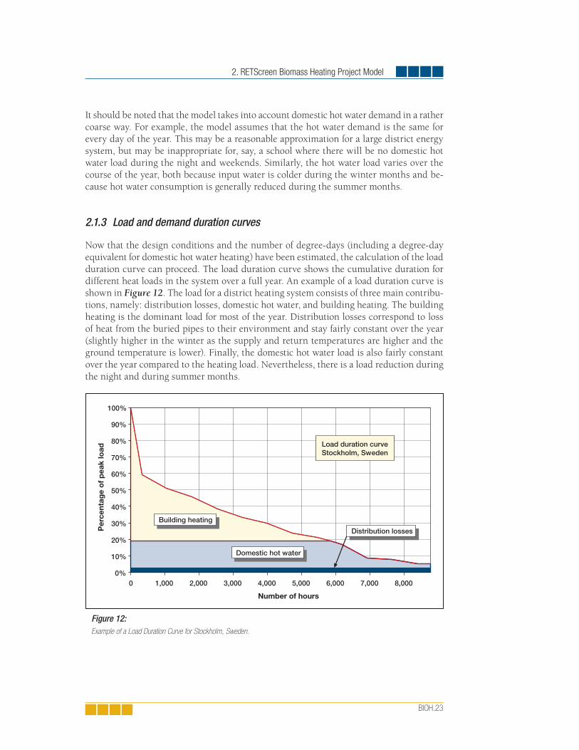
2. RETScreen Biomass Heating Project Model
BIOH.23
It should be noted that the model takes into account domestic hot water demand in a rather coarse way. For example, the model assumes that the hot water demand is the same for every day of the year. This may be a reasonable approximation for a large district energy system, but may be inappropriate for, say, a school where there will be no domestic hot water load during the night and weekends. Similarly, the hot water load varies over the course of the year, both because input water is colder during the winter months and be-cause hot water consumption is generally reduced during the summer months.
2.1.3 Load and demand duration curves
Now that the design conditions and the number of degree-days (including a degree-day equivalent for domestic hot water heating) have been estimated, the calculation of the load duration curve can proceed. The load duration curve shows the cumulative duration for different heat loads in the system over a full year. An example of a load duration curve is shown in Figure 12. The load for a district heating system consists of three main contribu-tions, namely: distribution losses, domestic hot water, and building heating. The building heating is the dominant load for most of the year. Distribution losses correspond to loss of heat from the buried pipes to their environment and stay fairly constant over the year (slightly higher in the winter as the supply and return temperatures are higher and the ground temperature is lower). Finally, the domestic hot water load is also fairly constant over the year compared to the heating load. Nevertheless, there is a load reduction during the night and during summer months.
0%
10%
20%
30%
40%
50%
60%
70%
80%
90%
100%
0 1,000 2,000 3,000 4,000 5,000 6,000 7,000 8,000
Number of hours
Per
cent
age
of
pea
k lo
ad
Load duration curveStockholm, Sweden
Building heating
Domestic hot water
Distribution losses
Figure 12:Example of a Load Duration Curve for Stockholm, Sweden.

Biomass Heating Project Analysis Chapter
BIOH.24
In principle, the load duration curve should be derived from hourly loads to show all pos-sible variations to the system. However, this information is rarely available for a system in the design or pre-feasibility stage. For this reason, a method has been developed to derive the load duration curve from monthly degree-days. The data used to develop the method is taken from very detailed studies of a relatively large biomass heating system in Upp-sala, Sweden. It includes empirical monthly factors, Fi′ , which represent the influence of solar gains, wind, and occupants’ habits on the energy requirements of the building. This monthly empirical factor is presented in Table 2 for ′ =i 0 1 13, … 4.
′i 0 1 2 3 4 5 6 7 8 9 10 11 12 13
Fi′ 1.00 0.50 0.60 0.60 0.70 0.77 0.66 0.68 0.68 0.69 0.78 0.80 0.92 1.00
Table 2: Empirical Factors Fi′
The algorithm to determine the load and demand duration curves is described below and is illustrated with a step-by-step example. The example used is a heating system for Stockholm (Sweden) with a heating design temperature (Tdes ) of –19.4°C and with a frac-tion ( d ) of the domestic hot water demand equal to 19% of the annual energy demand. The monthly heating degree-days ( DDi ) for Stockholm are given in Table 3. According to equation (2), the annual degree-days (DD ) is therefore equal to 4,238.6, and based on equation (8), the equivalent number of degree-days per day for domestic hot water heating ( ddDHW ) is 2.72°C-d/d.
STEP 1:
Calculate the monthly degree-days per day ddi (this is to eliminate the effect of months having different number of days), including in this quantity the equivalent degree-days for domestic hot water heating (calculated through equation 8):
where DDi is the degree-days for month i and Ni the number of days in that month. These values are calculated for the Stockholm example and are shown in Table 3. It should be noted that January has the highest degree-days values, followed by December and February. However, due to the influence of the fewer number of days, Ni , in the calculation of equation (9), February has the highest degree-days per day, ddi , than both January and December.
(9)
4. ′ =i 0 is the start of the months sorted by degree-days in ascending order, ′ =i 1 is the month with the highest number
of degree-days … ′ =i 12 is the month with the lowest number of degree-days, and ′ =i 13 is the end of the sorted
months.

2. RETScreen Biomass Heating Project Model
BIOH.25
Month Jan Feb Mar Apr May Jun Jul Aug Sep Oct Nov Dec
i 1 2 3 4 5 6 7 8 9 10 11 12
DDi 654.1 596.4 564.2 411.0 235.6 81.0 35.0 65.2 192.0 334.8 471.0 598.3
Ni 31 28 31 30 31 30 31 31 30 31 30 31
ddi 23.8 24.0 20.9 16.4 10.3 5.4 3.8 4.8 9.1 13.5 18.4 22.0
Table 3: Degree-Days for Stockholm, Sweden.
STEP 2:
Sort the monthly degree-days per day ( ddi′ ) in ascending order for ′ =i 0 1 13, … as previously defined. The sorted values of ddi′ and Ni′ for the Stockholm example are shown in Table 4 (note that February is listed last).
STEP 3:
Determine the coefficient Ci′ for fourteen cumulative durations, C C C′ ′ ′0 1 13, ... defined as:
…
(10-0)
(10-1)
(10-2)
(10-3)
(10-12)
(10-13)

Biomass Heating Project Analysis Chapter
BIOH.26
where C ′0 corresponds to the number of hours in a full year and C ′1 to C12′ cor-respond to the number of hours from the beginning of the year to the middle of the sorted months. The Ci′ values calculated for the example are shown in Table 4.
STEP 4:
Calculate the fractions of peak load Di′ corresponding to the fourteen cumulative durations Ci′ :
…
where F F F′ ′ ′0 1 13, … are the empirical monthly factors, Fi′ , mentioned earlier in Table 2. ∆Tdes is the difference between the set point temperature (Tset = 18°C) and the design heating temperature Tdes for the specified location (see Section 2.1.1):
These fourteen points C Di i′ ′( ), define the load duration curve expressed as a per-centage of the peak load. The Di′ values calculated for the Stockholm example are shown in Table 4 and the resulting load duration curve is shown in Figure 13.
(11-0)
(11-1)
(11-2)
(11-12)
(11-13)
(12)

2. RETScreen Biomass Heating Project Model
BIOH.27
The next two steps enable the calculation of the demand duration curve, which represents the amount of energy required as a function of the level of power over a full year. The calculation of this curve is obtained by integrating the load dura-tion curve with respect to time (i.e. determine the area under the load duration curve) followed by normalizing the values since it is more convenient to express the demand duration curve relative to the total yearly demand.
STEP 5:
Integrate the load duration curve with respect to time by calculating fourteen coefficients Gi′ with a simple trapezoidal rule leading to fourteen coefficients G G G′ ′ ′0 1 13, ... that express the demand relative to the maximum power (as will be seen in Section 2.1.4, coefficient G13′ is intimately related to number of equivalent full-load hours):
…
The coefficients Gi′ calculated for the Stockholm example are shown in Table 4.
(13-0)
(13-1)
(13-2)
(13-3)
(13-12)
(13-13)

Biomass Heating Project Analysis Chapter
BIOH.28
STEP 6:
Normalize the value Gi′ by determining fourteen coefficients Hi′, defined as:
…
These fourteen points H Di i′ ′( ), together with the origin 0 0,( ) define the demand duration curve expressed as a fraction relative to the total energy demand. The cal-culation of coefficients Hi′ for the example is shown in Table 4 and the resulting demand duration curve is shown in Figure 14.
(14-0)
(14-1)
(14-12)
(14-13)
′i 0 1 2 3 4 5 6 7 8 9 10 11 12 13
ddi′ (°C-d/d)
-- 3.8 4.8 5.4 9.1 10.3 13.5 16.4 18.4 20.9 22.0 23.8 24.0 --
Ni′ (days)
-- 31 31 30 30 31 31 30 30 31 31 31 28 --
Ci′ (hours)
8,760 8,388 7,644 6,912 6,192 5,460 4,716 3,984 3,264 2,532 1,788 1,044 336 0
Di′ (%)
5.1% 5.1% 7.7% 8.7% 17.0% 21.2% 23.8% 29.8% 33.5% 38.6% 45.9% 50.9% 59.0% 100.0%
Gi′(hours)
445 445 655 725 1,273 1,517 1,650 1,911 2,042 2,190 2,348 2,420 2,476 2,545
Hi′ (%)
17.5% 17.5% 25.7% 28.5% 50.0% 59.6% 64.8% 75.1% 80.3% 86.1% 92.3% 95.1% 97.3% 100.0%
Table 4: Stockholm Example of Coeffi cients Calculation Sorted by the Ascending Order of the Monthly Degree-Days per Day (ddi′).

2. RETScreen Biomass Heating Project Model
BIOH.29
The load duration curve and the demand duration curve are both expressed as a percentage of, respectively, the peak load and the annual demand. Absolute values of the peak heating load and the annual energy demand have yet to be calculated. This will be described in Sections 2.2.1 and 2.2.2.
0%
10%
20%
30%
40%
50%
60%
70%
80%
90%
100%
0 1,000 2,000 3,000 4,000 5,000 6,000 7,000 8,000
Number of hours
Per
cen
tag
e o
f p
eak
load
C7′C8′
D8′D7′
Figure 13:Example of the Load Duration Curve Calculated for Stockholm.
0%
10%
20%
30%
40%
50%
60%
70%
80%
90%
100%
0% 10% 20% 30% 40% 50% 60% 70% 80% 90% 100%
Percentage of total demand
Per
cent
age
of
pea
k lo
ad
D6′
D7′
H6′
H7′
Figure 14:Example of the Demand Duration Curve Calculated for Stockholm.
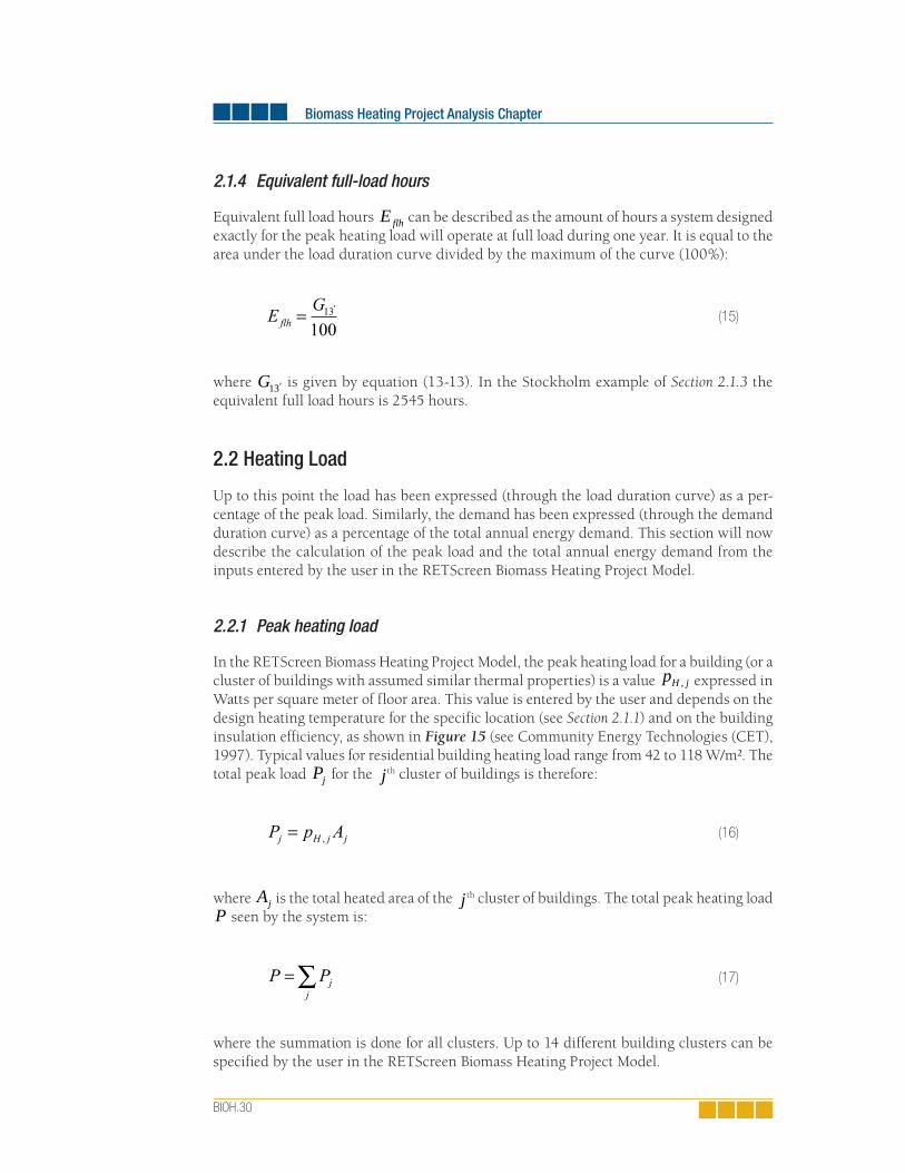
Biomass Heating Project Analysis Chapter
BIOH.30
2.1.4 Equivalent full-load hours
Equivalent full load hours Eflh can be described as the amount of hours a system designed exactly for the peak heating load will operate at full load during one year. It is equal to the area under the load duration curve divided by the maximum of the curve (100%):
where G13′ is given by equation (13-13). In the Stockholm example of Section 2.1.3 the equivalent full load hours is 2545 hours.
2.2 Heating Load
Up to this point the load has been expressed (through the load duration curve) as a per-centage of the peak load. Similarly, the demand has been expressed (through the demand duration curve) as a percentage of the total annual energy demand. This section will now describe the calculation of the peak load and the total annual energy demand from the inputs entered by the user in the RETScreen Biomass Heating Project Model.
2.2.1 Peak heating load
In the RETScreen Biomass Heating Project Model, the peak heating load for a building (or a cluster of buildings with assumed similar thermal properties) is a value pH j, expressed in Watts per square meter of floor area. This value is entered by the user and depends on the design heating temperature for the specific location (see Section 2.1.1) and on the building insulation efficiency, as shown in Figure 15 (see Community Energy Technologies (CET), 1997). Typical values for residential building heating load range from 42 to 118 W/m². The total peak load Pj for the j th cluster of buildings is therefore:
where Aj is the total heated area of the j th cluster of buildings. The total peak heating load P seen by the system is:
where the summation is done for all clusters. Up to 14 different building clusters can be specified by the user in the RETScreen Biomass Heating Project Model.
(15)
(16)
(17)

2. RETScreen Biomass Heating Project Model
BIOH.31
2.2.2 Annual heating energy demand
Annual heating energy demand Q is calculated as:
where P is the peak heating load (equation 17) and Eflh the equivalent full load hours (equation 15).
2.2.3 Fuel consumption (base case system)
To evaluate the financial viability of a biomass heating project, the quantity of fuel that would be used if the biomass system were not installed should be calculated. This is the alternative fuel consumption, or what is referred to as the base case system.
Units used to measure fuel consumption and calorific values depend on the type of fuel used. Table 5 summarizes the units and calorific values for the different fuel types in the RETScreen Biomass Heating Project Model.
40
50
60
70
80
90
100
110
120
-50 -45 -40 -35 -30 -25 -20 -15 -10 -5 0
Design temperature (˚C)
Bui
ldin
g h
ea
ting
loa
d (W
/m2 )
Good insulation
Medium insulation
Poor insulation
Figure 15:Residential Building Heating Load (CET, 1997).
(18)
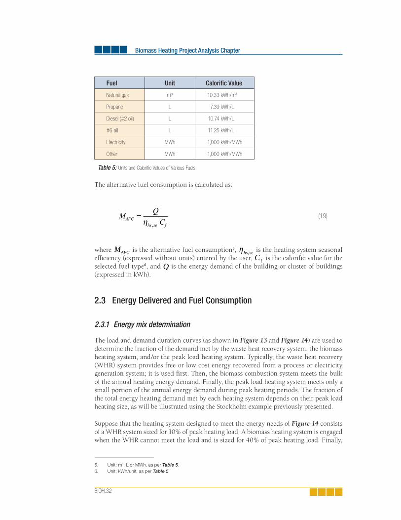
Biomass Heating Project Analysis Chapter
BIOH.32
Fuel Unit Calorifi c Value
Natural gas m³ 10.33 kWh/m3
Propane L 7.39 kWh/L
Diesel (#2 oil) L 10.74 kWh/L
#6 oil L 11.25 kWh/L
Electricity MWh 1,000 kWh/MWh
Other MWh 1,000 kWh/MWh
Table 5: Units and Calorifi c Values of Various Fuels.
The alternative fuel consumption is calculated as:
where MAFC is the alternative fuel consumption5, ηhs se, is the heating system seasonal efficiency (expressed without units) entered by the user, C f is the calorific value for the selected fuel type6, and Q is the energy demand of the building or cluster of buildings (expressed in kWh).
2.3 Energy Delivered and Fuel Consumption
2.3.1 Energy mix determination
The load and demand duration curves (as shown in Figure 13 and Figure 14) are used to determine the fraction of the demand met by the waste heat recovery system, the biomass heating system, and/or the peak load heating system. Typically, the waste heat recovery (WHR) system provides free or low cost energy recovered from a process or electricity generation system; it is used first. Then, the biomass combustion system meets the bulk of the annual heating energy demand. Finally, the peak load heating system meets only a small portion of the annual energy demand during peak heating periods. The fraction of the total energy heating demand met by each heating system depends on their peak load heating size, as will be illustrated using the Stockholm example previously presented.
Suppose that the heating system designed to meet the energy needs of Figure 14 consists of a WHR system sized for 10% of peak heating load. A biomass heating system is engaged when the WHR cannot meet the load and is sized for 40% of peak heating load. Finally,
(19)
5. Unit: m3, L or MWh, as per Table 5.
6. Unit: kWh/unit, as per Table 5.

2. RETScreen Biomass Heating Project Model
BIOH.33
a peaking boiler with 50% of peak capacity is installed. Then, as shown in Figure 16, the WHR system will meet 31% of annual heating energy demand; the biomass heating system will produce 64% (95% - 31%) of the annual demand. The remaining part will be met by the peaking boiler, which will deliver a total of 5% of the annual heating energy demand.
The use of this method requires that the WHR system capacity and biomass heating system capacity be expressed as a percentage of the peak heating load, and calculate the energy delivered as a fraction of the total demand. To convert from actual system capacities to percentage of peak load, and from percentage of annual demand to actual energy delivered is straightforward.
In the RETScreen Biomass Heating Project Model, the user enters the WHR system capacity PWHR and the biomass heating system capacity Pbio in kW. The percentages of peak load (as in Figure 16) are pWHR,% and pbio,% , given simply by:
where P is the peak load for heating calculated from equation (17). Similarly, if qWHR,% , qbio,% , and qPLHS ,% are the percentages of annual heating energy demand met respectively by the WHR, the biomass, and the peak load heating systems, as obtained by Figure 16, then the heating energy delivered by the WHR system, QWHR, by the biomass system, Qbio, and by the peak load heating system, QPLHS , are given by:
where Q is the total demand as calculated in equation (18).
(20)
(21)
(22)
(23)
(24)
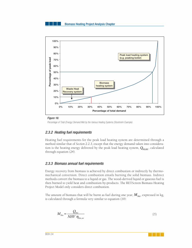
Biomass Heating Project Analysis Chapter
BIOH.34
2.3.2 Heating fuel requirements
Heating fuel requirements for the peak load heating system are determined through a method similar that of Section 2.2.3, except that the energy demand taken into considera-tion is the heating energy delivered by the peak load heating system, QPLHS , calculated through equation (24).
2.3.3 Biomass annual fuel requirements
Energy recovery from biomass is achieved by direct combustion or indirectly by thermo-mechanical conversion. Direct combustion entails burning the solid biomass. Indirect methods convert the biomass to a liquid or gas. The wood-derived liquid or gaseous fuel is then burned to yield heat and combustion by-products. The RETScreen Biomass Heating Project Model only considers direct combustion.
The amount of biomass that will be burnt as fuel during one year, Mbio, expressed in kg, is calculated through a formula very similar to equation (19):
0%
10%
20%
30%
40%
50%
60%
70%
80%
90%
100%
0% 10% 20% 30% 40% 50% 60% 70% 80% 90% 100%
Percentage of total demand
Per
cent
age
of
pea
k lo
ad
Waste Heat Recovery system
Biomass heating system
Peak load heating system (e.g. peaking boiler)
Figure 16:Percentage of Total (Energy) Demand Met by the Various Heating Systems (Stockholm Example).
(25)
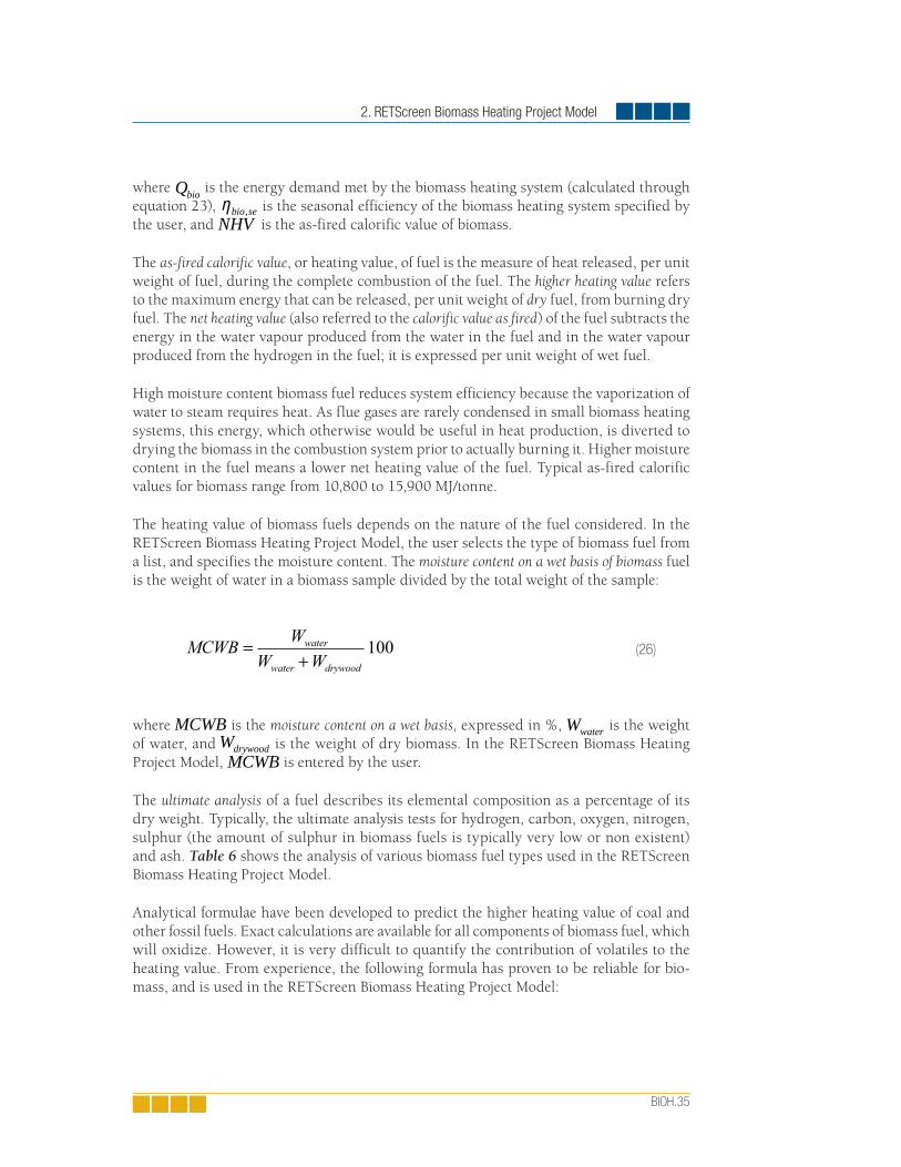
2. RETScreen Biomass Heating Project Model
BIOH.35
where Qbio is the energy demand met by the biomass heating system (calculated through equation 23), ηbio se, is the seasonal efficiency of the biomass heating system specified by the user, and NHV is the as-fired calorific value of biomass.
The as-fired calorific value, or heating value, of fuel is the measure of heat released, per unit weight of fuel, during the complete combustion of the fuel. The higher heating value refers to the maximum energy that can be released, per unit weight of dry fuel, from burning dry fuel. The net heating value (also referred to the calorific value as fired) of the fuel subtracts the energy in the water vapour produced from the water in the fuel and in the water vapour produced from the hydrogen in the fuel; it is expressed per unit weight of wet fuel.
High moisture content biomass fuel reduces system efficiency because the vaporization of water to steam requires heat. As flue gases are rarely condensed in small biomass heating systems, this energy, which otherwise would be useful in heat production, is diverted to drying the biomass in the combustion system prior to actually burning it. Higher moisture content in the fuel means a lower net heating value of the fuel. Typical as-fired calorific values for biomass range from 10,800 to 15,900 MJ/tonne.
The heating value of biomass fuels depends on the nature of the fuel considered. In the RETScreen Biomass Heating Project Model, the user selects the type of biomass fuel from a list, and specifies the moisture content. The moisture content on a wet basis of biomass fuel is the weight of water in a biomass sample divided by the total weight of the sample:
where MCWB is the moisture content on a wet basis, expressed in %, Wwater is the weight of water, and Wdrywood is the weight of dry biomass. In the RETScreen Biomass Heating Project Model, MCWB is entered by the user.
The ultimate analysis of a fuel describes its elemental composition as a percentage of its dry weight. Typically, the ultimate analysis tests for hydrogen, carbon, oxygen, nitrogen, sulphur (the amount of sulphur in biomass fuels is typically very low or non existent) and ash. Table 6 shows the analysis of various biomass fuel types used in the RETScreen Biomass Heating Project Model.
Analytical formulae have been developed to predict the higher heating value of coal and other fossil fuels. Exact calculations are available for all components of biomass fuel, which will oxidize. However, it is very difficult to quantify the contribution of volatiles to the heating value. From experience, the following formula has proven to be reliable for bio-mass, and is used in the RETScreen Biomass Heating Project Model:
(26)

Biomass Heating Project Analysis Chapter
BIOH.36
where HHV is the higher heating value in MJ/kg, and C , H , O, N and S are the per-centage weight for carbon, hydrogen, oxygen, nitrogen, and sulphur respectively. The cor-responding net heating value (as-fired) NHV , in MJ/kg, is given by:
where MCWB is the moisture content on a wet basis of biomass entered by the user, and ex-pressed in %. The value from equation (28) is used in equation (25) to calculate the annual biomass requirements of the heating system.
Type Carbon Hydrogen Oxygen Nitrogen Sulphur Ash
Bagasse 48.64% 5.87% 42.85% 0.16% 0.04% 2.44%
Peat 51.20% 5.70% 33.20% 1.40% 0.30% 8.20%
Rice husks 38.83% 4.75% 35.59% 0.52% 0.05% 20.26%
Switchgrass 47.45% 5.75% 42.37% 0.74% 0.08% 3.61%
Wheat straw 46.96% 5.69% 42.41% 0.43% 0.19% 4.32%
Wood high HV 52.10% 5.70% 38.90% 0.20% 0.00% 3.10%
Wood low HV 52.00% 4.00% 41.70% 0.30% 0.00% 2.00%
Wood medium HV 48.85% 6.04% 42.64% 0.71% 0.06% 1.70%
Table 6: Biomass Fuel Type.
2.4 District Heating Network Design
District heating network design is included in the RETScreen Biomass Heating Project Model so that the user can perform a preliminary sizing of the pipes and costing of the installation. Its results have no influence on the energy calculation.
A district heating piping distribution system consists of an underground hot water distri-bution network with supply and return pipelines in a closed circuit. Each building is con-nected to the network via a building heat transfer station that regulates and measures the energy taken from the distribution system. The network consists of a main distribution line which connects several buildings, or clusters of buildings, to the heating plan, and second-
(27)
(28)
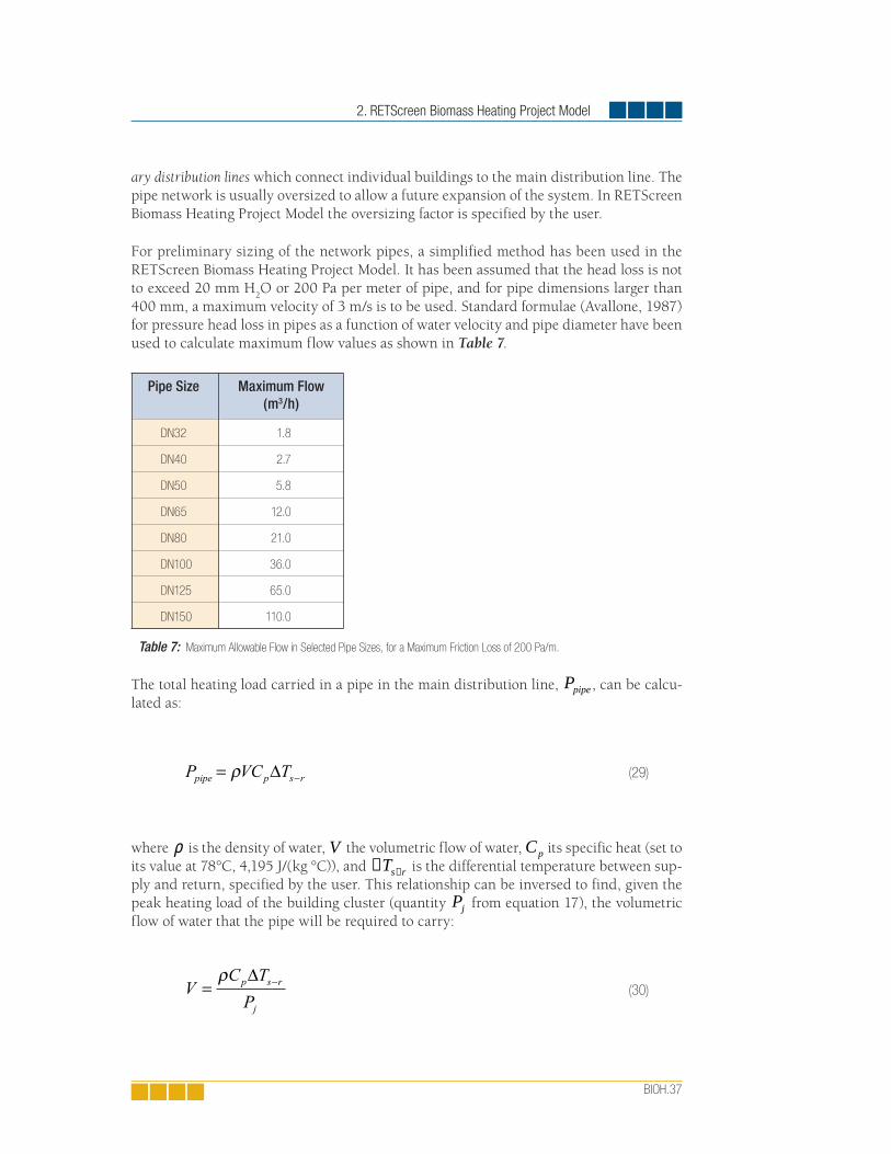
2. RETScreen Biomass Heating Project Model
BIOH.37
ary distribution lines which connect individual buildings to the main distribution line. The pipe network is usually oversized to allow a future expansion of the system. In RETScreen Biomass Heating Project Model the oversizing factor is specified by the user.
For preliminary sizing of the network pipes, a simplified method has been used in the RETScreen Biomass Heating Project Model. It has been assumed that the head loss is not to exceed 20 mm H
2O or 200 Pa per meter of pipe, and for pipe dimensions larger than
400 mm, a maximum velocity of 3 m/s is to be used. Standard formulae (Avallone, 1987) for pressure head loss in pipes as a function of water velocity and pipe diameter have been used to calculate maximum flow values as shown in Table 7.
Pipe Size Maximum Flow(m3/h)
DN32 1.8
DN40 2.7
DN50 5.8
DN65 12.0
DN80 21.0
DN100 36.0
DN125 65.0
DN150 110.0
Table 7: Maximum Allowable Flow in Selected Pipe Sizes, for a Maximum Friction Loss of 200 Pa/m.
The total heating load carried in a pipe in the main distribution line, Ppipe , can be calcu-
lated as:
where ρ is the density of water, V the volumetric flow of water, Cp its specific heat (set to its value at 78°C, 4,195 J/(kg °C)), and ∆Ts r− is the differential temperature between sup-ply and return, specified by the user. This relationship can be inversed to find, given the peak heating load of the building cluster (quantity Pj from equation 17), the volumetric flow of water that the pipe will be required to carry:
(29)
(30)

Biomass Heating Project Analysis Chapter
BIOH.38
The actual formula used in the RETScreen Biomass Heating Project Model includes a factor for pipe oversizing; if κ is the main pipe oversizing factor, expressed in %, entered by the user, equation (30) becomes:
Table 7 provides the desirable pipe size given the flow. In the case where several clusters of buildings are served by the same main distribution line pipe, the load in equation (31) should naturally be replaced by the sum of the relevant loads.
Finally, a similar relationship holds for secondary distribution lines piping. The denomina-tor of (31) is then replaced with a load ′Pj given by:
where ′κ is the secondary pipe network oversizing factor specified by the user, and Nj is the number of buildings in the cluster.
2.5 Validation
Numerous experts have contributed to the development, testing and validation of the RET-Screen Biomass Heating Project Model. They include biomass heating modelling experts, cost engineering experts, greenhouse gas modelling specialists, financial analysis profes-sionals, and ground station and satellite weather database scientists.
Validation of the RETScreen Biomass Heating Project Model was done against other models used in the industry. The validation focused on three areas: calculation of the load duration curve (Section 2.5.1), calculation of the as-fired calorific value (e.g. heating value) of biomass (Section 2.5.2), and district heating network design (Section 2.5.3).
(31)
(32)
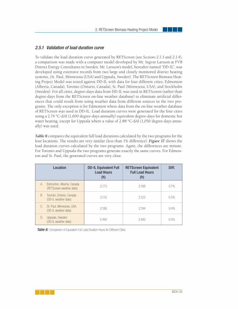
2. RETScreen Biomass Heating Project Model
BIOH.39
2.5.1 Validation of load duration curve
To validate the load duration curve generated by RETScreen (see Sections 2.1.3 and 2.1.4), a comparison was made with a computer model developed by Mr. Ingvar Larsson at FVB District Energy Consultants in Sweden. Mr. Larsson’s model, hereafter named “DD-IL”, was developed using extensive records from two large and closely monitored district heating systems, (St. Paul, Minnesota (USA) and Uppsala, Sweden). The RETScreen Biomass Heat-ing Project Model was tested against DD-IL with data for four different cities: Edmonton (Alberta, Canada), Toronto (Ontario, Canada), St. Paul (Minnesota, USA), and Stockholm (Sweden). For all cities, degree-days data from DD-IL was used in RETScreen (rather than degree-days from the RETScreen on-line weather database) to eliminate artificial differ-ences that could result from using weather data from different sources in the two pro-grams. The only exception is for Edmonton where data from the on-line weather database of RETScreen was used in DD-IL. Load duration curves were generated for the four cities using a 2.74 °C-d/d (1,000 degree-days annually) equivalent degree-days for domestic hot water heating, except for Uppsala where a value of 2.88 °C-d/d (1,050 degree-days annu-ally) was used.
Table 8 compares the equivalent full load durations calculated by the two programs for the four locations. The results are very similar (less than 1% difference). Figure 17 shows the load duration curves calculated by the two programs. Again, the differences are minute. For Toronto and Uppsala the two programs generate exactly the same curves. For Edmon-ton and St. Paul, the generated curves are very close.
Location DD-IL Equivalent Full Load Hours
(h)
RETScreen Equivalent Full Load Hours
(h)
Diff.
A. Edmonton, Alberta, Canada(RETScreen weather data)
2,173 2,188 0.7%
B. Toronto, Ontario, Canada (DD-IL weather data)
2,112 2,123 0.5%
C. St. Paul, Minnesota, USA (DD-IL weather data)
2,186 2,194 0.4%
D. Uppsala, Sweden (DD-IL weather data)
2,492 2,492 0.0%
Table 8: Comparison of Equivalent Full Load Duration Hours for Different Cities.

Biomass Heating Project Analysis Chapter
BIOH.40
Figure 17a and 17b: Comparison of Load Duration Curves Calculated with DD-IL and RETScreen for Four Different Cities.
Load duration curves for Edmonton, Alberta, Canada
0%
10%
20%
30%
40%
50%
60%
70%
80%
90%
100%
0 1,000 2,000 3,000 4,000 5,000 6,000 7,000 8,000
Number of hours
Per
cent
age
of p
eak
load
DD-ILRETScreen
0%
10%
20%
30%
40%
50%
60%
70%
80%
90%
100%
0 1,000 2,000 3,000 4,000 5,000 6,000 7,000 8,000
Load duration curves for Toronto, Ontario, Canada
Number of hours
Per
cent
age
of p
eak
load
DD-ILRETScreen
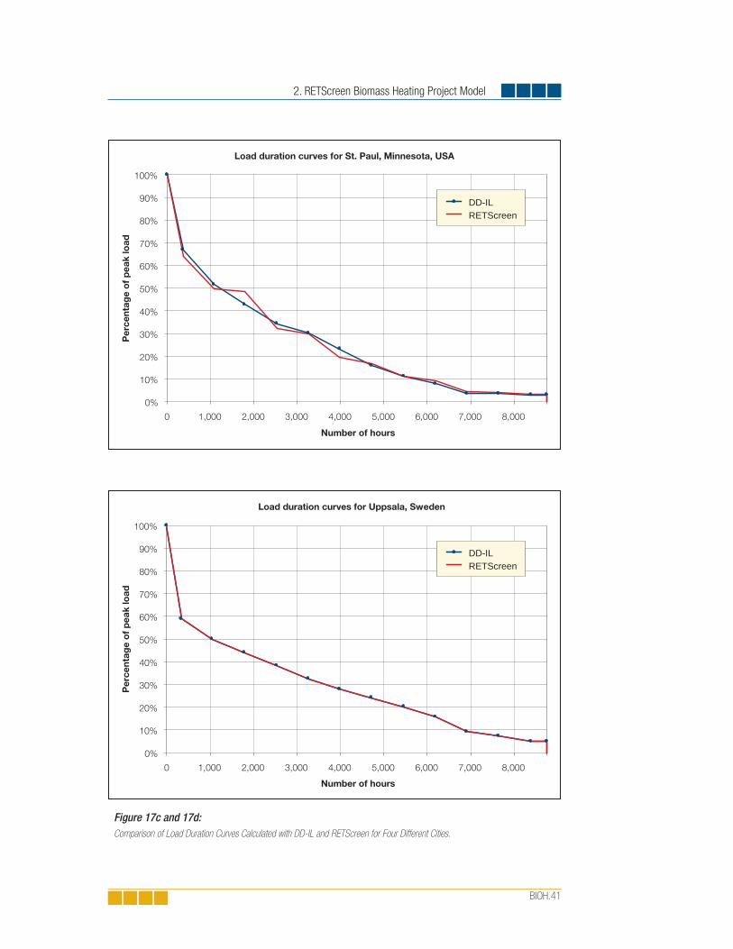
2. RETScreen Biomass Heating Project Model
BIOH.41
Load duration curves for St. Paul, Minnesota, USA
Number of hours
Per
cent
age
of
pea
k lo
ad
0%
10%
20%
30%
40%
50%
60%
70%
80%
90%
100%
0 1,000 2,000 3,000 4,000 5,000 6,000 7,000 8,000
DD-ILRETScreen
Load duration curves for Uppsala, Sweden
Number of hours
Per
cent
age
of
pea
k lo
ad
0%
10%
20%
30%
40%
50%
60%
70%
80%
90%
100%
0 1,000 2,000 3,000 4,000 5,000 6,000 7,000 8,000
DD-ILRETScreen
Figure 17c and 17d: Comparison of Load Duration Curves Calculated with DD-IL and RETScreen for Four Different Cities.

Biomass Heating Project Analysis Chapter
BIOH.42
2.5.2 Validation of as-fi red calorifi c value (heating value) algorithm
To validate the as-fired calorific value (heating value) algorithm used by the RETScreen Biomass Heating Project Model (see Section 2.3.3), its predictions were compared to find-ings reported in the Summer Meeting of the Technical Section, Canadian Pulp and Paper Association, Quebec, Quebec, Canada, June 6 to 8, 1955. In the paper, entitled Determina-tion of Bark Volumes and Fuel Properties, data was collected from thirty mills by the Forest Products Laboratories of Canada and the Federal Department of Mines and Technical Sur-veys. The chemical analyses (proximate and ultimate) from the samples were performed by the same laboratory. The heating values were statistically analyzed by the Forest Products Laboratories with the following results:
Age: no correlation between heating value and the age of the tree was noticeable.
Geographical origin: analyses of tests did not reveal any signifi cant differences among heating values due to origin.
Species: the tests show a signifi cant difference in the heating value among various species in the following order (highest fi rst): 1) Balsam, 2) Jack Pine, 3) Poplar, 4) Spruce.
Table 9 summarizes the heating values measured in the test. These values should be com-pared to those proposed by the RETScreen Biomass Heating Project Model for the heating value of wood waste, which range from a low of 17,723 MJ/t to a high of 19,760 MJ/t with an average of 18,673 MJ/t. The variation according to this test is +/- 3% for Jack Pine and up to –5% for Black Spruce. The estimate given by RETScreen Biomass Heating Project Model is amply sufficient at the pre-feasibility stage of a project.
Eastern Canadian BarkNo. of
Samples
Heating Value (MJ/t)Average Probable
minimumProbable maximum
Balsam All Varieties 28 21,167 20,911 21,422
Black Spruce 15 20,027 18,957 20,259
White Spruce 11 19,841 19,399 20,073
Red Spruce 3 20,073
Jack Pine 12 20,771 20,213 21,329
Poplar 6 20,492 20,004 20,981
White Birch 3 23,981
Yellow Birch 2 21,399
Hard Maple 2 19,143
Soft Maple 1 18,841
Elm soft 1 17,678
Beech 1 17,771
Tamarack 1 20,957
Hemlock Eastern 1 20,678
Table 9 : Measured Heating Values of Eastern Canadian Bark.
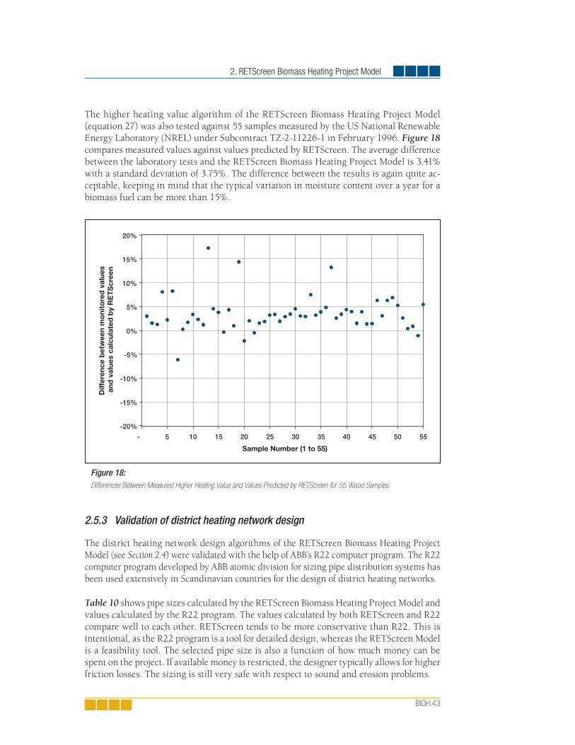
2. RETScreen Biomass Heating Project Model
BIOH.43
The higher heating value algorithm of the RETScreen Biomass Heating Project Model (equation 27) was also tested against 55 samples measured by the US National Renewable Energy Laboratory (NREL) under Subcontract TZ-2-11226-1 in February 1996. Figure 18 compares measured values against values predicted by RETScreen. The average difference between the laboratory tests and the RETScreen Biomass Heating Project Model is 3.41% with a standard deviation of 3.75%. The difference between the results is again quite ac-ceptable, keeping in mind that the typical variation in moisture content over a year for a biomass fuel can be more than 15%.
2.5.3 Validation of district heating network design
The district heating network design algorithms of the RETScreen Biomass Heating Project Model (see Section 2.4) were validated with the help of ABB’s R22 computer program. The R22 computer program developed by ABB atomic division for sizing pipe distribution systems has been used extensively in Scandinavian countries for the design of district heating networks.
Table 10 shows pipe sizes calculated by the RETScreen Biomass Heating Project Model and values calculated by the R22 program. The values calculated by both RETScreen and R22 compare well to each other. RETScreen tends to be more conservative than R22. This is intentional, as the R22 program is a tool for detailed design, whereas the RETScreen Model is a feasibility tool. The selected pipe size is also a function of how much money can be spent on the project. If available money is restricted, the designer typically allows for higher friction losses. The sizing is still very safe with respect to sound and erosion problems.
-20%
-15%
-10%
-5%
0%
5%
10%
15%
20%
- 10 20 30 40 50 555 15 25 35 45
Sample Number (1 to 55)
Diff
eren
ce b
etw
een
mo
nito
red
val
ues
an
d v
alue
s ca
lcul
ated
by
RE
TS
cree
n
Figure 18:Differences Between Measured Higher Heating Value and Values Predicted by RETScreen for 55 Wood Samples.

Biomass Heating Project Analysis Chapter
BIOH.44
Theoretically, the main distribution pipes should be sized with low friction losses and allow higher losses in the secondary distribution pipes to minimize required pumping load and investment costs. However, in practice space is often limited and capital costs need to be controlled resulting in a small main line. As for the secondary line, it is typically over-sized, since the customers’ heating load is not well defined and to avoid noise problems.
InputRETScreenCalculation
ABB-R22Calculation
ABB-R22Calculation
Supply(°C)
Return(°C)
Delta T(°C)
Load(kW)
Pipe Size DN Pipe SizeDN
Friction Losses7
mmwc/m95 65 30 25 32 25 4.9
95 65 30 50 32 32 5.3
95 65 30 75 40 32 11.5
95 65 30 100 50 40 9.4
95 65 30 200 50 50 10.8
95 65 30 250 65 65 4.5
95 65 30 400 65 65 11.2
95 65 30 420 80 65 12.3
95 65 30 720 80 80 15.4
95 65 30 740 100 100 4.3
95 65 30 1,250 100 100 11.8
95 65 30 1,260 125 100 12.0
95 65 30 2,260 125 125 12.6
95 65 30 2,270 150 125 12.7
95 65 30 3,830 150 150 13.3
95 65 30 4,250 N/A 200 4.0
120 75 45 50 32 25 8.4
120 75 45 90 32 32 7.4
120 75 45 100 40 32 9.1
120 75 45 140 40 40 8.1
120 75 45 150 50 40 9.3
120 75 45 300 50 50 10.7
120 75 45 310 65 50 11.4
120 75 45 620 65 65 11.8
120 75 45 630 80 65 12.2
120 75 45 1,090 80 80 15.6
120 75 45 1,100 100 100 4.2
120 75 45 1,880 100 100 11.8
120 75 45 1,900 125 100 12.1
120 75 45 3,400 125 125 12.6
120 75 45 3,450 150 125 13.0
120 75 45 5,750 150 150 13.3
120 75 45 6,400 N/A 200 4.1
Table 10: Comparison of the RETScreen District Heating Network Design (Pipe Sizing) Algorithm with ABB’s R22 Computer Program.
7. mmwc/m: millimeters water column per meter of pipe.

2. RETScreen Biomass Heating Project Model
BIOH.45
2.6 Summary
In this section, the algorithms used by the RETScreen Biomass Heating Project Model have been shown in detail. This model uses a combination of algorithms to predict the energy delivered, on a yearly basis, by a biomass heating system. The load and demand duration curves are derived from monthly degree-days data entered by the user; and domestic hot water is included in the load by defining equivalent degree-days for hot water heating. The peak load heating system is determined from the design temperature specified by the user and from heating loads specified for each cluster of buildings. The demand duration curve is then used to predict what fraction of the demand is met by each of the three heat-ing systems (waste heat recovery system, biomass heating system, and peak load heating system) given their respective capacities. Calculation of heating energy and biomass re-quirements follow; biomass consumption depends on the type of wood fuel considered. Finally, a separate algorithm is used to provide a preliminary sizing of the distribution network. Various parts of the model have been validated against other programs or against values published in the literature. Despite the relative simplicity of the model, its accuracy proves acceptable, at least at the pre-feasibility or feasibility stage, when compared with other software tools or with experimental data.


BIOH.47
REFERENCES
Arkay, K. and Blais, C., The District Energy Option in Canada, Community Energy Technologies (CET), CANMET, Natural Resources Canada, 1996.
ASHRAE, Handbook, Fundamentals, SI Edition, American Society of Heating, Refrigerating and Air-Conditioning Engineers, Inc., 1791 Tullie Circle, N.E., Atlanta, GA, 30329, USA, 1997.
ASTM International, Standard Test Method for Gross Calorifi c Value of Refuse-Derived Fuel by the Bomb Calorimeter, ASTM E711-87(1996).
Avallone, E.A. and Baumeister, T. III (1987), Marks Standard Handbook for Mechanical Engineers, McGraw-Hill, Inc., Community Energy Technologies (CET), 1997.
Community Energy Technologies (CET), “Personal communication,” CETC, 1997.
Hayden, S., “Personal communication,” CETC, 1997.
McCallum, B., Case Studies of Small Commercial Biomass Combustion Systems in PEI, Natural Resources Canada, June 1995.
McCallum, B., Small-Scale Automated Biomass Energy Heating Systems: A Viable Option For Remote Canadian Communities?, CFS’s Great Lake Forestry Centre and CEDRL of Natural Resources Canada (NRCan), 1997.
NRCan, Buyer’s Guide To Small Commercial Biomass Combustion Systems, Natural Resources Canada’s Renewable and Electrical Energy Division, ISBN 0-662-28899-8, Catalogue no. M92-186/2000E, 52 pages, 2002.
Randløv, P., District Heating Handbook, European District Heating Pipe Manufacturers Association, ISBN87-90488-00-8, 1997.
Sykes, B., “Personal communication,” Natural Resources Canada’s Canadian Forest Services, 1997.


SOLAR AIR HEATING PROJECT ANALYSIS CHAPTER
CLEAN ENERGY PROJECT ANALYSIS:RETSCREEN® ENGINEERING & CASES TEXTBOOK
DisclaimerThis publication is distributed for informational purposes only and does not necessarily reflect the views of the Government of Canada nor constitute an endorsement of any commercial product or person. Neither Canada, nor its ministers, officers, employees and agents makeany warranty in respect to this publication nor a s s u m e a n y l i a b i l i t y a r i s i n g o u t o f t h i s publication.
© Minister of Natural Resources Canada 2001 - 2004.
www.retscreen.net
RETScreen® InternationalClean Energy Decision Support Centre

ISBN: 0-662-35673-XCatalogue no.: M39-100/2003E-PDF
© Minister of Natural Resources Canada 2001 - 2004.

SAH.3
TABLE OF CONTENTS
1 SOLAR AIR HEATING BACKGROUND . . . . . . . . . . . . . . . . . . . . . . . . . . . . . . . . . . 5
1.1 Description of Solar Air Heating Systems . . . . . . . . . . . . . . . . . . . . . . . . . . . . . . . . 7
1.2 Solar Air Heating System Application Markets. . . . . . . . . . . . . . . . . . . . . . . . . . . . . 91.2.1 Commercial and residential buildings . . . . . . . . . . . . . . . . . . . . . . . . . . . . . . . . . . . . . . 9
1.2.2 Industrial buildings . . . . . . . . . . . . . . . . . . . . . . . . . . . . . . . . . . . . . . . . . . . . . . . . . . 10
1.2.3 Process air . . . . . . . . . . . . . . . . . . . . . . . . . . . . . . . . . . . . . . . . . . . . . . . . . . . . . . . 11
2 RETSCREEN SOLAR AIR HEATING PROJECT MODEL. . . . . . . . . . . . . . . . . . . . . 13
2.1 Collected Solar Energy Savings . . . . . . . . . . . . . . . . . . . . . . . . . . . . . . . . . . . . . . 152.1.1 Usable incident solar energy calculation . . . . . . . . . . . . . . . . . . . . . . . . . . . . . . . . . . . 16
2.1.2 Average collector effi ciency. . . . . . . . . . . . . . . . . . . . . . . . . . . . . . . . . . . . . . . . . . . . 17
2.1.3 Solar utilization . . . . . . . . . . . . . . . . . . . . . . . . . . . . . . . . . . . . . . . . . . . . . . . . . . . . 18
2.1.4 Active solar energy savings . . . . . . . . . . . . . . . . . . . . . . . . . . . . . . . . . . . . . . . . . . . . 20
2.2 Building Heat Recapture Savings . . . . . . . . . . . . . . . . . . . . . . . . . . . . . . . . . . . . . 20
2.3 Destratifi cation Savings . . . . . . . . . . . . . . . . . . . . . . . . . . . . . . . . . . . . . . . . . . . . 21
2.4 Energy Savings for Heating Systems for Non-Industrial Buildings . . . . . . . . . . . . . 22
2.5 Energy Savings for Heating Systems for Industrial Buildings . . . . . . . . . . . . . . . . . 23
2.6 Validation . . . . . . . . . . . . . . . . . . . . . . . . . . . . . . . . . . . . . . . . . . . . . . . . . . . . . . . 24
2.7 Summary . . . . . . . . . . . . . . . . . . . . . . . . . . . . . . . . . . . . . . . . . . . . . . . . . . . . . . . 28
REFERENCES . . . . . . . . . . . . . . . . . . . . . . . . . . . . . . . . . . . . . . . . . . . . . . . . . . . . 29


1. Solar Air Heating Background
SAH.5
SOLAR AIR HEATING PROJECT ANALYSIS CHAPTERClean Energy Project Analysis: RETScreen® Engineering & Cases is an electronic textbook for professionals and univer-sity students. This chapter covers the analysis of potential solar air heating projects using the RETScreen® International Clean Energy Project Analysis Software, including a technology background and a detailed description of the algorithms found in the RETScreen® Software. A collection of project case studies, with assignments, worked-out solutions and information about how the projects fared in the real world, is available at the RETScreen® International Clean Energy Decision Support Centre Website www.retscreen.net.
1 SOLAR AIR HEATING BACKGROUND1
The Solar Air Heating (SAH) system developed by Conserval Engineering is a proven sys-tem for heating or preheating air in various applications. The system, commonly known as “Solarwall®,” is most widely used to heat ventilation air in buildings, but it has also been applied in processes such as crop drying where heated air is an important requirement. Figure 1 shows the world’s largest solar air heating system installed at a manufacturing plant of Bombardier’s Canadair Division in Montreal, Canada. This particular industrial building installation has 10,000 m² of solar air heating collectors.
Figure 1:Industrial Building SAH Project.
Photo Credit: Conserval Engineering
1. Some of the text in this “Background” description comes from the following reference: Enermodal Engineering Limited, The Market for Solar Preheated Ventilation Systems in Canadian Remote Communities, Report prepared for Natural Resources Canada, 1997.

Solar Air Heating Project Analysis Chapter
SAH.6
The worldwide demand for this relatively new and unique technology has increased rapidly over the past decade. Years of research and testing have resulted in this new concept for heating air with solar energy. Solar air heating installations are beginning to be used more and more for the “cladding” of exterior walls (which face the equator) on industrial, com-mercial and apartment style buildings (Figure 2), as well as for single-family residences. Solar air heating systems have also been used for drying agricultural crops such as tea-leaves, and their potential has been demonstrated for a wide variety of other cultivated products.
Typically, the most cost-effective installations of solar air heating systems on buildings occur in new construction since the solar collector cladding (or plate) allows the use of less expensive wall cladding material as a backing; and no additional ventilation fan is required. The second most cost-effective installation is generally for retrofits when there are plans to repair or upgrade an existing wall, improve indoor air quality, or add more ventilation or makeup air to balance exhaust air. Many existing process air heating systems can also be easily retrofitted to include low-cost solar air preheating. Where heating costs are high, solar air heating systems are often financially attractive, even in retrofit situations that don’t meet the above criteria.
Figure 2:Multi-Unit Residential
Solar Air Heating Project.
Photo Credit: Conserval Engineering

1. Solar Air Heating Background
SAH.7
1.1 Description of Solar Air Heating Systems
The solar air heating system consists of two parts: a solar collector mounted on the side of the building facing the equator and a fan and air distribution system installed inside the building, as depicted in Figure 3.
A unique feature of the Solarwall solar air heating system is that it uses a perforated plate (or transpired-plate) as the solar collector (Figure 4) eliminating the need for a glass cover, common in most other solar collectors used for heating purposes. Air is drawn through small holes in the dark coloured solar collector plate and is warmed as it passes over and through the plate. The air collects in a cavity between the solar collector and building wall and is ducted into the building. High-efficiencies are possible because the solar collector plate is only a few degrees warmer than the outdoor air. Therefore, there is little heat loss and most of the solar radiation is transferred to heat the air.
Figure 3:Solar Air Heating
System Components.
Figure 4:Transpired-Plate Solar Collector.
Photo Credit: Enermodal Engineering

Solar Air Heating Project Analysis Chapter
SAH.8
Bypass dampers can be located in the face of the canopy. These dampers allow ambient air to be fed directly into the building or process when no heating is required. In ventila-tion applications, an adjustable thermostat that senses outdoor temperature controls the two-position damper. The thermostat is typically set to open the damper when the outdoor temperature is warm enough to eliminate the need for heating (typically above 15 to 20ºC). Figure 5 presents a schematic of a typical solar air heating system.
The size of solar air heating system collectors depends on the ventilation rate and wall area available for solar collector installation. Solar air heating systems are typically sized to provide either a high temperature rise or high solar collection efficiency. A high efficiency design objective will increase the annual energy savings and possibly decrease the solar collector size. However, the average air temperature rise will be reduced.
Indoor RecirculationDamper
Distribution Ducting
SummerBypassDamper
Heat Loss ThroughWall Brought Back byIncoming Air
Outside Air is Heated PassingThrough Absorber
Air Gap
Air Space UnderNegative Pressure
Profiled Sheet ProvidesWind Boundary Layer
Solar Heat Absorber
Air Space
Fan Unit
Figure 5:Solar Air Heating System Schematic.
Credit: Conserval Engineering

1. Solar Air Heating Background
SAH.9
1.2 Solar Air Heating System Application Markets
Applications for solar air heating systems include both building ventilation air heating and process air heating. Systems used for ventilation heating vary depending on the type of building on which the system will be installed (e.g. industrial, commercial or residential). This applies to new construction and retrofit situations. The method of solar air heat-ing system air delivery depends on the type of building and the existing air distribution system.
1.2.1 Commercial and residential buildings
Most commercial and residential build-ings need ventilation air. Solar ventila-tion air preheating systems preheat this air before bringing it into the building. An air-handling unit pulls ventilation air through the solar collector and delivers it throughout the building with conven-tional ductwork. On cold days, the solar collectors preheat the air and a heater in the air-handling unit provides the neces-sary remaining heat. On cool sunny days, the solar system can likely provide all the necessary air heating. In the summer, a bypass damper is opened, avoiding an unnecessary load on the air-condition-ing system.
An additional advantage of making the solar collector a part of the building façade is that the collector can recapture building wall heat loss. As the heat conducts out the building wall, it reaches the collector air channel. At this point the ventilation air blowing through the channel picks up this heat and blows it back into the building. Typically the ventilation air recaptures half of the wall heat loss.
Most commercial, multi-unit residential and institutional buildings have existing air han-dling systems. In some cases (e.g. apartment buildings, schools), the air handling system is a dedicated ventilation system. In other buildings (e.g. offices), the air handling system provides space heating, cooling and ventilation with ventilation air making up between 10 and 20% of the total airflow. In either case, the solar air heating system is connected to the outdoor air intake and the air is distributed through conventional ductwork. The solar air heating system supplies a constant flow of outdoor air preheating the ventilation air.
RETScreen® InternationalSolar Air Heating Project Model
The RETScreen® International Solar Air Heat-ing Project Model can be used world-wide to easily evaluate the energy production (or savings), life-cycle costs and greenhouse gas emissions reduction for two basic applications: ventilation air heating and process air heat-ing. The model is designed specifically for the analysis of transpired-plate solar collectors. This technology has been successfully applied in a range of applications from small residen-tial to larger commercial/industrial scale ventilation systems, as well in the air-drying processes for various crops.
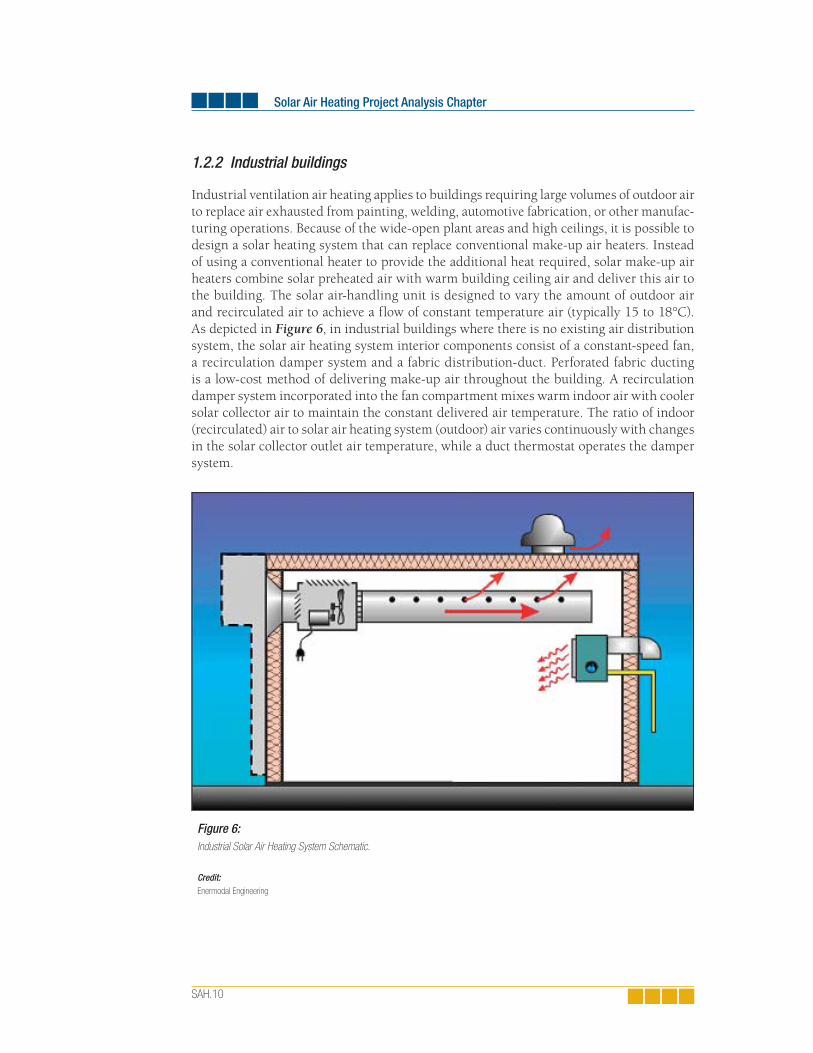
Solar Air Heating Project Analysis Chapter
SAH.10
1.2.2 Industrial buildings
Industrial ventilation air heating applies to buildings requiring large volumes of outdoor air to replace air exhausted from painting, welding, automotive fabrication, or other manufac-turing operations. Because of the wide-open plant areas and high ceilings, it is possible to design a solar heating system that can replace conventional make-up air heaters. Instead of using a conventional heater to provide the additional heat required, solar make-up air heaters combine solar preheated air with warm building ceiling air and deliver this air to the building. The solar air-handling unit is designed to vary the amount of outdoor air and recirculated air to achieve a flow of constant temperature air (typically 15 to 18°C). As depicted in Figure 6, in industrial buildings where there is no existing air distribution system, the solar air heating system interior components consist of a constant-speed fan, a recirculation damper system and a fabric distribution-duct. Perforated fabric ducting is a low-cost method of delivering make-up air throughout the building. A recirculation damper system incorporated into the fan compartment mixes warm indoor air with cooler solar collector air to maintain the constant delivered air temperature. The ratio of indoor (recirculated) air to solar air heating system (outdoor) air varies continuously with changes in the solar collector outlet air temperature, while a duct thermostat operates the damper system.
Figure 6:Industrial Solar Air Heating System Schematic.
Credit: Enermodal Engineering

1. Solar Air Heating Background
SAH.11
The mixture of ventilation air and recirculated air is distributed to the plant through per-forated fabric ducts, which are located at ceiling level. Because the air from the ducting is cooler than air at the ceiling, the ventilation air will cool the ceiling reducing heat loss through the roof at the temperature of exhaust air (for ceiling exhausters) and the air will naturally fall, mixing and destratifying the building air.
Another advantage of the system is that it too can recapture building wall heat loss if the collectors are mounted on the building wall.
1.2.3 Process air
Large quantities of outdoor air are used for process air heating applications. Drying of ag-ricultural products is a good application for solar energy, as the required temperature rise must be kept relatively low to prevent damaging the crops. Those crops that are harvested continuously over the year are well suited because all the available solar radiation can be used. Solar systems can also serve as a preheater to (high temperature) industrial drying systems.
Solar process air heating systems are similar to ventilation air preheating systems. The perforated plate absorber is located in any convenient location that has good exposure to the sun. Sloped roofs as well as walls are suitable mounting structures. A constant flow of air is taken through the collectors and is ducted into the air intake of the process. If necessary, additional heat can be added from auxiliary sources to deliver the desired air temperature and some or all of the process air can bypass the collectors if the air is above the desired temperature.


2. RETScreen Solar Air Heating Project Model
SAH.13
2 RETSCREEN SOLAR AIR HEATING PROJECT MODEL
The RETScreen Solar Air Heating Project Model can be used world-wide to evaluate solar air heating projects, from larger scale industrial building developments to smaller scale residential applications, anywhere in the world. It is also able to model process air heating applications, such as the drying of crops. Solar air heating systems can save conventional energy in three ways, depending upon the application:
Collection of solar energy through active solar air heating for buildings and processes;
Recapture of equator side wall heat loss (heat lost out the original build-ing wall is captured by the ventilation air and recirculated back into the building); and
Destratifi cation of building air in buildings with high ceilings, for example, industrial manufacturing plants or warehouses.
Six worksheets (Energy Model, Solar Resource, Cost Analysis, Greenhouse Gas Emission Reduc-tion Analysis (GHG Analysis), Financial Summary and Sensitivity and Risk Analysis (Sensitivity)) are provided in the Solar Air Heating Project Workbook file.
The Energy Model and Solar Resource worksheets are completed first. The Cost Analysis worksheet should then be completed, followed by the Financial Summary worksheet. The GHG Analysis and Sensitivity worksheets are optional analysis. The GHG Analysis work-sheet is provided to help the user estimate the greenhouse gas (GHG) mitigation potential of the proposed project. The Sensitivity worksheet is provided to help the user estimate the sensitivity of important financial indicators in relation to key technical and financial parameters. In general, the user works from top-down for each of the worksheets. This process can be repeated several times in order to help optimize the design of the solar air heating project from an energy use and cost standpoint.
To help the user characterize a solar air heating system before evaluating its cost and en-ergy performance, some values are suggested for component sizing (e.g. “Suggested solar collector area”). Suggested or estimated values are based on input parameters and can be used as a first step in the analysis and are not necessarily the optimum values.
This section describes the various algorithms used to calculate, on a month-by-month basis, the energy savings of solar air heating systems in RETScreen. A flowchart of the al-gorithms is shown in Figure 7. Sections 2.1 to 2.3 present the calculation of the three modes of energy savings: collected solar energy (Section 2.1), building heat recapture (Section 2.2), and destratification (Section 2.3) savings. How these three modes contribute to the overall energy savings is shown in Section 2.4 for heating systems for non-industrial buildings and in Section 2.5 for heating systems for industrial buildings. A validation of the RETScreen Solar Air Heating Project Model is presented in Section 2.6.
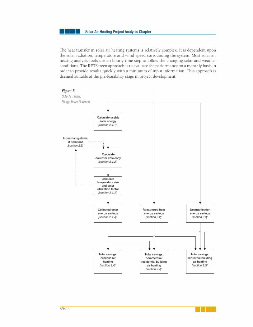
Solar Air Heating Project Analysis Chapter
SAH.14
The heat transfer in solar air heating systems is relatively complex. It is dependent upon the solar radiation, temperature and wind speed surrounding the system. Most solar air heating analysis tools use an hourly time step to follow the changing solar and weather conditions. The RETScreen approach is to evaluate the performance on a monthly basis in order to provide results quickly with a minimum of input information. This approach is deemed suitable at the pre-feasibility stage in project development.
Collected solarenergy savings[section 2.1.4]
Recaptured heatenergy savings
[section 2.2]
Destratificationenergy savings
[section 2.3]
Total savings:process air
heating[section 2.4]
Total savings:commercial/
residential buildingair heating
[section 2.4]
Total savings:industrial building
air heating[section 2.5]
Calculate usablesolar energy
[section 2.1.1]
Calculatetemperature rise
and solarutilization factor[section 2.1.3]
Calculatecollector efficiency
[section 2.1.2]
Industrial systems:3 iterations[section 2.5]
Figure 7:Solar Air Heating
Energy Model Flowchart.

2. RETScreen Solar Air Heating Project Model
SAH.15
In RETScreen, process air heating is assumed to benefit only from collected active solar energy savings. It is assumed that the building does not require space heating and any reduction in wall or roof heat loss does not save energy. Furthermore, because the heated air goes straight from the solar collector to the drying ovens, or other process machinery, there is no potential for destratifying the building air.
Commercial/residential buildings benefit from two modes of energy savings: collected active solar energy savings and recaptured heat savings. Industrial buildings, due to the method of air circulation on the building and the height of the ceilings, benefit from all three methods of energy savings.
Because of simplifications introduced, the RETScreen Solar Air Heating Model has a certain number of limitations:
The ventilation model does not incorporate a detailed energy consumption and make-up system analysis for the existing building. This minimised data requirement approach will make it much easier for the user to prepare an analysis, but modelling accuracy will be partially reduced as a result.
The model does not currently include advanced heat recovery technologies currently under development for the solar air heating system. Therefore, the model may understate the potential savings of a combined advanced heat recovery/solar air heating system.
The model is specifi c to the Solarwall® technology developed by Conserval Engineering and does not model other solar air heating systems that may be available on the market.
Finally, the model assumes industrial buildings have a balanced ventilation system for the calculation of destratifi cation savings.
For the majority of applications, these limitations are without consequence.
2.1 Collected Solar Energy Savings
Solar radiation incident upon the tilted collector must be calculated from data input by the user, namely, daily solar radiation on a horizontal surface and operating multiplier. This is detailed in Section 2.1.1. Energy collected by the solar collector is calculated by multiplying incident radiation by the average collector efficiency; calculation of this latter quantity is detailed in Section 2.1.2. However, only part of the energy collected will actually be usable; the concept of solar utilization is covered in Section 2.1.3.

Solar Air Heating Project Analysis Chapter
SAH.16
2.1.1 Usable incident solar energy calculation
For each month, i, the total amount of solar energy usable by the collector, Gcoll i, , is cal-
culated. This value is obtained from the average daily amount of solar energy incident on the collector, Gtilt i, , the collector area Acoll , and the operating schedule of the SAH system fop i, :
The solar radiation incident on the collector, Gtilt i, , is derived from the user-entered av-erage daily solar radiation on the horizontal surface, Ghorz i, , using the Liu and Jordan algorithm (see Duffie and Beckman, 1991; this algorithm is also described in the Solar Water Heating Project Analysis Chapter of this textbook). The value for fop i, demonstrates the importance of the operating schedule to the total energy savings of a SAH system. It is calculated using:
where ndays i, is the number of days in month i, fsys i, is the user-entered fraction of the month used for system operation, hop daytime, is the number of hours of operation during sunlight hours, hsunlight i, is the number of hours of sunlight per day for month i, and dop is the user-entered number of operating days per week.
When the system is shut down, energy cannot be captured. Therefore to account for the weekly operating schedule, dop is divided by 7 days a week in equation (2). To account for the daily operating schedule the number of operating hours per day (hop daytime, ) is divided by the number of daylight hours on the “average” day of the month (hsunlight i, ), which is calculated with formulae from Duffie and Beckman (1991). It should be noted, depending on the time of year and latitude, that during some months of the year the user-entered hours per day of operating time (hop ) may be greater than hours of daylight (hsunlight i, ). In this situation the lesser of hop and hsunlight i, is used for hop daytime, . This calculation also in-troduces an approximation since no consideration is given to the actual time of operation. Thus, the relative intensity of solar radiation at the different times of day is not accounted for. Hours of operation are assumed to be distributed evenly around noon.
(1)
(2)
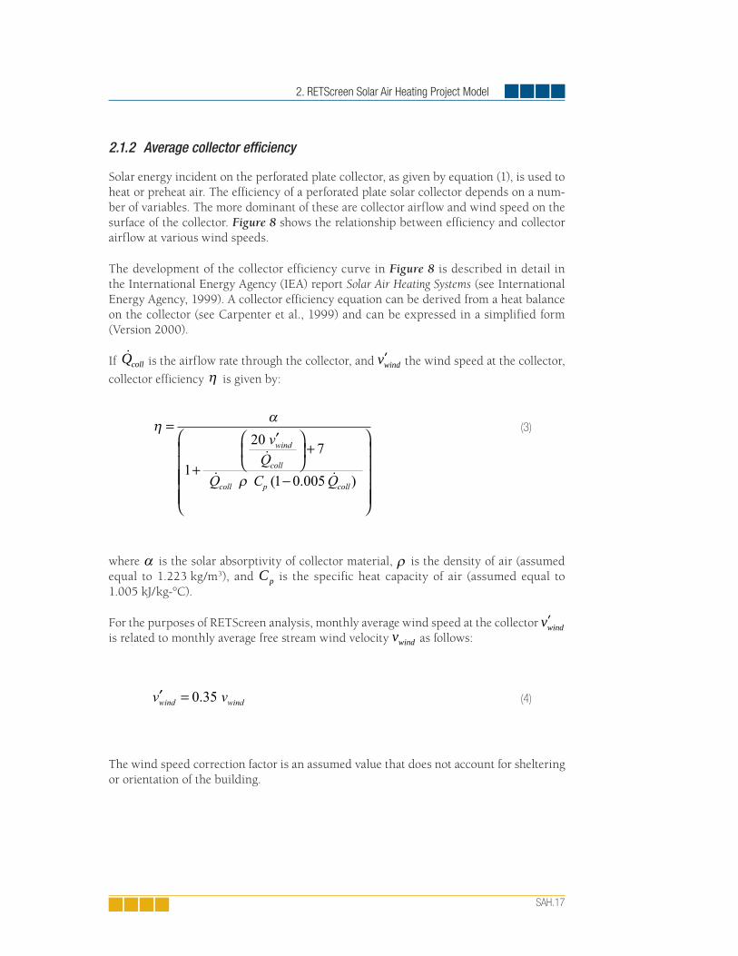
2. RETScreen Solar Air Heating Project Model
SAH.17
2.1.2 Average collector effi ciency
Solar energy incident on the perforated plate collector, as given by equation (1), is used to heat or preheat air. The efficiency of a perforated plate solar collector depends on a num-ber of variables. The more dominant of these are collector airflow and wind speed on the surface of the collector. Figure 8 shows the relationship between efficiency and collector airflow at various wind speeds.
The development of the collector efficiency curve in Figure 8 is described in detail in the International Energy Agency (IEA) report Solar Air Heating Systems (see International Energy Agency, 1999). A collector efficiency equation can be derived from a heat balance on the collector (see Carpenter et al., 1999) and can be expressed in a simplified form (Version 2000).
If Qcoll is the airflow rate through the collector, and ′vwind the wind speed at the collector,
collector efficiency η is given by:
where α is the solar absorptivity of collector material, ρ is the density of air (assumed equal to 1.223 kg/m3), and Cp is the specific heat capacity of air (assumed equal to 1.005 kJ/kg-°C).
For the purposes of RETScreen analysis, monthly average wind speed at the collector ′vwind is related to monthly average free stream wind velocity vwind as follows:
The wind speed correction factor is an assumed value that does not account for sheltering or orientation of the building.
(3)
(4)
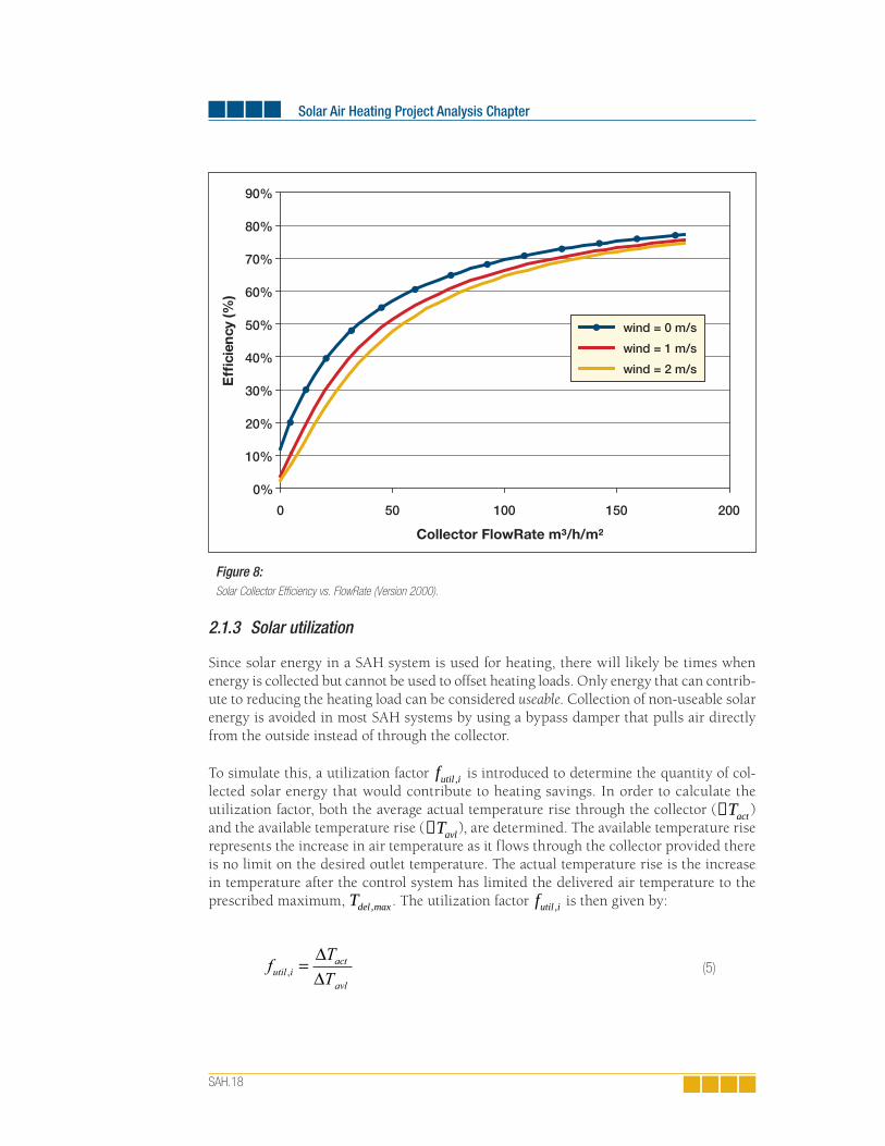
Solar Air Heating Project Analysis Chapter
SAH.18
2.1.3 Solar utilization
Since solar energy in a SAH system is used for heating, there will likely be times when energy is collected but cannot be used to offset heating loads. Only energy that can contrib-ute to reducing the heating load can be considered useable. Collection of non-useable solar energy is avoided in most SAH systems by using a bypass damper that pulls air directly from the outside instead of through the collector.
To simulate this, a utilization factor futil i, is introduced to determine the quantity of col-lected solar energy that would contribute to heating savings. In order to calculate the utilization factor, both the average actual temperature rise through the collector (∆Tact ) and the available temperature rise (∆Tavl ), are determined. The available temperature rise represents the increase in air temperature as it flows through the collector provided there is no limit on the desired outlet temperature. The actual temperature rise is the increase in temperature after the control system has limited the delivered air temperature to the prescribed maximum, Tdel max, . The utilization factor futil i, is then given by:
Figure 8: Solar Collector Effi ciency vs. FlowRate (Version 2000).
0%
10%
20%
30%
40%
50%
60%
70%
80%
90%
0 50 100 150 200
Collector FlowRate m³/h/m²
Eff
icie
ncy
(%)
wind = 0 m/s
wind = 1 m/s
wind = 2 m/s
(5)

2. RETScreen Solar Air Heating Project Model
SAH.19
Available temperature rise is found using the collector efficiency and the collector airflow rate, Qcoll . For month i:
where, ρ and Cp are, as described previously, the density of air and the specific heat capacity of air.
The actual temperature rise is limited by conditions imposed on the temperature of the air exiting the collector, also called delivered temperature. The actual delivered temperature Tdel act, is constrained so as not to exceed the maximum delivered air temperature, Tdel max, , entered by the user. Equations (7) to (9) demonstrate how ∆Tact is determined:
where Tdel avl, is the available delivered temperature and Tamb is the average outside ambi-ent temperature. ∆Toffset is a temperature offset of 3ºC added to the ambient temperature on the assumption that the daytime temperature is higher than the average temperature. A negative result is not allowed and if necessary the actual temperature rise is forced to zero.
(6)
(7)
(8)
(9)

Solar Air Heating Project Analysis Chapter
SAH.20
2.1.4 Active solar energy savings
Solar energy delivered over the year, Qsol , is obtained by summing monthly contributions:
where monthly collector efficiency ηi is calculated from equation (3), total amount of solar energy usable by the collector Gcoll i, is given by equation (1), and the utilization factor futil i, is calculated through equation (5).
2.2 Building Heat Recapture Savings
When a SAH collector is installed on a building, there is an added benefit due to the return of lost building heat through the collector. If the collector is not running, there is a small benefit associated with a slightly increased RSI-value (thermal resistance) of the building wall. The model estimates building heat recapture savings under three different modes: daytime operating, nighttime operating, and during shutdown times. The net savings Qrecap are found by simply summing these three quantities:
where Qrecap op daytime i, , , is the daytime heat recapture while the air handler is operating for month i, Qrecap op nighttime i, , , is the nighttime heat recapture while the air handler is operating for month i, Qrecap shutdown i, , is the heat recapture while the air handler is not operating for month i, and
fsys i, is the user-entered fraction of month i used for system operation. Heat recapture for the three modes is calculated as follows:
(10)
(11)
(12)
(13)
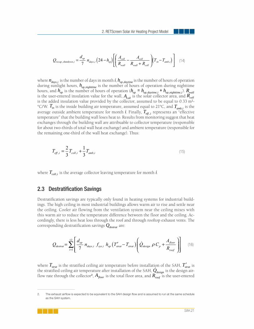
2. RETScreen Solar Air Heating Project Model
SAH.21
where ndays i, is the number of days in month i, hop daytime, is the number of hours of operation during sunlight hours, hop nighttime, is the number of hours of operation during nighttime hours, and hop is the number of hours of operation (h h hop op daytime i op nighttime i= +, , , , ). Rwall is the user-entered insulation value for the wall, Acoll is the solar collector area, and Rcoll is the added insulation value provided by the collector, assumed to be equal to 0.33 m²-°C/W. Tin is the inside building air temperature, assumed equal to 21°C, and Tamb i, is the average outside ambient temperature for month i. Finally, Teff i, represents an “effective temperature” that the building wall loses heat to. Results from monitoring suggest that heat exchanges through the building wall are attribuable to collector temperature (responsible for about two-thirds of total wall heat exchange) and ambient temperature (responsible for the remaining one-third of the wall heat exchange). Thus:
where Tcoll i, is the average collector leaving temperature for month i.
2.3 Destratifi cation Savings
Destratification savings are typically only found in heating systems for industrial build-ings. The high ceiling in most industrial buildings allows warm air to rise and settle near the ceiling. Cooler air flowing from the ventilation system near the ceiling mixes with this warm air to reduce the temperature difference between the floor and the ceiling. Ac-cordingly, there is less heat loss through the roof and through rooftop exhaust vents. The corresponding destratification savings Qdestrat are:
where Tstrat is the stratified ceiling air temperature before installation of the SAH, ′Tstrat is the stratified ceiling air temperature after installation of the SAH, Qdesign is the design air-flow rate through the collector2, Afloor is the total floor area, and Rroof is the user-entered
(14)
(15)
(16)
2. The exhaust airfl ow is expected to be equivalent to the SAH design fl ow and is assumed to run at the same schedule as the SAH system.
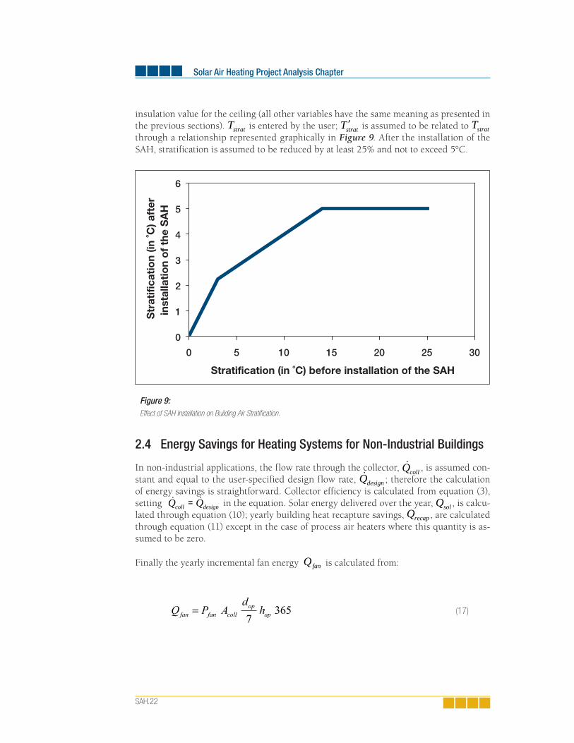
Solar Air Heating Project Analysis Chapter
SAH.22
insulation value for the ceiling (all other variables have the same meaning as presented in the previous sections). Tstrat is entered by the user; ′Tstrat is assumed to be related to Tstrat through a relationship represented graphically in Figure 9. After the installation of the SAH, stratification is assumed to be reduced by at least 25% and not to exceed 5°C.
2.4 Energy Savings for Heating Systems for Non-Industrial Buildings
In non-industrial applications, the flow rate through the collector, Qcoll , is assumed con-stant and equal to the user-specified design flow rate, Qdesign ; therefore the calculation of energy savings is straightforward. Collector efficiency is calculated from equation (3), setting Q Qcoll design= in the equation. Solar energy delivered over the year, Qsol , is calcu-lated through equation (10); yearly building heat recapture savings, Qrecap , are calculated through equation (11) except in the case of process air heaters where this quantity is as-sumed to be zero.
Finally the yearly incremental fan energy Qfan is calculated from:
Figure 9: Effect of SAH Installation on Building Air Stratifi cation.
0
1
2
3
4
5
6
0 5 10 15 20 25 30
Stratification (in ˚C) before installation of the SAH
Str
atifi
cati
on
(in ˚C
) aft
er
inst
alla
tio
n o
f th
e S
AH
(17)
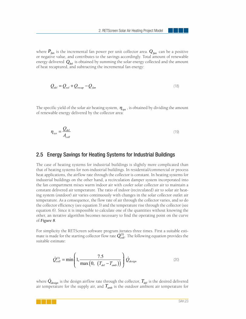
2. RETScreen Solar Air Heating Project Model
SAH.23
where Pfan is the incremental fan power per unit collector area. Qfan can be a positive or negative value, and contributes to the savings accordingly. Total amount of renewable energy delivered Qdel is obtained by summing the solar energy collected and the amount of heat recaptured, and subtracting the incremental fan energy:
The specific yield of the solar air heating system, ηsys , is obtained by dividing the amount
of renewable energy delivered by the collector area:
2.5 Energy Savings for Heating Systems for Industrial Buildings
The case of heating systems for industrial buildings is slightly more complicated than that of heating systems for non-industrial buildings. In residential/commercial or process heat applications, the airflow rate through the collector is constant. In heating systems for industrial buildings on the other hand, a recirculation damper system incorporated into the fan compartment mixes warm indoor air with cooler solar collector air to maintain a constant delivered air temperature. The ratio of indoor (recirculated) air to solar air heat-ing system (outdoor) air varies continuously with changes in the solar collector outlet air temperature. As a consequence, the flow rate of air through the collector varies, and so do the collector efficiency (see equation 3) and the temperature rise through the collector (see equation 6). Since it is impossible to calculate one of the quantities without knowing the other, an iterative algorithm becomes necessary to find the operating point on the curve of Figure 8.
For simplicity the RETScreen software program iterates three times. First a suitable esti-mate is made for the starting collector flow rate Qcoll
( )1 . The following equation provides the suitable estimate:
where Qdesign is the design airflow rate through the collector, Tdel is the desired delivered air temperature for the supply air, and Tamb is the outdoor ambient air temperature for
(18)
(19)
(20)
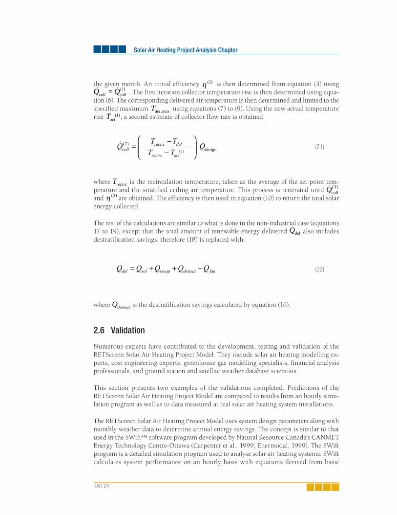
Solar Air Heating Project Analysis Chapter
SAH.24
the given month. An initial efficiency η ( )1 is then determined from equation (3) using
Q Qcoll coll= ( )1 . The first iteration collector temperature rise is then determined using equa-tion (6). The corresponding delivered air temperature is then determined and limited to the specified maximum Tdel max, using equations (7) to (9). Using the new actual temperature rise Tact , a second estimate of collector flow rate is obtained:
where Trecirc is the recirculation temperature, taken as the average of the set point tem-perature and the stratified ceiling air temperature. This process is reiterated until Qcoll
( )3 and η
( )3 are obtained. The efficiency is then used in equation (10) to return the total solar energy collected.
The rest of the calculations are similar to what is done in the non-industrial case (equations 17 to 19), except that the total amount of renewable energy delivered
Qdel also includes destratification savings; therefore (18) is replaced with:
where Qdestrat is the destratification savings calculated by equation (16).
2.6 Validation
Numerous experts have contributed to the development, testing and validation of the RETScreen Solar Air Heating Project Model. They include solar air heating modelling ex-perts, cost engineering experts, greenhouse gas modelling specialists, financial analysis professionals, and ground station and satellite weather database scientists.
This section presents two examples of the validations completed. Predictions of the RETScreen Solar Air Heating Project Model are compared to results from an hourly simu-lation program as well as to data measured at real solar air heating system installations.
The RETScreen Solar Air Heating Project Model uses system design parameters along with monthly weather data to determine annual energy savings. The concept is similar to that used in the SWift™ software program developed by Natural Resource Canada’s CANMET Energy Technology Centre-Ottawa (Carpenter et al., 1999; Enermodal, 1999). The SWift program is a detailed simulation program used to analyse solar air heating systems. SWift calculates system performance on an hourly basis with equations derived from basic
(21)
(22)
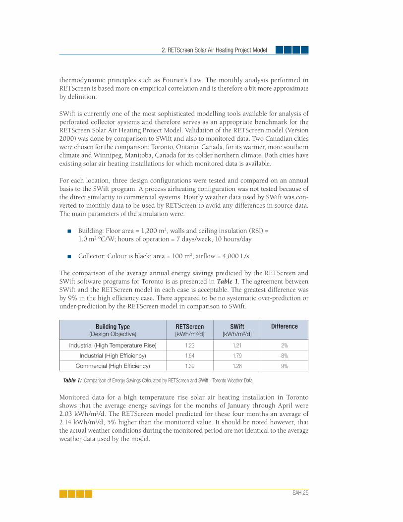
2. RETScreen Solar Air Heating Project Model
SAH.25
thermodynamic principles such as Fourier’s Law. The monthly analysis performed in RETScreen is based more on empirical correlation and is therefore a bit more approximate by definition.
SWift is currently one of the most sophisticated modelling tools available for analysis of perforated collector systems and therefore serves as an appropriate benchmark for the RETScreen Solar Air Heating Project Model. Validation of the RETScreen model (Version 2000) was done by comparison to SWift and also to monitored data. Two Canadian cities were chosen for the comparison: Toronto, Ontario, Canada, for its warmer, more southern climate and Winnipeg, Manitoba, Canada for its colder northern climate. Both cities have existing solar air heating installations for which monitored data is available.
For each location, three design configurations were tested and compared on an annual basis to the SWift program. A process airheating configuration was not tested because of the direct similarity to commercial systems. Hourly weather data used by SWift was con-verted to monthly data to be used by RETScreen to avoid any differences in source data. The main parameters of the simulation were:
Building: Floor area = 1,200 m2, walls and ceiling insulation (RSI) = 1.0 m² ºC/W; hours of operation = 7 days/week, 10 hours/day.
Collector: Colour is black; area = 100 m2; airfl ow = 4,000 L/s.
The comparison of the average annual energy savings predicted by the RETScreen and SWift software programs for Toronto is as presented in Table 1. The agreement between SWift and the RETScreen model in each case is acceptable. The greatest difference was by 9% in the high efficiency case. There appeared to be no systematic over-prediction or under-prediction by the RETScreen model in comparison to SWift.
Building Type(Design Objective)
RETScreen[kWh/m²/d]
SWift[kWh/m²/d]
Difference
Industrial (High Temperature Rise) 1.23 1.21 2%
Industrial (High Efficiency) 1.64 1.79 -8%
Commercial (High Efficiency) 1.39 1.28 9%
Table 1: Comparison of Energy Savings Calculated by RETScreen and SWift - Toronto Weather Data.
Monitored data for a high temperature rise solar air heating installation in Toronto shows that the average energy savings for the months of January through April were 2.03 kWh/m²/d. The RETScreen model predicted for these four months an average of 2.14 kWh/m²/d, 5% higher than the monitored value. It should be noted however, that the actual weather conditions during the monitored period are not identical to the average weather data used by the model.
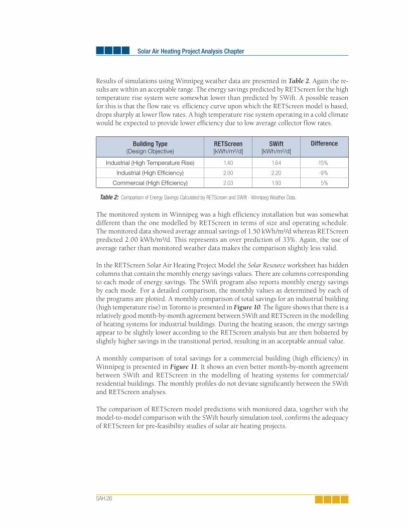
Solar Air Heating Project Analysis Chapter
SAH.26
Results of simulations using Winnipeg weather data are presented in Table 2. Again the re-sults are within an acceptable range. The energy savings predicted by RETScreen for the high temperature rise system were somewhat lower than predicted by SWift. A possible reason for this is that the flow rate vs. efficiency curve upon which the RETScreen model is based, drops sharply at lower flow rates. A high temperature rise system operating in a cold climate would be expected to provide lower efficiency due to low average collector flow rates.
Building Type(Design Objective)
RETScreen[kWh/m²/d]
SWift[kWh/m²/d]
Difference
Industrial (High Temperature Rise) 1.40 1.64 -15%
Industrial (High Effi ciency) 2.00 2.20 -9%
Commercial (High Effi ciency) 2.03 1.93 5%
Table 2: Comparison of Energy Savings Calculated by RETScreen and SWift - Winnipeg Weather Data.
The monitored system in Winnipeg was a high efficiency installation but was somewhat different than the one modelled by RETScreen in terms of size and operating schedule. The monitored data showed average annual savings of 1.50 kWh/m²/d whereas RETScreen predicted 2.00 kWh/m²/d. This represents an over prediction of 33%. Again, the use of average rather than monitored weather data makes the comparison slightly less valid.
In the RETScreen Solar Air Heating Project Model the Solar Resource worksheet has hidden columns that contain the monthly energy savings values. There are columns corresponding to each mode of energy savings. The SWift program also reports monthly energy savings by each mode. For a detailed comparison, the monthly values as determined by each of the programs are plotted. A monthly comparison of total savings for an industrial building (high temperature rise) in Toronto is presented in Figure 10. The figure shows that there is a relatively good month-by-month agreement between SWift and RETScreen in the modelling of heating systems for industrial buildings. During the heating season, the energy savings appear to be slightly lower according to the RETScreen analysis but are then bolstered by slightly higher savings in the transitional period, resulting in an acceptable annual value.
A monthly comparison of total savings for a commercial building (high efficiency) in Winnipeg is presented in Figure 11. It shows an even better month-by-month agreement between SWift and RETScreen in the modelling of heating systems for commercial/residential buildings. The monthly profiles do not deviate significantly between the SWift and RETScreen analyses.
The comparison of RETScreen model predictions with monitored data, together with the model-to-model comparison with the SWift hourly simulation tool, confirms the adequacy of RETScreen for pre-feasibility studies of solar air heating projects.
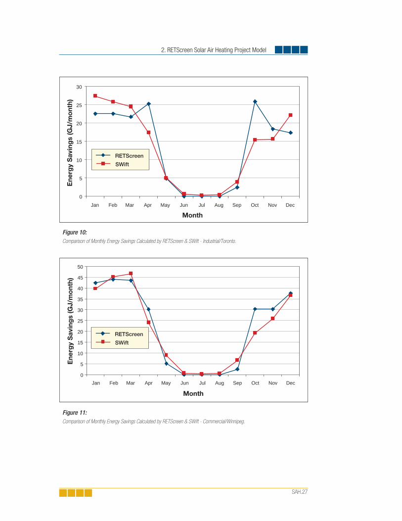
2. RETScreen Solar Air Heating Project Model
SAH.27
Figure 10: Comparison of Monthly Energy Savings Calculated by RETScreen & SWift - Industrial/Toronto.
0
5
10
15
20
25
30
Ene
rgy
Sav
ing
s (G
J/m
ont
h)
Month
RETScreen
SWift
Jan Feb Mar Apr May Jun Jul Aug Sep Oct Nov Dec
Figure 11: Comparison of Monthly Energy Savings Calculated by RETScreen & SWift - Commercial/Winnipeg.
0
5
10
15
20
25
30
35
40
45
50
Jan Feb Mar Apr May Jun Jul Aug Sep Oct Nov Dec
Ene
rgy
Sav
ing
s (G
J/m
ont
h)
Month
RETScreen
SWift

Solar Air Heating Project Analysis Chapter
SAH.28
2.7 Summary
In this section the algorithms used by the RETScreen Solar Air Heating Project Model have been shown in detail. The model calculates energy savings resulting from the installation of a perforated plate solar collector. Energy savings are the sum of solar energy actively collected, building heat recapture savings, and destratification savings. Depending on the type of system considered, only some of these savings may apply: process heat systems only benefit from active gains, residential/commercial systems also benefit from building heat recapture and heating systems for industrial buildings benefit from all three modes of savings. Active solar energy gains are calculated with the help of an empirical collec-tor efficiency curve. Other savings are approximated from simple energy balances using monthly average values. The calculation of overall energy savings is straightforward in the case of commercial/residential and process heat systems, where the collector flow rate is set by design; the calculation is more complicated in the case of heating systems for industrial buildings because collector flow rate depends on the mixing ratio with recirculated air, and an iterative procedure has to be used.
Despite the simplifications introduced, comparison of the RETScreen model predictions to results of an hourly simulation program and to monitored data shows that the accuracy of the RETScreen Solar Air Heating Project Model is excellent in regards to the preparation of pre-feasibility studies. This is particularly true given the fact that RETScreen only requires 12 points of weather data versus 8,760 points of data for hourly simulation models.

SAH.29
REFERENCES
Carpenter, S., Daniels, S., Kemp, S., Kokko, J. and Van Decker,, G., New Tools for Assessing the Performance of Solar Ventilation Air Heating Systems, Proc. 8th Biannual Conference on Solar Energy in High Latitudes (North Sun ‘99), Incorporating the 25th Annual Conference of the Solar Energy Society of Canada Inc. (SESCI), Edmonton, AB, Canada, 1999.
Duffi e, J.A. and Beckman, W.A., Solar Engineering of Thermal Processes, 2nd Edition, John Wiley & Sons, 1991.
Energy, Mines and Resources Canada (EMR), Heating and Cooling Equipment (Steam and Water), Energy Management Series 9, 1985.
Enermodal Engineering Limited, The Market for Solar Preheated Ventilation Systems in Canadian Remote Communities, Report prepared for Natural Resources Canada, 1997.
Enermodal, The SWift Computer Program, Available from Enermodal Engineering Limited, 650 Riverbend Drive, Kitchener, ON, Canada, N2K 3S2, 1999.
International Energy Agency, Low Cost, High Performance Solar Air-Heating Systems Using Perforated Absorbers: A Report of Task 14 – Air Systems Working Group, Morse Associates, Inc., Washington, DC, USA, 1999.


SOLAR WATER HEATING PROJECT ANALYSIS CHAPTER
CLEAN ENERGY PROJECT ANALYSIS:RETSCREEN® ENGINEERING & CASES TEXTBOOK
DisclaimerThis publication is distributed for informational purposes only and does not necessarily reflect the views of the Government of Canada nor constitute an endorsement of any commercial product or person. Neither Canada, nor its ministers, officers, employees and agents makeany warranty in respect to this publication nor a s s u m e a n y l i a b i l i t y a r i s i n g o u t o f t h i s publication.
© Minister of Natural Resources Canada 2001 - 2004.
www.retscreen.net
RETScreen® InternationalClean Energy Decision Support Centre

ISBN: 0-622-35674-8 Catalogue no.: M39-101/2003E-PDF
© Minister of Natural Resources Canada 2001 - 2004.
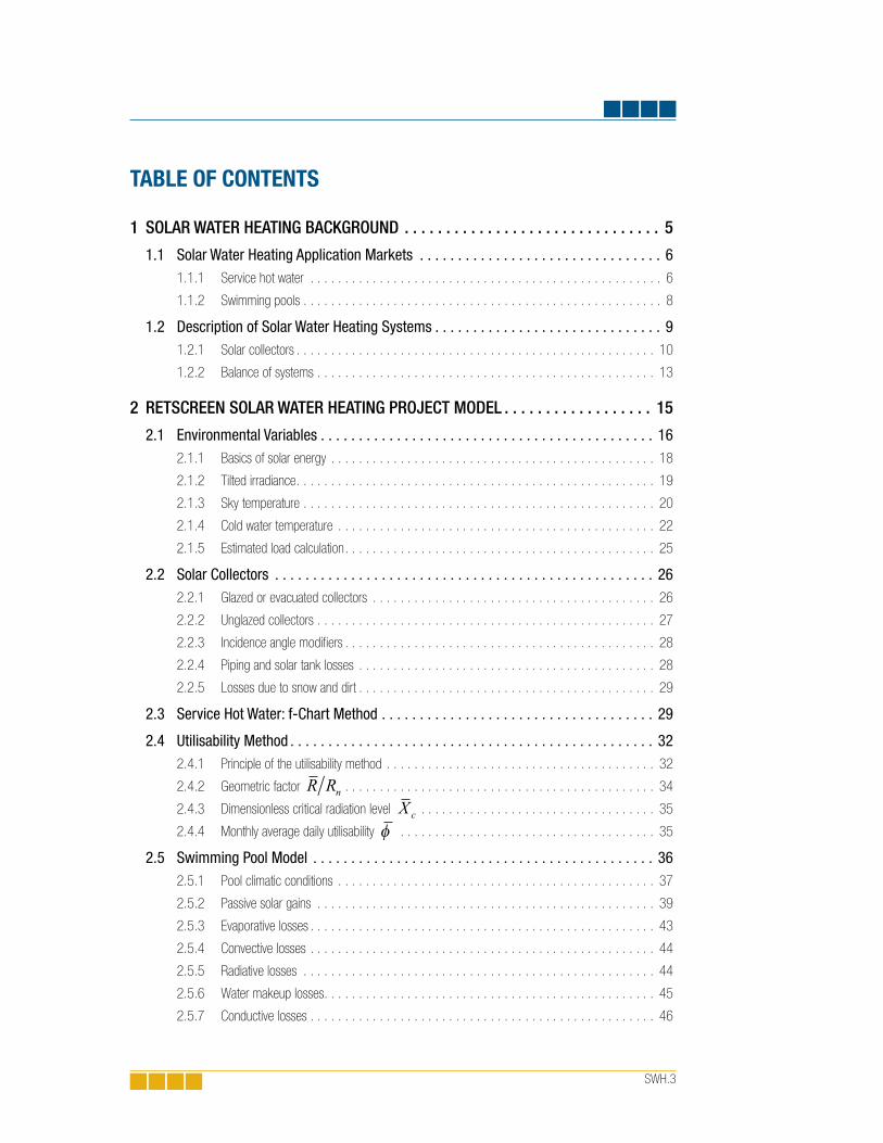
SWH.3
TABLE OF CONTENTS
1 SOLARWATERHEATINGBACKGROUND . . . . . . . . . . . . . . . . . . . . . . . . . . . . . . . 5
1.1 SolarWaterHeatingApplicationMarkets . . . . . . . . . . . . . . . . . . . . . . . . . . . . . . . . 61.1.1 Service hot water . . . . . . . . . . . . . . . . . . . . . . . . . . . . . . . . . . . . . . . . . . . . . . . . . . . 6
1.1.2 Swimming pools . . . . . . . . . . . . . . . . . . . . . . . . . . . . . . . . . . . . . . . . . . . . . . . . . . . . 8
1.2 DescriptionofSolarWaterHeatingSystems. . . . . . . . . . . . . . . . . . . . . . . . . . . . . . 91.2.1 Solar collectors . . . . . . . . . . . . . . . . . . . . . . . . . . . . . . . . . . . . . . . . . . . . . . . . . . . . 10
1.2.2 Balance of systems . . . . . . . . . . . . . . . . . . . . . . . . . . . . . . . . . . . . . . . . . . . . . . . . . 13
2 RETSCREENSOLARWATERHEATINGPROJECTMODEL . . . . . . . . . . . . . . . . . . 15
2.1 EnvironmentalVariables. . . . . . . . . . . . . . . . . . . . . . . . . . . . . . . . . . . . . . . . . . . . 162.1.1 Basics of solar energy . . . . . . . . . . . . . . . . . . . . . . . . . . . . . . . . . . . . . . . . . . . . . . . 18
2.1.2 Tilted irradiance . . . . . . . . . . . . . . . . . . . . . . . . . . . . . . . . . . . . . . . . . . . . . . . . . . . . 19
2.1.3 Sky temperature . . . . . . . . . . . . . . . . . . . . . . . . . . . . . . . . . . . . . . . . . . . . . . . . . . . 20
2.1.4 Cold water temperature . . . . . . . . . . . . . . . . . . . . . . . . . . . . . . . . . . . . . . . . . . . . . . 22
2.1.5 Estimated load calculation . . . . . . . . . . . . . . . . . . . . . . . . . . . . . . . . . . . . . . . . . . . . . 25
2.2 SolarCollectors . . . . . . . . . . . . . . . . . . . . . . . . . . . . . . . . . . . . . . . . . . . . . . . . . . 262.2.1 Glazed or evacuated collectors . . . . . . . . . . . . . . . . . . . . . . . . . . . . . . . . . . . . . . . . . 26
2.2.2 Unglazed collectors . . . . . . . . . . . . . . . . . . . . . . . . . . . . . . . . . . . . . . . . . . . . . . . . . 27
2.2.3 Incidence angle modifiers . . . . . . . . . . . . . . . . . . . . . . . . . . . . . . . . . . . . . . . . . . . . . 28
2.2.4 Piping and solar tank losses . . . . . . . . . . . . . . . . . . . . . . . . . . . . . . . . . . . . . . . . . . . 28
2.2.5 Losses due to snow and dirt . . . . . . . . . . . . . . . . . . . . . . . . . . . . . . . . . . . . . . . . . . . 29
2.3 ServiceHotWater:f-ChartMethod. . . . . . . . . . . . . . . . . . . . . . . . . . . . . . . . . . . . 29
2.4 UtilisabilityMethod. . . . . . . . . . . . . . . . . . . . . . . . . . . . . . . . . . . . . . . . . . . . . . . . 322.4.1 Principle of the utilisability method . . . . . . . . . . . . . . . . . . . . . . . . . . . . . . . . . . . . . . . 32
2.4.2 Geometric factor R Rn . . . . . . . . . . . . . . . . . . . . . . . . . . . . . . . . . . . . . . . . . . . . . 34
2.4.3 Dimensionless critical radiation level X c . . . . . . . . . . . . . . . . . . . . . . . . . . . . . . . . . . 35
2.4.4 Monthly average daily utilisability φ . . . . . . . . . . . . . . . . . . . . . . . . . . . . . . . . . . . . . 35
2.5 SwimmingPoolModel . . . . . . . . . . . . . . . . . . . . . . . . . . . . . . . . . . . . . . . . . . . . . 362.5.1 Pool climatic conditions . . . . . . . . . . . . . . . . . . . . . . . . . . . . . . . . . . . . . . . . . . . . . . 37
2.5.2 Passive solar gains . . . . . . . . . . . . . . . . . . . . . . . . . . . . . . . . . . . . . . . . . . . . . . . . . 39
2.5.3 Evaporative losses . . . . . . . . . . . . . . . . . . . . . . . . . . . . . . . . . . . . . . . . . . . . . . . . . . 43
2.5.4 Convective losses . . . . . . . . . . . . . . . . . . . . . . . . . . . . . . . . . . . . . . . . . . . . . . . . . . 44
2.5.5 Radiative losses . . . . . . . . . . . . . . . . . . . . . . . . . . . . . . . . . . . . . . . . . . . . . . . . . . . 44
2.5.6 Water makeup losses . . . . . . . . . . . . . . . . . . . . . . . . . . . . . . . . . . . . . . . . . . . . . . . . 45
2.5.7 Conductive losses . . . . . . . . . . . . . . . . . . . . . . . . . . . . . . . . . . . . . . . . . . . . . . . . . . 46

SWH.4
2.5.8 Active solar gains . . . . . . . . . . . . . . . . . . . . . . . . . . . . . . . . . . . . . . . . . . . . . . . . . . 46
2.5.9 Energy balance . . . . . . . . . . . . . . . . . . . . . . . . . . . . . . . . . . . . . . . . . . . . . . . . . . . . 46
2.6 OtherCalculations . . . . . . . . . . . . . . . . . . . . . . . . . . . . . . . . . . . . . . . . . . . . . . . . 472.6.1 Suggested solar collector area . . . . . . . . . . . . . . . . . . . . . . . . . . . . . . . . . . . . . . . . . . 47
2.6.2 Pumping energy . . . . . . . . . . . . . . . . . . . . . . . . . . . . . . . . . . . . . . . . . . . . . . . . . . . 48
2.6.3 Specific yield, system efficiency and solar fraction . . . . . . . . . . . . . . . . . . . . . . . . . . . . 48
2.7 Validation. . . . . . . . . . . . . . . . . . . . . . . . . . . . . . . . . . . . . . . . . . . . . . . . . . . . . . . 482.7.1 Domestic water heating validation – compared with hourly model and monitored data . . . 49
2.7.2 Swimming pool heating validation – compared with hourly model and monitored data . . . . 52
2.8 Summary. . . . . . . . . . . . . . . . . . . . . . . . . . . . . . . . . . . . . . . . . . . . . . . . . . . . . . . 56
REFERENCES . . . . . . . . . . . . . . . . . . . . . . . . . . . . . . . . . . . . . . . . . . . . . . . . . . . . 57

1. Solar Water Heating Background
SWH.5
SOLAR WATER HEATING PROJECT ANALYSIS CHAPTERClean Energy Project Analysis: RETScreen® Engineering & Cases is an electronic textbook for professionals and university students. This chapter covers the analysis of potential solar water heating projects using the RETScreen® International Clean Energy Project Analysis Software, including a technology background and a detailed description of the algorithms found in the RETScreen® Software. A collection of project case studies, with assignments, worked-out solutions and information about how the projects fared in the real world, is available at the RETScreen® International Clean Energy Decision Support Centre Website www.retscreen.net.
1 SOLAR WATER HEATING BACKGROUND1
Using the sun’s energy to heat water is not a new idea. More than one hundred years ago, black painted water tanks were used as simple solar water heaters in a number of coun-tries. Solar water heating (SWH) technology has greatly improved during the past century. Today there are more than 30 million m2 of solar collectors installed around the globe. Hundreds of thousands of modern solar water heaters, such as the one shown in Figure 1, are in use in countries such as China, India, Germany, Japan, Australia and Greece. In fact, in some countries the law actually requires that solar water heaters be installed with any new residential construction project (Israel for example).
1. Some of the text in this “Background” description comes from the following reference: Marbek Resources Consultants, Solar Water Heaters: A Buyer’s Guide, Report prepared for Energy, Mines and Resources Canada, 1986.
Figure 1:Evacuated Tube Solar
Collector in Tibet, China.
Photo Credit: Alexandre Monarque

SolarWaterHeatingProjectAnalysisChapter
SWH.6
In addition to the energy cost savings on water heating, there are several other benefits derived from using the sun’s energy to heat water. Most solar water heaters come with an additional water tank, which feeds the conventional hot water tank. Users benefit from the larger hot water storage capacity and the reduced likelihood of running out of hot water. Some solar water heaters do not require electricity to operate. For these systems, hot water supply is secure from power outages, as long as there is sufficient sunlight to operate the system. Solar water heating systems can also be used to directly heat swimming pool water, with the added benefit of extending the swimming season for outdoor pool applications.
1 .1 SolarWaterHeatingApplicationMarkets
Solar water heating markets can be classified based upon the end-use application of the technology. The most common solar water heating application markets are service hot water and swimming pools.
1.1.1 Service hot water
There are a number of service hot water applications. The most common application is the use of domestic hot water systems (DHWS), generally sold as “off-the-shelf” or standard kits as depicted in Figure 2.
Figure 2:Solar Domestic Hot Water (Thermosiphon) System in Australia.
Photo Credit: The Australian Greenhouse Office

1. Solar Water Heating Background
SWH.7
Other common uses include providing process hot water for commercial and institu-tional applications, including multi-unit houses and apartment buildings, as depicted in Figure 3, housing developments as shown in Figure 4, and in schools, health centres, hospitals, office buildings, restaurants and hotels.
Small commercial and industrial ap-plications such as car washes, laun-dries and fish farms are other typical examples of service hot water. Figure 5 shows a solar water heating system at the Rosewall Creek Salmon Hatchery in British Columbia, Canada. 260 m² unglazed solar collectors heat make-up water and help increase fingerlings pro-duction at the aquaculture facility. Stor-age tanks help regulate temperature of make-up water. This particular project had a five-year simple payback period.
Solar water heating systems can also be used for large industrial loads and for providing energy to district heat-ing networks. A number of large sys-tems have been installed in northern Europe and other locations.
Figure 3:Glazed Flat-Plate Solar Collectors Integrated into Multi-Unit Housing.
Photo Credit: Chromagen
Figure 4:Housing Development, Küngsbacka, Sweden.
Photo Credit: Alpo Winberg/Solar Energy Association of Sweden

SolarWaterHeatingProjectAnalysisChapter
SWH.8
1.1.2 Swimming pools
The water temperature in swimming pools can also be regulated using solar water heating systems, extending the swimming pool season and saving on the conventional energy costs. The basic principle of these systems is the same as with solar service hot water systems, with the difference that the pool itself acts as the thermal stor-age. For outdoor pools, a properly sized solar water heater can replace a conventional heater; the pool water is directly pumped through the solar collectors by the existing filtration system.
Swimming pool applications can range in size from small summer only outdoor pools, such as the one shown at a home in Figure 6, to large Olym-pic size indoor swimming pools that operate 12 months a year.
Figure 5:Solar Water Heating Project at a Salmon Hatchery,
Canada.
Photo Credit: Natural Resources Canada
Figure 6:Unglazed Solar Collector Pool Heating System in Canada.
Photo Credit: Aquatherm Industries/ NREL Pix

1. Solar Water Heating Background
SWH.9
There is a strong demand for solar pool heating systems. In the United States, for example, the majority of solar collector sales are for unglazed panels for pool heating applications.
When considering solar service hot water and swimming pool application markets, there are a number of factors that can help determine if a particular project has a reasonable market potential and chance for successful implementation. These fac-tors include a large demand for hot water to reduce the relative importance of proj-ect fixed costs; high local energy costs; unreliable conventional energy supply; and/or a strong environmental interest by potential customers and other project stakeholders.
1 .2 DescriptionofSolarWaterHeatingSystems
Solar water heating systems use solar collectors and a liquid handling unit to transfer heat to the load, generally via a storage tank. The liquid handling unit includes the pump(s) (used to circulate the working fluid from the collectors to the storage tank) and control and safety equipment. When properly designed, solar water heaters can work when the outside temperature is well below freezing and they are also protected from overheating on hot, sunny days. Many systems also have a back-up heater to ensure that all of a consumer’s hot water needs are met even when there is insufficient sunshine. Solar water heaters perform three basic operations as shown in Figure 7:
Collection: Solar radiation is “captured” by a solar collector;
Transfer: Circulating fluids transfer this energy to a storage tank; circulation can be natural (thermosiphon systems) or forced, using a circulator (low-head pump); and
Storage: Hot water is stored until it is needed at a later time in a mechanical room, or on the roof in the case of a thermosiphon system.
RETScreen® International Solar Water Heating Project Model
The RETScreen® International Solar Water Heating Project Model can be used world-wide to easily evaluate the energy production, life-cycle costs and greenhouse gas emissions re-duction for three basic applications: domestic hot water, industrial process heat and swim-ming pools (indoor and outdoor), ranging in size from small residential systems to large scale commercial, institutional and industrial systems.

SolarWaterHeatingProjectAnalysisChapter
SWH.10
1.2.1 Solar collectors
Solar energy (solar radiation) is collected by the solar collector’s absorber plates. Selective coatings are often applied to the absorber plates to improve the overall collection efficiency. A thermal fluid absorbs the energy collected.
There are several types of solar collectors to heat liquids. Selection of a solar collector type will depend on the temperature of the application being considered and the intended sea-son of use (or climate). The most common solar collector types are: unglazed liquid flat-plate collectors; glazed liquid flat-plate collectors; and evacuated tube solar collectors.
Unglazed liquid flat-plate collectors
Unglazed liquid flat-plate collectors, as depicted in Figure 8, are usually made of a black polymer. They do not normally have a selective coating and do not include a frame and insulation at the back; they are usually simply laid on a roof or on a wooden support. These low-cost collectors are good at capturing the energy from the sun, but thermal losses to the environment increase rapidly with water tempera-ture particularly in windy locations. As a result, unglazed collectors are commonly used for applications requiring energy delivery at low temperatures (pool heating, make-up water in fish farms, process heating applications, etc.); in colder climates they are typically only operated in the summer season due to the high thermal losses of the collector.
Figure 7:System Schematic for Typical Solar Domestic Water Heater.

1. Solar Water Heating Background
SWH.11
Glazed liquid flat-plate collectors
In glazed liquid flat-plate collectors, as depicted in Figure 9, a flat-plate absorber (which often has a selective coating) is fixed in a frame between a single or double layer of glass and an insulation panel at the back. Much of the sunlight (solar energy) is prevented from escaping due to the glazing (the “greenhouse effect”). These col-lectors are commonly used in moderate temperature applications (e.g. domestic hot water, space heating, year-round indoor pools and process heating applications).
SolarUnglazed Collector
Flow Channel ProducesEven Flow Through Tubes
Flow Metering Slots
2" Header Pipe
Flow fromPool
Channel Entrance
Figure 8:System Schematic for Unglazed Flat-Plate Solar Collector.
Figure 9:System Schematic for
Glazed Flat-Plate Solar Collector.

SolarWaterHeatingProjectAnalysisChapter
SWH.12
Evacuated tube solar collectors
Evacuated tube solar collectors, as depicted in Figure 10, have an absorber with a selective coating enclosed in a sealed glass vacuum tube. They are good at capturing the energy from the sun; their thermal losses to the environment are extremely low. Systems presently on the market use a sealed heat-pipe on each tube to extract heat from the absorber (a liquid is vaporised while in contact with the heated absorber, heat is recovered at the top of the tube while the vapour condenses, and condensate returns by gravity to the absorber). Evacuated collectors are good for applications requiring energy delivery at moderate to high temperatures (domestic hot water, space heating and process heating applications typically at 60°C to 80°C depending on outside temperature), particularly in cold climates.
Heat PipeAbsorber Plate
Vapour andCondensed Liquid within Heat Pipe
Figure 10:System Schematic for Evacuated Tube Solar Collector.

1. Solar Water Heating Background
SWH.13
1.2.2 Balance of systems
In addition to the solar collector, a solar water heating system typically includes the fol-lowing “balance of system” components:
1. Solar collector array support structure, as depicted in the Figure 11;
2. Hot water storage tank (not required in swimming pool applications and in some large commercial or industrial applications when there is a continuous service hot water flow);
3. Liquid handling unit, which includes a pump required to transfer the fluid from the solar collector to the hot water storage tank (except in thermosi-phon systems where circulation is natural, and outdoor swimming pool applications where the existing filtration system pump is generally used); it also includes valves, strainers, and a thermal expansion tank;
4. Controller, which activates the circulator only when useable heat is avail-able from the solar collectors (not required for thermosiphon systems or if a photovoltaic-powered circulator is used);
5. Freeze protection, required for use during cold weather operation, typi-cally through the use in the solar loop of a special antifreeze heat transfer fluid with a low-toxicity. The solar collector fluid is separated from the hot water in the storage tank by a heat exchanger; and
6. Other features, mainly relating to safety, such as overheating protection, seasonal systems freeze protection or prevention against restart of a large system after a stagnation period.
Typically, an existing conventional water heating system is used for back-up to the solar water heating system, with the exception that a back-up system is normally not required for most outdoor swimming pool applications.
Figure 11:Solar Array Support Structure.
Photo Credit: Ducey Roch A./NREL Pix


2. RETScreen Solar Water Heating Project Model
SWH.15
2 RETSCREEN SOLAR WATER HEATING PROJECT MODEL
The RETScreen Solar Water Heating Project Model can be used to evaluate solar water heating projects, from small-scale domestic hot water applications and swimming pools, to large-scale industrial process hot water systems, anywhere in the world. There are three basic applications that can be evaluated with the RETScreen software:
Domestic hot water;
Industrial process heat; and
Swimming pools (indoor and outdoor).
Six worksheets (Energy Model, Solar Resource and Heating Load Calculation (SR&HLC), Cost Analysis, Greenhouse Gas Emission Reduction Analysis (GHG Analysis), Financial Summary and Sensitivity and Risk Analysis (Sensitivity)) are provided in the Solar Water Heating Project Workbook file. The SR&HLC worksheet is used to calculate the monthly energy load required to heat water to the de-sired temperature. This worksheet also calculates the annual solar radiation on the tilted collector array for any array orientation, using monthly values of solar radiation on a horizontal surface.
The annual performance of a solar water heating system with a storage tank is dependent on system characteristics, solar radiation available, ambient air temperature and on heating load characteristics. The RETScreen
SWH Project Model has been designed to help the user define
the hot water needs, integrating a Water Heating Load Calculation section in the SR&HLC worksheet. This section is based on data readily available to building owners or managers. The suggested values of daily hot water usage are based on ASHRAE (1995).
To help the user characterize a SWH system before evaluating its cost and energy performance, some values are suggested for component sizing (e.g. number of collectors). Suggested or esti-mated values are based on input parameters and can be used as a first step in the analysis and are not necessarily the optimum values.
The Energy Model worksheet and SR&HLC worksheet are completed first. The Cost Analysis worksheet should then be completed, followed by the Financial Summary worksheet. The GHG Analysis and Sensitivity worksheets are an optional analysis. The GHG Analysis work-sheet is provided to help the user estimate the greenhouse gas (GHG) mitigation potential of the proposed project. The Sensitivity worksheet is provided to help the user estimate the sensitivity of important financial indicators in relation to key technical and financial pa-rameters. In general, the user works from top-down for each of the worksheets. This process can be repeated several times in order to help optimize the design of the solar water heating project from an energy use and cost standpoint.
This section describes the various algorithms used to calculate, on a month-by-month basis, the energy savings of solar water heating systems in RETScreen. A flowchart of the algorithms is shown in Figure 12. The behaviour of thermal systems is quite complex and changes from one instant to the next depending on available solar radiation, other meteorological variables such as ambient temperature, wind speed and relative humidity, and load. RETScreen does not do a detailed simulation of the system’s behaviour. Instead, it uses simplified models which

SolarWaterHeatingProjectAnalysisChapter
SWH.16
enable the calculation of average energy savings on a monthly basis. There are essentially three models, which cover the basic applications considered by RETScreen:
Service water heating with storage, calculated with the f-Chart method;
Service water heating without storage, calculated with the utilisability method; and
Swimming pools, calculated by an ad-hoc method. There are two variants of the last model, addressing indoor and outdoor pools.
All of the models share a number of common methods, for example to calculate cold water temperature, sky temperature, or the radiation incident upon the solar collector. These are described in Section 2.1. Another common feature of all models is that they need to calcu-late solar collector efficiency; this is dealt with in Section 2.2. Then, three sections which deal with the specifics of each application are described: Section 2.3 covers the f-Chart method, Section 2.4 the utilisability method, and Section 2.5 swimming pool calculations. Section 2.6 deals with auxiliary calculations (pumping power, solar fraction). A validation of the RETScreen Solar Water Heating Project Model is presented in Section 2.7.
Because of the simplifications introduced in the models, the RETScreen Solar Water Heat-ing Project Model has a few limitations. First, the process hot water model assumes that daily volumetric load is constant over the season of use. Second, except for swimming pool applications, the model is limited to the preheating of water; it does not consider stand-alone systems that provide 100% of the load. For service hot water systems without storage, only low solar fractions (and penetration levels) should be considered as it is assumed that all the energy collected is used. For swimming pools with no back-up heaters, results should be considered with caution if the solar fraction is lower than 70%. And third, sun tracking and solar concentrator systems currently cannot be evaluated with this model; neither can Integral Collector Storage (ICS) systems. However, for the majority of applica-tions, these limitations are without consequence.
2 .1 EnvironmentalVariables
A number of environmental variables have to be calculated from the weather data sup-plied by the user (or copied from the RETScreen Online Weather Database). The values to compute are the:
Monthly average daily irradiance in the plane of the solar collector, used to calculate collector efficiency and solar energy collected;
Sky temperature, used to calculate energy collected by unglazed collectors, and radiative losses of swimming pools to the environment;
Cold water temperature, used to determine the heating load the system has to meet; and the
Load (except for swimming pools).

2. RETScreen Solar Water Heating Project Model
SWH.17
Calculate environmentalvariables, including solar
radiation in plane of collector[section 2.1]
Calculate solar energythat can be collected
[section 2.2]
f-Chart method[section 2.3]
Utilisability method[section 2.4]
Evaluate pool energyrequirements
[sections 2.5.1 to 2.5.7]
Calculate renewableenergy delivered and
auxiliary heating needs[section 2.5.8]
Other calculations:suggested collector area,
pumping needs, etc.[section 2.6]
Service hot waterwithout storage
Service hot waterwith storage Swimming pools
Figure 12:Solar Water Heating
Energy Model Flowchart.

SolarWaterHeatingProjectAnalysisChapter
SWH.18
2.1.1 Basics of solar energy
Since the solar water heating model deals with solar energy, some basic concepts of solar energy engineering first needs to be explained. This section does not intend to be a course on the fundamentals of solar energy; the reader interested in such topics could benefit from consulting a textbook on the subject, such as Duffie and Beckman (1991), from which most of the equations in this section are derived. This section does intend, however, to detail the calculation of a few variables that will be used throughout the model. The first few variables are also defined in the textbook in the Photovoltaic Project Analysis Chapter.
Declination
The declination is the angular position of the sun at solar noon, with respect to the plane of the equator. Its value in degrees is given by Cooper’s equation:
where n is the day of year (i.e. n =1 for January 1, n =32 for February 1, etc.). Dec-lination varies between -23.45° on December 21 and +23.45° on June 21.
Solar hour angle and sunset hour angle
The solar hour angle is the angular displacement of the sun east or west of the local meridian; morning negative, afternoon positive. The solar hour angle is equal to zero at solar noon and varies by 15 degrees per hour from solar noon. For example at 7 a.m. (solar time2) the solar hour angle is equal to –75° (7 a.m. is five hours from noon; five times 15 is equal to 75, with a negative sign because it is morning).
The sunset hour angle ωs is the solar hour angle corresponding to the time when the sun sets. It is given by the following equation:
where δ is the declination, calculated through equation (1), and ψ is the latitude of the site, specified by the user.
(1)
(2)
2. Solar time is the time based on the apparent motion of the sun across the sky. Solar noon corresponds to the moment when the sun is at its highest point in the sky.

2. RETScreen Solar Water Heating Project Model
SWH.19
Extraterrestrial radiation and clearness index
Solar radiation outside the earth’s atmosphere is called extraterrestrial radiation. Daily extraterrestrial radiation on a horizontal surface, H0 , can be computed for the day of year n from the following equation:
where Gsc is the solar constant equal to 1,367 W/m2, and all other variables have the same meaning as before.
Before reaching the surface of the earth, radiation from the sun is attenuated by the atmosphere and the clouds. The ratio of solar radiation at the surface of the earth to extraterrestrial radiation is called the clearness index. Thus the monthly average clearness index, K T , is defined as:
where H is the monthly average daily solar radiation on a horizontal surface and H0 is the monthly average extraterrestrial daily solar radiation on a horizontal sur-face. K T values depend on the location and the time of year considered; they are usually between 0.3 (for very overcast climates) and 0.8 (for very sunny locations).
2.1.2 Tilted irradiance
Solar radiation in the plane of the solar collector is required to estimate the efficiency of the collector (Section 2.2) and the actual amount of solar energy collected (Sections 2.3 and 2.4). The RETScreen SWH Project Model uses Liu and Jordan’s isotropic diffuse algorithm (see Duffie and Beckman, 1991, section 2.19) to compute monthly average radiation in the plane of the collector, HT :
The first term on the right-hand side of this equation represents solar radiation coming directly from the sun. It is the product of monthly average beam radiation Hb times a purely geometrical factor, Rb , which depends only on collector orientation, site latitude,
(3)
(4)
(5)

SolarWaterHeatingProjectAnalysisChapter
SWH.20
and time of year3. The second term represents the contribution of monthly average diffuse radiation, Hd , which depends on the slope of the collector, β . The last term represents reflection of radiation on the ground in front of the collector, and depends on the slope of the collector and on ground reflectivity,
ρg . This latter value is assumed to be equal to 0.2
when the monthly average temperature is above 0°C and 0.7 when it is below -5°C; and to vary linearly with temperature between these two thresholds.
Monthly average daily diffuse radiation is calculated from global radiation through the following formulae:
for values of the sunset hour angle ωs less than 81.4°:
for values of the sunset hour angle ωs greater than 81.4°:
The monthly average daily beam radiation Hb is simply computed from:
2.1.3 Sky temperature
Sky long-wave radiation is radiation originating from the sky at wavelengths greater than 3 μm. As will be seen in Sections 2.2.2 and 2.5.5, it is required to quantify radiative transfer exchanges between a body (solar collector or swimming pool) and the sky. An alternate variable intimately related to sky radiation is the sky temperature,
Tsky , which is the tem-
perature of an ideal blackbody emitting the same amount of radiation. Its value in °C is computed from sky radiation Lsky through:
3. The derivation of Rb does not present any difficulty but has been left out of this section to avoid tedious mathematical developments, particularly when the solar azimuth is not zero. For details see Duffie and Beckman (1991) sections 2.19 and 2.20.
(6)
(7)
(8)

2. RETScreen Solar Water Heating Project Model
SWH.21
where σ is the Stefan-Boltzmann constant (5.669x10⁻⁸ (W/m2)/K4). Sky radiation varies de-pending on the presence or absence of clouds – as experienced in everyday life, clear nights tend to be colder and overcast nights are usually warmer. Clear sky long-wave radiation (i.e. in the absence of clouds) is computed using Swinbank’s formula (Swinbank, 1963):
where Ta is the ambient temperature expressed in °C. For cloudy (overcast) skies, the
model assumes that clouds are at a temperature ( )Ta − 5 and emit long wave radiation
with an emittance of 0.96, that is, overcast sky radiation is computed as:
The actual sky radiation falls somewhere in-between the clear and the cloudy values. If c is the fraction of the sky covered by clouds, sky radiation may be approximated by:
To obtain a rough estimate of c over the month, the model establishes a correspondence between cloud amount and the fraction of monthly average daily radiation that is diffuse. A clear sky will lead to a diffuse fraction K H Hd d= around 0.165; an overcast sky will lead to a diffuse fraction of 1. Hence,
(9)
(10)
(11)
(12)
(13)

SolarWaterHeatingProjectAnalysisChapter
SWH.22
Kd is calculated from the monthly average clearness index KT using the Collares-Pereira and Rabl correlation (cited in Duffie and Beckman, 1991, note 11, p. 84), written for the “average day” of the month (i.e. assuming that the daily clearness index KT is equal to its monthly average value KT ):
2.1.4 Cold water temperature
Temperature of the cold water supplied by the public water system is used to calculate the energy needed to heat water up to the desired temperature. There are two options to calculate cold water temperature. In the first option, cold water temperature is computed automatically from monthly ambient temperature values entered by the user (or copied from the RETScreen Online Weather Database). In the second option, it is computed from minimum and maximum values specified by the user.
Automatic calculation
Diffusion of heat in the ground obeys approximately the equation of heat:
where T stands for soil temperature, t stands for time, α is the thermal diffusivity of soil (in m2/s), and z is the vertical distance. For a semi-infinite soil with a periodic fluctuation at the surface:
where T0 is the amplitude of temperature fluctuation at the surface and ∆t z= /σω is its frequency for month i. The solution to equation (16), giving the temperature T(z,t) at a depth z and a time t, is simply:
(17)
(14)
(15)
(16)

2. RETScreen Solar Water Heating Project Model
SWH.23
where σ is a spatial scale defined by:
In other words, a seasonal (yearly) fluctuation of amplitude ∆T at the surface will be felt at a depth z with an amplitude and with a delay ∆t z= /σω .
The RETScreen SWH Project Model assumes that cold water temperature is equal to soil temperature at an appropriate depth. The model takes α = 0.52x10⁻⁶ m2/s (which corresponds to a dry heavy soil or a damp light soil, according to the 1991 ASHRAE Applications Handbook; see ASHRAE, 1991), and z = 2 m, the assumed depth at which water pipes are buried. This leads to:
This theoretical model was tuned up in light of experimental data for Toronto, Ontario, Canada (see Figure 13). It appeared that a factor of 0.35 would be better suited than 0.42 in equation (20), and a time lag of 1 month gives a better fit than a time lag of 2 months. The tune up is necessary and methodologically acceptable given the coarseness of the assumptions made in the model.
The model above enables the calculation of water temperature for any month, with the following algorithm. Water temperature for month i is equal to the yearly average water temperature, plus 0.35 times the difference between ambient temperature and average temperature for month i-1. In addition, the model also limits water tempera-ture to +1 in the winter (i.e. water does not freeze). Table 1 and Figure 13 compare measured and predicted water temperatures for Toronto and indicate that this sim-plified method of cold water temperature calculation is satisfactory, at least for this particular example.
(18)
(19)
(20)
(21)
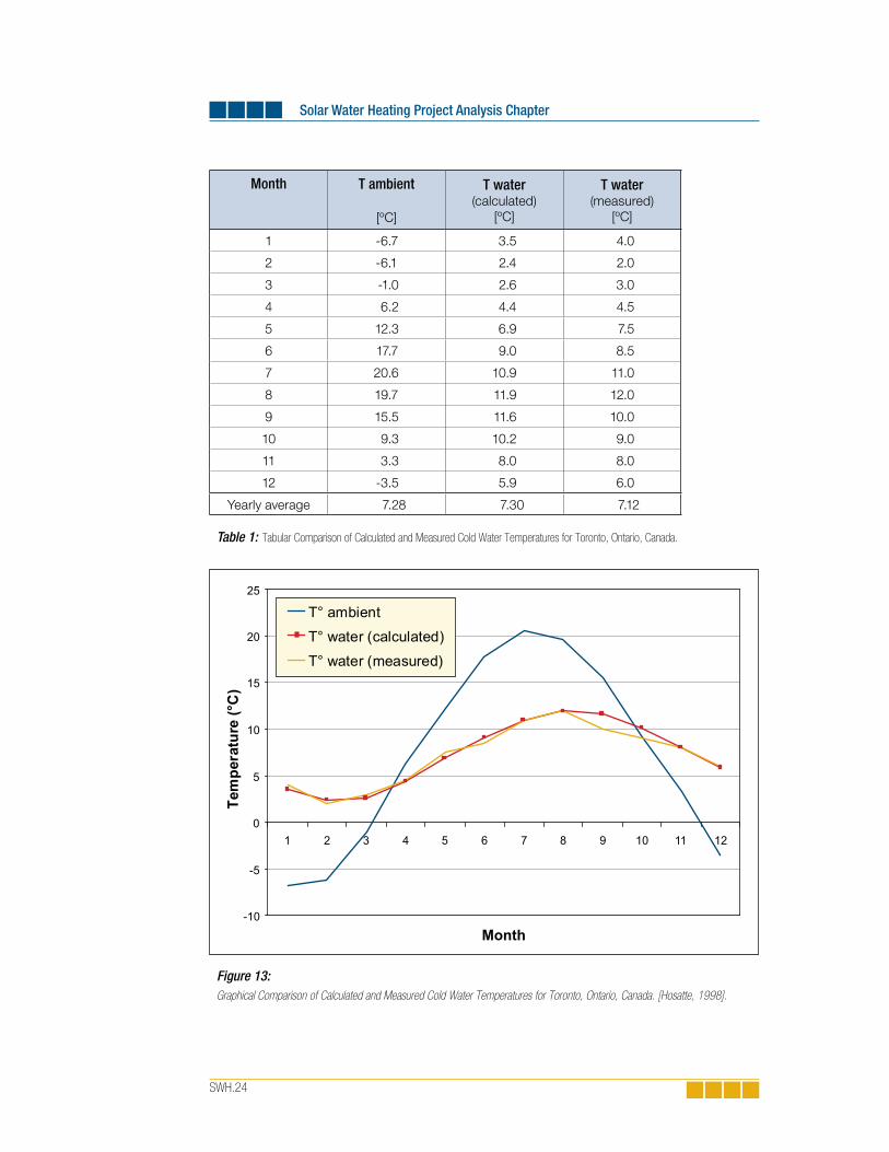
SolarWaterHeatingProjectAnalysisChapter
SWH.24
Month Tambient
[ºC]
Twater(calculated)
[ºC]
Twater(measured)
[ºC]
1 -6.7 3.5 4.0
2 -6.1 2.4 2.0
3 -1.0 2.6 3.0
4 6.2 4.4 4.5
5 12.3 6.9 7.5
6 17.7 9.0 8.5
7 20.6 10.9 11.0
8 19.7 11.9 12.0
9 15.5 11.6 10.0
10 9.3 10.2 9.0
11 3.3 8.0 8.0
12 -3.5 5.9 6.0
Yearly average 7.28 7.30 7.12
Table 1: Tabular Comparison of Calculated and Measured Cold Water Temperatures for Toronto, Ontario, Canada.
Figure 13: Graphical Comparison of Calculated and Measured Cold Water Temperatures for Toronto, Ontario, Canada. [Hosatte, 1998].
-10
-5
0
5
10
15
20
25
1 2 3 4 5 6 7 8 9 10 11 12
Month
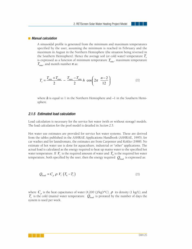
2. RETScreen Solar Water Heating Project Model
SWH.25
Manual calculation
A sinusoidal profile is generated from the minimum and maximum temperatures specified by the user, assuming the minimum is reached in February and the maximum in August in the Northern Hemisphere (the situation being reversed in the Southern Hemisphere). Hence the average soil (or cold water) temperature Ts is expressed as a function of minimum temperature Tmin , maximum temperature Tmax , and month number n as:
where h is equal to 1 in the Northern Hemisphere and –1 in the Southern Hemi-sphere.
2.1.5 Estimated load calculation
Load calculation is necessary for the service hot water (with or without storage) models. The load calculation for the pool model is detailed in Section 2.5.
Hot water use estimates are provided for service hot water systems. These are derived from the tables published in the ASHRAE Applications Handbook (ASHRAE, 1995); for car washes and for laundromats, the estimates are from Carpenter and Kokko (1988). No estimate of hot water use is done for aquaculture, industrial or “other” applications. The actual load is calculated as the energy required to heat up mains water to the specified hot water temperature. If Vl is the required amount of water and Th is the required hot water temperature, both specified by the user, then the energy required Qload is expressed as:
where Cp is the heat capacitance of water (4,200 (J/kg)/ºC), ρ its density (1 kg/L), and
Tc is the cold (mains) water temperature. Qload is prorated by the number of days the system is used per week.
(22)
(23)

SolarWaterHeatingProjectAnalysisChapter
SWH.26
2 .2 SolarCollectors
Solar collectors are described by their efficiency equations. Three types of collectors are considered in the RETScreen SWH Project Model:
Glazed collectors
Evacuated collectors
Unglazed collectors
Glazed and evacuated collectors share the same basic, wind-independent efficiency equa-tion. Unglazed collectors use a wind-dependent efficiency equation. Effects of angle of incidence, losses due to snow and dirt, and loss of heat through the piping and the solar tank are accounted for through separate factors.
2.2.1 Glazed or evacuated collectors
Glazed or evacuated collectors are described by the following equation (Duffie and Beckman, 1991, eq. 6.17.2):
where Qcoll is the energy collected per unit collector area per unit time, FR is the
collector’s heat removal factor, τ is the transmittance of the cover, α is the shortwave absorptivity of the absorber, G is the global incident solar radiation on the collector, UL is the overall heat loss cœfficient of the collector, and ∆T is the temperature differential between the working fluid entering the collectors and outside.
Values of FR τα( ) and F UR L are specified by the user or chosen by selecting a solar col-lector from the RETScreen Online Product Database. For both glazed and evacuated col-lectors, FR τα( ) and F UR L are independent of wind.
“Generic” values are also provided for glazed and evacuated collectors. Generic glazed collectors are provided with FR τα( ) = 0.68 and F UR L = 4.90 (W/m2)/ºC. These val-ues correspond to test results for ThermoDynamics collectors (Chandrashekar and Thevenard, 1995). Generic evacuated collectors are also provided with FR τα( ) = 0.58 and F UR L = 0.7 (W/m2)/ºC. These values correspond to a Fournelle evacuated tube col-lector (Philips technology; Hosatte, 1998).
(24)

2. RETScreen Solar Water Heating Project Model
SWH.27
2.2.2 Unglazed collectors
Unglazed collectors are described by the following equation (Soltau, 1992):
where ε is the longwave emissivity of the absorber, and L is the relative longwave sky irradiance. L is defined as:
where Lsky is the longwave sky irradiance (see Section 2.1.3) and Ta the ambient temperature
expressed in °C.
FRα and F UR L are a function of the wind speed V incident upon the collector. The values of FRα and F UR L , as well as their wind dependency, are specified by the user or chosen by selecting a collector from the RETScreen Online Product Database. The wind speed incident upon the collector is set to 20% of the free stream air velocity specified by the user (or copied from the weather database). The ratio ε α/ is set to 0.96.
Because of the scarcity of performance measurements for unglazed collectors, a “generic” unglazed collector is also defined as:
These values were obtained by averaging the performance of several collectors (NRCan, 1998).
(25)
(26)
(27)
(28)

SolarWaterHeatingProjectAnalysisChapter
SWH.28
Equivalence between glazed and unglazed collectors
As can be seen from equations (24) and (25), equations for glazed and unglazed collector efficiency are different. A problem arises when using the f-Chart method (see Section 2.3) or the utilisability method (see Section 2.4), both of which were developed for glazed collectors. The approach taken in RETScreen was to re-write equation (25) into the form of (24), by defining an effective radiation on the collec-tor Geff
as:
where G is the global solar radiation incident in the plane of the collector , α is the shortwave absorptivity of the absorber, ε is the longwave emissivity of the absorber ( ε α/ is set to 0.96, as before), and L is the relative longwave sky irradiance. In the RETScreen algorithms, effective irradiance is substituted to irradiance in all equations involving the collector when an unglazed collector is used. The reader has to keep this in mind when encountering the developments of algorithms in Sections 2.3 and 2.4.
2.2.3 Incidence angle modifiers
Part of the solar radiation incident upon the collector may bounce off, particularly when the rays of the sun hit the surface of the collector with a high angle of incidence. At the pre-feasi-bility stage it is not necessary to model this phenomenon in detail. Instead, the average effect of angle of incidence upon the collector was estimated through simulations to be roughly 5%. Therefore, FR τα( ) is multiplied by a constant factor equal to 0.95.
2.2.4 Piping and solar tank losses
The water circulating in the pipes and the tank is hot, and since the pipes and the tank are imperfectly insulated, heat will be lost to the environment. Piping and solar tank losses are taken into account differently for systems with storage and for systems without storage (including pool). In systems without storage the energy delivered by the solar collector, Qdld , is equal to the energy collected Qact minus piping losses, expressed as a fraction flosof energy collected ( flos is entered by the user):
(29)
(30)

2. RETScreen Solar Water Heating Project Model
SWH.29
For systems with storage, the situation is slightly different since the system may be able, in some cases, to compensate for the piping and tank losses by collecting and storing extra energy. Therefore, the load Qload tot, used in the f-Chart method (see Section 2.3) is increased to include piping and tank losses:
2.2.5 Losses due to snow and dirt
Snow and dirt impact on the irradiance level experienced by the collector. Therefore, FR τα( ) is multiplied by 1−( )fdirt where fdirt
are the losses due to snow and dirt ex-pressed as a fraction of energy collected (this parameter is entered by the user).
2 .3 ServiceHotWater:f-ChartMethod
The performance of service hot water systems with storage is estimated with the f-Chart method. The purpose of the method is to calculate f , the fraction of the hot water load that is provided by the solar heating system (solar fraction). Once f is calculated, the amount of renewable energy that displaces conventional energy for water heating can be determined. The method is explained in detail in Chapter 20 of Duffie and Beckman (1991) and is briefly summarized here. The method enables the calculation of the monthly amount of energy delivered by hot water systems with storage, given monthly values of incident solar radiation, ambient temperature and load.
Two dimensionless groups X and Y are defined as:
where Ac is the collector area, ′FR is the modified collector heat removal factor, UL is the collector overall loss cœfficient,
Tref is an empirical reference temperature equal to 100°C,
Ta is the monthly average ambient temperature, L is the monthly total heating load, is the collector’s monthly average transmittance-absorptance product, HT is the monthly
(31)
(32)
(33)

SolarWaterHeatingProjectAnalysisChapter
SWH.30
average daily radiation incident on the collector surface per unit area, and N is the number of days in the month.
′FR accounts for the effectiveness of the collector-storage heat exchanger (see Figure 14 for a diagram of the system). The ratio ′F FR R/ is a function of heat exchanger effectiveness ε (see Duffie and Beckman, 1991, section 10.2):
where m is the flow rate and Cp is the specific heat. Subscripts c and min stand for collector-side and minimum of collector-side and tank-side of the heat exchanger.
If there is no heat exchanger, ′FR is equal to FR . If there is a heat exchanger, the model assumes that the flow rates on both sides of the heat exchanger are the same. The spe-cific heat of water is 4.2 (kJ/kg)/ºC, and that of glycol is set to 3.85 (kJ/kg)/ºC. Finally the model assumes that the ratio A mc / is equal to 140 m2 s/kg; this value is computed from ThermoDynamics collector test data (area 2.97 m2, test flow rate 0.0214 kg/s; Chan-drashekar and Thevenard, 1995).
X has to be corrected for both storage size and cold water temperature. The f-Chart method was developed with a standard storage capacity of 75 litres of stored water per square meter of collector area. For other storage capacities X has to be multiplied by a cor-rection factor X Xc / defined by:
(34)
Figure 14: Diagram of a Solar Domestic Hot Water System.
Preheatstorage
tank
Aux.storage
tank
Auxiliaryheater
Mixingvalve
Watermains
Mixingvalve
Load
Tempering loop
Storage-load
exchanger
Collector-storage
exchanger
Collectorpump
Collector
2. RETScreen Solar Water Heating Project Model
SWH.31
This equation is valid for ratios of actual to standard storage capacities between 0.5 and 4. Finally, to account for the fluctuation of supply (mains) water temperature Tm and for the minimum acceptable hot water temperature Tw , both of which have an influence on the performance of the solar water heating system, X has to be multiplied by a correction factor X Xcc / defined by:
where Ta is the monthly mean ambient temperature.
The fraction f of the monthly total load supplied by the solar water heating system is given as a function of X and Y as:
There are some strict limitations on the range for which this formula is valid. However as shown in Figure 15, the surface described by equation (37) is fairly smooth, so extrapola-tion should not be a problem. If the formula predicts a value of f less than 0, a value of 0 is used; if f is greater than 1, a value of 1 is used.
(35)
(36)
(37)
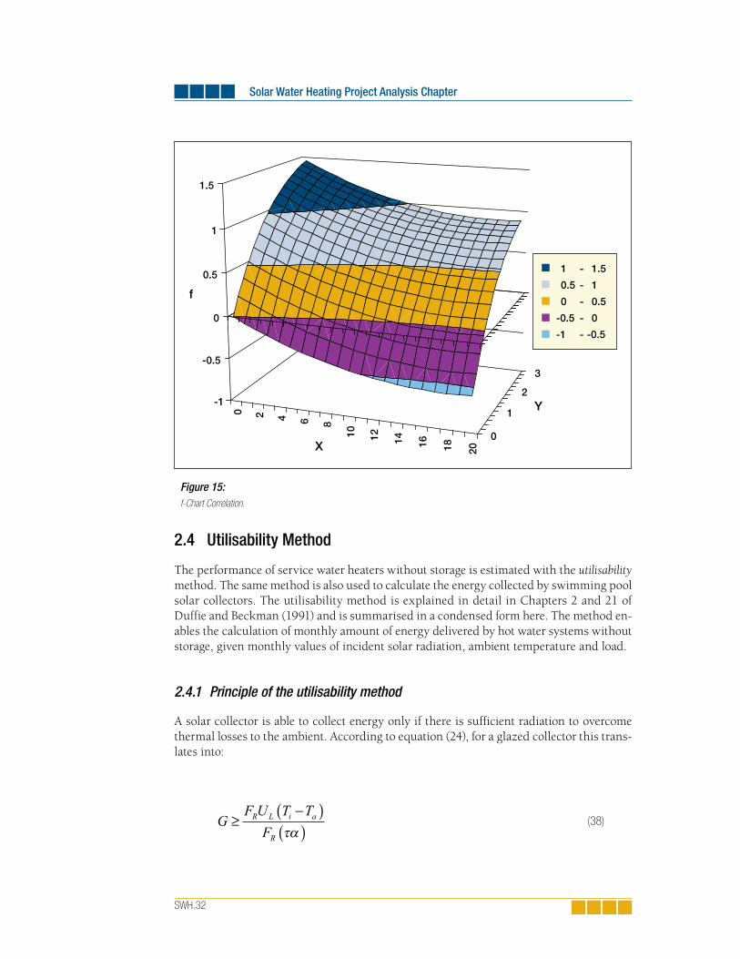
SolarWaterHeatingProjectAnalysisChapter
SWH.32
2 .4 UtilisabilityMethod
The performance of service water heaters without storage is estimated with the utilisability method. The same method is also used to calculate the energy collected by swimming pool solar collectors. The utilisability method is explained in detail in Chapters 2 and 21 of Duffie and Beckman (1991) and is summarised in a condensed form here. The method en-ables the calculation of monthly amount of energy delivered by hot water systems without storage, given monthly values of incident solar radiation, ambient temperature and load.
2.4.1 Principle of the utilisability method
A solar collector is able to collect energy only if there is sufficient radiation to overcome thermal losses to the ambient. According to equation (24), for a glazed collector this trans-lates into:
Figure 15: f-Chart Correlation.
0 2 4 6 8
10 12 14 16 18 20
0
1
2
3
-1
-0.5
0
0.5
1
1.5
f
X
Y
1
0.5
0
-0.5
-1
1.5
1
0.5
0
-0.5
-
-
-
-
-
(38)

2. RETScreen Solar Water Heating Project Model
SWH.33
where Ti is the temperature of the working fluid entering the collector and all other vari-ables have the same meaning as in equation (24). This makes it possible to define a critical irradiance level
Gc which must be exceeded in order for solar energy collection to occur.
Since the model is dealing with monthly averaged values, Gc is defined using monthly
average transmittance-absorptance and monthly average daytime temperature Ta (assumed to be equal to the average temperature plus 5°C) through:
Combining this definition with equation (24) leads to the following expression for the average daily energy Q collected during a given month:
where N is the number of days in the month, G is the hourly irradiance in the plane of the collector, and the + superscript denotes that only positive values of the quantity between brackets are considered.
The monthly average daily utilisability φ , is defined as the sum for a month, over all hours and days, of the radiation incident upon the collector that is above the critical level, divided by the monthly radiation:
where HT is the monthly average daily irradiance in the plane of the collector. Substituting this definition into equation (40) leads to a simple formula for the monthly useful energy gain:
(39)
(40)
(41)
(42)
SolarWaterHeatingProjectAnalysisChapter
SWH.34
The purpose of the utilisability method is to calculate φ from the collector orientation and the monthly radiation data entered by the user (or copied from the RETScreen Online Weather Database). The method correlates φ to the monthly average clearness index
KT
and two variables: a geometric factor R Rn and a dimensionless critical radiation level
X c , as described hereafter.
2.4.2 Geometric factor R Rn
R is the monthly ratio of radiation in the plane of the collector, HT , to that on a horizontal surface, H :
where HT is calculated as explained in Section 2.1.2. Rn is the ratio for the hour centered at noon of radiation on the tilted surface to that on a horizontal surface for an average day of the month. This is expressed through the following equation:
where rt n, is the ratio of hourly total to daily total radiation, for the hour centered around solar noon. rd n, is the ratio of hourly diffuse to daily diffuse radiation, also for the hour centered around solar noon. This formula is computed for an “average day of month,” i.e. a day with daily global radiation H equal to the monthly average daily global radiation H ; Hd is the monthly average daily diffuse radiation for that “average day” (calculated through equation 14), β is the slope of the collector, and ρg is the average ground albedo (see Section 2.1.2).
rt n, is computed by the Collares-Pereira and Rabl equation (Duffie and Beckman, 1991, ch. 2.13), written for solar noon:
(43)
(44)
(45)

2. RETScreen Solar Water Heating Project Model
SWH.35
with ωs the sunset hour angle (see equation 2), expressed in radians. rd n, is computed by the Liu and Jordan equation, written for solar noon:
2.4.3 Dimensionless critical radiation level X c
X c is defined as the ratio of the critical radiation level to the noon radiation level on the typical day of the month:
where rt n, is given by (45) and Rn by (44).
2.4.4 Monthly average daily utilisability φ
Finally, the correlation giving the monthly average daily utilisability φ , as a function of the two factors
R Rn and X c calculated previously, is:
(46)
(47)
(48)
(49)
(50)

SolarWaterHeatingProjectAnalysisChapter
SWH.36
with:
With this, the amount of energy collected can be computed, as shown earlier in equation (42).
2 .5 SwimmingPoolModel
The energy requirements of the pool are established by assuming that the pool is main-tained at the desired pool temperature. Therefore, the model does not include calculations of heat storage by the pool, nor does it consider possible excursions in temperature above the desired pool temperature (both of which would require iterative calculations beyond the scope of a spreadsheet-based tool).
The energy requirements of the pool are calculated by comparing the pool’s energy losses and gains (see Figure 16). Losses are due to evaporation, convection, conduction, radia-tion, and the addition of makeup water. Gains include passive solar gains, active solar gains and gains from auxiliary heating. In the sections that follow, those gains and losses are expressed as rates or powers, i.e. per unit time. The conversion from a power
Q to the corresponding monthly energy Q is done with a simple formula:
where Ndays is the number of days in the month and 86,400 is the number of seconds
in a day.
(51a)
(51b)
(51c)
(52)

2. RETScreen Solar Water Heating Project Model
SWH.37
2.5.1 Pool climatic conditions
Climatic conditions experienced by the pool depend on whether the pool is inside or out-side. In the case of an indoor pool, the following conditions are assumed:
Dry bulb temperature: the maximum of 27°C (ASHRAE, 1995, p. 4.6) and the ambient temperature;
Relative humidity: 60% (ASHRAE, 1995, p. 4.6);
Wind speed: 0.1 m/s. This is consistent with assuming that there are 6 to 8 air changes per hour, i.e. air flows across a characteristic dimension of the pool in 450 s; thus if the pool is 25 m long, assuming a 5 m wide walking area around the pool, one obtains a flow rate of 35/450 = 0.08 m/s; and
Sky temperature: computed from pool ambient temperature.
In the case of an outdoor pool, the local climatic conditions are those entered by the user (or copied from the RETScreen Online Weather Database), with the exception of wind speed and relative humidity which receive special attention, as explained below.
Figure 16: Energy Gains and Losses in a Swimming Pool.
Active solar gains
Passive solar gains
Radiativelosses
Auxiliarygains
Conductivelosses
Evaporativelosses
Convectivelosses
SWIMMING POOL
SOLARCOLLECTOR
WATERMAKEUP
Makeuplosses
AUXILIARYHEATER

SolarWaterHeatingProjectAnalysisChapter
SWH.38
Wind speed
Simulations show that if a pool cover (also called blanket) is used for part of the day and the monthly average wind speed is used for the simulation, evaporative losses are underestimated. This can be related to the fact that wind speed is usually much higher during the day (when the pool cover is off) than at night. Observations made for Toronto, ON; Montreal, QC; Phoenix, AZ; and Miami, FL roughly show that the maximum wind speed in the afternoon is twice the minimum wind speed at night. Consequently wind speed fluctuation during the day is modelled in RETScreen SWH Project Model by a sinusoidal function:
where Vh is the wind velocity at hour h, V is the average of the wind speed fluctua-
tion, and h0 represents a time shift. The model assumes that the maximum wind speed occurs when the cover is off; averaging over the whole period with no cover leads to the following average value:
where Nblanket is the number of hours per day the cover is on. Similarly, the average wind speed when the pool cover is on is:
Finally, wind speed is multiplied by the user-entered sheltering factor to account for reduction of wind speed due to natural obstacles around the pool.
(53)
(54)
(55)

2. RETScreen Solar Water Heating Project Model
SWH.39
Relative humidity
Evaporation from the pool surface depends on the moisture contents of the air. In RETScreen, the calculation of evaporation cœfficients is done using the humidity ratio of the air, rather than its relative humidity; this is because the humidity ratio (expressed in kg of water per kg of dry air) is usually much more constant during the day than the relative humidity, which varies not only with moisture contents but also with ambient temperature. The humidity ratio calculation is done according to formulae from ASHRAE Fundamentals (ASHRAE, 1997).
2.5.2 Passive solar gains
Passive solar gains differ depending on whether or not a cover (also called blanket) is installed on the pool.
Passive solar gains without cover
In the absence of cover, passive solar gains can be expressed as:
where Ap is the pool area, rb is the average reflectivity of water to beam radiation and rd is the average reflectivity of water to diffuse radiation. As before, Hb and Hd are the monthly average beam and diffuse radiation (see equations 6 to 8). The user-specified shading cœfficient s applies only to the beam portion of radiation.
A short mathematical development will explain how rb and rd are calculated. A ray of light entering water with an angle of incidence θ z will have an angle of refrac-tion θw in the water defined by Snell’s law (Duffie and Beckman, 1991, eq. 5.1.4; see Figure 17):
(56)
(57)

SolarWaterHeatingProjectAnalysisChapter
SWH.40
where nair and
nwater are the indices of refraction of air and water:
rb can be computed with the help of Fresnel’s laws for parallel and perpendicular components of reflected radiation (Duffie and Beckman, 1991, eqs. 5.1.1 to 5.1.3):
(58)
(59)
(60)
(61)
(62)
AIR
WATER
z
w
Figure 17: Snell’s Law.

2. RETScreen Solar Water Heating Project Model
SWH.41
Once all calculations are made, it is apparent that rb is a function of θ z only. Figure 18 shows that rb can be safely approximated by:
To account for the fact that the sun is lower on the horizon in the winter, a sepa-rate value of rb is computed for each month. The equation above is used with θ z calculated 2.5 h from solar noon (the value 2.5 h comes from Duffie and Beckman, 1991, p. 244).
Reflectivity to diffuse radiation is independent of sun position and is basically equal to the reflectivity calculated with an angle of incidence of 60º (Duffie and Beckman, 1991, p. 227). Using the exact equation, a value of rd = 0.060 is found.
(63)
Figure 18: Reflectivity of Water as a Function of the Cosine of the Zenith Angle.
0.0
0.2
0.4
0.6
0.8
1.0
1.2
0.0 0.1 0.2 0.3 0.4 0.5 0.6 0.7 0.8 0.9 1.0
cos(zenith angle)
wat
er r
efle
ctiv
ity
Exact formula
Approximation

SolarWaterHeatingProjectAnalysisChapter
SWH.42
Passive solar gains with cover
In the case of a pool with a blanket, passive solar gains are expressed as:
where αc is the absorptivity of the blanket, set to 0.4, and H is, as before, the monthly average global radiation on the horizontal.
Total of passive solar gains
Passive solar gains are a combination of gains with the blanket on and off. The mod-el assumes that the blanket is on predominantly at night. If the blanket is on Nblanket hours per day, and for the average day of the month the day length is Ndaytime , then the number of hours
Nno blanket
the blanket is off during daytime is:
and the passive solar gain is simply assumed to be equal to the sum of passive solar gains with and without cover, prorated by the number of hours the blanket is off during daytime:
Expressed per unit time, the passive solar gain rate is calculated according to equa-tion (52):
(64)
(65)
(66)
(67)

2. RETScreen Solar Water Heating Project Model
SWH.43
2.5.3 Evaporative losses
There are several methods in the literature to compute evaporative losses, including that of ASHRAE (ASHRAE, 1995) revised by Smith et al. (1994) and those cited in Hahne and Kübler (1994). The RETScreen SWH Project Model adopts the equation of ISO TC 180 (Hahne and Kübler, 1994):
where Qeva is the power (in W) dissipated as a result of evaporation of water from the
pool, he is a mass transfer cœfficient, and Pv sat, and Pv amb, are the partial pressure of
water vapour at saturation and for ambient conditions. The mass transfer cœfficient he
(in (W/m2)/Pa) is expressed as:
where V is the wind velocity at the pool surface, expressed in m/s. The partial pressure of water vapour at saturation, Pv sat, , is calculated with formulae from ASHRAE (1997). The partial pressure of water vapour for ambient conditions, Pv amb, , is calculated from the humidity ratio, also with formulae from ASHRAE (1997).
The rate of evaporation of water from the pool, meva , in kg/s, is related to Qeva by:
where λ is the latent heat of vaporisation of water (2,454 kJ/kg).
When the pool cover is on, it is assumed to cover 90% of the surface of the pool and there-fore evaporation is reduced by 90%. When the pool cover is off, losses are multiplied by two to account for activity in the pool (Hahne and Kübler, 1994).
(68)
(69)
(70)

SolarWaterHeatingProjectAnalysisChapter
SWH.44
2.5.4 Convective losses
Convective losses are estimated using the equation cited in Hahne and Kübler (1994):
where Qcon is the rate of heat loss due to convective phenomena (in W), Tp is the pool
temperature, Ta is the ambient temperature, and the convective heat transfer cœfficient hcon is expressed as:
with the wind speed V expressed in m/s.
2.5.5 Radiative losses
Radiative losses to the ambient environment in the absence of pool blanket, (in W) are expressed as:
where εw is the emittance of water in the infrared (0.96), σ is the Stefan-Boltzmann constant (5.669x10⁻⁸ (W/m2)/K4), Tp is the pool temperature and Tsky is the sky tempera-ture (see Section 2.1.3). In the presence of a blanket, assuming 90% of the pool is covered, radiative losses become:
(71)
(72)
(73)
(74)

2. RETScreen Solar Water Heating Project Model
SWH.45
where εc is the emissivity of the pool blanket. Depending on the cover material the emis-sivity can range from 0.3 to 0.9 (NRCan, 1998). A mean value of 0.4 is used. Combining the two previous equations with the amount of time the cover is on and the values of εw and εc mentioned above one obtains:
2.5.6 Water makeup losses
Fresh water is added to the pool to compensate for: evaporative losses, water lost because of swimmers’ activity, and voluntary water changes. If fmakeup is the makeup water ratio entered by the user (which does not include compensation for evaporative losses), ex-pressed as a fraction of the pool volume renewed each week, the rate of water makeup (in kg/s) can be expressed as:
where ρ is the water density (1,000 kg/m3) and Vp is the pool volume. The pool volume
is computed from the pool area assuming an average depth of 1.5 m:
The rate of energy requirement corresponding to water makeup, Qmakeup , is:
where Tc is the cold (mains) temperature (see Section 2.1.4) and Cp is the heat capacitance
of water (4,200 (J/kg)/ºC).
(75)
(76)
(77)
(78)
SolarWaterHeatingProjectAnalysisChapter
SWH.46
2.5.7 Conductive losses
Conductive losses are usually only a small fraction of other losses. The RETScreen SWH Project Model assumes that conductive losses
Qcond represent 5% of other losses:
2.5.8 Active solar gains
Maximum possible active solar gains Qact are determined by the utilisability method (see
Section 2.4), assuming the pool temperature is equal to its desired value.
2.5.9 Energy balance
The energy rate Qreq required to maintain the pool at the desired temperature is expressed as the sum of all losses minus the passive solar gains:
This energy has to come either from the backup heater, or from the solar collectors. The rate of energy actually delivered by the renewable energy system,
Qdvd , is the minimum of the energy required and the energy delivered by the collectors:
If the solar energy collected is greater than the energy required by the pool, then the pool tem-perature will be greater than the desired pool temperature. This could translate into a lower en-ergy requirement for the next month, however this is not taken into account by the model. The auxiliary power
Qaux required to maintain the pool at the desired temperature is simply the difference between power requirements and power delivered by the renewable energy system:
(79)
(80)
(81)
(82)

2. RETScreen Solar Water Heating Project Model
SWH.47
2 .6 OtherCalculations
2.6.1 Suggested solar collector area
The suggested solar collector area depends upon the load, the type of system, and the collector.
For service hot water with storage, the sizing load for each month is the monthly load including tank and piping losses.
For service hot water without storage, the sizing load for each month is set to 14% of the monthly load, times 1+( )flos to account for piping losses. The value of 14% is chosen so that the energy delivered does not exceed the recommended 15% of the load.
For swimming pools, the sizing load is equal to the energy required, times 1+( )flos to account for piping losses.
The suggested solar collector area is based on the utilisability method. Optimally, for each month the usable energy should be equal to the sizing load. Using equation (42):
which is then solved for the collector area, Ac . This provides 12 monthly values of sug-gested solar collector area. Then:
For service hot water, the model takes the smallest of the monthly values. For a system without storage this ensures that even for the sunniest month the renewable energy delivered does not exceed 15% of the load. For a system with storage, 100% of the load would be provided for the sunniest month, if the system could use all the energy available. However because systems with storage are less efficient (since they work at a higher tem-perature), the method will usually lead to smaller solar fractions, typically around 70% for the sunniest month.
For swimming pools, the method above does not work since the load may be zero during the sunniest months. Therefore the model takes the average of the calculated monthly suggested solar collector areas over the season of use.
The number of solar collectors is calculated as the suggested collector area divided by the area of an individual collector, rounded up to the nearest integer.
(83)
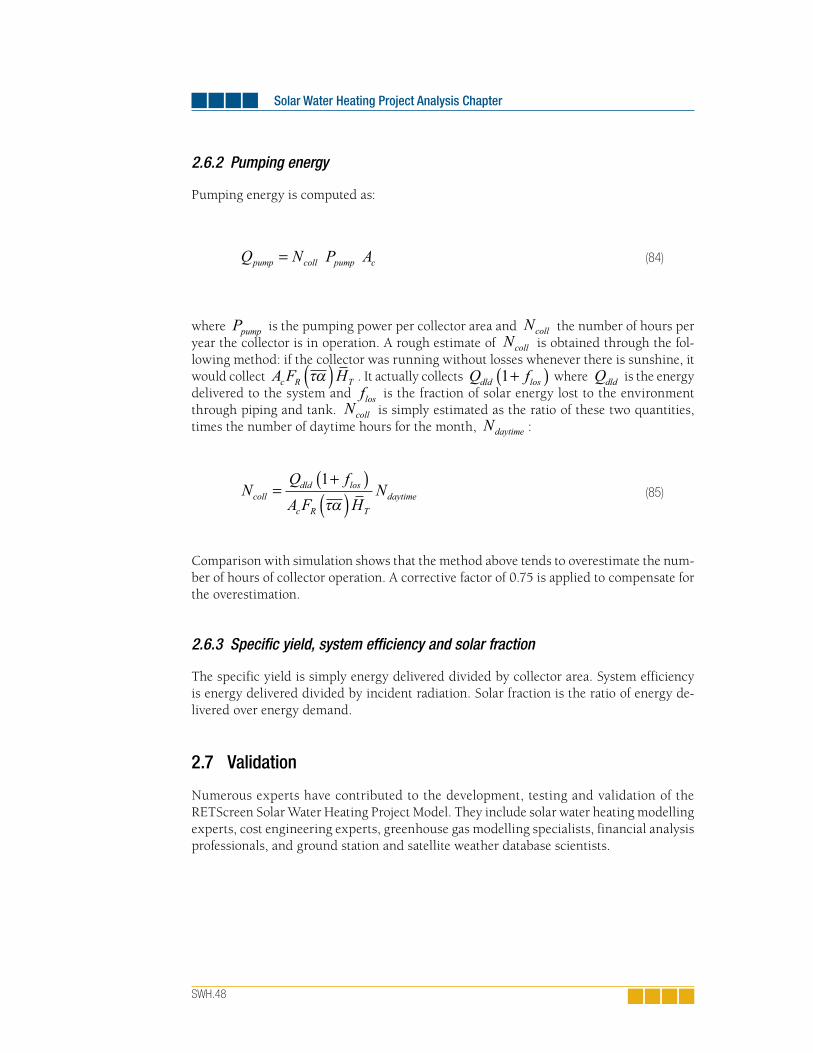
SolarWaterHeatingProjectAnalysisChapter
SWH.48
2.6.2 Pumping energy
Pumping energy is computed as:
where Ppump is the pumping power per collector area and Ncoll the number of hours per
year the collector is in operation. A rough estimate of Ncoll is obtained through the fol-lowing method: if the collector was running without losses whenever there is sunshine, it would collect . It actually collects Q fdld los1+( ) where
Qdld is the energy delivered to the system and
flos is the fraction of solar energy lost to the environment
through piping and tank. Ncoll is simply estimated as the ratio of these two quantities, times the number of daytime hours for the month,
Ndaytime :
Comparison with simulation shows that the method above tends to overestimate the num-ber of hours of collector operation. A corrective factor of 0.75 is applied to compensate for the overestimation.
2.6.3 Specific yield, system efficiency and solar fraction
The specific yield is simply energy delivered divided by collector area. System efficiency is energy delivered divided by incident radiation. Solar fraction is the ratio of energy de-livered over energy demand.
2 .7 Validation
Numerous experts have contributed to the development, testing and validation of the RETScreen Solar Water Heating Project Model. They include solar water heating modelling experts, cost engineering experts, greenhouse gas modelling specialists, financial analysis professionals, and ground station and satellite weather database scientists.
(84)
(85)
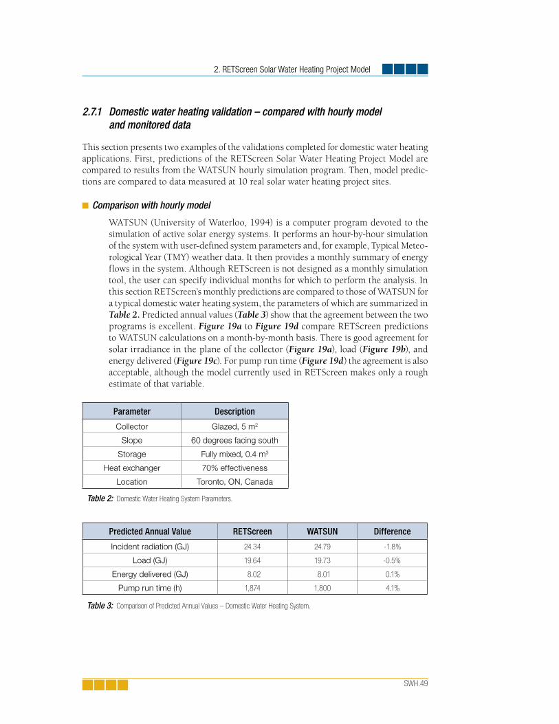
2. RETScreen Solar Water Heating Project Model
SWH.49
2.7.1 Domestic water heating validation – compared with hourly model and monitored data
This section presents two examples of the validations completed for domestic water heating applications. First, predictions of the RETScreen Solar Water Heating Project Model are compared to results from the WATSUN hourly simulation program. Then, model predic-tions are compared to data measured at 10 real solar water heating project sites.
Comparison with hourly model
WATSUN (University of Waterloo, 1994) is a computer program devoted to the simulation of active solar energy systems. It performs an hour-by-hour simulation of the system with user-defined system parameters and, for example, Typical Meteo-rological Year (TMY) weather data. It then provides a monthly summary of energy flows in the system. Although RETScreen is not designed as a monthly simulation tool, the user can specify individual months for which to perform the analysis. In this section RETScreen’s monthly predictions are compared to those of WATSUN for a typical domestic water heating system, the parameters of which are summarized in Table 2. Predicted annual values (Table 3) show that the agreement between the two programs is excellent. Figure 19a to Figure 19d compare RETScreen predictions to WATSUN calculations on a month-by-month basis. There is good agreement for solar irradiance in the plane of the collector (Figure 19a), load (Figure 19b), and energy delivered (Figure 19c). For pump run time (Figure 19d) the agreement is also acceptable, although the model currently used in RETScreen makes only a rough estimate of that variable.
Parameter Description
Collector Glazed, 5 m2
Slope 60 degrees facing south
Storage Fully mixed, 0.4 m3
Heat exchanger 70% effectiveness
Location Toronto, ON, Canada
Table 2: Domestic Water Heating System Parameters.
PredictedAnnualValue RETScreen WATSUN Difference
Incident radiation (GJ) 24.34 24.79 -1.8%
Load (GJ) 19.64 19.73 -0.5%
Energy delivered (GJ) 8.02 8.01 0.1%
Pump run time (h) 1,874 1,800 4.1%
Table 3: Comparison of Predicted Annual Values – Domestic Water Heating System.
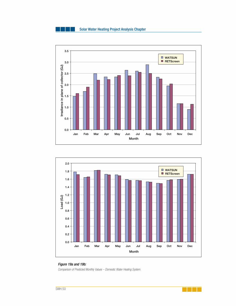
SolarWaterHeatingProjectAnalysisChapter
SWH.50
Figure 19a and 19b: Comparison of Predicted Monthly Values – Domestic Water Heating System.
0.0
0.2
0.4
0.6
0.8
1.0
1.2
1.4
1.6
1.8
2.0
Month
Load
(GJ)
Jan Feb Mar Apr May Jun Jul Aug Sep Oct Nov Dec
WATSUNRETScreen
0.0
0.5
1.0
1.5
2.0
2.5
3.0
3.5
Jan Feb Mar Apr May Jun Jul Aug Sep Oct Nov Dec
Month
Irra
dia
nce
in p
lane
of
colle
cto
r (G
J)WATSUNRETScreen

2. RETScreen Solar Water Heating Project Model
SWH.51
0
50
100
150
200
250
Month
Pum
p r
un t
ime
(h)
WATSUNRETScreen
Jan Feb Mar Apr May Jun Jul Aug Sep Oct Nov Dec
0.0
0.2
0.4
0.6
0.8
1.0
1.2
Month
Ene
rgy
del
iver
ed (G
J)
WATSUNRETScreen
Jan Feb Mar Apr May Jun Jul Aug Sep Oct Nov Dec
Figure 19c and 19d: Comparison of Predicted Monthly Values – Domestic Water Heating System.

SolarWaterHeatingProjectAnalysisChapter
SWH.52
Comparison with monitored data
To further validate the RETScreen Solar Water Heating Project Model for domestic water heating applications, the model predictions were compared to monitored data gathered for 10 systems under the S2000 project in Guelph, Ontario, Canada (Enermodal, 1999). These systems feature a 5.9 m2 solar collector, a 270 L tank, a heat exchanger (assumed to be 60% efficient in RETScreen), and loads varying on average from 90 L/day to 380 L/day. Results are shown in Figure 20. It is apparent from the figure that RETScreen is somewhat optimistic in its energy predictions, particularly for systems with low loads (these systems end up mostly in the left part of the figure). The agreement is better for systems with a high load (right part of the figure). For the 10 systems under consideration, the overestimation averages 29% which is well within the range required for pre-feasibility and feasibility analysis studies; the overestimation falls to 15% if only the three systems with highest loads are considered.
2.7.2 Swimming pool heating validation – compared with hourly model and monitored data
This section presents two examples of the validations completed for swimming pool heat-ing applications. First, predictions of the RETScreen Solar Water Heating Project Model are compared to results from the ENERPOOL hourly simulation program. Then, model predictions are compared to data measured at a real solar pool heating project site.
Figure 20: Comparison of RETScreen Predictions to Monitored Data for Guelph, Ontario, Canada.
500
1,000
1,500
2,000
2,500
3,000
500 1,000 1,500 2,000 2,500 3,000
Measured annual solar energy delivered (kWh)
RE
TS
cree
n p
red
icte
d a
nnua
l so
lar
ener
gy
del
iver
ed (k
Wh)
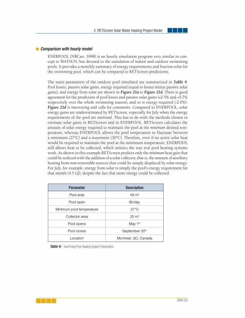
2. RETScreen Solar Water Heating Project Model
SWH.53
Comparison with hourly model
ENERPOOL (NRCan, 1998) is an hourly simulation program very similar in con-cept to WATSUN, but devoted to the simulation of indoor and outdoor swimming pools. It provides a monthly summary of energy requirements and fraction solar for the swimming pool, which can be compared to RETScreen predictions.
The main parameters of the outdoor pool simulated are summarized in Table 4. Pool losses, passive solar gains, energy required (equal to losses minus passive solar gains), and energy from solar are shown in Figure 21a to Figure 21d. There is good agreement for the prediction of pool losses and passive solar gains (+2.5% and +5.7% respectively over the whole swimming season), and so is energy required (-2.0%). Figure 21d is interesting and calls for comments. Compared to ENERPOOL, solar energy gains are underestimated by RETScreen, especially for July when the energy requirements of the pool are minimal. This has to do with the methods chosen to estimate solar gains in RETScreen and in ENERPOOL. RETScreen calculates the amount of solar energy required to maintain the pool at the minimum desired tem-perature, whereas ENERPOOL allows the pool temperature to fluctuate between a minimum (27°C) and a maximum (30°C). Therefore, even if no active solar heat would be required to maintain the pool at the minimum temperature, ENERPOOL still allows heat to be collected, which mimics the way real pool heating systems work. As shown in this example RETScreen predicts only the minimum heat gain that could be realized with the addition of a solar collector, that is, the amount of auxiliary heating from non-renewable sources that could be simply displaced by solar energy. For July, for example, energy from solar is simply the pool’s energy requirement for that month (4.5 GJ), despite the fact that more energy could be collected.
Parameter Description
Pool area 48 m2
Pool open 8h/day
Minimum pool temperature 27°C
Collector area 25 m2
Pool opens May 1st
Pool closes September 30th
Location Montreal, QC, Canada
Table 4: Swimming Pool Heating System Parameters.

SolarWaterHeatingProjectAnalysisChapter
SWH.54
Figure 21a and 21b: Comparison of Predicted Monthly Values – Swimming Pool Heating System.
0
10
20
30
40
50
60
May Jun Jul Aug Sep
Month
To
tal l
oss
es (G
J)
ENERPOOLRETScreen
0
5
10
15
20
25
30
Month
Pas
sive
so
lar
gai
ns (G
J)
May Jun Jul Aug Sep
ENERPOOLRETScreen

2. RETScreen Solar Water Heating Project Model
SWH.55
Figure 21c and 21d: Comparison of Predicted Monthly Values – Swimming Pool Heating System.
0
5
10
15
20
25
30
35
Month
To
tal h
eatin
g e
nerg
y re
qui
red
(GJ)
ENERPOOLRETScreen
May Jun Jul Aug Sep
0
1
2
3
4
5
6
7
8
9
10
Month
Ene
rgy
fro
m s
ola
r (G
J)
ENERPOOLRETScreen
May Jun Jul Aug Sep
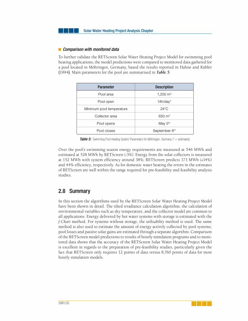
SolarWaterHeatingProjectAnalysisChapter
SWH.56
Comparison with monitored data
To further validate the RETScreen Solar Water Heating Project Model for swimming pool heating applications, the model predictions were compared to monitored data gathered for a pool located in Möhringen, Germany, based the results reported in Hahne and Kübler (1994). Main parameters for the pool are summarised in Table 5.
Parameter Description
Pool area 1,200 m2
Pool open 14h/day*
Minimum pool temperature 24°C
Collector area 650 m2
Pool opens May 5th
Pool closes September 6th
Table 5: Swimming Pool Heating System Parameters for Möhringen, Germany (* = estimated).
Over the pool’s swimming season energy requirements are measured at 546 MWh and estimated at 528 MWh by RETScreen (-3%). Energy from the solar collectors is measured at 152 MWh with system efficiency around 38%; RETScreen predicts 173 MWh (+14%) and 44% efficiency, respectively. As for domestic water heating the errors in the estimates of RETScreen are well within the range required for pre-feasibility and feasibility analysis studies.
2 .8 Summary
In this section the algorithms used by the RETScreen Solar Water Heating Project Model have been shown in detail. The tilted irradiance calculation algorithm, the calculation of environmental variables such as sky temperature, and the collector model are common to all applications. Energy delivered by hot water systems with storage is estimated with the f-Chart method. For systems without storage, the utilisability method is used. The same method is also used to estimate the amount of energy actively collected by pool systems; pool losses and passive solar gains are estimated through a separate algorithm. Comparison of the RETScreen model predictions to results of hourly simulation programs and to moni-tored data shows that the accuracy of the RETScreen Solar Water Heating Project Model is excellent in regards to the preparation of pre-feasibility studies, particularly given the fact that RETScreen only requires 12 points of data versus 8,760 points of data for most hourly simulation models.

SWH.57
REFERENCES
ASHRAE, Applications Handbook, American Society of Heating, Refrigerating and Air-Conditioning Engineers, Inc., 1791 Tullie Circle, N.E., Atlanta, GA, 30329, USA, 1991.
ASHRAE, Applications Handbook (SI) - Service Water Heating, American Society of Heating, Refrigerating, and Air- Conditioning Engineers, Inc., 1791 Tullie Circle, N.E., Atlanta, GA, 30329, USA, 1995.
ASHRAE, Handbook - Fundamentals, SI Edition, American Society of Heating, Refrigerating and Air-Conditioning Engineers, Inc., 1791 Tullie Circle, N.E., Atlanta, GA, 30329, USA, 1997.
Carpenter, S. and Kokko, J., Estimating Hot Water Use in Existing Commercial Buildings, ASHRAE Transactions, Summer Meeting 1988, Ottawa, ON, Canada, 1988.
Chandrashekar, M. and Thevenard, D., Comparison of WATSUN 13.1 Simulations with Solar Domestic Hot Water System Test Data from ORTECH/NSTF – Revised Report, Watsun Simulation Laboratory, University of Waterloo, Waterloo, ON, Canada, N2L 3G1, 1995.
Duffie, J.A. and Beckman, W.A., Solar Engineering of Thermal Processes, 2nd Edition, John Wiley & Sons, 1991.
Enermodal, Monitoring Results for the Waterloo-Wellington S-2000 Program, Report Prepared by Enermodal Engineering Ltd., and Bodycote Ortech for Natural Resources Canada, Enermodal Engineering Ltd., 650 Riverbend Drive, Kitchener, ON, Canada, N2K 3S2, 1999.
Hahne, E. and Kübler, R., Monitoring and Simulation of the Thermal Performance of Solar Heated Outdoor Swimming Pools, Solar Energy 53, l, pp. 9-19, 1994.
Hosatte, P., “Personal Communication,” 1998.
Marbek Resource Consultants, Solar Water Heaters: A Buyers Guide, Report Prepared for Energy, Mines and Resources Canada, 1986.
NRCan, ENERPOOL Program, Version 2.0, 1998.
Smith, C. C., Löf, G. and Jones, R., Measurement and Analysis of Evaporation from an Inactive Outdoor Swimming Pool, Solar Energy 53, 1, pp. 3-7, 1994.
Soltau, H., Testing the Thermal Performance of Uncovered Solar Collectors, Solar Energy 49, 4, pp. 263-272, 1992.
Swinbank, W. C., Long-Wave Radiation from Clear Skies, Quarterly J. Royal Meteorological Soc., 89 (1963) pp. 339-348, 1963.
University of Waterloo, WATSUN Computer Program, Version 13.2, University of Waterloo, Waterloo, ON, Canada, N2L 3G1, 1994.


PASSIVE SOLAR HEATING PROJECT ANALYSISCHAPTER
CLEAN ENERGY PROJECT ANALYSIS:RETSCREEN® ENGINEERING & CASES TEXTBOOK
DisclaimerThis publication is distributed for informational purposes only and does not necessarily reflect the views of the Government of Canada nor constitute an endorsement of any commercial product or person. Neither Canada, nor its ministers, officers, employees and agents makeany warranty in respect to this publication nor a s s u m e a n y l i a b i l i t y a r i s i n g o u t o f t h i s publication.
© Minister of Natural Resources Canada 2001 - 2004.
www.retscreen.net
RETScreen® InternationalClean Energy Decision Support Centre

ISBN: 0-662-35675-6Catalogue no.: M39-102/2003E-PDF
© Minister of Natural Resources Canada 2001 - 2004.
PSH.3
TABLE OF CONTENTS
1 PASSIVE SOLAR HEATING BACKGROUND . . . . . . . . . . . . . . . . . . . . . . . . . . . . . . 5
1.1 Description of Passive Solar Heating Systems. . . . . . . . . . . . . . . . . . . . . . . . . . . . . 7
2 RETSCREEN PASSIVE SOLAR HEATING PROJECT MODEL. . . . . . . . . . . . . . . . . 11
2.1 Adjustment of Window Thermal Properties . . . . . . . . . . . . . . . . . . . . . . . . . . . . . . 13
2.2 Heating Energy Savings . . . . . . . . . . . . . . . . . . . . . . . . . . . . . . . . . . . . . . . . . . . . 172.2.1 Monthly heating demand . . . . . . . . . . . . . . . . . . . . . . . . . . . . . . . . . . . . . . . . . . . . . 17
2.2.2 Monthly internal heat gain . . . . . . . . . . . . . . . . . . . . . . . . . . . . . . . . . . . . . . . . . . . . . 18
2.2.3 Monthly usable solar gains over the heating season . . . . . . . . . . . . . . . . . . . . . . . . . . . 19
2.2.4 Annual heating energy savings. . . . . . . . . . . . . . . . . . . . . . . . . . . . . . . . . . . . . . . . . . 21
2.3 Cooling Energy Savings . . . . . . . . . . . . . . . . . . . . . . . . . . . . . . . . . . . . . . . . . . . . 21
2.4 Annual Energy Savings . . . . . . . . . . . . . . . . . . . . . . . . . . . . . . . . . . . . . . . . . . . . . 23
2.5 Validation . . . . . . . . . . . . . . . . . . . . . . . . . . . . . . . . . . . . . . . . . . . . . . . . . . . . . . . 242.5.1 Validation of passive solar heating model compared with a detailed model . . . . . . . . . . . . 24
2.5.2 Validation of passive solar heating model compared with standard rating method . . . . . . . 25
2.6 Summary . . . . . . . . . . . . . . . . . . . . . . . . . . . . . . . . . . . . . . . . . . . . . . . . . . . . . . . 25
REFERENCES . . . . . . . . . . . . . . . . . . . . . . . . . . . . . . . . . . . . . . . . . . . . . . . . . . . . 27


PSH.5
PASSIVE SOLAR HEATING PROJECT ANALYSIS CHAPTERClean Energy Project Analysis: RETScreen® Engineering & Cases is an electronic textbook for professionals and university students. This chapter covers the analysis of potential passive solar heating projects using the RETScreen® International Clean Energy Project Analysis Software, including a technology background and a detailed description of the algorithms found in the RETScreen® Software. A collection of project case studies, with assignments, worked-out solutions and information about how the projects fared in the real world, is available at the RETScreen® International Clean Energy Decision Support Centre Website www.retscreen.net.
1 PASSIVE SOLAR HEATING BACKGROUND
Passive solar heating (PSH) is the heating of buildings with the solar gains available through windows. The annual heating demand can be significantly reduced by selecting high-performance windows (low heat loss and high solar transmission) and by orienting the bulk of the window area to face towards the equator (south-facing in the Northern Hemisphere). Studies have shown that houses designed using passive solar principles can require less than half the heating energy of the same house using conventional windows with random window orientation (Enermodal, 1993). Passive solar designs can also pro-vide a better use of natural daylight for lighting purposes, not to mention a pleasant living environment, and the proper selection of shading devices (e.g. overhangs, trees) can result in reduced cooling loads. Figures 1 and 2 show good examples of passive solar heating design in residential applications.
Figure 1: Passive Solar Design in
a Residential Application
in Canada.
Photo Credit: Waterloo Green Home
1. Passive Solar Heating Background

Passive Solar Heating Project Analysis Chapter
PSH.6
Typically, the most cost-effective imple-mentation of passive solar designs occurs in new construction since the designer has the freedom to adjust window ori-entation and add shading devices at very little extra cost. In new construction the designer can take advantage of the lower peak heating load to reduce the size of the heating (and possibly cooling) equipment and distribution systems. Pas-sive solar heating is also cost-effective in retrofits when there are plans to either repair or upgrade the building envelope. The replacement of conventional win-dows with high-performance windows can significantly reduce annual heating requirements.
Figure 2:Passive Solar Design Incorporating a Solarium in a Home in France.
Photo Credit: Pamm McFadden/NREL Pix
RETScreen® InternationalPassive Solar Heating Project Model
The RETScreen® International Passive Solar Heating Project Model can be used world-wide to easily evaluate the energy production (or savings), life-cycle costs and greenhouse gas emissions reduction for passive solar designs and/or energy efficient window use in low-rise residential and small commercial building ap-plications. The model can be used where there is a relatively significant heating load. The model calculates, for both retrofit and new construction projects, the difference in heat-ing and cooling energy consumption between a proposed passive solar building design (or energy efficient window use) and an identical building but without the passive solar (or en-ergy efficient window) features.

1. Passive Solar Heating Background
PSH.7
Passive solar heating is best applied to buildings where the heating demand is high relative to the cooling demand. Low-rise residential buildings in moderate to cold climates are the best application.
Passive solar heating is more difficult to apply to office and other commercial or industrial buildings where there are high internal heat gains especially during the day. However, even in these commercial or industrial applications passive solar design principles, as depicted in Figure 3, have been implemented successfully.
1.1 Description of Passive Solar Heating Systems
The primary elements in passive solar heating systems are windows. Glass has the ben-eficial property of transmitting solar radiation allowing energy from the sun to enter the building and warm the interior spaces. Glass is, however, opaque to thermal (or long-wave) radiation, thus heat is not as easily transmitted back outdoors. This phenomenon, known as the “greenhouse effect” is particularly useful for supplying heating energy in the winter. Clearly, the larger the windows, the more sunlight that will enter the building. Unfor-tunately, windows are not as thermally insulating as the building walls. A passive solar design will optimize window surface area, orientation and thermal properties to increase the energy input from the sun and minimise heat losses to the outside, while ensuring occupant comfort.
Figure 3:Passive Solar Design in a Commercial Building Application (NREL) in the United States.
Photo Credit: Warren Gretz/NREL Pix

Passive Solar Heating Project Analysis Chapter
PSH.8
Figure 4 shows the floor plan for a house designed with passive solar principles (Waterloo Green Home shown in Figure 1). Sixty percent of the window area is on the south-facing façade. This light mass building has a south-facing window area equal to seven percent of the house floor area. If larger window area were used, additional thermal mass would be required. The windows are triple glazed with 2 low-e coatings, argon gas fills, and insulat-ing edge spacer in an insulated fibreglass frame. The casement and fixed windows have U-values of 1.11 and 1.05 W/(m²-°C) and solar heat gain cœfficients (SHGC) of 0.38 and 0.45 respectively.
Because the sun shines for only part of the day, its heating energy is not always available. A good passive solar design will include some sort of heat storage method. For buildings with modest window area (less than 10% window area to above-grade floor area), tradi-tional North American lightweight construction of wood or steel frame walls with gypsum board offers sufficient thermal mass to store solar gains and prevent overheating on cold sunny days. Heavy materials such as stone or concrete can be used to store heat inside the building during the day releasing it slowly overnight. The thermal mass of the building construction is important for passive solar heating systems with large window area.
Figure 4:Floor Plans for a Passive Solar House (Waterloo Green Home).
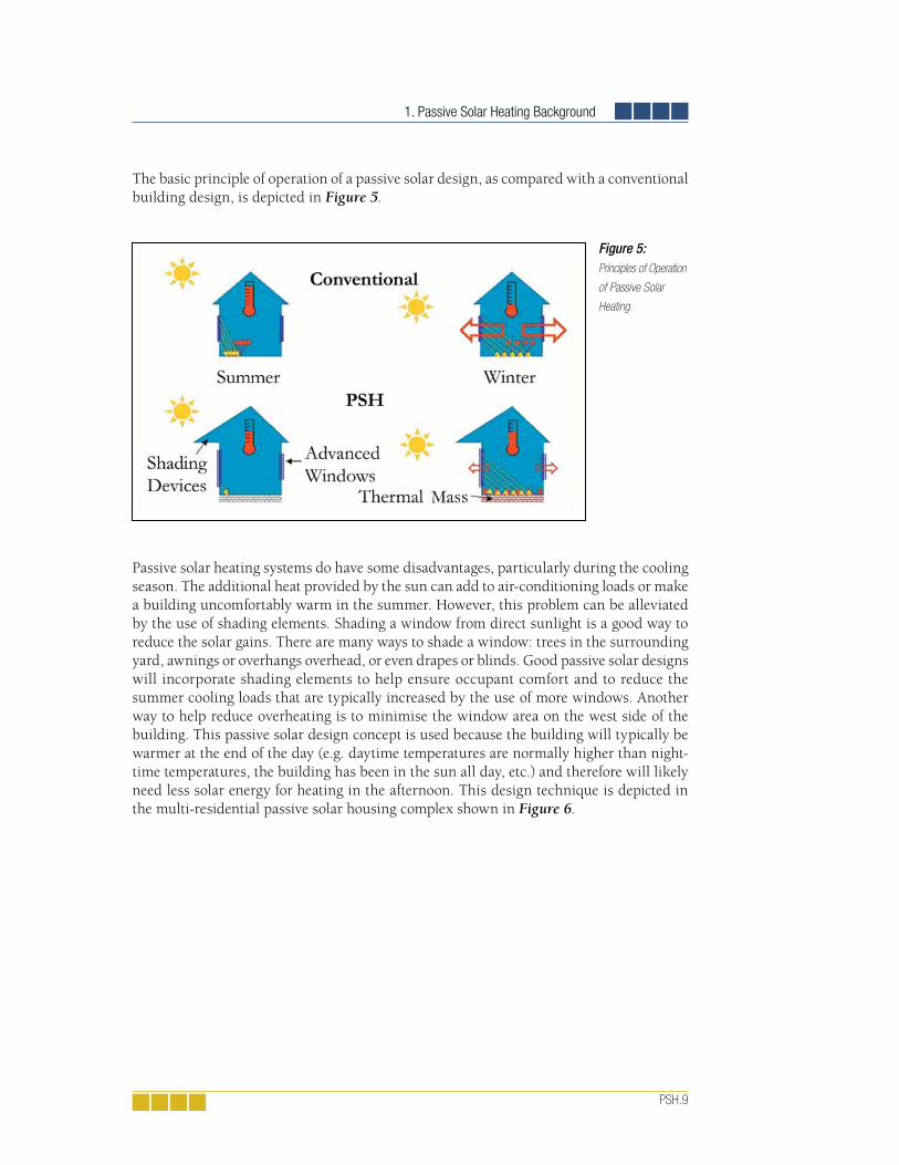
1. Passive Solar Heating Background
PSH.9
The basic principle of operation of a passive solar design, as compared with a conventional building design, is depicted in Figure 5.
Passive solar heating systems do have some disadvantages, particularly during the cooling season. The additional heat provided by the sun can add to air-conditioning loads or make a building uncomfortably warm in the summer. However, this problem can be alleviated by the use of shading elements. Shading a window from direct sunlight is a good way to reduce the solar gains. There are many ways to shade a window: trees in the surrounding yard, awnings or overhangs overhead, or even drapes or blinds. Good passive solar designs will incorporate shading elements to help ensure occupant comfort and to reduce the summer cooling loads that are typically increased by the use of more windows. Another way to help reduce overheating is to minimise the window area on the west side of the building. This passive solar design concept is used because the building will typically be warmer at the end of the day (e.g. daytime temperatures are normally higher than night-time temperatures, the building has been in the sun all day, etc.) and therefore will likely need less solar energy for heating in the afternoon. This design technique is depicted in the multi-residential passive solar housing complex shown in Figure 6.
Figure 5:Principles of Operation
of Passive Solar
Heating.
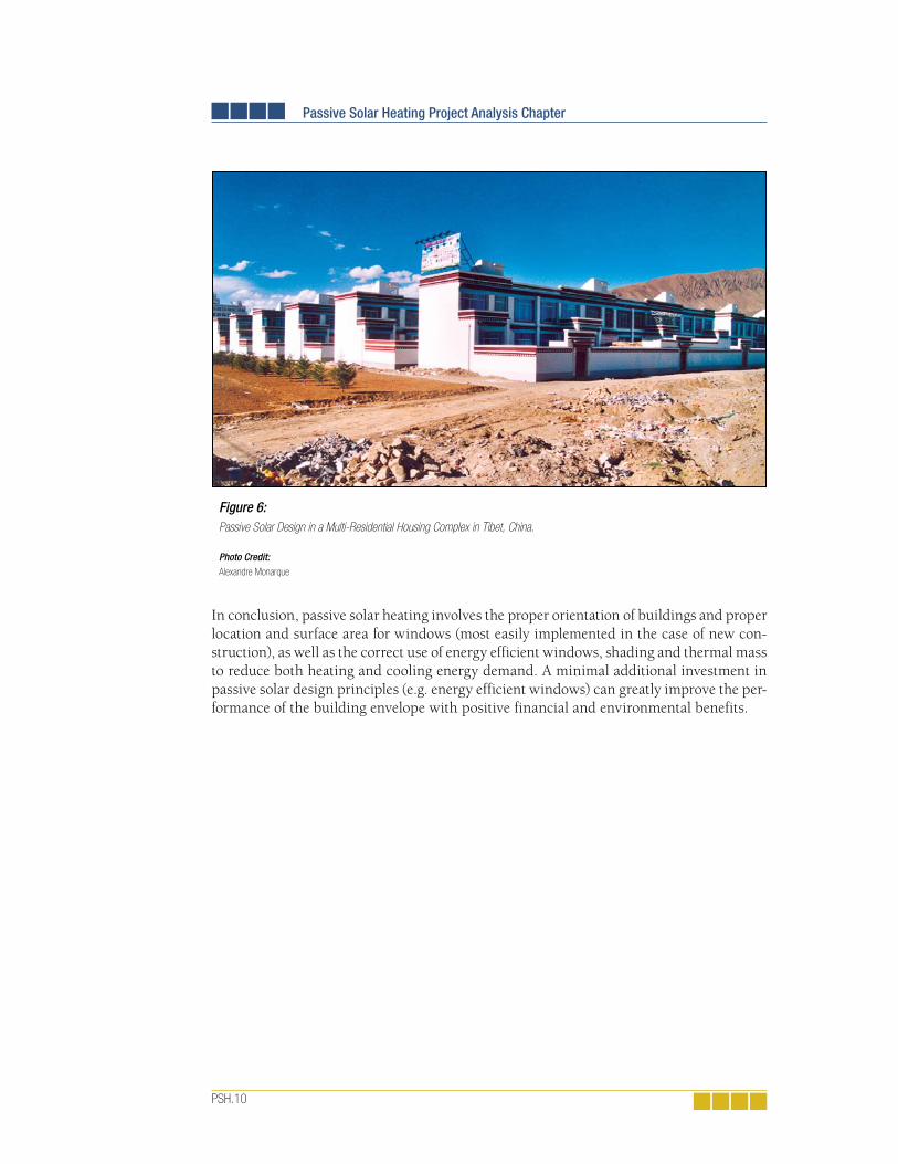
Passive Solar Heating Project Analysis Chapter
PSH.10
In conclusion, passive solar heating involves the proper orientation of buildings and proper location and surface area for windows (most easily implemented in the case of new con-struction), as well as the correct use of energy efficient windows, shading and thermal mass to reduce both heating and cooling energy demand. A minimal additional investment in passive solar design principles (e.g. energy efficient windows) can greatly improve the per-formance of the building envelope with positive financial and environmental benefits.
Figure 6:Passive Solar Design in a Multi-Residential Housing Complex in Tibet, China.
Photo Credit: Alexandre Monarque

2. RETScreen Passive Solar Heating Project Model
PSH.11
2 RETSCREEN PASSIVE SOLAR HEATING PROJECT MODEL
The RETScreen Passive Solar Heating Project Model can be used to evaluate the energy production (or savings) and financial performance associated with energy efficient window use. The model is intended for low-rise residential applications, although it can be used for small commercial buildings, and it applies anywhere in the world where there is a sig-nificant heating load. Basically, the model can be used to determine how efficient window use can affect building energy use in four ways:
Increased solar heat gains to the building through larger and better-oriented windows;
Reduced heat loss through more insulating windows;
Increased or reduced solar gains through the use of appropriate glazing; and
Reduced cooling energy demand due to improved shading.
The RETScreen Passive Solar Heating Project Model determines each of these energy sav-ings. A passive solar heating system can incorporate high-performance windows, modified window areas and orientations, and shading elements.
Seven worksheets (Energy Model, Solar Resource and Heating Load Calculation (SR&HLC), Window Worksheet, Cost Analysis, Greenhouse Gas Emission Reduction Analysis (GHG Analysis), Financial Summary and Sensitivity and Risk Analysis (Sensitivity)) are provided in the Passive Solar Heating Project Workbook file.
The Energy Model worksheet, the SR&HLC worksheet and the optional Window work-sheet are completed first. The Cost Analysis worksheet should then be completed, followed by the Financial Summary worksheet. The GHG Analysis and Sensitivity worksheets are optional analysis. The GHG Analysis worksheet is provided to help the user estimate the greenhouse gas (GHG) mitigation potential of the proposed project. The Sensitivity work-sheet is provided to help the user estimate the sensitivity of important financial indicators in relation to key technical and financial parameters. In general, the user works from top-down for each of the worksheets. This process can be repeated several times in order to help optimize the design of the passive solar heating project from an energy use and cost standpoint.
The calculation of solar gains to a building, and the amount of heat lost by conduction is relatively complex. It is dependent upon the solar radiation and outdoor temperature, as well as the thermal properties of the window. The most accurate analysis is to compute these heat transfer on an hourly basis based on detailed characteristics of the building. However, hourly data is rarely available for performing a detailed analysis.
RETScreen uses simplified algorithms to minimise data input required to calculate each source of energy savings. The model does not predict the building total heating or cooling energy consumption, rather it determines the difference in heating and cooling energy consumption between the proposed passive solar building and an identical building but

Passive Solar Heating Project Analysis Chapter
PSH.12
without the passive solar design features (referred to as the “base case”). In retrofit situ-ations, the base case building would be the existing building before any passive solar alterations. In new construction, the base case would be a building constructed according to standard practices in that region.
The basic premise of the RETScreen Passive Solar Heating Project Model is as follows. The base case configuration consists of a building with standard windows (e.g. in North Amer-ica, double-glazed with a wood or vinyl frame) with varying window area in each of the cardinal directions. The proposed case allows for redistribution of the window area in order to collect more incoming solar radiation and allow for an improvement in window proper-ties so as to increase solar heat gains and/or reduce conductive heat losses. The comparison is performed in terms of the benefit of a reduced heating demand and, in cases where a cooling system is incorporated, the potential penalty of increased cooling demand.
Simplifying assumptions include calculating heat loss and gain based on monthly aver-age solar radiation levels and outdoor temperature, as opposed to hour-by-hour data. The utilisation (or usefulness) of the solar heat gains in reducing heating demand is based on a method developed by Barakat and Sander (1982). A unique feature of the RETScreen software is that it adjusts window thermal properties based on the size of the window using an approach recommended by Baker and Henry (1997). It is understood that some margin of error will be introduced by simplifying the models, however, comparison with more complex software models has shown that the RETScreen model performs accurately enough to be an acceptable pre-feasibility tool (see Section 2.5).
The net heating and cooling demands are calculated on a monthly basis and summed for the year. The passive solar savings are the difference between the results for the base case and the proposed case buildings. For each month, an energy balance is performed between internal and solar heat gains and conduction losses through the building envelope. The dif-ference between the gains and losses is the net energy saved by the passive solar design; a positive change indicates that the design has contributed to a reduction in the building’s en-ergy demand. The model refers to this as renewable energy delivered although it may simply represent a reduction in conventional energy use due to more efficient design. A schematic diagram of the energy model algorithm is shown in Figure 7. Section 2.1 describes how window thermal properties are adjusted to account for actual window size. Sections 2.2 and 2.3 detail the calculation of heating and cooling energy savings. Finally, Section 2.4 sums these contributions to calculate the yearly renewable energy delivered. A validation of the RETScreen Passive Solar Heating Project Model is presented in Section 2.5.
The traditional definition of “passive solar heating” usually encompasses both the collection of solar energy, for example through windows, and its storage, for example in concrete floors or walls. RETScreen deals exclusively with the “window” aspect of passive solar heating. For the majority of applications, this is without consequence. Other limitations of the model include the fact that: the model should only be used for low-rise residential and small commercial buildings (under 600 m² of floor area) in heating-dominated climates; window distribution is limited to four orientations, with a 90o difference in azimuth (the building can be rotated to face any azimuth angle); and shading effects are calculated using average shading factors that are intended to be representative of seasonal mean values. Because shading factors are time-dependent parameters that change with sun position and time of day, the shading impact

2. RETScreen Passive Solar Heating Project Model
PSH.13
should only be viewed as a rough estimate. These limitations, however, are acceptable at the conceptual design stage to ensure ease-of-use in preparing pre-feasibility studies, especially given the fact that detailed hourly data for a building is not usually available anyhow.
2.1 Adjustment of Window Thermal Properties
A unique feature of the RETScreen Passive Solar Heating Project Model is the ability to select specific window manufacturers’ products for energy analysis. The software incorpo-rates the RETScreen Online Product Database, which includes more than 1,000 windows that have thermal performance ratings. As a first step in the modeling process, the software adjusts the window thermal properties for the actual window sizes (not the tested or rated window size) using a method recommended by Baker and Henry (1997).
Adjust window thermal properties
[section 2.1]
Calculatebase/proposed
heating demand[section 2.2.1]
HEATINGENERGYSAVINGS
COOLINGENERGYSAVINGS
Calculate internal gains[section 2.2.2]
Calculate base/proposedusable solar gains
over heating season[section 2.2.3]
Calculate energy savingsover heating season
[section 2.2.4]
Calculatebase/proposedcooling demand
[section 2.3]
Calculate base/proposedincrease in cooling
load due to solar gains[section 2.3]
Calculate energy savingsover cooling season
[section 2.3]
Calculate overallenergy savings
[section 2.4]
Calculatepeak heating load
and peak cooling loadreductions
[section 2.4]
Figure 7:Passive Solar
Heating Energy
Model Flowchart.
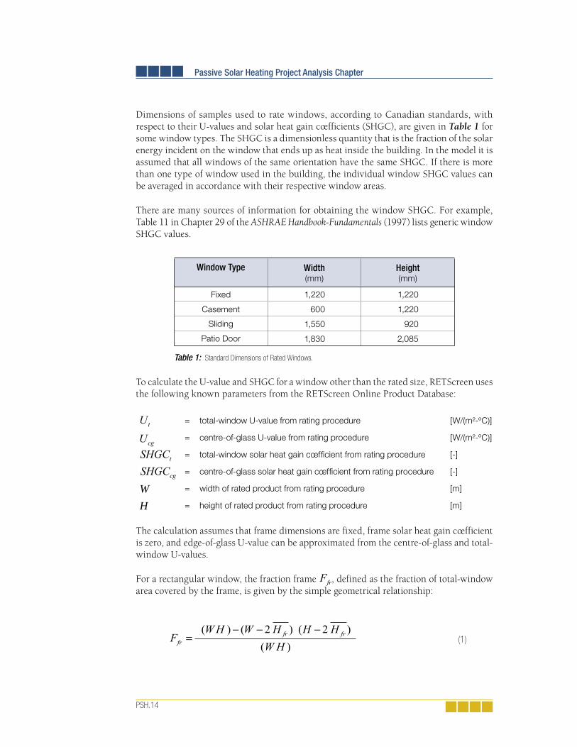
Passive Solar Heating Project Analysis Chapter
PSH.14
Dimensions of samples used to rate windows, according to Canadian standards, with respect to their U-values and solar heat gain cœfficients (SHGC), are given in Table 1 for some window types. The SHGC is a dimensionless quantity that is the fraction of the solar energy incident on the window that ends up as heat inside the building. In the model it is assumed that all windows of the same orientation have the same SHGC. If there is more than one type of window used in the building, the individual window SHGC values can be averaged in accordance with their respective window areas.
There are many sources of information for obtaining the window SHGC. For example, Table 11 in Chapter 29 of the ASHRAE Handbook-Fundamentals (1997) lists generic window SHGC values.
Window Type Width(mm)
Height(mm)
Fixed 1,220 1,220
Casement 600 1,220
Sliding 1,550 920
Patio Door 1,830 2,085
Table 1: Standard Dimensions of Rated Windows.
To calculate the U-value and SHGC for a window other than the rated size, RETScreen uses the following known parameters from the RETScreen Online Product Database:
= total-window U-value from rating procedure [W/(m²-ºC)]
= centre-of-glass U-value from rating procedure [W/(m²-ºC)]
= total-window solar heat gain cœffi cient from rating procedure [-]
= centre-of-glass solar heat gain cœffi cient from rating procedure [-]
W = width of rated product from rating procedure [m]
H = height of rated product from rating procedure [m]
The calculation assumes that frame dimensions are fixed, frame solar heat gain cœfficient is zero, and edge-of-glass U-value can be approximated from the centre-of-glass and total-window U-values.
For a rectangular window, the fraction frame , defined as the fraction of total-window area covered by the frame, is given by the simple geometrical relationship:
(1)

2. RETScreen Passive Solar Heating Project Model
PSH.15
where is the average frame height. Assuming that the frame does not contribute to the solar gain, the fraction frame is also equal to:
Solving (1) for the average frame height gives1:
The estimated frame/edge U-value is determined by solving:
where , and are the total, glass and frame areas, calculated from window width
and height and from average frame height through:
(2)
(3)
(4)
(5)
(6)
(7)
1. As shown in equation (3), only the subtracted root is retained from quadratic equation (1) since the added root would yield average frame heights greater than the total-window area, which is unrealistic.

Passive Solar Heating Project Analysis Chapter
PSH.16
Solving equation (4) leads to:
Size-specific U-value and solar heat gain cœfficient can then be determined from:
where is the approximate size-specific U-value, is the approximate size-specific solar heat gain cœfficient, and size-specific areas , and are calculated from ac-tual window dimensions through equations (5) to (7).
Similar calculations are performed for horizontal-sliding windows and vertical-sliding windows, using different equations to describe the window geometry.
In the RETScreen Passive Solar Heating Project Model windows can be facing four orien-tations, with a 90o difference in azimuth (the building can be rotated to face any azimuth angle). For each orientation, values from equations (9) and (10) are summed to obtain the global U-value and solar heat gain cœfficient for all windows at that orientation:
(8)
(9)
(10)
(11)
(12)
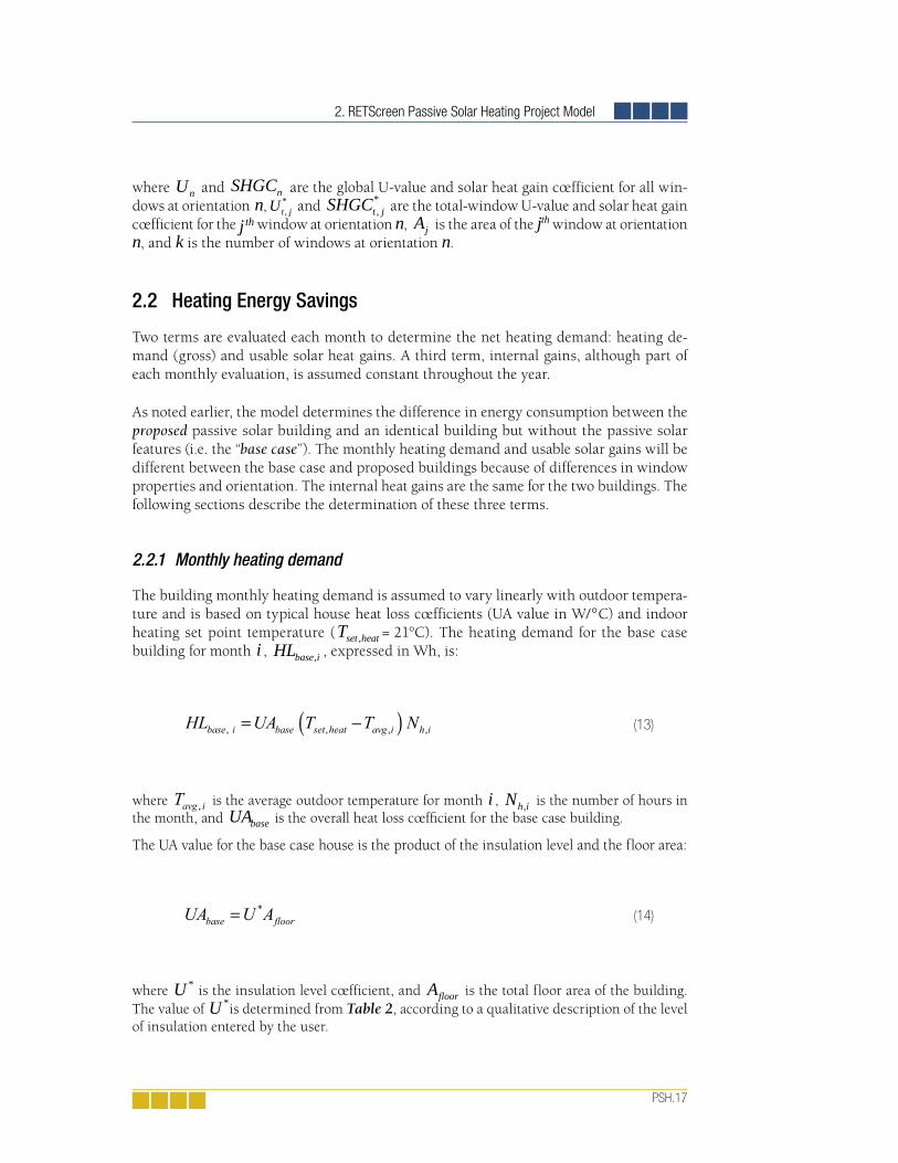
2. RETScreen Passive Solar Heating Project Model
PSH.17
where Un and SHGCn are the global U-value and solar heat gain cœfficient for all win-dows at orientation n, Ut j,
* and SHGCt j,* are the total-window U-value and solar heat gain
cœfficient for the j th window at orientation n, Aj is the area of the jth window at orientation n, and k is the number of windows at orientation n.
2.2 Heating Energy Savings
Two terms are evaluated each month to determine the net heating demand: heating de-mand (gross) and usable solar heat gains. A third term, internal gains, although part of each monthly evaluation, is assumed constant throughout the year.
As noted earlier, the model determines the difference in energy consumption between the proposed passive solar building and an identical building but without the passive solar features (i.e. the “base case”). The monthly heating demand and usable solar gains will be different between the base case and proposed buildings because of differences in window properties and orientation. The internal heat gains are the same for the two buildings. The following sections describe the determination of these three terms.
2.2.1 Monthly heating demand
The building monthly heating demand is assumed to vary linearly with outdoor tempera-ture and is based on typical house heat loss cœfficients (UA value in W/°C) and indoor heating set point temperature (Tset heat, = 21°C). The heating demand for the base case building for month i , HLbase i, , expressed in Wh, is:
where
is the average outdoor temperature for month i , Nh i, is the number of hours in the month, and UAbase is the overall heat loss cœffi cient for the base case building.
The UA value for the base case house is the product of the insulation level and the floor area:
where U * is the insulation level cœfficient, and Afloor is the total floor area of the building. The value of U *is determined from Table 2, according to a qualitative description of the level of insulation entered by the user.
(13)
(14)
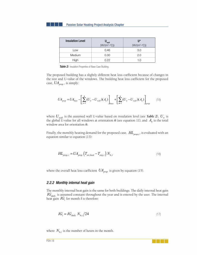
Passive Solar Heating Project Analysis Chapter
PSH.18
Insulation Level Uwall
(W/(m2-oC))U*
(W/(m2-oC))
Low 0.46 3.0
Medium 0.30 2.0
High 0.22 1.0
Table 2: Insulation Properties of Base Case Building.
The proposed building has a slightly different heat loss cœfficient because of changes in the size and U-value of the windows. The building heat loss cœfficient for the proposed case, , is simply:
where is the assumed wall U-value based on insulation level (see Table 2), is the global U-value for all windows at orientation n (see equation 11), and is the total window area for orientation n.
Finally, the monthly heating demand for the proposed case, , is evaluated with an equation similar to equation (13):
where the overall heat loss cœfficient is given by equation (15).
2.2.2 Monthly internal heat gain
The monthly internal heat gain is the same for both buildings. The daily internal heat gain
is assumed constant throughout the year and is entered by the user. The internal
heat gain for month i is therefore:
where is the number of hours in the month.
(16)
(15)
(17)

2. RETScreen Passive Solar Heating Project Model
PSH.19
2.2.3 Monthly usable solar gains over the heating season
Solar radiation transmitted into the building through the windows helps offset the heating demand of the building. However, only some of the solar gains are useful in reducing the heating demand. This section describes the calculation of solar gains and the estimation of the utilisation factor determining what part of the solar gain is usable.
Solar gains
The increase in solar heat gains obtained in the proposed case configuration is the sum of two terms: first, the associated increase in solar gains due to higher trans-mission of short-wave radiation through the glazing, and second, the re-distribution of window area that changes the total amount of solar energy captured by the win-dows due to their orientations. The solar gains for the ith month for the base case,
and for the proposed case, are determined as follows:
where is the total daily solar radiation incident on a vertical surface of orien-tation n for month i,
is the seasonal shading factor for windows at orientation
n for month i, is the global solar heat gain cœfficient for all windows of orientation n (see equation 12), is the global window area for orientation n and
is the number of hours in month i. 0.93 is an off-angle incidence correction factor.
The incident solar radiation,
, is calculated using the methods described by Duffie and Beckman (1991) and uses an algorithm similar to the one used in the RETScreen Solar Water Heating Project Model. The window shading factor (Dn,i ) is selected between two values (both user-defined) according to the season (sum-mer or winter). The seasons are considered six-month periods corresponding to the sun’s movement. Regardless of hemisphere, the summer is considered to be the months where the sun is highest in the sky and winter corresponds to the months where the sun is lowest.
(18)
(19)

Passive Solar Heating Project Analysis Chapter
PSH.20
Utilisation factor for solar gains during the heating season
The utilisation factor, , is calculated according to methods used in the HOT2000 software program available from Natural Resources Canada, originally developed by Barakat and Sander (1982). The factor, which varies by month, is determined from the equation:
The cœfficients (a, b, c and d ) are a function of the mass level of building and the acceptable indoor air temperature swing. Values for a 5.5°C temperature swing are used in the software program (this is likely the maximum swing that could be tol-erated in a passive solar house). The variation with mass level is given in Table 3. The mass level is user-defined.
Mass Level a b c d
Low 1.156 -0.3479 1.117 -0.4476
Medium 1.000 4.8380 4.533 3.6320
High 1.000 0.2792 0.245 0.4230
Table 3: Cœffi cients Used in Utilisation Function.
The gain load ratio (GLR) is determined as follows:
where is the monthly solar gain (equations 18 and 19), is the monthly heating load (equations 13 and 16), and is the monthly internal gain (equation 17).
The resulting utilisation factor indicates the proportion of the transmitted solar gains that are utilised to offset heating load. Because the solar gains are likely differ-ent between the base case and the proposed case, distinct utilisation factors
and must be computed for each case.
(20)
(21)
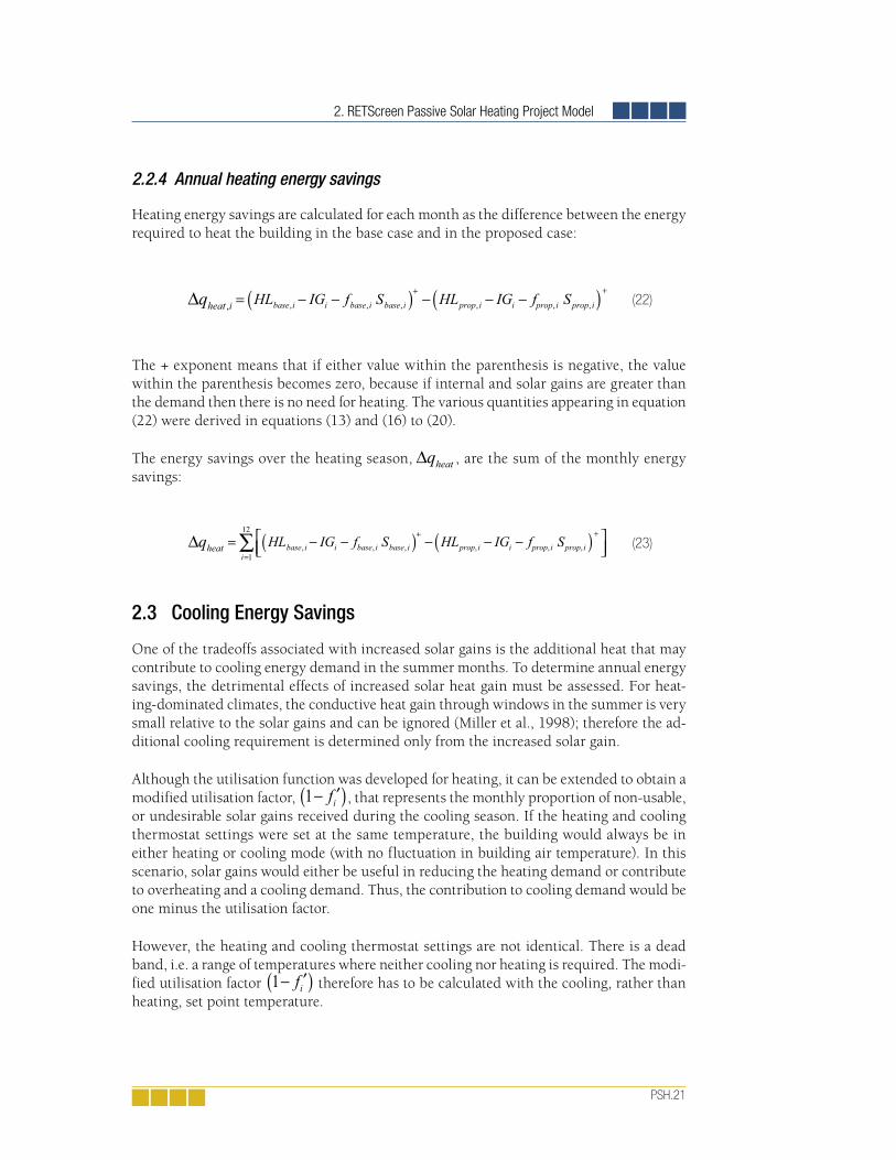
2. RETScreen Passive Solar Heating Project Model
PSH.21
2.2.4 Annual heating energy savings
Heating energy savings are calculated for each month as the difference between the energy required to heat the building in the base case and in the proposed case:
The + exponent means that if either value within the parenthesis is negative, the value within the parenthesis becomes zero, because if internal and solar gains are greater than the demand then there is no need for heating. The various quantities appearing in equation (22) were derived in equations (13) and (16) to (20).
The energy savings over the heating season, , are the sum of the monthly energy savings:
2.3 Cooling Energy Savings
One of the tradeoffs associated with increased solar gains is the additional heat that may contribute to cooling energy demand in the summer months. To determine annual energy savings, the detrimental effects of increased solar heat gain must be assessed. For heat-ing-dominated climates, the conductive heat gain through windows in the summer is very small relative to the solar gains and can be ignored (Miller et al., 1998); therefore the ad-ditional cooling requirement is determined only from the increased solar gain.
Although the utilisation function was developed for heating, it can be extended to obtain a modified utilisation factor, , that represents the monthly proportion of non-usable, or undesirable solar gains received during the cooling season. If the heating and cooling thermostat settings were set at the same temperature, the building would always be in either heating or cooling mode (with no fluctuation in building air temperature). In this scenario, solar gains would either be useful in reducing the heating demand or contribute to overheating and a cooling demand. Thus, the contribution to cooling demand would be one minus the utilisation factor.
However, the heating and cooling thermostat settings are not identical. There is a dead band, i.e. a range of temperatures where neither cooling nor heating is required. The modi-fied utilisation factor therefore has to be calculated with the cooling, rather than heating, set point temperature.
(22)
(23)

Passive Solar Heating Project Analysis Chapter
PSH.22
The concept of heating and cooling utilisation factors is depicted by example in Figure 8. The lower curve represents the utilisation factor for heating, , for a climate in the Northern Hemisphere. During the winter months the heating utilisation approaches 100%, meaning that almost all solar gains are useful towards reducing the heating energy demand. During the summer, this value tapers down to 0% as the need for heating is eliminated.
During the winter months the utilisation factor for cooling,
, is 100% meaning that the contribution of solar gains to the cooling demand, , is 0%. As the cooling utilisa-tion factor drops in the summer, its conjugate increases, approaching 100%. Thus in the summer, almost all solar gains are detrimental to the cooling demand.
The space between the two curves represents the dead band. The model ignores the per-centage of solar gains that neither reduce the heating demand nor increase the cooling demand, as they do not contribute to energy savings.
The procedure followed to calculate the cooling energy savings is therefore similar to what is described in Section 2.2.3, and the energy savings over the cooling seasons, , are expressed through an equation similar to equation (23), but with no heating demand term and with replaced by :
0%
10%
20%
30%
40%
50%
60%
70%
80%
90%
100%
Jan Feb Mar Apr May Jun Jul Aug Sep Oct Nov Dec
f' = Solar gains adding to cooling demand
f = Solar gains usable for heating
Figure 8:Example of Heating and Cooling Utilisation Factors.
(24)

2. RETScreen Passive Solar Heating Project Model
PSH.23
The modified utilisation factor,
, is calculated through equation (20). However, the gain load ratio GLR appearing in that equation has to use the heating demand calculated using the cooling set point temperature
rather than heating set point temperature ;
equations (13) and (16) are therefore replaced with:
In the model, the cooling set point temperature is set to = 25°C. As before, because of the differences between cases, separate modified utilisation factors are needed for both the proposed case and the base case.
2.4 Annual Energy Savings
Annual energy savings, referred to in the model as renewable energy delivered, , are obtained by simply summing heating and cooling energy savings (equations 23 and 24):
Finally, the model also calculates the peak heating or cooling load (power) reductions, which indicate to the user opportunities to reduce the capacity of the conventional heat-ing system or that of the air-conditioning system. Peak heating load reduction is calculated using the following equation:
where and
were calculated through equations (14) and (15), is the
heating set point temperature (21°C), and is the heating design temperature. The calculation of the peak cooling load reduction is only slightly more complicated:
(25)
(26)
(27)
(28)
(29)

Passive Solar Heating Project Analysis Chapter
PSH.24
where
is the design cooling temperature, is the cooling set point tempera-ture (25°C), and is the maximum solar gain. This latter value is calculated assuming that the peak cooling load occurs on a sunny summer day (normal irradiance equal to 1,100 W/m2); solar angles are calculated to estimate the values on north, south, east and west facing windows (see complete equations in McQuiston et al., 2000).
2.5 Validation
Numerous experts have contributed to the development, testing and validation of the RETScreen Passive Solar Heating Project Model. They include passive solar heating mod-elling experts, cost engineering experts, greenhouse gas modelling specialists, financial analysis professionals, and ground station and satellite weather database scientists.
Two sets of evaluations were done to assess the accuracy of the RETScreen Passive Solar Heating Project Model. First, the RETScreen model was tested against HOT2-XP to assess the accuracy of the calculated energy flow. HOT2-XP is the quick entry version of Natural Resources Canada’s (NRCan’s) HOT2000 detailed residential energy analysis software. The second evaluation was to see how RETScreen ranked the energy performance of windows, compared to that predicted by the Energy Rating (ER) method. The ER method is a Cana-dian standard that was developed based on hourly energy simulations.
2.5.1 Validation of passive solar heating model compared with a detailed model
HOT2-XP and RETScreen were each used to simulate a typical Canadian house. The in-puts to both models were matched as close as possible so the results could be accurately compared. The house was a typical Canadian wood frame construction (light mass and medium insulation level) and did not include shading. The house was 200 m², two-story, rectangular and had short sides on the north and south. The front was designated as the south face with a glazing area equal to 15% of the floor area distributed on the front and back only. The thermal performance values for the windows were U-value of 2.94 W/(m2-oC) and SHGC of 0.60 (clear double-glazed window in a wood frame using a metal spacer and air fill). The house was equipped with a gas furnace operating at 80% efficiency and a standard type air-conditioning with a COP of 3.0.
Using HOT2-XP, the base case house produced a figure for yearly energy required for heating, hot water and cooling of 28,787 kWh. The windows in the base model were then upgraded to double-glazed units with a single low-e coating and argon fill in a fibreglass frame. The thermal performance values for the upgraded window system were U-value = 2.08 W/(m2-oC) and SHGC = 0.54. The window area remained the same. The simulation was run again producing a yearly figure of 25,988 kWh, a difference of 2,798 kWh.
Using RETScreen, the two window systems were compared and the higher performing win-dows showed an energy benefit of 2,302 kWh. This implies that RETScreen, at least in com-parison with HOT2-XP for this example, underestimated the benefit of the window upgrade by less than 500 kWh or 18%: a difference that is acceptable at the pre-feasibility stage.

2. RETScreen Passive Solar Heating Project Model
PSH.25
2.5.2 Validation of passive solar heating model compared with standard rating method
In Table 4, a comparison of the relative performance of windows simulated using RETScreen and windows evaluated using the Energy Rating (ER) Method (see CSA, 1998) is shown. Testing windows over a range of U-values and SHGC combinations, it can be seen that RETScreen closely matches the ER system in terms of ranking window perfor-mance. A correlation between ER and annual energy savings also gives good agreement with the RETScreen results. Note that the difference in ER values was multiplied by the number of heating hours in a year, 5,400 hours in this case.
Window Properties RETScreen ER Method
TestWindow
(#)
U-Value
(W/(m²-°C))
SHGC
(-)
WindowEnergyRating(ER)
RelativeRanking
AnnualEnergySavings
(kWh/m²)
RelativeRanking
AnnualEnergySavings
(kWh/m²)
1 3.63 0.63 -34.0 0% 0.0 0% 0.0
2 2.78 0.57 -20.0 30% 92.6 29% 82.0
3 2.78 0.46 -28.0 16% 47.8 13% 35.1
4 1.87 0.52 -3.0 64% 196.0 63% 181.5
5 1.70 0.42 -7.0 57% 176.2 56% 158.1
6 1.65 0.30 -14.0 42% 127.8 40% 117.1
7 1.76 0.26 -20.0 30% 91.7 29% 82.0
8 0.85 0.36 7.0 86% 265.1 85% 240.1
9 0.45 0.34 15.0 100% 307.8 100% 286.9
Table 4: RETScreen Compared to Window Energy Rating Method.
2.6 Summary
The RETScreen Passive Solar Heating Project Model calculates changes in heating demand and solar gains that result from the adoption of energy efficient window technologies. Changes in heating demand between the base case and the new proposed design are cal-culated by evaluating the variation in heat loss cœfficient related to the proposed changes in the size and U-value of the windows. Changes in solar gain are evaluated by calculating solar gains in both the base and the proposed design, and estimating what part of the solar gain is usable for heating purposes. The same methodology is applied to calculate the as-sociated penalty in cooling demand during the summer months.
The model has been validated by comparing its predictions to those of other methods. Despite the simplifications introduced, the predictions of the Passive Solar Heating Project Model prove adequate at the pre-feasibility stage. This is particularly true given the fact that RETScreen only requires 12 points of data versus 8,760 points of data for most hourly models.


PSH.27
REFERENCES
ASHRAE, Handbook – Fundamentals, American Society of Heating, Refrigerating and Air-Conditioning Engineers, Inc., 1791 Tullie Circle, N.E., Atlanta, GA, 30329, USA, 1997.
ASHRAE, Applications Handbook, American Society of Heating, Refrigerating and Air-Conditioning Engineers, Inc., 1791 Tullie Circle, N.E., Atlanta, GA, 30329, USA, 1991.
ASHRAE, Applications Handbook, American Society of Heating, Refrigerating and Air-Conditioning Engineers, Inc., 1791 Tullie Circle, N.E., Atlanta, GA, 30329, USA, 1995.
Baker, J.A. and Henry, R., Determination of Size-Specifi c U-factors and Solar Heat Gain Cœffi cients from Rated Values at Established Sizes – A Simplifi ed Approach, ASHRAE Transactions 103, Part 1, 1997.
Barakat, S.A. and Sander, D.M., Utilisation of Solar Gain Through Windows for Heating Houses, BR Note No. 184, Division of Building Research, National Research Council, Ottawa, ON, Canada, 1982.
CSA, Energy Performance Evaluation of Windows and Other Fenestration Systems, Standard CAN/CSA A440.2, Canadian Standards Association, 178 Rexdale Boulevard, Toronto, ON, Canada, M9W 1R3, 1998.
Duffi e, J.A. and Beckman, W.A., Solar Engineering of Thermal Processes, 2nd Edition, John Wiley & Sons, 1991.
Enermodal Engineering Limited, Performance of Windows Used in the Advanced Houses Program, Prepared for Natural Resources Canada, 1993.
IEA, Low Cost, High Performance Solar Air-Heating Systems Using Perforated Absorbers: A Report of Task 14, Air Systems Working Group, Morse Associates Inc., Washington, DC, USA, September 1999.
McQuiston, F.C., Parker, J.D. and Spitler, J.D., Heating, Ventilation and Air-Conditioning: Analysis and Design, John Wiley & Sons, 2000.
Miller, S., McGowan, A. and Carpenter, S., Window Annual Energy Rating Systems, ASHRAE Transactions, Annual Meeting, Toronto, ON, Canada, June 1998.
NRCan, HOT2000, Available at Natural Resources Canada, CANMET Energy Technology Centre-Ottawa, 580 Booth Street, Ottawa, ON, Canada, K1A 0E4, www.buildingsgroup.rncan.gc.ca/software/hot2000_e.html


GROUND-SOURCEHEAT PUMP PROJECT ANALYSIS CHAPTER
CLEAN ENERGY PROJECT ANALYSIS:RETSCREEN® ENGINEERING & CASES TEXTBOOK
DisclaimerThis publication is distributed for informational purposes only and does not necessarily reflect the views of the Government of Canada nor constitute an endorsement of any commercial product or person. Neither Canada, nor its ministers, officers, employees and agents makeany warranty in respect to this publication nor a s s u m e a n y l i a b i l i t y a r i s i n g o u t o f t h i s publication.
© Minister of Natural Resources Canada 2001 - 2005.
www.retscreen.net
RETScreen® InternationalClean Energy Decision Support Centre

ISBN: 0-662-39150-0Catalogue no.: M39-110/2005E-PDF
© Minister of Natural Resources Canada 2001 - 2005.

GSHP.3
TABLE OF CONTENTS
1 GROUND-SOURCE HEAT PUMP BACKGROUND . . . . . . . . . . . . . . . . . . . . . . . . . . 5
1.1 Description of Ground-Source Heat Pump Systems . . . . . . . . . . . . . . . . . . . . . . . . . 91.1.1 Heat pump . . . . . . . . . . . . . . . . . . . . . . . . . . . . . . . . . . . . . . . . . . . . . . . . . . . . . . . . 91.1.2 Earth connection . . . . . . . . . . . . . . . . . . . . . . . . . . . . . . . . . . . . . . . . . . . . . . . . . . . 12
1.1.3 Heating and cooling distribution system. . . . . . . . . . . . . . . . . . . . . . . . . . . . . . . . . . . . 17
1.2 Ground-Source Heat Pump Application Markets . . . . . . . . . . . . . . . . . . . . . . . . . . 181.2.1 Residential buildings. . . . . . . . . . . . . . . . . . . . . . . . . . . . . . . . . . . . . . . . . . . . . . . . . 191.2.2 Commercial & institutional buildings . . . . . . . . . . . . . . . . . . . . . . . . . . . . . . . . . . . . . . 20
2 RETSCREEN GROUND-SOURCE HEAT PUMP PROJECT MODEL . . . . . . . . . . . . . 23
2.1 Bin Method and Design Conditions . . . . . . . . . . . . . . . . . . . . . . . . . . . . . . . . . . . . 24
2.2 Weather Data . . . . . . . . . . . . . . . . . . . . . . . . . . . . . . . . . . . . . . . . . . . . . . . . . . . . 272.2.1 Generation of temperature bins . . . . . . . . . . . . . . . . . . . . . . . . . . . . . . . . . . . . . . . . . 272.2.2 Ground temperature estimation . . . . . . . . . . . . . . . . . . . . . . . . . . . . . . . . . . . . . . . . . 27
2.3 Building Load Calculation – Descriptive Data Method . . . . . . . . . . . . . . . . . . . . . . 282.3.1 Commercial (institutional) & industrial buildings . . . . . . . . . . . . . . . . . . . . . . . . . . . . . . . 292.3.2 Residential buildings. . . . . . . . . . . . . . . . . . . . . . . . . . . . . . . . . . . . . . . . . . . . . . . . . 40
2.4 Building Load Calculation – Energy Use Method . . . . . . . . . . . . . . . . . . . . . . . . . . 45
2.5 Building Load Calculation for each Temperature Bin . . . . . . . . . . . . . . . . . . . . . . . 48
2.6 Earth Connection - Closed-Loop Ground Heat Exchangers (GHX) . . . . . . . . . . . . . . 492.6.1 Ground heat exchanger (GHX) sizing . . . . . . . . . . . . . . . . . . . . . . . . . . . . . . . . . . . . . 492.6.2 Design entering water temperature (Tewt ) . . . . . . . . . . . . . . . . . . . . . . . . . . . . . . . . . . 512.6.3 Part load factor (F ) . . . . . . . . . . . . . . . . . . . . . . . . . . . . . . . . . . . . . . . . . . . . . . . . . 51
2.7 Earth Connection - Open Loop Systems (Groundwater) . . . . . . . . . . . . . . . . . . . . . 52
2.8 Heat Pump System . . . . . . . . . . . . . . . . . . . . . . . . . . . . . . . . . . . . . . . . . . . . . . . . 542.8.1 Coeffi cient of performance (COP) and capacity (Qc h/ ) . . . . . . . . . . . . . . . . . . . . . . . . . 552.8.2 Entering water temperature (Tw i, ) for closed-loop ground exchanger . . . . . . . . . . . . . . . 572.8.3 Entering water temperature (Tewt ) for open-loop (groundwater) systems . . . . . . . . . . . . . 58
2.9 Energy Use Evaluation . . . . . . . . . . . . . . . . . . . . . . . . . . . . . . . . . . . . . . . . . . . . . 592.9.1 Heat pump run time and energy use of auxiliary pumps . . . . . . . . . . . . . . . . . . . . . . . . . 592.9.2 Supplemental heating or cooling needs . . . . . . . . . . . . . . . . . . . . . . . . . . . . . . . . . . . . 60
2.10 Validation . . . . . . . . . . . . . . . . . . . . . . . . . . . . . . . . . . . . . . . . . . . . . . . . . . . . . . . 602.10.1 Validation of the generation of temperature bins . . . . . . . . . . . . . . . . . . . . . . . . . . . . . . 602.10.2 Validation of the earth connection sizing for vertical closed-loop GHX . . . . . . . . . . . . . . . 63
2.11 Summary . . . . . . . . . . . . . . . . . . . . . . . . . . . . . . . . . . . . . . . . . . . . . . . . . . . . . . . 68
REFERENCES . . . . . . . . . . . . . . . . . . . . . . . . . . . . . . . . . . . . . . . . . . . . . . . . . . . . 69

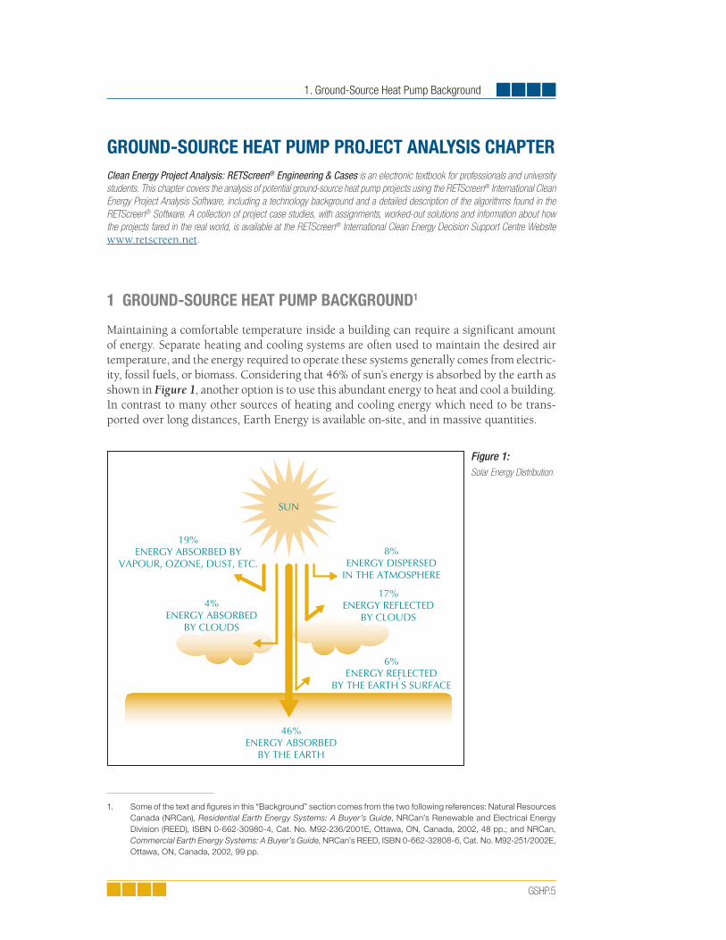
GSHP.5
GROUND-SOURCE HEAT PUMP PROJECT ANALYSIS CHAPTERClean Energy Project Analysis: RETScreen® Engineering & Cases is an electronic textbook for professionals and university students. This chapter covers the analysis of potential ground-source heat pump projects using the RETScreen® International Clean Energy Project Analysis Software, including a technology background and a detailed description of the algorithms found in the RETScreen® Software. A collection of project case studies, with assignments, worked-out solutions and information about how the projects fared in the real world, is available at the RETScreen® International Clean Energy Decision Support Centre Website www.retscreen.net.
1 GROUND-SOURCE HEAT PUMP BACKGROUND1
Maintaining a comfortable temperature inside a building can require a significant amount of energy. Separate heating and cooling systems are often used to maintain the desired air temperature, and the energy required to operate these systems generally comes from electric-ity, fossil fuels, or biomass. Considering that 46% of sun’s energy is absorbed by the earth as shown in Figure 1, another option is to use this abundant energy to heat and cool a building. In contrast to many other sources of heating and cooling energy which need to be trans-ported over long distances, Earth Energy is available on-site, and in massive quantities.
1. Some of the text and fi gures in this “Background” section comes from the two following references: Natural Resources
Canada (NRCan), Residential Earth Energy Systems: A Buyer’s Guide, NRCan’s Renewable and Electrical Energy
Division (REED), ISBN 0-662-30980-4, Cat. No. M92-236/2001E, Ottawa, ON, Canada, 2002, 48 pp.; and NRCan,
Commercial Earth Energy Systems: A Buyer’s Guide, NRCan’s REED, ISBN 0-662-32808-6, Cat. No. M92-251/2002E,
Ottawa, ON, Canada, 2002, 99 pp.
1. Ground-Source Heat Pump Background
Figure 1: Solar Energy Distribution.
SUN
19%ENERGY ABSORBED BY
VAPOUR, OZONE, DUST, ETC.8%
ENERGY DISPERSEDIN THE ATMOSPHERE
4%ENERGY ABSORBED
BY CLOUDS
17%ENERGY REFLECTED
BY CLOUDS
6%ENERGY REFLECTED
BY THE EARTH S SURFACE’
46%ENERGY ABSORBED
BY THE EARTH
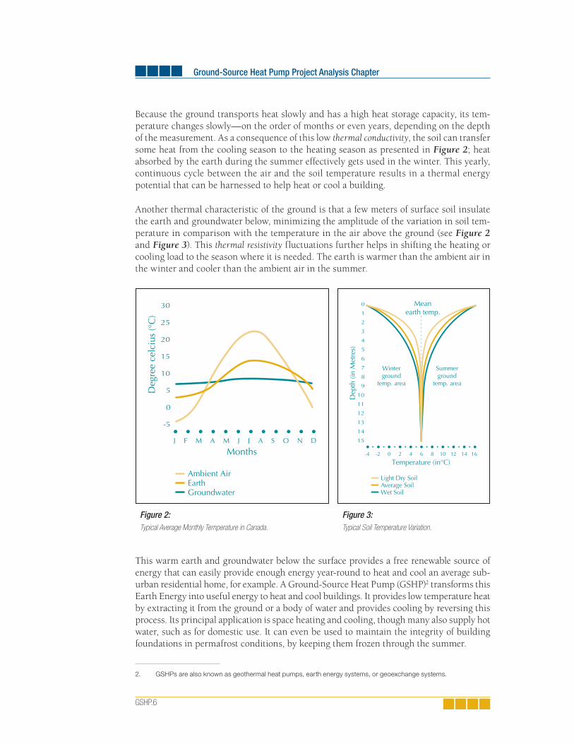
Ground-Source Heat Pump Project Analysis Chapter
GSHP.6
Because the ground transports heat slowly and has a high heat storage capacity, its tem-perature changes slowly—on the order of months or even years, depending on the depth of the measurement. As a consequence of this low thermal conductivity, the soil can transfer some heat from the cooling season to the heating season as presented in Figure 2; heat absorbed by the earth during the summer effectively gets used in the winter. This yearly, continuous cycle between the air and the soil temperature results in a thermal energy potential that can be harnessed to help heat or cool a building.
Another thermal characteristic of the ground is that a few meters of surface soil insulate the earth and groundwater below, minimizing the amplitude of the variation in soil tem-perature in comparison with the temperature in the air above the ground (see Figure 2 and Figure 3). This thermal resistivity fluctuations further helps in shifting the heating or cooling load to the season where it is needed. The earth is warmer than the ambient air in the winter and cooler than the ambient air in the summer.
This warm earth and groundwater below the surface provides a free renewable source of energy that can easily provide enough energy year-round to heat and cool an average sub-urban residential home, for example. A Ground-Source Heat Pump (GSHP)2 transforms this Earth Energy into useful energy to heat and cool buildings. It provides low temperature heat by extracting it from the ground or a body of water and provides cooling by reversing this process. Its principal application is space heating and cooling, though many also supply hot water, such as for domestic use. It can even be used to maintain the integrity of building foundations in permafrost conditions, by keeping them frozen through the summer.
2. GSHPs are also known as geothermal heat pumps, earth energy systems, or geoexchange systems.
Months
Deg
ree
celc
ius
(°C
)
J F M A M J J A S O N D
Ambient AirEarth Groundwater
30
25
20
15
10
5
0
-5
Figure 2:Typical Average Monthly Temperature in Canada.
Temperature (in°C)
0
1
2
3
4
5
6
7
8
9
10
11
12
13
14
15
Dep
th (i
n M
etre
s)
Light Dry SoilAverage SoilWet Soil
0-2-4 2 4 6 8 10 12 14 16
Meanearth temp.
Winterground
temp. area
Summerground
temp. area
Figure 3:Typical Soil Temperature Variation.

1. Ground-Source Heat Pump Background
GSHP.7
A heat pump is used to concentrate or upgrade this free heat energy from the ground before distributing it in a building through conventional ducts. It operates much as a refrigerator or conventional air conditioning system in that it relies on an external source of energy - typically electricity - to concentrate the heat and shift the temperature. Typically, each kilowatt (kW) of electricity used to operate a GSHP system draws more than 3 kW of re-newable energy from the ground. Heat pumps typically range from 3.5 to 35 kW in cool-ing capacity (about 1 to 10 refrigeration tons), and a single unit is generally sufficient for a house or a small commercial building. For larger commercial, institutional or industrial buildings, multiple heat pumps units will often be employed.
Since a GSHP system does not directly create any combustion products and because it draws additional free energy from the ground (see Figure 4), it can actually produce more energy than it uses. Because of this, GSHP efficiencies routinely average 200 to 500% over a season. GSHP systems are more efficient than air-source heat pumps, which exchange heat with the outside air, due to the stable, moderate temperature of the ground. They are also more efficient than conventional heating and air-conditioning technologies, and typically have lower maintenance costs. They require less space, especially when a liquid building loop replaces voluminous air ducts, and are not prone to vandalism like conven-tional rooftop units. Peak electricity consumption during cooling season is lower than with conventional air-conditioning, so utility demand charges may be also reduced.
For the above reasons, significant energy savings can be achieved through the use of GSHPs in place of conventional air-conditioning systems and air-source heat pumps. Re-ductions in energy consumption of 30% to 70% in the heating mode and 20% to 50% in the cooling mode can be obtained. Energy savings are even higher when compared with combustion or electrical resistance heating systems. This potential for significant energy savings has led to the use of GSHPs in a variety of applications.
Figure 4:GSHP System - The Horizontal Burial
of an Earth Connection (Heat Exchanger).
Photo Credit: Craig Miller Productions

Ground-Source Heat Pump Project Analysis Chapter
GSHP.8
Today, GSHP systems are one of the fastest growing applications of renewable energy in the world, with most of this growth happening in USA and Europe, but also in other coun-tries such as Japan and Turkey. By the end of 2004, the worldwide installed capacity was estimated at almost 12 GW
th with an annual energy use of 20 TWh. Today, around one
million GSHP system units have been installed worldwide, and annual increases of 10% have occurred in about 30 countries over the past 10 years [Lund, 2004].
In the USA alone, over 50,000 GSHP units are sold each year, with a majority of these for residential applications. It is estimated that a half million units are installed, with 85% closed-loop earth connections (46% vertical, 38% horizontal) and 15% open loop systems (groundwater) [Lund, 2004].
As of mid 2005, the world’s largest GSHP system is for a building cluster in Louisville (KY), USA, which provides heating and cooling for 600 rooms, 100 apartments, and 89,000 square meters of office space, representing a total area of 161,650 m2. It makes use of groundwater to supply 15.8 MW of cooling and 19.6 MW of heating capacity, demonstrat-ing that GSHPs are not limited to small-scale applications. Running for 15 years with no system problems, it has reduced the overall energy consumption by 47% and provides monthly savings of CDN$30,000 compared to an adjacent, similar building (see Figure 5) [DOE, 1999].
The following sections describe the main components of a GSHP system (heat pumps, earth connection, and distribution system) and discuss the GSHP markets for residential, commercial, and institutional building type applications.
Figure 5:World’s Largest GSHP Systems installed in a Building Cluster at the Galt House East Hotel
and Waterfront Offi ce Buildings in Louisville (KY), USA.
Photo Credit: Marion Pinckley (NREL PIX)

1. Ground-Source Heat Pump Background
GSHP.9
1.1 Description of Ground-Source Heat Pump Systems
A ground-source heat pump (GSHP) system has three major components: a heat pump, an earth connection and an interior heating or cooling distribution system (see Figure 6). These three major components, together with the different earth connection configurations of a typical GSHP installation, are explained in the following sections.
1.1.1 Heat pump
The heat pump transfers the heat between the heating/cooling distribution system and the earth connection. It is the basic building block of the GSHP system.
The most common type of heat pump used with GSHP systems is a “water-to-air” unit ranging in size from 3.5 kW to 35 kW of cooling capacity. The water-to-air designation indicates that the fluid carrying heat to and from the earth connection is water or a water/antifreeze mix and that the heat distribution system inside the building relies on hot or cold air. The heat pump may be an extended range unit, allowing lower entering fluid temperatures in heating mode and higher entering fluid temperatures in cooling mode. All the components of this type of heat pump are in one enclosure: the compressor, an earth connection-to-refrigerant heat exchanger, controls, and an air distribution system containing the air handler, duct fan, filter, refrigerant-to-air heat exchanger, and conden-sate removal system for air conditioning. A typical packaged heat pump unit is illustrated in Figure 7.
Figure 6:The three GSHP System Major Components:
(1) Heat Pump,
(2) Earth Connection, and
(3) Heating/Cooling Distribution system.

Ground-Source Heat Pump Project Analysis Chapter
GSHP.10
For residential applications and small commercial systems, a single heat pump unit will suffice. For larger commercial, institutional or industrial systems, multiple heat pump units are typically used in a distributed network connected to a common fluid loop.
The heat pump operates using the same cycle as a refrigerator. The heat pump uses com-pression and expansion of a refrigerant to drive heat flows between the inside of the build-ing and the earth connection. As per the Second Law of Thermodynamics, heat will flow only from hotter to colder matter, but a heat pump will draw heat from the ground at, say, 5ºC and use it to warm a building to 21ºC. At certain times of the year, the temperature of the ground will be such that heat would flow in the desired direction anyway. The heat pump may still need to operate, however, in order to ensure that the rate of heat flow is sufficient. This rate is related to the temperature difference between the heat pump and the earth connection: during cooling, the higher the temperature of the building, the better the rate of transfer with the earth connection would be.
In heating mode, the heat pump works as follows: heat from the earth connection arrives at an earth connection-to-refrigerant heat exchanger called the evaporator (see Figure 8). On the other side of the heat exchanger is cold refrigerant in a mostly liquid state. The refrigerant is colder than the temperature of the heat transfer fluid from the earth connec-tion, so heat flows into the refrigerant. This heat causes the liquid refrigerant to evaporate; its temperature does not increase much. This gaseous, low pressure and low temperature refrigerant then passes into an electrically-driven compressor. This raises the refrigerant’s pressure and, as a consequence, its temperature.
Figure 7:Typical Heat Pump Unit.

1. Ground-Source Heat Pump Background
GSHP.11
The high temperature, high pressure, gaseous output of the compressor is fed into a second heat exchanger, called the condenser. In water-to-air heat pumps, a fan blows air to be heated through this “air coil”. In water-to-water heat pumps, water which will heat the building flows through the condenser. Since the refrigerant is hotter than the air or water, it transfers heat to it. As it loses heat, the refrigerant’s temperature drops somewhat and it condenses.
This high temperature liquid refrigerant then passes through an expansion valve. The valve reduces the pressure of the refrigerant, and as a consequence, its temperature drops significantly. Now, this low temperature liquid flows to the evaporator, and the cycle starts again. In this way, the heat from the water or other heat transfer fluid in the earth connec-tion is transferred to the air or water in the building: hence the name “water-to-air heat pump” or “water-to-water heat pump”.
One significant difference between a ground-source heat pump and a refrigerator is that the ground-source heat pump is meant to run in both directions. When in cooling mode, the earth connection-to-refrigerant heat exchanger becomes the condenser, and the re-frigerant-to-air heat exchanger becomes the evaporator. This is accomplished through a reversing valve inside the heat pump.
A desuperheater, as illustrated in Figure 8, provides domestic hot water when the compres-sor is operating. The desuperheater is a small auxiliary heat exchanger at the compressor outlet. It transfers excess heat from the compressed gas to water that circulates to a hot water tank. During the cooling season, when air-conditioning runs frequently, a desuper-heater may provide all the hot water needed in a residential application. Some residential heat pumps are designed to provide hot water year round in quantities sufficient to meet a household’s needs.
High-pressure,High-temperature
vapour
High-pressure,High-temperature
liquid
low-pressure,low-temperature
vapour
Low-pressure,Low-temperature
liquid
COMPRESSOR(Not always present)DESUPERHEATER
CO
ND
ENSE
R
EXPANSION VALVE
EVA
POR
ATO
R
HEAT HEAT
Figure 8:The Refrigeration Cycle (Heating Mode) of a Typical Packaged Heat Pump Unit.

Ground-Source Heat Pump Project Analysis Chapter
GSHP.12
1.1.2 Earth connection
The earth connection is where heat transfer between the GSHP system and the soil occurs. GSHPs comprise a wide variety of systems that use the ground, ground water, or surface water as a heat source and sink. One common type of earth connection entails tubing buried in horizontal trenches or vertical boreholes, or alternatively, submerged in a lake or pond. An antifreeze mixture, water, or another heat-transfer fluid is circulated from the heat pump, around the tubing, and back to the heat pump in a “closed loop.” “Open loop” earth connections draw water from a well or a body of water, transfer heat to or from the water, and then return it to the ground or the body of water.
The following nomenclature has been adopted by the American Society of Heating, Re-frigerating and Air-Conditioning Engineers (ASHRAE)3 to distinguish among the various types of earth connection systems:
Ground-Coupled Heat Pumps (GCHPs) - use the ground as a heat source and sink, either with vertical or horizontal Ground Heat eXchangers (GHXs);
Groundwater Heat Pumps (GWHPs) - use underground (aquifer) water as a heat source and sink;
Surface Water Heat Pumps (SWHPs) - use surface water bodies (lakes, ponds, etc.) as a heat source and sink; and
Ground Frost Heat Pump (GFHPs) - maintain sound structural fi ll in natural permafrost around foundations by extracting heat from the fi ll.
Since all earth connections in a GSHP sys-tem are usually very difficult to access after installation, the materials and workmanship used in construction must be of the highest quality. High-density polyethylene piping and fusion-bonded pipe connections are used almost exclusively. Experienced GSHP installers should implement ground-heat exchangers and groundwater wells using specialised equipment (see Figure 9).
3. http://www.ashrae.org/
Figure 9: Drilling Technology for
GSHP’s Earth Connection.
Photo Credit: Geothermix Inc.

1. Ground-Source Heat Pump Background
GSHP.13
Ground-Coupled Heat Pumps (GCHPs): In a GCHP system, a series of buried pipes cir-culates a heat transfer fluid in a closed loop: the fluid never leaves the system, but rather travels back and forth in a loop between the earth connection and the heat pump. This circulating fluid is either water or an antifreeze solution4, if freezing temperatures are ex-pected. The ground heat exchanger can make use of a series of deep vertical holes (bore-holes) or a horizontal arrangement of pipes buried a few of metres below the surface.
The vertical GHX is well suited to larger buildings where the bedrock is close to the surface, when minimal disruption of the landscaping is desired, or where little land is available for the GHX (see Figure 10). Because the ground temperature is steady year round below the surface, vertical GHXs are more efficient than horizontal GHXs, which may experience seasonal temperature fluctuations. Vertical loops are generally more expensive to install than horizontal ones, but require less piping due to the stable temperatures.
The boreholes, 45 to 150 m in depth, are drilled by rigs normally used for drilling wells. They contain either one or two loops of pipe with a U-bend at the bottom. After the pipe is inserted, the hole is backfilled and grouted. The grout prevents surface water from drain-ing into the borehole and the groundwater, and also prevents the water from one borehole from leaking into an adjacent borehole. Following backfilling and grouting, the vertical pipes are connected to horizontal underground supply and return header pipes. The header pipes carry the GHX heat transfer fluid to and from the heat pump. Figure 11 illustrates a typical vertical GHX system.
4. The antifreeze solution often employed is glycol whose proportion may vary based on the local weather conditions, the
soil thermal conductivity characteristics and the fl ow rate of the fl uid in the GHX. In the RETScreen Ground-Source Heat
Pump Project Model, the proportion of glycol is conservatively considered to be 25% of the total circulating fl uid. This
assumption only impacts the cost analysis, where the cost of the circulating fl uid is considered. The cost is relatively
small compared to the overall initial cost of a GSHP system.
Figure 10:Vertical Ground Heat Exchanger (GHX)
of a Ground-Coupled Heat Pump (GCHP) System.

Ground-Source Heat Pump Project Analysis Chapter
GSHP.14
The horizontal GHX configuration is often less expensive to install than the vertical ar-rangement, but requires a larger land area (see Figure 12). For this reason, it is usually better suited to smaller applications such as residential and small commercial buildings. It can be especially attractive if excavating and trenching equipment is available and when the upper few metres of the ground are amenable to excavation.
A horizontal GHX consists of a series of pipes laid out in trenches, usually one to two meters below the surface. Typically, about 35 to 55 meters of pipe are installed per kW of heating and cooling capacity. Many configurations of the horizontal GHX are possible, as illustrated in Figure 13. When land area is limited, a coiled pipe, also called “slinky” or spiral, may be used in order to fit more piping into a trench area. While this reduces the amount of land used it requires more pipes, which results in additional costs. The trench is backfilled once the pipe has been laid out.
EARTH BACKFILLED TRENCH
REVERSE RETURN HEADER(to balance pressure losses)
GROUT(and earth backfillwhen permitted)
BOREHOLE
GROUND LOOP PIPE
U-BEND
SUPPLY HEADER
Figure 11:Vertical Ground Heat Exchanger (GHX).
Figure 12:Horizontal Ground Heat Exchanger (GHX) of
a Ground-Coupled Heat Pump (GCHP) System.

1. Ground-Source Heat Pump Background
GSHP.15
A
TURNAROUNDS
SUPPLYHEADER
REVERSE RETURN HEADER(to balance pressure losses)
COILED PIPE
B
C D
E F
G H
1.2 m
0.4 m
E. LAYOUT OF PARALLEL TWO-PIPE SHOWING TURNAROUNDS AND HEADERF. COILED PIPE LAID EITHER HORIZONTALLY IN A WIDE TRENCH OR VERTICALLY IN A NARROW TRENCHG. COILED PIPE LAID VERTICALLY IN A NARROW TRENCHH. COILED PIPE LAID HORIZONTALLY IN A WIDE TRENCH
A. SINGLE PIPEB. STACKED TWO-PIPE (SAND FILL IS REQUIRED ONLY IF ROCKS LARGER THAN 5 CM ACROSS ARE PRESENT.)C. PARALLEL TWO-PIPED. STACKED PARALLEL FOUR-PIPE
EARTHBACKFILL
GROUNDLOOP PIPE
SAND FILL
min.1.2 m
min.1.2 m
min.0.6 m
1.2 m
0.4 m
Figure 13:Various Confi gurations of Horizontal Ground Heat Exchangers (GHX).

Ground-Source Heat Pump Project Analysis Chapter
GSHP.16
Groundwater Heat Pumps (GWHPs): Groundwater heat pump systems are, in contrast to GCHPs, open loop systems: they use a constant supply of groundwater as the heat trans-fer fluid (see Figure 14). A GWHP earth connection simply consists of water wells where groundwater from an aquifer is pumped directly from the well to the heat pump’s earth connection-to-refrigerant (or, in this case, water-to-refrigerant) heat exchanger or to an intermediate heat exchanger. The intermediate heat exchanger transfers the heat from the open groundwater loop to a closed building loop, and thus isolates the heat pump from the well water, protecting its heat exchanger from the potentially fouling, abrasive or corrosive well water. After leaving the building, the water is pumped back into the same aquifer via a second well, called an injection well.
The GWHP was the first type of GSHP to appear on the market and GWHPs have been used successfully for decades. They are the simplest type of system to install. However, local environmental regulations and insufficient water availability may limit their use in some areas.
Standing column wells are a newer variation of the GWHP system. Standing wells are typically six inches in diameter and may be as deep as 450 meters. In this system, water from the bottom of the well is pumped to the building’s heat exchanger and returned to the top of the same well. The well may also provide potable water. For this system to work adequately, ground water must be in abundant supply. This type of system is not used where the water table is especially deep, since the required pumping power renders the system prohibitively expensive.
Surface Water Heat Pumps (SWHPs): The surface water heat pump is a viable and rela-tively low-cost GSHP option. A series of coiled pipes submerged below the surface of a lake or pond serves as the heat exchanger. This requires minimal piping and excavation, but the pond or lake must be deep and large enough. The heat transfer fluid is pumped through the pipe in a closed loop, as in a GCHP system, avoiding adverse impacts on the aquatic ecosystem. Many successful systems are currently in operation.
Figure 14:Ground-Water Heat Pump (GWHP) System.

1. Ground-Source Heat Pump Background
GSHP.17
Ground Frost Heat Pumps (GFHPs): Another specialized application of GSHPs is the cooling of building foundations in areas with permafrost. Building foundations transmit heat, melting any permafrost and thus undermining the structural soundness of the foun-dation. By extracting heat from the ground around the foundation, a GFHP can ensure that the permafrost remains frozen. Moreover, the extracted heat can provide up to 20 to 50% of the building’s space heating requirements and the costs of traditional measures for maintaining the structural soundness of foundations in permafrost can be avoided. Me-chanically chilled foundations can be much less expensive, both initially and on a life-cycle cost basis, than conventional permafrost foundations.
The GFHP earth connection is buried in the fill below the foundation, and the heat pump keeps the fill frozen while supplying supplemental heat to the building. The heat transfer fluid, circulated in a closed loop, is usually a mix of water and glycol that will not freeze at the lowest temperatures experienced by the granular fill.
The use of GSHPs in permafrost introduces several additional considerations. Heat gain to the ground from building foundations must be considered when designing the earth connection in GFHPs or in GHXs installed beneath foundations. Heat must be extracted at the same rate as it is gained from the foundation in order to maintain a constant ground temperature. Also, given the low mean earth temperature, conventional GCHPs may not be justified in these situations. Finally, long-term operation depends on the ground being reheated by solar energy incident during summertime. Local ecological disturbances may occur if the ground is kept frozen beyond its natural cycle.
Because the consequences of GFHP failure are severe (sinking foundations), the heat ex-changer should use premium quality hermetic piping and be installed by experts. Insula-tion between the frozen gravel pad and the foundation slab should be adequate to maintain the pad in a frozen state should the heat pump become temporarily inoperative.
1.1.3 Heating and cooling distribution system
The heating/cooling distribution system delivers heating or cooling from the heat pump to the building. It usually takes the form of an air duct distribution system, although water loop systems (also known as hydronic systems), which heat or cool floors and ceilings are also used. Heating and cooling distribution in a GSHP system is generally the same as in conventional systems. However, larger installations may use multiple heat pumps, perhaps one for each building zone, where each heat pump is attached to a common build-ing loop. The various types of air delivery systems that can be used are well documented [ASHRAE, 1992] and consist mainly of air ducts, diffusers, fresh air supply systems and control components.

Ground-Source Heat Pump Project Analysis Chapter
GSHP.18
1.2 Ground-Source Heat Pump Application Markets
The development of ground-source heat pumps dates to 1912 when the first patent using a ground loop was recorded in Switzerland. However, it was not until the 1970’s that GSHPs gained significant market acceptance. The first commercial GSHPs were designed for the residential sector and were groundwater-type systems. By the mid 1980’s, advances in heat pump efficiencies and operating ranges, combined with better materials for ground loops, allowed for ground-coupled earth connections. At about the same time, commercial and institutional applications became more common.
Today, the technology can be considered mature and is facing mainly non-technical bar-riers for further deployment. Even if strong markets for GSHP systems exist in many in-dustrialised countries where heating and cooling energy requirements are high, the main constraint hindering increased market penetration of GSHPs is their high initial cost, which is generally:
almost double that of conventional central systems in residential applications;
20% to 40% more than constant volume, single zone rooftop units; and
up to 20% more than multizone or central two-pipe chilled water arrangements.
Nevertheless, GSHPs generally have lower life-cycle costs than conventional systems due to their efficiency and lower maintenance requirements. The RETScreen Ground-Source Heat Pump Project Model has been developed to compare the life-cycle costs of GSHPs with conventional technologies.
Markets for GSHPs tend to be par-ticularly strong when climate, energy prices and the nature of the project are favourable. First, a climate re-quiring both heating and cooling is preferable to one that requires just one or the other. While the same GSHP system can provide both heating and cooling, two separate conventional systems may be required, each dedicated to only one task—either heating or cooling. This increases the capital cost of the competing conventional technology, making the GSHP a more attractive option. Furthermore, since it is operating year-round, the GSHP system can generate larger energy savings, rather than, for example, an air-conditioning unit which only operates in summer and an oil furnace which only operates in the winter.
Second, large seasonal variations in temperature will favour the GSHP system over air-source heat pumps, whose capacity and efficiency decrease at temperature extremes and ensure that there is significant energy demand on which the GSHP can generate savings.
RETScreen® InternationalGround-Source Heat Pump Project Model
The RETScreen® International Ground-Source Heat Pump Project Model can be used world-wide to easily evaluate the energy production (or sav-ings), life-cycle costs and greenhouse gas emis-sions reduction for the heating and/or cooling of residential, commercial, institutional and indus-trial buildings. The model can be used to evaluate both retrofit and new construction projects using either ground-coupled (horizontal and vertical closed-loop) or groundwater heat pumps.

1. Ground-Source Heat Pump Background
GSHP.19
Third, if there is already a useable heating and cooling system installed, the purchase and installation of a GSHP is rarely justified on the basis of its energy benefits alone. Thus, the GSHP is most cost-effective in new construction, especially since this facilitates trenching and drilling, or when an existing heating and cooling system has reached the end of its life and must be replaced.
If heating is the dominant energy requirement, then low electricity prices and high gas or oil prices will make the GSHP more attractive than combustion systems. If cooling is dominant, then high electricity prices will favour ground-source heat pumps over conven-tional air conditioning, which is less efficient. If both heating and cooling requirements are high, then GSHPs are ideal where electricity prices are low year round, but high peak load charges are levied during summertime.
Whenever building heating and cooling loads are substantially different, it may be financially advantageous to reduce the cost of the earth connection loop by sizing it for the lower of the two loads. In this way, the overall initial cost of the system is reduced but supplemental heating or heat rejection capacity becomes necessary. Supplemental capacity usually entails heating using conventional systems and cooling towers for heat rejection. The best option can be de-termined through a sensitivity analysis at the pre-feasibility stage using the RETScreen GSHP Project Model and with detailed simulations at the design stage of project development.
GSHPs can also provide moderately hot water, e.g. for domestic use, through a device called a desuperheater. This dual use of the GSHP increases efficiency and energy savings. Other GSHP applications include heating water distribution pipes to prevent freezing, hot water pre-heating, heating of sewage conduits and treatment lagoons, and ice rink cooling.
Considering the above elements, the GSHP markets for residential, commercial, and insti-tutional building type applications are further discussed in the following sections.
1.2.1 Residential buildings
While GSHPs are used for all types of residential buildings, high-end residential construc-tion tends to be the focus of this market. The higher initial costs of the GSHP do not con-stitute an especially large fraction of these expensive homes and the homeowners generally view the GSHP system as a long-term investment in their home. Furthermore, they are swayed by the environmental benefits and the improvements in comfort and air-quality associated with the GSHP.
Electric utilities often subsidize the residential market for GSHPs. Utilities benefit through increases to their base load and reductions in their peak load. Utilities also recognize that the system’s environmental benefits accrue to society as a whole, and therefore the initial costs should not be borne by the system’s owner alone. Regardless, such a subsidy can be a major consideration in the homeowner’s decision to install a GSHP. For example, a typi-cal 2,200 ft2 (205 m2) residential building in the US that requires about 11 kW of heating supply (depending on climate), will need a GSHP system that will cost approximately CDN$30,000 for 230 m of horizontal closed-loop GHX or about CDN$34,000 for 165 m of vertical closed-loop GHX.

Ground-Source Heat Pump Project Analysis Chapter
GSHP.20
1.2.2 Commercial & institutional buildings
The viability of GSHPs for commercial buildings can be impeded by demands for short simple payback periods, generally less than 5 years, and by limited availability of land for large earth connections. Nevertheless, there are many such installations (see Figure 15).
GSHPs offer several advantages that make them particularly attractive in commercial build-ings. Since the heat pump is physically smaller than conventional heating and cooling plants, and since heat distribution in a large building can be achieved with a compact liquid loop rather than voluminous air ducts, the ground-source heat pump can free build-ing space for commercial uses. The use of multiple heat pumps distributed around a large building also simplifies control of the interior environment. The elimination of rooftop units, cooling towers and chimneys reduces opportunities for vandalism. Moreover, with increased efficiency over conventional air conditioners, the ground-source heat pump re-duces summertime peak load charges often levied by utilities on commercial customers.
Large buildings using GSHPs have multiple heat pump units, located around the building, transferring heat to and from a common building loop. This arrangement is very beneficial. First, large buildings often have simultaneous heating and cooling loads: for example, the core of the building may need cooling while perimeter areas need heating. The common building loop can transfer heat from cooling loads to heating loads, reducing the demand on the earth connection and improving efficiency. Second, climate control is simplified and occupant comfort is improved, since each heat pump affects only the space in its vi-cinity. Controls can be local, rather than part of a complex building-wide system. Third, the common building loop transfers heat using a liquid, which permits it to be much more compact than the ducting required by air distribution systems tied to conventional central heating plants; space is freed up for more productive uses.
Figure 15:GSHP System in a Commercial Buildings.
Photo Credit: Geothermal Heat Pump Consortium (NREL PIX)

1. Ground-Source Heat Pump Background
GSHP.21
Specialized markets among certain types of commercial buildings are under development. Buildings with simultaneous heating and cooling requirements—such as those having freezers or ice-making equipment as well as heated areas—can benefit from the liquid building loop commonly used in commercial applications of GSHP: heat is extracted from the cooling loads and passed to the heating loads. Promising possibilities include super-markets and gas station/convenience store combinations.
Ground-source heat pumps can also be very well suited to institutional buildings (see Figure 16). Institutional building owners and operators are often willing to accept longer paybacks than in the commercial sector. They may also be more open to innovative de-signs and technologies like GSHPs. As in commercial buildings, many institutional build-ings have a simultaneous need for heating and cooling, which the building loop of a ground-source heat pump system can take advantage of.
Figure 16:GSHP Systems in an Institutional Building (Philadelphia Enterprise Centre, USA – 28 GSHPs for Heating and Cooling).
Photo Credit: Geothermal Heat Pump Consortium (NREL PIX)

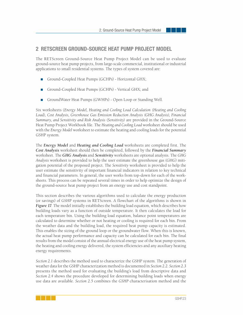
2. Ground-Source Heat Pump Project Model
GSHP.23
2 RETSCREEN GROUND-SOURCE HEAT PUMP PROJECT MODEL
The RETScreen Ground-Source Heat Pump Project Model can be used to evaluate ground-source heat pump projects, from large-scale commercial, institutional or industrial applications to small residential systems. The types of system covered are:
Ground-Coupled Heat Pumps (GCHPs) - Horizontal GHX;
Ground-Coupled Heat Pumps (GCHPs) - Vertical GHX; and
GroundWater Heat Pumps (GWHPs) - Open Loop or Standing Well.
Six worksheets (Energy Model, Heating and Cooling Load Calculation (Heating and Cooling Load), Cost Analysis, Greenhouse Gas Emission Reduction Analysis (GHG Analysis), Financial Summary, and Sensitivity and Risk Analysis (Sensitivity) are provided in the Ground-Source Heat Pump Project Workbook file. The Heating and Cooling Load worksheet should be used with the Energy Model worksheet to estimate the heating and cooling loads for the potential GSHP system.
The Energy Model and Heating and Cooling Load worksheets are completed first. The Cost Analysis worksheet should then be completed, followed by the Financial Summary worksheet. The GHG Analysis and Sensitivity worksheets are optional analysis. The GHG Analysis worksheet is provided to help the user estimate the greenhouse gas (GHG) miti-gation potential of the proposed project. The Sensitivity worksheet is provided to help the user estimate the sensitivity of important financial indicators in relation to key technical and financial parameters. In general, the user works from top-down for each of the work-sheets. This process can be repeated several times in order to help optimize the design of the ground-source heat pump project from an energy use and cost standpoint.
This section describes the various algorithms used to calculate the energy production (or savings) of GSHP systems in RETScreen. A flowchart of the algorithms is shown in Figure 17. The model initially establishes the building load equation, which describes how building loads vary as a function of outside temperature. It then calculates the load for each temperature bin. Using the building load equation, balance point temperatures are calculated to determine whether or not heating or cooling is required for each bin. From the weather data and the building load, the required heat pump capacity is estimated. This enables the sizing of the ground loop or the groundwater flow. When this is known, the actual heat pump performance and capacity can be calculated for each bin. The final results from the model consist of the annual electrical energy use of the heat pump system, the heating and cooling energy delivered, the system efficiencies and any auxiliary heating energy requirements.
Section 2.1 describes the method used to characterize the GSHP system. The generation of weather data for the GSHP characterization method is documented in Section 2.2. Section 2.3 presents the method used for evaluating the building’s load from descriptive data and Section 2.4 shows the procedure developed for determining building loads when energy use data are available. Section 2.5 combines the GSHP characterisation method and the

Ground-Source Heat Pump Project Analysis Chapter
GSHP.24
buildings loads calculated. Section 2.6 deals with the modeling of the closed-loop systems, both vertical and horizontal, and Section 2.7 presents the methodology employed for open loop systems. Section 2.8 presents the heat pump related equations, and Section 2.9 shows how the energy use by the system is evaluated. Finally, Section 2.10 presents a validation of the RETScreen GSHP Project Model by comparing the results obtained from RETScreen against monitored data and other software.
There are some limitations to the methodology chosen to make the calculation in the GSHP Project Model. In some instances, the model cannot capture phenomenon such as simultaneous heating and cooling demands, which can sometimes occur in commercial buildings; neither can it capture complex building usage profiles. Residential applications lend themselves readily to a simplified approach given the more homogeneous nature of the buildings and the more limited usage patterns possible. Other limitations of the GSHP Project Model include:
The long-term thermal imbalances are not included in the ground heat exchanger (GHX) calculations.
The ground-coupled heat pump (GCHP) horizontal ground heat exchanger (GHX) confi guration considered is a stacked two pipe system, (31.8 mm nominal diameter) with one pipe 1.8 m deep and the other 1.2 m below the surface.
The ground-coupled heat pump (GCHP) vertical ground heat exchanger (GHX) confi guration consists of one 31.8 mm diameter U-tube per borehole.
The building heating and cooling energy consumption and peak loads are evaluated using a simplifi ed version of ASHRAE's modifi ed bin method (ASHRAE, 1985). The interior set point temperature is considered constant at 23°C and remains the same for both heating and cooling.
Despite these limitations, the RETScreen GSHP Project Model can be used for the pre-liminary evaluation of ground-source heat pump systems and is sufficiently accurate for pre-feasibility and feasibility stages of a project.
2.1 Bin Method and Design Conditions
The behaviour of the coupled GSHP-Building system is relatively complex and is time and temperature dependent. Trying to capture these dependencies for the purpose of detailed design often requires a dynamic model using relatively short time steps, which is not neces-sary at the preliminary feasibility stages of a project. Therefore, a simplified approach was investigated, which uses outside temperature as the critical variable.
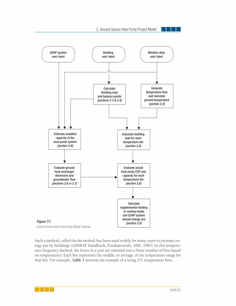
2. Ground-Source Heat Pump Project Model
GSHP.25
Such a method, called the bin method, has been used widely for many years to estimate en-ergy use by buildings (ASHRAE Handbook, Fundamentals, 1981, 1985). In this tempera-ture frequency method, the hours in a year are summed into a finite number of bins based on temperatures. Each bin represents the middle, or average, of the temperature range for that bin. For example, Table 1 presents an example of a using 2°C temperature bins.
Evaluate groundheat exchangerdimension and
groundwater flow[sections 2.6 or 2.7]
Evaluate actualheat pump COP and
capacity for eachtemperature bin
[section 2.8]
Calculatesupplemental heating
or cooling needsand GSHP systemannual energy use
[section 2.9]
Calculate buildingload for each
temperature bin[section 2.5]
CalculateBuilding load
and balance points[sections 2.3 & 2.4]
Generatetemperature bins
and calculateground temperature
[section 2.2]
Weather datauser input
Buildinguser input
GSHP systemuser input
Estimate installedcapacity of the
heat pump system[section 2.8]
Figure 17:Ground-Source Heat Pump Energy Model Flowchart.

Ground-Source Heat Pump Project Analysis Chapter
GSHP.26
Bins# of hours
of occurrencein a year
-20 15
-18 35
-16 75
-14 132
[…] […]
24 185
26 79
28 24
30 12
Total 8760
Table 1: Example of a 2°C Temperature Bins.
Therefore, from Table 1, there would be 15 hours in that year where the temperature is less than –19°C but greater or equal to – 21°C. A basic level of time dependency can also be incorporated in the bin method. This is achieved by splitting up the temperature bins as a function of time. Hence, bins can be compiled, for example, for approximate daytime hours and separately for night time hours.
Using this bin approach, it is possible to capture the GSHP-Building system temperature dependant behaviour and some time dependant parameters, and estimate the system’s annual energy use. A further refinement of the method, called the modified bin method, is presented in ASHRAE Handbook, Fundamentals (1985). This method allows for off-de-sign calculations by using an estimated diversified load rather than peak load values in establishing the building’s load as a function of temperature. The building’s calculation algorithms employed in the RETScreen GSHP Project Model are largely inspired from this modified bin method.
Using the modified bin method allows for estimating the energy demand from the build-ing, but the GSHP system’s heat pumps and ground loop performances still need to be addressed. Fortunately, the bin method can readily be extended for treating GSHP systems. The method adopted for doing so was largely adapted from the International Ground-Source Heat Pump Association’s (IGSHPA) Closed-Loop/Ground-Source Heat Pump Systems – In-stallation Guide (1988).
It should be noted that some parts of the GSHP model are concerned chiefly with sizing, for example when determining heating or cooling energy demand (Sections 2.3 and 2.4), or the length of the ground heat exchanger (Section 2.6) or the groundwater flow in an

2. Ground-Source Heat Pump Project Model
GSHP.27
open-loop system (Section 2.7). In these cases, calculations are then performed for extreme circumstances called the design conditions. For example, the heating design temperature represents the minimum temperature that has been measured for a frequency level of at least 1% over the year, for the specific location. Similarly the cooling design temperature represents the maximum temperature that has been measured for a frequency level of at least 1% over the year.
Other parts of the GSHP model are concerned with determining the seasonal energy use or supplemental energy delivered (see Section 2.5). This requires evaluating the performance of the system over the whole year, that is, for all temperature bins.
2.2 Weather Data
Basically, GSHP systems are designed by balancing the heating and cooling load of a build-ing with the heating and cooling capacity that could be extracted from the ground. Since this load and this capacity are in direct relation with the air and soil temperatures varia-tions, this data is needed to assess a GSHP project. This section presents how the GSHP Project Model deals with this data requirement.
2.2.1 Generation of temperature bins
Fundamental to the GSHP model philosophy is the availability of temperature bins for daytime and nighttime hours for the selected location. Additionally, bin data for the coldest and hottest months (corresponding to design heating and cooling conditions) are required for the ground loop calculation. Such a heavy user-data requirement would render the model impractical. Alternatively, storing the data within the model would translate into an excessively large file if even a moderate number of locations around the world were to be included.
To circumvent this problem, an hourly weather data generator is included in the RETScreen GSHP Project Model. This generator is based on empirical correlations between measured hourly weather data and their design temperatures and latitude, as defined in ASHRAE (1997). A validation of the generation of temperature bins by the RETScreen GSHP Project Model can be found in Section 2.10.1. Note that the use of a generator does not restrict the generality of the method. If appropriate bin data are available, they could be used in the GSHP model without any change to the other algorithms.
2.2.2 Ground temperature estimation
The method for sizing the ground heat exchanger (GHX) described in Section 2.6.1 requires knowledge of the minimum and maximum ground temperature at the GHX depth. Ground temperature is also used in the model to evaluate residential building basement heat losses, as presented in Section 2.3.2.
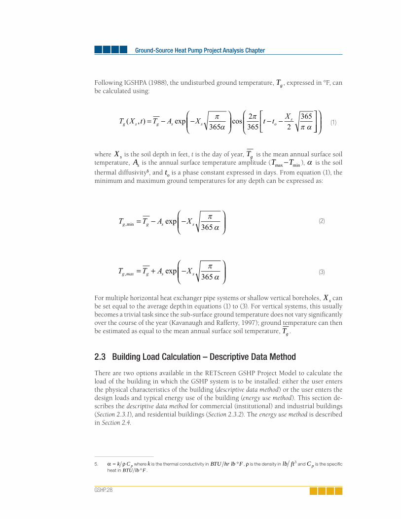
Ground-Source Heat Pump Project Analysis Chapter
GSHP.28
Following IGSHPA (1988), the undisturbed ground temperature, Tg , expressed in °F, can be calculated using:
(1)
where X s is the soil depth in feet, t is the day of year, Tg is the mean annual surface soil temperature, As is the annual surface temperature amplitude (T Tmax min ), α is the soil
thermal diffusivity5, and to is a phase constant expressed in days. From equation (1), the minimum and maximum ground temperatures for any depth can be expressed as:
(2)
(3)
For multiple horizontal heat exchanger pipe systems or shallow vertical boreholes, X s can be set equal to the average depth
in equations (1) to (3). For vertical systems, this usually
becomes a trivial task since the sub-surface ground temperature does not vary significantly over the course of the year (Kavanaugh and Rafferty, 1997); ground temperature can then be estimated as equal to the mean annual surface soil temperature, Tg .
2.3 Building Load Calculation – Descriptive Data Method
There are two options available in the RETScreen GSHP Project Model to calculate the load of the building in which the GSHP system is to be installed: either the user enters the physical characteristics of the building (descriptive data method) or the user enters the design loads and typical energy use of the building (energy use method). This section de-scribes the descriptive data method for commercial (institutional) and industrial buildings (Section 2.3.1), and residential buildings (Section 2.3.2). The energy use method is described in Section 2.4.
5. pCk ρα = where k is the thermal conductivity in FlbhrBTU ° , ρ is the density in 3ftlb and pC is the specifi c
heat in FlbBTU ° .
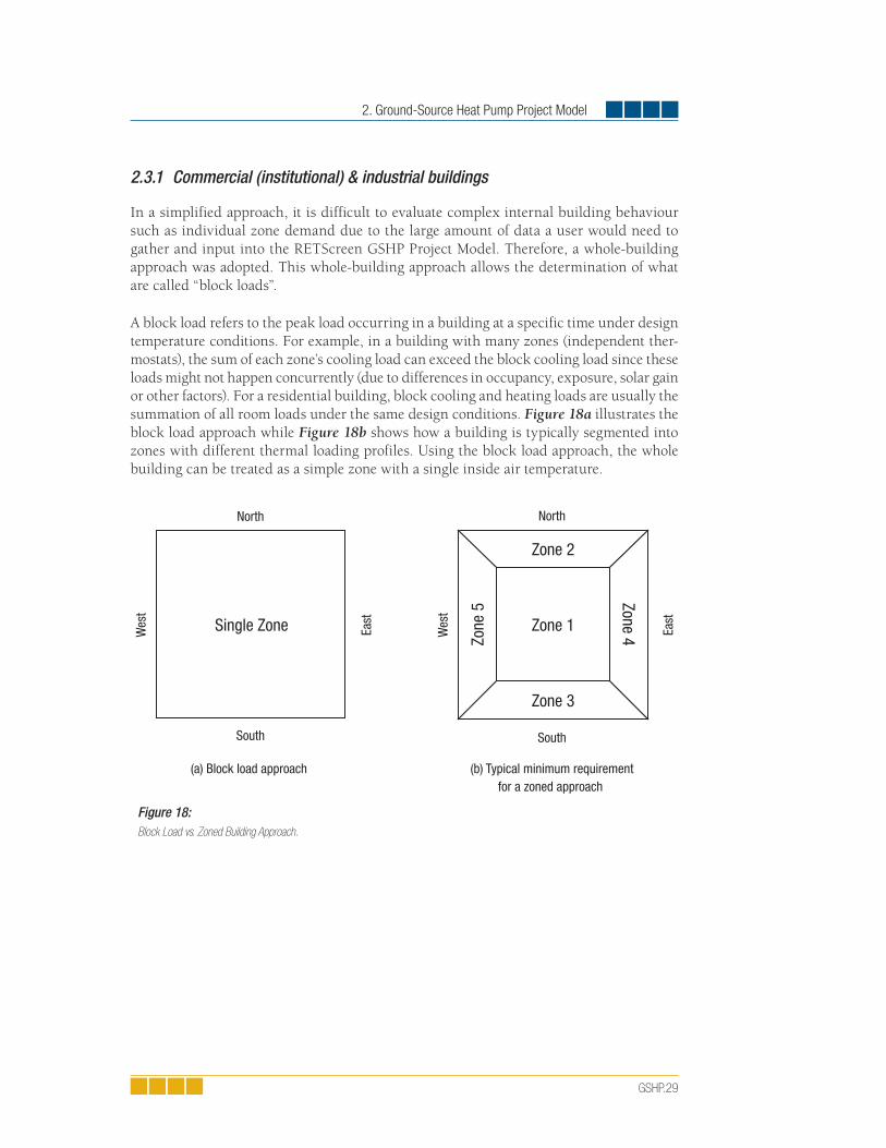
2. Ground-Source Heat Pump Project Model
GSHP.29
2.3.1 Commercial (institutional) & industrial buildings
In a simplified approach, it is difficult to evaluate complex internal building behaviour such as individual zone demand due to the large amount of data a user would need to gather and input into the RETScreen GSHP Project Model. Therefore, a whole-building approach was adopted. This whole-building approach allows the determination of what are called “block loads”.
A block load refers to the peak load occurring in a building at a specific time under design temperature conditions. For example, in a building with many zones (independent ther-mostats), the sum of each zone’s cooling load can exceed the block cooling load since these loads might not happen concurrently (due to differences in occupancy, exposure, solar gain or other factors). For a residential building, block cooling and heating loads are usually the summation of all room loads under the same design conditions. Figure 18a illustrates the block load approach while Figure 18b shows how a building is typically segmented into zones with different thermal loading profiles. Using the block load approach, the whole building can be treated as a simple zone with a single inside air temperature.
Single Zone
North
East
South
Wes
t
Wes
t
North
East
South
Zone 1
Zone 2
Zone 3
Zone 4Zone
5
(a) Block load approach (b) Typical minimum requirementfor a zoned approach
Figure 18:Block Load vs. Zoned Building Approach.

Ground-Source Heat Pump Project Analysis Chapter
GSHP.30
Relationships between outside temperature and the various building heating and cooling load components must be established, as described in the modified bin method presented in ASHRAE (1985). The following load components are treated in the RETScreen GSHP Project Model:
Transmission losses (conductive and convective);
Solar gains (sensible);
Fresh air loads (latent and sensible);
Internal gains (latent and sensible); and
Occupant loads (latent and sensible)6.
Each load component is expressed as a polynomial of zeroth, first or second order, as shown in the following generic equations (4), (5) and (6):
(4)
(5)
(6)
where q j is the building load from source j (e.g. transmission losses, solar gains, fresh air, internal gains, and occupant loads), To is the outside air temperature, and c j0, , c j1, and c j2, are polynomial coefficients derived from physical building characteristics related to source j . The modified bin method presented in ASHRAE (1985) does not use 2nd order polynomi-
als. This term has been added in the RETScreen GSHP Project Model to account for fresh air latent loads, as will be shown later. The global building load equation as a function of outside air temperature can be obtained through a summation of all n load components:
(7)
6. Air-conditioning cooling loads are made up of two components called sensible and latent loads. Sensible loads refer
to the capacity required to maintain the temperature of the indoor air while latent loads refer to the capacity required
to maintain the humidity, or water content, of the indoor air. A typical air-conditioner can be designed with 60 to 80%
of its capacity intended for sensible heat loads and 20 to 40% for latent, dehumidifying loads. Most of the latent load
comes from fresh air makeup and from building occupants.
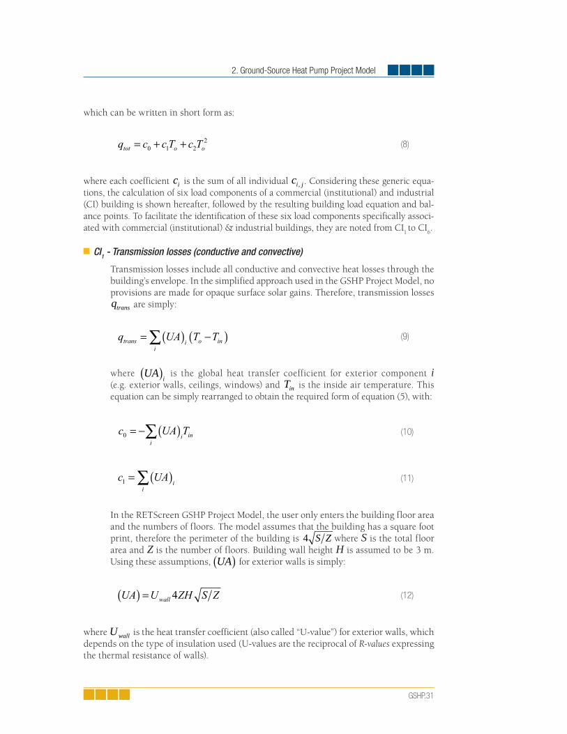
2. Ground-Source Heat Pump Project Model
GSHP.31
which can be written in short form as:
(8)
where each coefficient ci is the sum of all individual ci j, . Considering these generic equa-tions, the calculation of six load components of a commercial (institutional) and industrial (CI) building is shown hereafter, followed by the resulting building load equation and bal-ance points. To facilitate the identification of these six load components specifically associ-ated with commercial (institutional) & industrial buildings, they are noted from CI
1 to CI
6.
CI1 - Transmission losses (conductive and convective)
Transmission losses include all conductive and convective heat losses through the building’s envelope. In the simplified approach used in the GSHP Project Model, no provisions are made for opaque surface solar gains. Therefore, transmission losses qtrans are simply:
(9)
where UAi( ) is the global heat transfer coefficient for exterior component i
(e.g. exterior walls, ceilings, windows) and Tin is the inside air temperature. This equation can be simply rearranged to obtain the required form of equation (5), with:
(10)
(11)
In the RETScreen GSHP Project Model, the user only enters the building floor area and the numbers of floors. The model assumes that the building has a square foot print, therefore the perimeter of the building is 4 S Z where S is the total floor area and Z is the number of floors. Building wall height H is assumed to be 3 m. Using these assumptions, UA( ) for exterior walls is simply:
(12)
where Uwall is the heat transfer coefficient (also called “U-value”) for exterior walls, which depends on the type of insulation used (U-values are the reciprocal of R-values expressing the thermal resistance of walls).
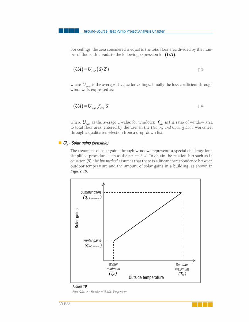
Ground-Source Heat Pump Project Analysis Chapter
GSHP.32
For ceilings, the area considered is equal to the total floor area divided by the num-ber of floors; this leads to the following expression for UA( ):
(13)
where Uceil is the average U-value for ceilings. Finally the loss coefficient through windows is expressed as:
(14)
where Uwin is the average U-value for windows; fwin is the ratio of window area to total floor area, entered by the user in the Heating and Cooling Load worksheet through a qualitative selection from a drop-down list.
CI2 - Solar gains (sensible)
The treatment of solar gains through windows represents a special challenge for a simplified procedure such as the bin method. To obtain the relationship such as in equation (5), the bin method assumes that there is a linear correspondence between outdoor temperature and the amount of solar gains in a building, as shown in Figure 19.
Sola
r gai
ns
Outside temperature
Summer gains(qsol, summer)
Winter gains(qsol, winter )
Winterminimum
(Tph)
Summermaximum
(Tpc)
Figure 19:Solar Gains as a Function of Outside Temperature.
2. Ground-Source Heat Pump Project Model
GSHP.33
Solar gains through windows are thus expressed as:
(15)
which can be rearranged in the form of equation (5) as , with:
(16)
(17)
In the equations above, Sc represents the building conditioned floor area, and M is the solar heat gain interpolation coefficient, expressed as:
(18)
where qsol winter, and qsol summer, are the average solar contribution for winter and summer at the building location, and Tph and Tpc are the winter (heating) and summer (cooling) design day average temperatures. The design day average tem-peratures are obtained from the heating and cooling design day temperatures Td heat, and Td cool, entered by the user in the Heating and Cooling Load worksheet of the GSHP Project Model, through:
(19)
(20)
where DR is the mean daily temperature range, also specified by the user. The cal-culation of the winter and summer average solar gains is based on the ASHRAE’s Cooling Load Factor (CLF) method (see ASHRAE, 1985, ch. 26). For the RETScreen Software modeling needs, the solar gain using this method is expressed as:
Ground-Source Heat Pump Project Analysis Chapter
GSHP.34
(21)
where ori is the orientation (North, East, South, West assumed in the GSHP Project Model), season is the warmest or coolest month (e.g. January or July in the north-ern hemisphere), MSHGFori season, is the maximum solar heat gain factor for orien-tation ori and month season at the building’s latitude, AGori is the glass area for exposure ori , SCori is the shading coefficient of glass for exposure ori , CLFtot ori, is the 24-hour sum of the cooling load factors for orientation ori , FPSseason is the fraction of possible sunshine for season , nhseason is the number of operating hours of air conditioning equipment for season , and Sc is, as before, the building con-ditioned floor area.
According to ASHRAE (1985) typical values can be assumed for the following parameters: , for summer and 0.45 for winter, nhseason = 12 for summer and 24 for winter. Finally, glass area on all orientations is assumed to be equal (and is therefore one quarter of the total glass area AG for each of the four orientations). It becomes therefore possible to factor out all constant parameters in equation (21), which becomes:
(22)
Values for the maximum solar heat gain factor MSHGFori season, are tabulated in ASHRAE (1985), Ch. 26, Table 11; they depend on orientation, month, and lati-tude. Cooling load factors CLFtot ori, are listed in Table 13 of the same reference (RETScreen GSHP Project Model assumes a “medium” thermal mass), and depend only on orientation. Consequently, the summation term in equation (22) depends only on month and latitude. To speed up calculations in the GSHP Project Model, the summation term was plotted against latitude for both winter and summer and curve fitting was used. The resulting plots and fit equations are displayed in Figure 20.
CI3 - Internal gains (sensible)
The treatment of the sensible internal gains is very simple and straightforward. Every internal gain source is assumed independent of outside temperature. As a consequence, the expression for sensible internal gains qint sens, takes the form of equation (4) (zero order polynomial) as , with:
(23)
where Kl , Ke and K p sens, are respectively gains from lighting, equipment and occu-pants. The values selected for these constants were taken from ASHRAE (1985) and PMSK (1991), as indicated in Table 2.
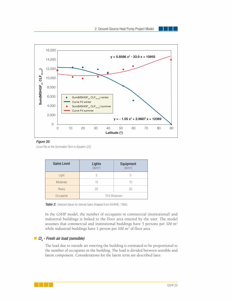
2. Ground-Source Heat Pump Project Model
GSHP.35
Gains Level Lights(W/m2)
Equipment(W/m2)
Light 5 5
Moderate 15 10
Heavy 25 20
Occupants 74.6 W/person
Table 2: Selected Values for Internal Gains (Adapted from ASHRAE, 1985).
In the GSHP model, the number of occupants in commercial (institutional) and industrial buildings is linked to the floor area entered by the user. The model assumes that commercial and institutional buildings have 5 persons per 100 m2 while industrial buildings have 1 person per 100 m2 of floor area.
CI4 - Fresh air load (sensible)
The load due to outside air entering the building is estimated to be proportional to the number of occupants in the building. The load is divided between sensible and latent component. Considerations for the latent term are described later.
Figure 20: Curve Fits on the Summation Term in Equation (22).
0
2,000
4,000
6,000
8,000
10,000
12,000
14,000
16,000
0 10 20 30 40 50 60 70 80 90Latitude (°)
Sum
(MS
HG
F ori C
LFto
t,o
ri)
Sum(MSHGFori CLFtot,ori) winter
Curve Fit winter
Sum(MSHGFori CLFtot,ori) summer
Curve Fit summer
y = 0.8586 x2 - 33.9 x + 10955
y = - 1.55 x2 + 2.9687 x + 12369
Ground-Source Heat Pump Project Analysis Chapter
GSHP.36
The generic equation for calculating the sensible load q f sens, from an outside air stream is:
(24)
where ρ is the density of air, Cp its specific heat, and V is the volumetric flow rate of entering air. This equation is readily adaptable to the generic form of equation (5) as:
(25)
with:
(26)
(27)
The model assumes constant values for air density and specific heat (ρ = 1.2 kg/m2, Cp = 1.005 (kJ/kg)/°C). The amount of fresh air entering the building, from all sources, is estimated at 20 L/s/person. A 50% heat exchange between this outside air stream and the air extracted from the building is assumed. Therefore, the net effective airflow per occupant is reduced to 10 L/s for thermal balance calculations.
CI5 - Fresh air load (latent)
The latent load considered in the GSHP model affects only air-conditioning needs. The model does not consider any type of humidification needs during the heating season. The conventional method of calculating an outside air latent load is to use the wet bulb temperature of the air entering from the outside and indoor air to obtain the water content in both streams. From the water content, and the enthalpy of saturated water vapour, the latent load q f lat, can be calculated as:
(28)
where W is the air water content expressed in kg of water per kg of dry air, is the enthalpy of saturated water vapour expressed in kJ/kg,
and Tair is the air temperature in °C. Subscripts “o” and “in” denote outside and inside air, respectively. While this formulation is exact, it requires knowing the wet bulb temperature, or the relative humidity, of the exterior air at all times. However, this information is not available in the GSHP Project Model since only dry bulb temperature bins are used.

2. Ground-Source Heat Pump Project Model
GSHP.37
Therefore, a method was adopted to allow for a basic evaluation of the fresh air latent load. In the GSHP Project Model, the user is asked to qualitatively define the project location’s humidity level. From this qualitative information, the model generates an equivalent fresh air latent load proportional to the sensible load and linearly correlated to outside temperature, as shown in Figure 21. The maximum fraction of latent load, f , to sensible load is defined as a function of the qualitative user input, as presented in Table 3. The minimum fraction, fmin, and the design day average temperature range, DT , were determined empirically to be 0.1 and 30°C respectively. The 30°C wide range insures that no negative latent load will occur for the building’s temperature bins, even though the function shown in Figure 21 can produce negative loads at sufficiently low exterior temperature.
Humidity Level Maximum latent to sensible fraction
Low 0.5
Medium 1.5
High 2.5
Table 3: Latent-to-Sensible Ratio.
Frac
tion
of s
ensi
ble
load
f
Outside temperature
Max. fractionfmax
Summer designTd,cool
Min. fractionfmin Td,cool - DT
Figure 21:Relationship between Latent and Sensible Fresh Air Load as a function of Outside Temperature.
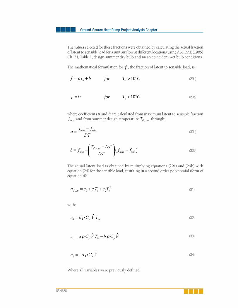
Ground-Source Heat Pump Project Analysis Chapter
GSHP.38
The values selected for these fractions were obtained by calculating the actual fraction of latent to sensible load for a unit air flow at different locations using ASHRAE (1985) Ch. 24, Table 1, design summer dry bulb and mean coincident wet bulb conditions.
The mathematical formulation for f , the fraction of latent to sensible load, is:
for T Co > °10 (29a)
f = 0 for T Co < °10 (29b)
where coefficients a and b are calculated from maximum latent to sensible fraction fmax and from summer design temperature Td cool, through:
(30a)
(30b)
The actual latent load is obtained by multiplying equations (29a) and (29b) with equation (24) for the sensible load, resulting in a second order polynomial (form of equation 6):
(31)
with:
(32)
(33)
(34)
Where all variables were previously defined.
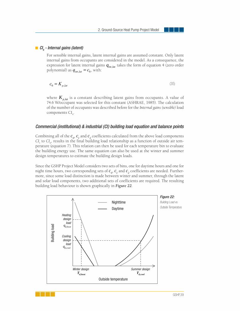
2. Ground-Source Heat Pump Project Model
GSHP.39
CI6 - Internal gains (latent)
For sensible internal gains, latent internal gains are assumed constant. Only latent internal gains from occupants are considered in the model. As a consequence, the expression for latent internal gains qint lat, takes the form of equation 4 (zero order polynomial) as , with:
(35)
where K p lat, is a constant describing latent gains from occupants. A value of 74.6 W/occupant was selected for this constant (ASHRAE, 1985). The calculation of the number of occupants was described before for the Internal gains (sensible) load components CI
4.
Commercial (institutional) & industrial (CI) building load equation and balance points
Combining all of the c0, c1 and c2 coefficients calculated from the above load components CI
1 to CI
6, results in the final building load relationship as a function of outside air tem-
perature (equation 7). This relation can then be used for each temperature bin to evaluate the building energy use. The same equation can also be used at the winter and summer design temperatures to estimate the building design loads.
Since the GSHP Project Model considers two sets of bins, one for daytime hours and one for night time hours, two corresponding sets of c0, c1 and c2 coefficients are needed. Further-more, since some load distinction is made between winter and summer, through the latent and solar load components, two additional sets of coefficients are required. The resulting building load behaviour is shown graphically in Figure 22.
Build
ing
load
Outside temperature
Summer designTd,cool
Winter designTd,heat
Heatingdesign
loadqd,heat
Coolingdesign
loadqd,cool
Nighttime
Daytime
Figure 22:Building Load vs.
Outside Temperature.
Ground-Source Heat Pump Project Analysis Chapter
GSHP.40
In order for the model to be able to select between the heating and cooling load coefficients, the building balance temperatures must be estimated for heating and cooling conditions. These balance points represent the temperature above and below which the building does not require heating and cooling respectively. These balance points can be seen in Figure 22, at the locations where the curves intercept the x-axis. The balance temperature Tbal can be found by finding the roots of equation (7):
(36)
(One of the two roots is selected based on physical considerations). For the case where there is no quadratic term, the equation simplifies to:
(37)
2.3.2 Residential buildings
The approach selected for residential buildings is very similar to the one presented for com-mercial (institutional) & industrial buildings in the previous Section 2.3.1. The assumption of a single zone model, as shown in Figure 18a, is also applied here. However, contrary to CI buildings, this assumption is a fair approximation of what is mostly encountered in the residential sector, especially for homes equipped with central heating systems.
Therefore, the simplified building model for residential applications should lead to more ro-bust estimations of building loads and energy use when choosing the descriptive method. This is attributable in part to the more closely matched zoning assumption but also to the greater homogeneity in building use and architecture in the residential market.
While most of the heat loss and heat gain components presented in Section 2.3.1 are com-mon to residential applications, a number of specific adaptations are suited to this type of building. Most important are the explicit consideration of basement loads, and the modified treatment of fresh air load calculations. Basement heat losses are not considered for CI buildings since they are assumed to be negligible compared to the overall building demand. This is not the case for residential or small commercial buildings, where basement heat losses can account for a significant portion of the total design demand.
As for CI buildings described in Section 2.3.1, each heating or cooling load is expressed through an explicit relation between the load and the outside air temperature (equations 4 to 6). However, the presence of below-grade components results in one additional type of relation being considered:
(38)
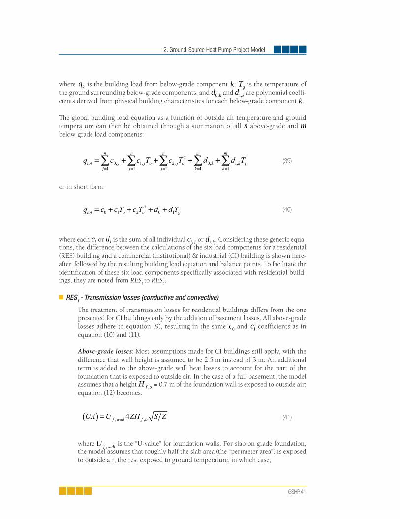
2. Ground-Source Heat Pump Project Model
GSHP.41
where qk is the building load from below-grade component k , Tg is the temperature of the ground surrounding below-grade components, and d k0, and d k1, are polynomial coeffi-cients derived from physical building characteristics for each below-grade component k.
The global building load equation as a function of outside air temperature and ground temperature can then be obtained through a summation of all n above-grade and m below-grade load components:
(39)
or in short form:
(40)
where each ci or di is the sum of all individual ci j, or di k, . Considering these generic equa-tions, the difference between the calculations of the six load components for a residential (RES) building and a commercial (institutional) & industrial (CI) building is shown here-after, followed by the resulting building load equation and balance points. To facilitate the identification of these six load components specifically associated with residential build-ings, they are noted from RES
1 to RES
6.
RES1 - Transmission losses (conductive and convective)
The treatment of transmission losses for residential buildings differs from the one presented for CI buildings only by the addition of basement losses. All above-grade losses adhere to equation (9), resulting in the same c0 and c1 coefficients as in equation (10) and (11).
Above-grade losses: Most assumptions made for CI buildings still apply, with the difference that wall height is assumed to be 2.5 m instead of 3 m. An additional term is added to the above-grade wall heat losses to account for the part of the foundation that is exposed to outside air. In the case of a full basement, the model assumes that a height H f o, = 0.7 m of the foundation wall is exposed to outside air; equation (12) becomes:
(41)
where U f wall, is the “U-value” for foundation walls. For slab on grade foundation, the model assumes that roughly half the slab area (the “perimeter area”) is exposed to outside air, the rest exposed to ground temperature, in which case,

Ground-Source Heat Pump Project Analysis Chapter
GSHP.42
(42)
where U f floor, is the “U-value” for the basement floor.
Below-grade losses: The approach for estimating below-grade foundation heat losses is largely inspired from the approach used in the low-rise residential energy analysis and design software HOT2000TM (1991). The losses for full basement below-grade components are divided in four parts:
1. Upper below-grade wall, representing approximately 1/3 of the below-grade height;
2. Lower below-grade wall, representing the remaining 2/3 of the below-grade height;
3. Floor perimeter area, assumed in the model to be half the fl oor area; and
4. Floor centre area, assumed to be half the fl oor area.
For slab on grade foundation, only the fourth component applies. Transmission losses are expressed in a way similar to (9), except that outside air temperature must be replaced by ground temperature:
(43)
Since the bin method only provides air temperature distribution, a linear correlation between the outside air temperature and the ground temperature is used to obtain the ground temperature for each bin:
(44)
where Tbin is the bin temperature. The resulting d0 and d1 coefficients for each below-grade components are for below-grade walls (full foundation):
(45)
(46)

2. Ground-Source Heat Pump Project Model
GSHP.43
and for below-grade floor (full foundation):
(47)
(48)
For slab on grade foundations, only the last two equations, divided by 2, applies. The treatment of ceiling and windows is similar to the CI building case (CI
1), except
that windows are assumed to occupy a constant 20% of the total floor area.
RES2 - Solar gains (sensible)
Calculation of solar gains for residential buildings is identical to that of CI build-ings ones (CI
2), with the exception of window area, which is defined for the load
components RES1 as having an equal distribution of the window surface across the
four wall orientations.
RES3 - Internal gains (sensible)
The treatment of internal gains is similar to the CI building case (CI3), where
, but with:
(49)
where Kint represents gains from all equipment, lights and appliances, and K p sens, represents gains from occupants. The constants in the equation above were assumed to be 14 W/m2 for internal gains and 74.6 W/person for occupants (ASHRAE, 1985). Unlike commercial (institutional) & industrial buildings, the number of occupants is not linked to the floor area. The model considers that residential buildings have 2 adults and 2 children at all times; the average heat gain from children is taken as half that of an adult.
RES4 - Fresh air load (sensible)
The load due to outside air entering into the building is estimated exactly as described for the CI buildings load component (CI
4). However, the volume of fresh air into a
residential building is not related to the number of occupants but rather to the level of insulation indicated qualitatively by the user: the higher the insulation level, the lower the amount of air entering the building. Table 4 shows the number of air changes per hour (ACH), as a function of insulation level (Hydro-Québec, 1994).
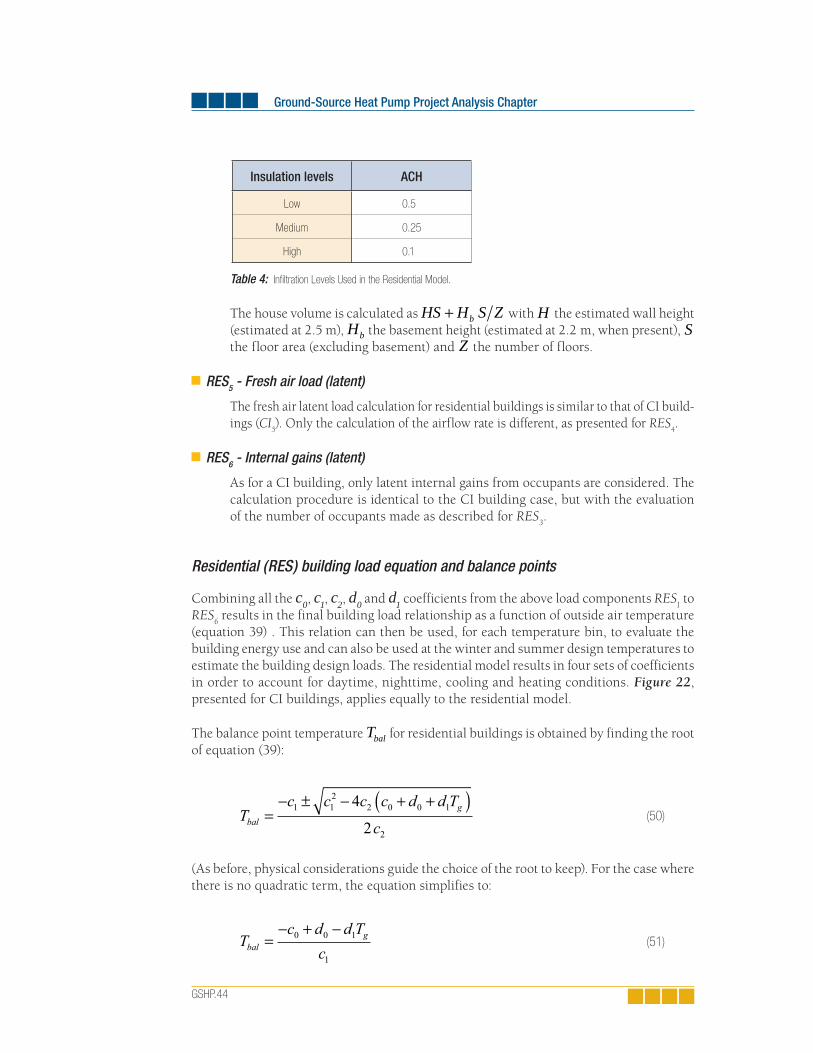
Ground-Source Heat Pump Project Analysis Chapter
GSHP.44
Insulation levels ACH
Low 0.5
Medium 0.25
High 0.1
Table 4: Infi ltration Levels Used in the Residential Model.
The house volume is calculated as HS H S Zb+ with H the estimated wall height (estimated at 2.5 m), Hb the basement height (estimated at 2.2 m, when present), S the floor area (excluding basement) and Z the number of floors.
RES5 - Fresh air load (latent)
The fresh air latent load calculation for residential buildings is similar to that of CI build-ings (CI
5). Only the calculation of the airflow rate is different, as presented for RES
4.
RES6 - Internal gains (latent)
As for a CI building, only latent internal gains from occupants are considered. The calculation procedure is identical to the CI building case, but with the evaluation of the number of occupants made as described for RES
3.
Residential (RES) building load equation and balance points
Combining all the c0, c1, c2, d0 and d1 coefficients from the above load components RES1 to
RES6 results in the final building load relationship as a function of outside air temperature
(equation 39) . This relation can then be used, for each temperature bin, to evaluate the building energy use and can also be used at the winter and summer design temperatures to estimate the building design loads. The residential model results in four sets of coefficients in order to account for daytime, nighttime, cooling and heating conditions. Figure 22, presented for CI buildings, applies equally to the residential model.
The balance point temperature Tbal for residential buildings is obtained by finding the root of equation (39):
(50)
(As before, physical considerations guide the choice of the root to keep). For the case where there is no quadratic term, the equation simplifies to:
(51)

2. Ground-Source Heat Pump Project Model
GSHP.45
2.4 Building Load Calculation – Energy Use Method
The descriptive data method for building load calculation, detailed in the previous Section 2.3, is useful when dealing with a new building. However, this approach may not always be appropriate, especially for commercial (institutional) & industrial buildings which are usually more complex. An alternate method is to have the user enter known building energy related information, namely the building’s annual energy use and its de-sign loads. From this information, a relation similar to equation (5) can be derived. This method, called the Energy use method, is described in this section.
Build
ing
heat
ing
load
(a) Outside temperature
(b) Temperature bins
Heatingdesign
loadqd,heat
Winter designTd,heat
Balance pointTbal
Hour
s of
occ
urre
nce
Figure 23:Information Available
for Energy Use Method.
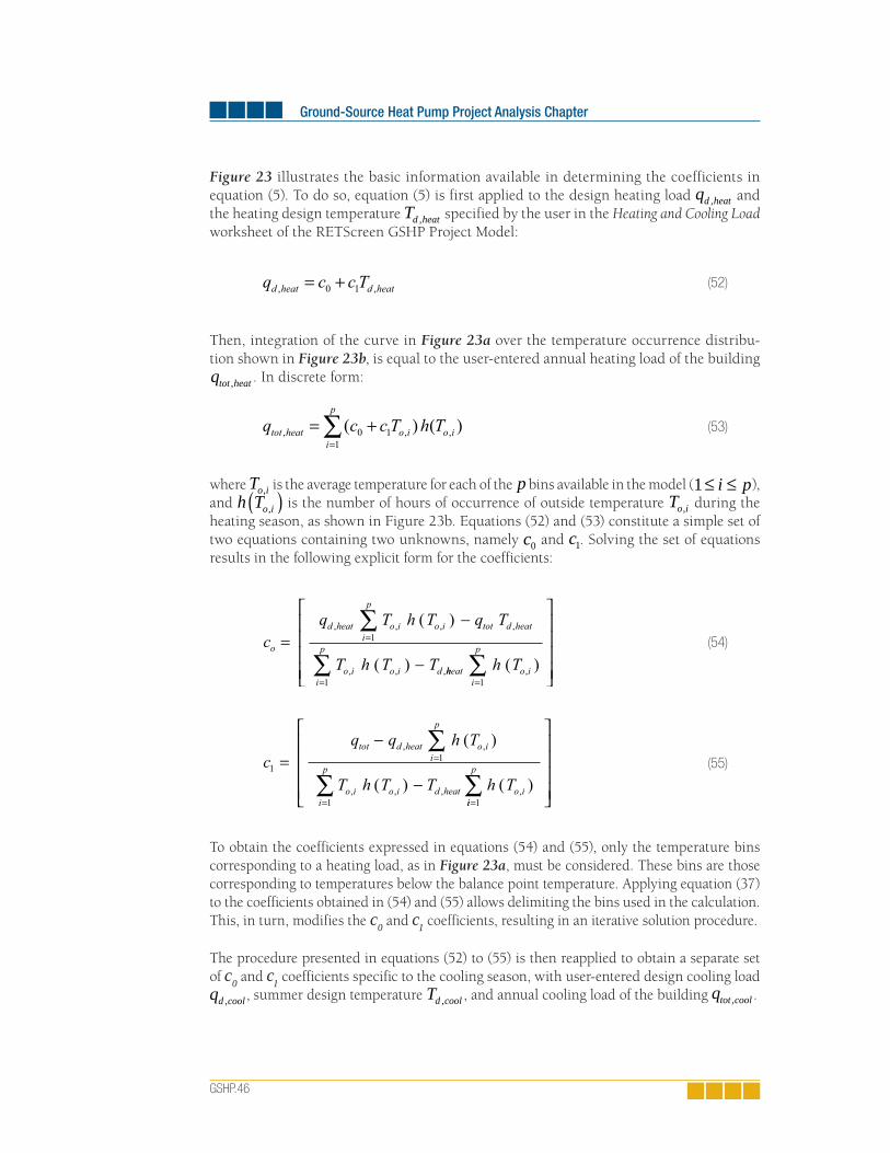
Ground-Source Heat Pump Project Analysis Chapter
GSHP.46
Figure 23 illustrates the basic information available in determining the coefficients in equation (5). To do so, equation (5) is first applied to the design heating load qd heat, and the heating design temperature Td heat, specified by the user in the Heating and Cooling Load worksheet of the RETScreen GSHP Project Model:
(52)
Then, integration of the curve in Figure 23a over the temperature occurrence distribu-tion shown in Figure 23b, is equal to the user-entered annual heating load of the building qtot heat, . In discrete form:
(53)
where To i, is the average temperature for each of the p bins available in the model (1≤ ≤i p), and h To i,( ) is the number of hours of occurrence of outside temperature To i, during the heating season, as shown in Figure 23b. Equations (52) and (53) constitute a simple set of two equations containing two unknowns, namely c0 and c1. Solving the set of equations results in the following explicit form for the coefficients:
(54)
(55)
To obtain the coefficients expressed in equations (54) and (55), only the temperature bins corresponding to a heating load, as in Figure 23a, must be considered. These bins are those corresponding to temperatures below the balance point temperature. Applying equation (37) to the coefficients obtained in (54) and (55) allows delimiting the bins used in the calculation. This, in turn, modifies the c0 and c1 coefficients, resulting in an iterative solution procedure.
The procedure presented in equations (52) to (55) is then reapplied to obtain a separate set of c0 and c1 coefficients specific to the cooling season, with user-entered design cooling load qd cool, , summer design temperature Td cool, , and annual cooling load of the building qtot cool, .
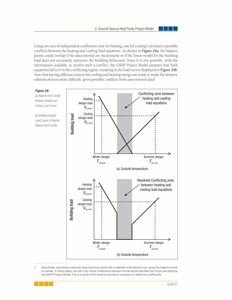
2. Ground-Source Heat Pump Project Model
GSHP.47
Using two sets of independent coefficients (one for heating, one for cooling) can lead to possible conflicts between the heating and cooling load equations. As shown in Figure 24a, the balance points could overlap if the data entered are inconsistent or if the linear model for the building load does not accurately represent the building behaviour. Since it is not possible, with the information available, to resolve such a conflict, the GSHP Project Model assumes that both equations fall to 0 in the conflicting region, resulting in the load curves displayed in Figure 24b. Note that having different sources for cooling and heating energy use tends to make the iterative solution process more difficult, given possible conflicts from user-entered data7.
7. Specifi cally, specifying a relatively large load associated with a relatively small demand can cause the balance points
to overlap. In these cases, the user may notice a difference between the demands specifi ed and those calculated by
the GSHP Project Model. This is a result of the iterative procedure necessary to obtain the coeffi cients.
Conflicting zone betweenheating and cooling
load equations
Resolved Conflicting zone between heating and
cooling load equations
Build
ing
load
Build
ing
load
Heatingdesign load
qd,heat
Coolingdesign load
qd,cool
Heatingdesign load
qd,heat
Coolingdesign load
qd,cool
Winter designTd,heat
Summer designTd,cool
Winter designTd,heat
Summer designTd,cool
(a) Outside temperature
(b) Outside temperature
Figure 24:(a) Balance Point Confl ict
Between Heating and
Cooling Load Curves.
(b) Modifi ed Building
Load Curves to Resolve
Balance Point Confl ict.

Ground-Source Heat Pump Project Analysis Chapter
GSHP.48
2.5 Building Load Calculation for each Temperature Bin
The steps described in previous Section 2.3 and Section 2.4 for respectively the Descriptive Data Method and the Energy Use Method lead to the calculation of building load for each temperature bin generated (see Section 2.2.1). This is done through equations (7) for com-mercial (institutional) & industrial buildings, and (39) for residential buildings, taking into account the balance point temperatures.
As an example of such calculation, Table 5 shows the application of the method to a 2°C daytime temperature bin. The building’s total energy demand for heating and cooling is simply evaluated by combining the calculated demand with the hours of occurrence of the temperature bins and the balance point temperatures, using the algorithms shown in the previous sections.
Bins
(°C)
January
(h)
July
(h)
Rest of year
(h)
Cooling Demand(yes/no)
Heating Demand(yes/no)
Building load(- for cooling)
(kW)
-12 0 0 0 no yes 4.59
-10 2 0 0 no yes 4.39
-8 9 0 3 no yes 4.18
-6 27 0 12 no yes 3.98
-4 56 0 68 no yes 3.77
-2 101 0 128 no yes 3.57
0 54 0 188 no yes 3.36
2 62 0 223 no yes 3.16
4 17 0 275 no yes 2.95
6 5 0 235 no yes 2.75
8 0 0 189 no yes 2.54
10 0 0 218 no yes 2.34
12 0 0 162 yes yes 0.00
14 0 0 191 yes yes 0.00
16 0 0 167 yes yes 0.00
18 0 0 193 yes no -1.62
20 0 10 208 yes no -1.82
22 0 28 260 yes no -2.02
24 0 57 236 yes no -2.22
26 0 89 195 yes no -2.42
28 0 67 121 yes no -2.62
30 0 57 58 yes no -2.82
32 0 23 21 yes no -3.02
34 0 0 0 yes no -3.22
Table 5: Example of Building Load Calculation for a 2°C Temperature Bins (building occupancy is from 8 a.m. to 7 p.m., leading to 4,015 hours of use during the year).
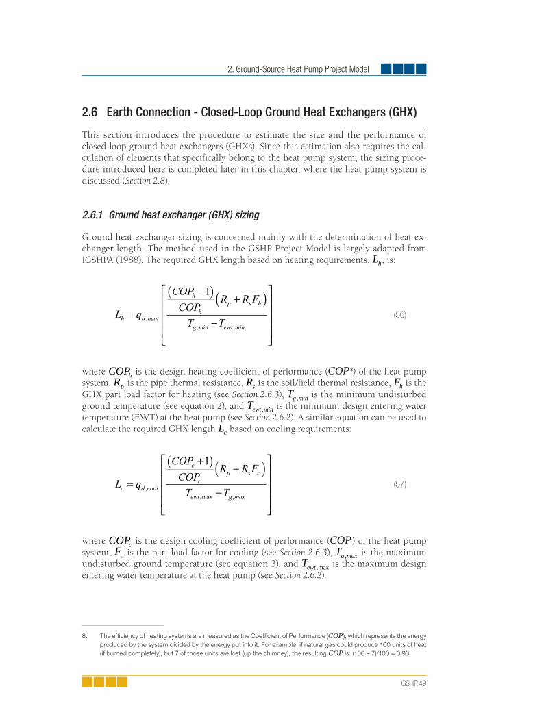
2. Ground-Source Heat Pump Project Model
GSHP.49
2.6 Earth Connection - Closed-Loop Ground Heat Exchangers (GHX)
This section introduces the procedure to estimate the size and the performance of closed-loop ground heat exchangers (GHXs). Since this estimation also requires the cal-culation of elements that specifically belong to the heat pump system, the sizing proce-dure introduced here is completed later in this chapter, where the heat pump system is discussed (Section 2.8).
2.6.1 Ground heat exchanger (GHX) sizing
Ground heat exchanger sizing is concerned mainly with the determination of heat ex-changer length. The method used in the GSHP Project Model is largely adapted from IGSHPA (1988). The required GHX length based on heating requirements, Lh, is:
(56)
where COPh is the design heating coefficient of performance (COP 8) of the heat pump system, Rp is the pipe thermal resistance, Rs is the soil/field thermal resistance, Fh is the GHX part load factor for heating (see Section 2.6.3), Tg min, is the minimum undisturbed ground temperature (see equation 2), and Tewt min, is the minimum design entering water temperature (EWT) at the heat pump (see Section 2.6.2). A similar equation can be used to calculate the required GHX length Lc based on cooling requirements:
(57)
where COPc is the design cooling coefficient of performance (COP) of the heat pump system, Fc is the part load factor for cooling (see Section 2.6.3), Tg max, is the maximum undisturbed ground temperature (see equation 3), and Tewt ,max is the maximum design entering water temperature at the heat pump (see Section 2.6.2).
8. The effi ciency of heating systems are measured as the Coeffi cient of Performance (COP ), which represents the energy
produced by the system divided by the energy put into it. For example, if natural gas could produce 100 units of heat
(if burned completely), but 7 of those units are lost (up the chimney), the resulting COP is: (100 – 7)/100 = 0.93.

Ground-Source Heat Pump Project Analysis Chapter
GSHP.50
These two equations represent a simplification of the ones developed by Ingersoll and presented in Kavanaugh and Rafferty (1997). Equations (56) and (57) do not take into consideration long-term thermal imbalances that could alter the soil temperature field over a period of many years. These thermal imbalances are generally attributable to significant differences between the annual heat extracted from the ground and the heat that is rejected to the ground during the cooling season. However, this simplification could be considered acceptable at the preliminary feasibility evaluation stage.
There are a large number of possible configurations for both vertical and horizontal systems (see Figure 12). To simplify the input requirements, the RETScreen GSHP Project Model is based on one type of horizontal and one type of vertical GHX configuration. A stacked two-pipe system (31.8 mm nominal diameter with one pipe 1.8 m deep and the other 1.2 m below the surface), is used for horizontal GHX (see Figure 25a), while one U-tube (31.8 mm nominal diameter) per borehole is used for vertical GHX (see Figure 25b).
Equations (56) and (57) require the determination of pipe thermal resistance Rp and soil/field thermal resistance Rs. These are determined from geometrical and physical considerations, as shown in IGSHPA (1988). For horizontal GHX, the method takes into account surface ef-fects that have a significant influence on horizontal soil/field resistance values. Soil resistance values are tabulated as a function of radial distance for different kinds of soil (e.g. light soil or heavy soil, damp or dry, rock, etc.). Thermal resistances for permafrost were extrapolated from those for regular soil, based on soil conductivity properties.
As shown by equations (56) and (57), there are two possible heat exchanger lengths that can be used for designing a closed-loop system. The choice between using the cooling or heat-ing length is left to the user in the Energy Model worksheet of the RETScreen GSHP Project Model. This design decision has an impact on both cost and performance of the GSHP sys-tem. Selecting a GHX length that will not be sufficient for heating will require an auxiliary heating system. Using a GHX length insufficient for cooling will require a supplemental heat rejector. The GSHP Project Model takes into account these two possibilities when modelling the GHX. For example, if the cooling mode design criterion was selected by the user in the Heating and Cooling Load worksheet, the RETScreen GSHP Project Model will estimate the maximum heating capacity that will be available based on the cooling length selected.
(b) Vertical arrangement(viewed from top)
(a) Horizontal arrangement(cross-section)
1.2 m1.8 m
Figure 25:RETScreen GSHP Project
Model GHX Confi gurations.
2. Ground-Source Heat Pump Project Model
GSHP.51
2.6.2 Design entering water temperature (Tewt )
The design of a GHX is in many ways similar to that of a conventional heat exchanger. For a conventional heat exchanger, the inlet and outlet temperatures are usually provided for sizing the heat exchanger. This also applies for a GHX: the final size of the GHX is in great part determined by the user’s requirements for the minimum or maximum temperatures allowed at the GHX’s outlet during the course of the year.
However, the values for the maximum and minimum GHX outlet temperatures have a fairly limited range of acceptable values. Practical constraints, mainly from the heat pumps, tend to make this design decision more straightforward.
For example, extended range heat pumps will usually have a 20°F (-6.7°C) recommended minimum design entering water temperature (Tewt min, ) and 110°F (92.2°C) recommended maximum design entering water temperature (Tewt ,max ). Specific designs may go below and above these temperatures but are not common. From a literature review (ASHRAE 1995, Kavanaugh and Rafferty 1997, IGSHPA 1988), the following design entering water temperature estimates were used in the GSHP model:
Minimum design entering water temperature:
Maximum design entering water temperature:
Since the model was also designed to be used in permafrost, the 20°F minimum entering water temperature limitation was not implemented.
2.6.3 Part load factor (F )
Determining the GHX length using equations (56) and (57) requires the evaluation of the GHX part load factor. The part load factor (F ) represents the fraction of equivalent full load hours during the design month to the total number of hours in that month, as seen by the GHX (Kavanaugh and Rafferty, 1997). It can be evaluated as:
(58)
where q and qmax are the average load and peak load for the month respectively. The part load factor F is evaluated for the design cooling month and the design heating month, typically July and January in the Northern Hemisphere, leading to the values Fc and Fh used in equations (56) and (57).
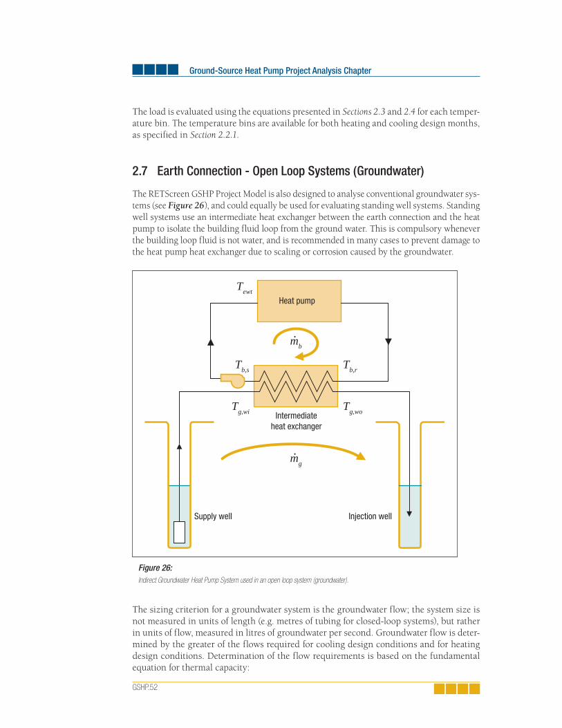
Ground-Source Heat Pump Project Analysis Chapter
GSHP.52
The load is evaluated using the equations presented in Sections 2.3 and 2.4 for each temper-ature bin. The temperature bins are available for both heating and cooling design months, as specified in Section 2.2.1.
2.7 Earth Connection - Open Loop Systems (Groundwater)
The RETScreen GSHP Project Model is also designed to analyse conventional groundwater sys-tems (see Figure 26), and could equally be used for evaluating standing well systems. Standing well systems use an intermediate heat exchanger between the earth connection and the heat pump to isolate the building fluid loop from the ground water. This is compulsory whenever the building loop fluid is not water, and is recommended in many cases to prevent damage to the heat pump heat exchanger due to scaling or corrosion caused by the groundwater.
The sizing criterion for a groundwater system is the groundwater flow; the system size is not measured in units of length (e.g. metres of tubing for closed-loop systems), but rather in units of flow, measured in litres of groundwater per second. Groundwater flow is deter-mined by the greater of the flows required for cooling design conditions and for heating design conditions. Determination of the flow requirements is based on the fundamental equation for thermal capacity:
Heat pump
Intermediateheat exchanger
Supply well Injection well
Tb,s Tb,r
Tg,woTg,wi
Tewt
mb
mg
Figure 26:Indirect Groundwater Heat Pump System used in an open loop system (groundwater).

2. Ground-Source Heat Pump Project Model
GSHP.53
(59)
QC T T
COPCOP
d cool
p g wo g wi
c
c
= ( )+( ),
, ,
1 (60)
where mheat and mcool are the required well water flow rate for heating and cooling, Qd heat, and Qd cool, are the design heating and cooling heat pump capacities (see Section 2.8.1), COPh and COPc are the heat pump performances at design heating and cooling condi-tions (see Section 2.8.1), ρ is the density of water, Cp is the specific heat of water, and Tg wi, and Tg wo, are the groundwater temperatures entering and leaving the intermediate heat exchanger located between the earth connection and the heat pump as shown in Figure 26. As a first approximation, the groundwater temperature Tg wi, is assumed to be equal to the mean annual surface soil temperature Tg (see Section 2.2.2).
In order to complete the evaluation of equations (59) and (60), the temperature of ground-water leaving the intermediate heat exchanger (Tg wo, ) must be evaluated. This can be achieved by the following two design methods, refering to Figure 26:
Select an approach temperature ΔTa between the building return temperature (Tb r, ) and the groundwater temperature leaving the intermediate heat exchanger (Tg wo, ). This approach temperature design method is explained below in this section;
or
Select a value for the heat pump heating and cooling design entering water temperature (Tewt). Since this design entering water temperature Tewt value selection design method requires the calculation of elements that specifi cally belong to heat pump system, it is explained later, as part of Section 2.8.3, assuming, in fi rst approximation, that the building supply temperature Tb s, is close to Tewt (see equation 78).
Approach temperature design method
Chapter 6 in ASHRAE (1995) gives typical values for the approach temperatures as well as for the design entering water temperatures:
[cooling] (61)
[heating] (62)
(63)
Ground-Source Heat Pump Project Analysis Chapter
GSHP.54
where Tg is the mean annual surface soil temperature.
For heating conditions, the required intermediate heat exchanger groundwater leaving temperature (Tg wo, ) can then be derived from:
(64)
(65)
where mb is the flow rate in the heat pump building loop, and ρbuilding and Cp building, are the density and the specific heat of the liquid in the building loop. Substituting equation (65) into (64) leads to:
(66)
The typical flow rate value of the fluid in the heat pump building loop (mb) recommended by groundwater-source heat pump manufacturers is 3 usgpm/Ton of installed cooling capacity (ASHRAE 1995).
Similarly for cooling conditions, the temperature of groundwater leaving the intermediate heat exchanger (Tg wo, ) is expressed as:
(67)
Resolving equations (66) and (67) gives the temperature of groundwater leaving the inter-mediate heat exchanger (Tg wo, ) that is necessary to resolve equations (59) and (60), which in turn allow to size the earth connection (e.g. the open loop system) by the determination of the required design well flow rate (m) for heating and cooling.
2.8 Heat Pump System
This section presents the modelling elements associated with the heat pump system. The calculation of these elements are necessary to finalize the earth connection sizing of either closed-loop ground heat exchangers (GHXs) or open loop systems (groundwater) previously introduced in Sections 2.6 and 2.7, respectively. The heat pump coefficient of performance (COP), and their related capacity (Qc h/ ) are evaluated first, followed by the determination of the heat pump entering water temperature for both types of earth connection.
2. Ground-Source Heat Pump Project Model
GSHP.55
2.8.1 Coeffi cient of performance (COP) and capacity (Q / )
The coefficient of performance (COP) of a heat pump system is a function of the entering water temperature. The model used in the RETScreen GSHP Project Model, which cor-relates the COP of any heat pump to the entering water temperature, is inspired by the approach employed by Tarnawski (1990).
The ground heat exchanger load and heat pump useful capacity are linked through:
For cooling:
(68)
For heating:
(69)
where Qc is the heat pump cooling capacity at the evaporator, Qhe c, is the heat rejected to the GHX at the heat pump condenser in cooling mode, Qh is the heat pump heating capacity at the condenser, and Qhe h, is the heat extracted from the GHX at the heat pump evaporator in heating mode.
The method used to model the COP and the capacity as a function of the entering fluid temperature uses a quadratic polynomial correlation:
(70)
(71)
where COPactual is the actual COP of the heat pump, COPbaseline is the nominal COP of the heat pump (e.g. measured at standard rating conditions, 0°C for heating and 25°C for cooling), Qc h/ is the capacity of the heat pump for cooling or heating, and ki and λi are correlation coefficients listed in Table 6. Finally, χ is a capacity multiplier, calculated so that the system meets either the building’s heating or cooling load.
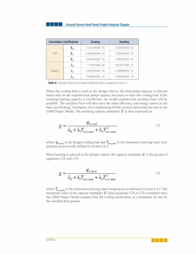
Ground-Source Heat Pump Project Analysis Chapter
GSHP.56
Correlation Coeffi cients Cooling Heating
COP
ki0 1.53105836E+00 1.00000000E+00
ki1 -2.29609500E-02 1.55970900E-02
ki2 6.87440000E-05 -1.59310000E-04
Capacity
λi0 1.41186164E+00 6.67872140E-01
λi1 -2.56202000E-03 2.79889800E-02
λi2 -7.24820000E-05 -1.06360000E-04
Table 6: Quadratic Polynomial Correlation Coeffi cients Used in equations (70) and (71).
When the cooling load is used as the design criteria, the heat pump capacity is selected based only on the required heat pump capacity necessary to meet the cooling load. If the resulting heating capacity is insufficient, the model assumes that auxiliary heat will be available. The auxiliary heat will then have the same efficiency and energy source as the base case Heating, Ventilation, Air Conditioning (HVAC) system defined by the user in the GSHP Project Model. The resulting capacity multiplier χ is then expressed as:
(72)
where qd cool, is the design cooling load and Tewt max, is the maximum entering water tem-perature as previously defined in Section 2.6.2.
When heating is selected as the design criteria, the capacity multiplier χ is the greater of equations (72) and (73):
(73)
where Tewt ,min is the minimum entering water temperature as defined in Section 2.6.2. The maximum value of the capacity multiplier χ from equations (72) or (73) is retained since the GSHP Project Model assumes that the cooling needs must, at a minimum, be met by the installed heat pumps.
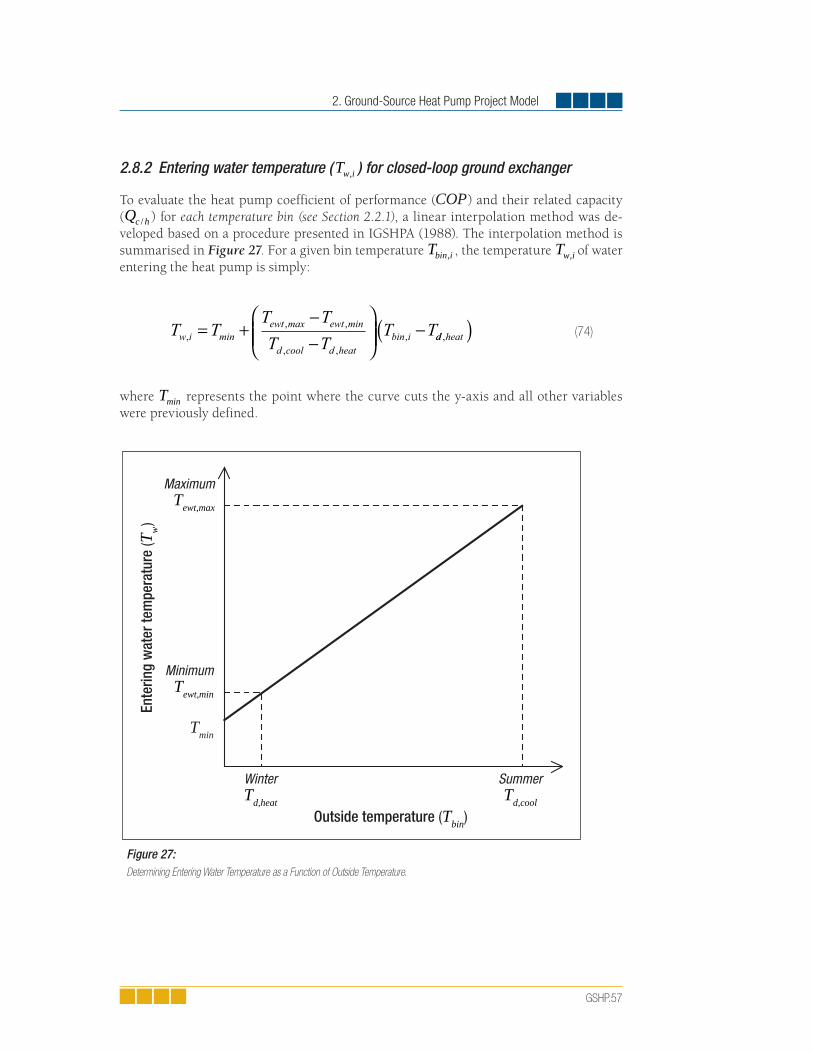
2. Ground-Source Heat Pump Project Model
GSHP.57
2.8.2 Entering water temperature ( Tw i, ) for closed-loop ground exchanger
To evaluate the heat pump coefficient of performance (COP) and their related capacity (Qc h/ ) for each temperature bin (see Section 2.2.1), a linear interpolation method was de-veloped based on a procedure presented in IGSHPA (1988). The interpolation method is summarised in Figure 27. For a given bin temperature Tbin i, , the temperature Tw i, of water entering the heat pump is simply:
(74)
where Tmin represents the point where the curve cuts the y-axis and all other variables were previously defined.
Ente
ring
wat
er te
mpe
ratu
re (T
w)
Outside temperature (Tbin)
MaximumTewt,max
MinimumTewt,min
WinterTd,heat
SummerTd,cool
Tmin
Figure 27:Determining Entering Water Temperature as a Function of Outside Temperature.

Ground-Source Heat Pump Project Analysis Chapter
GSHP.58
2.8.3 Entering water temperature (Tewt ) for open-loop (groundwater) systems 9
For groundwater systems, the entering water temperature into the heat pump is linked to the groundwater temperature and the building load by combining equation (66) with the following equation for the intermediate heat exchanger capacity on the ground loop side:
(75)
where Qg he, is the intermediate heat exchanger capacity, ρ is the density of water, Cp the specific heat of water, and gmg
. is the water flow on the ground loop side of the heat
exchanger, and the other variables were previously defined (see Figure 26).
Solving for Tb s, as a function of Tg wi, gives the required relation for the entering water temperature (Tw i, ):
For heating:
(76)
For cooling:
(77)
An additional term can be added to equations (76) and (77) to account for the temperature rise attributable to the groundwater pump. This term is expressed as:
(78)
The pump power qpump is obtained as the work required to rise the water over a height Δh from the pumping depth to the surface, plus a constant additional height Cst to account for the remainder of the groundwater loop losses:
9. The calculation made in this section completes the value selection design method introduced in Section 2.7 for sizing
open-loop systems.

2. Ground-Source Heat Pump Project Model
GSHP.59
(79)
where η pump is the pump efficiency and g is the acceleration due to gravity (9.81 m/s2). The value of Cst is set to 50 feet (15.24 m) of water.
2.9 Energy Use Evaluation
The energy use evaluations presented in this section concern the energy use by auxiliary pumps that serve to meet the heating or cooling loads that are not covered by the GSHP system.
2.9.1 Heat pump run time and energy use of auxiliary pumps
The theoretical heat pump RunTime is simply calculated for each temperature bin as:
(80)
where qtot is the building load (see Sections 2.3 and 2.4) and Q is the heat pump capacity (see Section 2.8.1). The heat pump part load factor F is calculated as:
(81)
where cd is an empirical factor (set to 0.15) accounting for the transient start/stop perform-ance penalties (ARI, 1993). This factor is commonly known as the degradation coefficient. The smaller the values of RunTime, the greater the penalty due to the degradation coefficient.
The electric energy use of the heat pump and auxiliary pumps is evaluated for every tem-perature bin. The heat pump electric demand is simply calculated as:
(82)
The auxiliary building loop pumping power is assumed to be 17 W per kW of installed cooling capacity (Kavanaugh & Rafferty, 1997). The groundwater system pumping power is obtained by dividing equation (79) by a motor efficiency.

Ground-Source Heat Pump Project Analysis Chapter
GSHP.60
2.9.2 Supplemental heating or cooling needs
The supplemental heating or cooling needs are determined for each temperature bin simply by the difference of the building load minus the capacity of the heat pump. The electric energy Qe used by the heat pump and auxiliary pumps is:
(83)
where Bin h( ) is the number of hours in the bin, F is the heat pump part load factor ini-tially introduced in Section 2.6.3 and just above in equation (81), and AUX e is the sum of all auxiliary electrical demands.
The design auxiliary heating load is calculated by subtracting the heat pump system’s heating capacity at minimum entering water conditions from the building design load. The design supplemental heat rejector load is calculated by subtracting the GHX capacity at maximum entering water conditions from the building design cooling load.
2.10 Validation
Numerous experts have contributed to the development, testing and validation of the RET-Screen Ground-Source Heat Pump Project Model. They include ground-source heat pump modelling experts, cost engineering experts, greenhouse gas modelling specialists, finan-cial analysis professionals, and ground station and satellite weather database scientists.
This section presents two examples of validation. The first example deals with the vali-dation against real data, of the temperature bins generator included in the GSHP Project Model. The second example shows the validation against seven other models and a set of real data, of the earth connection sizing for vertical closed-loop GHX.
2.10.1 Validation of the generation of temperature bins
Three types of comparison were done to verify the validity of the weather data generator included in the RETScreen GSHP Project Model (see Section 2.2.1). The first type of com-parison, shown on Figure 28, compares generated temperature bins from the GSHP Project Model with real temperature bins obtained from Environment Canada. The results of this comparison show a good correlation between each set of data for all three Canadian cities evaluated: Charlottetown (PE), Montreal (QC), and Toronto (ON).

2. Ground-Source Heat Pump Project Model
GSHP.61
A global comparison of the resulting degree-days was also performed for the following three Canadian cities: Montreal (QC), Quebec (QC), and Schefferville (QC). The results, displayed in Table 7, demonstrate that the weather data generated by the RETScreen GSHP Project Model are excellent, and only differ by 1.2% on average from real data, over the three cities.
The third type of comparison for the energy use for typical air-air heat pump is presented in Table 8. The data compared in this table is based on generated temperature bins from the GSHP Project Model and the ones obtained from Environment Canada. With a diver-gence of less than 2% on average for all the five Canadians cities evaluated, this comparison demonstrates that the estimations made by the RETScreen GSHP Project Model are very close to real data.
In conclusion, this validation of the temperature bins generated by the RETScreen GSHP Project Model shows a satisfactory level of accuracy that is more than sufficient for the purpose of preliminary feasibility studies.
0
200
400
600
800
1,000
1,200
1,400
1,600
-40 -30 -20 -10 0 10 20 30 40 50
Temperature bins
Ho
urs
of
occ
urre
nce
RETScreen DataMeasured Data
Figure 28:Temperature Bin Data Comparison for Charlottetown (PE), Canada.
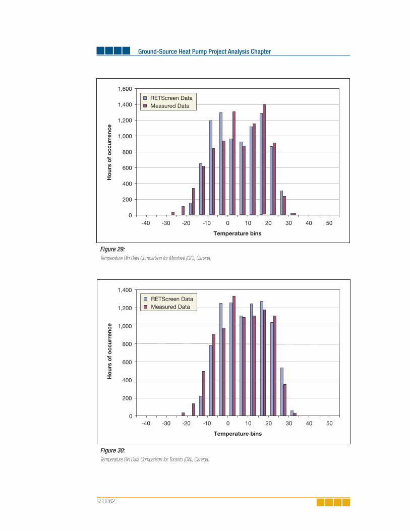
Ground-Source Heat Pump Project Analysis Chapter
GSHP.62
0
200
400
600
800
1,000
1,200
1,400
1,600
-40 -30 -20 -10 0 10 20 30 40 50
Temperature bins
Ho
urs
of
occ
urre
nce
RETScreen DataMeasured Data
Figure 29:Temperature Bin Data Comparison for Montreal (QC), Canada.
-40 -30 -20 -10 0 10 20 30 40 50
Temperature bins
Ho
urs
of
occ
urre
nce
0
200
400
600
800
1,000
1,200
1,400
RETScreen DataMeasured Data
Figure 30:Temperature Bin Data Comparison for Toronto (ON), Canada.

2. Ground-Source Heat Pump Project Model
GSHP.63
CityMeasured Data from Environment Canada
(degree-days)
RETScreen GSHP Model Generated Data(degree-days)
Difference
Montreal (QC) 4,406 4,435 0.7%
Quebec (QC) 4,855 4,949 1.9%
Schefferville (QC) 8,049 7,988 0.8%
Table 7: Degree-days comparison (18°C base) for three Canadian cities.
CityTypical air-air heat pump
heating energy use(kWh)
RETScreen GSHP Model Generated Data
(kWh)Difference
Toronto (ON) 36,690 37,200 1.4%
Montreal (QC) 35,490 36,140 1.8%
Charlottetown (PE) 36,920 37,160 0.6%
Winnipeg (MB) 32,930 33,240 1.0%
Vancouver (BC) 39,020 37,890 -3.0%
Table 8: Typical Heat Pump Energy Use Comparison for Four Canadian Cities.
2.10.2 Validation of the earth connection sizing for vertical closed-loop GHX
A literature review was also performed to identify benchmark cases to which a techni-cal evaluation of the RETScreen GSHP Project Model could be made. As a result, several parts of the GSHP Project Model were evaluated separately. Amongst the benchmark cases found, two documents (Shonder et al. 1999, Shonder et al. 2000) were specifically written for evaluating vertical closed-loop GHX against seven commercial software programs used for sizing GHXs. As described below, the evaluations presented in these two papers are based on real data from residential and commercial buildings.
Residential building cases
The paper by Shonder et al. (1999) uses two real residential buildings where monitored data were available to perform a comparative evaluation of six commercially available GHX sizing software programs. In addition, a calibrated detailed simulation program is used to obtain input values required by the six software programs, which were not readily available from the monitored data. The monitored data were used to calibrate the detailed model’s results. A total of seven predicted GHX sizes were obtained for comparison purposes. The residences selected included one heating and one cooling dominated load.

Ground-Source Heat Pump Project Analysis Chapter
GSHP.64
The energy use and design demand for the two cases were used to obtain a first set of RETScreen GSHP Project Model predicted GHX sizes. Other input data such as soil type and heat pump performances were also available in the paper. Furthermore, the model’s descriptive option was also used to obtain a second set of predicted GHX sizes. However, since little was known about the thermal envelope of the buildings, a qualitative estimate based on the available energy use data was done. Table 9 presents the data for the two residential buildings cases.
Data Unit Residential BuildingCase #1
Residential BuildingCase #2
Location - Fort Polk, LA Sun Prairie, WI
Building fl oor area m2 97.7 127.3
Basement type - Slab Full
Insulation level - Medium Medium
Heating load kW 4.8 5.8
Peak heating demand kWh 2,200 6,800
Cooling load kW 4.6 4
Peak cooling demand kWh 6,400 1,500
COPh - 3.7 3.6
COPc - 4.8 5.5
Ks BTU/(h ft °F) 1.4 1.64
ρ Χπ BTU/(cu ft °F) 40 64
Table 9: Data for Two Residential Building Cases [Shonder, 1999].
Predicted GHX lengths are presented in the paper as length per ton of installed heat pump capacity. This allows isolating the GHX size evaluation from the house and heat pump al-gorithms. Table 10 presents the results obtained with the RETScreen GSHP Project Model and the seven other software programs studied in the paper. Also shown in Table 10 are the actual installed GHX sizes. The results are given for a one-year design length, neglect-ing the long-term thermal imbalances.
The results from Table 10 indicate that, despite being a simplified pre-feasibility tool, the GHX calculations performed by the RETScreen GSHP Project Model are in good agreement with the commercial sizing programs. In fact, the average difference between the GHX sizing programs and the RETScreen GSHP Project Model (6%) was less than the average difference found amongst the seven GHX sizing programs (9%), when compared together. Also, no notable differences were found in the accuracies of the two methods employed in RETScreen to evaluate building loads (average difference of 6% for the descriptive data method, and of 7% for the energy use method), leading to the conclusion that both meth-ods are adequate for evaluating GSHP projects at the preliminary feasibility stage.

2. Ground-Source Heat Pump Project Model
GSHP.65
Even if the actual installed lengths (e.g. monitored data) are a bit higher than the average predicted results from the RETScreen GSHP Project Model, the divergences of the RET-Screen Data are equivalent to the ones obtained from the seven other GHX sizing software programs, even when compared to the detailed simulation software results (average differ-ence of 23%). This suggests that comparing predicted loop sizes by commercial software, including RETScreen, to actual monitored data might not necessarily be a reliable basis of validation, since there is no way to assert that real-case systems are the proper size, and represent a basis on which to judge design software. This applies to sizing data as well as to annual energy data since the latter are a function of the GHX size. Only when detailed monitoring data are available, including entering water temperatures, throughout the year should a valid comparison could be made.
1-year design
GHX Sizing Software ProgramPort FolkEWT = 90
Sun PrairieEWT = 30
Commercial Program A 245 m 118 m
Commercial Program B 256 m 97 m
Commercial Program C 283 m 110 m
Commercial Program D 271 m 150 m
Commercial Program E 269 m 135 m
Commercial Program F 240 m 132 m
Detailed Simulation Software 300 m 126 m
Predicted Size Average (A) 266 m 124 m
RETScreen GSHP Project ModelDescriptive Data Method (B)
257 m 135 m
Differences (A vs. B) -3% 9%
RETScreen GSHP Project ModelEnergy Use Method (C)
236 m 127 m
Differences (A vs. C) -11% 2%
Monitored Data (D) 344 m 160 m
RETScreen Descriptive Data Method (B) Difference (B vs. D)
-25% -16%
RETScreen Energy Use Method (C) Difference (C vs. D)
-31% -21%
Program Predicted Size Average (A) Difference (A vs. D)
-23% -23%
Table 10: Predicted and Actual GHX Length for Two Residential Building Cases.
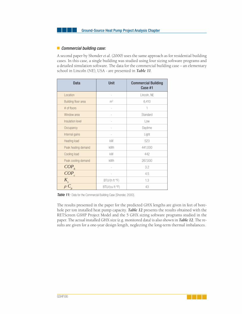
Ground-Source Heat Pump Project Analysis Chapter
GSHP.66
Commercial building case:
A second paper by Shonder et al. (2000) uses the same approach as for residential building cases. In this case, a single building was studied using four sizing software programs and a detailed simulation software. The data for the commercial building case – an elementary school in Lincoln (NE), USA - are presented in Table 11.
Data Unit Commercial BuildingCase #1
Location - Lincoln, NE
Building fl oor area m2 6,410
# of fl oors - 1
Window area - Standard
Insulation level - Low
Occupancy - Daytime
Internal gains - Light
Heating load kW 523
Peak heating demand kWh 441,000
Cooling load kW 442
Peak cooling demand kWh 267,000
COPh - 3.2
COPc - 4.5
Ks BTU/(h ft °F) 1.3
ρ Cp BTU/(cu ft °F) 43
Table 11: Data for the Commercial Building Case [Shonder, 2000].
The results presented in the paper for the predicted GHX lengths are given in feet of bore-hole per ton installed heat pump capacity. Table 12 presents the results obtained with the RETScreen GSHP Project Model and the 5 GHX sizing software programs studied in the paper. The actual installed GHX size (e.g. monitored data) is also shown in Table 12. The re-sults are given for a one-year design length, neglecting the long-term thermal imbalances.
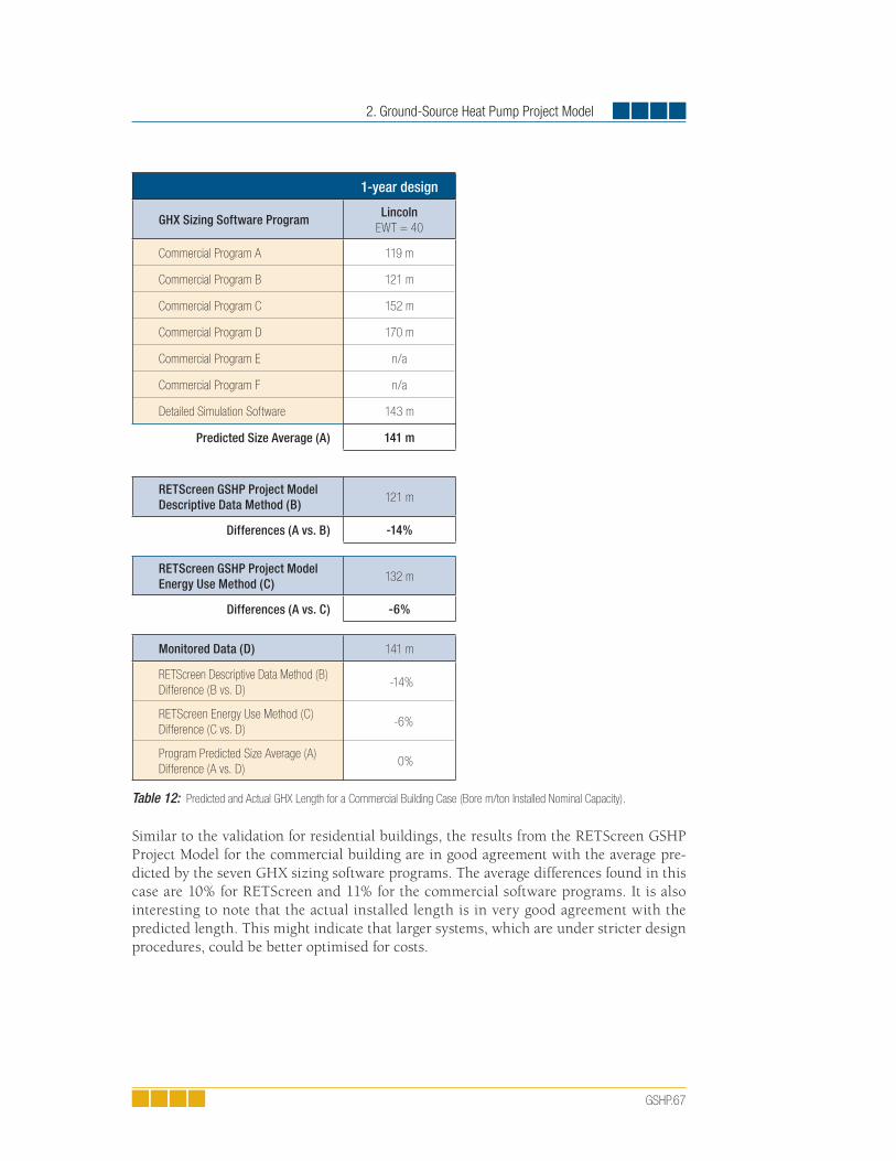
2. Ground-Source Heat Pump Project Model
GSHP.67
1-year design
GHX Sizing Software ProgramLincoln
EWT = 40
Commercial Program A 119 m
Commercial Program B 121 m
Commercial Program C 152 m
Commercial Program D 170 m
Commercial Program E n/a
Commercial Program F n/a
Detailed Simulation Software 143 m
Predicted Size Average (A) 141 m
RETScreen GSHP Project ModelDescriptive Data Method (B)
121 m
Differences (A vs. B) -14%
RETScreen GSHP Project ModelEnergy Use Method (C)
132 m
Differences (A vs. C) -6%
Monitored Data (D) 141 m
RETScreen Descriptive Data Method (B) Difference (B vs. D)
-14%
RETScreen Energy Use Method (C) Difference (C vs. D)
-6%
Program Predicted Size Average (A) Difference (A vs. D)
0%
Table 12: Predicted and Actual GHX Length for a Commercial Building Case (Bore m/ton Installed Nominal Capacity).
Similar to the validation for residential buildings, the results from the RETScreen GSHP Project Model for the commercial building are in good agreement with the average pre-dicted by the seven GHX sizing software programs. The average differences found in this case are 10% for RETScreen and 11% for the commercial software programs. It is also interesting to note that the actual installed length is in very good agreement with the predicted length. This might indicate that larger systems, which are under stricter design procedures, could be better optimised for costs.

GSHP.68
2.11 Summary
In this section the algorithms used by the RETScreen Ground-Source Heat Pump (GSHP) Project Model have been shown in detail. As inputs, the model requires weather data, building data, and GSHP related data. The modified bin method used allows the estimate of building loads. Weather data are used to generate temperature bins and calculate the temperature of the ground. Building data are used to calculate heating and cooling load vs. temperature relationships and the building’s balance points. Combining weather and building data enables the calculation of building loads for each temperature bin. With the GSHP related data, it then becomes possible to evaluate the actual heat pump performance and capacity for each temperature bin, and finally calculate the yearly performance of the GSHP system assessed. A validation of the algorithm shows that the RETScreen GSHP Project Model is more than adequate at the preliminary feasibility stage of GSHP system project implementation.
Ground-Source Heat Pump Project Analysis Chapter

GSHP.69
REFERENCES
ARI, Standard for Ground-source Closed-Loop Heat Pump Equipment, ARI 330-93, Air-Conditioning & Refrigeration Institute, Arlington, VA 22203, USA, 1993.
ASHRAE, Commercial/Institutional Ground-Source Heat Pump Engineering Manual, American Society of Heating, Refrigerating and Air-Conditioning Engineers, Inc., 1791 Tullie Circle, N.E., Atlanta, GA, USA, 1995.
ASHRAE, Handbook, Fundamentals, American Society of Heating, Refrigerating and Air-Conditioning Engineers, Inc., 1791 Tullie Circle, N.E., Atlanta, GA, USA, 1981.
ASHRAE, Handbook, Fundamentals, American Society of Heating, Refrigerating and Air-Conditioning Engineers, Inc., 1791 Tullie Circle, N.E., Atlanta, GA, USA, 1985.
ASHRAE, Handbook, Fundamentals, American Society of Heating, Refrigerating and Air-Conditioning Engineers, Inc., 1791 Tullie Circle, N.E., Atlanta, GA, USA, 1997.
ASHRAE, Handbook, HVAC Systems and Equipment, American Society of Heating, Refrigerating and Air- Conditioning Engineers, Inc., 1791 Tullie Circle, N.E., Atlanta, GA, USA, 1992.
Henderson H.I., Implications of Measured Commercial Building Loads on Geothermal System Sizing, ASHRAE Transactions 105, SE-99-20-02, 1999.
HOT-2000, HOT-2000, Technical Manual version 6, Buildings Group, Energy Mines and Resources Canada, 1991.
Hydro-Québec, Projet ÉVAL-ISO : Rapport fi nal sur le potentiel d’amélioration de l’enveloppe thermique des habitations du Québec, Vice-présidence, Effi cacité énergétique, Service Conception de programmes - Marché résidentiel, July 1994.
IGSHPA, Closed-Loop/Ground-Source Heat Pump Systems – Installation Guide, International Ground-source Heat Pump Association, Oklahoma State University, Stillwater, Oklahoma, USA, 1988.
International Summer School on Direct Application of Geothermal Energy, Design of closed-loop geothermal heat exchangers in the U.S., International Course on Geothermal Heat Pumps, Chapter 2.4, edited by Lund, J.W., Geo-Heat Center (GHC), pp 134-146.
Kavanaugh, P.K. and Rafferty, K., Ground-source Heat Pumps – Design of Geothermal Systems For Commercial and Institutional Buildings, American Society of Heating, Refrigerating and Air-Conditioning Engineers, Inc., 1791 Tullie Circle, N.E., Atlanta, GA, USA, 1997.
Khan, M.H., and Spitler, J.D., Performance analysis of a residential ground source heat pump system with antifreeze solution, School of Mechanical and Aerospace Engineering, Oklahoma State University, Stillwater, Oklahoma, USA, 10 pp.
Lund, J.W. et al.̧ Geothermal (Ground-Source) Heat Pumps – A World Overview, edited and updated version of the article from Renewable Energy World (July-Aug, 2003, Vol. 6, No. 4), Geo-Heat Center (GHC) Quarterly Bulletin, Vol. 25, No. 3, ISSN 0276-1084, September 2004, 10 pp.

Ground-Source Heat Pump Project Analysis Chapter
GSHP.70
McRae, S.G., Practical Pedology: Studying Soils in the Field, Halstead Press, New York, NY, USA, 1988.
Means, R.S., Mechanical Cost Data, 21st Annual Edition, R.S. Means Company Inc., Kingston MA, 1998.
NASA Langley Research Center, Earth’s Energy Budget, Students’ Cloud Observations On-Line Project, asd-www.larc.nasa.gov/SCOOL/budget.gif, 2005.
NRCan, Commercial Earth Energy Systems: A Buyer’s Guide, Natural Resources Canada’s Renewable and Electrical Energy Division, ISBN 0-662-32808-6, Cat. No. M92-251/2002E, Ottawa, ON, Canada, 99 pages, 2002.
NRCan, Residential Earth Energy Systems: A Buyer’s Guide, Natural Resources Canada’s Renewable and Electrical Energy Division, ISBN 0-662-30980-4, Cat. No. M92-236/2001E, Ottawa, ON, Canada, 41 pages, 2002.
Peat Marwick Stevenson & Kellogg (PMSK) in association with Marbek Resource Consultants, Torrie Smith and Associates, The economically attractive potential for energy effi ciency gains in Canada, WATSRF, May 1991.
Shonder, A.S., Hughes, P.J., Baxter, V.D. and Thornton, J.W., A Comparison of Vertical Ground Heat Exchanger Design Methods for Residential Applications, ASHRAE Transactions 105, SE-99-20-01, 1999.
Shonder, A.S., Hughes, P.J., Baxter, V.D. and Thornton, J.W., A Comparison of Vertical Ground Heat Exchanger Design Software for Commercial Applications, ASHRAE Transactions 106, DA-00-13-01, 2000.
U.S. Department of Energy (DOE), Geothermal Heat pumps for Medium and Large Buildings, Offi ce of Geothermal Technologies, 1000 Independence Avenue, SW Washington, DC 20585-0121, USA, DOE/GO-10098-648, September 1998, reprinted April 1999, 4 pp.


www.retscreen.net


