Embed Size (px)
Citation preview
Full Terms & Conditions of access and use can be found athttp://www.tandfonline.com/action/journalInformation?journalCode=raec20
Download by: [179.210.116.235] Date: 11 February 2016, At: 07:31
Applied Economics
ISSN: 0003-6846 (Print) 1466-4283 (Online) Journal homepage: http://www.tandfonline.com/loi/raec20
Cost and learning efficiency drivers in Australianschools: a two-stage network DEA approach
Peter Wanke, Vincent Blackburn & Carlos Pestana Barros
To cite this article: Peter Wanke, Vincent Blackburn & Carlos Pestana Barros (2016): Cost andlearning efficiency drivers in Australian schools: a two-stage network DEA approach, AppliedEconomics
To link to this article: http://dx.doi.org/10.1080/00036846.2016.1142656
Published online: 11 Feb 2016.
Submit your article to this journal
View related articles
View Crossmark data

Cost and learning efficiency drivers in Australian schools: a two-stage networkDEA approachPeter Wankea, Vincent Blackburnb and Carlos Pestana Barrosc
aCenter for Studies in Logistics, Infrastructure and Management, COPPEAD Graduate Business School, Federal University of Rio de Janeiro,Rio de Janeiro, Brazil; bEssential Education Economics (E3), Ground Unit 5, Pyrmont, New South Wales, Australia; cUECE (Research Unit onComplexity and Economics), ISEG-Lisbon School of Economics and Management, Universidade de Lisboa, Lisbon, Portugal
ABSTRACTThis article explore performance issues in Australian public schools, using a two-stage DEAnetwork model, which accounts simultaneously for both cost and learning efficiency levels. Inthe cost efficiency stage, different types of expenses and investments are employed to support agiven number of students, teachers and administrative staff. In the learning efficiency stage,these groups of individuals help to produce important outputs related to performance in studenttests and school rankings. Results indicate that Australian public schools are heterogeneous.Policy implications are also discussed.
KEYWORDSSchool; network dea;Australia; cost efficiency;learning efficiency
JEL CLASSIFICATIONB23; C14; C23; H52; H77
I. Introduction
It is common to hear policy makers argue that cutsin government spending will not impact on thedelivery of educational of services as there will beefficiency gains. This is an important issue, as whatat first appears to be inefficient performance ineducation may actually be a reflection of the diffi-culty of providing services in a particular context.Looking at this issue from the perspective of publiceducation, it is of utmost importance to examine theefficiency levels and contextual variables that makeup the educational process. A comparison of howschool efficiency varies with school characteristicsmay indicate those factors which help some schoolsto do well, despite having comparatively low levels offunding.
Although research on efficiency in schooling is arecurrent topic over the course of time (see forexample Kirjavainen and Loikkanent 1998;Ruggiero and Vitaliano 1999; Grosskopf andMoutray 2001; Ouellette and Vierstraete 2005;Oliveira and Santos 2005; Essid, Ouellette, andVigeant 2010; Johnes 2015), cost (Deller andRudnicki 1993; Marlow 2000; Ruggiero 2001;Gronberg, Jansen, and Taylor 2012; Flaker 2014),and also on learning efficienct levels (Bosman,Huygevoort, and Verhoeven 2006; Primont and
Domazlicky 2006; Thieme, Prior, and Tortosa-Ausina 2013), these two topics have not yet beenconsidered simultaneously in previous research.Besides, Australian public education has been thefocus of very few past studies, examples beingthose of Abbott and Doucouliagos (2003),Ryan (2013), and Blackburn, Brennan, andRuggiero (2014). The latter applied a traditionalnon-discretionary DEA model for Australian publicschools and found that they are moderately ineffi-cient and that efficiency increases for the quintile ofschools that have the most favourable environment.Therefore, this article differs from previous ones, inthat it applies, for the first time, the DEA model for aproductive network of two stages, which was pro-posed by Liang, Cook, and Zhu (2008) and Zhu(2011), on a panel set of 1,343 primary and 371secondary Australian public schools (2008–2010),to ensure that cost and learning efficiency levels aresimultaneously optimized.
The contribution of this research to the literatureis fivefold. Firstly, this article analyses, for the firsttime, to the best of our knowledge, the efficiencylevels of both primary and secondary education in arepresentative emerging economy – Australia.Secondly, an analysis of student achievement as aresult of a two-stage network process which
CONTACT Peter Wanke [email protected]
APPLIED ECONOMICS, 2016http://dx.doi.org/10.1080/00036846.2016.1142656
© 2016 Taylor & Francis
Dow
nloa
ded
by [
179.
210.
116.
235]
at 0
7:31
11
Febr
uary
201
6

simultaneously encompasses cost and learning per-formance has not been conducted to date. It isimportant to consider that the conventional assump-tions of frontier models cannot handle the specificsof the educational process anymore (Podinovskiet al. 2014). Thirdly, this article contributes to thecurrent theoretical research on schooling efficiencyby using some of the innovative two-stage networkDEA models with multiplicative efficiency decom-position, as duly described in Halkos, Tzeremes, andKourtzidis (2014). Fourthly, this article expands onthe existing literature, due to the fact that it usesneural networks to predict and interpret the role ofmajor contextual variables in achieving higher levelsof cost and learning efficiency in primary and sec-ondary schools. Besides, this segmentation is a sig-nificant contribution to the current research onschooling in terms of policy elaboration. As a matterof fact, a set of contextual or environmental vari-ables, which impact on school efficiency are tested –most of which are related to demographics or to theschool itself. Fifthly, our analysis covers a meta-frontier of the period from 2008 to 2010. By usingdata reduction techniques for reducing the numberof input and output variables, it was possible tocontrol for undesirable effects derived from outliersand from the curse of data dimensionality.
The article is organized as follows: Section II pre-sents the contextual setting on Australian primaryand secondary public education. Section III isdevoted to the literature review on schooling effi-ciency and their main drivers. Section IV focuses onthe data source and the modelling issues. Section Vis devoted to the analysis and discussion of theresults. Policy implications and conclusions are pre-sented in Section VI.
II. Contextual setting
Over the past two decades, governments worldwidehave increasingly sought to maximize ‘value formoney’ in school education. This need has stimu-lated the analysis of performance, which is mainlyfocussed on measuring the efficiency and productiv-ity of public schools. In the case of Australia,increasing attention has been paid to the efficiencyof the use of funds devoted to school education(Chakraborty and Blackburn 2013). Ever since2008, Australia recognized the importance of the
need for school efficiency studies in relation tomoney spent. Furthermore, socio-demographic vari-ables outside the control of schools are taken intoaccount in this research (Pugh et al. 2014).
Year 2008 marks the date of the introduction bythe Australian Commonwealth Government of the‘My School’ website, which was developed by theAustralian Curriculum and Reporting Agency(ACARA, 2010). This website reports student testscores, student and family characteristics, and alsothe funding for each school. There are, however, fewstudies that examine the effects of school and non-school inputs in the context of Australian schools,examples being: financial resources, teacher charac-teristics, family socio-economic status, and studentcomposition on student outcomes (Pugh et al. 2014;Blackburn, Brennan, and Ruggiero 2014). Studiessuch as these could be useful sources for contribut-ing to the design of educational policies and for thefunding allocation among schools, according to sev-eral criteria.
For instance, the Australian state of New SouthWales (NSW) currently operates a centralized sys-tem of funding for public schools. Approximately82.5% of school annual resources are providedthrough NSW Departmental state-wide formula allo-cations (Chakraborty and Blackburn 2013). TheCommonwealth government allocations make up13% and this amount having grown since 2009,through increased Federal funding under the‘Building the Education Revolution’, and theNational Partnership programmes (Keating et al.2011). School-generated revenue makes up about5% of school funding.
School staff positions are centrally allocated,based on a formula, with some capacity for variationwhich results from negotiations between personnelfrom the school and the Department of Educationand Communities. Schools contract additional staffif they have a budget surplus. The staffing expendi-ture is about 81% of the operational costs of aschool. Effective budget allocations using the sameformula can vary, depending on the different salarybrackets of teachers (Blackburn, Brennan, andRuggiero 2014).
Additional human, physical or monetaryresources are employed to compensate those schoolsthat are affected by specific circumstances, such asurgent minor maintenance work and geographic
2 P. WANKE ET AL.
Dow
nloa
ded
by [
179.
210.
116.
235]
at 0
7:31
11
Febr
uary
201
6
isolation. An example of such additional resources isthe New South Wales environment (Pugh et al.2014). Global funding also operates, in order totake into account rural location and socio-economiccharacteristics. Furthermore, as well the above allo-cations, a further range of services and grants isdelivered by central and regional staff to schools,such as school cleaning and maintenance, as well asprofessional development programmes.
III. Literature review
School performance evaluation has received greatattention over the past years both for theoreticaland practical purposes (Johnes 2015). Several studieshave provided supportive evidence that the academicperformance of students is impacted by a number ofcontextual variables, such as school type, teachercharacteristics and family background (Okpala,Okpala, and Smith 2001; Okpala 2002;Scippacercola and D’Ambra 2014). The relationshipsbetween these variables and school efficiency hasbeen the object of the study of several papers andis of great interest to policy makers, as it can lead toa better understanding of the major underlying fac-tors, which explain performance differences betweenschools (Blackburn, Brennan, and Ruggiero 2014).Unveiling the relationships between students, tea-chers and school resources helps in assisting decisionmaking and in promoting higher levels of efficiencyin the educational process (Johnes 2015; Mizala,Romaguera, and Farren 2002).
The methods for exploring these relationships aretraditionally grouped into two main approaches:parametric and nonparametric (Deller andRudnicki 1993; Wang 2003; Essid, Ouellette, andVigeant 2010). The most popular parametric methodin educational efficiency is known as the stochasticfrontier approach, according to Scippacercola andD’Ambra (2014), whereas the most popular non-parametric method is DEA (Katharaki andKatharakis 2010; Harrison and Rouse 2014). Thefollowing paragraphs suggest that efficiency studiesin schooling are usually focused on understandingthe drivers for higher efficiency levels in terms ofcosts (expenditures, funds, resources, etc.), or learn-ing (academic achievement, score tests, attendance,etc.), but in an isolated fashion that does not con-sider cost and learning efficiency as different facets
of the very same productive process. Besides, con-textual variables appear to be heterogeneous in theirvery nature, and, over the course of time, past stu-dies have explored new possible drivers for higherefficiency levels in schooling.
Turning specifically to learning efficiency, a largenumber of literature exists on the influences of con-textual variables on student achievement. Brennan,Haelermans, and Ruggiero (2014) showed that thecontextual environment influences the productivityindex, as well as the technical efficiency.Furthermore, it also influences scale and environ-mental change components in the educational pro-cess. On the other hand, Harrison and Rouse (2014)used a categorical DEA model in New Zealand´spublic schools, and found that average school per-formance tends to be higher when schools arelocated in areas of high competition. However, thisresult appears to vary depending on school size,which suggests that competition can lead to a widen-ing in the existing gap between the best and theworst performing schools.
Some research has focused on the socio-economicstatus of students (Caldas and Bankston 1997, 1999;Sirin 2005), which is one of the most importantvariables in explaining students’ achievement (Sirin2005; Shokoohi, Hanif, and Dali 2012; Rajchert,Żułtak, and Smulczyk 2014; Agasisti andLongobardi 2014; Jehangir, Glas, and Berg 2015).There is evidence in the literature that schools witha higher percentage of ‘poor’ children tend to under-perform in terms of learning efficiency (Tajalli andOpheim 2005; Agasisti and Longobardi 2014;Jehangir, Glas, and Berg 2015).
Teacher characteristic is another relevant contex-tual variable used to understand learning efficiency.Empirical evidence suggests that the amount thatteachers know about their subject impacts positivelyon the performance of students (Treputtharat andTayiam 2014; Buddin and Zamarro 2009; Darling-Hammond, Berry, and Thoreson 2001; Ferguson andBrown 2000; Fetler 2001; Brewer and Goldhaber1996; Monk 1994).
On the other hand, the evidence of the positiveimpact of educational expenditure on school perfor-mance has been well-established, decades ago(Erdogdu and Erdogdu 2015; Prasetyo and Zuhdi2013; Gershberg and Schuermann 2001). For exam-ple, Dolan and Schmidt (1987) verified a positive
APPLIED ECONOMICS 3
Dow
nloa
ded
by [
179.
210.
116.
235]
at 0
7:31
11
Febr
uary
201
6
relationship between educational resources and stu-dent performance. Greenwald, Hedges, and Laine(1996), Elliott (1998) and Nyhan and Alkadry(1999) corroborated this finding for primary andsecondary schools. One possible explanation forthis result is that increased per-pupil expenditureprovides students with access to highly educatedteachers. These educated teachers use more effectivepedagogical methods in their classrooms, resultingin higher achievement.
Apart from the socio-economic status of students,teacher characteristics and school expenditures, it isworth noting, however, that literature is prolific interms of different circumstances, analytical tools andcontextual variables used as learning efficiency dri-vers. For instance, Kirjavainen and Loikkanent(1998) studied differences among Finnish seniorsecondary schools. They found higher learning inef-ficiency levels in schools with smaller classes.Furthermore, schools with more heterogeneous stu-dent populations present higher inefficiency levels,as do private schools, when compared to publicones. On the other hand, a positive effect of smallclass sizes on efficiency levels was foundbyWößmann and West (2006), Conroy and Arguea(2008) and Barrett and Toma (2013).
Parents’ educational level was found to be posi-tively related to academic achievements (Kirjavainenand Loikkanent 1998). A similar study was con-ducted by Miningou and Vierstraete (2013) inBurkina Fasso´s schools, focussing on households’living situations. Primont and Domazlicky (2006)analysed student achievement and efficiency inMissouri schools, using DEA to measure the impactof the 2001 No Child Left Behind Act (annual yearlyprogress). Thieme, Prior, and Tortosa-Ausina (2013)used a multilevel methodology for evaluating educa-tional attainment in Chilean schools. Results indi-cated that less than 30% of the variance in students’educational attainment is attributable to theirschools, which corroborated previous studies.Deller and Rudnicki (1993) reported the efficiencyof Maine elementary schools and attempted to iden-tify the distinct patterns for the measures of effi-ciency, across three alternative policy-relatedvariables, namely: school size, administrative organi-zation and administrative expenditure. However,these authors failed to generate any additionalinsights.
Moving to cost efficiency drivers, teacher–pupilratio is a traditional single input–output ratio, whichproxies average class size. Furthermore, according toOkpala et al. (2000), class size is an indicator of theavailability of teachers’ capacity to interact with stu-dents (Wößmann and West 2006; Conroy andArguea 2008; Barrett and Toma 2013). There is atrade-off between cost efficiency and studentachievement, however. The higher this ratio, thelower the cost efficiency, and vice versa. Previousstudies on relationship between class size (cost effi-ciency) and student achievement (learning effi-ciency) failed to produce consistent conclusionsover the course of time. For instance, althoughsome researchers have suggested that children learnbetter in smaller classes (McGiverin, Gilman, andTillitski 1989; Finn and Achilles 1990), otherauthors, such as Nyhan and Alkadry (1999) andSanders, Wright, and Horn (1997), established aninverse relationship between class size and studentachievement in primary and secondary education.Despite a lack of consensus, the examination of therelationship between class size and learning perfor-mance continues to be carried out, suggesting thatreduced class size is a policy option that needs to beconsidered (Wößmann and West 2006; Conroy andArguea 2008; Barrett and Toma 2013).
Taking salaries as a point, they are regarded as atrade-off between cost and learning efficiency.Sanders (1993) and Smith (2004) present evidencethat increase in average salaries of teachers generatesan increase in graduation rates and the percentage ofcollege-bound students. However, besides cost andlearning efficiency trade-offs, a number of differentcontextual variables have emerged over the course ofthe years for assessing cost efficiency drivers.Haelermans and Ruggiero (2013) applied a condi-tional DEA model in order to analyse the technicaland allocative efficiency of Dutch secondary schools.The results show that allocative efficiency representsa significant 37% of overall cost efficiency on aver-age. This result suggests that the impact of the envir-onment largely differs between schools and thathaving a more unfavourable environment is verynegative for a school’s performance. Grosskopf andMoutray (2001), for instance, used DEA to assess theintroduction of site-based management on the costefficiency levels of Chicago public high schools. Bymeans of a cost indirect output distance function,
4 P. WANKE ET AL.
Dow
nloa
ded
by [
179.
210.
116.
235]
at 0
7:31
11
Febr
uary
201
6

the authors found very little improvements in pro-ductivity. Essid, Ouellette, and Vigeant (2010) usedbootstrapped DEA models in the context of quasi-fixed inputs to evaluate cost efficiency levels of highschools in Tunisia. Results indicate that schools withboarding facilities are less efficient than ordinaryones. Waldo (2007) analyses technical efficiency inSwedish upper secondary school, and attempts tounveil the impacts of gender distribution and effortallocation between subjects. His results, however,showed to be inconclusive.
IV. Methodology
This section discusses the major methodologicalsteps used in this research. All analyses were carriedout in Maple and R codes developed by the authors.
Two-stage network DEA model
Network DEA model decomposes the productionprocess and the traditional black box in processes,which result in an output, enabling the researchprocess that is usually hidden in the traditionalDEA analysis. The modelling of productive struc-tures, which encompass a series of individual activ-ities, using and simultaneously generatingintermediate inputs and outputs, was first developedby Färe (1991). This concept was further improvedby Färe and Whittaker (1995), Färe and Grosskopf(1996a, 1996b, 2000) and Tone and Tsutsui (2009,2010). The productive structures formed by two-stages have received considerable attention fromscholars over the course of time (Liang et al. 2006;Liang, Cook, and Zhu 2008; Yang 2006; Kao andHwang 2008, 2011; Kao 2009; Chen, Cook, et al.2009; Chen, Liang, and Zhu 2009; Chen, Zhu, andCook 2010; Chen et al. 2012; Zha and Liang 2010;Wang and Chin 2010; Lozano 2011; Maghbouli,Amirteimoori, and Kordrostami 2014; Tavana andKhalili-Damghani 2014). The inherent trade-off oftwo-stages productive structures, which emergesfrom the decision whether intermediate inputs/out-puts should be reduced or augmented, in order tomaximize overall efficiency levels is the key issue ofthese studies (Kao and Hwang 2008; Liang et al.,2008; Zhu 2011; Matin and Azizi 2015). More pre-cisely, the second stage may have to reduce theintermediate inputs consumed in order to increase
efficiency, but, on the other hand, this action nega-tively impacts on the efficiency of the first stage, asits intermediates outputs are consequently reducedby definition (Cook, Liang, and Zhu 2010).
According to Cook, Liang, and Zhu (2010), twoapproaches are used for computing efficiency scoresin two-stage productive processes. Researchers eitheruse the non-cooperative, or the cooperative approach.Regarding the cooperative approach, as both stages aresimultaneously taken into account for overall perfor-mance optimization, by breaking-out the trade-off aspreviously described, the models are commonlyreferred to as ‘centralized efficiency models’ (Zhu2011). Liang, Cook, and Zhu (2008) give an examplewhere the product of the individual efficiencies of eachstage are used to assess the overall efficiency.
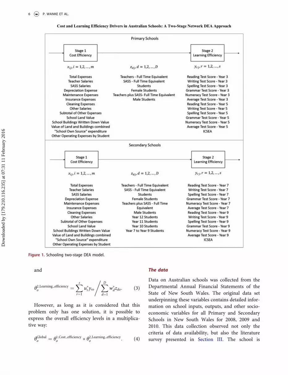
The notations for the two-stage network DEAmodel proposed by Liang, Cook, and Zhu (2008)and Zhu (2011) is given next. It is assumed thatDMUj (j ¼ 1; 2; . . . ; n) has D intermediate mea-sures zdj ðd ¼ 1; 2; . . . ; DÞ, together with theinitial inputs xij ði ¼ 1; 2; . . . ; mÞ, and the finaloutputs yrj ðr ¼ 1; 2; . . . ; sÞ (cf. Figure 1). It isalso considered that vi;wdand urare non-negativeweights, which are unknown. The following linearprogramme represents the two-stage centralizedDEA model:
θGlobalo ¼ MaxXs
r¼1
uryro
s:t:
Xs
r¼1
uryrj �XDd¼1
wdzdj � 0; j ¼ 1; 2; . . . ; n;
XDd¼1
wdzdj �Xmi¼1
vixij � 0; j ¼ 1; 2; . . . ; n;
Xmi¼1
vixio ¼ 1;
wd � 0; d ¼ 1; 2; . . . ; D; vi � 0;
i ¼ 1; 2; . . . ; m; ur � 0; r ¼ 1; 2; . . . s;
(1)
where θGlobalo is overall (global) efficiency level forDMUo. Assuming that model (1) generates a uniquesolution, the efficiencies for both stages are pre-sented as follows:
θ1;Cost efficiencyo ¼
XDd¼1
w�dzdo; (2)
APPLIED ECONOMICS 5
Dow
nloa
ded
by [
179.
210.
116.
235]
at 0
7:31
11
Febr
uary
201
6
and
θ2;Learning efficiencyo ¼
Xs
r¼1
u�r yro
,XDd¼1
w�dzdo: (3)
However, as long as it is considered that thisproblem only has one solution, it is possible toexpress the overall efficiency levels in a multiplica-tive way:
θGlobalo ¼ θ1;Cost efficiencyo � θ2;Learning efficiency
o : (4)
The data
Data on Australian schools was collected from theDepartmental Annual Financial Statements of theState of New South Wales. The original data setunderpinning these variables contains detailed infor-mation on school inputs, outputs, and other socio-economic variables for all Primary and SecondarySchools in New South Wales for 2008, 2009 and2010. This data collection observed not only thecriteria of data availability, but also the literaturesurvey presented in Section III. The school is
Figure 1. Schooling two-stage DEA model.
6 P. WANKE ET AL.
Dow
nloa
ded
by [
179.
210.
116.
235]
at 0
7:31
11
Febr
uary
201
6

assumed to be a DMU, which uses human (students,teachers and administrative staff) and financialresources (expenses and salaries) to generate scoresfor student tests and school rankings (Jeon andShields 2005; Wenger 2000).
With respect to the variables used to represent theinputs and the outputs, it is worth recalling one ofthe major objectives of this research: to define theproduction links between cost and learning stages inAustralian schools, taking three groups of indivi-duals (students, teachers and administrative staff)as cornerstone, or as intermediate resources. Inother words, the main objective of this research isto represent Australian schools as a sequence ofeducational activities which convert financial andhuman resources into learning, by means of a two-stage productive process. Within stage one, costs,expenses, and investments of different natures con-stitute the inputs which support the humanresources (intermediate resources) and which aredirectly involved in the achievement of some learn-ing outcomes (final product). The idea is to mini-mize the financial resources needed to support acertain number of students, teacher, and adminis-trative staff (Dodson and Garrett 2004). Within thesecond stage, these group of human resources con-stitute the production focus of important schoolingoutputs, namely: test grades and school rankings.This educational process is presented in Figure 1.
With regards to the three-time ratio between thenumber of inputs and outputs employed in themodel, and also the number of DMUs, a necessarycondition is to ensure score discrimination, and it ispossible to affirm that this ratio, which was origin-ally proposed by Cooper et al. (2001), was observedin this research. Analyses of correlation suggest posi-tive and significant relationships between outputsand inputs, which are, therefore, isotonic, andshould thus be considered in the model (Wang, Lu,and Tsai 2011). All data relate to the time spam of2008, 2009 and 2010. Their descriptions are pre-sented in Table 1.
In addition, 59 contextual variables were used ascost and learning efficiency drivers. These environ-mental-related variables are also presented inTable 2, and they relate to several demographicsvariables related to school location (provincial,metropolitan, remoteness, etc.), extra-curricularemphasis or schooling focus (agricultural,
technology, selective, only boys, only girls, etc.),basic productivity indicators (average salaries, etc.)and teacher profile (years of experience, etc.). It isworth noting that these contextual variables reflectmost of the efficiency drivers that have been pre-viously discussed in Section III, both in terms oflearning (socio-economic status, teacher characteris-tics, educational expenditure, class size, heteroge-neous student bodies, parent´s educational level,school size, administrative and organizational expen-diture) and cost efficiency (teacher–pupil ratio, classsize, average teacher salaries, site-based manage-ment, residence service, gender mix, etc.).
Data reduction in efficiency measurement
Efficiency measurement techniques often employsome kind of weighting on the inputs and outputsfor each observation. This being the case, wheneverinputs and outputs are strongly correlated, the accu-racy of the scores computed for each observationmay be biased (Madeira Junior et al. 2012).Another frequent problem found in some efficiencymeasurement techniques resides on their reduceddiscriminatory capability, that is, sometimes effi-ciency scores are concentrated towards ‘1’ (Bian2012; Jenkins and Anderson 2003). To mitigatethese problems, a principal component analysis(PCA) factor extraction is proposed in this researchaltogether with the network DEA model, for effi-ciency measurement, and neural networks, for pos-terior identification of efficiency sources. Kao, Lu,and Chiu (2011) verified that PCA is effective as asolution to the discrimination problem of the DEAmodel. Some of the pioneer works which appliedfactor extraction and efficiency measurement tech-niques are by Adler and Golany (2001, 2002) andAdler and Yazhemsky (2010), who used PCA toincrease the discriminatory capability of DEA scoresand, therefore, reduce the so-called curse of dimen-sionality (Jenkins and Anderson 2003).
As a matter of fact, the lack of differentiationbetween DMUs is a common issue in DEA (Hadi-Vencheh and Esmaeilzadeh 2013). This is causedwhen the sum of the number of input and outputvariables is large when compared to the numberobservations in the sample (Adler and Berechman2001). Following Cooper, Seiford, and Tone (2007),the sample size is one critical aspect of DEA
APPLIED ECONOMICS 7
Dow
nloa
ded
by [
179.
210.
116.
235]
at 0
7:31
11
Febr
uary
201
6

methodology. Specifically, according to Barros,Gonçalves, and Peypoch (2012), the data collectedshould observe the DEA convention that the mini-mum number of DMU observations should be atleast three times larger than the sum of the numberof outputs and inputs. Therefore, it is necessary todecide on a statistical basis to see which variable canbe excluded, whilst ensuring that information loss isminimal (Jenkins and Anderson 2003; Herrbach2001). This is an often neglected issue, and decisionswith regarding this are usually taken on an ad hoc
basis (Jenkins and Anderson 2003; Samoilenko andOsei-Bryson 2008; Nadimi and Jolai 2008).
PCA, therefore, explains the variance structure ofa data matrix through linear combinations of vari-ables, consequently reducing the data to a few prin-cipal components, which generally account for80–90% of data variance. If most of the populationvariance can be attributed to the first few compo-nents, then they can replace the original variableswith minimum loss of information. As statedin Hair et al. (1995), let the random vector
Table 1. Summary statistics for the sample – inputs, outputs and intermediate variables.Model variables (2008–2010) Mean SD Coefficient of variation
Inputs Total expenses $ 3,683,247.29 $ 2,770,662.13 0.75Teacher salaries $ 2,857,669.93 $ 2,214,214.70 0.77School administrative and support staffsalaries
$ 361,611.46 $ 277,720.71 0.77
Depreciation expense $ 154,127.22 $ 148,170.20 0.96Maintenance expenses $ 112,573.78 $ 83,098.47 0.74Insurance expenses $ 29,570.33 $ 28,518.57 0.96Cleaning expenses $ 107,934.31 $ 70,760.98 0.66Other salaries $ 59,760.26 $ 91,275.61 1.53Subtotal of other expenses $ 463,965.90 $ 360,068.26 0.78School land value $ 3,066,081.07 $ 4,136,103.90 1.35School buildings written down value $ 3,363,951.52 $ 4,687,110.05 1.39Value of land and buildings combined $ 6,430,032.59 $ 6,642,831.29 1.03‘School Own Source’ expenditure $ 638,023.57 $ 510,618.46 0.80Other operating expenses by student $1,301.77 $ 986.91 0.76
Intermediate inputs/outputs Teachers – full time equivalent 27.08 21.39 0.79School administrative and support staff – fulltime equivalent
5.37 4.52 0.84
Students 410.31 293.25 0.71Female students 199.37 161.98 0.81Teachers plus school administrative andsupport staff – full time equivalent
32.45 25.64 0.79
Male students 210.94 162.07 0.77Year 12 students 19.32 43.71 2.26Year 11 students 24.35 53.17 2.18Year 10 students 29.65 61.93 2.09Year 7 to year 9 students 94.65 195.49 2.07
Outputs Reading test score – year 3 312.36 176.33 0.56Writing test score – year 3 318.30 178.36 0.56Spelling test score – year 3 311.78 174.65 0.56Grammar test score – year 3 314.50 177.28 0.56Numeracy test score – year 3 304.32 170.98 0.56Average test score – year 3 312.59 174.88 0.56Reading test score – year 5 372.37 210.07 0.56Writing test score – year 5 368.61 207.43 0.56Spelling test score – year 5 375.44 210.10 0.56Grammar test score – year 5 379.66 213.54 0.56Numeracy test score – year 5 372.21 209.34 0.56Average test score – year 5 374.13 209.43 0.56Reading test score – year 7 115.04 219.61 1.91Writing test score – year 7 112.24 214.24 1.91Spelling test score – year 7 116.88 223.06 1.91Grammar test score – year 7 113.49 216.91 1.91Numeracy test score – year 7 116.51 222.99 1.91Average test score – year 7 114.83 219.31 1.91Reading test score – year 9 123.17 234.89 1.91Writing test score – year 9 119.08 227.36 1.91Spelling test score – year 9 125.32 248.58 1.98Grammar test score – year 9 122.23 233.32 1.91Numeracy test score – year 9 125.95 240.70 1.91Average test score – year 9 123.15 235.38 1.91ICSEA 994.45 110.36 0.11
8 P. WANKE ET AL.
Dow
nloa
ded
by [
179.
210.
116.
235]
at 0
7:31
11
Febr
uary
201
6

Table2.
Summarystatisticsforthesample–contextual
variables.
Contextual
variables
Specialist
Not
specialist
Agricultural
PerformingArts
Lang
uage
Sport
Techno
logy
Junior
Intensive
English
centre
Creativearts
Ruraltechn
olog
yMarine
techno
logy
Mean
0.03
0.97
0.00
0.00
0.00
0.00
0.01
0.01
0.00
0.00
0.00
0.00
SD0.17
0.17
0.05
0.05
0.05
0.06
0.07
0.10
0.02
0.02
0.02
0.02
Coefficient
of variatio
n
5.71
0.18
20.67
20.67
20.67
15.61
13.76
9.44
41.38
41.38
41.38
41.38
Contextual
variables
Sydn
eyHun
ter/
Central
Coast
Riverin
aIllaw
arra
and
SouthEast
New
England
Western
NSW
North
Coast
SouthWestern
Sydn
eyNorthern
Sydn
eyWestern
Sydn
eyType
(prim
ary/
second
ary)
Inner
Metropo
litan
Mean
0.11
0.15
0.06
0.11
0.04
0.06
0.12
0.14
0.09
0.13
0.22
0.50
SD0.31
0.35
0.24
0.31
0.20
0.24
0.32
0.35
0.28
0.33
0.41
0.50
Coefficient
of variatio
n
2.87
2.42
3.84
2.90
4.88
3.97
2.74
2.45
3.23
2.61
1.90
0.99
Contextual
variables
Inner
provincial
Outer
metropo
litan
Provincial
50,000
to99,999
Outer
provincial
Provincial
25,000
to49,999
Very
remote
Remote
Not
selective
Partselective
Agriculture
Fully
selective
Boys
Mean
0.15
0.15
0.03
0.11
0.04
0.00
0.01
0.97
0.01
0.00
0.01
0.01
SD0.36
0.36
0.17
0.32
0.19
0.04
0.08
0.16
0.11
0.05
0.10
0.10
Coefficient
of variatio
n
2.36
2.34
5.60
2.78
5.16
23.88
13.05
0.16
8.77
20.67
9.99
9.44
Contextual
variables
Girls
Co-Ed
Teacher
salary
bystud
ent
Scho
oladministrative
andsupp
ortstaff
salariesby
stud
ent
Stud
ent/
teacherratio
Stud
ent/scho
oladministrative
andsupp
ort
staffratio
Average
teacher
salaries
Averagescho
oladministrativeand
supp
ortstaffsalaries
Yearsof
service
Englishsecond
lang
uage
stud
ents
percentage
over
total
Aboriginalstud
ents
percentage
over
total
Spec.
education
percentage
over
total
Mean
0.01
0.98
7,044.25
1,042.45
16.12
84.67
108,294.08
72,447.54
16.36
0.24
0.07
0.04
SD0.12
0.15
1,910.23
616.85
3.18
35.86
11,027.31
20,305.19
6.49
0.28
0.10
0.04
Coefficient
of variatio
n
8.57
0.16
0.27
0.59
0.20
0.42
0.10
0.28
0.40
1.18
1.54
1.02
Contextual
variables
Stud
ents
pertotal
expenses
Percentage
offemale
stud
ents
Valueof
scho
olland
bystud
ent
Writtendo
wn
valueof
scho
olbu
ildings
bystud
ent
Valueof
land
andbu
ildings
combinedby
stud
ent
Attend
ance
Teacher
salaries
percentage
over
total
expenses
Averagescho
oladministrativeand
supp
ortstaffsalaries
over
totale
xpenses
Other
expenses
percentage
over
total
expenses
Num
berof
teachersper
100Stud
ents
Num
berof
scho
oladministrativeand
supp
ortstaffper
100stud
ents
Mean
9,388.46
0.48
8,710.51
8,722.12
17,432.63
0.86
0.76
0.11
0.13
6.52
1.46
SD3,005.46
0.09
15,679.18
21,910.10
27,952.90
0.24
0.06
0.04
0.04
1.68
0.79
Coefficient
ofvariatio
n0.32
0.19
1.80
2.51
1.60
0.28
0.08
0.34
0.29
0.26
0.54
APPLIED ECONOMICS 9
Dow
nloa
ded
by [
179.
210.
116.
235]
at 0
7:31
11
Febr
uary
201
6

X ¼ X1;X2; . . . ;Xp� �
(i.e. the original inputs/outputschosen to be aggregated) have the correlation matrixC with eigenvalues λ1 � λ2 � . . . � λp � 0 and nor-malized eigenvectors l1; l2; :::; lp:Consider the linearcombinations, where the superscript t represents thetranspose operator:
XPCi ¼ ltiX ¼ l1iX1 þ l2iX2 þ . . .þ lpiXp;
Var XPCið Þ ¼ ltiCli;i ¼ 1; 2; . . . ; p;
Correlation XPCi ;XPCkð Þ ¼ ltiClk;i ¼ 1; 2; . . . ; p; k
¼ 1; 2; . . . ; p:
The principal components (PCs) are the uncorre-lated linear combinations XPCi ;XPC2 ; . . . ;XPCp
ranked by their variances in descending order. ThePCA used here is based on correlation rather thanon covariance, as the variables used in the networkDEA model are often quantified in different units ofmeasure. In general, inputs and outputs of a DEAmodel need to be strictly positive; however, PCs cancontain negative values.
Readers should note that PCA identify underlyingvariables that are uncorrelated with each other.Intuitively, this is desirable because the underlyingvariables that account for a set of measured variablesshould correspond to physically different processes,which, in turn, should have outputs that are uncorre-lated with each other. If a few factors can account formost of the variance, it is then possible to replace theoriginal variables, without incurring a substantial lossof information (Shao et al. 2014; Xiao and Feng 2014).When compared to other techniques for reducing vari-ables, Adler and Yazhemsky (2005) observed, bymeans of simulation, that PCA consistently returnedmore accurate outcomes. In this article, PCA is used toidentify the most influential inputs and outputs for theproduction frontier, by extracting the factors.
Artificial neural networks
Readers should note that the previous studies pre-sented in the literature review tried to explain theefficiency drivers, whereas no predictive analysis hasbeen carried out in the past. However, it is extremelyimportant to predict the performance of schools, asbad performance may lead to a worse learning. Thus,the development of a model for predicting the effi-ciency of primary and secondary schools could be
adequate for limiting, or for avoiding, such undesir-able consequences for students. In this sense, thisresearch advocates using contextual variables for pre-dicting the efficiency of Australian schools. Artificialneural networks have been subject to a training toevaluate how contextual variables could be used aspredictors of efficiency levels in Australian schools(Daponte and Grimaldi 1998; Decanio 1999).
Neural networks are one of the most popularlearning models used in prediction (Daponte andGrimaldi 1998; Koh and Tan 1999; Ledolter 2013).An artificial neural network has its roots in biology,where neurons present interconnections which allowthe process of learning by past experiences. Artificialneural networks are formed of nodes disposed inlayers, which are connected by a system of weightswith the preceding layer (Gurney 1997; Indro et al.1999). The neural networks’ most successful applica-tions have been the multilayer feed forward, despitethe existing number of different architectures (Fausett1994; Rahimi-Ajdadi and Abbaspour-Gilandeh 2011).This particular arrangement is formed by one inputlayer, one or more hidden layers, and an output layer.Shmueli, Patel, and Bruce (2010) should be consultedin case more explanations is required.
Neural networks are defined by important para-meters which cannot be estimated from the data in adirect fashion (Palomares-Salas et al. 2014). Theseparameters are usually referred to as ‘tuning para-meters’, as no analytical formula exists for determin-ing appropriate values for them (Kuhn and Johnson2013). Cross-validation may be used to control thechoice of tuning parameters, avoiding what is called‘over-fitting’. It designates a situation in which themodel learns the structure of the data set so well thatwhen the model is applied to the original data, itcorrectly predicts every sample (Kuhn and Johnson2013). This type of model is said to be ‘over-fit’, andit usually shows poor accuracy when predicting anew sample (James et al. 2013).
Hence, cross-validation allows for the assessment ofthe accuracy profile for a given model, across thecandidate values of the tuning parameter (Kuhn andJohnson 2013). In such cases, it is very common to findthat accuracy rapid increases with the tuning para-meter and then, after the peak, it decreases at a slowerrate, as over-fitting begins to occur. The best model isthen chosen, based on the numerically optimal value ofthe tuning parameter, that is to say, that which yields
10 P. WANKE ET AL.
Dow
nloa
ded
by [
179.
210.
116.
235]
at 0
7:31
11
Febr
uary
201
6

the higher accuracy. The number of hidden layers andthe decay rate (weighs) are the two tuning parametersmost frequently used in neural networks (Torgo 2011).
On global separability and the adequacy ofregressing DEA estimates
Simar and Wilson (2011) examined the wide-spreadpractice where efficiency estimates are regressed onsome environmental variables in what is commonlyknown as a two-stage analysis. In a broader sense,the authors argue that this is done without specify-ing a statistical model in which such structureswould follow from the first stage where the initialDEA are estimated. As such, these two-stageapproaches are not structural, but rather ad hoc.The most important underlying assumption regard-ing two-stage analysis concerns global separability(Kourtesi, Fousekis, and Polymeros 2012). The nextparagraphs develop this assumption.
In general lines, the vector for environmental factorsor contextual variables may either affect the range ofattainable values of the inputs and the outputs includ-ing the shape of the production set, or it may onlyaffect the distribution of inefficiencies inside a set withboundaries not depending on them or both (Bădin,Daraio, and Simar 2012). Putting in other words,under separability, the environmental factors have noinfluence whatsoever on the support of the input–out-put vectors, and the only potential remaining impact ofthe environmental factors on the production processmay be on the efficiencies’ distribution. If separabilityassumption holds, we should expect these statistics tobe ‘close’ to 0; otherwise, we should expect them to lie‘far’ from 0.1
V. Results and discussion
Before presenting and discussing the major findings ofthis article, it is important to mention that, due to thespecifics of each production process, the analyses per-formed were segmented in primary and secondaryschools, whenever applicable. Basically, it is worthnoting that a greater emphasis is placed by secondaryschools in preparing for college/university admissiontests.
The delivery of publicly funded resources to NewSouth Wales primary and secondary schools is basedupon a centrally determined common State wideresource allocation model. Both teaching and non-teaching staff allocations and salary scales are basedon this State wide formulae. A similar model appliesto non-staff resources as well as funding for targetedspecific student group ‘catch up’ programs. Thesecentralized funding mechanisms enable school edu-cation to be delivered with a greater emphasis onvalue for money and maximizing stability in recur-rent school input prices. (‘Mapping School Fundingand Regulatory Arrangements across theCommonwealth, State and Territories’, June 2011,University of Melbourne Graduate School ofEducation, pp. 9, 19, 47–49).
The NSW Department of Education andCommunities (DEC) also operates a common Statewide planning system for the delivery of infrastruc-ture and land acquisition. It regularly buys and sellsland to ensure the adequate provision of governmentschool education facilities. This land banking policyensures greater price stability in school land andwider school asset provision. The NSW DEC oper-ates a continuous infrastructure planning processand a Life Cycle Costing approach to Total AssetManagement. This centralized process also enablesthe delivery of school education facilities with agreater emphasis on value for money issues thatfacilitate greater stability in asset input prices.(‘NSW Infrastructure: Education InfrastructureBaseline Report, Infrastructure NSW, PriceWaterhouse Coopers, Sydney, June 2012.)
Main analytical components
Primary schoolsThe PCA extraction from the inputs and the outputsof the Australian primary schools observed the gen-eral guidelines presented in Tabachnick and Fidell(2001) and Warming-Rasmussen and Jensen (1998).Varimax standardized rotation was the extractionmethod used, and 0.50 was the cut-off value adoptedfor interpreting the factor loads. Results are pre-sented in Table 3, which only cover auto-valuesgreater than 1.
1In this research, an R code was structured upon the packages np (Hayfield and Racine 2008) and FNN (Beygelzimer, Kakadet, and Langford 2015) tocompute the statistics of this test.
APPLIED ECONOMICS 11
Dow
nloa
ded
by [
179.
210.
116.
235]
at 0
7:31
11
Febr
uary
201
6

Table3.
Factor
extractio
n.Primaryscho
ols
Inpu
ts
Factors
Interm
ediate
Factors
Outpu
ts
Factors
Assetinvestmentand
direct
operating
expenses
Assetdepreciatio
nand
indirect
operating
expenses
Stud
ents
and
teachers
Indirect
person
nel
Learning
outcom
eat
year
3
Learning
outcom
eat
year
5
Totale
xpenses
0.91
0.37
Teachers–fulltim
eequivalent
0.80
0.49
Readingtest
score–year
30.98
0.02
Teachersalaries
0.92
0.33
Scho
oladministrativeandsupp
ort
staff–fulltim
eequivalent
0.45
0.89
Writingtest
score–year
30.97
0.01
Scho
oladministrative
andsupp
ortstaff
salaries
0.77
0.32
Stud
ents
0.88
0.48
Spellingtest
score–year
30.99
(0.00)
Depreciationexpense
0.35
0.88
Femalestud
ents
0.89
0.45
Grammar
test
score–year
30.99
(0.01)
Maintenance
expenses
0.22
0.85
Teachersplus
scho
oladministrative
andsupp
ortstaff–fulltim
eequivalent
0.76
0.64
Num
eracytestscore–year
30.98
0.00
Insuranceexpenses
0.40
0.85
Malestud
ents
0.86
0.50
Averagetestscore–year
30.99
(0.01)
Cleaning
expenses
0.22
0.77
Kaiser–M
eyer–O
lkin
measure
ofsamplingadequacy
0.8687025
Readingtest
score–year
50.006
0.972
Other
salaries
0.55
0.42
Bartlett’stest
ofsphericity
Approx.chi-squ
are
99078.67
Writingtest
score–year
50.02
0.97
Subtotal
ofother
expenses
0.57
0.76
Degreeof
freedo
m(df)
0Spellingtest
score–year
5(0.01)
0.99
Scho
olland
value
0.51
0.18
Sig.
15Grammar
test
score–year
5(0.01)
0.99
Scho
olbu
ildings
writtendo
wnvalue
0.30
0.80
Percentof
varianceexplainedby
the
factors
0.99
Num
eracytestscore–year
5(0.005)
0.986
Valueof
land
and
buildings
combined
0.69
0.41
Averagetestscore–year
5(0.014)
0.992
‘SchoolO
wnSource’
expend
iture
0.87
0.33
ICSEA
0.154
0.155
Other
operating
expenses
bystud
ent
(0.68)
0.55
Kaiser–M
eyer–O
lkin
measure
ofsamplingadequacy
0.70
Kaiser–M
eyer–O
lkin
measure
ofsampling
adequacy
0.84
Bartlett’stestof
sphericity
Approx.chi-
square
172,408.60
Bartlett’stest
ofsphericity
Approx.chi-squ
are
90,477.39
df–
df–
Sig.
78.00
Sig.
91.00
Percentof
variance
explainedby
thefactors
0.90
Percentof
variance
explainedby
the
factors
0.75
Second
aryscho
ols
Inpu
tsFactors
Interm
ediate
Factors
Outpu
tsFactors
Assetdepreciatio
nand
indirect
operating
expenses
Assetinvestmentand
direct
operating
expenses
Stud
ents,teachers
andindirect
person
nel
Final
year’s
stud
ents
Learning
outcom
eat
years
7and9
Learning
outcom
eat
ICSEA
Totale
xpenses
0.19
0.95
Teachers–fulltim
eequivalent
0.89
0.42
Readingtest
score–year
70.96
0.01
Teachersalaries
0.09
0.95
Scho
oladministrativeandsupp
ort
staff–fulltim
eequivalent
0.89
0.16
Writingtest
score–year
70.96
0.02
Scho
oladministrative
andsupp
ortstaff
salaries
0.11
0.79
Stud
ents
0.85
0.46
Spellingtest
score–year
70.95
0.01 (Continued)
12 P. WANKE ET AL.
Dow
nloa
ded
by [
179.
210.
116.
235]
at 0
7:31
11
Febr
uary
201
6
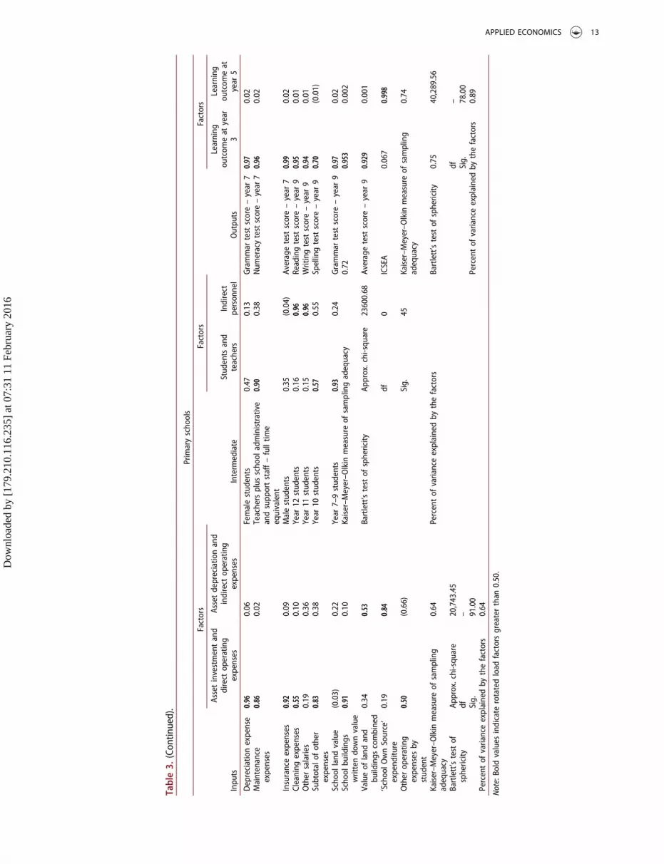
Table3.
(Con
tinued).
Primaryscho
ols
Inpu
ts
Factors
Interm
ediate
Factors
Outpu
ts
Factors
Assetinvestmentand
direct
operating
expenses
Assetdepreciatio
nand
indirect
operating
expenses
Stud
entsand
teachers
Indirect
person
nel
Learning
outcom
eat
year
3
Learning
outcom
eat
year
5
Depreciationexpense
0.96
0.06
Femalestud
ents
0.47
0.13
Grammar
test
score–year
70.97
0.02
Maintenance
expenses
0.86
0.02
Teachersplus
scho
oladministrative
andsupp
ortstaff–fulltim
eequivalent
0.90
0.38
Num
eracytestscore–year
70.96
0.02
Insuranceexpenses
0.92
0.09
Malestud
ents
0.35
(0.04)
Averagetest
score–year
70.99
0.02
Cleaning
expenses
0.55
0.10
Year
12stud
ents
0.16
0.96
Readingtest
score–year
90.95
0.01
Other
salaries
0.19
0.36
Year
11stud
ents
0.15
0.96
Writingtest
score–year
90.94
0.01
Subtotalof
other
expenses
0.83
0.38
Year
10stud
ents
0.57
0.55
Spellingtest
score–year
90.70
(0.01)
Scho
olland
value
(0.03)
0.22
Year
7–9stud
ents
0.93
0.24
Grammar
test
score–year
90.97
0.02
Scho
olbu
ildings
writtendo
wnvalue
0.91
0.10
Kaiser–M
eyer–O
lkin
measure
ofsamplingadequacy
0.72
0.953
0.002
Valueof
land
and
buildings
combined
0.34
0.53
Bartlett’stest
ofsphericity
Approx.chi-squ
are
23600.68
Averagetest
score–year
90.929
0.001
‘SchoolO
wnSource’
expend
iture
0.19
0.84
df0
ICSEA
0.067
0.998
Other
operating
expenses
bystud
ent
0.50
(0.66)
Sig.
45Kaiser–M
eyer–O
lkin
measure
ofsampling
adequacy
0.74
Kaiser–M
eyer–O
lkin
measure
ofsampling
adequacy
0.64
Percentof
varianceexplainedby
thefactors
Bartlett’stest
ofsphericity
0.75
40,289.56
Bartlett’stest
ofsphericity
Approx.chi-squ
are
20,743.45
df–
df–
Sig.
78.00
Sig.
91.00
Percentof
varianceexplainedby
thefactors
0.89
Percentof
varianceexplainedby
thefactors
0.64
Note:Bo
ldvalues
indicate
rotatedload
factorsgreaterthan
0.50.
APPLIED ECONOMICS 13
Dow
nloa
ded
by [
179.
210.
116.
235]
at 0
7:31
11
Febr
uary
201
6

Two main factors represent the Australian pri-mary schools inputs, which are duly interpretedbelow. Total expenses, teacher salaries, schooladministrative and support staff salaries, other sal-aries, school land value, and school own sourceexpenditure all make up Factor 1, which is inter-preted as the Asset Investment and Direct OperatingExpenses Index. This index shows the size of a givenprimary school in terms of its operational inputs(e.g. lower values refer to smaller primary schools,whilst higher values account for the opposite). Inturn, depreciation expense, maintenance expenses,insurance costs, cleaning, the subtotal of otherexpenses, school buildings’ written down value, andother student operating expenses are all the variableswhich make up factor 2, which is interpreted andnamed as the Asset Depreciation and IndirectOperating Expenses Index.
Turning to the intermediate inputs/outputs, twofactors were extracted. The Students and TeachersIndex encompasses the following variables: teachersfull-time equivalent, students, female students, andteacher plus school administrative and support stafffull time equivalent. In turn, the Indirect PersonnelIndex is directly related to the schools’ administra-tive and support staff full-time equivalent.
On the other hand, thirteen production outputrelated variables were reduced to just two factors.These have straightforward interpretations: LearningOutcome at Year 3 Index, and Learning Outcome atYear 5 Index.
Secondary schoolsSimilar steps were taken with for 371 Australiansecondary schools (cf. Table 3). Although the factorextraction of the input variables led to a similarinterpretation, subtle differences in the network pro-duction process implied a different arrangement forintermediate input/output variables, and for the out-puts. These differences are related to an increasedfocus on preparation for college/university admis-sion tests. Therefore, two factors were extractedwith respect to the intermediate input/outputs:Students, Teachers and the Indirect PersonnelIndex, and the Final Year’s Students Index. Withrespect to the final outputs, the extraction resultedin the Learning Outcome at Years 7 and 9 Index,
and the Learning Outcome at ICSEA Index, whereICSEA stands for Index of Community Socio-Educational Advantage.
Efficiency scores
As regards to the contextual variables and the testfor global separability (Daraio et al. 2010), theempirical values of the test statistic for the cost andlearning efficiency scores in primary and secondaryschools were found to be close to ‘0’. As expected,this test value gets far from ‘0’ in cases where esti-mates are biased towards ‘1’. Global separability,therefore, it appears to be consistent with the useof the network DEA on the sample data in bothtypes of schools. This suggests that the contextualvariables considered here affect only the distributionof efficiencies and not the attainable input/outputcombinations (or the shape of the underlying pro-duction set).
Primary and secondary schoolsThe results for the learning and cost efficiency levelsderived from the use of the two-stage DEA model onAustralian schools are presented in Figure 2. It isnoteworthy that, for both primary and secondaryschools, the median values for learning efficiencywere substantially lower than those for cost effi-ciency – 0.61 and 0.58 versus 0.83 and 0.86, respec-tively – which therefore indicates that Australianschools tend to be more efficient, in comparativeterms, in transforming investments and administra-tive and personnel expenses into a quantitative ofhuman resources involved in the two-stage produc-tion process, rather than in managing their academicachievement as a counterpart of the learning process.Besides, and being different from that found in sec-ondary schools, primary schools in Australia presenta clear trade-off between learning efficiency and costefficiency levels, that is to say: learning efficiencytends to be smaller for higher levels of cost effi-ciency, which thus confirms previous studies whichindicate the negative impact of cut-offs in educa-tional expenditure on the academic achievement ofstudents. Figure 3 depicts the distributional forms ofthe cost and learning efficiency estimates for primaryand secondary Australian schools.
14 P. WANKE ET AL.
Dow
nloa
ded
by [
179.
210.
116.
235]
at 0
7:31
11
Febr
uary
201
6

Exploring group differences
Primary and secondary schoolsThe median values of the learning and cost efficiencylevels were considered as the cut-off points in anexploratory preliminary analysis conducted on theinputs and outputs of the educational process.According to Samoilenko and Osei-Bryson (2008),
this is a necessary step for deriving sound conclu-sions and it helps in discriminating the results. Asindicated in Figure 3, a total of four quadrants orgroups are delimited. Table 4 presents the descrip-tive analysis for each group. Discussions follow next.
As one can easily see, primary and secondaryschools located in Group No. 1 present the bestcost–benefit in terms of global efficiency levels.
Figure 2. Efficiency decomposition.
Figure 3. Empirical distributions of efficiency estimates.
APPLIED ECONOMICS 15
Dow
nloa
ded
by [
179.
210.
116.
235]
at 0
7:31
11
Febr
uary
201
6

Table 4. Differences between groups.
Variables (mean values)
Groups of primary schools
Both high cost andlearning efficiency
levels
Both low cost andlearning efficiency
levels
High cost efficiency levelbut low learning efficiency
level
Low cost efficiency levelbut high learningefficiency level
Inputs Total expenses $1,373,284.701 $3,430,457.020 $3,634,995.046 $1,427,816.001Teacher salaries $1,015,663.218 $2,612,595.175 $2,926,465.766 $1,044,818.664School administrative and supportstaff salaries
$143,198.288 $404,138.279 $284,316.430 $181,609.417
Depreciation expense $64,913.636 $127,520.049 $126,088.254 $59,296.610Maintenance expenses $63,619.936 $104,023.129 $117,235.294 $55,159.090Insurance expenses $12,369.654 $24,438.524 $23,890.366 $11,224.217Cleaning expenses $54,512.594 $104,172.633 $105,421.683 $50,730.465Other salaries $19,007.376 $53,569.231 $51,577.254 $24,977.537Subtotal of other expenses $214,423.196 $413,723.566 $424,212.850 $201,387.920School land value $1,089,291.835 $3,679,954.481 $3,566,768.064 $2,160,086.312School buildings written downvalue
$1,388,756.788 $2,844,256.212 $2,933,817.484 $1,170,281.663
Value of land and buildingscombined
$2,478,048.623 $6,524,210.692 $6,500,585.549 $3,330,367.975
‘School own source’ expenditure $249,654.824 $604,583.547 $627,369.014 $298,596.929Other operating expenses bystudent
$1,535.965 $1,123.647 $868.171 $1,482.511
Intermediateinputs/outputs
Teachers – full time equivalent 9.367 24.533 28.136 9.481School administrative and supportstaff – full time equivalent
2.023 5.460 4.041 2.243
Students 159.019 383.916 508.679 152.184Female students 77.619 181.352 246.969 73.269Teachers plus school administrativeand support staff – full timeequivalent
11.389 29.993 32.177 11.724
Male students 81.400 202.564 261.710 78.915Outputs Reading test score – year 3 392.396 392.479 415.306 389.121
Writing test score – year 3 398.215 404.447 424.133 393.971Spelling test score – year 3 385.360 397.668 420.653 382.500Grammar test score – Year 3 395.706 394.718 420.500 389.316Numeracy test score – year 3 381.346 383.625 404.260 379.269Average test score – year 3 390.893 395.339 417.572 386.981Reading test score – year 5 466.206 472.758 494.056 463.052Writing test score – year 5 456.633 472.521 491.513 456.136Spelling test score – year 5 461.963 483.822 504.201 461.305Grammar test score – year 5 473.447 481.918 507.172 469.770Numeracy test score – year 5 462.029 475.019 498.101 459.469Average test score – year 5 464.161 477.776 499.845 462.622ICSEA 997.085 973.989 1030.453 992.547
Efficiencylevels
Global efficiency 60.720% 46.005% 46.191% 57.493%Cost efficiency 84.906% 80.788% 85.064% 80.050%Learning efficiency 71.458% 56.991% 54.404% 71.928%
Number of cases 240 240 431 431
Groups of secondary schools
Variables (mean values)
Both high cost andlearning efficiency
levels
Both low cost andlearning efficiency
levels
High-cost efficiency levelbut low learning efficiency
level
Low-cost efficiency levelbut high learningefficiency level
Inputs Total expenses $5,920,540.090 $10,020,861.061 $8,818,834.349 $7,281,451.750Teacher salaries $4,569,311.559 $7,899,089.950 $7,004,134.216 $5,445,825.754School administrative and supportstaff salaries
$541,573.888 $1,013,278.167 $799,757.601 $740,560.098
Depreciation expense $297,872.247 $404,527.311 $373,543.465 $407,882.420Maintenance expenses $176,546.307 $228,763.896 $222,362.455 $215,150.049Insurance expenses $57,688.277 $77,772.815 $72,151.309 $79,430.156Cleaning expenses $175,970.453 $244,370.790 $226,448.517 $209,496.308Other salaries $101,577.358 $153,058.132 $120,436.786 $183,106.965Subtotal of other expenses $809,654.643 $1,108,492.945 $1,014,942.532 $1,095,065.898School land value $1,775,475.948 $5,188,186.378 $3,609,154.681 $6,956,984.806School buildings written downvalue
$5,527,245.342 $10,121,894.018 $7,382,332.316 $9,021,457.229
Value of land and buildingscombined
$7,302,721.290 $15,310,080.396 $10,991,486.996 $15,978,442.035
‘School Own Source’ expenditure $899,519.868 $1,626,691.614 $1,284,967.262 $1,448,015.357Other operating expenses bystudent
$1,770.622 $1,150.222 $1,117.962 $2,188.017
(Continued )
16 P. WANKE ET AL.
Dow
nloa
ded
by [
179.
210.
116.
235]
at 0
7:31
11
Febr
uary
201
6

This is mainly achieved by presenting, in most cases,the lowest direct/indirect operating expenses, invest-ments, depreciations, and write-offs, besides havingthe lowest intermediate inputs/outputs amongst thefour groups. Although primary and secondaryschools located in Group No. 1 did not present thehighest academic achievement scores among allgroups, they were however either close to the higherones (in case of secondary schools), or they pre-sented an intermediate performance (in the case ofprimary schools).
These four groups indicate possible short andmedium term action courses which could be imple-mented to improve production outputs in both thecost and learning stages. For instance, policies couldbe segmented, considering each group delimited inFigure 3 and their most relevant contextual vari-ables, as long as a unique police force was unableto reach all schools on an equal basis. The nextsection provides the grounds for not assuming thatthis set of primary and secondary schools is a homo-geneous sample.
Predicting efficiency levels
A neural network analysis was performed on thetwo-stage efficiency scores, using the contextual vari-ables presented in Section III as their predictors. Allsteps taken followed those presented in Faraway(2006), and in Kuhn and Johnson (2013).
When different cross-validation measures areapplied and different numbers of hidden layers areconsidered, a clear picture emerges with respect tothe response bias, or over-fitting within each predic-tive technique. Figure 4 illustrates the apparentRMSE, which tends to increase with the number ofhidden layers of the neural network. This resultclearly suggests a response bias towards a large num-ber of hidden layers.
However, on the other hand, Figure 5(a) and (b)illustrates, for secondary schools only, that a com-mon pattern exists within the cross-validation meth-ods when the RMSE peaks at lower hidden layervalues, decays, and then stays roughly constantwithin the window given by 0.400 and 0.500. Themost accurate neural network obtained (RMSE
Table 4. (Continued).
Variables (mean values)
Groups of primary schools
Both high cost andlearning efficiency
levels
Both low cost andlearning efficiency
levels
High cost efficiency levelbut low learning efficiency
level
Low cost efficiency levelbut high learningefficiency level
Intermediateinputs/outputs
Teachers – full time equivalent 43.843 75.057 67.661 50.923School administrative and supportstaff – full time equivalent
9.315 16.046 13.782 11.499
Students 526.518 999.084 938.586 633.748Female students 261.966 494.230 490.983 275.074Teachers plus school administrativeand support staff – full timeequivalent
53.158 91.102 81.443 62.422
Male students 264.552 504.854 447.603 358.674Year 12 students 63.251 117.104 109.628 66.642Year 11 students 80.363 149.547 140.059 79.762Year 10 students 94.060 176.493 165.632 110.757Year 7 to year 9 students 288.844 555.941 523.267 376.586Reading test score – year 7 525.921 528.352 526.177 543.653Writing test score – year 7 512.730 515.407 516.392 527.764Spelling test score – year 7 532.322 536.874 537.028 551.684Grammar test score – year 7 518.176 520.915 519.427 536.924Numeracy test score – year 7 530.045 532.767 527.625 560.486Average test score – year 7 523.876 526.893 525.340 544.108Reading test score – year 9 564.742 566.504 564.063 579.097Writing test score – year 9 543.442 546.915 547.875 560.340Spelling test score – year 9 566.891 590.067 570.705 586.698Grammar test score – year 9 558.805 561.337 559.351 577.316Numeracy test score – year 9 574.251 577.548 572.063 601.587Average test score – year 9 561.618 568.463 562.806 581.031ICSEA 972.868 971.546 985.213 936.624
Efficiencylevels
Global efficiency 60.038% 44.650% 47.608% 53.366%Cost efficiency 89.496% 83.535% 87.967% 78.422%Learning efficiency 67.013% 53.459% 54.110% 68.591%
Number of cases 89 90 96 96
APPLIED ECONOMICS 17
Dow
nloa
ded
by [
179.
210.
116.
235]
at 0
7:31
11
Febr
uary
201
6
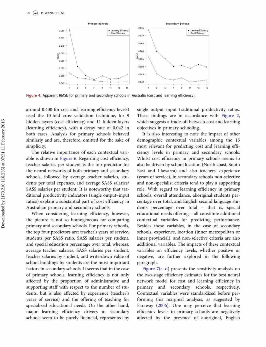
around 0.400 for cost and learning efficiency levels)used the 10-fold cross-validation technique, for 9hidden layers (cost efficiency) and 11 hidden layers(learning efficiency), with a decay rate of 0.042 inboth cases. Analysis for primary schools behavedsimilarly and are, therefore, omitted for the sake ofsimplicity.
The relative importance of each contextual vari-able is shown in Figure 6. Regarding cost efficiency,teacher salaries per student is the top predictor forthe neural networks of both primary and secondaryschools, followed by average teacher salaries, stu-dents per total expenses, and average SASS salaries/SASS salaries per student. It is noteworthy that tra-ditional productivity indicators (single output–inputratios) explain a substantial part of cost efficiency inAustralian primary and secondary schools.
When considering learning efficiency, however,the picture is not so homogeneous for comparingprimary and secondary schools. For primary schools,the top four predictors are: teacher’s years of service,students per SASS ratio, SASS salaries per student,and special education percentage over total; whereas:average teacher salaries, SASS salaries per student,teacher salaries by student, and write-down value ofschool buildings by students are the most importantfactors in secondary schools. It seems that in the caseof primary schools, learning efficiency is not onlyaffected by the proportion of administrative andsupporting staff with respect to the number of stu-dents, but is also affected by experience (teacher’syears of service) and the offering of teaching forspecialized educational needs. On the other hand,major learning efficiency drivers in secondaryschools seem to be purely financial, represented by
single output–input traditional productivity ratios.These findings are in accordance with Figure 2,which suggests a trade-off between cost and learningobjectives in primary schooling.
It is also interesting to note the impact of otherdemographic contextual variables among the 15most relevant for predicting cost and learning effi-ciency levels in primary and secondary schools.Whilst cost efficiency in primary schools seems toalso be driven by school location (North coast, SouthEast and Illawarra) and also teachers’ experience(years of service), in secondary schools non-selectiveand non-specialist criteria tend to play a supportingrole. With regard to learning efficiency in primaryschools, overall attendance, aboriginal students per-centage over total, and English second language stu-dents percentage over total – that is, specialeducational needs offering – all constitute additionalcontextual variables for predicting performance.Besides these variables, in the case of secondaryschools, experience, location (inner metropolitan orinner provincial), and non-selective criteria are alsoadditional variables. The impacts of these contextualvariables on efficiency levels, whether positive ornegative, are further explored in the followingparagraph.
Figure 7(a–d) presents the sensitivity analysis onthe two-stage efficiency estimates for the best neuralnetwork model for cost and learning efficiency inprimary and secondary schools, respectively.Contextual variables were standardized before per-forming this marginal analysis, as suggested byFaraway (2006). One may perceive that learningefficiency levels in primary schools are negativelyaffected by the presence of aboriginal, English
Figure 4. Apparent RMSE for primary and secondary schools in Australia (cost and learning efficiency).
18 P. WANKE ET AL.
Dow
nloa
ded
by [
179.
210.
116.
235]
at 0
7:31
11
Febr
uary
201
6

Figure 5. (a) Cross-validated performance profiles over different values of the tuning parameter (cost efficiency). (b) Cross-validatedperformance profiles over different values of the tuning parameter (learning efficiency).
APPLIED ECONOMICS 19
Dow
nloa
ded
by [
179.
210.
116.
235]
at 0
7:31
11
Febr
uary
201
6

second language, and special education students,whilst they are positively affected by attendance,years of service of teachers and by a higher ratio ofschool administrative and support staff per student[cf. Figure 7(b)]. Curiously, when considering costefficiency in primary schools, the years of service ofteachers also plays a positive role in keeping school-ing costs under control. Obviously, the higher theyears of service of teachers, the higher is the teachersalary by student and the average teacher salary [cf.Figure 7(a)].
On the other hand, with regard to secondaryschools, cost efficiency levels are higher in selectiveand specialist schools, thus indicating that, to someextent, the cost and managerial benefits are derivedfrom operational focus. Although there is also apositive relationship between teacher salaries perstudent and average teacher salaries (proxies foryears of service/experience of teachers), it is note-worthy that a lower level of school administrativeand support staff salaries per student seems to be thekey for cost control. With regard to learning effi-ciency, it is interesting to note the positive impact ofan inner metropolitan location, whilst the benefits
derived from focus are ambiguous: fully selectiveschools and non-selective schools presented contra-dictory results. Similar to that which was found inprimary schools, learning efficiency tends to belower when the percentage of English second lan-guage students is high. It is also interesting to notethe cost versus learning efficiency trade-off is moreaccentuated in secondary schools, when the aspectrelated to supportive staff and administrativeexpenses per students is taken in to consideration.Readers should recall Figure 2, where this trade-offclearly emerged through a visual inspection in pri-mary schools.
VI. Policy implications and conclusions
This research assessed the efficiency drivers inAustralian public schools, using a network DEAmodel of two stages. To date, this is the first timethat a two-stage network DEA model has beenapplied in the educational context, simultaneouslyassessing cost and learning efficiency levels (Abbottand Doucouliagos 2003; Ryan 2013; and Blackburn,Brennan, and Ruggiero 2014). Another contribution
Figure 6. Relative importance of contextual variables for primary and secondary schools (cost and learning efficiency).
20 P. WANKE ET AL.
Dow
nloa
ded
by [
179.
210.
116.
235]
at 0
7:31
11
Febr
uary
201
6

Figure 7. (a) Neural network sensitivity analysis for the cost efficiency scores in primary schools (selected contextual variables). (b)Neural network sensitivity analysis for the learning efficiency scores in primary schools (selected contextual variables). (c) Neuralnetwork sensitivity analysis for the cost efficiency scores in secondary schools (selected contextual variables). (d) Neural networksensitivity analysis for the learning efficiency scores in secondary schools (selected contextual variables).
APPLIED ECONOMICS 21
Dow
nloa
ded
by [
179.
210.
116.
235]
at 0
7:31
11
Febr
uary
201
6

Figure 7. (Continued).
22 P. WANKE ET AL.
Dow
nloa
ded
by [
179.
210.
116.
235]
at 0
7:31
11
Febr
uary
201
6

of this article is the use of valuable factors to repre-sent the educational production process. As a matterof fact, the inputs, outputs and the intermediateresources of this two-stage cost/learning educationalprocess can be considered as being operational, well-known, variables within the school context. Forinstance, on the side of cost efficiency, inputs canbe proxied by asset investment and direct opera-tional expenses, together with asset depreciationand indirect operational expenses. Regarding learn-ing efficiency, its outputs could be proxied by thelearning outcomes over several years of the school-ing process. Human resources such as teachers,indirect personnel (support staff) and graduate stu-dents all constitute the intermediate resources,which link costs to learning.
A synthetic framework of the findings presentedin this article is provided in Table 5, which is derivedfrom the previous discussions of the results. Thespecific policy implications for cost and learningefficiency in primary and secondary Australianschools is that experienced teachers and school loca-tion appear to be the most comprehensive and rele-vant drivers for cost and learning efficiency inprimary and secondary schools. Although schoollocation is mostly a non-discretionary factor forpolicy makers – schools are located not only inareas with positive environments but also in negativeones – this particular result indicates the systemicbenefits of teacher skills and training in consumingless financial resources, whilst generating higher stu-dent achievement at the same time. On the otherhand, student selectivity appears to be a primary
issue for cost and learning efficiency in secondaryschools, suggesting that policy makers should paymore attention to the issue of secondary schooladmission process segmentation. Besides, specificallyapplying to primary education, it is worth noting therole played by attendance and special educationofferings on student performance, which suggests akey focus can be found on these issues with regard tolearning efficiency.
In general terms, the policy implications of thisresearch for Australian schools is the need to adoptbenchmarking practices for a regular evaluation oftheir relative efficiency. In addition, these schoolsshould continue to be treated in a segmented way,as the drivers for cost and learning efficiency levelsdiffer substantially between primary and secondaryeducation. More precisely, the results – which werepreviously analysed in the light of school differences– indicate that a number of efficiency drivers affectcost and learning efficiency levels, examples being:experience, location, school type and attendance, toname just a few. This corroborates the inherentheterogeneity of the Australian public educationalsystem.
Therefore, the findings indicate that there is anambiguous impact of different contextual variableson efficiency levels within the context of primaryand secondary schools in Australia. Whilst it is pos-sible to affirm in a broader sense that the factor ofproductivity (teachers, support personnel, etc.) perstudent helps to explain a substantial amount of theefficiency scores for cost and learning, some context-specific variables exist which should not be neglected
Table 5. A synthetic framework on the most relevant efficiency drivers in public Australian schools.Primary schools Secondary schoolsInputs● Asset investment and direct operational expenses● Asset depreciation and indirect operational expenses
Inputs● Asset investment and direct operational expenses● Asset depreciation and indirect operational expenses
Outputs● Learning outcome at year 3● Learning outcome at year 5
Outputs● Learning outcome at Years 7 and 9● Learning outcome at ICSEA
Intermediate● Students and teachers● Indirect personnel
Intermediate● Students, teachers and indirect personnel● Final year´s students
Cost efficiency School location School specializationExperienced teachers Student selectivity
Learning efficiency Attendance School locationSpecial educational offering Student selectivityExperienced teachers Experienced teachers
APPLIED ECONOMICS 23
Dow
nloa
ded
by [
179.
210.
116.
235]
at 0
7:31
11
Febr
uary
201
6

when deriving educational policies. For instance,apart from the environmental factors, primaryschools appear to be more sensitive to cut-offs ineducational funds than secondary ones, as there is aclear trade-off between cost and learning efficiency(cf. Figure 2).
One limitation of this research relates to the spe-cifics of the Australian public school system, whichmakes it more difficult to replicate and to generalizethe findings of this study to other educational sys-tems. Future research should consider the applica-tion of this two-stage DEA model in other countries/circumstances to help enhance the big picture of costand learning efficiency drivers in public education.
Disclosure statement
No potential conflict of interest was reported by the authors.
References
Abbott, M., and C. Doucouliagos. 2003. “The Efficiency ofAustralian Universities: A Data Envelopment Analysis.”Economics of Education Review 22 (1): 89–97.doi:10.1016/S0272-7757(01)00068-1.
Adler, N., and J. Berechman. 2001. “Measuring AirportQuality from the Airlines’ Viewpoint: An Application ofData Envelopment Analysis.” Transport Policy 8 (3): 171–181. doi:10.1016/S0967-070X(01)00011-7.
Adler, N., and B. Golany. 2001. “Evaluation of DeregulatedAirline Networks Using Data Envelopment AnalysisCombined with Principal Component Analysis with anApplication to Western Europe.” European Journal ofOperational Research 132 (2): 260–273.
Adler, N., and B. Golany. 2002. “Including PrincipalComponent Weights to Improve Discrimination in DataEnvelopment Analysis.” Journal of the OperationalResearch Society 53 (9): 985–991. doi:10.1057/palgrave.jors.2601400.
Adler, N., and E. Yazhemsky. 2005. ImprovingDiscrimination in Data Envelopment Analysis: PCA-DEA versus Variable Reduction. Which Method at WhatCost, Working paper, The Hebrew University ofJerusalem.
Adler, N., and E. Yazhemsky. 2010. “ImprovingDiscrimination in Data Envelopment Analysis: PCA-DEA or Variable Reduction.” European Journal ofOperational Research 202 (1): 273–284. doi:10.1016/j.ejor.2009.03.050.
Agasisti, T., and S. Longobardi. 2014. “Inequality inEducation: Can Italian Disadvantaged Students Close theGap?” Journal of Behavioral and Experimental Economics52: 8–20. doi:10.1016/j.socec.2014.05.002.
Australian Curriculum Assessment and Reporting Authority.(2010). NAPLAN Achievement in Reading, Writing,Language Conventions and Numeracy: Report for 2010.www.acara.edu.au.
Bădin, L., C. Daraio, and L. Simar. 2012. “How to Measurethe Impact of Environmental Factors in a NonparametricProduction Model.” European Journal of OperationalResearch 223 (3): 818–833. doi:10.1016/j.ejor.2012.06.028.
Barrett, N., and E. F. Toma. 2013. “Reward or Punishment?Class Size and Teacher Quality.” Economics of EducationReview 35: 41–52. doi:10.1016/j.econedurev.2013.03.001.
Barros, C. P., O. Gonçalves, and N. Peypoch. 2012. “FrenchRegional Public Airports Technical Efficiency.”International Journal of Transp Economics 39 (2): 255–274.
Beygelzimer, A., S. Kakadet, and J. Langford. 2015. “PackageFNN.” Accessed June 1. http://cran.r-project.org/web/packages/FNN/FNN.pdf
Bian, Y. 2012. “A Gram–Schmidt Process Based Approachfor Improving DEA Discrimination in the Presence ofLarge Dimensionality of Data Set.” Expert Systems withApplications 39 (3): 3793–3799. doi:10.1016/j.eswa.2011.09.080.
Blackburn, V., S. Brennan, and J. Ruggiero. 2014. “MeasuringEfficiency in Australian Schools: A Preliminary Analysis.”Socio-Economic Planning Sciences 48 (1): 4–9. ISSN0038-0121, doi:10.1016/j.seps.2013.08.002.
Bosman, A., M. Huygevoort, and L. Verhoeven. 2006.“Spelling Feedback in an ICT-Learning Environment:Issues of Proficiency, Training Efficiency, andTransfer.” International Journal of Educational Research45 (6): 341–361. doi:10.1016/j.ijer.2007.01.001.
Brennan, S., C. Haelermans, and J. Ruggiero. 2014.“Nonparametric Estimation of Education ProductivityIncorporating Nondiscretionary Inputs with anApplication to Dutch Schools.” European Journal ofOperational Research 234 (3): 809–818. ISSN 0377-2217,doi:10.1016/j.ejor.2013.10.030.
Brewer, D., and D. Goldhaber. 1996. “EducationalAchievement and Teacher Qualifications: New Evidencefrom Microlevel Data.” In Advances In EducationalProductivity Volume 6: Optimizing Education Resources,edited by Cooper, B. S. and S. T. Speakman, 243–264.Greenwich, CT: JAI Press.
Buddin, R., and G. Zamarro. 2009. “Teacher Qualificationsand Student Achievement in Urban Elementary Schools.”Journal of Urban Economics 66 (2): 103–115. ISSN0094-1190, doi:10.1016/j.jue.2009.05.001.
Caldas, S. J., and C. Bankston. 1997. “Effect of SchoolPopulation Socioeconomic Status on Individual AcademicAchievement.” The Journal of Educational Research 90 (5):269–277. doi:10.1080/00220671.1997.10544583.
Caldas, S. J., and C. Bankston. 1999. “Multilevel Examinationof Student, School, and District-Level Effects on AcademicAchievement.” The Journal of Educational Research 93 (2):91–100. doi:10.1080/00220679909597633.
Chakraborty, K., and V. Blackburn. 2013. “Efficiency andEquity in Funding for Government Schools in Australia.”
24 P. WANKE ET AL.
Dow
nloa
ded
by [
179.
210.
116.
235]
at 0
7:31
11
Febr
uary
201
6
Australian Economic Papers 52 (3–4): 127–142.doi:10.1111/1467-8454.12012.
Chen, Y., W. D. Cook, C. Kao, and J. Zhu. 2012. “NetworkDEA Pitfalls: Divisional Efficiency and Frontier Projectionunder General Network Structures.” European Journal ofOperational Research 226 (3): 507–515. doi:10.1016/j.ejor.2012.11.021.
Chen, Y., W. D. Cook, N. Li, and J. Zhu. 2009. “AdditiveEfficiency Decomposition in Two-Stage DEA.” EuropeanJournal of Operational Research 196 (3): 1170–1176.doi:10.1016/j.ejor.2008.05.011.
Chen, Y., L. Liang, and J. Zhu. 2009. “Equivalence in Two-Stage DEA Approaches.” European Journal of OperationalResearch 193 (2): 600–604. doi:10.1016/j.ejor.2007.11.040.
Chen, Y., J. Zhu, and W. D. Cook. 2010. “Deriving the DEAFrontier for Two-Stage Processes.” European Journal ofOperational Research 202 (1): 138–142. doi:10.1016/j.ejor.2009.05.012.
Conroy, S. J., and N. M. Arguea. 2008. “An Estimation ofTechnical Efficiency for Florida Public ElementarySchools.” Economics of Education Review 27 (6): 655–663.doi:10.1016/j.econedurev.2007.08.002. December 2008.
Cook, W. D., L. Liang, and J. Zhu. 2010. “MeasuringPerformance of Two Stage Network Structures by DEA:A Review and Future Perspective.” Omega 38 (6): 423–430.doi:10.1016/j.omega.2009.12.001.
Cooper, W. W., L. M. Seiford, and K. Tone. 2007. DataEnvelopment Analysis: A Comprehensive Text withModels, Applications, References and DEA–SolverSoftware. New York: Springer.
Cooper, W. W., S. Li, L. M. Seiford, R. M. Thrall, and J. Zhu.2001. “Sensitivity and Stability Analysis in DEA: SomeRecent Developments.” Journal of Productivity Analysis15 (3): 217–246. doi:10.1023/A:1011128409257.
Daponte, P., and D. Grimaldi. 1998. “Artificial NeuralNetworks in Measurements.” Measurement 23 (2,March): 93–115. doi:10.1016/S0263-2241(98)00013-X.
Daraio, C. et al. (2010). Testing Whether Two-StageEstimation is Meaningful in Nonparametric Models ofProduction. Discussion Paper #1031, Institut deStatistique, UCL, Belgium.
Darling-Hammond, L., B. Berry, and A. Thoreson. 2001.“Does Teacher Certification Matter? Evaluating theEvidence.” Educational Evaluation and Policy Analysis 23(1): 57–77. doi:10.3102/01623737023001057.
Decanio, S. J. 1999. “Estimating the Non-EnvironmentalConsequences of Greenhouse Gas Reductions Is Harderthan You Think.” Contemporary Economic Policy 17: 279–295. doi:10.1111/j.1465-7287.1999.tb00682.x.
Deller, S. C., and E. Rudnicki. 1993. “Production Efficiencyin Elementary Education: The Case of Maine PublicSchools.” Economics of Education Review 12 (1): 45–57.doi:10.1016/0272-7757(93)90042-F.
Dodson, M. E., and T. A. Garrett. 2004. “InefficientEducation Spending in Public School Districts: A Casefor Consolidation?” Contemporary Economic Policy 22:270–280. doi:10.1093/cep/byh019.
Dolan, R. C., and R. M. Schmidt. 1987. “Assessing the Impactof Expenditure on Achievement: Some Methodologicaland Policy Considerations.” Economics of EducationReview 6 (3): 285–299. doi:10.1016/0272-7757(87)90007-0.
Elliott, M. 1998. “School Finance and Opportunities to Learn:Does Money Well Spent Enhance Students’Achievement?” Sociology of Education 71 (3): 223–245.doi:10.2307/2673203.
Erdogdu, F., and E. Erdogdu. 2015. “The Impact of Accessto ICT, Student Background and School/HomeEnvironment on Academic Success of Students in Turkey:An International Comparative Analysis.” Computers &Education 82: 26–49. doi:10.1016/j.compedu.2014.10.023.March 2015.
Essid, H., P. Ouellette, and S. Vigeant. 2010. “MeasuringEfficiency of Tunisian Schools in the Presence of Quasi-Fixed Inputs: A Bootstrap Data Envelopment AnalysisApproach.” Economics of Education Review 29 (4): 589–596. doi:10.1016/j.econedurev.2009.10.014.
Faraway, J. J. 2006. Extending the Linear Model with R:Generalized Lienar, Mixed Effects and NonparametricRegression Models. Boca Raton: Chapman & Hall/CRC.
Färe, R. 1991. “Measuring Farrell Efficiency for a Firm withIntermediate Inputs.” Academia Economic Papers 19 (12):329–340. doi:10.1016/j.dss.2009.06.002.
Färe, R., and S. Grosskopf. 1996a. Intertemporal ProductionFrontiers: With Dynamic DEA. Boston: Kluwer Academic.doi:10.2307/3180285.
Färe, R., and S. Grosskopf. 1996b. “Productivity andIntermediate Products: A Frontier Approach.” EconomicsLetters 50 (1): 65–70. doi:10.1016/0165-1765(95)00729-6.
Färe, R., and S. Grosskopf. 2000. “Network DEA.” Socio-Economic Planning Sciences 34 (1): 35–49. doi:10.1016/S0038-0121(99)00012-9.
Färe, R., and G. Whittaker. 1995. “An Intermediate InputModel of Dairy Production Using Complex Survey Data.”Journal of Agricultural Economics 46 (2): 201–213.doi:10.1111/j.1477-9552.1995.tb00766.x.
Fausett, L. 1994. Fundamentals of Neural NetworksArchitectures, Algorithms, and Applications. Prentice Hall,NJ: Upper Saddle River.
Ferguson, R. F., and J. Brown. 2000. “Certification TestScores, Teacher Quality, and Student Achievement.” InAnalytic Issues in the Assessmentof Student Achievement,edited by Grissmer, D. W. and J. M. Ross. Washington,DC: U.S. Department of Education.
Fetler, M. 2001. “Student Mathematics Achievement TestScores, Dropout Rates, and Teacher Characteristics.”Teacher Education Quarterly 28 (1): 151–168.
Finn, J. D., and C. M. Achilles. 1990. “Answers andQuestions about Class Size: A Statewide Experiment.”American Educational Research Journal 27 (3): 557–577.doi:10.3102/00028312027003557.
Flaker, A. 2014. “School Management and Efficiency: AnAssessment of Charter Vs. Traditional Public Schools.”International Journal of Educational Development 39:225–236. doi:10.1016/j.ijedudev.2014.07.001.
APPLIED ECONOMICS 25
Dow
nloa
ded
by [
179.
210.
116.
235]
at 0
7:31
11
Febr
uary
201
6
Gershberg, A., and T. Schuermann. 2001. “The Efficiency–Equity Trade-Off of Schooling Outcomes: PublicEducation Expenditures and Welfare in Mexico.”Economics of Education Review 20 (1): 27–40.doi:10.1016/S0272-7757(99)00036-9.
Greenwald, R., L. V. Hedges, and R. D. Laine. 1996. “TheEffect of School Resources on Student Achievement.”Review of Educational Research 66 (3): 361–396.doi:10.3102/00346543066003361.
Gronberg, T. J., D. W. Jansen, and L. Taylor. 2012. “TheRelative Efficiency of Charter Schools: A Cost FrontierApproach.” Economics of Education Review 31 (2): 302–317. doi:10.1016/j.econedurev.2011.07.001.
Grosskopf, S., and C. Moutray. 2001. “EvaluatingPerformance in Chicago Public High Schools in theWake of Decentralization.” Economics of EducationReview 20 (1): 1–14. doi:10.1016/S0272-7757(99)00065-5.
Gurney, K. 1997. An Introduction to Neural Networks.London: UCL Press.
Haelermans, C., and J. Ruggiero 2013. “Estimating Technicaland Allocative Efficiency in the Public Sector: ANonparametric Analysis of Dutch Schools.” EuropeanJournal of Operational Research 227 (1): 174–181. ISSN0377-2217, doi:10.1016/j.ejor.2012.12.004.
Hadi-Vencheh, A., and A. Esmaeilzadeh. 2013. “A NewSuper-Efficiency Model in the Presence of NegativeData.” Journal of the Operational Research Society 64 (3):396–401.
Hair, J. F., R. E. Anderson, R. L. Tatham, & W. C. Black.1995. Multivariate Data Analysis. Englewood Cliffs, NJ:Prentice-Hall.
Halkos, G. E., N. G. Tzeremes, and S. A. Kourtzidis. 2014. “AUnified Classification of Two-Stage DEA Models.” Surveysin Operations Research and Management Science 19 (1): 1–16. doi:10.1016/j.sorms.2013.10.001.
Harrison, J., and P. Rouse. 2014. “Competition and PublicHigh School Performance.” Socio-Economic PlanningSciences 48 (1): 10–19.
Hayfield, T., and J. Racine. 2008. “NonparametricEconometrics: The Np Package.” Journal of StatisticalSoftware 27: 1–32. doi:10.18637/jss.v027.i05.
Herrbach, O. 2001. “Audit Quality, Auditor Behaviour andthe Psychological Contract.” European Accounting Review10 (4): 787–802.
Indro, D. C., C. X. Jiang, B. E. Patuwo, & G. P. Zhang, G. P.1999. “Predicting Mutual Fund Performance UsingArtificial Neural Networks.” Omega 27 (3): 373–380.
James, G., D. Witten, T. Hastie, and R. Tibshirani. 2013. AnIntroduction to Statistical Learning with Applications in R.New York: Springer.
Jehangir, K., C. A. W. Glas, and S. Berg. 2015. “Exploring theRelation between Socio-Economic Status and ReadingAchievement in PISA 2009 through an Intercepts-And-Slopes-As-Outcomes Paradigm.” International Journal ofEducational Research 71: 1–15. doi:10.1016/j.ijer.2015.02.002.
Jenkins, L., and M. Anderson. 2003. “A MultivariateStatistical Approach to Reducing the Number ofVariables in Data Envelopment Analysis.” EuropeanJournal of Operational Research 147 (1): 51–61.doi:10.1016/S0377-2217(02)00243-6.
Jeon, Y., and M. P. Shields. 2005. “Integration and Utilizationof Public Education Resources in Remote andHomogenous Areas: A Case Study of the UpperPeninsula of Michigan.” Contemporary Economic Policy23: 601–614. doi:10.1093/cep/byi044.
Johnes, J. 2015. “Operational Research in Education.”European Journal of Operational Research 243 (3): 16,683–696. ISSN 0377-2217, doi:10.1016/j.ejor.2014.10.043.
Kao, C. 2009. “Efficiency Decomposition in Network DataEnvelopment Analysis: A Relational Model.” EuropeanJournal of Operational Research 192 (3): 949–962.doi:10.1016/j.ejor.2007.10.008.
Kao, C., and S.-N. Hwang. 2008. “Efficiency Decompositionin Two-Stage Data Envelopment Analysis: An Applicationto Non-Life Insurance Companies in Taiwan.” EuropeanJournal of Operational Research 185 (1): 418–429.doi:10.1016/j.ejor.2006.11.041.
Kao, L.-J., C.-J. Lu, and -C.-C. Chiu. 2011. “EfficiencyMeasurement Using Independent Component Analysisand Data Envelopment Analysis.” European Journal ofOperational Research 210 (2): 310–317. doi:10.1016/j.ejor.2010.09.016.
Katharaki, M., and G. Katharakis. 2010. “A ComparativeAssessment of Greek Universities’ Efficiency UsingQuantitative Analysis.” International Journal ofEducational Research 49 (4–5): 115–128. doi:10.1016/j.ijer.2010.11.001.
Keating, J., P. Annett, G. Burke, and C. O’Hanlon. 2011.Mapping Funding and Regulatory Arrangements acrossthe Commonwealth and States and Territories, MelbourneGraduate School of Education. Melbourne: University ofMelbourne. Melbourne Graduate School of Education.
Kirjavainen, T., and H. Loikkanent. 1998. “EfficiencyDifferences of Finnish Senior Secondary Schools: AnApplication of DEA and Tobit Analysis.” Economics ofEducation Review 17 (4): 377–394. doi:10.1016/S0272-7757(97)00048-4.
Koh, H. C., and S. S. Tan. 1999. “A Neural NetworkApproach to the Prediction of Going Concern Status.”Accounting and Business Research 29 (3): 211–216.
Kourtesi, S., P. Fousekis, and A. Polymeros. 2012.“Conditional Efficiency Estimation With EnvironmentalVariables: Evidence From Greek Cereal Farms.” ScientificBulletin - Economic Sciences University of Pitesti, 11 (1):43–52.
Kuhn, M., and K. Johnson. 2013. Applied PredictiveModeling. New York: Springer.
Ledolter, J. 2013. Data Mining and Business Analytics with R.New Jersey: Wiley.
Liang, L., W. Cook, and J. Zhu. 2008. “DEA Models for Two-Stage Processes: Game Approach and Efficiency
26 P. WANKE ET AL.
Dow
nloa
ded
by [
179.
210.
116.
235]
at 0
7:31
11
Febr
uary
201
6

Decomposition.” Naval Research Logistics 55 (7): 643–653.doi:10.1002/nav.20308.
Liang, L., F. Yang, W. D. Cook, and J. Zhu. 2006. “DEAModels for Supply Chain Efficiency Evaluation.” Annals ofOperations Research 145 (1): 35–49. doi:10.1007/s10479-006-0026-7.
Lozano, S. 2011. “Scale and Cost Efficiency Analysis ofNetworks of Processes.” Expert Systems with Applications38 (6): 6612–6617. doi:10.1016/j.eswa.2010.11.077.
Madeira Junior, A. G., M. Cardoso Junior, M. N. Belderrain,A. R. Correia, and S. H. Schwanz. 2012. “Multicriteria andMultivariate Analysis for Port Performance Evaluation.”International Journal of Production Economics 140 (1):450–456. doi:10.1016/j.ijpe.2012.06.028.
Maghbouli, M., A. Amirteimoori, and S. Kordrostami. 2014.“Two-Stage Network Structures with Undesirable Outputs:A DEA Based Approach.” Measurement 48 (February):109–118. doi:10.1016/j.measurement.2013.10.032.
Marlow, M. L. 2000. “Spending, School Structure, and PublicEducation Quality. Evidence from California.” Economicsof Education Review 19 (1): 89–106. doi:10.1016/S0272-7757(99)00035-7. February 2000.
Matin, R. K., and R. Azizi. 2015. “A Unified Network-DeaModel for Performance Measurement of ProductionSystems.” Measurement 60: 186–193. January 2015.
McGiverin, J., D. Gilman, and C. Tillitski. 1989. “A Meta-Analysis of the Relation between Class Size andAchievement.” The Elementary School Journal 90 (1): 47–56. doi:10.1086/461601.
Miningou, É. W., and V. Vierstraete. 2013. Households’Living Situation and the Efficient Provision of PrimaryEducation in Burkina Faso. Economic Modelling 35: 910–917. ISSN 0264-9993, doi:10.1016/j.econmod.2013.03.002.
Mizala, A., P. Romaguera, and D. Farren. 2002. “TheTechnical Efficiency of Schools in Chile.” AppliedEconomics 34 (12): 1533–1552. doi:10.1080/00036840110103256.
Monk, D. H. 1994. “Subject Area Preparation of SecondaryMathematics and Science Teachers and StudentAchievement.” Economics of Education Review 13: 125–145. doi:10.1016/0272-7757(94)90003-5.
Nadimi, R., and F. Jolai. 2008. “Joint Use of Factor Analysis(FA) and Data Envelopment Analysis (DEA) for Rankingof Data Envelopment Analysis.” International Journal ofMathematical, Physical and Engineering Sciences 2 (4):218–222.
Nyhan, R. C., and M. G. Alkadry. 1999. “The Impact ofSchool Resources on Student Achievement Test Scores.”Journal of Education Finance 25 (2): 211–227.
Okpala, C. O. 2002. “Educational Resources, StudentDemographics and Achievement Scores.” Journal ofEducation Finance 27 (3): 885–907.
Okpala, C. O., A. O. Okpala, and F. E. Smith. 2001. “ParentalInvolvement, Instructional Expenditures, FamilySocioeconomic Attributes, and Student Achievement.”The Journal of Educational Research 95 (2): 110–115.doi:10.1080/00220670109596579.
Okpala, C. O., F. Smith, E. Jones, and R. Ellis. 2000. “A ClearLink between School and Teacher Characteristics, StudentDemographics, and Student Achievement.” Education 120(3): 487–494.
Oliveira, M. A., and C. Santos. 2005. “Assessing SchoolEfficiency in Portugal Using FDH and Bootstrapping.”Applied Economics 37 (8): 2005.
Ouellette, P., and V. Vierstraete. 2005. “An Evaluation of theEfficiency of Québec’s School Boards Using the DataEnvelopment Analysis Method.” Applied Economics 37(14): 1643–1653. doi:10.1080/00036840500173247.
Palomares-Salas, J. C., A. Agüera-Pérez, J. J. Rosa, and A.Moreno-Muñoz. 2014. “A Novel Neural Network MethodforWind Speed Forecasting Using ExogenousMeasurementsfrom Agriculture Stations.” Measurement 55 (September):295–304. doi:10.1016/j.measurement.2014.05.020.
Podinovski, V. V., I. Ismail, T. Bouzdine-Chameeva, and W.Zhang. 2014. “Combining the Assumptions of Variableand Constant Returns to Scale in the EfficiencyEvaluation of Secondary Schools.” European Journal ofOperational Research 239 (2): 504–513. doi:10.1016/j.ejor.2014.05.016.
Prasetyo, A. D., and U. Zuhdi. 2013. “The GovernmentExpenditure Efficiency towards the Human Development.”Procedia Economics and Finance 5: 615–622.
Primont, D. F., and B. Domazlicky. 2006. “StudentAchievement and Efficiency in Missouri Schools and theNo Child Left behind Act.” Economics of Education Review25 (1): 77–90. doi:10.1016/j.econedurev.2004.11.002.
Pugh, G., J. Mangan, V. Blackburn, and D. Radicic. 2014.“School Expenditure and School Performance: Evidencefrom New South Wales Schools Using a Dynamic PanelAnalysis.” British Educational Research Journal.doi:10.1002/berj.3146.
Rahimi-Ajdadi, F., and Y. Abbaspour-Gilandeh. 2011.“Artificial Neural Network and Stepwise Multiple RangeRegression Methods for Prediction of Tractor FuelConsumption.” Measurement 44 (10, December): 2104–2111. doi:10.1016/j.measurement.2011.08.006.
Rajchert, J. M., T. Żułtak, and M. Smulczyk. 2014.“Predicting Reading Literacy and Its Improvement in thePolish National Extension of the PISA Study: The Role ofIntelligence, Trait- and State-Anxiety, Socio-EconomicStatus and School-Type.” Learning and IndividualDifferences 33: 1–11. doi:10.1016/j.lindif.2014.04.003.
Ruggiero, J. 2001. “Determining the Base Cost Of Education:An Analysis Of Ohio School Districts.” ContemporaryEconomic Policy 19: 268–279. doi:10.1093/cep/19.3.268.
Ruggiero, J., andD. F. Vitaliano. 1999. “Assessing the Efficiencyof Public Schools Using Data Envelopment Analysis andFrontier Regression.” Contemporary Economic Policy 17:321–331. doi:10.1111/j.1465-7287.1999.tb00685.x.
Ryan, C. 2013. “What Is behind the Decline in StudentAchievement in Australia?” Economics of EducationReview 37: 226–239. doi:10.1016/j.econedurev.2013.08.008.
Samoilenko, S., and K. M. Osei-Bryson. 2008. “Increasing theDiscriminatory Power of DEA in the Presence of the
APPLIED ECONOMICS 27
Dow
nloa
ded
by [
179.
210.
116.
235]
at 0
7:31
11
Febr
uary
201
6
Sample Heterogeneity with Cluster Analysis and DecisionTrees.” Expert Systems with Applications 34 (2): 1568–1581. doi:10.1016/j.eswa.2007.01.039.
Sanders, W. 1993. “Expenditures and Student Achievementin Illinois: New Evidence.” Journal of Public Economics 52(3): 403–416. doi:10.1016/0047-2727(93)90043-S.
Sanders, W. L., S. P. Wright, and S. P. Horn. 1997. “Teacherand Classroom Context Effects on Student Achievement:Implications for Teacher Evaluation.” Journal of PersonnelEvaluation in Education 11 (1): 57–67. doi:10.1023/A:1007999204543.
Scippacercola, S., and L. D’Ambra. 2014. Estimating theRelative Efficiency of Secondary Schools by StochasticFrontier Analysis. Procedia Economics and Finance 17:79–88. ISSN 2212-5671, doi:10.1016/S2212-5671(14)00881-8.
Shao, R., W. Hu, Y. Wang, and X. Qi. 2014. “The FaultFeature Extraction and Classification of Gear UsingPrincipal Component Analysis and Kernel PrincipalComponent Analysis Based on the Wavelet PacketTransform.” Measurement 54 (August): 118–132.doi:10.1016/j.measurement.2014.04.016.
Shmueli, G., N. R. Patel, and P. C. Bruce. 2010. Data Miningfor Business Intelligence: Concepts, Techniques, andApplications in Microsoft Office Excel with XLMiner. 2nded. New Jersey: Wiley.
Shokoohi, R., N. R. Hanif, and M. Dali. 2012. Influence of theSocio-Economic Factors on Children’s School Travel.Procedia - Social and Behavioral Sciences 50: 135–147.ISSN 1877-0428, doi:10.1016/j.sbspro.2012.08.022.
Simar, L., and P. Wilson. 2011. “Two-Stage DEA: CaveatEmptor.” Journal of Productivity Analysis 36 (2): 205–218. doi:10.1007/s11123-011-0230-6.
Sirin, S. R. 2005. “Socioeconomic Status and AcademicAchievement: A Meta-Analytic Review of Research.”Review of Educational Research 75 (3): 417–453.doi:10.3102/00346543075003417.
Smith, M. O. 2004. “How the Apportionment of DistrictMoney Is Associated with Differences in the Grade 8Mathematics and Reading Achievement Scores forMinnesota Students.” Journal of Education Finance 29(4): 299–314.
Tabachnick, B. G., and L. S. Fidell. 2001. Using MultivariateStatistics. Boston: Allyn and Bacon.
Tajalli, H., and C. Opheim. 2005. “Strategies for Closing theGap: Predicting Student Performance in EconomicallyDisadvantaged Schools.” Educational Research Quarterly28 (4): 44–54.
Tavana, M., and K. Khalili-Damghani. 2014. “A New Two-Stage Stackelberg Fuzzy Data Envelopment AnalysisModel.” Measurement 53 (July): 277–296. doi:10.1016/j.measurement.2014.03.030.
Thieme, C., D. Prior, and E. Tortosa-Ausina. 2013. “AMultilevel Decomposition of School Performance UsingRobust Nonparametric Frontier Techniques.” Economicsof Education Review 32: 104–121. doi:10.1016/j.econedurev.2012.08.002.
Tone, K., and M. Tsutsui. 2009. “Network DEA: A Slacks-Based Measure Approach.” European Journal of OperationalResearch 197 (1): 243–252. doi:10.1016/j.ejor.2008.05.027.
Tone, K., and M. Tsutsui. 2010. “Dynamic DEA: A Slacks-Based Measure Approach.” Omega 38 (3–4): 145–156.doi:10.1016/j.omega.2009.07.003.
Torgo, L. 2011. Data Mining with R: Learning with CaseStudies. Boca Raton: CRC Press.
Treputtharat, S., and S. Tayiam. 2014. School ClimateAffecting Job Satisfaction of Teachers in PrimaryEducation, Khon Kaen, Thailand. Procedia - Social andBehavioral Sciences 116: 996–1000. ISSN 1877-0428,doi:10.1016/j.sbspro.2014.01.334.
Waldo, S. 2007. “ on the Use of Student Data in EfficiencyAnalysis: Technical Efficiency in Swedish UpperSecondary School.” Economics of Education Review 26(2): 173–185. doi:10.1016/j.econedurev.2005.06.005.
Wang, S. 2003. “Adaptive Non-Parametric EfficiencyFrontier Analysis: A Neural-Network-Based Model.”Computers & Operations Research 30 (2): 279–295.doi:10.1016/S0305-0548(01)00095-8.
Wang, W.-K., W.-M. Lu, and C.-J. Tsai. 2011. “TheRelationship between Airline Performance and CorporateGovernance Amongst US Listed Companies.” Journal ofAir Transport Management 17 (2): 148–152. doi:10.1016/j.jairtraman.2010.06.005.
Wang, Y.-M., and K.-S. Chin. 2010. “Some Alternative DEAModels for Two-Stage Process.” Expert Systems withApplications 37 (12): 8799–8808. doi:10.1016/j.eswa.2010.06.024.
Warming-Rasmussen, B., and L. Jensen. 1998. “QualityDimensions in External Audit Services – An ExternalUser Perspective.” European Accounting Review 7 (1). 65–82. doi:10.1080/096381898336583.
Wenger, J. W. 2000. “What Do Schools Produce?Implications of Multiple Outputs in Education.”Contemporary Economic Policy 18: 27–36. doi:10.1111/j.1465-7287.2000.tb00003.x.
Wößmann, L., andM.West. 2006. “Class-Size Effects in SchoolSystems around the World: Evidence from Between-GradeVariation in TIMSS.” European Economic Review 50 (3):695–736. doi:10.1016/j.euroecorev.2004.11.005.
Xiao, Y., and L. Feng. 2014. “A Novel Linear RidgeletNetwork Approach for Analog Fault Diagnosis UsingWavelet-Based Fractal Analysis and Kernel PCA asPreprocessors.” Measurement 45 (3, April): 297–310.doi:10.1016/j.measurement.2011.11.018.
Yang, Z. 2006. “A Two-Stage DEA Model to Evaluate theOverall Performance of Canadian Life and HealthInsurance Companies.” Mathematical and ComputerModelling 43 (7–8): 910–919. doi:10.1016/j.mcm.2005.12.011.
Zha, Y., and L. Liang. 2010. “Two-Stage Cooperation Modelwith Input Freely Distributed among the Stages.”European Journal of Operational Research 205 (2): 332–338. doi:10.1016/j.ejor.2010.01.010.
Zhu, J. 2011. ‘Airlines Performance via Two-StageNetworkDEAApproach.’ Journal of CENTRUM Cathedra 4 (2): 260–269.
28 P. WANKE ET AL.
Dow
nloa
ded
by [
179.
210.
116.
235]
at 0
7:31
11
Febr
uary
201
6