Electronic copy available at: http://ssrn.com/abstract=1649968

Correlation of Revenue Growth Across Industriesin Business Cycle∗

Stefan Erdorf† Nicolas Heinrichs‡

Graduate School of Risk ManagementUniversity of Cologne

Working PaperMay 2010

Abstract

In this article we investigate the correlation between growth rates of revenues acrossdifferent industries linked to the phases of the business cycle over a 40 year (1969-2009)period. Using a large sample of quarterly firm revenues aggregated to industry revenues,we find that correlations of revenue growth across industries are not constant among crisis,boom and common phase. We provide empirical evidence that average correlations arehigher during crisis than in common phase. The empirical outcome also shows that averagecorrelations are higher in crisis than in boom and higher in boom than in common phase.We test the hypotheses that average correlations are significantly different by applyingpermutation and bootstrap techniques. The existence of structural changes in correlationof revenue growth through the phases of business cycle should be applied to research infirm valuation and has implications for diversification decisions in portfolio analysis andrisk management.

JEL-Classification: C12, E32, M49

Keywords: revenues, correlation, business cycle, filtration, bootstrap, permutation test∗We thank the following for their valuable comments: Prof. Dr. Thomas Hartmann-Wendels, Prof. Dr.

Dieter Hess, Prof. Dr. Carsten Homburg, Prof. Dr. Joachim Grammig, Antonios Ioannidis, KonstantinGlombek, Carsten Körner, Thomas Kerpen and especially for his support Stefan Günther.†Graduate School of Risk Management, Meister-Ekkehart-Str. 11, University of Cologne, 50923 Cologne,

Germany, e-mail: Erdorf@wiso.uni-koeln.de‡Graduate School of Risk Management, Meister-Ekkehart-Str. 11, University of Cologne, 50923 Cologne,

Germany, e-mail: Heinrichs@wiso.uni-koeln.de

1

Electronic copy available at: http://ssrn.com/abstract=1649968

1 Introduction

The state of the economy influences the amount of correlation between revenue growth across

industries. Numerous articles have examined the correlation structure of stocks, government

bonds, corporate bonds and currencies in different market environments but correlation be-

tween revenues has not been investigated so far. The intent of this study is to examine corre-

lation between industry growth rates of revenues conditioned on the state of its environment.

The main contribution of this article is the disclosure of structural differences in correlation

of revenue growth through the phases of business cycle. Especially the finding that the times

of crisis are those with the highest correlation has consequences for portfolio allocation and

diversification decisions. When dealing with correlations, the different levels of correlation in

the phases of business cycle have to be taken into account. The higher the correlations in times

of crisis are, the higher the bankruptcy probability of portfolios is, which is often neglected

carelessly in valuation of assets. If all revenues tend to fall together as the economy plunges

down, the value of diversification may be overstated by those not regarding the higher correla-

tions in crisis. Beside that, we document estimations of unconditional correlations of revenues

between industries and compare them with the conditional correlations. While the results of

previous studies have implications for equity and bond portfolio allocation, our findings are

important for portfolio management of business segments in multi-business firms. Moreover,

it influences the choice of merger and acquisitions and private equity investments.

Our sample contains firms with available quarterly revenue data from Standard & Poor’s

COMPUSTAT database during the period of 1969 to 2009. We aggregate these revenues to two

industry panels according to the Standard Industry Classification (SIC) code and the Fama-

French 48 (FF48) industry classification. In order to analyze correlation behavior the panels

are conditioned on business cycle. After cleaning the growth rates of revenues for autocorre-

lation and heteroskedasticity, we therefore divide each of the two panels into three sub panels

‘boom’, ‘crisis’ and ‘common phase’.1 The separation of these sub panels is reached by em-

ploying the Chicago Fed National Activity Index (CFNAI) and capacity utilization growth

(CUG) as business cycle indicators. The challenge of research with revenue data is its limited1Note, common phase includes all quarters which are neither classified as crisis nor classified as boom.

2

availability. While stocks and bonds are traded daily, revenue data is only provided by firms

quarterly. Furthermore, quarterly data of revenues has only been sufficiently available for the

last 40 years in the COMPUSTAT database. Because we do not observe more time points of rev-

enue data, the statistical significance of hypotheses tests is limited in some cases. We test the

hypotheses that average correlations of the phases are significantly different from each other

by applying permutation and bootstrap techniques. Using Pearson’s correlation coefficient and

Kendall’s τ we provide empirical evidence that average correlations2 are higher during crisis

than in times of common phase. The empirical outcome also indicates that average correlations

are higher in crisis than in boom and higher in boom than in common phase. However, the

last-mentioned results are rarely statistically significant due to the above-noted data availabil-

ity. Furthermore, the average correlations in crisis are higher and those in common phase are

lower than the unconditional ones.

As already mentioned, several articles address the question of correlation behavior depending

on different market phases. Kaplanis (1988) is one of the first who investigates the correlation

stability of financial asset returns. By applying the Jennrich-χ2 test her analysis shows that

the hypothesis of correlation stability between monthly returns during 1967 and 1982 cannot

be rejected.3 Erb et al. (1994) find that cross-equity correlations in certain countries are in-

fluenced by the business cycle. They state that correlations are higher in times of recessions

than during growth periods. When business cycles of two countries are classified as out of

phase, correlations are low. They compare the average correlations by classifying the returns

with two approaches. In their first approach they differentiate between equity co-movements

in bull and bear markets by segmenting the data by ex-post returns. A month is defined as

"up" when the returns have an above-average performance and as "down" when the returns

are below average. They classify the market into the following categories: up-up, down-down

and up-down/down-up. In their second approach the returns are segmented into three busi-

ness cycle categories (recession-recession, growth-growth and out of phase) by applying the

Center for International Business Cycle Research (CIBCR) indicator for peaks and troughs.2Note, for the sake of simplification, we use the term "correlation" as a synonym for both Pearson’s correlation

coefficient and Kendall’s τ as it is often done in literature.3See Ratner (1992) and Tang (1995) who support these findings.

3

Ang and Chen (2002) test asymmetries in conditional correlations between U.S. stocks and the

aggregate U.S. market and provide evidence that correlations for downside moves are higher

than for upside moves. They classify the downside correlations by equity returns and market

returns below a pre-specified level and the upside correlations by equity returns and market

returns above a pre-specified level. Further studies focus on the correlation behavior between

financial asset returns during stable and turbulent market periods (e.g. Bertero and Mayer

(1990), King and Wadhwani (1990), Lee and Kim (1993) and Ramchand and Susmel (1998)).

These articles provide evidence of increasing correlations in volatile market periods. Based

on a multivariate GARCH model, Longin and Solnik (1995) analyze data of monthly stock

indices for industrial countries and conclude that the correlations between international finan-

cial markets increase in high volatile periods. Moreover, Bernhart et al. (2009) examine the

correlations between stocks, corporate bonds and government bonds in calm and turbulent

market periods. They show that correlations within these asset classes increase in turbulent

markets. A number of further articles also find significant differences in correlations among

international equity returns in bull and bear markets.4

Several studies reveal that computing correlations which are conditioned on low or high re-

turns, or on low or high volatility, causes a conditioning bias in the correlation estimates. For

example, Boyer et al. (1999) state that a selection bias is induced by splitting the sample

according to the observed or realized data alone. Forbes and Rigobon (2002) show that a bias

occurs due to heteroskedasticity of financial return series. To circumvent these bias problems

we apply exogenous indicators to classify the phases of business cycle and clean the growth

rates of revenues for autocorrelation and heteroskedasticity by using a filtration approach.

The remainder of this article is as follows. In section 2 we discuss the classification of revenues

by industries and the partition of quarters by business cycle indicators. Section 3 describe the

research methodology by introducing the dependence measures, the sample and our hypothe-

ses. Section 4 presents the results of average correlations and of the hypotheses tests. The

final section 5 concludes the article.4For example, see Karolyi and Stulz (1996), Longin and Solnik (2001), Ang and Bekaert (2002), Campbell

et al. (2002), Das and Uppal (2004), Patton (2004), Poon et al. (2004) and Dobric et al. (2007).

4

2 Classification of Revenues

In this section we describe the role of revenues for financial research. We introduce industry

classification schemes to separate firms into industry portfolios and business cycle indicators

to partition quarters according to the state of the economy.

2.1 Why is Research About Revenues an Important Issue?

Revenues contain sustainable information on firm performance. As Kama (2009) states, on one

hand, revenues generate current earnings and cash flows. On the other hand, revenues serve

as an indicator of future performance and persistence. Revenues enable a better reflection of

firm performance than other fundamentals, like expenses. Chandra and Ro (2008) state that

product differentiation reflected in revenue increase is more difficult to copy by competitors

than cost-cutting strategies. Ghosh et al. (2005) explain that expenses are also cut in response

to financial distress and could be increased in anticipation of future profits. Revenue change

therefore provides more accurate information about future prospects than changes in expenses.

Revenues differ in persistence from expenses and earnings. Ertimur et al. (2003) mention that

revenues are more persistent than expenses because revenues are more homogeneous and more

difficult to be influenced by managers.5 The greater persistence of revenues is lost when

it is aggregated with gains, losses and expenses into earnings. Swaminathan and Weintrop

(1991) point out that revenues have information content that is incremental to earnings. The

application of earnings management reduces the information content of earnings. For example,

managers can hide changes in their firm’s performance using financial reporting opportunities

to smooth earnings.6 As a result, revenues are more persistent and less influenced through

accounting discretion. Consequently, the revenues’ co-movement with the business cycle should

be stronger than the co-movement of other fundamentals with the business cycle. Finally,

revenues are a fundamental indicator of future cash flows. As mentioned by Rappaport (1986)5As an indicator of the higher revenue persistence, Ertimur et al. (2003) reveal higher autocorrelation for

revenues than for expenses.6The variability of reported earnings can be smoothed by changing the accounting component of earnings,

namely accruals. See Healy and Wahlen (1999) and Leuz et al. (2003) about findings on earnings management.Furthermore, Burgstahler and Dichev (1997) and Degeorge et al. (1999) provide evidence that U.S. managersuse accounting discretion to prevent reporting losses.

5

and Penman (2010), revenues are one of the key drivers in valuing firms.7

2.2 Industry Classification Schemes

Firm revenues can be distorted by M&A activities. After an acquisition, the firm taken over dis-

appears from the sample and the revenues of the acquiring firm increase heavily, only caused by

the acquisition itself. To deal with these M&A-effects, the firm revenues should be aggregated

to industry revenues assuming that the M&A-effects tend to balance out within an indus-

try class and across industries. In this section we discuss the common industry classification

schemes in capital market research.8 Industry classification generates additional information

for financial and economic analyses by dividing firms into homogeneous groups.

The Standard Industrial Classification (SIC) codes have become the first algorithm for depict-

ing industrial activities in the United States and are largely used in financial research. The SIC

scheme was introduced by the Interdepartmental Committee on Industrial Classification and

classifies all industries in the U.S. economy. Starting from industry divisions (one-digit SIC

codes) finer partitions are defined, namely major groups (two-digit SIC codes), industry groups

(three-digit SIC codes) as well as industries (four-digit SIC codes).9 To account for changes

in the organization and segmentation of industries, SIC codes were updated until the imple-

mentation of a new system. The North American Industry Classification System (NAICS) was

established by the U.S. Census Bureau and jointly developed with Canada and Mexico in order

to replace the SIC codes. Both SIC codes and NAICS are production and technology oriented,

but the aim of NAICS is to improve the SIC by identifying new industries and reorganizing

industry groups to a more precise reflection of economy’s dynamics, as mentioned by Saun-

ders (1999).10 During the current transfer process both systems are offered in the COMPUSTAT

database. In our study we prefer SIC codes to NAICS for several reasons. First, SIC codes

are commonly used in academic research. Second, in our sample the data availability of SIC

codes is greater than for NAICS. Finally, as stated by Bhojraj et al. (2003), the performance7Applications of revenues in firm valuation are discounted cash flow models, revenue-based multiples,

value driver models (see Rappaport (1986)) and stochastic models (see Schwartz and Moon (2000) andErdorf et al. (2010)).

8A broad comparison of industry classification is discussed in Bhojraj et al. (2003).9For further information about the SIC codes see http://www.osha.gov/oshstats/index.html.

10Krishnan and Press (2003) compare the differences between SIC codes and NAICS in their study.

6

of both are fairly similar in most financial applications. The Fama-French 48 (FF48) industry

classification, introduced by Fama and French (1997), reorganizes firms by the four-digit SIC

codes into 48 industry groups.11 The intent of Fama and French is to form groups of industries

according to their common risk characteristics. Similar to SIC codes, the FF48 industry classi-

fication is widely used and has a great impact on academic research. Nevertheless, Chan et al.

(2007) mention that Fama and French do not offer sufficient evidence about how well their clas-

sification system generates groups of economically similar firms. Another approach of industry

classification is the Global Industry Classifications Standard (GICS) system, which was jointly

developed by Standard & Poor’s and Morgan Stanley Capital International. Firms are cate-

gorized by their core business activities. The classification does not only consider operational

aspects but it is also based on information about the perceptions of investors concerning the

firm’s core business. The GICS system is applied among financial practitioners, but contrary

to FF48 industry classification it is not commonly used by academic researchers.

In our empirical study we classify the firms of the sample by SIC codes and FF48 industry clas-

sification. We do not use NAICS and GICS because of the incomplete observations. Precisely,

through the application of NAICS and GICS five to ten percent of the observations currently

available from COMPUSTAT database would be omitted.

2.3 Business Cycle Indicators

In order to analyze the correlation behavior of industry revenues in the business cycle, we divide

it into different phases. In times of crisis, when markets fall jointly, we expect correlation to

increase heavily. We also expect joint behavior of revenues in times of boom. Therefore,

we separate crisis and boom from each other and the remaining states of the economy. If

a quarter is neither classified as crisis nor classified as boom, it remains in common phase.

A more detailed differentiation within common phase is redundant in our study. Because of

the assumption that correlations vary between crisis, boom and common phase, a business

cycle indicator which differentiates between those three phases is indispensable. To avoid11For the transformation of SIC codes into these industries see Appendix of Fama and French (1997). De-

tailed information about the FF48 industry classification is available at the website of Kenneth R. French,http://mba.tuck.dartmouth.edu/pages/faculty/ken.french.

7

a selection bias12, we require an exogenous indicator to partition the quarters of revenue

growth. Several business cycle indicators are considered in financial research. In our empirical

study we apply both the Chicago Fed National Activity Index (CFNAI) and the log growth

of capacity utilization (CUG) as exogenous indicators.13 As an additional verification of our

business cycle partition we compare it with the National Bureau of Economic Research (NBER)

turning points. These turning points are defined by peaks and troughs in business cycle that

frame economic recession and expansion. The NBER states that a recession is not defined

in terms of two consecutive quarters of decline in real GDP. A recession is described as a

significant decline in economic activity spread across the economy, lasting more than a few

months, generally indicated by the real GDP, real income, employment, industrial production,

and trade.14 According to the NBER, the vast majority of months are defined as expansions.

Most of them can be interpreted as common phases of the economy. There is no differentiation

between common phase and boom. However, the NBER recessions can be compared to crises

identified by CFNAI and CUG.

The CFNAI is a monthly summary index constructed to measure overall economic activity

and associated inflationary pressure. It corresponds to the index of economic activity by

Stock and Watson (1999). The CFNAI is a weighted average of 85 monthly indicators of

U.S. activity. These 85 economic indicators are selected from four comprehensive categories

which are (1) production and income, (2) employment, unemployment and hours, (3) personal

consumption and housing, as well as (4) sales, orders, and inventories. The CFNAI is centered

to a value of zero and has a standard deviation of one. When the value of the index is zero,

the U.S. economy is growing at the economy’s historical trend growth rate. A negative value

for the CFNAI indicates that the U.S. economy is growing below its average growth rate while

a positive value indicates above average growth. Beside the monthly index, the CFNAI is

provided as a three-month moving average. Because the monthly index can be volatile and

revenue observations are provided quarterly, we choose the index’s three-month moving average12See Boyer et al. (1999).13A further often applied business cycle indicator is the Experimental Coincident Recession Index (XRIC)

developed by Stock and Watson (1989). The advantage, that this index is a forecasting indicator, is irrelevantin our context. Furthermore, the availability of XRIC data is limited to the end of 2003 which makes the XRICinappropriate for our study.

14For more information, see http://www.nber.org/cycles.html.

8

of the last month in the current quarter as one of our two business cycle indicators. As defined

by the Chicago Fed, an increasing likelihood for a started recession is indicated by a value of

the three-month moving average below -0.7 when it is following an expansion period. After

a contraction period, a value above -0.7 indicates an increasing likelihood and a value above

+0.2 indicates a significant likelihood that a recession has ended.15 Considering our study,

crisis is determined by values of the CFNAI’s three-month moving average below -0.7. Because

we differentiate the sample in three phases, we also have to assume an upper threshold to

distinguish between common phase and boom. The CFNAI definition does not provide any

Figure 1: Three-month moving average CFNAI (1969-2009)

Shaded areas indicate the NBER recessions between 1969 and 2009.

threshold which indicates boom phases, therefore we define a threshold which identifies a boom

in line with the commonly known booms. All values above 0.55 are assigned to boom and all

quarters which are between the two thresholds are classified as common phase.16 Remember,

the NBER only differentiates between recession and other states of the economy, which the

NBER calls expansion. As shown in figure 1, comparing our identified quarters of crisis with15Evans et al. (2002) critically discuss these thresholds of the CFNAI.16The historical and current data of the CFNAI are provided by the Chicago Fed on their website,

http://www.chicagofed.org/webpages/research/data/cfnai/current_data.cfm.

9

the NBER turning points reveals that our partition identifies all NBER recessions.

As a second business cycle indicator we employ the capacity utilization growth (CUG). In

Corrado and Mattey (1997) capacity utilization is defined as a ratio of the actual level of

output to a sustainable maximum level of output, or capacity. The Federal Reserve Board

calculates the capacity utilization quarterly for the industrial sector of the U.S. economy. In

order to use the capacity utilization as a business cycle indicator, we calculate its quarterly

log growth rates.17 This resulting new indicator ought to represent the different phases in the

business cycle according to changes of capacity utilization and independent of its level. To

differentiate between our three phases we again have to define two thresholds. To be consistent

both with the NBER indicator and with our CFNAI partition, we choose the upper threshold

as 0.008 and the lower threshold as -0.013. As shown in figure 2, growth rates above 0.008 and

Figure 2: Capacity Utilization Growth CUG (1969-2009)

Shaded areas indicate the NBER recessions between 1969 and 2009.

below -0.013 indicate boom and crisis, respectively. The resulting crises are in line with the

crises given by NBER. The values between -0.013 and 0.008 are specified as common phase.17The seasonally adjusted, quarterly data of the capacity utilization total index are available on the website

of The Federal Reserve Board, http://www.federalreserve.gov/datadownload/.

10

As shown in the figures, the partition in the three phases is not inevitably identical through both

business cycle indicators. Further details about the partition of quarterly revenue growth in our

study will be presented in section 3. Moreover, the differences between correlations conditioned

on the three phases are only slightly sensitive to the variety of the applied thresholds of the

two business cycle indicators.

3 Research Methodology

In this section we introduce the two dependence measures Pearson’s correlation coefficient and

Kendall’s τ . Afterwards we describe our sample and prepare the data for our analysis. We

estimate the correlation matrices and define our hypotheses.

3.1 Dependence Measures

We measure the correlation18 of revenue growth rates by using Pearson’s correlation coefficient

and Kendall’s τ . To define their conditional empirical versions we regard a sample of n points

(xk, yk), for k = 1, . . . , n, of two random variables X and Y . Let S be a subsample of these

points. Projected on our sample, X and Y are the residuals of two industry revenue growth

rates and S is a subsample of the observations in one of the three business cycle phases. The

conditional empirical version of Pearson’s correlation coefficient is defined as:

Corr(X,Y |S) =∑nk=1,(xk,yk)∈S(xk − x)(yk − y))√∑n

k=1,(xk,yk)∈S(xk − x)2√∑n

k=1,(xk,yk)∈S(yk − y)2. (1)

Pearson’s correlation coefficient is invariant under strictly increasing linear transformations.

However, the right use of this coefficient depends on the assumptions made with respect to

the data to be analyzed. An important assumption is that the distributions of both variables

should be normal and that the scatter-plots should be linear and homoskedastic. In situations

where the assumptions are injured, Pearson’s correlation coefficient can become inadequate to

explain a given relationship, e.g. it fails to show perfect dependence if the relationship between18Remember, for the sake of simplification, we use the term "correlation" as a synonym for both Pearson’s

correlation coefficient and Kendall’s τ .

11

two variables is not linear. The Pearson’s correlation coefficient is affected by the marginal

distributions of time series and its estimates of equation (1) are sensitive to outliers. To

verify our results, we employ Kendall’s τ as a second measure. If we consider all possible pairs

((xk, yk), (xl, yl)) within S and either denote each of them as concordant if (xk−xl)(yk−yl) > 0

or as discordant if (xk − xl)(yk − yl) < 0, we can define the conditional empirical version of

Kendall’s τ as

τ(X,Y |S) = c− dc+ d

, (2)

where c denotes the number of concordant pairs and d the number of discordant pairs in the

subsample S. In practice there might arise cases in which xk = xl or yk = yl. Therefore

one should employ the adjusted version of Kendall’s τ , where these cases are not accounted

in the enumerator, but of course in the denominator.19 Kendall’s τ is invariant under strictly

increasing transformations. The unconditional version can be interpreted as the probability of

concordance minus the probability of discordance of the two random variables X and Y .

3.2 Sample Description

The sample contains quarterly firm revenues over a 40 year period from the first quarter in

1969 to the first quarter in 2009. We use the Standard & Poor’s COMPUSTAT quarterly database

of U.S. and Canadian market information on active and inactive publicly listed firms to obtain

information about revenues. We drop all financial institutes because of their different char-

acteristics. Revenues of financial firms are not comparable with those of industrial firms and

they are rarely provided by COMPUSTAT. We regard 21,266 different firm identifier and 923,234

observations of quarterly revenues. The revenues in the sample exhibit a mean of $288.05 mil-

lion and a standard deviation of $1,696.71 million. As shown in table 1, the mean number of

observed firms per quarter is 6,712 with a standard deviation of 1,976. The minimum number

of firms is 2,001 in the first quarter of 1969 and the maximum number of firms is 9,355 in the

first quarter of 1999.

To deal with M&A-effects, firm revenues are aggregated to industry revenues and grouped by

two different industry classifications. First, in panel A all firms are grouped in SIC industry19For more information see e.g. Lindskog (2000).

12

Table 1: Number of firms per quarter

Variable Mean Std. Dev. Min. Max.Firms 6,712 1,976 2,001 9,355

The table reports descriptive statistics about the number offirms per quarter.

portfolios by their SIC code (1-digit). As already mentioned, we exclude revenues from the

financial sector by dropping SIC codes 6000-6999 (finance, insurance and real estate). Here-

after, the remaining industries are indicated by the index i, i = 1, . . . , 9. Second, in panel B

the firms are grouped in Fama-French 48 (FF48) industry portfolios by their FF48 industry

classification. Again, after dropping the financials 44-47 (banking, insurance, real estate and

trading), the portfolios are denoted by a consecutive index j, j = 1, . . . , 44.20 Descriptive

statistics about the number of firms which are grouped in an industry portfolio per quarter are

presented in table 2.

Table 2: Number of firms per industry portfolio and per quarter

Variable Mean Std. Dev. Min. Max.Panel A: SIC 1,182 646 3 2,570Panel B: FF48 314 300 3 1,602

The table reports descriptive statistics about the number of firmswhich are grouped in an industry portfolio per quarter.

3.3 Data Preparation

The log growth rates of industry revenues rAi,t (rBj,t) for panel A (panel B) are computed by the

current industry revenues RAi,t (RBj,t) and previous industry revenues RAi,t−1 (RBj,t−1):

rAi,t = log(

RAi,tRAi,t−1

), rBj,t = log

(RBj,tRBj,t−1

), (3)

with i = 1, . . . , 9 and j = 1, . . . , 44.

Industry revenues can be biased by new stock listed firms and delisting of firms through20The SIC codes are provided by the COMPUSTAT database. For the transformation of four-digit SIC codes

into FF48 industry portfolios see Appendix of Fama and French (1997).

13

bankruptcy, among others. The sample consists of both active and inactive firms. We do

not drop the inactive firms with incomplete times series. To circumvent the problem of in-

complete time series we have to decide at each time point, which firms are involved in the

calculation of the industry growth rate. A firm is involved every time revenue data is provided

for the two consecutive time points (t and t−1). If that is not the case, the firm is not included

in the calculation of rAi,t (rBj,t) for the specific time point t. Moreover, the log growth rates of

revenues are demeaned by subtracting the respective time series mean from each growth rate.21

After computing revenue growth for all industry portfolios, we obtain 160 quarters of demeaned

growth rates.

To estimate correlations and to obtain time invariant results, the time series of growth rates

have to be stationary. Therefore, the panels A and B are tested for the presence of a unit root

by the augmented Dickey-Fuller test.22 The null hypothesis, that growth rates contain a unit

root, can be rejected at a 1% significance-level for both panels.23 Thus, we assume that the

growth rates of both panels are generated by a stationary process.

Forbes and Rigobon (2002) show that in previous research, the calculation of correlation is bi-

ased due to heteroskedasticity of financial return series. To circumvent it, we clean the growth

rates of revenues for autocorrelation and heteroskedasticity by using a filtration approach. As

a first step, we analyze the distribution of the demeaned revenue growth rates to choose an

appropriate filtration approach for our data.24 The skewness and kurtosis indicate that most

of the time series do not follow the Gaussian distribution. The skewness is negative for all time

series in panel A and for most of those in panel B, which implies that there is a substantial

probability for attaining growth rates below the mean. In more than half of the cases the excess

kurtosis is positive, which could result from heavy tails in the distributions. To verify these

impressions, we perform Jarque-Bera tests and Omnibus tests for normality.25 As expected,21Note, Pearson’s correlation coefficient and Kendall’s τ are invariant under strictly increasing linear trans-

formation.22The test is introduced by Dickey and Fuller (1979).23We provide the Dickey-Fuller test statistic with zero lags for panel A in table 8 in Appendix A. The test

results for panel B are similar.24In Appendix A, we present summary statistics of the growth rates for panel A and B in tables 9 and 10.25The Jarque-Bera test is described by Jarque and Bera (1980) and the Omnibus test is proposed by Doornik

and Hansen (2008). In Appendix A, we report the test results for panel A in table 11.

14

the null hypothesis of normality has to be rejected for most of the times series in panel A and

for more than two-thirds of the time series in panel B at a 5% significance level. Because of

the observed skewness, we choose to filter the growth rates with a semi parametric approach.

We apply the GJR-model which models asymmetry in the GARCH process and is described

by Glosten et al. (1993).

The demeaned growth rates of industry revenues are filtered with the following AR(1)-GJR(1,1)

model assuming Gaussian residuals for all industry portfolios i in panel A and j in panel B.

Note, to simplify we omit the indices i and j in the notation of the model.

rt = a0 + a1 · rt−1 + ut (4)

ut = ht · zt, ztiid∼ N(0, 1)

ht = b0 + b1 · u2t−1 + b2 · ht−1 + b3 · u2

t−1 · δt−1 (5)

with

δt =

1, if ut < 0

0, if ut ≥ 0.

For each time series of growth rates the Ljung-Box test for autocorrelation is applied in lags

15 and 25.26 If a time series of an industry portfolio passes the test, a constant-GJR(1,1)

model with Gaussian residuals is estimated. If a time series does not pass the test, the AR(1)-

GJR(1,1) model with Gaussian residuals is estimated.27 After having cleaned the times series

of growth rates for first order autocorrelation and heteroskedasticity, we obtain the residuals

ut resulting from the filtration.

Finally, the residuals are assigned to the three business cycle phases through the two indicators

CFNAI and CUG. Using our defined thresholds for the CFNAI, the sample is divided in 25

quarters of crisis, 100 quarters of common phase and 35 quarters of boom during the period of

1969 to 2009. Following the CUG, the sample period covers 25 quarters of crisis, 99 quarters of26The test is introduced by Ljung and Box (1978).27The estimated parameter from the AR(1)-GJR(1,1) model for panel A are presented in table 12 in

Appendix A. For the filtration we use the approach of Vogiatzoglou (2009).

15

common phase and 36 quarters of boom. Table 3 summarizes the two partitions. Although the

number of quarters per phase is nearly equal through both indicators, the quarters themselves

are not inevitably identical.

Table 3: Quarters of business cycle phases

State of CFNAI CUGthe economy Freq. Percent Freq. Percent

Crisis 25 15.63 25 15.63Common phase 100 62.50 99 61.88

Boom 35 21.88 36 22.50Total 160 100.00 160 100.00

The table reports the number of quarters assigned to three statesof the economy. The business cycle phases are partitioned throughCFNAI and CUG in crisis, common phase and boom.

3.4 Hypotheses

After dividing both panel A and B through CFNAI and CUG into the three sub panels crisis

(C), common phase (O) and boom (B), we estimate correlation matrices by using both Pear-

son’s correlation coefficient and Kendall’s τ . Furthermore, we estimate the unconditional (UC)

correlation matrices for the undivided panels A and B. The correlations are calculated between

the obtained residuals u within each industry classification:28

ρC = Corr(u·k , u·l |C) or ρC = τ(u·k , u·l |C) (6)

ρO = Corr(u·k , u·l |O) or ρO = τ(u·k , u·l |O) (7)

ρB = Corr(u·k , u·l |B) or ρB = τ(u·k , u·l |B) (8)

ρUC = Corr(u·k , u·l) or ρUC = τ(u·k , u·l) (9)

In the case of panel A, the residuals uik , uil result from the filtration of the growth rates rAi

with industries k, l = 1, . . . , 9. In the case of panel B, ujk , ujl result from rBj with industries

k, l = 1, . . . , 44.29 ρ indicates the estimates of Pearson’s correlation coefficient and Kendall’s τ .28Correlation matrices of SIC industry portfolios are presented in tables 14 and 15 in Appendix B.29Compare the definition of revenue growth rates in equation (3).

16

While stocks and bonds are traded daily, revenue data is only provided by firms quarterly.

Additionally, quarterly data of revenues has been only sufficiently available for the last 40 years

in the COMPUSTAT database. As already shown in table 3, the number of observed quarters is

small in the sub panels crisis and boom. To evaluate the validity of the conditional correlations

we bootstrap the correlation’s standard error.30 The number of bootstrap replications is set

to 10,000. The bootstrap distributions are not skewed and centered close to the correlation

estimates of the original sub panels. Hence, they have only small biases. The bootstrap

standard errors indicate that a pairwise comparison of individual correlations between the sub

panels is not meaningful.31 Therefore, we consider the median ˜ρ of the entries in the correlation

matrices instead of analyzing individual correlations. A further advantage of applying the

median is its statistical property. In contrast to the mean, the median is not sensitive to

outliers. This is especially important because some of the quarterly industry growth rates are

only based on a few revenue observations. The resulting correlation estimates can be heavily

biased which can lead to outliers. Beside the median correlations ˜ρ, we estimate the absolute

median correlations |ρ| because some correlations are negative. For example, the correlations

between the SIC industry portfolio i = 1 (agriculture, forestry and fishing) and most of the

other portfolios are negative.

We suppose that average correlations are higher in crisis than in common phase. In crisis

macroeconomic shocks pertain almost all industries and their revenues plunge down jointly.

Increasing demand often effects all industries together in boom, most revenues increase jointly.

This results in a higher average correlation in boom than in common phase. We assume

the negative effect of macroeconomic shocks is stronger than the positive effect of increasing

demand. We expect that average correlations in crisis are higher than in boom. Following

our assumptions, we investigate the differences between these average correlations. The null30Bootstrap methods for standard errors are shown in Efron and Tibshirani (1986).31Standard errors for the sub panels and the undivided panel for SIC industry portfolios are reported in

tables 16 and 17 in Appendix B.

17

hypotheses we are going to test can be formalized as:

HI0 : ˜ρC − ˜ρB ≤ 0 vs. HI1 : ˜ρC − ˜ρB > 0 (10)

HII0 : ˜ρB − ˜ρO ≤ 0 vs. HII1 : ˜ρB − ˜ρO > 0 (11)

HIII0 : ˜ρC − ˜ρO ≤ 0 vs. HIII1 : ˜ρC − ˜ρO > 0 (12)

The rejection of the null hypotheses would reinforce our assumptions. Beside the hypotheses

of differences between the median correlations, we also test the differences between absolute

median correlations:

HIV0 : |ρC | − |ρB | ≤ 0 vs. HIV1 : |ρC | − |ρB | > 0 (13)

HV0 : |ρB | − |ρO| ≤ 0 vs. HV1 : |ρB | − |ρO| > 0 (14)

HV I0 : |ρC | − |ρO| ≤ 0 vs. HV I1 : |ρC | − |ρO| > 0 (15)

4 Empirical Results

We present the estimates of median and absolute median correlation coefficients and discuss

their differences in the business cycle. The results are examined with hypotheses tests. We

apply the Jennrich-χ2 test, a permutation test and a bootstrap approach.

4.1 Average Correlation Coefficients

The estimation results of median and absolute median of conditional correlation coefficients

as well as the median differences and absolute median differences are presented in table 4. All

results are provided for Pearson’s correlation coefficient and Kendall’s τ . For both measures

we analyze panel A and B separately, whereas for both panels the sample is partitioned by

CFNAI as well as by CUG. Additionally, the median and the absolute median of unconditional

correlations are presented.

The results support our three hypotheses. As expected, all differences are positive, i.e. over all

states the median and absolute median correlations are always the highest in crisis and always

18

Table 4: Average correlation coefficients and correlation differences

Pearson’s Correlation Kendall’s τ

Panel A: SIC Panel B: FF48 Panel A: SIC Panel B: FF48

CFNAI CUG CFNAI CUG CFNAI CUG CFNAI CUG˜ρC 0.4225 0.4037 0.2738 0.2763 0.3200 0.2833 0.1867 0.1867˜ρO 0.2018 0.2125 0.1643 0.1571 0.1590 0.1602 0.1077 0.1039˜ρB 0.3042 0.3492 0.1685 0.2334 0.2000 0.2270 0.1143 0.1460˜ρUC 0.2712 0.2138 0.1997 0.1339

|ρC | 0.4225 0.4124 0.3078 0.2993 0.3200 0.2833 0.2033 0.2067

|ρO| 0.2400 0.2705 0.2138 0.2138 0.1877 0.1983 0.1408 0.1383

|ρB | 0.3692 0.3608 0.2523 0.2646 0.2134 0.2556 0.1664 0.1746

|ρUC | 0.2758 0.2393 0.2025 0.1543˜ρC − ˜ρB 0.1182 0.0545 0.1053 0.0429 0.1200 0.0563 0.0724 0.0406˜ρB − ˜ρO 0.1025 0.1367 0.0042 0.0762 0.0410 0.0668 0.0066 0.0421˜ρC − ˜ρO 0.2207 0.1912 0.1095 0.1191 0.1610 0.1232 0.0790 0.0828

|ρC | − |ρB | 0.0533 0.0516 0.0556 0.0347 0.1066 0.0278 0.0369 0.0321

|ρB | − |ρO| 0.1291 0.0903 0.0385 0.0507 0.0258 0.0572 0.0256 0.0363

|ρC | − |ρO| 0.1824 0.1419 0.0940 0.0855 0.1323 0.0850 0.0625 0.0683

According to equations (6) - (9), ρ indicates either the estimates of Pearson’s correlation coeffi-cient or Kendall’s τ . The abbreviations denote C = crisis, O = common phase, B = boom andUC = unconditional. ˜ρ symbolizes the median of the correlation matrix, |ρ| the absolute median, ˜ρ−˜ρ isthe median difference, whereas |ρ| − |ρ| denotes the difference between absolute medians. Industries areclassified by SIC portfolios (panel A) and Fama-French portfolios (panel B). The business cycle phasesare partitioned through CFNAI and CUG.

the lowest in common phase. The correlations in boom are lower than in crisis and higher

than in common phase. The differences between crisis and common phase are larger than the

differences between boom and common phase. These results are consistent for Pearson’s cor-

relation coefficient and Kendall’s τ , for panel A and panel B as well as for CFNAI and CUG.

First, note that Kendall’s τ is always lower than Pearson’s correlation coefficient. Second, for

panel A the differences of the median and absolute median correlations are higher than for

panel B. We assert that the average correlations of panel A are higher than those of panel B.

According to Bhojraj et al. (2003), the intent of Fama and French (1997) is to form industry

portfolios in a way that they are more likely to share common risk characteristics than SIC

portfolios. We argue that through the finer level of disaggregation in panel B the groups are

19

more homogeneous concerning their co-movement in revenue growth. Thus, the correlations

increase within industries and decrease across industries compared to panel A.32 Third, the

disparities in results between CFNAI and CUG are a result of differences of correlations in

times of boom. The average correlations in times of boom conditioned on CUG are mostly

higher than those conditioned on CFNAI. Therefore, conditioned on CFNAI the differences

between average correlations between crisis and boom are higher and the differences between

average correlations between boom and common phase are lower than those conditioned on

CUG. Classified by panel B and conditioned on CFNAI the median correlations in boom and

common phase are close to each other, nevertheless we observe slightly higher median correla-

tions in boom.

Although the level of correlations differs across industry classification and business cycle par-

tition, our three hypotheses are reinforced. There seems to be a structural break in correlation

across economic phases. We find the following descending order concerning the level of corre-

lations: crisis, boom and common phase. The unconditional average correlations are between

the correlations in boom and common phase, except in panel B for CFNAI. The results are

only slightly sensitive to a variety of the thresholds of the two business cycle indicators.33

4.2 Hypotheses Tests

We investigate the statistical significance of the three hypotheses with a permutation test and

verify the results with a bootstrap approach. Additionally, to get a first impression about the

Pearson’s correlation matrices we perform the Jennrich-χ2 test.34 The hypothesis of this test

differs slightly from our hypotheses because it is two-sided instead of one-sided. We apply the

Jennrich-χ2 test with the null hypothesis of two equal Pearson’s correlation matrices. The null

hypothesis is tested pairwise for the correlation matrices of the three states of the economy. The

tests show that all null hypotheses of equality can be rejected at a 1% significance level. The32Chan et al. (2007) examine the correlation of revenue growth within industries and outside industries

grouped by GICS and FF48 Industry Classification.33Moreover, we checked our results by using the mean instead of the median and find similar results which

are not reported.34The asymptotic χ2 test is derived by Jennrich (1970) and is based on independent sub panels from two

bivariate normal populations. The assumption of normality can be maintained in most of the cases afterapplying the Jarque-Bera test as reported in table 13 in Appendix A.

20

p-values are close to zero.35 The results are confirmed for both panels and both business cycle

indicators. The results support our assumption that correlation matrices of the three business

cycle phases are unequal. To get a more precise impression about the order of the matrices

and to check our hypotheses we perform two tests on the differences of the correlations.

Permutation Test

In order to test the significance of the difference between two medians of correlations we

use a permutation test.36 Assuming that the null hypotheses of section 3.4 are true, e.g.

HIII0 : ˜ρC − ˜ρO ≤ 0, we estimate the sampling distribution of the test statistic and the p-value

by resampling in a consistent manner with the null hypotheses. To apply resampling, we take

the difference between the two medians of correlations as the test statistic. We put the sub

panels, e.g. the observations for crisis and common phase, together in one sample and choose

permutation resamples from this data without replacement. That means we allocate each of

the observed quarters to one of these two phases randomly. Now the quarters are regrouped

into two sub panels which have the same sizes as the two original ones. We repeat the resam-

pling 100,000 times and obtain a permutation distribution of the statistic of the resamples.

The p-value of each permutation test is the proportion of the 100,000 resamples which exhibits

a median difference at least as high as the original observed median difference.

As reported in table 5, the null hypothesis HIII0 concerning differences of median correlations

between crisis and common phase can be rejected for both business cycle indicators in both

panels for both correlation measures at a 10% significance level. The rejection of this null

hypothesis is in case of CFNAI in panel A and in case of CUG in panel B even significant at a

5% level. For the differences of absolute median correlations between crisis and common phase

the null hypothesis HV I0 can be rejected in most cases at a 10% level, and even at a 5% level

in case of CFNAI in panel A measured with Kendall’s τ . Those p-values for this hypothesis,

which are not lower than the 10% level, are only slightly above 10%. The null hypotheses HII0

and HV0 concerning differences of median and absolute median correlations between boom and

common phase cannot be rejected at a 10% level, except of the median correlations for CUG35The Jennrich-χ2 test results are reported in table 18 in Appendix C.36The permutation test is evolved from Fisher (1935), Pitman (1937) and Pitman (1938).

21

Table 5: P-values of permutation test

Pearson’s Correlation Kendall’s τPanel A: SIC Panel B: FF48 Panel A: SIC Panel B: FF48

H0 CFNAI CUG CFNAI CUG CFNAI CUG CFNAI CUG˜ρC − ˜ρB ≤ 0 0.1696 0.3260 0.1195 0.3261 0.0855∗ 0.2453 0.1375 0.2779˜ρB − ˜ρO ≤ 0 0.1940 0.1232 0.4858 0.0720∗ 0.2263 0.1444 0.4264 0.1369˜ρC − ˜ρO ≤ 0 0.0307∗∗ 0.0676∗ 0.0620∗ 0.0486∗∗ 0.0157∗∗ 0.0561∗ 0.0523∗ 0.0451∗∗

|ρC | − |ρB | ≤ 0 0.3369 0.3399 0.2521 0.3614 0.0962∗ 0.3739 0.2707 0.3209|ρB | − |ρO| ≤ 0 0.0619∗ 0.1468 0.3082 0.1803 0.3538 0.1734 0.3002 0.1576|ρC | − |ρO| ≤ 0 0.0514∗ 0.1166 0.0767∗ 0.1047 0.0333∗∗ 0.1261 0.0872∗ 0.0673∗

The null hypotheses H0 are that the difference of two median correlations (two absolute median correlations)is less or equal zero. The alternative hypotheses H1 are that the difference is greater than zero, see equations(10) to (15). The number of replications is 100,000. The abbreviations denote C = crisis, O = common phaseand B = boom. Where ρ indicates either the estimates of Pearson’s correlation coefficient or Kendall’s τ .˜ρ − ˜ρ is the difference of two median correlations, whereas |ρ| − |ρ| denotes the difference of two absolutemedians. Industries are classified by SIC portfolios (panel A) and Fama-French portfolios (panel B). Thebusiness cycle phases are partitioned through CFNAI and CUG. ∗, ∗∗, ∗∗∗, indicate that H0 can be rejectedat a 10%, 5% and 1% significance level.

in panel B measured with Pearson’s correlation coefficient. The p-values in case of CUG are

between 10% and 20% but clearly higher in case of CFNAI. For the differences between crisis

and boom the null hypotheses HI0 and HIV0 cannot be rejected at any significance level, except

for CFNAI in panel A measured with Kendall’s τ .

As already discussed, the availability of quarterly data is restricted. As a consequence the

permutation test results show that the differences are limited statistically significant. Never-

theless, the large differences observed in median correlations between crisis and common phase

are confirmed by the permutation test. The differences between boom and common phase as

well as between crisis and boom are hardly significant, because the differences are smaller.

However, these differences are consistently positive for both indicators in both panels and for

both correlation measures.

Bootstrap Approach

To compare the results of the permutation test with a bootstrap approach, we calculate boot-

strap confidence intervals for the differences of median and absolute median correlations. The

bootstrap percentile confidence intervals also provide information about the statistical signifi-

cance of the differences. In contrast to permutation resamples, which are drawn from both sub

22

panels without replacement, bootstrap samples are drawn separately from each sub panel with

replacement. We therefore build resamples of the quarters with the same size as the original

sub panels, e.g. we draw a resample of quarters with replacement from the sub panel crisis

and a separate resample from the sub panel common phase. We use 10,000 replications of

the resampling process and compute for each combined resample the difference of median and

absolute median correlations. The 10,000 differences shape a bootstrap distribution, which is

approximately normally distributed. The bootstrap distributions have a small bias because

they are centered close to the true values of the differences. The interval between the 2.5% and

97.5% percentiles of the bootstrap distribution is used as the 95% confidence interval. Beside

the 95% interval we also present the 90% and 85% confidence intervals for the differences of

median and absolute median correlations in tables 6 and 7. The confidence intervals give a

wide range for the population of the differences of median and absolute median correlations

between the phases. If a confidence interval fails to include the value of zero, the observed

difference of average correlations is significant at the corresponding level.

As presented in table 6 for panel A, the value of zero for the differences between crisis and

common phase is not included in the 85% intervals; for CFNAI even in the 90% intervals and

for CFNAI measured with Kendall’s τ in the 95% intervals. Thus, the differences between

crisis and common phase are statistically significant at the corresponding levels. As reported

in table 7 for panel B, the value of zero for the differences between crisis and common phase

is excluded in the 95% confidence intervals, except in case of the differences between median

correlations measured with Kendall’s τ . There the value of zero is only not included in the

90% intervals. Additionally, the value of zero for the differences of absolute median correlations

between boom and common phase is not included in the 95% intervals for all cases. Thus, the

mentioned differences between crisis and common phase as well as between boom and common

phase are statistically significant at the corresponding levels.

We assert differences of median and absolute median correlations between business cycle phases

for growth rates of revenues across industries. The results of the three significance tests in-

dicate empirical evidence for the existence of structural changes in correlation among crisis,

boom and common phase.

23

Table6:

Pan

elA:Boo

tstrap

confi

denceintervals

Pearson

’scorrelationcoeffi

cient

CFNAI

CUG

Differen

ces

85%

90%

95%

85%

90%

95%

˜ ρ C−˜ ρ B

[-0.0020,

0.2663]

[-0.0208,

0.2842]

[-0.0517,

0.3167]

[-0.0835,

0.2194]

[-0.1029,

0.2417]

[-0.1358,

0.2738]

˜ ρ B−˜ ρ O

[-0.0371,

0.1743]

[-0.0523,

0.1887]

[-0.0773,

0.2077]

[-0.0242,

0.2032]

[-0.0418,

0.2209]

[-0.0727,

0.2420]

˜ ρ C−˜ ρ O

[0.0619,

0.3371]

[0.0420,

0.3573]

[0.0140,

0.3864]

[0.0159,

0.3003]

[-0.0020,

0.3186]

[-0.0326,

0.3473]

|ρC|−|ρB|

[-0.0228,

0.2150]

[-0.0397,

0.2313]

[-0.0658,

0.2571]

[-0.0906,

0.1805]

[-0.1095,

0.1994]

[-0.1356,

0.2277]

|ρB|−|ρO|

[-0.0209,

0.1501]

[-0.0343,

0.1639]

[-0.0529,

0.1817]

[-0.0170,

0.1748]

[-0.0313,

0.1871]

[-0.0517,

0.2091]

|ρC|−|ρO|

[0.0344,

0.2878]

[0.0155,

0.3050]

[-0.0086,

0.3317]

[0.0000,

0.2531]

[-0.0177,

0.2697]

[-0.0447,

0.2958]

Ken

dall’sτ

CFNAI

CUG

Differen

ces

85%

90%

95%

85%

90%

95%

˜ ρ C−˜ ρ B

[0.0080,

0.2277]

[-0.0069,

0.2442]

[-0.0305,

0.26

85]

[-0.0553,

0.1854]

[-0.0726,

0.2034]

[-0.0994,

0.2311]

˜ ρ B−˜ ρ O

[-0.0467,

0.1161]

[-0.0583,

0.1264]

[-0.0761,

0.1440]

[-0.0266,

0.1425]

[-0.0396,

0.1549]

[-0.0595,

0.1724]

˜ ρ C−˜ ρ O

[0.0504,

0.2586]

[0.0365,

0.2723]

[0.0134,

0.2945]

[0.0135,

0.2330]

[-0.0018,

0.2483]

[-0.0262,

0.2724]

|ρC|−|ρB|

[0.0038,

0.1955]

[-0.0092,

0.2079]

[-0.0307,

0.22

94]

[-0.0533,

0.1569]

[-0.0680,

0.1722]

[-0.0905,

0.1938]

|ρB|−|ρO|

[-0.0355,

0.1026]

[-0.0459,

0.1127]

[-0.0595,

0.1279]

[-0.0127,

0.1289]

[-0.0225,

0.1404]

[-0.0393,

0.1596]

|ρC|−|ρO|

[0.0359,

0.2297]

[0.0222,

0.2423]

[0.0037,

0.2641]

[0.0106,

0.2097]

[-0.0025,

0.2231]

[-0.0202,

0.2450]

The

tablepresents

the85%,9

0%an

d95%

confi

denceintervalsforthediffe

rences

ofmedianan

dab

solute

mediancorrelations

betw

eenbu

siness

cycle

phases.Ifaconfi

denceinterval

fails

toinclud

ethevalueof

zero,the

observed

diffe

renceof

medianan

dab

solute

mediancorrelations

issign

ificant

atthecorrespo

ndinglevel.

The

numbe

rof

replications

is10,000.The

abbreviation

sdeno

teC

=crisis,O

=common

phasean

dB

=bo

om.W

hereρ

indicateseither

theestimates

ofPearson

’scorrelationcoeffi

cientor

Kenda

ll’sτ.˜ ρ−˜ ρ

isthediffe

renc

eof

twomediancorrelations,w

hereas|ρ|−|ρ|

deno

testhediffe

renceof

twoab

solute

medians.Indu

stries

areclassifiedby

SIC

portfolio

s.The

business

cycleph

ases

arepa

rtitionedthroug

hCFNAI

andCUG.

24

Table7:

Pan

elB:Boo

tstrap

confi

denceintervals

Pearson

’scorrelationcoeffi

cient

CFNAI

CUG

Differen

ces

85%

90%

95%

85%

90%

95%

˜ ρ C−˜ ρ B

[0.0095,

0.2041]

[-0.0053,

0.2170]

[-0.0305,

0.23

40]

[-0.0672,

0.1414]

[-0.0830,

0.1539]

[-0.1084,

0.1766]

˜ ρ B−˜ ρ O

[-0.0646,

0.0812]

[-0.0732,

0.0922]

[-0.0871,

0.1082]

[0.0042,

0.1631]

[-0.0058,

0.1755]

[-0.0226,

0.1948]

˜ ρ C−˜ ρ O

[0.0323,

0.1924]

[0.0197,

0.2032]

[0.0004,

0.2189]

[0.0401,

0.2027]

[0.0261,

0.2134]

[0.0035,

0.2302]

|ρC|−|ρB|

[-0.0165,

0.1108]

[-0.0247,

0.1208]

[-0.0393,

0.1344]

[-0.0420,

0.0987]

[-0.0520,

0.1081]

[-0.0695,

0.1250]

|ρB|−|ρO|

[0.0136,

0.0957]

[0.0084,

0.1027]

[0.0003,

0.1145]

[0.0230,

0.1245]

[0.0168,

0.1334]

[0.0081,

0.1483]

|ρC|−|ρO|

[0.0440,

0.1576]

[0.0368,

0.1666]

[0.0271,

0.1808]

[0.0451,

0.1609]

[0.0376,

0.1696]

[0.0275,

0.1832]

Ken

dall’sτ

CFNAI

CUG

Differen

ces

85%

90%

95%

85%

90%

95%

˜ ρ C−˜ ρ B

[0.0013,

0.1523]

[-0.0101,

0.162]

[-0.0262,

0.17

79]

[-0.0518,

0.1081]

[-0.0645,

0.1193]

[-0.0811,

0.1370]

˜ ρ B−˜ ρ O

[-0.0469,

0.0550]

[-0.0528,

0.0627]

[-0.0623,

0.0762]

[-0.0002,

0.1168]

[-0.0070,

0.1257]

[-0.0185,

0.1402]

˜ ρ C−˜ ρ O

[0.0137,

0.1444]

[0.0044,

0.1540]

[-0.0125,

0.1670]

[0.0198,

0.1528]

[0.0108,

0.1620]

[-0.0050,

0.1769]

|ρC|−|ρB|

[-0.0092,

0.0879]

[-0.0154,

0.0957]

[-0.0241,

0.1096]

[-0.0271,

0.0799]

[-0.0353,

0.0877]

[-0.0487,

0.1010]

|ρB|−|ρO|

[0.0107,

0.0658]

[0.0071,

0.0706]

[0.0012,

0.0796]

[0.0187,

0.0932]

[0.0148,

0.1010]

[0.0087,

0.1120]

|ρC|−|ρO|

[0.0312,

0.1222]

[0.0260,

0.1296]

[0.0188,

0.1406]

[0.0372,

0.1290]

[0.0323,

0.1366]

[0.0254,

0.1494]

The

tablepresents

the85%,9

0%an

d95%

confi

denceintervalsforthediffe

rences

ofmedianan

dab

solute

mediancorrelations

betw

eenbu

siness

cycle

phases.Ifaconfi

denceinterval

fails

toinclud

ethevalueof

zero,the

observed

diffe

renceof

medianan

dab

solute

mediancorrelations

issign

ificant

atthecorrespo

ndinglevel.

The

numbe

rof

replications

is10,000.The

abbreviation

sdeno

teC

=crisis,O

=common

phasean

dB

=bo

om.W

hereρ

indicateseither

theestimates

ofPearson

’scorrelationcoeffi

cientor

Kenda

ll’sτ.˜ ρ−˜ ρ

isthediffe

renc

eof

twomediancorrelations,w

hereas|ρ|−|ρ|

deno

testhediffe

renceof

twoab

solute

medians.

Indu

stries

areclassifiedby

Fama-French

portfolio

s.The

business

cycleph

ases

arepa

rtitioned

throug

hCFNAIan

dCUG.

25

5 Conclusion

The intent of this article is to develop a simple approach to compare differences between

average correlations conditioned on business cycle. To do that we apply firm revenues ag-

gregated to industry classes according to SIC codes and FF48 industry classification. After

calculating growth rates of revenues, each industry time series is cleaned for autocorrelation

and heteroskedasticity and grouped by the business cycle measures CFNAI and CUG. Using

Pearson’s correlation coefficient and Kendall’s τ we compute the median and absolute median

correlations. We provide empirical evidence that the average correlations are higher in times

of crisis than in common phase. These correlations are significantly different which is tested

through permutation and bootstrap approaches. The average correlations are higher in crisis

than in boom and higher in boom than in common phase but these results are rarely statis-

tically significant because of limited data availability. Moreover, we document estimations of

unconditional correlations of revenues between industries and compare them with the condi-

tional correlations. The average correlations in crisis are higher and those in common phase

are lower than the unconditional average correlations. In most cases the average correlations

in times of boom are slightly above the unconditional ones.

An important remark is that we have not extensively explored the reasons why the correlation

of revenues between industry classes is very diverse and change during the business cycle. How-

ever, researchers and practitioners should be aware of structural changes in correlation when

valuing firms and deciding about diversification in portfolio analysis and risk management.37

Especially, higher correlations in crisis increase the bankruptcy probability of portfolios which

is often neglected carelessly in valuation. As a result the value of diversification is often over-

stated in M&A activities and private equity investments. Further research should investigate

conditioned correlations of other fundamentals, like expenses and earnings.

37Erdorf et al. (2010) value multi-business firms by using state dependent correlations of revenues in theirmodel.

26

6 Appendix

A Data Statistics and Results of Preliminary Tests

Table 8: Panel A: Stationary test of demeaned revenue growth rates

Dickey-Fuller test for unit root Number of obs = 159

SIC ——— Interpolated Dickey-Fuller ———Industry Test 1% Critical 5% Critical 10% CriticalPortfolio i Statistic Value Value Value

1 Z1(t) -15.743 -3.490 -2.886 -2.5762 Z2(t) -12.035 -3.490 -2.886 -2.5763 Z3(t) -10.749 -3.490 -2.886 -2.5764 Z4(t) -21.029 -3.490 -2.886 -2.5765 Z5(t) -14.134 -3.490 -2.886 -2.5766 Z6(t) -21.375 -3.490 -2.886 -2.5767 Z7(t) -24.108 -3.490 -2.886 -2.5768 Z8(t) -19.906 -3.490 -2.886 -2.5769 Z9(t) -24.818 -3.490 -2.886 -2.576

The approximate p-values for all Zi(t) are almost zero with zero lags. Industriesare classified by SIC portfolios i (panel A). The null hypothesis, that the demeanedgrowth rates contain a unit root, can be rejected at a 1% significance-level. For panelB, the null hypothesis can also be rejected at a 1%-significance level. For detailedinformation about panel B please contact the authors.

Table 9: Panel A: Descriptive statistics of demeaned revenue growth rates

i Quarter Mean Std. Dev. Min. Max. Skewness Kurtosis1 160 0 0.175 -0.393 0.360 -0.223 2.3582 160 0 0.072 -0.289 0.130 -0.773 4.3303 160 0 0.056 -0.297 0.127 -1.338 7.8514 160 0 0.067 -0.333 0.137 -0.842 5.6265 160 0 0.052 -0.138 0.107 -0.549 2.8226 160 0 0.097 -0.199 0.157 -0.530 2.3097 160 0 0.084 -0.255 0.161 -0.650 3.4268 160 0 0.043 -0.178 0.137 -0.075 4.9759 160 0 0.130 -0.377 0.341 -0.508 3.177

Industries are classified by SIC portfolios i (panel A). The means exhibit a value of zero becausethe growth rates of revenues are demeaned.

27

Table 10: Panel B: Descriptive statistics of demeaned revenue growth rates

j Quarter Mean Std. Dev. Min. Max. Skewness Kurtosis1 160 0 0.179 -0.394 0.381 -0.209 2.3992 160 0 0.045 -0.119 0.104 -0.641 3.2413 160 0 0.117 -0.232 0.299 0.531 2.6464 160 0 0.116 -0.258 0.248 -0.208 2.3175 160 0 0.131 -0.577 0.378 -1.390 7.4446 160 0 0.195 -0.913 0.374 -1.221 5.8237 160 0 0.067 -0.384 0.261 -0.788 10.0448 160 0 0.089 -0.217 0.176 -0.551 2.4199 160 0 0.060 -0.197 0.094 -0.791 2.74710 160 0 0.085 -0.142 0.190 0.641 2.39211 160 0 0.055 -0.363 0.312 -0.343 20.40012 160 0 0.041 -0.120 0.086 -0.433 3.42313 160 0 0.039 -0.133 0.131 -0.058 4.44014 160 0 0.060 -0.165 0.162 0.063 3.01215 160 0 0.058 -0.175 0.130 0.013 3.39816 160 0 0.057 -0.202 0.146 -0.299 3.81017 160 0 0.071 -0.176 0.146 0.152 2.78318 160 0 0.093 -0.261 0.170 -0.707 2.72719 160 0 0.080 -0.478 0.183 -1.650 11.20320 160 0 0.066 -0.270 0.177 -0.397 4.10521 160 0 0.052 -0.243 0.117 -0.705 4.81522 160 0 0.118 -0.520 0.383 -0.977 5.99223 160 0 0.110 -0.551 0.268 -0.854 5.60824 160 0 0.094 -0.205 0.307 0.031 2.55725 160 0 0.059 -0.165 0.255 0.495 4.86626 160 0 0.141 -0.401 0.391 -0.196 3.23927 160 0 0.088 -0.244 0.250 -0.047 3.26228 160 0 0.170 -0.479 0.599 0.146 4.59929 160 0 0.093 -0.314 0.347 0.398 5.23330 160 0 0.092 -0.467 0.237 -1.141 7.24031 160 0 0.121 -0.287 0.242 -0.702 2.41432 160 0 0.048 -0.174 0.144 -0.844 5.05433 160 0 0.049 -0.129 0.107 -0.075 2.42434 160 0 0.104 -0.316 0.215 -0.572 3.50635 160 0 0.076 -0.286 0.141 -0.852 4.13236 160 0 0.085 -0.267 0.290 -0.128 3.28237 160 0 0.062 -0.219 0.132 -0.383 3.43138 160 0 0.039 -0.150 0.093 -0.528 4.23039 160 0 0.081 -0.251 0.247 -0.293 2.99640 160 0 0.046 -0.166 0.094 -0.532 3.43541 160 0 0.046 -0.306 0.083 -2.292 14.88842 160 0 0.124 -0.259 0.196 -0.555 2.37943 160 0 0.059 -0.148 0.158 -0.042 2.78344 160 0 0.108 -0.335 0.288 -0.529 3.123

Industries are classified by Fama-French industry portfolios j (panel B). The meansexhibit a value of zero because the growth rates of revenues are demeaned.

28

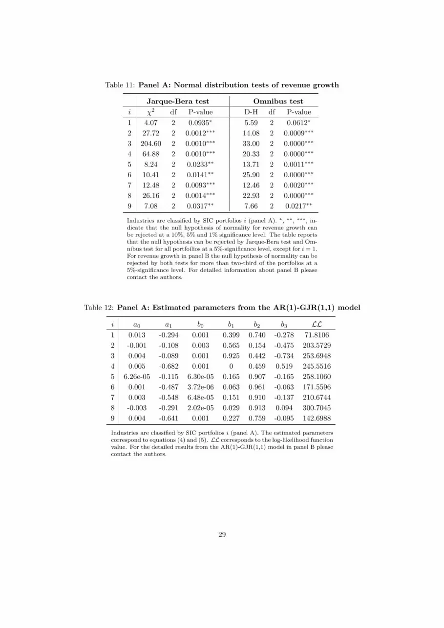
Table 11: Panel A: Normal distribution tests of revenue growth

Jarque-Bera test Omnibus testi χ2 df P-value D-H df P-value1 4.07 2 0.0935∗ 5.59 2 0.0612∗

2 27.72 2 0.0012∗∗∗ 14.08 2 0.0009∗∗∗

3 204.60 2 0.0010∗∗∗ 33.00 2 0.0000∗∗∗

4 64.88 2 0.0010∗∗∗ 20.33 2 0.0000∗∗∗

5 8.24 2 0.0233∗∗ 13.71 2 0.0011∗∗∗

6 10.41 2 0.0141∗∗ 25.90 2 0.0000∗∗∗

7 12.48 2 0.0093∗∗∗ 12.46 2 0.0020∗∗∗

8 26.16 2 0.0014∗∗∗ 22.93 2 0.0000∗∗∗

9 7.08 2 0.0317∗∗ 7.66 2 0.0217∗∗

Industries are classified by SIC portfolios i (panel A). ∗, ∗∗, ∗∗∗, in-dicate that the null hypothesis of normality for revenue growth canbe rejected at a 10%, 5% and 1% significance level. The table reportsthat the null hypothesis can be rejected by Jarque-Bera test and Om-nibus test for all portfoilios at a 5%-significance level, except for i = 1.For revenue growth in panel B the null hypothesis of normality can berejected by both tests for more than two-third of the portfolios at a5%-significance level. For detailed information about panel B pleasecontact the authors.

Table 12: Panel A: Estimated parameters from the AR(1)-GJR(1,1) model

i a0 a1 b0 b1 b2 b3 LL1 0.013 -0.294 0.001 0.399 0.740 -0.278 71.81062 -0.001 -0.108 0.003 0.565 0.154 -0.475 203.57293 0.004 -0.089 0.001 0.925 0.442 -0.734 253.69484 0.005 -0.682 0.001 0 0.459 0.519 245.55165 6.26e-05 -0.115 6.30e-05 0.165 0.907 -0.165 258.10606 0.001 -0.487 3.72e-06 0.063 0.961 -0.063 171.55967 0.003 -0.548 6.48e-05 0.151 0.910 -0.137 210.67448 -0.003 -0.291 2.02e-05 0.029 0.913 0.094 300.70459 0.004 -0.641 0.001 0.227 0.759 -0.095 142.6988

Industries are classified by SIC portfolios i (panel A). The estimated parameterscorrespond to equations (4) and (5). LL corresponds to the log-likelihood functionvalue. For the detailed results from the AR(1)-GJR(1,1) model in panel B pleasecontact the authors.

29

Table 13: Panel A: Jarque-Bera test of normality for residuals

CFNAI

Crisis Common phase Boomi χ2 P-value χ2 P-value χ2 P-value1 1.54 0.2403 6.03 0.0415∗∗ 2.70 0.11082 1.12 0.3936 7.65 0.0270∗∗ 0.09 >0.50003 0.08 >0.5000 2.28 0.2295 4.17 0.0579∗

4 0.28 >0.5000 1.73 0.3364 0.11 >0.50005 2.92 0.0828∗ 1.15 >0.5000 3.34 0.0798∗

6 0.98 0.4594 4.91 0.0596∗ 3.41 0.0772∗

7 0.19 >0.5000 2.97 0.1469 1.58 0.27648 0.95 0.4783 58.34 0.0010∗∗∗ 31.20 0.0011∗∗∗

9 0.10 >0.5000 1.28 0.4600 1.86 0.2114

CUG

Crisis Common phase Boomi χ2 P-value χ2 P-value χ2 P-value1 1.13 0.3870 6.71 0.0343∗∗ 2.60 0.11932 1.21 0.3534 8.25 0.0233∗∗ 0.28 >0.50003 0.13 >0.5000 4.61 0.0663∗ 8.68 0.0178∗∗

4 3.03 0.0784∗ 2.17 0.2461 0.55 >0.50005 2.57 0.1000 1.05 >0.5000 3.31 0.0820∗

6 1.39 0.2877 3.41 0.1144 3.98 0.0625∗

7 0.52 >0.5000 2.60 0.1845 1.81 0.22448 1.24 0.3401 77.29 0.0010∗∗∗ 12.17 0.0094∗∗∗

9 0.31 0.5000 0.37 > 0.5000 1.72 0.2439

Industries are classified by SIC portfolios i (panel A). The business cyclephases are partitioned through CFNAI and CUG. ∗, ∗∗, ∗∗∗, indicatethat the null hypothesis of normality for the residuals can be rejectedat a 10%, 5% and 1% significance level. The table reports that the nullhypothesis cannot be rejected for all portfolios at a 1%-significance level,except for i = 8 in common phase and boom. For panel B the rejectionof the null hypothesis of normality can only be made for less than 10%of the conditional Fama-French portfolios at a 1% level. For detailedinformation about panel B please contact the authors.

30

B Correlation Matrices and Standard Errors

Table 14: Panel A: Correlation matrices conditioned on CFNAI

Crisis - Pearson’s correlation (normal) and Kendall’s τ (italics)

i 1 2 3 4 5 6 7 8 91 1 -0.1067 -0.0600 0.0733 -0.1600 -0.3000 -0.1733 0.0600 -0.12672 -0.2341 1 0.6467 0.4067 0.2000 0.3133 0.4400 0.2600 0.34003 -0.0752 0.7952 1 0.4400 0.2733 0.3867 0.6067 0.2933 0.38674 0.0827 0.5308 0.4594 1 0.3267 0.4133 0.5000 0.2933 0.50675 -0.2410 0.2747 0.3309 0.5142 1 0.2867 0.3200 0.0333 0.16676 -0.3823 0.5236 0.4077 0.5939 0.4219 1 0.4867 0.3200 0.64007 -0.3284 0.6044 0.6030 0.6045 0.5149 0.7240 1 0.3400 0.39338 0.0556 0.4192 0.3605 0.4230 0.0645 0.4697 0.4753 1 0.33339 -0.2087 0.4124 0.3415 0.5933 0.1144 0.7815 0.4838 0.4396 1

Common phase - Pearson’s correlation (normal) and Kendall’s τ (italics)

i 1 2 3 4 5 6 7 8 91 1 -0.1337 -0.0735 0.0024 -0.4210 -0.3172 -0.3426 0.0521 -0.20042 -0.1810 1 0.5737 0.1608 0.1341 0.2808 0.3281 0.1200 0.25943 -0.0986 0.7907 1 0.1782 0.1337 0.2505 0.2824 0.1293 0.19034 -0.0347 0.2370 0.2382 1 0.1135 0.0533 0.2339 0.1576 0.09745 -0.6426 0.1855 0.1573 0.1372 1 0.2182 0.2590 -0.0598 0.14106 -0.4863 0.3837 0.3484 0.1804 0.3477 1 0.6473 0.1604 0.46067 -0.4674 0.4614 0.4537 0.4065 0.3655 0.8581 1 0.1851 0.51688 0.0982 0.1607 0.0871 0.1773 -0.1086 0.1868 0.2419 1 0.20939 -0.3139 0.3660 0.3150 0.1770 0.2217 0.5825 0.7095 0.2167 1

Boom - Pearson’s correlation (normal) and Kendall’s τ (italics)

i 1 2 3 4 5 6 7 8 91 1 0.0992 0.2101 0.0387 -0.2168 -0.0151 -0.0353 0.3008 -0.18662 0.0687 1 0.4924 0.2807 -0.1092 0.2874 0.3815 0.3613 0.30423 0.2161 0.6757 1 0.1899 0.0420 0.4521 0.4857 0.3916 0.38154 0.0485 0.3652 0.3731 1 -0.0017 0.0185 0.1059 0.0857 0.00175 -0.4467 -0.1452 0.0220 -0.0533 1 0.0723 0.1395 -0.2101 0.23036 -0.0754 0.4338 0.6146 -0.0717 0.2251 1 0.6370 0.2538 0.55977 -0.0265 0.4694 0.6628 0.1712 0.3046 0.8442 1 0.2202 0.55978 0.3940 0.4450 0.5002 0.0334 -0.3780 0.4004 0.2925 1 0.18329 -0.2916 0.4389 0.5082 0.0021 0.3907 0.8172 0.7362 0.3038 1

Industries are classified by SIC portfolios i (panel A). The business cycle phases are partitioned throughCFNAI. Pearson’s correlation coefficients are normal and Kendall’s τ coefficients are italics. For detailedinformation about panel B please contact the authors.

31

Table 15: Panel A: Correlations conditioned on CUG and unconditionedCrisis - Pearson’s correlation (normal) and Kendall’s τ (italics)

i 1 2 3 4 5 6 7 8 91 1 -0.1200 -0.1267 -0.0933 -0.2600 -0.2600 -0.2533 0.0333 -0.08002 -0.2448 1 0.6467 0.4267 0.1533 0.2467 0.4667 0.3133 0.24003 -0.1363 0.7769 1 0.4200 0.2800 0.3467 0.6333 0.3733 0.27334 -0.0872 0.5327 0.4312 1 0.2333 0.3800 0.4400 0.2867 0.37335 -0.3042 0.2070 0.3168 0.4138 1 0.2800 0.3400 0.1200 -0.02006 -0.3009 0.4472 0.3402 0.5829 0.3792 1 0.5000 0.4133 0.51337 -0.4109 0.6273 0.6113 0.5842 0.4917 0.6994 1 0.4200 0.28008 0.0607 0.4310 0.3936 0.4509 0.1550 0.6198 0.5944 1 0.42009 -0.1440 0.3113 0.2122 0.4393 -0.0553 0.6387 0.3633 0.4974 1

Common phase - Pearson’s correlation (normal) and Kendall’s τ (italics)

i 1 2 3 4 5 6 7 8 91 1 -0.1239 -0.0423 0.0761 -0.3622 -0.3102 -0.2604 0.0802 -0.20882 -0.1746 1 0.5605 0.1561 0.1622 0.2966 0.3094 0.1354 0.28923 -0.0925 0.7846 1 0.1783 0.1482 0.3032 0.3119 0.1404 0.25054 0.0593 0.2313 0.2480 1 0.1231 0.0744 0.2430 0.1878 0.14045 -0.5741 0.2064 0.1805 0.1326 1 0.2496 0.2797 -0.0674 0.21426 -0.4551 0.4194 0.4404 0.1756 0.3610 1 0.6417 0.0917 0.48637 -0.3602 0.4477 0.5015 0.3915 0.3734 0.8583 1 0.1581 0.52308 0.1277 0.1717 0.0934 0.2186 -0.1326 0.0891 0.1833 1 0.18169 -0.3329 0.4091 0.4074 0.2233 0.2930 0.6328 0.7230 0.1635 1

Boom - Pearson’s correlation (normal) and Kendall’s τ (italics)

i 1 2 3 4 5 6 7 8 91 1 0.0254 0.1270 -0.1524 -0.3746 -0.0413 -0.2254 0.2508 -0.22862 -0.0338 1 0.5619 0.2825 -0.0730 0.3556 0.4254 0.3238 0.32703 0.1059 0.7965 1 0.1619 0.0540 0.4000 0.4190 0.3746 0.37144 -0.2529 0.4804 0.3111 1 0.1175 0.1460 0.2921 0.1460 0.16835 -0.6267 -0.0797 0.0382 0.1664 1 0.0698 0.2032 -0.1778 0.19376 -0.2491 0.4482 0.4462 0.2284 0.2865 1 0.6254 0.4095 0.60327 -0.3189 0.5233 0.4912 0.4243 0.3536 0.8829 1 0.2889 0.64768 0.3193 0.3973 0.4436 0.1595 -0.3260 0.4718 0.3680 1 0.26039 -0.3850 0.4094 0.3872 0.2166 0.3521 0.8670 0.8488 0.3463 1

Undivided panel - Pearson’s correlation (normal) and Kendall’s τ (italics)

i 1 2 3 4 5 6 7 8 91 1 -0.0893 -0.0217 0.0368 -0.3110 -0.2336 -0.2258 0.0942 -0.18842 -0.1446 1 0.5714 0.2252 0.1116 0.3050 0.3629 0.1932 0.28523 -0.0373 0.7868 1 0.2651 0.1623 0.3258 0.3984 0.2002 0.27554 0.0290 0.3763 0.3820 1 0.1792 0.1409 0.2978 0.1533 0.16675 -0.5084 0.1724 0.2003 0.2360 1 0.2223 0.2701 -0.0719 0.19436 -0.3564 0.4330 0.4296 0.2829 0.3516 1 0.6214 0.2140 0.53217 -0.3232 0.5195 0.5540 0.4910 0.4084 0.8257 1 0.2388 0.51898 0.1471 0.2564 0.2087 0.1884 -0.1352 0.2758 0.2899 1 0.23449 -0.2737 0.4021 0.3680 0.3011 0.2489 0.6753 0.6565 0.2725 1

Industries are classified by SIC portfolios i (panel A). The business cycle phases are partitionedthrough CUG. Moreover, the correlations for the undivided panel are presented. Pearson’s correla-tion coefficients are normal and Kendall’s τ coefficients are italics. For detailed information aboutpanel B please contact the authors.

32

Table 16: Panel A: Bootstrap standard errors of correlations for CFNAI

Crisis - bootstrap standard errors of correlations

i 1 2 3 4 5 6 7 8 91 0 0.1283 0.1390 0.1482 0.1597 0.1443 0.1566 0.1655 0.13952 0.1654 0 0.0943 0.1324 0.1595 0.1202 0.1112 0.1265 0.13043 0.1664 0.0779 0 0.0994 0.1479 0.1263 0.0913 0.1159 0.13974 0.2027 0.1667 0.1002 0 0.1571 0.1204 0.1113 0.1485 0.10035 0.2027 0.2048 0.1681 0.1510 0 0.1572 0.1553 0.1683 0.16256 0.1957 0.1305 0.1699 0.1337 0.1855 0 0.1142 0.1670 0.09967 0.1696 0.1016 0.1159 0.1070 0.1520 0.1073 0 0.1430 0.13108 0.1976 0.1497 0.1226 0.1810 0.2149 0.1868 0.1842 0 0.13769 0.1749 0.1711 0.2126 0.0900 0.2109 0.0716 0.1434 0.1470 0

Common phase - bootstrap standard errors of correlations

i 1 2 3 4 5 6 7 8 91 0 0.0616 0.0656 0.0646 0.0547 0.0505 0.0476 0.0618 0.05412 0.0797 0 0.0447 0.0667 0.0653 0.0628 0.0655 0.0742 0.07363 0.0877 0.0387 0 0.0686 0.0675 0.0713 0.0739 0.0716 0.07244 0.0932 0.0928 0.0905 0 0.0677 0.0695 0.0675 0.0665 0.06695 0.0602 0.0866 0.0932 0.0945 0 0.0698 0.0616 0.0656 0.06556 0.0647 0.0695 0.0919 0.0999 0.0800 0 0.0398 0.0735 0.05967 0.0658 0.0795 0.0905 0.0843 0.0713 0.0260 0 0.0701 0.05408 0.0773 0.1264 0.1374 0.0883 0.0788 0.1091 0.1203 0 0.06969 0.0714 0.1026 0.1004 0.0926 0.0833 0.0845 0.0561 0.1177 0

Boom - bootstrap standard errors of correlations

i 1 2 3 4 5 6 7 8 91 0 0.1184 0.1104 0.1235 0.1199 0.1139 0.1144 0.1060 0.11282 0.1589 0 0.1082 0.1090 0.1420 0.1109 0.1294 0.0968 0.11363 0.1413 0.0718 0 0.0994 0.1487 0.0894 0.0868 0.0868 0.11894 0.1577 0.1411 0.1675 0 0.1244 0.0926 0.1057 0.1167 0.11675 0.1005 0.1668 0.1491 0.1613 0 0.1494 0.1358 0.1314 0.13316 0.1510 0.1172 0.1414 0.1436 0.1333 0 0.0674 0.1325 0.07807 0.1554 0.1288 0.1617 0.1281 0.1210 0.0325 0 0.1140 0.07808 0.1257 0.0898 0.0803 0.1479 0.1305 0.1245 0.1036 0 0.11669 0.1397 0.1356 0.1838 0.1572 0.1309 0.0310 0.0410 0.1272 0

Industries are classified by SIC portfolios i (panel A). The business cycle phases are partitionedthrough CFNAI. The number of bootstrap replications is set to 10,000. The bootstrap standarderrors of Pearson’s correlation coefficients are normal and those of Kendall’s τ coefficients areitalics. For detailed information about panel B please contact the authors.

33

Table 17: Panel A: Bootstrap standard errors (CUG and unconditioned)

Crisis - bootstrap standard errors of correlations

i 1 2 3 4 5 6 7 8 91 0 0.1433 0.1507 0.1626 0.1682 0.1576 0.1581 0.1597 0.14972 0.1824 0 0.1016 0.1411 0.1588 0.1386 0.1183 0.1321 0.14363 0.1828 0.0828 0 0.1106 0.1469 0.1375 0.1004 0.1000 0.14644 0.2128 0.1882 0.1198 0 0.1652 0.1439 0.1173 0.1372 0.13695 0.2127 0.2136 0.1747 0.1826 0 0.1646 0.1484 0.1556 0.15136 0.2081 0.1484 0.1807 0.1410 0.1946 0 0.1230 0.1438 0.13397 0.1645 0.1044 0.1230 0.1172 0.1540 0.1098 0 0.1054 0.13928 0.2001 0.1533 0.1205 0.1661 0.2059 0.1328 0.1168 0 0.11879 0.1829 0.1699 0.2248 0.1413 0.1925 0.1389 0.1644 0.1299 0

Common phase - bootstrap standard errors of correlations

i 1 2 3 4 5 6 7 8 91 0 0.0608 0.0614 0.0652 0.0607 0.0518 0.0538 0.0626 0.05342 0.0772 0 0.0481 0.0637 0.0675 0.0635 0.0640 0.0790 0.07273 0.0837 0.0417 0 0.0669 0.0675 0.0672 0.0701 0.0757 0.06784 0.0960 0.0897 0.0909 0 0.0676 0.0666 0.0667 0.0643 0.06545 0.0696 0.0872 0.0931 0.0964 0 0.0692 0.0646 0.0676 0.06646 0.0688 0.0690 0.0829 0.0963 0.0875 0 0.0410 0.0757 0.05477 0.0751 0.0789 0.0792 0.0822 0.0769 0.0268 0 0.0752 0.04988 0.0797 0.1371 0.1508 0.0908 0.0811 0.1124 0.1303 0 0.07219 0.0668 0.1024 0.0916 0.0917 0.0829 0.0683 0.0473 0.1287 0

Boom - bootstrap standard errors of correlations

i 1 2 3 4 5 6 7 8 91 0 0.1177 0.1180 0.1115 0.1178 0.1141 0.1165 0.1048 0.11312 0.1612 0 0.0925 0.1224 0.1249 0.0989 0.1202 0.0905 0.10673 0.1421 0.0728 0 0.1137 0.1323 0.1019 0.1158 0.0832 0.11894 0.1586 0.1414 0.1675 0 0.1071 0.1005 0.1128 0.1184 0.12325 0.1004 0.1669 0.1509 0.1615 0 0.1374 0.1013 0.1264 0.12016 0.1531 0.1197 0.1429 0.1454 0.1341 0 0.0695 0.1157 0.06067 0.1570 0.1296 0.1649 0.1278 0.1192 0.0325 0 0.0881 0.06988 0.1257 0.0892 0.0806 0.1482 0.1314 0.1236 0.1029 0 0.11269 0.1401 0.1366 0.1842 0.1571 0.1296 0.0308 0.0408 0.1254 0

Undivided panel - bootstrap standard errors of correlations

i 1 2 3 4 5 6 7 8 91 0 0.0500 0.0517 0.0523 0.0485 0.0455 0.0469 0.0497 0.04562 0.0678 0 0.0353 0.0541 0.0552 0.0478 0.0503 0.0557 0.05453 0.0720 0.0303 0 0.0487 0.0533 0.0496 0.0491 0.0523 0.05464 0.0781 0.0773 0.0589 0 0.0537 0.0539 0.0511 0.0535 0.05175 0.0594 0.0770 0.0734 0.0793 0 0.0576 0.0489 0.0541 0.05266 0.0661 0.0550 0.0671 0.0767 0.0678 0 0.0334 0.0561 0.03857 0.0653 0.0567 0.0558 0.0623 0.0590 0.0288 0 0.0521 0.04058 0.0645 0.0901 0.0974 0.0793 0.0711 0.0854 0.0858 0 0.05189 0.0670 0.0767 0.0864 0.0706 0.0702 0.0480 0.0565 0.0834 0

Industries are classified by SIC portfolios i (panel A). The business cycle phases are parti-tioned through CUG. The number of bootstrap replications is set to 10,000. Moreover, thebootstrap standard errors of correlations for the undivided panel are presented. The boot-strap standard errors of Pearson’s correlation coefficients are normal and those of Kendall’sτ coefficients are italics. For detailed information about panel B please contact the authors.

34

C Hypotheses test results

Table 18: Jennrich-χ2 test for equality of Pearson’s correlation matrices

Panel A: SIC industry portfolios

CFNAI CUGH0 χ2 df P-value χ2 df P-value

ΣC = ΣB 121.91 36 2.07e-12∗∗∗ 87.13 36 3.98e-06∗∗∗

ΣB = ΣO 105.10 36 2.88e-11∗∗∗ 66.93 36 0.0013∗∗∗

ΣC = ΣO 152.90 36 1.10e-08∗∗∗ 129.08 36 2.07e-12∗∗∗

Panel B: FF48 industry portfolios

CFNAI CUGH0 χ2 df P-value χ2 df P-value

ΣC = ΣB 14,174.06 946 0∗∗∗ 12,272.02 946 0∗∗∗

ΣB = ΣO 4,504.19 946 0∗∗∗ 4,081.57 946 0∗∗∗

ΣC = ΣO 3,999.24 946 0∗∗∗ 4,040.27 946 0∗∗∗

Industries are classified by SIC portfolios (panel A) and Fama-French portfolios (panel B).The business cycle phases are partitioned through CFNAI and CUG. The abbreviationsdenote C = crisis, O = common phase and B = boom. Σ symbolizes the correlationmatrix. The Jennrich test has an asymptotic χ2 distribution with 36 degrees of freedomfor the nine-by-nine SIC industry matrices and with 946 degrees of freedom for the44-by-44 Fama-French industry matrices. The null hypothesis H0 is the equality oftwo correlation matrices. The alternative hypothesis is the inequality of two correlationmatrices. The table shows that the p-values are close to zero. H0 can be rejected for allsub panels at a 1% significance level. ∗, ∗∗, ∗∗∗, indicate that H0 can be rejected at 10%,5% and 1% significance level.

35

References

Ang, A. and Bekaert, G. (2002). International asset allocation with regime shifts. Review of

Financial Studies, 15(4):1137 – 1187.

Ang, A. and Chen, J. (2002). Asymmetric correlations of equity portfolios. Journal of Financial

Economics, 63(3):443 – 494.

Bernhart, G., Hoecht, S., Neugebauer, M., Neumann, M., and Zagst, R. (2009). Asset corre-

lations in turbulent markets and their implications on asset management. Working Paper,

HVB Institute for Mathematical Finance.

Bertero, E. and Mayer, C. (1990). Structure and performance: Global interdependence of stock

markets around the crash of october 1987. European Economic Review, 34(6):1155 – 1180.

Bhojraj, S., Lee, C. M. C., and Oler, D. K. (2003). What’s my line? A comparison of

industry classification schemes for capital market research. Journal of Accounting Research,

41(5):745 – 774.

Boyer, B. H., Gibson, M. S., and Loretan, M. (1999). Pitfalls in tests for changes in correla-

tions. Finance Discussion Paper 597, Board of Governors of the Federal Reserve System,

Washington, DC.

Burgstahler, D. and Dichev, I. (1997). Earnings management to avoid earnings decreases and

losses. Journal of Accounting & Economics, 24(1):99.

Campbell, R., Koedilk, K., and Kofman, P. (2002). Increased correlation in bear markets.

Financial Analysts Journal, Jan/Feb 58:87–94.

Chan, L. K. C., Lakonishok, J., and Swaminathan, B. (2007). Industry classifications and

return comovement. Financial Analysts Journal, 63(6):56 – 70.

Chandra, U. and Ro, B. T. (2008). The role of revenue in firm valuation. Accounting Horizons,

22:199–222.

Corrado, C. and Mattey, J. (1997). Capacity utilization. Journal of Economic Perspectives,

11(1):151 – 167.

36

Das, S. R. and Uppal, R. (2004). Systemic risk and international portfolio choice. Journal of

Finance, 59(6):2809 – 2834.

Degeorge, F., Patel, J., and Zeckhauser, R. (1999). Earnings management to exceed thresholds.

Journal of Business, 72(1):1 – 33.

Dickey, D. A. and Fuller, W. A. (1979). Distribution of the estimators for autoregressive time

series with a unit root. Journal of the American Statistical Association, 74(366):427.

Dobric, J., Frahm, G., and Schmid, F. (2007). Dependence of stock returns in bull and

bear markets. Discussion paper, Seminar of Economic and Social Statistics, University of

Cologne.

Doornik, J. A. and Hansen, H. (2008). An omnibus test for univariate and multivariate nor-

mality. Oxford Bulletin of Economics & Statistics, 70:927 – 939.

Efron, B. and Tibshirani, R. (1986). Bootstrap methods for standard errors, confidence inter-

vals, and other measures of statistical accuracy. Statistical Science, 1(1):54–75.

Erb, C. B., Harvey, C. R., and Viskanta, T. E. (1994). Forecasting international equity corre-

lations. Financial Analysts Journal, November-December:32–45.

Erdorf, S., Hartmann-Wendels, T., Heinrichs, N., and Hess, D. (2010). Firm value and the

effect of bankruptcy costs: A multivariate copula approach. Working Paper, Graduate School

of Risk Management, University of Cologne.

Ertimur, Y., Livnat, J., and Martikainen, M. (2003). Differential market reactions to revenue

and expense surprises. Review of Accounting Studies, 8(2/3):185 – 211.

Evans, C. L., Chin Te, L., and Pham-Kanter, G. (2002). The 2001 recession and the Chicago

Fed National Activity Index: Identifying business cycle turning points. Economic Perspec-

tives, 26(3):26.

Fama, E. F. and French, K. R. (1997). Industry costs of equity. Journal of Financial Economics,

43(2):153 – 193.

Fisher, R. A. (1935). The Design of Experiments. Hafner Press, New York.

37

Forbes, K. J. and Rigobon, R. (2002). No contagion, only interdependence: Measuring stock

market comovements. Journal of Finance, 57(5):2223 – 2261.

Ghosh, A., Gu, Z., and Jain, P. C. (2005). Sustained earnings and revenue growth, earnings

quality, and earnings response coefficients. Review of Accounting Studies, 10(1):33 – 57.

Glosten, L. R., Jagannathan, R., and Runkle, D. E. (1993). On the relation between the

expected value and the volatility of the nominal excess return on stocks. The Journal of

Finance, 48(5):1779–1801.

Healy, P. M. and Wahlen, J. M. (1999). A review of the earnings management literature and

its implications for standard setting. Accounting Horizons, 13(4):365 – 383.

Jarque, C. M. and Bera, A. K. (1980). Efficient tests for normality, homoscedasticity and serial

independence of regression residuals. Economics Letters, 6(3):255 – 259.

Jennrich, R. I. (1970). An asymptotic χ2 test for the equality of two correlation matrices.

Journal of the American Statistical Association, 65(330):904 – 912.

Kama, I. (2009). On the market reaction to revenue and earnings surprises. Journal of Business

Finance and Accounting, 36(1-2):31 – 50.

Kaplanis, E. C. (1988). Stability and forecasting of the comovement measures of international

stock market returns. Journal of International Money and Finance, 7(1):63 – 75.

Karolyi, G. A. and Stulz, R. M. (1996). Why do markets move together? an investigation of

U.S.-Japan stock return comovements. Journal of Finance, 51(3):951 – 986.

King, M. A. and Wadhwani, S. (1990). Transmission of volatility between stock markets.

Review of Financial Studies, 3(1):5 – 33.

Krishnan, J. and Press, E. (2003). The north american industry classification system and its

implications for accounting research. Contemporary Accounting Research, 20(4):685 – 717.

Lee, S. B. and Kim, K. J. (1993). Does the october 1987 crash strengthen the co-movements

among national stock markets?. Review of Financial Economics, 3(1-2):89 – 102.

38

Leuz, C., Nanda, D., and Wysocki, P. D. (2003). Earnings management and investor protection:

an international comparison. Journal of Financial Economics, 69(3):505 – 527.

Lindskog, F. (2000). Linear correlation estimation. Working Paper, RiskLab, Eidgenössische

Technische Hochschule Zürich.

Ljung, G. M. and Box, G. E. P. (1978). On a measure of lack of fit in time series models.

Biometrika, 65(2):297 – 303.

Longin, F. and Solnik, B. (1995). Is the correlation in international equity returns constant:

1960-1990?. Journal of International Money and Finance, 14(1):3 – 26.

Longin, F. and Solnik, B. (2001). Extreme correlation of international equity markets. Journal

of Finance, 56(2):649 – 676.

Patton, A. J. (2004). On the out-of-sample importance of skewness and asymmetric dependence

for asset allocation. Journal of Financial Econometrics, 2(1):130 – 168.

Penman, S. H. (2010). Financial statement analysis and security valuation. McGraw-Hill Irwin,

Boston, 4th edition.

Pitman, E. J. G. (1937). Significance tests which may be applied to samples from any popu-

lation. Royal Staistical Society Supplement, 4:119 – 130 and 225 – 332.

Pitman, E. J. G. (1938). Significance tests which may be applied to samples from any popu-

lation - the analysis of variance test. Biometrika, 29:322 – 335.

Poon, S.-H., Rockinger, M., and Tawn, J. (2004). Extreme value dependence in financial

markets: Diagnostics, models, and financial implications. Review of Financial Studies,

17(2):581 – 610.

Ramchand, L. and Susmel, R. (1998). Volatility and cross correlation across major stock

markets. Journal of Empirical Finance, 5(4):397 – 416.

Rappaport, A. (1986). Creating shareholder value - the new standard for business performance.

Free Press, New York, 14th edition.

39

Ratner, M. (1992). Portfolio diversification and the inter-temproal stability of international

stock indices. Global Finance Journal, 3(1):67.

Saunders, N. C. (1999). The north american industry classification system: Change on the

horizon. Occupational Outlook Quarterly, Fall:34 – 37.

Schwartz, E. S. and Moon, M. (2000). Rational pricing of internet companies. Financial

Analysts Journal, 56(4):62 – 75.

Stock, J. H. and Watson, M. W. (1989). New indexes of coincident and leading economic

indicators. NBER/Macroeconomics Annual (MIT Press), 4(1):351 – 394.

Stock, J. H. and Watson, M. W. (1999). Forecasting inflation. Journal of Monetary Economics,

44(2):293 – 335.

Swaminathan, S. and Weintrop, J. (1991). The information content of earnings, revenues, and

expenses. Journal of Accounting Research, 29(2):418 – 427.

Tang, G. Y. N. (1995). Intertemporal stability in international stock market relationships: A

revisit. Quarterly Review of Economics and Finance, 35:579 – 593.

Vogiatzoglou, M. (2009). Dynamic copula toolbox. Working Paper, University of Macedonia.

40