Board of Governors of the Federal Reserve System

International Finance Discussion Papers

Number 756

January 2003

Consumption, Durable Goods, and Transaction Costs

Robert F. Martin

NOTE: International Finance Discussion Papers are preliminary materials circulated to stimulatediscussion and critical comment. References in publications to International Finance Discussion Papers(other than an acknowledgment that the writer has had access to unpublished material) should be clearedwith the author or authors. Recent IFDPs are available on the Web at www.federalreserve.gov/pubs/ifdp/.

Consumption, Durable Goods, and Transaction Costs

Robert F. Martin*

Abstract: We study consumption of durable and nondurable goods when the durable good is subject totransaction costs. In the model, agents derive utility from a service flow of a durable good and a consumptionflow of a nondurable good. The key feature of the model is the existence of a fixed transaction cost in thedurable good market. The fixed cost induces an inaction region in the purchase of the durable good. Moreimportantly, the inability to adjust the durable stock induces variation in consumption of the nondurable goodover the inaction region. The variation is a function of the degree of complementarity between durable andnondurable goods in the period utility function, the rate of intertemporal substitution, and a precautionarymotive induced by incomplete markets. We test the model using the PSID. Housing serves as the durablegood. The data indicate an increase in consumption before moving to a smaller house and a decrease inconsumption before moving to a larger house. This result is consistent with the model when there existscomplementarity between the durable and nondurable good or when there is a strong precautionary effect.

Keywords: housing, consumption, durable goods, transaction costs, PSID

* Staff economist of the Division of International Finance of the Federal Reserve Board. Email:robert.f.martin@frb.gov. I thank Fernando Alvarez, Jess Gaspar, Lars Hansen, Eric Hurst, Robert Lucas,Maurizio Mazzocco, and Mark Wright. The views in this paper are solely the responsibility of the author andshould not be interpreted as reflecting the views of the Board of Governors of the Federal Reserve Systemor of any other person associated with the Federal Reserve System..

1 Introduction

We study consumption of durable and nondurable goods when the durable good is subject

to transaction costs. In the model, the agent derives utility from a service ßow of a durable

good and a consumption ßow of a nondurable good. Transactions in the nondurable good

are frictionless; however, in order to change the level of durable good consumption, the agent

must pay a Þxed transaction cost. Once the transaction cost has been incurred the agent

may freely adjust his stock of the durable good. Agents face uninsured idiosyncratic risk.

The durable good in the model is quite general; however, we Þnd it most natural to interpret

it as housing. Grossman and Laroque (1990) study a continuous time version of this model

in the absence of the nondurable good.

The implications of the Þxed transaction cost on the policy function for durable consump-

tion are immediate. The introduction of a Þxed transaction cost forces agents to reduce the

frequency of transactions in the durable goods market. In the presence of transaction costs,

agents employ an optimal stopping rule for purchase of the durable good. The stopping rule

is deÞned by two boundaries, (yl, yh), and an optimal return point, y∗. The interval (yl, yh)

deÞnes the inaction region. In our model, y will be the ratio of Þnancial wealth to durable

wealth plus a constant.

Agents make no change to the stock of the durable good until the wealth to durable good

ratio, y, hits a boundary of the continuation region. If the agent hits yl, he will increase his

stock of the durable good. If instead he hits yh, he will decrease his stock. Independent

1

of the boundary hit, upon hitting a boundary, the agent will return the wealth to durable

good ratio to y∗.

Our main result focuses on the implications transaction costs in the durable goods market

have for non-durable consumption. In the model, the pattern of nondurable consumption

changes signiÞcantly as the agent approaches the boundary of the inaction region. Changes

in consumption result from the degree of complementarity between the two goods, the in-

tertemporal rate of substitution, and a precautionary motive. The precautionary motive is

induced by the large changes in wealth at the boundaries of the inaction region. In order

to disentangle precaution, we also solve the model for the risk-free case.

In the neighborhood of y∗, agents engage in consumption policies which will tend to keep

them near the optimal return point. If the current y is greater than y∗,the agent increases

consumption, if y is less than y∗ the agent decreases consumption.

Consumption in the neighborhood of the boundaries follows a different pattern than

consumption in the neighborhood of y∗. The pattern is parameter dependent. When the two

goods are complements, an agent sufficiently close to the boundary alters his consumption

such that the probability of hitting a boundary is increased. In this case, the agent prefers

to spend time in the vicinity of y∗. When he is sufficiently close to the boundary the fastest

way back to y∗is to hit the boundary and jump. The resulting effect is for consumption

to decrease in the periods before increasing the durable stock and for it to increase before

reducing the durable stock. The precautionary motive reinforces this effect.

2

When the two goods are substitutes, consumption increases toward the upper boundary

and decreases toward the lower boundary. The resulting effect on consumption is not as

strong in this case because the precautionary motive works as a counter force.

We compare the results of the model to data from the Panel Survey of Income Dynamics

(PSID). We compare consumption growth rates of agents with differing proximity to the

boundaries of the continuation region. The state variable will be the ratio of nonhous-

ing wealth to housing wealth. We Þnd households with a sufficiently high probability of

moving to a larger house (higher dollar value) decrease consumption. Likewise, households

sufficiently likely to move to a smaller house (lower dollar value) increase their consumption.

1.1 Literature Review

The response of non-durable consumption changes in house value has been studied by several

authors. Skinner (1993) uses aggregate data between 1950 and 1989 to estimate the marginal

propensity to consume out of housing wealth. He found a point estimate of .03 percent that

was not statistically signiÞcant. Skinner (1989) focusing exclusively on non-movers regressed

change in house price on change in consumption and found essentially no effect. Bhatia

(1987) and Hendershot and Peek (1989) found consumption increased 4 to 5 cents for every

dollar increase in equity. Hoynes and McFadden (1994) Þnd that an increase in the growth

rate of housing prices of ten percentage points leads on average to an increase in total

savings of 2.28 percentage points. However, the change in non-housing saving is statistically

3

insigniÞcant. Engelhardt (1996b) Þnds home owners which receive an unanticipated real

capital loss increase their marginal propensity to save by .03 percent. In the same study,

he Þnds homeowners which receive unanticipated capital gains have no change in marginal

propensity to save. None of these studies attempt to measure or condition the probability

of moving.

The paper closest to ours and to which we owe an intellectual debt, is that of Grossman

and Laroque (1990). Grossman and Laroque solve our model in continuous time in the

absence of the nondurable consumption good. Dunn (1998), Eberly (1994), and Beaulieu

(1993) also solve models similar to Grossman and Laroque.

2 The Model

Our model is one in which an agent derives utility from a service ßow (proportional to the

stock) of a durable good and a consumption ßow of a nondurable good. Transactions in

the nondurable good are frictionless; however, in order to change the level of durable good

consumption, the agent must pay a Þxed transaction cost1.

1The transaction cost paid will be proportional to the stock. This assumption maintains the homogeneityof the problem while allowing us to study the effects of a Þxed cost. While there is no question that movingentails large Þxed costs, it is arguable whether making these Þxed costs proportional to the stock is realistic.We will justify this assumption by showing that move frequency does not depend on house value.

4

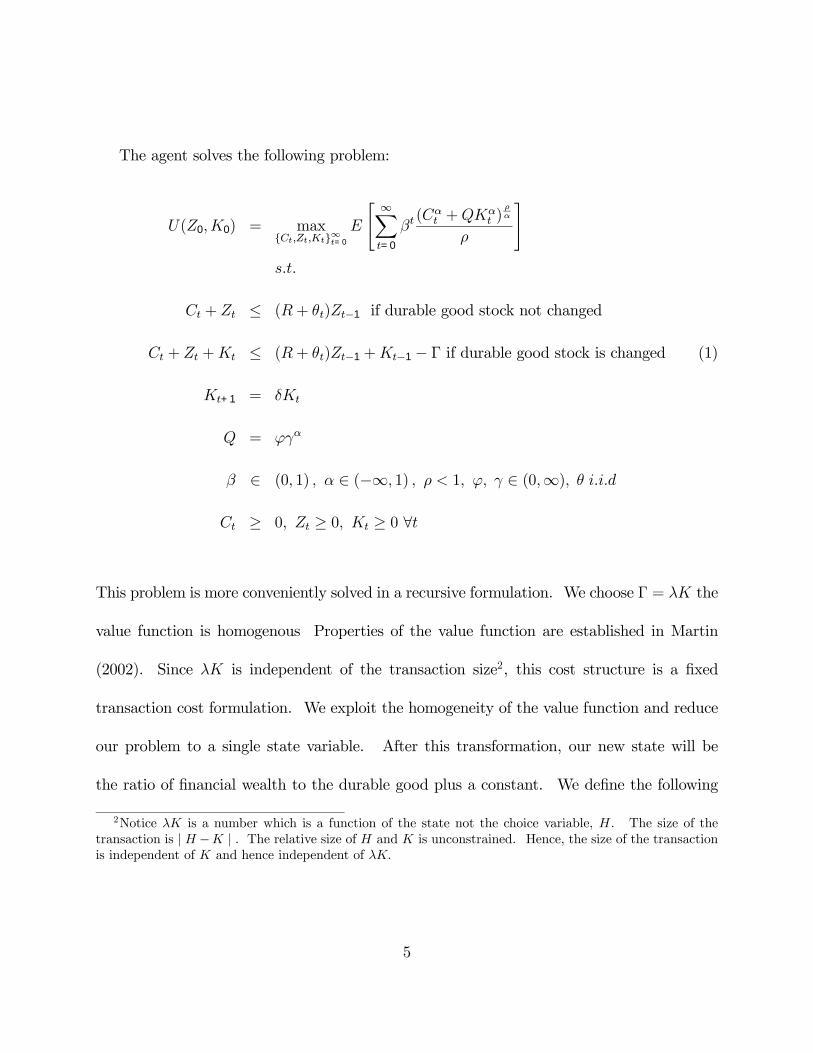
The agent solves the following problem:

U(Z0,K0) = max{Ct,Zt,Kt}∞t=0

E

" ∞Xt=0

βt(Cαt +QK

αt )

ρα

ρ

#s.t.

Ct + Zt ≤ (R+ θt)Zt−1 if durable good stock not changed

Ct + Zt +Kt ≤ (R+ θt)Zt−1 +Kt−1 − Γ if durable good stock is changed (1)

Kt+1 = δKt

Q = ϕγα

β ∈ (0, 1) , α ∈ (−∞, 1) , ρ < 1, ϕ, γ ∈ (0,∞), θ i.i.d

Ct ≥ 0, Zt ≥ 0, Kt ≥ 0 ∀t

This problem is more conveniently solved in a recursive formulation. We choose Γ = λK the

value function is homogenous Properties of the value function are established in Martin

(2002). Since λK is independent of the transaction size2, this cost structure is a Þxed

transaction cost formulation. We exploit the homogeneity of the value function and reduce

our problem to a single state variable. After this transformation, our new state will be

the ratio of Þnancial wealth to the durable good plus a constant. We deÞne the following

2Notice λK is a number which is a function of the state not the choice variable, H. The size of thetransaction is | H −K | . The relative size of H and K is unconstrained. Hence, the size of the transactionis independent of K and hence independent of λK.

5

transformed variables:

y =Z +K

K− λ; a = A

K; h =

H

K; c =

C

K; (2)

We have the following transformed problem:

V (y) = max

max{c, a}

¡U(c, 1) + βδρ

RV (y0)φ(θ0)

¢,

max{c, a, h}¡U(c, h) + β(δh)ρ

RV (y0)φ(θ0)

¢

top s.t. c+ a ≤ y − 1 + λ (3)

bottom s.t. c+ a+ h ≤ y

y0 =θ

δha+ 1− λ

We are now in a position to characterize the agent�s problem.

3 Characterization

In order to better understand the solution to the agent�s problem, we will Þrst characterize

the solution to the problem when θ = 0. This case will help us to understand which

aspects of the model are driven by a precautionary motive and which are driven by the

complementarity between durable and nondurable goods. We will then turn to numerical

solutions of the general problem.

6

3.1 Characterization: θ constant

In this section, we replace the risky asset with a risk-free asset with constant return, R.

The solution to the model consists of a deterministic set of stopping times at which the

agent will update their capital stock. Consumption will evolve deterministically over each

interval. We wish to characterize the path of nondurable consumption between stopping

times and the behavior of consumption and durable goods at each stopping time. This

example will demonstrate the importance of the interaction between ρ, δ, and the degree of

complementarity between durable and nondurable goods.

For any time interval in which the durable good is not adjusted, we have the following

Euler equation:

Uc¡Ct, δ

tK0

¢= βRUc

¡Ct+1, δ

t+1K0

¢(4)

Where we have substituted for the evolution equation for K. For simplicity of exposition,

we will work with the case of βR = 1. With the durable good, the Þrst condition still holds

but the depreciating durable stock implies that for nonseparable utility Ct must also evolve.

First, we study the general case with CES preferences

U (C,K) =(aCα + (1− a)Kα)

ρα

aρa ∈ (0, 1), ρ ∈ (−∞, 1),α ∈ (−∞, 1) (5)

In this case, the Euler equation does not offer a closed form solution of Ct+1 in terms of

Ct. However, we can solve numerically for the sequence of C implied by the Euler equation

7

from any starting point, (C0, K0). Assuming βR = 1, average consumption of durable and

nondurable goods must not be increasing or decreasing over time. This fact implies that

K0 = Kτ and C0 = Cτ for every stopping time τ . C is increasing or decreasing over the

interval depending on the sign of α-ρ. If α > ρ, consumption is increasing over the interval.

If α < ρ, consumption is decreasing over the interval. In this case, the curvature of the

time path of consumption is determined by the distance between α and ρ. For the case

α < ρ, the time path of consumption is more convex the more negative α becomes. In other

words, increasing the complementarity between durable and nondurable goods increases the

curvature of the time path of consumption.

In the Cobb-Douglass case, U(C,K) = (CaK(1−a))ρ

aρ. The Euler equation implies

Caρ−1t

¡δtK0

¢(1−a)ρ= Caρ−1

t+1

¡δt+1K0

¢(1−a)ρ

or (6)

Ct+1 = δ(a−1)ρ/(aρ−1)Ct

Consumption is increasing or decreasing over the interval depending on the sign of ρ. If ρ

is positive, consumption is decreasing over the interval. If ρ is negative, consumption is

increasing over the interval. We can know write Ct as an explicit function of Co, Ct =

δ(a−1)ρaρ−1

tC0. Substituting this value of C into the Euler equation we verify that marginal

utility is constant. Since the Euler equation for nondurable consumption must also hold

8

across the boundary, we can also determine the behavior of C at any stopping time.

Therefore, with a depreciating durable stock, K > KT . The durable stock is always

increased at the boundary. If ρ is positive, then C0 > CT . The opposite is true if ρ is

negative.

The separable case is the easiest to solve. We consider U(C,K) = Cρ

ρ+ v (k) . Here, the

Euler equation evolves as it does in the absence of the durable good. C is constant across

the inaction region. Hence, C is constant for all t. The durable good is increased at each

stopping time.

3.2 Numerical Characterization

3.3 Durable Good

The policy function for the durable good is characterized by three numbers (yl, y∗, yh). yl

is the smallest ratio to which the agent allows the Þnancial wealth to durable good ratio to

fall, while yh is the highest. Hence, the interesting question is how the interval changes for

changes in parameter values and how large of an interval do we expect to observe.

The primary variable which controls the width of the inaction region is the size of the

transaction costs. Our choices of λ are governed by empirical Þndings from the CEX. The

average costs an agent pays to change housing is just over 7% of their house value. We vary

transaction costs around this number.

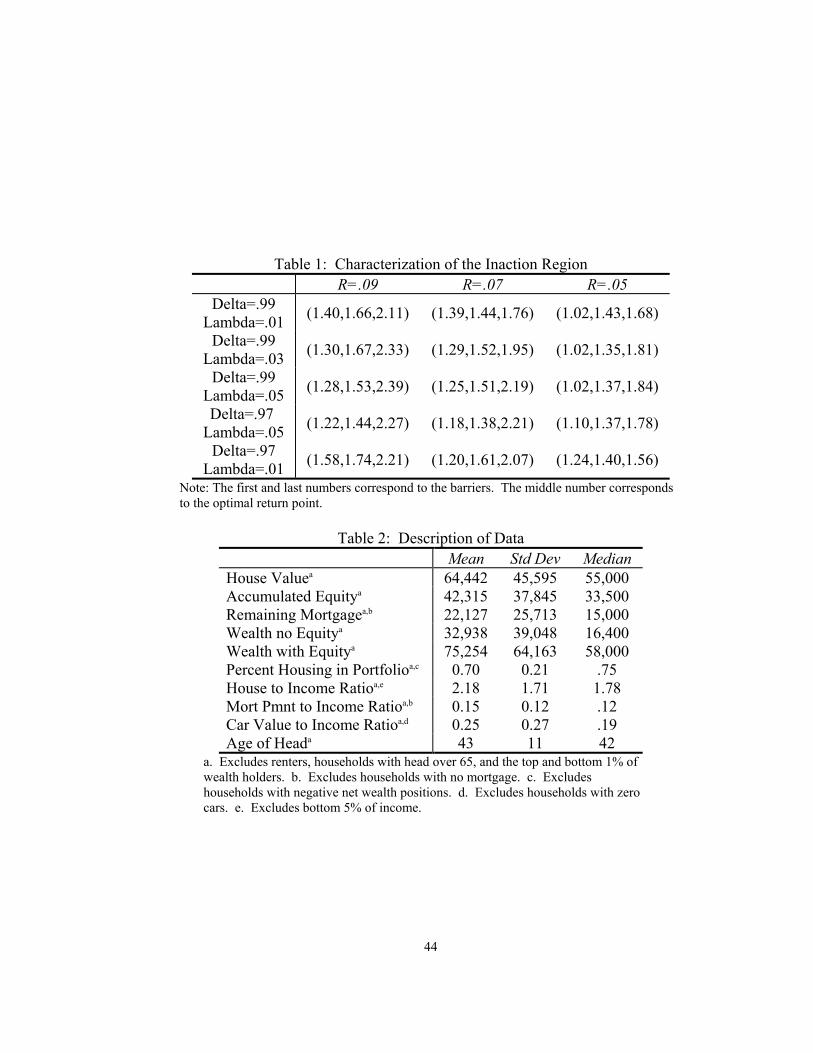
Table 1 gives values of (yl, y∗, yh) for several different parameter speciÞcations. As ex-

9

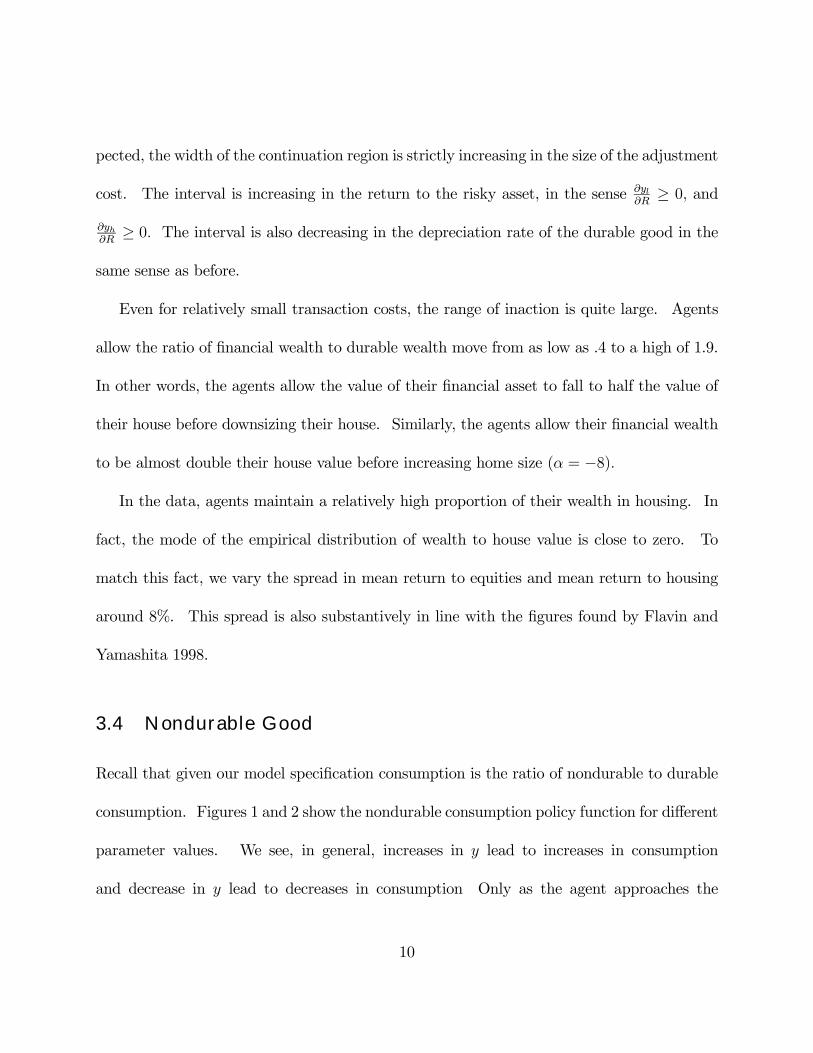
pected, the width of the continuation region is strictly increasing in the size of the adjustment

cost. The interval is increasing in the return to the risky asset, in the sense ∂yl∂R≥ 0, and

∂yh∂R≥ 0. The interval is also decreasing in the depreciation rate of the durable good in the

same sense as before.

Even for relatively small transaction costs, the range of inaction is quite large. Agents

allow the ratio of Þnancial wealth to durable wealth move from as low as .4 to a high of 1.9.

In other words, the agents allow the value of their Þnancial asset to fall to half the value of

their house before downsizing their house. Similarly, the agents allow their Þnancial wealth

to be almost double their house value before increasing home size (α = −8).

In the data, agents maintain a relatively high proportion of their wealth in housing. In

fact, the mode of the empirical distribution of wealth to house value is close to zero. To

match this fact, we vary the spread in mean return to equities and mean return to housing

around 8%. This spread is also substantively in line with the Þgures found by Flavin and

Yamashita 1998.

3.4 Nondurable Good

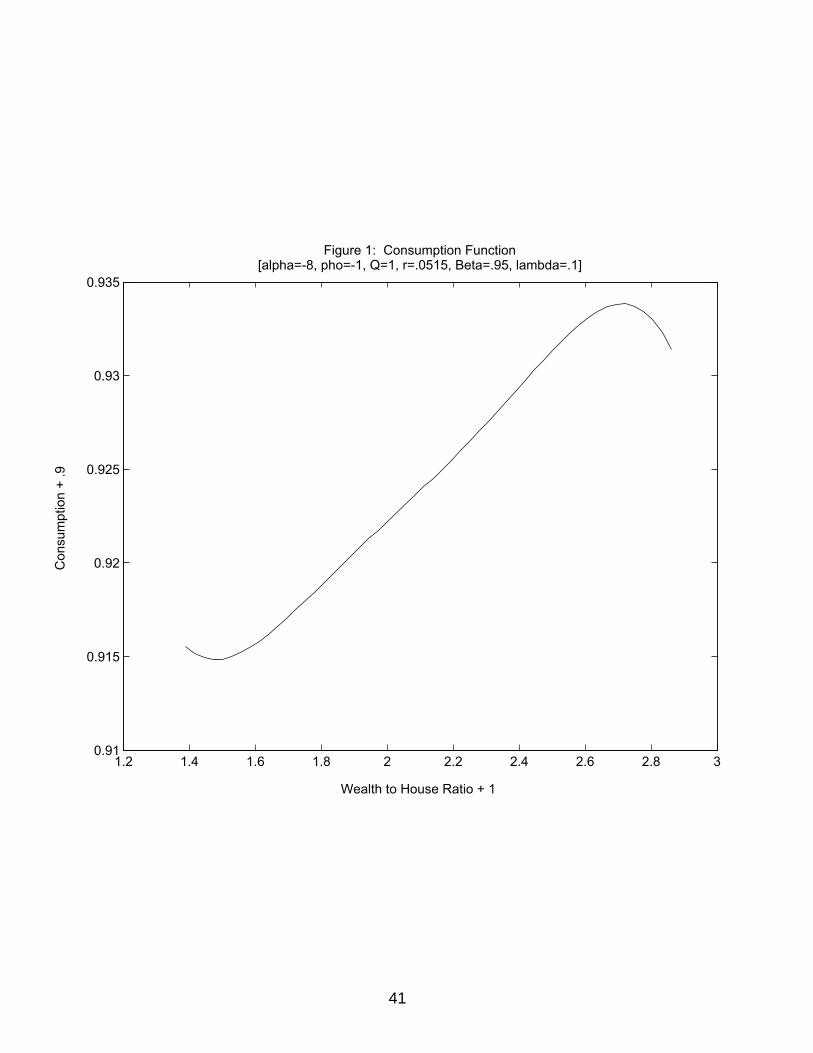
Recall that given our model speciÞcation consumption is the ratio of nondurable to durable

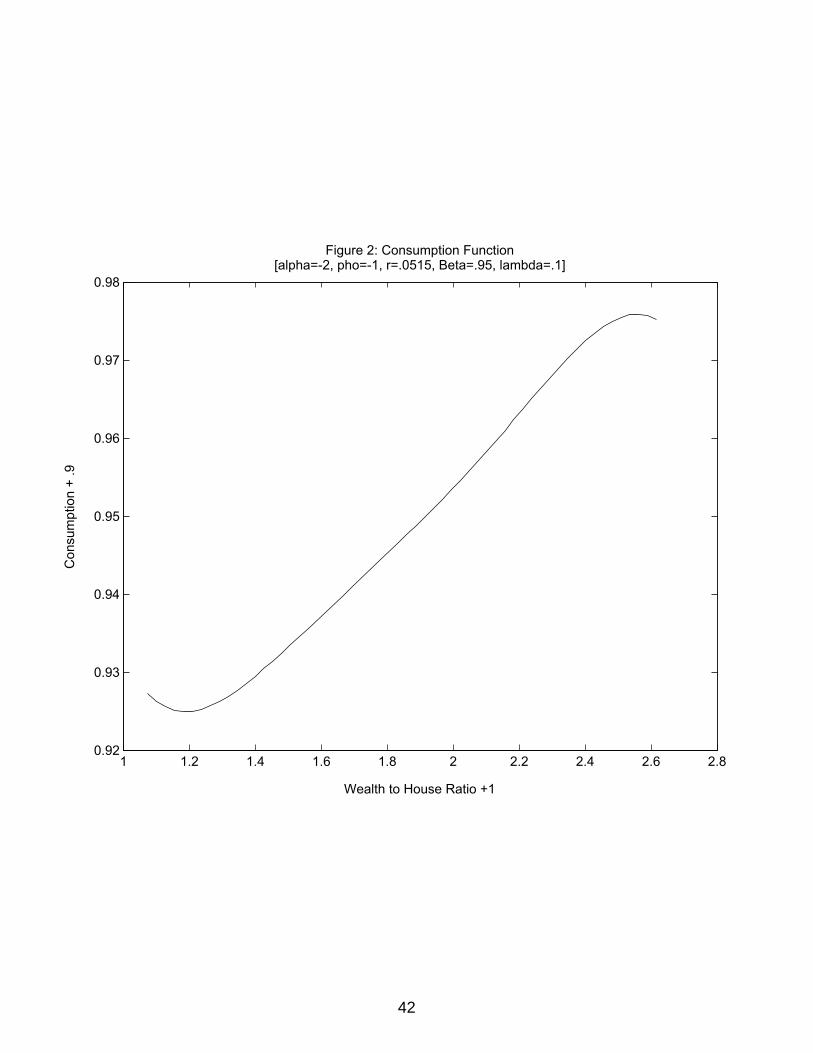
consumption. Figures 1 and 2 show the nondurable consumption policy function for different

parameter values. We see, in general, increases in y lead to increases in consumption

and decrease in y lead to decreases in consumption Only as the agent approaches the

10

boundary does this effect change. We can see that sharp changes in consumption occur

only over a relatively small region. The region over which agents change their consumption

behavior is very important for empirical testing of the model. We only expect to see

changes in consumption for a relatively short period of time before the household updates

their durable stock. The shape of the optimal policy function changes with changes to

the complementarity between durable and nondurable goods and with changes in variance.

In general, increases in the complementarity between the two goods increases the change

in consumption as we approach the boundary. This change occurs for the same reasons

as in the complete market case above. For a Þxed level of the durable good, increases in

nondurable consumption provide smaller and smaller increments to the agents utility. Table

1a gives the percent change in consumption at the upper boundary for differing values of

α. When the two goods are on the boundary between being substitutes and compliments

(α = ρ), consumption of the nondurable good ßattens but does not become negative. For

the choice of return structure and ρ − 1, the slope of the consumption function is zero.

When we increase the complementarity to −2, the percent change in consumption between

the highest nondurable consumption and the boundary is .9. For values of -8, the change

is 4.5%. Finally, for the relatively high level of complementarity α = −20, the change is a

large 12%.

The second factor affecting the shape of the consumption function is the degree of market

incompleteness. While the case of complete markets has been studied at length above, we

11

also show that as the variance of the model is reduced the percent change in consumption

reduces as well. For the borderline case of (α = ρ), the consumption function is eventually

smooth at the boundary. In other words, for small enough variance the shape of the

consumption function does not change as we approach the boundary. With α = −20, the

change in consumption is reduced form 12% to only about 4% when the variance is reduced

by 50%. With the variance reduced by 90%, the change in consumption is less the 1%.

Therefore, the changes in consumption produced by this model are strongest when the

durable and nondurable goods are strongly complimentary and when markets are not com-

plete. When we test these consumption changes in the data, we will be looking for changes

in consumption near the boundary.

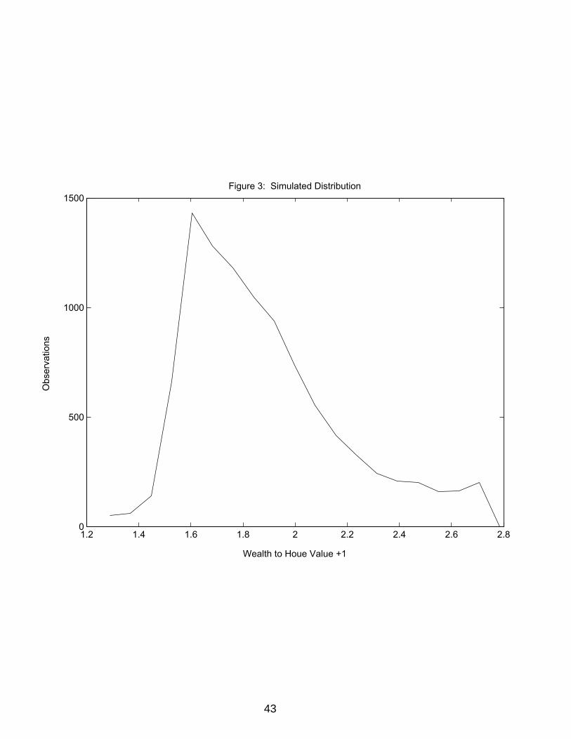
3.5 Distribution

We examine the model for the case in which each agent receives independent shocks to wealth

and housing. In our model, we do not allow an interaction between the price of housing

and the aggregate statistics of the economy. In effect, we have Þxed the relative price

of nondurable and durable goods. Under this assumption, computation of the invariant

distribution is quite simple. Starting from any initial distribution of agents, we apply the

policy function for nondurable and durable consumption to the distribution. This gives

us a mapping between the distribution in period n and the distribution in period n + 1.

We continue to apply this mapping until the distribution has approximately converged. In

12

practice, we do this for each type of agent and then aggregate to get the Þnal distribution

whenever we want to model heterogenous agents. We now give the results of this exercise.

The aggregate distribution in this case consists of 5 types of agents. 60% of agents face

transaction costs of 10%, 20% face 5% costs, and 20% face 1% costs. The mean return for all

agents is 4%. The agents face an equal probability of realizing the following returns [-.01,

.02, .04, .06, .09]. The durable good appreciates 5% per year. Agents are homogenous in

all other aspects.

We plot the resulting distribution in Figure 3. The hump of the distribution occurs at

a wealth to durable ratio of .6. The average return of the asset is such that over time most

agents increase their stock of the durable good. The distribution reduces mass away from

the optimal return point relatively slowly at Þrst then drops away fairly quickly. Close to the

boundary the mass of agents drops away very fast. We can see from this distribution that

the agents close to the boundary will have very little affect on aggregate statistics because

their relative mass is quite low.

The general shape of the simulated distribution closely replicates the empirical distrib-

ution. In all cases, the distributions are right skewed with the hump occurring for very

low levels of the ratio of wealth to house value. As seen in Table 2, agents employ opti-

mal return points biased toward the lower boundary whenever consumption is increasing on

average over time. For most agents in our model, increasing consumption proÞles are the

case. In the data, most agents increase consumption and wealth over the life-cycle.

13

An important feature of the empirical distribution is the existence of agents with negative

values of y. In our model, the absence of labor income implies y must be bounded below

by zero. If we reinterpret our wealth as incorporating the present value of income, then

the appropriate comparison to the data is to add to current wealth a measure of the present

value of labor income. This addition will shift the empirical distribution away from zero.

We are not able to replicate the tails of the distribution. Even with transaction costs of

forty percent we only get maximal state values of around 4. Only by increasing the mean

return on non-housing wealth (or equivalently decreasing the return to housing) can we shift

agents far enough to begin to match the tails. However, these agents tend to increase their

optimal return point as well, signiÞcantly reducing the hump of the distribution. Also as

seen in Table 2, to get an upper boundary above 6, the returns on non-housing Þnancial

wealth must be very high.

4 Data

We use the from the University of Michigan�s Panel Study of Income Dynamics (PSID)

for the years 1983-1985. The PSID began in 1968 with 4,802 households and over 18,000

individuals and by 1994 it had nearly 8,500 families and over 50,000 individuals. Of the

initial 4,802 households, 2,930 were selected from the Survey Research Center�s random

sample of the U.S. population, while the remaining 1,872 families were drawn from the

Survey of Economics Opportunity�s (SEO) sample of the low-income population. Starting in

14

1968, the PSID has re-interviewed individuals from those households every year - adults have

been followed as they have grown older, and children have been observed as they advance

through childhood and into adulthood. The main focus of the PSID�s data collection effort is

on economic and demographic characteristic, especially with respect to earned an unearned

income, employment, family composition and geographic location.

While the study does not, in general, attempt to collect data on the consumption patterns

of households, it does gather two components of consumption which are critical for this study.

The Þrst component is food consumption. Each year each respondent is asked to estimate

their total expenditures on both food consumed at home and food consumed out of the home.

While food consumption is certainly not a perfect substitute for total consumption it has

been shown to be highly correlated with total consumption by Skinner (1989). The second

component of consumption which is collected by the PSID is housing. The survey collects

detailed information on rents, mortgages, and owner estimated house value. This information

will allow us to compare the growth rate in consumption for agents in the proximity of the

boundary and agents far from the boundary. It also allows us to differentiate between agents

which move to a larger house and agents which move to a smaller house.

For the purpose of this study, a key feature of the PSID is the wealth supplements

collected in 1984, 1989, 1994, and 1999. Funded by grants through the National Institute

on Aging (NIA), the wealth supplements contain comprehensive data on net worth, deÞned

as liquid assets (checking accounts, savings account, CSs, IRAs, bond and stock values), the

15

value of business equity, real estate and vehicle equity, less any outstanding debts. The PSID

wealth data compares favorable with other, more targeted, wealth survey such as the Survey

on Consumer Finances (Curtin et. al. 1989; Juster et. al., 1999).

Most of the analysis presented in this study will surround the 1984 wealth supplement. We

choose to focus on this year since the 1987 and 1988 PSID did not collect food consumption.

For the 1994 wealth supplement, release 2 data is not yet available. For 1999, the survey

data is not yet available. We will use the wealth supplements in 1989, 1994, and 1999 only

to give descriptive characteristics of the empirical distribution of wealth to housing ratios.

In the data, our measure of wealth includes all Þnancial assets of the household. These

include traditional savings and stocks as well as small business capital, car value, and other

owned real estate. The measure also includes liabilities outstanding to the household.

Outstanding liabilities are subtracted from the total assets to give the agents net wealth

position. Approximately Þve percent of agents in the data set hold negative net wealth

positions.

Our measure of house value is given by the home owners estimate of home value. Home

value is problematic in that on average there is a large amount of measurement error in the

Þgure quoted. Goodman and Ittner (1992) estimate this error to average 6% in the PSID.

We maintain the assumption that while most home owners only have a general idea of the

value of their home, owners which are near the boundary or who have recently updated have

very precise knowledge of the value of their home.

16

4.1 Housing as the Durable Good

The relative size and special characteristic of housing make it a natural choice as the durable

good for the purposes of testing the model. Treated as a consumption good, the home is

the single largest expenditure made by consumers over their lifetime. The price of a home is

generally measured in multiples of a family�s annual income. The median household has a

house value which is almost two times their annual income; while, the ßow cost of housing is

greater than seventeen percent of annual income for the median household. In comparison,

median car value is less than twenty percent of annual income for the average household.

Treated as an asset, the home dominates the portfolios of most households. Seventy-Five

percent of the median households portfolio is allocated to housing. We arrive at this Þgure

by treating the mortgage as a short position in the bond market and the house as a long

position in real estate. Since the correlation between the two assets is far less than one,

these two assets do not imply a zero net position. This Þgure drops to thirty Þve percent

if we only consider equity. Fewer than Þve percent of households have a portfolio with less

than a twenty percent share allocated to their home; almost ten percent of households hold

no assets which are unrelated to housing. For details of these statistics see Table 1. For

simplicity of exposition, the statistics in this paper apply primary to home owners. Clearly,

non-homeowners do not hold a signiÞcant portion of their assets in housing. However,

saving toward home ownership is one the most common reason given for asset accumulation

in young households (Engelhardt 1996b, Tachibanaki 1994). In some sense, these assets can

17

also be attributed to housing.

The housing market is also characterized by features which prevent it from being easily

aggregated into a composite consumption good. First, agency problems (both on the renter

and landlord side), search costs, and tax advantages to home ownership, make rental housing

an imperfect substitute for owned housing. In other words, for the same service ßow, the ßow

cost of owned housing is lower than that of rental housing. The second feature distinguishing

housing from other goods is its durability. While virtually all consumption goods have some

component of durability, housing is the most durable good which is regularly consumed by

households. Finally and most importantly, the housing market is characterized by large

transaction costs. Monetary costs of buying a new home range on average between 7 and

11 percent of the purchase price of a home (CEX 1993). The bulk of these costs are for

agent fees but transfer taxes, appraisal and inspection fees etc. are also signiÞcant costs. In

addition, before the new housing ßow can be consumed, the household must physically move.

While the true costs of moving are difficult to measure, they are certainly not negligible and

involve signiÞcant expenditures of time, effort, and money.

5 Empirical Model and Results

The theoretical model presented above will proved us with a speciÞc framework in which to

perform empirical analysis of the behavior of the consumption of durable and nondurable

goods. We wish to compare the behavior of the consumption of nondurable consumption of

18

agents which are located at different point in the state space. SpeciÞcally, we wish to look for

changes in the behavior of consumption as agents approach the lower and upper boundaries

of the inaction region. The simplest test of the model is then to observe the changes in

consumption as the agent approaches the boundary. Ideally, we would simply follow agents

across time and observe the changes in the consumption growth rate as a function of their

wealth and house value over the entire inaction region. Unfortunately, this approach is not

feasible in the PSID since wealth is only observed at Þve year intervals and food consumption

is not observed in every year in which we have wealth data. Therefore, in order to conduct

this analysis, we must Þrst identify the boundaries of the inaction region.

The empirical study will take two stages. First, we will attempt to identify the location

of agents within the inaction region. Since we do not have direct information on the agents

location, we will have to infer their location. Second, with the agents location in hand, we

will use the information from the Þrst step to compare consumption growth rates of agents

which are in the vicinity of the boundary and agents which are far from the boundary.

5.1 Identification of the Inaction Region

The difficulty in identifying the inaction region is that for household not engaging in a

transaction neither the optimal return point nor the band are observable. Our model

informs us that the band width is a function of the degree of complementarity between

durable and non durable goods (i.e. the opportunity cost of deviating from the optimal level

19

of durable consumption is a function of the degree of complementarity), the transaction

costs, and the structure of returns to wealth and the durable good. Since we do not have

a nice Þrst order condition determining the boundaries of the inaction region that can be

exploited for empirical analysis, and since the main parameter, the size of the transaction

cost is unobservable in the PSID, we will rely on a more fundamental property of the model.

Recall in the model, an agent only updates his stock of the durable good when his ration

of Þnancial wealth to durable good stock moves sufficiently far form the optimal ratio. When

the ratio is sufficiently low, the agent will decrease his stock of the durable good. When the

ratio is sufficiently high, the agent increases his stock. Independent of the parameterization,

the model predicts that agents with high values of the sate variable are more likely to be

near the upper boundary; agents with low state values are more likely to be near the lower

boundary. We will identify the hazard function of agents moving as a function of the ratio

of wealth to durable good.

To reiterate, we want to identify the probability of an agent hitting a boundary in the

next period conditional on their current value other ratio of wealth to house value. We

want to know the probability of moving tomorrow for an agent who has already made an

allocation decision today. In other words, we wish to Þnd the probability that y0 > yh or

y0 < yl. Essentially, this is a statement on the size of the inaction region and the return

structure of the model. In order to Þnd the appropriate statistical model, we will Þrst derive

these probabilities from the theoretically model.

20

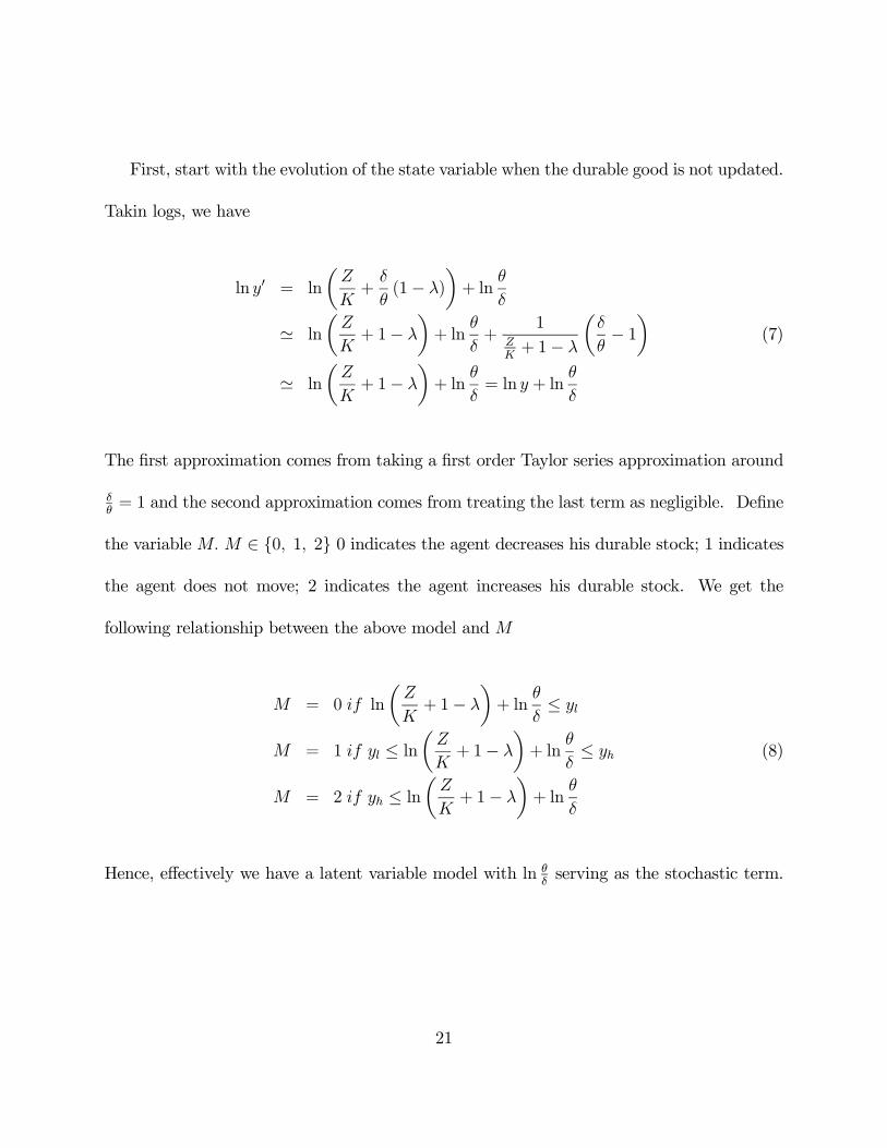
First, start with the evolution of the state variable when the durable good is not updated.

Takin logs, we have

ln y0 = ln

µZ

K+δ

θ(1− λ)

¶+ ln

θ

δ

' ln

µZ

K+ 1− λ

¶+ ln

θ

δ+

1ZK+ 1− λ

µδ

θ− 1¶

(7)

' ln

µZ

K+ 1− λ

¶+ ln

θ

δ= ln y + ln

θ

δ

The Þrst approximation comes from taking a Þrst order Taylor series approximation around

δθ= 1 and the second approximation comes from treating the last term as negligible. DeÞne

the variable M. M ∈ {0, 1, 2} 0 indicates the agent decreases his durable stock; 1 indicates

the agent does not move; 2 indicates the agent increases his durable stock. We get the

following relationship between the above model and M

M = 0 if ln

µZ

K+ 1− λ

¶+ ln

θ

δ≤ yl

M = 1 if yl ≤ lnµZ

K+ 1− λ

¶+ ln

θ

δ≤ yh (8)

M = 2 if yh ≤ lnµZ

K+ 1− λ

¶+ ln

θ

δ

Hence, effectively we have a latent variable model with ln θδserving as the stochastic term.

21

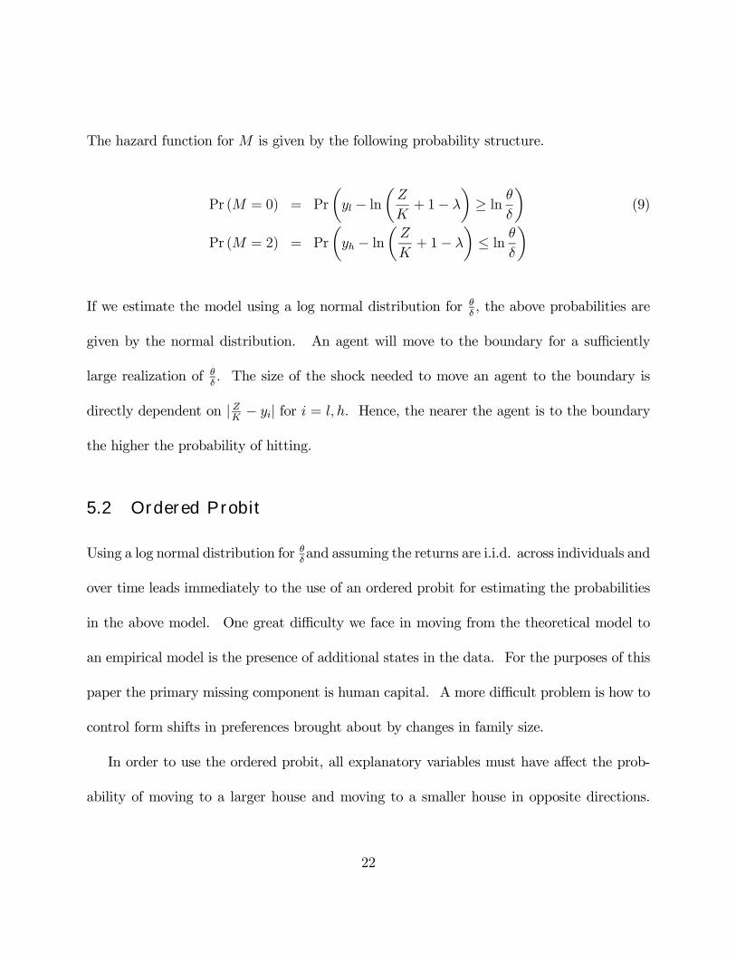
The hazard function for M is given by the following probability structure.

Pr (M = 0) = Pr

µyl − ln

µZ

K+ 1− λ

¶≥ ln θ

δ

¶(9)

Pr (M = 2) = Pr

µyh − ln

µZ

K+ 1− λ

¶≤ ln θ

δ

¶

If we estimate the model using a log normal distribution for θδ, the above probabilities are

given by the normal distribution. An agent will move to the boundary for a sufficiently

large realization of θδ. The size of the shock needed to move an agent to the boundary is

directly dependent on | ZK− yi| for i = l, h. Hence, the nearer the agent is to the boundary

the higher the probability of hitting.

5.2 Ordered Probit

Using a log normal distribution for θδand assuming the returns are i.i.d. across individuals and

over time leads immediately to the use of an ordered probit for estimating the probabilities

in the above model. One great difficulty we face in moving from the theoretical model to

an empirical model is the presence of additional states in the data. For the purposes of this

paper the primary missing component is human capital. A more difficult problem is how to

control form shifts in preferences brought about by changes in family size.

In order to use the ordered probit, all explanatory variables must have affect the prob-

ability of moving to a larger house and moving to a smaller house in opposite directions.

22

Increases in the number of children increase the probability of moving in both directions.

We have a similar problem with time reaming in the work force in our deÞnition of human

capital. Increases in age decreases unconditionally the probability of moving. We will

attempt to control for these ideas when we perform a sensitivity check with a multinomial

logit. In order to maintain the use of the ordered probit, we assume that all wealth enters

linearly into a summary variable for total wealth. We think of human capital in the context

of this model as the present value of the agent�s lifetime labor income. The absence of

the ability to borrow against human capital will lead to the main difference between the

theoretical model and the empirical results. In the data, many agents hold negative values

of Þnancial wealth. These agents are borrowing against a positive present value of lifetime

nonÞnancial wealth. If we had a good measure of the expected value of total lifetime wealth,

we would not expect to see negative wealth values. In the model, the agent�s current wealth

summarizes accurately the agent�s lifetime expected wealth.

The empirical model is built around a latent regression: y∗ = β0x + ε. x is a vector

containing log wealth, log house value, human capital. We will assume human capital is a

linear function of years reaming in work force, education, race, and current income. These

variables will all enter in levels to correspond with the theoretical model. ε represents

unobservable heterogeneity in the population, error in the measurement of x, and the current

shock to total wealth for the household this period. We follow the Þnancial literature to

assume innovations to Þnancial wealth are log normally distributed and we follow Vissing-

23

Jorgensen (2002) to make the same assumptions on nonÞnancial wealth. ε is unobserved by

the econometrician.

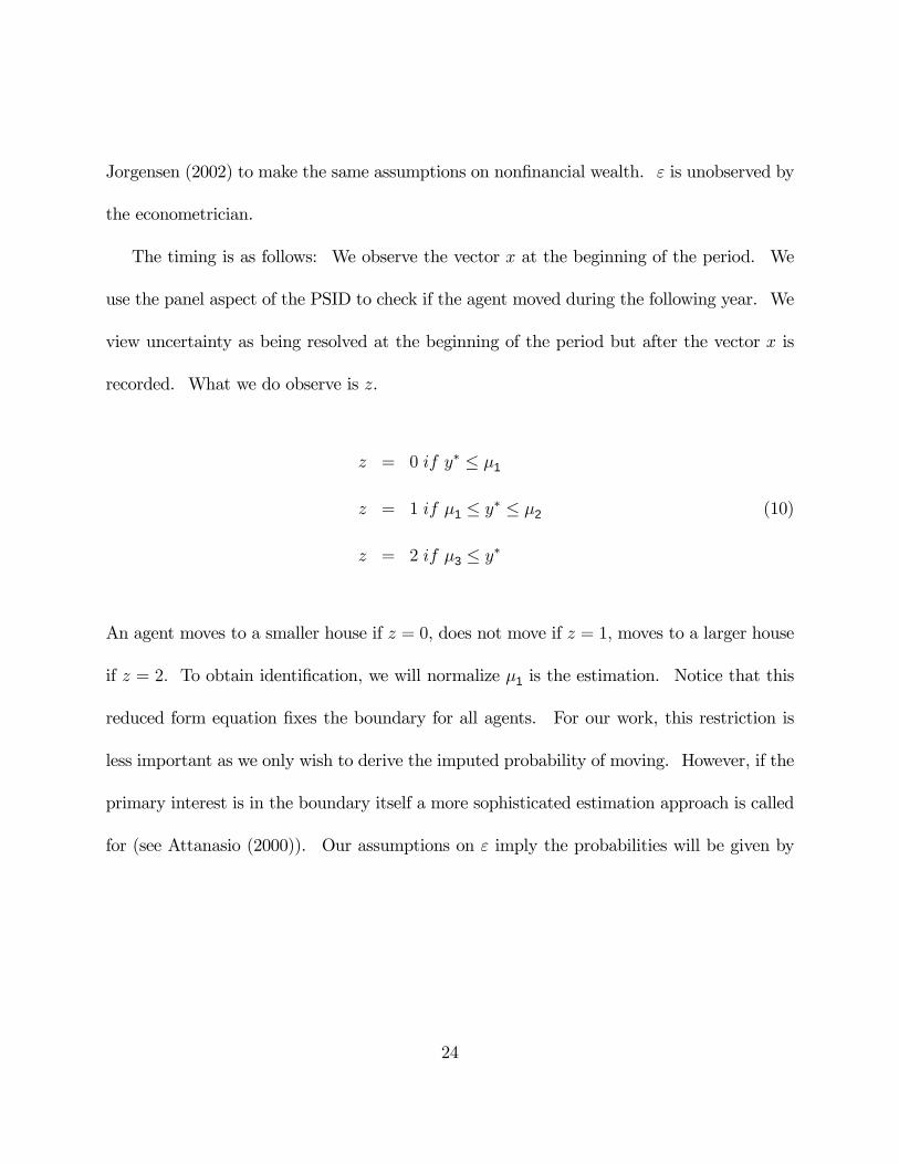
The timing is as follows: We observe the vector x at the beginning of the period. We

use the panel aspect of the PSID to check if the agent moved during the following year. We

view uncertainty as being resolved at the beginning of the period but after the vector x is

recorded. What we do observe is z.

z = 0 if y∗ ≤ µ1

z = 1 if µ1 ≤ y∗ ≤ µ2 (10)

z = 2 if µ3 ≤ y∗

An agent moves to a smaller house if z = 0, does not move if z = 1, moves to a larger house

if z = 2. To obtain identiÞcation, we will normalize µ1 is the estimation. Notice that this

reduced form equation Þxes the boundary for all agents. For our work, this restriction is

less important as we only wish to derive the imputed probability of moving. However, if the

primary interest is in the boundary itself a more sophisticated estimation approach is called

for (see Attanasio (2000)). Our assumptions on ε imply the probabilities will be given by

24

the normal distribution.

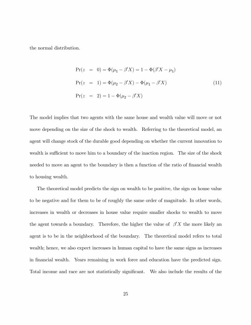
Pr(z = 0) = Φ(µ1 − β0X) = 1− Φ(β0X − µ1)

Pr(z = 1) = Φ(µ2 − β0X)− Φ(µ1 − β0X) (11)

Pr(z = 2) = 1−Φ(µ2 − β0X)

The model implies that two agents with the same house and wealth value will move or not

move depending on the size of the shock to wealth. Referring to the theoretical model, an

agent will change stock of the durable good depending on whether the current innovation to

wealth is sufficient to move him to a boundary of the inaction region. The size of the shock

needed to move an agent to the boundary is then a function of the ratio of Þnancial wealth

to housing wealth.

The theoretical model predicts the sign on wealth to be positive, the sign on house value

to be negative and for them to be of roughly the same order of magnitude. In other words,

increases in wealth or decreases in house value require smaller shocks to wealth to move

the agent towards a boundary. Therefore, the higher the value of β0X the more likely an

agent is to be in the neighborhood of the boundary. The theoretical model refers to total

wealth; hence, we also expect increases in human capital to have the same signs as increases

in Þnancial wealth. Years remaining in work force and education have the predicted sign.

Total income and race are not statistically signiÞcant. We also include the results of the

25

probit using only the log ratio of wealth to house value. This model is the most directly

comparable to the results in the simulated economy. Obviously, in the simulated economy

we are not able to separate house value and wealth.

Table 3 gives the results of the ordered probit. Ordered Probit 1 gives the results of

the ordered probit when we include human capital. All the coefficients are signiÞcant at

traditional levels with the exception of age and age squared. We can see the signs on the

coefficients are as predicted by the model. Higher wealth conditional on house value increases

the probability of moving to a larger house. Similarly, higher house value conditional on

wealth decreases the probability. Larger increases in two year income also lead to higher

probability of moving to a larger house. Households whose head has more than a high school

education are more likely to move to a larger house. They are also more likely to move

than households with high school education or less. Notice, wealth and house value enter

with approximately the same order of magnitude. Ordered Probit 2 gives the results of an

ordered probit using only wealth and house value to predict movers (i.e. no human capital

proxy). As in the Þrst probit, the coefficients are strongly statistically signiÞcant and the

signs are consistent with theory. Ordered Probit 3 gives the results for the ordered probit

using the log ratio of wealth to house value. The result is not equivalent to Ordered Probit

2 because it adds the restriction that the coefficient on wealth and house value be the same.

However, the coefficient is signiÞcant and matches that prediction of theory. We run this

probit as it is the most direct comparison with the Ordered Probit we will conduct on the

26

simulated data.

We next want to examine changes in consumption growth rates as a function of the

predicted probabilities. Table 4a gives summary statistics of the predicted probabilities

from Ordered Probit 1. As is to be expected, the predicted probability of moving is quite

small for most households. The predicted probability of moving to a smaller house for each

quartile is much smaller that of moving to a larger house. This effect reßects the higher

unconditional probability of moving to a larger house. A household is almost twice as likely

to move to a larger house as it is to move to a smaller house. We Þnd this result to be

true independent of age and is true for 1982 to 1990 in the PSID. In other words, this

effect is unlikely to be entirely due to life-cycle effects. Another possible explantation is

asymmetric tax treatment of capital gains and losses in housing. In the United States before

1995, households under the age of 55 paid capital gains taxes on all housing capital gains

not rolled over to the new property at the time of purchase. Households over the age of 55

could sell one home without incurring the capital gains tax. Hence, downgrading housing

stock entailed relatively higher transaction costs for young households. The asymmetric

transaction cost theory does not full explain the pattern, since conditioning on age > 55

does not affect the result. We do not have an explantation of this point. This fact must

have implications for the rate of growth of the housing stock. It would be interesting to see

if estimated growth rates of the housing stock match the implied Þgures from PSID data.

27

5.3 Multinomial Logit

The primary difference between the multinomial Logit and the ordered probit is in the

assumption over the ordering of the dependent variable. The ordered probit forces the

sign on all explanatory variables to have opposite signs for moving to a larger house and

moving to a smaller house. This characteristic increases the probability of observing the

correct signs on house value and wealth. It also prevents us from exploring the usefulness

of other variables such as changes in family size and age which affect the overall probability

of moving. The multinomial logit makes no such ordering assumptions. For instance, the

coefficient on age in the ordered probit regressions is invariably insigniÞcant. The reason

for the insigniÞcance is that increases in age decrease the probability of moving. Hence, the

sign of the coefficient should be negative for both moving to a larger house and to a smaller

house. Most importantly for our purposes, the logit regression allows the sign on wealth

and house value to be arbitrary. Therefore, as an additional test of the characteristics of

the inaction region we repeat the above exercise using a multinomial logit. We could follow

Attanasio (2000) and run separate probit regressions for the probability of increasing and

the probability of decreasing. However, we feel the advantage of joint estimation outweigh

the change in the distributional assumptions made in the shift from probit to logit.

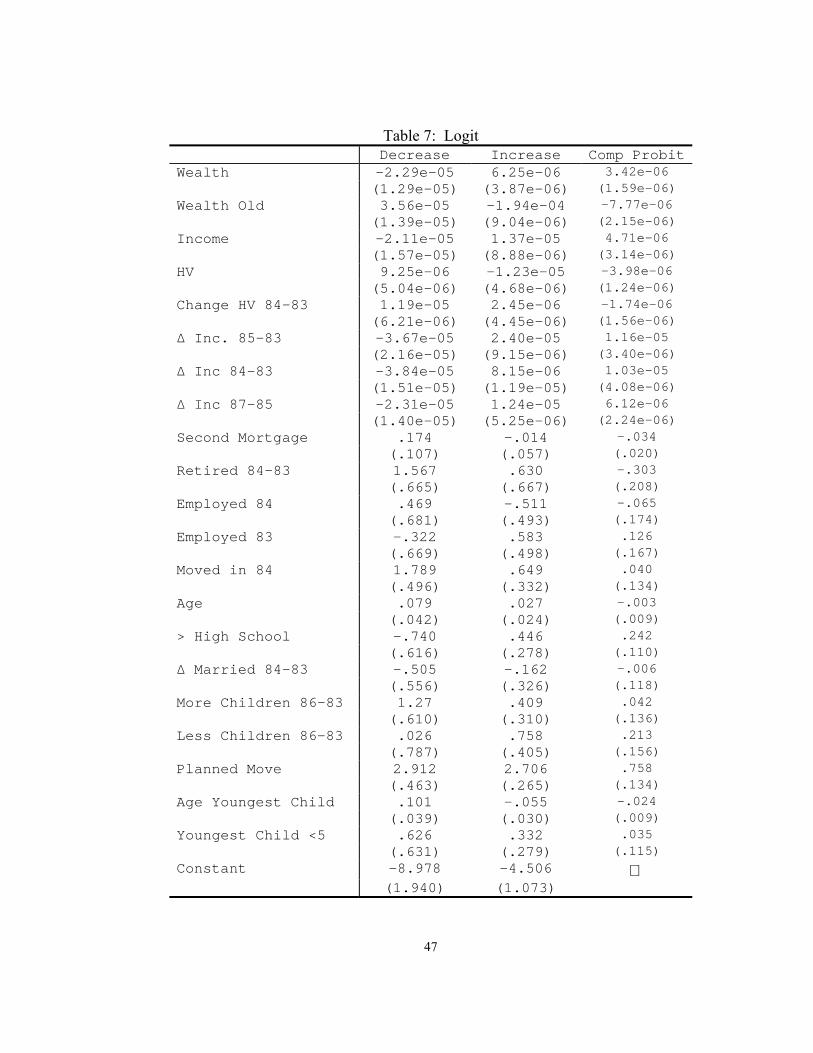
Table 7 gives the results of the multinomial logit regression as well as the results from

an ordered probit with exactly the same variables for comparison purposes. First and

foremost, we see the signs on the variables for wealth and house value match the predictions

28

of the model and of the ordered probit. Increases in wealth increase the probability of

moving to a larger house; while decreases in wealth, increase the probability of moving to a

smaller house. The opposite holds true for house value. However, the effect is not entirely

symmetric. Increases in income and decreases in house value have a stronger effect on

moving to a larger house than do the opposite movement in income and house value have for

decreasing house size. This effect is anticipated in the fact that unconditionally household

are more likely to increase than decrease house size.

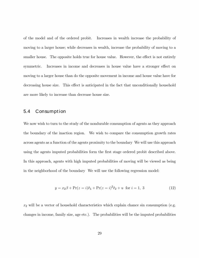
5.4 Consumption

We now wish to turn to the study of the nondurable consumption of agents as they approach

the boundary of the inaction region. We wish to compare the consumption growth rates

across agents as a function of the agents proximity to the boundary We will use this approach

using the agents imputed probabilities form the Þrst stage ordered probit described above.

In this approach, agents with high imputed probabilities of moving will be viewed as being

in the neighborhood of the boundary We will use the following regression model:

y = x2β +Pr(z = i)δ1 +Pr(z = i)2δ2 + u for i = 1, 3 (12)

x2 will be a vector of household characteristics which explain chance sin consumption (e.g.

changes in income, family size, age etc.). The probabilities will be the imputed probabilities

29

from the Þrst stage probit regression. We assume u to be normally distributed, i.i.d., and

u ⊥ ε. The least squares estimates of β and δ are consistent. However, the standard errors

must be corrected for the fact that the imputed probabilities are measured with sampling

error (Pagan 1984, Hansen 1982). The correction term in the two step procedure is a positive

deÞnite matrix under the assumption of independence between u and ε. Hence, the naive

standard errors given by least squares are always smaller than the true standard errors. The

standard errors given in the table have been corrected.

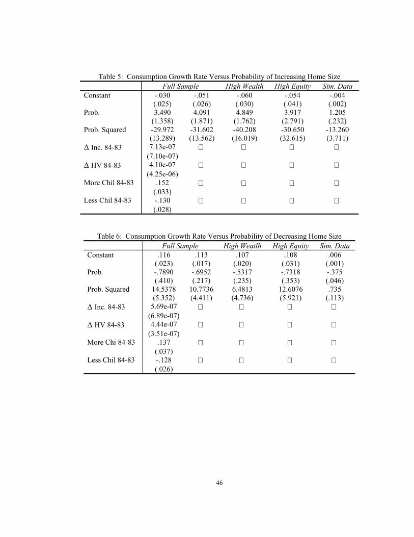
The results of the regressions are given in Tables 5 and 6. Table 5 gives the results of

consumption growth regressed on the predicted probability of increasing house size. We

conduct these regression for the full sample, the high wealth sample, the high equity sample,

and the high wealth and equity sample. The Þrst column we control for other factors

potentially affecting consumption growth rates. The last column contains the results from

the simulated economy - we discuss this regression below. Table 6 has the same lay out and

is for consumption growth regressed on the predicted probability of decreasing house size..

We can see that the full sample regression is consistent with the presence of complentarity

between durable and nondurable goods and the presence of a precautionary motive. The

coefficients for the probability of increasing (decreasing) and the probability squared are of

the correct signs and are signiÞcant. Consumption growth is increasing in the probability

of moving to a larger house over a certain range; however, once the probability of moving is

high enough the consumption growth rate starts to fall. Consumption growth is decreasing

30

in the probability of moving to a smaller house over some range and then increasing as the

probability gets high enough. Keep in mind the high correlation between the probability of

moving and wealth in interpreting these results. What is most remarkable in these results

is the magnitude of the quadratic term. Consumption growth changes a lot as household

approach the boundaries of the continuation region. The changes in consumption before

purchasing a smaller house are particular dramatic. The changes in consumption in the

data are larger (for reasonable values of α) than the changes predicted by our model. These

results hold true even when controlling for changes in income, house value and family size.

While these results are in support of our model, they do not distinguish well between

our model and models of traditional liquidity constraints. Therefore, in an effort to make

this distinction we repeat the test on a several subsets of the population. In picking these

subsets we want to choose groups which are least likely to be liquidity constrained. Following

Zeldes (1989) and Hurst and Stafford (2001), We assume agents with high levels of Þnancial

assets and agents with high amount of equity in their current house are the least likely to be

liquidity constrained Therefore, we rerun the same regressions on the following subsets: 1)

agents holding Þnancial assets above the median level 2) agents with equity above median

equity 3) agents with both equity and Þnancial wealth above the median.

For the high wealth subset, the results are very much the same as in the full sample.

We see a slight reduction in signiÞcance but all coefficients are still signiÞcant at traditional

levels. The only exception to this is the quadratic term for household reducing their house

31

size when house value and wealth levels are not controlled for. This result is slightly in

favor of liquidity constraints not explaining the movement in consumption. However, recall

from our model, that we are predicting the economy to be fairly homogenous in wealth.

Therefore, a household with very high wealth and a large house value can still be liquidity

constrained in our model.

The need to be speciÞc becomes clear as we examine the result from the high equity

sample. The regressions for households which are likely to decrease house size stay ap-

proximately the same. However, the quadratic term for increasing house size becomes very

statistically insigniÞcant. We interpret this to be in support of liquidity constraints.

The Þnal set of regressions subsets the data for households with both high equity and

high wealth. In this sample, we lose the signiÞcance of both quadratic terms.

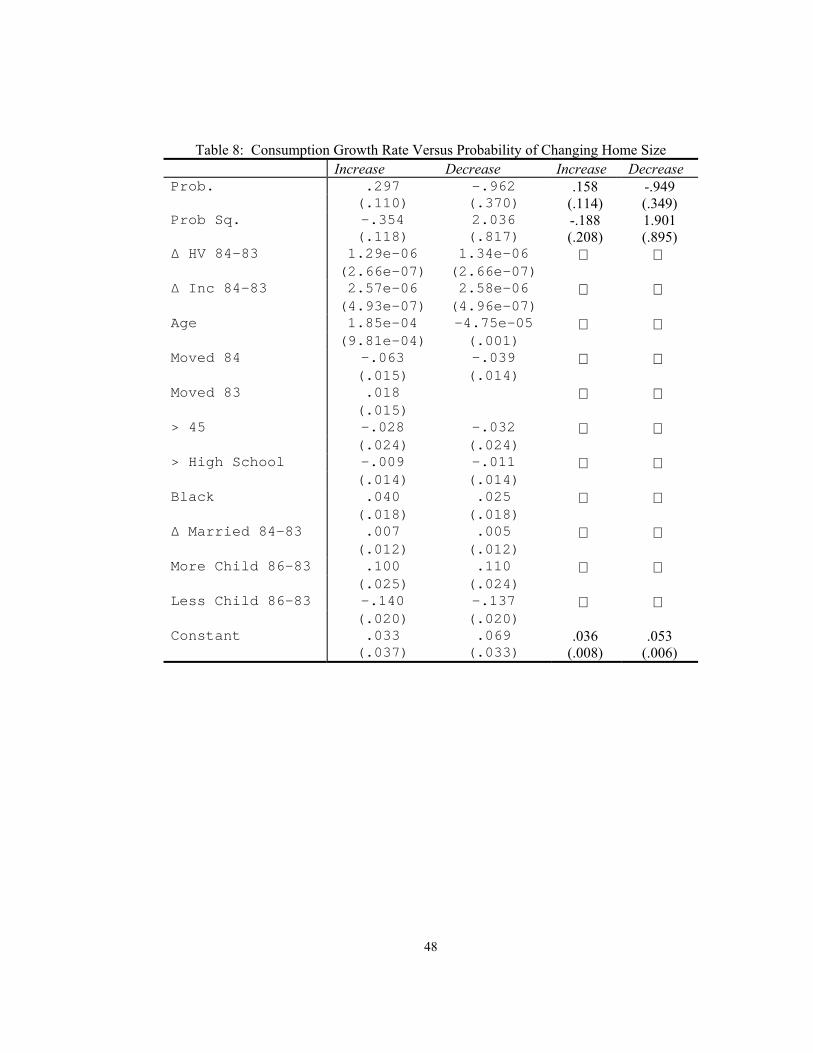
Finally, we wish to run the same exercise using the predicted boundaries from the multino-

mial logit regression. The results are presented in Table 8. The results form the logit are

not as strong as the results from the probit. In the multivariate regression, the signs of

the coefficients on the probability are correct and signiÞcant. However, the signs on the

regressions including only the probability the coefficients are of the right sign but are not

signiÞcant.

32

5.5 Simulated Data

We repeat the same exercises on the simulated economy represented by the simulated dis-

tribution computed above. The Þnal column of Table 3 gives the results of the ordered

probit on the log ratio of wealth to house value. The important result here is that the

sign of the coefficient matches between the simulated data and the data from the PSID.

However, the coefficient on the simulated data is approximately ten times the size of the

coefficient in the empirical data. The main reason for this large difference is in the support

of the distribution between the simulated and empirical data. As we described above in the

construction of the simulated data, reasonable levels of transaction costs can not replicate

the size of the observed inaction region. The support of the simulated data is about 1/6th

the size of the support of the empirical data. One thought for the under estimate for the

size of the inaction region is that the transaction costs which we use greatly underestimate

the true transaction costs involved with moving. We use data on Þnancial cost of relocation

from the CEX arriving at an empirical Þgure of 7-11% of the value of the agent�s house.

The true total cost of moving must also include the cost of the time and disruption caused

by move. However, in our simulations, only by including transaction costs on the order of

50-60% could we come close to matching the empirical support. When we run an ordered

probit on data generated by a 60% transaction cost, we achieve a coefficient of .285 which

we consider to be reasonably close to that found in the empirical data. Clearly, this level

of transaction cost is unlikely to be supported by including these other costs.

33

An alternative speciÞcation is that some agents are prohibited from moving for reasons

outside of our model. We naively simulate such a model by recoding a portion of the

simulated data. A subset of agents who have chosen to move are prohibited from doing

so. Applying this recoding to 20% of the population reduces the magnitude of the probit

coefficient by a factor of 2.

The approximate magnitude of the imputed probabilities of increase, no move, and de-

crease are the same between the simulated distribution and the data. However, in the

simulated economy, the overall probability of moving is lower than in the data. In other

words, agents in the model have policy functions which are much better at keeping the agents

in the center of the inaction region. We could increase the percent of agents moving by

increasing the volatility of returns. In particular, adding a jump process to the evolution of

assets would increase this probability considerably. We view the jump process as modeling

unexpected large changes in the preset value of human capital (i.e. the jumps would measure

aspects of labor income such as layoffs and promotions). Dunn (1998) tests whether shift

in the probability of unemployment affect the timing of purchases of housing. She Þnds

increases in the probability of unemployment decrease the probability of buying a house.

She does not condition on whether the household is likely to increase or decrease their stock

of housing.

The last column of Tables 5 and 6 give the result of regressing changes in consumption

growth on the predicted probabilities of moving in the simulated economy. Our primary test

34

of the model is passed. The signs on the imputed probability coefficients match between the

simulated data and the empirical data and they do so for very reasonable levels of transaction

costs. While the magnitude of the two sets of coefficients are quite different, the shape of

the implied curves is quite similar between the data and the simulated economy. In other

words, while the magnitude of the curve is not matched, both curves reach their maxima at

approximately the same probability of moving and both curves decrease but approximately

the percent as the agent nears the boundary.

6 Conclusion

We have presented a model which explicitly considers durable and nondurable consumption

when the durable market is not frictionless. We have shown that nondurable and durable

consumption are, in general, not separable. Nondurable consumption is not a constant

proportion of Þnancial wealth in this model except when the assets span the risk in the

economy and nondurable and durables are separable in the utility function. Further, we

have shown that the behavior of the model is substantively supported by consumption data

from the PSID. The model matches both the shape of the average individual consumption

policy and the shape of the distribution of wealth to house value ratios.

We also shed light on the recent empirical debate over the effects of unexpected capital

gains on savings-consumption decisions We show that much of the empirical work is con-

sistent, once we understand the expected relationships between nondurable consumption,

35

durable consumption, and wealth. The relationship in this model is more complex than

that given by the standard asset accumulation model.

As with most models of this class, we have not been able to allow the price of housing

to interact with the distribution over agents. In our setup with only idiosyncratic risk, the

assumption of no price effects is justiÞed. However, to fully understand a market as complex

as housing, one must allow aggregate shocks. We can see from the work of Martin (2000)

that the dynamics in the presence of aggregate risk can be very revealing. Once aggregate

risk is incorporated, the distribution over agents and the price of housing must be allowed

to interact. In other words, positive aggregate shocks which tend to make the households

increase their stocks of the durable good should have the effect of increasing either the price

or the total stock of housing. In this manner, we can have a set of agents increasing their

stock at the same time as other agents are decreasing their stocks.

A study of the effects of transaction costs on life-cycle expenditures on nondurable and

durable goods would be a signiÞcant extension of this work. The existence of the transaction

cost has many implications for the life-cycle model. We would expect young households

facing increasing wage proÞles to purchase relatively large houses. As the households age

and their income proÞle stabilizes, we expect the household to be fairly stable in their housing

stock. We also predict that older households should be less likely to move than younger

households. They will consume the new durable for a relatively short period of time making

the transaction costs relatively high. Modeling the effect of transaction costs in a Þnite

36

life-cycle is also computationally less burdensome. As a result, adding life-cycle income to

the model is feasible.

One Þnal note, the shape of the consumption function has implications for the correlation

in consumption between agents. In this model, we no longer predict that the correlation

between the consumption of any two agents to be one, even in a world where agents have

identical preferences and face no idiosyncratic shocks. Here, two agents may have a negative

correlation in consumption growth when they differ only in initial endowment. The low

correlation in consumption between agents is well documented and robust (Deaton 1992).

Our result does not resolve the aggregate consumption correlation puzzle. It fails to do so

because the mass of agents near the boundary of the inaction region is relatively small. For

most agents, the correlation in consumption in response to the same shock is quite high.

Second, part of the force driving the changes in consumption is the incomplete market

structure. Incomplete market structures inherently reduce the correlation in consumption

across agents.

37

References

[1] Attanasio, Orazio P, �Consumer Durables and Inertial Behavior: Estimation of (S,s)Rules for Automobile Purchases,� Review of Economic Studies 67:4 (2000), 667-696.

[2] Beaulieu, James, �Optimal Durable and Nondurable Consumption with TransactionCosts,� Board of Governors of the Federal Reserve System, Finance and EconomicsDiscussion Series No. 93-12 (1993).

[3] Bhatia, Kul B, �Real Estate Assets and Consumer Spending,� Quarterly Journal ofEconomics 102 (1987), 437-443.

[4] Brock, W., Mirman, L., �Optimal Economic Growth and Uncertainty: The DiscountedCase,� Journal of Economic Theory 4 (1985), 479-513.

[5] Caballero, Ricardo J. and Engel, Eduardo M. R. A., �Dynamic (S,s) Economies,�Econometrica 59 (1991), 1659-1686.

[6] Caballero, Ricardo J. and Engel, Eduardo M. R. A., �Microeconomic AdjustmentHazards and Aggregate Dynamics,� Quarterly Journal of Economics 108 (1993), 313-358.

[7] Deaton, Angus, Understanding Consumption (Oxford, New York: Oxford UniversityPress, 1992).

[8] Dunn, Wendy, �Unemployment Risk, Precautionary saving, and Durable Goods Pur-chase Decisions.� Board of Governors of the Federal Reserve System, Finance andEconomics Discussion Series. No. 1998-49 (1998).

[9] Eberly, Janice C, �Adjustment of Consumers� Durable Stocks: Evidence from Auto-mobile Purchases,� Journal of Political Economy, 102 (1994), 403-437.

[10] Engelhardt, Gary V., �Consumption, Down Payments, and Liquidity Constraints,�Journal of Money Credit and Banking, 28 (1996a), 255-270.

[11] Engelhardt, Gary V., �House Prices and Home Owner Saving Behavior,� RegionalScience and Urban Economics 26 (1996b), 313-336.

[12] Flavin, Marjorie, �The Adjustment of Consumption to Changing Expectations aboutFuture Income,� Journal of Political Economy 89 (1981), 974-1009.

[13] Goodman, John L. and John B. Ittner, �The Accuracy of Home Owners� Estimates ofHouse Value,� Journal of Housing Economics 2 (1992), 339-357.

38

[14] Grossman, Sanford J., and Guy Laroque �Asset Pricing and Optimal Portfolio Choicein the Presence of Illiquid Durable Consumption Goods,� Econometrica, 58 (1990),25-51.

[15] Hansen, Lars Peter, �Large Sample Properties of Generalized Method of MomentsEstimators,� Econometrica 50 (1982), 1029-1054.

[16] Hendershott, Patric H., and Joe Peek, �Aggregate U.S. Private Saving: ConceptualMeasures and Empirical Tests,� In Robert E. Lipsey and Helen Stone Tice, eds., TheMeasurement of Saving, Investment, and Wealth (Chicago, IL: University of ChicagoPress,1989).

[17] Hopenhayn, H., and Edward C. Prescott, �Stochastic Monotonicity and StationaryDistributions for Dynamic Economics,� Econometrica 60 (1992), 1387-1406.

[18] Hoynes, Hilary Williamson, and Daniel McFadden, �The Impact of Demographics onHousing and Non-Housing Wealth in the United States,� NBER Working Paper 4666(1994).

[19] Hurst, Eric. �Household Financial Decision Making: Wealth Accumulation, MortgageReÞnancing, and Bankruptcy,� Dissertation: University of Michigan, (1999).

[20] Hurst, Eric, and Frank Stafford, �Home is Where the Equity Is: Liquidity Constraints,ReÞnancing and Consumption,� University of Chicago Working Paper (2000).

[21] Juster, F. Thomas, James P. Smith, and Frank Stafford, �The Measurement and Struc-ture of Household Wealth,� Labour Economics 6:2 (1999), 253-275.

[22] Martin, Robert F., �Dynamics of Aggregate Purchases of an Illiquid Durable Good withrisky Assets and Heterogenous Agents,� Conference Proceedings: WEHIA (2000).

[23] Martin, Robert F., �Consumption, Durable Goods, and Transaction Costs,� Disserta-tion: University of Chicago, (2002).

[24] Pagan, Adrian, �Econometric Issues in the Analysis of Regressions with GeneratedRegressors,� International Economic Review 25 (1984), 221-247.

[25] Rosen, Sherwin, �Manufactured Inequality,� Journal of Labor Economics 15:2 (1997),189-196.

[26] Skinner, Jonathan, �Housing Wealth and Aggregate Saving,� Regional Science andUrban Economics 19 (1989), 305-324.

[27] Skinner, Jonathan, �Is Housing Wealth a Side Show,� Economics of Aging, David A.Wise ed., (Chicago, IL: The University of Chicago Press, 1993).

39

[28] Skinner, Jonathan, �Housing and Saving in the United States,� In Yukio Noguchi andJames M. Poterba eds., Housing Markets in the United States and Japan (Chicago,IL: University of Chicago Press, 1994).

[29] Stokey, Nancy L.,Robert E. Lucas, with Edward C. Prescott, Recursive Methods inEconomic Dynamics (Cambridge, Mass.: Harvard University Press, 1989).

[30] Tachibanaki, Toshiaki, �Housing and Saving in Japan,� In Yukio Noguchi and JamesM. Poterba, eds., Housing Markets in the United States and Japan (Chicago, IL:University of Chicago Press, 1994).

[31] Vissing-Jorgensen, Annette, �Towards an Explanation of Household Portfolio ChoiceHeterogeneity: NonÞnancial Income and Participation Cost Structures,� NBERWork-ing Paper 8884 (2002).

[32] Yamashita, Takahi, and Marjorie Flavin, �Owner-Occupied Housing and the Composi-tion of the Household Portfolio over the Life-Cycle,� University of California San DiegoDiscussion Paper 98-02 (1998).

[33] Zeldes, Stephen, �Consumption and Liquidity Constraints: An Empirical Investiga-tion,� Journal of Political Economy 97 (1989), 305-346.

40

1.2 1.4 1.6 1.8 2 2.2 2.4 2.6 2.8 30.91

0.915

0.92

0.925

0.93

0.935

Figure 1: Consumption Function[alpha=-8, pho=-1, Q=1, r=.0515, Beta=.95, lambda=.1]

Wealth to House Ratio + 1

Con

sum

ptio

n +

.9

41

1 1.2 1.4 1.6 1.8 2 2.2 2.4 2.6 2.80.92

0.93

0.94

0.95

0.96

0.97

0.98

Figure 2: Consumption Function[alpha=-2, pho=-1, r=.0515, Beta=.95, lambda=.1]

Wealth to House Ratio +1

Con

sum

ptio

n +

.9

42

1.2 1.4 1.6 1.8 2 2.2 2.4 2.6 2.80

500

1000

1500Figure 3: Simulated Distribution

Wealth to Houe Value +1

Obs

erva

tions

43

44

Table 1: Characterization of the Inaction RegionR=.09 R=.07 R=.05

Delta=.99Lambda=.01 (1.40,1.66,2.11) (1.39,1.44,1.76) (1.02,1.43,1.68)

Delta=.99Lambda=.03 (1.30,1.67,2.33) (1.29,1.52,1.95) (1.02,1.35,1.81)

Delta=.99Lambda=.05 (1.28,1.53,2.39) (1.25,1.51,2.19) (1.02,1.37,1.84)

Delta=.97 Lambda=.05 (1.22,1.44,2.27) (1.18,1.38,2.21) (1.10,1.37,1.78)

Delta=.97Lambda=.01 (1.58,1.74,2.21) (1.20,1.61,2.07) (1.24,1.40,1.56)

Note: The first and last numbers correspond to the barriers. The middle number correspondsto the optimal return point.

Table 2: Description of DataMean Std Dev Median

House Valuea 64,442 45,595 55,000Accumulated Equitya 42,315 37,845 33,500Remaining Mortgagea,b 22,127 25,713 15,000Wealth no Equitya 32,938 39,048 16,400Wealth with Equitya 75,254 64,163 58,000Percent Housing in Portfolioa,c 0.70 0.21 .75House to Income Ratioa,e 2.18 1.71 1.78Mort Pmnt to Income Ratioa,b 0.15 0.12 .12Car Value to Income Ratioa,d 0.25 0.27 .19Age of Heada 43 11 42

a. Excludes renters, households with head over 65, and the top and bottom 1% ofwealth holders. b. Excludes households with no mortgage. c. Excludeshouseholds with negative net wealth positions. d. Excludes households with zerocars. e. Excludes bottom 5% of income.

45

Table 3: Ordered ProbitProbit 1 Probit 2 Probit 3 Sim. Data

Log Ratio Wealth to .135 1.20House Value (HV) (.048) (.049)Ln Wealth .163 .111

(.0614) (.049)Ln House Value (HV) -.302 -.209

(.069) (.057)Income 1.88e-06

(4.20e-06)Yrs Left to Retirement .022

(.004)> High School .311

(.099)Non-White -.092

(.153)Age -.024

(.029)Age Squared 1.74e-05

(3.20e-04)Note: The regression results in tables 4 and 5 use the predicted probabilities from Ordered Probit 1.

Table 4a: Predicted Probabilities from Ordered Probit 1Mean Std Dev 25% 50% 75% 90%

Increase .039 .038 .014 .029 .051 .079No Move .939 .037 .935 .949 .956 .958Decrease .022 .030 .007 .015 .029 .048

Table 4b: Predicted Probabilities from Simulated DataMean Std Dev 25% 50% 75% 90%

Increase .006 .013 2e-04 .001 .005 .020No Move .965 .074 .972 .989 .994 .995Decrease .029 .076 9e-04 .004 .016 .072

46

Table 5: Consumption Growth Rate Versus Probability of Increasing Home Size

Full Sample High Wealth High Equity Sim. DataConstant -.030 -.051 -.060 -.054 -.004

(.025) (.026) (.030) (.041) (.002)Prob. 3.490 4.091 4.849 3.917 1.205

(1.358) (1.871) (1.762) (2.791) (.232)Prob. Squared -29.972 -31.602 -40.208 -30.650 -13.260

(13.289) (13.562) (16.019) (32.615) (3.711)∆ Inc. 84-83 7.13e-07

(7.10e-07)∆ HV 84-83 4.10e-07

(4.25e-06)More Chil 84-83 .152

(.033)Less Chil 84-83 -.130

(.028)

Table 6: Consumption Growth Rate Versus Probability of Decreasing Home SizeFull Sample High Weatlh High Equity Sim. Data

Constant .116 .113 .107 .108 .006(.023) (.017) (.020) (.031) (.001)

Prob. -.7890 -.6952 -.5317 -.7318 -.375(.410) (.217) (.235) (.353) (.046)

Prob. Squared 14.5378 10.7736 6.4813 12.6076 .735(5.352) (4.411) (4.736) (5.921) (.113)

∆ Inc. 84-83 5.69e-07 (6.89e-07)

∆ HV 84-83 4.44e-07 (3.51e-07)

More Chi 84-83 .137 (.037)

Less Chil 84-83 -.128 (.026)

47

Table 7: LogitDecrease Increase Comp Probit

Wealth -2.29e-05 6.25e-06 3.42e-06

(1.29e-05) (3.87e-06) (1.59e-06)

Wealth Old 3.56e-05 -1.94e-04 -7.77e-06

(1.39e-05) (9.04e-06) (2.15e-06)

Income -2.11e-05 1.37e-05 4.71e-06

(1.57e-05) (8.88e-06) (3.14e-06)

HV 9.25e-06 -1.23e-05 -3.98e-06

(5.04e-06) (4.68e-06) (1.24e-06)

Change HV 84-83 1.19e-05 2.45e-06 -1.74e-06

(6.21e-06) (4.45e-06) (1.56e-06)

∆ Inc. 85-83 -3.67e-05 2.40e-05 1.16e-05

(2.16e-05) (9.15e-06) (3.40e-06)

∆ Inc 84-83 -3.84e-05 8.15e-06 1.03e-05

(1.51e-05) (1.19e-05) (4.08e-06)

∆ Inc 87-85 -2.31e-05 1.24e-05 6.12e-06

(1.40e-05) (5.25e-06) (2.24e-06)

Second Mortgage .174 -.014 -.034

(.107) (.057) (.020)

Retired 84-83 1.567 .630 -.303

(.665) (.667) (.208)

Employed 84 .469 -.511 -.065

(.681) (.493) (.174)

Employed 83 -.322 .583 .126

(.669) (.498) (.167)

Moved in 84 1.789 .649 .040

(.496) (.332) (.134)

Age .079 .027 -.003

(.042) (.024) (.009)

> High School -.740 .446 .242

(.616) (.278) (.110)

∆ Married 84-83 -.505 -.162 -.006

(.556) (.326) (.118)

More Children 86-83 1.27 .409 .042

(.610) (.310) (.136)

Less Children 86-83 .026 .758 .213

(.787) (.405) (.156)

Planned Move 2.912 2.706 .758

(.463) (.265) (.134)

Age Youngest Child .101 -.055 -.024

(.039) (.030) (.009)

Youngest Child <5 .626 .332 .035

(.631) (.279) (.115)

Constant -8.978 -4.506 (1.940) (1.073)

48

Table 8: Consumption Growth Rate Versus Probability of Changing Home SizeIncrease Decrease Increase Decrease

Prob. .297 -.962 .158 -.949(.110) (.370) (.114) (.349)

Prob Sq. -.354 2.036 -.188 1.901(.118) (.817) (.208) (.895)

∆ HV 84-83 1.29e-06 1.34e-06 (2.66e-07) (2.66e-07)

∆ Inc 84-83 2.57e-06 2.58e-06 (4.93e-07) (4.96e-07)

Age 1.85e-04 -4.75e-05 (9.81e-04) (.001)

Moved 84 -.063 -.039 (.015) (.014)

Moved 83 .018 (.015)

> 45 -.028 -.032 (.024) (.024)

> High School -.009 -.011 (.014) (.014)

Black .040 .025 (.018) (.018)

∆ Married 84-83 .007 .005 (.012) (.012)

More Child 86-83 .100 .110 (.025) (.024)

Less Child 86-83 -.140 -.137 (.020) (.020)

Constant .033 .069 .036 .053(.037) (.033) (.008) (.006)