Embed Size (px)
Citation preview
Technische Universität MünchenLehrstuhl für Kommunikationsnetze
Connectivity and Decentralized QoSProvisioning in Vehicular Networks
Dipl.-Ing. Univ. Robert Nagel
Vollständiger Abdruck der von der Fakultät Elektrotechnik und Informationstechnik der Tech-nischen Universität München zur Erlangung des akademischen Grades eines
Doktor-Ingenieurs (Dr.-Ing.)
genehmigten Dissertation.
Vorsitzender: Univ.-Prof. Dr.-Ing. Andreas JossenPrüfer der Dissertation: 1. Univ.-Prof. Dr.-Ing. Jörg Eberspächer
2. Univ.-Prof. Dr.-Ing. Sandra Hirche
Die Dissertation wurde am 16. Dezember 2010 bei der Technischen Universität München ein-gereicht und durch die Fakultät für Elektrotechnik und Informationstechnik am 17. Mai 2011angenommen.
AbstractThe introduction of wireless ad-hoc networks in vehicles will significantly enhance safety andcomfort of driving in the future. However, as of today, we find many important issues re-garding the choice of an appropriate networking technology and concerning application de-sign unanswered. This thesis presents an open mathematical framework that allows for aholistic analysis of network performance in arbitrary road traffic situations, so that relevantparameters can be identified and optimized. Based on this analysis, a novel QoS algorithmfor distributed wireless networks is introduced that guarantees a defined service level andallows the adaptation of applications to networking conditions at runtime. It is shown howthe algorithm can complemented by future network topology prediction, and discussed howapplications can benefit from this information. Finally, a prototypical integration of wirelessnetworking in an existing software architecture for cognitive vehicles is introduced.
KurzfassungDie Einführung drahtloser Kommunikation zwischen Fahrzeugen wird die Sicherheit und denKomfort des Reisens deutlich steigern. Jedoch sind noch viele Fragen bezüglich der Auswahleiner geeigneten Kommunikationstechnologie und des Entwurfs von Anwendungen offen. Indieser Arbeit wird ein mathematisches Rahmenwerk vorgestellt, das die ganzheitliche Ana-lyse der Leistungsfähigkeit drahtloser Netze in beliebigen Strassenverkehrsszenarien ermög-licht. Dadurch können relevante Parameter identifiziert und für den Einsatz optimiert wer-den. Basierend auf der vorhergegangenen Analyse der Anforderungen und verfügbaren Tech-nologien wird ein neuartiger QoS Mechanismus für drahtlose Netze vorgestellt, der es ermög-licht, sowohl anwendungsseitig eine definierte Dienstgüte zu garantieren als auch die netzre-levanten Parameter von Anwendungen zur Laufzeit an den Zustand des Netzes anzupassen.Der Mechanismus wird um ein Verfahren zur Vorhersage zukünftiger möglicher Netztopolo-gien ergänzt. Es wird gezeigt, wie diese Information gewinnbringend an Anwendungenzurückgeführt werden kann. Abschließend wird eine prototypische Integration drahtloserKommunikation in einer existierenden Softwarearchitektur für kognitive Fahrzeuge vorge-stellt.
ii

IN LOVING MEMORY OF MY FATHER,FRIEDRICH ERIK
DEDICATED TO MY FAMILY


Preface
Foremost, I would like to express my gratitude to my advisor Professor Dr. Jörg Eberspächer,for literally being what is called a “doctoral father” in German. He gave me the necessaryliberty to freely pursue my research and the right impulses at the right times. I always ap-preciated his counsel and his reliable support in challenging and turbulent situations. In hisdedication to people and scientific work, he has become a role model to me.
My doctoral family at the Institute of Communication Networks (LKN) at Technische Uni-versität München has provided me with a pleasant, productive, and inspiring environment.For their encouragement, the invaluable discussions, and – of course – for the good timeswe had and the friendships that have developed during my five years at LKN, I would liketo thank Michael Eichhorn, Dr. Stephan Eichler, Dr. Moritz Kiese, Dr. Gerald Kunzmann,Silke Meister, Christian Merkle, my officemate Bernd Müller-Rathgeber, Martin Pfannenstein,Dr. Robert Prinz, Matthias Scheffel, Christoph Spleiß, Dr. Robert Vilzmann, Dr. Hans-MartinZimmermann, and Dr. Stefan Zöls.
Dr. Martin Maier, our administrative genie, master of the thousand windows, and Red Baronto be, deserves my gratitude for making practically everything possible and simply for beinga good pal. Many thanks go to our secretary and good fairy, Sabine Strauss, for her openears and consolation in times of need. I owe Thomas “Willy” Kurzhals for his support withtechnical issues and for teaching me the mysteries of offside situations. As the curator of ourinstitution’s museum of telephony, it was a pleasure for me to work with Helmut “R-Relay”Edlinger, who deeply impressed me with his passion for antiquated telephone exchanges andtaught me the beauty of simplicity.
Among numerous students, I would like to especially thank Stefan Morscher for his valuablecontribution to my scientific work.
Last but not least, I would like to express my deepest gratitude to my family and especiallymy loving partner Martin for their endless support and understanding. I owe you a lot.
v

vi
Contents
1. Introduction 11.1. Motivation . . . . . . . . . . . . . . . . . . . . . . . . . . . . . . . . . . . . . . . . 31.2. Contributions . . . . . . . . . . . . . . . . . . . . . . . . . . . . . . . . . . . . . . 31.3. Organization . . . . . . . . . . . . . . . . . . . . . . . . . . . . . . . . . . . . . . . 4
2. Cooperation Between Vehicles: Scenarios and Requirements 72.1. Cooperative Applications . . . . . . . . . . . . . . . . . . . . . . . . . . . . . . . 8
2.1.1. Cooperative Perception . . . . . . . . . . . . . . . . . . . . . . . . . . . . 82.1.2. Cooperative Behavior . . . . . . . . . . . . . . . . . . . . . . . . . . . . . 112.1.3. Other forms of cooperation . . . . . . . . . . . . . . . . . . . . . . . . . . 12
2.2. Wireless Communication Technologies . . . . . . . . . . . . . . . . . . . . . . . . 122.2.1. IEEE 802.11 Wireless Local Area Network (WLAN) . . . . . . . . . . . . 132.2.2. IEEE 802.11p and the WAVE DSRC Stack . . . . . . . . . . . . . . . . . . 142.2.3. Cellular Networks . . . . . . . . . . . . . . . . . . . . . . . . . . . . . . . 162.2.4. Other Technologies . . . . . . . . . . . . . . . . . . . . . . . . . . . . . . . 17
2.3. Conclusion . . . . . . . . . . . . . . . . . . . . . . . . . . . . . . . . . . . . . . . . 17
3. Connectivity in Vehicular Ad-Hoc Networks 193.1. Related Work . . . . . . . . . . . . . . . . . . . . . . . . . . . . . . . . . . . . . . 193.2. Channel Models . . . . . . . . . . . . . . . . . . . . . . . . . . . . . . . . . . . . . 20
3.2.1. Path Loss . . . . . . . . . . . . . . . . . . . . . . . . . . . . . . . . . . . . 223.2.2. Large-Scale (Shadow) Fading . . . . . . . . . . . . . . . . . . . . . . . . . 253.2.3. Small-Scale (Multipath) Fading . . . . . . . . . . . . . . . . . . . . . . . . 263.2.4. Vehicular Channel Models in the Literature . . . . . . . . . . . . . . . . . 29
3.3. Spatial Node Distribution and Mobility Models . . . . . . . . . . . . . . . . . . . 303.3.1. The Random Direction Model . . . . . . . . . . . . . . . . . . . . . . . . . 313.3.2. Vehicular Mobility Models . . . . . . . . . . . . . . . . . . . . . . . . . . 32
3.4. Node Degree . . . . . . . . . . . . . . . . . . . . . . . . . . . . . . . . . . . . . . . 383.4.1. Geometry . . . . . . . . . . . . . . . . . . . . . . . . . . . . . . . . . . . . 383.4.2. Distance Headways . . . . . . . . . . . . . . . . . . . . . . . . . . . . . . 413.4.3. Discussion . . . . . . . . . . . . . . . . . . . . . . . . . . . . . . . . . . . . 43
3.5. Link Lifetime . . . . . . . . . . . . . . . . . . . . . . . . . . . . . . . . . . . . . . 513.5.1. Geometry . . . . . . . . . . . . . . . . . . . . . . . . . . . . . . . . . . . . 523.5.2. Velocity Distributions . . . . . . . . . . . . . . . . . . . . . . . . . . . . . 523.5.3. Discussion . . . . . . . . . . . . . . . . . . . . . . . . . . . . . . . . . . . . 53
3.6. Link Generation and Link Break Rate . . . . . . . . . . . . . . . . . . . . . . . . 613.6.1. Geometry . . . . . . . . . . . . . . . . . . . . . . . . . . . . . . . . . . . . 643.6.2. Discussion . . . . . . . . . . . . . . . . . . . . . . . . . . . . . . . . . . . . 66
3.7. Conclusion . . . . . . . . . . . . . . . . . . . . . . . . . . . . . . . . . . . . . . . . 69
4. QoS Analysis and Provisioning in Vehicular Ad-Hoc Networks 71
vii
Contents
4.1. Related Work . . . . . . . . . . . . . . . . . . . . . . . . . . . . . . . . . . . . . . 714.2. Network Model . . . . . . . . . . . . . . . . . . . . . . . . . . . . . . . . . . . . . 73
4.2.1. Connectivity Matrix . . . . . . . . . . . . . . . . . . . . . . . . . . . . . . 734.2.2. Traffic Vector . . . . . . . . . . . . . . . . . . . . . . . . . . . . . . . . . . 74
4.3. Medium Access Protocols . . . . . . . . . . . . . . . . . . . . . . . . . . . . . . . 764.3.1. Collision Recovery Protocols . . . . . . . . . . . . . . . . . . . . . . . . . 794.3.2. Collision Avoidance Protocols . . . . . . . . . . . . . . . . . . . . . . . . 804.3.3. 802.11(e) Distributed Coordination Function (DCF) and Enhanced Dis-
tributed Channel Access (EDCA) . . . . . . . . . . . . . . . . . . . . . . . 814.3.4. Reservation-Based Protocols . . . . . . . . . . . . . . . . . . . . . . . . . 824.3.5. Discussion . . . . . . . . . . . . . . . . . . . . . . . . . . . . . . . . . . . . 83
4.4. Providing Quality of Service (QoS) in Contention-Based Networks . . . . . . . 864.4.1. Global Traffic Limits Determination . . . . . . . . . . . . . . . . . . . . . 864.4.2. Distributed Traffic Limits Determination . . . . . . . . . . . . . . . . . . 874.4.3. Admitted traffic and load distribution . . . . . . . . . . . . . . . . . . . . 884.4.4. Stub nodes . . . . . . . . . . . . . . . . . . . . . . . . . . . . . . . . . . . . 934.4.5. Fairness . . . . . . . . . . . . . . . . . . . . . . . . . . . . . . . . . . . . . 95
4.5. Application Selection and Parameterization . . . . . . . . . . . . . . . . . . . . . 984.6. Conclusion . . . . . . . . . . . . . . . . . . . . . . . . . . . . . . . . . . . . . . . . 99
5. Predictive QoS Provisioning in Vehicular Ad-Hoc Networks 1015.1. Related Work . . . . . . . . . . . . . . . . . . . . . . . . . . . . . . . . . . . . . . 1025.2. Problem Statement . . . . . . . . . . . . . . . . . . . . . . . . . . . . . . . . . . . 1045.3. Mobility Prediction . . . . . . . . . . . . . . . . . . . . . . . . . . . . . . . . . . . 105
5.3.1. Concept . . . . . . . . . . . . . . . . . . . . . . . . . . . . . . . . . . . . . 1055.3.2. Speed Prediction . . . . . . . . . . . . . . . . . . . . . . . . . . . . . . . . 1065.3.3. Distance Calculation . . . . . . . . . . . . . . . . . . . . . . . . . . . . . . 1095.3.4. Position Prediction . . . . . . . . . . . . . . . . . . . . . . . . . . . . . . . 1105.3.5. Simulative Evaluation of Speed and Position Prediction Accuracy . . . . 111
5.4. Channel Parameter Estimation and Prediction . . . . . . . . . . . . . . . . . . . 1185.5. Connectivity Prediction . . . . . . . . . . . . . . . . . . . . . . . . . . . . . . . . 1245.6. Conclusions and Outlook . . . . . . . . . . . . . . . . . . . . . . . . . . . . . . . 125
6. A System Architecture for Cooperative Cognitive Technical Systems 1296.1. A Lightweight Network Layer Protocol . . . . . . . . . . . . . . . . . . . . . . . 129
6.1.1. Radio As A Sensor . . . . . . . . . . . . . . . . . . . . . . . . . . . . . . . 1306.1.2. Timing Measurement . . . . . . . . . . . . . . . . . . . . . . . . . . . . . . 1316.1.3. Identification . . . . . . . . . . . . . . . . . . . . . . . . . . . . . . . . . . 132
6.2. The Communication Manager . . . . . . . . . . . . . . . . . . . . . . . . . . . . . 1326.2.1. Network Topology Information . . . . . . . . . . . . . . . . . . . . . . . . 1326.2.2. Time-triggered Communication . . . . . . . . . . . . . . . . . . . . . . . 1336.2.3. Event-triggered Applications . . . . . . . . . . . . . . . . . . . . . . . . . 1366.2.4. System Integration . . . . . . . . . . . . . . . . . . . . . . . . . . . . . . . 138
6.3. Conclusion . . . . . . . . . . . . . . . . . . . . . . . . . . . . . . . . . . . . . . . . 139
7. Conclusion and Outlook 1417.1. Results and Contributions . . . . . . . . . . . . . . . . . . . . . . . . . . . . . . . 1417.2. Outlook . . . . . . . . . . . . . . . . . . . . . . . . . . . . . . . . . . . . . . . . . . 142
viii
Contents
A. A Spline-Shaped Road Model 143A.1. Definition of a Spline . . . . . . . . . . . . . . . . . . . . . . . . . . . . . . . . . . 143A.2. Shape Generation . . . . . . . . . . . . . . . . . . . . . . . . . . . . . . . . . . . . 144A.3. Length of a Spline . . . . . . . . . . . . . . . . . . . . . . . . . . . . . . . . . . . . 145
A.3.1. Numerical Integration . . . . . . . . . . . . . . . . . . . . . . . . . . . . . 146A.3.2. Parameter lookup . . . . . . . . . . . . . . . . . . . . . . . . . . . . . . . . 147
A.4. Fitting . . . . . . . . . . . . . . . . . . . . . . . . . . . . . . . . . . . . . . . . . . . 147
B. Physical Layer Parameters 149
C. Analysis Workflow 151C.1. Networking Parameters . . . . . . . . . . . . . . . . . . . . . . . . . . . . . . . . 151C.2. QoS Analysis . . . . . . . . . . . . . . . . . . . . . . . . . . . . . . . . . . . . . . 151
List of Figures 153
List of Tables 157
Abbreviations 159
Mathematical Notations 161
Bibliography 165
ix

1. Introduction
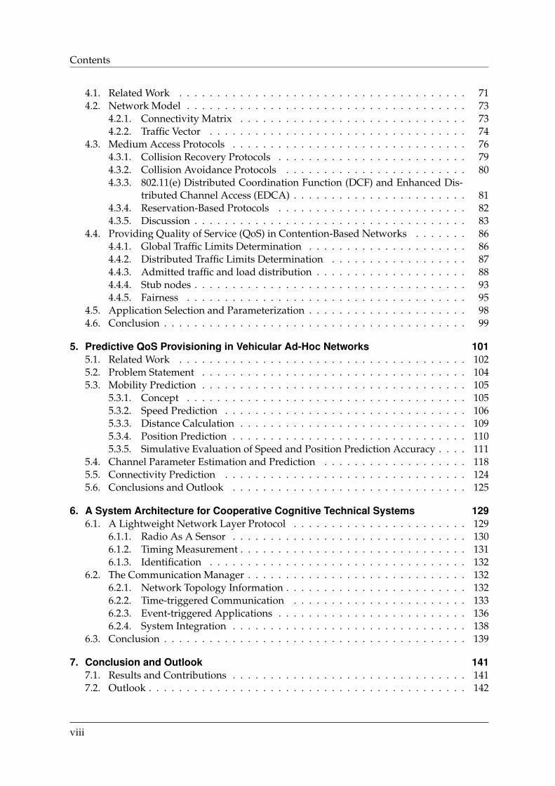
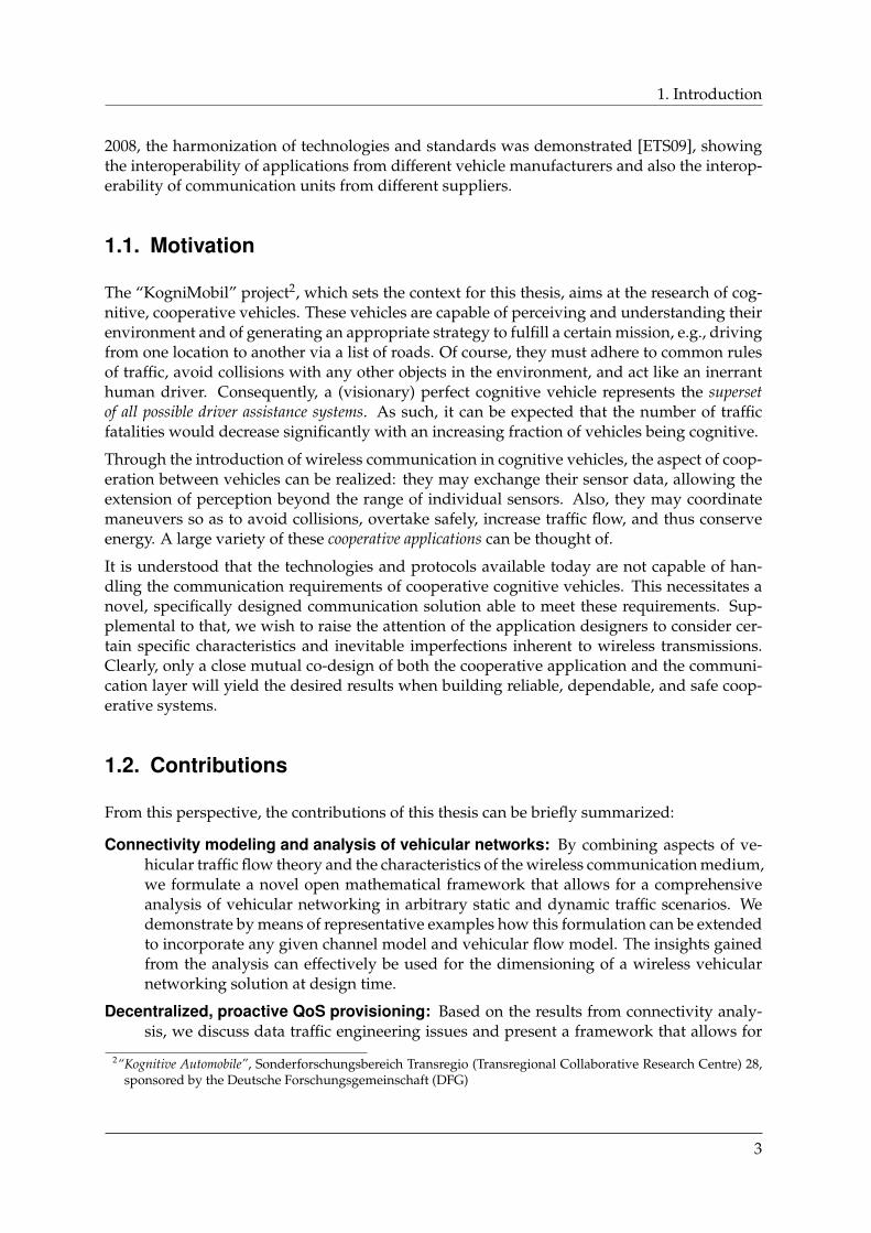
German road traffic statistics reveal that the number of casualties has remained more or lessconstant over the last 60 years. The number of fatalities, however, has decreased significantly,especially since the late 1970s (see Figure 1.1), although the number of vehicles — and conse-quently the number of accidents — has significantly increased in the same period. One canconclude that driving has become much safer over time, an observation that becomes moreobvious when the numbers are related to the years of when governmental regulations wereenacted. The figures also suggest that the introduction of new (active and passive) technolo-gies of vehicular safety significantly contributed to that process.
In 2002, the eSafety Working Group of leading traffic experts published their final report onimproving road safety in Europe by means of Information and Communication Technologies(ICT) [The02]. Among the 28 recommendations of the report, the working group demandedthat “the accelerated standardisation of emerging communications protocols” shall be pro-moted “for vehicle-vehicle and vehicle-infrastructure communications”. Consequently, in2003 the European Commission (EC) set the goal to further reduce the number of road fa-talities by 50% until 2010 [Com03] and stated that the eSafety report concluded that “thegreatest potential [...] in solving road transport safety problems is offered by the IntelligentVehicle Safety Systems”, emphasizing the need for cooperative technologies based on Vehicle-to-Vehicle (V2V) and Vehicle-to-Infrastructure (V2I) communication.
At the time the report was published, using wireless communications between vehicles wasnot an entirely new idea — as early as 1989, Takada et al [TTIF89] proposed the first V2Icommunications system that would enable advanced services, such as positioning, navigationbased on real-time traffic information, tolling, vehicle identification, and individual communi-cation. Also, the issue of market penetration was raised and the expenditures for installing thenecessary infrastructure were analyzed; questions that are still important and mostly unan-swered today. At about the same time, researchers with the U.S. PATH1 project began exper-imenting with automatic longitudinal control (platooning) of two vehicles [CLD+91], whichwas successfully extended to four vehicles and demonstrated in 1994. Concluding, the au-thors pointed out that “when a large number of vehicles is used in a platoon, the complexityof the communication scheme increases”. Also in 1994, Collier and Weiland, impressed bythe positive response of navigation system field trials, drafted a vision of future intelligentvehicles [CW94] that encompassed not only navigation, but also aspects of traffic manage-ment and cooperative driving. Consequently, they argued that in the future, vehicles wouldbe equipped with some kind of radio technology, enabling V2I and V2V communications.An extensive amount of research has subsequently been put into the field of Inter-VehicleCommunication (IVC), in terms of applications, protocols, hardware, etc.; a very comprehen-sive survey can be found in [WTM09].
EC’s eSafety Initiative has spawned many research projects related to IVC, both pan-europeanas well as on national levels, and one can expect that with the dawn of new, more elabo-rate and — most importantly — networked driver assistance systems and safety equipment,
1California Partners for Advanced Transit and Highways (PATH). For a detailed history, see [Shl07].
1
4000
6000
8000
10000
12000
14000
16000
18000
20000
22000
2000
0
1960 1970 1980 1990 2000 2010
1984: belts obligatory
1980: helmets obligatory
1972: Speed limit of100 km/h on rural roads
1973: 0,8‰ limit on blood alcohol level1973/74: oil crisis
1957: Speed limit of50 km/h in cities
1998: 0,5‰ limit on blood alcohol level
Figure 1.1.: Traffic-related fatalities in Germany [Bun09].
we will soon see another dramatic decrease of casualties and fatalities. The most prominentexamples among the research projects are Cooperative Vehicle Infrastructure Systems (CVIS),Global System for Telematics (GST), PReVENTive and Active Safety Applications (PReVENT),Secure Vehicular Communication (SeVeCom), FleetNet or Network on Wheels (NoW) and, re-cently launched, the german “Sichere Intelligente Mobilität – Testfeld Deutschland (SIM-TD)”which provides researchers and industry with a state-wide testbed for vehicular networking.Other worldwide research project are the Vehicle Safety Communication Consortium (VSC)and the Vehicle Infrastructure Integration Initiative (VII) in the U.S., the Advanced Safety Ve-hicle (ASV) project as well as the InternetITS Consortium in Japan.
Today, common efforts are taken to promote worldwide standards specifically for the vehicu-lar environment; a radio platform is being defined by the IEEE 802.11p working group, proto-cols and an architecture has been specified by the IEEE 1609 “WAVE” working group. In 1999,the Federal Communications Commission (FCC) has allocated 75 MHz of spectrum in the5.9 GHz range for Dedicated Short Range Communication (DSRC). Very recently, the Euro-pean Commission has allocated 50 MHz of spectrum in the 5.9 GHz band for “Smart VehicleCommunication Systems”, a decision that is mainly attributed to the dedicated work of theCar-to-Car Communication Consortium (C2CCC), a task force that has been inaugurated byresearch institutions and industry to enforce the development of IVC technology and stan-dards. Vehicle manufacturers and component suppliers are developing strategies and busi-ness models to widely introduce communication and are actively supporting the C2CCC. In
2
1. Introduction
2008, the harmonization of technologies and standards was demonstrated [ETS09], showingthe interoperability of applications from different vehicle manufacturers and also the interop-erability of communication units from different suppliers.
1.1. Motivation
The “KogniMobil” project2, which sets the context for this thesis, aims at the research of cog-nitive, cooperative vehicles. These vehicles are capable of perceiving and understanding theirenvironment and of generating an appropriate strategy to fulfill a certain mission, e.g., drivingfrom one location to another via a list of roads. Of course, they must adhere to common rulesof traffic, avoid collisions with any other objects in the environment, and act like an inerranthuman driver. Consequently, a (visionary) perfect cognitive vehicle represents the supersetof all possible driver assistance systems. As such, it can be expected that the number of trafficfatalities would decrease significantly with an increasing fraction of vehicles being cognitive.
Through the introduction of wireless communication in cognitive vehicles, the aspect of coop-eration between vehicles can be realized: they may exchange their sensor data, allowing theextension of perception beyond the range of individual sensors. Also, they may coordinatemaneuvers so as to avoid collisions, overtake safely, increase traffic flow, and thus conserveenergy. A large variety of these cooperative applications can be thought of.
It is understood that the technologies and protocols available today are not capable of han-dling the communication requirements of cooperative cognitive vehicles. This necessitates anovel, specifically designed communication solution able to meet these requirements. Sup-plemental to that, we wish to raise the attention of the application designers to consider cer-tain specific characteristics and inevitable imperfections inherent to wireless transmissions.Clearly, only a close mutual co-design of both the cooperative application and the communi-cation layer will yield the desired results when building reliable, dependable, and safe coop-erative systems.
1.2. Contributions
From this perspective, the contributions of this thesis can be briefly summarized:
Connectivity modeling and analysis of vehicular networks: By combining aspects of ve-hicular traffic flow theory and the characteristics of the wireless communication medium,we formulate a novel open mathematical framework that allows for a comprehensiveanalysis of vehicular networking in arbitrary static and dynamic traffic scenarios. Wedemonstrate by means of representative examples how this formulation can be extendedto incorporate any given channel model and vehicular flow model. The insights gainedfrom the analysis can effectively be used for the dimensioning of a wireless vehicularnetworking solution at design time.
Decentralized, proactive QoS provisioning: Based on the results from connectivity analy-sis, we discuss data traffic engineering issues and present a framework that allows for
2“Kognitive Automobile”, Sonderforschungsbereich Transregio (Transregional Collaborative Research Centre) 28,sponsored by the Deutsche Forschungsgemeinschaft (DFG)
3
1.3. Organization
the analysis of QoS abilities of vehicular networks in any arbitrary traffic scenario, andwith special respect to the chosen Medium Access Control (MAC) protocol. Again, theformulation of the MAC model is open so that it can easily be extended to any givenprotocol.
Built on this foundation, we describe a novel resource sharing algorithm that allows forvehicular network nodes to equally share the wireless channel so that a pre-defined QoSlevel can be guaranteed to the applications that shall be deployed using the network.The presented algorithm is novel in that it is completely decentralized, deterministicand fast and requires only minimal information about the network’s current topology.Its specific properties, such as traffic assignment fairness and attained optimality, areanalyzed and discussed in detail.
The approach is finally extended through the prediction of future vehicle positions andchannel states so as to allow for a statistical forecast of the future network topology. Thisinformation can then be fed back to the resource sharing algorithm, supporting appli-cations with an estimate of their expected future share of the wireless channel. Thus,we can provide applications with an aid for the decision of future actions that may de-pend on the availability of certain communication relations, of a minimum necessarydata rate, etc.
System integration and protocol provisioning: In the context of the KogniMobil project, aprototypical software architecture for cognitive vehicles was developed. We present howthis solution can be augmented to provide applications with means of networking anddiscuss how the QoS concepts developed earlier can be integrated in the architecture. Wealso present a networking protocol that has been tailored to service the specific needs ofcognitive vehicles.
1.3. Organization
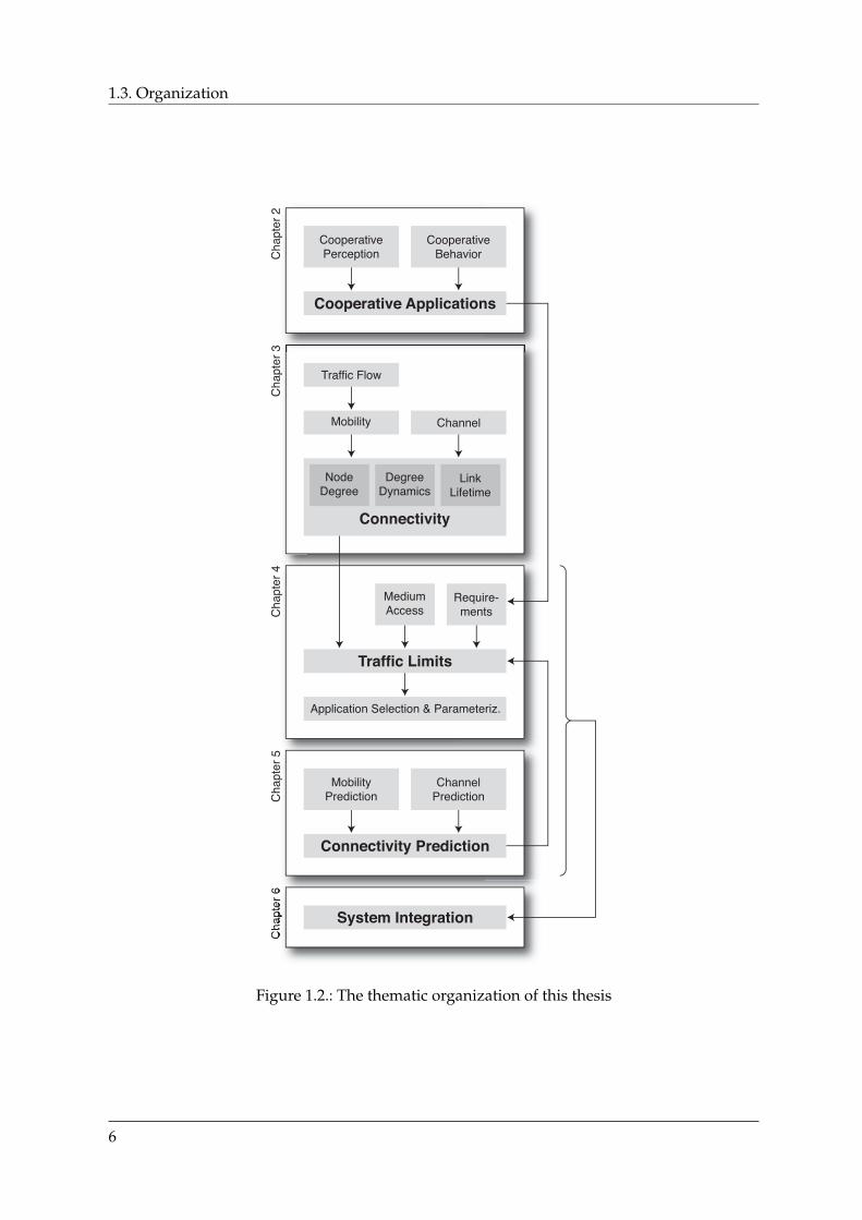
The thesis is structured as follows: each chapter will give a short introduction as well as anoutline and discussion of previous work related to the chapter. Then, the respective contribu-tions are presented. Each chapter closes with a short conclusion. See Figure 1.2 for a graphicalrepresentation of the thematic organization.
Chapter 2 gives an overview of the vision of cognitive autonomous vehicles, their generalarchitecture and the specific requirements imposed upon the communication layer. Cooper-ative applications are presented and the communication relations necessary to the individualapplications are discussed. The range of current wireless IVC technologies available to thesystem designer today are presented and their individual advantages and shortcomings arediscussed.
Chapter 3 introduces the term connectivity and describes how the state of “being connected”is related to the physical location of the respective radios on the one hand and the conditionof the wireless channel between these locations on the other hand. Relevant channel prop-erties and appropriate models are presented, along with a literature survey of contemporaryvehicular channel models. The fundamental relations between traffic flow theory and radiomobility are established and networking parameters such as the distribution of node degrees,communication durations and a measure for the fluctuation of a vehicular network’s topol-ogy are discussed in detail, based on analysis and simulation. This chapter presents the pre-
4
1. Introduction
determined physical layer factors relevant to a V2V network’s performance, i.e., factors thatare dictated by the environment and are thus only subject to limited control at design time.
Based on the connectivity properties derived before, Chapter 4 introduces the concept of howa time-variant network topology (i.e., connectivity on the scale of a network) in conjunctionwith the choice of a specific MAC protocol influences the level of QoS that can be providedto individual applications. A decentralized, distributed algorithm is designed for wireless ap-plications that allows radio network nodes to share the available resources in a fair mannerwhile at the same time ensuring that a defined level of QoS is always attained. We use this in-formation to select and parametrize applications, effectively optimizing the global benefit forthe networked vehicles. The results and implications that can be derived from the algorithm’sformulation are discussed in detail.
An algorithm that facilitates the connectivity prediction in vehicular networks is presentedin Chapter 5. A method for increasing the precision of position prediction by using digitalmaps information is introduced. By applying an adaptive filter, the positions of the involvedvehicles can be predicted for a certain amount of time with a certain accuracy. The choice ofparameters and the resulting accuracy are then discussed in detail. We present and discuss achannel parameter estimation based on a particle filter. By fusing the positions predictions andforecasting the estimated channel parameters over the desired time interval, we show how astatistical predication about the future topology of the network can be attained. Using thisinformation, it is then possible to improve the selection and parameterization of applicationsthat perform tasks that take a certain time to complete and require a minimum QoS duringruntime. Also, prediction can help to decide whether an application should actually be started,given its networking requirements.
Founded on the previously discussed mechanisms and algorithms, a novel communicationsolution is presented in Chapter 6. The prototypical integration with an information-basedprocessing architecture for cognitive vehicles is demonstrated. A prototypical, lightweightcross-layer networking protocol is introduced that supports QoS provisioning for cooperativeperception and driving applications.
Chapter 7 concludes and summarizes the results of this thesis and gives an outlook on possiblefuture research issues.
5
1.3. Organization
Figure 1.2.: The thematic organization of this thesis
6

2. Cooperation Between Vehicles: Scenarios andRequirements
Cognition in a human context comprehends the processes of perception, thinking and insight.In the domain of technical systems, cognition characterizes the capability of a machine to per-ceive itself and its environment by means of appropriate sensorial devices, and to process andrearrange this information — possibly against the background of already acquired knowledge— in a way that allows the machine to interact with its environment in a sensible way andaccording to its mission. Cooperation between cognitive machines postulates the machines’capability to communicate with each other to exchange sensorial information and knowledge,and to coordinate their individual actions so that a coherent cooperative action can be attained.
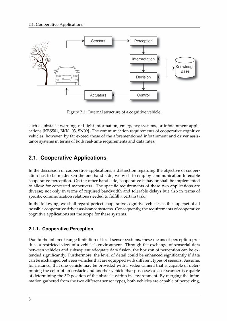
One objective of the Transregional Collaborative Research Centre (TCRC) 28 “Cognitive Au-tomobiles” — the context from which this thesis originated — was to investigate cooperativecognitive behavior among autonomous vehicles. Sticking to the above definition of cognitivesystems, cognitive behavior of a singular vehicle implies an understanding of the perceivedenvironment and the ability to generate strategies to successfully navigate within this envi-ronment [SFK07, GAB+08]. The internal structure of such a vehicle is arrange as depicted inFigure 2.1: the environment of the vehicle (such as obstacles, pedestrians, other vehicles, etc.)and the vehicle therein (i.e., its position, speed, etc.) is perceived through appropriate sensors,such as positioning systems, odometry, video cameras, laser scanners, etc. This informationis then interpreted by identifying (and potentially tracking) environmental objects; drivablelanes are determined, and a scene representation of the environment is established. Basedon the scene interpretation, the mission of the vehicle, and knowledge such as traffic rules, adecision about the desired direction and velocity of motion is made and a trajectory for driv-ing is planned. This decision is passed on to a control module, which, through appropriateactuators, guides the vehicles along the planned trajectory.
Through wireless communication, aspects of cooperation between cognitive vehicles becomefeasible. For instance, vehicles could expand their range of perception beyond the horizonof their own sensors (denoted as cooperative perception in the following), allowing a vehicle toreact to environmental factors before they can be registered by the vehicle itself. Another ex-ample could be the mutual validation or falsification of uncertain sensor data: if an object isregistered by more than one vehicle, its probability of existence increases. Furthermore, vehi-cles could constitute cooperative groups of vehicles and act as such groups [FBB08], in termsof conducting coordinated maneuvers such as, for instance, platooning or avoiding collisions(denoted as cooperative behavior in the following). The benefits are obvious: while the formerwill increase the efficiency of traffic in terms of both travel times and use of energy, the latterhelps in avoiding casualties and potentially life-threatening injuries.
During the last years, V2V Communication has been in the focus of many research groupsall around the world ([c2c, gst, now], to name a few). Very recently, the European Commis-sion has allocated 50 MHz of spectrum in the 5.9 GHz band for “Smart Vehicle Communica-tion Systems”. These systems are mainly geared towards advanced driver assistance systems
7
2.1. Cooperative Applications
Figure 2.1.: Internal structure of a cognitive vehicle.
such as obstacle warning, red-light information, emergency systems, or infotainment appli-cations [KBSS01, BKK+03, SN09]. The communication requirements of cooperative cognitivevehicles, however, by far exceed those of the aforementioned infotainment and driver assis-tance systems in terms of both real-time requirements and data rates.
2.1. Cooperative Applications
In the discussion of cooperative applications, a distinction regarding the objective of cooper-ation has to be made: On the one hand side, we wish to employ communication to enablecooperative perception. On the other hand side, cooperative behavior shall be implementedto allow for concerted maneuvers. The specific requirements of these two applications arediverse; not only in terms of required bandwidth and tolerable delays but also in terms ofspecific communication relations needed to fulfill a certain task.
In the following, we shall regard perfect cooperative cognitive vehicles as the superset of allpossible cooperative driver assistance systems. Consequently, the requirements of cooperativecognitive applications set the scope for these systems.
2.1.1. Cooperative Perception
Due to the inherent range limitation of local sensor systems, these means of perception pro-duce a restricted view of a vehicle’s environment. Through the exchange of sensorial databetween vehicles and subsequent adequate data fusion, the horizon of perception can be ex-tended significantly. Furthermore, the level of detail could be enhanced significantly if datacan be exchanged between vehicles that are equipped with different types of sensors. Assume,for instance, that one vehicle may be provided with a video camera that is capable of deter-mining the color of an obstacle and another vehicle that possesses a laser scanner is capableof determining the 3D position of the obstacle within its environment. By merging the infor-mation gathered from the two different sensor types, both vehicles are capable of perceiving,
8
2. Cooperation Between Vehicles: Scenarios and Requirements
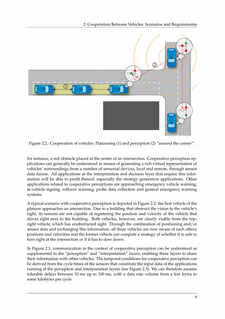
Figure 2.2.: Cooperation of vehicles: Platooning (1) and perception (2) “around the corner”.
for instance, a red obstacle placed at the center of an intersection. Cooperative perception ap-plications can generally be understood as means of generating a rich virtual representation ofvehicles’ surroundings from a number of sensorial devices, local and remote, through sensordata fusion. All applications at the interpretation and decision layer that require this infor-mation will be able to profit thereof, especially the strategy generation applications. Otherapplications related to cooperative perceptions are approaching emergency vehicle warning,in-vehicle signing, rollover warning, probe data collection and general emergency warningsystems.
A typical scenario with cooperative perception is depicted in Figure 2.2: the first vehicle of theplatoon approaches an intersection. Due to a building that obstruct the vision to the vehicle’sright, its sensors are not capable of registering the position and velocity of the vehicle thatdrives right next to the building. Both vehicles, however, are clearly visible from the top-right vehicle, which has unobstructed sight. Through the combination of positioning and/orsensor data and exchanging this information, all three vehicles are now aware of each otherspositions and velocities and the former vehicle can compute a strategy of whether it is safe toturn right at the intersection or if it has to slow down.
In Figure 2.1, communication in the context of cooperative perception can be understood assupplemental to the “perception” and “interpretation” layers, enabling these layers to sharetheir information with other vehicles. The temporal conditions for cooperative perception canbe derived from the cycle times of the sensors that constitute the input data of the applicationsrunning at the perception and interpretation layers (see Figure 2.3). We can therefore assumetolerable delays between 10 ms up to 100 ms, with a data rate volume from a few bytes tosome kilobytes per cycle.
9

2.1. Cooperative Applications
1s100ms10ms1ms 10s Cycle time100ms s 10
Vertical
Lateral
Longitudinal
Vehicle BodyControl
1-lineSICK
LIDAR Vide
o 64-lineVelodyne
LIDAR
INS/IMU/GPS
On-BoardSensors
Cooperative Control
Cooperative Perception
Cooperative Behavior
Infotainment
50km/h
100km
/h
130km
/h
10m Tr
avel tim
e
50km/h
100km
/h
130km
/h
100m Tr
avel tim
e
urbanhighway
Recommended
safety distance
Figure 2.3.: Cycle times of sensors, controllers and cooperative tasks.
It is remarkable that since each piece of sensor information is a gain of knowledge and furtherdetails a vehicle’s perception of its environment, receiving another vehicle’s sensor data resultsin an immediate benefit for every vehicle. Since a receiver’s benefit is also a function of its dis-tance to the sender, i.e., its distance to the point where the sensor data was generated [ESKS06],we constitute that unprocessed sensor data shall be broadcasted (connectionless) and thus bedisseminated only one hop from its source. Thus, the problem of coordinating a multi-hopcommunication has been moved into the application: if it is desirable or the application de-mands to do so, it is possible to aggregate received sensor data, maybe fuse it with local sensorinformation and then re-broadcast it to other vehicles in the proximity (effectively forwardingthe information over multiple hops). Apart from a reduced complexity of the communicationlayer, the number of (re-)transmitted messages and thus the network load can be significantlydecreased [EMS06].
In the course of this thesis, we will describe that the time-variant and highly density-variantnetwork topology imposes significant restrictions on the available data rate for exchangingsensorial information. As data from sensors may be voluminous, we advise that applicationsfor cooperative perception be scalable and adaptable to the situation, an paradigm that hasalso been recently backed by the authors of [vEWKH09, vEKH10]. We will show that availabledata rate has a certain correlation to the traffic situation vehicles find themselves in, especiallythat significant rate limitation can be found in congested traffic situations, i.e., in situationswhere the temporal entropy of sensor data is low. It is clear that this fact should be exploitedat the design time of cooperative perception applications.
10
2. Cooperation Between Vehicles: Scenarios and Requirements
2.1.2. Cooperative Behavior
As mentioned before, communication can also be used to enable cooperative behavior of agroup of vehicles. By exchanging information about vehicles’ missions, their planned (short-term) trajectories, or — in the most simple cast — their positions, applications such as colli-sions avoidance, concerted evasive maneuvers, etc. can be realized. Also, cooperative lateraland/or longitudinal control has been studied and their beneficial impact, especially in termsof fuel efficiency, has been demonstrated [vAvDV06, LPvA09]. Other cooperative driving ap-plications include intersection collision avoidance, transit or emergency vehicle priority.
In Figure 2.1, communication supplemental to the “interpretation” and “decision” layer en-ables cooperative behavior of vehicles. By allowing the interpretation and decision layers toexchange their information, vehicles can generate a common strategy for the situation theyfind themselves in. The temporal conditions for cooperative behavior generation can not eas-ily be derived. As an example, let us assume that a certain situation demands a group ofvehicles to find a common solution for avoiding a collision. The shortest distance betweentwo vehicles is 10 m and the vehicles move at a speed of 50 km/h; consequently, the time un-til collision is 720 ms. Without considering the time necessary to actually guide the vehicleson their individual collision-free trajectory, the decision for these trajectories has to be foundwithin the time until collision. Figure 2.3 shows the times it takes to cover a certain distancefor various common speeds and the recommended safety distances. We can therefore sensi-bly assume that these applications need a communication solution that allows them to reacha safe decision (possibly after some iterations, a number that should be bounded above andknown at design time) within some 100 ms up to 10 s.
From a technical standpoint, based on the current operative situation picture, cooperativegroups of several vehicles form up. Within these groups, the necessary pieces of informationare exchanged and finally a maneuver is agreed upon by the participating vehicles. For in-stance, an evasive maneuver could imply that a vehicle traveling on the fast lane reduces itsspeed to let another vehicle that is yielding an obstacle change its lane. Another example isshown in Figure 2.2, where three vehicles (to the left, highlighted) have teamed up an formeda platoon of vehicles. The leading vehicles sets the direction and velocity and as long as thevehicles’ missions coincide regarding the lane they drive on, they use exchanged positioningand velocity information to drive safely and efficiently, potentially with high velocities andreduced headways, increasing the throughput of the lane.
From a networking point of view, vehicles within a cooperative group form an enclosed mul-ticast group, potentially spreading over a large portion of the network necessitating multi-hoprouting capabilities. Group communication in our concept is provided by a mechanism called“channels”, in which every cooperative group uses its own channel. Communications overa channel may be authenticated or even encrypted, if necessary. The formation of groups it-self is done on the application level, supported by the extended operative situation picture asprovided by the cooperative perception applications and by using a special “paging” channelthat can be used to forward information to vehicles in a certain geographical area.
When designing safety-critical applications that may potentially impose a threat to life in thecase of failure, it must be clear that these applications have to be built in a way that makes themresilient to failures of the communication layer. Wireless channels are inherently unreliableand may be disrupted due to unavoidable external influences. It is absolutely crucial that theseapplications generate a “plan B” for the case that communications fail during a cooperative
11

2.2. Wireless Communication Technologies
maneuver and to implement recurrent checkpointing for error detection while a maneuver isperformed.
2.1.3. Other forms of cooperation
Another form of cooperation is sharing more static knowledge among cars in a peer-to-peerfashion, such as information about long-term environment conditions, traffic rules, newlylearned objects, etc. For instance, floating car data (FCD) that is collected by individual ve-hicles may be aggregated, disseminated and forwarded to a traffic center in a decentralizedfashion. This information can for instance be used for dynamic diversion if a part of theplanned route is jammed.
Other applications that are based on the cooperation between vehicles and/or between ve-hicles and road-side equipment — such as traffic signs, signals, warning beacons etc. — aregeared towards increased road safety, efficiency, and comfort. They include, but are not lim-ited to, intersection assistance, black spot warning, curve warning, optimal speed advisory, ortolling applications. These application can be categorized as cooperative perception applica-tions, yet the temporal span of the validity of exchanged information is usually much longerthan in true cooperative perception applications.
While the mentioned applications employ communications as a means of exchanging theirknowledge that is being used by the “interpretation” and “decision” layer, they have ratherlong time horizons regarding the validity of their information. We may, however, possibly seethe extension of the vehicle-guiding algorithms’ control loops beyond the scope of isolated ve-hicles, if the strong temporal requirements can be fulfilled by the networking technology (seeFigure 2.3). Cooperation at the “control” layer could, for instance, allow for better cooperativecruise control systems or enhanced cooperative collision mitigation.
2.2. Wireless Communication Technologies
Sensitive services that potentially pose threats on lives can only be realized through reliablecommunication connections. The question of connectivity is of primary interest and plays aconstitutional rule: if the networks capacity drops under a certain critical bound in situationswhere vehicle densities (and, consequently, connectivity) is high, such as heavy congestion,insufficient resources may be available for the individual services to function correctly. On theother hand side, highways with free-flow traffic reveal vehicle densities so low that the prob-ability of a vehicle being disconnected, effectively rendering its communication equipmentuseless, is significant.
Especially the problem of insufficient connectivity could be solved by using static roadsidenetwork nodes that constitute a communications infrastructure, potentially even providinga dedicated backbone network that interlinks the individual infrastructure nodes. Also, in-frastructure may be helpful in overload scenarios, as a central entity managing the flow ofmessages. Shortcuts through the infrastructure backbone networks could also be used to ef-fectively send messages to distant regions of the network. However, the use of infrastructureposes an elementary problem: regarding the costly deployment, infrastructure may not beavailable everywhere where communication is desired. Especially in remote rural regions,it is very unlikely that the necessary equipment is to be deployed promptly. Even worse, a
12
2. Cooperation Between Vehicles: Scenarios and Requirements
failure of the infrastructure equipment may significantly reduce the benefit or even disable allcommunications in the covered area. Therefore, we require that all functionality of the com-munications layer is completely decentralized and that the network is fully operational with-out any infrastructure and without any central entity. The term ad-hoc network is commonlyused for wireless, decentralized, self-configuring, and potentially time-variant networks.
The term QoS refers to the effort of provisioning communications relations over a given net-work with a certain performance level, regarding data rate, packet loss probability, and delays.Depending on the configuration of the network, especially the Medium Access Control (MAC)used, as well as the actual in-situ connectivity, the individual performance numbers vary sig-nificantly and, mostly, it is not trivial to guarantee a certain service level. The influential factorswill be discussed later and we will demonstrate how, based on a statistical description of theenvironment, a probabilistic estimation of the expected service level can be made and QoS caneben be guaranteed. However, it is most important to keep in mind that wireless networks areinherently unreliable and that the overall behavior will be highly undeterministic.
A comprehensive overview of MAC protocols for general ad-hoc networks can be foundin [GL00], where the authors outline design challenges and present a classification of pro-tocols. Performance issues and application domains are also discussed. In [JLB10] designguidelines for ad-hoc networks are presented and a large number of different protocols isstudied and classified. With a focus on vehicular ad-hoc networks, an overview on selectedprotocols (802.11 and ADHOC MAC [BCCF03]) as well as a qualitative comparison can befound in [MFL06]. A comprehensive survey on the whole vehicular networking stack andsimulation models can be found in [SK08]. In [WTM09], a taxonomy for vehicular applica-tions is presented and the relevance of communication protocols for various applications isestablished.
Although a large number of communication technologies have been suggested and studiedin great detail in the literature, we shall present only those that are established and actuallyavailable for deployment in this section.
2.2.1. IEEE 802.11 WLAN
The first commercially relevant standard that allowed wireless interconnection and interoper-ability among a group of equipped computers was the IEEE 802.11 standard [IEE07a], todaycommonly denoted as “WLAN” (wireless local area network) or more recently as “WiFi”. Itwas originally approved and published by the Institute of Electrical and Electronics Engineers(IEEE) in 1997. In its first version, 802.11 supported a variety of physical layer interfaces, suchas infrared and 2.4 GHz radio using frequency hopping (FHSS) or direct sequence (DSSS)spread spectrum, and data rates of up to 2 Mbit/s. It also introduced the ability of operatingthe network using infrastructure (so-called access points) and without infrastructure (ad-hocmode). While transmission coordination may be controlled by the Access Point (AP) in in-frastructure mode using Point Coordination Function (PCF), it is inherently self-organizing inad-hoc mode, using the Distributed Coordination Function (DCF). The radio channel itselfis shared among the participating nodes using the contention-based Carrier Sense MultipleAccess with Collision Avoidance (CSMA/CA) MAC scheme, with optional RTS/CTS flowcontrol for point-to-point connections.
Over the years, the standard saw many amendments, mostly providing improved PHY speci-fications that allowed higher data rates - such as 1999’s 11b amendment that allowed that data
13

2.2. Wireless Communication Technologies
rates of up to 11 Mbit/s in the 2.4 GHz ISM band and, widely adopted by equipment manu-facturers and customers, made the standard a commercial success. At the same time, the 11aamendment — not so well known in Europe as it was originally not admitted due to frequencyband licensing issues — even allowed data rates of up to 54 Mbit/s in the 5 GHz U-NII band,using the novel Orthogonal Frequency Division Multiplex (OFDM) modulation scheme. TheOFDM modulation and coding scheme used in 11a was later adopted in 2003 for the 2.4 GHzband under the 11g revision. The latest addition to the standard was the 11n amendment,approved in 2009, that introduced MIMO techniques and specifies channel bandwidths up to40 MHz, allowing for data rates of up to 600 Mbit/s.
Apart of the constant increase in available data rate, the 11e amendment provided the basisfor differentiated prioritization of individual services and thus a fundament for the realiza-tion of QoS over 802.11-based wireless networks. The WiFi-Alliance, founded by equipmentmanufacturers, certified compliant devices and coined the term Wireless Multimedia Extensions(WME) or Wi-Fi Multimedia (WMM) for QoS-enabled equipment. With a clear emphasis onthe support of wireless multimedia applications, 11e offered the possibility to assign fourdifferent traffic classes to each packet, effectively altering the time before channel access isgranted (the so-called Contention Window (CW)) through a modified coordination function,the EDCA. The actual effect of prioritization, however, strongly depends on a careful choice oftraffic classes for individual applications, and an incorrect assignment can result in significantperformance degradation.
Due to the complex, non-deterministic, contention-based MAC scheme and its dependency ona large number of parameters, determining an expected throughput or packet loss probabilityis not trivial and only statistical measures can be derived; several publications exist that coverthe topic through analysis and simulation. It is worth noting that even if the 11e QoS extensionis implemented, it is not possible to guarantee a certain service level (see also Chapter 4).
However, 802.11a/b/g/n+e is the only readily-available standard today, with low prices forhigh-quality equipment. Its specific properties have been studied by many researchers and ithas been (and still is) implemented in almost all V2V scenarios. In the context of the “Cogni-tive Automobiles” research project, we have specified and successfully used 802.11a/g+e asthe communication basis for tested cooperative applications.
2.2.2. IEEE 802.11p and the WAVE DSRC Stack
Due to several shortcomings of the IEEE 802.11 standards and the advent of novel applicationsfor networked vehicles, various new requirements have arisen demanding that the communi-cations solution is able to:
• support longer ranges of operation (up to 1000 m),
• handle high relative speeds of vehicles (up to 500 km/h),
• cope with extreme multipath environments such as urban scenarios where the wirelesssignal experiences many reflections with long delays of up to 5 µs maximum excess,
• operate in a dedicated portion of the frequency spectrum,
• provide multiple overlapping ad-hoc networks with extremely high quality of service,
• tightly support automotive applications and their communication requirements (such asfor instance reliable broadcast).
14
2. Cooperation Between Vehicles: Scenarios and Requirements
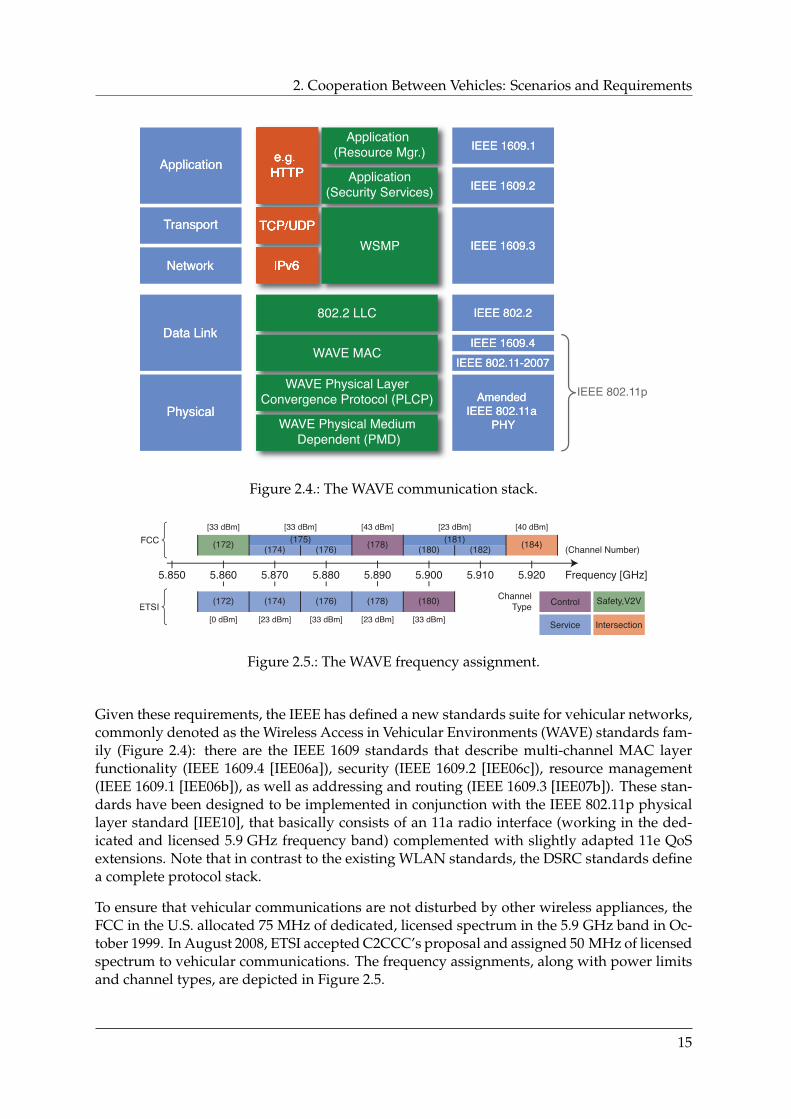
Figure 2.4.: The WAVE communication stack.
5.8605.850 5.8805.870 5.9005.890 5.9205.910 Frequency [GHz]
[43 dBm][33 dBm] [23 dBm][33 dBm] [40 dBm]
[33 dBm][23 dBm] [23 dBm][0 dBm] [33 dBm]
Figure 2.5.: The WAVE frequency assignment.
Given these requirements, the IEEE has defined a new standards suite for vehicular networks,commonly denoted as the Wireless Access in Vehicular Environments (WAVE) standards fam-ily (Figure 2.4): there are the IEEE 1609 standards that describe multi-channel MAC layerfunctionality (IEEE 1609.4 [IEE06a]), security (IEEE 1609.2 [IEE06c]), resource management(IEEE 1609.1 [IEE06b]), as well as addressing and routing (IEEE 1609.3 [IEE07b]). These stan-dards have been designed to be implemented in conjunction with the IEEE 802.11p physicallayer standard [IEE10], that basically consists of an 11a radio interface (working in the ded-icated and licensed 5.9 GHz frequency band) complemented with slightly adapted 11e QoSextensions. Note that in contrast to the existing WLAN standards, the DSRC standards definea complete protocol stack.
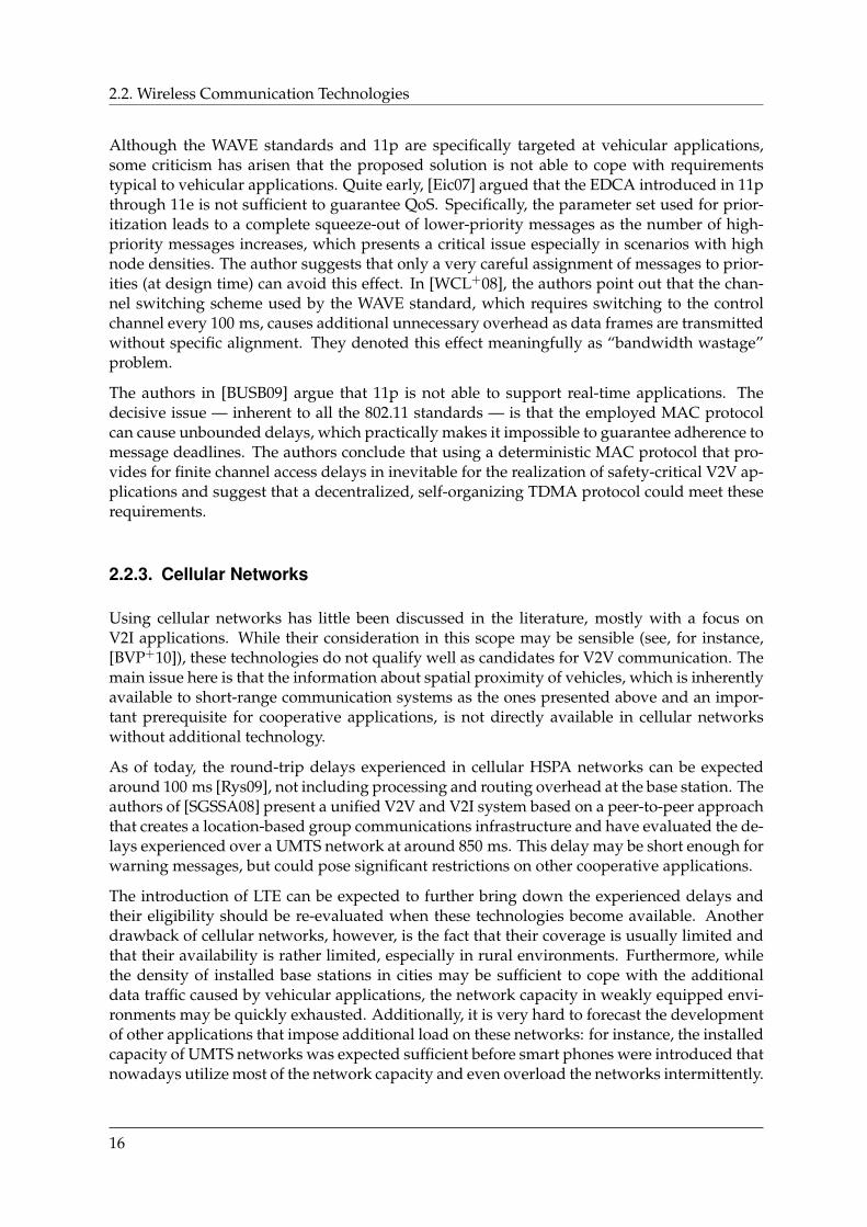
To ensure that vehicular communications are not disturbed by other wireless appliances, theFCC in the U.S. allocated 75 MHz of dedicated, licensed spectrum in the 5.9 GHz band in Oc-tober 1999. In August 2008, ETSI accepted C2CCC’s proposal and assigned 50 MHz of licensedspectrum to vehicular communications. The frequency assignments, along with power limitsand channel types, are depicted in Figure 2.5.
15
2.2. Wireless Communication Technologies
Although the WAVE standards and 11p are specifically targeted at vehicular applications,some criticism has arisen that the proposed solution is not able to cope with requirementstypical to vehicular applications. Quite early, [Eic07] argued that the EDCA introduced in 11pthrough 11e is not sufficient to guarantee QoS. Specifically, the parameter set used for prior-itization leads to a complete squeeze-out of lower-priority messages as the number of high-priority messages increases, which presents a critical issue especially in scenarios with highnode densities. The author suggests that only a very careful assignment of messages to prior-ities (at design time) can avoid this effect. In [WCL+08], the authors point out that the chan-nel switching scheme used by the WAVE standard, which requires switching to the controlchannel every 100 ms, causes additional unnecessary overhead as data frames are transmittedwithout specific alignment. They denoted this effect meaningfully as “bandwidth wastage”problem.
The authors in [BUSB09] argue that 11p is not able to support real-time applications. Thedecisive issue — inherent to all the 802.11 standards — is that the employed MAC protocolcan cause unbounded delays, which practically makes it impossible to guarantee adherence tomessage deadlines. The authors conclude that using a deterministic MAC protocol that pro-vides for finite channel access delays in inevitable for the realization of safety-critical V2V ap-plications and suggest that a decentralized, self-organizing TDMA protocol could meet theserequirements.
2.2.3. Cellular Networks
Using cellular networks has little been discussed in the literature, mostly with a focus onV2I applications. While their consideration in this scope may be sensible (see, for instance,[BVP+10]), these technologies do not qualify well as candidates for V2V communication. Themain issue here is that the information about spatial proximity of vehicles, which is inherentlyavailable to short-range communication systems as the ones presented above and an impor-tant prerequisite for cooperative applications, is not directly available in cellular networkswithout additional technology.
As of today, the round-trip delays experienced in cellular HSPA networks can be expectedaround 100 ms [Rys09], not including processing and routing overhead at the base station. Theauthors of [SGSSA08] present a unified V2V and V2I system based on a peer-to-peer approachthat creates a location-based group communications infrastructure and have evaluated the de-lays experienced over a UMTS network at around 850 ms. This delay may be short enough forwarning messages, but could pose significant restrictions on other cooperative applications.
The introduction of LTE can be expected to further bring down the experienced delays andtheir eligibility should be re-evaluated when these technologies become available. Anotherdrawback of cellular networks, however, is the fact that their coverage is usually limited andthat their availability is rather limited, especially in rural environments. Furthermore, whilethe density of installed base stations in cities may be sufficient to cope with the additionaldata traffic caused by vehicular applications, the network capacity in weakly equipped envi-ronments may be quickly exhausted. Additionally, it is very hard to forecast the developmentof other applications that impose additional load on these networks: for instance, the installedcapacity of UMTS networks was expected sufficient before smart phones were introduced thatnowadays utilize most of the network capacity and even overload the networks intermittently.
16

2. Cooperation Between Vehicles: Scenarios and Requirements
Is is questionable whether the providers would like to see their networks become congestedby vehicular applications.
2.2.4. Other Technologies
Over the time, a variety of alternative technologies have been suggested for deploymentin vehicular networks. In [LHSR01], the authors suggest an adapted UTRA-TDD PhysicalLayer (PHY) and MAC mechanism and argue that the time-division properties of the prop-erties allow for relatively simple QoS provisioning. The suitability of Bluetooth for V2V net-works has been discussed in great detail in [SD05]. Also, ultra-wideband (UWB) and ZigBeetechnologies have been suggested for vehicular networks [NHB05]. However, none of thetechnologies have actually gained any significance and shall therefore not be discussed here.
Relatively new approaches geared towards directed point-to-point connections between ve-hicles comprise free-space optical technologies [AL10] and data transmission using OFDMmodulated radar [SZW09] (which can be expected to be available in a wide range of future ve-hicles). Solutions geared towards wide-area information dissemination into vehicles throughunidirectional broadcast (traffic information, etc.) have been discussed being based on tech-nologies such as DRM, RDS, and DVB (see [BVP+10]).
While the former technologies are potential candidates for the cooperative applications pre-sented above (and their performance may actually be studied using the presented methods),the latter are very specialized and applicable mostly to point-to-point and wide-area broad-cast. The reader shall be referred to the references for further information.
2.3. Conclusion
In this section, we have classified cooperative applications into the two main categories: coop-erative perception and cooperative behavior. We have discussed exemplary applications andtheir requirements. In the second part, contemporary and readily available communicationtechnologies are presented and their adequacy for cooperative vehicles has been discussed.
For obvious reasons, we do not give any recommendations regarding the choice of a specificcommunication technology here, as the requirements of actually deployed applications mayvary greatly and this choice has to be made with respect to these requirements. In the nextchapters, we will present analytical tools that can be used to analyze communication tech-nologies, given an application and a deployment scenario, and that are ultimately to supportthis choice.
We have argued above that, when designing cooperative applications, it is absolutely crucialthat:
• applications are built in a way that allows them to scale and adapt to a varying commu-nication situation,
• applications cope with inherent and unavoidable shortcomings of the wireless medium,especially connections breaking down unexpectedly (have a plan “B” ready).
17
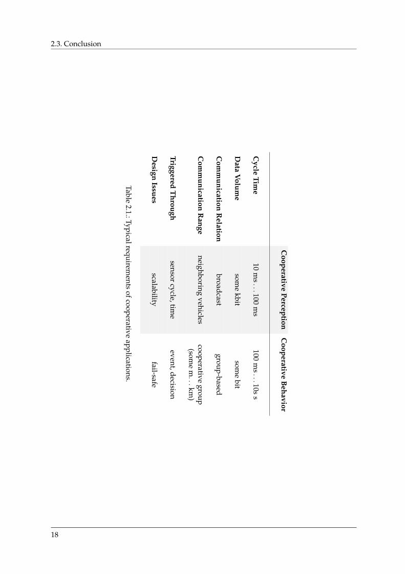
2.3. Conclusion
Cooperative
PerceptionC
ooperativeB
ehavior
Cycle
Time
10m
s...100
ms
100m
s...10s
s
Data
Volum
esom
ekbit
some
bit
Com
munication
Relation
broadcastgroup-based
Com
munication
Range
neighboringvehicles
cooperativegroup
(some
m...km
)
TriggeredT
hroughsensor
cycle,time
event,decision
Design
Issuesscalability
fail-safe
Table2.1.:Typicalrequirem
entsofcooperative
applications.
18
3. Connectivity in Vehicular Ad-Hoc Networks
This chapter studies the implications of the specific mobility of vehicles traveling on streets onthe networking aspects of wireless vehicular ad-hoc networks.
We will first elaborate on the fundamental interdependence of nodes’ spatial proximity andthe probability that these nodes can exchange messages through means of wireless transmis-sion, commonly termed as “connectivity”. We present and discuss several channel models,which can be ultimately interpreted as the tie between spatial properties of the network andconsequent connection probability. These spatial properties of wireless vehicular networks areevidently determined by the physical properties of vehicular traffic flow. As such, we intro-duce and discuss various parameters of (vehicular) traffic modeling, which — in conjunctionwith appropriate channel models — constitutes the basis for subsequent analysis.
On the basis of the derived framework that integrates channel and mobility models, we shallanalyze fundamental properties of connectivity in vehicular networks. As a first step, wemake the connection between the node degree (i.e. the number of communication partners)and the distance distribution of vehicles. Then, we investigate the distribution of connectiontimes as a result of the velocity distribution of vehicles. Finally, we combine the node de-gree and the connection times and obtain the rate at which the connections between vehicleschange as a measure of the dynamic of vehicular networks. We derive all necessary formu-las that characterize network properties, introduce representative scenarios and discuss theresults on their basis.
The main contribution of this chapter is a comprehensive mathematical formulation of num-ber of relevant factors that determine the static and dynamic connectivity of a vehicular net-work. All results in this chapter are abstract of the radio technology used to actually form thenetwork; instead, they are universally valid theoretical considerations and reasonings aboutconnectivity that contribute to the state of art as a guideline to the design of a physical layerin vehicular networks. Furthermore, these considerations form the basis for the developmentof dedicated teletraffic engineering mechanisms in the next chapter. Some of the material inthis chapter has been published in [NE08, Nag10b].
To avoid ambiguity, the term “traffic” in this chapter refers to the movement and interactionof vehicles on roads.
3.1. Related Work
Connectivity in MANETs and one-dimensional networks has been thoroughly studied throughsimulation and analysis [MA06, DTH02]. The main part of these contributions address theproblem of connectivity in the context of static networks and are thus more applicable to sen-sor networks. The impact of mobility and the consequences for connectivity is extensivelystudied in [Bet04], but the studied mobility models are not applicable to vehicular ad-hoc net-works as they are not capable of reflecting the specific properties of vehicular traffic flows. Fur-
19
3.2. Channel Models
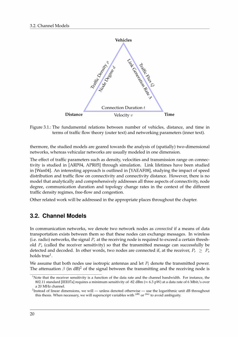
Vehicles
Distance Time
Traf
ficD
ensi
tyρ
Nod
eD
egre
ed
Velocity v
Connection Duration t
Traffic FluxQ
LinkG
enerationRate
Λ
Figure 3.1.: The fundamental relations between number of vehicles, distance, and time interms of traffic flow theory (outer text) and networking parameters (inner text).
thermore, the studied models are geared towards the analysis of (spatially) two-dimensionalnetworks, whereas vehicular networks are usually modeled in one dimension.
The effect of traffic parameters such as density, velocities and transmission range on connec-tivity is studied in [ARP04, APR05] through simulation. Link lifetimes have been studiedin [Wan04]. An interesting approach is outlined in [YAEAF08], studying the impact of speeddistribution and traffic flow on connectivity and connectivity distance. However, there is nomodel that analytically and comprehensively addresses all three aspects of connectivity, nodedegree, communication duration and topology change rates in the context of the differenttraffic density regimes, free-flow and congestion.
Other related work will be addressed in the appropriate places throughout the chapter.
3.2. Channel Models
In communication networks, we denote two network nodes as connected if a means of datatransportation exists between them so that these nodes can exchange messages. In wireless(i.e. radio) networks, the signal Pr at the receiving node is required to exceed a certain thresh-old Ps (called the receiver sensitivity) so that the transmitted message can successfully bedetected and decoded. In other words, two nodes are connected if, at the receiver, Pr ≥ Psholds true1.
We assume that both nodes use isotropic antennas and let Pt denote the transmitted power.The attenuation β (in dB)2 of the signal between the transmitting and the receiving node is
1Note that the receiver sensitivity is a function of the data rate and the channel bandwidth. For instance, the802.11 standard [IEE07a] requires a minimum sensitivity of -82 dBm (≈ 6.3 pW) at a data rate of 6 Mbit/s overa 20 MHz channel.
2Instead of linear dimensions, we will — unless denoted otherwise — use the logarithmic unit dB throughoutthis thesis. When necessary, we will superscript variables with (dB) or (lin) to avoid ambiguity.
20

3. Connectivity in Vehicular Ad-Hoc Networks
Attenuation
Path Loss
Friis, Log-distance,
Dual-Slope
Fading
Large-scale
fading
Log-normal
Small-scale
fading
Rice,Gauss,
Rayleigh
Figure 3.2.: Classification of attenuation effects (red) and their distributions (blue).
then given by:
β(dB) = 10 log10
(P (lin)t
P (lin)r
)= 10 log10
(P (lin)t
)− 10 log10
(P (lin)r
)(3.1)
= P (dB)t − P (dB)
r (3.2)
Attenuation is a result of the propagation of the electromagnetic wave through space and theassociated physical effects that reduce the power density of the wave. It is therefore a functionof both the environment and the positions of the transmitter xa(t) and a receiver xb(t) therein.
In the literature, a variety of channel models exists which — to a certain extent — describe oneor more aspects of this relation (Figure 3.2); a very good and comprehensive survey of propa-gation models can be found in [SJK+03]. Beside the (commonly used) statistical channel mod-els, ray-tracing methods [Mau05] have become popular over the last years as a consequenceof increased computational power. Ray-tracing can give extremely realistic results; however,very good knowledge and precise modeling of the environment is required, a prerequisite thatcannot always be taken for granted. A very thorough survey on V2V propagation channels,especially measured characteristics and parameters, can be found in [MTKM09].
We denote the maximum possible attenuation βmax as the margin between transmitted powerPt and the receiver sensitivity Ps (Equation (3.2)):
βmax = Pt − Ps (3.3)
21
3.2. Channel Models
In the following, we will discuss formulas for the probability that two nodes A and B placedat distinct positions xa and xb are connected, i.e. the probability that the attenuation betweenthe nodes is below βmax, and formulate the channel model as a function of nodes’ physicalpositions:
χ(xa,xb) = P (β(xa,xb) ≤ βmax) (3.4)
More precisely, let us define χ(xa,xb) to be the probability that node A can transmit messagesto node B. If the channel is reciprocal,
χ(xa,xb) = χ(xb,xa) (3.5)
3.2.1. Path Loss
The most obvious effect of attenuation is a result of the expansion of the wave front in space,resembling the shape of a growing sphere. This effect is generally denoted as path loss, relatingattenuation to the distance d = ‖xa − xb‖ between transmitter and receiver.
Friis Path Loss
The simplest form of path loss can be given for a free-space environment in which the wavecan expand freely in all three dimensions. It has been originally proposed [Fri46] that thereceived power decays quadratically with the distance d:
βf (d) = 20 log10
4πd
λ(3.6)
The parameter λ represents the wavelength. Note however that Equation (3.6) is only validfor distances d in the far-field of the transmitting antenna and is related to the largest lineardimension of the antenna aperture D:
d! 2D2
λ∨ d
! D ∨ d
! λ (3.7)
Log-Distance Path Loss
To account for environments in which parts of the wave front are reflected or absorbed, Equa-tion (3.6) has been extended through the introduction of the path loss exponent α:
βp(d) = βr(d0) + 10α log10
d
d0(3.8)
= 20 log10
4πd0
λ+ 10α log10
d
d0(3.9)
Equation (3.6) and Equation (3.9) are homologous for α = 2. In environments in which partsof the wave front are reflected or absorbed, higher values of α are used; for example, urbanenvironments that include buildings and other obstacles are commonly modeled by lettingα = 3 . . . 6 [Rap96]. On the other hand, tunnels or undercrossings may act as waveguides, sothat α < 2.
22
3. Connectivity in Vehicular Ad-Hoc Networks
The distance d0 at which the reference path loss βr(d0) is measured or calculated (using Equa-tion (3.6)) must obey the far-field constraints of Equation (3.7). It can safely be chosen asd0 = 1 m for the radio technologies discussed in this thesis.
We can now determine the distance r for the maximum possible attenuation βmax so that thereceived signal is just greater or equal to the receiver sensitivity (Equation (3.3)). This distanceis commonly denoted as the radio range:
r = d0
((λ
4πd0
)2
100.1βmax
)1/α
(3.10)
For the log-distance path loss model, r is independent of the actual positions of transmitterand receiver and thus the radius of a disc-shaped area centered at the transmitter. The proba-bility that two nodes at xa and xb are connected is thus
χ(xa,xb) =
1 if ‖xa − xb‖ ≤ r0 otherwise
(3.11)
Dual-Slope Path Loss
In [NE08], we have proposed the application of a dual slope model for the computation ofmore realistic path loss. It is based on the consideration of static objects (such as buildings) inthe environment whose properties (position, shape, etc.) are known: given the positions of thetransmitter and the receiver, as well as the position of objects, we can determine the segmentdl ≤ d that the wave travels without hitting an object, i.e. the Line-Of-Sight (LOS) distance.The segment dn = d− dl is assumed to be Non-Line-Of-Sight (NLOS). The path loss exponentαl is used for computing the path loss on dl, while αn is used for the path loss on dn (hencethe term dual slope):
βp(d) = 20 log10
4πd0
λ+ 10αl log10
dld0
+ 10αn log10
d
dl(3.12)
The dual slope model has originally been proposed to model attenuation in cellular systems(900 MHz up to 1900 MHz) and is predominantly used in this context [FBR+94], although itsapplicability has been demonstrated for other areas, such as ultra-wideband (UWB) [CWM02,DAA+04]. Various methods for the prediction of the breakpoint distance (dl) are investigatedin [PWR99]. Chia et al. [CS92], however, related the dual-slope breakpoint distance to “the ap-proximate distance at which the LOS path is lost” and showed that the dual-slope model per-formed significantly better in urban and highway scenarios than the single-slope log-distancemodel. Recent studies [CHBS08b] have shown that vehicle-to-vehicle channels can be success-fully modeled by the dual slope model.
The radio range r(dl) is a function of the length dl of the LOS segment. It is therefore notnecessarily disc-shaped, but depends on the properties of the static objects surrounding thetransmitter:
r(dl) = dl
((λ
4πd0
)2(d0
dl
)αl100.1βmax
)1/αn
(3.13)
23
3.2. Channel Models
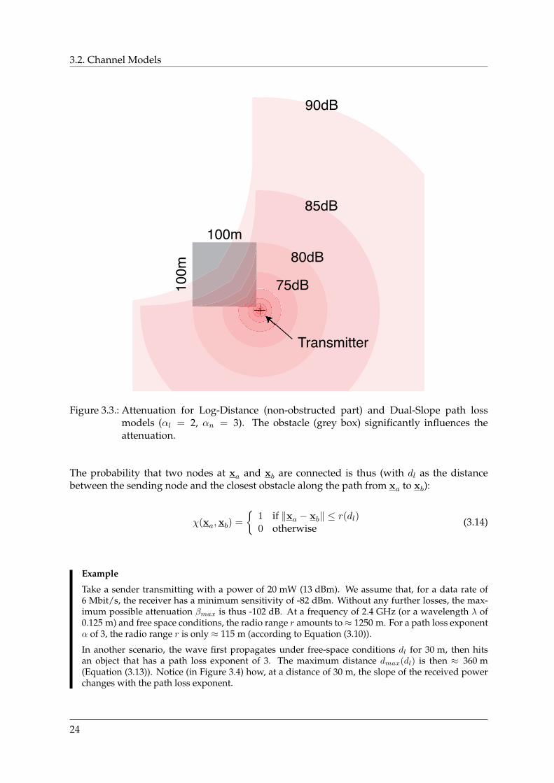
90dB
85dB
80dB75dB
100m
100m
Transmitter
Figure 3.3.: Attenuation for Log-Distance (non-obstructed part) and Dual-Slope path lossmodels (αl = 2, αn = 3). The obstacle (grey box) significantly influences theattenuation.
The probability that two nodes at xa and xb are connected is thus (with dl as the distancebetween the sending node and the closest obstacle along the path from xa to xb):
χ(xa,xb) =
1 if ‖xa − xb‖ ≤ r(dl)0 otherwise
(3.14)
Example
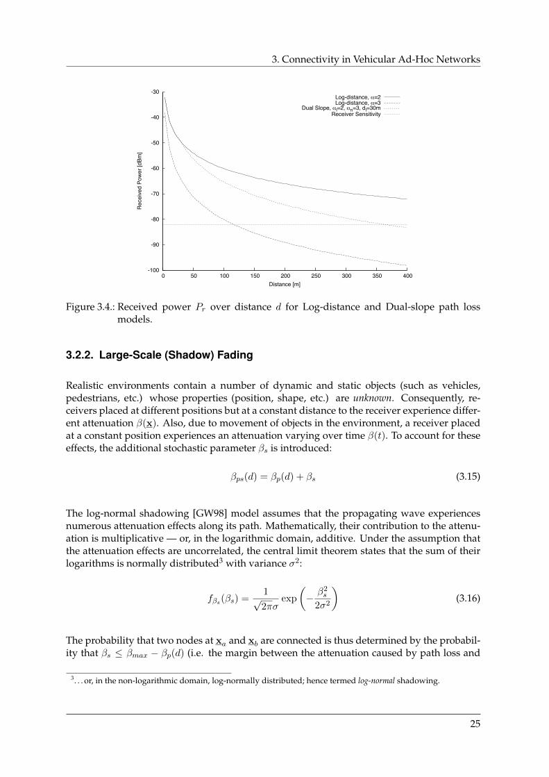
Take a sender transmitting with a power of 20 mW (13 dBm). We assume that, for a data rate of6 Mbit/s, the receiver has a minimum sensitivity of -82 dBm. Without any further losses, the max-imum possible attenuation βmax is thus -102 dB. At a frequency of 2.4 GHz (or a wavelength λ of0.125 m) and free space conditions, the radio range r amounts to≈ 1250 m. For a path loss exponentα of 3, the radio range r is only ≈ 115 m (according to Equation (3.10)).
In another scenario, the wave first propagates under free-space conditions dl for 30 m, then hitsan object that has a path loss exponent of 3. The maximum distance dmax(dl) is then ≈ 360 m(Equation (3.13)). Notice (in Figure 3.4) how, at a distance of 30 m, the slope of the received powerchanges with the path loss exponent.
24
3. Connectivity in Vehicular Ad-Hoc Networks
-100
-90
-80
-70
-60
-50
-40
-30
0 50 100 150 200 250 300 350 400
Rec
eive
d Po
wer
[dBm
]
Distance [m]
Log-distance, =2Log-distance, =3
Dual Slope, l=2, n=3, dl=30mReceiver Sensitivity
Figure 3.4.: Received power Pr over distance d for Log-distance and Dual-slope path lossmodels.
3.2.2. Large-Scale (Shadow) Fading
Realistic environments contain a number of dynamic and static objects (such as vehicles,pedestrians, etc.) whose properties (position, shape, etc.) are unknown. Consequently, re-ceivers placed at different positions but at a constant distance to the receiver experience differ-ent attenuation β(x). Also, due to movement of objects in the environment, a receiver placedat a constant position experiences an attenuation varying over time β(t). To account for theseeffects, the additional stochastic parameter βs is introduced:
βps(d) = βp(d) + βs (3.15)
The log-normal shadowing [GW98] model assumes that the propagating wave experiencesnumerous attenuation effects along its path. Mathematically, their contribution to the attenu-ation is multiplicative — or, in the logarithmic domain, additive. Under the assumption thatthe attenuation effects are uncorrelated, the central limit theorem states that the sum of theirlogarithms is normally distributed3 with variance σ2:
fβs(βs) =1√2πσ
exp
(− β2
s
2σ2
)(3.16)
The probability that two nodes at xa and xb are connected is thus determined by the probabil-ity that βs ≤ βmax − βp(d) (i.e. the margin between the attenuation caused by path loss and
3. . . or, in the non-logarithmic domain, log-normally distributed; hence termed log-normal shadowing.
25
3.2. Channel Models
the maximum possible attenuation)4:
χ(xa,xb) =
∫ βmax−βp(‖xa−xb‖
−∞fβs(βs)dβs (3.17)
=1
2+
1
2erf
(βmax − βp(‖xa − xb‖)√
2σ
)(3.18)
Note that at the border of the radio range r (βmax = βp(r)), the probability that βs ≤ 0 is0.5. As a consequence, the previously well-defined borderline of the radio range should —under shadow fading conditions — rather be regarded as a set of borderlines, with individualconnection probabilities.
Example
In the previous example, we have calculated a radio range r of 115 m for a path loss exponent of3. According to Equation (3.18), this is the border of the area in which the connection probability isat least 0.5. Assume that the standard deviation of the shadow fading process σ is 8 dB. We wishto determine the radius of the area in which the connection probability is greater than 0.95. Theshadow fading must then be:
βs ≤√
2σ · erf−1 (1− 2 ·χ(xa,xb)) (3.19)
i.e. βs ≤ -13.16 dB. The equivalent radio range r0.95 can thus be determined through Equation (3.10):
r0.95 = r(102 dB− 13.16 dB) ≈ 42 m (3.20)
3.2.3. Small-Scale (Multipath) Fading
Multipath propagation occurs if objects in the environment reflect, diffract or scatter the prop-agating wave. The distances covered by the individual propagation paths have differentlengths, therefore their phase at the receiver is not equal so that interference — and, as aconsequence, attenuation — occurs. The sum of the individual paths changes significantly ifthe receiver moves by very small distances (one-half the wavelength).
Due to the delays τ caused by the individual path lengths, inter-symbol interference may oc-cur. ISI’s frequency domain dual, the coherence bandwidth BC (as a function of the rms delayspread στ ) is defined as the bandwidth over which the frequency correlation (i.e., the band-width over which all spectral components have equal gain and linear phase) is above a certainthreshold. The channel is frequency-flat if the symbol duration Ts > στ and the transmission’sbandwidth BS < BC . Otherwise, the channel is called frequency-selective.
Moving terminals experience Doppler shift on the various propagation paths, depending ontheir direction of movement. The sum of the shifts results in a widening of the signals spec-trum, commonly denoted as Doppler spread BD. Its time domain dual, denoted as coherencetime TC , is a measure of the time period in which the channels fading intensity is almost con-stant. It is usually utilized to distinguish between slow and fast fading: if the symbol durationTS < Tc and the transmission’s bandwidth BS > BD, the fading is called slow. Otherwise, thefading is called fast.
4erf denotes the error function, defined as erf(x) = 2√π
∫ x0
e−t2
dt.
26
3. Connectivity in Vehicular Ad-Hoc Networks
Recent channel measurement campaigns in both the 2.4 GHz [ATI04] and 5 GHz [MFW02,MSXY05, PKC+07] ISM bands as well as in the dedicated 5.9 GHz [CHBS08a, CHC+08] DSRCband have revealed maximum Root Mean Square (RMS) delay spreads of less than 1 µs andmedium RMS delay spreads around 0.1 µs. These delay spreads correspond to propagationpath length deviations of 300 m and 30 m, respectively, and appear reasonable in vehicle-to-vehicle communication scenarios. Under the requirement that the frequency correlationis above 0.5, the resulting coherence bandwidth BC is between 200 kHz and 2 MHz. TheIEEE 802.11 standard’s OFDM PHY specification for 10 MHz channels, as used in the 802.11pvehicle-to-vehicle amendment, dictates sub-carriers bandwidths of 156.25 kHz, therefore thechannel can be considered frequency-flat for these radios.
The Doppler shift fm is determined from the relative velocity v between transmitter andreceiver and the wavelength used for the transmission. Considering PHY operation in the5.9 GHz DSRC band and vehicles moving with a relative velocity of v = 30 m/s, the dopplerspread BD is 590 Hz and the coherence time for a required frequency correlation of 0.5 isTC ≈ 1 ms. With a symbol duration of 8 µs, we can transmit up to ≈ 125 symbols — or 375 Bin the 3 Mbit/s data rate mode — under the condition that the channel fades slowly duringthe transmission.
Rice, Rayleigh and Gaussian Fading
The amplitude envelope x of a received frequency-flat fading signal in a multipath environ-ment is commonly modeled by the Ricean distribution5:
fX(x) =x
σ2exp
(−x
2 + ν2
2σ2
)I0
(xνσ2
)(3.21)
The local-mean of scattered power is denoted as σ2 and the dominant, non-fading compo-nent’s power is identified as 1
2ν2. The ratio of the dominant component’s power to scattered
power is called Rician K-Factor, K = ν2
2σ2 . The distribution of the attenuation βf can be derivedfrom the amplitude distribution as a non-central chi-square distribution with two degrees offreedom and non-centrality parameter ν2.
In a scenario with weak or non-existent LOS path (small or zero ν), the distribution becomesRayleigh [Rap96]. In case of a dominant, very strong LOS path, the distribution becomesGaussian [AS64, GW98].
Nakagami Fading
Unfortunately, usage of Equation (3.21) is mathematically cumbersome, especially due to thenecessary evaluation of the Bessel function. Due to good fit to empirical results, several au-thors have suggested to use the Nakagami m-distribution [Nak60] for modeling fading chan-nels [TJM+04, MSX06, CHS+07]. The amplitude envelope is parameterized by a shape param-eter m that represents the fading intensity (which is dependent on the environment and thedistance to the sender) and a spread parameter Ω (the average received power at a specific
5I0(x) denotes the Bessel function of the first kind with zeroth order, defined as I0(x) =∑∞m=0
1m!Γ(m+1)
(x2
)2m.
27
3.2. Channel Models
distance). Its distribution is given by6:
fX(x,m,Ω) =2mm
Γ(m)Ωmx2m−1 exp
(−m
Ωx2)
(3.22)
The Nakagami model is a generalization of the Rayleigh model and is equivalent to Equa-tion (3.21) (ν = 0) ifm = 1. Due to its analytical simplicity it is also widely used as an approxi-mation for Ricean fading channels. Although both fading models behave almost equivalentlynear their mean value, some authors argue that Nakagami’s practical utility appears question-able [Ste87] because it does not provide a good approximation in the near-zero region — i.e.a model’s deep fade behavior — which is crucial for the analysis of outage probabilities: theNakagami model yields excessively optimistic deep fade probabilities.
Influence on Connectivity
The actual influence of small-scale fading effects in vehicular networks is strongly depen-dent on the environment. In a highway scenarios with low vehicle density, we will mostlyfind LOS conditions between the transmitter and receiving nodes; a scenario in which thereceived signal’s LOS power can be expected to be much stronger than the scattered power(large Ricean K) thus rendering the influence of small-scale fading negligible. As the vehicledensity increases, the scattered power may become stronger due to reflections on other vehi-cles. Depending on the speed of movement of one or more nodes involved in a transmission,the attenuation of the signal due to small-scale fading changes very quickly. The intensity ofthe fluctuations may also be very strong, and fluctuation of several tens of dB are likely tobe seen. Two paths of equal power may even interfere complete destructive, giving a zeroamplitude at the receiver.
Fortunately, modern receivers can resort to advanced techniques that help mitigate these un-wanted effects: OFDM modulation uses several carriers that are spaced densely, yet suffi-ciently far apart to experience independent fading (frequency diversity). If only some carriersare impacted, only some of the bits in the received bitstream will be defective; using an ap-propriate channel coding scheme may help to correct the errors. Spatial diversity, i.e., severalantennas spaced at least half a wavelength apart, is widely employed: if the signal under-goes a deep fade at one antenna, it may still be strong enough at another. If the signals fromthe antennas are brought together effectively, for instance through Maximal Ratio Combin-ing [Kah54, Cox83], fading can be compensated for.
From a connectivity point-of-view, the influence of small-scale fading needs further discus-sion. While the positive effect of large-scale fading on connectivity has been demonstrated byseveral authors [BH05, Mio08], recent work [ZDJ08] has shown that while small-scale fadingreduces local connectivity, beneficial influences on global connectivity are revealed at the sametime.
In our opinion, connectivity reflects the ability to exchange messages between involved nodesfor a period of time longer than that of a potential drop-out due to small-scale fading, i.e., aperiod longer than the coherence time. In contrast to large-scale fading, which does directlydetermine connectivity, small-scale fading is rather a statistical factor that reflects the prob-ability that despite the fact that two nodes are actually connected, the link between them is
6Γ(x) denotes the Gamma function, defined as Γ(x) = (x− 1)!, x ∈ Z.
28
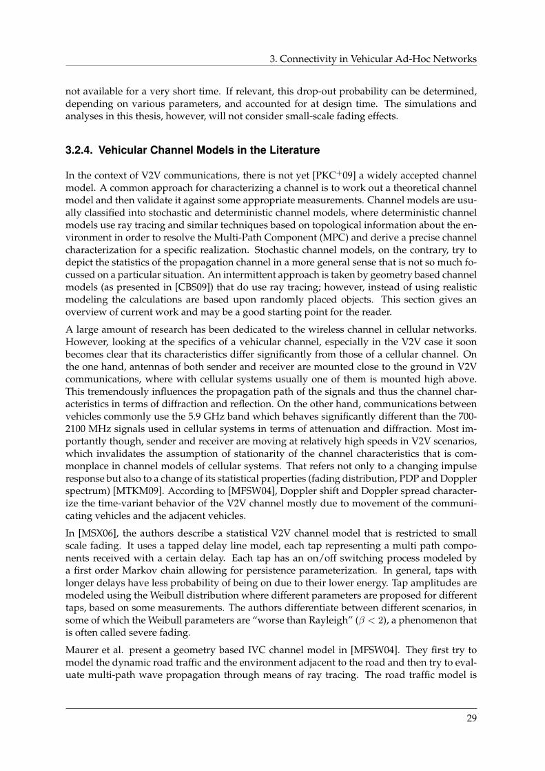
3. Connectivity in Vehicular Ad-Hoc Networks
not available for a very short time. If relevant, this drop-out probability can be determined,depending on various parameters, and accounted for at design time. The simulations andanalyses in this thesis, however, will not consider small-scale fading effects.
3.2.4. Vehicular Channel Models in the Literature
In the context of V2V communications, there is not yet [PKC+09] a widely accepted channelmodel. A common approach for characterizing a channel is to work out a theoretical channelmodel and then validate it against some appropriate measurements. Channel models are usu-ally classified into stochastic and deterministic channel models, where deterministic channelmodels use ray tracing and similar techniques based on topological information about the en-vironment in order to resolve the Multi-Path Component (MPC) and derive a precise channelcharacterization for a specific realization. Stochastic channel models, on the contrary, try todepict the statistics of the propagation channel in a more general sense that is not so much fo-cussed on a particular situation. An intermittent approach is taken by geometry based channelmodels (as presented in [CBS09]) that do use ray tracing; however, instead of using realisticmodeling the calculations are based upon randomly placed objects. This section gives anoverview of current work and may be a good starting point for the reader.
A large amount of research has been dedicated to the wireless channel in cellular networks.However, looking at the specifics of a vehicular channel, especially in the V2V case it soonbecomes clear that its characteristics differ significantly from those of a cellular channel. Onthe one hand, antennas of both sender and receiver are mounted close to the ground in V2Vcommunications, where with cellular systems usually one of them is mounted high above.This tremendously influences the propagation path of the signals and thus the channel char-acteristics in terms of diffraction and reflection. On the other hand, communications betweenvehicles commonly use the 5.9 GHz band which behaves significantly different than the 700-2100 MHz signals used in cellular systems in terms of attenuation and diffraction. Most im-portantly though, sender and receiver are moving at relatively high speeds in V2V scenarios,which invalidates the assumption of stationarity of the channel characteristics that is com-monplace in channel models of cellular systems. That refers not only to a changing impulseresponse but also to a change of its statistical properties (fading distribution, PDP and Dopplerspectrum) [MTKM09]. According to [MFSW04], Doppler shift and Doppler spread character-ize the time-variant behavior of the V2V channel mostly due to movement of the communi-cating vehicles and the adjacent vehicles.
In [MSX06], the authors describe a statistical V2V channel model that is restricted to smallscale fading. It uses a tapped delay line model, each tap representing a multi path compo-nents received with a certain delay. Each tap has an on/off switching process modeled bya first order Markov chain allowing for persistence parameterization. In general, taps withlonger delays have less probability of being on due to their lower energy. Tap amplitudes aremodeled using the Weibull distribution where different parameters are proposed for differenttaps, based on some measurements. The authors differentiate between different scenarios, insome of which the Weibull parameters are “worse than Rayleigh” (β < 2), a phenomenon thatis often called severe fading.
Maurer et al. present a geometry based IVC channel model in [MFSW04]. They first try tomodel the dynamic road traffic and the environment adjacent to the road and then try to eval-uate multi-path wave propagation through means of ray tracing. The road traffic model is
29
3.3. Spatial Node Distribution and Mobility Models
based on the so called Wiedemann model and uses results from the authors previous works.As it seems very difficult to obtain real data with the necessary level of detail and the cover-age, a stochastic model is utilized in order to place objects in the surroundings of the road.Different morphographic classes are defined for urban, suburban and highway scenarios thatare assigned specific probabilities for different types of objects (trees, buildings, cars, bridges,traffic signs, etc.). Multi-path components are represented by rays, each of which can experi-ence several propagation phenomena like diffraction or reflection. By calculating consecutivesnapshots, a time-series of channel impulse responses can be obtained that classifies the chan-nel for the current surrounding. The authors present measurements that validate the channelmodel with a standard deviation of less than 3 dB in both LOS and NLOS scenarios.
[PKC+09] presents some measurements of V2V propagation in suburban driving conditionsusing Global Positioning System (GPS) receivers. The authors on the one hand derive both asingle slope and a dual slope path loss model from their results where the better dual slopemodel achieves deviations between 2.6 and 5.6 dB compared to the measured path loss. How-ever, they find that received power is significantly less if no LOS propagation is possible.Fading on the other hand is modeled using a Nakagami distribution with variable parame-ters as already proposed in other works. While the distribution is Rician β > 2 as long as aLOS component is present, it turns out that fading can be “worse than Rayleigh” β < 2 oncethe LOS connection is lost intermittently at large distances between transmitter and receiver.Furthermore, the authors propose that the Doppler spread is dependent on the effective speedand the distance between transmitter and receiver. The dependance on distance is explainedby the increasing number of scatterers at larger distances. Using this dependence, the authorspresent the speed-separation diagram that can help predict the expected Doppler spread andthus small scale fading characteristics at a certain distance.
In [MTKM09], the authors provide a survey on V2V channel models and measurements basedon a variety of previous works on the subjects, some of which have already been discussedhere. We recommend this paper as an introductory reading on the subject as it introduces im-portant factors for channel characterization and includes a table that summarizes importantparameters gathered from multiple measurement campaigns. Important aspects like envi-ronment characterization and antenna placements are also discussed that we omit here. Oneimportant result from the evaluated measurements is that at least path loss coefficients in V2Vcommunication channels are rather similar to well-known cellular systems as long as a LOSconnection is given. In terms of small-scale fading and Doppler spread, the results go along-side those presented in [PKC+09]. The authors finally conclude that the amount of comparablemeasurements carried out on V2V channels is too insignificant in order to allow the formu-lation of a channel model that resembles the real-world V2V channel and important aspectssuch as antenna placement and shadowing by adjacent vehicles have not yet been sufficientlyexplored.
3.3. Spatial Node Distribution and Mobility Models
In the previous section, we have described how channel models relate the physical positions ofcommunicating nodes to their connectivity. If we wish to analyze the connectivity propertiesof a system of communicating nodes, we also need to model how the nodes are placed onthe playground and how their positions change over time. Generally, one can classify theseso-called mobility models in microscopic and macroscopic models.
30

3. Connectivity in Vehicular Ad-Hoc Networks
(xa,ya)
va(xb,yb)
vb
Figure 3.5.: Position x = (x, y)T and velocity v as descriptive states of two communicatingnodes a and b.
Microscopic models describe the state, i.e., position x, velocity v and possibly the accelerationa of mobile nodes (users, vehicles, etc., see Figure 3.5) as functions of time7 and/or previousstate(s) of the node (and possibly also of other nodes, if node interaction is accounted for):
(xn,vn,an) = f(n,xn−1,vn−1,an−1, . . .), n ∈ N (3.23)
A complete description encompasses not only f(. . .), but also a (presumably random) initialnode state (x0,v0,a0). Using a simulator, the spatial positions of moving nodes can then beevaluated for each time step.
Macroscopic models describe the node states through their stochastic properties, such as prob-ability distributions and related identifying properties. If stochastic properties of a networkrelated to mobility shall be studied, using macroscopic models is mathematically more con-venient. In some cases it is possible to directly deduce a macroscopic representation from amodel’s microscopic description, however the effort to do so analytically may be much greaterthan to simulate a model and then find a stochastic approximation of the simulation results.In the course of this chapter, we will use macroscopic models for the analytical derivation ofrelevant network parameters.
3.3.1. The Random Direction Model
The Random Direction (RD) mobility model has first been described in [Gue87] and thor-oughly studied in [Bet04]. Nodes are initially placed randomly and uniformly on the play-ground A. For M movement phases of negative-exponentially distributed duration tm, theassociated movement vector’s (vm) direction is chosen uniformly γ ∈ [0 . . . 2π], with a velocity
7in this context, discrete time n. Of course, time-continuous notation is also possible. The wide-spread use oftime-discrete simulators, however, spawns discrete notations.
31
3.3. Spatial Node Distribution and Mobility Models
v
(a)
v
(b)
Figure 3.6.: Border strategies for random direction mobility.
of v8. During a phase m, where∑m−1
i=0 ti < n ≤∑m
i=0 ti, the law of movement is:
xn = xn−1 + vm
If the playground A is bounded, the number of nodes on A decreases as time advances andnodes move out of the playground. Therefore, a border behavior needs to be carefully de-fined. To conserve a uniform node distribution, two schemes have proven adequate: Usingthe “wrap-around” approach (Figure 3.6(a)), nodes that hit the boundary of the playgroundare mirrored to the opposite boundary and continue their movement from the new position.The “bounce-back” solution (Figure 3.6(b)) horizontally and/or vertically mirrors the velocityvector of a respective node as that node hits the boundary. It can be shown that the resultingsteady state Probability Density Functions (PDFs) for node positions x and velocities v are:
fX0(x0) =
1|A| if x0 ∈ A0 otherwise
∀m : fVm(vm) =
1
2π if |vm| = v0 otherwise
The RD mobility model is a generalization of the Random Waypoint (RWP) model (first de-scribed in [JM96] and thoroughly studied in [BHPC02]): instead of randomly choosing a di-rection vector at the end of a movement phase, a new random waypoint on the playground ischosen and the velocity vector is adjusted accordingly so that the waypoint is reached withinin the next period of movement. Despite its popularity in ad-hoc networks research, RWP hasbeen shown to yield a spatial node distribution that concentrates nodes in the middle of theplayground. Even worse, it can be shown that — without further precautions — the averagenode velocity decreases over time.
3.3.2. Vehicular Mobility Models
The random direction model can be used to model the mobility of nodes that can move freelyon a two-dimensional playground, for instance on an (idealized) parking lot or in open-area
8Note that there are modified versions of the random direction model that choose v according to a distributionfunction. Also, some implementations support pause times during which the velocity v = 0.
32
3. Connectivity in Vehicular Ad-Hoc Networks
off-road scenarios. Usually, however, vehicles are bound to driving on one-dimensional roadsand to preventing collisions with obstacles, especially other cars. This chapter is devoted tothe macroscopic study of traffic flow properties. For a comprehensive survey of vehicularmobility models, we recommend [HFB09] for reading. Regarding microscopic models, cellu-lar automata have been studied in [Wol99] and the Intelligent Driver Model was introducedin [THH00]. A joint discussion of micro- and macroscopic simulation results can be foundin [HHST02].
Density, Velocity, and Flow
From a macroscopic point of view, the flow of traffic along the lanes of a street can be modeledas a flow of (interacting) particles along a one-dimensional structure. Let the density of vehicles(number of vehicles per lane unit) on a lane i at position x and time t be ρi(x, t). The sum ofthe individual lane densities on a road with I lanes is called the total density ρt(x, t), theirarithmetic average is denoted as the average density of vehicles ρ(x, t):
ρt(x, t) =∑i
ρi(x, t) = I · ρ(x, t) (3.24)
ρ(x, t) =1
I
∑i
ρi(x, t) =1
I· ρt(x, t) (3.25)
Let us assume that vehicles on a lane i travel with a certain velocity vi(x, t). Let us behold a lanesection of length ∆x that is long enough so that it comprises enough vehicles to deduce a goodmeasure of the density ρi(x, t), but short enough so that the vehicles’ density and velocity isapproximately constant over the segment’s length9. The number of vehicles contained in thissection is thus n = ∆x · ρi(x, t). Let all vehicles of the segment pass by an observer at a fixedposition beneath the lane within the time interval ∆t = ∆x/vi(x, t). The flow of vehiclesQi(x, t), i.e., the number of vehicles that the observer sees per time interval, is then
Qi(x, t) =n
∆t=
∆x · ρi(x, t)∆t
= ρi(x, t) · vi(x, t) (3.26)
This relation is often denoted as the flow-density relation. The sum of individual lane flows iscalled the total flow Qt(x, t), their arithmetic average gives the average flow Q(x, t):
Qt(x, t) =∑i
Qi(x, t) = I ·Q(x, t) (3.27)
Q(x, t) =1
I
∑i
Qi(x, t) =1
I·Qt(x, t) (3.28)
Finally, if we define the average velocity v(x, t) as the arithmetic average of the individual lanevelocities weighted with the relative densities:
v(x, t) =∑i
ρi(x, t)
ρt(x, t)· vi(x, t) (3.29)
we get the rule of hydrodynamic flow:
Q(x, t) = ρ(x, t) · v(x, t) (3.30)Qt(x, t) = ρt(x, t) · v(x, t) (3.31)
9Both constraints are usually met for ∆x = 100 m.
33
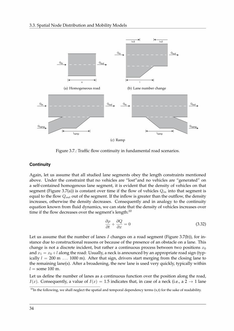
3.3. Spatial Node Distribution and Mobility Models
Qin Qout
x
(a) Homogeneous road
l
Qin Qout
I=2 I=3
(b) Lane number change
Qin
Qramp
Qout
lramp
Qin
Qramp
Qout
lramp
(c) Ramp
Figure 3.7.: Traffic flow continuity in fundamental road scenarios.
Continuity
Again, let us assume that all studied lane segments obey the length constraints mentionedabove. Under the constraint that no vehicles are “lost”and no vehicles are “generated” ona self-contained homogenous lane segment, it is evident that the density of vehicles on thatsegment (Figure 3.7(a)) is constant over time if the flow of vehicles Qin into that segment isequal to the flow Qout out of the segment. If the inflow is greater than the outflow, the densityincreases, otherwise the density decreases. Consequently and in analogy to the continuityequation known from fluid dynamics, we can state that the density of vehicles increases overtime if the flow decreases over the segment’s length:10
∂ρ
∂t+∂Q
∂x= 0 (3.32)
Let us assume that the number of lanes I changes on a road segment (Figure 3.7(b)), for in-stance due to constructional reasons or because of the presence of an obstacle on a lane. Thischange is not a discrete incident, but rather a continuous process between two positions x0
and x1 = x0 + l along the road: Usually, a neck is announced by an appropriate road sign (typ-ically l = 200 m . . . 1000 m). After that sign, drivers start merging from the closing lane tothe remaining lane(s). After a broadening, the new lane is used very quickly, typically withinl = some 100 m.
Let us define the number of lanes as a continuous function over the position along the road,I(x). Consequently, a value of I(x) = 1.5 indicates that, in case of a neck (i.e., a 2 → 1 lane
10In the following, we shall neglect the spatial and temporal dependency terms (x,t) for the sake of readability.
34

3. Connectivity in Vehicular Ad-Hoc Networks
transition), half of the vehicles have changed from the closing to the remaining lane at x. Incase of a broadening (i.e., a 1 → 2 lane transition), half of the vehicles have changed to thenew lane at x.
Equation (3.32) is valid both for the average as well as for the total density and flow numbers.With continuous I(x), we can rewrite Equation (3.32) for ρt(x, t) = I(x)ρ(x, t) (Equation (3.24))and Qt(x, t) = I(x)Q(x, t) (Equation (3.27)):
∂(I · ρ)
∂t+∂(I ·Q)
∂x= 0
I∂ρ
∂t+Q
∂I
∂t+ I
∂Q
∂t= 0
∂ρ
∂t+∂Q
∂x= −Q
I
∂I
∂x(3.33)
The right-hand side term in Equation (3.33) corresponds to a “source” term that representsthe flow either from the closing lane to the remaining lanes or from the lanes available as yetto the new lane, respectively. Consequently, if I(x) increases (broadening), the source term isnegative and the density decreases and vice versa.
Next, we examine locations where roads join and traffic flows merge or split (Figure 3.7(c)).Under the assumption that the inflow (Qramp > 0) respectively the outflow (Qramp < 0) is dis-tributed equally along the length of the ramp l, there is an additional flow gradient φramp(x, t)in the area of the ramp and Equation (3.32) becomes:
φramp(x, t) =
Qramp(t)I · l if x on ramp
0 otherwise
∂ρ
∂t+∂Q
∂x= φramp(x, t) (3.34)
Finally, putting Equations (3.32), (3.33), and (3.34) together and lettingQ = ρV (Equation (3.30)),we get:
∂ρ
∂t+∂Q
∂x= −Q
I
∂I
∂x+ φramp(x, t) (3.35)
∂ρ
∂t+∂ (ρv)
∂x= −ρv
I
∂I
∂x+ φramp(x, t) (3.36)
The Fundamental Diagram
Equations (3.35) and (3.36) are partial differential equations in two variables: the density ρand either flow Q or velocity v. To complete the formal description, an additional equa-tion is required that describes the relation between density and flow or velocity. This gapwas closed by Lighthill and Williams, and Richards, respectively, in their 1955/56 milestonepapers [LW55a, LW55b, Ric56] through complementing the continuity equation with the as-sumption that there is a certain — density-dependant — equilibrium velocity Ve (and resultingequilibrium flow Qe) that solve the continuity equation in case of a homogenous and station-ary traffic11:
Qe(ρ(x, t)) = ρ(x, t)Ve(ρ(x, t)) (3.37)11Homogenous and stationary traffic means that vehicles travel with the same velocity and distance. Obviously,
this is an idealization that can not be observed in reality.
35

3.3. Spatial Node Distribution and Mobility Models
0
500
1000
1500
2000
0 20 40 60 80 100 120 140 0
20
40
60
80
100
120
140Tr
affic
Flo
w [v
eh/h
/lane
]
Velo
city
[km
/h]
Traffic Density [veh/km/lane]
FreeFlow
Congestion
Traffic FlowVelocity
(a) Highway
0
500
1000
1500
2000
0 20 40 60 80 100 120 140 160 0
10
20
30
40
50
60
Traf
fic F
low
[veh
/h/la
ne]
Velo
city
[km
/h]
Traffic Density [veh/km/lane]
FreeFlow
Congestion
Traffic FlowVelocity
(b) City
Figure 3.8.: Fundamental diagrams of (a) highway and (b) city traffic flow.
36
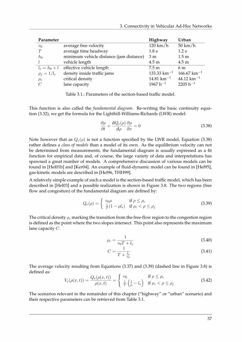
3. Connectivity in Vehicular Ad-Hoc Networks
Parameter Highway Urbanv0 average free velocity 120 km/h 50 km/hT average time headway 1.8 s 1.2 sh0 minimum vehicle distance (jam distance) 3 m 1.5 ml vehicle length 4.5 m 4.5 mle = h0 + l effective vehicle length 7.5 m 6 mρj = 1/le density inside traffic jams 133.33 km−1 166.67 km−1
ρc critical density 14.81 km−1 44.12 km−1
C lane capacity 1967 h−1 2205 h−1
Table 3.1.: Parameters of the section-based traffic model.
This function is also called the fundamental diagram. Re-writing the basic continuity equa-tion (3.32), we get the formula for the Lighthill-Williams-Richards (LWR) model:
∂ρ
∂t+
dQe(ρ)
dρ∂ρ
∂x= 0 (3.38)
Note however that as Qe(ρ) is not a function specified by the LWR model, Equation (3.38)rather defines a class of models than a model of its own. As the equilibrium velocity can notbe determined from measurements, the fundamental diagram is usually expressed as a fitfunction for empirical data and, of course, the large variety of data and interpretations hasspawned a great number of models. A comprehensive discussion of various models can befound in [Hel01b] and [Ker04]. An example of fluid-dynamic model can be found in [Hel95],gas-kinetic models are described in [Hel96, THH99].
A relatively simple example of such a model is the section-based traffic model, which has beendescribed in [Hel03] and a possible realization is shown in Figure 3.8. The two regions (freeflow and congestion) of the fundamental diagram are defined by:
Qe(ρ) =
v0ρ if ρ ≤ ρc1T (1− ρle) if ρc < ρ ≤ ρj
(3.39)
The critical density ρc marking the transition from the free-flow region to the congestion regionis defined as the point where the two slopes intersect. This point also represents the maximumlane capacity C.
ρc =1
v0T + le(3.40)
C =1
T + lev0
(3.41)
The average velocity resulting from Equations (3.37) and (3.39) (dashed line in Figure 3.8) isdefined as:
Ve(ρ(x, t)) =Qe(ρ(x, t))
ρ(x, t)=
v0 if ρ ≤ ρc1T
(1ρ − le
)if ρc < ρ ≤ ρj
(3.42)
The scenarios relevant in the remainder of this chapter (“highway” or “urban” scenario) andtheir respective parameters can be retrieved from Table 3.1.
37
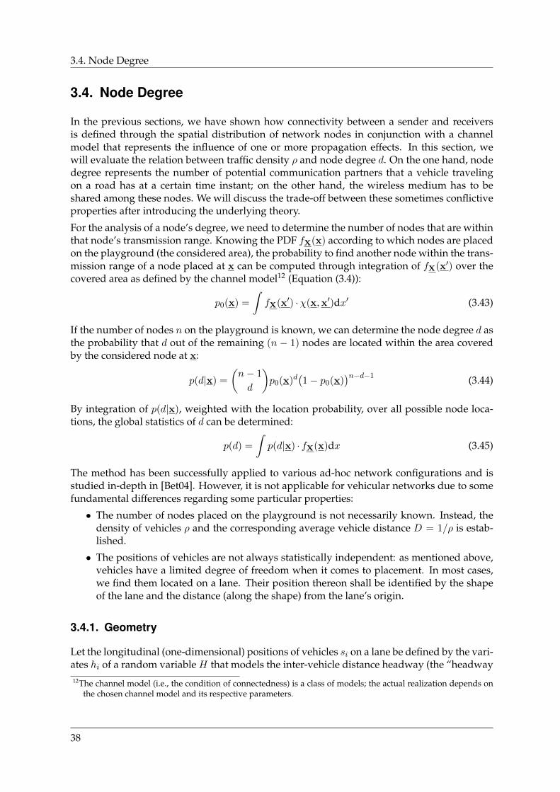
3.4. Node Degree
3.4. Node Degree
In the previous sections, we have shown how connectivity between a sender and receiversis defined through the spatial distribution of network nodes in conjunction with a channelmodel that represents the influence of one or more propagation effects. In this section, wewill evaluate the relation between traffic density ρ and node degree d. On the one hand, nodedegree represents the number of potential communication partners that a vehicle travelingon a road has at a certain time instant; on the other hand, the wireless medium has to beshared among these nodes. We will discuss the trade-off between these sometimes conflictiveproperties after introducing the underlying theory.
For the analysis of a node’s degree, we need to determine the number of nodes that are withinthat node’s transmission range. Knowing the PDF fX(x) according to which nodes are placedon the playground (the considered area), the probability to find another node within the trans-mission range of a node placed at x can be computed through integration of fX(x′) over thecovered area as defined by the channel model12 (Equation (3.4)):
p0(x) =
∫fX(x′) ·χ(x,x′)dx′ (3.43)
If the number of nodes n on the playground is known, we can determine the node degree d asthe probability that d out of the remaining (n − 1) nodes are located within the area coveredby the considered node at x:
p(d|x) =
(n− 1
d
)p0(x)d
(1− p0(x)
)n−d−1 (3.44)
By integration of p(d|x), weighted with the location probability, over all possible node loca-tions, the global statistics of d can be determined:
p(d) =
∫p(d|x) · fX(x)dx (3.45)
The method has been successfully applied to various ad-hoc network configurations and isstudied in-depth in [Bet04]. However, it is not applicable for vehicular networks due to somefundamental differences regarding some particular properties:
• The number of nodes placed on the playground is not necessarily known. Instead, thedensity of vehicles ρ and the corresponding average vehicle distance D = 1/ρ is estab-lished.
• The positions of vehicles are not always statistically independent: as mentioned above,vehicles have a limited degree of freedom when it comes to placement. In most cases,we find them located on a lane. Their position thereon shall be identified by the shapeof the lane and the distance (along the shape) from the lane’s origin.
3.4.1. Geometry
Let the longitudinal (one-dimensional) positions of vehicles si on a lane be defined by the vari-ates hi of a random variable H that models the inter-vehicle distance headway (the “headway12The channel model (i.e., the condition of connectedness) is a class of models; the actual realization depends on
the chosen channel model and its respective parameters.
38
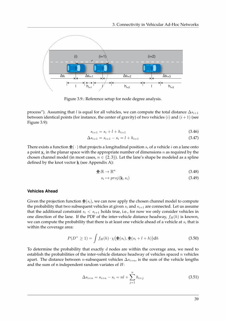
3. Connectivity in Vehicular Ad-Hoc Networks
r
!si+1 !si+2!si !si+3
hi+1 l hi+2 ll hi+3
(i) (i+1) (i+2)
Figure 3.9.: Reference setup for node degree analysis.
process”). Assuming that l is equal for all vehicles, we can compute the total distance ∆si+1
between identical points (for instance, the center of gravity) of two vehicles (i) and (i+ 1) (seeFigure 3.9):
si+1 = si + l + hi+1 (3.46)∆si+1 = si+1 − si = l + hi+1 (3.47)
There exists a function Φ( · ) that projects a longitudinal position si of a vehicle i on a lane ontoa point xi in the planar space with the appropriate number of dimensions n as required by thechosen channel model (in most cases, n ∈ 2, 3). Let the lane’s shape be modeled as a splinedefined by the knot vector k (see Appendix A):
Φ:R→ Rn (3.48)si 7→ proj(k, si) (3.49)
Vehicles Ahead
Given the projection function Φ(si), we can now apply the chosen channel model to computethe probability that two subsequent vehicles at given si and si+1 are connected. Let us assumethat the additional constraint si < si+1 holds true, i.e., for now we only consider vehicles inone direction of the lane. If the PDF of the inter-vehicle distance headway, fH(h) is known,we can compute the probability that there is at least one vehicle ahead of a vehicle at si that iswithin the coverage area:
P (D+ ≥ 1) =
∫fH(h) ·χ
(Φ(si),Φ(si + l + h)
)dh (3.50)
To determine the probability that exactly d nodes are within the coverage area, we need toestablish the probabilities of the inter-vehicle distance headway of vehicles spaced n vehiclesapart. The distance between n-subsequent vehicles ∆si+n, is the sum of the vehicle lengthsand the sum of n independent random variates of H :
∆si+n = si+n − si = nl +n∑j=1
hi+j (3.51)
39
3.4. Node Degree
The PDF resulting from the addition of random variables is the convolution13 of the individ-ual PDFs. In this case, the PDF of the inter-vehicle distance headway between n-subsequentvehicles corresponds to the recursive convolution of fH(h):
f(1)H (h) = fH(h) (3.52)
f(n)H (h) = f
(n−1)H (h) ∗ fH(h) (3.53)
Combining the Equations (3.53) and (3.50), we can determine the probability that there are atleast d, d ∈ N vehicles ahead of a vehicle at si that are within the coverage area:
P (D+ ≥ d) =
∫f
(d)H (h) ·χ
(Φ(si),Φ(si + dl + h)
)dh (3.54)
Consequently, the Probability Mass Function (PMF) of the degree distribution fD+(d), itsCumulated Density Function (CDF) FD+(d) and the expected node degree ED+ are then
fD+ [d] = P (D+ = d) = P (D+ ≥ d)− P (D+ > d)
= P (D+ ≥ d)− P (D+ ≥ d+ 1) (3.55)FD+ [d] = P (D+ ≤ d) = 1− P (D+ > d)
= 1− P (D+ ≥ d+ 1) (3.56)
ED+ =
∞∑d=0
d · fD+ [d] (3.57)
Multiple Lanes
In the derivation above, we have considered only subsequent vehicles ahead of a vehicle i:si < si+1 and retrieved the PMF of the random process D+. The degree distribution regardingvehicles in the behind directionD− is computed likewise. The individual degree distributionsare independent; to retrieve the total degree distribution, the discrete convolution14 of the two(ahead and behind) distributions needs to be calculated:
D = D− +D+ (3.58)
fD[d] =d∑i=0
fD+ [i] · fD− [d− i] (3.59)
The expected node degree ED is then the sum of the two individual expected node degrees:
ED = ED++ ED− (3.60)
If more than one lane shall be studied, under the assumption that the distance between adja-cent parallel lanes is small compared to the radius of the coverage area, determination of thecomposite expected node degree can be simplified by adding up the individual expected nodedegrees. For other geometries, the effective range sr must be used instead of the 2r term (seenext section).13The continuous convolution is defined as (f ∗ g)(t) =
∫∞−∞ f(τ)g(t− τ)dτ .
14The discrete convolution is defined as (f ∗ g)[n] =∑∞m=−∞ f [m]g[n − m]. Because fD[d] is only defined for
d ∈ N0+, summation borders are i = 0 . . . d.
40
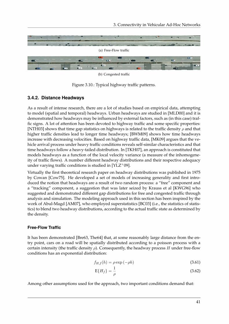
3. Connectivity in Vehicular Ad-Hoc Networks
(a) Free-Flow traffic
(b) Congested traffic
Figure 3.10.: Typical highway traffic patterns.
3.4.2. Distance Headways
As a result of intense research, there are a lot of studies based on empirical data, attemptingto model (spatial and temporal) headways. Urban headways are studied in [MLD00] and it isdemonstrated how headways may be influenced by external factors, such as (in this case) traf-fic signs. A lot of attention has been devoted to highway traffic and some specific properties:[NTH03] shows that time gap statistics on highways is related to the traffic density ρ and thathigher traffic densities lead to longer time headways; [BWM09] shows how time headwaysincrease with decreasing velocities. Based on highway traffic data, [MK09] argues that the ve-hicle arrival process under heavy traffic conditions reveals self-similar characteristics and thattime headways follow a heavy-tailed distribution. In [TKH07], an approach is constituted thatmodels headways as a function of the local velocity variance (a measure of the inhomogene-ity of traffic flows). A number different headway distributions and their respective adequacyunder varying traffic conditions is studied in [YLZ+09].
Virtually the first theoretical research paper on headway distributions was published in 1975by Cowan [Cow75]. He developed a set of models of increasing generality and first intro-duced the notion that headways are a result of two random process: a “free” component anda “tracking” component, a suggestion that was later seized by Krauss et al [KWG96] whosuggested and demonstrated different gap distributions for free and congested traffic throughanalysis and simulation. The modeling approach used in this section has been inspired by thework of Abul-Magd [AM07], who employed superstatistics [BC03] (i.e., the statistics of statis-tics) to blend two headway distributions, according to the actual traffic state as determined bythe density.
Free-Flow Traffic
It has been demonstrated [Bre63, The64] that, at some reasonably large distance from the en-try point, cars on a road will be spatially distributed according to a poisson process with acertain intensity (the traffic density ρ). Consequently, the headway process H under free-flowconditions has an exponential distribution:
fH,f (h) = ρ exp (−ρh) (3.61)
EHf =1
ρ(3.62)
Among other assumptions used for the approach, two important conditions demand that:
41
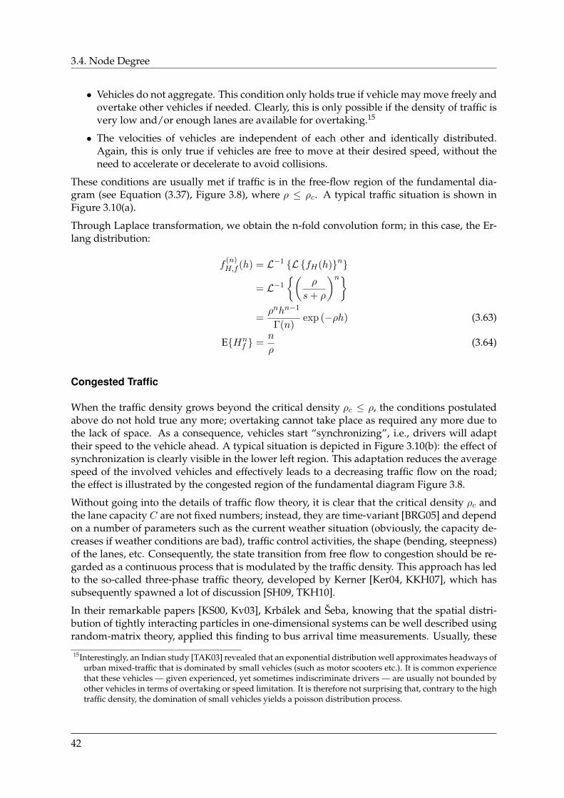
3.4. Node Degree
• Vehicles do not aggregate. This condition only holds true if vehicle may move freely andovertake other vehicles if needed. Clearly, this is only possible if the density of traffic isvery low and/or enough lanes are available for overtaking.15
• The velocities of vehicles are independent of each other and identically distributed.Again, this is only true if vehicles are free to move at their desired speed, without theneed to accelerate or decelerate to avoid collisions.
These conditions are usually met if traffic is in the free-flow region of the fundamental dia-gram (see Equation (3.37), Figure 3.8), where ρ ≤ ρc. A typical traffic situation is shown inFigure 3.10(a).
Through Laplace transformation, we obtain the n-fold convolution form; in this case, the Er-lang distribution:
f(n)H,f (h) = L−1 L fH(h)n
= L−1
(ρ
s+ ρ
)n=ρnhn−1
Γ(n)exp (−ρh) (3.63)
EHnf =
n
ρ(3.64)
Congested Traffic
When the traffic density grows beyond the critical density ρc ≤ ρ, the conditions postulatedabove do not hold true any more; overtaking cannot take place as required any more due tothe lack of space. As a consequence, vehicles start “synchronizing”, i.e., drivers will adapttheir speed to the vehicle ahead. A typical situation is depicted in Figure 3.10(b): the effect ofsynchronization is clearly visible in the lower left region. This adaptation reduces the averagespeed of the involved vehicles and effectively leads to a decreasing traffic flow on the road;the effect is illustrated by the congested region of the fundamental diagram Figure 3.8.
Without going into the details of traffic flow theory, it is clear that the critical density ρc andthe lane capacity C are not fixed numbers; instead, they are time-variant [BRG05] and dependon a number of parameters such as the current weather situation (obviously, the capacity de-creases if weather conditions are bad), traffic control activities, the shape (bending, steepness)of the lanes, etc. Consequently, the state transition from free flow to congestion should be re-garded as a continuous process that is modulated by the traffic density. This approach has ledto the so-called three-phase traffic theory, developed by Kerner [Ker04, KKH07], which hassubsequently spawned a lot of discussion [SH09, TKH10].
In their remarkable papers [KS00, Kv03], Krbálek and Šeba, knowing that the spatial distri-bution of tightly interacting particles in one-dimensional systems can be well described usingrandom-matrix theory, applied this finding to bus arrival time measurements. Usually, these
15Interestingly, an Indian study [TAK03] revealed that an exponential distribution well approximates headways ofurban mixed-traffic that is dominated by small vehicles (such as motor scooters etc.). It is common experiencethat these vehicles — given experienced, yet sometimes indiscriminate drivers — are usually not bounded byother vehicles in terms of overtaking or speed limitation. It is therefore not surprising that, contrary to the hightraffic density, the domination of small vehicles yields a poisson distribution process.
42
3. Connectivity in Vehicular Ad-Hoc Networks
times can be modeled as a poisson process; the data used in their case studies, however, wasobtained in a special context: due to certain influences, bus drivers were forced to optimizethe inter-arrival times of their buses:
• Autonomously: the drivers know only the temporal distance to the previous bus. Theirmeans of adjustment are acceleration or deceleration.
• As long a time gap as possible: The random arrival process of passengers at the bus stop(which, technically, controls the systems) leads to a growing number of passengers. Inorder to maximize the income, the bus driver will slow down as much as possible andthus increase the time gap to the preceding bus to take as many passengers as possible.
• As short a time gap as necessary: If the driver slows down too much, he expects to beovertaken by the following bus.
This constitutes a self-organizing system that autonomously adapts the inter-arrival times ofthe buses to the current demand (the arrival rate of passengers). The resulting inter-vehicledistribution is well modeled using the Gaussian Unitary Ensemble (GUE) of random-matrixtheory. The conceptual parallels to dense traffic are obvious: a driver sees the distance to thevehicle he is following, and he will try to adjust that distance to a safe value (as long as pos-sible) while trying to keep up with the preceding vehicle (as short as necessary). Subsequentwork has shown that GUE is well suited for modeling inter-vehicle headways in dense traffic(see [AM07] for a summary):
fH,c(h) =32ρ3
π2h2 exp
(−4ρ2
πh2
)(3.65)
EHc =1
ρ(3.66)
Following the concept of headway components [KWG96], [AM07] argues that using a pois-sonian process for the free-flow region and the GUE process for the congested region andblending the resulting PDFs using a density-dependent parameter α very well fits the head-way processes actually measured on roads. Consequently, we shall regard the actual headwayprocess on an arbitrary road as the weighted combination of the two processes introduced inthis section:
fH(h) = αfH,f (h) + (1− α)fH,c(h) (3.67)
The determination of the parameter α is not straightforward as it depends on the actual trafficsituation and external parameters (as mentioned above) and thus subject to fitting to actualmeasured data. It is therefore not possible to directly study the headway distribution in thetransition phase. However, studying the two cases α = 0, 1 allows us to identify two condi-tions that represent the two extreme network realizations: The realization of an actual networkwill be somewhere in between.
3.4.3. Discussion
For the sake of simplicity, let us first model the considered road segment as a straight hori-zontal line so that Φ(t) = [t, 0]T (an idealized highway segment). As channel model, we use
43
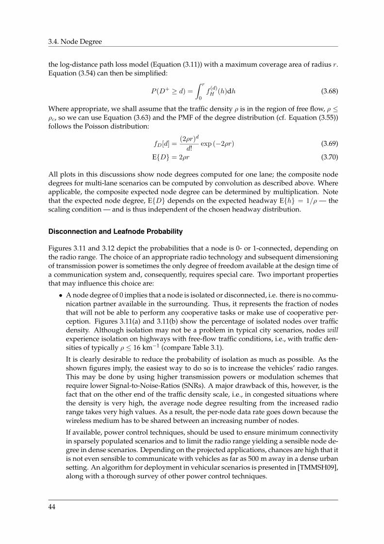
3.4. Node Degree
the log-distance path loss model (Equation (3.11)) with a maximum coverage area of radius r.Equation (3.54) can then be simplified:
P (D+ ≥ d) =
∫ r
0f
(d)H (h)dh (3.68)
Where appropriate, we shall assume that the traffic density ρ is in the region of free flow, ρ ≤ρc, so we can use Equation (3.63) and the PMF of the degree distribution (cf. Equation (3.55))follows the Poisson distribution:
fD[d] =(2ρr)d
d!exp (−2ρr) (3.69)
ED = 2ρr (3.70)
All plots in this discussions show node degrees computed for one lane; the composite nodedegrees for multi-lane scenarios can be computed by convolution as described above. Whereapplicable, the composite expected node degree can be determined by multiplication. Notethat the expected node degree, ED depends on the expected headway Eh = 1/ρ — thescaling condition — and is thus independent of the chosen headway distribution.
Disconnection and Leafnode Probability
Figures 3.11 and 3.12 depict the probabilities that a node is 0- or 1-connected, depending onthe radio range. The choice of an appropriate radio technology and subsequent dimensioningof transmission power is sometimes the only degree of freedom available at the design time ofa communication system and, consequently, requires special care. Two important propertiesthat may influence this choice are:
• A node degree of 0 implies that a node is isolated or disconnected, i.e. there is no commu-nication partner available in the surrounding. Thus, it represents the fraction of nodesthat will not be able to perform any cooperative tasks or make use of cooperative per-ception. Figures 3.11(a) and 3.11(b) show the percentage of isolated nodes over trafficdensity. Although isolation may not be a problem in typical city scenarios, nodes willexperience isolation on highways with free-flow traffic conditions, i.e., with traffic den-sities of typically ρ ≤ 16 km−1 (compare Table 3.1).
It is clearly desirable to reduce the probability of isolation as much as possible. As theshown figures imply, the easiest way to do so is to increase the vehicles’ radio ranges.This may be done by using higher transmission powers or modulation schemes thatrequire lower Signal-to-Noise-Ratios (SNRs). A major drawback of this, however, is thefact that on the other end of the traffic density scale, i.e., in congested situations wherethe density is very high, the average node degree resulting from the increased radiorange takes very high values. As a result, the per-node data rate goes down because thewireless medium has to be shared between an increasing number of nodes.
If available, power control techniques, should be used to ensure minimum connectivityin sparsely populated scenarios and to limit the radio range yielding a sensible node de-gree in dense scenarios. Depending on the projected applications, chances are high that itis not even sensible to communicate with vehicles as far as 500 m away in a dense urbansetting. An algorithm for deployment in vehicular scenarios is presented in [TMMSH09],along with a thorough survey of other power control techniques.
44

3. Connectivity in Vehicular Ad-Hoc Networks
0
0.1
0.2
0.3
0.4
0.5
0.6
0.7
0.8
0.9
1
0 10 20 30 40 50
Dis
conn
ectio
n Pr
obab
ility
Traffic Density [veh/km]
50m range free (sim)50m range free (an)
100m range free (sim)100m range free (an)
200m range free (sim)200m range free (an)
500m range free (sim)500m range free (an)
(a) Disconnection probabilities in free-flow traffic
0
0.1
0.2
0.3
0.4
0.5
0.6
0.7
0.8
0.9
1
0 10 20 30 40 50
Dis
conn
ectio
n Pr
obab
ility
Traffic Density [veh/km]
50m range congested (sim)50m range congested (an)
100m range congested (sim)100m range congested (an)
(b) Disconnection probabilities in congested traffic
Figure 3.11.: Disconnection probabilities over traffic density.
45
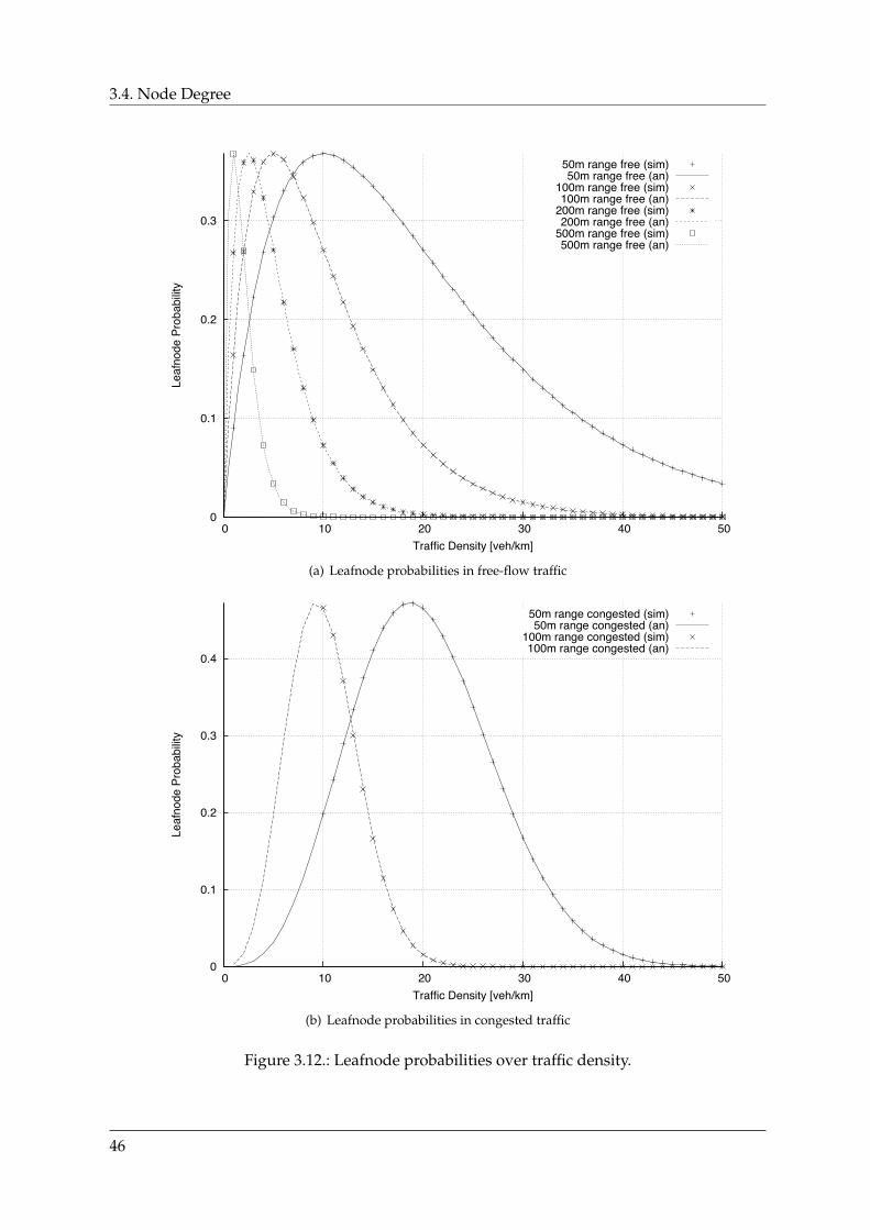
3.4. Node Degree
0
0.1
0.2
0.3
0 10 20 30 40 50
Leaf
node
Pro
babi
lity
Traffic Density [veh/km]
50m range free (sim)50m range free (an)
100m range free (sim)100m range free (an)
200m range free (sim)200m range free (an)
500m range free (sim)500m range free (an)
(a) Leafnode probabilities in free-flow traffic
0
0.1
0.2
0.3
0.4
0 10 20 30 40 50
Leaf
node
Pro
babi
lity
Traffic Density [veh/km]
50m range congested (sim)50m range congested (an)
100m range congested (sim)100m range congested (an)
(b) Leafnode probabilities in congested traffic
Figure 3.12.: Leafnode probabilities over traffic density.
46
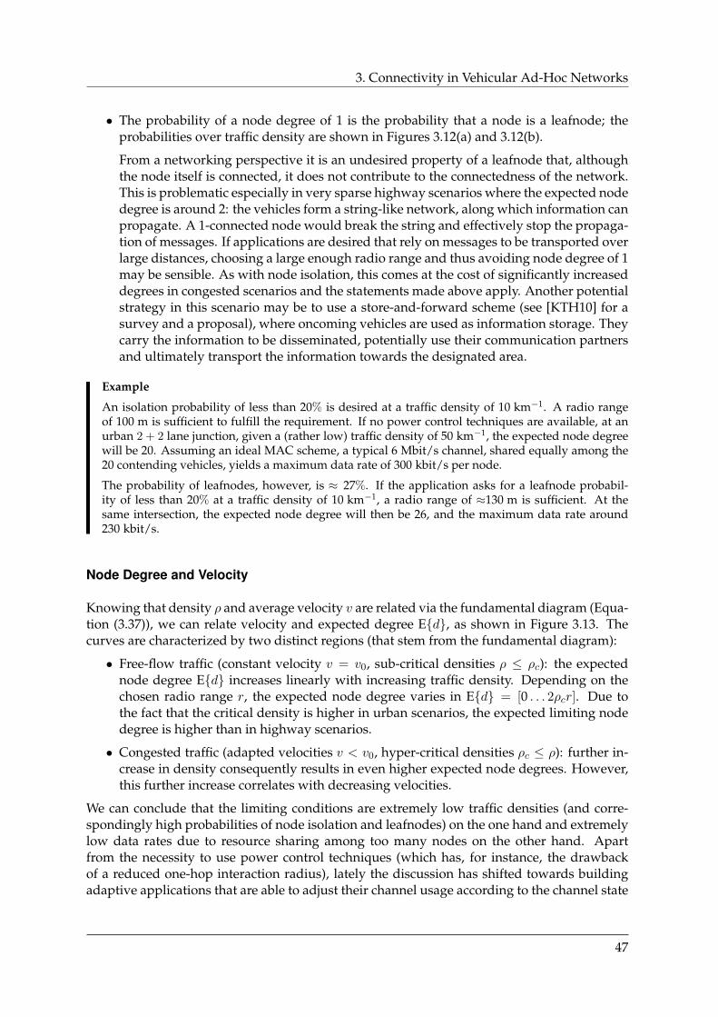
3. Connectivity in Vehicular Ad-Hoc Networks
• The probability of a node degree of 1 is the probability that a node is a leafnode; theprobabilities over traffic density are shown in Figures 3.12(a) and 3.12(b).
From a networking perspective it is an undesired property of a leafnode that, althoughthe node itself is connected, it does not contribute to the connectedness of the network.This is problematic especially in very sparse highway scenarios where the expected nodedegree is around 2: the vehicles form a string-like network, along which information canpropagate. A 1-connected node would break the string and effectively stop the propaga-tion of messages. If applications are desired that rely on messages to be transported overlarge distances, choosing a large enough radio range and thus avoiding node degree of 1may be sensible. As with node isolation, this comes at the cost of significantly increaseddegrees in congested scenarios and the statements made above apply. Another potentialstrategy in this scenario may be to use a store-and-forward scheme (see [KTH10] for asurvey and a proposal), where oncoming vehicles are used as information storage. Theycarry the information to be disseminated, potentially use their communication partnersand ultimately transport the information towards the designated area.
Example
An isolation probability of less than 20% is desired at a traffic density of 10 km−1. A radio rangeof 100 m is sufficient to fulfill the requirement. If no power control techniques are available, at anurban 2 + 2 lane junction, given a (rather low) traffic density of 50 km−1, the expected node degreewill be 20. Assuming an ideal MAC scheme, a typical 6 Mbit/s channel, shared equally among the20 contending vehicles, yields a maximum data rate of 300 kbit/s per node.
The probability of leafnodes, however, is ≈ 27%. If the application asks for a leafnode probabil-ity of less than 20% at a traffic density of 10 km−1, a radio range of ≈130 m is sufficient. At thesame intersection, the expected node degree will then be 26, and the maximum data rate around230 kbit/s.
Node Degree and Velocity
Knowing that density ρ and average velocity v are related via the fundamental diagram (Equa-tion (3.37)), we can relate velocity and expected degree Ed, as shown in Figure 3.13. Thecurves are characterized by two distinct regions (that stem from the fundamental diagram):
• Free-flow traffic (constant velocity v = v0, sub-critical densities ρ ≤ ρc): the expectednode degree Ed increases linearly with increasing traffic density. Depending on thechosen radio range r, the expected node degree varies in Ed = [0 . . . 2ρcr]. Due tothe fact that the critical density is higher in urban scenarios, the expected limiting nodedegree is higher than in highway scenarios.
• Congested traffic (adapted velocities v < v0, hyper-critical densities ρc ≤ ρ): further in-crease in density consequently results in even higher expected node degrees. However,this further increase correlates with decreasing velocities.
We can conclude that the limiting conditions are extremely low traffic densities (and corre-spondingly high probabilities of node isolation and leafnodes) on the one hand and extremelylow data rates due to resource sharing among too many nodes on the other hand. Apartfrom the necessity to use power control techniques (which has, for instance, the drawbackof a reduced one-hop interaction radius), lately the discussion has shifted towards buildingadaptive applications that are able to adjust their channel usage according to the channel state
47
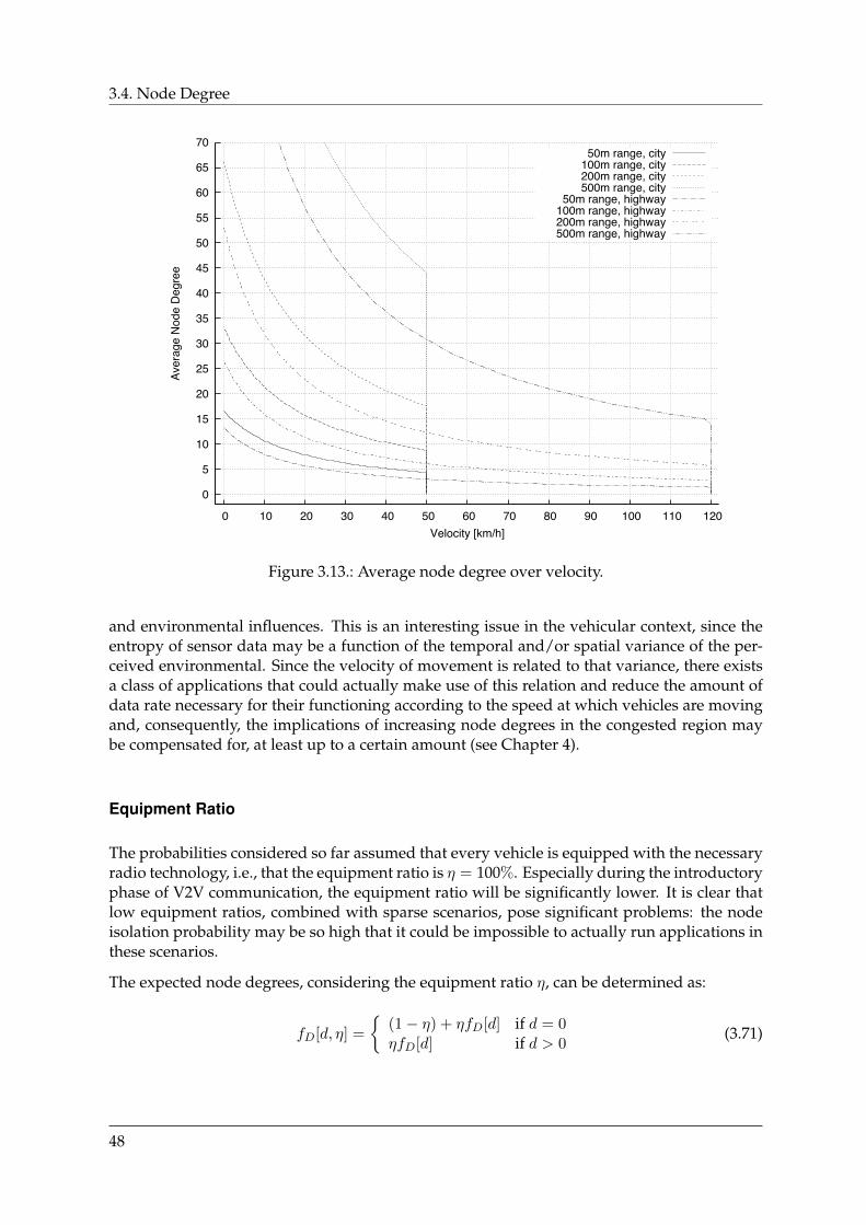
3.4. Node Degree
0
5
10
15
20
25
30
35
40
45
50
55
60
65
70
0 10 20 30 40 50 60 70 80 90 100 110 120
Aver
age
Nod
e D
egre
e
Velocity [km/h]
50m range, city100m range, city200m range, city500m range, city
50m range, highway100m range, highway200m range, highway500m range, highway
Figure 3.13.: Average node degree over velocity.
and environmental influences. This is an interesting issue in the vehicular context, since theentropy of sensor data may be a function of the temporal and/or spatial variance of the per-ceived environmental. Since the velocity of movement is related to that variance, there existsa class of applications that could actually make use of this relation and reduce the amount ofdata rate necessary for their functioning according to the speed at which vehicles are movingand, consequently, the implications of increasing node degrees in the congested region maybe compensated for, at least up to a certain amount (see Chapter 4).
Equipment Ratio
The probabilities considered so far assumed that every vehicle is equipped with the necessaryradio technology, i.e., that the equipment ratio is η = 100%. Especially during the introductoryphase of V2V communication, the equipment ratio will be significantly lower. It is clear thatlow equipment ratios, combined with sparse scenarios, pose significant problems: the nodeisolation probability may be so high that it could be impossible to actually run applications inthese scenarios.
The expected node degrees, considering the equipment ratio η, can be determined as:
fD[d, η] =
(1− η) + ηfD[d] if d = 0ηfD[d] if d > 0
(3.71)
48
3. Connectivity in Vehicular Ad-Hoc Networks
0
0.1
0.2
0.3
0.4
0.5
0.6
0.7
0.8
0.9
1
0 10 20 30 40 50 60 70 80 90 100
Cum
ulat
ed P
roba
bilit
y
Distance [m]
Free-flowCongested
Figure 3.14.: CDFs of free-flow and congested traffic headway distributions for a traffic densityof ρ = 40 km−1.
Regulatory directives allow transmission powers of up to 2 W on dedicated DSRC channels which,under perfect conditions, allows a maximum radio range of approximately 2.3 km at a data rate of6 Mbit/s. Because for densities ρ ≥ 2 km−1
fD[0] = exp (−2ρr) ≈ 0 (3.72)
the isolation probability of a node is then
fD[0, η] ≈ 1− η (3.73)
Node Degree Dispersion
Figure 3.15 shows the probability distributions for both free-flow and congested traffic situa-tions over the range of traffic densities that a vehicle can be expected to actually experiencein real-life traffic. It is remarkable that the range in which the degree varies (the degree dis-persion) is extremely wide in free-flow traffic, especially when compared to the dispersion inthe case of congested traffic condition. Although the average node degree is equal for bothtraffic conditions (see above), the distribution of node degree under free-flow conditions arebe characterized by:
• Increased spatial degree inhomogeneity, causing some nodes in the network to experi-ence significantly higher degrees than other (possibly neighboring) nodes. Due to rea-sons that we will study in the next chapter, this effectively reduces the globally available
49
3.4. Node Degree
0 10 20 30 40 50Node Degree
0
20
40
60
80
100
120
140
160Tr
affic
Den
sity
[veh
/km
]
0
0.05
0.1
0.15
0.2
0.25
0.3
Prob
abilit
y
(a) Free-flow traffic
0 10 20 30 40 50Node Degree
0
20
40
60
80
100
120
140
160
Traf
fic D
ensi
ty [v
eh/k
m]
0
0.05
0.1
0.15
0.2
0.25
0.3
Prob
abilit
y
(b) Congested traffic
Figure 3.15.: Dispersion of node degree probabilities over traffic density for (a) freeflow and(b) congested traffic. Radio range is r = 100 m.
50
3. Connectivity in Vehicular Ad-Hoc Networks
data rate for applications and, consequently, the experienced QoS. For the same reasons,fairness among nodes regarding the assignment of resources is reduced.
• Increased temporal degree inhomogeneity, necessitating a strong and fast adaptation tointense degree variations over time. The range in which the degree varies over time andthe rapidity of these swings correlates with the effort necessary to maintain an updatedview on the networks topology.
The reason for the higher degree dispersion of free-flow traffic is the higher variance of theunderlying free-flow headway distribution, when compared to the congested traffic’s distri-bution (which is also clearly visible in Figure 3.14):
VarHf =1
ρ2> VarHc =
1
ρ2
(3π
8− 1
)(3.74)
We have already argued that with increasing traffic densities, the headway distribution changesfrom free-flow towards that of congested traffic. The highest degree dispersion should con-sequently be expected at a traffic flow close to the lane capacity whereas at high and lowdensities, the dispersion will be rather small. This is an important finding since high trafficdensities cause high expected degree and thus presents a potentially problematic situation tothe application designer: it can be stated that the negative impact of degree inhomogeneity, atleast, is not relevant in these scenarios.
3.5. Link Lifetime
Beside a node’s degree, the lifetime of the individual communication relations of that nodeto any other node within its communication range is an important factor that needs to beaddressed when studying vehicular networks’ properties. In this section, we will discusshow spatial distribution and movement patterns of vehicles, combined with a channel model,determines this lifetime.
In the following, let the dynamic state of a vehicle be described by three vectors (analogous tothe formulation used in Section 3.3): the position of the vehicle x(t), its velocity v(t) and itsacceleration a(t). From kinematics, the relations between these variables are:
a(t) =∂
∂tv(t) =
∂2
∂t2x(t)
v(t) =∂
∂tx(t) = v0 +
∫ t
0a(τ)dτ
x(t) = x0 +
∫ t
0v(τ)dτ
= x0 + v0t+
∫ t
0
[∫ τ
0a(τ ′)dτ ′
]dτ (3.75)
Generally, the expected total time t at which two vehicles A and B are located within eachother’s covered area as defined by the channel can be computed through integration:16
t =
∫χ(xa(τ),xb(τ)
)dτ (3.76)
16The integration boundaries should be adjusted so that multiple encounters are avoided.
51
3.5. Link Lifetime
vb
va
r
sy
Figure 3.16.: Reference setup for link lifetime analysis.
3.5.1. Geometry
These equations fully describe the free movement of vehicles and may be used for any setup.As in Section 3.4, we wish to study real scenarios where the movement of vehicles is restrictedto actual lanes. For two vehicles a and b, let us use the projection function Φa/b( · ) and re-writeEquation (3.76):
xa(t) = Φa(sa(t))
xb(t) = Φb(sb(t))
t =
∫χ(Φa(sa(τ)),Φb(sb(τ))
)dτ (3.77)
Note the time dependence of the vehicles position. Analogous to Equation (3.75), we can writethe vehicle position as:
s(t) = s0 +
∫ t
0v(τ)dτ (3.78)
= s0 + v0t+
∫ t
0
[∫ τ
0a(τ ′)dτ ′
]dτ (3.79)
3.5.2. Velocity Distributions
Velocity is a constitutional dimension of the fundamental diagram. The section-based model,as an exemplary realization thereof, relates vehicles’ velocities to the traffic density (Equa-tion (3.42)). For instance, in the free-flow regime, the resulting velocity is equal to the averagefree velocity v0, a parameter to the model. As the traffic density ρ increases beyond the criticaldensity, the average velocity decreases with 1/ρ.
It is commonly accepted that the distribution of vehicles’ velocities under free-flow conditionsfollows a normal distribution. Recent empirical studies on urban freeway traffic flow [GH08]suggest that this also holds true for denser traffic conditions. A very detailed discussion ofthis finding can, for instance, be found in [Hel01a].
In the following, let us model the vehicles’ velocity distributions with the normal distribution:
fV (v, v, σ) =1√
2πσ2exp
(−1
2
(v − v)2
σ2
)(3.80)
52
3. Connectivity in Vehicular Ad-Hoc Networks
Experimental findings support the intuitive hypothesis that both mean velocity v as well asvelocity variance σ are rather high in the free-flow regime and then decrease as vehicles startsynchronizing. It is clear that as long as vehicles enjoy unlimited overtaking possibilities, ve-locity variance reflects the individual velocity choices of drivers and the capabilities of theirvehicles. The transition to congested traffic, however, leads to a gradual adjustment of differ-ential (i.e., inter-vehicle) velocities until synchronicity is reached [Hel01b].
A similar behavior can be observed studying the differential velocities between vehicles driv-ing on the right (regular) and the left (fast) lane of a highway. Up to a certain density, vehicleson the fast lane travel significantly faster than on the regular lane; also, the variance of thedifferential velocity is much higher. Vehicles then start changing lanes to maximize their in-dividual velocity, a process that finally leads to equal velocities on both lanes. Consequently,the differential velocities scatter around zero.
Common literature about traffic studies characterize vehicles’ velocities by the average veloc-ity v and the velocity of the 85 percentile, v85. Assuming a normal distribution, 84.13 % of thevariates lie within the interval [−∞ . . . v + σ]. Consequently, the velocity’s standard deviationis approximately:
σ = v85 − v (3.81)
If va and vb of two vehicles A and B are distributed normally, the differential velocity is alsodistributed normally. Assuming that A and B are traveling at an angle of ϕ, the resultingexpected differential velocity and the differential variance are given by:
v =√v2a + v2
b − 2vavb cosϕ (3.82)
σ2 = σ2a + σ2
b (3.83)
3.5.3. Discussion
As in Section 3.4, we shall assume a log-distance path loss model (Equation (3.11)) with amaximum coverage area of radius r.17 Under the condition of unaccelerated movement, letsa/b be the initial positions and va/b the time-invariant velocities of two vehicles a and b. Theinequality holds true for all times τ during which the two vehicles are within each otherscoverage radius:
∀τ ∈ [t0 . . . t1] : ‖Φa(sa + vaτ)−Φb(sb + vbτ)‖ ≤ r (3.84)
Consequently, the total link lifetime t is the length of the interval [t0 . . . t1]. Let the lane seg-ments be straight and have an angle of θ. The resulting projection function is then:
Φ(s(t)) =
[x0
y0
]+ s(t)
[cos θsin θ
](3.85)
In the following, we describe the scenario by the initial distance vector x and velocity differ-ence vector v. It may be more convenient in some scenarios to use the polar notation of the
17It is clear that an additional component modeling large-scale fading yields the same results. It is, however,mathematically cumbersome to compute analytically.
53

3.5. Link Lifetime
velocity difference vector (with length v and angle ϕ):
xa(t)− xb(t) = Φa(sa + va · t)−Φb(sb + vb · t)= x + v · t (3.86)
= x + v · t[cosϕsinϕ
](3.87)
where
x =
[xa − xb + sa cos θa − sb cos θbya − yb + sa sin θa − sb sin θb
](3.88)
v =
[va cos θa + vb cos θbva sin θa + vb cos θb
](3.89)
v = ‖v‖ =√v2a + v2
b − 2vavb cos(θa − θb) (3.90)
ϕ = ∠v = arctan
(va sin θa + vb sin θbva cos θa + vb cos θb
)(3.91)
The total time that the two vehicles are in each other’s range (i.e. the link lifetime) is then:
t = 2
√2xxxyvxvy + v2
x(r2 − x2y) + v2
y(r2 − x2
x)
v2x + v2
y
(3.92)
=2
|v|
√r2 − (xx sinϕ− xy cosϕ)2 (3.93)
Time Distribution
If the distribution of the vehicles’ velocities fV (v) is known, the distribution of link lifetimesfT (t) can be computed by transforming fV (v) through Equation (3.76):
fT (t) = fV (v(t)) · dv(t)
dt(3.94)
Due to lane shape constraints, we can assume that the orientation of the differential veloc-ity vector v does not change, i.e., ϕ is constant. Therefore, we can introduce a geometry-dependent constant, sr, that represents the distance (in meters) that the two nodes travel,being within each others radio range or simply the effective range:
sr = 2√r2 − (xx sinϕ− xy cosϕ)2 (3.95)
Solving Equation (3.76) for t and subsequent differentiation yields:
v = ± srt
(3.96)
dvdt
= ± srt2
(3.97)
54
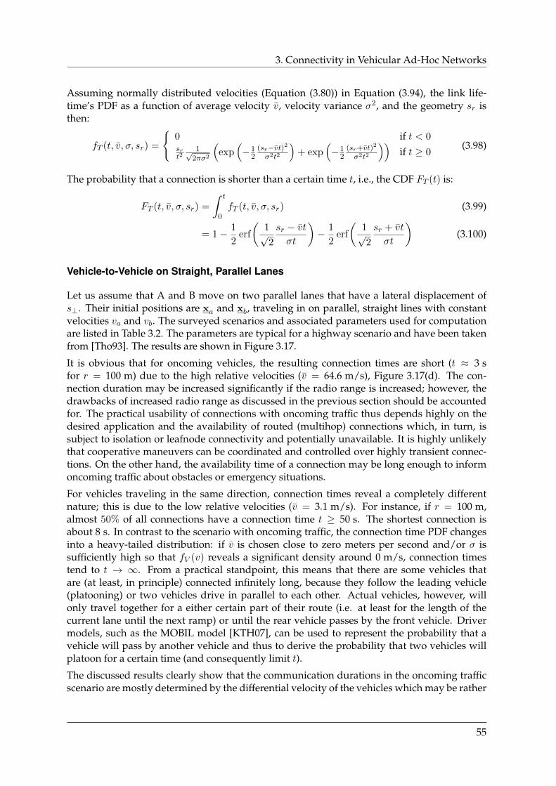
3. Connectivity in Vehicular Ad-Hoc Networks
Assuming normally distributed velocities (Equation (3.80)) in Equation (3.94), the link life-time’s PDF as a function of average velocity v, velocity variance σ2, and the geometry sr isthen:
fT (t, v, σ, sr) =
0 if t < 0srt2
1√2πσ2
(exp
(−1
2(sr−vt)2
σ2t2
)+ exp
(−1
2(sr+vt)
2
σ2t2
))if t ≥ 0
(3.98)
The probability that a connection is shorter than a certain time t, i.e., the CDF FT (t) is:
FT (t, v, σ, sr) =
∫ t
0fT (t, v, σ, sr) (3.99)
= 1− 1
2erf
(1√2
sr − vtσt
)− 1
2erf
(1√2
sr + vt
σt
)(3.100)
Vehicle-to-Vehicle on Straight, Parallel Lanes
Let us assume that A and B move on two parallel lanes that have a lateral displacement ofs⊥. Their initial positions are xa and xb, traveling in on parallel, straight lines with constantvelocities va and vb. The surveyed scenarios and associated parameters used for computationare listed in Table 3.2. The parameters are typical for a highway scenario and have been takenfrom [Tho93]. The results are shown in Figure 3.17.
It is obvious that for oncoming vehicles, the resulting connection times are short (t ≈ 3 sfor r = 100 m) due to the high relative velocities (v = 64.6 m/s), Figure 3.17(d). The con-nection duration may be increased significantly if the radio range is increased; however, thedrawbacks of increased radio range as discussed in the previous section should be accountedfor. The practical usability of connections with oncoming traffic thus depends highly on thedesired application and the availability of routed (multihop) connections which, in turn, issubject to isolation or leafnode connectivity and potentially unavailable. It is highly unlikelythat cooperative maneuvers can be coordinated and controlled over highly transient connec-tions. On the other hand, the availability time of a connection may be long enough to informoncoming traffic about obstacles or emergency situations.
For vehicles traveling in the same direction, connection times reveal a completely differentnature; this is due to the low relative velocities (v = 3.1 m/s). For instance, if r = 100 m,almost 50% of all connections have a connection time t ≥ 50 s. The shortest connection isabout 8 s. In contrast to the scenario with oncoming traffic, the connection time PDF changesinto a heavy-tailed distribution: if v is chosen close to zero meters per second and/or σ issufficiently high so that fV (v) reveals a significant density around 0 m/s, connection timestend to t → ∞. From a practical standpoint, this means that there are some vehicles thatare (at least, in principle) connected infinitely long, because they follow the leading vehicle(platooning) or two vehicles drive in parallel to each other. Actual vehicles, however, willonly travel together for a either certain part of their route (i.e. at least for the length of thecurrent lane until the next ramp) or until the rear vehicle passes by the front vehicle. Drivermodels, such as the MOBIL model [KTH07], can be used to represent the probability that avehicle will pass by another vehicle and thus to derive the probability that two vehicles willplatoon for a certain time (and consequently limit t).
The discussed results clearly show that the communication durations in the oncoming trafficscenario are mostly determined by the differential velocity of the vehicles which may be rather
55
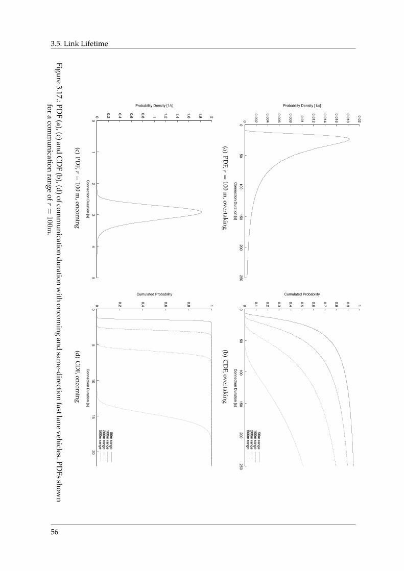
3.5. Link Lifetime
0
0.002
0.004
0.006
0.008
0.01
0.012
0.014
0.016
0.018
0.02
0 50
100 150
200 250
Probability Density [1/s]
Connection D
uration [s]
(a)PD
F ,r
=100
m,overtaking
0
0.1
0.2
0.3
0.4
0.5
0.6
0.7
0.8
0.9 1
0 50
100 150
200 250
Cumulated Probability
Connection D
uration [s]
50m range
100m range
200m range
500m range
(b)C
DF ,overtaking
0
0.2
0.4
0.6
0.8 1
1.2
1.4
1.6
1.8 2
0 1
2 3
4 5
Probability Density [1/s]
Connection D
uration [s]
(c)PD
F,r
=100
m,oncom
ing
0
0.2
0.4
0.6
0.8 1
0 5
10 15
20
Cumulated Probability
Connection D
uration [s]
50m range
100m range
200m range
500m range
(d)C
DF,oncom
ing
Figure3.17.:PD
F(a),(c)and
CD
F(b),(d)ofcom
munication
durationw
ithoncom
ingand
same-direction
fastlanevehicles.PD
Fsshow
nfor
acom
munication
rangeofr
=100m
.
56
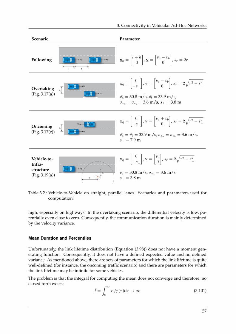
3. Connectivity in Vehicular Ad-Hoc Networks
Scenario Parameter
Following va vb
hl
x0 =
[l + h
0
], v =
[va − vb
0
], sr = 2r
Overtaking(Fig. 3.17(a)) va
vbs!
x0 =
[0−s⊥
], v =
[va − vb
0
], sr = 2
√r2 − s2
⊥
va = 30.8 m/s, vb = 33.9 m/s,σva = σvb = 3.6 m/s, s⊥ = 3.8 m
Oncoming(Fig. 3.17(c))
vbs!
x0 =
[0−s⊥
], v =
[va + vb
0
], sr = 2
√r2 − s2
⊥
va = vb = 33.9 m/s, σva = σvb = 3.6 m/s,s⊥ = 7.9 m
Vehicle-to-Infra-structure(Fig. 3.19(a))
rs!
va
x0 =
[0−s⊥
], v =
[va0
], sr = 2
√r2 − s2
⊥
va = 30.8 m/s, σva = 3.6 m/ss⊥ = 3.8 m
Table 3.2.: Vehicle-to-Vehicle on straight, parallel lanes. Scenarios and parameters used forcomputation.
high, especially on highways. In the overtaking scenario, the differential velocity is low, po-tentially even close to zero. Consequently, the communication duration is mainly determinedby the velocity variance.
Mean Duration and Percentiles
Unfortunately, the link lifetime distribution (Equation (3.98)) does not have a moment gen-erating function. Consequently, it does not have a defined expected value and no definedvariance. As mentioned above, there are sets of parameters for which the link lifetime is quitewell-defined (for instance, the oncoming traffic scenario) and there are parameters for whichthe link lifetime may be infinite for some vehicles.
The problem is that the integral for computing the mean does not converge and therefore, noclosed form exists:
t =
∫ ∞0
τ fT (τ)dτ →∞ (3.101)
57
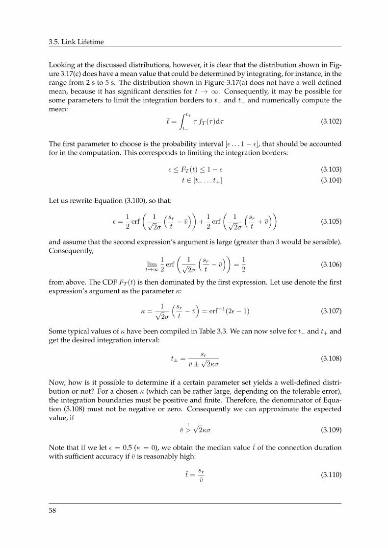
3.5. Link Lifetime
Looking at the discussed distributions, however, it is clear that the distribution shown in Fig-ure 3.17(c) does have a mean value that could be determined by integrating, for instance, in therange from 2 s to 5 s. The distribution shown in Figure 3.17(a) does not have a well-definedmean, because it has significant densities for t → ∞. Consequently, it may be possible forsome parameters to limit the integration borders to t− and t+ and numerically compute themean:
t =
∫ t+
t−
τ fT (τ)dτ (3.102)
The first parameter to choose is the probability interval [ε . . . 1 − ε], that should be accountedfor in the computation. This corresponds to limiting the integration borders:
ε ≤ FT (t) ≤ 1− ε (3.103)t ∈ [t− . . . t+] (3.104)
Let us rewrite Equation (3.100), so that:
ε =1
2erf
(1√2σ
(srt− v))
+1
2erf
(1√2σ
(srt
+ v))
(3.105)
and assume that the second expression’s argument is large (greater than 3 would be sensible).Consequently,
limt→∞
1
2erf
(1√2σ
(srt− v))
=1
2(3.106)
from above. The CDF FT (t) is then dominated by the first expression. Let use denote the firstexpression’s argument as the parameter κ:
κ =1√2σ
(srt− v)
= erf−1(2ε− 1) (3.107)
Some typical values of κ have been compiled in Table 3.3. We can now solve for t− and t+ andget the desired integration interval:
t± =sr
v ±√
2κσ(3.108)
Now, how is it possible to determine if a certain parameter set yields a well-defined distri-bution or not? For a chosen κ (which can be rather large, depending on the tolerable error),the integration boundaries must be positive and finite. Therefore, the denominator of Equa-tion (3.108) must not be negative or zero. Consequently we can approximate the expectedvalue, if
v!>√
2κσ (3.109)
Note that if we let ε = 0.5 (κ = 0), we obtain the median value t of the connection durationwith sufficient accuracy if v is reasonably high:
t =srv
(3.110)
58
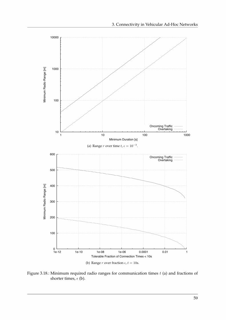
3. Connectivity in Vehicular Ad-Hoc Networks
10
100
1000
10000
1 10 100 1000
Min
imum
Rad
io R
ange
[m]
Minimum Duration [s]
Oncoming TrafficOvertaking
(a) Range r over time t, ε = 10−3.
0
100
200
300
400
500
600
1e-12 1e-10 1e-08 1e-06 0.0001 0.01 1
Min
imum
Rad
io R
ange
[m]
Tolerable Fraction of Connection Times < 10s
Oncoming TrafficOvertaking
(b) Range r over fraction ε, t = 10s.
Figure 3.18.: Minimum required radio ranges for communication times t (a) and fractions ofshorter times, ε (b).
59

3.5. Link Lifetime
ε κ
10−1 −0.906210−2 −1.645010−3 −2.185110−4 −2.629710−5 −3.015710−6 −3.3612. . . . . .
10−9 −4.241110−12 −4.9741
Table 3.3.: Some values of κ as a function of ε.
Radio Range Adaptation
For all κ ≤ v/√
2σ and corresponding ε, Equation (3.108) yields a valid lower integrationboundary, t−. The integral
ε ≈∫ t−
0fT (τ)dτ (3.111)
represents the fraction of nodes that have a connection time shorter than t−.18 We have arguedabove that the linear relation of the radio range to the communication duration makes it seemsensible to adjust the range so as to satisfy the demands of the application.
Using a representative set of scenario parameters (v, σ), it is possible to calculate the necessaryminimum radio range to provide enough (i.e., a fraction of more than ε) connections withdurations of at least t seconds by solving Equation (3.108) for sr and consequently solving srfor r:
sr = t(v −√
2κσ) (3.112)
Example
An application may be unavailable with a probability of ε = 10−3 (1 h) and requires connectionswith a minimum duration of t = 10 s. Given the overtaking and oncoming traffic scenario fromTable 3.2, what is the minimum radio range required to meet these demands?
For the desired ε, κ = -2.1851. Solving Equation (3.112) for the overtaking scenario (v = 3.1 m/s,σ =
√2 · (3.6 m/s)2 = 5.091 m/s) yields sr = 188.32 m and, consequently,
r =1
2
√s2r + 4s2⊥ ≈ 94 m (3.113)
For the oncoming traffic scenario with much higher relative velocities (v = 67.8 m/s), the connectiondurations are much shorter so the necessary radio range can be expected to be much greater than inthe overtaking scenario: sr = 835.32 m and, consequently, r ≈ 418 m.
The minimum required radio ranges over the desired ε, given a minimum communication durationof t = 10 s are shown for both scenarios in Figure 3.18(b). Conversely, the ranges over the desiredminimum communication durations t, given a tolerable fraction of lower durations ε = 10−3 areshown in Figure 3.18(a).
18This approximation stems from the fact that we neglected the second erf( · ) term of Equation (3.100) during thederivation of Equation (3.108).
60
3. Connectivity in Vehicular Ad-Hoc Networks
Vehicle-to-Infrastructure on Straight, Parallel Lanes
In the previous sections, we have considered two communicating vehicles, each moving withan individual velocity va and vb, respectively. Using the same mathematical framework, itis quite easy to analyze the communication durations between a moving vehicle and road-side infrastructure, i.e. a V2I constellation. To do so, we consider only one vehicle, let vb =0 m/s, and adjust the position vector accordingly — in the demonstrated case, we assume theinfrastructure equipment to be mounted with a lateral offset of s⊥ relative to the lane’s center.The results have been depicted in Figure 3.19.
Of course, the above considerations regarding radio range adjustment are also applicable inthe V2I scenario. However, in contrast to the V2V scenario, we can expect not to find infiniteconnection durations; instead, the mean duration may be assumed rather well defined.
Duration and Traffic Density
Unless we consider a pure V2I scenario, the link duration does not depend on the velocity ofa vehicle itself but rather on the differential velocities between vehicles. Therefore, it is noteasily possible to make a statement about the link duration based on the average velocity asa function of the traffic density ρ, Equation (3.37). If, however, the fundamental diagrams ofthe lanes on which two communicating vehicles travel are known, the traffic densities of theselanes are known, and the degree of correlation between the lanes are known, the average linklifetimes could be calculated.
The results shown in Figure 3.20 have been computed assuming that the fundamental dia-grams of neighboring lanes A and B are equal and parameterized according to the highwayscenario specified in Table 3.1. Under free-flow conditions, the fundamental diagram speci-fies equal average velocities for vehicles which, in turn, lead to infinite connection durations;hence the white triangle in the lower left corner. It is clear from the diagram that under heav-ily congested traffic conditions and/or very synchronous traffic (equal densities), connectiondurations are significantly longer than under conditions in which the densities differ more.
On the contrary, if a pure V2I scenario with fixed infrastructure equipment should be studied,the velocity of vehicles can be easily determined. The resulting median connection duration tis shown in Figure 3.21, assuming the highway scenario as used above.
3.6. Link Generation and Link Break Rate
The third relevant dimension of connectivity is the rate at which communication relationschange over time. As new vehicles enter a vehicle’s range radio, a new link is established.Other vehicles leave the radio range and links break away. The rate at which these eventshappen, Λ, is relevant because it defines a measure of a network’s dynamic. In the previoussections, we have discussed how the node degree d is related to the traffic density ρ and howlink lifetimes t are defined by (differential) velocities v. Knowing that traffic density and ve-locities are related through the measure of traffic flow, Q, this section will discuss how the linkgeneration rate Λ is related to Q.
Little’s Law [Lit61], a fundamental law in queueing theory, states that the average number ofcustomers in a shop is the arrival rate of customers multiplied with the average time spent in
61
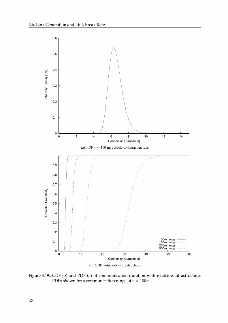
3.6. Link Generation and Link Break Rate
0
0.1
0.2
0.3
0.4
0.5
0.6
0 2 4 6 8 10 12 14
Prob
abilit
y D
ensi
ty [1
/s]
Connection Duration [s]
(a) PDF, r = 100 m, vehicle-to-infrastructure
0
0.1
0.2
0.3
0.4
0.5
0.6
0.7
0.8
0.9
1
0 10 20 30 40 50 60
Cum
ulat
ed P
roba
bilit
y
Connection Duration [s]
50m range100m range200m range500m range
(b) CDF, vehicle-to-infrastructure
Figure 3.19.: CDF (b) and PDF (a) of communication duration with roadside infrastructure.PDFs shown for a communication range of r = 100m.
62
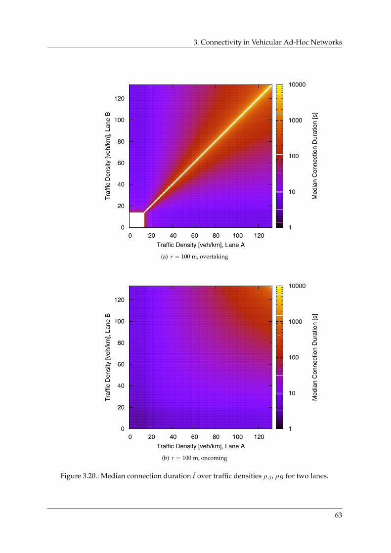
3. Connectivity in Vehicular Ad-Hoc Networks
0 20 40 60 80 100 120Traffic Density [veh/km], Lane A
0
20
40
60
80
100
120Tr
affic
Den
sity
[veh
/km
], La
ne B
1
10
100
1000
10000
Med
ian
Con
nect
ion
Dur
atio
n [s
]
(a) r = 100 m, overtaking
0 20 40 60 80 100 120Traffic Density [veh/km], Lane A
0
20
40
60
80
100
120
Traf
fic D
ensi
ty [v
eh/k
m],
Lane
B
1
10
100
1000
10000
Med
ian
Con
nect
ion
Dur
atio
n [s
]
(b) r = 100 m, oncoming
Figure 3.20.: Median connection duration t over traffic densities ρA, ρB for two lanes.
63
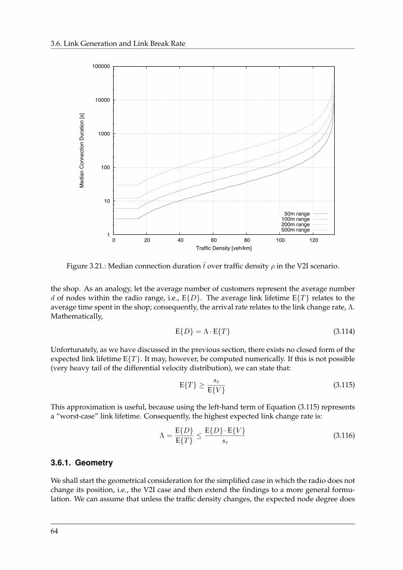
3.6. Link Generation and Link Break Rate
1
10
100
1000
10000
100000
0 20 40 60 80 100 120
Med
ian
Con
nect
ion
Dur
atio
n [s
]
Traffic Density [veh/km]
50m range100m range200m range500m range
Figure 3.21.: Median connection duration t over traffic density ρ in the V2I scenario.
the shop. As an analogy, let the average number of customers represent the average numberd of nodes within the radio range, i.e., ED. The average link lifetime ET relates to theaverage time spent in the shop; consequently, the arrival rate relates to the link change rate, Λ.Mathematically,
ED = Λ ·ET (3.114)
Unfortunately, as we have discussed in the previous section, there exists no closed form of theexpected link lifetime ET. It may, however, be computed numerically. If this is not possible(very heavy tail of the differential velocity distribution), we can state that:
ET ≥ srEV
(3.115)
This approximation is useful, because using the left-hand term of Equation (3.115) representsa “worst-case” link lifetime. Consequently, the highest expected link change rate is:
Λ =EDET
≤ ED ·EV sr
(3.116)
3.6.1. Geometry
We shall start the geometrical consideration for the simplified case in which the radio does notchange its position, i.e., the V2I case and then extend the findings to a more general formu-lation. We can assume that unless the traffic density changes, the expected node degree does
64
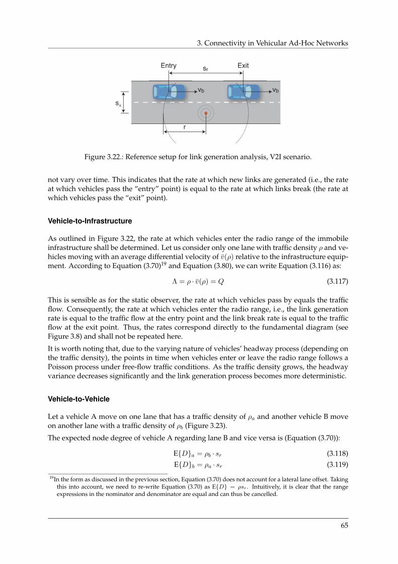
3. Connectivity in Vehicular Ad-Hoc Networks
vbvb
r
s!
srEntry Exit
Figure 3.22.: Reference setup for link generation analysis, V2I scenario.
not vary over time. This indicates that the rate at which new links are generated (i.e., the rateat which vehicles pass the “entry” point) is equal to the rate at which links break (the rate atwhich vehicles pass the “exit” point).
Vehicle-to-Infrastructure
As outlined in Figure 3.22, the rate at which vehicles enter the radio range of the immobileinfrastructure shall be determined. Let us consider only one lane with traffic density ρ and ve-hicles moving with an average differential velocity of v(ρ) relative to the infrastructure equip-ment. According to Equation (3.70)19 and Equation (3.80), we can write Equation (3.116) as:
Λ = ρ · v(ρ) = Q (3.117)
This is sensible as for the static observer, the rate at which vehicles pass by equals the trafficflow. Consequently, the rate at which vehicles enter the radio range, i.e., the link generationrate is equal to the traffic flow at the entry point and the link break rate is equal to the trafficflow at the exit point. Thus, the rates correspond directly to the fundamental diagram (seeFigure 3.8) and shall not be repeated here.
It is worth noting that, due to the varying nature of vehicles’ headway process (depending onthe traffic density), the points in time when vehicles enter or leave the radio range follows aPoisson process under free-flow traffic conditions. As the traffic density grows, the headwayvariance decreases significantly and the link generation process becomes more deterministic.
Vehicle-to-Vehicle
Let a vehicle A move on one lane that has a traffic density of ρa and another vehicle B moveon another lane with a traffic density of ρb (Figure 3.23).
The expected node degree of vehicle A regarding lane B and vice versa is (Equation (3.70)):
EDa = ρb · sr (3.118)EDb = ρa · sr (3.119)
19In the form as discussed in the previous section, Equation (3.70) does not account for a lateral lane offset. Takingthis into account, we need to re-write Equation (3.70) as ED = ρsr . Intuitively, it is clear that the rangeexpressions in the nominator and denominator are equal and can thus be cancelled.
65
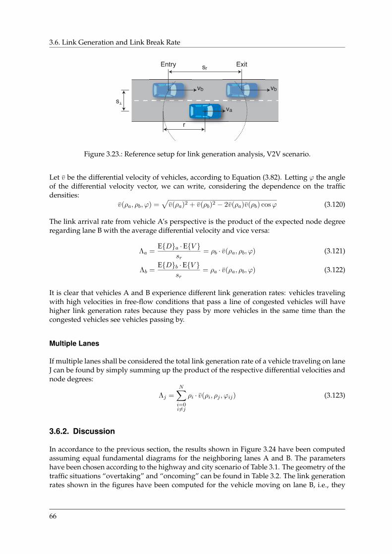
3.6. Link Generation and Link Break Rate
vbvb
va
r
s!
srEntry Exit
Figure 3.23.: Reference setup for link generation analysis, V2V scenario.
Let v be the differential velocity of vehicles, according to Equation (3.82). Letting ϕ the angleof the differential velocity vector, we can write, considering the dependence on the trafficdensities:
v(ρa, ρb, ϕ) =√v(ρa)2 + v(ρb)2 − 2v(ρa)v(ρb) cosϕ (3.120)
The link arrival rate from vehicle A’s perspective is the product of the expected node degreeregarding lane B with the average differential velocity and vice versa:
Λa =EDa ·EV
sr= ρb · v(ρa, ρb, ϕ) (3.121)
Λb =EDb ·EV
sr= ρa · v(ρa, ρb, ϕ) (3.122)
It is clear that vehicles A and B experience different link generation rates: vehicles travelingwith high velocities in free-flow conditions that pass a line of congested vehicles will havehigher link generation rates because they pass by more vehicles in the same time than thecongested vehicles see vehicles passing by.
Multiple Lanes
If multiple lanes shall be considered the total link generation rate of a vehicle traveling on laneJ can be found by simply summing up the product of the respective differential velocities andnode degrees:
Λj =N∑i=0i6=j
ρi · v(ρi, ρj , ϕij) (3.123)
3.6.2. Discussion
In accordance to the previous section, the results shown in Figure 3.24 have been computedassuming equal fundamental diagrams for the neighboring lanes A and B. The parametershave been chosen according to the highway and city scenario of Table 3.1. The geometry of thetraffic situations “overtaking” and “oncoming” can be found in Table 3.2. The link generationrates shown in the figures have been computed for the vehicle moving on lane B, i.e., they
66
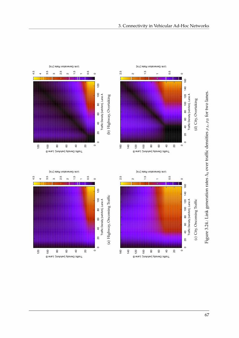
3. Connectivity in Vehicular Ad-Hoc Networks
0 2
0 4
0 6
0 8
0 1
00 1
20Tr
affic
Den
sity
[veh
/km
], La
ne A
0 20
40
60
80
100
120
Traffic Density [veh/km], Lane B
0 0.5
1 1.5
2 2.5
3 3.5
4 4.5
Link Generation Rate [1/s]
(a)
Hig
hway
,Onc
omin
gTr
affic
0 2
0 4
0 6
0 8
0 1
00 1
20Tr
affic
Den
sity
[veh
/km
], La
ne A
0 20
40
60
80
100
120
Traffic Density [veh/km], Lane B
0 0.5
1 1.5
2 2.5
3 3.5
4 4.5
Link Generation Rate [1/s]
(b)
Hig
hway
,Ove
rtak
ing
0 2
0 4
0 6
0 8
0 1
00 1
20 1
40 1
60Tr
affic
Den
sity
[veh
/km
], La
ne A
0 20
40
60
80
100
120
140
160
Traffic Density [veh/km], Lane B
0 0.5
1 1.5
2 2.5
Link Generation Rate [1/s]
(c)
Cit
y,O
ncom
ing
Traf
fic
0 2
0 4
0 6
0 8
0 1
00 1
20 1
40 1
60Tr
affic
Den
sity
[veh
/km
], La
ne A
0 20
40
60
80
100
120
140
160
Traffic Density [veh/km], Lane B 0 0
.5
1 1.5
2 2.5
Link Generation Rate [1/s]
(d)
Cit
y,O
vert
akin
g
Figu
re3.
24.:
Link
gene
rati
onra
tes
Λb
over
traf
ficde
nsit
iesρA
,ρB
for
two
lane
s.
67

3.6. Link Generation and Link Break Rate
represent Λb. However, reversing the two axes yields the rates for a vehicle moving on lane A,i.e., Λa.
Intuitively, one would expect the highest link generation rates in situations where vehiclesmove with high relative velocities, i.e., in scenarios with oncoming traffic. The results shownin Figures 3.24(a) and 3.24(c), however, show only very moderate rates. At a traffic densityof ρ = 20 km−1, we obtain rates for the highway scenario of Λb ≈ 0.94 s−1 and for the cityscenario of Λb ≈ 0.6 s−1.
If both vehicles travel in the same direction, their differential velocity will be almost equal ifthe traffic densities are equal and consequently, the link generation rate is zero. The highestrates are always obtained in situations where one vehicle is stuck in highly congested traffic forthe vehicle passing by the congestion, independent of the direction (overtaking or oncoming).It is, however, unlikely to be found in a realistic situation that two equidirectional lanes revealsignificant differences regarding their traffic densities.
If the lanes are aligned counterdirectional — such as on a highway — the situation is verylikely to be found and needs further consideration. If routing should be implemented in thenetwork, the link generation rate and the link break rate represent the dynamic at which thenetwork’s topology changes and consequently correspond to the rate at which routing tableshave to be updated. Careful consideration is necessary to decide if routing can sensibly beimplemented under all traffic situations.
Example
Let us consider a highway. Lane A is jammed (ρa = 120 km−1), the counterdirection lane B is free(ρb = 10 km−1). The expected differential velocity, assuming the fundamental diagrams parame-terized according to Table 3.1, is then v = 33.8 m/s. Consequently, the experienced link generationrates are:
Λa = ρb · v = 0.338 s−1 (3.124)
Λb = ρa · v = 4.056 s−1 (3.125)
Let us assume a radio range of r = 200 m. Consequently, the expected node degrees of a node withrespect to lanes A and B can be determined:
EDa = 2rρa = 48 (3.126)EDb = 2rρb = 4 (3.127)
The protocol specifies that upon every topology change, a routing message shall be transmitted. Wehave argued above that the topology change rate is the link generation rate plus the link break rate,which are assumed to be equal here. Therefore, a node on lane A will transmit a routing messageat a rate of 2Λa and receive 2Λa ·EDa messages from other vehicles on lane A that are in range.Also, it will receive 2Λb ·EDb messages from vehicles in range on lane B. The total message rate isthen:
λ = 2Λa(1 + EDa) + 2Λb ·EDb (3.128)
≈ 66 s−1 (3.129)
Depending on the protocol, the routing messages can have various sizes. For simplicity, let usassume that the total message size including all headers is 100 B and the medium offers a data rateof 6 Mbit/s. The total offered traffic from routing messages is thus:
g = 66 s−1 · 100 B6 Mbit/s
≈ 0.01 (3.130)
68

3. Connectivity in Vehicular Ad-Hoc Networks
This means that approximately one percent of the channel capacity will be occupied by routinginformation. The number does not seem very high, but — as we will discuss in the next chapter —it is a significant amount of traffic. Futhermore, we have only considered one lane per direction; thepresence of two lanes in each direction (the usual geometry on highways) doubles the traffic.
3.7. Conclusion
In this section, we have discussed various channel models and presented a mathematical for-malism that captures the individual properties of these models. We have then introduced thebasics of vehicular traffic flow theory and discussed the fundamental diagram and variousmodels thereof. We have discussed how traffic flow Q, traffic density ρ, and vehicle speed vare related.
Using traffic flow theory as a mobility model and combining it with an appropriate channelmodel, we have presented an analytical framework that relates important parameters of theroad traffic to networking parameters. We have outlined the defining states of traffic flow, free-flow and congestion and the transition phase between these two states. Then, we have deriveda mathematical framework that allows to relate ρ to the node degree d and its distribution forall traffic states in a rather straight-forward manner. Using some simple scenarios, we havepointed out some issues with node degree, including the isolation and leafnode probability,discussed the impact of equipment ratio and the dispersion of node degrees. Through thefundamental diagram, a relation between the average vehicle speed and the expected nodedegree has been established and the consequences have been discussed.
We have then presented a geometry-based model that allows for the computation of the dis-tribution of connection durations fT (t) according to the situation’s geometry and velocitydistributions. We have discussed typical results for both oncoming traffic and overtakingsituations in highway scenarios and consequences for wireless connections. Also, we havediscussed mathematical issues related to the connection duration distribution function, espe-cially related to the non-existence of the distribution function’s moment generating function.Furthermore, we have discussed how adjusting the radio range could help enabling sensiblecommunication in oncoming traffic scenarios that typically have very short communicationdurations. Finally, we have extended our considerations from the V2V to the V2I situation.The relation between connection duration and traffic density has been established by meansof representative scenarios.
The last section of the chapter discusses the rate Λ at which new links are generated and atwhich links break and related this rate to the node degree and the connection duration throughLittle’s Law. Starting from the consideration of a V2I scenario in which the relation of Λ to thetraffic flow, Q, was established we have generalized the formula to a V2V scenario. In thediscussion, we have presented typical rates for highway and urban settings. An exemplarysituation has been discussed showing that the topology change rate is the sum of the link gen-eration and the link break rate and we have argued how the topology change rate determinesthe teletraffic caused by routing messages in the network.
The formulas and numbers derived in this section are suitable to describe the overall connec-tivity properties of a vehicular network and shall form the basis of the data teletraffic engi-neering methods that we will introduce in the next chapter. They are summarized in Table 3.4.
69
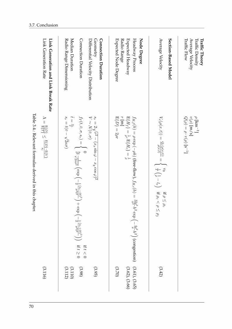
3.7. ConclusionTraf fic
Theory
TrafficD
ensityρ
[km−
1]A
verageVelocity
v(ρ
)[m
/s]Traffic
FlowQ
(ρ)
=ρ·v
(ρ)
[s −1]
Section-Based
Model
Average
VelocityVe (ρ
(x,t))
=Qe(ρ
(x,t))
ρ(x,t)
= v
0ifρ≤ρc
1T (1ρ−le )
ifρc<ρ≤ρj
(3.42)
Node
Degree
Headw
ayProcess
fH,f (h
)=ρ
exp
(−ρh
)(free-flow
),fH,c (h
)=
32ρ
3
π2h
2ex
p (−4ρ
2
πh
2 )(congestion)
(3.61),(3.65)Expected
Headw
ayEHf
=1ρ ,EH
c =
1ρ(3.62),(3.66)
Radio
Range
r[m
]Expected
Node
Degree
ED
=2ρr
(3.70)
Connection
Duration
Geom
etrysr
=2 √
r2−
(xx
sinϕ−xy
cosϕ
)2
(3.95)D
ifferentialVelocityD
istributionV∼N
(v,σ
)
Connection
Duration
fT
(t,v,σ,sr )
= 0
ift<
0srt2
1√
2πσ
2 (ex
p (−12
(sr −vt)
2
σ2t2 )
+ex
p (−12
(sr+vt)
2
σ2t2 ))
ift≥
0(3.98)
Median
Duration
t=
srv
(3.110)R
adioR
angeD
imensioning
sr
=t(v−√
2κσ
)(3.112)
LinkG
enerationand
LinkB
reakR
ateLink
Generation
Rate
Λ=
ED
ET≤
ED·E
V
sr
(3.116)
Table3.4.:R
elevantformulas
derivedin
thischapter.
70
4. QoS Analysis and Provisioning in Vehicular Ad-HocNetworks
In the previous chapter, we have discussed three fundamental connectivity properties of ve-hicular networks: node degree, connection duration and topology dynamics. These insightshave mainly arisen from the consideration of connection probabilities between two nodes. Inthis chapter, we extend the meaning of connectivity to describe the communication relationsbetween a subset of nodes in a potentially infinitely large network and we shall focus on theparticular characteristics of wireless networks.
It has been demonstrated early [Tob74, KL75, KT75] that for all random access MAC schemes,there exists a relation between the teletraffic offered to the medium and the collision (i.e.,packet loss) probability. One consequence of an increase of collisions is a decrease of a net-work’s throughput due to packets rendered useless. The other consequence is that if acknowl-edged transmissions are to be implemented, the delay a packet experiences (caused by — pos-sibly several — necessary re-transmissions) before it is successfully received increases with in-creasing collisions. Throughput, packet loss and packet delay are today commonly subsumedunder the label Quality of Service (QoS).
In this chapter, we will demonstrate how QoS can be attained and even guaranteed in arbi-trarily connected networks. In contrast to previous works, we will not try to adapt an existingMAC scheme to our needs or even design a new scheme; instead, we introduce a mechanismthat controls the amount of traffic offered to the medium. As a matter of fact, the choice ofa particular MAC scheme is not important for our reasonings; rather, we demonstrate howthe relevant protocol properties can be described and consequently studied. Although wewill make a certain choice of MAC schemes for illustrative reasons, the methods used andmechanisms introduced in this chapter can ultimately be applied to any contention-basedscheme1. We will start our considerations for a situation in which either one central nodeor all distributed nodes have global knowledge about the network’s connectivity. Then, wedemonstrate how our QoS algorithm may be implemented in a decentralized manner, withonly minimal local connectivity information. Finally, we will discuss how applications can beselected from a set of applications and even parameterized, utilizing cross-layer informationfrom the QoS algorithm. Some of the material in this chapter has been published in [Nag10a].
To avoid ambiguity, the term “traffic” in this chapter refers to data being exchanged betweennetworked nodes.
4.1. Related Work
With the advent of affordable and powerful computers in the seventies, it became necessaryto interconnect host computers and remote terminals. Soon it was realized that because of
1The mechanism is implicitly included in reservation-based schemes.
71
4.1. Related Work
the bursty data generation process at the terminals as well as that of the host computer, onlya fraction of the available data rate of circuit-switched connections is used. Consequently,random access mechanisms were invented in which a number of users share one channel.Due to the multiplexing of a large number of users generating bursty traffic, the resultingcombined traffic (in the optimal case) is smoothened. Because of the non-deterministic natureof data generation, collisions on the channel may occur and recovery procedures are necessaryto avoid data loss. Consequently, it is not possible for a random access scheme to achieve themaximum throughput of a channel.
General analysis of the throughput of (slotted) ALOHA and CSMA schemes can be foundin the pioneering papers [KT75, Abr77], in which the authors study the performance of theprotocols in terms of collision (packet loss) probability, resulting throughput and retransmis-sion delays. The concept of “hearing graphs” (i.e., connectivity matrices) was introducedin [Tob74, TK75] to analyze the effect of hidden terminals, but was not applied to traffic di-mensioning problems. We will discuss relevant work related to MAC protocols in Section 4.3.
Quite early it was realized that it is desirable to achieve or even guarantee a certain throughputand/or bounded delay to individual users. In [LK75], the authors propose various dynamiccontrol procedures to ensure stable operation of slotted ALOHA systems. It is shown that op-timal traffic control policies exist that can maximize the stationary channel throughput and atthe same time minimize the average packet delay. However, the proposed procedures requirestate information about the channel that are not known a priori and must consequently beestimated. To a certain extent, this paper can be regarding as the first work dedicated to QoSprovisioning over random access network.
In the following years, a large number of MAC protocols have been presented that couldprovide users and applications with QoS under certain scenarios, the most prominent examplebeing the relatively new 802.11e standard for wireless local area networks. Other approachescan be found at the network layer, such as IntServ (RSVP) and DiffServ. These extension tothe Internet Protocol (IP) control the routing and queueing procedures that guide a packetthrough the network. As for DiffServ, it provides only a framework to differentiate traffic intovarious classes; it does not specify how labeled packets should be treated along the path andtherefore it is difficult to predict the actual end-to-end behavior of a connection. The idea tohave applications differentiate and prioritize their traffic, however, is crucial and prerequisiteto all QoS approaches throughout the whole networking stack.
The idea of limiting the rate at which messages are sent to the network is not entirely new.The authors of [Inz04] suggest traffic control mechanism that are based on a number of delay,bandwidth and packet-loss metrics instead of simply fair and/or flexible bandwidth man-agement. The proposed mechanism, however, is based on the channel state and is thus notdeterministic. The same holds true for the traffic shaper proposed by the authors of [BKSM06],that uses the current throughput and number of frame retransmissions as inputs. In [WR05],the authors provide a utility-based packet forwarding and congestion control scheme schemethat works on top of the IEEE 802.11 MAC protocol and is focused on non-safety applications.Other authors have argued that this approach needs the road to be segmented into sections forcalculating the message utility metric, thus it cannot be used directly in the context of safetyapplications. In [ZGZC09], the authors suggest a cross-layer design that jointly addresses theproblems of rate control, medium access and routing for unidirectional flows in routed net-works. Unfortunately, their approach requires its own MAC protocol and is thus not generallyapplicable.
72

4. QoS Analysis and Provisioning in Vehicular Ad-Hoc Networks
We will discuss further related work throughout the chapter where appropriate.
4.2. Network Model
Assuming that we have a connected ad-hoc network, let V = v1, . . . , vn denote the set ofnodes (i.e., the set of radios) and let n = |V| be its cardinality. Let E be the set of connectionsbetween the nodes: a tuple (vi, vj) ∈ E indicates that the nodes vi and vj are connected.
In the previous chapter, we have defined connectivity between two nodes vi and vj as a resultof the attenuation between them (Equation 3.4). Attenuation itself depends on the physicalpositions of the two nodes, xi and xj , as well as on their radio environment, described bymeans of an appropriate channel model, χ(xi,xj).
Note that the channel model determines the probability that a connection exists between twonodes; in this chapter, however, we study the connectivity properties of actual static realiza-tions of a network. Consequently, a pair of nodes is either connected or not; therefore, wedefine the connection probability obtained from the channel model as the average over aninfinite amount of realizations:
P((vi, vj) ∈ E
)= χ(xi,xj) (4.1)
4.2.1. Connectivity Matrix
The network’s graph G := (V, E) can also be described through its connectivity matrix C˜ (G) =(cij)
2, where
cij =
1 if (vi, vj) ∈ E0 otherwise
(4.2)
In our considerations, we assume that the links in the network are always bidirectional, i.e.that if node vi is connected to node vj , node vj is also connected to node vi. Because of thisassumption, the connectivity matrix is symmetric:
cij = cji (4.3)
Hypergraph Notation
In contrast to a fixed network in which individual links may be technically realized as ded-icated links, the broadcast nature of the shared wireless channel causes one message to bereceived by all adjacent nodes of the sender at the same time. Consequently, when studyingwireless networks, we should consider their representation as a hypergraph H , i.e., a general-ized graph in which edges are ordered pairs of sets (hyperarcs) rather than tuples: H := (V,A).A hyperarc a is a pair of a set of senders S and a set of receiversR:
a = (Sa,Ra) ∈ A (4.4)Sa ∩Ra = ∅ (4.5)
The type of relation between the nodes is a one-to-many relation, but there are two perspec-tives:
2The adjacency matrix of the graph: C˜ (G) ∈ 0, 1n×n.
73
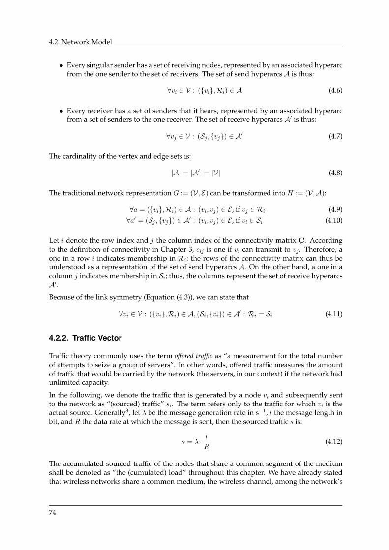
4.2. Network Model
• Every singular sender has a set of receiving nodes, represented by an associated hyperarcfrom the one sender to the set of receivers. The set of send hyperarcs A is thus:
∀vi ∈ V : (vi,Ri) ∈ A (4.6)
• Every receiver has a set of senders that it hears, represented by an associated hyperarcfrom a set of senders to the one receiver. The set of receive hyperarcs A′ is thus:
∀vj ∈ V : (Sj , vj) ∈ A′ (4.7)
The cardinality of the vertex and edge sets is:
|A| = |A′| = |V| (4.8)
The traditional network representation G := (V, E) can be transformed into H := (V,A):
∀a = (vi,Ri) ∈ A : (vi, vj) ∈ E , if vj ∈ Ri (4.9)∀a′ = (Sj , vj) ∈ A′ : (vi, vj) ∈ E , if vi ∈ Si (4.10)
Let i denote the row index and j the column index of the connectivity matrix C˜ . Accordingto the definition of connectivity in Chapter 3, cij is one if vi can transmit to vj . Therefore, aone in a row i indicates membership in Ri; the rows of the connectivity matrix can thus beunderstood as a representation of the set of send hyperarcs A. On the other hand, a one in acolumn j indicates membership in Si; thus, the columns represent the set of receive hyperarcsA′.
Because of the link symmetry (Equation (4.3)), we can state that
∀vi ∈ V : (vi,Ri) ∈ A, (Si, vi) ∈ A′ : Ri = Si (4.11)
4.2.2. Traffic Vector
Traffic theory commonly uses the term offered traffic as “a measurement for the total numberof attempts to seize a group of servers”. In other words, offered traffic measures the amountof traffic that would be carried by the network (the servers, in our context) if the network hadunlimited capacity.
In the following, we denote the traffic that is generated by a node vi and subsequently sentto the network as “(sourced) traffic” si. The term refers only to the traffic for which vi is theactual source. Generally3, let λ be the message generation rate in s−1, l the message length inbit, and R the data rate at which the message is sent, then the sourced traffic s is:
s = λ · lR
(4.12)
The accumulated sourced traffic of the nodes that share a common segment of the mediumshall be denoted as “the (cumulated) load” throughout this chapter. We have already statedthat wireless networks share a common medium, the wireless channel, among the network’s
74

4. QoS Analysis and Provisioning in Vehicular Ad-Hoc Networks
a
b
c
dddeeeee
f
g
h
i
jjjk
l
c
b,c
c,f
b,c,f
b
f
Figure 4.1.: Exemplary network. The radio ranges are indicated for nodes B, C, and F.
nodes. It is, however, relevant to understand that there exists a number of different “seg-ments” of the wireless network that are determined by the network nodes that are in rangeand actually make use of that network segment.
As a convention, we define network segments according to the set of receive hyperarcsA′ andwe shall in the following denote these segments the collision domains. At a node vj ∈ V , themedium is shared between vj and the nodes that vj can hear, i.e. the nodes in the set Sj .
The cumulated load is then the sum of the traffic for which the nodes in Sj are sources, plusthe traffic for which vj is the source. We denote the load as uj :
uj = sj +∑vi∈Sj
si (4.13)
= sj +N∑i=0
cij · gi (4.14)
Let u denote the load vector where ui is the cumulated load at node vi’s collision domain. Thevector s denotes the source traffic vector where si is the traffic sourced into the network bynode vi. Then, the vector:
u = C˜ T s + s
=(C˜ T + I˜)s (4.15)
3... and thus omitting the appropriate node indices ...
75
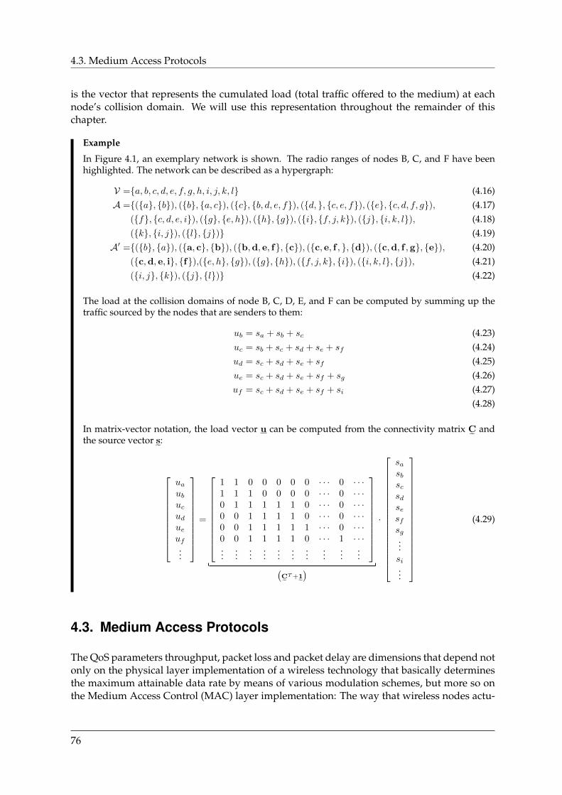
4.3. Medium Access Protocols
is the vector that represents the cumulated load (total traffic offered to the medium) at eachnode’s collision domain. We will use this representation throughout the remainder of thischapter.
Example
In Figure 4.1, an exemplary network is shown. The radio ranges of nodes B, C, and F have beenhighlighted. The network can be described as a hypergraph:
V =a, b, c, d, e, f, g, h, i, j, k, l (4.16)A =(a, b), (b, a, c), (c, b, d, e, f), (d, , c, e, f), (e, c, d, f, g), (4.17)
(f, c, d, e, i), (g, e, h), (h, g), (i, f, j, k), (j, i, k, l), (4.18)(k, i, j), (l, j) (4.19)
A′ =(b, a), (a, c, b), (b,d, e, f, c), (c, e, f , , d), (c,d, f ,g, e), (4.20)(c,d, e, i, f),(e, h, g), (g, h), (f, j, k, i), (i, k, l, j), (4.21)(i, j, k), (j, l) (4.22)
The load at the collision domains of node B, C, D, E, and F can be computed by summing up thetraffic sourced by the nodes that are senders to them:
ub = sa + sb + sc (4.23)uc = sb + sc + sd + se + sf (4.24)ud = sc + sd + se + sf (4.25)ue = sc + sd + se + sf + sg (4.26)uf = sc + sd + se + sf + si (4.27)
(4.28)
In matrix-vector notation, the load vector u can be computed from the connectivity matrix C˜ andthe source vector s˜:
uaubucudueuf...
=
1 1 0 0 0 0 0 · · · 0 · · ·1 1 1 0 0 0 0 · · · 0 · · ·0 1 1 1 1 1 0 · · · 0 · · ·0 0 1 1 1 1 0 · · · 0 · · ·0 0 1 1 1 1 1 · · · 0 · · ·0 0 1 1 1 1 0 · · · 1 · · ·...
......
......
......
......
...
(C˜T+1˜
)
·
sasbscsdsesfsg...si...
(4.29)
4.3. Medium Access Protocols
The QoS parameters throughput, packet loss and packet delay are dimensions that depend notonly on the physical layer implementation of a wireless technology that basically determinesthe maximum attainable data rate by means of various modulation schemes, but more so onthe Medium Access Control (MAC) layer implementation: The way that wireless nodes actu-
76
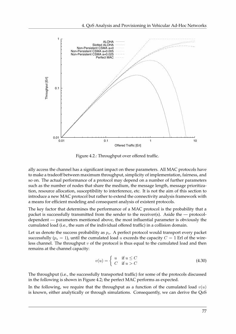
4. QoS Analysis and Provisioning in Vehicular Ad-Hoc Networks
0.01
0.1
1
0.01 0.1 1 10
Thro
ughp
ut [E
rl]
Offered Traffic [Erl]
ALOHASlotted ALOHA
Non-Persistent CSMA a=0Non-Persistent CSMA a=0.005Non-Persistent CSMA a=0.025
Perfect MAC
Figure 4.2.: Throughput over offered traffic.
ally access the channel has a significant impact on these parameters. All MAC protocols haveto make a tradeoff between maximum throughput, simplicity of implementation, fairness, andso on. The actual performance of a protocol may depend on a number of further parameterssuch as the number of nodes that share the medium, the message length, message prioritiza-tion, resource allocation, susceptibility to interference, etc. It is not the aim of this section tointroduce a new MAC protocol but rather to extend the connectivity analysis framework witha means for efficient modeling and consequent analysis of existent protocols.
The key factor that determines the performance of a MAC protocol is the probability that apacket is successfully transmitted from the sender to the receiver(s). Aside the — protocol-dependent — parameters mentioned above, the most influential parameter is obviously thecumulated load (i.e., the sum of the individual offered traffic) in a collision domain.
Let us denote the success probability as ps. A perfect protocol would transport every packetsuccessfully (ps = 1), until the cumulated load u exceeds the capacity C = 1 Erl of the wire-less channel. The throughput v of the protocol is thus equal to the cumulated load and thenremains at the channel capacity:
v(u) =
u if u ≤ CC if u > C
(4.30)
The throughput (i.e., the successfully transported traffic) for some of the protocols discussedin the following is shown in Figure 4.2; the perfect MAC performs as expected.
In the following, we require that the throughput as a function of the cumulated load v(u)is known, either analytically or through simulations. Consequently, we can derive the QoS
77
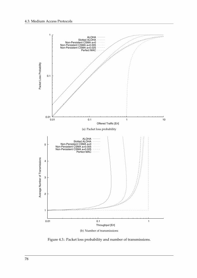
4.3. Medium Access Protocols
0.01
0.1
1
0.01 0.1 1 10
Pack
et L
oss
Prob
abilit
y
Offered Traffic [Erl]
ALOHASlotted ALOHA
Non-Persistent CSMA a=0Non-Persistent CSMA a=0.005Non-Persistent CSMA a=0.025
Perfect MAC
(a) Packet loss probability
1
2
3
4
5
0.01 0.1 1
Aver
age
Num
ber o
f Tra
nsm
issi
ons
Throughput [Erl]
ALOHASlotted ALOHA
Non-Persistent CSMA a=0Non-Persistent CSMA a=0.005Non-Persistent CSMA a=0.025
Perfect MAC
(b) Number of transmissions
Figure 4.3.: Packet loss probability and number of transmissions.
78
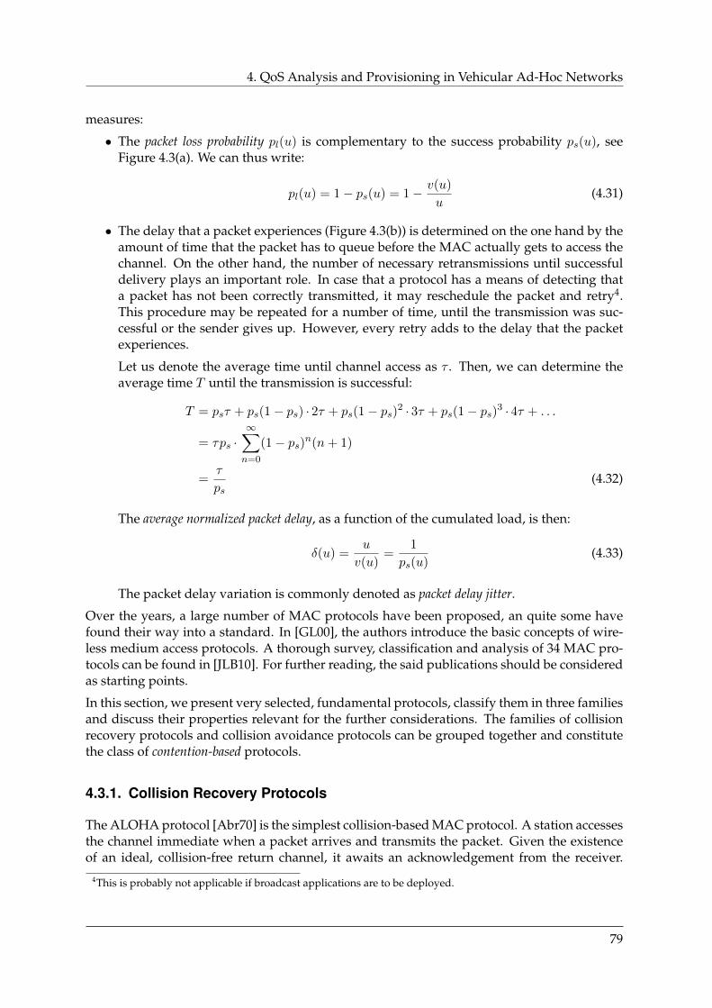
4. QoS Analysis and Provisioning in Vehicular Ad-Hoc Networks
measures:
• The packet loss probability pl(u) is complementary to the success probability ps(u), seeFigure 4.3(a). We can thus write:
pl(u) = 1− ps(u) = 1− v(u)
u(4.31)
• The delay that a packet experiences (Figure 4.3(b)) is determined on the one hand by theamount of time that the packet has to queue before the MAC actually gets to access thechannel. On the other hand, the number of necessary retransmissions until successfuldelivery plays an important role. In case that a protocol has a means of detecting thata packet has not been correctly transmitted, it may reschedule the packet and retry4.This procedure may be repeated for a number of time, until the transmission was suc-cessful or the sender gives up. However, every retry adds to the delay that the packetexperiences.
Let us denote the average time until channel access as τ . Then, we can determine theaverage time T until the transmission is successful:
T = psτ + ps(1− ps) · 2τ + ps(1− ps)2 · 3τ + ps(1− ps)3 · 4τ + . . .
= τps ·∞∑n=0
(1− ps)n(n+ 1)
=τ
ps(4.32)
The average normalized packet delay, as a function of the cumulated load, is then:
δ(u) =u
v(u)=
1
ps(u)(4.33)
The packet delay variation is commonly denoted as packet delay jitter.
Over the years, a large number of MAC protocols have been proposed, an quite some havefound their way into a standard. In [GL00], the authors introduce the basic concepts of wire-less medium access protocols. A thorough survey, classification and analysis of 34 MAC pro-tocols can be found in [JLB10]. For further reading, the said publications should be consideredas starting points.
In this section, we present very selected, fundamental protocols, classify them in three familiesand discuss their properties relevant for the further considerations. The families of collisionrecovery protocols and collision avoidance protocols can be grouped together and constitutethe class of contention-based protocols.
4.3.1. Collision Recovery Protocols
The ALOHA protocol [Abr70] is the simplest collision-based MAC protocol. A station accessesthe channel immediate when a packet arrives and transmits the packet. Given the existenceof an ideal, collision-free return channel, it awaits an acknowledgement from the receiver.
4This is probably not applicable if broadcast applications are to be deployed.
79
4.3. Medium Access Protocols
If a certain timeout expires and no acknowledgement was received, the station retries thetransmission to recover from the collision.
Let us assume that the channel access inter-arrival times follow a poisson process, we candetermine the throughput of ALOHA as:
vA(u) = u · exp (−2u) (4.34)
The ALOHA protocol was later improved by adding the rule that the channel may not beaccessed at random points in time but only at the beginning of a time slot. Hence, the extendedversion was called Slotted ALOHA [Rob75, KL75]. The throughput is given by:
vSA(u) = u · exp (−u) (4.35)
Figure 4.2 shows that the maximum throughput is attained at an offered traffic of u = 0.5 Erl,where the throughput is vA(0.5 Erl) ≈ 0.18 Erl. The packet loss probability at this point, how-ever, is ≈ 63.2 % and the average number of necessary transmissions until success is about2.72. It is remarkable that through increasing collisions, the throughput actually decreasesto zero if the amount of offered traffic is increased beyond 0.5 Erl. This is called the stabil-ity criterion. The maximum throughput of Slotted ALOHA is increased to twice that of pureALOHA (due to the shortened critical time where collisions may occur), at an offered trafficof u = 1 Erl: vSA(1 Erl) ≈ 0.37 Erl. The packet loss probability at this point is equal to that ofALOHA at the throughput maximum; consequently, the number of required transmissions isequal.
In the following years, a number of protocols have been developed that build on the foun-dation of ALOHA, among which the R-ALOHA protocol [CRW+73] is most noteworthy: itunites both elements of contention and reservation. Nodes contend for time slots and, uponhaving successfully transmitted a message in one slot, may keep “their” slot for a certain timethus achieving reservation of a certain resource share. Its performance in terms of through-put, delay and packet loss has been studied in [Lam80]. In [BCCF03], the authors proposeRR-ALOHA, a distributed, reliable, reservation-based ALOHA variant for use in mobile ap-plications (sometimes also denoted as ADHOC MAC).
4.3.2. Collision Avoidance Protocols
The large family of Carrier Sense Multiple Access (CSMA) MAC protocols is based on theprinciple of sensing the medium for the existence of a carrier before starting a transmission,i.e., testing if the channel is already busy with another transmission. If so, the station defersthe access to a later point in time, otherwise, it starts its transmission. This way, the protocoltries to avoid collisions on the channel. There are numerous different variants and a mostcomprehensive study (along with performance considerations) can be found in the landmarkpapers [KT75, TK75, TK76, TK77].
A rough classification can be made by means of the persistence:
• After the channel is found busy, p-persistent protocols continuously check the channeluntil it is found free. Then, it starts transmitting with a probability of p. A 1-persistentprotocol, for instance, starts transmitting immediately after the channel is found unused.
80
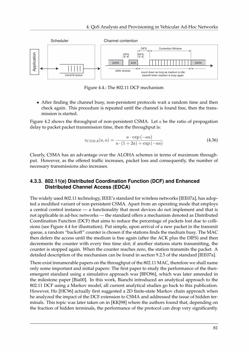
4. QoS Analysis and Provisioning in Vehicular Ad-Hoc Networks
transmit queue
Scheduler
SIFS SIFS
DIFS Contention Window
defer access count down as long as medium is idlebackoff when medium is busy again
Channel contention
Figure 4.4.: The 802.11 DCF mechanism
• After finding the channel busy, non-persistent protocols wait a random time and thencheck again. This procedure is repeated until the channel is found free, then the trans-mission is started.
Figure 4.2 shows the throughput of non-persistent CSMA. Let a be the ratio of propagationdelay to packet packet transmission time, then the throughput is:
vCSMA(u, a) =u · exp (−au)
u · (1 + 2a) + exp (−au)(4.36)
Clearly, CSMA has an advantage over the ALOHA schemes in terms of maximum through-put. However, as the offered traffic increases, packet loss and consequently, the number ofnecessary transmissions also increases.
4.3.3. 802.11(e) Distributed Coordination Function (DCF) and EnhancedDistributed Channel Access (EDCA)
The widely used 802.11 technology, IEEE’s standard for wireless networks [IEE07a], has adop-ted a modified variant of non-persistent CSMA. Apart from an operating mode that employsa central control instance — a functionality that most devices do not implement and that isnot applicable in ad-hoc networks — the standard offers a mechanism denoted as DistributedCoordination Function (DCF) that aims to reduce the percentage of packets lost due to colli-sions (see Figure 4.4 for illustration). Put simple, upon arrival of a new packet in the transmitqueue, a random “backoff” counter is chosen if the stations finds the medium busy. The MACthen defers the access until the medium is free again (after the ACK plus the DIFS) and thendecrements the counter with every free time slot; if another stations starts transmitting, thecounter is stopped again. When the counter reaches zero, the station transmits the packet. Adetailed description of the mechanism can be found in section 9.2.5 of the standard [IEE07a].
There exist innumerable papers on the throughput of the 802.11 MAC, therefore we shall nameonly some important and initial papers: The first paper to study the performance of the then-emergent standard using a simulative approach was [BFO96], which was later amended inthe milestone paper [Bia00]. In this work, Bianchi introduced an analytical approach to the802.11 DCF using a Markov model; all current analytical studies go back to this publication.However, Ho [HC96] actually first suggested a 2D finite-state Markov chain approach whenhe analyzed the impact of the DCF extension to CSMA and addressed the issue of hidden ter-minals. This topic was later taken on in [KKJ98] where the authors found that, depending onthe fraction of hidden terminals, the performance of the protocol can drop very significantly.
81
4.3. Medium Access Protocols
high priority
medium priority
low priority
Scheduler
SIFS SIFS
AIFS[0]
AIFS[1]
AIFS[2,3]
defer access count down as long as medium is idlebackoff when medium is busy again
Channel contention
Figure 4.5.: The 802.11 EDCA mechanism
The so-called capture effect, i.e., the ability of a receiver to correctly decode a transmissionin the presence of other lower-power transmissions, and the resulting capacity of the 802.11MAC protocol in multipath-faded channels has initially been studied in [HVS02].
Recently, broadcast services (especially in the context of vehicular networks) have gained moreattention and consequently some dedicated studies on the performance of 802.11 in broad-cast networks were published. A performance analysis under saturation conditions was pub-lished in [MC08], in which the authors point out that the choice of the range from whichthe backoff counter chooses its value is critical to throughput. The used model was then ex-tended [WAFS09] to also account for non-saturated conditions.
The EDCA of the 802.11e standard offers the possibility to differentiate traffic into four accessclasses, each with their own priority. To achieve this, the DCF mechanism has been modifiedsuch that decreasing the backoff counter is only allowed after variable-length AIFS times havepassed. By this means, higher-priority traffic gain privileged channel access so that AC0 isserved before AC1, which in turn is served before AC2 and AC3 (see Figure 4.5).
Again, a number of studies on the performance have been published. In [TFM05], the authorsanalyze the throughput and delay under saturation conditions and show the effectiveness ofthe prioritization. Using Markov chains, [HD05] presents a unified analytical model for per-formance analysis. Another analytical model is presented in [PPQ10] and the various modelparameters are discussed to facilitate proper design for specific applications. A simulativestudy of the packet loss probability in vehicular broadcast network using priorities is pub-lished in [TMJH04], where the authors analyze the impact of some design parameters andshow that prioritization effectively reduces packet delay. Since the EDCA mechanism wasadopted for the upcoming 802.11p vehicular radio standard [IEE10], a thorough analysis ofEDCA in the control channel can be found in [GMM09]. Some criticism of the EDCA has beenexpressed in [Eic07], where the author states that a careful choice and assignment of applica-tions to access classes is inevitable to provide the desired QoS characteristics of the 802.11pMAC.
4.3.4. Reservation-Based Protocols
In reservation-based protocols (such as, for example, Time Division Multiple Access (TDMA)),the medium is divided into resource partitions (such as time slot, frequencies, codes, etc.)which are then assigned to the individual network nodes. Let us denote a node’s share of the
82
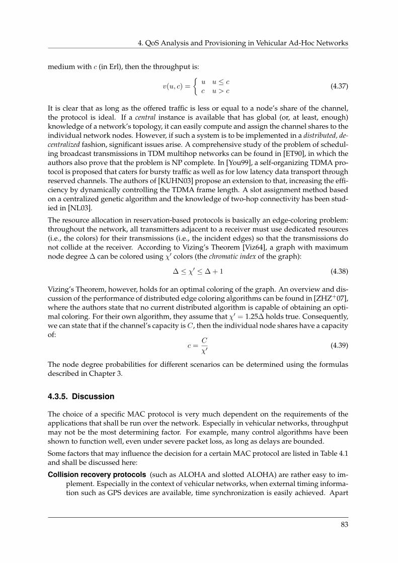
4. QoS Analysis and Provisioning in Vehicular Ad-Hoc Networks
medium with c (in Erl), then the throughput is:
v(u, c) =
u u ≤ cc u > c
(4.37)
It is clear that as long as the offered traffic is less or equal to a node’s share of the channel,the protocol is ideal. If a central instance is available that has global (or, at least, enough)knowledge of a network’s topology, it can easily compute and assign the channel shares to theindividual network nodes. However, if such a system is to be implemented in a distributed, de-centralized fashion, significant issues arise. A comprehensive study of the problem of schedul-ing broadcast transmissions in TDM multihop networks can be found in [ET90], in which theauthors also prove that the problem is NP complete. In [You99], a self-organizing TDMA pro-tocol is proposed that caters for bursty traffic as well as for low latency data transport throughreserved channels. The authors of [KUHN03] propose an extension to that, increasing the effi-ciency by dynamically controlling the TDMA frame length. A slot assignment method basedon a centralized genetic algorithm and the knowledge of two-hop connectivity has been stud-ied in [NL03].
The resource allocation in reservation-based protocols is basically an edge-coloring problem:throughout the network, all transmitters adjacent to a receiver must use dedicated resources(i.e., the colors) for their transmissions (i.e., the incident edges) so that the transmissions donot collide at the receiver. According to Vizing’s Theorem [Viz64], a graph with maximumnode degree ∆ can be colored using χ′ colors (the chromatic index of the graph):
∆ ≤ χ′ ≤ ∆ + 1 (4.38)
Vizing’s Theorem, however, holds for an optimal coloring of the graph. An overview and dis-cussion of the performance of distributed edge coloring algorithms can be found in [ZHZ+07],where the authors state that no current distributed algorithm is capable of obtaining an opti-mal coloring. For their own algorithm, they assume that χ′ = 1.25∆ holds true. Consequently,we can state that if the channel’s capacity is C, then the individual node shares have a capacityof:
c =C
χ′(4.39)
The node degree probabilities for different scenarios can be determined using the formulasdescribed in Chapter 3.
4.3.5. Discussion
The choice of a specific MAC protocol is very much dependent on the requirements of theapplications that shall be run over the network. Especially in vehicular networks, throughputmay not be the most determining factor. For example, many control algorithms have beenshown to function well, even under severe packet loss, as long as delays are bounded.
Some factors that may influence the decision for a certain MAC protocol are listed in Table 4.1and shall be discussed here:
Collision recovery protocols (such as ALOHA and slotted ALOHA) are rather easy to im-plement. Especially in the context of vehicular networks, when external timing informa-tion such as GPS devices are available, time synchronization is easily achieved. Apart
83
4.3. Medium Access Protocols
Collision
Recovery
Collision
Avoidance
Reservation-B
asedA
LOH
A,slotted
ALO
HA
CSM
A,802.11
TDM
A
Com
plexityLow
Medium
High
Time
SynchronizationN
otN
eeded(unslotted)
/M
andatory(slotted)
NotN
eededM
andatory
Mobility
SupportG
oodG
oodProblem
atic
ScalabilityG
oodG
oodLim
ited
ChannelU
sageEfficiency
Low–
Medium
High
High
(dependingon
applica-tion)
Reliability
LowM
ediumH
igh
Susceptibleto
Hidden
Terminals
No
YesN
o
Delay
Characteristics
Determ
inisticProbabilistic
Determ
inistic
Table4.1.:Som
echaracteristics
ofMA
Cprotocolfam
ilies.
84
4. QoS Analysis and Provisioning in Vehicular Ad-Hoc Networks
from that, no further synchronization or interaction with other radios is required. There-fore, these schemes do not require any adaptation to support mobility. The channelusage efficiency, as shown above, is low (≈ 0.18 Erl) to medium (≈ 0.37 Erl) depend-ing on the scheme. The great advantage of (slotted) ALOHA, however, is that it is notsusceptible to hidden terminals and that it offers deterministic delays: upon arrival of anew packet, the channel is either immediately accessed or at the beginning of the nextslot. The outcome of the transmission, however, is rather unreliable.
Collision avoidance protocols (such as CSMA or 802.11) are more complex than collisionrecovery protocols, as they require queues and the additional carrier sense mechanism.This very mechanism also makes their performance susceptible to hidden terminalswhich can reduce their performance significantly, even well below that of slotted ALOHA(see for instance [TK75, KKJ98]). Especially in vehicular scenarios, this effect may be sig-nificant and can render the additional complexity pointless. In scenarios with a lowpercentage of hidden nodes and only a few contending stations, however, the channelusage efficiency can be quite high and the reliability of transmissions is good. The ma-jor drawback of this family of protocols, however, is that their delay characteristic isnon-deterministic: depending on the back-off strategy, the time between packet gener-ation and the actual transmission may vary greatly. Scalability (to a certain extent) andmobility support, however, are good.
Reservation-based protocols (such as TDMA) are most complex to implement, especially ifthere is no central entity that assigns the resources to the individual network nodes. ForTDMA, time synchronization among nodes is crucial for obvious reasons. The changingnetwork topology, especially in vehicular scenarios, imposes great requirements on theresource distribution mechanism. In the same way, the scalability of these networks isconstricted as the administrative effort for resource management increases more thanlinearly with the number of network nodes. The throughput efficiency is high for con-tinuous traffic and low for bursty traffic; a careful consideration of the suitability of sucha protocol should thus be made with respect to the desired applications. Reservation-based protocols, on the other hand, have significant benefits over the other protocols:because contention for resources is not necessary and every node has a guaranteed shareof the medium, the reliability of transmission is very high and the delay characteristicsare absolutely deterministic.
Special respect should also be paid to the type of communication relations: in case that broad-cast applications are to be deployed, ALOHA schemes may have an advantage over CSMAschemes due to infeasible packet-level acknowledgements. Depending on the node degreesin the network and the chosen backoff interval, CSMA schemes will not perform better thanALOHA in terms of packet loss and still reveal non-deterministic delays (see [MC08] for adetailed study of these effects).
The delay distributions of slotted ALOHA and CSMA in unicast scenarios and a comparisonof the two schemes can be found in [YY03]. The global throughput of obstacle-free multi-hop network using ALOHA and CSMA has been studied in [MSQT04]. Other interestingconclusions are drawn in a recent study [KJ08], in which the authors conclude that in networkswith low densities, ALOHA outperforms CSMA. For higher densities, however, the situationreverses. Knowing the density and the structure of a network, these findings raise the questionif a dynamically parameterized MAC layer protocol could be sensible.
Thorough overviews of existing MAC protocols with an explicit emphasis on the deployment
85
4.4. Providing QoS in Contention-Based Networks
in vehicular networks are presented in [MFL06, SK08], in which the authors review designchoices and compare various technologies.
4.4. Providing QoS in Contention-Based Networks
In this section, we assume that a contention-based MAC protocol has been chosen for deploy-ment. In the desire to provide applications with a pre-defined QoS, it is now necessary thatthe application designer specifies at least one of the following QoS parameters:
• Maximum tolerable average packet loss: Using Equation 4.31, the traffic limit u for thecandidate MAC mechanism can be determined.
• Maximum tolerable average delay: With Equation 4.33, the traffic limit u can be deter-mined.
If the cumulated load u in all collision domains is below the determined load limit u, thedesired QoS is attained. The QoS criterion is thus (Equation (4.15)):
u1 ≤(C˜ T + I˜)s (4.40)
As we have described in the previous section, the traffic vector s comprises all traffic that isgenerated by the individual nodes (i.e., unicast, multicast, and broadcast traffic) due to thebroadcast nature of the wireless medium.
To fulfill the QoS criterium given the current network connectivity C˜ , a control algorithm shallbe designed that determines a traffic vector s that (in Equation 4.40):
• guarantees that the load in every collision domain is bounded: ∀i : ui ≤ u, (R1)
• maximizes the traffic si that may be sourced by each node, (R2)
• allocates the amount of traffic sourced so that a fairness criterion among contendingnodes is met (R3).
There are several ways of obtaining s: either, a central instance with global knowledge of thenetwork could compute a global s and then distribute it to the nodes. Or, the nodes themselvescould — through exchanging the appropriate bits of information — compute their own si. Thedynamically computed si shall then be used at the nodes to control their traffic, so that the pre-defined QoS is attained throughout the network.
Obviously, in a purely decentralized ad-hoc scenario, the latter approach is more desirableas infrastructure with global network knowledge is not available. Furthermore, the exchangeof messages with a central entity would either introduce additional messaging overhead orrequire additional communication hardware.
4.4.1. Global Traffic Limits Determination
Although impracticable in a distributed network, a simple iterative global algorithm for bench-marking purposes is outlined in Algorithm 1. Given the vertex set V and the degree vectord5, the algorithm starts with those nodes that have the highest degree di. The QoS criterion
5The degree vector d can be determined through:
d = C˜T1 (4.41)
86
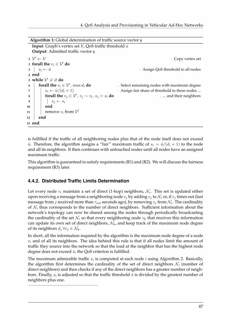
4. QoS Analysis and Provisioning in Vehicular Ad-Hoc Networks
Algorithm 1: Global determination of traffic source vector s
Input: Graph’s vertex set V , QoS traffic threshold uOutput: Admitted traffic vector s
1 V ′ ← V . Copy vertex set2 forall the vi ∈ V ′ do3 si ← u . Assign QoS threshold to all nodes4 end5 while V ′ 6= ∅ do6 forall the vi ∈ V ′, max di do . Select remaining nodes with maximum degree7 si ← u/(di + 1) . Assign fair share of threshold to these nodes ...8 forall the vj ∈ V ′, vj ∼ vi, sj > si do . ... and their neighbors9 sj ← si
10 end11 remove vi from V ′12 end13 end
is fulfilled if the traffic of all neighboring nodes plus that of the node itself does not exceedu. Therefore, the algorithm assigns a “fair” maximum traffic of si = u/(di + 1) to the nodeand all its neighbors. It then continues with untouched nodes until all nodes have an assignedmaximum traffic.
This algorithm is guaranteed to satisfy requirements (R1) and (R2). We will discuss the fairnessrequirement (R3) later.
4.4.2. Distributed Traffic Limits Determination
Let every node vi maintain a set of direct (1-hop) neighbors, Ni. This set is updated eitherupon receiving a message from a neighboring node vj by adding vj toNi or, if vj times out (lastmessage from j received more than τout seconds ago), by removing vj fromNi. The cardinalityof Ni thus corresponds to the number of direct neighbors. Sufficient information about thenetwork’s topology can now be shared among the nodes through periodically broadcastingthe cardinality of the set Ni so that every neighboring node vk that receives this informationcan update its own set of direct neighbors, Nk, and keep track of the maximum node degreeof its neighbors dj ∀vj ∈ Nk.
In short, all the information required by the algorithm is the maximum node degree of a nodevi and of all its neighbors. The idea behind this rule is that if all nodes limit the amount oftraffic they source into the network so that the load at the neighbor that has the highest nodedegree does not exceed u, the QoS criterion is fulfilled.
The maximum admissible traffic si is computed at each node i using Algorithm 2. Basically,the algorithm first determines the cardinality of the set of direct neighbors Ni (number ofdirect neighbors) and then checks if any of the direct neighbors has a greater number of neigh-bors. Finally, si is adjusted so that the traffic threshold u is divided by the greatest number ofneighbors plus one.
87
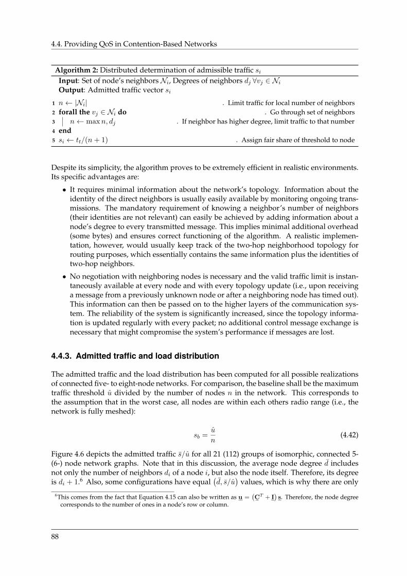
4.4. Providing QoS in Contention-Based Networks
Algorithm 2: Distributed determination of admissible traffic siInput: Set of node’s neighbors Ni, Degrees of neighbors dj ∀vj ∈ NiOutput: Admitted traffic vector si
1 n← |Ni| . Limit traffic for local number of neighbors2 forall the vj ∈ Ni do . Go through set of neighbors3 n← maxn, dj . If neighbor has higher degree, limit traffic to that number4 end5 si ← tt/(n+ 1) . Assign fair share of threshold to node
Despite its simplicity, the algorithm proves to be extremely efficient in realistic environments.Its specific advantages are:
• It requires minimal information about the network’s topology. Information about theidentity of the direct neighbors is usually easily available by monitoring ongoing trans-missions. The mandatory requirement of knowing a neighbor’s number of neighbors(their identities are not relevant) can easily be achieved by adding information about anode’s degree to every transmitted message. This implies minimal additional overhead(some bytes) and ensures correct functioning of the algorithm. A realistic implemen-tation, however, would usually keep track of the two-hop neighborhood topology forrouting purposes, which essentially contains the same information plus the identities oftwo-hop neighbors.
• No negotiation with neighboring nodes is necessary and the valid traffic limit is instan-taneously available at every node and with every topology update (i.e., upon receivinga message from a previously unknown node or after a neighboring node has timed out).This information can then be passed on to the higher layers of the communication sys-tem. The reliability of the system is significantly increased, since the topology informa-tion is updated regularly with every packet; no additional control message exchange isnecessary that might compromise the system’s performance if messages are lost.
4.4.3. Admitted traffic and load distribution
The admitted traffic and the load distribution has been computed for all possible realizationsof connected five- to eight-node networks. For comparison, the baseline shall be the maximumtraffic threshold u divided by the number of nodes n in the network. This corresponds tothe assumption that in the worst case, all nodes are within each others radio range (i.e., thenetwork is fully meshed):
sb =u
n(4.42)
Figure 4.6 depicts the admitted traffic s/u for all 21 (112) groups of isomorphic, connected 5-(6-) node network graphs. Note that in this discussion, the average node degree d includesnot only the number of neighbors di of a node i, but also the node itself. Therefore, its degreeis di + 1.6 Also, some configurations have equal
(d, s/u
)values, which is why there are only
6This comes from the fact that Equation 4.15 can also be written as u =(C˜T + I˜) s. Therefore, the node degree
corresponds to the number of ones in a node’s row or column.
88

4. QoS Analysis and Provisioning in Vehicular Ad-Hoc Networks
0.2
0.25
0.3
0.35
0.4
2.5 3 3.5 4 4.5 5
Aver
age
Traf
fic P
er N
ode
Average Node Degree
(a) 5-node networks
0.15
0.2
0.25
0.3
0.35
0.4
2.5 3 3.5 4 4.5 5 5.5 6
Aver
age
Traf
fic P
er N
ode
Average Node Degree
(b) 6-node networks
Figure 4.6.: Average admitted traffic per node s (in units of u) over average node degree d.Upper and lower bounds are also shown (dashed lines).
89
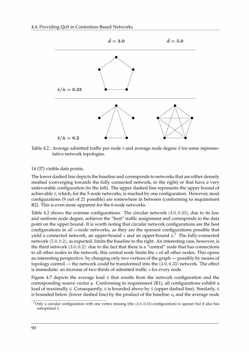
4.4. Providing QoS in Contention-Based Networks
d = 3.0 d = 5.0
s/u = 0.33
s/u = 0.2
Table 4.2.: Average admitted traffic per node s and average node degree d for some represen-tative network topologies.
14 (37) visible data points.
The lower dashed line depicts the baseline and corresponds to networks that are either denselymeshed (converging towards the fully connected network, to the right) or that have a veryunfavorable configuration (to the left). The upper dashed line represents the upper bound ofachievable s, which, for the 5-node networks, is reached by one configuration. However, mostconfigurations (9 out of 21 possible) are somewhere in between (conforming to requirementR2). This is even more apparent for the 6-node networks.
Table 4.2 shows the extreme configurations. The circular network (3.0, 0.33), due to its lowand uniform node degree, achieves the “best” traffic assignment and corresponds to the datapoint on the upper bound. It is worth noting that circular network configurations are the bestconfigurations in all n-node networks, as they are the sparsest configurations possible thatyield a connected network, an upper-bound s and an upper-bound u.7 The fully-connectednetwork (5.0, 0.2), as expected, limits the baseline to the right. An interesting case, however, isthe third network (3.0, 0.2): due to the fact that there is a “central” node that has connectionsto all other nodes in the network, this central node limits the s of all other nodes. This opensan interesting perspective: by changing only two vertices of the graph — possibly by means oftopology control — the network could be transformed into the (3.0, 0.33) network. The effectis immediate: an increase of two thirds of admitted traffic s for every node.
Figure 4.7 depicts the average load u that results from the network configuration and thecorresponding source vector s. Conforming to requirement (R1), all configurations exhibit aload of maximally u. Consequently, u is bounded above by u (upper dashed line). Similarly, uis bounded below (lower dashed line) by the product of the baseline sb and the average node
7Only a circular configuration with one vertex missing (the (2.6, 0.33)-configuration) is sparser but it also hassuboptimal u.
90

4. QoS Analysis and Provisioning in Vehicular Ad-Hoc Networks
0.5
0.6
0.7
0.8
0.9
1
2.5 3 3.5 4 4.5 5
Aver
age
Load
Average Node Degree
(a) 5-node networks
0.4
0.5
0.6
0.7
0.8
0.9
1
2.5 3 3.5 4 4.5 5 5.5 6
Aver
age
Load
Average Node Degree
(b) 6-node networks
Figure 4.7.: Average load u (in units of u) over average node degree d. Upper and lowerbounds are also shown (dashed lines).
91
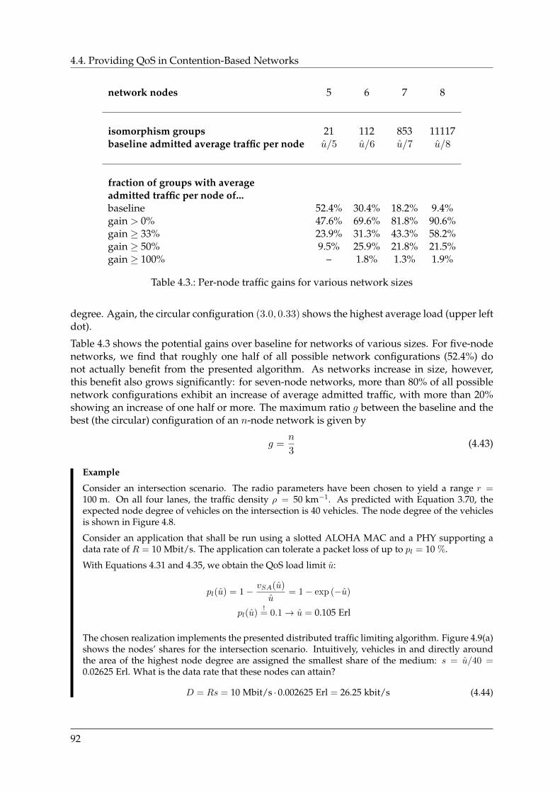
4.4. Providing QoS in Contention-Based Networks
network nodes 5 6 7 8
isomorphism groups 21 112 853 11117baseline admitted average traffic per node u/5 u/6 u/7 u/8
fraction of groups with averageadmitted traffic per node of...baseline 52.4% 30.4% 18.2% 9.4%gain > 0% 47.6% 69.6% 81.8% 90.6%gain ≥ 33% 23.9% 31.3% 43.3% 58.2%gain ≥ 50% 9.5% 25.9% 21.8% 21.5%gain ≥ 100% – 1.8% 1.3% 1.9%
Table 4.3.: Per-node traffic gains for various network sizes
degree. Again, the circular configuration (3.0, 0.33) shows the highest average load (upper leftdot).
Table 4.3 shows the potential gains over baseline for networks of various sizes. For five-nodenetworks, we find that roughly one half of all possible network configurations (52.4%) donot actually benefit from the presented algorithm. As networks increase in size, however,this benefit also grows significantly: for seven-node networks, more than 80% of all possiblenetwork configurations exhibit an increase of average admitted traffic, with more than 20%showing an increase of one half or more. The maximum ratio g between the baseline and thebest (the circular) configuration of an n-node network is given by
g =n
3(4.43)
Example
Consider an intersection scenario. The radio parameters have been chosen to yield a range r =100 m. On all four lanes, the traffic density ρ = 50 km−1. As predicted with Equation 3.70, theexpected node degree of vehicles on the intersection is 40 vehicles. The node degree of the vehiclesis shown in Figure 4.8.
Consider an application that shall be run using a slotted ALOHA MAC and a PHY supporting adata rate of R = 10 Mbit/s. The application can tolerate a packet loss of up to pl = 10 %.
With Equations 4.31 and 4.35, we obtain the QoS load limit u:
pl(u) = 1− vSA(u)
u= 1− exp (−u)
pl(u)!= 0.1→ u = 0.105 Erl
The chosen realization implements the presented distributed traffic limiting algorithm. Figure 4.9(a)shows the nodes’ shares for the intersection scenario. Intuitively, vehicles in and directly aroundthe area of the highest node degree are assigned the smallest share of the medium: s = u/40 =0.02625 Erl. What is the data rate that these nodes can attain?
D = Rs = 10 Mbit/s · 0.002625 Erl = 26.25 kbit/s (4.44)
92
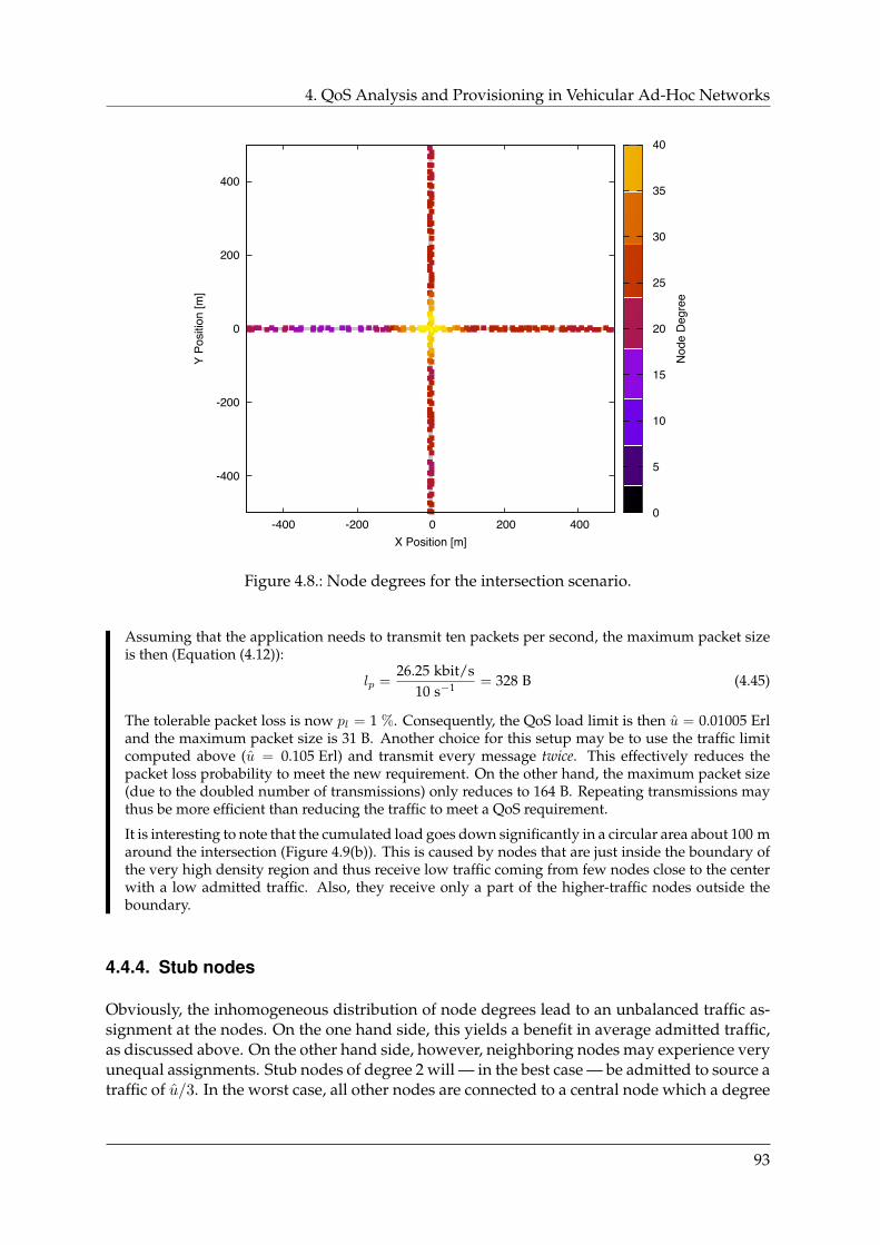
4. QoS Analysis and Provisioning in Vehicular Ad-Hoc Networks
-400
-200
0
200
400
-400 -200 0 200 400
Y Po
sitio
n [m
]
X Position [m]
0
5
10
15
20
25
30
35
40
Nod
e D
egre
e
Figure 4.8.: Node degrees for the intersection scenario.
Assuming that the application needs to transmit ten packets per second, the maximum packet sizeis then (Equation (4.12)):
lp =26.25 kbit/s
10 s−1 = 328 B (4.45)
The tolerable packet loss is now pl = 1 %. Consequently, the QoS load limit is then u = 0.01005 Erland the maximum packet size is 31 B. Another choice for this setup may be to use the traffic limitcomputed above (u = 0.105 Erl) and transmit every message twice. This effectively reduces thepacket loss probability to meet the new requirement. On the other hand, the maximum packet size(due to the doubled number of transmissions) only reduces to 164 B. Repeating transmissions maythus be more efficient than reducing the traffic to meet a QoS requirement.
It is interesting to note that the cumulated load goes down significantly in a circular area about 100 maround the intersection (Figure 4.9(b)). This is caused by nodes that are just inside the boundary ofthe very high density region and thus receive low traffic coming from few nodes close to the centerwith a low admitted traffic. Also, they receive only a part of the higher-traffic nodes outside theboundary.
4.4.4. Stub nodes
Obviously, the inhomogeneous distribution of node degrees lead to an unbalanced traffic as-signment at the nodes. On the one hand side, this yields a benefit in average admitted traffic,as discussed above. On the other hand side, however, neighboring nodes may experience veryunequal assignments. Stub nodes of degree 2 will — in the best case — be admitted to source atraffic of u/3. In the worst case, all other nodes are connected to a central node which a degree
93
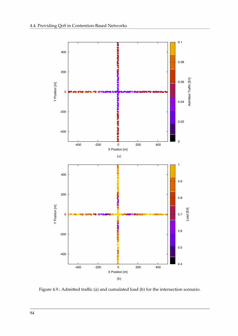
4.4. Providing QoS in Contention-Based Networks
-400
-200
0
200
400
-400 -200 0 200 400
Y Po
sitio
n [m
]
X Position [m]
0
0.02
0.04
0.06
0.08
0.1
Adm
itted
Tra
ffic
[Erl]
(a)
-400
-200
0
200
400
-400 -200 0 200 400
Y Po
sitio
n [m
]
X Position [m]
0.4
0.5
0.6
0.7
0.8
0.9
1
Load
[Erl]
(b)
Figure 4.9.: Admitted traffic (a) and cumulated load (b) for the intersection scenario.
94
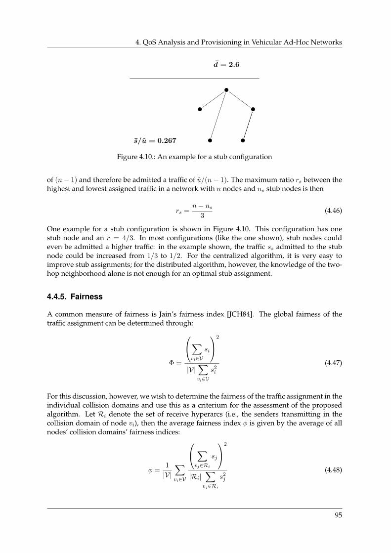
4. QoS Analysis and Provisioning in Vehicular Ad-Hoc Networks
d = 2.6
s/u = 0.267
Figure 4.10.: An example for a stub configuration
of (n− 1) and therefore be admitted a traffic of u/(n− 1). The maximum ratio rs between thehighest and lowest assigned traffic in a network with n nodes and ns stub nodes is then
rs =n− ns
3(4.46)
One example for a stub configuration is shown in Figure 4.10. This configuration has onestub node and an r = 4/3. In most configurations (like the one shown), stub nodes couldeven be admitted a higher traffic: in the example shown, the traffic ss admitted to the stubnode could be increased from 1/3 to 1/2. For the centralized algorithm, it is very easy toimprove stub assignments; for the distributed algorithm, however, the knowledge of the two-hop neighborhood alone is not enough for an optimal stub assignment.
4.4.5. Fairness
A common measure of fairness is Jain’s fairness index [JCH84]. The global fairness of thetraffic assignment can be determined through:
Φ =
∑vi∈V
si
2
|V|∑vi∈V
s2i
(4.47)
For this discussion, however, we wish to determine the fairness of the traffic assignment in theindividual collision domains and use this as a criterium for the assessment of the proposedalgorithm. Let Ri denote the set of receive hyperarcs (i.e., the senders transmitting in thecollision domain of node vi), then the average fairness index φ is given by the average of allnodes’ collision domains’ fairness indices:
φ =1
|V|∑vi∈V
∑vj∈Ri
sj
2
|Ri|∑vj∈Ri
s2j
(4.48)
95
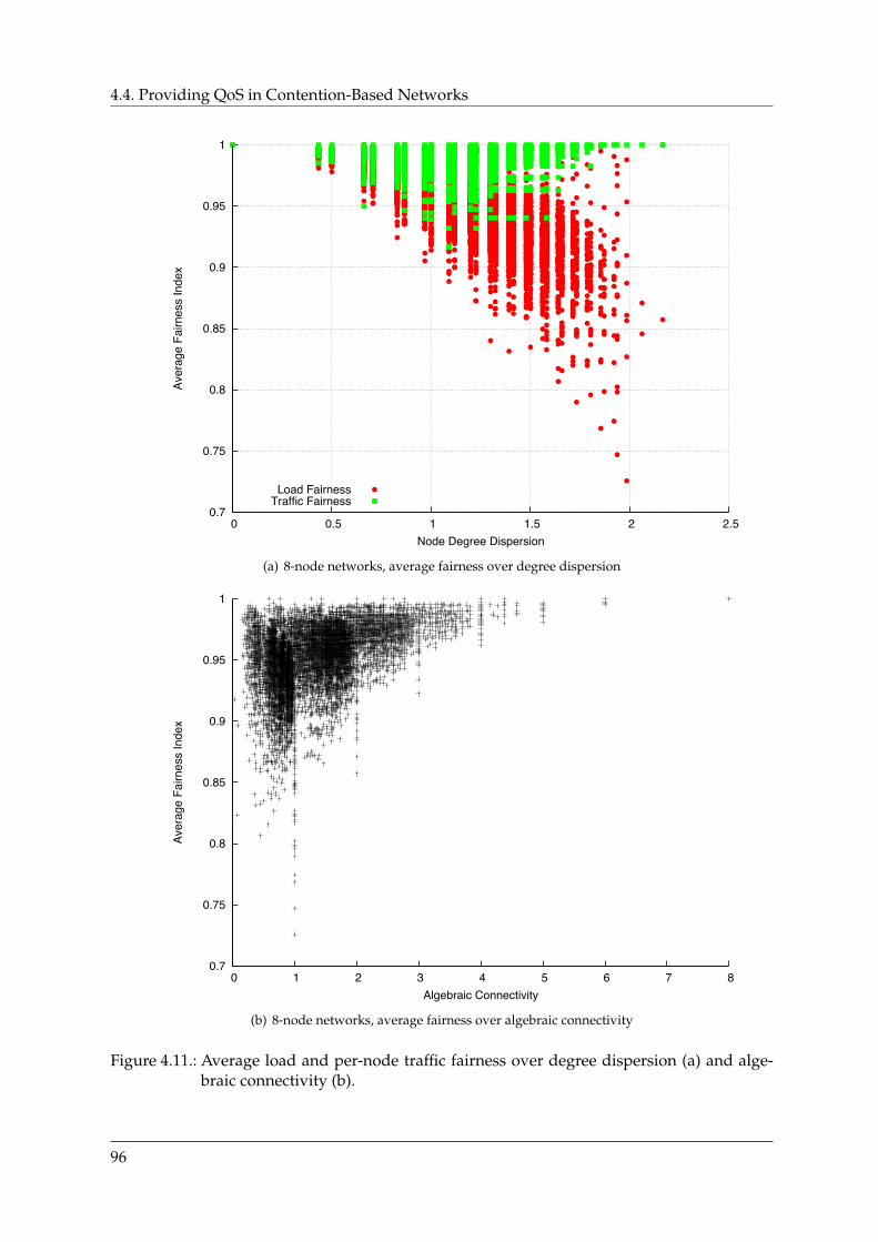
4.4. Providing QoS in Contention-Based Networks
0.7
0.75
0.8
0.85
0.9
0.95
1
0 0.5 1 1.5 2 2.5
Aver
age
Fairn
ess
Inde
x
Node Degree Dispersion
Load FairnessTraffic Fairness
(a) 8-node networks, average fairness over degree dispersion
0.7
0.75
0.8
0.85
0.9
0.95
1
0 1 2 3 4 5 6 7 8
Aver
age
Fairn
ess
Inde
x
Algebraic Connectivity
(b) 8-node networks, average fairness over algebraic connectivity
Figure 4.11.: Average load and per-node traffic fairness over degree dispersion (a) and alge-braic connectivity (b).
96
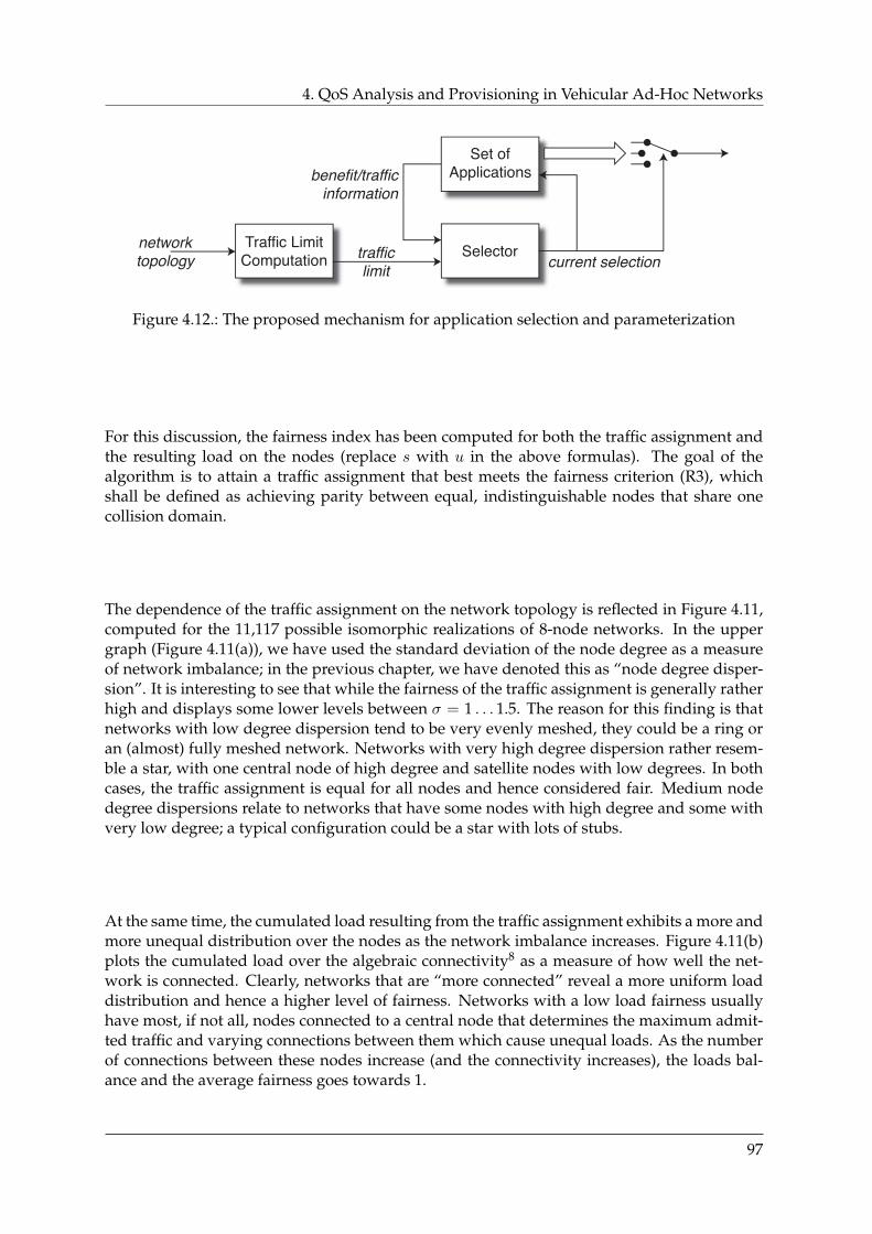
4. QoS Analysis and Provisioning in Vehicular Ad-Hoc Networks
Figure 4.12.: The proposed mechanism for application selection and parameterization
For this discussion, the fairness index has been computed for both the traffic assignment andthe resulting load on the nodes (replace s with u in the above formulas). The goal of thealgorithm is to attain a traffic assignment that best meets the fairness criterion (R3), whichshall be defined as achieving parity between equal, indistinguishable nodes that share onecollision domain.
The dependence of the traffic assignment on the network topology is reflected in Figure 4.11,computed for the 11,117 possible isomorphic realizations of 8-node networks. In the uppergraph (Figure 4.11(a)), we have used the standard deviation of the node degree as a measureof network imbalance; in the previous chapter, we have denoted this as “node degree disper-sion”. It is interesting to see that while the fairness of the traffic assignment is generally ratherhigh and displays some lower levels between σ = 1 . . . 1.5. The reason for this finding is thatnetworks with low degree dispersion tend to be very evenly meshed, they could be a ring oran (almost) fully meshed network. Networks with very high degree dispersion rather resem-ble a star, with one central node of high degree and satellite nodes with low degrees. In bothcases, the traffic assignment is equal for all nodes and hence considered fair. Medium nodedegree dispersions relate to networks that have some nodes with high degree and some withvery low degree; a typical configuration could be a star with lots of stubs.
At the same time, the cumulated load resulting from the traffic assignment exhibits a more andmore unequal distribution over the nodes as the network imbalance increases. Figure 4.11(b)plots the cumulated load over the algebraic connectivity8 as a measure of how well the net-work is connected. Clearly, networks that are “more connected” reveal a more uniform loaddistribution and hence a higher level of fairness. Networks with a low load fairness usuallyhave most, if not all, nodes connected to a central node that determines the maximum admit-ted traffic and varying connections between them which cause unequal loads. As the numberof connections between these nodes increase (and the connectivity increases), the loads bal-ance and the average fairness goes towards 1.
97
4.5. Application Selection and Parameterization
4.5. Application Selection and Parameterization
A potential implementation of a higher-layer application selector and parameterization is out-lined in Figure 4.12: Once a node vi has computed its traffic limit si, the information can beused at higher layers to select a subset of active applications for a set of runnable applications.Also, the selected applications can then be parameterized by assigning them a specific shareof the admitted traffic.
Let us assume that the application selector has a specific set of applications P to choose from.Every application has an associated utility function that accepts as a parameter the applica-tion’s share of the admitted traffic, sp:
∀p ∈ P : Up(sp) (4.50)
Selecting the set of active applications P∗ ⊆ P is then a maximization problem, as describedand discussed in [FC05]:
maximize∑p∈P∗
Up(sp) (4.51)
subject to∑p∈P∗
sp ≤ si (4.52)
where the variables are sp and P∗. It should be noted that applications also need to have prior-ities associated so that during the selection process, safety-critical applications are consideredbefore non-critical applications are assessed.
Feeding back the traffic allocation to the applications could enable them to adapt to the currentspecific network state and to better select, quantize, and/or reduce the transmitted informa-tion and thus increase the overall utility. Some examples of parametrizable applications are:
• Cooperative awareness applications can be parameterized so that for instance the reso-lution of the transmitted data can be adjusted or the range of the transmitted informationis limited. This could be done, for instance, with occupancy maps as well as with im-ages or live video streams. Also, GPS data could be quantified according to the availablebandwidth. The global utility may be much greater if more applications can be run atlower data rates (for example, low-resolution video plus low-resolution GPS) than onlyone application run at a higher data rate.
• Cooperative driving applications could be parameterized so that potentially unsafe sit-uations can be avoided. For instance, a cooperative adaptive cruise control could beadjusted so that the time gap between the controlled vehicle and the leading vehicle islong enough to ensure safe operation of the algorithm, even if the status of the networkdoes not allow very high resolution of communicated sensor data.
Furthermore, the applications should be able to dynamically alter their utility function, de-pending on the current driving situation. For instance, an intersection assistant has a higher
8The algebraic connectivity is commonly defined as the second-smallest eigenvector λ2 of the Laplacian matrixL˜ of the network’s graph [Fie73], where C˜ is the connectivity matrix as defined above:
L˜ = diag(C˜T1)−C˜T (4.49)
98
4. QoS Analysis and Provisioning in Vehicular Ad-Hoc Networks
utility when driving in a city than when driving on a highway. At the same time, a colli-sion avoidance application may run at lower data rates with the same utility when driving inheavily congested traffic than in free-flow traffic.
The exact realization of such a solution shall not be discussed here, instead we would like torefer the reader to the works of Eichler [ESKS06] and Zhou [ZGZC09], where these optimiza-tion issues are addressed in-depth.
4.6. Conclusion
In this chapter, we have demonstrated a graph-theoretic representation of network connec-tivity using hypergraphs and connectivity matrices. We have discussed the broadcast natureof the wireless medium and introduced the concept of traffic vectors that we use to describethe traffic in a network and to study the cumulated load as the result of the connectivity andthe traffic. Furthermore, we have presented various relevant MAC protocols that qualify forimplementation in a vehicular network. By quantifying their specific traffic/packet loss re-lations, based on their specific offered traffic to throughput relation (v(u)), we could infer amethod to determine the maximum allowable load, given a desired level of QoS, which maybe described by either the maximum allowable packet loss or delay for a specific application.The insights gained from the MAC protocol and network modeling as described here can beused for the performance analysis of MAC protocols, given scenarios described through themeans presented in Chapter 3.
These insights can also be used as input parameters for the algorithm presented in the fol-lowing, that allows for fast computation of the maximum admissible traffic at any node in agiven network. We have demonstrated both a centralized algorithm using global knowledge,and a decentralized algorithm that uses two-hop connectivity information to instantaneouslycompute the admissible traffic at each node. We have shown through complete simulations forfive-, six-, seven-, and eight-node networks that both algorithms guarantee that the network isnot overloaded and that most nodes achieve the highest possible traffic assignment. We havealso discussed exceptions and bounds. Using the presented algorithm, we can ensure that themaximum load chosen at design time is never exceeded at runtime and that, consequently, thedesired QoS is attained at all times. The algorithms is thus perfectly suited for implementationin networks as an effective QoS control mechanism.
Further work on this topic should seize on the opportunity to not only compute an optimal sfor a given connectivity matrix C˜ , but also to try to optimize the connectivity matrix itself fora desired traffic. This may be attained through advanced techniques such as power control (asimplicitly presented in [TMMSH09]) or smart antennas. Another starting point may also beto study how one node can maintain a set of connectivity matrices for diverse data rates andconsequently, since traffic is the quotient of a message’s packet size times its generation rateover the data rate at which it is being sent, diverse traffic and cumulated load. This may bedesirable since closer nodes could be served at higher data rates (and lower traffic) withoutdisturbing long-haul transmissions that run at lower data rates (and thus cause higher traffic).To do so, it would be necessary to introduce the idea of a receiver sets for certain messagesand then choosing optimal C˜ s for these transmissions.
99
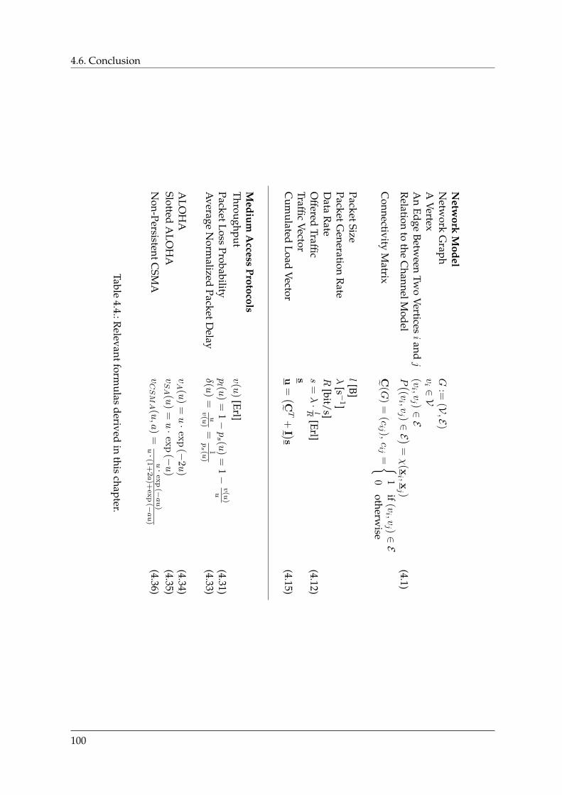
4.6. Conclusion
Netw
orkM
odelN
etwork
Graph
G:=
(V,E
)A
Vertexvi ∈V
An
EdgeBetw
eenTw
oVertices
iandj
(vi ,v
j )∈E
Relation
tothe
ChannelM
odelP ((v
i ,vj )∈
E )=χ
(xi ,x
j )(4.1)
Connectivity
Matrix
C˜( G
)=
(cij ),
cij
= 1
if(vi ,v
j )∈E
0otherw
ise
PacketSizel[B]
PacketGeneration
Rate
λ[s −
1]D
ataR
ateR
[bit/s]O
fferedTraffic
s=λ·lR
[Erl](4.12)
T rafficVector
sC
umulated
LoadVector
u= (C˜
T+
I˜ )s(4.15)
Medium
Access
ProtocolsThroughput
v(u
)[Erl]
PacketLossProbability
pl (u
)=
1−ps (u
)=
1−
v(u
)u
(4.31)A
verageN
ormalized
PacketDelay
δ(u)
=uv(u
)=
1ps(u
)(4.33)
ALO
HA
vA
(u)
=u·
exp
(−2u
)(4.34)
SlottedA
LOH
AvSA
(u)
=u·
exp
(−u
)(4.35)
Non-PersistentC
SMA
vCSMA
(u,a
)=
u·ex
p(−au
)u·
(1+
2a)+
exp
( −au
)(4.36)
Table4.4.:R
elevantformulas
derivedin
thischapter.
100
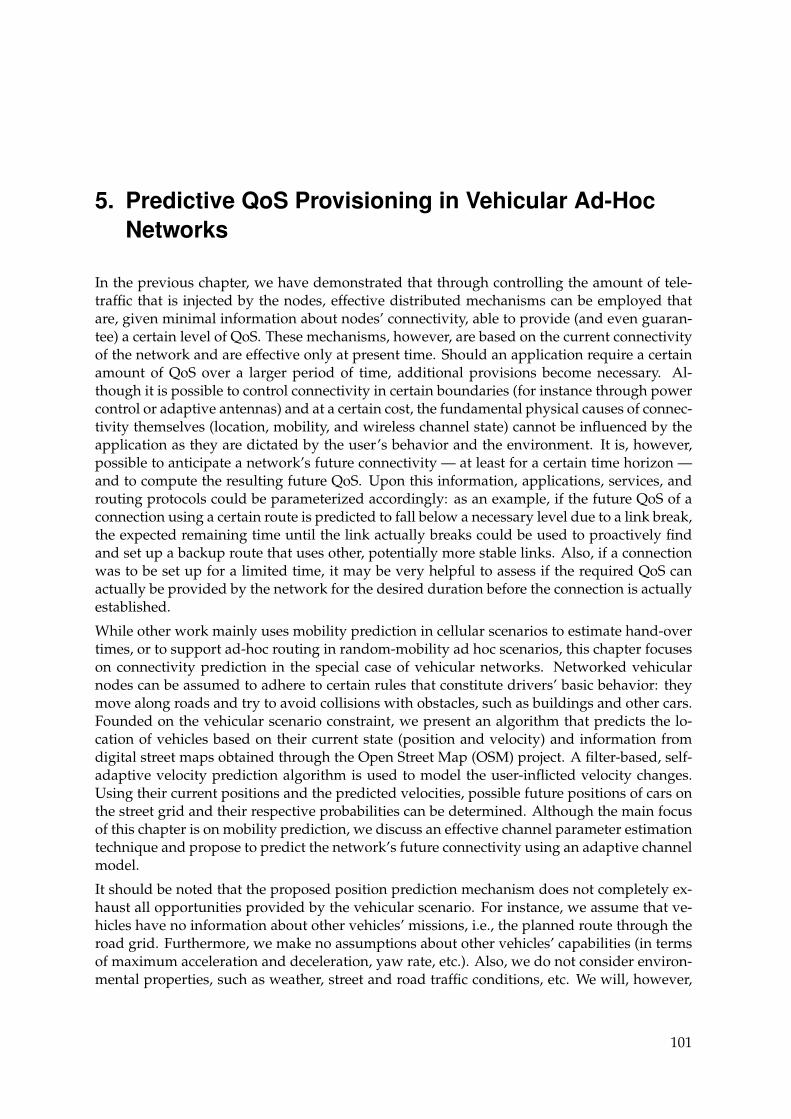
5. Predictive QoS Provisioning in Vehicular Ad-HocNetworks
In the previous chapter, we have demonstrated that through controlling the amount of tele-traffic that is injected by the nodes, effective distributed mechanisms can be employed thatare, given minimal information about nodes’ connectivity, able to provide (and even guaran-tee) a certain level of QoS. These mechanisms, however, are based on the current connectivityof the network and are effective only at present time. Should an application require a certainamount of QoS over a larger period of time, additional provisions become necessary. Al-though it is possible to control connectivity in certain boundaries (for instance through powercontrol or adaptive antennas) and at a certain cost, the fundamental physical causes of connec-tivity themselves (location, mobility, and wireless channel state) cannot be influenced by theapplication as they are dictated by the user’s behavior and the environment. It is, however,possible to anticipate a network’s future connectivity — at least for a certain time horizon —and to compute the resulting future QoS. Upon this information, applications, services, androuting protocols could be parameterized accordingly: as an example, if the future QoS of aconnection using a certain route is predicted to fall below a necessary level due to a link break,the expected remaining time until the link actually breaks could be used to proactively findand set up a backup route that uses other, potentially more stable links. Also, if a connectionwas to be set up for a limited time, it may be very helpful to assess if the required QoS canactually be provided by the network for the desired duration before the connection is actuallyestablished.
While other work mainly uses mobility prediction in cellular scenarios to estimate hand-overtimes, or to support ad-hoc routing in random-mobility ad hoc scenarios, this chapter focuseson connectivity prediction in the special case of vehicular networks. Networked vehicularnodes can be assumed to adhere to certain rules that constitute drivers’ basic behavior: theymove along roads and try to avoid collisions with obstacles, such as buildings and other cars.Founded on the vehicular scenario constraint, we present an algorithm that predicts the lo-cation of vehicles based on their current state (position and velocity) and information fromdigital street maps obtained through the Open Street Map (OSM) project. A filter-based, self-adaptive velocity prediction algorithm is used to model the user-inflicted velocity changes.Using their current positions and the predicted velocities, possible future positions of cars onthe street grid and their respective probabilities can be determined. Although the main focusof this chapter is on mobility prediction, we discuss an effective channel parameter estimationtechnique and propose to predict the network’s future connectivity using an adaptive channelmodel.
It should be noted that the proposed position prediction mechanism does not completely ex-haust all opportunities provided by the vehicular scenario. For instance, we assume that ve-hicles have no information about other vehicles’ missions, i.e., the planned route through theroad grid. Furthermore, we make no assumptions about other vehicles’ capabilities (in termsof maximum acceleration and deceleration, yaw rate, etc.). Also, we do not consider environ-mental properties, such as weather, street and road traffic conditions, etc. We will, however,
101
5.1. Related Work
point out and discuss the potential spots where these additional informations could be ex-ploited to further augment the proposed algorithm.
Most of the material in this chapter has been published in [NM11].
5.1. Related Work
One possible way of predicting a network’s future connectivity is to use a model that reflectsthe individual mobility properties of a node. Given the knowledge of the initial position ve-locity of a node, a future position could be projected by multiplying the velocity vector withthe desired time interval. Obviously, this approach does not account for changes in the lengthand/or direction of the velocity vector. Several more sophisticated approaches have beensuggested and today, mobility prediction has become a common research topic in wirelessnetworks.
Due to the distinct characteristics of vehicular ad-hoc networks, especially the high speeds andrestricted degree of freedom in the movement of vehicles, most of the work on prediction forad hoc networks is too general and thus inappropriate for vehicular networks. Nevertheless,some approaches are discussed here because they give an overview of mobility prediction ingeneral. Material specific to mobility prediction in vehicular networks is very rare and thetopic is often neglected in works on vehicular ad hoc networks.
[KK10] presents an approach for mobility prediction using neural networks. Although it isnot specifically designed for vehicular networks it should perform better than other generalapproaches as it is independent of the underlying mobility model. A trajectory is calculatedfor multiple steps in the future using several past positions in quite a similar manner as theadapting Finite Impulse Response (FIR) filter for velocity prediction presented in this work.However, the approach does not use any map material and hence the predicted positions maylie far off the road and may thus be unrealistic. The approach using neural networks could beused for velocity prediction in the constellation presented in this works to substitute the FIRfilter, however it is expected to perform in a very similar manner and the FIR filter seems lesscomplex to implement.
A similar approach for mobility prediction using spatial contextual maps and Dempster-Shafer’s theory for decision making is formulated in [SK05]. A framework is presented thatallows prediction of the users mobility trajectory based on various bits of contextual informa-tion from e.g. user profile and map data. The approach is motivated by the fact that contextualinformation is becoming more common for adapting services towards the users needs and ituses the additional information in order to predict the users mobility. The concept seems fea-sible for e.g. cell phone users traveling on foot but does not seem appropriate for vehicularnetworks as the only contextual information possibly available and relevant to the future mo-bility is the chosen route to the destination. A complex theory to combine evidence into aprediction is not necessary in this case.
[HCY+08] suggests a prediction algorithm based on fuzzy logic that aims at the prediction ofa possible link break or a congested link which then triggers the construction of an alternateroute. Similar to our algorithm, the prediction of a link break is based on the prediction ofthe future vehicle speed, the basis on which the predicted distance to the vehicle can be deter-mined. This requires the generation of a fuzzy rule base that is then dynamically trained usingParticle Swarm optimization (which in our approach is done using the adaptive filter for speed
102
5. Predictive QoS Provisioning in Vehicular Ad-Hoc Networks
prediction). The authors use similar ideas in terms of the speed prediction but implements afundamentally different concept. Furthermore, it is focussed on route break prediction andhence the performance of the isolated velocity prediction compared to our algorithm cannotbe easily evaluated.
In [BRP09], the authors present some general thoughts on mobility prediction in vehicularnetworks and propose a simple prediction algorithm based on movement vectors in order toreduce the frequency of location beacons without introducing a higher mean error in respectto the positions used for routing packets. In [RPB09], the same authors introduce the NetworkNeighbor Prediction protocol (NNP) that uses the results from their prior works to predictnew routes that are going to be available in the near future and to calculate the lifetime ofthose routes that are currently in use.
Another approach, although developed in the context of a different problem, is describedby [ASB10]. The authors compute the set of points that could be reached by vehicles withinthe prediction times, given the capabilities (minimum and maximum acceleration, yaw rate,etc). of the considered vehicles. The approach is computationally complex and requires a lotof contextual information.
These previous works have demonstrated in their simulation results that mobility predictionis a useful and necessary aspect in vehicular networks and should be researched in greaterdetail than it currently is. Our approach extends the available mechanisms by complementingthe adaptive FIR filter approach with road data from digital maps, which further increases theprecision of prediction.
Using the predicted position it should also be possible to predict the future connectivity to acertain extent using an appropriate channel model. Due to the complexity of the V2V chan-nel (see literature survey in Section 3.2.4), an adequate prediction of channel quality seemschallenging. Analogous to position prediction, an estimation of channel quality can be seenas a trade-off between computational complexity and prediction accuracy. An approach in-volving ray-tracing similar to the one presented in [MSX06] on the one hand produces ratheradequate results if provided with the necessary extent of details concerning the surroundingenvironment (including moving and parked vehicles), building geometries, plants and roadsigns. However, it seems unrealistic and infeasible to supply an on-board connectivity predic-tion engine with this amount of knowledge. Measurements suggest a dual-slope model forthe Path Loss Exponent (PLE) as a simple yet effective approach. Small-scale fading is usu-ally modeled using statistical models with strong dependency upon separation distance whichlimits the possibilities of a prediction to a qualitative worst case approximation. [PKC+09] alsoidentifies significant differences between LOS and NLOS cases in both path loss and fadingstatistics.
A sophisticated approach to predict the PLE using a particle filter has been proposed in [RC10],based on a log-normal fading channel model in wireless sensor networks. Particles are ini-tialized in a random state with their respective weights being iteratively updated to providean estimation of the path loss exponent. Weak particles with low weights are periodicallyreplaced to avoid degeneration. The filter is parameterized with the type of the fading distri-bution and its variance. The authors, too, show that the PLE changes significantly as soon asthe LOS is lost.
Our work extends the particle filter approach in that it bases on the dual-slope channel modelas presented in Chapter 3. By using digital map information, it is possible to obtain the lengthof the LOS path and to estimate the channel’s LOS and NLOSÊPLEs. In conjunction with the
103
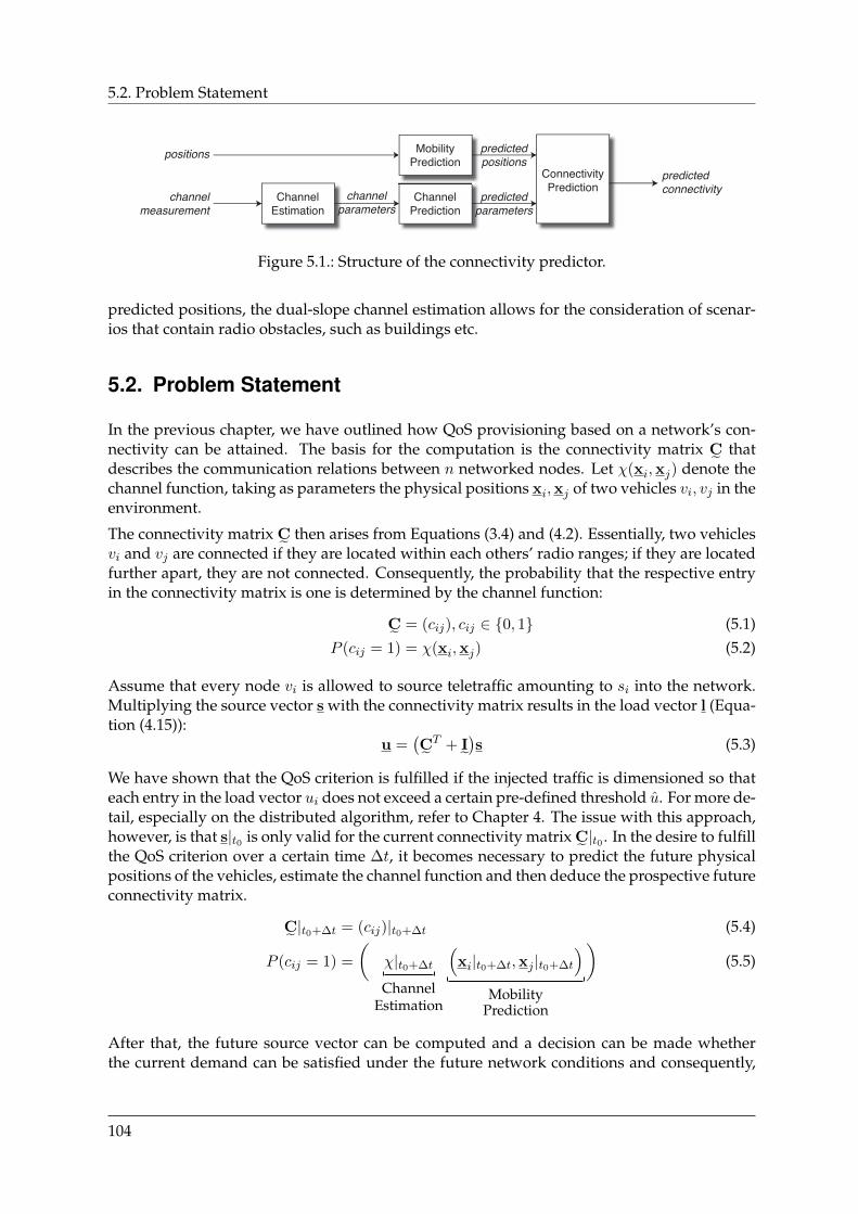
5.2. Problem Statement
Figure 5.1.: Structure of the connectivity predictor.
predicted positions, the dual-slope channel estimation allows for the consideration of scenar-ios that contain radio obstacles, such as buildings etc.
5.2. Problem Statement
In the previous chapter, we have outlined how QoS provisioning based on a network’s con-nectivity can be attained. The basis for the computation is the connectivity matrix C˜ thatdescribes the communication relations between n networked nodes. Let χ(xi,xj) denote thechannel function, taking as parameters the physical positions xi,xj of two vehicles vi, vj in theenvironment.
The connectivity matrix C˜ then arises from Equations (3.4) and (4.2). Essentially, two vehiclesvi and vj are connected if they are located within each others’ radio ranges; if they are locatedfurther apart, they are not connected. Consequently, the probability that the respective entryin the connectivity matrix is one is determined by the channel function:
C˜ = (cij), cij ∈ 0, 1 (5.1)P (cij = 1) = χ(xi,xj) (5.2)
Assume that every node vi is allowed to source teletraffic amounting to si into the network.Multiplying the source vector s with the connectivity matrix results in the load vector l (Equa-tion (4.15)):
u =(C˜ T + I˜)s (5.3)
We have shown that the QoS criterion is fulfilled if the injected traffic is dimensioned so thateach entry in the load vector ui does not exceed a certain pre-defined threshold u. For more de-tail, especially on the distributed algorithm, refer to Chapter 4. The issue with this approach,however, is that s|t0 is only valid for the current connectivity matrix C˜ |t0 . In the desire to fulfillthe QoS criterion over a certain time ∆t, it becomes necessary to predict the future physicalpositions of the vehicles, estimate the channel function and then deduce the prospective futureconnectivity matrix.
C˜ |t0+∆t = (cij)|t0+∆t (5.4)
P (cij = 1) =
(χ|t0+∆t
ChannelEstimation
(xi|t0+∆t,xj |t0+∆t
)Mobility
Prediction
)(5.5)
After that, the future source vector can be computed and a decision can be made whetherthe current demand can be satisfied under the future network conditions and consequently,
104

5. Predictive QoS Provisioning in Vehicular Ad-Hoc Networks
Figure 5.2.: Structure of the mobility predictor.
adequate measures can be taken. The structure of the connectivity predictor is shown in Fig-ure 5.1.
5.3. Mobility Prediction
Generally, the spatial behavior of a vehicle is defined by two factors: On the one hand, speedand direction are controlled by the driver who adapts to the environment and the current sit-uation. On the other hand, movement of a car is restricted to roads so the surrounding roadtopology is the major limiting factor. This is the key criterion that simplifies location predic-tion for vehicles compared to regular mobile users. Cars are usually not allowed to travelanywhere, they are bound to a relatively small portion of the world, the lanes. Combinedwith a small memory of past positions, the current velocity and direction of movement canbe calculated. This further limits the amount of available future positions, as cars are usuallynot expected to u-turn spontaneously and velocity changes are bounded by the maximumdeceleration and the maximum acceleration.
5.3.1. Concept
The prerequisite for the prediction is knowledge about a vehicle’s current position, directionof movement and the surrounding road topology. The latter is provided by digital street maps(available, for instance, through the OpenStreetMap Project). All of these factors are verystable in terms of prediction. The destination or rather the mission of the car is assumed to beunknown to the algorithm, so at a crossroads basically all directions seem equally probable.The velocity of a car, however, is far less stable and predictable as it is directly controlled bythe user and indirectly influenced by environmental factors such as road traffic density, roadsigns and the weather. Especially abrupt speed changes are almost impossible to predict asthey are often unexpected, even to the driver himself. The algorithm is sketched in Figure 5.2.
For speed prediction, we use a filter based approach that employs concepts of adaptive filtersinitially developed to adapt to varying channel conditions in wireless communications. Likethe channel characteristics change depending on the environment, the speed change behaviorof a car - or rather its driver - adapts to various environmental factors. This includes urbanscenarios with steep velocity slopes and rural roads with fairly constant speeds. The characterof the driver and the performance of the car also influence the prediction to a certain extent andare automatically taken into account by the adaptive filter. A self-adapting FIR filter approachbased on a Least Mean Squares (LMS) algorithm with relatively low depth seems ideal toadapt to both the personal behavior of a driver and the current situation. Using past andcurrent velocities, an ideal weight vector for the past situation is calculated. Due to the low
105
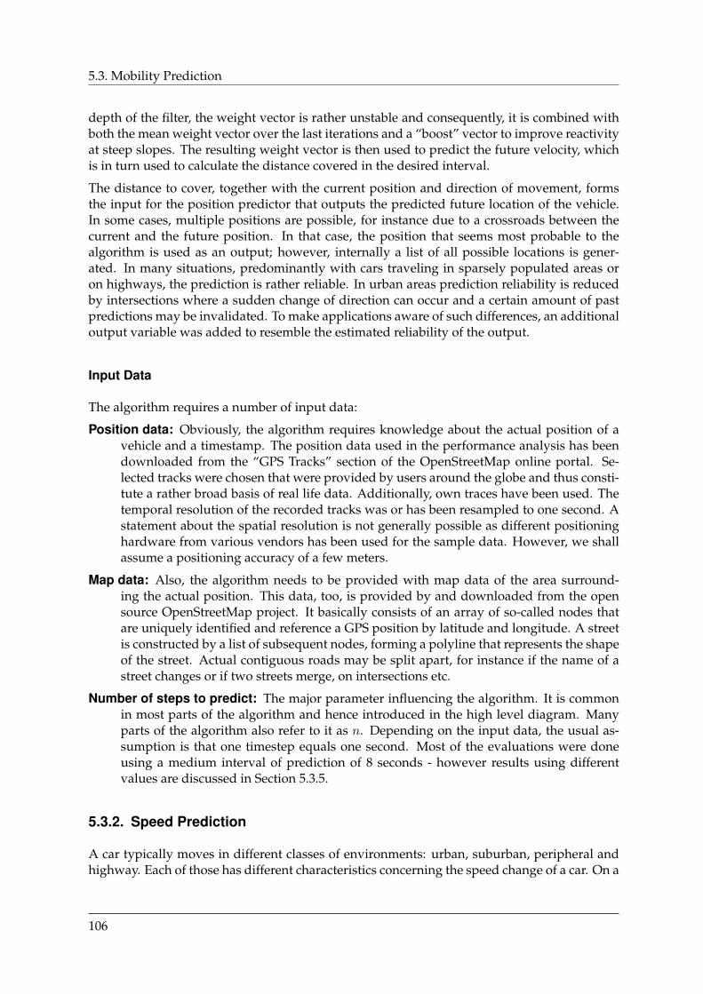
5.3. Mobility Prediction
depth of the filter, the weight vector is rather unstable and consequently, it is combined withboth the mean weight vector over the last iterations and a “boost” vector to improve reactivityat steep slopes. The resulting weight vector is then used to predict the future velocity, whichis in turn used to calculate the distance covered in the desired interval.
The distance to cover, together with the current position and direction of movement, formsthe input for the position predictor that outputs the predicted future location of the vehicle.In some cases, multiple positions are possible, for instance due to a crossroads between thecurrent and the future position. In that case, the position that seems most probable to thealgorithm is used as an output; however, internally a list of all possible locations is gener-ated. In many situations, predominantly with cars traveling in sparsely populated areas oron highways, the prediction is rather reliable. In urban areas prediction reliability is reducedby intersections where a sudden change of direction can occur and a certain amount of pastpredictions may be invalidated. To make applications aware of such differences, an additionaloutput variable was added to resemble the estimated reliability of the output.
Input Data
The algorithm requires a number of input data:
Position data: Obviously, the algorithm requires knowledge about the actual position of avehicle and a timestamp. The position data used in the performance analysis has beendownloaded from the “GPS Tracks” section of the OpenStreetMap online portal. Se-lected tracks were chosen that were provided by users around the globe and thus consti-tute a rather broad basis of real life data. Additionally, own traces have been used. Thetemporal resolution of the recorded tracks was or has been resampled to one second. Astatement about the spatial resolution is not generally possible as different positioninghardware from various vendors has been used for the sample data. However, we shallassume a positioning accuracy of a few meters.
Map data: Also, the algorithm needs to be provided with map data of the area surround-ing the actual position. This data, too, is provided by and downloaded from the opensource OpenStreetMap project. It basically consists of an array of so-called nodes thatare uniquely identified and reference a GPS position by latitude and longitude. A streetis constructed by a list of subsequent nodes, forming a polyline that represents the shapeof the street. Actual contiguous roads may be split apart, for instance if the name of astreet changes or if two streets merge, on intersections etc.
Number of steps to predict: The major parameter influencing the algorithm. It is commonin most parts of the algorithm and hence introduced in the high level diagram. Manyparts of the algorithm also refer to it as n. Depending on the input data, the usual as-sumption is that one timestep equals one second. Most of the evaluations were doneusing a medium interval of prediction of 8 seconds - however results using differentvalues are discussed in Section 5.3.5.
5.3.2. Speed Prediction
A car typically moves in different classes of environments: urban, suburban, peripheral andhighway. Each of those has different characteristics concerning the speed change of a car. On a
106
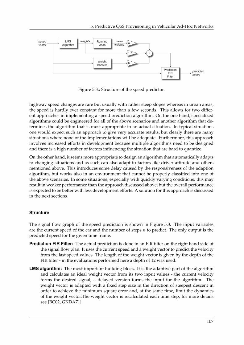
5. Predictive QoS Provisioning in Vehicular Ad-Hoc Networks
Figure 5.3.: Structure of the speed predictor.
highway speed changes are rare but usually with rather steep slopes whereas in urban areas,the speed is hardly ever constant for more than a few seconds. This allows for two differ-ent approaches in implementing a speed prediction algorithm. On the one hand, specializedalgorithms could be engineered for all of the above scenarios and another algorithm that de-termines the algorithm that is most appropriate in an actual situation. In typical situationsone would expect such an approach to give very accurate results, but clearly there are manysituations where none of the implementations will be adequate. Furthermore, this approachinvolves increased efforts in development because multiple algorithms need to be designedand there is a high number of factors influencing the situation that are hard to quantize.
On the other hand, it seems more appropriate to design an algorithm that automatically adaptsto changing situations and as such can also adapt to factors like driver attitude and othersmentioned above. This introduces some delay caused by the responsiveness of the adaptionalgorithm, but works also in an environment that cannot be properly classified into one ofthe above scenarios. In some situations, especially with quickly varying conditions, this mayresult in weaker performance than the approach discussed above, but the overall performanceis expected to be better with less development efforts. A solution for this approach is discussedin the next sections.
Structure
The signal flow graph of the speed prediction is shown in Figure 5.3. The input variablesare the current speed of the car and the number of steps n to predict. The only output is thepredicted speed for the given time frame.
Prediction FIR Filter: The actual prediction is done in an FIR filter on the right hand side ofthe signal flow plan. It uses the current speed and a weight vector to predict the velocityfrom the last speed values. The length of the weight vector is given by the depth of theFIR filter - in the evaluations performed here a depth of 12 was used.
LMS algorithm: The most important building block. It is the adaptive part of the algorithmand calculates an ideal weight vector from its two input values - the current velocityforms the desired signal, a delayed version forms the input for the algorithm. Theweight vector is adapted with a fixed step size in the direction of steepest descent inorder to achieve the minimum square error and, at the same time, limit the dynamicsof the weight vector.The weight vector is recalculated each time step, for more detailssee [BC02, GKDA71].
107

5.3. Mobility Prediction
parameter example value descriptionn 8 number of steps to predictl 12 depth of FIR filters and dimension of weights vectora 0.275 influence of the mean weights vectorb 2 influence of weight boosterc 0.2 boost limitd 1 boost gain
Table 5.1.: Speed Prediction parameters with example values used during development.
Mean Weight: Because the weight vector generated by the LMS algorithm is very reactiveto acceleration and deceleration processes, it is averaged by a running mean block thatcalculates the mean weight vector over the length of the situation. Both the mean andthe LMS weight vector are combined into a slowed weight vector by multiplication withthe parameter a or 1− a respectively.
Weight Booster: The LMS algorithm adapts to new situations with a delay that is roughly itsdepth l plus the length of the prediction interval n, which equals the number of memoryelements involved in the adaption. A change in velocity needs to pass through most ofthe memory elements before its effect becomes visible in the weight vector. For instance,for a car traveling in a city, the weight vector produces rather stable results while the caris traveling at a constant speed but it will react slowly to sharp braking or fast acceler-ation. The algorithm is designed to fix this problem by manipulating the weight vectorin order to emphasize the most recent speed history elements to react more quickly to aspontaneous change in behavior: a length l base vector is multiplied with a scalar calcu-lated from the slope of the velocity curve and is bounded above by the boost limit c. Inorder for the impact of the booster to remain present for a longer period, the generated“impulse” is broadened using a unity-weight FIR filter.
Parameters
The performance and precision of the speed predictor depends on some fundamental param-eters that are summarized in Table 5.1. The given values are the result of some evaluationsduring the design phase based on few exemplary scenarios and should give a rough idea tostart an implementation. However for a proper implementation a more thorough, numericaloptimization is recommended but out of scope of this essay.
It is important to note that all of the below parameters influence the prediction in a way thatusually makes adoptions to all parameters necessary if one parameter is changed. In manycases more than one possibility exists that can lead to a desired result for one scenario, butlooking at multiple scenarios usually only one if any of the possibilities lead to an overallimprovement of performance.
n – Number of steps to predict: This key parameter determines the number of steps to bepredicted — n = 8 means the algorithm predicts the speed in 8 time steps. Obviouslya higher value increases the prediction error, whereas lower values gives more precisepredictions. The setting of this parameter is very important because its influence on theother parameters is tremendous, for instance a high value for n will on the one handrequire a higher a and on the other hand require more influence of the weight booster,
108
5. Predictive QoS Provisioning in Vehicular Ad-Hoc Networks
b. Also, this parameter is common with all components of the algorithm, so its influencehas to be regarded globally. Different settings and their impact, especially on positionprediction, are discussed in Section 5.3.5.
l – Depth of FIR filters: The FIR filters’ depth used in the speed predictor is a common valuebecause all blocks share the weight vector. Also the parameter l is, unlike all other pa-rameters mentioned here, a design time parameter that cannot be changed easily as itis hard-coded into the FIR filters and the constants. Nevertheless, its influence on theprediction should be discussed here.For the fact that the depth of a filter resembles its amount of memory elements, highervalues for l give more stable and less reactive prediction results. Changes in the situa-tion need more time to propagate through the memory elements, hence it takes a longertime to adapt to changes. Smaller values for l improve reaction time but also result inless stable and more fluctuating predictions that often overshoot at slight changes.
a – Influence of the Mean Weights Vector: The weight vector in the standard case (disre-garding the weight booster) is combined from the current weight vector produced bythe LMS algorithm and its running average. Setting a to the maximal appropriate valuea = 1 produces a very stable weight vector but also removes the direct influence of theLMS algorithm to the weight vector and thus the reactivity. This is caused by the factthat in this model, the mean weight vector is never reset and thus provides an “all timeaverage”.
b – Influence of the Weight Booster: This parameter determines the overall influence of theweight booster. Higher values tend to produce overshoots as a trade-off to slow responseto a change in situation if lower values are used. Generally all three values influencingthe weight booster should be tuned according to the length of the prediction n. Withhigh n, b should be increased because a faster reaction is necessary due to the latency ofthe LMS algorithm.
c – Boost Limit: The “boost” vector, or more precisely its scalar values, are influenced by theslope of the velocity curve. The “boost limit” defines an upper bound to those scalarvalues.
d – Boost Gain: This parameter multiplies the influence of the slope difference before thebroadening and limiting of the pulse. Thus a higher value generates very quick increaseonce a steep slope is detected - in other words, it pushes the boost weight vector morequickly to the limit. Lower values produce a smoother response to steep velocity slopes.
5.3.3. Distance Calculation
The speed predictor predicts the vehicle speed some time steps ahead. The position predic-tor in turn requires as an input the distance to cover in the next time steps to calculate thefuture position. The most precise approach is to predict a velocity value for each time step inthe prediction period and sum up the difference. Because this requires a set of n speed pre-dictors which increases the computational efforts by n, a simpler approach is chosen in thisimplementation. Our algorithm uses the current speed and the predicted speed and calculatesa linear approximation between the two. The distance to cover s is then the area under thespeed curve for a duration of t (n time steps):
s =t
2(vcurrent + vpred)
109
5.3. Mobility Prediction
5.3.4. Position Prediction
The position predictor uses the current position and direction of movement, digital map dataas well as the predicted distance to cover as inputs and outputs a predicted position and itsreliability. It is invoked once per time step and tries to first find the current road segment ofthe vehicle, then determines a number of possible prediction paths and finally chooses themost probable path and returns its end point.
Determine current road segment
All known nearby road segments (taken from the digital map) are evaluated for the distanceof the current position to the closest point on the respective road segment. Three criteria mustbe met in order for a road segment to be chosen:
1. The distance to the closest point is smaller than a threshold.
2. The absolute value of the difference between the direction of movement and the roadsegment’s direction is not larger than π/2 because vehicles usually do not move perpen-dicular to streets.
3. It is the closest road segment satisfying both criteria 1 and 2.
In case no road segment is found that fulfills all of the above criteria, the algorithm returns thecurrent position as prediction result with an estimated accuracy of 0%. Possible causes rangefrom wrong GPS positions during the initialization phase of the GPS device and inexact mapmaterial to driving or parking on streets or private property that is not (yet) included in themap material.
Determine possible paths
First, the remaining distance from the current position to the respective end point of the roadsegment sr is calculated. If the road segment’s end point is further away than the distance tocover (sr ≥ s), the predicted position will be located between the current position and the roadsegment’s end point. Therefore, the predicted position is determined along the road segment’spolyline towards the end point, covering the given distance s.
In the case that the remaining distance sr is smaller than the distance to cover (sr < s), thepredicted position is moved to the road segment’s end point and that distance is subtractedfrom the remaining distance. Subsequently, the next road segment of the prediction path isdetermined. If the mission of the vehicle is known in advance, the next road segment is chosenaccording to that mission. Otherwise, in order to find the next road segment, the number ofpossibilities is determined from the digital map: at a junction, all connected street segmentsare considered possible candidates. The current road segment, however, is not considered asan alternative — in other words, the vehicle is not expected to u-turn. Three cases exist:
(a) No candidates exist, so the current road segment ends in a node that has no other roadsegments referenced. In this case the relative probability of the current path is decreasedin the relation to the amount of distance already covered.
(b) One candidate means there is no choice and the vehicle is moving along a road withoutan intersection at the current node. Determining the next road segment and updatingthe path accordingly is trivial.
110
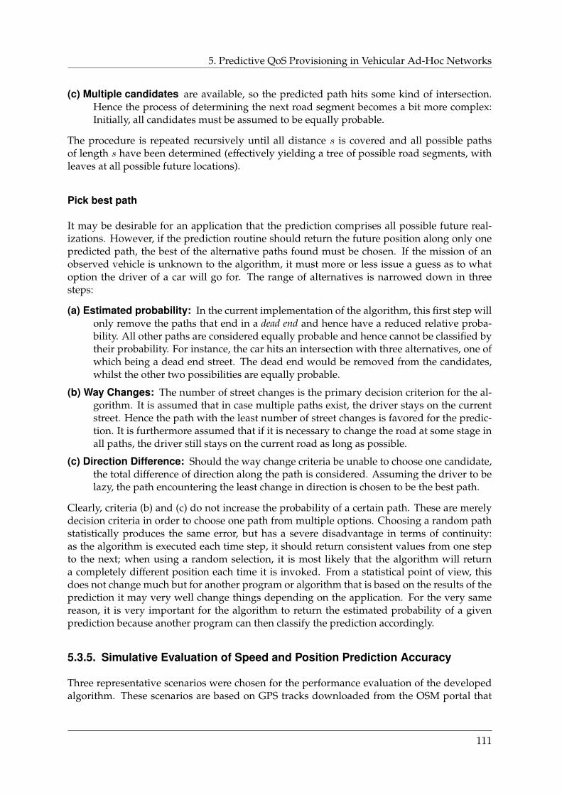
5. Predictive QoS Provisioning in Vehicular Ad-Hoc Networks
(c) Multiple candidates are available, so the predicted path hits some kind of intersection.Hence the process of determining the next road segment becomes a bit more complex:Initially, all candidates must be assumed to be equally probable.
The procedure is repeated recursively until all distance s is covered and all possible pathsof length s have been determined (effectively yielding a tree of possible road segments, withleaves at all possible future locations).
Pick best path
It may be desirable for an application that the prediction comprises all possible future real-izations. However, if the prediction routine should return the future position along only onepredicted path, the best of the alternative paths found must be chosen. If the mission of anobserved vehicle is unknown to the algorithm, it must more or less issue a guess as to whatoption the driver of a car will go for. The range of alternatives is narrowed down in threesteps:
(a) Estimated probability: In the current implementation of the algorithm, this first step willonly remove the paths that end in a dead end and hence have a reduced relative proba-bility. All other paths are considered equally probable and hence cannot be classified bytheir probability. For instance, the car hits an intersection with three alternatives, one ofwhich being a dead end street. The dead end would be removed from the candidates,whilst the other two possibilities are equally probable.
(b) Way Changes: The number of street changes is the primary decision criterion for the al-gorithm. It is assumed that in case multiple paths exist, the driver stays on the currentstreet. Hence the path with the least number of street changes is favored for the predic-tion. It is furthermore assumed that if it is necessary to change the road at some stage inall paths, the driver still stays on the current road as long as possible.
(c) Direction Difference: Should the way change criteria be unable to choose one candidate,the total difference of direction along the path is considered. Assuming the driver to belazy, the path encountering the least change in direction is chosen to be the best path.
Clearly, criteria (b) and (c) do not increase the probability of a certain path. These are merelydecision criteria in order to choose one path from multiple options. Choosing a random pathstatistically produces the same error, but has a severe disadvantage in terms of continuity:as the algorithm is executed each time step, it should return consistent values from one stepto the next; when using a random selection, it is most likely that the algorithm will returna completely different position each time it is invoked. From a statistical point of view, thisdoes not change much but for another program or algorithm that is based on the results of theprediction it may very well change things depending on the application. For the very samereason, it is very important for the algorithm to return the estimated probability of a givenprediction because another program can then classify the prediction accordingly.
5.3.5. Simulative Evaluation of Speed and Position Prediction Accuracy
Three representative scenarios were chosen for the performance evaluation of the developedalgorithm. These scenarios are based on GPS tracks downloaded from the OSM portal that
111
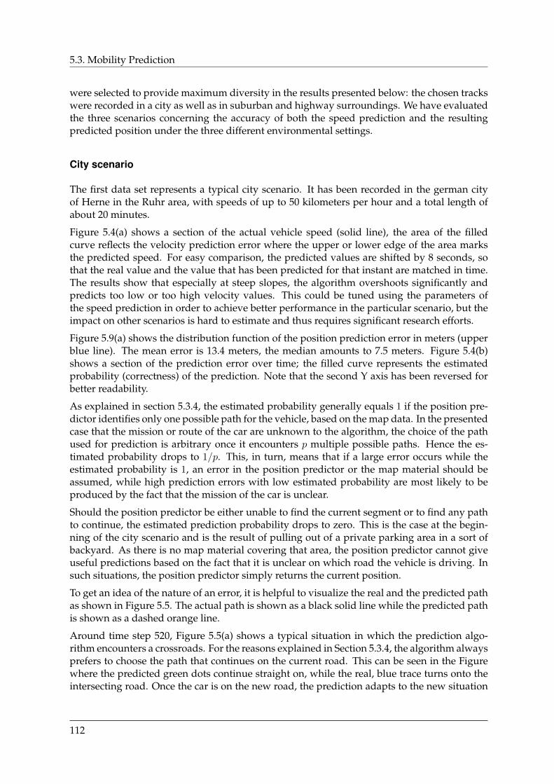
5.3. Mobility Prediction
were selected to provide maximum diversity in the results presented below: the chosen trackswere recorded in a city as well as in suburban and highway surroundings. We have evaluatedthe three scenarios concerning the accuracy of both the speed prediction and the resultingpredicted position under the three different environmental settings.
City scenario
The first data set represents a typical city scenario. It has been recorded in the german cityof Herne in the Ruhr area, with speeds of up to 50 kilometers per hour and a total length ofabout 20 minutes.
Figure 5.4(a) shows a section of the actual vehicle speed (solid line), the area of the filledcurve reflects the velocity prediction error where the upper or lower edge of the area marksthe predicted speed. For easy comparison, the predicted values are shifted by 8 seconds, sothat the real value and the value that has been predicted for that instant are matched in time.The results show that especially at steep slopes, the algorithm overshoots significantly andpredicts too low or too high velocity values. This could be tuned using the parameters ofthe speed prediction in order to achieve better performance in the particular scenario, but theimpact on other scenarios is hard to estimate and thus requires significant research efforts.
Figure 5.9(a) shows the distribution function of the position prediction error in meters (upperblue line). The mean error is 13.4 meters, the median amounts to 7.5 meters. Figure 5.4(b)shows a section of the prediction error over time; the filled curve represents the estimatedprobability (correctness) of the prediction. Note that the second Y axis has been reversed forbetter readability.
As explained in section 5.3.4, the estimated probability generally equals 1 if the position pre-dictor identifies only one possible path for the vehicle, based on the map data. In the presentedcase that the mission or route of the car are unknown to the algorithm, the choice of the pathused for prediction is arbitrary once it encounters p multiple possible paths. Hence the es-timated probability drops to 1/p. This, in turn, means that if a large error occurs while theestimated probability is 1, an error in the position predictor or the map material should beassumed, while high prediction errors with low estimated probability are most likely to beproduced by the fact that the mission of the car is unclear.
Should the position predictor be either unable to find the current segment or to find any pathto continue, the estimated prediction probability drops to zero. This is the case at the begin-ning of the city scenario and is the result of pulling out of a private parking area in a sort ofbackyard. As there is no map material covering that area, the position predictor cannot giveuseful predictions based on the fact that it is unclear on which road the vehicle is driving. Insuch situations, the position predictor simply returns the current position.
To get an idea of the nature of an error, it is helpful to visualize the real and the predicted pathas shown in Figure 5.5. The actual path is shown as a black solid line while the predicted pathis shown as a dashed orange line.
Around time step 520, Figure 5.5(a) shows a typical situation in which the prediction algo-rithm encounters a crossroads. For the reasons explained in Section 5.3.4, the algorithm alwaysprefers to choose the path that continues on the current road. This can be seen in the Figurewhere the predicted green dots continue straight on, while the real, blue trace turns onto theintersecting road. Once the car is on the new road, the prediction adapts to the new situation
112
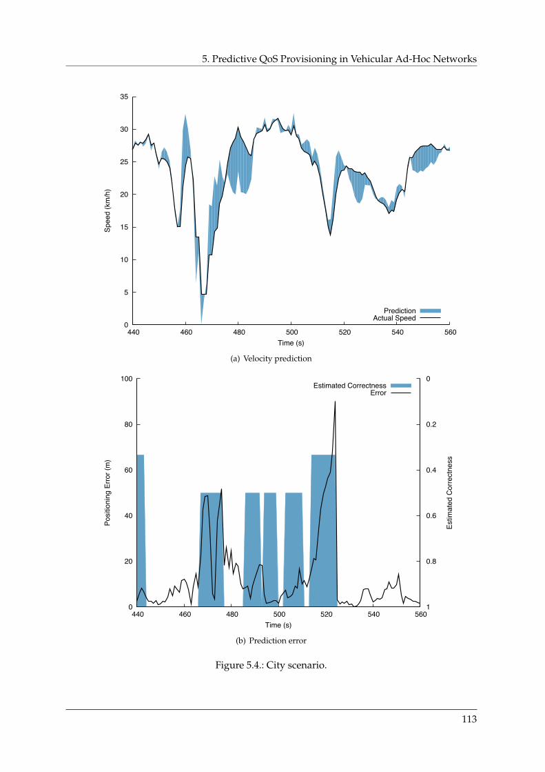
5. Predictive QoS Provisioning in Vehicular Ad-Hoc Networks
0
5
10
15
20
25
30
35
440 460 480 500 520 540 560
Spee
d (k
m/h
)
Time (s)
PredictionActual Speed
(a) Velocity prediction
0
20
40
60
80
100
440 460 480 500 520 540 560
0
0.2
0.4
0.6
0.8
1
Posi
tioni
ng E
rror (
m)
Estim
ated
Cor
rect
ness
Time (s)
Estimated CorrectnessError
(b) Prediction error
Figure 5.4.: City scenario.
113
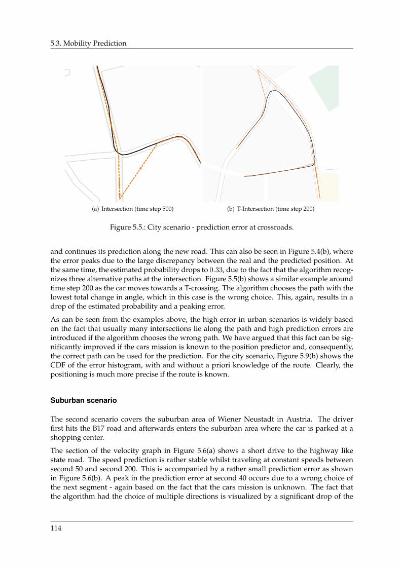
5.3. Mobility Prediction
(a) Intersection (time step 500) (b) T-Intersection (time step 200)
Figure 5.5.: City scenario - prediction error at crossroads.
and continues its prediction along the new road. This can also be seen in Figure 5.4(b), wherethe error peaks due to the large discrepancy between the real and the predicted position. Atthe same time, the estimated probability drops to 0.33, due to the fact that the algorithm recog-nizes three alternative paths at the intersection. Figure 5.5(b) shows a similar example aroundtime step 200 as the car moves towards a T-crossing. The algorithm chooses the path with thelowest total change in angle, which in this case is the wrong choice. This, again, results in adrop of the estimated probability and a peaking error.
As can be seen from the examples above, the high error in urban scenarios is widely basedon the fact that usually many intersections lie along the path and high prediction errors areintroduced if the algorithm chooses the wrong path. We have argued that this fact can be sig-nificantly improved if the cars mission is known to the position predictor and, consequently,the correct path can be used for the prediction. For the city scenario, Figure 5.9(b) shows theCDF of the error histogram, with and without a priori knowledge of the route. Clearly, thepositioning is much more precise if the route is known.
Suburban scenario
The second scenario covers the suburban area of Wiener Neustadt in Austria. The driverfirst hits the B17 road and afterwards enters the suburban area where the car is parked at ashopping center.
The section of the velocity graph in Figure 5.6(a) shows a short drive to the highway likestate road. The speed prediction is rather stable whilst traveling at constant speeds betweensecond 50 and second 200. This is accompanied by a rather small prediction error as shownin Figure 5.6(b). A peak in the prediction error at second 40 occurs due to a wrong choice ofthe next segment - again based on the fact that the cars mission is unknown. The fact thatthe algorithm had the choice of multiple directions is visualized by a significant drop of the
114
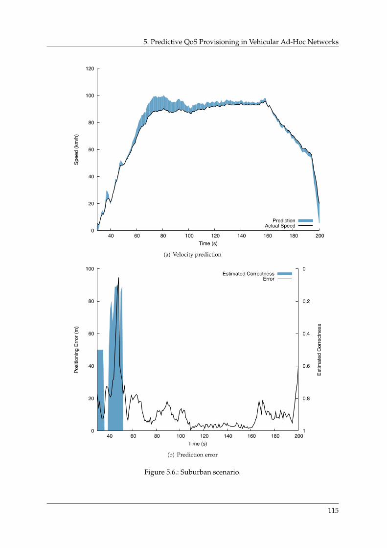
5. Predictive QoS Provisioning in Vehicular Ad-Hoc Networks
0
20
40
60
80
100
120
40 60 80 100 120 140 160 180 200
Spee
d (k
m/h
)
Time (s)
PredictionActual Speed
(a) Velocity prediction
0
20
40
60
80
100
40 60 80 100 120 140 160 180 200
0
0.2
0.4
0.6
0.8
1
Posi
tioni
ng E
rror (
m)
Estim
ated
Cor
rect
ness
Time (s)
Estimated CorrectnessError
(b) Prediction error
Figure 5.6.: Suburban scenario.
115

5.3. Mobility Prediction
Figure 5.7.: Highway scenario - prediction error at highway bridge.
estimated correctness curve.
Due to a very sharp deceleration around second 200, Figure 5.6(b) shows another peak withouta drop in probability for the fact that no other possible directions are identified. The reasonfor the braking is unclear, an explanation cannot be found in the map material nor the satelliteimage of the area. Figure 5.6(b) also shows a few more peaks based on decisions for the wrongdirections and braking actions.
The distribution function shown in Figure 5.10(a) (upper blue line) is slightly flatter than theone from scenario 1. The median error (about 10 meters) is slightly higher than in the city,probably caused by the fact that either map material or the GPS device used to record thetrack are less precise than in the city scenario. The 90% percentile is significantly smaller(22 meters compared to 34 meters), which supports the before assumption and leads to theconclusion that the overall position prediction is better in the suburban scenario. The meanerror of 13.5 meters, however, is almost identical to the city scenario.
Highway scenario
The third scenario covers a ride on a highway near the English town of Cambridge duringrush hour traffic, which explains the unsteady velocity curve shown in Figure 5.8(a). Again, arepresentative section has been chosen for presentation.
The prediction error plotted in Figure 5.8(b) shows constantly low prediction errors. Fromthe distribution function shown in Figure 5.10(b) (upper blue line) reveals a very steep slope,which means excellent performance of the algorithm as more than 95% of all errors are below10 meters. The mean error amounts to only 4.6 meters and the median is 3.8 meters.
One notable peak of the error, accompanied by a drop in the estimated probability occursaround time step 800 (see Figure 5.8(b)). Figure 5.7 visualizes both the real trace (shownas blue arrows) and the predicted trace (shown as green dots). At the instant when the caris crossing a highway bridge — as highlighted in the screenshot — the algorithm wrongly
116
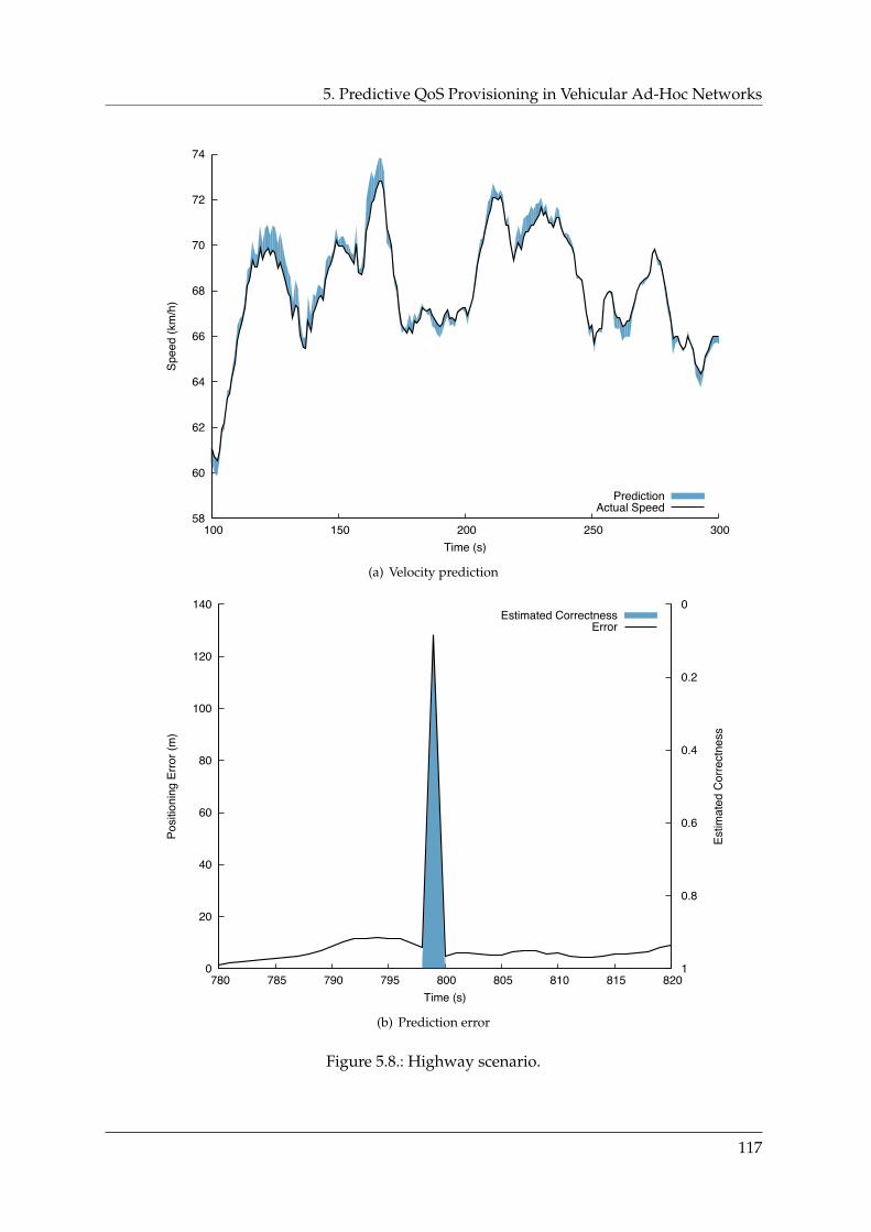
5. Predictive QoS Provisioning in Vehicular Ad-Hoc Networks
58
60
62
64
66
68
70
72
74
100 150 200 250 300
Spee
d (k
m/h
)
Time (s)
PredictionActual Speed
(a) Velocity prediction
0
20
40
60
80
100
120
140
780 785 790 795 800 805 810 815 820
0
0.2
0.4
0.6
0.8
1
Posi
tioni
ng E
rror (
m)
Estim
ated
Cor
rect
ness
Time (s)
Estimated CorrectnessError
(b) Prediction error
Figure 5.8.: Highway scenario.
117
5.4. Channel Parameter Estimation and Prediction
chooses the current road segment to be part of the road below the bridge that shares a nodewith the highway. Consequently, the algorithm chooses the wrong road segment to continueprediction. This error is caused by an unfortunate combination of a small measuring errorof the GPS device and an imprecision of the map material, where the highway shares a nodewith the intersecting road (although they are on different levels).
Another error source stems from the fact that in the used map material, a road is representedby a polyline, and all vehicles are assumed to be positioned on this line. In reality, highwaysconsists of a number of parallel lanes that have a certain lateral displacement. Although asuitable representation of road lanes has been suggested, the data available today does notyet represent different lanes. We expect, however, that the error would be decreased if thisinformation could be accounted for in the prediction.
Influence of Prediction Length
The results that we have discussed above were obtained through prediction with period lengthsof eight seconds. This sections evaluates the same scenarios with longer prediction lengths of16 and 32 seconds. The resulting position error distribution functions are shown in Figures 5.9and 5.10.
The steepness of the distribution functions decrease as the prediction length increases, due toless prediction accuracy across a longer period of time, i.e., the tendency to produce greatererrors. The maximum error also increases dramatically, because in case that a wrong pathis chosen, the prediction continues along the wrong path for a much longer time before it iscorrected as the car turns the other way. The mean error is also shifted towards higher valueswith increasing prediction intervals.
In the city and suburban scenarios, the prediction is already significantly less reliable withn = 16 time steps (i.e., seconds) as a prediction interval. It is rendered basically useless with aprediction interval of n = 32 and the majority of errors are out of scale of the histogram. Thehighway scenario, however, behaves much more stable as the prediction interval is increasedand still returns useful results using a prediction horizon of 32 seconds. To a large extent, thisis based on the relatively stable velocities and absent alternative paths along the way.
5.4. Channel Parameter Estimation and Prediction
It is clear from Equation (5.5) that the network’s future connectivity does not only dependon the future vehicles’ positions. An adequate channel model has to be chosen and constantlyupdated to reflect the changing radio environment. In Equation (3.9), we have shown a simplechannel function, the disc model. We shall call two nodes i and j connected if the path loss β(d),a function of the distance between the two nodes, does not exceed a certain threshold βmax:
βmax!> β(d) = 20 log10
4πd0
λ+ 10α log10
d
d0(5.6)
The path loss consists of two components: a constant addend that reflects the loss related tothe wavelength of the signal and a distance-dependent term that represents the propagation ofthe radio wave through space and the resulting diminishment of power due to the growth of
118

5. Predictive QoS Provisioning in Vehicular Ad-Hoc Networks
0.1
0.2
0.3
0.4
0.5
0.6
0.7
0.8
0.9
1
0 10 20 30 40 50 60 70 80 90 100
Prob
abilit
y
Positioning Error (m)
n=8 secondsn=16 secondsn=32 seconds
(a) City scenario
0
0.1
0.2
0.3
0.4
0.5
0.6
0.7
0.8
0.9
1
0 5 10 15 20
Prob
abilit
y
Positioning Error (m)
route unknownroute known
(b) City scenario - Route known
Figure 5.9.: Prediction error histogram - different prediction lengths for the city scenarios andthe influence of known routes on prediction accuracy.
119
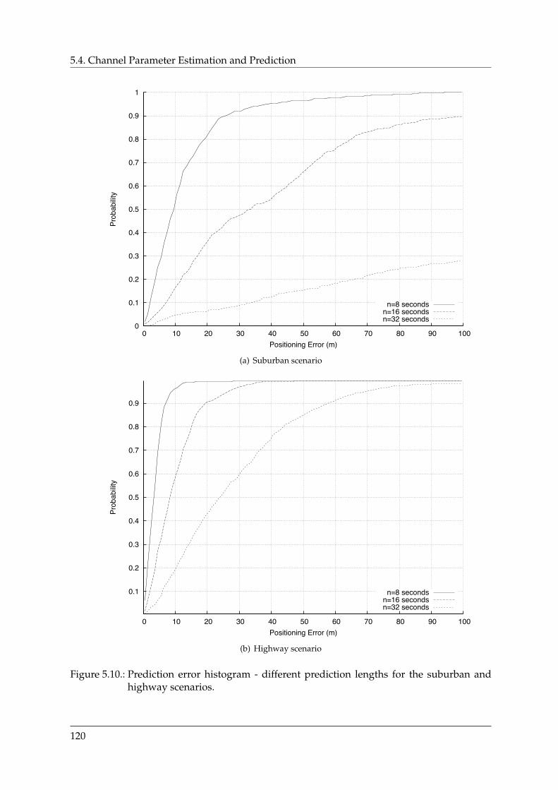
5.4. Channel Parameter Estimation and Prediction
0
0.1
0.2
0.3
0.4
0.5
0.6
0.7
0.8
0.9
1
0 10 20 30 40 50 60 70 80 90 100
Prob
abilit
y
Positioning Error (m)
n=8 secondsn=16 secondsn=32 seconds
(a) Suburban scenario
0.1
0.2
0.3
0.4
0.5
0.6
0.7
0.8
0.9
0 10 20 30 40 50 60 70 80 90 100
Prob
abilit
y
Positioning Error (m)
n=8 secondsn=16 secondsn=32 seconds
(b) Highway scenario
Figure 5.10.: Prediction error histogram - different prediction lengths for the suburban andhighway scenarios.
120
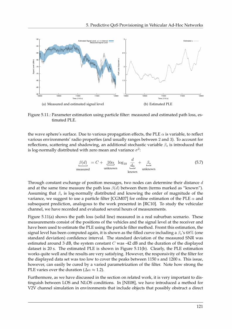
5. Predictive QoS Provisioning in Vehicular Ad-Hoc Networks
-90
-85
-80
-75
-70
-65
-60
-55
-50
10000 10500 11000 11500 12000
Sign
al L
evel
(dBm
)
Time (1/10 s)
Estimated Signal Level, +/- 1 IntervalMeasured Signal Level
(a) Measured and estimated signal level
1
1.5
2
2.5
3
10000 10500 11000 11500 12000
Path
Los
s Ex
pone
nt
Time (1/10 s)
Estimated
(b) Estimated PLE
Figure 5.11.: Parameter estimation using particle filter: measured and estimated path loss, es-timated PLE.
the wave sphere’s surface. Due to various propagation effects, the PLE α is variable, to reflectvarious environments’ radio properties (and usually ranges between 2 and 3). To account forreflections, scattering and shadowing, an additional stochastic variable βs is introduced thatis log-normally distributed with zero mean and variance σ2:
β(d)
measured
= C + 10α
unknown
log10
d
d0
known
+ βs
unknown
(5.7)
Through constant exchange of position messages, two nodes can determine their distance dand at the same time measure the path loss β(d) between them (terms marked as “known”).Assuming that βs is log-normally distributed and knowing the order of magnitude of thevariance, we suggest to use a particle filter [CGM07] for online estimation of the PLE α andsubsequent prediction, analogous to the work presented in [RC10]. To study the vehicularchannel, we have recorded and evaluated several hours of measurements.
Figure 5.11(a) shows the path loss (solid line) measured in a real suburban scenario. Thesemeasurements consist of the positions of the vehicles and the signal level at the receiver andhave been used to estimate the PLE using the particle filter method. Fromt this estimation, thesignal level has been computed again, it is shown as the filled curve including a βs’s 68% (onestandard deviation) confidence interval. The standard deviation of the measured SNR wasestimated around 3 dB, the system constant C was -42 dB and the duration of the displayeddataset is 20 s. The estimated PLE is shown in Figure 5.11(b). Clearly, the PLE estimationworks quite well and the results are very satisfying. However, the responsivity of the filter forthe displayed data set was too low to cover the peaks between 1150 s and 1200 s. This issue,however, can easily be cured by a varied parametrization of the filter. Note how strong thePLE varies over the duration (∆α ≈ 1.2).
Furthermore, as we have discussed in the section on related work, it is very important to dis-tinguish between LOS and NLOS conditions. In [NE08], we have introduced a method forV2V channel simulation in environments that include objects that possibly obstruct a direct
121
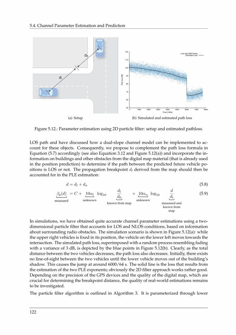
5.4. Channel Parameter Estimation and Prediction
(a) Setup
50
60
70
80
90
100
110
120
0 1000 2000 3000 4000 5000 6000 7000 8000
Path
loss
[dB]
Time [1/64s]
Loss with 3dB FadingEstimated Loss
(b) Simulated and estimated path loss
Figure 5.12.: Parameter estimation using 2D particle filter: setup and estimated pathloss.
LOS path and have discussed how a dual-slope channel model can be implemented to ac-count for these objects. Consequently, we propose to complement the path loss formula inEquation (5.7) accordingly (see also Equation 3.12 and Figure 5.12(a)) and incorporate the in-formation on buildings and other obstacles from the digital map material (that is already usedin the position prediction) to determine if the path between the predicted future vehicle po-sitions is LOS or not. The propagation breakpoint dl derived from the map should then beaccounted for in the PLE estimation:
d = dl + dn (5.8)
βp(d)
measured
= C + 10αl
unknown
log10
dld0
known from map
+ 10αn
unknown
log10
d
dl
measured andknown from
map
(5.9)
In simulations, we have obtained quite accurate channel parameter estimations using a two-dimensional particle filter that accounts for LOS and NLOS conditions, based on informationabout surrounding radio obstacles. The simulation scenario is shown in Figure 5.12(a): whilethe upper right vehicles is fixed in its position, the vehicle on the lower left moves towards theintersection. The simulated path loss, superimposed with a random process resembling fadingwith a variance of 3 dB, is depicted by the blue points in Figure 5.12(b). Clearly, as the totaldistance between the two vehicles decreases, the path loss also decreases. Initially, there existsno line-of-sight between the two vehicles until the lower vehicle moves out of the building’sshadow. This causes the jump at around 6000/64 s. The solid line is the loss that results fromthe estimation of the two PLE exponents; obviously the 2D filter approach works rather good.Depending on the precision of the GPS devices and the quality of the digital map, which arecrucial for determining the breakpoint distance, the quality of real-world estimations remainsto be investigated.
The particle filter algorithm is outlined in Algorithm 3. It is parameterized through lower
122
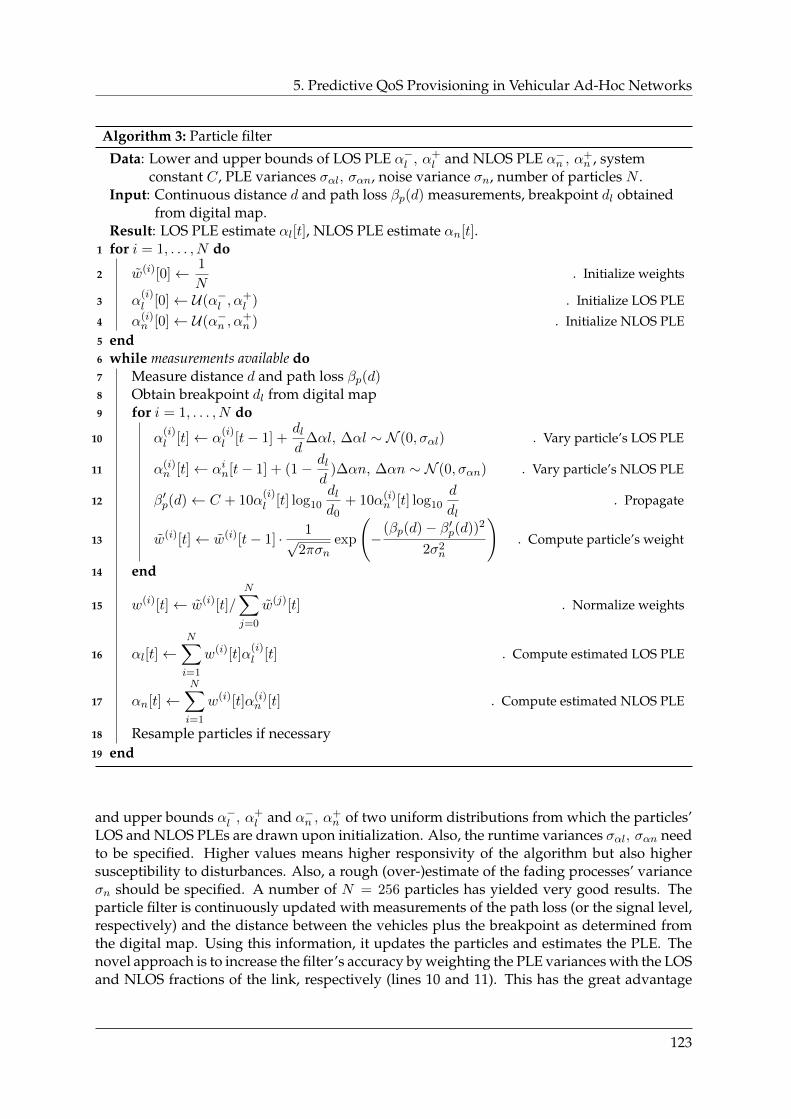
5. Predictive QoS Provisioning in Vehicular Ad-Hoc Networks
Algorithm 3: Particle filter
Data: Lower and upper bounds of LOS PLE α−l , α+l and NLOS PLE α−n , α+
n , systemconstant C, PLE variances σαl, σαn, noise variance σn, number of particles N .
Input: Continuous distance d and path loss βp(d) measurements, breakpoint dl obtainedfrom digital map.
Result: LOS PLE estimate αl[t], NLOS PLE estimate αn[t].1 for i = 1, . . . , N do
2 w(i)[0]← 1
N. Initialize weights
3 α(i)l [0]← U(α−l , α
+l ) . Initialize LOS PLE
4 α(i)n [0]← U(α−n , α
+n ) . Initialize NLOS PLE
5 end6 while measurements available do7 Measure distance d and path loss βp(d)8 Obtain breakpoint dl from digital map9 for i = 1, . . . , N do
10 α(i)l [t]← α
(i)l [t− 1] +
dld
∆αl, ∆αl ∼ N (0, σαl) . Vary particle’s LOS PLE
11 α(i)n [t]← αin[t− 1] + (1− dl
d)∆αn, ∆αn ∼ N (0, σαn) . Vary particle’s NLOS PLE
12 β′p(d)← C + 10α(i)l [t] log10
dld0
+ 10α(i)n [t] log10
d
dl. Propagate
13 w(i)[t]← w(i)[t− 1] · 1√2πσn
exp
(−
(βp(d)− β′p(d))2
2σ2n
). Compute particle’s weight
14 end
15 w(i)[t]← w(i)[t]/N∑j=0
w(j)[t] . Normalize weights
16 αl[t]←N∑i=1
w(i)[t]α(i)l [t] . Compute estimated LOS PLE
17 αn[t]←N∑i=1
w(i)[t]α(i)n [t] . Compute estimated NLOS PLE
18 Resample particles if necessary19 end
and upper bounds α−l , α+l and α−n , α+
n of two uniform distributions from which the particles’LOS and NLOS PLEs are drawn upon initialization. Also, the runtime variances σαl, σαn needto be specified. Higher values means higher responsivity of the algorithm but also highersusceptibility to disturbances. Also, a rough (over-)estimate of the fading processes’ varianceσn should be specified. A number of N = 256 particles has yielded very good results. Theparticle filter is continuously updated with measurements of the path loss (or the signal level,respectively) and the distance between the vehicles plus the breakpoint as determined fromthe digital map. Using this information, it updates the particles and estimates the PLE. Thenovel approach is to increase the filter’s accuracy by weighting the PLE variances with the LOSand NLOS fractions of the link, respectively (lines 10 and 11). This has the great advantage
123
5.5. Connectivity Prediction
that the algorithm can universally be used both in LOS and NLOS scenarios.
For the subsequent channel parameter prediction, we propose to employ the same conceptsas used for position prediction to at least estimate the trend of the PLE. Also, it is clear thatthe effects of large-scale fading have a large impact on the future connectivity but are hardto account for. Small-scale fading effects can impossibly be accounted for due to positioningerrors. Therefore, fading effects should be considered through an additional stochastic com-ponent. When evaluating the connectivity matrix computed from the predicted positions andthe predicted channel, additional information about the reliability of the prediction should beprovided and considered.
5.5. Connectivity Prediction
To determine the future connectivity of a network, a node has to predict the positions of allrelevant vehicles (usually the one- or two-hop radio neighborhood) and determine the result-ing path loss to decide whether it will be connected to this vehicle or not. The first error sourceof the path loss estimation is, of course, the error induced by inaccurate position prediction.Fortunately, this error term strongly depends on the distance d between the two involvedvehicles. Let us assume that the estimating vehicle has perfect ego positioning and positionprediction (the estimating vehicle also needs to know its future position) and let ∆d denotethe maximum positioning error. The resulting absolute estimation error range (peak-to-peak)is then:
∆β(d,∆d) = β(d+ ∆d)− β(d−∆d) = 10α log10
(d+ ∆d
d−∆d
)(5.10)
The second influence on path loss estimation is the accuracy of the predicted PLE. Let ∆αdenote the PLE’s maximum estimation error. The resulting absolute path loss estimation erroris:
∆β(d,∆α) = β(d, α+ ∆α)− β(d, α−∆α) = 20∆α log10
(d
d0
)(5.11)
Clearly, there exists a strong negative correlation between the path loss estimation error andthe distance to the tracked vehicle, d. With increasing d, the implications of prediction errorsbecome less important with respect to the path loss. The situation is contrary regarding thePLE estimation: because the relation is linear, a large path loss estimation error results if thedistance d to the tracked vehicle increases. The problem is that ∆d and ∆α are not knownat runtime; therefore, we suggest to keep the prediction results and constantly compare themagainst the predictions to obtain a statistic of the errors. This information should consequentlybe used to determine a prediction’s reliability.
Let us assume that through constant observation the distribution of the estimated distance d,fD(d), is known, and that the distribution of the estimated PLE α, fα(α), is also known. Wewish to determine the distribution of the path loss estimation, fβ(β), as a function of fD(d)and fα(α):
β = 10α log10 d (5.12)
124
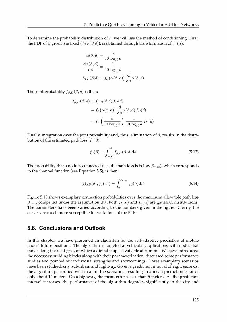
5. Predictive QoS Provisioning in Vehicular Ad-Hoc Networks
To determine the probability distribution of β, we will use the method of conditioning. First,the PDF of β given d is fixed (fβ|D(β|d)), is obtained through transformation of fα(α):
α(β, d) =β
10 log10 d
dα(β, d)
dβ=
1
10 log10 d
fβ|D(β|d) = fα(α(β, d)
) ddβ
α(β, d)
The joint probability fβ,D(β, d) is then:
fβ,D(β, d) = fβ|D(β|d) fD(d)
= fα(α(β, d)
) ddβ
α(β, d) fD(d)
= fα
(β
10 log10 d
)1
10 log10 dfD(d)
Finally, integration over the joint probability and, thus, elimination of d, results in the distri-bution of the estimated path loss, fβ(β):
fβ(β) =
∫ ∞−∞
fβ,D(β, d)dd (5.13)
The probability that a node is connected (i.e., the path loss is below βmax), which correspondsto the channel function (see Equation 5.5), is then:
χ(fD(d), fα(α)) =
∫ βmax
0fβ(β)dβ (5.14)
Figure 5.13 shows exemplary connection probabilities over the maximum allowable path lossβmax, computed under the assumption that both fD(d) and fα(α) are gaussian distributions.The parameters have been varied according to the numbers given in the figure. Clearly, thecurves are much more susceptible for variations of the PLE.
5.6. Conclusions and Outlook
In this chapter, we have presented an algorithm for the self-adaptive prediction of mobilenodes’ future positions. The algorithm is targeted at vehicular applications with nodes thatmove along the road grid, of which a digital map is available at runtime. We have introducedthe necessary building blocks along with their parameterization, discussed some performancestudies and pointed out individual strengths and shortcomings. Three exemplary scenarioshave been studied: city, suburban, and highway. Given a prediction interval of eight seconds,the algorithm performed well in all of the scenarios, resulting in a mean prediction error ofonly about 14 meters. On a highway, the mean error is less than 5 meters. As the predictioninterval increases, the performance of the algorithm degrades significantly in the city and
125
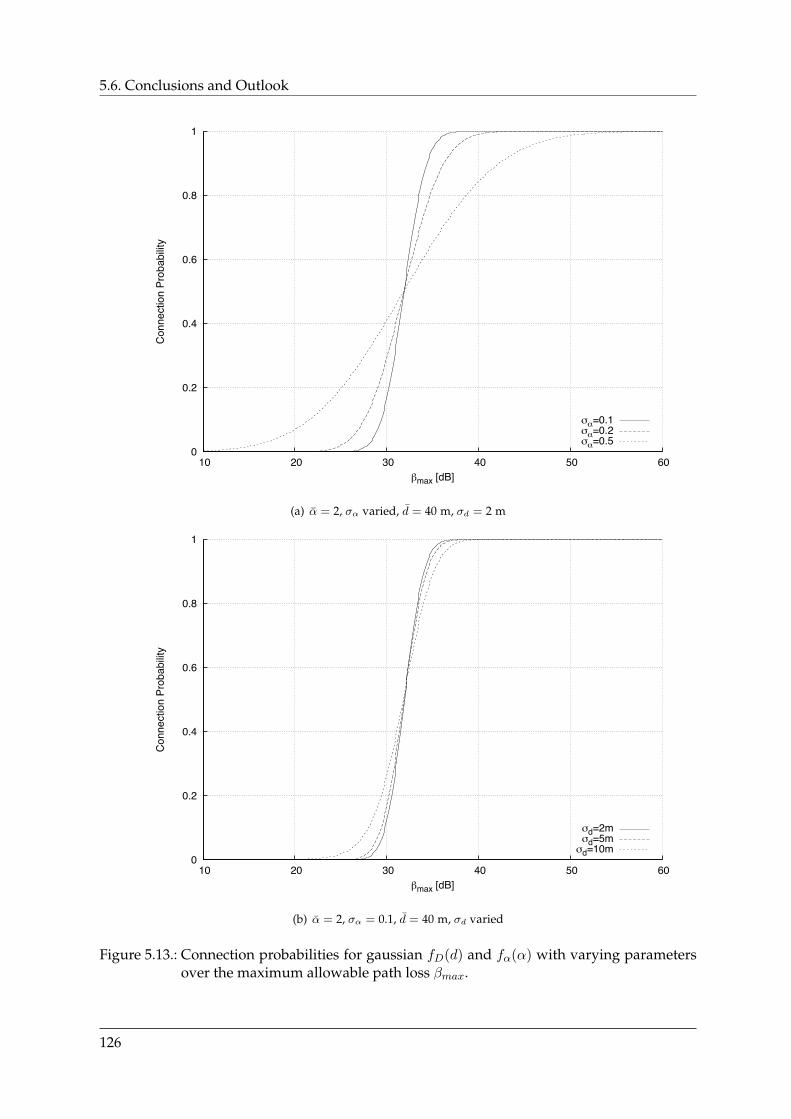
5.6. Conclusions and Outlook
0
0.2
0.4
0.6
0.8
1
10 20 30 40 50 60
Con
nect
ion
Prob
abilit
y
max [dB]
=0.1=0.2=0.5
(a) α = 2, σα varied, d = 40 m, σd = 2 m
0
0.2
0.4
0.6
0.8
1
10 20 30 40 50 60
Con
nect
ion
Prob
abilit
y
max [dB]
d=2md=5m
d=10m
(b) α = 2, σα = 0.1, d = 40 m, σd varied
Figure 5.13.: Connection probabilities for gaussian fD(d) and fα(α) with varying parametersover the maximum allowable path loss βmax.
126
5. Predictive QoS Provisioning in Vehicular Ad-Hoc Networks
suburban scenario. On a highway, however, the mean error is around 30 meters for an intervalof 32 seconds which may still be acceptable, depending on the application.
We have already argued in the discussion that the position prediction accuracy in the city andsuburban scenario is mainly degraded due to an incorrect path selection as the consideredvehicle approaches an intersection. In our studies, the future path has been selected randomlyfrom the set of possible paths. The necessary assumptions have been explained in Section 5.3.4.If the information is available, we strongly propose to consider vehicles’ missions for pathprediction. Considering the city scenario, if only those prediction errors are evaluated forwhich the path selection is correct (i.e., the predictor estimates the correctness as 1), the meanerror can be decreased to about 8 meters, the median to about 5 meters. Taking the missioninto account, these extremely low errors seem feasible.
The computation of the distance to cover is currently calculated using the area under a lineargraph between the current velocity and the predicted velocity, thus assuming a linear accel-eration. Some thoughts should be given to a substitution of this simple approximation witha more sophisticated implementation. One idea that is rather complex in terms of computa-tional efforts is to use n velocity predictors to predict a velocity for each time instant and thusremoving the interpolation. Another approach could be to model the acceleration and decel-eration behavior of a typical driver. If the vehicle is autonomous, reproducing the design ofthe longitudinal controller could increase the prediction performance.
Velocity prediction, too, offers some optimizations opportunities. The key measure necessaryhere is a numerical optimization of the parameters a, b and c mentioned in Table 5.1 over alarge number of scenarios of adequate length. Appropriate parameter sets could be computedbeforehand (and even optimized online) and information about the current driving situationcould be used to select the most suitable set. This selection, in turn, could be used to provideother applications with valuable information about the current environment. It is expectedthat an adoption of these parameters will lead to a somewhat significant improvement of thespeed prediction. An urban scenario requires much quicker reactions to speed changes andthus needs more contributions and stronger influence of the weight booster than a highwayscenario. The highway scenario, in turn, profits from a more stable prediction based to a largeextent on the mean weight vector and requires virtually no influence of the weight booster.
We have proposed a particle-based method for the fast and efficient online-estimation of thePath Loss Exponent (PLE) using signal level measurements from the physical layer and ex-changed positioning information and we have discussed the performance with actual datameasured in a suburban environment. We have then demonstrated how the estimator couldbe extended to account also for NLOSs conditions and discussed results obtained from simu-lations. The mathematical foundation for a channel function that computes connection proba-bilities from the estimated parameters, distance between vehicles and PLE, has been laid anddiscussed. From the shown results, it is clear that the connectivity prediction is more sus-ceptible to wrong estimations of the PLE, which gives raise to the need for development ofeffective channel estimation and — most importantly — further improved channel parameterprediction mechanism.
Longer-term prediction of the wireless channel still imposes the largest problem when it comesto evaluate the future connectivity from predicted positions. Further work is necessary to eval-uate the dynamics of the radio channel and design an appropriate predictor. We propose toinclude further information about the environment (see above) in order to distinguish betweendifferent surroundings and consequently adjust the appropriate channel parameters (such as
127

5.6. Conclusions and Outlook
the variance of the large-scale fading). An interesting idea in this context is to share and aggre-gate knowledge of the communication channel obtained from measurements between nearbyvehicles. Another situation that requires attention is the channel prediction for vehicles thatare actually outside of a node’s communication range and channel parameter estimation isobviously not possible. In this case, the channel has to be estimated from measurements con-ducted with and from nearby vehicles.
128

6. A System Architecture for Cooperative CognitiveTechnical Systems
In the following, we present a communication solution tailored to the communication needs ofcooperative vehicles as seen from an application perspective. We describe how such a solutioncan integrate into and amend the software structure of cognitive vehicles. Without going intothe technical details of the underlying PHY and MAC layers, we describe the data object transfermechanism geared towards cooperative perception modules, its integration in the data flow,and discuss some protocol issues. The channels mechanism is elaborated, which is specificallydesigned for management and control of cooperative groups of vehicles.
Data transfer in networks is generally handled by the protocols of the network layer andabove. The most commonly known network layer protocol is the Internet Protocol (IP) andits companion transport layer protocols, Transmission Control Protocol (TCP) for reliable end-to-end connections and User Datagram Protocol (UDP) for unreliable datagram communica-tions. Today, these protocols are used throughout the internet and in almost all Local AreaNetworks (LANs). They offer various features, such as a hierarchical addressing scheme forrouting, fragmentation, differentiated services and large packet sizes.
The applications that we have presented in Chapter 2, however, do not make use of thesefeatures. Connections are mostly local, point-to-multipoint and routing (if needed) is usuallydetermined by geographical positions rather than network addresses. Adhering to the tradi-tional IP network stack, the headers of UDP and IPv4 would sum up to a total length of 28 B,without being relevant. Due to the shortage of IPv4 addresses, many studies suggest to useIPv6 for future networks, and hence for vehicular networks, which would increase the totallength of the headers to 48 B. Checksum are unnecessary because packet errors are alreadydetected and handled at lower layers.
Consequently, the decision has been made to build a complete protocol that covers the net-working layer up to the session layer. In this section, we will discuss the details of the protocoland show how a prototypical communication solution integrates seamlessly with the softwarearchitecture proposed in the KogniMobil project. Most of the material in this chapter has beenpublished in [NEE07, TAB+08, GAB+08, Nag09].
6.1. A Lightweight Network Layer Protocol
In order to keep transmissions as short as possible to save valuable airtime, we have decidedto drop the IP stack as the network layer of choice and replaced it with a proprietary protocolthat better suits our needs. This significantly reduces the amount of overhead due to headerswhich are not used anyway and the amount of configuration effort, since no IP addresses needto be assigned. The computational complexity needed to process IP packets is also saved.
Every packet is assembled from information pieces (Packet Elements (PEs), such as, for exam-ple, measurement PEs, object update PEs, etc.) that are retrieved either periodically or on-
129
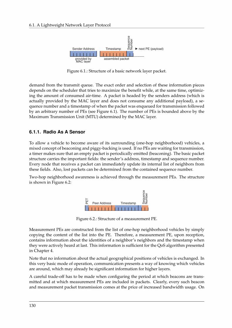
6.1. A Lightweight Network Layer Protocol
Figure 6.1.: Structure of a basic network layer packet.
demand from the transmit queue. The exact order and selection of these information piecesdepends on the scheduler that tries to maximize the benefit while, at the same time, optimiz-ing the amount of consumed air-time. A packet is headed by the senders address (which isactually provided by the MAC layer and does not consume any additional payload), a se-quence number and a timestamp of when the packet was enqueued for transmission followedby an arbitrary number of PEs (see Figure 6.1). The number of PEs is bounded above by theMaximum Transmission Unit (MTU) determined by the MAC layer.
6.1.1. Radio As A Sensor
To allow a vehicle to become aware of its surrounding (one-hop neighborhood) vehicles, amixed concept of beaconing and piggy-backing is used. If no PEs are waiting for transmission,a timer makes sure that an empty packet is periodically emitted (beaconing). The basic packetstructure carries the important fields: the sender’s address, timestamp and sequence number.Every node that receives a packet can immediately update its internal list of neighbors fromthese fields. Also, lost packets can be determined from the contained sequence number.
Two-hop neighborhood awareness is achieved through the measurement PEs. The structureis shown in Figure 6.2:
Figure 6.2.: Structure of a measurement PE.
Measurement PEs are constructed from the list of one-hop neighborhood vehicles by simplycopying the content of the list into the PE. Therefore, a measurement PE, upon reception,contains information about the identities of a neighbor’s neighbors and the timestamp whenthey were actively heard at last. This information is sufficient for the QoS algorithm presentedin Chapter 4.
Note that no information about the actual geographical positions of vehicles is exchanged. Inthis very basic mode of operation, communication presents a way of knowing which vehiclesare around, which may already be significant information for higher layers.
A careful trade-off has to be made when configuring the period at which beacons are trans-mitted and at which measurement PEs are included in packets. Clearly, every such beaconand measurement packet transmission comes at the price of increased bandwidth usage. On
130
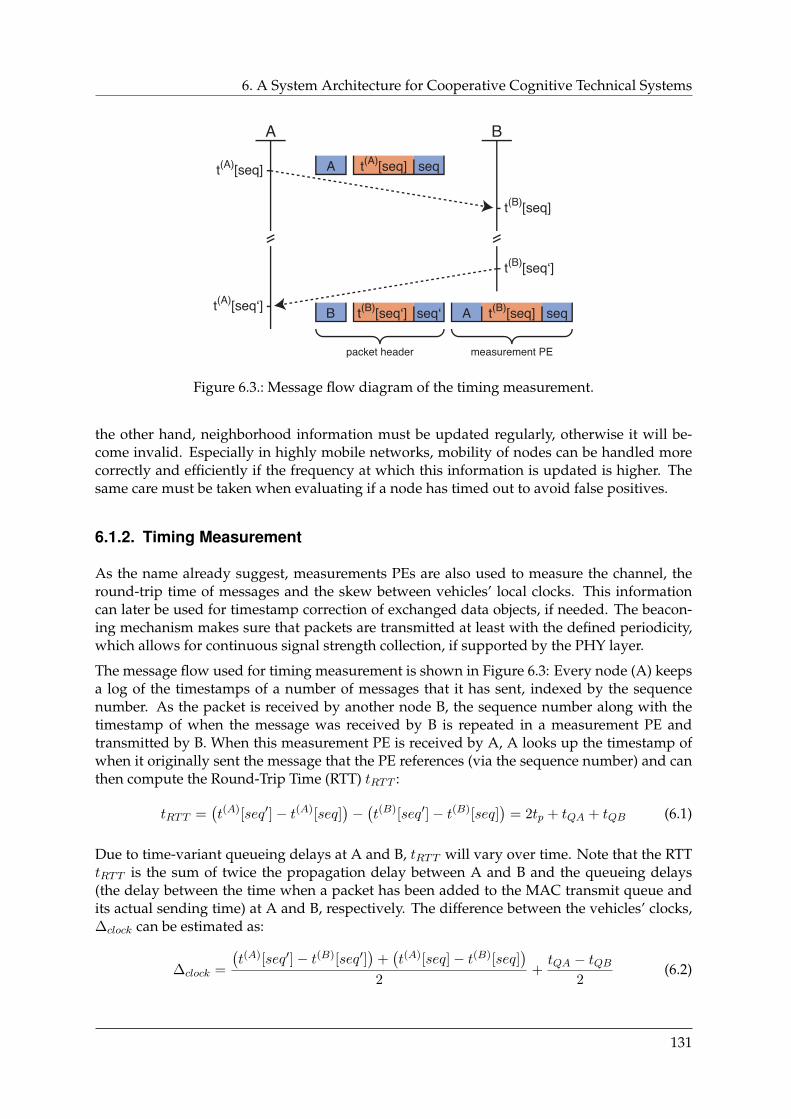
6. A System Architecture for Cooperative Cognitive Technical Systems
A B
t(A)[seq]
t(B)[seq]
t(B)[seq‘]
t(A)[seq‘]
packet header measurement PE
Figure 6.3.: Message flow diagram of the timing measurement.
the other hand, neighborhood information must be updated regularly, otherwise it will be-come invalid. Especially in highly mobile networks, mobility of nodes can be handled morecorrectly and efficiently if the frequency at which this information is updated is higher. Thesame care must be taken when evaluating if a node has timed out to avoid false positives.
6.1.2. Timing Measurement
As the name already suggest, measurements PEs are also used to measure the channel, theround-trip time of messages and the skew between vehicles’ local clocks. This informationcan later be used for timestamp correction of exchanged data objects, if needed. The beacon-ing mechanism makes sure that packets are transmitted at least with the defined periodicity,which allows for continuous signal strength collection, if supported by the PHY layer.
The message flow used for timing measurement is shown in Figure 6.3: Every node (A) keepsa log of the timestamps of a number of messages that it has sent, indexed by the sequencenumber. As the packet is received by another node B, the sequence number along with thetimestamp of when the message was received by B is repeated in a measurement PE andtransmitted by B. When this measurement PE is received by A, A looks up the timestamp ofwhen it originally sent the message that the PE references (via the sequence number) and canthen compute the Round-Trip Time (RTT) tRTT :
tRTT =(t(A)[seq′]− t(A)[seq]
)−(t(B)[seq′]− t(B)[seq]
)= 2tp + tQA + tQB (6.1)
Due to time-variant queueing delays at A and B, tRTT will vary over time. Note that the RTTtRTT is the sum of twice the propagation delay between A and B and the queueing delays(the delay between the time when a packet has been added to the MAC transmit queue andits actual sending time) at A and B, respectively. The difference between the vehicles’ clocks,∆clock can be estimated as:
∆clock =
(t(A)[seq′]− t(B)[seq′]
)+(t(A)[seq]− t(B)[seq]
)2
+tQA − tQB
2(6.2)
131
6.2. The Communication Manager
Note that if the queueing delays tQA and tQB are equal, the last term of Equation (6.2) iszero and the clock skew estimation is correct. Clearly, if the packets contained the times-tamps of when they were actually sent, the term would also be zero. However, since thestatistics of tQA + tQB is known, we can use deconvolution to retrieve the distributions oftQA and tQB and find the distribution of tQA − tQB . Under the assumption that tQA and tQBare equally distributed, averaging can be used to estimate the clock skew. See also the NTPprotocol [MMBK10].
6.1.3. Identification
In many cases, it is desirable to transmit some information about the sender, such as a cleartextidentifier, certificates, keys, etc. This information can be transmitted in every message or witha certain period, using an identification PE:
Figure 6.4.: Structure of an identification PE.
Note that the structure of the identification data itself is not specified and can be determinedby higher-layer software.
6.2. The Communication Manager
The information flow (Figure 6.5 from top-left to bottom-right) within the vehicles softwaremodules is based on a real-time database, which is basically a shared memory segment [GF08]that provides functions to create, update, retrieve and delete data objects as well as the possi-bility for software modules to subscribe to data objects and receive notifications upon updatesof subscribed objects.
Following this paradigm, every sensor used in the vehicle has a corresponding data object.For instance, images taken by the onboard cameras or LIDAR data are stored as databaseobjects, which are updated periodically as the sensor completes a cycle. These database objectsare subscribed by instances of lane trackers, object detectors and classifiers which, in turn,have associated data objects that contain the outputs of these modules. The behavior controlalgorithms process these output contents and finally decide on a track that should be used fordriving. Again, this track is routed through the database to the body control modules thatcontrol the vehicle’s actors.
6.2.1. Network Topology Information
We have stated before that the information gathered by exchanging beacons, packets and mea-surement PEs can be seen as a kind of additional sensorial information. Consequently, the
132
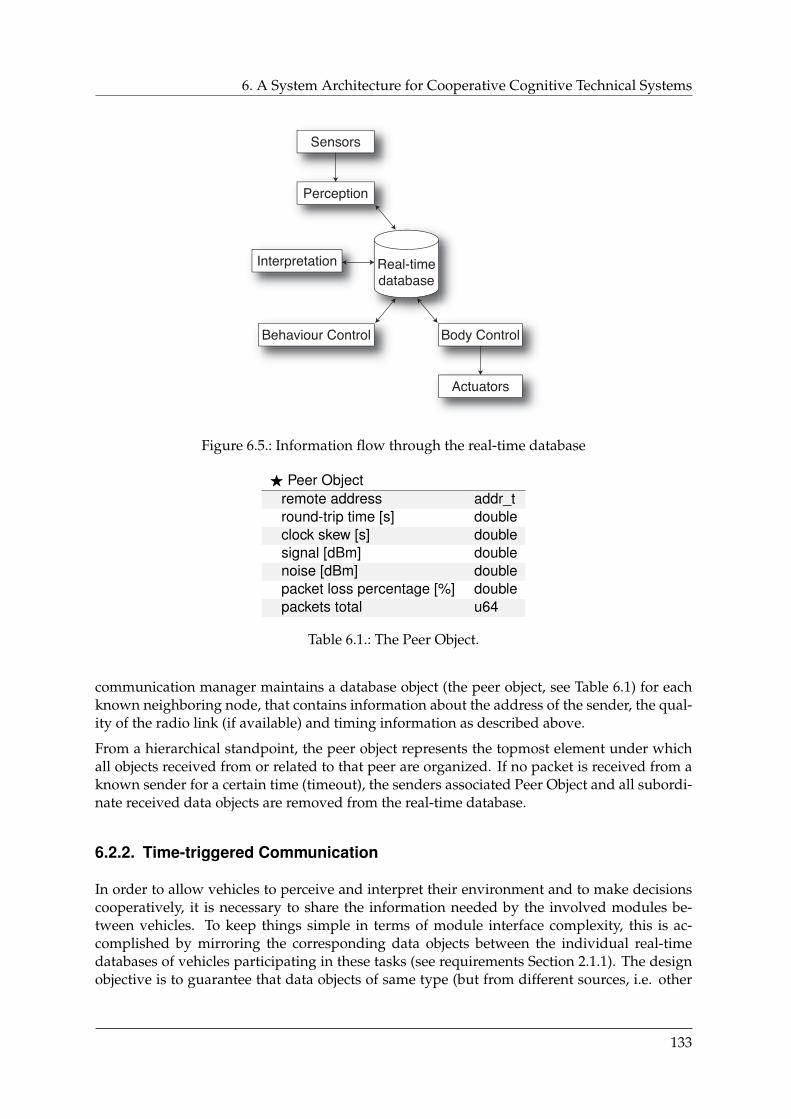
6. A System Architecture for Cooperative Cognitive Technical Systems
Real-timedatabase
Perception
Interpretation
Behaviour Control Body Control
Sensors
Actuators
Figure 6.5.: Information flow through the real-time database
F Peer Objectremote address addr_tround-trip time [s] doubleclock skew [s] doublesignal [dBm] doublenoise [dBm] doublepacket loss percentage [%] doublepackets total u64
Table 6.1.: The Peer Object.
communication manager maintains a database object (the peer object, see Table 6.1) for eachknown neighboring node, that contains information about the address of the sender, the qual-ity of the radio link (if available) and timing information as described above.
From a hierarchical standpoint, the peer object represents the topmost element under whichall objects received from or related to that peer are organized. If no packet is received from aknown sender for a certain time (timeout), the senders associated Peer Object and all subordi-nate received data objects are removed from the real-time database.
6.2.2. Time-triggered Communication
In order to allow vehicles to perceive and interpret their environment and to make decisionscooperatively, it is necessary to share the information needed by the involved modules be-tween vehicles. To keep things simple in terms of module interface complexity, this is ac-complished by mirroring the corresponding data objects between the individual real-timedatabases of vehicles participating in these tasks (see requirements Section 2.1.1). The designobjective is to guarantee that data objects of same type (but from different sources, i.e. other
133
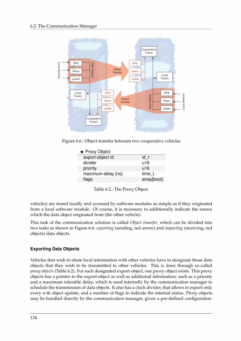
6.2. The Communication Manager
LIDAR
Vision
GPS
LocalFusion
Data O
bjects
CooperativeFusion
LIDAR
Vision
GPS
LIDAR
Vision
GPS
LocalFusion
Dat
a O
bje
cts
CooperativeFusion
LIDAR
Vision
GPS
ObjectTransfer
ObjectTransfer
Local Sensors
Loca
l Sen
sors
Figure 6.6.: Object transfer between two cooperative vehicles
F Proxy Objectexport-object id id_tdivider u16priority u16maximum delay [ns] time_tflags array[bool]
Table 6.2.: The Proxy Object.
vehicles) are stored locally and accessed by software modules as simple as if they originatedfrom a local software module. Of course, it is necessary to additionally indicate the sourcewhich the data object originated from (the other vehicle).
This task of the communication solution is called Object transfer, which can be divided intotwo tasks as shown in Figure 6.6: exporting (sending, red arrow) and importing (receiving, redobjects) data objects.
Exporting Data Objects
Vehicles that wish to share local information with other vehicles have to designate those dataobjects that they wish to be transmitted to other vehicles. This is done through so-calledproxy objects (Table 6.2). For each designated export-object, one proxy object exists. This proxyobjects has a pointer to the export-object as well as additional information, such as a priorityand a maximum tolerable delay, which is used internally by the communication manager toschedule the transmission of data objects. It also has a clock divider, that allows to export onlyevery n-th object update, and a number of flags to indicate the internal status. Proxy objectsmay be handled directly by the communication manager, given a pre-defined configuration.
134
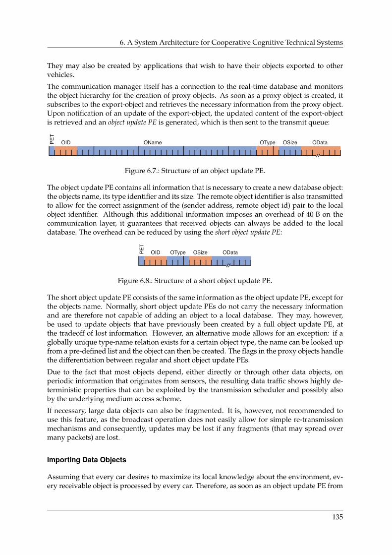
6. A System Architecture for Cooperative Cognitive Technical Systems
They may also be created by applications that wish to have their objects exported to othervehicles.
The communication manager itself has a connection to the real-time database and monitorsthe object hierarchy for the creation of proxy objects. As soon as a proxy object is created, itsubscribes to the export-object and retrieves the necessary information from the proxy object.Upon notification of an update of the export-object, the updated content of the export-objectis retrieved and an object update PE is generated, which is then sent to the transmit queue:
Figure 6.7.: Structure of an object update PE.
The object update PE contains all information that is necessary to create a new database object:the objects name, its type identifier and its size. The remote object identifier is also transmittedto allow for the correct assignment of the (sender address, remote object id) pair to the localobject identifier. Although this additional information imposes an overhead of 40 B on thecommunication layer, it guarantees that received objects can always be added to the localdatabase. The overhead can be reduced by using the short object update PE:
Figure 6.8.: Structure of a short object update PE.
The short object update PE consists of the same information as the object update PE, except forthe objects name. Normally, short object update PEs do not carry the necessary informationand are therefore not capable of adding an object to a local database. They may, however,be used to update objects that have previously been created by a full object update PE, atthe tradeoff of lost information. However, an alternative mode allows for an exception: if aglobally unique type-name relation exists for a certain object type, the name can be looked upfrom a pre-defined list and the object can then be created. The flags in the proxy objects handlethe differentiation between regular and short object update PEs.
Due to the fact that most objects depend, either directly or through other data objects, onperiodic information that originates from sensors, the resulting data traffic shows highly de-terministic properties that can be exploited by the transmission scheduler and possibly alsoby the underlying medium access scheme.
If necessary, large data objects can also be fragmented. It is, however, not recommended touse this feature, as the broadcast operation does not easily allow for simple re-transmissionmechanisms and consequently, updates may be lost if any fragments (that may spread overmany packets) are lost.
Importing Data Objects
Assuming that every car desires to maximize its local knowledge about the environment, ev-ery receivable object is processed by every car. Therefore, as soon as an object update PE from
135
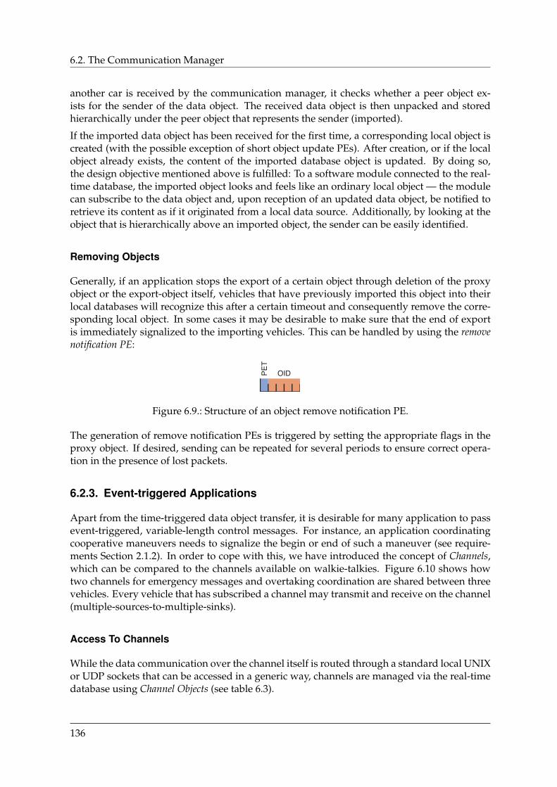
6.2. The Communication Manager
another car is received by the communication manager, it checks whether a peer object ex-ists for the sender of the data object. The received data object is then unpacked and storedhierarchically under the peer object that represents the sender (imported).
If the imported data object has been received for the first time, a corresponding local object iscreated (with the possible exception of short object update PEs). After creation, or if the localobject already exists, the content of the imported database object is updated. By doing so,the design objective mentioned above is fulfilled: To a software module connected to the real-time database, the imported object looks and feels like an ordinary local object — the modulecan subscribe to the data object and, upon reception of an updated data object, be notified toretrieve its content as if it originated from a local data source. Additionally, by looking at theobject that is hierarchically above an imported object, the sender can be easily identified.
Removing Objects
Generally, if an application stops the export of a certain object through deletion of the proxyobject or the export-object itself, vehicles that have previously imported this object into theirlocal databases will recognize this after a certain timeout and consequently remove the corre-sponding local object. In some cases it may be desirable to make sure that the end of exportis immediately signalized to the importing vehicles. This can be handled by using the removenotification PE:
Figure 6.9.: Structure of an object remove notification PE.
The generation of remove notification PEs is triggered by setting the appropriate flags in theproxy object. If desired, sending can be repeated for several periods to ensure correct opera-tion in the presence of lost packets.
6.2.3. Event-triggered Applications
Apart from the time-triggered data object transfer, it is desirable for many application to passevent-triggered, variable-length control messages. For instance, an application coordinatingcooperative maneuvers needs to signalize the begin or end of such a maneuver (see require-ments Section 2.1.2). In order to cope with this, we have introduced the concept of Channels,which can be compared to the channels available on walkie-talkies. Figure 6.10 shows howtwo channels for emergency messages and overtaking coordination are shared between threevehicles. Every vehicle that has subscribed a channel may transmit and receive on the channel(multiple-sources-to-multiple-sinks).
Access To Channels
While the data communication over the channel itself is routed through a standard local UNIXor UDP sockets that can be accessed in a generic way, channels are managed via the real-timedatabase using Channel Objects (see table 6.3).
136
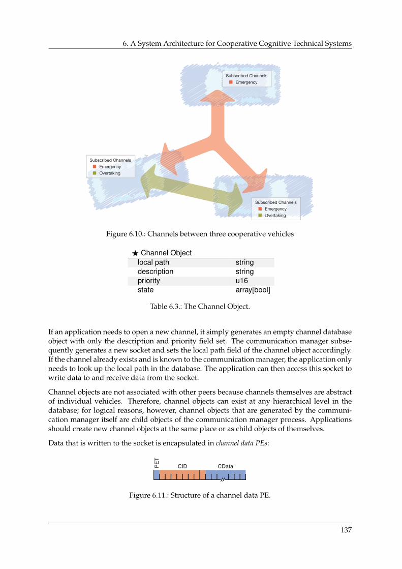
6. A System Architecture for Cooperative Cognitive Technical Systems
Subscribed Channels
Overtaking
Emergency
Subscribed Channels
Overtaking
Emergency
Subscribed Channels
Emergency
Figure 6.10.: Channels between three cooperative vehicles
F Channel Objectlocal path stringdescription stringpriority u16state array[bool]
Table 6.3.: The Channel Object.
If an application needs to open a new channel, it simply generates an empty channel databaseobject with only the description and priority field set. The communication manager subse-quently generates a new socket and sets the local path field of the channel object accordingly.If the channel already exists and is known to the communication manager, the application onlyneeds to look up the local path in the database. The application can then access this socket towrite data to and receive data from the socket.
Channel objects are not associated with other peers because channels themselves are abstractof individual vehicles. Therefore, channel objects can exist at any hierarchical level in thedatabase; for logical reasons, however, channel objects that are generated by the communi-cation manager itself are child objects of the communication manager process. Applicationsshould create new channel objects at the same place or as child objects of themselves.
Data that is written to the socket is encapsulated in channel data PEs:
Figure 6.11.: Structure of a channel data PE.
137
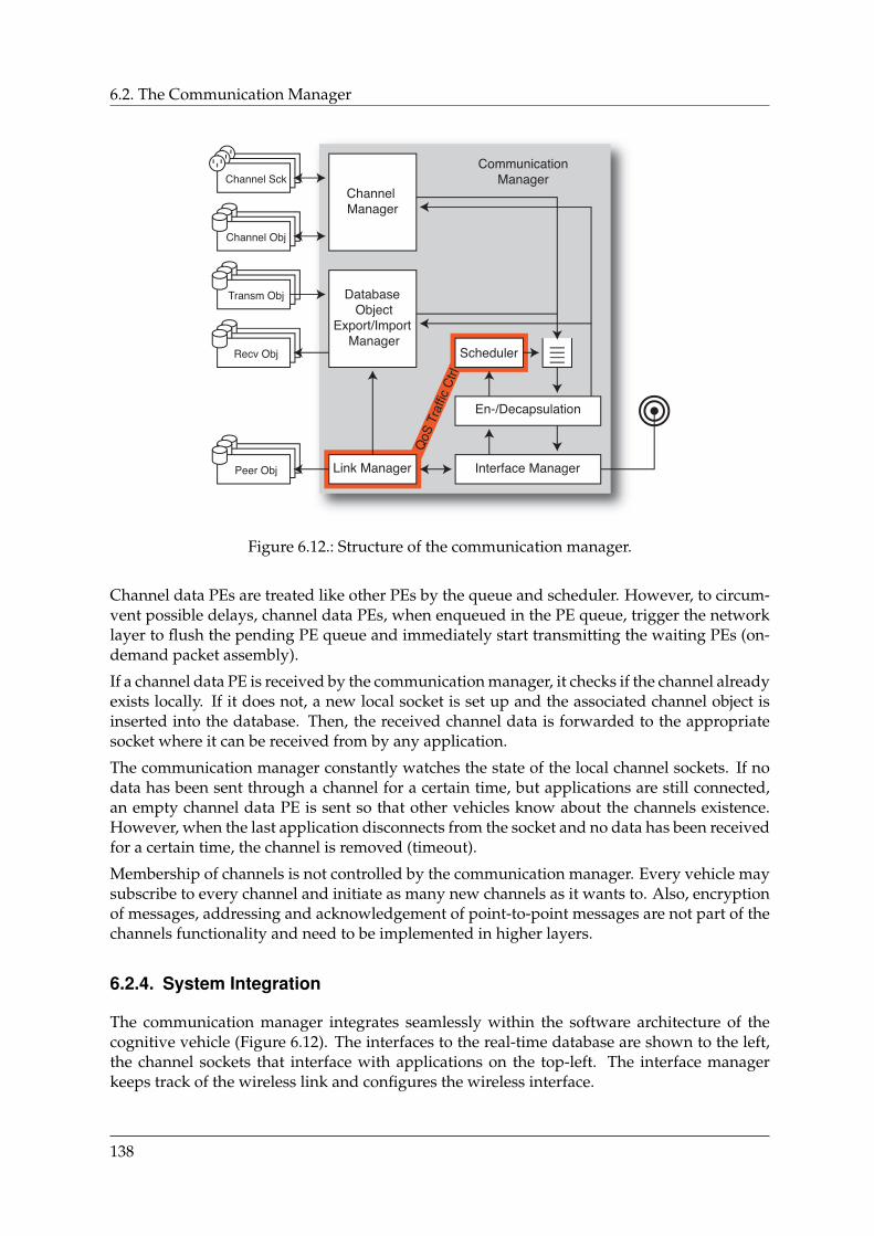
6.2. The Communication Manager
CommunicationManagerChannel Sck
Channel Obj
Transm Obj
Recv Obj
Peer Obj
QoS
Traffic
Ctrl
Figure 6.12.: Structure of the communication manager.
Channel data PEs are treated like other PEs by the queue and scheduler. However, to circum-vent possible delays, channel data PEs, when enqueued in the PE queue, trigger the networklayer to flush the pending PE queue and immediately start transmitting the waiting PEs (on-demand packet assembly).
If a channel data PE is received by the communication manager, it checks if the channel alreadyexists locally. If it does not, a new local socket is set up and the associated channel object isinserted into the database. Then, the received channel data is forwarded to the appropriatesocket where it can be received from by any application.
The communication manager constantly watches the state of the local channel sockets. If nodata has been sent through a channel for a certain time, but applications are still connected,an empty channel data PE is sent so that other vehicles know about the channels existence.However, when the last application disconnects from the socket and no data has been receivedfor a certain time, the channel is removed (timeout).
Membership of channels is not controlled by the communication manager. Every vehicle maysubscribe to every channel and initiate as many new channels as it wants to. Also, encryptionof messages, addressing and acknowledgement of point-to-point messages are not part of thechannels functionality and need to be implemented in higher layers.
6.2.4. System Integration
The communication manager integrates seamlessly within the software architecture of thecognitive vehicle (Figure 6.12). The interfaces to the real-time database are shown to the left,the channel sockets that interface with applications on the top-left. The interface managerkeeps track of the wireless link and configures the wireless interface.
138
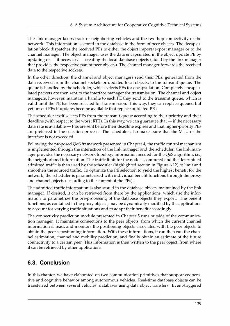
6. A System Architecture for Cooperative Cognitive Technical Systems
The link manager keeps track of neighboring vehicles and the two-hop connectivity of thenetwork. This information is stored in the database in the form of peer objects. The decapsu-lation block dispatches the received PEs to either the object import/export manager or to thechannel manager. The object manager uses the data encapsulated in the object update PE byupdating or — if necessary — creating the local database objects (aided by the link managerthat provides the respective parent peer objects). The channel manager forwards the receiveddata to the respective sockets.
In the other direction, the channel and object managers send their PEs, generated from thedata received from the channel sockets or updated local objects, to the transmit queue. Thequeue is handled by the scheduler, which selects PEs for encapsulation. Completely encapsu-lated packets are then sent to the interface manager for transmission. The channel and objectmanagers, however, maintain a handle to each PE they send to the transmit queue, which isvalid until the PE has been selected for transmission. This way, they can replace queued butyet unsent PEs if updates become available that replace outdated PEs.
The scheduler itself selects PEs from the transmit queue according to their priority and theirdeadline (with respect to the worst RTT). In this way, we can guarantee that — if the necessarydata rate is available — PEs are sent before their deadline expires and that higher-priority PEsare preferred in the selection process. The scheduler also makes sure that the MTU of theinterface is not exceeded.
Following the proposed QoS framework presented in Chapter 4, the traffic control mechanismis implemented through the interaction of the link manager and the scheduler: the link man-ager provides the necessary network topology information needed for the QoS algorithm, i.e.,the neighborhood information. The traffic limit for the node is computed and the determinedadmitted traffic is then used by the scheduler (highlighted section in Figure 6.12) to limit andsmoothen the sourced traffic. To optimize the PE selection to yield the highest benefit for thenetwork, the scheduler is parameterized with individual benefit functions through the proxyand channel objects (according to the content of the PEs).
The admitted traffic information is also stored in the database objects maintained by the linkmanager. If desired, it can be retrieved from there by the applications, which use the infor-mation to parametrize the pre-processing of the database objects they export. The benefitfunctions, as contained in the proxy objects, may be dynamically modified by the applicationsto account for varying traffic situations and to adapt their benefit accordingly.
The connectivity prediction module presented in Chapter 5 runs outside of the communica-tion manager. It maintains connections to the peer objects, from which the current channelinformation is read, and monitors the positioning objects associated with the peer objects toobtain the peer’s positioning information. With these informations, it can then run the chan-nel estimation, channel and mobility prediction, and finally obtain an estimate of the futureconnectivity to a certain peer. This information is then written to the peer object, from whereit can be retrieved by other applications.
6.3. Conclusion
In this chapter, we have elaborated on two communication primitives that support coopera-tive and cognitive behavior among autonomous vehicles. Real-time database objects can betransferred between several vehicles’ databases using data object transfers. Event-triggered
139
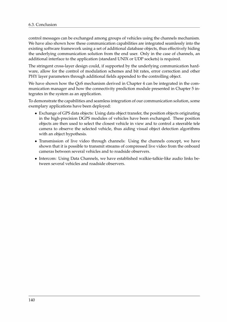
6.3. Conclusion
control messages can be exchanged among groups of vehicles using the channels mechanism.We have also shown how these communication capabilities are integrated seamlessly into theexisting software framework using a set of additional database objects, thus effectively hidingthe underlying communication solution from the end user. Only in the case of channels, anadditional interface to the application (standard UNIX or UDP sockets) is required.
The stringent cross-layer design could, if supported by the underlying communication hard-ware, allow for the control of modulation schemes and bit rates, error correction and otherPHY layer parameters through additional fields appended to the controlling object.
We have shown how the QoS mechanism derived in Chapter 4 can be integrated in the com-munication manager and how the connectivity prediction module presented in Chapter 5 in-tegrates in the system as an application.
To demonstrate the capabilities and seamless integration of our communication solution, someexemplary applications have been deployed:
• Exchange of GPS data objects: Using data object transfer, the position objects originatingin the high-precision DGPS modules of vehicles have been exchanged. These positionobjects are then used to select the closest vehicle in view and to control a steerable telecamera to observe the selected vehicle, thus aiding visual object detection algorithmswith an object hypothesis.
• Transmission of live video through channels: Using the channels concept, we haveshown that it is possible to transmit streams of compressed live video from the onboardcameras between several vehicles and to roadside observers.
• Intercom: Using Data Channels, we have established walkie-talkie-like audio links be-tween several vehicles and roadside observers.
140
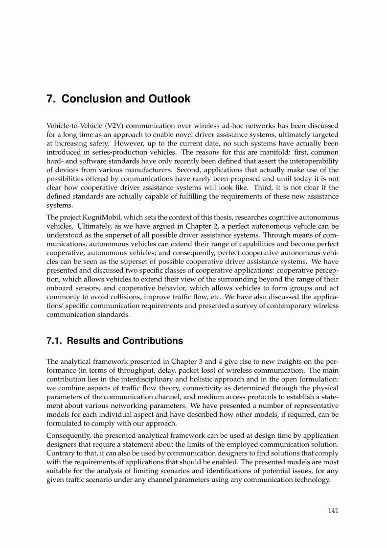
7. Conclusion and Outlook
Vehicle-to-Vehicle (V2V) communication over wireless ad-hoc networks has been discussedfor a long time as an approach to enable novel driver assistance systems, ultimately targetedat increasing safety. However, up to the current date, no such systems have actually beenintroduced in series-production vehicles. The reasons for this are manifold: first, commonhard- and software standards have only recently been defined that assert the interoperabilityof devices from various manufacturers. Second, applications that actually make use of thepossibilities offered by communications have rarely been proposed and until today it is notclear how cooperative driver assistance systems will look like. Third, it is not clear if thedefined standards are actually capable of fulfilling the requirements of these new assistancesystems.
The project KogniMobil, which sets the context of this thesis, researches cognitive autonomousvehicles. Ultimately, as we have argued in Chapter 2, a perfect autonomous vehicle can beunderstood as the superset of all possible driver assistance systems. Through means of com-munications, autonomous vehicles can extend their range of capabilities and become perfectcooperative, autonomous vehicles; and consequently, perfect cooperative autonomous vehi-cles can be seen as the superset of possible cooperative driver assistance systems. We havepresented and discussed two specific classes of cooperative applications: cooperative percep-tion, which allows vehicles to extend their view of the surrounding beyond the range of theironboard sensors, and cooperative behavior, which allows vehicles to form groups and actcommonly to avoid collisions, improve traffic flow, etc. We have also discussed the applica-tions’ specific communication requirements and presented a survey of contemporary wirelesscommunication standards.
7.1. Results and Contributions
The analytical framework presented in Chapter 3 and 4 give rise to new insights on the per-formance (in terms of throughput, delay, packet loss) of wireless communication. The maincontribution lies in the interdisciplinary and holistic approach and in the open formulation:we combine aspects of traffic flow theory, connectivity as determined through the physicalparameters of the communication channel, and medium access protocols to establish a state-ment about various networking parameters. We have presented a number of representativemodels for each individual aspect and have described how other models, if required, can beformulated to comply with our approach.
Consequently, the presented analytical framework can be used at design time by applicationdesigners that require a statement about the limits of the employed communication solution.Contrary to that, it can also be used by communication designers to find solutions that complywith the requirements of applications that should be enabled. The presented models are mostsuitable for the analysis of limiting scenarios and identifications of potential issues, for anygiven traffic scenario under any channel parameters using any communication technology.
141
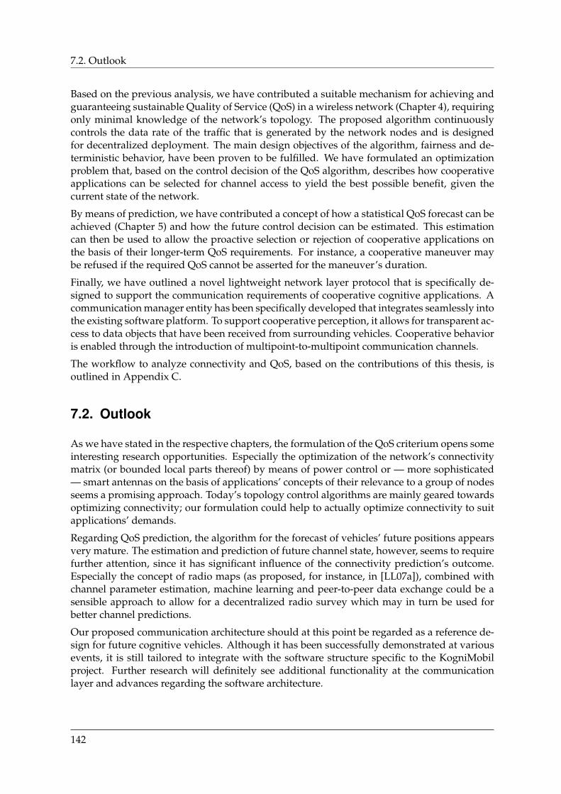
7.2. Outlook
Based on the previous analysis, we have contributed a suitable mechanism for achieving andguaranteeing sustainable Quality of Service (QoS) in a wireless network (Chapter 4), requiringonly minimal knowledge of the network’s topology. The proposed algorithm continuouslycontrols the data rate of the traffic that is generated by the network nodes and is designedfor decentralized deployment. The main design objectives of the algorithm, fairness and de-terministic behavior, have been proven to be fulfilled. We have formulated an optimizationproblem that, based on the control decision of the QoS algorithm, describes how cooperativeapplications can be selected for channel access to yield the best possible benefit, given thecurrent state of the network.
By means of prediction, we have contributed a concept of how a statistical QoS forecast can beachieved (Chapter 5) and how the future control decision can be estimated. This estimationcan then be used to allow the proactive selection or rejection of cooperative applications onthe basis of their longer-term QoS requirements. For instance, a cooperative maneuver maybe refused if the required QoS cannot be asserted for the maneuver’s duration.
Finally, we have outlined a novel lightweight network layer protocol that is specifically de-signed to support the communication requirements of cooperative cognitive applications. Acommunication manager entity has been specifically developed that integrates seamlessly intothe existing software platform. To support cooperative perception, it allows for transparent ac-cess to data objects that have been received from surrounding vehicles. Cooperative behavioris enabled through the introduction of multipoint-to-multipoint communication channels.
The workflow to analyze connectivity and QoS, based on the contributions of this thesis, isoutlined in Appendix C.
7.2. Outlook
As we have stated in the respective chapters, the formulation of the QoS criterium opens someinteresting research opportunities. Especially the optimization of the network’s connectivitymatrix (or bounded local parts thereof) by means of power control or — more sophisticated— smart antennas on the basis of applications’ concepts of their relevance to a group of nodesseems a promising approach. Today’s topology control algorithms are mainly geared towardsoptimizing connectivity; our formulation could help to actually optimize connectivity to suitapplications’ demands.
Regarding QoS prediction, the algorithm for the forecast of vehicles’ future positions appearsvery mature. The estimation and prediction of future channel state, however, seems to requirefurther attention, since it has significant influence of the connectivity prediction’s outcome.Especially the concept of radio maps (as proposed, for instance, in [LL07a]), combined withchannel parameter estimation, machine learning and peer-to-peer data exchange could be asensible approach to allow for a decentralized radio survey which may in turn be used forbetter channel predictions.
Our proposed communication architecture should at this point be regarded as a reference de-sign for future cognitive vehicles. Although it has been successfully demonstrated at variousevents, it is still tailored to integrate with the software structure specific to the KogniMobilproject. Further research will definitely see additional functionality at the communicationlayer and advances regarding the software architecture.
142

A. A Spline-Shaped Road Model
Cubic splines are widely used in the design of (free-form) curves and surfaces in computer-aided design applications, especially in the construction of ships, airplanes and cars. They arealso being used in the process of laying railroad tracks. Their adequacy can be justified by thefact that for every curve section, boundary conditions can be defined in the terms of pointsand values for the first and second derivative (i.e, gradient and curvature). By doing so, it canbe ensured that the curvature along a route, which may consist of many individual segments,is always continuous. Consequently, the resulting lateral acceleration when traveling alongthe route is also continuous; a prerequisite for the planning of roads. For this reason, cubicsplines are very well suited as road models.
A.1. Definition of a Spline
The basis function for cubic splines is shown in Figure A.1. It is defined as:
γ (t) =1
6
(2 + t)3 if − 2 < t ≤ −14− 6t2 − 3t3 if − 1 < t ≤ 04− 6t2 + 3t3 if 0 < t ≤ 1(2− t)3 if 1 < t ≤ 20 otherwise
(A.1)
A segment n of the spline is defined as a parametric curve xn (t) , t ∈ [0 . . . 1] as the weightedsum of the positions of its so-called knots. Every segment is defined by four knots kn+i, i ∈0, 1, 2, 3. The weights γi result from the four highlighted sections of the basis function (seeFigure A.1) and are dependent of the parameter t:
γ0(t) =1
6
(−t3 + 3t2 − 3t+ 1
)γ1(t) =
1
6
(3t3 − 6t2 + 4
)γ2(t) =
1
6
(−3t3 + 3t2 + 3t+ 1
)γ3(t) =
1
6t3
The position xn(t) of a point on the spline segment n at time t is then:
xn(t) = knγ0(t) + kn+1γ1(t) + kn+2γ2(t) + kn+3γ3(t)
=[t3 t2 t 1
]M˜
knkn+1
kn+2
kn+3
(A.2)
143
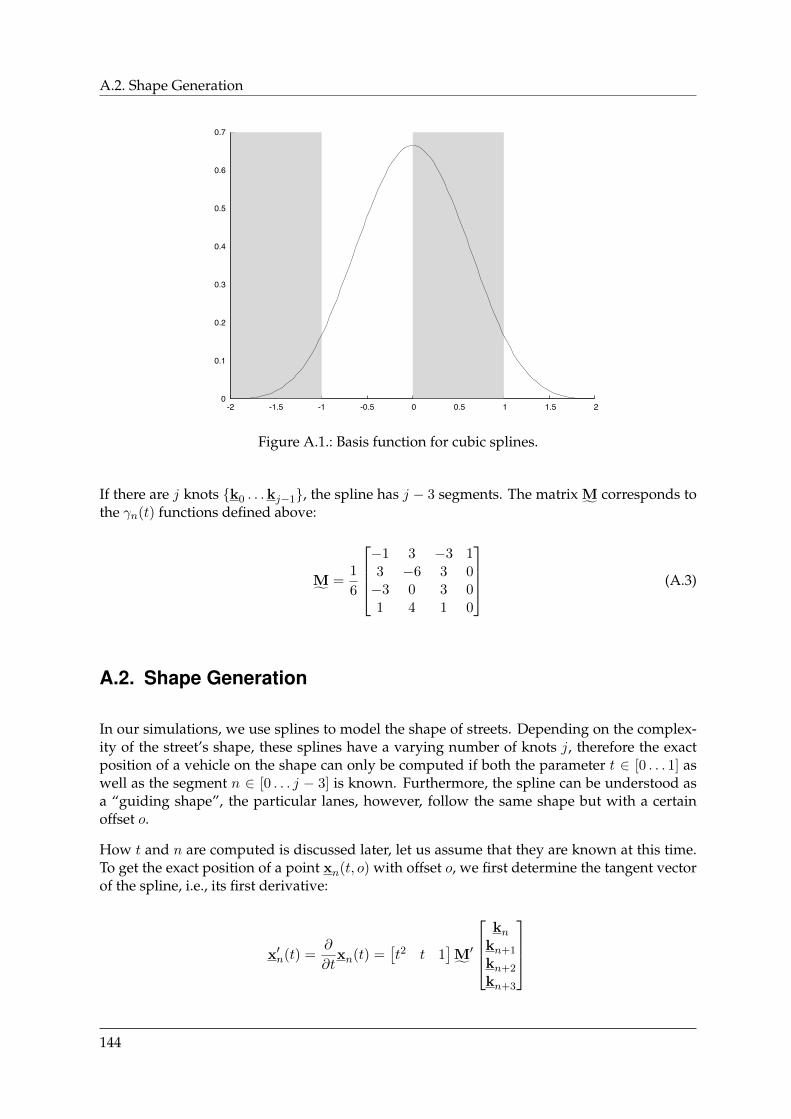
A.2. Shape Generation
0
0.1
0.2
0.3
0.4
0.5
0.6
0.7
-2 -1.5 -1 -0.5 0 0.5 1 1.5 2
Figure A.1.: Basis function for cubic splines.
If there are j knots k0 . . .kj−1, the spline has j − 3 segments. The matrix M˜ corresponds tothe γn(t) functions defined above:
M˜ =1
6
−1 3 −3 13 −6 3 0−3 0 3 01 4 1 0
(A.3)
A.2. Shape Generation
In our simulations, we use splines to model the shape of streets. Depending on the complex-ity of the street’s shape, these splines have a varying number of knots j, therefore the exactposition of a vehicle on the shape can only be computed if both the parameter t ∈ [0 . . . 1] aswell as the segment n ∈ [0 . . . j − 3] is known. Furthermore, the spline can be understood asa “guiding shape”, the particular lanes, however, follow the same shape but with a certainoffset o.
How t and n are computed is discussed later, let us assume that they are known at this time.To get the exact position of a point xn(t, o) with offset o, we first determine the tangent vectorof the spline, i.e., its first derivative:
x′n(t) =∂
∂txn(t) =
[t2 t 1
]M˜′
knkn+1
kn+2
kn+3
144
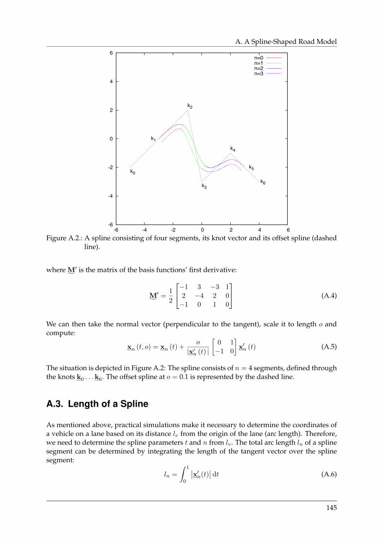
A. A Spline-Shaped Road Model
-6
-4
-2
0
2
4
6
-6 -4 -2 0 2 4 6
k0
k1
k2
k3
k4
k5
k6
n=0n=1n=2n=3
Figure A.2.: A spline consisting of four segments, its knot vector and its offset spline (dashedline).
where M˜′ is the matrix of the basis functions’ first derivative:
M˜′ = 1
2
−1 3 −3 12 −4 2 0−1 0 1 0
(A.4)
We can then take the normal vector (perpendicular to the tangent), scale it to length o andcompute:
xn (t, o) = xn (t) +o
|x′n (t) |
[0 1−1 0
]x′n (t) (A.5)
The situation is depicted in Figure A.2: The spline consists of n = 4 segments, defined throughthe knots k0 . . .k6. The offset spline at o = 0.1 is represented by the dashed line.
A.3. Length of a Spline
As mentioned above, practical simulations make it necessary to determine the coordinates ofa vehicle on a lane based on its distance lv from the origin of the lane (arc length). Therefore,we need to determine the spline parameters t and n from lv. The total arc length ln of a splinesegment can be determined by integrating the length of the tangent vector over the splinesegment:
ln =
∫ 1
0
∣∣x′n(t)∣∣ dt (A.6)
145
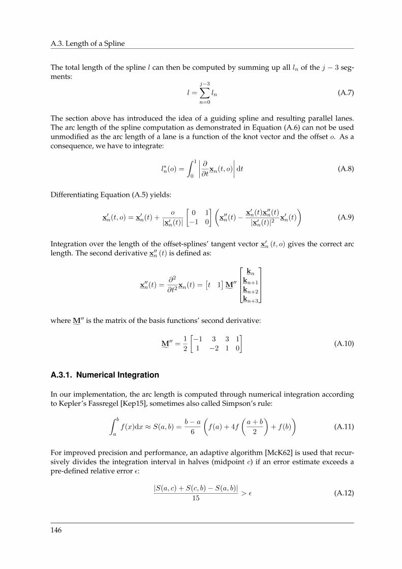
A.3. Length of a Spline
The total length of the spline l can then be computed by summing up all ln of the j − 3 seg-ments:
l =
j−3∑n=0
ln (A.7)
The section above has introduced the idea of a guiding spline and resulting parallel lanes.The arc length of the spline computation as demonstrated in Equation (A.6) can not be usedunmodified as the arc length of a lane is a function of the knot vector and the offset o. As aconsequence, we have to integrate:
l∗n(o) =
∫ 1
0
∣∣∣∣ ∂∂txn(t, o)
∣∣∣∣ dt (A.8)
Differentiating Equation (A.5) yields:
x′n(t, o) = x′n(t) +o
|x′n(t)|
[0 1−1 0
](x′′n(t)− x′n(t)x′′n(t)
|x′n(t)|2x′n(t)
)(A.9)
Integration over the length of the offset-splines’ tangent vector x′n (t, o) gives the correct arclength. The second derivative x′′n (t) is defined as:
x′′n(t) =∂2
∂t2xn(t) =
[t 1
]M˜′′
kn
kn+1
kn+2
kn+3
where M˜′′ is the matrix of the basis functions’ second derivative:
M˜′′ = 1
2
[−1 3 3 11 −2 1 0
](A.10)
A.3.1. Numerical Integration
In our implementation, the arc length is computed through numerical integration accordingto Kepler’s Fassregel [Kep15], sometimes also called Simpson’s rule:∫ b
af(x)dx ≈ S(a, b) =
b− a6
(f(a) + 4f
(a+ b
2
)+ f(b)
)(A.11)
For improved precision and performance, an adaptive algorithm [McK62] is used that recur-sively divides the integration interval in halves (midpoint c) if an error estimate exceeds apre-defined relative error ε:
|S(a, c) + S(c, b)− S(a, b)|15
> ε (A.12)
146
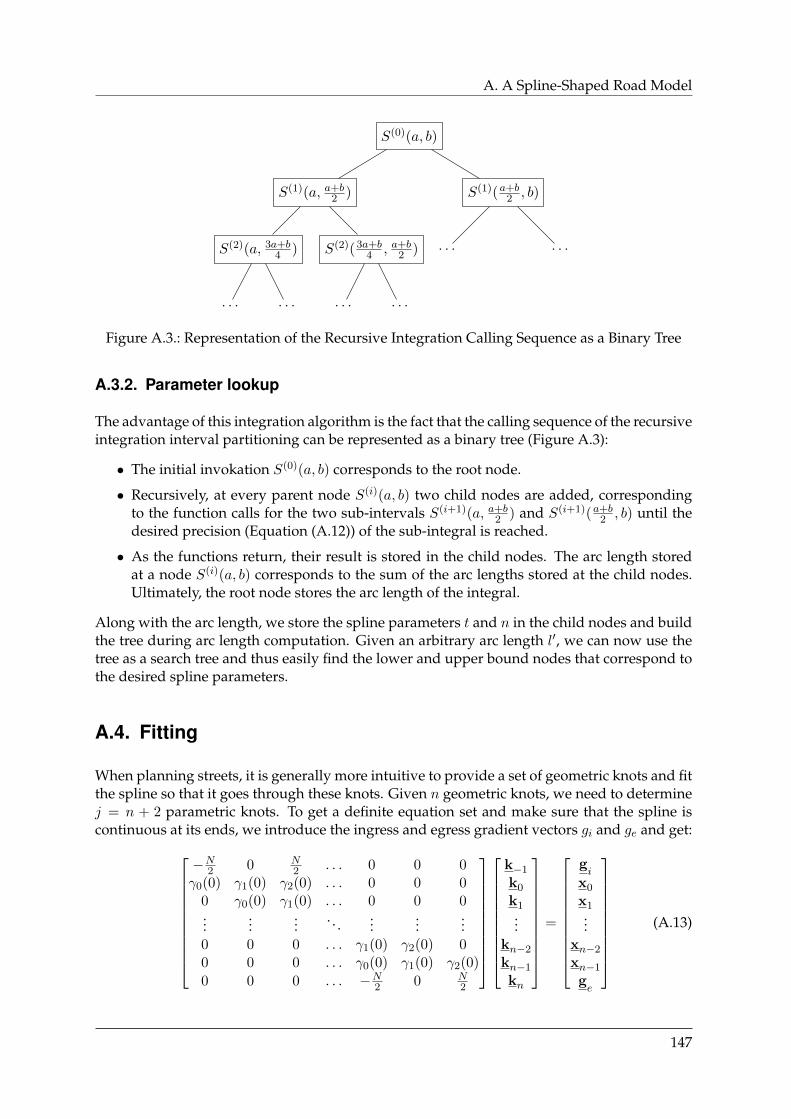
A. A Spline-Shaped Road Model
S(0)(a, b)
S(1)(a, a+b2 )
S(2)(a, 3a+b4 )
. . . . . .
S(2)(3a+b4 , a+b
2 )
. . . . . .
S(1)(a+b2 , b)
. . . . . .
Figure A.3.: Representation of the Recursive Integration Calling Sequence as a Binary Tree
A.3.2. Parameter lookup
The advantage of this integration algorithm is the fact that the calling sequence of the recursiveintegration interval partitioning can be represented as a binary tree (Figure A.3):
• The initial invokation S(0)(a, b) corresponds to the root node.
• Recursively, at every parent node S(i)(a, b) two child nodes are added, correspondingto the function calls for the two sub-intervals S(i+1)(a, a+b
2 ) and S(i+1)(a+b2 , b) until the
desired precision (Equation (A.12)) of the sub-integral is reached.
• As the functions return, their result is stored in the child nodes. The arc length storedat a node S(i)(a, b) corresponds to the sum of the arc lengths stored at the child nodes.Ultimately, the root node stores the arc length of the integral.
Along with the arc length, we store the spline parameters t and n in the child nodes and buildthe tree during arc length computation. Given an arbitrary arc length l′, we can now use thetree as a search tree and thus easily find the lower and upper bound nodes that correspond tothe desired spline parameters.
A.4. Fitting
When planning streets, it is generally more intuitive to provide a set of geometric knots and fitthe spline so that it goes through these knots. Given n geometric knots, we need to determinej = n + 2 parametric knots. To get a definite equation set and make sure that the spline iscontinuous at its ends, we introduce the ingress and egress gradient vectors gi and ge and get:
−N2 0 N
2 . . . 0 0 0γ0(0) γ1(0) γ2(0) . . . 0 0 0
0 γ0(0) γ1(0) . . . 0 0 0...
......
. . ....
......
0 0 0 . . . γ1(0) γ2(0) 00 0 0 . . . γ0(0) γ1(0) γ2(0)
0 0 0 . . . −N2 0 N
2
k−1
k0
k1...
kn−2
kn−1
kn
=
gi
x0
x1...
xn−2
xn−1
ge
(A.13)
147

A.4. Fitting
Through matrix inversion, we can then determine the set of parametric knots k−1 . . .kn.Another possibility to achieve intuitive behavior of splines is to use “clamped” splines, thatpass through defined start and end points. To achieve this, we need to add two parametricknots k−1 and kj , so that
k−1 = 2k0 − k1 (A.14)kj = 2kj−1 − kj−2 (A.15)
Clamping has been used to generate the spline in Figure A.2: Its knots k0 and k6 have beendetermined using the above equations.
148
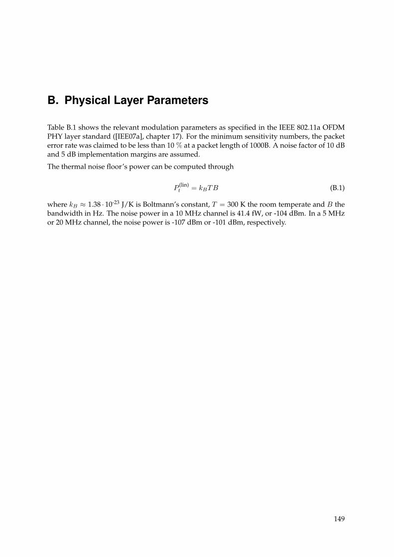
B. Physical Layer Parameters
Table B.1 shows the relevant modulation parameters as specified in the IEEE 802.11a OFDMPHY layer standard ([IEE07a], chapter 17). For the minimum sensitivity numbers, the packeterror rate was claimed to be less than 10 % at a packet length of 1000B. A noise factor of 10 dBand 5 dB implementation margins are assumed.
The thermal noise floor’s power can be computed through
P (lin)t = kBTB (B.1)
where kB ≈ 1.38 · 10-23 J/K is Boltmann’s constant, T = 300 K the room temperate and B thebandwidth in Hz. The noise power in a 10 MHz channel is 41.4 fW, or -104 dBm. In a 5 MHzor 20 MHz channel, the noise power is -107 dBm or -101 dBm, respectively.
149
5M
Hz
10M
Hz
20M
Hz
OFD
MParam
eterC
hannelSpacingC
hannelSpacingC
hannelSpacing
Data
subcarriersN
SD
4848
48Pilotsubcarriers
NSP
44
4Subcarrier
frequencyspacing
∆F
78.125kH
z156.25
kHz
312.5kH
zFFT/IFFT
periodTF
=1/∆
F12.8
µs6.4
µs3.2
µsG
uardinterval
TG
=TF/4
3.2µs
1.6µs
0.8µs
Symbolduration
TS
=TF
+TG
16.0µs
8.0µs
4.0µs
Preamble
durationTP
64µs
32µs
16µs
Minim
umD
ataM
inimum
Data
Minim
umD
ataM
odulation[C
odingR
ate,Sensitivity
Rate
SensitivityR
ateSensitivity
Rate
Data
Bits
/Symbol]
(dBm
)(M
bit/s)(dB
m)
(Mbit/s)
(dBm
)(M
bit/s)
BPSK[1/2,24]
-881.5
-853
-826
BPSK[3/4,36]
-872.25
-844.5
-819
QPSK
[1/2,48]-85
3-82
6-79
12Q
PSK[3/4,72]
-834.5
-809
-7718
16-QA
M[1/2,96]
-806
-7712
-7424
16-QA
M[3/4,144]
-769
-7318
-7036
64-QA
M[2/3,192]
-7212
-6924
-6648
64-QA
M[3/4,216]
-7113.5
-6827
-6554
TableB.1.:IEEE
802.11aO
FDM
PhysicalLayerSpecifications
150
C. Analysis Workflow
In this thesis, we have contributed means of analyzing the connectivity of vehicular networksand the QoS that can be attained in these networks. This chapter gives a brief summary ofthe workflow of such an analysis and should be regarded as a guideline for application andnetworking designers. It may be used iteratively in the design process, to tune parameters toobtain an optimal conformance of applications when deployed.
The workflow is illustrated in Figure C.1.
C.1. Networking Parameters
At the beginning of the connectivity analysis process as described in Chapter 3, the user needsan appropriate formulation of the channel model χ( · , · ) and to determine the maximum tol-erable attenuation βmax (see, for instance, Table B.1).
The formulation of the physical layout of the traffic scenario is accomplished by using a roadmodel as the projection function Φ( · ). We suggest splines as road model, see Appendix A.The properties of the traffic flow itself are represented through the traffic density ρ and thechoice of a fundamental diagram Q(ρ) or v(ρ), respectively (see Equation (3.37)).
Using these input parameters, the user can then determine:
• the distribution of node degrees fD[d], through Equation (3.54)
• the distribution of link durations fT (t), through Equation (3.76), (3.98)
• the expected link generation and break rate Λ, through Equation (3.116)
C.2. QoS Analysis
As a prerequisite for QoS analysis as described in Chapter 4, the user needs statistical infor-mation about the node degree. For instance, the degree distribution fD[d] as obtained abovecan be used here. Alternatively, one can model the degree distribution to represent a desiredscenario. It is also possible to use the channel model and a spatial distribution as input pa-rameters. It is also necessary to know the throughput function of the MAC protocol v(u).Subsequently, the requirements from the application (see Chapter 2) are used to determine themaximum allowable load u.
By using either Algorithm 1 (centralized) or Algorithm 2 (decentralized), the traffic limits si forthe individual network nodes vi can be determined. This figure can then be used in the designphase to determine if the traffic limits are sufficient for the application or be used to decideif the analyzed MAC protocol is suitable for the application. Given the benefit functions, theoutput from the traffic limits algorithms can also be used to determine which applicationswould be selected in a certain situation and how they would be parameterized.
151
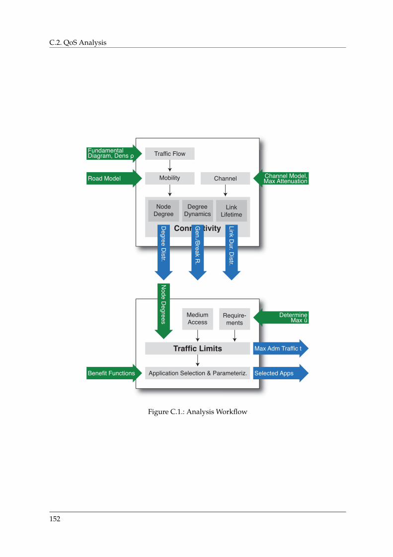
C.2. QoS Analysis
Figure C.1.: Analysis Workflow
152
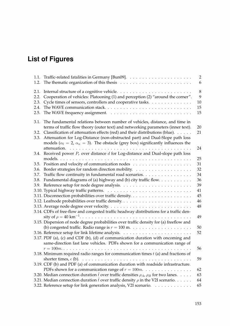
List of Figures
1.1. Traffic-related fatalities in Germany [Bun09]. . . . . . . . . . . . . . . . . . . . . 21.2. The thematic organization of this thesis . . . . . . . . . . . . . . . . . . . . . . . 6
2.1. Internal structure of a cognitive vehicle. . . . . . . . . . . . . . . . . . . . . . . . 82.2. Cooperation of vehicles: Platooning (1) and perception (2) “around the corner”. 92.3. Cycle times of sensors, controllers and cooperative tasks. . . . . . . . . . . . . . 102.4. The WAVE communication stack. . . . . . . . . . . . . . . . . . . . . . . . . . . . 152.5. The WAVE frequency assignment. . . . . . . . . . . . . . . . . . . . . . . . . . . 15
3.1. The fundamental relations between number of vehicles, distance, and time interms of traffic flow theory (outer text) and networking parameters (inner text). 20
3.2. Classification of attenuation effects (red) and their distributions (blue). . . . . . 213.3. Attenuation for Log-Distance (non-obstructed part) and Dual-Slope path loss
models (αl = 2, αn = 3). The obstacle (grey box) significantly influences theattenuation. . . . . . . . . . . . . . . . . . . . . . . . . . . . . . . . . . . . . . . . 24
3.4. Received power Pr over distance d for Log-distance and Dual-slope path lossmodels. . . . . . . . . . . . . . . . . . . . . . . . . . . . . . . . . . . . . . . . . . . 25
3.5. Position and velocity of communication nodes . . . . . . . . . . . . . . . . . . . 313.6. Border strategies for random direction mobility. . . . . . . . . . . . . . . . . . . 323.7. Traffic flow continuity in fundamental road scenarios. . . . . . . . . . . . . . . . 343.8. Fundamental diagrams of (a) highway and (b) city traffic flow. . . . . . . . . . . 363.9. Reference setup for node degree analysis. . . . . . . . . . . . . . . . . . . . . . . 393.10. Typical highway traffic patterns. . . . . . . . . . . . . . . . . . . . . . . . . . . . 413.11. Disconnection probabilities over traffic density. . . . . . . . . . . . . . . . . . . . 453.12. Leafnode probabilities over traffic density. . . . . . . . . . . . . . . . . . . . . . . 463.13. Average node degree over velocity. . . . . . . . . . . . . . . . . . . . . . . . . . . 483.14. CDFs of free-flow and congested traffic headway distributions for a traffic den-
sity of ρ = 40 km−1. . . . . . . . . . . . . . . . . . . . . . . . . . . . . . . . . . . . 493.15. Dispersion of node degree probabilities over traffic density for (a) freeflow and
(b) congested traffic. Radio range is r = 100 m. . . . . . . . . . . . . . . . . . . . 503.16. Reference setup for link lifetime analysis. . . . . . . . . . . . . . . . . . . . . . . 523.17. PDF (a), (c) and CDF (b), (d) of communication duration with oncoming and
same-direction fast lane vehicles. PDFs shown for a communication range ofr = 100m. . . . . . . . . . . . . . . . . . . . . . . . . . . . . . . . . . . . . . . . . . 56
3.18. Minimum required radio ranges for communication times t (a) and fractions ofshorter times, ε (b). . . . . . . . . . . . . . . . . . . . . . . . . . . . . . . . . . . . 59
3.19. CDF (b) and PDF (a) of communication duration with roadside infrastructure.PDFs shown for a communication range of r = 100m. . . . . . . . . . . . . . . . 62
3.20. Median connection duration t over traffic densities ρA, ρB for two lanes. . . . . 633.21. Median connection duration t over traffic density ρ in the V2I scenario. . . . . . 643.22. Reference setup for link generation analysis, V2I scenario. . . . . . . . . . . . . 65
153
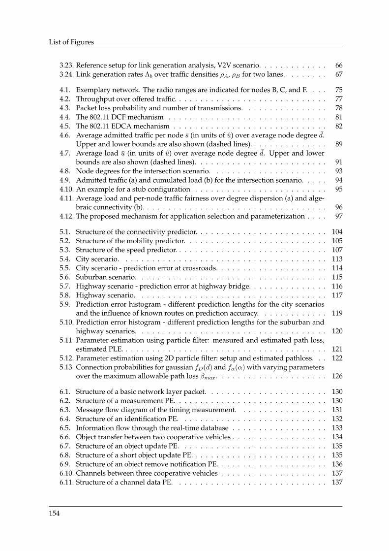
List of Figures
3.23. Reference setup for link generation analysis, V2V scenario. . . . . . . . . . . . . 663.24. Link generation rates Λb over traffic densities ρA, ρB for two lanes. . . . . . . . 67
4.1. Exemplary network. The radio ranges are indicated for nodes B, C, and F. . . . 754.2. Throughput over offered traffic. . . . . . . . . . . . . . . . . . . . . . . . . . . . . 774.3. Packet loss probability and number of transmissions. . . . . . . . . . . . . . . . 784.4. The 802.11 DCF mechanism . . . . . . . . . . . . . . . . . . . . . . . . . . . . . . 814.5. The 802.11 EDCA mechanism . . . . . . . . . . . . . . . . . . . . . . . . . . . . . 824.6. Average admitted traffic per node s (in units of u) over average node degree d.
Upper and lower bounds are also shown (dashed lines). . . . . . . . . . . . . . . 894.7. Average load u (in units of u) over average node degree d. Upper and lower
bounds are also shown (dashed lines). . . . . . . . . . . . . . . . . . . . . . . . . 914.8. Node degrees for the intersection scenario. . . . . . . . . . . . . . . . . . . . . . 934.9. Admitted traffic (a) and cumulated load (b) for the intersection scenario. . . . . 944.10. An example for a stub configuration . . . . . . . . . . . . . . . . . . . . . . . . . 954.11. Average load and per-node traffic fairness over degree dispersion (a) and alge-
braic connectivity (b). . . . . . . . . . . . . . . . . . . . . . . . . . . . . . . . . . . 964.12. The proposed mechanism for application selection and parameterization . . . . 97
5.1. Structure of the connectivity predictor. . . . . . . . . . . . . . . . . . . . . . . . . 1045.2. Structure of the mobility predictor. . . . . . . . . . . . . . . . . . . . . . . . . . . 1055.3. Structure of the speed predictor. . . . . . . . . . . . . . . . . . . . . . . . . . . . . 1075.4. City scenario. . . . . . . . . . . . . . . . . . . . . . . . . . . . . . . . . . . . . . . 1135.5. City scenario - prediction error at crossroads. . . . . . . . . . . . . . . . . . . . . 1145.6. Suburban scenario. . . . . . . . . . . . . . . . . . . . . . . . . . . . . . . . . . . . 1155.7. Highway scenario - prediction error at highway bridge. . . . . . . . . . . . . . . 1165.8. Highway scenario. . . . . . . . . . . . . . . . . . . . . . . . . . . . . . . . . . . . 1175.9. Prediction error histogram - different prediction lengths for the city scenarios
and the influence of known routes on prediction accuracy. . . . . . . . . . . . . 1195.10. Prediction error histogram - different prediction lengths for the suburban and
highway scenarios. . . . . . . . . . . . . . . . . . . . . . . . . . . . . . . . . . . . 1205.11. Parameter estimation using particle filter: measured and estimated path loss,
estimated PLE. . . . . . . . . . . . . . . . . . . . . . . . . . . . . . . . . . . . . . . 1215.12. Parameter estimation using 2D particle filter: setup and estimated pathloss. . . 1225.13. Connection probabilities for gaussian fD(d) and fα(α) with varying parameters
over the maximum allowable path loss βmax. . . . . . . . . . . . . . . . . . . . . 126
6.1. Structure of a basic network layer packet. . . . . . . . . . . . . . . . . . . . . . . 1306.2. Structure of a measurement PE. . . . . . . . . . . . . . . . . . . . . . . . . . . . . 1306.3. Message flow diagram of the timing measurement. . . . . . . . . . . . . . . . . 1316.4. Structure of an identification PE. . . . . . . . . . . . . . . . . . . . . . . . . . . . 1326.5. Information flow through the real-time database . . . . . . . . . . . . . . . . . . 1336.6. Object transfer between two cooperative vehicles . . . . . . . . . . . . . . . . . . 1346.7. Structure of an object update PE. . . . . . . . . . . . . . . . . . . . . . . . . . . . 1356.8. Structure of a short object update PE. . . . . . . . . . . . . . . . . . . . . . . . . . 1356.9. Structure of an object remove notification PE. . . . . . . . . . . . . . . . . . . . . 1366.10. Channels between three cooperative vehicles . . . . . . . . . . . . . . . . . . . . 1376.11. Structure of a channel data PE. . . . . . . . . . . . . . . . . . . . . . . . . . . . . 137
154
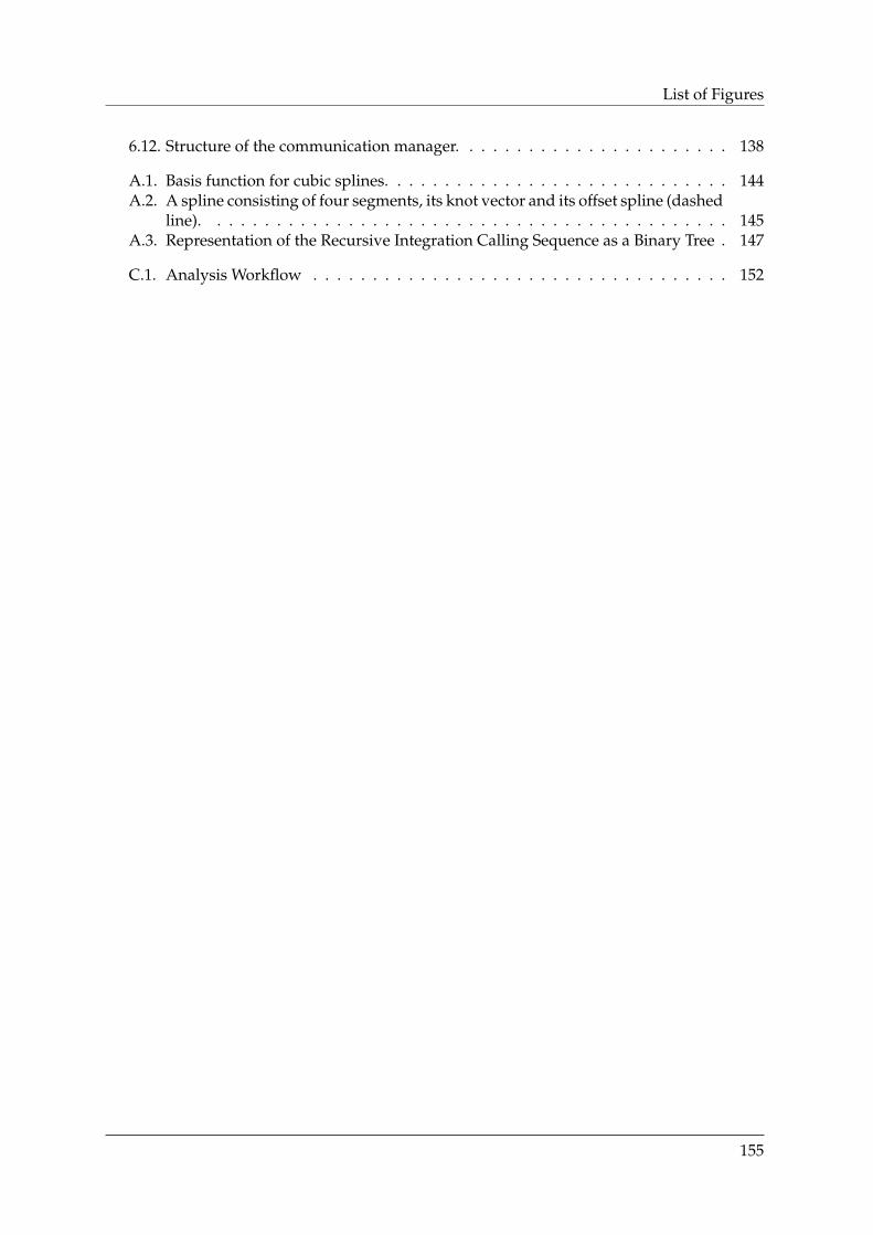
List of Figures
6.12. Structure of the communication manager. . . . . . . . . . . . . . . . . . . . . . . 138
A.1. Basis function for cubic splines. . . . . . . . . . . . . . . . . . . . . . . . . . . . . 144A.2. A spline consisting of four segments, its knot vector and its offset spline (dashed
line). . . . . . . . . . . . . . . . . . . . . . . . . . . . . . . . . . . . . . . . . . . . 145A.3. Representation of the Recursive Integration Calling Sequence as a Binary Tree . 147
C.1. Analysis Workflow . . . . . . . . . . . . . . . . . . . . . . . . . . . . . . . . . . . 152
155

List of Figures
156
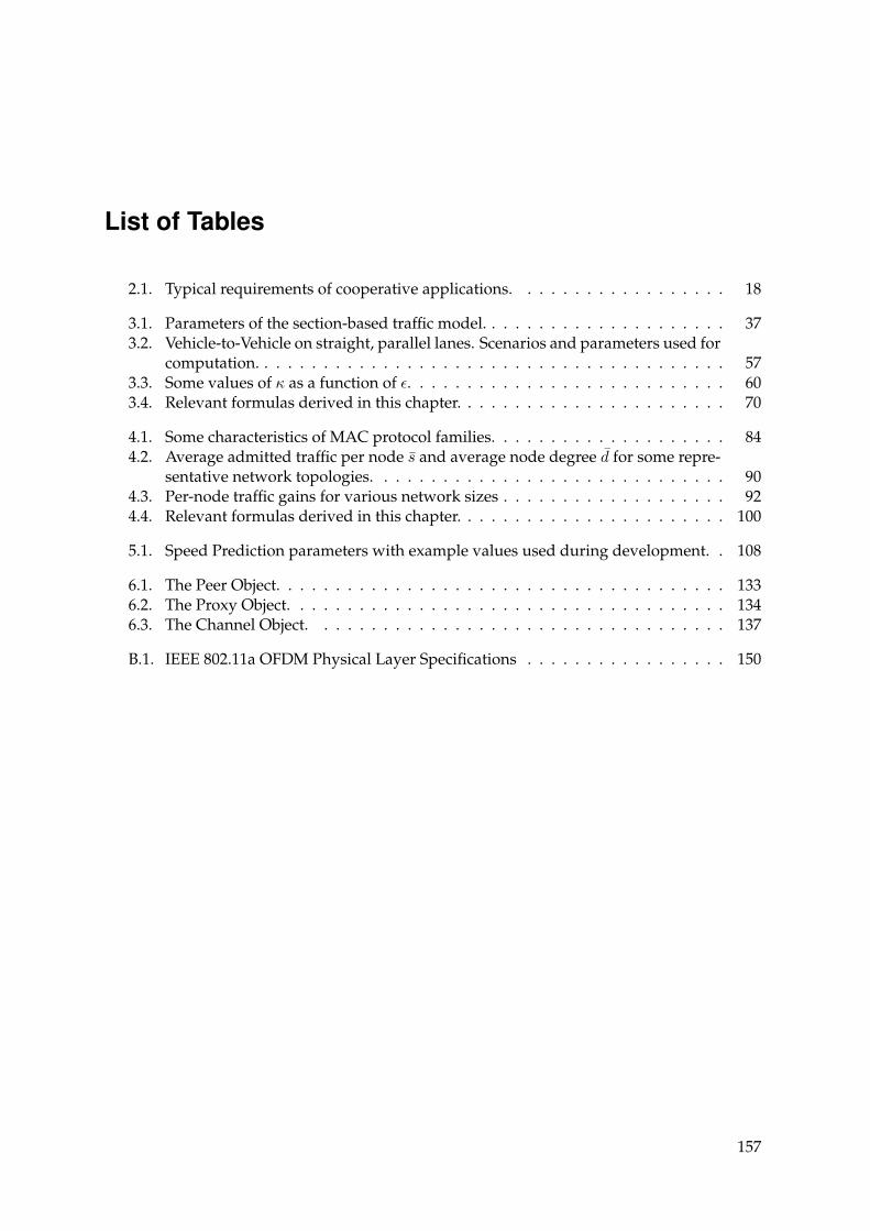
List of Tables
2.1. Typical requirements of cooperative applications. . . . . . . . . . . . . . . . . . 18
3.1. Parameters of the section-based traffic model. . . . . . . . . . . . . . . . . . . . . 373.2. Vehicle-to-Vehicle on straight, parallel lanes. Scenarios and parameters used for
computation. . . . . . . . . . . . . . . . . . . . . . . . . . . . . . . . . . . . . . . . 573.3. Some values of κ as a function of ε. . . . . . . . . . . . . . . . . . . . . . . . . . . 603.4. Relevant formulas derived in this chapter. . . . . . . . . . . . . . . . . . . . . . . 70
4.1. Some characteristics of MAC protocol families. . . . . . . . . . . . . . . . . . . . 844.2. Average admitted traffic per node s and average node degree d for some repre-
sentative network topologies. . . . . . . . . . . . . . . . . . . . . . . . . . . . . . 904.3. Per-node traffic gains for various network sizes . . . . . . . . . . . . . . . . . . . 924.4. Relevant formulas derived in this chapter. . . . . . . . . . . . . . . . . . . . . . . 100
5.1. Speed Prediction parameters with example values used during development. . 108
6.1. The Peer Object. . . . . . . . . . . . . . . . . . . . . . . . . . . . . . . . . . . . . . 1336.2. The Proxy Object. . . . . . . . . . . . . . . . . . . . . . . . . . . . . . . . . . . . . 1346.3. The Channel Object. . . . . . . . . . . . . . . . . . . . . . . . . . . . . . . . . . . 137
B.1. IEEE 802.11a OFDM Physical Layer Specifications . . . . . . . . . . . . . . . . . 150
157

List of Tables
158
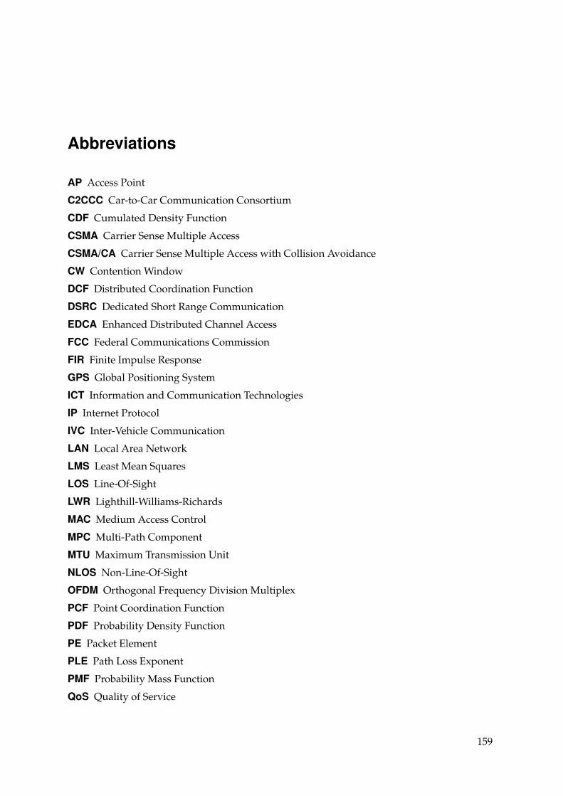
Abbreviations
AP Access Point
C2CCC Car-to-Car Communication Consortium
CDF Cumulated Density Function
CSMA Carrier Sense Multiple Access
CSMA/CA Carrier Sense Multiple Access with Collision Avoidance
CW Contention Window
DCF Distributed Coordination Function
DSRC Dedicated Short Range Communication
EDCA Enhanced Distributed Channel Access
FCC Federal Communications Commission
FIR Finite Impulse Response
GPS Global Positioning System
ICT Information and Communication Technologies
IP Internet Protocol
IVC Inter-Vehicle Communication
LAN Local Area Network
LMS Least Mean Squares
LOS Line-Of-Sight
LWR Lighthill-Williams-Richards
MAC Medium Access Control
MPC Multi-Path Component
MTU Maximum Transmission Unit
NLOS Non-Line-Of-Sight
OFDM Orthogonal Frequency Division Multiplex
PCF Point Coordination Function
PDF Probability Density Function
PE Packet Element
PLE Path Loss Exponent
PMF Probability Mass Function
QoS Quality of Service
159
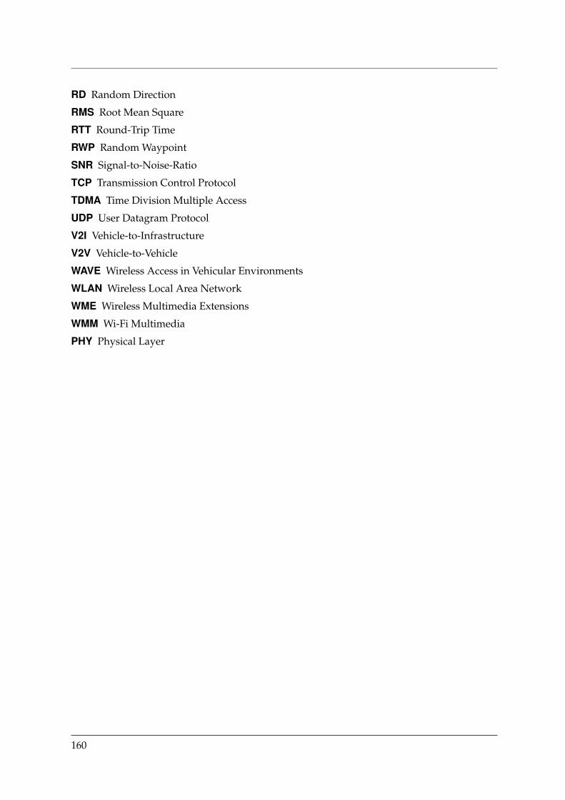
RD Random Direction
RMS Root Mean Square
RTT Round-Trip Time
RWP Random Waypoint
SNR Signal-to-Noise-Ratio
TCP Transmission Control Protocol
TDMA Time Division Multiple Access
UDP User Datagram Protocol
V2I Vehicle-to-Infrastructure
V2V Vehicle-to-Vehicle
WAVE Wireless Access in Vehicular Environments
WLAN Wireless Local Area Network
WME Wireless Multimedia Extensions
WMM Wi-Fi Multimedia
PHY Physical Layer
160
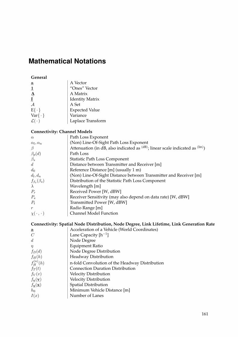
Mathematical Notations
Generala A Vector1 “Ones” VectorA˜ A MatrixI˜ Identity MatrixA A SetE · Expected ValueVar · VarianceL( · ) Laplace Transform
Connectivity: Channel Modelsα Path Loss Exponentαl, αn (Non) Line-Of-Sight Path Loss Exponentβ Attenuation (in dB, also indicated as (dB); linear scale indicated as (lin))βp(d) Path Lossβs Statistic Path Loss Componentd Distance between Transmitter and Receiver [m]d0 Reference Distance [m] (usually 1 m)dl, dn (Non) Line-Of-Sight Distance between Transmitter and Receiver [m]fβs(βs) Distribution of the Statistic Path Loss Componentλ Wavelength [m]Pr Received Power [W, dBW]Ps Receiver Sensitivity (may also depend on data rate) [W, dBW]Pt Transmitted Power [W, dBW]r Radio Range [m]χ( · , · ) Channel Model Function
Connectivity: Spatial Node Distribution, Node Degree, Link Lifetime, Link Generation Ratea Acceleration of a Vehicle (World Coordinates)C Lane Capacity [h−1]d Node Degreeη Equipment RatiofD(d) Node Degree DistributionfH(h) Headway Distributionf
(n)H (h) n-fold Convolution of the Headway DistributionfT (t) Connection Duration DistributionfV (v) Velocity Distributionfv(v) Velocity Distributionfx(x) Spatial Distributionh0 Minimum Vehicle Distance [m]I(x) Number of Lanes
161

l Vehicle Length [m]le Effective Vehicle Length [m]Λ Link Generation Rate [s−1]ϕ Direction of Velocity []Φ( · ) Projection Functionρ(x, t) Average Density of Vehicles [kmlane−1]ρt(x, t) Total Density of Vehicles [km−1]ρi(x, t) Density of Vehicles on lane i [km−1]ρj Traffic Jam Density [km−1]ρc Critical Density [km−1]si Longitudinal Position of Vehicle i on a Lane [m]sr Effective Radio Range [m]s⊥ Lateral Lane Offset [m]σv Velocity Standard Deviation [m/s]t Time [s]T Average Time Headway [s]t Median Connection Duration [s]v Magnitude of Velocity [m/s]v Average Velocity [m/s]v(x, t) Average Velocity [m/s]v0 Average Free Velocity [m/s]Ve(ρ) Equilibrium Velocity [m/s]vi(x, t) Velocity of Vehicles on lane i [m/s]v Velocity of a Vehicle (World Coordinates)Q(x, t) Average Flow of Vehicles [hlane−1]Qi(x, t) Flow of Vehicles on lane i [h−1]Qt(x, t) Total Flow of Vehicles [h−1]Qe(ρ) Fundamental Diagram [h−1]x Position of a Vehicle (World Coordinates)
QoS Analysis and ProvisioningA Set of Send HyperarcsA′ Set of Receive HyperarcsC˜ Connectivity Matrixcij Connectivity of Nodes vi and vj∆ Maximum Node Degreeδ(u) Average Normalized Packet Delay at Offered Traffic u [s]E Set of EdgesG A Network Graphl Message Length [bit, B]λ Message Generation Rate [s−1]L˜ Laplacian Matrixn Number of Nodesns Number of Stub NodesP Set of Applicationspl(u) Packet Loss Probability at Offered Traffic uΦ Global Fairnessφ Local Fairness
162
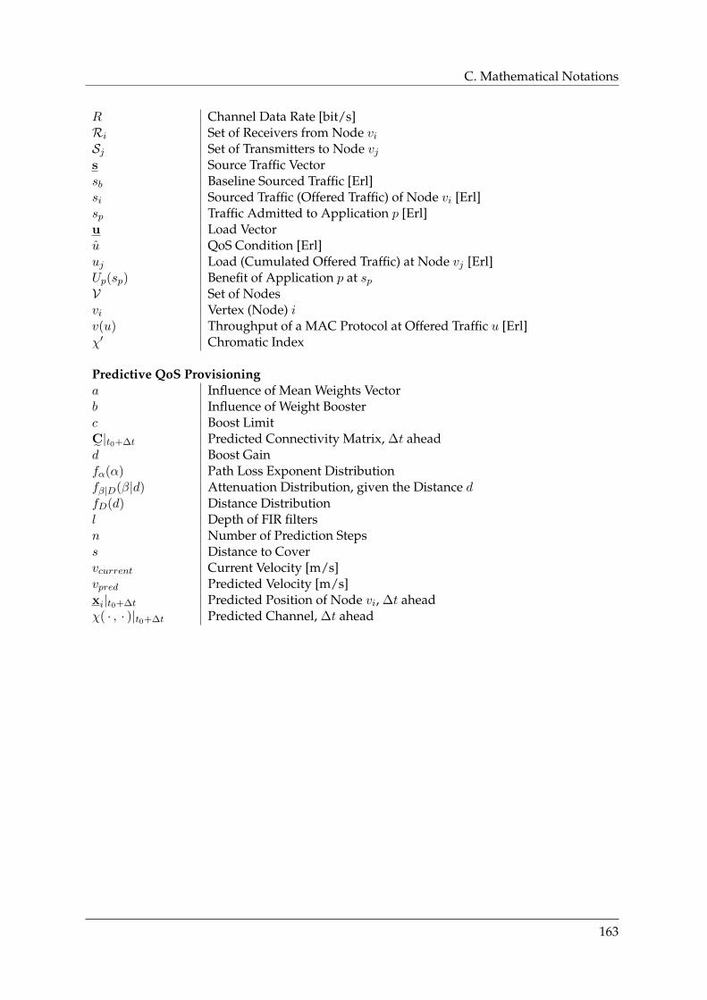
C. Mathematical Notations
R Channel Data Rate [bit/s]Ri Set of Receivers from Node viSj Set of Transmitters to Node vjs Source Traffic Vectorsb Baseline Sourced Traffic [Erl]si Sourced Traffic (Offered Traffic) of Node vi [Erl]sp Traffic Admitted to Application p [Erl]u Load Vectoru QoS Condition [Erl]uj Load (Cumulated Offered Traffic) at Node vj [Erl]Up(sp) Benefit of Application p at spV Set of Nodesvi Vertex (Node) iv(u) Throughput of a MAC Protocol at Offered Traffic u [Erl]χ′ Chromatic Index
Predictive QoS Provisioninga Influence of Mean Weights Vectorb Influence of Weight Boosterc Boost LimitC˜ |t0+∆t Predicted Connectivity Matrix, ∆t aheadd Boost Gainfα(α) Path Loss Exponent Distributionfβ|D(β|d) Attenuation Distribution, given the Distance dfD(d) Distance Distributionl Depth of FIR filtersn Number of Prediction Stepss Distance to Covervcurrent Current Velocity [m/s]vpred Predicted Velocity [m/s]xi|t0+∆t Predicted Position of Node vi, ∆t aheadχ( · , · )|t0+∆t Predicted Channel, ∆t ahead
163

164
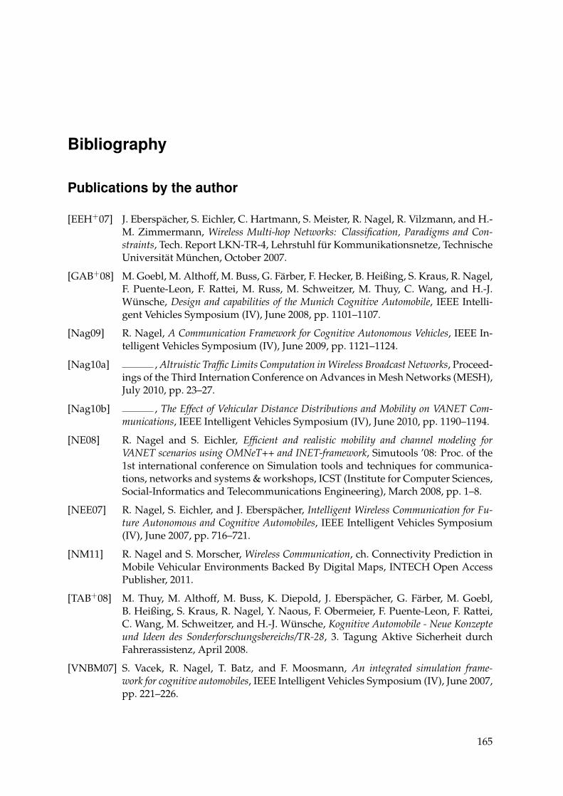
Bibliography
Publications by the author
[EEH+07] J. Eberspächer, S. Eichler, C. Hartmann, S. Meister, R. Nagel, R. Vilzmann, and H.-M. Zimmermann, Wireless Multi-hop Networks: Classification, Paradigms and Con-straints, Tech. Report LKN-TR-4, Lehrstuhl für Kommunikationsnetze, TechnischeUniversität München, October 2007.
[GAB+08] M. Goebl, M. Althoff, M. Buss, G. Färber, F. Hecker, B. Heißing, S. Kraus, R. Nagel,F. Puente-Leon, F. Rattei, M. Russ, M. Schweitzer, M. Thuy, C. Wang, and H.-J.Wünsche, Design and capabilities of the Munich Cognitive Automobile, IEEE Intelli-gent Vehicles Symposium (IV), June 2008, pp. 1101–1107.
[Nag09] R. Nagel, A Communication Framework for Cognitive Autonomous Vehicles, IEEE In-telligent Vehicles Symposium (IV), June 2009, pp. 1121–1124.
[Nag10a] , Altruistic Traffic Limits Computation in Wireless Broadcast Networks, Proceed-ings of the Third Internation Conference on Advances in Mesh Networks (MESH),July 2010, pp. 23–27.
[Nag10b] , The Effect of Vehicular Distance Distributions and Mobility on VANET Com-munications, IEEE Intelligent Vehicles Symposium (IV), June 2010, pp. 1190–1194.
[NE08] R. Nagel and S. Eichler, Efficient and realistic mobility and channel modeling forVANET scenarios using OMNeT++ and INET-framework, Simutools ’08: Proc. of the1st international conference on Simulation tools and techniques for communica-tions, networks and systems & workshops, ICST (Institute for Computer Sciences,Social-Informatics and Telecommunications Engineering), March 2008, pp. 1–8.
[NEE07] R. Nagel, S. Eichler, and J. Eberspächer, Intelligent Wireless Communication for Fu-ture Autonomous and Cognitive Automobiles, IEEE Intelligent Vehicles Symposium(IV), June 2007, pp. 716–721.
[NM11] R. Nagel and S. Morscher, Wireless Communication, ch. Connectivity Prediction inMobile Vehicular Environments Backed By Digital Maps, INTECH Open AccessPublisher, 2011.
[TAB+08] M. Thuy, M. Althoff, M. Buss, K. Diepold, J. Eberspächer, G. Färber, M. Goebl,B. Heißing, S. Kraus, R. Nagel, Y. Naous, F. Obermeier, F. Puente-Leon, F. Rattei,C. Wang, M. Schweitzer, and H.-J. Wünsche, Kognitive Automobile - Neue Konzepteund Ideen des Sonderforschungsbereichs/TR-28, 3. Tagung Aktive Sicherheit durchFahrerassistenz, April 2008.
[VNBM07] S. Vacek, R. Nagel, T. Batz, and F. Moosmann, An integrated simulation frame-work for cognitive automobiles, IEEE Intelligent Vehicles Symposium (IV), June 2007,pp. 221–226.
165
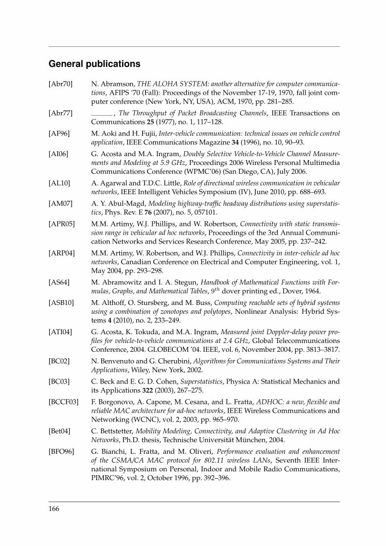
General publications
[Abr70] N. Abramson, THE ALOHA SYSTEM: another alternative for computer communica-tions, AFIPS ’70 (Fall): Proceedings of the November 17-19, 1970, fall joint com-puter conference (New York, NY, USA), ACM, 1970, pp. 281–285.
[Abr77] , The Throughput of Packet Broadcasting Channels, IEEE Transactions onCommunications 25 (1977), no. 1, 117–128.
[AF96] M. Aoki and H. Fujii, Inter-vehicle communication: technical issues on vehicle controlapplication, IEEE Communications Magazine 34 (1996), no. 10, 90–93.
[AI06] G. Acosta and M.A. Ingram, Doubly Selective Vehicle-to-Vehicle Channel Measure-ments and Modeling at 5.9 GHz, Proceedings 2006 Wireless Personal MultimediaCommunications Conference (WPMC’06) (San Diego, CA), July 2006.
[AL10] A. Agarwal and T.D.C. Little, Role of directional wireless communication in vehicularnetworks, IEEE Intelligent Vehicles Symposium (IV), June 2010, pp. 688–693.
[AM07] A. Y. Abul-Magd, Modeling highway-traffic headway distributions using superstatis-tics, Phys. Rev. E 76 (2007), no. 5, 057101.
[APR05] M.M. Artimy, W.J. Phillips, and W. Robertson, Connectivity with static transmis-sion range in vehicular ad hoc networks, Proceedings of the 3rd Annual Communi-cation Networks and Services Research Conference, May 2005, pp. 237–242.
[ARP04] M.M. Artimy, W. Robertson, and W.J. Phillips, Connectivity in inter-vehicle ad hocnetworks, Canadian Conference on Electrical and Computer Engineering, vol. 1,May 2004, pp. 293–298.
[AS64] M. Abramowitz and I. A. Stegun, Handbook of Mathematical Functions with For-mulas, Graphs, and Mathematical Tables, 9th dover printing ed., Dover, 1964.
[ASB10] M. Althoff, O. Stursberg, and M. Buss, Computing reachable sets of hybrid systemsusing a combination of zonotopes and polytopes, Nonlinear Analysis: Hybrid Sys-tems 4 (2010), no. 2, 233–249.
[ATI04] G. Acosta, K. Tokuda, and M.A. Ingram, Measured joint Doppler-delay power pro-files for vehicle-to-vehicle communications at 2.4 GHz, Global TelecommunicationsConference, 2004. GLOBECOM ’04. IEEE, vol. 6, November 2004, pp. 3813–3817.
[BC02] N. Benvenuto and G. Cherubini, Algorithms for Communications Systems and TheirApplications, Wiley, New York, 2002.
[BC03] C. Beck and E. G. D. Cohen, Superstatistics, Physica A: Statistical Mechanics andits Applications 322 (2003), 267–275.
[BCCF03] F. Borgonovo, A. Capone, M. Cesana, and L. Fratta, ADHOC: a new, flexible andreliable MAC architecture for ad-hoc networks, IEEE Wireless Communications andNetworking (WCNC), vol. 2, 2003, pp. 965–970.
[Bet04] C. Bettstetter, Mobility Modeling, Connectivity, and Adaptive Clustering in Ad HocNetworks, Ph.D. thesis, Technische Universität München, 2004.
[BFO96] G. Bianchi, L. Fratta, and M. Oliveri, Performance evaluation and enhancementof the CSMA/CA MAC protocol for 802.11 wireless LANs, Seventh IEEE Inter-national Symposium on Personal, Indoor and Mobile Radio Communications,PIMRC’96, vol. 2, October 1996, pp. 392–396.
166
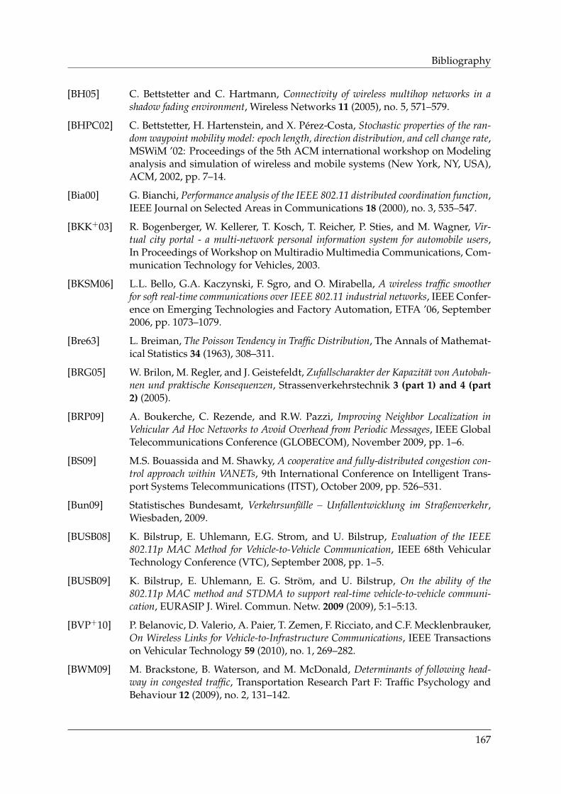
Bibliography
[BH05] C. Bettstetter and C. Hartmann, Connectivity of wireless multihop networks in ashadow fading environment, Wireless Networks 11 (2005), no. 5, 571–579.
[BHPC02] C. Bettstetter, H. Hartenstein, and X. Pérez-Costa, Stochastic properties of the ran-dom waypoint mobility model: epoch length, direction distribution, and cell change rate,MSWiM ’02: Proceedings of the 5th ACM international workshop on Modelinganalysis and simulation of wireless and mobile systems (New York, NY, USA),ACM, 2002, pp. 7–14.
[Bia00] G. Bianchi, Performance analysis of the IEEE 802.11 distributed coordination function,IEEE Journal on Selected Areas in Communications 18 (2000), no. 3, 535–547.
[BKK+03] R. Bogenberger, W. Kellerer, T. Kosch, T. Reicher, P. Sties, and M. Wagner, Vir-tual city portal - a multi-network personal information system for automobile users,In Proceedings of Workshop on Multiradio Multimedia Communications, Com-munication Technology for Vehicles, 2003.
[BKSM06] L.L. Bello, G.A. Kaczynski, F. Sgro, and O. Mirabella, A wireless traffic smootherfor soft real-time communications over IEEE 802.11 industrial networks, IEEE Confer-ence on Emerging Technologies and Factory Automation, ETFA ’06, September2006, pp. 1073–1079.
[Bre63] L. Breiman, The Poisson Tendency in Traffic Distribution, The Annals of Mathemat-ical Statistics 34 (1963), 308–311.
[BRG05] W. Brilon, M. Regler, and J. Geistefeldt, Zufallscharakter der Kapazität von Autobah-nen und praktische Konsequenzen, Strassenverkehrstechnik 3 (part 1) and 4 (part2) (2005).
[BRP09] A. Boukerche, C. Rezende, and R.W. Pazzi, Improving Neighbor Localization inVehicular Ad Hoc Networks to Avoid Overhead from Periodic Messages, IEEE GlobalTelecommunications Conference (GLOBECOM), November 2009, pp. 1–6.
[BS09] M.S. Bouassida and M. Shawky, A cooperative and fully-distributed congestion con-trol approach within VANETs, 9th International Conference on Intelligent Trans-port Systems Telecommunications (ITST), October 2009, pp. 526–531.
[Bun09] Statistisches Bundesamt, Verkehrsunfälle – Unfallentwicklung im Straßenverkehr,Wiesbaden, 2009.
[BUSB08] K. Bilstrup, E. Uhlemann, E.G. Strom, and U. Bilstrup, Evaluation of the IEEE802.11p MAC Method for Vehicle-to-Vehicle Communication, IEEE 68th VehicularTechnology Conference (VTC), September 2008, pp. 1–5.
[BUSB09] K. Bilstrup, E. Uhlemann, E. G. Ström, and U. Bilstrup, On the ability of the802.11p MAC method and STDMA to support real-time vehicle-to-vehicle communi-cation, EURASIP J. Wirel. Commun. Netw. 2009 (2009), 5:1–5:13.
[BVP+10] P. Belanovic, D. Valerio, A. Paier, T. Zemen, F. Ricciato, and C.F. Mecklenbrauker,On Wireless Links for Vehicle-to-Infrastructure Communications, IEEE Transactionson Vehicular Technology 59 (2010), no. 1, 269–282.
[BWM09] M. Brackstone, B. Waterson, and M. McDonald, Determinants of following head-way in congested traffic, Transportation Research Part F: Traffic Psychology andBehaviour 12 (2009), no. 2, 131–142.
167
[CBS09] L. Cheng, F. Bai, and D.D. Stancil, A new geometrical channel model for vehicle-to-vehicle communications, IEEE Antennas and Propagation Society InternationalSymposium (APSURSI), June 2009, pp. 1–4.
[CGM07] O. Cappe, S.J. Godsill, and E. Moulines, An Overview of Existing Methods and Re-cent Advances in Sequential Monte Carlo, Proceedings of the IEEE 95 (2007), no. 5,899–924.
[CHBS08a] L. Cheng, B. Henty, F. Bai, and D.D. Stancil, Doppler Spread and Coherence Time ofRural and Highway Vehicle-to-Vehicle Channels at 5.9 GHz, IEEE Global Telecom-munications Conference (GLOBECOM), December 2008, pp. 1–6.
[CHBS08b] L. Cheng, B.E. Henty, F. Bai, and D.D. Stancil, Highway and rural propagation chan-nel modeling for vehicle-to-vehicle communications at 5.9 GHz, IEEE Antennas andPropagation Society International Symposium (AP-S), July 2008, pp. 1–4.
[CHC+08] L. Cheng, B. Henty, R. Cooper, D.D. Stancil, and F. Bai, Multi-Path PropagationMeasurements for Vehicular Networks at 5.9 GHz, IEEE Wireless Communicationsand Networking Conference (WCNC), April 2008, pp. 1239–1244.
[CHS+07] L. Cheng, B.E. Henty, D.D. Stancil, F. Bai, and P. Mudalige, Mobile Vehicle-to-Vehicle Narrow-Band Channel Measurement and Characterization of the 5.9 GHz Ded-icated Short Range Communication (DSRC) Frequency Band, IEEE Journal on Se-lected Areas in Communications 25 (2007), no. 8, 1501–1516.
[CLD+91] K.S. Chang, W. Li, P. Devlin, A. Shaikhbahai, P. Varaiya, J.K. Hedrick, D. McMa-hon, V. Narendran, D. Swaroop, and J. Olds, Experimentation with a vehicle platooncontrol system, Vehicle Navigation and Information Systems Conference, vol. 2,October 1991, pp. 1117–1124.
[Com03] Commission of the European Communities, Communication from the Commissionto the Council and the European Parliament COM(2003) 542, September 2003.
[Cow75] Richard J. Cowan, Useful headway models, Transportation Research 9 (1975), no. 6,371–375.
[Cox83] D. Cox, Antenna Diversity Performance in Mitigating the Effects of Portable Radiotele-phone Orientation and Multipath Propagation, IEEE Transactions on Communica-tions 31 (1983), no. 5, 620–628.
[Cox95] D.C. Cox, Wireless personal communications: what is it?, IEEE Personal Communi-cations 2 (1995), no. 2, 20–35.
[CRW+73] W. Crowther, R. Rettberg, D. Walden, S. Ornstein, and F. Heart, A system for broad-cast communication: Reservation-ALOHA, Proc. 6th HICSS (Honolulu, Hawaii),jan 1973.
[CS92] S.T.S. Chia and P. Snow, Characterising radio-wave propagation behaviour at 1700MHz for urban and highway microcells, IEEE Colloquium on Micro-Cellular Prop-agation Modelling, November 1992.
[CW94] W.C. Collier and R.J. Weiland, Smart cars, smart highways, IEEE Spectrum 31(1994), no. 4, 27–33.
[CWM02] D. Cassioli, M.Z. Win, and A.F. Molisch, The ultra-wide bandwidth indoor channel:from statistical model to simulations, IEEE Journal on Selected Areas in Communi-cations 20 (2002), no. 6, 1247–1257.
168
Bibliography
[DAA+04] M. Dohler, B. Allen, A. Armogida, S. McGregor, M. Ghavami, and H. Aghvami,A new twist on UWB pathloss modelling, IEEE 59th Vehicular Technology Confer-ence (VTC), vol. 1, May 2004, pp. 199–203.
[DTH02] O. Dousse, P. Thiran, and M. Hasler, Connectivity in ad-hoc and hybrid networks,Proceedings of 21st Annual Joint Conference of the IEEE Computer and Com-munications Societies (INFOCOM), vol. 2, 2002, pp. 1079–1088.
[Eic07] S. Eichler, Performance Evaluation of the IEEE 802.11p WAVE Communication Stan-dard, 66th Vehicular Technology Conference (VTC), oct 2007, pp. 2199–2203.
[EMS06] S. Eichler, C. Merkle, and M. Strassberger, Data Aggregation System for Distribut-ing Inter-Vehicle Warning Messages, 31st IEEE Conference on Local ComputerNetworks, November 2006, pp. 543–544.
[ESKS06] S. Eichler, C. Schroth, T. Kosch, and M. Strassberger, Strategies for Context-Adaptive Message Dissemination in Vehicular Ad Hoc Networks, 3rd Annual Inter-national Conference on Mobile and Ubiquitous Systems - Workshops, July 2006,pp. 1–9.
[ET90] A. Ephremides and T.V. Truong, Scheduling broadcasts in multihop radio networks,IEEE Transactions on Communications 38 (1990), no. 4, 456–460.
[ETS09] ETSI, C2C-CC Demonstrator 2008, Use Cases and Technical Specifications, Tech. Re-port TR 102 698, ETSI, June 2009.
[FBB08] C. Frese, T. Batz, and J. Beyerer, Kooperative Verhaltensentscheidung für Grup-pen kognitiver Automobile auf Grundlage des gemeinsamen Lagebilds, at - Automa-tisierungstechnik 56 (2008), no. 12, 644–652.
[FBR+94] M.J. Feuerstein, K.L. Blackard, T.S. Rappaport, S.Y. Seidel, and H.H. Xia, Pathloss, delay spread, and outage models as functions of antenna height for microcellularsystem design, IEEE Transactions on Vehicular Technology 43 (1994), no. 3, 487–498.
[FC05] M. Fazel and M. Chiang, Network Utility Maximization With Nonconcave UtilitiesUsing Sum-of-Squares Method, 44th IEEE Conference on Decision and Control and2005 European Control Conference (CDC-ECC ’05), December 2005, pp. 1867–1874.
[Fie73] M. Fiedler, Algebraic connectivity of graphs, Czechoslovak Mathematical Journal23 (1973), no. 2, 298–305.
[Fri46] H.T. Friis, A Note on a Simple Transmission Formula, Proceedings of the IRE 34(1946), no. 5, 254–256.
[GF08] M. Goebl and G. Färber, Interfaces for integrating cognitive functions into IntelligentVehicles, IEEE Intelligent Vehicles Symposium (IV), June 2008, pp. 1093–1100.
[GH08] W. Guan and S. He, Statistical features of traffic flow on urban freeways, Physica A:Statistical Mechanics and its Applications 387 (2008), no. 4, 944–954.
[GKDA71] Ernst A. Guillemin, R. E. Kalman, N. DeClaris, and Jonny Andersen, Aspects ofnetwork and system theory, Holt Rinehart and Winston, New York, 1971.
[GL00] A. C. V. Gummalla and J. O. Limb, Wireless medium access control protocols, IEEECommunications Surveys & Tutorials 3 (2000), no. 2, 2–15.
169
[GMM09] J.R. Gallardo, D. Makrakis, and H.T. Mouftah, Performance Analysis of the EDCAMedium Access Mechanism over the Control Channel of an IEEE 802.11p WAVE Ve-hicular Network, IEEE International Conference on Communications (ICC), June2009, pp. 1–6.
[Gue87] R.A. Guerin, Channel occupancy time distribution in a cellular radio system, IEEETransactions on Vehicular Technology 36 (1987), no. 3, 89–99.
[GW98] N. Geng and W. Wiesbeck, Planungsmethoden für die Mobilkommunikation,Springer, 1998.
[HC96] T.-S. Ho and K.-C. Chen, Performance analysis of IEEE 802.11 CSMA/CA mediumaccess control protocol, Seventh IEEE International Symposium on Personal, In-door and Mobile Radio Communications (PIMRC), vol. 2, October 1996, pp. 407–411.
[HCY+08] C.-J. Huang, Y.-T. Chuang, D.-X. Yang, I.-F. Chen, Y.-J. Chen, and K.-W. Hu, Amobility-aware link enhancement mechanism for vehicular ad hoc networks, EURASIPJ. Wirel. Commun. Netw. 2008 (2008), 1–10.
[HD05] J. Hui and M. Devetsikiotis, A unified model for the performance analysis of IEEE802.11e EDCA, IEEE Transactions on Communications 53 (2005), no. 9, 1498–1510.
[Hel95] D. Helbing, Improved fluid-dynamic model for vehicular traffic, Phys. Rev. E 51(1995), no. 4, 3164–3169.
[Hel96] , Gas-kinetic derivation of Navier-Stokes-like traffic equations, Phys. Rev. E 53(1996), no. 3, 2366–2381.
[Hel01a] , Traffic and related self-driven many-particle systems, Rev. Mod. Phys. 73(2001), no. 4, 1067–1141.
[Hel01b] , Verkehrsdynamik. Neue physikalische Modellierungskonzepte, Springer,2001.
[Hel03] , A section-based queueing-theoretical traffic model for congestion and traveltime analysis in networks, Journal of Physics A: Mathematical and General 36(2003), no. 46, L593.
[HFB09] J. Harri, F. Filali, and C. Bonnet, Mobility models for vehicular ad hoc networks: asurvey and taxonomy, IEEE Communications Surveys & Tutorials 11 (2009), no. 4,19–41.
[HHM+03] G.R. Hiertz, J. Habetha, P. May, E. Weib, R. Bagul, and S. Mangold, A decentralizedreservation scheme for IEEE 802.11 ad hoc networks, 14th IEEE Proceedings on Per-sonal, Indoor and Mobile Radio Communications (PIMRC), vol. 3, September2003, pp. 2576–2580.
[HHST02] D. Helbing, A. Hennecke, V. Shvetsov, and M. Treiber, Micro- and macro-simulation of freeway traffic, Mathematical and Computer Modelling 35 (2002),no. 5-6, 517–547.
[HVS02] Z. Hadzi-Velkov and B. Spasenovski, On the Capacity of IEEE 802.11 DCF withCapture in Multipath-Faded Channels, International Journal of Wireless Informa-tion Networks 9 (2002), 191–199, 10.1023/A:1016037711861.
170
Bibliography
[IEE06a] IEEE, IEEE Trial-Use Standard for Wireless Access in Vehicular Environments(WAVE) - Multi-Channel Operation, IEEE Std 1609.4-2006 (2006).
[IEE06b] , IEEE Trial-Use Standard for Wireless Access in Vehicular Environments(WAVE) - Resource Manager, IEEE Std 1609.1-2006 (2006).
[IEE06c] , IEEE Trial-Use Standard for Wireless Access in Vehicular Environments(WAVE) - Security Services for Applications and Management Messages, IEEE Std1609.2-2006 (2006).
[IEE07a] , IEEE Standard for Information Technology-Telecommunications and Informa-tion Exchange Between Systems-Local and Metropolitan Area Networks-Specific Re-quirements - Part 11: Wireless LAN Medium Access Control (MAC) and PhysicalLayer (PHY) Specifications, IEEE Std 802.11-2007 (Revision of IEEE Std 802.11-1999) (2007).
[IEE07b] , IEEE Trial-Use Standard for Wireless Access in Vehicular Environments(WAVE) - Networking Services, IEEE Std 1609.3-2007 (2007).
[IEE10] , IEEE Draft Standard for Information Technology - Telecommunications andinformation exchange between systems - Local and metropolitan area networks - Specificrequirements - Part 11: Wireless LAN Medium Access Control (MAC) and PhysicalLayer (PHY) specifications Amendment : Wireless Access in Vehicular Environments,IEEE Unapproved Draft Std P802.11p /D11.0, Mar 2010 (2010).
[Inz04] T. Inzerilli, Design and performance modeling for traffic control in wireless links, IEEEInternational Conference on Communications, vol. 4, June 2004, pp. 2307–2311.
[JCH84] R. Jain, D. Chiu, and W. Hawe, A Quantitative Measure of Fairness and Discrimina-tion for Resource Allocation in Shared Computer System, Tech. Report TR-301, DECResearch Report, 1984.
[JLB10] R. Jurdak, C.V. Lopes, and P. Baldi, Performance analysis of IEEE 802.11e enhanceddistributed channel access, IEEE Communications Surveys & Tutorials 4 (2010),no. 6, 728–738.
[JM96] David B. Johnson and David A. Maltz, Dynamic Source Routing in Ad Hoc WirelessNetworks, Mobile Computing, Kluwer Academic Publishers, 1996, pp. 153–181.
[Kah54] L. Kahn, Ratio Squarer, Proceedings of the IRE (Correspondence) 42 (1954), 1074.
[KBSS01] W. Kellerer, C. Bettstetter, C. Schwingenschlogl, and P. Sties, (Auto) mobile com-munication in a heterogeneous and converged world, IEEE Personal Communications8 (2001), no. 6, 41–47.
[Kep15] Johannes Kepler, Novia Stereometria Doliorum (Stereometrie der Fässer), 1615.
[Ker04] B. S. Kerner, The Physics of Traffic, Springer, 2004.
[KHB09] M. Kuehn, T. Hummel, and J. Bende, Benefit estimation of advanced driver assis-tance systems for cars derived from real-life accidents, Tech. Report 09-0317, GermanInsurers Accident Research, 2009.
[KJ08] M. Kaynia and N. Jindal, Performance of ALOHA and CSMA in Spatially Dis-tributed Wireless Networks, IEEE International Conference on Communications(ICC), May 2008, pp. 1108–1112.
171
[KK93] B. S. Kerner and P. Konhäuser, Cluster effect in initially homogeneous traffic flow,Phys. Rev. E 48 (1993), no. 4, R2335–R2338.
[KK10] H. Kaaniche and F. Kamoun, Mobility Prediction in Wireless Ad Hoc Networks usingNeural Networks, Journal of Telecommunications 2 (2010), no. 1, 95–101.
[KKH07] B. S. Kerner, S. Klenov, and A. Hiller, Empirical test of a microscopic three-phasetraffic theory, Nonlinear Dynamics 49 (2007), 525–553.
[KKHR06] Boris S. Kerner, Sergey L. Klenov, Andreas Hiller, and Hubert Rehborn, Micro-scopic features of moving traffic jams, Phys. Rev. E 73 (2006), no. 4, 046107.
[KKJ98] S. Khurana, A. Kahol, and A.P. Jayasumana, Effect of hidden terminals on the perfor-mance of IEEE 802.11 MAC protocol, 23rd Annual Conference on Local ComputerNetworks (LCN), October 1998, pp. 12–20.
[KL75] L. Kleinrock and S. Lam, Packet Switching in a Multiaccess Broadcast Channel: Per-formance Evaluation, IEEE Transactions on Communications 23 (1975), no. 4, 410–423.
[Krb07] M. Krbálek, Equilibrium distributions in a thermodynamical traffic gas, Journal ofPhysics A: Mathematical and Theoretical 40 (2007), no. 22, 5813.
[KS00] M. Krbalek and P. Seba, The statistical properties of the city transport in Cuernavaca(Mexico) and random matrix ensembles, Journal of Physics A 33 (2000), 229–234.
[KT75] L. Kleinrock and F. Tobagi, Packet Switching in Radio Channels: Part I–Carrier SenseMultiple-Access Modes and Their Throughput-Delay Characteristics, IEEE Transac-tions on Communications 23 (1975), no. 12, 1400–1416.
[KTH07] A. Kesting, M. Treiber, and D. Helbing, General lane-changing model MOBIL forcar-following models, Journal of the Transportation Research Board 1999 (2007),86–94.
[KTH10] A. Kesting, M. Treiber, and D. Helbing, Connectivity Statistics of Store-and-ForwardIntervehicle Communication, IEEE Transactions on Intelligent Transportation Sys-tems 11 (2010), no. 1, 172–181.
[KUHN03] A. Kanzaki, T. Uemukai, T. Hara, and S. Nishio, Dynamic TDMA slot assignmentin ad hoc networks, 17th International Conference on Advanced Information Net-working and Applications (AINA), March 2003, pp. 330–335.
[Kv03] M. Krbalek and P. Šeba, Headway statistics of public transport in Mexican cities,Journal of Physics A: Mathematical and General 36 (2003), no. 1, L7.
[KvW01] M. Krbalek, P. Šeba, and P. Wagner, Headways in traffic flow: Remarks from a physi-cal perspective, Phys. Rev. E 64 (2001), no. 6, 066119.
[KWG96] S. Krauss, P. Wagner, and C. Gawron, Continuous limit of the Nagel-Schreckenbergmodel, Phys. Rev. E 54 (1996), no. 4, 3707–3712.
[Lam80] S. S. Lam, Packet Broadcast Networks A Performance Analysis of the R-ALOHA Pro-tocol, IEEE Trans. Comput. 29 (1980), no. 7, 596–603.
[LHSR01] M. Lott, R. Halfmann, E. Schultz, and M. Radimirsch, Medium access and radioresource management for ad hoc networks based on UTRA TDD, Proceedings of the2nd ACM international symposium on Mobile ad hoc networking & computing(New York, NY, USA), MobiHoc ’01, ACM, 2001, pp. 76–86.
172
Bibliography
[Lit61] J. D. C. Little, A Proof for the Queueing Formula: L=λW, Operations Research 9(1961), no. 3, 383–387.
[LK75] S. Lam and L. Kleinrock, Packet Switching in a Multiaccess Broadcast Channel: Dy-namic Control Procedures, IEEE Transactions on Communications 23 (1975), no. 9,891–904.
[LL07a] K. Lidstrom and T. Larsson, Cooperative Communication Disturbance Detectionin Vehicle Safety Systems, IEEE Intelligent Transportation Systems Conference(ITSC), October 2007, pp. 522–527.
[LL07b] Y.-C. Lin and W.K. Lai, Adaptive bandwidth sharing mechanism for quality of serviceadministration in infrastructure wireless networks, Communications, IET 1 (2007),no. 5, 846–857.
[LPvA09] F. Liu, R. Pueboobpaphan, and B. van Arem, Assessment of traffic impact on futurecooperative driving systems: Challenges and considerations, International Confer-ence on Ultra Modern Telecommunications Workshops (ICUMT), October 2009,pp. 1–5.
[LW55a] M.J. Lighthill and G. B. Whitham, On Kinematic Waves. I. Flood Movement in LongRivers, Proceedings of the Royal Society of London. Series A. Mathematical andPhysical Sciences 229 (1955), no. 1178, 281–316.
[LW55b] , On Kinematic Waves. II. A Theory of Traffic Flow on Long Crowded Roads,Proceedings of the Royal Society of London. Series A. Mathematical and Physi-cal Sciences 229 (1955), no. 1178, 317–345.
[MA06] D. Miorandi and E. Altman, Connectivity in one-dimensional ad hoc networks: aqueueing theoretical approach, Wirel. Netw. 12 (2006), no. 5, 573–587.
[Mau05] J. Maurer, Strahlenoptisches Kanalmodell für die Fahrzeug-Fahrzeug-Funkkommunikation, Ph.D. thesis, Universität Karlsruhe, 2005.
[MC08] X. Ma and X. Chen, Performance Analysis of IEEE 802.11 Broadcast Scheme in AdHoc Wireless LANs, IEEE Transactions on Vehicular Technology 57 (2008), no. 6,3757–3768.
[McK62] W. M. McKeeman, Algorithm 145: Adaptive numerical integration by Simpson’s rule,Commun. ACM 5 (1962), no. 12, 604.
[MFL06] H. Menouar, F. Filali, and M. Lenardi, A survey and qualitative analysis of mac proto-cols for vehicular ad hoc networks, IEEE Transactions on Wireless Communications13 (2006), no. 5, 30–35.
[MFSW04] J. Maurer, T. Fügen, T. Schäfer, and W. Wiesbeck, A new inter-vehicle communi-cations (IVC) channel model, IEEE 60th Vehicular Technology Conference (VTC),vol. 1, September 2004, pp. 9–13.
[MFW02] J. Maurer, T. Fügen, and W. Wiesbeck, Narrow-band measurement and analysis ofthe inter-vehicle transmission channel at 5.2 GHz, IEEE 55th Vehicular TechnologyConference (VTC), vol. 3, 2002, pp. 1274–1278.
[Mio08] D. Miorandi, The Impact of Channel Randomness on Coverage and Connectivity ofAd Hoc and Sensor Networks, IEEE Transactions on Wireless Communications 7(2008), no. 3, 1062–1072.
173
[MK09] Q. Meng and H. L. Khoo, Self-Similar Characteristics of Vehicle Arrival Pattern onHighways, Journal of Transportation Engineering 135 (2009), no. 11, 864–872.
[MLD00] P. G. Michael, F. C. Leeming, and W. O. Dwyer, Headway on urban streets: observa-tional data and an intervention to decrease tailgating, Transportation Research PartF: Traffic Psychology and Behaviour 3 (2000), no. 2, 55–64.
[MSQT04] P. Mühlethaler, M. Salaun, A. Qayyum, and Y. Toor, Comparison between Aloha andCSMA in multiple hop ad hoc networks, Research Report RR-5129, INRIA, 2004.
[MSX06] D. W. Matolak, I. Sen, and W. Xiong, Channel Modeling for V2V Communications,3rd Annual International Conference on Mobile and Ubiquitous Systems - Work-shops, July 2006, pp. 1–7.
[MSXY05] D.W. Matolak, I. Sen, Wenhui Xiong, and N.T. Yaskoff, 5 GHZ wireless channelcharacterization for vehicle to vehicle communications, IEEE Military Communica-tions Conference (MILCOM), vol. 5, October 2005, pp. 3016–3022.
[MTKM09] A. Molisch, F. Tufvesson, J. Karedal, and C. Mecklenbräuker, A survey on vehicle-to-vehicle propagation channels, IEEE Transactions on Wireless Communications16 (2009), no. 6, 12–22.
[Nak60] N. Nakagami, The $m$-distribution, a general formula for intensity distribution ofrapid fading, Statistical Methods in Radio Wave Propagation (W. G. Hoffman,ed.), Oxford, England: Pergamon, 1960.
[NHB05] T. Nolte, H. Hansson, and L. L. Bello, Wireless Automotive Networks, Proceedingsof the 4th International Workshop on Real-Time Networks (RTN) in conjunc-tion with the 17th Euromicro International Conference on Real-Time Systems(ECRTS) (Jörg Kaiser, ed.), ISBN 3-929757-90-7, July 2005, pp. 35–38.
[NL03] C.Y. Ngo and V.O.K. Li, Centralized broadcast scheduling in packet radio networksvia genetic-fix algorithms, IEEE Transactions on Communications 51 (2003), no. 9,1439–1441.
[NTH03] K. Nishinari, M. Treiber, and D. Helbing, Interpreting the wide scattering of syn-chronized traffic data by time gap statistics, Phys. Rev. E 68 (2003), no. 6, 067101.
[PKC+07] A. Paier, J. Karedal, N. Czink, H. Hofstetter, C. Dumard, T. Zemen, F. Tufves-son, A.F. Molisch, and C.F. Mecklenbrauker, Car-to-car radio channel measurementsat 5 GHz: Pathloss, power-delay profile, and delay-Doppler spectrum, 4th Interna-tional Symposium on Wireless Communication Systems (ISWCS), October 2007,pp. 224–228.
[PKC+09] A. Paier, J. Karedal, N. Czink, C. Dumard, T. Zemen, F. Tufvesson, A. F. Molisch,and C. F. Mecklenbräuker, Characterization of Vehicle-to-Vehicle Radio Channelsfrom Measurements at 5.2 GHz, Wirel. Pers. Commun. 50 (2009), no. 1, 19–32.
[PPQ10] F. Peng, B. Peng, and D. Qian, Performance analysis of IEEE 802.11e enhanced dis-tributed channel access, Communications, IET 4 (2010), no. 6, 728–738.
[PWR99] S.C.M. Perera, A.G. Williamson, and G.B. Rowe, Prediction of breakpoint distancein microcellular environments, Electronics Letters 35 (1999), no. 14, 1135–1136.
[Rap96] T. S. Rappaport, Wireless Communications: Principles and Practice, Prentice Hall,1996.
174

Bibliography
[RC10] J. Rodas and C. J. Escudero Cascon, Dynamic Path-Loss Estimation Using A ParticleFilter, International Journal of Computer Science Issues 7 (2010), no. 3, 1–5.
[Ric56] P. I. Richards, Shock Waves on the Highway, Operations Research 4 (1956), no. 1,42–51.
[RML02] M. Rudack, M. Meincke, and M. Lott, On the Dynamics of Ad Hoc Networks forInter Vehicle Communications, ICWN, 2002.
[Rob75] L. G. Roberts, ALOHA packet system with and without slots and capture, SIGCOMMComput. Commun. Rev. 5 (1975), no. 2, 28–42.
[RPB09] C. G. Rezende, R. W. Pazzi, and A. Boukerche, An efficient neighborhood predictionprotocol to estimate link availability in VANETs, Proceedings of the 7th ACM inter-national symposium on Mobility management and wireless access (MobiWAC)(New York, NY, USA), ACM, 2009, pp. 83–90.
[SD05] A. Sugiura and C. Dermawan, In traffic jam IVC-RVC system for ITS using Blue-tooth, IEEE Transactions on Intelligent Transportation Systems 6 (2005), no. 3,302–313.
[SFK07] C. Stiller, G. Farber, and S. Kammel, Cooperative Cognitive Automobiles, IEEE In-telligent Vehicles Symposium (IV), June 2007, pp. 215–220.
[SGSSA08] J. Santa, A. F. Gómez-Skarmeta, and M. Sánchez-Artigas, Architecture and eval-uation of a unified V2V and V2I communication system based on cellular networks,Comput. Commun. 31 (2008), 2850–2861.
[SH09] M. Schönhof and D. Helbing, Criticism of three-phase traffic theory, TransportationResearch Part B: Methodological 43 (2009), no. 7, 784–797.
[Shl07] S.E. Shladover, PATH at 20 – History and Major Milestones, IEEE Transactions onIntelligent Transportation Systems 8 (2007), no. 4, 584–592.
[SJK+03] T.K. Sarkar, Z. Ji, K. Kim, A. Medouri, and M. Salazar-Palma, A survey of vari-ous propagation models for mobile communication, IEEE Antennas and PropagationMagazine 45 (2003), no. 3, 51–82.
[SK05] N. Samaan and A. Karmouch, A mobility prediction architecture based on contextualknowledge and spatial conceptual maps, IEEE Transactions on Mobile Computing 4(2005), no. 6, 537–551.
[SK08] M.L. Sichitiu and M. Kihl, Inter-vehicle communication systems: a survey, IEEECommunications Surveys & Tutorials 10 (2008), no. 2, 88–105.
[SM08] I. Sen and D.W. Matolak, Vehicle–Vehicle Channel Models for the 5-GHz Band, IEEETransactions on Intelligent Transportation Systems 9 (2008), no. 2, 235–245.
[SN09] T. Sukuvaara and P. Nurmi, Wireless traffic service platform for combined vehicle-to-vehicle and vehicle-to-infrastructure communications, IEEE Wireless Communica-tions 16 (2009), no. 6, 54–61.
[Ste87] S. Stein, Fading Channel Issues in System Engineering, IEEE Journal on SelectedAreas in Communications 5 (1987), no. 2, 68–89.
[SZW09] C. Sturm, T. Zwick, and W. Wiesbeck, An OFDM System Concept for Joint Radarand Communications Operations, IEEE 69th Vehicular Technology Conference(VTC), April 2009, pp. 1–5.
175

[TAK03] V. Thamizh Arasan and R. Z. Koshy, Headway Distribution of Heterogeneous Trafficon Urban Arterials, Journal of the Institution of Engineers, India. Civil Engineer-ing Division 84 (2003), 210–215.
[Ter07] P. Terren, The Big Picture: Step Away from the Vehicle!, IEEE Spectrum 44 (2007),no. 5, 18–19.
[TFM05] J.W. Tantra, Chuan Heng Foh, and A.B. Mnaouer, Throughput and delay analysisof the IEEE 802.11e EDCA saturation, IEEE International Conference on Commu-nications (ICC), vol. 5, May 2005, pp. 3450–3454.
[TH99] M. Treiber and D. Helbing, Macroscopic simulation of widely scattered synchronizedtraffic states, Journal of Physics A: Mathematical and General 32 (1999), no. 1,L17.
[The64] T. Thedeen, A note on the Poisson tendency in traffic distribution., Ann. Math. Stat.35 (1964), 1823–1824 (English).
[THH99] M. Treiber, A. Hennecke, and D. Helbing, Derivation, properties, and simulation ofa gas-kinetic-based, nonlocal traffic model, Phys. Rev. E 59 (1999), no. 1, 239–253.
[THH00] , Congested traffic states in empirical observations and microscopic simulations,Phys. Rev. E 62 (2000), no. 2, 1805–1824.
[Tho93] J. Thoma, Geschwindigkeitsverhalten und Risiken bei verschiedenen Strassenzustän-den, Wochentagen und Tageszeiten, bfu-Report 20, Bern, Schweiz, 1993.
[TJM+04] V. Taliwal, D. Jiang, H. Mangold, C. Chen, and R. Sengupta, Empirical deter-mination of channel characteristics for DSRC vehicle-to-vehicle communication, Pro-ceedings of the 1st ACM international workshop on Vehicular ad hoc networks(VANET) (New York, NY, USA), ACM, 2004, pp. 88–88.
[TK75] F. Tobagi and L. Kleinrock, Packet Switching in Radio Channels: Part II–The HiddenTerminal Problem in Carrier Sense Multiple-Access and the Busy-Tone Solution, IEEETransactions on Communications 23 (1975), no. 12, 1417–1433.
[TK76] , Packet Switching in Radio Channels: Part III–Polling and (Dynamic) Split-Channel Reservation Multiple Access, IEEE Transactions on Communications 24(1976), no. 8, 832–845.
[TK77] , Packet Switching in Radio Channels: Part IV–Stability Considerations andDynamic Control in Carrier Sense Multiple Access, IEEE Transactions on Commu-nications 25 (1977), no. 10, 1103–1119.
[TKH07] M. Treiber, A. Kesting, and D. Helbing, Variance-Driven Traffic Dynamics, Trafficand Granular Flow ’05 (A. Schadschneider, T. Pöschel, R. Kühne, M. Schrecken-berg, and D. E. Wolf, eds.), Springer Berlin Heidelberg, 2007, pp. 551–557.
[TKH10] , Three-phase traffic theory and two-phase models with a fundamental diagramin the light of empirical stylized facts, Transportation Research Part B: Methodolog-ical 44 (2010), no. 8-9, 983–1000.
[TMJH04] M. Torrent-Moreno, D. Jiang, and H. Hartenstein, Broadcast reception rates andeffects of priority access in 802.11-based vehicular ad-hoc networks, Proceedings ofthe 1st ACM international workshop on Vehicular ad hoc networks (New York,NY, USA), VANET ’04, ACM, 2004, pp. 10–18.
176
Bibliography
[TMMSH09] M. Torrent-Moreno, J. Mittag, P. Santi, and H. Hartenstein, Vehicle-to-Vehicle Com-munication: Fair Transmit Power Control for Safety-Critical Information, IEEE Trans-actions on Vehicular Technology 58 (2009), no. 7, 3684–3703.
[Tob74] F. Tobagi, Random Access Techniques For Data Transmission Over Packet SwitchedRadio Networks, Ph.D. thesis, University of California, Los Angeles, 1974.
[TTIF89] K. Takada, Y. Tanaka, A. Igarashi, and D. Fujita, Road/Automobile CommunicationSystem (RACS) and its economic effect, Conference Record Vehicle Navigation andInformation Systems Conference, vol. A, September 1989, pp. 15–21.
[vAvDV06] B. van Arem, C.J.G. van Driel, and R. Visser, The Impact of Cooperative Adap-tive Cruise Control on Traffic-Flow Characteristics, IEEE Transactions on IntelligentTransportation Systems 7 (2006), no. 4, 429–436.
[vEKH10] M. van Eenennaam, G. Karagiannis, and G. J. Heijenk, Towards Scalable Beaconingin VANETs, Fourth ERCIM workshop on eMobility, Luleå University of Technol-ogy, Sweden, May 2010, pp. 103–108.
[vEWKH09] M. van Eenennaam, W.K. Wolterink, G. Karagiannis, and G. Heijenk, Exploringthe solution space of beaconing in VANETs, IEEE Vehicular Networking Conference(VNC), October 2009, pp. 1–8.
[Viz64] V. G. Vizing, On an estimate of the chromatic class of a p-graph, Diskret. Analiz(1964), no. 3, 25–30.
[WAFS09] J. C.-P. Wang, M. Abolhasan, D. R. Franklin, and F. Safaei, Characterising the be-haviour of IEEE 802.11 broadcast transmissions in ad hoc wireless LANs, Proceedingsof the 2009 IEEE international conference on Communications (Piscataway, NJ,USA), ICC’09, IEEE Press, 2009, pp. 4934–4938.
[Wan04] S.Y. Wang, Predicting the lifetime of repairable unicast routing paths in vehicle-formedmobile ad hoc networks on highways, 15th IEEE International Symposium on Per-sonal, Indoor and Mobile Radio Communications (PIMRC), vol. 4, September2004, pp. 2815–2819.
[WCL+08] S.-Y. Wang, H.-L. Chao, K.-C. Liu, T.-W. He, C.-C. Lin, and C.-L. Chou, Evaluatingand improving the TCP/UDP performances of IEEE 802.11(p)/1609 networks, IEEESymposium on Computers and Communications (ISCC), July 2008, pp. 163–168.
[Wol99] D. E. Wolf, Cellular automata for traffic simulations, Physica A: Statistical Mechan-ics and its Applications 263 (1999), no. 1-4, 438–451, Proceedings of the 20thIUPAP International Conference on Statistical Physics.
[WR05] L. Wischhof and H. Rohling, Congestion control in vehicular ad hoc networks, IEEEInternational Conference on Vehicular Electronics and Safety, October 2005,pp. 58–63.
[WTM09] T.L. Willke, P. Tientrakool, and N.F. Maxemchuk, A survey of inter-vehicle commu-nication protocols and their applications, IEEE Communications Surveys & Tutorials11 (2009), no. 2, 3–20.
[YAEAF08] S. Yousefi, E. Altman, R. El-Azouzi, and M. Fathy, Analytical Model for Connectiv-ity in Vehicular Ad Hoc Networks, IEEE Transactions on Vehicular Technology 57(2008), no. 6, 3341–3356.
177
[YLZ+09] S. Yin, Z. Li, Y. Zhang, D. Yao, Y. Su, and L. Li, Headway distribution modelingwith regard to traffic status, IEEE Intelligent Vehicles Symposium (IV), June 2009,pp. 1057–1062.
[You99] C.D. Young, USAP multiple access: dynamic resource allocation for mobile multihopmultichannel wireless networking, IEEE Military Communications Conference Pro-ceedings (MILCOM), vol. 1, 1999, pp. 271–275.
[YY03] Y. Yang and T.-S.P. Yum, Delay distributions of slotted ALOHA and CSMA, IEEETransactions on Communications 51 (2003), no. 11, 1846–1857.
[ZDJ08] X. Zhou, S. Durrani, and H.M. Jones, Connectivity of ad hoc networks: Is fading goodor bad?, 2nd International Conference on Signal Processing and CommunicationSystems (ICSPCS), December 2008, pp. 1–5.
[ZGZC09] L. Zhou, B. Geller, B. Zhengi, and J. Cui, Cross-layer design for scheduling in co-operative VANETs, 9th International Conference on Intelligent Transport SystemsTelecommunications (ITST), October 2009, pp. 505–509.
[ZHZ+07] X. Zhang, J. Hong, L. Zhang, X. Shan, and V.O.K. Li, CC-TDMA: Coloring- andCoding-Based Multi-Channel TDMA Scheduling for Wireless Ad Hoc Networks, IEEEWireless Communications and Networking Conference (WCNC), 2007, pp. 133–137.
Cited websites
[c2c] Car 2 Car Communication Consortium, URL: http://www.car-to-car.org.
[gst] Global System for Telematics, URL: http://www.gstforum.org.
[MMBK10] D. Mills, J. Martin, J. Burbank, and W. Kasch, Network Time Protocol Version 4:Protocol and Algorithms Specification, RFC 5905 (Proposed Standard), June 2010.
[now] NOW: Network on Wheels, URL: http://www.network-on-wheels.de.
[Rys09] P. Rysavy, HSPA to LTE-Advanced. 3GPP Broadband Evolution to IMT-Advanced(4G), URL: http://www.3gamericas.org/documents/3G_Americas_RysavyResearch_HSPA-LTE_Advanced_Sept2009.pdf, sept 2009.
[The02] The eSafety Working Group on Road Safety, Final Report, URL: http://ec.europa.eu/information_society/activities/esafety/doc/wg/esafety_wg_final_report_nov02_final.pdf, nov 2002.
178