Vehicular network sensor placement optimization under uncertainty

Transportation Research Part C 29 (2013) 14–31

Contents lists available at SciVerse ScienceDirect

Transportation Research Part C

journal homepage: www.elsevier .com/locate / t rc

Vehicular network sensor placement optimization underuncertainty

0968-090X/$ - see front matter � 2013 Elsevier Ltd. All rights reserved.http://dx.doi.org/10.1016/j.trc.2013.01.004

⇑ Corresponding author. Tel.: +86 10 587 48778; fax: +86 10 587 4 8330.E-mail address: [email protected] (X. Fei).

Xiang Fei a,⇑, Hani S. Mahmassani b, Pamela Murray-Tuite c

a IBM China Research Lab, 2/F, Building 19, Zhongguancun Software Park, 8 Dongbeiwang West Road, Haidian District, Beijing 100094, Chinab Department of Civil and Environmental Engineering, Northwestern University, Evanston, IL 60208, USAc Department of Civil and Environmental Engineering, Virginia Tech, Falls Church, VA 22043, USA

a r t i c l e i n f o

Article history:Received 3 July 2010Received in revised form 13 January 2013Accepted 14 January 2013

Keywords:Sensor locationTwo-stage stochastic modelHybrid Greedy Randomized Adaptive SearchProcedureDynamic traffic assignmentOD demand estimation

a b s t r a c t

Uncertainty is one of the major factors that transportation system analysts and plannershave to deal with when making transportation planning decisions. Finding the set of opti-mal sensor locations under uncertainty is a network design problem. This paper presents anonlinear two-stage stochastic model. The first stage provides a sensor location plan tomaximize the origin–destination (OD) flow coverage and link information gains, subjectto a budgetary limitation, before considering any random events, while the recourse func-tion associated with the second stage calculates the expected cost of vehicular flowchanges, after random events occur. This novel two-stage stochastic bi-objective modelsimultaneously maximizes a weighted combination of link information gains and OD flowcoverage to locate network passive point sensors. An iterative heuristic solution algorithm,hybrid Greedy Randomized Adaptive Search Procedure (HGRASP), is developed to find thenear-optimal locations for this problem. The proposed methodology is tested on the Coor-dinated Highways Action Response Team network (Washington DC–Baltimore, Marylandcorridor), in a mesoscopic traffic simulator. The results confirm the expectations that,under stochastic conditions, the sensor location plans obtained under the assumption ofstochastic conditions result in better performance than plans developed for deterministic(normal) conditions. Also as expected, a greater number of optimally deployed sensorsreduces demand uncertainty for both normal and incident conditions.

� 2013 Elsevier Ltd. All rights reserved.

1. Introduction

The transportation system is one of the most complicated dynamic socio-technical systems, as it includes humans, vehi-cles, roads, and freeway and arterial control systems; interactions among these different components lead to inherent uncer-tainties. Further sources of uncertainties include disasters, such as hurricanes, earthquakes, floods, and biological/chemical/nuclear hazards, as well as more common traffic incidents, such as vehicle crashes. To monitor traffic conditions during theseatypical events as well as normal travel days, transportation agencies deploy sensors (e.g., loop detectors, radar detectors) ina network, usually before any events occur. Thus, the sensor placement can be viewed as part of a network planning problem.Information from the sensors is essential for helping cities address their planning and operational needs as well as providingtravelers with trip guidance (Fei and Mahmassani, 2011). However, due to the uncertain characteristics of the randomevents, such as locations, durations, and severities, as well as day-to-day demand evolution, it is difficult to identify a robustsensor location plan with a deterministic model.

http://crossmark.dyndns.org/dialog/?doi=10.1016/j.trc.2013.01.004&domain=pdf

http://dx.doi.org/10.1016/j.trc.2013.01.004

mailto:[email protected]

http://dx.doi.org/10.1016/j.trc.2013.01.004

http://www.sciencedirect.com/science/journal/0968090X

http://www.elsevier.com/locate/trc

X. Fei et al. / Transportation Research Part C 29 (2013) 14–31 15

The nature of this planning problem suggests a two-stage sequence of decisions. The first stage provides a strategic sensorlocation plan before considering any random events, while the recourse function associated with the second stage calculatesthe expected cost of vehicular flow changes, after random events occur. Thus, the proposed sensor location problem undernetwork uncertainty in this paper is formulated as a two-stage stochastic model with recourse. One important view of thestochastic problem is nonanticipativity, which means the planning decisions must be made before a random event is ob-served. In other words, the planning decision is made while the random variables’ values are unknown, so the decision can-not be determined based on any particular realized values of the random variables. By viewing the sensor location problemas a stochastic optimization problem that accounts for network uncertainty, the proposed stochastic model determines a fea-sible sensor location plan, which may not be optimal for every scenario, but performs well by hedging against various ran-dom scenarios.

This paper is among the first to apply a stochastic programming model to locating sensors optimally within a traffic sen-sor network under the assumption of time-dependent user equilibrium. The two-stage stochastic bi-objective formulationmaximizes expected information gain and origin–destination (OD) coverage simultaneously from a set of point sensors,while accounting for random road disruptions (incidents in this paper). The historical OD demand is assumed to be charac-terized by the a priori mean and the corresponding estimation error variances over the period of interest. The proposed mod-el takes into account several important potential errors from the OD demand estimation process, such as the uncertaintyassociated with a priori demand estimates and measurement errors, and seeks maximal information gains to reduce the esti-mated a priori OD demand uncertainty through sensor placement. However, the travelers’ route decisions may be impactedby road incidents, and consequently impact the measurements of gained information and demand coverage. These routechanges allow examination of sensor placement with respect to changes in network conditions, not just demand fluctua-tions. We propose a new model to determine optimal sensor locations in terms of maximal information gains and demandcoverage under random incident conditions.

The incidents are conceptually modeled by a scenario tree which describes system uncertainty evolution across all stages(severity and number – 0, 1, or 2 – in this paper). The formulation is solved to near-optimality with a hybrid Greedy Ran-domized Adaptive Search Procedure, which is an adaptation of Fei and Mahmassani’s (2011) previous technique for thedeterministic sensor location problem. The feasibility of the approach is demonstrated for a real world traffic network. Thisapplication also allows examination of the effects of (1) the objective function weights on sensor locations, and (2) the num-ber of sensors on sensor location.

The remainder of this paper is comprised of four sections. Section 2 briefly reviews the relevant research on stochasticproblems. Section 3 proposes a framework for approaching the stochastic sensor location problem. The framework includesthe proposed two stage stochastic model that is constrained by a limited number of sensors. The model solution procedure isalso presented in this section. The problem and solution method are applied to a traffic network in Maryland with the assis-tance of a mesoscopic traffic simulation package, and the results are analyzed in Section 4. Section 5 concludes the paper anddelineates some areas of future work.

2. Background

Fei et al. (2007) proposed deterministic models that use the Kalman filtering method to explore time-dependent maximalinformation gains across all the links in the network. This earlier work did not take into account the dual objectives of max-imizing link information gains and OD flow coverage, and ignored the impact of network uncertainty on sensor deployment.

Stochastic programming models, however, have the ability to incorporate uncertainties. Stochastic models are usuallycategorized as (i) multi-stage recourse problems or (ii) chance constrained problems. For the purposes of this paper, prob-ability is incorporated into the objective function rather than the constraints, thus conforming to multi-stage recourse prob-lems rather than chance constrained problems. As with traditional two-stage stochastic programming with recourse models,the formulation in this paper is organized into two stages. Decisions are implemented before the random events are ob-served in the first stage, after which, a response action made in the second stage is applied to each outcome of the randomevents that might be observed.

The classical two-stage stochastic linear program model with recourse was first proposed by Dantzig (1955) and Beale(1955) to solve the linear model under uncertainty, which can be formulated as in Birge and Louveaux (1997). For a givenrealization, the second stage problem data become known. If the recourse function in the second stage is given, the stochasticprogram can be converted to an equivalent ordinary deterministic program.

Stochastic mathematical models have been widely applied in the transportation and operations research areas. Gend-reau et al. (1996) reviewed the stochastic vehicle routing studies during the past decades from a theoretical perspective.Waller and Ziliaskopoulos (2001) introduced a two-stage stochastic model with recourse to solve the network designproblem by accounting for uncertain network demand and traffic conditions. Sawaya et al. (2001) proposed a multistagestochastic model with recourse to design real-time traffic control strategies to respond to freeway congestion caused byunexpected incidents. Their model accounted for demand variations and incident severities. Liu and Fan (2007) intro-duced a two-stage stochastic model to support making retrofit decisions, considering randomly occurring earthquakes.Despite the varied contexts described above, we did not find a study applying a stochastic model to the sensor locationproblem.

16 X. Fei et al. / Transportation Research Part C 29 (2013) 14–31

Two major challenges exist in solving the sensor location problem under network uncertainty. The first challenge involvesthe randomness of the events’ characteristics (i.e., incident locations, durations, severities) and their influences on the asso-ciated traffic patterns and traveler behavior dynamics. Our model, described in the next section, addresses this challenge byintegrating the random events and the associated traffic flow pattern changes into the sensor location model formulation.The second challenge is to define and determine the critical links where incidents are most likely to occur. Maryland’s MUT-CD (Maryland State Highway Administration, 2006) defines a traffic incident as an emergency road user occurrence, a naturaldisaster, or other unplanned event that affects or impedes the normal flow of traffic. It divides traffic incidents into threegeneral classes of duration, each of which has unique traffic control characteristics and needs. These classes are: (a) Ma-jor—expected duration of more than 2 h; (b) Intermediate—expected duration of 30 min to 2 h; and (c) Minor—expectedduration under 30 min. Chiu et al. (2001) assumed the occurrence of sa incidents on a link followed a Poisson process whenthey investigated optimally locating variable message signs (VMS) under stochastic incident scenarios. Inspired by the logicof their study in the context of dynamic traffic assignment, this paper models the sensor location problem as a stochasticproblem under the assumption of network time-dependent user equilibrium. The system uncertainties (incidents) are con-ceptually modeled by a scenario tree which describes system uncertainty evolution across all stages. The scenario tree withall possible incident scenarios (three severity levels) on its leaves is used in conjunction with the optimization model to pro-duce robust sensor location strategies.

3. Problem formulation

A nonlinear two-stage stochastic bi-objective model is presented in this section. In the first stage, the traffic plannermakes decisions on sensor deployment in the network to maximize the origin–destination (OD) flow coverage and minimizethe expected uncertainty of the estimated OD demand, before considering any random events. These objectives are subjectto a budgetary constraint that defines the upper bound on the number of sensors deployed, and the motorists are assigned tothe time-dependent user equilibrium routes. The network, and consequently the routes, are subject to incident realizationsin the second stage, while the recourse function associated with the second stage calculates the expected cost of vehicularflow switching after random events occur. In this paper, the motorists are presumed to have full knowledge of the traveltimes over all the routes of interest and make their route selection in response to the incidents. The traffic flow pattern isconsequently assumed to be a time-dependent user equilibrium (TDUE) which was initially introduced by Wardrop(1952), namely, that for each OD pair, at user equilibrium, the travel time on all used paths, no matter which combinationof travel routes and departure times the travelers choose, are equal and less than or equal to the travel time that would beexperienced by a single vehicle on any unused path. The TDUE constraints in the proposed Stochastic Optimal Sensor Loca-tion Problem (SOSLP) result in a Stochastic Mathematical Program with Equilibrium Constraints (SMPECs) (Patriksson andWynter, 1999).

The first stage’s decision variables are binary integer variables, which denote the sensor locations. The decision variablesin the second stage are the assignment matrices on the selected sensor links induced by the TDUE paths. The TDUE formu-lation is based on the work of Peeta and Mahmassani (1995) and Chiu et al. (2001). Due to the computational complexity andintensity of the assignment matrix in a large scale network, the time-dependent assignment matrix in this paper is obtainedfrom a simulation-based dynamic traffic assignment model, DYNASMART-P (Mahmassani et al., 2000) which integratesTDUE procedures. The notation and problem definition are introduced below, before the model formulation.

3.1. Notation and problem definition

Let G = (N, A) represent a directed traffic network, with the set N of nodes and the set A of edges. Incidents reduce thecapacity of the edges they directly impact according to their severities. This capacity reduction occurs for a specified amountof time. Define the remaining notation as below:

Random events
X Set of all random event scenarios x A specific random event scenario (x e X) with respect to the probability space (X, P) Px Probability of the random event scenario x (e.g., Px = P(n = x)) n Random vector of incidents (nt, if indexed by time) with realizations n (without boldface)� nt
a
1; if an incident occurs on linkaduring time t0; otherwise
S
Number of random events (incidents) in the network sa Number of incidents on link a l Rate of incident occurrence on a link Pa Probability of sa incidents on link a PG Probability of S incidents in the network G


Network set up
I Set of origin nodes; indexed by i J Set of destination nodes; indexed by j W Set of OD pairs; indexed by w, w1, w2
N
Set of nodes; indexed by n Nx Set of nodes where impacted vehicles take alternative routes to their destinations due to an incident under
scenario x; indexed by nx

A
Set of links; indexed by a L Set of links with measurements, L # A, cardinality of L = |L| OB(n) Set of links outbound from node n IB(n) Set of links inbound to node n; Paths C Network path set Cs;u;x
w
Set of paths connecting OD pair w during departure time s under scenario x for vehicles of type u; indexedby c8
/s;t;xw;nx
1; if a vehicle generated from OD pairwa departure times leaves from
intermediate nodenx along its path at time t under scenariox; s 6 t0;otherwise

<:
Vehicles Vx0
Set of vehicles that are impacted by scenario x; indexed by v
V x Set of vehicles that are not impacted by scenario x; indexed by v0
0
u General indicator of vehicle type (impacted or not impacted), u = v, v Ot;x
n
Total number of vehicles exiting the network from node n during time t under scenario x
Os;u;t;xi;n;c

Number of vehicles of type u, coming from origin node i assigned at time s along path c and leaving thenetwork from node n during time t under scenario x

It;xn

Total number of vehicles entering the network at node n during time t under scenario x

Is;u;t;xn;j
Number of vehicles of type u departing at time s who wish to enter the network from node n to destinationnode j during time t under scenario x
mt;xa
Total number of vehicles that exit link a during time t under scenario x
ms;u;t;xi;j;c;a

Number of vehicles of type u generated from origin node i to destination node j assigned to path c atdeparture time s which exit link a during time t under scenario x

bt;xa

Total number of vehicles that enter link a during time t under scenario x

bs;u;t;xw;c;a

Number of vehicles of type u generated for OD pair w assigned to path c at departure time s which enterlink a during time t under scenario x

xt;xa
Number of vehicles on link a during time t under scenario x
xt;v;xnx ;j;c

Number of impacted vehicles v leaving from node nx to destination node j at time t along path c underscenario x

Time
T Planning horizon s Index denoting departure time interval, 0 6 s 6 T t Index of time D Length of a time interval Ts;u;x
i;j;c
Experienced travel time of the vehicles of type u (impacted or non- impacted) leaving from origin node i todestination node j along path c at departure time s under scenario x
ps;v;xnx ;j;c
Minimal travel time for the impacted vehicles v rerouting from node nx to destination node j along path c
under scenario x
Demand
dswð�Þ
a priori estimated OD demand for OD pair w at departure time s
PbDð�Þ
a priori variance covariance matrix of the demand matrix
PbDðþÞ
a posteriori variance covariance matrix of the demand matrix
H
Matrix (|L| � |W|) mapping the demand flow to link counts K Kalman gain matrix (|W| � |L|) weighting the contribution of link observation to the OD demand estimation I Identity Matrix (|W| � |W|), In = diag(1,1, . . . ,1) Pt
w1 ;w2
a priori variance covariance matrix between OD pairs w1 and w2 at time t, Pt
w1 ;w22 PbDð�Þ

ra
Standard deviation of the measurement error corrupting the measurements kt;x
w;a
Kalman gain of link a brought by OD pair w at time t under scenario x
(continued on next page)


hs;t;xw;a

Assignment proportion of OD pair w on link a departing at time s during observation time interval t underscenario x8

/ðhs;t;xw;a Þ
1; ifhs;t;x
w;a > 0and OD pairwhas never been covered bysensor on linkaby time t;8w; a; s; t;x0;Otherwise

<:�
hs;t;x
w;a
1; ifhs;t;xw;a > 0;8w; a; s; t;x
0;Otherwise
Function parameters and additional terms k Objective function weight for link gains, 0 6 k 6 1; ð1� kÞ is the weight associated with OD coverage� za 1; if the sensor is located on linka;8a 2 A
0;Otherwise
Z Vector of decision variables, za e Z F(Z) First stage objective function Q(H(x, Z)) Second stage value function with random assignment matrix arguments H(x, Z) under scenario x and
senor deployment plan Z.

3.2. Model formulation

The problem objectives are to maximize the expected OD coverage and minimize variation of the estimated OD matrixunder different scenarios x e X. Eq. (1) shows the relation between the demand a posteriori variance and the link informa-tion gains (Fei et al., 2007).

PbDðþÞ ¼ ðI� KHÞPbDð�Þ ð1Þ

KH measures the degree of uncertainty reduction due to the inclusion of new measurements, and can be viewed as a ma-trix specifying the value of additional information to recursively update the a priori demand variance covariance matrix,PbDð�Þ (Eisenman et al., 2006; Zhou and List, 2010). Hence, it is essential to find a subset of network links which contain max-imal information brought by vehicular flow observation of the associated OD pairs to minimize the estimated demand errorsin response to stochastic traffic conditions. The problem thus can be formulated as follows:

g ¼ MaxfPr½FðZÞ þ QðHðx;ZÞÞ�g ¼ MaxfFðZÞ þ EnðQðHðx;ZÞÞÞg ð2Þ

where En(Q(H(x, Z))) is referred to as a recourse function. The measurements of gained information and demand coverage areobtained from the motorists who took the recourse actions (also called the second-stage decision, e.g., taking alternativeroutes, changing departure times) due to incidents under scenario x.

In this paper, there are no first-stage costs (F(Z) = 0) in the objective function since the first-stage variable za is reflectedbyP

a2Aza 6 jLj: i.e., the transportation planning agency already owns this set of sensors and no additional costs are incurred.The second stage value function with the random arguments can be formulated as follows:

QðHðx;ZÞÞ ¼ kXt2T

Xa2A

Xw2W

kt;xw;a � za

� �þ ð1� kÞ

Xt2T

Xa2A

Xw2W

dtwð�Þ � / hs;t;x

w;a

� �� za

� �8 s 6 t;x 2 X ð3Þ

where kt;xw;a � za is the information gain under scenario x brought by the observation of OD pair w at time t if a sensor was

deployed on link a, and dtwð�Þ � /ðhs;t;x

w;a Þ � za is the coverage of OD pair w by link a at time t if a sensor was deployed on thisparticular link. Weight k reflects the decision maker’s relative preference for link gains (or 1 � k for OD coverage). Note that kis determined a priori.

3.2.1. Stochastic Optimal Sensor Location Problem (SOSLP)The objective of the SOSLP is to maximize the long run average of the second-stage random values from realizations of

stochastic incidents (e.g., number of incidents, severities, and locations) in the network. A recourse decision can be made inthe second stage to correct the sensor locations, as a result of the first stage decision, to cover the associated traffic flow im-pacted by the random incidents. The proposed stochastic model is an expansion of the deterministic model proposed by Feiand Mahmassani (2011). The formulation details are as follows:

g ¼ MaxfEnðQðHðx;ZÞÞÞg ð4Þ

subject to:
Xa2A
za 6 jLj ð5Þ

kt;xw1 ;a¼

Ps6t

Pw22W Pt

w1 ;w2� hs;t;x

w2 ;aPs6t

Pw22W hs;t;x

w1 ;a� Pt

w1 ;w2� hs;t;x

w2 ;aþ ra

8w1 2W;x 2 X; a 2 A ð6Þ


hs;t;xw;a ¼ fx ds

wð�Þ; t� �

8w 2W; a 2 A; s 6 t;x 2 X ð7Þ

Ts;v;xnx ;j;c P ps;v ;x

nx ;j;c 8nx 2 Nx; j 2 J; v 2 Vx; c 2 Cs;Vx ;xw ; s 6 t;x 2 X ð8Þ

xs;v ;xnx ;j;c � Ts;v;x

nx ;j;c � ps;v;xnx ;j;c

� �¼ 0 8nx 2 Nx; j 2 J; v 2 Vx; c 2 Cs;Vx ;x

w ; s 6 t;x 2 X ð9Þ

Xa2OBðnÞ

bt;xa ¼

Xa2IBðnÞ

mt;xa þ It;x

n � Ot;xn 8x 2 X; t;n 2 N ð10Þ

xt;xa ¼ xt�1;x

a þ bt�1;xa �mt�1;x

a 8a 2 A;x 2 X; t ð11Þ

xt;xa ¼

Xw2W

Xs6t

dswð�Þ � hs;t;x

w;a

� �8a 2 A;x 2 X; t ð12Þ

/s;t;xw;nx ¼ wx ds

wð�Þ; t� �

8w 2W;nx 2 Nx; s 6 t; t;x 2 X ð13Þ

Xj2J

Xc

xt;v;xnx

v ;j;c¼Xs6t

Xw2W

dswð�Þ � /s;t;x

w;nx

� �8w 2W;nx 2 Nx;x 2 X; t ð14Þ

Xc

Ts;u;xi;j;c ¼

Xt

Xa

hs;t;xw;a � D

� �8w ¼ ði; jÞ 2W;x 2 X; s 6 t ð15Þ

bt;xa ¼

Xw2W

Xs6t

Xu

Xc

bs;u;t;xw;c;a 8a 2 A; t;x 2 X ð16Þ

mt;xa ¼

Xi2I

Xj2J

Xs6t

Xu

Xc

ms;u;t;xi;j;c;a 8a 2 A; t;x 2 X ð17Þ

Is;xn ¼Xj2J

Xu

Is;u;xn;j 8s;n 2 N;x 2 X ð18Þ

Ot;xn ¼

Xi2I

Xa2IBðnÞ

Xs6t

Xu

Xc

ms;u;t;xi;n;c;a 8t;x 2 X; n 2 J ð19Þ

/s;t;xw;nx ¼ 0 or 1 8x 2 X;w 2W; s 6 t;nx 2 Nx; t 2 T ð20Þ

za ¼ 0 or 1 8a 2 A ð21Þ

Ot;xn ; It;x

n P 0 8n 2 N; t;x 2 X

Os;u;t;xi;n;c P 0 8i 2 I;n 2 N; c; t;u; s 6 t;x 2 X

It;xn;j P 0 8n 2 N; j 2 J; t;x 2 X

mt;xa ; bt;x

a ; xt;xa P 0 8a 2 A; t;x 2 X

ms;u;t;xi;j;c;a P 0 8i 2 I; j 2 J; a 2 A; c; t;u; s 6 t;x 2 X

bs;u;t;xw;c;a P 0 8w 2W; a 2 A; c; t;u; s 6 t;x 2 X

xt;v ;xnx ;j;c P 0 8nx 2 Nx; j 2 J; c; t; v;x 2 X

Ts;u;xi;j;c P 0 8i 2 I; j 2 J; c; u; s;x 2 X

ps;v;xnx ;j;c P 0 8nx 2 Nx; j 2 J; c; s; v;x 2 X

hs;t;xw;a P 0 8w 2W; a 2 A; t; s 6 t;x 2 X

ð22Þ

Constraint (5) ensures that the total number of network sensors is within the budgetary/resource limit.Constraint (6) is the information gain on link a brought by the vehicular flow observation of the associated OD pair w1

(w1 e W) during interval t under scenario x.The constraint indicates that the time-dependent link information gain is a function of time-dependent link proportion

values (assignment matrix). The scenario-dependent link proportion value, that captures the impacted vehicular flows


switching from their original paths, leads to a random recourse function. The details behind constraint (6) were addressed byEisenman et al. (2006) in their conceptual sensor location problem framework.

Constraint (7) expresses the link proportion values as a function of network time-dependent link flows. Functionfxðds

wð�Þ; tÞ is a complicated time-dependent non-linear function, which embeds the impact of traffic link flow, routing pol-icy, signal control, traffic demand, etc., on the link proportion values over a planning horizon. Analytically, the assignmentmatrix is determined by the route choice fraction and network traffic flow propagation (Cascetta et al., 1993).

hs;t;xw;a ¼

Xu

Xc

as;t;u;xw;a;c � qs;u;x

w;c

� �ð23Þ

where as;t;u;xw;a;c is the link-path incidence fraction for OD pair w under scenario x, qs;u;x

w;c is the average fraction of the OD de-mand choosing path c at departure time s for OD pair w under scenario x. Based on the assumption that the vehicles areuniformly distributed in a packet and travel times are observable, Cascetta et al. (1993) derived a relationship betweenthe link path incidence and travel time. Due to its dynamics and complexity, the link proportion values in this paper are ob-tained from DYNASMART-P simulation results.

Constraints (8) and (9) state the TDUE principle. With the non-negative path flow restriction, these two constraints arethe general first-order conditions for the dynamic user equilibrium. The vehicles whose original paths traverse the incidentimpacted area may take alternative routes to their destinations at the decision node nx so as to minimize their travel times.The paths connecting node nx to any destination during any departure time can be divided into two categories: those car-rying flow, on which the travel time must be minimal; and those not carrying flow, on which the travel time must be greaterthan or equal to the minimal travel time.

Constraint (10) denotes the node flow conservation under scenario x. Constraint (11) represents the link flow conserva-tion. It shows that flows on a link during observation time interval t are determined by the inflow, outflow, and vehicles onthat link during the last time interval t � 1.

Constraint (12) indicates that the number of vehicles on a link during any time interval is determined by the demand andthe corresponding link proportion value hs;t;x

w;a .Constraint (13) determines the time-dependent node-path incidence variable. Similar to constraint (7), wxðds

wð�Þ; tÞ is anon-linear function of traffic demand and is determined by the interaction of different components, such as link traffic flow,incident characteristics and signal settings. It is obtained from DYNASMART-P in this paper. Constraint (14) relates the num-ber of impacted vehicles rerouting to their destinations at any time interval t to the OD demand and the node-path incidencevariable under scenario x.

Constraint (15) defines the total path travel time for OD pair w (from origin node i to destination node j, w = (i, j)) acrossthe path set Cs;u;x

w at departure time s using assignment proportion hs;t;xw;a under scenario x. Based on the discrete packet

assumption, Peeta and Mahmassani (1995) gave a detailed discussion on implications of the formulation in actual travel timecalculation using time-dependent link-path incidence matrices for network loading. This paper adopts the same concept tomodel path flows on the network.

Constraints (16) and (17) are the definitional constraints of the number of vehicles entering and exiting a link at differenttimes under scenario x. Constraints (18) and (19) are the definitional constraints of the number of vehicles entering andexiting the network from a node at different times under scenario x.

Constraints (20) and (21) define the binary integer variables. Constraints (22) make sure all variables are non-negative.

3.2.2. Random incident generation modelThis paper uses an extended incident generation model, based on the work by Chiu et al. (2001), to generate random inci-

dents in the network. It is assumed that (1) the occurrence of sa incidents on link a follows a Poisson process with occurrencerate l; (2) the occurrence rate l is identical for all the links; (3) each link has a nonzero probability of having an incident onit; and (4) the incidents are independent of each other. Due to time-dependent link congestion levels, the incident occur-rence probabilities could be varied among different time intervals and locations. In this case, the probability that sa incidentsoccur on link a during time interval t can be formulated as

Ptaðxa ¼ saÞ ¼

ðl� da � faðtÞÞsa � e�l�da�faðtÞ

sa!ð24Þ

where Pta is the time dependent incident occurrence probability for link a, l is occurrence rate per unit length and unit flow

of the network, da is the length of link a, fa(t) is the link flow during time interval t, and xa is the incident index on link a.For simplicity, this paper assumes that the incident probability is not time-dependent and has the following expression:

Paðxa ¼ saÞ ¼ðl� da � ~f aÞsa � e�l�da�~f a

sa!ð25Þ

where Pa is the time independent incident occurrence probability for link a and ~f a is the total volume of link flow across thesimulation horizon T, ~f a ¼

Pt2T faðtÞ.


The probability PG of a single incident (xG = 1) occurring in the network is

PGðxG ¼ 1Þ ¼ l�Xa2A

ð~f a � daÞ !

� e�l�Xa2A

ð~f a�daÞ

ð26Þ

According to Bayes’ theorem, the conditional probability that an incident occurs on link a, given there is an incident in thenetwork is as follows

Paðxa ¼ 1jxG ¼ 1Þ ¼ Paðxa ¼ 1Þ � P�aðx�a ¼ 0ÞPGðxG ¼ 1Þ ¼

~f a � daPk2Að~f k � dkÞ

ð27Þ

where x�a is the incident index on links except link a.Eq. (26) indicates that the incident occurrence probability on link a is the ratio of the weighted lane-miles of link a to the

total weighted lane-miles if one incident occurs in the network. Thus, the likelihood of an incident occurring on a link is pro-portional to the link length, number of lanes, and congestion level.

Similarly, the probability of one incident occurring on link a and the other incident on link b when two incidents happenis given by:

Pa;bðxa ¼ 1; xb ¼ 1jxG ¼ 2Þ ¼ Paðxa ¼ 1Þ � Pbðxb ¼ 1Þ � P�a;�bðx�a;�b ¼ 0ÞPGðxG ¼ 2Þ ¼ ð

~f a � daÞ � ð~f b � dbÞPk2Að~f k � dkÞ

� �2 ð28Þ

where xb is the incident index on link b, x�a,�b is the incident index on links except link a and b. Note that the probability oftwo incidents occurring on the same link is

Paðxa ¼ 2jxG ¼ 2Þ ¼ ð~f a � daÞ2Pk2Að~f k � dkÞ

� �2 ð29Þ

The above results show that links with longer length, more lanes, and larger flows exhibit higher incident occurrenceprobabilities.

3.2.3. Deterministic equivalency of sensor location modelEn(Q(H(x, Z))) is the expected OD coverage and link information gain under different scenarios, i.e. zero incident, one inci-

dent, two incidents, etc. In addition, based on fuzzy logic, an incident scenario can be further categorized as low, medium, orhigh severity. Under a finite discrete distribution assumption for the random scenarios, SOSLP can be formulated as a deter-ministic equivalent program as follows:

g ¼ MaxfEnðQðHðx;ZÞÞÞg ð30Þ

subject toConstraints (5)–(22)where

EnðQðHðx;ZÞÞÞ ¼XS

x¼0

fPðn ¼ xÞðQðHðx;ZÞÞjn ¼ xÞg ¼ PGðxG ¼ 0Þ½ðQðHðx;ZÞÞ� þ PGðxG ¼ 1Þ½Xa2A

Paðxa ¼ 1jxG

¼ 1ÞðQðHðx;ZÞÞjntaÞ� þ PGðxG ¼ 2Þ½

Xa;b2A

Pa;bðxa ¼ 1; xb ¼ 1jxG ¼ 2ÞðQðHðx;ZÞÞjnta; n

tbÞ� þ � � � ð31Þ

The above deterministic equivalent model converts the SOSLP to a mixed integer non-linear model. The model accounts formultiple incident scenarios (0, 1, or 2 incidents in this paper). The integer L-Shaped based algorithm can be applied to stochasticprogramming models. Motivated by the cutting plane method, the L-Shaped method iteratively solves a series of dual sub-prob-lems to identify optimal simplex multipliers. The multipliers are then used to generate cutting planes during each iteration (VanSlyke and Wets, 1969). However, for a large scale network, the L-shaped method would consume greater computational re-sources to solve the complicated linear problem for its induced thousands of realizations and require additional effort on thedecomposition techniques, such as Benders’ decomposition, to take advantage of the model structure. Furthermore, the L-shaped method requires convexity of the recourse function in order to construct feasibility and optimality cuts. Althoughthe sub-problems in the SOSLP are always feasible, the SOSLP is not a convex linear problem due to the complicated dynamiccharacteristics of the assignment matrix. This provides a motivation to develop a heuristic approach, which can find robust solu-tions to the given large-scale non-convex stochastic program.

3.3. Solution procedure

The solution procedure uses a hybrid Greedy Randomized Adaptive Search Procedure (HGRASP), as a combinatorial opti-mization algorithm to search for the best solution in the feasible domain, which is in turn evaluated by the multiple


user classes procedure integrated in the DTA assignment simulation tool, DYNASMART-P (Mahmassani et al., 2000). Theformulation in Eqs. (7)–(22) is embedded in DYNASMART-P to determine the link assignment proportions. For each inci-dent realization (x), the affected vehicle paths and associated zones are delineated. Step 2(2.a) of Fig. 1 shows how theincident realizations feed the remainder of the solution process. All vehicles generated during the incident from theseimpacted origin zones and the en-route impacted vehicles (those that would have originally traversed the incident link)are classified as user class Vx and are provided with diversion guidance to take routes that minimize their travel time.All other vehicles will be classified as user class V

0x and retain their original assigned paths. The path assignment isperformed by DTA simulation, as illustrated in Step 2(2.b) of Fig. 1. The next section illustrates the hybrid GreedyRandomized Adaptive Search Procedure.

Step

2

Step

1

Begin

Step 0: Initialize. −∞== )( ** ZFF

Step1(1.a): Construct a greedy randomized solution Z (set of sensor locations)

Step2(2.a): Generate a random incident realization

Step2(2.b): Evaluate sensor locations Z' with DTA simulation for the random incident realization

Have k realizations been evaluated?

Step2(2.c): Evaluate F(Z'). Update Tabu list. Update solution Z*.

Tabu search stopping criterion met?

GRASP stopping criterion met?

Step 3: Output Z*

no

yes

yes

yes

no

no

Step1(1.b): Local Search(Tabu Search): find the local optimal vector Z’ in the neighborhood N(Z)

Fig. 1. Hybrid GRASP-DTA solution procedure for SOSLP.


3.3.1. Hybrid Greedy Randomized Adaptive Search Procedure (HGRASP)Fei and Mahmassani (2011) proposed a hybrid Greedy Randomized Adaptive Search Procedure (HGRASP) (Lin and Kerni-

ghan, 1973; Feo and Resende, 1995; Festa and Resende, 2001; Pitsoulis and Resende, 2001) to find optimal sensor locationsconstrained by a budgetary limitation under deterministic traffic conditions. Interested readers are referred to their paper formore details on HGRASP. This paper uses the fundamental ideas of HGRASP while reestablishing the solution procedure toaccount for the impact of the random incidents on the optimal sensor locations. The random incident scenarios are generatedand traffic is assigned with DYNASMART-P for each realization. After the GRASP stopping criterion is satisfied, the locationproblem is solved. Fig. 1 depicts the solution procedure flow chart for the SOSLP, which is summarized in the following steps:

3.3.1.1. HGRASP-DTA solution procedure for SOSLP. As discussed in Fei and Mahmassani (2011), each GRASP iteration requires asolution construction step and a solution improvement step. In the construction phase, a randomized greedy solution is gen-erated. Then, this solution enters the solution improvement phase, which iteratively improves the solution until a local opti-mum is obtained. The HGRASP method follows the general steps below, with additional details following the general procedure:

Step 0 (Initialization): Set F� = F(Z�) = �1, where Z� is the solution vector representing the best locations found so far.Step 1 (Construction & Searching): Repeat if the GRASP stopping criterion is not satisfied.

(1.a) Construct a greedy randomized solution Z.(1.b) Local Search (Tabu Search): find the local optimal vector Z’ in the neighborhood N(Z).

Step 2 (Incident Generation & Solution Evaluation):
(2.a) Generate random incident realizations.
(i) Draw a random number b1 from a uniform distribution (0,1) b1 e UNIF[0, 1], and map it to the correspondingPoisson distribution probability PG(xG = S) to generate the number of network incidents in the scenario (xG = S);

(ii) Draw a random number b2 from a uniform distribution (0,1) b2 e UNIF[0, 1], and map it to the correspondingconditional Poisson distribution probability Pa1 ;...;aq ða1 ¼ 1; . . . ; aq ¼ 1jxG ¼ SÞ for the link a1, . . . , aq (see Eqs.(26)–(28));

(2.b) Evaluate the selected sensor locations Z’ with DTA simulation. Divert impacted vehicles that originally passthrough the incident location to other TDUE paths.

(2.c) Go back to Step2(2.a) and repeat for k incident realizations.(2.d) Update the Tabu list and solution: if FðZ0Þ > F�; letF� ¼ FðZ0ÞandZ� ¼ Z0: If the Tabu search stopping criterion is

not satisfied, go to Step1(1.b), otherwise go to Step1(1.a).
Step 3 (Best Solution Found): Return the best locations found Z�.
In the construction phase (Step1(1.a) above), the candidate locations, ranked with respect to a greedy function whichmeasures the benefit of choosing each location, are randomly selected one at a time. Pitsoulis and Resende (2001) summa-rized different random element selection methods to build a list of best candidates, but not necessarily the top candidates,during every HGRASP iteration. The list is called a restricted candidate list (RCL). This selection technique enables the heu-ristic to diversify the exploration in the search space. In this paper, a randomly generated value b e UNIF[0, 1], coupled withan adaptive greedy function, is used to build the RCL at each HGRASP iteration. Below is the procedure followed in the con-struction phase:

Construct a greedy randomized solution Z.Step 0 (Initialization): Set~Z ¼ fg.Step 1 (Construction): Repeat until the total elements in set ~Z is equal to the number of sensors |L|.P P

(a) cmax ¼ MaxfcaðtÞjcaðtÞ ¼ s6t w2Wðhs;t;xw;a � ds

wð�ÞÞ; a 2 Ag, where cmax is the maximal link flow under the normal trafficcondition across the whole planning horizon T.

(b) RCL ¼ fm 2 Ajca P d� cmaxg; where d e [0, 1] is a scalar.(c) Pick a at random from RCL, while a R fLcjLc 2 Rt

wðazÞ;8az 2 ~Z; t 6 T;w 2Wg.(d) ~Z ¼ ~Z [ fag;A ¼ A n fag.

Step 2: Vectorize ~Z into Z, return the solution vector Z.
Rt
wðazÞ is the set of paths that traverses link az and connects OD pair w during time interval t; Lc denotes the set of links onpath c. Step 1(c) shows that the candidate link a cannot be on any path c that crosses the links in set ~Z (the decision variableset). The inherent idea in step 1(c) is to select links that contribute greater information gains while keeping the rank ofassignment matrix H full. By keeping the selected links uncorrelated, the procedure is able to obtain more informationfor the OD matrix quality improvement. It should be noted that the measurements from those locations between whichthere are no intermediate intersections or entry/exit ramps are highly correlated and contribute very little (if any) new trafficinformation. Step 1(c), in the construction phase, rules out those possible sensor sites that are located upstream or down-stream of the selected locations or do not have entry or exit points between them.

The solutions from the HGRASP-DTA construction phase are usually not locally optimal, thus a local search procedure isemployed to exploit the neighborhood N(Z) of solution Z in every HGRASP iteration. Tabu Search, introduced by Glover(1986), is a metaheuristic method for intelligent problem solving (Glover and Laguna, 1993). The following describes thelocal search procedure for the SOSLP (Step(1.b) of Fig. 1). Recency-based Tabu memory functions were used in this paperto identify the starting and ending iterations of an attribute during which the attribute is Tabu-active. A dynamic neighbor-hood structure was employed in this paper to overcome local optima.


Local Search: finding the local optimal vector Z0 in the neighborhood N(Z).Step 0 (Initialization): Setk = 0, empty the Tabu list.Step 1: Repeat until the stopping criterion is satisfied.

(a) (Drop Move). Randomly choose a selected sensor location v e Z.(b) (Add Move). Setk = k + 1, the neighborhood of v, Nðv; kÞ ¼ fmjm 2 Rt

wðvÞ;8t;w 2Wg.

A logit formulation is used to determine the selection probability, which makes each link have a nonzero probability ofbeing selected and links with larger flows have a higher likelihood of being selected.

Pm ¼ea�cmP

g2Nðx;kÞea�cg ð32Þ

where Pm is the probability for choosing link m cm ¼P

t6T

Ps6t

Pw2Wðh

s;t;x0w;m � ds

wð�ÞÞ;m 2 Nðv; kÞ is the summation of simu-lated link flows on link m in planning horizon T, a is a scaling parameter

Scanning the Tabu list, if the selected link a is not on the list or if the selected link m is on the list, but the aspiration cri-terion is satisfied, add this link m at the bottom of the list. Otherwise, ignore this link and choose another link m0, Vector

Z0 ¼ ðZ=fvgÞ [ fmg

(c) (Update). If FðZ0Þ > FðZÞ; setZ ¼ Z0; FðZÞ ¼ FðZ0Þ, update the Tabu list and aspiration conditions.(d) If k 6 Ktabu; where Ktabu is the maximal Tabu iterations, go to (a), otherwise, go to step 2.

Step 2: Retu
rn the local optimal solution set Z.
4. Experimental design and procedure

4.1. Experimental design and network configuration

The proposed methodology is tested on a real world traffic network – the CHART (Coordinated Highways Action ResponseTeam) network – in Maryland. This network was developed for use in real-time traffic management. The study area is con-centrated around the I-95 corridor north of Washington, D.C. and south of Baltimore, MD. The network is bounded by I-695to the north, I-495 to the south, US 29 to the west, and I-295 to the east. The network consists of 2182 nodes and 3387 links,divided into 111 zones. The links include four main freeways (I-95, I-295, I-495 and I-695), as well as two main arterials(US29 and Route 1). The network also includes 262 signals. Fig. 2 shows the Maryland CHART network and signal locations.The time horizon of interest is the morning peak from 6:30AM to 8:30AM. A traffic assignment software package, DYNA-SMART-P is used to load a priori time-dependent OD demand (119,189 vehicles) into the network and assign them pathsbased on the network traffic conditions.

The simulation experiments were implemented on an Intel Xeon CPU 3.20 GHZ 64 bit machine with 8 GB memory. All ofthe algorithms were implemented in Visual Fortran and Visual C++ on the Windows platform with the Windows XP profes-sional operation system.

As an a priori variance and covariance matrix is not available, it is assumed that the a priori standard deviation of demandvolume is 20% of the corresponding historical OD demand volume and the standard deviation of the link flow measurementerror is 10% of the corresponding simulated link flow. Based on the CHART network incident statistics data in years 2001 and2002 (Liu et al., 2004), it is assumed that one or two incidents may occur at the same time during each incident realization.The probability of having one or two incidents in the network would be 0.36 and 0.14 under the assumption of the same linkincident occurrence rate 4 � 10�8/veh-lane-mile-day throughout the network. The incident duration is from 7:00AM to7:40AM with severity 0.7, which causes the remaining available capacity of the incident link to be 0.3 or 30% of the originallink capacity. The impacted traffic diversion rate is assumed to be 80%. We set the HGRASP stopping criterion as 10 iterations,the Tabu search stopping criterion as 50 iterations and the Tabu tenure as 2. The size of the RCL is 364 links; these links havethe highest link flows in the network across the simulation horizon.

In the proposed HGRASP solution procedure, each candidate Tabu move is evaluated under a set of incident realizations andevery incident realization requires a single run of the simulation. So the balance between computational intensity and solutionquality needs to be well treated. A Ranking Similarity Index can be used to compare the solution similarity generated by twodifferent realizations (Chiu et al., 2001). In this paper, we set the incident realizations for a set of sensor locations as 50.

These settings were used to test two aspects of the formulation: the weights associated with the competing objectives inEq. (3) and the budget limit in Eq. (5).

4.2. Effects of the objective weight on the sensor locations

A sensor location plan derived from the proposed methodology takes into account the competing objectives of maximiz-ing OD coverage rate and demand uncertainty reduction. In this section, the effects of weight k e [0, 1] associated with the

Fig. 2. Maryland CHART network.


total link information gain are demonstrated by varying the weight by increments of 0.2. Table 1 displays the effect of theweight on total information gain and OD coverage with 30 sensors. The network total OD flow coverage, total link informa-tion gains, and the associated demand uncertainty reduction are calculated under different scenarios with a variety ofweights from 0 to 1. The total uncertainty reduction is calculated using Eq. (33).

Table 1OD cov

WeigOD c

(0.0,(0.2,(0.4,(0.6,(0.8,(1.0,

Pt

PwPw;tð�Þ �

Pt

PwPw;tðþÞP

t

PwPw;tð�Þ

ð33Þ

where Pw,t(�), Pw,t(+) are the a priori and a posteriori demand variance of OD pair w during time interval t, respectively. Thus,PtP

wPw,t(�) is the total a priori demand variance andP

tP

wPw,t(+) is the total a posteriori demand variance.The sensor location plans derived from the proposed stochastic model with different weights were tested under two

cases, normal conditions (recurrent) and stochastic conditions (nonrecurrent). As expected, in both cases, the total

erage and information gains for various weights with 30 sensors.

hts (link information gains,overage) (k,1 � k)

No incident With incidents

Total ODflow covered

Totalinformationgain

Total uncertaintyreduction (%)

Expected ODflow covered

Expectedinformationgain

Expecteduncertaintyreduction (%)

1.0) 70,756 222.00 12.96 72,430 232.91 13.970.8) 70,186 238.70 14.60 72,074 272.76 15.920.6) 67,624 256.73 15.29 72,074 272.76 15.920.4) 61,341 276.05 16.43 71,004 276.75 16.610.2) 61,341 276.05 16.43 71,004 276.75 16.610.0) 61,341 276.05 16.43 69,705 277.06 16.93

Table 2List of the 6 OD pairs with the highest uncertainty in 10 sensor plan (k = 0.6).

Weights (k = 0.6) Measured link ID (56,913,1095,1758,1938,1946,1950,1989,2250,2317)

Time interval(total demand)

Originzone

Destinationzone

Historical 5-mindemand

% of Demand tothe total

Posteriorvariance

Variancereduction (%)

Number ofcovering sensors

7:20AM–7:25AM(4858 veh/5 min)

41 1 53 1.09 94.84 16 187 85 52 1.07 98.69 9 2

8 91 47 0.97 73.55 17 186 91 44 0.91 77.44 0 095 10 42 0.86 62.55 11 240 110 35 0.72 46.16 6 1

7:25AM–7:30AM(4914 veh/5 min)

41 1 56 1.14 113.67 9 187 85 49 1.00 80.49 16 240 110 44 0.90 67.46 13 183 85 42 0.85 68.16 3 386 91 41 0.83 67.24 0 034 1 39 0.79 58.91 3 1

Table 3List of the 6 OD pairs with the highest uncertainty in 30 sensor plan (k = 0.6).

Weights (k = 0.6) Measured link ID (37,48,308,426,526,764,952,967,1051,1258,1267,1373,1446,1732,1853,1859,1863,1874,1887,1898,1950,1989,2036,2126,2199,2237,2252,2504,2522,2547)

Time interval (totaldemand)

Originzone

Destinationzone



Posteriorvariance


Number of coveringsensors

7:20AM–7:25AM (4858veh/5 min)

41 1 53 1.09 45.04 60 387 85 52 1.07 105.81 2 1

8 91 47 0.97 65.85 25 286 91 44 0.91 77.44 0 095 10 42 0.86 0.01 100 740 110 35 0.72 36.75 25 3

7:25AM–7:30AM (4914veh/5 min)

41 1 56 1.14 52.04 59 387 85 49 1.00 90.42 6 140 110 44 0.90 57.44 26 383 85 42 0.85 69.43 2 286 91 41 0.83 67.24 0 034 1 39 0.79 42.15 31 3


information gain is increased with the augmentation of the associated weight. The expected OD flow coverage and informa-tion gains under stochastic conditions are greater than those obtained under the normal condition with the same weight.This behavior is expected because the sensor location plans were obtained under the assumption of stochastic conditions,which results in better performance under stochastic conditions than plans developed under the assumption of normal con-ditions. Note that, as shown in Table 1, the results are less sensitive to the weight k after k P 0.6 in both scenarios. So, k = 0.6is used in the subsequent experiments.

4.3. Effect of the number of sensors on the sensor locations

The greater number of optimally deployed sensors a network contains, the more demand uncertainty is reduced (Fei et al.,2007). This section evaluates the contributions of the number of sensors to the demand uncertainty reduction by comparingthe location plans with 10 and 30 sensors.

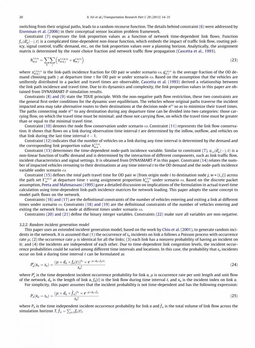
Tables 2 and 3 present the demand uncertainty reductions for 10 min during the morning peak period (7:20AM to7:30AM) for the six OD pairs with the most uncertainty when 10 and 30 sensors are available, respectively. The results inthe tables confirm our previous research finding that a greater number of better placed sensors can lead to more demanduncertainty reduction in a vehicular network. Specifically, OD pair (41, 1) during 7:20AM–7:25AM in the 10 sensor planwas covered by one sensor and the uncertainty reduction was 16% while the same OD pair in the 30 sensor plan was coveredby three sensors and experienced a 60% uncertainty reduction during that time interval. The 1 h demand uncertainty reduc-tion tables with 10 sensor and 30 sensor plans can be found in Appendix A, Tables A1 and A2, respectively.

In short, the two sensor budgets tested in this section indicated that significant reductions of the demand uncertaintywere obtained when sensors were optimally deployed in terms of maximal information gains and demand coverage andintercepted more OD pairs. However, although some particular OD pairs such as (87, 85) and (40,110) have been coveredby additional sensors, the demands of those OD pairs still have significant uncertainties due to the magnitude of originaldemand values and the volume distribution over paths at a particular time.

Table A1List of time-dependent OD pairs with the 6 highest variances by 10 sensors (k = 0.6).



Originzone

Destinationzone



Posteriorvariance



7:00AM–7:05AM (5035veh/5 min)

41 1 58 1.15 120.87 10 1

87 85 55 1.09 60.98 50 28 91 55 1.09 79.60 34 1

86 91 45 0.89 59.23 27 183 85 45 0.89 59.46 27 3

4 110 45 0.89 76.38 6 1

7:05AM–7:10AM (4832veh/5 min)

41 1 72 1.49 193.34 7 1

87 85 54 1.12 37.63 68 28 91 51 1.06 78.81 24 1

34 1 41 0.85 64.84 4 192 91 40 0.83 64 0 083 85 40 0.83 57.38 10 3

7:10AM–7:15AM (4739veh/5 min)

87 85 53 1.12 48.95 56 2

86 91 44 0.93 56.01 28 141 1 44 0.93 72.97 6 178 27 41 0.87 66.63 1 2

8 91 41 0.87 65.86 2 140 110 38 0.80 55.16 5 1

7:15AM–7:20AM (4684veh/5 min)

41 1 51 1.09 93.70 10 1

8 91 48 1.02 75.34 18 188 31 40 0.85 62.37 3 186 91 39 0.83 54.71 10 140 110 39 0.83 58.47 4 187 85 37 0.79 34.39 37 2

7:20AM–7:25AM (4858veh/5 min)

41 1 53 1.09 94.84 16 1

87 85 52 1.07 98.69 9 28 91 47 0.97 73.55 17 1

86 91 44 0.91 77.44 0 095 10 42 0.86 62.55 11 240 110 35 0.72 46.16 6 1

7:25AM–7:30AM (4914veh/5 min)

41 1 56 1.14 113.67 9 1

87 85 49 1.00 80.49 16 240 110 44 0.90 67.46 13 183 85 42 0.85 68.16 3 386 91 41 0.83 67.24 0 034 1 39 0.79 58.91 3 1

7:30AM–7:35AM (4955veh/5 min)

41 1 62 1.25 132.29 14 1

87 85 52 1.05 81.83 24 240 110 46 0.93 78.28 8 1

8 91 41 0.83 61.44 9 183 85 38 0.77 56.10 3 386 91 37 0.75 51.85 5 1

7:35AM–7:40AM (5036veh/5 min)

41 1 58 1.15 114.88 15 1

86 91 51 1.01 89.00 14 18 91 51 1.01 75.47 27 1

87 85 50 0.99 85.65 14 283 85 45 0.89 74.93 8 334 1 43 0.85 69.11 7 1

7:40AM–7:45AM (5079veh/5 min)

41 1 59 1.16 123.66 11 1

8 91 53 1.04 66.08 41 187 85 52 1.02 88.58 18 295 10 45 0.89 61.28 24 286 91 43 0.85 65.34 12 1



Table A1 (continued)



Originzone

Destinationzone



Posteriorvariance



83 85 42 0.83 65.26 8 3

7:45AM–7:50AM (5037veh/5 min)

41 1 63 1.25 133.58 16 1

8 91 54 1.07 77.41 34 187 85 53 1.05 75.48 33 286 91 42 0.83 67.73 4 140 110 41 0.81 63.78 5 134 1 40 0.79 61.24 4 1

7:50AM–7:55AM(4973 veh/5 min)

87 85 52 1.05 91.38 16 2

41 1 50 1.00 90.66 9 186 91 49 0.99 83.24 13 1

8 91 47 0.95 68.32 23 134 1 40 0.80 58.62 8 143 110 36 0.72 51.44 1 1

7:55AM–8:00 AM(4875 veh/5 min)

41 1 56 1.15 95.99 23 1

8 91 501 1.03 72.46 28 195 10 42 0.86 61.85 12 186 91 40 0.82 64.00 0 140 110 40 0.82 59.33 7 134 1 39 0.80 54.46 10 1

�The total number of vehicles in the 2-h period is 119,189 vehicles.


5. Concluding remarks

Uncertainty is pervasive in transportation planning and has significant influence in the transportation operational strat-egies’ evaluations and other decision making. With particular emphasis on the time-dependent OD demand estimation prob-lem under a variety of a priori unknown incident scenarios, this paper proposed a two-stage stochastic model to find anoptimal set of sensor locations, subject to a budget constraint, with the dual objectives of maximizing the long run expec-tation of the link information gains and the OD flow coverage in a large scale traffic network. A HGRASP-DTA search proce-dure was used to find the near optimal sensor locations in the context of user equilibrium dynamic traffic assignment andstochastic scenarios. A numerical example based on the Baltimore–Washington network illustrated the proposed method-ology and explored the effects of the weight in the objective function and the sensor budget limit. The expected OD flowcoverage and information gains under stochastic conditions are greater than those obtained under normal conditions withthe same weight for the objective function components, suggesting that, under stochastic conditions, the sensor locationplans obtained under the assumption of stochastic conditions result in better performance than plans developed for normalconditions. Examination of the effects of the number of sensors available confirmed previous findings (Fei et al., 2007) that agreater number of optimally deployed sensors reduces the demand uncertainty compared to fewer sensors. However, someOD pairs still have significant demand uncertainties due to the magnitude of original demand values and the volume distri-bution over paths at a particular time.

The main contributions of this paper include: (1) it is among the first to consider network uncertainty in the sensor loca-tion problem through a two-stage stochastic formulation; (2) the proposed formulation of the sensor location problem wasimplemented in the context of dynamic traffic assignment which is a realistic representation of the actual trafficcharacteristics; (3) a HGRASP-DTA solution procedure was developed to find the sensor locations in an efficient mannerwithout requiring excessive memory and intractable computational time; (4) the proposed methodology considers multipleincident scenarios (0, 1, or 2 incidents) and classified the impacted and un-impacted vehicles into different classes in a senseto minimize the user travel time by diverting the impacted vehicles to alternative routes.

Future work may consider the sensor location problem as a chance constrained model to maximize the probabilities ofreaching a certain goal, such as the number of OD pairs covered by a sensor. Instead of assuming independence amongthe simultaneously incidents with given incident severity rates, the impact of the correlation among incidents to the sensorlocations will be explored. A natural extension of the sensor location problem concerned with OD demand estimation appli-cations is to relax the time-dependent user equilibrium (TDUE) assumption to the stochastic user equilibrium (SUE) by con-sidering travelers’ perception in the path choice in the context of incidents.

Appendix A

See Tables A1 and A2.

Table A2List of time-dependent OD pairs with the 6 highest variances by 30 sensors k = 0.6).

Weights (k = 0.6) Measured link ID(37,48,308,426,526,764,952,967,1051,1258,1267,1373,1446,1732,1853,1859,1863,1874,1887,1898,1950,1989,2036,2126,2199,2237,2252,2504,2522,2547)

Time interval (total demand) Origin zone Destination zone Historical 5-min demand % of Demand to the total Posterior variance Variance reduction (%) Number of covering sensors

7:00AM–7:05AM (5035 veh/5 min) 41 1 58 1.15 72.22 46 387 85 55 1.09 88.81 27 1

8 91 55 1.09 34.87 71 286 91 45 0.89 49.77 39 283 85 45 0.89 60.60 25 2

4 110 45 0.89 65.16 20 3

7:05AM–7:10AM (4832 veh/5 min) 41 1 72 1.49 32.81 84 387 85 54 1.12 75.71 35 1

8 91 51 1.06 63.17 39 234 1 41 0.85 46.72 31 392 91 40 0.83 39.20 39 283 85 40 0.83 58.58 8 2

7:10AM–7:15AM (4739 veh/5 min) 87 85 53 1.12 79.06 30 186 91 44 0.93 43.93 43 241 1 44 0.93 33.49 57 378 27 41 0.87 66.93 0 1

8 91 41 0.87 37.03 45 240 110 38 0.80 34.71 40 3

7:15AM–7:20AM (4684 veh/5 min) 41 1 51 1.09 46.70 55 38 91 48 1.02 19.17 79 2

88 31 40 0.85 34.19 47 586 91 39 0.83 50.71 17 240 110 39 0.83 41.60 32 387 85 37 0.79 43.79 20 1

7:20AM–7:25AM (4858 veh/5 min) 41 1 53 1.09 45.04 60 387 85 52 1.07 105.81 2 1

8 91 47 0.97 65.85 25 286 91 44 0.91 77.44 0 095 10 42 0.86 0.01 100 740 110 35 0.72 36.75 25 3

7:25AM–7:30AM (4914 veh/5 min) 41 1 56 1.14 52.04 59 387 85 49 1.00 90.42 6 140 110 44 0.90 57.44 26 383 85 42 0.85 69.43 2 286 91 41 0.83 67.24 0 034 1 39 0.79 42.15 31 3

7:30AM–7:35AM (4955 veh/5 min) 41 1 62 1.25 74.53 52 387 85 52 1.05 96.12 11 140 110 46 0.93 57.38 32 3

8 91 41 0.83 27.08 60 383 85 38 0.77 56.62 2 286 91 37 0.75 50.51 8 2

7:35AM–7:40AM (5036 veh/5 min) 41 1 58 1.15 14.19 89 3


X.Fei

etal./Transportation

Research

PartC

29(2013)

14–31

29

Table A2 (continued)

Weights (k = 0.6) Measured link ID(37,48,308,426,526,764,952,967,1051,1258,1267,1373,1446,1732,1853,1859,1863,1874,1887,1898,1950,1989,2036,2126,2199,2237,2252,2504,2522,2547)

Time interval (total demand) Origin zone Destination zone Historical 5-min demand % of Demand to the total Posterior variance Variance reduction (%) Number of covering sensors

86 91 51 1.01 80.61 23 28 91 51 1.01 61.67 41 2

87 85 50 0.99 93.38 7 183 85 45 0.89 78.16 4 234 1 43 0.85 51.43 30 3

7:40AM–7:45AM (5079 veh/5 min) 41 1 59 1.16 39.25 72 38 91 53 1.04 56.21 50 1

87 85 52 1.02 98.28 9 195 10 45 0.89 0.00 100 886 91 43 0.85 61.23 17 283 85 42 0.83 67.46 4 2

7:45AM–7:50AM (5037 veh/5 min) 41 1 63 1.25 51.61 67 38 91 54 1.07 81.79 30 3

87 85 53 1.05 95.99 15 186 91 42 0.83 67.73 4 240 110 41 0.81 50.88 24 334 1 40 0.79 46.20 28 3

7:50AM–7:55AM (4973 veh/5 min) 87 85 52 1.05 103.29 5 141 1 50 1.00 47.77 52 386 91 49 0.99 79.64 17 2

8 91 47 0.95 23.01 74 234 1 40 0.80 43.66 32 343 110 36 0.72 36.59 29 4

7:55AM–8:00 AM (4875 veh/5 min) 41 1 56 1.15 56.66 55 38 91 501 1.03 34.74 65 2

95 10 42 0.86 15.05 79 786 91 40 0.82 62.57 2 240 110 40 0.82 46.65 27 334 1 39 0.80 40.84 33 3

�The total number of vehicles in the 2-h period is 119,189 vehicles.

30X

.Feiet

al./TransportationR

esearchPart

C29

(2013)14–

31


References

Beale, E.M.L., 1955. On minimizing a convex function subject to linear inequalities. Journal of Royal Statistical Society series B17, 173–184.Birge, J.R., Louveaux, F., 1997. Introduction to Stochastic Programming. Springer-Verlag, New York.Cascetta, E., Inaudi, D., Marquis, G., 1993. Dynamic estimator of origin-destination matrices using traffic counts. Transportation Science 27 (4), 363–373.Chiu, Y.-C., Huynh, N., Mahmassani, H.S., 2001. Determining optimal locations for variable message signs under stochastic incident scenarios. In: 80th

Annual Meeting of the Transportation Research Board, Washington, D.C.Dantzig, G.B., 1955. Linear programming under uncertainty. Management Science 1, 197–206.Eisenman, S.M., Fei, X., Zhou, X.S., Mahmassani, H.S., 2006. Number and location of sensors for real-time network traffic estimation and prediction: a

sensitivity analysis. Transportation Research Record 1964, 253–260.Fei, X., Mahmassani, H.S., 2011. Structural analysis of near-optimal sensor locations for a stochastic large-scale network. Transportation Research Part C 19

(2), 440–453.Fei, X., Mahmassani, H.S., Eisenman, S.M., 2007. Sensor coverage and location for real-time traffic prediction in large-scale networks. Transportation

Research Record 2039, 1–15.Feo, T.A., Resende, M.G.C., 1995. Greedy randomized adaptive search procedures. Journal of Global Optimization 6, 109–133.Festa, P., Resende, M.G.C., 2001. GRASP: An Annotated Bibliography. AT&T Labs Research Technical Report.Gendreau, M., Laporte, G., Seguin, R., 1996. Stochastic vehicle routing. European Journal of Operational Research 88, 3–12.Glover, F., 1986. Future paths for integer programming and links to artificial intelligence. Computers and Operations Research 13 (5), 533–549.Glover, F., Laguna, M., 1993. Tabu search. In: Reeves, C.R. (Ed.), Modern Heuristic Techniques for Combinatorial Problems. Blackwell Scientific Publications,

Oxford.Lin, S., Kernighan, B.W., 1973. An effective heuristic algorithm for the traveling salesman problem. Operations Research 21, 498–516.Liu, C., Fan, Y., 2007. A two-stage stochastic programming model for transportation network retrofit. In: 86th Annual Meeting of the Transportation

Research Board, Washington, D.C.Liu, Y., Lin, P.W., Zou, N., Chang, G.L., Point-Du-Jour, J.Y., 2004. Emergency incident management, benefits and operational issues – a performance and

benefits evaluation of CHART. In: 2004 IEEE International Conference on Networking, Sensing and Control, Taipei, Taiwan.Mahmassani, H.S., Abdelghany, A., Chiu, Y.-C., Huynh, N., Zhou, X., 2000. DYNASMART-P, Intelligent Transportation Network Planning Tool Vols. I and II.

Report ST067-85-PII, Prepared for Federal Highway Administration, January, Austin, Texas, USA. University of Texas at Austin, Austin.Maryland State Highway Administration, 2006. Part 6, Temporary Traffic Control, Maryland Manual on Uniform Traffic Control Devices for Streets and

Highways.Patriksson, M., Wynter, L., 1999. Stochastic mathematical programs with equilibrium constraints. Operations Research Letters 25, 159–167.Peeta, S., Mahmassani, H.S., 1995. System optimal and user equilibrium time-dependent traffic assignment in congested network. Annals of Operations

Research 60, 81–113.Pitsoulis, L.S., Resende, M.G.C., 2001. Greedy Randomized Adaptive Search Procedures. AT&T Labs Research Technical Report.Sawaya, O.B., Doan, D.L., Ziliaskopoulos, A.K., Fourer, R., 2001. A multistage stochastic system optimum dynamic traffic assignment program with recourse

for incident traffic management. Transportation Research Record 1748, 116–124.Van Slyke, R., Wets, R.B., 1969. L-shaped linear programs with application to optimal control and stochastic programming. SIAM Journal on Applied

Mathematics 17 (4), 638–663.Waller, S.T., Ziliaskopoulos, A.K., 2001. Stochastic dynamic network design problem. Transportation Research Record 1771, 106–113.Wardrop, J.G., 1952. Some theoretical aspects of road traffic research. Proceedings of the Institution of Civil Engineers II (1), 325–378.Zhou, X.S., List, G.F., 2010. An information-theoretic sensor location model for traffic origin destination demand estimation applications. Transportation

Science 44 (2), 254–273.

Documents

Vehicular network sensor placement optimization under uncertainty