Computation- and Space-EfficientImplementation of SSA

Anton KorobeynikovDepartment of Statistical Modelling,Saint Petersburg State University

198504, Universitetskiy pr. 28, Saint Petersburg, Russiaasl@math.spbu.ru

April 20, 2010

AbstractThe computational complexity of different steps of the basic SSA is

discussed. It is shown that the use of the general-purpose “blackbox”routines (e.g. found in packages like LAPACK) leads to huge waste of timeresources since the special Hankel structure of the trajectory matrix is nottaken into account.

We outline several state-of-the-art algorithms (for example, Lanczos-based truncated SVD) which can be modified to exploit the structure ofthe trajectory matrix. The key components here are Hankel matrix-vectormultiplication and the Hankelization operator. We show that both canbe computed efficiently by the means of Fast Fourier Transform.

The use of these methods yields the reduction of the worst-case compu-tational complexity from O(N3) to O(kN logN), where N is series lengthand k is the number of eigentriples desired.

1 IntroductionDespite the recent growth of SSA-related techniques it seems that little attentionwas paid to their efficient implementations, e.g. the singular value decomposi-tion of Hankel trajectory matrix, which is a dominating time-consuming step ofthe basic SSA.

In almost all SSA-related applications only a few leading eigentriples aredesired, thus the use of general-purpose “blackbox” SVD implementations causesa huge waste of time and memory resources. This almost prevents the use of theoptimum window sizes even on moderate length (say, few thousand) time series.The problem is much more severe for 2D-SSA [15] or subspace-based methods[2, 8, 13], where large window sizes are typical.

We show that proper use of state-of-art singular value decomposition al-gorithms can significantly reduce the amount of operations needed to compute

1

arX

iv:0

911.

4498

v2 [

cs.N

A]

13

Apr

201

0

truncated SVD suitable for SSA purposes. This is possible because the informa-tion about the leading singular triples becomes available long before the costlyfull decomposition.

These algorithms are usually based on Lanczos iterations or related methods.This algorithm can be modified to exploit the Hankel structure of the datamatrix effectively. Thus the computational burden of SVD can be considerablyreduced.

In section 2 we will outline the computational and storage complexity ofthe steps of the basic SSA algorithm. Section 3 contains a review of well-known results connected with the Lanczos singular value decompostion algo-rithm. Generic implementation issues in finite-precision arithmetics will bediscussed as well. The derivation of the efficient Hankel SSA trajectory matrix-vector multiplication method will be presented in section 4. This method is a keycomponent of the fast truncated SVD for the Hankel SSA trajectory matrices.In the section 5 we will exploit the special structure of the rank 1 Hankelizationoperator which allows its efficient implementation. Finally, all the implementa-tions of the mentioned algorithms are compared in sections 6 and 7 on artificialand real data.

2 Complexity of the Basic SSA AlgorithmLet N > 2. Denote by F = (f1, . . . , fN ) a real-valued time series of lengthN . Fix the window length L, 1 < L < N . The Basic SSA algorithm for thedecomposition of a time series consists of four steps [14]. We will consider eachstep separately and discuss its computational and storage complexity.

2.1 EmbeddingThe embedding step maps original time series to a sequence of lagged vectors.The embedding procedure forms K = N − L+ 1 lagged vectors Xi ∈ RL:

Xi = (fi, . . . , fi+L−1)T, 1 6 i 6 K.

These vectors form the L-trajectory (or trajectory) matrix X of the series F :

X =

f1 f2 · · · fK−1 fKf2 f3 · · · fK fK+1

......

......

fL fL+1 · · · fN−1 fN

.

Note that this matrix has equal values along the antidiagonals, thus it is a Hankelmatrix. The computational complexity of this step is negligible: it consists ofsimple data movement which is usually considered a cheap procedure. However,if the matrix is stored as-is, then this step obviously has storage complexity ofO(LK) with the worst case being O(N2) when K ∼ L ∼ N/2.

2

2.2 Singular Value DecompositionThis step performs the singular value decomposition of the L × K trajectorymatrix X. Without loss of generality we will assume that L 6 K. Then theSVD can be written as

X = UTΣV,

where U = (u1, . . . , uL) is a L × L orthogonal matrix, V = (v1, . . . , vK) is aK×K orthogonal matrix, and Σ is a L×K diagonal matrix with nonnegative realdiagonal entries Σii = σi, for i = 1, . . . , L. The vectors ui are called left singularvectors, the vi are the right singular vectors, and the σi are the singular values.We will label the singular values in descending order: σ1 > σ2 > · · · > σL. Notethat the singular value decomposition of X can be represented in the form

X = X1 + · · ·+XL,

where Xi = σiuivTi . The matrices Xi have rank 1, therefore we will call them

elementary matrices. The triple (σi, ui, vi) will be called a singular triple.Usually the SVD is computed by means of Golub and Reinsh algorithm [12]

which requires O(L2K + LK2 + K3) multiplications having the worst compu-tational complexity of O(N3) when K ∼ L ∼ N/2. Note that all the data mustbe processed at once and SVDs even of moderate length time series (say, whenN > 5000) are essentially unfeasible.

2.3 GroupingThe grouping procedure partitions the set of indices {1, . . . , L} into m disjointsets I1, . . . , Im. For the index set I = {i1, . . . , ip} one can define the resultantmatrix XI = Xi1 + · · · + Xip . Such matrices are computed for I = I1, . . . , Imand we obtain the decomposition

X = XI1 + · · ·+XIm .

For the sake of simplicity we will assume that m = L and each Ij = {j} lateron. The computation of each elementary matrixXj costs O(LK) multiplicationsand O(LK) storage yielding overall computation complexity of O(L2K) andO(L2K) for storage. Again the worst case is achieved at L ∼ K ∼ N/2 withthe value O(N3) for both computation and storage.

2.4 Diagonal Averaging (Hankelization)This is the last step of the Basic SSA algorithm transforming each groupedmatrix XIj into a new time series of length N . This is performed by meansof diagonal averaging procedure (or Hankelization). It transforms an arbitraryL×K matrix Y to the series g1, . . . , gN by the formula:

gk =

1k

∑kj=1 yj,k−j+1, 1 6 k 6 L,

1L

∑Lj=1 yj,k−j+1, L < k < K,

1N−k+1

∑Lj=k−K+1 yj,k−j+1, K 6 k 6 N.

3

Note that these two steps are usually combined. One just forms the elemen-tary matrices one by one and immediately applies the Hankelization operator.This trick reduces the storage requirements considerably.

O(N) multiplications and O(LK) additions are required for performing thediagonal averaging of one elementary matrix. Summing these values for L el-ementary matrices we obtain the overall computation complexity for this stepbeing O(L2K) additions and O(NL) multiplications. The worst case complexitywill be then O(N3) additions and O(N2) multiplications

Summing the complexity values alltogether for all four steps we obtain theworst case computational complexity to be O(N3). The worst case occurs ex-actly when window length L equals N/2 (the optimal window length for asymp-totic separability [14]).

3 Truncated Singular Value DecompositionThe typical approach to the problem of computating the singular triples(σi, ui, vi) of A is to use the Schur decomposition of some matrices related toA, namely

1. the cross product matrices AAT , ATA, or

2. the cyclic matrix C =(

0 AAT 0

).

One can prove the following theorem (see, e.g. [11, 19]):

Theorem 1 Let A be an L ×K matrix and assume without loss of generalitythat K > L. Let the singular value decomposition of A be

UTAV = diag (σ1, . . . , σL) .

Then

V T(ATA

)V = diag (σ2

1 , . . . , σ2L, 0, . . . , 0︸ ︷︷ ︸

K−L

),

UT(AAT

)U = diag (σ2

1 , . . . , σ2L).

Moreover, if V is partitioned as

V = (V1, V2) , V1 ∈ RK×L, V2 ∈ RK×(K−L),

then the orthonormal columns of the (L+K)× (L+K) matrix

Y =1√2

(U −U 0

V1 V1√

2V2

)form an eigenvector basis for the cyclic matrix C and

Y TCY = diag (σ1, . . . , σL,−σ1, . . . ,−σL, 0, . . . , 0︸ ︷︷ ︸K−L

).

4

The theorem tells us that we can obtain the singular values and vectors ofA by computing the eigenvalues and corresponding eigenvectors of one of thesymmetric matrices. This fact forms the basis of any SV D algorithm.

In order to find all eigenvalues and eigenvectors of the real symmetric matrixone usually turns it into a similar tridiagonal matrix by the means of orthogo-nal transformations (Householder rotations or alternatively via Lanczos recur-renses). Then, for example, another series of orthogonal transformations can beapplied to the latter tridiagonal matrix which converges to a diagonal matrix[11].

Such approach, which in its original form is due to Golub and Reinsh [12]and is used in e.g. LAPACK [1], computes the SVD by implicitly applying theQR algorithm to the symmetric eigenvalue problem for ATA.

For large and sparse matrices the Golub-Reinsh algorithm is impractical.The algorithm itself starts out by applying a series of transformations directlyto matrix A to reduce it to the special bidiagonal form. Therefore it requires thematrix to be stored explicitlly, which may be impossible simply due to its size.Moreover, it may be difficult to take advantage of any structure (e.g. Hankel inSSA case) or sparsity in A since it is quickly destroyed by the transformationsapplied to the matrix. The same argument applies to SVD computation via theJacobi algorithm.

Bidiagonalization was proposed by Golub and Kahan [10] as a way of tridi-agonalizing the cross product matrix without forming it explicitly. The methodyields the decomposition

A = PTBQ,

where P and Q are orthogonal matrices and B is an L × K lower bidiagonalmatrix. Here BBT is similar to AAT . Additionally, there are well-known SVDalgorithms for real bidiagonal matrices, for example, the QRmethod [11], divide-and-conquer [16], and twisted [7] methods.

The structure of our exposition follows [19].

3.1 Lanczos BidiagonalizationFor a rectangular L × K matrix A the Lanczos bidiagonalization computes asequence of left Lanczos vectors uj ∈ RL and right Lanczos vectors vj ∈ RK

5

and scalars αj and βj , j = 1, . . . , k as follows:

Algorithm 1: Golub-Kahan-Lanczos BidiagonalizationChoose a starting vector p0 ∈ RL1

β1 ←− ‖p0‖2, u1 ←− p0/β1, v0 ←− 02

for j ← 1 to k do3

rj ←− ATuj − βjvj−14

αj ←− ‖rj‖2, vj ←− rj/αj5

pj ←− Avj − αjuj6

βj+1 ←− ‖pj‖2, uj+1 ←− pj/βj+17

end8

Later on we will refer to one iteration of the for loop at line 3 as a Lanczos step(or iteration). After k steps we will have the lower bidiagonal matrix

Bk =

α1

β2 α2

β3. . .. . . αk

βk+1

.

If all the computations performed are exact, then the Lanczos vectors will beorthornomal:

Uk+1 = (u1, . . . , uk+1) ∈ RL×(k+1), UTk+1Uk+1 = Ik+1,

andVk+1 = (v1, . . . , vk+1) ∈ RK×(k+1), V Tk+1Vk+1 = Ik+1,

where Ik is k × k identity matrix. By construction, the columns of Uk+1 andVk+1 satisfy the recurrences

αjvj = ATuj − βjvj−1,βj+1uj+1 = Avj − αjuj ,

and can be written in the compact form as follows:

AVk = Uk+1Bk, (1)ATUk+1 = VkB

Tk + αk+1vk+1e

Tk+1. (2)

Also, the first equiality can be rewritten as

UTk+1AVk = Bk,

explaining the notion of left and right Lanczos vectors. Moreover, uk ∈Kk(AAT , u1

), vk ∈ Kk

(ATA, v1

), where

Kk(AAT , u1

)={u1, AA

Tu1, . . . ,(AAT

)ku1

}, (3)

Kk(ATA, v1

)={v1, A

TAv1, . . . ,(ATA

)kv1

}, (4)

6

and therefore u1, u2, . . . , uk and v1, v2, . . . , vk form an orthogonal basis for thesetwo Krylov subspaces.

3.2 Lanczos Bidiagonalization in Inexact ArithmeticsWhen the Lanczos bidiagonalization is carried out in finite precision arithmeticsthe Lanczos recurrence becomes

αjvj = ATuj − βjvj−1 + fj ,

βj+1uj+1 = Avj − αjuj + gj ,

where fj ∈ RK , gj ∈ RL are error vectors accounting for the rounding errorsat the j-th step. Usually, the rounding terms are small, thus after k stepsthe equations (1), (2) still hold to almost machine accuracy. In contrast, theorthogonality among left and right Lanczos vectors is lost.

However, the Lanzos algorithm possesses a remarkable feature that the ac-curacy of the converged Ritz values is not affected by the loss of orthogonality,but while the largest singular values of Bk are still accurate approximations tothe largest singular values of A, the spectrum of Bk will in addition contain falsemultiple copies of converged Ritz values (this happens even if the correspond-ing true singular values of A are isolated). Moreover, spurious singular values(“ghosts”) periodically appear between the already converged Ritz values (see,e.g. [19] for illustration).

There are two different approaches with respect to what should be done toobtain a robust method in finite arithmetics.

3.2.1 Lanczos Bidiagonalization with no orthogonalization

One approach is to apply the simple Lanczos process “as-is” and subsequentlyuse some criterion to detect and remove spurious singular values.

The advantage of this method is that it completely avoids any extra workconnected with the reorthogonalization, and the storage requirements are verylow since only few of the latest Lanczos vectors have to be remembered. Thedisadvantage is that many iterations are wasted on simply generating multiplecopies of the large values [23]. The number of extra iterations required comparedto that when executing the Lanczos process in exact arithmetics can be verylarge: up to six times the original number as reported in [24]. Another disdvan-tage is that the criterion mentioned above can be rather difficult to implement,since it depends on the correct choice of different thresholds and knobs.

3.2.2 Lanczos Bidiagonalization using reorthogonalization

A different way to deal with loss of orthogonalizy among Lanczos vectors isto apply some reorthogonalization scheme. The simplest one is so-callled fullreorthogonalization (FRO) where each new Lanczos vector uj+1 (or vj+1) isorthogonalized against all the Lanczos vectors generated so far using, e.g., themodified Gram-Schmidt algorithm.

7

This approach is usually too expensive, since for the large problem the run-ning time needed for reorthogonalization quickly dominate the execution timeunless the necessary number of iterations k is very small compared to the di-mensions of the problem (see section 3.3 for full analysis of the complexity).The storage requirements of FRO might also be a limiting factor since all thegenerated Lanczos vectors need to be saved.

A number of different schemes for reducing the work associated with keepingthe Lanczos vectors orthogonal were developed (see [3] for extensive review).The main idea is to estimate the level of orthogonality among the Lanczosvectors and perform the orthogonalization only when necessary.

For example, the so-called partial reorthogonalization scheme (PRO) de-scribed in [27, 26, 19] uses the fact that the level of orthogonality among theLanczos vectors satisfies some recurrence relation which can be derived from therecurrence used to generate the vectors themselves.

3.3 The Complexity of the Lanczos BidiagonalizationThe computational complexity of the Lanczos bidiagonalization is determined bythe two matrix-vector multiplications, thus the overall complexity of k Lanczositerations in exact arithmetics is O(kLK) multiplications.

The computational costs increase when one deals with the lost of orthog-onality due to the inexact computations. For FRO scheme the additionalO(k2(L + K)) operations required for the orthogonalization quickly dominatethe execution time, unless the necessary number of iterations k is very smallcompared to the dimension of the problem. The storage requirements of FROmay also be a limiting factor since all the generated Lanczos vectors need to besaved.

In general, there is no way to determine in advance how many steps willbe needed to provide the singular values of interest within a specified accuracy.Usually the number of steps is determined by the distribution of the singularnumbers and the choice of the starting vector p0. In the case when the singularvalues form a cluster the convergence will not occur until k, the number ofiterations, gets very large. In such situation the method will also suffer fromincreased storage requirements: it is easy to see that they are O(k(L+K)).

These problems can be usually solved via limiting the dimension of theKrylov subspaces (3), (4) and using restarting schemes: restarting the iterationsafter a number of steps by replacing the starting vector with some “improved”starting vector (ideally, we would like p0 to be a linear combination of the rightsingular vectors of A associated with the desired singular values). Thus, if welimit the dimension of the Krylov subspaces to d the storage complexity dropsto O(d(L+K)) (surely the number of desired singular triples should be greaterthan d). See [3] for the review of the restarting schemes proposed so far andintroduction to the thick-restarted Lanczos bidiagonalization algorithm. In thepapers [30, 31] different strategies of choosing the best dimension d of Krylovsubspaces are discussed.

8

If the matrix being decomposed is sparse or structured (for example, Hankelin Basic SSA case or Hankel with Hankel blocks for 2D-SSA) then the compu-tational complexity of the bidiagonalization can be significantly reduced giventhat the efficient matrix-vector multiplication routine is available.

4 Efficient Matrix-Vector Multiplication forHankel Matrices

In this section we will present efficient matrix-vector multiplication algorithmfor Hankel SSA trajectory matrix. By means of the fast Fourier transformthe cost of the multiplication drops from ordinary O(LK) multiplications toO ((L+K) log(L+K)). The idea of using the FFT for computing a Han-kel matrix-vector product is nothing new: it was probably first described byBluestein in 1968 (see [28]). A later references are [21, 5].

This approach reduces the computational complexity of the singu-lar value decomposition of Hankel matrices from O

(kLK + k2(L+K)

)to

O(k(L+K) log(L+K) + k2(L+K)

). The complexity of the worst case when

K ∼ L ∼ N/2 drops significantly from O(kN2 + k2N

)to O

(kN logN + k2N

)1.

Also the discribed algorithms provide an efficient way to store the HankelSSA trajectory matrix reducing the storage requirements from O(LK) to O(L+K).

4.1 Matrix Representation of Discrete Fourier Transformand Circulant Matrices

The 1-d discrete Fourier transform (DFT) of a (complex) vector (fk)N−1k=0 is

defined by:

fl =

N∑k=0

e−2πikl/Nfk, k = 0, . . . , N − 1.

Denote by ω the primitive N -root of unity, ω = e−2πi/N . Introduce the DFTmatrix FN :

FN =

1 1 · · · 11 ω1 · · · ωN−1

1 ω2 · · · ω2(N−1)

......

......

1 ωN−1 · · · ω(N−1)(N−1)

.

Then the 1-d DFT can be written in matrix form: f = FNf . The inverse of theDFT matrix is given by

F−1N =1

NF∗N ,

1Compare with O(N3

)for full SVD via Golub-Reinsh method.

9

where F∗N is the adjoint (conjugate transpose) of DFT matrix FN . Thus, theinverse 1-d discrete Fourier transform (IDFT) is given by

fk =1

N

N−1∑l=0

e2πikl/N fl, k = 0, . . . , N − 1.

The fast Fourier transform is an efficient algorithm to compute the DFT(and IDFT) in O(N logN) complex multiplications instead of N2 complex mul-tiplications in direct implementation of the DFT [20, 9].

Definition 1 An N ×N matrix C of the form

C =

c1 cN cN−1 · · · c3 c2c2 c1 cN · · · c4 c3...

......

......

cN−1 cN−2 cN−3 · · · c1 cNcN cN−1 cN−2 · · · c2 c1

is called a circulant matrix.

A circulant matrix is fully specified by its first column c = (c1, c2, . . . , cN )T

The remaining columns of C are each cyclic permutations of the vector c withoffset equal to the column index. The last row of C is the vector c in reverseorder, and the remaining rows are each cyclic permutations of the last row.

The eigenvectors of a circulant matrix of a given size are the columns of theDFT matrix of the same size. Thus a circulant matrix is diagonalized by theDFT matrix:

C = F−1N diag (FNc)FN ,

so the eigenvalues of C are given by the product FNc.This factorization can be used to perform efficient matrix-vector multiplica-

tion. Let v ∈ RN and C be an N ×N circulant matrix. Then

Cv = F−1N diag (FNc)FNv = F−1N (FNc� FNv) ,

where � denotes the element-wise vector multiplication. This can be computedefficiently using the FFT by first computing the two DFTs, FNc and FNv, andthen computing the IDFT F−1N (FNc� FNv). If the matrix-vector multiplicationis performed repeatedly with the same circulant matrix and different vectors,then surely the DFT FNc needs to be computed only once.

In this way the overall computational complexity of matrix-vector productfor the circulant matrices drops from O(N2) to O(N logN).

10

4.2 Toeplitz and Hankel MatricesDefinition 2 A L×K matrix of the form

T =

tK tK−1 · · · t2 t1tK+1 tK · · · t3 t2

......

......

tK+L−1 tK+L−2 · · · tL+1 tL

is called a (non-symmetric) Toeplitz matrix.

A Toeplitz matrix is completely determined by its last column and last row, andthus depends on K +L− 1 parameters. The entries of T are constant down thediagonals parallel to the main diagonal.

Given an algorithm for the fast matrix-vector product for circulant matrices,it is easy to see the algorithm for a Toeplitz matrix, since a Toeplitz matrix canbe embedded into a circulant matrix CK+L−1 of size K + L − 1 with the firstcolumn equals to (tK , tK+1, . . . , tK+L−1, t1, t2, . . . , tK−1)

T :

CK+L−1 =

tK · · · t1 tK+L−1 · · · tK+1

tK+1 · · · t2 t1 · · · tK+2

tK+2 · · · t3 t2 · · · tK+3

......

......

tK+L−1 · · · tL tL−1 · · · t1t1 · · · tL+1 tL · · · t2t2 · · · tL+2 tL+1 · · · t3...

......

...tK−1 · · · tK+L−1 tK+L−2 · · · tK

, (5)

where the leading L×K principal submatrix is T . This technique of embeddinga Toeplitz matrix in a larger circulant matrix to achieve fast computation iswidely used in preconditioning methods [6].

Using this embeddings, the Toeplitz matrix-vector product Tv can be rep-resented as follows:

CK+L−1

(v

0L−1

)=

(Tv∗

), (6)

and can be computed efficiently in O ((K + L) log(K + L)) time and O(K +L)memory using the FFT as described previously.

Recall that an L×K matrix of form

H =

h1 h2 · · · hK−1 hKh2 h3 · · · hK hK+1

......

......

hL hL+1 · · · hK+L−2 hK+L−1

is called Hankel matrix.

11

A Hankel matrix is completely determined by its first column and last row,and thus depends on K+L−1 parameters. The entries of H are constant alongthe antidiagonals. One can easily convert Hankel matrix into a Toeplitz one byreversing its columns. Indeed, define

P =

0 0 · · · 0 10 0 · · · 1 0...

......

...0 1 · · · 0 01 0 · · · 0 0

the backward identity permutation matrix. Then HP is a Toeplitz matrix forany Hankel matrix H, and TP is a Hankel matrix for any Toeplitz matrix T .Note that P = PT = P−1 as well. Now for the product Hv of Hankel matrixH and vector v we have

Hv = HPPv = (HP )Pv = Tw,

where T is Toeplitz matrix and vector w is obtained as vector v with entries inreversed order. The product Tw can be computed using circulant embeddingprocedure as described in (6).

4.3 Hankel SSA Trajectory Matrices

Now we are ready to exploit the connection between the time series F = (fj)Nj=1

under decomposition and corresponding trajectory Hankel matrix to derive thematrix-vector multiplication algorithm in terms of the series itself. In this waywe will effectively skip the embedding step of the SSA algorithm and reduce thecomputational and storage complexity.

The entries of the trajectory matrix of the series are hj = fj , j = 1, . . . , N .The entries of Toeplitz matrix T = HP are tj = hj = fj , j = 1, . . . , N . Thecorresponding first column of the embedding circulant matrix (5) is

cj =

{tN−L+j = fN−L+j , 1 6 j 6 L;

tj−L+1 = fj−L+1 L < j 6 N,

and we end with the following algorithm for matrix-vector multiplication for

12

trajectory matrix:Algorithm 2: Matrix-Vector Multiplication for SSA Trajectory Matrix

Input: Time series F = (fj)Nj=1, window length L, vector v of length

N − L+ 1.Output: p = Xv, where X is a trajectory matrix for F given window

length L.

c←− (fN−L+1, . . . , fN , f1, . . . , fN−L)T

1

c←− FFTN (c)2

w ←− (vN−L+1, . . . , v1, 0, . . . , 0)T

3

w ←− FFTN (w)4

p′ ←− IFFTN (w � c)5

p←− (p′1, . . . , p′L)T

6

where (w � c) denotes element-wise vector multiplication.If the matrix-vector multiplicationXv is performed repeatedly with the same

matrix X and different vectors v then steps 1, 2 should be performed only onceat the beginning and the resulting vector c should be reused later on.

The overall computational complexity of the matrix-vector multiplicationis O(N logN). Memory space of size O(N) is required to store precomputedvector c.

Note that the matrix-vector multiplication of the transposed trajectory ma-trix XT can be performed using the same vector c. Indeed, the bottom-rightK×L submatrix of circulant matrix (5) contains the Toeplitz matrix XTP andwe can easily modify algorithm 2 as follows:Algorithm 3: Matrix-Vector Multiplication for transpose of SSA Trajec-tory Matrix

Input: Time series F = (fj)Nj=1, window length L, vector v of length L.

Output: p = XT v, where X is a trajectory matrix for F given windowlength L.

c←− (fN−L+1, . . . , fN , f1, . . . , fN−L)T

1

c←− FFTN (c)2

w ←− (0, . . . , 0, vL, . . . , v1)T

3

w ←− FFTN (w)4

p′ ←− IFFTN (w � c)5

p←−(p′L−1, . . . , p

′N

)T6

5 Efficient Rank 1 HankelizationLet us recall the diagonal averaging procedure as described in 2.4 which trans-forms an arbitrary L×K matrix Y into a Hankel one and therefore into a series

13

gk, k = 1, . . . , N .

gk =

1k

∑kj=1 yj,k−j+1, 1 6 k 6 L,

1L

∑Lj=1 yj,k−j+1, L < k < K,

1N−k+1

∑Lj=k−K+1 yj,k−j+1, K 6 k 6 N.

(7)

Without loss of generality we will consider only rank 1 hankelization whenmatrix Y is elementary and can be represented as Y = σuvT with vectors u andv of length L and K correspondingly. Then equation (7) becomes

gk =

σk

∑kj=1 ujvk−j+1, 1 6 k 6 L,

σL

∑Lj=1 ujvk−j+1, L < k < K,

σN−k+1

∑Lj=k−K+1 ujvk−j+1, K 6 k 6 N.

(8)

This gives a hint how the diagonal averaging can be efficiently computed.Indeed, consider the infinite series u′n, n ∈ Z such that u′n = un when

1 6 n 6 L and 0 otherwise. The series v′n are defined in the same way, sov′n = vn when 1 6 n 6 K and 0 otherwise. The linear convolution u′n ∗ v′n of u′nand v′n can be written as follows:

(u′n ∗ v′n)k =

+∞∑j=−∞

u′jv′k−j+1 =

L∑j=1

u′jv′k−j+1 =

=

∑kj=1 ujvk−j+1, 1 6 k 6 L,∑Lj=1 ujvk−j+1, L < k < K,∑Lj=k−K+1 ujvk−j+1, K 6 k 6 N.

(9)

Comparing the equations (7) and (9) we deduce that

gk = ck (u′n ∗ v′n)k ,

where the constants ck are known in advance.The linear convolution u ∗ v can be defined in terms of the circular convolu-

tion, as follows. Pad the vectors u and v with the zeroes up to length L+K−1.Then the linear convolution of the original vectors u and v is the same as thecircular convolution of the extended series of length L+K − 1, namely

(u ∗ v)k =

L+K−1∑j=1

ujvk−j+1,

where k− j+1 is evaluated mod (L+K−1). The resulting circular convolutioncan be calculated effeciently via the FFT [4]:

(u ∗ v)k = IFFTN (FFTN (u′)� FFTN (v′)) .

Here N = L + K − 1, and u′, v′ denote the zero-padded vectors u and vcorrespondingly.

14

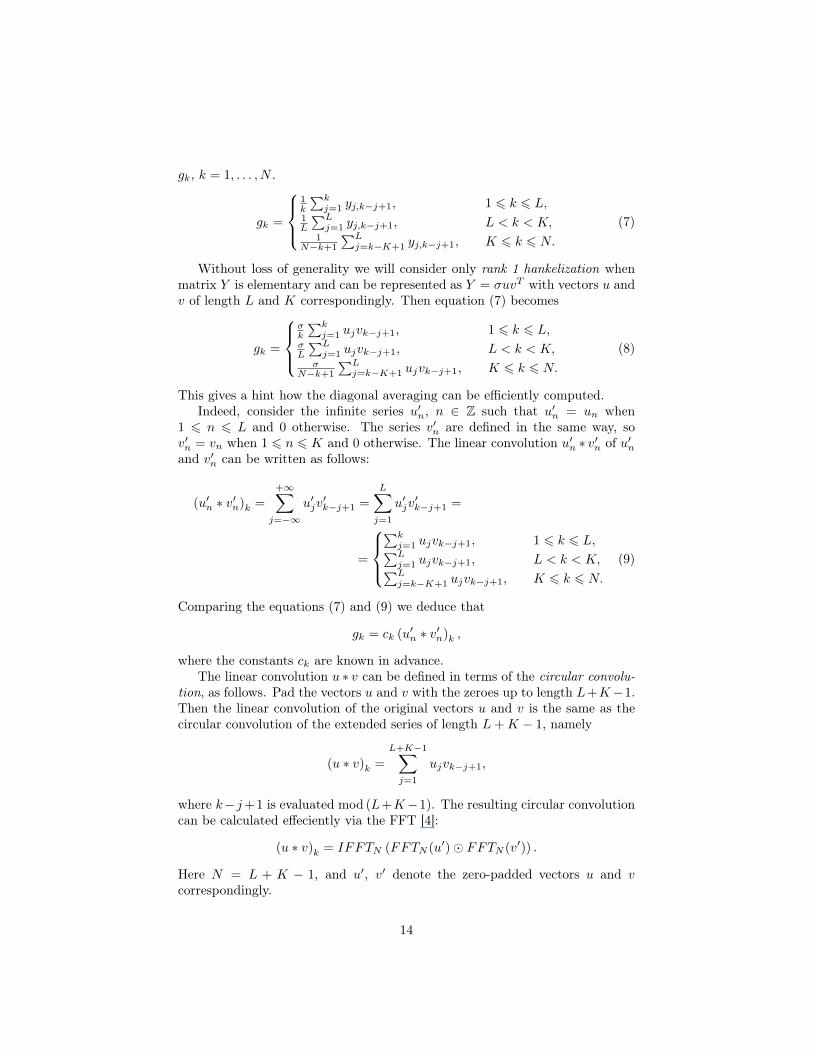
And we end with the following algorithm for the hankelization via convolu-tion:Algorithm 4: Rank 1 Hankelization via Linear ConvolutionInput: Vector u of length L, vector v of length K, singular value σ.Output: Time series G = (gj)

Nj=1 corresponding to the matrix Y = σuvT

after hankelization.

u′ ←− (u1, . . . , uL, 0, . . . , 0)T ∈ RN1

u←− FFTN (u′)2

v′ ←− (v1, . . . , vK , 0, . . . , 0)T ∈ RN3

v ←− FFTN (v′)4

g′ ←− IFFTN (v � u)5

w ←− (1, . . . , L, L, . . . , L, L, . . . , 1) ∈ RN6

g ←− σ (w � g′)7

The computational complexity of this algorithm is O(N logN) multiplicationsversus O(LK) for naıve direct approach. Basically this means that the worstcase complexity of the diagonal averaging drops from O(N2) to O(N logN).

6 Implementation ComparisonThe algorithms presented in this paper have much better asymptotic complexitythan standard ones, but obviously might have much bigger overhead and thuswould not be suitable for the real-world problems unless series length and/orwindow length becomes really big.

The mentioned algorithms were implemented by the means of the Rssa2

package for the R system for statistical computing [25]. All the comparions werecarried out on the 4 core AMD Opteron 2210 workstation running Linux. Wherepossible we tend to use state-of-the-art implementations of various computa-tional algorithms (e.g. highly optimized ATLAS [29] and ACML implementationsof BLAS and LAPACK routines). We used R version 2.8.0 throughout the tests.

We will compare the performance of such key components of the fast SSAimplementation as rank 1 diagonal averaging and the Hankel matrix-vector mul-tiplication. The performance of the methods which use the “full” SSA, namelythe series bootstrap confidence interval construction and series structure changedetection, will be considered as well.

6.1 Fast Hankel Matrix-Vector ProductFast Hankel matrix-vector multiplication is the key component for the Lanczosbidiagonalization. The algorithm outlined in the section 4.3 was implementedin two different ways: one using the core R FFT implementation and anotherone using FFT from FFTW library [9]. We selected window size equal to thehalf of the series length since this corresponds to the worst case both in terms

2The package will be submitted to CRAN soon, yet it can be obtained from author.

15

of computational and storage complexity. All initialization times (for example,Hankel matrix construction or circulant precomputation times) were excludedfrom the timings since they are performed only once in the beginning. So, wecompare the performance of the generic DGEMV [1] matrix-vector multicationroutine versus the performance of the special routine exploiting the Hankelstructure of the matrix.

●

●

●

●

●

●

●

●

●

●●

●

●●

●

●

●●

●●

●

●

●

●●

●

●

●

●

●

●

0 2000 4000 6000 8000 10000

0.1

1.0

10.0

100.0

Series length, N

Tim

e fo

r 10

0 m

atrix

−ve

ctor

pro

duct

s, s

econ

ds

●●●

●●●

●●●●

● ●● ●

● ● ● ●● ● ● ●

● ● ● ● ●

● ●●

●

●

●

ATLAS DGEMVR fast productFFTW fast productACML DGEMV

Figure 1: Hankel Matrix-Vector Multiplication Comparison

The running times for 100 matrix-vector products with different serieslengths are presented on the figure 1. Note that we had to use logarithmic scalefor the y-axis in order to outline the difference between the generic routines andour implementations properly. One can easily see that all the routines indeedpossess the expected asymptotic complexity behaviour. Also special routinesare almost always faster than generic ones, thus we recommend to use them forall window sizes (the overhead for small series lengths can be neglected).

6.2 Rank 1 HankelizationThe data access during straightforward implementation of rank 1 hankelizationis not so regular, thus pure R implementation turned out to be slow and wehaven’t considered it at all. In fact, two implementations are under comparison:straightforward C implementation and FFT-based one as described in section5. For the latter FFTW library was used. The window size was equal to thehalf of the series length to outline the worst possible case.

16

●

●

●

●

●

●

●

●

●

●

●

●

●

●

●

●

●

●●

●●

●●

●●

●

●

●

●

●

●

●

●

●

●

0 5000 10000 15000 20000

0.1

1.0

10.0

100.0

Series length, N

Tim

e fo

r 10

00 r

ank

1 ha

nkel

izat

ions

, sec

onds

●

●●●●●●●

●●

●●

● ●● ●

● ●● ● ● ● ●

● ● ●●

● ●

● ●

●●

● ●

●

●

DirectFFT−based

Figure 2: Rank 1 Hankelization Implementation Comparison

The results are shown on the figure 2. As before, logarithmic scale was usedfor the y-axis. From this fugure one can see that the computational complexityof the direct implementation of hankelization quickly dominates the overheadof the more complex FFT-based one and thus the latter can be readily used forall non-trivial series lengths.

6.3 Bootstrap Confidence Intervals ConstructionFor the comparison of the implementations of the whole SSA algorithm theproblem of bootstrap confidence intervals construction was selected. It can bedescribed as follows: consider we have the series FN of finite rank d. Form theseries F ′N = FN + σεN , where εi denotes the uncorrelated white noise (thus theseries F ′N are of full rank). Fix the window size L < N and let GN denote theseries reconstructed from first d eigentriples of series F ′N . This way GN is aseries of rank d as well.

Since the original series FN are considered known, we can study large-sampleproperties of the estimate GN : bias, variance and mean square error. Having thevariance estimate one can, for example, construct bootstrap confidence intervalsfor the mean of the reconstructed series GN .

Such simulations are usually quite time-consuming since we need to per-form few dozen reconstructions for the given length N in order to estimate thevariance.

17

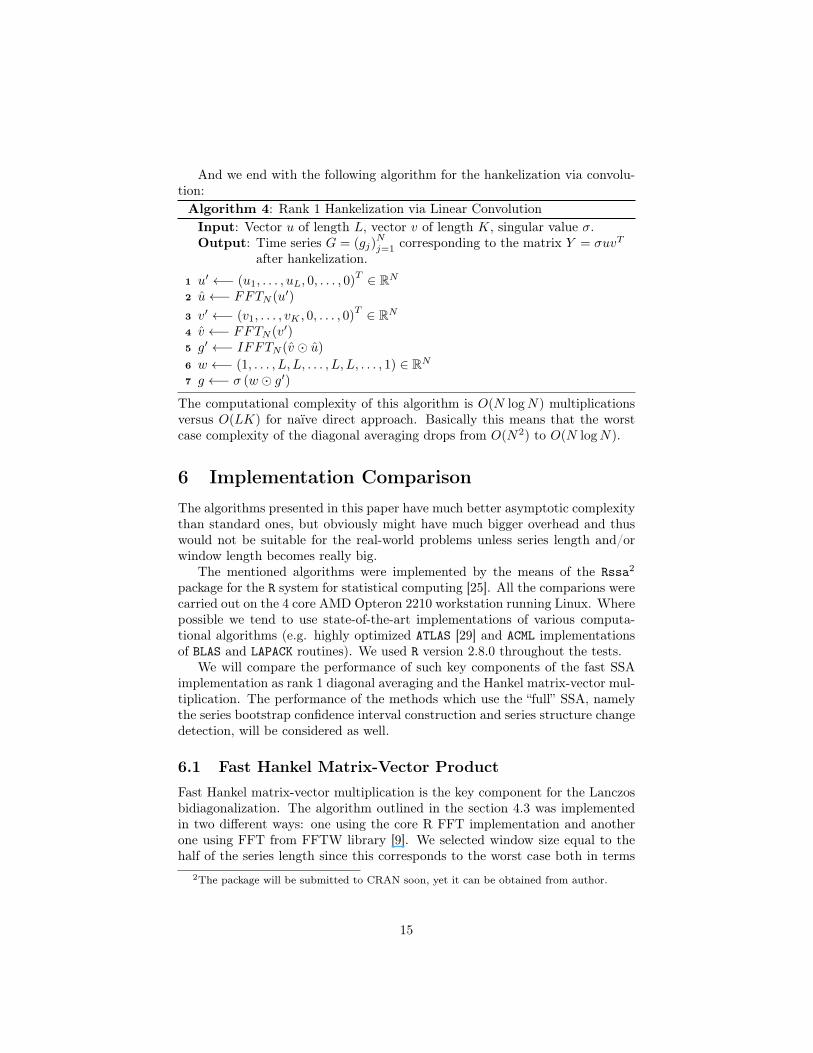
For the simulation experiments we consider the series FN = (f1, . . . , fN ) ofrank 5 with

fn = 10e−5n/N + sin

(2π

13

n

N

)+ 2.5 sin

(2π

37

n

N

)and σ = 5. The series F1000 (white) and F ′1000 (black) are shown on the figure4.

0 200 400 600 800 1000

−10

010

20

Figure 3: The Series F1000 and F ′1000.

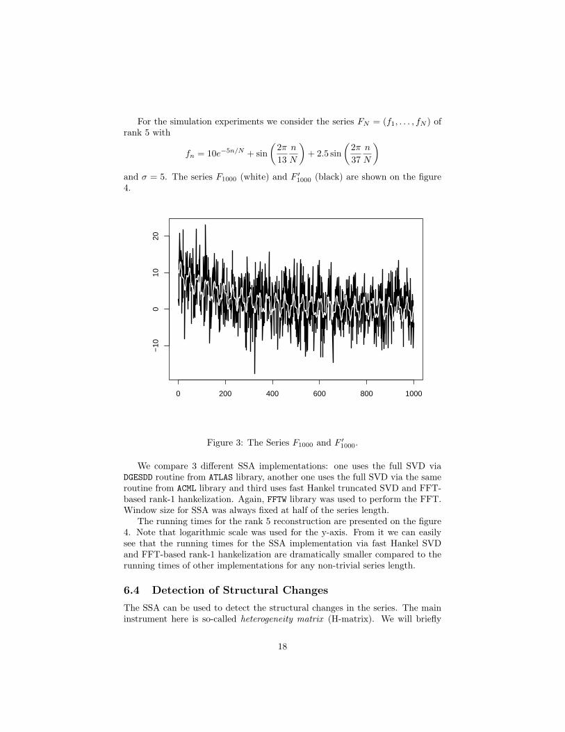
We compare 3 different SSA implementations: one uses the full SVD viaDGESDD routine from ATLAS library, another one uses the full SVD via the sameroutine from ACML library and third uses fast Hankel truncated SVD and FFT-based rank-1 hankelization. Again, FFTW library was used to perform the FFT.Window size for SSA was always fixed at half of the series length.

The running times for the rank 5 reconstruction are presented on the figure4. Note that logarithmic scale was used for the y-axis. From it we can easilysee that the running times for the SSA implementation via fast Hankel SVDand FFT-based rank-1 hankelization are dramatically smaller compared to therunning times of other implementations for any non-trivial series length.

6.4 Detection of Structural ChangesThe SSA can be used to detect the structural changes in the series. The maininstrument here is so-called heterogeneity matrix (H-matrix). We will briefly

18

●

●

●

●

●

●

●

●

●

●

0 2000 4000 6000 8000 10000

Series length, N

Tim

e fo

r 5

reco

nstr

uctio

ns, s

econ

ds

0.1

1

10

100

1000

●● ●

●

●●

●●

●●

●

●

ACML DGESDDFast Hankel SVDATLAS DGESDD

Figure 4: Reconstruction Time Comparison.

describe the algorithm for construction of such matrix, discuss the computa-tion complexity of the contruction and compare the performances of differentimplementations.

Exhaustive exposition of the detection of structural changes by the meansof SSA can be found in [14].

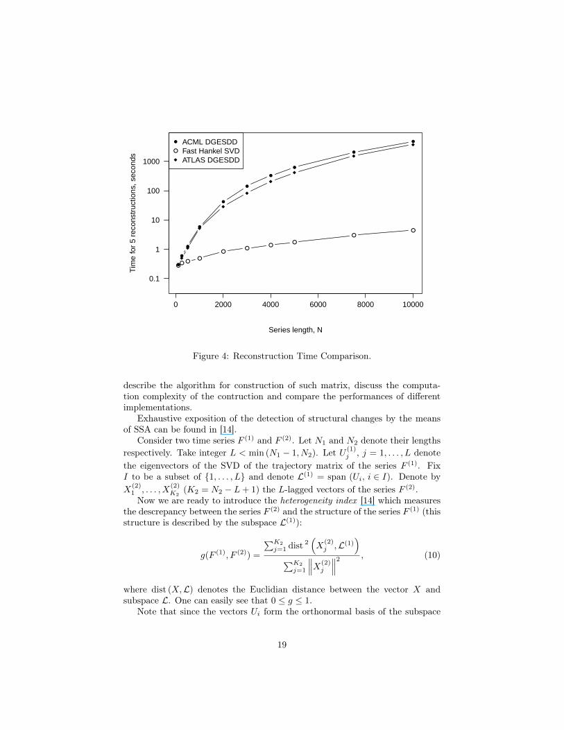
Consider two time series F (1) and F (2). Let N1 and N2 denote their lengthsrespectively. Take integer L < min (N1 − 1, N2). Let U (1)

j , j = 1, . . . , L denotethe eigenvectors of the SVD of the trajectory matrix of the series F (1). FixI to be a subset of {1, . . . , L} and denote L(1) = span (Ui, i ∈ I). Denote byX

(2)1 , . . . , X

(2)K2

(K2 = N2 − L+ 1) the L-lagged vectors of the series F (2).Now we are ready to introduce the heterogeneity index [14] which measures

the descrepancy between the series F (2) and the structure of the series F (1) (thisstructure is described by the subspace L(1)):

g(F (1), F (2)) =

∑K2

j=1 dist 2(X

(2)j ,L(1)

)∑K2

j=1

∥∥∥X(2)j

∥∥∥2 , (10)

where dist (X,L) denotes the Euclidian distance between the vector X andsubspace L. One can easily see that 0 ≤ g ≤ 1.

Note that since the vectors Ui form the orthonormal basis of the subspace

19

L(1) equation (10) can be rewritten as

g(F (1), F (2)) = 1−

∑K2

j=1

∑i∈I

(UTi X

(2)j

)2∑K2

j=1

∥∥∥X(2)j

∥∥∥2 .

Having this descrepancy measure for two arbitrary series in the hand onecan obviously construct the method of detection of structural changes in thesingle time series. Indeed, it is sufficient to calculate the heterogeneity index gfor different pairs of subseries of the series F and study the obtained results.

The heterogeneity matrix (H-matrix) [14] provides a consistent view overthe structural descrepancy between different parts of the series. Denote by Fi,jthe subseries of F of the form: Fi,j = (fi, . . . , fj). Fix two integers B > Land T ≥ L. These integers will denote the lengths of base and test subseriescorrespondingly. Introduce the H-matrix GB,T with the elements gij as follows:

gij = g(Fi,i+B , Fj,j+T ),

for i = 1, . . . , N − B + 1 and j = 1, . . . , N − T + 1. In simple words we splitthe series F into subseries of lengths B and T and calculate the heteregoneityindex between all possible pairs of the subseries.

The computation complexity of the calculation of the H-matrix is formed bythe complexity of the SV Ds for series Fi,i+B and complexity of calculation ofall heteregeneity indices gij as defined by equation (10).

The worst-case complexity of the SVD for series Fi,i+B corresponds to thecase when L ∼ B/2. Then the single decomposition costs O(B3) for full SVD viaGolub-Reinsh method and O(kB logB+k2B) via fast Hankel SVD as presentedin sections 3 and 4. Here k denotes the number of elements in the index setI. Since we need to make N − B + 1 decompositions a total we end with thefollowing complexities of the worst case (when B ∼ N/2): O(N4) for full SVDand O(kN2 logN + k2N2) for fast Hankel SVD.

Having all the desired eigenvectors Ui for all the subseries Fi,i+B in hand onecan calculate the H-matrix GB,T in O(kL(T −L+1)(N−T +1)+(N−T +1)L)multiplications. The worst case corresponds to L ∼ T/2 and T ∼ N/2 yieldingthe O(kN3) complexity for this step. We should note that this complexity canbe further reduced with the help of fast Hankel matrix-vector multiplication,but for the sake of simplicity we won’t present this result here.

Summing the complexities we end with O(N4) multiplications for H-matrixcomputation via full SVD and O(kN3 + k2N2) via fast Hankel SVD.

For the implementation comparison we consider the series FN = (f1, . . . , fN )of the form

fn =

{sin(2π10n)

+ 0.01εn, n < Q,

sin(

2π10.5n

)+ 0.01εn, n ≥ Q,

(11)

where εn denotes the uncorrelated white noise.

20

50 100 150 200 250 300

5010

015

020

025

030

0

Figure 5: H-matrix for the series (11).

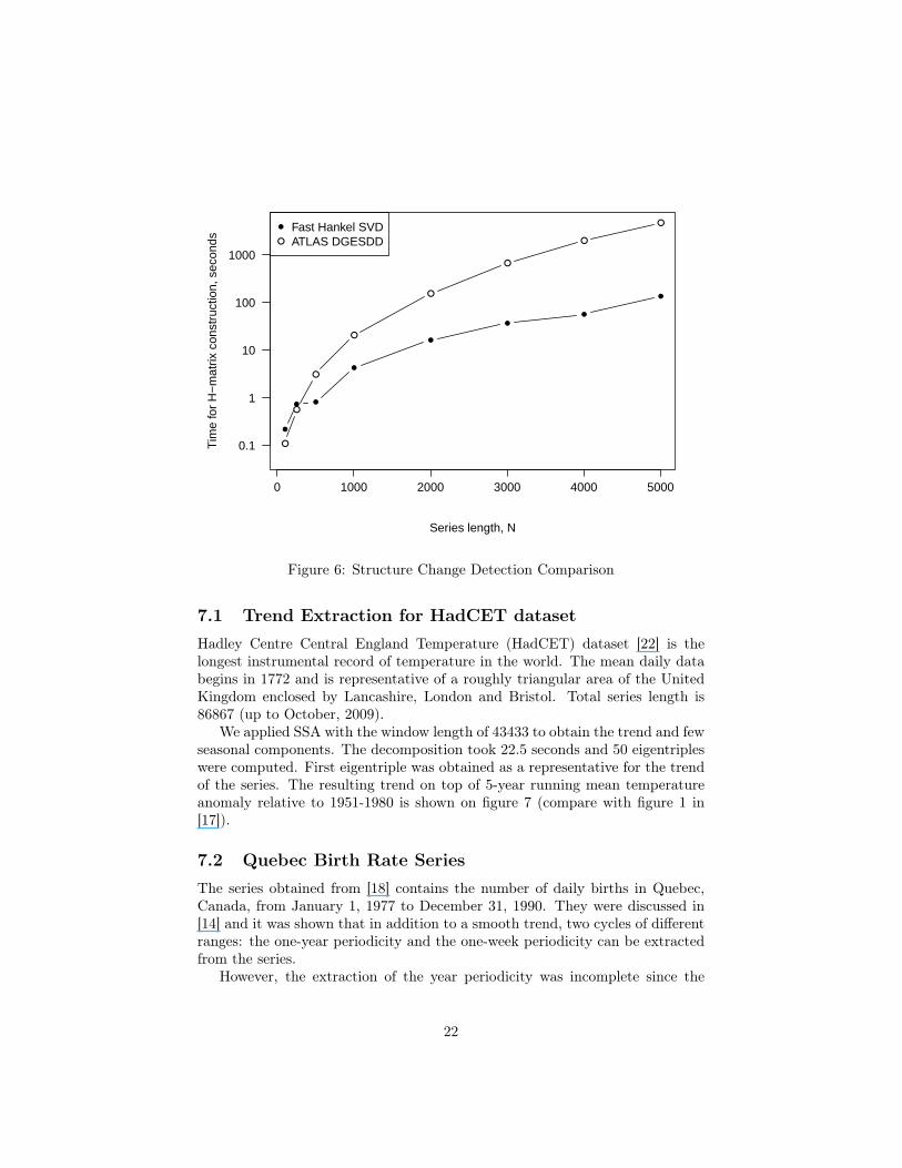
The typical H-matrix for such series is shown on the figure 5 (compare withfigure 3.3 in [14]). The parameters used for this matrix are N = 400, Q = 200,B = 100, T = 100, L = 50 and I = {1, 2}.

To save some computational time we compared not the worst case complex-ities, but some intermediate situation. The parameters used were Q = N/2,B = T = N/4, L = B/2 and I = {1, 2}. For full SVD DGESDD routine fromATLAS library [29] was used (as it was shown below, it turned out to be thefastest full SVD implementation available for our platform).

The obtained results are shown on the figure 6. As before, logarithmic scalewas used for the y-axis. Notice that the implementation of series structurechange detection using fast Hankel SVD is more than 10 times faster even onseries of moderate length.

7 Real-World Time SeriesFast SSA implementation allows us to use large window sizes during the decom-position, which was not available before. This is a crucial point in the achievingof asymptotic separability between different components of the series [14].

21

●

● ●

●

●

●

●

●

0 1000 2000 3000 4000 5000

Series length, N

Tim

e fo

r H

−m

atrix

con

stru

ctio

n, s

econ

ds

0.1

1

10

100

1000

●

●

●

●

●

●

●

●●

●

Fast Hankel SVDATLAS DGESDD

Figure 6: Structure Change Detection Comparison

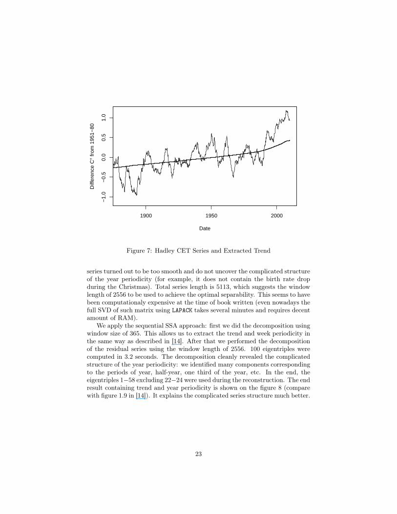
7.1 Trend Extraction for HadCET datasetHadley Centre Central England Temperature (HadCET) dataset [22] is thelongest instrumental record of temperature in the world. The mean daily databegins in 1772 and is representative of a roughly triangular area of the UnitedKingdom enclosed by Lancashire, London and Bristol. Total series length is86867 (up to October, 2009).

We applied SSA with the window length of 43433 to obtain the trend and fewseasonal components. The decomposition took 22.5 seconds and 50 eigentripleswere computed. First eigentriple was obtained as a representative for the trendof the series. The resulting trend on top of 5-year running mean temperatureanomaly relative to 1951-1980 is shown on figure 7 (compare with figure 1 in[17]).

7.2 Quebec Birth Rate SeriesThe series obtained from [18] contains the number of daily births in Quebec,Canada, from January 1, 1977 to December 31, 1990. They were discussed in[14] and it was shown that in addition to a smooth trend, two cycles of differentranges: the one-year periodicity and the one-week periodicity can be extractedfrom the series.

However, the extraction of the year periodicity was incomplete since the

22

−1.

0−

0.5

0.0

0.5

1.0

Date

Diff

eren

ce C

° fr

om 1

951−

80

1900 1950 2000

Figure 7: Hadley CET Series and Extracted Trend

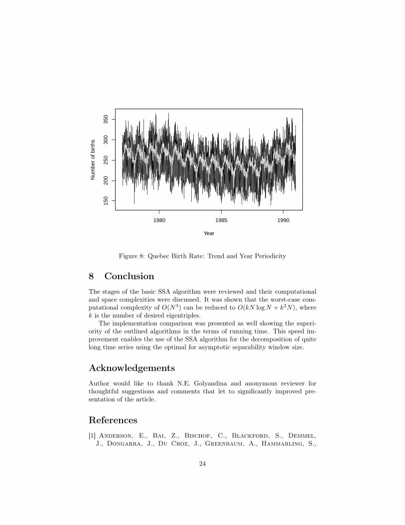
series turned out to be too smooth and do not uncover the complicated structureof the year periodicity (for example, it does not contain the birth rate dropduring the Christmas). Total series length is 5113, which suggests the windowlength of 2556 to be used to achieve the optimal separability. This seems to havebeen computationaly expensive at the time of book written (even nowadays thefull SVD of such matrix using LAPACK takes several minutes and requires decentamount of RAM).

We apply the sequential SSA approach: first we did the decomposition usingwindow size of 365. This allows us to extract the trend and week periodicity inthe same way as described in [14]. After that we performed the decompositionof the residual series using the window length of 2556. 100 eigentriples werecomputed in 3.2 seconds. The decomposition cleanly revealed the complicatedstructure of the year periodicity: we identified many components correspondingto the periods of year, half-year, one third of the year, etc. In the end, theeigentriples 1−58 excluding 22−24 were used during the reconstruction. The endresult containing trend and year periodicity is shown on the figure 8 (comparewith figure 1.9 in [14]). It explains the complicated series structure much better.

23

150

200

250

300

350

Year

Num

ber

of b

irth

s

1980 1985 1990

Figure 8: Quebec Birth Rate: Trend and Year Periodicity

8 ConclusionThe stages of the basic SSA algorithm were reviewed and their computationaland space complexities were discussed. It was shown that the worst-case com-putational complexity of O(N3) can be reduced to O(kN logN + k2N), wherek is the number of desired eigentriples.

The implementation comparison was presented as well showing the superi-ority of the outlined algorithms in the terms of running time. This speed im-provement enables the use of the SSA algorithm for the decomposition of quitelong time series using the optimal for asymptotic separability window size.

AcknowledgementsAuthor would like to thank N.E. Golyandina and anonymous reviewer forthoughtful suggestions and comments that let to significantly improved pre-sentation of the article.

References[1] Anderson, E., Bai, Z., Bischof, C., Blackford, S., Demmel,

J., Dongarra, J., Du Croz, J., Greenbaum, A., Hammarling, S.,

24

McKenney, A., and Sorensen, D. (1999). LAPACK Users’ Guide, Thirded. Society for Industrial and Applied Mathematics, Philadelphia, PA.

[2] Badeau, R., Richard, G., and David, B. (2008). Performance of ES-PRIT for estimating mixtures of complex exponentials modulated by polyno-mials. Signal Processing, IEEE Transactions on 56, 2 (Feb.), 492–504.

[3] Baglama, J. and Reichel, L. (2005). Augmented implicitly restartedLanczos bidiagonalization methods. SIAM J. Sci. Comput. 27, 1, 19–42.

[4] Briggs, W. L. and Henson, V. E. (1995). The DFT: An Owner’s Manualfor the Discrete Fourier Transform. SIAM, Philadelphia.

[5] Browne, K., Qiao, S., and Wei, Y. (2009). A Lanczos bidiagonalizationalgorithm for Hankel matrices. Linear Algebra and Its Applications 430, 1531–1543.

[6] Chan, R. H., Nagy, J. G., and Plemmons, R. J. (1993). FFT-Basedpreconditioners for Toeplitz-block least squares problems. SIAM Journal onNumerical Analysis 30, 6, 1740–1768.

[7] Dhillon, I. S. and Parlett, B. N. (2004). Multiple representations tocompute orthogonal eigenvectors of symmetric tridiagonal matrices. LinearAlgebra and its Applications 387, 1 – 28.

[8] Djermoune, E.-H. and Tomczak, M. (2009). Perturbation analysis ofsubspace-based methods in estimating a damped complex exponential. SignalProcessing, IEEE Transactions on 57, 11 (Nov.), 4558–4563.

[9] Frigo, M. and Johnson, S. G. (2005). The design and implementation ofFFTW3. Proceedings of the IEEE 93, 2, 216–231. Special issue on “ProgramGeneration, Optimization, and Platform Adaptation”.

[10] Golub, G. and Kahan, W. (1965). Calculating the singular values andpseudo-inverse of a matrix. SIAM J. Numer. Anal 2, 205–224.

[11] Golub, G. and Loan, C. V. (1996). Matrix Computations, 3 ed. JohnsHopkins University Press, Baltimore.

[12] Golub, G. and Reinsch, C. (1970). Singular value decomposition andleast squares solutions. Numer. Math. 14, 403–420.

[13] Golyandina, N. (2009). Approaches to parameter choice for SSA-similarmethods. Unpublished manuscript.

[14] Golyandina, N., Nekrutkin, V., and Zhiglyavsky, A. (2001). Anal-ysis of time series structure: SSA and related techniques. Monographs onstatistics and applied probability, Vol. 90. CRC Press.

25

[15] Golyandina, N. and Usevich, K. (2009). 2D-extensions of singularspectrum analysis: algorithm and elements of theory. In Matrix Methods:Theory, Algorithms, Applications. World Scientific Publishing, 450–474.

[16] Gu, M. and Eisenstat, S. C. (1995). A divide-and-conquer algorithmfor the bidiagonal SVD. SIAM J. Matrix Anal. Appl. 16, 1, 79–92.

[17] Hansen, J., Sato, M., Ruedy, R., Lo, K., Lea, D. W., and Elizade,M. M. (2006). Global temperature change. Proceedings of the NationalAcademy of Sciences 103, 39 (September), 14288–14293.

[18] Hipel, K. W. and Mcleod, A. I. (1994). Time Series Modellingof Water Resources and Environmental Systems. Elsevier, Amsterdam.http://www.stats.uwo.ca/faculty/aim/1994Book/.

[19] Larsen, R. M. (1998). Efficient algorithms for helioseismic inversion.Ph.D. thesis, University of Aarhus, Denmark.

[20] Loan, C. V. (1992). Computational frameworks for the fast Fourier trans-form. Society for Industrial and Applied Mathematics, Philadelphia, PA,USA.

[21] O’Leary, D. and Simmons, J. (1981). A bidiagonalization-regularizationprocedure for large scale discretizations of ill-posed problems. SIAM J. Sci.Stat. Comput. 2, 4, 474–489.

[22] Parker, D. E., Legg, T. P., and Folland, C. K. (1992). A new dailycentral England temperature series. Int. J. Climatol 12, 317–342.

[23] Parlett, B. (1980). The Symmetric Eigenvalue Problem. Prentice-Hall,New Jersey.

[24] Parlett, B. and Reid, J. (1981). Tracking the progress of the Lanczosalgorithm for large symmetric eigenproblems. IMA J. Numer. Anal. 1, 2,135–155.

[25] R Development Core Team. (2009). R: A Language and Environmentfor Statistical Computing. R Foundation for Statistical Computing, Vienna,Austria. ISBN 3-900051-07-0, http://www.R-project.org.

[26] Simon, H. (1984a). Analysis of the symmetric Lanczos algorithm withreothogonalization methods. Linear Algebra Appl. 61, 101–131.

[27] Simon, H. (1984b). The Lanczos algorithm with partial reorthogonaliza-tion. Math. Comp. 42, 165, 115–142.

[28] Swarztrauber, P., Sweet, R., Briggs, W., Hensen, V. E., andOtto, J. (1991). Bluestein’s FFT for arbitrary N on the hypercube. ParallelComput. 17, 607–617.

26

[29] Whaley, R. C. and Petitet, A. (2005). Minimizing development andmaintenance costs in supporting persistently optimized BLAS. Software:Practice and Experience 35, 2 (February), 101–121.

[30] Wu, K. and Simon, H. (2000). Thick-restart Lanczos method for largesymmetric eigenvalue problems. SIAM J. Matrix Anal. Appl. 22, 2, 602–616.

[31] Yamazaki, I., Bai, Z., Simon, H., Wang, L.-W., and Wu, K. (2008).Adaptive projection subspace dimension for the thick-restart Lanczos method.Tech. rep., Lawrence Berkeley National Laboratory, University of California,One Cyclotron road, Berkeley, California 94720. October.

27