4th International Conference on Earthquake Engineering Taipei, Taiwan

October 12-13, 2006

Paper No. 116 EFFICIENT COMPUTATION FOR DYNAMIC ANALYSIS OF INELASTIC

STRUCTURES WITH SMOOTH HYSTERESIS

Chi-hsiang Wang1 and Shuenn-Yih Chang2

ABSTRACT

This paper presents a higher-order step-by-step integration algorithm for dynamic analysis of structures with smooth hysteretic behavior under earthquakes. This algorithm solves the integral of the equation of motion; it therefore requires the ground motion velocities, rather than the ground motion accelerations typically used in conventional 2nd-order algorithms such as the Newmark-β method, as the excitations. A velocity time history is smoother and has fewer cyclic reversals than its acceleration counterpart, making possible the use of large incremental time step size that in turn lessens computer time. Systems of single-degree-of-freedom (SDOF) with (1) linear, (2) non-pinching, hysteretic, and (3) pinching, hysteretic, behaviors under the SAC ground motions are investigated. The computational efficiency of the developed algorithm is compared to that of the average acceleration method. Numerical studies found that for inelastic systems under earthquake excitation, the developed algorithm gives more accurate result and is more efficient than the average acceleration method even when typical ground motion time steps, e.g. 0.02 second, are used. If larger time step sizes are taken, for the SDOF inelastic systems considered herein, the higher-order algorithm can save more than 50% of computer time than the average acceleration method. Response statistics obtained using the SAC ground motion suite show that the higher-order algorithm could be a powerful and efficient method that saves significant computer time for Monte Carlo simulation. Keywords: Hysteresis, Direct integration, Higher-order integration, Simulation

INTRODUCTION The most widely used technique for time-history nonlinear structural analysis may be the step-by-step integration algorithms, such as the Newmark-β method and the α method (Hilber et al., 1977). These methods belong to the second-order integration formulation that takes ground motion acceleration as the external excitation. To capture the rapid cyclic reversals of the acceleration time history, the sometimes non-negligible contribution of high-frequency vibration modes, and the gradual or sharp change in resistance due to yielding or unloading, it is often necessary to make the integration time steps small. The use of small time steps, however, requires intensive computational effort, particularly with Monte Carlo simulations, which needs multiple runs of analysis. Moreover, if the resistance varies smoothly, rather than piecewise, due to material or geometric nonlinearity, the time steps need to be made even smaller to avoid unacceptable linearization error. A family of higher-order integration algorithms developed by Chang (1994) solves the integral of the equation of motion. The higher-order algorithms require the ground motion velocities, rather than the ground motion accelerations typically used in conventional 2nd-order algorithms, as the excitations. A

1 Senior Research Scientist, CSIRO Sustainable Ecosystems, Melbourne, Australia, Chi-hsiang.Wang@csiro.au 2 Professor, Dept. of Civil Engineering, National Taipei University of Technology, Taipei, Taiwan, changsy@ntut.edu.tw

velocity time history is smoother and has fewer cyclic reversals than its acceleration counterpart; it thus lessens the impact of the rapid cyclic reversals of external excitation common in the recorded ground-motion accelerations. The higher-order integration algorithms make possible the use of larger incremental time steps, which reduces computer time. The higher-order integration algorithms have been applied to linear and elasto-plastic systems (Chang, 1994), but yet to smooth hysteretic systems. This paper extends Chang′s higher-order methods and proposes an algorithm for inelastic systems with smooth hysteretic behavior that can be modeled by the Bouc–Wen family of hysteresis models (e.g. Wen, 1976; Wang and Wen, 2000). The computational efficiency of the developed algorithm, as compared to that of the average acceleration method (a special case of the Newmark–β method), is investigated by the study of three SDOF systems: (1) linear, (2) hysteretic without pinching phenomenon, and (3) hysteretic with pinching phenomenon. The SAC ground motion suite (Somerville et al., 1997) generated for Los Angeles, California, is used as the excitations.

SMOOTH HYSTERESIS MODEL For simplicity but without loss of generality, degradation in stiffness and strength as well as asymmetry in positive and negative yield strengths observed in hysteresis curves will not be considered for they have negligible effect on computational efficiency. Pinching phenomenon, however, will be studied as it adds a significant degree of nonlinearity in hysteretic behavior. A generic form of the Bouc-Wen type of hysteresis models neglecting pinching is of the form ( ) ( ) ( )z t H t u t′= (1) where u denotes the displacement, t is time and the dots overhead denote the derives with time, and z is an internal variable proportional to the hysteretic restoring force. One expression of ( )H t′ is as follows,

( ) ( ) ( ) ( )( ){ }1 1 sgn 1n

u

z tH t u t z t

z⎡ ⎤′ = − +β −⎣ ⎦ (2)

where ( )sgn i is the signum function; the parameter n, taken as an integer, determines the sharpness of the hysteresis before yielding (the larger the n value, the more it resembles a bi-linear hysteresis); β is a parameter controlling the unloading shape of the hysteresis (When 0 0.5β< < , the hysteresis loop takes a slim S shape; when 0.5β = , it exhibits linear unloading; when 0.5β > , it takes a bulge shape).

uz is the ultimate value of the internal variable z. When pinching is considered, the slip–lock behavior of pinching (Baber and Noori, 1985) can be approximated by the following bell-shaped function

( ) ( ) ( )( ) ( ) 2

sgn2 1exp

2u

z tu t

s t zp t

⎧ ⎫⎡ ⎤⎪ ⎪−μ⎢ ⎥⎪ ⎪⎢ ⎥= −⎨ ⎬⎢ ⎥π σ σ⎪ ⎪⎢ ⎥⎪ ⎪⎣ ⎦⎩ ⎭

(3)

in which the parameter s controls the length (or spread) of slip ( 0s = means no pinching); σ controls the sharpness of pinching (i.e. a smaller σ value gives a flatter pinching region); μ denotes the fraction

of zu at which the stiffness reaches the minimum, thus controlling the “thickness” of pinching area. The smooth hysteresis model considering pinching thus becomes (Wang and Wen, 2000)

( ) ( )( ) ( ) ( ) ( ) ( )

1H t

z t u t H t u tp t H t

′= =

′+ (4)

where ( )H t denotes the hysteresis model considering pinching. Eq. 4 may be written in an alternative incremental form, ( )( )sgn ,i i i iz H uu zΔ = Δ (5)

where 1i i iz z z+Δ = − and 1i i iu u u+Δ = − ; iu and iz denote the u and z values, respectively, at time step i. One potential advantage of using the higher-order integration algorithm, to be discussed in a later section, is to allow the computation to take large time steps. In this regard, if the increment of z is simply assumed to be proportional to H at time step i, the linearization error in some cases may be too large for the iterative solution to converge. A strategy employed in the fourth-order Runge-Kutta method (e.g. Press et al., 1992) is used herein, which requires four evaluations of H in a time interval: one at the initial point, two at the mid-points, and one at the end point. The four intermediate values of

zΔ are

( )1

12

23

4 3

sgn ,

sgn ,2

sgn ,2

sgn ,

2

2

i i

i i

i i

i i

z H u z u

zz H u z u

zz H u z u

z H u z z u

uhuhu

h

⎡ ⎤Δ = Δ⎣ ⎦⎡ ⎤Δ⎛ ⎞Δ = + + Δ⎜ ⎟⎢ ⎥

⎝ ⎠⎣ ⎦⎡ ⎤Δ⎛ ⎞Δ = + + Δ⎜ ⎟⎢ ⎥

⎝ ⎠⎣ ⎦⎡ ⎤⎛ ⎞Δ = + + Δ Δ⎜ ⎟⎢ ⎥

⎝ ⎠⎣ ⎦

Δ

Δ

Δ

(6)

Then izΔ is estimated by ( )1

1 2 3 46 2 2iz z z z zΔ = Δ + Δ + Δ + Δ (7) Eq. 7 will be used in tandem with Eq. 12 if the Newmark–β method, or Eq. 22 if the higher-order algorithm, is employed to solve for iuΔ and izΔ , as is described in the next section.

INCREMENTAL NEWMARK INTEGRATION ALGORITHM For a SDOF system of mass m and damping coefficient c subjected to ground acceleration gu , the governing equation of motion is ( ) ( ) ( ) ( )gmu t cu t q t mu t+ + = − (8) The restoring force q may be decomposed into one elastic and one hysteretic components; i.e. ( ) ( ) ( ) ( )1q t ku t kz t= α + −α (9)

where k is the initial stiffness, α is the ratio of stiffness before yielding to that after yielding. Then Eq. 8 can be written in an incremental form, at a time step i, as follows, ( )1i i i i gim u c u k u k z m uΔ + Δ + α Δ + −α Δ = − Δ (10) in giuΔ denotes the incremental ground acceleration at time step i. For the Newmark–β method, the incremental displacement and velocity are approximated by

( )

212i i i i

i i i

u u h u u h

u u u h

⎛ ⎞Δ = + +βΔ⎜ ⎟⎝ ⎠

Δ = + γΔ (11)

in which h is the time step size. After arithmetic manipulation Eq. 10 can be written as ( )ˆ ˆ 1i i i ik u R k zΔ = Δ − −α Δ (12) where

2

ˆ

ˆ 12 2

i

i gi i i

m ck k

h h

m c mR m u u ch u

h

γ= α + +

β β

γ γΔ = − Δ + + + − −

β β β β⎡ ⎤⎛ ⎞ ⎛ ⎞

⎜ ⎟ ⎜ ⎟⎢ ⎥⎝ ⎠ ⎝ ⎠⎣ ⎦

(13)

Eqs. 7 and 12 can be solved for iuΔ and izΔ by a suitable iterative method for solution of nonlinear equations such as the Newton-Raphson method (e.g. Press et al., 1992; Bathe, 1996). When 1 2γ = and 1 4β = , the Newmark–β method becomes the unconditionally stable, energy-conserving average acceleration method without artificial damping. This will be used for comparison of computational efficiency with the higher-order integration algorithm developed in the next section.

HIGHER-ORDER INTEGRATION ALGORITHM If we denote uk k= α , ( )1zk k= −α , and ( ) gf t mu= − , then Eq. 8 can be written as ( )u zmu cu k u k z f t+ + + = (14) Now consider the governing equation at time step 1i + , 1 1 1 1 1i i u i z i imu cu k u k z f+ + + + ++ + + = (15) and the integration of Eq. 15 with respect to time, 1 1 1 1 1i i u i z i imu cu k u k z f+ + + + ++ + + = (16) where , ,u z f denote the time integration of , ,u z and f , respectively. Use the following quadratures ( ) ( )2

1 1 1 2 3 1 4i i i i i iu u h u u h u u+ + += + + − −θ θ θ θ (17)

( ) ( )21 1 1 2 3 1 4i i i i i iu u h u u h u u+ + += + + − −θ θ θ θ (18)

( ) ( )21 1 1 2 3 1 4i i i i i iz z h z z h z z+ + += + + − −θ θ θ θ (19)

in which jθ , 1, ,4,j = … are defined as

1 2 3 4

1 1; ; ;

2 2 4 4x x y x y x+ − + −

= = = =θ θ θ θ (20)

where x and y are the integration parameters. Substituting Eq. 4 into Eq. 19 we get ( ) ( )2

1 1 1 2 3 1 1 4i i i i i i i iz z h z z h H u H u+ + + += + + − −θ θ θ θ (21) From Eqs. 15 to 18 and Eq. 21, the following equation for evaluating 1iu + can be derived 1iWu b+ = (22) where ( )2 2 2 1 3 1 2 2 4 1

1 1 3 3 1 3 3 31 1u u H u Hi iW m hc h k h cm c h cm k h k h k m k− − −

+ += + + − + + − +θ θ θ θ θ θ θ θ (23)

2 2 2 1 3 11 2 3 4 5 61H H Hi i i

b mb hcb h k b h k b h cm cb h cm k b− −

+= + + + + + (24)

in which ( )1H ii

k kH= −α (25)

and

( )( ) ( )( ) ( )

( )

21 1 2 4

2 11 1 3 1 1 2 1 3 1

2 12 1 1 2 3 2 3 3 1 2 3 1 3 1

2 2 2 13 3 2 3 3 4 3 1 1

4 1 4

i i i

i i i i z i

i i i i i i z i

i i i i z i

i

b u hu h u

f f hf hf hk z hm

b u hu h u f f hf hk z hm

b u hu h u f k z h m

b hu

−+ + +

−+ +

−+ +

= + + +

+ − − − − −

= + + + + − − −

= − − − + −

= −

⎡ ⎤⎣ ⎦⎡ ⎤⎣ ⎦

θ θ θ

θ θ θ θ θ θ

θ θ θ θ θ θ θ θ θ θ θ

θ θ θ θ θ θ

θ θ

5 3 2 3

6 3 4

i i

i

b u hu

b hu

= +

= −

θ θ θ

θ θ

(26)

Then 1iu + and 1iu + are determined by

( ) ( )

( )1

2 2 1 2 11 2 4 3 1 1 1 1 3

11 1 1 1 1

i i i i i i z i u i

i i i u i z i

u u u hu h u h f k z k u m h h cm

u f cu k u k z m

+− −

+ + + +

−+ + + + +

= ⎡ ⎤− − − + − − +⎣ ⎦

= − − −

θ θ θ θ θ (27)

Note that the integration parameters x and y dictate the order of integration. If 1 3y = , then when

0x > , it results in a third-order energy-dissipating algorithm; when 0x = , it becomes a fourth-order energy-conserving method (Chang, 2004). This paper concentrates on the latter that causes neither artificial energy dissipation nor amplitude compensation; therefore, an iterative scheme (e.g. Press et

al., 1992; Bathe, 1996) is required to solve Eqs. 7 and 22 for the inelastic system responses at time step 1i + .

NUMERICAL EXPERIMENTS: AVERAGE ACCELERATION METHOD VERSUS FOURTH-ORDER ALGORITHM

Since the average acceleration method is an energy-conserving method, the fourth-order integration (i.e. 0x = and 1 3y = ) of the developed algorithm, which is also energy conserving, is employed in the numerical study. The purpose of this exercise is to compare the performance and computational efficiency of the four-order integration algorithm to that of the average acceleration method for inelastic system dynamic analysis. To see the effect of hysteretic nonlinearity on the efficiency of computation, three types of systems are considered: (1) linear elastic system; (2) hysteretic system without pinching; and (3) hysteretic system with pinching. The dynamic properties and hysteretic parameters of the systems are given in Table 1. For the pinching hysteretic system, it is assumed to have zero initial pinching length and the spread of pinching at time t, ( )s t , is dependent only on the

maximum displacement experienced, ( ) ( ){ }max max ; 0, ,2 ,u t u t t h h= = … ; i.e.,

( ) ( )max

4 u

u ts t

z= (28)

Table 1 Structural and hysteretic properties of the example systems

System m c k α uz n β μ σ Linear 1 0.16 16 — — — — — —

Hysteretic (no pinching) 1 0.16 16 0.03 20 1 1 — — Hysteretic (w/ pinching) 1 0.16 16 0.03 20 1 1 0.1 0.05

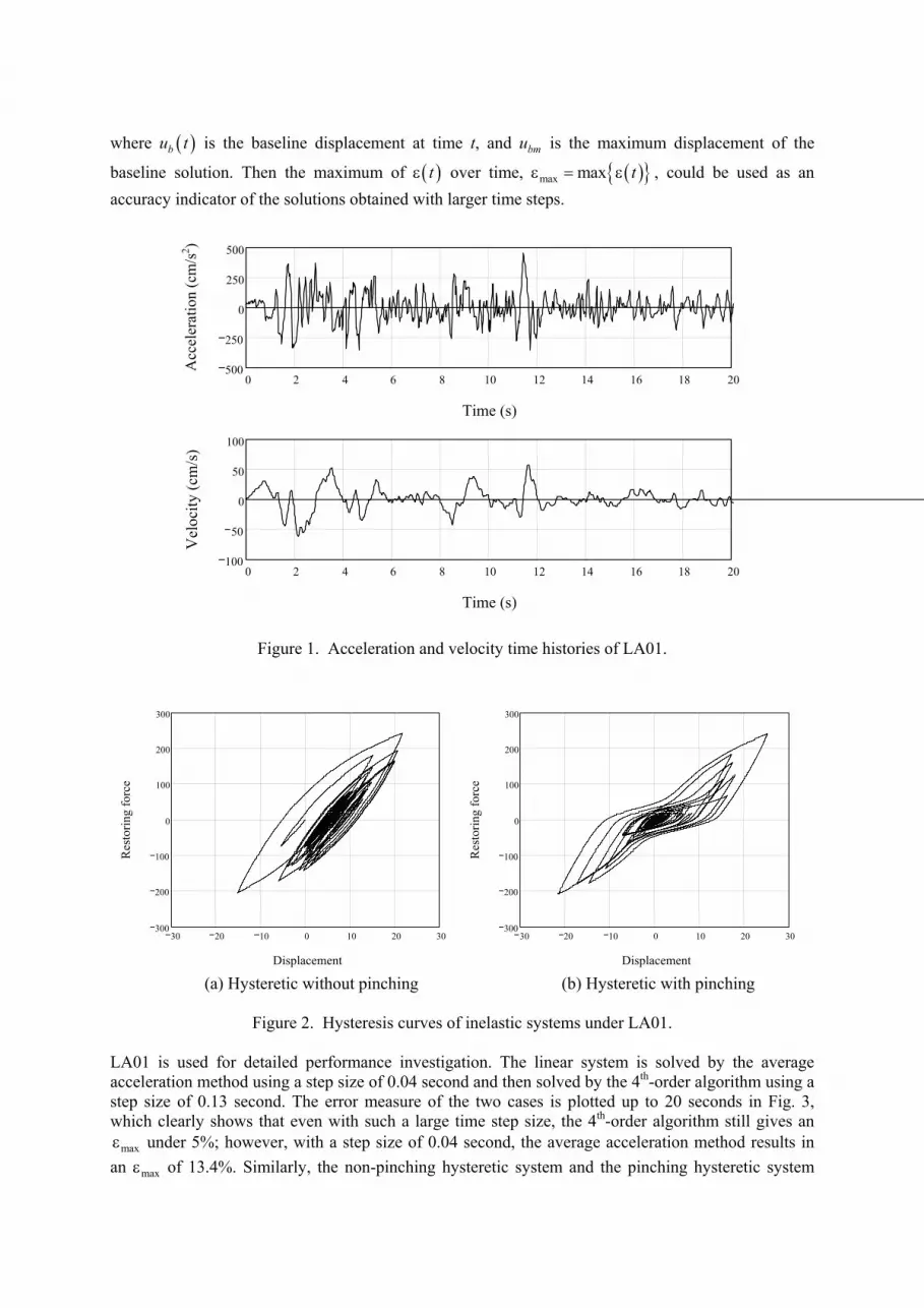
The SAC ground motion suite (Somerville et al., 1997) developed for Los Angeles, California, is used as the excitations. It consists of ground motions at three exceedance probability levels: 50%, 10%, and 2% probabilities of exceedance in 50 years. There are 10 ground motions for each probability level, each ground motion consisting of two components: fault-normal and fault-parallel. Since this paper discusses SDOF systems only, there are 20 ground acceleration records at each probability level, resulting in a total of 60 across the three levels, for use in dynamic response analysis. Fig. 1 shows the acceleration time history of LA01, a fault-normal component, of the SAC ground motions and its corresponding velocity by integrating it using the trapezoidal rule. It was obtained by multiplying a scale factor of 2.01 to an acceleration time history recorded from the 1940 El Centro earthquake, at a distance of 10 km to the epicenter. The PGA is 452 cm/s2 after scaling. It is clearly seen in Fig. 1 that the velocity time history is smoother and has much less cyclic reversals, of which the developed higher-order algorithm takes advantage. The hysteresis curves of the two inelastic systems under LA01 are shown in Fig. 2. First we investigate the accuracy of the average acceleration method and the 4th-order integration algorithm. To do so, the obtained results will be compared with a baseline result determined by the average acceleration method with a time step size of 0.001 second. When the time step size is increased, the accuracy of analysis will generally deteriorate due to negligence of partial information on the ground motions. The question is to what extent the impact of this negligence of information on the results is tolerable. To this end, an error estimate at a given time instant t, ( )tε , may be defined as

( )( ) ( )

100%b

bm

u t u tt

u−

ε = × (29)

where ( )bu t is the baseline displacement at time t, and bmu is the maximum displacement of the

baseline solution. Then the maximum of ( )tε over time, ( ){ }max max tε = ε , could be used as an accuracy indicator of the solutions obtained with larger time steps.

0 2 4 6 8 10 12 14 16 18 20500

250

0

250

500

Time (s)

Acc

eler

atio

n

0 2 4 6 8 10 12 14 16 18 20100

50

0

50

100

Time (s)

Vel

ocity

(cm

/s)

Figure 1. Acceleration and velocity time histories of LA01.

30 20 10 0 10 20 30300

200

100

0

100

200

300

Displacement

Res

torin

g fo

rce

30 20 10 0 10 20 30300

200

100

0

100

200

300

Displacement

Res

torin

g fo

rce

(a) Hysteretic without pinching (b) Hysteretic with pinching

Figure 2. Hysteresis curves of inelastic systems under LA01. LA01 is used for detailed performance investigation. The linear system is solved by the average acceleration method using a step size of 0.04 second and then solved by the 4th-order algorithm using a step size of 0.13 second. The error measure of the two cases is plotted up to 20 seconds in Fig. 3, which clearly shows that even with such a large time step size, the 4th-order algorithm still gives an

maxε under 5%; however, with a step size of 0.04 second, the average acceleration method results in an maxε of 13.4%. Similarly, the non-pinching hysteretic system and the pinching hysteretic system

Acc

eler

atio

n (c

m/s

2 )

are solved by the 4th-order algorithm with time-step sizes of 0.08 and 0.04 seconds, respectively; they are found to have an maxε of 5.1% and 1.5%, respectively. The displacement time histories of these cases are plotted in Fig. 4. It is seen that the average acceleration method with a step size of 0.04 second gives responses that deviate notably from the baseline results, whereas the responses given by the 4th-order algorithm, even with step sizes ≥ 0.04 second, closely follow the baseline solutions.

0 5 10 15 2020

10

0

10

204th-order, h = 0.13 sAve. acc., h = 0.04 s

Time (s)

Erro

r mea

sure

(%)

Figure 3. Error measure ( )tε of the linear system under LA01.

0 5 10 15 2030

20

10

0

10

20

30Ave. acc., h = 0.001 sAve. acc., h = 0.04 s4th-order, h = 0.13 s

Time (s)

Dis

plac

emen

t

0 5 10 15 2030

20

10

0

10

20

30

Ave. acc., h = 0.001 sAve. acc., h = 0.04 s4th-order, h = 0.08 s

Time (s)

Dis

plac

emen

t

(a) Linear (b) Inelastic without pinching

0 5 10 15 2030

20

10

0

10

20

30Ave. acc., h = 0.001 sAve. acc., h = 0.04 s4th-order, h = 0.04 s

Time (s)

Dis

plac

emen

t

(c) Inelastic with pinching

Figure 4. Displacement time histories of the example systems under LA01.

For investigation of computational efficiency, all sixty SAC ground motions are used as the excitations. A laptop computer with Pentium Mobile-technology processor of CPU speed 2.0 GHz is used for the computation. Table 2 tabulates the computer time taken for the computation of the three systems under the sixty ground motions. It is seen in Table 2 that for linear system using the same step size the average acceleration method takes less time than the 4th-order algorithm because of the absence of nonlinearity and the fact that the 4th-order algorithm is more involved. When nonlinearity is present and larger time steps are used; e.g., 0.02h ≥ second, the 4th-order algorithm becomes more efficient, as revealed in Table 2, because it takes advantage of the smoothing effect of ground motion velocities. Moreover, if the 4th-order algorithm with a larger time step size is used and deemed to give results of acceptable accuracy, the time saved is even more significant. For example, for the non-pinching hysteretic system, the 4th-order algorithm with 0.08h = second takes about 40% of computer time needed for the average acceleration method with 0.02h = second. Likewise, for pinching hysteretic system, the 4th-order algorithm with 0.04h = second takes about 47% of time needed for the average acceleration method with 0.02h = second. The mean values and the coefficients of variation (COV) of displacement of the three systems at the three exceedance probability levels (50/50, 10/50, and 2/50) obtained with 0.001h = second and with large time step sizes are tabulated in Table 3. The average acceleration method is used for 0.001h = and 0.02h = seconds, while the 4th-order algorithm is used for other large time step sizes. Table 3 reveals that the displacement statistics determined by using large step sizes are close to that by 0.001h = and 0.02h = seconds, suggesting that the 4th-order algorithm could be a powerful method which saves computer time and still gives acceptable accuracy for Monte Carlo simulation.

Table 2 Computer time for analysis of the example systems under sixty SAC ground motions

Execution time (sec.) System Time step size (sec.) Ave. acc. method 4th-order method

0.001 0.859 0.906 0.020 0.125 0.203 Linear 0.130 — 0.094 0.001 17.188 17.672 0.020 1.172 1.031 Hysteretic

(no pinching) 0.080 — 0.469 0.001 27.859 20.734 0.020 1.656 1.281 Hysteretic

(w/ pinching) 0.040 — 0.781

Table 3 Displacement statistics of the example systems under the SAC ground motions

50/50 10/50 2/50 System Time step size (sec.) Mean COV (%) Mean COV (%) Mean COV (%)

0.001 15.50 36.7 34.13 42.7 78.01 36.1 0.020 15.48 36.6 34.07 42.6 77.91 36.1

Linear

0.130 15.33 37.1 33.54 42.7 76.99 36.0 0.001 10.97 32.2 22.88 31.8 54.53 40.1 0.020 10.95 32.2 22.86 31.8 54.56 40.1

Hysteretic (no pinching)

0.080 10.92 31.8 22.86 31.8 55.16 40.2 0.001 11.03 32.8 26.88 32.0 63.29 43.9 0.020 11.03 32.8 26.78 31.8 62.75 43.2

Hysteretic (w/ pinching)

0.040 11.04 33.0 26.94 32.1 62.58 42.6

CONCLUSIONS This paper presents a higher-order integration algorithm for the solution of inelastic systems with smooth hysteretic behavior modeled by the Bouc–Wen type hysteresis. Instead of solving the equation of motion directly, it integrates the governing equation once with respect to time; therefore, the ground motion velocities become the input excitations, which are smoother and have fewer cyclic reversals than the ground motion accelerations. The developed algorithm is particularly useful for structural analysis dominated by lower-mode responses and influenced negligibly by high-frequency modes. The integration parameters 0x = and 1 3y = of the developed algorithm are chosen for numerical studies, which is a 4th-order energy conserving integration method. For analysis of hysteretic systems with commonly used time step sizes, say 0.02 second, the 4th-order algorithm is computationally more efficient than the average acceleration method due to smoothing effect of the velocity time history. Numerical experiments show that, under earthquake ground motions, it is possible to use large incremental time step size for analysis of highly hysteretic systems and still obtain results of acceptable accuracy. If larger step sizes are taken, for the SDOF inelastic systems considered in this paper the 4th-order algorithm can save more than 50% of computer time than the average acceleration method. Displacement statistics obtained using the SAC ground motion suite show that this algorithm could be a powerful and efficient method that saves significant computer time for Monte Carlo simulations. Implementation and investigation of the developed algorithm to the solution of multi-degrees-of-freedom systems will be carried out in future work. Algorithmic stability and convergence of the higher-order integration method have been investigated for analysis of linear systems (Chang, 1994) but more studies are needed for inelastic systems. The algorithm with integration parameters 2x = and 1 3y = is a third-order dissipative algorithm and has been shown to possess excellent amplitude-compensating property for the solution of some classes of nonlinear systems (Chang, 1994). If such amplitude-compensating effect can satisfactorily compensate for the lost accuracy due to linearization of the material nonlinearity, an iterative solution may not be necessary; then this algorithm could save even more computer time. Whether this desirable property holds true for the hysteretic behaviors considered in this paper is unclear at present. It will be a subject of future studies.

REFERENCES Baber, T.T. and M.N. Noori, (1985). “Random Vibration of Degrading, Pinching Systems,” J. Eng. Mech.,

ASCE, 111(8), 1010–1026.

Bathe, K.J., (1996). Finite Element Procedures, Prentice-Hall, Inc., NJ.

Chang, S.Y., (1994). Improved dynamic analysis for linear and nonlinear systems. Ph.D. Thesis, University of Illinois, Urbana-Champaign.

Hilber, H.M., T.J.R. Hughes, and R.L. Taylor, (1977). “Improved numerical dissipation for time integration algorithms in structural dynamics,” Earthq. Eng. Struct. Dyn., 5, 283–292.

Press, W.H., S.A. Teukolsky, W.T. Vetterling, and B.P. Flannery, (1992). Numerical Recipes in Fortran 77: The Art of Scientific Computing, 2nd ed. Cambridge University Press.

Somerville, P., N. Smith, S. Punyamurthula, and J. Sun, (1997). Development of ground motion time histories for Phase 2 of the FEMA/SAC steel project, Report No. SAC/BD-97/04, Applied Technology Council, Washington, D.C.

Wang, C-H. and Y.K. Wen, (2000). “Evaluation of Pre-Northridge Low-Rise Steel Buildings. I: Modeling,” J. Struct. Eng., ASCE 126(10), 1160–1168.

Wen, Y.K., (1976). “Method for Random Vibration of Hysteretic Systems.” J. Eng. Mech., ASCE, 102(EM2), 249–263.