Compressive Deconvolution of MRI Imaging via ℓ1-ℓ2 Regularization

by

TALON JOHNSON

Presented to the Faculty of the Graduate School of

The University of Texas at Arlington in Partial Fulfillment

of the Requirements

for the Degree of

DOCTOR OF PHILOSOPHY

THE UNIVERSITY OF TEXAS AT ARLINGTON

August 2021

Copyright © by Talon Johnson 2021

All Rights Reserved

ACKNOWLEDGEMENTS

I would like to first thank my family for always being understanding and

supportive of me in all of my endeavors during my time as I matriculated through

my graduate studies. The dedication you have towards me has greatly impacted the

way perceive myself as a scholar, a mathematician, but most in importantly as an

individual. Without your love, I would not be where I am today.

Secondly, I wish to thank my advisor, Dr. Jianzhong Su, for his guidance and

expertise throughout my graduate-level mathematical and research journey. Without

his support, I wouldn’t have been able to navigate the Ph.D. and thesis process. I’m

genuinely grateful for everything he has done in my graduate studies here at UTA.

I’d also like to thank my advising committee, Dr. Hristo Kojouharov, Dr. Ren-Cang

Li, Dr. Li Wang, and Dr. Jimin Ren, for their interest in my research and for taking

the time to serve in my comprehensive and dissertation.

I would like to thank Lona, Libby, Laura, and Michael for their time and

assistance throughout my graduate career.Additionally, I would like to thank Dwight,

Ariel, Omomayowa, John, Crystal, Anthony, Amanda, Saul, Michelangelo, and many

others, for their help and encouragement during my five years as a graduate student

here at UTA. As well as the fun times we got to spend with each other outside of the

math department. You all are the best.

iii

Finally, I would also like to extend my appreciation to Dr. Duane Cooper and

Dr. Shelby Wilson for encouraging me to pursue a Ph.D. They continue to support

and provide me with insight to this very day.

July 30, 2021

iv

ABSTRACT

Compressive Deconvolution of MRI Imaging via ℓ1-ℓ2 Regularization

Talon Johnson, Ph.D.

The University of Texas at Arlington, 2021

Supervising Professor: Jianzhong Su

The evolution of technology has drastically impacted the imaging field, particu-

larly magnetic resonance imaging (MRI). Compared to other imaging technologies,

MRI offers multiple contrasting mechanisms to distinguish tissues and fat, is radiation-

free, and provides anatomical and molecular information about the tissue in question.

However, data acquisition times to produce those images require a patient to lie still

for a relatively long time. Consequently, it may lead to the voluntary or involuntary

movement of the patient due to discomfort. Combined with the underlying issue of

inherent noise, MRI is often blurry and contains artifacts. Mathematically, one can

describe this behavior as the convolution between the MRI and some unwanted PSF.

In this thesis, we present a new approach to speed up the MR data acquisition

through sparse signal reconstruction and deconvolving the unwanted convolution

simultaneously. This approach is part of an ever-growing area known as compressive

deconvolution. We propose a novel compressive deconvolution method for two

dimensional MRI data sets via an ℓ1 − ℓ2 regularization via ℓ1–magic : TV2 and

Tikhonov regularization.

v

TABLE OF CONTENTS

ACKNOWLEDGEMENTS . . . . . . . . . . . . . . . . . . . . . . . . . . . . iii

ABSTRACT . . . . . . . . . . . . . . . . . . . . . . . . . . . . . . . . . . . . v

Chapter Page

1. Introduction . . . . . . . . . . . . . . . . . . . . . . . . . . . . . . . . . . . 1

1.1 Problems and Limitations in Medical Imaging . . . . . . . . . . . . . 1

1.2 Imaging Basics . . . . . . . . . . . . . . . . . . . . . . . . . . . . . . 2

1.3 Image Blurring . . . . . . . . . . . . . . . . . . . . . . . . . . . . . . 3

1.4 Properties of Blurs and Common Blur Types in Imaging Systems . . 5

1.5 Boundary Conditions . . . . . . . . . . . . . . . . . . . . . . . . . . . 8

1.6 Special Structured Matrices . . . . . . . . . . . . . . . . . . . . . . . 9

1.6.1 One-Dimensional Convolution, Toeplitz, and Circulant Matrices 10

1.6.2 Two Dimensional Convolution, Block Toeplitz with Toeplitz

Blocks (BTTB), and Block Circulant with Circulant Blocks

(BCCB) Matrices . . . . . . . . . . . . . . . . . . . . . . . . . 13

1.6.3 Separable Blurs . . . . . . . . . . . . . . . . . . . . . . . . . . 17

1.6.4 Summary of Matrix Structures . . . . . . . . . . . . . . . . . 19

2. COMPRESSIVE DECONVOLUTION . . . . . . . . . . . . . . . . . . . . 20

2.1 Compressed Sensing . . . . . . . . . . . . . . . . . . . . . . . . . . . 20

2.2 Deconvolution . . . . . . . . . . . . . . . . . . . . . . . . . . . . . . . 22

2.3 Compressive Deconvolution . . . . . . . . . . . . . . . . . . . . . . . 23

3. MATHEMATICAL BACKGROUND . . . . . . . . . . . . . . . . . . . . . 25

3.1 Linear Conjugate Gradient Method . . . . . . . . . . . . . . . . . . . 25

vi

3.2 Newton’s Method for Unconstrained Minimization Problems . . . . . 28

3.3 The Interior-Point Method via Log Barrier Function . . . . . . . . . . 30

3.4 Least Squares Approximation . . . . . . . . . . . . . . . . . . . . . . 33

3.4.1 The Singular Value Decomposition and Pseudoinverse . . . . . 35

3.5 Spectral Filtering . . . . . . . . . . . . . . . . . . . . . . . . . . . . . 37

3.5.1 Truncated SVD (TSVD) . . . . . . . . . . . . . . . . . . . . . 38

3.5.2 Tikhonov Regularization . . . . . . . . . . . . . . . . . . . . . 39

4. 2D IMAGE RECOVERY . . . . . . . . . . . . . . . . . . . . . . . . . . . 42

4.1 Interior Point Method for SOCPs . . . . . . . . . . . . . . . . . . . . 43

5. Our Method . . . . . . . . . . . . . . . . . . . . . . . . . . . . . . . . . . . 45

5.1 Compressed Sensing with Interior Point Method via Log-Barrier Function 46

5.2 Computing gs . . . . . . . . . . . . . . . . . . . . . . . . . . . . . . . 47

5.3 Computing Hs . . . . . . . . . . . . . . . . . . . . . . . . . . . . . . . 50

5.4 Reduce the System . . . . . . . . . . . . . . . . . . . . . . . . . . . . 52

5.5 Deblurring Step via Regularization . . . . . . . . . . . . . . . . . . . 53

5.5.1 Parameter of Choice Method . . . . . . . . . . . . . . . . . . . 56

6. Numerical Results . . . . . . . . . . . . . . . . . . . . . . . . . . . . . . . 60

6.1 Image Reconstruction Metrics . . . . . . . . . . . . . . . . . . . . . . 60

6.2 Performance of Reconstruction . . . . . . . . . . . . . . . . . . . . . . 61

6.2.1 Reconstruction Results using Zero Boundary Conditions . . . 62

6.2.2 Reconstruction Regularization using Periodic Boundary Condi-

tions . . . . . . . . . . . . . . . . . . . . . . . . . . . . . . . . 64

6.2.3 Extra: Motion Blur Recovery . . . . . . . . . . . . . . . . . . 66

7. Conclusion and Future Works . . . . . . . . . . . . . . . . . . . . . . . . . 68

REFERENCES . . . . . . . . . . . . . . . . . . . . . . . . . . . . . . . . . . . 70

BIOGRAPHICAL STATEMENT . . . . . . . . . . . . . . . . . . . . . . . . . 76

vii

CHAPTER 1

Introduction

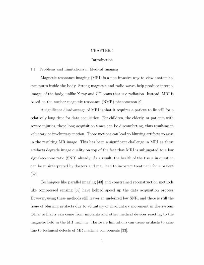
1.1 Problems and Limitations in Medical Imaging

Magnetic resonance imaging (MRI) is a non-invasive way to view anatomical

structures inside the body. Strong magnetic and radio waves help produce internal

images of the body, unlike X-ray and CT scans that use radiation. Instead, MRI is

based on the nuclear magnetic resonance (NMR) phenomenon [9].

A significant disadvantage of MRI is that it requires a patient to lie still for a

relatively long time for data acquisition. For children, the elderly, or patients with

severe injuries, these long acquisition times can be discomforting, thus resulting in

voluntary or involuntary motion. Those motions can lead to blurring artifacts to arise

in the resulting MR image. This has been a significant challenge in MRI as these

artifacts degrade image quality on top of the fact that MRI is subjugated to a low

signal-to-noise ratio (SNR) already. As a result, the health of the tissue in question

can be misinterpreted by doctors and may lead to incorrect treatment for a patient

[32].

Techniques like parallel imaging [43] and constrained reconstruction methods

like compressed sensing [38] have helped speed up the data acquisition process.

However, using these methods still leaves an undesired low SNR, and there is still the

issue of blurring artifacts due to voluntary or involuntary movement in the system.

Other artifacts can come from implants and other medical devices reacting to the

magnetic field in the MR machine. Hardware limitations can cause artifacts to arise

due to technical defects of MR machine components [33].

1

In this work, we will tackle the problem of how to handle the data acquisition

and blurring artifacts using a novel approach in the area of compressive deconvolution.

We first discuss imaging basics and how to mathematically described blurring in

imaging systems.

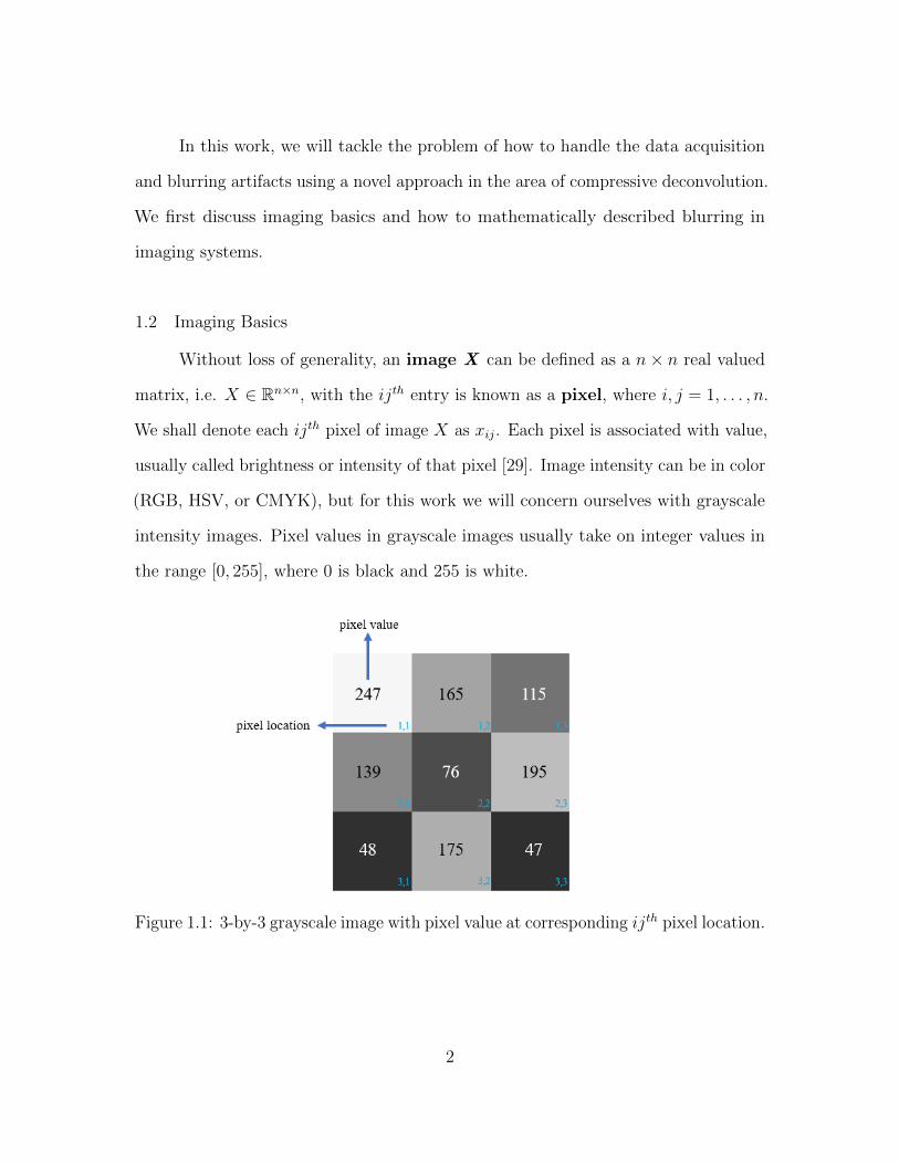
1.2 Imaging Basics

Without loss of generality, an image X can be defined as a n× n real valued

matrix, i.e. X ∈ Rn×n, with the ijth entry is known as a pixel, where i, j = 1, . . . , n.

We shall denote each ijth pixel of image X as xij . Each pixel is associated with value,

usually called brightness or intensity of that pixel [29]. Image intensity can be in color

(RGB, HSV, or CMYK), but for this work we will concern ourselves with grayscale

intensity images. Pixel values in grayscale images usually take on integer values in

the range [0, 255], where 0 is black and 255 is white.

Figure 1.1: 3-by-3 grayscale image with pixel value at corresponding ijth pixel location.

2

We will use MATLAB in order to perform several image processing and optimization

algorithms. These algorithms will require many operations to be done on the pixel

values, so it is best to convert images to double-precision floating-point numbers in

the interval [0, 1] [30], and this can be achieved by using MATLAB’s built-in function

rescale to do so. Several other built-in functions that are used for image processing

in MATLAB included:

� im2double and,

� mat2gray.

They will serve to convert our images to double-precision floating-point numbers with

grayscale intensity.

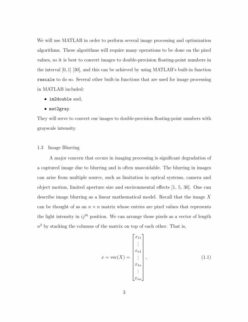
1.3 Image Blurring

A major concern that occurs in imaging processing is significant degradation of

a captured image due to blurring and is often unavoidable. The blurring in images

can arise from multiple source, such as limitation in optical systems, camera and

object motion, limited aperture size and environmental effects [1, 5, 30]. One can

describe image blurring as a linear mathematical model. Recall that the image X

can be thought of as an n× n matrix whose entries are pixel values that represents

the light intensity in ijth position. We can arrange those pixels as a vector of length

n2 by stacking the columns of the matrix on top of each other. That is,

x = vec(X) =

x11...

xn1...

x1n...

xnn

, (1.1)

3

where x is the vectorization of X, denoted by vec(X). In MATLAB, this can be

done by simply typing X(:) in the command window. Similarly, we can denote the

blurred representation of X as the matrix B ∈ Rn×n and its vectorization as

b = vec(B) =

b11...bn1...b1n...

bnn

. (1.2)

The relationship between x and b is given by the existence of a large matrix C ∈ RN×N ,

with N = n2, such that

Cx = b. (1.3)

The matrix C in (1.3) represents the blurring process that degrades the true image

X to the the blurred image B.

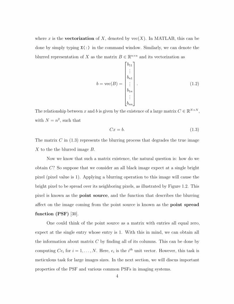
Now we know that such a matrix existence, the natural question is: how do we

obtain C? So suppose that we consider an all black image expect at a single bright

pixel (pixel value is 1). Applying a blurring operation to this image will cause the

bright pixel to be spread over its neighboring pixels, as illustrated by Figure 1.2. This

pixel is known as the point source, and the function that describes the blurring

affect on the image coming from the point source is known as the point spread

function (PSF) [30].

One could think of the point source as a matrix with entries all equal zero,

expect at the single entry whose entry is 1. With this in mind, we can obtain all

the information about matrix C by finding all of its columns. This can be done by

computing Cei for i = 1, . . . , N . Here, ei is the ith unit vector. However, this task is

meticulous task for large images sizes. In the next section, we will discus important

properties of the PSF and various common PSFs in imaging systems.

4

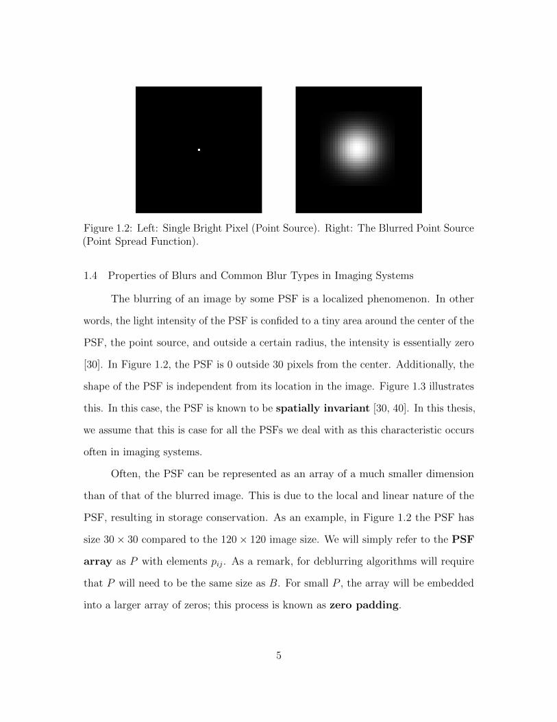
Figure 1.2: Left: Single Bright Pixel (Point Source). Right: The Blurred Point Source(Point Spread Function).

1.4 Properties of Blurs and Common Blur Types in Imaging Systems

The blurring of an image by some PSF is a localized phenomenon. In other

words, the light intensity of the PSF is confided to a tiny area around the center of the

PSF, the point source, and outside a certain radius, the intensity is essentially zero

[30]. In Figure 1.2, the PSF is 0 outside 30 pixels from the center. Additionally, the

shape of the PSF is independent from its location in the image. Figure 1.3 illustrates

this. In this case, the PSF is known to be spatially invariant [30, 40]. In this thesis,

we assume that this is case for all the PSFs we deal with as this characteristic occurs

often in imaging systems.

Often, the PSF can be represented as an array of a much smaller dimension

than of that of the blurred image. This is due to the local and linear nature of the

PSF, resulting in storage conservation. As an example, in Figure 1.2 the PSF has

size 30× 30 compared to the 120× 120 image size. We will simply refer to the PSF

array as P with elements pij. As a remark, for deblurring algorithms will require

that P will need to be the same size as B. For small P , the array will be embedded

into a larger array of zeros; this process is known as zero padding.

5

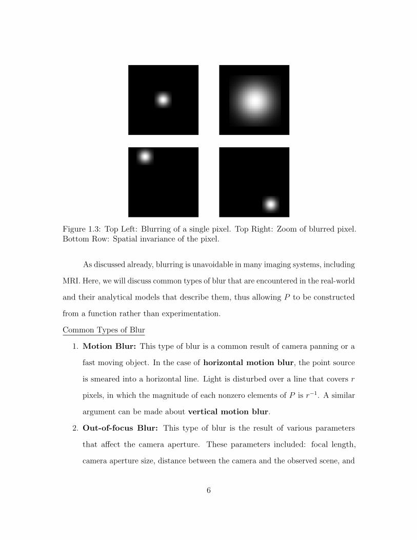
Figure 1.3: Top Left: Blurring of a single pixel. Top Right: Zoom of blurred pixel.Bottom Row: Spatial invariance of the pixel.

As discussed already, blurring is unavoidable in many imaging systems, including

MRI. Here, we will discuss common types of blur that are encountered in the real-world

and their analytical models that describe them, thus allowing P to be constructed

from a function rather than experimentation.

Common Types of Blur

1. Motion Blur: This type of blur is a common result of camera panning or a

fast moving object. In the case of horizontal motion blur, the point source

is smeared into a horizontal line. Light is disturbed over a line that covers r

pixels, in which the magnitude of each nonzero elements of P is r−1. A similar

argument can be made about vertical motion blur.

2. Out-of-focus Blur: This type of blur is the result of various parameters

that affect the camera aperture. These parameters included: focal length,

camera aperture size, distance between the camera and the observed scene, and

6

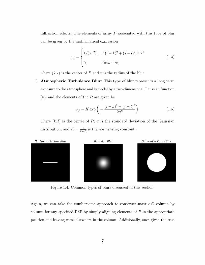
diffraction effects. The elements of array P associated with this type of blur

can be given by the mathematical expression

pij =

1/(πr2), if (i− k)2 + (j − l)2 ≤ r2

0, elsewhere,

(1.4)

where (k, l) is the center of P and r is the radius of the blur.

3. Atmospheric Turbulence Blur: This type of blur represents a long term

exposure to the atmosphere and is model by a two-dimensional Gaussian function

[45] and the elements of the P are given by

pij = K exp

(− (i− k)2 + (j − l)2

2σ2

), (1.5)

where (k, l) is the center of P , σ is the standard deviation of the Gaussian

distribution, and K = 12πσ2 is the normalizing constant.

Figure 1.4: Common types of blurs discussed in this section.

Again, we can take the cumbersome approach to construct matrix C column by

column for any specified PSF by simply aligning elements of P in the appropriate

position and leaving zeros elsewhere in the column. Additionally, once given the true

7

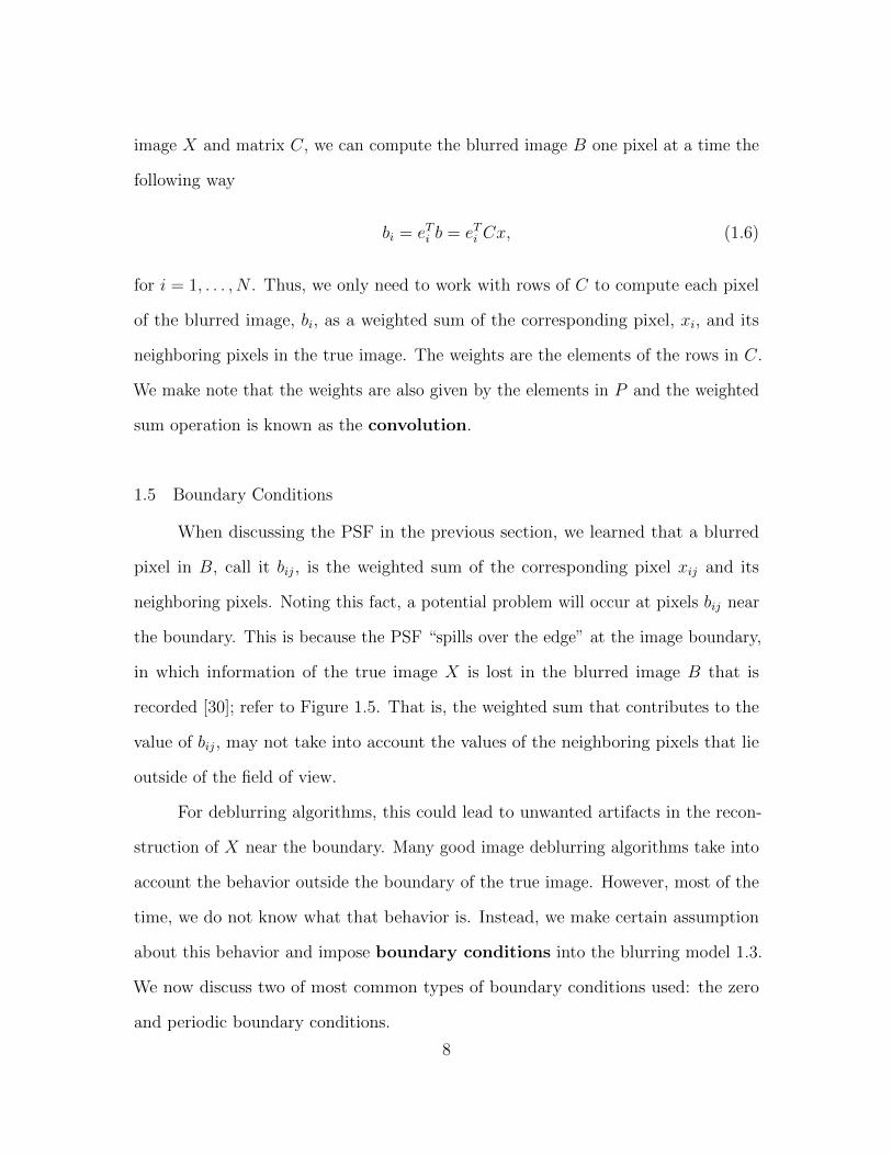
image X and matrix C, we can compute the blurred image B one pixel at a time the

following way

bi = eTi b = eTi Cx, (1.6)

for i = 1, . . . , N . Thus, we only need to work with rows of C to compute each pixel

of the blurred image, bi, as a weighted sum of the corresponding pixel, xi, and its

neighboring pixels in the true image. The weights are the elements of the rows in C.

We make note that the weights are also given by the elements in P and the weighted

sum operation is known as the convolution.

1.5 Boundary Conditions

When discussing the PSF in the previous section, we learned that a blurred

pixel in B, call it bij, is the weighted sum of the corresponding pixel xij and its

neighboring pixels. Noting this fact, a potential problem will occur at pixels bij near

the boundary. This is because the PSF “spills over the edge” at the image boundary,

in which information of the true image X is lost in the blurred image B that is

recorded [30]; refer to Figure 1.5. That is, the weighted sum that contributes to the

value of bij, may not take into account the values of the neighboring pixels that lie

outside of the field of view.

For deblurring algorithms, this could lead to unwanted artifacts in the recon-

struction of X near the boundary. Many good image deblurring algorithms take into

account the behavior outside the boundary of the true image. However, most of the

time, we do not know what that behavior is. Instead, we make certain assumption

about this behavior and impose boundary conditions into the blurring model 1.3.

We now discuss two of most common types of boundary conditions used: the zero

and periodic boundary conditions.

8

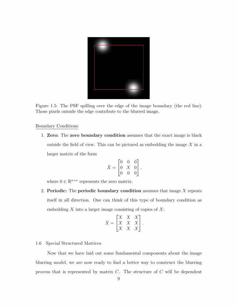
Figure 1.5: The PSF spilling over the edge of the image boundary (the red line).Those pixels outside the edge contribute to the blurred image.

Boundary Conditions

1. Zero: The zero boundary condition assumes that the exact image is black

outside the field of view. This can be pictured as embedding the image X in a

larger matrix of the form

X =

0 0 00 X 00 0 0

,

where 0 ∈ Rn×n represents the zero matrix.

2. Periodic: The periodic boundary condition assumes that image X repeats

itself in all direction. One can think of this type of boundary condition as

embedding X into a larger image consisting of copies of X:

X =

X X XX X XX X X

.

1.6 Special Structured Matrices

Now that we have laid out some fundamental components about the image

blurring model, we are now ready to find a better way to construct the blurring

process that is represented by matrix C. The structure of C will be dependent

9

on the boundary conditions we impose. We first discuss how these structures can

arise from the one-dimensional convolution and then we will extend upon this in the

two-dimensional case.

1.6.1 One-Dimensional Convolution, Toeplitz, and Circulant Matrices

Recall that a blurred image can be thought of as convolution between the true

image and a specified PSF. In the one dimensional case, given two integrable functions

p(s) and x(s), the convolution of p and x, denoted p⊛ x, produces a third function b

defined by

b(s) = (p⊛ x)(s) =

∫ ∞

−∞p(s− t)x(t) dt, (1.7)

for t ∈ R. Equation 1.7 is also known as the continuous convolution. The function

b(s) is the weighted average of the values of x(t), where the weights are given by the

function p(t). Graphically, the graph of b can produce by reflecting the graph of p(t)

to obtain p(−t), shifting the reflected graph to obtain p(s− t), and then sliding the

graph of p(s− t) across the graph of x(t), stopping at each t to compute the integral

of the product where the two graphs intersect [23].

The discrete convolution can be given as the summation over a finite number

of terms. We do not give this formulation explicitly, but instead, demonstrate with an

example how to compute the convolution of a one-dimensional image and PSF based

10

on the approach presented in [30]. Suppose the true image and PSF are represented

respectively, by the one-dimensional arrays

x =

w1

w2

x1

x2

x3

x4

x5

w3

w4

and p =

p1p2p3p4p5

,

where the wi’s represents pixels in the original scene that are outside the field of view.

The corresponding blurred image is given by

b =

b1b2b3b4b5

.

One can compute p⊛ x to produce b as follows :

1. Rotate the PSF, p, 180 degrees about the center.

2. Match coefficients of the rotated PSF array with those in x by placing the

center of the PSF array over the ith entry in x.

3. Multiply the corresponding components, and sum them to get the ith entry of b.

Assuming that the center of p is p3 we have that bi entries are given by the system

b1 = p5w1 + p4w2 + p3x1 + p2x2 + p1x3 (1.8)

b2 = p5w2 + p4x1 + p3x2 + p2x3 + p1x4

b3 = p5x1 + p4x2 + p3x3 + p2x4 + p1x5

b4 = p5x2 + p4x3 + p3x4 + p2x5 + p1w3

b5 = p5x3 + p4x4 + p3x5 + p2w3 + p1w4.

11

We now can write the convolution as a matrix-vector multiplication,

b1b2b3b4b5

=

p5 p4 p3 p2 p1

p5 p4 p3 p2 p1p5 p4 p3 p2 p1

p5 p4 p3 p2 p1p5 p4 p3 p2 p1

w1

w2

x1

x2

x3

x4

x5

w3

w4

. (1.9)

Recall that the pixels outside the field of views, the wi’s, also contribute to the pixels

of the observed blurred image. Again, we do not know what the behavior is outside

the of the field, so we impose boundary conditions. Using the boundary conditions

we discussed in Section 1.5 we have the following:

� Zero Boundary Condition. Here, wi = 0, and thus (1.9) can be rewritten asb1b2b3b4b5

=

p3 p2 p1p4 p3 p2 p1p5 p4 p3 p2 p1

p5 p4 p3 p2p5 p4 p3

x1

x2

x3

x4

x5

. (1.10)

Notice that the matrix C formed has entries such that cij = ci+1,j+1. This type

of matrix is known as a Toeplitz matrix [27].

� Periodic Boundary Conditions. In this case, we assume that the one-dimensional

image is embedded into a larger image whose made up of replicas of itself in

all directions. Thus, w1 = p4, w2 = p5, w3 = p1, and w4 = p2 and (1.9) can be

rewritten as b1b2b3b4b5

=

p3 p2 p1 p5 p4p4 p3 p2 p1 p5p5 p4 p3 p2 p1p1 p5 p4 p3 p2p2 p1 p5 p4 p3

x1

x2

x3

x4

x5

. (1.11)

12

Here the matrix C is a special type of Toeplitz matrix known as a circulant

matrix. Notice that every row of a circulant matrix is a cyclic right shift of

the one above it..

1.6.2 Two Dimensional Convolution, Block Toeplitz with Toeplitz Blocks (BTTB),

and Block Circulant with Circulant Blocks (BCCB) Matrices

A recorded 2D blurred image B, can be thought of as the convolution of a 2D

PSF array, P , with the 2D true image, X. Computing the 2D convolution has a

similar procedure as the 1D case. To compute pixel bij , the procedure goes as follows:

1. Rotate the PSF, P , 180 degrees about the center.

2. Slide the center element of P so that it lies on top of the corresponding pixel

value, xij.

3. Match coefficients of rotated P and X.

4. Multiply the corresponding components, and sum them to get the ijth entry of

B.

As an example, let

X =

x11 x12 x13

x21 x22 x23

x31 x32 x33

, P =

p11 p12 p13p21 p22 p23p31 p32 p33

, and B =

b11 b12 b13b21 b22 b23b31 b32 b33

,

with p22 being the center of P . Now suppose that we want to compute b22 corre-

sponding to x22. Following the first three step in procedure yieldsx11p33x12p32

x13p31x21p23

x22p22x23p21

x31p13x32p12

x33p11

,

and b22 is the weighted sum of x22 and its neighboring pixel value (step 4), that is,

b22 = p33x11 + p32x12 + p31x13+

p23x21 + p22x22 + p21x23+

13

p13x31 + p12x32 + p11x33.

Computing b22 is simple as all the neighboring pixels that contribute to its value are

within the field of view and are within the radius of P . However, let us consider what

happens at the edge, specifically, pixel b11. Following the same procedure yields

?p33 ?p32 ?p31?p23 x11p22

x12p21x13

?p13 x21p12x22p11

x23

x31 x32 x33

,

with

b11 = p33? + p32? + p31?+

p23? + p22x11 + p21x12+

p13? + p12x21 + p11x22.

We again impose boundary conditions for the missing pixel values outside of the field

of view. We have the following

� Zero Boundary Condition.

0p33 0p32 0p310p23 x11p22

x12p21x13

0p13 x21p12x22p11

x23

x31 x32 x33

,

with

b11 = p330 + p320 + p310+

p230 + p22x11 + p21x12+

p130 + p12x21 + p11x22.

14

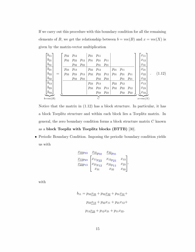
If we carry out this procedure with this boundary condition for all the remaining

elements of B, we get the relationship between b = vec(B) and x = vec(X) is

given by the matrix-vector multiplication

b11b21b31b21b22b32b13b23b33

︸ ︷︷ ︸b=vec(B)

=

p22 p12 p21 p11p32 p22 p12 p31 p21 p11

p32 p22 p31 p21p23 p13 p22 p12 p21 p11p33 p23 p13 p32 p22 p12 p31 p21 p11

p33 p23 p32 p22 p31 p21p23 p13 p22 p12p33 p23 p13 p32 p22 p12

p33 p23 p32 p22

︸ ︷︷ ︸

C

x11

x12

x31

x21

x22

x32

x13

x23

x33

︸ ︷︷ ︸x=vec(X)

. (1.12)

Notice that the matrix in (1.12) has a block structure. In particular, it has

a block Toeplitz structure and within each block lies a Toeplitz matrix. In

general, the zero boundary condition forms a block structure matrix C known

as a block Toepliz with Toeplitz blocks (BTTB) [30].

� Periodic Boundary Condition. Imposing the periodic boundary condition yields

us with

x33p33 x31p32x32p31

x13p23 x11p22x12p21

x13

x23p13 x21p12x22p11

x23

x31 x32 x33

,

with

b11 = p33x33 + p32x32 + p31x31+

p23x13 + p22x11 + p21x12+

p13x23 + p12x21 + p11x22.

15

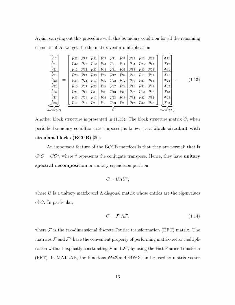
Again, carrying out this procedure with this boundary condition for all the remaining

elements of B, we get the the matrix-vector multiplication

b11b21b31b21b22b32b13b23b33

︸ ︷︷ ︸b=vec(B)

=

p22 p12 p32 p21 p11 p31 p23 p13 p33p32 p22 p12 p31 p21 p11 p33 p23 p13p12 p32 p22 p11 p31 p21 p13 p33 p23p23 p13 p33 p22 p12 p32 p21 p11 p31p33 p23 p13 p32 p22 p12 p31 p21 p11p13 p33 p23 p12 p32 p22 p11 p31 p21p21 p11 p31 p23 p13 p33 p22 p12 p32p31 p21 p11 p33 p23 p13 p32 p22 p12p11 p31 p21 p13 p33 p23 p12 p32 p22

︸ ︷︷ ︸

C

x11

x12

x31

x21

x22

x32

x13

x23

x33

︸ ︷︷ ︸x=vec(X)

. (1.13)

Another block structure is presented in (1.13). The block structure matrix C, when

periodic boundary conditions are imposed, is known as a block circulant with

circulant blocks (BCCB) [30].

An important feature of the BCCB matrices is that they are normal; that is

C∗C = CC∗, where * represents the conjugate transpose. Hence, they have unitary

spectral decomposition or unitary eigendecomposition

C = UΛU∗,

where U is a unitary matrix and Λ diagonal matrix whose entries are the eigenvalues

of C. In particular,

C = F∗ΛF , (1.14)

where F is the two-dimensional discrete Fourier transformation (DFT) matrix. The

matrices F and F∗ have the convenient property of performing matrix-vector multipli-

cation without explicitly constructing F and F∗, by using the Fast Fourier Transform

(FFT). In MATLAB, the functions fft2 and ifft2 can be used to matrix-vector

16

multiplication of F and F∗, respectively. Note, implementation of fft2 and ifft2

involve a sclaing factor, that is,

fft2(X)←→√NFx,

and

ifft2(X)←→ 1√NFx.

Additionally, we can compute the eigenvalues of C easily since the first column

of F are made up of 1’s. So let denote the first column of C and F by c1 and f1

respectively. Notice that,

C = F∗ΛF ⇒ FC = ΛF ⇒ Fc1 = Λf1 =1√Nλ,

where λ ∈ RN is a vector containing all the eigenvalues of C. Thus, we can compute

the eigenvalues of C by multiplying the matrix√NF by the first column of C, scaled

by the square of the dimension. We can find the first column of C by the PSF and

the MATLAB function cirschift, refer to [30], and we can compute b and efficiently

since

b = Cx = F∗ΛFx. (1.15)

1.6.3 Separable Blurs

In image processing, some PSF are capable to be decomposed in to their vertical

and horizontal components. These types PSF are called seperable [30, 36]. So given

a separable m× n PSF array P , we can rewrite P as

P = vhT =

v1v2...vm

[h1 h2 · · · hn

],

17

where v represent the vertical components of the PSF that blurs across the columns

of the image, h represents the horizontal components of the PSF that blurs the rows

of the image.

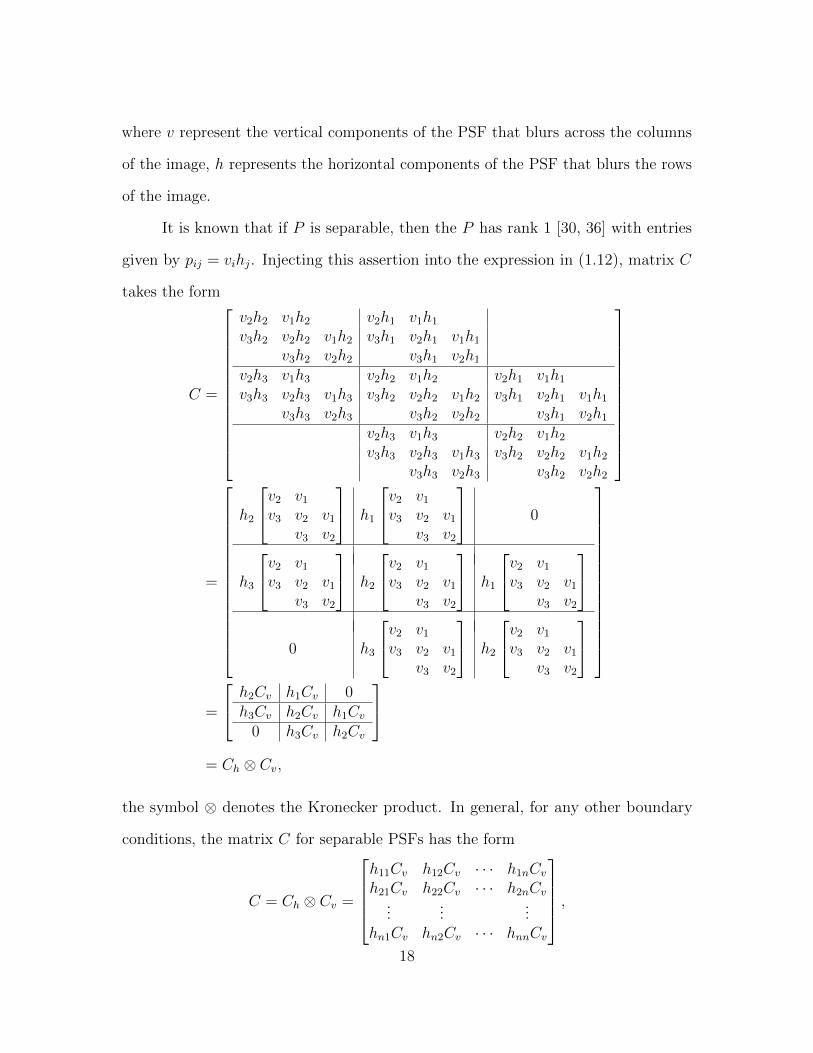
It is known that if P is separable, then the P has rank 1 [30, 36] with entries

given by pij = vihj. Injecting this assertion into the expression in (1.12), matrix C

takes the form

C =

v2h2 v1h2 v2h1 v1h1

v3h2 v2h2 v1h2 v3h1 v2h1 v1h1

v3h2 v2h2 v3h1 v2h1

v2h3 v1h3 v2h2 v1h2 v2h1 v1h1

v3h3 v2h3 v1h3 v3h2 v2h2 v1h2 v3h1 v2h1 v1h1

v3h3 v2h3 v3h2 v2h2 v3h1 v2h1

v2h3 v1h3 v2h2 v1h2

v3h3 v2h3 v1h3 v3h2 v2h2 v1h2

v3h3 v2h3 v3h2 v2h2

=

h2

v2 v1v3 v2 v1

v3 v2

h1

v2 v1v3 v2 v1

v3 v2

0

h3

v2 v1v3 v2 v1

v3 v2

h2

v2 v1v3 v2 v1

v3 v2

h1

v2 v1v3 v2 v1

v3 v2

0 h3

v2 v1v3 v2 v1

v3 v2

h2

v2 v1v3 v2 v1

v3 v2

=

h2Cv h1Cv 0h3Cv h2Cv h1Cv

0 h3Cv h2Cv

= Ch ⊗ Cv,

the symbol ⊗ denotes the Kronecker product. In general, for any other boundary

conditions, the matrix C for separable PSFs has the form

C = Ch ⊗ Cv =

h11Cv h12Cv · · · h1nCv

h21Cv h22Cv · · · h2nCv...

......

hn1Cv hn2Cv · · · hnnCv

,

18

where Cv is an m×m matrix and Ch is an n× n matrix. Recall, we assume that C

is of size n2 × n2, hence Cv and Ch are both of size n× n.

Exploiting properties of the Kronecker, we can now write the blurring model in

(1.3) as the matrix-matrix relation

B = CvXCTh . (1.16)

What (1.16) tells us is that we can produce B by first performing a convolution

of the columns of X with the vertical components of P , then perform another

convolution with the resulting rows with the horizontal components of P . Since

matrix multiplication is associative, we can perform the convolution in vice versa.

1.6.4 Summary of Matrix Structures

The table below summarize the important structures for matrix C we have built

up in this chapter based on the characteristics of the PSF and the type of boundary

conditions we impose in the blurring model. For the remainder of this thesis, we call

matrix C the convolution or blurring matrix associated with the PSF.

Matrix Structure of CBoundary

Condition

Nonseparable PSF Separable PSF

Zero BTTB Kronecker Product of Toeplitz matricesPeriodic BCCB Kronecker Product of circulant matrices

(1.17)

19

CHAPTER 2

COMPRESSIVE DECONVOLUTION

Another concern in image processing is to be able to store an image efficiently

through highly compressed measurements without losing image fidelity and quality.

However, it is often the case to acquire an accurate representation of the recorded

image is achieved through enforcing the Shannon-Nyquist theorem. The Shannon-

Nyquist theorem states that the image sampling rate must be at least twice the

maximum frequency value of the image [23]. This theorem makes one assume that it

is impossible to reconstruct an image without the sacrificing image fidelity or quality

using highly compressed measurements, or so it would seem.

2.1 Compressed Sensing

The theory of compressed sensing has been used in a wide variety of appli-

cations in mathematics, computer science, radiology, and engineering which include

image processing [21], magnetic resonance imaging (MRI) [55], synthetic aperture

radar (SAR) imaging [54], and more. Through the umbrella of compressed sensing,

far fewer measurements than what Shannon-Nyquist imposes are needed to get an

approximate reconstruct of the desired image without much loss of meaning and

granularity [10]-[13]. Given image X ∈ Rn×n, the standard compressed sensing linear

model is given by

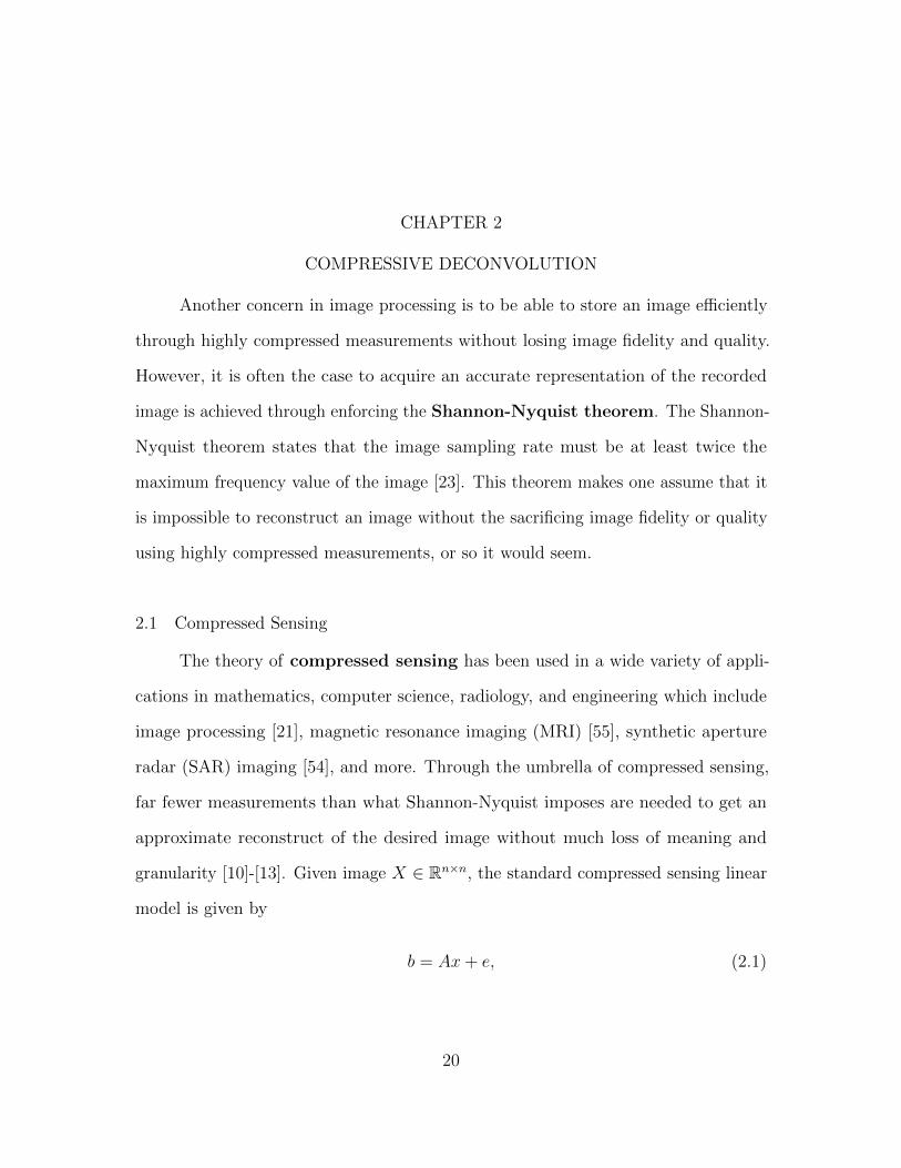
b = Ax+ e, (2.1)

20

where is A ∈ Rm×N is the measurement matrix, x ∈ RN is the vectorization of X,

e ∈ Rm represents noise, and b ∈ Rm are compressed observed measurements. Note

that m << N = n2. Figure 2.1 helps illustrate this model.

Figure 2.1: Compressed Sensing Model for sparse signal/image recovery.

Clearly, (2.1) presents us with an ill-posed problem. However, compressed

sensing theory tells us that we can recover a unique solution x from measurements b

provided that

� the image must have a sparse representation in a known basis (i.e., Fourier,

wavelet, curvelet, etc.) and,

� the sampling is incoherent (random) which is conveyed through the restricted

isometry property in [10].

The presence of noise allows one to see that sparsity is never really achieve. Fortunately,

many images tend to be naturally sparse or almost sparse in a certain basis. That is to

say that most of the coefficients are arbitrarily small, and only a few large coefficients

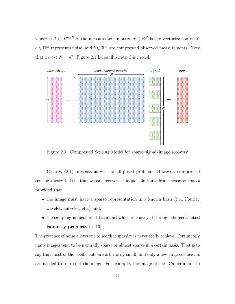
are needed to represent the image. For example, the image of the “Cameraman” in

21

Figure 2.2 has been been taken in to the Fourier space, also referred to as the k-space

in MRI [39]. Most of the Fourier coefficients in that space are small in magnitude,

and only a few relatively large coefficients contain most of the information about the

image. Here, we knock out coefficients whose magnitude are smaller than a certain

tolerance (10−3), and only 12% of the largest coefficients are needed to recover a

decent approximation to the original image.

Figure 2.2: Left: Original Image. Mid-Left: Fully Sampled Image in k-space. Mid-Right 12% Sampling Right. Right: Recovered Image

Even though, the signal of interest is sparse, we do not know where the nonzero

elements are located as a priori. There have been several algorithms proposed to

solve this problem. Such algorithms incluede, ℓ1-magic [14], basis pursuit denoising

[16], and the Least Absolute Shrinkage and Selection Operator (LASSO) [48]. The

first of which we will discuss further in Chapter 4 and extend upon in Chapter 5 in

this thesis.

2.2 Deconvolution

In Chapter 1, we discussed that the blurring process is an inherent problem in

imaging. The recorded blurred image, B, can be thought of as the convolution of

the true image X and an undesired PSF, which can be further extended to a linear

22

system as in 1.3. The natural question is: can we recover X from B that is related

by an undesired PSF? The process of recovering X from blurred measurements B is

known as deconvolution [46], also referred to as deblurring.

Referring back to the model 1.3, the standard deconvolution model with noisy

blurred measurements is given by

b = Cx+ e, (2.2)

where C ∈ RN×N denotes the convolution matrix associated with the PSF caused

by a shaky camera, lack of focus, atmospheric turbulence, rippling, etc., x ∈ RN

and e ∈ RN represents the vectorization of true image X ∈ Rn×n signal and noise,

respectively.

As with the compressed sensing, the objective of deconvolution is not an easy

task to achieve. The reasons for this is that deconvolution is

� an ill-posed inverse problem, and

� in many situations the PSF is usually an unknown a priori.

Methods that assume the the PSF is known are called non-blind deconvolution

methods [19], such as the Wiener filtering [53] and the Richardson-Lucy algorithms

[44]. Analogously, blind deconvolution methods assume that the PSF is unknown

and these methods fall under one of two categories: a priori identification or joint

identification methods [8]. In our work, we assume that the PSF is known. Thus,

we will be developing a non-blind deconvolution algorithm.

2.3 Compressive Deconvolution

In recent years, there have been algorithms developed to solve the compressed

sensing and deconvolution problem jointly, rather than a sequential approach. A

problem of this type is known as compressive deconvolution. This area is relatively

23

new and has shown applications in image processing [1] and medical ultrasound

imaging [17].

The goal of compressive deconvolution is to recover image X from the recorded

compressed and blurred measurements B. Naturally, another question is introduce:

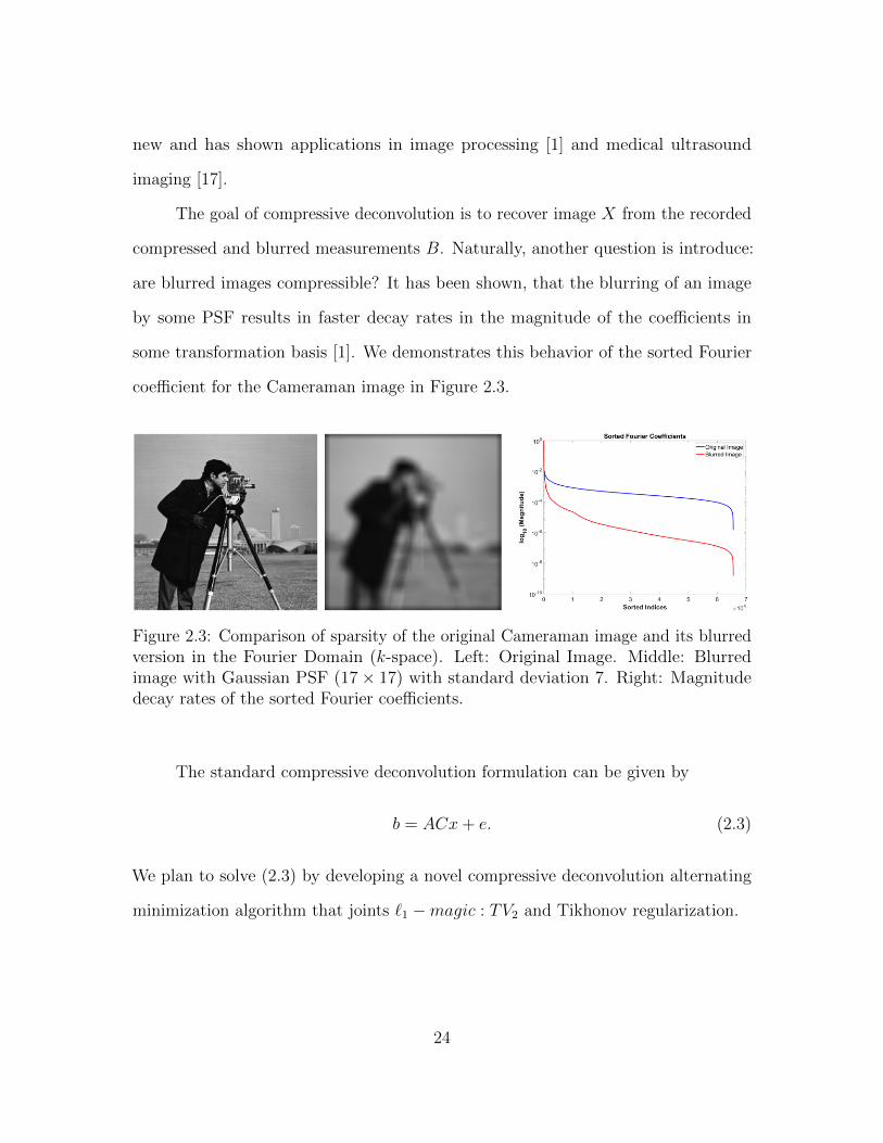
are blurred images compressible? It has been shown, that the blurring of an image

by some PSF results in faster decay rates in the magnitude of the coefficients in

some transformation basis [1]. We demonstrates this behavior of the sorted Fourier

coefficient for the Cameraman image in Figure 2.3.

Figure 2.3: Comparison of sparsity of the original Cameraman image and its blurredversion in the Fourier Domain (k-space). Left: Original Image. Middle: Blurredimage with Gaussian PSF (17× 17) with standard deviation 7. Right: Magnitudedecay rates of the sorted Fourier coefficients.

The standard compressive deconvolution formulation can be given by

b = ACx+ e. (2.3)

We plan to solve (2.3) by developing a novel compressive deconvolution alternating

minimization algorithm that joints ℓ1 −magic : TV2 and Tikhonov regularization.

24

CHAPTER 3

MATHEMATICAL BACKGROUND

In this chapter, we will review some numerical optimization methods we will

use to solve (5.1). We first discuss some background on how to solve the optimization

problem

minx

f(x) subject to ∥Ax− b∥2 ≤ ϵ,

where A ∈ Rn×n, b ∈ Rn and f(x) : Rn 7→ R, is some convex objective function, for

2D image reconstruction. Methods included the Conjugate Gradient (CG) method,

the Newton method, and the interior point method via log-barrier function.

We will then discuss techniques to solve the least squares approximation problem

minx∥Cx− d∥2,

where C ∈ Rm×n and d ∈ Rm, for image deblurring. The methods used will be the

singular value decomposition (SVD) and spectral filtering via truncated SVD (TSVD)

and Tikhonov regularization.

3.1 Linear Conjugate Gradient Method

The Conjugate Gradient method is a very popular iterative method developed

by Hestenes and Stiefel [34] to solve the large linear system Ax = b of n linear

equations in n steps, where A is symmetric positive definite. Normally, the goal is to

find an approximate solution x to the linear system such that the residual

r = Ax− b (3.1)

25

is less than some specified tolerance. In [42, p.101-111, p.120-125], this is equivalent

to minimizing the following convex quadratic function

minx

f(x) with f(x) :=1

2xTAx− bTx. (3.2)

Notice, taking the gradient of f , that is

∇f(x) = Ax− b, (3.3)

we can see that it is equal to the residual r in (3.1). This means that −r or the

negative gradient direction is the fastest descent direction. Such a method that finds

this descent direction iteratively is called the method of steepest descent [7, p.

481]. There is merit to this method in nonlinear systems, but for linear system the

method tends to have slow convergence.

As an alternate approach, the CG method iteratively constructs a set of A-

orthogonal search direction vectors denoted as {p0, p1, . . . , pn}. A set of vectors,

{p0, pn, . . . , pn}, is called A-orthogonal if

pTi Apj = 0, ∀i = j.

This choice of search directions with this property is important as f(x) can be

minimized successively along each of the individual search directions. Additionally,

each of the approximation is the optimal solution from the subspace spanned by all

the search direction vectors up to that point. Each of the successive points can be

written as

xi+1 = xi + αipi, (3.4)

where αi is how far we move along the direction pi. This is equivalent to finding the

minimum of h(αi), where

26

h(αi) = f(xi + αipi)

=1

2(xi + αipi)

TA(xi + αipi)− bT (xi + αipi)

=1

2(xi + αipi)

TA(xi + αipi)− bTxi − αibTpi

=1

2(xT

i Axi + αixTi Api + αip

Ti Axi + α2

i pTi Api)− bTxi − αib

Tpi

=1

2α2i p

Ti Api + αip

Ti (Axi − b) + (

1

2xTi Axi − bTxi)

=1

2α2i p

Ti Api + αip

Ti (Axi − b) + f(xi).

For each fixed xi and αi, we have that h assumes a minimal value when h′(αi) = 0,

because the coefficient of α2i , p

Ti Api, is positive. That is,

h′(αi) = αipTi Api + pTi (Axi − b)

= 0,

and solving for αi to get

αi =pTi ripiApi

. (3.5)

Notice that we have a way to compute our approximations xi iteratively as well as

the residuals which have expression given by

ri = Axi − b

= A(xi−1 + αi−1pi−1)− b

= Axi−1 − b+ αi−1Api−1

= ri−1 + αi−1Api−1. (3.6)

Equations (3.4), (3.5), and (3.6) are dependent on the search directions pi. The CG

method sets p0 = r0 and iteratively defines the next search direction as

pi = −ri + βipi−1. (3.7)

27

Thus αi can be simplified to

αi =rTi ripiApi

, (3.8)

and βi is given by [42, p.101-111, p.120-125][7, p. 485] as

βi =rTi+1ri+1

rTi ri. (3.9)

Thus, the CG method does not have to store the previous search directions, and the

complexity of the method reduces to O(km), where m is number of nonzero entries

of A and k is the number of CG iterations [42]. In summary, the CG method can be

outlined as

αi =rTi ripiApi

, (3.10)

xi+1 = xi + αipi, (3.11)

ri+1 = ri−1 + αi−1Api−1 (3.12)

βi =rTi+1ri+1

rTi ri,(3.13)

pi = −ri + βipi−1, (3.14)

where x0 = 0 and p0 = −r0 = b − Ax0. The CG method will continue to iterate

through this outlined procedure until ∥ri∥∥r0∥ is less than some tolerance or the maximum

number of iteration has been reached [25].

3.2 Newton’s Method for Unconstrained Minimization Problems

Newton’s method is one of the most useful and well-known numerical methods

for solving root-finding problems. This method can be extended to multivariate

functions and attempts to find a point at which a function’s gradient is zero using a

quadratic approximation of the function. We will apply Newton’s method to iteratively

28

solve the log barrier form of (5.1) by forming a series of quadratic approximation [3],

which will be discussed later in this chapter. Now consider a real-valued function

f(x) : Rn 7→ Rn. The second-order Taylor approximation of a single variable function,

f(x) near x, is given as follows

f(x+∆x) ≈ f(x) + f ′(x)∆x+1

2f ′′(x)∆x2.

The multivariate function analog to this is

f(x+∆x) ≈ f(x) +∇f(x)T∆x+1

2∆xT∇2f(x)∆x, (3.15)

where ∇f represents the gradient and ∇2f represents the Hessian of f [2]. Assuming

that the Hessian, ∇2f(x), is positive definite, we seek to find the ∆x that minimizes

f(x+∆x). By setting the derivative of the right hand of (3.15) and setting it equal

to zero

0 =d

d∆x

(f(x) +∇f(x)T∆x+

1

2∆xT∇2f(x)∆x

)= ∇f(x)T +∆xT∇2f(x), (3.16)

we get an explicit formula form for what is known as the Newton step or Newton

direction [31, 42]

∆x = −∇2f(x)−1∇f(x). (3.17)

Thus by iterating over x, the unique minimum is obtained at xn+1 = x+∆xn, where

∆x is given by (3.17). In practice, the step size is usually controlled in order to avoid

divergence of the descent direction. A popular approach is to do a backtracking

line search [47, p.108] where we add the parameter β and get the modified Newton

iteration

xn+1 = xn + β ·∆xn. (3.18)

29

Now that we have our scheme, given by (3.19), the question is now: when do

we stop iterating? A typical stopping criterion for Newton’s method involves the

Newton decrement, denoted by λ(x) [3, 6]. At a point x, the Newton decrement is

expressed as

λ(x) =[∇f(x)T∇2f(x)−1∇f(x)

] 12. (3.19)

A typical stopping criterion is given by

λ2(x)

2≤ ϵ, (3.20)

where ϵ is a specified tolerance.

3.3 The Interior-Point Method via Log Barrier Function

Recall we wish to solve a problem of the form

minx

f0(x)

subject to fi(x) ≤ 0 for i = 1, . . . ,m. (3.21)

We will convert this constrained problem to an unconstrained one in order for

us to apply Newton’s Method discussed in Section 3.2. In order for this to happen,

we will embed the inequality constraints of (3.21) into the objective function using

an interior point method via log-barrier function. Once embedded, we will iteratively

solve it using Newton’s method.

In order to use Newton’s method, it is required that the objective function

embedded with the inequality constraints is smooth and differentiable. Additionally,

30

the minimization problem must be penalized for not meeting the inequality constraints.

Consider the indicator function I : R 7→ R,

I (x) =

0, x < 0

∞, x > 0.

(3.22)

One can change (3.21) as the following unconstrained problem

minx

f0(x) +n∑

i=1

I (fi(x)). (3.23)

Notice that if any of the inequality constraints is greater than 0, then the indicator

function,∑n

i=1 I (fi(x)), is infinity. The minimization problem is indeed penalized

for not meeting at least one of the inequality constraints which are now part of the

objective function, however, the objective function is clearly not differentiable. Thus,

Newton’s method can not be applied here.

So now, consider the alternative function

I (x) =−1τ

log(−x), (3.24)

where dom(I ) = {x ∈ R|x < 0}, and τ > 0 is an accuracy parameter [6]. This

function is differentiable and it does penalize the objective function. To see the latter

condition, we observe some plots for various values of τ .

31

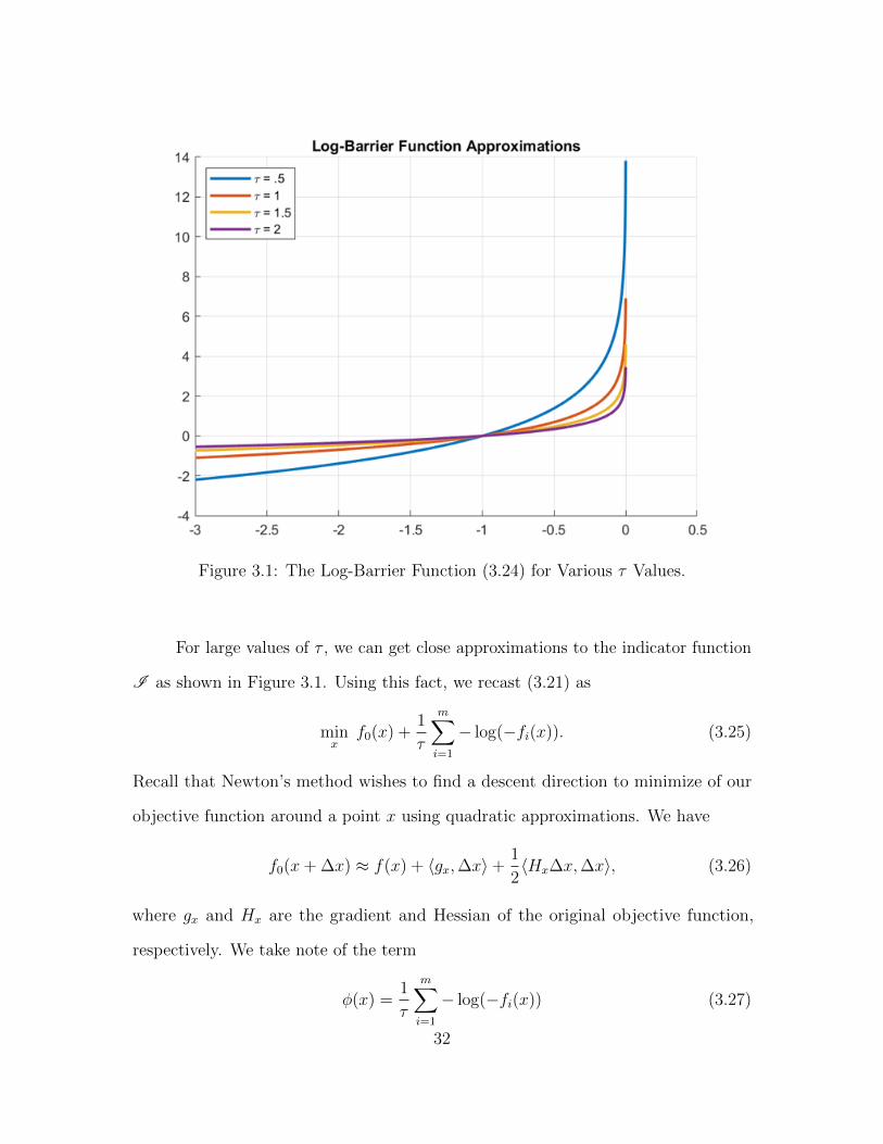
Figure 3.1: The Log-Barrier Function (3.24) for Various τ Values.

For large values of τ , we can get close approximations to the indicator function

I as shown in Figure 3.1. Using this fact, we recast (3.21) as

minx

f0(x) +1

τ

m∑i=1

− log(−fi(x)). (3.25)

Recall that Newton’s method wishes to find a descent direction to minimize of our

objective function around a point x using quadratic approximations. We have

f0(x+∆x) ≈ f(x) + ⟨gx,∆x⟩+ 1

2⟨Hx∆x,∆x⟩, (3.26)

where gx and Hx are the gradient and Hessian of the original objective function,

respectively. We take note of the term

ϕ(x) =1

τ

m∑i=1

− log(−fi(x)) (3.27)

32

is known as the log-barrier function and the gradient, ∇ϕ(x), and Hessian, ∇2ϕ(x)

as

∇ϕ(x) =m∑i=1

1

−fi(x)∇fi(x), (3.28)

and

∇2ϕ(x) =m∑i=1

1

fi(x)2∇fi(x)∇fi(x)T +

m∑i=1

1

−fi(x)∇2fi(x). (3.29)

Equations (3.28) and (3.29) will be for later reference in Chapters 4 and 5. Thus,

assuming our starting point x is feasible, the direction ∆x along which a new

approximation to minimize (3.27) is the solution to the following linear system

Hx∆x = −gx. (3.30)

The system is solved using the CG since the Hessian, Hx, is symmetric positive

definite [14].

3.4 Least Squares Approximation

For a given matrix C ∈ Rm×n, square or rectangular, the goal of the least

squares approximation is to find a close approximate solution, x∗, for the system

Cx = d,

whose has no solution. This is equivalent of trying to find the vector x ∈ Rn such

that

∥Cx∗ − d∥2 = minx∥Cx− d∥2. (3.31)

Another interpretation is that we are trying to find the vector Cx∗ in the column

space of C, which we will denote it as W , that is the closest to d among all of the

vectors in W . It turns out that the closest vector to d is the vector x∗ such that

Cx∗ = PWd, (3.32)

33

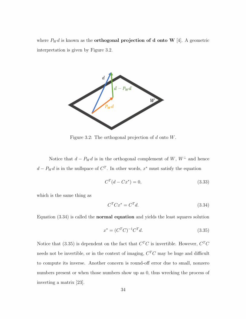
where PWd is known as the orthogonal projection of d onto W [4]. A geometric

interpretation is given by Figure 3.2.

Figure 3.2: The orthogonal projection of d onto W .

Notice that d − PWd is in the orthogonal complement of W , W⊥ and hence

d− PWd is in the nullspace of CT . In other words, x∗ must satisfy the equation

CT (d− Cx∗) = 0, (3.33)

which is the same thing as

CTCx∗ = CTd. (3.34)

Equation (3.34) is called the normal equation and yields the least squares solution

x∗ = (CTC)−1CTd. (3.35)

Notice that (3.35) is dependent on the fact that CTC is invertible. However, CTC

needs not be invertible, or in the context of imaging, CTC may be huge and difficult

to compute its inverse. Another concern is round-off error due to small, nonzero

numbers present or when those numbers show up as 0, thus wrecking the process of

inverting a matrix [23].

34

3.4.1 The Singular Value Decomposition and Pseudoinverse

The singular value decomposition (SVD) allows for any matrix C ∈ Rm×n

to be written in the form

C = UΣV T , (3.36)

where U ∈ Rm×m and V ∈ Rn×n are orthogonal matrices and Σ ∈ Rm×n is a diagonal

matrix whose diagonal elements satisfies σ1 ≥ σ2 ≥ · · · ≥ σr ≥ σr+1 ≥ . . . σn ≥ 0 :

Σ =

σ1

σ2

. . .

σr

. . .

σn

. (3.37)

The σi’s are called the singular values of C and are the positive square roots of the

eigenvalues of CTC. Note that σr is the smallest nonzero singular value and that the

rank of matrix C is equal to the number of positive singular values. The columns

ui of U are called the left singular vectors, while the columns vi of V are called

the right singular vectors. Since U is orthogonal, then the following holds for the

column vectors of U

uTi uj =

0, i = j

1, i = j,

and UT = U−1. A similar argument can be said about the columns of V . The singular

value decomposition of C can be expressed as the sum

C = UΣV T

=[u1 . . . un

] σ1

. . .

σn

v

T1...vTn

35

= u1σ1vT1 + · · ·+ σnunv

Tn

=n∑

i=1

σiuivTi . (3.38)

Any matrix can be decomposed this way [37].

An important application of the SVD is that it allows for a generalization of

matrix inversion for an any matrix. So for the moment, let’s assume that the singular

values of C are strictly positive. Thus, the inverse of C is given by

C−1 = V Σ−1UT

=n∑

i=1

1

σi

viuTi , (3.39)

where Σ−1 ∈ Rn×m is a diagonal matrix. We make note that the diagonal entries of

Σ−1 are the reciprocals of the diagonal entries of Σ, that is, 1σi. However, this presents

a problem as Σ will likely have entries σi = 0. Hence, Σ−1 will not exist.

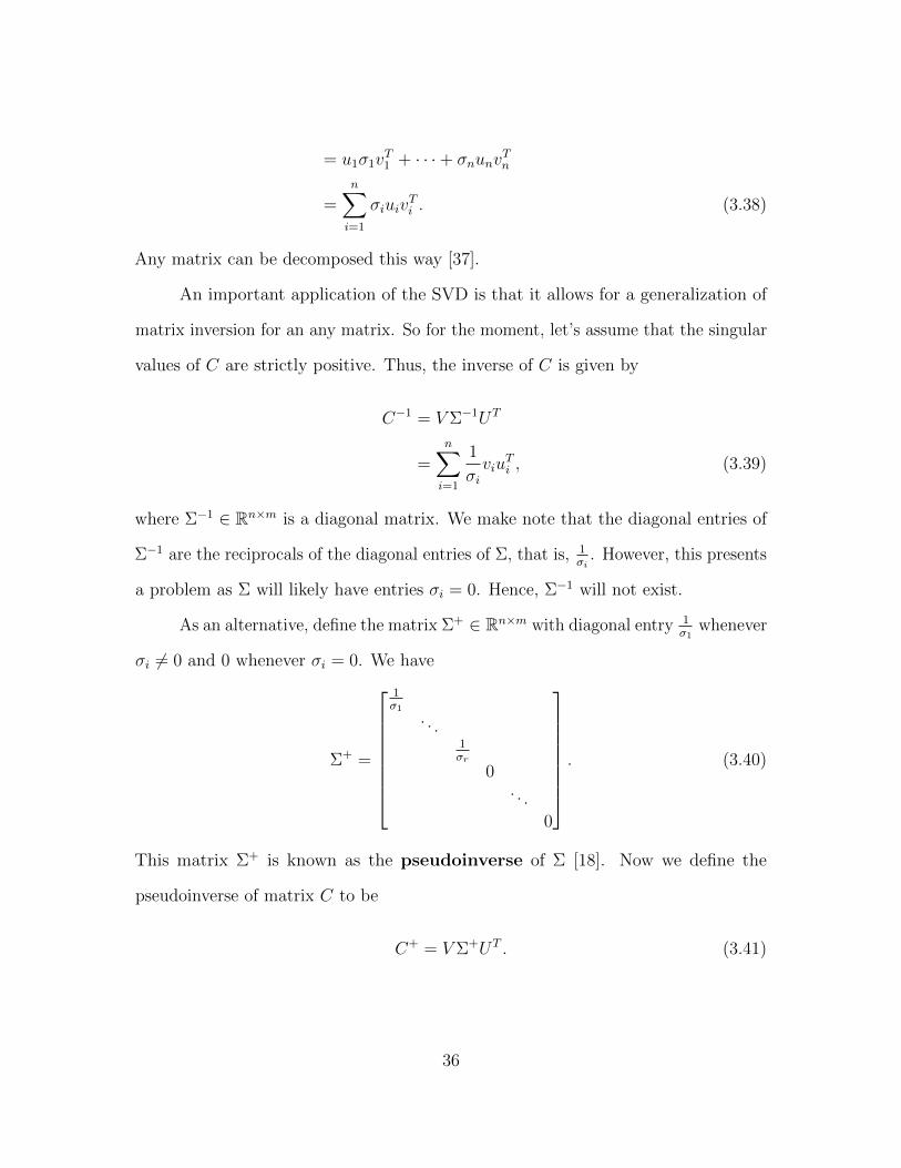
As an alternative, define the matrix Σ+ ∈ Rn×m with diagonal entry 1σ1

whenever

σi = 0 and 0 whenever σi = 0. We have

Σ+ =

1σ1

. . .1σr

0. . .

0

. (3.40)

This matrix Σ+ is known as the pseudoinverse of Σ [18]. Now we define the

pseudoinverse of matrix C to be

C+ = V Σ+UT . (3.41)

36

Recall that we aim to find the x∗ such that solves (3.31) and this was equivalent to

finding a solution to the normal equation in (3.34). The pseudoinverse of C gives us

the solution to the normal equations as

x+ = C+d

= V Σ+UTd, (3.42)

and is a optimal solution to (3.31).

3.5 Spectral Filtering

Referring back to the linear system,

Cx = d,

C is said to be ill-conditioned if a small perturbation in d leads to relatively large

changes in the solution x. As an alternative definition, C is ill-conditioned if its

condition number is large. Otherwise, C is said to be well-conditioned. The

condition number of C, denoted κ(C), can be computed as the ratio between the

largest and smallest positive singular values of C [23, 30], that is,

κ(C) =σ1(C)

σr(C). (3.43)

So let’s assume that d is subjugate to noise e ∈ Rm. Then the linear system we aim

to solve is

Cx = d, (3.44)

with d = dexact + e. Applying the SVD, we get the solution (naive)

xnaive = C−1d

= C−1(dexact + e)

37

= V Σ−1UTdexact + V Σ−1UT e

=n∑

i=1

uTi dexactσi

vi +n∑

i=1

uTi e

σi

vi︸ ︷︷ ︸inverted noise

. (3.45)

The term,uTi e

σi, presents a problem if C is ill-conditioned. As i increases, the σi’s

will decrease, and 1σi’s will increase. This results in the terms

uTi e

σito become large in

magnitude and thus amplifying the noise present in the system. This effect will cause

the noise term to dominate the computation of the solution xnaive.

The effects caused by the division of small singular values must be dampened to

control the noise term. One way to do this is through spectral filtering methods,

also known as regularization[22, 23, 30]. The spectral filtering methods work by

choosing filtering factors ϕi such that the solution (filtered or regularized)

xfilt =n∑

i=1

ϕiuTi d

σi

vi (3.46)

produces a desirable solution by reducing the effects of the amplified noise. We now

discuss now two spectral filtering methods: the truncated SVD (TSVD) method

and Tikhonov regularization.

3.5.1 Truncated SVD (TSVD)

In the TSVD, we select the k largest positive singular values and approximate

C by Ck =∑k

i=1 σiuivTi . This is equivalent of saying that Ck = UkΣkVk, where Uk

and Vk are formed by just by the first k columns of U and V , respectively, and Σk is

a k × k diagonal matrix with entries σ1 ≥ σ2 · · · > σk > 0. Note that the rank of Ck

equal to k < r and it captures much of the behavior of C [23]. We can interpret the

corresponding regularized solution by

xTSV D =n∑

i=1

ϕiuTi d

σi

vi,

38

with

ϕi =

1, i = 1, . . . , k

0, i = k + 1 . . . n.

(3.47)

The parameter k is known as the truncation parameter [30] and determines the

number of SVD components maintained in the corresponding regularized solution

xTSV D. That is, TSVD enforces an upper bound on the size of the reciprocal of the

singular values that are used, thus preventing the division by small σi.

Another way to implement the TSVD is to replace σi by 0 if |σi| ≤ ϵ, where ϵ

is some specified tolerance.

3.5.2 Tikhonov Regularization

In Tikhonov regularization, rather enforcing an upperbound on the singular

value, C is modified such that all the singular values are strictly positive. Consider

the normal equation

(CTC + α2I)x = CTd, (3.48)

where I ∈ Rn×n represents the identity matrix and α is known as the Tikhonov

regularization parameter. Thus, we are interested in solving the minimization

problem

minx

∥∥∥ [Cxαx

]−

[d0

] ∥∥∥2

2= min

x

∥∥∥ [Cx− dαx

] ∥∥∥2

2

= {minx∥Cx− d∥22 + α2∥x∥22}. (3.49)

Simply inverting (CTC + α2I) yields the result,

xα = (CTC + α2I)−1CTd. (3.50)

39

However, as stated in Section 3.4, the inverse of the matrix in (3.50) maybe difficult to

compute and maybe be subjected to round-off error. So instead, we take the singular

value approach to this problem.

Consider the eigendecomposition of CTC = V DV T , and the SVD of C = UΣV T ,

where D ∈ Rn×n is a diagonal matrix whose entries are the eigenvalues of CTC. Hence,

(CTC + α2I) = V (D + α2I)V T , where the matrix (D + α2I) is a diagonal matrix

whose entries are of the form σ2i + α2, where σi’s are singular values of C.

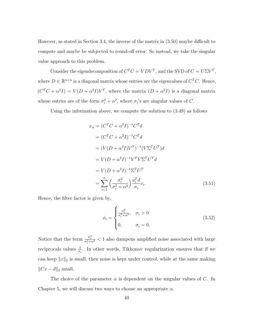
Using the information above, we compute the solution to (3.49) as follows

xα = (CTC + α2I)−1CTd

= (CTC + α2I)−1CTd

= (V (D + α2I)V T )−1(V ΣTUT )d

= V (D + α2I)−1V TV ΣTUTd

= V (D + α2I)−1ΣTUT

=n∑

i=1

( σ2i

σ2i + α2

)uTi d

σi

vi. (3.51)

Hence, the filter factor is given by,

ϕi =

σ2i

σ2i +α2 , σi > 0

0, σi = 0.

(3.52)

Notice that the termσ2i

σ2i +α2 < 1 also dampens amplified noise associated with large

reciprocals values 1σi. In other words, Tikhonov regularization ensures that if we

can keep ∥x∥2 is small, then noise is kept under control, while at the same making

∥Cx− d∥2 small.

The choice of the parameter α is dependent on the singular values of C. In

Chapter 5, we will discuss two ways to choose an appropriate α.

40

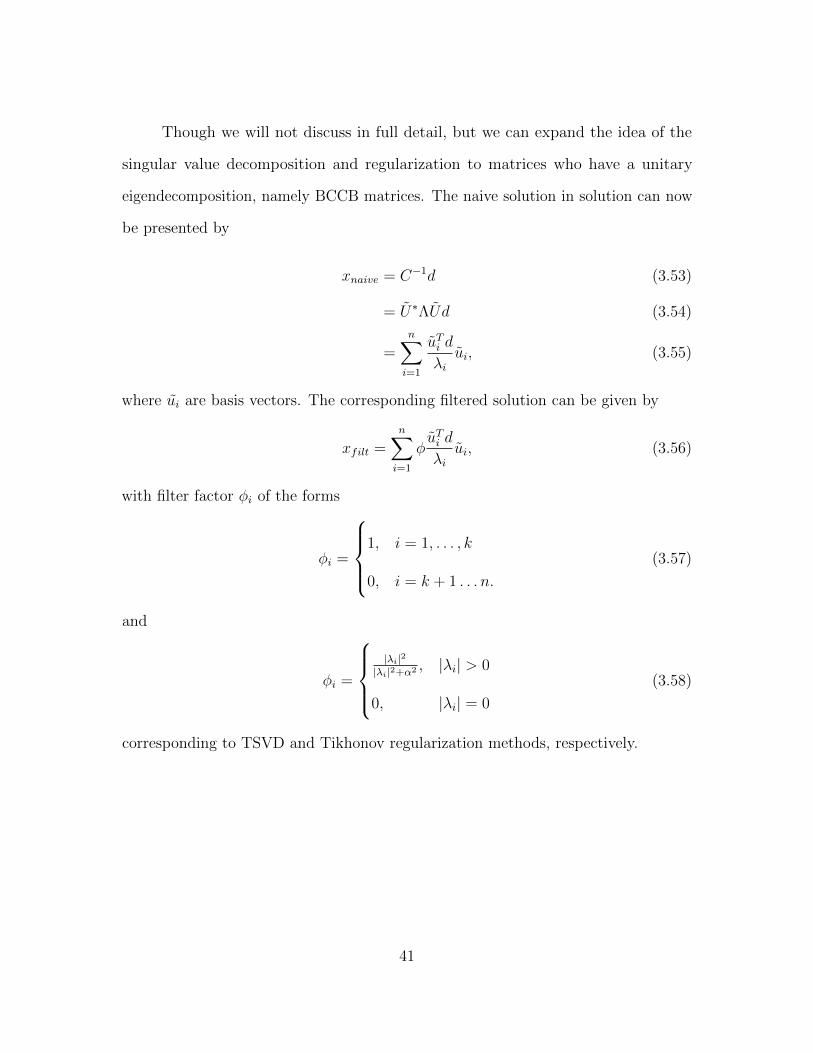
Though we will not discuss in full detail, but we can expand the idea of the

singular value decomposition and regularization to matrices who have a unitary

eigendecomposition, namely BCCB matrices. The naive solution in solution can now

be presented by

xnaive = C−1d (3.53)

= U∗ΛUd (3.54)

=n∑

i=1

uTi d

λi

ui, (3.55)

where ui are basis vectors. The corresponding filtered solution can be given by

xfilt =n∑

i=1

ϕuTi d

λi

ui, (3.56)

with filter factor ϕi of the forms

ϕi =

1, i = 1, . . . , k

0, i = k + 1 . . . n.

(3.57)

and

ϕi =

|λi|2

|λi|2+α2 , |λi| > 0

0, |λi| = 0

(3.58)

corresponding to TSVD and Tikhonov regularization methods, respectively.

41

CHAPTER 4

2D IMAGE RECOVERY

In this chapter, we discuss a popular 2D image reconstruction algorithm known

as ℓ1-magic : TV2, which we will simply refer to it as ℓ1-magic [14]. The authors of

[14] attempt to solve the following 2D minimization problem

minX

TV(X) subject to ∥A(X)−B∥2 ≤ ϵ, (4.1)

where A : Rn×n is the 2D Sparse Fourier Transformation, B ∈ Rn×n is the measured

observation of sampled pixels of an image in the k-space and TV : Rn×n 7→ R is a

function that computes the total variation of X in the x− and y− directions.

The authors solve (4.1) by recasting the problem into a Second Order Cone

Problem (SOCP) and solve a new problem using the interior point method via the

log barrier function based from [6]. Before doing so, we must define a few terms.

We define the TV function in (4.1) in order to use Newton’s method. The

Total Variation of a 2D image is defined as the sum of the finite differences of

pixels with their vertical and horizontal neighboring pixels. Mathematically, given an

two-dimensional image X ∈ Rn×n, whose ijth pixel is denoted as Xij and define the

operators

Dh;ijX =

Xi,j+1 −Xij, i < n

0, i = n

Dv;ijX =

Xi+1,j −Xij, j < n

0, j = n

42

where Dh;ij and Dv;ij are the horizontal and vertical difference operators, respectively.

Furthermore, define the vector DijkX ∈ R2 as

DijX =

[Dh;ijXDv;ijX

]. (4.2)

This vector, DijX, is known as the discrete gradient of the image at the ijth pixel,

and hence the total variation in (4.1) is defined as follows

TV(X) =∑ij

√(Dh;ijX)2 + (Dv;ijX)2 =

∑ij

∥DijX∥2. (4.3)

4.1 Interior Point Method for SOCPs

We can rewrite (4.1) as the SOCP [3, 6, 14]

minX,T

∑ij

Tij subject to ∥DijX∥2 ≤ Tij i, j = 1, . . . , n, (4.4)

∥A(X)−B∥2 ≤ ϵ.

where T = [Tij] is a n× n matrix. In order to use the log barrier method, we define

the functions

fTijk=

1

2(∥DijX∥22 − T 2

ij) i, j,= 1, . . . , n (4.5a)

fϵ =1

2(∥A(X)−B∥22 − ϵ2), (4.5b)

and embedded them into the objective function via the log-barrier function.

Now applying the log-barrier function and making the functions (4.5a) and

(4.5b) implicit into the objective function, we obtain the functional

F (s) = ⟨c0, s⟩ −1

τ

[∑ijk

log(fTijk(s)) + log(−fϵ(s))

], (4.6)

43

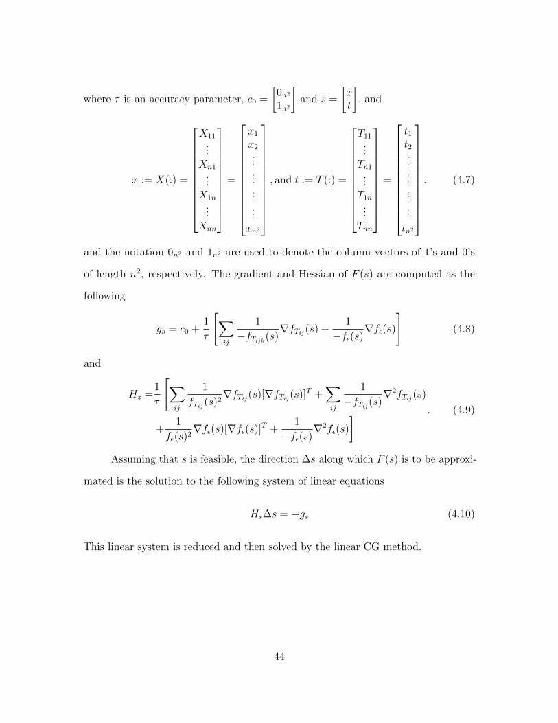
where τ is an accuracy parameter, c0 =

[0n2

1n2

]and s =

[xt

], and

x := X(:) =

X11...

Xn1...

X1n...

Xnn

=

x1

x2............

xn2

, and t := T (:) =

T11...

Tn1...

T1n...

Tnn

=

t1t2............tn2

. (4.7)

and the notation 0n2 and 1n2 are used to denote the column vectors of 1’s and 0’s

of length n2, respectively. The gradient and Hessian of F (s) are computed as the

following

gs = c0 +1

τ

[∑ij

1

−fTijk(s)∇fTij

(s) +1

−fϵ(s)∇fϵ(s)

](4.8)

and

Hz =1

τ

[∑ij

1

fTij(s)2∇fTij

(s)[∇fTij(s)]T +

∑ij

1

−fTij(s)∇2fTij

(s)

+1

fϵ(s)2∇fϵ(s)[∇fϵ(s)]T +

1

−fϵ(s)∇2fϵ(s)

] . (4.9)

Assuming that s is feasible, the direction ∆s along which F (s) is to be approxi-

mated is the solution to the following system of linear equations

Hs∆s = −gs (4.10)

This linear system is reduced and then solved by the linear CG method.

44

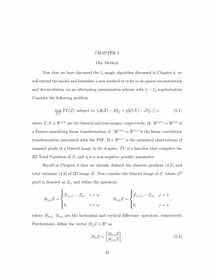
CHAPTER 5

Our Method

Now that we have discussed the ℓ1-magic algorithm discussed in Chapter 4, we

will extend the model and formulate a new method in order to do sparse reconstruction

and deconvolution via an alternating minimization scheme with ℓ1− ℓ2 regularization.

Consider the following problem

minZ,X

TV(Z) subject to ∥A(Z)−B∥2 + η∥C(X)− Z∥2 ≤ ϵ, (5.1)

where Z,X ∈ Rn×n are the blurred and true images, respectively, A : Rn×n 7→ Rn×n is

a Fourier sparsifying linear transformation, C : Rn×n 7→ Rn×n is the linear convolution

transformation associated with the PSF, B ∈ Rn×n is the measured observations of

sampled pixels of a blurred image in the k-space, TV is a function that computes the

2D Total Variation of Z, and η is a non-negative penalty parameter.

Recall in Chapter 4 that we already defined the discrete gradient (4.2) and

total variation (4.3) of 2D image X. Now consider the blurred image of Z, whose ijth

pixel is denoted as Zij and define the operators

Dh;ijZ =

Zi,j+1 − Zij, i < n

0, i = n

Dv;ijZ =

Zi+1,j − Zij, j < n

0, j = n

,

where Dh;ij, Dv;ij are the horizontal and vertical difference operators, respectively.

Furthermore, define the vector DijZ ∈ R2 as

DijZ =

[Dh;ijZDv;ijZ

], (5.2)

45

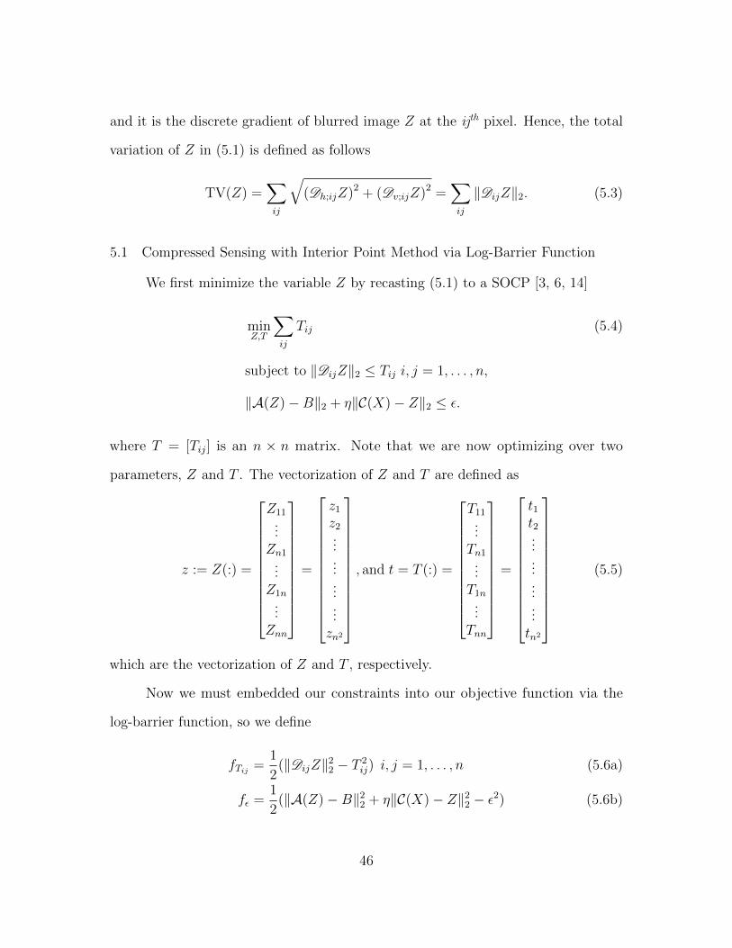
and it is the discrete gradient of blurred image Z at the ijth pixel. Hence, the total

variation of Z in (5.1) is defined as follows

TV(Z) =∑ij

√(Dh;ijZ)

2 + (Dv;ijZ)2 =

∑ij

∥DijZ∥2. (5.3)

5.1 Compressed Sensing with Interior Point Method via Log-Barrier Function

We first minimize the variable Z by recasting (5.1) to a SOCP [3, 6, 14]

minZ,T

∑ij

Tij (5.4)

subject to ∥DijZ∥2 ≤ Tij i, j = 1, . . . , n,

∥A(Z)−B∥2 + η∥C(X)− Z∥2 ≤ ϵ.

where T = [Tij] is an n × n matrix. Note that we are now optimizing over two

parameters, Z and T . The vectorization of Z and T are defined as

z := Z(:) =

Z11...

Zn1...

Z1n...

Znn

=

z1z2............

zn2

, and t = T (:) =

T11...

Tn1...

T1n...

Tnn

=

t1t2............tn2

(5.5)

which are the vectorization of Z and T , respectively.

Now we must embedded our constraints into our objective function via the

log-barrier function, so we define

fTij=

1

2(∥DijZ∥22 − T 2

ij) i, j = 1, . . . , n (5.6a)

fϵ =1

2(∥A(Z)−B∥22 + η∥C(X)− Z∥22 − ϵ2) (5.6b)

46

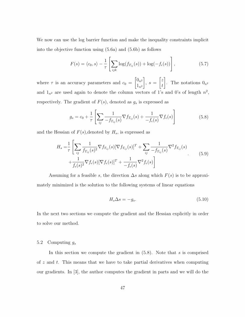
We now can use the log barrier function and make the inequality constraints implicit

into the objective function using (5.6a) and (5.6b) as follows

F (s) = ⟨c0, s⟩ −1

τ

[∑ijk

log(fTij(s)) + log(−fϵ(s))

], (5.7)

where τ is an accuracy parameters and c0 =

[0n2

1n2

], s =

[zt

]. The notations 0n2

and 1n2 are used again to denote the column vectors of 1’s and 0’s of length n2,

respectively. The gradient of F (s), denoted as gs is expressed as

gs = c0 +1

τ

[∑ij

1

−fTij(s)∇fTij

(s) +1

−fϵ(s)∇fϵ(s)

](5.8)

and the Hessian of F (s),denoted by Hs, is expressed as

Hs =1

τ

[∑ij

1

fTij(s)2∇fTij

(s)[∇fTij(s)]T +

∑ij

1

−fTij(s)∇2fTij

(s)

+1

fϵ(s)2∇fϵ(s)[∇fϵ(s)]T +

1

−fϵ(s)∇2fϵ(s)

] . (5.9)

Assuming for a feasible s, the direction ∆s along which F (s) is to be approxi-

mately minimized is the solution to the following systems of linear equations

Hs∆s = −gs. (5.10)

In the next two sections we compute the gradient and the Hessian explicitly in order

to solve our method.

5.2 Computing gs

In this section we compute the gradient in (5.8). Note that s is comprised

of z and t. This means that we have to take partial derivatives when computing

our gradients. In [3], the author computes the gradient in parts and we will do the

47

same here. We will compute the term∑

ij1

fTij (s)∇fTij

(s) first. Define the row vectors

Dh;ij, Dv;ij,∈ R1×n2such that

Dh;ijz = Dh;ijZ (5.11a)

Dv;ijz = Dv;ijZ. (5.11b)

We now can express fTijas

fTij=

1

2(

∥∥∥∥[Dh;ijzDv;ijz

]∥∥∥∥2

2

− T 2ij)

=1

2(∥Dijz∥22 − T 2

ij) i, j = 1, . . . , n, (5.12)

where Dij =

[Dh;ijZDv;ijZ

]. By expanding (3.14) we obtain the expression

fTij=

1

2(∥Dijz∥22 − T 2

ij)

=1

2((Dijz)

T (Dijz)− T 2ij)

=1

2(zTDT

ijDijz − T 2ij) i, j = 1, . . . , n. (5.13)

Thus, taking the gradient of fTijand noting that it is of quadratic form in z we can

write ∑ij

1

fTij(s)∇fTij

(s) =∑ij

1

fTij(s)

[DT

ijDijz−Tijδij

]=

[DT

hF−1t Dhz +DT

v F−1t Dvz

−F−1t t

](5.14)

where δij ∈ Rn2is a vector that is 1 in the ijth entry and 0 elsewhere, F−1

t =

diag(1 ⊘ fT ), where fT ∈ Rn2contains the fTij

elements listed in lexicographical

order according to their ijth indices. The ⊘ notation is used to denote element-wise

division, i.e. given vectors x and y, x ⊘ y = xi

yi. Finally, the Dh, Dv,∈ Rn2×n2

are

comprised of the row vectors Dh;ij, Dv;ij ∈ R1×n2, for i, j = 1, . . . , n, that have been

vectorized. Based on lexicographical ordering, we can express

Dh = B ⊗ In

48

Dv = In ⊗B,

where

B =

−1 1

. . . . . .

−1 10 0

∈ Rn×n.

We now compute the terms 1fϵ(s)∇fϵ(s). For implementation, we first note

that, A(Z) and C(X) are equivalent to matrix-vector multiplication, Az and Cx, by

formally writing Az := (A(Z))(:) and Cx := (C(X))(:). Similarly, we compare the

resulting vectors to the vectors b := B(:) and z := Z(:). Now we can expand the

equivalent fϵ expression as

fϵ =1

2(∥Az − b∥22 + η∥Cx− z∥22 − ϵ2)

=1

2((Az − b)T (Az − b) + η((Cx− b)T (Cx− b))− ϵ2)

=1

2(zTATAz − 2AT bz + bT b+ η(xTCTCx− 2zTCx+ zT z)− ϵ2). (5.15)

Taking the gradient of (5.15), we get

∇fϵ(s) =[ATAz − AT b+ η

2(−2Cx+ 2z)

0n2

]=

[AT (Az − b)− η(Cx− z)

0n2

]=

[AT r1 − ηr2

0n2

], (5.16)

where r1 = Az − b and r2 = Hx− z are residual terms and 0n2 ∈ Rn2. Note that AT

is equivalent to applying the tranpose operation of A that can be denoted as

AT r1 := (AT (R1))(:),

where AT : Rn×n 7→ Rn×n and R1 = A(Z)−B. Thus,

1

fϵ(s)∇fϵ(s) =

1

fϵ(z)

[AT r1 − ηr2

0n2

]. (5.17)

49

We are ready to compute gs for our reconstruction problem. Now substitute the

results of (5.14) and (5.17) into (5.8), we get that the gradient of our objective

function is

gs = c0 +1

τ

[∑ij

1

−fTij(s)∇fTij

(s) +1

−fϵ(s)∇fϵ(s)

]

=

[0n3

1n3

]+−1τ

([DT

hF−1t Dhz +DT

v F−1t Dvz

−F−1t t

]+

1

fϵ(s)

[AT r1 − ηr2

0n2

])=−1τ

[DT

hF−1t Dhz +DT

v F−1t Dvz +

1fϵ(s)

(AT r1 − ηr2)

−τ1n2 − F−1t t

]. (5.18)

5.3 Computing Hs

We now need to compute the Hessian in (5.9), Hs, but first we need to compute

four quantities:

1.∑

ij1

fTij (s)2∇fTij

(s)[∇fTij(s)]T

2.∑

ij1

−fTij (s)∇2fTij

(s)

3. 1fϵ(s)2∇fϵ(s)[∇fϵ(s)]T

4. 1−fϵ(s)

∇2fϵ(s)

We will begin by find quantities 1 and 3 since we already have expressions for the∑ij

1−fTij (s)

∇fTij(s) and 1

−fϵ(s)∇fϵ(s). By using expression (5.14), we get

∑ij

1

fTij(s)2∇fTij

(s)[∇fTij(s)]T =

[z

−F−1t t

] [zT −F−1

t tT ]], (5.19)

where z = DThF

−1t Dhz + DT

v F−1t Dvz. Computing the left top block matrix of the

resulting matrix is given by

zzT = (DThF

−1t Dhz +DT

v F−1t Dvz)(D

ThF

−1t Dhz +DT

v F−1t Dvz)

T

= (DThDhz +DT

v Dvz)F−1t F−1

t (DThDhz +DT

v Dv)T

= BF−2t BT , (5.20)

50

where B = DThΣh +DT

v Σv, with Σh = diag(Dhz) and Σv = diag(Dvz). Computing

the top right entry gives us

−zF−1t = −(DT

hF−1t Dhz +DT

v F−1t Dvz)F

−1t tT

= −BTF−2t (5.21)

where T = diag(t) and F−2t = diag(1⊘ f 2

t ). The remaining blocks are obvious, thus

we get

∑ij

1

fTij(s)2∇fTij

(s)[∇fTij(s)]T =

[BF−2

t BT −BTF−2t

−F−2t TBT F−2

t T 2

]. (5.22)

Now we examine how to compute the term 1fϵ(s)2∇fϵ(s)[∇fϵ(s)]T . Recall the

expression we obtained from (5.17), and plug it in to get

1

fϵ(s)2∇fϵ(s)[∇fϵ(s)]T =

1

fϵ(s)2

[AT r1 − ηr2

0

] [(AT r1 − ηr2)

T 0]

=1

fϵ(s)2

[(AT r1 − ηr2)(r

T1 A− ηrT2 ) 0

0 0

]. (5.23)

We now calculate the final terms of our Hessian:∑

ij1

−fTij (s)∇2fTij

(s) and 1−fϵ(s)

∇2fϵ(s).

Noting that the Hessian is the Jacobian of the gradient, we get that

∑ij

1

−fTij(s)∇2fTij

(s) =

[DT

h (−F−1t )Dh +DT

v (−F−1t )Dv 0

0 F−1t

], (5.24)

and

1

−fϵ(s)∇2fϵ(s) =

1

−fϵ(s)

[ATA+ ηIn 0

0 0

]. (5.25)

Note that ATAz + η := ((AT (A(Z))) + ηIn)(:) but for consistency we use ATA+ ηIn

in writing for the Hessian. We now have all the expression to compute Hs

Hs =1

τ

[∑ij

1

fTij(s)2∇fTij

(s)[∇fTij(s)]T +

∑ij

1

−fTij(s)∇2fTij

(s)

+1

fϵ(s)2∇fϵ(s)[∇fϵ(s)]T +

1

−fϵ(s)∇2fϵ(s)

]51

=1

τ

([BF−2

t BT −BTF−2T

−F−2t TBT F−2

t T 2

]+

[DT

h (−F−1t )Dh +DT

v (−F−1t )Dv 0

0 F−1t

]+

[fϵ(z)

−2(AT r1 − ηr2)(rT1 A− ηrT2 ) 0

0 0

]+

[−fϵ(s)−1(ATA+ ηIn) 0

0 0

])=

1

τ

[H11 −BTF−2

t

−F−2t TBT F−2

t T 2 + F−1t

], (5.26)

where

H11 = BF−2t BT +DT

h (−F−1t )Dh +DT

v (−F−1t )Dv + fϵ(z)

−2(AT r1 − ηr2)(rT1 A− ηrT2 )

− fϵ(z)−1(ATA+ ηIn) (5.27)

As in [3], we will simplify the notation here. So define

Σ12 = −TF−2t , (5.28a)

Σ22 = F−2t T + F−2

t , (5.28b)

and thus

Hs =1

τ

[H11 BΣ12

ΣBT Σ22

]. (5.29)

5.4 Reduce the System

In the previous section, we found the expressions for gs and Hs stated in (5.18)

and (5.29). We now use Newton’s method to solve a large scale system, so substituting

(5.18) and (5.29) in (5.10) yields[H11 BΣ12

ΣBT Σ22

] [∆z∆t

]=

[DT

hF−1t Dhz +DT

v F−1t Dvz +

1fϵ(s)

(AT r1 − ηr2)

−τ − F−1t t

]:=

[ν1ν2

]. (5.30)

We begin to reduce the system of equation by eliminating ∆t in equation (5.30)

Σ12BT∆z + Σ22∆t = ν2 =⇒ ∆t = Σ−1

22 (ν2 − Σ12BT∆z). (5.31)

52

Using this expression results in system reductions as the following

H11∆z +BΣ12∆t = ν1

=⇒ H11∆z +BΣ12[Σ−122 (ν2 − Σ12B

T∆z)] = ν1

=⇒ H11∆z +BΣ12Σ−122 ν2 −BΣ12Σ22B

T∆z = ν1

=⇒ (H11 −BΣ212Σ

−122 B

T )∆z = ν1 −BΣ12Σ−122 ν2

=⇒ H11∆z = ν1, (5.32)

where H11 = H11 − BΣ212Σ

−122 B

T and ν1 = ν1 − BΣ12Σ−122 ν2. In order to make the

coding of the problem easier to implement we get a more simplified expression for H;

refer to [3].

5.5 Deblurring Step via Regularization

After each log-barrier iteration that has been solved by Newton’s method, the

approximation of n×n compressed and blurred image Z is updated. We then use this

updated Z to solve the least squares problem using the singular value decomposition

minx∥Cx− z∥2, (5.33)

to update the approximation of the n × n ground truth image X. Recall that the

matrix C ∈ RN×N is the blurring matrix associated with the unwanted PSF and its

structure is dependent on the boundary conditions imposed with N = n2. It is a

known fact that the blurring matrix is highly ill-conditioned [23, 30]. That is, the

naive solution we get by the singular value decomposition

xnaive = C−1z = V Σ−1UT z (5.34)

maybe contaminated by unwanted noise due to division of small singular values, 1σ1.

53

Filtering or regularization methods are used to reduce the effects of inverted

noise by enforcing regularity conditions on the solution. The two regularization

methods we focus on are

� TSVD, and

� Tikhonov regularization.

The degree of regularization enforced by these two techniques are governed by a

regularization parameter as discussed in Chapter 3. This regularization parameter

must be chosen carefully and we will discuss potential ways to find an appropriate

regularization parameter later on.

The singular value decomposition can be used for general problems or for

problems that have a Kronecker structure (i.e., separable blurs) [36, 56] with the

filtered solution of the form

xfilt =N∑i=1

ϕiuTi z

σi

vi, (5.35)

while the unitary spectral decomposition can be used when we can use FFT algorithms,

such as the case for BCCB matrices:

xfilt =N∑i=1

ϕiuTi z

λi

ui, (5.36)

with filter factor ϕi of the forms

ϕi =

1, i = 1, . . . , k

0, i = k + 1 . . . N

and ϕi =

σ2i

σ2i +α2 , σi > 0

0, σi = 0,

for TSVD and Tikhonov regularization, respectively, for the SVD, and

ϕi =

1, i = 1, . . . , k

0, i = k + 1 . . . N

and ϕi =

|λi|2

|λi|2+α2 , |λi| > 0

0, |λi| = 0

for the unitary spectral decomposition.

54

For the remainder of the discussion, we discuss the SVD to simplify things but

can also be applied to the unitary spectral decomposition. So now we rewrite the

filtered solution as

xfilt = V ΦΣ−1z, (5.37)

where Φ ∈ RN×N is a diagonal matrix whose entries are the filter factors ϕi for the

particular regularization methods. That is, the diagonal entries are of Φ are of the

form

Φii =

1, i = 1, . . . , k

0, i = k + 1 . . . N

(5.38)

for TSVD and

Φii =σ2i

σ2i + α2

(5.39)

for Tikhonov regularization. Observe that

xfilt = V ΦΣ−1UT z

= V ΦΣ−1UT (zexact + e)

= V ΦΣ−1UT zexact + V ΦΣ−1UT e

= V ΦΣ−1UTCxexact + V ΦΣ−1UT e

= V ΦΣ−1UT (UΣV T )xexact + V ΦΣ−1UT e

= V ΦV Txexact + V ΦΣ−1UT e,

and therefore the error of the filtered solution is given by

xexact − xfilt = (IN − V ΦV T )xexact − V ΦΣ−1UT e. (5.40)

Here, the error consist of two types of contributions, the regularization error and

perturbation error [30].

55

� The regularization error, represented by the first component, (IN−V ΦV T )xexact,

is caused by the using a regularized inverse matrix V ΦΣ−1UT (rather than

that of the original inverse matrix (C−1 = V Σ−1UT ). The matrix V ΦV T

describes the mapping between xexact and xfilt. If the diagonal entries of Φ are

relatively small, then the regularization error becomes large. On the contrary,

if Φ approaches the identity matrix IN , then the regularization error becomes

small.

� The perturbation error, V ΦΣ−1UT , consists of the inverted noise and filtered

noise. If Φ = 0, then the perturbation error is zero. When the most of the entries

of Φ are small, then the inverted noise is heavily dampened and perturbation

error is small.

The change of Φ and the two types of errors are dependent on the changes in

the regularization parameter. The relationship can be summed up as follows

1. When many filter factors ϕi are close to 1, then the regularization error is

small, while the perturbation error is large. Thus, our reconstructed image is

undersmoothed.

2. When too few filters factors ϕi are close 1, then the perturbation error is small,

while the regularization error is large. Thus, our reconstructed image will be

oversmoothed.

A proper choice of the truncation parameter k or Tikhonov regularization parameter

α is needed to balance these two types of error.

5.5.1 Parameter of Choice Method

We present two different parameter choice methods: user experimentation

and the generalized cross validation (GCV) [26, 30, 41]. In user experimentation,

the user chooses the regularization parameter that they feel results in the best

56

reconstruction. However, this is a tedious process as one is selecting the parameter

ad hocly.

The idea of the GCV is that, if one omits a data value, then a good value of

the parameter α should be able to predict the missing data point. According to the

authors of [26], this can be achieved by choosing the parameter that minimizes the

GCV function

G(α) =∥(IN − CV ΦΣ−1UT )z∥22

(trace(IN − CV ΦΣ−1UT ))2. (5.41)

Note that we abuse notation here for parameter α as we are using it as the regular-

ization parameter for both TSVD and Tikhonov, with α = 1kwhere k is the TSVD

cutoff. The author of [30] gives a formulation of the numerator

∥IN − CV ΦΣ−1UT )z∥22 = ∥b− Cxfilt∥22 =N∑i=1

((1− ϕi)uTi z)

2 (5.42)

and that the denominator can be evaluated easily as the trace of matrix is the sum

of its main diagonal elements

trace(IN − CV ΦΣ−1UT ) = trace(IN − UΣV TV ΦΣ−1UT )

= trace(U(IN − Φ)UT )

= trace(IN − Φ)

= N −N∑i=1

ϕi. (5.43)

Hence,

G(α) =∥(IN×N − CV ΦΣ−1UT )z∥22

(trace(IN×N − CV ΦΣ−1UT ))2=

∑Ni=1((1− ϕi)u

Ti z)

2

N −∑N

i=1 ϕi

. (5.44)

In particular, we want to find the minimum of the functions,

G(k) =1

N − k

N∑i=k+1

(uTi z)

2, (5.45)

57

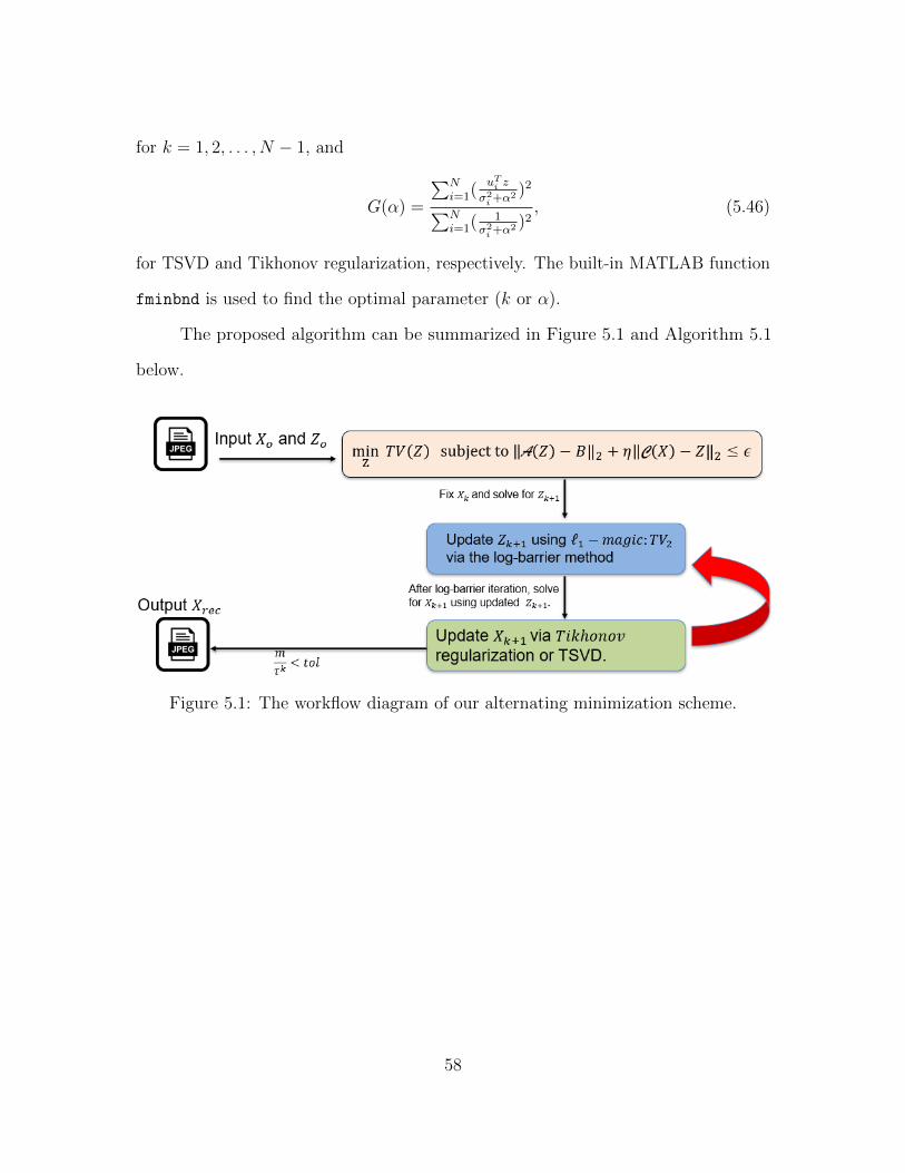
for k = 1, 2, . . . , N − 1, and

G(α) =

∑Ni=1(

uTi z

σ2i +α2 )

2∑Ni=1(

1σ2i +α2 )2

, (5.46)

for TSVD and Tikhonov regularization, respectively. The built-in MATLAB function

fminbnd is used to find the optimal parameter (k or α).

The proposed algorithm can be summarized in Figure 5.1 and Algorithm 5.1

below.

Figure 5.1: The workflow diagram of our alternating minimization scheme.

58

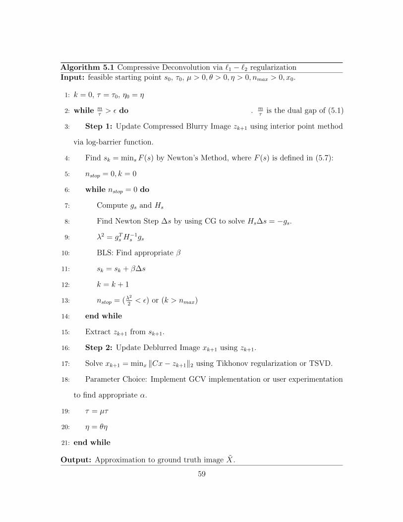
Algorithm 5.1 Compressive Deconvolution via ℓ1 − ℓ2 regularization

Input: feasible starting point s0, τ0, µ > 0, θ > 0, η > 0, nmax > 0, x0.

1: k = 0, τ = τ0, η0 = η

2: while mτ> ϵ do ▷ m

τis the dual gap of (5.1)

3: Step 1: Update Compressed Blurry Image zk+1 using interior point method

via log-barrier function.

4: Find sk = mins F (s) by Newton’s Method, where F (s) is defined in (5.7):

5: nstop = 0, k = 0

6: while nstop = 0 do

7: Compute gs and Hs

8: Find Newton Step ∆s by using CG to solve Hs∆s = −gs.

9: λ2 = gTs H−1s gs

10: BLS: Find appropriate β

11: sk = sk + β∆s

12: k = k + 1

13: nstop = (λ2

2< ϵ) or (k > nmax)

14: end while

15: Extract zk+1 from sk+1.

16: Step 2: Update Deblurred Image xk+1 using zk+1.

17: Solve xk+1 = minx ∥Cx− zk+1∥2 using Tikhonov regularization or TSVD.

18: Parameter Choice: Implement GCV implementation or user experimentation

to find appropriate α.

19: τ = µτ

20: η = θη

21: end while

Output: Approximation to ground truth image X.

59

CHAPTER 6

Numerical Results

This chapter discusses some results of the recovery of a 2D brain image from

subsampled and blurred data in k−space. To evaluate the quality of the reconstructed

images, we used three imaging metrics: (1) the structural similarity (SSIM) index

[51]; (2) the peak signal-to-noise ratio; and (3) the human perception.

6.1 Image Reconstruction Metrics

The peak signal-to-noise ratio (PSNR) is the ratio between the maximum

possible power (value) of a signal and the power of the noise that affects the quality of

its representation. Due to signals having a wide dynamic range, the PSNR is typically

expressed in terms of logarithmic decibel scale (dB). A higher PSNR typically indicates

a better image reconstruction. However, there have been cases where images with

higher PSNR values look worse than those with a lower PSNR value, and ultimately,

human perception is the deciding factoring [3, 35].

Given two m× n 2D images X and Y , we first compute the mean square error

(MSE) as

MSE =1

nm

m∑i=1

n∑j=1

((X(i, j)− Y (i, j))2. (6.1)

The PSNR is defined as

PSNR = 10 log10

( I2max

MSE

), (6.2)

where I2max is the maximum possible pixel value of the image on Y . Implementation

of the PSNR can be done in MATLAB using the built-in function psnr.

60

The other metric used to evaluate our reconstruction is the structural similar-

ity (SSIM) index, and it improves upon the deficiencies of PSNR as the PSNR does

not take into account any biological factors of the human vision system [51, 52]. The

SSIM index is used to evaluate the similarity of the intensity, contrast, and structure

between the ground-truth image (fully sampled) and the image reconstructed by our

algorithm using compressed and blurred samples. The SSIM is defined as follows

SSIM(X, Y ) =(2µXµY + c1)(2σXY + c2)

(µ2X + µ2

Y + c1)(σ2X + σ2

Y + c2), (6.3)

whereX and Y denote the ground truth and reconstructed images, respectively, µ’s are

the averages of the respective image intensities, σ’s are the variances, and c1 = (k1L)2,

c2 = (k2L)2 are two variables that stabilizes the division by the denominator. L is

the dynamic range of the pixel values with k1 = 0.01 and k2 = 0.03. Two identical

grayscale images will have a maximum SSIM value of 1, while a value 0 indicates

they are two completely different images. The code for SSIM can be download from

www.mathworks.com/matlabcentral/answers/9217-need-ssim-m-code.

The last metric is the human perception. No matter what the PSNR or SSIM

tell us, we get the final say on how the reconstruction compares to the ground truth.

This will become more evident as we at look some of the images we recovered from

our method.

6.2 Performance of Reconstruction

The imaging data that is presented in this section comes from the Radiology

229: MRI Signals and Sequences course at Standford University provided Drs. Daniel

Ennis and Brian Hargreaves 1. It is a 2D brain image that was collected in 2016 and

contains 512× 512 complex data that was fully sampled in the k-space.

1Their dataset can be found at https://github.com/mribri999/MRSignalsSeqs

61

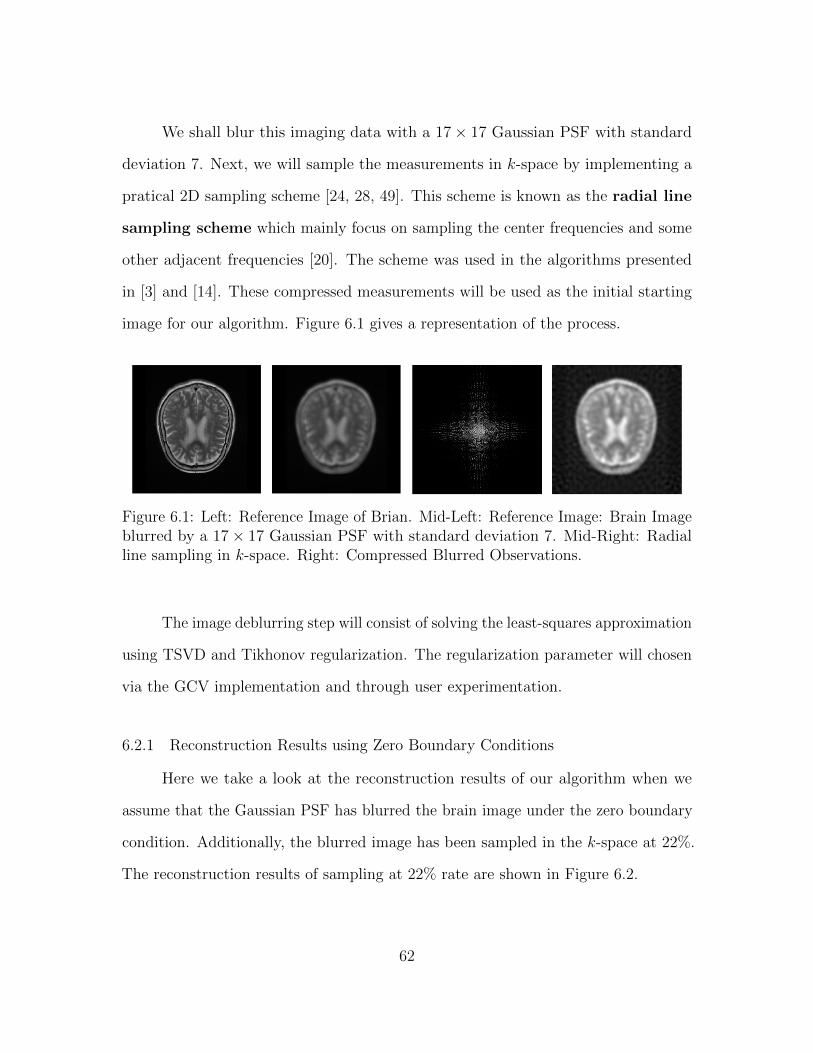
We shall blur this imaging data with a 17× 17 Gaussian PSF with standard

deviation 7. Next, we will sample the measurements in k-space by implementing a

pratical 2D sampling scheme [24, 28, 49]. This scheme is known as the radial line

sampling scheme which mainly focus on sampling the center frequencies and some

other adjacent frequencies [20]. The scheme was used in the algorithms presented

in [3] and [14]. These compressed measurements will be used as the initial starting

image for our algorithm. Figure 6.1 gives a representation of the process.

Figure 6.1: Left: Reference Image of Brian. Mid-Left: Reference Image: Brain Imageblurred by a 17× 17 Gaussian PSF with standard deviation 7. Mid-Right: Radialline sampling in k-space. Right: Compressed Blurred Observations.

The image deblurring step will consist of solving the least-squares approximation

using TSVD and Tikhonov regularization. The regularization parameter will chosen

via the GCV implementation and through user experimentation.

6.2.1 Reconstruction Results using Zero Boundary Conditions

Here we take a look at the reconstruction results of our algorithm when we

assume that the Gaussian PSF has blurred the brain image under the zero boundary

condition. Additionally, the blurred image has been sampled in the k-space at 22%.

The reconstruction results of sampling at 22% rate are shown in Figure 6.2.

62

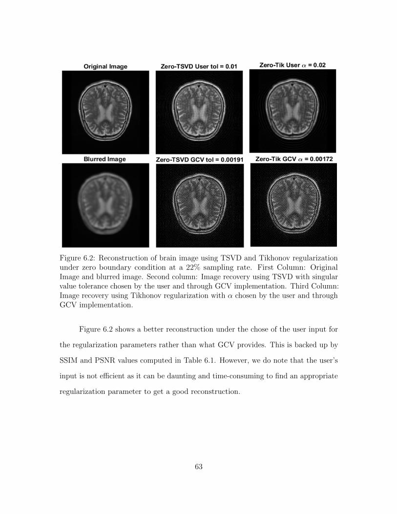
Figure 6.2: Reconstruction of brain image using TSVD and Tikhonov regularizationunder zero boundary condition at a 22% sampling rate. First Column: OriginalImage and blurred image. Second column: Image recovery using TSVD with singularvalue tolerance chosen by the user and through GCV implementation. Third Column:Image recovery using Tikhonov regularization with α chosen by the user and throughGCV implementation.

Figure 6.2 shows a better reconstruction under the chose of the user input for

the regularization parameters rather than what GCV provides. This is backed up by

SSIM and PSNR values computed in Table 6.1. However, we do note that the user’s

input is not efficient as it can be daunting and time-consuming to find an appropriate

regularization parameter to get a good reconstruction.

63

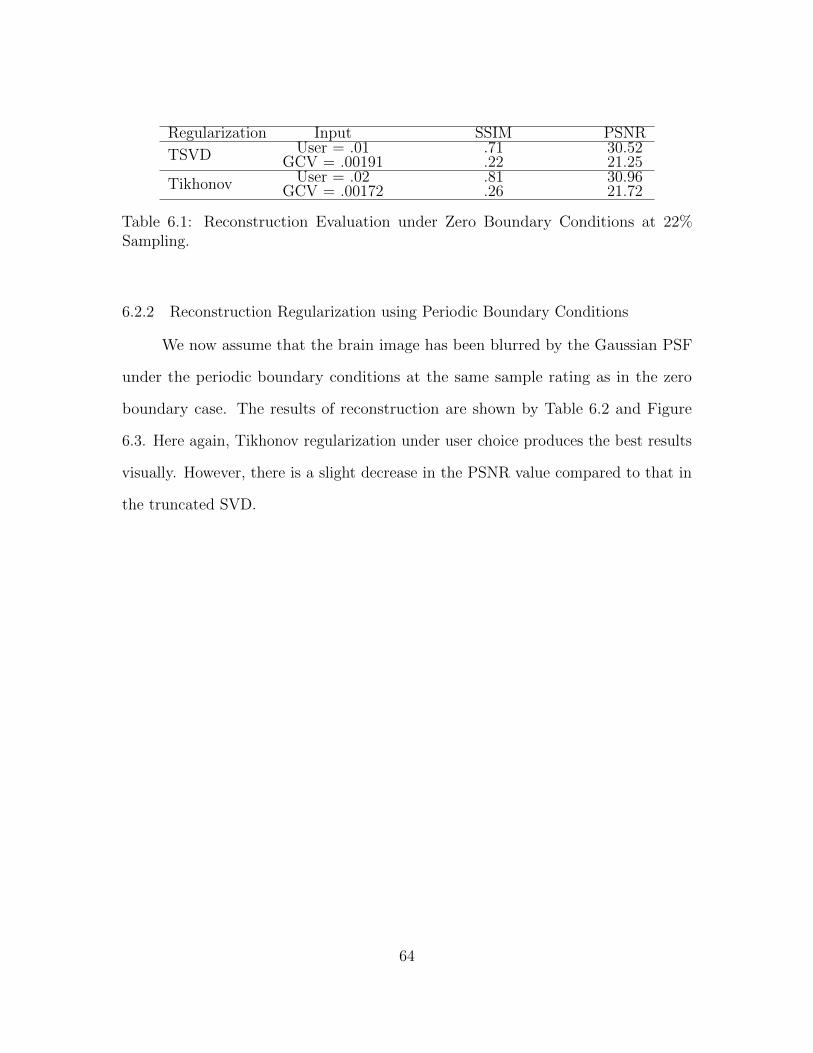
Regularization Input SSIM PSNR

TSVD User = .01 .71 30.52GCV = .00191 .22 21.25

Tikhonov User = .02 .81 30.96GCV = .00172 .26 21.72

Table 6.1: Reconstruction Evaluation under Zero Boundary Conditions at 22%Sampling.

6.2.2 Reconstruction Regularization using Periodic Boundary Conditions

We now assume that the brain image has been blurred by the Gaussian PSF

under the periodic boundary conditions at the same sample rating as in the zero

boundary case. The results of reconstruction are shown by Table 6.2 and Figure

6.3. Here again, Tikhonov regularization under user choice produces the best results

visually. However, there is a slight decrease in the PSNR value compared to that in

the truncated SVD.

64

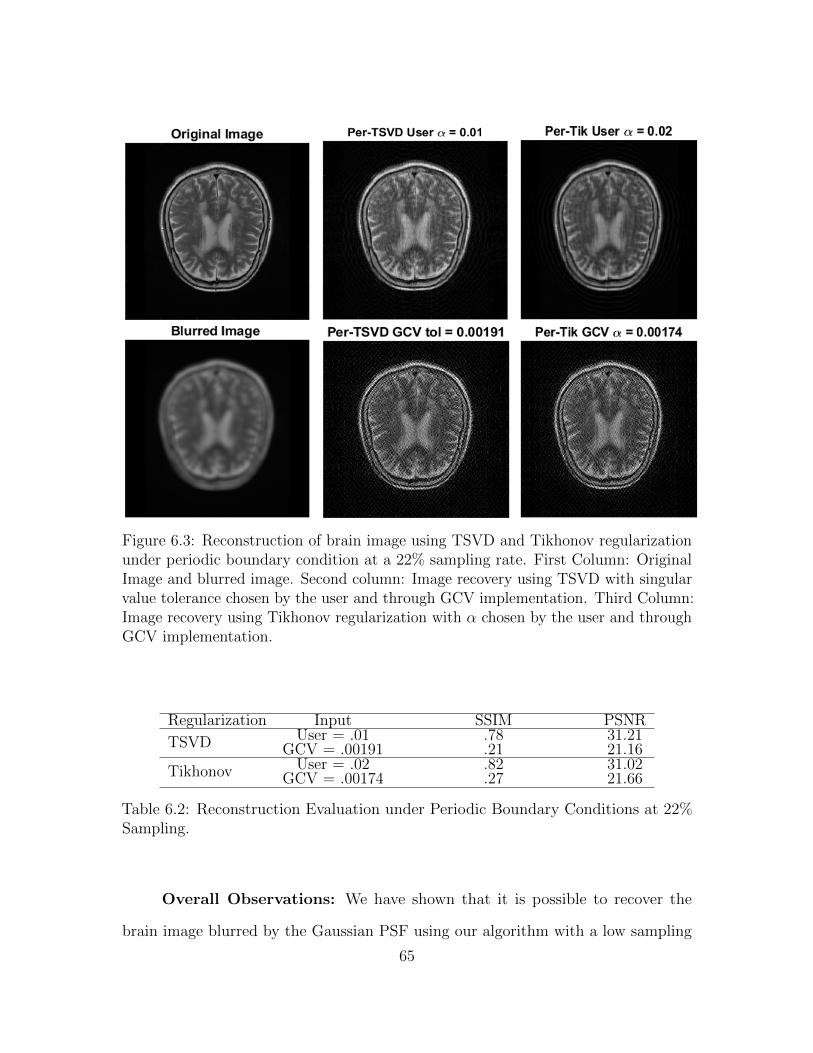
Figure 6.3: Reconstruction of brain image using TSVD and Tikhonov regularizationunder periodic boundary condition at a 22% sampling rate. First Column: OriginalImage and blurred image. Second column: Image recovery using TSVD with singularvalue tolerance chosen by the user and through GCV implementation. Third Column:Image recovery using Tikhonov regularization with α chosen by the user and throughGCV implementation.

Regularization Input SSIM PSNR

TSVD User = .01 .78 31.21GCV = .00191 .21 21.16

Tikhonov User = .02 .82 31.02GCV = .00174 .27 21.66

Table 6.2: Reconstruction Evaluation under Periodic Boundary Conditions at 22%Sampling.

Overall Observations: We have shown that it is possible to recover the

brain image blurred by the Gaussian PSF using our algorithm with a low sampling

65

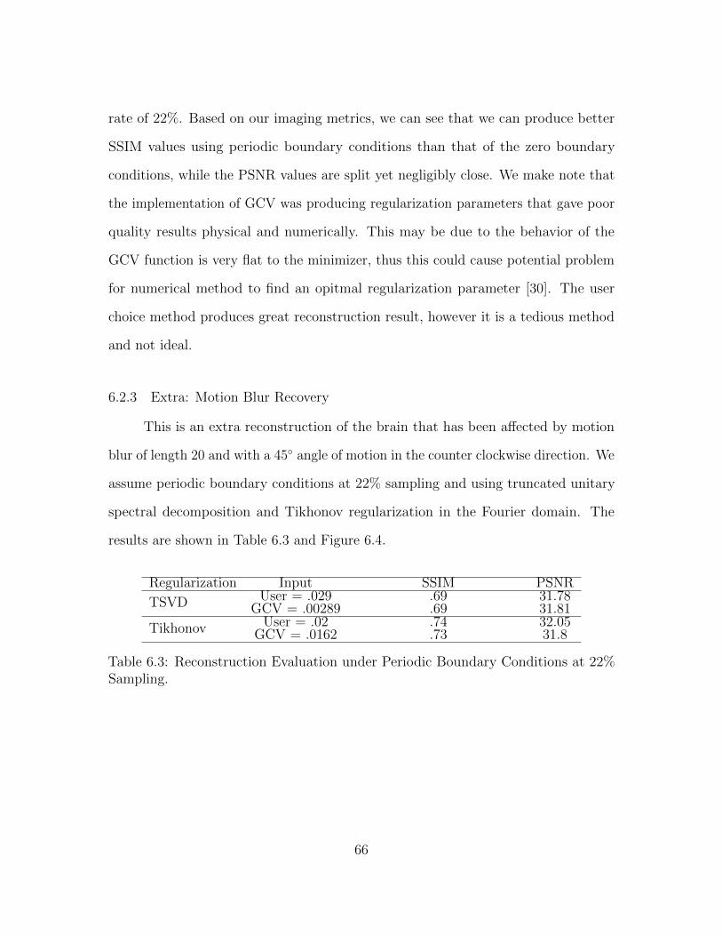
rate of 22%. Based on our imaging metrics, we can see that we can produce better

SSIM values using periodic boundary conditions than that of the zero boundary

conditions, while the PSNR values are split yet negligibly close. We make note that

the implementation of GCV was producing regularization parameters that gave poor

quality results physical and numerically. This may be due to the behavior of the

GCV function is very flat to the minimizer, thus this could cause potential problem

for numerical method to find an opitmal regularization parameter [30]. The user

choice method produces great reconstruction result, however it is a tedious method

and not ideal.

6.2.3 Extra: Motion Blur Recovery

This is an extra reconstruction of the brain that has been affected by motion

blur of length 20 and with a 45◦ angle of motion in the counter clockwise direction. We

assume periodic boundary conditions at 22% sampling and using truncated unitary

spectral decomposition and Tikhonov regularization in the Fourier domain. The

results are shown in Table 6.3 and Figure 6.4.

Regularization Input SSIM PSNR

TSVD User = .029 .69 31.78GCV = .00289 .69 31.81

Tikhonov User = .02 .74 32.05GCV = .0162 .73 31.8

Table 6.3: Reconstruction Evaluation under Periodic Boundary Conditions at 22%Sampling.

66

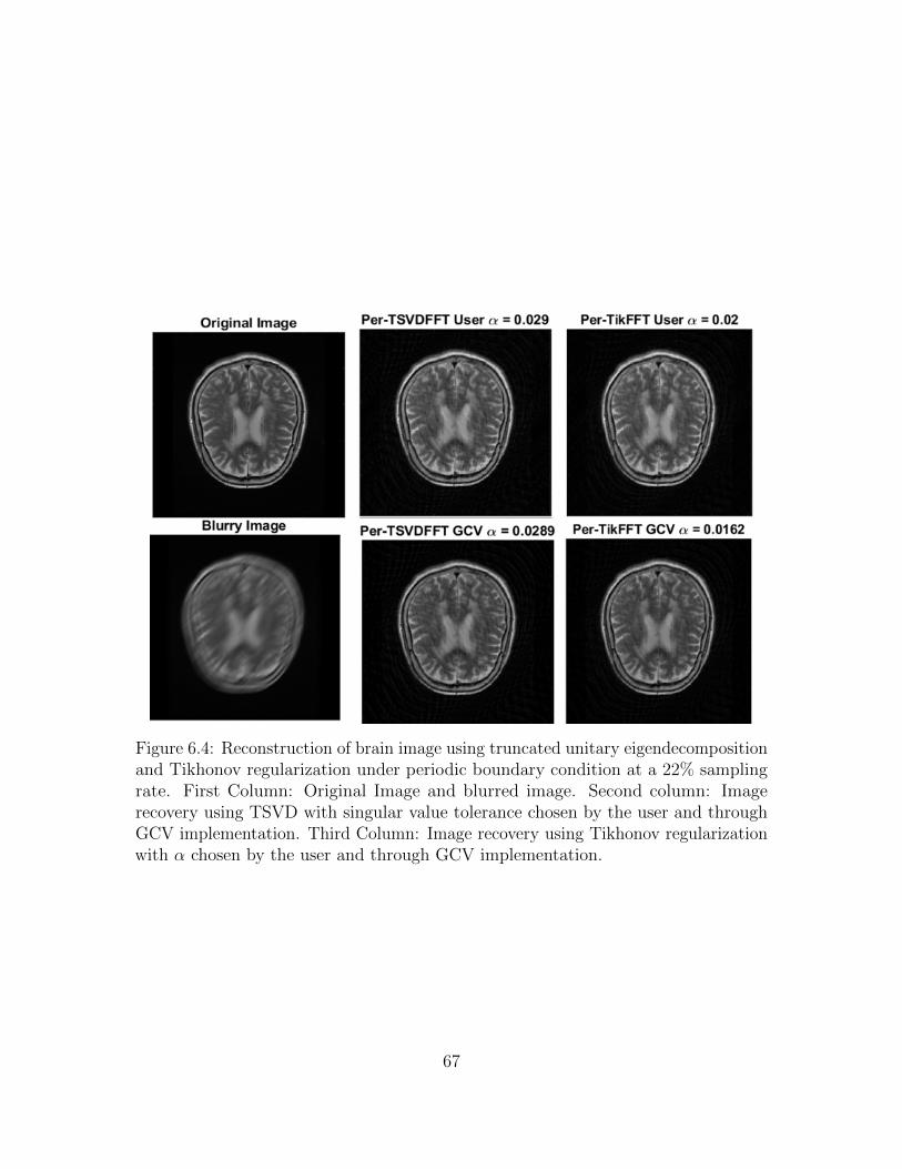
Figure 6.4: Reconstruction of brain image using truncated unitary eigendecompositionand Tikhonov regularization under periodic boundary condition at a 22% samplingrate. First Column: Original Image and blurred image. Second column: Imagerecovery using TSVD with singular value tolerance chosen by the user and throughGCV implementation. Third Column: Image recovery using Tikhonov regularizationwith α chosen by the user and through GCV implementation.

67

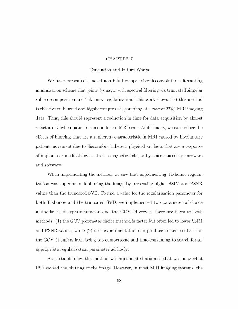
CHAPTER 7

Conclusion and Future Works

We have presented a novel non-blind compressive deconvolution alternating

minimization scheme that joints ℓ1-magic with spectral filtering via truncated singular

value decomposition and Tikhonov regularization. This work shows that this method

is effective on blurred and highly compressed (sampling at a rate of 22%) MRI imaging

data. Thus, this should represent a reduction in time for data acquisition by almost

a factor of 5 when patients come in for an MRI scan. Additionally, we can reduce the

effects of blurring that are an inherent characteristic in MRI caused by involuntary

patient movement due to discomfort, inherent physical artifacts that are a response

of implants or medical devices to the magnetic field, or by noise caused by hardware

and software.

When implementing the method, we saw that implementing Tikhonov regular-

ization was superior in deblurring the image by presenting higher SSIM and PSNR

values than the truncated SVD. To find a value for the regularization parameter for

both Tikhonov and the truncated SVD, we implemented two parameter of choice

methods: user experimentation and the GCV. However, there are flaws to both

methods: (1) the GCV parameter choice method is faster but often led to lower SSIM

and PSNR values, while (2) user experimentation can produce better results than

the GCV, it suffers from being too cumbersome and time-consuming to search for an

appropriate regularization parameter ad hocly.

As it stands now, the method we implemented assumes that we know what

PSF caused the blurring of the image. However, in most MRI imaging systems, the

68

PSF is typically unknown. In the future, we want to extend this method to perform

blind compressive deconvolution, and we plan to refine this method for 3D images.

Additionally, we plan to incorporate machine learning and create an AI method that

performs auto compressive deconvolution for respiratory motion related blurring in

3T MRI imaging that affects extraction and evaluation of metabolic information

about fat infiltration and muscle atrophy in the shoulder.

69

REFERENCES

[1] Amizic, B., Spinoulas, L., Molina, R., and Katsaggelos, A., Compressive Blind

Image Deconvolution. IEEE Transactions on Image Processing 22, 2013: 3994-4006.

[2] Apostol, M., Mathematical Analysis. Addison-Welsey, 2nd edition, 1974.

[3] Au, M., Three dimensional image reconstruction (3DIRECT) of sparse signal with

MRI application. Ph.D. thesis, The University of Texas at Arlington, 2016.

[4] Axler, S., Linear Algebra Done Right. Undergraduate Texts in Mathematics, 2014.

[5] Blackledge, J., Digital Image processing. Horwood Publishing, vol: ISBN:1-898563-

49-7, 2005.

[6] Boyd, S. and Vandenberghe, L., Convex Optimization. Cambridge University

Press, 2004.

[7] Burden, R. L. and Faires, J. D., Numerical Analysis. Cengage Learning, 2011.

[8] Campisi, P., and Egiazarian, K., Blind Image Deconvolution: Theory and Appli-

cations. CRC Press, 2007. https://doi.org/10.1201/9781420007299

[9] Elvidge, J., Applications of Nuclear Magnetic Resonance Spectroscopy in Organic

Chemistry, 1970.

[10] Candes, E., The restricted isometry property and its implications for compressed

sensing, Comptes Rendus Mathematique, vol. 346, no. 2, pp. 589–592, 2008.

[11] Candes, E.,Romberg, J., and Tao, T., Robust uncertainty principles: Exact

signal reconstruction from highly incomplete frequency information, IEEE Trans.

Inf. Theory, vol. 52, no. 2, pp. 489–509, 2006.

70

[12] Candes, E., Tao, T., and Romberg, J., Stable signal recovery from incomplete and

inaccurate measurements, Comm. Pure Appl. Math., vol. 59, no. 8, pp. 1207–1223,

2006.

[13] Candes, E. and Tao, T., Near optimal signal recovery from random projections:

Universal encoding strategies? IEEE Trans. Inf. Theory, vol. 52, no. 12, pp.

5406–5425, 2006.

[14] Candes, E. and Romberg, J., l1 -Magic: Recovery of sparse signals via convex

programming. Available online1. 2005.

[15] Candes, E. and Wakin, M., An Introduction To Compressive Sampling,

IEEE Signal Processing Magazine, vol. 25, no. 2, pp. 21-30, 2008, doi:

10.1109/MSP.2007.914731.

[16] Chen, S., Basis pursuit, Ph.D. dissertation, CA, 1995.

[17] Chen, Z., Basarab, A. and Kouame, D., Compressive Deconvolution in Medical

Ultrasound Imaging, IEEE Transactions on Medical Imaging, vol. 35, no. 3, pp.

728-737, 2016, doi: 10.1109/TMI.2015.2493241

[18] Cheney, E. W., and Kincaid, D., Numerical Mathematics and Computing. Brook-

s/Cole, 2020.

[19] Chowdhury, M., Qin, J., and Lou, Y., Non-blind and Blind Deconvolution under

Poisson Noise using Fractional-order Total Variation, Journal of Mathematical

Imaging and Vision, 2020.

[20] Dale, B. M., Lewin, J. S., and Duerk, J. L., Optimal design of k-space trajectories

using a multi-objective genetic algorithm. Magn. Reson. Med., 52(4):831–841, 2004.

[21] Egiazarian, K., Foi, A., and Katkovnik, V., Compressed sensing image recon-

struction via recursive spatially adaptive filtering, IEEE International Conference

on Image Processing, vol. 1, pp. 549–552, 2007.

1https://statweb.stanford.edu/ candes/software/l1magic/downloads/l1magic.pdf

71

[22] Engl, H. W., Hanke, M. and Neubauer, M., Regularization of inverse problems.

Kluwer, 1996.

[23] Freeman, T., The Mathematics of Medical Imaging: A Beginner’s Guide. Springer,

2nd Edition, 2015.

[24] Glover, G. H. and Pauly, J. M., Projection reconstruction technique for reduction

of motion effects in MRI. Magn. Reson. Med., 28:275–289, 1992.

[25] Golub, G. E. and Von Loan, C. F., Matrix Computations. The Johns Hopkins

University Press, 1989.

[26] Golub, G. H., Heath, M., and Wahba, G., Generalized cross-validation as a

method for choosing a good ridge parameter. Technometrics, 21:215–223, 1979.

[27] Gray, R. M., Toeplitz and Circulant Matrices: A Review.Foundations and Trends

in Communications and Information Theory: Vol. 2: No. 3, pp 155-239, 2006.

[28] Greiser, A. and von Kienlin, M., Efficient k-space sampling by density-weighted

phase-encoding. Magn. Reson. Med., 50(6):1266–1275, 2003.

[29] Gonzalez, R. and Woods, R., Digital Image Processing. 2nd Edition. Prentice

Hall, 2004.

[30] Hansen, P.C., Nagy, J., and O’Leary, D., Deblurring Images: Matrices, Spectra,

and Filtering. Philadelphia: SIAM, Society for Industrial and Applied Mathematics.

Available online 2. 2006.

[31] Hauser, K., Multivariate Newton’s Method and Quasi-Newton methods. Algo-

rithms for Optimization and Learning CSB553. Retrieved from Duke University.

Delivered January 25, 2012.

[32] Havsteen, I., Ohlhues, A., Madsen, K. H., Nybing, J. D., Christensen, H.,

and Christensen, A. Are Movement Artifacts in Magnetic Resonance Imag-

2https://epubs.siam.org/doi/book/10.1137/1.9780898718874?mobileUi=0

72

ing a Real Problem?-A Narrative Review. Frontiers in neurology, 8, 232. 2017.

https://doi.org/10.3389/fneur.2017.00232

[33] Heiland, S., From A as in aliasing to Z as in zipper: artifacts in MRI. Clin

Neuroradiol, 2008; 1:25-36.

[34] Hestenes, M. R., and Stiefel, E., Methods of conjugate gradients for solving

linear systems. Journal of Research of the National Bureau of Standards, Vol. 49,

p. 409, 2006.

[35] Huynh-Thu, Q. and Ghanbari, M., Scope of validity of PSNR in image/video

quality assessment. Electronics Letters, 44(13):800 – 801, 2008.

[36] Kamm, J. and Nagy, J.M., Kronecker Product and SVD Approximations in

Image Restoration. Linear Algebra and Its Applications, vol. 284, no. 1–3, 1998,

pp. 177–92. Crossref, doi:10.1016/s0024-3795(98)10024-1.

[37] Leon, J. S., Linear Algebra with Applications.6th Edition. 2002.

[38] Lustig, M., Donoho, D., and Pauly, J. M., Sparse MRI: The application of

compressed sensing for rapid MR imaging. Magn Reson Med, vol. 58,pp. 1182–1195.

2007.

[39] Moratal, D., Valles-Luch, A., Martı-Bonmatı, L., and Brummer, M.,

k-space tutorial: an MRI educational tool for a better understanding

of k-space. Biomedical imaging and intervention journal, 2008, 4(1), e15.

https://doi.org/10.2349/biij.4.1.e15

[40] Nagy, J.G. and O’Leary, D.P., Fast iterative image restoration with a spatially

varying PSF, Proc.SPIE 3162, Advanced Signal Processing: Algorithms, Architec-

tures, and Implementations VII, 1997; doi: 10.1117/12.279513

[41] Nguyen, T. and Chung, J., Learning regularization parameters for general-form

Tikhonov. Inverse Problems 33:7, 074004. 2007.

73

[42] Nocedal, J. and Wright, S. J., Numerical Optimization. Springer. 2nd edition.

2006.

[43] Pruessmann, K. P., Weiger, M., Scheidegger, M. B., and Boesiger, P., Sense:

sensitivity encoding for fast mri., Magnetic Resonance in Medicine, vol. 42,no. 5,

pp. 952–962, 1999.

[44] Richardson, W. H., Bayesian-based iterative method of image restoration. Journal

of the Optical Society of America, 62(1):55–59, 1972.

[45] Roggemann, M. C. and Welsh, B., Imaging Through Turbulence. CRC Press,

Boca Raton, FL, 1996.

[46] Smith, S. W., The Scientist and Engineer’s Guide to Digital Signal Processing.

California Technical Pub, 1997.

[47] Sun, W. and Yuan, Y-X., Optimization Theory and Methods: Nonlinear Pro-

gramming. Springer. 2006.

[48] Tibshirani, R., Regression Shrinkage and Selection Via the Lasso. Journal of

the Royal Statistical Society: Series B (Methodological), vol. 58, no. 1, 1996, pp.

267–88. Crossref, doi:10.1111/j.2517-6161.1996.tb02080.x.

[49] Tsai, C. M. and Nishimura, D. G., Reduced aliasing artifacts using variable

density k-space sampling trajectories. Magn. Reson. Med., 43(3):452–458, 2000.

[50] Varah, J. M., Pitfalls in the numerical solution of linear ill-posed problems. SIAM

J. Sci. Stat. Comput., 4:164–176, 1983.

[51] Wang, Z., Bovik, A.C., Sheikh, H.R., and Simoncelli, E.P., Image quality assess-

ment: from error visibility to structural similarity. IEEE Trans. Image Process. 13,

600–612, 2004.

[52] Wang, Z., Simoncelli, E. P., and Bovik, A. C., Multiscale structural similarity for

image quality assessment,The Thrity-Seventh Asilomar Conference on Signals, Sys-

tems & Computers, 2003, pp. 1398-1402 Vol.2, doi: 10.1109/ACSSC.2003.1292216.

74

[53] Wiener, N., Extrapolation, interpolation, and smoothing of stationary time series:

With engineering applications. MIT Press, 113(21):1043–54, 1949.

[54] Yang, Jungang, Tian Jin, Chao Xiao, and Xiaotao Huang., Compressed Sensing

Radar Imaging: Fundamentals, Challenges, and Advances” Sensors 2019, no. 14:

3100. https://doi.org/10.3390/s19143100

[55] Ye, J.C., Compressed sensing MRI: a review from signal processing perspective.

BMC biomed eng1, 8, 2019. https://doi.org/10.1186/s42490-019-0006-z

[56] Zhang, Y., Li, Y., Wang, S., and Wang, C. -X., Image Restoration Based

on the Convolution Kernel Matrix Reconstructed by Kronecker Product,IEEE

5th International Conference on Signal and Image Processing (ICSIP), 2020, pp.

185-189, doi: 10.1109/ICSIP49896.2020.9339404.

75

BIOGRAPHICAL STATEMENT

Talon Johnson was born in Dallas, Texas, in 1994. He earned a Bachelor of

Science in Mathematics at Morehouse College in Atlanta, GA of May 2016. As an

undergraduate, he participated in research projects through the National Science

Foundation sponsored Math Summer Program In Research And Learning (Math

SPIRAL) and the National Institute for Mathematical and Biological Synthesis

(NIMBioS). He served as the vice president of Pi Mu Epsilon Delta Chapter and has

received a Best Presentation Award at the Joint Mathematics Meeting in 2015. After

receiving his Bachelors degree, Talon entered the mathematical doctoral program at

the University of Texas at Arlington (UTA), where he worked under the supervision

of Jianzhong Su on projects related to math biology and computational neurosciences.

Talon was awarded with the Michael B. and Wanda G. Ray Graduate Fellowship and

the Graduate Assistance in Areas of National Need (GAANN) Fellowship. During his

graduate studies, he became a member of the UTA American Mathematical Society

and the Society of Industrial and Applied Mathematics, co-president of the College

of Science Black Graduate Student Association, and was a mentor for the Army

Educational Outreach Program.

76