energies

Article

Comparison of Four Methods for Borehole HeatExchanger Sizing Subject to Thermal Response TestParameter Estimation

Xuedan Zhang 1 , Tiantian Zhang 2,3, Bingxi Li 1,* and Yiqiang Jiang 2,3,*1 School of Energy Science and Engineering, Harbin Institute of Technology, Harbin 150001, China;

dreamscometrue2008@163.com2 School of Architecture, Harbin Institute of Technology, Harbin 150001, China; x418298537@163.com3 Key Laboratory of Cold Region Urban and Rural Human Settlement Environment Science and Technology,

Ministry of Industry and Information Technology, Harbin 150001, China* Correspondence: libx@hit.edu.cn (B.L.); jyq7245@sina.com (Y.J.)

Received: 16 August 2019; Accepted: 22 October 2019; Published: 25 October 2019�����������������

Abstract: The impact of different parameter estimation results on the design length of a borehole heatexchanger has received very little attention. This paper provides an in-depth investigation of thisproblem, together with a full presentation of six data interpretation models and a comprehensivecomparison of four representative sizing methods and their inter models. Six heat transfer modelswere employed to interpret the same thermal response test data set. It was found that the estimatedparameters varied with the data interpretation model. The relative difference in borehole thermalresistance reached 34.4%, and this value was 11.9% for soil thermal conductivity. The resultingparameter estimation results were used to simulate mean fluid temperature for a single borehole andthen to determine the borehole length for a large bore field. The variations in these two correlatedparameters caused about 15% and 5% relative difference in mean fluid temperature in the beginningand at the end of the simulation period, respectively. For computing the borehole design length,software-based methods were more sensitive to the influence of parameter estimation results thansimple equation-based methods. It is expected that these comparisons will be beneficial to anyoneinvolved in the design of ground-coupled heat pump systems.

Keywords: borehole heat exchanger; thermal response test; parameter estimation; designand simulation

1. Introduction

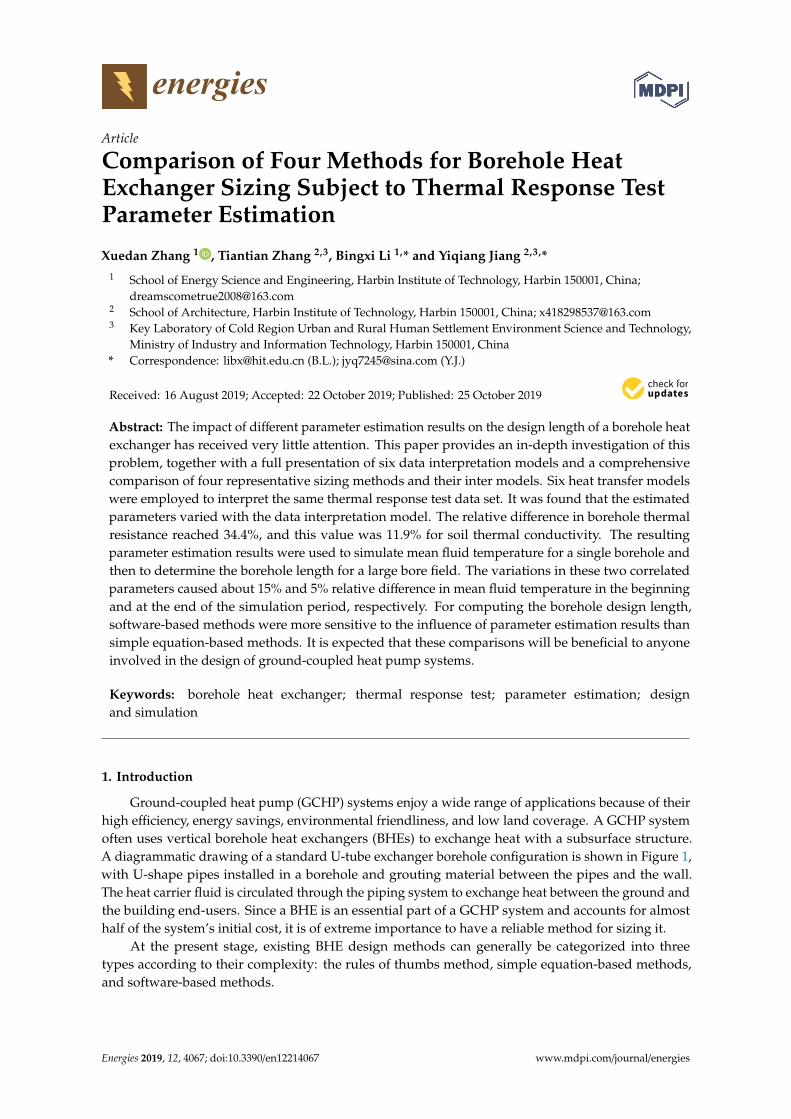
Ground-coupled heat pump (GCHP) systems enjoy a wide range of applications because of theirhigh efficiency, energy savings, environmental friendliness, and low land coverage. A GCHP systemoften uses vertical borehole heat exchangers (BHEs) to exchange heat with a subsurface structure.A diagrammatic drawing of a standard U-tube exchanger borehole configuration is shown in Figure 1,with U-shape pipes installed in a borehole and grouting material between the pipes and the wall.The heat carrier fluid is circulated through the piping system to exchange heat between the ground andthe building end-users. Since a BHE is an essential part of a GCHP system and accounts for almosthalf of the system’s initial cost, it is of extreme importance to have a reliable method for sizing it.

At the present stage, existing BHE design methods can generally be categorized into threetypes according to their complexity: the rules of thumbs method, simple equation-based methods,and software-based methods.

Energies 2019, 12, 4067; doi:10.3390/en12214067 www.mdpi.com/journal/energies

Energies 2019, 12, 4067 2 of 30Energies 2019, 12, x FOR PEER REVIEW 2 of 29

Figure 1. Layout of a typical U-tube configuration.

Simple equation-based methods are widely used in practice for their quick calculations. A significant feature of simple equation-based methods is that the number of heat pulses adopted is limited. An example of such a method is the ASHRAE method [2], which originated from Kavanaugh and Rafferty’s work [3] and is now described in the ASHRAE Handbook. Another representative is the IGSHPA method [4], which used to be a standard method to size BHEs in North America. The design equations of such methods are consolidated from analytical heat transfer models through a series of simplifications; they also retain a limited number of heat pulse parameters, and they determine the length of the BHE required for both heating and cooling (the larger value is retained) to achieve the desired system performance on the basis of a worst-case scenario.

Software-based methods are somewhat more complicated because they often employ a more complex underlying model that can more realistically consider load representation, bore field geometry, borehole configuration, soil and fluid thermal properties, and dynamic heat pump characteristics, among other factors. Herein, this kind of method mainly refers to those methods in which monthly or hourly loads are used, not only software or simulation tool-based ones. These design tools or simulation programs compute the mean fluid temperatures of the heat pump(s) after inputting the system parameters and then compare the simulated minimum or maximum fluid temperature of the heat pump(s) with the user-specified constraint values. The smallest length that satisfies the requirement is sought iteratively. A number of design and analysis computer programs are available—such as EED, GLHEPRO using Eskilson’s non-dimensional temperature response factor g-functions [5], and TRNSYS software with the embedded duct ground heat storage model (DST) component developed by Pahud and Hellstrom [6,7].

Each method has its own inter model, referring to a combination of mathematical equations or the calculation steps to obtain design borehole length. For each method, its inter model is often formulated from a specified underlying heat transfer model [8,9]. Assessing the performances of these methods is a tough task. On the one hand, it is necessary to figure out how each method works since the underlying models of the methods differ in their settings of basic assumptions, initial and boundary conditions, simplified methods, as well as solutions. On the other hand, a range of system parameters should be collected to complete a large number of comparison runs; these parameters include all the physical and thermal properties of different materials and equipment related to the calculation of building thermal loads, interpretation of thermal response test data, and rating of the heat pump, and other factors. Validating the methods experimentally is even more difficult because of a lack of sufficient operation data support. Consequently, only a handful of studies have compared multiple BHE design methods or experimentally validated different methods.

Thornton et al. [10] compared the results of five practical vertical BHE sizing programs with the results of a calibrated simulation model, and Shonder et al. [11] added one more program to the updated versions of these five in a follow-up study. One main conclusion made by the authors is that the existing commercial programs yield inconsistent results, with differences of about 6–16%.

Figure 1. Layout of a typical U-tube configuration.

In the rule of thumb method, the required length that satisfies the peak cooling or heating loaddemand is determined according to an estimated heat transfer rate (with a unit of W/m). This methodrelies mostly on the past project experience of the designers and lacks a scientific basis. Thus, it is notconsidered in this paper [1,2].

Simple equation-based methods are widely used in practice for their quick calculations.A significant feature of simple equation-based methods is that the number of heat pulses adopted islimited. An example of such a method is the ASHRAE method [2], which originated from Kavanaughand Rafferty’s work [3] and is now described in the ASHRAE Handbook. Another representative is theIGSHPA method [4], which used to be a standard method to size BHEs in North America. The designequations of such methods are consolidated from analytical heat transfer models through a series ofsimplifications; they also retain a limited number of heat pulse parameters, and they determine thelength of the BHE required for both heating and cooling (the larger value is retained) to achieve thedesired system performance on the basis of a worst-case scenario.

Software-based methods are somewhat more complicated because they often employ a morecomplex underlying model that can more realistically consider load representation, bore field geometry,borehole configuration, soil and fluid thermal properties, and dynamic heat pump characteristics,among other factors. Herein, this kind of method mainly refers to those methods in which monthlyor hourly loads are used, not only software or simulation tool-based ones. These design tools orsimulation programs compute the mean fluid temperatures of the heat pump(s) after inputting thesystem parameters and then compare the simulated minimum or maximum fluid temperature of theheat pump(s) with the user-specified constraint values. The smallest length that satisfies the requirementis sought iteratively. A number of design and analysis computer programs are available—such as EED,GLHEPRO using Eskilson’s non-dimensional temperature response factor g-functions [5], and TRNSYSsoftware with the embedded duct ground heat storage model (DST) component developed by Pahudand Hellstrom [6,7].

Each method has its own inter model, referring to a combination of mathematical equations or thecalculation steps to obtain design borehole length. For each method, its inter model is often formulatedfrom a specified underlying heat transfer model [8,9]. Assessing the performances of these methods is atough task. On the one hand, it is necessary to figure out how each method works since the underlyingmodels of the methods differ in their settings of basic assumptions, initial and boundary conditions,simplified methods, as well as solutions. On the other hand, a range of system parameters should becollected to complete a large number of comparison runs; these parameters include all the physical andthermal properties of different materials and equipment related to the calculation of building thermalloads, interpretation of thermal response test data, and rating of the heat pump, and other factors.Validating the methods experimentally is even more difficult because of a lack of sufficient operation

Energies 2019, 12, 4067 3 of 30

data support. Consequently, only a handful of studies have compared multiple BHE design methodsor experimentally validated different methods.

Thornton et al. [10] compared the results of five practical vertical BHE sizing programs withthe results of a calibrated simulation model, and Shonder et al. [11] added one more program to theupdated versions of these five in a follow-up study. One main conclusion made by the authors is thatthe existing commercial programs yield inconsistent results, with differences of about 6–16%. However,in these studies, the programs used for sizing were referenced by a letter designation (A–F), withoutmuch focus on the design algorithms. Kurevija et al. [12] performed a comparison between Eskilson’sg-function method and the ASHRAE method for one building in Croatia and showed that the ASHRAEmethod produced smaller sizes for a 30-year design. A comparison between these two methods usingexperimental data sets for four locations was carried out by Cullin et al. [13], who showed that theASHRAE method produced errors from –21% to 167%. Similar comparisons [14] have been performedfor simulated buildings and different kinds of design methods. However, these comparisons havegiven little attention to the inter models and the design algorithms themselves.

In the design of vertical GCHPs, accurate knowledge of soil thermal properties is critical. In practice,a thermal response test (TRT) is usually used to provide important design parameters for a GCHPsystem. In most cases, a TRT is used to estimate both borehole thermal resistance and soil thermalconductivity, which are then used in the design calculations of BHEs. This technology is realized byinstalling a pilot borehole of approximately the same size and depth as those planned for the project,recording temperatures and flow rates measured during the test, comparing the tested data with thatcalculated from a selected heat transfer model, and then estimating ground thermal properties usinga parameter estimation (PE) method. ASHRAE suggests that the line source, the cylindrical, or anumerical algorithm be applied and that, when possible, more than one of these methods be applied toenhance the reported accuracy. However, a tricky issue has long been overlooked: When applying morethan one inverse method, should the estimated parameters be averaged? Or should a more convincingresult be selected? Furthermore, a consistent problem still arises between performing independentmeasurements of ground thermal properties and applying these properties to determine boreholelength for a BHE. For example, Beier maintained that the calculation method of fluid temperatureevolution should be consistent in both the test analysis and the design approach [15]; otherwise,significant errors will be introduced to the design. Although there are relevant studies dealing with thecomparison of TRT interpretation models [16–18], few have concentrated on the influence of TRTPEmodels on the BHE system design. Are the heat transfer model used in TRT data interpretation and theunderlying model in the design calculation based on a consistent assumption? How much impact willit have if the two models do not match each other? Alternatively, under what circumstances will theinconsistency problem significantly affect the final borehole length result? Under what circumstanceswill it have little impact? These are all open questions at this moment.

The above analysis reveals that although various kinds of heat transfer models and sizing methodshave been developed for the design and analysis of BHEs and GCHP systems, little attention has beenpaid to comparing them, especially with the aim of thoroughly understanding the basic formulationsand fundamental principles of these methods. To the best of our knowledge, to date, there has been nolumped assessment of different types of BHE design methods that have comprehensively comparedtheir underlying model performances during TRT interpretation. Accordingly, this paper attemptsto evaluate different types of BHE design methods in principle and compare the behaviors of theirunderlying inter models. Most importantly, this paper tries to fill a gap in the literature by investigatingthe influence of different TRTPE results on the temperature field simulation for a single borehole,as well as on the design of the borehole length for a bore field.

2. Heat Transfer Models for TRTPE

The TRT was first developed by Mogenson [19] and has since become a routine method that isused throughout the world to obtain information about ground thermal properties [20]. As mentioned

Energies 2019, 12, 4067 4 of 30

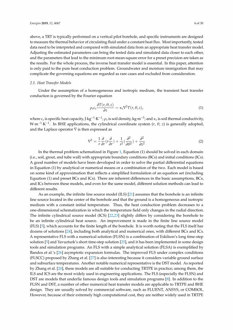
above, a TRT is typically performed on a vertical pilot borehole, and specific instruments are designedto measure the thermal behavior of circulating fluid under a constant heat flux. Most importantly, testeddata need to be interpreted and compared with simulated data from an appropriate heat transfer model.Adjusting the estimated parameters can bring the tested data and simulated data closer to each other,and the parameters that lead to the minimum root-mean-square error for a preset precision are taken asthe results. For the whole process, the inverse heat transfer model is essential. In this paper, attentionis only paid to the pure heat conduction problem. Groundwater and moisture immigration that maycomplicate the governing equations are regarded as rare cases and excluded from consideration.

2.1. Heat Transfer Models

Under the assumption of a homogeneous and isotropic medium, the transient heat transferconduction is governed by the Fourier equation

ρscs∂T(r,θ, z)

∂τ= κs∇

2T(r,θ, z), (1)

where cs is specific heat capacity, J·kg−1·K−1; ρs is soil density, kg·m−3; and κs is soil thermal conductivity,

W·m−1·K−1. In BHE applications, the cylindrical coordinate system (r, θ, z) is generally adopted,

and the Laplace operator ∇ is then expressed as

∇2 =

1r∂∂r

(r∂∂r

) +1r2 (

∂2

∂θ2 ) +∂2

∂z2 (2)

In the thermal problem schematized in Figure 1, Equation (1) should be solved in each domain(i.e., soil, grout, and tube wall) with appropriate boundary conditions (BCs) and initial conditions (ICs).A good number of models have been developed in order to solve the partial differential equationsin Equation (1) by analytical or numerical means or a combination of the two. Each model is basedon some kind of approximation that reflects a simplified formulation of an equation set (includingEquation (1) and preset BCs and ICs). There are inherent differences in the basic assumptions, BCs,and ICs between these models, and even for the same model, different solution methods can lead todifferent results.

As an example, the infinite line source model (ILS) [21] assumes that the borehole is an infiniteline source located in the center of the borehole and that the ground is a homogeneous and isotropicmedium with a constant initial temperature. Thus, the heat conduction problem decreases to aone-dimensional schematization in which the temperature field only changes in the radial direction.The infinite cylindrical source model (ICS) [22,23] slightly differs by considering the borehole tobe an infinite cylindrical heat source. An improvement is made in the finite line source model(FLS) [5], which accounts for the finite length of the borehole. It is worth noting that the FLS itself hasdozens of solutions [24], including both analytical and numerical ones, with different BCs and ICs.A representative FLS with a numerical solution (FLSN) is a combination of Eskilson’s long time-stepsolution [5] and Yavuzturk’s short time-step solution [25], and it has been implemented in some designtools and simulation programs. An FLS with a simple analytical solution (FLSA) is exemplified byBandos et al.’s [26] asymptotic expansion formulas. The improved FLS under complex conditions(FLSCC) proposed by Zhang et al. [27] is also interesting because it considers variable ground surfaceand subsurface temperatures. Another notable numerical representative is the DST model. As reportedby Zhang et al. [20], these models are all suitable for conducting TRTPE in practice; among them, theILS and ICS are the most widely used in engineering applications. The FLS (especially the FLSN) andDST are models that underlie famous design tools and simulation programs [8]. In addition to theFLSN and DST, a number of other numerical heat transfer models are applicable to TRTPE and BHEdesign. They are usually solved by commercial software, such as FLUENT, ANSYS, or COMSOL.However, because of their extremely high computational cost, they are neither widely used in TRTPE

Energies 2019, 12, 4067 5 of 30

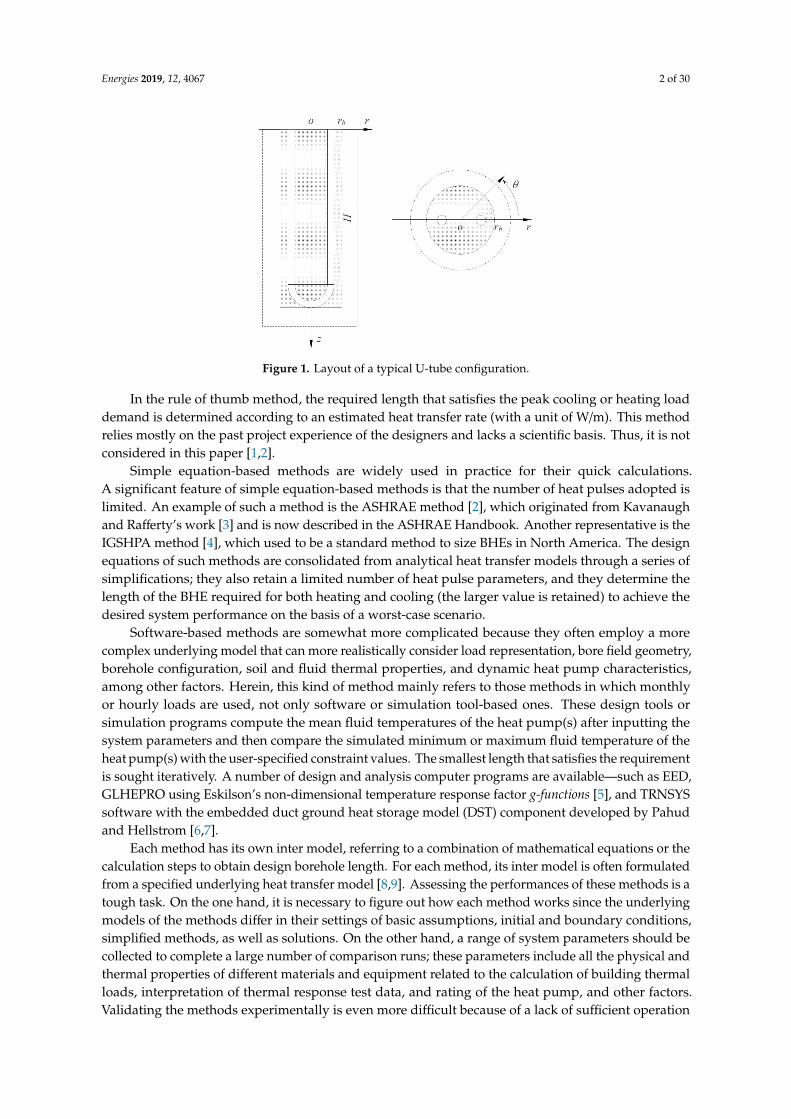
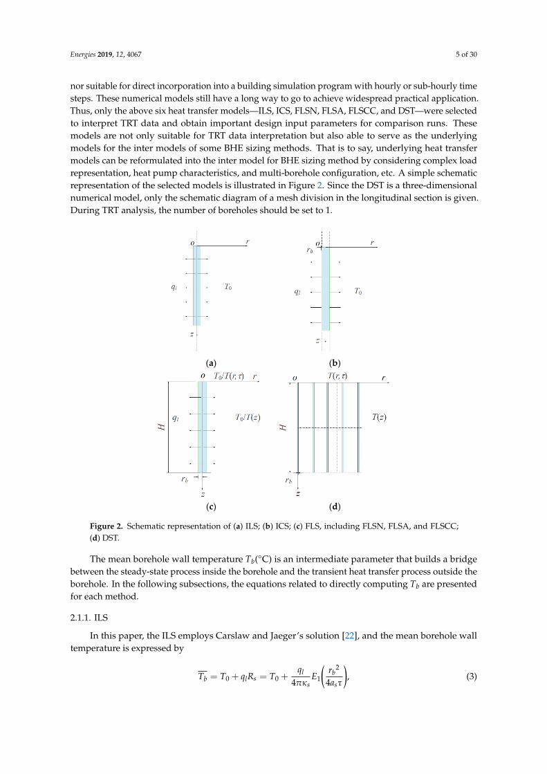
nor suitable for direct incorporation into a building simulation program with hourly or sub-hourly timesteps. These numerical models still have a long way to go to achieve widespread practical application.Thus, only the above six heat transfer models—ILS, ICS, FLSN, FLSA, FLSCC, and DST—were selectedto interpret TRT data and obtain important design input parameters for comparison runs. Thesemodels are not only suitable for TRT data interpretation but also able to serve as the underlyingmodels for the inter models of some BHE sizing methods. That is to say, underlying heat transfermodels can be reformulated into the inter model for BHE sizing method by considering complex loadrepresentation, heat pump characteristics, and multi-borehole configuration, etc. A simple schematicrepresentation of the selected models is illustrated in Figure 2. Since the DST is a three-dimensionalnumerical model, only the schematic diagram of a mesh division in the longitudinal section is given.During TRT analysis, the number of boreholes should be set to 1.

Energies 2019, 12, x FOR PEER REVIEW 5 of 29

Figure 2. Since the DST is a three-dimensional numerical model, only the schematic diagram of a mesh division in the longitudinal section is given. During TRT analysis, the number of boreholes should be set to 1.

(a) (b)

(c) (d)

Figure 2. Schematic representation of (a) ILS; (b) ICS; (c) FLS, including FLSN, FLSA, and FLSCC; (d) DST.

The mean borehole wall temperature T—

b (˚C) is an intermediate parameter that builds a bridge between the steady-state process inside the borehole and the transient heat transfer process outside

the borehole. In the following subsections, the equations related to directly computing T—

b are presented for each method.

2.1.1. ILS

In this paper, the ILS employs Carslaw and Jaeger’s solution [22], and the mean borehole wall temperature is expressed by

0 0

2

14 4l

b l sb

s s

qT T q R T rEaπ τκ

+ = +

= , (3)

where T0 refers to undisturbed ground temperature, °C; ql is the heat transfer rate, W�m−1; rb is the borehole radius, m; Rs is the equivalent thermal resistance of soil, K�m�W−1; and αs is soil thermal diffusivity, m²�s−1

= /s s s scκα ρ (4)

The exponential integral E1 in Equation (4) is computed by means of a power series expansion

2

2 2 2

11

4

( 1)ln4 4 ! 4

τ

γτ τ τ

−∞ ∞

=

− = = − − − ⋅ b

s

nu nb b b

nrs s sa

r r reE dua u a n n a , (5)

where γ is Euler’s constant, 0.5772.

Figure 2. Schematic representation of (a) ILS; (b) ICS; (c) FLS, including FLSN, FLSA, and FLSCC;(d) DST.

The mean borehole wall temperature Tb(◦C) is an intermediate parameter that builds a bridgebetween the steady-state process inside the borehole and the transient heat transfer process outside theborehole. In the following subsections, the equations related to directly computing Tb are presentedfor each method.

2.1.1. ILS

In this paper, the ILS employs Carslaw and Jaeger’s solution [22], and the mean borehole walltemperature is expressed by

Tb = T0 + qlRs = T0 +ql

4πκsE1

(rb

2

4asτ

), (3)

Energies 2019, 12, 4067 6 of 30

where T0 refers to undisturbed ground temperature, ◦C; ql is the heat transfer rate, W·m−1; rb is theborehole radius, m; Rs is the equivalent thermal resistance of soil, K·m·W−1; and αs is soil thermaldiffusivity, m2

·s−1

αs = κs/ρscs (4)

The exponential integral E1 in Equation (4) is computed by means of a power series expansion

E1

(rb

2

4asτ

)=

∞∫rb

2

4asτ

e−u

udu = − ln

(rb

2

4asτ

)− γ−

∞∑n=1

[(−1)n

n · n!

(rb

2

4asτ

)n], (5)

where γ is Euler’s constant, 0.5772.

2.1.2. ICS

Instead of complex integral expressions with Bessel functions, tabulated values at a specificdimensionless radius [23], or fitting formulae [28], the solution of the ICS utilizes the equation proposedby Baudoin [29], expressed by

Tb = T0 + qlRs = T0 + qlG(τ)

κs= T0 +

ql

2πκsrb

10∑j=1

[V j

jK0(ω jr)

ω jK1(ω jrb)

], (6)

ω j =

√j ln(2)αsτ

, (7)

V j =

min( j,5)∑k=Int( j+1

2 )

(−1) j−5k5(2k)!(5− k)!(k− 1)!k!( j− k)!(2k− j)!

, (8)

where K0 and K1 are modified Bessel functions of the second kind of order 0 and 1, respectively.The term G(τ)/κs is the equivalent thermal resistance of soil Rs, K·m·W−1.

2.1.3. FLSN

Calculating the solution of FLSN can be facilitated by using a combination of the short time-stepg-function from Yavuzturk’s numerical solution [25] and the long time-step g-function from Eskilson [5]proposed by Maestre et al. [30], expressed as

Tb = T0 +ql

2πκsg(ττss

,rbH

), (9)

where H is the borehole depth, m. The boundaries of the unsteady state τmin (s) and the steady stateτss (s) are defined as

τmin = 5rb2/αs, (10)

τss = H2/9αs (11)

When τ < τmin,

g(ττss

, rbH

)= gst

(ττss

, rbH

)= β1,FLSN ln4

(ττss

)+ β2,FLSN ln3

(ττss

)+β3,FLSN ln2

(ττss

)+ β4,FLSN ln

(ττss

)+ β5,FLSN − ln

( rb0.0005H

) (12)

where βi,FLSN is a fitting parameter for i =1 – 5.

Energies 2019, 12, 4067 7 of 30

When τ > τmin,

glt

(ττss

,rbH

)=

ln(

H2rb

)+ 1

2 ln(ττss

)τmin < τ < τss

ln(

H2rb

)τ > τss

(13)

This treatment with the FLSN is, in fact, implemented analytically. As a result, it can be easilyused for TRTPE, together with an optimization algorithm.

2.1.4. FLSA

The solution of FLSA employs the findings of Bandos et al. [26], as illustrated in Equations (14)and (15).

When 5τmin << τ << τss/9,

Tb =ql

4πκs

ln 36τH2

τssrb2 − γ+

3rbH −

18√π

√4ττss

−1√π

rb2

2H2

√τss4τ +

rb2

H2τss36τ

(14)

When τ >> τss/9,

Tb =ql

4πκs

4sinh−1 H

2rb− 2sinh−1 3H

2rb+

3rbH − 4

√1 + rb

2

H2

+

√4 + rb

2

H2 −τss

3/2

324τ3/2 √π

[1− τss(1+rb

2/H2)60τ

] (15)

2.1.5. FLSCC

The FLSCC is an FLS model under more complex ICs and BCs proposed by Zhang et al. [27].The boundary condition is replaced by a shortened form of Kusuda and Achenbach’s [31] mathematicalmodel to describe the subsurface temperature field. For ground surface (z = 0), the variation in theground surface temperature ψ(τ) (◦C) can be expressed as

ψ(τ) = Tm + Tam sin(ωτ+ω∆τ), (16)

ω = 2π/τpd, (17)

where Tm is the annual mean ground surface temperature, ◦C; Tam is the amplitude of temperatureoscillations, ◦C; ω is the angular frequency, rad·s−1; ω∆τ is the initial phase, rad; and τpd is the periodof temperature oscillations, s.

For capturing random weather changes that occur over a few days, for instance, during a TRT,the temperature information needs to be transformed into the superposition of sinusoidal functions,expressed as

ψ(τ) =n∑

i=1

[Tami sin(ωiτ+ωi∆τi)] (18)

For the subsurface, the undisturbed subsurface temperature at the initial condition ϕ(τ = 0) (◦C)is expressed by

ϕ(z) = T0s + k∇z, (19)

where T0s is the ground surface temperature at the point z = 0, ◦C, and k5 represents the geothermalgradient, ◦C·m−1. It should be noted that ψ(0) at z = 0 should be equal to ϕ(0) at τ = 0.

Energies 2019, 12, 4067 8 of 30

The solution resulting from complex initial and boundary conditions is given by

Tgs + T∇ =n∑

i=1

{Tamidpie

−H/dpi [cos(H/dpi−ωiτ−ωi∆τi)+sin(H/dpi−ωiτ−ωi∆τi)]

2H +Tamidpi[sin(ωiτ+ωi∆τi)−cos(ωiτ+ωi∆τi)]

2H

}+T0ser f

(H√

4αsτ

)+ Tmer f c

(H√

4αsτ

)+ Tm+T0s

H

[√4αsτπ exp

(−

H2

4αsτ

)−

√4αsτπ

] (20)

where dp is the depth of thermal penetration from the ground surface and equal to the square root of ωdivided by twice of αs, expressed in units of m.

dp =√ω/(2αs) (21)

The final solution of the FLSCC is obtained by calculating the superposition of Equations (14),(15), and (20). Therefore, for the FLSCC, the mean borehole wall temperature is found by the following.

When 5τmin << τ << τss/9,

Tb =ql

4πκs

ln 36τH2

τssrb2 − γ+

3rbH −

18√π

√4ττss−

1√π

rb2

2H2

√τss4τ +

rb2

H2τss36τ

+

n∑i=1

{Tamidpie

−H/dpi [cos(H/dpi−ωiτ−ωi∆τi)+sin(H/dpi−ωiτ−ωi∆τi)]

2H +Tamidpi[sin(ωiτ+ωi∆τi)−cos(ωiτ+ωi∆τi)]

2H

}+T0ser f

(H√

4αsτ

)+ Tmer f c

(H√

4αsτ

)+ Tm+T0s

H

[√4αsτπ exp

(−

H2

4αsτ

)−

√4αsτπ

] (22)

When τ >> τss/9,

Tb =ql

4πκs

{4sinh−1 H

2rb− 2sinh−1 3H

2rb+

3rbH − 4

√1 + rb

2

H2 +

√4 + rb

2

H2 −τss

3/2

324τ3/2 √π

[1− τss(1+rb

2/H2)60τ

]}+

n∑i=1

{Tamidpie

−H/dpi [cos(H/dpi−ωiτ−ωi∆τi)+sin(H/dpi−ωiτ−ωi∆τi)]

2H +Tamidpi[sin(ωiτ+ωi∆τi)−cos(ωiτ+ωi∆τi)]

2H

}+T0ser f

(H√

4αsτ

)+ Tmer f c

(H√

4αsτ

)+ Tm+T0s

H

[√4αsτπ exp

(−

H2

4αsτ

)−

√4αsτπ

] (23)

Equations (22) and (23) indicate that the only difference between the FLSCC and FLSN is whetherthe solution resulting from complex ICs and BCs is added by superposition. In other words, the FLSCCis reduced to the FLSA if the ICs and BCs are set to constant. Although the final solution of theFLSCC contains many functional relationships and integral forms, most of them are basic functions,and others are solvable special functions. It is easy to solve using computing tools, such as MATLABor Mathematica.

2.1.6. DST

The DST was developed by Hellström [6] and has been embedded in the commercial softwareTRNSYS [7]. In this model, the computational domain is called the storage volume, within which thebore field can only be a cross-sectional area with a certain depth, and boreholes can only be uniformlyplaced. The basic problem in the analysis is divided into three thermal processes: a global thermalprocess, a local thermal process, and a steady-flux process. The final solution is a superposition ofthe solutions of these three parts. The global thermal process through the storage volume and thesurrounding soil and the local thermal process around a single BHE are solved numerically using atwo-dimensional explicit finite difference method, whereas a steady-flux regime uses Carslaw andJaeger’s infinite line source analytical solution [22]. Basically, the interaction between the storageregion and the surrounding soil (including the interaction between the BHEs within the storage region)

Energies 2019, 12, 4067 9 of 30

is covered by the global solution, the short time variations are accounted for by the local problems,and the slow redistribution of heat during injection/extraction is handled by the steady-flux solution.

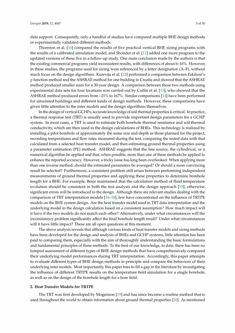
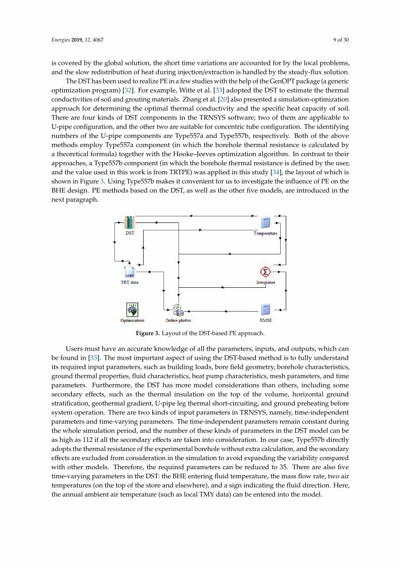
The DST has been used to realize PE in a few studies with the help of the GenOPT package (a genericoptimization program) [32]. For example, Witte et al. [33] adopted the DST to estimate the thermalconductivities of soil and grouting materials. Zhang et al. [20] also presented a simulation-optimizationapproach for determining the optimal thermal conductivity and the specific heat capacity of soil.There are four kinds of DST components in the TRNSYS software; two of them are applicable toU-pipe configuration, and the other two are suitable for concentric tube configuration. The identifyingnumbers of the U-pipe components are Type557a and Type557b, respectively. Both of the abovemethods employ Type557a component (in which the borehole thermal resistance is calculated bya theoretical formula) together with the Hooke–Jeeves optimization algorithm. In contrast to theirapproaches, a Type557b component (in which the borehole thermal resistance is defined by the user,and the value used in this work is from TRTPE) was applied in this study [34], the layout of which isshown in Figure 3. Using Type557b makes it convenient for us to investigate the influence of PE on theBHE design. PE methods based on the DST, as well as the other five models, are introduced in thenext paragraph.Energies 2019, 12, x FOR PEER REVIEW 9 of 29

Figure 3. Layout of the DST-based PE approach.

Users must have an accurate knowledge of all the parameters, inputs, and outputs, which can be found in [33]. The most important aspect of using the DST-based method is to fully understand its required input parameters, such as building loads, bore field geometry, borehole characteristics, ground thermal properties, fluid characteristics, heat pump characteristics, mesh parameters, and time parameters. Furthermore, the DST has more model considerations than others, including some secondary effects, such as the thermal insulation on the top of the volume, horizontal ground stratification, geothermal gradient, U-pipe leg thermal short-circuiting, and ground preheating before system operation. There are two kinds of input parameters in TRNSYS, namely, time-independent parameters and time-varying parameters. The time-independent parameters remain constant during the whole simulation period, and the number of these kinds of parameters in the DST model can be as high as 112 if all the secondary effects are taken into consideration. In our case, Type557b directly adopts the thermal resistance of the experimental borehole without extra calculation, and the secondary effects are excluded from consideration in the simulation to avoid expanding the variability compared with other models. Therefore, the required parameters can be reduced to 35. There are also five time-varying parameters in the DST: the BHE entering fluid temperature, the mass flow rate, two air temperatures (on the top of the store and elsewhere), and a sign indicating the fluid direction. Here, the annual ambient air temperature (such as local TMY data) can be entered into the model.

2.2. Parameter Estimation Methods

For TRTPE, the mean fluid temperature at the inlet and outlet of the BHE T—

f (°C) should be calculated and then compared with tested values. For design purposes, this parameter is also needed to compare with preset constraint values in software-based methods or to calculate the required length directly in simple equation-based methods. If the process inside the borehole is in a steady

state, then T—

f can be described by the so-called effective borehole thermal resistance Rb (K�m�W−1)

f bl bT q R T= + , (24)

where T—

b can be obtained by using Equations (3)–(5) for the ILS, (6)–(8) for the ICS, (9)–(13) for the

FLSN, (14) and (15) for the FLSA, and (22) and (23) for the FLSCC. In the DST, the calculation of T—

b is

not really necessary because the model can directly calculate T—

f and then compare the calculated values with the measured values from the TRT.

The purpose of PE is to obtain the required design input parameters by inversely using the above heat transfer models. This method usually involves two basic problems. One is choosing the objective function to be minimized, and the other is finding a suitable iterative minimization algorithm. The commonly chosen objective function to be minimized is the error sum of squares (SSE), which is

Figure 3. Layout of the DST-based PE approach.

Users must have an accurate knowledge of all the parameters, inputs, and outputs, which canbe found in [33]. The most important aspect of using the DST-based method is to fully understandits required input parameters, such as building loads, bore field geometry, borehole characteristics,ground thermal properties, fluid characteristics, heat pump characteristics, mesh parameters, and timeparameters. Furthermore, the DST has more model considerations than others, including somesecondary effects, such as the thermal insulation on the top of the volume, horizontal groundstratification, geothermal gradient, U-pipe leg thermal short-circuiting, and ground preheating beforesystem operation. There are two kinds of input parameters in TRNSYS, namely, time-independentparameters and time-varying parameters. The time-independent parameters remain constant duringthe whole simulation period, and the number of these kinds of parameters in the DST model can beas high as 112 if all the secondary effects are taken into consideration. In our case, Type557b directlyadopts the thermal resistance of the experimental borehole without extra calculation, and the secondaryeffects are excluded from consideration in the simulation to avoid expanding the variability comparedwith other models. Therefore, the required parameters can be reduced to 35. There are also fivetime-varying parameters in the DST: the BHE entering fluid temperature, the mass flow rate, two airtemperatures (on the top of the store and elsewhere), and a sign indicating the fluid direction. Here,the annual ambient air temperature (such as local TMY data) can be entered into the model.

Energies 2019, 12, 4067 10 of 30

2.2. Parameter Estimation Methods

For TRTPE, the mean fluid temperature at the inlet and outlet of the BHE Tf (◦C) should becalculated and then compared with tested values. For design purposes, this parameter is also neededto compare with preset constraint values in software-based methods or to calculate the required lengthdirectly in simple equation-based methods. If the process inside the borehole is in a steady state,then Tf can be described by the so-called effective borehole thermal resistance Rb (K·m·W−1)

T f = qlRb + Tb, (24)

where Tb can be obtained by using Equations (3)–(5) for the ILS, (6)–(8) for the ICS, (9)–(13) for theFLSN, (14) and (15) for the FLSA, and (22) and (23) for the FLSCC. In the DST, the calculation of Tbis not really necessary because the model can directly calculate Tf and then compare the calculatedvalues with the measured values from the TRT.

The purpose of PE is to obtain the required design input parameters by inversely using theabove heat transfer models. This method usually involves two basic problems. One is choosing theobjective function to be minimized, and the other is finding a suitable iterative minimization algorithm.The commonly chosen objective function to be minimized is the error sum of squares (SSE), which is

f = minn∑

i=1

[(T f ,cal)i − (T f ,mea)i]2 (25)

In Equation (25), f is the objective function, n is the total number of measurements, Tf,cal iscalculated from the models in Section 2.1, and Tf,mea refers to the mean fluid temperature measured fora selected time interval.

Sometimes, the root-mean-square error (RMSE) is also used as an indicator.

f = min

√√√√ n∑i=1

[(T f ,cal)i − (T f ,mea)i]2

n(26)

Theoretically, the estimated parameters can be any combination of the unknowns. However,sensitivity analysis has revealed that the simultaneous estimation of more than three parameters isproblematic because some of these parameters are strongly correlated. Li and Lai [35] found that theestimation method was usually formulated as a two-variable model, in which soil thermal conductivityand borehole thermal resistance are the best choices in most cases for design purposes. Technically,this combination can prevent the optimization process from becoming trapped in a local minimum.

There are several iterative methods suitable for performing the least-squares minimization methodto solve the inverse heat conduction problem [36–38]; among these methods are the Gauss linearizationmethod, the conjugate gradient method, the Levenberg–Marquardt method, and the interior trust regionmethod subject to bounds. In this study, the interior trust region method was adopted, as recommendedby Li and Lai [35], while the estimation process based on the DST model employed the Nelder–Meadsimplex algorithm, which is embedded in a generic optimization program package, GenOpt.

3. TRT Experimental Data and the Results of PE

3.1. Experimental Data from the Thermal Response Test

The technology of the TRT itself has many sources of uncertainty [39]. PEs should be derivedfrom the same data set when obtaining different PE results using the six selected heat transfer modelsfor a comparison run. Other influential factors, such as the simulation starting time, should also bein accordance. The experimental data set was collected from the existing literature. The test wasperformed by researchers in the Laval University [40]. The temperature responses were recorded every

Energies 2019, 12, 4067 11 of 30

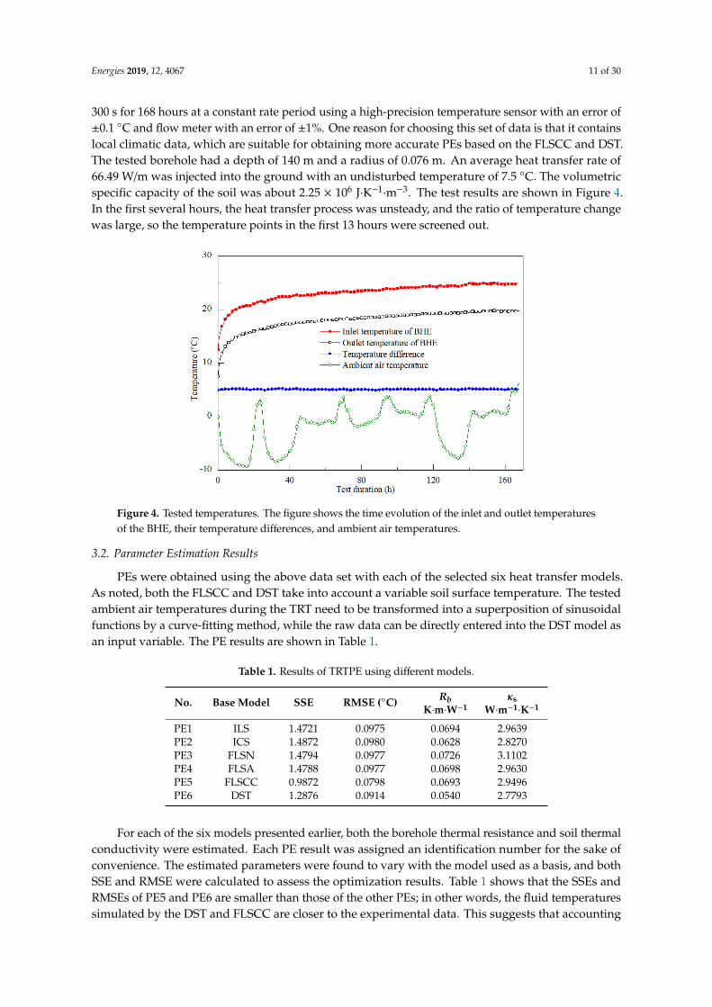
300 s for 168 hours at a constant rate period using a high-precision temperature sensor with an error of±0.1 ◦C and flow meter with an error of ±1%. One reason for choosing this set of data is that it containslocal climatic data, which are suitable for obtaining more accurate PEs based on the FLSCC and DST.The tested borehole had a depth of 140 m and a radius of 0.076 m. An average heat transfer rate of66.49 W/m was injected into the ground with an undisturbed temperature of 7.5 ◦C. The volumetricspecific capacity of the soil was about 2.25 × 106 J·K−1

·m−3. The test results are shown in Figure 4.In the first several hours, the heat transfer process was unsteady, and the ratio of temperature changewas large, so the temperature points in the first 13 hours were screened out.

Energies 2019, 12, x FOR PEER REVIEW 11 of 29

and both SSE and RMSE were calculated to assess the optimization results. Table 1 shows that the SSEs and RMSEs of PE5 and PE6 are smaller than those of the other PEs; in other words, the fluid temperatures simulated by the DST and FLSCC are closer to the experimental data. This suggests that accounting for the variation in ground surface and subsurface temperatures helps improve the accuracy of the model. As shown in Table 1, only the differences between PE1 and PE4 are negligible. Although the values of soil thermal conductivity from PE1 and PE5 are almost the same, the values of the other estimated parameter Rb are different. Furthermore, the relative difference in the borehole thermal resistance between PE1 and PE6 is as high as 34.4%. For soil thermal conductivity, the relative difference reaches 11.9%.

Figure 4. Tested temperatures. The figure shows the time evolution of the inlet and outlet temperatures of the BHE, their temperature differences, and ambient air temperatures.

Table 1. Results of TRTPE using different models

No. Base Model SSE RMSE (°C) Rb K·m·W−1

κs

W·m−1·K−1 PE1 ILS 1.4721 0.0975 0.0694 2.9639 PE2 ICS 1.4872 0.0980 0.0628 2.8270 PE3 FLSN 1.4794 0.0977 0.0726 3.1102 PE4 FLSA 1.4788 0.0977 0.0698 2.9630 PE5 FLSCC 0.9872 0.0798 0.0693 2.9496 PE6 DST 1.2876 0.0914 0.0540 2.7793

The impact of the variation in soil thermal conductivity and diffusivity on the design length and, consequently, on the system capacities was reported by Kavanaugh [41]. The conclusion was derived from investigating an office building GCHP system using a design program. It was reported that a 10% variation in these parameters caused the design length to differ by 4.5–5.8%. Since soil thermal conductivity, thermal diffusivity, and borehole thermal resistance are highly correlated [42], there is no doubt that the variation in soil thermal conductivity and borehole thermal resistance will have some impacts on the final design output, which is examined in the rest of the paper.

4. Comparison of the Time Evolution of Mean Fluid Temperatures for a Single Borehole

For design purposes, the heat pump entering fluid temperatures (EFTs) are used as design constraints in most cases. Here, the constraints also indicate the minimum (if the building thermal loads are heating dominated) or maximum (if the building thermal loads are cooling dominated) values of the BHE exiting fluid temperature since these two parameters are nearly equal. The mean

Figure 4. Tested temperatures. The figure shows the time evolution of the inlet and outlet temperaturesof the BHE, their temperature differences, and ambient air temperatures.

3.2. Parameter Estimation Results

PEs were obtained using the above data set with each of the selected six heat transfer models.As noted, both the FLSCC and DST take into account a variable soil surface temperature. The testedambient air temperatures during the TRT need to be transformed into a superposition of sinusoidalfunctions by a curve-fitting method, while the raw data can be directly entered into the DST model asan input variable. The PE results are shown in Table 1.

Table 1. Results of TRTPE using different models.

No. Base Model SSE RMSE (◦C) RbK·m·W−1

κsW·m−1·K−1

PE1 ILS 1.4721 0.0975 0.0694 2.9639PE2 ICS 1.4872 0.0980 0.0628 2.8270PE3 FLSN 1.4794 0.0977 0.0726 3.1102PE4 FLSA 1.4788 0.0977 0.0698 2.9630PE5 FLSCC 0.9872 0.0798 0.0693 2.9496PE6 DST 1.2876 0.0914 0.0540 2.7793

For each of the six models presented earlier, both the borehole thermal resistance and soil thermalconductivity were estimated. Each PE result was assigned an identification number for the sake ofconvenience. The estimated parameters were found to vary with the model used as a basis, and bothSSE and RMSE were calculated to assess the optimization results. Table 1 shows that the SSEs andRMSEs of PE5 and PE6 are smaller than those of the other PEs; in other words, the fluid temperaturessimulated by the DST and FLSCC are closer to the experimental data. This suggests that accounting

Energies 2019, 12, 4067 12 of 30

for the variation in ground surface and subsurface temperatures helps improve the accuracy of themodel. As shown in Table 1, only the differences between PE1 and PE4 are negligible. Although thevalues of soil thermal conductivity from PE1 and PE5 are almost the same, the values of the otherestimated parameter Rb are different. Furthermore, the relative difference in the borehole thermalresistance between PE1 and PE6 is as high as 34.4%. For soil thermal conductivity, the relative differencereaches 11.9%.

The impact of the variation in soil thermal conductivity and diffusivity on the design length and,consequently, on the system capacities was reported by Kavanaugh [41]. The conclusion was derivedfrom investigating an office building GCHP system using a design program. It was reported that a10% variation in these parameters caused the design length to differ by 4.5–5.8%. Since soil thermalconductivity, thermal diffusivity, and borehole thermal resistance are highly correlated [42], there is nodoubt that the variation in soil thermal conductivity and borehole thermal resistance will have someimpacts on the final design output, which is examined in the rest of the paper.

4. Comparison of the Time Evolution of Mean Fluid Temperatures for a Single Borehole

For design purposes, the heat pump entering fluid temperatures (EFTs) are used as designconstraints in most cases. Here, the constraints also indicate the minimum (if the building thermalloads are heating dominated) or maximum (if the building thermal loads are cooling dominated)values of the BHE exiting fluid temperature since these two parameters are nearly equal. The mean

fluid temperature of the BHE inlet and outlet–Tf as an intermediate parameter reflects the design

length to some degree. Regardless of the model used as a basis, most methods need to compute thetemperature response around a single borehole because of a constant heat pulse. Then, a multiple loadaggregation algorithm is used to account for dynamic thermal loads, and it superimposes solutions formultiple boreholes to deal with heat accumulation effects. In this section, we first show the extent towhich the PE results influence the mean fluid temperature through the results of a simple test, namely,the temperature response from a single borehole under a constant heat pulse.

In the simulation of the time evolution of the mean fluid temperature for a long period—50 years inthis case—the parameters concerning borehole configurations and test conditions were consistent withthose reported in Section 3.1. The six combinations of Rb and κs in Table 1 were inversely employedand substituted back into the base models to conduct the comparison runs. That is, each PE resultcorresponds to one base model, so there are 36 time-evolution curves in total. For the FLSCC and DST,hourly variation in the ground surface temperature was simulated by Equations (16) and (17), in whichthe annual mean ground surface temperature Tm was set to 7.5 ◦C, the amplitude of temperatureoscillations Tam was 18 ◦C, and the initial phase ω∆τ was 0.24 rad. In practice, it is better for designersand engineers to find statistical data on the project location. Otherwise, curve fitting using Equations(16) and (17) using local TMY data is a good alternative. This is also the case for the DST model.

According to the simulation results, for one base model, the absolute maximum temperaturedifferences between the two curves were around 1.1 ◦C in the beginning and about 2.1 ◦C at theend of the simulation period. With further simulation, these temperature differences rose to 3–6 ◦Cwhen the heat transfer rate was increased to 100 W/m and the simulation time period was doubled.Because absolute values may change with simulation parameters, the relative difference was definedto illustrate the temperature differences subject to PE

εT,RE =(Ti − T0) − (Tbase − T0)

Tbase − T0× 100%, (27)

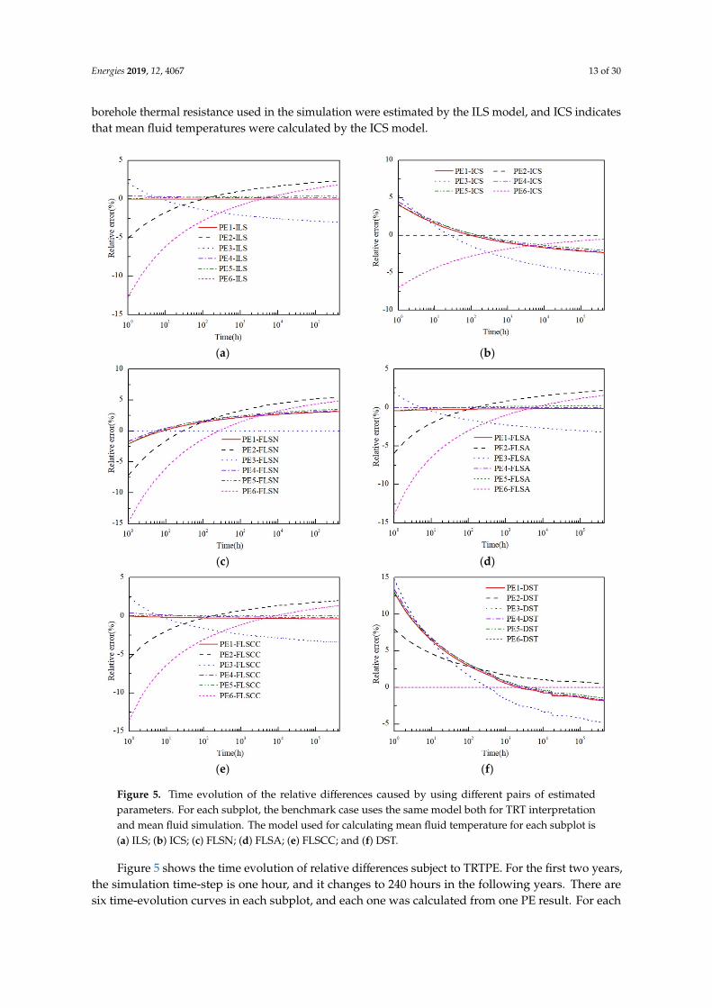
where εT,RE represents the relative difference, %; Tbase refers to the mean fluid temperature calculatedby the same model as TRTPE, ◦C; and Ti is the mean fluid temperature calculated by different modelswith TRTPE, ◦C. The relative difference curves are plotted in Figure 5. The labels in this figure indicatethe models used; for example, for PE1-ICS, PE1 means that the values of soil thermal conductivity and

Energies 2019, 12, 4067 13 of 30

borehole thermal resistance used in the simulation were estimated by the ILS model, and ICS indicatesthat mean fluid temperatures were calculated by the ICS model.

Energies 2019, 12, x FOR PEER REVIEW 13 of 29

Figure 5e displays the relative differences in the mean fluid temperature simulated by the DST model. Compared with PE6, PE1, PE3, PE4, and PE5 share the same changing trend. The values of their relative differences first decrease and then increase until the end of the simulation. In contrast, the values of the PE2-DST curve always decrease: from 7.8% in the first hour to 0.2% in the end.

(a) (b)

(c) (d)

(e) (f)

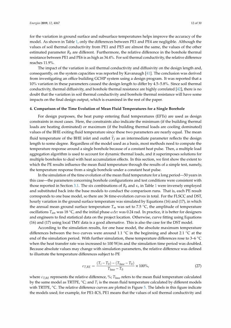
Figure 5. Time evolution of the relative differences caused by using different pairs of estimated parameters. For each subplot, the benchmark case uses the same model both for TRT interpretation and mean fluid simulation. The model used for calculating mean fluid temperature for each subplot is (a) ILS; (b) ICS; (c) FLSN; (d) FLSA; (e) FLSCC; and (f) DST.

In sum, the PE results cause about a 15% relative difference in the very beginning and 5% at the end of the simulation period. It can also be observed that the parameters estimated by the ILS, FLSA, or FLSCC have little difference, so there are no significant differences in the relative differences based on these three models. However, for the ICS, FLSN, and DST-based estimated parameters, it is

Figure 5. Time evolution of the relative differences caused by using different pairs of estimatedparameters. For each subplot, the benchmark case uses the same model both for TRT interpretationand mean fluid simulation. The model used for calculating mean fluid temperature for each subplot is(a) ILS; (b) ICS; (c) FLSN; (d) FLSA; (e) FLSCC; and (f) DST.

Figure 5 shows the time evolution of relative differences subject to TRTPE. For the first two years,the simulation time-step is one hour, and it changes to 240 hours in the following years. There aresix time-evolution curves in each subplot, and each one was calculated from one PE result. For each

Energies 2019, 12, 4067 14 of 30

subplot, the benchmark case is the curve that uses the same model in both the TRTPE and the meanfluid temperature simulation.

Figure 5a shows that PE6 causes up to a 15% relative difference in the very beginning comparedwith PE1. PE2 and PE3 cause around 5% relative differences in the beginning hours and at the endof system operation, while the relative difference due to the use of PE4 and PE5 is always within 1%from the beginning to the end. Similar conclusions can be drawn from Figure 4d,f. This is because theparameters estimated by these three models have little difference.

Figure 5b shows that, compared with PE2, the relative differences caused by PE1, PE3, PE4,and PE5 are less than 5% throughout the simulation time period. The relative differences from PE3 area little bigger than those from PE1, PE4, and PE5 and about as twice as high in the late hours. Althoughrelative differences from PE6 are more than 5% in the first 10 hours, they become progressively smallerover time.

Figure 5c indicates that for PE3, the relative differences due to all the other PE results decrease atfirst and then increase to 2.5–5%. Relative differences due to PE6 in the beginning hours are as high as15% and still bigger than the other PE results.

Figure 5e displays the relative differences in the mean fluid temperature simulated by the DSTmodel. Compared with PE6, PE1, PE3, PE4, and PE5 share the same changing trend. The values oftheir relative differences first decrease and then increase until the end of the simulation. In contrast,the values of the PE2-DST curve always decrease: from 7.8% in the first hour to 0.2% in the end.

In sum, the PE results cause about a 15% relative difference in the very beginning and 5% at theend of the simulation period. It can also be observed that the parameters estimated by the ILS, FLSA,or FLSCC have little difference, so there are no significant differences in the relative differences based onthese three models. However, for the ICS, FLSN, and DST-based estimated parameters, it is importantto highlight that relatively big differences can result if the PE and temperature field simulation useinconsistent models. Especially in the beginning hours of operation, the relative difference in theshort-time response of the BHE subject to PE is significant. Moreover, the relative difference in thelong-time response is also considerable. For design purposes, the influence of PE on the design outputstill needs detailed investigation.

5. Sizing Methods for BHE

A good number of design methods, either numerical or analytical, have been proposed to sizeand optimize BHEs; their underlying thermal response analysis models, treatment of building thermalloads, consideration of thermal interference, and other settings are of varying complexity and differfrom each other. In this section, some representative vertical BHE design methods available in theliterature are presented and compared to highlight their strengths and weaknesses in relation to theirinter models. The most commonly used methods for sizing heat exchangers include the IGSHPAmethod [3], the ASHRAE method [2], g-function-based design tools [5,8,24], such as EED or theGLHEPRO program based on Eskilson’s approach, and the DST-based method [6,7]. The following isa brief description of the selected sizing methods used for comparison runs in this study.

5.1. IGSHPA Method

The IGSHPA method determines the length of heat exchangers required for heating and coolingloads by applying the design equations

Lh =Qh(Rp + RsFh)

T0 − TL·

COPh − 1COPh

, (28)

Lc =Qc(Rp + RsFc)

TH − T0·

COPc + 1COPc

, (29)

Energies 2019, 12, 4067 15 of 30

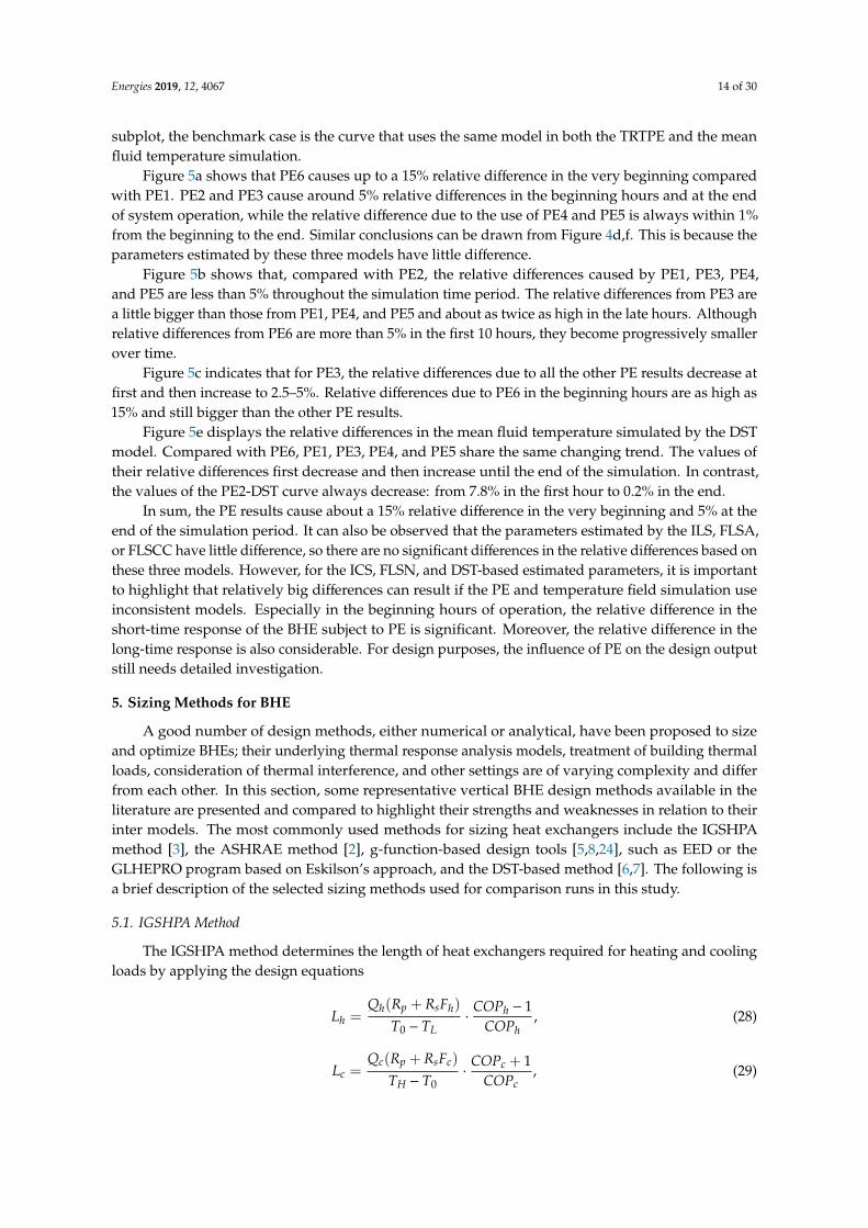
where the subscript h represents the heating mode, and c represents the cooling mode; L is the requireddesign length, m; Q is the design load or total unit capacity at the design EFT, W; F is the run fraction;COP is the coefficient of performance; Rs is the soil resistance, K·m·W−1; TL and TH refer to the specifiedminimum and maximum heat pump EFT Tin,hp, ◦C; and Rp is the pipe resistance to heat flow, K·m·W−1.A detailed presentation of the IGSHPA method and the determination method of each parameter canbe found in [43].

5.2. ASHRAE Method

The ASHRAE handbook [2] sets forth a BHE design equation that is suitable for quick calculations

Lh =QaRsa + Qh(Rb + PLFmRsm + FscRsd)

T0 −Tin,hp+Tout,hp

2 − Tp

·COPh − 1

COPh, (30)

Lc =QaRsa + Qc(Rb + PLFmRsm + FscRsd)

Tin,hp+Tout,hp2 − T0 − Tp

·COPh + 1

COPh, (31)

where Qa is the net annual average heat transfer to the ground, W; PLFm is the part-load factor for thedesign month; Rsa, Rsm, and Rsd are the effective thermal resistances of the ground to the annual pulse,monthly pulse, and peak daily pulse, K·m·W-1, respectively; Fsc is the short-circuit heat loss factor;and Tp is the temperature penalty for interference of adjacent bores, ◦C.

5.3. FLSCC-Based Method

Since the g-function method proposed by Zhang et al. is more accessible than others, it waschosen to represent g-function methods [27,44]. This method is similar to the one used in EED software,in which the superposition principle [45] is applied (as required) to model effects such as equipmenton/off cycling and thermal interference effects. However, the handling of the building block load isdifferent. There is one drawback to using simulation-based design tools; that is, such frequent calls ofEskilson’s numerical model-based g-functions impose quite a heavy calculation burden. The time stepis usually set to a month to improve computation speed. However, in this FLSCC-based g-functionmethod, it is more convenient to use analytical formulas to calculate g-functions and thus possible torun hourly or sub-hourly simulations. Here, a short introduction to this method is given.

By superimposing solutions for multiple boreholes, FLSCC-based g-functions can be created fromEquations (22)–(24) as a function of time and heat pulse. The mean fluid temperature at the end oftime step n is then

T f =n∑

i=1

(qi − qi−1)

2πκsgc(

τn − τi−1

τss,

rbH

,BH) + qiRb + T0, (32)

where qi is the heat transfer rate per unit length at the ith time step, W·m−1; gc is the value of theg-function at the specified point; τn is the current time of interest, s; τi−1 is the time at the (i − 1)th timestep, s; and B is borehole spacing, m.

With Tf known, the heat pump EFT Tin,hp (or the BHE exiting fluid temperature Tout,BHE) and theheat pump exiting fluid temperature Tout,hp (or the BHE entering fluid temperature Tin,BHE) can becomputed using a heat balance equation.

Tin,hp = T f −qiHNb

2.

mC f, (33)

where Nb is the number of boreholes, –;.

m is the mass flow rate, kg·s−1; and Cf is the specific heat of thefluid, J·kg−1

·K−1.

Energies 2019, 12, 4067 16 of 30

The FLSCC-based method determines a borehole length by assuming an initial guess. Then,the maximum and minimum heat pump EFT can be produced and compared with the design constraintsuntil the required precision is obtained. More details can be found in our upcoming paper [44].

5.4. DST-Based Method

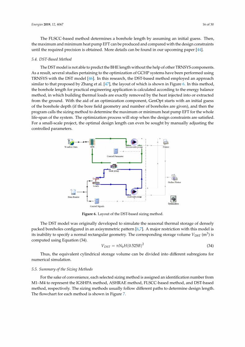
The DST model is not able to predict the BHE length without the help of other TRNSYS components.As a result, several studies pertaining to the optimization of GCHP systems have been performed usingTRNSYS with the DST model [46]. In this research, the DST-based method employed an approachsimilar to that proposed by Zhang et al. [47], the layout of which is shown in Figure 6. In this method,the borehole length for practical engineering application is calculated according to the energy balancemethod, in which building thermal loads are exactly removed by the heat injected into or extractedfrom the ground. With the aid of an optimization component, GenOpt starts with an initial guessof the borehole depth (if the bore field geometry and number of boreholes are given), and then theprogram calls the sizing method to determine the maximum or minimum heat pump EFT for the wholelife-span of the system. The optimization process will stop when the design constraints are satisfied.For a small-scale project, the optimal design length can even be sought by manually adjusting thecontrolled parameters.Energies 2019, 12, x FOR PEER REVIEW 16 of 29

Figure 6. Layout of the DST-based sizing method.

The DST model was originally developed to simulate the seasonal thermal storage of densely packed boreholes configured in an axisymmetric pattern [6,7]. A major restriction with this model is its inability to specify a normal rectangular geometry. The corresponding storage volume VDST (m3) is computed using Equation (34).

2(0.525 )DST bV N H Bπ= (34)

Thus, the equivalent cylindrical storage volume can be divided into different subregions for numerical simulation.

5.5. Summary of the Sizing Methods

For the sake of convenience, each selected sizing method is assigned an identification number from M1–M4 to represent the IGSHPA method, ASHRAE method, FLSCC-based method, and DST-based method, respectively. The sizing methods usually follow different paths to determine design length. The flowchart for each method is shown in Figure 7.

(a) (b) (c) (d)

Figure 7. Flowcharts of the typical steps required to size a BHE bore field for different sizing methods: (a) M1, (b) M2, (c) M3, and (d) M4.

Figure 6. Layout of the DST-based sizing method.

The DST model was originally developed to simulate the seasonal thermal storage of denselypacked boreholes configured in an axisymmetric pattern [6,7]. A major restriction with this model isits inability to specify a normal rectangular geometry. The corresponding storage volume VDST (m3) iscomputed using Equation (34).

VDST = πNbH(0.525B)2 (34)

Thus, the equivalent cylindrical storage volume can be divided into different subregions fornumerical simulation.

5.5. Summary of the Sizing Methods

For the sake of convenience, each selected sizing method is assigned an identification number fromM1–M4 to represent the IGSHPA method, ASHRAE method, FLSCC-based method, and DST-basedmethod, respectively. The sizing methods usually follow different paths to determine design length.The flowchart for each method is shown in Figure 7.

Energies 2019, 12, 4067 17 of 30

Energies 2019, 12, x FOR PEER REVIEW 16 of 29

Figure 6. Layout of the DST-based sizing method.

The DST model was originally developed to simulate the seasonal thermal storage of densely packed boreholes configured in an axisymmetric pattern [6,7]. A major restriction with this model is its inability to specify a normal rectangular geometry. The corresponding storage volume VDST (m3) is computed using Equation (34).

2(0.525 )DST bV N H Bπ= (34)

Thus, the equivalent cylindrical storage volume can be divided into different subregions for numerical simulation.

5.5. Summary of the Sizing Methods

For the sake of convenience, each selected sizing method is assigned an identification number from M1–M4 to represent the IGSHPA method, ASHRAE method, FLSCC-based method, and DST-based method, respectively. The sizing methods usually follow different paths to determine design length. The flowchart for each method is shown in Figure 7.

(a) (b) (c) (d)

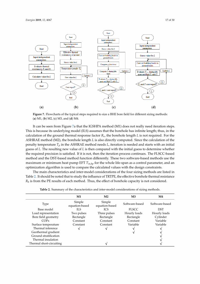
Figure 7. Flowcharts of the typical steps required to size a BHE bore field for different sizing methods: (a) M1, (b) M2, (c) M3, and (d) M4. Figure 7. Flowcharts of the typical steps required to size a BHE bore field for different sizing methods:(a) M1, (b) M2, (c) M3, and (d) M4.

It can be seen from Figure 7a that the IGSHPA method (M1) does not really need iteration steps.This is because its underlying model (ILS) assumes that the borehole has infinite length; thus, in thecalculation of the ground thermal response factor Rs, the borehole length L is not required. For theASHRAE method (M2), the borehole length L is also directly computed. Since the calculation of thepenalty temperature Tp in the ASHRAE method needs L, iteration is needed and starts with an initialguess of L. The resulting new value of L is then compared with the initial guess to determine whetherthe required precision is satisfied. If it is not, then the iteration process continues. The FLSCC-basedmethod and the DST-based method function differently. These two software-based methods use themaximum or minimum heat pump EFT Tin,hp for the whole life-span as a control parameter, and anoptimization algorithm is used to compare the calculated values with the design constraints.

The main characteristics and inter-model considerations of the four sizing methods are listed inTable 2. It should be noted that to study the influence of TRTPE, the effective borehole thermal resistanceRb is from the PE results of each method. Thus, the effect of borehole capacity is not considered.

Table 2. Summary of the characteristics and inter-model considerations of sizing methods.

M1 M2 M3 M4

Type Simpleequation-based

Simpleequation-based Software-based Software-based

Base model ILS ICS FLSCC DSTLoad representation Two pulses Three pulses Hourly loads Hourly loadsBore field geometry Rectangle Rectangle Rectangle Cylinder

COPs Constant Constant Constant VariableSurface temperature Constant Constant Variable VariableThermal inference

√ √ √ √

Geothermal gradient√ √

Ground stratification√

Thermal insulation√

Thermal short-circuiting√ √

Energies 2019, 12, 4067 18 of 30

6. Comparison of Borehole Design Lengths for a Bore Field

6.1. Parameter Settings for Comparison Runs

6.1.1. Building Thermal Loads

IGSHPA equations use a constant load to represent the heat pump capacity at the design EFTthroughout the design month, and it is nearly equal to the building peak load. Additionally, IGSHPAuses Rp to account for the steady heat transfer in the reference borehole, and the equivalent pipediameter is defined for single or multiple U-tubes. Here, it involves the ILS model’s assumptionthat the difference between soil and grout materials can be neglected. As a result, borehole thermalresistance does not appear in the simulation using this method. Rp is calculated by

Rp =1

2πκpln(

ro

ri), (35)

where κp is pipe thermal conductivity, W·m−1·K−1; ro is the pipe outside radius, m; and ri is the pipe

inside radius, m.ASHRAE equations use a constant load throughout the course of operation, with a magnitude

equal to the average value, plus a peak ‘block load’ for which no guidance is given to determinemagnitude or duration. For the ASHRAE method, the annual, monthly, and daily resistance values(Rsa, Rsm, and Rsd, respectively) can be directly computed using the ICS model. Fourier numbers forthe total runtime (1 year or more, depending on system; this study used 10 years), monthly (30 days),and peak (6 hours) pulses were computed. Instead of using the logarithmic chart provided by thehandbook, the individual resistance terms can be obtained using Equations (6)–(8).

Rsa = [G(τa + τm + τd) −G(τm + τd)]/κs, (36)

Rsm = [G(τm + τd) −G(τd)]/κs, (37)

Rsd = G(τd)/κs, (38)

where τy, τm, and τd are the operation times of a 10-year pulse, a 1-month pulse, and a 0.25-day pulse,respectively, s.

In the simulations, synthetic loads were determined using the following sinusoidal function fromBernier [39], taking into account hourly variations, and then used to estimated possible building loadvalues. Synthetic loads were used since the objective was not to calculate the exact loads of a specificbuilding but rather to provide a realistic estimation.

Q = f (τ; β1, β2, β3) + (−1) f loor(β4

8760 (τ−β2))abs( f (τ; β1, β2, β3)) + β5(−1) f loor(β4

8760 (τ−β2))signum(cos( πβ44380 (τ− β6)) + β7), (39)

f (τ; β1, β2, β3) = β1 sin( π12 (τ− β2)) sin( π4380 (τ− β2)) ×

{168−β3

168 + [3∑

i=1

1πi (cos(πiβ3

84 ) − 1)(sin πi84 (τ− β2))]

}(40)

In the above equations, Q is the load, the angles are measured in radians, τ is the time variable,floor is the largest integer less than or equal to the number considered, abs denotes the absolute valueof the expression, and signum is equal to plus or minus one according to the sign of the expressionevaluated. This synthetic symmetric profile was obtained using the following parameters: β1 = 1000,β2 = 1000, β3 = 80, β4 = 2, β5 = 0.01, β6 = 0, and β7 = 0.95.

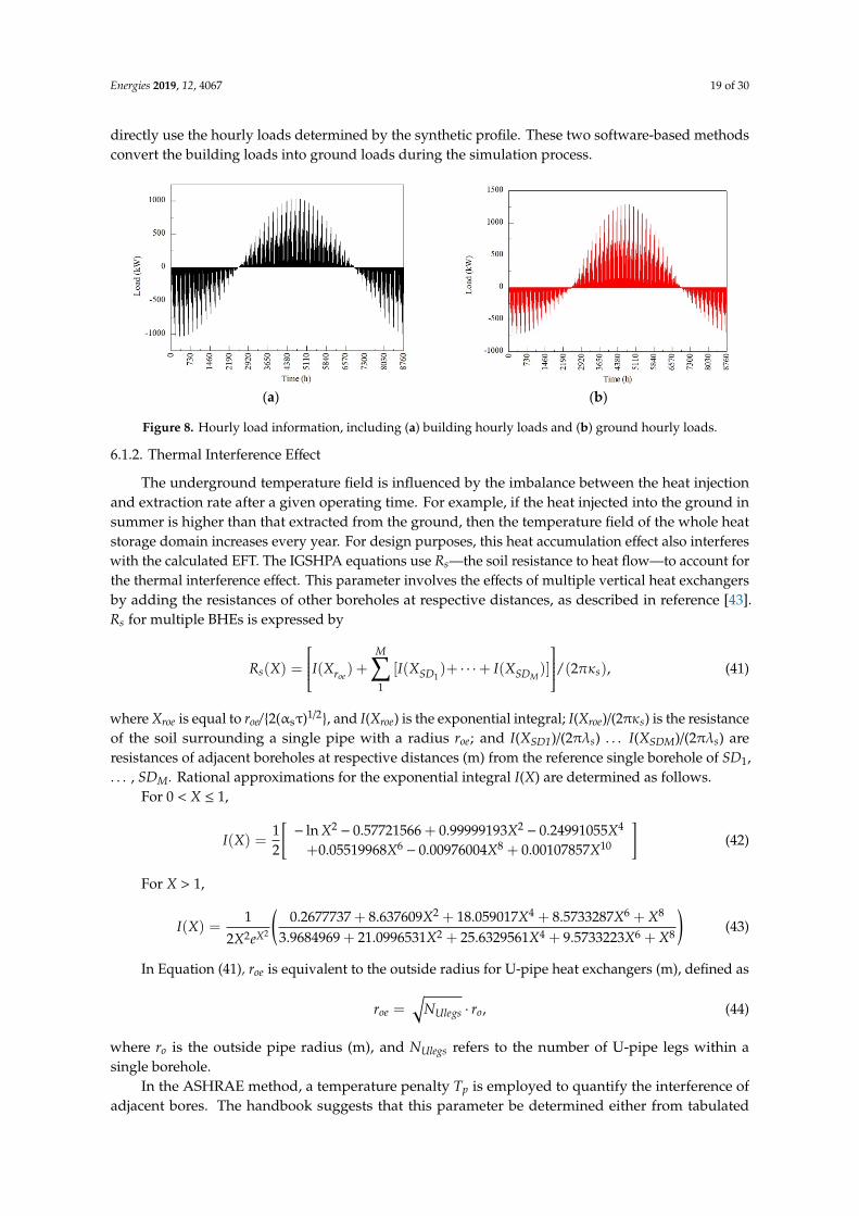
According to the synthetic profile shown in Figure 8a, the peak heating and cooling loads Qhand Qc were both set to 1030 kW. A building load can be converted into a ground load by adding orsubtracting the compressor power at peak load. Figure 8b shows the results obtained; the COPs usedto develop the ground loads are given in Section 6.1.4. The net annual average heat transfer to theground Qa was 31.7 kW, according to Figure 8b. The DST-based method and the FLS-based method

Energies 2019, 12, 4067 19 of 30

directly use the hourly loads determined by the synthetic profile. These two software-based methodsconvert the building loads into ground loads during the simulation process.

Energies 2019, 12, x FOR PEER REVIEW 18 of 29

[ ( ) ( )] /sa a m d m d sR G Gτ τ τ τ τ κ= + + − + , (36)

[ ( ) ( )] /sm m d d sR G Gτ τ τ κ= + − , (37)

( ) /sd d sR G τ κ= , (38)where τy, τm, and τd are the operation times of a 10-year pulse, a 1-month pulse, and a 0.25-day pulse, respectively, s.

In the simulations, synthetic loads were determined using the following sinusoidal function from Bernier [39], taking into account hourly variations, and then used to estimated possible building load values. Synthetic loads were used since the objective was not to calculate the exact loads of a specific building but rather to provide a realistic estimation.

4 42 2( ( )) ( ( ))

48760 87601 2 3 1 2 3 5 6 7( ; , , ) ( 1) ( ( ; , , )) ( 1) (cos( ( )) )

4380floor floor

Q f abs f signumβ βτ β τ β πβτ β β β τ β β β β τ β β

− −= + − + − − + , (39)

33 3

1 2 3 1 2 2 21

168 1( ; , , ) sin( ( ))sin( ( )) [ (cos( ) 1)(sin ( ))]12 4380 168 84 84i

i ifi

β π βπ π πτ β β β β τ β τ β τ βπ=

− = − − × + − −

(40)

In the above equations, Q is the load, the angles are measured in radians, τ is the time variable, floor is the largest integer less than or equal to the number considered, abs denotes the absolute value of the expression, and signum is equal to plus or minus one according to the sign of the expression evaluated. This synthetic symmetric profile was obtained using the following parameters: β1 = 1000, β2 = 1000, β3 = 80, β4 = 2, β5 = 0.01, β6 = 0, and β7 = 0.95.

According to the synthetic profile shown in Figure 8a, the peak heating and cooling loads Qh and Qc were both set to 1030 kW. A building load can be converted into a ground load by adding or subtracting the compressor power at peak load. Figure 8b shows the results obtained; the COPs used to develop the ground loads are given in Section 6.1.4. The net annual average heat transfer to the ground Qa was 31.7 kW, according to Figure 8b. The DST-based method and the FLS-based method directly use the hourly loads determined by the synthetic profile. These two software-based methods convert the building loads into ground loads during the simulation process.

(a) (b)

Figure 8. Hourly load information, including (a) building hourly loads and (b) ground hourly loads.

6.1.2. Thermal Interference Effect

The underground temperature field is influenced by the imbalance between the heat injection and extraction rate after a given operating time. For example, if the heat injected into the ground in summer is higher than that extracted from the ground, then the temperature field of the whole heat storage domain increases every year. For design purposes, this heat accumulation effect also interferes with the calculated EFT. The IGSHPA equations use Rs—the soil resistance to heat flow—to account for the thermal interference effect. This parameter involves the effects of multiple vertical heat exchangers by adding the resistances of other boreholes at respective distances, as described in reference [43]. Rs for multiple BHEs is expressed by

Figure 8. Hourly load information, including (a) building hourly loads and (b) ground hourly loads.

6.1.2. Thermal Interference Effect

The underground temperature field is influenced by the imbalance between the heat injectionand extraction rate after a given operating time. For example, if the heat injected into the ground insummer is higher than that extracted from the ground, then the temperature field of the whole heatstorage domain increases every year. For design purposes, this heat accumulation effect also interfereswith the calculated EFT. The IGSHPA equations use Rs—the soil resistance to heat flow—to account forthe thermal interference effect. This parameter involves the effects of multiple vertical heat exchangersby adding the resistances of other boreholes at respective distances, as described in reference [43].Rs for multiple BHEs is expressed by

Rs(X) =

I(Xroe) +

M∑1

[I(XSD1)+ · · ·+ I(XSDM

)]

/(2πκs), (41)

where Xroe is equal to roe/ {2(αsτ)1/2}, and I(Xroe) is the exponential integral; I(Xroe)/(2πκs) is the resistanceof the soil surrounding a single pipe with a radius roe; and I(XSD1)/(2πλs) . . . I(XSDM)/(2πλs) areresistances of adjacent boreholes at respective distances (m) from the reference single borehole of SD1,. . . , SDM. Rational approximations for the exponential integral I(X) are determined as follows.

For 0 < X ≤ 1,

I(X) =12

[− ln X2

− 0.57721566 + 0.99999193X2− 0.24991055X4

+0.05519968X6− 0.00976004X8 + 0.00107857X10

](42)

For X > 1,

I(X) =1

2X2eX2

(0.2677737 + 8.637609X2 + 18.059017X4 + 8.5733287X6 + X8

3.9684969 + 21.0996531X2 + 25.6329561X4 + 9.5733223X6 + X8

)(43)

In Equation (41), roe is equivalent to the outside radius for U-pipe heat exchangers (m), defined as

roe =√

NUlegs · ro, (44)

where ro is the outside pipe radius (m), and NUlegs refers to the number of U-pipe legs within asingle borehole.

In the ASHRAE method, a temperature penalty Tp is employed to quantify the interference ofadjacent bores. The handbook suggests that this parameter be determined either from tabulated

Energies 2019, 12, 4067 20 of 30

values [2] or by direct computation [4]. In this work, the temperature penalty was computed directlyusing Kavanaugh and Rafferty’s analytical solution [4], which estimates the stored heat E (the unit isW) for 10 years in a hollow cylinder located in an open bore field by

Tp =N4 + 0.5N3 + 0.25N2 + 0.1N1

N4 + N3 + N2 + N1·

EρscsB2L

, (45)

where E is the total heat stored in a cylindrical region, J; Ni is the number of boreholes in the fieldadjacent to i other boreholes.

Either Rs or Tp can be regarded as an index to evaluate the long-term behavior of the bore fieldduring system operation: the greater the imbalance between the required heating and cooling loads,the higher the values of these two parameters and, consequently, the greater the influence on the sizingprocess. In contrast to these two simple equation-based methods, the DST-based method directlycalculates the mean temperature of the heat storage domain using a numerical DST model, and theFLSCC-based method uses the g-functions to obtain the temperature rise or drop caused by a clusterof BHEs.

6.1.3. Temperatures

The IGSHPA method recommends using the Kusuda equation [31] to calculate the undisturbedground temperature T0. For vertical BHEs, T0 can be set to the value of the annual mean groundsurface temperature Tm. The ASHRAE method suggests determining T0 from local water well logsand geological surveys or less accurate sources, such as temperature contour maps provided by theauthoritative department. In this study, the value was measured directly by the TRT. The variation inground surface temperature is represented by the Kusuda equation in both the FLSCC-based methodand the DST-based method.

The design values of the minimum EFT TL and maximum EFT TH are chosen from a rationalrange provided by some national standards, and variances in these thresholds can be geographicallydriven [48]. For example, the ASHRAE handbook suggests that this value be 11–17 ◦C higher than T0

in summer and 6–11 ◦C lower than T0 in winter in the USA, while the limits of TL and TH in China arerecommended to be 4 ◦C in heating and 33 ◦C in cooling [49]. Generally, TL and TH are assumed to behigher than 0 ◦C in winter and less than 35 ◦C in summer. In this case study, TL and TH were assumedto be 1 ◦C and 32 ◦C, respectively. The selection of EFT is not arbitrary in practice. Choosing maximumvalues that are too high or minimum values that are too low can lead to inefficient system performance.Conversely, choosing values that are close to T0 can result in fairly large BHE dimensions. This selectionrequires a comprehensive consideration of energy consumption and system efficiency. Consequently,it is better to adjust these temperature limits according to the expected system efficiency target. TL andTH are input parameters in the simple equation-based method, while—in the FLSCC-based methodand the DST-based method—they serve as design constraints, as illustrated in Figure 7c,d.

6.1.4. Heat Pump Characteristics

The IGSHPA, ASHRAE, and FLSCC-based methods use a single value of the heat pump COP as adesign condition to compute the actual amount of energy injected into or extracted from the BHEs.COPh and COPc are evaluated at TL (1 ◦C) and TH (32 ◦C) and have values of 3.351 and 3.993 in heatingand cooling, respectively. FLSCC utilizes these two values to convert building loads into ground loads,as shown in Figure 7c. In the TRNSYS software, the heat pump unit is simulated using the Type 668component. Users need to input the actual performance of the sample unit under different operatingconditions according to the manufactory’s data [50]. The performance of the heat pump unit also has agreat impact on the efficiency and energy consumption of the whole system; thus, it is important tomodel the heat pump more accurately in practice.

Energies 2019, 12, 4067 21 of 30

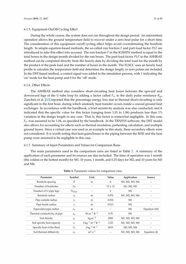
6.1.5. Equipment On/Off Cycling Effect

During the whole course, the system does not run throughout the design period. An intermittentoperation allows the ground temperature field to recover under a zero heat pulse for a short time.The consideration of this equipment on/off cycling effect helps avoid overestimating the boreholelength. In simple equation-based methods, the so-called run fraction F and part-load factor PLF areintroduced to take this effect into account. The run fraction F in the IGSHPA method is equal to thetotal hours in the design month divided by the run hours. The part-load factor PLF in the ASHRAEmethod can be computed directly from the hourly data by dividing the total load for the month bythe product of the peak load and the number of hours in the month. The FLSCC uses an hourly loadprofile to calculate the temperature field and determine the design length, so zero pulses are included.In the DST-based method, a control signal was added to the simulation process, with 1 indicating the‘on’ mode for the heat pump and 0 for the ‘off’ mode.

6.1.6. Other Effects

The ASHRAE method also considers short-circuiting heat losses between the upward anddownward legs of the U-tube loop by adding a factor called Fsc to the daily pulse resistance Rga.Zanchini et al. [42] reported that the percentage energy loss due to thermal short-circuiting is onlysignificant in the first hour, during which unsteady heat transfer occurs inside a coaxial ground heatexchanger. In accordance with the handbook, a brief sensitivity analysis was also conducted, and itindicated that the specific value for this factor (ranging from 1.01 to 1.06) produces less than 1%variation in the design length in any case. That is, this factor is somewhat negligible. In this case,Fsc was assumed to be 1.04, as specified by the handbook. In the TRNSYS software, the DST modelalso allows for accounting for effects such as thermal insulation, preheating calculation, and multipleground layers. Since a virtual case was used as an example in this study, these secondary effects werenot considered. It is worth noting that heat gains/losses in the piping between the BHE and the heatpump were assumed to be negligible in this case.

6.1.7. Summary of Input Parameters and Values for Comparison Runs

The main parameters used in the comparison runs are listed in Table 3. A summary of theapplication of each parameter and its sources are also included. The time of operation was 1 month(the coldest or the hottest month) for M1; 10 years, 1 month, and 0.25 days for M2; and 10 years for M3and M4.

Table 3. Parameter values for comparison runs.

Parameter Symbol Unit Value Application Source

Borehole spacing B m 6 M1, M2, M3, M4 –

Number of boreholes Nb – 12 × 12 M1, M2, M3 –

Number of U-pipe legs NUlegs – 2 M1 –

Borehole radius rb m 0.076 M1, M2, M3, M4 –

Pipe outside radius ro m 0.016 M1 –

Pipe inside radius ri m 0.013 M1 –

Equivalent pipe radius roe m – M1 Equation (44)

Thermal conductivity of pipe κp W·m−1·K−1 0.70 M1 –

Soil density ρs kg·m−3 2000 M1, M2, M3, M4 –

Soil specific heat capacity cs J·kg−1·m−3

·K−1 1125 M1, M2, M3, M4 –

Specific heat of the fluid Cf J·kg−1·K−1 4019 M2, M3, M4 –

Soil thermal diffusivity αs m2·s−1 – M1, M2, M3, M4 Equation (4)

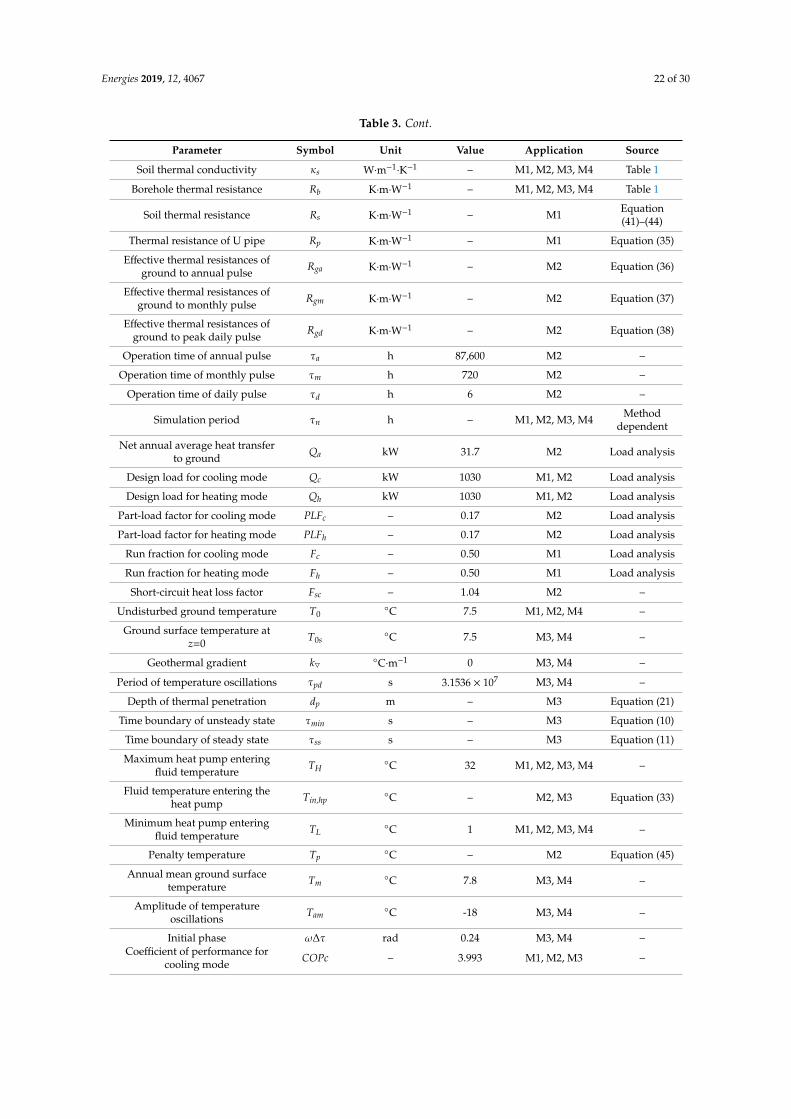
Energies 2019, 12, 4067 22 of 30

Table 3. Cont.

Parameter Symbol Unit Value Application Source

Soil thermal conductivity κs W·m−1·K−1 – M1, M2, M3, M4 Table 1

Borehole thermal resistance Rb K·m·W−1 – M1, M2, M3, M4 Table 1

Soil thermal resistance Rs K·m·W−1 – M1 Equation(41)–(44)

Thermal resistance of U pipe Rp K·m·W−1 – M1 Equation (35)

Effective thermal resistances ofground to annual pulse Rga K·m·W−1 – M2 Equation (36)

Effective thermal resistances ofground to monthly pulse Rgm K·m·W−1 – M2 Equation (37)

Effective thermal resistances ofground to peak daily pulse

Rgd K·m·W−1 – M2 Equation (38)

Operation time of annual pulse τa h 87,600 M2 –

Operation time of monthly pulse τm h 720 M2 –

Operation time of daily pulse τd h 6 M2 –

Simulation period τn h – M1, M2, M3, M4 Methoddependent

Net annual average heat transferto ground Qa kW 31.7 M2 Load analysis

Design load for cooling mode Qc kW 1030 M1, M2 Load analysis

Design load for heating mode Qh kW 1030 M1, M2 Load analysis

Part-load factor for cooling mode PLFc – 0.17 M2 Load analysis

Part-load factor for heating mode PLFh – 0.17 M2 Load analysis

Run fraction for cooling mode Fc – 0.50 M1 Load analysis

Run fraction for heating mode Fh – 0.50 M1 Load analysis

Short-circuit heat loss factor Fsc – 1.04 M2 –

Undisturbed ground temperature T0◦C 7.5 M1, M2, M4 –

Ground surface temperature atz=0 T0s

◦C 7.5 M3, M4 –

Geothermal gradient k5 ◦C·m−1 0 M3, M4 –

Period of temperature oscillations τpd s 3.1536 × 107 M3, M4 –

Depth of thermal penetration dp m – M3 Equation (21)

Time boundary of unsteady state τmin s – M3 Equation (10)

Time boundary of steady state τss s – M3 Equation (11)

Maximum heat pump enteringfluid temperature TH

◦C 32 M1, M2, M3, M4 –

Fluid temperature entering theheat pump

Tin,hp◦C – M2, M3 Equation (33)

Minimum heat pump enteringfluid temperature TL

◦C 1 M1, M2, M3, M4 –

Penalty temperature Tp◦C – M2 Equation (45)

Annual mean ground surfacetemperature Tm

◦C 7.8 M3, M4 –

Amplitude of temperatureoscillations Tam

◦C -18 M3, M4 –

Initial phase ω∆τ rad 0.24 M3, M4 –Coefficient of performance for

cooling mode COPc – 3.993 M1, M2, M3 –

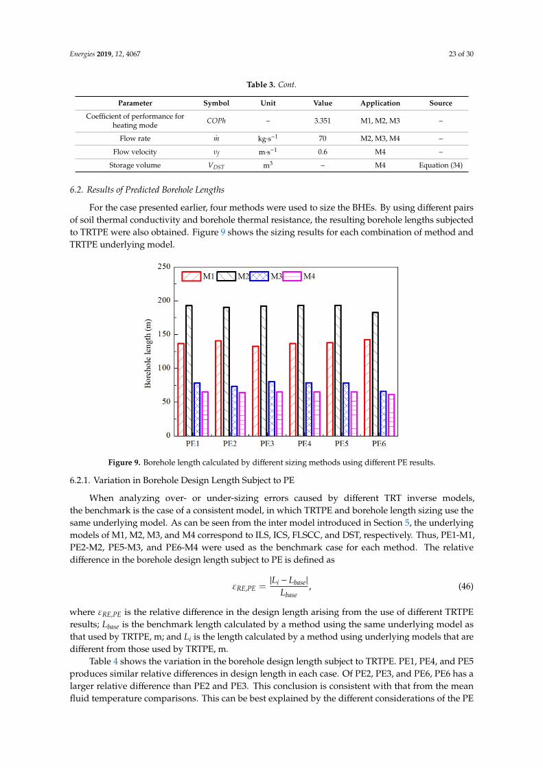
Energies 2019, 12, 4067 23 of 30

Table 3. Cont.

Parameter Symbol Unit Value Application Source

Coefficient of performance forheating mode COPh – 3.351 M1, M2, M3 –

Flow rate.

m kg·s−1 70 M2, M3, M4 –

Flow velocity υf m·s−1 0.6 M4 –

Storage volume VDST m3 – M4 Equation (34)

6.2. Results of Predicted Borehole Lengths

For the case presented earlier, four methods were used to size the BHEs. By using different pairsof soil thermal conductivity and borehole thermal resistance, the resulting borehole lengths subjectedto TRTPE were also obtained. Figure 9 shows the sizing results for each combination of method andTRTPE underlying model.

Energies 2019, 12, x FOR PEER REVIEW 22 of 29

Minimum heat pump entering fluid temperature

TL °C 1 M1, M2, M3,

M4 --

Penalty temperature Tp °C -- M2 Equation (45) Annual mean ground surface

temperature Tm °C 7.8 M3, M4 --

Amplitude of temperature oscillations Tam °C -18 M3, M4 -- Initial phase ω∆τ rad 0.24 M3, M4 --

Coefficient of performance for cooling mode

COPc -- 3.993 M1, M2, M3 --

Coefficient of performance for heating mode

COPh -- 3.351 M1, M2, M3 --

Flow rate m kg�s−1 70 M2, M3, M4 -- Flow velocity υf m�s−1 0.6 M4 --

Storage volume VDST m3 -- M4 Equation (34)

6.2. Results of Predicted Borehole Lengths

For the case presented earlier, four methods were used to size the BHEs. By using different pairs of soil thermal conductivity and borehole thermal resistance, the resulting borehole lengths subjected to TRTPE were also obtained. Figure 9 shows the sizing results for each combination of method and TRTPE underlying model.

Figure 9. Borehole length calculated by different sizing methods using different PE results.

6.2.1. Variation in Borehole Design Length Subject to PE

When analyzing over- or under-sizing errors caused by different TRT inverse models, the benchmark is the case of a consistent model, in which TRTPE and borehole length sizing use the same underlying model. As can be seen from the inter model introduced in Section 5, the underlying models of M1, M2, M3, and M4 correspond to ILS, ICS, FLSCC, and DST, respectively. Thus, PE1-M1, PE2-M2, PE5-M3, and PE6-M4 were used as the benchmark case for each method. The relative difference in the borehole design length subject to PE is defined as

,i base

RE PEbase

L LL

ε−

= , (46)

where εRE,PE is the relative difference in the design length arising from the use of different TRTPE results; Lbase is the benchmark length calculated by a method using the same underlying model as that used by TRTPE, m; and Li is the length calculated by a method using underlying models that are different from those used by TRTPE, m.

Figure 9. Borehole length calculated by different sizing methods using different PE results.

6.2.1. Variation in Borehole Design Length Subject to PE

When analyzing over- or under-sizing errors caused by different TRT inverse models,the benchmark is the case of a consistent model, in which TRTPE and borehole length sizing use thesame underlying model. As can be seen from the inter model introduced in Section 5, the underlyingmodels of M1, M2, M3, and M4 correspond to ILS, ICS, FLSCC, and DST, respectively. Thus, PE1-M1,PE2-M2, PE5-M3, and PE6-M4 were used as the benchmark case for each method. The relativedifference in the borehole design length subject to PE is defined as

εRE,PE =|Li − Lbase|

Lbase, (46)

where εRE,PE is the relative difference in the design length arising from the use of different TRTPEresults; Lbase is the benchmark length calculated by a method using the same underlying model asthat used by TRTPE, m; and Li is the length calculated by a method using underlying models that aredifferent from those used by TRTPE, m.

Table 4 shows the variation in the borehole design length subject to TRTPE. PE1, PE4, and PE5produces similar relative differences in design length in each case. Of PE2, PE3, and PE6, PE6 has alarger relative difference than PE2 and PE3. This conclusion is consistent with that from the meanfluid temperature comparisons. This can be best explained by the different considerations of the PE

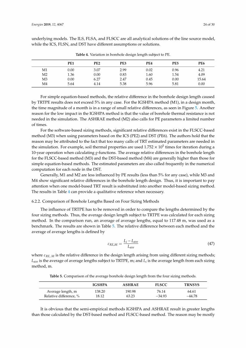
Energies 2019, 12, 4067 24 of 30

underlying models. The ILS, FLSA, and FLSCC are all analytical solutions of the line source model,while the ICS, FLSN, and DST have different assumptions or solutions.

Table 4. Variation in borehole design length subject to PE.

PE1 PE2 PE3 PE4 PE5 PE6

M1 0.00 3.07 2.99 0.02 0.96 4.21M2 1.36 0.00 0.83 1.60 1.54 4.09M3 0.00 6.27 2.47 0.45 0.00 15.64M4 5.64 4.14 5.38 5.96 5.81 0.00

For simple equation-based methods, the relative difference in the borehole design length causedby TRTPE results does not exceed 5% in any case. For the IGSHPA method (M1), in a design month,the time magnitude of a month is in a range of small relative differences, as seen in Figure 5. Anotherreason for the low impact in the IGSHPA method is that the value of borehole thermal resistance is notneeded in the simulation. The ASHRAE method (M2) also calls for PE parameters a limited numberof times.

For the software-based sizing methods, significant relative differences exist in the FLSCC-basedmethod (M3) when using parameters based on the ICS (PE2) and DST (PE6). The authors hold that thereason may be attributed to the fact that too many calls of TRT estimated parameters are needed inthe simulation. For example, soil thermal properties are used 1.752 × 105 times for iteration during a10-year operation when calculating g-functions. The average relative differences in the borehole lengthfor the FLSCC-based method (M3) and the DST-based method (M4) are generally higher than those forsimple equation-based methods. The estimated parameters are also called frequently in the numericalcomputation for each node in the DST.

Generally, M1 and M2 are less influenced by PE results (less than 5% for any case), while M3 andM4 show significant relative differences in the borehole length design. Thus, it is important to payattention when one model-based TRT result is substituted into another model-based sizing method.The results in Table 4 can provide a qualitative reference when necessary.

6.2.2. Comparison of Borehole Lengths Based on Four Sizing Methods

The influence of TRTPE has to be removed in order to compare the lengths determined by thefour sizing methods. Thus, the average design length subject to TRTPE was calculated for each sizingmethod. In the comparison run, an average of average lengths, equal to 117.48 m, was used as abenchmark. The results are shown in Table 5. The relative difference between each method and theaverage of average lengths is defined by

εRE,M =Li − Lave

Lave(47)

where εRE, M is the relative difference in the design length arising from using different sizing methods;Lave is the average of average lengths subject to TRTPE, m; and Li is the average length from each sizingmethod, m.

Table 5. Comparison of the average borehole design length from the four sizing methods.

IGSHPA ASHRAE FLSCC TRNSYS

Average length, m 138.20 190.98 76.14 64.61Relative difference, % 18.12 63.23 −34.93 −44.78

It is obvious that the semi-empirical methods IGSHPA and ASHRAE result in greater lengthsthan those calculated by the DST-based method and FLSCC-based method. The reason may be mostly

Energies 2019, 12, 4067 25 of 30

attributed to the different approaches to load representation. As mentioned above, both the IGSHPAand ASHRAE methods use a constant load over the design month or the course of operation, and itis nearly equal to peak heating or cooling load. The ASHRAE method also adds an additional peakdaily pulse to consider the worst-case scenario. This also suggests the reason that the design lengthdetermined by the ASHRAE method is greater than that computed by the IGSHPA method. In simpleequation-based approaches, namely, the IGSHPA and ASHRAE methods, the parameter definitionsare vague and confuse designers, and there is no real justification for using excessively simplifiedexpressions. When using a simple equation-based approach, designers need to select a value of aparameter from a certain range given by the handbook, and a random selection may lead to either over-or under-design. These simple equations are not suitable for design purposes in their existing forms.

The other two methods—namely, the DST-based method and the FLSCC-based method—directlyuse the hourly load data. The design output of the FLSCC-based method is about 9.7% greater thanthat of the DST-based method. According to the authors’ analysis, one possible reason may be thatwhen calculating thermal interference effects, the FLS method uses the borehole located in the center ofthe heat storage region as a reference, and this is where the heat accumulation effect is the strongest.On the other hand, the DST model adopts a numerically explicit difference method and superpositionmethod to calculate the temperature field of the heat storage region.

From examining the inter models of different sizing methods, the more thoughtfullydeveloped software-based methods—such as the FLSCC-based method and DST-basedmethod—are recommended.

7. Conclusions

This paper presents an assessment of four BHE sizing methods and their inter models,with emphasis on investigating the influence of TRTPE results. The comparisons range from thesimulation of the time evolution of mean fluid temperature for a single borehole to the borehole designlength for a bore field.

The time evolution of mean fluid temperature was simulated for a single borehole stimulated by aconstant heat pulse for a 50-year operation, and a defined relative difference between temperaturescalculated using different PE results was compared. The results of this comparison exercise show thatthe relative differences in temperature are up to 15% at the very beginning and around 5% at the end ofsystem operation. Furthermore, the parameters estimated by the ILS, FLSA, or FLSCC (PE1, PE4, andPE5) have little difference, whereas more attention should be paid to the ICS, FLSN, and DST-basedestimated parameters (PE2, PE3, and PE6).

The comparison of BHE sizing methods was performed by using four methods to size the lengthfor a bore field. The design length calculated by the same underlying model as that used for TRTPEwas used as a benchmark, and the relative difference in the predicted borehole length was definedand compared for each sizing method. This conclusion drawn from the comparison of the boreholedesign length subject to PE coincides with that from the comparison of mean fluid temperature. UsingICS-based PE results, FLSN-based PE results, and DST-based PE results causes significant relativedifferences compared with using FLSA-based PE results and FLSCC-based PE results. Additionally,the estimated soil thermal properties are invoked numerous times during a simulation cycle using theFLSCC-based method and the DST-based method, so these methods are more sensitive to the influenceof PE results.

In the final step, the average length from each sizing method was compared. The results showthat, for the test case with a symmetric synthetic load profile, simple equation-based approachespredict a much larger BHE length than software-based methods, while the design output of theFLSCC-based method is similar to that of the DST-based method. From examining their intermodels, it is concluded that simple equation-based methods are somewhat rudimentary by today’sstandard. Thus, the FLSCC-based method and the DST-based method are recommended since they aremore thoughtfully formulated, computationally fast, and more stable.

Energies 2019, 12, 4067 26 of 30

Comprehensive comparisons of TRT interpretation models and BHE sizing inter models can playa significant role in the discovery of modeling differences or the selection of appropriate methods.This provides a reference for designers, engineers, and researchers in this field. Since this work’smain focus is on the influence of TRTPE, further investigations of other effects on BHE sizing areexpected, with additional factors such as test cases with different load schemes, variations in heat pumpcharacteristics, variations in surface and subsurface temperature, and inhomogeneous soil formulation.

Author Contributions: Conceptualization, X.Z. and T.Z.; Methodology, X.Z.; Validation, X.Z. and T.Z.; Formalanalysis, X.Z.; Investigation, T.Z.; Data curation, T.Z.; Writing—original draft preparation, X.Z.; Writing—reviewand editing, B.L.; Supervision, B.L. and Y.J.; Project administration, B.L.; Funding acquisition, Y.J.

Funding: This research was funded by the National Key R&D Program of China, grant number 2017YFC0702900.

Acknowledgments: The authors would like to thank two anonymous reviewers for their scientific attitude andinsightful suggestions. Their comments helped improve the quality of this paper.

Conflicts of Interest: The authors declare no conflict of interest.

Nomenclature

B Borehole spacing, m;cs Soil specific heat capacity, J·kg−1

·K−1;Cf Fluid specific heat, J·kg−1

·K−1;COPc Coefficient of performance for cooling mode, –;COPh Coefficient of performance for heating mode, –;dp Depth of thermal penetration, m;E Total heat stored in a cylindrical region, J;Fc Run fraction for cooling mode, –;Fh Run fraction for heating mode, –;Fsc Short-circuit heat loss factor, –;g g function, –;glt Long-term response factor g function, –;gst Short-term response factor g function, –;G G factor, –;H Borehole depth, m;k5 Geothermal gradient, ◦C·m−1;K0 Modified Bessel functions of the second kind of order 0;K1 Modified Bessel functions of the second kind of order 0;Lave Average length of design length for each sizing method, m;Lbase Design length benchmark for comparison subject to parameter estimation, m;Lc Required design length for cooling mode, m;Lh Required design length for heating mode, m;.

m Flow rate, m3·s−1;

PLFm Part load factor, –;ql Heat transfer rate, W·m−1;Qa Net annual average heat transfer to ground, W;Qc Design load for cooling mode, W;Qh Design load for heating mode, W;rb Borehole radius, m;ri Pipe inside radius, m;ro Pipe outside radius, m;roe Equivalent pipe radius, m;Rb Borehole thermal resistance, K·m·W−1;Rga Effective thermal resistances of ground to annual pulse, K·m·W−1;Rgd Effective thermal resistances of ground to peak daily pulse, K·m·W−1;Rgm Effective thermal resistances of ground to monthly pulse, K·m·W−1;Rp Pipe thermal resistance, K·m·W−1;Rs Soil thermal resistance, K·m·W−1;

Energies 2019, 12, 4067 27 of 30

T0 Undisturbed ground temperature, ◦C;T0s Ground surface temperature at z = 0, ◦C;Tair Air temperature, ◦C;Tam Amplitude of temperature oscillations, ◦C;–Tb Mean borehole wall temperature, ◦C;Tbase Mean fluid temperature calculated by base parameter estimation result, ◦C;–Tf Mean fluid temperature, ◦C;Tin,hp Fluid temperature entering the heat pump, ◦C;Tout,hp Fluid temperature leaving the heat pump, ◦C;Tin,BHE Fluid temperature entering the borehole heat exchanger, ◦C;Tout,BHE Fluid temperature leaving the borehole heat exchanger, ◦C;TL Minimum heat pump entering fluid temperature, ◦C;TH Maximum heat pump entering fluid temperature, ◦C;Tgs Contribution portion of ground surface temperature, ◦C;Tm Annual mean ground surface temperature, ◦C;Tp Penalty temperature, ◦C;T5 Contribution portion of undisturbed ground temperature, ◦C;VDST Storage volume, m3;Greek lettersαs Soil thermal diffusivity, m2

·s−1;εRE,PE Relative difference of mean borehole temperature subject to parameter estimation, –;εRE, M, Relative difference of average length subject to sizing method, –;ϕ Undisturbed ground temperature in the vertical direction, ◦C;γ Euler’s constant;κs Soil thermal conductivity, W·m−1

·K−1;ρs Soil density, kg·m−3;τa Operation time of annual pulse, s;τd Operation time of daily pulse, s;τm Operation time of monthly pulse, s;τmin Time boundary of unsteady state, s;τn Simulation period, s;τpd Period of temperature oscillations, s;τss Time boundary of steady state, s;υf Flow velocity, m·s−1;ω Angular frequency, rad·s−1;∆τ Phase constant, s;ψ Ground surface temperature, ◦C;AbbreviationsBHE Borehole heat exchangerCOP Coefficient of performanceDST Duct ground heat storage modelEFT Entering fluid temperatureFLS Finite line source modelFLSA Finite line source model with analytical solutionFLSCC Finite line source model considering complex initial and boundary conditionsFLSN Finite line source model with numerical solutionGCHP Ground coupled heat pumpICS Infinite cylinder source modelIGSHPA International Ground Source Heat Pump AssociationILS Infinite line source modelRMSE Root-mean-square errorSSE Error sum of squaresTRT Thermal response test

Energies 2019, 12, 4067 28 of 30

References

1. Ball, D.A.; Fischer, R.D.; Hodgett, D.L. Design methods for ground-source heat pumps. ASHRAE Trans. 1983,89, 416–440.

2. ASHRAE. ASHRAE Handbook—HVAC Applications; Chapter 34. Geothermal Energy; American Society ofHeating, Refrigerating and Air Conditioning Engineers (ASHRAE): Atlanta, GA, USA, 2011.

3. Kavanaugh, S.P.; Rafferty, K. Ground-source Heat Pumps—Design of Geothermal System for Commercial andInstitutional Buildings; ASHRAE: Atlanta, GA, USA, 1997.

4. IGSHPA. Ground Source Heat Pump Residential and Light Commercial: Design and Installation Guide; OklahomaState University: Stillwater, OK, USA, 2009.

5. Eskilson, P. Thermal Analysis of Heat Extraction Boreholes. Ph.D. Thesis, University of Lund, Lund,Switzerland, 1987.

6. Hellström, G. Ground Heat Storage Thermal Analyses of Duct Storage System I. Theory. Ph.D. Thesis,University of Lund, Lund, Switzerland, 1991.

7. Pahud, D.; Hellström, G. The new duct ground heat model for TRNSYS. In Seminar 49 Physical Models forThermal Energy Stores; Eindhoven University of Technology: Eindhoven, The Netherlands, 1996.

8. Yang, H.; Cui, P.; Fang, Z. Vertical-borehole ground-coupled heat pumps: A review of models and systems.Appl. Energy 2010, 87, 16–27. [CrossRef]

9. Rainieri, S.; Bozzoli, F.; Pagliarini, G. Modeling approaches applied to the thermal response test: A criticalreview of the literature. HVAC&R Res. 2011, 17, 977–990.

10. Thornton, J.W.; McDowell, T.P.; HuBHEs, P.J. Comparison of practical vertical ground heat exchanger sizingmethods to a Fort Polk datamodel benchmark. ASHRAE Trans. 1997, 8, 675–683.

11. Shonder, J.A.; Baxter, V.; Thornton, J.; HuBHEs, P. A comparison of vertical ground heat exchanger softwarefor commercial applications. ASHRAE Trans. 2000, 106, 831–842.

12. Kurevija, T.; Vulin, D.; Krapec, V. Effect of borehole array geometry and thermal interferences on groundsource heat pump system. Energy Convers. Manag. 2012, 60, 134–142. [CrossRef]

13. Cullin, J.R.; Spitler, J.D.; Montagud, C. Validation of vertical ground heat exchanger design methodologies.Sci. Technol. Built Environ. 2015, 21, 137–149. [CrossRef]

14. Staiti, M. The Sizing of Borehole Heat Exchangers for Ground Source Heat Pumps: A Comparison BetweenTwo Methods. Master’s Thesis, Politecnico di Milano, Milan, Italy, 2014.

15. Beier, R.A. Vertical temperature profile in ground heat exchanger during in-situ test. Renew. Energy 2011, 36,1578–1587. [CrossRef]

16. Conti, P. Dimensionless Maps for the Validity of Analytical Ground Heat Transfer Models for GSHPApplications. Energies 2016, 9, 890. [CrossRef]

17. Zarrella, A.; Emmi, G.; Graci, S.; De Carli, M.; Cultrera, M.; Santa, G.; Galgaro, A.; Bertermann, D.; Müller, J.;Pockelé, L.; et al. Thermal Response Testing Results of Different Types of Borehole Heat Exchangers:An Analysis and Comparison of Interpretation Methods. Energies 2017, 10, 801. [CrossRef]

18. Urchueguía, J.; Lemus-Zúñiga, L.; Oliver-Villanueva, J.; Badenes, B.; Pla, M.; Cuevas, J. How Reliable AreStandard Thermal Response Tests? An Assessment Based on Long-Term Thermal Response Tests UnderDifferent Operational Conditions. Energies 2018, 11, 3347. [CrossRef]

19. Morgensen, P. Fluid to Duct Wall Heat Transfer in Duct System Heat Storages. In International Conference onSurface Heat Storage in Theory and Practice; Swedish Council for Building Research: Stockholm, Switzerland,1983; pp. 652–657.

20. Zhang, C.; Guo, Z.; Liu, Y.; Cong, X.; Peng, D. A review on thermal response test of ground-coupled heatpump systems. Renew. Sustain. Energy Rev. 2014, 40, 851–867. [CrossRef]

21. Ingersoll, L.R.; Plass, H.J. Theory of the ground pipe heat source for heat pump. Heat. Pip. Air Cond. 1948,20, 119–122.

22. Carslaw, H.S.; Jaeger, J.C. Conduction of Heat in Solids, 2nd ed.; Oxford University Press: Oxford, UK, 1959;p. 510.

23. Ingersioll, L.; Zobel, O.J.; Ingersoll, A.C. Heat Conduction: With Engineering Geological and Other Applications;Mc Graw-Hill: New York, NY, USA, 1954; p. 325.

24. Cimmino, M.; Bernier, M.; Adams, F. A contribution towards the determination of g-functions using thefinite line source. Appl. Therm. Eng. 2013, 51, 401–412. [CrossRef]

Energies 2019, 12, 4067 29 of 30

25. Yavuzturk, C. Modeling of Vertical Ground Loop Heat Exchangers for Ground Source Heat Pump Systems.Ph.D. Thesis, Oklahoma State University, Stillwater, OK, USA, 1999.

26. Bandos, T.V.; Montero, Á.; Fernández, E.; Santander, J.L.G.; Isidro, J.M.; Pérez, J.; De Córdoba, P.J.F.;Urchueguíab, J.F. Finite line-source model for borehole heat exchangers: Effect of vertical temperaturevariations. Geothermics 2009, 38, 263–270. [CrossRef]

27. Zhang, X.; Zhang, T.; Jiang, Y.; Li, B. Improvement on an analytical finite line source model consideringcomplex initial and boundary conditions: Part 1, model development and validation. Energy Build. 2019,198, 1–10. [CrossRef]

28. Bernier, M.A. Ground-coupled heat pump system simulation. ASHRAE Trans. 2001, 107, 605–616.29. Baudoin, A.E. Stockage Intersaisonnier de Chaleur Dans le sol par Batterie D’echangeurs Baionnette Verticaux:

Modele de Predimensionnement. Ph.D. Thesis, Université de Reims, Reims, France, 1988.30. Maestre, I.R.; Gallero, F.J.G.; Gómez, P.Á.; Pérez-Lombard, L. A new RC and g-function hybrid model to

simulate vertical ground heat exchangers. Renew. Energy 2015, 78, 631–642. [CrossRef]31. Kusuda, T.; Achenbach, P.R. Earth temperature and thermal diffusivity selected stations in the United States.

ASHRAE Trans. 1965, 71, 61–76.32. Witte, H.J.L. Advances in geothermal response testing. Therm. Energy Storage Sustain. Energy Consum. 2007,

234, 177–192.33. Pahud, D.; Hellström, G.; Mazzarella, L. Heat storage in the ground Duct ground heat storage model for TRNSYS

(TRNVDST) User manual for the October 1996 version; project report for Laboratoire des systèmes énergétiques(LASEN): Lausanne, Switzerland, 1996.

34. Zhang, X.; Jiang, Y.; Yao, Y.; Deng, S. A TRNSYS-based thermal response test parameter estimation method.Int. J. Electr. Energy 2016, 4, 28–31. [CrossRef]

35. Li, M.; Lai, A.C.K. Parameter estimation of in-situ thermal response tests for borehole ground heat exchangers.Int. J. Heat Mass Transf. 2012, 55, 2615–2624. [CrossRef]

36. Beck, J.V.; Arnold, K.J. Parameter Estimation in Engineering and Science; John Wiley & Sons: New York, NY,USA, 1977.

37. Ozisik, M.N.; Orlande, H.R.B. Inverse Heat Transfer: Fundamentals and Applications; Taylor & Francis: NewYork, NY, USA, 2000.

38. Wetter, M. Optimization Program. User Manual Version 3.1.1; Office of Scientific & Technical Information;U.S.Department of Energy: Washington, DC, USA, 2009.

39. Zhang, X.; Huang, G.; Jiang, Y.; Zhang, T. Ground heat exchanger design subject to uncertainties arisingfrom thermal response test parameter estimation. Energy Build. 2015, 102, 442–452. [CrossRef]

40. Raymond, J.; Therrien, R.; Gosselin, L.; Lefebvre, R. A review of thermal response test analysis using pumpingtest concepts. Groundwater 2011, 49, 932–945. [CrossRef]

41. Kavanaugh, S.P. Field tests for ground thermal properties—Methods and impact on ground-source heatpump design. Chin. J. Explos. Propellants 2000, 32, 1–4.

42. Marcotte, D.; Pasquier, P. On the estimation of thermal resistance in borehole thermal conductivity test.Renew. Energy 2008, 33, 2407–2415. [CrossRef]

43. Cane, R.L.D.; Forgas, D.A. Modeling of ground-source heat pump performance. ASHRAE Trans. 1991, 17,909–925.

44. Zhang, X.; Zhang, T.; Jiang, Y.; Li, B. Improvement on an analytical finite line source model consideringcomplex initial and boundary conditions: Part 2, model application in system design. Energy Building 2019.

45. Bernier, M.; Pinel, P.; Labib, R.; Paillot, R. A multiple load aggregation algorithm for annual hourly simulationsof GCHP systems. HVAC&R Res. 2004, 10, 471–487.

46. Park, S.; Kim, E. Optimal Sizing of Irregularly Arranged Boreholes Using Duct-Storage Model. Sustainability2019, 11, 4338. [CrossRef]

47. Zhang, X.; Jiang, Y.; Yang, Y. Improved method and case study of ground-coupled heat pump system design.Energy Procedia 2012, 14, 849–854. [CrossRef]

48. Dehkordi, S.E.; Schincariol, R.A. Guidelines and the design approach for vertical geothermal heat pumpsystems: Current status and perspective. Can. Geotech. J. 2014, 51, 647–662. [CrossRef]

Energies 2019, 12, 4067 30 of 30

49. The PRC Ministry of Construction. Technical Code for Ground-Source Heat Pump System (2009); GB 50366-2009;China Architecture & Building Press: Beijing, China, 2009.

50. Huang, G. Heat Transfer Model and Characteristics of Helix Ground Heat Exchanger Under DynamicEnvironment. Ph.D. Thesis, Chongqing University, Chongqing, China, 2014. (In Chinese).

© 2019 by the authors. Licensee MDPI, Basel, Switzerland. This article is an open accessarticle distributed under the terms and conditions of the Creative Commons Attribution(CC BY) license (http://creativecommons.org/licenses/by/4.0/).