Embed Size (px)
Citation preview
Hydrol. Earth Syst. Sci., 13, 2069–2094, 2009www.hydrol-earth-syst-sci.net/13/2069/2009/© Author(s) 2009. This work is distributed underthe Creative Commons Attribution 3.0 License.
Hydrology andEarth System
Sciences
Comparative predictions of discharge from an artificial catchment(Chicken Creek) using sparse data
H. M. Holl ander1, T. Blume2, H. Bormann3, W. Buytaert4,*, G.B. Chirico5, J.-F. Exbrayat6, D. Gustafsson7,H. Holzel8, P. Kraft 6, C. Stamm9, S. Stoll10, G. Bloschl11, and H. Fluhler12
1Chair of Hydrology and Water Resources Management, Brandenburg University of Technology Cottbus,03046 Cottbus, Germany2Helmholtz Centre Potsdam, GFZ German Research Centre for Geosciences, Telegrafenberg, C4 2.25,14473 Potsdam, Germany3Department of Biology and Environmental Sciences, Carl von Ossietzky University of Oldenburg,26129 Oldenburg, Germany4School of Geographical Sciences, University of Bristol, BS8 1SS, UK5Dipartimento di ingegneria agraria e agronomia del territorio, Universita di Napoli Federico II, 80055 Naples, Italy6Institute for Landscape Ecology and Resources Management, University of Giessen, 35392 Giessen, Germany7Department of Land and Water Resources Engineering, Royal Institute of Technology KTH, 10044 Stockholm, Sweden8Department of Geography, University of Bonn, 53113 Bonn, Germany9Department Environmental Chemistry, Eawag, 8600 Dubendorf, Switzerland10Institute of Environmental Engineering, ETH Zurich 8093 Zurich, Switzerland11Institute of Hydraulic Engineering and Water Resources Management, TU Vienna, 1040 Vienna, Austria12Department of Environmental Sciences, ETH Zurich, 8092 Zurich, Switzerland* now at: Department of Civil and Environmental Engineering, Imperial College London, London SW7 2AZ, UK
Received: 1 April 2009 – Published in Hydrol. Earth Syst. Sci. Discuss.: 15 April 2009Revised: 25 September 2009 – Accepted: 30 September 2009 – Published: 4 November 2009
Abstract. Ten conceptually different models in predictingdischarge from the artificial Chicken Creek catchment inNorth-East Germany were used for this study. Soil textureand topography data were given to the modellers, but dis-charge data was withheld. We compare the predictions withthe measurements from the 6 ha catchment and discuss theconceptualization and parameterization of the models. Thepredictions vary in a wide range, e.g. with the predicted ac-tual evapotranspiration ranging from 88 to 579 mm/y and thedischarge from 19 to 346 mm/y. The predicted componentsof the hydrological cycle deviated systematically from theobservations, which were not known to the modellers. Dis-charge was mainly predicted as subsurface discharge with lit-tle direct runoff. In reality, surface runoff was a major flowcomponent despite the fairly coarse soil texture. The actualevapotranspiration (AET) and the ratio between actual andpotential ET was systematically overestimated by nine of the
Correspondence to:H. M. Hollander([email protected])
ten models. None of the model simulations came even closeto the observed water balance for the entire 3-year study pe-riod. The comparison indicates that the personal judgementof the modellers was a major source of the differences be-tween the model results. The most important parameters tobe presumed were the soil parameters and the initial soil-water content while plant parameterization had, in this par-ticular case of sparse vegetation, only a minor influence onthe results.
1 Rationale and scientific concept
Hydrological catchment modelling is a tool for testing theassumptions and the conceptualization of the dominant sys-tem properties. It advances our process understanding ofdischarge formation. Often, the discharge record is knownto the modeller when setting up the model, but in the caseof ungauged catchments, this is not the case. The PUB re-search initiative (Predictions inUngaugedBasins) addresses
Published by Copernicus Publications on behalf of the European Geosciences Union.
2070 H. M. Hollander et al.: Comparative predictions of discharge using sparse data
the problem of a priori predicting an unknown system re-sponse (Sivapalan et al., 2003). Such endeavours are typicalfor real world applications when the dominant processes areunknown and the data are too sparse to meet the model re-quirements. An important question is how to improve thepredictive model performance by acquiring additional infor-mation on process understanding and catchment characteris-tics and/or by reducing the parametric requirements.
In this study, we make use of data obtained in an arti-ficial catchment for a comparative prediction of discharge.Artificial catchments are per se the opposite of ungaugedcatchments because they are supposed to provide a well doc-umented case (e.g. a clear definition of catchment geome-try and boundary conditions). We use conceptually differentmodels to predict the discharge – yet unknown to the mod-ellers – based on minimum information. The purpose of thiscollective exercise is neither a rating of model suitability norsuccess, but the question about the crucial elements of dis-charge modelling for an “a priori prediction” of the catch-ment response. This prediction exercise is the first of threesteps. In a second step, more detailed information on thecatchment characteristics will be provided to the modellers.In a third step, the entire database including the dischargerecords will be made available to the modellers, which en-ables them to calibrate the model. The process of stepwise insatisfying the model needs will allow us to relate the gain ofpredictive performance to the efforts and costs of providingthe information needed for the model parameterization. Thispaper documents the first step of the exercise and focuses onthe comparison of the underlying model assumptions and therole of the modeller’s experience.
2 Artificial catchments and predictions inungauged basins
Artificial catchments are an approximation to hydrologicalsystems in their initial phase, because of the short time spansince construction. Hydrological processes have been stud-ied in artificial catchments, e.g. in China (Gu and Freer,1995), Canada (Barbour et al., 2001), Spain (Nicolau, 2002),and Germany (Gerwin et al., 2009). The main objective ofmost of these studies was to determine the water and el-ement budgets of catchments under well-defined boundaryconditions to identify the flow paths through and the storagebehaviour of the various catchment compartments by char-acterizing the processes of runoff formation (Hansen et al.,1997; Kendall et al., 2001). There is a general agreementthat a good correspondence of observed and calculated dis-charge at a catchment outlet is a weak and insufficient cri-terion for the validity of a hydrological model (Grayson andBloschl, 2000a). Additional knowledge on internal variablesis required for calibration (e.g. Beven, 1989). Both localboundary conditions (e.g. catchment surface and subsurfacesize) and internal structures (e.g. discharge points and strat-
ification) can be controlled and more precisely documentedin artificially constructed systems. Detailed observations ofdischarge, soil-water status and groundwater dynamics, bothin terms of quantity and quality, allow for verifying the hy-potheses about the causes of the system’s multi-responsesprovided the catchment properties do not change too rapidlyduring the very initial phase of catchment formation. Suchdata sets reduce the uncertainties by using part of them foran “a posteriori” calibration. In our case, we will use theartificial catchment data set only after having predicted thesystem response based on information that is usually avail-able in catchments at the regional scale.
The “a priori” attempt – when target variables such as dis-charge are yet unknown – is an important step in any modelapplication if the system, including its boundary conditions,changes or if a calibrated model is used for analogous but un-gauged catchment. This can only work if the dominant andsystem-relevant processes are known and can be adequatelydescribed. Here, we use the artificial catchment “ChickenCreek” in Lusatia, Germany (Gerwin et al., 2009, this issue)to test the “a priori” attempt of discharge prediction.
Predicting state variables within and fluxes between com-partments, as well as across catchment boundaries, is oftenhampered due to the considerable uncertainties which may bedue to catchment heterogeneity and poorly defined boundaryand initial conditions. The PUB initiative aims to developand improve methods for such cases. Sivapalan et al. (2003)propose several approaches to addressing this problem eitherby conceptually simplifying process-based models and/or byusing more comprehensive data including proxy data. Pre-tending that the Chicken Creek catchment is a data-poor, un-gauged catchment allows us to investigate the dependence ofthe predictive performance on the amount of data availableto the modellers.
3 Experiment and models
3.1 Chicken Creek catchment
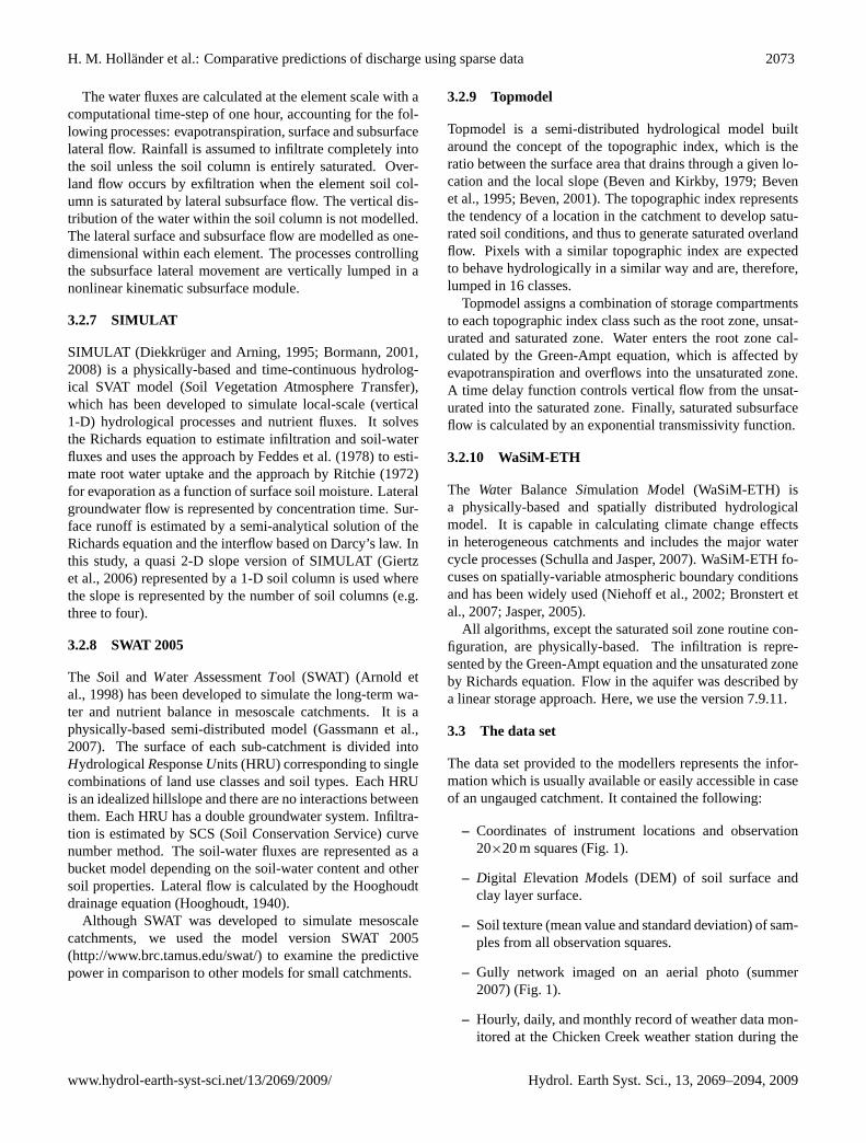
The Chicken Creek catchment (Fig. 1) is 6 ha in size and cur-rently the largest artificial catchment worldwide. It was builtin 2005 by Vattenfall Europe Mining in scientific cooperationwith the Brandenburg University of Technology (Gerwin etal., 2009). It is located in an open mining pit area in Lusatia,Germany. The catchment bottom is a 2 m thick tertiary claylayer placed on top of the reclaimed mining land. The claylayer forms a 450 m long and 150 m wide catchment, whichdrains into a depression at the bottom outlet. This depres-sion is now a small lake which collects the outflow from thecatchment. The longitudinal slope is 1 to 5% and 0.5 to 2%in transverse direction (Fig. 2a and b). A 2 to 3 m thick sandlayer has been put onto the clay basement. It consists mainlyof quaternary sand with variable fractions of 2 to 25% siltand 2 to 16% of clay. The slope of the surface is roughly
Hydrol. Earth Syst. Sci., 13, 2069–2094, 2009 www.hydrol-earth-syst-sci.net/13/2069/2009/
H. M. Hollander et al.: Comparative predictions of discharge using sparse data 2071
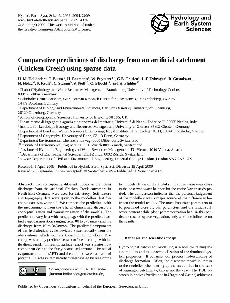
Fig. 1. GIS framework of the Chicken Creek catchment.
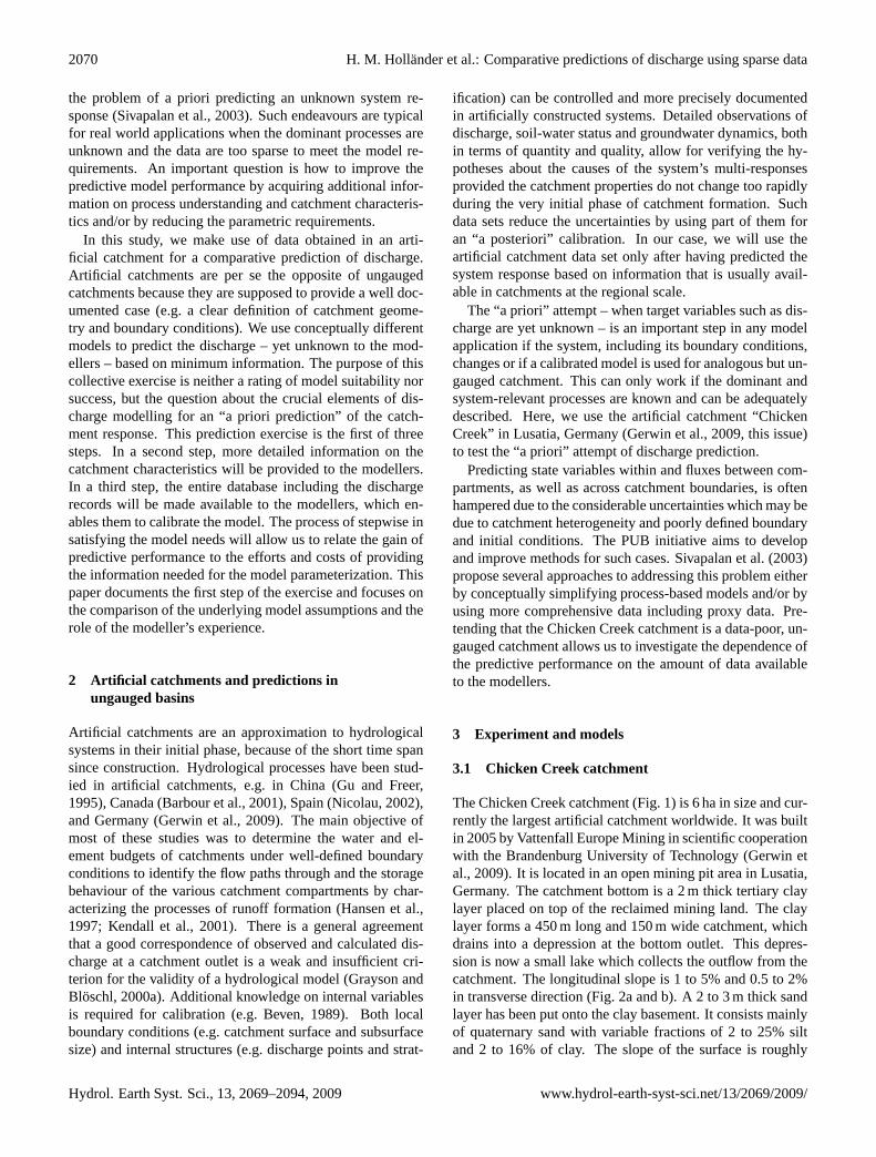
given by the slope of the clay base but the thickness of thesand layer tapers off towards the lake. Hence, the clay layerforms the lake bottom. The catchment boundary is definedby the high edges of the clay layer. The catchment and thedepression are separated by a V-shaped clay dam to funnelthe deep seepage through a narrow outlet into the depression(Fig. 2b). The climate is temperate and humid. Annual pre-cipitation in the past decades has varied from 335 mm (1976)to 865 mm (1974), and the mean annual temperature is about9.3◦C (1971–2000). The catchment remained unplanted afterthe construction, and the establishment of the natural vegeta-tion is being closely monitored (Gerwin et al., 2009).
3.2 Hydrological models
In this section, we describe the conceptual differences of theten models, which were independently used by ten groupsfor predicting the discharge. The models are listed and fol-lowed by a brief description and pertinent model references(Table 1). We discuss the underlying assumptions and thebasic concepts such as the dimensionality of the various ap-proaches from 1-D to 3-D, and the different handling of sur-face processes, e.g. the links to the channel network. Further-more, we highlight the similarities of the models, e.g. the de-scription of evapotranspiration. We use the term “physically-based” according to the wording where the model is beingdiscussed in the literature, not inferring that the process de-scription is based on “ab initio” physical laws.
Fig. 2. Schematic of the transverse(a) and longitudinal(b) transectof the Chicken Creek catchment.
3.2.1 Catflow
Catflow (Maurer, 1997; Zehe and Fluhler, 2001a; Zehe andBloeschl, 2004; Zehe et al., 2005) is a physically-basedmodel. It relies on a detailed process representation: thesoil-water dynamic is described with the Richards equation(mixed form), evapotranspiration by the Penman-Monteithequation, surface runoff by the convection-diffusion equa-tion, which is an approximation to the 1-D Saint Venantequation. Surface saturation, infiltration excess runoff, re-infiltration of surface runoff, lateral subsurface flow and re-turn flow can be simulated by Catflow. It has been used asa virtual landscape generator to investigate the role of initialsoil moisture and precipitation in runoff processes (Zehe etal., 2005), for simulating water flow and bromide transportin a loess catchment (Zehe and Fluhler, 2001b), and for pro-cess analysis within a slowly moving landslide terrain (Lin-denmaier et al., 2005), among other applications. Here, weused the quasi-3-D hillslope module of the model.
3.2.2 CMF
The CatchmentModelling Framework (CMF) is a multi-model toolkit. The work on it is still in progress (Kraft et al.,2008). The main objective of the model framework is to con-nect local scale transport models with lateral transport pro-cesses between neighbouring sites. So far, a model similarto DHSVM (Distributed Hydrology Soil Vegetation Model)(Wigmosta et al., 1994) has been implemented in CMF, basedon previous work by Vache and McDonnell (2006). Themodel represents subsurface transport and water flow by the3-D solution of the Richards equation. Infiltration and unsat-urated percolation is calculated with the Richards equation,and the lateral saturated flow with Darcy’s law. Infiltrationexcess and ponded water is directly routed to the stream net-work using a mass balance approach and re-infiltration is ne-glected. We used the two layer approach with an unsaturatedand a saturated zone per cell, where the depth of the boundarybetween the two layers changes according to the saturation ofthe soil column.
www.hydrol-earth-syst-sci.net/13/2069/2009/ Hydrol. Earth Syst. Sci., 13, 2069–2094, 2009
2072 H. M. Hollander et al.: Comparative predictions of discharge using sparse data
Table 1. Catchment models.
model full name of acronym modeller institution
Catflow T. Blume GFZ PotsdamCMF CatchmentModelling P. Kraft Univ. of Giessen
FrameworkCoupModel Coupled Heat and Mass D. Gustafsson Royal Institute of
TransferModel for Soil- Technology KTHPlant-Atmosphere System Stockholm
Hill-Vi S. Stoll ETH ZurichHYDRUS-2Da C. Stamm EawagNetThales G. B. Chirico Univ. of NaplesSIMULATa H. Bormann Univ. of OldenburgSWAT Soil andWaterAssessment J.-F. Exbrayat Univ. of Giessen
ToolTopmodel Topography-basedmodel W. Buytaert Univ. of BristolWaSiM-ETH Water BalanceSimulation H. Holzel Univ. of Bonn
Model-ETH
a Although HYDRUS-2D and SIMULAT are not catchment models in its proper sense, they are adapted to be used as such.
3.2.3 CoupModel
The CoupModel is a physically-based model for coupled heatand mass transfer in soil-plant-atmosphere systems (Jans-son and Moon, 2001). Vertical movement of water in a 1-D soil profile is described with the Richards equation us-ing a water retention function (Brooks and Corey, 1964)and an unsaturated hydraulic conductivity function (Mualem,1976) for each soil layer. Lateral water fluxes are consid-ered as a drainage system, with horizontal outflow from satu-rated soil layers to a hypothetical drainage pipe following theHooghoudt drainage equation (Hooghoudt, 1940). Semi-2-Dand semi-3-D representation is achieved by taking the out-flow from one or several 1-D soil column as lateral inputs toa downstream column. The model accounts for soil freezing,including effects on the thermal and hydraulic conductivity(Stahli et al., 1996). Water and heat exchange between soiland atmosphere are calculated separately for different sur-face compartments including bare soil, snow, vegetation, andinterception, with individual energy balance sub-models.
3.2.4 Hill-Vi
The physically-based hillslope model Hill-Vi was developedby Weiler and McDonnell (2004) to test the benefit of vir-tual experiments to hillslope hydrology. Subsequently, it hasbeen modified to simulate nutrient flushing (Weiler and Mc-Donnell, 2006) and the effects of preferential flow networks(Weiler and McDonnell, 2007).
At each grid cell there are two storage compartments: theunsaturated zone from the soil surface to the water table andthe saturated zone from the water table to the impermeablesoil-bedrock interface. The water balance of the unsaturatedzone is calculated based on precipitation input, actual evapo-
transpiration, and vertical recharge into the saturated zone,described by gravity flow and using the equations by vanGenuchten (1980). The lateral water exchange in the sat-urated zone are controlled by the Dupuit-Forchheimer as-sumption (Freeze and Cherry, 1979), based on an explicitgrid cell approach, as presented by Wigmosta and Letten-maier (1999).
3.2.5 HYDRUS-2D
HYDRUS-2D simulates the movement of water, heat and so-lutes in 2-D variably saturated porous media. The Richardsequation is numerically solved for the saturated-unsaturatedflow region considering vertical and horizontal flow un-der variable boundary conditions such as atmospheric con-ditions, free drainage or seepage faces. A detailed man-ual describes the relevant technical details (Simunek et al.,1999). Lateral groundwater and unsaturated flow is repre-sented by Richards’ equation. All precipitation infiltratesinto the soil except in some scenarios during frozen soil con-ditions. Evapotranspiration is determined by the Penman-Monteith method. Here, we use HYDRUS-2D in a catch-ment context and simulate the water flow through the longi-tudinal transect of the catchment.
3.2.6 NetThales
NetThales (Chirico et al., 2003) is a distributed, continuous,terrain-based hydrological model, simulating the hydrolog-ical processes distributed on a spatial network of elements.The properties are defined by terrain analysis of DEMs,which provides the spatial dimensions of the elements, theflow directions within the elements and the connectivity be-tween the elements.
Hydrol. Earth Syst. Sci., 13, 2069–2094, 2009 www.hydrol-earth-syst-sci.net/13/2069/2009/
H. M. Hollander et al.: Comparative predictions of discharge using sparse data 2073
The water fluxes are calculated at the element scale with acomputational time-step of one hour, accounting for the fol-lowing processes: evapotranspiration, surface and subsurfacelateral flow. Rainfall is assumed to infiltrate completely intothe soil unless the soil column is entirely saturated. Over-land flow occurs by exfiltration when the element soil col-umn is saturated by lateral subsurface flow. The vertical dis-tribution of the water within the soil column is not modelled.The lateral surface and subsurface flow are modelled as one-dimensional within each element. The processes controllingthe subsurface lateral movement are vertically lumped in anonlinear kinematic subsurface module.
3.2.7 SIMULAT
SIMULAT (Diekkruger and Arning, 1995; Bormann, 2001,2008) is a physically-based and time-continuous hydrolog-ical SVAT model (Soil VegetationAtmosphereTransfer),which has been developed to simulate local-scale (vertical1-D) hydrological processes and nutrient fluxes. It solvesthe Richards equation to estimate infiltration and soil-waterfluxes and uses the approach by Feddes et al. (1978) to esti-mate root water uptake and the approach by Ritchie (1972)for evaporation as a function of surface soil moisture. Lateralgroundwater flow is represented by concentration time. Sur-face runoff is estimated by a semi-analytical solution of theRichards equation and the interflow based on Darcy’s law. Inthis study, a quasi 2-D slope version of SIMULAT (Giertzet al., 2006) represented by a 1-D soil column is used wherethe slope is represented by the number of soil columns (e.g.three to four).
3.2.8 SWAT 2005
The Soil and Water AssessmentTool (SWAT) (Arnold etal., 1998) has been developed to simulate the long-term wa-ter and nutrient balance in mesoscale catchments. It is aphysically-based semi-distributed model (Gassmann et al.,2007). The surface of each sub-catchment is divided intoHydrologicalResponseUnits (HRU) corresponding to singlecombinations of land use classes and soil types. Each HRUis an idealized hillslope and there are no interactions betweenthem. Each HRU has a double groundwater system. Infiltra-tion is estimated by SCS (Soil ConservationService) curvenumber method. The soil-water fluxes are represented as abucket model depending on the soil-water content and othersoil properties. Lateral flow is calculated by the Hooghoudtdrainage equation (Hooghoudt, 1940).
Although SWAT was developed to simulate mesoscalecatchments, we used the model version SWAT 2005(http://www.brc.tamus.edu/swat/) to examine the predictivepower in comparison to other models for small catchments.
3.2.9 Topmodel
Topmodel is a semi-distributed hydrological model builtaround the concept of the topographic index, which is theratio between the surface area that drains through a given lo-cation and the local slope (Beven and Kirkby, 1979; Bevenet al., 1995; Beven, 2001). The topographic index representsthe tendency of a location in the catchment to develop satu-rated soil conditions, and thus to generate saturated overlandflow. Pixels with a similar topographic index are expectedto behave hydrologically in a similar way and are, therefore,lumped in 16 classes.
Topmodel assigns a combination of storage compartmentsto each topographic index class such as the root zone, unsat-urated and saturated zone. Water enters the root zone cal-culated by the Green-Ampt equation, which is affected byevapotranspiration and overflows into the unsaturated zone.A time delay function controls vertical flow from the unsat-urated into the saturated zone. Finally, saturated subsurfaceflow is calculated by an exponential transmissivity function.
3.2.10 WaSiM-ETH
The Water BalanceSimulation Model (WaSiM-ETH) isa physically-based and spatially distributed hydrologicalmodel. It is capable in calculating climate change effectsin heterogeneous catchments and includes the major watercycle processes (Schulla and Jasper, 2007). WaSiM-ETH fo-cuses on spatially-variable atmospheric boundary conditionsand has been widely used (Niehoff et al., 2002; Bronstert etal., 2007; Jasper, 2005).
All algorithms, except the saturated soil zone routine con-figuration, are physically-based. The infiltration is repre-sented by the Green-Ampt equation and the unsaturated zoneby Richards equation. Flow in the aquifer was described bya linear storage approach. Here, we use the version 7.9.11.
3.3 The data set
The data set provided to the modellers represents the infor-mation which is usually available or easily accessible in caseof an ungauged catchment. It contained the following:
– Coordinates of instrument locations and observation20×20 m squares (Fig. 1).
– Digital Elevation Models (DEM) of soil surface andclay layer surface.
– Soil texture (mean value and standard deviation) of sam-ples from all observation squares.
– Gully network imaged on an aerial photo (summer2007) (Fig. 1).
– Hourly, daily, and monthly record of weather data mon-itored at the Chicken Creek weather station during the
www.hydrol-earth-syst-sci.net/13/2069/2009/ Hydrol. Earth Syst. Sci., 13, 2069–2094, 2009
2074 H. M. Hollander et al.: Comparative predictions of discharge using sparse data
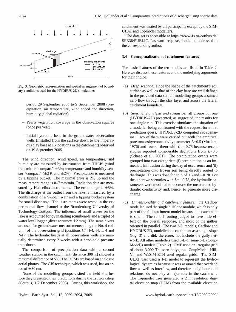
Fig. 3. Geometric representation and spatial arrangement of bound-ary conditions used for the HYDRUS-2D simulations.
period 29 September 2005 to 9 September 2008 (pre-cipitation, air temperature, wind speed and direction,humidity, global radiation).
– Yearly vegetation coverage in the observation squares(once per year).
– Initial hydraulic head in the groundwater observationwells (installed from the surface down to the impervi-ous clay base at 15 locations in the catchment) observedon 19 September 2005.
The wind direction, wind speed, air temperature, andhumidity are measured by instruments from THEIS (windtransmitter “compact”±3%; temperature and humidity sen-sor “compact” (±2 K and±2%). Precipitation is measuredby a tipping bucket. The maximal error is 2% up and themeasurement range is 0–7 mm/min. Radiation data are mea-sured by Hukseflux instruments. The error range is±5%.The discharge at the outlet from the lake is measured by acombination of a V-notch weir and a tipping bucket systemfor small discharge. The instruments were tested in the ex-perimental flow channel at the Brandenburg University ofTechnology Cottbus. The influence of small waves on thelake is accounted for by installing scumboards and a triplet ofwater level logger (diver accuracy±2 mm). The same diversare used for groundwater measurements along the No. 4 col-umn of the observation grid (positions C4, F4, I4, L 4 andN4). The hydraulic heads at all observation wells are man-ually determined every 2 weeks with a hand-held pressuretransducer.
The comparison of precipitation data with a secondweather station in the catchment (distance 300 m) showed amaximal difference of 5%. The DEMs are based on analogueaerial photos. The GIS technique, which was used, has an er-ror of ±30 cm.
None of the modelling groups visited the field site be-fore they presented their predictions during the 1st workshop(Cottbus, 1/2 December 2008). During this workshop, the
catchment was visited by all participants except by the SIM-ULAT and Topmodel modellers.
The data set is accessible athttps://www-fs.tu-cottbus.de/SFB38/PUBLIC.Password requests should be addressed tothe corresponding author.
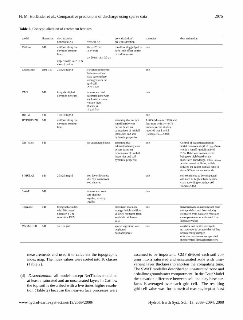
3.4 Conceptualization of catchment features
The basic features of the ten models are listed in Table 2.Here we discuss these features and the underlying argumentsfor their choice.
(a) Deep seepage:since the shape of the catchment’s soilsurface as well as that of the clay base are well definedin the provided data set, all modelling groups assumedzero flow through the clay layer and across the lateralcatchment boundary.
(b) Sensitivity analysis and scenarios:all groups but one(HYDRUS-2D) presented, as suggested, the results forone single run. This exercise simulates the situation ofa modeller being confronted with the request for a firstprediction guess. HYDRUS-2D computed six scenar-ios. Two of them were carried out with the empiricalpore tortuosity/connectivity parameterL=0.5 (Mualem,1976) and four of them withL=−0.78 because recentstudies reported considerable deviations fromL=0.5(Schaap et al., 2001). The precipitation events weregrouped into two categories: (i) precipitation as an im-mediate infiltration during the day of occurrence and (ii)precipitation onto frozen soil being directly routed todischarge. This was done for anL of 0.5 and−0.78. Forthe other two scenarios withL=−0.78, the hydraulic pa-rameters were modified to decrease the unsaturated hy-draulic conductivity and, hence, to generate more dis-charge.
(c) Dimensionality and catchment feature:the Catflowmodeller used the single hillslope module, which is onlypart of the full catchment model because the catchmentis small. The runoff routing judged to have little ef-fect on the overall response, and most of the gulliesoriented in parallel. The two 2-D models, Catflow andHYDRUS-2D, modelled the catchment as a single slope(Fig. 3) and did, therefore, not include the gully net-work. All other modellers used 3-D or semi-3-D (Coup-Model)) models (Table 2). CMF used an irregular gridof about 3.000 Thiessen polygons. CoupModel, Hill-Vi, and WaSiM-ETH used regular grids. The SIM-ULAT user used a 1-D model to represent the hydro-logical dynamics because it was assumed that overlandflow as well as interflow, and therefore neighbourhoodrelations, do not play a major role in the catchment.The Topmodel user generated a 2 m resolution digi-tal elevation map (DEM) from the available elevation
Hydrol. Earth Syst. Sci., 13, 2069–2094, 2009 www.hydrol-earth-syst-sci.net/13/2069/2009/
H. M. Hollander et al.: Comparative predictions of discharge using sparse data 2075
Table 2. Conceptualization of catchment features.
model dimension discretization pre-calculation/ scenarios data estimationhorizontal1x vertical1z pre-consideration
Catflow 2-D uniform along the 0<z<20 cm: runoff routing judged to oneelevation contour 1z=4 cm have little effect on thelines overall response
z>20 cm:1z=20 cmupper slope:1x=10 m,else:1x=1 m
CoupModel semi-3-D 20×20 m grid elevation difference onebetween soil andclay base surfaceaveraged over thegrid cell;1z≥0.5 m
CMF 3-D irregular digital unsaturated and oneelevation network saturated zone with
each with a time-variant layerthickness:1z≥0.5 m
Hill-Vi 3-D 10×10 m grid one
HYDRUS-2D 2-D uniform along the assuming that surface L=0.5 (Mualem, 1976) andelevation contour runoff hardly ever four runs withL=−0.78lines occurs based on because recent studies
comparison of rainfall reported thatL�0.5intensities and soil (Schaap et al., 2001).hydraulic properties
NetThales 3-D no unsaturated zone assuming that one Control of evapotranspiration:infiltration hardly ever initial root-zone depth1zroot=5 cmoccurs based on yields a runoff-rainfall ratio ofcomparison of rainfall 70%. Ratio was considered asintensities and soil being too high based on thehydraulic properties modeller’s knowledge. Thus,1zroo
was increased to 30 cm, whichreduced the runoff-rainfall ratio toabout 50% at the annual scale
SIMULAT 1-D 20×20 m grid soil layer thickness one soil considered to be compacteddirectly taken from and used he highest bulk densitysoil data set class according to .Adhoc AG
Boden (2005)
SWAT 3-D unsaturated zone oneand shallowaquifer, no deepaquifer
Topmodel 3-D topographic index maximum root zone one transmissivity, maximum root zonewith 16 classes storage deficit and flow storage deficit and flow velocitybased on a 2 m velocity estimated from estimated from data set.; recessionresolution DEM available catchment curve parameterm estimated from
data literature values
WaSiM-ETH 3-D 5×5 m grid sparse vegetation was one available soil depths averaged;neglected no macropores because the soil hasno macropores been recently dumped
effective parameters are upscaledmeasurement-derived parameters
measurements and used it to calculate the topographicindex map. The index values were sorted into 16 classes(Table 2).
(d) Discretization:all models except NetThales modelledat least a saturated and an unsaturated layer. In Catflowthe top soil is described with a five times higher resolu-tion (Table 2) because the near-surface processes were
assumed to be important. CMF divided each soil col-umn into a saturated and unsaturated zone with time-variant layer thickness to shorten the computing time.The SWAT modeller described an unsaturated zone anda shallow groundwater compartment. In the CoupModelthe elevation difference between soil and clay base sur-faces is averaged over each grid cell. The resultinggrid cell value was, for numerical reasons, kept at least
www.hydrol-earth-syst-sci.net/13/2069/2009/ Hydrol. Earth Syst. Sci., 13, 2069–2094, 2009
2076 H. M. Hollander et al.: Comparative predictions of discharge using sparse data
0.5 m. WaSiM-ETH reduced the calculation effort byaggregating the DEM to a 5×5 m raster. The aggregatedDEM does not resolve the gully structures nor the claydam.
(e) Surface runoff: the aerial photo of summer 2007showed evidence of surface runoff across the entirecatchment. However, the modellers, except Coup-Model, neglected it due to the soil texture data. TheHYDRUS-2D group compared rainfall intensities andtexture-derived estimates of soil hydraulic propertiesand concluded that surface runoff (not accounted forby HYDRUS-2D) would hardly ever occur. Similarly,the NetThales modellers argued that infiltration ex-cess runoff cannot be generated using a 1-D Richardequation based infiltration model because the soil hy-draulic conductivity (estimated with pedotransfer func-tions from soil texture) was definitely larger than themaximum hourly rainfall intensity. The only dominantrunoff generation mechanism was, therefore, saturationexcess runoff (Table 2). HYDRUS-2D generated runoffby modifying the porosities and hydraulic conductivi-ties upslope of the clay dam (Fig. 3). The soil param-eters were estimated according to Schaap et al. (2001)using the routine implemented in the HYDRUS-2D pro-gram. The CMF modeller did not make use of the pro-vided gully network, because the shape and depth of thegullies were lacking. However, the mere existence ofgullies was included as infiltration excess. The Hill-Vigroup assumed that surface runoff is important becauseof the distinctive gully network but they had difficul-ties in accounting for large hydraulic conductivities onone hand, and large amounts of surface runoff on theother. Hill-Vi recalculated the drainage network for ev-ery time step so that the information of the gullies wasnot incorporated in the model. Preliminary Hill-Vi testruns with a snowmelt routine did not yield notable ef-fects. Snow was, therefore, disregarded in the model.The CoupModel group did not use the information onthe initial ground water levels assuming that the catch-ment already existed long enough to be “initialized”.The role of the gullies was incorporated in the parame-terization of the surface runoff by reducing the surfacepool threshold to get a faster surface runoff response.The SIMULAT user neglected the information on exist-ing gullies. The NetThales modeller considered evapo-transpiration and the “root-zone depth”1zroot to be crit-ical features. Initially, they assumed that1zroot=5 cm.This led to an annual runoff-rainfall ratio of 70%. Basedon the modeller’s knowledge of relatively dry Austrianand German catchments, the NetThales modellers ar-gued that in Brandenburg this ratio is less than 30%.Since the plant cover was almost non-existent, a largerrunoff ratio was expected, but certainly not 70%. Alsothe baseflow contribution of the initial simulations was
considered too high in this climate. Thus, the1zroot wasincreased to 30 cm, which reduced the runoff-rainfall ra-tio to about 50% at the annual scale.
(f) Soil parameters:catflow treated the soil as a homo-geneous loamy sand, parameterized after Carsel andParrish (1988), because soil texture of the soil layershows little variability across the catchment and withdepth. The Hill-Vi modeller applied the Rosetta database (Schaap et al., 2001) to estimate soil hydraulic pa-rameters with hierarchical pedotransfer functions. Forthe CoupModel the hydraulic properties of the soil layerwere estimated from the numerous soil-water retentiondata of Swedish sandy soils (Lundmark and Jansson,2009). In SIMULAT the thickness of the soil layer wasdirectly taken from the soil data set. The SIMULATmodeller treated the soil to be compacted because itwas dumped and shaped with large machines and usedthe highest bulk density class according to Adhoc AGBoden (2005). Based on the soil and the soil layer in-formation, it was concluded that subsurface runoff ex-ceeds surface runoff with a minor contribution of inter-flow, making baseflow the dominant runoff component.The main principle of the soil parameterisation was “assimple as possible”. Therefore, the data from each soildepth were aggregated to a single average value. Thiswas parameterised with literature values (AdHoc-AGBoden, 1999). The WaSiM-ETH user did not considermacropores because the soil material had been recentlydumped and repacked and also because of the initialstate of the vegetation. In WaSiM-ETH the effectiveparameters are upscaled measurement-derived parame-ters, which are gathered “normally” during the calibra-tion by measured outputs. Therefore, they were takenfrom another headwater catchment in Germany (Holzeland Diekkruger, in press, 2008).
(g) Process assumptions:topmodel does not account forseveral processes that do occur in this particular catch-ment, such as snowmelt, gully erosion. Its semi-distributed nature does not allow for describing the claydam. Although Topmodel could be customised to indi-rectly include such processes, the modeller decided notto do so at this stage of the modelling process, in or-der to provide a reference performance. Transmissivity,maximum root zone storage deficit, and flow velocitywere estimated from the available catchment data. Onlyone parameter, the shape of the recession curve, was es-timated from literature values.
3.5 Process concepts and implementation
3.5.1 Infiltration, saturated and unsaturated flow
The saturated and unsaturated flow was simulated ei-ther as 1-D linear storage (CoupModel, Topmodel,
Hydrol. Earth Syst. Sci., 13, 2069–2094, 2009 www.hydrol-earth-syst-sci.net/13/2069/2009/
H. M. Hollander et al.: Comparative predictions of discharge using sparse data 2077
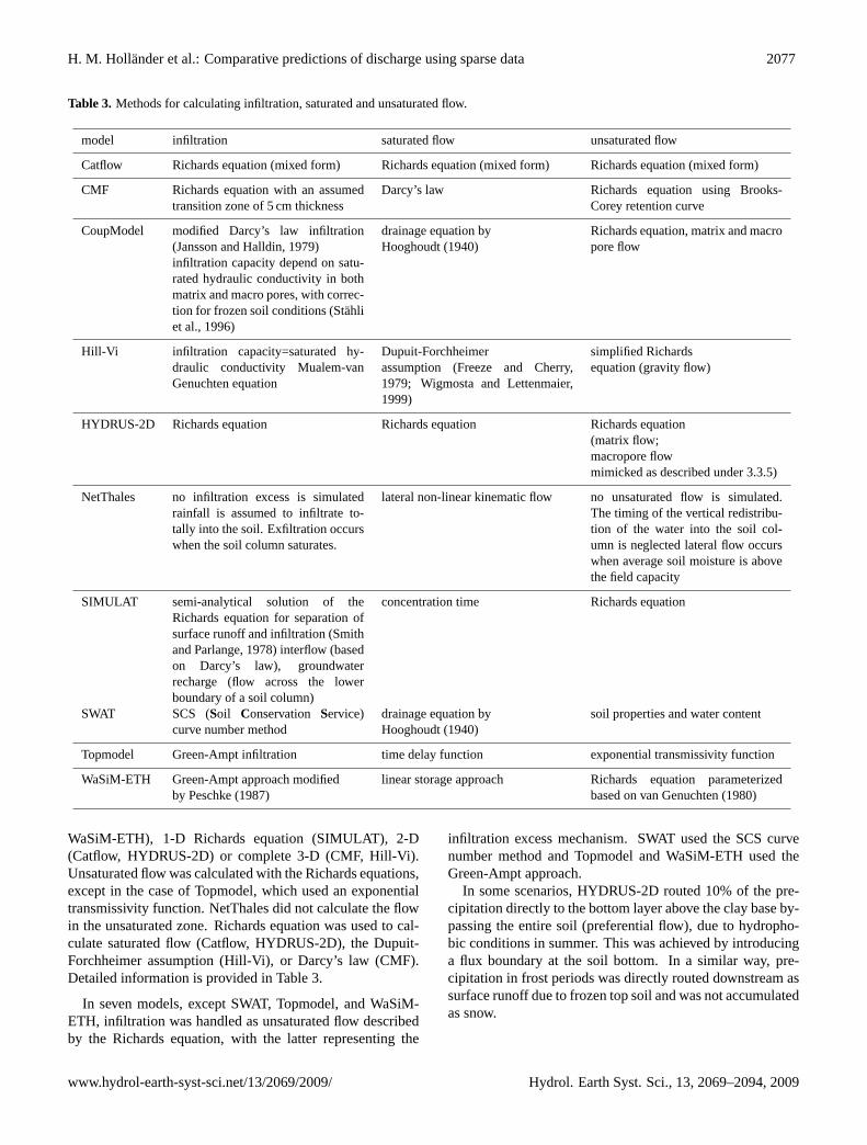
Table 3. Methods for calculating infiltration, saturated and unsaturated flow.
model infiltration saturated flow unsaturated flow
Catflow Richards equation (mixed form) Richards equation (mixed form) Richards equation (mixed form)
CMF Richards equation with an assumedtransition zone of 5 cm thickness
Darcy’s law Richards equation using Brooks-Corey retention curve
CoupModel modified Darcy’s law infiltration(Jansson and Halldin, 1979)infiltration capacity depend on satu-rated hydraulic conductivity in bothmatrix and macro pores, with correc-tion for frozen soil conditions (Stahliet al., 1996)
drainage equation byHooghoudt (1940)
Richards equation, matrix and macropore flow
Hill-Vi infiltration capacity=saturated hy-draulic conductivity Mualem-vanGenuchten equation
Dupuit-Forchheimerassumption (Freeze and Cherry,1979; Wigmosta and Lettenmaier,1999)
simplified Richardsequation (gravity flow)
HYDRUS-2D Richards equation Richards equation Richards equation(matrix flow;macropore flowmimicked as described under 3.3.5)
NetThales no infiltration excess is simulatedrainfall is assumed to infiltrate to-tally into the soil. Exfiltration occurswhen the soil column saturates.
lateral non-linear kinematic flow no unsaturated flow is simulated.The timing of the vertical redistribu-tion of the water into the soil col-umn is neglected lateral flow occurswhen average soil moisture is abovethe field capacity
SIMULAT semi-analytical solution of theRichards equation for separation ofsurface runoff and infiltration (Smithand Parlange, 1978) interflow (basedon Darcy’s law), groundwaterrecharge (flow across the lowerboundary of a soil column)
concentration time Richards equation
SWAT SCS (Soil Conservation Service)curve number method
drainage equation byHooghoudt (1940)
soil properties and water content
Topmodel Green-Ampt infiltration time delay function exponential transmissivity function
WaSiM-ETH Green-Ampt approach modifiedby Peschke (1987)
linear storage approach Richards equation parameterizedbased on van Genuchten (1980)
WaSiM-ETH), 1-D Richards equation (SIMULAT), 2-D(Catflow, HYDRUS-2D) or complete 3-D (CMF, Hill-Vi).Unsaturated flow was calculated with the Richards equations,except in the case of Topmodel, which used an exponentialtransmissivity function. NetThales did not calculate the flowin the unsaturated zone. Richards equation was used to cal-culate saturated flow (Catflow, HYDRUS-2D), the Dupuit-Forchheimer assumption (Hill-Vi), or Darcy’s law (CMF).Detailed information is provided in Table 3.
In seven models, except SWAT, Topmodel, and WaSiM-ETH, infiltration was handled as unsaturated flow describedby the Richards equation, with the latter representing the
infiltration excess mechanism. SWAT used the SCS curvenumber method and Topmodel and WaSiM-ETH used theGreen-Ampt approach.
In some scenarios, HYDRUS-2D routed 10% of the pre-cipitation directly to the bottom layer above the clay base by-passing the entire soil (preferential flow), due to hydropho-bic conditions in summer. This was achieved by introducinga flux boundary at the soil bottom. In a similar way, pre-cipitation in frost periods was directly routed downstream assurface runoff due to frozen top soil and was not accumulatedas snow.
www.hydrol-earth-syst-sci.net/13/2069/2009/ Hydrol. Earth Syst. Sci., 13, 2069–2094, 2009
2078 H. M. Hollander et al.: Comparative predictions of discharge using sparse data
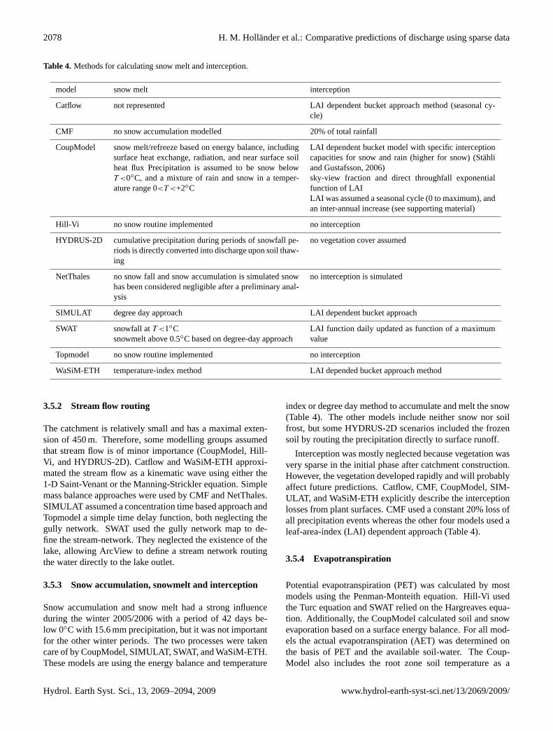
Table 4. Methods for calculating snow melt and interception.
model snow melt interception
Catflow not represented LAI dependent bucket approach method (seasonal cy-cle)
CMF no snow accumulation modelled 20% of total rainfall
CoupModel snow melt/refreeze based on energy balance, includingsurface heat exchange, radiation, and near surface soilheat flux Precipitation is assumed to be snow belowT <0◦C, and a mixture of rain and snow in a temper-ature range 0<T <+2◦C
LAI dependent bucket model with specific interceptioncapacities for snow and rain (higher for snow) (Stahliand Gustafsson, 2006)sky-view fraction and direct throughfall exponentialfunction of LAILAI was assumed a seasonal cycle (0 to maximum), andan inter-annual increase (see supporting material)
Hill-Vi no snow routine implemented no interception
HYDRUS-2D cumulative precipitation during periods of snowfall pe-riods is directly converted into discharge upon soil thaw-ing
no vegetation cover assumed
NetThales no snow fall and snow accumulation is simulated snowhas been considered negligible after a preliminary anal-ysis
no interception is simulated
SIMULAT degree day approach LAI dependent bucket approach
SWAT snowfall atT <1◦Csnowmelt above 0.5◦C based on degree-day approach
LAI function daily updated as function of a maximumvalue
Topmodel no snow routine implemented no interception
WaSiM-ETH temperature-index method LAI depended bucket approach method
3.5.2 Stream flow routing
The catchment is relatively small and has a maximal exten-sion of 450 m. Therefore, some modelling groups assumedthat stream flow is of minor importance (CoupModel, Hill-Vi, and HYDRUS-2D). Catflow and WaSiM-ETH approxi-mated the stream flow as a kinematic wave using either the1-D Saint-Venant or the Manning-Strickler equation. Simplemass balance approaches were used by CMF and NetThales.SIMULAT assumed a concentration time based approach andTopmodel a simple time delay function, both neglecting thegully network. SWAT used the gully network map to de-fine the stream-network. They neglected the existence of thelake, allowing ArcView to define a stream network routingthe water directly to the lake outlet.
3.5.3 Snow accumulation, snowmelt and interception
Snow accumulation and snow melt had a strong influenceduring the winter 2005/2006 with a period of 42 days be-low 0◦C with 15.6 mm precipitation, but it was not importantfor the other winter periods. The two processes were takencare of by CoupModel, SIMULAT, SWAT, and WaSiM-ETH.These models are using the energy balance and temperature
index or degree day method to accumulate and melt the snow(Table 4). The other models include neither snow nor soilfrost, but some HYDRUS-2D scenarios included the frozensoil by routing the precipitation directly to surface runoff.
Interception was mostly neglected because vegetation wasvery sparse in the initial phase after catchment construction.However, the vegetation developed rapidly and will probablyaffect future predictions. Catflow, CMF, CoupModel, SIM-ULAT, and WaSiM-ETH explicitly describe the interceptionlosses from plant surfaces. CMF used a constant 20% loss ofall precipitation events whereas the other four models used aleaf-area-index (LAI) dependent approach (Table 4).
3.5.4 Evapotranspiration
Potential evapotranspiration (PET) was calculated by mostmodels using the Penman-Monteith equation. Hill-Vi usedthe Turc equation and SWAT relied on the Hargreaves equa-tion. Additionally, the CoupModel calculated soil and snowevaporation based on a surface energy balance. For all mod-els the actual evapotranspiration (AET) was determined onthe basis of PET and the available soil-water. The Coup-Model also includes the root zone soil temperature as a
Hydrol. Earth Syst. Sci., 13, 2069–2094, 2009 www.hydrol-earth-syst-sci.net/13/2069/2009/
H. M. Hollander et al.: Comparative predictions of discharge using sparse data 2079
Table 5. Methods for calculating the potential and actual evapotranspiration (PET and AET, respectively).
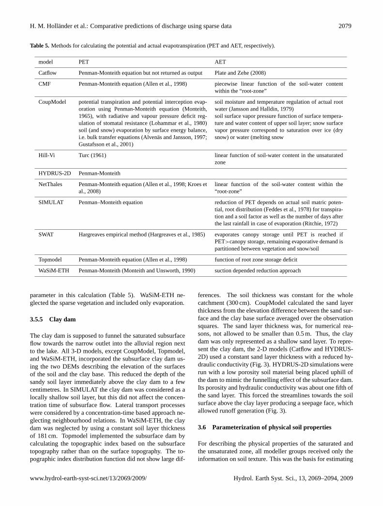
model PET AET
Catflow Penman-Monteith equation but not returned as output Plate and Zehe (2008)
CMF Penman-Monteith equation (Allen et al., 1998) piecewise linear function of the soil-water contentwithin the “root-zone”
CoupModel potential transpiration and potential interception evap-oration using Penman-Monteith equation (Monteith,1965), with radiative and vapour pressure deficit reg-ulation of stomatal resistance (Lohammar et al., 1980)soil (and snow) evaporation by surface energy balance,i.e. bulk transfer equations (Alvenas and Jansson, 1997;Gustafsson et al., 2001)
soil moisture and temperature regulation of actual rootwater (Jansson and Halldin, 1979)soil surface vapor pressure function of surface tempera-ture and water content of upper soil layer; snow surfacevapor pressure correspond to saturation over ice (drysnow) or water (melting snow
Hill-Vi Turc (1961) linear function of soil-water content in the unsaturatedzone
HYDRUS-2D Penman-Monteith
NetThales Penman-Monteith equation (Allen et al., 1998; Kroes etal., 2008)
linear function of the soil-water content within the“root-zone”
SIMULAT Penman–Monteith equation reduction of PET depends on actual soil matric poten-tial, root distribution (Feddes et al., 1978) for transpira-tion and a soil factor as well as the number of days afterthe last rainfall in case of evaporation (Ritchie, 1972)
SWAT Hargreaves empirical method (Hargreaves et al., 1985) evaporates canopy storage until PET is reached ifPET>canopy storage, remaining evaporative demand ispartitioned between vegetation and snow/soil
Topmodel Penman-Monteith equation (Allen et al., 1998) function of root zone storage deficit
WaSiM-ETH Penman-Monteith (Monteith and Unsworth, 1990) suction depended reduction approach
parameter in this calculation (Table 5). WaSiM-ETH ne-glected the sparse vegetation and included only evaporation.
3.5.5 Clay dam
The clay dam is supposed to funnel the saturated subsurfaceflow towards the narrow outlet into the alluvial region nextto the lake. All 3-D models, except CoupModel, Topmodel,and WaSiM-ETH, incorporated the subsurface clay dam us-ing the two DEMs describing the elevation of the surfacesof the soil and the clay base. This reduced the depth of thesandy soil layer immediately above the clay dam to a fewcentimetres. In SIMULAT the clay dam was considered as alocally shallow soil layer, but this did not affect the concen-tration time of subsurface flow. Lateral transport processeswere considered by a concentration-time based approach ne-glecting neighbourhood relations. In WaSiM-ETH, the claydam was neglected by using a constant soil layer thicknessof 181 cm. Topmodel implemented the subsurface dam bycalculating the topographic index based on the subsurfacetopography rather than on the surface topography. The to-pographic index distribution function did not show large dif-
ferences. The soil thickness was constant for the wholecatchment (300 cm). CoupModel calculated the sand layerthickness from the elevation difference between the sand sur-face and the clay base surface averaged over the observationsquares. The sand layer thickness was, for numerical rea-sons, not allowed to be smaller than 0.5 m. Thus, the claydam was only represented as a shallow sand layer. To repre-sent the clay dam, the 2-D models (Catflow and HYDRUS-2D) used a constant sand layer thickness with a reduced hy-draulic conductivity (Fig. 3). HYDRUS-2D simulations wererun with a low porosity soil material being placed uphill ofthe dam to mimic the funnelling effect of the subsurface dam.Its porosity and hydraulic conductivity was about one fifth ofthe sand layer. This forced the streamlines towards the soilsurface above the clay layer producing a seepage face, whichallowed runoff generation (Fig. 3).
3.6 Parameterization of physical soil properties
For describing the physical properties of the saturated andthe unsaturated zone, all modeller groups received only theinformation on soil texture. This was the basis for estimating
www.hydrol-earth-syst-sci.net/13/2069/2009/ Hydrol. Earth Syst. Sci., 13, 2069–2094, 2009
2080 H. M. Hollander et al.: Comparative predictions of discharge using sparse data
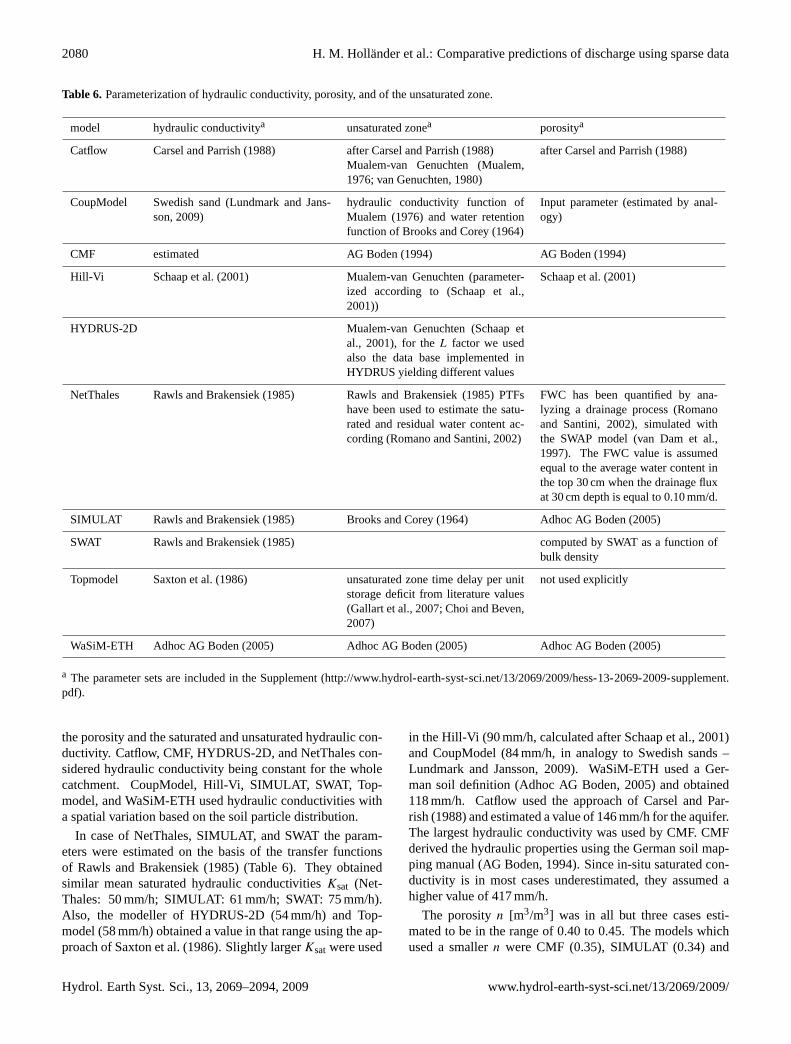
Table 6. Parameterization of hydraulic conductivity, porosity, and of the unsaturated zone.
model hydraulic conductivitya unsaturated zonea porositya
Catflow Carsel and Parrish (1988) after Carsel and Parrish (1988)Mualem-van Genuchten (Mualem,1976; van Genuchten, 1980)
after Carsel and Parrish (1988)
CoupModel Swedish sand (Lundmark and Jans-son, 2009)
hydraulic conductivity function ofMualem (1976) and water retentionfunction of Brooks and Corey (1964)
Input parameter (estimated by anal-ogy)
CMF estimated AG Boden (1994) AG Boden (1994)
Hill-Vi Schaap et al. (2001) Mualem-van Genuchten (parameter-ized according to (Schaap et al.,2001))
Schaap et al. (2001)
HYDRUS-2D Mualem-van Genuchten (Schaap etal., 2001), for theL factor we usedalso the data base implemented inHYDRUS yielding different values
NetThales Rawls and Brakensiek (1985) Rawls and Brakensiek (1985) PTFshave been used to estimate the satu-rated and residual water content ac-cording (Romano and Santini, 2002)
FWC has been quantified by ana-lyzing a drainage process (Romanoand Santini, 2002), simulated withthe SWAP model (van Dam et al.,1997). The FWC value is assumedequal to the average water content inthe top 30 cm when the drainage fluxat 30 cm depth is equal to 0.10 mm/d.
SIMULAT Rawls and Brakensiek (1985) Brooks and Corey (1964) Adhoc AG Boden (2005)
SWAT Rawls and Brakensiek (1985) computed by SWAT as a function ofbulk density
Topmodel Saxton et al. (1986) unsaturated zone time delay per unitstorage deficit from literature values(Gallart et al., 2007; Choi and Beven,2007)
not used explicitly
WaSiM-ETH Adhoc AG Boden (2005) Adhoc AG Boden (2005) Adhoc AG Boden (2005)
a The parameter sets are included in the Supplement (http://www.hydrol-earth-syst-sci.net/13/2069/2009/hess-13-2069-2009-supplement.pdf).
the porosity and the saturated and unsaturated hydraulic con-ductivity. Catflow, CMF, HYDRUS-2D, and NetThales con-sidered hydraulic conductivity being constant for the wholecatchment. CoupModel, Hill-Vi, SIMULAT, SWAT, Top-model, and WaSiM-ETH used hydraulic conductivities witha spatial variation based on the soil particle distribution.
In case of NetThales, SIMULAT, and SWAT the param-eters were estimated on the basis of the transfer functionsof Rawls and Brakensiek (1985) (Table 6). They obtainedsimilar mean saturated hydraulic conductivitiesKsat (Net-Thales: 50 mm/h; SIMULAT: 61 mm/h; SWAT: 75 mm/h).Also, the modeller of HYDRUS-2D (54 mm/h) and Top-model (58 mm/h) obtained a value in that range using the ap-proach of Saxton et al. (1986). Slightly largerKsatwere used
in the Hill-Vi (90 mm/h, calculated after Schaap et al., 2001)and CoupModel (84 mm/h, in analogy to Swedish sands –Lundmark and Jansson, 2009). WaSiM-ETH used a Ger-man soil definition (Adhoc AG Boden, 2005) and obtained118 mm/h. Catflow used the approach of Carsel and Par-rish (1988) and estimated a value of 146 mm/h for the aquifer.The largest hydraulic conductivity was used by CMF. CMFderived the hydraulic properties using the German soil map-ping manual (AG Boden, 1994). Since in-situ saturated con-ductivity is in most cases underestimated, they assumed ahigher value of 417 mm/h.
The porosityn [m3/m3] was in all but three cases esti-mated to be in the range of 0.40 to 0.45. The models whichused a smallern were CMF (0.35), SIMULAT (0.34) and
Hydrol. Earth Syst. Sci., 13, 2069–2094, 2009 www.hydrol-earth-syst-sci.net/13/2069/2009/
H. M. Hollander et al.: Comparative predictions of discharge using sparse data 2081
WaSiM-ETH (0.38), all of them using the German soil defi-nition (Adhoc AG Boden, 2005). The German soil definition,the estimators of Carsel and Parrish (1988) and of Saxton etal. (1986), and the analogy to Swedish sands do not requirebulk density nor organic matter content, information whichwas not available in this case. The estimates of the water con-tent at the wilting point varied from 0.045 to 0.090 [m3/m3]and the field capacity from 0.125 to 0.280 [m3/m3].
The hydraulic parameterization of the unsaturated zonewas mostly done using the methods of Mualem (1976) andvan Genuchten (1980) (Catflow, Hill-Vi, HYDRUS-2D) orthat of Brooks and Corey (1964) (CoupModel, NetThales,SIMULAT). The empirical pore tortuosity/connectivity pa-rameterL is usually assumed to be 0.5 (Mualem, 1976),but was varied in some HYDRUS-2D simulations becausemore recent studies revealed considerable deviations fromthis value (Schaap et al., 2001). The pore-size indexλ asdefined by Brooks and Corey is here expressed in terms oftheαsg, andnvG parameters as defined by van Genuchten. Ifα·hb>> 1 then
λ = nvG −1 (1)
WaSiM-ETH used the smallestnvG (1.13) CoupModel a con-stantnvG (1.42), HYDRUS-2DnvG between 1.15 and 1.88,Catflow a soil specificnvG (loamy sand: 2.28 and sandy clayloam: 1.48). The models CMF, Hill-Vi, and SIMULAT as-sumed a spatial variation ofnvG from 1.15 to 1.37, 1.37 to3.57, and 1.56 to 2.33, respectively. NetThales, SWAT, andTopmodel did not account for unsaturated flow, nor did theyuse Richards equation for representing the unsaturated flow.In Topmodel, the flow between the unsaturated and satu-rated storage is controlled by one parameter representing thetime delay per unit storage deficit (Gallart et al., 2007; Choiand Beven, 2007). The complete parameter sets are listedin the Supplement (http://www.hydrol-earth-syst-sci.net/13/2069/2009/hess-13-2069-2009-supplement.pdf).
3.7 Initial conditions
The initial conditions were not well defined, in particular theinitial volumetric soil-water contentθ(t0) [m3/m3]. SIM-ULAT estimated the soil to be dry. Other models wererun to initialize this variable and its spatial variation: Hill-Vi three times (0.20±0.25) and CMF (0.22±0.06), SWAT(θ (t0)=0.11±0.04), and WaSiM-ETH (θ (t0)=0.27±0.05)once. CMF used the 3-year rainfall record for the initial-ization run, with a wet year in 2008. Catflow was run twiceto find stable initial conditions, in this case not for the soil-water content but for matric potential. Pre-runs were used toachieve quasi-steady-state conditions, which were then usedas initial condition. WaSiM-ETH archived system-stable ini-tial conditions of the whole model period using default val-ues.
CoupModel initialized the soil moisture at field capacity.HYDRUS-2D was run with differentθ (t0). The wet scenar-
ios assumed a constant matric potential of−0.3 m, whereasthe dry runs started with a matric potential of−1.0 m. Whenmodel runs were started, assuming dry soil, the dischargewas too little to fill the lake at the outlet of the catchmentwithin the first year. Since the presence of the lake wasknown to the modellers, such model runs were rejected.SIMULAT assumed a matric potential of−3 m at the bot-tom of the sand layer and decreasing values towards the soilsurface assuming hydrostatic equilibrium. Topmodel used aninitial vertical subsurface flow parameter of 0.017 mm/h perunit area which was estimated from the mean annual rainfallof 496 mm and the assumed runoff coefficient of 0.3.
The groundwater levels were part of the initial data set butnone of the models except SIMULAT made use of it, be-cause the case of an “empty”, newly constructed catchmentwithout initial groundwater was not considered, because itwould lead to numerical problems. Therefore, Catflow, Hill-Vi, and WaSiM-ETH used a warm-up run for the formationof a groundwater table. HYDRUS-2D defined the ground-water table at 40 to 60 cm within a soil cover of constantthickness (1.90 m) (Fig. 3).
3.8 Water budget of the Chicken Creek
The measurements used to close the water budget of theChicken Creek catchment were precipitation, discharge fromthe lake, lake storage change, and changes of the levels ofthe groundwater table. Soil moisture measurements wereavailable from mid 2007 onwards. For reference, the po-tential evapotranspiration PET was calculated using grass-referenced Penman-Monteith using the standard parameter-ization (Allen et al., 1994) and the reference actual evapo-transpiration AET was estimated using a modified Black ap-proach (Black et al., 1969; DVWK, 1996). The continuousdata by the Black approach were compared with some AETdata by the Bowen Ratio method. The comparison showeda good agreement of the AET during summer months but anunderestimation of AET during the windy seasons of springand autumn.
The Chicken Creek catchment drains into a lake (Fig. 1).The gauge for measuring the catchment discharge is locatedat the outflow of the lake. The inflow into the lake is notmonitored. Since several models did not consider the lake asa buffer compartment, we determined the catchment outflowinto the lake by subtracting the observed lake storage changesand precipitation onto the lake from the measured lake out-flow and added the evaporative losses from the lake. Theback calculated inflow into the lake is the standard againstwhich the modelled discharge is compared.
For the above calculation, we assume that the clay baseprevents any vertical seepage. Vattenfall Europe Mining AGconstructed the clay layer and tested the clay beforehand.The hydraulic conductivity of the clay is 2 10−10 m/s. Usingthe maximum water level in the lake (2.50 m) and a clay layerthickness of 1.50 m, the losses through the clay would be in
www.hydrol-earth-syst-sci.net/13/2069/2009/ Hydrol. Earth Syst. Sci., 13, 2069–2094, 2009
2082 H. M. Hollander et al.: Comparative predictions of discharge using sparse data
Table 7. Time to set up the models and computation time.
model model development computation computer performance(men-days) time
Catflow 5 9 h 2.0 GHz, Dual Core, 2 GBRAM
CMF 14a 1 h 2.6 GHz, Quad CoreCoupModel 7 20 min standard personal computerHill-Vi 15 a 15 min 3.16 GHz, Dual Core, 3 GB
RAMHYDRUS-2D 35 15–20 minb 1.8 GHz, Dual Core, 1 GB
12 h and morec RAMNetThales 6 23 min 2.2 GHz, Dual Core, 2 GB
RAMSIMULAT 4 2 h standard personal computerSWAT 3 5 s 2.0 GHz, Dual Core, 2 GB
RAMTopmodel 2 >1 s any personal computerWaSiM-ETH 2 2.5 h 2.6 GHz
a including code implementation.b standard run without numerical problems.c run with numerical problems.
the order of 17 mm/y. Precipitation into the lake were takenfrom the weather station data. The largest uncertainty re-sults from the evaporation. This was calculated by the Daltonmethod including the Richter wind function (Richter, 1977)and a wind function for small water bodies (Penman, 1948;Nenov, 2009). The comparison with the measured declinesof the lake levels during dry season showed a good agree-ment.
3.9 Computation time
Models, including the pre-calculations, were set up in oneweek, except for CMF, Hill-Vi, and HYDRUS-2D. The CMFand the Hill-Vi user needed to adjust the model to the specificneeds of an artificial catchment. The HYDRUS-2D modellerapplied the model in a catchment context. Since the modeldoes not simulate surface runoff, direct runoff, e.g. due tofrozen soil conditions, needed to be calculated before. Addi-tional time was needed because the HYDRUS-2D modellerdeveloped several scenarios. All computations were run ona standard personal computer. The fastest run was done byTopmodel which ran within one second. Similar was the run-time of SWAT (5 s). CoupModel, Hill-Vi, and NetThalesused less than one hour and all other models needed morethan one hour. Catflow used the maximum calculation timeof 9 h. HYDRUS-2D simulations needed 15 to 20 min ifno numerical problems were available. Numerical problemswere due to saturation of surface-near cell which would pro-duce overland flow which HYDRUS-2D is not able to simu-late. This increased simulation times to 12 or more hours perrun (Table 7).
4 Results
We first compare the predictions and observations in termsof the water budget, discharge, and groundwater levels. Thepredictions are presented for the three hydrological yearsfrom November through October (2005/2006, 2006/2007,and 2007/2008 only until 8 September 2008). These periodsare referred to as the 1st, 2nd, and 3rd year.
4.1 Water budget
Below, the annual values of the 1st, 2nd, and 3rd year arereported as triplets (1st, 2nd, and 3rd year). Annual pre-cipitation used as input was 373, 566, and 511 mm/y (Ta-ble 8a–c). All models used hourly data except HYDRUS-2D,where wind-corrected daily precipitation was used. Coup-Model used wind-corrected hourly precipitation. In CMF, a20% interception loss of the total precipitation (Table 4) wasassumed.
The calculated reference PET was 779, 782, and511 mm/y. PET, predicted by the ten model, ranges from 146to 807 mm/y (1st year). The values for the 2nd and 3rd yearvary in the same range. The reference AET, calculated by themodified Black method (Black et al., 1969; DVWK, 1996)was 163, 165, and 137 mm/y, which yields a ratio AET/PETof 0.21, 0.21, and 0.27. Only Hill-Vi predicted a similarbehaviour. The other models systematically overestimatedAET relative to PET.
CMF predicted the significantly lowest PET and AET,whereas Hill-Vi predicted a high PET but a low AET. Cat-flow produced AETs of 161, 170 and 163 mm/y assuming avegetation cover of 5%, an LAI ranging between 1 and 2, a
Hydrol. Earth Syst. Sci., 13, 2069–2094, 2009 www.hydrol-earth-syst-sci.net/13/2069/2009/

H. M. Hollander et al.: Comparative predictions of discharge using sparse data 2083
Table 8a.Predicted and observed water budget of the Chicken Creek catchment for the 1st year.
P PET AET Discharge Storage Balance(mm/y) (mm/y) (mm/y) (mm/y) (mm/y) (mm/y)
Catflow 373 NA 161 249 −59 22CMFb 298 146 88 208 −44 46CoupModel 401 NA 437 12 −48 0Hill-Vi 373 717 153 306 −63 −23HYDRUS-2D 431 611 409–545 34–48 −158–−38 −5–22NetThales 373 392 226 189 −38 −4SIMULAT 373 680 239 189 25 −80SWAT 373 807 350 76 −4 −49Topmodel 373 570 271 94 0 8WaSiM-ETH 373 700 283 107 0 −17Chicken Creek 373 779 163 113d 35 62
Table 8b. Predicted and observed water budget of the Chicken Creek catchment for the 2nd year.
P PET AET Discharge Storage Balance(mm/y) (mm/y) (mm/y) (mm/y) (mm/y) (mm/y)
Catflow 565 NA 170 262 80 53CMFb 452 139 104 238 13 97CoupModel 666 NA 563 27 76 0Hill-Vi 565 718 156 346 58 5HYDRUS-2D 635 602 520–579 19–67 27–33 1–17NetThales 565 421 284 259 23 −1SIMULAT 565 713 318 339 −9 −83SWAT 565 815 409 145 18 −7Topmodel 565 573 384 171 0 10WaSiM-ETH 565 689 371 162 0 32Chicken Creek 565 782 165 105 69 226
Table 8c.Predicted and observed water budget of the Chicken Creek catchment for the 3rd year.
P PET AET Discharge Storage Balance(mm/y) (mm/y) (mm/y) (mm/y) (mm/y) (mm/y)
Catflow 511 NA 163 258 55 35CMFb 409 116 78 250 −39 120CoupModel 563 NA 498 76 −11 0Hill-Vi 511 588 128 329 44 10HYDRUS-2Dc 357 331 277–313 34–64 −9–7 2–26NetThales 511 307 199 275 39 −2SIMULAT 511 628 278 283 17 −67SWAT 511 706 331 164 −4 20Topmodel 511 486 294 198 NA 19WaSiM-ETH 511 573 272 178 NA 61Chicken Creek 511 674 137 113 162 99
a until 8 September 2008.b 20% interception losses.c until 3 July 2008.d 69 mm were needed to fill up the lake.
www.hydrol-earth-syst-sci.net/13/2069/2009/ Hydrol. Earth Syst. Sci., 13, 2069–2094, 2009
2084 H. M. Hollander et al.: Comparative predictions of discharge using sparse data
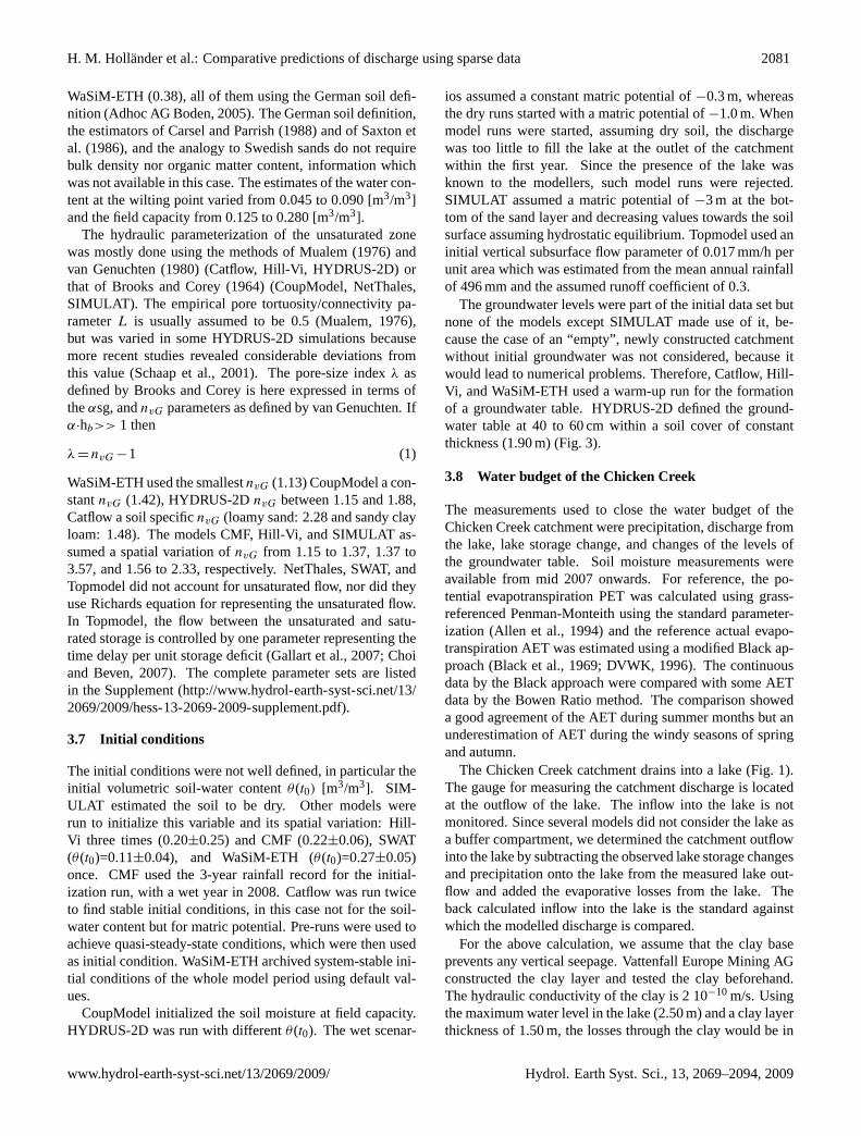
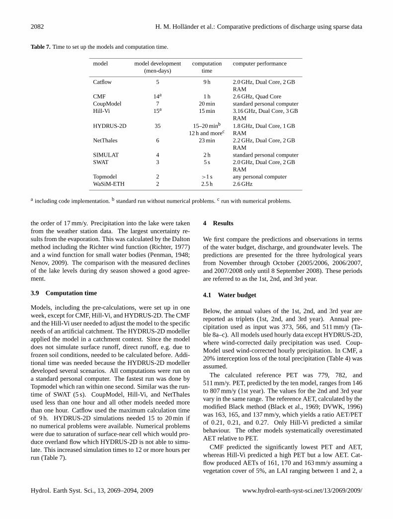
Fig. 4a. Predicted discharge for the hydrological year 2005/2006.
Fig. 4b. Predicted discharge for the hydrological year 2006/2007.
canopy height increasing in the course of the growing seasonfrom 13 to 40 cm, and a stomatal resistance of 200 s/m.
The measured discharge from the catchment was 113, 105,and 113 mm/y. The range of the ten discharge predictionswas 12 to 306, 27 to 346, and 76 to 329 mm/y. Expressedas percentage of the measured discharge, the predicted dis-charge ranges from 10 to 221, 19 to 329, and 30 to 290%(Fig. 4a–c). The catchment was built by dumping relativelydry soil onto the clay base so that the groundwater graduallyfilled up after construction. At the end of the three years, thegroundwater storage was 35, 69, and 162 mm, determinedaccording to the water-table fluctuation method (Meinzer,1923; Healy and Cook, 2002) using the means of porosityand groundwater table rise. Water storage in the unsaturatedzone was not available as model input. The predicted storagechanges (sum of ground and soil-water) varied between−63and 25,−9 and 76, and−39 and 44 mm.
The modellers were unaware that the dumped soil materialwas relatively dry (see Sect. 3.7) and groundwater absent.
Most of them assumed an initial water content correspond-ing to field capacity or they estimated the soil-water contentsfrom pre-runs. Therefore, the predictions cannot be directlycompared with the observed data but can be placed there inrelation to each other. All models, except SIMULAT, pre-dicted a loss of soil- and groundwater for the first year. Thisis not surprising because the precipitation was less than thelong-term mean.
The errors in the internal model mass balance1Merror[mm/y] are
1Merror= P −AET−Q−1S (2)
with P being measured and AET,Q , and1S simulated en-tities (Table 8a–c). The CoupModel, Hill-Vi, HYDRUS-2D,NetThales, Topmodel and WaSiM-ETH produce a1Merrorof less than 5% ofP , Catflow 7%, and CMF, SIMULAT andSWAT more than 10%, and CMF up to 25%.
Hydrol. Earth Syst. Sci., 13, 2069–2094, 2009 www.hydrol-earth-syst-sci.net/13/2069/2009/
H. M. Hollander et al.: Comparative predictions of discharge using sparse data 2085
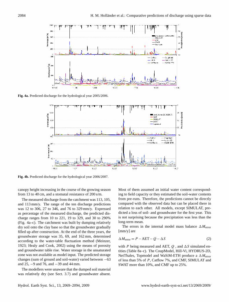
Fig. 4c. Predicted discharge for the hydrological year 2007/2008.
4.2 Discharge dynamics
The predicted discharge is illustrated in Fig. 4a–c for thethree years. NetThales, SIMULAT and Hill-Vi produced alarger baseflow compared to the other models, that is 35,25, and 50 m3/d, respectively. Hill-Vi used the Dupuit-Forchheimer assumption (Freeze and Cherry, 1979; Wig-mosta and Lettenmaier, 1999) for saturated flow and a largeKsat of 90 mm/h. NetThales and SIMULAT used aKsat of50 and 75 mm/h, respectively. Catflow predicted a baseflowof 20 to 25 m3/d based on Richards equation using a largeKsat of 146 mm/h. SWAT and HYDRUS-2D showed a sea-sonally differing baseflow. SWAT predicted a winter base-flow of 5 m3/d, which increased up to 15 m3/d in spring.HYDRUS-2D consistently predicted a minimum baseflowof nearly zero in autumn and winter and a maximum inspring (10 to 20 m3/d). SWAT uses the Hooghoudt (1940)approach and aKsat of 75 mm/h, whereas HYDRUS-2D theRichards equation and aKsat of 54 mm/h. The other models(CoupModel, Topmodel, and WaSiM-ETH) predicted lessthan 10 m3/d baseflow. These three models use different flowequations (Hooghoudt (1940), time delay function, and lin-ear storage approach, respectively) and aKsat of 84, 58, and118 mm/h, respectively. CMF predicted nearly no baseflowusing Darcy’s law and the largestKsat of 420 mm/h.
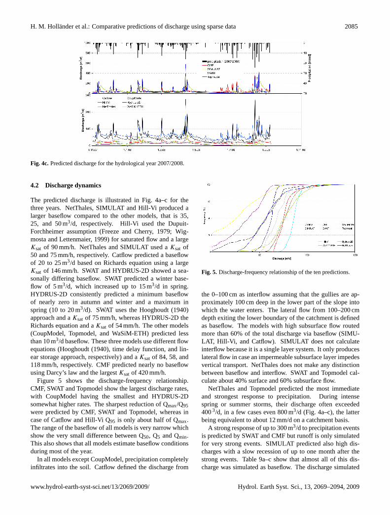
Figure 5 shows the discharge-frequency relationship.CMF, SWAT and Topmodel show the largest discharge rates,with CoupModel having the smallest and HYDRUS-2Dsomewhat higher rates. The sharpest reduction of Qmax/Q95were predicted by CMF, SWAT and Topmodel, whereas incase of Catflow and Hill-Vi Q95 is only about half of Qmax.The range of the baseflow of all models is very narrow whichshow the very small difference between Q50, Q5 and Qmin.This also shows that all models estimate baseflow conditionsduring most of the year.
In all models except CoupModel, precipitation completelyinfiltrates into the soil. Catflow defined the discharge from
Fig. 5. Discharge-frequency relationship of the ten predictions.
the 0–100 cm as interflow assuming that the gullies are ap-proximately 100 cm deep in the lower part of the slope intowhich the water enters. The lateral flow from 100–200 cmdepth exiting the lower boundary of the catchment is definedas baseflow. The models with high subsurface flow routedmore than 60% of the total discharge via baseflow (SIMU-LAT, Hill-Vi, and Catflow). SIMULAT does not calculateinterflow because it is a single layer system. It only produceslateral flow in case an impermeable subsurface layer impedesvertical transport. NetThales does not make any distinctionbetween baseflow and interflow. SWAT and Topmodel cal-culate about 40% surface and 60% subsurface flow.
NetThales and Topmodel predicted the most immediateand strongest response to precipitation. During intensespring or summer storms, their discharge often exceeded4003/d, in a few cases even 800 m3/d (Fig. 4a–c), the latterbeing equivalent to about 12 mm/d on a catchment basis.
A strong response of up to 300 m3/d to precipitation eventsis predicted by SWAT and CMF but runoff is only simulatedfor very strong events. SIMULAT predicted also high dis-charges with a slow recession of up to one month after thestrong events. Table 9a–c show that almost all of this dis-charge was simulated as baseflow. The discharge simulated
www.hydrol-earth-syst-sci.net/13/2069/2009/ Hydrol. Earth Syst. Sci., 13, 2069–2094, 2009
2086 H. M. Hollander et al.: Comparative predictions of discharge using sparse data
Table 9a.Discharge components predicted for the 1st yeara.
runoff interflow baseflow total discharge(mm/y) (mm/y) (mm/y) (mm/y)
Catflow 90 159 249CMF 208CoupModel 8 4 12Hill-Vi >1 305 306HYDRUS 34–48NetThales 189SIMULAT >1 0 189 189SWAT 27 51 76Topmodel 31 63 94WaSiM-ETH 0 83 24 107
Chicken Creek 113
Table 9b. Discharge components predicted for the 2nd yeara.
runoff interflow baseflow total discharge(mm/y) (mm/y) (mm/y) (mm/y)
Catflow 101 161 262CMF 238CoupModel 20 7 27Hill-Vi >1 346 346HYDRUS 19–67NetThales 259SIMULAT >1 0 339 339SWAT 61 84 145Topmodel 75 96 171WaSiM-ETH 2 138 22 162
Chicken Creek 105
by Hill-Vi during precipitation events was relatively slowcompared to those of the other models and reached a max-imum of 170 m3/d. HYDRUS-2D predicted some peak dis-charge rates in the 1st year but this model barely respondedto the intensive events in the summer of the 2nd and 3rd year.Changing theL-factor (tortuosity) increased the responsesomewhat, but only negligibly compared to the much largerdischarge of the other predictions. Catflow and CoupModelpredicted the smallest response to the very strong summerevents (Fig. 4a–c). CoupModel showed the lowest dischargeof all models, whereas Catflow predicted mainly baseflow.
Predicted discharge of the other models is mainly interflowand baseflow. WaSiM-ETH and Hill-Vi are the only modelswhich separate the discharge into all three components. Hill-Vi identified about 97% of the discharge as subsurface flow.WaSiM-ETH gave a similar result but with about 80% inter-flow, about 20% baseflow, and a very small amount of sur-face runoff. Although the hydraulic conductivity was largerthan in Hill-Vi, most of the water did not reach groundwatertable before it laterally discharged. Catflow predicted onlyinterflow (40%) and baseflow (60%) using a higher hydraulicconductivity. Interflow was assumed to be released from the
Table 9c.Discharge components predicted for the 3rd yeara.
runoff interflow baseflow total discharge(mm/y) (mm/y) (mm/y) (mm/y)
Catflow 112 146 258CMF 250CoupModel 62 14 76Hill-Vi >1 329 329HYDRUS 34–64NetThales 275SIMULAT >1 0 283 283SWAT 57 112 164Topmodel 94 104 198WaSiM-ETH 148 30 178
Chicken Creek 113
a no value is equal to no information.
upper 1 m of the soil so that it can enter the gullies. The claydam developed a build-up of the groundwater table whichresulted in groundwater discharge. SIMULAT quantifies in-terflow and baseflow, but interflow was not simulated at anytime step. The clay dam had no influence on these predic-tions because the concentration time method does not con-sider any barrier. Figure 4a–c shows that the predicted sub-surface flow of SIMULAT is baseflow given the long andslow recession of the discharge. CMF and NetThales didnot provide information about the different discharge com-ponents.
The calculated direct runoff played a minor role for thetotal of the simulated discharge (Table 9a–c), seen in the 1styear, when no direct runoff was predicted at all. CoupModelproduced the largest surface runoff in relative terms, about80% of the total discharge because it simulated the secondlowest total of discharge with a maximum direct runoff of62 mm/y in the 3rd year. Topmodel simulated a larger directrunoff (95 mm/y) in this period, which was only about 40%of the predicted total discharge.
Although seven models included the clay dam into theirmodel, the dam had a minor impact on the flow characteris-tics. CoupModel and CMF needed to allow a sand layer of atleast 0.5 m for numerical reasons. HYDRUS-2D simulatedits discharge caused by the clay wall but had numerical prob-lems during some simulations due to saturation of grid cellsnear to the surface which would produce surface runoff. Themain problem was that HYDRUS-2D is not able to handlesurface runoff.
4.3 Groundwater levels
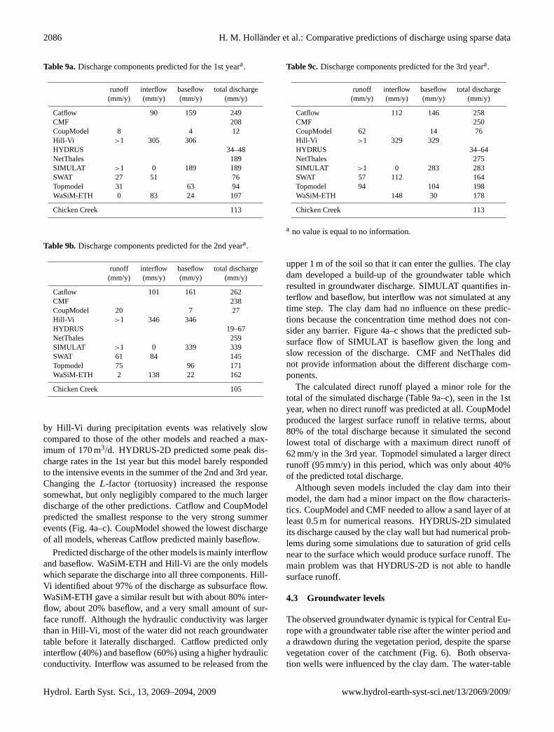
The observed groundwater dynamic is typical for Central Eu-rope with a groundwater table rise after the winter period anda drawdown during the vegetation period, despite the sparsevegetation cover of the catchment (Fig. 6). Both observa-tion wells were influenced by the clay dam. The water-table
Hydrol. Earth Syst. Sci., 13, 2069–2094, 2009 www.hydrol-earth-syst-sci.net/13/2069/2009/
H. M. Hollander et al.: Comparative predictions of discharge using sparse data 2087
fluctuations of the two neighbouring observation wells areclosely linked.
Figure 6 illustrates the groundwater fluctuations at the ob-servation wells F4 and L4 and the corresponding predictionsof Catflow, CMF, Hill-Vi, HYDRUS-2D, and WaSiM-ETH.Observation wells F4 and L4 were chosen because they arelocated in the central part of the catchment (Fig. 6) and arealso represented by the 2-D models (Catflow and HYDRUS-2D). The measured average groundwater level exhibited anincreasing trend over the three years. This is also evidentfrom the positive storage term in the water budget (Table 8a–c). Since there was no information on the initial soil-watercontents, the soil-water storage was handled differently bythe various modellers (see Sect. 4.7). The same applies tothe groundwater storage. Surprisingly, none of the mod-elling groups used the information that initially there was nogroundwater present.
The fluctuations of the groundwater level predicted atthe two observation wells were similar. This indicatesthat Ksat at the two locations is similar (see the Sup-plementhttp://www.hydrol-earth-syst-sci.net/13/2069/2009/hess-13-2069-2009-supplement.pdf). The predicted ground-water tables did not show any influence of the clay dam. Thegroundwater fluctuations F4 and L4 predicted by CMF, Hill-Vi and WaSiM-ETH were fairly similar and showed smallvariations and no seasonal trend. CMF predicted a ground-water table drawdown of about 50 cm in the 1st year, a riseof 50 cm in the 2nd year and a nearly constant water tableheight in the 3rd year. Hill-Vi states a non-seasonal fluctua-tion of about 30 cm. WaSiM-ETH gave only a single averagegroundwater table height for the whole catchment. Duringthe first year, the simulated average groundwater table heightdropped by 50 cm and remained constant afterwards. A con-stant groundwater table height within a catchment through-out the year is the result of a balance between recharge anddischarge at all times. All three models usedKsat. Hill-Vi predicted the highest discharge but used the lowestKsatof the three models. It reported that the discharge was al-most entirely subsurface flow but it did not provide directinformation on the groundwater flow. The estimated initialgroundwater table level was near the surface. WaSiM-ETHpredicted the lowest baseflow of 22 to 30 mm/y and used thelowestKsatof the three models. The total porosity of all threemodels was 0.38.
Catflow and HYDRUS-2D were the only models whichshowed a seasonal fluctuation of the groundwater table. Cat-flow showed a maximum amplitude of 80 cm with rapidchanges. This is a consequence of the model structure be-cause in these models a grid cell is either completely sat-urated (=groundwater) or not. The use of a cell thick-ness of 20 cm produced groundwater table jumps of 20 cm.The groundwater tables by HYDRUS-2D are calculated forsix scenarios. The fluctuations of HYDRUS-2D are thelargest of all models and exceeded the measured fluctuations.The amplitude was about 1 m and was constant throughout
Fig. 6. Predicted and measured hydraulic heads at the observationwells F4 and L4.
the simulated period. The two scenarios by HYDRUS-2D(Fig. 6) were calculated with two differentL-factors, thelower groundwater table being predicted using anL-factor of0.5 and the higher forL=−0.78. Both scenarios have beenstarted with the same initial groundwater level and developeddifferently during the 1st year. The fluctuated groundwatertables of HYDRUS-2D is nearly parallel to the 2nd and the3rd year.
Catflow and HYDRUS-2D simulate the same fluctuationpattern. The difference in the amplitude is due to the differentKsat. Catflow assumed aKsat, which is three times as large(146 mm/h) as in HYDRUS-2D (54 mm/h). Neither Catflownor HYDRUS-2D predicted the sharp groundwater table risetoward the end of each winter period or the long and veryslow drawdown during spring, summer, and fall months.
5 Discussion
5.1 Water budget
The errors in the measured mass balance,1Merror, werelarge. In the second year, the error was 40% ofP . The largeerrors are due to the fact that the actual evapotranspirationAET was not measured but estimated according to Black etal. (1969; DVWK, 1996). This approach was developed forbare soils and neglects the effect of vegetation. Additionally,the influence of soil-water storage on AET is neglected. Theerror in the first year was mainly due to the neglected soil-water storage changes, whereas, the error in the last year wasdue to AET of a denser and taller vegetation.
The1Merror≈10% for SWAT is due to the fact that SWATwas not designed for small catchments. Therefore, the rep-resentation of detailed processes within an artificial, newlyconstructed small catchment caused relatively large errors.CMF had the highest1Merror (up to 25%), probably becauseit is a recently developed code under construction.
Using the grass-referenced potential evapotranspiration,PET most likely overestimates the role of the sparse vege-tation in the Chicken Creek, so PET is likely to be smaller
www.hydrol-earth-syst-sci.net/13/2069/2009/ Hydrol. Earth Syst. Sci., 13, 2069–2094, 2009
2088 H. M. Hollander et al.: Comparative predictions of discharge using sparse data
than presented in Table 8a–c. Although most models pre-dicted a PET in the order of 600 to 800 mm/y, few valueswere surprisingly smaller, e.g. the 139 mm/y (CMF) and the421 mm/y (NetThales, 2nd year, Table 8b), despite the factthat most groups used the Penman-Monteith method and thatthe information on vegetation coverage was available. There-fore, the differences originate from the parameter choice, inthe case of CMF due to the constant PET-independent inter-ception and the time-invariant sparse vegetation for all threeyears (LAI=0.1, plant height 10 cm). The models, whichdid not account for any vegetation, predicted both about600 mm/y (HYDRUS-2D and Topmodel). The PET of SIM-ULAT (680 mm/y) using sparse vegetation and stomatal re-sistances of 50 s/m was nearly the same as that of WaSiM-ETH (700 mm/y), which only used evaporation and stom-atal resistances of 150 s/m. Only the two models, whichdid not use the Penman-Monteith method, predicted a largerPET. SWAT calculated the highest PET using the Hargreavesequation and Hill-Vi the second highest (Turc equation). InSWAT a relatively well established plant cover (maximumLAI=2.68, plant height 50 cm) and the lowest stomatal re-sistance were assumed. The Turc equation, calculated byHill-Vi yields a grass-referenced PET, excluding additionalinformation about the vegetation. It overestimates the role ofthe vegetation and, therefore, PET.
Evidently, the plant parameterization was in this case, ofminor importance because the catchment was left for a natu-ral slow invasion of plants. The choice of the pore size index(van Genuchten parameter nvG) had the main impact on esti-mating the actual evapotranspiration.
5.2 Soil parameterization
The range of predicted AET was, in all cases, a function ofPET and of the soil-water status. Since the range of PET issimilar for most models, the differences must originate fromthe differing soil-water content. The main inputs and param-eters, beside precipitation (P ), were the available field capac-ity, the hydraulic conductivityKsat, and theα-parameter ofthe soil-water characteristicsθ (h) and the unsaturated con-ductivity K(θ ) function. The groups used different pedo-transfer functions (Table 5) to estimate the hydraulic soil pa-rameters from soil texture.
The mean saturated hydraulic conductivity was predictedwithin a small range from 54 to 146 mm/h. Only CMF useda much largerKsat (417 mm/h). The van Genuchten param-eternvG varied from 1.13 to 2.28. The lowest value is usedby WaSiM-ETH and introduces a small reduction ofK(Se)on small changes inSe. This leads to a larger water hold-ing capacity in the top layer of the soil. Therefore, AET inWaSiM-ETH is considerably larger than in Catflow, whichuses the largestnvG-parameter. The low AET of HillVi is aconsequence also of the parameterization and of the modelstructure. Due to the assumed saturated hydraulic conduc-tivity and low L, only small amounts of water are stored in
the unsaturated zone, which reduces the water content de-pendent AET. The influence of the assumedKsat can alsobe seen from the AET predicted by CMF. Infiltration sensi-tivity changes the level of the water table in Hill-Vi leavingonly a shallow unsaturated zone, which results in a reducedAET. CoupModel used the second lowestnvG and calculatedthe second highest AET. HYDRUS-2D predicted the largestAET using a low to intermediatenvG. Different to othermodels, the groundwater flow is limited by the clay damwhich results in a rising groundwater table near the dam.Therefore, the upper soil also has on average a higher soilmoisture than in the other models. The changes ofL fromthe standard value 0.5 to−0.78 resulted in a lower AET. Net-Thales calculated an AET just below the mean of all modelsusing the smallestKsat. NetThales neglects the vertical re-distribution of water within the vertical soil column so thatthere is no unsaturated flow. The water holding capacity inNetThales corresponds to the available field capacity of thesand (0.11). SIMULAT and SWAT predicted an AET justabove the mean. TheirKsat are very similar. SIMULAT usesannvG in the upper range.
The hydraulic soil properties affect discharge as well. Theinfiltration calculations (Table 3) are based onKsat as limit-ing parameter. For example, Catflow predicted a large base-flow using a largeKsat and an intermediatenvG. The chosenhydraulic conductivities of all models except CoupModel re-sulted in either no or little surface runoff and high infiltration,which leads mainly to interflow and baseflow. The saturatedzone contributes mostly to baseflow. Models with a largerwater holding capacity – due to a small pore size indexnvG
– predicted large AETs and, therefore, lower baseflow be-cause the water was primarily lost by evapotranspiration (e.g.CoupModel and HYDRUS-2D) and vice-versa (e.g. Hill-Viand SIMULAT). In CoupModel, the water was stored for along time in the upper soil compartment and resulted in ahigh AET and often also in surface runoff due to the satura-tion. Therefore, CoupModel predicted the highest amount ofsurface runoff and the second lowest total discharge.
In Topmodel, the partitioning between baseflow and sur-face runoff is mainly controlled bym, the shape factor of therecession curve, and the maximum root zone storage deficit.Contrary to the latter,m is often a very sensitive parame-ter. Errors in the estimation ofm, therefore, severely affectthe partitioning. It describes a catchment behaviour, whichis difficult to relate to measurable catchment characteristics(other than discharge) and, therefore, it is not trivial to “apriori” estimate the value ofm. It can be stated that the re-cession curve depends on porosity and storage capacity, sothat overestimating the porosity and storage capacity wouldobviously result in underestimating surface runoff and vice-versa. In this study, the lack of a physical interpretation ofm may be seen as a problem for applying Topmodel becausethere is no analogue for this kind of a catchment in the liter-ature.
Hydrol. Earth Syst. Sci., 13, 2069–2094, 2009 www.hydrol-earth-syst-sci.net/13/2069/2009/
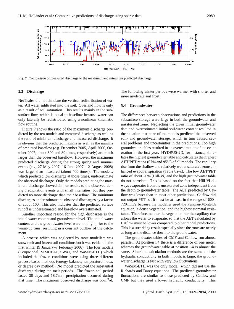
H. M. Hollander et al.: Comparative predictions of discharge using sparse data 2089
Fig. 7. Comparison of measured discharge to the maximum and minimum predicted discharge.
5.3 Discharge
NetThales did not simulate the vertical redistribution of wa-ter. All water infiltrated into the soil. Overland flow is onlyas a result of soil saturation. This results mainly in the sub-surface flow, which is equal to baseflow because water canonly laterally be redistributed using a nonlinear kinematicflow routine.
Figure 7 shows the ratio of the maximum discharge pre-dicted by the ten models and measured discharge as well asthe ratio of minimum discharge and measured discharge. Itis obvious that the predicted maxima as well as the minimaof predicted baseflow (e.g. December 2005, April 2006, Oc-tober 2007; about 300 and 80 times, respectively) are muchlarger than the observed baseflow. However, the maximumpredicted discharge during the strong spring and summerevents (e.g. 27 May 2007, 16 June 2007, 12 August 2008)was larger than measured (about 400 times). The models,which predicted low discharge at those times, underestimatethe observed discharge. Only the models predicting the max-imum discharge showed similar results to the observed dur-ing precipitation events with small intensities, but they pre-dicted no more discharge than their baseflow. The minimumdischarges underestimate the observed discharges by a factorof about 100. This also indicates that the predicted surfacerunoff is underestimated and baseflow overestimated.
Another important reason for the high discharges is theinitial water content and groundwater level. The initial watercontent and the groundwater level were too high prior to thewarm-up runs, resulting in a constant outflow of the catch-ment.
A process which was neglected by most modellers wassnow melt and frozen soil conditions but it was evident in thefirst winter (9 January–7 February 2006). The four models(CoupModel, SIMULAT, SWAT, and WaSiM-ETH) whichincluded the frozen conditions were using three differentprocess-based methods (energy balance, temperature index,or degree day method). No model predicted the substantialdischarge during the melt periods. The frozen soil periodlasted 30 days and 18.7 mm precipitation occurred duringthat time. The maximum observed discharge was 55 m3/d.
The following winter periods were warmer with shorter andmore moderate soil frost.
5.4 Groundwater
The differences between observations and predictions in thesubsurface storage were large in both the groundwater andunsaturated zone. Neglecting the given initial groundwaterdata and overestimated initial soil-water content resulted inthe situation that none of the models predicted the observedsoil- and groundwater storage, which in turn caused sev-eral problems and uncertainties in the predictions. Too highgroundwater tables resulted in an overestimation of the evap-oration in the first year. HYDRUS-2D, for instance, simu-lates the highest groundwater table and calculates the highestAET/PET ratios (67% and 95%) of all models. The capillaryrise from the shallow and relatively wet unsaturated zone en-hanced evapotranspiration (Table 8a–c). The low AET/PETratio of about 20% (Hill-Vi) and the high groundwater tabledo not correlate. This is based on the fact that Hill-Vi al-ways evaporates from the unsaturated zone independent fromthe depth to groundwater table. The AET predicted by Cat-flow was lower than in most other predictions. Catflow didnot output PET but it must be at least in the range of 600–720 mm/y because the modeller used the Penman-Monteithequation, a dense vegetation, and the highest stomatal resis-tance. Therefore, neither the vegetation nor the capillary riseallows the water to evaporate, so that the AET calculated byCatflow must be lower compared to other model predictions.This is a surprising result especially since the roots are nearlyas long as the distance down to the groundwater.
The groundwater tables of CMF and Catflow run almostparallel. At position F4 there is a difference of one meter,whereas the groundwater table at position L4 is almost thesame. Since the calculation methods are the same and thehydraulic conductivity in both models is large, the ground-water discharge is fast with very low fluctuations.
WaSiM-ETH was the only model, which did not use theRichards and Darcy equations. The predicted groundwaterfluctuations are similar to those predicted by Catflow andCMF but they used a lower hydraulic conductivity. This
www.hydrol-earth-syst-sci.net/13/2069/2009/ Hydrol. Earth Syst. Sci., 13, 2069–2094, 2009
2090 H. M. Hollander et al.: Comparative predictions of discharge using sparse data
indicates that the linear storage function is flexible enoughto simulate the strong changes during recharge periods. Allmodels have one feature in common: the amplitudes of thegroundwater table fluctuations and, therefore, also the esti-mated porosity is not correct. Catflow, CMF, Hill-Vi, andWaSiM-ETH estimate the drainable porosity to be too largeand HYDRUS-2D used a too low a drainable porosity.
5.5 Modeller experience
An important issue is the scientific background and the per-sonal experience of the modellers. For instance, the Coup-Model user used soil parameters from Swedish sands. TheNetThales modellers concluded that the initially estimatedrunoff coefficient of 70% was too large, so they increased theeffective root zone to make the runoff coefficient more real-istic. Similarly, some results of the modellers indicate thatapparently they had no prior experience with barren, sandysoils as they significantly overestimated AET. Also the un-derestimation of surface runoff was related to specific priorexperience. A visual inspection of soil texture and erosiongullies from photos did provide evidence that surface runoffcould be important, but only the CoupModel user accountedfor it. It was obviously difficult to combine conflicting ev-idence like, for instance, large hydraulic conductivities andgully formation at the same time.
6 Lessons learned for future modelling studies inungauged basins
While the comparative study mainly focused on the techni-cal aspects of estimating discharge in the artificial catchment,the modelling group has indeed learned important lessonsduring the comparative assessment that have wider implica-tions. When estimating runoff in an ungauged catchment,one has to decide on three main things: model structure,model parameters and model inputs (our boundary condi-tions) (Bloschl, 2005). Most previous model comparisonshave attempted to identify the relative merits of alternativeapproaches to each of the three. Intercomparison studies ingauged catchments have generally focused on whether onemodel structure is superior to the other (e.g. Naef, 1981;Goodrich, 1990; Reed, 2004). In contrast to these studies,we found that the more complex models do not perform bet-ter than their simpler counterparts which were usually tracedback to parameter identifiability problems.
Intercomparison studies for the ungauged catchment casehave attempted to find optimum parameter estimation meth-ods (Parajka et al., 2005; Oudin et al., 2008) including pedo-transfer functions (Wosten et al., 2001). These studies havenever highlighted the role of the modeller; in fact have triedto treat the intercomparison as subjectively as possible as ifthe modellers were interchangeable. The results of this pa-per, in contrast, indicate that the modeller is an intrinsic partof the modelling study and has a major bearing on the model
results – even more so in ungauged catchments where thereare more degrees of freedom in making modelling decisions.This is indeed a new paradigm in hydrological modelling.The question ofwhat methodto choose seems to be lessimportant than the hydrological community has previouslythought, and the question ofwhomakes the choices seems tobe more important. This study has shown that the modelleris just part of the entire modelling process, his/her prior ex-perience in the field and his/her experience with the chosenmodel. Not only should this be recognised in comparativestudies but, in fact, in any simulation exercise. This studyhas shown that it is not sufficient to choose the right mod-elling code, it is equally important to choose the modellerwith the best intuition for the system to be modelled.
The second general lesson learned during this study wasthe role of dominant processes. The artificial catchmentwas chosen for the comparison in view of the overwhelm-ing hydrological process complexity one usually encountersin catchments. The hope was that, in an artificial catchment,there will be minimum heterogeneity and processes will besimple, so modelling will be much easier than in catchmentsthat have evolved over a longer time period. The results ofthe models were expected to converge, and this would bea good starting point to proceed for a model comparison innatural, more challenging catchments. This model compar-ison showed that we have been overly optimistic. Even asmall artificial catchment exhibits heterogeneities which leadto similar modelling problems as in natural catchments. Wedid find, similar to natural catchments, that knowledge aboutthe dominant processes is essential and can vastly improvethe modelling results (Seibert and McDonnell, 2002). Thisknowledge was found to be very useful even if it is purelyof a qualitative nature, as can be obtained by visual inspec-tion of catchment photos to judge erosion marks and canopyfeatures that might be indicative for surface runoff and rootwater uptake. Clearly, this type of information will help themodeller to make more informed choices on model structureand better guesses of model parameters. This may also helpin the modelling strategies along the lines of the “dominantprocess concept” (DCP) to avoid overparameterisation by fo-cusing on the most important processes occurring at the scaleof the system to be modelled (Grayson and Bloschl, 2000b).Equally important, this finding highlights the need for fieldvisits. While in the scientific literature on the problem of un-gauged basins (PUB) field trips are usually downplayed, thisstudy has made it very clear that, while a catchment may haveno historic discharge data, there may be a wealth of qualita-tive information available that gives clues on the catchmentdynamics (Bloschl, 2005). There is a lot that a hydrolo-gist can gather by walking through a catchment and search-ing for complementary, qualitative data that can substantiallycontribute to process understanding and, hence, improve themodel predictions (Fenicia et al., 2008). It is suggested thatqualitative field evidence should play a more prominent rolein hydrological modelling of ungauged basins.
Hydrol. Earth Syst. Sci., 13, 2069–2094, 2009 www.hydrol-earth-syst-sci.net/13/2069/2009/
H. M. Hollander et al.: Comparative predictions of discharge using sparse data 2091
The two lessons learned from this model/modeller inter-comparison are closely linked. The experience of a mod-eller is crucial in the (subjective) process of deciding uponthe dominant processes that seem to be sufficiently impor-tant to be incorporated into the model. The cumulated expe-rience will also play an important role in how different piecesof evidence from, for example, field inspections, will mod-ify the initial conceptual understanding. One could say, ina Bayesian framework, that the different modellers differ intheir prior estimates (on the conceptual understanding) caus-ing also posterior estimates/perceptions to differ unless thenew evidence (from field visits, for example) overrides theprior understanding.
7 Conclusions
Ten modelling groups used ten different catchment modelsto predict the major hydrological variables of the small artifi-cial catchment Chicken Creek based on the same small dataset. The observed discharge was not known to the modellers.This constellation of a minimal set of easily accessible datamimics the modeller’s situation when confronted with pre-dicting the response of ungauged catchments. The variousmodellers had a different background and were used to ap-plying their models to catchments of quite different scalesand features. This affected the choice of the optional modelstructures and parameters. For an “a priori prediction” themodeller’s experience turned out to be very relevant. The dis-charge predictions differed in a wide parameter mainly dueto a different process understanding, catchment conceptual-ization, and different parameter estimation.
The initial soil-water content was not available. Most ofthe models estimated it on the basis of pre-runs or by assum-ing a certain field capacity. Also, the initial groundwater situ-ation was determined by pre-runs, despite the fact that it waspart of the provided data. This influenced the predictions be-cause the soil and groundwater compartments of the modelswere already full at the beginning of the simulation, contraryto what was observed in the catchment. Therefore, none ofthe models reproduced the steadily increasing groundwatertable.
Catflow, HYDRUS-2D, WaSiM-ETH and, up to a cer-tain degree, also SIMULAT and Hill-Vi are based on cal-culations using Richards equation. However, the predictionsvary in a wide range. The largest differences were predictedin the case of the discharge with an extremely wide rangein peak flow from 15 to 840 m3/d. This was mainly an ef-fect of the estimated hydraulic soil properties. The modelswhich predicted a low actual evapotranspiration predicted ahigher runoff. These models mainly used a small pore sizeindex (van Genuchten parameternvG). Surface runoff wasalso under-predicted by most models. The observations –not known to the modellers – show that surface runoff is,however, the main flow component. “A posteriori”, it is ob-
vious that this process must have been dominant in absenceof vegetation and on unconsolidated soils, which dry out insummer and freeze during winter. Hence, understanding thedominant processes appears to be essential for any “a priori”prediction of catchment response.
None of the models included the influence of the subsur-face clay dam on how the lower catchment area was beingdrained. Predicted groundwater discharge was, therefore,larger than measured. Neglecting the aerial photo informa-tion of the gully network, resulted in underestimating directrunoff. Only CoupModel integrated this information and pre-dicted the highest direct runoff. After visiting the catchment,the modellers immediately revised their view on the catch-ment processes occurring in this particular case. Hence, on-site information, even when it is purely of a qualitative na-ture, is very conclusive.
Choosing parameters involves a degree of guess-work andguessing is an art. The hydraulic conductivities and in par-ticular the infiltration rates were too large, which overempha-sized subsurface flow. The guessing-algorithms – pedotrans-fer functions or estimation by analogy to other (Swedish)soils – were less important relative to the assumptions of flowrouting. The large infiltration capacities kept the soil-waterstorage on a high level, which resulted in a large actual evap-otranspiration.
One important reason why the predictions suffered wasfrom misjudging the initial conditions. Assuming an initiallywet catchment instead of a dry one, resulted in wrong storagefunctions and too large discharge rates, or in other cases, inan overestimated actual evapotranspiration.
Some process assumptions were ineffective for reproduc-ing the hydrological behaviour of the Chicken Creek catch-ment. The most obvious is the failure when using the energybalance, the temperature index, and the degree-day methodto predict snow accumulation and soil frost, or the over-prediction of the potential evapotranspiration using the Turcmethod in case of a sparse vegetation.
Acknowledgements.These investigations were supported bythe German Research Foundation (DFG) and the BrandenburgMinistry of Science, Research and Culture (MWFK, Potsdam) inthe framework of the Transregional Collaborative Research Centre38 (SFB/TRR 38). The authors thank Vattenfall Europe Mining AGfor providing the research site. We acknowledge the contribution byIvo Strahm (Eawag) who carried out the HYDRUS-2D simulations.We explicitly acknowledge the positive role of the reviewers whochallenged us to make the essence of this prediction exercise asvisible as possible.
Edited by: J. Seibert
www.hydrol-earth-syst-sci.net/13/2069/2009/ Hydrol. Earth Syst. Sci., 13, 2069–2094, 2009
2092 H. M. Hollander et al.: Comparative predictions of discharge using sparse data
References
Adhoc AG Boden: Bodenkundliche Kartieranleitung, 5th edn.,Hannover, Germany, 438 p., 2005.
AG Boden: Bodenkundliche Kartieranleitung, 4th edn., Hannover,Germany, 392 p., 1994.
Allen, R. G., Pereira, L. S., Raes, D., and Smith, M.: Crop evapo-transpiration. Guidelines for computing crop water requirements,Irrigation and Drainage Paper, FAO, Rome, 300 pp., 1998.
Alvenas, G. and Jansson, P.-E.: Model for evaporation, moistureand temperature of bare soil: calibration and sensitivity analysis,Agric. For. Met., 88, 47–56, 1997.
Arnold, J. G., Srinivasan, R., Muttiah, R. S., and Williams, J. R.:Large area hydrologic modelling and assessment part I: modeldevelopment, J. Am. Water Resour. Assoc., 34, 73–89, 1998.
Barbour, S. L., Boese, C., and Stolte, B.: Water balance for recla-mation covers on oil sands mining overburden piles, CanadianGeotechnical Conference, 313–319, 2001.
Beven, K.: Changing ideas in hydrology – The case of physically-based models, J. Hydrol., 105, 157–172, 1989.
Beven, K., Lamb, R., Quinn, P., Romanowicz, R., and Freer, J.:Topmodel, in: Computer Models of Watershed Hydrology, Col-orado, USA, 627–668, 1995.
Beven, K. J. and Kirkby, M. J.: A physically based variable con-tributing area model of basin hydrology, Hydrol. Sci. Bull., 24,43–69, 1979.
Beven, K. J.: Rainfall-runoff modelling: The Primer, John Wiley &Sons, Chichister, 372 pp., 2001.
Black, T. A., Gardner, W. R., and Thurtell, G. W.: The prediction ofevaporation, drainage and soil-water storage for a bare soil., SoilSci. Soc. Amer. Proc., 33, 655–660, 1969.
Bloschl, G.: Rainfall-runoff modelling of ungauged catchments, ar-ticle 133, in: Encyclopedia of Hydrological Sciences, edited by:Anderson, M. G., John Wiley & Sons, Chichester, 2061–2080,2005.
Bormann, H.: Hochskalieren von prozessorientierten Wasser-transportmodellen – Methoden und Grenzen, Reihe Geowis-senschaften, Herbert-Utz-Verlag – Wissenschaft Munchen,164 pp., 2001.
Bormann, H.: Sensitivity of a regionally applied soil vegetation at-mosphere scheme to input data resolution and data classification,J. Hydrol., 351, 154–169, 2008.
Bronstert, A., Bardossy, A., Bismuth, C., Buiteveld, H., Disse, M.,Engel, H., Fritsch, U., Hundecha, Y., Lammersen, R., Niehoff,D., and Ritter, N.: Multi-scale modelling of land-use change andriver training effects on floods in the Rhine basin, 2007.
Brooks, R. H. and Corey, A. T.: Hydraulic properties of porousmedia, Colorado State University, Fort Collins, Colorado, 27 pp.,1964.
Carsel, R. F. and Parrish, R. S.: Developing Joint Probability Dis-tributions of soil-water Retention Characteristics, Water Resour.Res., 24, 755–769, 1988.
Chirico, G. B., Grayson, R. B., and Western, A. W.: Onthe computation of the quasi-dynamic wetness index withmultiple-flow-direction algorithms, Water Resour. Res., 39,1115, doi:10.1029/2002WR001754, 2003.
Choi, H. T. and Beven, K.: Multi-period and multi-criteria modelconditioning to reduce prediction uncertainty in an application oftopmodel within the glue framework, J. Hydrol., 332, 316–336,2007.
Diekkruger, B. and Arning, M.: Simulation of water fluxes usingdifferent methods for estimating soil parameters, Ecol. Model.,81, 83–95, 1995.
DVWK: Ermittlung der Verdunstung von Land- und Wasserflachen,Merkblatter, Kommissionsbetrieb Wirtschafts- und Verlagswe-sen Gas und Wasser mbH, Bonn, 135 pp., 1996.
Feddes, R. A., Kowalik, P. J., and Zaradny, H.: Simulation of fieldwater use and crop yield, in: Simulations Monograph, Pudoc,Wageningen, 188 pp., 1978.
Fenicia, F., McDonnell, J. J., and Savenije, H. H. G.: Learn-ing from model improvement: On the contribution of comple-mentary data to process understanding, Water Resour. Res., 44,W06419, doi:10.1029/2007WR006386, 2008.
Freeze, R. A. and Cherry, J. A.: Groundwater, Prentice-Hall, Engle-wood Cliffs, NJ, 604 pp., 1979.
Gallart, F., Latron, J., Llorens, P., and Beven, K.: Using internalcatchment information to reduce the uncertainty of discharge andbaseflow predictions, Adv. Water Resour., 30, 808–823, 2007.
Gassmann, P. W., Reyes, M. R., Green, C. H., and Arnold, J. G.:The soil and water assessment tool: historical development, ap-plications and future research directions, T. ASAE, 50, 1211–1250, 2007.
Gerwin, W., Raab, T., Biemelt, D., Bens, O., and Huttl, R. F.: Theartificial water catchment “Chicken Creek” as an observatory forcritical zone processes and structures, Hydrol. Earth Syst. Sci.Discuss., 6, 1769–1795, 2009,http://www.hydrol-earth-syst-sci-discuss.net/6/1769/2009/.
Giertz, S., Diekkruger, B., and Steup, G.: Physically-based mod-elling of hydrological processes in a tropical headwater catch-ment (West Africa) – process representation and multi-criteriavalidation, Hydrol. Earth Syst. Sci., 10, 829–847, 2006,http://www.hydrol-earth-syst-sci.net/10/829/2006/.
Goodrich, D. C.: Geometric simplification of a distributed rainfall-runoff model over a range of basin scales, Ph.D. Thesis, The Uni-versity of Arizona, 361 pp., 1990.
Grayson, R. B. and Bloschl, G.: Spatial Patterns in CatchmentHydrology: Observations and Modelling, Cambridge UniversityPress, Cambridge, UK, 404 pp., 2000a.
Grayson, R. B. and Bloschl, G.: Summary of pattern recognitionand concluding remarks, in: Spatial Patterns in Catchment Hy-drology, edited by: Grayson, R. B. and Bloschl, G., CambridgeUniversity Press, Cambridge,UK, 355–367, 2000b.
Gu, W.-Z. and Freer, J.: Patterns of surface and subsurface runoffgeneration, IAHS Publications, 229, 265–273, 1995.
Gustafsson, D., Stahli, M., and Jansson, P.-E.: The surface energybalance of a snow cover: comparing measurements to two differ-ent simulation models, Theor. Appl. Climatol., 70, 81–96, 2001.
Hansen, D. P., Jakeman, A. J., Kendall, C., and Gu, W.-Z.: Identifi-cation of internal flow dynamics in two experimental catchments,Math. Comput. Simulat., 43, 367–375, 1997.
Hargreaves, G. L., Hargreaves, G. H., and Riley, J. P.: Agriculturalbenefits for Senegal River Basin, J. Irrig. and Drain. Engr., 111,113–124, 1985.
Healy, R. W. and Cook, P. G.: Using groundwater levels to estimaterecharge, Hydrogeol. J., 10, 91–109, 2002.
Holzel, H. and Diekkruger, B.: Hydrological analyses as a prereq-uisite for soil erosion modeling – Landscape related studies ina mesoscale hydrological catchment, in: Landform – structure,evolution, process control, International Symposium on Land-
Hydrol. Earth Syst. Sci., 13, 2069–2094, 2009 www.hydrol-earth-syst-sci.net/13/2069/2009/
H. M. Hollander et al.: Comparative predictions of discharge using sparse data 2093
form, in press, 2008.Hooghoudt, S. B.: Bijdragen tot de kennis van enige natuurkundige
grootheden van de ground, Versl. Landb. Onderz, 42, 449–541,1940.
Jansson, P.-E. and Halldin, S.: Model for the annual water and en-ergy flow in a layered soil, Comparison of Forest and EnergyExchange Models, Copenhagen, 145–163, 1979.
Jansson, P.-E. and Moon, D. S.: A coupled model of water, heat andmass transfer using object orientation to improve flexibility andfunctionality, Environ. Modell. Softw., 16, 37–46, 2001.
Jasper, K.: Hydrological Modelling of Alpine River Catchmentsusing Output Variables from Atmospheric Models, ETH Zurich,138 pp., 2005.
Kendall, C., Mc Donnell, J. J., and Gu, W.-Z.: A look inside “blackbox” hydrograph seperation models: a study at the Hydrohillcatchment, Hydrol. Process., 15(10), 1877–1902, 2001.
Kraft, P., Vache, K. B., Breuer, L., and Frede, H.-G.: A soluteand water flux library for catchment models, Proceedings of theiEMSs Fourth Biennial Meeting: International Congress on En-vironmental Modelling and Software Barcelona, 2008.
Kroes, J. G., van Dam, J. C., Groenendijk, P., Hendriks, R. F. A.,and Jacobs, C. M. J.: SWAP version 3.2., Theory description anduser manual, Alterra, Wageningen, 262 pp., 2008.
Lindenmaier, F., Zehe, E., Dittfurth, A., and Ihringer, J.: Processidentification at a slowmoving landslide in the Vorarlberg Alps,Hydrol. Process., 19, 1635–1651, 2005.
Lohammar, T., Larsson, S., Linder, S., and Falk, S. O.: FAST – sim-ulation medels of gaseous exchange in Scots pine, in: Structureand Function of Northern Coniferous Forests – An EcosystemStudy, edited by: Persson, T., Ecological Bullentins Stockholm,505–523, 1980.
Lundmark, A. and Jansson, P.-E.: Generic soil descriptions formodelling water and chloride dynamics in the unsaturated zonebased on Swedish soils, Geoderma, 150, 85–95, 2009.
Maurer, T.: Physikalisch begrundetete, zeitkontinuierliche Model-lierung des Wassertransports in kleinen landlichenen Einzugsge-bieten, Universitat Karlsruhe, 1997.
Meinzer, O. E.: The occurrence of groundwater in the UnitedStates with a discussion of principles, US Geol. Surv. Water-SupplyPaper, 489, 321 pp., 1923.
Monteith, J. L.: Evaporation and environment, in: The Companyof Biologists, The State and Movement of Water in Living Or-ganisms, 19th Symp. Soc. Exp. Biol., Cambridge, UK, 205–234,1965.
Monteith, J. L. and Unsworth, M. H.: Principles of environmentalphysics, edited by: Arnold, S. E., London, UK, 291 pp., 1990.
Mualem, Y.: A new model for predicting the hydraulic conductivityof unsaturated porous media, Water Resour. Res., 12, 513–522,1976.
Naef, F.: Can we model the rainfall-runoff today? HydrologicalSciences Bulletin, 26, 281–289, 1981.
Nenov, R.: Determination of the evapotranspiration from the arti-ficial catchment Huhnerwasser, Chair of Hydrology and WaterManagement, Brandenburg University of Technology, Cottbus,100 pp., 2009.
Nicolau, J.: Runoff generation and routing on artificial slopes ina Mediterranean continental environment, Hydrol. Process., 16,631–647, 2002.
Niehoff, D., Fritsch, U., and Bronstert, A.: Land-use impacts on
storm-runoff generation: scenarios of land-use change and sim-ulation of hydrological response in a meso-scale catchment inSW-Germany, J. Hydrol., 267, 80–93, 2002.
Oudin, L., Andreassian, V., Perrin, C., Michel, C., and Le Moine,N.: Spatial proximity, physical similarity, regression and un-gaged catchments: A comparison of regionalization approachesbased on 913 French catchments, Water Resour. Res., 44,W03413, doi:10.1029/2007WR006240, 2008.
Parajka J., Merz, R., and Bloschl, G.: A comparison of regionali-sation methods for catchment model parameters, Hydrol. EarthSyst. Sc., 9, 157–171, 2005.
Penman, H. L.: Natural evaporation from open water, bare soil andgrass. Proc. Roy. Meteorol. Soc. A, 193, 120–145, 1948.
Peschke, G.: Moisture and Runoff Components from a PhysicallyFounded Approach, Acta Hydrophys., 31, 191–205, 1987.
Plate, E. and Zehe, E.: Hydrologie und Stoffdynamik kleinerEinzugsgebiete: Prozesse und Modelle. Schweizerbart, 366 pp.,2008.
Rawls, W. J. and Brakensiek, D. L.: Prediction of soil-water prop-erties for hydrologic modeling, in: Proceedings of Symposiumon Watershed Management, ASCE, 293–299, 1985.
Richter, D.: Zur einheitlichen Berechnung der Wassertemperaturund der Verdunstung von freien Wasserflchen auf statistischerGrundlage, Abh. Meteor. Dienst der DDR, 16, 35 pp., 1977.
Ritchie, J. T.: A model for predicting evaporation from a row cropwith incomplete cover, Water Resour. Res., 8, 1204–1213, 1972.
Reed, S., Koren, V., Smith, M., Zhang, Z., Moreda, F., and Seo, D.J.: Overall distributed model intercomparison project results, J.Hydrol., 298, 27–60, 2004.
Romano, N. and Santini, A.: Water retention and storage: Field,in: Methods of Soil Analysis, edited by: Topp, J. H. D. a. G. C.,SSSA Book Series No. 5, Madison, Wi, USA, 721–738, 2002.
Saxton, K. E., Rawls, W., Romberger, J., and Papendick, R.: Esti-mating generalized soil-water characteristics from texture, 1031–1035, 1986.
Schaap, M. G., Leij, F. J., and van Genuchten, M. T.: A computerprogram for estimating soil hydraulic parameters with hierarchi-cal pedotransfer functions, J. Hydrol., 251, 163–176, 2001.
Schulla, J. and Jasper, K.: Model Description WaSiM-ETH, ETHZrich, Zrich, 181 pp., 2007.
Seibert, J. and McDonnell, J. J.: On the dialog between experi-mentalist and modeler in catchment hydrology: Use of soft datafor multicriteria model calibration, Water Resour. Res., 38(11),1241, doi:10.1029/2001WR000978, 2002.
Simunek, J., Sejna, M., and van Genuchten, M. T.: The HYDRUS2Code for Simulating the Two-Dimensional Movement of Water,Heat, and Multiple Solute in Variably-Saturated Porous Media,edited by: Service, U. S. S. L. A. R., US Department of Agricul-ture, Riverside, California, USA, 251 pp., 1999.
Sivapalan, M., Takeuchi, K., Franks, S., Gupta, V., Karambiri,H., Lakshmi, V., Liang, X., McDonnell, J., Mendiondo, E.,O’Connell, P., Oki, T., Pomeroy, J., Schertzer, D., Uhlenbrook,S., and Zehe, E.: IAHS decade on Predictions in UngaugedBasins (PUB), 2003–2012: Shaping an exciting future for thehydrological sciences, Hydrolog Sci. J., 48, 857–880, 2003.
Smith, R. E. and Parlange, J. Y.: A parameter-efficient hydrologicinfiltration model, Water Resour. Res., 14, 533–538, 1978.
Stahli, M., Jansson, P.-E., and Lundin, L.-C.: Preferential waterflow in a frozen soil – a two-domain model approach, Hydrol.
www.hydrol-earth-syst-sci.net/13/2069/2009/ Hydrol. Earth Syst. Sci., 13, 2069–2094, 2009
2094 H. M. Hollander et al.: Comparative predictions of discharge using sparse data
Process., 10, 1305–1316, 1996.Stahli, M. and Gustafsson, D.: Long-term investigations of the snow
cover in a subalpine semi-forested catchment, Hydrol. Process.,20, 411–428, 2006.
Turc, L.: Evaluation des besoins en eau irrigation,l’ evapotranspiration potentielle, Ann. Agron, 12, 13–49,1961.
Vache, K. and McDonnell, J. J.: A process-based rejectionist frame-work for evaluating catchment runoff model structure, Water Re-sour. Res., 42, W02409, doi:10.1029/2005WR004247, 2006.
van Dam, J. C., Huygen, J., Wesseling, J. G., Feddes, R. A., Ka-bat, P., van Walsum, P. E. V., Groenendijk, P., and van Diepen,C. A.: Theory of SWAP version 2.0. Simulation of water flow,solute transport and plant growth in the Soil-Water-Atmosphere-Plant environment, Wageningen University, Wageningen, 165pp., 1997.
van Genuchten, M. T.: A closed-form equation for predicting thehydraulic conductivity of unsaturated soils, Soil Sciences Societyof America, 44, 892–898, 1980.
Weiler, M. and McDonnell, J. J.: Virtual experiments: A new ap-proach for improving process conceptualisation in hillslope hy-drology, J. Hydrol, 285, 3–18, 2004.
Weiler, M. and McDonnell, J. J.: Testing nutrient flushing hypothe-ses at the hillslope scale: A virtual experiment approach, J. Hy-drol., 319, 339–356, 2006.
Weiler, M. and McDonnell, J. J.: Conceptualizing lateral preferen-tial flow and flow networks and simulating the effects on gaugedand ungauged hillslopes, Water Resour. Res., 43, W03403,doi:10.1029/2006WR004867, 2007.
Wigmosta, M., Vail, L., and Lettenmaier, D. P.: Distributedhydrology-vegetation model for complex terrain, Water Resour.Res., 30, 1665–1679, 1994.
Wigmosta, M. and Lettenmaier, D. P.: A comparison of simplifiedmethods for routing topographically driven subsurface flow, Wa-ter Resour. Res., 35, 255–264, 1999.
Wosten, J. H. M., Pachepsky, Y. A., and Rawls W. J.: Pedotransferfunctions: bridging the gap between available basic soil data andmissing soil hydraulic characteristics, J. Hydrol., 251, 123–150,2001.
Zehe, E. and Fluhler, H.: Preferential transport of isoproturon ata plot scale and a field scale tile-drained site, J. Hydrol., 247,100–115, 2001a.
Zehe, E. and Fluhler, H.: Slope scale variation of flow patterns insoil profiles, J. Hydrol., 247, 116–132, 2001b.
Zehe, E. and Bloeschl, G.: Predictability of hydrologic response atthe plot and catchment scales: Role of initial conditions, WaterResour. Res., 40, W10202, doi:10.1029/2003WR002869, 2004.
Zehe, E., Becker, R., Bardossy, A., and Plate, E.: Uncertainty ofsimulated catchment runoff response in the presence of thresh-old processes: Role of initial soil moisture and precipitation, J.Hydrol., 315, 183–202, 2005.
Hydrol. Earth Syst. Sci., 13, 2069–2094, 2009 www.hydrol-earth-syst-sci.net/13/2069/2009/


