Assigning confidence to conditional branch predictions

Assigning Confidence to Conditional Branch Predictions

Erik Jacobsen, Eric Rotenberg†, and J. E. SmithDepartments of Electrical and Computer Engineering and

† Computer SciencesUniversity of Wisconsin-Madison

Madison, WI [email protected], [email protected], [email protected]

Copyright 1996 IEEE. Published in the Proceedings of the 29th Annual International Symposium onMicroarchitecture, Dec. 2-4, 1996, Paris, France. Personal use of this material is permitted. How-ever, permission to reprint/republish this material for advertising or promotional purposes or forcreating new collective works for resale or redistribution to servers or lists, or to reuse any copy-righted component of this work in other works, must be obtained from the IEEE. Contact:Manager, Copyrights and PermissionsIEEE Service Center445 Hoes LaneP.O. Box 1331Piscataway, NJ 08855-1331,USA. Telephone: + Intl. 908-562-3966.

Assigning Confidence to Conditional Branch Predictions

Erik Jacobsen, Eric Rotenberg†, and J. E. SmithDepartments of Electrical and Computer Engineering and

† Computer SciencesUniversity of Wisconsin-Madison

Madison, WI [email protected], [email protected], [email protected]

AbstractMany high performance processors predict condi-

tional branches and consume processor resources basedon the prediction. In some situations, resource allocationcan be better optimized if a confidence level is assigned toa branch prediction; i.e. if the quantity of resources allo-cated is a function of the confidence level. To supportsuch optimizations, we consider hardware mechanismsthat partition conditional branch predictions into twosets: those which are accurate a relatively high percen-tage of the time, and those which are accurate a relativelylow percentage of the time. The objective is to concen-trate as many of the mispredictions as practical into arelatively small set of low confidence dynamic branches.

We first study an ideal method that profiles branchpredictions and sorts static branches into high and lowconfidence sets, depending on the accuracy with whichthey are dynamically predicted. We find that about 63percent of the mispredictions can be localized to a set ofstatic branches that account for 20 percent of the dynamicbranches. We then study idealized dynamic confidencemethods using both one and two levels of branch correct-ness history. We find that the single level method per-forms at least as well as the more complex two levelmethod and is able to isolate 89 percent of the mispredic-tions into a set containing 20 percent of the dynamicbranches. Finally, we study practical, less expensiveimplementations and find that they achieve most of theperformance of the idealized methods.

1. IntroductionIt is becoming common practice in high perfor-

mance processors to predict conditional branches[4, 7, 9, 13] and speculatively execute instructions basedon the prediction [2, 8]. Typically, when speculation isused, all branch predictions are acted upon because thereis low penalty for speculating incorrectly. I.e. mostresources available to speculative instructions would beunused anyway. And, on average, a branch predictionwill be correct a high percentage of the time.

However, as processors become more advanced,we can envision implementations where the penalty for anincorrect speculation may be high enough that it may bebetter not to speculate in those instances where the likeli-hood of a branch misprediction is relatively high. That is,it may be desirable to vary behavior depending on thelikelihood of a misprediction. Consequently, we wouldlike to develop hardware methods for assessing the likeli-hood that a conditional branch prediction is correct; werefer to these as branch prediction confidence mechan-isms. Consider the following potential applications.

1) Selective Dual Path Execution: Resources may bemade available for simultaneously executing instructionsdown both paths following a conditional branch. How-ever, it will likely be too expensive to follow both pathsafter all branches, especially when several conditionalbranches may be unresolved at any given time. Conse-quently, it may be desirable to set a limit of two threads atany given time and to fork a second execution thread forthe non-predicted path only in those instances when abranch prediction is made with relatively low confidence.After most predicted branches only the predicted pathwould be speculatively followed, but occasionally, bothpaths would be followed.

2) Guiding instruction fetching in simultaneous mul-tithreading (SMT): In SMT, instruction fetching has beenidentified as a critical resource [10]. This resource can bemore efficiently used by fetching instructions only downpredicted paths that have a high likelihood of beingcorrectly predicted. That is, threads predicted with a highconfidence should be given priority over those with lowconfidence. This will reduce the number of wastedinstruction fetches caused by following the wrong specu-lative path.

3) Dynamic Selector for a hybrid branch predictor:Hybrid branch predictors [1, 5] use more than one predic-tor and select the prediction made by one of them basedon the history of prediction accuracies of the constituentpredictors. The methods proposed in [1, 5] are basicallyad hoc confidence mechanisms developed for this specificapplication. By studying confidence mechanisms in gen-eral, we may be able to arrive at more accurate hybrid

selectors.

4) Branch Prediction Reverser: If the confidence in abranch prediction can be determined to be less than 50%,then the prediction should be reversed. Hence, aconfidence mechanism could be used to generate a"reverse prediction" signal for those branch predictionswith a less than 50% accuracy.

In theory, one could focus on developing hardwarethat computes probabilities that individual branch predic-tions are correct (or incorrect). However, in practice thiscould be rather complex (because a division is implied),and a computed probability for each branch is not what isreally wanted, anyway. Rather, we attempt to dividebranch predictions into two sets: those in which there ishigh confidence, and those in which there is lowconfidence. A binary signal is generated simultaneouslywith a branch prediction to indicate the confidence set towhich the prediction belongs. The pair of prediction andconfidence signals are illustrated in Fig. 1. To see how aconfidence signal could be used, consider again the fourapplications listed above.

1) For Selective Dual Path Execution, the confidence sig-nal can be used to trigger the forking of a second threadfor low confidence branch predictions.

2) For the SMT instruction fetching application, theconfidence signal can be used to enable instruction fetch-ing for speculative threads in which there is highconfidence.

3) For designing a hybrid prediction selector, confidencesignals from the multiple predictors can be compared toselect the prediction to be used.

4) For the reverser application, if the confidence thresholdcan be set at approximately 50% accuracy, then theconfidence signal can be used to reverse a prediction.

For each of these applications, we would like todivide the predictions into high and low confidence setsand concentrate as many of the mispredicted branches as

BranchPredictor

taken/not taken

Execution

Pipelines

high/lowconfidenceMechanism

ConfidenceInstruction

Fetch Unit

Fig. 1. A generic speculative processor con-taining a branch prediction signal pairedwith high/low confidence signal.

possible into the low confidence set -- while at the sametime keeping the low confidence set relatively small.Note that in general, one could divide the branches intomultiple sets with a range of confidence levels. To date,we have not pursued this generalization and consider onlytwo confidence sets in this paper.

To generate the signal that separates the twoconfidence sets, we propose using benchmarks to collectprediction accuracy data. This data can then be used todesign logic so that the high and low confidence sets havethe characteristics we desire. Note that this logic isdesigned using data for our selected benchmarks. How-ever, once implemented, the confidence logic is used forall programs. That is, to simplify the hardware design, wedo not dynamically adjust the criteria for determining thehigh and low confidence sets.

1.1. Previous WorkIn [9] there is a proposal for assigning confidence

levels to different counter values in predictors based onsaturating counters. There is also a relatively abstractexample of optimizing performance by speculating to dif-ferent degrees based on the confidence level.

In [12] the authors use branch probability levels toguide disjoint eager execution when forking multiplethreads. Multiple threads are forked, with the most prob-able being forked first. Because of the difficulties withdynamically computing the probabilities, static profile-based probabilities are used in the suggested implementa-tion.

Regarding the specific application to reversingpredictions, some processors have static "predictionreversal" bits. The Livermore S-1 [3] made a staticbranch prediction, but had a dynamic "reverse" bit in theinstruction cache that was used to reverse the static pred-iction after it was found to be incorrect. The more recentPowerPC 601 microprocessor [6] makes a predictionbased on the opcode and direction of the branch, butallows the compiler to place a "reverse" bit in the instruc-tion to change the default prediction.

1.2. Simulation MethodologyWe collected branch prediction accuracy data using

trace-driven simulation. For benchmarks, we used theMach version of the IBS benchmark suite [11] -- chosenbecause they more accurately represent branch charac-teristics of real programs than the commonly used SPECbenchmarks, and, because they include kernel code.

We arrive at composite data for the collection ofbenchmarks by averaging. We do this by weighting theresults so that each benchmark, in effect, executes thesame number of conditional branches.

An important part of the study is the underlyingbranch predictor. In most of our simulations, we use afairly aggressive predictor. It is the gshare predictor [5]with 216 entries -- each of which is a saturating 2-bit

counter. The counter array is addressed with theexclusive-OR of bits 17 through 2 of the program counterand the most recent 16 branch outcomes held in a branchhistory register (BHR). In Section 5 we consider perfor-mance using less expensive predictors.

1.3. Paper OverviewWe focus on methods of assigning confidence to

branch predictions -- not the applications of theconfidence methods. We are currently investigating someof the more interesting applications, and our goal here isto establish a set of base confidence methods to use as astarting point for other studies. In Section 2, we collectbranch prediction accuracy statistics and relate them tostatic branches. This exercise establishes the generalmethod we will use to display confidence results, and itsuggests an optimal static confidence method that we useas a baseline for comparing the dynamic methods to fol-low. In Section 3, we look at a number of generaldynamic confidence methods, using both one and two lev-els of tables. In Section 4, we give some experimentalresults for the dynamic methods using the IBS benchmarksuite. In Section 5, we consider some practical imple-mentation issues for dynamic confidence methods with agoal of reducing logic complexity and cost. Section 6concludes the paper.

2. Analysis of Static BranchesWe first consider an idealized method where all

static branches are assigned either high or low confidencelevels, based on the accuracy with which they can bepredicted. We begin with the relatively powerful gsharedynamic predictor described in Section 1.2 and collectstatistics for each static branch: 1) the number of timesthe branch is executed, and 2) the number of incorrectpredictions. Consequently, the misprediction rate foreach static branch can be generated.

Then we combine the branches for all the bench-marks and normalize them so that each benchmark effec-tively contributes the same number of dynamic branches.Next, we sort the static branches according to theirmisprediction rates, highest rate first. This concentratesthe most difficult to predict static branches at the top ofthe sorted list, and the sorted list can then be used todivide the predicted branches into low and highconfidence sets.

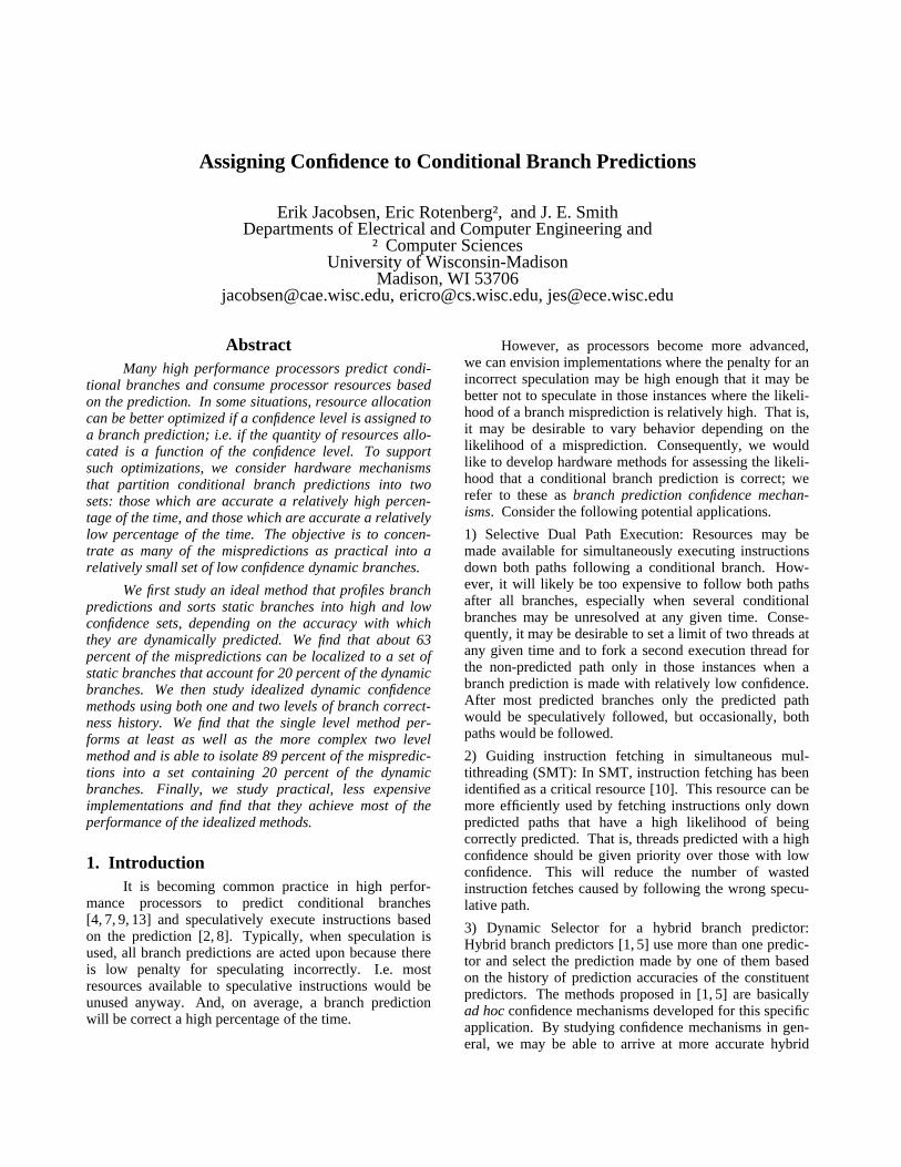
Of course, many such sets are possible, dependingon what we define to be "low" and "high" -- we have thusfar been vague on this point. To understand the range ofpossibilities, we go down the the sorted list of branchstatistics and plot accumulated fractions of mispredictedbranches versus the accumulated fractions of executedbranches that produce them. For the IBS benchmarks,Fig. 2 is the resulting plot.

Note that the graph has discrete data points(although they run together when plotted), corresponding

0

20

40

60

80

100

0 20 40 60 80 100

% o

f M

ispr

edic

ts

% of Dynamic Branches

(25.2, 70.6)

"static"

Fig. 2. Cumulative mispredictions versus cu-mulative dynamic branches.

to each static branch that occurs in the sorted list. Eachsuch point defines a pair of high and low confidencebranch prediction sets. To interpret the graph, considerthe data point (25.2,70.6), marked on the graph. At thispoint, 25.2 percent of the dynamic branches have beenaccumulated by the time we reach the static branch inquestion, and 70.6 of the mispredictions are included.That is, we can separate the branches so that 25.2 percentof executed branches are placed in the low confidence setand account for 70.6 percent of the mispredictions.

The general shape of the curve is a steep rise thatrounds a "knee" into a nearly horizontal line. This partic-ular curve for static branches has a rather gentle knee;some of the dynamic methods given in the next sectionhave much sharper knees. The steeper the initial slopeand the farther to the left the knee occurs, the better.With a curve of this shape, more mispredictions are con-centrated within a smaller set of low confidence predic-tions. Or, in other words, the branches in the lowerconfidence set have a higher misprediction rate, and, con-versely, the branches in the higher confidence set have alower misprediction rate. The ideal low confidence setwould consist solely of mispredicted branches. Thecorresponding graph would have a straight line parallel tothe y-axis shifted to the right from the origin by themispredict rate.

One could develop a static branch confidencemethod based on the procedure just followed. That is,one could profile branches as we have just done. Then athreshold misprediction rate could be set, with all staticbranches above the threshold being tagged one way (lowconfidence), and those below tagged another (highconfidence). Or, alternatively, a fraction of mispredic-tions could be chosen, and the corresponding set of staticbranches could be selected as the low confidence ones.

For the static confidence method just described, thegraph in Fig. 2 provides an optimistic estimate of the per-formance. The method is optimistic because it represents"perfect" profiling -- we are executing the programs withexactly the same data as for the profile. Nevertheless, weuse the results from this optimistic static method for com-parison with the dynamic methods we consider in the fol-lowing sections. At a minimum, we would like thedynamic methods to exceed the performance of the staticmethod.

3. Dynamic Confidence MechanismsIn the previous section we partitioned static

branches into high and low confidence sets. That is, alldynamic predictions of the same static branch areassigned to the same confidence set. However, we canalso partition branches so that dynamic predictions of thesame static branch can be assigned to different confidencesets. This partitioning is done based on dynamic history,and we refer to these as dynamic confidence mechanisms.There are a large number of dynamic confidence mechan-isms available. They are first cousins of dynamic branchpredictors, and many such branch predictors have beenproposed over the years [4, 7, 9, 13]. In this paper, wecannot explore the entire design space. But we selectsome representative confidence methods -- those thatpreliminary experiments indicated as being more interest-ing variations.

We begin with generic confidence mechanisms thatare somewhat idealized. In Section 5 we refine them tomore practical implementations.

3.1. One-Level Confidence MethodsThe one level dynamic confidence methods are so-

named because they use a single level of table lookup;this is illustrated in Fig. 3. The table contains the n mostrecent correct/incorrect indications for the given tableentry. These n-bit entries are essentially shift registers.We call each of these a Correct/Incorrect Register (CIR,pronounced "sir"), and we refer to the entire table as theCIR Table (CT). We use the convention that a 1 in a CIRindicates an incorrect prediction, and a 0 indicates correctprediction. For example if a prediction is correct 3 times,followed by an incorrect prediction, followed by 4 correctpredictions, then an 8-bit CIR contains 00010000.

There are a number of possibilities for accessingthe table. In one, the (truncated) program counter for abranch instruction is used as an index into the CT. Alter-natively, one could keep track of global branch outcomesin a branch history register (BHR) and use it to index intothe CT. A third alternative is to maintain a global CIR(i.e. correct/incorrect status collected for the most recentdynamic branches) and use it to index into the CT.

Beginning with these three basic methods of index-ing into the CT (PC, global BHR, global CIR), one canconstruct a number of others by concatenating portions of

Program Counter

m bits

m

global BHR

CIR History Table

2^m entries

n bit entries

reductionfunction confidence

high/low

signaln

Fig. 3. One Level Dynamic ConfidenceMechanism(s).

each or exclusive-ORing them. Preliminary studies wehave done indicate that exclusive-ORing is more effectivethan concatenating sub-fields. However, this can beinfluenced by the table size and deserves further study.Our preliminary studies also indicate that indexing with aglobal CIR is of little value -- it gives low performancewhen used alone and typically reduces performance whenadded to the others. Consequently, we will report resultsonly for implementations using the PC and global BHR.This leads to three variations for indexing into the CT: PCalone, global BHR alone, and PC xor BHR.

Now, to divide the branches into two sets, we haveto take the CIR accessed from the table and reduce it to asingle binary signal. In general, we do this by passing theCIR through a combinational logic block, named the"reduction" function in Fig. 3. For example, the reductionfunction could perform a ones count on the CIR: moreones indicate a higher number of recent mispredictionswhich would tend to indicate lower accuracy. In Section5, we will consider this ones count reduction function,along with some others.

In an actual implementation, complete CIRs couldbe kept in the CT, with a separate logic block implement-ing the reduction function, exactly as shown in Fig. 3.However, one might also use implementations that main-tain a compressed form of the CIRs in the CT along witha simplified reduction function. These will be discussedmore in Section 5.

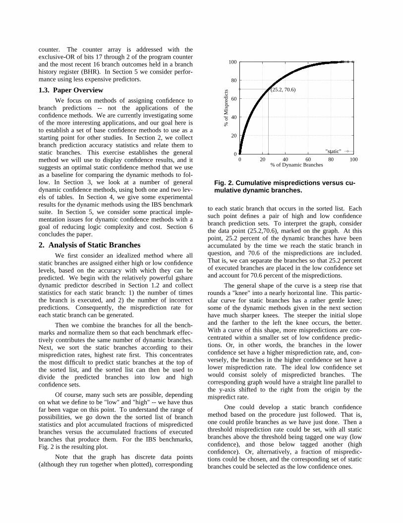
3.2. Two Level methodsWith two level dynamic confidence methods, we

index into a first level CT in a manner similar to the onelevel methods, then combine the CIR read from the tablewith some combination of the PC and global BHR toindex into a second level CT. The second level table con-tains the Correct/Incorrect values for the p most recenttimes the first level CIR/PC/BHR combination occurred.Finally, the CIR read out of the second level table passesthrough a combinational reduction function as in the pre-vious one level methods.

n p

reductionfunction

m2^m entries

CIR History TableLevel 1

Level 2

n bit entries

Program Counter

m bits

global BHR

CIR History Table

p bit entries

2^n entrieshigh/low

confidencesignal

Fig. 4. Two Level Dynamic ConfidenceMechanism(s).

There are several variations of the two-levelmethod (refer to Fig. 4). In general, one can hash somecombination of PC and global BHR for the first table,then hash the output of the first table with some combina-tion of PC and global BHR. This leads to 12 differentpossibilities -- and other two level structures could prob-ably be made (one could consider using the global CIRwhen computing the index into the second level table, forexample). After some preliminary exploration, we settleon only three representative methods.

In the first variation, the PC alone is used to readthe first table, and the CIR alone is used to access thesecond level table. In the second variation, the PC xorBHR is used to read the first level table, and the CIR readfrom the table is used to read the second level table. Thethird variation is like the second except the PC and BHRare exclusive-ORed with the CIR read from the first leveltable before indexing into the second level table.

4. Experimental ResultsWe now use trace-driven simulation to study the

dynamic confidence methods outlined in the previous sec-tion. As stated earlier, the underlying branch predictor isa gshare predictor using a table with 216 two-bit counters.The prediction table is accessed with the exclusive-OR ofthe 16 low order PC bits and a 16 bit global BHR. For theone level confidence methods, the CIR tables also have216 entries, each of which contains a 16 bit CIR. Wesimulate the IBS benchmark suite. Results are averagedby weighting the individual benchmarks so that each con-tributes the same total number of dynamic branches. For

the relatively large underlying branch predictor we use,the overall misprediction rate is 3.85 percent.

For all methods, we initialize the branch predictortable to "weakly taken" and the CIR tables to all ones.All ones was found to give better results than other initialCT values we studied; additional information on initialvalues will be given in Section 5.

Initially, we will collect separate statistics for eachCIR value read from the CT (the second level CT in thecase of the two level methods). For each CIR pattern wekeep track of number of times the pattern appears and thefraction of incorrect predictions that occurred when thatCIR pattern was read.

After collecting this data for each CIR pattern, wesort and construct a graph similar to that used for thestatic method in section 2. In particular, we sort the CIRpatterns according to misprediction rates, highest rate atthe top. The sorted list is used to plot data points -- oneper CIR. For each point the X axis value is the fraction ofaccumulated conditional branches corresponding to thisCIR and those higher on the list; the Y axis value is thefraction of mispredictions the conditional branchesaccount for. Now, each point can be used to define highand low confidence prediction sets. A combinationalreduction function that detects the sets selects only thoseCIRs above (low confidence) or below (high confidence)the CIR in question. The CIRs define minterms for thereduction function.

As in the static method, this method of determiningthe confidence sets is idealized because the reductionfunction is tuned to a specific set of data input values. Inaddition, the combinational reduction function could bevery complicated, i.e. it could have many prime impli-cants -- many of which could conceivably be minterms.In Section 5 we look at more practical reduction func-tions.

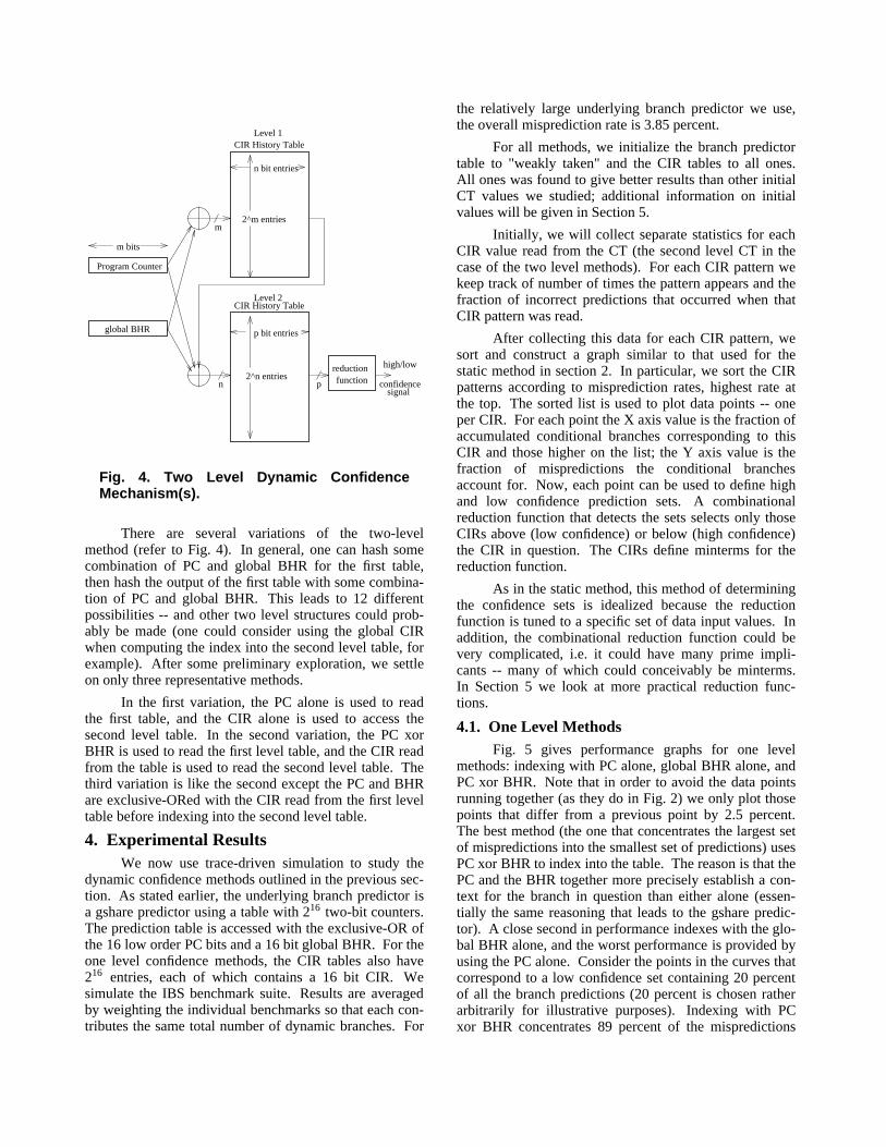
4.1. One Level MethodsFig. 5 gives performance graphs for one level

methods: indexing with PC alone, global BHR alone, andPC xor BHR. Note that in order to avoid the data pointsrunning together (as they do in Fig. 2) we only plot thosepoints that differ from a previous point by 2.5 percent.The best method (the one that concentrates the largest setof mispredictions into the smallest set of predictions) usesPC xor BHR to index into the table. The reason is that thePC and the BHR together more precisely establish a con-text for the branch in question than either alone (essen-tially the same reasoning that leads to the gshare predic-tor). A close second in performance indexes with the glo-bal BHR alone, and the worst performance is provided byusing the PC alone. Consider the points in the curves thatcorrespond to a low confidence set containing 20 percentof all the branch predictions (20 percent is chosen ratherarbitrarily for illustrative purposes). Indexing with PCxor BHR concentrates 89 percent of the mispredictions

into the low confidence set; BHR alone concentrates 85percent, and the PC concentrates 72 percent.

Also shown in the Fig. 5 graph is a curve for thestatic method given in Section 2. We see that thedynamic methods are capable of performing much betterthan the optimistic static method. For comparison, withthe static method 20 percent of the branches concentrateonly about 63 percent of the mispredictions.

For the dynamic methods, the all zeros CIR occursfrequently, and we refer to this all zeros CT entry as the"zero bucket". The zero bucket corresponds to the casewhere the table entry has seen a correct prediction the last16 times in a row. It is not surprising that the zero bucketis accessed frequently, given that the overall predictionaccuracy is 96.15 percent. The large zero bucket explainsthe long gap between data points for the dynamic methodsin the right side of the graph. For example, with the twobetter dynamic methods, about 80 percent of the branchpredictions lead to the all zeros CIR, and 12-15 percent ofthe mispredictions occur with the all zeros CIR. Hence,in the 20 to 100 percent dynamic branch region of thegraph, the dynamic methods have no data points. Thestatic method does have data points, however, and thesepoints allow the static curve to arc above the interpolatedcurves for the dynamic methods in this region.

Finally, we note once again that the dynamic resultsare idealized in a way similar to the way the staticbranches are. In particular, we sort the CIRs from worstto best based on their performance for the IBS bench-marks, and effectively use an optimal reduction functionfor the resulting CT. When we look at practical reductionfunctions, this level of optimism will be mitigated.

0

20

40

60

80

100

0 20 40 60 80 100

% o

f M

ispr

edic

ts


"static""PC"

"BHR""BHRxorPC"

Fig. 5. Cumulative mispredictions versus cu-mulative dynamic branches for one leveldynamic confidence methods.

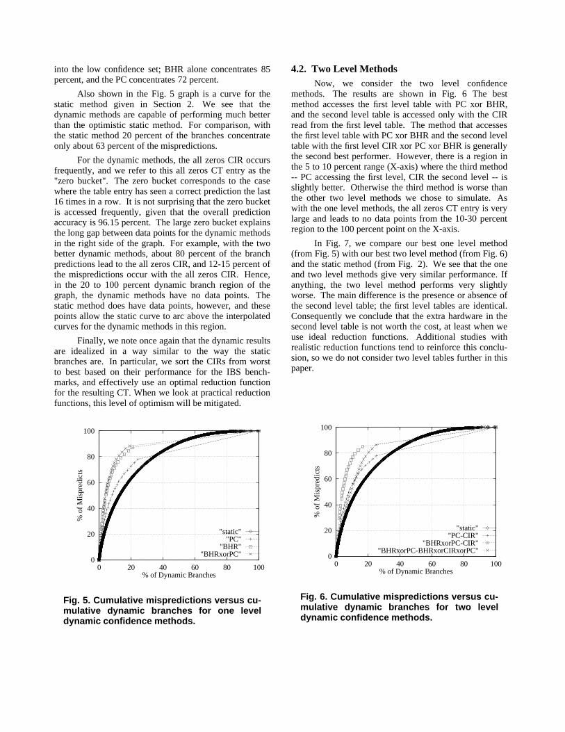
4.2. Two Level MethodsNow, we consider the two level confidence

methods. The results are shown in Fig. 6 The bestmethod accesses the first level table with PC xor BHR,and the second level table is accessed only with the CIRread from the first level table. The method that accessesthe first level table with PC xor BHR and the second leveltable with the first level CIR xor PC xor BHR is generallythe second best performer. However, there is a region inthe 5 to 10 percent range (X-axis) where the third method-- PC accessing the first level, CIR the second level -- isslightly better. Otherwise the third method is worse thanthe other two level methods we chose to simulate. Aswith the one level methods, the all zeros CT entry is verylarge and leads to no data points from the 10-30 percentregion to the 100 percent point on the X-axis.

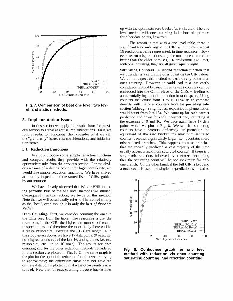
In Fig. 7, we compare our best one level method(from Fig. 5) with our best two level method (from Fig. 6)and the static method (from Fig. 2). We see that the oneand two level methods give very similar performance. Ifanything, the two level method performs very slightlyworse. The main difference is the presence or absence ofthe second level table; the first level tables are identical.Consequently we conclude that the extra hardware in thesecond level table is not worth the cost, at least when weuse ideal reduction functions. Additional studies withrealistic reduction functions tend to reinforce this conclu-sion, so we do not consider two level tables further in thispaper.

0

20

40

60

80

100

0 20 40 60 80 100

% o

f M

ispr

edic

ts


"static""PC-CIR"

"BHRxorPC-CIR""BHRxorPC-BHRxorCIRxorPC"

Fig. 6. Cumulative mispredictions versus cu-mulative dynamic branches for two leveldynamic confidence methods.

0

20

40

60

80

100

0 20 40 60 80 100

% o

f M

ispr

edic

ts


"static""BHRxorPC"

"BHRxorPC-CIR"

Fig. 7. Comparison of best one level, two lev-el, and static methods.

5. Implementation IssuesIn this section we apply the results from the previ-

ous section to arrive at actual implementations. First, welook at reduction functions, then consider what we callthe "granularity" issue, cost considerations, and initializa-tion issues.

5.1. Reduction FunctionsWe now propose some simple reduction functions

and compare results they provide with the relativelyoptimistic results from the previous section. For the obvi-ous reasons of reducing cost and/or logic complexity, wewould like simple reduction functions. We have arrivedat three by inspection of the sorted lists of CIRs, guidedby our intuition.

We have already observed that PC xor BHR index-ing performs best of the one level methods we studied.Consequently, in this section, we focus on this method.Note that we will occasionally refer to this method simplyas the "best", even though it is only the best of those westudied.

Ones Counting. First, we consider counting the ones inthe CIRs read from the table. The reasoning is that themore ones in the CIR, the higher the number of recentmispredictions, and therefore the more likely there will bea future mispredict. Because the CIRs are length 16 inthe study given above, we have 17 data points (0 ones, i.e.no mispredictions out of the last 16, a single one, i.e. onemispredict, etc. up to 16 ones). The results for onescounting and for the other reduction methods consideredin this section are plotted in Fig. 8. On the same graph isthe plot for the optimistic reduction function we are tryingto approximate; the optimistic curve does not have thediscrete data points plotted to make the other points easierto read. Note that for ones counting the zero bucket lines

up with the optimistic zero bucket (as it should). The onelevel method with ones counting falls short of optimumfor other data points, however.

The reason is that with a one level table, there issignificant time ordering in the CIR, with the most recent16 predictions being represented, in time sequence. How-ever, recent mispredictions, e.g. the most recent, correlatebetter than the older ones, e.g. 16 predictions ago. Yet,with ones counting, they are all given equal weight.

Saturating Counters. A second reduction function thatwe consider is a saturating ones count on the CIR values.We do not expect this method to perform any better thanones counting. However, it could lead to a less costlyconfidence method because the saturating counters can beembedded into the CT in place of the CIRs -- leading toan essentially logarithmic reduction in table space. Usingcounters that count from 0 to 16 allow us to comparedirectly with the ones counters from the preceding sub-section (although a slightly less expensive implementationwould count from 0 to 15). We count up for each correctprediction and down for each incorrect one, saturating atthe extremes of 0 and 16. We once again have 17 datapoints which we plot in Fig. 8. We see that saturatingcounters have a potential deficiency. In particular, theequivalent of the zero bucket, the maximum saturatedcounter, becomes significantly larger; i.e. it contains moremispredicted branches. This happens because branchesthat are correctly predicted a vast majority of the timeusually access a maximum saturated counter. If there is asingle misprediction, followed by a correct prediction,then the saturating count will be non-maximum for onlyone branch. On the other hand, if the full CIR is kept anda ones count is used, the single misprediction will lead to

0

20

40

60

80

100

0 20 40 60 80 100

% o

f M

ispr

edic

ts


"BHRxorPC""BHRxorPC.1Cnt"

"BHRxorPC.Reset""BHRxorPC.Sat"

Fig. 8. Confidence graph for one levelmethod with reduction via ones counting,saturating counting, and resetting counting.

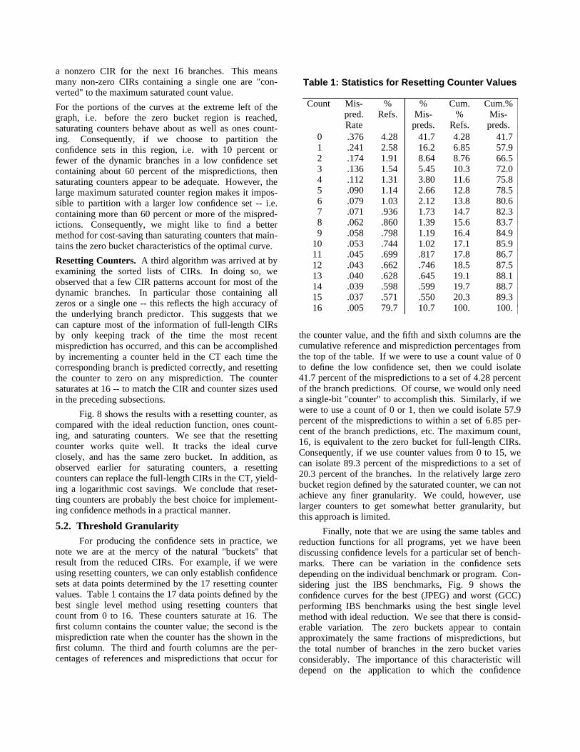
a nonzero CIR for the next 16 branches. This meansmany non-zero CIRs containing a single one are "con-verted" to the maximum saturated count value.

For the portions of the curves at the extreme left of thegraph, i.e. before the zero bucket region is reached,saturating counters behave about as well as ones count-ing. Consequently, if we choose to partition theconfidence sets in this region, i.e. with 10 percent orfewer of the dynamic branches in a low confidence setcontaining about 60 percent of the mispredictions, thensaturating counters appear to be adequate. However, thelarge maximum saturated counter region makes it impos-sible to partition with a larger low confidence set -- i.e.containing more than 60 percent or more of the mispred-ictions. Consequently, we might like to find a bettermethod for cost-saving than saturating counters that main-tains the zero bucket characteristics of the optimal curve.

Resetting Counters. A third algorithm was arrived at byexamining the sorted lists of CIRs. In doing so, weobserved that a few CIR patterns account for most of thedynamic branches. In particular those containing allzeros or a single one -- this reflects the high accuracy ofthe underlying branch predictor. This suggests that wecan capture most of the information of full-length CIRsby only keeping track of the time the most recentmisprediction has occurred, and this can be accomplishedby incrementing a counter held in the CT each time thecorresponding branch is predicted correctly, and resettingthe counter to zero on any misprediction. The countersaturates at 16 -- to match the CIR and counter sizes usedin the preceding subsections.

Fig. 8 shows the results with a resetting counter, ascompared with the ideal reduction function, ones count-ing, and saturating counters. We see that the resettingcounter works quite well. It tracks the ideal curveclosely, and has the same zero bucket. In addition, asobserved earlier for saturating counters, a resettingcounters can replace the full-length CIRs in the CT, yield-ing a logarithmic cost savings. We conclude that reset-ting counters are probably the best choice for implement-ing confidence methods in a practical manner.

5.2. Threshold GranularityFor producing the confidence sets in practice, we

note we are at the mercy of the natural "buckets" thatresult from the reduced CIRs. For example, if we wereusing resetting counters, we can only establish confidencesets at data points determined by the 17 resetting countervalues. Table 1 contains the 17 data points defined by thebest single level method using resetting counters thatcount from 0 to 16. These counters saturate at 16. Thefirst column contains the counter value; the second is themisprediction rate when the counter has the shown in thefirst column. The third and fourth columns are the per-centages of references and mispredictions that occur for

Table 1: Statistics for Resetting Counter Values� ��

Count Mis- % % Cum. Cum.%pred. Refs. Mis- % Mis-Rate preds. Refs. preds.� ��

0 .376 4.28 41.7 4.28 41.71 .241 2.58 16.2 6.85 57.92 .174 1.91 8.64 8.76 66.53 .136 1.54 5.45 10.3 72.04 .112 1.31 3.80 11.6 75.85 .090 1.14 2.66 12.8 78.56 .079 1.03 2.12 13.8 80.67 .071 .936 1.73 14.7 82.38 .062 .860 1.39 15.6 83.79 .058 .798 1.19 16.4 84.9

10 .053 .744 1.02 17.1 85.911 .045 .699 .817 17.8 86.712 .043 .662 .746 18.5 87.513 .040 .628 .645 19.1 88.114 .039 .598 .599 19.7 88.715 .037 .571 .550 20.3 89.316 .005 79.7 10.7 100. 100.� ��

��

��

��

��

��

��

��

the counter value, and the fifth and sixth columns are thecumulative reference and misprediction percentages fromthe top of the table. If we were to use a count value of 0to define the low confidence set, then we could isolate41.7 percent of the mispredictions to a set of 4.28 percentof the branch predictions. Of course, we would only needa single-bit "counter" to accomplish this. Similarly, if wewere to use a count of 0 or 1, then we could isolate 57.9percent of the mispredictions to within a set of 6.85 per-cent of the branch predictions, etc. The maximum count,16, is equivalent to the zero bucket for full-length CIRs.Consequently, if we use counter values from 0 to 15, wecan isolate 89.3 percent of the mispredictions to a set of20.3 percent of the branches. In the relatively large zerobucket region defined by the saturated counter, we can notachieve any finer granularity. We could, however, uselarger counters to get somewhat better granularity, butthis approach is limited.

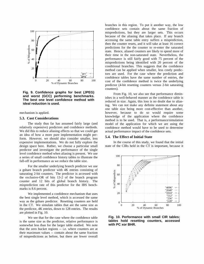
Finally, note that we are using the same tables andreduction functions for all programs, yet we have beendiscussing confidence levels for a particular set of bench-marks. There can be variation in the confidence setsdepending on the individual benchmark or program. Con-sidering just the IBS benchmarks, Fig. 9 shows theconfidence curves for the best (JPEG) and worst (GCC)performing IBS benchmarks using the best single levelmethod with ideal reduction. We see that there is consid-erable variation. The zero buckets appear to containapproximately the same fractions of mispredictions, butthe total number of branches in the zero bucket variesconsiderably. The importance of this characteristic willdepend on the application to which the confidence

0

20

40

60

80

100

0 20 40 60 80 100

% o

f M

ispr

edic

ts


"gcc""jpeg"

Fig. 9. Confidence graphs for best (JPEG)and worst (GCC) performing benchmarks.The best one level confidence method withideal reduction is used.

mechanism is applied.

5.3. Cost ConsiderationsThe study thus far has assumed fairly large (and

relatively expensive) predictors and confidence methods.We did this to reduce aliasing effects so that we could getan idea of how a more pure implementation might per-form. However, we should also consider smaller, lessexpensive implementations. We do not fully explore thedesign space here. Rather, we choose a particular smallpredictor and investigate the performance of the singlelevel confidence method when aliasing is present. We usea series of small confidence history tables to illustrate thefall-off in performance as we reduce the table size.

For the smaller underlying branch predictor we usea gshare branch predictor with 4K entries consisting ofsaturating 2-bit counters. The predictor is accessed withthe exclusive-OR of bits 13-2 of the branch programcounter and 12 bits of global branch history. Themisprediction rate of this predictor for the IBS bench-marks is 8.6 percent.

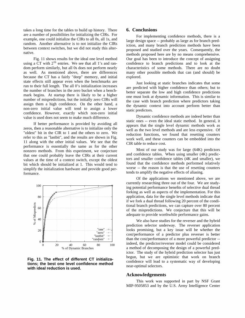
We implemented a confidence mechanism that usesthe best single level method, which is accessed the sameway as the gshare predictor. Resetting counters are heldin the CT. We simulate tables that are the same size asthe predictor, 4K entries, down to 128 entries. The resultsare plotted in Fig. 10.

We see that for the case where the confidence tableis the same size as the predictor, relative performance issomewhat less than for the larger table studied. We notethat the zero bucket regions -- i.e. where counters are attheir maximum values -- contain about the same fractionof mispredictions as before, but there are fewer overall

branches in this region. To put it another way, the lowconfidence sets contain about the same fraction ofmispredictions, but they are larger sets. This occursbecause of the aliasing that takes place. If any branchaccessing the same table entry suffers a misprediction,then the counter resets, and it will take at least 16 correctpredictions for the the counter to re-enter the saturatedstate. Hence, aliased counters are likely to spend more oftheir time in the non-saturated state. Nevertheless, theperformance is still fairly good with 75 percent of themispredictions being identified with 20 percent of theconditional branches. This suggests that the confidencemethod can be applied when smaller, less costly predic-tors are used. For the case where the prediction andconfidence tables have the same number of entries, thecost of the confidence method is twice the underlyingpredictor (4-bit resetting counters versus 2-bit saturatingcounters).

From Fig. 10, we also see that performance dimin-ishes in a well-behaved manner as the confidence table isreduced in size. Again, this loss is no doubt due to alias-ing. We can not make any definite statement about anyone table size being more cost-effective than another,however, because to do so would require someknowledge of the application where the confidencemethod is to be used. That is, a performance/simulationmodel of the application for which we are using theconfidence method would have to be used to determineactual performance impact of the confidence sets.

5.4. The Effect of Initial StateIn the course of this study, we found that the initial

state of the CIRs held in the CT is important, because it

0

20

40

60

80

100

0 20 40 60 80 100

% o

f M

ispr

edic

ts


"4096""2048""1024""512""256""128"

Fig. 10. Performance with small CIR tables;tables hold resetting counters, accessedwith PC xor BHR.

takes a long time for the tables to build up history. Thereare a number of possibilities for initializing the CIRs. Forexample, one could initialize the CIRs to all 0s, all 1s, andrandom. Another alternative is to not initialize the CIRsbetween context switches, but we did not study this alter-native.

Fig. 11 shows results for the ideal one level methodusing a CT with 216 entries. We see that all 1’s and ran-dom perform similarly, but all 0s does not perform nearlyas well. As mentioned above, there are differencesbecause the CT has a fairly "deep" memory, and initialstate effects still appear even when the benchmarks arerun to their full length. The all 0’s initialization increasesthe number of branches in the zero bucket when a bench-mark begins. At startup there is likely to be a highernumber of mispredictions, but the initially zero CIRs willassign them a high confidence. On the other hand, anon-zero initial value will tend to assign a lowerconfidence. However, exactly which non-zero initialvalue is used does not seem to make much difference.

If better performance is provided by avoiding allzeros, then a reasonable alternative is to initialize only the"oldest" bit in the CIR to 1 and the others to zero. Werefer to this as "lastbit", and the results are shown in Fig.11 along with the other initial values. We see that theperformance is essentially the same as for the othernonzero methods. From this experiment, we conjecturethat one could probably leave the CIRs at their currentvalues at the time of a context switch, except the oldestbit which should be initialized at 1. This would tend tosimplify the initialization hardware and provide good per-formance.

0

20

40

60

80

100

0 20 40 60 80 100

% o

f M

ispr

edic

ts


"one""zero"

"lastbit""random"

Fig. 11. The effect of different CT initializa-tions; the best one level confidence methodwith ideal reduction is used.

6. ConclusionsFor implementing confidence methods, there is a

large design space -- probably as large as for branch pred-iction, and many branch prediction methods have beenproposed and studied over the years. Consequently, themethods proposed here are by no means comprehensive.Our goal has been to introduce the concept of assigningconfidence to branch predictions and to look at thecharacteristics of some methods. There are no doubtmany other possible methods that can (and should) beexplored.

Just looking at static branches indicates that someare predicted with higher confidence than others; but tobetter separate the low and high confidence predictionsone must look at dynamic information. This is similar tothe case with branch prediction where predictors takingthe dynamic context into account perform better thanstatic predictors.

Dynamic confidence methods are indeed better thanstatic ones -- even the ideal static method. In general, itappears that the single level dynamic methods work aswell as the two level methods and are less expensive. Ofreduction functions, we found that resetting counterswork well, and these counters can be embedded into theCIR table to reduce cost.

Most of our study was for large (64K) predictorsand confidence tables. When using smaller (4K) predic-tors and smaller confidence tables (4K and smaller), wefound that the confidence methods performed relativelyworse -- the reason is that the use of resetting counterstends to amplify the negative effects of aliasing.

Of the applications we mentioned above, we arecurrently researching three out of the four. We are study-ing potential performance benefits of selective dual threadforking as well as aspects of the implementation. For thisapplication, data for the single level methods indicate thatif we fork a dual thread following 20 percent of the condi-tional branch predictions, we can capture over 80 percentof the mispredictions. We conjecture that this will beadequate to provide worthwhile performance gains.

We also have studies for the reverser and the hybridprediction selector underway. The reverser applicationlooks promising, but a key issue will be whether thecost/performance of a predictor plus reverser is betterthan the cost/performance of a more powerful predictor --indeed, the predictor/reverser model could be considereda method of decomposing the design of a powerful pred-ictor. The study of the hybrid prediction selector has justbegun, but we are optimistic that work on branchconfidence will lead to a systematic way of developingnear-optimal selectors.

AcknowledgementsThis work was supported in part by NSF Grant

MIP-9505853 and by the U.S. Army Intelligence Center

and Fort Huachuca under Contract DABT63-95-C-0127and ARPA order no. D346. The views and conclusionscontained herein are those of the authors and should notbe interpreted as necessarily representing the official poli-cies or endorsements, either expressed or implied, of theU.S. Army Intelligence Center and Fort Huachuca, or theU.S. Government. Eric Rotenberg is funded by an IBMgraduate fellowship. Erik Jacobsen was funded by aWisconsin/Hilldale undergraduate research scholarship

The authors would like to thank Joel Emer for help-ful discussions while this work was in progress and forsuggesting potential applications.

References[1] M. Evers, P. Chang, and Y. Patt, ‘‘Using Hybrid

Branch Predictors to Improve Branch PredictionAccuracy in the Presence of Context Switches,’’International Symposium on Computer Architec-ture, pp. 3-11 , May 1996.

[2] Linley Gwennap, ‘‘MIPS R10000 Uses DecoupledArchitecture,’’ Microprocessor Report, vol. 8, pp.18-22, October 24, 1994.

[3] B. T. Hailpern and B. L. Hitson, ‘‘S-1 ArchitectureManual,’’ CSL Report STAN-CS-79-715., Stan-ford University, January 1979.

[4] J. K. F. Lee and A. J. Smith, ‘‘Branch PredictionStrategies and Branch Target Buffer Design,’’Computer, vol. 17, pp. 6 - 22, January 1984.

[5] S. McFarling, ‘‘Combining Branch Predictors,’’Digital Western Research Lab Technical NoteTN-36, June 1993.

[6] Motorola, ‘‘PowerPC 601 User’s Manual,’’ 1993,No. MPC601UM/AD.

[7] S.-T. Pan, K. So, and J. T. Rahmeh, ‘‘Improvingthe Accuracy of Dynamic Branch Prediction UsingBranch Correlation,’’ Proc. Architectural Supportfor Programming Languages and Operating Sys-tems (ASPLOS-V), pp. 76-84, October 1992.

[8] Michael Slater, ‘‘AMD’s K5 Designed to OutrunPentium,’’ Microprocessor Report, vol. 8, pp.1,6-11, October 24, 1994.

[9] J. E. Smith, ‘‘A Study of Branch Prediction Stra-tegies,’’ Proc. Eighth Annual Symposium on Com-puter Architecture, pp. 135-148, May 1981.

[10] D. Tullsen, S. Eggers, J. Emer, H. Levy, J. Lo, andR. Stamm, ‘‘Exploiting Choice: Instruction Fetchand Issue on an Implementable Simultaneous Mul-tithreading Processor,’’ Proc. 23rd Annual Interna-tional Symposium on Computer Architecture, pp.191-202, May 1996.

[11] Richard Uhlig, David Nagle, Trevor Mudge, StuartSechrest, and Joel Emer, ‘‘Instruction Fetching:Coping with Code Bloat,’’ Proc. 22nd AnnualSymposium on Computer Architecture, pp. 345-356, June 1995.

[12] A. K. Uht and V. Sindagi, ‘‘Disjoint Eager Execu-tion: An Optimal Form of Speculative Execution,’’Proc. 28th Annual International Symposium on Mi-croarchitecture, pp. 313-325, November 1995.

[13] T. Y. Yeh and Y. N. Patt, ‘‘Two-Level AdaptiveBranch Prediction,’’ Proc. 24th Annual Interna-tional Symposium on Microarchitecture, No-vember 1991.

Documents

Assigning confidence to conditional branch predictions