Comparative Explanation of East Asia's Growth Using Neoclassical and Post Keynesian Growth Models

Comparative Explanations of East Asia’s Growth Using Neoclassical and Post-Keynesian Models

by

Praopan Pratoomchat October 2013

Department of Economics, University of Utah Abstract The study estimates economic growth in eight selected East Asian countries

using two growth models from two competing schools of thought. The first model

is the Post-Keynesian model (Balance-of-Payment Constrained growth model).

In this model, demand variables from export and capital inflows determine the

limit of economic growth in the long run. The study uses prior estimates income

elasticity of demand for import and export using a two-stage least square

technique to eliminate the endogeniety problem then it calculates the predicted

growth by the definition of the Balance-of-Payment Constrained growth model.

The second model is the neoclassical model developed from Solow growth

model focusing on the supply side variables determining economic growth. The

study relaxes the assumption of exogenous technology and makes it

endogenous of capital inflows. Two predicted output growth series from two

models are obtained for each country and for the balanced panel data for the

whole region. The performance of each model is evaluated by two methods: the

discrimination approach and the discerning approach. The study found that the

output growth series defined by the augmented Solow growth model can better

explain the actual growth than the output growth series from the Balance-of-

Payment Constrained Model. In addition, the study hypothesized that financial

structure is one of the important factors that these two models omitted. A set of

financial variables representing a different part of the financial structure is used

for explaining the error series from both growth models. The results show that

the selected financial variables can better explain the error from the Post-

Keynesian model than the error from the neoclassical growth model.

2

Praopan Pratoomchat, Comparative Explanations of East Asia’s Growth Using Neoclassical and Post-Keynesian Models

Introduction

In this study, the corporative performance of both the neoclassical growth model

by Mankiw et al. (1992) and the balance-of-payments constrained growth model

by Thirlwall and Hussain (1982) are tested using econometric panel data

analysis. The area of study includes both developed countries and developing

countries in East Asia: Japan, Korea, Singapore, Indonesia, Malaysia, the

Philippines, Thailand and China. The time period is 1980-2010. Both models are

modified to have the same dependent variable, namely growth in income per

capita. In addition, the study relaxes the assumption of exogenous technology in

the supply-side model and treats foreign inflows as an important variable to

determine economic growth.

Two methods of comparing the explanatory power of the models to the actual

growth series are applied: the discrimination approach (goodness-of-fit

criterion), and the discerning approach (Non-nested J-test). The results from

both methods indicated that the augmented Solow model with endogenous

technology gives a better explanation of output growth in the selected East

Asian economies.

After the study tests the explanatory power of both models, the error series from

both models are obtained. The study further assumes that the financial structure

is the important factor that both models omitted in explaining the output growth.

Three selected financial variables are used to explain the errors of both models

using the Generalized Autoregressive Conditional Heteroskedasticity (GARCH)

model. The results show that the financial variables can better explain the error

from the post- Keynesian model.

Data and Methodology

Demand-side Model

For the developing countries, Thirlwall and Hussain (1982) introduced the role of

capital inflows into the simple Harrod foreign trade multiplier since it has played

a larger role in economic performance in recent decades. They found that since

3


some developing countries have experienced the bottleneck of foreign

exchange, their ever growing current account deficits are financed by capital

inflows, which allow these countries to grow permanently faster than otherwise

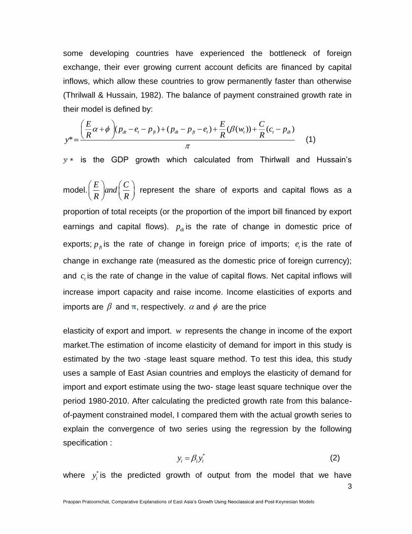
(Thrilwall & Hussain, 1982). The balance of payment constrained growth rate in

their model is defined by:

( ) ( ) ( ( )) ( )

*dt t ft dt ft t t t dt

E E Cp e p p p e w c p

R R Ry

(1)

is the GDP growth which calculated from Thirlwall and Hussain’s

model.E C

andR R

represent the share of exports and capital flows as a

proportion of total receipts (or the proportion of the import bill financed by export

earnings and capital flows). dtp is the rate of change in domestic price of

exports; ftp is the rate of change in foreign price of imports; te is the rate of

change in exchange rate (measured as the domestic price of foreign currency);

and tc is the rate of change in the value of capital flows. Net capital inflows will

increase import capacity and raise income. Income elasticities of exports and

imports are and , respectively. and are the price

elasticity of export and import. w represents the change in income of the export

market.The estimation of income elasticity of demand for import in this study is

estimated by the two -stage least square method. To test this idea, this study

uses a sample of East Asian countries and employs the elasticity of demand for

import and export estimate using the two- stage least square technique over the

period 1980-2010. After calculating the predicted growth rate from this balance-

of-payment constrained model, I compared them with the actual growth series to

explain the convergence of two series using the regression by the following

specification :

*

i i iy y (2)

where *

iy is the predicted growth of output from the model that we have

4


mentioned and iy is the actual growth rate of country i. Then the hypothesis

that 1i is tested. This study examines not only the single country, but also

the overall region using pooled time series data and compares the region’s

estimation results with the augmented Solow model estimation.

Supply-side Model

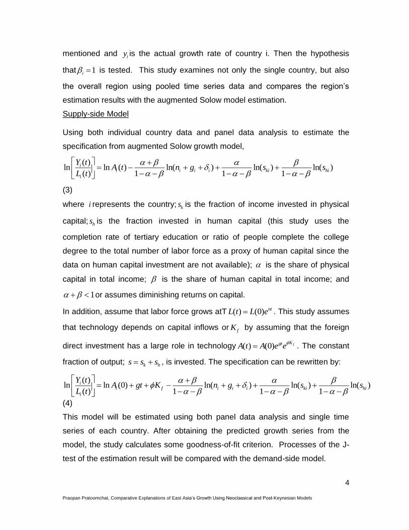
Using both individual country data and panel data analysis to estimate the

specification from augmented Solow growth model,

( )ln ln ( ) ln( ) ln( ) ln( )

( ) 1 1 1i

i i i i ki hi

i

Y tA t n g s s

L t

(3)

where i represents the country; ks is the fraction of income invested in physical

capital; hs is the fraction invested in human capital (this study uses the

completion rate of tertiary education or ratio of people complete the college

degree to the total number of labor force as a proxy of human capital since the

data on human capital investment are not available); is the share of physical

capital in total income; is the share of human capital in total income; and

1 or assumes diminishing returns on capital.

In addition, assume that labor force grows atT ( ) (0) ntL t L e . This study assumes

that technology depends on capital inflows or fK by assuming that the foreign

direct investment has a large role in technology ( ) (0) fKgtA t A e e

. The constant

fraction of output; k hs s s , is invested. The specification can be rewritten by:

( )ln ln (0) ln( ) ln( ) ln( )

( ) 1 1 1i

i f i i i ki hi

i

Y tA gt K n g s s

L t

(4)

This model will be estimated using both panel data analysis and single time

series of each country. After obtaining the predicted growth series from the

model, the study calculates some goodness-of-fit criterion. Processes of the J-

test of the estimation result will be compared with the demand-side model.

5


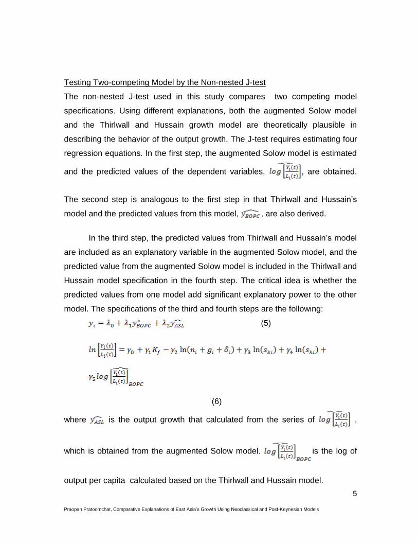
Testing Two-competing Model by the Non-nested J-test

The non-nested J-test used in this study compares two competing model

specifications. Using different explanations, both the augmented Solow model

and the Thirlwall and Hussain growth model are theoretically plausible in

describing the behavior of the output growth. The J-test requires estimating four

regression equations. In the first step, the augmented Solow model is estimated

and the predicted values of the dependent variables, , are obtained.

The second step is analogous to the first step in that Thirlwall and Hussain’s

model and the predicted values from this model, , are also derived.

In the third step, the predicted values from Thirlwall and Hussain’s model

are included as an explanatory variable in the augmented Solow model, and the

predicted value from the augmented Solow model is included in the Thirlwall and

Hussain model specification in the fourth step. The critical idea is whether the

predicted values from one model add significant explanatory power to the other

model. The specifications of the third and fourth steps are the following:

(5)

(6)

where is the output growth that calculated from the series of ,

which is obtained from the augmented Solow model. is the log of

output per capita calculated based on the Thirlwall and Hussain model.

6


Data

The data are in the form of both individual country’s time series data and pooled

time series data from selected East Asian countries: Japan, Korea, China,

Singapore, Philippines, Thailand, Indonesia, Malaysia, 1980-2010. The details of

data used for each variable in the study follow.

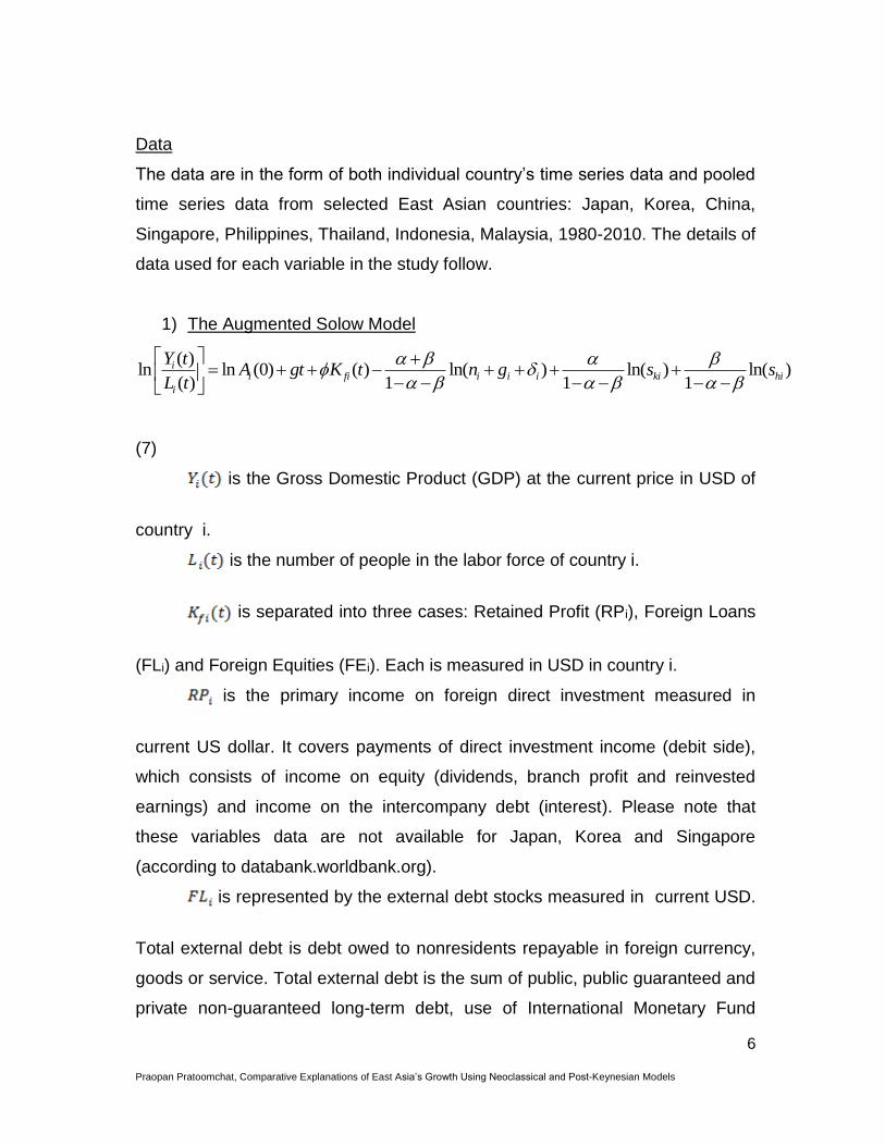
1) The Augmented Solow Model

( )ln ln (0) ( ) ln( ) ln( ) ln( )

( ) 1 1 1i

i fi i i i ki hi

i

Y tA gt K t n g s s

L t

(7)

is the Gross Domestic Product (GDP) at the current price in USD of

country i.

is the number of people in the labor force of country i.

is separated into three cases: Retained Profit (RPi), Foreign Loans

(FLi) and Foreign Equities (FEi). Each is measured in USD in country i.

is the primary income on foreign direct investment measured in

current US dollar. It covers payments of direct investment income (debit side),

which consists of income on equity (dividends, branch profit and reinvested

earnings) and income on the intercompany debt (interest). Please note that

these variables data are not available for Japan, Korea and Singapore

(according to databank.worldbank.org).

is represented by the external debt stocks measured in current USD.

Total external debt is debt owed to nonresidents repayable in foreign currency,

goods or service. Total external debt is the sum of public, public guaranteed and

private non-guaranteed long-term debt, use of International Monetary Fund

7


(IMF) credit and short-term debt. Short-term debt includes all debt having an

original maturity of 1 year or less and interest in arrears on long-term debt.

is represented by portfolio equity, net inflows in the balance of

payments, measured in current USD. It includes net inflow from equity securities

other than those recorded as direct investment and also includes shares, stocks,

depository receipts and direct purchases of shares in local stock markets by

foreign investors.

is the growth rate of labor force (age 15-60) of country i, measured as

a percentage.

ig is the total factor productivity, calculated from the growth accounting

approach and measured as a percentage.

i is the depreciation rate, represented by the percentage change of

consumption of fixed capital.

kis is the share of physical capital invested to total capital, represented by

the share of fixed capital to total investment.

his is the fraction invested in human capital. This study uses the

completion rate of tertiary education or ratio of people who complete a college

degree to the total number in the labor force as a proxy of human capital since

the data on human capital investment are not available. Data are obtained from

Barro R. and J.W. Lee (2010). Since the data are for a 5-year period, the study

uses the interpolation technique to generate the missing data.

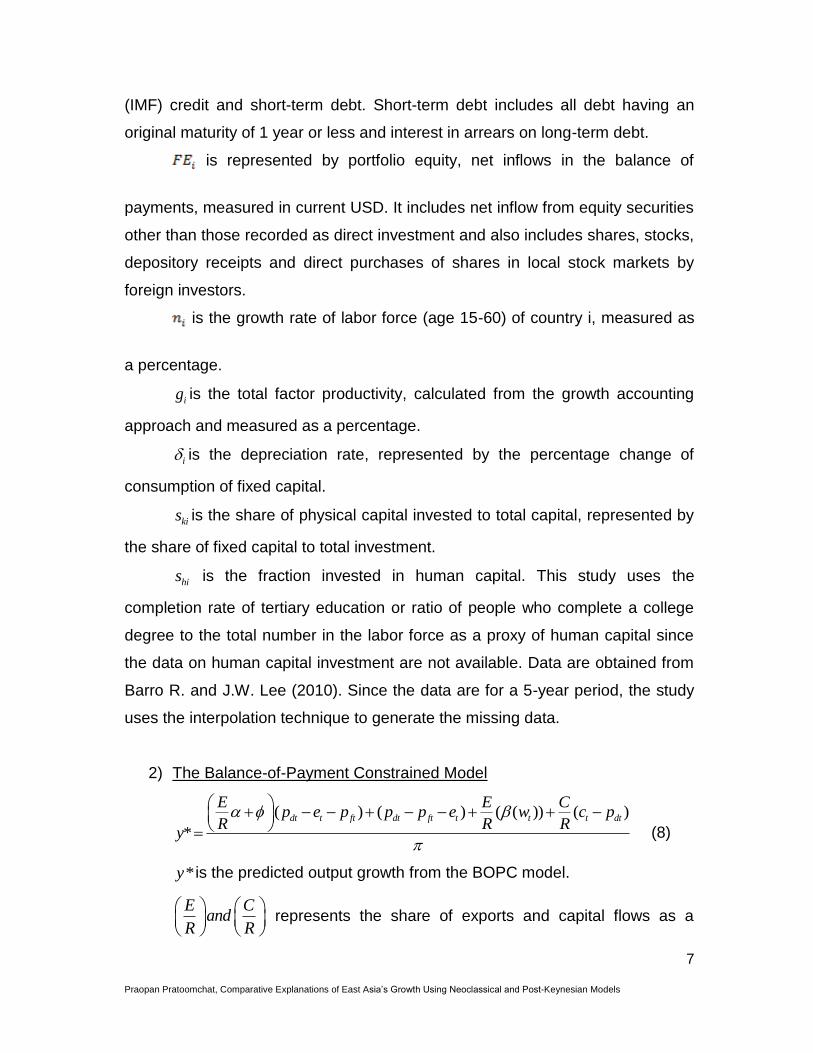
2) The Balance-of-Payment Constrained Model

( ) ( ) ( ( )) ( )



R R Ry

(8)

*y is the predicted output growth from the BOPC model.

E Cand

R R

represents the share of exports and capital flows as a

8


proportion of total receipts (or the proportion of the import bill financed by export

earnings and capital flows). The study uses the ratio of value of exports of goods

and services at the current price to total income. Total income is calculated by

the aggregation of the private capital flows and values of exports of goods and

services both measured in current US dollar.

Private capital flows consist of net foreign direct investment and portfolio

investment. Foreign direct investment is net inflows of investment to acquire a

lasting management interest (10% or more of voting stock) in an enterprise

operating in an economy other than that of the investor. It is the sum of equity

capital. The FDI included here is total net, that is, net FDI in the reporting

economy from foreign sources less net FDI by the reporting economy to the rest

of the world. Portfolio investment excludes liabilities constituting foreign

authorities’ reserves and cover transactions in equity securities and debt

securities.

dtp is the rate of change in domestic price of exports. The study uses the

export value index as a proxy. Export values are the current value of exports

(f.o.b) converted to US dollar and expressed as a percentage of average for the

base period. The data available on the World Bank database are based on year

2000 data. This study changes the base to be a year on year base.

ftp is the rate of change in foreign price of imports. The study uses the

import value index as a proxy. Import value indexes are the current value of

imports (c.i.f.) converted to US dollar and expressed as a percentage of the

average for the base period. The data available on the World Bank database are

based on 2000. This study changes the base to be a year on year base.

te is the rate of change in exchange rate (measured as the domestic price

of foreign currency).

tc is the rate of change in value of private capital flows.

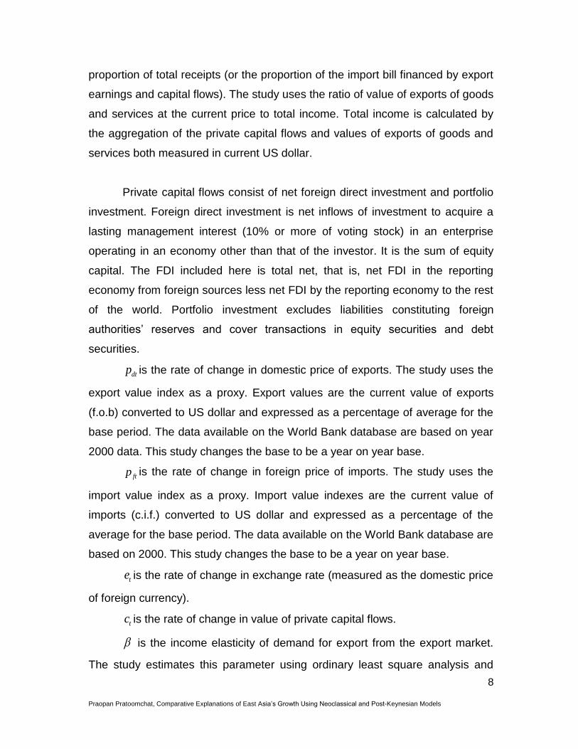
is the income elasticity of demand for export from the export market.

The study estimates this parameter using ordinary least square analysis and

9


based on the assumption that the export value of a country depends on price

and income using the following specification:

(9)

where is the rate of growth of (world income-country i’s income), is the

inflation rate in country i, is the change in import value index of country i.

is the income elasticity of demand for import of country i. The study

estimates this parameter using a two-stage least square technique to eliminate

the endogeniety problem and assumes that import values depends on domestic

income and import price using the following specification:

(10)

where is the income growth of country i. The instrumental variables are

and the constant term.

is the price elasticity of demand for imports

is the price elasticity of demand for export

w is the change in income of the export market. This study uses the

change of (world income-country i’s income) as a proxy for export market

income growth.

Explaining the Errors of the Growth Models by Financial Variables

After comparing the goodness-of-fit criteria of both models, the study also

found that there are some gaps between the actual output growth and the fitted

growth from the models. The study hypothesized that financial development

variables are crucial for explaining this region’s growth. The hypothesis is based

on the assumption that the financial sector facilitates other sectors’ flow of funds,

and leads to an increase in efficiency of the overall economy.

The study adds each single financial variable and also the respective

10


interaction terms to consider which financial variable has the most influential

impact on growth. The dummy variables for each break are also included. The

technique for estimation is Autoregressive Conditional Heteroschedasticity

(ARCH). Each country’s specifications for estimation are the following:

(11)

(12)

(13)

(14)

(15)

(16)

where y is the actual output growth and y* is the fitted growth from both models.

The selected financial variables are the following:

DEPTH: Liquid Liabilities to GDP is a traditional indicator of financial

depth. It equals currency plus demand and interest-bearing liabilities of banks

and other financial intermediaries divided by GDP, which is the broadest

available indicator of financial intermediation (Beck and Demirguc-Kunt, 2009).

BANK:; The ratio of deposit money bank domestic assets to deposit

money bank domestic assets plus central bank domestic assets shows the size

of service provided by deposit money banks in financial service. However, this

variable does not measure to whom the financial system is allocating credit.

PRIVY: This is the proportion of credit allocated to private enterprise by

the financial system. This measure equals the ratio of claims on private sector to

GDP. It represents credit allocation and overall size of the private sector and

degree of private sector borrowing, which indicates the share of credit funneled

through the private sector.

Following the standard literature, the theoretical literature predicts

DEPTH, BANK and PRIVY to be positive determinants of real income.

11


dum1 is the dummy variable representing the period 1991-1996



Autoregressive Conditional Heteroskedasticity

In conventional econometric models, the variance of the disturbance term

is assumed to be constant. However, many econometric time series exhibit

periods of unusually large volatility followed by periods of relative tranquility.

Figure 3.1 shows the fluctuation of the GDP growth of the countries selected for

this study. In such situations, the assumption of a constant variance

(homoscedasticity) is inappropriate. One approach to forecasting the variance is

to explicitly introduce an independent variable that helps to predict the volatility.

The variance of conditional on the observable value of is

(17)

Engle (1982) shows that it is possible to model the mean and variance of

series simultaneously. If the variance of is not constant, we can estimate

any tendency for sustained movements in the variance using an ARMA model

(Autoregressive Moving Average Model). For example, let denote the

estimated residuals from the model , so that the conditional

variance of is

(18)

Now suppose that the conditional variance is not constant. One simple

strategy is to model the conditional variance as an AR(q) process using the

square of the estimated residuals:

(19)

12


where = a white-noise process.

If the values of all equal zero, the estimated variance is

simply the constant . Otherwise, the conditional variance of evolves

according to the autoregressive process. Bollerslev (1986) extended Engle’s

original work by developing a technique that allows the conditional variance to

be an ARMA process. Now let the error process be such that

(20)

where

and (21)

Since is a white-noise process that is independent of past realization

of , the conditional and unconditional means of are equal to zero.

Taking the expected value of we get,

(22)

The generalized ARCH (p,q) model can be called GARCH(p,q). It allows

for both autoregressive and moving average components in the heteroskedastic

variance. The key feature of GARCH models is that the conditional variance of

the disturbances of the sequence constitutes an ARMA process. The ACF

(Autocorrelation Function) of the squared residuals can help identify the order of

the GARCH process.

The presence of heteroskedasticity can cause invalidation in the usual

standard error, t statistics and F statistics. In order to cope with these two

problems, we apply the Generalized Autoregressive Conditional

Heteroskedasticity (GARCH) model, which includes autoregressive terms as

13


well as the moving average terms in the variance equation using the following

specification in our study:

+ (23)

The mean value and the variance will be defined relative to the past

information set. The dependent variable in the present will be equal to the mean

value of itself based on the past information plus the standard deviation times

the error terms for the present period. The GARCH model with one

autoregressive lag and one moving average lag is typically called GARCH (1,1).

In this study we try among GARCH (0,1), GARCH(1,0), GARCH(1,1) to choose

the best model to fit each country and each financial variable.

Empirical Results and Analysis

Empirical Results of Thirlwall and Hussain’s Growth Model

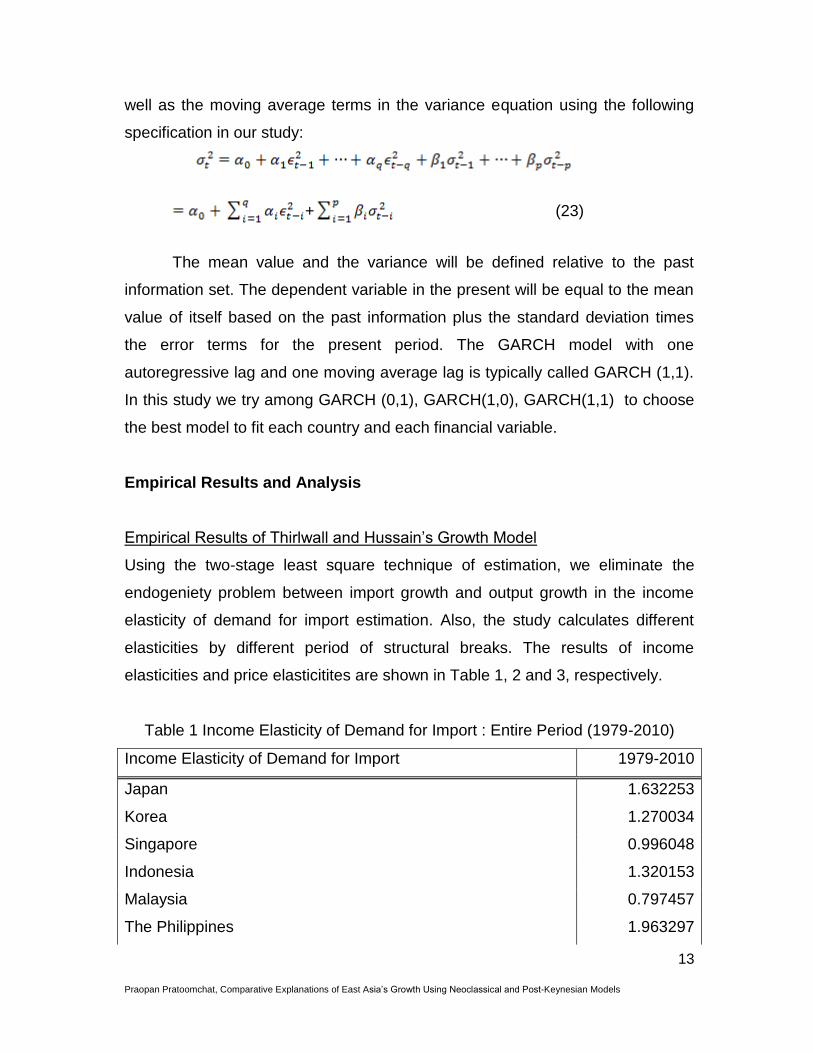
Using the two-stage least square technique of estimation, we eliminate the

endogeniety problem between import growth and output growth in the income

elasticity of demand for import estimation. Also, the study calculates different

elasticities by different period of structural breaks. The results of income

elasticities and price elasticitites are shown in Table 1, 2 and 3, respectively.

Table 1 Income Elasticity of Demand for Import : Entire Period (1979-2010)

Income Elasticity of Demand for Import 1979-2010

Japan 1.632253

Korea 1.270034

Singapore 0.996048

Indonesia 1.320153

Malaysia 0.797457

The Philippines 1.963297

14


Thailand 0.598586

China 4.046345

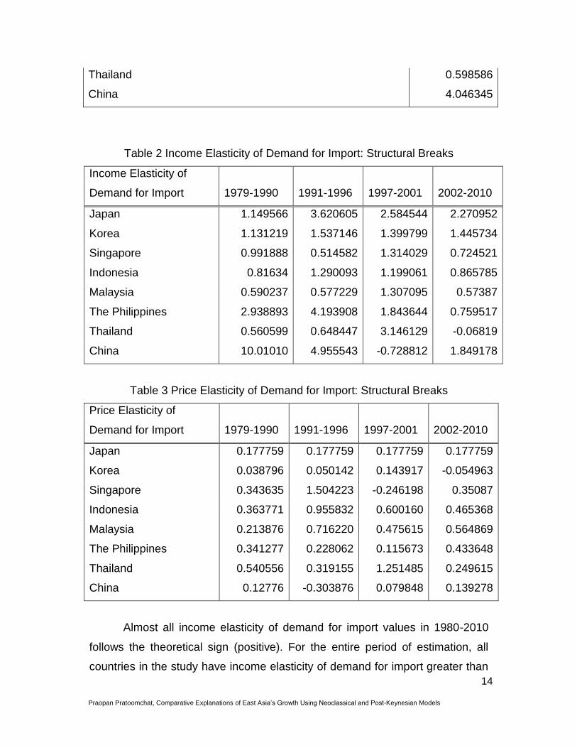
Table 2 Income Elasticity of Demand for Import: Structural Breaks

Income Elasticity of

Demand for Import 1979-1990 1991-1996 1997-2001 2002-2010

Japan 1.149566 3.620605 2.584544 2.270952

Korea 1.131219 1.537146 1.399799 1.445734

Singapore 0.991888 0.514582 1.314029 0.724521

Indonesia 0.81634 1.290093 1.199061 0.865785

Malaysia 0.590237 0.577229 1.307095 0.57387

The Philippines 2.938893 4.193908 1.843644 0.759517

Thailand 0.560599 0.648447 3.146129 -0.06819

China 10.01010 4.955543 -0.728812 1.849178

Table 3 Price Elasticity of Demand for Import: Structural Breaks

Price Elasticity of

Demand for Import 1979-1990 1991-1996 1997-2001 2002-2010

Japan 0.177759 0.177759 0.177759 0.177759

Korea 0.038796 0.050142 0.143917 -0.054963

Singapore 0.343635 1.504223 -0.246198 0.35087

Indonesia 0.363771 0.955832 0.600160 0.465368

Malaysia 0.213876 0.716220 0.475615 0.564869

The Philippines 0.341277 0.228062 0.115673 0.433648

Thailand 0.540556 0.319155 1.251485 0.249615

China 0.12776 -0.303876 0.079848 0.139278

Almost all income elasticity of demand for import values in 1980-2010

follows the theoretical sign (positive). For the entire period of estimation, all

countries in the study have income elasticity of demand for import greater than

15


zero, which means if the income increases one percent, imports will increase.

Among all countries and periods, China’s economy has the highest elasticity at

4.96 during 1991-1996 and Singapore’s has the lowest one at 0.515 during

1991-1996.

For more developed countries, Japan, Korea and Singapore’s elasticity

increased from the first period to the third eriod, and then dropped in the last

period. ASEAN-4 countries all had fluctuation in elasticity for the four periods.

In two cases income elasticities are lower than zero: China 1997-2001 and

Thailand 2002-2010.

For price elasticity of demand for import, almost all countries in the study

have a positive relationship between changes in price and changes in imports,

which means when there is an increase in price, imports will also increase.

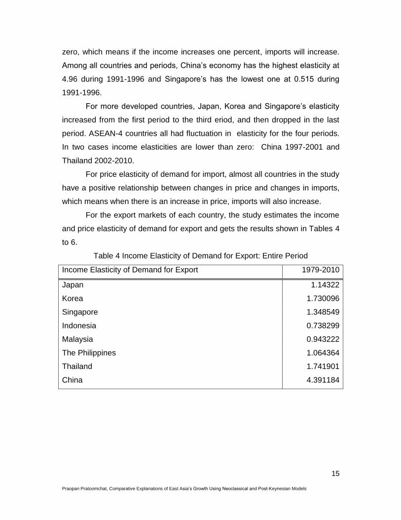
For the export markets of each country, the study estimates the income

and price elasticity of demand for export and gets the results shown in Tables 4

to 6.

Table 4 Income Elasticity of Demand for Export: Entire Period

Income Elasticity of Demand for Export 1979-2010

Japan 1.14322

Korea 1.730096

Singapore 1.348549

Indonesia 0.738299

Malaysia 0.943222

The Philippines 1.064364

Thailand 1.741901

China 4.391184

16


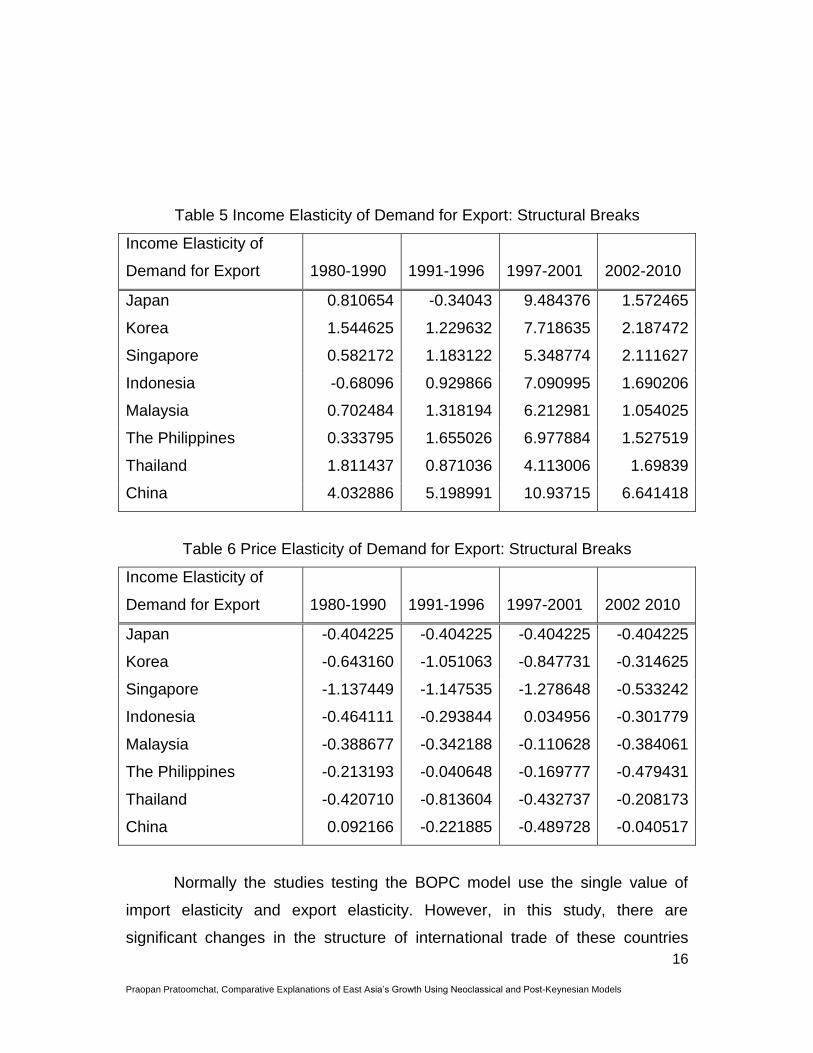
Table 5 Income Elasticity of Demand for Export: Structural Breaks


Demand for Export 1980-1990 1991-1996 1997-2001 2002-2010

Japan 0.810654 -0.34043 9.484376 1.572465

Korea 1.544625 1.229632 7.718635 2.187472

Singapore 0.582172 1.183122 5.348774 2.111627

Indonesia -0.68096 0.929866 7.090995 1.690206

Malaysia 0.702484 1.318194 6.212981 1.054025

The Philippines 0.333795 1.655026 6.977884 1.527519

Thailand 1.811437 0.871036 4.113006 1.69839

China 4.032886 5.198991 10.93715 6.641418

Table 6 Price Elasticity of Demand for Export: Structural Breaks


Demand for Export 1980-1990 1991-1996 1997-2001 2002 2010

Japan -0.404225 -0.404225 -0.404225 -0.404225

Korea -0.643160 -1.051063 -0.847731 -0.314625

Singapore -1.137449 -1.147535 -1.278648 -0.533242

Indonesia -0.464111 -0.293844 0.034956 -0.301779

Malaysia -0.388677 -0.342188 -0.110628 -0.384061

The Philippines -0.213193 -0.040648 -0.169777 -0.479431

Thailand -0.420710 -0.813604 -0.432737 -0.208173

China 0.092166 -0.221885 -0.489728 -0.040517

Normally the studies testing the BOPC model use the single value of

import elasticity and export elasticity. However, in this study, there are

significant changes in the structure of international trade of these countries

17


during the different periods so different values of elasticity are applied. The

changes of income elasticities of demand for import and export in this region

can be explained by the rise in the intraindustry trade, which has grown since

the 1980s. Grant et al. (1993) find indicators that intraindustry trade has

continued to grow as a share of overall national trade, most rapidly for the

rapidly developing countries of East and Southeast Asia. Multinational

corporations from Japan, Korea and Taiwan became large players in

international trade especially in the manufacturing sector. Manufacturing trade

showed strong growth during 1965-1990. By contrast, trade in agricultural and

other primary commodities has been weakening. From this phenomenon in

trade, the compositions of trade both import and export are shifting toward

goods with more advanced technologies, toward heterogeneous goods (away

from homogenous goods), and toward producer goods (away from consumer

goods) (Grant et al., 1993). Also, this region especially in ASEAN countries has

increased in its openness ratio (exports of goods and nonfactor services to

GDP multiplied by 100) compared to 1965 (World bank, 1992). The openness

ratio of selected countries in East Asia comparing between 1965 and 1990 is

shown in Table 7.

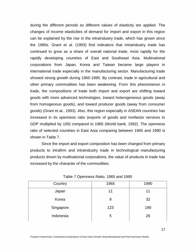
Since the import and export composition has been changed from primary

products to intrafirm and intraindustry trade in technological manufacturing

products driven by multinational corporations, the value of products in trade has

increased by the character of the commodities.

Table 7 Openness Ratio, 1965 and 1990

Country 1965 1990

Japan 11 11

Korea 9 32

Singapore 123 190

Indonesia 5 26

18


Malaysia 16 38

The Philippines 17 28

Thailand 16 38

Source: World Bank (1992), table 9, 234-35

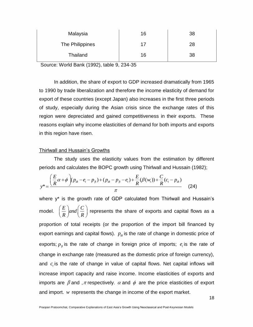
In addition, the share of export to GDP increased dramatically from 1965

to 1990 by trade liberalization and therefore the income elasticity of demand for

export of these countries (except Japan) also increases in the first three periods

of study, especially during the Asian crisis since the exchange rates of this

region were depreciated and gained competitiveness in their exports. These

reasons explain why income elasticities of demand for both imports and exports

in this region have risen.

Thirlwall and Hussain’s Growths

The study uses the elasticity values from the estimation by different

periods and calculates the BOPC growth using Thirlwall and Hussain (1982);

( ) ( ) ( ( )) ( )



R R Ry

(24)

where y* is the growth rate of GDP calculated from Thirlwall and Hussain’s

model. E C

andR R

represents the share of exports and capital flows as a

proportion of total receipts (or the proportion of the import bill financed by

export earnings and capital flows). dtp is the rate of change in domestic price of

exports; ftp is the rate of change in foreign price of imports; te is the rate of

change in exchange rate (measured as the domestic price of foreign currency),

and tc is the rate of change in value of capital flows. Net capital inflows will

increase import capacity and raise income. Income elasticities of exports and

imports are and , respectively. and are the price elasticities of export

and import. w represents the change in income of the export market.

19


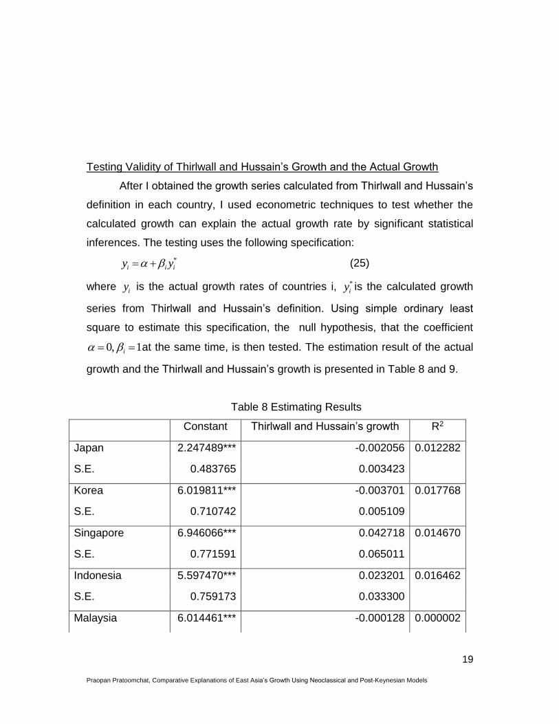
Testing Validity of Thirlwall and Hussain’s Growth and the Actual Growth

After I obtained the growth series calculated from Thirlwall and Hussain’s

definition in each country, I used econometric techniques to test whether the

calculated growth can explain the actual growth rate by significant statistical

inferences. The testing uses the following specification:

*

i i iy y (25)

where iy is the actual growth rates of countries i, *

iy is the calculated growth

series from Thirlwall and Hussain’s definition. Using simple ordinary least

square to estimate this specification, the null hypothesis, that the coefficient

0, 1i at the same time, is then tested. The estimation result of the actual

growth and the Thirlwall and Hussain’s growth is presented in Table 8 and 9.

Table 8 Estimating Results

Constant Thirlwall and Hussain’s growth R2

Japan 2.247489*** -0.002056 0.012282

S.E. 0.483765 0.003423

Korea 6.019811*** -0.003701 0.017768

S.E. 0.710742 0.005109

Singapore 6.946066*** 0.042718 0.014670

S.E. 0.771591 0.065011

Indonesia 5.597470*** 0.023201 0.016462

S.E. 0.759173 0.033300

Malaysia 6.014461*** -0.000128 0.000002

20


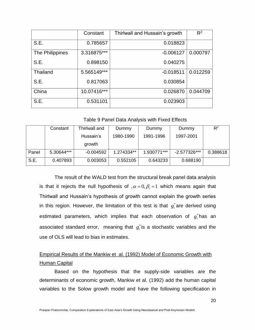
Constant Thirlwall and Hussain’s growth R2

S.E. 0.785657 0.018823

The Philippines 3.316875*** -0.006127 0.000797

S.E. 0.898150 0.040275

Thailand 5.565149*** -0.018511 0.012259

S.E. 0.817063 0.030854

China 10.07416*** 0.026870 0.044709

S.E. 0.531101 0.023903

Table 9 Panel Data Analysis with Fixed Effects

Constant Thirlwall and

Hussain’s

growth

Dummy

1980-1990

Dummy

1991-1996

Dummy

1997-2001

R2

Panel 5.30644*** -0.004592 1.274334** 1.930771*** -2.577326*** 0.388618

S.E. 0.407893 0.003053 0.552105 0.643233 0.688190

The result of the WALD test from the structural break panel data analysis

is that it rejects the null hypothesis of , 0, 1i which means again that

Thirlwall and Hussain’s hypothesis of growth cannot explain the growth series

in this region. However, the limitation of this test is that *

ig are derived using

estimated parameters, which implies that each observation of *

ig has an

associated standard error, meaning that *

ig is a stochastic variables and the

use of OLS will lead to bias in estimates.

Empirical Results of the Mankiw et al. (1992) Model of Economic Growth with

Human Capital

Based on the hypothesis that the supply-side variables are the

determinants of economic growth, Mankiw et al. (1992) add the human capital

variables to the Solow growth model and have the following specification in

21


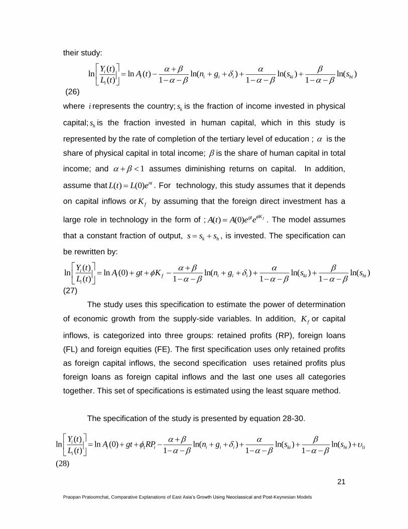
their study:

( )ln ln ( ) ln( ) ln( ) ln( )

( ) 1 1 1i

i i i i ki hi

i

Y tA t n g s s

L t

(26)

where i represents the country; ks is the fraction of income invested in physical

capital; hs is the fraction invested in human capital, which in this study is

represented by the rate of completion of the tertiary level of education ; is the

share of physical capital in total income; is the share of human capital in total

income; and 1 assumes diminishing returns on capital. In addition,

assume that ( ) (0) ntL t L e . For technology, this study assumes that it depends

on capital inflows or fK by assuming that the foreign direct investment has a

large role in technology in the form of ; ( ) (0) fKgtA t A e e

. The model assumes

that a constant fraction of output, k hs s s , is invested. The specification can

be rewritten by:

( )ln ln (0) ln( ) ln( ) ln( )

( ) 1 1 1i

i f i i i ki hi

i

Y tA gt K n g s s

L t

(27)

The study uses this specification to estimate the power of determination

of economic growth from the supply-side variables. In addition, fK or capital

inflows, is categorized into three groups: retained profits (RP), foreign loans

(FL) and foreign equities (FE). The first specification uses only retained profits

as foreign capital inflows, the second specification uses retained profits plus

foreign loans as foreign capital inflows and the last one uses all categories

together. This set of specifications is estimated using the least square method.

The specification of the study is presented by equation 28-30.

1 1

( )ln ln (0) ln( ) ln( ) ln( )

( ) 1 1 1

(28)

ii i i i i ki hi i

i

Y tA gt RP n g s s

L t

22


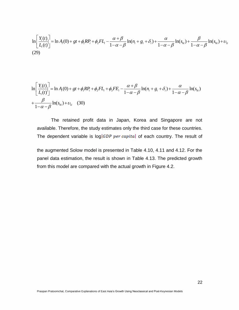
The retained profit data in Japan, Korea and Singapore are not

available. Therefore, the study estimates only the third case for these countries.

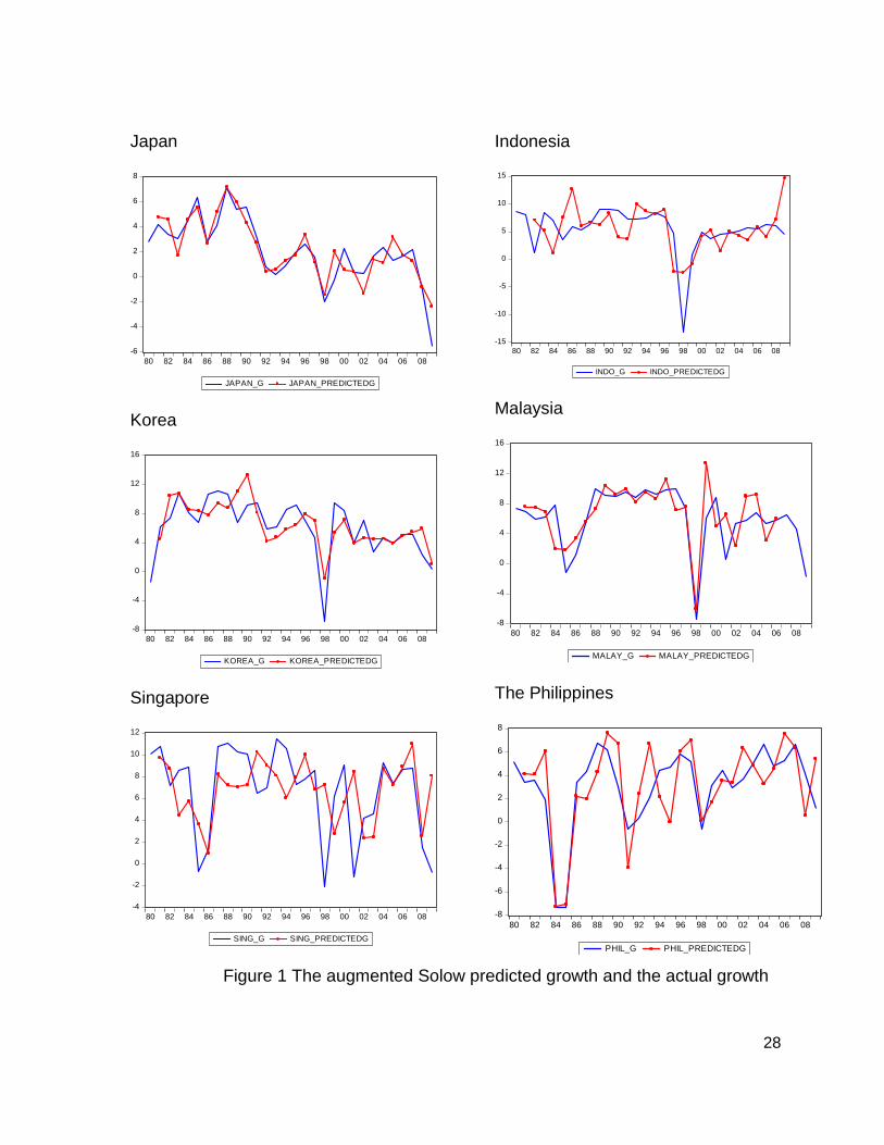
The dependent variable is log of each country. The result of

the augmented Solow model is presented in Table 4.10, 4.11 and 4.12. For the

panel data estimation, the result is shown in Table 4.13. The predicted growth

from this model are compared with the actual growth in Figure 4.2.

1 2 1

( )ln ln (0) ln( ) ln( ) ln( )

( ) 1 1 1

(29)

ii i i i i i ki hi i

i

Y tA gt RP FL n g s s

L t

1 2 3

1

( )ln ln (0) ln( ) ln( )

( ) 1 1

ln( ) (30)1

ii i i i i i i ki

i

hi i

Y tA gt RP FL FE n g s

L t

s


23

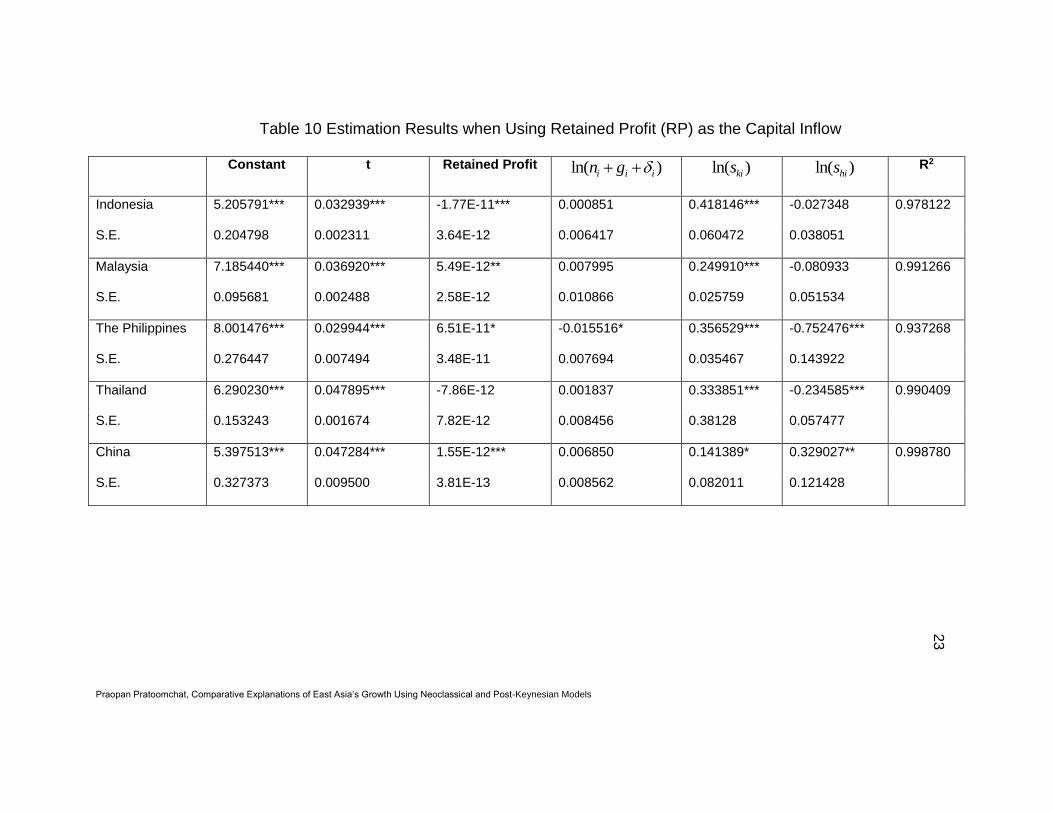
Table 10 Estimation Results when Using Retained Profit (RP) as the Capital Inflow

Constant t Retained Profit ln( )i i in g ln( )kis ln( )his R2

Indonesia 5.205791*** 0.032939*** -1.77E-11*** 0.000851 0.418146*** -0.027348 0.978122

S.E. 0.204798 0.002311 3.64E-12 0.006417 0.060472 0.038051

Malaysia 7.185440*** 0.036920*** 5.49E-12** 0.007995 0.249910*** -0.080933 0.991266

S.E. 0.095681 0.002488 2.58E-12 0.010866 0.025759 0.051534

The Philippines 8.001476*** 0.029944*** 6.51E-11* -0.015516* 0.356529*** -0.752476*** 0.937268

S.E. 0.276447 0.007494 3.48E-11 0.007694 0.035467 0.143922

Thailand 6.290230*** 0.047895*** -7.86E-12 0.001837 0.333851*** -0.234585*** 0.990409

S.E. 0.153243 0.001674 7.82E-12 0.008456 0.38128 0.057477

China 5.397513*** 0.047284*** 1.55E-12*** 0.006850 0.141389* 0.329027** 0.998780

S.E. 0.327373 0.009500 3.81E-13 0.008562 0.082011 0.121428


24

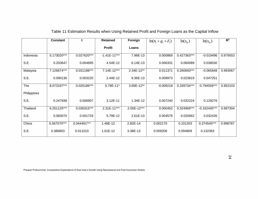
Table 11 Estimation Results when Using Retained Profit and Foreign Loans as the Capital Inflow

Constant t Retained

Profit

Foreign

Loans

ln( )i i in g ln( )kis ln( )his R2

Indonesia 5.173020*** 0.027620*** -1.41E-11*** 7.96E-13 0.000869 0.427363*** -0.019496 0.979553

S.E. 0.203647 0.004695 4.54E-12 6.14E-13 0.006331 0.060089 0.038030

Malaysia 7.126674*** 0.031198*** 7.14E-12*** 2.34E-12** 0.011371 0.260693*** -0.065848 0.993067

S.E. 0.090136 0.003220 2.44E-12 9.36E-13 0.009973 0.023819 0.047251

The

Philippines

8.073197*** 0.025186*** 5.79E-11* 3.65E-12** -0.009218 0.339734*** -0.794559*** 0.952103

S.E. 0.247938 0.006907 3.12E-11 1.34E-12 0.007240 0.032224 0.129276

Thailand 6.251125*** 0.036315*** 2.31E-11*** 2.05E-12*** 0.000452 0.324969*** -0.162445*** 0.997304

S.E. 0.083070 0.001733 5.79E-12 2.61E-13 0.004579 0.020662 0.032435

China 5.567570*** 0.044491*** 1.48E-12 2.82E-14 0.002170 0.101203 0.374545*** 0.998787

S.E. 0.386803 0.011010 1.01E-12 3.38E-13 0.009206 0.094809 0.132363


25

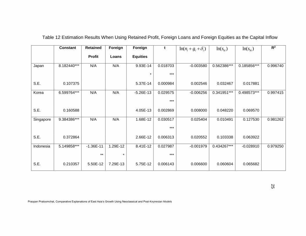
Table 12 Estimation Results When Using Retained Profit, Foreign Loans and Foreign Equities as the Capital Inflow

Constant Retained

Profit

Foreign

Loans

Foreign

Equities

t ln( )i i in g ln( )kis ln( )his R2

Japan 8.182440*** N/A N/A 9.93E-14

*

0.018703

***

-0.003580 0.562386*** 0.185856*** 0.996740

S.E. 0.107375 5.37E-14 0.000984 0.002546 0.032467 0.017881

Korea 6.599764*** N/A N/A -5.26E-13 0.029575

***

-0.006256 0.341951*** 0.498573*** 0.997415

S.E. 0.160588 4.05E-13 0.002869 0.008000 0.048220 0.069570

Singapore 9.384386*** N/A N/A 1.68E-12 0.030517

***

0.025404 0.010491 0.127530 0.981262

S.E. 0.372864 2.66E-12 0.006313 0.020552 0.103338 0.063922

Indonesia 5.149858*** -1.36E-11

**

1.29E-12

*

8.41E-12 0.027987

***

-0.001979 0.434267*** -0.028910 0.979250

S.E. 0.210357 5.50E-12 7.29E-13 5.75E-12 0.006143 0.006600 0.060604 0.065682


26

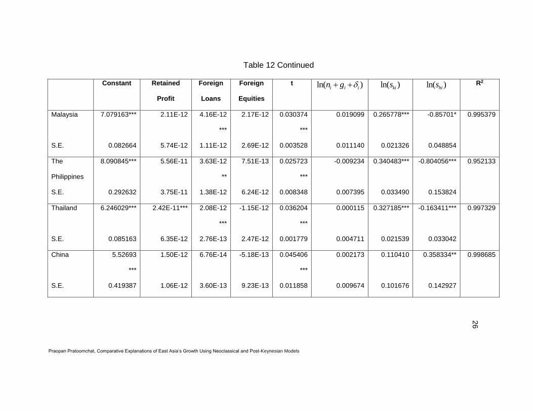
Table 12 Continued

Constant Retained

Profit

Foreign

Loans

Foreign

Equities

t ln( )i i in g ln( )kis ln( )his R2

Malaysia 7.079163*** 2.11E-12 4.16E-12

***

2.17E-12 0.030374

***

0.019099 0.265778*** -0.85701* 0.995379

S.E. 0.082664 5.74E-12 1.11E-12 2.69E-12 0.003528 0.011140 0.021326 0.048854

The

Philippines

8.090845*** 5.56E-11 3.63E-12

**

7.51E-13 0.025723

***

-0.009234 0.340483*** -0.804056*** 0.952133

S.E. 0.292632 3.75E-11 1.38E-12 6.24E-12 0.008348 0.007395 0.033490 0.153824

Thailand 6.246029*** 2.42E-11*** 2.08E-12

***

-1.15E-12 0.036204

***

0.000115 0.327185*** -0.163411*** 0.997329

S.E. 0.085163 6.35E-12 2.76E-13 2.47E-12 0.001779 0.004711 0.021539 0.033042

China 5.52693

***

1.50E-12 6.76E-14 -5.18E-13 0.045406

***

0.002173 0.110410 0.358334** 0.998685

S.E. 0.419387 1.06E-12 3.60E-13 9.23E-13 0.011858 0.009674 0.101676 0.142927


27

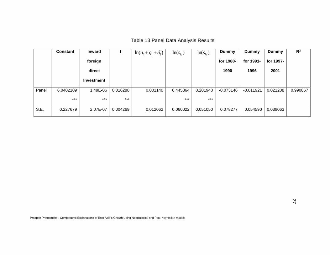
Table 13 Panel Data Analysis Results

Constant Inward

foreign

direct

Investment

t ln( )i i in g ln( )kis ln( )his Dummy

for 1980-

1990

Dummy

for 1991-

1996

Dummy

for 1997-

2001

R2

Panel 6.0402109

***

1.49E-06

***

0.016288

***

0.001140 0.445364

***

0.201940

***

-0.073146 -0.011921 0.021208 0.990867

S.E. 0.227679 2.07E-07 0.004269 0.012062 0.060022 0.051050 0.078277 0.054590 0.039063

28

Japan

-6

-4

-2

0

2

4

6

8

80 82 84 86 88 90 92 94 96 98 00 02 04 06 08

JAPAN_G JAPAN_PREDICTEDG

Korea

-8

-4

0

4

8

12

16

80 82 84 86 88 90 92 94 96 98 00 02 04 06 08

KOREA_G KOREA_PREDICTEDG

Singapore

-4

-2

0

2

4

6

8

10

12

80 82 84 86 88 90 92 94 96 98 00 02 04 06 08

SING_G SING_PREDICTEDG

Indonesia

-15

-10

-5

0

5

10

15

80 82 84 86 88 90 92 94 96 98 00 02 04 06 08

INDO_G INDO_PREDICTEDG

Malaysia

-8

-4

0

4

8

12

16

80 82 84 86 88 90 92 94 96 98 00 02 04 06 08

MALAY_G MALAY_PREDICTEDG

The Philippines

-8

-6

-4

-2

0

2

4

6

8

80 82 84 86 88 90 92 94 96 98 00 02 04 06 08

PHIL_G PHIL_PREDICTEDG

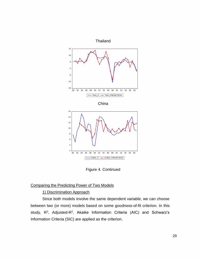
Figure 1 The augmented Solow predicted growth and the actual growth

29

Thailand

-15

-10

-5

0

5

10

15

80 82 84 86 88 90 92 94 96 98 00 02 04 06 08

THAI_G THAI_PREDICTEDG

China

2

4

6

8

10

12

14

16

80 82 84 86 88 90 92 94 96 98 00 02 04 06 08

CHINA_G CHINA_PREDICTEDG

Figure 4. Continued

Comparing the Predicting Power of Two Models

1) Discrimination Approach

Since both models involve the same dependent variable, we can choose

between two (or more) models based on some goodness-of-fit criterion. In this

study, R2, Adjusted-R2, Akaike Information Criteria (AIC) and Schwarz’s

Information Criteria (SIC) are applied as the criterion.

30

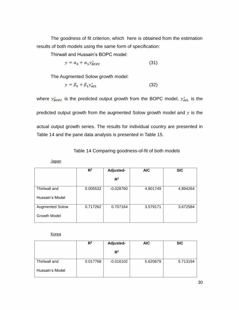
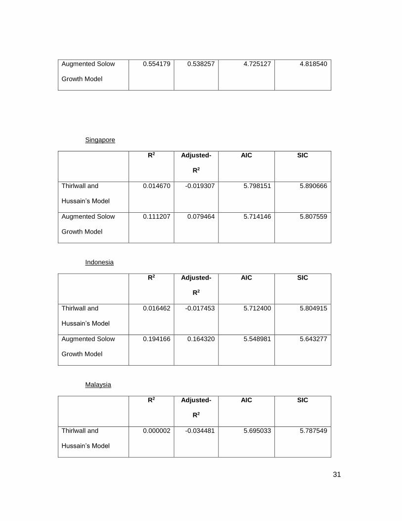
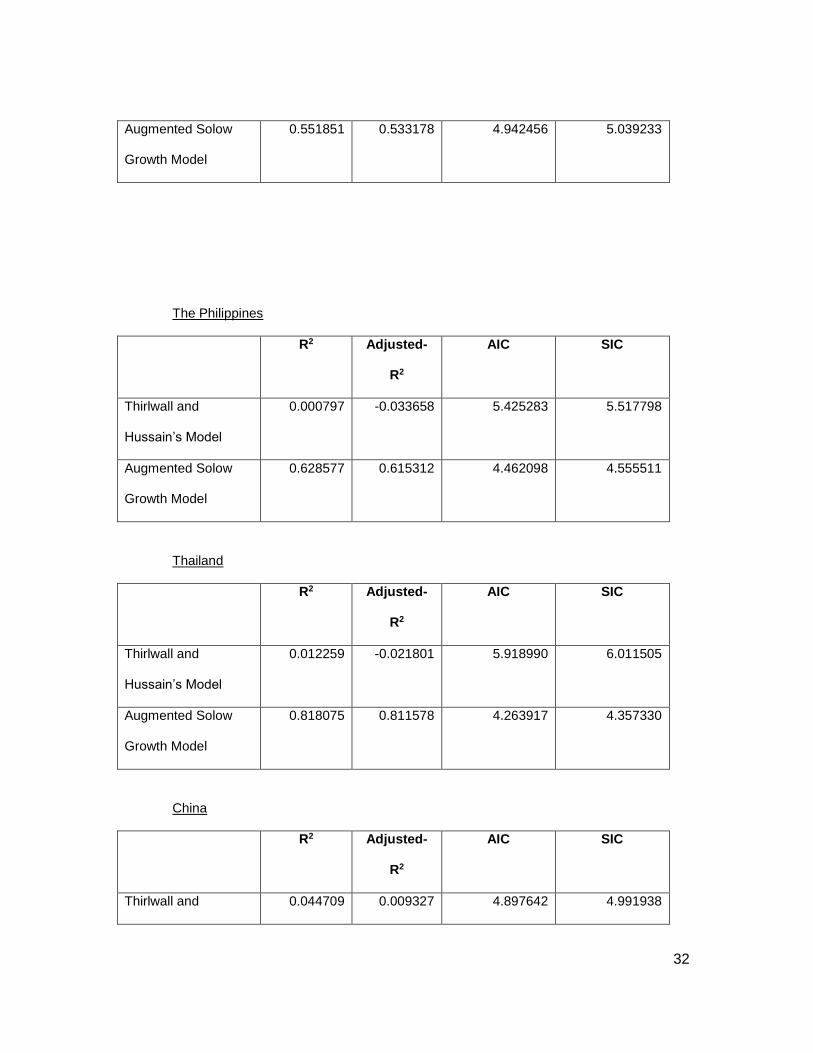
The goodness of fit criterion, which here is obtained from the estimation

results of both models using the same form of specification:

Thirwall and Hussain’s BOPC model:

(31)

The Augmented Solow growth model:

(32)

where is the predicted output growth from the BOPC model, is the

predicted output growth from the augmented Solow growth model and is the

actual output growth series. The results for individual country are presented in

Table 14 and the pane data analysis is presented in Table 15.

Table 14 Comparing goodness-of-fit of both models

Japan

R2 Adjusted-

R2

AIC SIC

Thirlwall and

Hussain’s Model

0.005532 -0.028760 4.801749 4.894264

Augmented Solow

Growth Model

0.717262 0.707164 3.579171 3.672584

Korea

R2 Adjusted-

R2

AIC SIC

Thirlwall and

Hussain’s Model

0.017768 -0.016102 5.620679 5.713194

31

Augmented Solow

Growth Model

0.554179 0.538257 4.725127 4.818540

Singapore

R2 Adjusted-

R2

AIC SIC

Thirlwall and

Hussain’s Model

0.014670 -0.019307 5.798151 5.890666

Augmented Solow

Growth Model

0.111207 0.079464 5.714146 5.807559

Indonesia

R2 Adjusted-

R2

AIC SIC

Thirlwall and

Hussain’s Model

0.016462 -0.017453 5.712400 5.804915

Augmented Solow

Growth Model

0.194166 0.164320 5.548981 5.643277

Malaysia

R2 Adjusted-

R2

AIC SIC

Thirlwall and

Hussain’s Model

0.000002 -0.034481 5.695033 5.787549

32

Augmented Solow

Growth Model

0.551851 0.533178 4.942456 5.039233

The Philippines

R2 Adjusted-

R2

AIC SIC

Thirlwall and

Hussain’s Model

0.000797 -0.033658 5.425283 5.517798

Augmented Solow

Growth Model

0.628577 0.615312 4.462098 4.555511

Thailand

R2 Adjusted-

R2

AIC SIC

Thirlwall and

Hussain’s Model

0.012259 -0.021801 5.918990 6.011505

Augmented Solow

Growth Model

0.818075 0.811578 4.263917 4.357330

China

R2 Adjusted-

R2

AIC SIC

Thirlwall and 0.044709 0.009327 4.897642 4.991938

33

Hussain’s Model

Augmented Solow

Growth Model

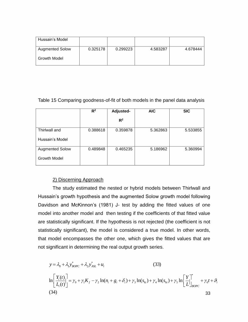
0.325178 0.299223 4.583287 4.678444

Table 15 Comparing goodness-of-fit of both models in the panel data analysis

R2 Adjusted-

R2

AIC SIC

Thirlwall and

Hussain’s Model

0.388618 0.359878 5.362863 5.533855

Augmented Solow

Growth Model

0.489848 0.465235 5.186962 5.360994

2) Discerning Approach

The study estimated the nested or hybrid models between Thirlwall and

Hussain’s growth hypothesis and the augmented Solow growth model following

Davidson and McKinnon’s (1981) J- test by adding the fitted values of one

model into another model and then testing if the coefficients of that fitted value

are statistically significant. If the hypothesis is not rejected (the coefficient is not

statistically significant), the model is considered a true model. In other words,

that model encompasses the other one, which gives the fitted values that are

not significant in determining the real output growth series.

* *

0 1 2 (33)BOPC ASL iy y y u

*

0 1 2 3 4 5 6

( )ln ln( ) ln( ) ln( ) ln

( )

(34)

if i i i ki hi i

BOPCi

Y t YK n g s s t

L t L

34

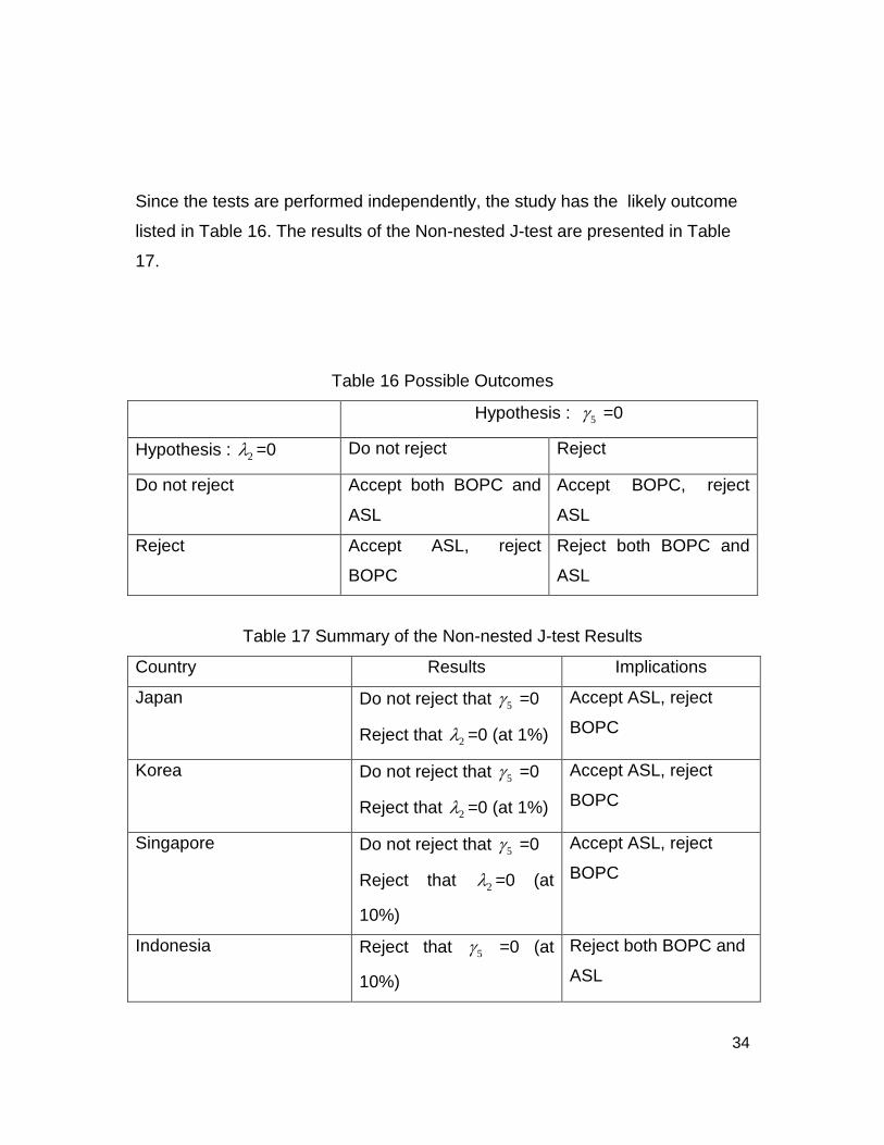
Since the tests are performed independently, the study has the likely outcome

listed in Table 16. The results of the Non-nested J-test are presented in Table

17.

Table 16 Possible Outcomes

Hypothesis : 5 =0

Hypothesis : 2 =0 Do not reject Reject

Do not reject Accept both BOPC and

ASL

Accept BOPC, reject

ASL

Reject Accept ASL, reject

BOPC

Reject both BOPC and

ASL

Table 17 Summary of the Non-nested J-test Results

Country Results Implications

Japan Do not reject that 5 =0

Reject that 2 =0 (at 1%)

Accept ASL, reject

BOPC

Korea Do not reject that 5 =0


Accept ASL, reject

BOPC

Singapore Do not reject that 5 =0

Reject that 2 =0 (at

10%)

Accept ASL, reject

BOPC

Indonesia Reject that 5 =0 (at

10%)

Reject both BOPC and

ASL

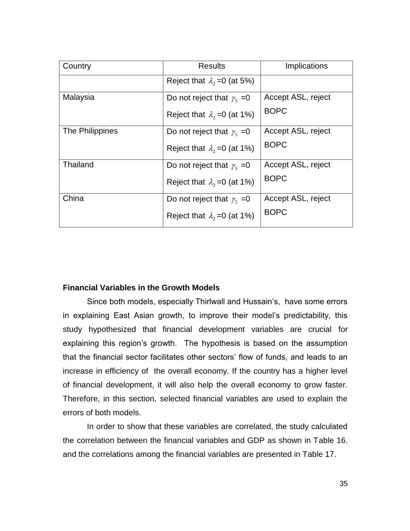
35

Country Results Implications


Malaysia Do not reject that 5 =0


Accept ASL, reject

BOPC

The Philippines Do not reject that 5 =0


Accept ASL, reject

BOPC

Thailand Do not reject that 5 =0


Accept ASL, reject

BOPC

China Do not reject that 5 =0


Accept ASL, reject

BOPC

Financial Variables in the Growth Models

Since both models, especially Thirlwall and Hussain’s, have some errors

in explaining East Asian growth, to improve their model’s predictability, this

study hypothesized that financial development variables are crucial for

explaining this region’s growth. The hypothesis is based on the assumption

that the financial sector facilitates other sectors’ flow of funds, and leads to an

increase in efficiency of the overall economy. If the country has a higher level

of financial development, it will also help the overall economy to grow faster.

Therefore, in this section, selected financial variables are used to explain the

errors of both models.

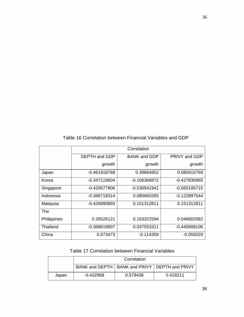
In order to show that these variables are correlated, the study calculated

the correlation between the financial variables and GDP as shown in Table 16.

and the correlations among the financial variables are presented in Table 17.

36

36

Table 16 Correlation between Financial Variables and GDP

Correlation

DEPTH and GDP

growth

BANK and GDP

growth

PRIVY and GDP

growth

Japan -0.461918768 0.39864952 0.080415769

Korea -0.347119604 -0.106366872 -0.427836965

Singapore -0.420577806 -0.536541941 -0.565195715

Indonesia -0.366718314 0.080660265 -0.122897544

Malaysia -0.426890893 0.151312811 0.151312811

The

Philippines 0.26526121 0.163322594 0.046802082

Thailand -0.368618807 0.037553311 -0.445908106

China 0.073473 -0.114359 -0.055029

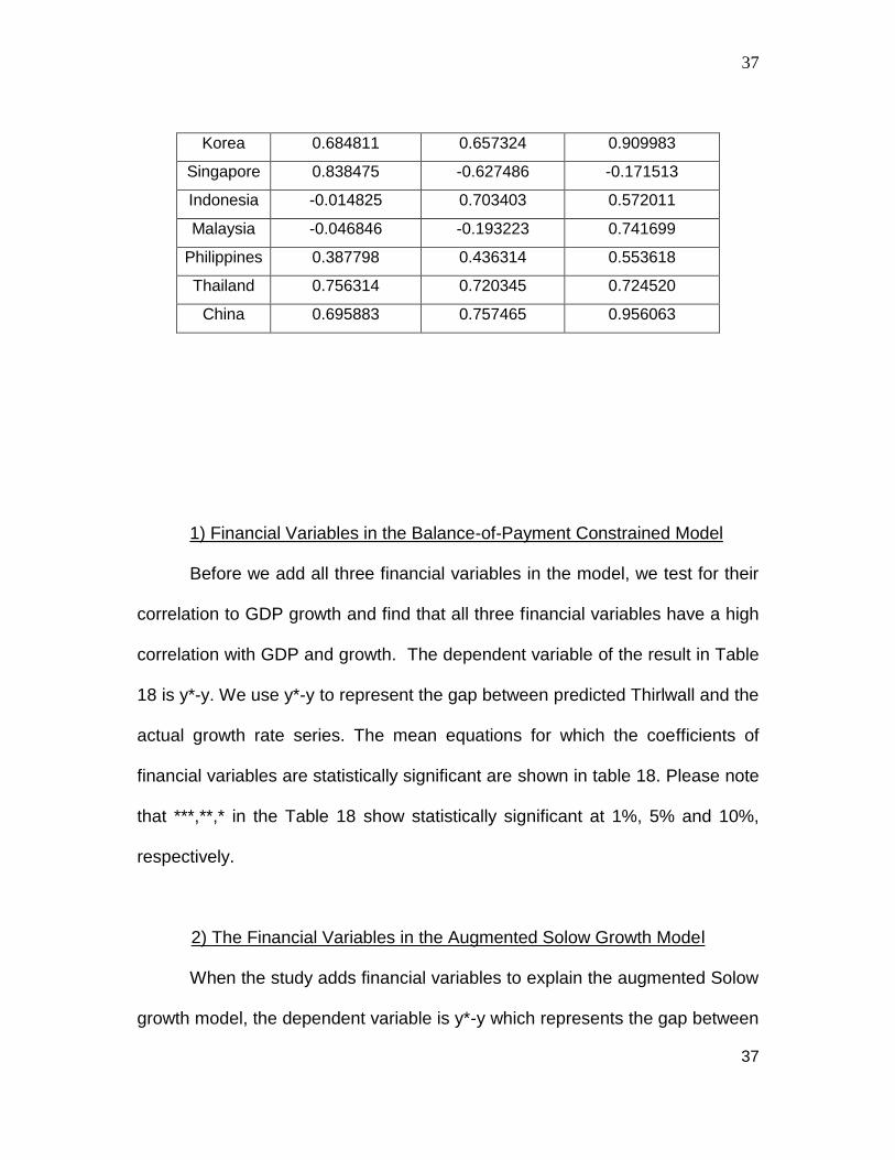
Table 17 Correlation between Financial Variables

Correlation

BANK and DEPTH BANK and PRIVY DEPTH and PRIVY

Japan -0.432968 0.579438 0.418211

37

37

Korea 0.684811 0.657324 0.909983

Singapore 0.838475 -0.627486 -0.171513

Indonesia -0.014825 0.703403 0.572011

Malaysia -0.046846 -0.193223 0.741699

Philippines 0.387798 0.436314 0.553618

Thailand 0.756314 0.720345 0.724520

China 0.695883 0.757465 0.956063

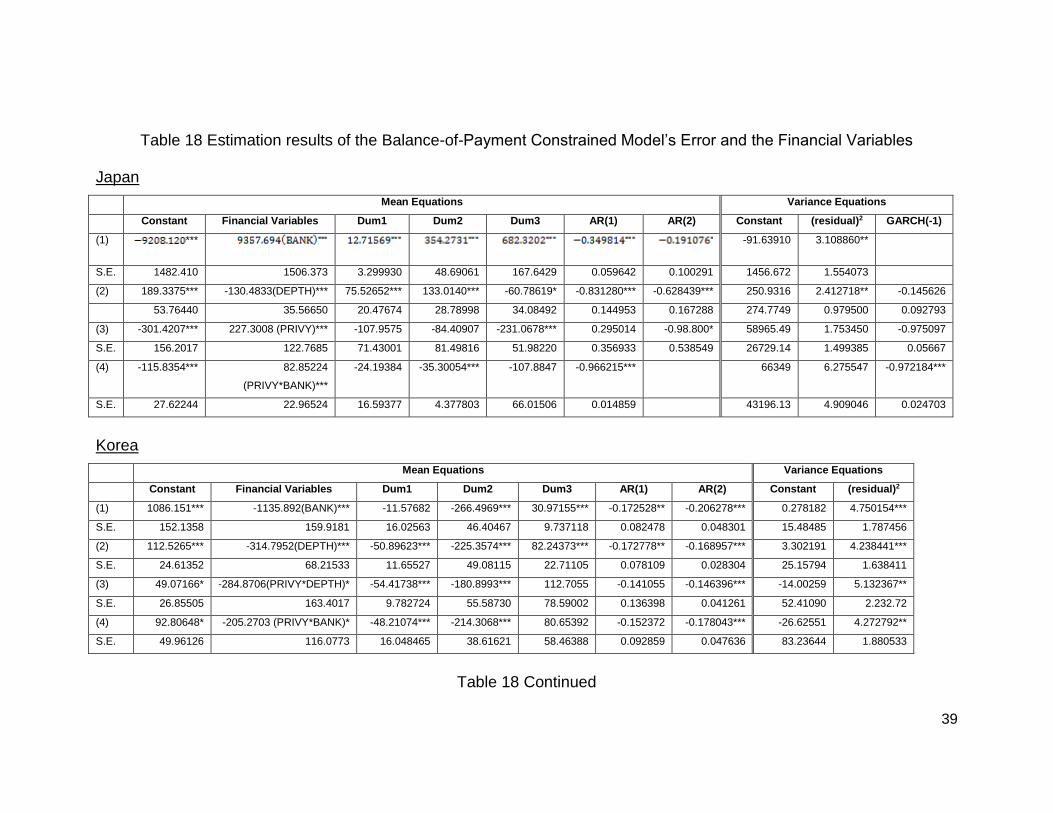
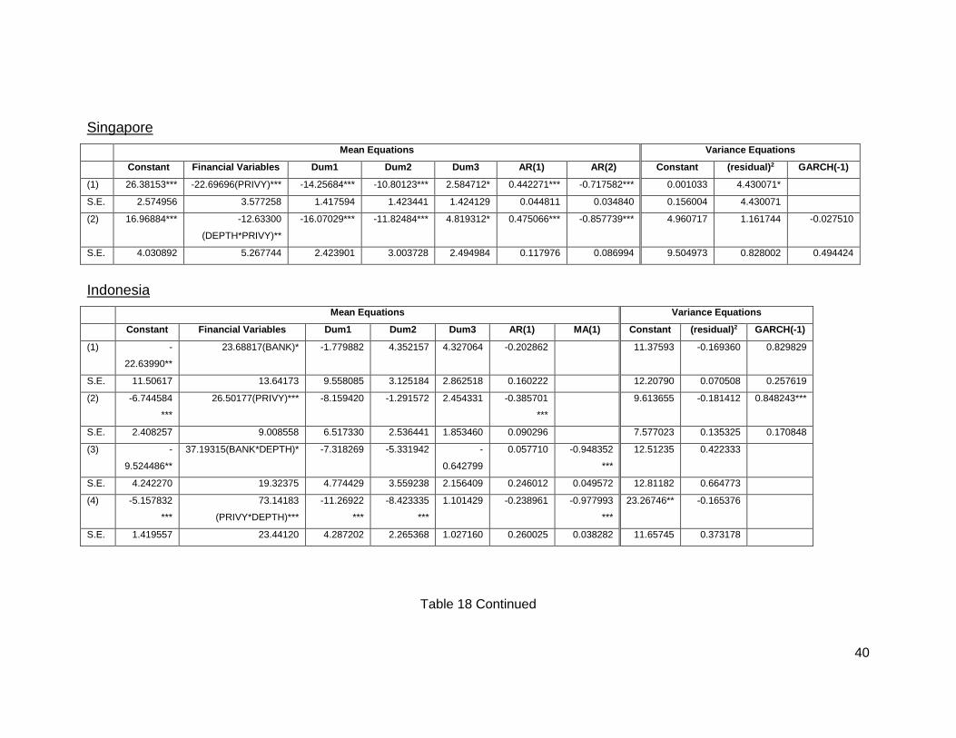
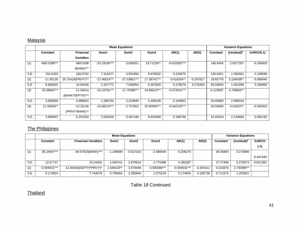
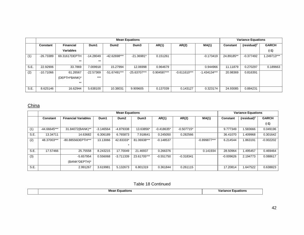
1) Financial Variables in the Balance-of-Payment Constrained Model

Before we add all three financial variables in the model, we test for their

correlation to GDP growth and find that all three financial variables have a high

correlation with GDP and growth. The dependent variable of the result in Table

18 is y*-y. We use y*-y to represent the gap between predicted Thirlwall and the

actual growth rate series. The mean equations for which the coefficients of

financial variables are statistically significant are shown in table 18. Please note

that ***,**,* in the Table 18 show statistically significant at 1%, 5% and 10%,

respectively.

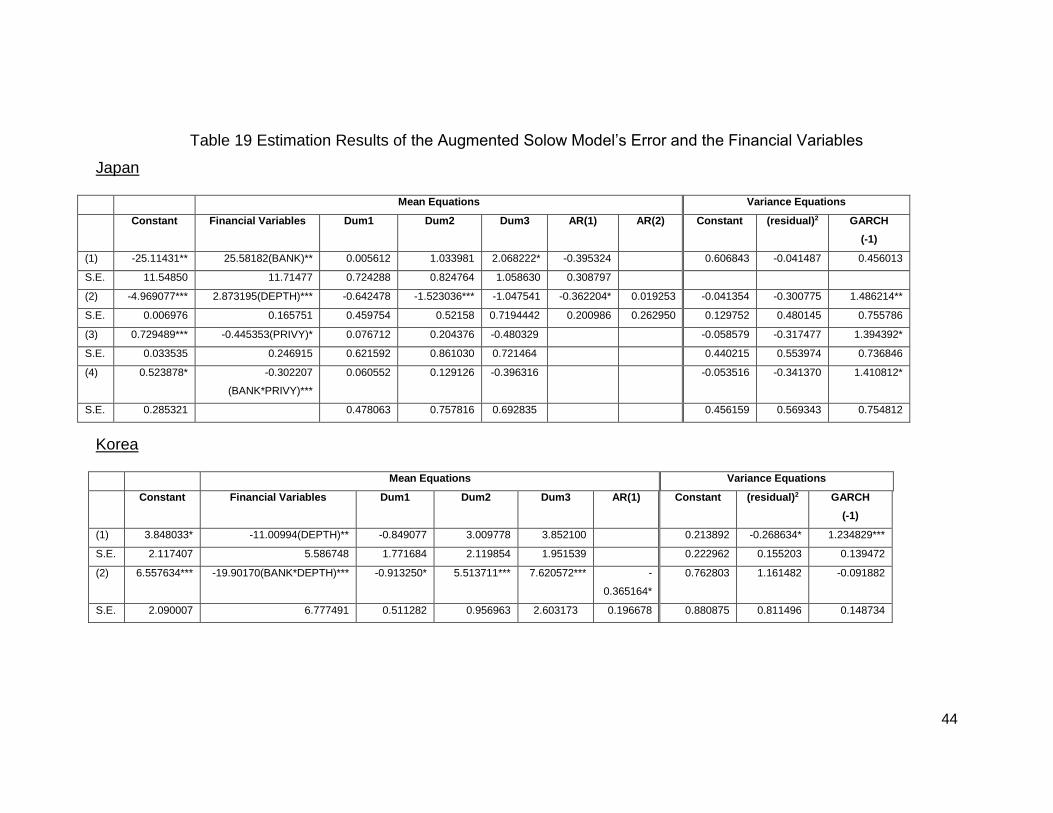
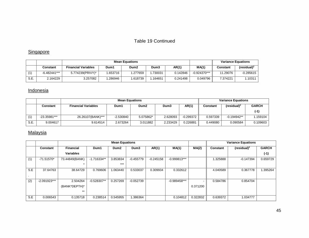
2) The Financial Variables in the Augmented Solow Growth Model

When the study adds financial variables to explain the augmented Solow

growth model, the dependent variable is y*-y which represents the gap between

38

38

predicted and the actual growth rate series. The mean equations for

which the coefficients of financial variables are statistically significant are shown

in table 19. Please note that the dependent variables are (y*-y) of each country

and ***,**,* are statistically significant at 1%, 5% and 10%, respectively.

39

Table 18 Estimation results of the Balance-of-Payment Constrained Model’s Error and the Financial Variables

Japan

Mean Equations Variance Equations

Constant Financial Variables Dum1 Dum2 Dum3 AR(1) AR(2) Constant (residual)2 GARCH(-1)

(1) ***

-91.63910 3.108860**

S.E. 1482.410 1506.373 3.299930 48.69061 167.6429 0.059642 0.100291 1456.672 1.554073

(2) 189.3375*** -130.4833(DEPTH)*** 75.52652*** 133.0140*** -60.78619* -0.831280*** -0.628439*** 250.9316 2.412718** -0.145626

53.76440 35.56650 20.47674 28.78998 34.08492 0.144953 0.167288 274.7749 0.979500 0.092793

(3) -301.4207*** 227.3008 (PRIVY)*** -107.9575 -84.40907 -231.0678*** 0.295014 -0.98.800* 58965.49 1.753450 -0.975097

S.E. 156.2017 122.7685 71.43001 81.49816 51.98220 0.356933 0.538549 26729.14 1.499385 0.05667

(4) -115.8354*** 82.85224

(PRIVY*BANK)***

-24.19384 -35.30054*** -107.8847 -0.966215*** 66349 6.275547 -0.972184***

S.E. 27.62244 22.96524 16.59377 4.377803 66.01506 0.014859 43196.13 4.909046 0.024703

Korea


Constant Financial Variables Dum1 Dum2 Dum3 AR(1) AR(2) Constant (residual)2

(1) 1086.151*** -1135.892(BANK)*** -11.57682 -266.4969*** 30.97155*** -0.172528** -0.206278*** 0.278182 4.750154***

S.E. 152.1358 159.9181 16.02563 46.40467 9.737118 0.082478 0.048301 15.48485 1.787456

(2) 112.5265*** -314.7952(DEPTH)*** -50.89623*** -225.3574*** 82.24373*** -0.172778** -0.168957*** 3.302191 4.238441***

S.E. 24.61352 68.21533 11.65527 49.08115 22.71105 0.078109 0.028304 25.15794 1.638411

(3) 49.07166* -284.8706(PRIVY*DEPTH)* -54.41738*** -180.8993*** 112.7055 -0.141055 -0.146396*** -14.00259 5.132367**

S.E. 26.85505 163.4017 9.782724 55.58730 78.59002 0.136398 0.041261 52.41090 2.232.72

(4) 92.80648* -205.2703 (PRIVY*BANK)* -48.21074*** -214.3068*** 80.65392 -0.152372 -0.178043*** -26.62551 4.272792**

S.E. 49.96126 116.0773 16.048465 38.61621 58.46388 0.092859 0.047636 83.23644 1.880533

Table 18 Continued

40

Singapore


Constant Financial Variables Dum1 Dum2 Dum3 AR(1) AR(2) Constant (residual)2 GARCH(-1)

(1) 26.38153*** -22.69696(PRIVY)*** -14.25684*** -10.80123*** 2.584712* 0.442271*** -0.717582*** 0.001033 4.430071*

S.E. 2.574956 3.577258 1.417594 1.423441 1.424129 0.044811 0.034840 0.156004 4.430071

(2) 16.96884*** -12.63300

(DEPTH*PRIVY)**

-16.07029*** -11.82484*** 4.819312* 0.475066*** -0.857739*** 4.960717 1.161744 -0.027510

S.E. 4.030892 5.267744 2.423901 3.003728 2.494984 0.117976 0.086994 9.504973 0.828002 0.494424

Indonesia


Constant Financial Variables Dum1 Dum2 Dum3 AR(1) MA(1) Constant (residual)2 GARCH(-1)

(1) -

22.63990**

23.68817(BANK)* -1.779882 4.352157 4.327064 -0.202862 11.37593 -0.169360 0.829829

S.E. 11.50617 13.64173 9.558085 3.125184 2.862518 0.160222 12.20790 0.070508 0.257619

(2) -6.744584

***

26.50177(PRIVY)*** -8.159420 -1.291572 2.454331 -0.385701

***

9.613655 -0.181412 0.848243***

S.E. 2.408257 9.008558 6.517330 2.536441 1.853460 0.090296 7.577023 0.135325 0.170848

(3) -

9.524486**

37.19315(BANK*DEPTH)* -7.318269 -5.331942 -

0.642799

0.057710 -0.948352

***

12.51235 0.422333

S.E. 4.242270 19.32375 4.774429 3.559238 2.156409 0.246012 0.049572 12.81182 0.664773

(4) -5.157832

***

73.14183

(PRIVY*DEPTH)***

-11.26922

***

-8.423335

***

1.101429 -0.238961 -0.977993

***

23.26746** -0.165376

S.E. 1.419557 23.44120 4.287202 2.265368 1.027160 0.260025 0.038282 11.65745 0.373178

Table 18 Continued

41

Malaysia


Constant Financial

Variables

Dum1 Dum2 Dum3 AR(1) AR(2) Constant (residual)2 GARCH(-1)

(1) -660.0188*** 689.0188

(BANK)***

-23.18195*** 5.659251 19.71218** -0.610281*** 146.9454 2.837720* -0.160603

S.E. 154.0323 160.0732 7.310477 4.831993 8.679262 0.219575 130.6451 1.560001 0.138586

(2) -11.95135 25.75418(PRIVY)** -17.46514*** -27.53801*** 17.38741*** -0.616254** -0.267817 19.65778 3.154638** -0.080640

S.E. 8.806002 10.84456 2.327772 7.036954 6.307820 0.278576 0.276493 93.04824 1.461058 0.186966

(3) 25.08663*** -11.50614

(BANK*DEPTH)***

-16.19791*** -17.76388*** 19.86613*** -0.574241*** -0.123097 4.758963**

S.E. 3.826959 3.968922 1.285705 2.314945 5.406239 0.194852 20.93960 2.098150

(4) 21.59050** -13.25146

(PRIVY*BANK)**

-10.89214*** -2.727652 25.90956*** -0.542102*** 28.50600 4.018227* -0.082816

S.E. 3.589407 5.251533 2.639159 5.407186 8.916599 0.195736 41.63319 2.139684 0.092192

The Philippines


Constant Financial Variables Dum1 Dum2 Dum3 AR(1) AR(2) Constant (residual)2 GARCH

(-1)

(1) 36.24657*** -39.67915(BANK)*** -1.199589 -0.017162 -2.580649 -0.206270 39.35894 0.275889 -

0.447349

S.E. 12.67737 15.24392 2.546741 2.879610 2.770488 0.282287 37.27499 0.276873 0.821365

(2) -0.559031*** 13.35504(DEPTH*PRIVY)* 1.648103** -3.076446 -4.590386*** -0.559031*** -0.304311 0.015876 2.730085**

S.E. 0.174824 7.744079 0.796654 2.392845 1.075219 0.174824 0.195736 0.711575 1.203921

Table 18 Continued

Thailand

42


Constant Financial

Variables

Dum1 Dum2 Dum3 AR(1) AR(2) MA(1) Constant (residual)2 GARCH

(-1)

(1) -26.73389 69.31617DEPTH

**

-14.28049

**

-42.62698*** -21.36981* 0.151261 -0.173419 24.89185** -0.377492 1.249713***

S.E. 22.92906 33.7869 7.009918 15.27994 12.06998 0.964679 0.944966 11.11879 0.270297 0.189663

(2) -10.71066 61.26567

(DEPTH*BANK)*

**

-22.57369

***

-51.67491*** -25.63707*** 0.904587*** -0.611610*** -1.434134*** 20.98369 0.816391

S.E. 8.625146 16.62944 5.638100 10.38031 9.909605 0.137039 0.143127 0.323174 24.93085 0.884231

China


Constant Financial Variables Dum1 Dum2 Dum3 AR(1) AR(2) MA(1) Constant (residual)2 GARCH

(-1)

(1) -44.66645*** 31.84072(BANK)** -3.146564 -4.879338 13.63856* -0.418635* -0.507715* 9.777349 1.583666 0.049196

S.E. 13.34711 14.63682 6.306189 6.765873 7.918641 0.245050 0.282566 36.41070 1.409968 0.301642

(2) 48.37003*** -80.88556DEPTH*** 13.13066 42.83333*

*

81.06938*** -0.148537 -0.899877*** 6.214544 1.863191 -0.002202

S.E. 17.57466 25.75558 8.243215 17.70049 21.46937 0.266376 0.141934 28.50964 1.495457 0.469464

(3) -5.657954

(BANK*DEPTH)*

0.556068 -3.711339 23.61705*** -0.551750 -0.318341 -0.009626 2.194773 0.088617

S.E. 2.991267 3.619981 5.132673 6.801319 0.361844 0.261115 17.20814 1.647522 0.638823

Table 18 Continued


43

Constan

t

Financial Variables Dum1 Dum2 Dum3 AR(1) AR

(2)

MA(1) Constant (residual)

2

GARCH

(-1)

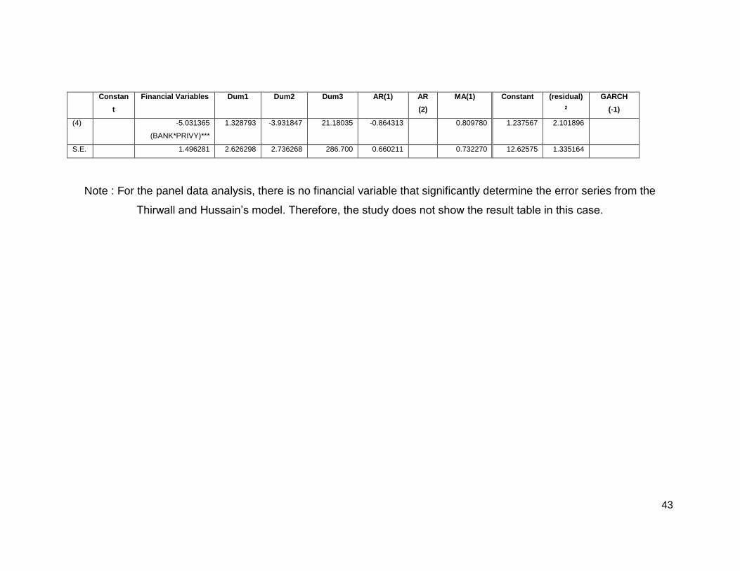
(4) -5.031365

(BANK*PRIVY)***

1.328793 -3.931847 21.18035 -0.864313 0.809780 1.237567 2.101896

S.E. 1.496281 2.626298 2.736268 286.700 0.660211 0.732270 12.62575 1.335164

Note : For the panel data analysis, there is no financial variable that significantly determine the error series from the

Thirwall and Hussain’s model. Therefore, the study does not show the result table in this case.

44

Table 19 Estimation Results of the Augmented Solow Model’s Error and the Financial Variables

Japan


Constant Financial Variables Dum1 Dum2 Dum3 AR(1) AR(2) Constant (residual)2 GARCH

(-1)

(1) -25.11431** 25.58182(BANK)** 0.005612 1.033981 2.068222* -0.395324 0.606843 -0.041487 0.456013

S.E. 11.54850 11.71477 0.724288 0.824764 1.058630 0.308797

(2) -4.969077*** 2.873195(DEPTH)*** -0.642478 -1.523036*** -1.047541 -0.362204* 0.019253 -0.041354 -0.300775 1.486214**

S.E. 0.006976 0.165751 0.459754 0.52158 0.7194442 0.200986 0.262950 0.129752 0.480145 0.755786

(3) 0.729489*** -0.445353(PRIVY)* 0.076712 0.204376 -0.480329 -0.058579 -0.317477 1.394392*

S.E. 0.033535 0.246915 0.621592 0.861030 0.721464 0.440215 0.553974 0.736846

(4) 0.523878* -0.302207

(BANK*PRIVY)***

0.060552 0.129126 -0.396316 -0.053516 -0.341370 1.410812*

S.E. 0.285321 0.478063 0.757816 0.692835 0.456159 0.569343 0.754812

Korea


Constant Financial Variables Dum1 Dum2 Dum3 AR(1) Constant (residual)2 GARCH

(-1)

(1) 3.848033* -11.00994(DEPTH)** -0.849077 3.009778 3.852100 0.213892 -0.268634* 1.234829***

S.E. 2.117407 5.586748 1.771684 2.119854 1.951539 0.222962 0.155203 0.139472

(2) 6.557634*** -19.90170(BANK*DEPTH)*** -0.913250* 5.513711*** 7.620572*** -

0.365164*

0.762803 1.161482 -0.091882

S.E. 2.090007 6.777491 0.511282 0.956963 2.603173 0.196678 0.880875 0.811496 0.148734

45

Table 19 Continued Singapore


Constant Financial Variables Dum1 Dum2 Dum3 AR(1) MA(1) Constant (residual)2

(1) -6.482441*** 5.774239(PRIVY)* 1.653716 1.277659 1.730031 0.142846 -0.924370*** 11.29076 -0.285615

S.E. 2.164229 3.257082 1.286946 1.618739 1.164651 0.241498 0.049796 7.374221 1.10311

Indonesia


Constant Financial Variables Dum1 Dum2 Dum3 AR(1) Constant (residual)2 GARCH

(-1)

(1) -23.35981*** 26.26107(BANK)*** -2.530840 5.075862* 2.628093 -0.299372 0.597339 -0.194942** 1.159104

S.E. 9.004617 9.614514 2.673264 3.011882 2.233429 0.226881 0.449080 0.090584 0.109603

Malaysia


Constant Financial

Variables

Dum1 Dum2 Dum3 AR(1) MA(1) MA(2) Constant (residual)2 GARCH

(-1)

(1) -71.51570* 73.44849(BANK)

*

-1.716334** 3.853834

***

-0.455779 -0.245158 -0.999813*** 1.325888 -0.147394 0.659729

S.E

.

37.64763 38.64729 0.769606 1.063440 0.533037 0.309934 0.332612 4.040589 0.367778 1.395264

(2) -2.091923*** 2.504264

(BANK*DEPTH)*

**

-0.528307** 0.257269 -0.052739 -0.989458*** -

0.371200

0.584786 0.854704

S.E 0.006543 0.135718 0.238514 0.545955 1.386364 0.104812 0.322832 0.639372 1.034777

46


Constant Financial

Variables

Dum1 Dum2 Dum3 AR(1) MA(1) MA(2) Constant (residual)2 GARCH

(-1)

.

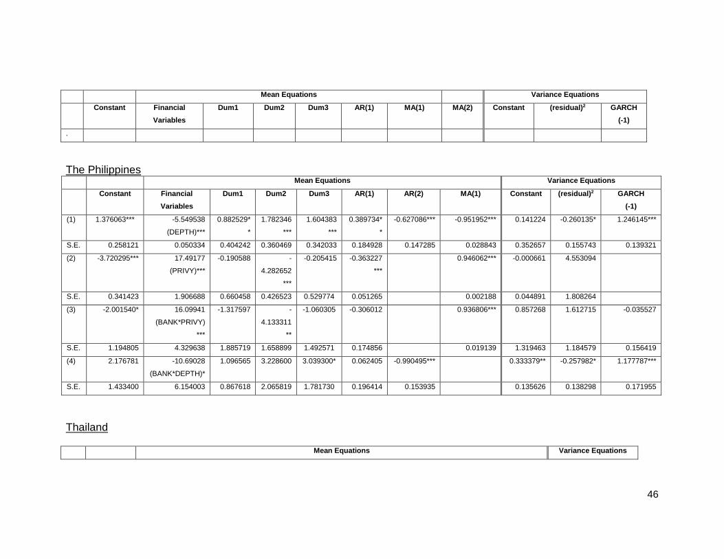
The Philippines


Constant Financial

Variables


(-1)

(1) 1.376063*** -5.549538

(DEPTH)***

0.882529*

*

1.782346

***

1.604383

***

0.389734*

*

-0.627086*** -0.951952*** 0.141224 -0.260135* 1.246145***

S.E. 0.258121 0.050334 0.404242 0.360469 0.342033 0.184928 0.147285 0.028843 0.352657 0.155743 0.139321

(2) -3.720295*** 17.49177

(PRIVY)***

-0.190588 -

4.282652

***

-0.205415 -0.363227

***

0.946062*** -0.000661 4.553094

S.E. 0.341423 1.906688 0.660458 0.426523 0.529774 0.051265 0.002188 0.044891 1.808264

(3) -2.001540* 16.09941

(BANK*PRIVY)

***

-1.317597 -

4.133311

**

-1.060305 -0.306012 0.936806*** 0.857268 1.612715 -0.035527

S.E. 1.194805 4.329638 1.885719 1.658899 1.492571 0.174856 0.019139 1.319463 1.184579 0.156419

(4) 2.176781 -10.69028

(BANK*DEPTH)*

1.096565 3.228600 3.039300* 0.062405 -0.990495*** 0.333379** -0.257982* 1.177787***

S.E. 1.433400 6.154003 0.867618 2.065819 1.781730 0.196414 0.153935 0.135626 0.138298 0.171955

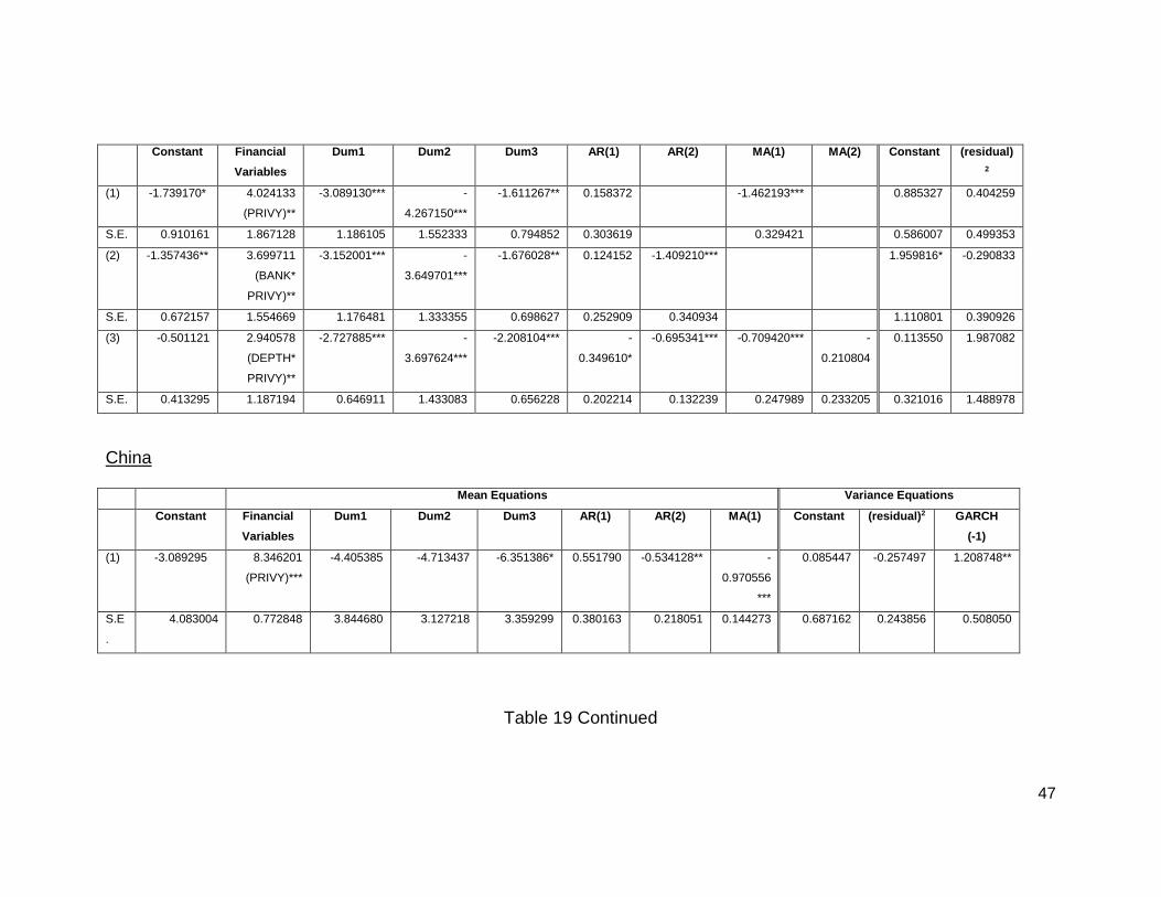
Thailand


47

Constant Financial

Variables

Dum1 Dum2 Dum3 AR(1) AR(2) MA(1) MA(2) Constant (residual)

2

(1) -1.739170* 4.024133

(PRIVY)**

-3.089130*** -

4.267150***

-1.611267** 0.158372 -1.462193*** 0.885327 0.404259

S.E. 0.910161 1.867128 1.186105 1.552333 0.794852 0.303619 0.329421 0.586007 0.499353

(2) -1.357436** 3.699711

(BANK*

PRIVY)**

-3.152001*** -

3.649701***

-1.676028** 0.124152 -1.409210*** 1.959816* -0.290833

S.E. 0.672157 1.554669 1.176481 1.333355 0.698627 0.252909 0.340934 1.110801 0.390926

(3) -0.501121 2.940578

(DEPTH*

PRIVY)**

-2.727885*** -

3.697624***

-2.208104*** -

0.349610*

-0.695341*** -0.709420*** -

0.210804

0.113550 1.987082

S.E. 0.413295 1.187194 0.646911 1.433083 0.656228 0.202214 0.132239 0.247989 0.233205 0.321016 1.488978

China


Constant Financial

Variables


(-1)

(1) -3.089295 8.346201

(PRIVY)***

-4.405385 -4.713437 -6.351386* 0.551790 -0.534128** -

0.970556

***

0.085447 -0.257497 1.208748**

S.E

.

4.083004 0.772848 3.844680 3.127218 3.359299 0.380163 0.218051 0.144273 0.687162 0.243856 0.508050

Table 19 Continued

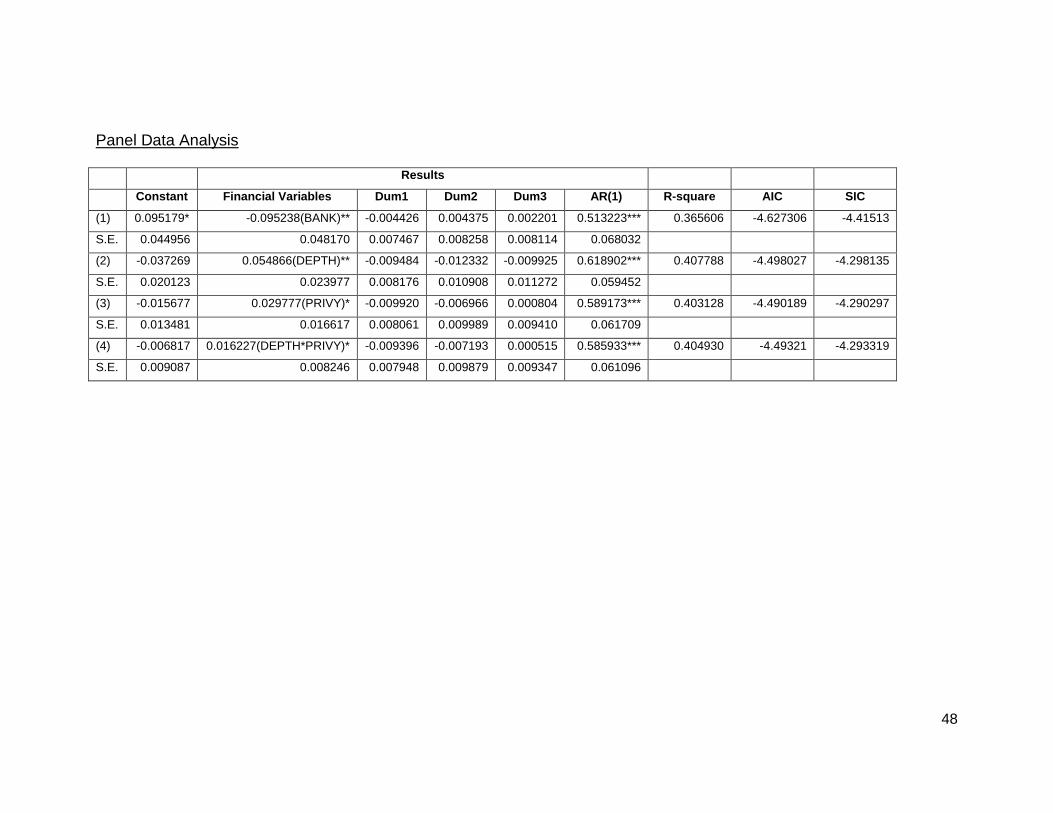
48

Panel Data Analysis

Results

Constant Financial Variables Dum1 Dum2 Dum3 AR(1) R-square AIC SIC

(1) 0.095179* -0.095238(BANK)** -0.004426 0.004375 0.002201 0.513223*** 0.365606 -4.627306 -4.41513

S.E. 0.044956 0.048170 0.007467 0.008258 0.008114 0.068032

(2) -0.037269 0.054866(DEPTH)** -0.009484 -0.012332 -0.009925 0.618902*** 0.407788 -4.498027 -4.298135

S.E. 0.020123 0.023977 0.008176 0.010908 0.011272 0.059452

(3) -0.015677 0.029777(PRIVY)* -0.009920 -0.006966 0.000804 0.589173*** 0.403128 -4.490189 -4.290297

S.E. 0.013481 0.016617 0.008061 0.009989 0.009410 0.061709

(4) -0.006817 0.016227(DEPTH*PRIVY)* -0.009396 -0.007193 0.000515 0.585933*** 0.404930 -4.49321 -4.293319

S.E. 0.009087 0.008246 0.007948 0.009879 0.009347 0.061096

49

50

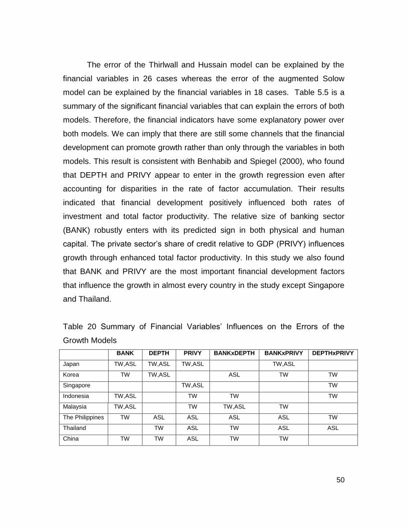
The error of the Thirlwall and Hussain model can be explained by the

financial variables in 26 cases whereas the error of the augmented Solow

model can be explained by the financial variables in 18 cases. Table 5.5 is a

summary of the significant financial variables that can explain the errors of both

models. Therefore, the financial indicators have some explanatory power over

both models. We can imply that there are still some channels that the financial

development can promote growth rather than only through the variables in both

models. This result is consistent with Benhabib and Spiegel (2000), who found

that DEPTH and PRIVY appear to enter in the growth regression even after

accounting for disparities in the rate of factor accumulation. Their results

indicated that financial development positively influenced both rates of

investment and total factor productivity. The relative size of banking sector

(BANK) robustly enters with its predicted sign in both physical and human

capital. The private sector’s share of credit relative to GDP (PRIVY) influences

growth through enhanced total factor productivity. In this study we also found

that BANK and PRIVY are the most important financial development factors

that influence the growth in almost every country in the study except Singapore

and Thailand.

Table 20 Summary of Financial Variables’ Influences on the Errors of the

Growth Models

BANK DEPTH PRIVY BANKxDEPTH BANKxPRIVY DEPTHxPRIVY

Japan TW,ASL TW,ASL TW,ASL TW,ASL

Korea TW TW,ASL ASL TW TW

Singapore TW,ASL TW

Indonesia TW,ASL TW TW TW

Malaysia TW,ASL TW TW,ASL TW

The Philippines TW ASL ASL ASL ASL TW

Thailand TW ASL TW ASL ASL

China TW TW ASL TW TW

51

Note: TW and ASL are shown for the case in which the financial variable can statistically

explain the error of Thirlwall and Hussain’s growth definition and the error of the augmented

Solow model, respectively.

3) Implications from the Results From the results shown, we found that there are two cases of financial

variables’ coefficient signs and constant terms. Each case implies different

correlations between financial variables and the error of predicted growth rates.

We explain each case below.

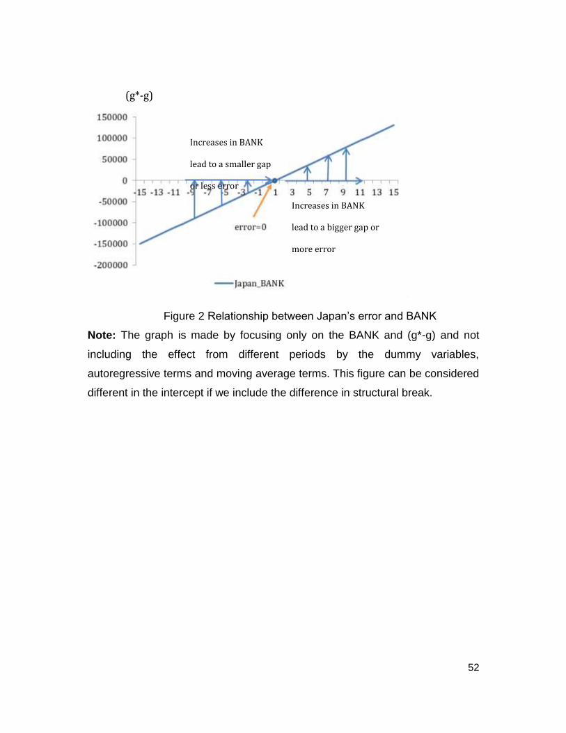
Case I Constant Term Is negative and Financial Variable Coefficient Is Positive

The correlation between the error between the predicted growth rates

and the actual growth rates and financial variable is positive. This implies that

when financial development increases, the error or the gap increases.

However, the constant term is negative, which means if the mean of financial

variables is less than the x-intercept (when the error is zero) the increase in

financial variables will lead to a smaller gap (less negative). We illustrate this

scenario in Figure 5.3, which focuses on the relationship between Japan’s gap

and Thirlwall and Hussain’s predicted growth rates and the actual growth and

BANK (the size of service provided by deposit money banks).

52

Figure 2 Relationship between Japan’s error and BANK

Note: The graph is made by focusing only on the BANK and (g*-g) and not

including the effect from different periods by the dummy variables,

autoregressive terms and moving average terms. This figure can be considered

different in the intercept if we include the difference in structural break.

Increases in BANK

lead to a bigger gap or

more error

(g*-g)

Increases in BANK

lead to a smaller gap

or less error

53

Therefore, the implication from this case depends on where the mean of

the financial variable locates. If the country’s mean of BANK is less than the

point that makes the error equal to zero, an increase in financial development

makes Thirlwall and Hussain’s predicted growth closer to the actual growth. On

the other hand, if the mean of BANK is higher than the point where the error is

zero, an increase in BANK makes a greater error of Thirlwall and Hussain’s

hypothesis.

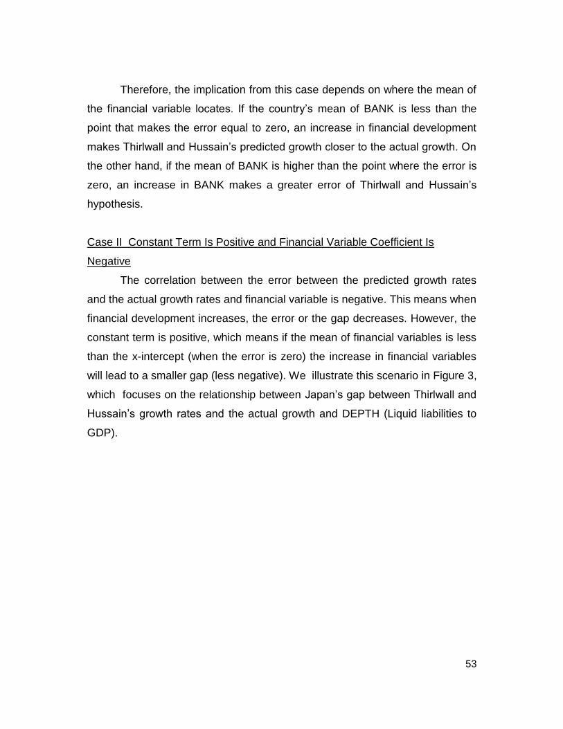
Case II Constant Term Is Positive and Financial Variable Coefficient Is

Negative

The correlation between the error between the predicted growth rates

and the actual growth rates and financial variable is negative. This means when

financial development increases, the error or the gap decreases. However, the

constant term is positive, which means if the mean of financial variables is less

than the x-intercept (when the error is zero) the increase in financial variables

will lead to a smaller gap (less negative). We illustrate this scenario in Figure 3,

which focuses on the relationship between Japan’s gap between Thirlwall and

Hussain’s growth rates and the actual growth and DEPTH (Liquid liabilities to

GDP).

54

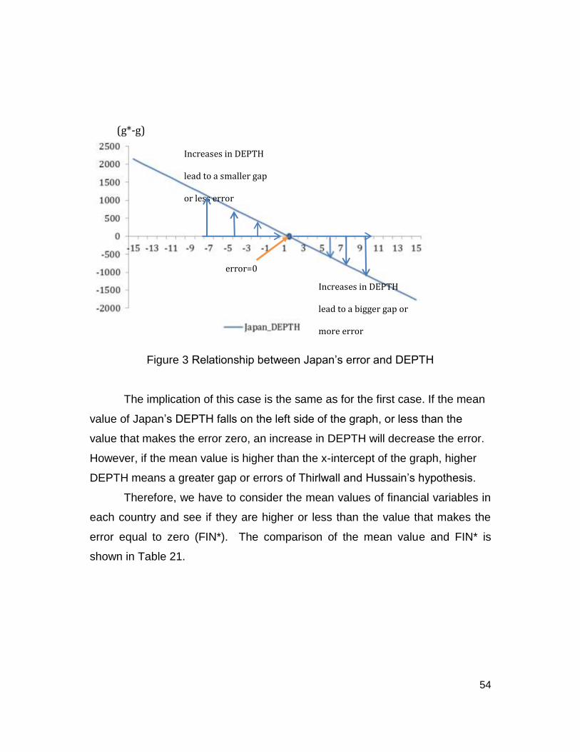
Figure 3 Relationship between Japan’s error and DEPTH

The implication of this case is the same as for the first case. If the mean

value of Japan’s DEPTH falls on the left side of the graph, or less than the

value that makes the error zero, an increase in DEPTH will decrease the error.

However, if the mean value is higher than the x-intercept of the graph, higher

DEPTH means a greater gap or errors of Thirlwall and Hussain’s hypothesis.

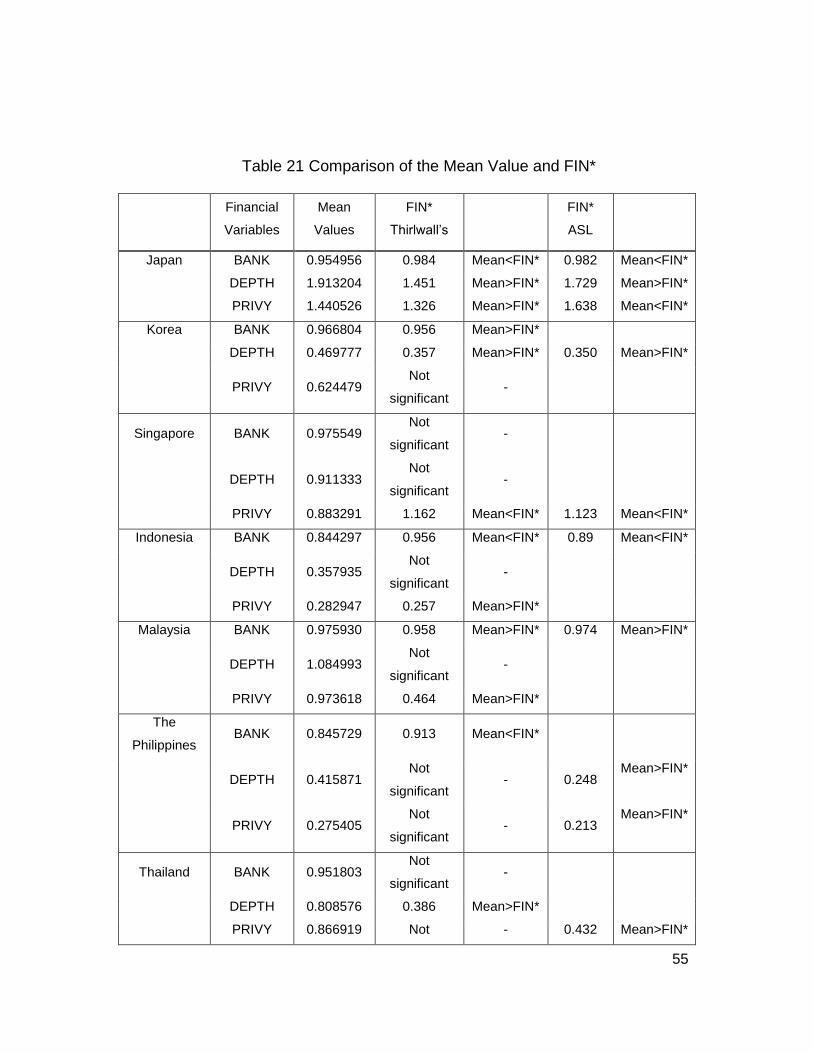
Therefore, we have to consider the mean values of financial variables in

each country and see if they are higher or less than the value that makes the

error equal to zero (FIN*). The comparison of the mean value and FIN* is

shown in Table 21.

(g*-g)

Increases in DEPTH

lead to a bigger gap or

more error

Increases in DEPTH

lead to a smaller gap

or less error

error=0

55

Table 21 Comparison of the Mean Value and FIN*

Financial

Variables

Mean

Values

FIN*

Thirlwall’s

FIN*

ASL

Japan BANK 0.954956 0.984 Mean<FIN* 0.982 Mean<FIN*

DEPTH 1.913204 1.451 Mean>FIN* 1.729 Mean>FIN*

PRIVY 1.440526 1.326 Mean>FIN* 1.638 Mean<FIN*

Korea BANK 0.966804 0.956 Mean>FIN*

DEPTH 0.469777 0.357 Mean>FIN* 0.350 Mean>FIN*

PRIVY 0.624479 Not

significant -

Singapore BANK 0.975549 Not

significant -

DEPTH 0.911333 Not

significant -

PRIVY 0.883291 1.162 Mean<FIN* 1.123 Mean<FIN*

Indonesia BANK 0.844297 0.956 Mean<FIN* 0.89 Mean<FIN*

DEPTH 0.357935 Not

significant -

PRIVY 0.282947 0.257 Mean>FIN*

Malaysia BANK 0.975930 0.958 Mean>FIN* 0.974 Mean>FIN*

DEPTH 1.084993 Not

significant -

PRIVY 0.973618 0.464 Mean>FIN*

The

Philippines BANK 0.845729 0.913 Mean<FIN*

DEPTH 0.415871 Not

significant - 0.248

Mean>FIN*

PRIVY 0.275405 Not

significant - 0.213

Mean>FIN*

Thailand BANK 0.951803 Not

significant -

DEPTH 0.808576 0.386 Mean>FIN*

PRIVY 0.866919 Not - 0.432 Mean>FIN*

56

Financial

Variables

Mean

Values

FIN*

Thirlwall’s

FIN*

ASL

significant

Note: ASL is the augmented Solow model

Table 21 Continued

Financial

Variables

Mean

Values

FIN*

Thirlwall’s

FIN*

ASL

China

BANK

DEPTH

PRIVY

0.968

1.111

0.935

1.403

0.598

Not

significant

Mean<FIN*

Mean>FIN*

0.370

Mean>FIN*

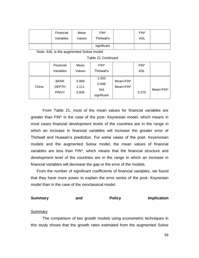
From Table 21, most of the mean values for financial variables are

greater than FIN* in the case of the post- Keynesian model, which means in

most cases financial development levels of the countries are in the range in

which an increase in financial variables will increase the greater error of

Thirlwall and Hussain’s prediction. For some cases of the post- Keyenesian

models and the augmented Solow model, the mean values of financial

variables are less than FIN*, which means that the financial structure and

development level of the countries are in the range in which an increase in

financial variables will decrease the gap or the error of the models.

From the number of significant coefficients of financial variables, we found

that they have more power to explain the error series of the post- Keynesian

model than in the case of the neoclassical model.

Summary and Policy Implication

Summary

The comparison of two growth models using econometric techniques in

this study shows that the growth rates estimated from the augmented Solow

57

model (Mankiw et al., 1992) can better explain the performance of output in

eight countries in East Asia during 1980-2010 than the growth rate calculated

from the Thirlwall and Hussain growth model (Thirlwall and Hussain, 1982). The

study uses R-squares, Adjusted R-squares, Akaike Information Criterion (AIC)

and Schwart Information Criterion (SIC) of the regression of the fitted output

growth from each model on the actual growth to be the comparison criterion. In

addition, the study applied a discerning approach using Davidson and

McKinnon’s (1981) J-test to consider which model should be accepted to

explain the growth in this region. For most of the individual countries, the J-test

accepts the augmented Solow model and rejects the Balance-of-Payment

constrained model (Thirlwall and Hussain’s). Only in the case of Indonesia did

the J-test reject both models to explain her growth.

The study further hypothesizes that the errors of both models are from

omitted variables, especially from the financial structures. Therefore, a set of

selected financial variables is used to explain the errors series and finds that

the financial variables can explain more in the case of the error from the

Thirlwall and Hussain model. Indeed, there are twenty-six out of forty-eight

cases in which the financial variables can explain the error of this model

whereas there are only eighteen cases in which the financial variables can be

the augmented Solow model errors. When the study considers the coefficient

values, there are two possible cases that lead to different policy implications.

The first case is when the constant term is negative and the financial variable

coefficient is positive, which implies that when the financial development

increases, the error or the gap increases. However, the constant term is

negative, which means if the mean of financial variables is less than x-intercept

(when the error is zero), the increase in financial variables will lead to a smaller

gap (less negative). Therefore, it depends on the mean values and the value of

financial variables, which make the error zero. If the mean values are greater

than the value that makes the error zero, increasing the financial variable value

will increase the gap between the actual and the predicted growth rate.

58

However, if the mean values of financial variables are less than the value that

makes the error zero, an increase in financial variable values will close the gap

of predicted and actual growth. The policy implication from this case is that the

country can promote the output growth using each growth model only when the

mean values of financial variables are less than the value that makes the error

zero.

The second possible outcome is when the constant term is positive and

the coefficient of the financial variable is negative. This means when financial

development increases, the error or the gap decreases. However, the constant

term is positive, which means if the mean of financial variables is less than the

x-intercept (when the error is zero) the increase in financial variables will lead to

a smaller gap (less negative). The policy implication is the same as in the first

case.

Policy Implications

1. Since the results of this study show that the supply-side growth

theory can explain more in the growth performance in East Asian countries

during 1980-2010 except in Indonesia, the supply variables should be

considered important factors to promote the output growth in these countries.

The determination of growth from the augmented Solow growth model consists

of growth of factors of production (labor and capital); technological progress,

which is partly brought by the foreign inflows; and also the accumulation and

growth of human capital. In this study we found that the rate of tertiary level of

education in the labor force is a significant factor for the output growth in the

panel data case. It is also mostly significant to determine the GDP growth in all

individual country cases. The results imply that if these countries experience a

shortage of all supply variables, the output growth will be affected.

2. For the human capital policy, the country can use a variety of policies

to improve overall human capital. Individuals can be healthier in a more

efficient healthcare system. Quality of education, which can be reflected in the

59

closer linkage between the academic and real sectors, is one important factor

for improved human capital. A literate population contributes to political stability

and consistency in the growth policy.

3. All countries’ growth performances in this study cannot be explained

by the Balance-of-Payment Constrained model by Thirlwall and Hussain

(1982). This result shows that in these countries, the balance- of- payment or

foreign exchanges shortages is not the limitation to growth. Countries in this

region are able to run balance- of- payment deficit and still have positive output

growth. The export growth and capital inflows are not important determinants of

the output growth in terms of the source for foreign exchange. One reason that

growth in these countries is not demand-driven is that developing Asia still

faces very elastic demand curves for their output in the world market. However,

the capital inflow is important in terms of the source for technological transfer

from foreign countries. Therefore, the countries should implement the policy for

capital inflows attraction, which guarantees that there will be some

technological transfer through the inflows. Foreign direct investment inflow is

one category that will fulfill that policy.

4. Financial structure has a large role to explain the error from both

growth models. The direction of promoting the efficiency in the financial

structure depends on the position or the mean value of the financial variables of

a particular country.

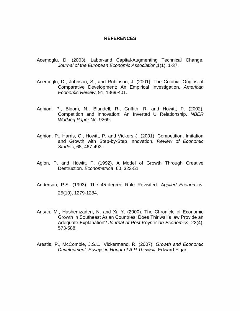
REFERENCES

Acemoglu, D. (2003). Labor-and Capital-Augmenting Technical Change. Journal of the European Economic Association,1(1), 1-37.

Acemoglu, D., Johnson, S., and Robinson, J. (2001). The Colonial Origins of Comparative Development: An Empirical Investigation. American Economic Review, 91, 1369-401.

Aghion, P., Bloom, N., Blundell, R., Griffith, R. and Howitt, P. (2002). Competition and Innovation: An Inverted U Relationship. NBER Working Paper No. 9269.

Aghion, P., Harris, C., Howitt, P. and Vickers J. (2001). Competition, Imitation and Growth with Step-by-Step Innovation. Review of Economic Studies, 68, 467-492.

Agion, P. and Howitt, P. (1992). A Model of Growth Through Creative Destruction. Econometrica, 60, 323-51.

Anderson, P.S. (1993). The 45-degree Rule Revisited. Applied Economics,

25(10), 1279-1284.

Ansari, M., Hashemzaden, N. and Xi, Y. (2000). The Chronicle of Economic Growth in Southeast Asian Countries: Does Thirlwall’s law Provide an Adequate Explanation? Journal of Post Keynesian Economics, 22(4), 573-588.

Arestis, P., McCombie, J.S.L., Vickermand, R. (2007). Growth and Economic Development: Essays in Honor of A.P.Thirlwall. Edward Elgar.

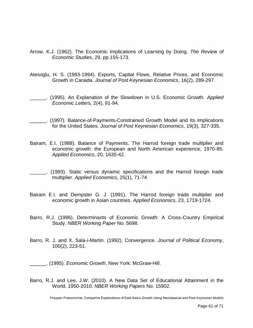
Praopan Pratoomchat, Comparive Explanations of East Asia’s Growth Using Neoclassical and Post-Keynesian Models

Page 61 of 71

Arrow, K.J. (1962). The Economic Implications of Learning by Doing. The Review of Economic Studies, 29, pp.155-173.

Atesoglu, H. S. (1993-1994). Exports, Capital Flows, Relative Prices, and Economic Growth in Canada. Journal of Post Keynesian Economics, 16(2), 289-297.

______. (1995). An Explanation of the Slowdown in U.S. Economic Growth. Applied Economic Letters, 2(4), 91-94.

______. (1997). Balance-of-Payments-Constrained Growth Model and Its Implications for the United States. Journal of Post Keynesian Economics, 19(3), 327-335.

Bairam, E.I. (1988). Balance of Payments, The Harrod foreign trade multiplier and economic growth: the European and North American experience, 1970-85. Applied Economics, 20, 1635-42.

______. (1993). Static versus dynamic specifications and the Harrod foreign trade multiplier. Applied Economics, 25(1), 71-74.

Bairam E.I. and Dempster G. J. (1991). The Harrod foreign trade multiplier and economic growth in Asian countries. Applied Economics, 23, 1719-1724.

Barro, R.J. (1996). Determinants of Economic Growth: A Cross-Country Empirical Study. NBER Working Paper No. 5698.

Barro, R. J. and X. Sala-i-Martin. (1992). Convergence. Journal of Political Economy, 100(2), 223-51.

______. (1995). Economic Growth, New York: McGraw-Hill.

Barro, R.J. and Lee, J.W. (2010). A New Data Set of Educational Attainment in the World, 1950-2010. NBER Working Papers No. 15902.


Page 62 of 71

Beach, C. and McKinnon, J. (1978). A maximum likelihood procedure for regression with autocorrelated errors. Econometrica, 46, pp.51-58.

Beck, T. and Demirgüç-Kunt, A. (2009). Financial Institutions and Markets Across Countries and over Time: Data and Analysis, World Bank Policy Research Working Paper, 4943.

Bencivenga, V.R. and Smith, B.O. (1991). Financial Intermediation and Endogenous Growth”, Review of Economic Studies, LVIII, 195-209.

Benhabib, J. and Spiegel, M.M. (2000). The Role of Financial Development in Growth and Investment, Journal of Economic Growth, 5, 341-360.

Blecker, R. (2002). Distribution, Demand and Growth in Neo-Kaleckian Macro-models in Setterfield, Mark (ed.), The Economics of Demand-Led Growth: Challenging the Supply-side Vision of the Long-run, Cheltenham: Edward Elgar.

Bollerslev, T.(1986). Generalized Autoregressive Conditional Heteroskedasticity Journal of Econometrics, 31, 307-327.

Burnanke, B., and Gurkaynak, R. (2002). Is Growth Exogenous? Taking Mankiw, Romer and Weil Seriously. NBER Macroeconomics Annual, 11-57.

Cass, D. (1965). Optimum Growth in an Aggregative Model of Capital Accumulation. Review of Economic Studies, XXXII, 233-40.

Chamberlain, G. (1982). Multivariate Regression Models for Panel Data. Journal of Econometrics, XVIII, 5-46.

______. (1983). Panel Data in Handbook of Econometrics, Zvi Griliches and Michael Intriligator (eds.), Amsterdam-North Holland, 1247-1318.

Chenery, H.B and Bruno, M. (1962). Development Alternatives in an Open Economy: The Case of Israel. Economic Journal, 72, 79-103.


Page 63 of 71

Chenery, H.B. and Strout, A.M. (1966). Foreign Assistance and Economic Development. The American Economic Review, 56(4).

Cox, D.R. (1961). Tests of Separate Families of Hypotheses. Proceeding of the Fourth Berkeley Symposium on Mathematical Statistics and Probability, 1, Berkeley: University of California Press.

_____. (1962). Further Results on Tests of Separated Families of Hypotheses. Journal

of the Royal Statistic Society, Series B, 24, 406-424.

Davidson, R. and MacKinnon, J.G. (1981). Several Tests for Model Specification in the Presence of Alternative Hypotheses. Econometrica, 49(3), 781-793.

Dickey, D.A., and Fuller, W.A. (1979). Distribution of the Estimators for Autoregressive Time Series with a Unit Root. Journal of the American Statistical Association, June, 74(366), 423-431.

Dixon, R. and Thirlwall, A.P. (1975). A Model of Regional Growth Rate Differences on Kaldorian Lines. Oxford Economic Papers, New Series, 27(2), 201-214.

Domar, E.D. (1946). Capital Expansion, Rate of Growth, and Employment. Econometrica, 14(2), 137-147.

Duesenberry, J.S. (1949). Income, Saving and the Theory of Consumer Behavior. Cambridge, Mass: Harvard University Press.

Dutt, A.K. (1984). Stagnation, income distribution, and monopoly power, Cambridge Journal of Economics, 8, 25-40.

Easterly, W. and Lavine, R. (2001). It’s Not Factor Accumulation: Stylized Facts and Growth Models. The World Bank Economic Review, 15(2), 177-219.


Page 64 of 71

______. (2003). Tropics, germs and crops: how endowments influence economic development. Journal of Monetary Economics, 50(1), 3-39.

Enders, W. (1995). Applied Econometric Time Series (Wiley series in probability and

mathematical statistics), John Wiley&Sons.

Greenwiid, R. and Scharfstein, D. (2013). The Growth of Finance. Journal of Economics Perspectives, 27(2), 3-28.

Goldsmith, R.W. (1969). Financial Structure and development. New Haven, CT: Yale University Press.

Goldstein, M. and Khan, M.S. (1978). The Supply and Demand for Exports: A

Simultaneous Approach. The Review of Economics and Statistics. 60(2).

Gouvea, R.R. and Lima, G.T. (2010). Structural change, balance of payments constraint and economic growth: evidence from the multisectoral Thirlwall’s Law. Journal of Post Keynesian Economics, 33(1), 169-204.

Grant, R.J., Papadakis, M.C. and Richardson, J.D. (1993). Global Trade Flows: Old Structures, New Issues, Empirical Evidence. In: Bergsten, C.F. and Noland, M. (ed.) Pacific Dynamism and the International Economic System. Institute for International Economics, Washington D.C.

Grossman, G.M., and Helpman, E. (1991). Quality Ladders in the Theory of Growth. Review of Economic Studies, 58, 43-61.

Greenwood, J. and Jovanovic, B. (1990). “Financial Development, Growth and the Distribution of Income”, Journal of Political Economy, 98(5), 1076-1107.

Gundlach, E. (2005). The Solow Model in the Empirics of Cross-country Growth. Kiel Institute for World Economics Working Paper, March.


Page 65 of 71

Hall, R.E., and Jones, C. (1999). Why Do Some Countries Produce So Much More Output per Worker than Others? Quarterly Journal of Economics, 114(1), 83-116.

Harrod, R. (1993). International Economics, London: James Nisbit and Cambridge University Press.

______. (1939). An Essay in Dynamic Theory. Economic Journal, 49, 14-33.

Hieke, H. (1997). Balance-of-Payment-Constrained Growth: A Reconsideration of the Evidence for the U.S. Economy. Journal of Post Keynesian Economics, 19(3), 313-325.

Hoeffler, A.E. (2000). The Augmented Solow Model and the African Growth Debate. Center for International Development at Harvard University, Working Paper No. 36, January.

Houthakker, H.S. and Magee, S.P. (1969). Income and Price Elasticities in World Trade. The Review of Economics and Statistics, 51(2), 111-125.

Hussain, M.N. (1999). The Balance-of-Payments Constraint and Growth Rate Differences among African and East Asian Economies. African Development Bank, Blackwell, 103-137.

Islam, N. (1995). Growth Empirics: A Panel Data Approach. The Quarterly Journal of Economics, 110, 1127-70.

Johansen, S. (1988). Statistical analysis of cointegration vectors. Journal of Economics and Control, June-September, 12(2-3), 231-254.

Johansen, S. and Juselius, K. (1990). Maximum Likelihood Estimation and Inference on Cointegration With Applications to the Demand for Money. Oxford Bulletin of Economics and Statistics, May, 52(2), 169-210.


Page 66 of 71

Jones, C.I. (1999). Growth: With or Without Scale Effects? American Economic Review Papers and Proceedings, 89(2), 139-44.

Kalaitzidakis, P., Mamuneas, T.P., Savvides, A. and Stengos, T. (2001). Measures of Human Capital and Nonlinearities in Economic Growth. Journal of Economic Growth, 6(3), 229-54.

Kaldor, N. (1995-6). Alternative Theories of Distribution. Review of Economic Studies, 23, 83-100.

______. (1957). A Model of Economic Growth. Economic Journal, 67, 591-624. ______. (1970). The case for regional policies. Scottish Journal of Political Economy,

18, 337-348.

______. (1975). What is Wrong with Economic Theory? Quarterly Journal of Economics, 89(3), 347-357.

______. (1985). Economics Without Equilibrium, Cardiff: University College Cardiff Press.

Kendrick, J.W. (1976). The Formation and Stocks of Total Capital. National Bureau of Economic Research, 22-64.

King, R. G. and Levine, R. (1993). Finance and Growth: Schumpeter Might be Right. The Quarterly Journal of Economics, 108 (3), 717-737.

Klenow, P. and Rodriguez-Clare, A. “Economic Growth. A Review Essay.” Journal of Monetary Economics, 1997, 40, pp.597-617.

Koopmans, T.C. (1965). On the Concept of Optimal Economic Growth. in The Economic Approach to Development Planning, Pontifical Academy of Sciences, Amsterdam: North Holland.


Page 67 of 71

Krueger, A.B. and Lindahl, M. (2000). Education for Growth: Why and For Whom? NBER Working Papers No. 7591.

Krugman, P. (1989). Differences in income elasticities and trends in real exchange rates. National Bureau of Economic Research, Working paper No. 2761.

Kumar C. S. (2006). Human capital and growth empirics. Journal of Development Areas, 40(1), 153-179.

Levine, R. and Zervos, S. (1993). Looking at the facts: what we know about policy and growth from cross-country analysis. Policy Research Working Paper Series No. 1115, The World Bank.

Lucas, R.E., Jr. (1988). On the Mechanics of Economic Development. Journal of Monetary Economics, 22, 3-42.

Mankiw, G. N., Romer, D. and Weil, D.N. (1992). A Contribution to the Empirics of Economic Growth. The Quarterly Journal of Economics, 107, 407-37.

McCombie, J.S.L. (1985). Economic Growth, the Harrod Trade Multiplier and the Hicks Super-Multiplier. Applied Economics, 17, 55-72.

______. (1985). The Balance of Payments as a Constraint on Economic Growth., Department of Economics, University of Melbourne, Research Paper No.137.

______. (1989). ‘Thirlwall’s Law’ and balance of payments constrained growth – a comment on the debate. Applied Economics, 21(5), 611-629.

______. (1997). On the Empirics of Balance-of-Payments Constrained Growth, Journal of Post Keynesian Economics, 19(3), 345-375.

McCombie, J.S.L. (2011). Criticism and defenses of the balance-of-payments constrained growth model: some old, some new. PSL Quarterly Review, 64(259), 353-392.


Page 68 of 71

McCombie, J.S.L. and Thirlwall, A.P. (1994). Economic Growth and Balance of Payments Constraint, London: McMillan.

McGregor, P.G. and Swales, J.K. (1985). Professor Thirlwall and Balance of Payments Constrained Growth. Applied Economics, 17, 17-32.

McKinnon, R.I. (1973). Money and Capital in Economic Development, Washington: The Brookings Institution.

McQuinn, K. and Whelan, K. (2007). Solow (1956) as a model of cross-country growth dynamics. Oxford Review of Economic Policy, 23(1), 45-62.

Myrdal, G. (1957). Economic Theory and Under-developed Regions, London: Gerald Duckworth&Co.

Nelson, R.R. and Phelps, E.S. (1966). Investment in Humans, Technological Diffusion, and Economic Growth. The American Economic Review, 56(1/2), 69-75.

Pasinetti, L.L. (1962). Rate of Profit and Income Distribution in Relation to the Rate of Economic Growth. Review of Economic Studies, 29, 267-279.

Perraton, J. (2003). Balance of Payment Constrained Growth and Developing Countries: An Examination of Thirlwall’s Hypothesis, International Review of Applied Economics, 17(1).

Pesaran, M.H. (1974). On the General Problem of Model Selection. Review of Economic Studies, 41, 153-171.

Pesaran, M.H. and Deaton, A.S. (1978). Testing Non-nested Nonlinear Regression Models. Econometrica, 46, 677-694.

Pritchett, L. (1996). Where has all the Education Gone? The World Bank Policy Research Working Paper No. 1581.


Page 69 of 71

Ramsey, F.P. (1928). A Mathematical Theory of Saving. The Economic Journal, 38(152), 543-559.

Rebelo, S. (1991). Long-Run Policy Analysis and Long-Run Growth. Journal of Political Economy, XCIX, 500-21.

Robinson, J. (1956). The Accumulation of Capital, London: Macmillan.

Rodrik, D., Subramanian, A. and Trebbi, F. (2004). Institutions rule: The primacy of institutions over geography and integration in economic development. Journal of Economic Growth, 9(2), 131-165.

Romer, P.M. (1986). Increasing Returns and Long-Run Growth. Journal of Political Economy, 94, 1002-37.

______. (1990). Endogenous Technological Change. Journal of Political Economy, 98, S71-S102.

______. (1990). Human Capital and Growth: Theory and Evidence. Carnegie-Rochester Conference Series on Public Policy, 32, 251-86.

Rowthorn, R.E. (1982). Demand, real wages and economic growth. Studi Economici, 18, 3-53.

Sen, A. (1999). Development as Freedom, Oxford: Oxford University Press.

Setterfiled, M. (2003). Supply and Demand in the Theory of Long-run Growth: introduction to a symposium on demand-led growth. Review of Political Economy, 15(1), 23-32.

Shaw, E. (1973). Financial Deepening in Economic Development, New York: Oxford University Press.


Page 70 of 71

Sheshinski, E. (1967). Tests of “Learning by Doing” Hypothesis. The Review of Economics and Statistics, 49(4), 568-578.

Schumpeter, J.A. (1911). The Theory of Economic Development, New York: Oxford University Press.

Solow, R. (1956). A Contribution to the Theory of Economic Growth. Quarterly Journal of Economics, 70, 65-94.

Swan, T.W. (1956). Economic Growth and Capital Accumulation. Economic Record, November, 32(2), 334-361.

Thirlwall, A.P. (1979). The Balance of Payments Constraint as an Explanation of International Growth Rate Differences. Banca Nazionale del Lavoro Quaterly Review, 128, 45-53.

______. (1980). Balance of Payments Theory and the United Kingdom Experience, London: Macmillian Press.

Thirlwall, A.P. and Gibson, H.D. (1992). Balance of Payments Theory and the United Kingdom Experience, London: MacMillan Press.

Thirlwall, A.P. (2003). Growth and Development: With Special Reference to Developing Economies, 7th Ed., Palgrave, 121-122.

Thirlwall, A.P. and Hussain, N.M. (1982). The Balance of Payments Constraint, Capital Flows and Growth Rate Differences between Developing Countries. Oxford Economic Papers, 34, 498-509.

Urata, S. (1993). Japanese Foreign Direct Investment and Its Effect on Foreign Trade in Asia," NBER Chapters, in: Trade and Protectionism, NBER-EASE (2), National Bureau of Economic Research, 273-304.

Uzawa, H. (1965). Optimum Technical Change in an Aggregative Model of Economic Growth. International Economic Review, 6(1), 18-31.

http://ideas.repec.org/h/nbr/nberch/8078.html

http://ideas.repec.org/h/nbr/nberch/8078.html

http://ideas.repec.org/s/nbr/nberch.html


Page 71 of 71

Verdoorn, J.P. (1993). On the Factors Determining the Growth of Labor Productivity, 1949, In Pasinetti, L.(ed.), Italian Economic Papers, Vol.11, Oxford: Oxford University Press.

World Bank. (1993). The Asian Miracle, Oxford: Oxford University Press.

World Bank. http://databank.worldbank.org, last accessed February, 2013.

Young, A. (1995). The Tyranny of Numbers: Confronting the Statistical Realities of the East Asian Growth Experience. The Quarterly Journal of Economics, 110(3), 641-680.

http://databank.worldbank.org/

Documents

Comparative Explanation of East Asia's Growth Using Neoclassical and Post Keynesian Growth Models