1

COLLOIDAL DISPERSIONS

Dispersed systems consist of particulate matter (known as the dispersed phase), distributed throughout a continuous phase (known as dispersion medium).

CLASSIFICATION OF DISPERSED SYSTEMS On the basis of mean particle diameter of the dispersed material, three types of dispersed systems are generally considered:

a) Molecular dispersions b) Colloidal dispersions, and c) Coarse dispersions

Molecular dispersions are the true solutions of a solute phase in a solvent. The solute is in the form of separate molecules homogeneously distributed throughout the solvent. Example: aqueous solution of salts, glucose Colloidal dispersions are micro-heterogeneous dispersed systems. The dispersed phases cannot be separated under gravity or centrifugal or other forces. The particles do not mix or settle down. Example: aqueous dispersion of natural polymer, colloidal silver sols, jelly Coarse dispersions are heterogeneous dispersed systems in which the dispersed phase particles are larger than 0.5µm. The concentration of dispersed phase may exceed 20%. Example: pharmaceutical emulsions and suspensions

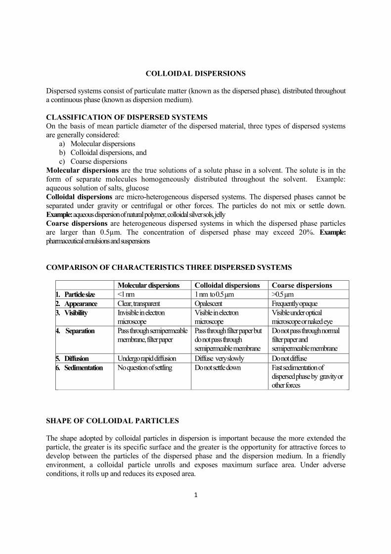
COMPARISON OF CHARACTERISTICS THREE DISPERSED SYSTEMS

Molecular dispersions Colloidal dispersions Coarse dispersions 1. Particle size <1 nm 1 nm to 0.5 µm >0.5 µm 2. Appearance Clear, transparent Opalescent Frequently opaque 3. Visibility Invisible in electron

microscope Visible in electron microscope

Visible under optical microscope or naked eye

4. Separation Pass through semipermeable membrane, filter paper

Pass through filter paper but do not pass through semipermeable membrane

Do not pass through normal filter paper and semipermeable membrane

5. Diffusion Undergo rapid diffusion Diffuse very slowly Do not diffuse 6. Sedimentation No question of settling Do not settle down Fast sedimentation of

dispersed phase by gravity or other forces

SHAPE OF COLLOIDAL PARTICLES

The shape adopted by colloidal particles in dispersion is important because the more extended the particle, the greater is its specific surface and the greater is the opportunity for attractive forces to develop between the particles of the dispersed phase and the dispersion medium. In a friendly environment, a colloidal particle unrolls and exposes maximum surface area. Under adverse conditions, it rolls up and reduces its exposed area.

2

The shapes that can be assumed by colloidal particles are: (a) spheres and globules, (b) short rods and prolate ellipsoids (rugby ball-shaped/elongated), (c) oblate ellipsoids (discus-shaped/flattened) and flakes, (d) long rods and threads, (e) loosely coiled threads, and (f) branched threads The following properties are affected by changes in the shape of colloidal particles:

a) Flowability b) Sedimentation c) Osmotic pressure d) Pharmacological action.

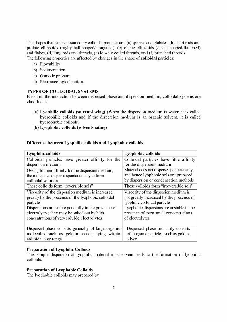
TYPES OF COLLOIDAL SYSTEMS Based on the interaction between dispersed phase and dispersion medium, colloidal systems are classified as

(a) Lyophilic colloids (solvent-loving) (When the dispersion medium is water, it is called hydrophilic colloids and if the dispersion medium is an organic solvent, it is called hydrophobic colloids)

(b) Lyophobic colloids (solvent-hating) Difference between Lyophilic colloids and Lyophobic colloids Lyophilic colloids Lyophobic colloids Colloidal particles have greater affinity for the dispersion medium

Colloidal particles have little affinity for the dispersion medium

Owing to their affinity for the dispersion medium, the molecules disperse spontaneously to form colloidal solution

Material does not disperse spontaneously, and hence lyophobic sols are prepared by dispersion or condensation methods

These colloids form “reversible sols” These colloids form “irreversible sols” Viscosity of the dispersion medium is increased greatly by the presence of the lyophobic colloidal particles

Viscosity of the dispersion medium is not greatly increased by the presence of lyophilic colloidal particles

Dispersions are stable generally in the presence of electrolytes; they may be salted out by high concentrations of very soluble electrolytes

Lyophobic dispersions are unstable in the presence of even small concentrations of electrolytes

Dispersed phase consists generally of large organic molecules such as gelatin, acacia lying within colloidal size range

Dispersed phase ordinarily consists of inorganic particles, such as gold or silver

Preparation of Lyophilic Colloids This simple dispersion of lyophilic material in a solvent leads to the formation of lyophilic colloids. Preparation of Lyophobic Colloids The lyophobic colloids may prepared by

3

(a) Dispersion method (a) Condensation method

Dispersion methods: This method involves the breakdown of larger particles into particles of colloidal dimensions. The breakdown of coarse material may be effected by the use of the Colloid mills, Ultrasonic treatment in presence of stabilizing agent such as a surface active agent. Condensation method: In this method, the colloidal particles are formed by the aggregation of smaller particles such as molecules. These involve a high degree of initial supersaturation followed by the formation and growth of nuclei. Supersaturation can be brought about by

(i) Change in solvent: For example, if sulfur is dissolved in alcohol and the concentrated solution is then poured into an excess of water, many small nuclei form in the supersaturated solution. These grow rapidly to form a colloidal sol. If a saturated solution of sulphur in acetone is poured slowly into hot water the acetone vaporizes, leaving a colloidal dispersion of sulphur.

(ii) Chemical reaction: For example, colloidal silver iodide may be obtained by reacting together dilute solutions of silver nitrate and potassium iodide. If a solution of ferric chloride is boiled with an excess of water produces red sol of hydrated ferric oxide by hydrolysis.

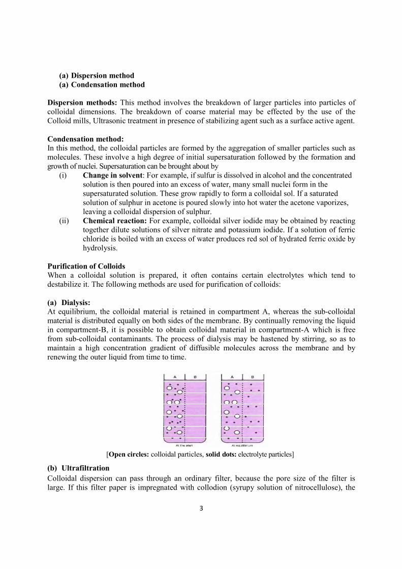
Purification of Colloids When a colloidal solution is prepared, it often contains certain electrolytes which tend to destabilize it. The following methods are used for purification of colloids: (a) Dialysis: At equilibrium, the colloidal material is retained in compartment A, whereas the sub-colloidal material is distributed equally on both sides of the membrane. By continually removing the liquid in compartment-B, it is possible to obtain colloidal material in compartment-A which is free from sub-colloidal contaminants. The process of dialysis may be hastened by stirring, so as to maintain a high concentration gradient of diffusible molecules across the membrane and by renewing the outer liquid from time to time.

[Open circles: colloidal particles, solid dots: electrolyte particles]

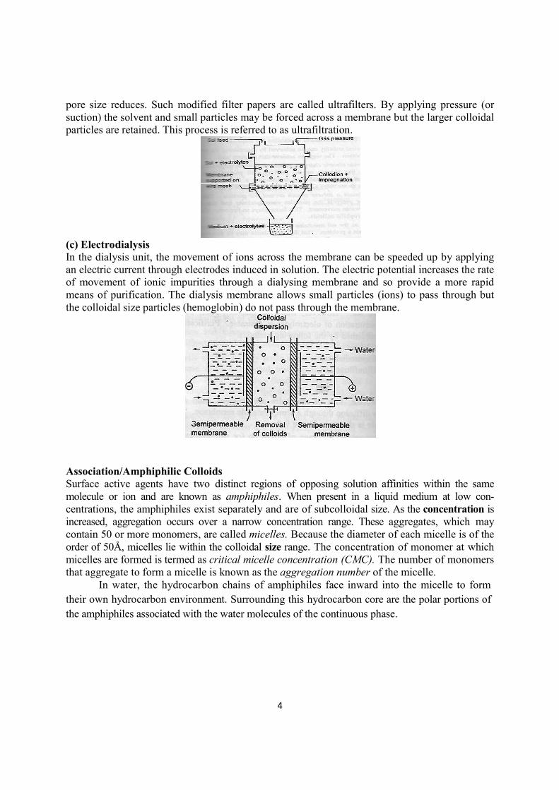
(b) Ultrafiltration Colloidal dispersion can pass through an ordinary filter, because the pore size of the filter is large. If this filter paper is impregnated with collodion (syrupy solution of nitrocellulose), the

4

pore size reduces. Such modified filter papers are called ultrafilters. By applying pressure (or suction) the solvent and small particles may be forced across a membrane but the larger colloidal particles are retained. This process is referred to as ultrafiltration.

(c) Electrodialysis In the dialysis unit, the movement of ions across the membrane can be speeded up by applying an electric current through electrodes induced in solution. The electric potential increases the rate of movement of ionic impurities through a dialysing membrane and so provide a more rapid means of purification. The dialysis membrane allows small particles (ions) to pass through but the colloidal size particles (hemoglobin) do not pass through the membrane.

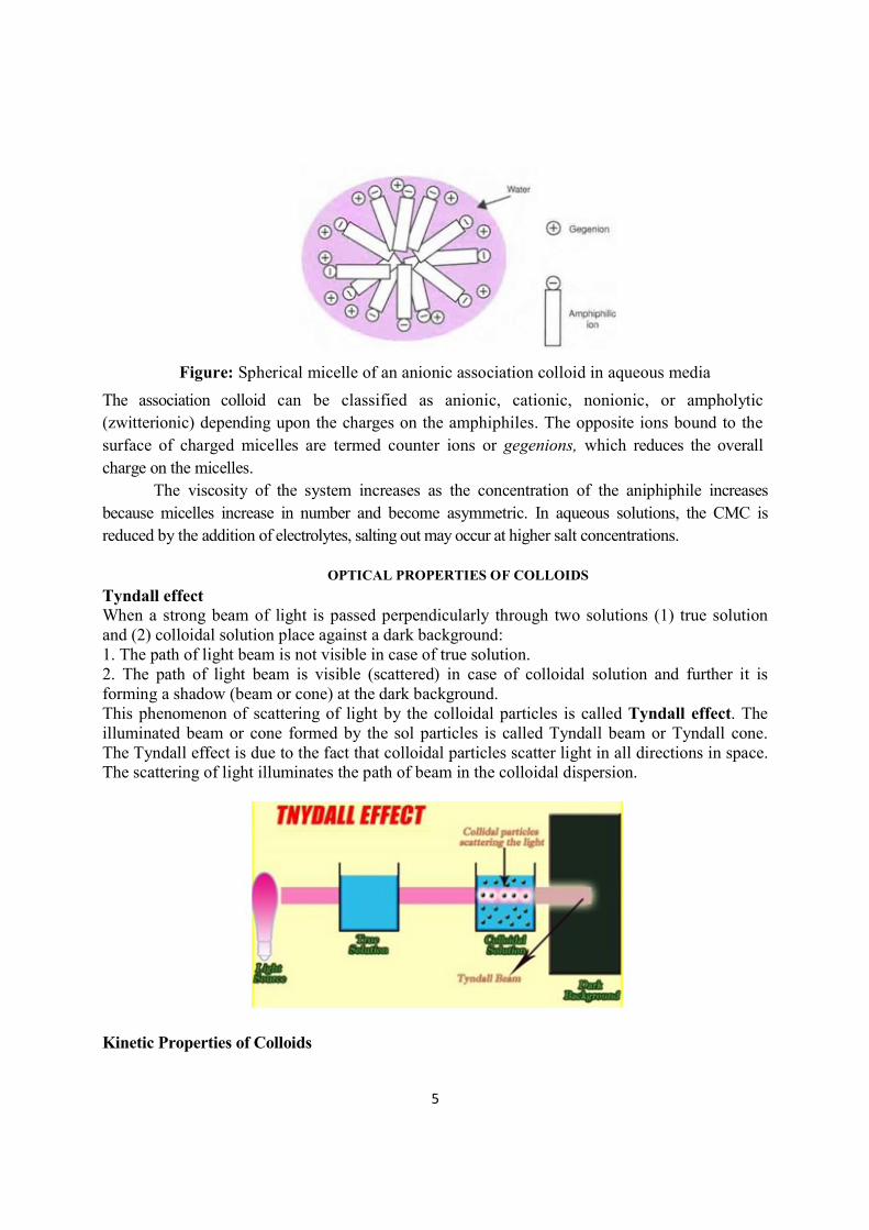
Association/Amphiphilic Colloids Surface active agents have two distinct regions of opposing solution affinities within the same molecule or ion and are known as amphiphiles. When present in a liquid medium at low con-centrations, the amphiphiles exist separately and are of subcolloidal size. As the concentration is increased, aggregation occurs over a narrow concentration range. These aggregates, which may contain 50 or more monomers, are called micelles. Because the diameter of each micelle is of the order of 50Å, micelles lie within the colloidal size range. The concentration of monomer at which micelles are formed is termed as critical micelle concentration (CMC). The number of monomers that aggregate to form a micelle is known as the aggregation number of the micelle.

In water, the hydrocarbon chains of amphiphiles face inward into the micelle to form their own hydrocarbon environment. Surrounding this hydrocarbon core are the polar portions of the amphiphiles associated with the water molecules of the continuous phase.

5

Figure: Spherical micelle of an anionic association colloid in aqueous media

The association colloid can be classified as anionic, cationic, nonionic, or ampholytic (zwitterionic) depending upon the charges on the amphiphiles. The opposite ions bound to the surface of charged micelles are termed counter ions or gegenions, which reduces the overall charge on the micelles.

The viscosity of the system increases as the concentration of the aniphiphile increases because micelles increase in number and become asymmetric. In aqueous solutions, the CMC is reduced by the addition of electrolytes, salting out may occur at higher salt concentrations.

OPTICAL PROPERTIES OF COLLOIDS

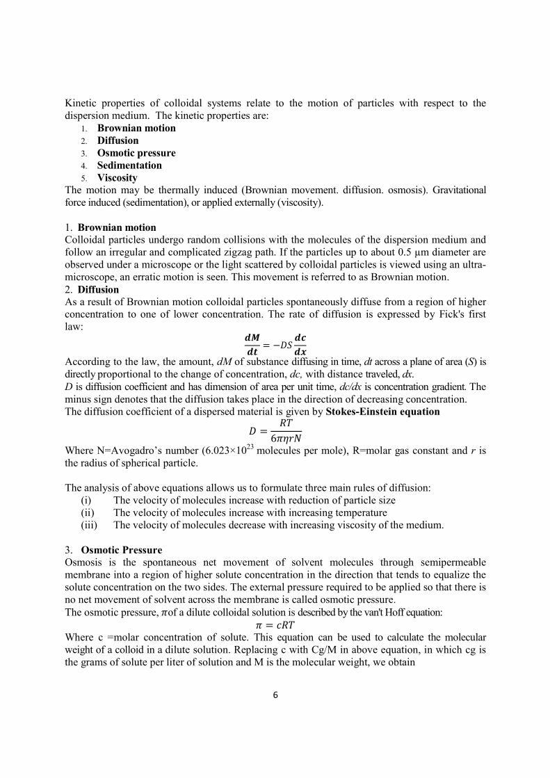
Tyndall effect When a strong beam of light is passed perpendicularly through two solutions (1) true solution and (2) colloidal solution place against a dark background: 1. The path of light beam is not visible in case of true solution. 2. The path of light beam is visible (scattered) in case of colloidal solution and further it is forming a shadow (beam or cone) at the dark background. This phenomenon of scattering of light by the colloidal particles is called Tyndall effect. The illuminated beam or cone formed by the sol particles is called Tyndall beam or Tyndall cone. The Tyndall effect is due to the fact that colloidal particles scatter light in all directions in space. The scattering of light illuminates the path of beam in the colloidal dispersion.

Kinetic Properties of Colloids

6

Kinetic properties of colloidal systems relate to the motion of particles with respect to the dispersion medium. The kinetic properties are:

1. Brownian motion 2. Diffusion 3. Osmotic pressure 4. Sedimentation 5. Viscosity

The motion may be thermally induced (Brownian movement. diffusion. osmosis). Gravitational force induced (sedimentation), or applied externally (viscosity). 1. Brownian motion Colloidal particles undergo random collisions with the molecules of the dispersion medium and follow an irregular and complicated zigzag path. If the particles up to about 0.5 µm diameter are observed under a microscope or the light scattered by colloidal particles is viewed using an ultra-microscope, an erratic motion is seen. This movement is referred to as Brownian motion. 2. Diffusion As a result of Brownian motion colloidal particles spontaneously diffuse from a region of higher concentration to one of lower concentration. The rate of diffusion is expressed by Fick's first law:

𝒅𝑴

𝒅𝒕= −𝐷𝑆

𝒅𝒄

𝒅𝒙

According to the law, the amount, dM of substance diffusing in time, dt across a plane of area (S) is directly proportional to the change of concentration, dc, with distance traveled, dx. D is diffusion coefficient and has dimension of area per unit time, dc/dx is concentration gradient. The minus sign denotes that the diffusion takes place in the direction of decreasing concentration. The diffusion coefficient of a dispersed material is given by Stokes-Einstein equation

𝐷 =𝑅𝑇

6𝜋𝜂𝑟𝑁

Where N=Avogadro’s number (6.023×1023 molecules per mole), R=molar gas constant and r is the radius of spherical particle. The analysis of above equations allows us to formulate three main rules of diffusion:

(i) The velocity of molecules increase with reduction of particle size (ii) The velocity of molecules increase with increasing temperature (iii) The velocity of molecules decrease with increasing viscosity of the medium.

3. Osmotic Pressure Osmosis is the spontaneous net movement of solvent molecules through semipermeable membrane into a region of higher solute concentration in the direction that tends to equalize the solute concentration on the two sides. The external pressure required to be applied so that there is no net movement of solvent across the membrane is called osmotic pressure. The osmotic pressure, 𝜋of a dilute colloidal solution is described by the van't Hoff equation:

𝜋 = 𝑐𝑅𝑇 Where c =molar concentration of solute. This equation can be used to calculate the molecular weight of a colloid in a dilute solution. Replacing c with Cg/M in above equation, in which cg is the grams of solute per liter of solution and M is the molecular weight, we obtain

7

𝜋 =𝐶

𝑀𝑅𝑇

=

The above equation is true when the concentration of colloids is low (ideal system). For linear lyophilic molecules or high molecular weight polymers (real system), the following equation is valid.

𝜋

𝑪𝒈= 𝑹𝑻 (

𝟏

𝑴+ 𝑩𝑪𝒈)

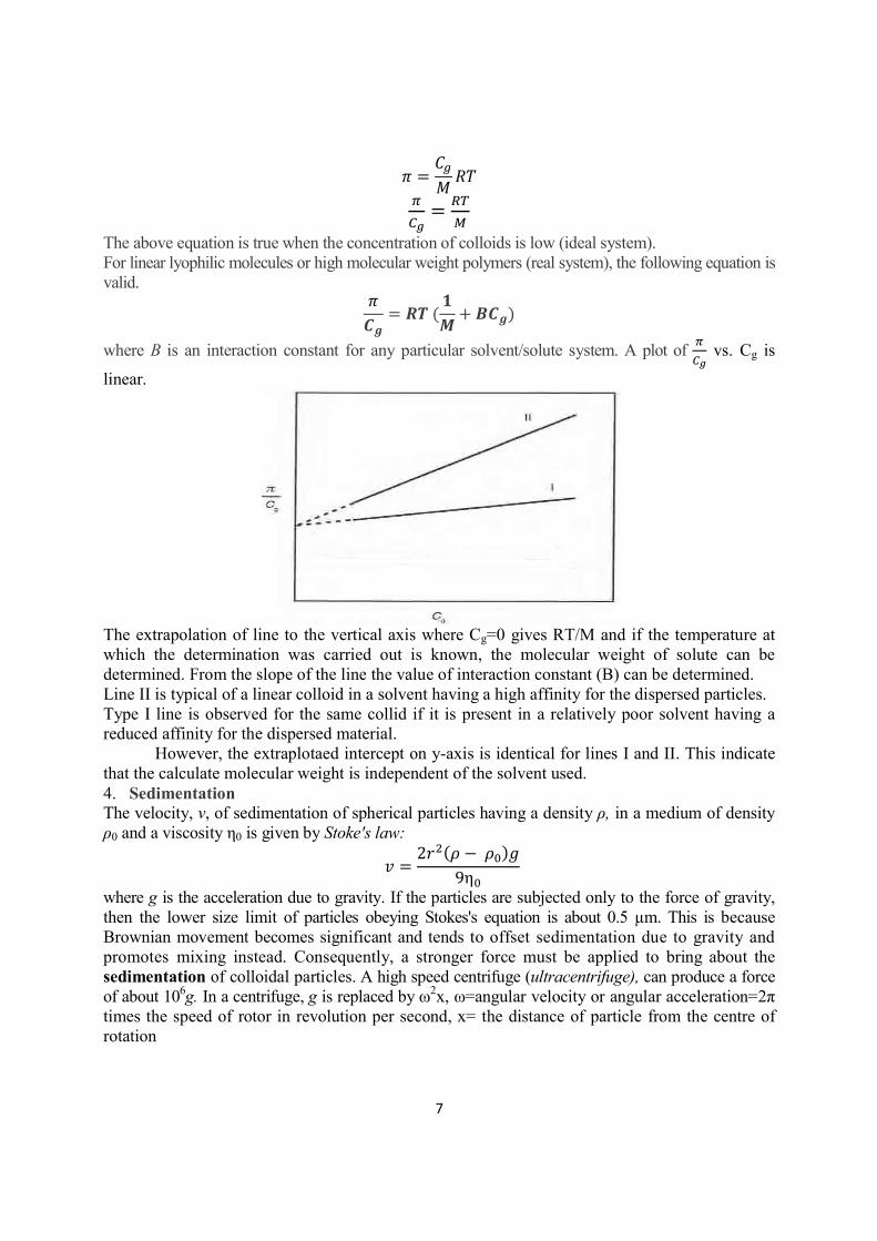
where B is an interaction constant for any particular solvent/solute system. A plot of vs. Cg is

linear.

The extrapolation of line to the vertical axis where Cg=0 gives RT/M and if the temperature at which the determination was carried out is known, the molecular weight of solute can be determined. From the slope of the line the value of interaction constant (B) can be determined. Line II is typical of a linear colloid in a solvent having a high affinity for the dispersed particles. Type I line is observed for the same collid if it is present in a relatively poor solvent having a reduced affinity for the dispersed material.

However, the extraplotaed intercept on y-axis is identical for lines I and II. This indicate that the calculate molecular weight is independent of the solvent used. 4. Sedimentation The velocity, v, of sedimentation of spherical particles having a density ρ, in a medium of density ρ0 and a viscosity η0 is given by Stoke's law:

𝑣 =2𝑟 (𝜌 − 𝜌 )𝑔

9η

where g is the acceleration due to gravity. If the particles are subjected only to the force of gravity, then the lower size limit of particles obeying Stokes's equation is about 0.5 µm. This is because Brownian movement becomes significant and tends to offset sedimentation due to gravity and promotes mixing instead. Consequently, a stronger force must be applied to bring about the sedimentation of colloidal particles. A high speed centrifuge (ultracentrifuge), can produce a force of about 106g. In a centrifuge, g is replaced by ω2x, ω=angular velocity or angular acceleration=2π times the speed of rotor in revolution per second, x= the distance of particle from the centre of rotation

8

𝑣 =𝑑𝑥

𝑑𝑡=

2𝑟 (𝜌 − 𝜌 )ω 𝑥

9η

5. Viscosity Einstein equation of flow for the colloidal dispersions of spherical particles is given by:

η = η (1 + 2.5ϕ) η0 is the viscosity of dispersion medium, η is the viscosity of dispersion when volume fraction of colloid particles is ϕ. The volume fraction is defined as the volume of the panicles divided by the total volume of the dispersion. Relative viscosity (ηrel) =

η

η = 1 + 2.5ϕ

Specific viscosity (ηsp ) = η

η− 1 = 2.5ϕ

or η

ϕ= 2.5

By determining η at various concentration and knowing η0 the specific viscosity can be calculated.

Because the volume fraction is directly related to concentration, we can write, η

= K, where C

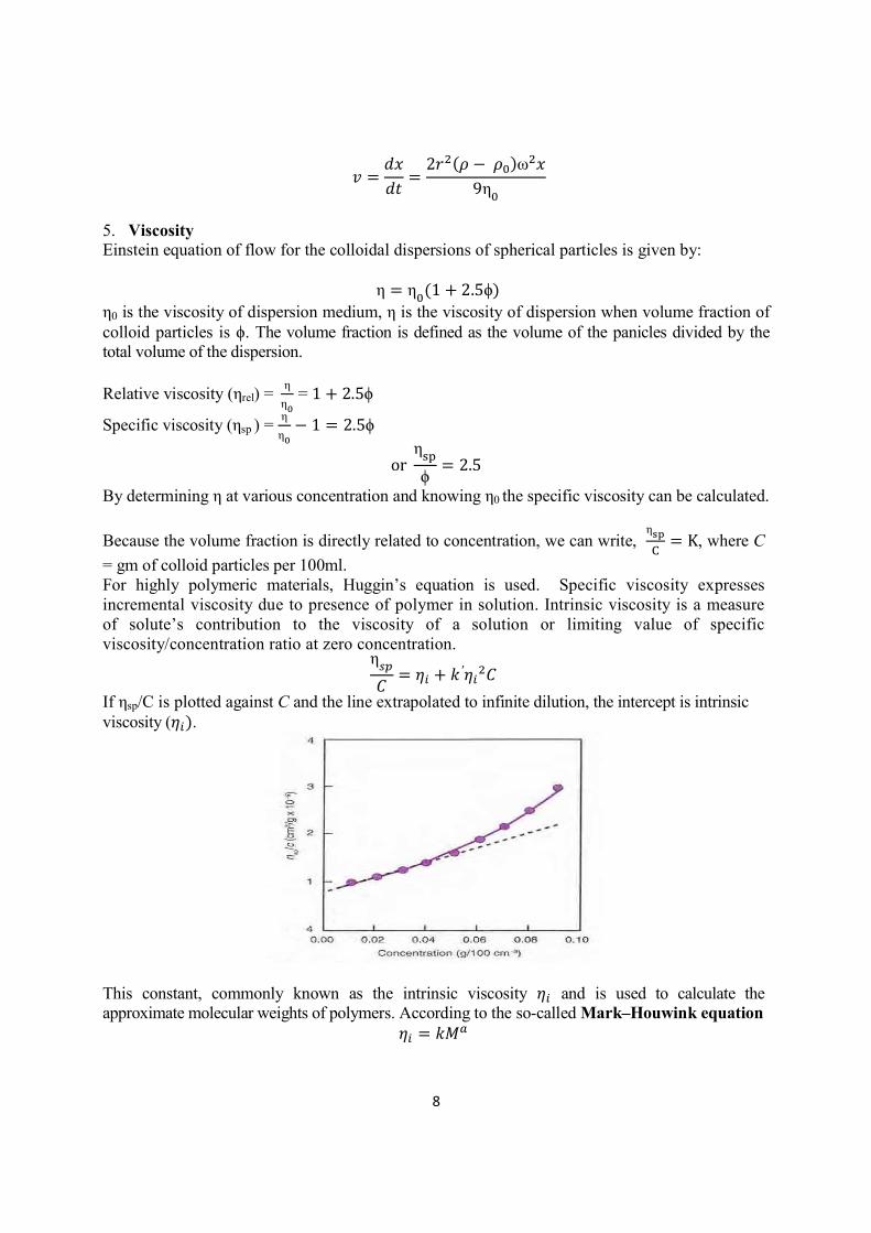
= gm of colloid particles per 100ml. For highly polymeric materials, Huggin’s equation is used. Specific viscosity expresses incremental viscosity due to presence of polymer in solution. Intrinsic viscosity is a measure of solute’s contribution to the viscosity of a solution or limiting value of specific viscosity/concentration ratio at zero concentration.

η

𝐶= 𝜂 + 𝑘′𝜂 𝐶

If ηsp/C is plotted against C and the line extrapolated to infinite dilution, the intercept is intrinsic viscosity (𝜂 ).

This constant, commonly known as the intrinsic viscosity 𝜂 and is used to calculate the approximate molecular weights of polymers. According to the so-called Mark–Houwink equation

𝜂 = 𝑘𝑀

9

Where k and a are constants, characteristics of a particular polymer-solvent system and are virtually independent of molecular weight.

log 𝜂 = log 𝑘 + 𝑎𝑙𝑜𝑔 𝑀 These constants are obtained initially by determining 𝜂 experimentally for polymer fractions whose molecular weights have been determined by other methods such as light scattering, osmotic pressure, or sedimentation. Then the specific viscosity for each fraction is determined and then intrinsic viscosity can be obtained.

If we plot log 𝜂 𝑣𝑠. log M 𝑡ℎ𝑒𝑛 𝑡ℎ𝑒 𝑠𝑙𝑜𝑝𝑒 𝑤𝑖𝑙𝑙 𝑔𝑖𝑣𝑒 ′𝑎 𝑣𝑎𝑙𝑢𝑒 𝑎𝑛𝑑

𝑡ℎ𝑒 𝑖𝑛𝑡𝑒𝑟𝑐𝑒𝑝𝑡 𝑤𝑖𝑙𝑙 𝑔𝑖𝑣𝑒 ′𝑘′ 𝑣𝑎𝑙𝑢𝑒.

Then, the molecular weight (M) of unknown fraction of the polymer can be obtained from Mark–Houwink equation.

Electrical properties of Colloids

The colloidal particles acquire a surface electric charge when brought into contact with an aqueous medium. The principal charging mechanisms are discussed below. 1. Surface Ionization Here the charge is controlled by the ionization of surface groupings. For example, carboxymethyl cellulose frequently has carboxylic acid groupings at the surface which ionize to give negatively charged particles. Amino acids and proteins acquire their charge mainly through the ionization of carboxyl and amino groups to give –COO- and NH3

+ ions. The ionization of these groups and hence the net molecular charge depends on the pH of the system. At a pH below the pKa of the COO- group the protein will be positively charged because of the protonation of this group, -COO- —> COOH, and the ionization of the amino group -NH2 —> -NH3

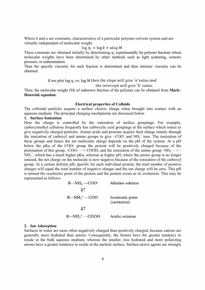
+, which has a much higher pKa; whereas at higher pH, where the amino group is no longer ionized, the net charge on the molecule is now negative because of the ionization of the carboxyl group. At a certain definite pH, specific for each individual protein, the total number of positive charges will equal the total number of negative charges and the net charge will be zero. This pH is termed the isoelectric point of the protein and the protein exists as its zwitterion. This may be represented as follows:

2. Ion Adsorption Surfaces in water are more often negatively charged than positively charged, because cations are generally more hydrated than anions. Consequently, the former have the greater tendency to reside in the bulk aqueous medium, whereas the smaller, less hydrated and more polarizing anions have a greater tendency to reside at the particle surface; Surface-active agents are strongly

10

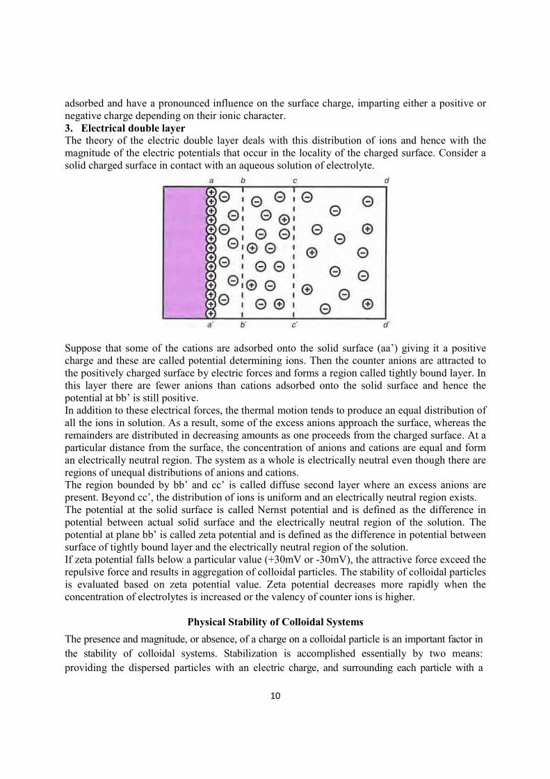
adsorbed and have a pronounced influence on the surface charge, imparting either a positive or negative charge depending on their ionic character. 3. Electrical double layer The theory of the electric double layer deals with this distribution of ions and hence with the magnitude of the electric potentials that occur in the locality of the charged surface. Consider a solid charged surface in contact with an aqueous solution of electrolyte.

Suppose that some of the cations are adsorbed onto the solid surface (aa’) giving it a positive charge and these are called potential determining ions. Then the counter anions are attracted to the positively charged surface by electric forces and forms a region called tightly bound layer. In this layer there are fewer anions than cations adsorbed onto the solid surface and hence the potential at bb’ is still positive. In addition to these electrical forces, the thermal motion tends to produce an equal distribution of all the ions in solution. As a result, some of the excess anions approach the surface, whereas the remainders are distributed in decreasing amounts as one proceeds from the charged surface. At a particular distance from the surface, the concentration of anions and cations are equal and form an electrically neutral region. The system as a whole is electrically neutral even though there are regions of unequal distributions of anions and cations. The region bounded by bb’ and cc’ is called diffuse second layer where an excess anions are present. Beyond cc’, the distribution of ions is uniform and an electrically neutral region exists. The potential at the solid surface is called Nernst potential and is defined as the difference in potential between actual solid surface and the electrically neutral region of the solution. The potential at plane bb’ is called zeta potential and is defined as the difference in potential between surface of tightly bound layer and the electrically neutral region of the solution. If zeta potential falls below a particular value (+30mV or -30mV), the attractive force exceed the repulsive force and results in aggregation of colloidal particles. The stability of colloidal particles is evaluated based on zeta potential value. Zeta potential decreases more rapidly when the concentration of electrolytes is increased or the valency of counter ions is higher.

Physical Stability of Colloidal Systems

The presence and magnitude, or absence, of a charge on a colloidal particle is an important factor in the stability of colloidal systems. Stabilization is accomplished essentially by two means: providing the dispersed particles with an electric charge, and surrounding each particle with a

11

protective solvent sheath that prevents mutual adherence when the particles collide as a result of Brownian movement. This second effect is significant only in the case of lyophilic sols.

Stability of lyophobic colloids A lyophobic sol is thermodynamically unstable. The particles in such cols are stabilized only by the presence of electric charges on their surfaces. The like charges produce a repulsion that prevents coagulation of the particles. Hence, addition of a small amount of electrolyte to a lyophobic sol tends to stabilize the system by imparting a charge to the particles.

In colloidal dispersions frequent encounters between the particles occur as a result of Brownian movement. Such interactions are mainly responsible for the stability of colloids. There are two types of interactions- van der Waals attraction and electrostatic repulsions. When attractions predominate, the particles adhere after collisions and aggregate is formed. When repulsions predominate, the particles rebound after collisions and remain individually dispersed.

At low electrolyte concentration, repulsive forces predominate so that the particles experience only repulsive forces upon approach. The particles remain independent and the system is considered dispersed or peptized. At high electrolyte concentration, the double layer repulsive forces are greatly reduced, so that van de Waals attractive forces predominate. These net attractive forces between particles cause the formation of aggregate of particles, a process known as coagulation. The concentration of electrolyte necessary, to collapse the repulsive force and permit coagulation depends on the valence of ions of opposite charge. Schulze-hardy rule states that the precipitation power of an ion on dispersed phase of opposite charge increases with increase in valence or charge of the ion. The higher the valency of ion, the greater is the precipitation power. Cations: Al+3> Ba+2> Na+ Anions: SO4

2- > Cl-

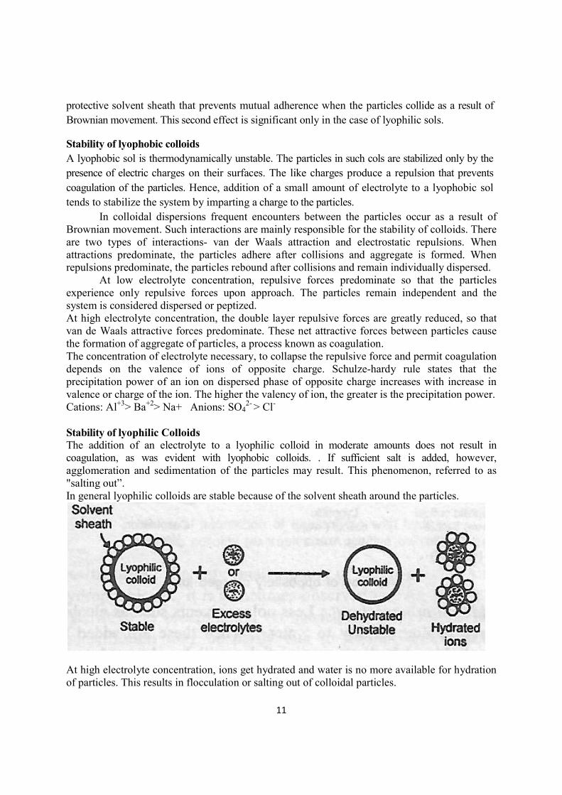
Stability of lyophilic Colloids The addition of an electrolyte to a lyophilic colloid in moderate amounts does not result in coagulation, as was evident with lyophobic colloids. . If sufficient salt is added, however, agglomeration and sedimentation of the particles may result. This phenomenon, referred to as "salting out”. In general lyophilic colloids are stable because of the solvent sheath around the particles.

At high electrolyte concentration, ions get hydrated and water is no more available for hydration of particles. This results in flocculation or salting out of colloidal particles.

12

The coagulating power of an ion is directly related to the ability of that ion to separate water molecules from colloidal particles. Hofmeister or lyotropic series ranks cations and anions in order of coagulation of hydrophilic sols. Anions: citrate>tartrate>sulfate>acetate>chloride>nitrate> bromine>iodine Cations: Mg+2>Ca+2>Ba+2>Na+>K+

Less polar solvents such as alcohol, acetone has greater affinity to water. When these are added to hydrophilic colloids, dehydration of particles occurs. Now the stability of particles depends on charge they carry. The addition of even small amount of electrolytes leads to flocculation or salting out the colloid easily. Coacervation When negatively and positively charged hydrophilic colloids are mixed, the particles may separate from the dispersion to form a layer rich in the colloidal aggregates. The colloid-rich layer is known as a coacervate, and the phenomenon in which macromolecular solutions separate into two liquid layers is referred to as coacervation. As an example, consider the mixing of gelatin and acacia. Gelatin at a pH below 4.7 (its isoelectric point) is positively charged; acacia carries a negative charge that is relatively unaffected by pH in the acid range, When solutions of these colloids are mixed in a certain proportion, coacervation results. The viscosity of the upper layer, now poor in colloid, is markedly decreased. The lower layer becomes rich in the coacervate.

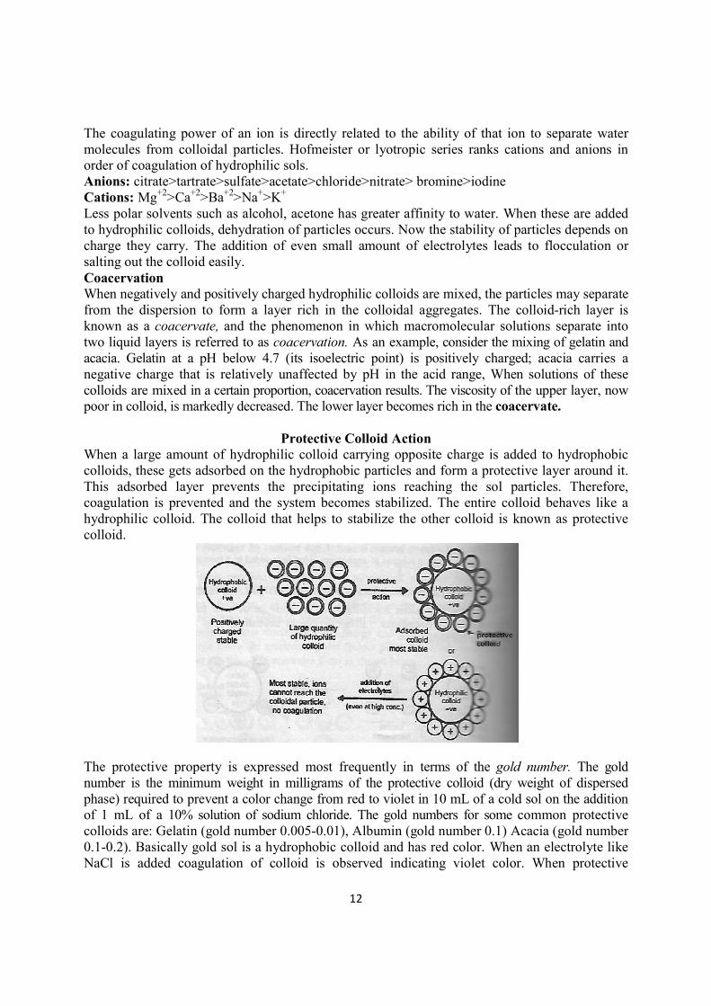
Protective Colloid Action

When a large amount of hydrophilic colloid carrying opposite charge is added to hydrophobic colloids, these gets adsorbed on the hydrophobic particles and form a protective layer around it. This adsorbed layer prevents the precipitating ions reaching the sol particles. Therefore, coagulation is prevented and the system becomes stabilized. The entire colloid behaves like a hydrophilic colloid. The colloid that helps to stabilize the other colloid is known as protective colloid.

The protective property is expressed most frequently in terms of the gold number. The gold number is the minimum weight in milligrams of the protective colloid (dry weight of dispersed phase) required to prevent a color change from red to violet in 10 mL of a cold sol on the addition of 1 mL of a 10% solution of sodium chloride. The gold numbers for some common protective colloids are: Gelatin (gold number 0.005-0.01), Albumin (gold number 0.1) Acacia (gold number 0.1-0.2). Basically gold sol is a hydrophobic colloid and has red color. When an electrolyte like NaCl is added coagulation of colloid is observed indicating violet color. When protective

13

colloids are added, these stabilize the gold sol and prevent the change to violet color. Lower the gold number, greater the protective action.

Reference:

Martin’s Physical Pharmacy and Pharmaceutical Sciences: physical, chemical and biopharmaceutical principles in the pharmaceutical sciences. 6th edition. Editors: Patrick J Sinko, Yashveer Singh. Wolters Kluwer Health, Lippincott Williams & Wilkins, Philadelphia, 2006.