WHOI-2010-03

Woods Hole Oceanographic Institution

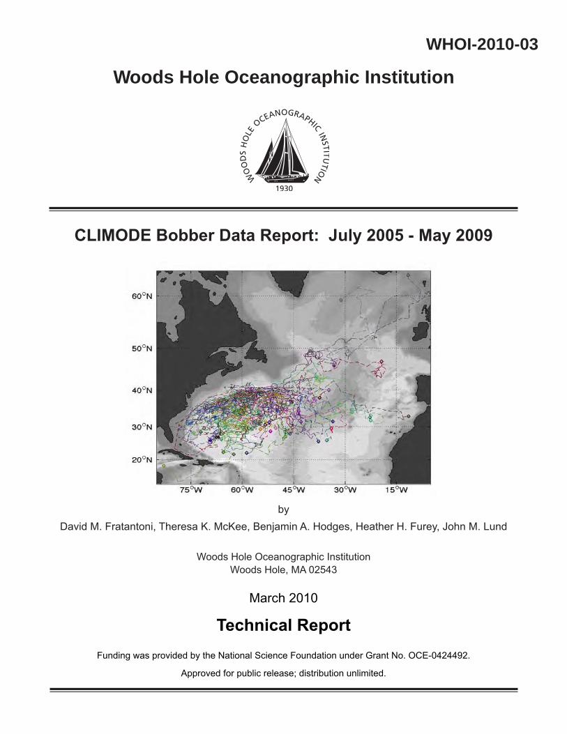
CLIMODE Bobber Data Report: July 2005 - May 2009

byDavid M. Fratantoni, Theresa K. McKee, Benjamin A. Hodges, Heather H. Furey, John M. Lund

Woods Hole Oceanographic Institution Woods Hole, MA 02543

March 2010

Technical ReportFunding was provided by the National Science Foundation under Grant No. OCE-0424492.

Approved for public release; distribution unlimited.

WHOI 2010·03

CLIMODE Bobber Data Report: July 2005 - May 2009

by

David M. Fratantoni, Theresa K. McKee, Benjamin A. Hodges, Heather H. Furey, John M. Lund

Woods Hole Oceanographic Institution Woods Hole, Massachusetts 02543

March 2010

Technical Report

Funding was provided by the National Science Foundation through Grant #OCE-0424492.

Reproduction in whole or in part is permitted for any purpose of the United States Government. This report should be cited as Woods Hole Oceanographic Institution Tech. Report, WHOI-2010-03.

Approved for public release; distribution unlimited.

Approved for Distribution:

Robert A. Weller, Chair

Department of Physical Oceanography

2

Abstract This report summarizes direct observations of Eighteen Degree Water (EDW) subduction and dispersal within the subtropical gyre of the North Atlantic Ocean. Forty acoustically-tracked bobbing, profiling floats (“bobbers”) were deployed to study the formation and dispersal of EDW in the western North Atlantic. The unique bobber dataset described herein provides insight into the evolution of EDW by means of direct, eddy-resolving measurement of EDW Lagrangian dispersal pathways and stratification. Bobbers are modified Autonomous Profiling Explorer (APEX) profiling floats which actively servo their buoyancy control mechanism to follow a particular isothermal surface. The CLIVAR Mode Water Dynamics Experiment (CLIMODE) bobbers tracked the 18.5oC temperature surface for 3 days, then bobbed quickly between the 17oC and 19oC isotherms. This cycle was repeated for one month, after which each bobber profiled to 1000 m before ascending to the surface to transmit data. The resulting dataset (37/40 tracked bobbers; more than half still profiling as of January 2010) yields well-resolved trajectories, unprecedented velocity statistics in the core of the subducting and spreading EDW, and detailed information about the Lagrangian evolution of EDW thickness and vertical structure. This report provides an overview of the experimental procedure employed and summarizes the initial processing of the bobber dataset.

3

Table of Contents 1. Introduction .................................................................................................................... 4 2. Methods.......................................................................................................................... 4 3. System Performance ...................................................................................................... 7 4. Data Processing .............................................................................................................. 8 5. Acknowledgements ...................................................................................................... 12 6. References .................................................................................................................... 12 Figure 1: CLIMODE bobbers being prepared for deployment aboard R/V Oceanus ........ 4 Figure 2: Location of RAFOS sound sources during the CLIMODE experiment ............ 5 Figure 3: Timeline of bobber deployments ........................................................................ 7 Figure 4: Samples of poor quality TOAs and excellent quality TOAs ............................ 10 Figure 5: Trajectories of the CLIMODE bobbers ............................................................ 11 Table 1: Bobber Launch Deployment Times and Positions ............................................ 13 Table 2: Sound Source Deployment Positions and Times ............................................... 14 Table 3: List of ARGOS Transmissions That Required Manual Repair of Messages .... 15 Table 4: Duration and Rate of Success of ARGOS Transmissions ................................ 16 Table 5: Float Clock Drift (ARGOS Time – Float Clock Time) for 37 Tracked Floats . 17 Table 6: Percentage of TOAs That Resulted in Acceptable Positions............................. 18 Appendix A: Mooring and Bobber Deployment/Recovery Schedule ............................. 19 Appendix B: CLIMODE Mooring Diagrams .................................................................. 20 Appendix C: Sample Sound Source File Entry................................................................ 24 Appendix D: Sample TOA File ....................................................................................... 25 Appendix E: Bobber ID Cross-Reference ........................................................................ 27 Appendix F: Sound Source Clock Drift Calculations ...................................................... 28 Appendix G: Bobber Trajectories and Profiles ................................................................ 29 Appendix H: Bobber TOAs and Engineering Data ....................................................... 111

4

1. Introduction Eighteen Degree Water (EDW) is the archetype for the anomalously thick and vertically homogenous mode waters that are typical of all subtropical western boundary current systems. EDW is associated with a shallow overturning circulation that carries heat northward and is an interannual reservoir of anomalous heat, nutrients and CO2. Understanding the annual cycle of EDW evolution, and in particular its associated circulation pathways and destruction mechanisms, is important because though EDW is isolated beneath the stratified upper-ocean at the end of each winter, it may reemerge in subsequent years to influence mixed layer properties and consequently air-sea interaction and primary productivity. Prior to this experiment, little was known about the physical mechanisms which redistribute EDW from its formation region near the Gulf Stream throughout the subtropical gyre. The CLIVAR Mode Water Dynamics Experiment (CLIMODE) field campaign included five research cruises conducted between November, 2005 and November, 2007, including two mid-winter cruises in the Gulf Stream. This program resulted in the most comprehensive data set of EDW-related measurements ever collected, including air-sea fluxes, detailed observations within the Gulf Stream, and broader-scale measurements of circulation and stratification throughout the subtropical gyre. As part of this effort, 40 acoustically-tracked bobbing, profiling floats (“bobbers”) were deployed to study the formation and dispersal of EDW in the western North Atlantic. The resulting dataset described herein yields well-resolved trajectories, unprecedented velocity statistics in the core of the subducting and spreading EDW, and detailed information about the Lagrangian evolution of EDW thickness and vertical structure.

2. Methods The acoustically-tracked bobbers are modified Autonomous Profiling Explorers ((APEX); Teledyne Webb Research, E. Falmouth, MA) profiling floats reprogrammed to actively servo their buoyancy control mechanism to follow a particular isothermal surface (Figure 1). In addition to custom software, the bobbers were outfitted with temperature and pressure sensors and a Receiver in Floats (RAFOS) hydrophone and audio acquisition system which detected and recorded the arrival times of acoustic transmissions from several moored sound sources. The aluminum pressure hulls were also specifically machined for a maximum operating depth of 1000 m. Figure 1. Several CLIMODE bobbers being

prepared for deployment aboard R/V Oceanus.

5

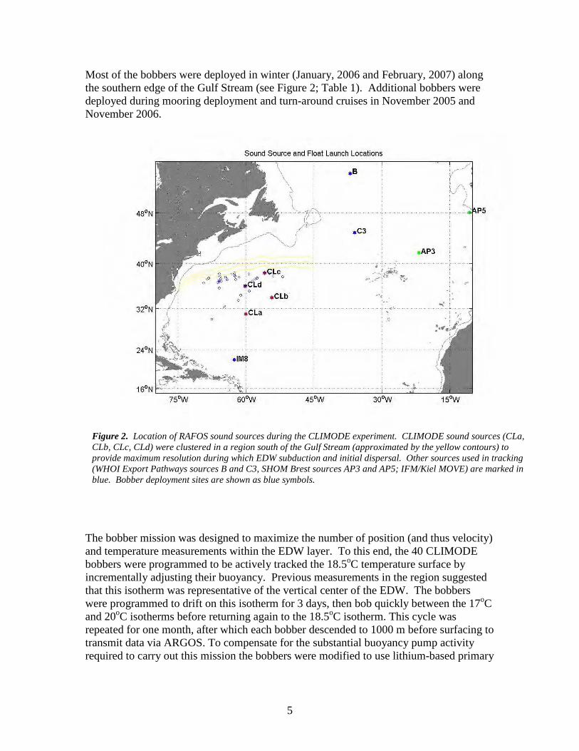
Most of the bobbers were deployed in winter (January, 2006 and February, 2007) along the southern edge of the Gulf Stream (see Figure 2; Table 1). Additional bobbers were deployed during mooring deployment and turn-around cruises in November 2005 and November 2006.

The bobber mission was designed to maximize the number of position (and thus velocity) and temperature measurements within the EDW layer. To this end, the 40 CLIMODE bobbers were programmed to be actively tracked the 18.5oC temperature surface by incrementally adjusting their buoyancy. Previous measurements in the region suggested that this isotherm was representative of the vertical center of the EDW. The bobbers were programmed to drift on this isotherm for 3 days, then bob quickly between the 17oC and 20oC isotherms before returning again to the 18.5oC isotherm. This cycle was repeated for one month, after which each bobber descended to 1000 m before surfacing to transmit data via ARGOS. To compensate for the substantial buoyancy pump activity required to carry out this mission the bobbers were modified to use lithium-based primary

Figure 2. Location of RAFOS sound sources during the CLIMODE experiment. CLIMODE sound sources (CLa, CLb, CLc, CLd) were clustered in a region south of the Gulf Stream (approximated by the yellow contours) to provide maximum resolution during which EDW subduction and initial dispersal. Other sources used in tracking (WHOI Export Pathways sources B and C3, SHOM Brest sources AP3 and AP5; IFM/Kiel MOVE) are marked in blue. Bobber deployment sites are shown as blue symbols.

6

batteries instead of the more common alkaline packs. Briefly, the rules used to construct the bobber’s mission were as follows:

1. Drift at 18.5oC +/- 0.2oC. Seek target isotherm hourly and adjust if out of band. If the 18.5oC does not exist or is shallower than 50 m, drift at 50 m. (The intent was to prevent bobbers from drifting for extended periods at the sea surface. The 50 m depth was assumed to be removed from the surface, yet representative of the surface mixed layer).

2. Once every 3 days, bob between 17oC and 20oC. If 17oC does not exist, bob to

500 m. If 20oC does not exist, bob to surface.

3. Once every 30 days perform at 1000 m then surface to transmit data.

4. Acquire temperature-depth samples according to a single 40-point lookup table on all upward profiles (including bobs). Vertical measurement resolution varied from 5 m near the surface to 20 m at depth.

5. Acquire one additional temperature-depth sample daily at the conclusion of the acoustic listening window.

6. Allow one, two-hour acoustic listening window per day (0000, 0030, 0100, 0130

Universal Time Coordinated (UTC)) and record the highest four correlation heights and time-of-arrivals (TOAs) within this window.

Two of the bobbers were used for system testing and were programmed to cycle more frequently with deep profiles and surfacing occurring after 12 days instead of the normal 30 days. Bobber 37518 was deployed by Jim Ledwell in July 2005 within a mesoscale eddy south of Bermuda. This unit was deployed prior to installation of the CLIMODE sound source array and did not receive any acoustic transmissions. A second test unit, 39476, was deployed in January 2006. An acoustic source array consisting of four University of Rhode Island/Graduate School of Oceanography RAFOS sound sources was deployed in November 2005 on R/V Oceanus cruise OC419 (Figure 2; Table 2). Additional sources deployed by other investigators from the U.S., France, and Germany were heard by the bobbers and subsequently used during acoustic tracking. The four CLIMODE sound sources were recovered in November, 2007. The bobbers continued to transmit satellite positions through June 1, 2009, when Service ARGOS real-time data delivery was terminated. More than half of the bobbers were still operating as of January 2010. This profile data will be recovered and processed at a later date.

7

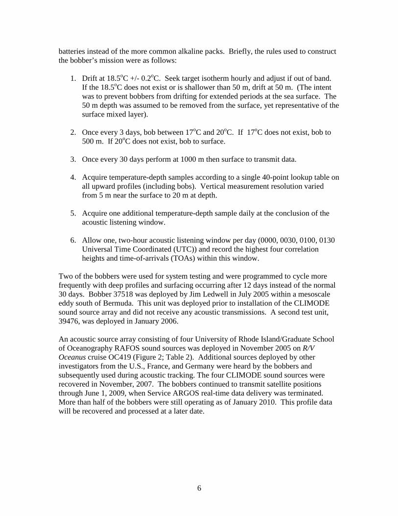
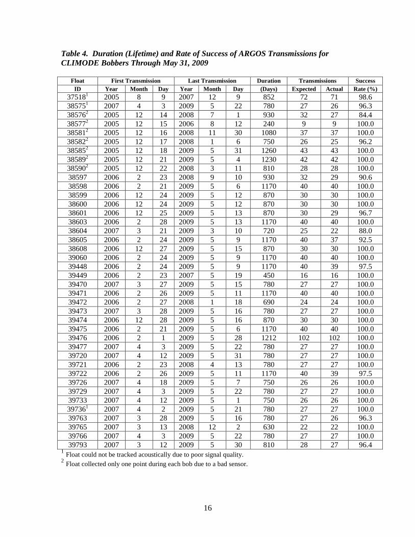
3. System Performance Figure 3 presents a timeline of the ARGOS transmissions from the 40 CLIMODE bobbers. Overall success rate was quite high with 98% of the transmissions during the bobber’s lifetime being complete enough to extract most or all acoustic data and temperature profiles. Thirty seven of the 40 floats could be acoustically tracked for all or some of their lifetime. Three floats (37518, 38575, and 39736) had consistently poor quality acoustic TOAs and could not be tracked. Seven floats (Table 4) were constructed with a faulty pressure sensor that caused only one measurement to be taken during each profile.

Figure 3. Timeline of bobber deployments. Red squares indicate deployment times. Filled gray squares indicate successful ARGOS transmissions with acoustic data and profiles. Unfilled gray squares indicate incomplete ARGOS transmissions that did not yield profiles. Blanks indicate failed transmissions, i.e., no message received or the message received was inadequate to provide any acoustic or profile data. Numbers on the vertical axes are bobber ARGOS IDs.

8

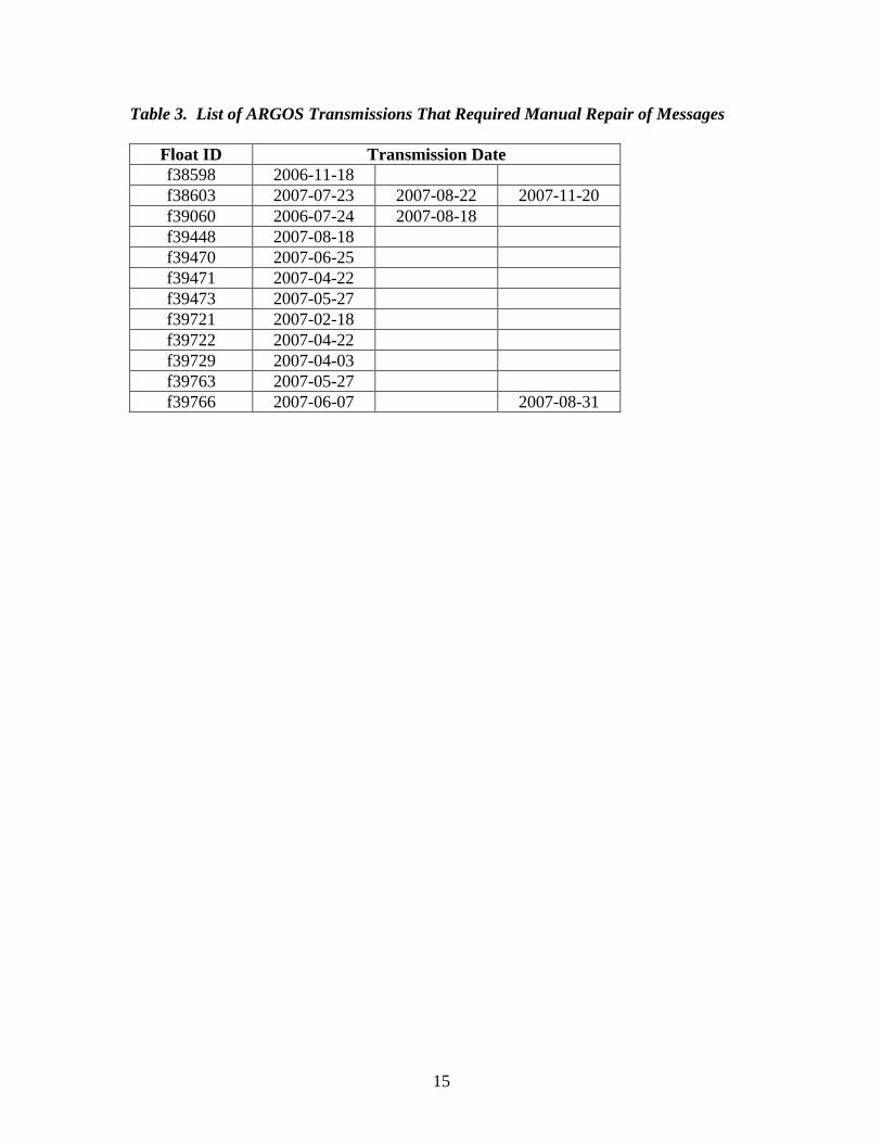
Occasionally, an incomplete message would require special handling in order to salvage data. In these cases, an attempt was made to manually repair the corrupted hex format to enable the parsing program to decode the acoustic data and profiles. This effort improved the data yield for these floats and transmission dates (Table 3).

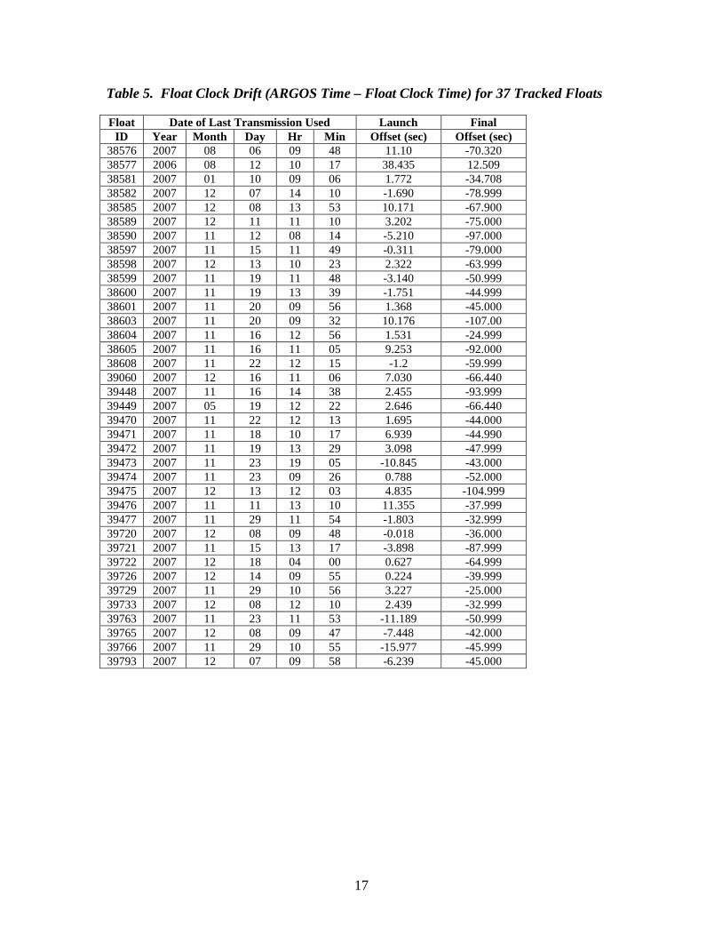
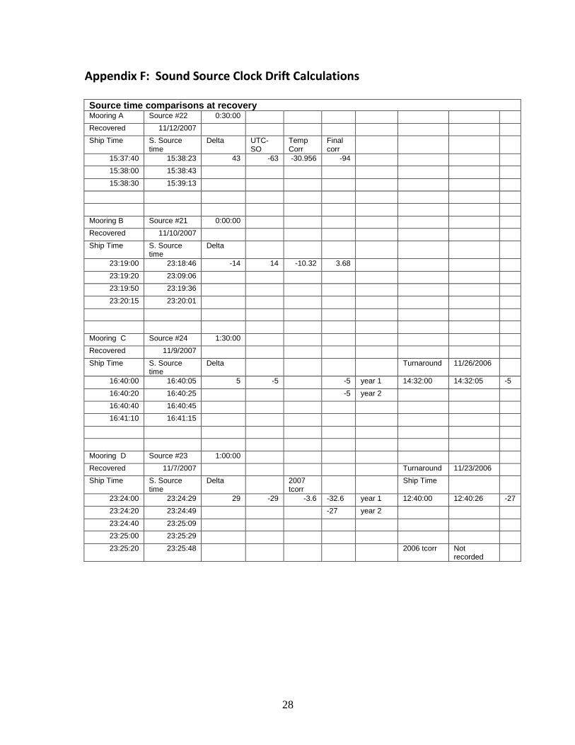
4. Data Processing Initial processing of the ARGOS message was accomplished on a Linux server through an automated process consisting of a series of shell, PERL, and Matlab scripts. Mail messages were read and combined to create a complete package of information, from which could be derived time and engineering information, acoustic signals (TOA and correlation heights), ambient temperature and pressure at the time the acoustic signal was received, and temperature and pressure profiles. Temperature profiles and engineering data were manually quality-controlled to remove obvious outliers. TOA (with ambient temperature and pressure) and profiles were extracted to separate files, and a float clock offset for each transmission interval was determined by comparing satellite time to float clock time. Start and final offsets were computed to be applied during the tracking process to correct the float clock. Float clocks tended to get slower over their lifetime in a mostly linear progression. A list of the clock offsets for each float can be seen in Table 5. Float clock drift was much larger than traditional RAFOS/DLD2 floats (57 second mean absolute offset versus < 2 second offset over approximately two years). In addition to correcting for float clock drift, it was essential to supply a correction for sound source clock drift within the sound source information file used as input. The drift was determined by comparing source clock times with UTC from the global positioning system (GPS). All sound source clocks with the exception of Source 21 (Mooring B) were fast. A single drift correction was applied to sources A and B, however source C and D were handled in two pieces since the clocks were reset when the batteries were replaced in November, 2006. Using an equation provided by George Schwartze (Graduate School of Oceanography, University of Rhode Island), the adjustments were computed as follows:

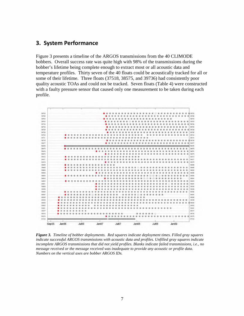
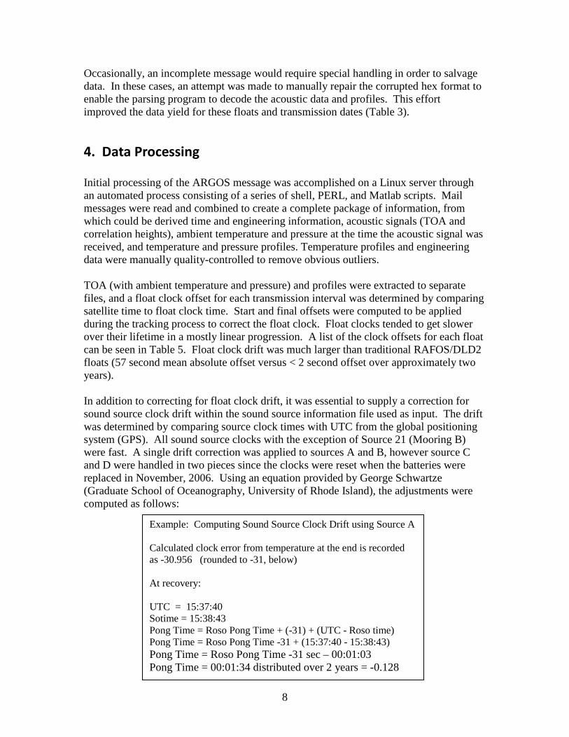
Example: Computing Sound Source Clock Drift using Source A Calculated clock error from temperature at the end is recorded as -30.956 (rounded to -31, below) At recovery: UTC = 15:37:40 Sotime = 15:38:43 Pong Time = Roso Pong Time + (-31) + (UTC - Roso time) Pong Time = Roso Pong Time -31 + (15:37:40 - 15:38:43) Pong Time = Roso Pong Time -31 sec – 00:01:03 Pong Time = 00:01:34 distributed over 2 years = -0.128

9

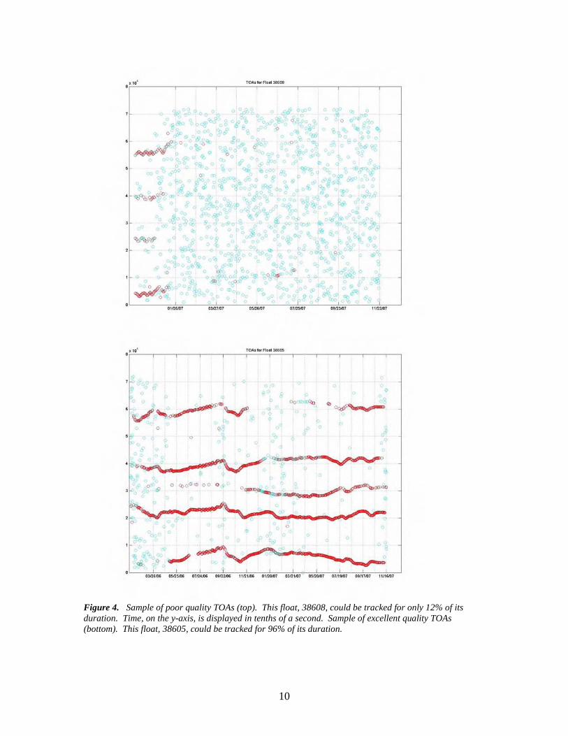
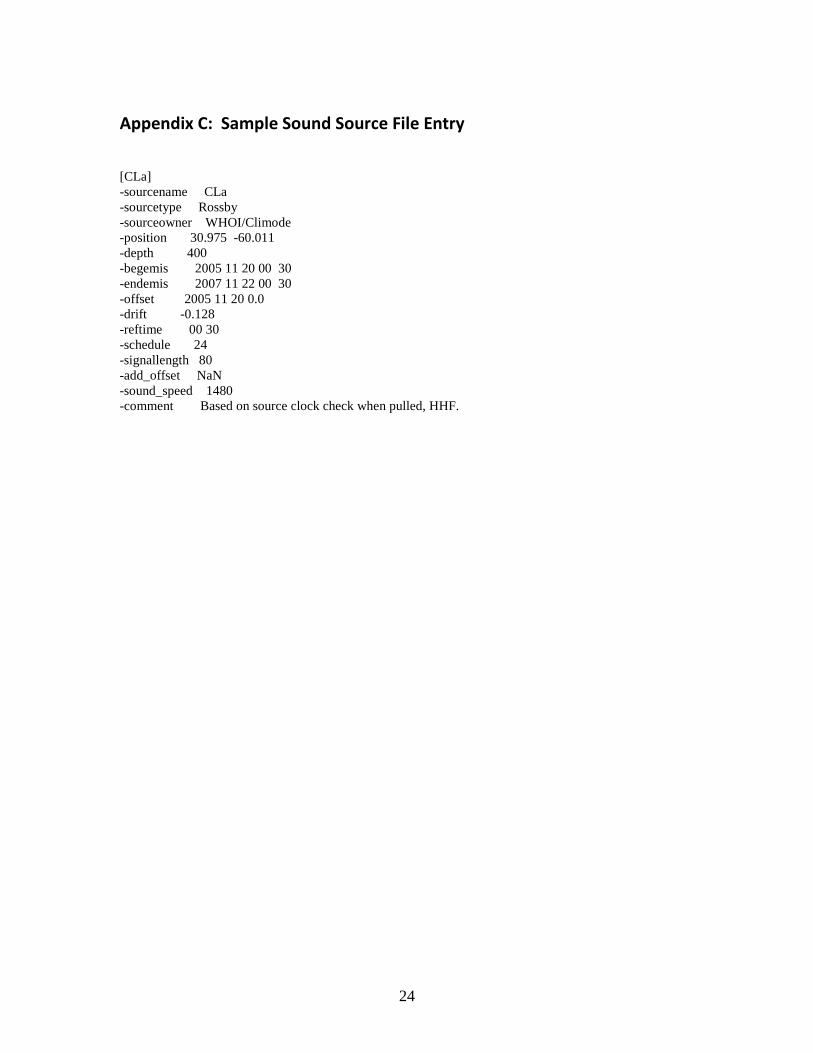
The CLIMODE sound source information file is included in the Appendix as is full documentation on sound source clock error. Calculations for corrections to all sources are contained in a spreadsheet in the Appendix. Floats were tracked using Matlab-based ARTOA3 software (Wooding et al., 2005; http://www.whoi.edu/science/PO/rafos/). Prior to tracking, a sound source file containing sound source positions, depth, signal time, schedule, and length was prepared as input. In addition, for each float, a file containing TOAs and correlation heights, daily temperature and pressure, and precise header information identifying start and end times and positions, number of cycles, and float clock offset also was assembled. After loading these files into the ARTOA program, the first step was to edit pressure and temperature recorded with each acoustic transmission to remove outliers that would adversely influence sound speed calculations. Next, highest quality TOAs were manually selected and applied to the appropriate sound source. TOAs were corrected for the Doppler shift and difference in transmission time, and then interpolated using variable width (10–30 days) linear or cubic-spline filter before tracking. Tracking used a least-squares method if more than two TOAs were available. Satellite positions were plotted over the tracks to check for agreement. The length and type of interpolation were adjusted to improve the agreement between the satellite positions and the tracked position. Determining sound velocity for these data proved to be challenging. Since floats received acoustic transmissions while traveling through different water masses, sound velocities varied substantially. There was no way to accurately determine these changes, so a certain amount of experimentation was used. The chosen velocities varied between 1.48 and 1.52 km/sec. For some floats, it was necessary to adjust the sound velocity over sections of the track to improve the fit, as floats travelled through very different water regimes (e.g., from the Sargasso Sea to the Iceland Basin). Differences between the tracked positions and the satellite positions were computed regularly during the tracking process, and, if the tracked position was not within 20 km of the satellite position, a section of the track was excised and not interpolated. Average differences were in the 5 to 10 km range overall. This was deemed acceptable and can be explained by resolution of the satellite position and by currents carrying the surfaced float away from the last acoustically-tracked position. Various checks were made to determine if poor agreement was related to incorrect clock drift calculations, distance from source, geographic location, season, or the depth of the float when it received the acoustic signal. Results indicated that proximity to the Gulf Stream contributed to inaccuracies in the tracking, but more frequently tracking errors were caused by loss of TOAs due to obstructions (Bermuda) or to baseline problems occurring when the float was in a direct line with two sound sources (Figure 4). A German sound source (IM8), located south of Bermuda (at 21.938˚N, 62.569˚W) at a depth of 1100m, proved to be very helpful in tracking many of the floats. Though we could not construct up-to-date information on clock drift for this source, it was often used to locate sections of track that the CLIMODE sources could not resolve. Floats that traveled near Bermuda required sources IM8; north and east of the tail of the Grand Banks required C3 and B. AP8 and AP3 were heard only

10

Figure 4. Sample of poor quality TOAs (top). This float, 38608, could be tracked for only 12% of its duration. Time, on the y-axis, is displayed in tenths of a second. Sample of excellent quality TOAs (bottom). This float, 38605, could be tracked for 96% of its duration.

11

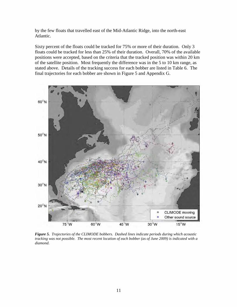
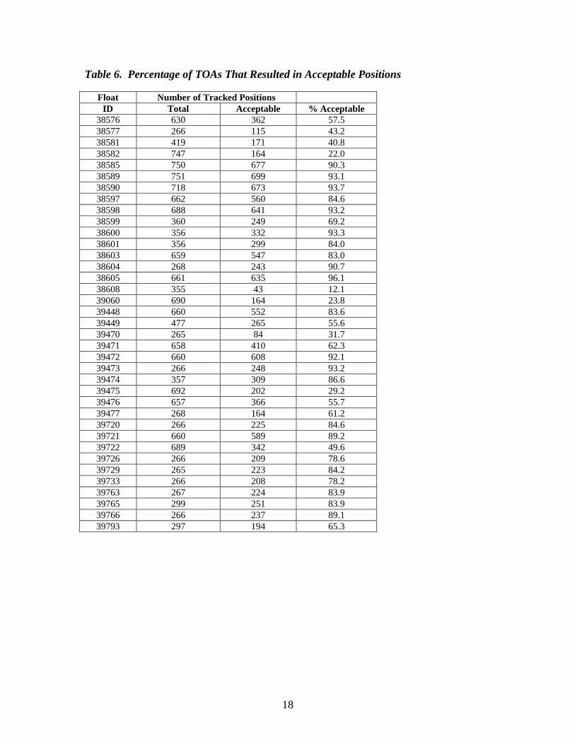
by the few floats that travelled east of the Mid-Atlantic Ridge, into the north-east Atlantic. Sixty percent of the floats could be tracked for 75% or more of their duration. Only 3 floats could be tracked for less than 25% of their duration. Overall, 70% of the available positions were accepted, based on the criteria that the tracked position was within 20 km of the satellite position. Most frequently the difference was in the 5 to 10 km range, as stated above. Details of the tracking success for each bobber are listed in Table 6. The final trajectories for each bobber are shown in Figure 5 and Appendix G.

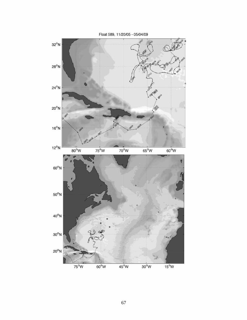
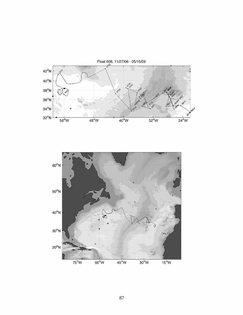
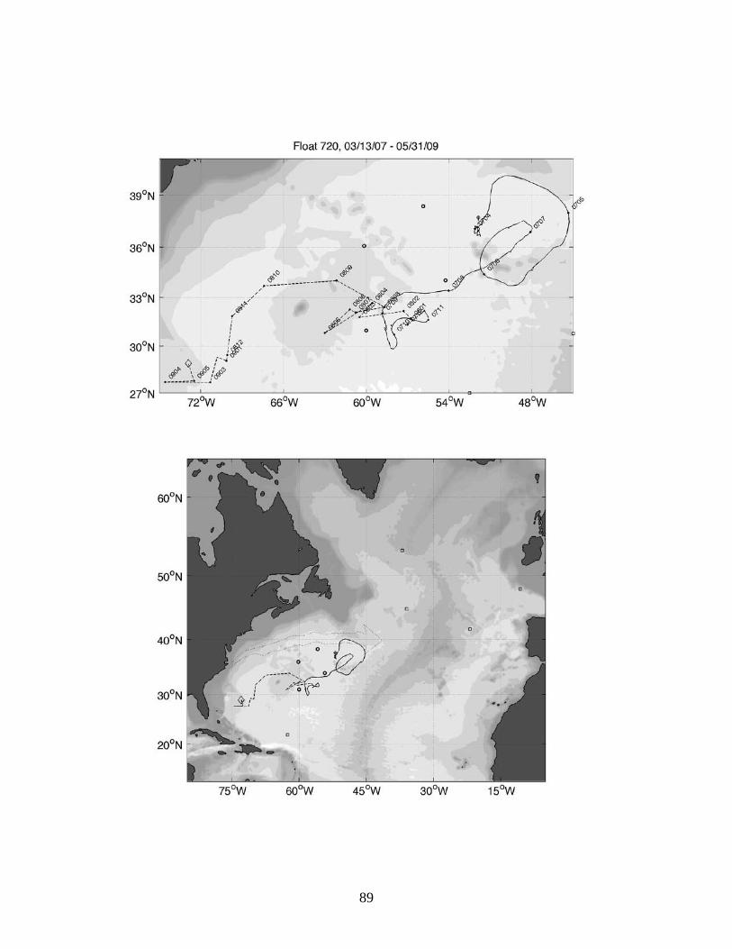
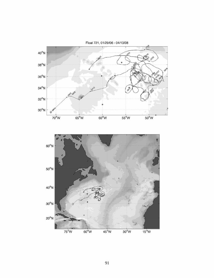
Figure 5. Trajectories of the CLIMODE bobbers. Dashed lines indicate periods during which acoustic tracking was not possible. The most recent location of each bobber (as of June 2009) is indicated with a diamond.

12

5. Acknowledgements We acknowledge the generous assistance of the Captains and crew of the Research Vessels Oceanus, Knorr, and Atlantis. The CLIMODE moorings were designed by George Tupper. Young-Oh Kwon performed the quality control of the temperature profiles. Ellyn Montgomery built the automated bobber data acquisition and processing system. Financial support was provided by the National Science Foundation through Grant OCE-0424492.

6. References Wooding, C. M., H. H. Furey, and M. A. Pacheco, 2005. RAFOS Float Processing at the Woods Hole Oceanographic Institution. Woods Hole Oceanogr. Inst. Tech Rept., WHOI-2005-02, 35 pp.

13

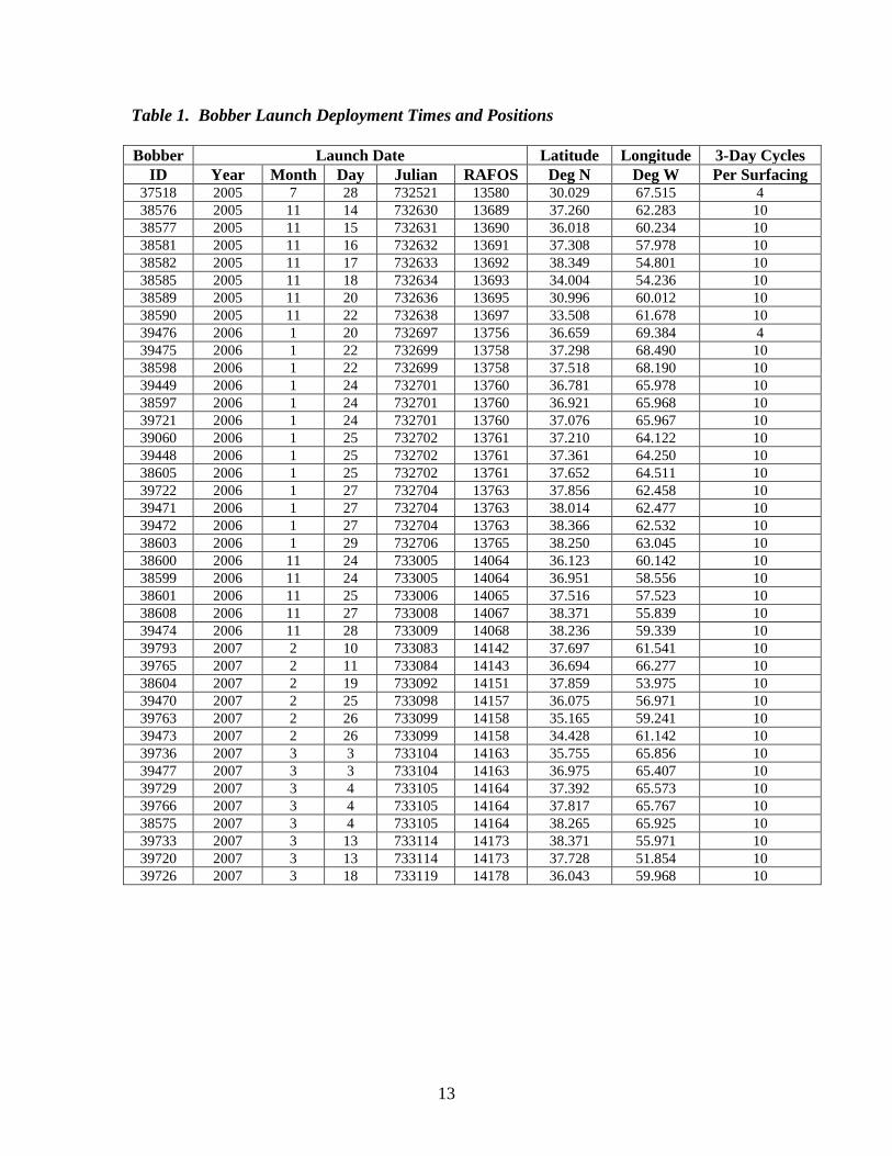
Table 1. Bobber Launch Deployment Times and Positions Bobber Launch Date Latitude Longitude 3-Day Cycles

ID Year Month Day Julian RAFOS Deg N Deg W Per Surfacing 37518 2005 7 28 732521 13580 30.029 67.515 4 38576 2005 11 14 732630 13689 37.260 62.283 10 38577 2005 11 15 732631 13690 36.018 60.234 10 38581 2005 11 16 732632 13691 37.308 57.978 10 38582 2005 11 17 732633 13692 38.349 54.801 10 38585 2005 11 18 732634 13693 34.004 54.236 10 38589 2005 11 20 732636 13695 30.996 60.012 10 38590 2005 11 22 732638 13697 33.508 61.678 10 39476 2006 1 20 732697 13756 36.659 69.384 4 39475 2006 1 22 732699 13758 37.298 68.490 10 38598 2006 1 22 732699 13758 37.518 68.190 10 39449 2006 1 24 732701 13760 36.781 65.978 10 38597 2006 1 24 732701 13760 36.921 65.968 10 39721 2006 1 24 732701 13760 37.076 65.967 10 39060 2006 1 25 732702 13761 37.210 64.122 10 39448 2006 1 25 732702 13761 37.361 64.250 10 38605 2006 1 25 732702 13761 37.652 64.511 10 39722 2006 1 27 732704 13763 37.856 62.458 10 39471 2006 1 27 732704 13763 38.014 62.477 10 39472 2006 1 27 732704 13763 38.366 62.532 10 38603 2006 1 29 732706 13765 38.250 63.045 10 38600 2006 11 24 733005 14064 36.123 60.142 10 38599 2006 11 24 733005 14064 36.951 58.556 10 38601 2006 11 25 733006 14065 37.516 57.523 10 38608 2006 11 27 733008 14067 38.371 55.839 10 39474 2006 11 28 733009 14068 38.236 59.339 10 39793 2007 2 10 733083 14142 37.697 61.541 10 39765 2007 2 11 733084 14143 36.694 66.277 10 38604 2007 2 19 733092 14151 37.859 53.975 10 39470 2007 2 25 733098 14157 36.075 56.971 10 39763 2007 2 26 733099 14158 35.165 59.241 10 39473 2007 2 26 733099 14158 34.428 61.142 10 39736 2007 3 3 733104 14163 35.755 65.856 10 39477 2007 3 3 733104 14163 36.975 65.407 10 39729 2007 3 4 733105 14164 37.392 65.573 10 39766 2007 3 4 733105 14164 37.817 65.767 10 38575 2007 3 4 733105 14164 38.265 65.925 10 39733 2007 3 13 733114 14173 38.371 55.971 10 39720 2007 3 13 733114 14173 37.728 51.854 10 39726 2007 3 18 733119 14178 36.043 59.968 10

14

Table 2. Sound Source Deployment Positions and Times All Sound sources transmitted for 80 seconds every 24 hours. Two of the sources, C and D, were recovered and redeployed midway through the experiment. The source clocks were reset during this turn-around. Mooring Source Depth Pong Latitude Longitude Deploy Recovery Number Number (m) Time Deg N Deg W Date Date

A 22 400 00:30 30.975 60.011 11/20/2005 11/22/2007 B 21 400 00:00 34.041 54.264 11/18/2005 11/10/2007 C 24 650 01:30 38.371 55.862 11/17/2005 11/26/2006

C-redeploy 24 650 01:30 38.371 55.873 11/27/2006 11/09/2007 D 23 650 01:00 36.090 60.171 11/15/2005 11/22/2006

D-redeploy 23 650 01:00 36.087 60.169 11/23/2006 11/07/2007

15

Table 3. List of ARGOS Transmissions That Required Manual Repair of Messages

Float ID Transmission Date f38598 2006-11-18 f38603 2007-07-23 2007-08-22 2007-11-20 f39060 2006-07-24 2007-08-18 f39448 2007-08-18 f39470 2007-06-25 f39471 2007-04-22 f39473 2007-05-27 f39721 2007-02-18 f39722 2007-04-22 f39729 2007-04-03 f39763 2007-05-27 f39766 2007-06-07 2007-08-31

16

Table 4. Duration (Lifetime) and Rate of Success of ARGOS Transmissions for CLIMODE Bobbers Through May 31, 2009

Float First Transmission Last Transmission Duration Transmissions Success ID Year Month Day Year Month Day (Days) Expected Actual Rate (%)

375181 2005 8 9 2007 12 9 852 72 71 98.6 385751 2007 4 3 2009 5 22 780 27 26 96.3 385762 2005 12 14 2008 7 1 930 32 27 84.4 385772 2005 12 15 2006 8 12 240 9 9 100.0 385812 2005 12 16 2008 11 30 1080 37 37 100.0 385822 2005 12 17 2008 1 6 750 26 25 96.2 385852 2005 12 18 2009 5 31 1260 43 43 100.0 385892 2005 12 21 2009 5 4 1230 42 42 100.0 385902 2005 12 22 2008 3 11 810 28 28 100.0 38597 2006 2 23 2008 9 10 930 32 29 90.6 38598 2006 2 21 2009 5 6 1170 40 40 100.0 38599 2006 12 24 2009 5 12 870 30 30 100.0 38600 2006 12 24 2009 5 12 870 30 30 100.0 38601 2006 12 25 2009 5 13 870 30 29 96.7 38603 2006 2 28 2009 5 13 1170 40 40 100.0 38604 2007 3 21 2009 3 10 720 25 22 88.0 38605 2006 2 24 2009 5 9 1170 40 37 92.5 38608 2006 12 27 2009 5 15 870 30 30 100.0 39060 2006 2 24 2009 5 9 1170 40 40 100.0 39448 2006 2 24 2009 5 9 1170 40 39 97.5 39449 2006 2 23 2007 5 19 450 16 16 100.0 39470 2007 3 27 2009 5 15 780 27 27 100.0 39471 2006 2 26 2009 5 11 1170 40 40 100.0 39472 2006 2 27 2008 1 18 690 24 24 100.0 39473 2007 3 28 2009 5 16 780 27 27 100.0 39474 2006 12 28 2009 5 16 870 30 30 100.0 39475 2006 2 21 2009 5 6 1170 40 40 100.0 39476 2006 2 1 2009 5 28 1212 102 102 100.0 39477 2007 4 3 2009 5 22 780 27 27 100.0 39720 2007 4 12 2009 5 31 780 27 27 100.0 39721 2006 2 23 2008 4 13 780 27 27 100.0 39722 2006 2 26 2009 5 11 1170 40 39 97.5 39726 2007 4 18 2009 5 7 750 26 26 100.0 39729 2007 4 3 2009 5 22 780 27 27 100.0 39733 2007 4 12 2009 5 1 750 26 26 100.0 397361 2007 4 2 2009 5 21 780 27 27 100.0 39763 2007 3 28 2009 5 16 780 27 26 96.3 39765 2007 3 13 2008 12 2 630 22 22 100.0 39766 2007 4 3 2009 5 22 780 27 27 100.0 39793 2007 3 12 2009 5 30 810 28 27 96.4

1 Float could not be tracked acoustically due to poor signal quality. 2 Float collected only one point during each bob due to a bad sensor.

17

Table 5. Float Clock Drift (ARGOS Time – Float Clock Time) for 37 Tracked Floats

Float Date of Last Transmission Used Launch Final ID Year Month Day Hr Min Offset (sec) Offset (sec)

38576 2007 08 06 09 48 11.10 -70.320 38577 2006 08 12 10 17 38.435 12.509 38581 2007 01 10 09 06 1.772 -34.708 38582 2007 12 07 14 10 -1.690 -78.999 38585 2007 12 08 13 53 10.171 -67.900 38589 2007 12 11 11 10 3.202 -75.000 38590 2007 11 12 08 14 -5.210 -97.000 38597 2007 11 15 11 49 -0.311 -79.000 38598 2007 12 13 10 23 2.322 -63.999 38599 2007 11 19 11 48 -3.140 -50.999 38600 2007 11 19 13 39 -1.751 -44.999 38601 2007 11 20 09 56 1.368 -45.000 38603 2007 11 20 09 32 10.176 -107.00 38604 2007 11 16 12 56 1.531 -24.999 38605 2007 11 16 11 05 9.253 -92.000 38608 2007 11 22 12 15 -1.2 -59.999 39060 2007 12 16 11 06 7.030 -66.440 39448 2007 11 16 14 38 2.455 -93.999 39449 2007 05 19 12 22 2.646 -66.440 39470 2007 11 22 12 13 1.695 -44.000 39471 2007 11 18 10 17 6.939 -44.990 39472 2007 11 19 13 29 3.098 -47.999 39473 2007 11 23 19 05 -10.845 -43.000 39474 2007 11 23 09 26 0.788 -52.000 39475 2007 12 13 12 03 4.835 -104.999 39476 2007 11 11 13 10 11.355 -37.999 39477 2007 11 29 11 54 -1.803 -32.999 39720 2007 12 08 09 48 -0.018 -36.000 39721 2007 11 15 13 17 -3.898 -87.999 39722 2007 12 18 04 00 0.627 -64.999 39726 2007 12 14 09 55 0.224 -39.999 39729 2007 11 29 10 56 3.227 -25.000 39733 2007 12 08 12 10 2.439 -32.999 39763 2007 11 23 11 53 -11.189 -50.999 39765 2007 12 08 09 47 -7.448 -42.000 39766 2007 11 29 10 55 -15.977 -45.999 39793 2007 12 07 09 58 -6.239 -45.000

18

Table 6. Percentage of TOAs That Resulted in Acceptable Positions

Float Number of Tracked Positions ID Total Acceptable % Acceptable

38576 630 362 57.5 38577 266 115 43.2 38581 419 171 40.8 38582 747 164 22.0 38585 750 677 90.3 38589 751 699 93.1 38590 718 673 93.7 38597 662 560 84.6 38598 688 641 93.2 38599 360 249 69.2 38600 356 332 93.3 38601 356 299 84.0 38603 659 547 83.0 38604 268 243 90.7 38605 661 635 96.1 38608 355 43 12.1 39060 690 164 23.8 39448 660 552 83.6 39449 477 265 55.6 39470 265 84 31.7 39471 658 410 62.3 39472 660 608 92.1 39473 266 248 93.2 39474 357 309 86.6 39475 692 202 29.2 39476 657 366 55.7 39477 268 164 61.2 39720 266 225 84.6 39721 660 589 89.2 39722 689 342 49.6 39726 266 209 78.6 39729 265 223 84.2 39733 266 208 78.2 39763 267 224 83.9 39765 299 251 83.9 39766 266 237 89.1 39793 297 194 65.3

19

Appendix A: Mooring and Bobber Deployment/Recovery Schedule Cruise ID Dates Chief Scientist(s) Activity OC419 Nov 9 – Nov 27, 2005 Fratantoni, Weller Moorings A, B, C, & D

deployed 7 bobbers deployed

AT13 Jan 18 – Jan 31, 2006 Joyce 13 bobbers launched OC434 Nov 16 – Dec 3, 2006 Weller Recover, redeploy Moorings

C & D 5 bobbers launched

KN188-01 Feb 7 – Feb 27, 2007 Joyce 6 bobbers launched KN188-02 Mar 2 – Mar 22, 2007 Joyce 8 bobbers launched OC442 Nov 5 – Nov 19, 2007 Fratantoni Moorings A, B, C, & D

recovered

20

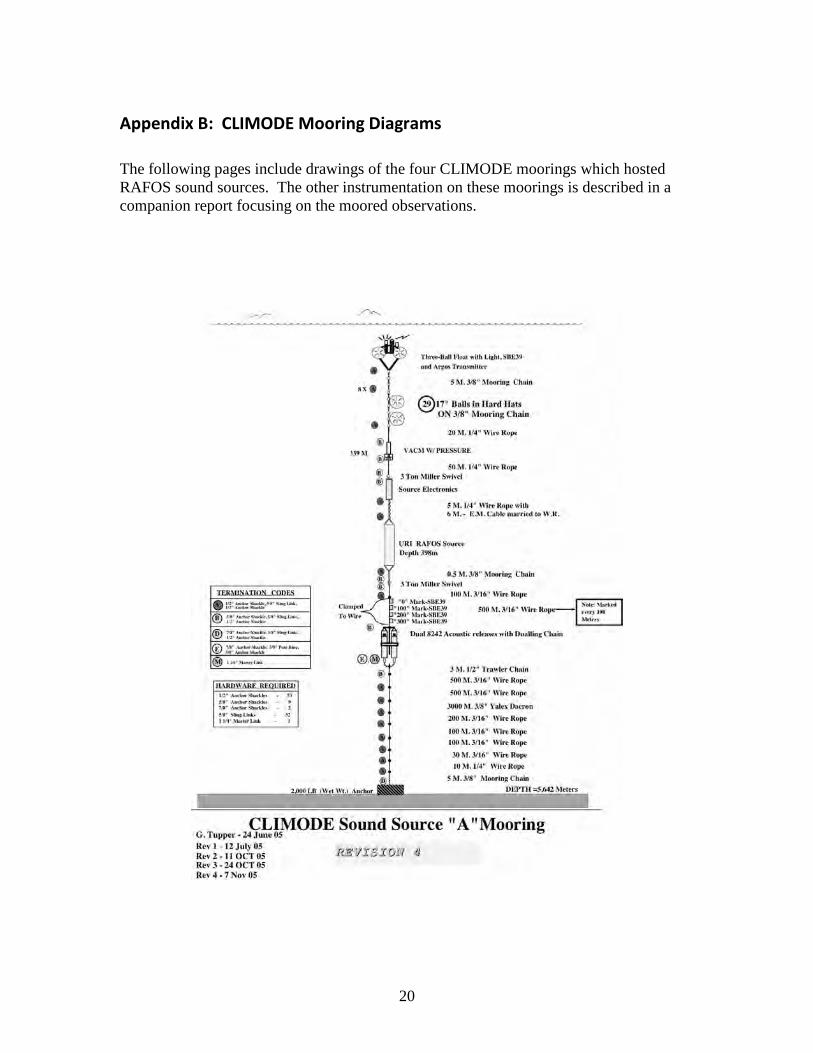
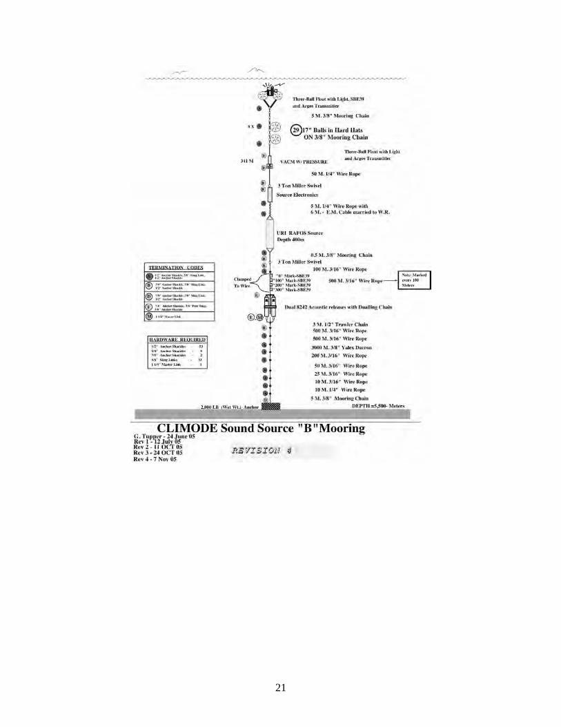
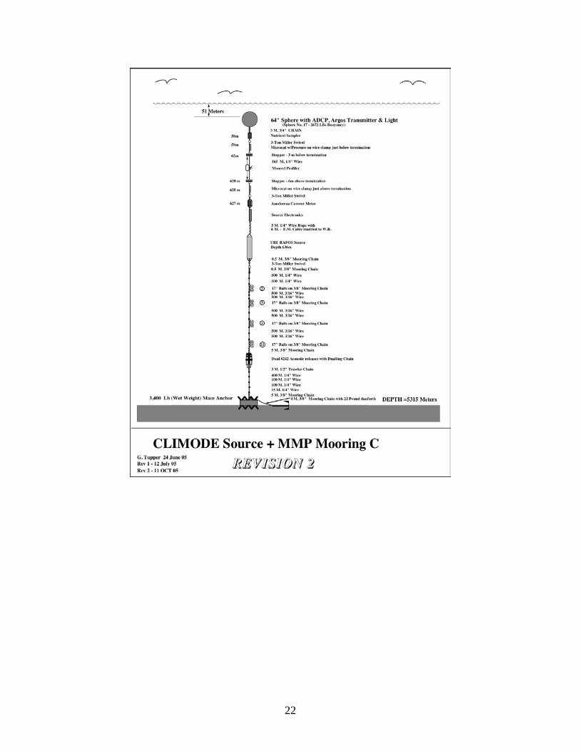
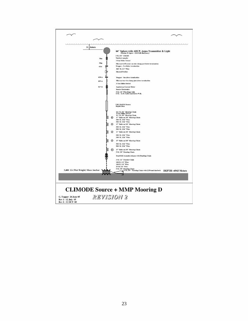
Appendix B: CLIMODE Mooring Diagrams The following pages include drawings of the four CLIMODE moorings which hosted RAFOS sound sources. The other instrumentation on these moorings is described in a companion report focusing on the moored observations.

21

22

23

24

Appendix C: Sample Sound Source File Entry [CLa] -sourcename CLa -sourcetype Rossby -sourceowner WHOI/Climode -position 30.975 -60.011 -depth 400 -begemis 2005 11 20 00 30 -endemis 2007 11 22 00 30 -offset 2005 11 20 0.0 -drift -0.128 -reftime 00 30 -schedule 24 -signallength 80 -add_offset NaN -sound_speed 1480 -comment Based on source clock check when pulled, HHF.

25

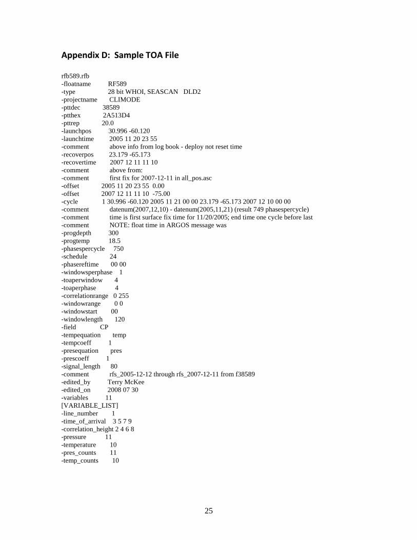
Appendix D: Sample TOA File rfb589.rfb -floatname RF589 -type 28 bit WHOI, SEASCAN DLD2 -projectname CLIMODE -pttdec 38589 -ptthex 2A513D4 -pttrep 20.0 -launchpos 30.996 -60.120 -launchtime 2005 11 20 23 55 -comment above info from log book - deploy not reset time -recoverpos 23.179 -65.173 -recovertime 2007 12 11 11 10 -comment above from: -comment first fix for 2007-12-11 in all_pos.asc -offset 2005 11 20 23 55 0.00 -offset 2007 12 11 11 10 -75.00 -cycle 1 30.996 -60.120 2005 11 21 00 00 23.179 -65.173 2007 12 10 00 00 -comment datenum(2007,12,10) - datenum(2005,11,21) (result 749 phasespercycle) -comment time is first surface fix time for 11/20/2005; end time one cycle before last -comment NOTE: float time in ARGOS message was -progdepth 300 -progtemp 18.5 -phasespercycle 750 -schedule 24 -phasereftime 00 00 -windowsperphase 1 -toaperwindow 4 -toaperphase 4 -correlationrange 0 255 -windowrange 0 0 -windowstart 00 -windowlength 120 -field CP -tempequation temp -tempcoeff 1 -presequation pres -prescoeff 1 -signal_length 80 -comment rfs_2005-12-12 through rfs_2007-12-11 from f38589 -edited_by Terry McKee -edited_on 2008 07 30 -variables 11 [VARIABLE_LIST] -line_number 1 -time_of_arrival 3 5 7 9 -correlation_height 2 4 6 8 -pressure 11 -temperature 10 -pres_counts 11 -temp_counts 10

26

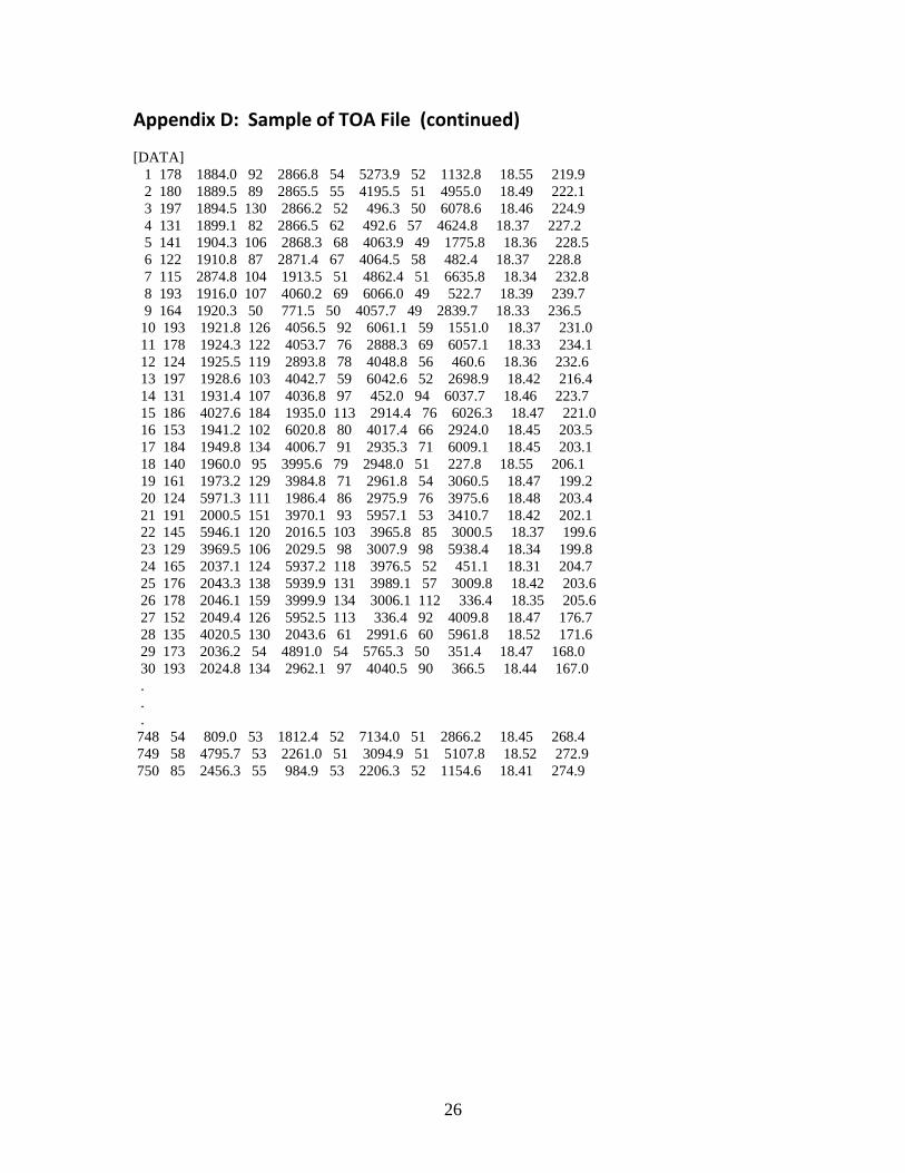
Appendix D: Sample of TOA File (continued) [DATA] 1 178 1884.0 92 2866.8 54 5273.9 52 1132.8 18.55 219.9 2 180 1889.5 89 2865.5 55 4195.5 51 4955.0 18.49 222.1 3 197 1894.5 130 2866.2 52 496.3 50 6078.6 18.46 224.9 4 131 1899.1 82 2866.5 62 492.6 57 4624.8 18.37 227.2 5 141 1904.3 106 2868.3 68 4063.9 49 1775.8 18.36 228.5 6 122 1910.8 87 2871.4 67 4064.5 58 482.4 18.37 228.8 7 115 2874.8 104 1913.5 51 4862.4 51 6635.8 18.34 232.8 8 193 1916.0 107 4060.2 69 6066.0 49 522.7 18.39 239.7 9 164 1920.3 50 771.5 50 4057.7 49 2839.7 18.33 236.5 10 193 1921.8 126 4056.5 92 6061.1 59 1551.0 18.37 231.0 11 178 1924.3 122 4053.7 76 2888.3 69 6057.1 18.33 234.1 12 124 1925.5 119 2893.8 78 4048.8 56 460.6 18.36 232.6 13 197 1928.6 103 4042.7 59 6042.6 52 2698.9 18.42 216.4 14 131 1931.4 107 4036.8 97 452.0 94 6037.7 18.46 223.7 15 186 4027.6 184 1935.0 113 2914.4 76 6026.3 18.47 221.0 16 153 1941.2 102 6020.8 80 4017.4 66 2924.0 18.45 203.5 17 184 1949.8 134 4006.7 91 2935.3 71 6009.1 18.45 203.1 18 140 1960.0 95 3995.6 79 2948.0 51 227.8 18.55 206.1 19 161 1973.2 129 3984.8 71 2961.8 54 3060.5 18.47 199.2 20 124 5971.3 111 1986.4 86 2975.9 76 3975.6 18.48 203.4 21 191 2000.5 151 3970.1 93 5957.1 53 3410.7 18.42 202.1 22 145 5946.1 120 2016.5 103 3965.8 85 3000.5 18.37 199.6 23 129 3969.5 106 2029.5 98 3007.9 98 5938.4 18.34 199.8 24 165 2037.1 124 5937.2 118 3976.5 52 451.1 18.31 204.7 25 176 2043.3 138 5939.9 131 3989.1 57 3009.8 18.42 203.6 26 178 2046.1 159 3999.9 134 3006.1 112 336.4 18.35 205.6 27 152 2049.4 126 5952.5 113 336.4 92 4009.8 18.47 176.7 28 135 4020.5 130 2043.6 61 2991.6 60 5961.8 18.52 171.6 29 173 2036.2 54 4891.0 54 5765.3 50 351.4 18.47 168.0 30 193 2024.8 134 2962.1 97 4040.5 90 366.5 18.44 167.0 . . . 748 54 809.0 53 1812.4 52 7134.0 51 2866.2 18.45 268.4 749 58 4795.7 53 2261.0 51 3094.9 51 5107.8 18.52 272.9 750 85 2456.3 55 984.9 53 2206.3 52 1154.6 18.41 274.9

27

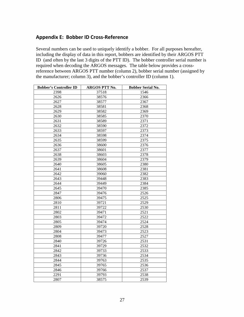
Appendix E: Bobber ID Cross-Reference Several numbers can be used to uniquely identify a bobber. For all purposes hereafter, including the display of data in this report, bobbers are identified by their ARGOS PTT ID (and often by the last 3 digits of the PTT ID). The bobber controller serial number is required when decoding the ARGOS messages. The table below provides a cross-reference between ARGOS PTT number (column 2), bobber serial number (assigned by the manufacturer; column 3), and the bobber’s controller ID (column 1). Bobber’s Controller ID ARGOS PTT No. Bobber Serial No.

2398 37518 1546 2626 38576 2366 2627 38577 2367 2628 38581 2368 2629 38582 2369 2630 38585 2370 2631 38589 2371 2632 38590 2372 2633 38597 2373 2634 38598 2374 2635 38599 2375 2636 38600 2376 2637 38601 2377 2638 38603 2378 2639 38604 2379 2640 38605 2380 2641 38608 2381 2642 39060 2382 2643 39448 2383 2644 39449 2384 2645 39470 2385 2847 39476 2526 2806 39475 2525 2810 39721 2529 2811 39722 2530 2802 39471 2521 2803 39472 2522 2805 39474 2524 2809 39720 2528 2804 39473 2523 2808 39477 2527 2840 39726 2531 2841 39729 2532 2842 39733 2533 2843 39736 2534 2844 39763 2535 2845 39765 2536 2846 39766 2537 2291 39793 2538 2807 38575 2539

28

Appendix F: Sound Source Clock Drift Calculations Source time comparisons at recovery Mooring A Source #22 0:30:00 Recovered 11/12/2007 Ship Time S. Source

time Delta UTC-

SO Temp Corr

Final corr

15:37:40 15:38:23 43 -63 -30.956 -94 15:38:00 15:38:43 15:38:30 15:39:13

Mooring B Source #21 0:00:00 Recovered 11/10/2007 Ship Time S. Source

time Delta

23:19:00 23:18:46 -14 14 -10.32 3.68 23:19:20 23:09:06 23:19:50 23:19:36 23:20:15 23:20:01

Mooring C Source #24 1:30:00 Recovered 11/9/2007 Ship Time S. Source

time Delta Turnaround 11/26/2006

16:40:00 16:40:05 5 -5 -5 year 1 14:32:00 14:32:05 -5 16:40:20 16:40:25 -5 year 2 16:40:40 16:40:45 16:41:10 16:41:15

Mooring D Source #23 1:00:00 Recovered 11/7/2007 Turnaround 11/23/2006 Ship Time S. Source

time Delta 2007

tcorr Ship Time

23:24:00 23:24:29 29 -29 -3.6 -32.6 year 1 12:40:00 12:40:26 -27 23:24:20 23:24:49 -27 year 2 23:24:40 23:25:09 23:25:00 23:25:29 23:25:20 23:25:48 2006 tcorr Not

recorded

29

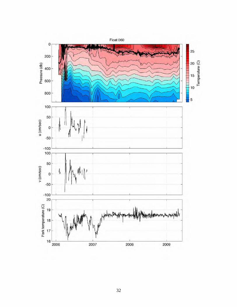
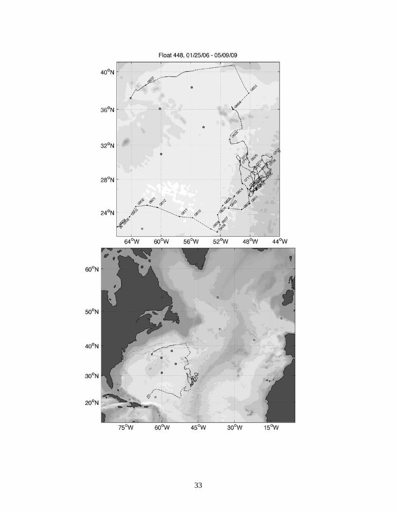
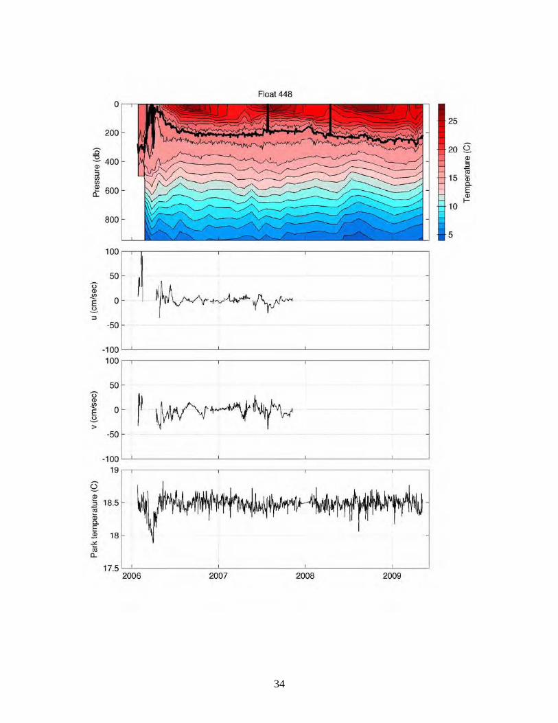
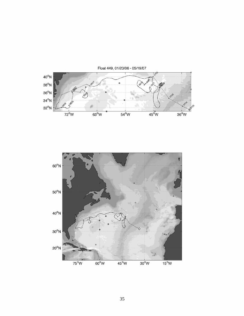
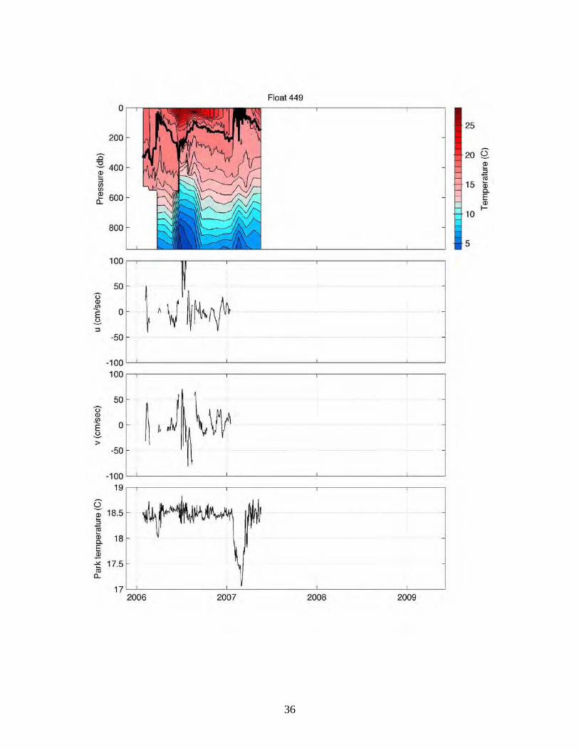
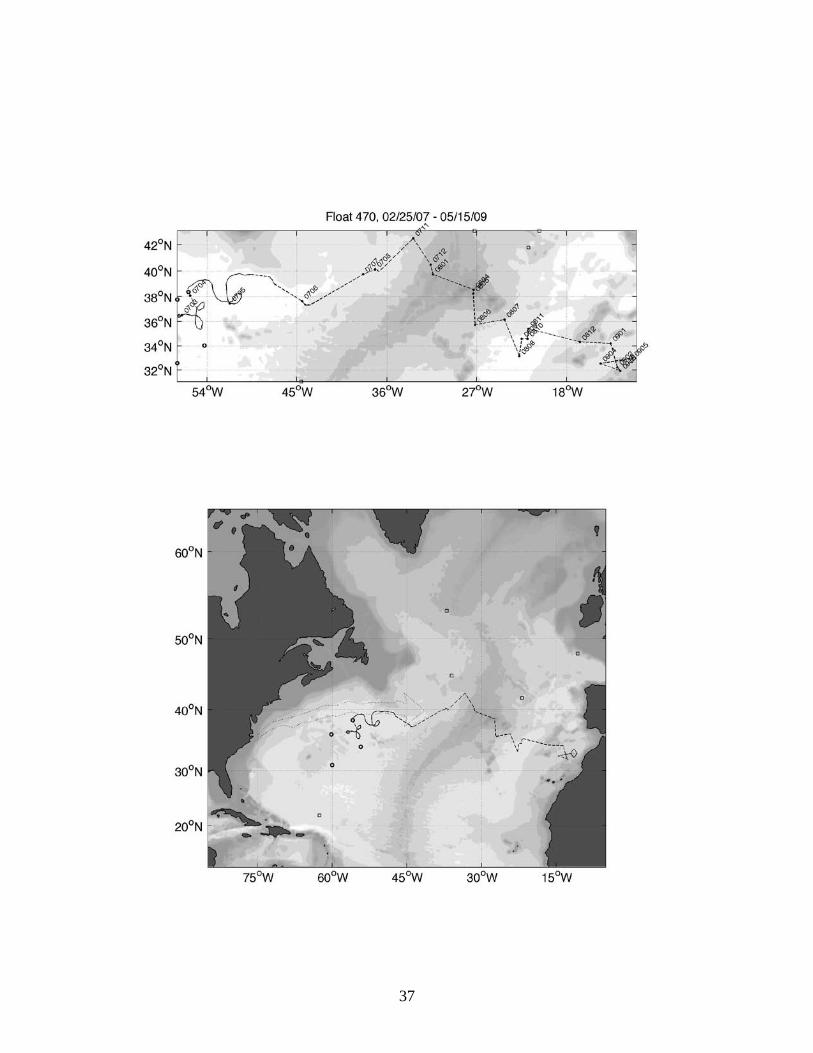
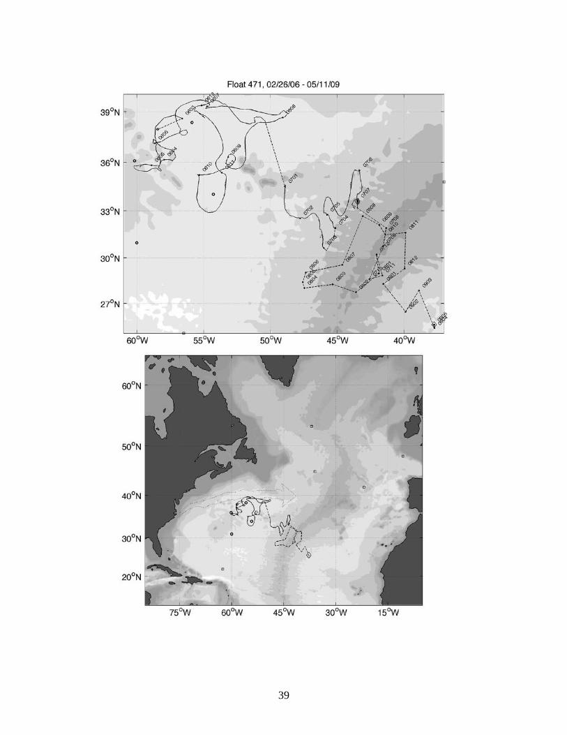
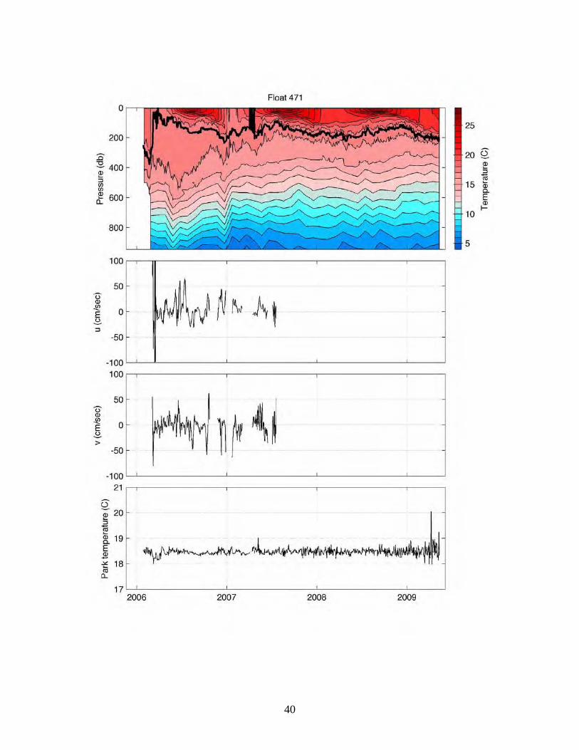
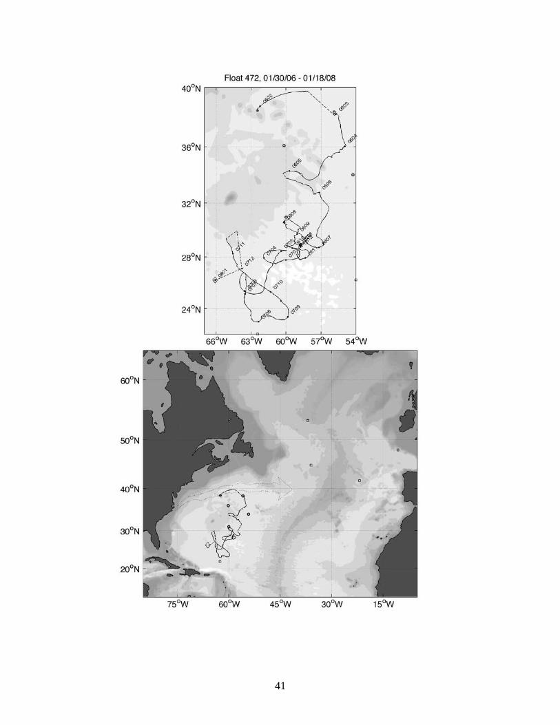
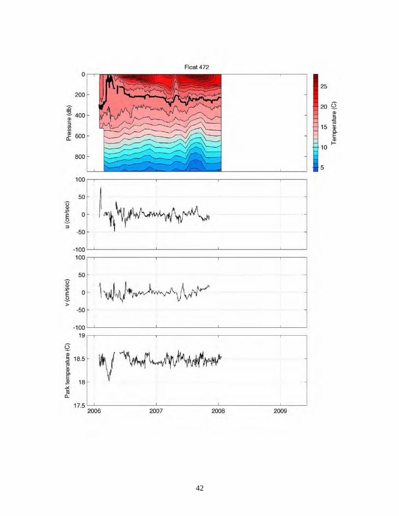
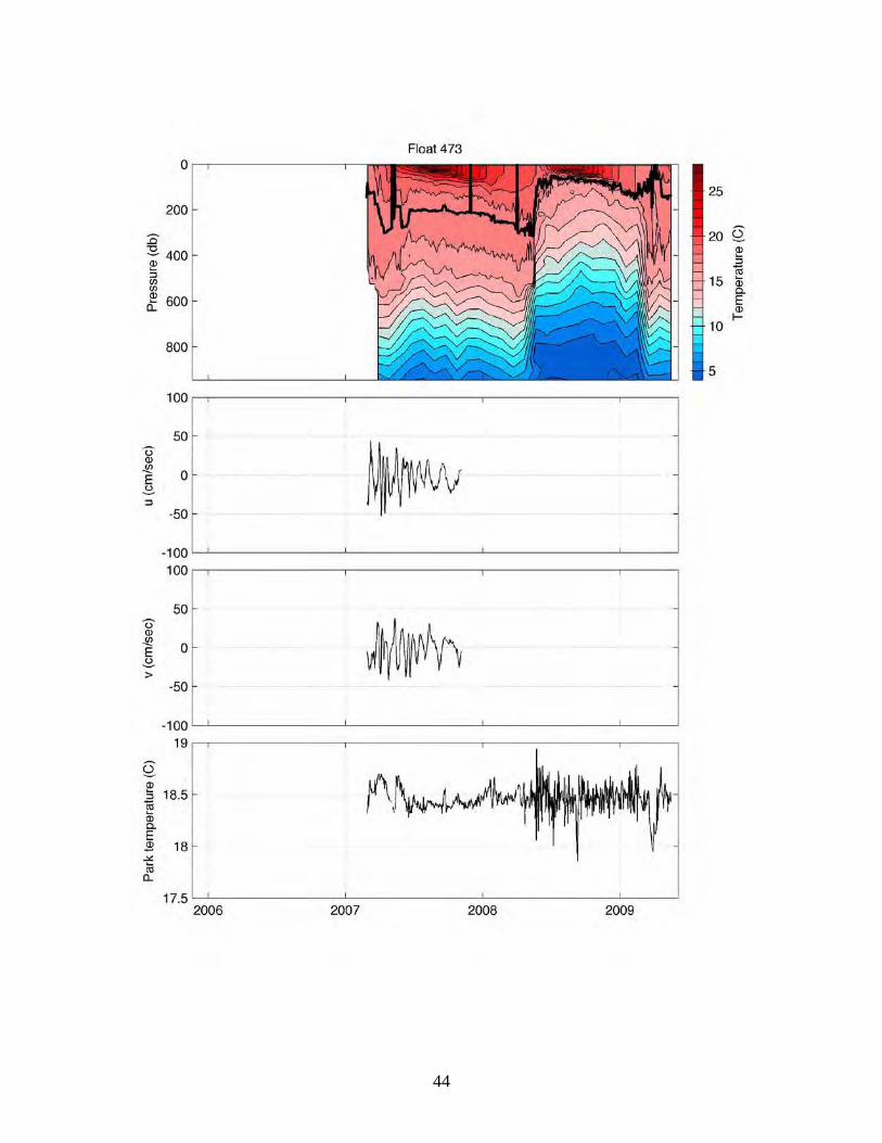
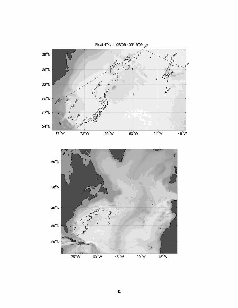
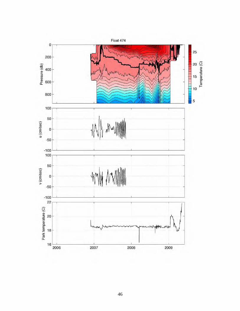
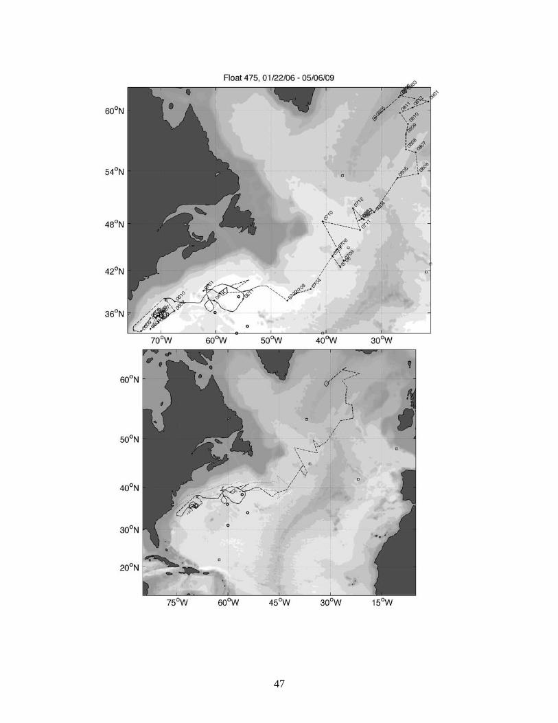
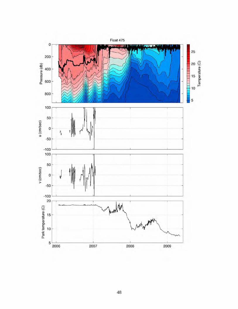
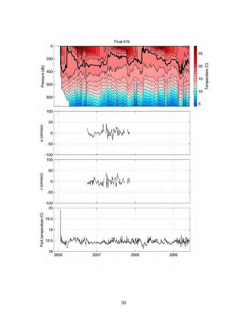
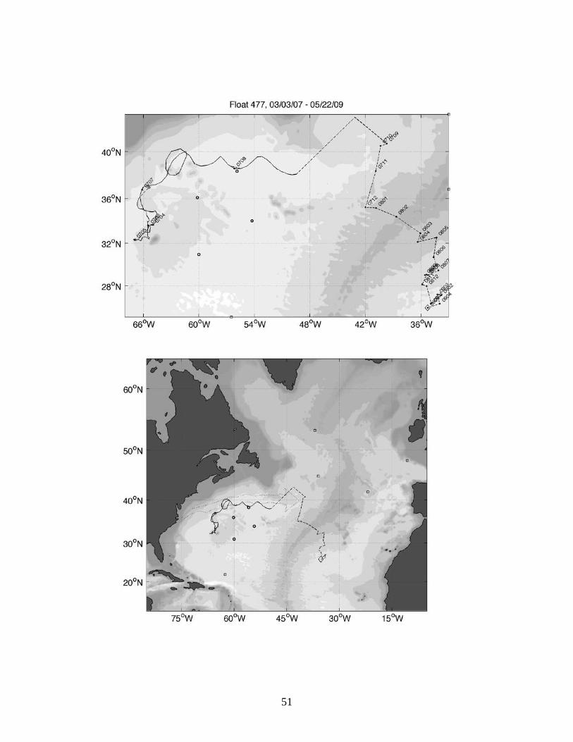
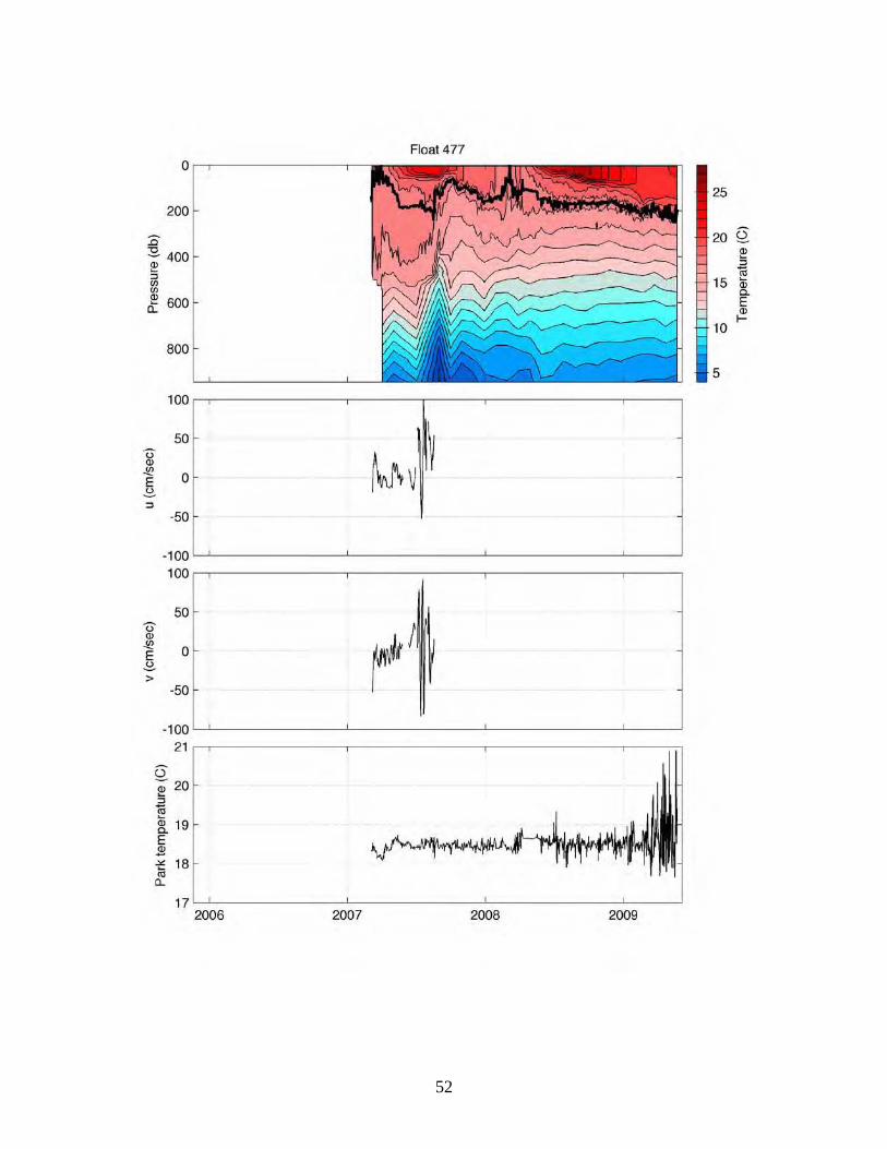
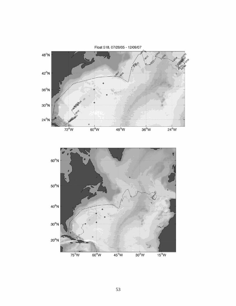
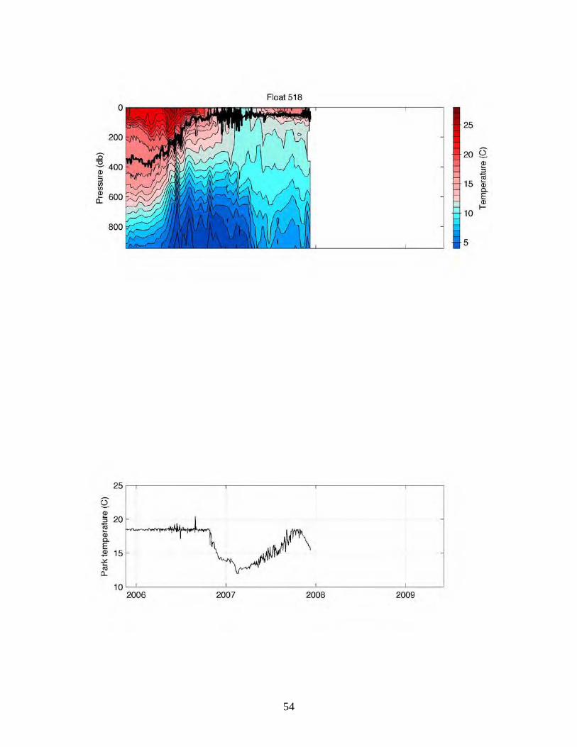
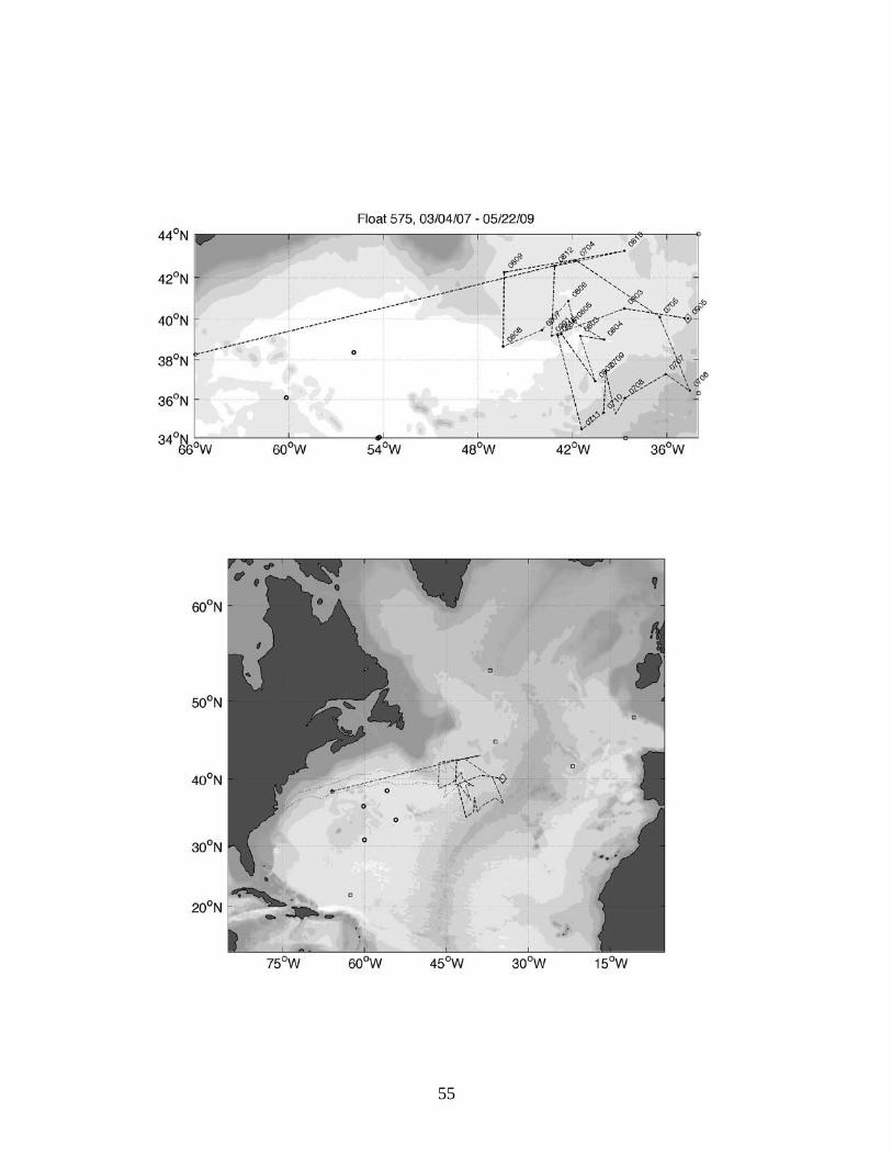
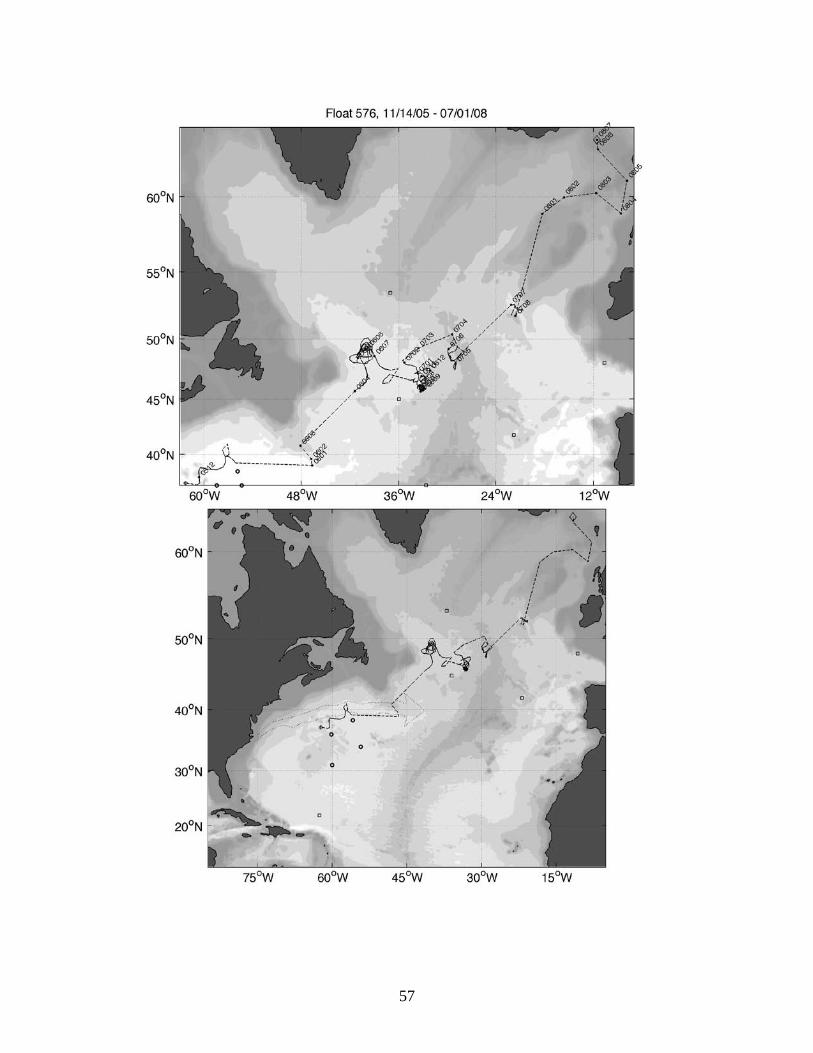
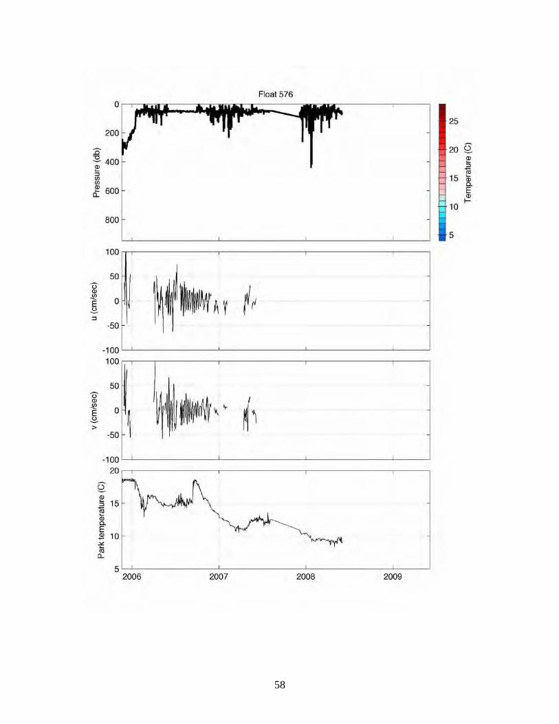
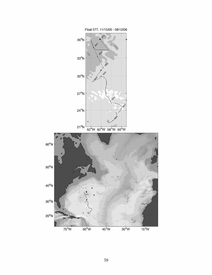
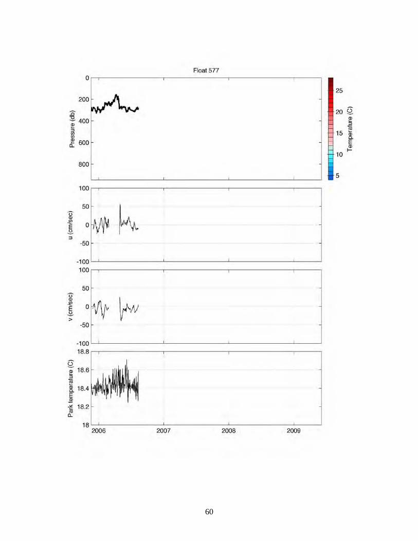
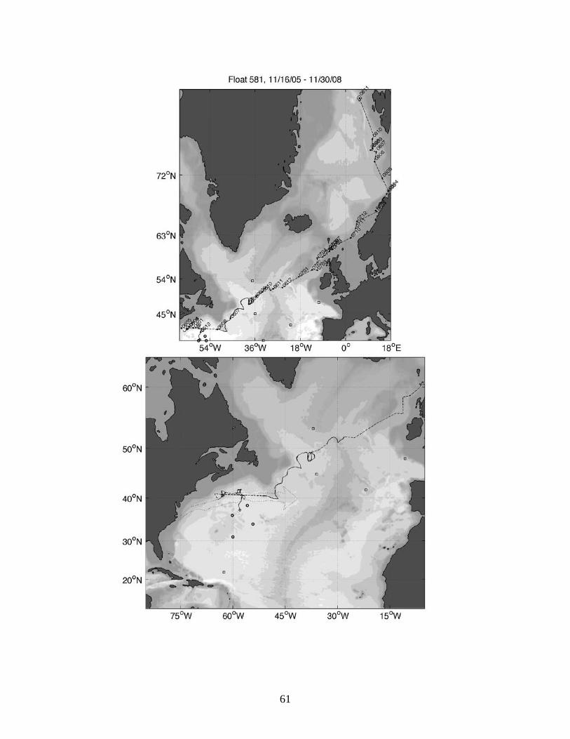
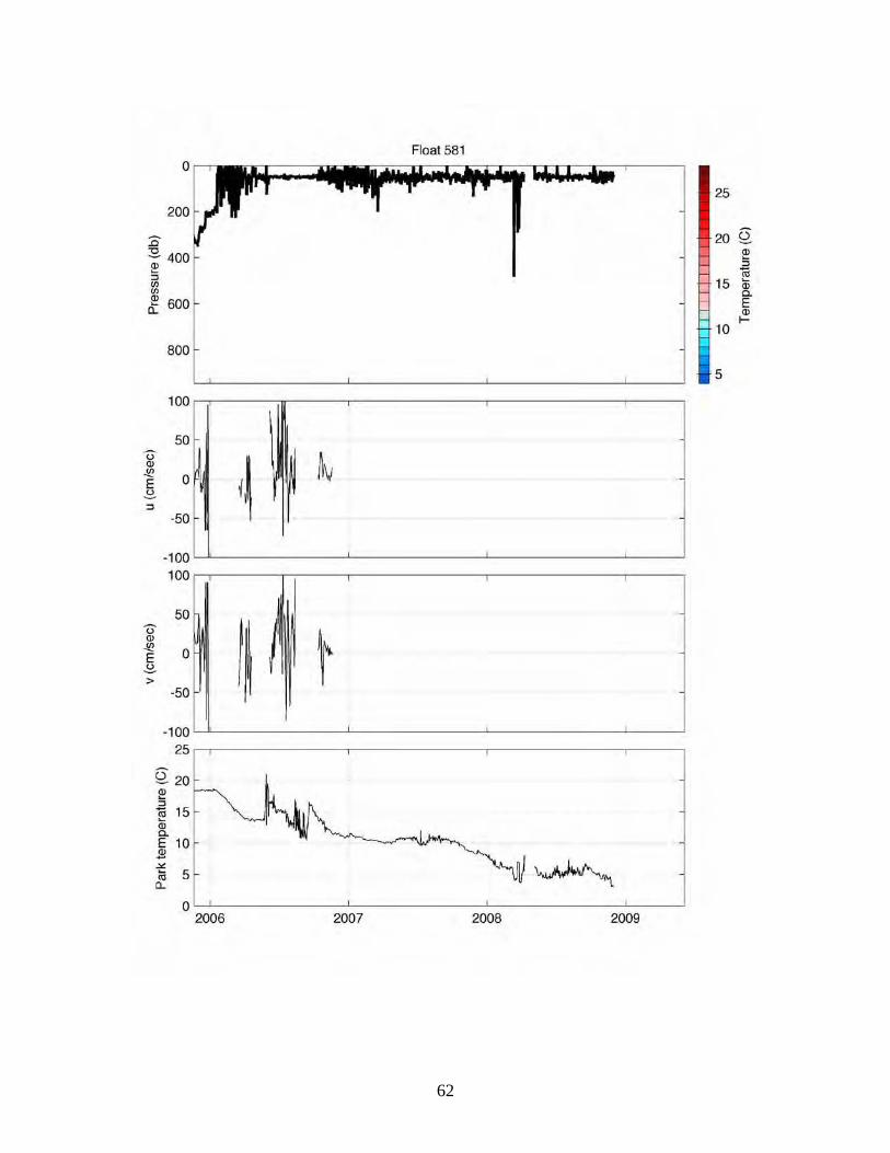
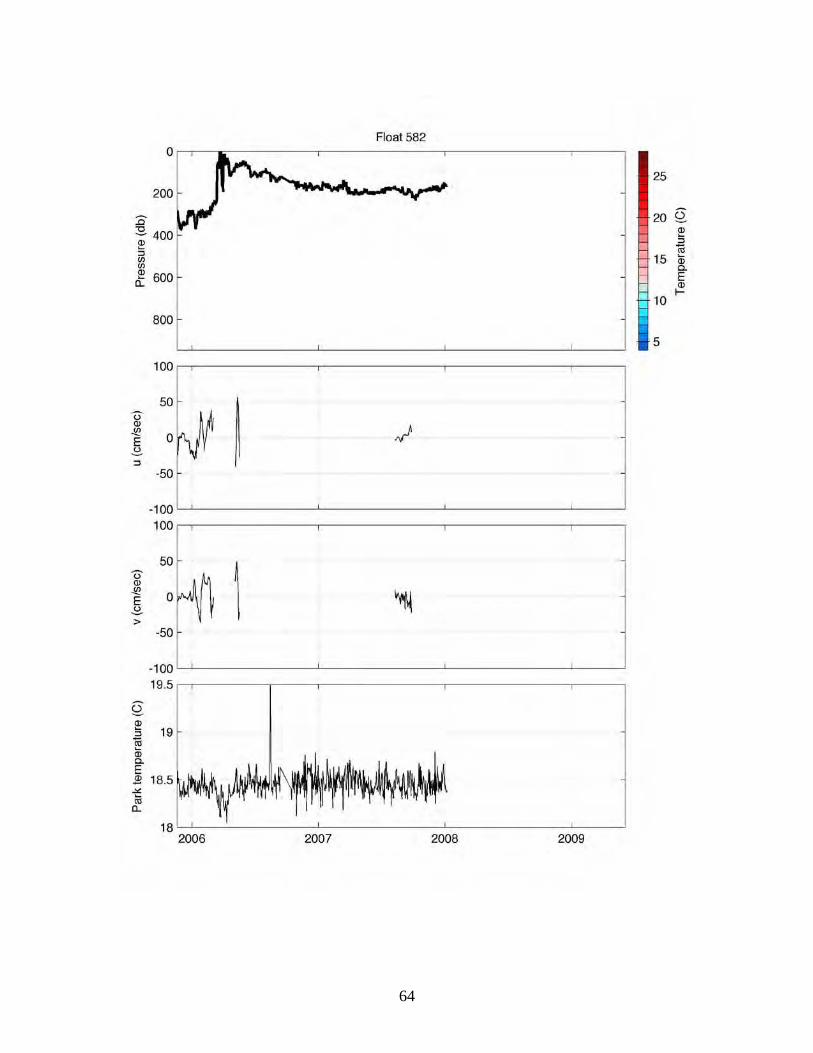
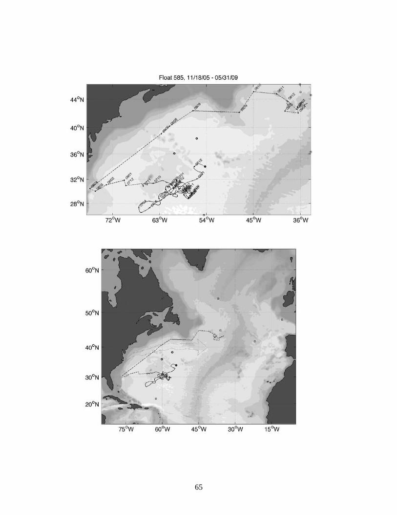
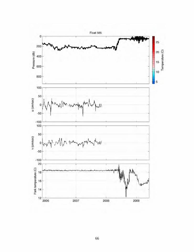
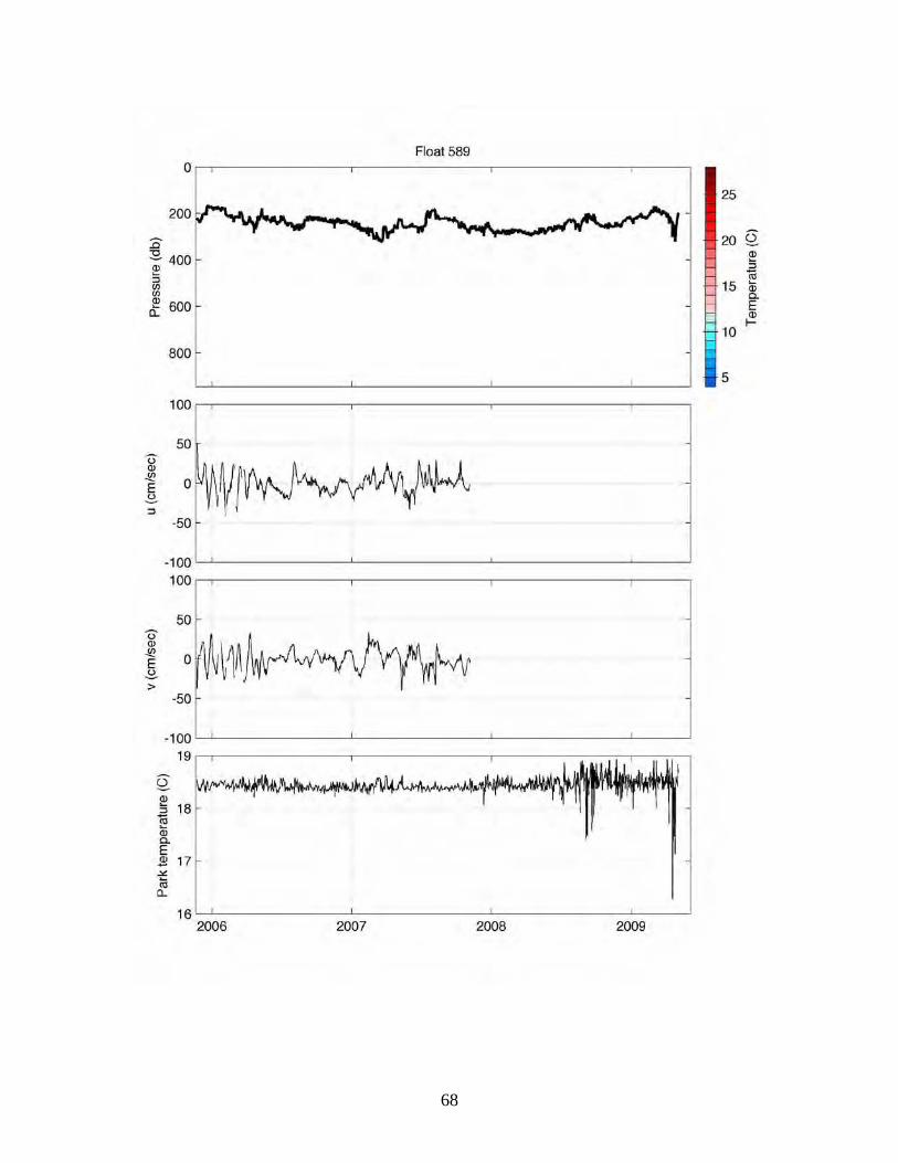
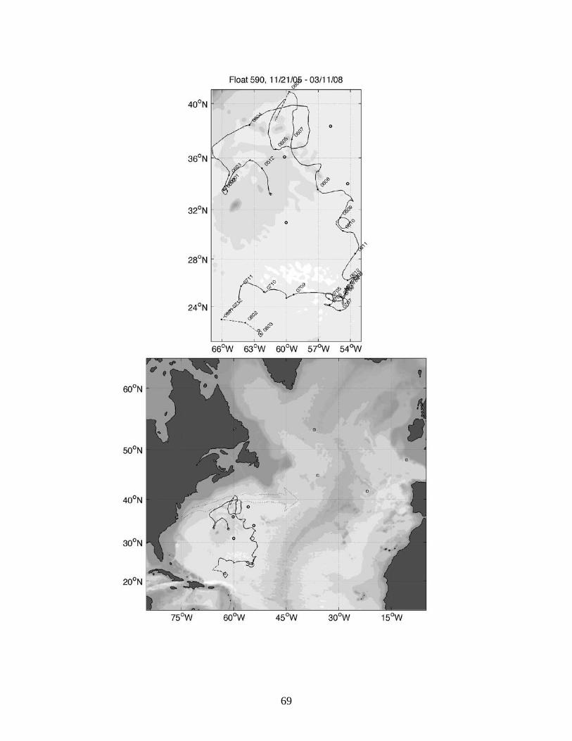
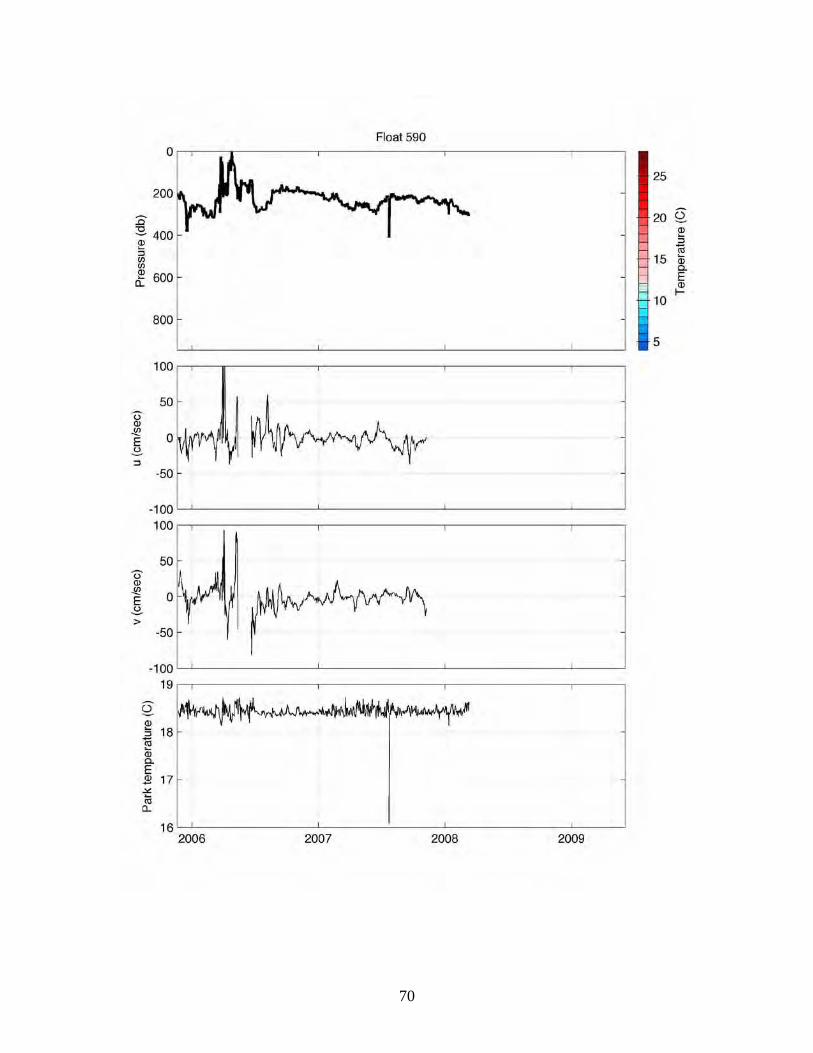
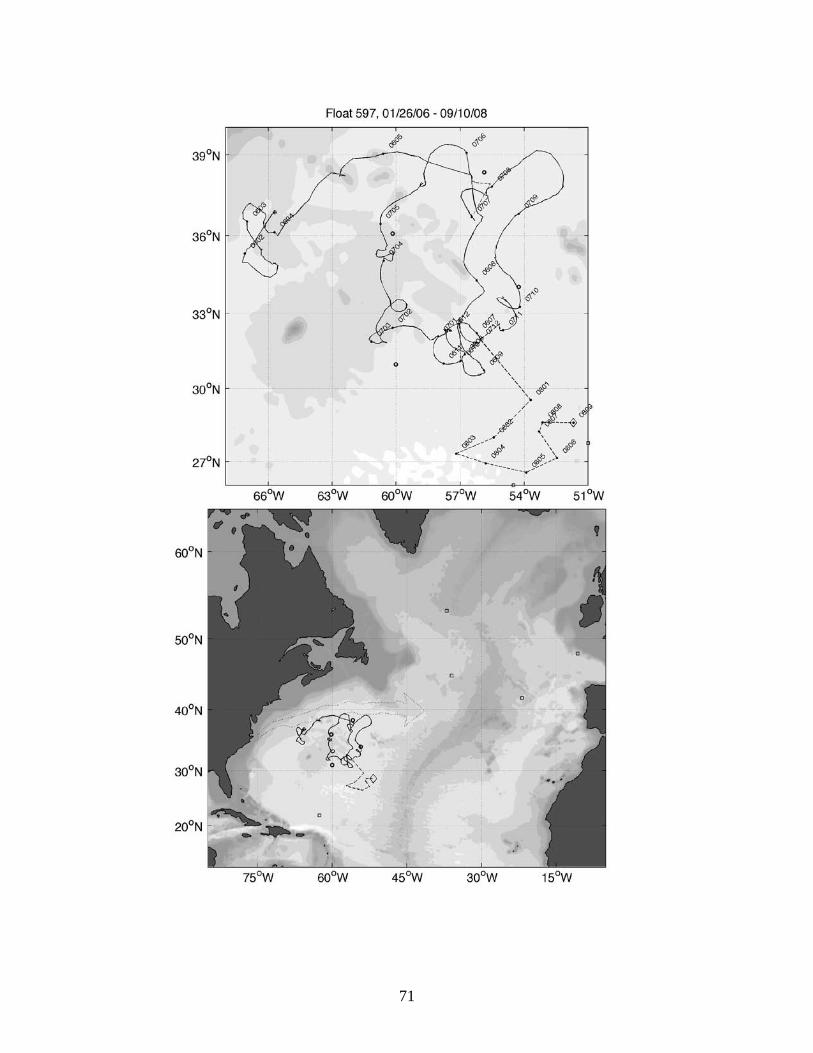
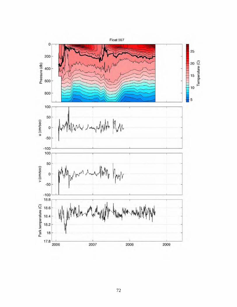
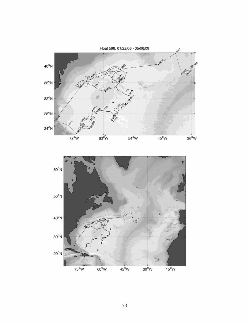
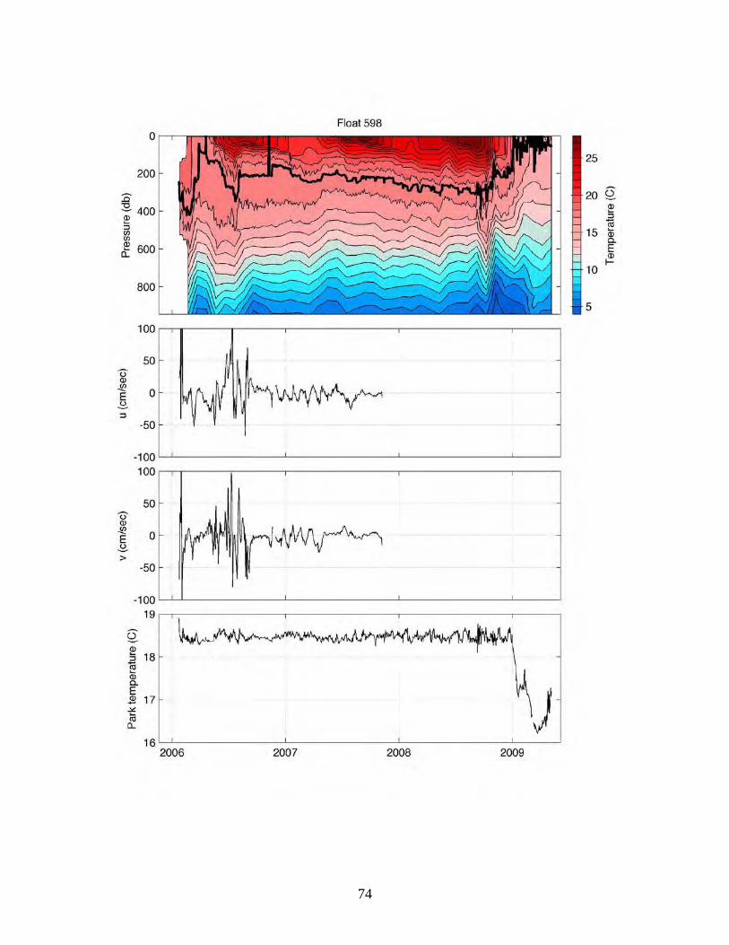
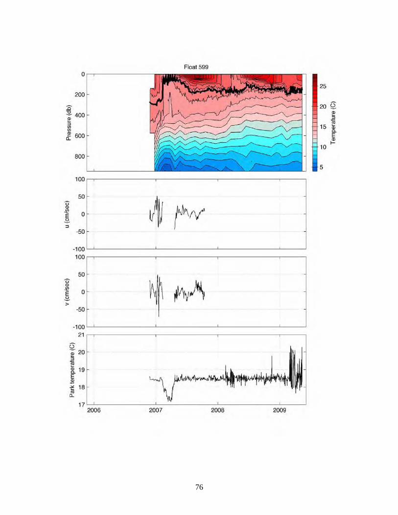
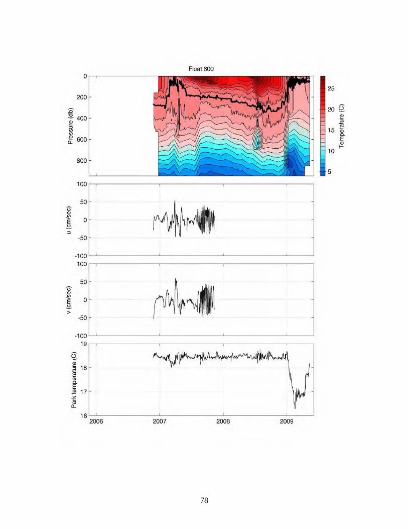
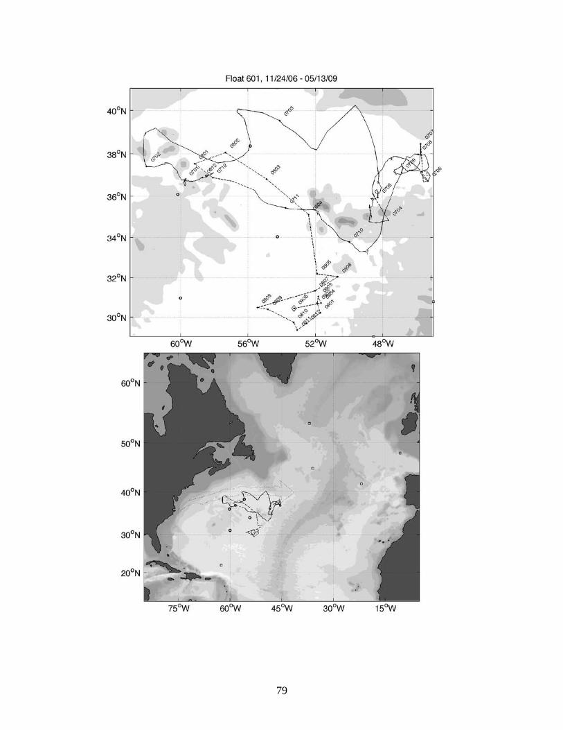
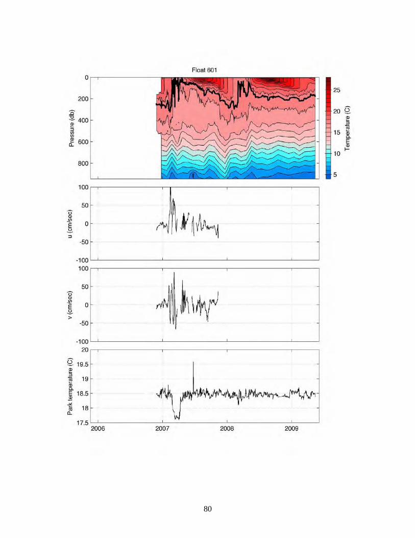
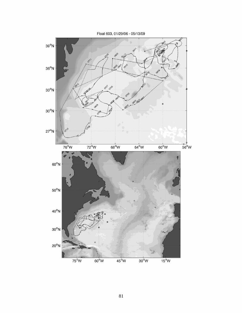
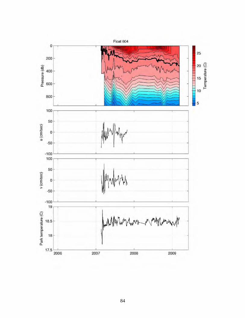
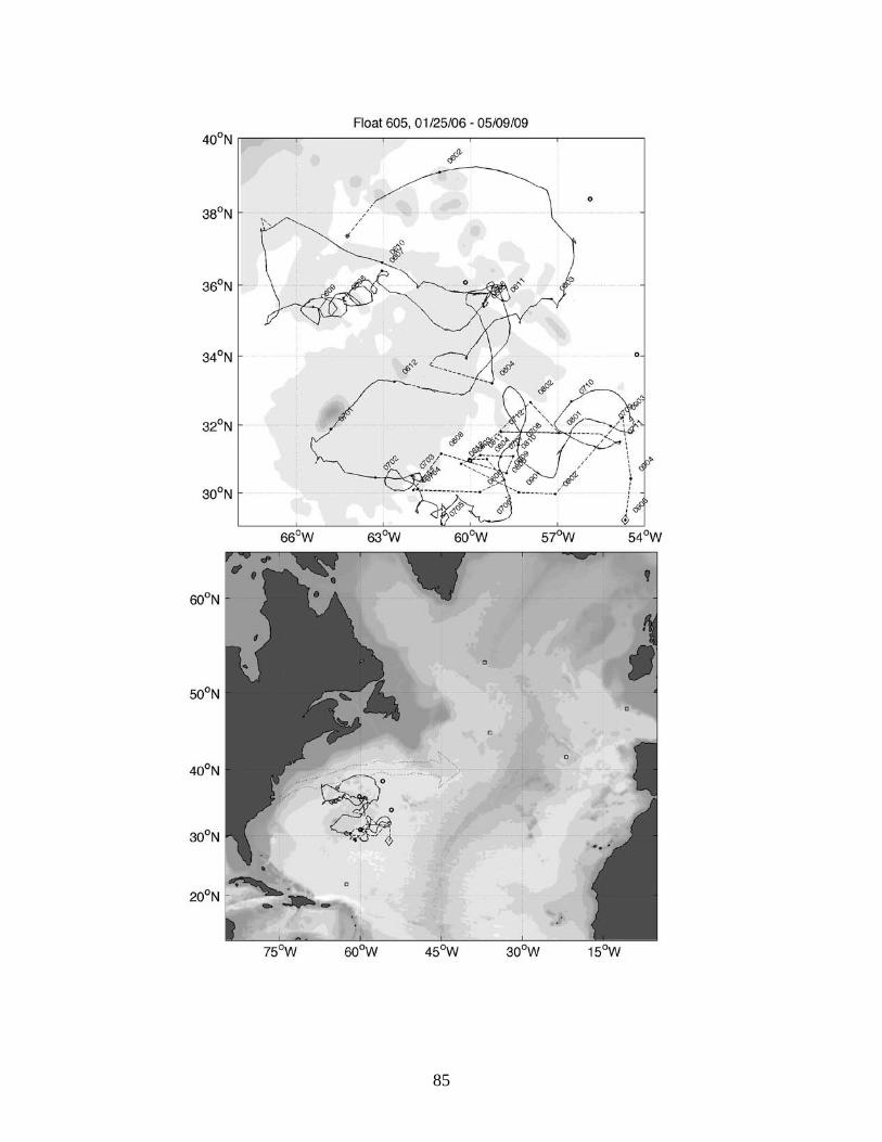
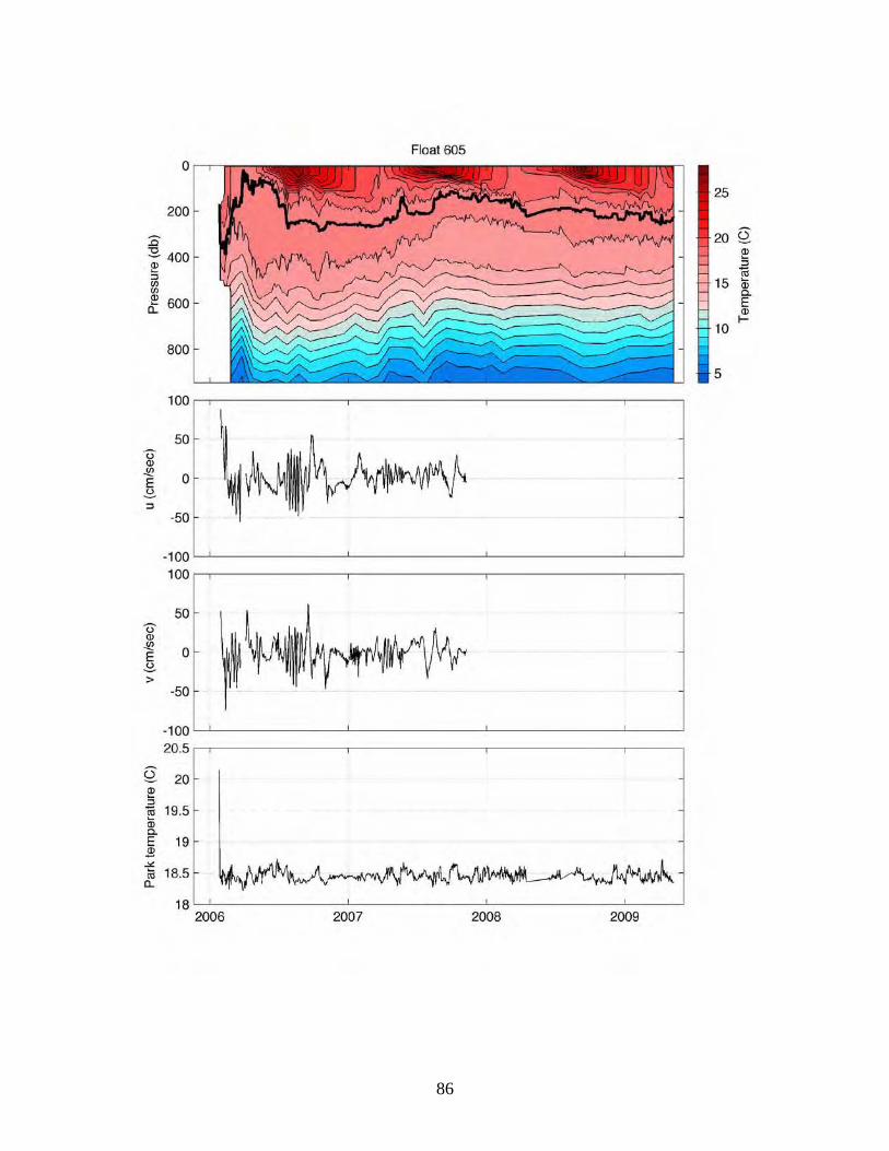
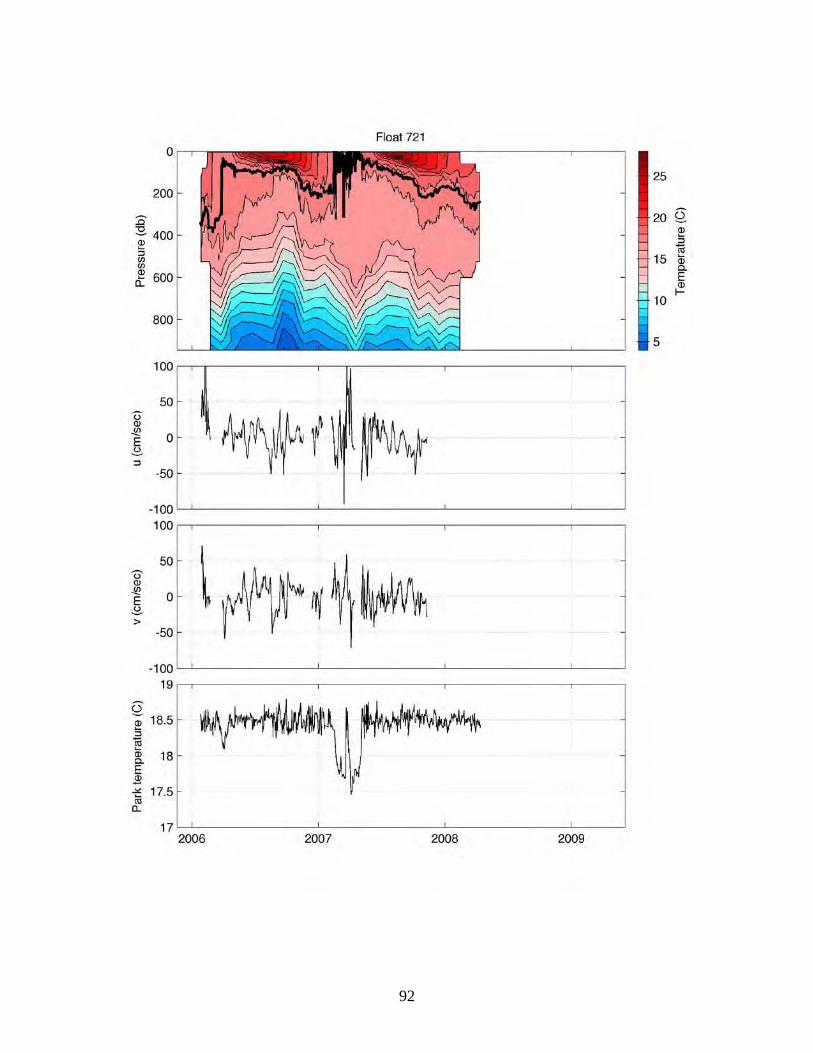
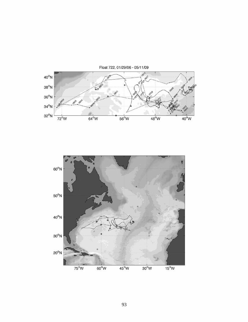
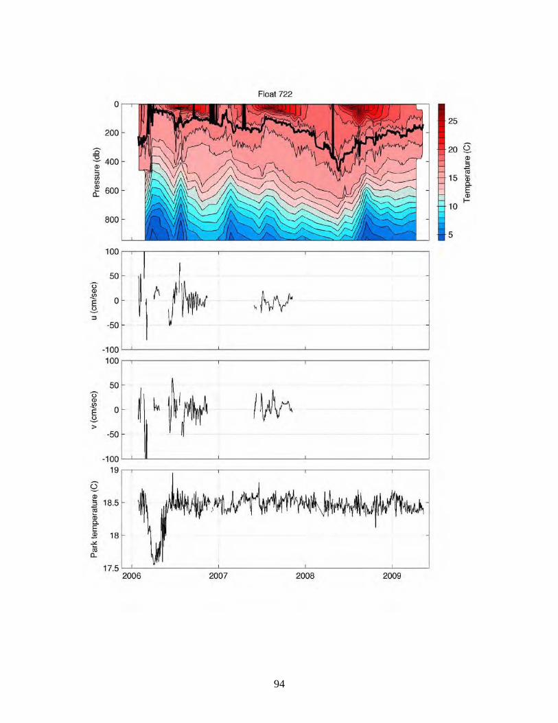
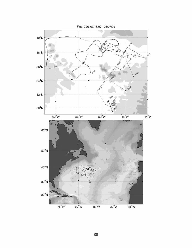
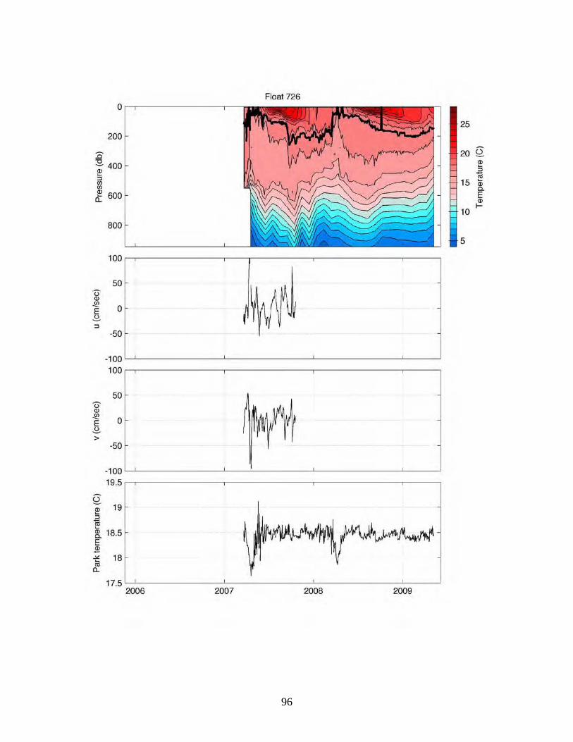
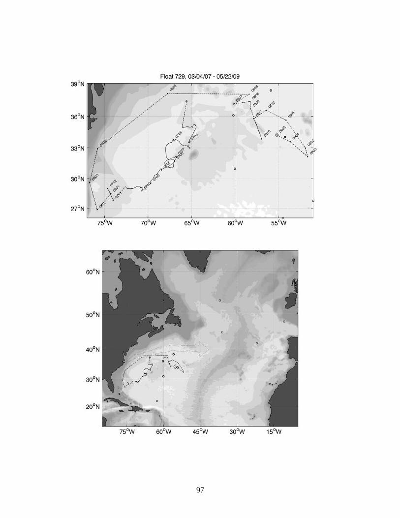
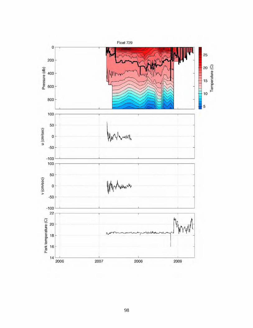
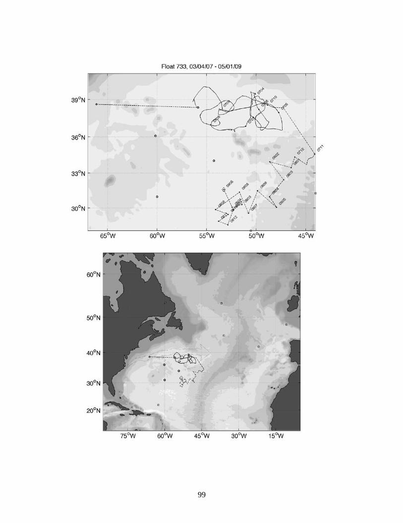
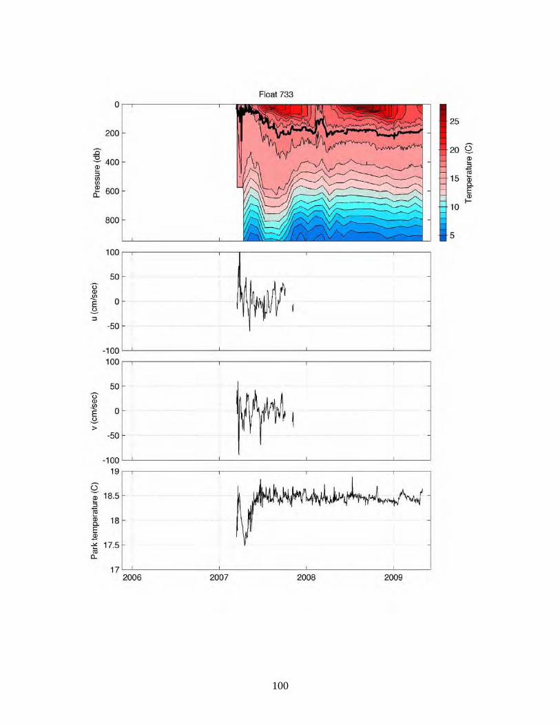
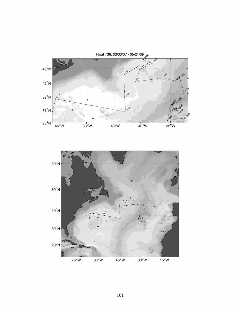
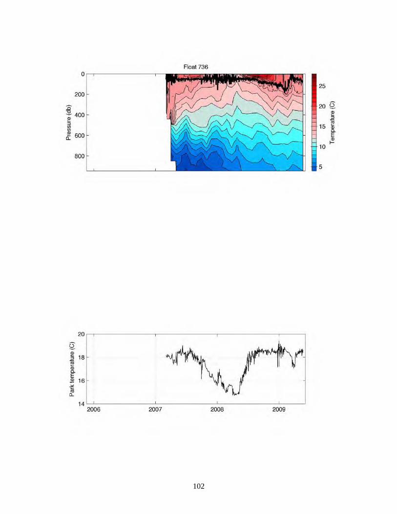
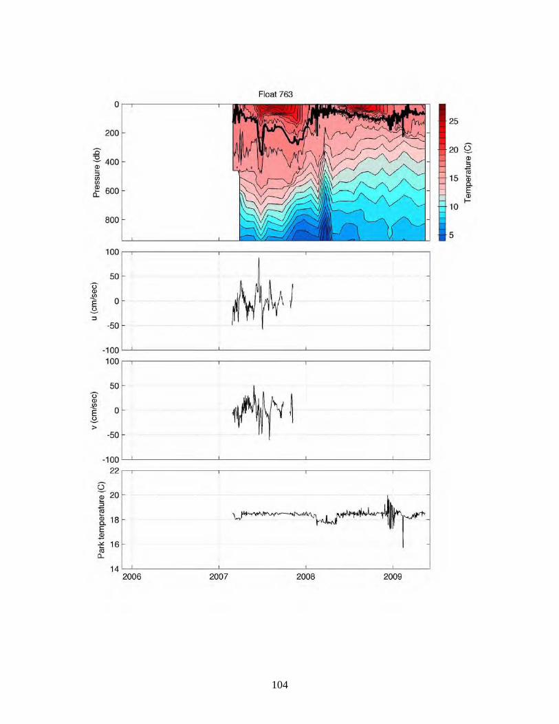
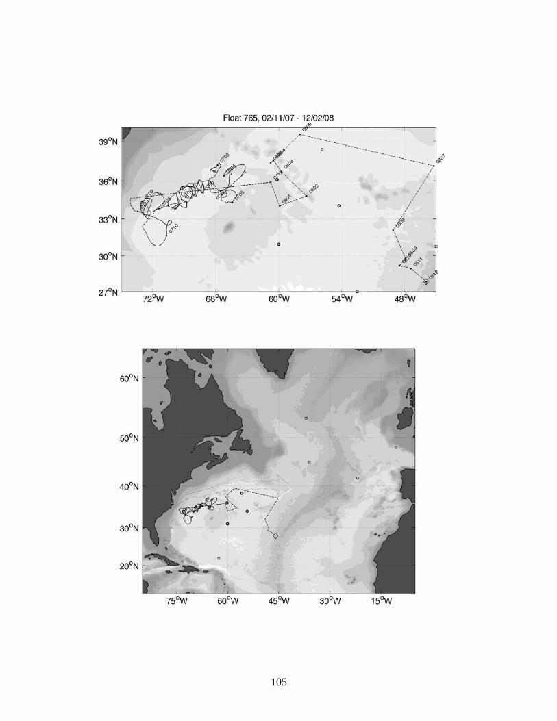
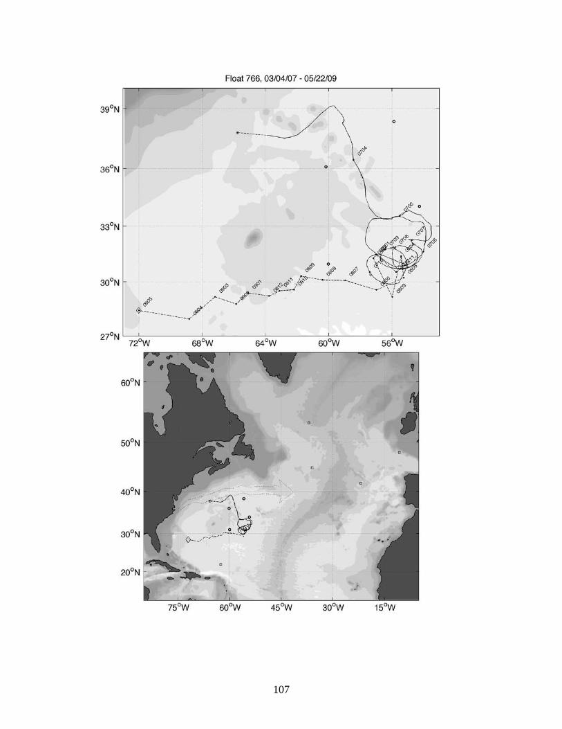
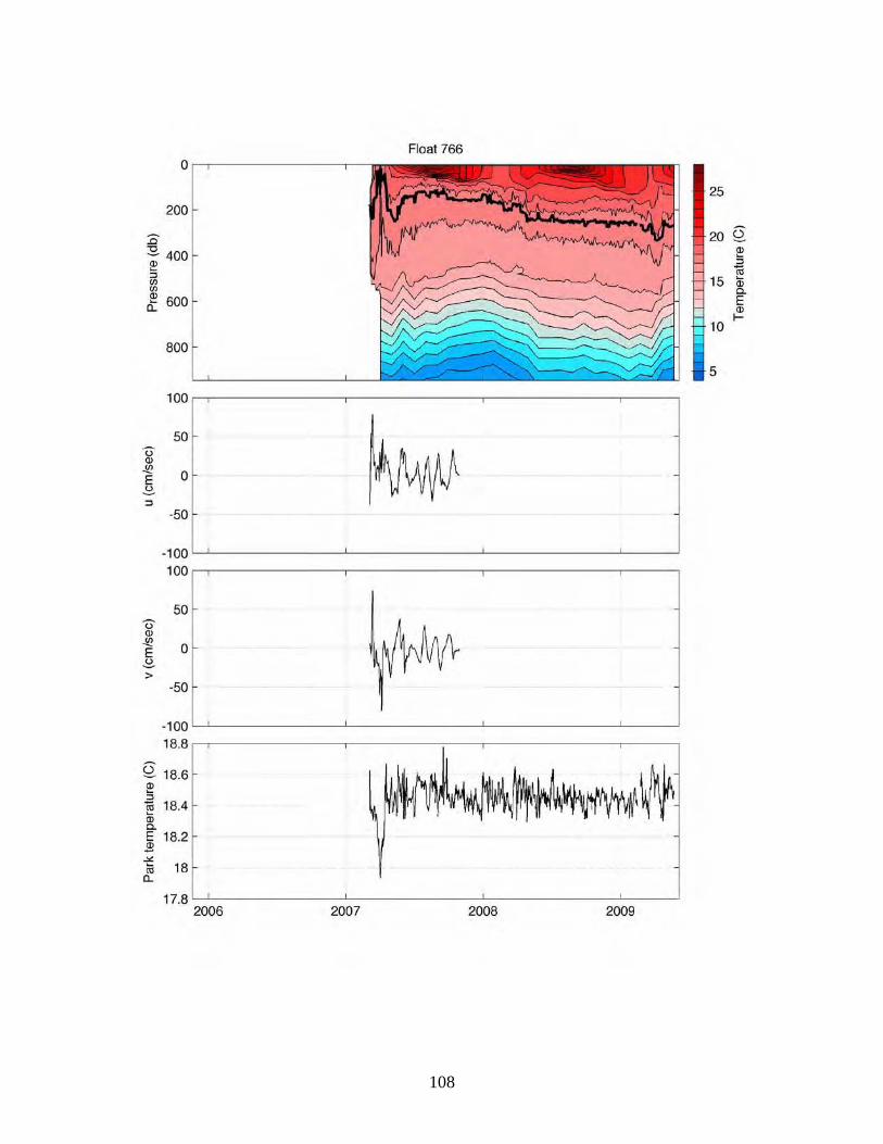
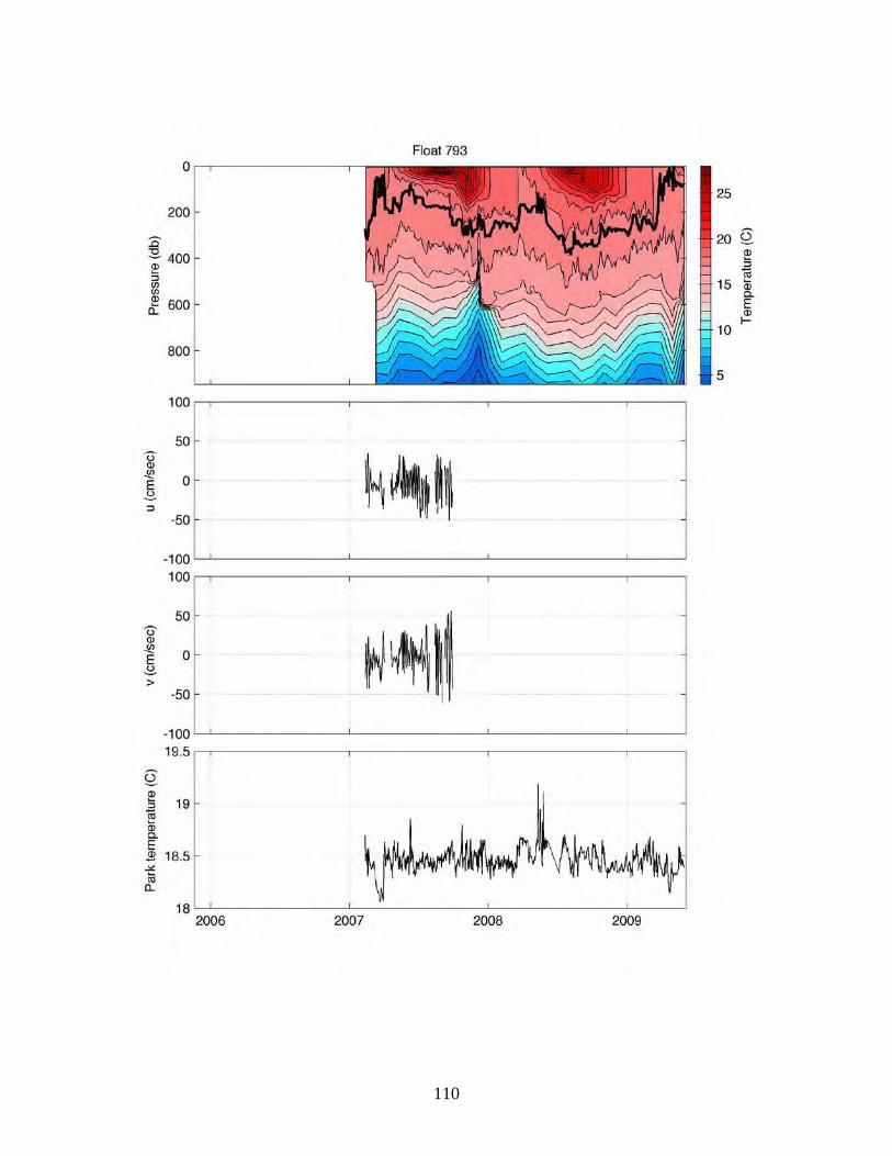
Appendix G: Bobber Trajectories and Profiles The following figures provide an overview of the data collected by each of the 40 CLIMODE bobbers. Bobbers are referenced to by the last 3 digits of their ARGOS PTT ID. (Left-hand page): Bobber trajectories are shown at two scales: as large as possible, with date markers in mmyy format included (upper panel), and at a North Atlantic scale which is the same for all bobbers (lower panel). Acoustically tracked sections of the trajectories are plotted as solid lines; where acoustic tracking was not possible, satellite fixes are connected by dashed lines. Deployment location is indicated by a small cross inside a circle, and latest known location by a diamond. Bold circles mark CLIMODE sound source mooring locations, with other sound sources denoted by squares. In the lower panel the typical position of the Gulf Stream north wall is indicated by an outlined arrow. Bathymetry is indicated by shading. (Right-hand page): Temperature profiles, velocity, and park temperature recorded by each bobber are shown. The upper panel is a depth-time contour plot of temperature in the upper 950 meters. Bobber park depth is plotted as a bold black line. Daily average zonal (black) and meridional (gray) current velocities from periods when acoustic float tracking was possible are shown in the third panel. The lower panel depicts the temperature during the bobber’s drift period (target = 18.5oC). Time, on the horizontal axis, spans the same range for all panels and all bobbers.

30

This page is intentionally left blank.

31

32

33

34

35

36

37

38

39

40

41

42

43

44

45

46

47

48

49

50

51

52

53

54

55

56

57

58

59

60

61

62

63

64

65

66

67

68

69

70

71

72

73

74

75

76

77

78

79

80

81

82

83

84

85

86

87

88

89

90

91

92

93

94

95

96

97

98

99

100

101

102

103

104

105

106

107

108

109

110

111

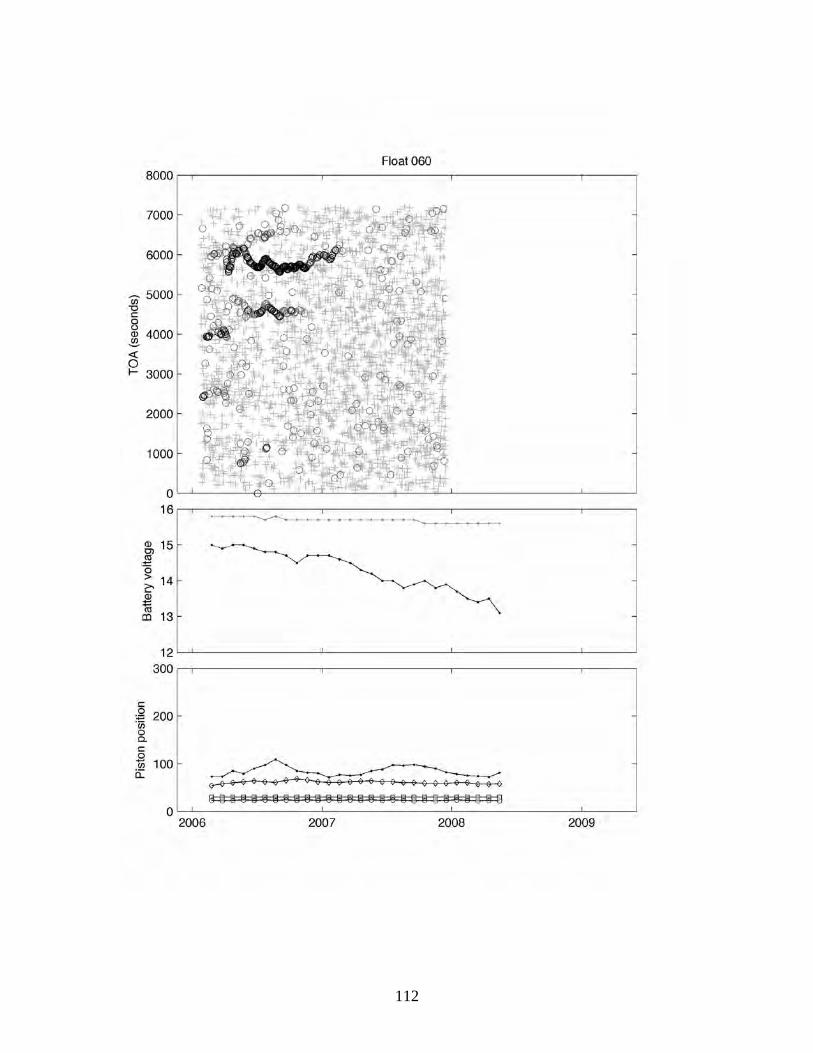
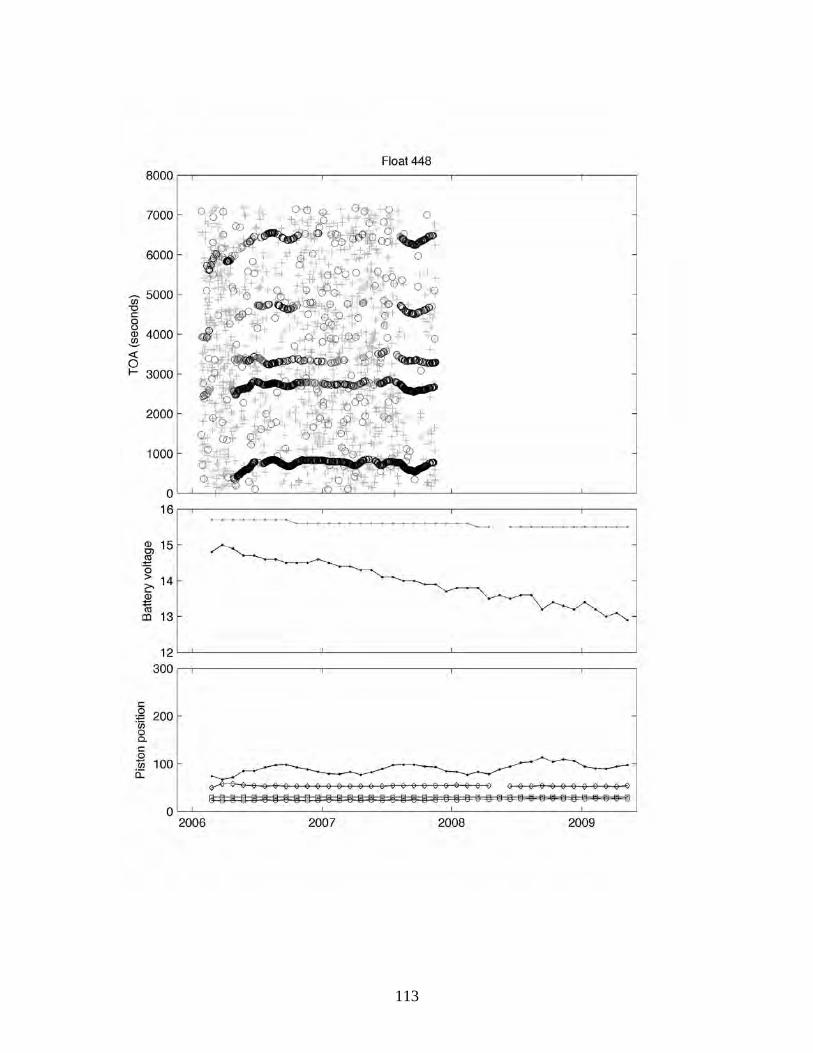
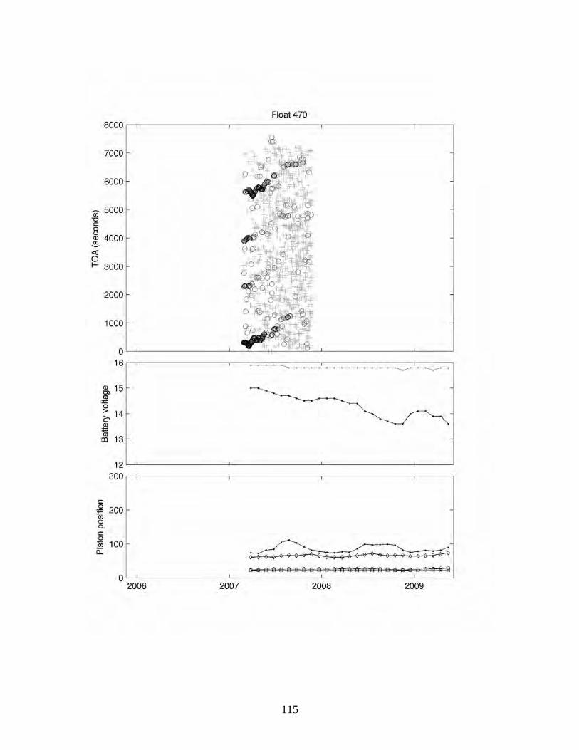
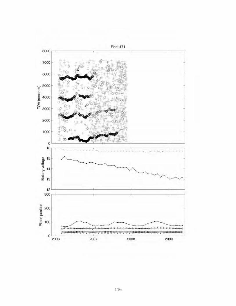
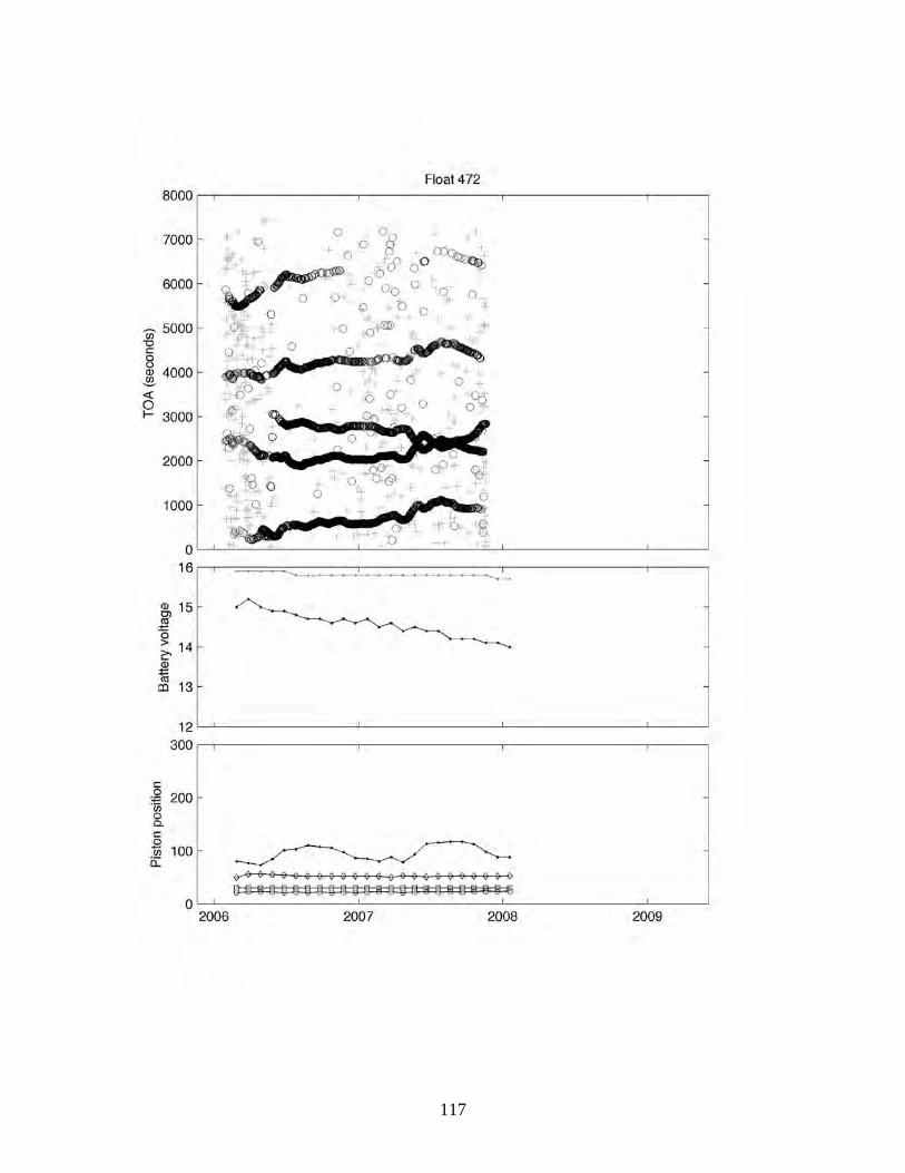
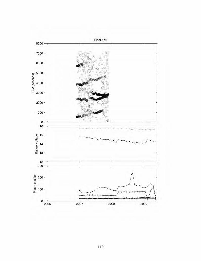
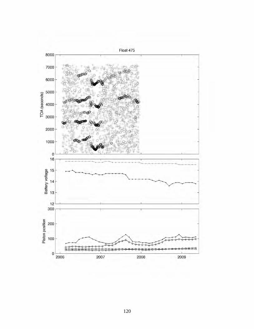
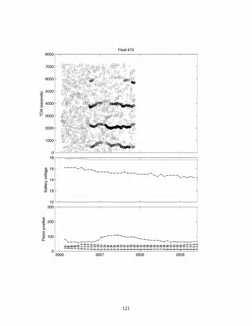
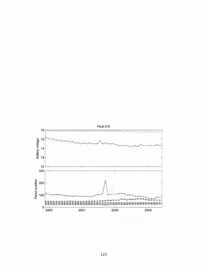
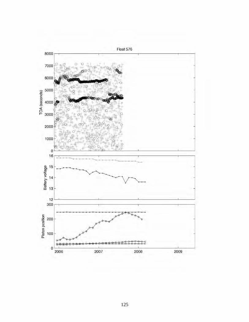
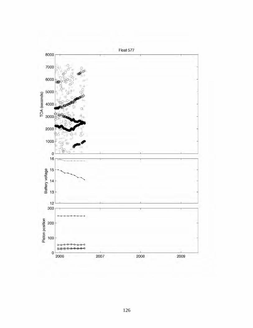
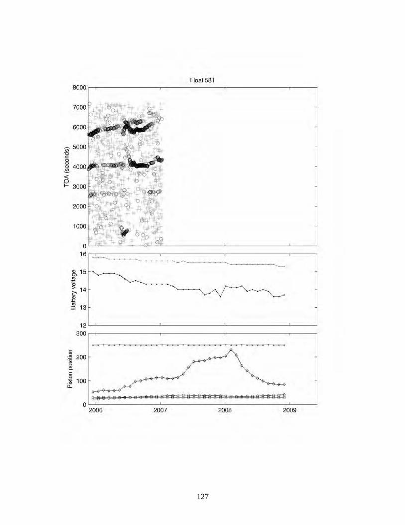
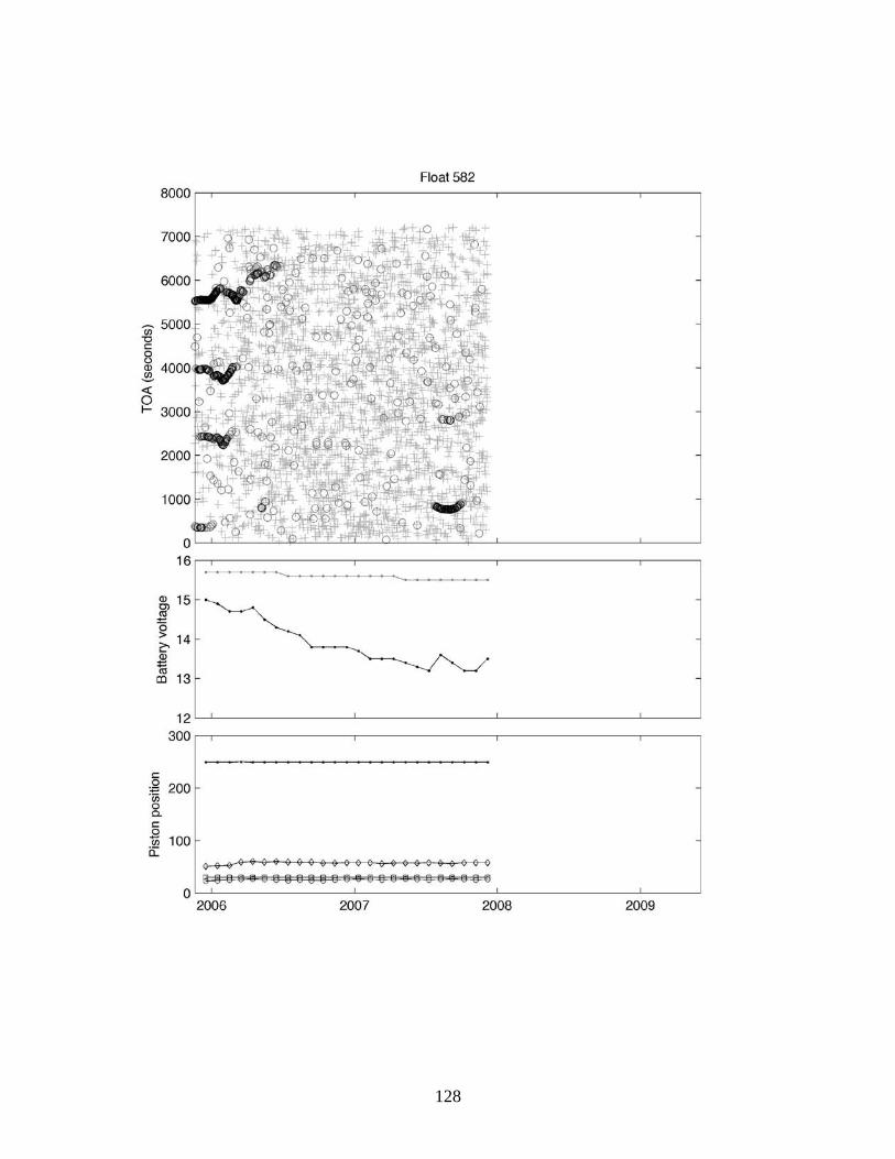
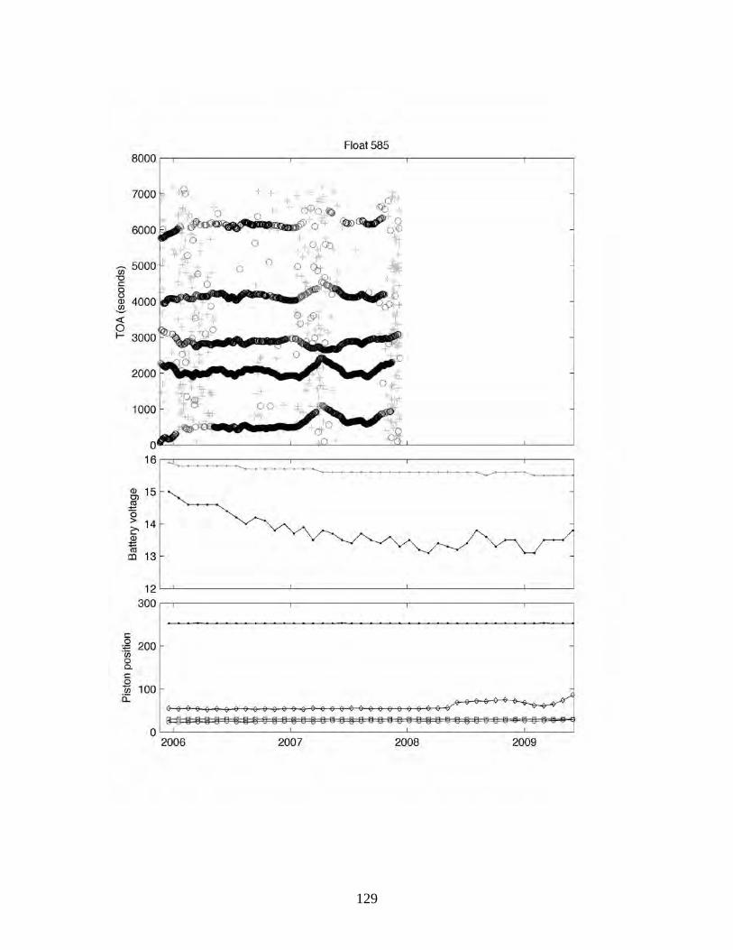
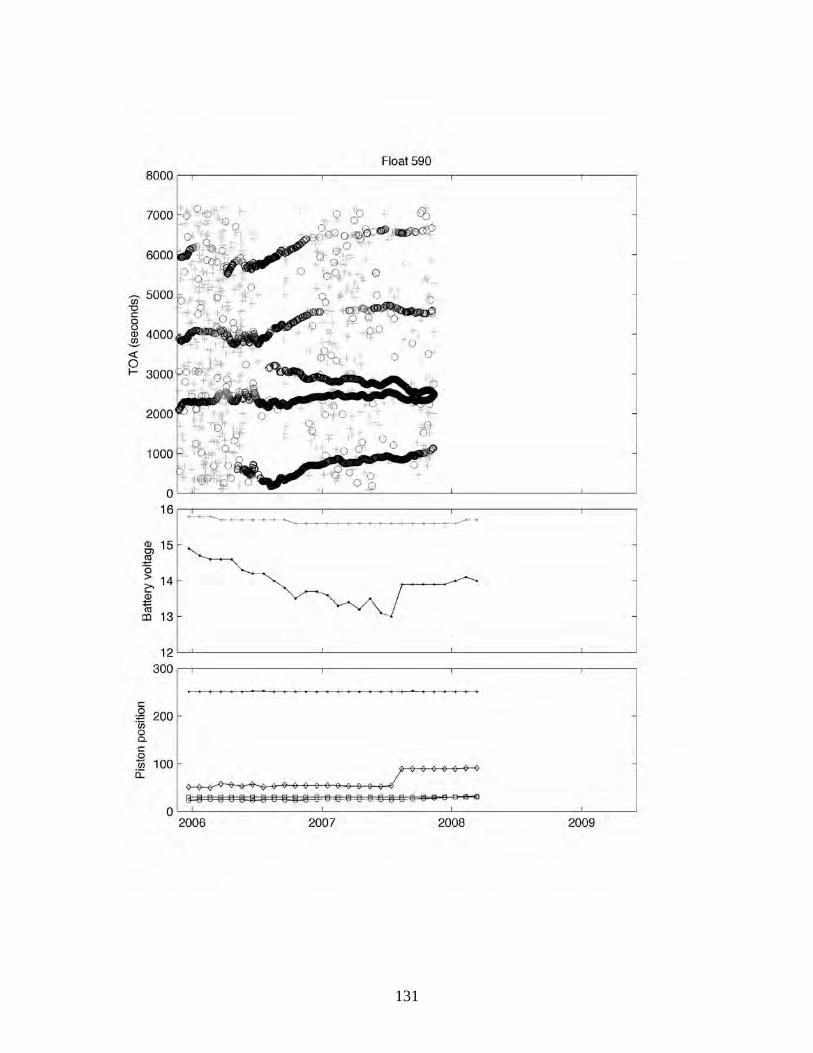
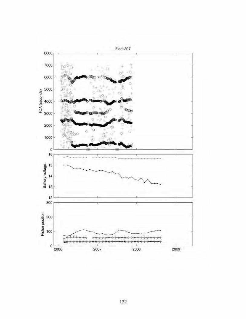
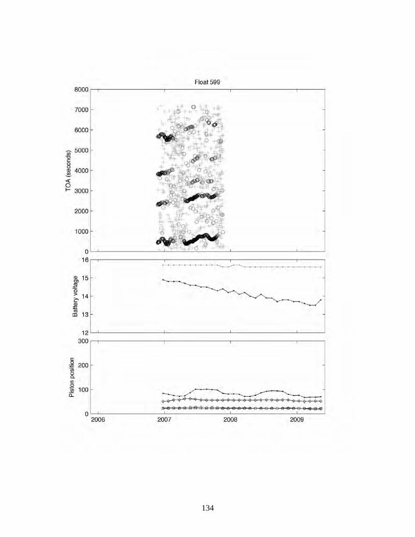
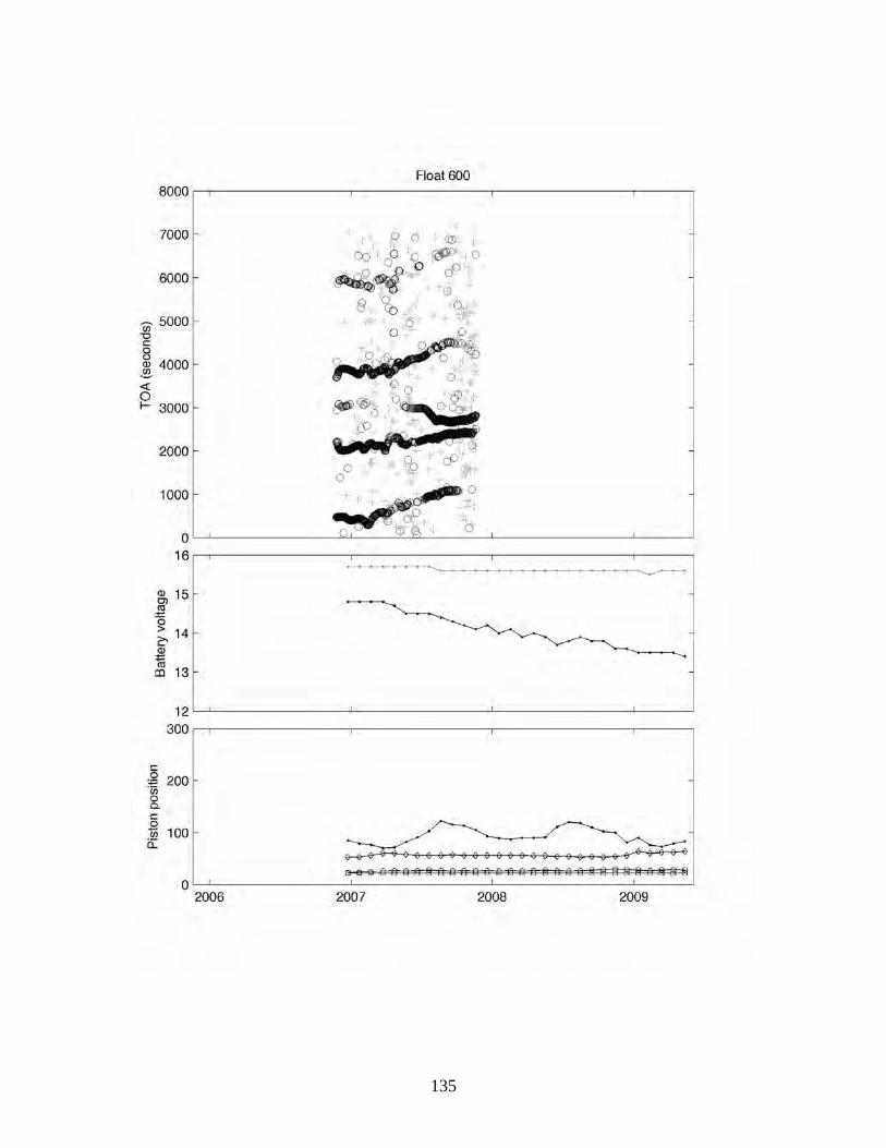
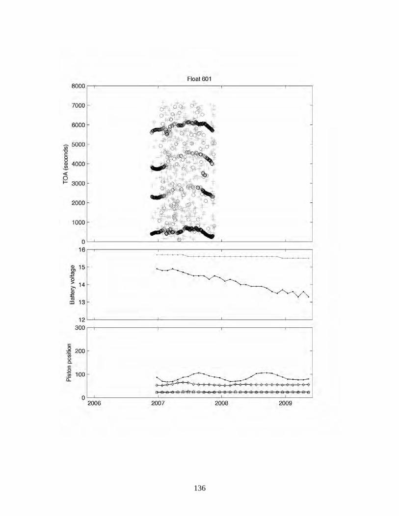
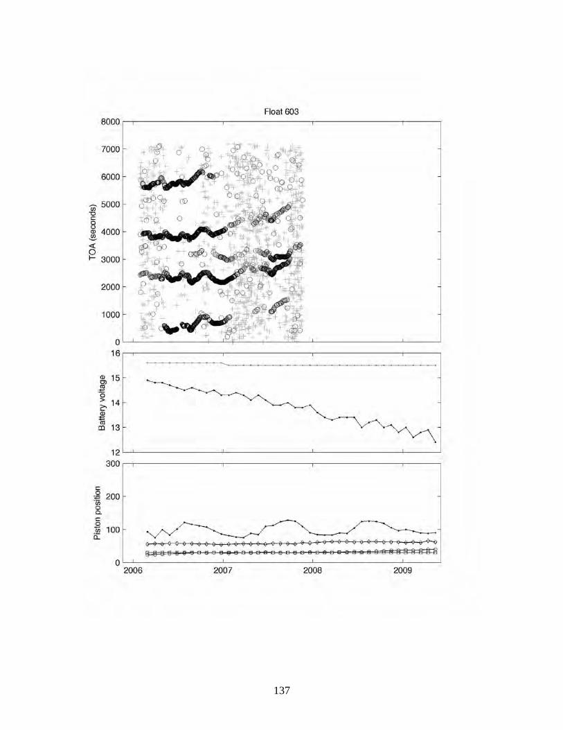
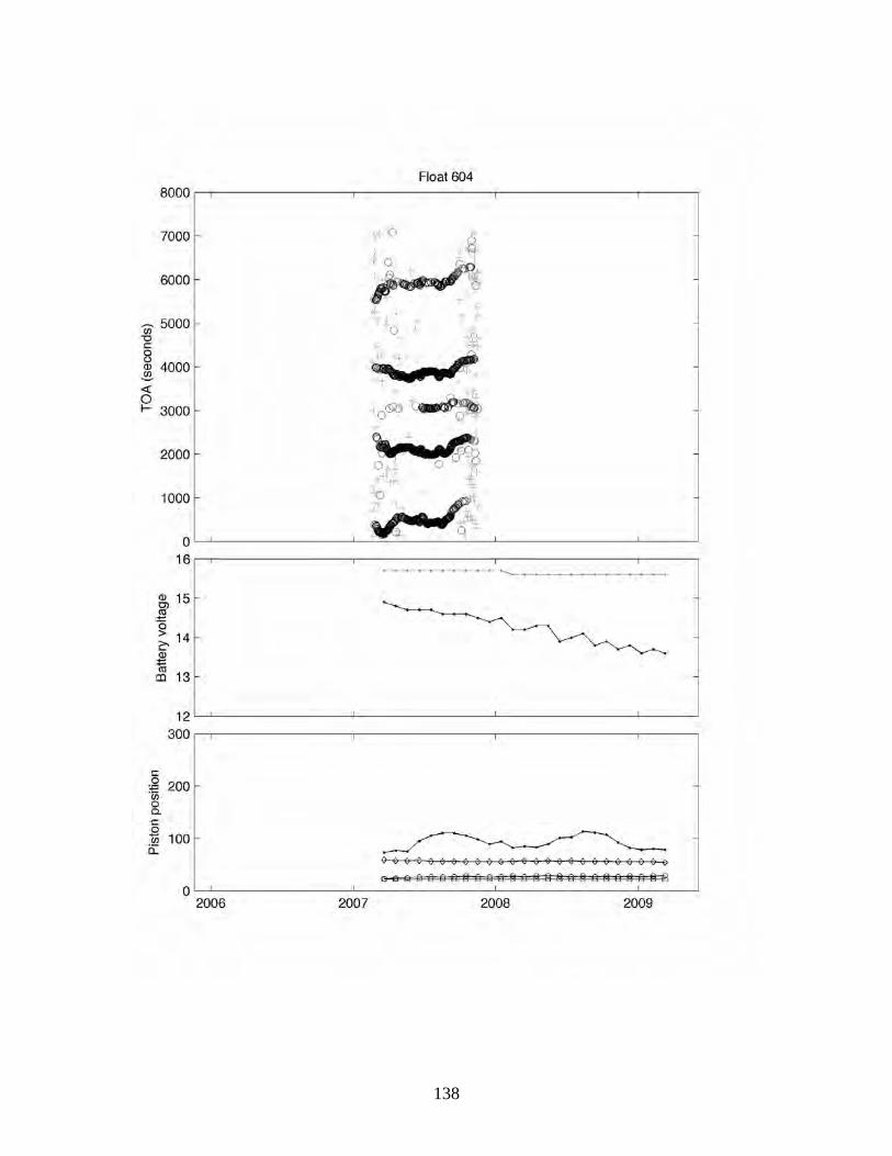
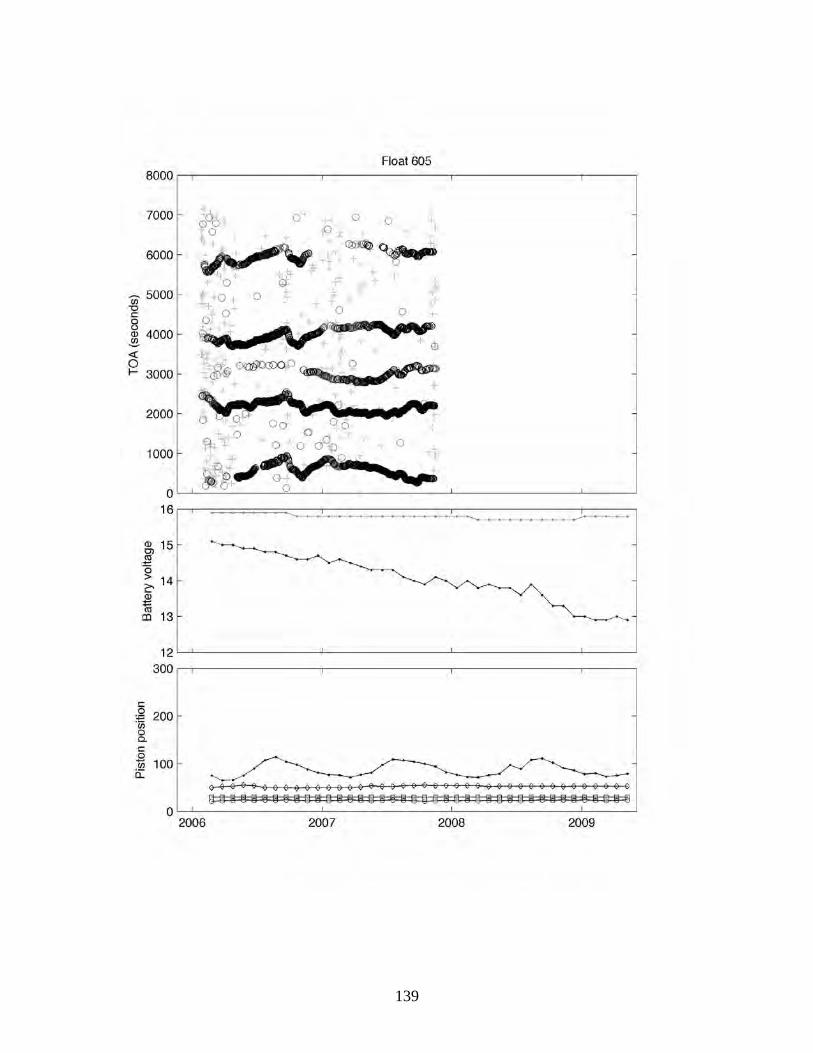
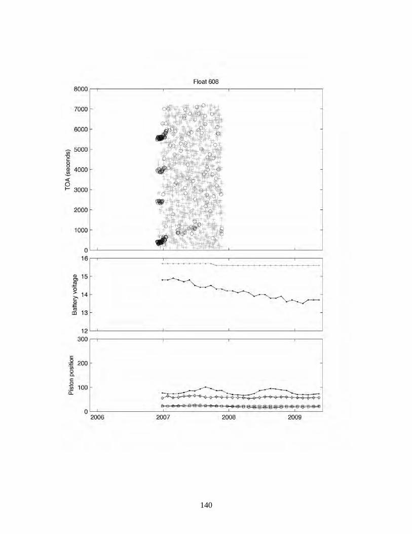
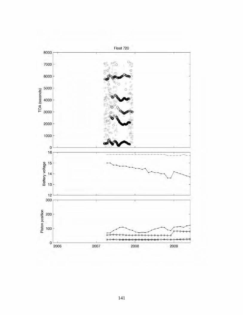
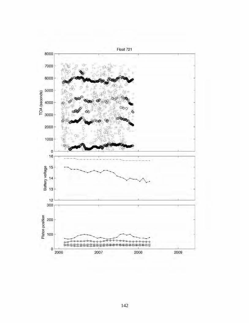
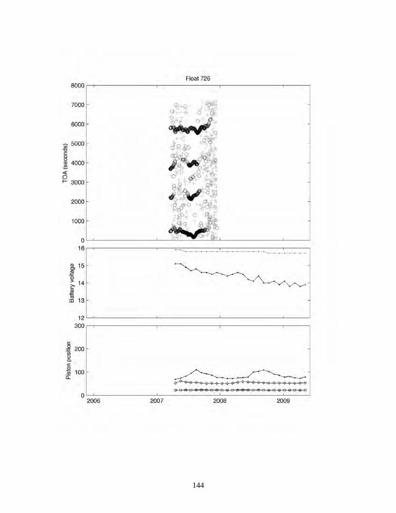
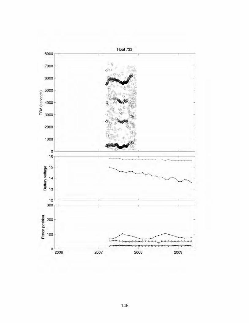
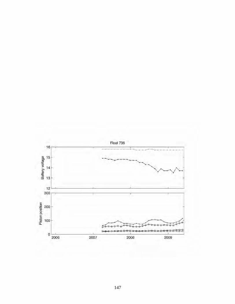
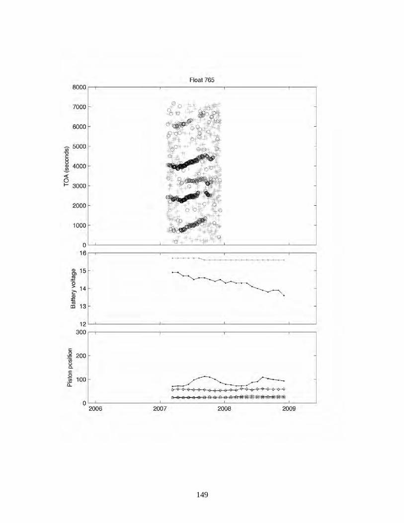
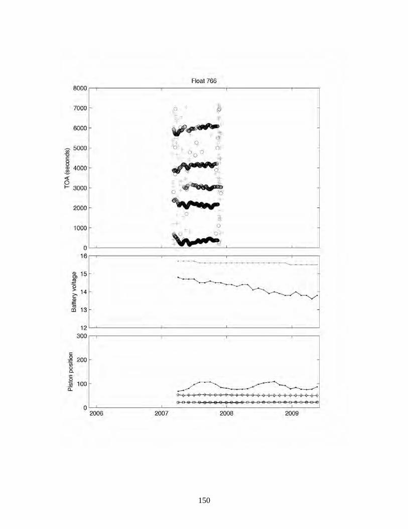
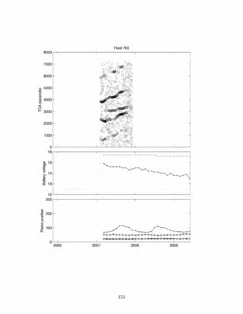
Appendix H: Bobber TOAs and Engineering Data In the plots that follow, bobbers are referenced to by the last 3 digits of their ARGOS PTT ID. (Upper Panel): Time-of-arrival (in seconds relative to the start of the acoustic listening window) of acoustic pongs from an array of moored sound sources. Circles indicate correlation heights exceeding 55 counts. (Middle Panel): Battery voltage during drift (light line) and buoyancy pump activation (dark line). (Lower Panel): Buoyancy pump piston position during surfacing (small circles), drift periods (diamond) and deep profiles (squares).

112

113

114

115

116

117

118

119

120

121

122

123

124

125

126

127

128

129

130

131

132

133

134

135

136

137

138

139

140

141

142

143

144

145

146

147

148

149

150

151

1. REPORT NO.

4. Title and Subtitle

7. Author(s)

9. Performing Organization Name and Address

12. Sponsoring Organization Name and Address

15. Supplementary Notes

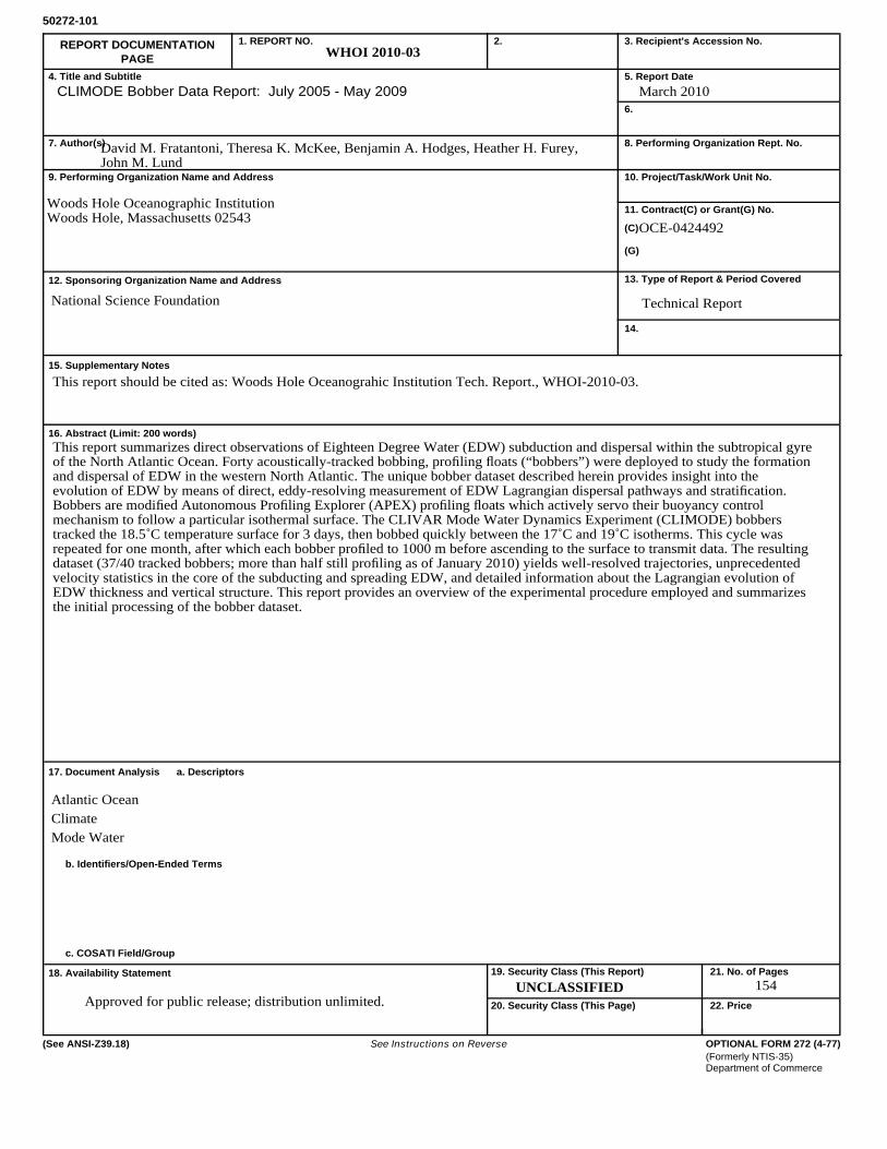
16. Abstract (Limit: 200 words)

17. Document Analysis a. Descriptors

b. Identifiers/Open-Ended Terms

c. COSATI Field/Group

18. Availability Statement

REPORT DOCUMENTATIONPAGE

2. 3. Recipient's Accession No.

5. Report Date

6.

8. Performing Organization Rept. No.

10. Project/Task/Work Unit No.

11. Contract(C) or Grant(G) No.

(C)

(G)

13. Type of Report & Period Covered

14.

50272-101

19. Security Class (This Report)

20. Security Class (This Page)

21. No. of Pages

22. Price

OPTIONAL FORM 272 (4-77)(Formerly NTIS-35)Department of Commerce

(See ANSI-Z39.18) See Instructions on Reverse

UNCLASSIFIED

WHOI 2010-03

CLIMODE Bobber Data Report: July 2005 - May 2009 March 2010

David M. Fratantoni, Theresa K. McKee, Benjamin A. Hodges, Heather H. Furey, John M. Lund

Woods Hole Oceanographic InstitutionWoods Hole, Massachusetts 02543

OCE-0424492

Technical ReportNational Science Foundation

This report summarizes direct observations of Eighteen Degree Water (EDW) subduction and dispersal within the subtropical gyreof the North Atlantic Ocean. Forty acoustically-tracked bobbing, profiling floats (“bobbers”) were deployed to study the formationand dispersal of EDW in the western North Atlantic. The unique bobber dataset described herein provides insight into the evolution of EDW by means of direct, eddy-resolving measurement of EDW Lagrangian dispersal pathways and stratification. Bobbers are modified Autonomous Profiling Explorer (APEX) profiling floats which actively servo their buoyancy control mechanism to follow a particular isothermal surface. The CLIVAR Mode Water Dynamics Experiment (CLIMODE) bobbers tracked the 18.5˚C temperature surface for 3 days, then bobbed quickly between the 17˚C and 19˚C isotherms. This cycle was repeated for one month, after which each bobber profiled to 1000 m before ascending to the surface to transmit data. The resultingdataset (37/40 tracked bobbers; more than half still profiling as of January 2010) yields well-resolved trajectories, unprecedented velocity statistics in the core of the subducting and spreading EDW, and detailed information about the Lagrangian evolution of EDW thickness and vertical structure. This report provides an overview of the experimental procedure employed and summarizesthe initial processing of the bobber dataset.

Atlantic OceanClimateMode Water

154Approved for public release; distribution unlimited.

This report should be cited as: Woods Hole Oceanograhic Institution Tech. Report., WHOI-2010-03.