1

Circulation and Mixing in the Skidaway River Estuary,

Savannah, GA

Daniela Mewes

Georgia Institute of Technology

April 24, 2012

2

Abstract

Turbulent mixing within a water column impacts the temperature and salinity profiles of the

column as well as oxygen and nutrient distribution. Nutrient loading from anthropogenic sources

can cause hypoxic conditions which can reduce marine habitats and lead to fish kills. Significant

mixing throughout the water column can counteract hypoxia. In this study, mixing within the

Skidaway estuary was assessed to determine its impact on biogeochemical processes. SCS, CTD

and ADCP data were collected throughout a cruise in both the small Skidaway estuary and the

South Atlantic Bight off the coast of Skidaway Island, Savannah, GA. The data suggested that

the estuary is more saline than it has been in the past two decades, which may be partially due to

a low discharge from the Savannah River. The saline conditions may be impacting mixing

within the estuary, although surface velocity magnitude values are comparable to similar

measurements made in the neighboring Satilla river estuary. Additionally, temperature and

salinity profiles from CTD casts at 14 stations along the estuary and off the coast of Skidaway

Island demonstrated a well-mixed to partially-mixed estuarine environment, which was not

indicative of decreases in turbulent mixing. Further studies of longer duration are needed to

assess the impacts of the current low discharge and high salinity water in the Skidaway estuary

on estuarine circulation to determine whether the estuary will become more susceptible to

eutrophication as a result.

Introduction

The degree to which a water column is mixed impacts its physico-chemical interaction with the

marine ecosystem and its surroundings. Water column stratification may result in hypoxic

conditions if dissolved oxygen consumed by benthic microfauna in sediments is only slowly

3

replaced by mixing in the water column (Stefanelli et. al., 2005). Anthropogenic nutrient loading

contributes to harmful algal bloom (HAB) which leads to decomposition of an increased number

of phytoplankton, a process resulting in further depletion of oxygen in the lower depths of the

water column (Stanley et. al., 1992; Anderson et. al., 2002). Nutrient loading and resultant HAB

has been associated with fish kills (Verity, 2010; Stanley et. al., 1992) and coral reef degradation

(Koop et. al., 2001). Hypoxia can reduce habitats for marine organisms and lead to impaired

recovery from additional stressors (Verity et. al., 2006). Strong vertical mixing can counteract

hypoxia by mixing oxygen to lower depths (Stanley et. al., 1992). Salinity and temperature

variations with depth along an estuary determine its degree of mixing and therefore its

susceptibility to eutrophication. Profiles of the velocity magnitude and direction along the

estuary can be correlated with these results to further characterize the mixing processes.

Vertical mixing in the ocean is primarily driven by wind and tidal forcing (Moum et. al., 2001). .

Winds initiate convection by breaking up and penetrating the surface layer, sending the warm

surface water to greater depths. Simultaneously, diurnal heat fluxes contribute to the cooling and

resultant sinking of surface water (Moum et. al., 2001). Convective plumes generated by the

movement of water create turbulences as they sink, further mixing the upper oceanic layer. The

degree of turbulence and therefore mixing depends on wind and wave speed at the surface

(Moum et. al., 2001; Stewart, 2005). The energy needed to mix water increases as a function of

depth and density (Stewart, 2005). As a result, below the mixed layer lies a region of rapidly

decreasing temperature termed the thermocline. In mid-latitude waters where evaporation

exceeds precipitation and the mixed-layer is more saline than the thermocline, this region

exhibits decreasing density with depth and is also referred to as the pycnocline (Moum et. al.,

2001; Stewart, 2005).

4

In estuaries, tidal forcing is an even greater contributor to mixing than wind. Spring tides,

occurring with the full and new moon of the lunar cycle, cause higher velocity currents than their

counterpart, neap tides (Blanton et. al., 2003). Turbulence is correlated with a high Reynold’s

number, which velocity, viscosity and density are all components of (Falkovich et. al., 2006).

Ebb and flood tides, which correspond to low and high water levels respectively, also contribute

to the mixing of freshwater and seawater in estuaries. Flood tide maximum velocities are

typically greater than ebb tide maxima, contributing to a greater turbulence (Trevethan et. al.,

2010; Blanton et. al., 2003). Additionally, the size of an estuary affects its degree of turbulent

response. Smaller estuaries are more likely to exhibit turbulent mixing than larger estuaries due

to a higher pressure in narrower channels contributing to a higher velocity flow (Trevethan et.

al., 2010). Currents contribute to the mixing process by distributing water from sources with

different physico-chemical properties and interacting with pre-existing estuarine and tidal

currents (Stewart, 2005; McClain et. al., 1984). In the Atlantic Ocean, the Labrador Current

provides a southward flow of cool water that interacts with the northward flowing warm Gulf

Stream off the coast of Cape Hatteras, generating turbulence as the two currents collide

(Huthance, 1995).

Estuaries are classified by their degree of mixing and their resultant salinity gradients. Salinity

increases from the head to the mouth of an estuary and with depth within the water column and

generally demonstrates a shape known as the isohaline curve (Pritchard, 1952). Relatively

unmixed, stratified estuaries exhibit a strong surface freshwater flow seaward and an isohaline

curve that tends towards the horizontal (Griffin et. al., 1990). Well-mixed estuaries retain

freshwater and exhibit a nearly vertical isohaline curve, whereas the isohaline of partially-mixed

estuaries is seen to slant (Griffin et. al., 1990). The Skidaway estuary is well-mixed, shallow and

5

tidally dominated with freshwater inputs from two primary sources: the Ogeechee River to the

south and the Savannah River to the north. Flows are typically highest early in the year from

January to March (Verity, 2010; Verity et. al., 2006). The Savannah River is one of the top 5

container ports on the eastern coast of the United States, and from 1970-2000 the coastal

counties of Georgia grew over 62% (Verity, 2010), demonstrating that the Georgia coast is

industrially active and continuing to grow. Peak and mean blooms of harmful algae have

increased over the last 22 years, attributed to increased nutrient loading from cultivation and

urbanization of the coast (Verity, 2010). Additionally, Gray’s reef, approximately 120 km

offshore from neighboring Sapelo Island, may be close enough to be affected by inland nutrient

loading. Similar systems have become more eutrophic and contain fewer live coral (Koop et. al.,

2001). There is a potential that Gray’s reef will be similarly affected, unless vertical mixing is

strong enough to counteract this or nutrients are being retained at the shore. Studies

characterizing vertical mixing have been conducted in the large Satilla estuary south of

Skidaway Island (Blanton et. al., 2001) and nutrient levels have been studied extensively in the

Skidaway estuary (Verity et. al., 2006). Studies on turbulent mixing are limited by a lack of

appropriate instrumentation (Trevethan et. al., 2010) and few studies have been conducted on

mixing in small estuarine systems such as the Skidaway estuary. Additional studies on estuarine

circulation are necessary to assess the effects of increased anthropogenic nutrient loading on the

estuaries of the Georgia coastal ecosystem.

This study examined: the surface temperature and salinity of the Skidaway River estuary, the

salinity and temperature profiles of the estuary and sampling stations offshore, and the velocity

profile along the estuary and the offshore transect. The culmination of the recorded data allowed

for an analysis of the estuarine circulation and mixing processes taking place during the Spring

6

tide cycle in the estuary. Establishing the degree of mixing present in the Skidaway estuary

determines whether the estuarine system can counteract any observed eutrophic changes and

allows for future impacts of eutrophication to be modeled.

Methods

Data was collected using several instruments on board the R/V Savannah, a research vessel

owned by the Skidaway Institute of Oceanography (SKIO), from March 9th

-March 10th

, 2012.

Additional ADCP data was attained following the completion of the cruise from March 10th

–

March 12th

, 2012. The cruise began at the SKIO dock on March 9th

and the ship traveled out of

the Skidaway River estuary towards the Atlantic Ocean, continuing on an eastward path. The

R/V Savannah began its return trip prior to reaching the continental shelf through the same

estuary. A trip could not be made around the entire perimeter of Skidaway Island due to the

construction of a new bridge. The R/V Savannah continued past SKIO to this bridge before

turning around and returning to SKIO where the cruise was completed at the SKIO dock, located

on the northwestern side of Skidaway Island.

Using the NOAA developed Shipboard Computer System (SCS Version 4.2.3) software, the R/V

Savannah recorded ancillary surface data 1 meter below the surface including: date/time,

latitude, longitude, depth, sea surface temperature, conductivity, and salinity along with other

meteorological variables not examined by this study along the ship track.

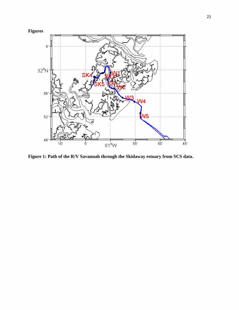
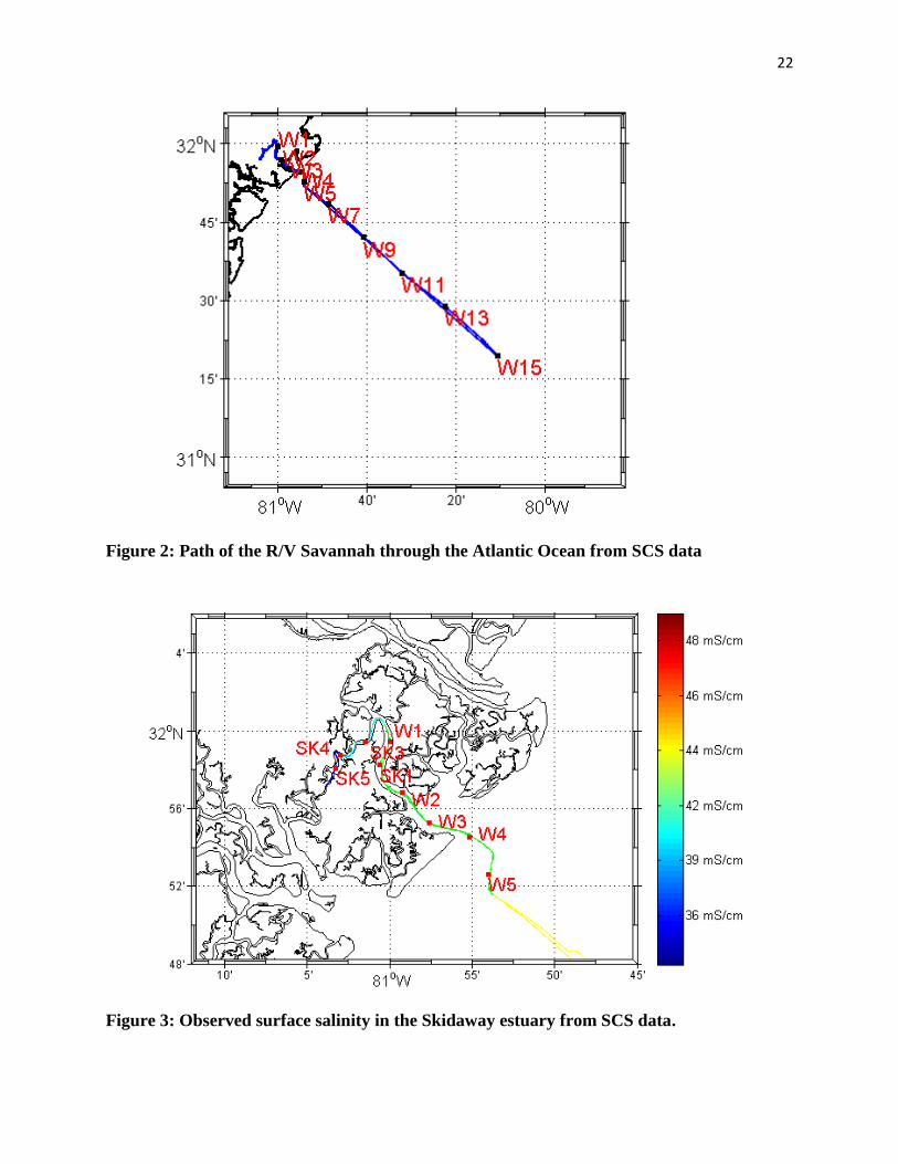
The GPS locations of 14 data acquisition stations were used to represent the ship track around

Skidaway Island (Figure 1), and the offshore transect (Figure 2). Coordinates designated with an

“SK” prefix were located in the Skidaway estuary, whereas coordinates with a prefix of “W”

were located along the transect.

7

A CTD or conductivity-temperature-depth instrument manufactured by Sea Bird Electronics

(SBE) was used to obtain salinity and temperature profiles of the water column at the 14 stations.

The CTD used in this study consisted of a water carousel (SBE 32) and datalogger (SBE 25)

which was lowered at each station by a winch, and data recording began once the CTD was

submerged 1 meter below the surface of the water. The CTD was lowered further until it was

approximately 2m above the ocean floor, at which point it was brought back on board and data

recording was completed for that station.

Acoustic Doppler Current Profilers (ADCP), as their names imply, utilize the Doppler effect to

determine the motion of particles and therefore the current in the ocean (Kostaschuk et. al.,

2005). Sediments and particles suspended in the water allow for backscattering of sound waves

emitted by the instrument. Particles moving away from the ADCP will result in a higher

frequency whereas particles moving towards the ADCP will result in a lower frequency, due to

the Doppler Effect. The sound waves are generated in beams, and instruments are manufactured

to produce a set number of beams at a set angle to the ADCP. Two four-beam ADCP instruments

were used in this study to attain current direction and magnitude along the ship track. T-RDI’s

300 kHz workhorse sentinel ADCP was mounted to the hull of the R/V Savannah, 2.5m below

the water line for the majority of the cruise. On the return trip, the ADCP 1m pole arm was

added in order to attach the 1200 kHz T-RDI workhorse sentinel for shallower depths. The 1200

kHz ADCP was fixed 1m below the water line. Following the completion of the research cruise,

the 1200 kHz ADCP was left attached to the R/V Savannah at the SKIO dock and recorded data

for an additional 42 hours. WINADCP version 1.10 was downloaded as freeware and used to

examine the ADCP data. The 1.10 version was produced in 2001 and does not have a simple

method for exporting the data as the export function featured in the program only exports header

8

information. Freeware ADCP scripts are often written for ADCP taken at stations, similar to the

CTD data used in this study. Only one program written to process ADCP “r” files in Matlab was

able to correctly process data, RDADCP by Rich Palowicz, last updated in 2010. The 42 hour

ADCP data was extracted using a variation of the adcpdemo.m file from the RDADCP program

and inserted as column-averaged magnitudes into Excel. This allowed the 42 hour ADCP

contour to be juxtaposed with NOAA water height tidal data from Fort Pulaski, GA, the nearest

NOAA station to Savannah. Meteorological data from the SKIO station was also downloaded to

examine temperature and dew point in correlation with the ADCP contour and water height.

The M_map package compiled by Rich Palowicz provided a database of coastal maps written for

Matlab. The M_map scripts were paired with scripts written to utilize the SCS data to extract the

ship track and station markers and display them on a map of the coast. Surface salinity and

temperature data from the SCS were plotted on the resulting map in Matlab using a colorbar

gradient that displayed the lowest value as a dark blue and the highest value as dark red to

magenta.

River discharge data for the Savannah River was attained from the United States Geological

Survey (USGS) station in Clyo, GA, approximately 35 miles north of Savannah. This was the

closest station to Savannah that was not affected by the tide. Data was attained from 2008

through 2012 to examine the trend of the river discharge over the past 4 years and plotted in

Excel.

CTD data was analyzed using SBE Data Processing version 7.21g, a publicly available program

from Sea Bird Electronics. The program required the input of a configuration (.CON) file and a

data (.hex) file and would output a .cnv file which was editable in text editor. The .cnv file could

9

be saved as a .txt file and imported into Excel or used in Matlab. A Matlab script was written to

display salinity and temperature as a function of depth. All stations were displayed on the same

graph in order of increasing salinity or temperature values.

Results

Surface salinity from the SCS data was observed to increase from the SKIO dock in the

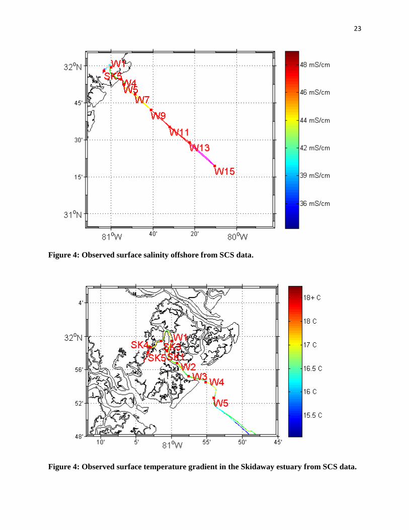
Skidaway estuary to the furthest offshore station, W15 (Figure 3 & 4). The values of surface

salinity observed along the ship’s track ranged from 38 to 49. Surface salinity exhibited a linear

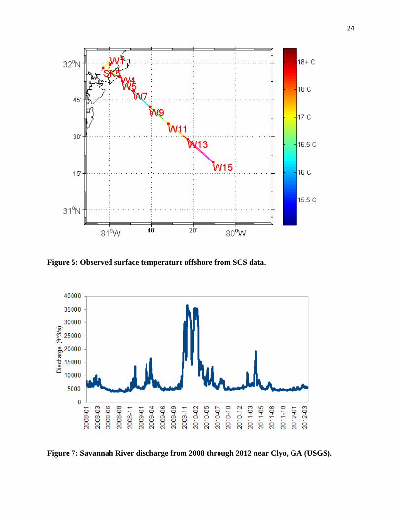
relationship to distance from the SKIO dock. Surface temperature decreased from shore to W7

after which point it increased until the ship reached W15, the furthest station offshore (Figure 5

& 6). The warmest surface water temperature in the Skidaway estuary was recorded at the

furthest inland station, SK5, at a temperature of 18 °C. The coolest surface water temperatures in

the estuary occurred at the estuary mouth, where temperatures in the vicinity of W5 decreased

from 16.5 °C to 15.5 °C. Surface temperatures began increasing prior to W7, ranging from 17 °C

to over 18 °C at W15; higher than observed at SK5.

Discharge data from the USGS for the Savannah River which feeds into the Skidaway estuary

demonstrated a mean of 10,000 cubic feet per second for the month of March over the time

interval from 2008 to 2012 (Figure 7). A high of approximately 17,000 cubic feet per second

was observed in 2010 with a low of 7000 cubic feet per second occurring in 2012. In March of

2008 and 20011, discharge was measured at approximately 10,000 cubic feet per second, the

next lowest recorded value in the 4 year interval. In March of 2009 discharge was observed at

14,000 cubic feet per second, closer to the maximum observed value for the month.

10

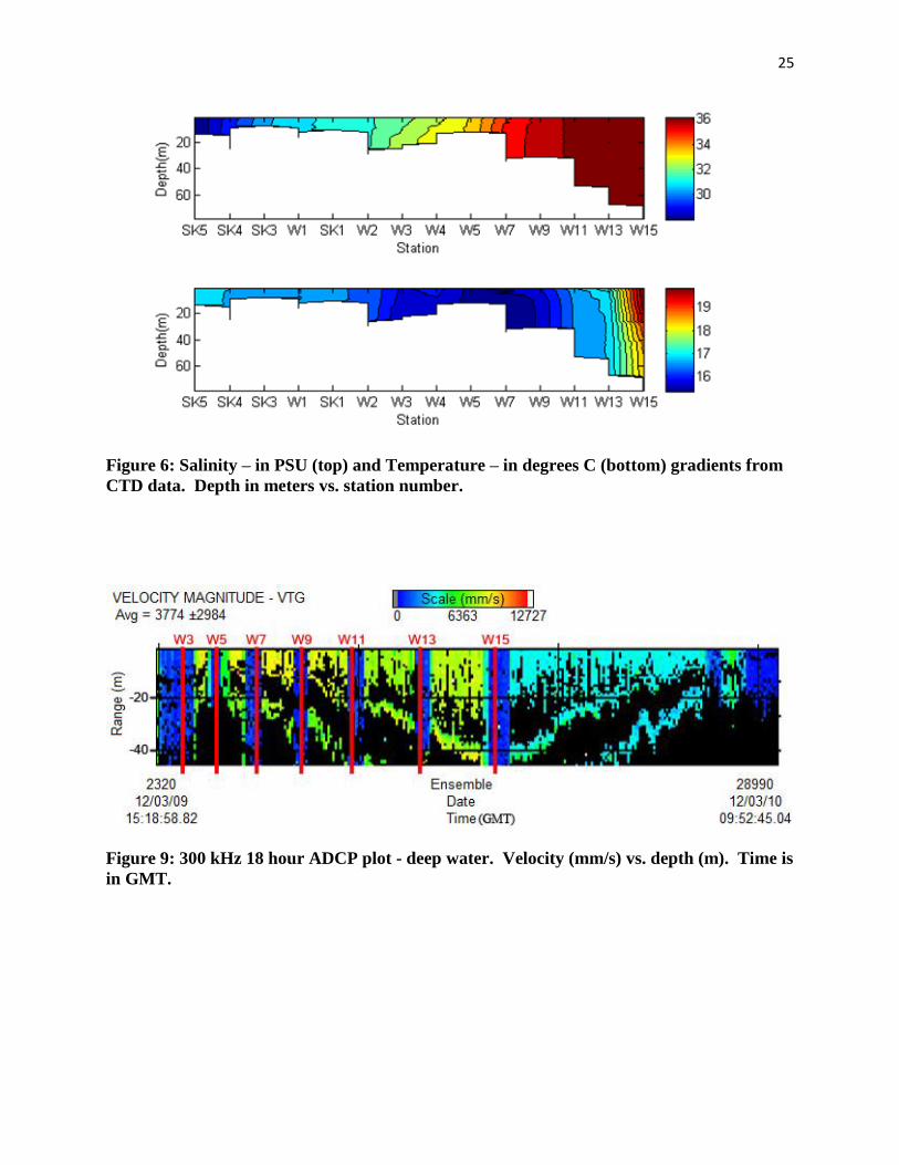
CTD data from the Skidaway estuary demonstrated an inverse correlation between distance

inland and temperature throughout the water column at the sampling stations (Figure 8). SK5,

the furthest station inland, demonstrated a surface temperature of 17.1 °C with temperatures

dropping to just below 17.1 °C by the bottom depth of 7 meters. Alternatively, SK1 and W1,

which were located in the estuary along the ship track as the ship headed towards the ocean,

demonstrated straight temperature profiles from surface to bottom at approximately 16.6 °C.

Intermediate temperature values in conjunction with a partially defined thermocline were

observed at SK3 and SK4. These stations were located between SK5 and SK1, thus contributing

to the observed trend in decreasing temperature with distance from shore.

Estuarine salinity profiles from CTD data exhibited the opposite correlation to that of the

temperature profiles (Figure 8). SK5 demonstrated the lowest salinity at approximately 28 with

a vertical salinity profile. The highest salinity values were observed at W1 and SK1 at 31.5, also

following a nearly vertical profile with depth. SK4 and SK3 were intermediate as with

temperature, demonstrating increased salinity with depth.

Data from CTD casts during the portion of the cruise outside of Skidaway estuary were

considered to be offshore casts and demonstrated roughly increasing temperatures throughout the

water columns with increased distance from the shore (Figure 8). W15, the furthest station

offshore, exhibited surface temperatures of nearly 20 °C and a defined thermocline layer between

10 and 20 meters of depth that resulted in a vertical layer of 18.7 °C water. W13 demonstrated a

similar, although less pronounced thermocline and ranged from 17.5 °C at the surface to 17 °C at

the ocean floor. W7 exhibited the lowest temperature of the offshore stations, ranging from 16

°C to 15.5 °C, but still exhibiting a thermocline layer. Stations W1 through W5 were all located

further inland than W7. W1 and W2 were the furthest inland and exhibited nearly vertical

11

temperature profiles at approximately 17.5 °C, and W1 was slightly warmer and shallower than

W2. W3, W4 and W5 were also shallow stations at less than 10 meters depth, however they

exhibited small thermocline layers at approximately 5 meters. W5 displayed the lowest bottom

temperature at 15.5 °C, and W3’s bottom temperature was slightly lower than that of W4 despite

its more inland position.

Offshore salinity profiles of the water column from CTD data yielded similar results to the

estuarine data. Salinity was observed to increase as a function of distance from shore; however,

W13 demonstrated slightly higher bottom salinity than W15 (Figure 8). Despite this feature,

W15 exhibited the highest surface salinity at approximately 36.5. The salinity gradient between

surface and bottom was greatest at W15, which was also the deepest station at 40 meters. In

comparison, W13 was nearly 35 meters deep and salinity values at this depth were nearly

identical to W15. This is not in agreement with the trend observed among the estuarine salinity

profiles in which salinity increased as a function of depth as well as distance from shore.

A 300 kHz ADCP was employed to monitor velocity in the water column for 18 hours of the

cruise duration (Figure 9). The observed velocity magnitude was approximately 6400 mm/s for

the first 10 hours of the cruise from 15:00 until 1:00 the next morning. Throughout this time, an

increase in depth was observed. At approximately 1:00, depth began to decrease as the ship

headed back towards shore, and velocity magnitude was observed to decrease to an approximate

value of 4000 mm/s. Vertical bands of uniform slow moving water were observed at regular

intervals from 15:00 until 1:00 and again at the end of the 300 kHz ADCP profile (Figure 9).

Mixed velocities were particularly notable in the top 20 meters of the water column where values

as high as 10,000 mm/s were seen prior to 1:00 on March 11th. Additionally, as depth increased

12

past 60 meters, velocity magnitudes ranging from 10,000 prior to 1:00 and 7,000 after 1:00 were

observed at 40 meter depths.

Similar vertical bands of uniform slow moving water were observed throughout the profile in the

estuary with one spanning nearly an hour from 8:00 to 9:00 which correlated with the same

vertical bands in the 300 kHz profile at that time (Figure 9 and 10). The fastest moving water

was observed near the surface, above 10 meters depth, at a velocity of approximately 7,000 mm/s

(Figure 10). The observed maximum velocity agrees with the 300 kHz ADCP data which also

recorded maximum velocity magnitudes near the surface after 1:00 EST at 7000 mm/s. Outside

of the uniform bands of slow moving water, velocity decreased with depth to approximately

4000 mm/s at the a depth of 15 to 20 meters. Occasional infusions of 6000 mm/s water were

observed in the lowest 5 meters of the water column.

Following the completion of the cruise, the 300 kHz ADCP arm remained attached to the R/V

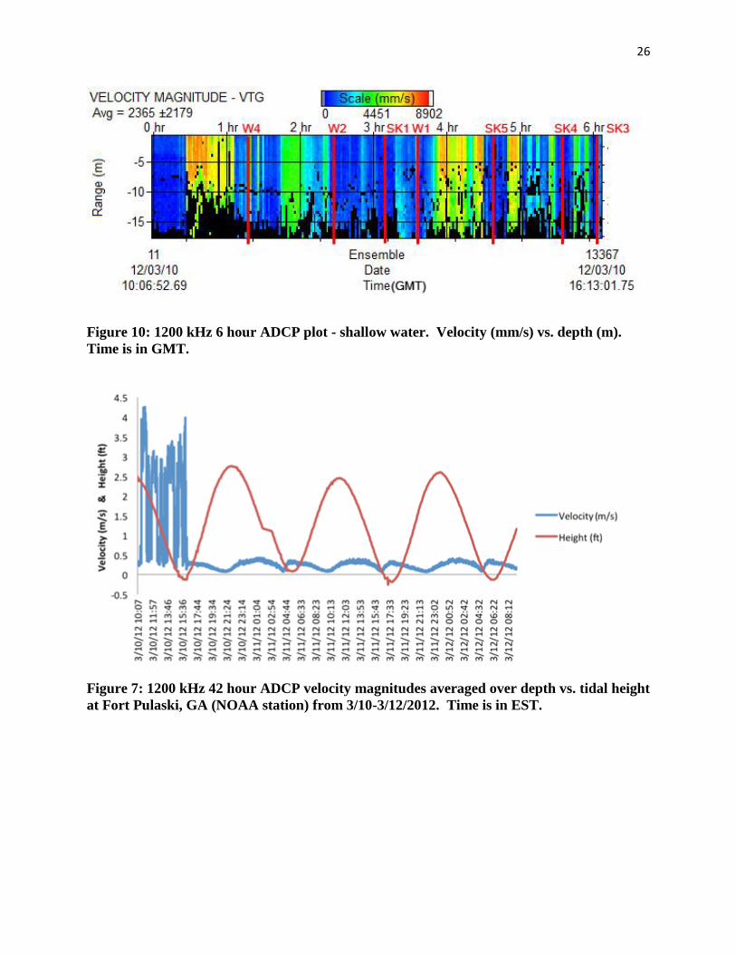
Savannah and recorded data for 42 hours at the site of the SKIO dock. The average of the

velocity magnitude for each unit in time was computed, and a contour generated that was

juxtaposed with tidal water level data (Figure 11). Aside from the first 5 hours of data, the

remaining average velocity contour demonstrated increasing velocity as water levels decreased,

with the highest velocities at approximately 0.5 m/s occurring in conjunction with the lowest

water levels. As water levels decreased, two separate velocity peaks were observed: one

following the peak water level as it decreased, and an additional velocity maximum following

the lowest water level. Velocity minimums were observed in conjunction with the onset of the

maximum water levels.

13

During the first 5 hours, from 10:00 until 15:00 EST, velocity maxima inconsistent with the

remainder of the data series were observed. During this time period velocity maxima ranged

from 3 to 5 m/s, compared to a maximum of 0.5 m/s for the remaining data.

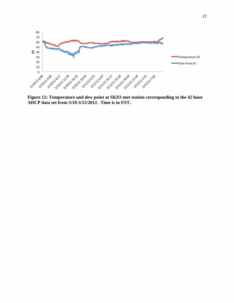
Temperature and dew point at SKIO from meteorological data recorded by the SKIO station

were examined (Figure 12). Dew point was 45°F to a low of 33°F from 8:00 until16:00, which

correlated with the same time interval of inconsistent high velocity values observed in the water

column at the SKIO dock (Figure 11). After 16:00, the dew point rapidly transitioned to a range

of 50°F to 55°F. A steep increase in temperature was observed from 50°F to 62°F during the time

period of 8:00 until 16:00 EST. Following this, temperature dropped and remained at

approximately 55°F, slightly higher than the observed dew point.

Discussion

Mixing in small estuaries is largely unexamined as the instrumentation required to attain

appropriate resolution is relatively expensive for small scale projects. The observed degree of

mixing defines the type of estuarine environment and characterizes the distribution of salinity,

temperature and oxygen at depth. Additionally, mixing counteracts eutrophication. The Georgia

coastal region demonstrates a continued pattern of population growth and is dominated by the

industrial city of Savannah (Verity, 2010). The Savannah River empties into several estuaries on

the coast including the Satilla estuary and Skidaway estuary. Eutrophic changes in the Skidaway

estuary have been noted since 1991 (Verity et. al., 2006), although few studies have been

conducted on the mixing processes taking place therein, focusing instead on larger neighboring

estuaries such as the Satilla estuary. This study utilized SCS, CTD and ADCP data to examine

the mixing processes governing estuarine circulation in the Skidaway estuary.

14

SCS values showed a range of 38 to 44 PSU within the Skidaway estuary (Figure 3). Verity et.

al. (2006) recorded surface salinity annually in the Skidaway estuary at a maximum of 32 PSU

from 1987 to 2006, lower than the observed value in 2012. These maxima were correlated with

extended dry periods from 1987 to 1989 and 1998 to 2003. Blanton et. al. (2001) observed that

periods of lower discharge in the neighboring Satilla River correlated with an increase in surface

salinity. The lowest discharge rates of the Savannah River from 2008-2012 were observed from

January through March of 2012 (Figure 7). These low discharge rates could have resulted in a

low freshwater input and therefore high surface salinity (Verity et. al., 2006) which could

negatively impact mixing in the Skidaway estuary.

Temperature data from both the SCS and CTD demonstrate a general trend of increase in

temperature in correlation with distance from the estuary mouth both in the inland and offshore

directions (Figures 5, 6, 8). Surface temperature data varied on the return trip through the

estuary, suggesting that diurnal temperature variations may be contributing to some of the

observed trend. Kawai et. al. (2007) determined that cooler surface temperatures are typically

observed at night. Warmer surface temperatures during the day are attributed to the uppermost

viscous skin layer of the water column, which typically is cooler than the layers beneath it,

absorbing radiation (Kawai et. al., 2007). Diurnal variations were observed in the SCS estuarine

temperature data, where warmer temperatures were measured on the return trip through the same

portion of the estuary mouth (Figure 5). However, this does not account for the warm surface

temperatures observed at W15, the latest station reached at 20:10. The warmer temperatures

observed at W15 may be a result of the Gulf Stream current, which flows north along the eastern

edge of the continental shelf in the South Atlantic Bight (McClain et. al., 1984), contributing

warm water from the Gulf of Mexico.

15

Peters (1997) and Kawai et. al. (2007) both observed decreasing temperature with depth during

the daytime in estuarine environments. Results from CTD data demonstrate comparable daytime

temperature profiles (Figure 8, Figure 9). At most stations, temperature demonstrated an inverse

profile to that of the corresponding salinity, which was in agreement with Peters (1997). CTD

profiles demonstrated an increase in salinity with depth (Figure 8) as previously observed in the

Satilla estuary (Blanton et. al., 2001). However, stations W1 and SK1 demonstrated nearly

vertical temperature profiles in correlation with nearly vertical salinity profiles. The vertical

nature of a salinity profile indicates that the water column may be well-mixed (Pritchard, 1952)

and thus a corresponding vertical temperature profile may be indicative of the same

characterization. The observed salinity profile of the water column ranged from nearly vertical to

semi-horizontal isohaline curves, defining the Skidaway estuary as well-mixed to partially-mixed

(Pritchard, 1952) in agreement with previous findings (Verity, 2010). The location of W1 and

SK1 intermediate to the inland and more saline offshore stations result in mixed water and

corresponding vertical profiles at the point where water flows out of the Skidaway estuary

channel (Figure 1).

ADCP data demonstrated the strength of subtidal currents in the Skidaway estuary; high velocity

lends to a high incidence of mixing and thus ADCP data was an important addition to a study on

the mixing within the Skidaway estuary. Regions of relatively high subsurface velocity in the

upper 10 meters of the water column were observed in the ADCP profiles of the Skidaway

estuary and the offshore transect. Blanton et. al. (2003) observed velocity maxima on the order of

0.5 – 1.0 m/s in the Satilla estuary immediately prior to tidal height minimums during the Spring

tide cycle. In comparison, 1200 kHz ADCP data (Figure 10) demonstrates maximum velocities

at 0.6-0.9 m/s in the Skidaway estuary. Periods of low velocity indicated a decrease in sediment

16

concentration or clearing of the water column (Blanton et. al., 2003) which is analogous with a

decrease in density and thus a decrease in the likelihood of turbulent mixing (Falkovich et. al.,

2006). High velocity regions thus contribute to and may be an indicator of turbulent mixing

(Trevethan et. al., 2010).

Bands of vertically uniform slow moving water were observed in both the 300 and 1200 kHz

ADCP data. These bands were correlated with stops for CTD casts during which the ship was

moored for a period of time (Figure 9, Figure 10). Blanton et. al. (2003) found similar slow

velocity bands in the Satilla estuary, and determined that these were related to tidal maxima,

which are correlated with minimum velocities. Given the knowledge that two velocity minima

and one maximum occur each with a tidal maximum, 3 slow-moving bands were expected per 6

hour period in the ADCP. Hours 0-6 of the 300 kHz data demonstrated 4 bands of slow velocity

and the 12-18 hour portion of the profile, during which no CTD casts were performed, did not

demonstrate any. Four bands are also present in the 6-hour 1200 kHz data. The presence of

more slow-moving bands than expected with tidal variation and a period lacking any bands

correlated with a period during which the vessel was continuously moving suggests that these

bands are not indicative of tidal variation and are instead correlated with the 14 CTD stations.

The presence of the slow-moving bands also indicates that the ADCP data was not corrected for

the vessel’s velocity, which may influence the maximum observed values for the 1200 and 300

kHz cruise data.

Velocity data acquired following the cruise with the 1200 kHz ADCP at the site of the SKIO

dock demonstrated a 6-hour event with maximum velocities in the range of 3 to 4.5 m/s that

could be indicative of increased mixing in the water column (Figure 11). Additional SCS and

CTD data during the event would be necessary to determine the degree of mixing that occurred.

17

The event was correlated with a decrease in dew point and increase in temperature recorded by

the SKIO meteorological station during the same time interval (Figure 12), suggesting a decrease

in humidity. The resultant dry air may have increased evaporation and thus increased the salinity

of the surface water. Increased salinity is analogous to an increase in density. Denser water

sinks in the water column, adding to turbulent mixing which may have taken place at the SKIO

dock. Further study on the individual components of the velocity vector to determine the

direction of the flow during this event is needed as well as salinity data to determine if the

sinking of dense, saline water due to evaporation was underlying the observed outlying

maximum velocities.

SCS, CTD and ADCP data from the Skidaway estuary support the idea that it is a well-mixed to

partially-mixed estuary that is strongly affected by tidal variations. Additionally, the region is

experiencing a period of low freshwater input from the Savannah River which may be affecting

estuarine circulation as it has contributed to an increase in surface salinity throughout the

estuary. Higher density water is more likely to undergo turbulent mixing; however, the decreased

flow rate of a main input to the Skidaway estuary, the Savannah River, may have a greater

negative influence on the likelihood of turbulent mixing within the estuary. A decrease in

turbulent mixing could result in oxygen depletion within the water column and potential hypoxic

conditions, posing a threat to immotile organisms on the ocean floor as well as increasing the

susceptibility of the estuary to further eutrophic changes.

Conclusions

Studies focusing primarily on the estuarine circulation and mixing processes of the Skidaway

estuary have not been previously published. This study characterized the mixing processes

18

taking place in the Skidaway estuary and the adjacent coastal waters of the Atlantic. The

Skidaway estuary and the associated Satilla estuary have both been affected by increases in

coastal population. Associated increases in anthropogenic nutrient loading have been observed

in the past decade in the Skidaway estuary.

The degree to which eutrophication affects an estuary depends on the degree of mixing taking

place within the estuary. An estuary undergoing various turbulent mixing processes can continue

to deliver oxygen to lower depths despite eutrophic changes. Velocity magnitudes in the upper

portion of the water column were comparable to those observed in the Satilla estuary, suggesting

that any eutrophication that has taken place in the following years has not had a major impact on

the mixing processes of the Skidaway estuary. Temperature and salinity profiles demonstrating

well- to partially-mixed water columns throughout the estuary further support the idea that

eutrophication has not impacted circulation in the Skidaway estuary.

However, a recent decrease in the discharge rate of the Savannah River has resulted in an

increase in salinity throughout the estuary to levels that exceed the maximum values on record

for similar events in the estuary. This change in salinity coupled with a decrease in flow could

potentially negatively impact the estuarine system by decreasing the potential for turbulent

mixing and thus rendering an estuary more susceptible to eutrophic changes. Further studies on

turbulent events in the estuarine system encompassing longer expanses of time are necessary to

fully characterize how circulation and mixing in the Skidaway estuary are being effected by

environmental and anthropogenic factors.

Acknowledgements

19

I wish to acknowledge several institutions and groups of individuals for assisting with

components of this study. The crew of the R/V Savannah worked around the clock to keep the

ship running smoothly and attached the 1200 kHz ADCP and arm at 4am purely for the sake of

this study. My colleagues made indispensable contributions in the field by assisting with CTD

deployment and station data that has been incorporated into this study. My advisor, Dr. Martial

Talliefert has continued to provide helpful feedback throughout the duration of this study.

Additionally, the Skidaway Institute of Oceanography provided research equipment and the use

of the R/V Savannah at the expense of the EAS department of the Georgia Institute of

Technology, both of whom I must thank for making this study, and those of my colleagues,

possible.

References

Anderson, D.M., Gilbert, P.M., Burkholder, J.M., Harmful algal blooms and

eutrophication: nutrient sources, composition and consequences, Estuaries, 25(4), 704-

726, 2002.

Blanton, J.O., Seim, H., Alexander, C., Amft, J., Kineke, G., Transport of salt and

suspended sediments in a curving channel of a coastal plain estuary: Satilla River, GA,

Estuarine Coastal and Shelf Science, 57, 993-1006, 2003.

Blanton, J., Alber, M., Sheldon, J., Salinity response of the Satilla river estuary to

seasonal changes in freshwater discharge, Proceedings of the 2001 Georgia Water

Resources Conference, 619-622, 2001.

Falkovich, G., Sreenivasan, K.R., Lessons from hydrodynamic turbulence, Physics

Today, 59, 43-49, 2006.

Griffin, D.A., LeBlond, P.H., Estuary/ocean exchange controlled by spring-neap tidal

mixing, Estuarine Coastal and Shelf Science, 30, 275-297, 1990.

Huthnance, J.M., Circulation, exchange, and water masses at the ocean margin: the role

of physical processes at the shelf edge, Progress in Oceanography, 35, 353-431, 1995.

20

Kawai, Y., Wada, A., Diurnal sea surface temperature variation and its impact on the

atmosphere and ocean: a review, Journal of Oceanography, 63, 721-744, 2007.

Koop, K., Booth, D., Broadbent, A., Brodie, J., Bucher, D., Capone, D., Coll, J.,

Dennison, W., Erdmann, M., Harrison, P., Hoegh-Guldberg, O., Hutchings, P., Jones,

G.B., Larkum, A.W.D., O’Neil, J., Steven, A., Tenton, E., Ward, S., Williamson, J.,

Yellowlees, D., ENCORE: The Effect of Nutrient Enrichment on Coral Reefs. Synthesis

of results and conclusions, Marine Pollution Bulletin, 42(2), 91-120, 2001.

Kostaschuk, R., Best, J., Villard, P., Peakall, J., Franklin, M., Flow velocity and sediment

transport with an Acoustic Doppler Current Profiler, Geomorphology, 68, 25-37, 2005.

McClain, C.R., Pietrafesa, L.J., Yoder, J.A., Observations of Gulf Stream-Induced and

Wind-Driven Upwelling in the Georgia Bight Using Ocean Color and Infrared Imagery,

Journal of Geophysical Research, 89, 3705-3723, 1984.

Peters, H., Observations of stratified turbulent mixing in an estuary: neap-to-spring

variations during high river flow, Estuarine Coastal and Shelf Science, 45, 69-88, 1997.

Pritchard, D.W., Estuarine hydrography, Advances in Geophysics 1. Academic Press,

New York. 243-280, 1952.

Stanley, D.W., Nixon, S.W., Stratification and bottom-water hypoxia in the Pamlico

River estuary, Coastal and Estuarine Research, 15(3), 270-281, 1992.

Stefanelli, S., Capotondi, L., Ciaranfi, N., Foraminiferal record and environmental

changes during the deposition of the Early-Middle Pleistocene sapropels in southern

Italy, Palaeogeography, Palaeoclimatology, Palaeoecology, 216, 27 – 52, 2005.

Stewart, R.H., Introduction to Physical Oceanography, Texas A&M University, 2005.

Trevethan, M., Chanson, H., Turbulence and turbulence flux events in a small estuary,

Environmental Fluid Mechanics, 10, 345-368, 2010.

Verity, P.G., Expansion of potentially harmful algal taxa in a Georgia Estuary (USA) ,

Harmful Algae, 9, 144-152, 2010.

Verity, P.G., Alber, M., Bricker, S.B., Development of hypoxia in well-mixed

Subtropical estuaries in the Southeastern USA, Estuaries and Coasts, 29(4), 665-673,

2006.

21

Figures

Figure 1: Path of the R/V Savannah through the Skidaway estuary from SCS data.

22

Figure 2: Path of the R/V Savannah through the Atlantic Ocean from SCS data

Figure 3: Observed surface salinity in the Skidaway estuary from SCS data.

23

Figure 4: Observed surface salinity offshore from SCS data.

Figure 4: Observed surface temperature gradient in the Skidaway estuary from SCS data.

24

Figure 5: Observed surface temperature offshore from SCS data.

Figure 7: Savannah River discharge from 2008 through 2012 near Clyo, GA (USGS).

25

Figure 6: Salinity – in PSU (top) and Temperature – in degrees C (bottom) gradients from

CTD data. Depth in meters vs. station number.

Figure 9: 300 kHz 18 hour ADCP plot - deep water. Velocity (mm/s) vs. depth (m). Time is

in GMT.

26

Figure 10: 1200 kHz 6 hour ADCP plot - shallow water. Velocity (mm/s) vs. depth (m).

Time is in GMT.

Figure 7: 1200 kHz 42 hour ADCP velocity magnitudes averaged over depth vs. tidal height

at Fort Pulaski, GA (NOAA station) from 3/10-3/12/2012. Time is in EST.

27

Figure 12: Temperature and dew point at SKIO met station corresponding to the 42 hour

ADCP data set from 3/10-3/12/2012. Time is in EST.