Embed Size (px)
Citation preview
ANNÉE 2015
THÈSE / UNIVERSITÉ DE RENNES 1sous le sceau de l'Université Européenne de Bretagne
pour le grade de
DOCTEUR DE L'UNIVERSITÉ DE RENNES 1
Mention : Informatique
Ecole doctorale MATISSE
présentée par
Chiheb Ben Ameur
préparée à l'unité de recherche UMR 6074 IRISAEquipes d'accueil :
Orange Labs OLPS/DTV/TV/PTC - IRISA/ADOPNETContrat CIFRE No 2012/1577
TCP Protocol
Optimization for
HTTP Adaptive
Streaming
Thèse soutenue à Rennes
le 17 décembre 2015
devant le jury composé de :
Tou�k AHMEDProfesseur à ENSEIRB-MATMECA/ rapporteur
Abdelhamid MELLOUKProfesseur à l'Université de Paris-Est Créteil /rapporteur
Julien BOURGEOISProfesseur à l'Université de Franche-Comté / exami-nateur
Dominique GAITIProfesseur à l'Université de technologie de Troyes /examinateur
Bernard COUSINProfesseur à l'Université de Rennes 1 / directeur deThèse
Emmanuel MORYDocteur et Ingénieur de recherches à Orange Labsde Rennes / co-encadrant de Thèse
To my beloved parents Radhia & Moncef
for making me who I am today.

Abstract
HTTP adaptive streaming (HAS) is a streaming video technique widely used over the Internet
for Video on Demand (VoD) and Live streaming services. It employs Transmission Control Pro-
tocol (TCP) as transport protocol and it splits the original video inside the server into segments of
same duration, called "chunks", that are transcoded into multiple quality levels. The HAS player,
on the client side, requests for one chunk each chunk duration and it commonly selects the quality
level based on the estimated bandwidth of the previous chunk(s). Given that the HAS clients are
located inside access networks, our investigation involves several HAS clients sharing the same
bottleneck link and competing for bandwidth inside the same home network. Here, a degradation
of both Quality of Experience (QoE) of HAS users and Quality of Service (QoS) of the access
network are often recorded. The objective of this thesis is to optimize the TCP protocol in order
to solve both QoE and QoS degradations.
Our first contribution consists of proposing a gateway-based shaping method, that we called
Receive Window Tuning Method (RWTM); it employs the TCP flow control and passive round
trip time estimation on the gateway side. We compared the performances of RWTM with an-
other gateway-based shaping method that is based on queuing discipline, called Hierarchical To-
ken Bucket shaping Method (HTBM). The results of evaluation indicate that RWTM outperforms
HTBM not only in terms of QoE of HAS but also in terms of QoS of access network by reducing
the queuing delay and significantly reducing packet drop rate at the bottleneck.
Our second contribution consists of a comparative evaluation between eight combinations that
result from combining two shaping methods, RWTM and HTBM, and four very common TCP
variants, NewReno, Vegas, Illinois and Cubic. The results show that there is a significant discor-
dance in performance between combinations. Furthermore, the best combination that improves
performances in the majority of scenarios is when combining Illinois variant with RWTM. In ad-
dition, the results reveal the importance of an efficient updating of the slow start threshold value,
ssthresh, to accelerate the convergence toward the best feasible quality level.
Our third contribution consists of proposing a novel HAS-based TCP variant, that we called
iv ABSTRACT
TcpHas; it is a TCP congestion control algorithm that takes into consideration the specifications
of HAS flow. Besides, it estimates the optimal quality level of its corresponding HAS flow based
on end-to-end bandwidth estimation. Then, it permanently performs HAS traffic shaping based
on the encoding rate of the estimated level. It also updates ssthresh to accelerate convergence
speed. A comparative performance evaluation of TcpHas with a recent and well-known TCP
variant that employs adaptive decrease mechanism, called Westwood+, was performed. Results
indicated that TcpHas largely outperforms Westwood+; it offers better quality level stability on the
optimal quality level, it dramatically reduces the packet drop rate and it generates lower queuing
delay.
Keywords: HTTP Adpative Streaming, TCP protocol, TCP congestion control, TCP flow
control, bandwidth management, traffic shaping, Quality of Experience, Quality of Service, access
network, bottleneck issue, cross-layer optimization.
Résumé
Le streaming vidéo adaptatif sur HTTP, couramment désigné par HTTP Adaptive Streaming
(HAS), est une technique de streaming vidéo largement déployée sur le réseau Internet pour les
services de vidéo en direct (Live) et la vidéo à la demande (VoD). Cette technique utilise le pro-
tocole TCP comme protocole de transport. Elle consiste à segmenter la vidéo originale, stockée
sur un serveur HTTP (serveur HAS), en petits segments (généralement de même durée de lec-
ture) désignés par "chunks". Chaque segment de vidéo est transcodé à plusieurs niveaux de qua-
lité, chaque niveau de qualité étant disponible sur un chunk indépendant. Le player, du côté du
client HAS, demande périodiquement un nouveau chunk une fois par durée de lecture du chunk.
Dans les cas communs, le player sélectionne le niveau de qualité en se basant sur l’estimation
de la bande passante du/des chunk(s) précédent(s). Étant donné que chaque clients HAS est situé
au sein d’un réseau d’accès, notre étude se concentre sur un cas particulier assez fréquent dans
l’usage quotidien : lorsque plusieurs clients partagent le même lien présentant un goulet d’étran-
gement (bottleneck) et se trouvants en état de compétition sur la bande passante. Dans ce cas, on
signale fréquemment une dégradation de la qualité d’expérience (QoE) des utilisateurs de HAS
et de la qualité de service (QoS) du réseau d’accès. Ainsi, l’objective de cette présente thèse est
d’optimiser le protocole TCP pour résoudre ces dégradations de QoE et QoS.
Notre première contribution consiste à proposer une méthode de bridage du débit HAS au ni-
veau de la passerelle. Cette méthode est désignée par "Receive Window Tuning Method" (RWTM)
et elle consiste dans l’utilisation du principe de contrôle de flux de TCP et l’estimation passive du
temps d’aller retour au niveau de la passerelle. Nous avons comparé les performances de cette
méthode avec une autre méthode récente implémentée à la passerelle et utilisant une discipline
particulière de gestion de la file d’attente, qui est désignée par "Hierarchical Token Bucket sha-
ping Method" (HTBM). Les résultats d’évaluations ont révélé que RWTM a non seulement une
meilleure QoE, mais aussi une meilleure QoS de réseau d’accès que pour l’utilisation de HTBM ;
plus précisément une réduction du délai de mise en file d’attente et une forte réduction du taux de
paquets rejetés au niveau du goulet d’étrangement.
vi RÉSUMÉ
Notre deuxième contribution consiste à mener une étude comparative combinant huit combi-
naisons résultant de la combinaison de deux méthodes de bridages, RWTM et HTBM, avec quatres
variantes TCP largement déployées, NewReno, Vegas, Illinois et Cubic. Les résultats de l’évalua-
tion montrent une discordance importante entre les performances des différentes combinaisons.
De plus, la combinaison qui améliore les performances dans la majorité des scénarios étudiés est
celle de RWTM avec Illinois. En outre, nous avons révélé qu’une mise à jour efficace de la valeur
du paramètre "Slow Start Threshold", ssthresh, peut accélérer la vitesse de convergence du client
vidéo vers la qualité de vidéo optimale.
Notre troisième contribution consiste à proposer une nouvelle variante de TCP adaptée aux
flux HAS, qu’on désigne par TcpHas ; c’est un algorithme de contrôle de congestion de TCP qui
prend en considération les spécifications de HAS. TcpHas estime le niveau de la qualité optimale
du flux HAS en se basant sur l’estimation de la bande passante de bout en bout. Ensuite, TcpHas
applique, d’une façon permanente, un bridage au trafic HAS en se basant sur le débit d’encodage
du niveau de qualité estimé. En plus, TcpHas met à jour ssthresh pour accélérer la vitesse de
convergence. Une étude comparative a été réalisée avec une variante de TCP, connue sous le nom
Westwood+, qui utilise le mécanisme de la diminution adaptative. Les résultats de l’évaluation ont
indiqué que TcpHas est largement plus performant que Westwood+ ; il offre une meilleure stabilité
autour de la qualité optimale, il réduit considérablement le taux de paquets rejetés au niveau du
goulet d’étrangement, et diminue le délai de la file d’attente.
Mots-clés : HTTP Adpative Streaming, protocole de transport TCP, le contrôle de congestion
TCP, le contrôle de flux TCP, la gestion de la bande passante, bridage du traffic, Qualité d’Expé-
rience, Qualité de Service, réseau d’accès, goulet d’étrangement, optimisation inter-couche.
Acknowledgments
I am most grateful to my advisors, Dr. Emmanuel MORY and Pr. Bernard COUSIN. Their
guidance and insights over the years have been invaluable to me. I feel especially fortunate for
the patience that they have shown with me when I firstly stepped into the field of HTTP Adaptive
Streaming and TCP congestion control. I am indebted to them for teaching me both research and
writing skills. Without their endless efforts, knowledge and patience, it would have been extremely
challenging to finish all my dissertation research and Ph.D study in three years. It has been a great
honor and pleasure for me to do research under their supervision. I would like to thank Pr. Ahmed
TOUFIK, Pr. Abdelhamid MELLOUK, Pr. Julien BOURGEOIS and Pr. Dominique GAITI for
serving as my Ph.D committee members and reviewing my dissertation.
I would like to thank my Orange Labs colleagues: UTA team members, especially Mr. Frédéric
HUGO, Mr. Fabien GUEROUT, Mr. Johnny SHEMASTI and Mr. Franck GESLIN; PTC team
leader François DAUDE; CDI project leader Ms. Claudia BECKER; doctors and PhD students,
especially Dr. Haykel BOUKADIDA, Dr. Moez BACCOUCHE, Ms. Sonia YOUSFI, Dr. Khaoula
BACCOUCHE, Mr. Imad JAMIL and Dr. Youssef MEGUEBLI. I would like to extend my thanks
to the members of ADOPNET team that I have had the pleasure to work with. Thanks to all my
colleagues with who I have enjoyed working with: Dr. Samer LAHOUD, Dr. Cedric GUEGUEN,
Mohamed YASSIN, Mehdi EZZAOUIA, Farah MOETY, Siwar BEN HADJ SAID and Melhem
ELHELOU.
I am thankful to all my friends for their continued help and support: the new ones, for the
life experiences we have shared in France, and the old ones, for staying present despite the dis-
tance. Especially Mohamed ELAOUD, Amine CHAABOUNI, Bassem KHALFI, Abdlehamid
ESSAIED and Ayoub ABID. Last, but by no means least, I must thank my family in Tunisia, who
supported me a lot. Without their endless love and encouragement I would have never completed
this dissertation. I would like to give the biggest thanks to my parents Radhia & Moncef, to my
brother Hazem, my sisters Ines and Randa, their spouses and their children.

Résumé français
Introduction
En 2019, le trafic des contenus vidéo sur Internet présentera environ 80% du trafic Internet, soit
64% de plus qu’en 2014, selon un rapport récent de Cisco [37]. Par conséquent, une adaptation des
fournisseurs de contenus vidéo (comme en l’occurrence YouTube, Netflix et Dailymotion) ainsi
que les fournisseurs d’accès à Internet (FAI) à cette utilisation croissante du streaming vidéo sur
Internet s’avère indispensable. Par exemple, YouTube, qui est l’un des plus grands fournisseurs
de contenus avec plus qu’un milliard d’utilisateurs, compte des centaines de millions d’heures de
vues chaque jour. De ce fait, améliorer les techniques utilisées pour le streaming vidéo (comme le
type du codec vidéo, le type du protocole de transport, la configuration du player) est actuellement
une piste prometteuse pour améliorer les services et les bénéfices des fournisseurs de contenus.
En plus, les débits d’encodages des contenus vidéo varient entre des faibles débits de l’ordre
de quelques dizaines de kilo-octets par seconde, typiquement pour servir les écrans de petites
tailles et de faibles capacités d’affichage, jusqu’à arriver aux débits de quelques dizaines de méga-
octets par seconde pour les écrans qui supportent les ultra hautes définitions, typiquement 4K
et 8K. Par conséquent, les FAI se concurrencent pour offrir le haut débit à leurs abonnées pour
satisfaire leurs besoins de regarder des vidéos en haute définition. De plus, un troisième acteur
s’est présenté depuis les années 2000 pour accélérer la distribution des contenus sur les cœurs
des réseaux des FAI. Cet acteur est dénommé fournisseur du réseau de livraison des contenus,
ou fournisseur de Content Delivery network (CDN). Ce dernier place des caches, appelés aussi
des proxies de contenus, distribués dans les réseaux jusqu ?au niveau cœur du réseau FAI afin de
pouvoir y stocker des contenus populaires et ainsi réduire la charge du trafic réseau sur les serveurs.
Plusieurs fournisseurs de CDN, comme Akamai, ont adapté leurs services de mise en cache aux
contenus vidéo transmis sur Internet. Globalement, 72% du trafic vidéo sur Internet sera géré par
les réseaux CDN en 2019, soit 57% de plus qu’en 2014 [37]. En conséquence, la collaboration
entre ces trois acteurs (c.-à-d. les fournisseurs de contenus vidéos, les FAI et les fournisseurs de
x RÉSUMÉ FRANÇAIS
CDN) demeure nécessaire pour offrir une meilleure qualité d’expérience (QoE) aux utilisateurs du
streaming vidéo et garantir une bonne qualité de service (QoS) [36].
L’objectif de cette thèse est d’améliorer la QoE et la QoS lorsqu’on utilise une technique
de streaming vidéo particulière et largement déployée, désignée par HTTP Adaptive Streaming
(HAS).
De ce fait, la Section 0.1 présente la problématique posée autour d’un cas d’usage répendu
de HAS. Puis, nos trois contributions majeures qui tentent à résoudre cette problématique sont
présentés aux sections 0.2, 0.3 et 0.4.
0.1 Problématique
Le streaming vidéo adaptatif sur HTTP, couramment désigné par HTTP Adaptive Streaming
(HAS), est une technique de streaming vidéo largement déployée sur le réseau Internet pour les
services de vidéo en directe (Live) et de vidéo à la demande (VoD). Cette technique consiste à
segmenter la vidéo originale, stockée sur un serveur HTTP (serveur HAS), en petits segments
(généralement de même durée de lecture) désignés par "chunks". Chaque segment de vidéo est
transcodé à plusieurs niveaux de qualité , chaque niveau de qualité étant disponible dans un chunk
indépendant. Le player, du côté du client HAS, demande les chunks du serveur HAS selon deux
phases différentes : la phase de la mise en mémoire tampon, "buffering phase state" et la phase
de régime stationnaire, "steady state phase". Pendant le buffering phase state, les chunks sont de-
mandés successivement les uns à la suite des autres jusqu’à remplir la file d’attente du player,
désignée par "playback buffer". Une fois que le playback buffer est suffisament rempli, le player
bascule vers la deuxième phase, steady state phase, durant laquelle le player est en train de deman-
der périodiquement, un nouveau chunk une fois par durée de lecture du chunk, afin de préserver
le même niveau de remplissage du playback buffer. En conséquence, cette périodicité créee des
périodes d’activité, désignées par périodes ON, durant lesquelles le chunk est en cours de télé-
chargement, suivis par des périodes d’inactivité, désignées par périodes OFF, durant lesquelles
le player attend pour lancer la nouvelle requête du prochain chunk. La périodicité des périodes
ON-OFF n’influence pas la continuité du décodage et la lecture de la vidéo demandée.
Le player HAS est doté d’une intelligence qui s’appelle le contrôleur de débit, désigné par
"bitrate controller". Son rôle est de choisir le niveau de qualité et l’instant de la demande du
prochain chunk. Dans les cas communs, ce contrôleur prend comme paramètres l’estimation de
la bande passante du/des chunk(s) précedent(s) et/ou le niveau de remplissage du playback buffer.
Néanmoins, le player HAS est dans l’incapacité d’estimer la bande passante durant la période
0.1. Problématique xi
OFF car pendant cette durée il ne reçoit pas de données. Ainsi, le player n’a aucune information
sur l’état du réseau durant les périodes OFF. Ce problème s’appelle "la contrainte de la période
OFF".
Notre investigation se concentre sur un cas particulier assez fréquent dans l’usage quotidien,
précisément lorsque plusieurs clients partagent le même lien présentant un goulot d’étranglement
(bottleneck) et se trouvant en état de compétition sur la bande passante. Un exemple plus concret
de ce cas est lorsque les clients HAS se trouvent dans un réseau domestique à l’issue d’un réseau
fixe d’accès à haut débit. Dans ce cas, la contrainte de la période OFF sera amplifiée. En effet, si
la période ON du premier client coïncide avec la période OFF d’un deuxième client, une sures-
timation de la bande passante sera enregistrée pour le premier client car il ignore l’existence du
flux HAS du deuxième client. Ce cas de figure peut engendrer plusieurs problèmes à savoir des
congestions au niveau du bottleneck, une instabilité des niveaux de qualité sélectionnés, un par-
tage inéquitable de la bande passante entre les flux HAS et même une déplétion du playback buffer
pouvant provoquer une interruption de la lecture de la vidéo dans le pire des cas. Ainsi, on peut
subir une dégradation de la qualité d’expérience (QoE) des utilisateurs de HAS et de la qualité de
service (QoS) du réseau d’accès.
Une des solution les plus pratiques pour améliorer les performances du HAS et réduire l’effet
indésirable de la contrainte de la période OFF est de dilater les périodes ON et ainsi de réduire
les périodes OFF. Dans ce cas, on maximise la connaissance des conditions réseaux pour le player
HAS, car il ne se retrouve quasiment qu’en périodes ON. Cette solution se manifeste par un bridage
du débit des flux HAS et est désignée par "traffic shaping".
Étant donné que HAS est basé sur le protocole de transport TCP, l’objectif de cette thèse est
de résoudre les problèmes cités ci-dessus en utilisant judicieusement certains des paramètres de
la couche TCP. En effet, certaines améliorations (qui sont en relation avec la gestion de la bande
passante et le bridage du trafic) sont plus efficaces à concrétiser au niveau de la couche TCP qu’à
celui de la couche applicative.
Pour l’ensemble des contributions, nous avons développé un émulateur de player HAS qui
prend en considération les caractéristiques communes entre les players commerciaux de HAS.
Nous avons également développé des tests sur une maquette pour valider les solutions proposées
pour trois scénarios simples avec seulement deux clients HAS en compétition. Ensuite, nous avons
étendu l’étude sur le simulateur de réseau ns-3 pour couvrir d’autres scénarios tels que l’augmen-
tation du nombre des clients en compétition, changer les paramètres du player HAS, changer les
conditions du réseau cœur du FAI, changer la taille de la file d’attente et l’algorithme de la gestion
de la file d’attente du lien du goulot d’étranglement.
xii RÉSUMÉ FRANÇAIS
0.2 Méthode de bridage du trafic HAS au niveau de la passerelle
Notre première contribution consiste à proposer une méthode de bridage de débit des flux HAS
au niveau de la passerelle. Cette méthode est désignée par "Receive Window Tuning Method"
(RWTM). Elle consiste dans l’utilisation du principe de contrôle de flux de TCP et l’estimation
passive du temps d’aller retour (RTT) au niveau de la passerelle. Le choix de l’implémentation au
niveau de la passerelle est justifié par le fait que cette passerelle a une visibilité totale sur toutes les
machines connectées sur même réseau domestique. RWTM utilise également un gestionnaire de
la bande passante au niveau de cette passerelle afin de pouvoir estimer la bande passante totale qui
peut être réservées aux flux HAS en identifiant les flux HAS qui la traverse. Ainsi, ce gestionnaire
de débit définit le débit de bridage pour chaque flux HAS en utilisant comme paramètre les débits
d’encodages disponibles pour chaque flux HAS. Donc, RWTM prend comme paramètre le débit
de bridage choisi par le gestionnaire de la bande passante multiplié par le temps d’aller-retour
(RTT) estimé. Ensuite, RWTM utilise le principe de contrôle de flux en changeant la taille de la
fenêtre de réception, rwnd, indiquée dans chaque paquet envoyé du client HAS au serveur HAS.
Nous avons comparé les performances de cette méthode avec une autre récente implémentée à
la passerelle qui utilise une discipline particulière de gestion de la file d’attente. Cette méthode est
désignée par "Hierarchical Token Bucket shaping Method" (HTBM). Les résultats d’évaluations
sur différents scénarios ont révélé que RWTM présente une meilleure QoE de HAS que HTBM.
En plus, RWTM améliore la QoS du réseau d’accès contrairement à HTBM ; en effet, RWTM
réduit le délai de mise en file d’attente et élimine presque totalement le taux de paquets rejetés
au niveau du goulot d’étranglement. Néanmoins, RWTM reste moins efficace que HTBM sur la
réduction de la fréquence des périodes OFF de durée supérieure au délai de retransmission TCP.
La raison est la mise à jour relativement longue du RTT employée par RWTM ; RWTM estime le
RTT une seule fois par chunk, au début de son téléchargement. Par conséquent, RWTM ne prend
pas en compte les variation de RTT au cours du téléchargement du chunk pour mettre rwnd à jour.
Les publications directement liées à cette contribution sont :
— Chiheb Ben Ameur, Emmanuel Mory, and Bernard Cousin. Shaping http adaptive streams
using receive window tuning method in home gateway. In Performance Computing and
Communications Conference (IPCCC), 2014 IEEE International, pages 1-2, 2014
— Chiheb Ben Ameur, Emmanuel Mory, and Bernard Cousin. Evaluation of gateway-based
shaping methods for http adaptive streaming. In Quality of Experience-based Management
for Future Internet Applications and Services (QoE-FI) workshop, International Confe-
rence on Communications (ICC), ICC workshops’04, 2015 IEEE International, pages 1-6,
2015.

0.3. Evaluation de l’effet du protocole de control de congestion TCP sur HAS xiii
0.3 Evaluation de l’effet du protocole de control de congestion TCP
sur HAS
Notre deuxième contribution consiste à mener une étude comparative combinant deux mé-
thodes de bridage, RWTM et HTBM, avec quatre variantes TCP largement déployées, NewReno,
Vegas, Illinois et Cubic. Les deux objectifs principaux de cette comparaison sont 1) d’étudier si
l’une ou l’autre des deux méthodes de bridage est(sont) sensible(s) à la modification de la variante
de TCP, et 2) d’identifier la meilleure combinaison en termes de performances de QoE et de QoS.
Les résultats de l’évaluation montrent une discordance importante entre les performances des dif-
férentes combinaisons. De plus, la combinaison qui améliore les performances dans la majorité
des scénarios étudiés est celle de RWTM avec Illinois. En outre, nous avons révélé qu’une mise à
jour efficace de la valeur du paramètre "Slow Start Threshold", ssthresh, peut accélérer la vitesse
de convergence du client vidéo vers la qualité de vidéo optimale.
La publication soumise directement liée à cette contribution est :
— Chiheb Ben Ameur, Emmanuel Mory, and Bernard Cousin. Combining Traffic Shaping
Methods with Congestion Control Variants for HTTP Adaptive Streaming, submitted to
Multimedia Systems, Springer (minor revision)
0.4 TCPHas : une variante TCP adaptée au service HAS
Notre troisième contribution, qui est basée sur le résultat de la deuxième contribution, consiste
à proposer une nouvelle variante de TCP adaptée aux flux HAS, désignée par TcpHas ; c’est un
algorithme de contrôle de congestion de TCP qui prend en considération les spécificités du HAS.
TcpHas estime le niveau de qualité optimale du flux HAS en se basant sur l’estimation de la bande
passante de bout-en-bout. Ensuite, TcpHas applique d’une façon permanente un bridage au trafic
HAS en se basant sur le débit d’encodage du niveau de qualité estimé. En plus, TcpHas met à
jour ssthresh pour accélérer la vitesse de convergence. On note ici que TcpHas est considéré à la
fois comme une variante TCP et un algorithme de bridage de HAS du côté du serveur totalement
intégrée à la couche de transport TCP.
Plus précisément, TcpHas utilise un mécanisme de contrôle de congestion avec une diminution
adaptative, adaptive decrease, utilisé par Westwood et Westwood+ ; il consiste à mettre ssthresh
à jour après chaque détection de congestion en se basant sur l’estimation de la bande passante de
bout-en-bout. TcpHas utilise également une méthode d’estimation de la bande passante qui évite
les problèmes des fausses estimations liées à la compression et le clustering des paquets. TcpHas
xiv RÉSUMÉ FRANÇAIS
utilise aussi les débits d’encodages disponibles pour le flux HAS pour calculer le débit de bridage
et appliquer le bridage sur le flux HAS. Le bridage employé consiste à modifier la fenêtre de
congestion de TCP, cwnd, pour correspondre au produit entre le RTT estimé et lissé, et le débit de
bridage calculé. TcpHas élimine la réduction de cwnd après chaque période de repos idle (c.-à-d.
lorsque sa durée est supérieure au délai de retransmission de TCP) afin d’éviter la déstabilisation
du débit de bridage. En outre, il met à jour ssthresh après chaque période idle pour améliorer
l’adaptabilité au changement des conditions du réseau sans causer des congestions.
Une étude comparative a été réalisée avec la variante Westwood+ de TCP qui utilise le mé-
canisme de la diminution adaptative. Les résultats de l’évaluation ont indiqué que TcpHas est
largement plus performant que Westwood+ ; il offre une meilleure stabilité autour de la qualité
optimale, réduit considérablement le taux de paquets rejetés au niveau du goulot d’étranglement,
diminue le délai de la file d’attente, et tend à maximiser l’occupation de la bande passante dis-
ponible. Néanmoins, TcpHas reste sensible aux surcharges des réseaux cœurs de FAI. Mais ce
problème doit être évité avec le déploiment du réseau CDN.
Conclusion
Nous avons étudié durant cette thèse la technique du streaming HAS, qui est largement dé-
ployée par les fournisseurs de contenus vidéo. Nous avons précisé que, malgré l’utilisation des
caches de CDN au niveau des réseaux cœur de FAI, un cas d’usage particulier et fréquent reste
encore problématique pour la qualité d’expérience des utilisateurs de HAS et à la qualité de service
du réseau d’accès de HAS : lorsque plusieurs clients HAS partagent le même lien présentant un
goulot d’étranglement (bottleneck) et se trouvent en état de compétition sur la bande passante.
Nous avons proposé deux méthodes de bridage différentes qui utilisent des mécanismes de
contrôle de la couche TCP : RWTM qui exploite le contrôle de flux de TCP au niveau de la
passerelle, et TcpHas qui propose une nouvelle variante de contrôle de congestion de TCP au
niveau du serveur HAS. Nous avons aussi présenté une étude comparative entre deux méthodes de
bridage implémentées à la passerelle : RWTM et HTBM avec quatre variantes de TCP (NewReno,
Vegas, Illinois et Cubic). Nous avons utilisé des critères objectifs pour l’évaluation de la QoE et
des critères spécifiques de la QoS du réseau d’accès de FAI.
Les résultats de l’évaluations des performances sont satisfaisants pour l’ensemble des scéna-
rios utilisés. D’autres pistes de travaux futures seront intéressants, comme l’implémentation réelle
de la solution RWTM sur la passerelle du réseau d’Orange, la "Livebox" ou l’implémentation de
TcpHas sur quelques serveurs déployés par un fournisseur des contenus vidéos, comme Dailymo-
0.4. TCPHas : une variante TCP adaptée au service HAS xv
tion. En plus, le placement des caches au niveau du réseau d’accès du FAI, proche de la passerelle,
est une piste de recherche intéressante qui permettra de réduire la charge du réseau sur le goulot
d’étranglement et d’améliorer la QoE des utilisateurs de HAS. En outre, nous avons remarqué
qu’une nouvelle stratégie est en train de se développer très récemment : elle consiste à réadapter
les techniques de streaming vidéo sur UDP en jonction avec des algorithmes de contrôle du débit
compatibles avec TCP, désigné par TCP-Friendly Rate Control (TFRC), comme en l’occurrence la
technique QUIC [53] développé par Google. Par conséquent, un travail futur consistera à adopter
les spécificités de notre variante TcpHas à TFRC.

Contents
Abstract v
Résumé vii
0.1 Problématique . . . . . . . . . . . . . . . . . . . . . . . . . . . . . . . . . . . . x
0.2 Méthode de bridage du trafic HAS au niveau de la passerelle . . . . . . . . . . . xii
0.3 Evaluation de l’effet du protocole de control de congestion TCP sur HAS . . . . xiii
0.4 TCPHas: une variante TCP adaptée au service HAS . . . . . . . . . . . . . . . . xiii
Acknowledgments viii
Résumé Français xvi
Contents xxii
List of Figures xxv
List of Tables xxv
1 Introduction 1
1.1 General Context . . . . . . . . . . . . . . . . . . . . . . . . . . . . . . . . . . . 2
1.1.1 HTTP Adaptive Streaming . . . . . . . . . . . . . . . . . . . . . . . . . 2
1.1.2 ISP Access Network . . . . . . . . . . . . . . . . . . . . . . . . . . . . 3
1.1.3 TCP protocol . . . . . . . . . . . . . . . . . . . . . . . . . . . . . . . . 3
1.1.4 What can we do ? . . . . . . . . . . . . . . . . . . . . . . . . . . . . . 4
xviii CONTENTS
1.2 Contributions . . . . . . . . . . . . . . . . . . . . . . . . . . . . . . . . . . . . 4
1.3 Thesis Organization . . . . . . . . . . . . . . . . . . . . . . . . . . . . . . . . . 6
2 State of the art 7
2.1 Introduction . . . . . . . . . . . . . . . . . . . . . . . . . . . . . . . . . . . . . 7
2.2 Video Streaming Over Internet . . . . . . . . . . . . . . . . . . . . . . . . . . . 7
2.2.1 Classification of Video Streaming Technologies . . . . . . . . . . . . . . 8
2.2.1.1 UDP-based Video Streaming . . . . . . . . . . . . . . . . . . 8
2.2.1.2 TCP-based Video Streaming . . . . . . . . . . . . . . . . . . 9
2.2.2 HTTP Adaptive Streaming (HAS) . . . . . . . . . . . . . . . . . . . . . 10
2.2.2.1 HAS General Description . . . . . . . . . . . . . . . . . . . . 11
2.2.2.2 HAS Commercial Products . . . . . . . . . . . . . . . . . . . 12
2.2.2.3 HAS Player Parameters . . . . . . . . . . . . . . . . . . . . . 16
2.3 Architecture Description and Use Cases . . . . . . . . . . . . . . . . . . . . . . 19
2.3.1 Network Architecture . . . . . . . . . . . . . . . . . . . . . . . . . . . . 19
2.3.1.1 HAS Client Inside Fixed Broadband Access Network . . . . . 20
2.3.1.2 HAS Client Inside Mobile Broadband Access Network . . . . 21
2.3.1.3 The Importance of Content Delivery Network . . . . . . . . . 22
2.3.2 Use Cases . . . . . . . . . . . . . . . . . . . . . . . . . . . . . . . . . . 24
2.3.2.1 Bottleneck Issue . . . . . . . . . . . . . . . . . . . . . . . . . 24
2.3.2.2 Competition between HAS Flows . . . . . . . . . . . . . . . . 25
2.4 QoE Characterization and Improvement . . . . . . . . . . . . . . . . . . . . . . 27
2.4.1 QoE Metrics . . . . . . . . . . . . . . . . . . . . . . . . . . . . . . . . 27
2.4.1.1 Subjective QoE Metrics . . . . . . . . . . . . . . . . . . . . . 27
2.4.1.2 Objective QoE Metrics . . . . . . . . . . . . . . . . . . . . . 28
2.4.2 Technical Influence factors of QoE and Cross-layer Optimization . . . . 30
2.4.2.1 Technical Influence Factors . . . . . . . . . . . . . . . . . . . 30
2.4.2.2 Cross-layer Optimizations . . . . . . . . . . . . . . . . . . . . 33
CONTENTS xix
2.5 Conclusion . . . . . . . . . . . . . . . . . . . . . . . . . . . . . . . . . . . . . 34
3 General Framework for Emulations, Testbeds, Simulations and Evaluations 35
3.1 Introduction . . . . . . . . . . . . . . . . . . . . . . . . . . . . . . . . . . . . . 35
3.2 Emulation of HAS Player . . . . . . . . . . . . . . . . . . . . . . . . . . . . . . 36
3.3 Testbed Description . . . . . . . . . . . . . . . . . . . . . . . . . . . . . . . . . 37
3.4 Simulating HAS Traffic over ns-3 . . . . . . . . . . . . . . . . . . . . . . . . . 40
3.4.1 HAS Module Implementation in ns-3 . . . . . . . . . . . . . . . . . . . 41
3.4.2 Network Architecture Implemented in ns-3 . . . . . . . . . . . . . . . . 43
3.5 Performance Metrics . . . . . . . . . . . . . . . . . . . . . . . . . . . . . . . . 46
3.5.1 QoE Metrics . . . . . . . . . . . . . . . . . . . . . . . . . . . . . . . . 46
3.5.1.1 Instability of Video Quality Level . . . . . . . . . . . . . . . . 47
3.5.1.2 Infidelity of Video Quality Level . . . . . . . . . . . . . . . . 47
3.5.1.3 Convergence Speed . . . . . . . . . . . . . . . . . . . . . . . 48
3.5.1.4 Initial Delay . . . . . . . . . . . . . . . . . . . . . . . . . . . 48
3.5.1.5 Stalling Event Rate . . . . . . . . . . . . . . . . . . . . . . . 49
3.5.1.6 QoE Unfairness . . . . . . . . . . . . . . . . . . . . . . . . . 49
3.5.2 QoS Metrics . . . . . . . . . . . . . . . . . . . . . . . . . . . . . . . . 49
3.5.2.1 Frequency of OFF periods per chunk . . . . . . . . . . . . . 50
3.5.2.2 Average Queuing Delay . . . . . . . . . . . . . . . . . . . . . 50
3.5.2.3 Congestion Rate . . . . . . . . . . . . . . . . . . . . . . . . . 51
3.5.2.4 Average Packet Drop Rate . . . . . . . . . . . . . . . . . . . . 51
3.6 Conclusion . . . . . . . . . . . . . . . . . . . . . . . . . . . . . . . . . . . . . 51
4 Gateway-based Shaping Methods 53
4.1 Introduction . . . . . . . . . . . . . . . . . . . . . . . . . . . . . . . . . . . . . 53
4.2 State of The Art . . . . . . . . . . . . . . . . . . . . . . . . . . . . . . . . . . . 54
4.2.1 The Efficiency of Traffic Shaping in The Context of HAS . . . . . . . . . 54
xx CONTENTS
4.2.2 Classification of HAS Traffic Shaping . . . . . . . . . . . . . . . . . . . 55
4.3 RWTM: Receive Window Tuning Method . . . . . . . . . . . . . . . . . . . . . 56
4.3.1 Constant RTT . . . . . . . . . . . . . . . . . . . . . . . . . . . . . . . . 57
4.3.2 General Case: Variable RTT . . . . . . . . . . . . . . . . . . . . . . . . 58
4.3.3 RWTM Implementation . . . . . . . . . . . . . . . . . . . . . . . . . . 59
4.4 Evaluation of Gateway-based Shaping Methods . . . . . . . . . . . . . . . . . . 60
4.4.1 Proposed Bandwidth Manager Algorithm . . . . . . . . . . . . . . . . . 60
4.4.2 Scenarios . . . . . . . . . . . . . . . . . . . . . . . . . . . . . . . . . . 61
4.4.3 Analysis of The Results . . . . . . . . . . . . . . . . . . . . . . . . . . 62
4.4.3.1 QoE Evaluation . . . . . . . . . . . . . . . . . . . . . . . . . 62
4.4.3.2 Congestion Window Variation . . . . . . . . . . . . . . . . . . 65
4.5 Extended Evaluation of RWTM . . . . . . . . . . . . . . . . . . . . . . . . . . 68
4.5.1 Effect of Increasing the Number of HAS Flows . . . . . . . . . . . . . . 69
4.5.2 Effect of Variation of Player Parameters . . . . . . . . . . . . . . . . . . 72
4.5.2.1 Playback Buffer Size effect . . . . . . . . . . . . . . . . . . . 72
4.5.2.2 Chunk Duration Effect . . . . . . . . . . . . . . . . . . . . . . 75
4.5.3 Effect of Variation of Network Parameters . . . . . . . . . . . . . . . . . 77
4.5.3.1 Initial round-trip propagation delay Effect . . . . . . . . . . . 77
4.5.3.2 IP Traffic Effect . . . . . . . . . . . . . . . . . . . . . . . . . 82
4.5.3.3 Bottleneck Queue Effect . . . . . . . . . . . . . . . . . . . . . 84
4.6 Conclusion . . . . . . . . . . . . . . . . . . . . . . . . . . . . . . . . . . . . . 86
5 TCP Congestion Control Variant Effect 89
5.1 Introduction . . . . . . . . . . . . . . . . . . . . . . . . . . . . . . . . . . . . . 89
5.2 State of the Art . . . . . . . . . . . . . . . . . . . . . . . . . . . . . . . . . . . 90
5.3 Evaluation of the Combinations Between TCP Variants and Gateway-based Shap-
ing Methods . . . . . . . . . . . . . . . . . . . . . . . . . . . . . . . . . . . . . 93
5.3.1 Scenarios . . . . . . . . . . . . . . . . . . . . . . . . . . . . . . . . . . 94
CONTENTS xxi
5.3.2 Scenario 1 . . . . . . . . . . . . . . . . . . . . . . . . . . . . . . . . . . 94
5.3.2.1 Measurements of Performance Metrics . . . . . . . . . . . . . 95
5.3.2.2 Analysis of cwnd Variation . . . . . . . . . . . . . . . . . . . 98
5.3.3 Scenarios 2 and 3 . . . . . . . . . . . . . . . . . . . . . . . . . . . . . . 105
5.3.4 Scenario 4 . . . . . . . . . . . . . . . . . . . . . . . . . . . . . . . . . . 107
5.3.5 Scenario 5 . . . . . . . . . . . . . . . . . . . . . . . . . . . . . . . . . . 109
5.4 Discussion . . . . . . . . . . . . . . . . . . . . . . . . . . . . . . . . . . . . . . 111
5.5 Conclusion . . . . . . . . . . . . . . . . . . . . . . . . . . . . . . . . . . . . . 112
6 TcpHas: HAS-based TCP Congestion Control Variant 113
6.1 Introduction . . . . . . . . . . . . . . . . . . . . . . . . . . . . . . . . . . . . . 113
6.2 State of The Art . . . . . . . . . . . . . . . . . . . . . . . . . . . . . . . . . . . 114
6.2.1 Optimal Quality Level Estimation . . . . . . . . . . . . . . . . . . . . . 114
6.2.2 Shaping Methods . . . . . . . . . . . . . . . . . . . . . . . . . . . . . . 115
6.2.3 How Can We Optimize Solutions ? . . . . . . . . . . . . . . . . . . . . 116
6.2.3.1 Adaptive Decrease Mechanism . . . . . . . . . . . . . . . . . 117
6.2.3.2 Bandwidth Estimation Schemes . . . . . . . . . . . . . . . . . 118
6.3 TcpHas Description . . . . . . . . . . . . . . . . . . . . . . . . . . . . . . . . . 122
6.3.1 Bandwidth Estimator of TcpHas . . . . . . . . . . . . . . . . . . . . . . 123
6.3.2 Optimal Quality Level Estimator of TcpHas . . . . . . . . . . . . . . . . 124
6.3.3 Ssthresh Modification of TcpHas . . . . . . . . . . . . . . . . . . . . . . 125
6.3.3.1 Congestion Events . . . . . . . . . . . . . . . . . . . . . . . . 125
6.3.3.2 Idle Periods . . . . . . . . . . . . . . . . . . . . . . . . . . . 125
6.3.3.3 Initialization . . . . . . . . . . . . . . . . . . . . . . . . . . . 126
6.3.4 Cwnd Modification of TcpHas for Traffic Shaping . . . . . . . . . . . . 127
6.4 TcpHas Evaluation . . . . . . . . . . . . . . . . . . . . . . . . . . . . . . . . . 129
6.4.1 TcpHas Parameter Settings . . . . . . . . . . . . . . . . . . . . . . . . . 129
6.4.2 Effect of Increasing the Number of HAS Flows . . . . . . . . . . . . . . 130
xxii CONTENTS
6.4.3 Effect of Variation of Player Parameters . . . . . . . . . . . . . . . . . . 133
6.4.3.1 Playback Buffer Size effect . . . . . . . . . . . . . . . . . . . 133
6.4.3.2 Chunk Duration Effect . . . . . . . . . . . . . . . . . . . . . . 134
6.4.4 Effect of Variation of Network Parameters . . . . . . . . . . . . . . . . . 138
6.4.4.1 Initial Round-trip Propagation Delay Effect . . . . . . . . . . 138
6.4.4.2 IP Traffic Effect . . . . . . . . . . . . . . . . . . . . . . . . . 141
6.4.4.3 Bottleneck Queue Effect . . . . . . . . . . . . . . . . . . . . . 143
6.5 Conclusion . . . . . . . . . . . . . . . . . . . . . . . . . . . . . . . . . . . . . 145
7 Conclusion and Perspectives 147
7.1 Achievements . . . . . . . . . . . . . . . . . . . . . . . . . . . . . . . . . . . . 149
7.2 Future Works . . . . . . . . . . . . . . . . . . . . . . . . . . . . . . . . . . . . 151
7.2.1 Testing the Proposed Solutions in Real Conditions . . . . . . . . . . . . 151
7.2.2 video Content Caching Inside Access Network . . . . . . . . . . . . . . 151
7.2.3 Optimizing UDP-based Video Streaming . . . . . . . . . . . . . . . . . 152
A List of Publications 155
A.1 International conferences with peer review . . . . . . . . . . . . . . . . . . . . . 155
A.2 International Journals with peer review . . . . . . . . . . . . . . . . . . . . . . . 155
Publications 156
Bibliography 170
Autorisation de publication 171
List of Figures
2.1 General description of HTTP Adaptive Streaming . . . . . . . . . . . . . . . . . 11
2.2 (f)MP4 file format [162] . . . . . . . . . . . . . . . . . . . . . . . . . . . . . . 13
2.3 Apple HLS description [16] . . . . . . . . . . . . . . . . . . . . . . . . . . . . 15
2.4 Abstract model of common HAS player [157] . . . . . . . . . . . . . . . . . . . 17
2.5 Fixed broadband access network architecture with triple play service [34] . . . . 20
2.6 A typical Cellular Network [27] . . . . . . . . . . . . . . . . . . . . . . . . . . 22
2.7 CDN description [93] . . . . . . . . . . . . . . . . . . . . . . . . . . . . . . . 23
2.8 The OFF period issue when two HAS clients compete for bandwidth . . . . . . 26
3.1 Architecture used in test bed . . . . . . . . . . . . . . . . . . . . . . . . . . . . 38
3.2 Network architecture used in ns-3 . . . . . . . . . . . . . . . . . . . . . . . . . 43
4.1 HAS traffic shaping when two HAS clients are competing for bandwidth . . . . 54
4.2 RTTC−S estimation in the home gateway . . . . . . . . . . . . . . . . . . . . . 59
4.3 Cwnd and ssthresh variation when using HTBM (IS=1.98% , IF=19.03%, V=33 s) 66
4.4 Cwnd and ssthresh variation when using RWTM (IS=1.78%, IF=5.5%, V=8 s) . 66
4.5 RTT1−S variation . . . . . . . . . . . . . . . . . . . . . . . . . . . . . . . . . 67
4.6 Performance measurements when increasing the number of HAS competing clients 71
4.7 Performance measurements when increasing the playback buffer size . . . . . . 74
4.8 Performance measurements when increasing the chunk duration . . . . . . . . . 76
4.9 Performance measurements when changing RTT 0C−S value . . . . . . . . . . . 78
xxiv LIST OF FIGURES
4.10 Performance measurements when increasing RTT 0C−S unfairness . . . . . . . . 81
4.11 Performance measurements when increasing PPBP burst arrival rate λp . . . . . 83
4.12 RWTM performance under different queuing disciplines and queue lengths . . . 85
5.1 Cwnd variation of {NewReno HTBM} (IS = 5.48%, IF = 35.68%, V = 180s,
frOFF
= 0.2, CNG = 43.33) . . . . . . . . . . . . . . . . . . . . . . . . . . . 99
5.2 Cwnd variation of {NewReno RWTM} . . . . . . . . . . . . . . . . . . . . . . 99
5.3 Cwnd variation of {Vegas HTBM} (IS = 1.31%, IF = 46.74%, V = 87s,
frOFF
= 0.4, CNG = 46.11) . . . . . . . . . . . . . . . . . . . . . . . . . . . 101
5.4 Cwnd variation of {Vegas RWTM} (IS = 5.32%, IF = 31.15%, V = 180s,
frOFF
= 0.29, CNG = 6.11) . . . . . . . . . . . . . . . . . . . . . . . . . . . 101
5.5 Cwnd variation of {Illinois HTBM} (IS = 2%, IF = 7.66%, V = 5s, frOFF
=
0.03, CNG = 51.11) . . . . . . . . . . . . . . . . . . . . . . . . . . . . . . . 102
5.6 Cwnd variation of {Illinois RWTM} (IS = 2.4%, IF = 5.47%, V = 27s,
frOFF
= 0.22, CNG = 0.55) . . . . . . . . . . . . . . . . . . . . . . . . . . . 103
5.7 Cwnd variation of {Cubic HTBM} (IS = 1.98%, IF = 19.03%, V = 33s,
frOFF
= 0.16, CNG = 186.11) . . . . . . . . . . . . . . . . . . . . . . . . . 104
5.8 Cwnd variation of {Cubic RWTM} (IS = 1.78%, IF = 5.5%, V = 8s,
frOFF
= 0.22, CNG = 1.66) . . . . . . . . . . . . . . . . . . . . . . . . . . . 105
5.9 Performance measurements when increasing RTTC−S standard deviation . . . . 110
6.1 Pattern of packet transmission [25] . . . . . . . . . . . . . . . . . . . . . . . . 120
6.2 Basic idea of TcpHas . . . . . . . . . . . . . . . . . . . . . . . . . . . . . . . . 122
6.3 Performance measurements when increasing the number of HAS competing clients 132
6.4 Performance measurements when increasing the playback buffer size . . . . . . 135
6.5 Performance measurements when increasing the chunk duration . . . . . . . . . 137
6.6 Performance measurements when changing RTT 0C−S value . . . . . . . . . . . 140
6.7 Performance measurements when increasing PPBP burst arrival rate λp . . . . . 142
6.8 TcpHas performance under different queuing disciplines and queue lengths . . . 144
7.1 Proposed implementation of proxy inside fixed broadband access network . . . . 152
LIST OF TABLES xxv
List of Tables
3.1 Video encoding bitrates . . . . . . . . . . . . . . . . . . . . . . . . . . . . . . . 38
3.2 Parameter description . . . . . . . . . . . . . . . . . . . . . . . . . . . . . . . . 47
4.1 Parameters description . . . . . . . . . . . . . . . . . . . . . . . . . . . . . . . 58
4.2 Performance metric measurements . . . . . . . . . . . . . . . . . . . . . . . . . 63
4.3 The relative differences of QoE mean values related to W/o . . . . . . . . . . . 69
4.4 The relative differences of QoE mean values related to RWTM . . . . . . . . . . 69
4.5 ISP network occupancy when varying λp . . . . . . . . . . . . . . . . . . . . . . 82
5.1 QoE measurements for client 1 in scenario 1 . . . . . . . . . . . . . . . . . . . . 95
5.2 QoE measurements for client 2 in scenario 1 . . . . . . . . . . . . . . . . . . . . 95
5.3 Congestion detection rate and frequency of OFF period for client 1 in scenario 1 97
5.4 QoE measurements for client 1 in scenarios 1, 2 and 3 . . . . . . . . . . . . . . . 106
5.5 ongestion detection rate and frequency of OFF period for client 1 in scenarios 1,
2 and 3 . . . . . . . . . . . . . . . . . . . . . . . . . . . . . . . . . . . . . . . . 106
5.6 QoE measurements for client 1 in scenarios 4 . . . . . . . . . . . . . . . . . . . 107
5.7 ongestion detection rate and frequency of OFF period for client 1 in scenarios 4 107
5.8 The final score for each combination . . . . . . . . . . . . . . . . . . . . . . . . 111

1
CHAPTER
1 Introduction
On n’est jamais servi si bien que par
soi-même
Charles-Guillaume Étienne
Globally, consumer Internet video traffic will present 80% of all consumer Internet traffic in
2019, up from 64% in 2014 according to a recent Cisco report [37]. Consequently, an adaptation
of the video content providers (such as YouTube, Netflix and Dailymotion) and Internet Service
Provides (ISP) to this growth of video streaming over Internet becomes needful. Youtube company,
which is one of the biggest video content providers, has over a billion users and every day people
watch hundreds of millions of hours on YouTube and generate billions of views [160]. Hence,
improving the technology of streaming (such as the video codec, the transport protocol and the
player configuration) becomes mandatory to increase profitability. In addition, today, the encoding
bitrates of video contents range from low bitrates, typically to fit small screen sizes such as small
handled devices, to Ultra High Definition, typically 4K and 8K. Consequently, ISPs are competing
to provide high-speed data services to their consumers in order to enable the access to high quality
videos and to satisfy the high demand of video contents. Moreover, in order to reduce the delay
of video content delivery between the servers of content providers and the clients located in the
access network of the ISPs, the Content Delivery Network (CDN) providers, such as Akamai, have
placed caches (i.e. content proxies) inside ISP core networks and have adapted the caching and
pre-fetching strategies to the video content. Globally, 72% of all Internet video traffic will cross
content delivery networks by 2019, up from 57% in 2014 [37]. Accordingly, the collaboration
between the video content providers, ISPs and CDN providers is necessary to deliver a superior
user’s Quality of Experience (QoE), a good quality of Service (QoS), and hence to increase their
revenues [36].
In this thesis, we aim to further improve the QoE and the QoS when employing a particular and
widely used video streaming technology, called HTTP Adaptive Streaming (HAS). Therefore, we
2 1. Introduction
present in Section 1.1 the general context of this thesis with additional details about one common
use case. Then, we explain the different contributions that we have performed during the last three
years in Section 1.2. Finally, we give the outlines of the thesis report in Section 1.3.
1.1 General Context
HAS is a streaming video technology that uses Transmission Control Protocol (TCP) as trans-
port protocol. It is increasingly employed over fixed and mobile access networks. Additionally,
one particular use case is being more and more frequent: it consists of having many HAS clients
connected to the same access network and are competing for bandwidth. Practically, this use case
is assimilated to many HAS users connected to the same home network inside fixed access net-
work. Similarly, it is also assimilated to many mobile devices requesting HAS content and are
connected to the same base station inside the mobile access network.
The general context of this thesis focuses on studying the described use case, and hence covers
three main areas of interest: the HTTP Adaptive Streaming technology, the access network char-
acteristics and TCP protocol properties. They are briefly described in the remaining of this section
in Subsections 1.1.1, 1.1.2 and 1.1.3, respectively.
1.1.1 HTTP Adaptive Streaming
Nowadays, video streaming with its both Live and Video on Demand (VoD) services are in-
creasingly employing the HTTP Adaptive Streaming (HAS) technology. HAS employs HTTP as
application layer protocol and Transmission Control Protocol (TCP) as transport protocol. It con-
sists of storing video contents on a web server, called HTTP server, and splitting the original file
into independent segments of the same duration, called "chunks". Each chunk is transcoded into
different lower encoding rates. The HAS player, on the client side, requests for chunks, decodes
and displays them successively on the client screen. The specificity of HAS technology is that it
offers adaptability to the network conditions; in fact, it enables the HAS client to switch from one
quality level to another within the same HAS stream. In common HAS implementations, the selec-
tion of the quality level of each requested chunk depends mainly on the estimation of the available
bandwidth on the client side. Many commercial products of HAS have been proposed, such as Mi-
crosoft Smooth Steaming (MSS), Apple HTTP Live Streaming (HLS) and Adobe HTTP Dynamic
Streaming. MPEG-DASH has been proposed in 2012 in order to converge different products into
one commercial standard. However, there is still dissimilarities not only between commercial
products, but also inside the same product, even inside MPEG-DASH: for example the chunk du-
1.1. General Context 3
ration, the playback buffer length and the configuration of the bitrate controller that selects the
quality level of the next chunk and the time of its request. Accordingly, further investigations
should be paid to these dissimilarities and their effect on HAS user’s QoE.
1.1.2 ISP Access Network
Many investigations have shown that the use case of many HAS clients connected to the same
ISP access network and competing for the same bandwidth presents a degradation of QoE of HAS
users. In fact, this competition results in an instability of video quality level selection for each
competing HAS player; each player switches frequently from one quality level to another without
being able to stabilize around the best feasible quality level. Besides, a high queuing delay as
well as a high congestion rate and high packet drop rate are generated because of this competi-
tion. Hence, a degradation of the QoS of the access network is also observed. Unfortunately, the
deployment of CDN caches inside ISP core networks does not resolve these degradations of the
investigated use case, because it is located inside the access network. Hence, a further investiga-
tion should be developed to improve both the QoE of all competing HAS users and the QoS of ISP
access network. Accordingly, we should take into consideration the characteristics of the access
network architecture, in addition to that of HAS, to accurately define the cause of performance
deterioration and find solutions of improvements.
1.1.3 TCP protocol
TCP protocol used by HAS was designed for general purpose and not for video streaming in
particular. In fact, TCP congestion control protocol aims to occupy the whole end-to-end available
bandwidth and its behavior may have many discordances with HAS behavior. Moreover, many
TCP congestion control variants have been proposed in the literature (such as NewReno, Vegas,
Illinois, Cubic and Westwood+) for general use and independently of the service and the applica-
tion layer of each corresponding TCP flow. However, these variants have different behaviors that
may induce divergent impacts on the QoE of HAS and the QoS of the access network. In addition,
the competition between HAS clients for bandwidth is a particular case of competition between
TCP flows; the only difference is the download of many chunks, instead of a unique file, within
the same TCP session.
Accordingly, an additional attention should be paid for this transport protocol and its con-
gestion control algorithms to understand its implication on the performances of HAS and access
network.
4 1. Introduction
1.1.4 What can we do ?
As discussed above, in presented use case, three major areas of interest are mandatory to
understand the different issues related to the degradation of the HAS user’s QoE and the QoS of
access network. Further investigations should be done in the three areas. Accordingly, the major
steps that we have followed in order to achieve our proposed contributions are as the following:
— identify the QoE and QoS criteria that are sensitive to the presented use case, in order to
be used for our evaluations
— overview the different HAS commercial products . Then propose a common HAS player
with accurate defined and justified parameters, based on different HAS implementations.
— identify the different characteristics of access network in order to be used for testbed and
simulations
— overview the TCP protocol, its congestion control algorithms and its behavior for different
proposed TCP variants
— overview recent proposed solutions in the same context
Once we get information and sufficient background from different items cited above, we would
be able to propose solutions and evaluate their performances.
1.2 Contributions
This thesis aims to give new solutions to resolve the issues cited above in the presented use
case. In the following, we summarize our main contributions:
— Our first contribution consists of proposing a novel technique of traffic shaping based on
TCP flow control and passive RTT estimation, that we called Receive Window Tuning
Method (RWTM). The traffic shaping consists of limiting the throughput of a given flow to
a desired value. In the context of HAS, it consists of limiting the throughput of each HAS
flow to the desired value that enables each HAS player to select its best feasible quality
level at each moment during the whole HAS session. The TCP flow control consists of
limiting the sending rate of the sender in the receiver. Its objective is to prevent the sender
to exceed the processing capacity of the receiver. The proposed method is implemented
in the gateway, which is the nearest device of the access network to the HAS clients
and which has visibility toward all connected devices inside the same local network. In
the gateway, we implemented a bandwidth manager; it detects the HAS flows, identify
the encoding rates of each HAS flow, estimates the available bandwidth inside the local
1.2. Contributions 5
network and gives as output the shaping rates for each HAS flow. RWTM shapes the HAS
traffics according to the computed shaping rates of the bandwidth manager. The novelty
of this approach is that not only it improves the QoE of HAS users, but it also improves
the access network QoS by reducing considerably the queuing delay and the congestion
rate. In order to validate this contribution, we compare the performances of RWTM with
a well-known gateway-based shaping method that it is based on queuing management,
called Hierarchical Token Bucket shaping Method (HTBM).
— Our second contribution is a comparative evaluation between the combinations of two
gateway-based shaping methods, RWTM and HTBM, and four different TCP congestion
control variants, NewReno, Vegas, Illinois and Cubic. The objectives of this contribution
are 1) to study whether one or both of the shaping methods are affected by the modification
of the congestion control variant or not, and 2) what is the best combination that offers
better performances. In this study, we present accurately not only the results of QoE and
QoS metric measurements, but also the variation of TCP congestion control parameters
over time for each combination. Results indicated that not only shaping methods or TCP
congestion control variants have an effect on QoE of HAS and access network QoS, but
also their combinations. Besides, the best combination that satisfies a maximum number of
our use cases is when using RWTM shaping method with Illinois TCP variant. Moreover,
our study reveals that the Slow Start Threshold (ssthresh) parameter has a great impact
on accelerating the convergence speed of HAS client to reach the best feasible quality level.
— Based on the results of the second contribution, our third contribution consists of proposing
a server-based shaping method: an HAS-based TCP congestion control variant. It consists
of using "adaptive decrease mechanism" when encountering a congestion detection, ac-
curately estimating the available bandwidth, and using the encoding bitrates of available
video quality levels in order to set the slow start threshold (ssthresh) parameter to match to
the best feasible video quality level. It also shapes the sending bitrate to match to the en-
coding bitrate of the best feasible quality level by handling the congestion window, cwnd
during the congestion avoidance phase. Results indicated a remarkable improvement of
HAS QoE and network QoS compared with a well-known adaptive decrease TCP variant
"Westwood+".
6 1. Introduction
1.3 Thesis Organization
The thesis dissertation is organized as the following:
First, we present in Chapter 2 the state of the art. It includes all details discussed in Subsection 1.1
about the general context.
Second, we present in Chapter 3 the general framework that we used and developed for emula-
tions, testbeds, simulations and evaluations.
Third, we explain and show our first contribution, RWTM, in Chapter 4 and we evaluate its per-
formances by a comparative evaluation with a recent gateway-based shaping method, HTBM.
Fourth, we evaluate in Chapter 5 the effect of TCP congestion control variant on HAS perfor-
mances and we give a comparative evaluation when combining shaping methods with TCP con-
gestion control variants.
Fifth, we present and evaluate TcpHas in Chapter 6; our HAS-based TCP congestion control vari-
ant which is a server-based solution totally implemented on the TCP layer.
Finally, we conclude this dissertation in Chapter 7 by summarizing our contributions and our main
evaluation results and discuss possible future works.
7
CHAPTER
2 State of the art
2.1 Introduction
Internet video streaming, also called video streaming over Internet, has been widely deployed
and studied for decades. According to a recent report of Cisco [37], it would take an individual
over 5 million years to watch the amount of video that will cross global IP networks each month
in 2019. Every second, nearly a million minutes of video content will cross the network by 2019.
Globally, consumer video traffic will present 80% of all consumer Internet traffic in 2019, up from
64% in 2014 [37]. This growth could generate drawbacks on quality of service of Internet network
such as networks overload and congestions. In addition, the video streaming users could have
some difficulties to satisfy the user’s quality of experience. Therefore, adapting the growth of
video streaming use to the different network conditions is nowadays a challenging issue for both
industry and academia. It is our overall objective in this thesis.
The purpose of this chapter is to give a state of the art of the research topics that are high-
lighted in this thesis. Section 2.2 presents a survey of the different video streaming technologies
that have been used over Internet and specifically describes HTTP Adaptive Streaming (HAS).
Section 2.3 overviews the different network architectures employed in conjunction with HTTP
Adaptive Streaming and some critical use cases. Section 2.4 surveys the Quality of Experience
(QoE) of HAS and its correlation with the Quality of Service (QoS).
2.2 Video Streaming Over Internet
Video streaming is a specific kind of downloading where a client video player can begin play-
ing the video before it has been entirely transmitted. Accordingly, the media is sent in a continuous
stream of data and is played as it arrives. Since the growth of Internet use, the improvement of
the quality of service of Internet Service Providers (ISP), the optimization of video compression
and encoding standards and the diversity of transport protocols, video streaming over Internet
8 2. State of the art
has experienced large improvements. In this section, we present a classification of video stream-
ing technologies that have been used over Internet according to the employed transport protocol.
Then, we overview the HTTP Adaptive Streaming technology, explain the cause of their wide use
and present its different commercial implementations.
2.2.1 Classification of Video Streaming Technologies
Video streaming technologies used over best effort network can be classified depending on
their transport protocol. We can distinguish two major categories: video streaming based on User
Datagram Protocol (UDP) [121], called UDP-based video streaming, or based on Transmission
Control Protocol (TCP) [9], called TCP-based video streaming. The two categories are described
in Subsections 2.2.1.1 and 2.2.1.2, respectively.
2.2.1.1 UDP-based Video Streaming
A large number of video streaming services have employed UDP as a transport protocol. In
fact, UDP is a simple connectionless transmission protocol without handshaking dialog and does
not offer the guarantee of delivery, ordering, or retransmission [121]. These characteristics sim-
plify data transmission and reduce the end-to-end delay. Therefore, UDP is suitable for real-time
applications, such as Live video streaming, that are sensitive to delay.
Consequently, to transfer real-time data streams, UDP was widely employed as a transport pro-
tocol in conjunction with specific application layer protocols, called Real-time Transport Protocol
(RTP) [130]. RTP provides end-to-end network transport functions suitable for applications trans-
mitting real-time data over multicast or unicast network services [84]. It does not address resource
reservation and does not guarantee quality-of-service for real-time services. Moreover, another
application layer protocol, called Real Time Streaming Protocol (RTSP) [84], has been usually
used with RTP. RTSP provides an extensible framework specific to media content to be used upon
RTP; it establishes and controls either a single or several time-synchronized streams of continuous
media such as audio and video stream. In addition to unicast/multicast network services, RTSP
provides operations, such as playback, pause, and record, for audio or video streaming clients
[61] and acts like a "network remote control" for multimedia servers, hence the reason of RTSP
employment for IPTV service. Besides, both RTP and RTSP [84] are supported by commercial
players such as Windows Media Player [101] and Real Player [124] which provide easy video
streaming access for Internet users.
Moreover, the data transport is augmented by a control protocol (RTCP) [48] which provides min-
2.2. Video Streaming Over Internet 9
imal control and stream identification functionality to allow the management of media delivery for
multicast networks. Note that RTP and RTCP are designed to be independent of the underlying
transport and network layers.
But even in the case of adopting RTP/RTCP, the effectiveness of video streaming will degrade
when RTP packets are lost or when delay time increases unexpectedly by any reason. In fact, in
[158] authors indicated that degradation of video quality by packet loss begins at the packet loss
ratio of about 2.5% regardless of video transmit rate. They also found that video quality degrades
when the standard deviation of round trip time (RTT) exceeds 30 ms. Many contributions have
been proposed in order to reduce the packet loss events. However, these contributions are still
either unreliable or complex to implement in real large-scale network architectures: For exam-
ple, in [119], authors proposed the use of Datagram Congestion Control Protocol (DCCP) [45], a
specified transport protocol which gives a general congestion control mechanism for UDP-based
applications. However, authors revealed many issues of running RTP/RTCP over DCCP; they are
mainly related to the complexity of managing multicast transmissions and the incompatibilities
between the behavior of DCCP and RTCP.
Moreover, MJ Prins et al. [120] added a fast retransmission mechanism inside RTP streams. Al-
though the proposed solution reduces packet loss, it adds some complexity in the clients and the
nodes containing the retransmission cache. Moreover, RTP/RTCP protocol (UDP-based commu-
nications in general) may have network access issues because its packets are often intercepted by
firewalls and/or Network Address Translations (NATs), which creates environments where video
streaming services cannot be offered [61].
Because of all reasons cited above, RTP/RTCP has been reserved for IPTV services inside a
managed network [92]. We note that the managed network is a built and secured network which
is entirely monitored, maintained and operated by the service provider (ISP) [148]. Actually, the
Quality of Service (QoS) of Orange managed network provides the guarantee of well employing
the IPTV service with RTP/RTCP protocols for Orange subscribers. However, offering a good
quality of streaming when users access to Internet, e.g. outside the managed network, is still diffi-
cult to achieve with RTP/RTCP protocols. Because of that, many researches have been developed
to use another transport protocol for video streaming over Internet such as TCP.
2.2.1.2 TCP-based Video Streaming
TCP is connection-oriented, end-to-end reliable protocol that provides ordered, and error-
checked delivery of a byte stream [9]. Nowadays, video streaming over Internet is usually based
on TCP owing to its reliability. Although TCP is currently the most widely used transport protocol
10 2. State of the art
in the Internet, it is commonly considered to be unsuitable for multimedia streaming. The main
reasons lies in 1) the TCP acknowledgment mechanism which does not scale well when the num-
ber of destinations increases for the same server, and 2) the retransmission mechanism which may
result in undesirable transmission delays and it may violate strict time requirements for streamed
live video [18, 46, 61]. In order to facilitate the traversal of NATs and firewalls, Hypertext Transfer
Protocol (HTTP) has been usually employed upon TCP [18]. As a consequence, the video player
is incorporated in a web browser.
For HTTP/TCP-based video streaming, there are essentially two categories: Progressive HTTP
Download and HTTP Adaptive Streaming (HAS):
Progressive HTTP download was initially adopted for Video on Demand (VoD) service by
popular video streaming services [2, 58], such as YouTube [159]. The video content on the server
side could be present with many different quality levels, and thus different encoding bitrates. The
client can select one of the offered quality levels based on its processing capability, its display
resolution and its available bandwidth [118]. However, it is still a static selection for the whole
video. In fact, this selection is made before transmission starts and the same video file with the
same quality level is used till the end [118]. The player employs a playback buffer that allows the
video file to be stored in advance in order to mitigate network jitter, and thus video interruptions
[38]. However, knowing that network conditions may vary during the streaming session, such
as the available bandwidth or end-to-end delay, the static selection of video quality level may be
unsuitable for real network conditions. Accordingly, dynamic adaptation to network conditions
would be an interesting way whereby we could switch from one video quality level to another into
the same streaming session [118].
In order to cope with this problem, a concept of dynamic adaptation was introduced by the HTTP
Adaptive Streaming (HAS) technology; it does not perform a progressive download of the com-
plete video file, but rather of each segment of it. HAS will be described with details in the next
Subsection (2.2.2).
2.2.2 HTTP Adaptive Streaming (HAS)
Over the past few years, HTTP Adaptive Streaming (HAS) has become a popular method for
streaming video over Internet. With HAS, the video content is adapted on-the-fly to the network
available bandwidth. This behavior represents a key advancement compared to classic progressive
HTTP download streaming for the following reasons [38]: 1) live video content can be delivered in
real-time, while progressive HTTP download is only limited to VoD service; 2) the video quality
can be continuously adapted to the network available bandwidth during the same streaming session
2.2. Video Streaming Over Internet 11
so that each user can watch its requested video at the maximum bitrate that is allowed by its time-
varying available bandwidth.
In this section, we describe the common characteristics of HAS in Subsection 2.2.2.1. Then,
we overview the actual HAS methods that are commercially employed for streaming service in
Subsection 2.2.2.2. Finally, we survey the parameters of HAS player and HAS streaming protocol
in Subsection 2.2.2.3.
2.2.2.1 HAS General Description
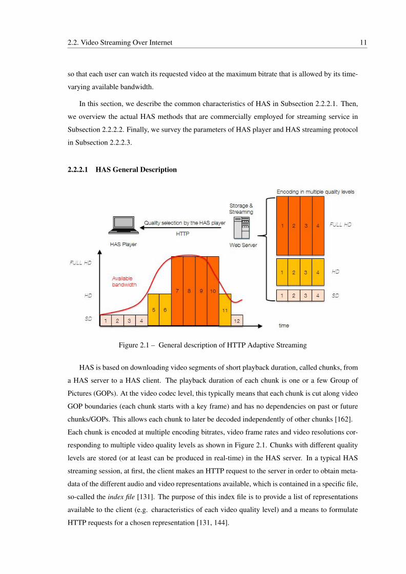
Figure 2.1 – General description of HTTP Adaptive Streaming
HAS is based on downloading video segments of short playback duration, called chunks, from
a HAS server to a HAS client. The playback duration of each chunk is one or a few Group of
Pictures (GOPs). At the video codec level, this typically means that each chunk is cut along video
GOP boundaries (each chunk starts with a key frame) and has no dependencies on past or future
chunks/GOPs. This allows each chunk to later be decoded independently of other chunks [162].
Each chunk is encoded at multiple encoding bitrates, video frame rates and video resolutions cor-
responding to multiple video quality levels as shown in Figure 2.1. Chunks with different quality
levels are stored (or at least can be produced in real-time) in the HAS server. In a typical HAS
streaming session, at first, the client makes an HTTP request to the server in order to obtain meta-
data of the different audio and video representations available, which is contained in a specific file,
so-called the index file [131]. The purpose of this index file is to provide a list of representations
available to the client (e.g. characteristics of each video quality level) and a means to formulate
HTTP requests for a chosen representation [131, 144].
12 2. State of the art
The adaptation engine in the client (also called bitrate controller), which distinguish HAS to
classic progressive HTTP download, decides which chunks should be downloaded based on their
availability (indicated by the index file), the actual network conditions (measured or estimated
available bandwidth), as shown in Figure 2.1, and media playout conditions (playback buffer oc-
cupancy) [131, 157]. Typically one HTTP GET request is sent from the player to the HAS server
for each chunk [144]. In addition, HAS employs HTTP/1.1 with enabled persistent connection
option in order to maintain the same TCP session throughout the entire video stream. Then, the
chunk is stored in the playback buffer of the player to be decoded and displayed.
As the chunks are downloaded at the client, and more precisely in the playback buffer of the
player, the player plays back the sequence of chunks in sequence order. Because the chunks are
carefully encoded without any gaps or overlaps between them, the chunks play back as a seamless
video [162]. In order to avoid the famine of playback buffer, the player operates in one of two
states: Buffering State and Steady State. During the Buffering-State, the player requests a set of
chunks consecutively until the playback buffer has been filled. Generally, the player selects the
lowest video quality level to accelerate buffering process. During this phase, the player does not
begin decoding and displaying video. This phase is called initial loading or initial buffering when
it is in the beginning of the HAS session and stalling or rebuffering when it happens later on in
time [50]. In general cases, the player shows a message to users indicating that the buffering is
processing. Once the playback buffer is filled, the player switches to Steady State by requesting
the chunks periodically to maintain a constant playback buffer size. Accordingly, this periodicity
creates periods of activity, so-called ON periods [6, 147], when the chunk is being downloaded,
followed by periods of inactivity, so-called OFF periods [6, 147], when the player is waiting for
the request message of the next chunk, without impacting the continuity of the video playing.
We also notice that unlike progressive HTTP download, HAS supports not only VoD stream-
ing, but also Live streaming [166] thanks to its adaptability to network changes. Accordingly,
employing HAS for both VoD and Live services by just adjusting some parameters (such as play-
back buffer length on the player side or chunk generating method on the server side) is more
practical for video service providers.
2.2.2.2 HAS Commercial Products
After the first launch of an HTTP adaptive streaming solution by Move Networks in 2006
[113, 161], HTTP adaptive streaming was commercially rolled out by three dominant companies
in parallel [131] :
2.2. Video Streaming Over Internet 13
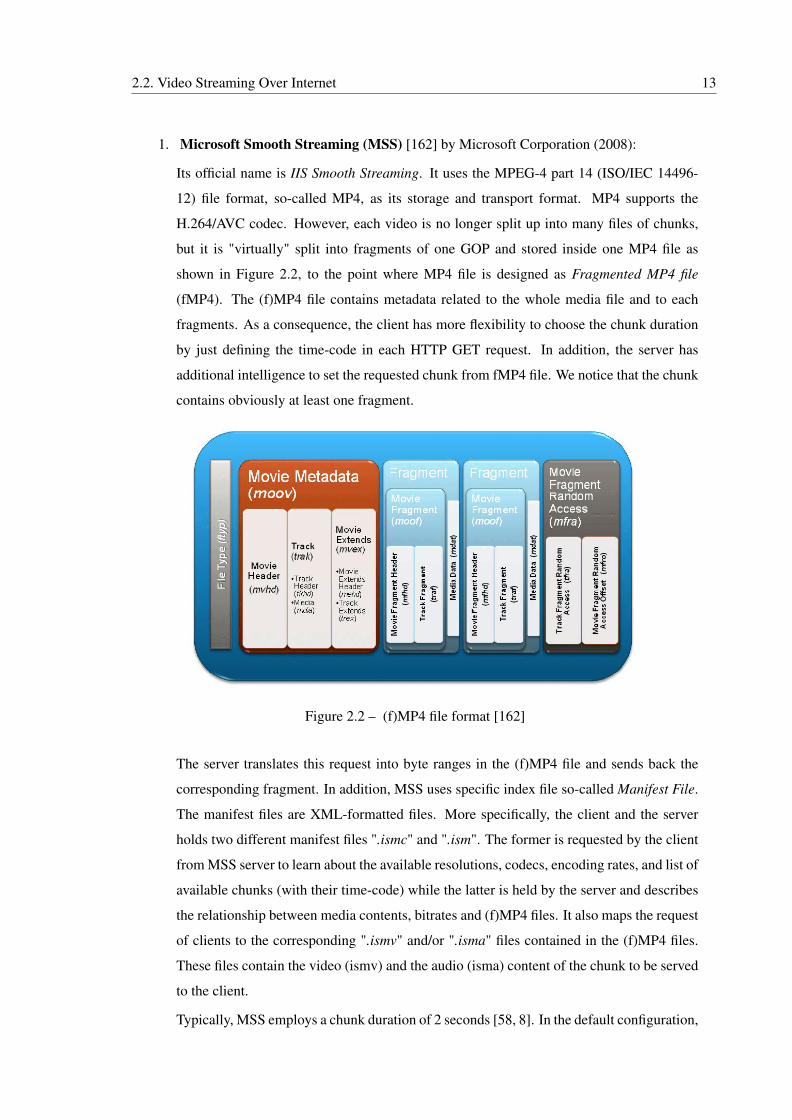
1. Microsoft Smooth Streaming (MSS) [162] by Microsoft Corporation (2008):
Its official name is IIS Smooth Streaming. It uses the MPEG-4 part 14 (ISO/IEC 14496-
12) file format, so-called MP4, as its storage and transport format. MP4 supports the
H.264/AVC codec. However, each video is no longer split up into many files of chunks,
but it is "virtually" split into fragments of one GOP and stored inside one MP4 file as
shown in Figure 2.2, to the point where MP4 file is designed as Fragmented MP4 file
(fMP4). The (f)MP4 file contains metadata related to the whole media file and to each
fragments. As a consequence, the client has more flexibility to choose the chunk duration
by just defining the time-code in each HTTP GET request. In addition, the server has
additional intelligence to set the requested chunk from fMP4 file. We notice that the chunk
contains obviously at least one fragment.
Figure 2.2 – (f)MP4 file format [162]
The server translates this request into byte ranges in the (f)MP4 file and sends back the
corresponding fragment. In addition, MSS uses specific index file so-called Manifest File.
The manifest files are XML-formatted files. More specifically, the client and the server
holds two different manifest files ".ismc" and ".ism". The former is requested by the client
from MSS server to learn about the available resolutions, codecs, encoding rates, and list of
available chunks (with their time-code) while the latter is held by the server and describes
the relationship between media contents, bitrates and (f)MP4 files. It also maps the request
of clients to the corresponding ".ismv" and/or ".isma" files contained in the (f)MP4 files.
These files contain the video (ismv) and the audio (isma) content of the chunk to be served
to the client.
Typically, MSS employs a chunk duration of 2 seconds [58, 8]. In the default configuration,
14 2. State of the art
MSS encodes the video stream in seven layers that range from 300 kbps to 2.4 Mbps [38].
The player of MSS is developped using Silverlight framework and called Smooth
Streaming Silverlight client. However, the most challenging part of this client is the
heuristics module of the adaptation engine (e.g bitrate controller) that determines
when and how to switch between bitrates. It is also customizable for developers. In
addition, Microsoft proposed an open video player (OVP) that provides a video player
plateform that it was used by Akamai on SmoothHD.com [162]. Netflix had also used
MSS with its Silverlight framework to stream videos [123]. However, as authors of
[8] said, each Netflix player maintains two TCP connections with the server. They also
indicated that each of these two connexions is managed in a similar way by the MSS player.
2. HTTP Live Streaming (HLS) [16] by Apple Inc. (2009):
As shown in Figure 2.3, inside the server, HLS begins by converting each new MPEG video
file into multiple MPEG-2 transport streams (MPEG-2 TS) also denoted by M2TS. Unlike
MSS, HLS server split each video stream into chunks, called media segment files, of con-
figurable duration and video quality using a software stream segmenter. These chunks are
stored on a web server as files with "*.ts" extension. Besides, the stream segmenter cre-
ates and maintains an index file which indicates the list of chunks related to the same video
stream and their characteristics (chunk number and encoding bitrates). The index file is so-
called a playlist. It has "*.m3u8" as file extension and includes the URL which identifies
each chunk. This URL does not necessarily include informations about the characteristics
of chunks, because they are well described in the playlist [16, 144]. Typically, the duration
of each chunk is 10 seconds. Less than 10 seconds will result in extra network overhead
because it causes more frequent refreshes of the index file [131]
We note here that M2TS is not as flexible as in the case of (f)MP4 [131, 162]; In fact, with
M2TS the duration of chunks is selected by the stream segmenter at the beginning and it is
unchangeable, while with (f)MP4 the player has always the possibility to select what ever
chunk duration it desires by choosing the number of media fragments per chunk.
We also note that HLS supports Live as well as VOD streaming services. For a Live
streaming, the chunks (*.ts) are created continuously and the playlists are regularly
refreshed.
HLS employs H.264 codec and it is available on any device running iPhone OS 3.0 or
later (including iPad), or any computer with QuickTime X or later installed [38]. Apple
TV 2 and later includes an HTTP Live Streaming client [16].
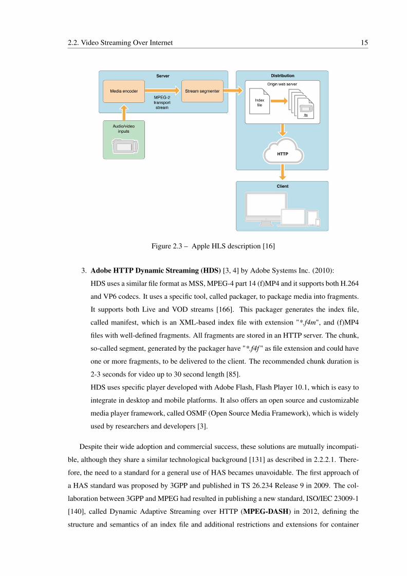
2.2. Video Streaming Over Internet 15
Figure 2.3 – Apple HLS description [16]
3. Adobe HTTP Dynamic Streaming (HDS) [3, 4] by Adobe Systems Inc. (2010):
HDS uses a similar file format as MSS, MPEG-4 part 14 (f)MP4 and it supports both H.264
and VP6 codecs. It uses a specific tool, called packager, to package media into fragments.
It supports both Live and VOD streams [166]. This packager generates the index file,
called manifest, which is an XML-based index file with extension "*.f4m", and (f)MP4
files with well-defined fragments. All fragments are stored in an HTTP server. The chunk,
so-called segment, generated by the packager have "*.f4f " as file extension and could have
one or more fragments, to be delivered to the client. The recommended chunk duration is
2-3 seconds for video up to 30 second length [85].
HDS uses specific player developed with Adobe Flash, Flash Player 10.1, which is easy to
integrate in desktop and mobile platforms. It also offers an open source and customizable
media player framework, called OSMF (Open Source Media Framework), which is widely
used by researchers and developers [3].
Despite their wide adoption and commercial success, these solutions are mutually incompati-
ble, although they share a similar technological background [131] as described in 2.2.2.1. There-
fore, the need to a standard for a general use of HAS becames unavoidable. The first approach of
a HAS standard was proposed by 3GPP and published in TS 26.234 Release 9 in 2009. The col-
laboration between 3GPP and MPEG had resulted in publishing a new standard, ISO/IEC 23009-1
[140], called Dynamic Adaptive Streaming over HTTP (MPEG-DASH) in 2012, defining the
structure and semantics of an index file and additional restrictions and extensions for container
16 2. State of the art
formats.
The MPEG-DASH standard uses an XML-based index file called Media Presentation Description
(MDP). It supports any type of codec, even recently the H.265 HEVC codec. The file format
could be either (f)MP4 or M2TS. The segment length is not specified and is left to individual
implementations.
Many DASH-compatible players have been proposed: VLC Media Player [110], libdash open
source player [20], DASH-JS [116] by University of Klagenfurt, bitdash player [19] provided by
bitmovin for HTML5 and Flash, Viblast player [146] for HTML5, iOS and Android, and OSMO4
[69] by Telecom ParisTech.
Nowaday, many video content providers have recently adopted MPEG-DASH standard, like
YouTube and Netflix [96]. MPEG-DASH has also developed special specifications for the Hy-
brid Broadcast Broadband TV (HbbTV) standard [129] which offers the service of getting digital
television content from various sources such as Internet, traditional broadcast TV and connected
devices in the home.
However, the diversity of HAS commercial products (MSS, HLS, HDS and the standard
MPEG-DASH) leads to having different behavior of the streaming among HAS methods and even
with the same method but using different configuration of the player (such as bandwidth estima-
tion method and playback buffer length). Studying this behavior is been investigated by some
researchers and will be further described in the next Subsection 2.2.2.3.
2.2.2.3 HAS Player Parameters
The HAS commercial products have common characteristics that have been integrated in the
MPEG-DASH standard. However, until now, there is still no convention for the values of player
parameters and they are still fully customizable. Figure 2.4 gives a presentation of the common
HAS player; it mainly depends on two parameters for its adaptation engine (i.e bitrate controller):
the bandwidth prediction and the actual buffer occupancy. Using these two parameters, the
player makes decision for the next chunk; its bitrate (i.e quality level) and its request time [157].
Accordingly, the difference between players is mainly around three questions: How is configured
the bitrate controller ? How is estimated the bandwidth ? And what is the length of playback
buffer ?
In this paragraph we try to give answers for these three questions by overviewing very common
and proposed players:
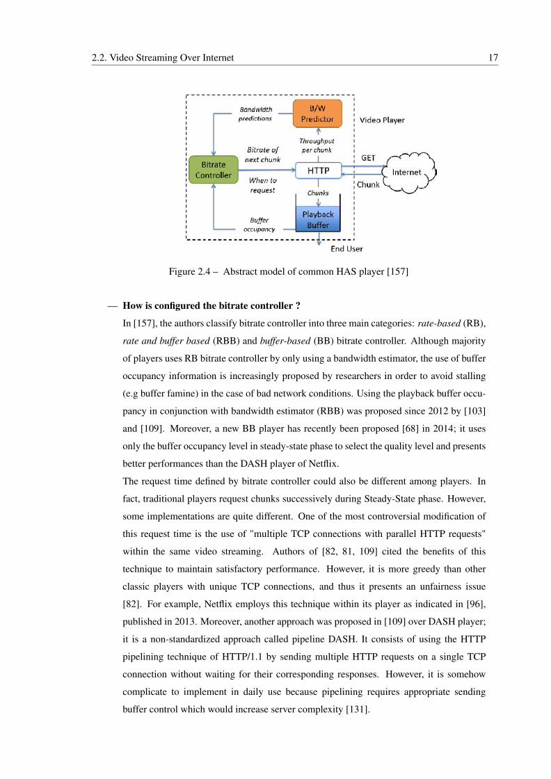
2.2. Video Streaming Over Internet 17
Figure 2.4 – Abstract model of common HAS player [157]
— How is configured the bitrate controller ?
In [157], the authors classify bitrate controller into three main categories: rate-based (RB),
rate and buffer based (RBB) and buffer-based (BB) bitrate controller. Although majority
of players uses RB bitrate controller by only using a bandwidth estimator, the use of buffer
occupancy information is increasingly proposed by researchers in order to avoid stalling
(e.g buffer famine) in the case of bad network conditions. Using the playback buffer occu-
pancy in conjunction with bandwidth estimator (RBB) was proposed since 2012 by [103]
and [109]. Moreover, a new BB player has recently been proposed [68] in 2014; it uses
only the buffer occupancy level in steady-state phase to select the quality level and presents
better performances than the DASH player of Netflix.
The request time defined by bitrate controller could also be different among players. In
fact, traditional players request chunks successively during Steady-State phase. However,
some implementations are quite different. One of the most controversial modification of
this request time is the use of "multiple TCP connections with parallel HTTP requests"
within the same video streaming. Authors of [82, 81, 109] cited the benefits of this
technique to maintain satisfactory performance. However, it is more greedy than other
classic players with unique TCP connections, and thus it presents an unfairness issue
[82]. For example, Netflix employs this technique within its player as indicated in [96],
published in 2013. Moreover, another approach was proposed in [109] over DASH player;
it is a non-standardized approach called pipeline DASH. It consists of using the HTTP
pipelining technique of HTTP/1.1 by sending multiple HTTP requests on a single TCP
connection without waiting for their corresponding responses. However, it is somehow
complicate to implement in daily use because pipelining requires appropriate sending
buffer control which would increase server complexity [131].
18 2. State of the art
Accordingly, the RBB bitrate controller with a unique TCP persistent connection, with
unique HTTP request per chunk and without HTTP pipelining represents the most common
use.
— How is estimated the bandwidth ?
The estimation of bandwidth is based on dividing the chunk size by its downloading dura-
tion. We notice that this estimation is obviously possible only in ON periods. Moreover,
it is possible to apply an exponential moving average function on actual and previous es-
timations [88] to give a smoothed estimation and thus could produce a more stable player.
A similar smoothed estimation technique is used by MSS [8].
In addition, an overall aggressiveness of players toward available end-to-end bandwidth
offered to the client is studied by Saamer Akhshabi et al. [8]; their investigations indicate
that Netflix player is more aggressive than MSS. The former tries to reach higher quality
level even at the expense of quality level changes and sometimes switches to a higher
bitrate than the available bandwidth.
Accordingly, the estimation of the bandwidth is commonly based on the estimation of
the throughput of the previous chunk. However, it may result on an instable player. The
aggressiveness is an important parameter for player design. But, this aggressiveness
should take the length of the playback buffer into consideration in order to avoid stalling
events.
— What is the length of playback buffer ?
The length of playback buffer is different between players and even between devices and
type of connection. For example, Netflix, which uses DASH standard, employs different
playback buffer sizes: they range from 30 seconds (on an Android WiFi device) to 4
minutes (on a Windows Wired device) [96]. OSMF player has a playback buffer size
around 10 seconds [8]. Furthermore, Saamer Akhshabi et al. [8] said that the playback
size for Live streaming is significantly lower than the typical playback buffer sizes of
VoD streaming; for example , in MSS player, the typical size of playback buffer is only
8 seconds for Live streaming while it is 30 seconds for VoD streaming. Obviously, the
objective of this dissimilarity is to reduce the playback delay to be near to Live streaming.
Nevertheless, tolerating few seconds of playback delay (e.g, 8 seconds in the case of MSS)
in Live streaming is unavoidable because shorter buffer size may increase stalling events.
Accordingly, the most common length of playback buffer is around 30 seconds for VoD
service and around 8 seconds for Live service.
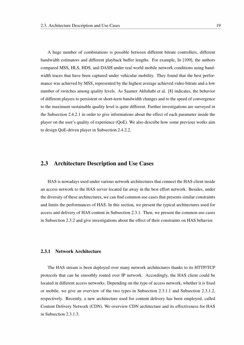
2.3. Architecture Description and Use Cases 19
A huge number of combinations is possible between different bitrate controllers, different
bandwidth estimators and different playback buffer lengths. For example, In [109], the authors
compared MSS, HLS, HDS, and DASH under real world mobile network conditions using band-
width traces that have been captured under vehicular mobility. They found that the best perfor-
mance was achieved by MSS, represented by the highest average achieved video bitrate and a low
number of switches among quality levels. As Saamer Akhshabi et al. [8] indicates, the behavior
of different players to persistent or short-term bandwidth changes and to the speed of convergence
to the maximum sustainable quality level is quite different. Further investigations are surveyed in
the Subsection 2.4.2.1 in order to give informations about the effect of each parameter inside the
player on the user’s quality of experience (QoE). We also describe how some previous works aim
to design QoE-driven player in Subsection 2.4.2.2.
2.3 Architecture Description and Use Cases
HAS is nowadays used under various network architectures that connect the HAS client inside
an access network to the HAS server located far away in the best effort network. Besides, under
the diversity of these architectures, we can find common use cases that presents similar constraints
and limits the performances of HAS. In this section, we present the typical architectures used for
access and delivery of HAS content in Subsection 2.3.1. Then, we present the common use cases
in Subsection 2.3.2 and give investigations about the effect of their constraints on HAS behavior.
2.3.1 Network Architecture
The HAS stream is been deployed over many network architectures thanks to its HTTP/TCP
protocols that can be smoothly routed over IP network. Accordingly, the HAS client could be
located in different access networks. Depending on the type of access network, whether it is fixed
or mobile, we give an overview of the two types in Subsection 2.3.1.1 and Subsection 2.3.1.2,
respectively. Recently, a new architecture used for content delivery has been employed, called
Content Delivery Network (CDN). We overview CDN architecture and its effectiveness for HAS
in Subsection 2.3.1.3.
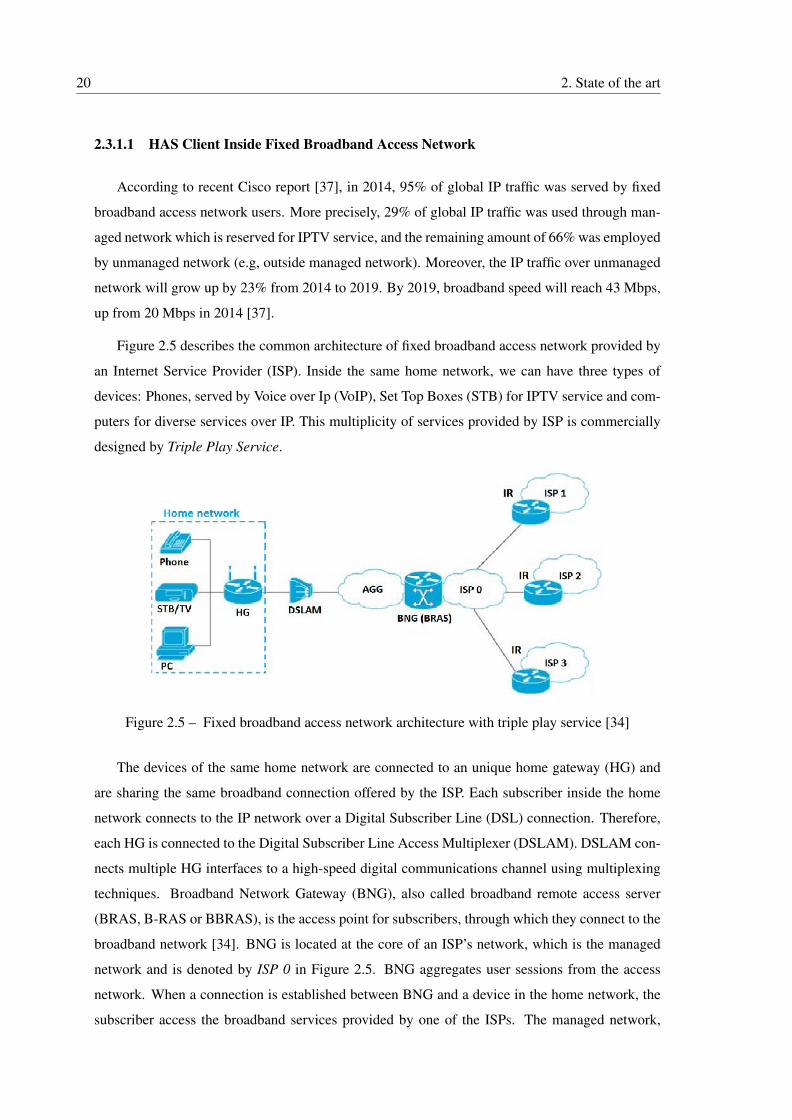
20 2. State of the art
2.3.1.1 HAS Client Inside Fixed Broadband Access Network
According to recent Cisco report [37], in 2014, 95% of global IP traffic was served by fixed
broadband access network users. More precisely, 29% of global IP traffic was used through man-
aged network which is reserved for IPTV service, and the remaining amount of 66% was employed
by unmanaged network (e.g, outside managed network). Moreover, the IP traffic over unmanaged
network will grow up by 23% from 2014 to 2019. By 2019, broadband speed will reach 43 Mbps,
up from 20 Mbps in 2014 [37].
Figure 2.5 describes the common architecture of fixed broadband access network provided by
an Internet Service Provider (ISP). Inside the same home network, we can have three types of
devices: Phones, served by Voice over Ip (VoIP), Set Top Boxes (STB) for IPTV service and com-
puters for diverse services over IP. This multiplicity of services provided by ISP is commercially
designed by Triple Play Service.
Figure 2.5 – Fixed broadband access network architecture with triple play service [34]
The devices of the same home network are connected to an unique home gateway (HG) and
are sharing the same broadband connection offered by the ISP. Each subscriber inside the home
network connects to the IP network over a Digital Subscriber Line (DSL) connection. Therefore,
each HG is connected to the Digital Subscriber Line Access Multiplexer (DSLAM). DSLAM con-
nects multiple HG interfaces to a high-speed digital communications channel using multiplexing
techniques. Broadband Network Gateway (BNG), also called broadband remote access server
(BRAS, B-RAS or BBRAS), is the access point for subscribers, through which they connect to the
broadband network [34]. BNG is located at the core of an ISP’s network, which is the managed
network and is denoted by ISP 0 in Figure 2.5. BNG aggregates user sessions from the access
network. When a connection is established between BNG and a device in the home network, the
subscriber access the broadband services provided by one of the ISPs. The managed network,
2.3. Architecture Description and Use Cases 21
denoted by ISP 0, offers the services of VoIP and STB. It is also connected to the Internet (i.e.
other ISP networks, denoted by ISP 1, ISP 2, etc. in Figure 2.5) via Internet Router (IR). Here we
denote by unmanaged network the network that it is located outside the ISP 0 network. Obviously,
the unmanaged network is not controlled by ISP 0.
We notice that the home network is a Local Area Network. Generally, STB and Phone are con-
nected with wired connection to HG. Other devices could use either wired or wireless connection
[15]. The wireless home network provided by HG -which behaves as an access point- is based on
802.11 families and called WiFi.
2.3.1.2 HAS Client Inside Mobile Broadband Access Network
The mobile broadband designates wireless Internet access delivered to mobile phone through
cellular network. Since the deployment of new generation of cellular network of 3G and beyond,
the delivery of diverse web contents from Internet has become possible. In addition, the mobile
phones has experienced a large improvement of their processing capacity and their display quality,
namely with smart-phones, that made high quality streaming video over cellular network possible.
According to recent Cisco report [37], actually, only less than 5% of global IP traffic was
served to mobile broadband access network users. Nevertheless, it will grow at a compound annual
growth rate (CAGR) of 57% between 2014 and 2019, reaching 24.2 exabytes per month by 2019.
Jiali Chen et al. [27] give the general architecture of typical cellular network as shown in
Figure 2.6. It consists of two parts; the Radio Access Network (RAN) and the Mobile IP Core
network. RAN is a network of base stations connected to a same Gateway called serving gateway.
This gateway handles and routes incoming and outcoming traffic to and from hundred of base
stations. Each base station provides wireless resource allocation across multiple flows of mobile
stations and performs radio resource management, handover initiation and interference reducing.
The Mobile IP core network includes principally the serving gateways and PDN (Packet Data Net-
work) gateways and principally provides the functionalities of IP connectivity. The PDN gateway
enables access to the Internet as well as to the managed newtork of the ISP (e.g mobile network
operator). Accordingly, HAS streaming is performed over the cellular network when the HAS
player inside the mobile station, which is connected to one base station, connects to a HAS server
located in the Internet and asks for video content.
Compared with fixed broadband access network, when HAS clients are located inside the mo-
bile broadband network, additional constraints are presents; 1) the variability of available band-
width due to the change of connected mobiles to the same base station; 2) the high variability of
22 2. State of the art
Figure 2.6 – A typical Cellular Network [27]
delay due to mobility and handover events when the mobile station changes its access from one
base station to another; and 3) a higher error rate (interference, shadowing, multipath fading, route
changes, connection loss) [87].
Nevertheless, many other similitudes are present between the two types of architectures (fixed
or mobile broadband access networks). For example, the serving gateway (respectively, the PNR
gateway) in cellular network is similar to DSLAM (respectively, the Internet Router (IR)) in fixed
broadband network.
Besides, for both architectures, the video content served by unmanaged network is called
Over The Top content (OTT). This content arrives from a third party of content provider such
us YouTube, Netflix, Hulu and Dailymotion. In this case, ISP has only the role of transporting IP
packets between the end-user and this third party provider. Consequently, many constraints related
to the unmanaged network, such as high delay, packet loss and low end-to-end-bandwidth could be
harmful for OTT user’s experience (QoE). In this context, the Content Delivery Network (CDN)
is employed in order to reduce these drawbacks.
2.3.1.3 The Importance of Content Delivery Network
Content Delivery Network (CDN) is a specific architecture for content delivery that has been
widely employed over Internet since the early 2000s. Moreover, according to recent Cisco report
[37], CDN will carry over half of Internet traffic by 2019. Globally, 62% of all Internet traffic will
cross content delivery networks by 2019 globally, up from 39% in 2014.
Figure 2.5 shows a simplified description of CDN. It consists of deploying caches (e.g,
proxies) inside IP network that store replicated contents from servers located far away inside data
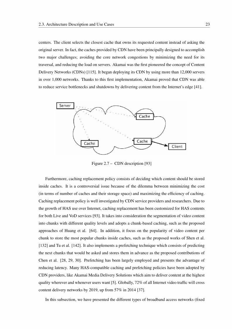
2.3. Architecture Description and Use Cases 23
centers. The client selects the closest cache that owns its requested content instead of asking the
original server. In fact, the caches provided by CDN have been principally designed to accomplish
two major challenges; avoiding the core network congestions by minimizing the need for its
traversal, and reducing the load on servers. Akamai was the first pioneered the concept of Content
Delivery Networks (CDNs) [115]. It began deploying its CDN by using more than 12,000 servers
in over 1,000 networks. Thanks to this first implementation, Akamai proved that CDN was able
to reduce service bottlenecks and shutdowns by delivering content from the Internet’s edge [41].
Figure 2.7 – CDN description [93]
Furthermore, caching replacement policy consists of deciding which content should be stored
inside caches. It is a controversial issue because of the dilemma between minimizing the cost
(in terms of number of caches and their storage space) and maximizing the efficiency of caching.
Caching replacement policy is well investigated by CDN service providers and researchers. Due to
the growth of HAS use over Internet, caching replacement has been customized for HAS contents
for both Live and VoD services [93]. It takes into consideration the segmentation of video content
into chunks with different quality levels and adopts a chunk-based caching, such as the proposed
approaches of Huang et al. [64]. In addition, it focus on the popularity of video content per
chunk to store the most popular chunks inside caches, such as the proposed works of Shen et al.
[132] and Tu et al. [142]. It also implements a prefetching technique which consists of predicting
the next chunks that would be asked and stores them in advance as the proposed contributions of
Chen et al. [28, 29, 30]. Prefetching has been largely employed and presents the advantage of
reducing latency. Many HAS-compatible caching and prefetching policies have been adopted by
CDN providers, like Akamai Media Delivery Solutions which aim to deliver content at the highest
quality wherever and whenever users want [5]. Globally, 72% of all Internet video traffic will cross
content delivery networks by 2019, up from 57% in 2014 [37].
In this subsection, we have presented the different types of broadband access networks (fixed
24 2. State of the art
and mobiles access networks) inside which the HAS clients are connected and are using the HAS
services. We have also presented the CDN networks that are implemented inside ISP networks
in order to improve the QoS of access networks, especially in the context of HAS. By taking into
consideration the similarities between the two access networks and the advantages of CDN, we
present the common use cases in the context of HAS that still present side effects.
2.3.2 Use Cases
Thanks to CDN, the constraints related to the quality of service of core network has been
reduced. Nevertheless, we still have some use cases where the HAS streams suffer from some
issues in the access network. In this section, we present two major issues that harm the quality
of HAS streaming: the bottleneck issue in Subsection 2.3.2.1 and the competition between HAS
flows in Subsection2.3.2.2.
2.3.2.1 Bottleneck Issue
The bottleneck in a network is a node or a link in which the bandwidth is reduced and the
transmission is slowed down due to limited resources or components. The severity of the bottle-
neck relates to the degree of mismatching between traffic demand and available capacity. In fact,
a bottleneck at an early stage may impact the network performance only slightly but it will lead
to increasing performance degradation with time [128]. More precisely, the bottleneck node, as
each network device, has one or many queues (also called buffers) which are outfitted with spe-
cific algorithm to schedule incoming and out-coming packets. This algorithm is called queuing
discipline; depending on the queue length, it decides whether to buffer, route or drop the incoming
packet. Consequently, when the incoming packet rate is higher that the out-coming rate, the bot-
tleneck node becomes more likely delay then to drop packets, hence the degradation of network
performance.
As described in Subsection 2.3.1.3 the CDN has improved the network capacity inside Inter-
net and has reduced considerably the bottleneck occurrence. Therefore, reducing bottleneck side
effects is more required over access networks.
In the fixed broadband access network, Jairo Esteban et al. [43] found in their investigations
that DSLAM is more likely to be the bottleneck. In fact, they report that DSLAM buffers are
smaller in comparison to those found in network device routers. Some authors like Xiaoqi Yin
[157] use the term of bottleneck link which refers to the link between HG and DSLAM. This
designation is equivalent to the DSLAM buffers because the bandwidth is dramatically reduced
2.3. Architecture Description and Use Cases 25
from aggregate link to HG-DSLAM link (see Figure 2.5). Moreover, inside cellular networks,
Fabio Ricciato et al. [126] and Jason J. Quinlan et al. [122] argue that bottleneck is more often
to be located in the RAN. In fact, inside RAN we can locate a geographical area that is frequently
overloaded because the provisioned radio capacity does not match the peak-hour traffic demand.
Grigorik et al. [54] indicated that depending on the location of radio resource controller, whether it
is in the base station (e.g, LTE) or in the serving gateway (e.g, 3G), the bottleneck could be located
inside RAN or in the serving gateway (SG). Accordingly, we can make the assumption that for
mobile broadband access network, the bottleneck link could be considered as located between the
serving Gateway and the base station. We denote it by SG-BS link.
Given that HAS is based on TCP protocol, it produces bursty traffic inside the access network.
Overloading bottleneck nodes and overflowing their buffers could happen more frequently with
the increase of the number of HAS flows. As a consequence, the bottleneck issues in HG-DSLAM
and SG-BS links could be accentuated. Nevertheless, some researches like [90] and [79] make
the assumption that the bottleneck between the HAS client and HAS server is more likely to be
located near the server. However, this assumption is no longer valid with the distributed cashes of
CDN that reduce the load on servers. Besides, the data centers where HAS servers are located are
supposed to be well designed to support high traffic bitrate by insuring low delay and negligible
loss rate.
Furthermore, the testbed used in the context of HAS to emulate the bottleneck of cellular
access network in [122] was similar to what it was used for DSL network in [94]. This similitude
in the architecture leads us to consider both mobile and fixed broadband access networks as the
same use case for emulations over testbeds and for simulations in this thesis. We just should
consider one shared bottleneck link (e.g, presenting SG-BS or HG-DSLAM link) near the HAS
clients and we also should take into consideration the difference of characteristics between wired
and wireless connection offered to clients.
2.3.2.2 Competition between HAS Flows
With an increasing demand for HAS video content over the Internet, the use case of two or
more HAS players sharing the same network bottleneck and competing for available bandwidth
is increasingly becoming more often. In addition, offering high video quality level content for
competing HAS players is becoming possible, although it increases the bottleneck overloading.
The investigation of Saamer Akshabi et al. [6] indicated the effect of this competition on the
behavior of MSS players; it leads to the instability of video quality level selection, unfairness
between players and bandwidth underutilization. The main cause of this degradation is the typical
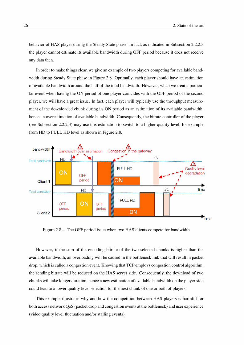
26 2. State of the art
behavior of HAS player during the Steady State phase. In fact, as indicated in Subsection 2.2.2.3
the player cannot estimate its available bandwidth during OFF period because it does not receive
any data then.
In order to make things clear, we give an example of two players competing for available band-
width during Steady State phase in Figure 2.8. Optimally, each player should have an estimation
of available bandwidth around the half of the total bandwidth. However, when we treat a particu-
lar event when having the ON period of one player coincides with the OFF period of the second
player, we will have a great issue. In fact, each player will typically use the throughput measure-
ment of the downloaded chunk during its ON period as an estimation of its available bandwidth,
hence an overestimation of available bandwidth. Consequently, the bitrate controller of the player
(see Subsection 2.2.2.3) may use this estimation to switch to a higher quality level, for example
from HD to FULL HD level as shown in Figure 2.8.
Figure 2.8 – The OFF period issue when two HAS clients compete for bandwidth
However, if the sum of the encoding bitrate of the two selected chunks is higher than the
available bandwidth, an overloading will be caused in the bottleneck link that will result in packet
drop, which is called a congestion event. Knowing that TCP employs congestion control algorithm,
the sending bitrate will be reduced on the HAS server side. Consequently, the download of two
chunks will take longer duration, hence a new estimation of available bandwidth on the player side
could lead to a lower quality level selection for the next chunk of one or both of players.
This example illustrates why and how the competition between HAS players is harmful for
both access network QoS (packet drop and congestion events at the bottleneck) and user experience
(video quality level fluctuation and/or stalling events).
2.4. QoE Characterization and Improvement 27
Many works have been developed in order to reduce the side effect of this use case for both
fixed and mobile broadband access network when bottleneck location is as described in Subsec-
tion 2.3.2.1. In addition, as the observation made by Saamer Akshabi et al. in [8] indicates when
using just two HAS players, the adaptation logic of the player’s bitrate controller "is not able to
avoid oscillations and it does not aim to reduce unfairness in bandwidth sharing competition". Ac-
cordingly, this observation leads us to look for other investigations other than in the application
layer inside the player to resolve "radically" the source of this issue.
The competition between HAS clients in the same network is one of the most critical scenario.
This thesis focuses mainly on this use case in order to improve the overall QoE of competing
players (QoE fairness) and reducing the bottleneck side effect. But, to be able to improve this QoE,
we first should characterize it and understand its interaction with user perception and technical
parameters, which will be described in the next Section 2.4.
2.4 QoE Characterization and Improvement
According to a recent Cisco report, [37], consumer VoD traffic will double by 2019; HD
will be 70% of IP VOD traffic in 2019, up from 59% in 2014. This forecast is challenging for
ISP, video content and CDN providers to enable users to enjoy watching high quality level with
highest experience (QoE). In this section, we describe and explain how QoE has been measured
with specific metrics in Subsection 2.4.1. Then, we overview a detailed investigation of different
factors that could affect this QoE in Subsection 2.4.2.
2.4.1 QoE Metrics
QoE (Quality of Experience) is an increasingly important overall quality attracting both in-
dustry and academia in the field of Information and Communication Technology (ICT) [136]. It
includes human subjective quality in addition to objective quality [22]. Therefore, the assessment
of QoE by using well-designed metrics would be an essential ingredient of successful deployment
of HAS. In this section, we present the two categories of QoE metrics; subjective (in Subsec-
tion 2.4.1.1) and objective metrics (in Subsection 2.4.1.2).
2.4.1.1 Subjective QoE Metrics
The most widely used metric of subjective quality measurement is MOS (Mean Opinion Score)
[125], which is an arithmetic average of scores (say, 1 through 5) given by many subjects to an ob-
28 2. State of the art
ject to be assessed. Historically, MOS has been adopted in Recommendations by ITU (e.g., [70])
for conventional ICT services typified by telephony and TV broadcast [136]. Many researches has
adopted MOS in order to collect an overall experience of HAS users, such as [26, 127]. Neverthe-
less, some limitations of MOS have been pointed out by many researchers [72, 63, 108, 137].
In fact, MOS value does not necessarily represent exact difference between the observer’s
sensory magnitude. Therefore, Shuji Tasaka et al. [137, 138] employed another metric called psy-
chological scale; it uses an interval scale instead of the MOS ordinal scale. Authors demonstrate
that this scale represents human subjectivity more accurately than MOS.
Moreover, the MOS measurements may vary between type of users (e.g, gender, country, cul-
ture); the process of averaging subjective ratings employed by MOS (and even by psychological
scale) eliminates the diversity of user assessments. Therefore, Tobias Hossfeld et al. [63] pro-
posed an additional subjective metric, SOS (Standard deviation of Opinion Scores), that gives the
standard deviation between opinion score measurements in order to get more accurate assessments
about opinion diversity.
However, the subjective criteria cited above do not give sufficient information about the dis-
turbing factors for users and/or their impact on user’s experience; they are still overall measure-
ments. Therefore, some authors have used acceptability threshold metric; it was defined by S.
Jumisko-Pyykkö et al. [76] in the context of video QoE as "binary measure to locate the threshold
of minimum acceptable quality that fulfills subject quality expectations and needs for a certain
application or system". In other words, acceptability metric is the user’s tolerance for videos con-
taining impairment and failure events. Petros Spacho et al. [135] have shown that technical factors
as well as the overall user’s experience have the major impact on acceptability.
The subjective metric involves collecting users’ opinions which is a heavy task in research
and industry. In [40] and [134], authors present QoE models that predict the MOS based on
characteristics of the received video. This kind of models lead us to further investigate arithmetic
metrics that represent objectively the user’s experience.
2.4.1.2 Objective QoE Metrics
Ideally, the HAS end-user likes to watch video without any annoying events. He/she gener-
ally does not care about technical factors related to streaming video, but he/she rather focuses on
perceptual factors like absence of artifact, high resolution, high video quality, small initial delay
and absence of stalling [131]. Many researches have been developed in order to map between
these perceptual factors and the QoE, and consequently propose objective analytic metric for each
2.4. QoE Characterization and Improvement 29
factor.
T. Zinner et al. [165] used an objective metric, Structural Similarity Metric (SSIM) [150],
that compares between the sent and the received video. They found that the worst QoE perceptual
factor is when having artifacts due to packet loss or error; it is much more severe than the reduction
of video quality. Knowing that HAS is using a reliable protocol (TCP), the risk of artifacts is very
negligible, hence the absence of this factor in the context of HAS in the literature. For this reason,
SSIM metric is no longer used in the context of HAS.
Moreover, video spatial resolution is a perceptual factor that is highly dependent on the end-
user device (e.g, its computational and display capacity). For example displaying a low video
resolution on a large screen would result in low user’s QoE. Besides, the HAS player is supposed
to select the adequate resolution which is suitable with the device capacity. For this reason, video
spacial resolution is almost not employed as objective QoE metric in the context of HAS. It is also
the same case for other similar perceptual factors that are intrinsic to computer vision field rather
than adaptive video streaming such as frame rate or type of video codec.
Nevertheless, many researches have used objective metrics related to video quality. For ex-
ample, [157, 78, 154] use the average video encoding rate as objective metric. The logic behind
this is that users generally prefer to watch high video quality during time. However, Jinyao Yan
et al. [153] find an important correlation between standard deviation of quality level and QoE. In
addition, Ricky K. P. Mok et al. [107] show that users prefer a gradual quality change between the
best and the worst quality levels, instead of an abrupt switching. Therefore, many authors have
adopted metrics based on this criterion, such as average quality variation in [157] and quality level
instability [133]. Moreover, M. Zink et al. [164] indicate that higher quality level in the end leads
to a higher QoE. Therefore, J. Jiang [74] uses an instability metric with a weight function that adds
penalty to a more recent switching of quality level.
Furthermore, the initial delay has been adopted by many authors [78, 133]. In fact, the user
dislikes waiting long duration before the beginning of video display. However, the impact of
initial delay on QoE is not severe [39]. As T. Hoßfeld et al.[65] indicate, an initial delay up to 16
seconds reduce the user’s QoE only marginally. However, they indicate that stalling is much more
harmful. We remember that stalling consists of video playback interruption due to playback buffer
depletion. During this interruption, the player is asking for chunks consecutively in order to fill its
buffer and to continue video displaying. Some authors have used the stalling time as a metric such
as [102] and others have employed analytic function that depends both on number and duration of
stalling events [133].
In the literature, authors select their own objective metrics depending on the perceptual factors
30 2. State of the art
they want to improve. Some authors employed more than one metric for evaluation, and consider
them like "independent" metrics such as [78, 133], while others inject their metrics inside one an-
alytic formula; for example, in [157] authors employ three metrics (average video quality, average
quality variation, total stalling time) inside one linear formula by using weight coefficients that
reflect the sensibility of users toward each metric. However, the big issue in this case is the choice
of the weight coefficients because they could vary between users.
Moreover, some authors have introduced other metrics suitable for each specific use case (such
as competition between HAS flows). In fact, each use case has its own major side effects that
should be considered to reduce their harmful consequences on user’s QoE. These metrics will be
more investigated in Chapter 3 (Section 3.5.1).
The subjective and objective metrics are still used nowadays in the context of HAS to make
a more accurate evaluation. For example, in [127], authors make both subjective and objective
metrics for their evaluations. Nevertheless, the measurements of QoE are still insufficient when
we consider only the perceptual factors. In fact, such technical factors could have an important
influence on the perceived QoE. This influence is further discussed in the next Subsection 2.4.2.
2.4.2 Technical Influence factors of QoE and Cross-layer Optimization
Factors affecting QoE are not only human being as the truly end-user but also traditional
QoS (Quality of Service) and all surrounding environments with which the end-user interacts
[83, 18, 106] that are designated as technical influence factors. For this reason, studying the impact
of these factors on QoE could be helpful for improving user’s experience. This section is organized
as the following; we give an overview of technical influence factors, classified according to OSI
model in Subsection 2.4.2.1. Then we overview the proposed improvements of QoE by involving
different OSI layers, so-called cross-layer optimizations, in Subsection 2.4.2.2.
2.4.2.1 Technical Influence Factors
— Application layer factors:
Jun Yao et al. [156] indicated the effect of playback buffer size and chunk duration on
QoE; there is a tradeoff between short and large values. In fact, small playback buffer size
results in short initial delay and short but frequent stalling events. However, a large buffer
reduces stalling events but it increases the initial delay. Furthermore, small chunk duration
results in a shorter delay to adapt the quality level to the estimated bandwidth, but it may
result in more quality level changes in the case of instable network conditions. However,
2.4. QoE Characterization and Improvement 31
a large chunk gives better stability and higher quality level selection, but it may cause
more stalling events because it may be incapable to adapt to rapid bandwidth fluctuations.
Additionally, R. Kuschnig et al. [80] and [79] reveal the harmful impact of long chunk
duration on fair concurrence between HAS players, although it offers higher bandwidth
utilization. Thorsten Lohmar et al. [91] have also reveled that longer chunks would cause
higher end-to-end delay which is harmful for OoE of HAS Live streaming.
Moreover, some new contributions include other application-level parameters in the
bitrate controller in order to improve the QoE. For example, in [75] authors proved
that taking the size of the chunk into consideration in the bitrate controller improves
the QoE in terms of video quality level and bitrate switching events. In [111] authors
include the frame rate parameter in their bitrate controller and proved that it optimizes
the user’s QoE by avoiding stalling, and pausing during video playback. In [68] authors
proposed a buffer-based (BB) bitrate controller by only using the buffer occupancy
level information for quality level selection. Their approach has reduced the stalling rate
by 10-20% compared to Netfix player, while improving the average steady-state video rate.
— Transport layer factors:
As described in Subsection 2.2.1.2, the TCP transport protocol was not designed specifi-
cally for video streaming. Consequently, some factors of TCP could be harmful for QoE:
the reaction toward congestions, packet loss and the congestion detection.
First, the congestion control algorithm used by TCP on the sender side has a significant
impact on throughput variation. In fact, when the sender detects a congestion event, it
reduces its congestion window, cwnd, by a multiplicative decrease factor (generally 0.5 in
standard implementation) [9]. This reduction means that the throughput will be reduced
by the same factor. The presence of bottleneck which increases the frequency of conges-
tion events would increase the throughput fluctuation. Consequently, the player could be
instable in its quality level selection. Hence there is a degradation in the QoE.
Second, the packet loss caused by network congestions results in TCP packet retransmis-
sions. However, retransmissions in HAS stream are harmful to QoE because it adds un-
desirable long transmission delays [18, 46, 61]. One mechanism was proposed to reduce
packet loss in routers and called Explicit Congestion Notification (ECN); Routers can set a
specific codepoint in the IP header of packets instead of dropping them, and TCP protocol
considers this codepoint as a congestion event. Hence, packet loss and retransmissions are
reduced considerably. Unfortuantely, ECN has not been widely deployed due to the need
of a specific configuration requirement inside routers. Moreover ECN bit positioning and
32 2. State of the art
analyzing are accused to add delay to packet forwarding in routers.
Third, there are many TCP congestion control variants with different methods of managing
cwnd and detecting congestion events. As H. Jamal et al. [71] indicate, these variants give
different performances according to some criteria, like average throughput, packet loss,
flow fairness and aggressiveness. Accordingly, the choice of TCP variant could impact the
HAS traffic behavior and could influence the QoE.
— Network layer factors:
The network layer factors that influence the QoE of HAS users could be reduced to two
elements: the length of router queues and the queuing disciplines.
In one hand, reducing the size of queues of routers would obviously increase the packet
drop rate, as described in Subsection 2.3.2.1. Nevertheless, large queues would cause
buffer bloat effect phenomenon; in which the excess buffering of packets causes high la-
tency and packet delay variation, as described in [51]. In this case, traffic can experience
very high queuing delays that can reach several hundreds of milliseconds and sometimes
even more than a second [155], which is very harmful to HAS QoE.
In another hand, the queuing discipline is a queuing management algorithm inside routers
(e.g, network devices in general) that decides whether to drop, route or buffer packets.
Many optimizations have been employed that could be classified into two major classes:
Drop Tail [117] and Random Early Detection (RED) [47]. With Drop Tail, when the queue
reaches its maximum capacity, the newly arriving packets are dropped until the queue has
enough space to accept incoming traffic. While with RED, the average queue size and
drops of packets are based on statistical probabilities; as the queue grows, the probability
for dropping an incoming packet grows too. Similarly, when the queue becomes full,
this probability reaches 1 and all incoming packets are dropped [47]. The dissimilarity
between the two categories would impact the packet drop rate and end-to-end delay as
well as the QoE of HAS.
— Link and physical layer factors:
Many factors related to physical and link layer (generally MAC layer) have a direct effect
QoE; such as the channel modulation and estimation, mobility and resource allocations
[152, 87], as well as collision detection or avoidance [145]. The cause of this influence
is that these factors could modify the network resource utilization and the bandwidth
allocation for each HAS player [1].
2.4. QoE Characterization and Improvement 33
In this subsection, we have presented the different technical factors that influence the QoE
of HAS users classified according to the OSI model. These factors have been exploited in many
contributions in order to improve this QoE as explained in the next Subsection 2.4.2.2.
2.4.2.2 Cross-layer Optimizations
Due to the multiplicity of technical factors which, as explain above, come from the different
OSI model layers, the maximization of QoE would become complex. Hence, the cross-layer
optimization has been employed by many researchers in the context of HAS [95]. It enables one
layer to exchange information with another layer and enable interactions [87]. In the literature, we
can find many cross-layer optimization methods using different parameters:
In [33] authors proposed effective adaptive cross-layer schemes for multimedia delivery over
the time varying link characteristics, including the channel coding (Forward Error correction),
MAC layer retransmission limit, the application layer, and packet size. In [151], authors propose
a novel approach for bitrate controller based on the estimated probability of stalling events. This
probability is calculated using an analytical model of playout buffer and TCP layer measurements
such as RTT. T. Kim et al. [77] proposed an optimal buffer length that depends on the video
bitrate, network characteristics from IP and TCP layers (packet loss rate, round-trip time, and
retransmission timeout) and desired video quality in order to offer best QoE. In [133], authors
present Open-Loop rAte Control (OLAC), an adaptive streaming architecture designed to support
low-latency streaming applications. The key components of their architecture are a server-side
simulation of the streaming client’s buffer, which provides a low-delay feedback for the video
rate selection, and a hybrid adaptation logic based on throughput and buffer information, which
stabilizes the adaptive response to dynamics of transport and application layers.
Moreover, some other cross-layer optimizations are more specific to mobile networks. For
example, in [112], authors propose to combine mobility management and application layer filtering
in order to optimize and maintain video quality. In [141], integration of the handover initiation into
a cross-layer mechanism is proposed aiming to improve the overall system performance. In [152]
authors present a module that allows the player to efficiently monitor the LTE base station physical
layer resource allocation, and then map such information to an estimation of available bandwidth.
In this subsection, we have overviewed the different technical factors that influence the QoE
of HAS users and the different proposed cross-layer optimizations. However, we remark that
the proposed cross-layer methods in the literature are implemented in the HAS server or/and the
HAS player and are controlled by the application layer. However, the concept of cross-layer
optimization can also be extended to the implementation inside other intermediate nodes between
34 2. State of the art
the HAS client and the HAS server and can also be controlled by another lower OSI layer than the
application layer.
2.5 Conclusion
In this chapter, we gave an overview of existing video streaming techniques used over Internet.
We found that HAS is the best efficient technique among all other techniques whether based on
UDP or TCP in terms of reliability and adaptability to network conditions. The diversity of HAS
implementations has led to a new standard called MPEG-DASH. However, previous implemen-
tations still exist and even the standard MPEG-DASH still contains parameter values inside the
player which are not conventional. This would cause a diversity of HAS behaviors among differ-
ent values of parameters. We also showed the architectures in which the HAS service is employed.
We gave an overview of fixed and mobile broadband access network where the HAS client could
be located. We gave the similarity and the dissimilarity between the two access architectures. We
also highlighted the benefits of using CDN networks in reducing latency and improving the quality
of streaming. We also described an increasingly frequent use case when HAS clients are compet-
ing for bottleneck link and we presented its drawbacks on QoS and QoE. Then we overviewed
the characterization of QoE of HAS by using objective and subjective criteria. We also gave a
classification of technical factors that influence the QoE in accordance with OSI model layers. We
also gave examples of cross-layer optimization that aims to improve the QoE by using several pa-
rameters from different OSI layers. Additionally, the background given by this state of the art will
be mandatory both for further assumptions that we could take throughout and for the frameworks
that we would employ for emulations, testbeds, simulations and evaluations. These frameworks
are described with details in Chapter 3.
The objective of this thesis is to add optimizations to the transport protocol TCP, which is not
well investigated in the literature in the context of HAS, in order to limit the drawbacks of the cited
scenario of HAS clients sharing the same bottleneck link and are competing for bandwidth. These
optimizations could be considered as cross-layer solutions. In the following sections, we will give
additional details of specific state of the art relative to each kind of proposed optimization (see
Sections 4.2, 5.2 and 6.2).
35
CHAPTER
3 General Framework for
Emulations, Testbeds,
Simulations and
Evaluations
3.1 Introduction
This chapter gives all the details about tools and parameters that we have used and imple-
mented during this thesis. The use case that we focus on is when HAS players share the same
bottleneck link and compete for bandwidth. In fact, during the thesis we have implemented a
testbed that it has been used for validation and evaluation of our proposed solutions by using real
machines. For extended evaluations, we have used network simulator ns-3 with precise speci-
fications that mimics real conditions. Besides, we have developed and used the same emulated
HAS player for both implementations (testbed and simulator). Moreover, we have used for our
evaluations specific performance metrics for both QoE and QoS criteria.
The objective of this chapter is to give the researchers the ability to re-implement our work,
verify results and understand the explanation of each choice we made for configuration, imple-
mentation and metrics of evaluation. To be more accurate, we refer to some recent references to
justify our choice among many alternatives.
This chapter is organized as the following: In Section 3.2 we describe the characteristics of our
emulated HAS player. In Section 3.3 we give details about the architecture used in our testbed and
the configurations made in each machine. In Section 3.4 we demonstrate the implementation of
HAS traffic in ns-3 simulator and the extensible architecture used for simulations. In Section 3.5
we present the performance metrics that are analytically defined for evaluating the QoE and the
36 3. General Framework for Emulations, Testbeds, Simulations and Evaluations
QoS based on related works and observations.
3.2 Emulation of HAS Player
Knowing that each parameter of the HAS player could affect the QoE as described in Chapter 2
(Subsections 2.2.2.3 and 2.4.2), we should pay attention to each parameter inside the player in
order to achieve two main goals: being close to common players and avoiding side effects of some
proposed players.
Maybe the reader would ask the question: "Why have we employed an emulated player instead
of a commercial player ?". The explanation of this choice has four major arguments:
— First, the commercial players have complicated implementation with many parameters.
Besides, the bitrate controller has dissimilarities among commercial players and even be-
tween different versions of the same player as discussed in Subsection 2.2.2.2. Accord-
ingly, using our own well-controlled player would be better for evaluations than a "black
box" commercial player that could give incomprehensible behaviors.
— Second, as we mentioned in Subsection 2.4.1, some perceptual factors related to computer
vision field (e.g video spatial resolution, frame rate or type of video codec) are not interest-
ing for HAS evaluation. Therefore, using an emulated player that mimics the behavior of
HAS player without decoding and displaying video content would conduct us to the same
evaluation purpose as with a real player.
— Third, the objective metrics are increasingly employed for HAS evaluation (see Subsec-
tion 2.4.1.2). Hence, with a fully controlled emulated player we can easily get the variation
of its parameters during time and employ them for objective QoE metric computation.
— Fourth, for testbeds and simulations, we need to automatize events such as triggering the
beginning and the end of HAS flow at precise moments. Using an emulated player offers
easier manipulation than real player, especially in the case of many players to be launched
at the same moment.
Our emulated HAS player is a Rate and Buffer Based (RBB) player (see Subsection 2.2.2.3).
This choice is justified by the fact that using buffer occupancy information is increasingly proposed
and used due to its advantages for reducing stalling events. In addition, the bandwidth estimator
we used consists of dividing the size of received chunk by its download duration. The buffer
occupancy information is used only to define an aggressiveness level of the player. In fact, this
aggressiveness enables the player to add additional amount to the estimated bandwidth to promote
higher quality level selection. As explained in [67], the bandwidth estimator does not take into
3.3. Testbed Description 37
consideration the increase of TCP congestion window from low value at the beginning of some
ON periods. As a consequence, an underestimation of available bandwidth becomes frequent and
leads to "downward spiral effect" phenomenon: a feedback loop that leads to undesirably variable
and low-quality video. For this purpose, we used a bitrate controller algorithm based on bandwidth
estimation in which we define an aggressiveness ρC(t) at time t that depends on playback buffer
occupancy as follows:
ρC(t) = σ × RC(t)
BC(3.1)
Where RC(t) is the filling level of the playback buffer at time t, BC is the size of the playback
buffer of client C, and σ is the aggressiveness constant. The fuller the playback buffer is, the closer
to σ the aggressiveness is. Accordingly, the player could be more aggressive only when it has less
risk of playback buffer underflow (e.g, stalling event).
The player employs a single TCP connection with a single HTTP request per chunk without
any overlap of HTTP requests among the same HAS flow because it is the most common type of
players. During buffering state, the player selects the lowest quality level while during steady state
phase, the chunks are asked successively every chunk duration. When a chunk takes more than
chunk duration to be downloaded, the next chunk will be asked immediately after the previous
chunk is entirely received.
As a default configuration to be used for testbeds and simulations, the chunk duration is equal
to 2 seconds, the buffer size is equal to 30 seconds of playback, i.e 15 chunks, like what it has been
used in [66]. This configuration includes the common parameters for VoD service as indicated
in Subsection 2.2.2.3. Besides, the aggressiveness constant σ is chosen to be equal to 0.2. The
justification of this value is to try to deliver the highest possible encoding rate even when the
latter is higher than the available bandwidth, as long as the playback occupancy is sufficiently
large. Besides, the selected aggressiveness gives a similar behavior of Netflix player, which was
experimentally evaluated in [8]: In fact, the player reacts rapidly to a rapid increase of available
bandwidth. In addition, it tries to preserves its selected quality level when the available bandwidth
suddenly decreases for short duration.
3.3 Testbed Description
We propose a testbed architecture, presented in Figure 3.1, that emulates our use case. The
choice of only two clients is sufficient to show the preliminary behavior of concurrence between
HAS flows in the same home network. This testbed has an objective of validating proposed meth-
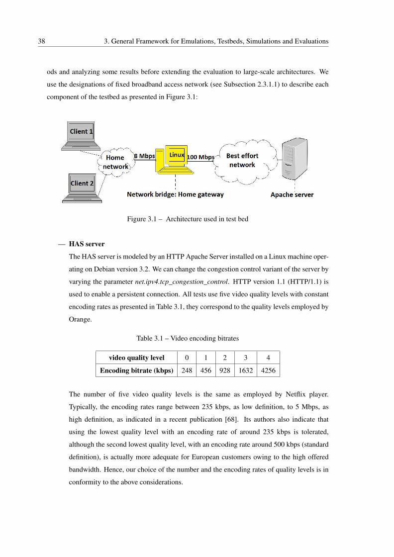
38 3. General Framework for Emulations, Testbeds, Simulations and Evaluations
ods and analyzing some results before extending the evaluation to large-scale architectures. We
use the designations of fixed broadband access network (see Subsection 2.3.1.1) to describe each
component of the testbed as presented in Figure 3.1:
Figure 3.1 – Architecture used in test bed
— HAS server
The HAS server is modeled by an HTTP Apache Server installed on a Linux machine oper-
ating on Debian version 3.2. We can change the congestion control variant of the server by
varying the parameter net.ipv4.tcp_congestion_control. HTTP version 1.1 (HTTP/1.1) is
used to enable a persistent connection. All tests use five video quality levels with constant
encoding rates as presented in Table 3.1, they correspond to the quality levels employed by
Orange.
Table 3.1 – Video encoding bitrates
video quality level 0 1 2 3 4
Encoding bitrate (kbps) 248 456 928 1632 4256
The number of five video quality levels is the same as employed by Netflix player.
Typically, the encoding rates range between 235 kbps, as low definition, to 5 Mbps, as
high definition, as indicated in a recent publication [68]. Its authors also indicate that
using the lowest quality level with an encoding rate of around 235 kbps is tolerated,
although the second lowest quality level, with an encoding rate around 500 kbps (standard
definition), is actually more adequate for European customers owing to the high offered
bandwidth. Hence, our choice of the number and the encoding rates of quality levels is in
conformity to the above considerations.
3.3. Testbed Description 39
— Best effort network
The best effort network is characterized by the presence of bursts and the presence of
packet loss which induces a variability to the delays of delivered packets. Therefore, in
order to offer a more realistic test bed, we employ the modeling formula of the round trip
time RTTC−S(t) in a best effort network as expressed in [104]:
RTTC−S(t) = aC−S +q(t)
ζ(3.2)
Where aC−S is a fixed propagation delay between client C and server S, q(t) is the instan-
taneous occupancy level of the queue of a single congested router (e.g, the bottleneck,
the DSLAM in fixed broadband access network), and ζ is the transmission capacity of
the router. q(t)ζ models the queuing processing delay. To comply with equation 3.2,
we emulate RTTC−S(t) of each HAS flow between server S and client C by a normal
distribution with a mean value aC−S and a standard deviation equal to 0.07×aC−S . Here,
the standard deviation emulates the queuing processing delay q(t)ζ . The choice of only
7% of aC−S is sufficient for our evaluation because it induces a similar RTT variation as
a real conditions. Besides, this standard deviation would also increased when the HAS
flows of competing clients cross the bottleneck link. The cause is that the queuing process
delay q(t)ζ will be more instable due to the high occupancy of the queue, the presence
of congestions, and the instability of HAS throughput as explained in Subsection 2.3.2.
In addition, using a higher standard deviation than 7% of aC−S would be reserved for a
more instable network, especially in the case of wireless access networks, such as WiFi
in the home network. This case of instable network is also tested in our evaluations. This
emulation is accomplished by using the "netem delay" parameter of the traffic controller
tool in the gateway machine interfaces.
We note that the emulated best effort network designates the ISP networks that contains
the managed network, controlled by ISP 0 (see Figure 2.5 in Subsection 2.3.1.1), and the
unmanaged networks that are crossed by the HAS flow to reach the HAS server.
— Home gateway
The emulated home gateway consists of a Linux machine configured as a network bridge
to forward packets between the home network and the best-effort network. Here we
merge DSLAM into HG (Home gateway) to make the testbed easier to manage without
changing the bottleneck behavior. We emulate the queuing discipline of DSLAM by using
Stochastic Fairness Queueing discipline (SFQ) [143]. SFQ is a classless queuing discipline
that we configured using the Traffic Controller tool (tc). SFQ schedules the transmission
of packets based on flow identification (the source and destination IP addresses and the
40 3. General Framework for Emulations, Testbeds, Simulations and Evaluations
source port) and injects them into hash buckets during the enqueuing process. Each of
these buckets should represent a unique flow. Besides, SFQ employs Round Robin fashion
for dequeuing packets by taking into consideration the bucket classification. The goal of
using buckets for enqueuing and Round Robin for dequeuing is to ensure fairness between
flows so that the queue is able to forward data in turn and prevents any single flow from
drowning out the rest. We also configured SFQ in order to support the Drop Tail algorithm
when the queue becomes full. Hence, this configuration of queuing discipline is classified
as a Drop Tail class (see Subsection 2.4.2.1). The queue length of SFQ, which is indicated
by parameter limit within tc tool, is set to the bandwidth-delay product.
— Home network
In the modeled home network, the clients are connected directly to the gateway. The total
download bitrate, or home available bandwidth, is limited to 8 Mbps. We choose this
value because it is lower than twice the video encoding bitrate of the highest quality level.
Accordingly, two clients in the home network cannot select the highest quality level at the
same time, unless they cause congestion and QoE degradation. In this case, one client
should select quality level n◦ 4 and the other should select the quality level n◦ 3 as optimal
qualities. We do not test a use case in which two clients have the same optimal quality
level, because this is a very specific case, and dissimilarity between optimal quality levels
is more general.
— HAS clients
We used two Linux machines as HAS clients. The emulated player described in Sec-
tion 3.2 was integrated in each machine using Python language.
3.4 Simulating HAS Traffic over ns-3
The network simulator version 3 (ns-3) [114] is a discrete-event network simulator for Internet
systems, targeted primarily for research and educational use. It is a free software, licensed under
the GNU GPLv2 license, and is publicly available for research, development, and use since 2008
[60]. The core is written in C++ but with an optional Python scripting interface. In ns-3, each
machine is modeled as a "node". Each node is designed to be faithful to real computer, including
its support for key interfaces such as network devices and sockets, multiple interfaces per nodes
and the use of IP addresses. In addition, we can design our network architecture by interconnecting
3.4. Simulating HAS Traffic over ns-3 41
nodes. Algorithms related to routing daemons, kernel protocol stacks, and packet trace analyzers
are well integrated in ns-3. Moreover, tracing and statistics gathering are enabled by using a
callback-based design.
In this section, we give a detailed description of our implemented work in the ns-3 simulator.
Therefore, we present, in Subsection 3.4.1, our HAS module and how it has been implemented in
ns-3. Then, we describe, in Subsection 3.4.2, the architecture and the configuration of its nodes
and links.
3.4.1 HAS Module Implementation in ns-3
Given that ns-3 is not outfitted with HTTP layer, simulating HAS flows could become an is-
sue. Fortunately, Yufei Cheng et al. proposed an HTTP traffic generator module [32, 31] in 2011.
It ensures the communication between two nodes using HTTP protocol; it includes all features
that generate and control HTTP Get Request and HTTP response messages. It uses two applica-
tion containers; HttpClientHelper and HttpServerHelper that should be installed on the client and
the server nodes, respectively. This module contains principally three main classes: http-client,
http-server and http-controller. The latter class enables the programmer to control parameters and
events of HTTP messages by using a user defined mode. In this mode, we can define the number of
web pages to be asked during the session between client and server, UserNumPages; it is helpful
to define the number of chunks to be displayed. It also defines the server response size, User-
ResponseSize, which can be considered as the chunk size for HAS flow. The time gap between
two consecutive page request messages is defined as UserPageRequestGap parameter; it is useful
to define the request time of each chunk and the chunk duration parameter. Besides, it supports
HTTP/1.1 with persistent connection.
Accordingly, many features of the proposed module provide a good background for im-
plementing HAS player on the client side. However, the defined parameters are exploited by
the http-controller class as "a priori" inputs to be executed without any modification during
simulation process. This configuration is not suitable for the bitrate controller of HAS player: we
should implement an intelligence inside http-client and http-controller classes in order to follow
the instructions of the bitrate controller. In other words, the modified algorithm should adapt the
size of the chunk (UserResponseSize parameter) and the chunk request time to the bandwidth
estimation and the buffer occupancy level. For that, based on HTTP module, we adapt classes,
their attributes and their functions to the HAS context in order to build our own HAS module. We
notice that all instructions of Section 3.2 related to our custom HAS player were respected in our
implementation described as the following:
42 3. General Framework for Emulations, Testbeds, Simulations and Evaluations
• We defined a table that contains all encoding bitrates corresponding to quality levels,
m_layers[]. It is compliant with Table 3.1. The size of chunk, UserResponseSize, is equal
to the encoding bitrate of the corresponding quality level multiplied by the chunk duration
UserPageRequestGap.
• We defined a playback buffer, m_actualFilledPlaybackBufferSize, that provides the buffer
occupancy level during time. The length of this buffer is defined as m_userBufferLength
parameter to be tuned by the programmer.
• We added a scheduler of chunk request time compatible with buffering and steady state
phases. This scheduler depends on the value of m_actualFilledPlaybackBufferSize; if it
becomes null (e.g. stalling event), the http-client asks for chunks of lowest quality level
consecutively until m_actualFilledPlaybackBufferSize reaches m_userBufferLength value.
Then, http-client asks for one chunk every UserPageRequestGap duration. If the chunk
takes longer delay to be downloaded than UserPageRequestGap, http-client asks for the
next chunk when the previous one is completely received.
• We added a bandwidth estimator function, getBitRate(), in the http-client class to estimate
the available bandwidth in the end of each ON period.
• We integrated the bitrate controller in the http-client with additional ability to modify
http-controller parameters during simulation process. It modifies the size (e.g, that
corresponds to one quality level) and the request time of chunk based on bandwidth
estimation, getBitRate(), buffer occupancy level, m_actualFilledPlaybackBufferSize, and
aggressiveness value in accordance with equation 3.1.
• We added callbacks that monitor all player parameters over time (e.g. selected quality
level, buffer occupancy level, bandwidth estimation, OFF period duration) and at the mo-
ment the http-client sends HTTP request message. These values are used for QoE and QoS
metric measurements.
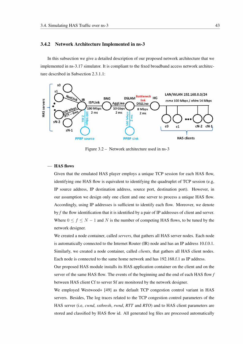
3.4. Simulating HAS Traffic over ns-3 43
3.4.2 Network Architecture Implemented in ns-3
In this subsection we give a detailed description of our proposed network architecture that we
implemented in ns-3.17 simulator. It is compliant to the fixed broadband access network architec-
ture described in Subsection 2.3.1.1:
Figure 3.2 – Network architecture used in ns-3
— HAS flows
Given that the emulated HAS player employs a unique TCP session for each HAS flow,
identifying one HAS flow is equivalent to identifying the quadruplet of TCP session (e.g,
IP source address, IP destination address, source port, destination port). However, in
our assumption we design only one client and one server to process a unique HAS flow.
Accordingly, using IP addresses is sufficient to identify each flow. Moreover, we denote
by f the flow identification that it is identified by a pair of IP addresses of client and server.
Where 0 ≤ f ≤ N − 1 and N is the number of competing HAS flows, to be tuned by the
network designer.
We created a node container, called servers, that gathers all HAS server nodes. Each node
is automatically connected to the Internet Router (IR) node and has an IP address 10.f.0.1.
Similarly, we created a node container, called clients, that gathers all HAS client nodes.
Each node is connected to the same home network and has 192.168.f.1 as IP address.
Our proposed HAS module installs its HAS application container on the client and on the
server of the same HAS flow. The events of the beginning and the end of each HAS flow f
between HAS client Cf to server Sf are monitored by the network designer.
We employed Westwood+ [49] as the default TCP congestion control variant in HAS
servers. Besides, The log traces related to the TCP congestion control parameters of the
HAS server (i.e, cwnd, ssthresh, rwnd, RTT and RTO) and to HAS client parameters are
stored and classified by HAS flow id. All generated log files are processed automatically
44 3. General Framework for Emulations, Testbeds, Simulations and Evaluations
just after simulation by our Shell scripts to generate performance metrics and to plot curves.
— NetLink configuration
In our design, the NetLink emulates the Internet network branch where the server is
located. For this purpose, we generate one NetLink link to connect one HAS server to the
IR node. The bandwidth inside this link is equal to 100 Mbps to emulate Internet network
with high capacity. In addition, using NetLink, we configure the round-trip delay of each
HAS flow.
We denote by RTT 0C−S the initial round-trip propagation delay between the HAS client C
and the server S. Knowing that the configured round-trip propagation delay between IR
and HG is equal to 6 ms (3× 2ms), the round-trip propagation between the IR and a HAS
server node is configured to be equal to RTT 0C−S − 6 ms. Here, the designer has just to
define the value of RTT 0C−S parameter for his custom simulation. The default value is set
to 100ms because it is often measured for streaming video applications [17].
— ISPLink configuration
The ISPLink emulates the ISP network. Given that the emulated network corresponds to
the managed network of ISP provider as described in Subsection 2.2.1.1, it is supposed to
offer a high QoS such as low delay and high bandwidth. For this reason, we configure IS-
PLink with low round-trip propagation delay of 2ms and a high bandwidth of 100Mbps.
— AggLine configuration
The bandwidth in the aggregate link, AggLine, is set to 10 Gbps, which is in conformity
with the literature [139]. We also select round-trip propagation delay of 2ms because
the delay between the two nodes DSLAM and BNG is designed to be very short. (see
Subsection 2.3.1.1).
— Internet traffic emulation (PPBP traffic)
We chose to generate Internet traffic that crosses ISPLink and AggLine. We selected this
location because the two emulated links are supposed to support a heavy traffic from ISP
networks. For this purpose, we employed the Poisson Pareto Burst Process (PPBP) model,
proposed by M. Zukerman [167], that emulates Internet Traffic. This model has been
considered as a simple and accurate traffic model that matches statistical properties of
real-life IP networks (such as their bursty behavior). The PPBP is a process based on the
overlapping of multiple bursts with heavy-tailed distributed lengths. Events in this process
3.4. Simulating HAS Traffic over ns-3 45
represent points of time at which one of an infinite population of users begins or stops
transmitting a traffic burst. The PPBP is closely related to the M/G/∞ queue model
[167].
Fortunately, Doreid Ammar et al. [14] provide a tool for PPBP implementation in ns-3
[13]. This implementation suggests using four parameters to configure the PPBP traffic:
• Burst arrival rate λp, which is in accordance with Poisson process.
• Hurst parameter H , which is the length of burst that follows Pareto distribution. Its
recommended value is 0.7.
• The mean length of burst, Ton.
• The bitrate of the burst, r: in PPBP each burst is modeled by a flow with constant
bitrate r.
For our simulations, the default configuration of PPBP is as the following:
• λp = 20; as used in [14]
• H = 0.7; as recommended in [42]
• Ton = 200ms; as used in [14]
• r = 10Mbps; we used a higher bitrate burst than that of [14] in order to be adequate
with the high capacity of ISP networks -that we have modeled by 100 Mbps in ISPLink
in our configuration-. Our justification is based on the observations of Cisco which
indicate that the large-capacity systems tend to observe large burst patterns [35].
Here we notice that the overall rate of the PPBP traffic, λ, is equal to λ = λp×Ton× r. In
our configuration, the overall rate of PPBP traffic is equal to 40 Mbps which is equivalent
to an occupancy of 40% of ISPLink capacity.
As shown in Figure 3.2, we used two nodes for traffic generation: PPBP source and PPBP
sink. They are connected to IR and DSLAM respectively.
— Bottleneck link configuration (DSLLine)
The bottleneck link is designed by DSLLine. Its bandwidth is set to 8 Mbps like the
configuration of the testbed. The round trip delay between the two extremities is set to 2
ms because, in real architecture, the delay between the two devices is designed to be very
low.
The net device of DSLAM node that is connected to DSLLine link has a small queue
length. It is fixed to 68 packets, which corresponds to the bandwidth delay product, when
bottleneck bandwidth is 8 Mbps, RTT 0C−S is 100 ms and packet size is 1500 bytes.
46 3. General Framework for Emulations, Testbeds, Simulations and Evaluations
— Queuing discipline configuration
The drop tail queuing discipline is been configured for all net devices of nodes. The
justification of employing drop tail discipline is its wide range use and its simplicity.
Excepting the net device of DSLAM node connected to DSLLine link, the length of each
queue is set large enough (1000 packets) to support large bandwidth of 100 Mbps without
causing packet losses.
— Home network
In practice, the home network is a local area network (LAN). Therefore, we define a node
container lan that connects the HG to the clients node container with network IP address
of 192.168.0.0/24. For wired LAN, we employed csma module with bandwidth of 100
Mbps. For wireless LAN, we used the wifi module with ofdm modulation and bandwidth
of 54 Mbps and a simple mobility model. In our simulations we are using wired LAN as a
default configuration. We notice that the home network could be configured as a wireless
LAN (WLAN) using WiFi protocol. In this case, a mobility model should be added to the
client nodes connected to WLAN.
3.5 Performance Metrics
To evaluate the use case of HAS players sharing the same bottleneck and competing for band-
width, we should define performance metrics for evaluations. Some metrics were inspired from
the literature and some others from our own observations during initial tests or simulations. We
classify our metrics into two categories: QoE and QoS metrics.
3.5.1 QoE Metrics
In this subsection, we define analytically the objective QoE metrics that we used for evalua-
tions and justify our selection. For this purpose, we define in Table 3.2 the parameters to be used
in this subsection.
Our QoE metrics that are sensitive to our use case are the Instability of video quality level, de-
scribed in Subsection 3.5.1.1, the Infidelity of video quality level, described in Subsection 3.5.1.2
and convergence speed, described in Subsection 3.5.1.3. In addition, we select two other QoE met-
rics from Subsection 2.4.1.2 that are used for general QoE evaluation purpose; initial delay and
stalling event rate, described in Subsection 3.5.1.4 and Subsection 3.5.1.5, respectively. We also
use the QoE fairness between competing HAS players, described in Subsection 3.5.1.6 as metric
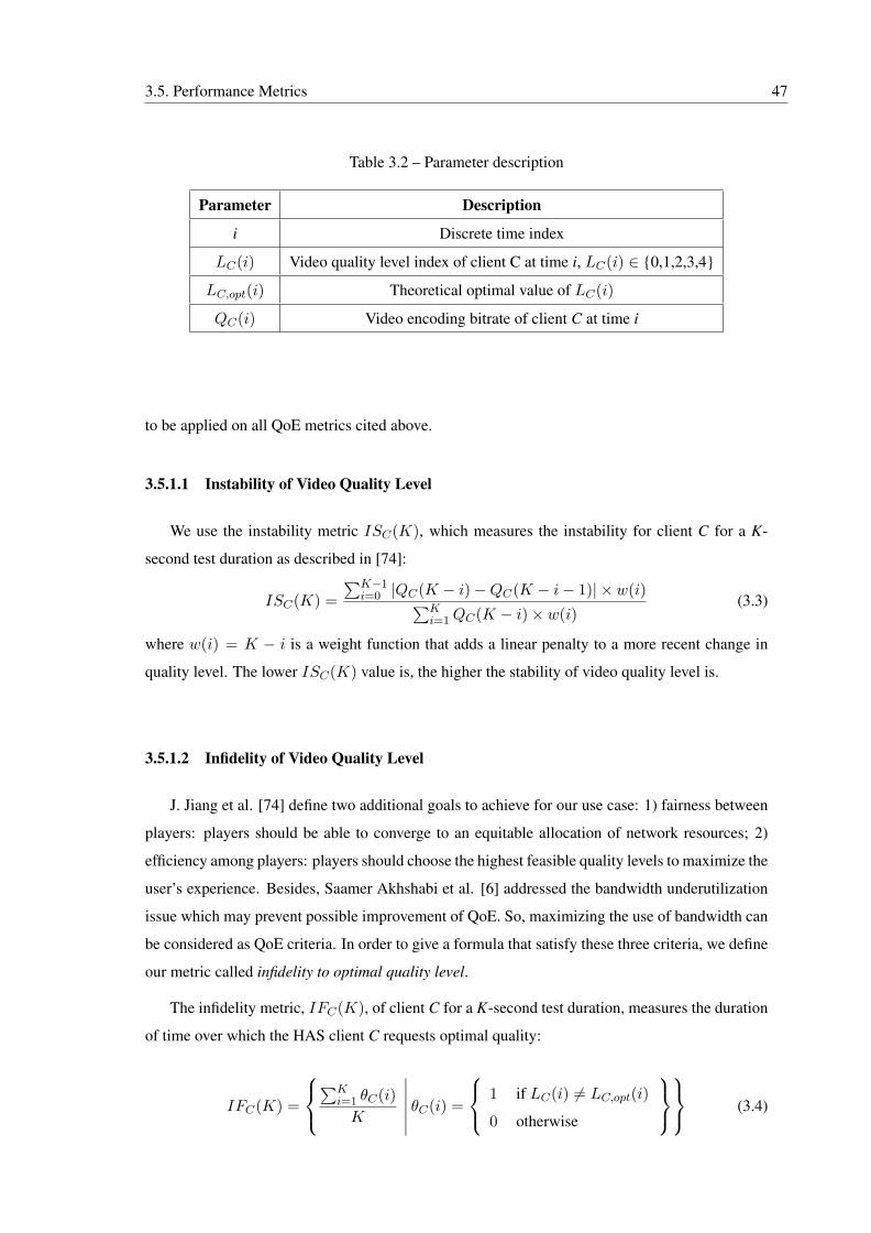
3.5. Performance Metrics 47
Table 3.2 – Parameter description
Parameter Description
i Discrete time index
LC(i) Video quality level index of client C at time i, LC(i) ∈ {0,1,2,3,4}
LC,opt(i) Theoretical optimal value of LC(i)
QC(i) Video encoding bitrate of client C at time i
to be applied on all QoE metrics cited above.
3.5.1.1 Instability of Video Quality Level
We use the instability metric ISC(K), which measures the instability for client C for a K-
second test duration as described in [74]:
ISC(K) =
∑K−1i=0 |QC(K − i)−QC(K − i− 1)| × w(i)∑K
i=1QC(K − i)× w(i)(3.3)
where w(i) = K − i is a weight function that adds a linear penalty to a more recent change in
quality level. The lower ISC(K) value is, the higher the stability of video quality level is.
3.5.1.2 Infidelity of Video Quality Level
J. Jiang et al. [74] define two additional goals to achieve for our use case: 1) fairness between
players: players should be able to converge to an equitable allocation of network resources; 2)
efficiency among players: players should choose the highest feasible quality levels to maximize the
user’s experience. Besides, Saamer Akhshabi et al. [6] addressed the bandwidth underutilization
issue which may prevent possible improvement of QoE. So, maximizing the use of bandwidth can
be considered as QoE criteria. In order to give a formula that satisfy these three criteria, we define
our metric called infidelity to optimal quality level.
The infidelity metric, IFC(K), of client C for a K-second test duration, measures the duration
of time over which the HAS client C requests optimal quality:
IFC(K) =
∑K
i=1 θC(i)
K
θC(i) = 1 if LC(i) 6= LC,opt(i)
0 otherwise
(3.4)
48 3. General Framework for Emulations, Testbeds, Simulations and Evaluations
The lower IFC(K) value is, the higher the fidelity to optimal quality is.
Here we note that the theoretical optimal quality level LC(i) aims to resolve the dilemma
between the two criteria of maximum use and fair share of bandwidth between HAS players. In
fact, considering only the fair share of bandwidth may cause bandwidth underutilization; in some
cases it may leave some residual bandwidth allocated to nobody. Hence, based on the optimal
quality level, the value of the infidelity metric is representative of user expectation.
3.5.1.3 Convergence Speed
The convergence speed metric was previously defined by R. Houdaille et al. [66]. We provide
an analytical definition as follows:
VC,T (K) =
{min
1≤d≤K(d) |LC(i) = LC,opt(i),∀i ∈ [d, d+ T ]
}(3.5)
This metric is the time that the player of HAS client C takes to reach and remain at optimal quality
level for at least T seconds during a K-second test duration. In fact, observations show that when
HAS players compete for bandwidth, the convergence to optimal quality level may take several
seconds or may be very hard to be achieved. Accordingly, the speed of this convergence is a
valuable QoE criteria for our evaluations. The lower VC,T (K) value is, the faster the convergence
to the optimal quality level is.
Here we note that when the player is not able to converge to the optimal quality level during
K-second test duration, the convergence speed value will take the following value:
VC,T (K) = K (3.6)
Although the value of equation 3.6 is not significant enough, because it could be an infinite value,
it enables us to compute the mean value among many runs.
3.5.1.4 Initial Delay
The initial delay, as explained in Subsection 2.4.1.2, is the time that the player takes to fill its
playback buffer. Given that the video displaying begins just when the playback buffer is filled,
the initial delay metric is important for QoE evaluation; in fact, the user prefers to get the video
displayed on his/her screen within a short delay after requesting the video.
3.5. Performance Metrics 49
3.5.1.5 Stalling Event Rate
As explained in Subsection 2.4.1.2, the stalling event consists of video display interruption on
the client side caused by a famine of the playback buffer. The stalling event is a hard penalizing
factor toward the QoE because the user is highly disturbed when the video display is interrupted
when he/she is concentrated on watching. Therefore, we define the stalling event rate metric,
StallingRate(K), as the number of stalling events during K-second test duration, divided by K
and multiplied by 100, as expressed in equation 3.7:
StallingRate(K) =number of stalling events during K seconds
K× 100 (3.7)
The lower StallingRate(K) value is, the better satisfaction of the user is. A zero stalling event
rate should be guaranteed.
3.5.1.6 QoE Unfairness
Z. Yan et al. [154] addressed the issue of QoE unfairness between competing HAS players.
This unfairness is a very valuable point. In fact we could have a mean measurement of QoE among
players that it is satisfying, while one of more players have a poor measurement. Accordingly,
computing the standard deviation between measured QoE metrics give us the idea about QoE
unfairness. For a given QoE metric (e.g, instability, infidelity, convergence speed, initial delay
or number of stalling events), that we denote by M, the QoE unfairness between N HAS clients,
denoted by UNFN (M) is described as the following:
UNFN (M) =
√∑N−1n=0 (Mn −meanN (M))2
N(3.8)
where Mi is the measurement of metric M of HAS client n and meanN (M) is the mean
measurement of metric M among N HAS clients, expressed as the following:
meanN (M) =
∑N−1n=0 (Mn)
N(3.9)
The lower the meanN (M) is, the better fairness of QoE between HAS players is.
3.5.2 QoS Metrics
Although the QoE objective metrics are interesting to measure the user’s experience, they are
not sufficient to analyse the results. Hence, QoS metrics are mandatory to understand the effect
50 3. General Framework for Emulations, Testbeds, Simulations and Evaluations
of each method that we propose on the QoS of access network. The remaining of this subsection
is organized to present four QoS metrics that we used for our evaluation, as the following: First,
we define the Frequency of OFF periods per chunk metric in Subsection 3.5.2.1. Second, we
present the average queuing delay metric in Subsection 3.5.2.2. Third, we explain the conges-
tion rate metric in Subsection 3.5.2.3. Fourth, we present the average packet drop rate metric in
Subsection 3.5.2.4.
3.5.2.1 Frequency of OFF periods per chunk
During HAS flow, an OFF period whose duration exceeds TCP retransmission timeout du-
ration (RTO) is denoted by OFF ; it is important for our evaluations because, as we revealed in
Subsection 4.4.3.2, when OFF period becomes larger than RTO a reduction of bitrate and a degra-
dation of performances would happen.
Our defined metric computes the frequency of OFF periods by chunk rather than by second.
In fact, the frequency by chunk is more significant due to its independence to the chunk duration.
This metric is denoted by frOFF
. It is equal to the total number of OFF periods divided by
the total number of downloaded chunks of one HAS flow.
3.5.2.2 Average Queuing Delay
We found in our investigations that the round-trip time RTTC−S in a HAS flow between
client C and server S could increase significantly. This additional increase is called queuing delay.
As described in Subsection 2.4.2.1, a high queuing delay is harmful to HAS and for real-time
applications.
By using specific tools on the server side (tcp_probe in Linux machine of the testbed, and
callbacks in ns-3 node), we can compute exhaustively the RTTC−S values during HAS ses-
sion at each reception of ACK packet. We compute the average value of RTTC−S , denoted
by MeanRTTC−S(K) among all RTTC−S samples of the whole HAS session for K-second
test duration. Then, we compute the average queuing delay, DelayC−S(K), by subtracting from
MeanRTTC−S(K) the initial round-trip propagation delay between the client C and the server S,
denoted by RTT 0C−S as described in equation 3.10:
DelayC−S(K) =MeanRTTC−S(K)−RTT 0C−S (3.10)
3.6. Conclusion 51
3.5.2.3 Congestion Rate
The congestion detection events are extremely influencing both QoS and QoE of HAS because
the server decreases its sending rate at each congestion detection. Hence, by analyzing the code
description of four TCP congestion control algorithms (NewReno, Vegas, Illinois and Cubic), we
found that the congestion event appears when the value of parameter slow start threshold (ssthresh)
decreases. Hence, we define a metric called congestion rate, denoted by CNGC−S(K) that com-
putes the rate of congestion events, that are detected on the server side, corresponding to the HAS
flow between client C and server S during a K-second test duration as shown in equation 3.11:
CNGC−S(K) =DssthreshC−S (K)
K× 100 (3.11)
Where DssthreshC−S (K) is the number of times the ssthresh has been decreased for the C-S HAS
session during K-second test duration.
3.5.2.4 Average Packet Drop Rate
The number of dropped packets at the bottleneck gives an idea about the congestion severity
of the bottleneck link. This metric is different from congestion rate of subsection 3.5.2.3. In fact,
the server could detect a congestion event whereas there is no packet loss. Indeed , the detection
of a congestion event depends on the TCP congestion control algorithm.
Our metric is denoted byDropPkt(K) and gives the average packet drop rate at the bottleneck
during K-second test duration as shown in equation 3.12:
DropPkt(K) =number of dropped packets during K seconds
K× 100 (3.12)
3.6 Conclusion
In this chapter, we have presented our emulated HAS player which imitates the behavior of
common HAS players without decoding and displaying video content. We justified the use of
different player parameters, its RBB bitrate controller with an aggressiveness that depends on the
playback occupancy level, its buffer length and its chunk duration. We have also presented our
testbed that we have implemented and used for the first part of our evaluation.
We have described the configuration of each connected Linux machine and explained how it
52 3. General Framework for Emulations, Testbeds, Simulations and Evaluations
matched with the real architecture. This testbed have been developed in order to give a realistic
evaluation when two HAS clients are sharing the same bottleneck link and are competing for the
same bandwidth. It has been used for evaluations in Chapter 4 and Chapter 5.
In addition, we have developed a more extensible architecture using the network simulator
ns-3 in order to give extended evaluations of our proposed solutions under various conditions;
when changing the number of competing HAS clients inside the home network, when changing
the player parameters and when changing the ISP network conditions. We have explained the
integrated and implemented modules and justified the different configurations of nodes and em-
ulated links in order to be compliant to the fixed broadband access network. This implemented
architecture has been used in our simulations. The evaluation results of our proposed methods are
presented in Chapter 4 and Chapter 6.
Besides, we have presented in this chapter the different metrics that we have used for evaluating
the QoE of HAS users and the QoS of access network: We have selected two important general
QoE metric (Stalling event rate and initial delay) and the most compliant QoE criteria that match
with our use case (instability of video quality level, infidelity of video quality level, convergence
speed and QoE unfairness). We have also selected four relevant QoS metrics (frequency of OFF
periods per chunk, average queuing delay, congestion rate and average packet drop rate). These
metrics are employed throughout the remainder of this thesis for evaluating our proposed solutions.
53
CHAPTER
4 Gateway-based Shaping
Methods
4.1 Introduction
Improving the QoE of HAS is being actually a challenging purpose. Moreover, as described in
Chapter 2 (section 2.3.2), when HAS players are sharing the same bottleneck link and are compet-
ing for bandwidth, the QoE degrades dramatically. The most disturbing user’s experience in this
case is the instability of video quality level, low fidelity to optimal quality level and slow conver-
gence speed to optimal quality level.
This use case is becoming more frequent in daily use not only in mobile broadband access network
but also in fixed broadband access network. Accordingly proposing a solution that limits the draw-
back effects of this use case on QoE is becoming highly demanded. One of the most convenient
solutions is to apply traffic shaping on HAS streams. One of convenient ways of implementation
is to carry out this shaping on the gateway side. Here we denote by gateway the home gateway
in the case of fixed broadband access network and base station in the case of mobile broadband
access network.
The objective of this chapter is to propose a new solution of HAS traffic shaping in the gate-
way to improve the QoE among competing players. For this purpose, we first study the state of
the art about traffic shaping methods in the context of HAS in Section 4.2. Second, we describe
in Section 4.3 our proposed method, called Receive Window Tuning Method (RWTM) which is a
shaping method implemented in the gateway. Third, we give in Section 4.4 a comparative eval-
uation between our proposed method and a well-known gateway-based shaping method, called
Hierarchical Tocken Bucket Method (HTBM). Finally, we extend the performance evaluation of
RWTM, in Section 4.5, by increasing the number of HAS flows, employing different values of
player parameters and exploring different network conditions.
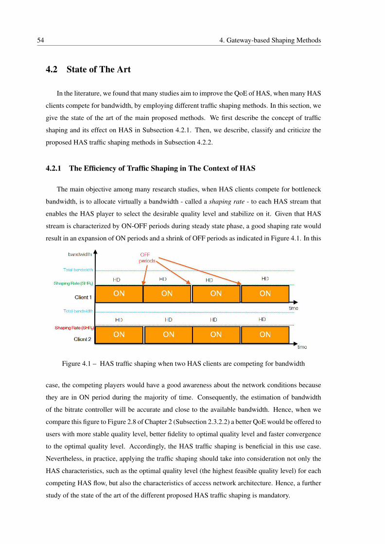
54 4. Gateway-based Shaping Methods
4.2 State of The Art
In the literature, we found that many studies aim to improve the QoE of HAS, when many HAS
clients compete for bandwidth, by employing different traffic shaping methods. In this section, we
give the state of the art of the main proposed methods. We first describe the concept of traffic
shaping and its effect on HAS in Subsection 4.2.1. Then, we describe, classify and criticize the
proposed HAS traffic shaping methods in Subsection 4.2.2.
4.2.1 The Efficiency of Traffic Shaping in The Context of HAS
The main objective among many research studies, when HAS clients compete for bottleneck
bandwidth, is to allocate virtually a bandwidth - called a shaping rate - to each HAS stream that
enables the HAS player to select the desirable quality level and stabilize on it. Given that HAS
stream is characterized by ON-OFF periods during steady state phase, a good shaping rate would
result in an expansion of ON periods and a shrink of OFF periods as indicated in Figure 4.1. In this
Figure 4.1 – HAS traffic shaping when two HAS clients are competing for bandwidth
case, the competing players would have a good awareness about the network conditions because
they are in ON period during the majority of time. Consequently, the estimation of bandwidth
of the bitrate controller will be accurate and close to the available bandwidth. Hence, when we
compare this figure to Figure 2.8 of Chapter 2 (Subsection 2.3.2.2) a better QoE would be offered to
users with more stable quality level, better fidelity to optimal quality level and faster convergence
to the optimal quality level. Accordingly, the HAS traffic shaping is beneficial in this use case.
Nevertheless, in practice, applying the traffic shaping should take into consideration not only the
HAS characteristics, such as the optimal quality level (the highest feasible quality level) for each
competing HAS flow, but also the characteristics of access network architecture. Hence, a further
study of the state of the art of the different proposed HAS traffic shaping is mandatory.
4.2. State of The Art 55
4.2.2 Classification of HAS Traffic Shaping
Many research studies have conducted to improve the QoE when several HAS clients are
located in the same home network. The methodology most often employed involved avoiding
incorrect estimations of the available bandwidth during ON periods in order to more effectively
select the video quality level. Three types of solutions have been proposed to improve HAS user’s
QoE: client-based, server-based and gateway-based solutions. They differ with respect to the
device in which the shaping solution is implemented. Below, we cite relevant methods for each
type of solution:
— Client-based solution
The client-based solutions involve only the HAS client in order to reduce its OFF
period durations. One of the recent client-based solutions is proposed in the FESTIVE
method [74]. It randomizes the events of chunk requests inside the player in order to
reduce the periodicity of ON periods. Consequently, most of the incorrect estimations of
bandwidth could be avoided when several HAS clients competed for bandwidth. However,
this method is not efficient enough to prevent all incorrect estimations. Moreover, the
client-based solutions do not provide coordination between HAS clients, which is required
to further improve bandwidth estimations and QoE.
— Server-based solution:
The server-based solutions consist of implicating only the HAS server. They proceed
according to two steps: First, finding the optimal quality level for each provided HAS flow,
and second, shaping the sending rate of the HAS server according to the encoding rate of
this level. S. Akhshabi et al. [7] propose a server-based method: it consists of detecting the
oscillation between quality levels on the server side and deciding which optimal quality
level must be selected. Although this method improves the QoE, it cannot conveniently
respond to the typical use cases of many HAS servers. Moreover, it requires an additional
processing task, which becomes burdensome and costly when many HAS clients are
demanding video contents from the same HAS server. In addition, the server-based
shaping methods are unable to have information about the other competing flows with
its corresponding HAS client(s). Hence, the selection of the optimal quality level in the
server is still just an estimation. This estimation is less accurate than a selection based on
a good knowledge about the access network of the corresponding HAS client(s).
56 4. Gateway-based Shaping Methods
— Gateway-based solution
The gateway-based solution consists of employing a bandwidth manager in the gateway
that divides the available bandwidth between the HAS clients. The bandwidth manager
defines a shaping rate for each HAS client based on the index files that define the available
quality levels for each HAS session. Then, this manager shapes the sending bitrate for each
client. This solution is more convenient than client-based and server-based solutions be-
cause the gateway can acquire information about the HAS traffic of all clients of the same
home network, which is not possible either for the server or for the client. Additionally,
the gateway-based solution does not require changes in the implementations of the player
or the server.
One of the recent gateway-based solutions is the HTB shaping Method (HTBM) [66]. It
is based on well-adapted queuing discipline in the gateway. It employs the bandwidth
manager with a specific shaping method, the Hierarchical Token Bucket (HTB) queuing
discipline; it uses one link, designated as the parent class, to emulate several slower links,
designated as the children classes, and to send different kinds of traffic on different emu-
lated links. HTB also employs the "token bucket" concept together with the class-based
system, to achieve better control over traffic and for shaping in particular [23]. A funda-
mental part of the HTB queuing discipline is the borrowing mechanism: children classes
borrow tokens from their parent once they have exceeded the shaping rate. A child class
will continue to try to borrow until it reaches a defined threshold of shaping, at which point
it will begin to queue packets that will be transmitted when more tokens become available.
HTBM considers each HAS stream as a child class. Accordingly, it enables shaping by
delaying packets received from a HAS server. R. Houdaille et al. [66] indicate that HTBM
improves the user’s QoE; features that are enhanced include stability of video quality level,
fidelity to optimal quality level, and convergence speed. However, delaying packets in the
bottleneck queue in order to reduce the sending rate of HAS flows to the selected shaping
rate may add additional delay that it is harmful for the QoS of access network. In fact, some
applications are very sensitive to the increase of delay, mainly the real-time applications
such as VoIP.
4.3 RWTM: Receive Window Tuning Method
Our proposed method, Receive Window Tuning Method (RWTM) [11], was also integrated
in the gateway due to the convenience of gateway-based solutions, cited above. It is based on
TCP flow control to define the shaping rate for each HAS client in accordance with the bandwidth
4.3. RWTM: Receive Window Tuning Method 57
manager policy.
RWTM is based on TCP flow control. In fact, TCP uses this flow control mechanism in
order to prevent a sender from sending more packets than the receiver capacity. In each TCP
acknowledgment (ACK) the receiver specifies the maximum amount of data that can be buffered.
The value of this amount is sent to the sender in the receiver’s advertised window field, rwnd,
of each TCP ACK. The sender cannot exceed the amount min(rwnd, cwnd) of bytes during one
round-trip time between the sender and the receiver (RTT). Where cwnd is the congestion window
size of the sender. In other words, the sending bitrate of a given TCP session is bounded by the
amountmin(rwnd, cwnd)
RTT. As a consequence, if rwnd becomes constant and cwnd exceeds it,
the send window will still be constant and equal to rwnd. Therefore, the theoretical sending rate
will be always limited by the maximum bitraterwnd
RTT, which can be considered as the shaping
rate.
The idea of RWTM is to modify the value of rwnd to have a sending rate limited byrwnd
RTT.
For instance, in Linux, it is possible to set the parameter net.ipv4.tcp_rmem on the client side.
However, this sets the maximum socket buffer size for all TCP connections on the client [94],
without regard to the specific needs or constraints of each connection. Instead, it is possible to
modify the header of each TCP Acknowledgment packet (ACK) sent from a HAS client to a HAS
server at the gateway.
Accordingly, the methodology of RWTM involves acquiring the shaping rate value, SHR,
from the bandwidth manager, to estimate the RTT value and to modify the rwnd of each HAS
client in the gateway to be equal to SHR × RTT . The modification of rwnd is ensured in the
gateway by modifying the rwnd field of each TCP acknowledgment (ACK) packet sent from
the HAS client to the HAS server. The modification of rwnd and the estimation of RTT will be
described in detail in Subsection 4.3.1 and Subsection 4.3.2, respectively.
4.3.1 Constant RTT
When RTTC−S is stationary, the definition of rwndC−S will depend only on SHRC−S after
the first estimation of RTTC−S . Accordingly, computing RTTC−S in the three-way handshake
phase of the TCP connection before data transfer, as proposed in [149], will be sufficient for
RWTM processing. However, the authors of SABRE [94] reveal that during the ON period of a
HAS stream, the RTTC−S value increases. It is caused by the queuing delay in the gateway. In
fact, the reception of several bursts of video packets fills the queue at the gateway, which causes
new packets to experience long delays until the queue is drained. Thus, in order to improve the
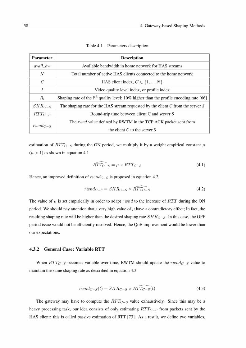
58 4. Gateway-based Shaping Methods
Table 4.1 – Parameters description
Parameter Description
avail_bw Available bandwidth in home network for HAS streams
N Total number of active HAS clients connected to the home network
C HAS client index, C ∈ {1, ..., N}
l Video quality level index, or profile index
Rl Shaping rate of the lth quality level; 10% higher than the profile encoding rate [66]
SHRC−S The shaping rate for the HAS stream requested by the client C from the server S
RTTC−S Round-trip time between client C and server S
rwndC−SThe rwnd value defined by RWTM in the TCP ACK packet sent from
the client C to the server S
estimation of RTTC−S during the ON period, we multiply it by a weight empirical constant µ
(µ > 1) as shown in equation 4.1
RTTC−S = µ×RTTC−S (4.1)
Hence, an improved definition of rwndC−S is proposed in equation 4.2
rwndC−S = SHRC−S × RTTC−S (4.2)
The value of µ is set empirically in order to adapt rwnd to the increase of RTT during the ON
period. We should pay attention that a very high value of µ have a contradictory effect; In fact, the
resulting shaping rate will be higher than the desired shaping rate SHRC−S . In this case, the OFF
period issue would not be efficiently resolved. Hence, the QoE improvement would be lower than
our expectations.
4.3.2 General Case: Variable RTT
When RTTC−S becomes variable over time, RWTM should update the rwndC−S value to
maintain the same shaping rate as described in equation 4.3
rwndC−S(t) = SHRC−S × RTTC−S(t) (4.3)
The gateway may have to compute the RTTC−S value exhaustively. Since this may be a
heavy processing task, our idea consists of only estimating RTTC−S from packets sent by the
HAS client: this is called passive estimation of RTT [73]. As a result, we define two variables,
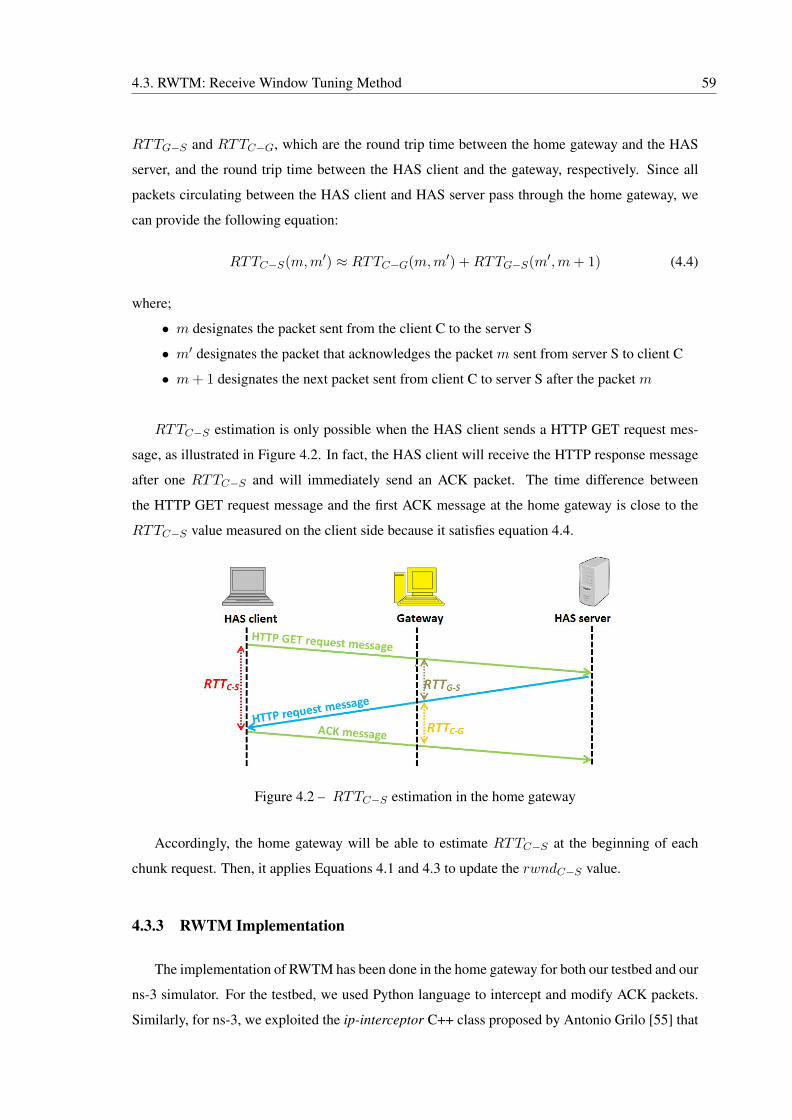
4.3. RWTM: Receive Window Tuning Method 59
RTTG−S and RTTC−G, which are the round trip time between the home gateway and the HAS
server, and the round trip time between the HAS client and the gateway, respectively. Since all
packets circulating between the HAS client and HAS server pass through the home gateway, we
can provide the following equation:
RTTC−S(m,m′) ≈ RTTC−G(m,m′) +RTTG−S(m
′,m+ 1) (4.4)
where;
• m designates the packet sent from the client C to the server S
• m′ designates the packet that acknowledges the packet m sent from server S to client C
• m+ 1 designates the next packet sent from client C to server S after the packet m
RTTC−S estimation is only possible when the HAS client sends a HTTP GET request mes-
sage, as illustrated in Figure 4.2. In fact, the HAS client will receive the HTTP response message
after one RTTC−S and will immediately send an ACK packet. The time difference between
the HTTP GET request message and the first ACK message at the home gateway is close to the
RTTC−S value measured on the client side because it satisfies equation 4.4.
Figure 4.2 – RTTC−S estimation in the home gateway
Accordingly, the home gateway will be able to estimate RTTC−S at the beginning of each
chunk request. Then, it applies Equations 4.1 and 4.3 to update the rwndC−S value.
4.3.3 RWTM Implementation
The implementation of RWTM has been done in the home gateway for both our testbed and our
ns-3 simulator. For the testbed, we used Python language to intercept and modify ACK packets.
Similarly, for ns-3, we exploited the ip-interceptor C++ class proposed by Antonio Grilo [55] that
60 4. Gateway-based Shaping Methods
enables the interception of packets that pass through one simulation node. Then, we modified the
ip-interceptor class to enable the modification of rwnd of each intercepted ACK packet sent from
each HAS client to its corresponding HAS server.
Concerning the classification of HAS flows, that is mandatory for bandwidth manager, we
used the two known IP source addresses of the two competing HAS clients in the testbed, while
we used the HAS flow id, f, in our ns-3 implementation, as described in Subsection 3.4.2. The
bandwidth manager defines the shaping rate SHRC−S that should be assigned for each HAS flow.
Concerning the RTT estimation, we used the passive estimation for both implementations as
described in Subsection 4.3.2.
4.4 Evaluation of Gateway-based Shaping Methods
The objective of this section is to compare between the two gateway-based shaping methods,
HTBM and RWTM, by using a same well-chosen bandwidth manager that is supposed to define the
optimal quality level for each HAS client [12]. For this purpose, we define our proposed bandwidth
manager algorithm in Subsection 4.4.1. Then we define three different scenarios of HAS client
competition in Subsection 4.4.2. Finally, we give our analysis of the results in Subsection 4.4.3.
We notice that in this section we use the developed testbed in conformity with its description in
Section 3.3 and we employ the emulated HAS player as described in Section 3.2
4.4.1 Proposed Bandwidth Manager Algorithm
The bandwidth manager is the fundamental component of the gateway-based solution. It uses
as inputs three parameters: the home available bandwidth avail_bw, the number of competing
HAS clients N, and the index file of each HAS stream that defines the encoding rates of each
quality level for each stream. Then, it computes the shaping rate for each HAS client as indicated
in Equation 4.5:
SHRC−S =
max(Rl)
Rl 6 C
N× avail_bw −
C−1∑j=1
SHRj−S
(4.5)
SHRC−S is chosen in a manner that enables the players to select optimal quality lev-
els by ensuring both the fairest share of avail_bw between HAS clients and the maximum
use of avail_bw. This choice necessitates that if the fair share of avail_bw according to{max(Rl)
Rl 6 avail_bwN
}involves avail_bw underutilization, and if the unused portion of
4.4. Evaluation of Gateway-based Shaping Methods 61
avail_bw enables one or more HAS clients to switch to a higher quality level, the bandwidth man-
ager will allow it. In other words, the shaping rate is chosen in a manner that it ensures the fairest
share of the available home bandwidth between clients with prioritization to achieve the maximum
use of the available home bandwidth. This entails that some clients could have a higher quality
level than others when their fair share of available home bandwidth is not sufficient to maximize
the use of the available home bandwidth.
The bandwidth manager is sufficiently sophisticated to be able to update the number of active
connected HAS clients to the home gateway, N, by sniffing the SYN and FIN flags in the header of
TCP packets. We also assume that it is capable of estimating the avail_bw and updating its value
over time. Accordingly, the manager updates the shaping rate when any change occurs. In order
to facilitate our implementation, the avail_bw of the configuration (of both testbed and ns-3) is
directly used as input by the bandwidth manager.
4.4.2 Scenarios
We define three scenarios that are typical to concurrence between HAS clients in a same home
network. We have chosen the duration of each test Z = 180 seconds. This duration resolves the
tradeoff between having sufficient long duration to have a significant number of measurements
(about 100 chunks are exchanged) and a not too long duration (to reduce the duration of the
simulation runs and the experimental executions):
1. Both clients start to play simultaneously and continue for Z seconds. This scenario illus-
trates how HAS clients compete.
2. Client 1 starts to play, the second client starts after 30 seconds, and both continue together
for Z − 30 seconds. This scenario shows how transition from one client to two clients
occurs.
3. Both clients start to play simultaneously, client 2 stops after 30 seconds, and client 1 con-
tinues alone for Z − 30 seconds. This scenario shows how a transition from two clients to
one takes place.
We note that we have chosen 30 seconds as the transitory duration before the change of the number
of competing HAS clients for scenarios 2 and 3. Our justification of this value is that the clients
reach a more stable state within around 30 seconds when employing a gateway-based shaping
method, HTBM or RWTM, as it will be described below in Subsection 4.4.3.1.
62 4. Gateway-based Shaping Methods
4.4.3 Analysis of The Results
In this section, we discuss the QoE measurements of the two shaping methods RWTM and
HTBM during the three scenarios, and we provide accurate explanations of the observed results
by showing the congestion window variation. The two compared methods shape bandwidth in the
gateway in accordance with the bandwidth manager’s decisions, as described in Subsection 4.4.1.
The shaping rate for each client is chosen as indicated in [66], Table 4.1 and Subsection 4.4.1; it is
10% higher than the encoding rate of the optimal quality level for each client. The weight constant
µ of equation 4.1 employed by RWTM is chosen empirically and is equal to µ = 1.275. We justify
this value by several experimental tests that measure the increase of RTT during the ON period:
we found that multiplying the first measured RTT of ON period by 1.275 is approximatively equal
to the mean value of RTT during the whole ON period.
4.4.3.1 QoE Evaluation
For each scenario, we repeat each test 60 times, and we employ the average value of QoE
metrics in our evaluation. The number of 60 runs is justified by the fact that the difference of the
average results obtained after 40 runs and 60 runs is lower than 6%. This observation is verified
for all scenarios. Accordingly, using 60 tests is sufficient to yield statistically significant results.
The average values of metrics are listed in Table 4.2. We note that convergence speed metric is
computed for scenarios 2 and 3 from 30 seconds instead of the beginning of the test. We justify this
choice by our objective of measuring the convergence speed just after the change of the number
of competing HAS clients, i.e. from the second 30. We also notice that for scenario 2 and 3 we
present the performance measurements only for client 1. In fact, the client 2 is just designed for
studying the effect of its presence and absence on the performances of client 1. In this table, we
denote by W/o the case that we does not use traffic shaping.
The overall evaluation indicates that the two gateway-based shaping methods improve QoE
(instability, infidelity and convergence speed) compared with W/o. This overall result confirms
the importance of employing a gateway-based shaping method for improving the QoE of the com-
peting HAS clients. In the following, we give our observations taken from Table 4.2 classified by
scenarios:
— For the first scenario, the simultaneous playing of two HAS clients involves better
QoE measurements for client 2 than for client 1. This behavior is expected because
the bandwidth manager assigns lower optimal quality level (n◦ 3) for client 2 than for
client 1 (n◦ 4). Obviously, the quality level n◦ 3 is easier to achieve than that of n◦ 4.
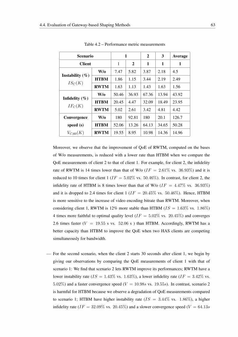
4.4. Evaluation of Gateway-based Shaping Methods 63
Table 4.2 – Performance metric measurements
Scenario 1 2 3 Average
Client 1 2 1 1 1
Instability (%)
ISC(K)
W/o 7.47 5.82 3.87 2.18 4.5
HTBM 1.86 1.15 3.44 2.19 2.49
RWTM 1.63 1.13 1.43 1.63 1.56
Infidelity (%)
IFC(K)
W/o 50.46 36.93 67.36 13.94 43.92
HTBM 20.45 4.47 32.09 18.49 23.95
RWTM 5.02 2.61 3.42 4.81 4.42
Convergence
speed (s)
VC,60(K)
W/o 180 92.81 180 20.1 126.7
HTBM 52.06 13.26 64.13 34.65 50.28
RWTM 19.55 8.95 10.98 14.36 14.96
Moreover, we observe that the improvement of QoE of RWTM, computed on the bases
of W/o measurements, is reduced with a lower rate than HTBM when we compare the
QoE measurements of client 2 to that of client 1. For example, for client 2, the infidelity
rate of RWTM is 14 times lower than that of W/o (IF = 2.61% vs. 36.93%) and it is
reduced to 10 times for client 1 (IF = 5.02% vs. 50.46%). In contrast, for client 2, the
infidelity rate of HTBM is 8 times lower than that of W/o (IF = 4.47% vs. 36.93%)
and it is dropped to 2.4 times for client 1 (IF = 20.45% vs. 50.46%). Hence, HTBM
is more sensitive to the increase of video encoding bitrate than RWTM. Moreover, when
considering client 1, RWTM is 12% more stable than HTBM (IS = 1.63% vs. 1.86%)
4 times more faithful to optimal quality level (IF = 5.02% vs. 20.45%) and converges
2.6 times faster (V = 19.55 s vs. 52.06 s ) than HTBM. Accordingly, RWTM has a
better capacity than HTBM to improve the QoE when two HAS clients are competing
simultaneously for bandwidth.
— For the second scenario, when the client 2 starts 30 seconds after client 1, we begin by
giving our observations by comparing the QoE measurements of client 1 with that of
scenario 1: We find that scenario 2 lets RWTM improve its performances; RWTM have a
lower instability rate (IS = 1.43% vs. 1.63%), a lower infidelity rate (IF = 3.42% vs.
5.02%) and a faster convergence speed (V = 10.98s vs. 19.55s). In contrast, scenario 2
is harmful for HTBM because we observe a degradation of QoE measurements compared
to scenario 1; HTBM have higher instability rate (IS = 3.44% vs. 1.86%), a higher
infidelity rate (IF = 32.09% vs. 20.45%) and a slower convergence speed (V = 64.13s
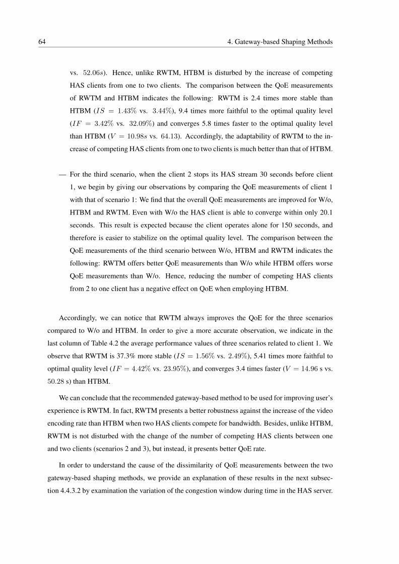
64 4. Gateway-based Shaping Methods
vs. 52.06s). Hence, unlike RWTM, HTBM is disturbed by the increase of competing
HAS clients from one to two clients. The comparison between the QoE measurements
of RWTM and HTBM indicates the following: RWTM is 2.4 times more stable than
HTBM (IS = 1.43% vs. 3.44%), 9.4 times more faithful to the optimal quality level
(IF = 3.42% vs. 32.09%) and converges 5.8 times faster to the optimal quality level
than HTBM (V = 10.98s vs. 64.13). Accordingly, the adaptability of RWTM to the in-
crease of competing HAS clients from one to two clients is much better than that of HTBM.
— For the third scenario, when the client 2 stops its HAS stream 30 seconds before client
1, we begin by giving our observations by comparing the QoE measurements of client 1
with that of scenario 1: We find that the overall QoE measurements are improved for W/o,
HTBM and RWTM. Even with W/o the HAS client is able to converge within only 20.1
seconds. This result is expected because the client operates alone for 150 seconds, and
therefore is easier to stabilize on the optimal quality level. The comparison between the
QoE measurements of the third scenario between W/o, HTBM and RWTM indicates the
following: RWTM offers better QoE measurements than W/o while HTBM offers worse
QoE measurements than W/o. Hence, reducing the number of competing HAS clients
from 2 to one client has a negative effect on QoE when employing HTBM.
Accordingly, we can notice that RWTM always improves the QoE for the three scenarios
compared to W/o and HTBM. In order to give a more accurate observation, we indicate in the
last column of Table 4.2 the average performance values of three scenarios related to client 1. We
observe that RWTM is 37.3% more stable (IS = 1.56% vs. 2.49%), 5.41 times more faithful to
optimal quality level (IF = 4.42% vs. 23.95%), and converges 3.4 times faster (V = 14.96 s vs.
50.28 s) than HTBM.
We can conclude that the recommended gateway-based method to be used for improving user’s
experience is RWTM. In fact, RWTM presents a better robustness against the increase of the video
encoding rate than HTBM when two HAS clients compete for bandwidth. Besides, unlike HTBM,
RWTM is not disturbed with the change of the number of competing HAS clients between one
and two clients (scenarios 2 and 3), but instead, it presents better QoE rate.
In order to understand the cause of the dissimilarity of QoE measurements between the two
gateway-based shaping methods, we provide an explanation of these results in the next subsec-
tion 4.4.3.2 by examination the variation of the congestion window during time in the HAS server.
4.4. Evaluation of Gateway-based Shaping Methods 65
4.4.3.2 Congestion Window Variation
In order to explain the cause of these results, we used the tcp_probe module in the HAS
server. This module shows the evolution of the congestion window, cwnd, and slow start threshold,
ssthresh, during each test. We select two tests that have the nearest QoE measurements of the
first column of Table 4.2 related to HTBM and RWTM, respectively. We present the cwnd and
ssthresh variation of the two tests in Figure 4.3 and 4.4. In the two figures, we indicate by a
vertical bold dotted line the moment of convergence. We observe that this moment coincides with
a considerably higher stability of ssthresh and higher stability of cwnd in the congestion avoidance
phase.
In order to be accurate in our analysis, based on the Cubic [57] congestion control algorithm
used in the server and its source code tcp_cubic.c, we present some important value updates of
cwnd and ssthresh for different events:
— Congestion event - we have two cases:
• When three duplicated ACKs are received, the Fast Recovery / Fast Retransmit
(FR/FR) phase reduces ssthresh by a multiplicative decrease factor and sets cwnd to
ssthresh+3. Hence, cwnd remains in congestion avoidance phase.
• When the retransmission timeout expires before receiving ACK of the supposed lost
packet, ssthresh is reduced by a multiplicative decrease factor, and cwnd is set to a
small value and restarts from slow start phase.
— Idle period: When the server sends a packet after an idle period that exceeds retrans-
mission timeout (RTO), ssthresh is set to max(ssthresh,3
4cwnd), and the cwnd value is
computed as in Algorithm 1:
Algorithm 1 cwnd update after an idle period
1: for i = 1 to int(idle
RTO) do
2: cwnd = max(min(cwnd, rwnd)
2, 1MSS)
. Where MSS is the maximum TCP segment size.
In the context of HAS, an idle period coincides with an OFF period between two
consecutive chunks. We denote by OFF the OFF period whose duration exceeds RTO.
After convergence, with HTBM we have a high congestion rate: as presented in Figure 4.3, the
majority of congestions is caused by retransmission timeout. In contrast, with RWTM, congestion
events are negligible: only two visible congestions occur in Figure 4.4. As a consequence, ssthresh
becomes lower when using HTBM than when using RWTM: 75 MSS in Figure 4.3 vs. 110 MSS
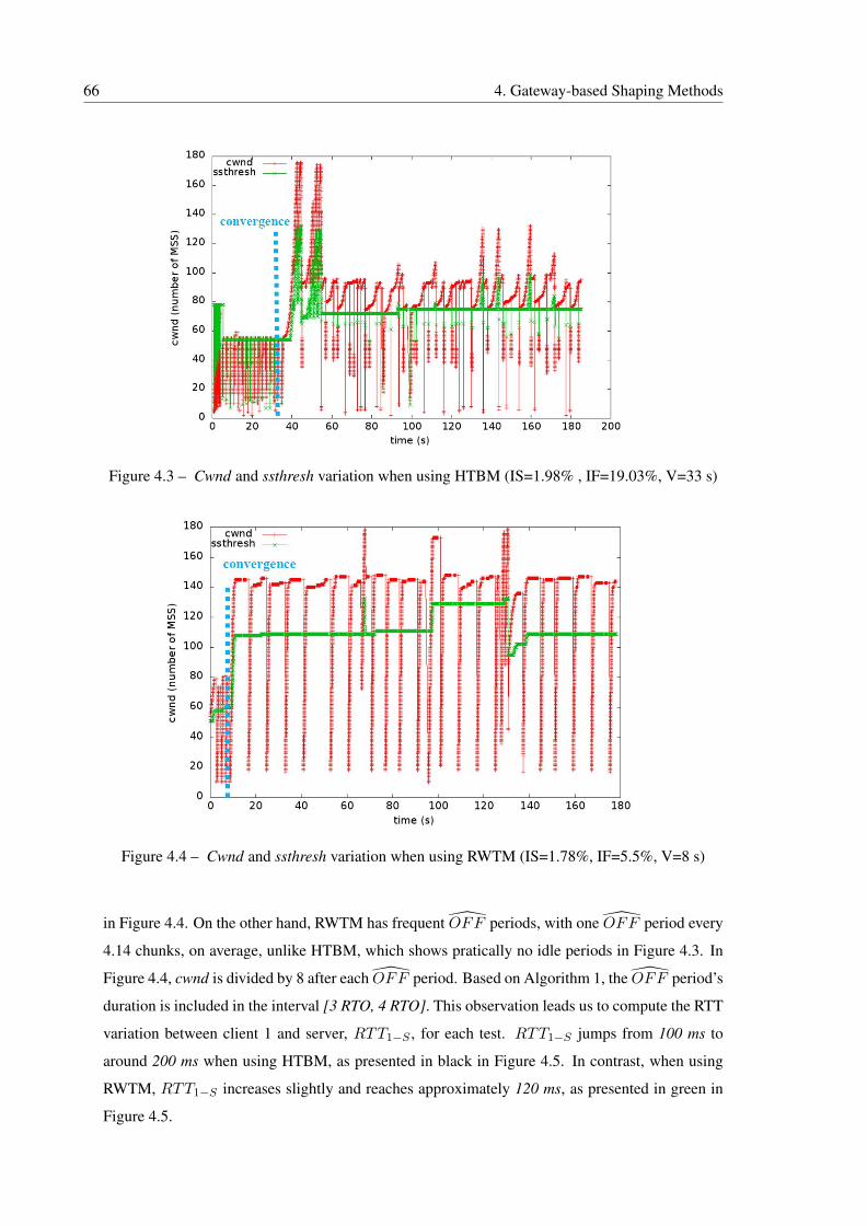
66 4. Gateway-based Shaping Methods
Figure 4.3 – Cwnd and ssthresh variation when using HTBM (IS=1.98% , IF=19.03%, V=33 s)
Figure 4.4 – Cwnd and ssthresh variation when using RWTM (IS=1.78%, IF=5.5%, V=8 s)
in Figure 4.4. On the other hand, RWTM has frequent OFF periods, with one OFF period every
4.14 chunks, on average, unlike HTBM, which shows pratically no idle periods in Figure 4.3. In
Figure 4.4, cwnd is divided by 8 after each OFF period. Based on Algorithm 1, the OFF period’s
duration is included in the interval [3 RTO, 4 RTO]. This observation leads us to compute the RTT
variation between client 1 and server, RTT1−S , for each test. RTT1−S jumps from 100 ms to
around 200 ms when using HTBM, as presented in black in Figure 4.5. In contrast, when using
RWTM, RTT1−S increases slightly and reaches approximately 120 ms, as presented in green in
Figure 4.5.
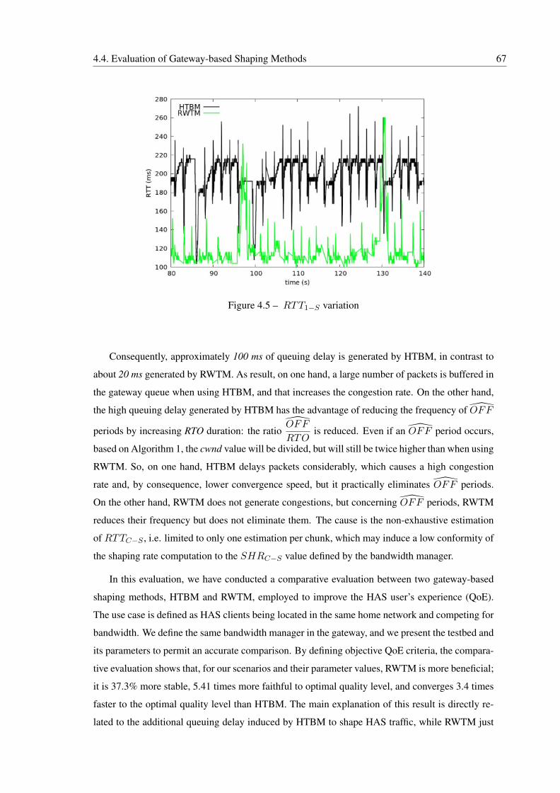
4.4. Evaluation of Gateway-based Shaping Methods 67
Figure 4.5 – RTT1−S variation
Consequently, approximately 100 ms of queuing delay is generated by HTBM, in contrast to
about 20 ms generated by RWTM. As result, on one hand, a large number of packets is buffered in
the gateway queue when using HTBM, and that increases the congestion rate. On the other hand,
the high queuing delay generated by HTBM has the advantage of reducing the frequency of OFF
periods by increasing RTO duration: the ratioOFF
RTOis reduced. Even if an OFF period occurs,
based on Algorithm 1, the cwnd value will be divided, but will still be twice higher than when using
RWTM. So, on one hand, HTBM delays packets considerably, which causes a high congestion
rate and, by consequence, lower convergence speed, but it practically eliminates OFF periods.
On the other hand, RWTM does not generate congestions, but concerning OFF periods, RWTM
reduces their frequency but does not eliminate them. The cause is the non-exhaustive estimation
of RTTC−S , i.e. limited to only one estimation per chunk, which may induce a low conformity of
the shaping rate computation to the SHRC−S value defined by the bandwidth manager.
In this evaluation, we have conducted a comparative evaluation between two gateway-based
shaping methods, HTBM and RWTM, employed to improve the HAS user’s experience (QoE).
The use case is defined as HAS clients being located in the same home network and competing for
bandwidth. We define the same bandwidth manager in the gateway, and we present the testbed and
its parameters to permit an accurate comparison. By defining objective QoE criteria, the compara-
tive evaluation shows that, for our scenarios and their parameter values, RWTM is more beneficial;
it is 37.3% more stable, 5.41 times more faithful to optimal quality level, and converges 3.4 times
faster to the optimal quality level than HTBM. The main explanation of this result is directly re-
lated to the additional queuing delay induced by HTBM to shape HAS traffic, while RWTM just
68 4. Gateway-based Shaping Methods
reduces the advertised window of HAS clients and thus does not add significant queueing delay.
4.5 Extended Evaluation of RWTM
In this section we evaluate RWTM under more different conditions using the ns-3 simulator. To
perform this evaluation, we use our implementation in ns-3 as described in Section 3.4 and RWTM
implementation as shown in Subsection 4.3.3. We also employ several QoE and QoS metrics in
conformity to their definition in Section 3.5. The competing players are playing simultaneously
during 180 seconds. All results are compared to the case without shaping, denoted by W/o.
Nevertheless, in order to be more accurate in our evaluation, we should test many runs for the
same scenario and compute the average value of performance metric measurements. However, we
should select a credible run number in order to resolve the following dilemma; giving an expressive
evaluation that presents a more general case with the minimum possible number of runs. In order
to define the number of runs that should be used for our evaluation, we use the method of the
relative difference between the mean values of criteria measurements. Let n1 and n2 two different
numbers of runs (n1 < n2), Mn1 and Mn2 the mean values, related to one criterion measurement,
among n1 and n2 runs, respectively. The relative difference between these two mean values,
denoted by Relative_Diff(n1, n2), is obtained as shown in Equation 4.6:
Relative_Diff(n1, n2) =|Mn1 −Mn2|
Mn1(4.6)
Concretely, we selected four run numbers which are power of 4: i.e 4, 16, 64 and 256. Then,
we compute Relative_Diff(n1, n2) of each two consecutive run numbers for three different
QoE criteria: instability IS, infidelity IF and convergence speed V. We note that we select only
these criteria because they are the most determinative QoE criteria for our evaluation. Then, we
select the number of run n1 when Relative_Diff(n1, n2) is lower than a threshold of 4%.
For example, when considering the scenario of two HAS clients competing for bandwidth, the
computation of Relative_Diff(n1, n2) related to W/o and RWTM are shown in Tables 4.3 and
4.4, respectively.
The two tables indicate that when increasing the number of runs from 16 to 64 runs, the relative
difference related to three QoE criteria among 16 and 64 runs is less than 4% for both W/o and
RWTM. Accordingly, it is not necessary to increase the number of runs above 16 runs. Hence,
employing 16 runs is sufficient to have a meaningful evaluation of the performances.
The remaining of this section is organized as the following: First, we evaluate the effect of in-
4.5. Extended Evaluation of RWTM 69
Table 4.3 – The relative differences of QoE mean values related to W/o
n1-n2QoE
criterion 4-16 16-64 64-256
IS 3.64 3.84 0.63
IF 7.25 0.46 0.01Relative_Diff(n1,n2) (%)
V 8.39 3.29 0.53
Table 4.4 – The relative differences of QoE mean values related to RWTM
n1-n2QoE
criterion 4-16 16-64 64-256
IS 0.01 0.01 0
IF 0.22 0.07 0Relative_Diff(n1,n2)(%)
V 0.26 0.39 2.56
creasing the number of HAS flows on the performances of RWTM in Subsection 4.5.1. Second, we
evaluate the RWTM performances when changing the HAS player parameters in Subsection 4.5.2.
Third, we study the effect of changing network conditions on RWTM performances in Subsec-
tion 4.5.3.
4.5.1 Effect of Increasing the Number of HAS Flows
In the literature, many authors reveal that increasing the number of HAS flows degrades the
QoE. For example, [131, 80] indicate that with a rising number of competing clients the unfairness
increases.
In this subsection we evaluate the robustness of RWTM against the increase of competing HAS
clients in the same home network. We vary the number of competing players from one to 9 clients.
We select 9 as the maximum number of competing HAS clients, because, in practice, the number
of users inside the home network does not exceed 9 users. The mean performance measurements
between competing players are presented in Figure 4.6. In this figure the performance unfairness
measurements between HAS clients are indicated with vertical error bars.
Concerning the QoE measurements, we observe that RWTM provides a good QoE rate and
keeps practically the same measurements independently with the number of competing HAS
clients. In fact, we observe in Figure 4.6a that the instability of RWTM is kept lower than 3%
with a negligible instability fairness between clients, while the instability of W/o is comprised be-
70 4. Gateway-based Shaping Methods
tween 5% and 13% and seems to increase when increasing the number of competing clients. The
infidelity rate of RWTM is maintained around 14% with a negligible infidelity unfairness rate as
presented in Figure 4.6b, while W/o presents a higher infidelity rate that exceeds 60% when the
number of competing HAS clients is higher than 6. In addition, Figure 4.6c shows that all HAS
clients rapidly converge to the optimal quality level within only 10∼15 seconds, in contrast to W/o
where the clients become unable to converge when the number of competing clients exceeds 5.
In addition, the initial delay of both RWTM and W/o is increased when the number of com-
peting HAS clients increases as shown in Figure 4.6d. This result is predictable. In fact, during
the buffering phase the HAS player asks for chunks successively. Consequently, when the number
of competing HAS clients increases, the bandwidth would be shared between instable HAS flows,
hence and additional delay is generated. We also remark that RWTM presents a slight lower initial
delay than W/o when the number of competing HAS clients exceeds 4 clients. The main cause is
that, during buffering state, when many unshaped HAS flows are competing for bandwidth they
are more aggressive than RWTM and cause many congestion events; as shown in Figure 4.6g,
the congestion rate is increasing from 4 competing HAS clients. Consequently, the HAS sending
rate would be obviously reduced because of these congestions. Hence, the initial delay of W/o is
slightly lower than that of RWTM. We note that the initial delay with 9 HAS competing clients
is around 9 seconds, which is lower than 16 seconds and does not disturb the QoE of users, as
described in Subsection 2.4.1.2. Moreover, RWTM generates no stalling event, as shown in Fig-
ure 4.6i, while W/o begins to cause stalling events with ascending rate from 7 competing clients.
This result is a direct consequence of the high stability rate, generated by the bandwidth man-
ager and the traffic shaping method of RWTM, that is well preserved even with a high number of
competing HAS clients.
Concerning QoS measurements, we observe a decrease of OFF period frequency, frOFF
,
for both W/o and RWTM in Figure 4.6e. Although frOFF
of RWTM is higher than that of W/o,
when increasing the number of competing clients, the frOFF
decreases and becomes close to W/o
(around 0.05 when the number of HAS clients is equal to 9). This decrease is beneficial to RWTM
because one of the objectives of shaping is to reduce the duration of OFF periods, and it results in
saving good QoE measurements as described above. In addition, we observe in Figure 4.6f that
the queuing delay increases proportionally with the number of HAS clients. Besides, the average
queuing delay is at least twice lower with RWTM than with W/o: for example when 6 HAS clients
are competing for bandwidth, the queuing delay of RWTM is equal to 30 ms while that of W/o
is equal to 62 ms. The obvious explanation is the efficiency of RWTM, in terms of bandwidth
management and traffic shaping, that avoids the aggressive competition between HAS flows and
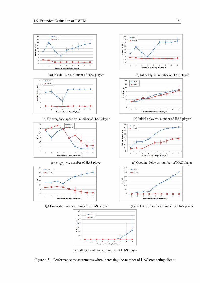
4.5. Extended Evaluation of RWTM 71
(a) Instability vs. number of HAS player (b) Infidelity vs. number of HAS player
(c) Convergence speed vs. number of HAS player (d) Initial delay vs. number of HAS player
(e) frOFF
vs. number of HAS player (f) Queuing delay vs. number of HAS player
(g) Congestion rate vs. number of HAS player (h) packet drop rate vs. number of HAS player
(i) Stalling event rate vs. number of HAS player
Figure 4.6 – Performance measurements when increasing the number of HAS competing clients
72 4. Gateway-based Shaping Methods
reduces the over-estimations of bandwidth which are responsible of the saturation of the bot-
tleneck queue. For the same reason, the congestion detection rate of RWTM on the server side is
reduced as indicated in Figure 4.6g and the packet drop rate at the bottleneck is still null as shown
in Figure 4.6h. In contrast, W/o highly increases the congestion detection rate and the packet drop
rate at the bottleneck.
To summarize, RWTM is not disturbed by the increase of the competing HAS clients in the
same home network in terms of access network QoS and HAS QoE. For QoE measurments, unlike
W/o, RWTM preserves a high instability, high fidelity and a rapid convergence speed, reduces
slightly the initial delay and does not generates stalling events. For QoS measurements, RWTM
reduces the queuing delay to less than the half, reduces the congestion detection rate and practically
does not cause packet drop at the bottleneck. However, the frequency of OFF periods is higher
than that of W/o. The cause of this high value is the low frequency of RTT estimations of RWTM,
which are done only one time per chunk.
4.5.2 Effect of Variation of Player Parameters
In this subsection, we study the effect of player parameters on RWTM shaping method per-
formances. For this purpose, we select two main important parameters: the player buffer size and
the chunk duration. The chosen scenario is when two HAS players are competing for bandwidth
simultaneously during 180 seconds.
4.5.2.1 Playback Buffer Size effect
Knowing that Live and VoD streaming services differ by the length of playback buffer as
explained in Subsection 2.2.2.3, studying of the effect of playback buffer length on RWTM per-
formances is equivalent to study the behavior of RWTM in Live and VoD video streaming.
In Figure 4.7 we show performance metric measurements of RWTM and W/o for different
lengths of playback buffer ranging from 6 to 30 seconds. We remember that the common value
of buffer length for Live streaming service is around 8 seconds and that for VOD around is 30
seconds as indicated in Subsection 2.2.2.3.
Considering the QoE measurements, RWTM outperforms W/o in three QoE criteria, insta-
bility, infidelity and convergence speed, for all playback buffer lengths: For instability rate, it
decreases with RWTM from 4% to 2% when increasing the playback buffer length from 6 to 30
seconds as presented in Figure 4.7a, while it is around 14% with W/o. Here we can say that RWTM
offers a more stable quality level with a longer playback buffer. In addition, when the playback
4.5. Extended Evaluation of RWTM 73
buffer is higher than 10 seconds, we observe the following: the infidelity rate of RWTM is main-
tained at a low value less than 14% while it is higher than 50% with W/o and the convergence
speed of RWTM is maintained at around 13 seconds while it is higher than 160 seconds with W/o,
as presented in Figures 4.7b and 4.7c, respectively. However, for a 6-second length buffer, we
observe a degradation in infidelity and convergence speed and a high unfairness between clients
for these criteria with RWTM. The cause of that is also related to the bitrate controller and the ag-
gressiveness employed in the formula 3.1: when the playback buffer is shorter, the loss of player
aggressiveness becomes faster. For example, one missing chunk (whose duration is 2 seconds) in
the 6-second length buffer results in decreasing the player aggressiveness by 1/3 which is five time
higher than with a 30-second length buffer. When a such player has its own bandwidth shaped
by RWTM that corresponds to a highest quality level which is difficult to achieve with a low ag-
gressiveness, the "downward spiral effect" described in Section 3.2 would take place. Moreover,
we observe in Figure 4.7d that the initial delay is increased for both W/o and RWTM, which is
expected because the HAS players have to request for more chunks in the buffering state. In ad-
dition, the initial delay of RWTM is slightly higher but it keeps the same ratio with W/o. This
slightly higher initial delay is not disturbing for users’ QoE as indicated in [65] because it is still
far lower than 16 seconds. Moreover, unlike W/o which generates high stalling event rate when
the playback buffer length is lower than 10 seconds, RWTM generates no stalling event for all
playback buffer sizes ranged between 6 and 30 seconds as indicated in Figure 4.7i.
Considering th QoS measurements, we observe in Figure 4.7e that the frequency of OFF pe-
riods is reduced for both RWTM and W/o when increasing the playback buffer length. This result
is predictable because a longer playback buffer results in requesting more chunks successively,
i.e. without any delay between them, during the buffering state phase. Besides, the frequency of
OFF of RWTM is still higher than W/o, which is caused by the non-exhaustive computation of
RTT as explained above in Subsection 4.4.3.2. Moreover, the queuing delay generated by RWTM
is maintained at the same low value, around 9 ms, for different playback buffer lengths while it
is comprised between two high values, 15 ms and 30 ms, with W/o, as shown in Figure 4.7f. In
addition, the congestion detection rate of RWTM is also maintained at a low value as presented in
Figure 4.7g and generates practically no packet drop at the bottleneck as shown in Figure 4.7h. In
contrast, W/o is still aggressive and generates high congestion detection rate and high packet drop
rate.
To summarize, RWTM improves both QoE and QoS for different playback buffer lengths
ranged between 6 and 30 seconds. Hence, we can say that RWTM improves performances for
both Live and VoD streaming services.
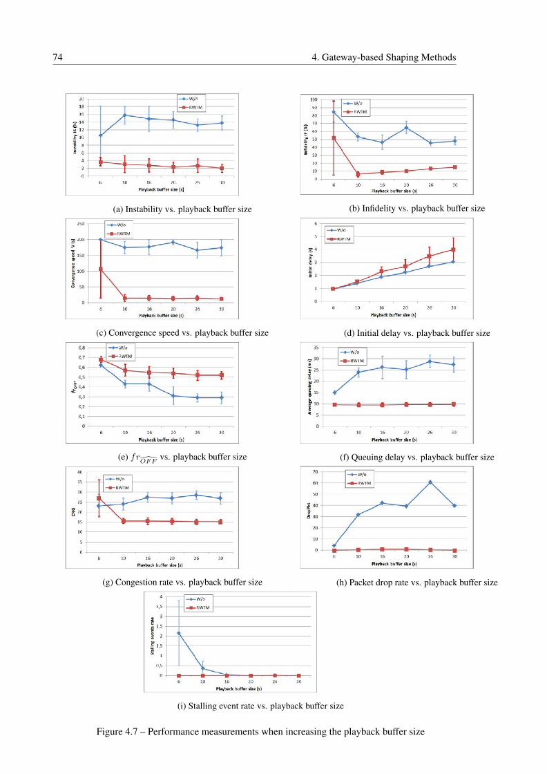
74 4. Gateway-based Shaping Methods
(a) Instability vs. playback buffer size (b) Infidelity vs. playback buffer size
(c) Convergence speed vs. playback buffer size (d) Initial delay vs. playback buffer size
(e) frOFF
vs. playback buffer size (f) Queuing delay vs. playback buffer size
(g) Congestion rate vs. playback buffer size (h) Packet drop rate vs. playback buffer size
(i) Stalling event rate vs. playback buffer size
Figure 4.7 – Performance measurements when increasing the playback buffer size
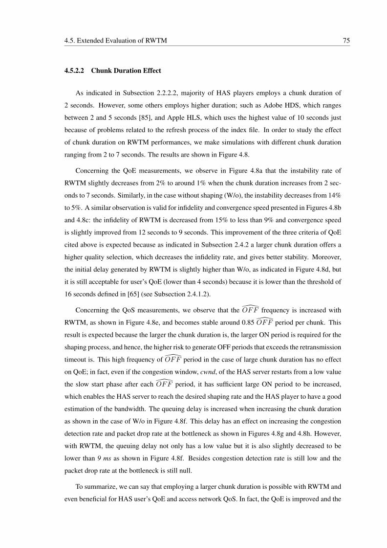
4.5. Extended Evaluation of RWTM 75
4.5.2.2 Chunk Duration Effect
As indicated in Subsection 2.2.2.2, majority of HAS players employs a chunk duration of
2 seconds. However, some others employs higher duration; such as Adobe HDS, which ranges
between 2 and 5 seconds [85], and Apple HLS, which uses the highest value of 10 seconds just
because of problems related to the refresh process of the index file. In order to study the effect
of chunk duration on RWTM performances, we make simulations with different chunk duration
ranging from 2 to 7 seconds. The results are shown in Figure 4.8.
Concerning the QoE measurements, we observe in Figure 4.8a that the instability rate of
RWTM slightly decreases from 2% to around 1% when the chunk duration increases from 2 sec-
onds to 7 seconds. Similarly, in the case without shaping (W/o), the instability decreases from 14%
to 5%. A similar observation is valid for infidelity and convergence speed presented in Figures 4.8b
and 4.8c: the infidelity of RWTM is decreased from 15% to less than 9% and convergence speed
is slightly improved from 12 seconds to 9 seconds. This improvement of the three criteria of QoE
cited above is expected because as indicated in Subsection 2.4.2 a larger chunk duration offers a
higher quality selection, which decreases the infidelity rate, and gives better stability. Moreover,
the initial delay generated by RWTM is slightly higher than W/o, as indicated in Figure 4.8d, but
it is still acceptable for user’s QoE (lower than 4 seconds) because it is lower than the threshold of
16 seconds defined in [65] (see Subsection 2.4.1.2).
Concerning the QoS measurements, we observe that the OFF frequency is increased with
RWTM, as shown in Figure 4.8e, and becomes stable around 0.85 OFF period per chunk. This
result is expected because the larger the chunk duration is, the larger ON period is required for the
shaping process, and hence, the higher risk to generate OFF periods that exceeds the retransmission
timeout is. This high frequency of OFF period in the case of large chunk duration has no effect
on QoE; in fact, even if the congestion window, cwnd, of the HAS server restarts from a low value
the slow start phase after each OFF period, it has sufficient large ON period to be increased,
which enables the HAS server to reach the desired shaping rate and the HAS player to have a good
estimation of the bandwidth. The queuing delay is increased when increasing the chunk duration
as shown in the case of W/o in Figure 4.8f. This delay has an effect on increasing the congestion
detection rate and packet drop rate at the bottleneck as shown in Figures 4.8g and 4.8h. However,
with RWTM, the queuing delay not only has a low value but it is also slightly decreased to be
lower than 9 ms as shown in Figure 4.8f. Besides congestion detection rate is still low and the
packet drop rate at the bottleneck is still null.
To summarize, we can say that employing a larger chunk duration is possible with RWTM and
even beneficial for HAS user’s QoE and access network QoS. In fact, the QoE is improved and the
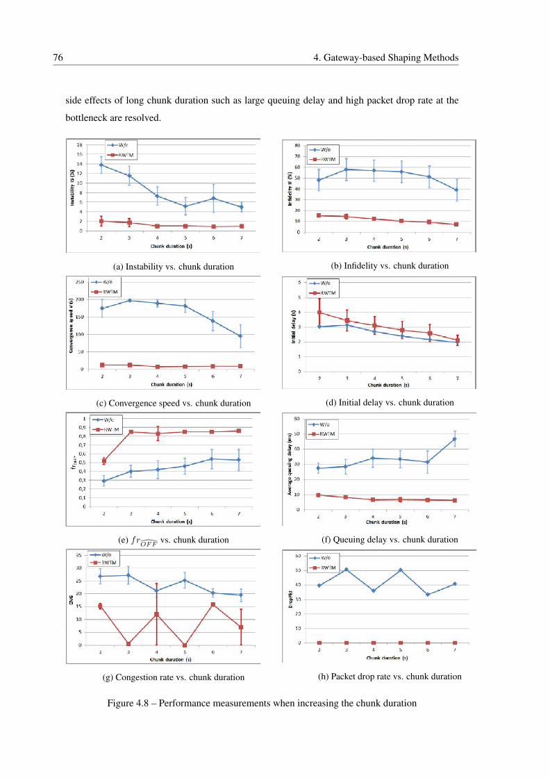
76 4. Gateway-based Shaping Methods
side effects of long chunk duration such as large queuing delay and high packet drop rate at the
bottleneck are resolved.
(a) Instability vs. chunk duration (b) Infidelity vs. chunk duration
(c) Convergence speed vs. chunk duration (d) Initial delay vs. chunk duration
(e) frOFF
vs. chunk duration (f) Queuing delay vs. chunk duration
(g) Congestion rate vs. chunk duration (h) Packet drop rate vs. chunk duration
Figure 4.8 – Performance measurements when increasing the chunk duration
4.5. Extended Evaluation of RWTM 77
4.5.3 Effect of Variation of Network Parameters
Network conditions have a direct implication on the HAS performances because they are re-
sponsible on changing the behavior of HAS players as overviewed in Subsection 2.4.2. For that,
we study the effect of varying the round-trip propagation delay and the arrival rate of IP traffic on
RWTM performances in Subsections 4.5.3.1 and 4.5.3.2, respectively.
4.5.3.1 Initial round-trip propagation delay Effect
In this subsection we study the effect of the initial round-trip propagation delay RTT 0C−S
on HAS performances when using RWTM shaping method. For this purpose, we show two use
cases: when two HAS flows have the same RTT 0C−S and when two HAS flows have different
RTT 0C−S . Here we notice that the queue length of the bottleneck (DSLLine in Figure 3.2) is set
to the bandwidth delay product value when changing RTT 0C−S for each simulation.
1. Same RTT 0C−S for HAS flows
We vary the initial round-trip propagation delay for both HAS clients from 25 ms to 200
ms. The performance measurements are shown in Figure 4.9.
Concerning the QoE measurements, we observe that RWTM presents better QoE than W/o
only when RTT 0C−S is lower than 150 ms; as presented in Figure 4.9a, the instability rate
of RWTM is lower than that of W/o but it increases from 1% to 10% when the RTT 0C−S
increases from 25 ms to 125 ms. We also remark that the instability rate of W/o is very
important for lowRTT 0C−S values (e.g. IS=16% whenRTT 0
C−S = 25ms). When exceed-
ing 150 ms, both W/o and RWTM offer similar instability rates. Moreover, as presented
in Figure 4.9b, the infidelity rate of RWTM is around 15% when RTT 0C−S is lower than
100 ms. But this rate increases and becomes close to that of W/o when RTT 0C−S is higher
than 150 ms. Similarly, as presented in Figure 4.9c, RWTM converges rapidly to the opti-
mal quality level within around 5 seconds when RTT 0C−S is equal to 25 ms and increases
slowly to around 12 seconds for an RTT 0C−S of 100 ms. However, it increases suddenly
from RTT 0C−S of 125 ms and is set practically on the same range of values of that of W/o
when exceeding 150 ms. In addition, we observe in Figure 4.9d that the initial delay of
RWTM is slightly lower than that of W/o for low RTT 0C−S values, lower than 100 ms, but
becomes higher for high RTT 0C−S values. We also remark that the initial delay increases
when increasing RTT 0C−S , which is obvious because higher round trip delay slows down
the delivery of chunks during the buffering state phase. The explanation of the above
results is given when examining the QoS measurements.
78 4. Gateway-based Shaping Methods
(a) Instability vs. RTT 0C−S (b) Infidelity vs. RTT 0
C−S
(c) Convergence speed vs. RTT 0C−S (d) Initial delay vs. RTT 0
C−S
(e) frOFF
vs. RTT 0C−S (f) Queuing delay vs. RTT 0
C−S
(g) Congestion rate vs. RTT 0C−S (h) Packet drop rate vs. RTT 0
C−S
Figure 4.9 – Performance measurements when changing RTT 0C−S value
Concerning the QoS measurements, on the one hand, we observe in Figure 4.9f that
W/o causes high queuing delay when RTT 0C−S is lower than 150 ms; for example, it
generates a queuing delay of 60% of RTT 0C−S when RTT 0
C−S is equal to 25 ms. In

4.5. Extended Evaluation of RWTM 79
addition, W/o generates high congestion detection rate and high packet drop rate for
low RTT 0C−S values, as shown in Figures 4.9g and 4.9h, respectively. The main cause
is that for low RTT 0C−S values, the server becomes more aggressive because its TCP
congestion window, cwnd, increases rapidly. Hence, the HAS sending rates offered by
HAS servers exceed the capacity of the home network and the length of the bottleneck
queue. Hence a high queuing delay, high congestion detection and high packet drop rate
are detected. In contrast, when employing RWTM, its traffic shaping that limits the server
sending rate by modifying the receive window, rwnd, prevents the server to be aggressive
and helps the HAS clients to stabilize on the optimal quality levels; hence the cause of
the improvement recorded for RWTM in terms of QoE. On the other hand, when the
RTT 0C−S exceeds 150 ms, we observe that both W/o and RWTM generates low queuing
delay, low congestion detection rate and practically no packet drop rate. The cause of
this observation is related to the slow increase of the congestion window, cwnd, on the
HAS server side, which is caused by high RTT 0C−S value. Consequently, the HAS server
becomes conservative and its sending rate is reduced. Even employing RWTM does
not changes results because cwnd is mostly below the modified receive window, rwnd.
Hence, we explain the similarity of QoE measurements between W/o and RWTM for high
RTT 0C−S values.
To summarize, the results indicate that RWTM gives satisfactory performances for low
and medium RTT 0C−S values. However, it generates low QoE measurements, similar
to W/o, when RTT 0C−S is higher than 150 ms. This result is important for RWTM
enhancement, because in the bandwidth manager algorithm we can attribute the highest
optimal quality to the HAS stream with the lowest RTT value. In fact, the HAS stream
with the lowest RTT value has the best potential to select higher quality level among
the competing HAS flows. This ascertainment leads us to test the effect of RTT 0C−S
unfairness between competing players on RWTM performance.
2. RTT 0C−S unfairness between HAS flows
To study the effect of RTT 0C−S unfairness between HAS flows, we employ the following
scenario: two competing HAS flows where RTT 0C−S of flow 0 is fixed to 25 ms and that
of the second flow 1 is a defined value; it ranges between 25 ms and 200 ms for each simu-
lation. In our configuration, the optimal quality level for flow 0 is higher than that of flow 1.
Concerning the QoE measurements, we observe that RWTM presents better QoE than
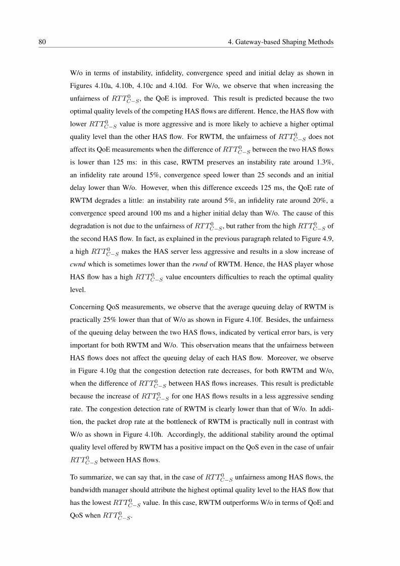
80 4. Gateway-based Shaping Methods
W/o in terms of instability, infidelity, convergence speed and initial delay as shown in
Figures 4.10a, 4.10b, 4.10c and 4.10d. For W/o, we observe that when increasing the
unfairness of RTT 0C−S , the QoE is improved. This result is predicted because the two
optimal quality levels of the competing HAS flows are different. Hence, the HAS flow with
lower RTT 0C−S value is more aggressive and is more likely to achieve a higher optimal
quality level than the other HAS flow. For RWTM, the unfairness of RTT 0C−S does not
affect its QoE measurements when the difference of RTT 0C−S between the two HAS flows
is lower than 125 ms: in this case, RWTM preserves an instability rate around 1.3%,
an infidelity rate around 15%, convergence speed lower than 25 seconds and an initial
delay lower than W/o. However, when this difference exceeds 125 ms, the QoE rate of
RWTM degrades a little: an instability rate around 5%, an infidelity rate around 20%, a
convergence speed around 100 ms and a higher initial delay than W/o. The cause of this
degradation is not due to the unfairness of RTT 0C−S , but rather from the high RTT 0
C−S of
the second HAS flow. In fact, as explained in the previous paragraph related to Figure 4.9,
a high RTT 0C−S makes the HAS server less aggressive and results in a slow increase of
cwnd which is sometimes lower than the rwnd of RWTM. Hence, the HAS player whose
HAS flow has a high RTT 0C−S value encounters difficulties to reach the optimal quality
level.
Concerning QoS measurements, we observe that the average queuing delay of RWTM is
practically 25% lower than that of W/o as shown in Figure 4.10f. Besides, the unfairness
of the queuing delay between the two HAS flows, indicated by vertical error bars, is very
important for both RWTM and W/o. This observation means that the unfairness between
HAS flows does not affect the queuing delay of each HAS flow. Moreover, we observe
in Figure 4.10g that the congestion detection rate decreases, for both RWTM and W/o,
when the difference of RTT 0C−S between HAS flows increases. This result is predictable
because the increase of RTT 0C−S for one HAS flows results in a less aggressive sending
rate. The congestion detection rate of RWTM is clearly lower than that of W/o. In addi-
tion, the packet drop rate at the bottleneck of RWTM is practically null in contrast with
W/o as shown in Figure 4.10h. Accordingly, the additional stability around the optimal
quality level offered by RWTM has a positive impact on the QoS even in the case of unfair
RTT 0C−S between HAS flows.
To summarize, we can say that, in the case of RTT 0C−S unfairness among HAS flows, the
bandwidth manager should attribute the highest optimal quality level to the HAS flow that
has the lowest RTT 0C−S value. In this case, RWTM outperforms W/o in terms of QoE and
QoS when RTT 0C−S .
4.5. Extended Evaluation of RWTM 81
(a) Instability vs. RTT 0C−S unfairness (b) Infidelity vs. RTT 0
C−S unfairness
(c) Convergence speed vs. RTT 0C−S unfairness (d) Initial delay vs. RTT 0
C−S unfairness
(e) frOFF
vs. RTT 0C−S unfairness (f) Queuing delay vs. RTT 0
C−S unfairness
(g) Congestion rate vs. RTT 0C−S unfairness (h) Packet drop rate vs. RTT 0
C−S unfairness
Figure 4.10 – Performance measurements when increasing RTT 0C−S unfairness
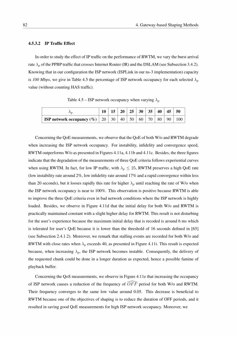
82 4. Gateway-based Shaping Methods
4.5.3.2 IP Traffic Effect
In order to study the effect of IP traffic on the performance of RWTM, we vary the burst arrival
rate λp of the PPBP traffic that crosses Internet Router (IR) and the DSLAM (see Subsection 3.4.2).
Knowing that in our configuration the ISP network (ISPLink in our ns-3 implementation) capacity
is 100 Mbps, we give in Table 4.5 the percentage of ISP network occupancy for each selected λp
value (without counting HAS traffic).
Table 4.5 – ISP network occupancy when varying λp
λp 10 15 20 25 30 35 40 45 50
ISP network occupancy (%) 20 30 40 50 60 70 80 90 100
Concerning the QoE measurements, we observe that the QoE of both W/o and RWTM degrade
when increasing the ISP network occupancy. For instability, infidelity and convergence speed,
RWTM outperforms W/o as presented in Figures 4.11a, 4.11b and 4.11c. Besides, the three figures
indicate that the degradation of the measurements of three QoE criteria follows experiential curves
when using RWTM. In fact, for low IP traffic, with λp ≤ 25, RWTM preserves a high QoE rate
(low instability rate around 2%, low infidelity rate around 17% and a rapid convergence within less
than 20 seconds), but it looses rapidly this rate for higher λp until reaching the rate of W/o when
the ISP network occupancy is near to 100%. This observation is positive because RWTM is able
to improve the three QoE criteria even in bad network conditions where the ISP network is highly
loaded. Besides, we observe in Figure 4.11d that the initial delay for both W/o and RWTM is
practically maintained constant with a slight higher delay for RWTM. This result is not disturbing
for the user’s experience because the maximum initial delay that is recoded is around 6 ms which
is tolerated for user’s QoE because it is lower than the threshold of 16 seconds defined in [65]
(see Subsection 2.4.1.2). Moreover, we remark that stalling events are recorded for both W/o and
RWTM with close rates when λp exceeds 40, as presented in Figure 4.11i. This result is expected
because, when increasing λp, the ISP network becomes instable. Consequently, the delivery of
the requested chunk could be done in a longer duration as expected, hence a possible famine of
playback buffer.
Concerning the QoS measurements, we observe in Figure 4.11e that increasing the occupancy
of ISP network causes a reduction of the frequency of OFF period for both W/o and RWTM.
Their frequency converges to the same low value around 0.05. This decrease is beneficial to
RWTM because one of the objectives of shaping is to reduce the duration of OFF periods, and it
resulted in saving good QoE measurements for high ISP network occupancy. Moreover, we
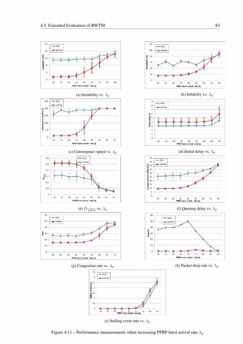
4.5. Extended Evaluation of RWTM 83
(a) Instability vs. λp (b) Infidelity vs. λp
(c) Convergence speed vs. λp (d) Initial delay vs. λp
(e) frOFF
vs. λp (f) Queuing delay vs. λp
(g) Congestion rate vs. λp (h) Packet drop rate vs. λp
(i) Stalling event rate vs. λp
Figure 4.11 – Performance measurements when increasing PPBP burst arrival rate λp
84 4. Gateway-based Shaping Methods
observe that the queuing delay is affected by the increase of ISP network occupancy. In fact,
as shown in Figure 4.11f the average queuing delay is increased for both W/o and RWTM and
reaches the same value around 40 ms when the ISP network is overloaded (λp = 50 ). However,
RWTM preserves lower queuing delay values due to its traffic shaping method that reduces the
bottleneck queue occupancy. In addition, we remark that, for W/o, the congestion detection rate is
increased while the packet drop rate at the bottleneck is reduced from λp = 35 and reaches 0 when
the ISP network is overloaded, as indicated in Figures 4.11g and 4.11h, respectively. Hence, when
λp is higher than 35, the real bottleneck link is being moved from the link between DSLAM and
HG to the ISP network. Given that the congestion detection rate of RWTM is maintained lower
than that of W/o and the packet drop rate is practically kept null for different λp values, RWTM
maintains better QoS than W/o.
To summarize, we can say that RWTM is sensitive to the increase of occupancy of ISP net-
works, through which the HAS flows are transmitted. However, RWTM is able to improve the
QoE for HAS users and to offer better QoS for access network even if the ISP networks is highly
loaded by IP traffic.
4.5.3.3 Bottleneck Queue Effect
As we indicated in Subsection 2.4.2.1, the length of a router queue and the type of its queuing
discipline, such as Drop Tail and RED, have an effect on HAS performances because they have a
direct impact on packet drop rate and end-to-end delay.
In this subsection, we employ in the bottleneck link one of two types of queuing disciplines,
Drop Tail or RED, with one of three lengths of queue: half, twice or equal to the bandwidth delay
product. RED is configured by setting the minimum threshold (minTh) to one third the queue
length and the maximum threshold (maxTh) to the queue length. Here we notice that minTh is the
number of buffered packets where RED begins to drop incoming packets with a low probability.
This probability increases to reach 1 when the buffered packets attains maxTh threshold. The
results of simulations are presented in Figure 4.12.
In the case without shaping, W/o, the size of the bottleneck queue has a great effect on QoE
of HAS and QoS. On the one hand, when employing small queue, we observe low instability, high
infidelity and difficulties to converge to optimal quality level, as shown in Figures 4.12a, 4.12b and
4.12c, respectively. We also remark a low queuing delay and low dropped packets, as presented
in Figures 4.12f and 4.12h, respectively. This observation means that there is a stability around a
lower quality level below optimal quality level and an underutilization of bottleneck bandwidth. In
fact, due to the small queue size, the competing HAS players become unable to select the optimal
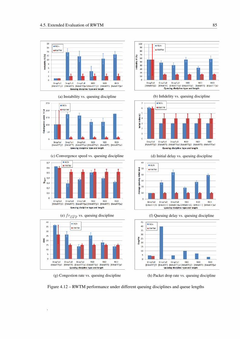
4.5. Extended Evaluation of RWTM 85
(a) Instability vs. queuing discipline (b) Infidelity vs. queuing discipline
(c) Convergence speed vs. queuing discipline (d) Initial delay vs. queuing discipline
(e) frOFF
vs. queuing discipline (f) Queuing delay vs. queuing discipline
(g) Congestion rate vs. queuing discipline (h) Packet drop rate vs. queuing discipline
Figure 4.12 – RWTM performance under different queuing disciplines and queue lengths
.
86 4. Gateway-based Shaping Methods
quality level. In fact, when they do, the queuing discipline drops packets and provokes a congestion
detection in the servers. On the other hand, when employing a large queue corresponding to twice
the bandwidth delay product, we observe a negligible packet drop rate and a clear reduction of
congestion detection rate on the server side. However, this result, beneficial to QoS, have no
impact on QoE: we still observe a high instability rate (higher than 10%), a high infidelity rate of
60% and inability to converge. The main cause is the very large queuing delay that exceeds 40 ms
as shown in Figure 4.12f. In this case, the RTT of each HAS streams is increased to around 140
ms which impacts negatively the QoE as observed in Subsection 4.5.3.1.
When focusing on RWTM results, we observe that it preserves practically the same perfor-
mances (instability around 2% infidelity around 15%, convergence speed around 12 seconds, ini-
tial delay around 4 seconds, average queuing delay less than 10 ms and a null packet drop rate) for
Drop Tail and RED queuing disciplines with different queue lengths, excepting Drop Tail with a
queue length equals to the half of bandwidth delay product. In the latter case, RWTM performs
like W/o.
Accordingly, we can say that RWTM is not affected, in terms of QoE and QoS, by the queuing
discipline of the bottleneck when the queue length is equal or higher than the bandwidth delay
product. Besides, when the queue length is equal to the half of the bandwidth delay product,
RWTM preserves its performances when employing RED queuing discipline.
4.6 Conclusion
In this chapter we have described our proposed gateway-based shaping method RWTM that it
is based on TCP flow control and employs RTT passive estimation. We have compared the perfor-
mances of RWTM with another recent gateway-based shaping method HTBM. Results indicated
that RWTM outperforms HTBM not only in QoE of HAS, but also in the QoS of the access net-
work by reducing the queuing delay at the bottleneck. However, the non-exhaustive estimation of
RTT employed by RWTM is the cause of longer OFF periods than HTBM. Moreover, we have
extensively evaluate RWTM performances in extended evaluation. RWTM preserves its high QoE
rate, its low queuing delay and its near null packet drop rate at the bottleneck link even when the
number of competing HAS clients is increased. Moreover, RWTM is able to improve the QoE
of Live HAS streaming where player is configured with a small playback buffer size. Besides,
it presents better performances when the chunk duration is increased to 7 seconds. In addition,
RWTM performs well when competing HAS flows have high initial round-trip delay below 150
ms without causing bandwidth underutilization. Unfair initial round-trip delay between compet-
4.6. Conclusion 87
ing HAS players lower than 125 ms does not disturb HAS performances. Nevertheless, RWTM
is sensitive to the increase of IP traffic in best effort network but it improves the QoE of HAS
unless the ISP network is overloaded. Furthermore, RWTM is not affected by the type of queuing
discipline employed in the bottleneck unless the queue length is small compared to the bandwidth
delay product. In the latter case, RED discipline is advisable to get improvement in QoE.

89
CHAPTER
5 TCP Congestion Control
Variant Effect
5.1 Introduction
Typically, the TCP congestion control algorithm on the sender side updates the congestion win-
dow value, cwnd, at each reception of acknowledgment (ACK) from the receiver. Consequently,
the sender’s sending rate depends on TCP congestion control algorithm. Given that many TCP
congestion control variants were proposed and have been employed, the performance of HAS may
be affected from one variant to another.
Moreover, traffic shaping methods have a beneficial effect on the QoE of HAS and on the QoS
of the access network. As presented in Chapter 4, we have compared two gateway-based shaping
methods, RWTM and HTBM, when the server is employing Cubic variant. Results indicated that
RWTM outperforms HTBM in terms of QoE and largely reduces the queuing delay. However,
HTBM reduces the frequency of OFF period more than RWTM. Nevertheless, given that this
result is valid for Cubic variant, we aim to study the effect of other well-known TCP conges-
tion control variants (NewReno, Vegas and Illinois) on the two shaping methods; in other words,
whether RWTM or HTBM are affected by the TCP variants or not.
Accordingly, in this chapter our objective is to study the effect of TCP congestion control
variants on HTTP adaptive streaming performance when employing a gateway-based shaping
method. Therefore, we classify and study theoretically each variant of TCP congestion control in
Section 5.2. Then, we evaluate the combination between the two gateway-based shaping methods,
RWTM and HTBM, and four well-known TCP congestion control variants in Section 5.3. Finally,
we summarize results and give a detailed discussion in Section 5.4.
90 5. TCP Congestion Control Variant Effect
5.2 State of the Art
All TCP congestion control variants have two common phases: a slow start phase and a conges-
tion avoidance phase. The slow start phase consists of increasing cwnd rapidly by one maximum
segment size (MSS) for each received acknowledgment (ACK), i.e. the cwnd value is doubled for
each round trip time (RTT). This rapid increase of cwnd has an objective of reaching a high bitrate
within a short duration. When the cwnd size exceeds a threshold, called Slow Start Threshold
(ssthresh), the TCP congestion control algorithm switches to the second phase: the congestion
avoidance phase. During this phase, cwnd is generally increased slowly. The justification of this
slow increase is to push carefully TCP to fill the maximum end-to-end available bandwidth with
lower risk of producing congestion.
TCP congestion control variants are classified according to two main criteria [59]:
1. The first criterion is the way cwnd is increasing during the congestion avoidance phase
and the way cwnd is decreased immediately following congestion detection. Generally,
the increase is additive, and the cwnd size increases by one MSS for each RTT. For de-
creasing cwnd, the standard variants employ multiplicative decreasing, i.e. the cwnd size
is weighted by a multiplicative decrease factor (1− β), where 0 < β < 1. This is the Ad-
ditive Increase Multiplicative Decrease (AIMD) approach. Other variants using different
techniques are classified as non-AIMD approaches.
2. The second criterion is the method by which the algorithm detects congestion. We distin-
guish three modes: loss-based, delay-based, and loss-delay-based modes. The loss-based
mode considers any detection of packet loss as a congestion event. A majority of TCP con-
gestion control variants that use the loss-based mode consider receiving three duplicated
ACKs from the receiver as an indication of a packet loss and, as a consequence, as an
indication of a congestion event. However, the delay-based mode considers a significant
increase in the RTT value as the only indication of a congestion event. The third mode,
the hybrid mode, combines the delay-based and loss-based modes to improve congestion
detection.
In order to facilitate our study, we chose four well-known congestion control variants and we
classify them according to the two criteria cited above:
— NewReno [44]:
This variant is designed as the standard TCP congestion control approach. It uses the
AIMD approach with the loss-based mode. Two mechanisms are employed immediately
following congestion detection: fast retransmit and fast recovery [62]. Fast retransmit
consist of performing a retransmission of what appears to be the missing packet (i.e. when
5.2. State of the Art 91
receiving 3 duplicate ACKs), without waiting for the retransmission timer to expire. After
the fast retransmit algorithm sends this packet, the fast recovery algorithm governs the
transmission of new data until a non-duplicate ACK arrives. The reason for using fast
recovery is to allow the continual sending of packets when the receiver is still receiving
packets, even if some packets are lost.
— Vegas [21]:
This non-AIMD variant is an Additive Increase Additive Decrease (AIAD) variant. It is a
delay-based variant that accurately estimates RTT for every sent packet and adjusts cwnd
size based on actual throughput and expected throughput. If RTT increases, cwnd decreases
by one MSS, and vice versa. Vegas is the smoothest TCP congestion control variant [71];
it is able to allocate a fair share of bandwidth with minimal packet loss events.
— Illinois [89]:
This is a TCP loss-delay-based congestion variant that employs a particular classification of
the AIMD approach, C-AIMD, which involves a concave window size curve. Packet loss
is used for primary congestion inference to determine the direction (increase or decrease)
of cwnd, with a delay for secondary congestion inference to adjust the value of the window
size change. More precisely, when the average queuing delay is small (small increase of
RTT), the sender supposes that the congestion is not imminent and sets a large additive
increase α and small multiplicative decrease β. In the opposite case, when the average
queuing delay is large (large increase of RTT), the sender supposes that the congestion is
imminent and sets a small α and large β. Illinois measures RTT for each received ACK
to update α and β. Moreover, it retains the same fast recovery and fast retransmit phases
as NewReno. Illinois was designed for high-speed and high-latency networks, where the
bandwidth-delay product is relatively high. Consequently, it enables higher throughput
than NewReno for high-speed and high-latency networks.
— Cubic [57]: This variant is loss-based, but it uses a non-AIMD approach. A cubic function
is used to increase the cwnd in the congestion avoidance phase immediately after the fast
recovery phase, and a multiplicative decrease approach is used to update the cwnd after
congestion event detection. The cubic function has a concave region followed by a convex
region. The plateau between the two regions, or the inflexion point (denoted by Wmax),
corresponds to the window size just before the last congestion event. The cubic function
enables a slow growth aroundWmax to enhance the stability of the bandwidth, and enables
a fast growth away from Wmax to improve scalability of the protocol. Upon receiving an
ACK during the congestion avoidance phase at time t, Cubic computes the new value of
cwnd corresponding to the cubic function at time t. As a consequence, Cubic uses the time
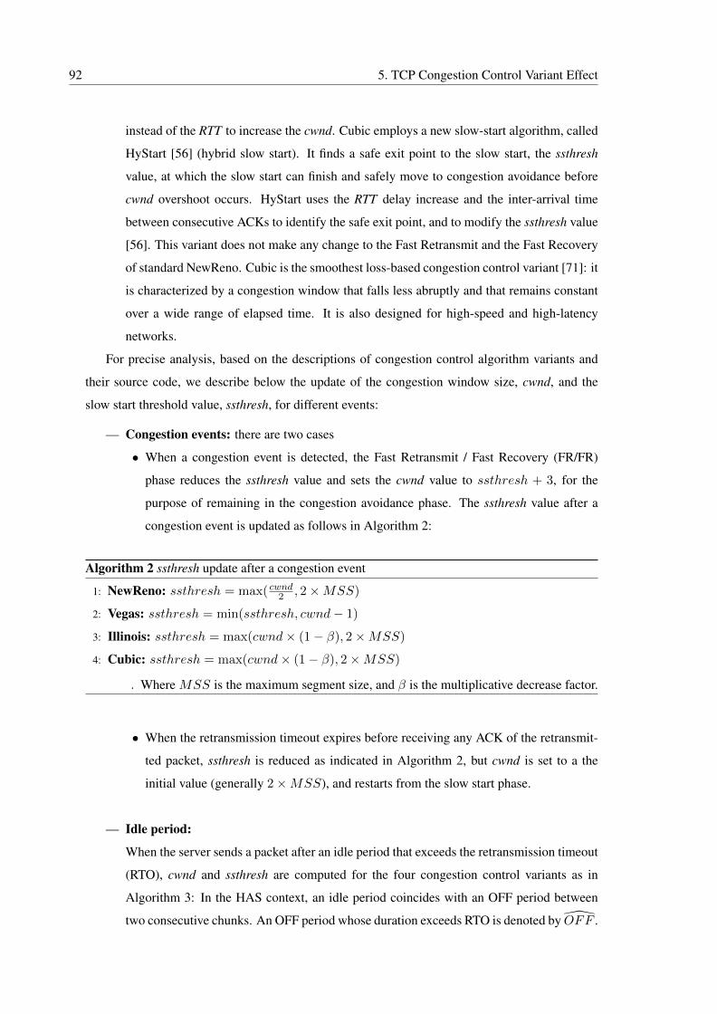
92 5. TCP Congestion Control Variant Effect
instead of the RTT to increase the cwnd. Cubic employs a new slow-start algorithm, called
HyStart [56] (hybrid slow start). It finds a safe exit point to the slow start, the ssthresh
value, at which the slow start can finish and safely move to congestion avoidance before
cwnd overshoot occurs. HyStart uses the RTT delay increase and the inter-arrival time
between consecutive ACKs to identify the safe exit point, and to modify the ssthresh value
[56]. This variant does not make any change to the Fast Retransmit and the Fast Recovery
of standard NewReno. Cubic is the smoothest loss-based congestion control variant [71]: it
is characterized by a congestion window that falls less abruptly and that remains constant
over a wide range of elapsed time. It is also designed for high-speed and high-latency
networks.
For precise analysis, based on the descriptions of congestion control algorithm variants and
their source code, we describe below the update of the congestion window size, cwnd, and the
slow start threshold value, ssthresh, for different events:
— Congestion events: there are two cases
• When a congestion event is detected, the Fast Retransmit / Fast Recovery (FR/FR)
phase reduces the ssthresh value and sets the cwnd value to ssthresh + 3, for the
purpose of remaining in the congestion avoidance phase. The ssthresh value after a
congestion event is updated as follows in Algorithm 2:
Algorithm 2 ssthresh update after a congestion event
1: NewReno: ssthresh = max( cwnd2 , 2×MSS)
2: Vegas: ssthresh = min(ssthresh, cwnd− 1)
3: Illinois: ssthresh = max(cwnd× (1− β), 2×MSS)
4: Cubic: ssthresh = max(cwnd× (1− β), 2×MSS)
. Where MSS is the maximum segment size, and β is the multiplicative decrease factor.
• When the retransmission timeout expires before receiving any ACK of the retransmit-
ted packet, ssthresh is reduced as indicated in Algorithm 2, but cwnd is set to a the
initial value (generally 2×MSS), and restarts from the slow start phase.
— Idle period:
When the server sends a packet after an idle period that exceeds the retransmission timeout
(RTO), cwnd and ssthresh are computed for the four congestion control variants as in
Algorithm 3: In the HAS context, an idle period coincides with an OFF period between
two consecutive chunks. An OFF period whose duration exceeds RTO is denoted by OFF .
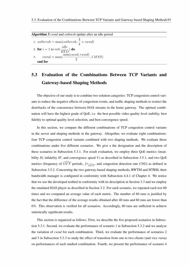
5.3. Evaluation of the Combinations Between TCP Variants and Gateway-based Shaping Methods93
Algorithm 3 cwnd and ssthresh update after an idle period
1: ssthresh = max(ssthresh,3
4× cwnd)
2: for i = 1 to int(idle
RTO) do
3: cwnd = max(min(cwnd, rwnd)
2, 1MSS)
end for
5.3 Evaluation of the Combinations Between TCP Variants and
Gateway-based Shaping Methods
The objective of our study is to combine two solution categories: TCP congestion control vari-
ants to reduce the negative effects of congestion events, and traffic shaping methods to restrict the
drawbacks of the concurrence between HAS streams in the home gateway. The optimal combi-
nation will have the highest grade of QoE, i.e. the best possible video quality level stability, best
fidelity to optimal quality level selection, and best convergence speed.
In this section, we compare the different combinations of TCP congestion control variants
in the server and shaping methods in the gateway. Altogether, we evaluate eight combinations:
four TCP congestion control variants combined with two shaping methods. We evaluate these
combinations under five different scenarios. We give a the designation and the description of
these scenarios in Subsection 5.3.1. For result evaluation, we employ three QoE metrics (insat-
bility IS, infidelity IF, and convergence speed V) as described in Subsection 3.5.1, and two QoS
metrics (frequency of OFF periods, frOFF
, and congestion detection rate CNG) as defined in
Subsection 3.5.2. Concerning the two gateway-based shaping methods, RWTM and HTBM, their
bandwidth manager is configured in conformity with Subsection 4.4.1 of Chapter 4. We notice
that we use the developed testbed in conformity with its description in Section 3.3 and we employ
the emulated HAS player as described in Section 3.2. For each scenario, we repeated each test 60
times and we computed an average value of each metric. The number of 60 runs is justified by
the fact that the difference of the average results obtained after 40 runs and 60 runs are lower than
6%. This observation is verified for all scenarios. Accordingly, 60 runs are sufficient to achieve
statistically significant results.
This section is organized as follows. First, we describe the five proposed scenarios in Subsec-
tion 5.3.1. Second, we evaluate the performance of scenario 1 in Subsection 5.3.2 and we analyze
the variation of cwnd for each combination. Third, we evaluate the performance of scenarios 2
and 3 in Subsection 5.3.3 to study the effect of transition from one to two clients (and vice versa)
on performances of each studied combination. Fourth, we present the performance of scenario 4
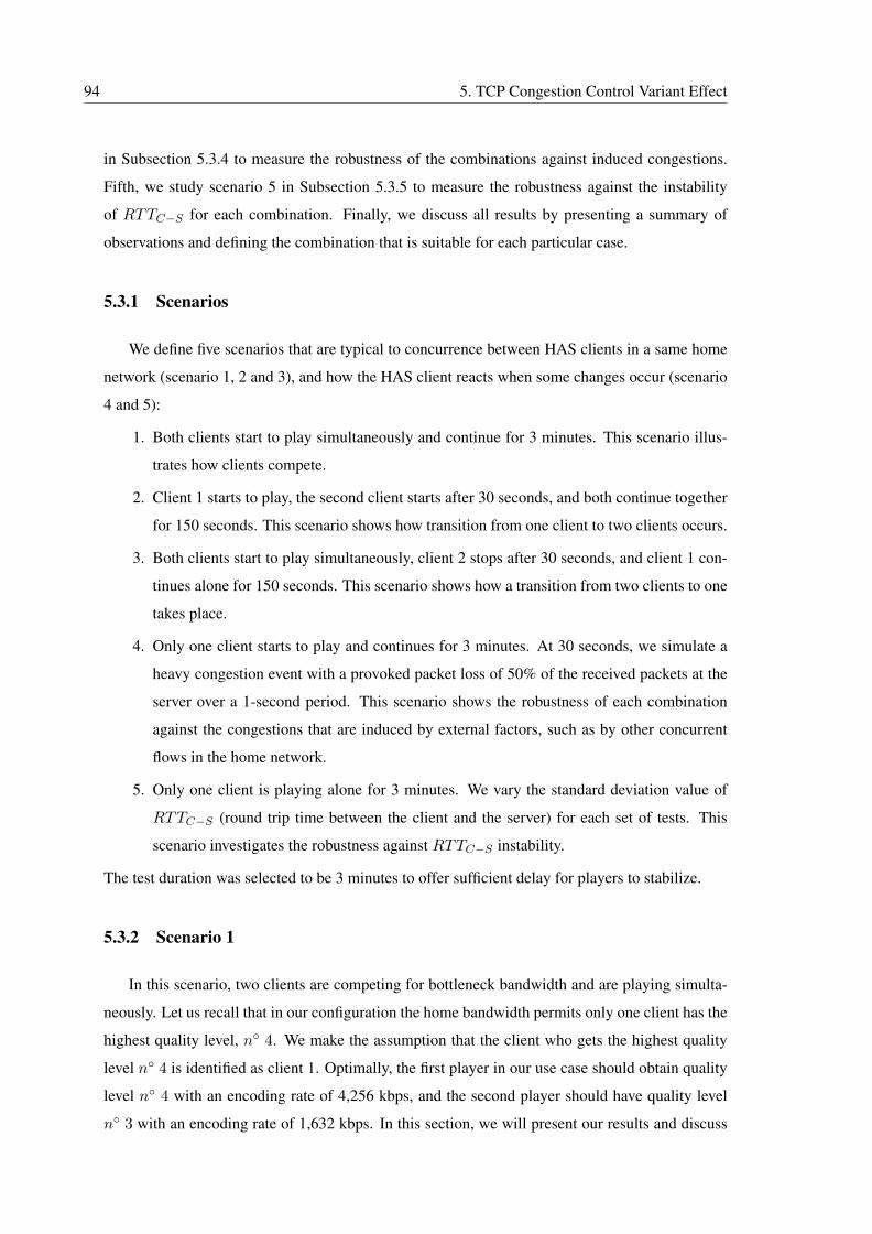
94 5. TCP Congestion Control Variant Effect
in Subsection 5.3.4 to measure the robustness of the combinations against induced congestions.
Fifth, we study scenario 5 in Subsection 5.3.5 to measure the robustness against the instability
of RTTC−S for each combination. Finally, we discuss all results by presenting a summary of
observations and defining the combination that is suitable for each particular case.
5.3.1 Scenarios
We define five scenarios that are typical to concurrence between HAS clients in a same home
network (scenario 1, 2 and 3), and how the HAS client reacts when some changes occur (scenario
4 and 5):
1. Both clients start to play simultaneously and continue for 3 minutes. This scenario illus-
trates how clients compete.
2. Client 1 starts to play, the second client starts after 30 seconds, and both continue together
for 150 seconds. This scenario shows how transition from one client to two clients occurs.
3. Both clients start to play simultaneously, client 2 stops after 30 seconds, and client 1 con-
tinues alone for 150 seconds. This scenario shows how a transition from two clients to one
takes place.
4. Only one client starts to play and continues for 3 minutes. At 30 seconds, we simulate a
heavy congestion event with a provoked packet loss of 50% of the received packets at the
server over a 1-second period. This scenario shows the robustness of each combination
against the congestions that are induced by external factors, such as by other concurrent
flows in the home network.
5. Only one client is playing alone for 3 minutes. We vary the standard deviation value of
RTTC−S (round trip time between the client and the server) for each set of tests. This
scenario investigates the robustness against RTTC−S instability.
The test duration was selected to be 3 minutes to offer sufficient delay for players to stabilize.
5.3.2 Scenario 1
In this scenario, two clients are competing for bottleneck bandwidth and are playing simulta-
neously. Let us recall that in our configuration the home bandwidth permits only one client has the
highest quality level, n◦ 4. We make the assumption that the client who gets the highest quality
level n◦ 4 is identified as client 1. Optimally, the first player in our use case should obtain quality
level n◦ 4 with an encoding rate of 4,256 kbps, and the second player should have quality level
n◦ 3 with an encoding rate of 1,632 kbps. In this section, we will present our results and discuss
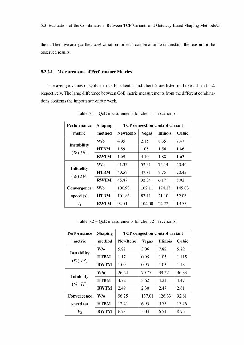
5.3. Evaluation of the Combinations Between TCP Variants and Gateway-based Shaping Methods95
them. Then, we analyze the cwnd variation for each combination to understand the reason for the
observed results.
5.3.2.1 Measurements of Performance Metrics
The average values of QoE metrics for client 1 and client 2 are listed in Table 5.1 and 5.2,
respectively. The large difference between QoE metric measurements from the different combina-
tions confirms the importance of our work.
Table 5.1 – QoE measurements for client 1 in scenario 1
Performance
metric
Shaping
method
TCP congestion control variant
NewReno Vegas Illinois Cubic
Instability
(%) IS1
W/o 4.95 2.15 8.35 7.47
HTBM 1.89 1.08 1.56 1.86
RWTM 1.69 4.10 1.88 1.63
Infidelity
(%) IF1
W/o 41.33 52.31 74.14 50.46
HTBM 49.57 47.81 7.75 20.45
RWTM 45.87 32.24 6.17 5.02
Convergence
speed (s)
V1
W/o 100.93 102.11 174.13 145.03
HTBM 101.83 87.11 21.10 52.06
RWTM 94.51 104.00 24.22 19.55
Table 5.2 – QoE measurements for client 2 in scenario 1
Performance
metric
Shaping
method
TCP congestion control variant
NewReno Vegas Illinois Cubic
Instability
(%) IS2
W/o 5.82 3.06 7.82 5.82
HTBM 1.17 0.95 1.05 1.115
RWTM 1.09 0.95 1.03 1.13
Infidelity
(%) IF2
W/o 26.64 70.77 39.27 36.33
HTBM 4.72 3.62 4.21 4.47
RWTM 2.49 2.30 2.47 2.61
Convergence
speed (s)
V2
W/o 96.25 137.01 126.33 92.81
HTBM 12.41 6.95 9.73 13.26
RWTM 6.73 5.03 6.54 8.95
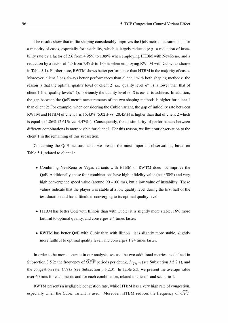
96 5. TCP Congestion Control Variant Effect
The results show that traffic shaping considerably improves the QoE metric measurements for
a majority of cases, especially for instability, which is largely reduced (e.g. a reduction of insta-
bility rate by a factor of 2.6 from 4.95% to 1.89% when employing HTBM with NewReno, and a
reduction by a factor of 4.5 from 7.47% to 1.63% when employing RWTM with Cubic, as shonw
in Table 5.1). Furthermore, RWTM shows better performance than HTBM in the majority of cases.
Moreover, client 2 has always better performances than client 1 with both shaping methods: the
reason is that the optimal quality level of client 2 (i.e. quality level n◦ 3) is lower than that of
client 1 (i.e. quality leveln◦ 4): obviously the quality level n◦ 3 is easier to achieve. In addition,
the gap between the QoE metric measurements of the two shaping methods is higher for client 1
than client 2: For example, when considering the Cubic variant, the gap of infidelity rate between
RWTM and HTBM of client 1 is 15.43% (5.02% vs. 20.45%) is higher than that of client 2 which
is equal to 1.86% (2.61% vs. 4.47% ). Consequently, the dissimilarity of performances between
different combinations is more visible for client 1. For this reason, we limit our observation to the
client 1 in the remaining of this subsection.
Concerning the QoE measurements, we present the most important observations, based on
Table 5.1, related to client 1:
• Combining NewReno or Vegas variants with HTBM or RWTM does not improve the
QoE. Additionally, these four combinations have high infidelity value (near 50%) and very
high convergence speed value (around 90∼100 ms), but a low value of instability. These
values indicate that the player was stable at a low quality level during the first half of the
test duration and has difficulties converging to its optimal quality level.
• HTBM has better QoE with Illinois than with Cubic: it is slightly more stable, 16% more
faithful to optimal quality, and converges 2.4 times faster.
• RWTM has better QoE with Cubic than with Illinois: it is slightly more stable, slightly
more faithful to optimal quality level, and converges 1.24 times faster.
In order to be more accurate in our analysis, we use the two additional metrics, as defined in
Subsection 3.5.2: the frequency of OFF periods per chunk, frOFF
(see Subsection 3.5.2.1), and
the congestion rate, CNG (see Subsection 3.5.2.3). In Table 5.3, we present the average value
over 60 runs for each metric and for each combination, related to client 1 and scenario 1.
RWTM presents a negligible congestion rate, while HTBM has a very high rate of congestion,
especially when the Cubic variant is used. Moreover, HTBM reduces the frequency of OFF
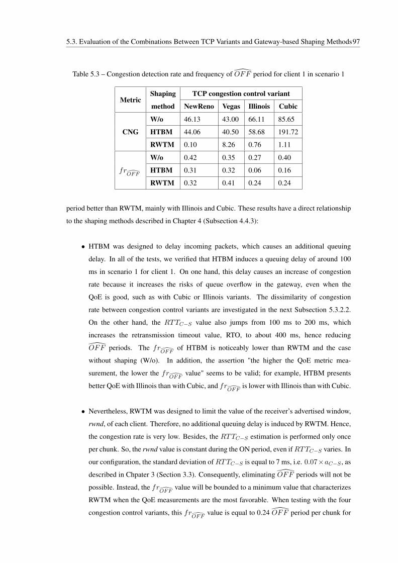
5.3. Evaluation of the Combinations Between TCP Variants and Gateway-based Shaping Methods97
Table 5.3 – Congestion detection rate and frequency of OFF period for client 1 in scenario 1
MetricShaping
method
TCP congestion control variant
NewReno Vegas Illinois Cubic
CNG
W/o 46.13 43.00 66.11 85.65
HTBM 44.06 40.50 58.68 191.72
RWTM 0.10 8.26 0.76 1.11
frOFF
W/o 0.42 0.35 0.27 0.40
HTBM 0.31 0.32 0.06 0.16
RWTM 0.32 0.41 0.24 0.24
period better than RWTM, mainly with Illinois and Cubic. These results have a direct relationship
to the shaping methods described in Chapter 4 (Subsection 4.4.3):
• HTBM was designed to delay incoming packets, which causes an additional queuing
delay. In all of the tests, we verified that HTBM induces a queuing delay of around 100
ms in scenario 1 for client 1. On one hand, this delay causes an increase of congestion
rate because it increases the risks of queue overflow in the gateway, even when the
QoE is good, such as with Cubic or Illinois variants. The dissimilarity of congestion
rate between congestion control variants are investigated in the next Subsection 5.3.2.2.
On the other hand, the RTTC−S value also jumps from 100 ms to 200 ms, which
increases the retransmission timeout value, RTO, to about 400 ms, hence reducing
OFF periods. The frOFF
of HTBM is noticeably lower than RWTM and the case
without shaping (W/o). In addition, the assertion "the higher the QoE metric mea-
surement, the lower the frOFF
value" seems to be valid; for example, HTBM presents
better QoE with Illinois than with Cubic, and frOFF
is lower with Illinois than with Cubic.
• Nevertheless, RWTM was designed to limit the value of the receiver’s advertised window,
rwnd, of each client. Therefore, no additional queuing delay is induced by RWTM. Hence,
the congestion rate is very low. Besides, the RTTC−S estimation is performed only once
per chunk. So, the rwnd value is constant during the ON period, even ifRTTC−S varies. In
our configuration, the standard deviation ofRTTC−S is equal to 7 ms, i.e. 0.07×aC−S , as
described in Chpater 3 (Section 3.3). Consequently, eliminating OFF periods will not be
possible. Instead, the frOFF
value will be bounded to a minimum value that characterizes
RWTM when the QoE measurements are the most favorable. When testing with the four
congestion control variants, this frOFF
value is equal to 0.24 OFF period per chunk for
98 5. TCP Congestion Control Variant Effect
the selected standard deviation. This means that RWTM can guarantee, in the best case,
one OFF period every 4.17 chunks. This frequency is useful, and will be discussed in the
next Subsection 5.3.2.2 and in further detail in scenario 5 (Subsection 5.3.5).
5.3.2.2 Analysis of cwnd Variation
To explain the results of scenario 1, we used the tcp_probe module in the HAS server. This
module shows the evolution of the congestion window, cwnd, and the slow start threshold, ssthresh,
during each run. For each combination, we selected a run whose performance values are the
nearest to its average values of Tables 2 and 4, i.e. instability IS, infidelity IF, convergence speed
V, frequency of OFF periods per chunk frOFF
, and congestion rate CNG. Then, we present
their cwnd and ssthresh evolution in Figures 5.1 through 5.8. We also indicate the moment of
convergence by a vertical bold dotted line. We observed that this moment corresponds to the
second from which the TCP congestion control is often processing under the congestion avoidance
phase; i.e. when cwnd > ssthresh. Hence, we observe that ssthresh is practically around a
constant value.
Figure 5.1 shows that the combination NewReno with HTBM cannot guarantee convergence
to the optimal quality level. The congestion rate is around 43 congestion event per 100 seconds,
which is lower than Illinois and Cubic. After 50 seconds, cwnd was able to reach the congestion
avoidance phase for short durations, but the continuous increase of cwnd with the additive increase
approach caused congestion detections. Moreover, the multiplicative decrease approach after con-
gestions employed by NewReno was very aggressive; in effect, as described in Subsection 5.2, the
new cwnd value will be reduced by half (more precisely, tocwnd
2+3×MSS following the FR/FR
phase) and ssthresh will also be reduced tocwnd
2. This aggressive decrease prevents the server
from rapidly reaching a desirable cwnd value and, as a consequence, prevents the player from cor-
rectly estimating the available bandwidth and causes a lower quality level selection. Furthermore,
the frOFF
value was relatively high (around 30 OFF period) which is more than twice of that of
Illinois and Cubic variants. This value is also caused by the multiplicative decrease approach that
generates a lower quality level selection. Due to the shaping rate that adapts the download bitrate
of the client to its optimal quality level, chunks with a lower quality level will be downloaded more
rapidly, which results in causing more frequent OFF periods. For this reason, the player is not
able to stabilize on the optimal quality level, resulting in a poor QoE.
When combining NewReno with RWTM, we observed that evaluation results diverged and
could be classified into two categories: those with infidelity value of 100% and that do not converge
(Figure 5.2a), and those with a low value of infidelity and that converge rapidly (Figure 5.2b). In
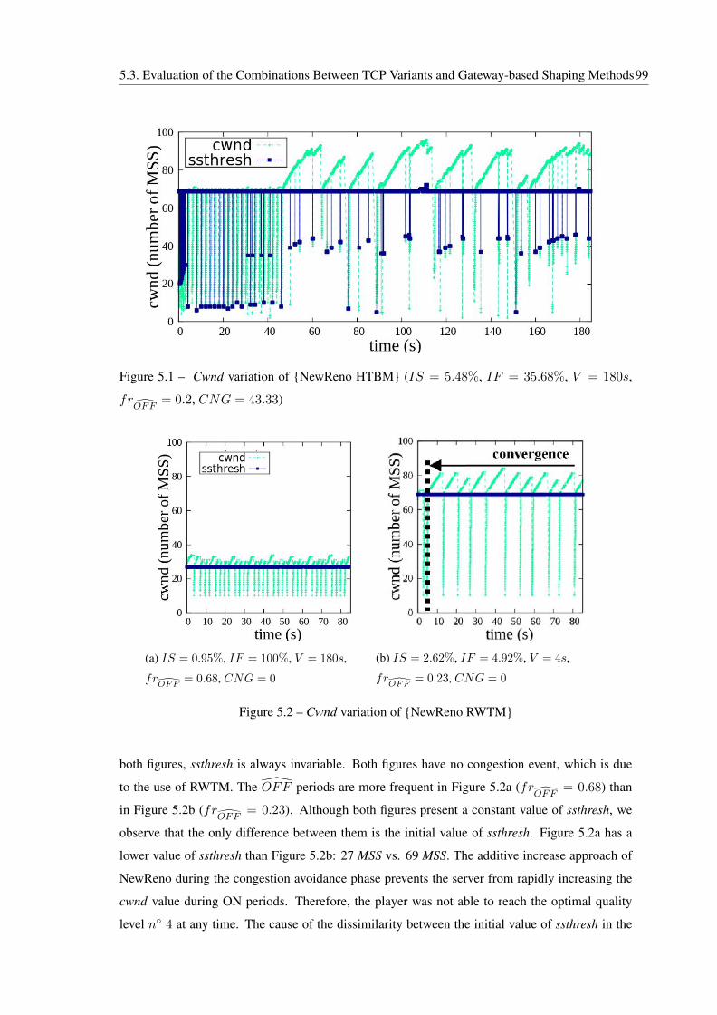
5.3. Evaluation of the Combinations Between TCP Variants and Gateway-based Shaping Methods99
Figure 5.1 – Cwnd variation of {NewReno HTBM} (IS = 5.48%, IF = 35.68%, V = 180s,
frOFF
= 0.2, CNG = 43.33)
(a) IS = 0.95%, IF = 100%, V = 180s,
frOFF
= 0.68, CNG = 0
(b) IS = 2.62%, IF = 4.92%, V = 4s,
frOFF
= 0.23, CNG = 0
Figure 5.2 – Cwnd variation of {NewReno RWTM}
both figures, ssthresh is always invariable. Both figures have no congestion event, which is due
to the use of RWTM. The OFF periods are more frequent in Figure 5.2a (frOFF
= 0.68) than
in Figure 5.2b (frOFF
= 0.23). Although both figures present a constant value of ssthresh, we
observe that the only difference between them is the initial value of ssthresh. Figure 5.2a has a
lower value of ssthresh than Figure 5.2b: 27 MSS vs. 69 MSS. The additive increase approach of
NewReno during the congestion avoidance phase prevents the server from rapidly increasing the
cwnd value during ON periods. Therefore, the player was not able to reach the optimal quality
level n◦ 4 at any time. The cause of the dissimilarity between the initial value of ssthresh in the
100 5. TCP Congestion Control Variant Effect
two figures is explained in [10] some implementations of NewReno use the size of the receiver’s
advertised window, rwnd, to define the initial value of ssthresh, but in fact, this value may be
arbitrarily chosen. Accordingly, the combination of NewReno with RWTM could have high QoE
rate if the initial value of ssthresh is well-chosen.
When combining Vegas with HTBM, we obtain cwnd variation, as shown in Figure 5.3. The
convergence moment (at 87 s in Figure 5.3) occurs when cwnd becomes often set higher than
ssthresh (i.e. TCP congestion control is often processing under congestion avoidance phase) and
ssthresh is often set at the same value. We can observe the additive increase and additive decrease
aspect of cwnd in the congestion avoidance phase after convergence. The additive decrease of
cwnd involved in Vegas is caused by the queuing delay increases resulting from HTBM. This
additive decrease has the advantage of maintaining a high throughput and reducing the dropping
of packets in the gateway. Therefore, the congestion rate, CNG, is relatively low; because it is
reduced in Figure 5.3 from around 75 congestion event per 100 seconds to only 15. The additive
decrease also has the advantage of promoting convergence to the optimal quality level, unlike
multiplicative decrease. As a result, the delay-based aspect with the additive decrease approach
improves the stability of the HAS player after convergence. In contrast, Vegas uses a slightly low
value of ssthresh (60 MSS) and employs the additive increase approach for cwnd updates during the
congestion avoidance phase. As a consequence, the server cannot rapidly increase the cwnd value
during the ON period, which results in slow convergence. Therefore, the player was not able to
reach the optimal quality level n◦ 4 at any time before the moment of convergence. Consequently,
the frequency of the OFF period increases before the convergence moment; hence, the high value
of frOFF
.
The performance worsens when Vegas is combined with RWTM. As presented in Figure 5.4,
the player was not able to converge. Instead, we observed many timeout retransmissions (such
as at seconds 90 and 159) characterized by ssthresh reduction and cwnd restarting from slow
start. The timeout retransmissions are generated by Vegas when only a duplicate ACK is received
and the timeout period of the oldest unacknowledged packet has expired [21]. Because of
this, Vegas generates more timeout retransmissions than NewReno. Hence, the CNG value is
worse than in the other combinations of RWTM. Moreover, OFF periods, characterized by a
drop of cwnd value while ssthresh is kept constant, are frequent during the first 45 seconds,
because the player requests quality level n◦ 3 instead of n◦ 4. In this phase, frOFF
reaches
practically the highest value of one OFF per chunk. Subsequently, OFF periods become
far less frequent (just at seconds 79, 125, 138, 150, 165 and 175) because the player was
able to switch to a optimal quality level (n◦ 4). Hence, frOFF
of the whole test duration
is equal to an acceptable value (0.29 OFF period per chunk). The player becomes able to
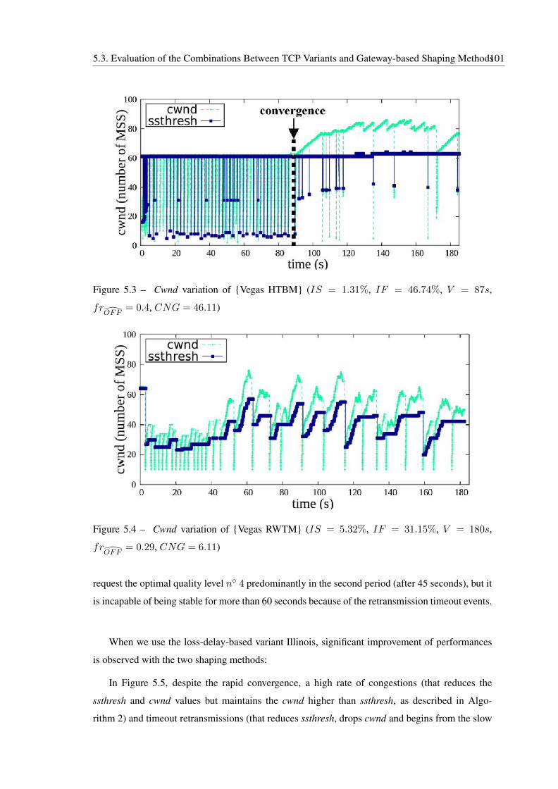
5.3. Evaluation of the Combinations Between TCP Variants and Gateway-based Shaping Methods101
Figure 5.3 – Cwnd variation of {Vegas HTBM} (IS = 1.31%, IF = 46.74%, V = 87s,
frOFF
= 0.4, CNG = 46.11)
Figure 5.4 – Cwnd variation of {Vegas RWTM} (IS = 5.32%, IF = 31.15%, V = 180s,
frOFF
= 0.29, CNG = 6.11)
request the optimal quality level n◦ 4 predominantly in the second period (after 45 seconds), but it
is incapable of being stable for more than 60 seconds because of the retransmission timeout events.
When we use the loss-delay-based variant Illinois, significant improvement of performances
is observed with the two shaping methods:
In Figure 5.5, despite the rapid convergence, a high rate of congestions (that reduces the
ssthresh and cwnd values but maintains the cwnd higher than ssthresh, as described in Algo-
rithm 2) and timeout retransmissions (that reduces ssthresh, drops cwnd and begins from the slow
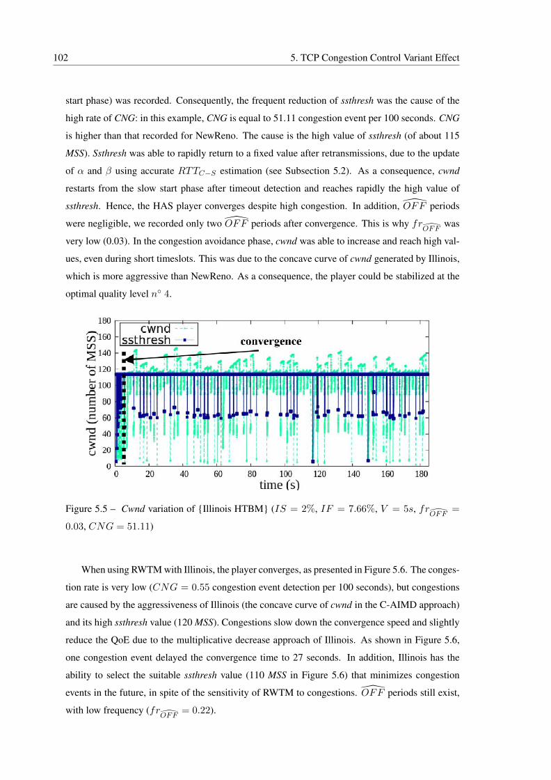
102 5. TCP Congestion Control Variant Effect
start phase) was recorded. Consequently, the frequent reduction of ssthresh was the cause of the
high rate of CNG: in this example, CNG is equal to 51.11 congestion event per 100 seconds. CNG
is higher than that recorded for NewReno. The cause is the high value of ssthresh (of about 115
MSS). Ssthresh was able to rapidly return to a fixed value after retransmissions, due to the update
of α and β using accurate RTTC−S estimation (see Subsection 5.2). As a consequence, cwnd
restarts from the slow start phase after timeout detection and reaches rapidly the high value of
ssthresh. Hence, the HAS player converges despite high congestion. In addition, OFF periods
were negligible, we recorded only two OFF periods after convergence. This is why frOFF
was
very low (0.03). In the congestion avoidance phase, cwnd was able to increase and reach high val-
ues, even during short timeslots. This was due to the concave curve of cwnd generated by Illinois,
which is more aggressive than NewReno. As a consequence, the player could be stabilized at the
optimal quality level n◦ 4.
Figure 5.5 – Cwnd variation of {Illinois HTBM} (IS = 2%, IF = 7.66%, V = 5s, frOFF
=
0.03, CNG = 51.11)
When using RWTM with Illinois, the player converges, as presented in Figure 5.6. The conges-
tion rate is very low (CNG = 0.55 congestion event detection per 100 seconds), but congestions
are caused by the aggressiveness of Illinois (the concave curve of cwnd in the C-AIMD approach)
and its high ssthresh value (120 MSS). Congestions slow down the convergence speed and slightly
reduce the QoE due to the multiplicative decrease approach of Illinois. As shown in Figure 5.6,
one congestion event delayed the convergence time to 27 seconds. In addition, Illinois has the
ability to select the suitable ssthresh value (110 MSS in Figure 5.6) that minimizes congestion
events in the future, in spite of the sensitivity of RWTM to congestions. OFF periods still exist,
with low frequency (frOFF
= 0.22).
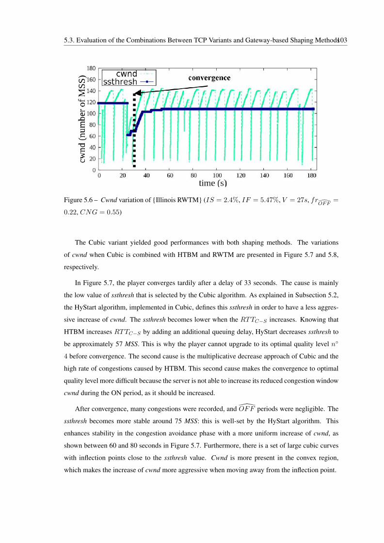
5.3. Evaluation of the Combinations Between TCP Variants and Gateway-based Shaping Methods103
Figure 5.6 – Cwnd variation of {Illinois RWTM} (IS = 2.4%, IF = 5.47%, V = 27s, frOFF
=
0.22, CNG = 0.55)
The Cubic variant yielded good performances with both shaping methods. The variations
of cwnd when Cubic is combined with HTBM and RWTM are presented in Figure 5.7 and 5.8,
respectively.
In Figure 5.7, the player converges tardily after a delay of 33 seconds. The cause is mainly
the low value of ssthresh that is selected by the Cubic algorithm. As explained in Subsection 5.2,
the HyStart algorithm, implemented in Cubic, defines this ssthresh in order to have a less aggres-
sive increase of cwnd. The ssthresh becomes lower when the RTTC−S increases. Knowing that
HTBM increases RTTC−S by adding an additional queuing delay, HyStart decreases ssthresh to
be approximately 57 MSS. This is why the player cannot upgrade to its optimal quality level n◦
4 before convergence. The second cause is the multiplicative decrease approach of Cubic and the
high rate of congestions caused by HTBM. This second cause makes the convergence to optimal
quality level more difficult because the server is not able to increase its reduced congestion window
cwnd during the ON period, as it should be increased.
After convergence, many congestions were recorded, and OFF periods were negligible. The
ssthresh becomes more stable around 75 MSS: this is well-set by the HyStart algorithm. This
enhances stability in the congestion avoidance phase with a more uniform increase of cwnd, as
shown between 60 and 80 seconds in Figure 5.7. Furthermore, there is a set of large cubic curves
with inflection points close to the ssthresh value. Cwnd is more present in the convex region,
which makes the increase of cwnd more aggressive when moving away from the inflection point.
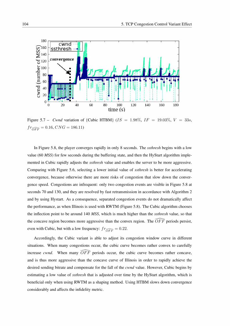
104 5. TCP Congestion Control Variant Effect
Figure 5.7 – Cwnd variation of {Cubic HTBM} (IS = 1.98%, IF = 19.03%, V = 33s,
frOFF
= 0.16, CNG = 186.11)
In Figure 5.8, the player converges rapidly in only 8 seconds. The ssthresh begins with a low
value (60 MSS) for few seconds during the buffering state, and then the HyStart algorithm imple-
mented in Cubic rapidly adjusts the ssthresh value and enables the server to be more aggressive.
Comparing with Figure 5.6, selecting a lower initial value of ssthresh is better for accelerating
convergence, because otherwise there are more risks of congestion that slow down the conver-
gence speed. Congestions are infrequent: only two congestion events are visible in Figure 5.8 at
seconds 70 and 130, and they are resolved by fast retransmission in accordance with Algorithm 2
and by using Hystart. As a consequence, separated congestion events do not dramatically affect
the performance, as when Illinois is used with RWTM (Figure 5.8). The Cubic algorithm chooses
the inflection point to be around 140 MSS, which is much higher than the ssthresh value, so that
the concave region becomes more aggressive than the convex region. The OFF periods persist,
even with Cubic, but with a low frequency: frOFF
= 0.22.
Accordingly, the Cubic variant is able to adjust its congestion window curve in different
situations. When many congestions occur, the cubic curve becomes rather convex to carefully
increase cwnd. When many OFF periods occur, the cubic curve becomes rather concave,
and is thus more aggressive than the concave curve of Illinois in order to rapidly achieve the
desired sending bitrate and compensate for the fall of the cwnd value. However, Cubic begins by
estimating a low value of ssthresh that is adjusted over time by the HyStart algorithm, which is
beneficial only when using RWTM as a shaping method. Using HTBM slows down convergence
considerably and affects the infidelity metric.
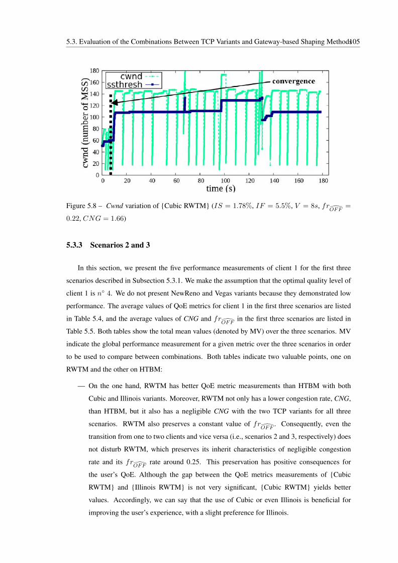
5.3. Evaluation of the Combinations Between TCP Variants and Gateway-based Shaping Methods105
Figure 5.8 – Cwnd variation of {Cubic RWTM} (IS = 1.78%, IF = 5.5%, V = 8s, frOFF
=
0.22, CNG = 1.66)
5.3.3 Scenarios 2 and 3
In this section, we present the five performance measurements of client 1 for the first three
scenarios described in Subsection 5.3.1. We make the assumption that the optimal quality level of
client 1 is n◦ 4. We do not present NewReno and Vegas variants because they demonstrated low
performance. The average values of QoE metrics for client 1 in the first three scenarios are listed
in Table 5.4, and the average values of CNG and frOFF
in the first three scenarios are listed in
Table 5.5. Both tables show the total mean values (denoted by MV) over the three scenarios. MV
indicate the global performance measurement for a given metric over the three scenarios in order
to be used to compare between combinations. Both tables indicate two valuable points, one on
RWTM and the other on HTBM:
— On the one hand, RWTM has better QoE metric measurements than HTBM with both
Cubic and Illinois variants. Moreover, RWTM not only has a lower congestion rate, CNG,
than HTBM, but it also has a negligible CNG with the two TCP variants for all three
scenarios. RWTM also preserves a constant value of frOFF
. Consequently, even the
transition from one to two clients and vice versa (i.e., scenarios 2 and 3, respectively) does
not disturb RWTM, which preserves its inherit characteristics of negligible congestion
rate and its frOFF
rate around 0.25. This preservation has positive consequences for
the user’s QoE. Although the gap between the QoE metrics measurements of {Cubic
RWTM} and {Illinois RWTM} is not very significant, {Cubic RWTM} yields better
values. Accordingly, we can say that the use of Cubic or even Illinois is beneficial for
improving the user’s experience, with a slight preference for Illinois.
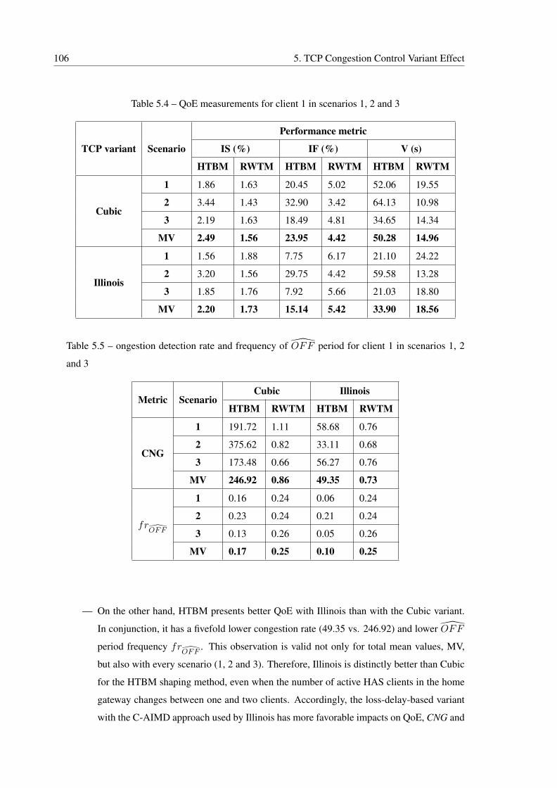
106 5. TCP Congestion Control Variant Effect
Table 5.4 – QoE measurements for client 1 in scenarios 1, 2 and 3
TCP variant Scenario
Performance metric
IS (%) IF (%) V (s)
HTBM RWTM HTBM RWTM HTBM RWTM
Cubic
1 1.86 1.63 20.45 5.02 52.06 19.55
2 3.44 1.43 32.90 3.42 64.13 10.98
3 2.19 1.63 18.49 4.81 34.65 14.34
MV 2.49 1.56 23.95 4.42 50.28 14.96
Illinois
1 1.56 1.88 7.75 6.17 21.10 24.22
2 3.20 1.56 29.75 4.42 59.58 13.28
3 1.85 1.76 7.92 5.66 21.03 18.80
MV 2.20 1.73 15.14 5.42 33.90 18.56
Table 5.5 – ongestion detection rate and frequency of OFF period for client 1 in scenarios 1, 2
and 3
Metric ScenarioCubic Illinois
HTBM RWTM HTBM RWTM
CNG
1 191.72 1.11 58.68 0.76
2 375.62 0.82 33.11 0.68
3 173.48 0.66 56.27 0.76
MV 246.92 0.86 49.35 0.73
frOFF
1 0.16 0.24 0.06 0.24
2 0.23 0.24 0.21 0.24
3 0.13 0.26 0.05 0.26
MV 0.17 0.25 0.10 0.25
— On the other hand, HTBM presents better QoE with Illinois than with the Cubic variant.
In conjunction, it has a fivefold lower congestion rate (49.35 vs. 246.92) and lower OFF
period frequency frOFF
. This observation is valid not only for total mean values, MV,
but also with every scenario (1, 2 and 3). Therefore, Illinois is distinctly better than Cubic
for the HTBM shaping method, even when the number of active HAS clients in the home
gateway changes between one and two clients. Accordingly, the loss-delay-based variant
with the C-AIMD approach used by Illinois has more favorable impacts on QoE, CNG and
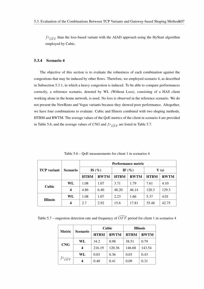
5.3. Evaluation of the Combinations Between TCP Variants and Gateway-based Shaping Methods107
frOFF
than the loss-based variant with the AIAD approach using the HyStart algorithm
employed by Cubic.
5.3.4 Scenario 4
The objective of this section is to evaluate the robustness of each combination against the
congestions that may be induced by other flows. Therefore, we employed scenario 4, as described
in Subsection 5.3.1, in which a heavy congestion is induced. To be able to compare performances
correctly, a reference scenario, denoted by WL (Without Loss), consisting of a HAS client
working alone in the home network, is used. No loss is observed in the reference scenario. We do
not present the NewReno and Vegas variants because they showed poor performance. Altogether,
we have four combinations to evaluate: Cubic and Illinois combined with two shaping methods,
HTBM and RWTM. The average values of the QoE metrics of the client in scenario 4 are provided
in Table 5.6, and the average values of CNG and frOFF
are listed in Table 5.7.
Table 5.6 – QoE measurements for client 1 in scenarios 4
TCP variant Scenario
Performance metric
IS (%) IF (%) V (s)
HTBM RWTM HTBM RWTM HTBM RWTM
CubicWL 1.08 1.07 3.71 1.79 7.61 4.10
4 4.86 6.40 48.20 46.14 120.3 129.3
IllinoisWL 1.08 1.07 2.23 1.66 5.37 4.01
4 2.7 2.92 15.6 17.81 35.48 42.75
Table 5.7 – ongestion detection rate and frequency of OFF period for client 1 in scenarios 4
Metric ScenarioCubic Illinois
HTBM RWTM HTBM RWTM
CNGWL 34.2 0.98 38.51 0.79
4 216.19 120.36 146.68 143.54
frOFF
WL 0.03 0.36 0.03 0.43
4 0.40 0.41 0.09 0.31
108 5. TCP Congestion Control Variant Effect
The measurements in the two tables indicate three major observations:
• The lowest QoE metric measurements are recorded for the Cubic variant for both
shaping methods: their instability is around 5∼6%, their infidelity is near 50%, and their
convergence speed is around 120∼130 ms. We also notice that the congestion rate, CNG,
is very high, between 120 and 220, and the frequency frOFF
is important around 0.4 (i.e.,
one OFF period occurs for every 2.5 chunks, on average). We observe not only lower
measurements, but also a higher degradation rate in performance: the gap of QoE metric
measurements, CNG and frOFF
, are clearly large between scenario WL and scenario 4.
Accordingly, Cubic is not suitable as a TCP congestion control variant of the HAS server
for both shaping methods when heavy congestion occurs. This result can be verified by
examining Figure 5.7 and 5.8 in Subsection 5.3.2.2, where Cubic has difficulties with
rapidly defining the suitable ssthresh value before convergence and after congestion,
respectively.
• The RWTM shaping method presents higher degradation in QoE metric measurements
than HTBM when we compare scenario WL to scenario 4 for both TCP congestion
variants, Cubic and Illinois. The cause is mainly related to the fact that HTBM is used to
generate congestion events and maintain high QoE under normal circumstances, which
is not the case with RWTM. Accordingly, we can say that RWTM is more sensitive to
induced congestions than HTBM. This result can be verified when examining Figures 5.6
and 5.8 in Subsection 5.3.2.2, in which a single congestion event instantaneously degrades
performances.
Under the first and the second observations, we can deduce that the best combination that
maintains optimal QoE metric measurements with low degradation and has the lowest frequency
of OFF periods, frOFF
, is ensured by the combination {Illinois HTBM}.
• The second-best combination is {Illinois RWTM}. Here, the QoE metric measurements
are acceptable, but the degradation rate is higher than the best combination {Illinois
HTBM}. This degradation indicates that {Illinois RWTM} cannot adequately resist against
induced congestions, especially when we have a highly congested link between client and
server. However, this combination could successfully be used with a link under less fre-
quent congestions.
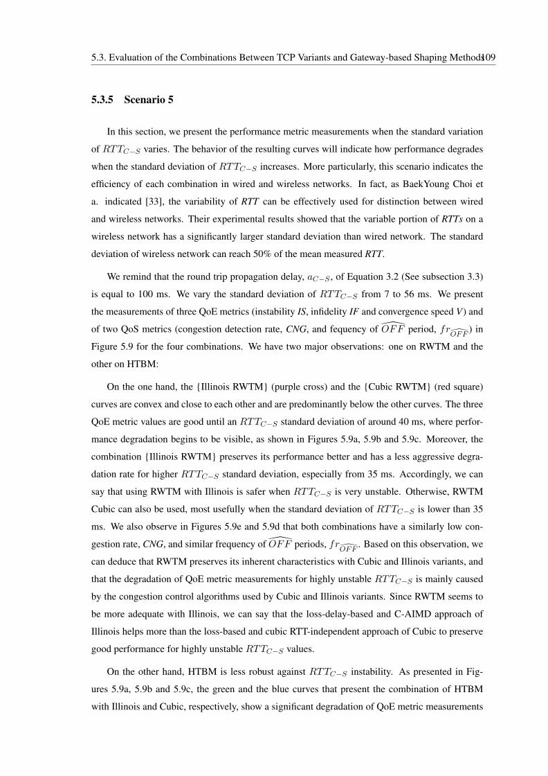
5.3. Evaluation of the Combinations Between TCP Variants and Gateway-based Shaping Methods109
5.3.5 Scenario 5
In this section, we present the performance metric measurements when the standard variation
of RTTC−S varies. The behavior of the resulting curves will indicate how performance degrades
when the standard deviation of RTTC−S increases. More particularly, this scenario indicates the
efficiency of each combination in wired and wireless networks. In fact, as BaekYoung Choi et
a. indicated [33], the variability of RTT can be effectively used for distinction between wired
and wireless networks. Their experimental results showed that the variable portion of RTTs on a
wireless network has a significantly larger standard deviation than wired network. The standard
deviation of wireless network can reach 50% of the mean measured RTT.
We remind that the round trip propagation delay, aC−S , of Equation 3.2 (See subsection 3.3)
is equal to 100 ms. We vary the standard deviation of RTTC−S from 7 to 56 ms. We present
the measurements of three QoE metrics (instability IS, infidelity IF and convergence speed V) and
of two QoS metrics (congestion detection rate, CNG, and fequency of OFF period, frOFF
) in
Figure 5.9 for the four combinations. We have two major observations: one on RWTM and the
other on HTBM:
On the one hand, the {Illinois RWTM} (purple cross) and the {Cubic RWTM} (red square)
curves are convex and close to each other and are predominantly below the other curves. The three
QoE metric values are good until an RTTC−S standard deviation of around 40 ms, where perfor-
mance degradation begins to be visible, as shown in Figures 5.9a, 5.9b and 5.9c. Moreover, the
combination {Illinois RWTM} preserves its performance better and has a less aggressive degra-
dation rate for higher RTTC−S standard deviation, especially from 35 ms. Accordingly, we can
say that using RWTM with Illinois is safer when RTTC−S is very unstable. Otherwise, RWTM
Cubic can also be used, most usefully when the standard deviation of RTTC−S is lower than 35
ms. We also observe in Figures 5.9e and 5.9d that both combinations have a similarly low con-
gestion rate, CNG, and similar frequency of OFF periods, frOFF
. Based on this observation, we
can deduce that RWTM preserves its inherent characteristics with Cubic and Illinois variants, and
that the degradation of QoE metric measurements for highly unstable RTTC−S is mainly caused
by the congestion control algorithms used by Cubic and Illinois variants. Since RWTM seems to
be more adequate with Illinois, we can say that the loss-delay-based and C-AIMD approach of
Illinois helps more than the loss-based and cubic RTT-independent approach of Cubic to preserve
good performance for highly unstable RTTC−S values.
On the other hand, HTBM is less robust against RTTC−S instability. As presented in Fig-
ures 5.9a, 5.9b and 5.9c, the green and the blue curves that present the combination of HTBM
with Illinois and Cubic, respectively, show a significant degradation of QoE metric measurements
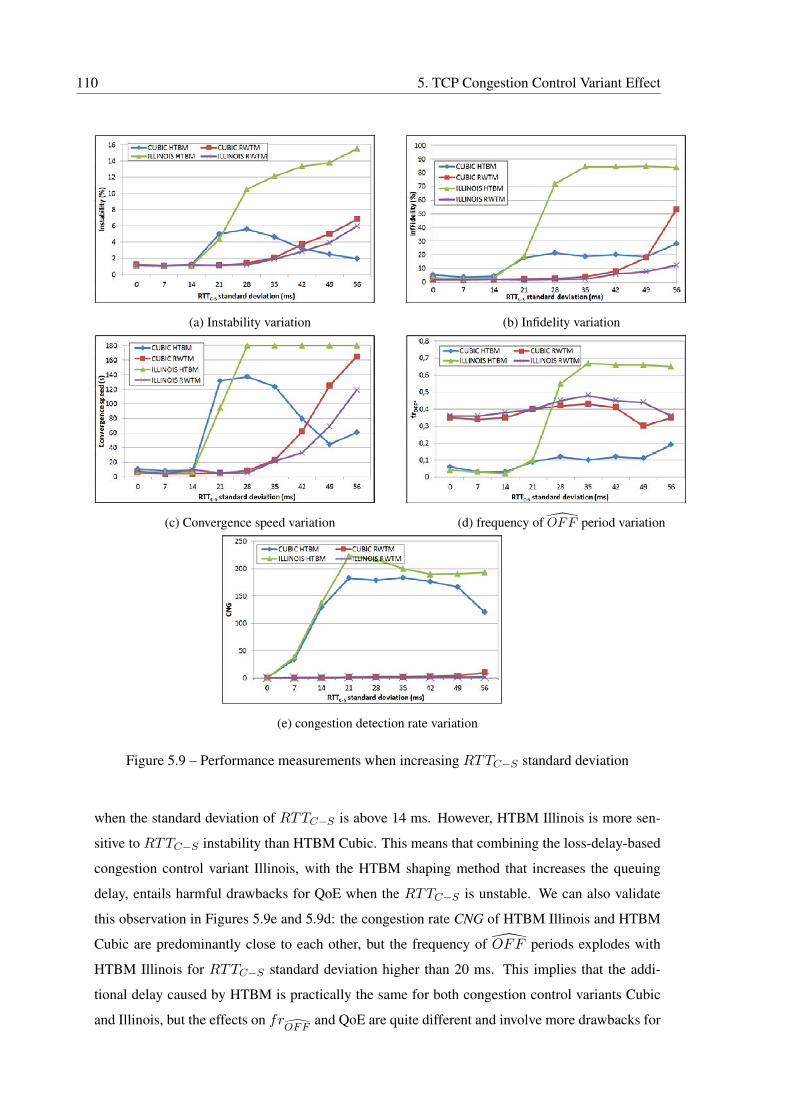
110 5. TCP Congestion Control Variant Effect
(a) Instability variation (b) Infidelity variation
(c) Convergence speed variation (d) frequency of OFF period variation
(e) congestion detection rate variation
Figure 5.9 – Performance measurements when increasing RTTC−S standard deviation
when the standard deviation of RTTC−S is above 14 ms. However, HTBM Illinois is more sen-
sitive to RTTC−S instability than HTBM Cubic. This means that combining the loss-delay-based
congestion control variant Illinois, with the HTBM shaping method that increases the queuing
delay, entails harmful drawbacks for QoE when the RTTC−S is unstable. We can also validate
this observation in Figures 5.9e and 5.9d: the congestion rate CNG of HTBM Illinois and HTBM
Cubic are predominantly close to each other, but the frequency of OFF periods explodes with
HTBM Illinois for RTTC−S standard deviation higher than 20 ms. This implies that the addi-
tional delay caused by HTBM is practically the same for both congestion control variants Cubic
and Illinois, but the effects on frOFF
and QoE are quite different and involve more drawbacks for
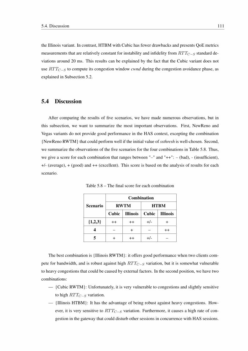
5.4. Discussion 111
the Illinois variant. In contrast, HTBM with Cubic has fewer drawbacks and presents QoE metrics
measurements that are relatively constant for instability and infidelity from RTTC−S standard de-
viations around 20 ms. This results can be explained by the fact that the Cubic variant does not
use RTTC−S to compute its congestion window cwnd during the congestion avoidance phase, as
explained in Subsection 5.2.
5.4 Discussion
After comparing the results of five scenarios, we have made numerous observations, but in
this subsection, we want to summarize the most important observations. First, NewReno and
Vegas variants do not provide good performance in the HAS context, excepting the combination
{NewReno RWTM} that could perform well if the initial value of ssthresh is well-chosen. Second,
we summarize the observations of the five scenarios for the four combinations in Table 5.8. Thus,
we give a score for each combination that ranges between "–" and "++": – (bad), - (insufficient),
+/- (average), + (good) and ++ (excellent). This score is based on the analysis of results for each
scenario.
Table 5.8 – The final score for each combination
Scenario
Combination
RWTM HTBM
Cubic Illinois Cubic Illinois
{1,2,3} ++ ++ +/- +
4 – + – ++
5 + ++ +/- –
The best combination is {Illinois RWTM}: it offers good performance when two clients com-
pete for bandwidth, and is robust against high RTTC−S variation, but it is somewhat vulnerable
to heavy congestions that could be caused by external factors. In the second position, we have two
combinations:
— {Cubic RWTM}: Unfortunately, it is very vulnerable to congestions and slightly sensitive
to high RTTC−S variation.
— {Illinois HTBM}: It has the advantage of being robust against heavy congestions. How-
ever, it is very sensitive to RTTC−S variation. Furthermore, it causes a high rate of con-
gestion in the gateway that could disturb other sessions in concurrence with HAS sessions.
112 5. TCP Congestion Control Variant Effect
5.5 Conclusion
A comparative evaluation has been developed in order to study the effect of combining two
well-known traffic shaping methods (HTBM and our own method RWTM) in the gateway with
four very common TCP congestion algorithms (NewReno, Vegas, Illinois, and Cubic) in the server
in the context of HTTP adaptive streaming technique. We examined the user’s QoE by applying
objective metrics. Furthermore, we observed the evolution of the congestion window on the server
side in order to explain the behavior of each combination and its relationship with QoE metrics.
We also used the congestion rate and the frequency of OFF periods that exceeds retransmission
timeout as indicators. We have addressed many scenarios: two HAS clients competing for the
home bandwidth simultaneously, adding or removing a HAS client, inducing a heavy congestion in
the gateway, and increasing the instability of the round trip time, RTT, between the HAS server and
the HAS client. The results show that there is a significant discordance in performance between
combinations. The best combination that improves the QoE, reduces the congestion rate, and
reduces the OFF periods in the majority of scenarios is when combining the loss-delay-based
congestion control variant, Illinois, which uses the C-AIMD approach, with the TCP flow control
based method, RWTM. The characteristics of the combination of Illinois and RWTM seem to
be similarly robust against high RTT instability. Hence, it would offer good performances in
wireless network, i.e. when the HAS clients are located in wireless home network. Moreover,
this combination does not disturb other real-time streams in the home network because it does
not induce additional queuing delay and it considerably reduces the congestion rate. However, it
is slightly vulnerable to heavy congestions that could be caused by external factors such as other
concurrent streams.
Having extended our knowledge about the combination of TCP congestion control variants
with shaping methods in this work, we intend in the next chapter to design a new TCP congestion
control variant that is compatible with all specifications of HAS and shaping methods.
113
CHAPTER
6 TcpHas: HAS-based TCP
Congestion Control
Variant
6.1 Introduction
The HTTP Adaptive Streaming technology is based on TCP protocol, which is not designed
for video streaming. Many TCP variants have been proposed to resolve the problems of high
bandwidth-delay product (such as Cubic, Illinois, and WestWood+) in order to be more reactive to
achieve high bandwidth in short delay. The high bandwidth-delay product TCP variants seem to
give better performances for HAS service as described in Chapter 5 (see Subsection 5.3.2) than the
previous TCP variants such as NewReno and Vegas. However, until today, there is no proposition
of TCP variant specifically designed for HAS application. Given that HAS differs from other types
of applications by its highly periodical ON-OFF activity pattern, proposing an HAS-based TCP
congestion control variant could improve HAS application performances: Implementing this TCP
variant inside HAS servers could mitigate the OFF period issues, offer better bandwidth share for
each HAS stream, reduce congestion events and improve the QoE of HAS users. Moreover, server-
based shaping methods have been proposed for the same purpose, but they are implemented in the
application layer. Nevertheless, these methods fall within the context of cross-layer optimization
because they are interacting with the TCP layer and its parameters such as the congestion window,
cwnd, and the round-trip time, RTT. Hence, integrating the HAS traffic shaping directly into the
TCP congestion control algorithm would be more practical and easier to manage.
In this chapter, we propose a new HAS-based TCP congestion control variant that we called
"TcpHas" which can be classified as a server-based shaping method totally implemented in the
TCP layer. The remainder of this chapter is organized as the following: First, we give a state of the
art of server-based shaping methods and describe possible optimizations that could be integrated
114 6. TcpHas: HAS-based TCP Congestion Control Variant
into TCP congestion control algorithm in Section 6.2. Second, we describe TcpHas algorithm in
Section 6.3. Finally, we give the performance evaluation of TcpHas under various scenarios in
Section 6.4.
6.2 State of The Art
In the literature, many server-based shaping methods have been proposed in order to improve
the QoE of HAS. Their main common steps can be grouped into two major functions:
1. The estimation of the best feasible quality level, i.e the optimal quality level: this function
is equivalent to the bandwidth manager in the context of gateway-based shaping methods
(Chapter 4)
2. The shaping function of the sending rate which should be suitable to the encoding rate of
the estimated optimal quality level.
The dissimilarity between the server-based shaping methods is located in both functions cited
above. The rest of this chapter will focus on the two functions separately, in Subsection 6.2.1
and 6.2.2, by describing their constraints and their proposed solutions. Then, we overview, in
Subsection 6.2.3, some possible ways to optimize and improve the two functions that provide the
background for TcpHas conception.
6.2.1 Optimal Quality Level Estimation
The major constraint of optimal quality level estimation is that the server has no visibility on
the set of flows which are competing with its corresponding HAS client inside the same home
network.
Akhshabi et al. [7] propose a server-based shaping method that aims to stabilize the quality
level sent by the server by detecting the oscillation events. The shaping function is only activated
when oscillations are detected. An algorithm was proposed to suggest an optimal quality level
based on the history of quality level oscillations. Then, the server shapes its sending rate based
on the encoding bitrate of the estimated optimal quality level. However, when the end-to-end
available bandwidth increases, the HAS player could not increase its quality level when the shaper
is activated. In fact, the sending bitrate is limited on the server side and when the end-to-end
available bandwidth increases, the player is still stable on the same quality level that matches with
the shaping rate. For that, authors deactivate the shaping function for some chunks and use two
TCP parameters, RTT and cwnd, to compute the connection throughput that corresponds to the
6.2. State of The Art 115
end-to-end available bandwidth (cwnd
RTT). If the estimated bandwidth is higher than the shaping
rate, the optimal quality level is increased to the next higher quality level, and the shaping rate is
increased to follow its encoding rate. This method is implemented in the application layer. It takes
as inputs the encoding rates of delivered chunks and two TCP parameters (RTT and cwnd). The
authors indicated that their method stabilizes the competing players inside the same home network
without significant bandwidth utilization loss.
Accordingly, the optimal quality estimation process is based on two different techniques: the
quality level oscillation detection and the bandwidth estimation using the throughput measure-
ment. The former is based on the application layer information (i.e the encoding rate of the actual
and previous sent chunks) and is sufficient to activate the shaping function (i.e the shaper). How-
ever, to verify whether the optimal quality level has been increased or not, the server is obliged
to deactivate the shaper in order to let TCP congestion control algorithm occupy the remaining
capacity available for HAS stream.
Although this proposed method offers performance improvements on both QoE and QoS, the
concept of activating and deactivating the shaper is not sufficiently solid especially against instable
network condition and could raise a number of questions about the duration of deactivation of the
traffic shaping and their impact on increasing the OFF period duration. Besides, this method is not
proactive and the shaper is activated only in the case of quality level oscillation.
What it is missing in this proposed method is a good estimation of the available bandwidth for
the corresponding HAS flow. This method is relying on the throughput measurement during non-
shaped phases. If we could give a bandwidth estimation that is less dependent to the congestion
window value, cwnd, we could keep the shaper activated during the whole HAS stream and adapt
the estimation of optimal quality level to the estimation of available bandwidth.
6.2.2 Shaping Methods
Ghobadi Monia et al. proposed a shaping method called "Trickle" [52] on the server side. This
method was proposed for YouTube since 2011 when it adopted progressive download technology.
The key idea of Trickle is to place a dynamic upper bound on the congestion window (cwnd)
such that TCP itself limits the overall data rate. The server application periodically computes the
cwnd bound from the product between the round-trip time (RTT) and the target streaming bitrate.
Then it uses a socket option to apply it to the TCP socket. Their results show that Trickle reduces
the average RTT by up to 28% and the average TCP loss rate by up to 43%. However, HAS
differs from progressive download by the change of encoding rate during streaming. Nevertheless,
116 6. TcpHas: HAS-based TCP Congestion Control Variant
Trickle method can also be suitable for HAS by adapting the cwnd bound to the encoding rate of
each chunk.
We note that the selection of the shaping rate by the server-based shaping methods does not
mean that the player will automatically start requesting that next higher quality level [7]. One
transition to another shaping rate may take place several chunks later, depending on the player’s
bitrate controller and the server-based shaping method efficiency.
Furthermore, we reported in Chapter 5 that the ssthresh has a predominant effect on conver-
gence speed of the HAS client to select the desired optimal quality level. In fact, when ssthresh
is set higher than the product of shaping rate and the round trip time, the server becomes aggres-
sive and would cause congestions and a reduction of quality level selection on the player side.
In contrast, when ssthresh is set lower than the product of the shaping rate and round trip time,
the congestion window cwnd would take several round trip times to reach the value of this prod-
uct, because in the congestion avoidance phase the increase of cwnd is relatively slow (one MSS
each round trip time). Consequently, the server becomes conservative and takes long duration to
occupy its selected shaping rate. Hence, the player would have difficulties to reach its optimal
quality level.
Accordingly, shaping the sending rate by limiting the congestion window, cwnd, as described
in Trickle, has a good effect for improving the QoE of HAS. However, it is still insufficient to
increase the reactivity of the HAS player and consequently to accelerate the convergence speed.
Hence, to improve the performance of the shaper, a modification of ssthresh is necessary. The
value of ssthresh should be set at the right value that enables the server to rapidly reach the desired
shaping rate.
6.2.3 How Can We Optimize Solutions ?
What we note from the different proposed methods for estimating the optimal quality level is
that we can improve their performances if we would be able to find an efficient end-to-end esti-
mator of available bandwidth, as shown in Subsection 6.2.1. In addition, the only parameter from
application layer that we need for shaping the HAS traffic is the encoding rate of each available
quality level of the corresponding HAS stream. As explained in Subsection 6.2.2, the remaining
parameters are located into the TCP layer: the congestion window cwnd, the slow start thresh-
old ssthresh, and the round-trip time RTT. Adjusting ssthresh value to accelerate the convergence
speed is also our primordial objective.
Accordingly, we said that the best manner to take into consideration the whole optimization
6.2. State of The Art 117
ways that we cited above is to propose a TCP congestion control variant. In fact, adjusting the
TCP behavior to the context of server-based HAS traffic shaping seems to be more efficient than a
cross-layer solution controlled by the application layer. Nevertheless, what it is missing here is to
find an efficient TCP-based method for end-to-end bandwidth estimation.
For the purposes cited above, we sought mechanism that adjusts ssthresh by employing the
output of bandwidth estimator scheme. We found a mechanism, called adaptive decrease mecha-
nism, which has been already used by some TCP congestion control variants. This mechanism
is presented in Subsection 6.2.3.1. Moreover, we overview the bandwidth estimator schemes
used by different TCP variants and we evaluate theoretically their estimation efficiency in Sub-
section 6.2.3.2.
6.2.3.1 Adaptive Decrease Mechanism
In the literature, we found a specific category of TCP congestion control variants that employs
bandwidth estimation for positioning the ssthresh value. This category performs a bandwidth es-
timation scheme, which is updated over time. However, this estimation is taken into consideration
by TCP only when a congestion event is detected. This mechanism of changing the ssthresh after
congestion detection by using bandwidth estimation is classified as adaptive decrease mechanism.
What is beneficial in this mechanism is described in [100] as the following: the adaptive window
setting provides a congestion window which is decreased more in the presence of heavy conges-
tion and less in the presence of light congestion or losses that are not due to congestion, such as
in the case of losses due to unreliable links. Moreover, the updating process of ssthresh is chosen
only after congestion detection. This low frequency of ssthresh updating is justified by Antonio
Capone [24] by the fact that, in the contrary, a frequent updating of ssthresh tends to force the
TCP source into congestion avoidance phase, preventing it from following the variations in the
available bandwidth.
Hence, the unique difference of this category with classical TCP congestion variant is only the
adaptive decrease mechanism when detecting a congestion; i.e when receiving 3 duplicated ACKs
or when the retransmission timeout expires before receiving ACK. This mechanism is described
in Algorithm 4:
We remark that the algorithm employs the estimated bandwidth, Bwe, multiplied by RTTmin
to update the ssthresh value. The use of RTTmin instead of actual RTT is justified by the fact that
RTTmin can be considered as an estimation of RTT of the connection when the network is not
congested.
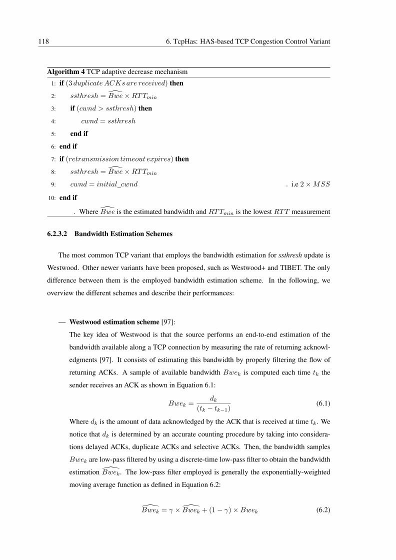
118 6. TcpHas: HAS-based TCP Congestion Control Variant
Algorithm 4 TCP adaptive decrease mechanism
1: if (3 duplicateACKsare received) then
2: ssthresh = Bwe×RTTmin3: if (cwnd > ssthresh) then
4: cwnd = ssthresh
5: end if
6: end if
7: if (retransmission timeout expires) then
8: ssthresh = Bwe×RTTmin9: cwnd = initial_cwnd . i.e 2×MSS
10: end if
. Where Bwe is the estimated bandwidth and RTTmin is the lowest RTT measurement
6.2.3.2 Bandwidth Estimation Schemes
The most common TCP variant that employs the bandwidth estimation for ssthresh update is
Westwood. Other newer variants have been proposed, such as Westwood+ and TIBET. The only
difference between them is the employed bandwidth estimation scheme. In the following, we
overview the different schemes and describe their performances:
— Westwood estimation scheme [97]:
The key idea of Westwood is that the source performs an end-to-end estimation of the
bandwidth available along a TCP connection by measuring the rate of returning acknowl-
edgments [97]. It consists of estimating this bandwidth by properly filtering the flow of
returning ACKs. A sample of available bandwidth Bwek is computed each time tk the
sender receives an ACK as shown in Equation 6.1:
Bwek =dk
(tk − tk−1)(6.1)
Where dk is the amount of data acknowledged by the ACK that is received at time tk. We
notice that dk is determined by an accurate counting procedure by taking into considera-
tions delayed ACKs, duplicate ACKs and selective ACKs. Then, the bandwidth samples
Bwek are low-pass filtered by using a discrete-time low-pass filter to obtain the bandwidth
estimation Bwek. The low-pass filter employed is generally the exponentially-weighted
moving average function as defined in Equation 6.2:
Bwek = γ × Bwek + (1− γ)×Bwek (6.2)
6.2. State of The Art 119
where 0 ≤ γ ≤ 1. Low-pass filtering is necessary since congestion is due to low frequency
components of the available bandwidth, and because delayed ACK option [86, 98].
However, this estimation scheme is affected by the ACK compression phenomenon. This phe-
nomenon occurs when the time spacing between the received ACKs is altered by the congestion of
the routers on the return path [163]. In fact, when ACKs pass through one congested router, which
generates additional queuing delay, they lose their original time spacing because during forwarding
they are spaced by the short ACK transmission time [24]. The result is ACK compression that can
lead to bandwidth overestimation when computing the bandwidth sample Bwek. Moreover, the
low-pass filtering process is also affected by ACK compression because it cannot filter bandwidth
samples that contain high frequency component [98]. Accordingly, the ACK compression causes
a systematic bandwidth overestimation when using Westwood bandwidth estimation scheme. The
ACK compression is commonly observed in real network operation [105] and thus should not be
neglected in the estimation scheme.
Another phenomenon that distorts the estimation scheme of Westwood is clustering: As
explained in [24, 163] the packets belonging to different TCP connections that share the same link
do not intermingle. As a consequence, many consecutive packets of the same connection can be
observed on a single channel. This means that each connection uses the full bandwidth of the link
for the time needed to transmit its cluster of packets. Hence, a problem of fairness between TCP
connections is experienced when the estimation scheme does not take the clustering phenomenon
into consideration and continues to estimate the bandwidth of the whole shared bottleneck link
instead of their available bandwidth.
— Westwood+ estimation scheme [99]
In order to correctly estimate the bandwidth and alleviate the effect of ACK compression
and clustering, a TCP source should observe its own link utilization for a time longer than
the time needed for entire cluster transmission. For this purpose, Westwood+ modifies
the bandwidth estimation mechanism to perform the sampling every RTT instead of every
ACK reception as described in Equation 6.3:
Bwe =dRTTRTT
(6.3)
Where dRTT is the amount of data acknowledged during one RTT . As indicated in [99],
the result is a more accurate bandwidth measurement that ensures better performance when
comparing with NewReno and it is still fair when sharing the network with other TCP
connections. Bwe is updated once every one RTT . The bandwidth estimation samples
are low-pass filtered to give better smoothed estimation Bwe.
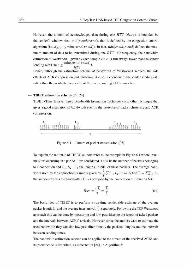
120 6. TcpHas: HAS-based TCP Congestion Control Variant
However, the amount of acknowledged data during one RTT (dRTT ) is bounded by
the sender’s window size, min(cwnd, rwnd), that is defined by the congestion control
algorithm (i.e, dRTT ≤ min(cwnd, rwnd)). In fact, min(cwnd, rwnd) defines the max-
imum amount of data to be transmitted during one RTT . Consequently, the bandwidth
estimation of Westwood+, given by each sampleBwe, is still always lower than the sender
sending rate (Bwe ≤ min(cwnd, rwnd)
RTT).
Hence, although the estimation scheme of bandwidth of Westwood+ reduces the side
effects of ACK compression and clustering, it is still dependent to the sender sending rate
rather than the available bandwidth of the corresponding TCP connection.
— TIBET estimation scheme [25, 24]:
TIBET (Time Interval based Bandwidth Estimation Technique) is another technique that
gives a good estimation of bandwidth even in the presence of packet clustering and ACK
compression.
Figure 6.1 – Pattern of packet transmission [25]
To explain the rationale of TIBET, authors refer to the example in Figure 6.1 where trans-
missions occurring in a period T are considered. Let n be the number of packets belonging
to a connection and L1, L2...Ln the lengths, in bits, of these packets. The average band-
width used by the connection is simply given by1
T
∑ni=1 Li. If we define L =
∑ni=1 Li,
the authors express the bandwidth (Bwe) occupied by the connection as Equation 6.4:
Bwe =nL
T=LTn
(6.4)
The basic idea of TIBET is to perform a run-time sender-side estimate of the average
packet length, L, and the average inter-arrival, Tn , separately. Following the TCP Westwood
approach this can be done by measuring and low-pass filtering the length of acked packets
and the intervals between ACKs’ arrivals. However, since the authors want to estimate the
used bandwidth they can also low-pass filter directly the packets’ lengths and the intervals
between sending times.
The bandwidth estimation scheme can be applied to the stream of the received ACKs and
its pseudocode is described, as indicated in [24], in Algorithm 5:
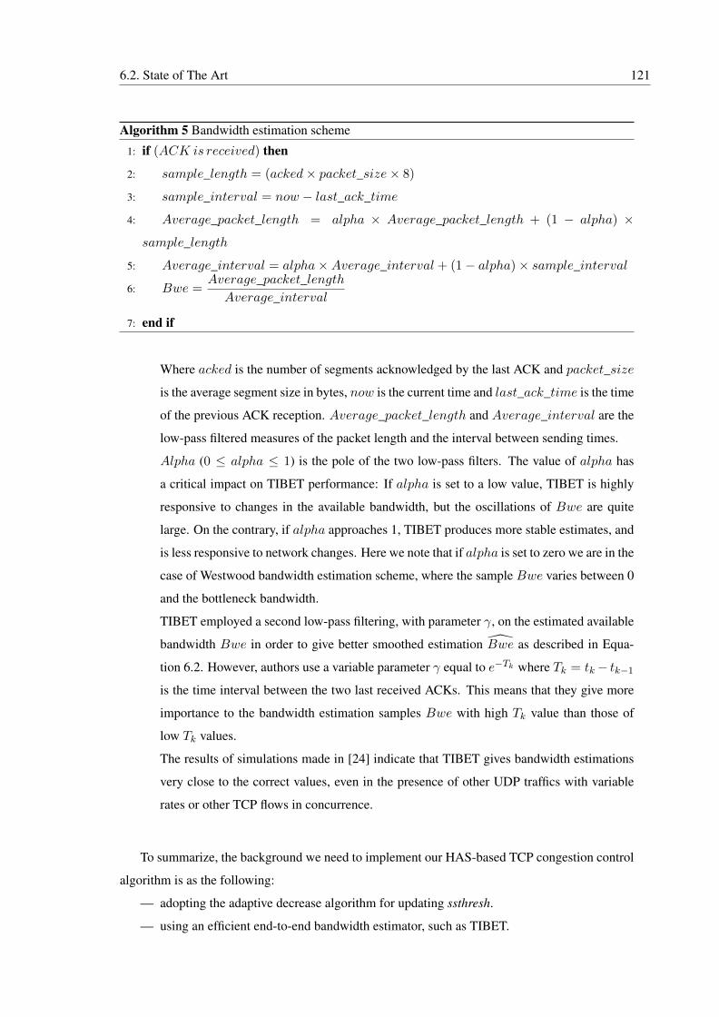
6.2. State of The Art 121
Algorithm 5 Bandwidth estimation scheme
1: if (ACK is received) then
2: sample_length = (acked× packet_size× 8)
3: sample_interval = now − last_ack_time
4: Average_packet_length = alpha × Average_packet_length + (1 − alpha) ×
sample_length
5: Average_interval = alpha×Average_interval + (1− alpha)× sample_interval
6: Bwe =Average_packet_lengthAverage_interval
7: end if
Where acked is the number of segments acknowledged by the last ACK and packet_size
is the average segment size in bytes, now is the current time and last_ack_time is the time
of the previous ACK reception. Average_packet_length and Average_interval are the
low-pass filtered measures of the packet length and the interval between sending times.
Alpha (0 ≤ alpha ≤ 1) is the pole of the two low-pass filters. The value of alpha has
a critical impact on TIBET performance: If alpha is set to a low value, TIBET is highly
responsive to changes in the available bandwidth, but the oscillations of Bwe are quite
large. On the contrary, if alpha approaches 1, TIBET produces more stable estimates, and
is less responsive to network changes. Here we note that if alpha is set to zero we are in the
case of Westwood bandwidth estimation scheme, where the sample Bwe varies between 0
and the bottleneck bandwidth.
TIBET employed a second low-pass filtering, with parameter γ, on the estimated available
bandwidth Bwe in order to give better smoothed estimation Bwe as described in Equa-
tion 6.2. However, authors use a variable parameter γ equal to e−Tk where Tk = tk− tk−1is the time interval between the two last received ACKs. This means that they give more
importance to the bandwidth estimation samples Bwe with high Tk value than those of
low Tk values.
The results of simulations made in [24] indicate that TIBET gives bandwidth estimations
very close to the correct values, even in the presence of other UDP traffics with variable
rates or other TCP flows in concurrence.
To summarize, the background we need to implement our HAS-based TCP congestion control
algorithm is as the following:
— adopting the adaptive decrease algorithm for updating ssthresh.
— using an efficient end-to-end bandwidth estimator, such as TIBET.
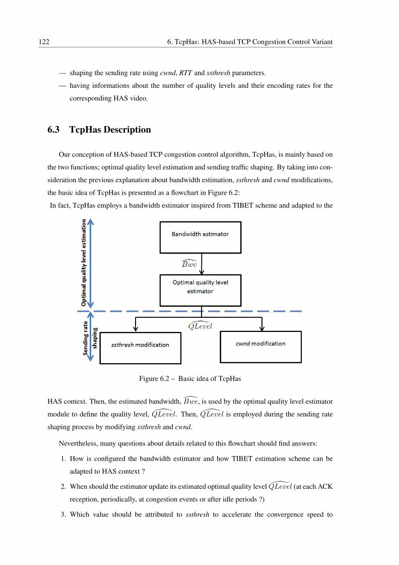
122 6. TcpHas: HAS-based TCP Congestion Control Variant
— shaping the sending rate using cwnd, RTT and ssthresh parameters.
— having informations about the number of quality levels and their encoding rates for the
corresponding HAS video.
6.3 TcpHas Description
Our conception of HAS-based TCP congestion control algorithm, TcpHas, is mainly based on
the two functions; optimal quality level estimation and sending traffic shaping. By taking into con-
sideration the previous explanation about bandwidth estimation, ssthresh and cwnd modifications,
the basic idea of TcpHas is presented as a flowchart in Figure 6.2:
In fact, TcpHas employs a bandwidth estimator inspired from TIBET scheme and adapted to the
Figure 6.2 – Basic idea of TcpHas
HAS context. Then, the estimated bandwidth, Bwe, is used by the optimal quality level estimator
module to define the quality level, QLevel. Then, QLevel is employed during the sending rate
shaping process by modifying ssthresh and cwnd.
Nevertheless, many questions about details related to this flowchart should find answers:
1. How is configured the bandwidth estimator and how TIBET estimation scheme can be
adapted to HAS context ?
2. When should the estimator update its estimated optimal quality level QLevel (at each ACK
reception, periodically, at congestion events or after idle periods ?)
3. Which value should be attributed to ssthresh to accelerate the convergence speed to
6.3. TcpHas Description 123
QLevel quality level ?
4. How should cwnd be limited to match with the sending rate (i.e the encoding rate of
QLevel) ?
In order to answer these four principal questions in a manner that we progressively present
TcpHas algorithm, the remaining of this section is organized as the following: First, we describe
TcpHas’ bandwidth estimator in Subsection 6.3.1. Second, we present TcpHas’ optimal quality
level estimator and the in Subsection 6.3.2. Third, we present the updating process of TcpHas’
ssthresh in Subsection 6.3.3. Finally, we describe how TcpHas adapts the cwnd value to the
shaping rate in Subsection 6.3.4.
6.3.1 Bandwidth Estimator of TcpHas
As described in Section 6.2, TIBET performs better than previous proposed schemes. It re-
duces the effect of ACK compression and packet clustering and is less dependent to the congestion
window, cwnd, than Westwood+.
However, the parameter γ employed by TIBET to smooth the Bwe estimations (see Equa-
tion 6.2) is variable and equal to e−Tk , where Tk is the time interval between the two last received
ACKs [25]. However, this variable parameter is not suitable to the context of HAS. In fact, when
HAS stream has a large OFF period, the HTTP Get request packet sent from client to the server to
ask for a new chunk is considered on the server side as a new ACK. As a consequence, the new
bandwidth estimation sample, Bwe, has an underestimated value and γ is reduced. Hence, this
filter gives higher importance to an underestimated value in the detriment of the previous better
estimations. For example, if OFF period is equal to 1 second, γ is equal to 0.36, which means that
we give a factor of 0.64 to the new underestimated value in the filtering process. Consequently,
the smoothed bandwidth estimation, Bwe, will be reduced at each high OFF period. However, our
objective is rather to maintain a good estimation of available bandwidth, even during idle periods.
For this purpose, we proposed that the parameter γ should be constant in order to avoid the risk of
available bandwidth underestimation during OFF periods.
Hence, the bandwidth estimator of TcpHas is the same as TIBET bandwidth estimation
scheme, except for the low-pass filtering process: we employ a constant value of γ instead of
e−Tk defined by TIBET.
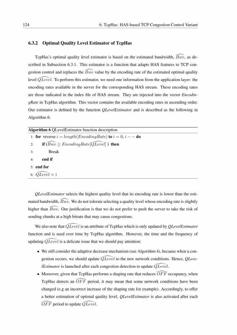
124 6. TcpHas: HAS-based TCP Congestion Control Variant
6.3.2 Optimal Quality Level Estimator of TcpHas
TcpHas’s optimal quality level estimator is based on the estimated bandwidth, Bwe, as de-
scribed in Subsection 6.3.1. This estimator is a function that adapts HAS features to TCP con-
gestion control and replaces the Bwe value by the encoding rate of the estimated optimal quality
level QLevel. To perform this estimator, we need one information from the application layer: the
encoding rates available in the server for the corresponding HAS stream. These encoding rates
are those indicated in the index file of HAS stream. They are injected into the vector Encodin-
gRate in TcpHas algorithm. This vector contains the available encoding rates in ascending order.
Our estimator is defined by the function QLevelEstimator and is described as the following in
Algorithm 6:
Algorithm 6 QLevelEstimator function description
1: for reverse i = length(EncodingRate) to i = 0, i−− do
2: if (Bwe ≥ EncodingRate[QLevel] ) then
3: Break
4: end if
5: end for
6: QLevel = i
QLevelEstimator selects the highest quality level that its encoding rate is lower than the esti-
mated bandwidth, Bwe. We do not tolerate selecting a quality level whose encoding rate is slightly
higher than Bwe. Our justification is that we do not prefer to push the server to take the risk of
sending chunks at a high bitrate that may cause congestions.
We also note that QLevel is an attribute of TcpHas which is only updated by QLevelEstimator
function and is used over time by TcpHas algorithm. However, the time and the frequency of
updating QLevel is a delicate issue that we should pay attention:
• We still consider the adaptive decrease mechanism (see Algorithm 4), because when a con-
gestion occurs, we should update QLevel to the new network conditions. Hence, QLeve-
lEstimator is launched after each congestion detection to update QLevel.
• Moreover, given that TcpHas performs a shaping rate that reduces OFF occupancy, when
TcpHas detects an OFF period, it may mean that some network conditions have been
changed (e.g an incorrect increase of the shaping rate for example). Accordingly, to offer
a better estimation of optimal quality level, QLevelEstimator is also activated after each
OFF period to update QLevel.
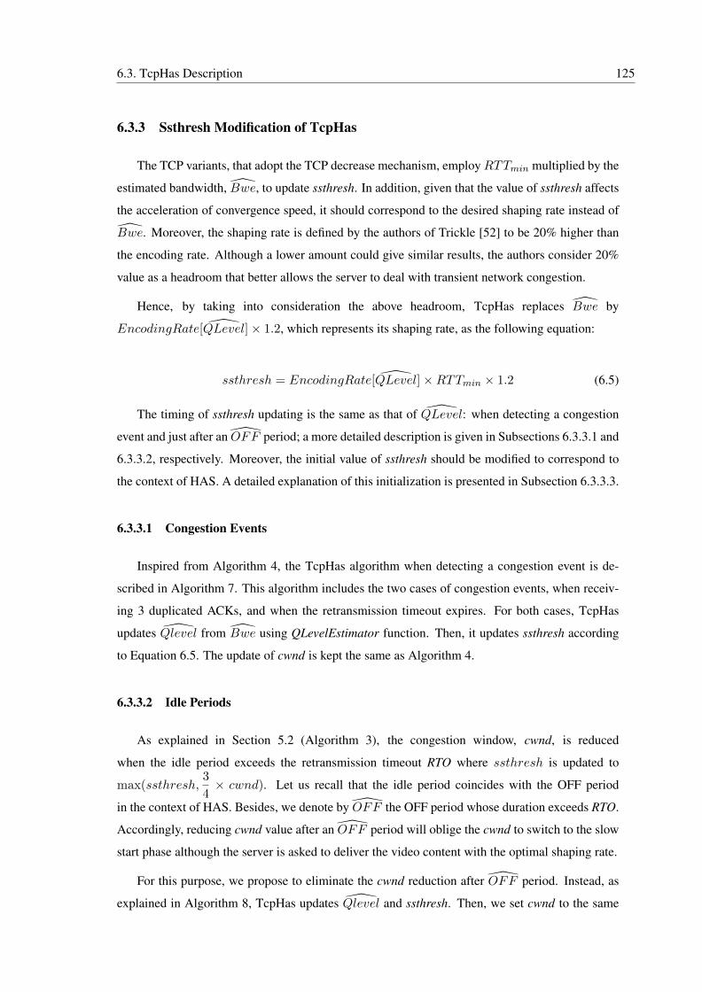
6.3. TcpHas Description 125
6.3.3 Ssthresh Modification of TcpHas
The TCP variants, that adopt the TCP decrease mechanism, employRTTmin multiplied by the
estimated bandwidth, Bwe, to update ssthresh. In addition, given that the value of ssthresh affects
the acceleration of convergence speed, it should correspond to the desired shaping rate instead of
Bwe. Moreover, the shaping rate is defined by the authors of Trickle [52] to be 20% higher than
the encoding rate. Although a lower amount could give similar results, the authors consider 20%
value as a headroom that better allows the server to deal with transient network congestion.
Hence, by taking into consideration the above headroom, TcpHas replaces Bwe by
EncodingRate[QLevel]× 1.2, which represents its shaping rate, as the following equation:
ssthresh = EncodingRate[QLevel]×RTTmin × 1.2 (6.5)
The timing of ssthresh updating is the same as that of QLevel: when detecting a congestion
event and just after an OFF period; a more detailed description is given in Subsections 6.3.3.1 and
6.3.3.2, respectively. Moreover, the initial value of ssthresh should be modified to correspond to
the context of HAS. A detailed explanation of this initialization is presented in Subsection 6.3.3.3.
6.3.3.1 Congestion Events
Inspired from Algorithm 4, the TcpHas algorithm when detecting a congestion event is de-
scribed in Algorithm 7. This algorithm includes the two cases of congestion events, when receiv-
ing 3 duplicated ACKs, and when the retransmission timeout expires. For both cases, TcpHas
updates Qlevel from Bwe using QLevelEstimator function. Then, it updates ssthresh according
to Equation 6.5. The update of cwnd is kept the same as Algorithm 4.
6.3.3.2 Idle Periods
As explained in Section 5.2 (Algorithm 3), the congestion window, cwnd, is reduced
when the idle period exceeds the retransmission timeout RTO where ssthresh is updated to
max(ssthresh,3
4× cwnd). Let us recall that the idle period coincides with the OFF period
in the context of HAS. Besides, we denote by OFF the OFF period whose duration exceeds RTO.
Accordingly, reducing cwnd value after an OFF period will oblige the cwnd to switch to the slow
start phase although the server is asked to deliver the video content with the optimal shaping rate.
For this purpose, we propose to eliminate the cwnd reduction after OFF period. Instead, as
explained in Algorithm 8, TcpHas updates Qlevel and ssthresh. Then, we set cwnd to the same
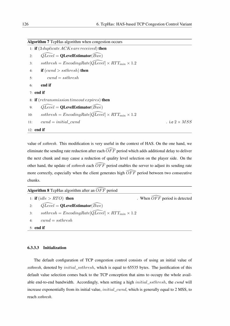
126 6. TcpHas: HAS-based TCP Congestion Control Variant
Algorithm 7 TcpHas algorithm when congestion occurs
1: if (3 duplicateACKsare received) then
2: QLevel = QLevelEstimator(Bwe)
3: ssthresh = EncodingRate[QLevel]×RTTmin × 1.2
4: if (cwnd > ssthresh) then
5: cwnd = ssthresh
6: end if
7: end if
8: if (retransmission timeout expires) then
9: QLevel = QLevelEstimator(Bwe)
10: ssthresh = EncodingRate[QLevel]×RTTmin × 1.2
11: cwnd = initial_cwnd . i.e 2×MSS
12: end if
value of ssthresh. This modification is very useful in the context of HAS. On the one hand, we
eliminate the sending rate reduction after each OFF period which adds additional delay to deliver
the next chunk and may cause a reduction of quality level selection on the player side. On the
other hand, the update of ssthresh each OFF period enables the server to adjust its sending rate
more correctly, especially when the client generates high OFF period between two consecutive
chunks.
Algorithm 8 TcpHas algorithm after an OFF period
1: if (idle > RTO) then . When OFF period is detected
2: QLevel = QLevelEstimator(Bwe)
3: ssthresh = EncodingRate[QLevel]×RTTmin × 1.2
4: cwnd = ssthresh
5: end if
6.3.3.3 Initialization
The default configuration of TCP congestion control consists of using an initial value of
ssthresh, denoted by initial_ssthresh, which is equal to 65535 bytes. The justification of this
default value selection comes back to the TCP conception that aims to occupy the whole avail-
able end-to-end bandwidth. Accordingly, when setting a high initial_ssthresh, the cwnd will
increase exponentially from its initial value, initial_cwnd, which is generally equal to 2 MSS, to
reach ssthresh.
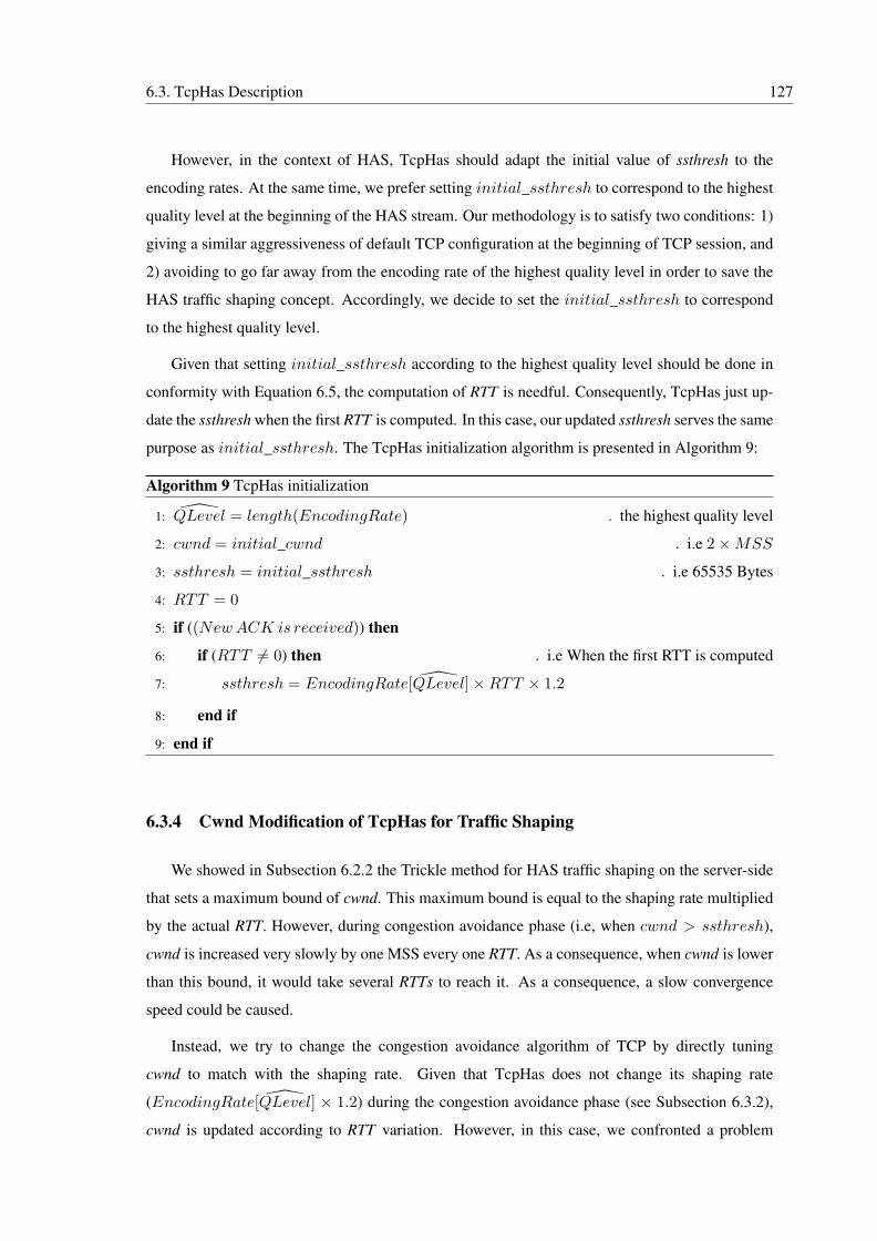
6.3. TcpHas Description 127
However, in the context of HAS, TcpHas should adapt the initial value of ssthresh to the
encoding rates. At the same time, we prefer setting initial_ssthresh to correspond to the highest
quality level at the beginning of the HAS stream. Our methodology is to satisfy two conditions: 1)
giving a similar aggressiveness of default TCP configuration at the beginning of TCP session, and
2) avoiding to go far away from the encoding rate of the highest quality level in order to save the
HAS traffic shaping concept. Accordingly, we decide to set the initial_ssthresh to correspond
to the highest quality level.
Given that setting initial_ssthresh according to the highest quality level should be done in
conformity with Equation 6.5, the computation of RTT is needful. Consequently, TcpHas just up-
date the ssthresh when the first RTT is computed. In this case, our updated ssthresh serves the same
purpose as initial_ssthresh. The TcpHas initialization algorithm is presented in Algorithm 9:
Algorithm 9 TcpHas initialization
1: QLevel = length(EncodingRate) . the highest quality level
2: cwnd = initial_cwnd . i.e 2×MSS
3: ssthresh = initial_ssthresh . i.e 65535 Bytes
4: RTT = 0
5: if ((NewACK is received)) then
6: if (RTT 6= 0) then . i.e When the first RTT is computed
7: ssthresh = EncodingRate[QLevel]×RTT × 1.2
8: end if
9: end if
6.3.4 Cwnd Modification of TcpHas for Traffic Shaping
We showed in Subsection 6.2.2 the Trickle method for HAS traffic shaping on the server-side
that sets a maximum bound of cwnd. This maximum bound is equal to the shaping rate multiplied
by the actual RTT. However, during congestion avoidance phase (i.e, when cwnd > ssthresh),
cwnd is increased very slowly by one MSS every one RTT. As a consequence, when cwnd is lower
than this bound, it would take several RTTs to reach it. As a consequence, a slow convergence
speed could be caused.
Instead, we try to change the congestion avoidance algorithm of TCP by directly tuning
cwnd to match with the shaping rate. Given that TcpHas does not change its shaping rate
(EncodingRate[QLevel] × 1.2) during the congestion avoidance phase (see Subsection 6.3.2),
cwnd is updated according to RTT variation. However, in this case, we confronted a problem
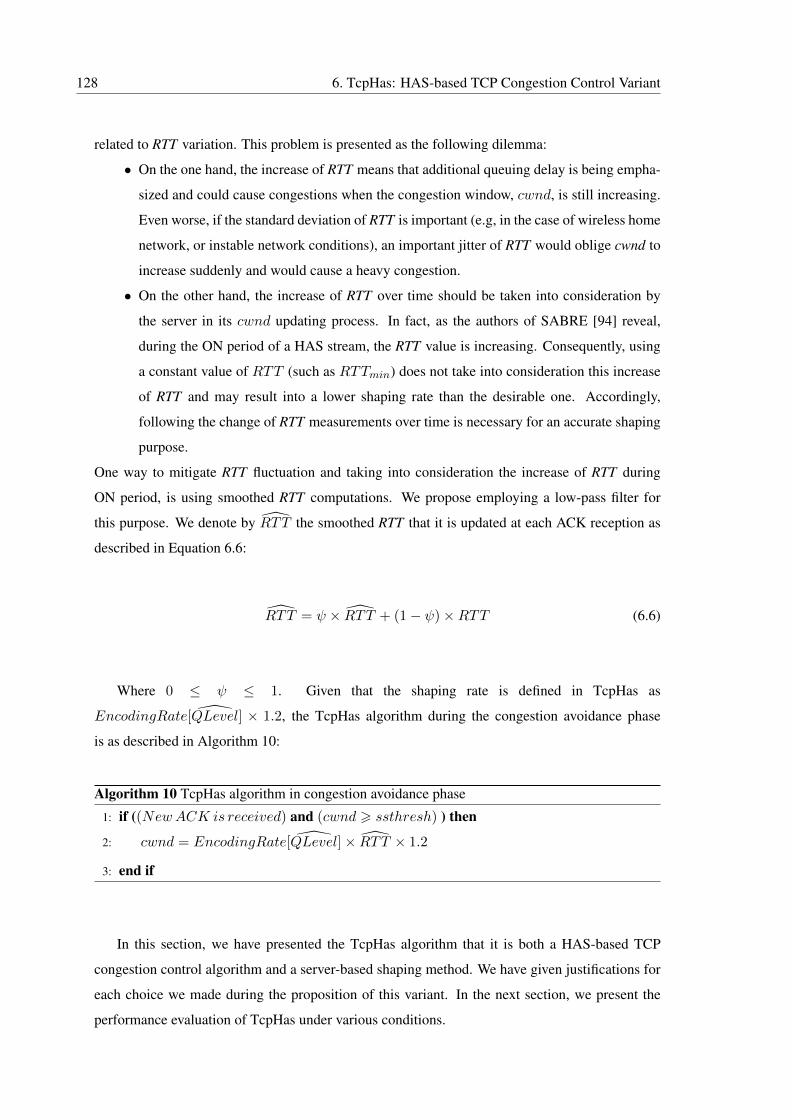
128 6. TcpHas: HAS-based TCP Congestion Control Variant
related to RTT variation. This problem is presented as the following dilemma:
• On the one hand, the increase of RTT means that additional queuing delay is being empha-
sized and could cause congestions when the congestion window, cwnd, is still increasing.
Even worse, if the standard deviation of RTT is important (e.g, in the case of wireless home
network, or instable network conditions), an important jitter of RTT would oblige cwnd to
increase suddenly and would cause a heavy congestion.
• On the other hand, the increase of RTT over time should be taken into consideration by
the server in its cwnd updating process. In fact, as the authors of SABRE [94] reveal,
during the ON period of a HAS stream, the RTT value is increasing. Consequently, using
a constant value of RTT (such as RTTmin) does not take into consideration this increase
of RTT and may result into a lower shaping rate than the desirable one. Accordingly,
following the change of RTT measurements over time is necessary for an accurate shaping
purpose.
One way to mitigate RTT fluctuation and taking into consideration the increase of RTT during
ON period, is using smoothed RTT computations. We propose employing a low-pass filter for
this purpose. We denote by RTT the smoothed RTT that it is updated at each ACK reception as
described in Equation 6.6:
RTT = ψ × RTT + (1− ψ)×RTT (6.6)
Where 0 ≤ ψ ≤ 1. Given that the shaping rate is defined in TcpHas as
EncodingRate[QLevel] × 1.2, the TcpHas algorithm during the congestion avoidance phase
is as described in Algorithm 10:
Algorithm 10 TcpHas algorithm in congestion avoidance phase
1: if ((NewACK is received) and (cwnd > ssthresh) ) then
2: cwnd = EncodingRate[QLevel]× RTT × 1.2
3: end if
In this section, we have presented the TcpHas algorithm that it is both a HAS-based TCP
congestion control algorithm and a server-based shaping method. We have given justifications for
each choice we made during the proposition of this variant. In the next section, we present the
performance evaluation of TcpHas under various conditions.
6.4. TcpHas Evaluation 129
6.4 TcpHas Evaluation
In this section, we evaluate the performance of HAS when employing our proposed TCP con-
gestion control variant, TcpHas. The use case is when HAS players are sharing the same bottle-
neck link and are competing for bandwidth inside the home network. For this evaluations, we used
our implementation of ns-3 as described in Section 3.4 and we employ QoE and QoS metrics in
conformity to their definitions in Section 3.5. We used the same HAS player as described in Sec-
tion 3.2. For all evaluations we used competing players which are playing simultaneously during
180 seconds. Then, we compare performances between TcpHas and Westwood+. We selected
Westwood+ as reference for our evaluation because it is a well-known TCP variant widely used
and it presents better performances than Westwood in the case of ACK compression and cluster-
ing. In addition, the Westwood+ has been used in Chapter 4 in our evaluation. Hence, we tend to
conserve the same reference to offer a better consistency between chapters.
We also notice that the optimal quality level LC−S,opt used in this evaluation is obtained by
selecting the highest encoding rate among quality levels (there are five quality levels with index
0 6 LC−S 6 4 in our implementation) that is lower than the result of dividing the bottleneck
bandwidth by the number of competing HAS players N, as described in Equation 6.7:
LC−S,opt =
{max
06LC−S64(LC−S)
(EncodingRate(LC−S)× 1.2) 6avail_bw
N
}(6.7)
In the case of same encoding rates among competing HAS players, our assumption means that all
competing HAS flows should have the same optimal quality level (i.e, same shaping rate). Here
we focus on fairness of quality level among HAS flows rather than the maximum occupancy of the
bottleneck bandwidth.
For this purpose, we describe the parameter settings that we used during our simulations for
both evaluation and configuration of TcpHas in Subsection 6.4.1. Then we give and comment
results of evaluation in different scenarios: when increasing the number of competing HAS flows
in the home network in Subsection 6.4.2, when varying the HAS player parameters in Subsec-
tion 6.4.3 and when changing network conditions in Subsection 6.4.4.
6.4.1 TcpHas Parameter Settings
The parameter γ of Bwe low-pass filter is configured as a constant value in conformity with
Subsection 6.3.1. We set γ = 0.99 in order to reduce the oscillation of bandwidth estimations,
Bwe, over time.
Moreover, the initial bandwidth estimation value of Bwe is set to the highest encoding rate.
130 6. TcpHas: HAS-based TCP Congestion Control Variant
This initial value is very important for the low-pass filtering process of Bwe. In fact, if the first
value is set to zero or to the first estimation sample, which both do not reflect the right estimation,
the low-pass filtering process with parameter γ = 0.99 will be too slow to reach the correct esti-
mation. In addition, our methodology is to be aggressive at the beginning of the HAS stream and
to try to reach the highest quality level, as explained in Subsection 6.3.3.3. Hence the justification
of adopting the highest encoding rate as initial value of Bwe for TcpHas.
The parameter alpha of TIBET estimation scheme (see Algorithm 5) is chosen empirically in
our simulations and is set to 0.8. In fact, on the one hand, using higher value such as 0.99 pro-
duces more stable estimations but less responsive to network changes: our simulations indicated
that TcpHas becomes too much conservative and is more likely to select lower quality level than
the optimal quality level, even when the HAS client is located alone inside the home network.
On the other hand, when alpha is set at a lower value, such as 0.6, TcpHas becomes more ag-
gressive and have tendency to select the quality level that corresponds to the whole bandwidth of
the home network: our simulations indicated that TcpHas engenders unfairness of quality level
selection between competing HAS players. The cause comes back to the bandwidth estimation at
the beginning where one of the competing players selects the highest quality level, and the rest of
competing players would share the rest of the available bandwidth. Here, we are more likely to
face the problems of ACK compression and packet clustering. For instance, the value of 0.8 seems
to be adequate in the majority of use cases in our simulations.
The parameter ψ used for low-pass filtering the RTT measurements in Subsection 6.3.4 is set to
0.99. Our justification of this value is that it reduces better the RTT fluctuations, and consequently
reduces cwnd fluctuation during congestion avoidance phase. Our simulations indicated that with
ψ = 0.99 TcpHas gives better performances especially when the network conditions degrade.
6.4.2 Effect of Increasing the Number of HAS Flows
In this subsection we show the robustness of TcpHas against the increase of competing HAS
clients in the same home network. Here, we vary the number of competing players from 1 to 9
clients. We select 9 as the maximum number of competing HAS clients, because, in practice, the
number of users inside the home network does not exceed 9 users. The mean performance mea-
surements between competing players are presented in Figure 6.3. We indicate the performance
unfairness measurements between HAS clients with vertical error bars.
Concerning the QoE measurements, the first observation is taken from the Figure 6.3a where
the instability rate of TcpHas is kept much lower than Westwood+ (less than 4%) with a negligible
6.4. TcpHas Evaluation 131
instability unfairness between players, while the instability of Westwood+ increases when increas-
ing the number of competing players. The infidelity and convergence speed of TcpHas gives good
measurements as presented in Figures 6.3b and 6.3c: infidelity rate is lower than 30% and con-
vergence speed lower than 50 seconds. This assumption is valid excepting two cases: when the
number of competing HAS clients is equal to 5 or 9. In fact, in these two cases, TcpHas selects
higher quality level than the optimal quality level that we define for our evaluation; TcpHas was
able to select higher quality level, to converge to it and be stable on it for all the time of simulation.
This result is rather beneficial, because TcpHas was able to maximize the occupancy of the home
bandwidth to near 100% in these two particular cases. Moreover, the initial delay of both TcpHas
and Westwood+ is increased when the number of competing HAS clients increases as presented
in Figure 6.3d: This result is predictable. In fact, during the buffering phase the HAS player asks
for chunks successively. Consequently, when the number of competing HAS clients increases, the
bandwidth would be shared between HAS flows and generates additional delay. We also remark
that TcpHas presents a slight lower initial delay than Weswood+. The main cause is that West-
wood+ is more dependent to cwnd than TcpHas. In fact, both variants select initial ssthresh at
a higher values (at 65535 for Westwood+ and at a value that corresponds to the highest quality
level for TcpHas). Hence, when increasing the number of competing HAS flows, the aggressive-
ness of HAS flows is increased. Consequently, a more imminent congestion event is generated.
Knowing that Westwood+ bandwidth estimation scheme is highly dependent to the congestion
window value, cwnd and given that cwnd cannot be sufficiently increased in the case of imminent
congestion, the new selected ssthresh is set to a low value. In contrast, TcpHas sets ssthresh at
a higher value because it is less dependent to cwnd in its bandwidth estimation scheme. Hence,
TcpHas offers better throughput to HAS clients which slightly accelerates the buffering phase. In
addition, we observe in Figure 6.3i that TcpHas generates no stalling events, unlike Westwood+.
In contrast, Westwood+ causes more stalling events when the number of competing HAS clients
exceeds 7 clients. This observation is a direct result of the high stability rate that TcpHas is able
to preserve even with high number of competing HAS clients.
Concerning QoS measurements, we remark that the OFF period frequency of TcpHas is kept
near to zero and far lower than Westwood+, excepting the case of only one HAS client presents
in the home network. As shown in Figure 6.3e, in the latter case, the optimal quality level is n◦4
whose encoding rate is 4.256 Mbps. Hence, the chunk size is equal to 8.512 Mbits. Consequently,
when TcpHas shapes the sending rate according to this encoding rate while delivering chunks
with large sizes, it would be difficult to reduce OFF periods below the retransmission timeout
duration, RTO. Fortunaltely, we have taken this case into consideration when proposing TcpHas
by eliminating the reduction of cwnd after idle periods in order to preserve high QoE. Moreover,
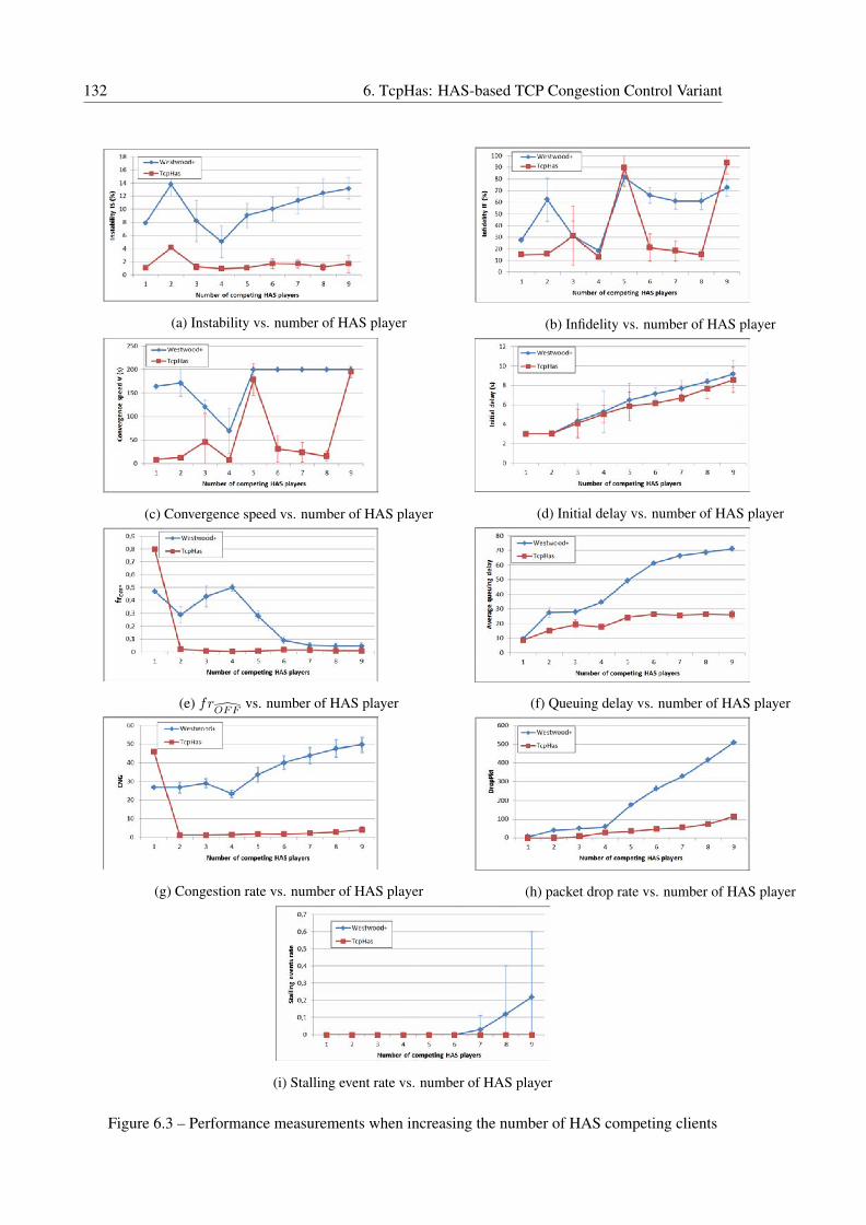
132 6. TcpHas: HAS-based TCP Congestion Control Variant
(a) Instability vs. number of HAS player (b) Infidelity vs. number of HAS player
(c) Convergence speed vs. number of HAS player (d) Initial delay vs. number of HAS player
(e) frOFF
vs. number of HAS player (f) Queuing delay vs. number of HAS player
(g) Congestion rate vs. number of HAS player (h) packet drop rate vs. number of HAS player
(i) Stalling event rate vs. number of HAS player
Figure 6.3 – Performance measurements when increasing the number of HAS competing clients
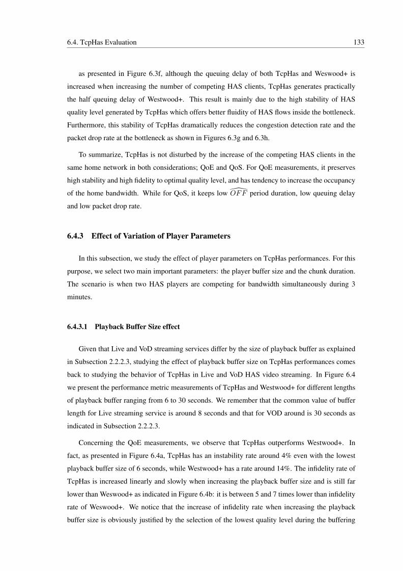
6.4. TcpHas Evaluation 133
as presented in Figure 6.3f, although the queuing delay of both TcpHas and Weswood+ is
increased when increasing the number of competing HAS clients, TcpHas generates practically
the half queuing delay of Westwood+. This result is mainly due to the high stability of HAS
quality level generated by TcpHas which offers better fluidity of HAS flows inside the bottleneck.
Furthermore, this stability of TcpHas dramatically reduces the congestion detection rate and the
packet drop rate at the bottleneck as shown in Figures 6.3g and 6.3h.
To summarize, TcpHas is not disturbed by the increase of the competing HAS clients in the
same home network in both considerations; QoE and QoS. For QoE measurements, it preserves
high stability and high fidelity to optimal quality level, and has tendency to increase the occupancy
of the home bandwidth. While for QoS, it keeps low OFF period duration, low queuing delay
and low packet drop rate.
6.4.3 Effect of Variation of Player Parameters
In this subsection, we study the effect of player parameters on TcpHas performances. For this
purpose, we select two main important parameters: the player buffer size and the chunk duration.
The scenario is when two HAS players are competing for bandwidth simultaneously during 3
minutes.
6.4.3.1 Playback Buffer Size effect
Given that Live and VoD streaming services differ by the size of playback buffer as explained
in Subsection 2.2.2.3, studying the effect of playback buffer size on TcpHas performances comes
back to studying the behavior of TcpHas in Live and VoD HAS video streaming. In Figure 6.4
we present the performance metric measurements of TcpHas and Westwood+ for different lengths
of playback buffer ranging from 6 to 30 seconds. We remember that the common value of buffer
length for Live streaming service is around 8 seconds and that for VOD around is 30 seconds as
indicated in Subsection 2.2.2.3.
Concerning the QoE measurements, we observe that TcpHas outperforms Westwood+. In
fact, as presented in Figure 6.4a, TcpHas has an instability rate around 4% even with the lowest
playback buffer size of 6 seconds, while Westwood+ has a rate around 14%. The infidelity rate of
TcpHas is increased linearly and slowly when increasing the playback buffer size and is still far
lower than Weswood+ as indicated in Figure 6.4b: it is between 5 and 7 times lower than infidelity
rate of Weswood+. We notice that the increase of infidelity rate when increasing the playback
buffer size is obviously justified by the selection of the lowest quality level during the buffering
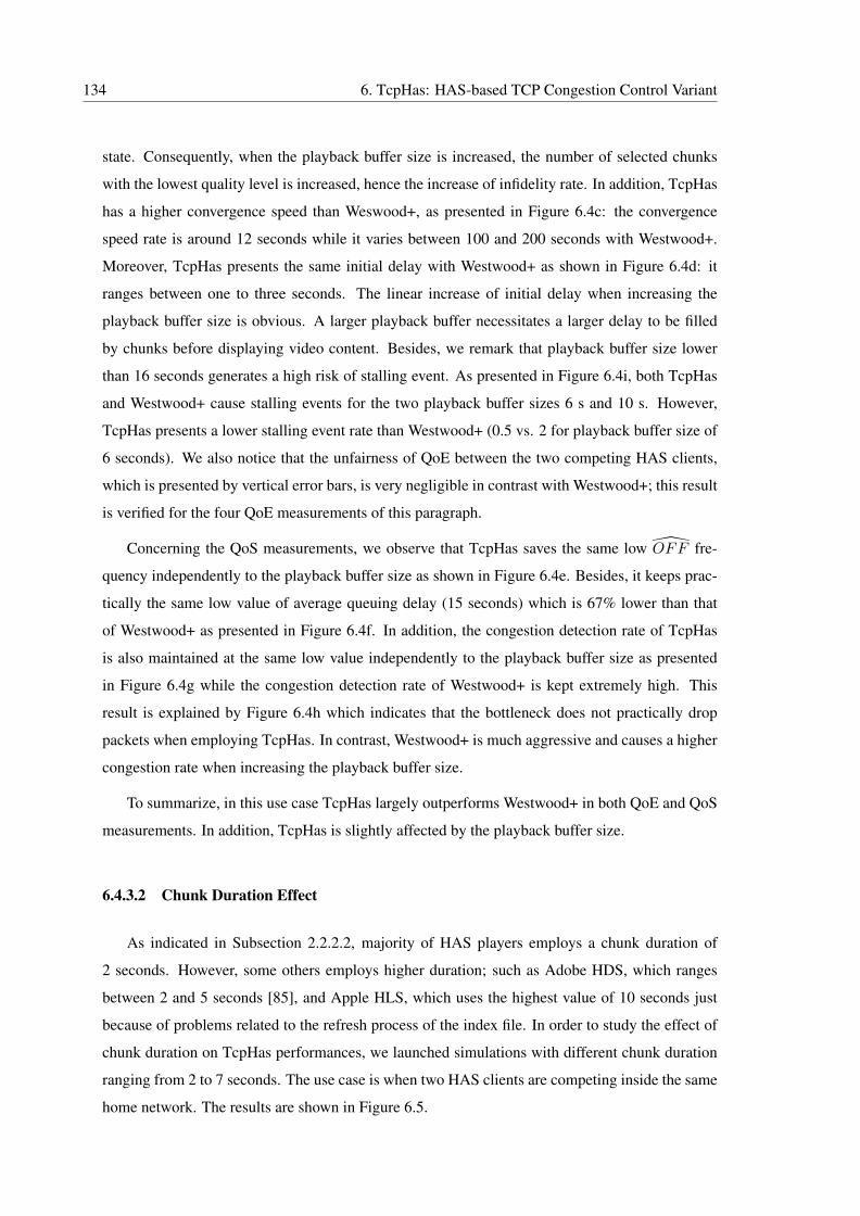
134 6. TcpHas: HAS-based TCP Congestion Control Variant
state. Consequently, when the playback buffer size is increased, the number of selected chunks
with the lowest quality level is increased, hence the increase of infidelity rate. In addition, TcpHas
has a higher convergence speed than Weswood+, as presented in Figure 6.4c: the convergence
speed rate is around 12 seconds while it varies between 100 and 200 seconds with Westwood+.
Moreover, TcpHas presents the same initial delay with Westwood+ as shown in Figure 6.4d: it
ranges between one to three seconds. The linear increase of initial delay when increasing the
playback buffer size is obvious. A larger playback buffer necessitates a larger delay to be filled
by chunks before displaying video content. Besides, we remark that playback buffer size lower
than 16 seconds generates a high risk of stalling event. As presented in Figure 6.4i, both TcpHas
and Westwood+ cause stalling events for the two playback buffer sizes 6 s and 10 s. However,
TcpHas presents a lower stalling event rate than Westwood+ (0.5 vs. 2 for playback buffer size of
6 seconds). We also notice that the unfairness of QoE between the two competing HAS clients,
which is presented by vertical error bars, is very negligible in contrast with Westwood+; this result
is verified for the four QoE measurements of this paragraph.
Concerning the QoS measurements, we observe that TcpHas saves the same low OFF fre-
quency independently to the playback buffer size as shown in Figure 6.4e. Besides, it keeps prac-
tically the same low value of average queuing delay (15 seconds) which is 67% lower than that
of Westwood+ as presented in Figure 6.4f. In addition, the congestion detection rate of TcpHas
is also maintained at the same low value independently to the playback buffer size as presented
in Figure 6.4g while the congestion detection rate of Westwood+ is kept extremely high. This
result is explained by Figure 6.4h which indicates that the bottleneck does not practically drop
packets when employing TcpHas. In contrast, Westwood+ is much aggressive and causes a higher
congestion rate when increasing the playback buffer size.
To summarize, in this use case TcpHas largely outperforms Westwood+ in both QoE and QoS
measurements. In addition, TcpHas is slightly affected by the playback buffer size.
6.4.3.2 Chunk Duration Effect
As indicated in Subsection 2.2.2.2, majority of HAS players employs a chunk duration of
2 seconds. However, some others employs higher duration; such as Adobe HDS, which ranges
between 2 and 5 seconds [85], and Apple HLS, which uses the highest value of 10 seconds just
because of problems related to the refresh process of the index file. In order to study the effect of
chunk duration on TcpHas performances, we launched simulations with different chunk duration
ranging from 2 to 7 seconds. The use case is when two HAS clients are competing inside the same
home network. The results are shown in Figure 6.5.
6.4. TcpHas Evaluation 135
(a) Instability vs. playback buffer size (b) Infidelity vs. playback buffer size
(c) Convergence speed vs. playback buffer size (d) Initial delay vs. playback buffer size
(e) frOFF
vs. playback buffer size (f) Queuing delay vs. playback buffer size
(g) Congestion rate vs. playback buffer size (h) Packet drop rate vs. playback buffer size
(i) Stalling event rate vs. playback buffer size
Figure 6.4 – Performance measurements when increasing the playback buffer size
136 6. TcpHas: HAS-based TCP Congestion Control Variant
Concerning the QoE measurements, we observe in Figure 6.5a that the instability rate of
TcpHas decreases from 4% to less than 2% when the chunk duration increases from 2 seconds
to 7 seconds. Similarly, Westwood+ decreases from 14% to 5%. Here, we notice that TcpHas is
much more stable than Westwood+ while they both improve their stability when increasing the
chunk duration. Moreover, the infidelity rate of TcpHas is maintained lower than Westwood+ (for
example 15% vs. 57% when using a 4-second-duration chunk) as shown in Figure 6.5b. This rate
is decreased for Westwood+ when increasing the chunk duration. However, we observe that the
infidelity suddenly increases with a high unfairness value (indicated by the red vertical error bars)
with TcpHas when the chunk duration is higher than 5 seconds. When examining the quality level
selection of both clients, we found that one of the players selects a higher quality level than the de-
fined optimal quality level, LC−S,opt. Given that the sum of the encoding rates of the two selected
quality levels does not exceed the home bandwidth but, instead, it maximizes its occupancy, we
can say that this result is rather positive. The cause of this behavior change of TcpHas is explained
in Subsection 2.4.2: a larger chunk duration offers higher quality selection and gives better stabil-
ity. Hence, when TcpHas estimates the bandwidth with a large chunk duration, the estimation is
much stable and much close to the real available bandwidth. Consequently, TcpHas tolerates to
set QLevel higher than LC−S,opt and adapts the shaping rate to its corresponding encoding rate
for one of the two HAS flows. The same remark is given for the convergence speed measurement
as indicated in Figure 6.5c. We observe that TcpHas offers and maintains a much higher conver-
gence speed than Westwood+ (lower than 13 seconds vs. higher that 100 seconds). When the
chunk duration is higher than 5 seconds, TcpHas rapidly converges to the selected quality levels
that maximize the bandwidth occupancy. Accordingly, we can conclude that increasing the chunk
duration improves the three QoE measurements (instability, infidelity and convergence speed) of
TcpHas; even a duration of chunk higher than 5 seconds would further improve the bandwidth
occupancy. Moreover, we observe in Figure 6.5d that the initial delay of both TcpHas and West-
wood+ slightly decreases when increasing the chunk duration. Although TcpHas records slightly
higher initial delay, it does not disturb the user’s QoE because it is still low (lower than 3 seconds)
and lower than the threshold of 16 seconds defined in [65] (see Subsection 2.4.1.2). We also note
that no stalling event has been recorded for both TCP variants.
Concerning the QoS measurements, we remark that the OFF frequency is suddenly increased
from a chunk duration of 2 seconds to 4 seconds as shown in Figure 6.5e and becomes stable
around 0.85 OFF period per chunk. This result is expected, because reducing the OFF periods of
large chunk durations below the retransmission timeout duration, RTO, during the shaping process
becomes more difficult. The QoE has not been affected by this parameter modification because
we eliminated in TcpHas the reduction of cwnd after each idle period. This modification was able
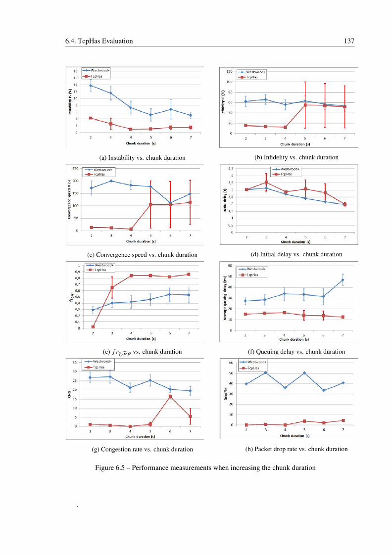
6.4. TcpHas Evaluation 137
(a) Instability vs. chunk duration (b) Infidelity vs. chunk duration
(c) Convergence speed vs. chunk duration (d) Initial delay vs. chunk duration
(e) frOFF
vs. chunk duration (f) Queuing delay vs. chunk duration
(g) Congestion rate vs. chunk duration (h) Packet drop rate vs. chunk duration
Figure 6.5 – Performance measurements when increasing the chunk duration
.
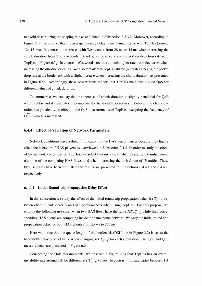
138 6. TcpHas: HAS-based TCP Congestion Control Variant
to avoid destabilizing the shaping rate as explained in Subsection 6.3.3.2. Moreover, according to
Figure 6.5f, we observe that the average queuing delay is maintained stable with TcpHas (around
12∼15 ms). In contrast, it increases with Westwood+ from 28 ms to 45 ms when increasing the
chunk duration from 2 to 7 seconds. Besides, we observe a low congestion detection rate with
TcpHas in Figure 6.5g. In contrast, Westwood+ records a much higher rate but it decreases when
increasing the duration of chunk. We also remark that TcpHas always generates a negligible packet
drop rate at the bottleneck with a slight increase when increasing the chunk duration, as presented
in Figure 6.5h. Accordingly, these observations reflects that TcpHas maintains a good QoS for
different values of chunk duration.
To summarise, we can say that the increase of chunk duration is slightly beneficial for QoE
with TcpHas and it stimulates it to improve the bandwidth occupancy. However, the chunk du-
ration has practically no effect on the QoS measurements of TcpHas, excepting the frequency of
OFF which is increased.
6.4.4 Effect of Variation of Network Parameters
Network conditions have a direct implication on the HAS performances because they highly
affect the behavior of HAS players as overviewed in Subsection 2.4.2. In order to study the effect
of the network conditions on TcpHas, we select two use cases: when changing the initial round
trip time of the competing HAS flows, and when increasing the arrival rate of IP traffic. These
two use cases have been simulated and results are presented in Subsections 6.4.4.1 and 6.4.4.2,
respectively.
6.4.4.1 Initial Round-trip Propagation Delay Effect
In this subsection we study the effect of the initial round-trip propagation delay RTT 0C−S be-
tween client C and server S on HAS performances when using TcpHas. For this purpose, we
employ the following use case: when two HAS flows have the same RTT 0C−S while their corre-
sponding HAS clients are competing inside the same home network. We vary the initial round-trip
propagation delay for both HAS clients from 25 ms to 200 ms.
Here we notice that the queue length of the bottleneck (DSLLine in Figure 3.2) is set to the
bandwidth delay product value when changing RTT 0C−S for each simulation. The QoE and QoS
measurements are presented in Figure 6.6.
Concerning the QoE measurements, we observe in Figure 6.6a that TcpHas has an overall
instability rate around 5% for different RTT 0C−S values. In contrast, this rate varies between 1%
6.4. TcpHas Evaluation 139
and 15%. TcpHas gives more guarantee of a good rate of instability. Moreover, we observe in
Figure 6.6b that TcpHas have a low instability metric when RTT 0C−S is ranging between 25 ms
and 100 ms. However, when increasing RTT 0C−S above 125 ms, the infidelity rate decreases to
reach 60% with a high infidelity unfairness value between the two competing clients (indicated
by red vertical error bars). When verifying the results of simulations, we found that one of the
competing clients select quality level 4 instead of quality level 3. Here we note that the optimal
quality level used for our evaluation, LC−S,opt, is equal to 3. In addition, we found that the
estimated optimal quality level of TcpHas, QLevel, is set to 4 instead of 3 for only one TCP
session. Hence, TcpHas offers a higher quality level for one HAS flows. Given that the sum of
the encoding rates of the two selected quality levels (3 and 4) does not exceed the total home
bandwidth but, instead, it maximizes its occupation, we can say that this result is rather positive.
The cause of this behavior of TcpHas for high RTT 0C−S is the length of the bottleneck queue
length. In fact, as we indicated above, this queue length is equal to the bandwidth-delay product.
The bandwidth used for this computation is the total home bandwidth. Accordingly, the remaining
amount of subtraction between the available bandwidth and two times the encoding rate of the
optimal quality level in our case is relatively important (it is equal to 4.1 Mbps in our simulations).
Multiplying this value with a higher RTT 0C−S generates a high supplementary available space in
the bottleneck queue. In addition to that, with a high RTT 0C−S value, the HAS flow fills slowly
the bottleneck queue. Consequently, TcpHas finds that it could select a higher quality level easily.
We also remark that the convergence speed to the estimated optimal quality level is very low as for
lower RTT 0C−S values as shown in Figure 6.6c. However, when increasing RTT 0
C−S above 125
ms , the convergence speed increases suddenly. We verify that the players converge rapidly to the
selected quality levels (3 and 4) instead of the quality level 3, which is rather beneficial. Moreover,
TcpHas offers practically the same initial delay as Westwood+ as shown in Figure 6.6d. They
both have their initial delay increased when using higher RTT 0C−S values. This result is obvious
because increasing RTT 0C−S increases the transmission delay and, consequently, increases the
buffering delay. Besides, the initial delay is kept relatively low, 5.3 seconds even with RTT 0C−S
equals to 200 ms. We also note that no stalling events have been recorded for the simulations of
this subsection.
Concerning the QoS measurements, we remark that TcpHas keeps a low frequency of OFF
periods for highRTT 0C−S values as presented in Figure 6.6e. Moreover, the mean queuing delay of
TcpHas is increased from 5 ms to 40 ms as shown in Figure 6.6f. However, in terms of percentage
and the quality level selection, the queuing delay of TcpHas is much lower than Weswood+. In
addition, we observe in Figure 6.6g and Figure 6.6h that the congestion detection rate and the
packet drop rate at the bottleneck of TcpHas is very negligible when RTT 0C−S is lower than 125
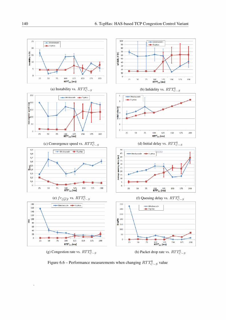
140 6. TcpHas: HAS-based TCP Congestion Control Variant
(a) Instability vs. RTT 0C−S (b) Infidelity vs. RTT 0
C−S
(c) Convergence speed vs. RTT 0C−S (d) Initial delay vs. RTT 0
C−S
(e) frOFF
vs. RTT 0C−S (f) Queuing delay vs. RTT 0
C−S
(g) Congestion rate vs. RTT 0C−S (h) Packet drop rate vs. RTT 0
C−S
Figure 6.6 – Performance measurements when changing RTT 0C−S value
.
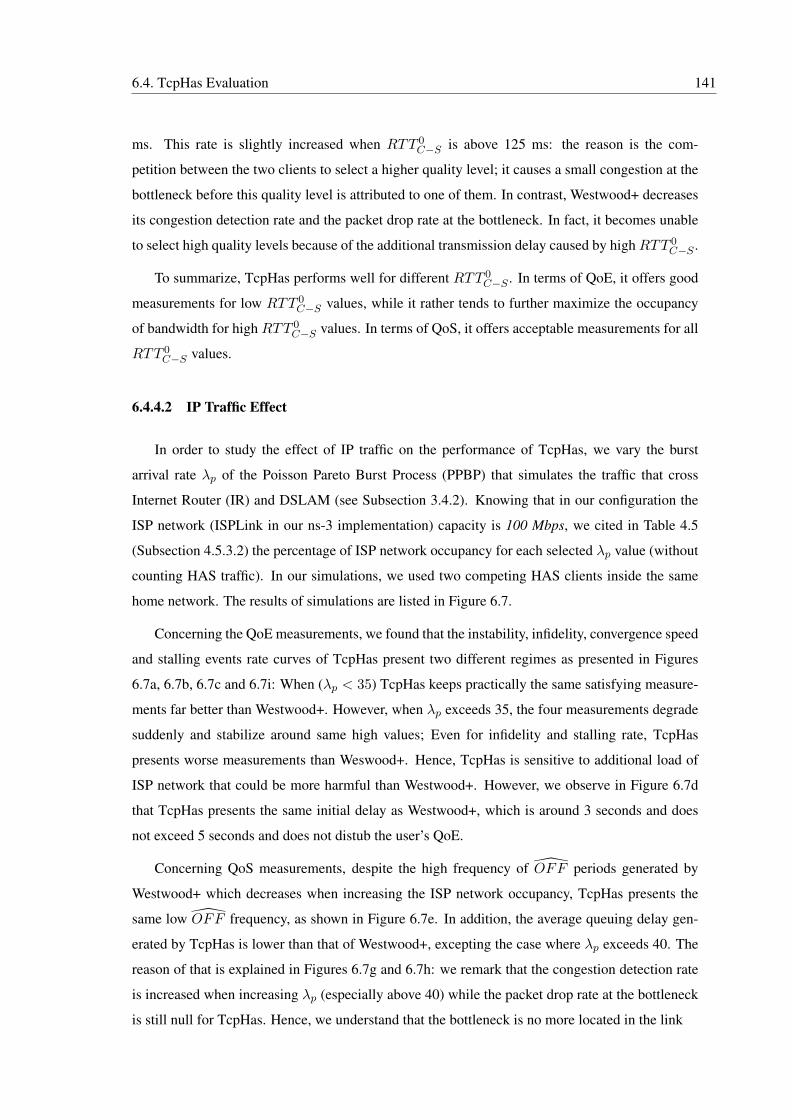
6.4. TcpHas Evaluation 141
ms. This rate is slightly increased when RTT 0C−S is above 125 ms: the reason is the com-
petition between the two clients to select a higher quality level; it causes a small congestion at the
bottleneck before this quality level is attributed to one of them. In contrast, Westwood+ decreases
its congestion detection rate and the packet drop rate at the bottleneck. In fact, it becomes unable
to select high quality levels because of the additional transmission delay caused by highRTT 0C−S .
To summarize, TcpHas performs well for different RTT 0C−S . In terms of QoE, it offers good
measurements for low RTT 0C−S values, while it rather tends to further maximize the occupancy
of bandwidth for high RTT 0C−S values. In terms of QoS, it offers acceptable measurements for all
RTT 0C−S values.
6.4.4.2 IP Traffic Effect
In order to study the effect of IP traffic on the performance of TcpHas, we vary the burst
arrival rate λp of the Poisson Pareto Burst Process (PPBP) that simulates the traffic that cross
Internet Router (IR) and DSLAM (see Subsection 3.4.2). Knowing that in our configuration the
ISP network (ISPLink in our ns-3 implementation) capacity is 100 Mbps, we cited in Table 4.5
(Subsection 4.5.3.2) the percentage of ISP network occupancy for each selected λp value (without
counting HAS traffic). In our simulations, we used two competing HAS clients inside the same
home network. The results of simulations are listed in Figure 6.7.
Concerning the QoE measurements, we found that the instability, infidelity, convergence speed
and stalling events rate curves of TcpHas present two different regimes as presented in Figures
6.7a, 6.7b, 6.7c and 6.7i: When (λp < 35) TcpHas keeps practically the same satisfying measure-
ments far better than Westwood+. However, when λp exceeds 35, the four measurements degrade
suddenly and stabilize around same high values; Even for infidelity and stalling rate, TcpHas
presents worse measurements than Weswood+. Hence, TcpHas is sensitive to additional load of
ISP network that could be more harmful than Westwood+. However, we observe in Figure 6.7d
that TcpHas presents the same initial delay as Westwood+, which is around 3 seconds and does
not exceed 5 seconds and does not distub the user’s QoE.
Concerning QoS measurements, despite the high frequency of OFF periods generated by
Westwood+ which decreases when increasing the ISP network occupancy, TcpHas presents the
same low OFF frequency, as shown in Figure 6.7e. In addition, the average queuing delay gen-
erated by TcpHas is lower than that of Westwood+, excepting the case where λp exceeds 40. The
reason of that is explained in Figures 6.7g and 6.7h: we remark that the congestion detection rate
is increased when increasing λp (especially above 40) while the packet drop rate at the bottleneck
is still null for TcpHas. Hence, we understand that the bottleneck is no more located in the link
142 6. TcpHas: HAS-based TCP Congestion Control Variant
(a) Instability vs. λp (b) Infidelity vs. λp
(c) Convergence speed vs. λp (d) Initial delay vs. λp
(e) frOFF
vs. λp (f) Queuing delay vs. λp
(g) Congestion rate vs. λp (h) Packet drop rate vs. λp
(i) Stalling event rate vs. λp
Figure 6.7 – Performance measurements when increasing PPBP burst arrival rate λp
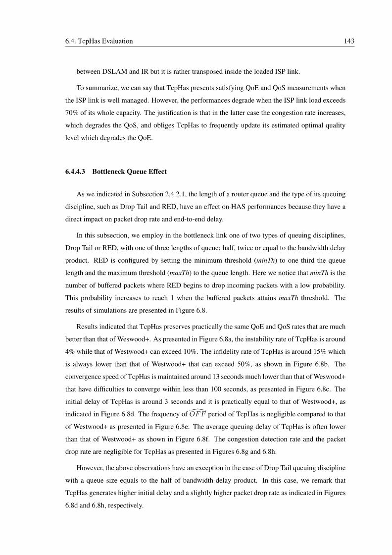
6.4. TcpHas Evaluation 143
between DSLAM and IR but it is rather transposed inside the loaded ISP link.
To summarize, we can say that TcpHas presents satisfying QoE and QoS measurements when
the ISP link is well managed. However, the performances degrade when the ISP link load exceeds
70% of its whole capacity. The justification is that in the latter case the congestion rate increases,
which degrades the QoS, and obliges TcpHas to frequently update its estimated optimal quality
level which degrades the QoE.
6.4.4.3 Bottleneck Queue Effect
As we indicated in Subsection 2.4.2.1, the length of a router queue and the type of its queuing
discipline, such as Drop Tail and RED, have an effect on HAS performances because they have a
direct impact on packet drop rate and end-to-end delay.
In this subsection, we employ in the bottleneck link one of two types of queuing disciplines,
Drop Tail or RED, with one of three lengths of queue: half, twice or equal to the bandwidth delay
product. RED is configured by setting the minimum threshold (minTh) to one third the queue
length and the maximum threshold (maxTh) to the queue length. Here we notice that minTh is the
number of buffered packets where RED begins to drop incoming packets with a low probability.
This probability increases to reach 1 when the buffered packets attains maxTh threshold. The
results of simulations are presented in Figure 6.8.
Results indicated that TcpHas preserves practically the same QoE and QoS rates that are much
better than that of Weswood+. As presented in Figure 6.8a, the instability rate of TcpHas is around
4% while that of Westwood+ can exceed 10%. The infidelity rate of TcpHas is around 15% which
is always lower than that of Westwood+ that can exceed 50%, as shown in Figure 6.8b. The
convergence speed of TcpHas is maintained around 13 seconds much lower than that of Weswood+
that have difficulties to converge within less than 100 seconds, as presented in Figure 6.8c. The
initial delay of TcpHas is around 3 seconds and it is practically equal to that of Westwood+, as
indicated in Figure 6.8d. The frequency of OFF period of TcpHas is negligible compared to that
of Westwood+ as presented in Figure 6.8e. The average queuing delay of TcpHas is often lower
than that of Westwood+ as shown in Figure 6.8f. The congestion detection rate and the packet
drop rate are negligible for TcpHas as presented in Figures 6.8g and 6.8h.
However, the above observations have an exception in the case of Drop Tail queuing discipline
with a queue size equals to the half of bandwidth-delay product. In this case, we remark that
TcpHas generates higher initial delay and a slightly higher packet drop rate as indicated in Figures
6.8d and 6.8h, respectively.
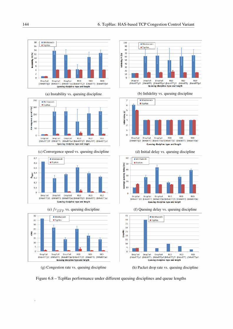
144 6. TcpHas: HAS-based TCP Congestion Control Variant
(a) Instability vs. queuing discipline (b) Infidelity vs. queuing discipline
(c) Convergence speed vs. queuing discipline (d) Initial delay vs. queuing discipline
(e) frOFF
vs. queuing discipline (f) Queuing delay vs. queuing discipline
(g) Congestion rate vs. queuing discipline (h) Packet drop rate vs. queuing discipline
Figure 6.8 – TcpHas performance under different queuing disciplines and queue lengths
.
6.5. Conclusion 145
Accordingly, we can say that TcpHas maintains its good QoE and QoS measurements for the
two types of queuing disciplines, Drop Tail and RED, with different queue lengths. We may add
that using RED queuing discipline is more safe.
6.5 Conclusion
In this chapter, we have presented server-based shaping methods that aim to stabilize the video
quality level and improve the QoE of HAS users. We have shown that they employ two functions;
1) the optimal quality level estimation of HAS flow, and 2) shaping the sending rate according to
the encoding rate of this level. We have shown that the first function depends on the end-to-end
bandwidth estimation, which can be computed using the arrival times of ACKs. We have proved
that the estimation scheme of TIBET offers more accurate estimations with less dependency to
actual throughput value and reduces the drawbacks of ACK compression and clustering. We have
indicated that the second function is dependent to the TCP layer parameters; it is highly dependent
to the congestion window, cwnd, and it can further improve performances by dynamically adjust-
ing the slow start threshold, ssthresh, on the product between the round-trip time, RTT, and the
encoding bitrate of the estimated optimal quality level.
Based on this detailed analysis, we have proposed and described TcpHas, an HAS-based TCP
congestion control variant that serves the same role of a server-based HAS traffic shaping method.
Our proposed algorithm is totally implemented in the TCP layer and obtains the encoding rate of
the available quality levels of the corresponding HAS flow from the application layer (the index
file). It is inspired from TCP adaptive decrease mechanism and employs the end-to-end bandwidth
estimation of TIBET in order to estimate the optimal quality level. Then, it shapes the sending
rate to correspond to the encoding rate of the estimated optimal quality level. The traffic shaping
process is based on updating ssthresh when detecting a congestion event and after an idle period. It
is also based on modifying cwnd during congestion avoidance phase. It also initializes the shaping
rate to correspond to the encoding rate of the highest quality level.
We evaluated TcpHas in the case of HAS clients that are sharing the same bottleneck link and
are competing for the same home network under various conditions. We have used ns-3 simulator
for our evaluation and our defined QoE and QoS metrics. Results indicated that, under the consid-
ered scenarios, TcpHas improves considerably both HAS QoS and network QoS. Concerning QoE
it offers a high stability, high fidelity to optimal quality level, a rapid convergence speed and an ac-
ceptable initial delay. Concerning QoS, it reduces OFF period frequency, reduces queuing delay
and dramatically reduces the packet drop rate in the shared bottleneck queue. TcpHas performs

146 6. TcpHas: HAS-based TCP Congestion Control Variant
well even when increasing the number of competing HAS clients without causing stalling events.
In addition, it practically maintains the same performances for various chunk durations, for various
initial end-to-end delays and for various lengths and types of queuing disciplines in the bottleneck.
However, TcpHas could cause stalling events in the case of Live streaming service where the buffer
length is set to a lower value (lower than 10 seconds). In addition, its performances degrade when
the ISP network is highly loaded with Internet traffic.
147
CHAPTER
7 Conclusion and
Perspectives
This thesis has studied the video streaming technologies. We have presented UDP-based and
TCP-based video streamings, their usages, their advantages and their drawbacks. We have shown
that TCP-based video streaming technologies benefit from the congestion control algorithm of
TCP when video-content is uploaded from a server located inside unmanaged network. Besides,
we have shown that HTTP Adaptive Streaming (HAS) presents tremendous advantages, especially
its adaptability to network conditions and its capability to switch from one quality level to another.
Moreover, we have presented the similarity between the fixed and mobile access networks; both
networks offer one shared bottleneck that presents a high risk of congestions and could degrades
both QoE of HAS and QoS of the access network. Furthermore, we have studied the use case
where many HAS clients are sharing the same bottleneck link and are competing for the same
home network. In this case, we have shown that the ON-OFF pattern of HAS during steady state
phase is also responsible of further performance degradation: In fact, during the Steady State
phase, the HAS client is asking for one chunk, each chunk duration, in order to preserve the same
playback buffer occupancy. Hence, the HAS client has no information about the network band-
width availability during OFF periods and it is only based on the previous bandwidth estimation of
the previous ON periods to select the quality level of the next chunk. However, when many clients
are competing for the same bandwidth, the discordance in time of ON-OFF patterns of the concur-
rent players would cause bandwidth overestimation in the players which may produce congestions
and QoE degradation.
We found that one of the most efficient solutions is to reduce OFF period durations. In this
case, the HAS player would be able to be aware about the network conditions, and hence, to get
a correct bandwidth estimation and quality level selection. This type of solution is designed as
"traffic shaping method". Applying this shaping on HAS traffic has given an improvement of
QoE. Some works have been proposed in this context, but they present dissimilarities. The first
148 7. Conclusion and Perspectives
dissimilarity is the network component on which we should apply the traffic shaping. Here we
have principally two classifications; Server-based and Gateway-based shaping methods. For the
latter methods, a bandwidth manager should be implemented in the gateway to decide to manage
the bandwidth among competing HAS flows and allocate bandwidth for each HAS flow. This
bandwidth manager should take into consideration the total bandwidth measurement, the number
of concurrent players and the encoding bitrates of each HAS flow. The second dissimilarity is the
method of traffic shaping. Here, we have principally found two categories; Queue-based shaping
method and TCP-based shaping method. The former employs the queuing discipline algorithms
while the latter applies TCP modifications in order to achieve the same purpose of traffic shaping.
Our contributions are based on these two classifications and we have made comparative evaluations
between our proposed shaping methods with a gateway-based and queue-based shaping method
called Hierarchical Token Bucket shaping Method (HTBM).
In order to better evaluate performances and more accurately discuss results, we have built
our own objective QoE and QoS criteria. Concerning the QoE criteria, we have used Instability
metric, IS, which computes the quality level selection instability of each player. Besides, we have
employed Infidelity metric, IF, which computes, for each player, the infidelity of the selected
quality levels to the optimal quality level that satisfy fair share and higher bandwidth occupancy.
Moreover, we have used Convergence speed to the optimal quality level, CS, which compute from
which second the player was able to select the optimal quality level and be stable on it for at least
60 seconds. We have also used the initial delay, the stalling event rate and QoE fairness between
the concurrent players. The latter have been used in order to be sure that we offer similar QoE
satisfaction for the users of concurrent players.
For QoS criteria, we have used the frequency of OFF periods whose duration exceeds the TCP
retransmission timeout duration, because we have found that the higher this frequency is, the lower
the QoE is. We have also employed the average queuing delay metric that computes the average
generated queuing delay for each HAS flow. Besides, we have exploited the congestion detection
rate, which is based on the slow start threshold (ssthresh) reduction during the TCP congestion
control processing in the HAS server, related to each HAS flow. Moreover, we have employed the
average packet drop rate at the bottleneck.
Furthermore, we have presented our emulated HAS player that takes into consideration the
main functions of HAS players and adopts the most used parameters among different proposed
commercial players, mainly those of the MPEG-DASH standard. We have justified the use of
parameters and the algorithm of the bitrate controller. In addition, we have built a prototype to
validate our proposed works and we have developed the architecture of fixed-broadband access
7.1. Achievements 149
network in the ns-3 simulator. For the latter, we have also added the HTTP layer and integrated
our emulated player. The QoE and QoS criteria are implemented for both works and their mea-
surements are generated automatically for each test.
The description of our proposed shaping methods of this thesis are presented in Section 7.1.
While our proposed future works are listed in Section 7.2:
7.1 Achievements
During this thesis, we have proposed three main contributions:
— The first contribution, Receive Window Tuning Method (RWTM), consists of proposing a
gateway-based and TCP-based shaping method for HAS services. The choice of gateway
as a network component on which we apply the shaping process is justified by the fact that
it is the unique component that have the best visibility toward all concurrent players inside
the home network. Whereas the choice of TCP comes back to the flow control mechanism
of TCP congestion control. In fact, the TCP receiver can inform the sender of the
maximum amount, of bytes, in the receiver’s sending window. This amount is transmitted
inside each TCP acknowledgment segment (ACK) sent from the receiver to the sender. It
is indicated by the receive window field, rwnd. Our method consists of using a bandwidth
manager in the gateway and shaping the bandwidth for each HAS flow according to the
bandwidth manager instructions by just modifying rwnd of each ACK sent from the HAS
client to the HAS server. Our scenarios have indicated that RWTM improves QoE of HAS
better than HTBM. Besides, it improves the QoS, mainly by reducing the queuing delay,
the rate of dropped packets at the bottleneck and the congestion rate. However, its OFF
period reduction is not large compared to HTBM. The cause is mainly due to the constant
RTT for each ON period; RWTM estimates RWTM only one time at the beginning of each
ON period and does not take into consideration the RTT variation for rwnd update.
— The second contribution was an extended comparative evaluation between the two
gateway-based shaping methods, RWTM and HTBM, and four different congestion
control variants, NewReno, Vegas, Illinois and Cubic. In our investigations, we have
found that the congestion control algorithm has an important effect on both QoE of
HAS and QoS of access network. The results of this contribution have indicated that
an additional consideration should be offered to the update of the slow start threshold
(ssthresh) value; if ssthresh is set near the product of the round trip time and the encoding
150 7. Conclusion and Perspectives
rate of the optimal quality level, the HAS player accelerates its convergence to the optimal
quality level when the HAS traffic shaping is applied.
— The third contribution is the result of the second contribution which have led us to design
a TCP congestion control algorithm compatible with HAS flows. However, we must also
maintain an HAS traffic shaping process in the server side within this algorithm. Hence,
this contribution is classified as a server-based shaping method. We have denoted it by
TcpHas; a HAS-based TCP congestion control variant. Our method has not been proposed
before in the literature. In fact all previous contributions are considered as application layer
solutions with a cross-layer optimization to access to the TCP layer for traffic shaping pur-
pose. TcpHas is inspired from TCP adaptive decrease mechanism, where the ssthresh is set
after congestion detection event based on the end-to-end bandwidth estimation. Moreover,
it adopts a sophisticated bandwidth estimator, called TIBET, that avoids the problems of
ACK compression and packet clustering. It uses the estimated bandwidth in conjunction
with the encoding bitrates of the available quality levels of the corresponding HAS flows
to estimate the optimal quality level of the shaping rate. Then, it updates the ssthresh
and the congestion window, cwnd, according to the encoding rate of the estimated quality
level. TcpHas eliminates the cwnd reduction after each long idle period (i.e, that exceeds
the retransmission timeout) in order to avoid destabilizing the shaped sending rate and
updates ssthresh after each idle period to add more dynamicity to the shaping rate when
network conditions changes without causing congestions. We have shown a comparative
performance evaluation of TcpHas with another well-known TCP variant that employed
adaptive decrease mechanism, called Westwood+. Results indicated that TcpHas largely
outperforms Westwood+. In terms of QoE, TcpHas preserves a high stability under various
networks conditions. Besides, it offers a good fidelity to optimal quality level and a fast
convergence speed. In addition, it tends to improve the occupancy of bandwidth. Concern-
ing QoS, it offers a negligible packet drop rate at the bottleneck and a lower queuing delay
than Westwood+. However, TcpHas is still sensitive to a high traffic occupancy inside ISP
network and Internet. This case should be avoided when optimizing the managed network
and employing the content caching of Content Delivery Network (CDN) providers. More-
over, TcpHas still presents stalling events when using a small buffer size, i.e. in the case
of Live streaming service.
7.2. Future Works 151
7.2 Future Works
Our research activities during the past three years have enlarged our knowledge about three
main major areas of interest; the HAS technology features, the access network characteristics and
the TCP protocol proprieties. This knowledge was necessary to build our testbed and simulation
environments and evaluating our proposed solutions. Hence, testing our proposed solutions on
real conditions is an important future work for their deployment, as it will be described in Subsec-
tion 7.2.1. Besides, we have explored other related areas, such as the Content Delivery Network
(CDN) and the importance of its caching and prefetching policies on the QoE of HAS users and
the QoS of ISP core network. Hence, we could propose similar caching properties inside the ac-
cess network in conjunction with our proposed solutions as a future work, as it will be described
in Subsection 7.2.2. Moreover, we have overviewed the characteristics of UDP-based stream-
ing video. Therefore, we could adapt our proposed solutions to them, as it will be explained in
Subsection 7.2.3.
7.2.1 Testing the Proposed Solutions in Real Conditions
Given that we have tested and validated our two proposed solutions, RWTM and TcpHas,
under ns-3 simulator and with conditions similar to a real daily use, it would be also important to
test them under real conditions and under different configurations. For this purpose, many steps
are important for the deployment of our solutions, which are indicated as the following:
— Employing the real fixed access network of Orange. In this case, the RWTM solutions
should be implemented in the "Livebox" device.
— Testing our proposed solutions with real HAS flows provided from video content providers,
such as YouTube, Netflix and Dailymotion.
— Testing TcpHas with many real HAS servers that are offering HAS contents for many HAS
clients located in different access networks.
— Testing the two proposed solutions when HAS flows coexist, in the home network, with
other different types of TCP and UDP flows.
7.2.2 video Content Caching Inside Access Network
A possible way to further optimize solutions is to take into consideration the content caching
jointly with the traffic shaping. One future work consists of installing proxies (caches) inside the
access network near the gateway, as indicated in Figure 7.1 for fixed broadband access network. In
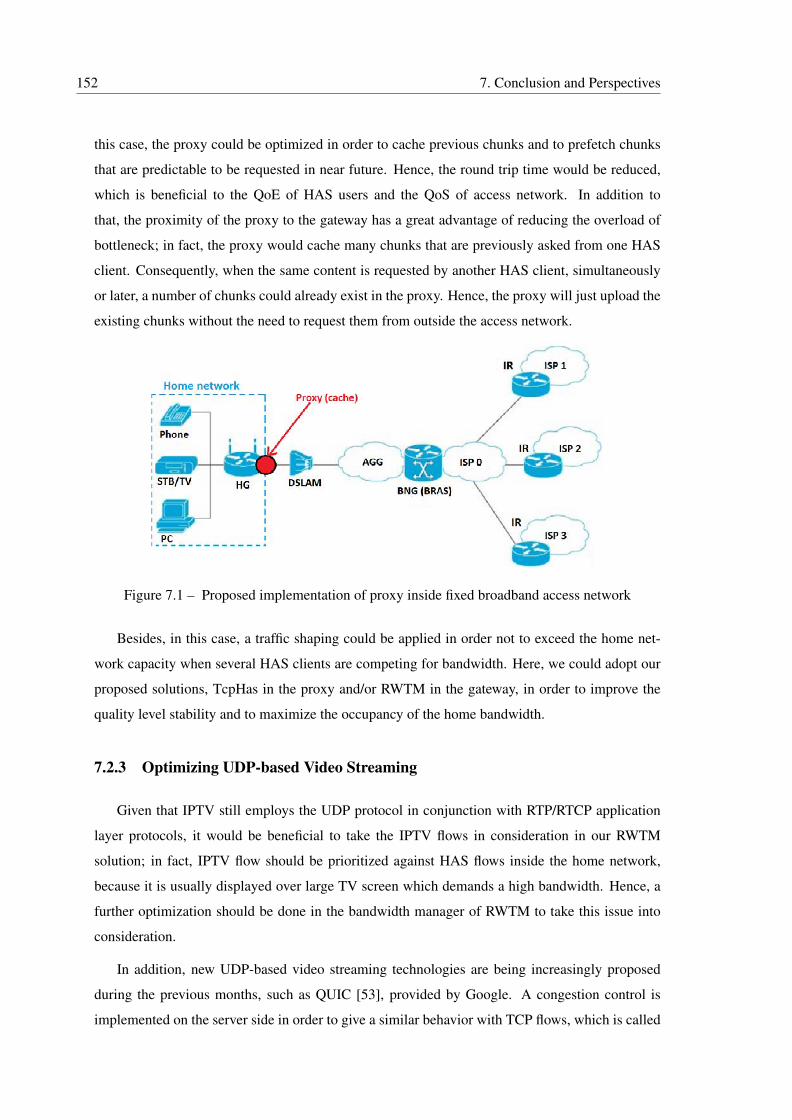
152 7. Conclusion and Perspectives
this case, the proxy could be optimized in order to cache previous chunks and to prefetch chunks
that are predictable to be requested in near future. Hence, the round trip time would be reduced,
which is beneficial to the QoE of HAS users and the QoS of access network. In addition to
that, the proximity of the proxy to the gateway has a great advantage of reducing the overload of
bottleneck; in fact, the proxy would cache many chunks that are previously asked from one HAS
client. Consequently, when the same content is requested by another HAS client, simultaneously
or later, a number of chunks could already exist in the proxy. Hence, the proxy will just upload the
existing chunks without the need to request them from outside the access network.
Figure 7.1 – Proposed implementation of proxy inside fixed broadband access network
Besides, in this case, a traffic shaping could be applied in order not to exceed the home net-
work capacity when several HAS clients are competing for bandwidth. Here, we could adopt our
proposed solutions, TcpHas in the proxy and/or RWTM in the gateway, in order to improve the
quality level stability and to maximize the occupancy of the home bandwidth.
7.2.3 Optimizing UDP-based Video Streaming
Given that IPTV still employs the UDP protocol in conjunction with RTP/RTCP application
layer protocols, it would be beneficial to take the IPTV flows in consideration in our RWTM
solution; in fact, IPTV flow should be prioritized against HAS flows inside the home network,
because it is usually displayed over large TV screen which demands a high bandwidth. Hence, a
further optimization should be done in the bandwidth manager of RWTM to take this issue into
consideration.
In addition, new UDP-based video streaming technologies are being increasingly proposed
during the previous months, such as QUIC [53], provided by Google. A congestion control is
implemented on the server side in order to give a similar behavior with TCP flows, which is called

7.2. Future Works 153
TCP-Friendly Rate Control (TFRC). Hence, a possible contribution is to implement a new TFRC
variant that takes into consideration the specifications of our HAS-based TCP congestion control
protocol, TcpHas.

155
APPENDIX
A List of Publications
A.1 International conferences with peer review
1. Chiheb Ben Ameur, Emmanuel Mory, and Bernard Cousin. Shaping http adaptive streams
using receive window tuning method in home gateway. In Performance Computing and
Communications Conference (IPCCC), 2014 IEEE International, pages 1-2, 2014
2. Chiheb Ben Ameur, Emmanuel Mory, and Bernard Cousin. Evaluation of gateway-based
shaping methods for http adaptive streaming. In Quality of Experience-based Management
for Future Internet Applications and Services (QoE-FI) workshop, International Confer-
ence on Communications (ICC), ICC workshops’04, 2015 IEEE International, pages 1-6,
2015.
A.2 International Journals with peer review
— Chiheb Ben Ameur, Emmanuel Mory, and Bernard Cousin. Combining Traffic Shaping
Methods with Congestion Control Variants for HTTP Adaptive Streaming, submitted to
Multimedia Systems, Springer (minor revision)

BIBLIOGRAPHY 157
Bibliography
[1] ABDALLAH, A., MEDDOUR, D. E., AHMED, T., AND BOUTABA, R. Cross layer opti-
mization architecture for video streaming in wimax networks. In Computers and Commu-
nications (ISCC), 2010 IEEE Symposium on (2010), IEEE, pp. 8–13.
[2] ADHIKARI, V. K., JAIN, S., CHEN, Y., AND ZHANG, Z.-L. Vivisecting youtube: An
active measurement study. In INFOCOM, 2012 Proceedings IEEE (2012), IEEE, pp. 2521–
2525.
[3] ADOBE. Http dynamic streaming 2013, available at http://www.adobe.com/products/hds-
dynamic-streaming.html.
[4] ADOBE. Http dynamic streaming on the adobe flash platform 2010, available at
https://bugbase.adobe.com/index.
[5] AKAMAI. Akamai media delivery solutions, available at
https://www.akamai.com/us/en/solutions/ products/media-delivery/index.jsp.
[6] AKHSHABI, S., ANANTAKRISHNAN, L., BEGEN, A. C., AND DOVROLIS, C. What hap-
pens when http adaptive streaming players compete for bandwidth? In Proceedings of the
22nd international workshop on Network and Operating System Support for Digital Audio
and Video (2012), ACM, pp. 9–14.
[7] AKHSHABI, S., ANANTAKRISHNAN, L., DOVROLIS, C., AND BEGEN, A. C. Server-
based traffic shaping for stabilizing oscillating adaptive streaming players. In Proceeding
of the 23rd ACM Workshop on Network and Operating Systems Support for Digital Audio
and Video (2013), ACM, pp. 19–24.
[8] AKHSHABI, S., BEGEN, A. C., AND DOVROLIS, C. An experimental evaluation of rate-
adaptation algorithms in adaptive streaming over http. In Proceedings of the second annual
ACM conference on Multimedia systems (2011), ACM, pp. 157–168.
[9] ALLMAN, M., PAXSON, V., AND BLANTON, E. Tcp congestion control. Tech. rep., 2009.
[10] ALLMAN, M., PAXSON, V., AND STEVENS, W. Rfc 2581: Tcp congestion control, 1999.
158 BIBLIOGRAPHY
[11] AMEUR, C. B., MORY, E., AND COUSIN, B. Shaping http adaptive streams using receive
window tuning method in home gateway. In Performance Computing and Communications
Conference (IPCCC), 2014 IEEE International (2014), pp. 1–2.
[12] AMEUR, C. B., MORY, E., AND COUSIN, B. Evaluation of gateway-based shaping meth-
ods for http adaptive streaming. In Quality of Experience-based Management for Future
Internet Applications and Services (QoE-FI) workshop, International Conference on Com-
munications (ICC),ICC workshops’04, 2015 IEEE International (2015), pp. 1–6.
[13] AMMAR, D. Ppbp implementation in ns-3, available at:
https://codereview.appspot.com/4997043/.
[14] AMMAR, D., BEGIN, T., AND GUERIN-LASSOUS, I. A new tool for generating real-
istic internet traffic in ns-3. In Proceedings of the 4th International ICST Conference on
Simulation Tools and Techniques (2011), ICST (Institute for Computer Sciences, Social-
Informatics and Telecommunications Engineering), pp. 81–83.
[15] ANDERSON, H. R. Fixed broadband wireless system design. John Wiley & Sons, 2003.
[16] APPLE. Http live streaming overview 2013, available at
http://developer.apple.com/library/ios/documentation/networkinginternet/conceptual
/streamingmediaguide/introduction/introduction.html.
[17] ARMITAGE, G., JAVIER, C., ZANDER, S., ET AL. Client rtt and hop count distributions
viewed from an australian âAŸenemy territoryâAZserver. Tech. rep., CAIA Technical Re-
port, 2006.
[18] BIERNACKI, A., AND TUTSCHKU, K. Performance of http video streaming under different
network conditions. Multimedia Tools and Applications 72, 2 (2014), 1143–1166.
[19] BITMOVIN. bitdash mpeg-dash player feature details, available at http://www.dash-
player.com/feature-details/.
[20] BITMOVIN. bitmovin, open-source dash client library, available at
http://www.bitmovin.net/.
[21] BRAKMO, L. S., O’MALLEY, S. W., AND PETERSON, L. L. TCP Vegas: New techniques
for congestion detection and avoidance, vol. 24. ACM, 1994.
[22] BROOKS, P., AND HESTNES, B. User measures of quality of experience: why being
objective and quantitative is important. Network, IEEE 24, 2 (2010), 8–13.
[23] BROWN, M. A. Traffic control howto. Guide to IP Layer Network (2006).
[24] CAPONE, A., FRATTA, L., AND MARTIGNON, F. Bandwidth estimation schemes for tcp
over wireless networks. Mobile Computing, IEEE Transactions on 3, 2 (2004), 129–143.
BIBLIOGRAPHY 159
[25] CAPONE, A., MARTIGNON, F., AND PALAZZO, S. Bandwidth estimates in the tcp con-
gestion control scheme. In IWDC (2001), Springer, pp. 614–626.
[26] CASAS, P., SACKL, A., SCHATZ, R., JANOWSKI, L., TURK, J., AND IRMER, R. On the
quest for new kpis in mobile networks: The impact of throughput fluctuations on qoe. In
Communication Workshop (ICCW), 2015 IEEE International Conference on (2015), IEEE,
pp. 1705–1710.
[27] CHEN, J., MAHINDRA, R., KHOJASTEPOUR, M. A., RANGARAJAN, S., AND CHIANG,
M. A scheduling framework for adaptive video delivery over cellular networks. In Pro-
ceedings of the 19th annual international conference on Mobile computing & networking
(2013), ACM, pp. 389–400.
[28] CHEN, S., SHEN, B., WEE, S., AND ZHANG, X. Designs of high quality streaming proxy
systems. In INFOCOM 2004. Twenty-third AnnualJoint Conference of the IEEE Computer
and Communications Societies (2004), vol. 3, IEEE, pp. 1512–1521.
[29] CHEN, S., SHEN, B., WEE, S., AND ZHANG, X. Segment-based streaming media proxy:
modeling and optimization. Multimedia, IEEE Transactions on 8, 2 (2006), 243–256.
[30] CHEN, S., SHEN, B., WEE, S., AND ZHANG, X. Sproxy: A caching infrastructure to
support internet streaming. Multimedia, IEEE Transactions on 9, 5 (2007), 1062–1072.
[31] CHENG, Y. Http traffic generator, available at: https://codereview.appspot.com/4940041.
[32] CHENG, Y., ÇETINKAYA, E. K., AND STERBENZ, J. P. Transactional traffic genera-
tor implementation in ns-3. In Proceedings of the 6th International ICST Conference on
Simulation Tools and Techniques (2013), ICST (Institute for Computer Sciences, Social-
Informatics and Telecommunications Engineering), pp. 182–189.
[33] CHOI, B.-Y., SONG, S., WANG, Y., AND PARK, E. K. Using rtt variability for adaptive
cross-layer approach to multimedia delivery in heterogeneous networks. Multimedia, IEEE
Transactions on 11, 6 (2009), 1194–1203.
[34] CISCO. Broadband network gateway overview, available at:
http://www.cisco.com/c/en/us/td/docs/routers/asr9000/software/asr9k_r4-
3/bng/configuration/guide/b_bng_cg43xasr9k/b_bng_cg43asr9k_chapter_01.html.
[35] CISCO. Measuring ip network performance, available at:
http://www.cisco.com/web/about/ac123/ac147/archived_issues/ipj_61/measuring_ip.html.
[36] CISCO. Wholesale content delivery networks: Unlocking new revenue streams and content
relationships, available at: http://www.cisco.com/c/en/us/products/collateral/video/content
-deliveryengineseries/white_paper_c11710667.html.
160 BIBLIOGRAPHY
[37] CISCO, I. Cisco visual networking index: Forecast and methodology, 2014–2019. CISCO
White paper (2015), 1–14.
[38] DE CICCO, L., AND MASCOLO, S. An experimental investigation of the Akamai adaptive
video streaming. Springer, 2010.
[39] DE PESSEMIER, T., DE MOOR, K., JOSEPH, W., DE MAREZ, L., AND MARTENS, L.
Quantifying the influence of rebuffering interruptions on the user’s quality of experience
during mobile video watching. Broadcasting, IEEE Transactions on 59, 1 (2013), 47–61.
[40] DE VRIENDT, J., DE VLEESCHAUWER, D., AND ROBINSON, D. Model for estimating
qoe of video delivered using http adaptive streaming. In Integrated Network Management
(IM 2013), 2013 IFIP/IEEE International Symposium on (2013), IEEE, pp. 1288–1293.
[41] DILLEY, J., MAGGS, B., PARIKH, J., PROKOP, H., SITARAMAN, R., AND WEIHL, B.
Globally distributed content delivery. Internet Computing, IEEE 6, 5 (2002), 50–58.
[42] DONALD GROSS, JOHN F. SHORTLE, M. J. F. D. M. B. M. Simulation input analysis:
difficulties in simulating queues with pareto service. In WSC ’02 Proceedings of the 34th
conference on Winter simulation: exploring new frontiers (2002), vol. 1, ACM, pp. 407–
415.
[43] ESTEBAN, J., BENNO, S. A., BECK, A., GUO, Y., HILT, V., AND RIMAC, I. Interactions
between http adaptive streaming and tcp. In Proceedings of the 22nd international work-
shop on Network and Operating System Support for Digital Audio and Video (2012), ACM,
pp. 21–26.
[44] FLOYD, S., AND GURTOV, A. The newreno modification to tcp’s fast recovery algorithm",
rfc 3782.
[45] FLOYD, S., HANDLEY, M., AND KOHLER, E. Datagram congestion control protocol
(dccp).
[46] FLOYD, S., HANDLEY, M., PADHYE, J., AND WIDMER, J. Equation-based congestion
control for unicast applications, vol. 30. ACM, 2000.
[47] FLOYD, S., AND JACOBSON, V. Random early detection gateways for congestion avoid-
ance. Networking, IEEE/ACM Transactions on 1, 4 (1993), 397–413.
[48] FRIEDMAN, T., CACERES, R., AND CLARK, A. Rtp control protocol extended reports
(rtcp xr). Tech. rep., 2003.
[49] GANGADHAR, S., NGUYEN, T. A. N., UMAPATHI, G., AND STERBENZ, J. P. Tcp west-
wood (+) protocol implementation in ns-3. In Proceedings of the 6th International ICST
Conference on Simulation Tools and Techniques (2013), ICST (Institute for Computer Sci-
ences, Social-Informatics and Telecommunications Engineering), pp. 167–175.
BIBLIOGRAPHY 161
[50] GARCIA, M., DYTKO, D., AND RAAKE, A. Quality impact due to initial loading, stalling,
and video bitrate in progressive download video services. In Quality of Multimedia Experi-
ence (QoMEX), 2014 Sixth International Workshop on (2014), IEEE, pp. 129–134.
[51] GETTYS, J., AND NICHOLS, K. Bufferbloat: Dark buffers in the internet. Queue 9, 11
(2011), 40.
[52] GHOBADI, M., CHENG, Y., JAIN, A., AND MATHIS, M. Trickle: Rate limiting youtube
video streaming. In Usenix Annual Technical Conference (2012), pp. 191–196.
[53] GOOGLE. Quic, a multiplexed stream transport over udp, available at:
https://www.chromium.org/quic.
[54] GRIGORIK, I. High Performance Browser Networking: What every web developer should
know about networking and web performance. " O’Reilly Media, Inc.", 2013.
[55] GRILO, A. How to "intercept" a packet in ns-3 , available at:
https://groups.google.com/forum/#!topic/ns-3-users/ba5qrduivvq.
[56] HA, S., AND RHEE, I. Taming the elephants: New tcp slow start. Computer Networks 55,
9 (2011), 2092–2110.
[57] HA, S., RHEE, I., AND XU, L. Cubic: a new tcp-friendly high-speed tcp variant. ACM
SIGOPS Operating Systems Review 42, 5 (2008), 64–74.
[58] HADDAD, M., ALTMAN, E., EL-AZOUZI, R., JIMÉNEZ, T., ELAYOUBI, S. E., JAMAA,
S. B., LEGOUT, A., AND RAO, A. A survey on youtube streaming service. In Proceedings
of the 5th International ICST Conference on Performance Evaluation Methodologies and
Tools (2011), ICST (Institute for Computer Sciences, Social-Informatics and Telecommu-
nications Engineering), pp. 300–305.
[59] HAYES, D., ARMITAGE, G., ET AL. Improved coexistence and loss tolerance for delay
based tcp congestion control. In Local Computer Networks (LCN), 2010 IEEE 35th Con-
ference on (2010), IEEE, pp. 24–31.
[60] HENDERSON, T. R., LACAGE, M., RILEY, G. F., DOWELL, C., AND KOPENA, J. Net-
work simulations with the ns-3 simulator. SIGCOMM demonstration 14 (2008).
[61] HISAMATSU, H., HASEGAWA, G., AND MURATA, M. Network friendly transmission
control for progressive download over tcp. Journal of Communications 7, 3 (2012), 213–
221.
[62] HO, C.-Y., CHEN, Y.-C., CHAN, Y.-C., AND HO, C.-Y. Fast retransmit and fast recovery
schemes of transport protocols: A survey and taxonomy. Computer Networks 52, 6 (2008),
1308–1327.
162 BIBLIOGRAPHY
[63] HOBFELD, T., SCHATZ, R., AND EGGER, S. Sos: The mos is not enough! In Quality
of Multimedia Experience (QoMEX), 2011 Third International Workshop on (2011), IEEE,
pp. 131–136.
[64] HONG, D., DE VLEESCHAUWER, D., AND BACCELLI, F. A chunk-based caching al-
gorithm for streaming video. In NET-COOP 2010-4th Workshop on Network Control and
Optimization (2010).
[65] HOSSFELD, T., EGGER, S., SCHATZ, R., FIEDLER, M., MASUCH, K., AND
LORENTZEN, C. Initial delay vs. interruptions: between the devil and the deep blue sea.
In Quality of Multimedia Experience (QoMEX), 2012 Fourth International Workshop on
(2012), IEEE, pp. 1–6.
[66] HOUDAILLE, R., AND GOUACHE, S. Shaping http adaptive streams for a better user expe-
rience. In Proceedings of the 3rd Multimedia Systems Conference (2012), ACM, pp. 1–9.
[67] HUANG, T.-Y., HANDIGOL, N., HELLER, B., MCKEOWN, N., AND JOHARI, R. Con-
fused, timid, and unstable: picking a video streaming rate is hard. In Proceedings of the
2012 ACM conference on Internet measurement conference (2012), ACM, pp. 225–238.
[68] HUANG, T.-Y., JOHARI, R., MCKEOWN, N., TRUNNELL, M., AND WATSON, M. A
buffer-based approach to rate adaptation: Evidence from a large video streaming service. In
Proceedings of the 2014 ACM conference on SIGCOMM (2014), ACM, pp. 187–198.
[69] INSTITUTE, M.-T. Osmo4 player of gpac, available at https://gpac.wp.mines-
telecom.fr/player/.
[70] ITU-T RECOMMENDATION, P. Subjective audiovisual quality assessment methods
for multimedia applications.
[71] JAMAL, H., AND SULTAN, K. Performance analysis of tcp congestion control algorithms.
International journal of computers and communications 2, 1 (2008), 18–24.
[72] JANOWSKI, L., AND PAPIR, Z. Modeling subjective tests of quality of experience with
a generalized linear model. In Quality of Multimedia Experience, 2009. QoMEx 2009.
International Workshop on (2009), IEEE, pp. 35–40.
[73] JIANG, H., AND DOVROLIS, C. Passive estimation of tcp round-trip times. ACM SIG-
COMM Computer Communication Review 32, 3 (2002), 75–88.
[74] JIANG, J., SEKAR, V., AND ZHANG, H. Improving fairness, efficiency, and stability in
http-based adaptive video streaming with festive. In Proceedings of the 8th international
conference on Emerging networking experiments and technologies (2012), ACM, pp. 97–
108.
BIBLIOGRAPHY 163
[75] JULURI, P., TAMARAPALLI, V., AND MEDHI, D. Sara: Segment aware rate adaptation
algorithm for dynamic adaptive streaming over http.
[76] JUMISKO-PYYKKÖ, S., MALAMAL VADAKITAL, V., AND HANNUKSELA, M. M. Ac-
ceptance threshold: A bidimensional research method for user-oriented quality evaluation
studies. International Journal of Digital Multimedia Broadcasting 2008 (2008).
[77] KIM, T., AVADHANAM, N., AND SUBRAMANIAN, S. Dimensioning receiver buffer re-
quirement for unidirectional vbr video streaming over tcp. In Image Processing, 2006 IEEE
International Conference on (2006), IEEE, pp. 3061–3064.
[78] KROGFOSS, B., AGRAWAL, A., AND SOFMAN, L. Analytical method for objective scor-
ing of http adaptive streaming (has). In Broadband Multimedia Systems and Broadcasting
(BMSB), 2012 IEEE International Symposium on (2012), IEEE, pp. 1–6.
[79] KUPKA, T., HALVORSEN, P., AND GRIWODZ, C. Performance of on-off traffic stemming
from live adaptive segmented http video streaming. In Local Computer Networks (LCN),
2012 IEEE 37th Conference on (2012), IEEE, pp. 401–409.
[80] KUSCHNIG, R., KOFLER, I., AND HELLWAGNER, H. An evaluation of tcp-based rate-
control algorithms for adaptive internet streaming of h. 264/svc. In Proceedings of the first
annual ACM SIGMM conference on Multimedia systems (2010), ACM, pp. 157–168.
[81] KUSCHNIG, R., KOFLER, I., AND HELLWAGNER, H. Improving internet video streaming
performance by parallel tcp-based request-response streams. In Consumer Communications
and Networking Conference (CCNC), 2010 7th IEEE (2010), IEEE, pp. 1–5.
[82] KUSCHNIG, R., KOFLER, I., AND HELLWAGNER, H. Evaluation of http-based request-
response streams for internet video streaming. In Proceedings of the second annual ACM
conference on Multimedia systems (2011), ACM, pp. 245–256.
[83] LAGHARI, K. U. R., AND CONNELLY, K. Toward total quality of experience: A qoe model
in a communication ecosystem. Communications Magazine, IEEE 50, 4 (2012), 58–65.
[84] LANPHIER, R. Real time streaming protocol (rtsp). Tech. rep., 1998.
[85] LEVKOV, M. Video encoding and transcoding recommendations for http dynamic stream-
ing on the adobe® flash® platform. White Paper, Adobe Systems Inc (2010).
[86] LI, S.-Q., CHONG, S., AND HWANG, C.-L. Link capacity allocation and network con-
trol by filtered input rate in high-speed networks. IEEE/ACM Transactions on Networking
(TON) 3, 1 (1995), 10–25.
[87] LINDEBERG, M., KRISTIANSEN, S., PLAGEMANN, T., AND GOEBEL, V. Challenges and
techniques for video streaming over mobile ad hoc networks. Multimedia Systems 17, 1
(2011), 51–82.
164 BIBLIOGRAPHY
[88] LIU, C., BOUAZIZI, I., AND GABBOUJ, M. Rate adaptation for adaptive http streaming.
In Proceedings of the second annual ACM conference on Multimedia systems (2011), ACM,
pp. 169–174.
[89] LIU, S., BASAR, T., AND SRIKANT, R. Tcp-illinois: A loss-and delay-based congestion
control algorithm for high-speed networks. Performance Evaluation 65, 6 (2008), 417–440.
[90] LIU, X., AND MEN, A. Qoe-aware traffic shaping for http adaptive streaming. Int. J.
Multimedia Ubiquitous Eng 9, 2 (2014), 33–44.
[91] LOHMAR, T., EINARSSON, T., FRÖJDH, P., GABIN, F., AND KAMPMANN, M. Dynamic
adaptive http streaming of live content. In World of Wireless, Mobile and Multimedia Net-
works (WoWMoM), 2011 IEEE International Symposium on a (2011), IEEE, pp. 1–8.
[92] LUEBBEN, R., LI, G., WANG, D., DOVERSPIKE, R., AND FU, X. Fast rerouting for ip
multicast in managed iptv networks. In Quality of Service, 2009. IWQoS. 17th International
Workshop on (2009), IEEE, pp. 1–5.
[93] MA, K. J., BARTOŠ, R., AND BHATIA, S. A survey of schemes for internet-based video
delivery. Journal of Network and Computer Applications 34, 5 (2011), 1572–1586.
[94] MANSY, A., VER STEEG, B., AND AMMAR, M. Sabre: A client based technique for
mitigating the buffer bloat effect of adaptive video flows. In Proceedings of the 4th ACM
Multimedia Systems Conference (2013), ACM, pp. 214–225.
[95] MANTZOURATOS, S., GARDIKIS, G., KOUMARAS, H., AND KOURTIS, A. Survey
of cross-layer proposals for video streaming over mobile ad hoc networks (manets). In
Telecommunications and Multimedia (TEMU), 2012 International Conference on (2012),
IEEE, pp. 101–106.
[96] MARTIN, J., FU, Y., WOURMS, N., AND SHAW, T. Characterizing netflix bandwidth
consumption. In Consumer Communications and Networking Conference (CCNC), 2013
IEEE (2013), IEEE, pp. 230–235.
[97] MASCOLO, S., CASETTI, C., GERLA, M., SANADIDI, M. Y., AND WANG, R. Tcp west-
wood: Bandwidth estimation for enhanced transport over wireless links. In Proceedings
of the 7th annual international conference on Mobile computing and networking (2001),
ACM, pp. 287–297.
[98] MASCOLO, S., AND GRIECO, L. Additive increase early adaptive decrease mechanism
for tcp congestion control. In Telecommunications, 2003. ICT 2003. 10th International
Conference on (2003), vol. 1, IEEE, pp. 818–825.
BIBLIOGRAPHY 165
[99] MASCOLO, S., GRIECO, L. A., FERORELLI, R., CAMARDA, P., AND PISCITELLI, G.
Performance evaluation of westwood+ tcp congestion control. Performance Evaluation 55,
1 (2004), 93–111.
[100] MASCOLO, S., AND RACANELLI, G. Testing tcp westwood+ over transatlantic links at
10 gigabit/second rate. In Protocols for Fast Long-distance Networks (PFLDnet) Workshop
(2005).
[101] MICROSOFT. Microsoft media player available at http://windows.microsoft.com/en-
us/windows/windows-media.
[102] MILLER, K., CORDA, N., ARGYROPOULOS, S., RAAKE, A., AND WOLISZ, A. Op-
timal adaptation trajectories for block-request adaptive video streaming. In Packet Video
Workshop (PV), 2013 20th International (2013), IEEE, pp. 1–8.
[103] MILLER, K., QUACCHIO, E., GENNARI, G., AND WOLISZ, A. Adaptation algorithm
for adaptive streaming over http. In Packet Video Workshop (PV), 2012 19th International
(2012), IEEE, pp. 173–178.
[104] MISRA, V., GONG, W.-B., AND TOWSLEY, D. Fluid-based analysis of a network of aqm
routers supporting tcp flows with an application to red. In ACM SIGCOMM Computer
Communication Review (2000), vol. 30, ACM, pp. 151–160.
[105] MOGUL, J. C. Observing TCP dynamics in real networks, vol. 22. ACM, 1992.
[106] MOK, R. K., CHAN, E. W., AND CHANG, R. K. Measuring the quality of experience of
http video streaming. In Integrated Network Management (IM), 2011 IFIP/IEEE Interna-
tional Symposium on (2011), IEEE, pp. 485–492.
[107] MOK, R. K., LUO, X., CHAN, E. W., AND CHANG, R. K. Qdash: a qoe-aware dash
system. In Proceedings of the 3rd Multimedia Systems Conference (2012), ACM, pp. 11–
22.
[108] MU, M., MAUTHE, A., TYSON, G., AND CERQUEIRA, E. Statistical analysis of ordinal
user opinion scores. In Consumer Communications and Networking Conference (CCNC),
2012 IEEE (2012), IEEE, pp. 331–336.
[109] MÜLLER, C., LEDERER, S., AND TIMMERER, C. An evaluation of dynamic adaptive
streaming over http in vehicular environments. In Proceedings of the 4th Workshop on
Mobile Video (2012), ACM, pp. 37–42.
[110] MÜLLER, C., AND TIMMERER, C. A vlc media player plugin enabling dynamic adaptive
streaming over http. In Proceedings of the 19th ACM international conference on Multime-
dia (2011), ACM, pp. 723–726.
166 BIBLIOGRAPHY
[111] MUSHTAQ, M. S., AUGUSTIN, B., AND MELLOUK, A. Regulating qoe for adaptive video
streaming using bbf method. In Communications (ICC), 2015 IEEE International Confer-
ence on (2015), IEEE, pp. 6855–6860.
[112] MYSIRLIDIS, C., LYKOYRGIOTIS, A., DAGIUKLAS, T., POLITIS, I., AND KOTSOPOU-
LOS, S. Media-aware proxy: Application layer filtering and l3 mobility for media streaming
optimization. In Communications (ICC), 2015 IEEE International Conference on (2015),
IEEE, pp. 6912–6917.
[113] NETWORKS, M. Move networks 2010. available at http://www.movenetworkshd.com.
[114] NS 3 DEVELOPERS. ns-3 simulator, available at: https://www.nsnam.org/.
[115] NYGREN, E., SITARAMAN, R. K., AND SUN, J. The akamai network: a platform for high-
performance internet applications. ACM SIGOPS Operating Systems Review 44, 3 (2010),
2–19.
[116] OF INFORMATION TECHNOLOGY, I. Dash-js, available at http://www-itec.uni-
klu.ac.at/dash/.
[117] PATEL, S., GUPTA, P., AND SINGH, G. Performance measure of drop tail and red al-
gorithm. In Electronic Computer Technology (ICECT), 2010 International Conference on
(2010), IEEE, pp. 35–38.
[118] PEREIRA, R., AND PEREIRA, E. Dynamic adaptive streaming over http and progressive
download: Comparative considerations. In Advanced Information Networking and Applica-
tions Workshops (WAINA), 2014 28th International Conference on (2014), IEEE, pp. 905–
909.
[119] PERKINS, C., AND GHARAI, L. Rtp and the datagram congestion control protocol. In
Multimedia and Expo, 2006 IEEE International Conference on (2006), IEEE, pp. 1521–
1524.
[120] PRINS, M., BRUNNER, M., KARAGIANNIS, G., LUNDQVIST, H., AND NUNZI, G. Fast
rtp retransmission for iptv-implementation and evaluation. In Global Telecommunications
Conference, 2008. IEEE GLOBECOM 2008. IEEE (2008), IEEE, pp. 1–6.
[121] PROTOCOL, U. D. Rfc 768 j. postel isi 28 august 1980. Isi (1980).
[122] QUINLAN, J. J., ZAHRAN, A. H., RAMAKRISHNAN, K., AND SREENAN, C. J. De-
livery of adaptive bit rate video: balancing fairness, efficiency and quality. In Local and
Metropolitan Area Networks (LANMAN), 2015 IEEE International Workshop on (2015),
IEEE, pp. 1–6.
BIBLIOGRAPHY 167
[123] RAO, A., LEGOUT, A., LIM, Y.-S., TOWSLEY, D., BARAKAT, C., AND DABBOUS, W.
Network characteristics of video streaming traffic. In Proceedings of the Seventh COnfer-
ence on emerging Networking EXperiments and Technologies (2011), ACM, p. 25.
[124] REAL. Real player available at http://www.real.com.
[125] REC, I. P. 800: Methods for subjective determination of transmission quality. International
Telecommunication Union, Geneva (1996).
[126] RICCIATO, F., VACIRCA, F., AND SVOBODA, P. Diagnosis of capacity bottlenecks via
passive monitoring in 3g networks: an empirical analysis. Computer Networks 51, 4 (2007),
1205–1231.
[127] SALVADOR, A., NOGUEIRA, J., AND SARGENTO, S. Qoe assessment of http adaptive
video streaming. In Wireless Internet. Springer, 2015, pp. 235–242.
[128] SCHIAVONE, M., ROMIRER-MAIERHOFER, P., RICCIATO, F., AND BAIOCCHI, A. To-
wards bottleneck identification in cellular networks via passive tcp monitoring. In Ad-hoc,
Mobile, and Wireless Networks. Springer, 2014, pp. 72–85.
[129] SCHIERBAUM, T., AND LAWRENCE, B. Version 1.5 of hbbtv specification released. Four
new members added to Steering Group, HbbTV, München (2012).
[130] SCHULZRINNE, H., CASNER, S., FREDERICK, R., AND JACOBSON, V. Rtp: A transport
protocol for real-time applications", rfc 1889.
[131] SEUFERT, M., EGGER, S., SLANINA, M., ZINNER, T., HOBFELD, T., AND TRAN-GIA,
P. A survey on quality of experience of http adaptive streaming. Communications Surveys
& Tutorials, IEEE 17, 1 (2014), 469–492.
[132] SHEN, L., TU, W., AND STEINBACH, E. A flexible starting point based partial caching
algorithm for video on demand. In Multimedia and Expo, 2007 IEEE International Confer-
ence on (2007), IEEE, pp. 76–79.
[133] SHUAI, Y., PETROVIC, G., AND HERFET, T. Olac: An open-loop controller for low-
latency adaptive video streaming. In Communications (ICC), 2015 IEEE International
Conference on (2015), IEEE, pp. 6874–6879.
[134] SINGH, K. D., HADJADJ-AOUL, Y., AND RUBINO, G. Quality of experience estimation
for adaptive http/tcp video streaming using h. 264/avc. In Consumer Communications and
Networking Conference (CCNC), 2012 IEEE (2012), IEEE, pp. 127–131.
[135] SPACHOS, P., LI, W., CHIGNELL, M., LEON-GARCIA, A., ZUCHERMAN, L., AND
JIANG, J. Acceptability and quality of experience in over the top video. In Communication
Workshop (ICCW), 2015 IEEE International Conference on (2015), IEEE, pp. 1693–1698.
168 BIBLIOGRAPHY
[136] TASAKA, S. A bayesian hierarchical model of qoe in interactive audiovisual communica-
tions. In Communications (ICC), 2015 IEEE International Conference on (2015), IEEE,
pp. 6983–6989.
[137] TASAKA, S., AND ITO, Y. Psychometric analysis of the mutually compensatory property
of multimedia qos. In Communications, 2003. ICC’03. IEEE International Conference on
(2003), vol. 3, IEEE, pp. 1880–1886.
[138] TASAKA, S., AND NUNOME, T. Qoe enhancement of multimedia communications by
user-assistance. In WTC 2014; World Telecommunications Congress 2014; Proceedings of
(2014), VDE, pp. 1–6.
[139] TECHNOLOGIES, A. Understanding dslam and bras access devices. White paper (2006),
1–16.
[140] TECHNOLOGY, I. Dynamic adaptive streaming over http (dash)-part 1: Media presentation
description and segment formats. In ISO/IEC 23009-1:2012 (2012).
[141] TRIANTAFYLLOPOULOU, D., PASSAS, N., KALOXYLOS, A., AND MERAKOS, L. Co-
ordinated handover initiation and cross-layer adaptation for mobile multimedia systems.
Multimedia, IEEE Transactions on 11, 6 (2009), 1131–1139.
[142] TU, W., STEINBACH, E., MUHAMMAD, M., AND LI, X. Proxy caching for video-on-
demand using flexible starting point selection. Multimedia, IEEE Transactions on 11, 4
(2009), 716–729.
[143] UBUNTU. Stochastic fairness queuing discipline, linux man page, available at:
http://manpages.ubuntu.com/manpages/trusty/man8/tc-sfq.8.html.
[144] VAN LANCKER, W., VAN DEURSEN, D., MANNENS, E., AND VAN DE WALLE, R. Http
adaptive streaming with media fragment uris. In Multimedia and Expo (ICME), 2011 IEEE
International Conference on (2011), IEEE, pp. 1–6.
[145] VESCO, A., SCOPIGNO, R. M., AND MASALA, E. Tducsma: Efficient support for triple-
play services in wireless home networks. In Communications (ICC), 2015 IEEE Interna-
tional Conference on (2015), IEEE, pp. 6941–6947.
[146] VIBLAST. Viblast player features, available at http://viblast.com/player/#features.
[147] VILLA, B. J., AND HEEGAARD, P. E. Group based traffic shaping for adaptive http video
streaming by segment duration control. In Advanced Information Networking and Applica-
tions (AINA), 2013 IEEE 27th International Conference on (2013), IEEE, pp. 830–837.
[148] WALKER, J., MORRIS, O., AND MARUSIC, B. Share it!-the architecture of a rights-
managed network of peer-to-peer set-top-boxes. In EUROCON 2003. Computer as a Tool.
The IEEE Region 8 (2003), vol. 1, IEEE, pp. 251–255.
BIBLIOGRAPHY 169
[149] WAN, S., AND HAO, Y. Research on tcp optimization strategy of application delivery
network. In Intelligent Computation and Bio-Medical Instrumentation (ICBMI), 2011 In-
ternational Conference on (2011), IEEE, pp. 241–244.
[150] WANG, Z., LU, L., AND BOVIK, A. C. Video quality assessment based on structural
distortion measurement. Signal processing: Image communication 19, 2 (2004), 121–132.
[151] WISNIEWSKI, P., BEBEN, A., BATALLA, J. M., AND KRAWIEC, P. On delimiting video
rebuffering for stream-switching adaptive applications. In Communications (ICC), 2015
IEEE International Conference on (2015), IEEE, pp. 6867–6873.
[152] XIE, X., ZHANG, X., KUMAR, S., AND LI, L. E. pistream: Physical layer informed
adaptive video streaming over lte.
[153] YAN, J., MÜHLBAUER, W., AND PLATTNER, B. Analytical framework for improving the
quality of streaming over tcp. Multimedia, IEEE Transactions on 14, 6 (2012), 1579–1590.
[154] YAN, Z., XUE, J., AND CHEN, C. W. Qoe continuum driven http adaptive streaming over
multi-client wireless networks. In Multimedia and Expo (ICME), 2014 IEEE International
Conference on (2014), IEEE, pp. 1–6.
[155] YANG, H., CHEN, X., YANG, Z., ZHU, X., AND CHEN, Y. Opportunities and challenges
of http adaptive streaming. International Journal of Future Generation Communication and
Networking 7, 6 (2014), 165–180.
[156] YAO, J., KANHERE, S. S., HOSSAIN, I., AND HASSAN, M. Empirical evaluation of
http adaptive streaming under vehicular mobility. In NETWORKING 2011. Springer, 2011,
pp. 92–105.
[157] YIN, X., SEKAR, V., AND SINOPOLI, B. Toward a principled framework to design dy-
namic adaptive streaming algorithms over http. In Proceedings of the 13th ACM Workshop
on Hot Topics in Networks (2014), ACM, p. 9.
[158] YOKOTA, M. Y. S., AND NAKAJIMA, T. A quality evaluation of high-speed video stream-
ing on congested ip networks. In Information and Telecommunication Technologies, 2005.
APSITT 2005 Proceedings. 6th Asia-Pacific Symposium on (2005), IEEE, pp. 53–58.
[159] YOUTUBE. Youtube http://www.youtube.com.
[160] YOUTUBE. Youtube statistics, available at: https://www.youtube.com/yt/press/statistics.html.
[161] ZAMBELLI, A. A history of media streaming and the future of connected
tv. available at http://www.theguardian.com/media-network/media-network-
blog/2013/mar/01/historystreaming-future-connected-tv.
170 BIBLIOGRAPHY
[162] ZAMBELLI, A. Smooth streaming technical overview, microsoft corp., red-
mond,wa, usa, tech. rep, available at http://www.iis.net/learn/media/on-demand-smooth-
streaming/smooth-streamingtechnical-overview.
[163] ZHANG, L., SHENKER, S., AND CLARK, D. D. Observations on the dynamics of a con-
gestion control algorithm: The effects of two-way traffic. ACM SIGCOMM Computer Com-
munication Review 21, 4 (1991), 133–147.
[164] ZINK, M., SCHMITT, J., AND STEINMETZ, R. Layer-encoded video in scalable adaptive
streaming. Multimedia, IEEE Transactions on 7, 1 (2005), 75–84.
[165] ZINNER, T., HOSSFELD, T., MINASH, T. N., AND FIEDLER, M. Controlled vs. un-
controlled degradations of qoe–the provisioning-delivery hysteresis in case of video. New
Dimensions in the Assessment and Support of Quality of Experience (QoE) for Multimedia
Applications (2010).
[166] ZONG, N. Survey and gap analysis for http streaming standards and implementations.
[167] ZUKERMAN, M., NEAME, T. D., AND ADDIE, R. G. Internet traffic modeling and future
technology implications. In INFOCOM 2003. Twenty-Second Annual Joint Conference of
the IEEE Computer and Communications. IEEE Societies (2003), vol. 1, IEEE, pp. 587–
596.

VU :
Le Directeur de Thèse
VU :
Le Responsable de l’École Doctorale
VU pour autorisation de soutenance
Rennes, le
Le Président de l’Université de Rennes 1
VU après soutenance pour autorisation de publication :
Le Président de Jury,