The Astrophysical Journal, 740:116 (8pp), 2011 October 20 doi:10.1088/0004-637X/740/2/116C© 2011. The American Astronomical Society. All rights reserved. Printed in the U.S.A.

SPECTROSCOPIC ANALYSIS OF INTERACTION BETWEEN AN EXTREME-ULTRAVIOLET IMAGINGTELESCOPE WAVE AND A CORONAL UPFLOW REGION

F. Chen1,2, M. D. Ding1,2, P. F. Chen1,2, and L. K. Harra31 Department of Astronomy, Nanjing University, Nanjing 210093, China; dmd@nju.edu.cn

2 Key Laboratory for Modern Astronomy and Astrophysics (Nanjing University), Ministry of Education, Nanjing 210093, China3 UCL-Mullard Space Science Laboratory, Holmbury St. Mary, Dorking RH5 6NT, UK

Received 2011 May 5; accepted 2011 July 26; published 2011 October 4

ABSTRACT

We report a spectroscopic analysis of an EUV Imaging Telescope (EIT) wave event that occurred in active region11081 on 2010 June 12 and was associated with an M2.0 class flare. The wave propagated nearly circularly. Thesoutheastern part of the wave front passed over an upflow region near a magnetic bipole. Using EUV ImagingSpectrometer raster observations for this region, we studied the properties of plasma dynamics in the wave front, aswell as the interaction between the wave and the upflow region. We found a weak blueshift for the Fe xii λ195.12and Fe xiii λ202.04 lines in the wave front. The local velocity along the solar surface, which is deduced from theline-of-sight velocity in the wave front and the projection effect, is much lower than the typical propagation speed ofthe wave. A more interesting finding is that the upflow and non-thermal velocities in the upflow region are suddenlydiminished after the transit of the wave front. This implies a significant change of magnetic field orientation whenthe wave passed. As the lines in the upflow region are redirected, the velocity along the line of sight is diminishedas a result. We suggest that this scenario is more in accordance with what was proposed in the field-line stretchingmodel of EIT waves.

Key words: Sun: corona – Sun: UV radiation – waves

Online-only material: animation, color figures

1. INTRODUCTION

Diffuse coronal waves were first observed by Moses et al.(1997) and Thompson et al. (1998) with the EUV ImagingTelescope (EIT; Delaboudiniere et al. 1995) aboard the Solarand Heliospheric Observatory (SOHO), and were commonlyknown as EIT waves. They are best seen in the runningdifference images as propagating bright fronts with a speed ofa few hundreds of km s−1, followed by an expanding dimmingregion (Thompson et al. 1998). EIT waves can be observed atseveral wavelengths, such as 171 Å, 195 Å, 284 Å, and 304 Å(Wills-Davey & Thompson 1999; Zhukov & Auchere 2004;Long et al. 2008). Many observational properties of EIT waveswere presented by Delannee & Aulanier (1999), Klassen et al.(2000), and Thompson & Myers (2009). Recent reviews on thistopic can be found in Wills-Davey & Attrill (2009), Warmuth(2010), and Gallagher & Long (2010).

It is natural that EIT waves are accompanied by some othersolar active events such as coronal mass ejections (CMEs) andflares. Statistical and case studies have shown that EIT wavesare closely related with CMEs rather than solar flares (Bieseckeret al. 2002; Okamoto et al. 2004; Chen 2006). In particular, theflares associated with many EIT wave events were very weak(Cliver et al. 2005; Veronig et al. 2008; Ma et al. 2009; Attrillet al. 2009). In spite of the coincidence of EIT waves and CMEs,their spatial relationship is still being debated. Vrsnak et al.(2006) reported a wave behind the CME flank, and Patsourakos& Vourlidas (2009) claimed that the EIT wave front is outsidethe CME frontal loop, whereas Chen (2009) and Dai et al. (2010)found that the EIT wave front is cospatial with the white-lightfrontal loop of CMEs. In addition, Warmuth (2010) found oneevent in which a wave front overtakes the CME flank.

Based on the observed properties of EIT waves, there are twomain interpretations. One is the wave model, which suggests that

EIT waves are fast-mode magnetohydrodynamic (MHD) wavesor shocks (Wang 2000; Wu et al. 2001; Warmuth et al. 2001,2004; Pomoell et al. 2008; Vrsnak & Cliver 2008). This modelcan explain some of the characteristics of the wave front and wassupported by a number of observations (Warmuth et al. 2005;Long et al. 2008; Veronig et al. 2008; Patsourakos & Vourlidas2009; Gopalswamy et al. 2009; Kienreich et al. 2009). The otherinterpretation is related to CME expansion. Delannee (2000)suggested that the bright front may result from the interactionbetween CME-induced expansion of magnetic field lines andsurrounding field lines. Chen et al. (2002, 2005) proposed afield-line stretching model, which predicts that there shouldexist a fast-moving coronal shock ahead of the slow EIT wave,which was recently confirmed by Chen & Wu (2011). The non-wave model can also explain many of the properties of the waveand was supported by Harra & Sterling (2003) and Zhukovet al. (2009). In addition, there are still other models such asslow-mode MHD waves (Wang et al. 2009), spherical currentshell (Delannee et al. 2008), successive magnetic reconnections(Attrill et al. 2007a, 2007b), and soliton (Wills-Davey et al.2007). A concept of a coupled coronal wave was proposed byZhukov & Auchere (2004) and Cohen et al. (2009).

In the last decade, the main approach to studying EITwaves has been by ultraviolet imaging observations. The mainlimitation comes from the cadence and spatial resolution ofthe instruments, such as EIT on board SOHO and ExtremeUltraViolet Imager on board the Solar TErrestrial RElationsObservatory (STEREO; Howard et al. 2008). AtmosphericImaging Assembly (AIA; Title & AIA team 2006) aboard theSolar Dynamics Observatory (SDO) has high spatio-temporalresolutions and signal-to-noise ratio, enabling us to study EITwaves in unprecedented detail. Liu et al. (2010) reportedthe first SDO/AIA observations of EIT waves. They foundone diffuse pulse and multiple sharp fronts and suggested

1

The Astrophysical Journal, 740:116 (8pp), 2011 October 20 Chen et al.

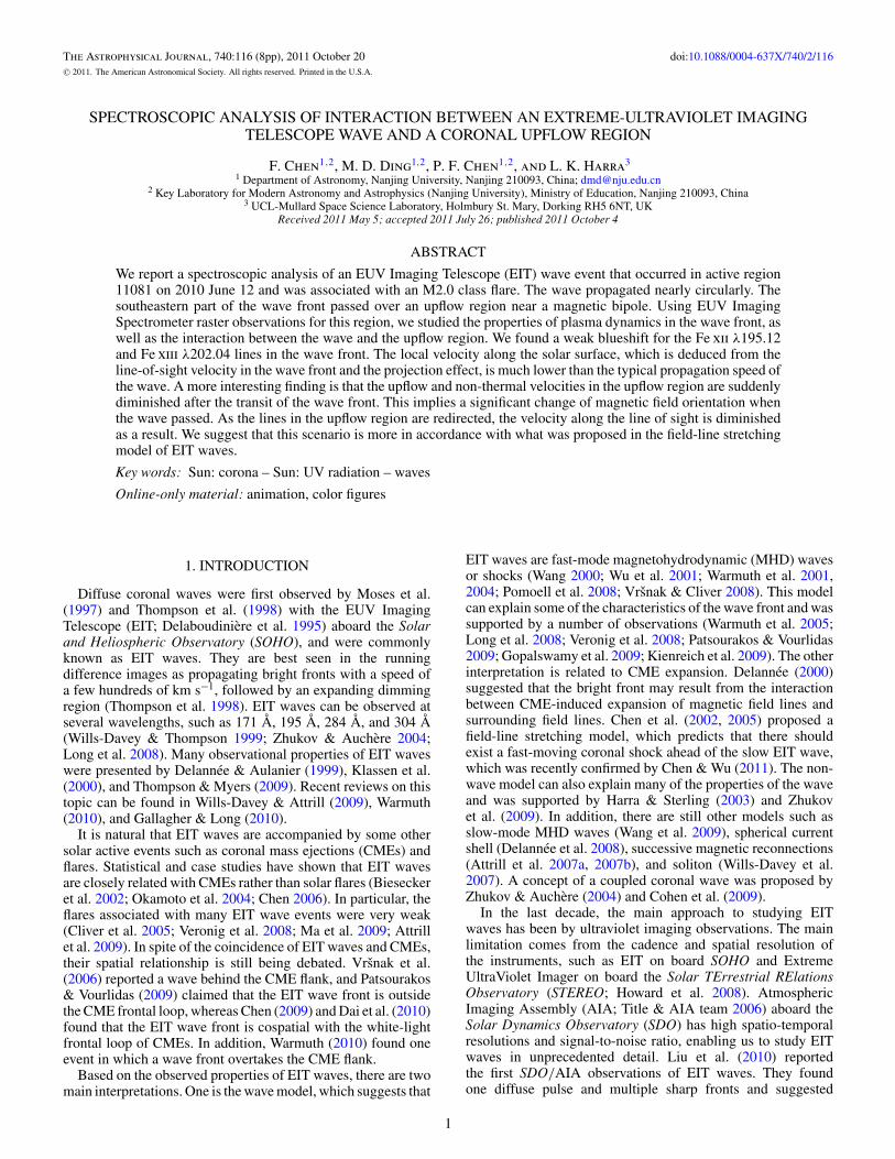
Figure 1. SDO/AIA 193 Å image and the magnetogram measured by the Michelson Doppler Imager (MDI; Scherrer et al. 1995) aboard SOHO. The white boxesindicate the EIS FOV.

a hybrid interpretation, combining both wave and non-wavemodels. In addition to the imaging observations, spectroscopicobservations are also very important, because they provideadditional information on plasma dynamics during the wavepropagation and aid clarification of the physical nature of EITwaves. Harra & Sterling (2003) did the first spectroscopicanalysis of EIT waves using Coronal Diagnostic Spectrometer(Harrison et al. 1995) on board the SOHO spacecraft. Theymeasured Doppler velocities in the wave front and the followingdimming. They found an absence of Doppler velocity in thewave front but an ejection of cold material after the wave frontpassed. Using the EUV Imaging Spectrometer (EIS; Culhaneet al. 2007) on Hinode, Asai et al. (2008) studied a fast-mode MHD shock wave visible in soft X-rays. Unfortunately,some of the EIT images suffered from scattered light in thetelescope. Therefore, the wave front in the EIT data was unclear.More recently, Chen et al. (2010) confirmed the studies of Harra& Sterling (2001, 2003), and further found an enhanced linebroadening at the outer edge of the dimming region whichcould be well explained by the field-line stretching model ofChen et al. (2002, 2005).

In this paper, we present a case study of Hinode/EIS ob-servation of an EIT wave event. We successfully obtained thetemporal evolution of the line intensity, line width, and Dopplervelocity for two iron lines in a sliced region overlapping a smallupflow region. Hence, we are able to reveal the interaction be-tween the EIT wave and the coronal upflow region spectro-scopically for the first time. We describe the observations anddata analysis in Section 2. Our results are shown in Section 3,followed by some discussions on the results in Section 4.

2. OBSERVATIONS AND DATA ANALYSIS

The EIT wave event we studied occurred in the active region11081 on 2010 June 12 and was associated with an M2.0 classflare. The EIS observations started at ∼00:35 UT, using a 1′′ slitwith a step of 1′′ and an exposure time of 60 s. The time gapbetween successive exposures is 2 s. The field of view (FOV)is 5′′ in the scanning direction and 240′′ in the slit direction.Therefore, a raster cadence of ∼310 s for EIS was achieved.

This raster was repeated 12 times. The FOV of EIS lay to thesouth of the active region where the flare occurred and the wavewas generated. The FOV covered the central part of a magneticbipole as shown in Figure 1.

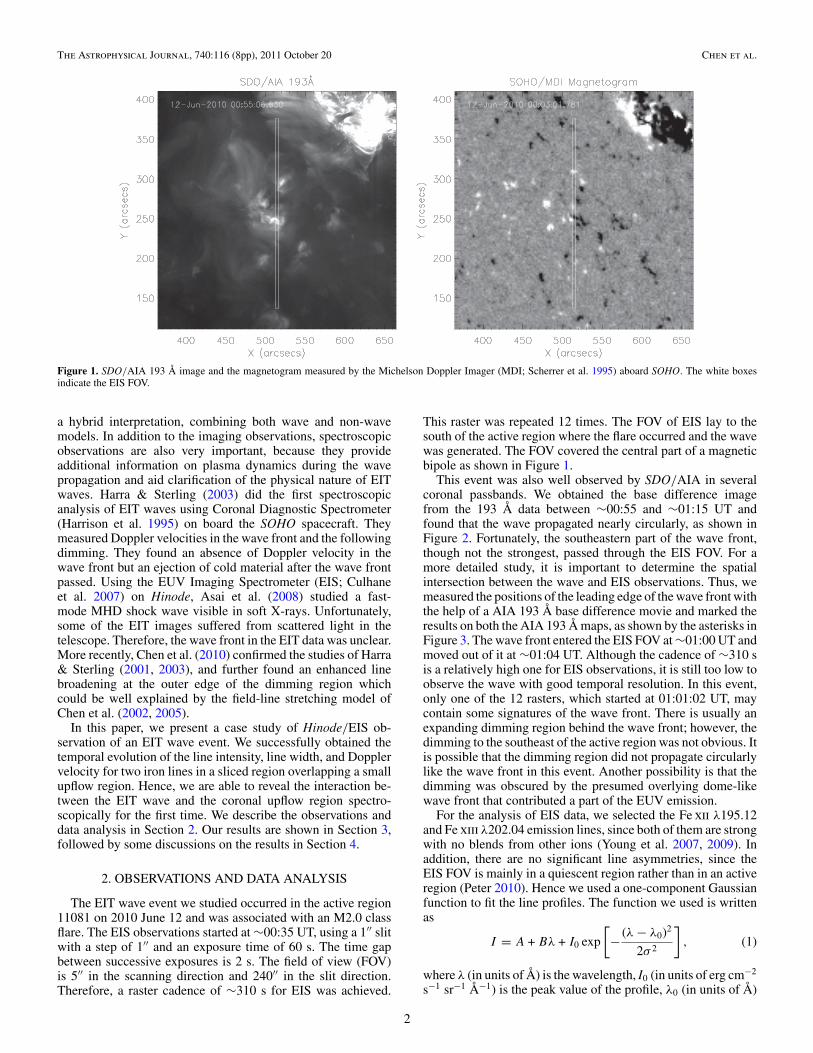
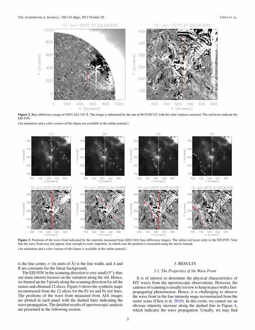
This event was also well observed by SDO/AIA in severalcoronal passbands. We obtained the base difference imagefrom the 193 Å data between ∼00:55 and ∼01:15 UT andfound that the wave propagated nearly circularly, as shown inFigure 2. Fortunately, the southeastern part of the wave front,though not the strongest, passed through the EIS FOV. For amore detailed study, it is important to determine the spatialintersection between the wave and EIS observations. Thus, wemeasured the positions of the leading edge of the wave front withthe help of a AIA 193 Å base difference movie and marked theresults on both the AIA 193 Å maps, as shown by the asterisks inFigure 3. The wave front entered the EIS FOV at ∼01:00 UT andmoved out of it at ∼01:04 UT. Although the cadence of ∼310 sis a relatively high one for EIS observations, it is still too low toobserve the wave with good temporal resolution. In this event,only one of the 12 rasters, which started at 01:01:02 UT, maycontain some signatures of the wave front. There is usually anexpanding dimming region behind the wave front; however, thedimming to the southeast of the active region was not obvious. Itis possible that the dimming region did not propagate circularlylike the wave front in this event. Another possibility is that thedimming was obscured by the presumed overlying dome-likewave front that contributed a part of the EUV emission.

For the analysis of EIS data, we selected the Fe xii λ195.12and Fe xiii λ202.04 emission lines, since both of them are strongwith no blends from other ions (Young et al. 2007, 2009). Inaddition, there are no significant line asymmetries, since theEIS FOV is mainly in a quiescent region rather than in an activeregion (Peter 2010). Hence we used a one-component Gaussianfunction to fit the line profiles. The function we used is writtenas

I = A + Bλ + I0 exp

[− (λ − λ0)2

2σ 2

], (1)

where λ (in units of Å) is the wavelength, I0 (in units of erg cm−2

s−1 sr−1 Å−1) is the peak value of the profile, λ0 (in units of Å)

2

The Astrophysical Journal, 740:116 (8pp), 2011 October 20 Chen et al.

Figure 2. Base difference image of SDO/AIA 193 Å. The image is subtracted by the one at 00:55:06 UT, with the solar rotation corrected. The red boxes indicate theEIS FOV.

(An animation and a color version of this figure are available in the online journal.)

Figure 3. Positions of the wave front indicated by the asterisks measured from SDO/AIA base difference images. The white/red boxes refer to the EIS FOV. Notethat the wave front may not appear clear enough in some snapshots, in which case the position is measured using the movie instead.

(An animation and a color version of this figure is available in the online journal.)

is the line center, σ (in units of Å) is the line width, and A andB are constants for the linear background.

The EIS FOV in the scanning direction is very small (5′′); thusour main interest focuses on the variation along the slit. Hence,we binned up the 5 pixels along the scanning direction for all therasters and obtained 12 slices. Figure 4 shows the synthetic mapsreconstructed from the 12 slices for the Fe xii and Fe xiii lines.The positions of the wave front measured from AIA imagesare plotted in each panel with the dashed lines indicating thewave propagation. The detailed results of spectroscopic analysisare presented in the following section.

3. RESULTS

3.1. The Properties of the Wave Front

It is of interest to determine the physical characteristics ofEIT waves from the spectroscopic observations. However, thecadence of scanning is usually too low to keep in pace with a fast-propagating phenomenon. Hence, it is challenging to observethe wave front in the line intensity maps reconstructed from theraster scans (Chen et al. 2010). In this event, we cannot see anobvious intensity increase along the dashed line in Figure 4,which indicates the wave propagation. Usually, we may find

3

The Astrophysical Journal, 740:116 (8pp), 2011 October 20 Chen et al.

Figure 4. Line intensity (left), Doppler velocity (middle), and width (right) for the Fe xii and Fe xiii lines as a function of time. The time is related to 00:30:00 UT.The asterisks indicate the positions of the wave front measured from Figure 3. Note that in the fourth column of Figure 3, the wave front is already out of the EIS FOV.The dashed lines connecting the asterisks indicate the wave propagation track.

(A color version of this figure is available in the online journal.)

some distinct features in line widths and Doppler velocities asrevealed in previous studies (Harra & Sterling 2003; Asai et al.2008; Chen et al. 2010). As shown in Figure 4, the variation ofline width along the wave propagation in the quiescent regionis insignificant and within the fitting error. This is differentfrom the result observed by Chen et al. (2010), in which anenhanced line broadening appeared at the outer edge of theensuing dimming, i.e., behind the wave front.

Unlike the wave-induced effect on the line intensity and linewidth, we discern a weak blueshift in lines along the wavepropagation in the upper part of the EIS FOV. The blueshift isstronger for the Fe xiii line. To illustrate the result, we calculatedthe average of the Doppler velocities between Y = 330′′ andY = 364′′ for each slice. The average Doppler velocity, as wellas other line parameters, is plotted as a function of time inFigure 5. We can confirm that the line intensity and line widthin this region did not vary significantly with time. At the time ofthe wave front transit (i.e., ∼33 minutes according to Figure 5),the blueshift for the Fe xii line suddenly increased to ∼4 km s−1,a value that was different from those observed earlier by nearly2 km s−1. For the Fe xiii line, the amplitude of the blueshiftwhen the wave passed was a little larger than that for the Fe xiiline. The average fitting error in this region was ∼1.41 km s−1.The blueshift, albeit weak, was beyond the errors.

3.2. Interaction Between the EIT Wave and the Upflow Region

The EIS FOV covered the central part of a magnetic bipole,which appeared as several minor loops and EUV bright points in

AIA images as shown in Figure 1. The photospheric magneticfield strength was generally less than 100 G. In Figure 3, wefound that the wave front was only slightly distorted whenit passed over these magnetic structures. It is known that theEIT wave front usually stops at active region boundaries andcoronal holes (Thompson et al. 1998; Veronig et al. 2006,2008). The magnetic bipole here may be too small to stop thewave propagation in either the wave scenario or the non-wavescenario.

There was an upflow region to the north of the magneticbipole core (Y ∼ 245′′) that appeared the brightest in both theAIA image and the EIS line intensity map. In the upflow region,the line intensities of both the iron lines were much lower. Thevelocity amplitude of the upflow was 15 km s−1 for the Fe xii lineand 20 km s−1 for the Fe xiii line. The line width in this upflowregion was larger than that in the ambient regions. Moreover,the non-thermal velocity (vnon) can be calculated by

FWHM2obs = FWHM2

ins + 4ln2λ2

c2

(2kT

M+ v2

non

), (2)

where the value of FWHMins is 0.056 Å, λ is the wavelength (inunits of Å), c is the speed of light, k is the Boltzmann constant, Tis the electron temperature, and M is the ion mass. The value ofFWHMobs (in units of Å) can be obtained from the line profile.In Figure 4, the upflow region was clear in the Doppler velocityand line width synthetic maps for both the iron lines. The upflowvelocity and line width stayed nearly unchanged until the wave

4

The Astrophysical Journal, 740:116 (8pp), 2011 October 20 Chen et al.

Figure 5. Average line intensity (in units of erg cm−2 s−1 sr−1), line width (in units of mÅ), and Doppler velocity (in units of km s−1) between Y = 330′′ and Y =364′′ as a function of time. See the legend for details. Negative values are for blueshifts. The dashed lines in the left column indicate 0 km s−1. The time is related to00:30:00 UT.

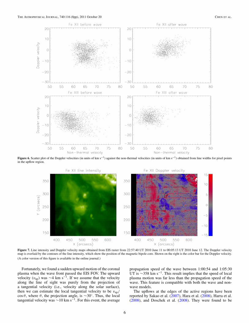
front passed. However, after the wave front passed the upflowregion, we found that the upflow velocity and line width to theright of the dashed line suddenly and significantly decreased forboth the lines. We refer to this phenomenon as a diminishingof upflow and non-thermal velocities. For a quantitative study,the Doppler velocity in this region is plotted against the non-thermal velocity, as shown in Figure 6. It is clear that after thewave front passed, the high-velocity tail was truncated so thatthe upflow velocity was �5 km s−1 and the non-thermal velocitywas �70 km s−1 for the Fe xii line, while the upflow velocitywas �10 km s−1 and the non-thermal velocity was �60 km s−1

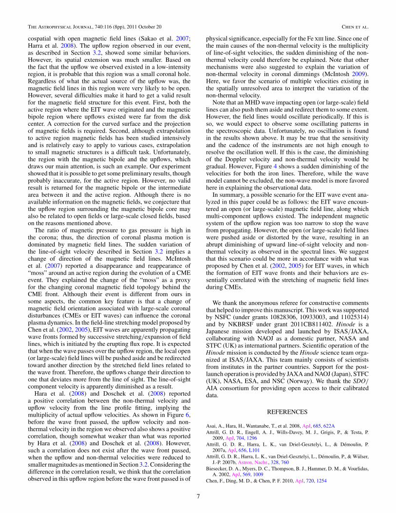
for the Fe xiii line.In addition, we analyzed the data obtained with a long raster

(a large FOV) on the day before the event. The line intensity andDoppler velocity maps are shown in Figure 7. We can confirmthat the upflow region existed at this position and exhibiteda similar velocity amplitude for many hours. The magneticbipole core is illustrated by the black contours on Figure 7(right panel). The abrupt diminishing of the upward Dopplervelocity and the non-thermal velocity in an ambient regionof magnetic structure may imply an interesting scenario inwhich the wave front interacts with the magnetic field during itspropagation.

4. DISCUSSION

We presented an EIT wave event, which was captured byHinode/EIS raster. We studied the spectroscopic properties ofthe coronal plasma during the wave transit. The most interestingresults are summarized below.

1. The wave front propagated nearly circularly, with its south-eastern part observed by EIS. The line intensity and linewidth showed no change when the wave front passed. How-ever, an enhanced blueshift of the line center, albeit weak,was observed at this time.

2. The wave front passed over an upflow region near amagnetic bipole. The shape of the wave front was onlyslightly distorted. For both of the iron lines studied, asudden and clear diminishing of the upflow and non-thermalvelocities in the upflow region was observed when the wavepassed.

In general, during the EIT wave front passage, one mayexpect to observe a line intensity enhancement, a commonfeature observed in coronal EUV images. In this event, how-ever, the variation of line intensity during the wave propaga-tion was within the fitting error. For the raster observationsof the wave, the line profile at a certain point is a compos-ite of the contribution from the background corona duringthe whole exposure time (50 s for this event) and the contri-bution from the wave front. The wave quickly passes over thispoint and in fact it contributes little to the line profile. There-fore, it is hard to observe similar signatures from spectroscopicand image observations. It was previously observed that EITwaves and the accompanying dimmings exhibited a very highspeed, so that their contribution to the line profile can result ina strong Doppler component (Harra & Sterling 2003; Asai et al.2008). In this case, some significant features of the wave orwave-perturbed plasma can be observed from the spectroscopicdata.

5

The Astrophysical Journal, 740:116 (8pp), 2011 October 20 Chen et al.

Figure 6. Scatter plot of the Doppler velocities (in units of km s−1) against the non-thermal velocities (in units of km s−1) obtained from line widths for pixel pointsin the upflow region.

Figure 7. Line intensity and Doppler velocity maps obtained from EIS raster from 22:57:40 UT 2010 June 11 to 00:05:13 UT 2010 June 12. The Doppler velocitymap is overlaid by the contours of the line intensity, which show the position of the magnetic bipole core. Shown on the right is the color bar for the Doppler velocity.

(A color version of this figure is available in the online journal.)

Fortunately, we found a sudden upward motion of the coronalplasma when the wave front passed the EIS FOV. The upwardvelocity (vup) was ∼4 km s−1. If we assume that the velocityalong the line of sight was purely from the projection ofa tangential velocity (i.e., velocity along the solar surface),then we can estimate the local tangential velocity to be vup/cos θ , where θ , the projection angle, is ∼30◦. Thus, the localtangential velocity was ∼10 km s−1. For this event, the average

propagation speed of the wave between 1:00:54 and 1:05:30UT is ∼358 km s−1. This result implies that the speed of localplasma motion was far less than the propagation speed of thewave. This feature is compatible with both the wave and non-wave models.

The upflows at the edges of the active regions have beenreported by Sakao et al. (2007), Hara et al. (2008), Harra et al.(2008), and Doschek et al. (2008). They were found to be

6

The Astrophysical Journal, 740:116 (8pp), 2011 October 20 Chen et al.

cospatial with open magnetic field lines (Sakao et al. 2007;Harra et al. 2008). The upflow region observed in our event,as described in Section 3.2, showed some similar behaviors.However, its spatial extension was much smaller. Based onthe fact that the upflow we observed existed in a low-intensityregion, it is probable that this region was a small coronal hole.Regardless of what the actual source of the upflow was, themagnetic field lines in this region were very likely to be open.However, several difficulties make it hard to get a valid resultfor the magnetic field structure for this event. First, both theactive region where the EIT wave originated and the magneticbipole region where upflows existed were far from the diskcenter. A correction for the curved surface and the projectionof magnetic fields is required. Second, although extrapolationto active region magnetic fields has been studied intensivelyand is relatively easy to apply to various cases, extrapolationto small magnetic structures is a difficult task. Unfortunately,the region with the magnetic bipole and the upflows, whichdraws our main attention, is such an example. Our experimentshowed that it is possible to get some preliminary results, thoughprobably inaccurate, for the active region. However, no validresult is returned for the magnetic bipole or the intermediatearea between it and the active region. Although there is noavailable information on the magnetic fields, we conjecture thatthe upflow region surrounding the magnetic bipole core mayalso be related to open fields or large-scale closed fields, basedon the reasons mentioned above.

The ratio of magnetic pressure to gas pressure is high inthe corona; thus, the direction of coronal plasma motion isdominated by magnetic field lines. The sudden variation ofthe line-of-sight velocity described in Section 3.2 implies achange of direction of the magnetic field lines. McIntoshet al. (2007) reported a disappearance and reappearance of“moss” around an active region during the evolution of a CMEevent. They explained the change of the “moss” as a proxyfor the changing coronal magnetic field topology behind theCME front. Although their event is different from ours insome aspects, the common key feature is that a change ofmagnetic field orientation associated with large-scale coronaldisturbances (CMEs or EIT waves) can influence the coronalplasma dynamics. In the field-line stretching model proposed byChen et al. (2002, 2005), EIT waves are apparently propagatingwave fronts formed by successive stretching/expansion of fieldlines, which is initiated by the erupting flux rope. It is expectedthat when the wave passes over the upflow region, the local open(or large-scale) field lines will be pushed aside and be redirectedtoward another direction by the stretched field lines related tothe wave front. Therefore, the upflows change their direction toone that deviates more from the line of sight. The line-of-sightcomponent velocity is apparently diminished as a result.

Hara et al. (2008) and Doschek et al. (2008) reporteda positive correlation between the non-thermal velocity andupflow velocity from the line profile fitting, implying themultiplicity of actual upflow velocities. As shown in Figure 6,before the wave front passed, the upflow velocity and non-thermal velocity in the region we observed also shows a positivecorrelation, though somewhat weaker than what was reportedby Hara et al. (2008) and Doschek et al. (2008). However,such a correlation does not exist after the wave front passed,when the upflow and non-thermal velocities were reduced tosmaller magnitudes as mentioned in Section 3.2. Considering thedifference in the correlation result, we think that the correlationobserved in this upflow region before the wave front passed is of

physical significance, especially for the Fe xiii line. Since one ofthe main causes of the non-thermal velocity is the multiplicityof line-of-sight velocities, the sudden diminishing of the non-thermal velocity could therefore be explained. Note that othermechanisms were also suggested to explain the variation ofnon-thermal velocity in coronal dimmings (McIntosh 2009).Here, we favor the scenario of multiple velocities existing inthe spatially unresolved area to interpret the variation of thenon-thermal velocity.

Note that an MHD wave impacting open (or large-scale) fieldlines can also push them aside and redirect them to some extent.However, the field lines would oscillate periodically. If this isso, we would expect to observe some oscillating patterns inthe spectroscopic data. Unfortunately, no oscillation is foundin the results shown above. It may be true that the sensitivityand the cadence of the instruments are not high enough toresolve the oscillation well. If this is the case, the diminishingof the Doppler velocity and non-thermal velocity would begradual. However, Figure 4 shows a sudden diminishing of thevelocities for both the iron lines. Therefore, while the wavemodel cannot be excluded, the non-wave model is more favoredhere in explaining the observational data.

In summary, a possible scenario for the EIT wave event ana-lyzed in this paper could be as follows: the EIT wave encoun-tered an open (or large-scale) magnetic field line, along whichmulti-component upflows existed. The independent magneticsystem of the upflow region was too narrow to stop the wavefrom propagating. However, the open (or large-scale) field lineswere pushed aside or distorted by the wave, resulting in anabrupt diminishing of upward line-of-sight velocity and non-thermal velocity as observed in the spectral lines. We suggestthat this scenario could be more in accordance with what wasproposed by Chen et al. (2002, 2005) for EIT waves, in whichthe formation of EIT wave fronts and their behaviors are es-sentially correlated with the stretching of magnetic field linesduring CMEs.

We thank the anonymous referee for constructive commentsthat helped to improve this manuscript. This work was supportedby NSFC (under grants 10828306, 10933003, and 11025314)and by NKBRSF under grant 2011CB811402. Hinode is aJapanese mission developed and launched by ISAS/JAXA,collaborating with NAOJ as a domestic partner, NASA andSTFC (UK) as international partners. Scientific operation of theHinode mission is conducted by the Hinode science team orga-nized at ISAS/JAXA. This team mainly consists of scientistsfrom institutes in the partner countries. Support for the post-launch operation is provided by JAXA and NAOJ (Japan), STFC(UK), NASA, ESA, and NSC (Norway). We thank the SDO/AIA consortium for providing open access to their calibrateddata.

REFERENCES

Asai, A., Hara, H., Wantanabe, T., et al. 2008, ApJ, 685, 622AAttrill, G. D. R., Engell, A. J., Wills-Davey, M. J., Grigis, P., & Testa, P.

2009, ApJ, 704, 1296Attrill, G. D. R., Harra, L. K., van Driel-Gesztelyi, L., & Demoulin, P.

2007a, ApJ, 656, L101Attrill, G. D. R., Harra, L. K., van Driel-Gesztelyi, L., Demoulin, P., & Wulser,

J.-P. 2007b, Astron. Nachr., 328, 760Biesecker, D. A., Myers, D. C., Thompson, B. J., Hammer, D. M., & Vourlidas,

A. 2002, ApJ, 569, 1009Chen, F., Ding, M. D., & Chen, P. F. 2010, ApJ, 720, 1254

7

The Astrophysical Journal, 740:116 (8pp), 2011 October 20 Chen et al.

Chen, P. F. 2006, ApJ, 641, L153Chen, P. F. 2009, ApJ, 698, L112Chen, P. F., Fang, C., & Shibata, K. 2005, ApJ, 622, 1202Chen, P. F., Wu, S. T., Shibata, K., & Fang, C. 2002, ApJ, 572, L99Chen, P. F., & Wu, Y. 2011, ApJ, 732, L20Cliver, E. W., Laurenza, M., Storini, M., & Thompson, B. J. 2005, ApJ, 631,

604Cohen, O., Attrill, G. D. R., Manchester, W. B., & Wills-Davey, M. J. 2009, ApJ,

705, 587Culhane, J. L., Harra, L. K., James, A. M., et al. 2007, Sol. Phys., 243, 19Dai, Y., Auchere, F., Vial, J.-C., et al. 2010, ApJ, 708, 913Delaboudiniere, J.-P., Artzner, G. E., Brunaud, J., et al. 1995, Sol. Phys., 162,

291Delannee, C. 2000, ApJ, 545, 512Delannee, C., & Aulanier, G. 1999, Sol. Phys., 190, 107Delannee, C., Torok, T., Aulanier, G., & Hochedez, J.-F. 2008, Sol. Phys., 247,

123Doschek, G. A., Warren, H. P., Mariska, J. T., et al. 2008, ApJ, 686, 1362Gallagher, P. T., & Long, D. M. 2010, Space Sci. Rev., 158, 365Gopalswamy, N., Yashiro, S., Temmer, M., et al. 2009, ApJ, 691, L123Hara, H., Watanabe, T., Harra, L. K., et al. 2008, ApJ, 678, L67Harra, L. K., Sakao, T., Mandrini, C. H., et al. 2008, ApJ, 676, L147Harra, L. K., & Sterling, A. C. 2001, ApJ, 561, L215Harra, L. K., & Sterling, A. C. 2003, ApJ, 587, 429Harrison, R. A., Sawyer, E. C., Carter, M. K., et al. 1995, Sol. Phys., 162, 233Howard, R. A., Moses, J. D., Vourlidas, A., et al. 2008, Space Sci. Rev., 136, 67Kienreich, I. W., Temmer, M., & Veronig, A. M. 2009, ApJ, 703, L118Klassen, A., Ausrass, H., Mann, G., & Tompson, B. J. 2000, A&AS, 141, 357Liu, W., Nitta, N. V., Schrijver, C. J., Title, A. M., & Tarbell, T. D. 2010, ApJ,

723, L53Long, D. M., Gallagher, P. T., McAteer, R. T. J., & Bloomfield, D. S. 2008, ApJ,

680, L81Ma, S., Wills-Davey, M. J., Lin, J., et al. 2009, ApJ, 707, 503McIntosh, S. W. 2009, ApJ, 693, 1306

McIntosh, S. W., Leamon, R. J., Davey, A. R., & Wills-Davey, M. J. 2007, ApJ,660, 1653

Moses, D., Clette, F., Delaboudiniere, J.-P., et al. 1997, Sol. Phys., 175, 571MOkamoto, T. J., Nakai, H., Keiyama, A., et al. 2004, ApJ, 608, 1124Patsourakos, S., & Vourlidas, A. 2009, ApJ, 700, L182Peter, H. 2010, A&A, 521, A51Pomoell, J., Vainio, R., & Kssmann, R. 2008, Sol. Phys., 253, 249Sakao, T., Kano, R., Narukage, N., et al. 2007, Science, 318, 1585Scherrer, P. H., Bogart, R. S., Bush, R. I., et al. 1995, Sol. Phys., 162, 129Thompson, B. J., & Myers, D. C. 2009, ApJS, 183, 225Thompson, B. J., Plunkett, S. P., Gurman, J. B., et al. 1998, Geophys. Res. Lett.,

25, 2465Title, A. M., & AIA team. 2006, BAAS, 38, 261Veronig, A. M., Temmer, M., & Vrsnak, B. 2008, ApJ, 681, 113Veronig, A. M., Temmer, M., Vrsnak, B., & Thalmann, J. K. 2006, ApJ, 647,

1466Vrsnak, B., & Cliver, E. W. 2008, Sol. Phys., 253, 215Vrsnak, B., Warmuth, A., Temmer, M., et al. 2006, A&A, 448, 739Wang, H., Shen, C., & Lin, J. 2009, ApJ, 700, 1716Wang, Y.-M. 2000, ApJ, 543, L89Warmuth, A. 2010, Adv. Space Res., 45, 527Warmuth, A., Mann, G., & Aurass, H. 2005, ApJ, 626, L121Warmuth, A., Vrsnak, B., Aurass, H., & Hanslmeier, A. 2001, ApJ, 560,

L105Warmuth, A., Vrsnak, B., Magdaleni, J., Hanslmeier, A., & Otruba, W.

2004, A&A, 418, 1117Wills-Davey, M. J., & Attrill, G. D. R. 2009, Space Sci. Rev., 149, 325Wills-Davey, M. J., DeForest, C. E., & Stenflo, J. O. 2007, ApJ, 664, 556Wills-Davey, M. J., & Thompson, B. J. 1999, Sol. Phys., 190, 467Wu, S. T., Zheng, H. N., Wang, S., et al. 2001, J. Geophys. Res., 106, 25089Young, P. R., Del Zanna, G., Mason, H. E., et al. 2007, PASJ, 59, 857Young, P. R., Watanabe, T., Hara, H., & Mariska, J. T. 2009, A&A, 495, 587Zhukov, A. N., & Auchere, F. 2004, A&A, 427, 705Zhukov, A. N., Rodriguez, L., & de Patoul, J. 2009, Sol. Phys., 259, 73

8