Chapter 2.1: Visualization of Metal Ion Buffering Via 3-D Topo

University of Montana University of Montana

ScholarWorks at University of Montana ScholarWorks at University of Montana

Water Topos: A 3-D Trend Surface Approach to Viewing and Teaching Aqueous Equilibrium Chemistry

Open Educational Resources (OER)

4-2021

Chapter 2.1: Visualization of Metal Ion Buffering Via 3-D Topo Chapter 2.1: Visualization of Metal Ion Buffering Via 3-D Topo

Surfaces of Complexometric Titrations Surfaces of Complexometric Titrations

Garon C. Smith

Md Mainul Hossain

Follow this and additional works at: https://scholarworks.umt.edu/topos

Part of the Chemistry Commons

Let us know how access to this document benefits you.

https://scholarworks.umt.edu/

https://scholarworks.umt.edu/topos



https://scholarworks.umt.edu/open_educational_resources

https://scholarworks.umt.edu/topos?utm_source=scholarworks.umt.edu%2Ftopos%2F5&utm_medium=PDF&utm_campaign=PDFCoverPages

http://network.bepress.com/hgg/discipline/131?utm_source=scholarworks.umt.edu%2Ftopos%2F5&utm_medium=PDF&utm_campaign=PDFCoverPages

https://goo.gl/forms/s2rGfXOLzz71qgsB2

April 9, 2021 2.1-1 Chapter 2.1 – Metal Buffering

Chapter 2.1 Visualization of Metal Ion Buffering Via 3-D Topo Surfaces of

Complexometric Titrations

Garon C. Smith1 and Md Mainul Hossain2

1Department of Chemistry and Biochemistry, University of Montana, Missoula, MT 59812, 2Department of Biochemistry and Microbiology, North South

University, Dhaka 1229, Bangladesh

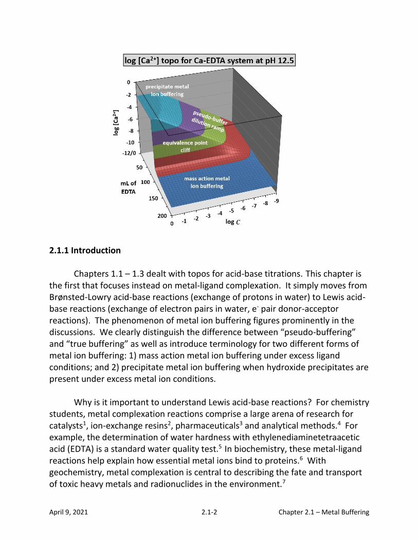
Abstract This chapter examines 1:1 metal-ligand complexometric titrations in aqueous media. It presents surfaces that plot computed equilibrium parameters above a composition grid with titration progress (mL of ligand) as the x-axis and overall system dilution (log C ) as the y-axis. The sample systems in this chapter are restricted to EDTA as a ligand. Other chelating ligands that form exclusively 1:1 complexes could also be modeled with this software. The surfaces show the quality of the equivalence point break under various conditions. More importantly, they develop the phenomenon of metal ion buffering. They clearly distinguish the difference between “pseudo-buffering” and “true buffering”. They introduce terminology for two different forms of metal ion buffering: 1) mass action metal ion buffering under excess ligand conditions; and 2) precipitate metal ion buffering when hydroxide precipitates are present under excess metal ion conditions. Systems modeled are EDTA titrations of Cu2+, Ca2+ and Mg2+. A final section demonstrates a second type of topo that helps evaluate the optimal pH for an EDTA titration. Supplemental files include the Complexation TOPOS software, an Excel workbook that generates topo surfaces in under 20 seconds, and teaching suggestions. Required inputs are: 1) stability constants for the metal-ligand complex; 2) acid dissociation constants for the ligand, 3) stability constants for hydroxy complexes from of the metal cation; and 4) a Ksp value and

stoichiometry for hydroxide precipitates. Many of these constants are contained in a workbook tab. Also included are a PowerPoint lecture and teaching materials (for lecture, homework, and pre-laboratory activities) that are suitable in general chemistry courses or third-year and graduate courses in analytical chemistry, biochemistry and geochemistry.


2.1.1 Introduction Chapters 1.1 – 1.3 dealt with topos for acid-base titrations. This chapter is the first that focuses instead on metal-ligand complexation. It simply moves from Brønsted-Lowry acid-base reactions (exchange of protons in water) to Lewis acid-base reactions (exchange of electron pairs in water, e- pair donor-acceptor reactions). The phenomenon of metal ion buffering figures prominently in the discussions. We clearly distinguish the difference between “pseudo-buffering” and “true buffering” as well as introduce terminology for two different forms of metal ion buffering: 1) mass action metal ion buffering under excess ligand conditions; and 2) precipitate metal ion buffering when hydroxide precipitates are present under excess metal ion conditions.

Why is it important to understand Lewis acid-base reactions? For chemistry students, metal complexation reactions comprise a large arena of research for catalysts1, ion-exchange resins2, pharmaceuticals3 and analytical methods.4 For example, the determination of water hardness with ethylenediaminetetraacetic acid (EDTA) is a standard water quality test.5 In biochemistry, these metal-ligand reactions help explain how essential metal ions bind to proteins.6 With geochemistry, metal complexation is central to describing the fate and transport of toxic heavy metals and radionuclides in the environment.7


Complexation TOPOS, a new computer program available as a supplemental file in this chapter, examines metal-ligand systems where only 1:1 complexes form. The most familiar systems of this type are metals interacting with hexadentate EDTA. The program creates 3-D trend surfaces above a composition grid that encompasses a wide range of solution conditions. The primary composition grid used has a titration curve x-axis (mL of EDTA) and a dilution y-axis (log C ). Other composition grids are possible, for example, mL of

EDTA vs. pH which appear later in this chapter. Variables that can be plotted as z-coordinates to form trend surfaces include free metal ([Mn+]), free ligand ([L]), metal-ligand complex ([ML]), protonated ligand forms ([HxL]) and hydroxy-metal complexes ([M(OH)x]). By including dilution as a composition grid dimension, the concept of metal ion buffering can be nicely visualized.

This chapter focuses on EDTA titrations. Treatment of simple EDTA

complexometric titrations is appropriate for inclusion in introductory chemistry courses. Complexation TOPOS includes competing side-reactions from protons and hydroxide ions. Discussions of these complications and metal ion buffering are more appropriate topics for upper division and graduate level chemistry courses.

2.1.2 The Chemical Model for 1:1 Complexation Systems

The aqueous equilibrium chemistry that occurs in a metal-ligand

complexation titration is more complicated than that for a simple Brønsted-Lowry acid-base system. As these procedures are being conducted in aqueous solution, there are competing reactions for both the metal ion and ligand components. Competition for the metal ion occurs between the ligand of interest and the ever-

present OH- of the water itself. In a similar fashion, there is competition for the

ligand’s binding sites between metal ions and the ever-present H3O+ of the water. Finally, if the concentration of metal and hydroxide ions gets sufficiently high, there is also the possibility of metal hydroxide precipitation. Because of these competing processes, metal complexation titrations are often done at constant pH to reduce the variables in the system. That practice is employed here.

A sample metal-ligand system will be useful for describing the competitive

reactions as well as introducing the symbol conventions adopted for the


equilibrium constants of each reaction. A computer simulation is only as good as the completeness of the chemical model from which it has been constructed. Thus, it pays to describe as much of the chemistry as is possible.

The initial system explored here consists of copper(II), Cu2+, as the metal ion and ethylenediaminetetraacetic acid, EDTA, a classic hexadentate ligand. EDTA forms a very stable 1:1 complex with cupric ion. The complex formed between Cu2+and EDTA really represents a displacement of the six H2O molecules that are in the coordination sphere of the aqueous Cu2+ ion. For simplicity we will ignore the water molecules in most of our formulas. Copper(II) can react in water

to form Cu(OH)+, Cu(OH)20, Cu(OH)3

- and Cu(OH)42- . If the pH is above 4.3 and

there is little or no EDTA present, Cu2+ can precipitate as Cu(OH)2(s). Below are the reactions and constants used in generating the accompanying figures for the Cu-EDTA system. All constants used in this paper are from Martel et al.’s NIST Critical Stability Constants of Metal Complexes Database 46.8

Complexation reactions: These are written as overall reactions as opposed

to step-wise reactions. Since there is just one stoichiometry here, only a 1 is required.

Cu2+ + EDTA ⇌ Cu(EDTA)2- β1 = 1018.80 (2.1-1)

As we discuss the shifts from one copper species to another, we will use coefficients to quantify how much is present in each form. These are analogous

to the coefficients used in acid-base species distribution diagrams.

0 represents the fraction present as free copper ion, i.e., Cu2+

1 represents the fraction present as CuEDTA2-

For simplicity, we are ignoring the hydroxide species in our values.

Protonation of ligand reactions: Acid-base chemistry is traditionally treated as loss of protons. Given the structure of our computer program, it is more convenient here to write these in the reverse direction. This is equivalent to forming “hydrogen complexes” of the ligands. All that needs to be done is switch the order of constants and change the sign on their pKa values. The last proton

lost is the same as the first proton “complexed”. These, too, are done as overall,


not step-wise, constants. Below is a comparison of the standard Ka notation and

the H notation used in our model equations. The Complexation TOPOS model asks the user to list pKa values and then automatically converts them into the log

H values that it employs.

Step-wise dissociation of EDTA:

H6EDTA2+ + H2O ⇌ H3O+ + H5EDTA+ Ka1 = 100.0 (2.1-2)

H5EDTA+ + H2O ⇌ H3O+ + H4EDTA0 Ka2 = 10-1.5 (2.1-3)

H4EDTA0 + H2O ⇌ H3O+ + H3EDTA- Ka3 = 10-2.00 (2.1-4)

H3EDTA- + H2O ⇌ H3O+ + H2EDTA2- Ka4 = 10-2.69 (2.1-5)

H2EDTA2- + H2O ⇌ H3O+ + HEDTA3- Ka5 = 10-6.13 (2.1-6)

HEDTA3- + H2O ⇌ H3O+ + EDTA4- Ka6 = 10-10.37 (2.1-7)

Overall constants for protonation of EDTA:

H+ + EDTA4- ⇌ HEDTA3- βH1 = 1010.37 (2.1-8)

2 H+ + EDTA4- ⇌ H2EDTA2- βH2 = 10(10.37 + 6.13) = 10 16.50 (2.1-9)

3 H+ + EDTA4- ⇌ H3EDTA- βH3 = 10( 16.50+2.69) = 10 19.19 (2.1-10)

4 H+ + EDTA4- ⇌ H4EDTA0 βH4 = 10( 19.19+2.00) = 1021.19 (2.1-11)

5 H+ + EDTA4- ⇌ H5EDTA+ H5 = 10(21.19+1.50) = 1022.69 (2.1-12)

6 H+ + EDTA4- ⇌ H6EDTA2+ H6 = 10(22.69+0.00) = 1022.69 (2.1-13)

Metal Hydrolysis Reactions: Whenever metal ions are dissolved in water,

there is a possible interaction with OH- as a ligand. We will ignore writing formulas with coordinated H2O because it is easier to follow the complexation chemistry. Stability constants for four hydroxy complexes of copper are included.


Cu2+ + OH- ⇌ Cu(OH)+ OH1 = 106.5 (2.1-14)

Cu2+ + 2 OH- ⇌ Cu(OH)20 OH2 = 1011.8 (2.1-15)

Cu2+ + 3 OH- ⇌ Cu(OH)3- OH3 = 1014.5 (2.1-16)

Cu2+ + 4 OH- ⇌ Cu(OH)42- OH4 = 1015.6 (2.1-17)

Hydroxide Precipitation: For the Cu2+ system, we also need to be alert for

the possibility of a 1:2 cupric hydroxide precipitate, Cu(OH)2(s). Thus, it is also necessary to have any pertinent Ksps available to check for precipitation

conditions.

Cu2+ + 2 OH- ⇌ Cu(OH)2(s) Ksp = 10-19.32 (2.1-18)

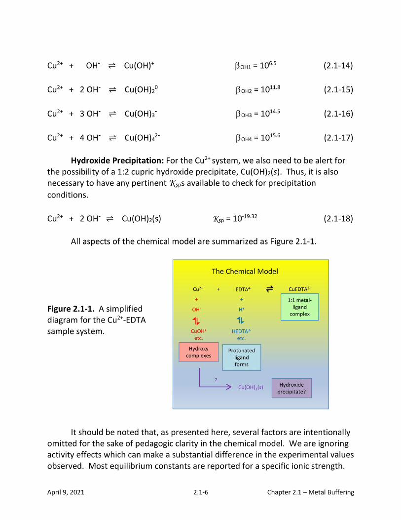
All aspects of the chemical model are summarized as Figure 2.1-1. Figure 2.1-1. A simplified diagram for the Cu2+-EDTA sample system.

It should be noted that, as presented here, several factors are intentionally omitted for the sake of pedagogic clarity in the chemical model. We are ignoring activity effects which can make a substantial difference in the experimental values observed. Most equilibrium constants are reported for a specific ionic strength.


We have chosen the reported values from the NIST8 tables which often were measured at an ionic strength of 0.10 M. In practice, when we have conducted experimental verifications, we have employed a total ionic strength adjustor (ISA) to eliminate variations caused by activity changes. This has necessitated confining our experimental solutions to less than 0.100 M ionic strength. We are also ignoring ion pair formation which brings together oppositely charged species as outer sphere complexes or fully solvated ions.

2.1-3 Traditional 2-D Ligand into Metal Titrations

Before presenting a full 3-D topo surface for a metal-ligand complexation

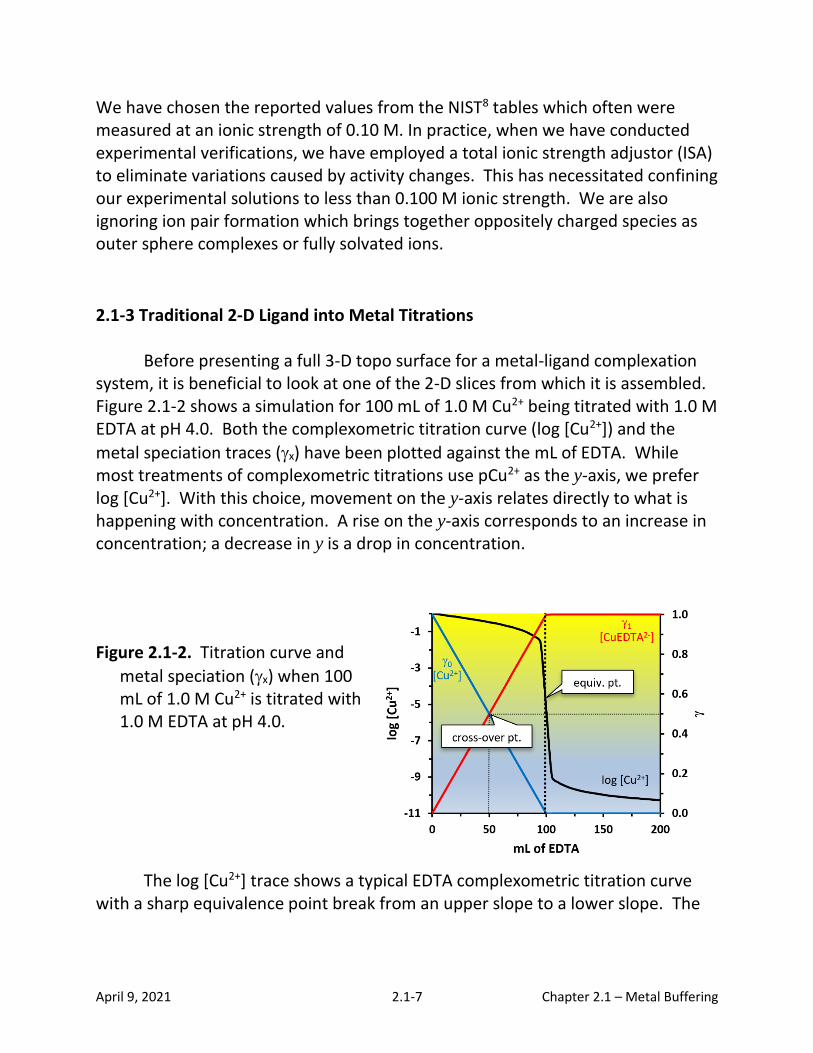
system, it is beneficial to look at one of the 2-D slices from which it is assembled. Figure 2.1-2 shows a simulation for 100 mL of 1.0 M Cu2+ being titrated with 1.0 M EDTA at pH 4.0. Both the complexometric titration curve (log [Cu2+]) and the

metal speciation traces (x) have been plotted against the mL of EDTA. While most treatments of complexometric titrations use pCu2+ as the y-axis, we prefer log [Cu2+]. With this choice, movement on the y-axis relates directly to what is happening with concentration. A rise on the y-axis corresponds to an increase in concentration; a decrease in y is a drop in concentration.

Figure 2.1-2. Titration curve and

metal speciation (x) when 100 mL of 1.0 M Cu2+ is titrated with 1.0 M EDTA at pH 4.0.

The log [Cu2+] trace shows a typical EDTA complexometric titration curve with a sharp equivalence point break from an upper slope to a lower slope. The


titration curve shows a fairly shallow slope both before and after the equivalence point is reached.

Species distribution diagrams for the fraction of free metal ion (0) and the

fraction of CuEDTA2- complex (1) also appear. These traces reveal the chemical

situation during the titration. As EDTA is added linearly, the two -curves track

the steady conversion of Cu2+ to CuEDTA2-. Half way to the equivalence point, the

speciation curves reach a cross-over; both 0 and 1 are 0.50. At 100 mL the

conversion is essentially complete with 1 near 1 and 0 close to 0. The complexometric titration curve illustrates that the value of log [Cu2+] is

somewhat stable before and after the equivalence point break. This is a situation akin to pH buffering in acid-base systems. Metal ion buffering occurs when changing solution composition does not cause large shifts in the log [Cu2+] value. Some authors9-11 have labeled both the before and after sections of the complexometric curve in Figure 2.1-2 as “buffer zones”. Creation of a log [Cu2+] topo surface over a titration-dilution composition grid, however, will demonstrate that the pre-equivalence point section is a “pseudo-buffer” region while the post-equivalence point section is a “true metal ion buffering” situation. Similar pseudo-buffing behavior for acid-base systems is discussed in Chapter 1.1.4.

2.1.4 The log [Cu2+] 3-D Topo Surface: Buffering vs. Pseudo-Buffering While a 2-D plot of a ligand-into-metal titration captures much about complexation equilibria, adding a dilution axis to create trend surfaces above a composition grid will reveal even more insights into possible system behaviors. Examination of the trend surfaces will quickly reveal the difference between metal ion pseudo-buffering and true metal ion buffering.

Our composition grid here consists of an x-axis that follows titration progress (mL of EDTA). The y-axis is the dilution parameter (log C ). Each grid

slice in the titration direction represents a system for which both the titrant and the analyte concentrations are at a specific pre-experiment value. Complexation TOPOS assumes both are equimolar. Thus, the log C = 0 front slice of the surface

is associated with titrating a 1.0 M Cu2+ sample with a 1.0 M EDTA solution. The log C = -1 slice represents titrating a 0.10 M Cu2+ sample with 0.10 M EDTA.


The Complexation TOPOS program will allow the user to easily generate a

variety of helpful topo surfaces. All that is required is the set of equilibrium constants for the desired system. Many of these are compiled within the Complexation TOPOS workbook itself under the “Selected constants” tab.

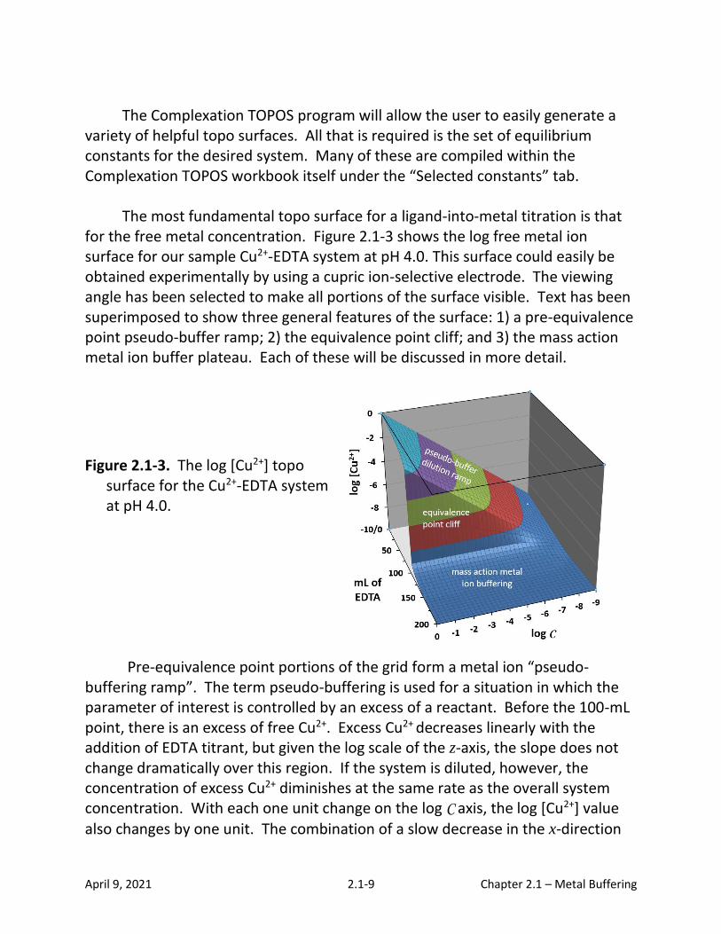
The most fundamental topo surface for a ligand-into-metal titration is that

for the free metal concentration. Figure 2.1-3 shows the log free metal ion surface for our sample Cu2+-EDTA system at pH 4.0. This surface could easily be obtained experimentally by using a cupric ion-selective electrode. The viewing angle has been selected to make all portions of the surface visible. Text has been superimposed to show three general features of the surface: 1) a pre-equivalence point pseudo-buffer ramp; 2) the equivalence point cliff; and 3) the mass action metal ion buffer plateau. Each of these will be discussed in more detail.

Figure 2.1-3. The log [Cu2+] topo surface for the Cu2+-EDTA system at pH 4.0.

Pre-equivalence point portions of the grid form a metal ion “pseudo-buffering ramp”. The term pseudo-buffering is used for a situation in which the parameter of interest is controlled by an excess of a reactant. Before the 100-mL point, there is an excess of free Cu2+. Excess Cu2+ decreases linearly with the addition of EDTA titrant, but given the log scale of the z-axis, the slope does not change dramatically over this region. If the system is diluted, however, the concentration of excess Cu2+ diminishes at the same rate as the overall system concentration. With each one unit change on the log C axis, the log [Cu2+] value

also changes by one unit. The combination of a slow decrease in the x-direction


and the steady decrease in the y-direction creates a ramp feature that descends at an angle of 45o. If the dilution were continued to even lower system concentrations, this ramp trend would continue. As one approaches the equivalence point volume at 100 mL, the change in log [Cu2+] becomes precipitous. Over the course of three grid points at 95, 100, and 105 mL, a 10 mL span, the curve drops to a low plateau. For the 1.0 M grid line this equivalence point cliff falls more than seven log units and shows a decrease in [Cu2+] of about 24,200,000 times. The height of the cliff decreases in the dilution direction because the starting value for [Cu2+] is successively lower. Note, though, that the plateau to which it drops, stays at essentially the same level. By a log C value of -7.75, the cliff has largely disappeared. Below the equivalence point cliff there is a broad plateau that comprises the “mass action metal ion buffer” zone. No matter which direction one moves in this region, the value of log [Cu2+] remains remarkably stable. The appearance of a plateau on a log free metal ion topo is the hallmark of a true metal buffering situation. Metal ion buffering is a concept infrequently encountered in analytical courses. With true metal ion buffering there is more chemistry occurring than simply a slow change caused by dilution of an excess species. The main difference between pseudo-buffering and mass action buffering for a metal ion is that, with the latter, dilution does not affect the free metal ion concentration substantially.

Consider the equilibrium constant expression for the 1:1 CuEDTA2- complex:

= 18.80

2-

1 2+ 4-

CuEDTA= 10

Cu EDTA (2.1-19)

This is based on eq 2.1-1 in the chemical model. Because this system is restricted

to 1:1 complexes, there is only a single overall stability constant, 1. (When

higher stoichiometries are present there would be a 2 for the 1:2 complex, a 3 for the 1:3 complex, and so forth.) Eq 2.1-19 can be rearranged to solve for [Cu2+]:


1

2-

2+

4-1

CuEDTACu = ×

EDTA (2.1-20)

When the logarithm of both sides is taken, a metal ion analog to the logarithmic form of the Guldberg and Waage Mass Action Law12 (see eq 1.1-2) for traditional acid-base buffers appears.

2-

2+1 4-

CuEDTAlog Cu = -log + log

EDTA (2.1-21)

Since log β1 is a constant, eq 2.1-21 indicates that log [Cu2+] is controlled by

the ratio of [CuEDTA2-] to [EDTA4-]. But once the equivalence point has been

passed, these two species track together. While the value for [EDTA4-] is quite

small (due to the 94.6% predominant H2EDTA2- form at pH 4), it slowly creeps toward its fractional concentration in the titrant solution as more is added. Only

tiny amounts of free Cu2+ remain. Adding titrant dilutes the [CuEDTA2-] that has

formed PLUS dissociates a small amount of it. As the system is diluted with water

under these conditions, [CuEDTA2-] and [EDTA4-] decrease proportionally at the

same rate. Thus, the ratio of the two important controlling species in eq 2.1-21 stays nearly constant.

How can the value of log [Cu2+] remain almost unchanged by dilution? The answer is because dilution, through the mass action effect, causes a tiny bit of the complex to dissociate. The dilution water molecules more effectively solvate and separate the Cu2+ and EDTA4- ions such that they cannot as easily re-encounter each other and re-complex. Consider the dissociation equation (2.1-22), the same formation equation (eq 2.1-1) with waters in the coordination sphere included:

Cu(H2O)6

2+ + EDTA4- ⇌ CuEDTA2- + 6 H2O (2.1-22)

Dilution is essentially perturbing the equilibrium by adding product. According to Le Chatelier’s principle, the system will regain equilibrium by shifting to the left. The amount of Cu2+ released by the tiny amount of dissociation, is exactly what is needed to keep the log [Cu2+] essentially constant. Table 2.1-1 follows this process for a 10-fold dilution that represents two points from the 150-mL dilution


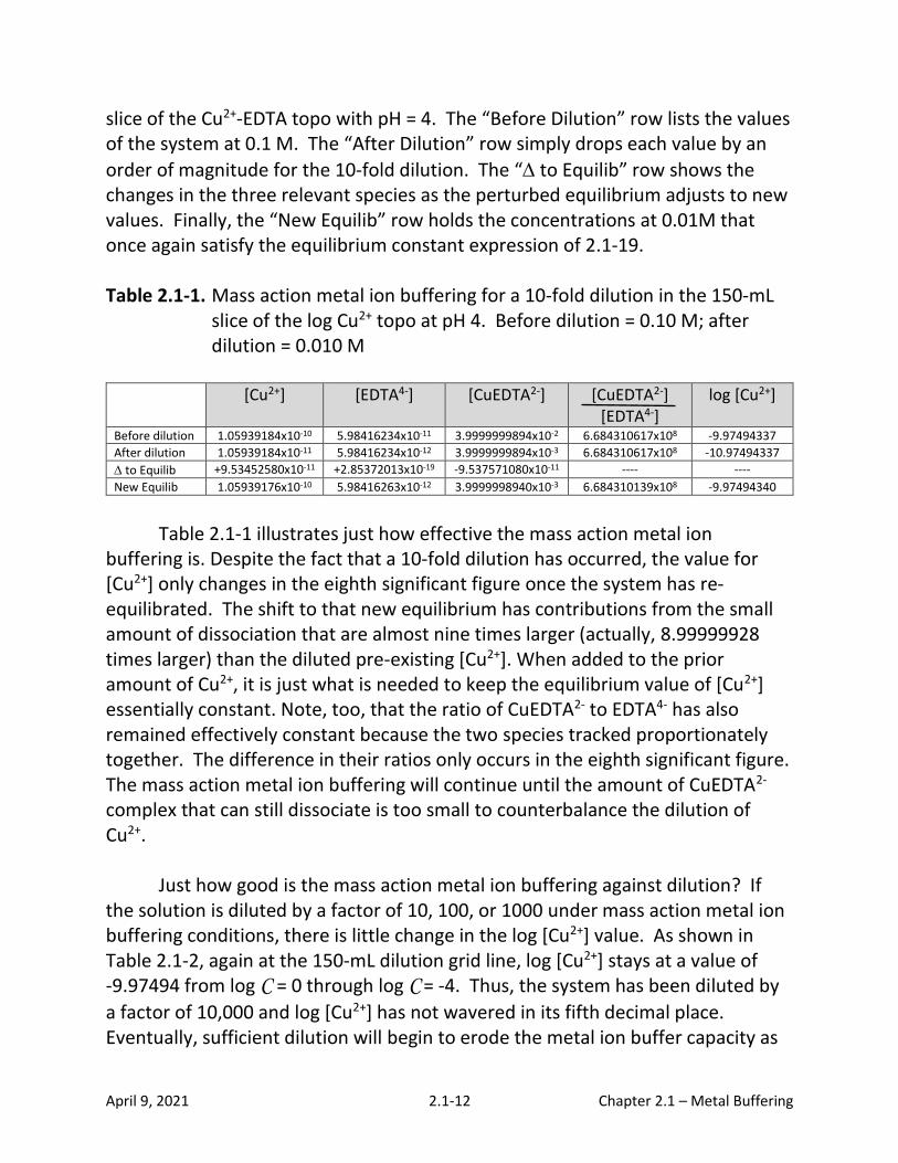
slice of the Cu2+-EDTA topo with pH = 4. The “Before Dilution” row lists the values of the system at 0.1 M. The “After Dilution” row simply drops each value by an

order of magnitude for the 10-fold dilution. The “ to Equilib” row shows the changes in the three relevant species as the perturbed equilibrium adjusts to new values. Finally, the “New Equilib” row holds the concentrations at 0.01M that once again satisfy the equilibrium constant expression of 2.1-19. Table 2.1-1. Mass action metal ion buffering for a 10-fold dilution in the 150-mL

slice of the log Cu2+ topo at pH 4. Before dilution = 0.10 M; after dilution = 0.010 M

[Cu2+] [EDTA4-] [CuEDTA2-] [CuEDTA2-] [EDTA4-]

log [Cu2+]

Before dilution 1.05939184x10-10 5.98416234x10-11 3.9999999894x10-2 6.684310617x108 -9.97494337

After dilution 1.05939184x10-11 5.98416234x10-12 3.9999999894x10-3 6.684310617x108 -10.97494337

to Equilib +9.53452580x10-11 +2.85372013x10-19 -9.537571080x10-11 ---- ----

New Equilib 1.05939176x10-10 5.98416263x10-12 3.9999998940x10-3 6.684310139x108 -9.97494340

Table 2.1-1 illustrates just how effective the mass action metal ion

buffering is. Despite the fact that a 10-fold dilution has occurred, the value for [Cu2+] only changes in the eighth significant figure once the system has re-equilibrated. The shift to that new equilibrium has contributions from the small amount of dissociation that are almost nine times larger (actually, 8.99999928 times larger) than the diluted pre-existing [Cu2+]. When added to the prior amount of Cu2+, it is just what is needed to keep the equilibrium value of [Cu2+] essentially constant. Note, too, that the ratio of CuEDTA2- to EDTA4- has also remained effectively constant because the two species tracked proportionately together. The difference in their ratios only occurs in the eighth significant figure. The mass action metal ion buffering will continue until the amount of CuEDTA2- complex that can still dissociate is too small to counterbalance the dilution of Cu2+.

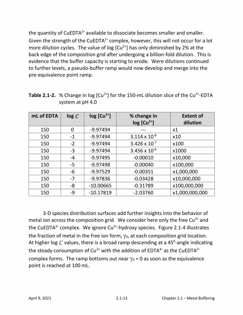
Just how good is the mass action metal ion buffering against dilution? If the solution is diluted by a factor of 10, 100, or 1000 under mass action metal ion buffering conditions, there is little change in the log [Cu2+] value. As shown in Table 2.1-2, again at the 150-mL dilution grid line, log [Cu2+] stays at a value of -9.97494 from log C = 0 through log C = -4. Thus, the system has been diluted by

a factor of 10,000 and log [Cu2+] has not wavered in its fifth decimal place. Eventually, sufficient dilution will begin to erode the metal ion buffer capacity as


the quantity of CuEDTA2- available to dissociate becomes smaller and smaller.

Given the strength of the CuEDTA2- complex, however, this will not occur for a lot

more dilution cycles. The value of log [Cu2+] has only diminished by 2% at the back edge of the composition grid after undergoing a billion-fold dilution. This is evidence that the buffer capacity is starting to erode. Were dilutions continued to further levels, a pseudo-buffer ramp would now develop and merge into the pre-equivalence point ramp.

Table 2.1-2. % Change in log [Cu2+] for the 150-mL dilution slice of the Cu2+-EDTA system at pH 4.0

mL of EDTA log C log [Cu2+] % change in log [Cu2+]

Extent of dilution

150 0 -9.97494 --- x1 150 -1 -9.97494 3.114 x 10-8 x10

150 -2 -9.97494 3.426 x 10-7 x100

150 -3 -9.97494 3.456 x 10-6 x1000 150 -4 -9.97495 -0.00010 x10,000

150 -5 -9.97498 -0.00040 x100,000 150 -6 -9.97529 -0.00351 x1,000,000

150 -7 -9.97836 -0.03428 x10,000,000 150 -8 -10.00665 -0.31789 x100,000,000

150 -9 -10.17819 -2.03760 x1,000,000,000

3-D species distribution surfaces add further insights into the behavior of

metal ion across the composition grid. We consider here only the free Cu2+ and

the CuEDTA2- complex. We ignore Cu2+-hydroxy species. Figure 2.1-4 illustrates

the fraction of metal in the free ion form, 0, at each composition grid location. At higher log C values, there is a broad ramp descending at a 450-angle indicating

the steady consumption of Cu2+ with the addition of EDTA4- as the CuEDTA2-

complex forms. The ramp bottoms out near 0 = 0 as soon as the equivalence point is reached at 100 mL.


Figure 2.1-4. The 0 trend surface (fraction of free Cu2+) for the Cu2+-EDTA system at pH 4.00.

The extent of dilution-driven dissociation of the complex is also shown on

this surface in the upward sweep of 0 as one gets to the lowest log C values of

the front edge of the figure. The dilution at which the upward sweep begins is

dependent on the value of 1 for a complex and the pH at which the system is being modeled. Its appearance indicates that the metal ion buffer capacity of the system is becoming depleted. For the 200-mL slice, 12.4 % of the complex has dissociated by the log C = -9 grid point.

The same effect can be seen in the 0 values on the pre-equivalence point consumption ramp. There is a slight upward curl at the point where dissociation of whatever complex is present begins to become significant. The CuEDTA2-

complex has such a large 1 that not much dissociation has occurred even at the lowest log C point of -9. The strength of H3O+ for a ligand cannot compete until it

hugely overwhelms the Cu2+ through mass action effects. At log C = -9, H3O+ is

present at about a 100,000-fold excess.


The companion 1 species surface, showing CuEDTA2- complex behavior, is

seen in Figure 2.1-5. For most log C values, a broad 450-ramp slopes upward

instead of downward because, in this instance, it represents formation of the complex. Once the equivalence point at 100 mL has been reached, there is an

expansive plateau with 1 essentially equal to 1. At the right edge, the surface begins to curve downwards, an indication that dilution-driven dissociation of the complex is beginning to be more significant, namely, the metal ion buffering capacity of the system is almost depleted. Were the surface continued to lower log C values, a descending logarithmic ramp would develop that ultimately levels

asymptotically to 1 = 0.

Figure 2.1-5. The 1 trend surface (fraction of CuEDTA2-) for the Cu2+-EDTA system at pH 4.00.

2.1.5 Metal Hydroxide Precipitates: Another Kind of Metal Ion Buffering

The Complexation TOPOS program will automatically check for the complication of metal hydroxide precipitate formation. The user is asked to supply the stoichiometry and the Ksp value for the solid metal hydroxide that

could form if the pH is too high. After a grid point has been solved for [Mn+], this

value is used with the [OH-] associated with the specified pH to compute a trial

ion product, TIP, that has the same form as the Ksp expression (eq 2.1-18). If the

TIP is larger than the Ksp, precipitate will be present and the grid cell in the TIP


data array will be colored yellow. Once metal hydroxide precipitates have been confirmed, it is easy to compute a corrected [Mn+] value from the Ksp expression.

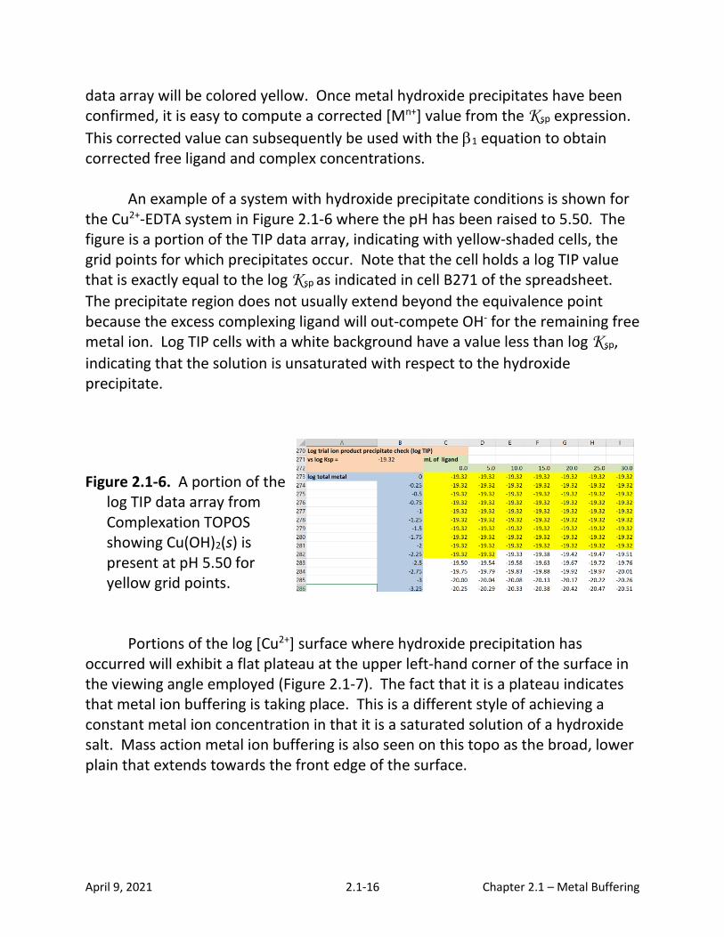
This corrected value can subsequently be used with the 1 equation to obtain corrected free ligand and complex concentrations. An example of a system with hydroxide precipitate conditions is shown for the Cu2+-EDTA system in Figure 2.1-6 where the pH has been raised to 5.50. The figure is a portion of the TIP data array, indicating with yellow-shaded cells, the grid points for which precipitates occur. Note that the cell holds a log TIP value that is exactly equal to the log Ksp as indicated in cell B271 of the spreadsheet.

The precipitate region does not usually extend beyond the equivalence point because the excess complexing ligand will out-compete OH- for the remaining free metal ion. Log TIP cells with a white background have a value less than log Ksp,

indicating that the solution is unsaturated with respect to the hydroxide precipitate.

Figure 2.1-6. A portion of the log TIP data array from Complexation TOPOS showing Cu(OH)2(s) is present at pH 5.50 for yellow grid points.

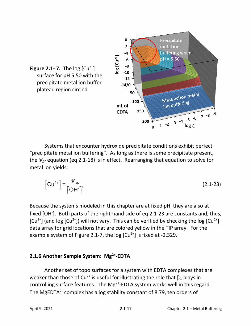
Portions of the log [Cu2+] surface where hydroxide precipitation has occurred will exhibit a flat plateau at the upper left-hand corner of the surface in the viewing angle employed (Figure 2.1-7). The fact that it is a plateau indicates that metal ion buffering is taking place. This is a different style of achieving a constant metal ion concentration in that it is a saturated solution of a hydroxide salt. Mass action metal ion buffering is also seen on this topo as the broad, lower plain that extends towards the front edge of the surface.


Figure 2.1- 7. The log [Cu2+]

surface for pH 5.50 with the precipitate metal ion buffer plateau region circled.

Systems that encounter hydroxide precipitate conditions exhibit perfect “precipitate metal ion buffering”. As long as there is some precipitate present, the Ksp equation (eq 2.1-18) is in effect. Rearranging that equation to solve for

metal ion yields:

n

K sp2+

-Cu =

OH (2.1-23)

Because the systems modeled in this chapter are at fixed pH, they are also at

fixed [OH-]. Both parts of the right-hand side of eq 2.1-23 are constants and, thus,

[Cu2+] (and log [Cu2+]) will not vary. This can be verified by checking the log [Cu2+] data array for grid locations that are colored yellow in the TIP array. For the example system of Figure 2.1-7, the log [Cu2+] is fixed at -2.329. 2.1.6 Another Sample System: Mg2+-EDTA

Another set of topo surfaces for a system with EDTA complexes that are

weaker than those of Cu2+ is useful for illustrating the role that 1 plays in controlling surface features. The Mg2+-EDTA system works well in this regard.

The MgEDTA2- complex has a log stability constant of 8.79, ten orders of


magnitude smaller than CuEDTA2-‘s value of 18.80. On the other hand, the log Ksp

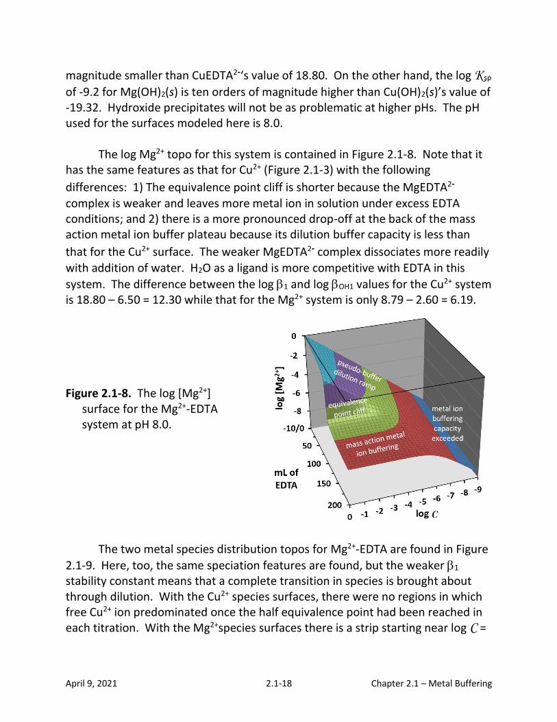
of -9.2 for Mg(OH)2(s) is ten orders of magnitude higher than Cu(OH)2(s)’s value of -19.32. Hydroxide precipitates will not be as problematic at higher pHs. The pH used for the surfaces modeled here is 8.0.

The log Mg2+ topo for this system is contained in Figure 2.1-8. Note that it

has the same features as that for Cu2+ (Figure 2.1-3) with the following

differences: 1) The equivalence point cliff is shorter because the MgEDTA2-

complex is weaker and leaves more metal ion in solution under excess EDTA conditions; and 2) there is a more pronounced drop-off at the back of the mass action metal ion buffer plateau because its dilution buffer capacity is less than

that for the Cu2+ surface. The weaker MgEDTA2- complex dissociates more readily

with addition of water. H2O as a ligand is more competitive with EDTA in this

system. The difference between the log 1 and log OH1 values for the Cu2+ system is 18.80 – 6.50 = 12.30 while that for the Mg2+ system is only 8.79 – 2.60 = 6.19.

Figure 2.1-8. The log [Mg2+]

surface for the Mg2+-EDTA system at pH 8.0.

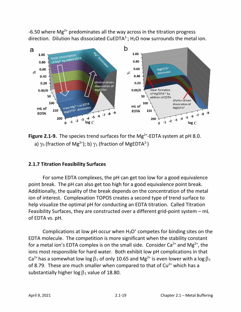
The two metal species distribution topos for Mg2+-EDTA are found in Figure

2.1-9. Here, too, the same speciation features are found, but the weaker 1 stability constant means that a complete transition in species is brought about through dilution. With the Cu2+ species surfaces, there were no regions in which free Cu2+ ion predominated once the half equivalence point had been reached in each titration. With the Mg2+species surfaces there is a strip starting near log C =


-6.50 where Mg2+ predominates all the way across in the titration progress direction. Dilution has dissociated CuEDTA2-; H2O now surrounds the metal ion.

Figure 2.1-9. The species trend surfaces for the Mg2+-EDTA system at pH 8.0.

a) 0 (fraction of Mg2+); b) 1 (fraction of MgEDTA2-) 2.1.7 Titration Feasibility Surfaces

For some EDTA complexes, the pH can get too low for a good equivalence point break. The pH can also get too high for a good equivalence point break. Additionally, the quality of the break depends on the concentration of the metal ion of interest. Complexation TOPOS creates a second type of trend surface to help visualize the optimal pH for conducting an EDTA titration. Called Titration Feasibility Surfaces, they are constructed over a different grid-point system – mL of EDTA vs. pH.

Complications at low pH occur when H3O+ competes for binding sites on the

EDTA molecule. The competition is more significant when the stability constant for a metal ion’s EDTA complex is on the small side. Consider Ca2+ and Mg2+, the ions most responsible for hard water. Both exhibit low pH complications in that

Ca2+ has a somewhat low log 1 of only 10.65 and Mg2+ is even lower with a log 1 of 8.79. These are much smaller when compared to that of Cu2+ which has a

substantially higher log 1 value of 18.80.


Traditionally, the inclusion of low pH complications has been handled with

a conditional stability (or formation) constant, 1’.13 A conditional constant is

computed using the species distribution coefficient for the completely

unprotonated form of the ligand. For EDTA, this corresponds to 6 (or sometimes noted as Y4-). An example conditional constant for Ca2+ would be written as:

2-

11 2+

6 6

CaEDTA' = =

Ca uncomplexed ligand

(2.1-24)

Accounting for low pH complications is often handled by providing a table or a

plot listing the pH at which the 1’ for individual metal ion species is equal to 108,

a value large enough to provide a good equivalence point break. Conditional constants as in eq 2.1-24 account for low pH complications, but not the high pH complications from OH- ions competing against EDTA for the metal cation of interest. Formation of hydroxy complexes and hydroxide precipitates also interfere with the equivalence point break by lowering the free metal ion concentration prior to its occurrence. Eq 2.1-24 could be further

modified to include a metal speciation coefficient, 0.

2-

11

0 6 0 6

CaEDTA" = =

uncomplexed Ca uncomplexed ligand

(2.1-25)

Here, the 0 includes not only 1 as above (the fraction of CuEDTA2-), but also OH1

(the fraction of CuOH+), OH2 (the fraction of Cu(OH)20), OH3 (the fraction of

Cu(OH)3-), OH4 (the fraction of Cu(OH)4

2-), and Cu(OH)2(s) (the fraction of Cu(OH)2(s)). A better solution to including titration complications from both too low and too high pHs is to construct a titration feasibility surface above a grid for which one axis is the titration progress (mL of EDTA) and the other runs the full range of pH values from 0 to 14. Complexation TOPOS includes this feature on a second calculation tab. It uses exactly the same input data as the metal ion topo calculations except that the pH is automatically cycled through all values and the total concentration of metal must be specified. It is fixed over the entire trend surface.


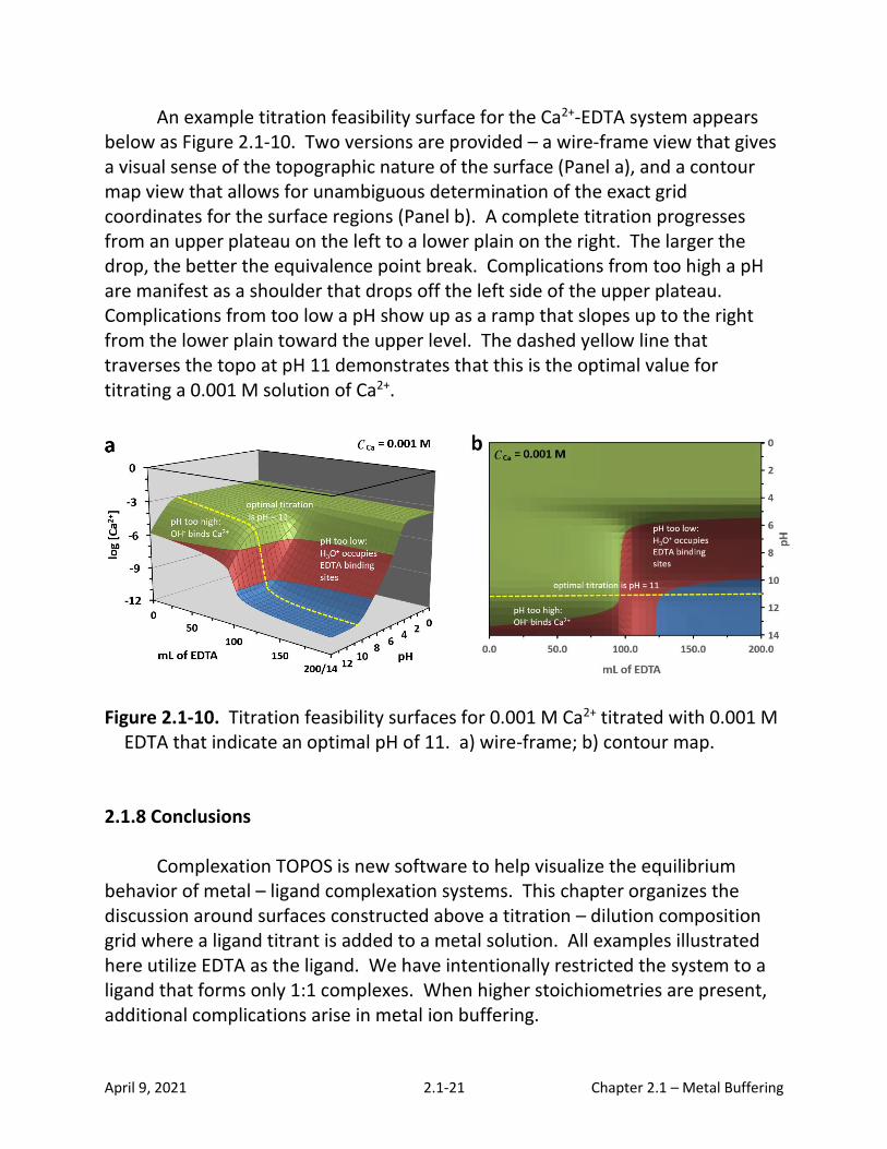
An example titration feasibility surface for the Ca2+-EDTA system appears below as Figure 2.1-10. Two versions are provided – a wire-frame view that gives a visual sense of the topographic nature of the surface (Panel a), and a contour map view that allows for unambiguous determination of the exact grid coordinates for the surface regions (Panel b). A complete titration progresses from an upper plateau on the left to a lower plain on the right. The larger the drop, the better the equivalence point break. Complications from too high a pH are manifest as a shoulder that drops off the left side of the upper plateau. Complications from too low a pH show up as a ramp that slopes up to the right from the lower plain toward the upper level. The dashed yellow line that traverses the topo at pH 11 demonstrates that this is the optimal value for titrating a 0.001 M solution of Ca2+.

Figure 2.1-10. Titration feasibility surfaces for 0.001 M Ca2+ titrated with 0.001 M

EDTA that indicate an optimal pH of 11. a) wire-frame; b) contour map. 2.1.8 Conclusions

Complexation TOPOS is new software to help visualize the equilibrium behavior of metal – ligand complexation systems. This chapter organizes the discussion around surfaces constructed above a titration – dilution composition grid where a ligand titrant is added to a metal solution. All examples illustrated here utilize EDTA as the ligand. We have intentionally restricted the system to a ligand that forms only 1:1 complexes. When higher stoichiometries are present, additional complications arise in metal ion buffering.


Viewing the topo surfaces produced by this Microsoft Excel workbook will

help students visualize several aqueous equilibrium concepts: - The surfaces dramatically demonstrate metal ion buffering, a topic not

traditionally included in most textbooks;

- The surfaces clearly distinguish the difference between “pseudo-buffering” (that only occurs in the titration direction) and real “metal ion buffering” (that happens in BOTH the titration and dilution directions);

- Two different types of metal ion buffering are introduced – mass action metal ion buffering in post-equivalence point settings, and precipitate metal ion buffering in OH- saturated pre-equivalence point conditions.

- Species distribution surfaces let students follow the formation of

complexes during a titration PLUS discern the dissociation of the complexes as the system is diluted;

- Sloped boundaries on the metal ion buffer plateaus illustrate when

buffer capacity has been exceeded; and - Titration feasibility surfaces provide a means to select the ideal pH for a

given analyte concentration.

The Complexation TOPOS software can be used in an introductory collegiate course of general chemistry. An understanding of its fine points, though, will require the chemical sophistication of students in junior- or graduate-level courses in analytical chemistry, biochemistry and aquatic geochemistry. The speed and ease with which new systems can be visualized makes this a powerful tool for simulation studies. Because it is implemented via Microsoft Excel, no new software need be purchased to run it. With run times usually less than 30 seconds, Complexation TOPOS can conveniently be used for “on the fly” calculations by an instructor during a classroom session. A query from a student about “What would happen if…” can easily be addressed with a new run of the program.


2.1.9 Supplementary files

Five downloadable files are included as additional supplements for this chapter:

1. The free, downloadable Complexation TOPOS software implemented as a Microsoft Excel workbook. A table of thermodynamic constants offers a variety of metal ion-EDTA systems to explore. Users, however, are free to supply their own constants as desired. Only systems with exclusively 1:1 complexes will work. Additional input data include protonation constants for the ligand, hydroxy complexation constants for the metal ion, and a Ksp

for potential hydroxide precipitates.

2. Microsoft PowerPoint slides from which to present a lecture on metal – ligand complexation titrations and metal ion buffering where only 1:1 complexes are formed. This is applicable to EDTA titrations, the most common complexometric procedure in chemistry courses. Teaching points are highlighted and illustrated with extensively annotated surfaces. Separate sections are identified as appropriate for either lower division or upper division students.

3. A “Teaching with Complexation TOPOS” document that lists itemized

teaching objectives. Each objective is matched to a range of slides in the PowerPoint lecture, so that an instructor can include whatever points are of interest. Following the discussion of the PowerPoint slides are suggested Complexation TOPOS workbook activities (homework, pre-lab, recitation or peer-led team discussions) and suggestions for coordinated laboratory experiments.

4. A detailed derivation of the mass balance equation that is solved for the equilibrium concentration of free ligand plus a section on the numerical techniques used to solve it.

5. A listing of the Visual Basic code for the Complexation TOPOS macros that

compute the concentration of free ligand for each grid point.

As downloaded, Complexation TOPOS worksheets are populated with the Cu2+-EDTA example for the metal ion topo and the 0.001 M Ca2+-EDTA titration feasibility surface presented in this chapter. Constants for other metals are


included in the “Selected Constants” tab of the Complexation TOPOS workbook. Other ligands that will display exclusively 1:1 behavior like EDTA include DCTA (trans-1,2-diaminocyclhexanetetraacetic acid) and ATP (adenosine triphosphate).

Ligands that form higher stoichiometries introduce further complications in

metal ion buffering. These complications are addressed in Chapter 2.2 Metal Ion Anti-Buffering.

Author Information

Corresponding Author

*E-mail: [email protected]

Acknowledgments

The project was partially supported by a grant from North South University, Award No. NSU/BIO/CTRGC/47. We thank Daniel Barry for assistance in confirmation experiments in the laboratory. Glenn Pinson fabricated the reaction vessel used in all complexometric studies. References

1. Elgrishi, N.; Chambers, M.B.; Wang, X.; Fontecave, M. Molecular polypyridine-based metal complexes as catalysts for the reduction of CO2. Chem. Soc. Rev., 2017, 46, 761-796. https://doi.org/10.1039/C5CS00391A

2. Randolf, K.; Wolfgang, H. H. Sorption of Heavy Metals onto Selective Ion-Exchange Resins with Aminophosphonate Functional Groups. Ind. Eng. Chem. Res., 2001, 40 (21), 4570-4576. https://doi.org/10.1021/ie010182l

3. Fish, R.H.; Gérard, J. Bioorganometallic Chemistry: Structural Diversity of Organometallic Complexes with Bioligands and Molecular Recognition Studies of Several Supramolecular Hosts with Biomolecules, Alkali-Metal Ions, and Organometallic Pharmaceuticals. Organometallics, 2003, 22 (11), 2166-2177. https://doi.org/10.1021/om0300777

mailto:[email protected]

https://doi.org/10.1039/C5CS00391A

https://doi.org/10.1021/ie010182l

https://doi.org/10.1021/om0300777


4. Isoo, K.; Terabe, S. Analysis of Metal Ions by Sweeping via Dynamic Complexation and Cation-Selective Exhaustive Injection in Capillary Electrophoresis. Anal. Chem., 2003,75 (24), 6789-6798. https://doi.org/10.1021/ac034677r

5. Yappert, M.C.; DuPre, D.B. Complexometric Titrations: Competition of Complexing Agents in the Determination of Water Hardness with EDTA. J. Chem. Educ., 1997, 74 (12), 1422. https://doi.org/10.1021/ed074p1422

6. Mauk, M.R.; Rosell, F.I.; Lelj-Garolla, B.; Moore, G. R.; Mauk, A. G. Metal ion binding to human hemopexin. Biochemistry,2005, 44, 1864−1871. https://doi.org/10.1021/bi0481747

7. Douglas, R.W.; Bolton, H. Jr. ; Moore, D. A.; Hess, N. J.; Choppin, G. R. Thermodynamic model for the solubility of PuO2(am) in the aqueous Na+- H+-OH–-Cl–-H2O-ethylenediaminetetraacetate system. Radiochim. Acta, 2001, 89, 67–74. https://doi.org/10.1524/ract.2001.89.2.067

8. Martell, A. E.; Smith, R. M.; Motekaitis, NIST Critical Stability Constants of Metal Complexes Database 46; Gaithersburg, MD, 2001.

9. Wanninen, E.V.; Ingman, F. Metal buffers in chemical analysis: Part I- Theoretical considerations. Pure & Appl. Chem. 1987, 59, 1681-1692.

10. Wanninen, E.V.; Ingman, F. Metal buffers in chemical analysis: Part II- Theoretical considerations. Pure & Appl. Chem. 1991, 63(4), 639-642.

11. Perrin, D. D.; Dempsey, B. Buffers for pH and Metal Ion Control, Chapman and Hall, London, 1974.

12. Guldberg, C.M.; Waage, P. Über Die Chemische Affinität, L. prakt Chem. 1879, 19(2), 69-114.

13. Butler, J.N. Ionic Equilibrium: A Mathematical Approach. Addison-Wesley, Reading, MA, 1964, p.378.

https://doi.org/10.1021/ac034677r

http://pubs.acs.org/author/Yappert%2C+M+Cecilia

http://pubs.acs.org/author/DuPre%2C+Donald+B

https://doi.org/10.1021/ed074p1422

https://doi.org/10.1021/bi0481747

https://doi.org/10.1524/ract.2001.89.2.067

https://doi.org/10.1524/ract.2001.89.2.067

Documents

Chapter 2.1: Visualization of Metal Ion Buffering Via 3-D Topo