An Update on Router Buffering - UCSC Directory of individual

© 2015 Cisco and/or its affiliates. All rights reserved. - Cisco Public Page 1 of 34

White Paper

White Paper

An Update on Router Buffering

Last Updated: August 2017

Buffering requirements for routers have been a much debated and ultimately

unresolved topic since the beginning of the Internet. This paper presents a technical

foundation for network designers to assess buffering requirements based on

applications as well as network and traffic characteristics. It also provides specific

recommendations for common scenarios for use in product selection and as a starting

point for deployment.

Author: Lane Wigley, Cisco Technical Marketing

© 2015 Cisco and/or its affiliates. All rights reserved -. Cisco Public

Page 2 of 34

Executive Summary

Buffers are the shock absorbers in a network, and their operation is critical to its operation. Router buffering design

is essentially determining what to do with packets that cannot immediately be forwarded. While that problem

statement is quite simple, the answer is one of the most challenging topics in networking.

In some cases, a network’s applications and their behaviors may be well understood; in others, a router may need

to support a wide range of applications. The target application may be specific such as an Enterprise VoIP service

or broader, such as web traffic carrier over the Internet.

Application requirements can often be defined in terms of bandwidth, tolerance for loss, latency, and packet delay

variation (“jitter”). In addition to the end-user-visible application, the application implementation also impacts

network requirements. For example, the transport protocol and the size of the host-side buffer influence a video

application’s tolerance for packet loss.

The network architecture and a device’s place in it greatly influence the type of router or switch required. For

example, it is usually critical to fully utilize expensive long-haul WAN links, data center routers and switches often

have the option of adding additional capacity for a relatively low cost as a way to minimize congestion. Round Trip

Time is another key variable that may range from tens of microseconds in a data center to multiple seconds on a

congested cellular network – over five orders of magnitude. This factor alone may drive an equally large difference

in buffer requirements, which is the reason for a similar range of capabilities among the products on the market

today which are optimized for those environments. In addition, a router’s place in the network also determines

bandwidth, oversubscription, traffic synchronization, the range of link speeds, and link latency.

Router architectures and their impact on buffering are also explored. Key factors include centralized vs. distributed

architectures, queuing models (e.g., central, VOQ, egress), the number of buffers, and sharing of buffers.

This paper explores these areas and the tradeoffs that should be considered both for selecting and configuring

routers. It focuses on the traditional SP router roles, but also highlights the unique characteristics of SP and Web

data center networks.

The paper doesn’t propose any single answer but attempts to cut through the dogmatic and simplistic extremes

which are frequently proposed so that network designers can effectively evaluate routers in the context of their

requirements. Recommendations are made as ranges and guidance is provided to adjust within or outside the

range.

In general, the recommendations are lower than legacy buffering requirements developed in the 1990s. Based on

these factors, the key recommendations are:

Core router buffering in the range of 5-10 msec

Edge router buffering in the range of 10-30 msec

Data Center buffering is highly dependent on architecture and applications. Low RTT, ease of adding

bandwidth, and traffic synchronization are critical considerations.


Page 3 of 34

Network Behaviors as Seen by Applications

Applications have a wide range of requirements from the network, and they have preferences for what the

network’s behavior should be when it is unable to immediately deliver packets along the “best” path. Starting with

the assumption that applications behave optimally when directly connected over a short distance via a media fast

enough to carry all traffic they can generate, what then are the differences between this ideal network and a real

network?

The most notable differences in a real-world network that affect service quality are packet loss, latency, reordering,

corruption/duplication, and packet delay variation. Collectively, these characteristics define the quality of the

network for the application.

Packet loss can occur for a number of reasons, most notably: congestion (due to link or router capacity); software

bugs; filters (e.g., ACL, uRPF, black holes); incorrect routing; and convergence events. This paper will focus on

loss from congestion as it is the most relevant to buffering. Note that these behaviors apply to L2 frames, MPLS

frames, or IP packets processed by switches and routers. Unless noted, “packets” to refer to all types user data

traffic.

The main sources of latency are propagation delay along the links, nominal device latency, and link-congestion

buffering (queuing latency). Propagation delay is a function of the speed of light (3.34 usec per km), but evaluating

the latency on a link between two points must take into account the actual fiber path and refraction inside the fiber.

A reasonable approximation for the refraction impact for conventional fiber is 1.46 (depending on fiber brand and

wavelength) which results in a speed of approximately 5 us / km [M2optics]. A common guideline used in buffering

calculations is a maximum terrestrial propagation delay of roughly 125 msec resulting in a max non-congested

route trip time (RTT) of 250 msec.

Nominal device latency is the time a packet is delayed by a non-congested network device. This includes time to

copy the packet into different memories, to perform packet operations, and serialization delay (the time to send bits

onto the fiber, which will be less for faster links and smaller packets). In low-RTT networks like Data Centers,

serialization delay can be a significant part of the RTT (1.2 us for 10G and 12us for 1G) and is a motivation for

10G-connected servers in some applications even when traffic is only in the 100s of Mbps.

Latency due to buffering results from the inability to forward all packets immediately. This is the shock absorber

function. It ranges from small delays for a microburst on a 10G link transitioning to a 1G link to large delays

measured in seconds when a low-speed interface with large buffers experiences persistent congestion, especially

in under-provisioned wireless networks.

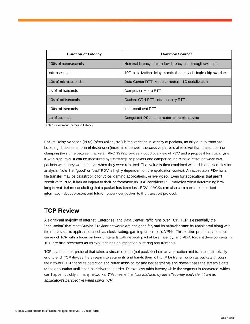
The table below illustrates the range of latency introduced from common sources.

Printed in USA CXX-XXXXXX-XX 10/11


Page 4 of 34

Duration of Latency Common Sources

100s of nanoseconds Nominal latency of ultra-low-latency cut-through switches

microseconds 10G serialization delay, nominal latency of single-chip switches

10s of microseconds Data Center RTT, Modular routers, 1G serialization

1s of milliseconds Campus or Metro RTT

10s of milliseconds Cached CDN RTT, intra-country RTT

100s milliseconds Inter-continent RTT

1s of seconds Congested DSL home router or mobile device

Table 1 - Common Sources of Latency

Packet Delay Variation (PDV) (often called jitter) is the variation in latency of packets, usually due to transient

buffering. It takes the form of dispersion (more time between successive packets at receiver than transmitter) or

clumping (less time between packets). RFC 3393 provides a good overview of PDV and a proposal for quantifying

it. At a high level, it can be measured by timestamping packets and comparing the relative offset between two

packets when they were sent vs. when they were received. That value is then combined with additional samples for

analysis. Note that “good” or “bad” PDV is highly dependent on the application context. An acceptable PDV for a

file transfer may be catastrophic for voice, gaming applications, or live video. Even for applications that aren’t

sensitive to PDV, it has an impact to their performance as TCP considers RTT variation when determining how

long to wait before concluding that a packet has been lost. PDV of ACKs can also communicate important

information about present and future network congestion to the transport protocol.

TCP Review

A significant majority of Internet, Enterprise, and Data Center traffic runs over TCP. TCP is essentially the

“application” that most Service Provider networks are designed for, and its behavior must be considered along with

the more specific applications such as stock trading, gaming, or business VPNs. This section presents a detailed

survey of TCP with a focus on how it interacts with network packet loss, latency, and PDV. Recent developments in

TCP are also presented as its evolution has an impact on buffering requirements.

TCP is a transport protocol that takes a stream of data (not packets) from an application and transports it reliably

end to end. TCP divides the stream into segments and hands them off to IP for transmission as packets through

the network. TCP handles detection and retransmission for any lost segments and doesn’t pass the stream’s data

to the application until it can be delivered in order. Packet loss adds latency while the segment is recovered, which

can happen quickly in many networks. This means that loss and latency are effectively equivalent from an

application’s perspective when using TCP.


Page 5 of 34

Congestion control is the mechanism that TCP uses to determine when to transmit segments. To implement

congestion control, TCP first probes the network by increasing the rate of transmission in order to determine the

optimal rate as represented by the number of packets “in flight” at any given time. Once it finds this level, it will

continually adjust based on signals from the network, traditionally packet loss and Round Trip Time (RTT). Newer

implementations of congestion control implement more complex algorithms, in some cases generated by machine

learning that are far beyond anything human architects could even consider.

TCP utilizes a receive window that is advertised in the header. The receive window communicates the available

buffer capacity on the receiver and changes when the buffer fills. The transmitter may never have more

unacknowledged segments in the network than the value of the receive window as doing so could cause an

overflow of the receiver’s buffer.

In the original implementation, a TCP session could complete the 3-way handshake and immediately transmit the

entire size of the receive window. For example, with a receive window of 8 * Max Segment Size (MSS) advertised,

the sender could burst 8 packets over a 10 Mbps Ethernet link. At the time, the NSFNet backbone ran at 56 Kbps

so a burst of 8 500-byte packets would congest a core link for over 500 msec. With this behavior and the lack of

any arbitration between flows, the resulting network was extremely fragile and experienced several catastrophic

failures known as congestion collapse events.

Slow Start and Congestion Avoidance

The TCP Congestion Avoidance scheme was initially proposed by Van Jacobson and Michael J. Karels after

observations of congestion collapse events in the mid-1980s. Long before PSY and Gangnam Style, it was literally

possible to “break the Internet” due to lack of congestion control. These were not mere degradations but drops of

three orders of magnitude in usable bandwidth even for nodes separated by only a few hops. Their seminal

Congestion Avoidance and Control paper [Jacobson & Karels] introduced a number of new algorithms to manage

TCP congestion. The stated goal of this scheme has stood the test of time: flows should exhibit a conservation of

packets:

“By ‘conservation of packets’ we mean that for a connection ‘in equilibrium’, i.e., running stably with a full

window of data in transit, the packet flow is what a physicist would call ‘conservative’: A new packet isn’t put

into the network until an old packet leaves.”

The two key mechanisms (Slow Start and Congestion Avoidance) from the initial paper were implemented in the

4.3.Tahoe release of the BSD Unix operating system and later became known as “TCP Tahoe”. While Tahoe is no

longer widely used, it represents the first stage in the evolution of TCP congestion control.

Starting with Tahoe, each end of a TCP session maintains two independent windows that determine how many

unacknowledged segments may be in transit at a time. The receive window operation is unchanged. The

congestion window dynamically represents the network capacity to support the flow. At any given time, the smaller

of the two windows is used to govern the number of unacknowledged packets that may be in transit. Together, the

RTT and congestion window size determine the overall throughput of the flow. Releasing new segments as

previous segments are acknowledged has the effect of clocking and pacing the network, and action must be taken

when this clock is lost which is detected via a timeout.


Page 6 of 34

The first stage in TCP congestion control was called slow start. The name is potentially misleading as it

exponentially ramps up the size of the congestion window, but it doesn’t allow the sender to immediately fill the

entire receive window as was allowed before. Slow Start increases the size of the congestion window by allowing

an additional packet to be “in flight” every time an ACK is received – each segment acknowledged allows two new

segments to be sent. Doubling the window and sending all the new segments as soon as possible results in a

bursty behavior which impacts buffering requirements.

The congestion window starts at some small multiple of MSS (max segment size, default of 536 or negotiated

during the handshake and often 1460 bytes today) and grows by the MSS with each ACK. This algorithm results in

an exponential increase in the window size so the rate can grow quickly. Increasing the window as ACKs are

received makes the rate at which the window size can increase highly dependent on RTT which illustrates one of

the ways that TCP behaves differently on the Internet vs. Data Center due to the 10000x difference in RTT (10s of

us vs. 100s of msec).

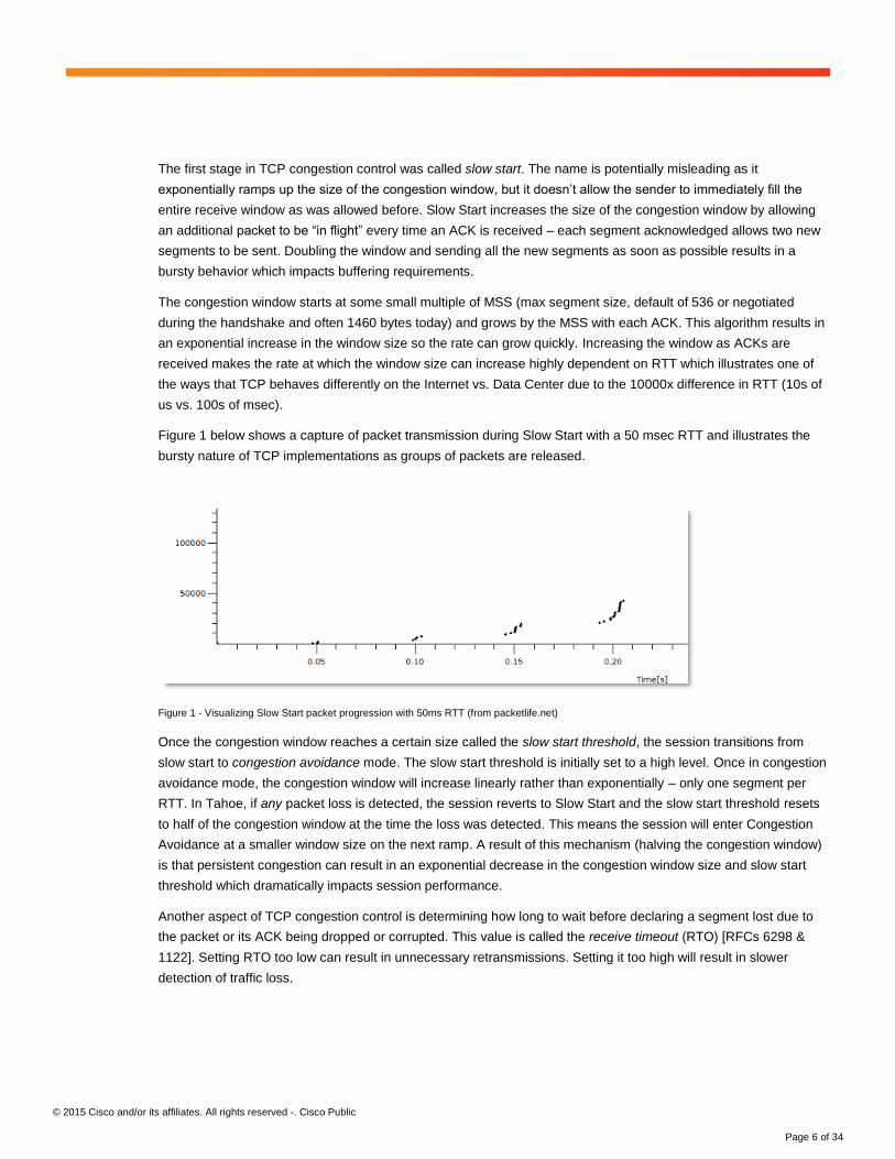
Figure 1 below shows a capture of packet transmission during Slow Start with a 50 msec RTT and illustrates the

bursty nature of TCP implementations as groups of packets are released.

Figure 1 - Visualizing Slow Start packet progression with 50ms RTT (from packetlife.net)

Once the congestion window reaches a certain size called the slow start threshold, the session transitions from

slow start to congestion avoidance mode. The slow start threshold is initially set to a high level. Once in congestion

avoidance mode, the congestion window will increase linearly rather than exponentially – only one segment per

RTT. In Tahoe, if any packet loss is detected, the session reverts to Slow Start and the slow start threshold resets

to half of the congestion window at the time the loss was detected. This means the session will enter Congestion

Avoidance at a smaller window size on the next ramp. A result of this mechanism (halving the congestion window)

is that persistent congestion can result in an exponential decrease in the congestion window size and slow start

threshold which dramatically impacts session performance.

Another aspect of TCP congestion control is determining how long to wait before declaring a segment lost due to

the packet or its ACK being dropped or corrupted. This value is called the receive timeout (RTO) [RFCs 6298 &

1122]. Setting RTO too low can result in unnecessary retransmissions. Setting it too high will result in slower

detection of traffic loss.


Page 7 of 34

Due to changing network conditions (e.g., routing path change or congestion), the RTO cannot be set to the best

case or even average Round Trip Time. Instead, a smoothed RTT and the RTT variance are calculated. RTO is set

to the smoothed RTT + 4 times the variation or 1 second, whichever is greater.

For further discussion of retransmit timeout, refer to RFC 6298. In Tahoe, RTO is not set below 1 second so

detecting network congestion via RTO can take a relatively long time, especially in low-RTT conditions. Later

developments in TCP address this and other limitations of Tahoe.

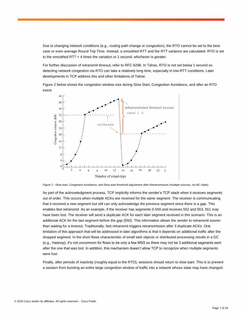
Figure 2 below shows the congestion window size during Slow Start, Congestion Avoidance, and after an RTO

event.

Figure 2 - Slow start, Congestion Avoidance, and Slow start threshold adjustment after Retransmission (multiple sources, via NC State)

As part of the acknowledgment process, TCP implicitly informs the sender’s TCP stack when it receives segments

out of order. This occurs when multiple ACKs are received for the same segment. The receiver is communicating

that it received a new segment but still can only acknowledge the previous segment since there is a gap. This

enables fast retransmit. As an example, if the receiver has segments 0-550 and receives 552 and 553, 551 may

have been lost. The receiver will send a duplicate ACK for each later segment received in this scenario. This is an

additional ACK for the last segment before the gap (550). This information allows the sender to retransmit sooner

than waiting for a timeout. Traditionally, fast retransmit triggers retransmission after 3 duplicate ACKs. One

limitation of this approach that will be addressed in later algorithms is that it depends on additional traffic after the

dropped segment. In the short flows characteristic of small web objects or distributed processing results in a DC

(e.g., Hadoop), it’s not uncommon for flows to be only a few MSS so there may not be 3 additional segments sent

after the one that was lost. In addition, this mechanism doesn’t allow TCP to recognize when multiple segments

were lost.

Finally, after periods of inactivity (roughly equal to the RTO), sessions should return to slow start. This is to prevent

a session from bursting an entire large congestion window of traffic into a network whose state may have changed.


Page 8 of 34

TCP Reno – Fast Recovery

TCP Reno adds a fast recovery mechanism which avoids returning the session to slow start if the loss is detected

via duplicate ACKs. Instead, when fast retransmit is triggered, the ssthresh and congestion window are both set to

half the current congestion window and the session remains in congestion avoidance mode. While the missing

segment is being resolved, the acknowledgment of the further out-of-order segments allows new segments to be

transmitted while still maintaining the allowed number of segments in flight. The duplicate ACKs do not trigger an

increase the congestion window size. If fast retransmit isn’t successful, a timeout (RTO) occurs which results in the

session reverting to slow start. In Reno, regular retransmission and a reset to slow start occur if more than one

segment is lost within an RTT. If the same segment must be retransmitted multiple times, the RTO window will

increase exponentially, and the session performance will be significantly impacted.

While other TCP options are now available, the mechanisms in TCP Reno provide the foundation for modern

congestion control and retransmission. Later models mainly refine the algorithms and recovery behaviors while still

following the receive window, congestion window, fast retransmission, and fast recovery model.

Leaving Nevada – More Congestion Control Algorithms

There are many other congestion control mechanisms such as SACK, New Reno, CUBIC, PRR, Vegas, BIC,

Compound TCP, DCTCP, MTCP, and others. In fact, the Linux kernel 3.14.0 supports 12 different congestion

control algorithms that either promise better performance overall, optimization for characteristics such as

constraining latency, or for specialized environments. It is important to note that the congestion control algorithm

isn’t negotiated and may be different for each host in a session. This allows for operating systems or even

applications to choose different algorithms and also to set their TCP parameters. For example, the initial

congestion window and initial RTO may also be set by the client. Initial congestion windows of 10-20 are now

common [Wu & Luckie], and there are discussions in IETF about eliminating the initial congestion window entirely

(when combined with pacing). While initial RTOs below 1 second make sense in many networks, caution should be

taken as network latency is not the only factor in RTT – gateways, VPN servers, and delayed ACKs may also add

latency.

Selective ACK (SACK) [RFC 2018] is a TCP option that improves the default behavior of cumulative

acknowledgment. Without SACK, when the host receives a duplicate ACK it cannot determine if segments other

than the one directly after the acknowledged segment were also lost so it doesn’t know what needs to be

retransmitted. If it just transmits the first unacknowledged segment, it will take a full RTT to identify another missing

segment. The ability to selectively acknowledge segments solves this problem. SACK must be negotiated between

hosts. Usage was above 90% in a recent experiment conducted by Google [Dukkipati, Mathis, Chueng & Ghobadi].

NewReno [RFC 3782] addresses the case of multiple segment loss when SACK isn’t enabled. In this case, the

sender doesn’t know that multiple segments are lost until the first retransmission is acknowledged. NewReno

updates the behavior for the “partial response” scenario when additional missing segments are detected after the

first retransmission. NewReno is commonly deployed and is the default in FreeBSD.

CUBIC improves the congestion control behavior of TCP on high-RTT, high-bandwidth networks while maintaining

fairness among new and existing flows and among flows with varying RTTs [Ha, Rhee & Xu]. Two of the key

innovations are using the time since the most recent packet loss to expand the congestion window (RTT neutral)


Page 9 of 34

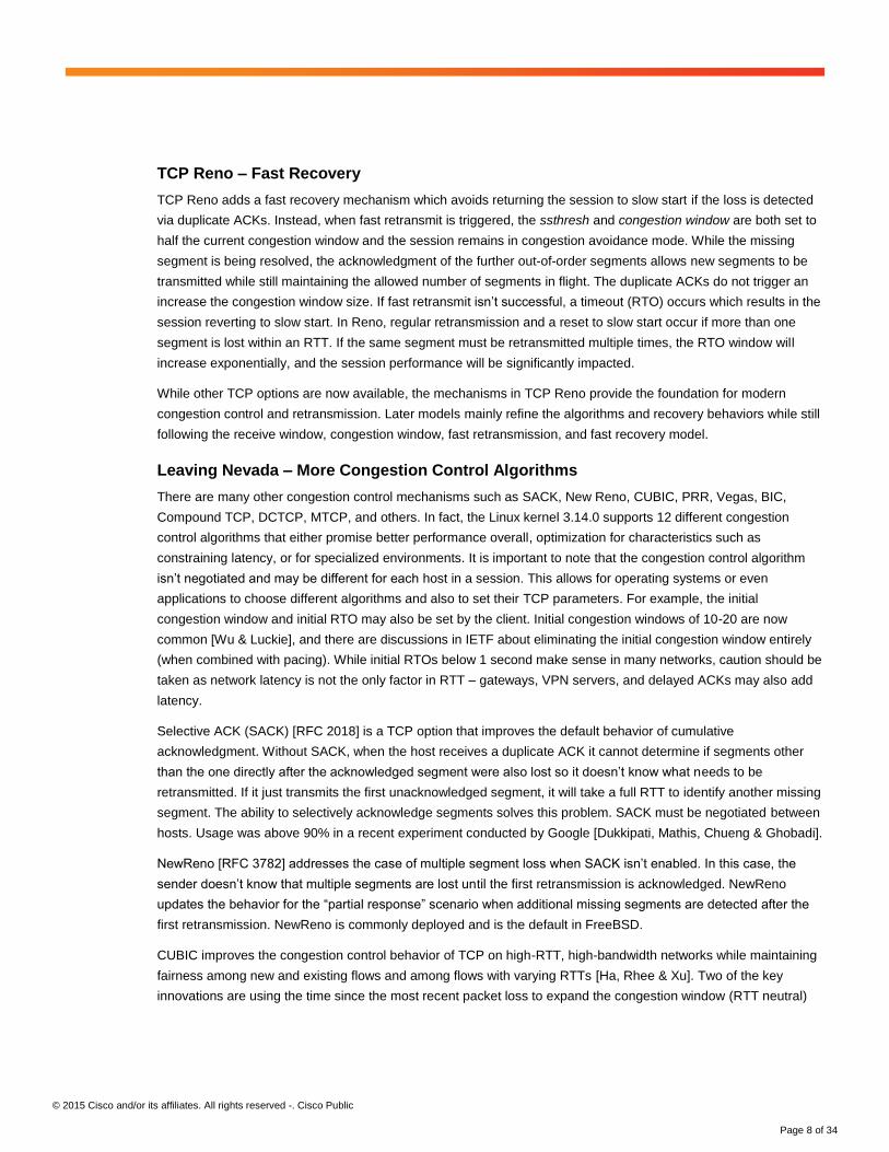
and expanding the window with a cubic function. The cubic function allows the window to grow rapidly before the

previous congestion level but more cautiously near the level where congestion was last observed. If the previous

congestion is no longer occurring, the rapid expansion resumes.

CUBIC is effective for high-bandwidth high-RTT networks as the congestion window growth is not dependent on

ACKs (and thus RTT). CUBIC is the default in Linux and MacOS Yosemite. CUBIC is the default congestion control

algorithm in Linux and is therefore broadly deployed. As Android uses Linux, it is also deployed in wireless

networks.

Figure 3 - CUBIC window expansion in red - via Geoff Huston

TCP Proportional Rate Reduction [Dukkipati, Mathis, Chueng & Ghobadi] was developed by Google to improve the

fast recovery mechanism; it is used in combination with congestion control algorithms such as CUBIC. PRR

smooths the retransmission behavior by pacing retransmissions and by reducing the congestion window by less

than half during recovery. PPR also introduces an early retransmit mechanism which reduces the number of

duplicate ACKs required to trigger fast retransmits when there are indications of a short flow that may not have

many additional segments. CUBIC + PRR has been the Linux default since kernel release 3.2.

In addition to the PPR proposal, the paper contains experimental data collected from two Google data centers

which is discussed later in this paper.

Compound TCP was developed by Microsoft and is the default in several of their operating systems. It is optimized

for large BDP environments. It does this by estimating queue delay and adding a “delay window” to the traditional

congestion window size.

Reno variations, BIC, CUBIC, and Compound TCP are all widely deployed. Their behaviors each present a

different load on router buffers. This factor is addressed in [Yang, Zhang & Xu]. One of the key findings in the


Page 10 of 34

paper is that the newer algorithms have a lower standard deviation in the congestion window size. That implies

less macro-level burst behavior from window size changes relative to earlier implementations.

Future Directions in Congestion Control

Many users now access the Internet primarily via mobile devices over cellular networks. These networks have

behaviors for which traditional TCP algorithms are not optimal. First, available local bandwidth can vary

dramatically and rapidly – by several orders of magnitude within seconds. Second, packet loss is less indicative of

congestion than in wired networks. Recent research from MIT and Stanford [Winstein] explores alternative ways to

receive “signals” from the network and leverages machine learning to derive novel congestion control algorithms

based on an application’s goals (e.g., maximize bandwidth while 95% of packets have latency below 100 msec)

and a range of parameters for the network. Two key innovations from Winstein’s work are Sprout which is a

transport protocol optimized for video conferencing over cellular networks and Remy which is a tool to generate

customized congestion control algorithms.

Sprout maintains a congestion window that is not dependent on packet drops. Instead, it predicts network capacity

based on factors such as inter-arrival delay of ACKs and RTT variation. This information is communicated by a

receiver back to the sender in real time. As mobile applications often communicate between two instances of the

same application, they present an opportunity for customized transport protocols. Note that Sprout is not a TCP

variation but an alternate transport protocol. It leverages the congestion window concept, but – unlike TCP –

utilizes communication about the network state between endpoints. In simulations using traces of real-world

network bandwidth (highly variable while driving around and switching mobile towers), Sprout was shown to

dramatically outperform widely-deployed TCP algorithms in quickly adapting to increases and decreases in

available bandwidth as well as limiting latency.

Remy [Winstein et al.] is a program that generates congestion control algorithms to fit network and application

constraints. It currently operates on three variables which highly correlate to future available bandwidth. They are

average inter-arrival time for acknowledgments, an average of the sender's timestamp echoed in those ACKs, and

the ratio of the most recent RTT and the minimum observed RTT on the connection. The computed algorithm then

maps these into values to adjust the congestion window and pace outgoing packets. Remy is not constrained to

these variables; they were the ones that showed the best predictive quality while remaining practical (around $10

of cloud computations to develop an algorithm). Remy is capable of generating congestion control algorithms for a

range of network conditions and application needs. How an individual algorithm actually works is a subject for

future research to reverse engineer their properties.

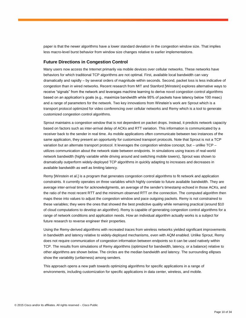
Using the Remy-derived algorithms with recreated traces from wireless networks yielded significant improvements

in bandwidth and latency relative to widely-deployed mechanisms, even with AQM enabled. Unlike Sprout, Remy

does not require communication of congestion information between endpoints so it can be used natively within

TCP. The results from simulations of Remy algorithms (optimized for bandwidth, latency, or a balance) relative to

other algorithms are shown below. The circles are the median bandwidth and latency. The surrounding ellipses

show the variability (unfairness) among senders.

This approach opens a new path towards optimizing algorithms for specific applications in a range of

environments, including customization for specific applications in data center, wireless, and mobile.


Page 11 of 34

Figure 4 – Median and variation in latency in throughput for congestion control schemes (upper right is best) - Winstein

Packet Bursts

It is accepted that router buffering should be designed to manage “bursts” of traffic, but there is no single definition

of what that means. At a high level, the term usually refers to a temporary increase in traffic that is not part of

persistent congestion. For example, a link with an average of 5% utilization over a minute that is seeing output

drops is likely to be experiencing bursts beyond its buffering capacity.

What constitutes a burst or defines the type of burst is dependent on the network context. From a host perspective,

one case of a significant microburst would be when the host generates a large number of packets in response to a

single event [Dukkipati, Mathis, Cheng & Ghobadi]. For example, if a single TCP ACK received by a 10GE-

attached server communicated that a large number of segments have been lost, the sender might replace them all

immediately. Wherever the interface speed is lower than 10G, they will need to be buffered even without persistent

congestion.

Microbursting behavior is common any time there is an interface speed drop along the path. It also occurs with

oversubscription, especially when traffic is synchronized by an application such as Hadoop MapReduce.

Usually, the desired behavior is to buffer the burst, avoid packet loss, and thus not signal the senders to slow

down. In automated stock trading, the added latency from buffering even microbursts may be unacceptable, and

the only solution is to increase the link bandwidth.

When planning for bursts, it is important to keep in mind the pacing behavior of TCP. When there are a range of

link speeds, the data packets for a flow become spread out on the faster links as the ACKs returning over the slow

link clock future transmissions.


Page 12 of 34

Bufferbloat

Jim Gettys has performed an extensive investigation into the interaction of buffering with TCP. His research began

with real-world experience and focuses on the sources and effects of too much buffering.

This problem is highlighted in 2011 IEEE article [Gettys]. Additional discussion can be found in a group discussion

on the topic [Gettys, Cerf, Jacobson & Weaver]. The central idea of the paper:

“Although some buffering is required to smooth bursts in communications systems, we’ve lost sight of

fundamentals: packet loss is (currently) the only way to signal congestion in the network, and congestion-avoiding

protocols such as TCP rely on timely congestion notification to regulate their transmission speeds.”

The result of not receiving timely notification is that TCP cannot operate at optimal performance, resulting in

reduced throughput, high latency, and retransmissions which perpetuate congestion. Gettys’ research started by

investigating multi-second latency on his home Internet connection. As he continued to untangle what was

happening, he noticed that large buffers were resulting in latency that distorted TCP’s view of the network. In one

case, he measured 8-second latency over what was normally a 10ms path. While this paper will focus on buffering

options available via router selection and configuration, it is important to keep in mind that multiple sources of

added latency (from buffers in hosts, modems, and home routers) may be occurring simultaneously, and a Service

Provider cannot fully control the end-to-end behavior.

Applying Congestion Control Concepts

If a router doesn’t have “enough” buffers, it will drop packets during periods of brief congestion that the applications

would have preferred to be delayed instead. Depending on the loss detection mechanism, TCP will delay the slow

start ramp up, enter fast retransmission/recovery, or return from congestion avoidance to slow start. Some of these

responses have minimal impact (fast retransmit within a Netflix movie) are desirable when the congestion is

persistent but not when the congestion is limited in duration and subsequent packets would have been forwarded

at the original rate. The Google experiment highlights the negative impact of drops on web traffic, resulting in

session completion latency significantly higher than without drops.

There are also risks of too much buffering. As shown in the Bufferbloat research, TCP usually relies on the packet

drop signal to limit its transmissions. Not dropping packets can result in the congestion window growing larger than

is justified, further adding to congestion. Not dropping packets sends the signal for hosts to increase their transmit

rate. An inflated congestion window will also prevent new flows from acquiring network bandwidth as it allows

existing flows to continue sending large bursts. The delay introduced by too much buffering also distorts the RTT

and RTT variance calculation which impacts the RTO timer, leading to slower loss detection.

In addition, if the packets that would have triggered duplicate ACKs are delayed in buffers, a lost packet is less

likely to be detected and recovered via fast retransmission. This results in an RTO and the session returning to

slow start rather than just reducing its window via fast recovery. In addition, if buffering significantly increases the

RTT, performance will degrade as the sender can only transmit a set number of segments per RTT. The risks of

too much buffering can be managed by configurable queue lengths, AQM techniques such as WRED, and QoS

mechanisms to prioritize important traffic.


Page 13 of 34

Therefore, there are risks of buffers that are too small or too large. The best size for a given link will depend on a

number of factors including the place in the network (e.g., RTT, link speeds, oversubscription, flow count, and

congestion) and applications as well as commercial considerations such as purchase price and ongoing expenses

such as space and power.

Best-laid Plans - Of Mice and Elephants

A significant complication in network and buffer design is the variation in TCP flows. Elephants are the one-

percenters of the network world and consume a large amount of bandwidth per-flow. They are relatively long-lived

(many RTTs) and thus spend much of their time in Congestion Avoidance mode (reacting to signals) with large

windows of segments in the network. If not managed appropriately, they can starve other flows.

Mice are short-lived, and many complete without leaving Slow Start. Elephants tend to be interested in bandwidth,

while mice tend to aim for short completion times. When mice and elephants share buffers, it doesn’t always work

out well for the mice, especially if the elephants are unresponsive to congestion. Large groups of synchronized

mice flows have recently been referred to as lemmings. They present a unique buffering challenge in data centers

in applications (e.g., Map/Reduce) where one server may launch connections to hundreds or thousands of other

servers that create a many-to-one response [Baker]. Because they are short-lived, mice and lemmings don’t easily

co-exist with the congestion and queue management schemes that control the elephant population. They don’t

need to be slowed down as they will complete quickly, and drops can significantly delay flow completion.

In addition to filling buffers, elephants can also cause problems when multiple paths exist such as L3 ECMP or L2

bundles. If too many of the elephants hash onto the same link, significant congestion can occur even when there is

available bandwidth remaining on other links.

Not all individual flows are elephants or mice. HTTPv2 supports low-volume long-lived sessions so that a new

socket isn’t created as often. In this case, TCP should still respect the guideline of reducing the congestion window

after periods of inactivity.

The presence of mice, elephants, and lemmings, and their behaviors are one of the reasons it is difficult to make

any generic recommendations for data center networks. Research is ongoing into the best way for these different

types of flows to co-exist. Solutions such as scheduling, dividing, or recognizing and steering elephants are being

explored.

TCP Summary

TCP responds to packet loss by returning to slow start (RTO detection), halting window growth (during fast

retransmit with unresolved segments), or reducing the congestion window (fast recovery). Packet loss is not

inherently detrimental to a network transporting TCP traffic. In fact, with currently deployed congestion control

algorithms, it is a necessary tool for TCP to function properly in the presence of congestion. When segments can

be recovered via SACK and fast retransmission, segment loss may not significantly slow down the overall

throughput of the session relative to the requirements of most applications. Packet loss detected via RTO is more

detrimental as it will return the TCP session to slow start. Multiple RTOs is the worst case and should be avoided if

at all possible since it dramatically will slow down the session. Infinite buffering does not prevent RTOs, but it may

prevent fast retransmission by delaying later packets.


Page 14 of 34

TCP is also responsive to signals other than packet loss. When persistent buffering occurs in the network, TCP

responds to increasing RTT and RTT variance by increasing the RTO. This slows future detection of loss via RTO

timeout.

With regard to designing a network for TCP traffic, the goal should be well-managed buffers and appropriate

packet drops as defined by application requirements. The ideal amount pf buffering for different parts of the

network should be determined by a combination of applications, bandwidth, round trip time, and traffic

characteristics.


Page 15 of 34

Academic Research on Buffering

The most-cited early paper in buffer sizing is “High Performance TCP in ANSNET” by Curtis Villamizar and Cheng

Song in 1994. The paper explored the buffering required to maximize link utilization with a very small number of

long-lived TCP flows. With a small number of sessions, packet loss may result in all the sessions returning to slow

start at the same time and thus all sessions increasing their rates exponentially at the same time. When congestion

occurs again, the sessions become synchronized and repeat the cycle of TCP synchronization.

The key conclusion was that the bottleneck link utilization is maximized with buffering sized to the product of

Bandwidth and Route Trip Time. This value is referred to as the Bandwidth Delay Product (BDP). For example, a

10 Gbps link that is part of a path with a total RTT of 0.2 seconds would have a buffer of 2 Gigabits or 250 MB. To

their credit, the authors recognized that an increased number of flows would lead to different results. More recently,

Michael Smitasin and Brian Tierney of the Berkeley Energy Sciences Institute reaffirmed benefits of large buffers

for “very large data transfers with large pipes and long distances between a small number of hosts”.

Villamizar and Song provided valuable insight into the interaction of buffering with TCP. Unfortunately, the

recommendation from this specific case became dogma for many years and resulted in over-building routers and

over-provisioning network buffers in places where their conditions don’t apply.

Stanford & Georgia Tech

The High Performance Networking Group at Stanford, led by Nick McKeown, has been the source of significant

research into many aspects of networking. Guido Appenzeller’s 2005 thesis “Sizing Router Buffers” provides

valuable insight and a statistics-based approach to buffer sizing for Internet core routers with many flows. A more

concise starting point to review his research is available in a Sigcomm paper [Appenzeller, Keslassy & McKeown].

With many flows, traffic may be unsynchronized, resulting in an aggregate smoothing effect and thus require less

buffering. The key recommendation from this research is that buffers should be sized based on BDP and the

number of long flows (TCP flows not in slow start) going through the link. Specifically: BW * RTT / sqrt (n) where n

is the number of long flows. Note that n also introduces a way to represent application characteristics as different

applications (video vs. small web object downloads) may vary in how much time they spend in Congestion

Avoidance. This is important as many TCP flows never leave slow start.

Appenzeller’s studies and simulations focus on core links, but the general idea of proportionality between buffers

and flows can be applied in other situations. For example, the core-facing uplink of an edge router may have a

medium number of flows and thus require less buffering than the customer-facing link on the same router which

may have all of its bandwidth consumed by a single flow.

Subsequent papers from researchers at Georgia Tech [Dhamdhere & Dovrolis] [Dhamdhere, Jiang & Dovrolis]

argue that while the Stanford Model is effective for achieving high link utilization, it may result in significant packet

loss (5-15% in simulation) in some situations. They contend this amount of packet loss then leads to high levels of

retransmissions and reduced application performance.

The Georgia Tech research introduces several new concepts. First, it suggests that links be classified as to

whether or not they are “saturable”. Even without going further into the research, this concept is important for

practical applications of buffering design. For example, if a particular Data Center environment allows additional


Page 16 of 34

links to be added at relatively low cost, buffering can be limited to a level needed for speed matching and

microbursts as persistent congestion can be avoided. On the other extreme, a DSL, cable, or wireless “last mile”

may experience significant persistent congestion. Their research agrees with the Stanford Model that “small’

buffers are sufficient for backbone links, but for a different reason: not being saturable based on current Service

Provider deployment practices.

The Georgia Tech research also states that any conclusions based on the number of TCP flows must limit the

counting of flows to long TCP flows that are not bottlenecked at other links and not bottlenecked by the end hosts

windows or attachment speed. They also present calculations in which they show that in the Stanford Model the

loss rate increases with the square of the number of flows bottlenecked at that link.

Another paper by Georgia Tech and Bell Labs [Prasad, Dovrolis & Thottan] seeks to find the buffer size that

maximizes the average per-flow TCP throughput. Their conclusion is that this is primarily a function of the

output/input capacity ratio, which is defined as output capacity relative to peak cumulative input flow size (not just

local ingress bandwidth but also taking into account the sources of the flows). Their results support the view that

buffers can be significantly smaller than BDP when a link carries many flows but also propose that values closer to

BDP are be merited in some cases.

A 2006 paper from Stanford [Ganjali & McKeown] addresses the Georgia Tech findings and proposes a heuristic

for core links which represents a compromise.

“And so for now, we would cautiously conclude that at the core of the Internet, where the number of flows is very large, the buffers can be reduced by a factor of ten, without expecting any adverse change to the network behavior; in fact, we would expect delays and delay variation to be reduced.”

With the Internet RTT of 250 msec, this “factor of ten” results in 25 msec buffers for a router serving the global

Internet core. Networks primarily serving regional or intra-continental traffic will need proportionally smaller buffers.

The collective research supports the argument that buffering requirements depend on many factors including the

desired outcome (e.g., keep link fully utilized, limit loss, or maximize per-flow throughput); the levels of

oversubscription and congestion; and the number, type, and synchronization of flows. That’s before considering the

sensitivity of applications to loss, latency, and jitter. While the research doesn’t provide a single answer, it opens up

some new ways to look at the problem and to evaluate alternatives in the context of their place in the network.

There is less research on edge and access buffer sizing, but what is available tends to support the idea that in

locations where a single flow can take all of a link’s bandwidth that BDP-sizing may be needed for that link. If

buffers are shared, the aggregate buffering may be reduced.

Other Views

Many of the research models rely on the assumption that packets arrive in a Poisson distribution (arrival time is not

dependent on other packets). In [Nichols & Jacobson], the case is made that pacing via ACKs creates standing

queues and non-Poisson packet arrival. They also reference [Vu-Brugier, Stanojevic, Leith & Shorten] which is

critical of smaller buffer proposals and experiments and advocates BDP buffers based on simulations.

Another reality is that business considerations may override the desire for an ideal design. Routers with small on-

chip buffering can be significantly denser, much less expensive, and consume less power that routers with deeper

off-chip buffers.


Page 17 of 34

The factors discussed in this paper should help assess where underprovisioning the ideal with have more or less

impact.

Real-world Buffer Experiments and Data

Stanford, University of Toronto at Level 3 – Core Buffer Sizing

In [Beheshti et al.] researchers from Stanford and the University of Toronto were able to conduct an experiment in

the Level 3 commercial backbone. A set of 3 parallel load-balanced (4-tuple flow-based) OC-48 links with very high

utilization (over 85% for 4 hours per day) were configured with varying amounts of buffering and monitored. The

researchers calculated an average of 10,000 flows per link. The default buffer size was 190 msec (60 MB or

125,000 500B packets), and no Active Queue Management (AQM) mechanisms were in use.

The buffers for the 3 links were reconfigured with one link always set to 190 msec and the other links set to two of

the experimental values (1, 2.5, 5, or 10 msec). Each buffer size was evaluated for at least 5 days. No drops were

seen with the 5, 10, and 190 msec buffers for the entire duration. Packet loss in the range of 0.02% to 0.09% was

seen with 2.5 msec of buffering and correlated to the link utilization. There was a relatively large increase in packet

loss with 1 msec of buffering, but link utilization was still maintained. Most of the loss occurred when the link

utilization was above 90% for a 30-second average. The packet drop level for the 1 msec buffer was still below

0.2%.

These experiments support the Stanford model for core buffering requirements and support the theory of highly-

smoothed traffic when many flows are present.

Facebook – Link and Buffer Utilization

Researchers at the University of California at San Diego recently performed in-depth analysis of traffic at Facebook

[Roy, Zeng, Bagga, Porter & Snoeren]. Their paper includes a range of findings, many of which are relevant to

buffering design.

Servers were 10G attached and average less than 1% 1-minute link utilization, 90% are under 10% utilization.

As seen in other studies [Kandula, et al.], Hadoop traffic exhibits extremely high rack locality – most of the traffic is

between the master and slave in the same rack. Hadoop flows are short. 70% send less than 10 KB and last less

than 10 seconds. The median Hadoop flow is less than 1 KB and 1 second and thus doesn’t ever enter congestion

avoidance. Only 5% exceed 1 MB.

Data on buffer utilization was collected at 10 usec intervals for links to web servers and cache nodes. Even with the

low aggregate utilization, the buffers were constantly in use on the ToR switches (Facebook Wedge with

Broadcom’s Trident II ASIC, which has 12 MB of shared buffers).

“Even though link utilization is on the order of 1% most of the time, over two-thirds of the available shared buffer is utilized during each 10-us interval.”


Page 18 of 34

Google – Initial Congestion Window

Google [Dukkipati, et al.] conducted experiments to investigate the effects of increasing the TCP initial congestion

window to 10 segments or higher. They found a substantial increase in the number of web transactions that could

be completed within one RTT and a corresponding decrease in completion time. The negative effects of this

change were limited and acceptable in most cases. They propose this approach as an alternative to opening large

numbers of parallel TCP connections. Data from CAIDA [Wu & Luckie] shows that many large sites are now taking

this approach with 60% having an initial congestion window between 10 and 16 segments. This evolution of TCP

does illustrate that the underlying flow behavior of traffic may change over time even if the traffic itself does not and

provides a motivation for allowing some room for change when selecting hardware, especially towards the edge

and access layers of the network where there are a smaller number of flows.

The evolution of the initial congestion window since the referenced buffering research at Stanford and Georgia

Tech and experiments needs to be taken into account when applying the conclusions today. The common TCP

stacks prior to recent developments used an initial window of 2-4 segments [RFC 3390]. In 2010, Google proposed

an initial window of 10 [Dukkipati et al.], and it has been widely adopted. As the congestion algorithm and settings

are independent for each sender and most traffic is server-to-client, it only takes a small number of top providers to

adopt this change to dramatically change the aggregate TCP behavior on the Internet. [Wu & Luckie] shows that

60% of the Alexa 10K sites are now using an initial congestion window of 10 or larger.

Google – Packet loss, session latency, and Proportional Rate Reduction

In the proposal for Proportional Rate Reduction [Dukkipati, Mathis, Cheng & Ghobadi], Google presents significant

real-world data on TCP behavior in two data centers. One was in the US providing multiple services to the east

coast and South America, and a second DC was in India serving Youtube exclusively. Some of the highlights are:

- There was an average of 3.1 HTTP requests per connection

- The average HTTP response size was 7.5 KB (5-6 segments, within the increased initial window sizes)

- 6.1% of HTTP responses have TCP retransmissions

- Sessions experiencing loss had 7-10 significantly longer completion times than the ideal

- 2.8% of TCP segments are retransmitted with 2.5% for the US DC and 5.6% for the India DC

- 54% of India DC retransmits and 24% of US were fast retransmits

- An average of 3 retransmissions per fast recovery event (loss is correlated)

- Sessions connecting to the India DC spent just under half the total time in a loss recovery mode

- Sessions in the India DC had an average RTT of 860 msec

These figures show that packet loss and RTOs are quite common. The former appears inevitable. The latter could

potentially be improved if losses were less correlated (via AQM mechanisms improving the drop behavior) and thus

more easily recovered. The India RTT is surprisingly high and is an indication that bufferbloat and heavy levels of

congestion are occurring along the path. It also demonstrates that even very large amounts of buffering do not

prevent packet loss.

The high India RTT raises the question of whether nominal or actual latency should be considered when using RTT

as part of a buffer sizing calculation. The actual RTT determines TCP’s responsiveness to congestion, but such

high variation makes it difficult to use in sizing.


Page 19 of 34

In these experiments, PRR was able to reduce session latency by 3-10% compared to the standard Linux recovery

mechanism at the time. PRR is now the default [as of 2015] for fast recovery in Linux, where it is combined with the

CUBIC congestion control algorithm.

Application Requirements

Applications have a wide range of requirements from the network and they all have preferences for the network’s

behavior. Starting with the most latency-sensitive applications, a range of requirements are presented below.

High-Frequency Trading

High-frequency Trading (HFT) is a well-known latency and PDV-sensitive application. Financial service providers

have literally moved mountains at a cost of hundreds of millions of dollars to shave several milliseconds of

propagation delay [NY Times]. In a pursuit of money that would make Austin Powers’ Dr. Evil proud, others have

used a sophisticated heat beam called a “laser” to minimize delay between the New York Stock Exchange and

New Jersey data centers. [WSJ]. Add in co-located servers with dedicated cores that are replaced quarterly, low-

latency NICs, kernel-bypass drivers, and the “race to zero” (latency) has may have reached the point of diminishing

returns with regard to nominal latency. Innovation is now occurring even at the protocol level – moving from a

human-readable flexible format to binary data that can be parsed more quickly by a computer.

In that context, it’s clear that all possible nominal device latency must be eliminated and buffering minimized. This

can be done by minimizing the number of memory operations and the use of cut-through switching in which frames

are transmitted on one fiber while still being received on the other. These transactions don’t consume a large

amount of bandwidth, so the general approach to designing these networks is to overbuild them to the point where

congestion of any kind is unlikely.

Gaming

Gaming comprises a range of applications with different requirements. Many of them have a latency constraint, and

it is mostly important to avoid high latency rather than to minimize latency. In addition, the financial drivers are

different and gaming-optimized service offerings from ISPs are minimal. More bandwidth, QoS-capable home

routers, and keeping your house mates off Netflix are often the only options an end-user has to improve their

gaming experience.

Game setup and chat are mostly performed with TCP and don’t have strict latency requirements. Gameplay usually

operates via UDP. Gameplay requirements depend on the type of game (e.g., first-person shooter or real-time

strategy) and the precision required for an individual action which is dependent on the location of another player

(e.g., sniper rifle vs. throwing a grenade in a first-person shooter). A good introduction to requirements for gaming

can be found in an ACM paper from researchers at WPI & MIT [Claypool & Claypool].

Most online games have relatively low bandwidth requirements (10s of kbps) and tolerance for latency of around

150-200 msec. Round-trip latency is called “ping” in gaming circles and is often displayed when selecting potential

opponents. Most games have techniques to mask latency up to this level by allowing the client to predict the result

of their actions. For example, the character may move and display an animation while a sound is played. If the

server later disagrees on the game state, a correction to the state is made. If a correction is required, the client will


Page 20 of 34

rerun everything that occurred after the corrected information, possibly resulting in a “jump” in the game as seen by

the client.

To scale and manage latency, major games will have sets of servers distributed geographically as a single hosting

location could not meet these requirements for everyone. For example, Blizzard has US, Europe, and Asia sites for

their Battle.net service which hosts World of Warcraft, Heroes of the Storm, and Starcraft. This still doesn’t allow for

much buffering as uncongested ping may reach 150 msec in Asia or between South America and the US. In the

US and Europe, uncongested latency is mostly under 100 msec. Gaming, therefore, is unlikely to benefit from

aggregate buffering beyond 50 msec for an individual flow.

Non-live Streaming Video

Video was 64% of all consumer Internet traffic in 2014 and is predicted to reach 80% in 2019 [Cisco]. Netflix,

YouTube, and sites using similar streaming technologies generate the vast majority of the video traffic so their

applications will provide valuable insight into video requirements.

Netflix and YouTube stream video over HTTP (TCP) and are normally capable of sufficient host-side buffering to

retransmit lost packets and tolerate moderate increases in latency. Note that there is variation among clients and

mobile devices will have distinct characteristics. Unless there is significant packet loss, overall quality is primarily a

function of bandwidth. When the host-side buffer is empty, the video pauses to rebuild the buffer. This is referred to

as “buffering” by users. On YouTube, the current depth of the host-size buffer is visible with a gray bar showing

much of the video has been received.

Both are capable of dynamically adapting video quality to bandwidth. Initial startup time is also important – more so

for Youtube as users are watching shorter videos rather than sitting down to watch an hour at a time. Prior to 2012,

YouTube would transmit what was effectively a single large file specific to the chosen resolution. Packets were

buffered in the application, and the video would pause when playback exhausted the buffer. In 2012, YouTube

moved towards a new model (Sliced Bread) which allows for shifting between resolutions as network conditions

changed. Further innovations such as preloading slices of related videos also improve performance during times of

reduced network capacity [gizmodo].

Once the host-side buffer has been built, non-live streaming video is tolerant of most network conditions other than

losing connectivity or bandwidth for an extended period of time (enough to exhaust the buffer, often several

seconds). Single-packet loss is well tolerated as lost packets can be retransmitted via fast retransmit, and TCP

enables packets to keep flowing while the loss is being resolved. With sufficient host buffering, limited RTO events

may also be tolerated without impacting end-user experience.

Most users access Netflix and Youtube via CDN caches rather than a central location. For example, Netflix is

present in almost every colocation facility in the US so uncongested RTTs are often under 20 msec. Given the

volume of video, this significantly impacts router buffering requirements. If most of the traffic passing through an

edge router is destined to a video cache with an RTT in the sub-20 msec range, TCP will respond more quickly to

loss than the traditional assumption of max RTTs (250 msec). Therefore, a weighted RTT may be considered in

hardware sizing on edge routers as long as signals are sent to the hosts in a timely manner.


Page 21 of 34

Live Streaming Video

Live video is more demanding as host-side buffering isn’t able to mask suboptimal network conditions. UDP is

usually used as retransmits would arrive too late to be of value. Live video is inherently bursty due to video

compression algorithms which don’t need to send as much data when there is less motion. Live video may

comprise video conferencing, sports, viewing gaming, and other applications. The required and available

bandwidth may vary dramatically. On the high end, Cisco Telepresence uses around 5 Mbps per direction in the

highest-quality 1080p mode [Cisco]. Telepresence recommends a maximum of 150 msec of latency. The

deployment guide suggests that users will perceive latency at levels from 250 to 350 msec. Live streaming is also

sensitive to packet delay variation (PDV). In Telepresence, the “jitter buffer” is initially set to 85 msec and may

increase to 245 msec if needed. Packets that are dropped or arrive late (beyond the jitter buffer) result in video

pixelization.

At 1080p, the uncompressed video stream is 1.5 Gbps and the compressed stream is 4 Mbps. Therefore, each

packet contains a large amount of video data. Cisco recommends a loss target (including late packets) of 0.05%. In

corporate networks, services like Telepresence should receive priority treatment in the network.

Other video conferencing applications such as Skype need to live with available bandwidth and adjust their

requirements to what is available, often very rapidly. They will suffer similar issues with packet loss, latency, and

delay variation.

Voice over IP

VoIP typically uses TCP for setup and UDP to transport packets for the call. VoIP uses relatively low bandwidth

and is sensitive to loss, jitter, and latency similar to video. These characteristics make it a good candidate for

priority treatment in network designs where traffic is differentiated. Guidelines for maximum latency are usually

between 150-250 msec with loss requirements below 1%. Without any prioritization, VOIP such as Skype over

commodity Internet may have highly variable quality depending on network conditions. VoIP should not be subject

to significant added latency due to buffering.

DNS

DNS primarily uses UDP for name resolution. This provides a faster response by avoiding the TCP handshake

which enables requests to complete in a single RTT. As it is a relatively simple transaction, TCP isn’t required –

DNS can just try again or use another server if a response isn’t received. DNS, therefore, doesn’t usually need any

special treatment in the network, but excessive queuing can impact user experience and should, therefore, be

minimized. Latency for DNS can also be managed by offering regional DNS servers. Finally, DNS servers are often

targeted by attackers and are therefore subject to unusual traffic patterns outside normal assumptions made for

queuing.

Web

Web browsing makes up the majority of Internet transactions. The total bandwidth is less than video, but there are

many smaller flows. Web traffic includes HTML, CSS, Javascript, graphics, flash, and other types of content. While

average access speeds continue to increase, the size of the average web page continues to grow as well. In 2010,

the average for the top 1000 sites was 626 KB; it is now over 2 MB [httparchive]. In theory, without any server or


Page 22 of 34

bandwidth constraints, 2MB takes 8 RTTs for the Reno algorithm with an initial window of 10 (14.6 KB in the 1st

RTT, 29.2 KB in the 2nd. . . 934 KB in the 7th , and 1.9 MB in the 8th). In reality, full page loads average roughly 7

seconds for wired and often over 10 seconds on mobile devices. The higher end of this range can lead to

significant abandonment, which must be minimized.

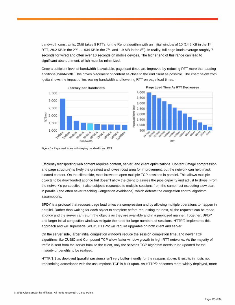
Once a sufficient level of bandwidth is available, page load times are improved by reducing RTT more than adding

additional bandwidth. This drives placement of content as close to the end client as possible. The chart below from

Igvita shows the impact of increasing bandwidth and lowering RTT on page load times.

Figure 5 - Page load times with varying bandwidth and RTT

Efficiently transporting web content requires content, server, and client optimizations. Content (image compression

and page structure) is likely the greatest and lowest-cost area for improvement, but the network can help mask

bloated content. On the client side, most browsers open multiple TCP sessions in parallel. This allows multiple

objects to be downloaded at once but doesn’t allow the client to assess the pipe capacity and adjust to drops. From

the network’s perspective, it also subjects resources to multiple sessions from the same host executing slow start

in parallel (and often never reaching Congestion Avoidance), which defeats the congestion control algorithm

assumptions.

SPDY is a protocol that reduces page load times via compression and by allowing multiple operations to happen in

parallel. Rather than waiting for each object to complete before requesting the next, all the requests can be made

at once and the server can return the objects as they are available and in a prioritized manner. Together, SPDY

and larger initial congestion windows mitigate the need for large numbers of sessions. HTTP/2 implements this

approach and will supersede SPDY. HTTP/2 will require upgrades on both client and server.

On the server side, larger initial congestion windows reduce the session completion time, and newer TCP

algorithms like CUBIC and Compound TCP allow faster window growth in high-RTT networks. As the majority of

traffic is sent from the server back to the client, only the server’s TCP algorithm needs to be updated for the

majority of benefits to be realized.

HTTP/1.1 as deployed (parallel sessions) isn’t very buffer-friendly for the reasons above. It results in hosts not

transmitting accordance with the assumptions TCP is built upon. As HTTP/2 becomes more widely deployed, more


Page 23 of 34

hosts will open fewer sessions and use them to transport more segments per session. This should have the net

effect of reducing buffer requirements.

Peer to Peer

Peer to peer protocols such as BitTorrent are used for a variety of purposes. While it is best known for piracy, it is

also used to download game updates by companies such as Blizzard, to distribute scientific data, and to distribute

Linux. Without peer to peer, it would be difficult to make large files available for free. For a protocol with such a bad

reputation, BitTorrent is actually very respectful of network resources. Current implementations use the Micro

Transport Protocol (uTP) which runs on UDP. uTP uses the Low Extra Delay Background Transport (LEDBAT)

method to avoid adding to network congestion. It is a delay-based algorithm that slows down when added latency

is detected. LEDBAT can also be used with TCP for lower priority tasks such as software updates (Apple).

Data transferred via peer to peer doesn’t normally have session completion constraints or expectations of

guaranteed bandwidth. Therefore, peer to peer traffic doesn’t need any special consideration for buffering.

Distributed Compute and Storage – MapReduce, HDFS

Hadoop is an example of an application’s behavior resulting in distinct network traffic patterns. Hadoop uses TCP

and expects the distributed operations to complete by a certain deadline and may ignore late responses which can

result in an incomplete or suboptimal result. Hadoop relies on parallel computation on multiple nodes in a cluster

which then return the results to the Master. This results in both high “rack locality” (traffic stays within the rack) and

synchronization of traffic that may result in TCP Incast [Chen, Grifit, Zats & Katz]. Incast is congestion caused by

many-to-one responses triggered by an application. In this case, the congestion is not due to persistent high traffic

or random collisions, but is the intrinsic behavior of the application.

For traffic belonging to short flows, it is preferable to buffer rather than drop and retransmit. There may be no other

data beyond the initial burst, and thus nothing to react to the “signal” of packet loss. This buffering can occur in the

network or it can occur on the servers themselves. Buffering on the servers is already occurring when there is more

data than TCP is allowed to send immediately. Newer TCP mechanisms may leverage this capability by using

pacing and jittering to take advantage of these buffers which may be preferable to adding additional buffering on

the router or switch. Another aspect of the solution is to increase link speeds and thus reduce the amount of

oversubscription that occurs. The best solutions to Incast are still being researched and debated.

Router Buffering Architectures

Off-chip vs. On-chip buffering

One of the tradeoffs a router architect needs to make is whether to buffer packets in memory inside the NPU /

Forwarding ASIC or in a memory external to the lookup engine (or connected to a separate queuing chip).

On-chip buffering minimizes power and board space but doesn’t allow for very large buffers. On-chip buffering

allows for denser routers and switches as it allows more of the ASIC’s resources to be used for physical ports. As

an example, a high-scale deep-buffer Network Processor may allocate I/O pins roughly equally among off-chip FIB,

off-chip buffers, fabric connections, and interface connections. In contrast, a System on a Chip router may allocate

almost all of the ASIC I/O capacity to external interfaces. This is one of the key factors underlying the wide range of


Page 24 of 34

port counts and power consumption of routers today. Fabric-capable forwarding chips with off-chip buffers currently

range from 200 to 700 Gbps while SoC models shipping in 2016 range up to 3.2 Tbps.

With off-chip buffering, there are two key requirements that must be met. First, the memory must be large enough

to buffer the required packets. Second, it must be fast enough to maintain the forwarding rate. While not as

challenging as FIB memory requirements (extremely high operations per second), the latter can be a challenge as

commodity memories are not designed for the speed of networking applications. Therefore, custom high-

performance memories or a large number of commodity memories are usually the only options to reach the

memory bandwidth requirement. In addition, memory parts may not be available in the sizes for optimal buffering

(e.g., a home router with 64MB when 64KB would be optimal). In these cases, it is important that vendors allow

queue sizes to be limited via software configuration.

Custom memories can be made to a wide range of specifications, including bandwidth, operations per second,

capacity, and physical size. For deep buffers, a router architect must choose between high-speed custom

memories or large banks of commodity memories. Custom memories save board space but are significantly more

expensive. They may also incur significant hardware development expenses (Non-Recurring Engineering)

internally or to a vendor. Off-chip buffering with commodity memory is less expensive but often requires much more

board space than custom memories due to the need to overprovision the memory size in order to get sufficient

memory bandwidth. Using a higher-performance commodity memory such as graphics memory (e.g., GDDR5)

helps, but still doesn’t provide the speed and efficiency of memory designed specifically for the application. A good

public technical presentation of custom vs. commodity memories is presented in Juniper’s blog announcing

products with the HMC Hybrid Memory Cube from Micron. Cisco uses similar fast custom memories on the CRS,

NCS 6000, and Nexus platforms.

As of 2016, on-chip memories current range from 10s to low 100s of MBs, while off-chip may go up to 12 GB for a

200G Network Processor. This is roughly the same ratio as the RTT variation between Data Center and Internet

traffic flows.

One goal of the very-small-buffering research is to explore the feasibility of routers in which packets are never

converted into the electrical signals but instead perform operations in the optical domain. One of the Stanford

papers explores the impact of the “few dozen” buffers that are becoming feasible with optical memories [Beheshti

et al.].

Platforms

Buffering may occur at any point of congestion, most commonly Forwarding ASICs, switch fabrics, and egress

interfaces. There are several common architectures that facilitate different buffering schemes. They differ in the

size and location of buffers, how the buffers are allocated, and their queue management mechanisms. No single

architecture is superior in all cases. Bigger is not always better, and there are tradeoffs that impact other areas of

design such as density and power.

The most common router buffering architectures are:

Single-chip systems with small on-chip shared memory (ASR 920, RSP2, NCS 5000)


Page 25 of 34

Single-chip system with deep buffers (RSP3, NCS 5501, ASR 1000)

Multiple forwarding chips with fabric interconnect and VOQ buffering (NCS 5502, modular NCS 5500), Arista 7500)

Multiple forwarding chips with fabric interconnect & VOQ and full egress buffering (GSR, Juniper PTX/MX)

Multiple forwarding chips with ingress & egress buffering (CRS & ASR 9000)

Multiple forwarding chips with small on-chip buffers and Ethernet fabric (Insieme, several Arista models)

Single forwarding processor with central on-chip buffer – By number of chassis, the most common router and

switch buffering architecture is a central on-chip shared memory that can be used for ingress and egress queuing

for any port. A small amount of memory is usually allocated to each interface on ingress as a FIFO for incoming

packets, a small amount is assigned per-port for egress, and the remaining memory can be flexibly allocated to

egress for ports experiencing congestion. As on-chip memories are relatively small today, these devices work best

in environments without congestion (microbursts only) or with low RTTs. They are popular for high-volume

applications such as Top of Rack due to their simplicity and low cost. Note that “small” on-chip memories in the

range of 10s of MB are able to provide significant buffering in low-RTT environments as the low RTT allows long-

lived flows to react quickly to congestion.

An extension of this architecture is adding deeper off-chip buffers to the single-chip system. This is often used for

access or smaller edge devices such as the ASR 1000 that require WAN buffering but do not require the scale of a

modular chassis.

Virtual Output Queues – To scale a router beyond a single forwarding node, the nodes must be connected via a

fabric. This may be a set of fabric chips to forward frames or cells among the nodes or a mesh directly connecting

the forwarding processors. The fabric may introduce another potential source of congestion. This can be solved in

a number of ways including scheduling and buffering or speedup.

Some early fabric-based routers suffered from head of line blocking in which packets going to a congested egress

card or interface blocked packets going to other destinations from being sent. This is analogous to a car trying to

turn in traffic preventing other cars going through an intersection where there is only one lane. This problem can be

solved with Virtual Output Queuing. In a VOQ model, separate queues are created on ingress for each output

queue. Packets may then be dequeued for any destination without blocking other queues. VOQs may be used

solely to manage switch fabric congestion with separate egress queues or they may be the primary buffers on the

router.

With VOQ-only models, the ingress traffic manager may or may not be aware of the depths of the queues on other

VoQs. If it is unaware of the status of other queues, the total max buffering is the sum of all the available buffers on

forwarding chips buffering packets for that destination. For example, if the VoQs are configured for a 20msec buffer

and traffic to the congested queue is buffered on 10 forwarding chips, the total buffering may reach 200msec,

which is usually detrimental to the network. In cases with a congested high-volume destination, even more

buffering may occur as some currently-shipping routers have up to 96 forwarding ASICs.

Egress Queuing – Like VOQs, egress queues may have multiple roles in different routers. In a system where

VOQs are the primary queues for congested interfaces, the egress queues may just be small FIFOs to reassemble


Page 26 of 34

and smooth the traffic to the link speed. In this case, the egress queues don’t have a significant buffering and may

be placed on-chip.

Other systems use the egress queues to provide the primary buffering for interface congestion. In this case, a full

set of Active Queue Management and Priority/Shaping behaviors may be implemented. All things being equal,

having all the outgoing packets for a port in a single set of egress queues is preferable to multiple VOQs since it

allows more visibility when performing operations that depend on queue depth. At the same time, a VOQ design

can still effectively implement QoS policy very effectively, and some VOQ systems can provide global visibility into

queue depths on other modules, thus allowing AQM decisions with global visibility.

Ingress & Egress Queueing – Routers may have both ingress and egress buffering. In this architecture, the

ingress buffering serves to manage any fabric congestion as well as oversubscription of any egress resources

(e.g., the egress packet processor, not the output queue). Ingress buffering may be triggered via backpressure or

request/grant mechanisms. It is possible to minimize ingress buffering by having sufficient “speedup” in the fabric

to effectively eliminate the fabric as a source of congestion. With speedup, the fabric has higher egress capacity

than ingress capacity and therefore allows multiple senders to send high rates of traffic to an egress card at the

same time.

In addition to the visible buffers, small amounts of buffering are often used to smooth out the transition of packets

from one stage of the router to the next. For example if one chip can send bursts at 11 Gbps and the other can

receive at 10 Gbps, a small buffer is used to address the speed mismatch. These are usually FIFO buffers. They

will contribute to the nominal latency as each memory copy into a buffer adds serialization delay. Minimizing the

number of FIFOs is therefore important in ultra-low latency applications. For WAN or edge applications, the FIFOs

are much smaller than interface congestion or propagation delays and are therefore less important for routers in

those roles. This type of buffer may also be used between the input interface and the forwarding chip and some

routers can prioritize traffic at this stage via preclassification and non-FIFO queuing.

Buffer Efficiency, Carving, and Sharing

The usable buffering capacity of a router is not equal to the sum of the memory components or the value listed on

the data sheet. Some factors that must be considered in calculating practical capacity are buffer sharing, number of

buffers, and packing efficiency. Buffer sharing may have physical or logical constraints. An example of the physical

case is that egress buffers on one line card cannot be used for ports on another line card. Similarly, a line card with

multiple Network Processors usually will not share buffering resources among them. An example of a logical

constraint is the common approach of allocating some fixed memory to each interface and then the remaining

memory into a shared pool.

In addition to constraints from the size of memory, there may also be limitations on the number of buffers (often

called packet descriptors) and the efficiency of buffer use. For example, if a router has 1 GB of memory for a queue

and 1 M packet descriptors, the average size of an individual buffer will be 1 KB. If the average packet size is 250B

and fixed 1 KB buffers are used, the effective buffering is limited to 250 MB. Routers may have fixed-size buffers,

variable-sized buffer pools (e.g., 64 bytes, 128 bytes, 256 bytes, 1500 bytes …), “chunks” where a packet may use

multiple buffers. These need to be taken into consideration when evaluating usable buffering capacity.


Page 27 of 34

Evolving Hardware Models – Hybrid Buffering

Memory bandwidth is one of the key factors limiting increases in performance of routers with deep buffers.

Commodity memory bandwidth maxes out under 500 Gbps and even custom memories cannot keep up with

bandwidth demands. Even on-chip memory can limit performance, leading to ingress-only lookup and buffering

models as they halve the number of FIB, statistics, and queuing operations.

A solution to this problem to support different speeds for on-chip and off-chip buffers. Packets in congested queues

are buffered off-chip while packets in empty or lightly-congested queues remain on-chip. This is called an evict /

readmit model. Recall that multiple ingress ASICs are likely queuing for the congested destination so the aggregate

off-chip buffering bandwidth may still greatly exceed the memory speed required to buffer every packet in

congested queues off-chip. In addition, if some of the traffic is sorted into assured forwarding or priority queues,

they should remain on-chip which limits off-chip bandwidth requirements to best effort traffic.

As of 2017, with the NCS 5500, the ratio of on to off-chip memory bandwidth is 720G to 480G. As ASIC logic will

develop more quickly than memory (Moore’s Law vs. 10% per year for commodity memory) this gap may grow

significantly over time. Even high-end custom memories will need to embrace this model as chip bandwidths

increase. This approach has an additional benefit of reduced power consumption relative to buffering all packets

off-chip.

How to measure buffer sizes?

Even for a single queue, there are multiple ways to state buffering capacity. In order of increasing complexity (and

utility), the first is physical memory size. “4 GB of buffering” on a data sheet usually means that there is a total of 4

GB of memory parts. This may or may not reflect the practical buffering capacity. The second way to measure is to

still use the memory size but focus on practical buffering capability. This takes into consideration any limits on the

actual number of buffers (i.e., packet descriptors), how large each buffer is, and average packet size to look at how

much of the memory is going to be used to store packets. Actual buffering capacity may be harder to identify, but it

may be much less than the physical capacity so it’s important to calculate. Third, the interface speed can be

included in the calculation which results in a time-based value such as 100 usec or 50 msec. This can be done for

either of the methods above. Finally, the amount of buffering may include the expected RTT and be measured of

BDP such as “200% of BDP”. It is strongly recommended that network designers focus on the actual-time-based

and BDP-based values when evaluating and deploying routers. These values then can be input into architecture

analysis.

Buffer Sizing Recommendations


Page 28 of 34

Importance of Round Trip Time

Understanding RTT is critical for correct buffer sizing. This should make intuitive sense as host pairs with short

RTTs can react more quickly to congestion and don’t require as many packets “in flight” for a given level of

throughput. The number of flows is also important, but its weight in the calculation is still subject to some debate.

Starting from one extreme, for this example let’s assume that the BDP (Bandwidth * RTT) is the upper limit of

potentially useful buffering. That allows an entire TCP window (or what the window would be without over-

buffering) of packets to be stored in a single queue. On the other extreme, the Stanford Core model recommends

dividing BDP by the square root of the number of long-lived flows (dividing by over 100 in the core. Recall that

original Stanford Model is proposed to keep the link full, but may result in nontrivial of packet loss.

Anchoring buffer sizing to BDP has another complication. It assumes that, on average, TCP flows have found their

optimal congestion windows. This is a valid assumption with a small number of flows transporting large files, but

not for web traffic where many sessions complete using only the initial congestion window’s segments. In fact, 90%

of individual HTTP responses from top sites fit within 16KB [Dukkipati et al.]. All the BDP-based models are

anchored to the idea of TCP responsiveness, and recent developments in TCP and traffic patterns have resulted in

fewer long flows.

Of course, not all traffic in a given network location has the same RTT. There isn’t much research available on how

to take this into consideration, but again intuition can provide some guidance. For a customer-facing edge link for

global business VPN or locations without caching, a large buffer based on a 250 msec RTT may be warranted. For

consumer Internet access, a large amount of traffic may be within the country and much of it terminated in caches

very close to the customer which may result in an average RTT below 30 msec.

Last-mile congestion is another important factor to consider. When RTTs above 300 msec are occurring, it’s

usually due to last-mile congestion, especially in mobile networks where bandwidth availability can vary

dramatically even second to second. Managing last-mile congestion is outside the scope of this paper.

Recommendations for Router Roles

This section presents recommendations for router selection with a focus on the maximum that may be required to

allow flexibility when deploying into each place in the network. Individual routers and interfaces should customize

buffering when appropriate. Using the router defaults or maximum capabilities is often not the best for network

performance.

In the absence of application-specific requirements, a router’s place in the network is the primary consideration for

buffer sizing. The most common characteristics that define various PINs include bandwidth, average route trip time,

oversubscription, and link speed range. Other factors such as traffic patterns and load are important, but these will

likely change over the router’s lifetime. A router’s place in the network may also change over its lifecycle, so that

must be kept in mind as well.


Page 29 of 34

Core

The core is defined by high link speeds and a large volume of concurrent flows, often greater than 10,000. The

large flow volume minimizes TCP synchronization and results in a traffic pattern that is smooth relative to other

parts of the network. The max nominal RTT depends on the network and may be up to 250 msec without

congestion, but is often less when the majority of traffic is local to a country or continent.

A router with an average capacity for 5-10 msec of buffering per port should perform well in the Core role,

especially when multiple ports dynamically share buffers (allowing 25 msec on a single port when needed). On the

upper end, 25 msec per port provides a wide margin of safety. This range of buffering is supported by [Beheshti]

and [Ganjail & McKeown] based on simulation and the Level 3 experiment.

SP Edge

In the traditional SP edge role, the core-facing and customer-facing links may be viewed separately as they have

different traffic characteristics with regard to flow count and frequency of congestion. Unfortunately, there is less

research and experimentation for the SP edge than the core, and a wide range of buffer, AQM, and QoS strategies

are deployed.

A small number of flows may dominate a customer-facing link. That implies that the smoothing effect of many flows

seen in the core does not apply. The most conservative approach would be provisioning for BDP buffers, but

practical considerations should allow a reduction from that level.

First, when buffers are shared among multiple customer-facing interfaces, and it is unlikely that they will all be

congested simultaneously, a reduction can be made to represent this sharing. This reduction should be

proportional to the expected number of interfaces experiencing congestion. The individual interfaces should still be

provisioned with buffers proportional to the bandwidth and mean RTT.

Second, the core-facing link should benefit from the TCP smoothing effect seen with an increased number of flows,

although not to the extent seen in the core. Sizing of buffering for the core-facing link may also benefit from sharing

buffers among interfaces.

For locations where a majority of traffic has a shorter RTT, an adjustment to worst-case BDP can be made to both

interface types. For example, most traffic from US Internet customers will stay within the US (50 msec RTT) and

many of the high-bandwidth flows will be to regional caches (Netflow, Google & Youtube) with much lower RTTs. In

other situations such as a router providing a global Enterprise VPN service or without caching, this scenario would

not apply.

Another characteristic of edge routers is significant speed differences between the core and edge-facing links.

Intuitively, this situation seems to require more buffering. Fortunately, this is not often the case. In designs with a

large speed mismatch, it is important to remember the underlying TCP behavior. As data packets and ACKs in a

long-lived flow cycle back and forth, the slowest link will create gaps between the packets when they are on faster

links. This reduces the potential bursts generated by a host directly attached to a fast interface.

As a heuristic for the most common deployments, the core-facing link buffering can be reduced to 50% of the

weighted average RTT based on the factors above. Buffering requirements for the customer-facing do not benefit

from a high flow count, but may still be reduced to the BDP with delay based on a weighted average RTT.


Page 30 of 34

Hardware with the capability for buffering all ports in the range of 10-30 msec should be adequate for most edge

routers. Longer queues may be provisioned on links that are part of high-RTT paths and shorter queues on other

links, especially core-facing. Designers are encouraged to evaluate each of the three factors with regard to their

network as the edge provisioning is highly network dependent. In cases where these assumptions don’t apply,

larger buffers may be needed, but care must be taken not to introduce too much latency.

Peering

Peering interfaces are among the most critical links in a Service Provider network. They pass traffic with relatively

high RTTs and flow counts and, therefore, have many characteristics of core links. In most cases, Providers

provision their peering links to minimize any congestion. In this case, they can be treated as core links.

Unfortunately, commercial considerations sometimes result in extreme persistent congestion. In this situation, the

capability for buffering on the upper end of core the range is recommended (25 msec).

Data Center

It is difficult to make any general recommendations for data center networks. In this environment, congestion is

often due to application behavior rather than the interaction of many random flows. Key factors to be considered

are traffic volume and patterns, flow duration, application tolerance for loss and latency, and RTT.

Alternate Approaches

Commercial considerations cannot be discounted when designing a network and, therefore, the desired amount of

buffering isn’t always feasible. Single-chip routers with on-chip buffering have higher density and often significantly

lower cost and power. A key consideration when deploying smaller buffers (10s of MB) is what type and amount of

congestion are expected as well as the queue management techniques available. The variables discussed in this

paper should provide a framework to assess the risks and impact of deploying these devices outside of the Data

Center.

There are also arguments for full BDP buffers in the core, notably from Van Jacobson, who suggests that

random/Poisson assumptions of traffic distribution are incorrect and that core traffic can become highly

synchronized.

Appendix – NCS 5500 Memory Usage and Hybrid Buffering

Routers use memory for many functions within the packet forwarding path. The key functions for memory are:

1. Executable software

2. Forward tables, including adjacencies and load sharing

3. Packet buffers

4. Statistics

Memory has three main characteristics that define its performance: capacity, bandwidth, and operations per

second (OPS). Historically, commodity memory capacity has followed Moore’s Law growth. Bandwidth and

operations per second have developed much more slowly, historically an average of roughly 10% year over year.


Page 31 of 34

Forwarding tables are very OPS sensitive (multiple lookups per packet to find next hop, resolve load balancing,

and update counters) while buffering is more bandwidth sensitive (write and read packets).

As routers need to evolve more quickly than commodity memory, there are several options. Some apply to

forwarding, some to buffering, and some to both.

1. Limit memory to on-chip only

2. Use high-performance custom memory

3. Populate very large amounts of commodity memory

4. Move forwarding and possibly statistics into an off-chip memory

5. Use a combination of on and off-chip memories

Limiting memory to on-chip only yields the highest performance, smallest forwarding tables, and buffers that are

1000x smaller than off-chip memories (10s of microseconds vs. 10s-100s of milliseconds). In addition to the

performance gain from only using the extremely fast on-chip memory, the ASIC gains additional bandwidth by not

using its I/O resources to connect to external memories. At Cisco, the NCS 5000 is an example of this model.

As of 2017, high performance custom memory supports up to approximately 500G of forwarding and buffering. It

enables forwarding table scale into the millions of routes and deep buffering of every packet in both ingress and

egress queues. It also allows extensive counters and load sharing due to the size of the memory and high

operations per second. The downside of custom memories are that they consume significant power (the memory

itself and the ASIC I/O to connect to it) and are extremely expensive (sometimes 1000X per MB relative to

commodity memory). At Cisco, the CRS and NCS 6000 use custom memories to provide large FIB scale, deep

buffers, as well as extensive multi-layer load balancing and counters. Juniper promotes a similar custom memory

called HMC in its SP platforms.

Another option is populating large amount of commodity memory. Individually, each memory has relatively low

bandwidth and operations per second, but collectively they can support NPUs up to approximately 200 Gbps. This

model supports large forwarding tables, many counters, and multiple levels of load sharing. At Cisco, the ASR

9000 uses this model. This model does not appear to scale well beyond 200G NPUs and thus approximately

1Tbps line cards.

Another option for the lookup (not buffering) is to move part of the lookup operation into a semi-custom memory

device, specifically a TCAM. With a TCAM, the NPU needs to make a single call to memory rather than multiple

accesses into a data structure. This memory is considered semi-custom as it is available to anyone (vs. specifically

developed for one router) but is much more expensive than commodity DDR memory. Note that this only helps with

the forwarding lookup, not with packet buffering. This approach is used on the NCS 5500 on the –SE cards.

The NCS 5500 uses the Jericho forwarding ASIC and the hybrid buffering model with external GDDR5 (graphics

memory). The GDDR5 memory has a bandwidth of approximately 900-950Gbps (ingress and egress combined).

The full bandwidth can be used for read or write so bursts can be absorbed at rates above a steady state (where

read and write are equal, such as with a traffic generator test) and then be transmitted at the output interface rates.


Page 32 of 34

The on-chip memory is approximately 16MB, which supports 10s of microseconds of buffering on each port

simultaneously. In this model, packets are primarily buffered on only ingress in VoQs (on and off-chip) so that all of

the memory bandwidth can be allocated there rather than being split between ingress and egress. Egress buffering

is on-chip only.

When analyzing the performance of this model, it is important to know which memories are used. On the NCS

5500, deep buffering occurs only on ingress. The result of this is that if an output port queue in a multi-ASIC router

is severely congested in a real-world scenario, the ingress queues in many different Jerichos are storing packets

for that queue. The available bandwidth to and from the off-chip memory is the aggregate bandwidth of all the

ingress Jericho memories sending to that port.

While it’s possible to create a situation in a lab where all traffic is coming from a single ingress Jericho, it’s clear

that in a network, traffic will ingress via multiple ports and ingress NPUs. In addition, some traffic may be classified

into various policies whose queues remain on-chip. In addition, with bursts of traffic, packets can be store in

memory at line rate even with the 900G Jericho+ ASIC.


Page 33 of 34

References

Van Jacobson and Michael J. Karels – Congestion Avoidance and Control

Guido Appenzeller – Sizing Router Buffers (Stanford Thesis)

Appenzeller, Keslassy & McKeown – Sizing Router Buffers (Sigcomm) –

conferences.sigcomm.org/sigcomm/2004/papers/p277-appenzeller1.pdf

Villamizer and Song – High Performance TCP in ANSNET

A. Dhamdhere and C. Dovrolis - Open issues in router buffer sizing

Amogh Dhamdhere, Hao Jiang, and C. Dovrolis – Buffer Sizing for Congested Internet Links

Prasad, Dovrolis, and Thottan – Router Buffering Sizing Revisited: The Role of the Output/Input Capacity Ratio

Yashar Ganjali and Nick NcKeown - Update on Buffer Sizing in Internet Routers

Mark Claypool and Kajal Claypool – Latency and Player Actions in Online Games

Cisco: Extended Reach: Implementing TelePresence over Cisco Virtual Office

DCTCP: Efficient Packet Transport for the Commoditized Data Center - Mohammad Alizadeh, Albert Greenberg,

David A. Maltz, Jitu Padhye, Parveen Patel, Balaji Prabhakar, Sudipta Sengupta & Murari Sridharan

Jim Gettys – Bufferbloat: Dark Buffers in the Internet

Jim Gettys – Bufferbloat talk -

http://mirrors.bufferbloat.net/Talks/BellLabs01192011/110126140926_BufferBloat12.pdf

Vint Cerf, Van Jacobson, Nick Weaver, and Jim Gettys – BufferBloat: What’s Wrong with the Internet

Smitasin and Tierney - Evaluating Network Buffer Size requirements for Very Large Data Transfers

http://www.es.net/assets/pubs_presos/NANOG64mnsmitasinbltierneybuffersize.pptx.pdf

Srikanth Kandula, Sudipta Sengupta, Albert Greenberg, Parveen Patel, and Ronnie Chaiken – The Nature of

Datacenter Traffic: Measurements & Analysis

Neda Beheshti, Emily Burmeister, Yashar Ganjali, John E. Bowers, Daniel J. Blumenthal, and Nick McKeown –

Optical Packet Buffers for Backbone Internet Routers

Experimental Study of Router Buffer Sizing – Neda Beheshti, Yashar Ganjali, Monia Ghobadi, Nick McKeown, and

Geoff Salmon

Controlling Queue Delay – Kathleen Nicols & Van Jacobson

A critique of recently proposed buffer-sizing strategies - G. Vu-Brugier, R.S. Stanojevic, D.J. Leith & R.N Shorten.

http://www.es.net/assets/pubs_presos/NANOG64mnsmitasinbltierneybuffersize.pptx.pdf


Page 34 of 34

Inside the Social Network’s (Datacenter) Network – Arjun Roy, Hongyi Zeng, Jasmeet Bagga, George Porter, and

Alex C. Snoeren

Initial Congestion Window Survey – Tiange Wu & Matthew Luckie UCSD http://www.caida.org/~mjl/icw-1460.png

http://www.ietf.org/mail-archive/web/tcpm/current/msg09502.html

Nandita Dukkipati, Tiziana Refice, Yuchung Cheng, Jerry Chu, Tom Herbert, Amit Agarwal, Arvind Jain and Natalia

Sutin – An Argument for Increasing TCP’s Initial Congestion Window – http://tools.ietf.org/html/draft-hkchu-tcpm-

initcwnd-01

Proportional Rate Reduction for TCP – Nandita Dukkipati, Matt Mathis, Yuchung Cheng & Monia Ghobadi

Youtube Sliced Bread - http://gizmodo.com/inside-youtubes-master-plan-to-kill-lag-dead-563844525

Understanding TCP Incast and Its Implications for Big Data Workloads – Yanpai Chen, Rean Griffit, David Zats &

Randy H. Katz

Cloudflare SPDY - https://blog.cloudflare.com/what-makes-spdy-speedy/

CUBIC: A New TCP-Friendly High-Speed TCP Variant – Sangtae Ha, Injong Rhee & Lisong Xu

TCP’s Congestion Control implementation in Linux Kernel – Somaya Arianfar

Sizing Router Buffer for the Internet with Heterogeneous TCP – Peng Yang, Ertong Zhang & Lisong Xu

Transport Architectures for an Evolving Internet – Keith Winstein

Remy - http://web.mit.edu/remy/ – Keith Winstein, Hari Balakrishnan, Anirudh Sivaraman & Pratiksha Thaker

Elephants, Mice, and Lemmings! Oh My! – Fred Baker (IETF presentation)

http://www.potaroo.net/ispcol/2004-07/tcp1.html – Geoff Huston

http://www.potaroo.net/ispcol/2005-06/faster.html – Geoff Huston

http://www.m2optics.com/blog/bid/70587/Calculating-Optical-Fiber-Latency

NY Times – Three Expensive Milliseconds 4/13/2014

WSJ – High-Speed Stock Traders Turn to Laser Beams 2/11/2014

Cisco Visual Networking Index 2015

Web page sizes – httparchive.org

HTTP/2 FAQ - https://http2.github.io/faq/

http://www.caida.org/~mjl/icw-1460.png

http://tools.ietf.org/html/draft-hkchu-tcpm-initcwnd-01

http://tools.ietf.org/html/draft-hkchu-tcpm-initcwnd-01

http://gizmodo.com/inside-youtubes-master-plan-to-kill-lag-dead-563844525

https://blog.cloudflare.com/what-makes-spdy-speedy/

http://web.mit.edu/remy/

http://www.potaroo.net/ispcol/2004-07/tcp1.html

http://www.potaroo.net/ispcol/2005-06/faster.html

http://www.m2optics.com/blog/bid/70587/Calculating-Optical-Fiber-Latency

Documents

An Update on Router Buffering - UCSC Directory of individual