Exercises 2.1 - Elsevier

1

Exercises 2.1

1. (a) yes; (b) no; (c) no3. f(x, y) = y1/5, so fy(t, y) = 1

5y−4/5 is not continuous at (0, 0) so uniqueness

is not guaranteed. Solutions: y =(45 t)5/4

, y = 0

5. f(t, y) = 2√|y| =

{2√y, y ≥ 0

2√−y, y < 0

, so fy(t, y) =

{y−1/2, y 0

−(−y)1/2, y < 0is not

continuous at (0, 0). Therefore, the hypotheses of the Existence and UniquenessTheorem are not satisfied.

7. Yes.dy

dt= y√t ⇒ 1

ydy = t1/2 dt ⇒ ln|y| = 2

3 t3/2 + C1 ⇒ y = Ce2t

3/2/3.

Application of the initial conditions yields y = exp(23 (t3/2 − 1)

)9. Yes. f(t, y) = sin y − cos t and fy(t, y) = cos y are continuous on a regioncontaining (π, 0).11. y = sec t so y′ = sec t tan t = y tan t and y(0) = 1. fy(t, y) = t is continuouson −π/2 < t < π/2 and f(t, y) = sec t is continuous on −π/2 < t < π/2 so thelargest interval on which the solution is valid is −π/2 < t < π/2.

13. f(t, y) =√y2 − 1 and fy(t, y) = 1

2 (y2 − 1)−1/2; unique solution guaranteedfor (a) only.

15. (0,∞). Solution is y = 14 t−1(t4 − 1).

17. (0,∞) because y = ln t has domain t > 0

19. (−∞, 1) because y = 1/(t−1) has domain (−∞, 1)∪ (1,∞) and y = 1/(t−3)has domain (−∞, 3) ∪ (3,∞)

21. (−2, 2)23. t > 0, y = t−1 sin t− cos t, −∞ < t <∞

-2 -1 0 1 2t

1

2

3

4y

21.

-6 -4 -2 2 4 6t

-6

-4

-2

2

4

6

y23.

2

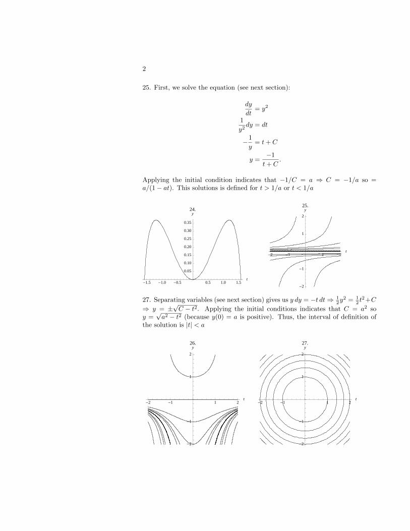
25. First, we solve the equation (see next section):

dy

dt= y2

1

y2dy = dt

−1

y= t+ C

y =−1

t+ C.

Applying the initial condition indicates that −1/C = a ⇒ C = −1/a so =a/(1− at). This solutions is defined for t > 1/a or t < 1/a

-1.5 -1.0 -0.5 0.5 1.0 1.5t

0.05

0.10

0.15

0.20

0.25

0.30

0.35

y24.

-2 -1 1 2t

-2

-1

1

2

y25.

27. Separating variables (see next section) gives us y dy = −t dt⇒ 12y

2 = 12 t

2+C

⇒ y = ±√C − t2. Applying the initial conditions indicates that C = a2 so

y =√a2 − t2 (because y(0) = a is positive). Thus, the interval of definition of

the solution is |t| < a

-2 -1 1 2t

-2

-1

1

2

y26.

-2 -1 1 2t

-2

-1

1

2

y27.

3

Exercises 2.2

1. Separate variables and integrate:

y2 dy = x dx

1

3y3 =

1

2x2 + C

y3 =3

2x2 + C

y =

(3

2x2 + C

)1/3

.

3. y =1− 2Cx+ C2x2

4x25. 3t+ 1

2 t4 + 5

2y −914y−7 = C

7. sinh 3x− 12 cosh 4y = C


1

y + 2dy =

1

2t+ 1dt

ln(2 + y) =1

2ln(2t+ 1) + C

ln(2 + y) = ln√

2t+ 1 + C

2 + y = Celn√2t+1

2 + y = C√

2t+ 1

y = −2 + C√

2t+ 1.

11. y = sin−1(− 3

4 cosx+ C)


dy

dt= −ky

1

ydy = −k dt

ln |y| = −kt+ C

y = Ce−kt

In the calculation above, remember that e−kt+C = e−kteC . C is arbitrary so eC

is positive and arbitrary.15. y = cosh−1

(− 1

120 sinh 6t− 116 cosh 4t+ C

)17. y = − 1

3 ln(− 3

2e2t + C

)19. 3

4 cos θ − 112 cos 3θ + 1

16 sin 4y − sin y = C21. y sin 2x+ 2xy + 2y2 + 5 + 4Cy = 0

4

23. This is a first-order separable equation. Separating and integrating gives us

y2 dy = (x2 + 1) dx

1

3y3 =

1

3x3 + x+ C

y =3√x3 + 3x+ C.

25. − 14x sin 2x+ 1

4x2 − 1

8 cos 2x− 2 sin√y = C

27. This is a first-order separable equation. Separating and integrating gives us

1

y2 + 1dy =

1

x+ 2dx

tan−1 y = ln |x+ 2|+ C

y = tan(ln |x+ 2|+ C).

29. 23 (lnx)3/2 + 1

3e3/y = C

31. Factor first, then separate, use partial fractions and simplify.

dy/dt = (t2 + 1)(y2 − 1)

1

y2 − 1dy = (t2 + 1) dt

1

2

(1

y − 1− 1

y + 1

)dy = (t2 + 1)dt

1

2ln

∣∣∣∣y − 1

y + 1

∣∣∣∣ =1

3t2 + t+ C

y − 1

y + 1= Ce

23 t

2+2t

y =1 + Ce

23 t

2+2t

1− Ce 23 t

2+2t

33. y =13 + 12C − 4x(3C + 1)

4C(x− 1)− 335.

1

y3 + 1dy = dt(

1

3(y + 1)+

2− y3(y2 − y + 1)

)dy = dt

−3t+√

3 tan−1(

2y − 1√3

)+ 3 ln

∣∣∣∣ (y + 1)1/3

(y2 − y + 1)1/6

∣∣∣∣ = C

5

-2 -1 1 2t

-2

-1

1

2

y

-2 -1 1 2t

-2

-1

1

2

y

-2 -1 1 2t

-2

-1

1

2

y

Figure 1: Direction fields for dy/dt = y3+y2, dy/dt = y3−y2, and dy/dt = y2−y3

37.

1

y3 + ydy = dt(

1

y− y

y2 + 1

)dy = dt

ln |y| − 1

2ln(y2 + 1

)= t+ C

y√y2 + 1

= Cet

y2 =Ce2t

1− Ce2t

y = ±√

Ce2t

1− Ce2t

39. (1

2(y − 1)− 1

y+

1

2(y + 1)

)dy = dt

1

2ln |y − 1| − ln |y|+ 1

2ln |y + 1| = t+ C√y2 − 1

y= Cet

y2 =1

1− Ce2t

y = ±√

1

1− Ce2t

6

41. dy = x3 dx⇒ y = 14x

4 +C. y(0) = 14 · 0

4 +C = 0⇒ C = 0 so y (x) = 1/4x4

43. Integrating gives us x = sin y+C and applying the initial condition gives usC = 2 so x (y) = sin (y) + 2

-2 -1 1 2x

1

2

3

4

y41.

-6 -4 -2 2 4 6y

1.5

2.0

2.5

3.0

x43.

45. y (t) = 2/3√

9 + 3 t3/2

47. y (t) = −1−√−1 + 2 et

49. y (x) = e√2√x, y (x) = e−

√2√x

51. y (x) = arctan (x) + 153. y = −3 + 4(3x+ 1)1/3

55. y = ln(12e

2x − 12 + e

)57. The solution for (a) is y = esin t, for (b) it is y =

1

1− sin t, and for (c) it is

y =1

4

(4 + r sin t+ sin2 t

).

-7.5 -5 -2.5 2.5 5 7.5t

-2.5

2.5

5

7.5

10

12.5

15

y

59. y = 2x(x− 2)−1

7

67. Use partial fractions.

1

12 + 4y − y2dt = dt(

1

y + 2− 1

y − 6

)dy = 8 dt

ln

∣∣∣∣y + 2

y − 6

∣∣∣∣ = 8t+ C

y + 2

y − 6= Ce8t

y = 23Ce8t + 1

Ce8t − 1.

71. y = exp(ct(t− 1)

)73. L(t) = L∞ − e−rBt

Exercises 2.3

1. The integrating factor is µ(t) = e−t. Multiplying through by the integratingfactor, applying the theorem, integrating and solving for y gives us

dy

dt− y = 10

e−tdy

dt− ye−t = 10e−t

d

dt

(e−ty

)= 10e−t

e−ty = −10e−t + C

y = −10 + Cet.

The preferred solution is to use undetermined coefficients. A general solution ofthe corresponding homogeneous equation, y′ − y = 0 is yh = Cet. The forcingfunction is f(t) = 10. The associated set of functions for a constant is F ={1}. Because no multiple of 1 is a solution to the corresponding homogeneousequation, we assume that a particular solution takes the form yp = A · 1 = A.Differentiating y′p = 0 and substituting into the nonhomogeneous equation givesus y′p − yp = −A = 10 so A = −10 and yp = −10. Therefore, a general solutionof the nonhomogeneous equation is y = yh + yp = −10 + Cet

3. The preferred method to solving the problem is undetermined coefficients. Thecorresponding homogeneous equation is y′ − y = 0 which has solution yh = Cet.The associated set for the forcing function, q(t) = 2 cos t is F = {cos t, sin t}.Because no member of F is a solution to the corresponding homogeneous equationwe assume that a particular solution of the nonhomogeneous equation is yp =A cos t+B sin t, where A and B are constants to be determined. Differentiating

8

yp gives us yp′ = B cos t − A sin t and substituting into the nonhomogeneous

equation results in

yp′ − yp = B cos t−A sin t− (A cos t+B sin t)

= (−A+B) cos t+ (−A−B) sin t

= 2 cos t.

Equating coefficients we have that −A+B = 2 (the coefficient of cosine is 2) and−A − B = 0 (the coefficient of sine is 0). Adding these two equations gives us−2A = 2 so A = −1 and then resubstituting that B = 1 so yp = − cos t + sin tand y = yh + yp = Cet − cos t+ sin t.

To use the an integrating factor, the integrating factor is µ(t) = e−t. Multi-plying through by the integrating factor and integrating we have

dy

dt− y = 2 cos t

e−tdy

dt− e−ty = 2e−t cos t

d

dt

(e−t y

)= 2e−t cos t

e−t y = −e−t cos t+ e−t sin t+ C

y = Cet − cos t+ sin t.

Observe that integrating eat cos bt and eat sin bt either require integration by partstwice, a table of integrals, or a computer algebra system for assistance. Note:

eat cos bt =1

a2 + b2eat (a cos bt+ b sin bt) and eat sin bt =

1

a2 + b2eat (−b cos bt+ a sin bt).

5. y = Cet − 2te−t − e−t7. y = Ce−t + t9. y = Ce−t − cos 2t+ 2 sin 2t11. y (t) = (t+ C) e−t

13. y (t) = −1/25− 1/5 t+ Ce5 t

15. y (t) = −2 cos (t) + 4 sin (t) + 4 et + Ce1/2 t

17. y (t) = 2/11 et + Ce−10 t

19. y (t) = (2 t+ C) et

21. y (t) = cos (t) + sin (t) + t− 1 + Ce−t

23. Use undetermined coefficients to find a general solution of the equation.yh = Ce−t. The associated set of functions for the forcing function f(t) = e−t isF = {e−t}. Because e−t is a solution to the corresponding homogeneous equation,multiply F by tn where n is the smallest integer so that no element of tnF is a solu-tion to the corresponding homogeneous equation. In this case, tF = {te−t} so weassume that a particular solution of the nonhomogeneous equation has the formyp = Ate−t. Differentiating yp, y

′p = −Ate−t + Ae−t, and substituting into the

nonhomogeneous equation yields y′p+yp = −Ate−t+Ae−t+Ate−t = Ae−t = e−t

so A = 1 and yp = te−t. Therefore a general solution of the nonhomogeneousequation is y = yh + yp = Ce−t + te−t. Application of the initial condition yields

9

y = e−t(t− 1).

1 2 3 4 5t

!1

!0.8

!0.6

!0.4

!0.2

y

25. A general solution of the corresponding homogeneous equation is yh =Ce−t/2. The associated set for the forcing function is F = {e−t} and no elementof F is a solution to the corresponding homogeneous equation so we assume thata particular solution of the nonhomogeneous equation has the form yp = Ae−t,where A is a constant to be determined. Differentiating yp, yp

′ = −Ae−t and sub-stituting yp into the nonhomogeneous equation results in yp

′+ 12yp = − 1

2Ae−t =

2e−t so A = −4 and yp = −4e−t. Therefore a general solution of the nonhomo-geneous equation is y = yh + yp = Ce−t/2 − 4e−t.

Applying the initial condition gives us y(0 = C − 4 = 0 ⇒ C = 4 so thesolution to the initial value problem is y = 4e−t/2 − 4e−t.

� � � � ��

��

�

�

�

�

��

27. A general solution of the corresponding homogeneous equation is yh = Ce−2t.The associated set for the forcing function is F = {e−2t}. Because y = e−2t is asolution to the corresponding homogeneous equation we multiply F by tn wheren is the smallest non-negative integer so that no member of tnF is a solutionto the corresponding homogeneous equation. We see that no member of theset tF = {te−2t} is a solution to the corresponding homogeneous equation sowe assume that a particular solution of the nonhomogeneous equation takes theform yp = Ate−2t, where A is a constant to be determined. Differentiating givesus yp

′ = −2Ate−2t + Ae−2t and substituting into the nonhomogeneous equationgives us

yp′ + 2yp = Ae2t =

1

2e−2t

10

so A = 1/2 and yp = 12 te−2t. A general solution of the nonhomogeneous equation

is then y = yh + yp = Ce−2t + 12 te−2t.

Applying the initial condition gives us y(0) = C = −1 so the solution to theinitial value problem is y = −e−2t + 1

2 te−2t.

� � � � ��

��

��

�

�

�

�

Exercises 2.4

1. The integrating factor is µ(t) = e∫dt = et. Multiplying through by the

integrating factor, applying the theorem, integrating, and solving for y gives us

y′ + y =1

1 + e2t

ety′ + ety =et

1 + e2t

d

dt(ety) =

et

1 + e2t

ety = tan−1 t+ C

y = e−t tan−1 t+ Ce−t.

3. The integrating factor is

µ(t) = e∫1/t dt = eln t = t.

Multiplying through by the integrating factor, applying the theorem, integrating,and solving for y gives us

dy

dt+

1

ty = sec2 t

tdy

dt+ t · 1

ty = t sec2 t

ty = t tan t+ ln(cos t) + C

y = tan t+ t−1 ln(cos t) + Ct−1.

11

5. The integrating factor is µ(t) = e∫tan t dt = eln sec t = sec t. Multiplying

through by the integrating factor, applying the theorem, integrating, and solvingfor y gives us

y′ + y tan t = cos t

y′ sec t+ y sec t tan t = sec t cos t

d

dt(y sec t) = 1

y sec t = t+ C

y = t cos t+ C cos t.

7. y = 12 t+ Ct−1

9. First write the equation in standard formdy

dx+

1

xy =

1

xe−x to see that

p(x) = 1/x. Then, an integrating factor is e∫1/x dx = xln x = x. Multiplying

through by the integrating factor and integrating gives us

xdy

dx+ y = e−x

d

dx(xy) = e−x

xy = −e−x + C

y = Cx−1 − x−1e−x.

11. y = 4t2 + 1 + C√

4t2 + 113. An integrating factor is µ(t) = e

∫cot t dt = e− ln csc t = sin t. Multiplying

through by the integrating factor, integrating the result, and solving for y resultsin

sin tdy

dt+ y cos t = sin t cos t

d

dt(y sin t) = sin t cos t

y sin t =1

2sin2 t+ C

y =1

2sin t+ C csc t,

which is equivalent to y = − 12 cos t cot t+C csc t because

∫sin t cos t dt = − 1

2 cos2 t+C when choosing u = cos t rather than u = sin t when calculating the integral.15. An integrating factor is

µ(t) = exp

(−∫

4t

4t2 − 9dt

)= exp

(−1

2ln(4t2 − 9)

)=

1√4t2 − 9

.

12

Multiplying through by the integrating factor, integrating the result, and solvingfor y results in

1√4t2 − 9

dy

dt− 1√

4t2 − 9

4t

4t2 − 9y =

t√4t2 − 9

d

dt

(1√

4t2 − 9y

)=

t√4t2 − 9

1√4t2 − 9

y =1

4

√4t2 − 9 + C

y =1

4(4t2 − 9) + C

√4t2 − 9.

17. An integrating factor is µ(t) = e2∫cot x dx = e−2 ln csc x = sin2 x. Multiplying

the equation by the integrating factor, integrating and solving for y yields

sin2 xdy

dx+ 2y sin2 x cotx = sin2 x cosx

d

dx

(sin2 x y

)= sin2 x cosx

sin2 x y =1

3sin3 x+ C

y =1

3sinx+ C csc2 x.

19. θ = −1 + Cer2/2

21. x(y) = −1− y + Cey

23. x(t) = C/(t3 − 1)25. v(s) = se−s + Ce−s

27. An integrating factor is µ(t) = e∫−2 dt = e−2t. Multiplying through by the

integrating factor, applying the theorem, integrating, and solving for y gives us

y′ − 2y =1

1 + e2t

e−2ty′ + e−2ty =e−2t

1 + e2t

d

dt(e−2ty) =

e−2t

1 + e2t

e−2ty = −1

2e−2t +

1

2ln(1 + e−2t) + C

y = −1

2+

1

2e2t ln(1 + e−2t) + Ce2t.

13

29. An integrating factor is µ(t) = e∫2t dt = et

2

. Multiplying the equation bythe integrating factor, integrating and solving for y yields

et2 dy

dt+ 2tet

2

y = 2tet2

d

dt

(et

2

y)

= 2tet2

et2

y = et2

+ C

y = 1 + Ce−t2

.

Applying the initial condition yields y = 1−2e−t2

.

1 2 3 4 5t

!1

!0.5

0.5

1y

31. A general solution is y = 2t−1(t−1)et+Ct−1. Applying the initial conditions

yields y = (2tet − 2et − 1)/t.

2 4 6 8 10t

!4

!2

2

4

y

14

33. y =t2 − 16

t2 + 42 4 6 8 10

t

!4

!2

2

4

y

43. y′+y = t has solution y = t−1+Ce−t. y(0) = 1⇒ C = 2 so y = t−1+2e−t

for 0 ≤ t < 1. When t = 1, y = 1− 1 + 2e−1 = 2/e. The solution to y′ + y = 0,

y(1) = 2/e is y = 2e−t. Thus, y(t) =

{t− 1 + 2e−t, 0 ≤ t < 1

2e−t, t ≥ 1.

45. y(t) =

{e−2t, 0 ≤ t < 1

e2−4t, t ≥ 1

47. y (t) = −2/5 cos (2 t)− 1/5 sin (2 t) + Cet

49. y (t) = (t+ C) e−t

63. y (t) = t − 1 + Ce−t, y (t) = −1/2 cos (t) + 1/2 sin (t) + Ce−t, y (t) =1/2 cos (t) + 1/2 sin (t) + Ce−t, y (t) = 1/2 et + Ce−t

65. y (t) = t − 1 − e−t, y (t) = t − 1, y (t) = t − 1 + e−t, y (t) = t − 1 + 2 e−t,y (t) = t− 1 + 3 e−t

Exercises 2.5

1. My(t, y) = 2y − 12 t−1/2 = Nt(t, y), exact

3. My(t, y) = cos ty − ty sin ty = Nt(t, y), exact5. The equations is exact because ∂t(sty

2) = 3y2 = ∂y(y3)7. My(t, y) = sin 2t 6= 2 sin 2t = Nt(t, y), not exact9. My(t, y) = y−1 = Nt(t, y), exact11. y = C + t3

13. y = 0, ty2 = C

15. Observe that the equation is exact because∂

∂y(2t+y3) = 3y2 =

∂

∂t(3ty2+4).

Let F (t, y) have total derivative (2t + y3) dt + (3ty2 + 4) dy. Then, F (t, y) =∫(2t + y3) dt = t2 + ty3 + g(y). Differentiating F with respect to y, Fy(t, y) =

3ty2 + g′(y) = 3ty2 + 4 ⇒ g′(y) = 4 so g(y) = 4y and F (t, y) = t2 + ty3 + 4y. Ageneral solution is then t2 + ty3 + 4y = C or t2 + ty3 + 4 y (t) = C.

17. The equation is exact because∂

∂y(2ty) = 2t =

∂

∂t(t2 + y2). Let F (t, y)

satisfy Ft(t, y)dt+ Fy(t, y)dy = 2ty dt+ (t2 + y2) dy. Then, F (t, y) =∫

2ty dt =t2y + g′(y) = t2 + y2 so g′(y) = y2 ⇒ g(y) = 1

3y3. Therefore F (t, y) = t2 + 1

3y3

15

and a general solution of the equation is t2 + 13y

3 = C. Observe that solvingthis as a homogeneous equation of degree 2 (see the next section) results in the

following form of the solution: −1/3 ln

(y(3 t2 + y2

)t3

)− ln (t) = C.


∂y(sin2 y) = 2 sin y cos y = sin 2y =

∂

∂t(t sin 2y).

Let F (t, y) satisfy Ft(t, y)dt+Fy(t, y)dy = sin2 y dt+ t sin 2y dy. Then, F (t, y) =∫sin2 y dt = t sin2 y + g(y) so g′(y) = 0 ⇒ g(y) = 0 and F (t, y) = t sin2 y. A

general solution is then t sin2 y = C or ln t+ 2 ln sin y = C.


∂y(et sin y) = et cos y =

∂

∂t(1 + et cos y).

Let F (t, y) satisfy Ft(t, y)dt + Fy(t, y)dy = et sin y dt + (1 + et cos y) dy. Then,F (t, y) =

∫et sin y dt = et sin y + g(y) so g′(y) = 1 ⇒ g(y) = t. Thus, F (t, y) =

et sin y + t and a general solution of the equation is et sin y + y = C.

-4 -2 2 4t

-4

-2

2

4

y17.

-6 -4 -2 2 4 6t

-6

-4

-2

2

4

6

y19.

-6 -4 -2 2 4 6t

-6

-4

-2

2

4

6

y21.

23. y = 0, y = C√

sec t2 + tan t2


∂y(1 + y2 cos ty) = 2y cos ty − ty2 sin ty =

∂

∂t(sin ty+ty cos ty). Let F (t, y) satisfy Ft(t, y)dt+Fy(t, y)dy = (1+y2 cos ty) dt+

(sin ty + ty cos ty) dy. Then, F (t, y) =∫

(1 + y2 cos ty) dt = t + y sin ty + g(y) soFy(t, y) = sin ty + ty cos yt + g′(y) so g′(y) = 0 and g(y) = 0. Then F (t, y) =t+ y sin(yt) and a general solution of the equation is t+ y sin yt = C.


∂y((3 + t) cos(t + y) + sin(t + y)) = cos(t +

y) − (3 + t) sin(t + y) =∂

∂t((3 + t) cos(t + y)). Let F (t, y) satisfy Ft(t, y)dt +

Fy(t, y)dy = ((3 + t) cos(t + y) + sin(t + y)) dt + (3 + t) cos(t + y) dy. Then,F (t, y) =

∫((3 + t) cos(t + y) + sin(t + y)) dt = (3 + t) sin(t + y) + g(y) so

Fy(t, y) = (3 + t) cos(t + y) + g′(y) = (3 + t) cos(t + y) ⇒ g′(y) = 0 ⇒ g(y) = 0so F (t, y) = 3 sin(t+ y) + t sin(t+ y) and 3 sin(t+ y) + t sin(t+ y) = C.


∂y

(−t−2y2ey/t + 1

)= −t−3yey/t(2t + y) =

∂

∂t

(ey/t(1 + y/t)

). Let F (t, y) satisfy Ft(t, y)dt+Fy(t, y)dy =

(−t−2y2ey/t + 1

)dt+

ey/t(1 + y/t) dy. Then, F (t, y) =(−t−2y2ey/t + 1

)dt = t + yey/t + g(y). Next,

16

Fy(t, y) = ey/t(1 + y/t) + g′(y) = ey/t(1 + y/t) so g′(y) = 0 ⇒ g(y) = 0. Thus,F (t, y) = yey/t + t and yey/t + t = C.

-6 -4 -2 2 4 6t

-6

-4

-2

2

4

6

y25.

-6 -4 -2 2 4 6t

-6

-4

-2

2

4

6

y27.

-6 -4 -2 2 4 6t

-6

-4

-2

2

4

6

y29.

31. This equation is exact because∂

∂y

(2ty2

)= 4ty =

∂

∂t

(2t2y

). Let F (t, y)

satisfy Ft(t, y) dt + Fy(t, y) dy = 2ty2 dt + 2t2y dy. Then, F (t, y) =∫

2ty2 dt =t2y2 + g(y) so Fy(t, y) = 2t2y + g′(y) = 2t2y, which means that g′(y) = 0 ⇒g(y) = 0. Therefore F (t, y) = t2y2 and a general solution (or, integral curves) ofthe differential equation are t2y2 = C. Application of the initial condition resultsin y2t2 − 1 = 0.

Observe that dividing the differential equation by 2ty yields y dt + t dy = 0,

which is equivalent to tdy

dt+ y = 0 or

dy

dt+

1

ty = 0. This is a first order linear

homogeneous equation with integrating factor µ(t) = e∫1/t dt = t. Multiplying

through by the integrating factor, integrating and solving for y gives us

tdy

dt+ y = 0

d

dt(ty) = 0

ty = C

y = Ct−1.

Observe that squaring both sides of the equation and solving for C gives us thesame result as that obtained by solving the equation as an exact equation.


∂y

(2ty + 3t2

)= 2t =

∂

∂t

(t2 − 1

). Let

F (t, y) satisfy Ft(t, y) dt + Fy(t, y) dy =(2ty + 3t2

)dt +

(t2 − 1

)dy. Then,

F (t, y) =∫ (

2ty + 3t2)dt = t2y + t3 + g(y) so Fy(t, y) = t2 + g′(y) = t2 − 1

⇒ g′(y) = −1 ⇒ g(y) = −y. Therefore, F (t, y) = t2y + t3 − y and the integralcurves are t2y+ t3−y = C. Applying the initial condition and solving for y gives

us y =−t3 − 1

(t− 1) (t+ 1).

17

-4 -2 2 4t

-4

-2

2

4

y31.

-4 -2 2 4t

-4

-2

2

4

y32.

-4 -2 2 4t

-4

-2

2

4

y33.


∂y(ey − 2ty) = ey − 2t =

∂

∂t

(tey − t2

).

Let F (t, y) satisfy Ft(t, y) dt+ Fy(t, y) dy = (ey − 2ty) dt+(tey − t2

)dy. Then,

F (t, y) =∫

(ey − 2ty) dt = tey − t2y + g(y). Differentiating with respect to y,Fy(t, y) = tey−t2+g′(y) = tey−t2 ⇒ g′(y) = 0⇒ g(y) = 0 so F (t, y) = tey−t2yand the integral curves are tey − t2y = C. Applying the initial condition resultsin tey − t2y = 0.


∂y

(y2 − 2 sin 2t

)= 2y =

∂

∂t(1 + 2ty). Let

F (t, y) satisfy Ft(t, y) dt + F (t, y) dy =(y2 − 2 sin 2t

)dt + (1 + 2ty) dy. Then,

F (t, y) =∫ (y2 − 2 sin 2t

)dt = ty2 + cos 2t + g(y). Differentiating with re-

spect to y, Fy(t, y) = 2ty + g′(y) = 1 + 2ty ⇒ g′(y) = 1 ⇒ g(y) = y soF (t, y) = ty2 + cos 2t + y and the integral curves are ty2 + cos 2t + y = C. Ap-plying the initial condition results in ty2 + cos (2 t) + y − 2 = 0.

-4 -2 2 4t

-4

-2

2

4

y35.

-4 -2 2 4t

-4

-2

2

4

y36.

-4 -2 2 4t

-4

-2

2

4

y37.


∂y

(1

1 + t2− y2

)= −2y =

∂

∂t(−2ty).

Let F (t, y) satisfy Ft(t, y) dt + Fy(t, y) dy =

(1

1 + t2− y2

)dt − 2ty dy. Then,

F (t, y) =∫ ( 1

1 + t2− y2

)dt = tan−1 t − ty2 + g(y). Differentiating with re-

spect to y, Fy(t, y) = −2ty + g′(y) = −2ty ⇒ g′(y) = 0 ⇒ g(y) = 0 soF (t, y) = tan−1 t − ty2 and the integral curves are tan−1 t − ty2 = C. Ap-

plying the initial condition results in y2 − arctan (t)

t= 0.

18

-6 -4 -2 2 4 6t

-6

-4

-2

2

4

6

y38.

-6 -4 -2 2 4 6t

-6

-4

-2

2

4

6

y39.

41. (a) The equation is exact because

∂

∂y(−2x− y cos(xy)) = − cos(xy) + xy sin(xy) =

∂

∂x(2y − x cos(xy)) .

The integral curves for the solution take the form F (x, y) = C, where

F (x, y) =

∫(−2x− y cos(xy)) dx = −x2 − sin(xy) + g(y).

Because

∂

∂yF (x, y) =

∂

∂y

(−x2 − sin(xy) + g(y)

)= 2y − x cos(xy) + g′(y),

g′(y) = 2y so g(y) = y2, F (x, y) = y2 − x2 − sin(xy), and the integral curves ofthe equation are given by y2 − x2 − sin(xy) = C. Applying the initial conditiony(0) = 0 results in 0 = C so that the solution to the initial value problem isy2 = x2 + sin(xy).Observe in the following figure that the initial condition y(0) = 0 does not resultin a unique solution.

-6 -4 -2 2 4 6x

-6

-4

-2

2

4

6

y

-6 -4 -2 2 4 6x

-6

-4

-2

2

4

6

y

19

(b) Writing the differential equation in differential form gives us

dy

dx=

2x+ y cos(xy)

2y − x cos(xy)︸︷︷︸f(x,y)

.

Using the notation in the theorem,

∂f

∂y= −

x(4(x2 + y2

)sin(xy) + cos(2xy) + 9

)2(x cos(xy)− 2y)2

.

The results do not contradict the Theorems because neither of these functions iscontinuous on a region containing the origin, (0, 0).

43. Here,dx

dt=

2xy√x2 + y2

anddy

dt= − y2 − x√

x2 + y2. Then,

dy

dx=dy/dt

dx/dt=y2 − x

2xy(−x+ y2

)dx+ 2xy dy = 0.

Using the notation in section, M(x, y) = −x+y2 so My(x, y) = 2y and N(x, y) =2xy so Nx(x, y) = 2y so the equation

(−x+ y2

)dx + 2xy dy = 0 is exact. Let

F (x, y) be the potential function. Then,

F (x, y) =

∫ (−x+ y2

)dx

F (x, y) = −1

2x2 + xy2 + g(y).

Next, Fy(x, y) = 2xy + g′(y) = 2xy so g′(y) = 0. We choose g(y) = 0 so that

F (x, y) = −1

2x2 + xy2 and the integral curves are given by −1

2x2 + xy2 = C.

-4 -2 2 4x

-4

-2

2

4

y

-4 -2 2 4x

-4

-2

2

4

y

-4 -2 2 4x

-4

-2

2

4

y

49. y =C

(et + t2)2/3

51. y−1 − −t+ C

t2= 0

20

53. yt5 + t4 (y)2

+ 1/4 t4 = C55. cos (y (t)) t2 + sin (y) t = C57. t2 + y cos ty = C

59. (a) (i) y = −t, t2 + 2ty + y2 = C (ii) y =1

C

(−Ct± 1

10

√10C2t2 + 10

)(iii)

y =1

C

(− 19

20Ct±120

√−39C2t2 + 40

)

-1.0 -0.5 0.5 1.0t

-1.0

-0.5

0.5

1.0

y

HiL

-1.0 -0.5 0.5 1.0t

-1.0

-0.5

0.5

1.0

y

HiiL

-1.0 -0.5 0.5 1.0t

-1.0

-0.5

0.5

1.0

y

HiiiL

Exercises 2.6

1. This is Bernoulli with n = −1. Let w = y1−(−1) = y2 ⇒ dw

dt= 2y

dy

dt

⇒ dy

dt=

1

2y−1

dw

dt. Then,

dy

dt− 1

2y = ty−1

1

2y−1

dw

dt− 1

2y = ty−1

dw

dt− y2 = 2t

dw

dt− w = 2t.

Use undetermined coefficients to solve for w. A general solution of the corre-sponding homogeneous equation is wh = Cet. The associated set of functions forthe forcing function f(t) = 2t is F = {t, 1}. Because no element of F is a solutionto the corresponding homogeneous equation we assume that a particular solutionhas the form wp = At+B ⇒ w′p = A. Substituting wp into the nonhomogeneousequation yields w′p − wp = −At + (A − B) = 2t so A = −2 and B = −2 sowp = −2t− 2. A general solution is then w = wh + wp = Cet − 2t− 2. Becausew = y2, y = ±

√Cet − 2t− 2.

3. This is Bernoulli with n = 3 so we let w = y1−3 = y−2. Then,dw

dt= −2y−3

dy

dt

21

so −1

2y3dw

dt=dy

dt. Substituting into the equation gives us

−ty3 dwdt− y = 2ty3 cos t

dw

dt+

1

ty−2 = −2 cos t

dw

dt+

1

tw = −2 cos t

d

dt(tw) = −2t cos t

tw = −2 cos t− 2t sin t+ C

w = −2t−1 cos t− 2 sin t+ Ct−1

1

y2= −2t−1 cos t− 2 sin t+ Ct−1

y = ± 1√−2t−1 cos t− 2 sin t+ Ct−1

.

or y = ±√− (2 cos (t) + 2 t sin (t)− C) t

2 cos (t) + 2 t sin (t)− C5. y3/2 + 9

20 cos (t)− 320 sin (t)− Ce3 t = 0

7. y =3t

t3 − 3C9. This is a Bernoulli equation with n = 2 so we let w = y1−2 = y−1 = 1/y.

Then,dw

dt= −y−2 dy

dtso

dy

dt= −y2 dw

dt. Then,

dy

dt− 1

ty =

y2

t

−y2 dwdt− 1

ty =

y2

tdw

dt+

1

ty−1 = −1

tdw

dt+

1

tw = −1

t.

The integrating factor fordw

dt+

1

tw = −1

tis µ(t) = e

∫1/t dt = eln t = t, t > 0.

Multiplying through by the integrating factor and solving for w gives us:

dw

dt+

1

tw = −1

t

tdw

dt+ w = −1

d

dt(tw) = −1

tw = −t+ C

w = Ct−1 − 1.

22

Because w = 1/y, y = 1/w, so 1/y = Ct−1−1 which means that y = 1/(Ct−1−1)or y = Ct/(1− Ct).11. Homogeneous of degree 013. Not homogeneous15. Not homogeneous17. The equation is homogeneous of degree 1. Let t = vy. Then, dt = vdy+ ydv.Substituting into the equation, separating and integrating yields

2tdt+ (y − 3t)dy = 0

2vy(vdy + ydv) + (y − 3vy)dy = 0

2v(vdy + ydv) + (1− 3v)dy = 0

(2v2 − 3v + 1)dy = −2vydv

1

ydy =

−2v

2v2 − 3v + 1dv

1

ydy = 2

(1

2v − 1− 1

v − 1

)dv

ln y = ln(2v − 1)− 2 ln(1− v) + C

y = C2v − 1

(v − 1)2

y = C(2t− y)y

(t− y)2

(t− y)2

2t− y= C.

Another form of the solution is−2 ln

(−−y + t

t

)+ ln

(y − 2 t

t

)− ln (t) = C.

19. The equation is homogeneous of degree 2. Observe that either t = vy or y =ut results in an equivalent problem. We choose to use y = ut⇒ dy = udt+ tdu.

23

Then,

(ty − y2)dt+ t(t− 3y)dy = 0

(t2u− t2u2)dt+ t(t− 3ut)(udt+ tdu) = 0

(u− u2)dt+ (1− 3u)(udt+ tdu) = 0

2u(1− 2u)dt+ t(1− 3u)du = 0

2u(1− 2u)dt = t(3u− 1)du

1

tdt =

3u− 1

2u(1− 2u)du

1

tdt = −1

2

(1

u+

1

2u− 1

)du

ln t = −1

2lnu− 1

4ln(2u− 1) + C

−4 ln t = 2 lnu+ ln(2u− 1) + C

1

t4= Cu2(2u− 1)

1

t4= C

y2(t− 2y)

t3

ty2(t− 2y) = C.

Another form of the solution is −1/4 ln

(−t+ 2 y

t

)− 1/2 ln

(yt

)− ln (t) = C.

21. y3 − (3 ln (t) + C) t3 = 023. This is homogeneous of degree 1. (Also, observe that this is a first orderlinear equation in y.) Solving it as a homogeneous equation, we let y = ut ⇒dy = udt+ tdu. Then,

(t− y)dt+ tdy = 0

(t− ut)dt+ t(udt+ tdu) = 0

(1− u)dt+ udt+ tdu = 0

dt = −tdu1

tdt = −du

ln t = −u+ C

ln t = −yt

+ C

y = t(C − ln t).

25. −2/3 ln

(3 y − 2 t

t

)+ 1/2 ln

(−t+ 2 y

t

)− ln (t) = C

27. The equation is homogeneous of degree 2. Let t = vy ⇒ dt = vdy + ydv.

24

Then,

y2dt = (ty − 4t2)dy

y2(vdy + ydv) = (vy2 − 4v2y2)dy

vdy + ydv = (v − 4v2)dy

ydv = −4v2dy

−4

ydy =

1

v2dv

−4 ln y = −1

v+ C

4 ln y =y

t+ C.

Another form of the solution is 1/4y

t− ln

(yt

)− ln (t) = C

29. y = −t, −1/2 ln

(t2 − ty + y2

t2

)+1/3

√3 arctan

(1/3

(t− 2 y)√

3

t

)−ln (t) =

C31. 1/2 (−y + t) y−1

(e−t/y

)−1 − ln (y) = C

33. y′ + 2y = t2y1/2 is Bernoulli with n = 1/2. Let w = y1−1/2 = y1/2. Then,dw

dt=

1

2y−1/2

dy

dt⇒ dy

dt= 2y1/2

dw

dt. Substituting into the equation yields

dy

dt+ 2y = t2y1/2

2y1/2dw

dt+ 2y = t2y1/2

dw

dt+ y1/2 =

1

2t2

dw

dt+ w =

1

2t2.

Using undetermined coefficients, a general solution is w = Ce−t + 12 t

2 − t + 1.Thus, y = (Ce−t + 1

2 t2 − t + 1)2. Applying the initial condition results in

y = 14 (4− 8 t+ 8 t2 − 4 t3 + t4).

1 2 3 4 5t

1

2

3

4

5

y

25

35. y = 1/2√

2 + 2 t2t37. y = −1/2 + 1/2 t2

39. y = 3√−3 ln (t) + 27t

-4 -2 2 4t

-15

-10

-5

5

10

15

y35.

-4 -2 2 4t

2

4

6

8

10

12y

37.

1 2 3 4 5t

50

100

150

200

250

y39.

41. y4dt + (t4 − ty3)dy = 0 is homogeneous of degree 4. Let t = vy ⇒ dt =vdy + ydv. Then,

y4dt+ (t4 − ty3)dy = 0

y4(vdy + ydv) + (v4y4 − vy4)dy = 0

(vdy + ydv) + (v4 − v)dy = 0

v4dy = −ydv1

ydy = − 1

v4dv

ln y =1

3v3+ C

3 ln y =y3

t3+ C.

Applying the initial condition results in1

3

y3

t3− ln

(yt

)− ln t− 8/3 + ln 2 = 0.

43. We need to solve dy/dt = y/t+ t/y subject to y(√e) =

√e. The equation is

homogeneous of degree 2. To see so, we rewrite the equation:

dy

dt=y2 + t2

yt

yt dy = (y2 + t2)dt.

Now, we let y = ut⇒ dy = udt+ tdu. Substituting then gives us

ut2(u dt+ t du) = (u2t2 + t2) dt

u(u dt+ t du) = (u2 + 1) dt

tu du = dt

1

tdt = u2 du

ln t =1

3u3 + C

ln t =1

3

y3

t3+ C.

26

Now apply the initial condition and solve for y, y =√

2 t√

ln t.

45. Solve y2 dx+ (x2 + y2) dy = 0; y = ±√−x2 ±

√x4 + C

47. The general solution is y−3 = (3 cotx+ C) sin3 x or y = 0. So, the solutionto the initial value problem is y = 0.49. Because M(t, y)dt+N(t, y)dy = 0 is homogeneous, we can write the equationin the form dy/dt = F (y, t). If t = r cos θ and y = r sin θ, dt = cos θ dy− r sin θdθand dy = sin θ dr + r cos θ dθ. Substituting into the equation gives us

dy/dt = F (t, y)

sin θ dr + r cos θ dθ

cos θ dr − r sin θdθ= F

(r sin θ

r cos θ

)= F (tan θ)

sin θ dr + r cos θ dθ = F (tan θ) cos θ dr − F (tan θ)r sin θdθ

F (tan θ)r sin θdθ + r cos θ dθ = F (tan θ) cos θ dr − sin θ dr

F (tan θ) sin θdθ + cos θ

F (tan θ) cos θ − sin θ=

1

rdr.

53. f(t) = t − 1; g(t) = t2 − t; General solution: (tc − y) − 1 = c2 − c ⇒

y = ct − 1 + c − c2; Singular solution:d

dt(ty′ − y − 1) =

d

dt

[(y′)2 − y′

]⇒

ty′′+ y′ = 2y′y′′− y′′ ⇒ (t− 2y′+ 1)y′′ = 0⇒ y′ = 12 (t+ 1)⇒ y = 1

4 t2 + 1

2 t−34 .

55. f(t) = 1 − 2t; g(t) = t−2; General solution: 1 − 2(tc − y) = c−2 ⇒ y =12 (c−2 + 2ct− 1); Singular solution: y = 1

2 (3t2/3 − 1)59. We see that the equation is a Lagrange equation by rewriting it in the formy = ty′2 + (3y′2 − 2y′3) and identifying f(y′) = y′2 and g(y) = 3y′2 − 2y′3.Differentiating with respect to t yields the equation y′ = y′2 + 2ty′y′′ + 6y′y′′ −6y′2y′′ and substituting p = y′ results in

p = p2 + 2tpdp

dt+ 6p

dp

dt− 6p2

dp

dt

p− p2 =(2xp+ 6p− 6p2

) dpdx

dx

dp=

2xp+ 6p− 6p2

p− p2dx

dp+

2p

p2 − px =

6p− p2

p− p2.

The solution of this linear equation is x =2p3 − 21p2 + 36p+ 6C

6 (p2 − 2p+ 1)so

y = xp2 + 3p2 − 2p3 =2p3 − 21p2 + 36p+ 6C

6 (p2 − 2p+ 1)p2 + 3p2 − 2p3.

61. Differentiating the equation gives us y′ = (2− y′) +xy′′+ 4y′y′′. Now, we let

27

p = y′ and solve for dx/dp:

y′ = (2− y′) + xy′′ + 4y′y′′

p = 2− p+ xdp

dx+ 4p

dp

dx

2p− 2 = (x+ 4p)dp

dxdx

dp=

x+ 4p

2(p− 1)

dx

dp+

1

2− 2px =

4p

2(p− 1).

This linear equation has solution x = − 83 + 4

3p+ 43p

2 + C√

2− 2p so

y = x(2− o) + 2p2 + 1 =

(−8

3+

4

3p+

4

3p2 + C

√2− 2p

)(2− p) + 2p2 + 1.

63. limt→∞ y(t) =ky0ay0

=k

a65. General solution: 2t2 ln |t| + t2 = Ct2. Initial value problem has two solu-tions: y = ±

√2√t2(ln 4− ln t).

-4 -2 2 4t

-4

-2

2

4

y64.

-4 -2 2 4t

-4

-2

2

4

y65.

Exercises 2.7

1. 47.3742, 63.25723. 1.8857, 2.098475. 79.8458, 123.0487. 1.95109, 1.953889. 83.6491, 88.603511. 2.37754, 2.4189713. 185.34, 206.981

28

15. 1.95547, 1.9560917. 90.6405, 90.692719. 216.582, 216.99223. 1.95629, 1.9562925-27. (a) y(t) = e−t, y(1) = 1/e ≈ 0.367879

h = 0.1 h = 0.005 h = 0.02525. (Euler’s) 0.348678 0.358486 0.36323226. (Improved) 0.368541 0.368039 0.36791827. (4th-Order RK) 0.429069 0.414831 0.3678829. y(0.5) ≈ 0.566144, 1.12971, 1.68832, 2.23992, 2.78297

Chapter 2 Review Exercises

1. y = 1/5 3√

25 t6 + 125C

3. The equationdy

dt− 1

ty =

1

ty2 is Bernoulli with n = 2. Let w = y1−2 = y−1.

Then, dw/dt = −y−2 dy/dt so −y2 dw/dt = dy/dt. With this substitution wehave,

dy

dt− 1

ty =

1

ty2

−y2 dwdt− 1

ty =

1

ty2

dw

dt+

1

ty−1 = −1

t(Divide by −y2.)

dw

dt+

1

tw = −1

t.

An integrating factor fordw

dt+

1

tw = −1

t, t > 0, is µ(t) = e

∫1/t dt = eln t = t.

Multiplyingdw

dt+

1

tw = −1

tby the integrating factor and solving for w gives us

dw

dt+

1

tw = −1

t

tdw

dt+ t

1

tw = −t · 1

td

dt(t w) = −1

tw = −t+ C

w = −1 +C

t1

y=−t+ C

t

y =t

−t+ C.

5. y4dy = e5tdt⇒ 15y

5 = 15e

5t + C ⇒ y5 = e5t + C → y = (e5t + C)1/5

29

7. y (t) = e±√−e−2 t+C

9. For this first-order linear equation, the preferred method of solution is usingthe method of undetermined coefficients to find a particular solution of the nonhomogeneous equation. The corresponding homogeneous equation is y′ + 3y = 0which is the first order linear homogeneous equation with constant coefficients,y′ + ky = 0, which has general solution y = Ce−kt with k = 3 so y′ + 3y = 0 hasgeneral solution yh = Ce−3t.

Now, look at the forcing function, f(t) = −10 sin t. The associated set forthis forcing function is F = {cos, sin t} and because neither of these is a solutionof the corresponding homogeneous equation, we assume that yp takes the formyp = A cos t + B sin t with derivative y′p = −A sin t + B cos t. Substituting intothe non homogeneous equation gives us

y′p + 3yp = (3A+B cos t+ (−A+ 3B sin t

= −10 sin t

so

3A+B = 0

−A+ 3B = −10,

which has solution A = 1 and B = −3. Therefore, yp = cos t − 3 sin t andy = yh + yp = Ce−3t + cos t− 3 sin t.

If you preferred to use the integrating factor approach, the integrating factoris µ(t) = e

∫3 dt = e3t. Now multiply through by the integrating factor and

integrate the result. Observe that integrating the right hand side by hand involvesintegration by parts twice.

y′ + 3y = −10 sin t

e3ty′ + 3e3ty = −10e3t sin t

d

dt

(e3ty

)= −10e3t sin t

e3ty = e3t cos t− 3e3t sin t+ C

y = cos t− 3 sin t+ Ce−3t.

11. The equation (y − t) dt + (t + y) dy = 0 is homogeneous of degree 1. Eithery = ut or t = vy result in an equivalent problem. We choose to use y = ut ⇒

30

dy = u dt+ t du. Then,

(y − t) dt+ (t+ y) dy = 0(u2 + 2u− 1

)dt = −t(u+ 1)du

1

tdt = − u+ 1

u2 + 2u− 1du

ln t = −1

2ln∣∣u2 + 2u− 1

∣∣+ C

t−2 = C(u2 + 2u− 1

)t−2 = Ct−2

(y2 + 2ty − t2

)y2 + 2ty − t2 = C.

y = −t± 1C

√2C2t2 + 1

13. The equation y2 dt + (ty + t2) dy = 0 is homogeneous of degree 2. We lett = vy so dt = v dy + y dv. Then, substituting and separating variables gives us

y2 dt+ (ty + t2) dy = 0

y2 (v dy + y dv) + (vy · y + (vy)2) dy = 0

(v dy + y dv) + (v + v2) dy = 0 (Divide by y2.)

(2v + v2) dy = −y dv

−1

ydy =

1

2v + v2dv

−1

ydy =

1

2

(1

v− 1

v + 2

)dv

− ln y =1

2(ln v − ln(2 + v)) + C

ln y =1

2ln

(2 + v

v

)+ C

y = C

√2 + v

v.

Now replace v with t/y and solve for C.

y = C

√2 + v

v

y = C

√2 + t/y

t/y

y2 = C2 + t/y

t/y

ty2

t+ 2y= C.

31

Solving for y instead of C results in y =C ±

√C2 + Ct2

t.

15. −5

8ln

(−−x+ 2 t

t

)− 5

8ln

(x+ 2 t

t

)+

1

4ln(xt

)− ln (t) = C

17. 13 t

3y − cos t− sin y = C19. 1

2 t2 ln y + y = C

21. y = 1 + Ce−t2/2

23. r = t−1(cos t+ t sin t+ C)25. y = t−1(6et − 6tet + 3t2et + C)1/3

27. y = −2 + 2 ln(−2/t), y = Ct+ 2 lnC

29. y = −1/3 t√

6 t− 6√t2 − 12C + 1

54

(6 t− 6

√t2 − 12C

)3/2,

y = 1/3 t√

6 t− 6√t2 − 12C − 1

54

(6 t− 6

√t2 − 12C

)3/2,

y = −1/3 t√

6 t+ 6√t2 − 12C + 1

54

(6 t+ 6

√t2 − 12C

)3/2,

y = 1/3 t√

6 t+ 6√t2 − 12C − 1

54

(6 t+ 6

√t2 − 12C

)3/231. y + sin(t− y) = π33. t sin y − y sin t = 035. t ln y + y ln t = 037.

32

39.

1. V (x) =∫ x0πy2dt, W (x) = ρV (x) = ρ

∫ x0πy2dt

2. σ(x) = F (x)A(x) where F (x) = W (x) + L and A(x) = πy2.

3. y(x) = K exp(ρx2σ

). If y(0) = 1, then K = 1.

41. dxdt = kx2, x(0) = 100, x(1) = 60. x(t) = −1

kt+C so that C = −1/100 and

k = −1/150. When t = 3, x(3) =(

3150 + 1

100

)−1= 100

3 ≈ 33.33 grams.

Differential Equations at Work

33

A. Modeling the Spread of a Disease

2.

0 2 4 6 8 10t0.0

0.2

0.4

0.6

0.8

1.0I

HbL

0 2 4 6 8 10t0.0

0.2

0.4

0.6

0.8

1.0I

HcL

4.

0 2 4 6 8 10t0.0

0.2

0.4

0.6

0.8

1.0I

HaL

0 2 4 6 8 10t0.0

0.2

0.4

0.6

0.8

1.0I

HbL

B. Linear Population Model with Harvesting

1. (a) ay−h = 0 has solution y = h/a. (c) y =1

a((ay0 − h)eat + h) (d) limt→∞ =

∞ (e) limt→∞ = h/a (f) limt→∞ = −∞; y(t) = 0 when t = −1

aln(

1− a

hy0

)2. (a) y = 2 (b) y = (y0 − 2)et/2 + 2 (c) ∞ (d) 2 (f) −∞; 2 ln 43. y = 1

2 (2 − et) = 0 when t = ln 2 ≈ 0.693; y = 12 (4 − 3et/2 = 0 when

t = 2 ln(4/3) ≈ 0.5754. y = 1

2 (2− et/2 = 0 when t = 2 ln 2 ≈ 1.386

5. First solve y′ = 12y −

12 , y(0) = 1/2 to obtain y = 1 − 1

2et/2. Then, y(1) =

1 − 12

√e ≈ 0.176. Then, for year two, solve y′ = 1

2y + 12 , y(1) = 1 − 1

2

√e to

obtain y = −1 + 2e(t−1)/2 − 12et/2 so y(2) = −1 + 2

√e − 1

2e ≈ 0.938. y′ =12y + r, y(1) = 1 − 1

2

√e has solution y = − 1

2et/2 − 2r + (2r + 1)e(t−1)/2 so

y(2) = − 12e− 2r + (2r + 1)

√e = 1

2 = y(0) when r = 14 (√e− 1) ≈ 0.162.

6. Set r = 0 in the above. Then, y(2) =√e − 1

2e ≈ 0.290. y(T ) = e(t−1)/2 −12et/2 = 1

2 = y(0) when T = −2 ln

(−1 +

2√e

)≈ 3.092

7.

34

0.2 0.4 0.6 0.8 1.0

20.2

20.4

20.6

20.8

21.0

HaL

0.2 0.4 0.6 0.8 1.0

20.05

20.10

20.15

20.20

HbL

0.2 0.4 0.6 0.8 1.0

19.0

19.5

20.0HcL

0.2 0.4 0.6 0.8 1.0

14

15

16

17

18

19

20HdL

8.

0.2 0.4 0.6 0.8 1.0

20.5

21.0

21.5

22.0

HaL

0.2 0.4 0.6 0.8 1.0

20.5

21.0

21.5

22.0

HbL

0.2 0.4 0.6 0.8 1.0

20.5

21.0

21.5

22.0

HcL

0.2 0.4 0.6 0.8 1.0

20.5

21.0

21.5

22.0HdL

C. Logistic Model with Harvesting

1. y =1

2c

(a±√a2 − 4ch

)2. (a) y = 2, y = 5 (b)

35

2 4 6 8 10t

1

2

3

4

5

6

7

y

(c) 5 (d) 5 (e) 0 (extinction)3. 49− 40h = 0 when h = 49/40

2 4 6 8 10t

1

2

3

4

5

6

7

yHaL

2 4 6 8 10t

1

2

3

4

5

6

7

yHbL

2 4 6 8 10t

1

2

3

4

5

6

7

yHcL

4.

1 2 3 4 5t

0.5

1.0

1.5

2.0

2.5

yNo Harvesting

1 2 3 4 5t

-12

-10

-8

-6

-4

-2

yHarvesting

5.

36

1 2 3 4 5t

2

4

6

8

10

12y

No Harvesting

1 2 3 4 5t

2

4

6

8

10

yHarvesting

6.

2 4 6 8 10 12t

2

4

6

8

10

12

14

y6.

2 4 6 8 10 12t

2

4

6

8

10

12

14

y7.

2 4 6 8 10t

2

4

6

8

10

12

14

y8.

2 4 6 8 10t

2

4

6

8

10

12

14

y9.

D. Logistic Model with Predation

1. a 2.

37

5 10 15 20t

5

10

15

20

WHaL

5 10 15 20t

5

10

15

20

WHbL

3. k > 19.3 will work

5 10 15 20

-5

-4

-3

-2

-1

k � 19.3

5 10 15 20

-5

-4

-3

-2

-1

k � 19.4

5 10 15 20

-5

-4

-3

-2

-1

k � 19.5

5 10 15 20

-5

-4

-3

-2

-1

k � 19.6

4.

38

5 10 15 20t

5

10

15

20

Wk � 19.1

5 10 15 20t

5

10

15

20

Wk � 19.2

5 10 15 20t

5

10

15

20

Wk � 19.3

5 10 15 20t

5

10

15

20

Wk � 19.4

5 10 15 20t

5

10

15

20

Wk � 19.5

5 10 15 20t

5

10

15

20

Wk � 19.6

5 10 15 20t

5

10

15

20

Wk � 19.7

5 10 15 20t

5

10

15

20

Wk � 19.8

5 10 15 20t

5

10

15

20

Wk � 19.9

6.

5 10 15 20t

5

10

15

20

WHaL

5 10 15 20t

5

10

15

20

WHbL

5 10 15 20t

5

10

15

20

WHcL

Documents

Exercises 2.1 - Elsevier