SOLUTIONS TO EXERCISES

CHAPTER 2

2.1. (a) 25; (e) 0.04; (i) 2.2360; (m) 11.1803;(b) 125; (f ) 0.008; ( j) 1.7099; (n) 0.5848;(c) 625; (g) 0.0016; (k) 1.4953; (o) 3.3437;(d) 625; (h) 0.0016; (l) 5; (p) 11.1803.

2.2. (a) 1; (e) add the exponents, 52 = 25;(b) 1; (f ) add the exponents, 5−8/3 = 0.0136798;(c) 1; (g) add the exponents, 51 = 5;(d) 1; (h) add the exponents, 251 = 25.

2.3. FV = 50(1 + 0.3)4 = 50(1.3)4 = 50 · 2.8561 = 142.805.

2.4. PV = 180(1 + 0.2)−0.5 = 180(1.2)−0.5 = 180 · 0.9128709 = 164.31677.

2.5. (a) y = 24x3(12x) = 288x4;(b) y = 7(−3x2 + 3x) + 4x = −21x2 + 21x + 4x = −21x2 + 25x;(c) y = 25 + {2x[3x + 4(x + 5)(x + 5) · 6] − 5} − 7x2

= 25 + {2x[3x + 4(x2 + 10x + 25) · 6] − 5} − 7x2

= 25 + {2x[3x + 24x2 + 240x + 600] − 5} − 7x2

= 25 + {6x2 + 48x3 + 480x2 + 1,200x − 5} − 7x2 = 48x3 + 479x2 + 1,200x + 20.

2.6. (a) y = 9(4(7 + 9)2)0.5 + 216 · 5(9) = 9(4(16)2)0.5 + 9,720= 9(4 · 256)0.5 + 9,720 = 9 · 1,0240.5 + 9,720 = 9 · 32 + 9,720 = 10,008;

(b) y = ((7 + 16)(27 · 16 + 2)3)−0.5 = (23(432 + 2)3)−0.5 = (23 · 4343)−0.5

= (23 · 81,746,504)−0.5 = 1,880,169,600−0.5 = 0.000023.

2.7. Simplify as follows:

= ⋅ −

⋅

= ⋅ −

$

.

. . $

.

.250

10 08

10 08 1 7138243

2501

0 081

0 1371059

PVA $

.

. ( . ) $

.

. ( . )= ⋅ −

⋅ +

= ⋅ −

⋅

250

10 08

10 08 1 0 08

2501

0 081

0 08 1 087 7

A P P E N D I X A

SOLUTIONS TO EXERCISES

QRMD02 9/17/01 4:52 PM Page 224

Solutions to exercises 225

= $250 · [12.5 − 7.29363]

= $250 · 5.20637 = $1,301.59.

2.8. (a) −13.8155; (c) 0; (e) 0.99325; (g) 1.0986; (i) 4.60517;(b) −0.693147; (d) 0.09531; (f ) 0.99989; (h) 2.3025; ( j) 6.90775.

2.9. Assume for each of the accounts that the initial deposit is 1 for each account and its futurevalue is 2. Then, the general procedure for each account is to solve the following for ngiven each interest rate i:

2 = 1(1 + i)n,

ln(2) = ln(1) + n · ln(1 + i ),

(a) 0.69314718 ÷ ln(1.03) = 23.44977 years;(b) 0.69314718 ÷ ln(1.05) = 14.20699 years;(c) 0.69314718 ÷ ln(1.07) = 10.24476 years;(d) 0.69314718 ÷ ln(1.10) = 7.27254 years;(e) 0.69314718 ÷ ln(1.12) = 6.11625 years;(f ) 0.69314718 ÷ ln(1.15) = 4.95948 years.

2.10. (a) 72 ÷ 3 = 24 years;(b) 72 ÷ 5 = 14.4 years;(c) 72 ÷ 7 = 10.286 years;(d) 72 ÷ 10 = 7.2 years;(e) 72 ÷ 12 = 6 years;(f ) 72 ÷ 15 = 4.8 years.

2.11. First, for sake of simplicity, assume PV to be 1 and FVn to be 2:

2 = 1 · ern = ern.

Now, find the natural logs of both sides:

ln(2) = rn,

ln(2) ≈ 0.693 ≈ 0.72 ≈ rn,

Thus, for example, if the interest rate equals 0.10, it will take approximately 7.2 yearsfor an account to double.

2.12. Our demonstration is as follows:

FVn = PV · ern = 1 · e0.1·10 = e.

2.13. (a) X1 = 15, X2 = 25, X3 = 35, X4 = 45;(b) 15 + 25 + 35 + 45 = 120;(c) 3 · 15 + 3 · 25 + 3 · 35 + 3 · 45 = 3 · 120 = 360;(d) 3 · 152 + 3 · 252 + 3 · 352 + 3 · 452 = 3 · 225 + 3 · 625 + 3 · 1225 + 3 · 2025

= 12,300;

0 72. .

rn≈

ni i

ln( ) ln( )

ln( )

. ln( )

.=−+

=−

+2 1

10 69314718 0

1

= ⋅ −

$

. .250

10 08

7 29363

QRMD02 9/17/01 4:52 PM Page 225

(e) ∏ 4t=13X 2

t = (3 · 152) · (3 · 252) · (3 · 352) · (3 · 452) = (3 · 225) · (3 · 625) · (3 · 1225) · (3 · 2025) ≈ 2.8255869 · 1013

= 28,255,869,000,000;(f ) ∑4

t =1Xt/n = (15 + 25 + 35 + 45)/4 = 120/4 = 30;(g) (∏ 4

t =1Xt)1/n = (15 · 25 · 35 · 45)1/4 = 27.722217.

2.14. (a) ∑3i =1wi = 0.4 + 0.5 + 0.1 = 1;

(b) ∑ 3i=1∑ 3

j=1wiwjxi,j = [0.4 · 0.4 · 7] + [0.4 · 0.5 · 4] + [0.4 · 0.1 · 9] + [0.5 · 0.4 · 6] + [0.5 · 0.5 · 4] + [0.5 · 0.1 · 12] + [0.1 · 0.4 · 3] + [0.1 · 0.5 · 2] + [0.1 · 0.1 · 17]= 1.12 + 0.8 + 0.36 + 0.12 + 1 + 0.6 + 1.2 + 0.1 + 0.17 = 5.47.

2.15. The three-year rate is based on a geometric mean of the short-term spot rates as follows:

2.16. FV = ∑4t =125(1 + 0.10)t = 25(1.1)1 + 25(1.1)2 + 25(1.1)3 + 25(1.1)4

= 25(1.1) + 25(1.21) + 25(1.331) + 25(1.4641) = 127.6275.

2.17. (a) x = 8! = 8 · 7 · 6 · 5 · 4 · 3 · 2 · 1 = 40,320;(b) x = 9! = 9 · 8! = 9 · 8 · 7 · 6 · 5 · 4 · 3 · 2 · 1 = 362,880;(c) x = 0! = 1.

2.18. (a) (6 · 5 · 4 · 3) = 360; (d) (6 · 5)/(2 · 1) = 15;(b) (4 · 3 · 2 · 1) = 24; (e) 1;(c) (8 · 7) = 56; (f ) (8 · 7)/(2 · 1) = 28.

CHAPTER 3

3.1. (a) 90 = 5x, 90/5 = x = 18;(b) −2,500 = −2x, (−2,500)/(−2) = 1,250;(c) 85 = 8x, 85/8 = x = 10.625;(d) 50 = 60 + 5x, −10 = 5x, −10/5 = x = −2;(e) 20 − 10 − 25 = −15/x, −15 = −15/x, x = 1;(f ) 25 − 100 = 3x − 2x + 5x, −75 = 6x, −75/6 = x = −12.5.

3.2. (a) 100 ÷ 90 = (1 + x)2, 1.1111111 = (1 + x)2, (1.1111111)1/2 = 1 + x, 1.05409 = 1 + x, x = 0.05409;

(b) 100 ÷ 90 = (1 + x)3, 1.1111111 = (1 + x)3, (1.1111111)1/3 = 1 + x, 1.03574 = 1 + x, x = 0.03574;

(c) 100 ÷ 90 = (1 + x)−2, 1.1111111 = (1 + x)−2, (1.1111111)−1/2 = 1 + x, 0.94868 = 1 + x, x = −0.051316;

(d) 90 ÷ 100 = (1 + x)−2, 0.9 = (1 + x)−2, 0.9−1/2 = 1 + x, 1.05409 = 1 + x, x = 0.05409.

3.3. (a) The value of $1 is equal to the value of £0.6. Thus, the value of £1 must be $1/0.6 = $1.6667. Since the value of $1 is ¥108, the value of £1 must be 1.6667 · ¥108 = ¥180. Thus, we could have solved as follows: £1 = ($1 ÷ 0.6) ·¥108 = ¥180.

(b) The value of $1 is equal to the value of ¥108. Thus, the value of ¥1 must be $1/¥108 = $0.0092593. Since the value of £1 is $1.6667, the value of ¥1 must

= + + + − = ( . )( . )( . ) . .1 0 05 1 0 06 1 0 07 1 0 059973

y y y y yn t t

t

nn

0 11

0 1 1 2 2 3

31 1 1 1 1 1, , , , , ( ) ( )( )( ) = + − = + + + −−

=∏

226 Appendix A

QRMD02 9/17/01 4:52 PM Page 226


be $1 ÷ (1.6667 · ¥108) = £0.0055556. Thus, we could have solved as follows: ¥1 = $1 ÷ (1/0.6 · ¥108) = £0.0055556.

(c) $300 = £0.6 · 300 = £180. $300 = ¥108 · 300 = ¥32,400.

3.4. The firm’s break-even production level is determined by solving for Q when profits π equalzero:

0 = 80Q − (500,000 + 50 · Q ).

First, we will add 500,000 to both sides:

500,000 = 80Q − 50Q.

Next, note that 80Q − 50Q = 30Q, so that we will divide both sides of the above equa-tion by 30 to obtain:

500,000 ÷ 30 = Q* = 16,666.67,

where Q* is the break-even production level (the asterisk does not represent a productsymbol here). Thus, the firm must produce 16,666.67 units to recover its fixed costs inorder to break even.


= (1 + 0.05)(1 + 0.06)(1 + 0.07) = 1.19091,

y0,3 = [(1 + 0.05)(1 + 0.06)(1 + 0.07)]1/3 − 1 = − 1 = 0.0599686.


(1 + y0,3)3 = (1.07)3 = 1.22504 = (1 + 0.05)(1 + 0.07)(1 + y2,3).

We solve for y2,3 as follows:

1.22504 ÷ [(1 + 0.05)(1 + 0.07)] − 1 = y2,3 = 0.07.

3.7. (a) The firm’s profit function, total revenues minus total costs, is

π = 50Q − 0.00002Q2 − (500,000 + 20Q + 0.00001Q2),

which simplifies to

π = −0.00003Q2 + 30Q − 500,000.

(b) Note that the terms are arranged in descending order of exponents for Q. Our coefficients for this quadratic equation are a = −0.00003, b = 30, and c = −500,000. We can solve for the break-even production level by setting πequal to zero, using the quadratic formula as follows:

= 16,954.11 and 983,045.88 units.

=

− ±−

=− ±

−=

−−

−−

.

.

.

..

..

30 8400 00006

30 28 9827530 00006

1 01724660 00006

58 9827530 00006

and

Q ( . ) ( , )

( . )

( )

.=

− ± − ⋅ − ⋅ −⋅ −

=− ± −

−30 30 4 0 00003 500 000

2 0 00003

30 900 60

0 00006

2

= + −=

∏ ( ),1 11

3

yt tt

1 190913

.

( ) ( ), ,1 10 33

11

3

+ = + −=

∏y yt tt

QRMD02 9/17/01 4:52 PM Page 227

Either of the above production levels will enable the firm to break even with a profit levelequal to zero.

3.8. We need to solve this equation for w1 using the quadratic formula. This is accomplishedas follows:

, where a = 0.25, b = −0.3, and c = 0.09.

We fill in our coefficients’ values to determine the proportion of the investor’s money tobe invested in stock 1:

The value under the square root sign (the radical) will be zero. Hence, there will be onlyone value for w1 = 0.6. Therefore, we find that the portfolio is riskless when w1 = 0.6.Thus, 60% of the riskless portfolio should be invested in stock 1 and 40% of the port-folio should be invested in stock 2.

3.9. First, number the equations as follows:

0.04x1 + 0.04x2 = 0.01, (A1)

0.04x1 + 0.16x2 = 0.11. (A2)

Now, write equation (A1) in terms of x1:

0.04x1 = 0.01 − 0.04x2,

x1 = 0.01/0.04 − 0.04x2/0.04,

x1 = 0.25 − 1x2.

Next, we substitute our revised version of x1 back into equation (A2) to obtain the following:

0.11 = 0.04(0.25 − 1x2) + 0.16x2,

which simplifies to

0.10 = −0.12x2. (B2)

Thus, x2 = 0.83333. Substitute x2 back into either equation (A1) or equation (A2) andwe find that x1 = −0.58333.

3.10. 20x − 5λ = −3 (1a)−5x − 0λ = −100 (2a)

x = 20 (2b) = (2a) ÷ −520 · 20 − 5λ = −3 (2a)

−5λ = −403λ = 403/5 = 80 , x = 20.

3.11. First, number the equations as follows:

962 = 100x1 + 100x2 + 1,100x3, (A1)

1,010.4 = 120x1 + 120x2 + 1,120x3, (A2)

970 = 100x1 + 1,100x2. (A3)

35

w1

20 3 0 3 4 0 25 0 09

2 0 250 3 0

0 50 6

. ( . ) . .

.

. .

. .=± − − ⋅ ⋅

⋅=

±=

w

b b ac

a1

2 42

=− + −

228 Appendix A

QRMD02 9/17/01 4:52 PM Page 228


Now, write equation (A3) in terms of x1:

100x1 = 970 − 1,100x2,

x1 = 970/100 − 1,100x2/100,

x1 = 9.7 − 11x2.

Next, we plug our revised version of x1 back into equations (A1) and (A2) to obtain thefollowing:

962 = 100(9.7 − 11x2) + 100x2 + 1,100x3,

1,010.4 = 120(9.7 − 11x2) + 120x2 + 1,120x3,

which simplifies to

−8 = −1,000x2 + 1,100x3, (B1)

−153.6 = −1,200x2 + 1,120x3. (B2)

Now solve equations (B1) and (B2) for x3 by multiplying equation (B1) by 1.2 and sub-tracting the result from equation (B2):

−153.6 = −1,200x2 + 1,120x3 (B2)(−9.6 = −1,200x2 + 1,320x3) (B1) ·1.2−144 = −200x3

Thus, x3 = 0.72. Plug x3 back into either equation (B1) or equation (B2) and we find that x2 = 0.8. Now, substitute x3 = 0.72 and x2 = 0.8 back into any of equa-tions (A1), (A2), or (A3) and we find that x1 = 0.9. Thus, we obtain x1 = 0.9, x2 = 0.8,and x3 = 0.72.

3.12. (a) 16.80 = 4 · GNP + 80 · i,9.00 = 2 · GNP + 50 · i ;

(b) 16.80 = 4 · GNP + 80 · i,9.00 = 2 · GNP + 50 · i.

16.80 = 4 · GNP + 80 · i18.00 = 4 · GNP + 100 · i−1.20 = −20i;

i = 0.06, GNP = 3.

3.13. Our first problem is to complete a pro-forma income statement for 2001. However, wedon’t know what the company’s interest expenditure in 2001 will be until we know howmuch money it will borrow (EFN ). At the same time, we cannot determine how muchmoney the firm needs to borrow until we know its interest expenditure (so we can solvefor retained earnings). Therefore, we must solve simultaneously for EFN and interest expend-iture. We know that EFN can be found as follows:

EFN = ∆ Assets − ∆CL − RE,

EFN = $400,000 − $60,000 − RE.

Retained earnings (RE) can be found using the following pro-forma income statementfor 2001:

QRMD02 9/17/01 4:52 PM Page 229

Pro-forma Income Statement, 2001

Sales (TR) ......................................... $1,050,000Cost of Goods Sold ........................... 450,000Gross Margin ................................... 600,000Fixed Costs ....................................... 150,000EBIT ................................................. 450,000Interest Payments............................ 50,000 + (0.10 · EFN)Earnings Before Tax ........................ 400,000 − (0.10 · EFN)Taxes (@ 40%) ................................ 160,000 − (0.04 · EFN)Net Income After Tax...................... 240,000 − (0.06 · EFN)Dividends (@ 33%).......................... 80,000 − (0.02 · EFN)Retained Earnings ........................... 160,000 − (0.04 · EFN)

Now, rewrite the EFN expression, substituting in for RE:

EFN = $400,000 − $60,000 − ($160,000 − (0.04 · EFN )),

EFN = $180,000 + 0.04 · EFN,

0.96 · EFN = $180,000,

EFN = $187,500.

Our EFN problem is complete. We now know that the firm must borrow $187,500. Thus,the firm’s total interest payments for 2001 must be $50,000 plus 10% of $187,500, or$68,750.

3.14. 1,200 = 100(1 + x + x2 + x3 + . . . + x9),

1,200x = 100(x + x2 + x3 + . . . + x10),

1,200x − 1,200 = 100(x + x2 + x3 + . . . + x10 − 1 − x − x2 − x3 − . . . − x9),

1,200(x − 1) = 100(x10 − 1),

12 = (x10 − 1)/(x − 1).

Substitute for x:

x = 1.0398905.

3.15. The expansion is performed as follows:

∆Y = ∆A + Y(c + c2 + c3 + . . . + c ∞ ), (B)

c∆Y = c∆A + Y(c2 + c3 + c4 + . . . + c ∞+1), (C)

(1 − c)∆Y = (1 − c)∆A + Y(c − c∞+1) where 0 < c ≤ 1, (D)

∆Y = ∆A + Y [c ÷ (1 − c)] where c∞+1 = 0. (E)

Thus, the income multiplier equals c/(1 − c) = c/s, where s represents the proportion ofmarginal income saved by individuals.

3.16. Plot several points for x and y for the functions, one function at a time. When enoughpoints have been plotted to determine the shape of the curve, map out the graph.Functions (a) and (b) will plot similarly to the two functions in figure 3.2 in section 3.5.Functions (c) and (d) will plot similarly to the two functions in figure 3.1 in section 3.5.

230 Appendix A

QRMD02 9/17/01 4:52 PM Page 230


CHAPTER 4

4.1. TV8 = 10,500(1 + 8 · 0.09) = 10,500 · 1.72 = 18,060.

4.2. (a) [10% · $10,000,000]/2 = $500,000;(b) 10% · $10,000,000 = 2 · $500,000 = $1,000,000;(c) $10,000,000 + $1,000,000 = principal + interest in year five = $11,000,000.

4.3. $10,000(1 + 0.055/365)5·365 = $13,165.03.

4.4. (a) TV8 = 10,500(1 + 0.09)8 = 10,500 · 1.99256 = 20,921.908;

(b) = 10,500 · 2.0223702 = 21,234.887;

(c) = 10,500 · 2.0489212 = 21,513.673;

(d) = 10,500 · 2.0542506 = 21,569.632;

(e) TV8 = 10,500e0.09·8 = 10,500 · 2.0544332 = 21,571.549.

4.5. $10,000(1 + 0.055/365)5·365 = $13,165.03.

4.6. For example, let X0 = $1,000 in each case:

for CD1, TV5 = 1,000(1 + 0.12)5 = 1,762.3417;

for CD2, = 1,648.6005.

4.7. Solve for X0:

4.8 Solve the following for APY:

4.9. In all cases here, FVn = 2X0. Thus, let FVn = 2,000 and X0 = 1,000:

(a) 2,000 = 1,000(1 + n · 0.1), 2 = (1 + n · 0.1), 1 = 0.1n, n = 10 years.(b) 2,000 = 1,000(1.1)n. Using logs:

log 2,000 = (log 1,000) + n · log(1.1),

3.30103 = 3 + n · (0.04139),

0.30103 = n(0.04139), n = 7.2725 years.

(c) 2 000 1 000 10 1012

12

, , .

:= +

n

APYi

m

m

.

. .= +

− = +

− =1 1 10 03

41 0 0303391

4

X

TV

in

n0 3110000

1 0 087 938 322

( )

,( . )

, . .=+

=+

=

TV5

365 5

1 000 10 10365

, .

= +

⋅

TV8

365 8

10 500 10 09365

, .

= +

⋅

TV8

12 8

10 500 10 0912

, .

= +

⋅

TV8

2 8

10 500 10 09

2 ,

.= +

⋅

QRMD02 9/17/01 4:53 PM Page 231

log 2,000 = (log 1,000) + 12n · log(1.008333),

n = 6.96059 years.

(d) 2,000 = 1,000e0.1·n. Use natural logs:

ln 2,000 = (ln 1,000) + 0.1n, n = 6.93148 years.

4.10. (a)

(b)

(c)

(d)

4.11. (a)

(b)

(c)

(d)

(note that six months is 0.5 of one year);

(e)

(note that 73 days is 0.2 of one year).

4.12.

PV = 1,851.85 + 2,572.02 = 5,556.83 = 9,980.70;

10,000 > 9,980.70.

Since P0 > PV, the investment should not be purchased.

4.13.

(a) = 2,000(20 − 12.892178) = 14,215.643;

(b) = 2,000(10 − 4.2409762) = 11,518.048;

(c) = 2,000(5 − 0.9690335) = 8,061.933. PVA

.

. ( . )= −

10 2

10 2 1 2 9

PVA ,

.

. ( . )= −

2 000

10 10

10 10 1 10 9

PVA = −

,

.

. ( . )2 000

10 05

10 05 1 05 9

PV CF

k k kn n

( ):= −

+

1 11

PVCF

kt

tt

n

( )

,.

,.

,.

;=+

= + +=∑ 1

2 0001 08

3 0001 08

7 0001 081

1 2 3

PV

,.

,

. , .

.= = =

10 0001 1

10 0001 0192449

9 811 1840 2

PV

,.

,.

,

. , .

. .= = = =

10 0001 1

10 0001 1

10 0001 0488088

9 534 6250 5 0 5

PV

,.

,.

, . ;= = =10 000

1 110 000

1 19 090 909

1

PV

,.

,

. , . ;= = =

10 0001 1

10 0002 5937425

3 855 43210

PV

,.

,

. , . ;= = =

10 0001 1

10 0006 7275

1 486 43620

PV

,.

,

, .= = =10 000

1 010 000

110 000

5

PV

,.

,

. , . ;= = =

10 0001 01

10 0001 0510101

9 514 6565

PV

,.

,

. , . ;= = =

10 0001 10

10 0001 61051

6 209 2135

PVCF

kn

n

( )

,( . )

,.

,

. , . ;=

+=

+= = =

110 000

1 0 2010 000

1 210 000

2 488324 018 775

5 5

232 Appendix A

QRMD02 9/17/01 4:53 PM Page 232


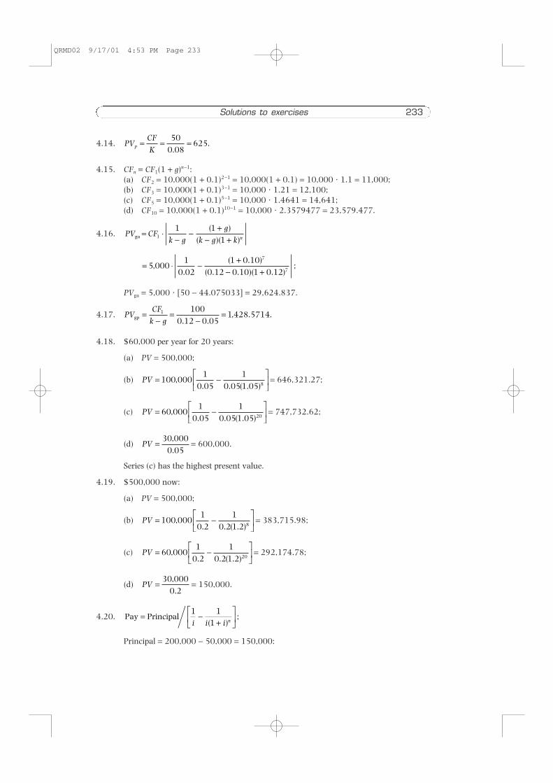
4.14.

4.15. CFn = CF1(1 + g)n−1:(a) CF2 = 10,000(1 + 0.1)2−1 = 10,000(1 + 0.1) = 10,000 · 1.1 = 11,000;(b) CF3 = 10,000(1 + 0.1)3−1 = 10,000 · 1.21 = 12,100;(c) CF5 = 10,000(1 + 0.1)5−1 = 10,000 · 1.4641 = 14,641;(d) CF10 = 10,000(1 + 0.1)10−1 = 10,000 · 2.3579477 = 23,579.477.

4.16.

PVga = 5,000 · [50 − 44.075033] = 29,624.837.

4.17.

4.18. $60,000 per year for 20 years:

(a) PV = 500,000;

(b) = 646,321.27;

(c) = 747,732.62;

(d) = 600,000.

Series (c) has the highest present value.

4.19. $500,000 now:

(a) PV = 500,000;

(b) = 383,715.98;

(c) = 292,174.78;

(d) = 150,000.

4.20.

Principal = 200,000 − 50,000 = 150,000:

Pay Principal

1

( ) ;= −

+

i i i n

11

PV

,.

=30 000

0 2

PV ,.

. ( . )

= −

60 000

10 2

10 2 1 2 20

PV ,.

. ( . )

= −

100 000

10 2

10 2 1 2 8

PV

,.

=30 000

0 05

PV ,.

. ( . )

= −

60 000

10 05

10 05 1 05 20

PV ,.

. ( . )

= −

100 000

10 05

10 05 1 05 8

PVCF

k ggp

. .

, . .=−

=−

=1 1000 12 0 05

1 428 5714

= ⋅ −+

− + ,

.

( . )( . . )( . )

;5 0001

0 021 0 10

0 12 0 10 1 0 12

7

7

PV CF

k g

g

k g k nga = ⋅−

−+

− +

( )( )( )1

1 11

PV

CF

Kp .

.= = =50

0 08625

QRMD02 9/17/01 4:53 PM Page 233

(a)

= 150,000/8.5135637 = 17,618.944;

(b)

= 150,000/103.62442 = 1,447.5352

(note that 10%/12 = 0.008333; 20 · 12 = 240.

4.21. Substitute discount rates into the present-value annuity function until you find one thatsets PV equal to the purchase price:

try 15%, PV = 9,543.1685 < 10,000;try 13%, PV = 10,803.31 > 10,000;try 14%, PV = 9,892.8294 < 10,000;try 13.7%, PV = 10,001.638 > 10,000;try 13.71%, PV = 9,997.977 < 10,000;try 13.704%, PV = 10,000.174 > 10,000.

Thus, K is approximately 13.704%.

4.22. (a)

(b)

(c)

(d) PV = 10,000 · e−0.1·20 = 1,353.3528.

4.23. (a) First, the monthly discount rate is 0.1 ÷ 12 = 0.008333:

= 1,000 · 113.95082 = $113,950.82.

(b) Yes, since the PV exceeds the $100,000 price.

(c)

Solve for k; by a process of substitution, we find that k = 0.11627.

4.24. Use the present-value annuity function to amortize the loan. The payment is $2,637.97.

4.25.

PV

k

gCF

g

k

g

k

g

k

n

nga ⋅++

=++

+++

+ +++

− −

− ( )( )

( )( )

( )( )

. . . ( )( )

;11

11

11

11

1

0

0

1

2

1

PV CF

g

k

g

k

g

k

n

nga =++

+++

+ +++

−

( )( )

( )( )

. . . ( )( )

;11

11

11

0

1

1

2

1

100 000 1 000

112

112 1 12 360

, , ( / )

( / ) ( / )

.= ⋅ −⋅ +

k k k

PV ,

.

. ( . )= ⋅ −

+

1 000

10 008333

10 008333 1 0 008333 360

PV ,

( . / )

,.

, . ;=+

= =⋅

10 0001 0 1 365

10 0007 3870321

1 353 7236365 20

PV ,

( . / )

,.

, . ;=+

= =⋅

10 0001 0 1 12

10 0007 328074

1 364 61512 20

PV ,.

,

. , . ;= = =

10 0001 1

10 0006 7275

1 486 43620

Pay

1 ,

.

. ( . )= −

150 000

0 0083331

0 008333 1 008333 240

Pay

1 ,

.

. ( . )= −

+

150 000

0 11

0 1 1 0 1 20

234 Appendix A

QRMD02 9/17/01 4:53 PM Page 234


4.26. This problem can be solved with either of the following:

4.27. The following Single-Stage Growth Model can be used to evaluate this stock:

Since the $100 purchase price of the stock is less than its $90 model value, the stockshould not be purchased.

4.28. The following Three-Stage Growth Model can be used to evaluate this stock:

Since the $100 purchase price of the stock exceeds its $92.0171 value, the stock shouldnot be purchased.

++ + +

− +=

− −

$ ( . ) ( . ) ( )

( . )( . ) . .

5 1 0 15 1 0 06 1 00 08 0 1 0 08

92 01710783 1 6 3

6

+

+ ++ −

−+ +

− +

− − − +

$( . ) ( . )

( . ) ( . . )

( . ) ( . )( . . )( . )

51 0 15 1 0 06

1 0 08 0 08 0 061 0 15 1 0 060 08 0 06 1 0 08

3 1

3

3 1 6 3 1

6

p0

3

35

10 08 0 15

1 0 150 08 0 15 1 0 08

$. .

( . )

( . . )( . )=

−−

+− +

++ + +

− +

− −

( ) ( ) ( )

( )( ),

( ) ( ) ( )

( )

DIV g g g

k g k

n n n

n1 1

1 12

2 13

32

1 1 11

+

+ ++ −

−+ +

− +

− − − +

( ) ( )

( ) ( )

( ) ( )( )( )

( )

( )

( ) ( ) ( )

( )DIV

g g

k k g

g g

k g k

n

n

n n n

n11

1 12

12

11 1

22 1 1

22

1 11

1 11

p DIV

k g

g

k g k

n

n0 11

11

11

1 11

( )

( )( )

( )

( )=

−−

+− +

p0

1 800 06 0 04

90 $ .

. . $ .=

−=

pDIV

k g01

,=

−

PV $ , .

. ( . )

$ , .

( . )

$ , . .= ⋅ −+

− ⋅ −+

=5 0001

0 121

0 12 1 0 125 000

10 12

11 0 12

14 973 4259 9

PV $ , .

. ( . )( . )

$ , . ;= ⋅−

++

=5 000

10 12

10 12 1 0 12

1 0 1214 973 42

50

9

PV CF

k g

g

k g k

n

nga

( )

( )( ).=

−−

+− +

1 11

PV

k g

gPV

k g

gCF

g

k

g

k

n

nga ga⋅+ − +

+=

−+

=++

−++

− −

( ) ( )

( )

( )( )

( )( )

( )( )

;1 1

1 111

11

1

0

1

PV

k

gPV CF

g

k

g

k

n

nga ga⋅++

− =++

−++

− −

( )( )

( )( )

( )( )

;11

11

11

1

0

1

QRMD02 9/17/01 4:53 PM Page 235

CHAPTER 5

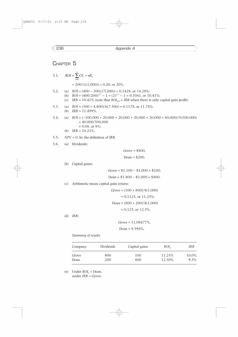
5.1.

= 200/(1(1,000)) = 0.20, or 20%.

5.2. (a) ROI = (400 − 200)/(7(200)) = 0.1428, or 14.28%;(b) ROI = (400/200)1/7 − 1 = (2)1/7 − 1 = 0.1041, or 10.41%;(c) IRR = 10.41% (note that ROIAG = IRR when there is only capital gain profit).

5.3. (a) ROI = (500 + 4,800)/6(7,500) = 0.1178, or 11.78%;(b) IRR = 11.499%.

5.4. (a) ROI = (−100,000 + 20,000 + 20,000 + 20,000 + 20,000 + 60,000)/5(100,000)= 40,000/500,000= 0.08, or 8%;

(b) IRR = 10.21%.

5.5. NPV = 0, by the definition of IRR.

5.6. (a) Dividends:

Grove = $800,

Dean = $200.

(b) Capital gains:

Grove = $1,100 − $1,000 = $100,

Dean = $1,800 − $1,000 = $800.

(c) Arithmetic mean capital gain return:

Grove = (100 + 800)/8(1,000)

= 0.1125, or 11.25%;

Dean = (800 + 200)/8(1,000)

= 0.125, or 12.5%.

(d) IRR:

Grove = 11.08477%,

Dean = 9.598%.

Summary of results

Company Dividends Capital gains ROIa IRR

Grove 800 100 11.25% 10.0%Dean 200 800 12.50% 9.5%

(e) Under ROIa = Dean,under IRR = Grove.

ROI CF nPtt

n

= ÷∑ 0=0

236 Appendix A

QRMD02 9/17/01 4:53 PM Page 236


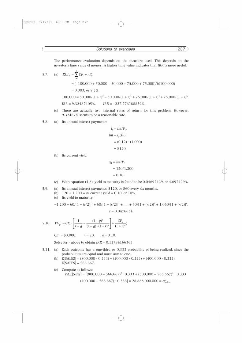
The performance evaluation depends on the measure used. This depends on theinvestor’s time value of money. A higher time value indicates that IRR is more useful.

5.7. (a)

= (−100,000 + 50,000 − 50,000 + 75,000 + 75,000)/6(100,000)

= 0.083, or 8.3%.

100,000 = 50,000/(1 + r)2 − 50,000/(1 + r)3 + 75,000/(1 + r)4 + 75,000/(1 + r)6,

IRR = 9.32487405%, IRR = −227.776188859%.

(c) There are actually two internal rates of return for this problem. However,9.32487% seems to be a reasonable rate.

5.8. (a) Its annual interest payments:

iy = Int/F0,

Int = iy(F0)

= (0.12) · (1,000)

= $120.

(b) Its current yield:

cy = Int/P0

= 120/1,200

= 0.10.

(c) With equation (4.8), yield to maturity is found to be 0.04697429, or 4.697429%.

5.9. (a) Its annual interest payments: $120, or $60 every six months.(b) 120 ÷ 1,200 = its current yield = 0.10, or 10%.(c) Its yield to maturity:

−1,200 + 60/[1 + (r/2)]1 + 60/[1 + (r/2)]2 + . . . + 60/[1 + (r/2)]5 + 1,060/[1 + (r/2)]6,

r = 0.0476634.

5.10.

CF1 = $3,000, n = 20, g = 0.10.

Solve for r above to obtain IRR = 0.11794166365.

5.11. (a) Each outcome has a one-third or 0.333 probability of being realized, since the probabilities are equal and must sum to one.

(b) E[SALES] = (800,000 · 0.333) + (500,000 · 0.333) + (400,000 · 0.333),E[SALES] = 566,667.

(c) Compute as follows:VAR[Sales] = [(800,000 − 566,667)2 · 0.333 + (500,000 − 566,667)2 · 0.333

(400,000 − 566,667) · 0.333] = 28,888,000,000 = σ 2sales.

PV CF

r g

g

r g r

CF

r

n

nn

nga

( )

( ) ( )

( );= ⋅

−−

+− ⋅ +

+

+1

1 11 1

ROI CF nPtt

n

A=0

= ÷∑ 0

QRMD02 9/17/01 4:53 PM Page 237

(d) Expected return of project A:

(0.3 · 0.333) + (0.15 · 0.333) + (0.01 · 0.333) = 0.15333.

(e) Variance of A’s returns:

[(0.3 − 0.1533)2 · 0.333 + (0.15 − 0.1533)2 · 0.333

+ (0.01 − 0.1533)2 · 0.333] = 0.0140222 = σ 2A.

(f ) Expected return of project B:

(0.2 · 0.333) + (0.13 · 0.333) + (0.09 · 0.333) = 0.14.

Variance of B’s returns:

[(0.2 − 0.14)2 · 0.333 + (0.13 − 0.14)2 · 0.333

+ (0.09 − 0.14)2 · 0.333] = 0.0020666 = σ 2B.

(g) Standard deviations are square roots of variances:

σsales = 169,964,

σA = 0.1184154,

σB = 0.0454606.

(h) Compute as follows:

COV[Sales] = (Salesi − E[Sales]) · (RAi − E[RA]) · Pi ,

COV[Sales, A] = (800,000 − 566,667) · (0.3 − 0.1533) · 0.333

+ (500,000 − 566,667) · (0.15 − 0.1533) · 0.333

+ (400,000 − 566,667) · (0.01 − 0.1533) · 0.333

= 19,444 = σsales,A.

(i)

( j) First, find the covariance between sales and returns on B:

COV[Sales, B] = (800,000 − 566,667) · (0.20 − 0.14) · 0.333

+ (500,000 − 566,667) · (0.13 − 0.14) · 0.333

+ (400,000 −566,667) · (0.09 − 0.14) · 0.333

= 7,666.67 = σsales,B;

(k) The coefficient of determination is the correlation coefficient squared: 0.9932 = 0.986.

5.12. Project A has a higher expected return; however, it is riskier. Therefore, it does not clearlydominate project B. Similarly, B does not dominate A. Therefore, we have insufficientevidence to determine which of the projects is better.

5.13. (a) BP = 0.062,BL = 0.106,BM = 0.098.

ρ σ

σ σsalessales

sales,

,

,

, . . .B

B

B

=⋅

=⋅

=7666

169964 0 04540 993

ρ σ

σ σssales

sales,

,

,

, . . .A

A

A

=⋅

=⋅

=19444

169964 0 1180 97

i

n

=∑

1

238 Appendix A

QRMD02 9/17/01 4:53 PM Page 238


(b) σ 2P = 0.000696

(remember to convert returns to percentages),

σ 2L = 0.008824,

σ 2M = 0.001576.

(c) COV[L,Y] = [(0.04 − 0.062) · (0.19 − 0.106) + (0.07 − 0.062) · (0.04 − 0.106)

+ (0.11 − 0.062) · (−0.04 − 0.106) + (0.04 − 0.062) · (0.21 − 0.106)

+ (0.05 − 0.062) · (0.13 − 0.106)]/5 = −0.002392,

(d) COV[L,M] = [(0.04 − 0.062) · (0.15 − 0.098) + (0.07 − 0.062) · (0.10 − 0.098)

+ (0.11 − 0.062) · (0.03 − 0.098) + (0.04 − 0.062) · (0.12 − 0.098)

+ (0.05 − 0.062) · (0.09 − 0.098)] ÷ 5 = −0.000956,

(e) COV[M,Y] = [(0.15 − 0.098) · (0.19 − 0.106) + (0.10 − 0.098) · (0.04 − 0.106)

+ (0.03 − 0.098) · (−0.04 − 0.106) + (0.12 − 0.098) · (0.21 − 0.106)

+ (0.09 − 0.098) · (0.13 − 0.106)] ÷ 5 = 0.003252,

5.14. Assuming variance and correlation stability, the forecasted values would be the same asthe historical values in problem 5.13.

5.15. Standardize returns by standard deviations and consult “z” tables: (Ri − E[R] ) ÷ σi = zi.Only use positive values for z.

(a) (0.05 − 0.15) ÷ 0.10 = z(low) = −1, (0.25 − 0.15) ÷ 0.10 = z(high) = 1.From the z-table in appendix B, we see that the probability that the security’sreturn will fall between 0.05 and 0.15 is 0.34. 0.34 is also the probability that thesecurity’s return will fall between 0.15 and 0.25. Therefore, the probability that thesecurity’s return will fall between 0.05 and 0.25 is 0.68.

(b) From part (a), we see that the probability is 0.34.(c) 0.16.(d) 0.0668.

5.16. Simply reduce the standard deviations in the z-scores in problem 5.15 to 0.05:

(a) 0.95;(b) 0.47;(c) 0.0228;(d) 0.0013.

5.17. (a) VAR = 0.0025.(b) 0. The coefficient of correlation between returns on any asset and returns on a risk-

less asset must be zero. Riskless asset returns do not vary.

ρσ σM,L

M Y

COV M,Y

[ ]

.. .

. .= =⋅

=0 003252

0 039 0 0940 872

ρσ σP M

P M

COV L,M,

[ ]

.. .

. .= =−

⋅= −

0 0009560 0264 0 039

0 912

ρσ σP L

P L

COV L,Y,

[ ]

.. .

. .= =−

⋅= −

0 0023920 0264 0 094

0 96521

QRMD02 9/17/01 4:53 PM Page 239

CHAPTER 6

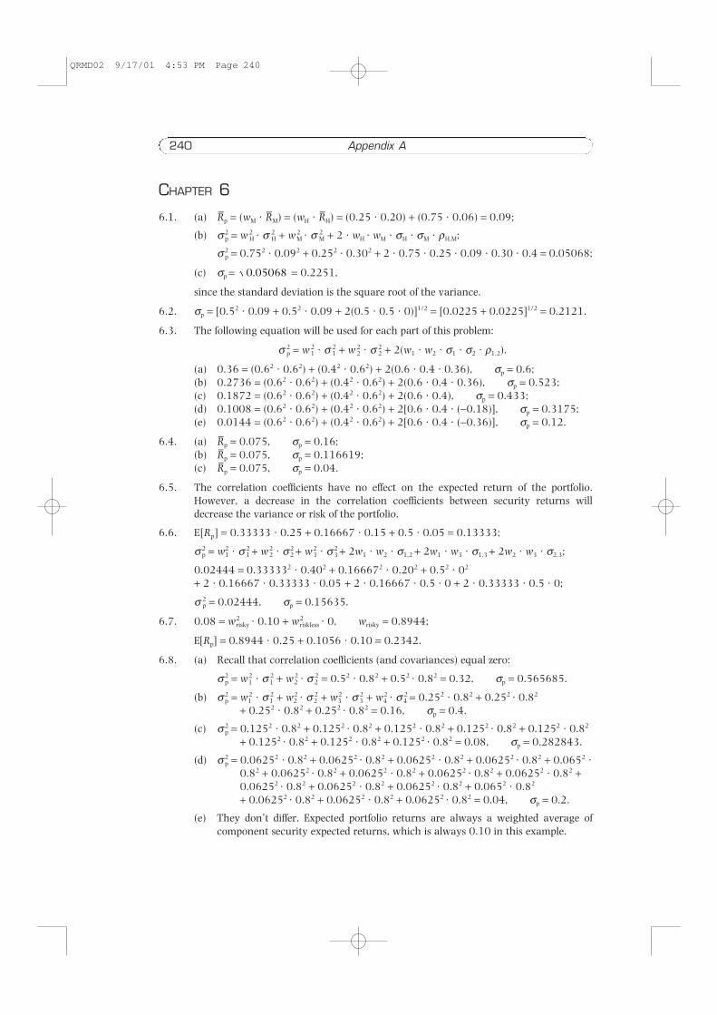
6.1. (a) Bp = (wM · BM) = (wH · BH) = (0.25 · 0.20) + (0.75 · 0.06) = 0.09;

(b) σ 2p = w 2

H · σ 2H + w 2

M · σ 2M + 2 · wH · wM · σH · σM · ρH,M;

σ 2p = 0.752 · 0.092 + 0.252 · 0.302 + 2 · 0.75 · 0.25 · 0.09 · 0.30 · 0.4 = 0.05068;

(c) σp = = 0.2251,

since the standard deviation is the square root of the variance.

6.2. σp = [0.52 · 0.09 + 0.52 · 0.09 + 2(0.5 · 0.5 · 0)]1/2 = [0.0225 + 0.0225]1/2 = 0.2121.

6.3. The following equation will be used for each part of this problem:

σ 2p = w 2

1 · σ 21 + w 2

2 · σ 22 + 2(w1 · w2 · σ1 · σ2 · ρ1,2).

(a) 0.36 = (0.62 · 0.62) + (0.42 · 0.62) + 2(0.6 · 0.4 · 0.36), σp = 0.6;(b) 0.2736 = (0.62 · 0.62) + (0.42 · 0.62) + 2(0.6 · 0.4 · 0.36), σp = 0.523;(c) 0.1872 = (0.62 · 0.62) + (0.42 · 0.62) + 2(0.6 · 0.4), σp = 0.433;(d) 0.1008 = (0.62 · 0.62) + (0.42 · 0.62) + 2[0.6 · 0.4 · (−0.18)], σp = 0.3175;(e) 0.0144 = (0.62 · 0.62) + (0.42 · 0.62) + 2[0.6 · 0.4 · (−0.36)], σp = 0.12.

6.4. (a) Bp = 0.075, σp = 0.16;(b) Bp = 0.075, σp = 0.116619;(c) Bp = 0.075, σp = 0.04.

6.5. The correlation coefficients have no effect on the expected return of the portfolio.However, a decrease in the correlation coefficients between security returns willdecrease the variance or risk of the portfolio.

6.6. E[Rp] = 0.33333 · 0.25 + 0.16667 · 0.15 + 0.5 · 0.05 = 0.13333;

σ 2p = w2

1 · σ 21 + w2

2 · σ 22 + w2

3 · σ 23 + 2w1 · w2 · σ1,2 + 2w1 · w3 · σ1,3 + 2w2 · w3 · σ2,3;

0.02444 = 0.333332 · 0.402 + 0.166672 · 0.202 + 0.52 · 02

+ 2 · 0.16667 · 0.33333 · 0.05 + 2 · 0.16667 · 0.5 · 0 + 2 · 0.33333 · 0.5 · 0;

σ 2p = 0.02444, σp = 0.15635.

6.7. 0.08 = w2risky · 0.10 + w2

riskless · 0, wrisky = 0.8944;

E[Rp] = 0.8944 · 0.25 + 0.1056 · 0.10 = 0.2342.

6.8. (a) Recall that correlation coefficients (and covariances) equal zero:

σ 2p = w1

2 · σ 12 + w2

2 · σ 22 = 0.52 · 0.82 + 0.52 · 0.82 = 0.32, σp = 0.565685.

(b) σ 2p = w1

2 · σ 12 + w2

2 · σ 22 + w3

2 · σ 32 + w4

2 · σ 42 = 0.252 · 0.82 + 0.252 · 0.82

+ 0.252 · 0.82 + 0.252 · 0.82 = 0.16, σp = 0.4.

(c) σ 2p = 0.1252 · 0.82 + 0.1252 · 0.82 + 0.1252 · 0.82 + 0.1252 · 0.82 + 0.1252 · 0.82

+ 0.1252 · 0.82 + 0.1252 · 0.82 + 0.1252 · 0.82 = 0.08, σp = 0.282843.

(d) σ 2p = 0.06252 · 0.82 + 0.06252 · 0.82 + 0.06252 · 0.82 + 0.06252 · 0.82 + 0.0652 ·

0.82 + 0.06252 · 0.82 + 0.06252 · 0.82 + 0.06252 · 0.82 + 0.06252 · 0.82 +0.06252 · 0.82 + 0.06252 · 0.82 + 0.06252 · 0.82 + 0.0652 · 0.82

+ 0.06252 · 0.82 + 0.06252 · 0.82 + 0.06252 · 0.82 = 0.04, σp = 0.2.

(e) They don’t differ. Expected portfolio returns are always a weighted average of component security expected returns, which is always 0.10 in this example.

0 05068.

240 Appendix A

QRMD02 9/17/01 4:53 PM Page 240


CHAPTER 7

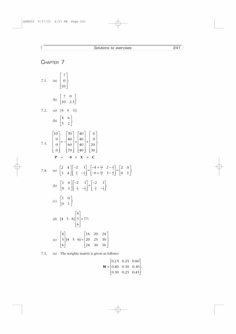
7.1. (a)

(b)

7.2. (a) [4 6 5];

(b)

7.3.

P = −S + X + C.

7.4. (a)

(b)

(c)

(d)

(e)

7.5. (a) The weights matrix is given as follows:

W

. . .

. . .

. . .

.=

0 15 0 25 0 60

0 40 0 30 0 30

0 30 0 25 0 45

4

5

6

4 5 6

16 20 24

20 25 30

24 30 36

=

[ ] .

[ ] ;4 5 6

4

5

6

77

=

1 0

0 1

;

1 0

0 1

2 1 2 132

12

32

12

−−

=−

−

;

2 4

3 4

2 1 4 2

6 3

2 0

0 132

12

122

42

122

42

−−

=− + −− + −

=

;

10

0

0

0

30

40

60

70

40

40

40

40

0

0

20

30

= −

+

+

,

4 6

5 2

.

7 0

10 2 5..

7

0

10

;

QRMD02 9/17/01 4:53 PM Page 241

(b) The returns vector is given as follows:

(c) The funds’ returns are computed as follows:

(d)

7.6. (a) Form a returns vector as follows:

(b) The covariance matrix is as follows:

(c) The weights vector is as follows:

(d) (a) 3 × 1; (b) 3 × 3; (c) 3 × 1.(e) The expected portfolio return is given as follows:

(f ) The portfolio variance is found as follows:

σ 2p = w′ V w;

σp2 0 30 0 50 0 20

0 04 0 01 0 02

0 01 0 16 0 08

0 02 0 08 0 36

0 30

0 50

0 20

[ . . . ]

. . .

. . .

. . .

.

.

.

,=

E

E

p

p

[ ] [ . . . ]

.

.

.

. ,

[ ] .

R

R

=

=

=

0 30 0 50 0 20

0 07

0 09

0 13

0 092

w r′

w

.

.

.

.=

0 30

0 50

0 20

V

. . .

. . .

. . .

.=

0 04 0 01 0 02

0 01 0 16 0 08

0 02 0 08 0 36

r

.

.

.

.=

0 07

0 09

0 13

13

13

13

0 207

0 174

0 189

0 19[ ]

=

.

.

.

. .

0 15 0 25 0 60

0 40 0 30 0 30

0 30 0 25 0 45

0 12

0 18

0 24

0 207

0 174

0 189

. . .

. . .

. . .

.

.

.

.

.

.

.

=

r

.

.

.

.=

0 12

0 18

0 24

242 Appendix A

QRMD02 9/17/01 4:53 PM Page 242


σ 2p = w′ V w = σ 2

p.

7.7. (a) 1/8 = 0.125.(b) The inverse of the identity matrix is the identity matrix:

(c) The inverse of a diagonal matrix is found by inverting each of the principle diag-onal elements:

(d) First, augment the matrix with the identity matrix:

Now use the Gauss–Jordan method to transform the original matrix to an identitymatrix; the resulting right-hand side will be the inverse of the original matrix:

Thus, the inverse matrix is

(e) Augment the matrix with the identity matrix and perform elementary row opera-tions to obtain the inverse matrix as follows:

The inverse matrix is

−−

100 50

75 25.

1 0 100 50

0 1 75 25

�

�

−−

.

1 2 50 0

0 50 1623

23

�

�

,

−

0 02 0 04 1 0

0 06 0 08 0 1

. .

. .,

�

�

−−

2 1

1 5 0 5. ..

2

2

1 0 2 1

1 5 0 5

1 2 2

2 1 0 6

a

b

a b

a

�

�

−0 1 . − .

− ×× −

( ) ( )

( ) /( . )

1

1

1 2 1

1

1 1

2 11 1

a

b

row

row a

�

�

( )

00 −0.6 − 3 3

×× −

row

row

.

1

2

1 2 1 0

3 4 0 1

�

�

0 25 0

0 2

..

1 0

0 1

.

σ p2 0 021 0 099 0 118

0 30

0 50

0 20

0 0794 [ . . . ]

.

.

.

. ,=

=

QRMD02 9/17/01 4:53 PM Page 243

(f ) The inverse matrix is

(g) The inverse matrix is

(h) Augment the matrix with the identity matrix and perform elementary row opera-tions to obtain the inverse matrix as follows:

The inverse matrix is

7.8.

C−1 · s = x = x.

See 7.4(b) above for the inverse matrix.

0 04 0 04

0 04 0 16

0 05

0 10

0 006

0 0181

2

. .

. .

.

.

.

.,

=

=

x

x

C− =

1 0 04 0 04

0 04 0 16

. .

. .;

0 5 0 0

0 25 0 25 0

0 0 1 0 05

.

. .

. .

.−−

1 0 0 0 5 0 0

0 1 0 0 25 0 25 0

0 0 1 0 0 1 0 05

�

�

�

.

. .

. .

.−−

1 0 0 0 5 0 0

0 1 0 0 25 0 25 0

0 0 2 0 2 1

�

�

�

.

. . ,−−

1 0 0 0 5 0 0

0 4 0 1 1 0

0 8 20 2 0 1

�

�

�

.

,−−

2 0 0 1 0 0

2 4 0 1 0

4 8 20 0 1

�

�

�

00

,

0 04 0 04

0 04 0 16

. .

. ..

1 2

3 4

.

244 Appendix A

QRMD02 9/17/01 4:53 PM Page 244


7.9. Our original system of equations is represented as follows:

C · x = s.

The elements of C and s are known; our problem is to find the weights in vector x. Thuswe will rearrange the system from Cx = s to C−1s = x, where C−1 is the inverse of matrixC. So, the time-consuming part of our problem is to find C−1. We will begin by augmentingmatrix C with the identity matrix I:

I C−1

C−1 · s = x = x.

0 0 10 2

0 0 10 1

10 10 24 2 4

2 1 2 4 0 32

0 1

0 1

0 1

0 1

0 8

0 9

2 16

0 308

1

2

3

4

−−

− −− −

⋅

=

=

−

−

.

. .

.

.

.

.

.

.

.

.

x

x

x

x

1

2

3

4

1 0 0 0 0 10 2

0 1 0 0 0 0 10 1

0 0 1 0 10 10 24 2 4

0 0 0 1 2 1 2 4 0 32

1 4 6 2

2 4 3 125

3 4

d

d

d

d

d a

c d

c d

�

�

�

�

0−

.. − .

−

− −−

− ⋅− ⋅ −− ⋅

( ) ( ) .

( ) ( ) ( . )

( ) ( ) .

( ) ( )/ .

7 5

4 1 3 125c ⋅ −

1

2

3

4

1 0 0 6 25 12 5 6 25 5 0

0 1 0 3 125 6 25 3 125 2 5 0

0 0 1 7 5 5 2 5 6 0

0 0 0 3 125 6 25 3 125 7 5 1

1 3 0 83

2 3

c

c

c

c

b c

b c

. . .

. . .

. .

.

( ) ( ) .

( ) (

�

�

�

�

−− −

−

− ⋅−.

−− . . − .

)) .

( ) ( ) / .

( ) ( ) ( . )

⋅− ⋅ −⋅ ⋅ −

0 416

3 3 1 1 6

4 3 1 25

b c

b c

1

2

3

4

1 0 0 8 12 5 16 4 1 0 0

0 1 0 41 0 4 1 4 1 0 0

0 0 1 12 5 8 4 1 10 0

0 0 1 25 12 5 12 5 0 0 1

1 2

2

b

b

b

b

a b

a

. . . .

. . .

. . . .

. .

( ) ( )

( )

3 6 6

6 6 6

6 3 6

�

�

�

�

−−

− − − −− −

−⋅

− .

( ) ( )

( )

13

3 2

4

a b

a

−

1

2

3

4

1 1 1 25 12 5 12 5 0 0 0

0 3 1 25 0 12 5 12 5 0 0

0 1 1 25 12 5 12 5 0 10 0

0 0 1 25 12 5 12 5 0 0 1

12 5

12 5 1

10 1

a

a

a

a

(row 1) .

(row 2) . ( a)

(row 3) ( a)

(row 4)

. .

.

. .

. .

�

�

�

�

.− . .− .− .

− −− −

⋅⋅ −⋅⋅⋅ − ( a)1 1

row 1

row 2

row 3

row 4

original system

0 08 0 08 0 1 1 1 0 0 0

0 08 0 32 0 2 1 0 1 0 0

0 1 0 2 0 0 0 0 1 0

1 1 0 0 0 0 0 1

. . .

. . .

. .

�

�

�

�

0 08 0 08 0 1 1

0 08 0 32 0 2 1

0 1 0 2 0 0

1 1 0 0

0 1

0 1

0 1

0 1

1

2

3

4

. . .

. . .

. .

.

.

.

.

,

=

x

x

x

x

QRMD02 9/17/01 4:53 PM Page 245

Now it is clear that:

x1 = (0 · 0.1) + (0 · 0.1) + (−10 · 0.1) + (2 · 0.1) = −0.8,

x2 = (0 · 0.1) + (0 · 0.1) + (10 · 0.1) + (−1 · 0.1) = 0.9,

x3 = (−10 · 0.1) + (10 · 0.1) + (−24 · 0.1) + (2.4 · 0.1) = −2.16,

x4 = (2 · 0.1) + (−1 · 0.1) + (2.4 · 0.1) + (−0.32 · 0.1) = 0.308.

7.10. Our first problem is to complete a pro-forma income statement for 2001. However, wedon’t know what the company’s interest expenditure in 2001 will be until we know howmuch money it will borrow (EFN ). At the same time, we cannot determine how muchmoney the firm needs to borrow until we know its interest expenditure (so that we can solve for retained earnings). Therefore, we must solve simultaneously for EFN andinterest expenditure. We know that EFN can be found as follows:

EFN = ∆Assets − ∆CL − RE,

EFN = $500,000 − $75,000 − RE.

Retained earnings (RE) can be found using the following pro-forma income statementfor 2001:

Pro-forma income statement, 2001

Sales (TR) ........................... $1,125,000Cost of Goods Sold ............. 450,000Gross Margin ..................... 675,000Fixed Costs ......................... 150,000EBIT ................................... 525,000Interest Payments.............. 50,000 + (0.10 · EFN )Earnings Before Tax .......... 475,000 − (0.10 · EFN )Taxes (@ 40%) .................. 190,000 − (0.04 · EFN )Net Income After Tax........ 285,000 − (0.06 · EFN )Dividends (@ 33%)............ 95,000 − (0.02 · EFN )Retained Earnings ............. 190,000 − (0.04 · EFN )

C · x = s;

C · x = s;

C · x = s.

Our EFN problem is complete. We now know that the firm must borrow $244,791.78.

1 0416667 0 0416667

1 0416667 1 0416667

190 000

425 000

180 208 45

244 791 78

. .

. .

,

,

, .

, .,

−−

=

1 0 04

1 1

190000

425000

.

,

,,

=

RE

EFN

1 0 1 1 0 4 1 0 333

1 1

525 000 50 000 1 0 4 1 0 333

500 000 75 000

[ . ( . ) ( . )]

[( , , ) ( . ) ( . )]

( , , ),

⋅ − ⋅ −

=

− ⋅ − ⋅ −−

RE

EFN

246 Appendix A

QRMD02 9/17/01 4:53 PM Page 246


7.11. (a) Solve the following system:

CF · d = P;

CF−1 = P = d.

Solve first for D1 = 0.90909, then D2 = 0.80826, then D3 = 0.71660, and finally D4 = 0.63328. Then, y0,1 = 0.10, y0,2 = 0.1123, y0,3 = 0.1175, and y0,4 = 0.1210.

(b) y1,3 = [(1 + y0,3)3 ÷ (1 + y0,1)]0.5 − 1 = [(1.1175)3 ÷ (1.1)]0.5 − 1 = 0.1264.

7.12. (a) First, solve the following system for the discount functions d:

CF · d = P0.

We find that D1 = 0.943396, D2 = 0.857338, and D3 = 0.751314. The spot ratesare obtained as follows:

(b) The weights are found by solving for w as follows:

CF · w = P0 ;

CF −1 · P0 = w.

−− −

−

=

0 03996 0 00396 0 002666

0 03885 0 00385 0 001667

0 00100 0 00100 0

150

150

1 150

. . .

. . .

. .

,

,

w

w

w

X

Y

Z

50 80 110

50 80 1 110

1 050 1 080 0

150

150

1 150

,

, ,

,

,

=

w

w

w

X

Y

Z

11

10 751314

1 0 1031 3 1 3D / /

.

. .− = − =

11

10 857338

1 0 0821 2 1 2D / /

.

. ,− = − =

11

10 943396

1 0 061D

.

. ,− = − =

50 50 1 050

80 80 1 080

110 1 110 0

878 9172

955 4787

1 055 4190

1

2

3

,

,

,

.

.

, .

,

=

D

D

D

0 000909 0 0 0

0 000083 0 000909 0 0

0 000075 0 000083 0 000909 0

0 000068 0 000075 0 000083 0 000909

1 000

980

960

940

1

2

3

4

.

. .

. . .

. . . .

,

,−− −− − −

=

=

D

D

D

D

1 100 0 0 0

100 1 100 0 0

100 100 1 100 0

100 100 100 1 100

1 000

980

960

940

1

2

3

4

,

,

,

,

,

,

=

D

D

D

D

QRMD02 9/17/01 4:53 PM Page 247

We find that wX = −2.3341, wY = 3.33295, and that wZ = 0. This means that bondQ is replicated by a portfolio with a short position in 2.3341 bonds X and a longposition in 3.33295 bonds Y.

7.13. The following system may be solved for b to determine exactly how many of each of thebonds are required to satisfy the fund’s cash flow requirements:

CF · b = P0.

First, we invert matrix CF to obtain CF −1:

CF−1.

Thus, by inverting matrix CF to obtain CF −1, and premultiplying vector P0 by CF −1 toobtain solutions vector b, we find that the purchase of 43,767.2 bonds 1, 67,929 bonds2, 95,650.9 bonds 3, and 124,880 bonds 4 satisfy the fund’s exact matching requirements.

7.14. (a) 120D1 + 1,120D2 = 957.9920, D1 = 0.925925,50D1 + 1,050D2 = 840.2471, D2 = 0.756143,y0,1 = 1/D1 − 1 = 0.08;

(b) y0,2 = (1/D2)0.5 − 1 = 0.15;

(c) 1,000 ÷ (1 + y0,2)2 = 756.1437;

(d) 120wA + 50wB = 0, wA = −0.714285,1,120wA + 1,050wB = 1,000, wB = 1.714285;

(e) 15,000 = 120#A + 50#B,12,000 = 1,120#A + 1,050#B,#A = 216.42857; #B = −219.42857.

Thus, sell 219.42857 B bonds for $184,374.22 and pay $207,336.83 for 216.42857A bonds.

7.15. Since the riskless return rate is 0.125, the current value of a security guaranteed to pay $1 in one year would be $1/1.125 = 0.8888889. The security payoff vectors are asfollows:

Portfolio holdings are determined as follows:

bu b c , , .=

=

=

20

32

1

1

4

16

0 000909 0 000083 0 00008 0 000079

0 0 000909 0 00009 0 000087

0 0 0 00090 0 000096

0 0 0 0 000892

. . . .

. . .

. .

.

,

− − −− −

−

1 100 100 110 120

0 1 100 110 120

0 0 1 110 120

0 0 0 1 120

80 000 000

100 000 000

120 000 000

140 000 000

1

2

3

4

,

,

,

,

, ,

, ,

, ,

, ,

,

=

b

b

b

b

248 Appendix A

QRMD02 9/17/01 4:53 PM Page 248


The following includes the inverse matrix:

We find that #bu = 1 and #b = −16. This implies that the payoff structure of a single callcan be replicated with a portfolio comprising 1 share of stock for a total of $24 and short-selling 16 T-bills for a total of $14.2222222. This portfolio requires a net investment of$9.7777778. Since the call has the same payoff structure as this portfolio, its currentvalue must be $9.7777778.

7.16. (a) First, we define the following payoff vectors:

We have a set of two payoff vectors in a two-outcome economy. The set is linearlyindependent. Hence, this set forms the basis for the two-outcome space. Since wehave market prices for these two securities, we can price all other securities in thiseconomy. First, we solve for the value of the $22-exercise price call as follows:

Thus, the call with an exercise price equal to $22 can be replicated with 0.42857calls with an exercise price equal to $18.

(b) The riskless return rate is determined as follows:

Since the riskless asset is replicated with 0.066667 shares of stock and short positions in 0.095238 calls, the value of the riskless asset is 0.666674, implying ariskless return rate equal to 1/0.666674 = 0.50.

(c) Solve for the value of the put as follows:

implying that its value is 1.6666667 · $20 − 3.90952 · 7 = 5.9667. Note that thisput value is lower than either of the two potential cash flows that it may generate.This is due to the particularly high riskless return rate.

0 066667 0

0 238095 0 142857

25

15

1 666667

3 90952

.

. .

.

.,

−

=

−

0 066667 0

0 238095 0 142857

1

1

0 066667

0 095238

.

. .

.

..

−

=

−

0 066667 0

0 238095 0 142857

0

3

0

0 42857

.

. .

..

−

=

15 0

25 7

0

3

1

18

=

−

=

#

#,

S

CX

15

25

0

7

18

=Stock

,

X

−−

=

−

0 0833333 0 083333

2 666667 1 666667

4

16

1

16

. .

. . .

20 1

32 1

4

16

=

#

# .

bu

b

QRMD02 9/17/01 4:53 PM Page 249

CHAPTER 8

8.1. Solve as follows:

8.2. The derivatives are found by using the power rule (polynomial rule) as follows:

(a) dy/dx = 5 · 0 · x0 −1 = 0;(b) dy/dx = 3 · 7 · x3−1 = 21x2;(c) dy/dx = 4 · 2 · x4−1 + 3 · 5 · x3−1 = 8x3 + 15x2;(d) dy/dx = 0.5 · 10 · x0.5−1 − 3 · 11 · x3−1 = 5x4 − 33x2;(e) dy/dx = (1/5) · 5 · x1/5−1 = (5/5)x−4/5 =(f ) dy/dx = −2 · 2 · x−2−1 + 1/2 · 2/3 · x1/2−1 + 1/5 · 3 · x−1/5−1 − 1 · 1 · x−1−1;

= −4x + (1/3)x−1/2 + 0.6x−0.8 − 1 = −4x + (1/3)/ + 0.6/x0.8 − 1.

8.3. Second derivatives are found as follows:

(a) dy/dx = 0;(b) dy/dx = 42x;(c) dy/dx = 24x2 + 30x;(d) dy/dx = 20x3 − 66x;(e) dy/dx = −0.8x−1.8;(f ) dy/dx = −4 − (1/6)/ − 0.48/x−1.8.

8.4. Find first derivatives, set them equal to zero, and solve for x. Then check second deriva-tives to ensure that they are negative:

(a) dy/dx = 30x; d2y/dx2 = 30; there is no finite maximum.(b) dy/dx = 6; d2y/dx2 = 0; there is no finite maximum.(c) dy/dx = −6x + 6; d2y/dx2 = −6; xmin = 1.(d) dy/dx = 3x2 + 6x + 2 = 0; d2y/dx2 = 6x + 6; xmax = −3.803848, xmax = −14.19615.(e) dy/dx = 36x2; d2y/dx2 = 72x; there is no finite maximum; the first derivative is zero

when x = 0, but when x = 0, d2y/dx2 is not negative.(f ) dy/dx = 2x + 10 = 0; d2y/dx2 = 2; the minimum occurs when x = −5.

8.5. Find first derivatives, set them equal to zero, and solve for x. Then check second derivat-ives to ensure that they are positive:

(a) dy/dx = 30x; d2y/dx2 = 30; xmin = 0.(b) dy/dx = 20; d2y/dx2 = 0; there is no finite minimum.(c) dy/dx = 6x + 6; d2y/dx2 = 6; xmin = −1.(d) dy/dx = 6x2 − 12x + 1; d2y/dx2 = 6x − 12; using the quadratic formula, we find

that x = 3.1366 and 68.86335. The second derivative is positive in both cases. Thisfunction has two minima.

(e) dy/dx = 36x2; d2y/dx2 = 72x; there is no finite minimum; the first derivative is zerowhen x = 0, but when x = 0, d2y/dx2 is not positive.

(f ) dy/dx = 2x + 10 = 0; d2y/dx2 = 2; the minimum occurs when x = −5.

x3

x

x45;

=

⋅ += + =

→ → lim

lim [ ] .

h h

x h h

hx h x

0

2

0

14 714 7 14

′ =

+ ⋅ ⋅ + −y

x x h h x

h

7 2 7 7 72 2 2

250 Appendix A

QRMD02 9/17/01 4:53 PM Page 250


8.6. (a) (i) First, find the yield to maturity (ytm) of the bond:

yield to maturity = ytm;

solve for ytm;

ytm = 0.111.

(ii) Use ytm from part (i) in the duration formula:

(note that negative signs are omitted);

(b) (i)

ytm = 0.118.

(ii)

(c) ytm = 0.126:

(d) There are several ways to work this problem. First, consider the cash flows of theportfolio:

P0 = 900 + 800 + 1,400 = 3,100;

CF1 = 1,000, CF2 = 1,000, CF3 = 2,000;

ytm = 0.122;

Dur = 2.161 years.

Second, notice that the portfolio duration is a weighted average of the bond dura-tions: (900/3,100) · 1 + (800/3,100) · 2 + (1,400/3,100) · 3 = 2.161.

(e) An equal dollar sum is invested into each portfolio. Thus, this portfolio’s durationis simply an average of the three bonds’ durations. The portfolio duration equals 2.

8.7. (a) (i) First find the bond’s ytm:

ytm = 0.0897.070

170

170 1000

1950

1 2 3

( )

( )

,( )

,= =+

++

+++

−NPVytm ytm ytm

Dur

tCF

ytm

P

tt

t

n

( )

,.

,

( . )

,( . )

,;=

⋅+

=

⋅+

⋅+

⋅=∑ 1

1 1 0001 122

2 1 0001 122

3 2 0001 122

3 1001

0

2 3

01 000

11 000

12 000

13 100

1 2 3

,( )

,

( )

,( )

, ,= =+

++

++

−NPVytm ytm ytm

Dur

,( . ),

.=⋅

=3

2 0001 126

1 4003

3

Dur

tCF

ytm

P

tt

t

n

( )

,. .=

⋅+

=⋅

==∑ 1 2

1 0001 118800

21

0

2

01

1 0001

8001

0 ( )

,

( ) ;= =

+− =

+−

=∑NPV t

CF

ytmP

ytmt

tt

n

t

Dur Dur

,. .=

⋅= =

11 0001 111900

1 year

Dur

tCF

ytm

P

tt

t

n

( )=

⋅+=

∑ 11

0

01 000

1900

1

,( )

,= =+

−NPVytm

01 0

1

( )

,= =+

−=∑NPV

CF

ytmPt

tt

n

QRMD02 9/17/01 4:53 PM Page 251

(ii) Now, use ytm to find Duration:

(b)

ytm = 0.1038;

(c)

ytm = 0.134;

(d)

ytm = 0.194;

8.8. (a) P1 = P0 + Dur · ∆(1 + r)/(1 + r) · P0, P1 = 950 − 2.8027 · 0.01/1.0897 · 950 = 925.57;(b) P1 = 1,040 − 2.696 · 0.01/1.1038 · 1,040 = 1,014.60;(c) P1 = 900 − 3.457 · 0.01/1.1339 · 900 = 872.56;(d) P1 = 800 − 2.703 · 0.01/1.194 · 800 = 781.89.

8.9.

8.10. Partial derivatives are found as follows:

(i) (a) ∂y/∂x = 5; (d) ∂y/∂x = 15x2 + 7z;(b) ∂y/∂x = 5x; (e) ∂y/∂x = 36x2z5 + 3z2;(c) ∂y/∂x = 14x6; (f ) ∂y/∂x = ∑ n

i=1nixi−1z2.(ii) (a) ∂y/∂z = 0; (d) ∂y/∂z = 20z + 7x;

(b) ∂y/∂z = 10; (e) ∂y/∂z = 60x3z4 + 6xz;(c) ∂y/∂z = 0; (f ) ∂y/∂z = 2z∑ n

i=1nxi.

8.11. Derivatives are found as follows:

(a) dy/dx = 12(4x + 2)2;

(b) dy/dx = 3x/

(c) dy/dx = 6x(12x2 + 10x) + 6(4x3 + 5x2 + 3) = 96x3 + 90x2 + 18;(d) dy/dx = 4.5(1.5x − 4)(2.5x − 3.5)3 + 10(1.5x − 4)(2.5x − 3.5)3;

( );3 82x +

Dur . ,

. ,,

. ,

. ,

. .= ⋅ + ⋅ + ⋅ + ⋅ =2 8027950

3 6902 696

10403 690

3 456900

3 6902 703

8003 690

2 910

Dur

.

( . )

,( . ) . .=

⋅+

⋅+

⋅

=

1 1001 194

2 1001 194

3 1 1001 194

8002 703

2 3

0100

1100

11 100

1800

1 2 3

( )

( )

,( )

,= =+

++

++

−NPVytm ytm ytm

Dur

.

( . )

( . )

,

( . ) . .=

⋅+

⋅+

⋅+

⋅

=

1 1001 134

2 1001 134

3 1001 134

4 1 1001 134

9003 456

2 3 4

0100

1100

1100

11 100

1900

1 2 3 4

( )

( )

( )

,( )

,= =+

++

++

++

−NPVytm ytm ytm ytm

Dur

.

( . )

( . ) . .=

⋅+

⋅+

⋅

=

1 1201 1038

2 1201 1038

3 11201 1038

9002 696

2 3

0120

1120

11 120

11 040

1 2 3

( )

( )

,( )

, ,= =+

++

++

−NPVytm ytm ytm

Dur

.

( . )

( . ) . .=

⋅+

⋅+

⋅

=

1 701 0897

2 701 0897

3 10701 0897

9502 8027

2 3

252 Appendix A

QRMD02 9/17/01 4:53 PM Page 252


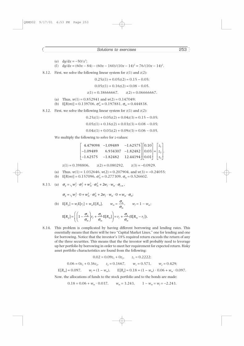
(e) dy/dx = −50/x3;(f ) dy/dx = (60x − 84) − (60x − 160)/(10x − 14)2 = 76/(10x − 14)2.

8.12. First, we solve the following linear system for z(1) and z(2):

0.25z(1) + 0.05z(2) = 0.15 − 0.05;

0.05z(1) + 0.16z(2) = 0.08 − 0.05.

z(1) = 0.38666667, z(2) = 0.06666667.

(a) Thus, w(1) = 0.852941 and w(2) = 0.147049;(b) E[R(m)] = 0.139706, σ 2

m = 0.197881, σm = 0.444838.

8.12. First, we solve the following linear system for z(1) and z(2):

0.25z(1) + 0.05z(2) + 0.04z(3) = 0.15 − 0.05;

0.05z(1) + 0.16z(2) + 0.03z(3) = 0.08 − 0.05;

0.04z(1) + 0.03z(2) + 0.09z(3) = 0.06 − 0.05.

We multiply the following to solve for z-values:

z(1) = 0.398806, z(2) = 0.080292, z(3) = −0.0929.

(a) Thus, w(1) = 1.032646, w(2) = 0.207904, and w(3) = −0.24055;(b) E[R(m)] = 0.157096, σ 2

m = 0.277309, σm = 0.526602.

8.13. (a)

(b) E[Rp] = wf E[rf ] + wmE[Rm], wm = wf = 1 − wm ;

8.14. This problem is complicated by having different borrowing and lending rates. Thisessentially means that there will be two “Capital Market Lines,” one for lending and onefor borrowing. Notice that the investor’s 18% required return exceeds the return of anyof the three securities. This means that the the investor will probably need to leverageup her portfolio by borrowing in order to meet her requirement for expected return. Riskyasset portfolio characteristics are found from the following:

0.02 = 0.09z1 + 0z2, z1 = 0.2222;

0.06 = 0z1 + 0.36z2, z2 = 0.1667, w1 = 0.571, w2 = 0.429;

E[Rm] = 0.097, wf = (1 − wm), E[Rp] = 0.18 = (1 − wm) · 0.06 + wm · 0.097.

Now, the allocations of funds to the stock portfolio and to the bonds are made:

0.18 = 0.06 + wm · 0.037, wm = 3.243, 1 − wm = wf = −2.243.

E E E[ ] [ ] ( [ ]).R r R r R rpp

mf

p

mm f

p

mm f= −

+

= + −1

σσ

σσ

σσ

σσ

p

m

,

σ σ σp f m m f m m mw w w w w= ⋅ + ⋅ + ⋅ ⋅ = ⋅ ;2 2 20 2 0

σ σ σ σp f f m m f m f mw w w w= ⋅ + ⋅ + ⋅ ⋅ ,,2 2 2 2 2

4 479098 1 09489 1 62575

1 09489 6 934307 1 82482

1 62575 1 82482 12 44194

0 10

0 03

0 01

1

2

3

. . .

. . .

. . .

.

.

.

.

− −− −− −

=

z

z

z

QRMD02 9/17/01 4:53 PM Page 253

Borrow $1,121,500.Invest $1,621,500 in the market: $925,876.5 in security 1 and $695,623.5 in secur-ity 2.

8.15. (a) dy/dx = 0.05e0.05x;(b) dy/dx = ex(x − 1)/x2;(c) dy/dx = 5/x;(d) dy/dx = ex(1/x + ln(x)) (using the product rule).

8.16. Durations and convexities are as follows:

(a) ytm = 0.052612Dur = [57.00064 + 108.3024 + 2,726.544]/1,020 = −2.8351446;Con = [102.8885 + 293.2354 + 9,843.047/1,020 = 10.0384;

(b) ytm = 0.0610701;Dur = [84.82003 + 159.8764 + 226.012 + 3,439.618]/1,100 = −3.554842;Con = [150.6747 + 426.0077 + 802.9775 + 15,275.38]/1,100 = 15.1409455.

8.17. (a) P1A = 944.78, P1B = 1,030.24;(b) P1A = 948.62, P1B = 1,033.22;(c) P1A = 948.56, P1B = 1,033.12.

The new bond values given in 8.17(c) are precise (subject to rounding). Note howmuch better the bond convexity model in 8.17(b) estimates revised bond prices than the duration model in 8.17(a). The duration model will tend to underestimatebond prices; the convexity model will tend to overestimate bond prices. However,the convexity model is normally closer to the true value.

8.18. First, set up the Lagrange function:

L = 50x2 − 10x + λ (100 − 0.1x).

Next, find the first order conditions:

∂y/∂x = 100x − 0.1λ = 10;

∂y/∂λ = −0.1x = −100.

We find that x = 1,000 and λ = 999,900.

8.19. First set up the Lagrange function:

L = (25 + 3x + 10x2) + λ (100 − 5x).

Next, find the first order conditions:

= 3 + 20x − 5λ = 0, 20x − 5λ = −3;

= 100 − 5x = 0, −5x − 0λ = −100.

(3) Next, solve the above system of equations for x and λ :

C · x = S;

x = 20, λ = 80 .35

20 5

5 0

3

100

−−

⋅

=

−−

,

x

λ

∂∂L

z

∂∂

L

x

254 Appendix A

QRMD02 9/17/01 4:53 PM Page 254


8.20. (a) (i) Our problem is defined as:

min: σ p2 = 0.04wA

2 + 0.16wB2 + 0.08wAwB (objective function)

s.t.: 0.15 = 0.1wA + 0.2wB (constraint 1),

1 = 1wA + 1wB (constraint 2).

First, set up the Lagrange function:

L = (0.04w A2 + 0.16w B

2 + 0.08wAwB) − λ1(0.15 − 0.1wA − 0.2wB) − λ2(1 − 1wA − 1wB).

Find first order conditions:

∂L/∂wA = 0.08wA + 0.08wB + 0.1λ1 + 1λ2 = 0;

∂L/∂wB = 0.32wB + 0.08wA + 0.2λ1 + 1λ2 = 0;

∂L/∂λ1 = 0.15 − 0.1wA − 0.2wB = 0;

∂L/∂λ2 = 1 − 1wA − 1wB = 0.

Now, we have four equations with four unknowns, which can be arrangedas follows:

0.08wA + 0.08wB + 0.1λ1 + 1λ2 = 0;

0.08wA + 0.32wB + 0.2λ1 + 1λ2 = 0;

0.1wA + 0.2wB + 0λ1 + 0λ2 = 0.15;

1wA + 1wB + 0λ1 + 0λ2 = 1.

We structure matrices to solve this system as follows:

C · x = S.

Step-by-step, we invert the coefficients matrix (augmented by the identity matrix)as follows:

1

2

3

4

1 1 1 25 12 5 12 5 0 0 0

0 3 1 25 0 12 5 12 5 0 0

0 1 1 25 12 5 12 5 0 10 0

0 0 1 25 12 5 12 5 0 0 1

1 12 5

2 12 5 1

a

a

a

a

row

row a

. . .

. . .

. . .

. . .

( ) .

( ) . (

�

�

�

�

−− − −− − −

⋅⋅ − ))

( ) ( )

( ) ( )

row a

row a

3 10 1

4 1 1

⋅⋅ −

row 1

row 2

row 3

row 4

original system

0 08 0 08 0 1 1 1 0 0 0

0 08 0 32 0 2 1 0 1 0 0

0 1 0 2 0 0 0 0 1 0

1 1 0 0 0 0 0 1

. . .

. . .

. .

�

�

�

�

0 08 0 08 0 1 1

0 08 0 32 0 2 1

0 1 0 2 0 0

1 1 0 0

0

0

0 15

11

2

. . .

. . .

. .

.,

=

w

wA

B

λλ

QRMD02 9/17/01 4:53 PM Page 255

I C−1

C−1 · s = x

We multiply to find the following:

wA = (0 · 0) + (0 · 0) + (−10 · 0.15) + (2 · 1) = 0.5;

wB = (0 · 0) + (0 · 0) + (10 · 0.15) + (−1 · 1) = 0.5;

λ1 = (−10 · 0) + (10 · 0) + (−24 · 0.15) + (2.4 · 1) = −1.2;

λ2 = (2 · 0) + (−1 · 0) + (2.4 · 0.15) + (−0.32 · 1) = 0.04.

Notice that since only two securities will be included in the portfolio, we caninfer immediately from the expected return constraint that wA must equal wB,which must equal 0.5. This simple algorithm will not work when the number of securities in the portfolio exceeds 2.

(ii) min: σ p2 = 0.04wA

2 + 0.16wB2 + 0.08wAwB

s.t.: 0.12 = 0.1wA + 0.2wB,

1 = 1wA + 1wB.

L = 0.04wA2 + 16wB

2 + 0.08wAwB − λ1(0.12 − 0.1wA − 0.2wB ) − λ 2(1 − 1wA − 1wB ).

First order conditions are:

∂L/∂wA = 0.08wA + 0.08wB + 0.1λ1 + 1λ 2 = 0;

∂L/∂wB = 0.08wA + 0.32wB + 0.2λ1 + 1λ 2 = 0;

0 0 10 2

0 0 10 1

10 10 24 2 4

2 1 2 4 0 32

0

0

0 15

11

2

−−

− −− −

=

.

. .

.

.

w

wA

B

λλ

1

2

3

4

1 0 0 0 0 0 10 2

0 1 0 0 0 0 10 1

0 0 1 0 10 10 24 2 4

0 0 0 1 2 1 2 4 0 32

1 4 6 2

2 4 3 125

3 4 7

d

d

d

d

c d

c d

c d

�

�

�

�

−−

− −− −

− ⋅− ⋅ −− ⋅.

. .

( ) ( ) .

( ) ( ) .

( ) ( ) ..

( ) [ /( . )]

5

4 1 3 125b ⋅ −

1

2

3

4

1 0 0 6 25 12 5 6 25 5 0

0 1 0 3 125 6 25 3 125 2 5 0

0 0 1 7 5 5 2 5 6 0

0 0 0 3 125 6 25 3 125 7 5 1

1 3 0 83

2 3

c

c

c

c

b c

b c

. . .

. . . .

. .

. . . .

( ) ( ) .

( ) (

�

�

�

�

−− −

−− − −

− ⋅− )) .

( ) [ /( . )]

( ) ( ) ( . )

⋅⋅ −− ⋅ −

0 416

3 1 1 6

4 3 1 25

b

b c

1

2

3

4

1 0 0 8 12 5 16 4 1 0 0

0 1 0 41 0 4 1 4 16 0 0

0 0 1 12 5 8 4 1 10 0

0 0 1 25 12 5 12 5 0 0 1

1 2

2

b

b

b

b

a b

a

. . . .

. . .

. . . .

. . .

( ) ( )

( )

3 6 6

6 6

6 3 6

�

�

�

�

−−

− − − −− − −

−⋅ 11 3

3 2

4

/

( ) ( )

( )

a b

a

−

256 Appendix A

QRMD02 9/17/01 4:53 PM Page 256


∂L/∂λ 1 = 0.1wA + 0.2wB + 0λ 1 + 0λ 2 = 0.12;

∂L/∂λ 2 = 1wA + 1wB + 0λ 1 + 0λ 2 = 1.

Thus, our system is:

C · x = S

Notice that the coefficients matrix (C) is identical to that in 21.a.i above. Thus,its inverse is identical to C−1 in part 8.19(a,i). Notice also that only elementthree in the solutions vector has changed. Thus, we determine our weightsas follows:

C−1 · S = x wA = 0.8,wB = 0.2.

(iii) Notice that only the third element in x has changed. Thus:

x wA = 0.2,wB = 0.8.

(b) Our asset returns and standard deviations are as follows:

Asset E(R) σ

A 0.10 0.20 σA,B = 0.04B 0.20 0.40 σA,rf = 0rf 0.09 0 σB,rf = 0

(i) The Lagrange Function is now:

L = (0.04wA2 + 0.16wB

2 + 0.08wAwB ) − λ 1(0.15 − 0.1wA − 0.2wB − 0.09wrf ) − λ 2(1 − 1wA − 1wB − 1wrf ).

Because σrf = σB,rf = σA,rf = 0, wrf terms are dropped from the first set of paren-theses. The first order conditions are:

w

w

w

w

A

B

C

D

=

.

.

.

.

,

0 2

0 8

1 92

0 112

0 0 10 2

0 0 10 1

10 10 24 2 4

2 1 2 4 0 32

0

0

0 12

1

0 8

0 2

0 48

0 0321

2

−−

− −− −

=

=−−

.

. .

.

.

.

.

.

w

wA

B

λλ

,

0 08 0 08 0 1 1

0 08 0 32 0 2 1

0 1 0 2 0 0

1 1 0 0

0

0

0 12

11

2

. . .

. . .

. .

..

=

w

wA

B

λλ

QRMD02 9/17/01 4:53 PM Page 257

∂L/∂wA = 0.08wA + 0.08wB + 0.1λ1 + 1λ2 = 0;

∂L/∂wA = 0.32wB + 0.08wA + 0.2λ1 + 1λ2 = 0;

∂L/∂wrf = −0.09λ1 − 1λ2 = 0;

∂L/∂λ1 = 0.15 − 0.1wA − 0.2wB − 0.09wrf = 0;

∂L/∂λ2 = 1 − 1wA − 1wB − 1wrf = 0.

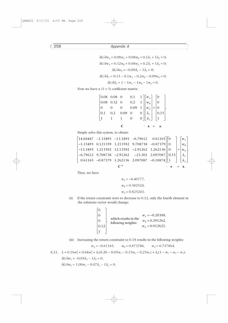
Now we have a (5 × 5) coefficient matrix:

C · x = s.

Simply solve this system, to obtain:

C−−1 · s = x.

Thus, we have

wA = −0.40777,

wB = 0.582524,

wrf = 0.825243.

(ii) If the return constraint were to decrease to 0.12, only the fourth element inthe solutions vector would change:

(iii) Increasing the return constraint to 0.18 results in the following weights:

wA = −0.61165, wB = 0.873786, wrf = 0.737864.

8.21. L = 0.16w22 + 0.64w3

2 + λ1(0.20 − 0.05w1 − 0.15w2 − 0.25w3) + λ2(1 − w1 − w2 − w3);

∂L/∂w1 = −0.05λ1 − 1λ2 = 0,

∂L/∂w2 = 1.00w2 − 0.07λ1 − 1λ2 = 0,

0

0

0

0 12

1

0 20388

0 291262

0 912621.

,

. ,

. ,

. .

= −==

which results in thefollowing weights:

A

B

w

w

wrf

14 68447 1 33495 13 3495 6 79612 0 61165

1 33495 0 121359 1 213592 9 708738 0 87379

13 3495 1 213592 12 13592 2 91262 1 262136

6 79612 9 708738 2 91262 23 301 2 097087

0 61165 0 87379 1 262136 2 097087 0 18874

0

0

0

0 15

1

. . . . .

. . . . .

. . . . .

. . . . .

. . . . .

.

− − −− −− −− − −

− −

=

,

w

w

wrf

A

B

λλ

1

2

0 08 0 08 0 0 1 1

0 08 0 32 0 0 2 1

0 0 0 0 09 1

0 1 0 2 0 09 0 0

1 1 1 0 0

0

0

0

0 15

11

2

. . .

. . .

.

. . .

.

,

=

w

w

wrf

A

B

λλ

258 Appendix A

QRMD02 9/17/01 4:53 PM Page 258


∂L/∂w3 = 1.62w3 − 0.11λ1 − 1λ2 = 0,

∂L/∂λ1 = −0.05w1 − 0.07w2 − 0.11w3 = −0.10,

∂L/∂λ2 = −w1 − w2 − w3 = −1;

w1 = −0.27451, w2 = 0.661765, w3 = 0.612745.

CHAPTER 9

9.1. (a) F(x) = k;(b) F(x) = 5x + k;(c) F(x) = 5x3 + k;(d) F(x) = 5x3 + 5x + k;(e) F(x) = ex + k;(f ) F(x) = e0.5x + k;(g) F(x) = 5x + k;(h) F(x) = ln(x) + k.

9.2. (a)

(b)

(c)

= 1,000,000e2 − 1,000,000e0 = 1,000,000(e2 − 1) = 6,389,056.

9.3. (a) (0.2 · 0.2) + (0.2 · 0.4) + (0.2 · 0.6) + (0.2 · 0.8) + (0.2 · 1) = 0.04 + 0.08 + 0.12+ 0.16 + 0.20 = 0.6;

(b) 2.96 + 3.12 + 3.28 + 3.44 + 3.6 = 16.4;(c) 596,730 + 890,216 + 1,328,047 + 1,981,213 + 2,955,622 = 7,751,828.

9.4. (a) P(x) = ∫p(x)dx = 0.5x3 + 0.5x2.(b) The distribution function for x will be ∫ f (x)p(x)dx, which, since f (x) = x, equals

∫ (x · 1.5x2 + x · x)dx = ∫ (1.5x3 + x2)dx = 0.375x4 + 0.3333x3. The probability thatx will be in the range 0.2–1.0 equals P[0.2 < x < 1] = (0.5x3 + 0.5x2) |1

0.2 = [(0.5 · 13

+ 0.5 · 12) − (0.5 · 0.23 + 0.5 · 0.22)][1 − 0.024] = 0.976. The expected value of xgiven that it falls within this range is a conditional distribution determined by:

E[x |0.2 < x < 1] = {∫ 10.2xp(x)}/{P[0.2 < x < 1]}

= [(0.375 · 14 + 0.3333 · 13) − (0.375 · 0.24 + 0.3333 · 0.23)]/0.976

= 0.7050666/0.976 = 0.7224043.

(c) The probability that x will be in the range 0–0.2 equals (0.5x3 + 0.5x2) | 00.2 =

[(0.5 · 0.23 + 0.5 · 0.22) − 0] = 0.024. The expected value of x given that it fallswithin this range is a conditional distribution determined by:

�

0

20

0 100 10

0

20

100 000 100 0000 10

, ,.

..

e det

t

t =

� �2

4

12

2

2

4

12

125 5 16 5 4 4 5 2 16( ) [ ] ( ) ( ) ;x x x x k k+ = + = ⋅ + ⋅ + − ⋅ + ⋅ + =d

� �0

1

12

2

0

1

12

120x x x k kd ( ) ( ) ;= = + − + =

QRMD02 9/17/01 4:53 PM Page 259

E[x |0 < x < 0.2] = {∫ 00.2xp(x)}/{P[0 < x < 0.2]}

= (0.375 · 0.24 + 0.3333 · 0.23) − (0.375 · 04 + 0.3333 · 03)]/0.024

= 0.0032667/0.024 = 0.136111.

(d) E[x] = ∫ 10xp(x) = [(0.375 · 14 + 0.3333 · 13) − (0.375 · 04 + 0.3333 · 03) = 0.7083333.

(e) σ 2 = ∫ 10[ f(x)]2p(x)dx − (∫ 1

0 f(x)p(x)dx)2

= ∫ 10x2p(x)dx − (∫ 1

0xp(x)dx)2 = ∫ 10x2 · (1.5x2 + x)dx − [∫ 1

0x · (1.5x2 + x)dx]2.

And since the term to the right of the minus sign is the expected value squared:

σ 2 = ∫ 10(1.5x4 + x3)dx − 0.7083332

= (0.3x5 + 0.25x4) | 10 − 0.70833332

= 0.55 − 0 − 0.5017 = 0.0483.

9.5. (a) P(x) = ∫p(x)dx = x.(b) E[S |50 ≤ S ≤ 100] = {∫ 1

0.5100xp(x)dx}/{P[50 ≤ S ≤ 100]} = {∫ 10.5100x · 1 dx}

/{∫ 10.5p(x)dx} = {50 · 12 − 50 · 0.52}/0.5 = 75.

(c) E[S |0 ≤ S ≤ 50] = {∫ 00.5100xp(x)dx}/{P[0 ≤ S ≤ 50]} = {∫ 0

0.5100x · 1 dx}/{∫ 00.5p(x)dx}

= {50 · 0.502 − 50 · 02}/0.5 = 12.5.(d) E[S] = ∫ 1

0 f(x)p(x)dx = ∫ 10100x dx = 50x2 |1

0 = 50.

(e) σ 2 = ∫ 10[ f(x)]2p(x)dx − (∫ 1

0 f (x)p(x)dx)2 = ∫ 1010,000x2p(x)dx − (∫ 1

0100xp(x)dx)2

= ∫ 1010,000x2dx − (∫ 1

0100x dx)2.Since the term to the right of the minus sign is the expected value:

σ 2 = ∫ 1010,000x2dx − 502 = (3333.33)x3 |1

0 − 502

= (3,333.33) · 1 − 0 − 2,500 = 833.33.

(f ) E[S − 50 |50 ≤ S ≤ 100] = 25.(g) E[CFt] = {0.5 · 0} + {0.5 · E[S − 50 |50 ≤ S ≤ 100]} = 12.5.(h) PV(E[CF]) = 12.5e−0.1·1 = 11.31.

9.6. We integrate the density functions as follows:

Pf (x) = ∫4x3 = x4 for 0 ≤ x ≤ 1,

Pg(x) = ∫ (3x4 + 0.08x) = + + k for 0 ≤ x ≤ 1.

9.7. The amount of dividend payment to be received at any infinitesimal time interval dt equalsf(t)dt = 3,000,000dt. The present value of this sum equals f (t)e−ktdt = 3,000,000e−0.06t.To find the present value of a sum received over a finite interval beginning with t = 0,one may apply the definite integral as follows:

PV [0,T ] = ∫ T0 f (t)e−ktdt,

9.8. The dividend stream is evaluated as follows:

PV[ , ]

,. .

( ) , . .( . . )0 210 000

0 05 0 031 19 605 280 03 0 05 2=

−− =− ⋅e

= − =−

, ,.

( ) $ , , ..3 000 0000 06

1 22 559 4180 6e

PV tt

t

[ , ] , , , ,.

..

0 10 3 000 000 3 000 0000 06

0

10

0 060 06

0

10

= = −

−

−� �e de

25

2x35

5x

260 Appendix A

QRMD02 9/17/01 4:53 PM Page 260


9.9. (a) The differential equation for this problem can be created in two steps. First, the accountshould generate interest continuously (including interest on any paymentsdeducted from the account) as follows:

However, deductions will be made continuously from the account. The interest thatthese deductions would have accumulated must be deducted from the total interestgiven above. These deductions will reduce the amount of interest that the accountwill draw in the future. Assume T − t relevant years in the future. The paymentsdeducted from the account continuously are PMTdt. These payments plus T − t yearsof interest that would otherwise have accumulated on those payments are as follows:

PMTei(T−t) dt.

The difference between these is the differential equation representing the evolutionof the account:

dFVt = [iFV0 − PMTei(T−t)] dt.

(b) To find the state of the account (system) at any time T, integrate over t the finalequation from part 9.9(a) as follows:

FVT = ∫ T0 [iFV0 − PMTei(T−t)]dt,

FVT = FV0eiT − ∫ T0 [PMTei(T−t)]dt,

where FV0 = $1,000,000. This integral is solved as follows:

(c) Substitute numbers in the solution to part 9.9(b) as follows:

FV10 = $1,000,000e0.06·10 +

= $1,822,118.8 − $1,027,648.5 = $794,470.3.

(d) Solve the following for T, to find that the retiree runs out of money in approximately26.83 years:

FVT = 0 = $1,000,000e0.06·T +

= −$250,000e0.06·T + $1,250,000;

ln(1,250,000) = ln(250,000) + 0.06T, T = 26.82397.

9.10. (a) First, the account should generate interest continuously (including interest on anypayments deducted from the account) as follows:

ddFV

tiFVt .= 0

$ ,.

[ ].75 0000 06

1 0 06 10− ⋅e

$ ,.

[ ].75 0000 06

1 0 06 10− ⋅e

FV FV

PMT

iTiT iT= + − [ ].0 1e e

FV FV

PMT

i

PMT

iTiT i T T i T= + −− − [ ] [ ],( ) ( )

00e e e

FV FV

iPMTT

iT i T t T= −−

− [ ] ,( )0 0

1e e |

ddFV

tiFVt .= 0

QRMD02 9/17/01 4:53 PM Page 261

However, deductions will be made continuously from the account. The interest that these deductions would have accumulated must be deducted from the total interest given above. These deductions will reduce the amount of interest that theaccount will draw in the future. Assume T − t relevant years in the future. The pay-ments deducted from the account continuously are PMT0egt dt. These payments plusT − t years of interest that would otherwise have accumulated on those paymentsare as follows:

PMT0egtei(T−t) dt.

The difference between these is the differential equation representing the evolutionof the account:

dFVt = [iFV0 − PMT0 e gt e i(T−t)]dt.

(b) To find the state of the account (system) at any time T, integrate over t the finalequation from part 9.10(a) as follows:

FVT = ∫ T0 [iFV0 − PMT0egtei(T−t)]dt,

FVT = FV0eiT − ∫ T0 [PMT0egtei(T−t)]dt,

where FV0 = $1,000,000. This integral is solved as follows:

(c) Substitute numbers in the solution to part 9.10(b) as follows:

FV10 = $1,000,000e0.06·10 +

= $1,822,118.8 − $1,126,342.6 = $695,776.22.

(d) Solve the following for T, to find that the retiree runs out of money in approximately19.05 years:

FVT = 0 = $1,000,000e0.06·T +

= −$875,000e0.06·T + $1,875,000e0.02T;

ln(1,875,000) = ln(875,000) + 0.04T, T = 19.0535.

CHAPTER 10

10.1. (a) cT = MAX[0,ST − X ]; cT = $0 or $15.(b) One can construct a one period hedge for a call option by shorting α shares of stock

per option contract such that cu − αuS0 = cd − αdS0. We solve for the hedge ratio αas follows:

$ ,. .

[ ]. .75 0000 06 0 02

0 02 0 06

−− ⋅e eT T

$ ,. .

[ ]. .75 0000 06 0 02

0 02 10 0 06 10

−−⋅ ⋅e e

FV FVPMT

i gTiT gT iT= +

−−

[ ].0

0e e e

FV FVPMT

i g

PMT

i gTiT gT i T T g i T= +

−−

−+ − ⋅ + −

[ ]

[ ],( ) ( )

00 0 0 0e e e

FV FVg i

PMTTiT gt i T t T= −

−+ −

[ ] ,( )

0 0 0

1e e |

262 Appendix A

QRMD02 9/17/01 4:53 PM Page 262


(c) Since shorting α shares of stock ensures that the portfolio is perfectly hedged, the hedgedportfolio must earn the riskless rate of return cu − αuS0 = cd − αdS0 = (c0 − αS0)e−rfT.Thus, the current value of the call can be solved for as follows:

10.2. The hedge ratio for the call equals 1. Since the riskless return rate is 0.125, the call’scurrent value must be $4.8888889.

10.3. The following are call and put values:

n c0 p0

2 4.62 29.963 3.91 29.258 3.87 29.21

10.4. c0 = $5.10; p0 = $11.61.

10.5. (a) d1 = 0.6172; d2 = 0.1178; N(d1) = 0.7314; N(d2) = 0.5469; c0 = 11.05; withput–call parity, p0 = 4.34.

(b) Use X = 30; d1 = 0.925; d2 = 0.4245; N(d2) = 0.6644; 1 − N(d2) = 0.3356.

10.6. First, value the calls using the Black–Scholes model, then use put–call parity to valuethe puts:

p0 = Xe−rT + c0 − S0.

Thus, we will first compute d1, d2, N(d1), and N(d2) for each of the calls; then we will com-pute each call’s value. Finally, we will use put–call parity to value each of the puts.

Option 1 Option 2 Option 3 Option 4

d1 0.957739 −0.163836 0.061699 0.131632d2 0.657739 −0.463836 −0.438301 −0.292626N(d1) 0.830903 0.434930 0.524599 0.552365N(d2) 0.744647 0.321383 0.330584 0.384904Call 7.395 2.455 4.841 4.623Put 0.939 5.416 7.803 5.665

10.7. First, value the calls using the Black–Scholes model, then use put–call parity to valuethe puts. Thus, we will first compute d1, d2, N(d1), and N(d2) for each of the calls; then

C0

1 1111 0 375 50 0 0 375 0 6 501 1111

8 68=⋅ ⋅ + − ⋅ ⋅

= ( . ) . . .

. . .

Cr S C S

rf d

f0

0 01

1=

+ + −+

,

α α d

α

( . . ) . .=

−−

=15 0

50 1 4 0 60 375

α

( ),=

−−

C C

S u du d

0

QRMD02 9/17/01 4:53 PM Page 263

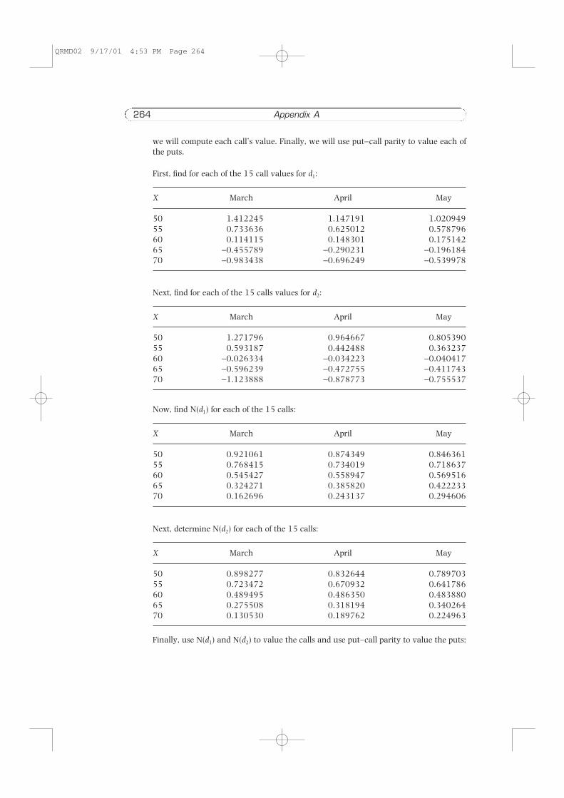
we will compute each call’s value. Finally, we will use put–call parity to value each ofthe puts.

First, find for each of the 15 call values for d1:

X March April May

50 1.412245 1.147191 1.02094955 0.733636 0.625012 0.57879660 0.114115 0.148301 0.17514265 −0.455789 −0.290231 −0.19618470 −0.983438 −0.696249 −0.539978

Next, find for each of the 15 calls values for d2:

X March April May

50 1.271796 0.964667 0.80539055 0.593187 0.442488 0.36323760 −0.026334 −0.034223 −0.04041765 −0.596239 −0.472755 −0.41174370 −1.123888 −0.878773 −0.755537

Now, find N(d1) for each of the 15 calls:

X March April May

50 0.921061 0.874349 0.84636155 0.768415 0.734019 0.71863760 0.545427 0.558947 0.56951665 0.324271 0.385820 0.42223370 0.162696 0.243137 0.294606

Next, determine N(d2) for each of the 15 calls:

X March April May

50 0.898277 0.832644 0.78970355 0.723472 0.670932 0.64178660 0.489495 0.486350 0.48388065 0.275508 0.318194 0.34026470 0.130530 0.189762 0.224963

Finally, use N(d1) and N(d2) to value the calls and use put–call parity to value the puts:

264 Appendix A

QRMD02 9/17/01 4:53 PM Page 264


Calls

X March April May

50 10.626 11.260 11.86655 6.558 7.522 8.32960 3.536 4.658 5.55765 1.658 2.681 3.53670 0.681 1.442 2.156

Puts

X March April May

50 0.319 0.742 1.14555 1.220 1.952 2.53660 3.168 4.037 4.69265 6.259 7.008 7.59970 10.251 10.717 11.147

The options whose values are underlined are overvalued by the market; they should besold. Other options are undervalued by the market; they should be purchased.

10.8. Implied volatilities are given as follows:

(a) X = 40, σ = 0.2579;(b) X = 45, σ = 0.3312;(c) X = 50, σ = 0.2851;(d) X = 55, σ = 0.2715;(e) X = 60, σ = 0.2704.

QRMD02 9/17/01 4:53 PM Page 265

Documents

SOLUTIONS TO EXERCISES